DOCUMENT RESUME

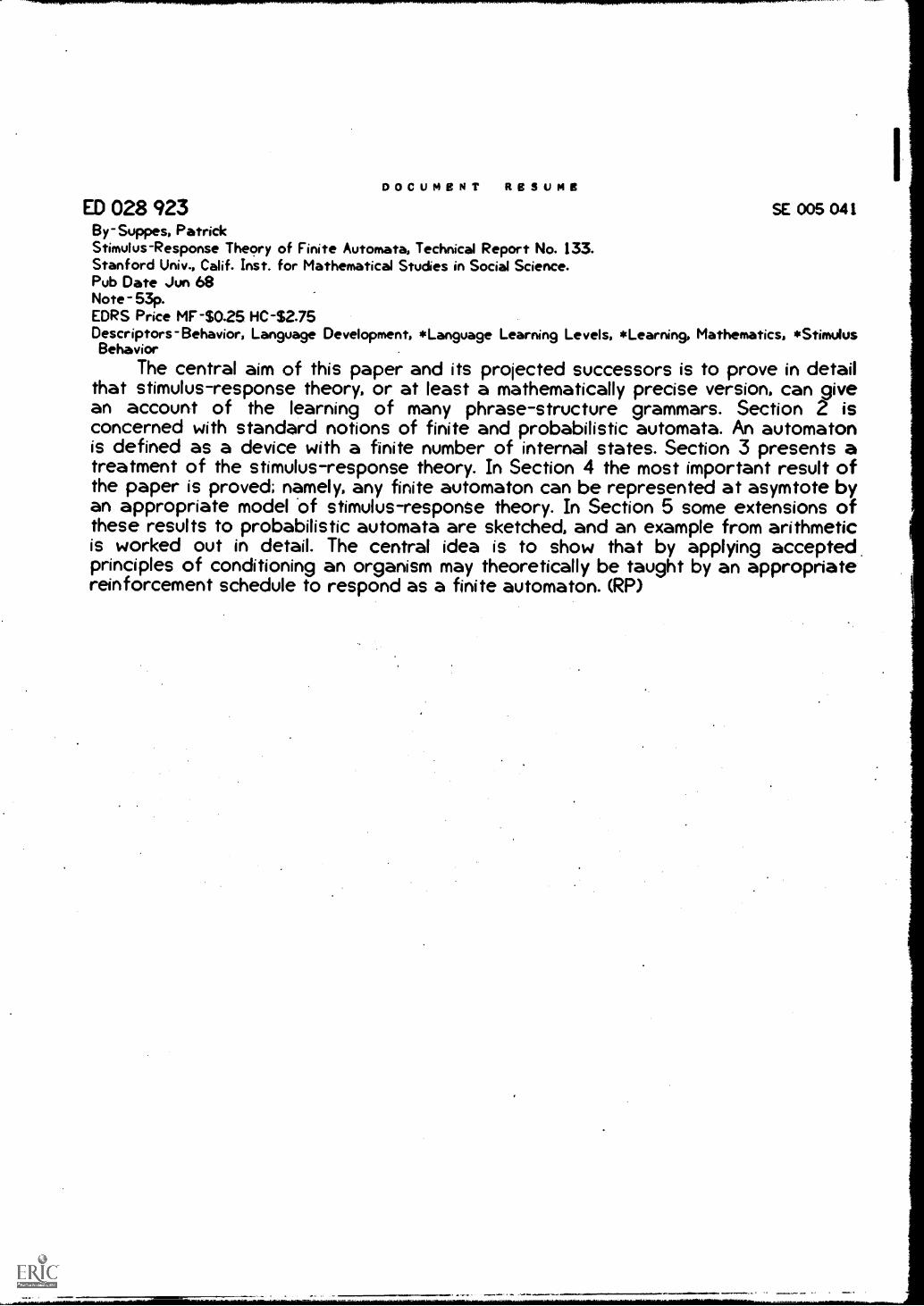
ED 028 923 SE 005 041By-Suppes, PatrickStimulus-Response Theory of Finite Automata, Technical Report No. 133.Stanford Univ., Calif. Inst. for Mathematical Studies in Social Science.Pub Date Jun 68Note-53p.EDRS Price MF-S0.25 HC-S2.75Descriptors-Behavior, Language Development, *Language Learning Levels, *Learning, Mathematics, *StimulusBehavior

The central aim of this paper and its projected successors is to prove in detailthat stimulus-response theory, or at least a mathematically precise version, can givean account of the learning of many phrase-structure grammars. Section 2 isconcerned with standard notions of finite and probabilistic automata. An automatonis defined as a device with a finite number of internal states. Section 3 presents atreatment of the stimulus-response theory. In Section 4 the most important result ofthe paper is proved; namely, any finite automaton can be represented at asymtote byan appropriate model .of stimulus-response theory. In Section 5 some extensions ofthese results to probabilistic automata are sketched, and an example from arithmeticis worked out in detail. The central idea is to show that by applying accepted,principles of conditioning an organism may theoretically be taught by an appropriatereinforcement schedule to respond as a finite automaton. (RP)

JUL 2 9 1968

STIMULUS-RESPONSE THEORY OF FINITE AUTOMATA

BY

PATRICK SUPPES

TECHNICAL REPORT NO. 133

June 19, 1968

PSYCHOLOGY SERIES

U.S. DEPARTMENT OF HEALTH, EDUCATION & WELFARE

OFFICE OF EDUCATION

THIS DOCUMENT HAS BEEN REPRODUCED EXACTLY AS RECEIVED FROM THE

PERSON OR ORGANIZATION ORIGINATING IT. POINTS OF VIEW OR OPINIONS

STATED DO NOT NECESSARILY REPRESENT OFFICIAL OFFICE OF EDUCATION

POSITION OR POLICY.

INSTITUTE FOR MATHEMATICAL S1UDIES IN THE SOCIAL SCIENCES

STANFORD UNIVERSITY

STANFORD, CALIFORNIA .

TECHNICAL Ir',PORTS

PSYCHOLOGY SERIES

INSTITUTE FOR MATHEMATICAL STUDIES IN THE SOCIAL SCIENCES

(Place of publication shown in parentheses; if published title is different from title of Technical Report,this is also shown In parentheses.)

(Fa reports no. I - 44, see Technical Report no. 125.)

50 R. C. Atkinson and R. C. Ca !fee. Mathematical learning theory. January 2,1963. (In B. B. Woiman (Ed.), Scientific Psychology. New York:Basic Books, Inc. , 1965. Pp. 254-275)

51 P. Suppes, E. Crothers, and R. Weir. Application of mathematical leaning theory and linguistic analysis to vowel phoneme matching inRussian words. December 28,1962.

52 R. C. Atkinson, R. Cal/et, G. Sommer, W. Jeffrey and R. Shoemaker. A test of three models for stimulus compounding with children.January 29,1963. U. exp. Psychol., 1964, 67, 52-58)

53 E. Crothers. General Markov models for learning with inter-trial forgetting. April 8,1963.54 J. L. Myers and R. C. Atkinson. Choice behavior and reward structure. May 24 , 1963. (Journal math. Psycho!. , 1964, 1,170-203)55 R. E. Robinson. A set-theoretical approach to empirical meaningfulness of measurement statements. June 10, 1963.56 E. Crothers, R. Weir and P. Palmer. The role of transcription in the learning of the orthographic representations of Russian sounds. June I7,. 1963.57 P. Suppes. Problems of optimization in learning a list of simple items. July 22,1963. (In Maynard W. Shelly, 11 and Glenn L. Bryan (Eds.),

Human Judgments and Optimality. New Yak: Wiley. 1964. Pp. 116-126)58 R. C. Atkinson and E. J. Crothers. Theoretical note: all-a-none learning and intertrial forgetting. July 24,1963.59 R. C. Coffee. Long-term behavior of rats under probabilistic reinforcement schedules. October!, 1963.60 R, C. Atkinson and E. J. Crothers. Tests of acquisition and retention, axioms for paired-associate learning. October 25, 1963. (A comparison

of paired-associate learning models having different acquisition and retention axioms, J. math. Psychol., 1964, 1, 285-315)61 W. J. McGill and J. Gibbon. The general-gamma distribution and reaction times. November 20,1963. (J. math. Psychol., 1965, 2,1-18)62 M. F. Norman. Incremental learning on random trials. December 9,1963. (J. math. Psycho!, 1964, j, 336-351)63 P. Suppes. The development of mathematical concepts in children. February 25,1964. (On the behavioral foundations of mathematical concepts.

Monographs of the Society fa Research in Child Development, 1965, 30, 60-96)64 P. Suppes. Mathematical concept famation in children. April 10, 1964. (Amer. Psychologiste 1966, 21,139-150)65 R. C. Calfee, R. C. Atkinson, and T. Shelton, Jr. Mathematical models for verbal learning. August 21,1964. (In N. Wiener and J. P. Schoda

(Eds.), Cybernetics of the Nervous System: Progress in Brain Research. Amsterdam, The Netherlands: Elsevier Publishing Co., 1965.Pp. 333-349)

66 L. Keller, M. Cole, C. J. Burke, and W. K. Estes. Paired associate learning with differential rewards. August 20,1964. (Reward andinformation values of trial outcomes in paired associate learning. (Psychol. Monogr., 1965, 79,1-21)

67 M. F. Norman. A probabilistic model fa free-responding. December 14 , 1964.68 W. K. Estes and H. A. Taylor. Visual detection in relation to display size and redundancy of critical elements. January 25,1965, Revised

7-1-65. (Perception and Psychophysics, 1966, 1, 9-16)69 P. Suppes and J. Donio. Foundations of stimulus-sampling theory for continuous-time processes. February 9,1965. (J. math. Psychol., 1967,

4, 202-225)70 R. C. Atkinson and R. A. Kinchia. A learning model for faced-choice detection experiments. February 10, 1965. (Br. J. math stat. Psychol.,

1965,18,184-206)71 E. J. Crothers. Presentation orders fa items from different categales. March 10, 1965.72 P. Suppes, G. Groen, and M. Schlag-Rey. Some models for response latency in paired-associates leaning. May 5,1965. U. math. pashol.,

1966, 3, 99-128)73 M. V. Levine. The generalization function in the probability learning experiment. June 3,1965.74 D. Hansen and T. S. Rodgers. An exploration of psycholinguistic units in initial reading. July 6, 1965.75 B. C. Arnold. A correlated urn-scheme fa a continuum of responses. July 20,1965.76 C. Izawa and W. K. Estes. Reinforcement-test sequences in paired-associate learning. August 1, 1965. (Psychol. Repcets, 1966, 18, 879-919)77 S. L. Blehart. Pattern discrimination learning with Rhesus monkeys. September!, 1965. (Psycho,. Reports, 1966,19, 311-324)78 J. L. Phillips and R. C. Atkinson. The effects of display size on short-term memory. August 31, 1965.79 R. C. Atkinson and R. PA. Shiffrin. Mathematical models for memory and learning. September 20,1965.80 P. Suppes. The psychological foundations of mathematics. October 25,1965. (Colloques Internationaux du Centre National de la Recherche

Scientifique. Editions du Centre National de la Recherche Scientiflque. Paris:1967. Pp. 213-242)81 P. Suppes. Computer-assisted instruction in the schools: potentialities, problems, prospects. October 29,1965.82 R. A. Kinchla, J. Townsend, J. Yellott, Jr., and R. C. Atkinson. Influence of correlated visual cues on auditory signal detection.

November 2,1965. (Perception and Psychophysics, 1966, I, 67-73)83 P. Suppes, M. Jerman, and G. Groin. Arithmetic drills and review on a computer-based teletype. November 5,1965. (Arithmetic Teacher,

April 1966, 303-309,84 P. Suppes and L. Hyman. Concept learning with non-verbal geometrical stimuli.. November 15, 1968.85 P. Holland. A variation on the minimum chl-sguare test, (J. math. Psychol., 1967, 3, 377-413).86 P. Suppes, Accelerated program in elementary-school mathematics -- the second yew. November 22,1965. (Psychology in the Schools, 1966,

3, 294-307)87 P. Lorenzen and F. Binford. Logic as a dialogical game. November 29,1963.88 L. Keifer, W. J. Thomson, J. R. Tweedy, and R. C. Atkinson. The effects of reinfacement interval on the acquisition of paired-associate

responses. December 10, 1965. ( J. ite. Psychol., 1967, 73, 268-277)89 J. 1, Yellott, Jr. Sone effects on noncontingent success in humen probability learning. December 15,1965.90 P. Suppes and G. Groen. Some counting models for first-grade performance data on simple addition facts. January 14,1966. (In J. M. Scandtwa

(Ed.), Research in Mathematics Education. Washington, D. C.: NCTPA, 1967. Pp. 35-43.

(Continued on Inside back clover)

STIMULUS-RESPONSE THEORY OF FINITE AUTOMATA

by

Patrick Suppes

TECHNICAL REPORT NO. 133

June 19, 1968

PSYCHOLOGY SERIES

Reproduction in Whole or in Part is Permitted for

any Purpose of the United States Government

INSTITUTE FCR MATHEMATICAL STUDIES IN THE SOCIAL SCIENCE3

STANFORD UNIVERSITY

STANFORD, CALIFORNIA

Stimulus-Response Theory of Finite Automata1

Patrick Suppes

Institute for Mathematical Studies in the Social Sciences

Stanford University

1. Introduction.

Ever since the appearance of Chomsky's famous review (1957) of

Skinner's Verbal Behavior (1957), linguists have conducted an effective

and active campaign against the empirical or conceptual adequacy of any

learning theory whose basic concepts are those of stimulus and response,

and whose basic processes are stimulus conditioning and stimulus

sampling.

Because variants of stimulus-response theory had dominated much of

experimental psychology in the two decades prior to the middle fifties,

there is no doubt that the attack of the linguists has had a salutary

effect in disturbing the theoretical complacency of many psychologists.

Indeed, it has posed for all psychologists interested in systematic

theory a number of difficult and embarrassing questions about language

learning and language behavior in general. However, in the flush of

their initial victories, many linguists have made extravagant claims

and drawn yweeping, but unsupported conclusions about the inadequacy of

stimulus-response theories to handle any central aspects of language

behavior. I say "extravagant" and "unsupported" for this reason. The

claims and conclusions so boldly enunciated are supported neither by

2

careful mathematical argument to show that in principle a conceptual

inadequacy is to be found in all standard stimulus-response theories,

nor by systematic presentation of empirical evidence to show that the

basic assumptions of these theories are empirically false. To cite two

recent books of some importance, neither theorems nor data are to be

found in Chomsky (1965) or Katz and Postal (1964), but one can find

rather many useful examples of linguistic analysis, many interesting and

insightful remarks about language behavior, and many badly formulated

and incompletely worked out arguments about theories of language

learning.

The central aim of the present paper and its projected successors

is to prove in detail that stimulus-response theory, or at least a

mathematically precise version, can indeed give an account of the learning

of many phrase-structure grammars. I hope that there will be no

misunderstanding about the claims I am making. The mathematical defi-

nitions and theorems given here are entirely subservient to the

conceptual task of showing that the basic ideas of stimulus-response

theory are rich enough to generate in a natural way the learning of

many phrase-structure grammars. I am not claiming that the mathematical

constructions in this paper correspond in any exact way to children's

actual learning of their first language or to the learning of a second

language at a later stage. A number of fundamental empirical questions

are generated by the formal developments in this paper, hut none of the

relevant investigations have yet been carried out. Some suggestions for

experiments are mentioned below. I have been concerned to show that the

linguists are quite mistaken in their claims that even in principle,

3

apart from any questions of empirical evidence, it is not possible for

conditioning theory to give an account of any essential parts of language

learning. The main results in this paper, and its sequel dealing with

general context-free languages, show that this linguistic claim is false.

The specific constructions given here show that linguistic objections

to the processes of stimulus-conditioning and sampling as being unable

in principle to explain any central aspects of language behavior must

be reformulated in less sweeping generality and with greater intellectual

precision in order to be taken seriously by psychologists.

The mathematical formulation and proof of the main results presented

here require the development of a certain amount of formal machinery.

In order not to obscure the main ideas, it seems desirable to describe

in a preliminary and intuitive fashion the character of the results.

The central idea is quite simpleit is to show how by applying

accepted principles of conditioning an organism may theoretically be

taught by an appropriate reinforcement schedule to respond as a finite

automaton. An automaton is defined as a device with a finite number of

internal states. When it is presented with one of a finite number of

letters from an alphabet, as a function of this letter of the alphabet

and its current internal state,it moves to another one of its internal

states. (A more precise mathematical formulation is given below.) In

order to show that an organism obeying general laws of stimulus conditioning

and sampling can be conditioned to become an automaton, it is necessary

first of all to interpret within the usual run of psydhological concepts,

the notion of a letter of an alphabet and the notion of an internal

state. In my own thinking about these matters, I was first misled by

the perhaps natural attempt to identify the internal state of the automaton

with the state of conditioning of the organism, This idea, however,

turned out to be clearly wrong. In the first place, the various possible

states of conditioning of the organism correspond to various possible

automata that the organism can be conditioned to become, Roughly

speaking, to each state of conditioning there corresponds a different

automaton, Probably the next most natural idea is to look at a given

conditioning state and use the conditioning of individual stimuli to

represent the internal states of the automaton, In very restricted cases

this correspondence will work, but in general it will not, for reasons

that will become clear later. The correspondence that turns out to work

is the following: the internal states of the automaton are identified

with the responses of the organism. There is no doubt that this "surface"

behavioral identification will make many linguists concerned with deep

structures (and other deep, dbstract ideas) uneasy, but fortunately it

is an identification already suggested in the literature of automata

theory by E. F. Moore and others. The suggestion was originally made

to simplify the formal characterization of automata by postulating a

one-one relation between internal states of the machine and outputs of

the machine. From a formal standpoint this means that the two separate

concepts of internal state and output can be welded into the single

concept of internal state and, for our purposes, the internal states can

be identified with responses of the organism, The correspondence to be

made between letters of the alphabet that the automaton will accept and

the appropriate objects within stimulus-response theory is fairly

dbvious. The letters of the alphabet correspond in a natural way to sets

5

of stimulus elements presented on a given trial to an organism. So

again, roughly speaking, the correspondence in this case is between the

alphabet and selected stimuli, It may seem like a happy accident, but

the correspondences between inputs to the automata and stimuli presented

to the organism, and between internal states of the machine and responses

of the organism, are conceptually very natural.

Because of the conceptual importance of the issues that have been

raised by linguists for the future development of psychological theory,

perhaps above all because language behavior is the most Characteristically

human aspect of our behavior patterns, it is important to be as clear as

possible about the claims that can be made for a stimulus-response theory

whose basic concepts seem so simple and to many so woefully inadequate

to explain complex behavior, including language ehavior. I cannot

refrain from mentioning two examples that present very useful analogies.

First is the reduction of all standard mathematics to the concept of

set and the simple relation of an element being a member of a set. From

a naive standpoint, it seems unbelievable that the complexities of higher

mathematics can be reduced to a relation as simple as that of set

membership. But this is indubitably the case, and we know in detail

how the reduction can be made. This is not to suggest, for instance,

that in thinking about a mathematical problem or even in formulating

and verifying it explicitly, a mathematician operates simply in terms

of endlessly complicated statements about set membership. By appropriate

explicit definition we introduce many additional concepts, the ones

actually used in discourse. The fact remains, however, that the reduction

to the singLe relationship of set membership can be made and in fact has

6

been carried out in detail. The second example, which is close to our

present inquiry, is the status of simple machine languages for computers.

Again, from the naive standpoint it seems incredible that modern computers

can do the things they can in terms either of information processing

or numerical computing when their basic language consist, essentially

just of finite sequences of l's and O's; but the more complex computer

languages that have been introduced are not at all for the convenience

of the machines but for the convenience of human users. It is perfectly

clear how any more complex language, like ALGOL, can be reduced by a

compiler or other device to a simple machine language. The same attitude,

it seems to me, is appropriate toward stimulus-response theory. We

cannot hope to deal directly in stimulus-response connections with complex

human behavior. We can hope, as in the two cases just mentioned, to

construct a satisfactory systematic theory in terms of which a chain of

explicit definitions of new and ever more complex concepts can be

introduced. It is these new and explicitly defined concepts that will

be related directly to the more complex forms of behavior. The basic

idea of stimulus-response association or connection is close enough in

character to the concept of set membership or to the basic idea of

automata to make me confident that new and better versions of stimulus-

response theory may be expected in the future and that the scientific

potentiality of theories stated essentially in this framework has by no

means been exhausted.

Before turning to specific mathematical developments, it will be

useful to make explicit how the developments in this paper may be used to

show that many of the common conceptions of conditioning, and particula iy

7

the claims that conditioning refers only to simple reflexds like those

of salivation or eye blinking, are mistaken. The mistake is to confuse

particular restricted applications of the fundamental theory with the

range of the theory itself. Experiments on classical conditioning do

indeed represent a narrow range of experiments from a broader conceptual

standpoint. It is imporbant to realize, however, that experiments on

classical conditioning do not define the range and limits of conditioning

theory itself. The main aim of the present paper is to show how any

finite automata, no matter how complicated, may be constructed purely

within stimulus-response theory. But from the standpoint of automata,

classical conditioning represents a particularly trivial example of an

automaton. Classical conditioning may be represented by an automaton

having a one-letter alphabet and a single internal state. This is the

most trivial possible example of an automaton. The next simplest one

corresponds to the structure of classical discrimination experiments.

Here there is more than a single letter to the alphabet, but the

transition table of the automaton depends in no way on the internal

state of the automaton. In the case of discrimination, we may again

think of the responses as corresponding to the internal states of the

automaton. In this sense there is more than one internal state, contrary

to the case of classical conditioning, but what is fundamental is that

the transition table of the automaton does not depend on the internal

states but only on the external stimuli presented. It is of the utmost

importance to realize that this restriction, as in the case of classical

conditioning experiments, is not a restriction that is in any sense

inherent in conditioning theory itself. It merely represents

concentration on a certain restricted class of experiments.

8

Leaving the technical details for later, it is still possible to

give a very clear example of conditioning that goes beyond the classical

cases and yet represents perhaps the simplest non-trivial automaton. By

non-triviaij mean: there is more than one letter in the alphabet;

there is more than one internal state; and the transition table of the

automaton is a function of both the external stimulus and the current

internal state. As an example, we may take a rat being run in a maze.

The reinforcement schedule for the rat is set up so as to make the

rat become a two-state automaton. We will use as the external alphabet

of the automaton a two-letter alphabet consisting of a black or a white

card. Each Choice point of the maze will consist of either a l'eft turn

or a right turn. At each Choice point either a black card or a white

card will be present. The following table describes both the rein-

forcement schedule and the transition table of the automaton.

L R

LB 1 0

LW 0 1

RB 0 1

RW 1 0

Thus the first row shows that when the previous response has been left

(L) and a black stimulus card (B) is presented at the choice point, with

probability one the animal is reinforced to turn left. The second row

indicates that when the previous response is left and a white stimulus

card is presented at the Choice point, the animal is reinforced

100 per cent of the time to turn right, and so forth,for the other

two possibilities.- From a formal standpoint this is a simple schedule

9

of reinforcement, but already the double aspect of contingency on both

the previous response and the displayed stimulus card makes the schedule

more complicated in many respects than the schedules of reinforcement

that are usually run with rats. I have not been able to get a uniform

prediction from my experimental colleagues as to whether it will be

possible to teach rats to learn this schedule. (Most of them are con-

fident pigeons can be trained to respond like non-trivial two-state

automata.) One thing to note about this schedule is that it is

recursive in the sense that if the animal is properly trained according

to the schedule, the length of the maze will be of no importance. He

will always make a response that depends only upon his previous response

and the stimulus card present at the choice point.

There is no pretense that this simple two-state automaton is in

any sense adequate to serious language learning. I am not proposing, for

example, that there is much chance of teaching even a simple one-sided

linear grammar to rats. I am proposing to psychologists, however, that

already automata of a small nuniber of states present immediate experimental

challenges in terms of what can be done with animals of each species.

For example, what is the most complicated automaton a monkey may be

trained to imitate? In this case, there seems some possibility of

approaching at least reasonably complex one-sided linear grammars (using

the theorem that any one-sided linear grammar is definable by a finite-

state automaton). In the case of the lower species, it will be necessary

to exploit to the fullest the kind of stimuli to which the organisms are

most sensitive and responsive in order to maximize the complexity of the

automata they can imitate.

10

If a generally agreed upon definition of complexity for finite

automata can be reached, it will be possible to use this measure to gauge

the relative level of organizational complexity that can be achieved by

a given species, at least in terms of an external schedule of conditioning

and reinforcement. I do want to emphasize that the measures appropriate

to experiments with animals are almost totally different from the measures

that have been discussed in the recent literature of automata as

complexity measures for computations. What is needed in the case of

animals is the simple and orderly arrangement on a complexity scale of

automata that have a relatively small number of states and that accept

a relatively small alphabet of stimuli. The number of distinct training

conditions is not a bad measure and can be used as a first approximation.

Thus in the case of classical conditioning,this number is one. In the

case of discrimination between black and white stimuli,the number is

two. In the case of the two-state automaton described for the maze

experiment, this number id four, but there are some problems with this

measure. It is not clear that we would regard as more complex than

this two-state automaton, an organism that masters a discrimination

experiment consisting of six different responses to six different

discriminating stimuli. Consequently, what I've said here about

complexity is pre-systematic. I do think the development of an appro-

priate scale of complexity can be of considerable theoretical interest,

particularly in crossspecies comparison of intellectual power.

The remainder of this paper is devoted to the technical development

of the general ideas already discussed. Section 2 is concerned with

standard notions of finite and probabilistic automata. Readers already

;

11

familiar with this literature should skip this section and go on to the

treatment of stimulus-response theory in Section 3. It has been

necessary to give a rigorous axiomatization of stimulus-response theory

in order to formulate the representation theorem for finite automata in

mathematically precise form. However, the underlying ideas of stimulus-

response theory as formulated in Section 3 will be familiar to all

experimental psychologists. In Section 4 the most important result of

the paper is proved, namely, that any finite automaton can be represented

at asymptote by an appropriate model of stimulus-response theory. In

Section 5 some extensions of these results to probabilistic automata

are sketched, and an example from arithmetic is worked out in detail.

The relationship between stimulus-response theory and grammars is

established in Section 5 by known theorems relating automata to grammars.

The results in the present paper are certainly restricted regarding

the full generality of context-free languages. Weakening these restric-

tions will be the focus of a subsequent paper.

Some results on tote hierarchies and plans in the sense of Miller,

Galanter and Pribram (1960) are also given in Section 4. The

representation of tote hierarchies by stimulus-response models follows

directly from the main theorem of that section.

12

2. Automata

The account of automata given here is formally self-contained,

but not really self-explanatory in the deeper sense of discussing and

interpreting in adequate detail the systematic definitions and theorms.

I have followed closely the development in the well-known article of

Rabin and Scott (1959), and for probabilistic automata, the article of

Rabin(1963).

Definition 1. A structure CX. < Al M, so, F > is a finite

(deterministic) automaton if and only if

(i) A is a finite, non-empty set (the set of states of CC))

(ii) E is a finite, non-empty set (the alphabet),

(iii) M is a function from the Cartesian product A x Z to A

(M defines the transition table of a),

(iv) so is in A (so is the initial state of Ot),

(v) F is a subset of A (F is the set of final states of (X).

In view of the generality of this definition it is apparent that there

are a great variety of automata, but as we shall see, this generality

is easily matched by the generality of the models of stimulus-response

theory.

In notation now nearly standardized, Z*

is the set of finite

sequences of elements of Z 1 including the empty sequence -A-. The

elements of Z* are ordinarily called tapes. If Tll .I Tk are in

Z then x 0-1 Tk

is in . (As we shall see, these tapes

correspond in a natural way to finite sequences of sets of stimulus

elements.) The function M can be extended to a function from A x

13

to A by the following recursive definition for s in A, x in e

and T in E.

) = S

M(s) ler) = M(M(S, X), T)

Definition 2. A tape x of e is accepted 122 crc if and only.

if M(so

1 x) is in F. A tape x that is accepted 1Di Or is a

sentence of O.

We shall also refer to tapes as strings of the alphabet 2%

Definition 3. The language L generated la Cr( is the set of

all sentences of 0-C, i.e., the set of all tapes accepted la (N:.

Regular languages'are sometimes defined just as those languages generated

by some finite automata. An independent, set-theoretical characteri-

zation is also possible. The basic result follows from Kleene's (1956)

fundamental analysis of the kind of events definable by McCulloch-Pitts

nets. Severkl equivalent formulations are given in the article by Rabin

and Scott. From a linguistic standpoint probably the most useful

characterization is that to be found in Chomsky (1963, pp. 368-371).

Regular languages are generated by one-sided linear grammars. Such

grammars have a finite number of rewrite rules, which in the case of

right-linear rule; are of the form

A -,30

Whichever of several equivalent formulations is used, the fundamental

theorem, originally due to KIeene, but closely related to the theorem of

Myhill given by Rabin and Scott, is this.

Theorem on Regular Languages. Am regular language is generated by

some finite automaton, and every finite automaton generates a regular

languaEt.

For the main theorem of this article, we need the concepts of isomor-

phism and equivalence of finite automata. The definition 6f isomorphism

is just the natural set-theoretical one for structures like automata.

Definition 4. Let aC = < A, E, M, so, F > and oc,

< M', so', F' > be finite automata. Then a( and CU are

isomorphic if and only if there exists a function f such that

f is one-one,

(ii) Domain of f is A U E and range of f is A' UE'

(iii) For every a in A U

a E A if and only if f(a) E A'

(iv) For every s in A and T in E

f(M(s, T) = W(f(s), f(T)),

(v) f(s0) . so'

(vi) For every s in A

s E F if and only if f(s) E F' .

It is apparent that conditions (i)-(iii) of the definition imply that

for every a in A U

a E E if and only if f(a) E

and consequently, this condition on E need not be stated. From the

standpoint of the general algebraic or set-theoretical concept of

isomorphismtit would have been more natural to define an automaton in

terms ofabasic set B.AUE, and then require that A and E are

both subsets of B. Rabin and Scott avoid the problem by not making E

a part of the automaton. They define the concept of an automaton

CX:= < A, M, so, F > with respect to an alphabet E, but for the

purposes of this paper At is also desirable to include the alphabet E

in the definition of OIC in order +0 make explicit the natural place

of the alphabet in the stimulus-response mod J_s, and above all) to

provide a simple setup for going from one aLphabet E to another :Et .

In any case, exactly how these matters are handled is not of central

importance here,

Definition 5. Two a'Aomata are Eativalent. If and alz if thez

accept exactly the same set of takes.

This is the standard definition of equivalence in the literature. As

it stands, it means that the definition of equivalence is neither

stronger nor weaker than the definition of isomorphism, because, on

the one hand, equivalent at.tomata are c.early not necessarily Isomorphic,

and, on the other hand, isomorphic automata wi4lh different alphabets

are not equivalent. It wolid seem natural to weaken the notion of

equivalence to include two atomata that generate dis; nct but

isomorphic languages, or se4s of tapes, b*At ihLs point will bear on matters

here only tangentially.

A finite automaton is connected if for every

tape x such that M(so; x)

s4.a4,e s there is a

s. It is easy to snow 1-hat every automa".on

is equivalent to a connected automaton, and ihe representation theorem

of Section 4 is restricted '.r'o connected automata. T. s apparent 7:diat

from a functiona :,.. eandpcAnt, slates that canno4, reacbed by any

16

tape are of no interest, and consequently;restriction to connected

automata does not represent any real loss of generality. The difficulty

of representing automata with unconnected states by stimulus-response

models is that we have no way to condition the organism with respect to

these states, at least in terms of the approach developed here.

It is also straightforward to establish a representation for

probabilistic automata within stimulus-response theory, and, as will

become apparent in Section 5, there are some interesting differences in

the way we may represent deterministic and prdbabilistic automata within

stimulus-response theory.

Definition 6. A structure DC= < A, p, so, F > is a (finite)

probabilistic automaton if and only if

(i) A is a finite, non-empty set,

(ii) is a finite, non-empty set,

(iii) p is a function on A X I such that for each s in A and

T in 2; psT is a probability density over A, i.e.,,

(a) for each s' in A, m(si) > o

(b) p ,(s') =

As' E s'-

(iv) so

is in A ,

(v) F is a subset of A

The only change in generalizing from Definition 1 to Definition 6 is

found in (iii), although it is natural to replace (iv) by an initial

probability density. It is apparent how Definition 4 must be modified to

characterize the isomorphism of probabilistic automata, and so the

explicit definition will not be given.

a

17

3. Stimulus-response Theory_

The formalization of stimulus-response theory given here follows

closely the treatment in Estes and Suppes (1959) and Suppes and

Atkinson (1960). Some minor changes have been made to facilitate the

treatment of finite automata, but it is to be strongly emphasized that

none of the basic ideas or assumptions has required modification.

The theory is based on six primitive concepts, each of which has

a direct psychological interpretation. The first one is the set S of

stimuli, which we shall assume is not empty, but which we will not

restrict to beingceither finite or infinite on all occasions. The second

primitive concept is the set R of responses and the third primitive

concept the set E of possible reinforcements. As in the case of the

set of stimuli, we need not assume that either R or E is finite, but

in the present applications to the theory of finite automata we shall

make this restrictive assumption. (Fpr a proper treatment of phonology

it will clearly be necessary to make R, and probably E as well,

infinite with at the very least a strong topological if not metric

structure.)

The fourth primitive concept is that of a measure 11 on the set of

stimuli. In case the set S is finite this measure is often the number

of elements in S. For the general theory we shall assume that the

measure of S itself is always finite, i.e., 4(s) < co .

The fifth primitive concept is the sample space X. Each element

x of the sample space represents a possible experiment, that is, an

infinite sequence of trials. In the present theory, each trial may be

described by an ordered quintuple < CI T, s, r, e >, where C is the

18

conditioning function, T is the subset of stimuli presented to the

organism on the given trial, s is the sampled subset of T, r is the

response made on the trial, and e is the reinforcement occurring on

that trial. It is not possible to make all the comments here that are

required for a full interpretation and understanding of the theory. For

those wanting a more detailed description, the tido references already

given will prove useful. A very comprehensive set of papers on stimulus-

sampling theory has been put together in the collection edited by

Neimark and Estes (1967). The present version of stimulus-response

theory should in many respects be called stimulus-sampling theory;

but I have held to the more general stimulus-response terminology to

emphasize the juxtaposiUon of the general ideas of behavioral psychology

on the one hand and linguistic theory on the other. In addition, in the

theoretical applications to be made here the specific sampling aspects of

stimulus-response theory are not as central as in the analysis of experi-

mental data.

Because of the importance to be attached later to the set T of

stimuli presented on each trial, its interpretation in classical learning

theory should be explicitly mentioned. In the case of simple learning,

for exampleoin classical conditioning, the set T is the same on all

trials and we would ordinarily identify the sets T and S. In the

case of discrimination learning, the set T varies from trial to trial,

and the application we are making to automata theory falls generally

under the discrimination case. The conditioning function C is defined

over the set R of responses and Cr is the subset of S conditioned

or connected to response r on the given trial. How the conditioning

function changes from trial to trial is made clear by the axioms.

19

From the quintuple description of a given trial it is clear that

certain assumptions about the behavior that occurs on a trial have

already been made. In particular it is apparent that we are assuming

that only one sample of stimuli is drawn on a given trial, that exactly

one response occurs on a trial and that exactly one reinforcement

occurs on a trial. These assumptions have been built into the set-

theoretical description of the sample space X and will not be an

explicit part of our axioms.

Lying behilAi the formality of the ordered quintuples representing

each trial is the intuitively conceived temporal ordering of events on

any trial, which may be represented by the following diagram:

State of

conditioningat beginning

of trial

. Cn

presen-sampling

tation--of -

of stimulistimuli

- -) Tn -o s

state ofconditioning

-0 'retpOnse-:-0 reinforce- -*at beginning

mentof new trial

rn

en -0 Cn+1

The sixth and final primitive concept is the probability measure P on

the appropriate Borel field of cylinder sets of X. The exact description

of this Borel field is rather complicated when the set of stimuli is not

finite, but the construction is standard,and we shall assume the reader

can fill in details familiar from general probability theory. It is to

be emphasized that all probabilities must be defined in terms of the

. measure P.

We also need certain notation to take us back and forth between

elements or subsets r.Jf the sets of stimuli, responses, and reinforcements

to events of the sample space X. First, rn is the event of response

r on trial n, that is, the set of all possible experimental realizations

20

or elements of X having r as a response on the nth trial. Similarly,

er,n

is the event of response r's being reinforced on trial n. The

event e is the event of no reinfoi.cement on trial n. In likeo n

fashion, Cn is the event of conditioning function C occurring on

trial n, Tn is the event of presentation set T occurring on trial n,

and so forth. AdditiOnal notation that does not follow these conventions

will be explicitly noted.

We also need a notation for sets defined by events occurring up to

a given trial. Reference to such sets is required in expressing that

central aspects of stimulus conditioning and sampling are independent

of the pattern of past events. If I say that Yn is an n-cylinder set)

I mean that the definition of Yn

does not depend on any event occurring

after trial n. However, an even finer breakdown is required that takes

account of the postulated sequence Cn -÷sn --orn -÷en on a given

trial, so in saying that Yn is a Cn-cylinder set what ir meant is

that its definition does not depend on any event occurring after Cn

on trial n, i.e., its definition could depend on Tn..1 or Cn

for

example, but not on Tn or sn

As an abbreviated notation, I shall

write y(c) for this set and similarly for other cylinder sets. The

notation Yn

without additional qualification shall always refer to

an n-cylinder set.

Also, to avoid an overly cumbersome notation, event notation of

the sort already indicated will be used, e.g., er,n

for reinforcement

of response r on trial n, but also the notation Cr E Cr,n

for the

event of stimulus T's being conditioned to response r on trial n.

21

To simplify the formal statement of the axioms it shall be

assumed without repeated explicit statement that any given events on

which probabilities are conditioned have positive probability. Thus,

for example, the tacit hypothesis of Axiom S2 is that P(Tm) > 0 and

P(Tn) > 0

The axioms naturally fall into three classes. Stimuli must be

sampled in order to be conditionedland they must be conditioned in order

for systematic response patterns to develop. Thus,there are naturally

three kinds of axioms: sampling axioms; conditioning axioms; and

response axioms. A verbal formulation of each axiom is given together

with its formal statement. Frcm the standpoint of formulations of the

theory already in the literature, perhaps the most unusual feature of the

present axioms is not to require that the set S of stimuli be finite.

It should also be emphasized that for any one specific kind of detailed

application additional specializing assumptions are needed. Some indi-

cation of these will be given in the particular application to automata

theory, but it would take us too far afield to explore these specializing

assumptions in any detail and with any faithfulness to the range of

assumptions needed for different experimental applications.

Definition 7. A structure 141= < S, R, E, 4, X, P > is a stimulus-

response model if and cnly if the following axioms are satisfied:

Sampling Axioms

Sl. P(I1(sn) > 0)

(On every trial a set of stimuli of positive measure is sampled

with probability 1.)

22

S2. P(smITm niTn) .

(If the same presentation set occurs on two different trials,

then the prdbability of a given sample is independent of the trial

number.)

S3. If s U s' c T and 14(s) =

then P(snITn) = P(s'n1Tn) .

(Samples of equal measure that are subsets of the presentation

set have an 23,1221 probabilit, of being sampled on a given trial.)

P(snITn,Yn(Cn)) = P(snITn) .

(The probability of a particular sample on trial n, given, the

presentation set of stimuli, is independent of Ex preceding pattern

Yn(Cn

) of events.)

Conditioning Axioms

Cl. If r, r'ER,r r' and C 0 , thenr r

P(C) = 0 .

(On every trial with probability 1 each stimulus element is

conditioned to at most one response.)

C2. There exists a c > 0 such that for every Clr', C, r, n, s,

er

and Yn

POT E Cr,n+1 IT r n2

TEs e.n2 r,nd n

(The probability is c of Ey sampled stimulus element's

becoming conditioned to the reinforced response if it is not already so

conditioned, and this probability is independent of the particular

response, trial number, or any preceding pattern Yn of events.)

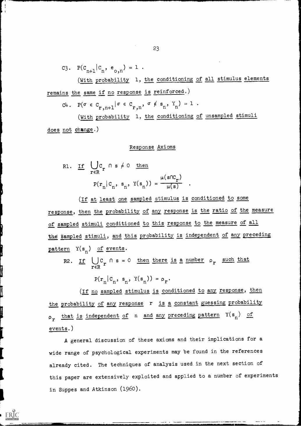
23

C3.1)(CICe). 1 .

n+1 n' o,n

(With probability 1, the conditioning of all stimulus elements

remains the same if no response is reinforced.)

c4. P(0- E cr n+1

(T E Crn

T sn, Yn) 1 .

(With probability 1, the conditioning of unsampled stimuli

does not change.)

Response Axioms

Rl. If (JCr

n s 0 then

reR4(snC )

P(rn1Cn, sn, Y(sn)) = -7175

(If at least one sampled stimulus is conditioned to some

response, then the probability of my response is the ratio of the measure

of sampled stimuli conditioned to this response to the measure of all

the 'amp1ed stimuli, and this probability is independent of any preceding

pattern Y(sn) of events.

R2. If L)Crn s = 0 then there is a number p

rsuch that

reR

P(rnIC

nsn

Y(sn)) p

r.

(If no sampled stimulus is conditioned to Lara response, then

the probability of any remonse r is a constant guessing probability

that is independent of n and any preceding pattern Y(sn) ofPr

events.)

A general discussion of these axioms and their implications for a

wide range of psychological experiments may be found in the references

already cited. The techniques of analysis used in the next section of

this paper are extensively exploited and applied to a number of experiments

in Suppes and Atkinson (1960).

24

4. Representation of Finite Automata

A useful beginning for the analysis of how we may represent finite

automata by stimulus-response models is to see what is wrong with the

most direct approach possible. The difficulties that turn up may be

illustrated by the simple example of a two-letter alphabet (i.e., two

stimuli T1

and T2'

as well as the "start-up" stimulus To

) and a

two-state automaton (i.e., two responses r1

and r2). Consideration

of this example, already mentioned in the introductory section, will

be useful for several points of later discussion.

By virtue of Axiom Sll the single presented stimulus must be

sampled on each trial,and we assume that for every n,

0 < P(To E sn), P(T1 E Sn), P(T2 E Sn) < 1 .

Suppose, further, the transition table of the machine is:

r1

0"I

r1

Cr2

r20-1

r2

Cr

2

r1 r2

1 0

0 1

0 1

1 0

whichrequiresknowledgeofbothr.and T to predict what response

should be next. The natural and obvious reinforcement schedule for

imitating this machine is:

P(e IT10 lr10-1 ) = 1

P(e IT2In 10, r20-1 ) = 1

P( e IT2In 21n/r10-1) 1

P(e 1lln 2In 1r 20-1)

25

where T. is theeventofstimuluscr.'s being sampled on trial n.ion 1

But for this reinforcement schedule the conditioning of each of the two

stimuli continues to fluctuate from trial to trial, as may be illustrated

by the following sequence. For simplification and without loss of

generality, we may assume that the conditioning parameter c is 1, and

we need indicate no sampling, because as already mentioned, the single

stimulus element in each presentation set will be sampled with probability

1. We may represent the states of conditioning (granted that each stimulus

is conditioned to either r1

or r2) by subsets ofS= TTT0' l' 2

Thustif ( T1°T2

represents the conditioning function, this means both

elements T1

and T2

are conditioned to rl'

T means that only1

T1

is conditioned to r19

and so forth. Consider then the following

sequence from trial n to n + 2:

The response on trial n + 1 satisfies the machine table, but already

on n 2 it does not, for r2,n+1

T2 n+2should be followed by r

1 n+2'

It is easy to show that this difficulty is fundamental and arises for

any of the four possible conditioning states. (In working out these

difficulties explicitly, the reader should assume that each stimulus is

conditioned to either r1

or r2'

which will be true for n much

larger than 1 and c = 1.)

What is needed is a quite different definition of the states of the

Markov chain of the stimulus-response model. (For proof of a general

Markov-chain theorem for stimulus-response theory, see Estes and Suppes

(1959).) Naively, it is natural to take as the states of the Markov

chain the possible states of conditioning of the stimuli in SI but this is

26

wrong on two counts ip the present situation. First, we must condition

the patterns of responses and presentation sets, so we take as the set of

stimuli for the model, R x S, i.e., the Cartesian product of the set

R of responses and the set S of stimuli. What the organism must be

conditioned to respond to on trial n is the pattern consisting of the

preceding response given on trial n - 1 and the presentation set

occurring on trial n.

It is still not sufficient to define the states of the Markov chain

in terms of the states of conditioning of the elements in R X S, because

for reasons that are given explicitly and illustrated by many examples

in Estes and Suppes (1959) and Suppes and Atkinson (1960), it is also

necessary to include in the definition of state the response ri that

actually occurred on the preceding trial. The difficulty that arises if

r is not included in the definition of state may be brought out by

attempting to draw the tree in the case of the two-state automaton

already considered. Suppose just the pattern r101 is conditioned,

and the other four patterns, To, r102, r201, and r202, are not. Let

us represent this conditioning state by Cl, and let Ti be the

noncontingent probability of cri, 0 < j < 2, on every trial with every

Ti > 0. Then the tree looks like this.

C1,n

r.1,n

r.,1,n

r.112,n

The tree is incomplete, because without knowing what response actually

occurred on trial n - 1 we cannot complete the branches (e.g., specify

the responses), and for a similar reason we cannot determine the

probabilities x, y and z. Moreover, we cannot remedy the situation

by including among the branches the possible responses on trial n - 12

for to determine their probabilities we would need to look at trial

n - 2, and this regression would not terminate until we reached trial 1.

So we include in the definition of state the response on trial

n - 1. On the other hand, it is not necessary in the case of deter-

ministic finite automata to permit among the states all possible conditioning

of the patterns in R x S. We shall permit only two possibilities--the

pattern is unconditioned or it is conditioned to the appropriate response

because conditioning to the wrong response occurs with probability zero.

Thus with p internal states or responses and m letters in El there

are (m + 1)p patterns, each of which is in one of two states,

conditioned or unconditioned, and there are p possible preceding

responses, so the number of states in the Markov chain is p2(m+l)p

Actually, it is convenient to reduce this nuMber further by treating

To

as a single pattern regardless of what preceding response it is

paired with. The number of states is then p2m1)41. Thus, for the

simplest 2-state, 2-alphabet automaton, the number of states is 64.

We may denote the states by ordered mp,4-2-tuples

>< rj9 o, o219""iolm"" p-101 9

where iIt/

is 0 or 1 depending on whether the pattern rkTi is

unconditioned or conditioned with 0 < k < p - 1 and 1 < / < m ;

r. is the response on the preceding trial, and io

is the state of0

28

conditioning of To

. What we want to prove is that starting in the

purelyunconditionedsetofstates<r.,0,0,...,0 >,with probability

1 the system will always ultimately be in a state that is a member

of the set of fully conditioned states < rj,1,1, ...1 > The proof

of this is the main part of the proof of the basic representation theorem.

Before turning to the theorem we need to define explicitly the

concept of a stimulus-response model's asymptotically becoming an

automaton. As has already been suggested, an important feature of this

definition is this. The basic set S .of stimuli corresponding to the

alpnabet of the automaton is not the basic set of stimuli of the

stimulus-response model, but rather, this basic set is the Cartesian

product R X S, where R is the set of responses. Moreover, the

definition has been framed in such a way as to permit only a single

element of S to be presented and sampled on each trial; this, however,

is an inessential restriction used here in the interest of conceptual

and notational simplicity. Without this restriction the basic set would

be not R X S, but R X P(S), where F(s) is the power set of S, i.e.,

the set of all subsets of S, and then each letter of the alphabet

would be a subset of S rather than a single element of S. What is

essential is to have R X S rather than S as the basic set of stimuli

to which the axioms of Definition 6 apply.

For example, the pair (ri, cri) must be sampled and conditioned

as a pattern, and the axioms are formulated to require that what is

sampled and conditioned be a subset of the presentation set T on a

given trial. In this connection to simplify notation I shall often

write Tn

(r T ) rather than

T =

29

but the meaning is clear. Tn is the presentation set consisting of the

single pattern (or element) made up of response ri on trial n - 1 and

stimulus element cri on trial n, and from Axiom 51 we know that the

pattern is sampled because it is the only one presented.

From a psychological standpoint something needs to be said about

part of the Presentation set being the previous response. In the first

place, and perhaps most importantly, this is not an ad hoc idea adopted

just for the purposes of this paper. It has already been used in a

number of experimental studies unconnected with automata theory. Several

worked-out examples are to be found in various chapters of Suppes and

Atkinson (1960).

Secondly, and more importantly, the use of R X S is formally

convenient, but is not at all necessary. The classical S-R tradition

of ana1ysis suggests a formally equivalent, but psychologically more

realistic approach. Each response r produces a stimulus Tr

or more

generally, a set of stimuli. Assuming again, for formal simplicity just

one stimulus element Tr,

rather than a set of stimuli, we may replace

R by the set of stimuli SR2

with the purely contingent presentation

schedule

P(Tr,n

1rn-1

) 1 ,

and in the model we now consider the Cartesian product SR X S rather

than R X S. Within this framework the important point about the

presentation set on each trial is that one component is purely subject-

controlled and the other purely experimenter-controlled--if we use

familiar experimental distinctions. The explicit use of SR

rather

than R promises to be important in training animals to perform like

30

automata, because the external introduction of Tr

reduces directly

the memory load on the anima1.3 The importance of

children's language learning is less clear.

and significantly

SR

for models of

Definition 8. Let Al = < R X S, R, E, 11, X, P > be a stimulus-

response model where

R = {Ir ro'

S = [T To ***9 3

m )

and 11(S') is the cardinality of S' for S' cz S. Then Zi asymptotically

becomes the automaton 0((J) = < RI S - M, ro, F > if and pnly if

(i) as n co the probdbility is 1 that the presentation set

T is (r Tn j,n

) for some i and j

(ii) M(r, T ) = r if and only if lim P(r IT = (r. T ))j

t, k,n n 1,n-1' j,n

= 1 for 0 < i < p -1 and 1 < j < m

(iii) lim P(r IT (ri,n-1'

Tovn

)) = 1 for 0 < i < p- 1 ,

n-403 opn n

(iv) F C R .

A minor but clarifying point about this definition is that the

stimulus To

is not part of the alphabet of the automaton OC(j)

because a stimulus is needed to put the automaton in the initial state

ro

, and from the standpoint of the theory being worked out here, this

requires a stimulus to which the organism will give response ro

.4 That

stimulus is To

. The definition also requires that asymptotically the

stimulus-response model xf is nothing but the automaton ar(j). It

should be clear that a much weaker and more general definition is

possible. The automaton CX(j) could merely be embedded asymptotically

31

in 4 and be only a part of the activities ofAd. The simplest way to

achieve this generalization is to make the alphabet of the automaton

only a proper subset of S - iTo

and correspondingly for the responses

that make up the internal states of the automaton; they need be only a

proper subset of the full set R of responses. This generalization

will not be pursued here, although something of the sort will clearly

be necessary to give an adequate stimulus-response account of the

semantical aspects of language.

Representation Theorem for Finite Automata. Given any connected

finite automaton, there is a stimuIus-response model that asymptotically

becomes isomorphic to it.

Proof: Let CC El MI so, F > be any connected finite

automaton. As indicated already, we represent the set A of internal

states by the set R of responses; we shall use the natural correspondence

s. -

Iri'

for 0 < i < p -1 where p is the number of states. We

represent the alphabet E by the set of stimuli T Tm'

and, for

reasons already made explicit, we augment this set of stimuli by To

to dbtain

s = 0-o' 1' ''''

oJ

For subsequent reference let f be the function defined on A U

that establishes the natural one-one correspondence between A and R4

and between E and S - iso,

?. (lb avoid some trivial technical points

I shall assume that A and E are disjoint.)

We take as the set of reinforcements

E = {e eo' 1,

ep-1 '

32

and the measure W(S') is the cardinality of S' for S' (= SI so that

as in Definition 8, we are considering a stimulus-response model

11. < R x SI R, E, X9 P > . In order to show that 09 asymptotically

becomes an automaton, we impose five additional restrictions on Af.

They are these.

First, in the case of reinforcement ec, the schedule is this:

P(e T ) 1o,n

I

i.e., if Toln

is part of the presentation set on trial n, then with

probability 1 response ro

is reinforced--note that the reinforcing

event e is independent of the actual occurrence of the event r

Second, the remaining reinforcement schedule is defined by the

transition table M of the automaton a. Explicitly, for j, k 0

and for all i and n

(1)

P(ek,n10-j, nri,n-l) 1 if and only if M(f- 1(ri), f-1(y) = f-1(rk) (2)

Third, essential to the proof is the additional assumption beyond

(1) and (2) that the stimuli To

..01 Tm

each have a positive, non-

contingent probability of occurrence on each trial (a model with a

weaker assumption could be constructed but it is not significant to

weaken this requirement). Explicitly, we then assume that for any

cylinder set Y(c) such that P(Y(Cn)) > 0

) = P(T. IY(0 )) > T. > 01,n I,n n

for 0 < i < m and for all trials n.

Fourth, we assume that the probability pi of response ri

occurring when no conditioned stimuli is sampled is also strictly

positive, i.e., for every response ri

(3)

33

pi > 0 (4)

which strengthens Axiom R2.

Fifth, for each integer k, o < k < mp+1, we define the set 9k

as the set of states that have exactly k patterns conditioned, and

Q. is the event of being in a state that is a member of Qk on trial

n. We assume that at the beginning of trial 1, no patterns are condi-

tioned, i.e.,

P(Q011) = 1 . ,( )

It is easy to prove that given the sets RI SI E and the

cardinality measure I, there are many different stimulus-response

models satisfying restrictions (1) - (5), but for the proof of the

theorem it is not necessary to select gome distinguished member of the

class of models because the argument that follows daaws that all the

members of the class asymptotically become isomorphic to GC

The mikin thing we want to prove is that as n -3 00

P(Qmp+1,n) 1

We first note that if j < k the probability of a transition from Qk

to Qj is zero, ite.,

moreover,

P(QjInNk,n-1) °

P(QJInNkIn_a) 0

(6)

even if j > k unless j = k + 1. In other words, in a single trial,

at most one pattern can become conditioned.

To show that asymptotically (6) holds, it will suffice to show

that there is an e > 0 such that on each trial n for 0 < k < mp < n

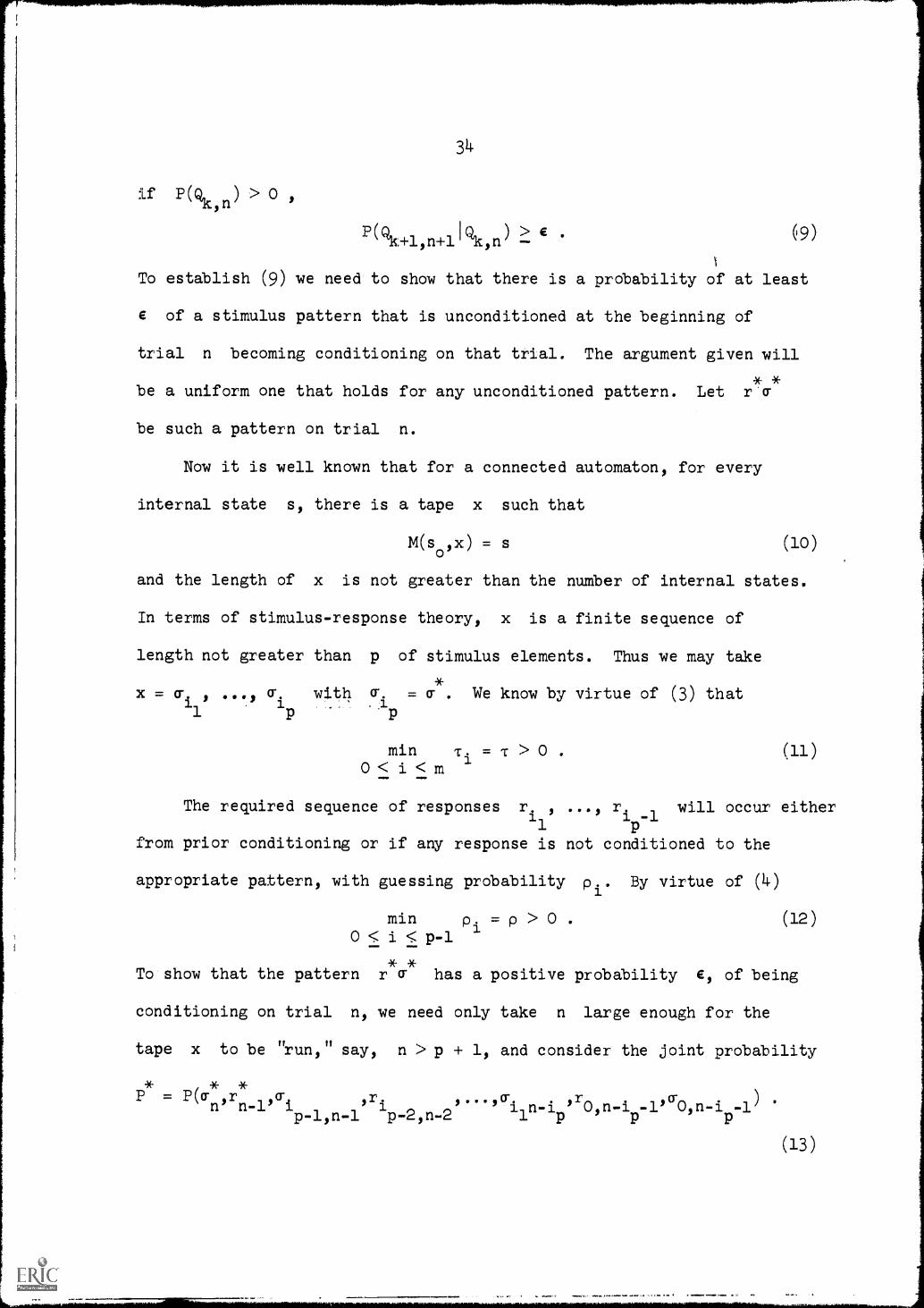
if P(01., ) > 0aln

314-

P(Q.a+1,n+11Q1c1n) e

(9)

To establish (9) we need to show that there is a probability of at least

e of a stimulus pattern that is unconditioned at the beginning of

trial n becoming conditioning on that trial. The argument given will

* *be a uniform one that holds for any unconditioned pattern. Let r'cr

be such a pattern on trial n.

Now it is well known that for a connected automaton, for every

internal state s, there is a tape x such that

M(soIx) = s (10)

and the length of x is not greater than the nunter of internal states.

In terms of stimulus-response theory, x is a finite sequence of

length not greater than p of stimulus elements. Thus we may take

x = cr.6"

T1

with T. = T . We know by virtue of (3) that. 1

1

min Ti = i > 0 .

0 < i < M

The required sequence of responses r. 1 ri will occur either11

from prior conditioning or if any response is not conditioned to the

appropriate pattern, with guessing prdbability pi. By virtue of (4)

min pi p > 0 .

0 i p-1(12)

To show that the pattern r* *

has a positive probability el of being

conditioning on trial n, we need only take n large enough for the

tape x to be vrun," say, n > p + 1, and consider the joint probability

* *P = P(T

n'rn-1, 1

cr

p-10-1 """ i1n-i

p'

r0 n-i

p-1/c1-00-i

p-1)

(13)

35

The basic axioms and the assumptions (1)-(5) determine a lower bound on

P independent of n. First we note that for each of the stimulus

elements To, Ti 9...T 9 by virtue of (3) and (11)

D( *I"Tni4") > ¶9 P(TO n-i

Similarly, from (4) and (12), as well as the response axioms, we know

r

1

*that for each of the responses r r

0' i '

/ * 10 ) > p, .0.) 13(r . IT ) > pn-1 00-1 -1 00-1 -1

P

Thus we know that

P* > ppTp+1

* *and given the occurrence of the event T

nrn-1,

the probability of

conditioning is c, whence we may take

e = cppTp+1

> 0 9

which establishes (9) and completes the proof.

Given the theorem just proved there are several significant corollaries

whose proofs are almost immediate. The first coMbines the representation

theorem for regular languages with that for finite automata to yield:

Oorollary, on Regular Languages. Ara regular language is generated

hy some stimulus-response, model at asymptote.

Once probabilistic considerations are made a fundamental part of the

scene, we can in several different ways go beyond the restriction of

stimulus-response generated languages to regular languages, but I shall

not explore these matters here.

36

I suspect thal; many psychologists or philosophers who are willing

to accept the sense given here to the reduction of finite automata and

regular languages to stimulus-response models will be less happy with

the claim that one well-defined sense of the concepts of intention,

plan and purpose can be similarly reduced. However, without any substantial

new analysis on my part this can be done by taking advantage of an analysis

already made by Miller and Chomsky (1963). The story goes like this.

In 1960 Miller, Galanter and Pribkam published a provocative book

entitled Plans and the Structure of Behavior. In this book they severely

criticized stimulus-response theories for being able to account for so

little of the significant behavior of men and the higher animals. They

especially Objected to the conditioned reflex as a suitable concept

for building up an adequate scientific psychology. It is my impression

that a number of cognitively oriented psychologists have felt that the

critique of S-R theory in this book is devastating.

As I indicated in the introductory section, I would agree that

conditioned reflex experiments are indeed far too simple to form an

adequate scientific basis for analyzing more complex behavior. This

is as hopeless as would be the attempt to derive the theory of

differential equations, let us say, from the elementary algebra of sets.

Yet the more general theory of sets does encompass in a strict mathematical

sense the theory of differential equations.

The same relation may be shown to hold between stimulus-response

theory and the theory of plans, insofar as the latter theory has been

systematically formulated by Miller and Chomsky.5 The theory of plans is

formulated in terms of tote units ("tote" is an acronym fox the cycle

37

test-operate-test-exit). A plan is then defined as a tote hierarchy,

which is just a form of oriented graph, and every finite oriented

graph may be represented as a finite automaton. So we have the result:

Corollary. Any tote hierarchy in the sense of Miller and Chomsky

is isomorphic to some stimulus-response model at asymptote.

5. Representation of Probabilistic Automata

From the standpoint of the kind of learning models and experiments

characteristic of the general area of what has come to be termed prob-

abiltty. learning, there is near at hand a straightforward approach to

probabilistic automata. It is worth illustrating this approachibut it

is perhaps even more desirable to discuss it with some explicitness in

order to show why it is not fully satisfactory, indeed for most

purposes considerably less satisfactory than a less direct approach that

follows from the representation of deterministic finite automata already

discussed.

The direct approach is dominated by two features: a probabilistic

reinforcement schedule and the conditioning of input stithuli rather than

response-stimulus patterns. The main simplification that results from

these features is that the number of states of conditioning and conse-

quently the number of states in the associated Markov chain is reduced.

A two-letter, two-state probabilistic automaton, for example, requires

36 states in the associated Markov chain, rather than 64, as in the

deterministic case. We have, as before, the three stimuli To'

Tl'

and

T2

and their conditioning possibilities, 2 for To

as before, but

now, in the probabilistic case, 3 for T1

and 02' and we also need

38

as part of the state, not for purposes of conditioning, but in order to

make the response-contingent reinforcement definite, the previous

response, which is always either rl or r2. Thus we have

2.3.3.2 = 36, Construction of the trees to compute transition

probabilities for the Markov chain follows closely the logic outlined

in the previous section. We may define the probabilistic reinforcement

schedule by two equations, the first of which is deterministic and plays

exactly the same role as previously:

and

P(e 1,n TI) = 1

P(e I T r .) 71'1,n i,n j,n-1 ij

for 1 < i,j < 2.

The fundamental weakness of this setup is that the asymptotic

transition table representing the probabilistic automaton only holds

in the mean. Even at asymptote the transition values fluctuate from

trial to trial depending upon the actual previous reinforcement, not

the probabilities It. Moreover, the transition table is no longer

the transition table of a Markov process. Knowledge of earlier

responses and reinforcements will lead to a different transition table,

whenever the number of stimuli representing a letter of the input

alphabet is greater than one. These matters are yell known in the

large theoretical literature of probabiLity learning and will not be

developed further here.

For most purposes of application it seems natural to think of

probabilistic automata as a generalization of detexministic automata

39

intended to handle the problem of errors. A similar consideration of

errors after a concept or skill has been learned is common in learning

theory. Here is a simple example. In the standard version of all-or-

none learning, the organism is in either the unconditioned state (U) or

the conditioned state (C). The transition matrix for these states is

C U

C 1 0

U c 1-c

and, consistent with the axioms of Section 3,

P(Correct responseIC) . 1 (1)

P(Correct responsellf) = p (2)

and

P(U1) = 1

i.e., the probability of being in state U on trial 1 is 1. Now by

changing (2) to

P(Correct responseIC) . 1 - e ,

for e > 0, we get a model that predicts errors after conditioning has

occurred.

Without changing the axioms of Section 3 we can incorporate such

probabilistic-error considerations into the derivation of a representation

theorem for probabilistic automata. One straightforward procedure is

to postulate that the pattern sampled on each trial actually consists of

N elements, and that in addition M background stimuli common to all

trials are sampled, or available for sampling. By specializing further

the sampling axioms S1 - S4 and by adjusting the parameters M and

N, we can obtain any desired probability e of an error.

4o

Because it seems desirable to develop the formal results with intended

application to detailed learning data, I shall not state and prove a

representation theorem for probabilistic automata here, but restrict

myself to considering one example of applying a probabilistic automaton

model to asymptotic performance data. The formal machinery for analyzing

learning data will be developed in a subsequent paper,

The example I consider is drawn from arithmetic. For more than

three years we have been collecting extensive data on the arithmetic

performance of elementary-school students, in the context of various

projects on computer-assisted instruction in elementary mathematics.

Prior to consideration of automaton models, the main tools of analysis

have been linear regression models. The dependent variables in these

models have been the mean probability of a correct response to an item

and the mean success latency, The independent variables have been

structural features of items, i.e., arithmetic problems, that may be

objectively identified independently of any analysis of response data,

Detailed results for such models are to be found in Suppes, Hyman

and Jerman (1967) and Suppes, Jerman and B.rian (1968). The main

conceptual weakness of the regression models is that they do not provide

an explicit temporal analysis of the steps being taken by a student in

solving a problem, They can identify the main variables but not connect

these variables in a dynamically meaningful way. In contrast, analysis

of the temporal process of problem solution is a natural and integral

part of an automaton model,

An example that is typical of the skills and concepts encountered

in arithmetic Is column addition of two integers. For simplicity I

shall consider only problems for which the two given numbers and their

sum all have the same number of digits. It will be useful to begin by

defining a deterministic automaton that will perform the desired addition

by outputting one digit at a time reading from right to left, just as

the students are required to do at computer-based teletype terminals.

For this purpose it is convenient to modify in inessential ways the

earlier definition of an automaton. An automaton will now be defined

asastructure ()(= <AZ Z,

M" gso> whereAZ and Z

I 0 I 0

are non-empty finite sets, with A being the set of internal states

as before, 9the input alphabet, and Zo the output alphabet.

Also as before, M is the transition function mapping A X into

A, and so is the initial state. The function Q is the output

function mapping A X Z1 into Z6.

For column addition of two integers in standard base ten

representation, an appropriate automaton is the following:

A = (0,1)

= ((m n). 0 < m,n < 9)I -E

(00 ' 1'9)

0 if m + n + k < 9 .

M(kl(mln))1 if m + n + k > 9, for k = 0,1 .

Q(k,(mln)) = (k + m + n)mod 10 .

so °

Thus the automaton operates by adding first the ones' column, storing

as internal state 0 if there is no carry, 1 if there is a carry,

outputting the sum of the ones'column modulus 10, and then moving on

to the input of the two tens' column digits, etc. The initial internal

state so

is 0 because at the beginning of the problem there is no

ncarry.

n

For the analysis of student data it is necessary to move from a

deterministic to a probabilistic automaton. The number of possible

parameters that can be introduced is uninterestingly large. Each

transition 101(m0)) may be replaced by a probabilistic transition

1 - e and e and each output Q(k(mln)), by ten probabilitiesk$m

$n kono

for a total of2200 parameters. Using the sort of linear regression model

described above we have found that a fairly good account of student

performance data can be obtained by considering two structural variables,

thenumberofcarriesinproblemitethe number of digits

or columns. Let pi be the mean probability of a correct response on

item i and let

1-piz = log

pi

The regression model is then characterized by the equation

zi = ao + aiCi + Di 0 (1)

and the coefficients a0°

a10

and a2

are estimated from the data.

A similar three-parameter automaton model is structurally very

natural. First, two parameters, e and 11 are introduced according to

whether there is a "carry" to the next column.

P(M(k,(mln)) = Olk+m+n < 9) = 1 - e

and

P(M(k,(mln)) = lIk+m+n > 9) = 1 - .

In other words, if there is no1

'carry, the probability of a correct

transition is 1 - e and if there is a "carry the probability of such

a transition is 1 - T. The bhird parameter, is simply the probability

43

of an output error. Conversely, the probability of a correct output is:

P(Q(k,(m,n)) = (k+m-i-n) mod 10) = 1 - y

Consider now problem i with C. carries and D. digits. If we

ignore the probability of two errors leading to a correct responsee.g.,

a transition error followed by an output errorthen the probability of a

correct answer is just

D. C. D.-C,-1P(Correct Answer to Problem i) = (1-7) 1(1-TI)

i(l_e)(2 )

As already indicated it is important to realize that this equation is an

approximation of the "true" probability. However, to compute the exact

probability it is necessary to make a definite assumption about how the

probability y of an output error is distributed among the 9 possible

wrong responses. A simple and intuitively appealing one-parameter model

is the one that arranges the 10 digits on a circle in natural order with

9 next to 0, and then makes the probability of an error j steps to

the right or left of the correct response 6j. For example, if 5 is

the correct digit, then the probability of responding 4 is b, of 3

is s2

, of 2 is 63

, of 1 is 64

, of 0 is 65

, of 6 is b, of

7 is 62

etc. Thus in terms of the original model

y = 2(5 + 52 + 53 + 54) + 55 .

Consider now the problem

.th . .

Then,whered,..the digit response,

P(d1=2) = (1-y)

P(d2=6) = (1-y)(1-11) + i .

Here the additional term is TI6, because if the state entered is 0 rather

44

than 1 when the pair (7,5) is input, the only way of obtaining a correct

answer is for 6 to be given as the sum of 0 + 4 + 1, which has a

probability B. Thus the probability of a correct response to this

prdblem is (1-7)[(1-7)(1-T1) + T16]. HereaPter we shall ignore the

T16 (or es) terms.

Returning to equation (2) we may get a direct comparison with the

linear regression model defined by equation (1), if we take the logarithm

of both sides to obtain:

log pi = Di log (1-7) + C. log (1-n) + (Di-Ci-1) log (1-e) (3)

and estimate log 1-7, log 1-n, and log 1-e by regression with the

additive constant set equal to zero. We also may use some other approach

to estimation such as minimum X2

or maximum likelihood. An analytic

solution of the standard maximum-likelihood equations is very messy

indeed, but the maximum of the likelihood function can be found

numerically.

The automaton model naturally suggests a more detailed analysis of

the data. Unlike the regression model, the automaton provides an

immediate analysis of the digit-by-digit responses. Ignoring the

66-type terms, we can in fact find the general maximum-likelihood

estitates of 7, e, and T1 when the response data are given in this

more explicit form.

Let there be n digit responses n a block of problems. For

1 < i < n let x. be the random variable that assumes the value 1 if

the ith

response is correct and 0 otherwise. It is then easy to see that

if i is a oneS';-column digit

p(I = 1 ) =(1-7)(1-6) if it is not a oneS' column and there is no

.thcarry to the digit

if there is a carry to the ith digit

45

granted that ce-type terms are ignored. Similarly for the same three

alternatives

qx,I. = 0) - (1-7)(1-6)

- (1-7)(1.-T1) .

So for a string of actual digit responses x1

. xn

we can write

the likelihood function as:

(1-) e[1-(1-7)(1-nflf (4)

where a = number of correct responses, b = number of incorrect responses

in the ones' column, c = number of correct responses not in the ones'

column when the internal state is 0, d = number of correct responses

when the internal state is 1, e = number of incorrect responses not

in the ones' column when the internal state is 0, and f = number of

incorrect responses when the internal state is 1. It is more convenient

to estimate 7' = 1 - 7, e = 1 - E, and n' = 1 - T. Making this change,

takini the log of both sides of (4) and differentiating with respect to

each of the variables, we obtain three equations that determine the maximum-

likelihood estimates of 7

a

1-7

e' and 11'.

ee1-7 e

e77r

y'= "0" 1757r-iT = 0

d

TIT

f7'

1 - 11

= 0

fni

1-7 nr = 0

Solving these equations, we obtain as estimates:

a-c-d?it _

afb-c-d '

46

c(a+b-c-d)(c+e)(a-c-d)

d(a+b-c-d)(d+f)(a-c-d)

The most interesting feature of these estimates is that y' is just the

ratio of correct responses to total responses in the ones' column.

The two equations that yield estimates of e

transparent if they are rewritten:

(1-y)(1-e) 7,e' .c+e

(1-y)(1- n) = 7,n, d

d+f

and T1' are especially

Additional analysis of this example will not be pursued here. I do

want to note that the internal states 0 and 1 are easily exter-

nalized as oral responses and most teachers do indeed require such

externalization at the beginning.

To many readers the sort of probabilistic automaton just analyzed

will seem far removed from the sort of device required to account for

language behavior. Certainly the automata that are adequate to

analyze arithmetic are simpler in structure than what is needed even

for the language output of a two-year old child. What I wanted to

illustrate is how we can bear down on detailed analysis of data with

specific automaton models. Hopefully, we shall in the future be able

to move to an equally detailed analysis of child language behavior,

but I have no illusions about the difficulty of the problems yet to be

solved.

References

Chomsky, N. Aspects of the theory )f syntax. Cambridge, Mass.:

M.I.T, Press, 1965,

Chomsky, N. Formal properties of grammars. In P. D. Luce, R. R. Bush,

& E. Galanter (Eds.), Handbook of mathematLcal psychology. Vol. II.

New York: Wiley, 1963. Ch. 12.

Chomsky, N, Syntactic structures, The Hague: Mouton, 1957,

Estes, W. K., & Suppes, P. F.Dundations of statistical learning theory,

II. The stimulus sampling model, Tech, Rept. No. 26, October 22,

1959, Stanford University, Institute for Mathematical Studies in

the Social Sciences,

Katz, J. J. & Postal, P. M. An integrated theory of linguistic

descriptions. Cambridge, Mass,: M,I.T. Press, 1964.

Kleene, S. C. Representation of events in nerve nets and finite

automata. In C. E. Shannon and J. McCarthy (Eds.), Automata

studies, Princeton, N. J.: Princet ,n University Press, 1956.

Pp. 3-41.

Millenson, J. R. An isomorphism between stimulus-xesponse notation

and information processing flow diagrams, The Psychological

Record, 1967, 17, 305-319.

Miller, G. A.5 & Chomsky, N, Finitary models of language users,

In P, D. Luce, R. R. Bush, & E. Galanter (Eds.), Handbook of

mathematical psychology. Vol. II. New York: Wiley, 1963. Ch. 13.

Miller, G. A. Galanter, E., & Pribram, K, H, Plans and the stnicture

of behavior, New York: Holt, 1960.

48

Neimark, E.; &Estes, W. K. Stimulus sampling theory. San Francisco:

Holden-Day, 1967.

Rabin, M. O. Prdbabilistic automata. Information and Control, 1963,

6, 230-245. Reprinted in E. F. Moore (Ed.), Sequential machines.

Reading, Mass.: Addison-Wesley, 1964. Pp. 98-114.

Rabin, M. 0., & Scott, D. Finite automata and their decision problems.

IBM Journal of Research and Development, 1959, 3, 114-125.

Reprinted in E. F. Moore, (Ed.), Sequential machines. Reading,

Mass.: Addison-Wesley, 1 964. Pp. 63-91.

Skinner, B. F. Verbal behavior. Ney York: Appleton, 1957.

Suppes, P., & Atkinson, R. C. Maxkov learning models for multiperson

interactions. Stanford: Stanford University Press, 1960.

Suppes, P., Hyman, L., & Jerman, M. Linear structural models for

response and latency performance in arithmetic on computer-

controlled terminals. In J. P. Hill (Ed.), Minnesota Symposia

on Child Psycholo_EL. Minneapolis: Univexsity of Minnesota Press,

1967. Pp. 160-200.

Suppes, P., Jerman, M., & Brian, D. Computer-assisted instruction:

Stanford's 1965-66 arithmetic program. New York: Academic Press,

1968.

Footnotes

1This research has been partially supported by the National Science

Foundation and the U. S. Office of Education. I am indebted to

Kenneth N. Wexler for a number of helpful comments on the manuscript.

2Indeed, Phoebe C. E. Diebold and Ebbey Bruce Ebbesen have already

successfully trained two pigeons. Sequences of several hundred responses

are easily obtained, and the error rate is surprisingly low--well under

one per cent. We are now tackling the training schedule of a three-

state automaton.

3Exactly such a proceduie has proved very successful in the pigeon

experiments with Diebold and Ebbesen mentioned in footnote 2.

4Two other points a:bout the definition are the following. First,

in this definition and throughout the rest of the article ec, is the

reinforcement of response r and not the null reinforcement, as in

Section 3. This conflict arises from the different notational conventions

in mathematical learning theory and automata theory. Second, strictly

speaking I should write (2CF(j) because F is not uniquely determined

by j.

5After this was written Gordon Bower brought to my attention the

article by Millenson (1967) that develops this point informally.

(Continued from inside front cover)

91 P. Suppes. Infcemation processing and choice behavice. January 31,1966.

92 G. Groen and R. C. Atkinson. Models for optimizing the learning process. February 11, 1966. (Psycho!. Bulletin, 1966, 66, 309-320)

93 R. C. Atkinson and D. Hansen. Computer-assisted instruction in Initial reading; Stanfced project. March 17, 1966. (Reading Research

Quarterly, 1966, 2, 5-25)94 P. Suppes. Probabilistic inference and the concept of total evidence. March 23,1966. (In J. HIntikka and P. Suppes (Eds.), Aspects of

Inductive Logic. Amsterdam North-Holland Publishing Co. , 1966. Pp. 49-65.95 P. Suppes. The axiomatic method in high-school mathematics. Apr1112,1966. (The Role of AxIomatics and Problem Solving in Mathematics.

The Conference Board of the Mathematical Sciences, Washington, D. C. Ginn and Co. , 1966. Pp. 69-76.

96 R. C. Atkinson, J. W. Breisford, and R. M. Shiffrin. Multi-process models foe memory with applications to a continuous presentation task.

Apr1113,1966. (J. math. Psychol., 1967, 4, 277-300 ).97 P. Suppes and E. Croihers. Some remarks on stimulus-response theories of language learning. June 12, 1966. ,

98 R. Bjork. All-or-none subprocesses in the Itwning of complex sequences. (J. math. Psychol., 1968, 1, 182-195).

99 E. Gammon. The statistical determination of linguistic units. July 1,1966.100 P. Suppes, L. Hyman, and M. Jerman. Linear structural models for response and latency perfcemance in arithmetic. On J. P. Hill (ed.),

Minnesota Symposia on Child Psychology. Minneapolis, Minn.:1967. Pp. 160-200).

101 J. L. Young, Effects of intervals between reinforcements and test trials in paired-associate learning. August 1,1966.102 H. A. Wilson. An investigation of linguistic unit size in memory processes. August 3, 1966.

103 J. T. Townsend. Choice behavior in a cued-recognition ttA. August 8,1966.104 W. H. Batchelder. A mathematical analysis of multi-level verbal learning. August 9, 1966.

105 H. A. Taylor. The observing response In a cued psychophysical task. August 10, 1966.

106 R. A. Mork . Learning and shcet-term reention of paired associates in relation to specific sequences of Interpresentation Intervals.

August 11,1966.

107 R. C. Atkinson and R. M. Shiffrin. Some Two-process models for memey. September 30,1966.

108 P. Suppes and C. Ihrke. Accelerated program In elementary-school mathematicsthe third yew. January 30, 1967.

109 P. Suppos and I. Rosenthal-Hill. Concept formation by kindergarten children In a card-sorting task. February 27,1967.

110 R. C. Atkinson and R. M. Shiffrin. Human memory: a proposed system and Its control processes. March 21,1967.

III Theodore S. Rodgers. Linguistic considerations In the design of the Stanford computer-based curriculum In Initial reading. June 1, 1967.

112 Jack M. Knutson. Spelling drills using a computer-assisted Instructional system. June 30,1967.

113 R. C. Atkinson. Instruction in initial reading under computer control: the Stanfced Project. July 14, 1967.

114 J. W. Brelsfced, Jr. and R. C. Atkinson. Recall of paired-associates as a function of overt and covert rehearsal procedures. July 21,1967.

115 J. H. Stelzer. Some results concerning subjective probability structures with umiceders. August 1,1967I 16 D. E. Rumelhart. Th. effects of interwesentation Intervals on performence in a continuous paired-associate task. August 11,1967.

117 E. J. Fishman, L. Keller, and R. E. Atkinson. Massed vs. distributed practice in computerized spelling drills. August 18, 1967.

118 G. J. Groen. An Investigation of some counting algorithms fce simple addition problems. August 21,1967.

119 H. A. Wilson and R. C. Atkinson. Computer-based instruction in initial reading: a progress report on the Stanford Project. August 25,1967.

120 F. S. Roberts and P. Swops. Some problems In the geometry of visual perception. August 31,1967. (Synth's., 1967, 17,173-201)121 D. Jamison, Bayesian decisions under total and partial Ignorance. D. Jamison and J. Kozlelocki. Subjective probabilities under total

uncertainty. September 4, 1967.122 R. C. Atkinson. Computerized Instruction and the learning process. September 15, 1967.

123 W. K. Estes. Outline of a thecey of punishment. October 1, 1967.124 T. S. Rodgers. Measuring vocabulary difficulty: An analysis of item vwlables In learning Russian-English and Japanese-English vocabulwy

parts. December 18,1967.125 W. K. Estes. Reinforcement in human learning. December 20,1967.

126 G. L. Wolford, 0, L, Wessel, W, K. Estes, Further evidence concerning scanning and sampling assumptions of visual detection

models, January 31,1968,

127 R. C. Atkinson and R, M. Shiffrin, Some cpeculations on storage and retrieval processes in long-term memory, February 2,1968,

128 John Holmgren, Visual detection wfth imperfect recognition, March 29,1968,129 Lucille B. Mlodnosky. The Frostig and the Bender Gestalt as predictors of reading achievement. April 12,1968,

130 P. Suppes. Information crocessing and choice behavior. April 15, 1968, (In I. Lakatos and A, Musgrave (Eds.), Problems in thePhilosophy of Science. Amsterdam; North-Holland Publishing Co,, 1968. Pp. 278-304)

131 G. M. Olson. Learning and retention in a continuous recognition task, May 15, 1968,132 Ruth Norene Hartley, An investigation of fist types and cues to facilitate initial reading vocabulary acquisition. May 29, 1968,133 P. Suppes. Stimulus-response theory of finite automata, June 19, 1968.