Embed Size (px)
Citation preview

AN ABSTRACT OF THE THESIS OF
Witoon Kittidacha for the degree of Doctor of Philosophy in Chemical Engineering
presented on June 2. 2004.
Title: Numerical Study of Mass Transfer Enhanced by Theromocapillary Convection in a
2-D Microscale Channel.
Abstract approved:
Jovanovic
The effect of unsteady thermocapillary convection on the mass transfer rate of a
solute between two immiscible liquids within a rectangular microscale channel with
differentially heated sidewalls was numerically investigated. A computational fluid
dynamic code in Fortran77 was developed using the finite volume method with Marker
and Cell (MAC) technique to solve the governing equations. The discrete surface
tracking technique was used to capture the location of the moving liquid-liquid interface.
The code produced results consistent with those reported in published literature.
The effect of the temperature gradients, the aspect ratio, the viscosity of liquid,
and the deformation of the interface on the mass transfer rate of a solute were studied.
The mass transfer rate increases with increasing temperature gradient. The improvement
of the mass transfer rate by the thermocapillary convection was found to be a function of
the Peclet number (Pe). At small Pe, the improvement of the mass transfer rate increases
with increasing Pe. At high Pe, increasing the Pe has no significant effect on increasing
Redacted for privacy

the mass transfer rate. Increasing the aspect ratio of the cavity up to 1 increases the mass
transfer rate. When the aspect ratio is higher than 1, the vortex moves only near the
interface, resulting in decreasing the mass transfer rate. By increasing the viscosity of the
liquid in top phase, the maximum tangential velocity at the interface decreases. As a
result, the improvement of the mass transfer rate decreases. The deformation of the
interface has no significant effect on the improvement of the mass transfer rate.
By placing the heating source at the middle of the cavity, two steady vortices can
be induced in a cavity. As a result, the mass transfer rate is slightly enhanced than that in
the system with one vortex. By reversing the direction of the temperature gradient, the
mass transfer rate decreases due to the decrease in the velocity of bulk fluid. The
thermocapillary convection also promotes the overall reaction process when the top wall
of the cavity is served as a catalyst.

© Copyright by Witoon KittidachaJune 2, 2004
All Rights Reserved

Numerical Study of Mass Transfer Enhanced by
Theromocapillary Convection in a 2-D Microscale Channel
by
Witoon Kittidacha
A THESIS
submitted to
Oregon State University
In partial fulfillment of
the requirements for the
degree of
Doctor of Philosophy
Completed June 2, 2004
Commencement June 2005

Doctor of Philosophy thesis of Witoon Kittidacha presented on June 2.. 2004.
APPROVED:
Major Professor, represñting Chemical Engineering
Head of the Department of Chemical Engineering
Dean of Graduate Schoci
I understand that my thesis will become part of the permanent collection of Oregon
State University libraries. My signature below authorizes release of my thesis to any
reader upon request.
Witoon Kittidacha, Author
Redacted for privacy
Redacted for privacy
Redacted for privacy
Redacted for privacy

ACKNOWLEDGEMENT
I would like to express my appreciation to my major professor, Dr. Goran N.
Jovanovic and my co-advisor, Dr. Ajoy Velayudhan for their support, patience and
technical advice while doing this study. My special thanks also go to Dr. Wassana
Yantasee and Dr. Eric Henry for reading and correcting the body of this thesis.
I would like to thank my mother and family for their encouragement and
support. Whenever I felt tired, they were always there for me. Special thanks to all my
friends at the Chemical Engineering Department. They all have made me feel like I am
at home while I am working here.
Special thanks are also extended to all professors for their dedication to
students.

TABLE OF CONTENTS
1. INTRODUCTION........................................................... 1
2. LITERATURE REVIEW AND OBJECTIVES......................... 5
2.1 Literature Review....................................................... 5
2.2 Objectives................................................................ 11
3. MATHEMATICAL MODEL ............................................. 13
3.1 Configuration............................................................ 13
3.2 Scaling .................................................................... 15
3.3 Governing Equations ................................................... 16
3.4 Boundary Conditions at Walls ......................................... 17
3.5 Boundary Conditions at the Interface................................. 18
3.5.1 Thermal Balance ................................................ 183.5.2 Concentration Balance ......................................... 193.5.3 Stress Balance................................................... 19
3.5.3.1 Normal Stress Balance .................................... 203.5.3.2 Tangential Stress Balance ................................. 21
3.5.4 Kinematic Condition........................................... 223.5.5 Global Mass Conservation .................................... 23
4. BASIC METHODOLOGY AND ALGORITHM....................... 25
4.1 Control Cells, Nodes, and Cell Faces withStaggered Grid Arrangement .......................................... 25
4.2 Interface Marker Points................................................. 28
4.3 Interface Control Cells.................................................. 30
4.4 Solving Kinematic Equation ........................................... 30

TABLE OF CONTENTS (Continued)
Page
4.5 Conservation Equation for the General Variable q$ ............... 32
4.6 Solving the Continuity Equation andthe Momentum Equation................................................ 45
4.7 Solving Balance Equations at the Interface.......................... 49
4.7.1 Thermal Balance................................................ 504.7.2 Concentration Balance......................................... 504.7.3 Normal Stress Balance......................................... 514.7.4 Tangential Stress Balance..................................... 52
4.8 Global Mass Conservation Constraint ................................ 53
4.9 Algorithm................................................................. 53
5. PROGRAM VALiDATION................................................ 55
5.1 Sensitivity Analysis ...................................................... 55
5.1.1 Mesh Sensitivity Analysis..................................... 555.1.2 Time Step Sensitivity Analysis............................... 57
5.2 Steady State Analysis ................................................... 57
5.3 Consistency Analysis................................................... 59
5.3.1 One Layer with Flat Interface at Steady State............... 595.3.2 One Layer with Deformable Interface at Steady State 645.3.3 One Layer with Deformable Interface at Unsteady State 695.3.4 Two Layers with Flat Interface at Steady State ............. 695.3.5 Comparison with the Experimental Results .................. 71
6. RESULTS AND DISCUSSIONS .......................................... 73
6.1 Effects of the Temperature Differences along the Interface ........ 73
6.2 Effects of the Aspect Ratio of the Cavity.............................. 85
TABLE OF CONTENTS (Continued)
Page
6.3 Effects of the Viscosity of the Liquid in Phase 2 ..................... 93
6.4 Effects of the Capillary Number (Ca).................................. 94
6.5 Case No. 1: Location of High Temperature is In the Middleofthe Cavity............................................................... 97
6.6 Case No. 2: Unsteady Temperature at Both Walls.................... 99
6.7 Case No. 3: Reaction at the Top Wall.................................. 106
7. Conclusions and Recommendations for Future Study..................... 110
7.1 Conclusions ................................................................. 110
7.2 Recommendations for Future Study..................................... 113
BIBLIOGRAPHY ................................................................... 114
APPENDICES ........................................................................ 118
Appendix A: Properties of Water and Hexane.............................. 119Appendix B: Order of Convergence and Richardson Extrapolation 120

LIST OF FIGURES
Figure Page
3.1 Geometry and coordination of the system.............................. 13
3.2 Stress components on the cross-sectional view of a controlvolume with an interface liquid of thickness 1.......................... 20
3.3 Contact angles of the interface at the sidewalls ........................
4.1 Control cells, nodes, cell faces with staggered grid arrangement.
4.2 Marker points, interfacial segments, full cells, interfacial cells,and partner cells .............................................................
4.3 Wave and droplet interface ................................................
4.4 Outward fluxes at w-, s-, e-, ne-face, and the interface ofthe control cell P............................................................
24
26
29
29
34
4.5 Trapazoidal region and six points stencil used in thetwo dimensional linear quadratic interpolation.(a) for computing at ne-face (b) for computing at w-face ............ 40
4.6 Three points stencil used in the one-dimensional quadraticinterpolation for both u and Une ......................................... 40
4.7 Normal and tangential probe for evaluation of the gradientat the interface ............................................................. 44
4.8 The algorithm ............................................................... 54
5.1 (a) Tangential velocity at the interface(b) Temperature at the interface, for the case withPr1,Re=100,A=1 .................................................. 61
5.2 (a) Tangential velocity at the interface(b) Temperature at the interface, for the case withPr1,Re=1,000,A=1 ................................................ 62

LIST OF FIGURES (Continued)
Figure Page
5.3 (a) Streamlines at equal increments with = 0.0048
(c) Isoterms, for the case with Pr 1, Re = 1,000, A = 1 ........... 63
5.4 Streamlines contour for fixed contact height with Ma = 1,Re=5,A=0.2,Ca=0.32,andBi=1 ................................. 66
5.5 Interface height for fixed contact height with Ma = 1,Re=5,A=0.2,Ca=0.32,andBi=1 ................................ 67
5.6 Streamfucntion at midplane for fixed contact height withMa=1,Re=5, A=0.2,Ca=0.32,andBi=1 ..................... 67
5.7 Interface height for fixed 90° contact angle with Ma = 1,Pr = 0.2, A = 0.2, and Ca = 0.04....................................... 68
5.8 Streamfucntion at midplane for fixed 90° contact angle withMa = 1, Pr = 0.2, A = 0.2, and Ca 0.04 .............................. 68
5.9 The time history at h(1) for Ma = 2, Re= 10, A = 0.2,Ca=0.1, and Q=0.1 ...................................................... 70
5.10 Steady characteristic velocity at midplane for Pr = 7.5,Ma=500,A=1/3 .......................................................... 70
5.11 Steady-state scaled horizontal velocity at midplane forPr 13.9, Ma350,A=0.2 ............................................ 72
6.1 Total relative mass in phase 1 (Mj) versus time atD= 109m2/sec,A=0.5 ................................................ 76
6.2 Total relative mass in phase 1 (M1) versus time atD= 1010m2/sec,A=0.5 ................................................ 77
6.3 Total relative mass in phase 1 (M1) versus time atD= 10h1 m2/sec,A=0.5 ................................................ 78
6.4 Streamlines at steady state for AT' = 0.05 °C,D =1x10⁹m2/s,A=0.5 ................................................ 81

LIST OF FIGURES (Continued)
Figure
6.5 Concentration plot for pure diffusion case with
D =1x10⁹m2/s,A5=0.5,Mj= 1.5 .................................... 81
6.6 Concentration plot for AT' = 0.05 °C,
D =1x10⁹m21s,A5=0.5,Mj= 1.5 at 1.3 s ........................... 82
6.7 Concentration plot for AT' 0.5 °C,
D=1xl0m2Is,A5=0.5,Mi=1.5at0.4s ........................... 82
6.8 Concentration plot for AT' = 1.0 °C,
D =1x10⁹m2/s,A5=0.5,M1= 1.5 at 0.3 s ........................... 83
6.9 Concentration plot for AT' = 5.0 °C,D = 1x10m2/s,A5= 0.5, M1= 1.5 at 0.2s ............................ 83
6.10 A plot of t99% /t%d..jofl versus Pei at three levels
of diffusion coefficient, A5 = 0.5 .......................................... 87
6.11 Plots of t99% / t99%dsion versus Pe1 at three levels of aspect ratio.... 90
6.12 (a) Streamlines and (b) Concentration plot, for A5 = 1.0,AT' = 1.0°C, D =1x10⁹m2/s , Mj= 1.5 .............................. 91
6.13 (a) Streamlines and (b) Concentration plot, for A5 2.0,AT'=l.O°C, D =1x10⁹m2/s,Mj=1.5.............................. 92
6.14 Interface height at three levels of Ca, D = lx 109m2/s,A5=0.5, AT'=O.l°C ..................................................... 95
6.15 Total relative mass in phase 1 versus time at different Ca,
D =1x10⁹m2/s,A5=0.5, AT'=O.l°C............................... 96
6.16 (a) Streamlines, (b) Concentration plot atM1 = 1.5, A, = 2.0,D = lx 10m2/s, AT' = 0.1°C when T is imposed atthe middle of the cavity................................................... 98

LIST OF FIGURES (Continued)
Figure Page
6.17 Temperature at left and right wall versus time ........................ 100
6.18 Plots of total relative mass in phase 1 versus time forfixed and varied wall temperature ....................................... 101
6.19 Transient velocityplot atA= 1.0, D = 1x10m2/s, AT' = 0.1°CAfter the temperature gradient reverses, (a) after 0.0005 s,(b) after 0.001 s, (c) after 0.0015 s, and (d) after 0.002 s ............ 103
6.20 Plots of total relative mass in phase 1 versus time forfixed and reversed temperature gradient............................... 105
6.21 Plots of total relative mass in phase 1 versus time forcases with the reaction at the top wall ................................... 108
6.22 Plots of total relative mass in phase 2 versus time forcases with the reaction at the top wall ................................... 109

LIST OF TABLES
Table ig2.1 Summary of problem characteristics, interface-tracking
techniques, type of field variables, and numerical methods .......... 7
4.1 Definition of q5, DG, and, S for each conservation equation ........ 34
5.1 Values of dimensionless groups in each phase ......................... 56
5.2 Order of convergence and average percentage relative errorin mesh sensitivity analysis ............................................... 58
5.3 Order of convergence and average percentage relative errorin time sensitivity analysis ................................................. 58
5.4 Values of dimensionless groups and mesh size......................... 59
6.1 Temperature differences along the interface used ateach level of diffusion coefficient......................................... 74
6.2 The parameter t and the ratio of t99% / t99%, dsion at
various values ofPe1 with A = 0.5 ........................................ 86
6.3 Maximum tangential velocity at the interface and t atvarious viscosities in phase 2 ................................................ 93

TABLE OF APPENDICES
Appendices ............................................................................... 118
Appendix A: Properties of Water and Hexane.............................. 119
Appendix B: Order of Convergence and Richardson Extrapolation ...... 120

NUMERICAL STUDY OF MASS TRANSFER ENHANCED BY
THERMOCAPILLARY CONVECTION IN A 2-D MICROSCALE CHANNEL
1. INTRODUCTION
Micromachining techniques, such as photochemical micromachining, wet
etching, and photolithography, have been introduced in the semiconductor industry.
These techniques enable the development of novel devices for performing traditional
chemical processes at miniaturized scales. Micron size channels can be fabricated
within metal, ceramic, or plastic substrates. At such small scales of the channels, the
distances for heat and mass transfer can be substantially reduced, leading to fast
transport rates that result in very short residence times and high throughput per unit
volume of the device. In addition, because of their compact size, the microscale
devices are often portable, making them suitable for personal uses in military or
medical applications. Unlike the development of conventional hardware, which
requires scale-up from bench-scale and pilot devices, all microscale devices are built
and tested at their actual size. If a greater throughput is required, more units of
identical dimensions can be added in a parallel to an existing structure. Chemical unit
operations such as heat exchangers, reactors, separators, and actuators can be
miniaturized and potentially integrated to reduce the total size of the systems.
In a microscale channel, thermocapillary forces, which are negligible in
macroscale systems, become dominant. The thermocapillary force is generated by
surface tension gradient at the fluid-fluid interface arising from the temperature

2
gradient. The surface tension is inversely proportional to temperature; as a point on an
interface experiences higher temperature, the surface tension at that point decreases.
This creates surface tension gradient, and the interface having the lower surface
tension is forced away laterally. The momentum caused by the interface movement is
transferred to the bulk of the fluid. The convective motion driven by thennocapillary
force is called "Marangoni Convection" or "Thermocapillary Convection".
Thermocapillary convection plays an important role in many different
industrial processes such as the motion in welding pools and in crystal growth melts at
low-gravity conditions. In the crystal growth process, thermocapillary convection is
undesirable because the movement in crystal growth melts creates imperfections.
However, in some processes, the movement caused by thermocapillary convection is
attractive because it promotes the mixing of fluids such as in liquid-liquid extraction.
Two mechanisms may promote the mass transfer rate between two immiscible fluids
in a microchannel liquid-liquid extractor. First, because the microscale channel that
houses two immiscible fluids contacting each other is smaller than the usual mass
transfer boundary layer, the mass transfer resistances between the two phases are
reduced, increasing the mass transfer rate. Second, since the thermocapillary
convection creates the mixing within each fluid phase, the concentration gradients
across the interface increases, resulting in an additional increase of the mass transfer
rate. As a result, the overall mass transfer rate can be significantly enhanced and the
residence time can be substantially reduced.
The goal of this research was to study the effects of the thermocapillary
convection on the mass transfer rate of a solute between two immiscible liquids within

a microscale channel. In this study we developed a computational fluid dynamic
(CFD) code, written in Fortran77 that served as an investigative tool. A finite volume
with marker and cell (MAC) method was utilized to solve mass, momentum, and
energy conservation equations in two dimensions. A discrete surface tracking
technique was used to determine the location of the moving fluid-fluid interface. The
normal and tangential stresses were balanced at the deformable interface to calculate
the interfacial velocities induced by the temperature gradient. Conservation of mass of
the solute that transfers across the interface was also incorporated into the model to
determine the changes in the concentration of solute in each phase as well as the
overall mass transport process. The code produced results that were second-order
accurate in space and first-order accurate in time. Compared to other methods used to
solve the same problem, this method is simpler and easier to be adapted for three-
dimensional problems.
The CFD code developed in this work is served as a preliminary tool to prove
that the thermocapillary convection can increase the mass transfer rate of a solute
between two immiscible liquids within of a microchannel liquid-liquid extractor,
resulting in reduced residence time. With this simulation tool, the fluid velocities and
flow pattern induced by the temperature differences along the interface can be
observed closely and the themocapillary convection phenomena in a microscale
channel can be studied. For operational purposes, the simulation tools may be used to
optimize the system parameters such as the geometry of the channel, the physical
properties of the liquids, the temperature difference along the interface, etc.

4
This numerical study was organized into seven chapters with Chapter 1 as the
Introduction. In Chapter 2, a literature review examines appropriate numerical
methods and techniques to solve the problem. Chapter 3 discusses the configuration of
a cavity, the governing equations, the boundary conditions at the walls, and the
balance equations at the interface. Complete details of numerical methods and
techniques used to solve the problems are illustrated in chapter 4. In Chapter 5,
sensitivity analyses of mesh size and time step size are presented. To validate the
usefulness of this computer code, the results obtained from the code are compared
with those from selected publications having the same input parameters. The effects of
the temperature difference along the interface, the geometry of the cavity, the viscosity
of liquids, and the deformable interface on the overall mass transfer rate are discussed
in Chapter 6. The simulations of three selected cases are also presented in this chapter.
The first case investigates a situation where the heat source is located at the middle of
the cavity. The second case investigates a situation where temperature is varied along
the walls of the cavity. Finally, Chapter 7 is the conclusions and the recommendations
for future work.

5
2. LITERATURE REVIEW AND OBJECTIVES
2.1 Literature Review
Thermocapillary convection is an important factor in many industrial processes
such as welding, crystal growth, and material processing. Thus a complete
understanding of the thermocapillary convection phenomena is necessary for the
control and optimization of these processes. Reviews and investigations on the
thermocapillary problems were presented by Ostrach (1982) and Davis (1987). Colinet
et al. (1999) provided a recent review about the industrial relevance studies in the
surface tension driven flow. This literature review focuses on the numerical methods
of solving thermocapillary problems with moving interface.
In early years, the thermocapillary convection problems were analyzed using
approximations approaches to obtain analytical models. For example, Pearson (1958)
used a small disturbance analysis or linear stability analysis to solve a problem of
infinite homogeneous liquid layer having a uniform thickness. Scriven and Sternling
(1964) considered a two-layer model in which each layer had an infinite depth and
also examined the local behavior of the system near the interface. Levich (1962) used
the lubrication approximations to simplify the analyses of the steady thermocapillary
flows in thin horizontally unbounded regions. Yih (1968) extended the similar analysis
to the three-dimensional motion and so did Adler and Sowerby (1970). Sen and Davis
(1982) developed analytical solutions for streamfunction and temperature at the mid

ri
plane and for the interfacial shapes using an asymptotic theory valid for -* 0,
where is the aspect ratio of a cavity.
With the advanced computational fluid dynamic techniques and computer
technology, the thermocapillary convection problems are studied numerically in
different flow configurations. Leypoldt et al. (2000) conducted the numerical studies
of thermocapillary flows in cylindrical liquid bridges, which are held between two
coaxial circular disks at different temperatures. Lai and Yang (1990) also studied the
unsteady-state thermocapillary flow with a deformable free interface in rectangular
liquid bridges by fixing the temperature at one end and sinusoidally varying at the
other end. Vertical Bridgman crystal growth was investigated by Liang and Lan
(1996). However, this review will focus on only the problems with thermocapillary
convection in a rectangular cavity having differentially heated sidewalls. Table 2.1
shows the summary of the characteristics of the problems, the interface-tracking
techniques, the type of field variables, and the numerical methods used to solve field
equations.
The free surface between a liquid layer and a gas layer or the interface between
two liquid layers is assumed to be flat, an assumption justified when the capillary
number is small. The capillary number is a dimensionless parameter for measuring the
free surface deformation (Zebib et al., 1985). With this assumption, the numerical
simulation is simplified remarkably (Rivas, 1991).

Table 2.1 Summary of problem characteristics, interface-tracking techniques, types of field variables, and numerical methods
Authors Dimensions Numberof fluidlayers
Timedependency
Interfacedeformation
Interfacetrackingtechnique
Type offieldvariables
Numericalmethod
Riva (1991) 2D 1 No Flat N/A Primitive Finite volumeXu and Zebib (1998) 2D 1 Yes Flat N/A 0) Finite volumeZebib et al. (1985) 2D 1 No Flat N/A Primitive Finite differenceChen et al. (1990) 2D 1 No Deformable Mapping -0) Finite differenceChen et al. (1991) 2D 1 Yes Deformable Mapping Finite differenceLabonia et al. (1997) 2D 1 No Deformable Mapping vw Finite volumeSasmal and Hochstein(1994)
2D 1 No Deformable VOF Primitive Finite volume
Lu (1994) 2D 1 No Deformable Adaptive Primitive Finite elementHamed and Floryan(1998)
2D 1 Yes Deformable Mapping Finite difference
Peltier et al. (1995) 2D 2 Yes Flat N/A Primitive Finite differenceFontaine and Sani(1996)
2D 2 No Deformable Adaptive Primitive Finite element
Saghir (1999) 2D 2 No Deformable Adaptive Primitive Finite elementWang and Kahawita(1996)
2D 2 Yes Flat N/A Primitive Finite difference
Liu et al. (1998) 2D 2 No Flat N/A Primitive Finite differenceBabu and Korpela(1990)
3D 1 No Flat N/A Primitive Finite difference
Bebnia et al. (1995) 3D 1 No Flat N/A Primitive Finite differenceSa3 et al. (1996) 3D 1 No Flat N/A Primitive Finite difference

Floryan and Rasmussen (1989) reviewed numerical algorithms for the analysis
of viscous flows with moving interfaces. Such algorithms may be based on Eulerian,
Lagrangian, or mixed formulations. Most algorithms used in thermocapillary problems
are based on Eulerian formulations, which consist of fixed grid methods, adaptive grid
methods, and mapping methods.
In the fixed grid method, the grids used in the computational domain are fixed
and the position of the interface is tracked separately either by surface tracking or
volume tracking. In the surface tracking, the interface is represented by a discrete set
of the marker points located on the interface. Locations of the marker points may be
collected as their heights above a given reference line. The marker points move
according to a surface evolution equation and their location information is saved at
each time step. Shyy et al. (1996) used the surface tracking in two-dimensional
solidification problems. Labonia et al. (1998) provided the formulation of the surface
tracking method in three dimensions. Although sharp resolution of the interface can be
accomplished by this method, trapezoidal control cells may be formed near the
interface. Thus a complicated interpolation of the field variables must be performed
repeatedly to calculate the fluxes in and out of these cells. In the volume tracking
method, the interface is constructed based on a quantity of the markers within the cell.
In the volume of fluid (VOF) method used by Sasmal and Hochstein (1994) for
solving thermocapillary convection problems in a cavity, the marker quantity was
represented by the fractional volume functionf, where f is unity if a cell is occupied
by a fluid and zero if not. The interface lies on cells each having the values off

between zero and one. The functionf evolves according to the kinematic condition as
follows.
at ax ay(2.1)
which states that the interface is a material line. The curvature of the free surface is
computed by the average value off within a cell and by the gradient off calculated
from the neighboring cells. A similar technique called the level set formulation was
used by Chang et al. (1996) and Sussman et al. (1994) to solve two-phase flow
problems. The level set function q is positive for fluid in phase 1, negative for that in
phase 2, and zero at the interface. The curvature can be expressed by 0 and its
derivatives. The main disadvantage of this method is that the location, the orientation,
and the curvature of the interface are not accurately determined (Hamed and Floryan,
1998). The curvature of the interface is crucial for modeling a normal stress balance at
the interface.
In the adaptive grid method, the computational grid lines are adjusted locally
so that the interface always coincides with one of the grid lines. At each time step as
the interface moves to a new location, the computational grid is constructed. Thus the
interface is well-defined and the information regarding the location and the curvature
is readily available. However, the calculation costs may be high due to repetitive
numerical coordinate generations (Homed and Floryan, 1998). Although the adaptive
grid method can be cooperated with both finite difference and finite element methods,
from Table 2.1, the adaptive grid method is more often used with finite element
method.

10
In the mapping method, an irregularly shaped, time-dependent computational
domain is transformed onto a fixed rectangular domain using a mapping function.
Hamed and Floryan (2000) transformed the computational domain in xy coordinates to
i coordinates by the mapping function shown in Equation 2.2
y
'1h(x,t)(2.2)
where h(x,t) is a given function to describing the location of the interface. This
transforms the domain 0< x <1, 0< y <h(x, t) onto the domain
0< <1, 0< i <1. The field equations with independent variables x andy are
transformed into the equations with independent variables and i. The transformed
field equations contain mixed derivatives that may lead to numerical difficulties,
especially for time-dependent (Floryan and Rasmussen, 1989) and 3D problems.
From Table 2.1, the mapping and adaptive grid methods have regularly been
used in thermocapillary flow problems with a deformable interface in two dimensions.
However, both methods are likely to pose difficulties with 3D problems. With a
potential to expanding this computer code to solve 3D problems, the fixed grid method
of the surface tracking techniques was chosen for this work.
The field variables in conservation equations can be expressed in three
different ways: primitive variables (i.e., u- and v-velocity), streamfunction and
vorticity (si' a), and velocity and vorticity ( v w). The advantages of using
streamfunction and vorticity formulation are that the incompressibility condition is
guaranteed (Hamed and Floryan, 2000) and the momentum conservation equations in
x- andy-direction can be reduced into one streamfunction-vorticity form. However,

11
these advantages disappear in 3-D problems since the streamfunction must be replaced
by a vector potential that has three components (Babu and Korpela, 1990). From Table
2.1, the primitive variables are often implemented in both 2-D and 3-D problems;
therefore, the primitive variables were chosen for this work.
In general, three methods may be used to solve the field equations: finite
difference, finite volume, and finite element. In the finite difference method, the
derivatives in the field equations are discretely approximated by Taylor series. In the
finite volume method, the fluxes of field variables are determined at the control cell
interfaces and then added to or subtracted from those from the neighboring cell such
that the total flux change remains zero. This leads to a conservative discretization. In
the finite element method, the field equations are explained my some function on the
nodes. From Table 2.1, all three methods have been used. This work chose the finite
volume method because it is compatible to the surface tracking method and the
conservation of field variables is guaranteed at every time step.
2.2 Obiectives
As previously mentioned, the goal of this research is to study the effect of the
thermocapillary convection on the mass transfer rate between two immiscible liquids
within a microscale channel. To accomplish this goal, the following tasks are
performed:

12
1. Develop mathematical models to represent the flow problems.
2. Develop a computer program to numerically solve the thermocapillary flow
problems of one and two fluid layers with a deformable interface in two
dimensions.
3. Verify the developed computer program with results reported in literature
and perform the sensitivity analysis of the results.
4. Study the effects of temperature difference along the interface, geometry of
the cavity, viscosity of the fluid, and deformation of the interface on the
mass transfer process.
5. Demonstrate that the thermocapillary convection can enhance the overall
mass transfer rate.

13
3. MATHEMATICAL MODEL
3.1 Confiuratiou
The system configuration consists of two immiscible liquid layers residing in a
two-dimensional cavity of length L' and height H', as shown in Figure 3.1.
Hot WallT1
1"
Figure 3.1 Geometry and coordination of the system.
Cold Wall
-0 X
Each liquid phase is assumed to be incompressible Newtonian having a
constant density (p,), dynamic viscosity (ji) kinematic viscosity (v1), thermal
conductivity (k,) and thermal diffusivity (K1), where i equals 1 or 2, representing the
liquid phase 1 or 2, respectively. In one-layer case, the second phase is assumed to be
a passive gas of negligible density and viscosity. The interface is initially flat with
heightH. The aspect ratio A5 is H / L'. The left vertical wall is maintained at

14
constant temperature T and the right wall is maintained at constant temperature T,
where T is greater than T. The bottom and top walls are adiabatic. The initial
temperature in both phases is equal to T. The liquid phase 1 contains a small amount
of soluble substance C having initial concentration c, while the liquid phase 2
initially contains zero amount of substance C. Only substance C transfers between the
two liquid phases. Both layers are dilute binary solutions with constant diffusion
coefficients ofD1 in phase 1 andD2 in phase 2. No chemical reaction occurs in the
system. The liquid-liquid interface is deformable with fixed contact angle (0) at the
wall. The surface tension at the interface (a') is assumed to be linearly dependent
only on the temperature, as expressed in Equation 3.1.
cr'=a' y(T'T'average average /(3.1)
where Ta'verage is the average temperature and defined by Ta'verage = (T + T )i 2, aerage
is the surface tension of the interface at Ta'verage and y is the temperature coefficient of
surface tension.
It is assumed that there are no external forces; specifically there is no gravity
(g = 0) acting on the control volume. Other forms of energy transport such as nuclear,
radiative, and electromagnetic are negligible. Also the irreversible rate of internal
energy increase per unit volume by viscous dissipation is disregarded.

15
3.2 Scaling
All variables are rendered to be dimensionless as follows:
xlLength: x = , y = (3.2a)
Height: h = _?.L (3.2b)H
Area: (3.2c)
H;2
U' V1Velocity: u = and v = (3.2d,e)
u* u
yAT'where u = and LT'=T T.
Ill'
UsTime: t=t'- (3.2J)
H
Pressure: p = (3.2g)7AT'
(T' Tt:verage) (T + T)where T' = (3.2h)Temperature: T =
AT' average2
Surfacetension:=10_y(TT __1
average!(3.2i)
average
Curvature: K = K'H (3.2j)
C,Concentration: c = -, where c is initial concentration in phase 1 (3.2k)
c;:l
The superscript ( ')denotes dimensional quantities.

16
3.3 Governing Equations
The governing equations can be written in dimensionless form using the
primitive dependent variables, velocity(u), temperature(T),concentration(c), and
pressure(p), as follows:
Continuity equation (v .u) =0 (3.3a)
Momentum conservation + (u V)u = i_V2u - ±_Vp (3.3b)Re Rep
1Energy conservation + u VT = V2T (3.3c)
Ma
ac 1Mass conservation of solute C + u Vc V2c (3.3d)
at Pe
The dimensionless groups for phase 1 are defined as
Reynolds number: Re (3.4a)
/i
Reynolds number in front of pressure term: Rep1 = Re1 (3.4b)
Marangom number: Ma1u*
1= (3.4c)K1
Peclect number: Pe1UH1
(34d)

17
Because all scaling factors are based on the properties of phase 1, the
dimensionless groups for phase 2 are defined differently as follows:
(°2 "°)Reynolds number: Re2 Re1(u2 i'ui)
(3.4e)
Reynolds number in front of pressure term: Rep2 = Re (3.4J)
p1
Marangoni number: Ma2 = Ma1 (3.4g)K2
Peclect number: Pe2 = Pe1 (3 .4h)
3.4 Boundary Conditions at Walls
No-slip and no-penetration conditions are imposed along all the rigid walls.
These boundary conditions are written in the dimensionless form as follows:
leftwall x=O: u=O, T=TH, (3.5a)ax
rightwall 1x=: u=O, ac--0 (3.5b)A ax
bottom wall y = 0: u = 0, = 0,a=o
(3.5c)ay ay
topwall H'y=--: u=0, (3.5d)ay ay

3.5 Boundary Conditions at The Interface
The interface is assumed to be at equilibrium; therefore, the thermal, mass, and
interfacial stresses are balanced. In these equations, n denotes the direction normal to
the interface and r denotes that tangential to the interface.
3.5.1 Thermal Balance
It is assumed that there is no heat accumulation in the interface layer and there
is no heat transfer caused by the mass transfer between the two phases. The thermal
balance at the interface can be written in dimensionless form as
kaT E3T1
phasel
= k2on phase2
(3.6a)
where k1 and k2 are the thermal conductivities of phases 1 and 2, respectively.
In a case of one fluid layer, the heat transfer from phase 1 to the interface is
assumed to be equal to the heat transfer from the interface to the passive gas layer. The
temperature of the passive gas layer is maintained at constant temperature Tg. The
thermal balance at the interface, in dimensionless form, is
OTI=Bi(T_Tg) (3.6b)
phase 1

19
The Biot number Bi is defined by
hHBi= g
k1
(3.6c)
where hg is the heat transfer coefficient between the interface and the passive gas
layer.
3.5.2 Concentration balance
Similar to the thermal balance, it is assumed that there is no accumulation of
mass in the interface layer. The dimensionless concentrations of the substance C in
phase 1 and 2 are in balance at the interface as follows:
ôcI ôcI'c1 = 'c2 (3.7)
ônII phase! phase2
where D1 and D2 are the diffusion coefficients of substance C in phases 1 and 2,
respectively.
3.5.3 Stress balance
In a two-dimensional configuration, the stress acting on the interface is
composed of four components as shown in Figure 3.2. By letting the interface
thickness 1 -+ 0, S and S are eliminated. There are only two remaining
components: S, stress in the direction normal to the interface, and S,,., stress in the
direction tangential to the interface.

snn
sir
interfaces
"F.
Figure 3.2 Stress components on the cross-sectional view of a control volume with aninterface liquid of thickness 1.
Surface tension also introduces two new terms: curvature and gradient in
surface tension. The curvature term has effects only in the normal direction, while the
gradient in surface tension has effects only in the tangential direction. Therefore, the
balance of forces at the interface can be expressed into two equations for normal and
tangential directions.
3.5.3.1 Normal stress balance
The jump of the normal stress across the interface is balanced by the surface
tension times the mean curvature. The normal stress balance can be represented by
5flfl hi SI + 2K'cr' = 0 (3.8)
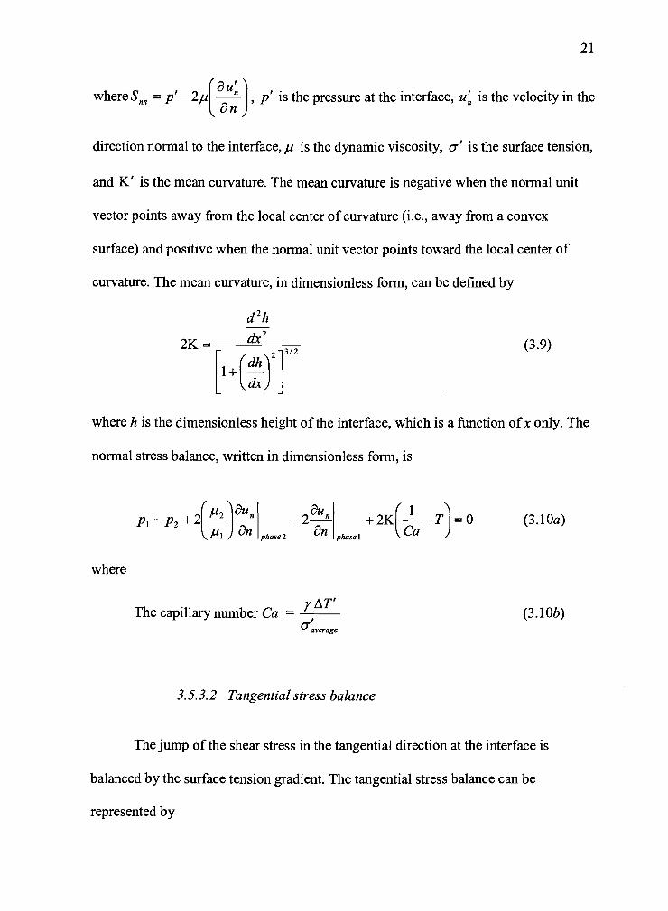
21
where S,,, = p' i- 'p' is the pressure at the interface, u is the velocity in the
on)
direction normal to the interface, p is the dynamic viscosity, 'is the surface tension,
and K' is the mean curvature. The mean curvature is negative when the normal unit
vector points away from the local center of curvature (i.e., away from a convex
surface) and positive when the normal unit vector points toward the local center of
curvature. The mean curvature, in dimensionless form, can be defined by
d2h
2K = 23I2 (3.9)(dh I
j
where h is the dimensionless height of the interface, which is a function of x only. The
normal stress balance, wriften in dimensionless form, is
where
Pi P2 + 2-'-' 2-' + 2K"-- TPi J phase2 phasel Ca ) =
yAT'The capillary number Ca
aaverage
3.5.3.2 Tangential stress balance
(3.lOa)
(3.lOb)
The jump of the shear stress in the tangential direction at the interface is
balanced by the surface tension gradient. The tangential stress balance can be
represented by

22
Sfljh! Sflphase2
(3.11)
Because the interface thickness is assumed to be zero, the shear stress can be
represented by S = where u is the velocity in the direction tangential toan)
the interface. From Equation 3.1, the tangential gradient of the surface tension can be
replaced by the tangential gradient of interface temperature. The tangential stress
balance, written in dimensionless form, is
P21
j (au 'iI
_(.?i = (3.12)')iphase2 (\anJ (a)
phase!
3.5.4 Kinematic condition
The position of the interface is defined as
F(x,y,t) = yh(x,t) = 0 (3.13)
Since the mass of each liquid phase (1 or 2) penetrating the interface is negligible and
the interface is a material boundary (i.e., a particle initially on the boundary will remain
on the boundary), the substantial time derivative of function F equals to zero. By the
definition of function F in (3.10 a), the kinematic equation in terms of the dimensionless
height of the interface (h) and velocities in x andy directions (u and v, respectively) at
the interface is
+u---v=O (3.14)ôt ax

23
3.5.5 Global mass conservation
In addition to thermal, concentration, and stress balances, the liquid must also
satisfy the global mass conservation constraint. Because the liquid is assumed to be
incompressible, its total volume in each phase must remain constant, as follows,
1 / A
Jh (x,t)dx=V (3.15a)
where V is the dimensionless initial volume of liquid in phase 1 and A is the aspect
ratio.
The contact points on the sidewalls of the interface can be specified into two
cases. The first case is the fixed contact location, i.e.
x=O and x=11A5: h(x,t)=l
The second case is the fixed contact angle, i.e.
left wall x = 0: = tan(OL)aX
at left wall
rightwall x=1/A: =tan(GR)aX
at right wall
(3.1 5b)
(3.15c)
(3.15d)
where °L is the contact angle at the left wall and °R is that at the right wall, as shown
in Figure 3.3.

phase 2
interface
phase 1
Figure 3.3 Contact angles of the interface at the sidewalls.
24

25
4. BASIC METHODOLOGY AND ALGORITHM
This chapter discusses the basic methodology and algorithm used in this
project. First, the definitions of control cells, nodes, and cell faces are described
followed by the introduction of the staggered grid arrangement. The surface tracking
technique with interface marker points is then explained. The finite volume with
adapted MAC method is discussed with the interpolation scheme. Finally, the
algorithm of the program is illustrated.
4.1 Control Cells, Nodes, and Cell Faces with Stag2ered Grid
Arrangement
The governing equations in Chapter 3 are solved numerically on discrete points
or nodes using the Finite Volume (FV) method. The computational domain in xy space
for a two-dimensional problem is divided into small control cells by a grid of lines, as
illustrated in Figure 4.1. The spacing of the grid lines in the x direction is uniform and
given by iXx and that in they direction is also uniform and given by Ay. However,
& and Ay are not necessarily equal. Nodes, at which the solutions to the governing
equations are to be obtained, are located at the center of the control cells. A control
cell has boundaries called cell faces. In Figure 4.1, for example, the control cell P is
surrounded by w-, e-, s-, and n-faces. Both convective and diffusive fluxes move in
and out of the control cell at the center of each face.

Jiast
Jlast-1
Jlast-1
j+1
J+1
J
J
i-i
J-1
1
1
26
CTUh,t:
I______________________- - == = : = ==
III
1111111
liii HI
II
II flIllIllIffluhIllhI
flfljIIIiIiIIII1IIIIfl-__,
I
1 i-i i j+ 1 j+2 Ilast- 1
1 I-i I 1+1 1+2 Ilast-1 Ilast
IfflJJIIIscalar cell scalar node
u-cell - u-node
v-cell v-node
Figure 4.1 Control cells, nodes, cell faces with staggered grid arrangement

27
The staggered grid arrangement for the velocity components (Harlow and
Welch, 1965) is employed. Scalar variables, such as pressure (p), temperature (7'), and
concentration (C) are to be evaluated at ordinary nodal points, but velocity
components are to be evaluated on a staggered grid centered around scalar cell faces.
In Figure 4.1, the scalar variables are stored at the nodes marked (s). The nodes for u-
velocities marked by horizontal arrows (>) are located at the left and right of the
scalar cell faces. The nodes for v-velocities marked by vertical arrows (1') are located
at the top and bottom of the scalar cell faces. The control cell for u-velocity (u-cell)
and the control cell for v-velocity (v-cell) have the same size as the scalar cell.
Although most computer programs based on staggered grids tend to be difficult to
interpret, this type of grid arrangement provides a convenient way to evaluate the
velocities in and out of the scalar cells to avoid unrealistic checkerboard pressure
pattern (Anderson, 1995).
To avoid confusion in referring to the staggered grid, a new notation based on
grid line and cell face numbering are introduced. In Figure 4.1 the unbroken grid lines
are numbered by capital letters: from 1, 2, ..., 1-1,1,1+1, 1+2, ..., Ilast in the x-
direction and from 1, 2, ..., J-1, J, J+1, J+2, ..., Jiast in they-direction. The dashed
lines that connect the scalar nodes are denoted by lower case letters: from 1, 2, ..., i-i,
i, 1+1, i+2, ..., ilast1 in the x-direction and from 1,2, ...,j-1,j,j+l,j+2, ...,jlast1
in they-direction. Scalar nodes, located at the intersection between two dashed lines,
are identified by two lower case letters, e.g. point P in Figure 4.1 is denoted by (i,j). In
the cell point P, for example, The u-velocities are stored at the w-and e-faces, located
at the intersection between a vertical un broken grid line and a horizontal dashed line,
I
28
while the v-velocities are stored at the n- and s- faces, located at the intersection
between a horizontal unbroken grid line and a vertical dashed line. Therefore, the u-
nodes are defined by the combinations of a capital letter and a lower case letter, e.g.
the w-face of the cell point P is denoted by (Li). Likewise, the storage locations for the
v-nodes are the combinations of a lower case letter and a capital letter, e.g. the s-face
is given by (i,J)
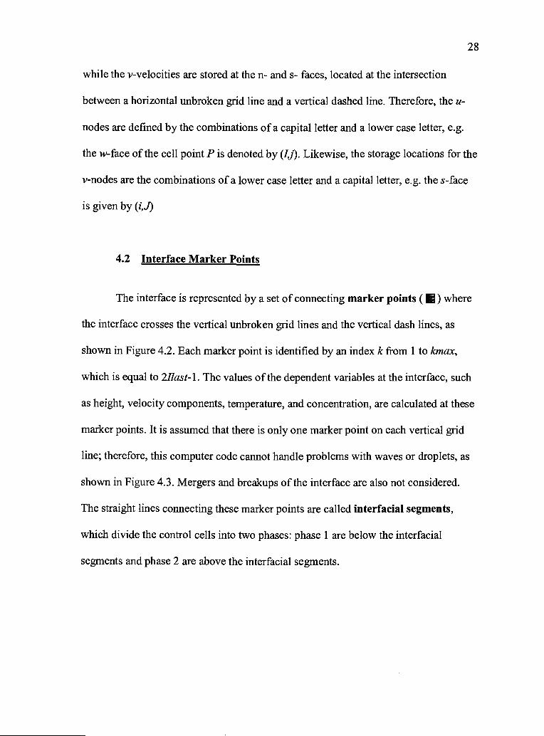
4.2 Interface Marker Points
The interface is represented by a set of connecting marker points () where
the interface crosses the vertical unbroken grid lines and the vertical dash lines, as
shown in Figure 4.2. Each marker point is identified by an index k from 1 to kmax,
which is equal to 2Ilast- 1. The values of the dependent variables at the interface, such
as height, velocity components, temperature, and concentration, are calculated at these
marker points. It is assumed that there is only one marker point on each vertical grid
line; therefore, this computer code cannot handle problems with waves or droplets, as
shown in Figure 4.3. Mergers and breakups of the interface are also not considered.
The straight lines connecting these marker points are called interfacial segments,
which divide the control cells into two phases: phase 1 are below the interfacial
segments and phase 2 are above the interfacial segments.

interfacial segment
Phase JIfia"[Tó
0 ....
Phase.1 Full cell
29
Marker points
1 k-i k k-i-i .. kmax
Figure 4.2 Marker points, interfacial segments, full cells, interfacial cells, and partnercells
Figure 4.3 Wave and droplet interface

30
4.3 Interfacial Control Cells
Most of the control cells are rectangular in shape with Lsx in width and iXy in
height, such as cell S shown in Figure 4.2. These cells are called full cells. However,
some of the control cells may be cut by the interfacial segments resulting in
trapezoidal cells. For instance, in Figure 4.2 since the marker point hk is located in cell
Nbut below its center point, the cell N is identified as an interfacial cell in phase 2.
Cell P is below cellN and identified as a partner cell in phase 1. The area of cellN
that is below the interface segment will become a part of cell P. Likewise, the area of
cell P that is above the interface segment will become a part of cell N. The height of
the left and right faces of a trapezoidal cell can be shorter or longer than Ay.
4.4 Solving Kinematic Equation
As discussed in Chapter 3, the interface moves according to the kinematic
conditions (Equation 3.14). To calculate the height of each marker point on the
interface (e.g., hk) at the forward time step (n+1), the kinematic condition equation is
approximated by the difference equation using the implicit backward-time centered-
space (BTCS) method (Hoffman, 1992)
h"1 h" h'1 h1k k n k+1 kI n+Uk
2(Ax/2)Vk =0 (4.1)

31
where h is the height of the interface, and u and v are the velocity in the x and y
directions on the interface, respectively, & is the increment in time, and Ax is the
spacing between the unbroken vertical grid lines. Superscript n represents the current
time step and n+1 represents the forward time step. Subscript k, k-i, and k+ 1
represents the location of marker points. Rearranging Equation 4.1 yields
ch +h1 +ch =vAt+h (4.2)
u;Atwhere c =
Ax
The height at forward time step (h;+1) cannot be solved explicitly because the two
neighboring values h and h are unknown. Thus, all the unknown variables must
be solved simultaneously. Equation 4.2 applies directly from points 2 to kmax-1. The
following set of linear equations are obtained:
ch11 + h1 + ch1 vAt + h
ch1 + + ch1 vAt + h'
+ + ch1 vAt + h
ch 2 +h"' +h?1 =v1At+h_1- k,nax1 2 "
for point 2
for point 3
forpoint4 (4.3)
for point k,nax-1
The boundary conditions of the contact points, made by the interface at the sidewalls,
are required for the linear equation at points 1 and kmax. From Chapter 3, there are
two cases for the boundary conditions: fixed contact points and fixed contact angle.

32
For case 1: fixed contact points, the boundary conditions are
h11 =1 forpointi (4.4)
h' 1 for point /cmax (4.5)kmax
For case 2: fixed contact angle, one can use a polynomial approach (Anderson, 1995)
to construct a second-order accurate finite-difference approximation for h / ax at the
left and right walls.
3h1 + 4h2 h3
= tan(OL) for point 1 (4.6)2(&/2)
3h2 4h1 + h= tan(OR) for point kinax (4.7)2(x/2)
where °L and °R is the contact angle of the interface at the left and the right walls,
respectively. The system of these linear equations is solved simultaneously using
subroutine DLSARG in the IMSL library.
form as
4.5 Conservation Efluation for the General Variable q'
The conservation equation for the variable qi can be written in a dimensionless
(4.8)
where DG is a dimensionless group and S is a source term. Table 4.1 shows the
definitions of q5, DG, and, S for the continuity, u-momentum, v- momentum, energy,
and conservation of mass equations.

33
In the finite volume method, the fluxes through the cell faces are evaluated.
The Equation 4.8 is integrated over the control cell and the divergence theorem is
employed. For a general variable q$, the integral form of the conservation equation in
two dimensions can be written as
JdA+f(uqi).ndl=J_cJVçb.ndl_JSdA (4.9)DG1 A
The first term on the left hand side of Equation 4.9 is the net rate of 0
accumulation in a control cell. The explicit discretization over the control cell at point
P (shown in Figure 4.4) can be written as
J._dAb
AAat At
(4.10)
where the superscripts n and n+1 indicate the time levels and At is the time step size.
The subscript P indicates the nodal point P, and A is the area of the interfacial cell.
The second term on the left hand side of Equation 4.9 is the line integral of the
outward normal convective fluxes, which can be expressed as
J(uqs). ñ dl = (Ueq$eXyD Yc)+ (UneOneXYF YD)(4.11)
(uWOWXyA YB)_(IYA Xxc -xB)
where u and v are the velocities in the x- andy-direction, respectively, evaluated at the
center of the cell faces. The variables x andy are the coordinates in x- andy-axis,
respectively. The subscripts e, ne, w, and s indicate the cell faces. The subscripts A, B,
C, D, and F indicate the points on the boundary around of the control cell P. It is
assumed that there is no convection of mass across the interface; thereby the
convective flux at the interface is negligible.

34
Table 4.1 Definition of qi, DG, and, S for each conservation equation
Type of conservation equation 0 DG S
continuity equation 1 1 0
u-momentum equation u Re
ax
v-momentum equation v Re ô.p
ay
energy equation T Ma 0
species equation C Pe 0
Figure 4.4 Outward fluxes at w-, s-, e-, ne-face, and the interface of the control cell P

35
The first term on the right side of Equation 4.9 is the line integral of the
outward normal diffusion fluxes, which can be computed as
(acb (ôØ\cJVq$.ndl=_) (YDYc)+_J (YFYD)ax
e ox(4.12)
(aqs" ('as(xc xB)+( AF(YA YB )
a )infax
where and are the gradients of q$ in the x- and '- directions, respectively,ax ay
is the normal gradient of q$ at the center of the interfacial segment from pointsan )inf
A to F, and lAF is the length of the interfacial segment from points A to F.
The second term on the right hand side of Equation 4.9 is the integration of the
source term, which only exists in u and v-momentum equations. For the u-
momentum equation, the source term can be written as
fSdA=(J A (4.13)A ax cell center
where is the pressure gradient in the x-direction evaluated at the u-cellax cell center
center. For the v-momentum equaiton, the source term can be written as
JSdA=[L?.J A (4.14)A cell center
where is the pressure gradient in the Y-direction evaluated at the v-cellcell center
center.

36
The key issue here is to evaluate with adequate accuracy the normal velocities
(u and v) and the b value in Equation 4.11, the normal gradients of q5 in Equation
4.12, and the pressure gradients in Equation 4.13 and 4.14, on the cell-faces of the
control cells. These values can be derived from such values at the neighboring cell-
nodes of the same phase. Several interpolation techniques are utilized as follows:
Linear approximation
For full cells, the fluxes and pressure gradients on the face-centers can be
calculated to the second-order accuracy by a simple linear approximation from such
values at the neighboring nodes. For trapezoidal interfacial cells, if the center location
of the cell-face lies in the middle between two neighboring nodes having the same
phase, the linear approximation of a value at the two neighboring nodes is adequate to
obtain the second-order accuracy of that value. For example, from Figure 4.4 the value
of q$ at the center of the e-face can be evaluated to second-order accuracy as
cbe
qi + t;bp(4.15)
The normal gradient of q$ can be approximated by a central-difference scheme as
1:) ISp cbE
t x)e xx(4.16)
This approximation is second-order accurate when the cell face is halfway between P
and E, i.e. for a uniform mesh having x xE equal to Ax. Similarly, the value of tb
at the center of the s-face can be wriften as

37
çbØ+cb
(4.17)2
and the normal gradient of q$ can be expressed as
(açb _ck-1.jJ5 Yp Ys
(4.18)
where y y5 = Ay
. Two-dimensional polynomial interpolation
On a given cell-face, an accurate evaluation of a value by the linear approximation
of variables stored at two neighboring nodes is not possible when (1) the center of the
cell-face is not in the middle between the two neighboring nodes or (2) one of the
neighboring nodes is not in the same phase as the cell-face. For example, in Figure
4.4, the N-node cannot be used in the linear approximation of a value on the ne-face
because the N-node and the ne-face are in different phases. On the w-face, the second
order accuracy of a value cannot be derived from a linear approximation of the
variables stored at the neighboring nodes Wand P because the center of the w-face is
not on the line connecting the two nodes. Under these circumstances, a two-
dimensional polynomial interpolating function in an appropriate region, proposed by
Ye et al. (1999), may be used. For example, to evaluate the fluxes on the ne-face of the
shaded trapezoidal region shown in Figure 4.5(a), the qi value is expressed as linear in
x and quadratic my as follows:
qi=c1xy2 +c2y2+c3xy+c4y+c5x+c6 (4.19)

where c1 to c6 are the six unknown coefficients. The normal derivative of q$ can be
written as:
2=c1y +c3y+c5ax
(4.20)
The benefit of using the interpolation function, as in Equation 4.19, is that the
second order approximation can be obtained with the most compact interpolant,
minimizing the size of the stencil required for the neighboring cells. Although
biquadratic interpolation function would lead to second-order accuracy, it contains
nine unknown coefficients, requiring nine neighboring cell-nodes. By using the
interpolation function as in Equation 4.19 that is only quadratic in y but linear in x, a
second-order accurate evaluation can be achieved with only six neighboring cell-nodes
required. In Figure 4.5(a), for example, since the ne-face is midway between the two
parallel sides of the trapezoid, linear interpolation in the x-direction is sufficient for
the second-order accurate evaluation of the derivative at this location. However, this
situation does not exist in they-direction, thus a quadratic interpolation is necessary in
this direction. Ye et al. (1999) demonstrated that the linear-quadratic interpolation
function could provide second-order accurate evaluation of values and derivatives on a
line that was located midway between the two parallel sides of a trapezoid.
In order to evaluate six unknown coefficients of Equation 4.19, four nodal
points (node P. S. E, and NE) and two points on the interface (point G and B) as
shown in Figure 4.5(a) are required. The following system of equations is obtained by
expressing q5 in terms of the linear-quadratic interpolating function (Equation 4.9) at
the six locations:

39
IqS1 [1y y x1y1 y1 x1 1 1 Ic, 1
02 ) X22 Y2 X2 1 C2(4.21)
1061 y x6y6 X6 1 jl6J
The matrix []in Equation 4.14 is called the Vandermonde matrix. The coefficients
can be expressed in terms of the 0 values at the six points by inverting Equation 4.21
as:
c n=1,2,...,6 (4.22)
where bnj represents the elements of the inversed Vandermode matrix. The value of 0
at the center of the ne-face is expressed as:
One = CiXneY + + C3XneYne + C4Yne + + C6 (4.23)
and by using c,, as in Equation 4.22, the Equation 4.23 can be rewritten in terms of 0 as
One
where
(4.24)
= bijXneY + b2y + b3jXneYne + b4jYne + bsjXne + (4.25)
(aThe value of
L'jneis expressed as
where
[tine i-i(4.26)
= + b3iy + (4.27)

(a) (b)
Figure 4.5 Trapazoidal region and six points stencil used in the two dimensionallinear quadratic interpolation. (a) for computing at ne-face (b) for computing atw-face
j+1
J+1
3
J
f-i
i-i I i 1+1 i+1
Figure 4.6 Three points stencil used in the one-dimensional quadratic interpolation forboth u and Une

41
The similar procedure is employed at the w-face of a trapezoidal region (Figure
4.5(b)) and relationships similar to Equation 4.24 and 4.25 are developed.
One-dimensional quadratic interpolation
As shown in Figure 4.6, the u-velocity at the e-face (Ue) and v-velocity at the
s-face (v )can be obtained directly at the u-node (i + 1,1) and v-node (i,J),
respectively. However, the evaluations of the u-velocities at the w-face and the ne-face
are more complicated since the face-centers are not located on any of the u-nodes. The
u-velocities are then evaluated by using a quadratic function in they-direction.
u(y)=a1y2 +a2y+a3 (4.28)
where a1 to a3 are three unknown coefficients which require two u-nodal points and
one point on the interface, illustrated in Figure 4.6, to evaluate. For example, u at
nodes (i, j) and (i,j i) and marker point A (u(A)) are required to evaluate the u-
velocity at the w-face, while u at node (i + 1,1) and (i +1,j i) and marker point F
(u(F)) are required at the ne-face. The method of solving Equation 4.28 is similar to
that used in the two-dimensional polynomial interpolation previously presented. The
u-velocity at the center of the w-face can be expressed as
where
= (4.29)
= d11y, + d2y + d3 (4.30)

42
and d,,,, where n is from 1 to 3, representing the elements of the inverse of the
Vandermode matrix obtained from a system of quadratic interpolating function. A
similar procedure is employed at the ne-face.
Probe method for gradients at the interface
The normal gradient at the interface in each phase can be evaluated in
different ways. First, since
I' 1"i +n I - I (4.31)Xa) Y)
where n and n are the two components of the unit vector nonnal to the interface.
One can obtain gradients and to second-order accuracy but inx) y)
practice this is found to be tedious to implement. Thus the probe method proposed by
Udaykumar et al. (1999) is employed in this work. This is done by extending a normal
probe from the center of the interfacial line into each phase as shown in Figure 4.7.
The two points on the normal probe are located at the distances of An and 2 An from
the interface, where An is set to be equal to Ày. The value of 0 at each point is
evaluated by a biquadratic function:
qi(x,y) = b1x2 + b2y2b3xy + b4x + b5y + b6 (4.32)
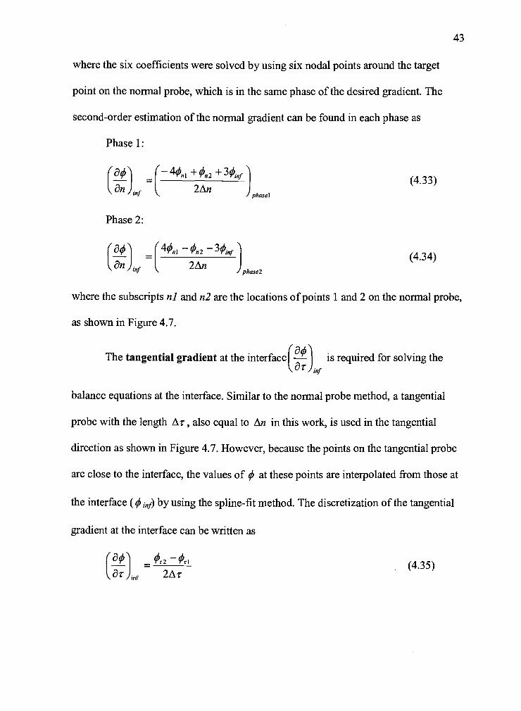
43
where the six coefficients were solved by using six nodal points around the target
point on the normal probe, which is in the same phase of the desired gradient. The
second-order estimation of the normal gradient can be found in each phase as
Phase 1:
acb') _(-4ø n2 +3q5/'(4.33)
a1)inj 2Anphasel
Phase 2:
(osJ141_2_3in1 (4.34)
inf 2An)phase2
where the subscripts ni and n2 are the locations of points 1 and 2 on the normal probe,
as shown in Figure 4.7.
The tangential gradient at the interface is required for solving the\ar ) inf
balance equations at the interface. Similar to the normal probe method, a tangential
probe with the length Ar, also equal to An in this work, is used in the tangential
direction as shown in Figure 4.7. However, because the points on the tangential probe
are close to the interface, the values of q$ at these points are interpolated from those at
the interface (b inf) by using the spline-fit method. The discretization of the tangential
gradient at the interface can be wriften as
(a" _r2ør12Av
(4.35)

I
I
I
I I
I I
--1
I I I
1----
t-- "1 t
\-
Points on the normal probe
A Points on the tangential probe
Nodes used in the biquadratic interpolation (in phase 1)
Nodes used in the biquadratic interpolation (in phase 2)
Figure 4.7 Normal and tangential probe for evaluation of the gradient at the interface

45
where r1 and r2 are the location of point 1 and 2 on the tangential probe, respectively,
as shown in Figure 4.7, respectively.
4.6 Solving the Continuity Equation and the Momentum Equation
The integral form of the non-dimensionalized governing equations is given by
mass conservation cfu ñ dl =0 (4.36)
momentum conservation fit dA + cju(u . ñ)dl = Vu . ft dl fvp dA
(4.37)
where A is the area of the control cell, 1 is the boundary of the control cell, and ñ is a
unit vector normal to the boundary of the control cell. The velocity components (u)
and pressure (p) are advanced from time step n to n+1 by using the adapted MAC
method by Harlow and Welch (1965). First the momentum conservation equation is
solved by the explicit forward-time centered-space scheme with the pressure gradient
term at the n time step. This scheme is first-order accurate in time and
second-order accurate in space. The semi-discrete form of the momentum equation
can be written as
ifdA =fu'(u' .n)dl+icf\7u" ft dl JVp1dA (4.38)
Re, A
Arranging Equation 4.38 yields
u1 =F _&(vp+1) (4.39)

where
F' = u" [_cfu"(u' .n)dl+-_cJvu" ñ dl) (4.40)
The solution of Equation 4.38 must satisfy the integral mass conservation equation
(Equation 4.36). Inserting the velocity u"1 (Equation 4.39) into Equation 4.36, results
in the integral version of the pressure Poisson equation:
dl =-L(F' .ñ)dlAt1
(4.41)
The following section will show an example of solving continuity and
momentum conservation equations with the adapted MAC method.
u-momentum equation
For the u-node (I,j), shown in Figure 4.1, the velocities at the u-cell faces are
defined by linear interpolation between two adjacent points as follows:
u(I-1,j)+u(I,j)w-face: u =
2
e-face:u(I, j) + u(I + 1,1)
Ue =2
s-face:u(I,j 1) + u(I,j) v(i 1,J) + v(i, J)
us = , vs =2 2
n-face: uu(I,j)+u(I,j+1) v(i-1,J+1)+v(i,J+1)
2'
2
From the u-momentum equation, the u-velocity at the node (I,]) and the time step
can be written as:

where
47
u;;' =F +.(p1'J pn+i) (4.42)
= u:u: .u:) (u: .v:u:
& + ;+1 ) (u;11 2u +u;1)](4.43)
+-Re (&)2 (A3)2
Similarly the u-velocity at node (I+1j) and the time step n+ith can be written as:
n+1 1 At(
n+i n+1u111 = + p1+1,1) (4.44)Rep Ax
. v-momentum eQuation
For the v-cell (i,J) shown in Figure 4.1, the velocities around the cell are
defined by linear interpolations between two adjacent nodes as follows:
w-face:u(I,j-1)+u(I,j)
vv(i 1,J)+v(i,J)
W2
' W2
e-face:u(I + 1,j 1)+ u(I +1,j) v(i,J)+ v(i +1,J)
Ue =2 2
s-face: v5v(i, J 1) + v(i, J)
2
v(i, J) + v(i, J +1)n-face: v =
2
The v-velocity at node (i,J) and the time step n +ith can be written as
= + . (p1 p1fl;) (4.45)
where
v:__:= v + v ) (;A
)]
&[v
+ vlJ ) 2v +(4.46)
+-Re (&)2 (Ay)2
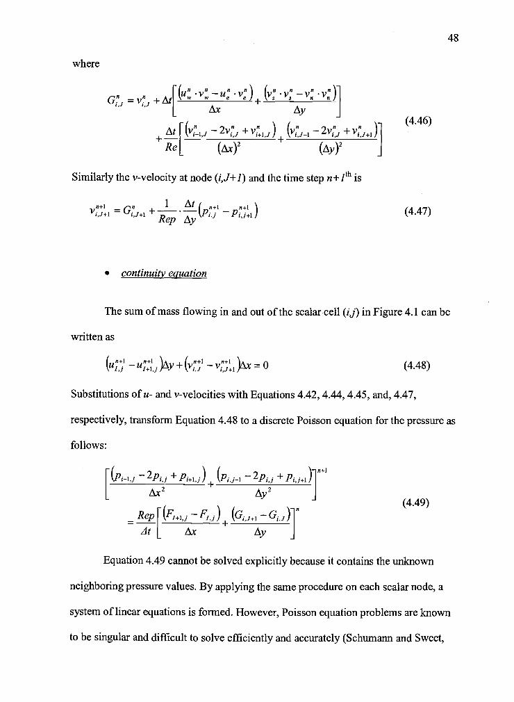
Similarly the v-velocity at node (4J+1) and the time step jth is
1 Ativ' = Gi,J+1 + pi,j+1 ,(4.47)
continuity equation
The sum of mass flowing in and out of the scalar cell (i,j) in Figure 4.1 can be
written as
(n+1 n+1u11 u11 )iy + v1 )& = 0 (4.48)
Substitutions of u- and v-velocities with Equations 4.42,4.44,4.45, and, 4.47,
respectively, transform Equation 4.48 to a discrete Poisson equation for the pressure as
follows:
RI \ IP-LJ + P+) +
[ +(4.49)
= (+1,j ) (c,)1
zlt[ Ax Ay jEquation 4.49 cannot be solved explicitly because it contains the unknown
neighboring pressure values. By applying the same procedure on each scalar node, a
system of linear equations is formed. However, Poisson equation problems are known
to be singular and difficult to solve efficiently and accurately (Schumann and Sweet,

1976) because there could be infinite solutions for the pressure or the pressure could
be a function of an arbitrary constant. The complexity of solving Equation 4.49 may
be avoided by setting one scalar cell as the reference cell (p irefjref) and let the pressure
at that cell to be constant (pref) as follows:
P,rej,jrej = Prej (4.50)
The new system of linear equations is not singular and can be solved simultaneously
using the direct Poisson solver method in the subroutine DLSARB of the IMSL
library. This set of pressure solutions is a function of the constantPref.
Once a solution for p are obtained and substituted into momentum
equations, i.e. Equations 4.42,4.44, 4.45, and 4.47, u1 and v can be computed.
All the pressure and velocity components satisfy both continuity and momentum
conservation equations.
4.7 So1vin Balance EQuations at Interface
Partial derivative terms in the balance equations at the interface are discretized
using the probe method for normal and tangential gradients at the interface discussed
in section 4.5.

50
4.7.1 Thermal Balance
The discretization of Equation 3.6(a) can be written as
4T +T12 +3T k24T21 T22 3T(4.51)
2An k1 2An
where An is the length of the probe. Rearranging Equation 4.41 yields
(k2 / k1X4T21 T22 )+ (4T11(4.52)
3(1+(k2/kl))
where T is the temperature of the marker points on the interface, and kl and k2 are
the thermal conductivities of phase 1 and 2, respectively. Subscripts pinl and pin2
indicate the first and second probe points in phase 1, respectively, whilep2nl and
p2n2 indicate those in phase 2, respectively.
4.7.2 Concentration Balance
Similar to the thermal balance equation, Equation 3.7 can be discretized as
4c1 c2 3c1 D24c21 c22 3c2(4.53)
2An 2An
where c is the concentration of solute C, and D1 and D2 are the diffusion coefficients
of the solute C in phases 1 and 2, respectively. Note that the concentrations of solute C
at the interface are not equal in both phases, thereby requiring additional governing
equations. By assuming that the system is at equilibrium, the relationship between the
concentration of solute C at the interface of phase 1 (c1) and that of phase 2 (c2)
can be expressed as

51
Cir2 =kdjSc (4.54)
where kd,S is the distribution coefficient of solute C between phases 1 and 2. By
inserting Equation 4.44 in 4.43, c1 can be expressed as
(D1 ID2 X4c21 c2,2 )+ (4c11(455)Cjf1
3[1+kdJD1
4.7.3 Normal Stress Balance
The discretization of Equation 3.1 Oa can be written as
2 ) +2(L1 4un21 un22 3un
J
2(4un11 + un2 + 3un
( uiJ 2An 2An )
+ 2K_!:_ TJ =
(4.56)
where p1 and p are the viscosities of phases 1 and phase 2, respectively. T is the
temperature at the interface and can be obtained from Equation 4.52. Ca is the
capillary number. The parameter K is the curvature at the interface. The pressure on
the interface of phases 1 (p1) and 2 (p2) are evaluated by using a quadratic
extrapolation method similar to the one-dimensional quadratic interpolation method
described in section 4.5. Since the pressure solution is a function of the constantPref
(see section 4.6), the pressure on the interface of phases 1 and 2 are also a function of
the constant Pref The first term on the left hand side of Equation 4.56 can be expressed
as p1 p2 + p. The normal velocities (un) on the normal probe are calculated from

52
the u-velocity and the v-velocity interpolated from the u-nodes and v-nodes,
respectively. Rearranging Equation 4.56 yields
AnUflfif :=_(p1 P2 +prej)
An 1+K --TM(Ca )
+ ---[-- (4un,,1 unp2fl2 )+ (4un11 un12)]M[p1
where M=3(1+p2Ipl).
4.7.4 Tangential Stress Balance
The discretization of Equation 3.12 can be written as
(4.57)
(p2 V 4ut21 ut2 3ut
J
(- 4ut1 + ut12 +
plJt 2An 2An(4.58)
(21L02Ar)
where Ut is the velocity in the tangential direction. The last term of Equation 4.58 is
the tangential gradient of temperature at the interface, as discussed in section 4.5.
Equation 4.58 can be rearranged to
An1I2 -1YUtjflfAit Ar )
(4.59)
M[pi1 [ (4ut21 ut )+ (4ut1,
[

53
4.8 Global Mass Conservation Constraint
The normal and tangential velocities at the interface from Equations 4.57 and
4.59 are then transformed to the velocities in the x- andy-directions. The location of
the interface at the forward time step can be calculated by substituting these interfacial
velocities into the kinematic equation (Equation 4.1). However, this new location may
not satisfy the global mass conservation constraint because the normal velocity is a
function of an arbitrary constant Prej A secant method is used to search for the values
of Prej that yields normal velocities that satisfy the global mass conservation
constraint.
4.9 Algorithm
The algorithm of the computer code is shown in Figure 4.8. Starting from the
time step flth, the interface marker points moves to the new location at the time step
+ith according to the kinematic equation. At this new location on the interface, the
shapes of the interfacial cells are determined. The Poisson equations are solved for
pressure (p) at scalar nodes. The velocity components at the u-nodes and v-nodes in
the computational domain are then calculated from the continuity and momentum
equations. Subsequently, the temperature (I) and concentration (C) at scalar nodes are
determined. Finally the independent variables at interface marker points are calculated
from the mass, thermal, and stress balances at the interface.

Start at time step (flth)
Solve kinematic equationMarker points move to the next time step (n+ ith)
Solve Poisson equationfor pressure (pfl+l)
Solve discretised momentum equations forvelocity components (u
'
,v)
Solve all other discretised conservation equations fortemperature (T') and concentration (C1 )
Solve all discretised balance equations at theinterface for velocities, temperature, and
concentration at the interface
Next time step (n+lth)
Figure 4.8 The algorithm
54

55
5. PROGRAM VALIDATION
Unlike exact or analytical solutions, numerical solutions of mathematical
models are associated with computational errors. In this chapter, several tests are
performed to validate that the numerical code developed in this study produces
accurate and consistent results.
5.1 Sensitivity Analysis
Numerical solutions are associated with discretization errors, which depend on
grid sizes in x-and y- direction (Ar and Ay) and time step sizes (At).
5.1.1 Mesh Sensitivity Analysis
A mesh sensitivity analysis is performed to determine the grid size in the x-
andy- direction that recurrently produces accurate solutions. We almost want to
evaluate the convergence order of the adopted discretization scheme. The test case is
water-hexane in a two-dimensional cavity. The configuration of the cavity is discussed
in Chapter 3. The bottom layer (phase 1) is water and the top layer (phase 2) is hexane.
The properties of both liquids are shown in Appendix A. The height of the bottom
layer is lx lO m, which is equal to the length of the cavity and the height of the top
layer. The aspect ratio of the cavity is 1. The temperature difference along the
interface (AT') is 1 °C. The diffusion coefficient of solute C in water and in hexane is

56
1 x 1 0 m2/s. With these physical parameters fixed, the values of the dimensionless
groups in each phase are shown in Table 5.1.
Table 5.1 Values of dimensionless groups in each phase
Re Rep Ma Sc Fr Fe
Phase 1 10.82 10.82 66.18 892.7 6.11 9,663
Phase2 21.10 7.11 119.7 459.0 5.68 9,663
Three different mesh sizes are investigated: 11 x21, 21 x41, and 41 x 81. The
method used to determine the order of convergence and the Richardson extrapolation
is shown in Appendix B. The order of convergence for velocity in x-direction (u),
velocity in y-direction (v), temperature (T), and concentration of solute (c) is
approximately equal to two, as shown in Table 5.2. This is consistent with the adopted
discretization scheme. The average percentage relative errors among the results at
each mesh size and the extrapolated values obtained by using Richardson
extrapolation are also illustrated in Table 5.2. As expected the relative error decreases
with increasing mesh size. Unfortunately computational time dramatically increases
with increasing mesh size. The mesh size of 31 x 61 is selected for cases where A5 is
equal to 1.0 and the mesh size of 61 x 61 is selected for cases whereA5 is equal to 0.5.
The relative percentage average error caused by the choice of the mesh size in all
cases presented in this study is always maintained at less than 5%.
57
5.1.2 Time Step Sensitivity Analysis
Similarly to the mesh sensitivity analysis, the time step sensitivity analysis is
performed to determine the appropriate time step size. The test case is similar to the
one used in section 5.1.1 with mesh 31 x 61. Three different dimensionless time step
sizes are examined: 5 x i0, lx 10, and 2 x 10'. The results are shown in Table
5.3. The order of convergence is approximately equal to one, which is consistent with
the discretization scheme. The average relative error is approximately less than 0.1%.
5.2 Steady State Test
A steady state test is conducted to show that the results at steady state are
independent to the initial conditions. Two test cases are performed with identical
configuration and parameters described in section 5.1.1 with mesh 31 x 61 and
dimensionless time step size 1 x 10. For the first case, the initial temperature in bulk
liquid is set to the temperature at the right wall (T). For the second case, the initial
temperature in bulk liquid is set to the average temperature ( Ta'verage). After 200,000
iterations when the steady state is reached, the velocity components and temperature in
the bulk liquid in the two cases are compared. The results from the both cases are
identical. Therefore, we can conclude that the results at steady state are independent
from the initial conditions.
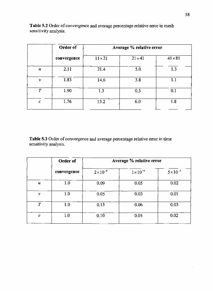
Table 5.2 Order of convergence and average percentage relative error in meshsensitivity analysis.
Order of
convergence
Average % relative error
11x21 21x41 41x81
u 2.11 21.4 5.0 1.3
v 1.83 14.6 3.8 1.1
T 1.90 1.3 0.3 0.1
c 1.76 13.2 6.0 1.8
Table 5.3 Order of convergence and average percentage relative error in timesensitivity analysis.
Order of
convergence
Average % relative error
2x10 lx1O 5x10⁵
u 1.0 0.09 0.05 0.02
v 1.0 0.05 0.03 0.01
T 1.0 0.13 0.06 0.03
c 1.0 0.10 0.05 0.02
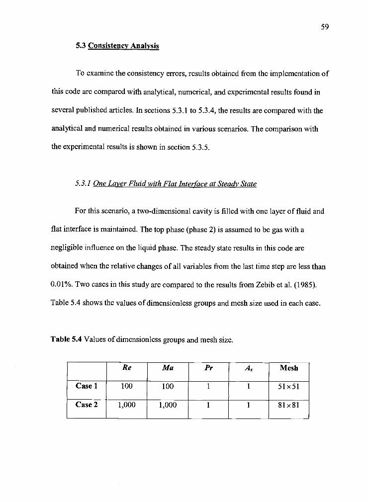
59
5.3 Consistency Analysis
To examine the consistency errors, results obtained from the implementation of
this code are compared with analytical, numerical, and experimental results found in
several published articles. In sections 5.3.1 to 5.3.4, the results are compared with the
analytical and numerical results obtained in various scenarios. The comparison with
the experimental results is shown in section 5.3.5.
5.3.1 One Layer Fluid with Flat Interface at Steady State
For this scenario, a two-dimensional cavity is filled with one layer of fluid and
flat interface is maintained. The top phase (phase 2) is assumed to be gas with a
negligible influence on the liquid phase. The steady state results in this code are
obtained when the relative changes of all variables from the last time step are less than
0.01%. Two cases in this study are compared to the results from Zebib et al. (1985).
Table 5.4 shows the values of dimensionless groups and mesh size used in each case.
Table 5.4 Values of dimensionless groups and mesh size.
Re Ma Pr A Mesh
Casel 100 100 1 1 51x51
Case 2 1,000 1,000 1 1 81 x 81

In the case 1, whenRe is equal to 100, tangential velocity and temperature at
the interface are consistent with the results from Zebib et al. as shown in Figure 5.1(a)
and (b). Slight differences of tangential velocity at the interface are observed near the
left and right wall. In case 2, when Re is equal to 1,000, the tangential velocity at the
interface calculated from this work is inconsistent with the results from Zebib et al.,
especially at the right wall. However, the streamlines and isotherms, as illustrated in
Figure 5.3, from this work are qualitatively similar to those from Zebib et al. The
numerical method used by Zebib et al. is the finite difference with velocity-pressure
coupling treatment, which is similar to this work. However, Zebib et al. used non-
uniform grids, with 62 points in the x-direction and 54 points in they-direction. The
smallest cell at the right corner is a square with mesh size 0.005. The mesh spacing
near the middle of the bottom boundary is less than 0.05. Tn this work, the finest mesh
size is 0.0 125 (1/80), which is approximately twice as large as the smallest mesh size
used in Zebib et al.'s work. The comparison reveals that at high Reynolds number
finer mesh size is required, especially in the vicinity of the walls and the interface, to
capture the gradients of velocities at the interface and the walls.

61
(a)
Re = 100
0.14w
012
010-P
G) 0.08.2
0.06
0.04
0.02
I-
0
0 0.2 0.4 0.6 0.8
x(I)
(b)
Re = 100
0.5
0.4Zebib et. al.
0.3
This work
02
0U U
-o.i 0.2 0.4 0.6 .8
-0.2
C). -0.3
E
-0.5 -'
x(I)
Figure 5.1 (a) Tangential velocity at the interface (b) Temperature at the interface, forthe case with Pr = 1, Re = 100, A = 1

(a)
(b)
Re = 1,000
0.12
o..
_Zebibetal.lThis work
>
z 0.082. 0.06
w c 0.04C
0
0.02
0 0.1 0.2 0.3 0.4 0.5 0.6 0.7 0.8 0.9
x(I)
Re = 1,000
0.5.
0.4.-Zebib et al.
a This workC,
0.3.
0.2
. 0.14-
0
-0.1 07 0 04 fl. 06 07.1
-0.2
-0.3
-0.4
-0.5
x(I)
62
Figure 5.2 (a) Tangential velocity at the interface (b) Temperature at the interface, forthe case with Pr = 1, Re = 1,000, A5 = 1
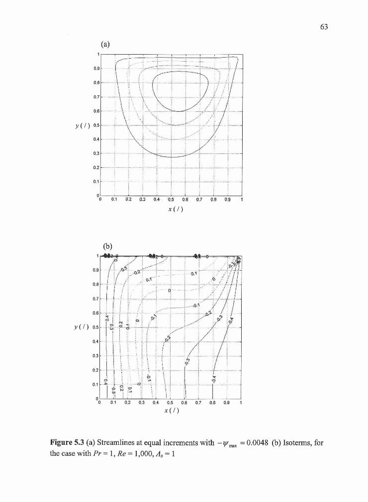
63
(a)
0.9
(b)1
0.9
0.8
0.7
0.6
y(/) 0.5
0.4
0.3
0.2
0.1
n0 0.1 0.2 0.3 0.4 0.5 0.6 0.7 0.8 0.9
x(/)
Figure 5.3 (a) Streamlines at equal increments with 0.0048 (b) Isoterms, forthe case with Pr= 1, Re = 1,000,A3 = 1

64
5.3.2 One Layer with Deformable Interface at Steady State
In this section, the present numerical results are compared with the analytical
solution presented by Sen and Davis (1982). Sen and Davis developed an analytical
expressions of the interface shape and the streamfunction at midplane (x' = L' / 2) for
the case where the gravity is zero, the aspect ratio is small, and the convective terms in
the energy equation are neglected.
There are two test cases based on the contact points of the interface at the
sidewalls: fixed contact height and fixed 900 contact angle.
Fixed Contact Height
Chen et al. (1990) ran a case with A3 = 0.2, Ca = 0.32, Bi = 1, Re = 5, and
Ma = 1, with 61 grids in the x-direction and 21 grids in they-direction. The contact
points of the interface on the left and right walls are fixed aty = 1. The governing
equations are solved by the finite difference method with a boundary-fitted curvilinear
coordinate system, which is generated numerically and always places the coordinate
line coincide with the current boundary surface. The field variables are streamfunction
and vorticity. To compare the results, the same case was run in this work. Figure 5.4
shows the streamline contour and the height of the interface, which are qualitatively
similar to those shown by Chen et al. The comparisons of the height of the interface
and the streamfunction at midplane between this work and the analytical solution by
Sen and Davis are shown in Figure 5.5 and 5.6, respectively. The graphs show the

65
consistency between the results from this program and those from the analytical
solution.
Fixed 90° contact angle
Labonia et al. (1997) compared the numerical evaluation of the height of the
interface to the analytical solution of Sen and Davis (1982) and the numerical solution
of Rivas (1991) with the following parameter values: A5 0.2, Ma = 5, Pr 0.2, and
Ca = 0.04, using an 81 x41 mesh. Note that the definitions of Ma used by Labonia et
al. (1997) are different from Ma in this work. The Marangoni (Ma) in this work is
equal to the Marangoni numer defined by Labonia et al. (1997) times the aspect ratio
(A5). The interface is perpendicular to both the left and the right walls. Labonia et al.
(1997) used a vorticity-velocity formulation discretization using a curvilinear
coordinate system. The free surface displacement and mesh description are solved
simultaneously using Newton's method. The results show that the numerical solutions
from both Labonia et al. (1997) and Riva (1991) are very close to the analytical
solution from Sen and Davis (1982), and the difference is negligible. In this work the
same case with Ma = 1 and 81 x41 mesh has been performed. The height of the
interface and the streamfunction at midplane from this work are very close to the
analytical solutions of Sen and Davis (1982), as shown in Figure 5.7 and 5.8.

1.1
I
0.9
0.8
0.7
0.6
0.5
0.4
0.3
0.2
0.1
111'
/ /
- - -//)
0.5 1 15 2 2.5 3 3.5 4 4.5
x(/)
Figure 5.4 Streamlines contour for fixed contact height with Ma = 1, Re 5, A5 = 0.2,Ca=O.32,andBi= 1

67
Figure 5.5 Interface height for fixed contact height with Ma 1, Re 5, A 0.2,
Ca = 0.32, andBi= 1
a
0.
0.
0.
y(/) 0.
0.
0.
0.
0.
-0.02 -0.O15 -0.01 O.O05 0
"(I)
Figure 5.6 Streamfucntion at midplane for fixed contact height with Ma = 1, Re = 5,
= 0.2, Ca = 0.32, and Bi = 1

I
I
0
0
0
h(/) 0
0
0
a
a
x(/)
Figure 5.7 Interface height for fixed 90° contact angle withMa = 1, Pr = 0.2, A = 0.2,
and Ca 0.04
y(/)
-O4 -0.035 -0.O3 -0.025 -0:02 -0.015 -0.01 -0.005 0
(I)
Figure 5.8 Streamfucntion at midplane for fixed 900 contact angle with Ma = 1,
Pr = 0.2, A = 0.2, and Ca = 0.04

5.3.3 One Layer with Deformable Interface at Unsteady State
Chen et al. (1991) have investigated the unsteady thermocapillary convection
in a rectangular cavity with an upper deformable free surface. The sidewalls are
maintained at constant temperature; however, the surface temperature distribution is
assigned as a function of time as
f(t, x) = sin(A5 r x) sin(Qt) (5.1)
where Q is the frequency of temperature oscillation. The problem has been solved by
the finite difference method with a time-dependent boundary-fitted curvilinear
coordinate system. In this work, a test case with Re = 10, Ma = 2, Ca = 0.1, A5 = 0.2,
and Q =0.1 is set to compare the time history of the interface height at x = 1. The
comparison is shown in Figure 5.9. The results are remarkably similar considering
very different numerical techniques implemented in these two studies. Only minor
differences in the amplitude of the interface height are observed.
5.3.4 Two Layer with Flat Interface at Steady State
A test case with Pr = 7.5, Ma = 500, A5 = 1/3 is set to compare the u-velocity at
midplane in both layers at steady state. The same case has been investigated by Wang
and Kahawita (1996) using the spline fractional step procedure with streamfunction-
vorticity variables. The comparison shows that the results from this work are
consistent with the results from Wang and Kawahita's, as shown in Figure 5.10. Noted
that the u-velocity in Figure 5.10 is the characteristic velocity, which is equal to
2400u/(Ma L,T')

70
Figure 5.9 The time history at h(1) for Ma = 2, Re= 10, A = 0.2, Ca = 0.1, and Q 0.1
1
0.9
0.8
0.7
0.6
0.5
0.4
0.3
0.2
0.1
0
This work
Wang and Kahawita (1996)
-300 -250 -200 -150 -100 -50 0 50 100
characteristic velocity at midplane (I)
Figure 5.10 Steady characteristic velocity at mIdplane for Pr = 7.5,Ma = 500, A 1/3
71
5.3.5 Comparison with the Experimental Results
Riley and Neitzel (1998) experimentally investigated the combined
thermocapillary-buoyancy convection in a thin rectangular geometry. The working
fluid used in these experiments was 1 cS Dow Corning silicone oil with the Prandtl
number equal to 13.9. The length (L') and width (W') of the rectangular cavity are 30
mm and 50 mm, respectively. A temperature gradient is produced between the two
sidewalls. The end-walls and bottom of the cavity are assumed adiabatic. The top of
the cavity is a free surface with the Capillary number in the order of 0.001, indicating
that a flat free surface is reasonable to assume. The quantitative measurements of
steady state velocity fields were performed using laser-Doppler velocimetry (LDV).
To study the steady unicellular flow, Riley and Neitzel performed an experiment with
the Marangoni number (Ma) equal to 350 and the dynamic Bond number (Bo) equal to
0.142, corresponding to a layer of 1.0 nm depth and the aspect ratio of 1/30. The
dynamic Bond number is a measure of the relative strength of buoyancy forces to
thermocapillary forces. A profile of horizontal velocity (u) in the core region, which is
away from both endwalls and sidewalls was measured by LDV technique.
In this work, a test case was performed with the Marangoni number (Ma) equal
to 350, the Prandtl number (Pr) equal to 13.9, the dynamic Bond number (Bo) equal to
zero, and the aspect ratio (A5) equal to 0.2. A 46x 121 mesh is used. Although the
aspect ratio and the dynamic Bond number are different, the comparison shows that
the profile of the horizontal velocity at midplane from this work is consistent with that
from Riley and Neitzel ' s, as shown in Figure 5.11.

72
1.00
0.80
0.60
This work
0.40Riley & Neitzel (1998)
0.20
0.00
-0.40 -0.20 0.00 0.20 0.40 0.60 0.80 1.00
U (I)
Figure 5.11 Steady-state scaled horizontal velocity at midplane for Pr = 13.9,Ma=350,A5=O.2
73
6. RESULTS AND DISCUSSIONS
As previously mentioned, the main objective of this work was to study the
effects of thermocapillary convection on the mass transfer of a solute in a microscale
liquid-liquid extractor. There are several variables and parameters involved in this
phenomenon; however, in this work, we focus on the following variables:
. The temperature difference along the interface (AT' (°C))
The aspect ratio of the cavity (A5 (1))
The viscosity of liquid in phase 2
The capillary number (Ca), CayAT
(/)aaverage
Also, three additional cases of special interest for us are performed in this
work. The first of these cases is designed to study the scenario in which the high
temperature is introduced in the middle of the cavity. The second case investigates
unsteady temperature changes at the left and right walls of the cavity. The third case
studies the case when the reaction of a solute takes place at the top wall.
6.1 Effects of the Temperature Differences alon2 the Interface
As mentioned in Chapter 1, the thermocapillary convection is induced by the
temperature difference along the cavity (AT'). The strength of the induced convection
is determined directly by this temperature difference. Numerical simulation
experiments are designed at three levels of diffusion coefficient (D = 1(y9,1
4o and

74
10h1 m2Is). Table 6.1 shows the set of values of AT' used at each level of the diffusion
coefficient.
Table 6.1 Temperature differences along the interface used at each level of diffusioncoefficient.
Diffusion coefficient (m2/sec) AT' (°C)
1x10⁹ 0.01, 0.05, 0.1, 0.5, 1.0, 5.0
1x101° 0.01, 0.025, 0.05, 0.1, 0.5
lxlO" 0.001, 0.005, 0.01
The geometrical configuration of the cavity is discussed in Chapter 3. The
bottom layer @hase 1) is water and the top layer (phase 2) is hexane. The properties of
both liquids are shown in Appendix A. The aspect ratio (A5) of the cavity is 0.5. The
height of the bottom layer (H) is 1 x 1 O m and the length of the cavity (L') is
2 x 1 O m. The height of the top layer (H) is equal to the height of the bottom layer;
therefore, the height of the whole cavity is 2 x 10 m. The mesh size used in the
simulation is 6 lx 61 and the dimensionless time step size is 1 x 1 0 (1). The
temperature of the liquid in the cavity and the temperature of the wall is initially low
(J). At time = 0, the temperature at the left wall is raised to a high temperature (Tb).
The temperature difference (AT') is defined as T1. - T. The average temperature,
which is defined as (T + 7) / 2, is 20 °C. It is assumed that, initially, small amount

75
of solute C is dissolved only in the water. The dimensionless concentration of solute
(c) in water is equal to 1, and is equal to 0 in hexane. The diffusion coefficient of
solute C in water (Dj) and in hexane (D2) are assumed to be identical and denoted as
D. At the interface, the distribution coefficient (ld,$) of C at equilibrium between
water and hexane is set at 1. Therefore, the dimensionless concentration at equilibrium
is 0.5 in both phases.
A graph indicating a total relative mass (M (I)) in phase 1 versus time is used
to illustrate the mass transfer process. The total relative mass (M) is the sum of the
dimensionless concentration (c) times the dimensionless area (A) in each control cell.
While the solute gradually transfers from phase 1 to phase 2, M1 (mass of solute in
phase 1) decreases with time while M2 increases with time until both M1 and M2 reach
to a constant at the equilibrium. In this case, with A5= 0.5, M1 decreases from 2 to 1
and M2increases from 0 to 1. The nature of the mass transfer process which is driven
by concentration difference requires infinite time from the start to the end. For this
reason, we use the parameter t99%, which is the time required to reach 99% of the
equilibrium, to indicate the duration of the mass transfer process. The same parameter
can be used to estimate the efficiency of the process. For = 0.5, the parameter t99%
is the time required forM1 to decrease from 2 to 1.01.
Graphs ofM1 versus time at each level of the diffusion coefficient are
illustrated in Figure 6.1 to 6.3. The results show that, at every level of diffusion
coefficient, the thermocapillary convection induced by the temperature difference
increases the overall mass transfer rate. The graphs show that M1 decreases to the
equilibrium faster when AT' is higher. With AT' =0, there is no convection and the

2
pure diffusion AT' = 0.00 °c1.9 _____________________________________
owith convection, AT' = 0.01 °C1.8 ____________________________________
1---- with convection, AT' = 0.05 °C2 1.7 ____________________________________X-- with convection, AT' = 0.10 °C
.E 1.6 _________________________________
I IILI
I i r0 2 4 6 8 10 12 14 16 18 20
Time (second)
Figure 6.1 Total relative mass in phase 1 (Mj) versus time at D = i0 m2lsec, A = 0.5

2.0
1.9
1.8
U)
1.7
1.6
U)
1.5
E1.4
0)1.2
01.1I1.0
0 20 40 60 80 100 120 140 160 180 200
Time (second)
pure diffusion
+ with convection,
.with convection,
AT' =
AT'
AT'
0.00 °c
= 0.01 °C
= 0.025 °C
E
Figure 6.2 Total relative mass in phase 1 (Mj) versus time at D = 10.10 m2/sec, A 0.5

2
... 1.9
Cl)
01.6
U)1.5 _________________________
E1.4
>1.3
1.2Cu
o 1.1I-
0 200 400 600 800 1000 1200 1400 1600 1800 2000
Time (second)
- pure diffusion
-- with convection,
with convection,
-*- with convection,
AT' =
AT' =
AT' =
AT'
0.000
0.00 1
0.005
= 0.010
°C
°C
°C
°C
Figure 6.3 Total relative mass in phase 1(Mj) versus time at D = 10h1 m2/sec, A = 0.5

solute C transfers from water to hexane by diffusion only. Since the driving force is
the concentration gradient of the solute, the solute transfers in they-direction, across
the interface, by diffusion only is illustrated in Figure 6.5. Figure 6.4 illustrated how
the temperature difference along the interface AT' creates vortices in both phases.
This vortex generates the micro mixing conditions in each phase. For the case
with AT' =0.05 °C, and D= 1 x 1o- m2/s, in liquid phase 1, the velocity near the
interface sweeps the low concentration liquid (green region) along the interface to the
right wall and the return flow carries the high concentration liquid (red region) at the
bottom of the cavity back to the interface near the left wall, as shown in Figure 6.6.
The same phenomenon happens in liquid phase 2. The high concentration liquid
(green region) is moved to the right wall and the low concentration liquid (blue
region) is pushed from the top of the cavity to the interface near the left wall. With
these vortices, the concentration gradient at the interface in phase 1 and phase 2 near
the left wall is higher; consequently, the mass transfer from phase 1 to phase 2
increases.
The mass transfer rate increases with increasing AT'. When AT' increases,
the velocity at the interface and the velocity in the bulk liquid also increases. The
increasing velocities create more mixing in each phase. As shown in Figure 6.7, with
AT' =0.5 °C and D= 1 x 1 o m2/s, in phase 1, the low concentration liquid (green
region) is pushed deeper to the bottom of the cavity and the high concentration liquid
(red region) is carried from the bottom of the cavity to the left wall and along the
interface. The low concentration liquid in phase 2 (blue region) is also swept from the
top of the cavity to the interface in the similar way. The concentration gradient along

EIC
the interface is higher and the mass transfer from phase 1 to phase 2 increases.
However, the rate of increase of mass transfer slows down when AT' is larger than 0.5
°C (for the case when D= 1 x 1 o- m2/s). This is the consequence of the fact that the
cavity is a closed vessel. As illustrated in Figure 6.8 (AT' =1.0 °C) and Figure 6.9
(AT'=5.0 °C), when the velocity is high, in phase 1, and the low concentration region
will be pushed to the right wall, moved to the bottom of the cavity and returned to the
interface at the left wall. The high concentration region is located at the middle of the
cavity, where the liquid is almost stagnant. At this point, increasing the velocity of the
vortex does not substantially increase the mixing in the liquid. The concentration
gradient along the interface does not significantly increase by further increasing the
temperature difference; hence, there is no significant improvement on the mass
transfer rate. The mass transfer rate can be improved by increasing the diffusion
coefficient to improve the diffusion process or by changing the geometry of the cavity.
The relative importance of AT' on the mass transfer is related to the
magnitude of the diffusion coefficient. The improvement is limited when AT' is higher
than 0.5°C forD=1x10⁹m2/s, 0.05°C forD=1x10'°m2/s, and 0.005°C for
D=1 x 10h1 m2/s. This can be explained by complementary contribution of the two
mass transfer mechanisms processes, which are the convection process and the
diffusion process. The convection mechanism, determined by the temperature
difference (AT'), moves the low concentration liquid near the interface along the wall
of the cavity, and back to the interface again near the left wall. The diffusion process,
characterized by the diffusion coefficient (Dr), spreads the solute C from the high
concentration region to the low concentration region. Consider the bottom layer, the

2
1.8
1.6
1.4
1.2
1
0.8
0.6
0.4
0.2
n0.5 1 1.5 2
Figure 6.4 Streamlines at steady state for AT' = 0.05 °C, D = lx 109m2/s, A = 0.5.
2
1.8
1.6
1.4
1.2
0.8
0.6
0.4
0.2
00
ill
............fl.............................-..
I
Figure 6.5 Concentration plot for pure diffusion case with D = I x 1 0 m2/s, A = 0.5,andM1= 1.5at2s.


- -- smNsnnsn.nn.n.nn.nnfl.na._na.n..nn.w

fluid with low concentration near the interface is swept to the right wall and moved to
the bottom of the cavity by the convection process.
If the diffusion process is faster than the convection process, the concentration
of the liquid that moves from the interface is increased by the diffusion process before
it can move to the bottom and the left wall by the convection. On the contrary, if the
diffusion process is slower than the convection process, the low concentration liquid
from the interface can move from the right to the left wall before its concentration is
increased by the diffusion process. For D= lx 1 O m2/s, the temperature difference
AT' has to be higher than 0.5 °C in order to create high enough velocity in the liquid
to carry the low concentration liquid from the interface around the cavity walls and
back to the interface again before its concentration is increased by the diffusion
process. For D= lx 10_li m2/s, the diffusion process is much slower; therefore, the
temperature difference needed to create the velocity sufficient for effective convective
mass transfer is lower.
The competition between the convection process and the diffusion process can
be expressed by the Peclet (Pe) number as
convection u*Hi y AT' H1(6.1)Pe= = -
dffusion D p D
where y is the temperature coefficient of the surface tension, p is the dynamic
viscosity, and H' is the dimensional height of the liquid layer. Subscript 1 refers to the
liquid phase 1. The improvement of the mass transfer rate by the thermocapillary
convection can be indicated by the ratio of the t99% from the case with convection over

the t99% from the same case without convection (pure diffusion case). We will denote
the parameter t99% from the pure diffusion case as t99%dff,,sion The results at each level
of diffusion coefficient investigated in this study are shown in Table 6.2. All the
results are graphed in t99% / t99%dffusion versus Pei as illustrated in Figure 6.10. For A5 =
0.5, the ratio t99% / t99%dsion decreases substantially when Pe1 increases to 1,000.
When Pe1 is in the range of 1,000 to 5,000, the ratio t99% I t99%dffi4sion slightly decreases
and approaches a constant when Pe1 is more than 5,000.
6.2 Effects of the Aspect Ratio of the Cavity
In this section, the effects of the geometry of the cavity are studied at three
levels of aspect ratio; A5 = 0.5, 1.0, and 2.0. The aspect ratio of the cavity is defined as
A=L (6.2)
where H1 is the height of the bottom phase and L' is the length of the cavity.
Graphs similar to Figure 6.10 are produced to compare the results amonge the
cavities with different aspect ratio. The case with A5 = 0.5 already discussed in section
6.1 will serve as the base case. Other parameters and initial conditions are the same as
in the base case except for the aspect ratio of the cavity and the mesh size. For all
cases, the height of the bottom phase is lx 10 m. The height of the top phase is
identical to the height of the bottom phase. For A5 1.0, the length of the cavity is

Table 6.2 The parameter t and the ratio of t99% / t99% dion at various values ofPe1
with A5 = 0.5.
D(2/)
AT'
(°C)
Pei
(I)t 99%(s)
t99% / t99% df1usion
(/)lx 1 o- Pure diffusion N/A 17.80 1.00
1x10⁹ 0.01 96.63 16.10 0.91
1x10⁹ 0.05 483.2 7.33 0.41
1x10⁹ 0.10 966.3 4.86 0.27
1x10⁹ 0.50 4,832 2.77 0.16
ixi0 1.00 9,663 2.51 0.14
1x10⁹ 5.00 48,320 2.38 0.13
D(m2/s)
AT'
(°C)
Pe1
(I)t 99%(s)
t99% / t99% dffusion
(/)1x101° Pure diffusion N/A 178.0 1.00
1x101° 0.01 966.3 48.6 0.27
1x10'° 0.025 2,416 33.3 0.19
1x10'° 0.05 4,832 27.7 0.16
1x101° 0.10 9,663 25.1 0.14
1x10'° 0.50 48,320 24.2 0.14
D(m2/s)
AT'
(°C)
Pei
(/)t 99%(s)
t99% /t99%dSOfl
(/)lxlo Pure diffusion N/A 1,780 1.00
1x10¹¹ 0.001 966.3 485 0.27
1x101' 0.005 4,832 277 0.16
1x101' 0.01 9,663 250 0.14
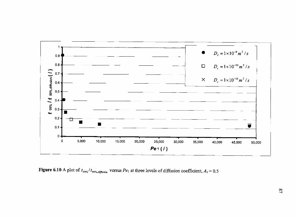
D =1x10⁹m2/s0.9 C
0.8 0 D=1x1O10m2/s- 0.7
06X D =1x1Om2/s
050'0)
0)o0.3
0.2-I
0.1
0 5,000 10,000 15,000 20,000 25,000 30,000 35,000 40,000 45,000 50,000
Pe 1 (I)
Figure 6.10 A plot of t99% /t99%dsion versus Pei at three levels of diffusion coefficient, A5 = 0.5

lx 1O m. The mesh size used in this case is 31x 61(31 in the x-direction and 61 in
the y-direction). For A5 = 2.0, the length of the cavity is 5 x i0 m. The mesh size is 21
x 61. For 1.0, the parameter t99% is the time required forM1 to decrease from 1 to
0.505. For = 2.0, the parameter t% is the time required for M1 to decrease from
0.5 to 0.2525. The graph showing t99% It99%dSjofl versus Pei is presented in Figure
6.11. For the pure diffusion case, the mass transfer rate does not depend on the aspect
ratio of the cavity. With the same diffusion coefficient and height of the bottom layer,
the time required to reach 99 % equilibrium (t99%dOfl) for A5 = 0.5, 1, and 2 is
identical. When the thermocapillary convection is induced in the cavity, the results
shows that the aspect ratio of the cavity has a significant effect on the mass transfer
rate. At Peclet numbers below 500, the parameters t99% I t99%dion for A5= 1.0 and for
A5 = 0.5 are almost identical. This is because at low Peclet number, the diffusion
process is dominant. As mentioned earlier, the diffusion process is independent of the
aspect ratio. However, at Peclet number higher than 500, the parameters
t99% It99%dffusion forA5 = 1.0 are higher than those for A5 = 0.5. At high Peclet number,
the convection process is dominant. Comparison between cases shown in Figure 6.8
forA5 = 0.5 and in the Figure 6.12 (b) forA5 = 1.0, where the length of the cavity is
shorter, indicates that the stagnant region at the middle of the cavity is smaller, and the
mixing of the liquid in the cavity is better. Consequently, in the cavity with A5 = 1.0,
the mass transfer process is more enhanced by the thermocapillary convection
However, when the length of the cavity is shorter than the height of the bottom
phase (A5 = 2.0), the parameter t99% It99%dsiDn is higher than those obtained for A5
0.5 and 1.0. This indicates that the mass transfer process is slower in the cavity with
aspect ratio larger than 1.0. Figure 6.13 (a) and (b) illustrate the streamlines and the
concentration plot for the case with A = 2.0. The plots show that the return flow of the
vortex does not extend to the bottom of the cavity. The convection can reach only
about half of the height of the liquid layer. Therefore the micro mixing process takes
place only in this region near the interface. The liquid near the top and the bottom of
the cavity is not carried to the interface by the convection. Therefore, the impact of
thethermocapillary convection on the mass transfer process is smaller.

0 1,000 2,000 3,000 4,000 5,000 6,000 7,000 8,000
Pel (I)
Figure 6.11 Plots of t99% / t99%dsion versus Fe1 at tbree levels of aspect ratio
9,000 10,000

91
UI'J
L"EI-
ii
iIIUU
:..4......a......-..........
lI_IU
I iJ
Figure 6.12 (a) Streamlines and (b) Concentration plot, for A = 1.0, AT' = 1.0°C,D =1x10⁹m2/s,M1= 1.5.

92
2 2
1.5 1.50.75
I i 0.5
05 05 i 025
0 0
0 0.5 0 0.5
(a) (b)
Figure 6.13 (a) Streamlines and (b) Concentration plot, for A = 2.0, AT' = 1.0°C,D =1x10⁹m2/s,M1= 1.5.

93
6.3 Effects of the Viscosity of the Luiuid in Phase 2
Similar to the case shown in the previous section we choose the base example,
for the purpose of comparison among different situations, to be the water-hexane case
in a cavity with A5 = 0.5, AT'= 0.1 °C, and D = lx i09 m2/s. The viscosity of hexane
(phase 2) used in the base case is 3 x 10 kg/m . s. The test is performed with four
different values of different viscosities; 0.1, 0.5, 2.0, and 10.0 times the viscosity of
the base case. The results are shown in Table 6.3. By increasing the viscosity in the
phase 2, the maximum tangential velocity at the interface decreases. With a decreasing
velocity at the interface, the effect of convection in both phases decreases and the time
required to reach 99 % of equilibrium increases.
Table 6.3 Maximum tangential velocity at the interface and t at various viscositiesin phase 2.
Viscosity in phase 2
(kglm.$)
Maximum tangential velocity at the interface
(mis)
t 99%
(s)
3.0x10⁵ 3.15x10³ 4.31
1.5x10⁴ 2.80x10³ 4.56
3.0x10⁴ 2.39x10³ 4.86
6.OxlO4 1.95x10³ 5.48
3.0x1O 0.75x10 12.79

6.4 Effects of the Capillary Number (Ca)
The capillary number is defined as
yAT'Ca = (6.3)
aaverage
where the variable is the temperature coefficient of the surface tension and
is the surface tension at the average temperature. The capillary number substantially
influences the height of the deformed interface at steady state. Therefore, we can study
the effect of the shape of the deformed interface on the mass transfer process by
changing the values of Ca. Again, the base case is the water-hexane case in a cavity
with A = 0.5. The temperature difference along the interface is constant at 0.1 °C and
the diffusion coefficient is 1 x 1 9 m2/s. The simulations are run for three values of
the capillary number (Ca = 0.5, 1, and 2). To keep y AT' constant, the capillary
number is increased by lowering the value ofaerage. It is assumed that the interface is
always perpendicular to the left and right wall.
The graphs indicating the interface height at steady state for each level of Ca
are shown in Figure 6.14. At Ca = 2, the length of the interface increases by 6%
compared to the flat interface. The increase in the length of the interface provides
more contact area for mass transfer. However, the graphs ofM1 versus time at each
level of Ca, shown in Figure 6.15, are almost identical. The relative difference
between the value of t99% when the interface is flat and the value oft99% when Ca = 2
is 1%. These results show that the deformation of the interface does not have
significant effect on the mass transfer process.
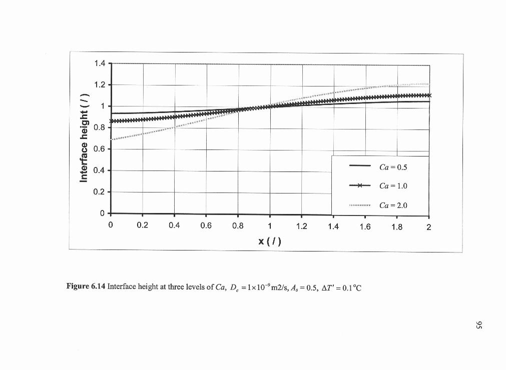
Figure 6.14 Interface height at three levels of Ca, D = lx 1 o m2Is, A5 0.5, AT' = 0.1 °C

2
flat interface1.9
a deformed interface with Ca = 0.51.8
1.7 e deformed interface with Ca = 1.02a.C
e deformed interface with Ca = 2.0
1.6
U)
E@>
1.4
1.3
0I- 1.1
I
0 1 2 3 4 5 6 7 8 9 10
Time (second)
Figure 6.15 Total relative mass in phase 1 versus time at different Ca, D = lx 10m2/s, A = 0.5, AT' = 0.1°C.
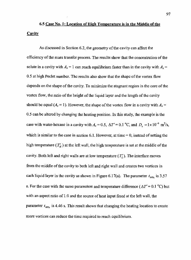
Cavity
6.5 Case No. 1: Location of High Temperature is in the Middle of the
As discussed in Section 6.2, the geometry of the cavity can affect the
97
efficiency of the mass transfer process. The results show that the concentration of the
solute in a cavity with A., = 1 can reach equilibrium faster than in the cavity with A.,
0.5 at high Peclet number. The results also show that the shape of the vortex flow
depends on the shape of the cavity. To minimize the stagnant region in the core of the
vortex flow, the ratio of the height of the liquid layer and the length of the cavity
should be equal (A., = 1). However, the shape of the vortex flow in a cavity with A., =
0.5 can be altered by changing the heating position. In this study, the example is the
case with water-hexane in a cavity with A., = 0.5, AT' = 0.1 °C, and D = lx 1 o m2/s,
which is similar to the case in section 6.1. However, at time = 0, instead of setting the
high temperature (T,) at the left wall, the high temperature is set at the middle of the
cavity. Both left and right walls are at low temperature (T). The interface moves
from the middle of the cavity to both left and right wall and creates two vortices in
each liquid layer in the cavity as shown in Figure 6.17(a). The parameter t99% is 3.57
s. For the case with the same parameters and temperature difference (AT' = 0.1 °C) but
with an aspect ratio of 1.0 and the source of heat input fixed at the left wall, the
parameter t99% is 4.46 s. This result shows that changing the heating location to create
more vortices can reduce the time required to reach equilibrium.

2
(a)
1.5
0.5
OL_0
2
(b)
1.5
0.5
00
0.5 1 1.5 2
0.5 1 1.5 2
0.9
0.8
0.7
0.6
0.5
0.4
0.3
0.2
0.1
Figure 6.16 (a) Streamlines, (b) Concentration plot at M1 = 1.5, A = 2.0,
D = 1 xlO9m2/s, AT' = 0.1°C when T. is imposed at the middle of the cavity.

6.6 Case No. 2: Unsteady Temperature at Both Walls
In this case, the effect of reversing the direction of the flow by changing the
direction of the temperature gradient is investigated. Complex transient patterns and
more mixing in the bulk fluid are expected.
We present the example of water-hexane in a cavity with A5 = 1.0, iT' = 1.0
°C and D = 1 x 1o- m2/s. The temperature at the left and the right wall is linearly
varied with time from T. to T as shown in Figure 6.17. The direction of the
temperature gradient reverses at time (t') = 0.5n-0.25 s, where n = 1, 2, 3, ..., 6. These
results can be compared with those presented in Section 6.2 where the high
temperature is fixed at the left wall and the low temperature is fixed at the right wall.
The graphs ofM1 versus time for the above mentioned cases are shown in Figure 6.18.
These graphs show that the mass transfer rate, which can be determined from the slope
of Mi, decreases when the direction of the temperature gradient reverses. At these
reversing points, the temperature gradients are also minimal, resulting in weak
convection. The results confirm that the mass transfer rate decreases with decreasing
temperature gradient.

20.5 -i- ____________________________
C.)
20 _____________________________ left
---*--- right waII
E / /0I-
19.5
0 0.5 1 1.5 2 2.5 3
Time (second)
Figure 6.17 Temperature at left and right wall versus time

1
£ pure diffusion- 0.95 ,\
varied temperature
\ fixed temperature0.85
0.8U)
0.75
0:
o 0.55II 1-.-.U..) I
0 0.5 1 1.5 2 2.5 3
Time (second)
Figure 6.18 Plots of total relative mass in phase 1 versus time for fixed and varied wall temperature

102
An additional test was performed to investigate the complex transient patterns
when the temperature gradient reverses without changing the magnitude of the
gradient. The same test case, as mentioned above, was adopted. The high temperature
(T) is fixed at the left wall and the low temperature (T) is fixed at the right wall. At
time = 0.56 s, the temperature at the left wall is suddenly changed to T1 and the right
wall temperature is changed to T. The transient velocity plots are shown in Figure
16.19(a), (b), (c), and (d). The reversed vortices start to develop near the left and the
right wall, diminishing the existing vortex. The process of developing the reversed
flow takes approximately 0.003 s. As shown in Figure 6.20, the mass transfer rate
slightly decreases during the development of the reversed flow due to the weakening
of the convection. The results show that the mass transfer rate depends on the strength
of the thermocapillary convection.

103
(a)
I.4'::'.:''I it,,,
- ___..S i t t $ *. . ''.._.%t S I I t ft....
' 5' ,, ' * , , . . .
L2... .t. 5" 5', .., 5'.'. .' 5'. -._,,__. .- .It- - .5' '5' ..., .5' .5' '.5' .5" .5" .--.--.,.--.-.-.-----....-.---'.,- -.. 'I. ," - - -
'I '"5".---' ._- - - .. .'...-.. - -.. - 1-I - -. '."''." -- 5'1. _ ,_ - ;:'
"- 'I
)8
'.5'-----
r
0 0.1 0.2 0.3 0.4 05 0.6 0.7 0.8 09 I
(b)
8
6
4
2 .
t - I, ,# I ---.5'I ". -. - ' 5' -., 5'- 5'- - - , t ' - ... - 5' 5'
4 .-...___._...___.._.___. - .- -5' -.----. - - 5' -.------'-.------5'-44_-___;5'_;"
"7 if' '. :._- ,-, tt,, - - rz---' -" " ' .- -
B ..
5. -I- ll -I...!,.0 0.1 0.2 0.3 0.4 0.5 0.8 0.7 0.8 0.9 1
Figure 6.19 Transient velocity plot at A= 1.0, D =1x10⁹m2/s, AT'=l.O°C afterthe temperature gradient reverses, (a) after 0.0005 s, (b) after 0.00 1 s,(c) after 0.0015 s, and (d) after 0.002 s.

104
(c)
18
16
1.4 : : :::::::: ::.:::: : :
1.2., - - - - t ._.....4'A___ -
,, 4. 4.; I..-..,,-fir I-.4 4 4 I S 4 * - - - 44-
.4. .-.4--.--.---.4 - - - -.- - - -. - . - -.--.----._---1------. -. -. -----.4.-. -- -_--
4.
t .4..,
_ s'' '-.4 -.4- 4 ............... -4,
I : : : : : : S
S : ; : : : : : : : : : : : : : :
0 Of 0.2 0.3 0.4 O5 06 0.7 0.8 0.9
1.8
1.6
14
1.2
I
0.8
0.6
OA
0.2
(d)
---i : :
t It,.. --------.------- I 4
.4.- .4- - .4- .4- *--*-----:-----.44-.---
'.4-...4- -----.4---- ..--*----------------4 I
4. ----4--4 S 4.4-'..... - -
. . - -
::::
_,. _,.. :_ :
01 0.2 03 04 05 06 0.7 0.8 09
Figure 6.19 Continued

fixed temperature0.95
gradient0.9 reversedo
0.85 gradient -
0.8..EU)U)
joO.6
0.550.5
0 0.2 0.4 0.6 0.8
time (second)
Figure 6.20 Plots of total relative mass in phase 1 versus time for fixed and reversed temperature gradient

106
6.7 Case No. 3: Reaction at the Top Wall
In this scenario, the microscale channel serves not only as a liquid-liquid
extractor, but also as a microscale reactor which support heterogeneous catalytic
reaction. The top wall is assumed to be a catalyst carrier where solute C decomposes
by the first order reaction kinetics. Solute C is extracted from the bottom liquid layer
(phase 1) into the top layer (phase 2) and then solute C reacts at the top wall.
The rate of reaction can be expressed as follow:
= k"c' (6.4)
where r" (mollm2s) is the rate of reaction based on catalyst surface, k" (mis) is
reaction rate constant, and c' is the dimensional concentration of solute C. It is
assumed that there is no accumulation of C at the top wall. The balance equation of C
at the top wall (boundary condition) can be expressed as follow:
D2 = k"c'dy'
(6.5)
where D2 (m2/s) is the diffusion coefficient of solute C in liquid phase 2. Using the
scaling factors described in Chapter 3, Equation 6.5 can be written in dimensionless
form:
dc k"H-= Cdy D2
(6.6)
where H (m) is the height of the bottom layer. Equation 6.6 is introduced as the
boundary condition at the top wall.
Two different reaction rate constant (k") are investigated: 2.5 x 1 0_6 and
1.0 x i0 mis. Both cases are water-hexane in the microscale cavity with A 1.0,

107
iT' = 1.0 °C, H = lx iO4m, and D = lx iO m2/s. A dimensionless quantity called
k"the Thiele modulus is defined as mH, where m = I . The first numerical
'DC2H
experiment with k? = 2.5 x 10 rn/s corresponds to a Thiele modulus of 0.5, which
indicates that the reaction is relatively slow compared to the diffusion. On the
contrary, the second numerical experiment with k' = 1.0 x 1o- rn/s corresponds to a
Thiele modulus of 10, which indicates relatively fast reaction. The graphs of M1 and
M2 versus time are shown in Figure 6.21 and Figure 6.22, respectively. The results
shows that in both cases the thermocapillary convection increases the rate of mass
transfer from phase 1 to phase 2. In both diffusion cases, M1 's are almost identical at
from the beginning of the process. This indicates that the rate of mass transfer from
phase 1 to phase 2 is higher than rate of reaction. After 4 s, M2 for the second run (fast
reaction) starts to decrease and the rate of reaction is higher than the rate of mass
transfer. For the two thermocapillary convection cases, the same phenomenon is
observed. However, the rate of mass transfer is much faster than in the two
corresponding diffusion cases. The rate of mass transfer seems to be unaffected by the
rate of reaction at the beginning of the process (up to 0.8 s). ConsiderM2 in the second
run (fast reaction) with the thermocapillary convection after 0.8 s. The rate of decrease
of M2 is much stronger than in those cases without convective flow. This indicates that
the thermocapillary convection promotes the overall rate of reaction process.

i diffusion, slow reaction
diffusion, fast reaction0.9
convection, slow reaction
08 convection, fast reaction
U)
0.4
0.2,
0I-
0.1
0U U
0.00 1.00 2.00 3.00 4.00 5.00 6.00 7.00 8.00
Time (second)
Figure 6.21 Plots of total relative mass in phase 1 versus time for cases with the reaction at the top wall

diffusion, slow reaction0.6
diffusion, fast reaction
0 ___________________________________convection, slow reaction
convection, fast reaction
.
0I-
0 I I
0.00 1.00 2.00 3.00 4.00 5.00 6.00 7.00 8.00
Time (second)
Figure 6.22 Plots of total relative mass in phase 2versus time for cases with the reaction at the top wall

110
7. CONCLUSIONS AND RECOMMENDATIONS FOR FUTURE STUDY
7.1 Conclusions
The effect of the thermocapillary convection on the mass transfer rate of a
solute between two immiscible liquids within a microscale channel has been
investigated. A tool developed in this study was a computational fluid dynamics code
written in Fortran77. The finite volume method with Marker and Cell (MAC)
technique was used to solve mass, momentum, and energy conservation equations.
The discrete surface tracking technique was used to determine the location of the
moving fluid-fluid interface. The probe technique was utilized to approximate normal
gradients at the interface for solving thermal, normal and tangential stresses balance
equations. The code produced results that were approximately second-order accurate
in space and first-order accurate in time, and consistent with results reported in several
papers.
Numerical simulation experiments were designed to study the effects of the
temperature difference along the interface, the aspect ratio of the cavity, the viscosity
of liquid in phase 2, and the capillary number. The test case was water-hexane system
where arbitrary solute C transfers from water to hexane. The parameter t99% which is
the time required to reach 99% of the equilibrium, was used to indicate the duration of
the mass transfer process. The improvement of the mass transfer process is indicated
by the ratio of the t99% from the case with convection over the t99% from the same case
without convection (pure diffusion case). The results are summarized as follows:

111
(1) The thermocapillary convection increases the overall mass transfer rate.
The simulations show that the thermocapillary convection generates the micro mixing
in each phase. Liquid near the top and the bottom wall is brought to the interface,
creating high concentration gradient across the interface, resulting in increasing the
mass transfer rate.
(2) The mass transfer rate increases with increasing the temperature difference
along the interface. The simulations show that the velocity in the bulk liquid increases
with increasing the temperature difference, resulting in more mixing in each phase.
(3) The improvement of the mass transfer rate by the thermocapillary
convection is found to be a function of Peclet number. For a cavity with aspect ratio
(A5) equal to 0.5, the thermocapillary convection improves the mass transfer rate
substantially when the Peclet number increases to 1,000. The improvement of the
mass transfer rate starts to reach the maximum point while the Peclet number is
reaching 5,000. At Peclet number equal to 5,000, the time required for the system to
reach 99% of equilibrium (t99%) is reduced by 86% compared to the system without
the thermocapillary convection (t99%dSfl.)
(4) The improvement of mass transfer rate increases when the aspect ratio of
the cavity increases to 1. However, the improvement of mass transfer rate decrease if
the aspect ratio is higher than 1. For the same system withA5 = 1, the parameter t99% is
reduced by 91% and for A5 =2, the parameter t% is reduced by 73%. The simulations
show that when the length of the cavity is smaller than the height of the bottom phase,

112
thermocapillary convection occurs only near the interface and the liquid at the bottom
and top of the cavity is almost stagnant.
(5) By increasing the viscosity of the liquid in phase 2, the maximum
tangential velocity at the interface decreases. As a result, the improvement of mass
transfer rate by the thermocapillary convection in both phases decreases and t99%
increases.
(6) For the case where A = 0.5, the deformation of the interface has no
significant effect on the improvement of mass transfer rate. By increasing Ca to be
equal to 2, the length of the interface increases by 6% compared to the flat interface;
however, the parameter t99% decreases just 1%.
(7) For a cavity with small aspect ratio, changing the heating location to create
more vortices can reduce t99%. For a cavity with A = 0.5, by setting the high
temperature at the middle of the cavity, two vortices are formed in each liquid layer.
The parameter t99% is 3.57, which is smaller than 4.46 for the same case but A5 = 1 and
the high temperature is fixed at the left wall.
(8) The results from the case with time dependent temperature at the left and
right walls confirm the conclusion that the mass transfer rate increases with increasing
temperature difference along the interface.

113
7.2 Recommendations for Future Study
(1) The performance of this software can be enhanced by implementing
parallel programming into the software, which could make the program run faster.
(2) It was found that the direct solver of Poisson equation is the most
time-consuming part of this computer software. Other methods such as the iterative
method should be investigated.
(3) The computer code could be expanded to solve 3-D problems. With 3-D
code, the effect of the velocity in the z-direction can be investigated. A complete
picture of liquid-liquid extraction in a microscale channel can be simulated and
modeled. The system can be optimized to find the optimal flow rate, temperature
difference, and geometry of the cavity.
(4) Experiments on liquid-liquid extraction in a microscale channel could be
performed to validate the results from the simulation.

114
BIBLIOGRAPHY
Adler, J., and Sowerby, L. 1970. Shallow three-dimensional flows with variablesurface tension. J. Fluid Mech. 42:549-559.
Anderson, J.D. 1995. Computationaifluid dynamics: the basics with applications.New York, NY: McGraw-Hill.
Babu, V., and Korpela, S.A. 1990. Three-dimensional thermocapillary convectionin a cavity. Computers Fluids 18:229-238.
Babu, V., and Korpela, S.A. 1994. Numerical solution of the incompressible, three-dimensional Navier-Stokes equation. Computers Fluids 23:675-69 1.
Behnia, M., Stella, F., and Guj, G. 1995. Numerical study of three-dimentional low-Pr buoyancy and thermocapillary convection. Numerical Heat Transfer, Part A27:73-88.
Chang, Y.C., Hou, T.Y., Merriman, B., and Osher, S. 1996. A level set formulation ofeulerian interface capturing methods for incompressible fluid flows.Journal of Computational Physics 124:449-464.
Chen, J.C., Sheu, J.C., and Jwu, S.S. 1990. Numerical computation of thermocapillaryconvection in a rectangular cavity. Numerical Heat Transfer, Part A17:287-308.
Chen, J.C., Chen W.C., and Hwu, F.S. 1991. Numerical computations of unsteadythermocapillary convection in a rectangular cavity with surface deformation.Heat Transfer in Metals and Containerless Processing and Manufacturing,HTD 162:89-95.
Colinet, P., Legros, J.C., and Velarde, M.G. 1999. Interfacial turbulence and masstransfer through interface. European Space Agency, ESAPS n SP-433:21 1-2 18
Davis, S.H. 1987. Thermocapillary instabilities, Ann. Rev. Fluid Mech. 19:403-435.
Floryan, J.M., and Rasmussen, H. 1989. Numerical methods for viscous flows withmoving boundaries. App!. Mech. Rev. 42:323-340.
Fontaine, J.-P., and Sani, R.L. 1996. Flow and transport in a multilayered fluid systemI. Influence of 1- or p -g environment. mt. J. Heat Mass Transfer 39:2751-2770

115
BIBLIOGRAPHY (Continued)
Hamed, M.S., and Floryan, J.M. 1998. Numerical simulation of unsteadynonisothermal capillary interfaces. Journal of Computational Physics145:110-140.
Hamed, M., and Floryan, J.M. 2000. Marangoni convection. Part 1. A cavity withdifferentially heated sidewalls. J Fluid Mech. 405:79-110.
Harlow, F.H., and Welch, B. 1965. Numerical calculation of time-dependent viscousincompressible flow of fluids with free surface. Phys. Fluids 8: 2182.
Hoffinaim, J.D. 1992. Numerical methods for engineers and scientists.New Yourk, NY: McGraw-Hill.
Labonia, G., Stella, F., Leonardi, E., and Guj, G. 1997. A numerical study of the effectof free surface deformation on buoyancy and thermocapillary convection.Journal of Computational Physics 132:34-50.
Labonia, G., Timchenko, V., Simpson, J.E., Garimella, S.V., Leonardi, E., andDavis, G.V. 1998. Reconstruction and advection of a moving interface inthree dimensions on a fixed grid. Numerical Heat Transfer, Part B 34:12 1-138.
Lai, C.L., and Yang, T.S. 1990. Unsteady thermocapillary flows and free surfaceoscillations. Acta Astronautica 21:629-640.
Levich, V.G. 1962. Physicochemical Hydrodynamics. Englewood Cliffs, NJ:Prentice-Hall.
Leypoldt, J., Kuhlmann, H.C., and Rath, H.J. 2000. Three-dimensional numericalsimulation of thermocapillary flows in cylindrical liquid bridges..1. Fluid Mech. 414:285-3 14.
Liang, M.C., and Lan, C.W. 1996. Three-dimensional convection and solutesegregation in vertical Bridgman crystal growth. Journal of Crytal Growth167:320-332.
Liu, Q.S., Roux, B., and Velarde, M.G. 1998. Thermocapillary convection in two layersystems. mt. J. Heat Mass Transfer 41:1499-1511.
Lu, W.Q. 1994. Boundary element analysis of thennocapillary convection with a freesurface in a rectangular cavity. mt. J. Heat Mass Transfer 37:1063-1071.

116
BIBLIOGRAPHY (Continued)
Ostrach, S. 1982. Low-gravity fluid flows. Ann. Rev. Fluid Mech. 14:313-345.
Pearson, J.R.A. 1958. On convection cells induced by surface tension. J Fluid Mech.4:489-500.
Peltier, L.J., Biringen, S., and Farhangnia, M. 1995. Numerical simulation of time-dependent thermocapillary convection in layered fluid systems.Journal of Thermophysics and Heat Transfer 9:702-707.
Riley, R.J., and Neitzel, G.P. 1998. Instability of thermocapillary-buoyancyconvection in shallow layers. Part 1. Characterization of steady and oscillatoryinstabilities. J. Fluid Mech. 359:143-164
Rivas, D. 1991. High-Reynolds-number thermocapillary flows in shallow enclosures.Phys. Fluids A 3:280-291.
Sa13, V., kuhlmann, H.C., and Rath, H.J. 1996. Investigation of three-dimensionalthermocapillary convection in a cubic container by a multi-grid method.mt. J. Heat Mass Transfer 39:603-613.
Saghir, M.Z. 1999. Convection in two-liquid-layer system with low Prandtl number.Energy Sources 21:139-144.
Sasmal, G.P., and Hochstein, J.I. 1994. Marangoni convection with a curved anddeforming free surface in a cavity. Journal of Fluids Engineering 116:577-582
Schumann, U., and Sweet, R.A. 1976. A direct method for the solution of Poissonsequation with Neumann boundary conditions on a staggered grid of arbitrarysize. Journal of Computational Physics 20:171-182.
Scriven, L.E., and Sternling, C.V. 1964. On cellular convection driven by surfacetension gradients: effect of mean surface tension and viscosity.J. Fluid Mech. 19:321-340.
Sen, A.K., and Davis, S.H. 1982. Steady thermocapillary flows in two-dimensionalslots.J Fluid Mech. 121:163-186.
Shyy, W., Udaykumar, H.S., Rao, M.M., and Smith, R.W. 1996. Computational FluidDynamics with Moving Boundaries. Hemisphere, Washington, DC.

117
BIBLIOGRAPHY (Continued)
Sussman, M., Smereka, P., and Osher, S. 1994. A level set approach for computingsolutions to incompressible two-phase flow. Journal of Computational Physics114:146-159.
Udaykumar, H.S., Mittal, R., and Shyy, W. 1999. Simulation offlow and heat transferwith phase boundaries and complex geometries on Cartesian grids. AmericanSociety of Mechanical Engineers, Heat Transfer Division, (Publication) HTD364-3: 357-370.
Wang, P., and Kahawita, R. 1996. Transient buoyancy-thermocapillary convection intwo superposed immiscible liquid layers. Numerical Heat Transfer, Part A30:477-501.
Xu, J., and Zebib, A. 1998. Oscillatory two- and three-dimensional thermocapillaryconvection. I Fluid Mech. 364:187-209.
Ye, T., Mittal, R., Udaykumar, H.S., and Shyy, W. 1999. An accurate Cartesian gridMethod for viscous incompressible flows with complex immersed boundaries.Journal of Computational Physics 156:209-240.
Yih, C.S. 1968. Fluid motion induced by surface-tension variation. Phys Fluids11:477-480.
Zebib, A., Homsy, G.M., and Meiburg, E. 1985. High marangoni number convectionin a square cavity. Phys. Fluids 28:3467-3476.

118
APPENDICES

119
Appendix A: Properties of Water and Hexane
Water Hexane
Density [kg/rn3] 9.97x10² 6.55x10²
Dynamic viscosity [kg/m.s] 8.9x10⁴ 3.0x10⁴
Thermal diffusivity [m2/s] 1.46 x iO 8.07 x 10⁸
Thermal conductivity [W/ m K] 6.09 x 10' 1.2 xl 0'
Surface tension (°verage) [N/rn] 8.6 x io
Temperature coefficient of surfacetension(y)[N/rn.K]
5.3 x 10_2

120
Appendix B: Order of Convergence and Richardson Extrapolation
The actual accuracy is determined on the basis of calculations with different
grid sizes and by observing the tendency of results as the grid size is decreased.
Solutions are obtained for grid sizes i = 1/N, 1/2N, 1/4N. If one assumes that the
discretization error is Ci', where C is a constant, then the order of convergence r can
be evaluate as:
where
r In[(e2N,4N)/(c1N/2N)]
ln[2]
1/2
=-62N/4N
1
j=1
1/2
61N/2Nj=1
(Bi)
In the above equations, q$ is a solution quantity, subscripts iN, 2W, 4N refer to
solutions obtained on grid size 1/N, 1/2N, 1/4N, respectively, Mis the total number of
points that overlap on all three grids employed. In our case, none of grid point is
overlap because of the staggered grid arrangement. Therefore 72 assigned points
inside the cavity were chosen: x 0.1, 0.2, ..., 0.9 andy = 0.1, 0.2, ..., 0.8. If these
points are not on the grid, biquadratic interpolation is used to calculate on those
points.

121
The Richardson extrapolation is used to calculate the values of variables where
N -* infinity. The Richardson extrapolated value can be expressed as:
0 = 04N04N 02N (B2)2' 1