Embed Size (px)
Citation preview

AN ABSTRACT OF THE THESIS OF
Mark H Shroyer for the degree ofDoctor ofPhilosophy in Physics presented on
November 30 1999
Title An NMR Study ofBistabJe Defects in CdTe and CdF2shy
Abstract approved
William W Warren
Bistable properties have been reported in CdF2 and CdTe systems doped with
In and Ga It is characteristic ofthese materials that the excited bistable state can be
accessed by optical excitation
In this work pulsed nuclear magnetic resonance (NMR) in conjunction with
illumination at low temperatures has been used to study 113Cd spin-lattice relaxation
(lIT1) In this way bistable effects have been observed These effects are interpreted
in terms of the negative-V DX models ofbistability that have been put forth for the
respective materials In the context of these models data concerning the respective
DX centers electronic states have been collected Conclusions are based in part on
the complementary nature of cation and anion host NMR
In CdTeGa under illumination at 31 K a non-persistent order ofmagnitude
enhancement of the 1l3Cd spin-lattice relaxation rate (l1T1) is observed After
illumination the rate is persistently enhanced by about 50 Over the temperature
Redacted for Privacy
range of31 K to 200 K the 113Cd relaxation rate appears to be due to an activated
process attributed to the thermal generation of paramagnetic centers An activation
energy ~=15 me V is determined
In CdF2 the 113Cd (1T1) is persistently enhanced by a factor oftwo following
illumination below 80 K Above 150 K the l13Cd (1T1) is strongly temperature
dependent This relaxation is attributed to thermally generated free carriers This
process is ineffective for 19F relaxation This activated process yields an activation
energy amp=185(10) meV The 19F nuclei do however appear to relax by an activated
process This relaxation is attributed to thermally generated paramagnetic centers and
yields an activation energy LiE=70(10) meV
In CdTeGa 69Ga has been observed It is shown that the observed 69Ga
resonance is due to Ga situated substitutionally on the Cd sublattice However these
Ga account for only about 10 ofthe Ga in the sample The 69Ga (lT1) has been
measured over the temperature range 200 K to 470 K These rates are consistent with
the T temperature dependence expected for quadrupolar relaxation due to lattice
vibrations
Copyright by Mark H Shroyer November 30 1999 All Rights Reserved
An NMR Study of Bistable Defects in CdTe and CdF 2
by
Mark H Shroyer
A THESIS
submitted to
Oregon State University
in partial fulfillment of the requirements for the
degree of
Doctor ofPhilosophy
Presented November 30 1999 Commencement June 2000
Doctor ofPhilosophy thesis ofMark H Shroyer presented on November 30 1999
Approved
Major Professor representing Physics
epartment ofPhYSICSChair of the
I understand that my thesis will become part ofthe pennanent collection of Oregon State University libraries My signature below authorizes release of my thesis to any reader upon request
___________Author
Redacted for Privacy
Redacted for Privacy
Redacted for Privacy
Redacted for Privacy
ACKNOWLEGMENT
I have had the good fortune ofbeing surrounded by loving supportive friends
and family my entire life It is not possible to express my appreciation in detail I
would like to acknowledge those who made this work possible
I would first like to acknowledge the National Science Foundation for their
support of this work I would like to thank Dr Ryskin Dr Furdyna and Dr Ramdas
for generously providing the samples used in this work
I am extremely grateful for the technical assistance and education provided by
John Archibald during the construction of the probe I would also like to thank John
Gardner and Henry Jansen for many insightful and enjoyable discussions
I wish to express my appreciation to my mentor Bill Warren He has been my
teacher in all things
To my wife Mary Jane thank you for your support and understanding And
finally a thanks to my daughter Jordan for making me smile on the darkest wettest
days
TABLE OF CONTENTS
Page 1 Introduction 1
2 NMR and Relaxation Theory 8
21 NMR Theory 8
211 Zeeman interaction 8 212 Magnetic moment in a magnetic field (classic model) 8 213 Pulse width condition 10 214 Detection of magnetization 10
22 Important Characteristic Times 11
221 Free induction decay time - T2 12 222 Irreversible transverse magnetization decay time - T 2 14 223 Spin-lattice relaxation time - T1 15 224 Caveats 15
23 Spin Ternperature 16
231 Definition of spin temperature 16 232 Relaxation with spin temperature 17 233 Relaxation without spin temperature 18
24 Spin-Lattice Relaxation Mechanisms 19
241 Relaxation via free electrons in semiconductors 19 242 Relaxation by paramagnetic centers via direct interaction 20 243 Relaxation by paramagnetic centers via spin diffusion 21 244 Relaxation by the nuclear quadrupolar interaction 28
3 Materials and Methods 32
31 Samples 32
311 CdTeCdMnTe 32 312 CdFz 33
TABLE OF CONTENTS (Continued)
Page 32 Hardware 35
321 The circuit 35 322 Temperature monitoring and regulation 37 323 Optical access 38 324 Protocol for low temperature NMR 41
33 Software 48
331 How to ensure equilibrium at start ofexperiment 49 332 90-degree pulse width condition when T 1 is long 50 333 Short FID and measuring T 1 51
4 Host ~ on CdMnTeGa 54
41 Host data 54
411 113Cd Data 54 412 Preliminary Te relaxation results 57
42 Analysis 58
421 Structure of 113Cd line 58 422 Effect ofMn on the 113Cd lineshape 59 423 Shifts in the l13Cd line 60 424 1l3Cd spin-lattice relaxation in the presence ofMn 61 425 Te relaxation in Cd99Mn01TeGa 65
43 Summary 65
5 ~ Study ofDX Defects in CdTe 68
51 Host Data 68
52 Impurity Data 75
53 Analysis 79
531 Effects of Ga and In on sRin-lattice relaxation 79 532 Efect of illumination on l3Cd relaxation 81 533 Effect of In on 113Cd lineshape in CdTeIn 83 534 Effect of Ga on dark relaxation of 113Cd in CdTeGa 87
TABLE OF CONTENTS (Continued)
Page 535 Assignment of69Ga impurity resonance (narrow line) 88 536 Assignment of69Ga impurity resonance (broad line-echo) 91 537 Fraction of substitutional Ga and other sites 93
a Impunty 53 8 Spm-middot Iattlce re IaxatlOn 0 f 69G 93
54 Summary 95
6 NMR Study ofDX Center and Bistability in CdF2In or Ga 98
61 Host Data 99
611 1l3Cd relaxation data 99 612 19F relaxation data 101 613 1l3Cd lineshape data 105 614 19F lineshape data 107
62 Analysis 111
621 Relaxation is not due to coupling of 1l3Cd and 19F nuclear systems 111
622 S~in-Iattice relaxation of 1l3Cd in CdF2 112 623 11 Cd relaxation in CdF2In above 150 K 113 624 113Cd relaxation in CdF2In versus temperature
and illumination 114 625 19F relaxation in CdF2below room temperature 116 626 19F relaxation in CdF2In 117 627 1l3Cd lineshape 120 628 19F lineshape 121 629 19p relaxation in CdF2above room temperature 122
63 Summary 123
7 Future Work and Conclusions 125
BIBLIOGRAPHY 130
APPENDICES 134
Appendix A Pulse-Programs 135 Appendix B Material Characteristics and Constants 139 Appendix C Second Moment Calculator 140 Appendix D Modeling ofQuadrupole Broadening 159
LIST OF FIGURES
Figure Page
11 Configuration Coordinate Diagram Energy vs lattice relaxation 4
21 On the left is a typical free induction decay plotting induced voltage versus time On the right is the Fourier transform of the FID plotting amplitude versus frequency 11
22 Spin Vz system in applied field 16
31 Zincblende structure Both host species are tetrahedrally coordinated 34
32 Fluorite structure Fluorine is tetrahedrally coordinated Cd occupies every other cube ofF simple cubic sub lattice 34
33 Probe circuit and schematic diagram oflow temperature probe 39
41 113Cd lineshape for various Mn concentrations Frequency shift is with respect to CdTe Intensities not to scale 55
42 113Cd lineshape in Cd99Mn01TeGa at various temperatures Intensities are to scale 56
43 113Cd recovery data The left and right plots show the difference from equilibrium magnetization verms recovery time for CdTeGa and Cd99Mn01TeGa respectively Line is a single exponential fit 56
44 113Cd spin-lattice relaxation rates versus temperature and Mn concentration in CdMnTeGa 58
45 113Cd paramagnetic shift versus lIT for peak POI in Cd99MnOlTeGa Shift is with respect to Cd line in CdTe 61
51 Spin-lattice relaxation rates for 113Cd in CdTe CdTeGa and CdTeIn vs reciprocal temperature 12312STe relaxation rate at room temperature 69
52 Spin-lattice relaxation rates for l13Cd in CdTeGa vs reciprocal temperature in the dark in situ illumination and dark after illumination 70
LIST OF FIGURES (Continued)
Figure Page
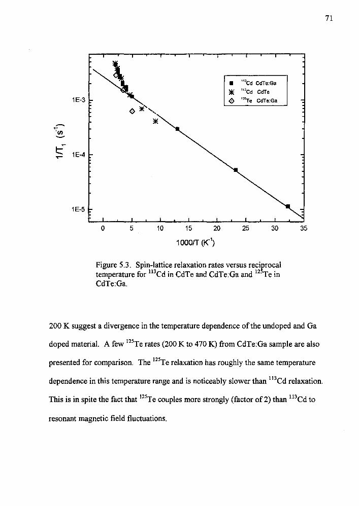
53 Spin-lattice relaxation rates versus rec~rocal temperature for 113Cd in CdTe and CdTeGa and 12 Te in CdTeGa 71
54 113Cd spectra from CdTeIn for various temperatures 72
55 113Cd linewidth in CdTeIn and CdTeGa versus reciprocal temperature 73
56 Resonance shifts for 113Cd in In and Ga doped and undoped CdTe and for 12STe and 69Ga in CdTeGa versus temperature 74
57 Host and impurity spectra 76
58 69Ga spectra versus rotation around coil axis with arbitrary zero 76
59 Quadrupolar echo Of 69Ga in CdTeGa at room temperature 76
510 Inversion recovery curves for narrow 69Ga resonance and echo Curve is a single exponential fit 78
511 Relaxation rates of69Ga in CdTeGa Solid line is a best fit for 1IT1=CT2 78
512 Configuration Coordinate Diagram Energy vs lattice relaxation 83
513 On the left are 1l3Cd rates versus reciprocal temperature in a log-log plot Straight line fit indicates power law dependence in CdTe and CdTeGa above 200 K On the right are 1l3Cd rates versus reciprocal temperature in a semi-log plot Straight line fit indicates an activated process 88
61 113Cd relaxation rates versus reciprocal temperature taken in the dark before and after illumination in CdF2In 99
62 113Cd relaxation rates versus reciprocal temperature for In doped and undoped CdF2 Also unreduced and reduced Ga doped CdF2 101
LIST OF FIGURES (Continued)
Figure Page
63 Left plot shows magnetization recovery ofleft and right shoulders Of 19F line with a long saturating comb A single exponential is plotted for comparison Right plot shows exponential recovery obtained with a short saturating comb 102
64 19p relaxation rates versus reciprocal temperature in undoped and In doped CdF2 104
65 19F relaxation rate versus applied field for CdF2 and CdF2In crystals 104
66 Left shows effect of temperature on 113Cd specra Right plots FWHM versus reciprocal temperature for undoped CdF2 powder and single crystal Vnns (from 2nd moment for powder) is shown for comparison 105
67 Linewidths versus reciprocal temperature for doped CdF2 At 300 K linewidth versus random orientation in CdF2In 106
68 Left shows the effect of decoupling RF on the Cd lineshape power corresponds to H-channel setting) Right plots FWHM versus decoupling field 107
69 19F spectra ofmodulus intensity versus frequency shift (kHz) in undoped CdF2 crystal at temperatures fi-om 200 K to 470 K All plotted with respect to RF=31885 NIHz at 80 T 109
610 19F spectra ofmodulus intensity versus frequency shift (kHz) in CdF2In at various temperatures RF = 31885 MHz at 80 T 110
611 Left plot shows 113Cd and 19F relaxation rates versus reciprocal temperature in CdF2In Right plot shows relative magnitude of resonant fluctuating magnetic fields at respective nuclear site 113
612 Configuration Coordinate Diagram Energy vs lattice relaxation 115
613 Left plot shows 113Cd and 19F relaxation rates versus liT in CdF2 crystaL Rjght plot shows relative magnitude of resonant fluctuating magnetic fields at respective nuclear site 117
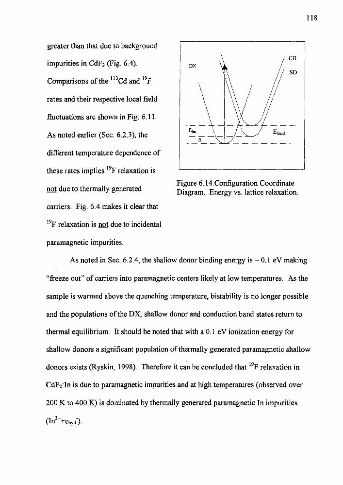
614 Configuration Coordinate Diagram Energy vs lattice relaxation 118
LIST OF TABLES
Table Page
21 Electronic relaxation rate versus temperature and field 22
22 Relaxation by spin diffusion 27
23 Quadrupole recovery 31
31 CdTe based samples 32
32 CdF2 based samples 33
41 Mn relaxation and 1l3Cd spin-diffusion 63
51 Theoretical probability density 80
52 Satellite intensities from nearest neighbors 90
LIST OF APPENDIX TABLES
Table Page
Bl Relevant isotopic constants l35
2ndCl moments of probe nuclei in CdTe l37
2ndC2 moments ofprobe nuclei in CdF2 l37
An NMR Study of Bistable )efects in CdTe and CdF~
1 Introduction
A semiconductor (or insulator) can be described in terms of its electronic band
structure A metal exists when the energy level of the highest occupied state at T=O
(Fermi level) falls insidea continuous band of allowed energy levels In a
semiconductor there is a separation (band gap) between the valence band (fully
occupied) and the conduction band (unoccupied at T=O) In an intrinsic
semiconductor the conduction band is partially occupied by thermally generated
carries from the valence band The probability of this is a function ofthe band gap
The size of the band gap gives rise to the somewhat arbitrary distinction made
between semiconductors and insulators Typically the band gap increases as the bond
in the compound becomes more ionic (IV ~ IlI-V ~ II-VI ~ I-VII compounds)
The utility of semiconductors is in the creation of electronic devices (diodes
transistors etc) In materials used in these devices it is possible (and necessary for
the device) to substitute low concentrations ofatoms from adjacent columns in the
periodic table for host atoms These atoms go into the host lattice substitutionally as
shallow donors or acceptors It is the ability to dope these materials n-type (donor) or
p-type (acceptor) that makes it possible to create these devices
A great deal of success has been achieved working with Si and Ge (IV) or III-V
materials such as GaAs One important application of these materials is the light
emitting diode (LED) The frequency of the light emitted is a function of the energy
2
gap in the region where holes and electrons recombine An alloy commonly used is
InxGal-xASyPl-y By varying the relative concentrations ofhost species a range of
wavelengths extending from infrared to yellow can be achieved (Bhattacharya 1994)
However there is an upper limit to the band gap and thus the frequency of the emitted
light
In the search for higher frequencies (so that the entire visible spectrum might
be used) II-VI materials have been studied for their larger band gaps It is not
sufficient that the material has a large band gap but it must be able to be heavily nshy
doped and p-doped It proves difficult to dope many of these 11-VI materials This
work will focus specifically on CdTe based compounds CdTe is ineffectively doped
with Ga In a sample ofCdTe doped with Ga for example an atomic concentration of
1019 atomslcm3 yields a carrier concentration of 1014 electronslcm3 Similar effects are
noted in CdMnTe and CdZnTe alloys when doped with Ga In and CI (Semaltianos et
al1993 1995 Leighton et at 1996 Thio et aI 1996) This suggests the presence of
some compensating defect that traps carriers
An interesting property of these materials is that under illumination carriers
are photo-excited and the samples become conducting Further at low temperatures
the carrier concentration remains even after the illumination is removed This is called
persistent photoconductivity (PPC) and is a property ofbistable defects It is the
bistable defect that is of interest in this work
CdF2 is another material that exhibits bistable properties when doped with Ga
or In In this case the refractive index of the material can be changed by illumination
with light of a sufficiently short wavelength (Alnlt650 nm Ryskin et at 1995
3
kalt500 nm Suchocki et al 1997) This photo-refractive effect is a very local
phenomenon and at low temperatures is persistent This is evidence ofbistability
These materials are ofpractical interest because of their potential as a medium for
high-density holographic data storage
Both of these bistable defects are explained in terms of the negative U effect
The general argument is that the impurity has both a shallow donor (hydro genic
substitutional) site and a deep ground state (DX state) in which the electron(s) are
highly localized The localization of the electron(s) in the DX center is accompanied
by a large lattice relaxation (Lang and Logan 1977) The decrease in potential energy
gained by the lattice relaxation more than offsets the increase in Coulombic potential
due to the electronic localization This is called the negative U effect Chadi and
Chang (1988 1989) presented a model to explain PPC observed in GaAs compounds
(review Mooney 1989) In the zincblende structure ofGaAs (and CdTe) host Ga is
tetrahedrally coordinated with As Chadi and Chang calculate that it is energetically
favorable for a shallow donor (ef + ehyq) to capture a second electron break a single
ef-As bond and move toward one of the faces of the distorted As tetrahedron
(ll)
More recently Park and Chadi (1995) have calculated stable defects of analogous
structure in CdTe ZnTe and CdZnTe alloys doped with Ga AI and In Experimental
work to date (above and Iseler et al 1972 Terry et al 1992 Khachaturyan et al
1989) supports this model
Park and Chadi (1999) have also calculated stable DX centers in CdF2 doped
with In and Ga The calculated structure of the DX center in CdF2 is slightly different
4
from that described above for CdT e
Fluorine makes a simple cubic sub-lattice in
which every other cube is occupied by a Cd DX
Park and Chadi calculate that it is
energetically favorable for the Mill impurity
to capture and localize a second electron
and slide into an interstitial site (one of the
empty F cubes) rather than go into the Cd
Figure 11 Configuration sub-lattice substitutionally For this model Coordinate Diagram Energy
vs lattice relaxation there is also a good deal ofexperimental
support This includes observation ofa
diamagnetic ground state and paramagnetic excited shallow donor state (Ryskin et al
1998) PPC (piekara et at 1986) and an open volume associated with the formation
of the DX center (Nissil et al 1999)
It is important to note the common features to both ofthese defect
models The excited state is paramagnetic (at low temperatures) and both sites of the
ground state are diamagnetic Both explain the observed bistable properties in terms
of a self-compensating defect that localizes a second electron and undergoes a large
lattice relaxation This lattice relaxation creates a vibronic barrier between the excited
shallow donor state (SD) and ground (DX) state (Fig 11 also shown is the conduction
band-CB) It is this barrier that accounts for the bistabiIity It is possible to excite the
defect optically from the ground state to the excited state When kTlaquoEbarrier the
defect has insufficient thermal energy to overcome the vibronic barrier and relax back
5
to the ground state This is the condition for bistability Vibronic barrier heights have
been determined by measuring the decay time ofholographic gratings (Ryskin et al
1995 Suchocki et aI 1997 Perault 1999)
When a sample containing an isotope with a non-zero nuclear spin is placed in
a magnetic field the degeneracy of the nuclear ground state is broken by the Zeeman
interaction When the nuclear system comes to equilibrium the populations of the
levels are given by a Boltzmann distribution the sample is said to be polarized and it
has a bulk magnetization Pulsed nuclear magnetic resonance (described in more
detail in chapter 2) is a technique that essentially measures that magnetization at some
instant In this way it is possiQle to detennine how the nuclear system comes into
thermal equilibrium (couples to the lattice) By studying the relaxation ofhost species
in materials in which backgroundintrinsic relaxation mechanisms are sufficiently
weak information about the electronic energy levels of the defects and bistability can
be gained These studies ofhost NMR in Ga and In doped CdTe and CdF2 exploit the
highly local chemical specificity with which NMR characterizes atomic
environments
Secondly pulsed NMR can give information about the local environments of
the probe species For isotopes with nuclear spin of Yl only information about the
local magnetic environment can be gained For isotopes with a quadrupole moment
(nuclear spin greater than Yl) it may be possible to determine the electric field gradient
and asymmetry parameter of the nuclear site
In general the best probes for weak relaxation mechanisms have an intense
resonance and a nuclear spin of Ih A relatively large gyro magnetic ratio and high
6
isotopic abundance will help with the intensity The spin ll is important in that only
magnetic coupling is possible (Nuclei with spin greater than ll have a quadrupole
moment and can couple to lattice vibrations Except at very low temperatures this
mechanism is often very effective in nuclear relaxation and would prevent the study of
weak relaxation mechanisms)
In these materials the host elements provide several isotopes that are
appropriate for relaxation measurements In CdTe there are 4 isotopes available as
probes These are l13Cd lllCd 125Te and 123Te (Appendix B) These all have nuclear
spin of ll relatively large gyromagnetic ratios and all but 123Te have isotopic
abundances on the order of 10 Even 123Te with an isotopic abundance less than
1 is a reasonable probe isotope in an 8 Tesla field In CdF2 F is an excellent probe
with a nuclear spin ofll a very large gyro magnetic ratio (second only to H) and
100 isotopic abundance It is particularly useful that in both materials there is at
least one excellent probe for weak relaxation for both the cation and anion sites
The impurities are well suited for their task It is the goal with the impurity
study to determine the local environment of the defect Ga has two probe isotopes
(9Ga and 7lGa) The both have relatively large gyro magnetic ratios nuclear spin of
32 with isotopic abundances of 60 and 40 respectively The quadrupole moment
is advantageous in two ways The efficient coupling to the lattice makes it possible to
average the many signals necessary to observe a weak impurity spectrum (due to the
low atomic concentration) Second as mentioned above these probes may yield
information about the local environment Similarly In has two probe isotopes (113In
7
and llSIn) with comparable gyro magnetic ratios nuclear spin of92 and respective
isotopic abundances of4 and 96
In these materials NMR is well suited to determine information about the
energy levels in Fig 11 and detemune structural information in the vicinity of the
defect Electron spin resonance has been used to some degree but is ill suited to
probe the diamagnetic ground state of the defect
The study ofbistability in these materials requires the measurement of
relaxation rates well below liquid nitrogen temperatures as well as the ability to
measure the rate before during and after illumination while at temperature This
required the design and construction of a new probe
This thesis contains the fiuit ofthese labors Effects of bistability in both
materials have been studied The work is focused on 113Cd relaxation as a function of
temperature and illumination Complementary work on the respective anion
relaxation has been performed in both materials and in the case ofCdTeGa impurity
data have been obtained
8
2 NMR and Relaxation Theory
21 NMR Theory
211 Zeeman interaction
There are over 100 stable nuclear isotopes with magnetic moments (CRC) For
a given isotope the magnetic moment is given by
(21)
in which r is the gyromagnetic ratio and I is the angular momentum operator There
exists a 21+1 degeneracy of the nuclear ground state where I is the nuclear spin Ifthe
nucleus is placed in a static magnetic field Ho taken along the z-axis the degeneracy is
broken through the Zeeman interaction
H = -peHo =-yli Holz (22)
The eigenenergies of this Hamiltonian are
(23)
in which m is a quantum number with values L 1-1 -1
It follows that the energy spacing between adjacent levels is
Em-1 -Em = yliHo = hat (24)
with at= rHo known as the Larmor frequency
212 Magnetic moment in a magnetic field (classic model)
A classical vector model is useful in visualizing what happens to a magnetic
moment (and consequently the bulk magnetization) in a constant applied field Ho
9
before during and after application ofan applied field H Jbull Lets begin with the
equation of motion ofa magnetic momentp initially at some angle owith respect to a
static field Ho taken along the z-axis (Stichter Chpt2 1980) This is given by
dpdt = Jl x (rHo)middot (25)
The solution is simply that J1 precesses about the z-axis at angle O
Next consider the effects on p of a rotating field HJ orthogonal to the static
field In the lab frame the total field is given by
A A A
H = HI cos(m()i +HI sin(mf)j + Hok (26)
in which mis the frequency of the rotating field Ifthe field is transformed into the
rotating reference frame (rotating at m) it becomes an effective field
-- OJHejJ =HI +(Ho --)k
A (27) r
Note that ifthe frequency ofthe alternating field is chosen to be fJ1L then the effective
field reduces to
(28)
Analyzing the effect of the rotating field onJi in the rotating reference frame then
becomes trivial since the equation ofmotion is the same as that of the static field in the
lab frame Therefore the result is simply that p precesses about the x-axis while the
rotating field is on
Note that the frequency needed to rotate the magnetization is the same as the
frequency corresponding to the energy spacing of the nuclear levels (Eq 24)
10
213 Pulse width condition
In thermal equilibrium the net magnetic moment is aligned with the applied
field Ho along the z-axis When H j is turned on Jl begins to precess about the x ~axis
in the y ~z plane with a frequency OJ = Hi Y Integration ofboth sides yields () = Hi rt
It follows that ifHi is turned on for some time ( (the pulse) that satisfies the condition
(29)
the net moment will precess into the x-y plane where it will then precess about the z-
axis This pulse ((90) is the 90-degree pulse and Eq 29 is referred to as the 90-degree
pulse width condition
214 Detection of magnetization
In practice the sample sits in a coil with the coil axis perpendicular to the
applied field When an RF pulse is applied a linearly polarized field (2Hi) alternating
at wis created in the coil This field can be decomposed into 2 circularly polarized
fields It is that circularly polarized field with the correct sense that is referred to
above
At equilibrium the net magnetic moment (or magnetization) is parallel to the
z-axis (the applied field Ho) After a 90-degree pulse with frequency at (or near) the
Larmor frequency is applied the net magnetic moment precesses in the x-y plane at
frequency at This is called the transverse magnetization This magnetization
induces a voltage in the coil that is detected It is the free induction decay (FID) ofthe
11
15
1e Absorption Spectrum 10 t from Fourier Transform of FID
10
8r0shyE 05
CD 01 e 6S ~ (5
CDgt 00 -c-c CD ~ 0 Ci 4j
-c E lt- -05
0
2 t shy
-10
0
-15 0 2 4 6 8 -4 -2 0 2 4 6 8 10
Decay Time (ms) frequency offset (kHz)
sfo=10699 MHz
Figure 21 On the left is a typical free induction decay plotting induced voltage versus time On the right is the Fourier transform of the FID plotting amplitude versus frequency
transverse magnetization that is recorded A representative FID in this case of 125Te
in CdTe is shown in Fig 21 The decay of the transverse magnetization results (in
most cases for this work) from a distribution of precession frequencies The Fourier
transform of the FID shows the distribution of frequencies composing the FID This
will be referred to as the lineshape or absorption spectrum (Fig 21- right)
22 Important Characteristic Times
In the context of magnetization decay and relaxation there are several
characteristic times frequently encountered Three of these are discussed below First
is the time T2 which characterizes the free induction decay Second is T2 which
characterizes the irreversible decay of the transverse magnetization And finally TJ is
12
the characteristic time for the return of the bulk magnetization to its equilibrium value
i e polarized in the z-direction
221 Free induction decay time- T2
The instant the magnetization is rotated into the x-y plane the nuclear system
is no longer in thermal equilibrium with the lattice For this discussion it is useful to
view the path back to equilibrium in three distinct stages After 190 the transverse
magnetization can be observed until it decays The FID is characterized by a time
constant T2 To the extent that the FID is faster than spin-spin or spin-lattice
relaxation (T2 lt lt T2) discussed below T2 is a measure ofthe time it takes for the
nuclei to lose phase correlation Each nucleus sees a slightly different local
environment and thus precesses at a slightly different frequency The loss of phase
correlation is a consequence of this distribution ofprecession frequencies This
connects naturally to frequency space where IIT2bull corresponds roughly to the
linewidth The imaginary component of the complex Fourier transform illustrates the
distribution of frequencies in the system (Fig 21)
This distribution of frequencies can be the result of several interactions First
consider only spin Y2 nuclei The precession frequency of these nuclei will only
depend on the magnetic field (Ho+HLoca~ A distribution of frequencies arises from
dipole-dipole interactions with neighboring nuclei and from inhomogeneity of the
applied field It should be noted that the magnet in the Keck lab when correctly
shimmed at 8 Tesla is homogeneous to better that 1 ppm and this is negligible when
13
compared to the width caused by dipole-dipole interactions (Appendix C) of the
materials under study
When considering spin I greater than Y2 it is appropriate to consider effects on
T2 (or broadening of the line) due to the quadrupole interaction The symmetry
orientation and strength of electric field gradients (EFGs) playa role in the quadrupole
interaction and thus affect perturbations of the precession frequency In cases of
lowered symmetry or a distribution ofEFGs there may be an extensive distribution of
frequencies leading to rapid dephasingand a very short T2
When T2 is so short that no longer is T2 gt gt t9O it can no longer be said that
the FID is representative ofall the nuclei in the system In the language of frequency
space it can be said that the Fourier components of the pulse (the pulse spectrum) do
not have a distribution of frequencies spanning the distribution in the natural line
width
It is always the case that the Fourier transform spectrum is a convolution of the
pulse spectrum and the natural line width When IJgt gt t90 width condition the pulse
spectrum is slowly changing on the scale of the line width and so the Fourier
transform spectrum ofthis convolution is essentially the linewidth Let FWHM be the
full width at half maximum of the naturallinewidth When IIFWHM lt lt t90 the
natural line shape is changing slowly on the scale of the pulse spectrum and the
Fourier transform spectrum ofthis convolution is essentially the pulse spectrum
Between these limits the Fourier transform will yield a distorted line shape
14
222 Irreversible transverse magnetization decay time - T2
As mentioned above a distribution of local environments leads to a
distribution ofresonant frequencies and thus a decay of the transverse magnetization
due to loss of phase correlation However none of these perturbations of the local
environment will cause a given nucleus to lose its phase memory This means that
the transverse decay as described above is reversible Through multiple-pulse
sequences it is possible to reverse this decay and recover the entire transverse
magnetization minus a portion ofthe magnetization that has lost its phase memory due
to irreversible relaxation effects To the degree that probe nuclei couple more easily to
each other than to the lattice (T2 lt lt T1) this irreversible loss of the transverse
magnetization is due to an energy conserving (energy conserving within the nuclear
system) spin-spin interactions (Bloembergen 1949) Considering a system of two like
spins in an applied field there are four states 1+ +gt 1+ -gt1- +gt and 1- -gt where (+)
represents a spin parallel to Ho and (-) is anti-parallel to Ho The dipolar Hamiltonian
(Slichter Chpt 3 1980) contains terms (rr andrr) which couple the 2nd and 3rd
states This is an energy-conserving interaction between like nuclei and these terms
are referred to as the flip-flop terms This interaction does nothing to bring the
nuclear system into thermal equilibrium with the lattice but it does destroy the phase
memory of a given nucleus and thus contributes to the irreversible decay of the
transverse magnetization Through measurements of this decay a characteristic time
T2 may be found and information about spin-spin coupling may be inferred
It is important to note that in matelials with more than one nuclear magnetic
species irreversible decay can be due to the flip-flop of the probe isotope or the flipshy
15
flop ofnearby neighboring nuclei of a different isotopic species The second gives
rise to a loss of phase memory since the local environment changes So simply a T2
event is an energy-conserving flip-flop changing either the probe nucleus with respect
to its environment or changing of the environment with respect to the probe nucleus
223 Spin-lattice relaxation time - TJ
Finally the recovery ofthe longitudinal magnetizationMz to equilibriumMo
will in many circumstances follow an exponential decay and can be characterized by
a spin-lattice relaxation time TJ This is the characteristic time for the nuclear system
to come back into thermal equilibrium with the lattice With knowledge of TJ it may
be possible to determine how the nuclei couple to the lattice and investigate properties
ofthe material A great deal of the data presented will be TJ data To interpret these
data an understanding of relaxation mechanisms is necessary Some of these
mechanisms will be discussed in section 24
224 Caveats
It should be noted that T2 is not always defined in the narrow specific way
above It is not unusual to find values quoted as T2 in the literature taken from the
linewidth Attention must be paid to the context to determine if this is appropriate or
not
It is also possible that the condition T2 lt lt TJ is not satisfied and the lineshape
is determined by TJ interactions This can be observed for example in liquids where
16
anisotropic shifts are motionally averaged and contact times for spin-spin interactions
are very short This is analogous to lifetime broadening in optical spectroscopy
23 Spin Temperature
231 Definition of spin temperature
The concept of spin
-12 xxxxxxxxtemperature when applicable is
Textremely useful in describing HoE
relaxation behavior Spin temperature 112 1
can be easily defined (Hebel 1963
Abragam 1963 Goldman 1970) for a Figure 22 Spin ~ system in applied field
spin ~ system (Fig 23) Given the
populations and energy gap E the ratio
of the populations
1112 =e-ElkTs (210)
RI2
defines a unique temperature Ts called the spin temperature When Ts = TL the
nuclear system is in thermal equilibrium with the lattice
Provided that the population distribution is spatially uniform any population
distribution in a 2-level system may be described by a single Ts This is not the case
for systems with more than 2-1evels The prerequisites for assigning a unique Ts for I
gt Y2 are equally spaced levels and a spatially uniform Boltzmann distribution in the
17
nuclear system Said another way the nuclear system itself comes into thermal
equilibrium in a time that is short compared to the time it takes for the nuclear system
to come into thermal equilibrium with the lattice This requires energy conserving
spin-spin interactions to be much more probable than spin-lattice interactions (Tss lt lt
Tl) This requirement is often stated loosely as T2laquoT1 This last statement is not
completely accurate It will always be the case that Tss gt T2 The distinction made
here becomes critical in the case where T2 laquo T1ltTss as can be the case when looking
at impurities with a large average separation distance and thus long Tss Under these
circumstances phase memory ofa nuclear system will be lost quickly (with respect to
T1) however spin temperature will not be established The consequences will be
discussed in 233
232 Relaxation with spin temperature
In relating the populations to a temperature the door is open to use
thermodynamic arguments in explaining behavior (Abragam 1996) This approach is
often very insightful Note that this leads to the ideas of infinite and negative
temperatures for saturated or inverted populations respectively If a spin temperature
is assumed for a spin I gt Yz system in a strong magnetic field then the energy levels are
given by equation 23 It follows that the ratio ofpopulations of states Em-1 and Em is
Pm--l =e-ElkTs =e-NflkTs (211)Pm
The net magnetization is given by
I I (212)J1z =Nyli ImPm =2NrliIm(Pm -P-m)
=-1 mgtO
18
In the high temperature approximation with kTsraquo yiHo the population difference
reduces to
(213)
with P== 11kTs (It should be noted that for an 8 TesIa field and the largest nuclear
magnetic moments the high temperature approximation is valid for T gt gt 20 mK) It
follows that I
M z =4fJNy 2Ji2Im2 (214) 111gt0
The recovery of the spin system being described by the single parameter Pcan then
be shown to follow the relation
dP = P- PL (215) dt 7
in which Ii is the equilibrium value The solution is a single exponential With Mz oc
P it then follows that
(216)
withMothe equilibrium magnetization T1 the spin lattice relaxation time (223) and A
determined by the initial conditions
233 Relaxation without spin temperature
If Ts is not established then the magnetization recovery mayor may not be
described by a single exponential There are two situations that prevent the
establishment of Ts that are relevant to this work First because of perturbing
interactions (ie static quadrupolar interactions) the levels may not be evenly spaced
This inhibits some spin-spin interactions since they are energy conserving interactions
19
Second due to a dilute probe species andor a strong spin-lattice relaxation the rate at
which the probe nuclei couple to the lattice may be greater than the rate at which a
spin-spin interaction occurs (Tss gt T1) Under these circumstances special attention
must be paid to the fit ofthe relaxation data This will be discussed in more detail
below in the context of the specific relaxation mechanisms
24 Spin-Lattice Relaxation Mechanisms
This section contains a brief survey ofrelevant relaxation mechanisms
Sections 241-243 presume a spin temperature and deal with nuclear coupling to a
fluctuating magnetic field Section 244 outlines the description of recovery in the
absence of spin temperature for nuclei coupling to fluctuating electric field gradients
(EFGs)
241 Relaxation via free electrons in semiconductors
In a semiconductorinsulator nuclear relaxation can occur through coupling
with conduction electrons The free electrons cause fluctuating local hyperfine fields
The electronic wave function can be viewed as a linear combination ofS- p- d- etc
atomic wavefhnctions The s-wavefunction is particularly effective in coupling to the
nuclei due to the contact hyperfine interaction When the electronic wave function has
significant atomic s-character of the probe nuclei the resonant components of the
fluctuating field can effectively induce a nuclear spin transition
20
In this treatment ofrelaxation in semiconductors (Abragam Chpt 9 1996) it
will be assumed that the free electrons obey Boltzmann statistics the conduction
energy band is spherically symmetric and that the most significant coupling is the
scalar contact interaction
(217)
Then the relaxation rate is given by
= 16r N (0)4 2 2(m3kT)~ (218)1 9 fJE reYn 21i
where N is the total number ofconduction electrons per unit volume 19pound(0)1 2
is the electronic probability density at the nucleus normalized to unity over the atomic
volume and In is the effective mass
It is important to note a general temperature dependence of
ex e-E1kT 112
1 that is a consequence of the exponential temperature dependence of the concentration
N of free carriers in which E represents the energy gap in a pure undoped material or
the binding energy in n-doped material In the latter case the dependence reduces to
T112 when the donor atoms are fully ionized In the temperature regime where the
electron population is strongly temperature-dependent it is possible to determine the
binding energy of an electron to its donor (or more generally to its trap)
242 Relaxation by paramagnetic centers via direct interaction
Paramagnetic centers contain unpaired electrons These electrons can be
either unpaired valence electrons (as is the case for Mn2 + with 5 unpaired d-shell
electrons) or hydrogenic electrons bound to an impurity iondefect At these centers
21
electronic relaxation is typically very fast (lTgt 108 Smiddotl) relative to nuclear relaxation
This rapidly fluctuating dipole can induce a transition through dipolar coupling
(Abragam Chpt 9 1996) Neglecting angular dependence this leads to a relaxation
rate given by 2 2 2
l = 3 r srl S(S + 1) T 2 2 = C (219)1 5 r 1+ tV I T r6
where r is the distance between the ion and probe nucleus Tis the transverse
electronic relaxation time While this can be a very effective method of relaxation for
those nuclei near the ion (ie 1l3Cd with a nearest neighbor Mn in Cd97Mno3Te has a
T1 - 50 ms) this mechanism is inefficient for long range relaxation due to the r-6
dependence (ie r=8ao implies a 113Cd T1 in the same material of about 24 hrs)
Any temperature dependence of the relaxation rate must be accounted for in
the electronic relaxation r Table 21 gives the temperature and field dependence for
many types of electron-lattice coupling (Abragam and Bleaney 1986)
243 Relaxation by paramagnetic centers via spin diffusion
Two mechanisms are involved in the relaxation of the nuclear system due to
paramagnetic impurities (ions) through spin diffusion First a fraction of the nuclei in
the system must interact directly with the ions as described above This allows energy
to flow between the lattice and the system Second it must be possible for the
magnetization to diffuse throughout the nuclear system This is achieved via spin-spin
interactions
There are several distance and time limits that must be taken into account
Some of these are requirements for spin diffusion of any kind while others result in
Table 21 Electronic relaxation rate versus temperature and fieldmiddot
Kramers InteractIon ec amsm Ion pm umts T emp FIeIdM h S L
L Spin-Spin Spin-Flip
I -
I -
I TO If
S L tfIce~pm- a Modulation of Spin-Spin Waller Direct
(I-phonon) - 112 coth(xT)
I H3coth(Hly)
Raman (2-phonon)
- - Tlaquo00 I T7 I If
I Raman - - Tgt0d2 T2 If
Modulation ofLigand Field (Spin-Orbit) Modulation
Direct No 112 coth(xlT) H3coth(HJy) Direct No S 2 112 liro2kTlaquo1 T I
H2
Direct Yes 112 coth(xiT4_ H5coth(HJy) T H4Direct Yes 112 lim2kTlaquo1
Orbach (2-Qhonon)
- kTlaquo8ltk00 83e-MKT If
Raman No 112 Tlaquo00 T7 If Raman No Sgt1I2 Tlaquo00 T5 If
I Order Raman Yes - Tlaquo00 T7 H2
2 Order Raman Yes - Tlaquo00 T9 If Raman - - Tgt0d2 T2 If
Murphy( 1966) (I-phonon)
Tgt0d2 T If
middotAbragam and Bleaney Chpt 10 (1970)
23
special cases This is an incomplete survey of relaxation by spin diffusion intended to
explain the essence of spin diffusion and touch on the cases that are relevant to this
work
Lets begin with the requirements (Blumberg 1960 Rorschach 1964) To
start with the ion concentration should be dilute enough so that the vast majority of
nuclei are not interacting directly For a given relaxation rate the maximum r needed
for direct interaction can be estimated from Eq 219 If relaxation is due to ions and
r is much less than the average distance between ions - ~113 (N == ion atomscm3)
then spin diffusion is present
The local magnetic field and field gradient near an ion are large (Hp oc r -3)
Each of these contributes to the isolation of nuclei from the system and has an
associated length parameter First consider the linewidth limit B due to the
paramagnetic field Around the ion there exists a spherical shell inside ofwhich the
magnetic field due to the impurity is greater than the local nuclear dipolar field The
condition for this shell is Hp = Ha which can be expressed as
lt J1 p gt _ J1d (220)F -~~
and thus
(221)
In this expression the spherical radius B is defined in terms of the nuclear magnetic
moment j1d most responsible for the dipolar field at the probe nucleus the average
24
moment ltf1pgt ofthe ion and the distance ad between probe nucleus and the nearest
neighbor contributing to the dipolar linewidth Inside radius B the Larmor frequency
of a nucleus is shifted outside the resonance line of the nuclei in the bulk
Since rlaquo T2 it is appropriate to use the average moment ltf1pgt as opposed
to the static moment f1p ofthe ion (In this work shortest T2 gtgt 10-5 s and the ion
relaxation times rlt 1O-8s) Considering a two level system the average moment of
the ion is given by
where (P+ - PJ is the difference in the probability of occupying each level In the high
temperature approximation (kTgt gt reliH) (p+ - P_=f1pHrkT Considering f1p == f1B and
an applied field H = 8 Tesla the approximation is valid for Traquo 5 K) So in the high
temperature limit and with r ltlt T2
2H B=(~y3ad
(223)kTpd
is the closest distance to an ion that a nucleus can be and still be seen in the resonance
line
More important with respect to relaxation is the length parameter b associated
with the field gradient When the gradient is large enough neighboring like nuclei
cannot couple through spin-spin interactions because they dont share the same
resonant frequency Note that the dipolar linewidth defines the limit of same If
between neighboring nuclei the field changes more than the dipolar field then spin
diffusion is impossible and these nuclei can be considered removed from the system
25
This condition may be expressed relating the change in the ion field between nearest
neighbors to the dipolar field
(224)
This gives
(225)
yielding in the high temperature limit
b= (3J
where b is the diffusion barrier radius
iHannda Y4 kT
(226)
Now the concentration prerequisite for spin diffusion that was mentioned earlier can
be stated more clearly in terms of the barrier radius as
41lb 3 1 --laquo- (227)3 N
where N is the impurity concentration The requirement stated more simply is just b
laquo~13
Surrounding the impurity is a shell of radius b It is in this shell that nuclei
can both couple to neighbors further from paramagnetic impurity through spin-spin
interactions and most strongly couple to the impurity (most strongly with respect to
shells subsequently further from impurity atoms) It is the relative effectiveness of the
respective couplings ofthis shell to the lattice (via the ions) and to the rest of the spin
system (via spin-spin interactions) that determine which of the spin diffusion limits
discussed below is appropriate
If the coupling of this shell to the nuclear system is much stronger than to the
lattice so that the rate of spin-spin interactions is much greater than the rate of direct
coupling to the paramagnetic centers at the barrier radius
--------
26
1 C -raquo-- (228)
b 5T ss
then the nuclear system can be treated as being in equilibrium with itself and the entire
nuclear system can be described by a single spin temperature Consequently the bulk
magnetization will recover by a single exponential The relaxation rate is given
(Rorschach 1964) by
1 4Jl NC -=----Tl 3 b 3
(229)
This is the rapid diffusion case
On the other hand if the spin-lattice coupling at b is more effective than the
spin-spin coupling C 1 -raquoshyb 5 T (230)
lt S5
then relaxation is limited by the rate at which magnetization can diffuse through the
nuclear system The spin-lattice relaxation rate is given as (Rorschach 1964)
(231)
in which D is the spin-spin diffusion coefficient and C == parameter describing the
strength of the ion coupling and is defined above This limit is the diffusion limited
case
Since the magnetization is diffusing through the sample it is clear that the
popUlations are not uniformly distributed A single spin temperature cannot be
assigned and the complete relaxation cannot be described by a single exponential So
long as there are portions of the sample which are not experiencing a nuclear
magnetization gradient and thus not recovering the recovery will not be exponential
(Blumburg 1960) shows the recovery to go like (12 while the magnetization gradient
Table 22 Relaxation by spin diffusion
Rapid Diffusion Iffl = 41tNC
3b3
Diffusion Limited Iff1 = 81tND34C1I4
3
S]in Temperature Single Temperature Distribution of Temperatures Short t Mz oc t l12
Recovery Single Exponential Longt vr-Mz oc e- I
COtlaquo I COtraquo I COt laquo I rotraquo I Temperature Dependence
tT34 T31t t V4 t-il4
Field Dependence tH-34 l[1lI4t t I4 t-1I4l[112
28
is moving through the system At the time when all regions of the nuclear
system can be described by some evolving spin temperature (not necessarily the same
temperature) art exponential recovery ofthe magnetization can be expected
It is important to know the temperature and field dependence of both
mechanisms With respect to direct coupling to paramagnetic centers note that the
factor C has a d(J +01 i) factor Two limits need to be discussed depending on
whether OJ raquo 1 or OJ[ laquo1 These are referred to as the short and long correlation
time limits (Abragam 1996) Table 22 summarizes the results in which nothing has
been presumed about 1 Table 22 in conjunction with Table 21 begins to illustrate
the complexity of this mechanism
244 Relaxation by the nuclear quadrupolar interaction
For nuclei with Igt Yz all ofthe above relaxation mechanisms are available In
addition due to the presence of the quadrupole moment Q it is possible to couple to
lattice vibrations These vibrations can be the result of thermal fluctuations or the
motion of a defect In a very good article Cohen and Reif (1957) present the
quadrupole interaction Hamiltonian
(ImIHQIIm) = eQ IJIm(Ik+lklj)-Ojk2IIm)Vk (232)61(21 -1) jk 2 J
where eQ is called th~ nuclear electric quadrupole moment All the matrix elements of
HQ can be summarized as
29
(mIHQlm) =A[3m2 - (1 + l)]Vo
(m plusmnIIHQI m) =A(2m plusmn1)[(1 +m)(I plusmnm+1)]1I2Vr (233)
(mplusmn2IHQm) = A[(I+ m)(I+ m-1)(1 plusmnm+1)]1I2V=F2
(mIHQlm) = 0 for Im-mj gt 2
Note that L1m = plusmn1 plusmn2 transitions are allowed vrith the exception of the central (Yz H
-Yz) transition
Consider for example a nuclear coupling to lattice vibrations The theory for
the coupling ofthe quadrupole moment to the lattice vibrations (phonons) was first
outlined by Van Kranendonk (1954) for ionic crystals and later by Mieher (1962) for
the zincblende lattice A Debye distribution with Debye temperature 190 is assumed
for the phonon spectrum It is shown that the absorptionemission of a single phonon
of frequency at (direct process) has a low probability since only a small portion of the
phonon spectrum is available What proves to be more effective is the 2-phonon
process (Raman process) in which the sum or difference of two phonons has frequency
at The entire phonon spectrum is available for this process When spin temperature
is valid the relaxation rate in the high temperature approximation (Tgt Eb2) takes the
form
(234)
where CQ is a constant This is a common mechanism for the relaxation of
quadrupolar nuclei at temperatures relevant to this work
If either the static quadrupole interaction perturbs the Zeeman splitting by
more than the dipolar linewidth or the spin-spin interactions are weak spin
30
temperature will not be established In this case the magnetization recovery will not
follow a single exponential but will instead be governed by a set of rate equations
This set of equations (often called the master equation) is
(235)
where Tp is the difference between the popUlation of thelh level and its equilibrium
population Wpq is that part of the transition probability that is independent of the
population distribution The solution to the master equation in the case of the
quadrupolar interaction for spin 1=312 is outlined by Clark (1961) Defining
Wi = ~2112 = WJ2-312 (Lim = +1) (236)
W 2 = W312-112 = WJI2-312 (Lim = +2)
and noting the anti-symmetry (Clark 1961)
dTjp dr_p -=--- (237)
dt dt
yields the solutions
(238)
Noting that the recovery of a two level transition is proportional to the population
difference of the levels Table 23 gives the coefficients and recovery curve for some
common experimental conditions A survey of relaxation due to magnetic interactions
in systems with Igt112 and in the absence of spin temperature is given by Andrew and
Tunstall (1961) However this mechanism was not relevant to this work
Table 23 Quadrupole recovery
Initial Conditions Central Recovery 32~112 Recovery Total Recovery
Complete Saturation 1+e-2Wlt_2e-2W2t l_e-2Wlt lO_2e-2Wlt_8e-2W2t
Complete Inversion 1 + 2e-2Wlt_4e-2W2t 1_2e-2Wlt 1 0-4e -2WI t-16e-2W2t
Saturate Central Transition 1-112e-2Wl t_] 12e-2W2t 1+1I2e-2Wlt -
Invelt Central Transition l_e-2Wlt_e-2W2t 1+e-2W1t -
w-
32
3 Materials and Methods
31 Samples
311 CdTelCdMnTe
In chapters 4 and 5 data on CdTe based systems is presented and discussed
CdTe has a zincblende structure in which Cd and Te occupy interpenetrating face-
centered cubic (FCC) sub-lattices that are offset by ao(V4 V4 V4) This implies that Cd
and Te are each tetrahedrally coordinated with the other (Fig 31) (For more data see
Appendix B)
In CdMnTe alloys Mn2 + goes into the lattice substitutionally for Cd In this
work the following samples were used
Table 31 CdTe based samples
Sample Form Supplier natomic CdTe Powder Commercial --CdTe Single crystal Furdyna -shy
CdTeIn Single crystal Furdyna -1019fcm~ CdTeGa Sin~le cI1stal Furdyna -101lcm3
Cd99MnOlTeGa Single cI1stal Ramdas _1019cm3
Cd97Mn03TeGa Single crystal Ramdas _101lcm3
The CdTe powder was obtained from Johnson Matthey Electronics and has a
quoted purity of99999 Hall measurements were performed on the CdTeIn and
CdTeGa crystals by Semaltianos (1993 1995) in the Furdyna group at Notre Dame
Carrier concentrations were determined at 330 K and 80 K In the CdTeIn sample the
33
carrier concentration is 35 x 1017 carrierscm3 at both temperatures In the CdTeGa
sample the carrier concentration is 25 x 1015 earnerscm3 at 330 K and 09 x 1015
carrierscm3 at 80 K The CcL1nTe alloys were prepared by I Miotkowski in the
Ramdas group
312 CdFl
Another set of experiments was performed on CdF2 materials These data and
results are presented in Chapter 6 CdF2has a fluorite structure Cd sits on an FCC
sub-lattice and F sits on a simple cubic (SC) sub-lattice The F is tetrahedrally
coordinated with Cd while Cd sits in the body center of a F cube Only every other F
cube is occupied Fig 32 The sampies used in this work are listed in Table 32 The
single crystal samples used in this work were provided by A R yskin at the S 1
Vavilov State Optical Institute in St Petersburg Russia
Table 32 CdF1 based samples
Sample Fonn Supplier natomic CdF2 Powder Commercial -shyCdF2 Single crystal Ryskin -shy
CdF2In (Cd reduced) Single crystal Ryskin -lOllScmj
CdF2Ga (Cd reduced) Single crystal Ryskin ~~lOllScmj
CdF2Ga (unreduced) Sinsle crystal Ryskin -lOllScmj
34
Cd Te
Te ~~_--- Cd __---~Te
Cd ~~
Figure 31 Zincblende structure Both host species are tetrahedrally coordinated
Cd F F F F F(
Cd
bull F F F
F omiddotmiddotmiddotmiddotmiddot-()oooooooumuum~ --J)ummomuumuop)Cd
F F
Figure 32 Fluorite structure Fluorine is tetrahedrally coordinated Cd occupies every other cube ofF simple cubic sublattice
~~_____-__ Cd
35
32 Hardware
For this study it was necessary to take long (hours) relaxation measurements at
low (below 77 K) temperatures either under illumination or in the dark A significant
amount ofwork went into the development and construction of a probe that could
meet these requirements The essence of the probe is a tank circuit that can be tuned
and can be impedance-matched The probe was situated in a He gas continuous flow
cryostat from Oxford so that the temperature could be regulated from 4 K to room
temperature A quartz light-pipe carriers the light from a window mounted in a flange
at the top of the probe to a sample situated at the sweet spot of an 8 Tesla
superconducting magnet made by American Magnetics Inc The sweet spot is a space
roughly 1 cm3 in which the magnetic field when correctly shimmed is homogenous to
1 ppm The details of the probe and its development are outlined below
321 The circuit
The probe circuit is a tank circuit with a variable capacitor that must be tuned
to the nuclear precession frequency (70 to 90 MHz) and impedance-matched to a
power amplifier with a 50 Ohm output impedance (AARL Handbook 1991) The
inductor in the circuit holds the sample The inductance of the coil follows in a
qualitative way only up to the limit ofa solenoid the equation (AARL Handbook
1991)
(31)
in which d is the diameter and I is the length of the coil in inches and n is the number
of turns L is in microhenrys
36
When the circuit is tuned and matched an optimum HJ is generated within the
coil (and thus the sample) This configuration also serves as a receiver detecting any
precession of the bulk magnetization
To operate over such a wide temperature range (4 K to 300 K) the circuit
needed to be robust All leads were hardwired to ensure contact even with extreme
thermal expansion and contraction Homemade variable capacitors were made with a
robust circuit in mind Concentric brass cylinders with a small space between inner
and outer diameters were hardwired into place The capacitance was varied by
raisinglowering a dielectric cylinder (Nylon with K = 33 from CRC) between the
brass cylinders Nylon was used for its relatively large 1( ease of machining and
relatively low coefficient ofthermal expansion
Each coil consisted of4-7 turns wrapped securely around the given sample so
as to assure a good filling factor as well as leave a good fraction of the crystal
exposed for illumination between the windings
It was important for the capacitors and coil to be in close proximity to
minimize stray RF pickup (The lead bringing RF power to the sample was shielded
by a brass tube that doubled as mechanical support) Further it is desirable for the
circuitsample to be at the same low temperature to minimize thermal (or Johnson)
noise (AARP Handbook 12-2 1991)
In practice though the tuning range was limited (about 5 to 8 MHz) these
capacitors did prove robust and the capacitance was weakly dependent on temperature
The shift of resonance from room temperature was usually less than 1 MHz One
drastic exception to this was when I tried to do a measurement in liquid N2 It was my
37
intent that this would offer greater temperature stability with little effort However
upon immersion in liquid N2 the resonance shifted dramatically This was attributed
to a liquid N2 dielectric constant of 1454 By placing the circuit in this dielectric bath
the resonance was changed by more thn 1 0 MHz and fell well outside the range of
the capacitors With the limited tuning range (If the circuit it proved impractical to do
measurements in liquid N2
322 Temperature monitoring and regulation
A top loaded Oxford He gas continuous flow cryostat was used to cool the
sample and probe The top of the probe is a flange that supports all the mechanical
electrical thermocouple and optical feed throughs The probe is designed so that it
may be lowered into the sample space (diameter 49 mm) of the cryostat The top
flange then rests on an O-ring that in tum sits on a flange that is fitted to the Oxford
cryostat These flanges are clamped into place forming an airtight seaL The cryostat
is then lowered into the sample space of the superconducting magnet
Before cooling the cryostat sample space it was necessary to evacuate the
outer chamber of the cryostat A high vacuum achieved via a diffusion pump served
to insulate the sample chamber The sample was cooled by the continuous flow ofhe
gas that resulted from the boil offof liquid He
The temperature was monitored by a homemade (Archibald) 2 junction
Copper-Constantan thermocouple (TC) connected to a calibrated Oxford ITC 503
temperature controller One TC junction was placed at the same height as the sample
while the other junction (reference junction) was placed in liquid N2
38
The general calibration procedure for the Oxford ITC is outlined in the ITC
reference manual This specific calibration of the Oxford ITC was performed by
supplying a reference voltage corresponding to a sample temperature at 20 K (taken
from Thermocouple Reference Tables) for the low point of calibration The high
point was set by placing the TC junction in a water bath at room temperature
Calibration was confirmed by measuring the temperature of liquid N2 and water in a
well-stirred ice bath From these measurements an accuracy of 01 K in the
calibration was assumed
It should be noted that strong RF coupling exists between the TC circuit and
the tank circuit For this reason it is necessary to decouple and ground the TC circuit
during NMR pulse sequences and during acquisition
There is a built-in heater designed to regulate the temperature of the cryostat
automatically However this regulation requires a continuous feedback from the TC
that is impossible for the above reason Therefore all temperature regulation was
performed manually through the regulation of the He gas flow rate This led to a
temperature fluctuationinstability through the course of a measurement on the order
of 1 K (Due to this concerns about 01 K accuracy mentioned above are dropped)
323 Optical access
Mounted in the center of the top flange is a window A quartz lightpipe with
flame polished ends is positioned with one end about 38 inch below the window and
38 inch above the sample (Fig 33) A parabolic mirror is positioned in such a way
so that the focus of the parabola is on the end of the lightpipe In this orientation a
39
Probe Circuit
Light pipe Ct
Cm
Variable Capacitor
Sample in J (E--- ThermocoupleCoil Junction
r He gas flow
Cryostat
Figure 33 Probe circuit and schematic diagram oflow temperature probe
40
collimated beam ofwhite light (or a laser) is focused into the pipe The pipe carries
this light (via total internal reflection) to the sample
A study of heating effects was conducted under maximum illumination with
the TC in thermal contact with the sample Maximum observed heating was on the
order of 05 K at room temperature From this an upper limit in the error in sample
temperature due to heating while under illumination of 2 K has been adopted for the
sake of arguments Any error in the sample temperature is believed to be even
smaller at low temperatures as the heat capacity ofHe gas increases though it is
acknowledged that this error still represents a larger percent error This motivated the
effort to perform measurements above 30 K so that the uncertainty and error in sample
temperature never exceeded 10
An Oriel white light tungsten filament lamp was used for sample illumination
With this lamp was provided a regulated power supply designed for high precision
lamp output Unfortunately this power supply generates small rapid pulses of current
to regulate the power output The pulsed regulation of the lamp output was detected
incidentally by the NMR receiver circuit When attempting impurity NMR this rapid
signal obscured the already weak signal In addition an uncorrelated 60 Hz signal
was superimposed upon the impurity signal On the time scale of the FID the 60 Hz
signal shows up as a DC offset With impurity NMR a large gain is used to amplify
the analog signal before the A-D conversion (discussed in more detail below) Any
DC (or apparent DC) offset results in clipping of the signal and a subsequent
distortion destruction of the waveform
41
The solution to this problem was to use a more primitive HP Harrison
6274ADC power supply This supply caused none of the previously mentioned
problems Small drifts in the average power output are more likely with this supply
However this is not a concern for the types of experiments performed in this work
324 Protocol for low temperature NMR
Below is the protocol for using the low temperature NMR probe This
discussion assumes that temperatures below 200 K are desired and that it is desirable
for the sample to initially be in the dark and later illuminated
1 The night before
The He Transfer Tube (IITT) does what it says It is shaped like an L on its
side One leg goes into the He Dewar the other goes into the transfer arm of
the cryostat For efficient He transfer the insulating chamber of the HTT must
be evacuated The night before the experiment put a high vacuum on the
chamber using the mechanicaVdiffusion pump station A pressure of less than
10-4 Torr should be easily attained Allow the pump to run all night
ll The next morning
A Close the HTT vacuum port isolating the insulating chamber disconnect
the vacuum
B Load cryostat (with probe) into the magnet sample space from the top (this
may take two people Be careful) The cryostat is shaped like r with the
arm of the r representing the transfer arm and the body contains the sample
42
space The transfer arm must be pointed away from the He vents on the
magnet so as to expose the cryostat port of the insulating vacuum chamber
(CVP) At the same time the transfer ann must be accessible A good rule
of thumb is to verify that there is a line extending from the transfer arm of
about 15 feet that is without obstruction This is where the platform for the
He Dewar will be
C Connect the vacuum pump to the CVP and repeat the pump down
procedure performed on the HTT In contrast to the HTT the vacuum will
be left on the cryostat for the duration of the experiment and until the
cryostat has returned to room temperature
D Check tuning While the cryostat vacuum is being established it is a good
time to optimize the room temperature tuning This will be a good
approximation of low temperature tuning
E Set up optics The table mounted on top of the magnet contains two tracks
Place the Oriel lamp on the track that is on the side of the cryostat vacuum
port Place the parabolic mirror on the other track moving it to a position
so that the focus of the mirrors parabola falls below the window of the
probe The cryostat may need to rotate a few degrees to accommodate the
translationrotation feed through used for tuning the capacitors There is
only one way for this to fit so dont force it At the time of this writing
the lamp and mirror heights had been calibrated and only the translational
positions of the lamp and mirror on the tracks must be attended to Test the
lampmirror positioning I have used this procedure to focus the image of
43
the filament on the light pipe Turn on the lamp slowly (maybe 01 Afs)
This increases the lifetime of the lamp Focus the image of the filament
(using the lamp lens adjustment) on a sheet ofpaper 38 inch above the
window Focus the image on the window noting how much the lamp lens
was adjusted Now adjust the lamp again by the same amount to lower the
image to the top ofthe lightpipe Once set tum off the lamp cover the
window (electrical tape works well) and dont touch
F Recheck the tuning The process of setting up the optics especially
rotating the cryostat a few degrees can shift the tuning
G Monitor temperature Plug in the homemade themlocouple leads into the
back (sensor 2) of the Oxford Temperature Controller (lTC) Connect
these leads to the leads of the homemade Copper-Constantan thermocouple
(TC) (orange~red green~black) that is hardwired into the probe
Connect the multi-pin cryostat connector to the ITC as well Get liquid N2
in a small glass Dewar Place the reference junction ofthe TC into the
Dewar of liquid N2 The other junction is inside the sample space about a
centimeter from the sample Tum on the ITC and verify that sensor 2 is
connected correctly and reading room temperature
1 If ITC reads room temperature for a few moments then temperature
increases and finally gives a nonsensical reading check the multi-pin
connector
2 IfITC reads 77 K check the reference junction andor the N2 level
3 IfITC reads ~10K check th~ polarity ofthe TC leads
44
H Before cool down Make sure the pressure in the cryostat chamber is less
than 10-4 Torr Make sure the inside of the cryostat is dry (It is a good
habit to air out the cryostat sample space in the daysweeks between runs
If the probe is left in place and atmospheric moisture gets in the space
during the warm up procedure condensation can last in the sample space
for weeks) It is good practice to have a slow flow ofHe gas from cylinder
going into the sample-space port with the shutoff valve that is on top of the
cryostat and venting from the arm of the cryostat This will dry the
capillaries near the bottom of the cryostat and is especially critical to the
prevention ofclogs in the rainy season when atmospheric humidity is high
This should take about 15 minutes and can be done while preparing for the
cool down Next move the He Dewar platformramp into place It should
be aligned with the cryostat transfer arm
1 Cooling the sample space For more details the Oxford cryostat operation
manual should be consulted The outline for cooling is below with special
attention paid to deviations from the manual protocol
1 Before inserting the HTT into the He Dewar first slide the top
flangelbladder-vent fitting onto the leg of the HTT Put bottom
flangelHe Dewar adapter and the a-ring on the Dewar Connect the
Oxford gas flow controller (GFC) to its port on the HTT This will pull
the He gas from boil-off through the HTT and ultimately the cryostat
The HTT valve should be open and the GFC on
45
2 Insert the HTT into the Dewar This step will probably require two
people First tum on the GFC Open the He Dewar Then with the
HTT tip protector still on slowly lower the HTT into the Dewar Take
care not to explode the He bladder (balloon) by going too fast A slow
rate also allows He gas to displace the atmosphere in the HTT The
lowering process should take about 60 seconds
3 Insert the HTT into the cryostat Once the HTT is lowered into the
Dewar remove the tip protector Gently insert the tip into the cryostat
arm (may take a second person to move He Dewar) Inside the arm
there are two obstacles for the tip to overcome (two occasions in which
the inner wall diameter decreases abruptly) Do not force this just
gently wiggle the arm past each resistance The arm will slide
smoothly if it is lined up correctly Once these obstacles are
negotiated fully engage the HTT and tighten the connector on the HTT
to the cryostat arm to finger tightness Note that this is a deviation
from the manual protocol I find that rather than cooling the HTT first
it is beneficial to get relatively warm He gas flowing through the
cryostat as soon as possible to reduce the risk ofclogs This uses a
modest amount ofextra He but this He insures against the waste
involved in removing a clog
4 Close the valve into the sample chamber and turn offHe gas from
cylinder that was used to purge the system
46
5 Flow rate on the GFC should be around 05 to 10 Llhr The HTTshy
cryostat connector should be periodically retightened as the system
cools When the path through the system cools sufficiently the flow
rate will increase and the temperature in the sample space should begin
to go down This should happen roughly 15 to 30 minutes after the
above step 4 The cooling rate may begin as slow as 01 Klmin but
will increase as the cryostat cools to as much as 2 Kimin under
optimum conditions
J Regulating the temperature Regulation of the temperature is done through
regulation of the flow rate with the GFC This done in a straightforward
way by just increasingdecreasing the flow-rate to achieve the desired
temperature However there are three things to keep in mind
1 The bladderlballoon must remain inflated to ensure an overpressure
inside the He Dewar This prevents atmosphere from getting inside and
freezing (In the HTT is frozen in place and you are ready to remove
the HTT by opening the valve and destroying the insulating vacuum
the HTT will be warmed briefly and can be removed This however
wil11ikely lead to condensation inside the HTT insulating chamber and
require attention)
2 The response time of the temperature inside the sample space after a
small change in the GFC flow rate is 2-3 minutes with equilibrium
occurring in about 15 minutes With this in mind it is most practical to
decide on a temperature range of about 10 degrees and then work at
47
whatever temperature the system equilibrates It is good practice to let
the system equilibrate for about an hour
3 It will almost always be necessary to squeeze the bladderlballoon to
maintain an overpressure However the difference in overpressure that
exists between a full balloon and a nearly empty one can cause the
temperature to change by 1 to 2 K (all other things held constant) If a
temperature fluctuation of less than 1 K is desired then it is likely that
the balloon diameter will have to be closely monitored It was typical
to give the balloon small squeezes every 15 minutes for the duration of
the experiment to maintain a temperature stability of 1 K Ifon the
other hand the settings of the day create a natural overpressure this
pressure must be released with a vent next to the bladder Same
arguments and reasoning as above
K Now the NMR experiment(s) can be performed While working in the 30 shy
80 K range a 30 L He Dewar will cool the system under optimal
conditions for almost 50 hours The remainder of a 30 L He Dewar that
has been used to refill the magnet will cool the system for 20 to 30 hours
L Warming the system A sure indication that the Dewar is out ofHe is that
it is impossible to keep the balloon filled At this stage it is possible for
atmosphere to get in and freeze the HTT in place The remedy for this is
discussed above Turn off the GFC and disconnect the HTT from the
cryostat Remove the HTT from the He Dewar Leave one or two ports to
the cryostat sample space open so that the expanding He can escape Do
48
not remove the vacuum on the insulating chamber of the cryostat until the
sample chamber has had ample time (several hours) to warm (In fact there
is no need to remove the vacuum at all It is good practice to close the
vacuum port before removing the vacuum system This will maintain a
vacuum in the insulating chamber for a few days However this old
vacuum is not adequate for subsequent experiments
These experiments are extremely labor-intensive The system requires constant
monitoring over the course of the experiment(s) Experimental time was most often
limited by He supply If continued experiments using a single He supply are desired
and stopping for several hours is unavoidable it is preferable to maintain an arbitrary
low temperature with settings conducive to a natural overpressure This will require
much much less time trouble and He in contrast to warming and cooling the cryostat
agaIn
33 Software
In the course of this work it proved necessary to modify the existing pulseshy
programs that are standard with the CMX spectrometer The experimental
circumstances (headache) and a qualitative explanation of the solution (remedy) of
some frequent problems are outlined below The pulse-program code is presented in
Appendix A
The terms pulse-program and macro will be used frequently A pulseshy
program is the software that controls the strength frequency channel phase and
49
timing of the transmitted pulses In addition it sets the parameters used in amplifying
filtering and digitizing the received analog signal In this context the term macro is
to mean a set of commands than nms a pulse program with a given set of parameters
saves the data varies one or more parameters runs the pulse program again and
repeats until the parameter list is exhausted The utility of the macro is to automate
data collection while varying a parameter (ie varying the recovery time in a TJ
measurement)
331 How to ensure equilibrium at start of experiment
The first modification was motivated by the fact that many of the systems
studied have TJ values that are greater than one hour Some experiments require the
initial condition of the nuclear system to be in thermal equilibrium with the lattice It
is not standard for the pulse programs to begin with a recycle delay before the first
acquisition In the case oflong T1 this would require waiting (maybe hours) for
equilibrium This is inconvenient to say the least Worse still it is disastrous when
running a macro since the recycle delay is never invoked and so the initial conditions
are not uniform for each experiment
The solution is simply to insert a delay at the beginning ofthe pulse-program
This is straightforward and an example of the code in a pulse-program 1 in Appendix
A The relevant code is in the start line and can be contrasted with the analogous
line in program 2 Mentioned not because the coding accomplishment is so
impressive but because the pitfall of not being aware of this problem in the standard
set of code can lead to bad data
50
332 90-degree pulse width condition when Tl is long
In the low temperature probe coils were wrapped around the sample to ensure
that the sample was secure and that maximum surface would be available for
illumination This introduced a challenge in determining the 90-degree pulse width
condition in samples with long TJbull
Typically the pulse width is determined on a reference with a strong signal
and a short TJ A macro that performs a single acquisition for various pulse widths is
run in which the nuclear system is allowed to return to thermal equilibrium between
measurements A long TJ makes this process tedious On the other hand the fact that
the coils are configured so tightly to the sample geometry in the low temperature
probe makes it inconvenient (as well as inaccurate to the degree the coil itself gets
distorted) to insert a reference sample for the pulse width measurement
The solution to this problem is to start with different initial conditions In a
situation in which TJ is long and the signal is strong an initial condition of saturation
may be used Saturation is achieved by using a comb of pulses with pulse width near
the 90-degree condition and a pulse separation on the order of T2
Note that the comb has two functions to make the net magnetization equal to
zero and to destroy coherence Therefore it is important that the time between pulses
be -T2 (the time to lose coherence) not T2 (the time to lose correlation) It is also
important that this time be much less than TJ so that appreciable spin-lattice recovery
does not occur between pulses in the comb
After saturating and waiting a fixed time -rfor the magnetization to recover a
single pulse can be applied By varying the pulse width of this single pulse (but not
51
varying the pulse width of the pulses in the comb) the 90-degree pulse width
condition may be determined This pulse-program is program 1 in Appendix A
333 Short FID and measuring T 1
Typically TJ is measured using inversion recovery or saturation recovery
techniques The names are descriptive of the technique in that the initial condition of
the nuclear system is prepared (inverted or saturated) and then left to relax for some
time r The magnetization (proportional to the FID) is then measured By taking the
magnetization as a function of l TJ can be determined However in the case of a
rapid FID the magnetization cannot be determined well This was the case with 113Cd
in CdMnTe alloys and with Ga in CdTeGa
The 69Ga signal in question has an FID that is too fast to observe accurately
When the rapid FID is due to static quadrupolar broadening (Carter et al 1977) as is
the case here the signal can be observed with a quadrupolar echo An echo can result
from a particular pulse sequence that refocuses (or re-correlates) those nuclei that have
lost their correlation due to some (ie static quadrupolar) interaction but not their
coherence
When applicable inversion recovery is a desirable relaxation technique
Starting with an inverted magnetization as the initial condition doubles the observed
recovery range while the noise in the measurement remains constant This effectively
doubles the signal to noise ratio in the measurement In the case of the 69Ga satellite
transition the pulse spectrum was greater than the linewidth This condition made it
possible to invert the quadrupole broadened 69Ga line
52
Putting all this together yields a pulse sequence of
tr (31)(PDgt5T)-tr-r- _t_(tr) 2 2
Initial ~ndition 9~ v
Echo
in which a recycle delay long enough for the system to come to equilibrium followed
by a 180-degree (tr) pulse that inverts the magnetization The system recovers for
time T and then the echo (proportional to the magnetization) is generated The details
of the echo sequence (Warren 1965) are beyond the scope of this discussion It
should be noted that this pulse sequence is not a novel creation however our pulse-
program library did not contain a sequence capable of measurements of this type The
code for this sequence is in program 2 of Appendix A
In the CdMnTe a slightly different challenge appears The 1l3Cd resonance
has structure that extends beyond the pulse spectrum However individual features of
the structure do fall within the pulse-spectrum and can be inverted With the presence
ofMn at the percent level the FID is shortened from roughly 1 ms to about 100 Jis
The spin of the 1l3Cd isotope is Y2 This means that the linewidth is not due to static
quadrupolar interactions but dipolar interactions Therefore to refocus the remaining
coherent signal a pulse sequence for a dipolar echo is appropriate (Slichter 1980)
This pulse sequence is
(PDgt 5J)-tr- r-tr- t-- tr
(32) 2 Initial ~ndition -----
Echo
As before the details of the dipolar or chemical shift echo sequence are beyond the
scope of this discussion and can be found in Abragam (1996) or Slichter (1980)
53
It should be clear that in a similar way the saturation recovery pulse-program
could be modified A program ofthis type would be called for if the FID is fast and
in contrast to the above examples it is not possible to invert the relevant part of the
line on which the TJ measurement was to be taken
54
4 Host NMR on CdMnTeGa
The presence ofMn in CdI1nTeMm alloys has been shown to stabilize the DX
center The temperature below which bistability ensues (quenching temperature TQ) is
sensitive to levels ofMn (Semaltianos et aI 1995 1993 Leighton et aI 1996) One
of the goals of this work was to observe the Ga impurity in its ground state (the DX
state) The stable moments ofGa r9Ga and 71Ga) both have quadrupole moments
Since the quadrupole interacts with electric field gradients a study ofthe impurity
lineshape can yield information about the local environment
Because the concentration of Ga is so low a great number of acquisitions is
required for signal averaging At low temperatures (below TQ) there is some concern
about the Ga Tl becoming too long Experimental work on these materials using 113Cd
NMR was done to explore the possibility ofusing Mn (a paramagnetic ion) to reduce
the relaxation time at low temperatures
41 Host Data
411 113Cd data
The data presented on the Cd1_xMnxTeGa system consist Of l13Cd line shapes
and spin-lattice relaxation measurements The relaxation data for Cd99MnOlTeGa
were obtained using a standard inversion recovery pulse sequence For the
Cd97Mn03TeGa sample T was short enough to require a standard dipolar echo (Sec
33) to extract the lineshape Relaxation rates were measured using a
55
CdTeGa l -1000 -500 0 500 1000
Frequency Shift (PPM)
Figure 41 1l3Cd lineshape for various Mn concentrations Frequency shift is with respect to CdTe Intensities not to scale
modified sequence which combines inversion recovery with the dipolar echo pulse
sequence (appendix A) Fig 41 shows the 113Cd lineshape for various concentrations
ofMn It is clear that the presence ofMn both broadens the Cd line and introduces
structure The effects of temperature on the 113Cd line were recorded for the
Cd99Mn01TeGa sample over temperatures ranging from 200 K to 470 K Both a
broadening and a shift to higher frequencies were observed as temperature was
decreased These data are shown in Fig 42 In this case the frequency shift scale is
set with respect to the frequency in a CdS04 reference solution
001
56
gt (j) c Q) c IJ)
l l
C o ~
middot1000 middot500 0 500 1000 1500
Frequency Shift (PPM) (reference CdSO solution)
Figure 42 113Cd lineshape in Cd99MnOlTeGa at various temperatures Intensities are to scale
C Q)
n E o 01 s
001
o 1000 2000 3000 4)00 middot100
RecoveryTlme (sec)
-
o 100 200 300
Recovery Time ems)
Figure 43 113Cd recovery data The left and right plots show the difference from equilibrium magnetization versus recovery time for CdTeGa and Cd99MnolTeGa respectively Line is a single exponential fit
57
Fig 43 illustrates the contribution ofMn to the magnetization recovery of the
113Cd and consequently the spin-lattice relaxation time The difference between the
equilibrium and instantaneous magnetization is plotted versus recovery time The left
plot is representative ofrecovery curves for 113Cd in CdTeGa The recovery data are
fit beautifully by a single exponential The presence ofMn at the percent level has
two effects on the relaxation First the relaxation rate is increased by 4 orders of
magnitude Second the magnetization recovery is no longer simply exponential
Over the temperature range investigated (200 K to 470 K) this non-exponential
behavior was systematically observed For short recovery times the recovery is quite
rapid (faster than exponential) however the latter portion of the curve can be fit
reasonably well to a single exponential Relaxation rates were extracted from the
data in this fashion Justification for this approach will be given below
Relaxation rates of 113Cd in Cd99MnOlTeGa at various temperatures are
plotted in Fig 44 and compared to rates ofCd in CdTeGa The presence ofMn at
1 increases the relaxation rate by up to four orders ofmagnitude Also in contrast
to the temperature dependence of the 1l3Cd rate observed in CdTeGa the 113Cd rate in
Cd99Mn01TeGa shows no temperature dependence over this temperature range
412 Preliminary Te relaxation results
f 123 125T I I h bE 1 e spm- attlce re axatlOn tlmes avexp oratory measurements 0 een
performed At room temperature 125Te has a Tj = 60 (10) ms and 123Te has a Tj=80
(10) ms It should be noted that the magnetization recovery of 123Te shows the nonshy
58
101
10deg
~ ~ rn -- 101
t r
102
103
I I I I I I
Cd9SMn01TeGa
-= -= -
shy
r r
CdTeGa ~ -
E 1
I I I I I I
200 250 300 350 400 450
Temperature (K)
Figure 44 l13Cd spin-lattice relaxation rates versus temperature and Mn concentration in CdMnTeGa
exponential magnetization recovery similar to that observed in the 113Cd recovery No
measurements ofTe relaxation were performed on the Cdo97MnomTeGa sample
42 Analysis
421 Structure of 113Cd line
In an NMR study of the transferred hyperfine interaction (THFI) in CdMnTe
(Beshah et al 1993) the structure in the Cd line was interpreted It was determined
that direct dipole-dipole interactions could not account for the structure However the
structure is well explained in terms of an indirect scalar coupling Excellent
59
agreement between experiment and theory was obtained when Cd nuclei were grouped
into shells defined by the number ofbonds to the nearest Mn nuclei (scalar coupling
mediated by chemical bond) as opposed to the Cd-Mn separation (direct coupling) So
instead ofthe terms nearest and next nearest neighbors the language of first (2 bonds)
and second ( 4 bonds) shells will be used with their line assignment
In Fig 41 the right-most peak of the Cd97~1n03TeGa spectrum is assigned to
Cd with a single Mn in the first shell and designated Pl This 3 concentration
broadens the main line and obscures structure due to 2nd and 3rd shells In the 1
material a peak due to the singly-occupied second shell can be resolved In keeping
with the notation ofBeshah et al this peak is designated POl denoting no Mn in the
first shell and one Mn ion in the second Though Beshah et aI through the use of
MAS obtain significantly higher resolution these data are completely consistent
422 Effect of Mn on the 113Cd lineshape
The presence ofMn significantly broadens the 113Cd line Two mechanisms
can contribute to this linewidth The first is paramagnetic broadening This is due to
the paramagnetic shifts from Mn nuclei in distant shells These shifts should have a
liT dependence There will also be broadening due to the anisotropic components of
the both the scalar and direct interactions with the Mn Second there may also be
broadening due to a distribution of chemical shifts as a result of the disorder
introduced by the presence ofMn Ifa comparison to the Cd1_xZnxTe has any validity
it can be noted that the presence a several percent ofZn can broaden the Cd line by a
few lOs of ppm (Beshah et al 1987) In the case ofMn at concentrations of 1 and
--
60
3 the broadening is too severe to be accounted for by a distribution of chemical
shifts comparable with those observed in the Zn alloys Further the temperature
dependence of the linewidth over a range of200 K to 400 K while difficult to
measure with precision is consistent with paramagnetic broadening
423 Shifts in the 113Cd line
The shift to higher frequencies ofthe right peak of the 113Cd line in Fig 42 at
lower temperatures is due to both a strong paramagnetic shift and a chemical shift It
should be noted that for first shell shifts (ie Pl) the chemical shift contribution is
negligible However for the second shell the chemical shift cannot be neglected A
correction for the temperature dependent chemical shift (Goebel 1994)
li(T) = 316 ppm - 0135T (ppmKJ (41)
is used to extract the paramagnetic shift
The paramagnetic shift for the axially symmetric case in which the indirect
scalar is much larger than the dipolar interaction is given by (Behshah et at 1993)
M3 gfiS(S +1) A (42)
B 3YnkT h
in which g is taken to be 2 Pis the Bohr magneton and S=52 for Mn Fig 45 plots
the paramagnetic shift ofP01 of Cd99MnOITeGa versus liT Curie-Weiss behavior is
observed and a slope of34(1) x 103 ppm-K is determined From this a measure of the
THFI constant between Mn and next nearest neighboring Cd is made yielding AOllh =
52 x 105 Hz or 17 x 10-5 em-I Without the chemical shift correction AOllh =22(1) x
10-5 em-I These results compare well with results of (Be shah et at 1993) though
---
61
150--- E a a 125
t=
c 100 (f)
0 z 75 Q) c 0) 50(U
E (U ~ (U 25 0
0 0 1 2 5
1OOOIT (K-1)
Figure 45 l13Cd paramagnetic shift versus liT for peak POI in Cd99MnolTeGa Shift is with respect to Cd line in CdTe
there is some discrepancy A value ofAo11h =25 x 10-5 cm-1is reported but there
exists some ambiguity in the notation and it is unclear whether this refers to the THFI
constant between a Cd or aTe nucleus and a next nearest neighbor Mn There is no
mention of a chemical shift correction
424 113Cd spin-lattice relaxation in the presence of Mn
It is no surprise that the presence ofMn increases the relaxation rate of 113Cd
Spin-lattice relaxation when due to paramagnetic centers occurs either through a
direct interaction with the ion (Sec 242) or through spin diffusion (Sec 243)
First consider the case in which a shifted line can be resolved (ie peak P1 in
Fig 41) The Mn transverse relaxation rate is much greater than the 113Cd spin-lattice
3 m = 34(1)x1 0 ppm-K
3 4
62
relaxation rate (11(raquo l1T1 Lambe and Kikuchi 1960) so the Cd sees an average
dipolar field from the ion This average field is not zero since the probability of level
occupation is not uniform The consequence is that some Cd nuclei have an additional
local field (Hp) due to a nearby Mn ion In the case in which this Hp is greater than
HLoca1 the precession frequency of l13Cd is shifted and these nuclei may be considered
isolated from the rest of the 113Cd nuclear system Having their frequency shifted
more than a linewidth with respect to their neighbors further away from the Mn ion
these nuclei can only relax through a direct interaction
Since the shifts due to the scalar coupling are so large it is easy to resolve Cd
nuclei with a specific Mn environment Specifically peak P 1 ofthe 3 sample shown
in Fig 41 is attributed to those 1l3Cd with a single nearest neighbor Mn (Beshah et aI
1993) Given that the relaxation is through a direct interaction is well understood and
the local environment is well defined it is possible to determine liT Recall from Eq
219 that the expression for the rate is given by
At room temperature a relaxation time T 1=40 (5) ms was measured for 1l3Cd in peak
P1 of sample Cd97Mn03TeGa Substituting this and known values into the above
equation yields the expression
1 2 2
+0) T =11xl09 s-1 (43) T
63
In this case both the long and short correlation time limits (llnraquo1 and an-lt1) yield
physical reasonable results for the relaxation time -r In Table 41 the results in both
limits are presented
Table 41 -rvin relaxation and 113Cd spin-diffusion
Relaxation Time t Rate lit DCd(ll3) (cmzs)
aJrlaquol 09 x 10-9 s 11 X 108 S-l 10(1) X 10-14
llnraquo1 51 x 10-9 s 20 x 1O~ so 56(5) X 1O-4
Lambe and Kikuchi (1960) estimate a Mn lj=1O-8 sat 300 K in CdTe with
about 001 Mn In addition strong temperature dependence is observed This
serves then as an upper limit for the transverse relaxation time (T2ltT1 Sec 222)
It is not possible to determine which of the correlation limits is appropriate
with only the current data However it should be possible to discriminate between
these limits by examining the field dependence of the nuclear relaxation rate When
llnraquo 1 liT] has a H o-2 field dependence while 11T1 is field independent when lln
laquo1
Now lets turn our attention to the central peak For those 113Cd in the central
peak that do not have Mn nearby flip-flop transitions are possible These nuclei can
relax due to spin diffusion Fig 43 illustrates the increase in the recovery rate due to
the presence ofMn The early non-exponential region of the recovery follows a 112
64
dependence This indicates relaxation due to spin diffusion in the diffusion limited
case (Sec 243) Recall that in this case the relaxation is initially faster while a
magnetization gradient moves through the sample Once the entire sample
experiences a gradient the recovery will be exponential The relaxation rate can then
be extracted by fitting the tail ofthe recovery curve to a single exponential Again the
expression for the spin-lattice relaxation rate in the diffusion-limited case from Eq
232 is given as
~ = 8JrND34 (2r~rh2S(S +1) -r )1J4
2 (44) ~ 3 5 1 + aJ -r2
in which if either the short or the long correlation limit is assumed the only unknown
is the spin diffusion coefficient D So in the 3 Mn sample in which -rwas previously
determined a 113Cd spin-lattice relaxation time of90(15) ms was measured In Table
41 the values for D that follow from Eq 44 are presented in both limits
The presence ofMn at the percent level increases the relaxation rate by up to
four orders of magnitude The non-exponential recovery of the magnetization shown
in Fig 43 combined with the rapid relaxation rate is evidence of 113Cd spin-lattice
relaxation through paramagnetic impurities via spin diffusion in the diffusion-limited
case The temperature dependence of the 113Cd relaxation rates in Cd99MnOlTeGa
and CdTeGa is shown in Fig 44 The 113Cd rates in the CdTeGa sample are slower
and have a clear temperature dependence In contrast the 113Cd rates are not only
much faster in the presence ofMn but are independent of temperature over the range
studied It then follows from Eq 44 that JI-rofthe Mn ion is also temperature
independent This suggests that JI-ris governed by spin-spin interactions at Mn
65
concentrations on the order of 1 This is consistent with the results ofLambe and
Kikuchi (1960) that find a temperature dependence on the slower ion spin-lattice
relaxation rate at lower concentrations in which spin-spin interactions do not
dominate These Mn spin-spin interactions may be through a direct interaction There
is also evidence ofa Mn2+_Mn2+ super exchange interaction mediated by intervening
bonds (Bose 1991 Ginter et al 1979)
425 Te relaxation in Cd99MnOlTeGa
The non-exponential recovery of the magnetization of 123Te as in the 113Cd
recovery indicates that relaxation is governed by the diffusion-limited case of spinshy
diffusion The quality ofthe 125Te recovery is poor and it is unclear to what extent this
entire recovery follows a single exponential It would not be totally unexpected for
the 125Te to be in the rapid diffusion limit With a higher isotopic abundance than
123Te and larger gyromagnetic ratio it would be expected that 125Te would be the first
isotope to cross into the rapid diffusion limit
43 Summary
Though not the direct intent in this study ofCd1_xMnxTe it is possible through
the measurement of spin-lattice and spin-spin relaxation rates to determine several
quantities The THFI constant between Mn and Cd (or Te) can be measured The
THFI constant between Mn and next nearest Cd is found to be AOllh = 52 x 105 Hz or
l7 x 10-5 em-I From study of Cd relaxation due to direct interaction with Mn the
transverse relaxation rate rofthe Mn ion is found to be either 2 x 10⁸ S-l or 11 x 108
66
S-l depending on the limit appropriate for the correlation time Study of l13Cd
relaxation due to spin-diffusion in conjunction with above results yields values of
either 6 x 10-14 cm2s or 10 x 10-14 cm2s for the spin-diffusion coefficient D again
depending on the appropriate limit It is clear that there still exist some ambiguity as
to which limit is appropriate however this can be resolved by study at lower fields
utilizing the Ho-2 field dependence of the LCTL
Relaxation measurements on the Te isotopes in Cd97Mno3TeGa have not been
performed to date At this Mn concentration the diffusion-limited case should be
ensured In the same way as above for 113Cd the diffusion constants D for the Te
isotopes may be detennined
The motivation of this portion of the work was to investigate the suitability of
Cd1-xMnxTeGa as a material in which to study bistability In this respect the results
are disappointing While the presence ofMn at percent levels stabilizes the DX center
it prohibits the study of the defects using the techniques employed in this work First
the Mn shortens the relaxation rates of 113Cd to such a degree that it is impossible to
observe the more subtle effects on the 113Cd rate due to the different electronic states
of the defect This eliminates 113Cd relaxation as a technique to study bistability
Second the Mn broadens the resonance to such a degree that signal averaging
becomes necessary even for the strong 113Cd signal This makes observing the Ga
resonance (impurity at concentrations lt01) not just prohibitively time consuming
but in this case impossible due to the dynamic range of the spectrometers AID
conversiOn
67
It has been observed that Zn also stabilizes the DX center Since Zn is not
paramagnetic there is no paramagnetic broadening of the linewidth In CdZnTe
alloys broadening from a distribution of chemical shifts due to strain (Beshah et al
1987) is on the order of lOs ofppm and much less than observed here Further the
strain is not an issue in ZnTe in which the DX center is found to be stable This
suggests that a study ofMm doped CdZnTe alloys may prove promising
68
5 NMR Study of DX Defects in CdTe
This section is devoted primarily to the study of I13Cd host NMR in CdTe
crystals undoped and doped with Ga and In on the order of 1019 atomscm3
Relaxation data as a function of temperature and illumination are used to determine
electronic properties ofthe defect states and investigate bistability of the defect at low
middot k h 123 125T h NMR d d AItemperatures P 1 Wit e ost IS Iscusse sore ImInary wor 69Ga
impurity NMR has been used to investigate the relaxation and environment of the
impurity site
51 Host Data
Spin-lattice relaxation rates for l13Cd in CdTe CdTeGa and CdTeIn were
measured over the temperature range 200 K to 470 K These data are plotted in Fig
51 The presence ofGa has no effect on the relaxation in this temperature range In
contrast the presence ofIn increases the relaxation rate up to nearly 2 orders of
magnitude The 125Te rate was measured at room temperature and is almost 4 times
the I13Cd rate
In CdTe and CdTeGa host NMR yields a very strong signal and a single
acquisition was adequate for good signal to noise In contrast the large uncertainty in
the measurements in CdTeIn is due to poor signal to noise It was difficult to
determine pulse width conditions and tuning was significantly disrupted when samples
containing In were used This is indicative ofa conducting sample in which shielding
currents are established during the pulse A remedy for this problem is to work with
69
1
-1 01
~
() Q) U)--t 001
II-0001
0 Q
I ~ I IL L _L L pound
- shy ~
0 I25Te CdTeln
0 123Te CdTeln 113Cd CdTeln
bull 113Cd CdTeGa ~
~ ~ 113CdCdTebull ~ bull ~ bull ~
20 25 30 35 40 45 50
10001T (K1)
Figure 51 Spin-lattice relaxation rates for l13Cd in CdTe CdTeGa and CdTeIn vs reciprocal temperature 12312STe relaxation rate at room temperature
powdered samples in which the grain size is less than the skin depth of the RF This
would be desirable for future work with CdTeIn
In Fig 52 only 113Cd rates in CdTeGa are shown These data include those
measurements taken with the new probe Relaxation rates were measured in the dark
under in situ illumination with white light from a tungsten filament lamp and again in
the dark after illumination The solid symbols represent rates taken in the dark before
illumination At the lowest temperatures the recovery time is nearly two days
Illumination ( open squares) has a significant non-persistent effect on the relaxation at
or below 77 K (where the dark rate is sufficiently small) At 31 K a non-persistent
70
Figure 52 Spin-lattice relaxation rates for 113Cd in CdTeGa vs reciprocal temperature in the dark in situ illumination and dark after illumination
order of magnitude increase in the rate was observed In addition at 31 K where the
background rate is weakest a persistent increase in the rate of about 50 was
observed after illumination is removed This enhancement was observed to persist for
more than 5 hours at which time the measurement was complete and the observation
ended
Fig 53 again shows relaxation rates taken in the dark for 113Cd in CdTeGa
plotted against reciprocal temperature over the full temperature range Above 200 K
the rate seems to follow a power law temperature dependence Below 200 K the
dependence appears exponential Limited data taken on CdTe at temperatures below
71
1E-3
-U)-t
T 1E-4
1E-5
o 5 10 15 20 35
bull 113Cd CdTeGa
JCd CdTe
ltgt 2~e CdTeGa
25 30
Figure 53 Spin-lattice relaxation rates versus recirrocal temperature for 113Cd in CdTe and CdTeGa and 12 Te in CdTeGa
200 K suggest a divergence in the temperature dependence of the undoped and Ga
doped material A few 125Te rates (200 K to 470 K) from CdTeGa sample are also
presented for comparison The 125Te relaxation has roughly the same temperature
dependence in this temperature range and is noticeably slower than 113Cd relaxation
This is in spite the fact that 125Te couples more strongly (factor of2) than 113Cd to
resonant magnetic field fluctuations
72
140
450 K 120
100
Q - 400 K ~
~ 80 ~ en s Q) +
s 60 350 K cu Q)
a 40
20
o 200 K
-40 -20 0 20 40
Bv (kHz)
sfo=7519 MHz
Figure 54 113Cd spectra from CdTeIn for various temperatures
--
bull bull bullbullbull bull bull
73
30
28 CdTeln26 1bull CdTeGa (Goebel)
24 bull CdTeGa
22
20
~ 18
~ 16
~ 14
S 12 u
10
08
06
04
02
00 L-LLI-L-I-l--L-JJLJ--L--L-L-LLI-l-L--LJ-L-I-------L-L-L-LLI-LJ
00 05 10 15 20 25 30 35 40 45 50 55 60 65 70 75
CdTeln
edTeG
a 4 6 (kHz)
Figure 55 113Cd linewidth in CdTeln and CdTeGa versus reciprocal temperature
Not only does the presence ofIn increase l1T1 it also broadens the 113Cd
lineshape Undoped and Ga doped CdTe have linewidths on the order of a few
hundred Hz The presence ofIn broadens the line to more than 1 kHz and introduces a
temperature dependence into the linewidth Fig 54 shows spectra for 1l3Cd in
CdTeIn and illustrates the effect of temperature on the linewidth and position Note
that there is some asymmetry to the line Fig 55 plots the full width at half maximum
versus reciprocal temperature of 1l3Cd in CdTeIn This is compared to linewidth data
ofCdTeGa (included for completeness are data taken by Goebel 1994) The inset of
Fig 55 shows representative 113Cd spectra taken at room temperature
74
(and higher concentrations- Figure 56 Resonance shifts for 113Cd in In and Ga doped and
Goebel) and contributes to a undoped CdTe and for 125Te and 69Ga in CdTeGa versus temperature
downward shift in the peak of the
resonance with respect to CdTeGa (Fig 55 inset)
The 113Cd resonance shift as a function of temperature in Ga and In doped
CdTe is presented in Fig 56 Also shown for comparison are the 125Te and 69Ga
shifts in CdTeGa All shifts are in ppm and plotted with respect to their room
temperature peak positions to emphasize the temperature dependences Goebel found
that the presence of Ga had no effect on the resonance or shift of l13Cd While the
presence ofIn does affect the lineshape and shifts the center of the line there is no
effect on the temperature dependence of the line over this temperature range In both
materials a temperature dependence on the resonance peak of -012 ppmK was
determined
A linear fit of the 70
linewidth yields a slope of480 60
(50) Kls and an intercept of400 50
40 (150) Hz The average value of
30
the linewidth in CdTeGa is 370 E 20 Q Q
(10) Hz There is an asymmetry 10
in the Cd line ofCdTeIn that -10
tails off to lower frequencies -20
This asymmetry is more -30
pronounced at lower temperatures
bull Cd CdTeln slope = -12 ppmlK
bull Cd CdTeGa slope =-12 ppmlK
ltgt 1e CdTeGa Slope = 24 ppmlK
X 00 _-=pP~
150 200 250 300 350 400 450 500
Temperature (K)
75
52 Impurity Data
A 69Ga resonance was first observed in CdTeGa by Goebel (1994) Fig 57
contains spectra of the host species l13Cd and 125Te as well as the impurity 69Ga
obtained at room temperature The host NMR was obtained after a single acquisition
For a 69Ga impurity spectrum on the order of two million acquisitions were required
to achieve the signal to noise observed At repetition rates of 50 ms this requires more
than 24 hrs of spectrometer time Spectra for isotopes lllCd 123Te and 7lGa have been
observed Each of these spectra features symmetric shoulders found in the same
proportions as the respective isotope ofthe same element The amplitude of the 69Ga
and 113Cd shoulders are comparable while the 125Te shoulders have an amplitude
roughly half that of the central line
A rough study of the angular dependence ofthe 69Ga satellites is presented in
Fig 58 The crystal is cylindrical It is uncut and has an unspecified orientation
Measurements are made with the cylinder axis aligned with the coil axis Rotation is
about this axis Angles are measured with respect to an arbitrary reference Thus only
qualitative remarks can be made It can be said that while the shape of the satellites
has some angular dependence there is clearly a significant isotropic component to the
splitting The average intensity of the satellites compared to the central peak is
measured to be 016(2) 1 016(2) Also note that the entire resonance has some
small angular dependence The temperature dependence of the peak is illustrated in
76
69Ga
-60 -40 -20 0 20 lt40 60 -10 -5 o 5 10
ppm v (Kl-lZJ st-~02MHz
Figure 57 Host and impurity spectra Figure 58 69Ga spectra versus rotation around coil axis with arbitrary zero
69Ga in CdTe(Ga)
a 200 400 600 800 Time (Jls)
Figure 59 Quadrupolar echo Of69
Ga in CdTeGa at room temperature
77
Fig 56 with a plot of shift versus temperature A slope of 0025 ppmK (roughly
20 of the 113Cd slope) is observed for the 69Ga line
Also detected by Goebel was a quadrupolar echo of69Ga An echo is shown in
Fig 59 It is centered at the same frequency as the narrow line A survey of
frequencies around this resonance verifies that the pulse spectrum is larger than the
resonance linewidth Therefore the linewidth can be estimated from echo width and is
roughly 30 kHz This line is too broad to be observed in the frequency domain above
the noise without being masked by the narrow line
The pulse spectrum for a typical K - pulse (-15 Jls) is large enough to invert
both lines It was verified that the pulse width conditions were the same for both the
narrow and broad lines For both lines inversion recovery experiments were
performed These data required spectrometer time of 1 and 3 days respectively The
recovery data for each case are shown in Fig 510 Both curves are fit to a single
exponential yielding essentially identical spin-lattice relaxation times The assignment
ofTl from a single exponential fit for spin 32 nuclei (Ga) will be motivated below
Relaxation rates have been measured over a temperature range of200 K to 400 K and
are plotted versus temperature in Fig 511 The curve is a fit for a rate proportional to
T
78
1500
40000
1000
-J-r -
t
I Narrow Ga Resonance T =293 K T1 =33 (5) ms
1 I
20000
500
0o
-500
-20000
middot1000
o 50 100 150 200 250 300
Recovery Time (ms)
bullbull I~-
rf I
I
f Broad Ga Resonance
T =293 K T1 =34 (5) ms
j o 50 100 150 200
Recovery Time (ms)
Figure 510 Inversion recovery curves for narrow 69Ga resonance and echo Curve is a single exponential fit
70
60
50
r-- 40 ~ t 30
=r T
o I I I
200 250 300 350 400
Temperature (K)
Figure 511 Relaxation rates of 69Ga in CdTeGa Solid line is a best fit for lTJ =CT
79
53 Analysis
531 Effects of Ga and In on spin-lattice relaxation
It is well established that In is a more effective dopant than Ga in CdTe For
the samples used in this work atomic concentration of the dopants are on the order of
1019cm3 while the carrier concentrations (N) have been determined from Hall
measurements (Semaltianos Notre Dame) where N1n = 3S X 1017 carrierscm3 and Naa
= 2S X 1015 carrierscm3 at 330 K At 83 K Nln = 2S X 1017 carrierscm3 and Naa =
09 X 1015 carrierscm3 at 83 K The presence of roughly 100 times more carriers in
the In doped sample suggests an explanation for the increase in lIT1 ofCdTeIn shown
in Fig 51 Recall from Sec 241 the expression for the relaxation rate due to free
carriers in semiconductors (Eq 217)
~ = 16n- NI (0)14 2(m3kT)~2 ~ 9 fJE YeYn 2n-
In this temperature range the In shallow donors are believed to be fully ionized since
EInlonization=22(2) meV (Devlin 1967) Though the uncertainty is large these data are
consistent with a rate having T112 temperature dependence
A ratio of the 1l3Cd and 125Te relaxation times at room temperature is measured
to be (7)Cd = 74(4)sec =37(4) (7)Te 20(2)sec (Sl)
A theoretical expression for this ratio can be found by taking the ratio ofEq 217
glvmg
(S2)
80
Table 51 Theoretical probability density
charge that i3 S
inside muffin tin(l) 1lt1gt(0)12 atomic(2)
(arb) Relative
Density (arb) lZTe 242 67 162
lUCd 378 I
I i
24 91
The relative s-character of the electronic wave function for T e and Cd has been
calculated at the conduction band minimum (Wei and Zunger1 1988) and is shown in
the first column ofTable 51 This is consistent with the intuitive idea that there is
some ionic nature to CdTe and the charge is more likely to be associated with the
cation A calculation (Jansen2 1999) of the relative atomic charge densities of the
appropriate s-state suggests Te has an atomic charge density nearly 3 times that of Cd
The higher density at the Te site accounts for the fact that
(J)lllCd =37 gt rITe = 20 (53) (J)l2Te rl13Cd
and can be used with Eq 52 to give a rough estimate of the TJ ratio of 63 It is
unclear to what extent these theoretical calculations can be used beyond the
qualitative
Substituting the l13Cd relaxation rate at room temperature and relevant CdTe
information (appendix B) into Eq 217 yields 1ltIgt(Cd)12=4300 from which 1V(Cd)12 =
63 x 1025cm-3 is calculated (Abragam 1996) This is a reasonable value (Look and
Moore 1972) which confirms that free electrons at this concentration can cause
relaxation at these rates Similar calculations for the 125Te relaxation yield 1ltIgt(Te)12 =
81
All these arguments taken together imply that spin-lattice relaxation of 113Cd
and 125Te is due to free electrons
As a consequence several things follow First the measured relaxation rates
are sensitive to carrier concentrations in this range of the order of 1017cm3 When
relaxation is due to condu(1ion electrons a benchmark by which to estimate the carrier
concentration exists Second since the presence of Ga is ineffective in enhancing the
relaxation rate it is clear that Ga impurity atoms are not going in as shallow donors
This is consistent with what is known about the relative carrier concentrations (Devlin
1967)) Finally preliminary data show that 125Te spin-lattice relaxation is affected
more strongly by conduction electrons and is less sensitive to background relaxation
mechanisms than 113Cd (Fig 53) This means that 125Te NMR can contrast electronic
versus background relaxation with higher resolution than Cd NMR
532 Effect of illumination on 113Cd relaxation
The results presented in Fig 52 are very exciting Relaxation rates of 113Cd
in the dark are shown over a wide temperature range (31 K to 470 K) decreasing with
decreasing temperature At and below 77 K the relaxation is enhanced during
illumination It should be noted that an upper limit ofL1T = 2 K has been established
for the change in temperature due to heating from illumination This in no way can
account for the dramatic increases in the relaxation rates observed This implies the
introduction of an additional mechanism for relaxation while the light is on What
might this be
82
The ineffective doping ofGa in CdT e has been attributed to the formation of
DX centers by the reaction
(54)
where cf is a shallow donor ct is the ionized donor and DX- is the doubly-occupied
impurity The increase in potential due to Coulomb repulsion in the DX center is
compensated for by a large lattice relaxation (Lang and Logan 1977) In alloys
containing a few percent ofMn or Zn the impurity complex is transformed under
illumination to shallow donor states and photoconductivity is exhibited At low
temperatures (Semaltianos et aI 1993 1995 Leighton 1996) illumination leads to
persistent photoconductivity (PPC) A vibronic barrier inhibits relaxation to the
ground state Bistability is present when kTltltEbarrier
In the context ofCdTeGa Eq 54 takes the form
(55)
The most widely accepted model (park and Chadi 1995) assigns the levels of the
generic configuration coordinate diagram in Fig 512 as follows Park and Chadi
calculate a stable configuration of the defect undergoing electron capture and a large
lattice relaxation It is more energetically favorable for Ga to capture a second
electron break a Ga-Te bond and move from a ~Cd) site to an interstitial site In the
ground state both Ga3+ and Ga1+ are diamagnetic This is the DTlevel At low
temperatures where electrons are frozen out the shallow donor site (Ga3++e) acts as
a paramagnetic center
--- -
83
It is with this model the
relaxation data in Fig 52 are
interpreted Dark relaxation is
attributed to accidental paramagnetic
impurities and becomes weaker at
lower temperature Under
illumination a steady state carrier
concentration is generated From
Eq 218 and results from Cd
relaxation in CdTeIn these steady
CB
DX
l SD
Barrier Energy - - - shy __ ~ ___ B-
Figure 5 12 Configuration Coordinate Diagram Energy vs lattice relaxation
state concentrations of 15-23 x 1015 carrierscm3 are calculated carrier
concentration at room temperature plus average recombination time makes this
number plausible After illumination at 31 K I observed a persistent increase in the
relaxation rate after illumination was removed The additional relaxation can be
explained by the generation ofbistable paramagnetic centers It is possible that
bistability exists above 31 K but cannot be observed because background relaxation
masks the smaller persistent contribution to relaxation These data are fully consistent
with the Park and Chadi model
533 Effect of In on 113Cd linesbape in CdTeIn
Fig 54 illustrates the effect of temperature on the 113Cd line in CdTeIn Fig
55 plots the Cd linewidth versus temperature for Ga and In doped CdTe Goebel
showed that the presence of Ga has no effect on the l13Cd linewidth with respect to
84
CdTe No temperature dependence is observed in the linewidth In contrast a linear
dependence of full width at half maximum versus reciprocal temperature is observed
for CdTeIn They-intercept of the linear fit ifFig 55 is in excellent agreement with
the intrinsic 113Cd linewidth Subtracting the intrinsic linewidth the linewidth in the
In doped material has a Curie-like temperature dependence This is evidence of
paramagnetic broadening
Paramagnetic broadening implies that the shallow donor electrons while
having some large probability of occupying the conduction band still have a
significant probability of being localized This raises the question might the
relaxation of 113Cd (discussed in Sec 531 and attributed to free carriers) be due to
paramagnetic centers
It is conceivable that localized electrons on impurity sites act as paramagnetic
centers and may contribute significantly to relaxation For this to happen the electron
must come into thermal equilibrium with the lattice on a time scale (T) short compared
to its average time spent localized (TL) From a density of states argument the
probability ofoccupying a shallow donor state is much less than the probability of
occupying the conduction band which implies the average time spent in the
conduction band is much longer than the time spent localized Therefore it is plausible
that
(56)
with TeE defined as the average time in the conduction band Under these conditions it
is easy to imagine paramagnetic centers turning on and off When the electron is
localized the center is on This shifts the nearby 1l3Cd resonance away from that of
85
the nuclear system and brings these nuclei into thermal equilibrium with the lattice
When the electron is in the conduction band the center is off The affected 113Cd
nuclei are again coupled to the nuclear system and these nuclei come into equilibrium
with the system eventually bringing the nuclear system to equilibrium with the lattice
Because of the onoffnature of the center in this context and the belief that tLlaquoT1
relaxation by spin diffusion as a function of a barrier radius should not playa role
However the spin-diffusion coefficient D should playa role
Because 123Te and 125Te differ by a factor of8 in isotopic abundance (087
and 70 respectively) they are perfect candidates for resolving whether or not
relaxation is due to a spin-diffusion limited process The experimental ratio of rates is
found to be (JIT1)12si(JT1)123 = 15 (5) The ratio ofgyro magnetic ratios squared
(from the predicted ratio of rates due to magnetic interactions) is calculated to be
(r12siY123i = 145 while the ratio due to a diffusion limited process would be equal to
the ratio of diffusion constants D raised to the power With D proportional to the
rate of spin-spin interaction this yields a predicted ratio of spin-lattice relaxation of
29 The predicted ratio of rates is in excellent agreement with elelt1ronic relaxation
and is inconsistent with relaxation due to diffusion limited spin-diffusion I conclude
that while the 113Cd line is broadened by short-lived paramagnetic centers spin-lattice
relaxation is dominated by the interaction of the nuclei with the electrons as free
carriers
In addition to broadening the 113Cd resonance the presence of In shifts the
center ofgravity to a lower frequency Since the wave functions of free carriers are
distributed over the entire sample a probe nucleus sees a contribution to its local field
86
from all carriers This contribution to the local field shifts the resonance This shift in
frequency is called the Knight shift and can be quite large in metals In
semiconductors it is usually small compared to the chemical shift and is proportional
to the carrier concentration
In this sample with a carrier concentration of35 x 1017cm3 a shift to lower
frequency of roughly 10 ppm is observed (Fig 55) with respect to CdTeGa line
(removing chemical shift contribution) This compares well with the findings ofLook
and Moore (1972) who observed a shift of -41 ppm in CdTeIn with a carrier
concentration of98 x 1017cm3
At room temperature the Knight shift is about -10 ppm versus a chemical shift
ofabout 280 ppm (with respect to CdS04 solution) The temperature dependence of
the resonance position in CdTeIn is indistinguishable from that ofGa doped and
undoped CdTe (Fig 57) A study of the 125Te resonance versus temperature may be
more appropriate for a study ofthe Knight shift since 1cent(TeJ 12 gt1 cent(CdJ 12 However the
broadening of the line may prohibit any conclusions requiring high resolution of shifts
With respect to the 125Te resonance in CdTeGa a Knight shift of -14(2) ppm has been
observed at room temperature
Another explanation for the linewidth could be made that it is due to a
distribution ofKnight shifts However the apparent Curie-like dependence points to
the paramagnetic broadening In addition the line is not entirely shifted negatively as
might be expected if the linewidth was mostly due to a distribution ofKnight shifts
In either case it seems that the dopant is not distributed homogeneously throughout the
87
sample Look and Moore make no mention of such a dramatic increase in linewidth
and are apparently able to resolve the line peak to high precision
534 Effect of Ga on dark relaxation of 113Cd in CdTeGa
Fig 53 suggests that the presence ofGa may introduce an additional dark
relaxation mechanism that becomes important below about 200 K Note that the
temperature dependence of the 1l3Cd llT1 changes from a power law to an exponential
temperature dependence In undoped CdTe the power law dependence continues
below 200 K Fig 513 shows these rate data and a fit yielding a r3 temperature
dependence The author has no explanation for this temperature dependence at
present An Arrhenius plot of the 1l3Cd rates in CdTeGa below 200 K versus
reciprocal temperature yields an activation energy of 15 meV This is in the range of
ionization energies for shallow donors in CdTe (Devlin 1967) and at first glance
suggests that relaxation at these temperatures might be due to thermally generated
carriers However a free carrier mechanism can be dismissed due to the Te relaxation
data (also in Fig 53) In CdTeGa 125Te relaxation rates are noticeably slower At
200 K for example 125Te T]=1600 s versus 1l3Cd Tl=870 s in spite ofthe larger
gyro magnetic ratio of 12STe Therefore since it has been shown that Te couples more
strongly to free carriers than Cd (section 531) it is possible to conclude that 1l3Cd
relaxation at and below 200 K is not due to free carriers
It would be a very practical matter to investigate in more detail relaxation rates
ofboth host species over the range of 100 K to 200 K It is also possible to study the
88
Exponetial Low Temperature Region E~=15 meV
1E-3
10
10-3
1E-5
5 10 15 20 25 30
Figure 513 On the left are 113Cd rates versus reciprocal temperature in a logshylog plot Straight line fit indicates power law dependence in CdTe and CdTeGa above 200 K On the right are 113Cd rates versus reciprocal temperature in a semi-log plot Straight line fit indicates an activated process
rates in CdTeGa as a function of (TIl concentration It should first be established more
firmly that the 113Cd rates do in fact deviate below 200 K with the presence of Ga
535 Assignment of 69Ga impurity resonance (narrow line)
Fig 57 shows the narrow 69Ga resonance with host spectra for comparison
The shoulders in the host spectra have been identified (Nolle 1979 Balz et aI 1980)
as a splitting due to the presence of a nearest neighbor magnetic moment Both 11ICd
and l13Cd are spin Yz isotopes and have nearly identical gyromagnetic ratios and
isotopic abundance For the purpose ofunlike interaction with Te they can be treated
35
89
as identical with a total abundance of about 25 On the other hand 125Te has an
abundance of 7 and 123Te is less than 1 abundant with a smaller gyromagnetic
ratio and so is neglected for the calculations in Table 53 Table 53 shows the
probability ofk nearest neighbors contributing to a splitting The last column shows
the relative intensities scaled to an intensity of unity when there are no nearest
neighbors with magnetic moments It follows from intensity arguments (Nolle 1979)
that the shoulders are due to coupling with nearest neighbor host nuclei However
direct interaction alone cannot account for the shoulder position In addition to strong
exchange (Bose 1991) and hyperfine interactions (Beshah et al 1993 Gavish et al
1993) mediated by bonds a strong indirect coupling ofnuclei is also found in CdTe
The indirect coupling has both isotropic and anisotropic components in which the
anisotropic component is assumed to have the same angular dependence as the direct
interaction Nolle measures these components and finds the isotropic component
J=640+ 15 Hz
At first glance the 69Ga line has a shape similar to the 113Cd line but with a
larger splitting Averaging over all the orientations shown in Fig 58 an average ratio
of intensities of 016(2) 1 016(2) is calculated Table 52 presents the probabilities
of a probe species having k nearest neighbor magnetic nuclei Also presented are the
relative intensities scaled to the intensity for the given probe species with no nearest
neighbor magnetic nuclei Intesities less than 001 are not shown From Table 52 an
excellent agreement is observed between the ratios of satellite to peak intensities
predicted due to a splitting from tetrahedrally coordinated 125Te in Table 52 A ratio
90
Table 52 Satellite intensities from nearest neighbors
k Pk4 Intensities 0 0316 1
0422 067 067112STe T0211 017 034 017 2 3 4
0047 0004
002 006 006 002
113Cd 0 1 2
0748 0225 0025
1 015 015
001 002 001 3 0002 4 0000
of 015 1 015 is predicted Therefore the narrow line is assigned to a substitutional
Ga on a Cd site or GCl(cd)
As in the host spectra neither the magnitude nor the isotropic component of
the splitting observed in the 69Ga spectra ofFig 58 can be accounted for by the direct
interaction Indirect coupling dominates the splitting of Ga as well The isotropic
component of indirect coupling for Ga-Te appears to be roughly twice that ofCd-Te
(JOa-2JCd) A better measurement ofJ can be made using magic angle spinning
(MAS) to record the 69Ga signal from a powder sampleofCdTeGa Due to the
narrow line this could be accomplished at relatively low spinning speeds of2-3 kHz
(Low speeds are critical for the safety of the probespinning module when working
with high density materials)
Since lattice relaxation is central to the defects in question it would be natural
to pursue splitting as a way to determine the Ga-Te separation However this is not
straightforward The splitting of the satellites is given by NoUe as
91
1 2Ltv = J + D ---(Jjl - JL )(l- 3cos 0) (57)
3
in which (13)(lj - J) and D = Yi2ll1r are the indirect and direct contributions to the
anisotropic component respectively The angle between the inter-nuclear axis and the
applied field Ho is defined () Also J=(13)(2JL+ljJ Nolle evaluatedljl and JL by
measuring the isotropic and anisotropic components of the splitting and calculating a
value for D using known values for the inter-nuclear distance r In this case r is the
value in question To separate the indirect and direct interactions given only a value
ofJ a relationship between Jil and JL is necessary Without this relationship it is not
possible to separate the indirect and direct interactions in the anisotropic component
Consequently D (and thus r) can not be determined from these measurements
It also may be noted in Fig 55 that the entire resonance shifts as a function of
rotation This is attributed to changes in bulk susceptibility due to asymmetry in the
sample geometry
536 Assignment or 69Ga impurity resonance (broad line-echo)
Also observed is a quadrupolar echo that is centered at the same frequency as
the narrow line From the echo width in the time domain a linewidth of 30 kHz is
estimated This is easily enveloped by even the 1C-pulse spectrum (gt60 kHz) and as
stated earlier both resonances have the same pulse conditions
This is a surprisingly important and useful bit of information when put in
context First note that 6971Ga nuclei are spin 32 isotopes and are subject to
92
resonance shifts from the quadrupole interaction To first order the quadrupolar
interaction shifts the satellite transitions but leaves the central transition unchanged
Second order effects can affect the central transition as well Generally speaking
when 2nd order broadening is observed in the central transition the satellite transitions
are shifted far from the central resonance (far meaning well outside the pulse
spectrum) In this later case the central transition can be treated as a 2-level system
(known as a fictitious spin Y2 Abragam Chpt 2 1996) Of interest here is the fact
that the 90-degree pulse condition is no longer
1C tfi1l=2
as outlined in Sec 213 for the rotation of the entire magnetization but becomes
(55)
Since both resonances have the same pulse width conditions they must both be
in the same limit Further these conditions are the same as those established on a
reference sample GaAs This implies that these resonances are not in the fictitious
spin limit From this it is possible to conclude that the echo is not from a central
transition (If it were then 2nd order broadening of the order of30 kHz would
certainly push the satellites outside of the pulse spectrum and place this line in the
fictitious spin limit) Therefore the echo must be from the satellite transitions
To summarize a resonance for 69~Cd) is observed with a line width of 500
Hz A resonance attributed to satellite transitions centered at the same frequency and
with a line width of roughly 30 kHz is observed From above arguments it is
93
reasonable to conclude that the narrow resonance is from the central transition and
echo is the resonance ofthe satellite transitions of69G~~
537 Fraction of substitutional Ga and other sites
By comparing the I13Cd and 69Ga integrated intensities and taking into account
gyro magnetic ratios isotopic abundance central transition in 69Ga number of
acquisitions and using repetition rates that allow for full relaxation the concentration
of substitutional Ga is estimated to be on the order of 1-2 x 10¹⁸ atomscm3 With a
doping level-1019 atomscm3 this leaves 80-90 of the Ga unaccounted for To date
no conclusive observations ofother Ga sites have been made
538 Spin-lattice relaxation of 69Ga impurity
Relaxation measurements of69Ga are complicated by three things impurity
concentration invalidity of spin temperature and determination of the initial
conditions (and thus the form) of the magnetization recovery The low concentration
as it relates to signal can be overcome through signal averaging However because
the average distance between impurity atoms is far and there is a shift of the satellite
transitions spin temperature is not established In this case it is necessary to refer to
Table 23 to determine the magnetization recovery since it has been determined by
Goebel (1996) that the spin-lattice relaxation is quadrupolar Care must be taken to
perform a recovery experiment with well defined initial conditions
The saturation recovery technique proves to be a poor choice Noticeable spinshy
lattice recovery occurs between pulses in the comb The recovery curve becomes a
94
function ofexperimental parameters of the saturation comb which invalidates the
measurement
Inversion recovery has proven to be a successful technique but it remains to
properly determine the initial conditions Since it is established that both the central
and satellite transitions have the same pulse conditions and fit within the pulse
spectrum a 1l-pulse inverts the magnetization of the entire system However in
practice either the central transition or satellite transition will be observed in a given
experiment Therefore it is appropriate to use the following equations from Table 23
to fit the recovery of the central and satellite transitions
in which WI and W2 are the probabilities ofLim = 1 and Lim=2 transitions respectively
If both recoveries of both resonances are recorded and fit it is possible to determine
the two transition probabilities In doing this I find WI =W2 within experimental
uncertainty
Mieher (1962) calculates the transition probabilities for the zincblende lattice
assuming a Debye phonon distribution For a spin 32 system the ratio of transition
probabilities is 7234 - 312a2
(56)645+78a 2
where d = aa+aa+aa with aI a2 and a3 representing the direction
cosines between the magnetic field and the [100] [010] and [001] crystal directions
respectively Letting a range from 0 to 1 a maximum range of ratios for the transition
95
probabilities can be established It can be shown that for an arbitrary orientation the
ratio of transition probabilities falls in the range of 057 S Wj IW2 S112 This is
consistent with the data observed though it should be noted that some dependence on
orientation should be expected
So after all of this it is permissible to fit the data to a single exponential and
measure a meaningful Tj However it must be reiterated that this is a consequence of a
special case in the two exponential recovery when transition probabilities are equal
and not due to the fact that the nuclear system fulfills the requirements for single
exponential recovery Recovery data at various temperatures have been fit with a
single exponential Relaxation rates from these data are shown in Fig 511 Though
there is considerable uncertainty in these measurements the temperature dependence
is consistent with a T2 dependence expected in the high temperature limit of nuclearshy
phonon coupling (Mieher 1962 Cohen and Reif 1957)
Understanding of the impurity relaxation is critical to collection ofimpurity
spectra at low temperatures (TltTQ) The spectrometer time required to collect a nice
spectrum at room temperature is on the order of24 hours using the most rapid
repetition rate (roughly 11Tj) that does not saturate the resonance
54 Summary
A study ofCdTeIn was done to contrast to CdTeGa since In is a much more
effective donor than Ga The presence ofIn broadens the Cd linewidth by a factor of
3 to 7 over the temperature range studied Linewidth versus temperature plots show a
96
Curie-like temperature dependence indicating that the broadening is due to shallow
donors that act as paramagnetic centers at least part of the time The line experiences
a I13Cd Knight shift of roughly -10 ppm at room temperature This is consistent with
Knight shifts measured by Look and Moore A Knight shift for 125Te of roughly -14
ppm at room temperature has also been observed I am unaware of reports of previous
Knight shift measurements on Te in CdTe (Carter et al 1977)
Based on temperature dependence strength ofcoupling and the relationship
between cationanion relaxation rates host spin-lattice relaxation is attributed to
conduction electrons Values for the density of the electronic wave function have
been calculated from the data for both hosts giving IlfICd) 12 = 63 x 1025 cm-3 and
3 1 VJ(Te)2 = 88 x 1025cm-
A study of 113Cd relaxation in CdTeGa reinforces the fact that Ga is a poor
donor Carrier concentration is low and this is reflected in the slow relaxation rate as
compared to that of I13Cd in the In doped sample Below 77 K a significant
enhancement in the rate is observed while the sample is illuminated This is attributed
to a coupling with a steady state population of free carriers estimated to be roughly 2 x
1015 carrierscm3 After illumination the carriers settle out of the conduction band
Below 31 K where the background relaxation is sufficiently weak a small persistent
increase in the relaxation is observed This increase is attributed to the generation of
bistable paramagnetic centers These data are consistent with the DX model ofPark
and Chadi
Resonances of the 69Ga impurity in CdTeGa have been studied The satellites
observed in the narrow line are due to an indirect coupling with a coupling constant
97
roughly twice that of 1l3Cd From the satellite intensity and linewidth arguments this
resonance is assigned to the central transition of GaCd) From pulse conditions
fictitious spin and linewidth arguments the echo is assigned to the satellite transitions
ofGC1(cd) A comparison of the 69Ga and l13Cd signal strengths leads to an estimate of
roughly 1-2 x 10¹⁸ GC1(Cdycm3 This leaves 80-90 ofthe Ga unobserved
Despite the fact that spin temperature is not valid under these conditions
relaxation of 69Ga can be fit with a single exponential and a meaningful T1 can be
determined This is because transition probabilities W1=W2 within uncertainty The
69Ga spin-lattice relaxation follows a T temperature dependence and is consistent with
nuclear-phonon coupling
98
6 NMR Study ofDX Center and Bistability in CdF2In or Ga
As noted earlier bistability has been observed in CdF2 when doped with In or
Ga and annealed in a Cd atmosphere (Ryskin et at 1998 Shcheulin el aI 1999) In
this material optical excitation from a localized deep state (DX) to a hydrogenic
shallow donor state is accompanied by a change in the refractive index when doped
with In or Ga (Ryskin et aI 1995 Suchocki et al 1997 respectively) This photoshy
induced change in the refractive index is a very local effect attributed to a large lattice
relaxation around the defect and is bistable at low temperatures These materials are
of interest for their holographic storage potential Park and Chadi (1999) calculate a
stable negative-V center in these materials The theory has been very successful in
explaining experimental data to date
The purpose of this section is to present results ofan NMR study ofhost
relaxation and bistability in CdF2In This main portion of this work is on 113Cd
relaxation in In doped and undoped CdF2 over a wide temperature range
Complementary work on 19p over a limited temperature range follows In addition
host lineshape data are also presented as well as preliminary work on 113Cd relaxation
in CdF2Ga From these data conclusions about the DX center are made
bull bull bull
bull bull bull bull bull bull
99
110 bull Pre-IlluminationI bull
0 Post-illumination 10 0
- bull0
10-1Q) en--- bullt~ ~ bull
bull -3
bullrI 0
10 0 0 0Do Q] 0 0
o 10 20 30 40 10001T (K1)
Figure 61 1l3Cd relaxation rates versus reciprocal temperature taken in the dark before and after illumination in CdF2In
61 Host Data
611 113Cd relaxation data
In an applied field of8 Tesla (755 MHz) the relaxation rates of l13Cd were
measured over a temperature range of 31 K to 470 K in the dark In all cases a single
exponential recovery of the magnetization was observed and TJ was determined in the
usual way These data are presented in Fig 61 (Dark Squares) in which (as in all
100
cases) the uncertainty is on the order of the symbol size unless otherwise noted
Above 150 K there is a strong exponential-like temperature dependence over which
the rates span more than 3 decades The T1 values range from several hundred
seconds to a few hundred ms decreasing with increasing temperature Below 100 K
the rate appears to be independent of temperature In this range TJ is about one hour
Experimental time for these measurements was about 5 hours
Under illumination the relaxation is more than doubled After illumination is
removed the increased rate persists unchanged (Fig 61 open squares) As the
sample is warmed the persistent enhancement is maintained up to a temperature of
about 80 K From 80 K to 100 K the rate is observed to decrease and finally becomes
indistinguishable from pre-illumination data above 150 K If the sample is then
cooled again from these temperatures the relaxation rate is identical to the slower preshy
illuminated rate at low temperatures
In the high temperature region (Tgt200 K) 113Cd relaxation rates have been
measured in undoped CdF2 CdF2Ga reduced in Cd atmosphere (yellow) and
unreduced CdF2Ga (white) These data are plotted in Fig 62 with CdTeIn data
Both the Ga (reduced) and In doped samples exhibit a strong nearly identical
exponential-like temperature dependence In the undoped and white Ga doped
sample much slower relaxation rates (2-3 orders of magnitude) with weaker
temperature dependencies are observed Below 250 K the rates of the undoped and
white Ga doped samples are indistinguishable At higher temperatures the relaxation
rate of the white sample is faster than the undoped sample and appears to approach a
101
101
bull CdF2lnbull ~ Undoped CdF2-shy
+ + CdF2Ga (reduced) + shy X CdF2Ga (unreduced) 10deg + bull-
-+ +
~ 10-1
() -+ -~ bull T +10-2
Xx bull xx
X X
~X 10-3 X
2 3 4 5
1OOOIT (K-1)
Figure 62 113Cd relaxation rates versus reciprocal temperature for In doped and undoped CdF2 Also unreduced and reduced Ga doped CdF2
temperature dependence similar to the reduced materials Measurements at higher
temperature are necessary to resolve this
612 19F relaxation data
Relaxation rates of 19F were measured in In doped and in undoped CdF2
These measurements were taken at 8 Tesla (31885 MHz) over a temperature range of
200 K to 470 K A pulse spectrum of more than 100 kHz was required to enclose the
entire 19F linewidth Pulse width conditions for inversion could not be achieved with
the current high frequency amplifier Therefore standard saturation recovery
140
102
--i 700 t I I I I I--- bull II a Cl ~
bullbullbull0 0 120 roo
1100 bull a c 0
IU 80 bull
0~ til
i so til yoO~ til on c 40 I shy
20
f0
Recovery of oF at 473 K
bull Left Shoulder a Right Shoulder
o 1000 2000 3000 4000 5000
Recovery Time (ms)
~- we
~5001400 I
shy
r-------- w Recovery of F at 293 K
I Qj T=17(2)s ~ 300 t L--_____-l
~ Q)
~200 ~
100
o
o 2000 4000 6000 8000 10000
Recovery Time (ms)
Figure 63 Left plot shows magnetization recovery of left and right shoulders of 19F line with a long saturating comb A single exponential is plotted for comparison Right plot shows exponential recovery obtained with a short saturating comb
techniques were employed with pulse combs consisting of24-1 00 pulses Unusual
recovery curves were obtained that could not be explained for a spin Yz system at
constant temperature These are shown to the left in Fig 63 The distortion is
attributed to heating of the sample during saturation This distortion came about in
part from the temperature dependence ofthe rate but mostly was due to a strong
(greater than 11) temperature dependence of the equilibrium intensity (discussed
below in Sec 614) Distortion can be reduced or eliminated when a shorter
saturating comb is used Under conditions of minimal heating the recovery of all
parts of the 19F line occurs at the same rate It is a fact that sample temperature may
have been affected in l13Cd relaxation measurements and went undetected due to a
103
much weaker temperature dependence of the equilibrium intensity of the resonance
Relaxation measurements taken by the inversion recovery method at higher
temperatures are consistent with data taken by the saturation recovery method
suggesting that this heating effect was not a systematic problem in the relaxation
measurements However this may contribute to the scatter in the relaxation data and
this effect can be reduced with attention In this way the 19F relaxation rates were
measured in undoped and In doped Cdh
In the high temperature range (Tgt200 K) the rate in CdF2In is weakly
temperature dependent (with respect to Cd relaxation) with T] increasing from 06 s to
5 s with decreasing temperatures In undoped CdF2 the relaxation rate is more than an
order of magnitude slower at 200 K with a weak temperature dependence At about
room temperature the temperature dependence becomes much stronger and the rates
intersect slightly above 400 K Relaxation rates for relaxation rates for 19F in the
reduced CdF2Ga (yellow sample) were found to be very similar to the rates in
CdF2In No 19F measurements were taken on the unreduced (white sampled) CdF2Ga
sample
A field dependence of the 19F relaxation rates in the CdF2 and CdF2In crystals
is observed (Fig 65) In both samples the rate increases with decreasing field The
CdF2In data show the rate increasing by an order of magnitude to almost 10 Smiddotl as the
field decreases from 8 Tesla to 0773 Tesla The straight line on the log-log plot
suggests that liT] oc rmiddot85(3) The rates in CdF2are more than an order of magnitude
slower than the CdF2In counterparts From the two points no specific field
dependence should be inferred
bull bull bull
104
10
Il8 CdF2ln I CdF2
Iii 1 tshy
II) - c -rshy
01 shy
10001T (1lt-)
Figure 64 19F relaxation rates versus reciprocal temperature in undoped and In doped CdF2
10 6- CdF2ln iii CdF
1
II)-c orshy
01
001 u-____~~~~~~L-__~__~~~~~~
103 104
Ho (Gauss)
Figure 65 19F relaxation rate versus applied field for CdF2
and CdF2In crystals
15
I
105
-40 -20 o Frequency (kHz)
sf=75145 101Hz
4 tv~ (powder) Llneshape of U3Cd
I in CdFcrys1JlJ
~ powder I ~ single crystal
2 2
f
3
I450K I t~ ~2
i i ~ 2a I293K 2f 05
I I
tv - tv F (powder) 00
0 2 3 4 5
20 40 60 10001T (1()
Figure 66 Left shows effect of temperature on l13Cd specra Right plots FWHM versus reciprocal temperature for undoped CdF2 powder and single crystal Vnns (from 2nd moment for powder) is shown for comparison
613 113Cd Iinesbape data
In the undoped CdF2 samples the Cd linewidth is sensitive to temperature
(Fig 66) Above 250 K the linewidth narrows with increasing temperature in both
the single crystal and the powder The powder FWHM ranges from over 3 kHz to less
than 15 kHz at 470 K The single crystal FWHM ranges from nearly 3 kHz to about
07 kHz in this particular random orientation From the slope of the linewidth versus
liT at the highest temperature observed (470 K) it is expected that the line will
continue to narrow In contrast no marked temperature dependence is observed in any
of the doped samples in this temperature range However the linewidth does appear
106
13 I
12 r + CdF2Ga (reduced)
11 X CdF2Ga (unreduced)
bull CdF~ln (reduced)10 -~- Vrms PowderTh
9
8-N If T I I II
II
I fell i I I XlI shyiE
x
6
7
l- i1II ~ I~ I
~ 5 I- shy4 I- shy3 I- shy
~
2 ++ + ++ +
I0 20 25 30 35 40 45 50
1000rr
Figure 67 Linewidths versus reciprocal temperature for doped CdF2 At 300 K linewidth versus random orientation in CdF2In
sensitive to orientation In CdF2In the linewidths for 3 random orientations taken at
room temperature on different dates were found to be different Also in the white
CdF2Ga and CdF2In the linewidths for some orientations are found to be much
greater than Vrms calculated from the 2nd moment It should be noted that the precision
ofthese measurements is poor In the collection ofthese data linewidth resolution
was secondary to the relaxation measurements To date a study of line width versus
orientation has not been performed on these samples
A double resonance experiment was performed at room temperature With
increasing RF power (HlF) at 19F resonant frequency the 19F magnetization precesses
faster and faster about the x~axis (in the rotating frame) When the precession
frequency about the x~axis is high enough (1PH1Fgt IIT2Cd) the 113Cd probe nucleus
107
35
30
25
5
o
middot20 middot10 0 10 20
Frequency (kHz) v-7515 MHz
T-300K
Fln single crystal (box) 5
Av_ (powder)4
I I
2
0~OL-~~~~-100L-~1~L-~200L-~25~O~
H (arbitrary)
Figure 68 Left shows the effect of decoupling RF on the Cd lineshape power corresponds to H-channel setting Right plots FWHM versus decoupling field
sees an average 19F dipolar field of zero The 113Cd system is then said to be
decoupled from the 19p system As illustrated in Fig 68 with increasing RFF power
H1F increases and the 113Cd line in CdF2In narrows from 4 kHz until it reaches a
plateau with a FWHM of700 Hz This is the 113Cd linewidth when the dipolar
interaction from the 19F system decoupled For comparison ~hns from the 2nd moment
of 113Cd in CdF2 powder is calculated with [391 kHz] and without [017 kHz] 19F
contribution These are also plotted in Fig 68
614 19F linesbape data
The difficulties that arose in the 19F relaxation measurements prompted an
investigation of the temperature dependence of the 19F lineshape Fig 69 shows the
108
evolution of the lineshape with increasing temperature In studying these data it is
important to note that the FID is quite rapid (50-100 -1s) A small but significant
fraction of the FID is lost in the time it takes for the spectrometer to begin data
acquisition (often -10 -1s) Also with the current power amplifier a relatively long
pulse width (pw-14 -1s) is the shortest that was obtained This is not in the limit with
the pulse spectrum much greater than the linewidth With these conditions in mind
the temperature dependence of the lineshape is described below
At room temperature the spectrum has two peaks (40 kHz apart) with
overlapping line shapes The lower frequency peak (LFP) has an amplitude that is
roughly 50 larger than the high frequency peak (HFP) As the sample is cooled the
intensity of the HFP decreases until it disappears ~t 200 K The intensity of the LFP
increases in a manner consistent with lIT Above room temperature the intensities of
both the LFP and the HFP become roughly the same In addition the total intensity
decreases significantly up to about 370 K (ratio of integrated intensity nearly 41) At
390 K a small peak or resonance (RP) begins to emerge between the flattened LFP
and HFP As the temperature increases the RP grows and narrows This continues up
to the highest temperature measured (470 K) with the integrated intensity increasing 3shy
fold in spite of loss of polarization at higher temperature
The effect of temperature on the 19p spectrum ofCdF2In is somewhat
different The LFP and HFP are found over the entire temperature range (200 K to
470 K) Fig 610 presents the spectra over a range of200 K to 400 K Above 400 K
the spectrum was observed but different experimental conditions make intensity
comparisons of intensity impossible
40
109
40
370K 10 10 ~K I~
o 100 -ill 0 50 100 middot100 -ampJ 0 50 100
40 40
20
380K 10
40
20
390K 10
O~
40
3J
20
f 20
JVW 293K
10 10
0o 100 -ampJ ill 100
middot100 -50 0 50 100
40
3J
400K 20
10 470K
~ middot100 -ill 0 50 100 0
middot100 middot50 0 50 100
Figure 69 19p spectra of modulus intensity versus frequency shift (kHz) in undoped CdF2 crystal at temperatures from 200 K to 470 K All plotted with respect to RF=31885 MHz at 80 T
110
26
24
22
20
18
16
(J 14 J J 12-0 0
E 10
8
6
4
2
0
-300 300
200 K
250K
293 K -I
350 K
400 K ~
-200 -100 0 100 200
Figure 610 19F spectra of modulus intensity versus frequency shift (kHz) in CdF2In at various temperatures RF = 31885 MHz at 80 T
111
62 Analysis
62 1 Relaxation is not due to coupling of 113Cd and 1~ nuclear systems
Before delving into the relaxation of ll3ed and 19p it is useful to establish that
the respective nuclear systems do in fact relax independently of each other This
argument is made by measuring the transverse relaxation time (T2F) of 19p in CdF2In
and estimating the rate at which a fluctuating 19p nucleus can induce a transition in a
nearest neighbor ll3Cd through the dipolar interaction The equation takes the same
form as Eq 219 (Abragam 1996)
_1_ = 2 r~dr~h2 (~) TF = ~ (61)7Cd 5 r6 4 1 + ugtcT r
In this case the LCTL is clearly appropriate Substituting into this equation
T~T2=50 Jls (to be most conservative in the estimate) and withHo==8 T a ll3Cd
rate of transition of 12 x 10-7 S-l is estimated This yields a (Tied-F) of about 100
days The longest T1 measured in these experiments is roughly 1 hour Therefore
coupling of the ll3Cd nuclear system to the 19p system need not be considered
A similar calculation would show that 19p coupling to ll3Cd system is still less
effective since transverse relaxation of ll3Cd is on the order of ms thus decreasing the
19p rate due to dipolar coupling to Cd by roughly 2 orders ofmagnitude
Since standard T2 experiments on Cd will reflect the time scale of local field
change due to 19p - 19p interactions the transverse relaxation of Cd is estimated from
decoupling experiment (Fig 68)
112
622 Spin-lattice relaxation of 113Cd in CdFl
Relaxation of l13Cd in CdF2 is slow and weakly temperature dependent (Fig
62) with respect to trivalent doped annealed samples Over a range of decreasing
temperature (470 K to 200 K) T1 increases from 300 to 1700 seconds It is known
that incidental paramagnetic impurities (Mn) are present at levels on the order of05-1
x 1018 cm-3 (Ryskin 1998) Relaxation of l13Cd at these slow rates is attributed to Mn
via spin diffusion In this narrow temperature range the best fit to a power law
dependence yields llT1 oc T 2oW It should be noted that the data can be fit equally
well by an exponential with an activation energy Eact=60 (2) meV It was not the
focus of this work to study the background relaxation in detail but simply to establish
the background rates
An interesting set ofexperiments to study relaxation by spin diffusion in this
material might include the investigation of I13Cd relaxation as a function of 19F
decoupling Decoupling the 19F system would have a two-fold effect on relaxation
The I13Cd line would be narrowed making it easier for the paramagnetic ion to shift
neighboring l13Cd out of the linewidth of the l13Cd system (Sec 243) This should
then increase the barrier radius and weaken the coupling of the ion to the system In
addition the magnetization should diffuse even more effectively through the l13Cd
system in this more homogeneous state In this way a study of the spin-diffusion
coefficient can be made
bullbull
bullbull bull
113
101
bull Cd~~ ~_J1 0
0
-
~ C)shy- 10-1
tshyshy
10-2
bull 10-3
2 3 4 5 6
1000fT (1(1)
10 bull CdFlnU)
t bull UCdbullc J bull bull Fbull~ 10-2
bull ~ c Lshy bull - sect 3 10- i shy t bullmiddotiii c bull bull t Q)
0
1 10-4 bull 1) Q) Co bullen
10-5
2 3 4 5 6
1000fT (1()
Figure 611 Left plot shows 113Cd and 19F relaxation rates versus reciprocal temperature in CdF2In Right plot shows relative magnitude of resonant fluctuating magnetic fields at respective nuclear site
623 113Cd relaxation in CdF2In above 150 K
In the high temperature region (Tgt 150 K) the presence ofIn introduces
additional relaxation increasing the rate by up to 3 orders of magnitude over the Cd
rates in undoped CdF2 (Fig 62) The strength and exponential-like temperature
dependence (Sec 241) suggest that the relaxation is due to thermally generated
earners
This argument can be strengthened by a comparison of the 113Cd and 19F
relaxation rates (Fig 61 I-left) By scaling the rates with a factor m-2 the resonant
fluctuating magnetic fields at the respective nuclei can be compared (Fig 6 1I-right)
Two features are evident First the temperature dependence is different implying
114
different relaxation mechanisms for the two systems Second the fluctuating field
especially at high temperatures is much stronger at the 113Cd site than the 19F site
This is expected if relaxation is due to free electrons The free electron wave function
has more s-character at the Cd nucleus (cation) than the F nucleus (anion) since there
is some ionic nature to CdF2 Further a larger nuclear charge serves to concentrate the
probability density of the s-state at the nucleus (evidenced by Knight shift data Carter
et al 1977) Therefore it is expected that the Cd nucleus would have a much higher
conduction electron probability density than the F nucleus This is consistent with the
data in Fig 611
Taken together these arguments imply that relaxation of 113Cd is due to
thermally generated carriers With the mechanism determined the rates can be fit
with Eq 218 in the limit in which the sites are not fully ionized This fit generates the
curve shown in Fig 611 and yields a binding energy Ebind = 185 (10) me V
624 113Cd relaxation in CdFlIn versus temperature and illumination
The weak temperature independent relaxation observed at low temperatures is
attributed to incidental paramagnetic impurities The concentration ofMn is known to
be 41 x 1017 Mncm3(Ryskin 1997) These rates are consistent with an extrapolation
of the rates measured in undoped CdF2 at higher temperatures
Illumination at low temperatures introduces an additional relaxation
mechanism (Fig 61) that is persistent at T lt 60 K This persistent increase in the rate
is bistable If the sample is warmed and the cooled again the slower dark relaxation
115
rate returns These data are discussed in the context of the DX model ofPark and
Chadi (1999)
Recall that a DXcenter lowers its potential through some large lattice
relaxation and can be represented by
(62)
In the case of CdF2In Park and Chadi calculate that it is energetically favorable for an
In to capture a second electron and overcome the increased Coulomb potential through
a relaxation intonear an interstitial site This can be expressed as
(63)
in which DX - is an In1+ accompanied by some lattice relaxation Note that in the
ground state the DX center and ionized In3 + are both diamagnetic while the shallow
donors on the left side are
paramagnetic when frozen out A
shallow donor binding energy of 100
meV has been cited by Park and
Chadi At 100 K the probability of
thermal excitation to the conduction
So in the ground state 1l3Cd
relaxation is dominated by Figure 612Configuration Coordinate
background processes After Diagram Energy vs lattice relaxation
illumination at low temperatures the
116
defect state is excited to the paramagnetic bistable state and the 113Cd relaxation rate
nearly doubles The increase in the rate is qualitatively consistent with an increase in
the number of paramagnetic centers from the background Mn (4 x 1017cm3) to Mn
plus In centers (_1018cm It is difficult to quantify since all paramagnetic centers
are not created equal The Mn center has 1=52 and unpaired electrons are valence
electrons The In center has a single unpaired electron in a hydro genic orbit with a
calculated Bohr radius rBohr= 37 Angstroms A dielectric constant of 3 14 (Ching
1995) and effective mass mefF 045 Illo (Langer et aI 1974) were used above
These data support the Park and Chadi DX model In this context the binding
energy found in Sec 622 can be assigned to be the energy between the DX-Ievel
minimum and conduction band minimum This is slightly lower than various previous
estimates of the binding energy Ebind - 250 meV (Langer 1990 Piekara et aI 1977)
625 19F relaxation in CdF2 below room temperature
In undoped CdF2 below room temperature the 19F relaxation rate is weakly
temperature dependent Above room temperature the temperature dependence of liT]
increases dramatically This implies that there are two relaxation mechanisms to
address
Fig 613 shows the rates for 113Cd and 19F over the temperature range 200 K to
470 K Also shown (to the right) is a plot of the relative magnitude of resonant
fluctuadng magnetic fields at the respective nuclear sites This is obtained by dividing
the rates by the factor (yProbe
117
10- ~
~ C
10-2
10-3
r-----Cd crystal
iii F lIE mCd
iii iii
lIE lIE lIE
lIE lIE
lIE
20 25 30 35 40
1000rr (1()
45 50
CdF2 crystal
iii F lIE Cd
lIE lIE
iii
lIE
20 25 30 35 40 45 50
Figure 613 Left plot shows 1l3Cd and 19F relaxation rates versus lIT in CdF2 crystal Right plot shows relative magnitude ofresonant fluctuating magnetic fields at respective nuclear site
Below room temperature the 19F and l13Cd relaxation appear to share the same
temperature dependence In addition the magnitude of the fluctuating fields are
similar It seems reasonable to attribute the 19F relaxation to the same mechanism as
113Cd namely relaxation due to incidental paramagnetic impurities via spin diffusion
In this mechanism it is expected that some difference in the fluctuating fields will exist
since for example Cd and F are in different positions with respect to the ion
626 19F relaxation in CdF2In
The presence ofIn in CdF2 introduces an additional 19F relaxation mechanism
Below room temperature the rate in CdF2In is more than an order of magnitude
118
greater than that due to background
impurities in CdF2 (Fig 64)
Comparisons of the 113Cd and 19F
rates and their respective local field
fluctuations are shown in Fig 611
As noted earlier (Sec 623) the
different temperature dependence of
these rates implies 19F relaxation is
not due to thermally generated
carriers Fig 64 makes it clear that
19F relaxation is not due to incidental
paramagnetic impurities
As noted in Sec 624 the shallow donor binding energy is - 01 eV making
freeze out of carriers into paramagnetic centers likely at low temperatures As the
sample is warmed above the quenching temperature bistability is no longer possible
and the populations of the DX shallow donor and conduction band states return to
thermal equilibrium It should be noted that with a 01 eV ionization energy for
shallow donors a significant population of thermally generated paramagnetic shallow
donors exists (Ryskin 1998) Therefore it can be concluded that 19F relaxation in
CdF2In is due to paramagnetic impurities and at high temperatures (observed over
200 K to 400 K) is dominated by thermally generated paramagnetic In impurities
Figure 614Configuration Coordinate Diagram Energy vs lattice relaxation
119
In this case relaxation is proportional to the concentration of shallow donors N
taking the form
1 N -N -JlKT- ex - oe (64) ~
with an activation energy 1 Fitting the rates to this function yields an activation
energy 1=70(10) meV In the context of the DXmodel 1 must be the energy between
the DX minimum and the shallow donor minimum
This is in excellent agreement with calculated value of 1 = 74 meV
(Gessmann etal unpublished) Taking the difference between the binding energy
found in Sec 623 and this energy 1 an ionization energy Eion = 115 (15) meV was
determined This also is in good agreement with published experimental values of the
ionization energy of01 eV (determined from conductivity measurements Shcheulin
et al 1999) and 014 determined indirectly by Piekara et al (1977) Similar
ionization energies have been found by Langer et al (1974) of 0116(5) 0110(5) and
0105(5) eV for Ga Sc and Gd respectively
My single concern is the limited temperature range over which the 19F rates
have been measured to date Taking care against sample heating from RF the
temperature range can be extended to 100 K to 470 K with little difficulty This
should yield another order of magnitude in the range of llTj bull
It is desirable to observe the 19F relaxation at sufficiently low temperatures that
the background relaxation dominates This can be done in two ways The low
temperature probe can be retooled for high frequency work Alternatively the field
can be lowered to about 2 Tesla and the probe can be used in its present configuration
120
(75-80 MHz) The set of illumination experiments performed on l13Cd can then be
repeated for 19F The 19F signal is quite strong so sensitivity at low field will not be
an issue Further the rates will be significantly faster than l13Cd rates In this way the
onset of thermally generated paramagnetic carriers can be observed the energy L1 can
be determined with greater precision and the resolution ofbistable effects can be
increased
627 113Cd linesbape
In undoped CdF2 motional narrowing has been observed (Fig 66) This
motion is due to intrinsic defects The presence ofM3 + impurities (whether the
sample is annealed in Cd atmosphere or not) suppresses the defect motion (Fig 67)
Fig 68 shows the effect of a decoupling field (HlF) at resonance with the 19F nuclei
As HlF is increased the 19F are decoupled from the 1l3Cd and the line narrows from a
linewidth dominated by the 19p dipolar interaction to a linewidth determined by the
l13Cd dipolar interaction andor broadening due to strain of the crystal
The decoupling experiment can be thought ofas the l13Cd taking a time
average ofthe 19F At higher H1F the number ofF states averaged over goes up until
the average goes to zero With motional narrowing the 1l3Cd nucleus sees several
environments As the temperature goes up the ensemble of environments to average
over in the time of the experiment increases until enough environments are sampled to
eliminate some types of broadening Therefore decoupling and motional narrowing
can be viewed to some degree as the effect of temporal and ensemble averaging
respectively
121
The similarities between the decoupling experiment and the motional
narrowing indicate motion ofF (Abragam 1996) In this argument it is noteworthy
that no motional narrowing is observed in the unreduced CdF2Ga sample in which
compensating fluorine interstitials (FI) are estimated at concentrations _1018cm3
Therefore these data indicate that the defect in motion is a fluorine vacancy (Fv)
It is also worth noting that there exist orientations in which the single crystal
linewidth of the doped CdF2 was found to be more than twice that of the undoped
powder This is curious and suggests that that the presence of impurities introduces
strain in the crystal adding to the linewidth No study of the angular dependence of
the linewidth has been performed to date
628 19F lineshape
In undoped CdF2 motional narrowing of the 19F line is observed above 400 K
This motional narrowing is not observed in CdF2In This behavior is similar to that of
the motional narrowing of the 1l3Cd line discussed above and is attributed to the
motion ofFv
The 19F resonance in both CdF2 and CdF2In has a two-peak structure that is
asymmetric and strongly temperature dependent This is unexpected Fluorine sits on
a simple cubic lattice It is well established that the free-induction decay is modulated
even on resonance (Lowe and Norberg 1957 Clark and Warren 1966) These beats
in the FID are known as Lowe-Norberg beats and have been explained by
incorporating effects of the 4th moment on the linewidth However these
considerations still predict a symmetric lineshape and cannot account entirely for the
122
asymmetry and temperature dependence observed particularly in the undoped sample
They also cannot account for the dramatic decrease in the signal intensity near 400 K
There are experimental concerns to consider There is a significant portion
(10-20) of the FID that is lost before data acquisition can begin This can distort the
lineshape but should not introduce asymmetry Also the linewidth is comparable
with the pulse spectrum At lower field the X-channel amplifier can be used This
offers power sufficient to have an appropriate pulse spectrum A consequence of this
is the ability to do echo experiments and thus eliminate the errors introduced into the
lineshape due to truncation ofthe FID
I do not have an interpretation of the structure and do not want to speculate
until low-field work has been performed
629 19F relaxation in CdF1 above room temperature
Above room temperature exponential-like temperature dependence is
observed in the 19F relaxation rate in undoped CdF2 which indicates an activated
process No increase in the l13Cd rate is observed (Fig 612) so relaxation is not due
to free electrons Motional narrowing is evident in both Cd (Fig 66) and F (Fig 69)
spectra above 250 K and 400 K respectively This is taken as evidence of motion of
Fv
The relaxation of 19F is attributed to motion of 19Fv The relaxation rate due to
defect motion takes the form (Abragam 1996)
1 -E kT -- oc - With r = e r (65)1 1+m22 0
123
in which r is the contact time of the moving defect and Eact is the activation energy
The increasing rate with increasing temperature implies the LCTL and thus the rate
increase exponentially with an exponential factor ofEack Fitting the rates to an
exponential over 112 decades to an exponential yields an activation energy of300 (30)
meV
63 Summary
Peripheral to the relaxation work in CdF2In host relaxation measurements in
CdF2 have been performed The relaxation of 113Cd is believed to be due to incidental
paramagnetic impurities The relaxation mechanism of 19F is likewise assigned at
temperatures below room temperature Above room temperature an activated process
is observed with Eact=300 (30) meV This process is believed to be Fv motion
Host spectra reveal the onset of motional narrowing in undoped samples
Doping with Mm impurities is sufficient to suppress the motion in the temperature
range investigated At temperatures below the onset of motional narrowing an
asymmetric strongly temperature dependent structure is observed in the 19F spectra
A similar structure is observed in the 19F spectra ofCdFIn At this time the structure
has not been satisfactorily explained
In CdF2In the host species prove extremely useful in studying the charge
states and energy levels of the bistable defect At low temperatures (Tlt150 K) 113Cd
relaxation has been measured in the dark before and after illumination For
temperatures below 70 K a persistent increase in the relaxation rate is observed When
the sample is warmed and cooled again the enhancement is lost and the preshy
124
illuminated dark rate is observed This is evidence of the diamagnetic ground state of
the defect being transformed through optical excitation into the bistable paramagnetic
shallow-donor state
In the high temperature range (Tgt 150 K) Cd as a cation with a relatively large
nuclear charge proves very effective in coupling to thermally generated free electrons
From the temperature dependence ofthe 113Cd relaxation a binding energy Ebind= 185
(10) meV has been determined Preliminary work on 1l3Cd relaxation in CdF2Ga has
been performed l13Cd relaxation due to thermally generated carriers is observed and
a binding energy similar to that in CdF2In has been found However there is some
concern that the CdF2Ga sample has been poisoned with In casting a shadow on
this result (Ryskin 1999) Also noteworthy is the fact that these data on CdF2Ga
predate an understanding of the contribution of heating from ionic conduction adding
uncertainty to the sample temperature during the measurement
In contrast 19F is an anion with a small nuclear charge It proves ineffective in
coupling with free carriers It is found that 19F relaxation is dominated by a weaker
impurity related mechanism Relaxation of 19F is attributed to thermally generated
paramagnetic centers (via an equilibrium population of shallow donors) From the
temperature dependence Ofl~ relaxation an activation energy ll=70 (10) meV is
determined~ This energy is assigned to the separation between the DX level minimum
and the shallow donor minimum Further Ebind -ll=115 (15) meV This is the
ionization energy and is good agreement with measurements (Shcheulin et al 1999)
in the literature giving confidence to the assignment of these energies
125
7 Future Work and Conclusions
Prior to reports of this work I was only aware of persistent effects observed in
doped CdTe resulting from hydrostatic pressure (Iseler et al 1972) Recently
(Espinosa et al 1999) reports have been published of persistent photo-induced lattice
relaxation in CdTeIn observed using XAFS However this work was done on
samples containing 6 In In this case more than half of the In are complexed with
other In atoms This suggests that the model ofPark and Chadi (1995) which is based
on isolated impurities imbedded in the host lattice may be inappropriate for those
samples
Ifpersistent effects in CdTeIn are due to DXcenters of the type observed in
CdTeGa and ascribed to Park and Chadis model then it should be possible to
confirm these effects with NMR This can be done with a study ofhost relaxation at
low temperatures analogous to that perfomled on 113Cd in CdTeGa Further if it
proves to be the case thatthis persistent effect is not related to the DXcenter as
described by Park and Chadi but is in fact a different bistable defect that is related to
an In-In complex NMR could prove well suited to study this defect
Future work should involve a continued study ofGa in the II-VI materials
One difficulty with CdTeGa is that persistent photoconductivity has only been
observed under high pressure at low temperature (Iseler 1972) Like Mn the
presence ofZn stabilizes the DX center and allows PPC While CdZnTe alloys would
be expected to broaden the 69Ga line due to a distribution of chemical shifts (Beshah et
aI 1987) this would not be expected in ZnTe Zn has a single isotope (7Zn) with
126
non-zero spin (1=52) that has a natural abundance of4 a gyromagnetic ratio
roughly Y4 that of 69Ga and a quadrupole moment of015 barns compared to those of
69Ga and 7lGa at 0178 bams and 0112 barns respectively 67Zn would be expected to
couple to the lattice through the quadrupole interaction in a similar way to Ga and thus
would not be expected to yield the kind of information gained from Cd relaxation
measurements However preliminary relaxation measurements on the T e host suggest
that Te is as good as if not superior to Cd in probing the electronic states oftheDX
center Further Zn may give insight into the temperature dependence of Ga
relaxation This information is critical for impurity NMR in which a great deal of
signal averaging is necessary for adequate signal-to-noise ratios In conjunction with
the widely reported persistent effects observed in ZnTe at temperatures well above 31
K these considerations suggest that Zn alloyed CdTe may be an superior candidate for
study ofDX centers and ZnTe an excellent candidate for the direct study of a bistable
impurity site
No significant effort was made to observe the 69Ga (or In) resonance in doped
CdF2 Following a few negative explorations it was assumed that the signal would be
just too weak This assumption was based on the fact that the atomic concentration of
Ga in CdF2Ga was an order of magnitude less than in CdTeGa Further considerable
dipolar broadening from the 19F was anticipated These facts suggested that 69Ga
observation would be prohibitively time consuming if not all together impossible
However a recent comparison of the 69Ga intensity to the 113Cd intensity in CdTeGa
indicates that only about 10 of the 69Ga are being observed This suggests that if a
signiticant percentage of69Ga are active in the resonance in CdF2 a reasonable signal
127
should be detectable in 12-24 hours under optimal conditions Both dipolar (for the
central transition) and quadrupolar (satellite transitions) echoes should be used in this
investigation
Observation of Ga in CdF2 is highly anticipated due to the fact that bistability
has been observed at temperatures above 250 K (Suchocki et al 1997) These
temperatures are easily and indefinitely obtained by the current refrigeration system in
the Keck laboratory (operational temperature range 200 K to 470 K) It might prove
practical to insert a fiber optic inside one ofthe homemade bottom loading single
resonance probes that is compatible with the refrigerated air system In this way the
sample can be illuminated and a direct study ofthe Ga site(s) in CdF2 might be made
A further note should be made regarding the search for the resonances of Ga
and In impurities that may sit in sites of lowered symmetry in these materials In these
cases it is important to recognize the likelihood that the nuclear system can be treated
as a 2-level system with a fictitious spin Yz (Abragam Chpt 2 1996 Sec 536) In
this case the pulse width conditions change TSample = TReference ~ TSample =
TReforencl(l+0) and the reference T90 is no longer appropriate In addition it would
not be unexpected for In with cubic symmetry to be treated as a 2-level system Since
115In has a nuclear spin of92 and a quadrupole moment of 116 barns (that is 65
times and 10 times larger than the quadrupole moments of 69Ga and 7lGa
respectively) any random strain in the crystal could reasonably be expected to shift
the satellites out of resonance This statement is based on the broadening of the
satellite transitions of 69Ga in CdTeGa [Searches for an In resonance in CdTeIn by
both Goebel (1994) and myself have proved unsuccessful Even in light of these
128
arguments the lack of an In signal is attributed to the intermittent paramagnetic nature
of the shallow donor site The consequence ofa temporarily localized electron would
be an extremely rapid spin-lattice relaxation that would prohibit observation of the In
FID] Future investigation of impurities with half integer spin greater than Yz should
be made with much consideration given to fictitious spin W
I will not repeat the statements made in the summaries of chapters 4 through 6
However there are a few general conclusions to make This work illustrates the utility
ofhost NMR in determining information about the electronic states of bistable defects
In both of these materials it proved fortuitous that the elements ofboth cation and
anion sites possess spin Yz isotopes The analysis of the data in both materials makes
use of the complementary features ofcation and anion host NMR The relaxation data
prove effective in determining the spacing of energy levels in the widely accepted DX
models ofPark and Chadi
While it has been possible to observe Ga in CdTeGa and assign the resonance
to (Ga)Cd to date and observation of those non-substitutional Ga has not been made
Direct observation ofthe impurity spectrum while difficult can provide a great deal
of information under the right circumstances If the impurity is in a site with static
electric field gradients and the nucleus has spin greater than Yz it is possible in
principle to measure the field gradient and asymmetry parameter This can lead to
information about the structure of the defect site
With these ideas in mind a general philosophy for the study ofbistable defects
with NMR emerges Recall that in general a DX center is described by a
configuration coordinate diagram (Fig 11) with a vertical axis of energy and a
129
horizontal axis of some (often unknOVl1) spatial coordinate A logical approach to a
defect study in general then is to use host N11R (if there is an isotope with nuclear
spin ofYz and background relaxation is weak) to measure relaxation rates as a probe
into the vertical axis (excitation energies) In addition when impurity nuclei have an
isotope with spin greater than Yz it is possible to use impurity NMR to measure the
lineshape as a probe for study ofthe horizontal axis (structural distortions) This work
demonstrates an assault on the nature of the DX centers in CdTe and CdF2 using this
approach
130
BmLIOGRAPHY
Abragam A (1996) Principles ofNuclear Magnetism Oxford Science Publications
Abragam A and Bleaney B (1986) Electron Paramagnetic Resonance of Transition Ions Dover Publications Inc
Andrew E R and Tunstall D P (1961) Proc Phys Soc 78 1
ARRL Handbook for Radio Amateurs The (1991) American Radio Relay Legue Newington CT
Balz R Haller M Hertler W E Lutz 0 Nolle A and Schafitel R (1980) J Mag Res 40 9
Beshah K Bec1a P and Griffin R G (1993) Phys Rev B 482183
Beshah K Zamir D Becla P Wolff P A and Griffin R G (1987) Phys Rev B 36 6420
Bhattacharya P (1994) Semiconductor Optoelectronic Devices Prentice Hall
Bloembergen N (1949) Physica 15 386
Blumberg W E (1960) Phys Rev 119 79
Bose M Phys Rev B (1991) 44 5343
Carter G C Bennett L H and Kahan D J (1977) Metallic Shifts in NMR Pergamon Press
Chadi D J and Chang K J (1988) Phys Rev Lett 61 873
Chadi D J and Chang K J (1989) Phys Rev B 39 10063
Ching W Y Gan F and Huang M (1995) Phys Rev B 52 1596
Clark W (1961) thesis (unpublished) Cornell University Cornell
Clark W arld Warren Jr W W (1966) Phys Lett 21 614
Cohen M H and Reif F (1957) Solid State Physics (Edited by F Seitz and D Turnbull) 5 Academic Press New York
131
BmLIOGRAPHY (Continued)
CRC handbook of Chemistry and Physics (1997) (Edited by R C Weast) CRC Press Cleveland
Devlin S S (1967) Physics and Chemistry ofII-VI Compounds (Edited by M Aven and J S Prener) John Wiley amp Sons Inc New York
Espinosa F J Mustre de Leon J Conradson S D Pena J L and Zapata-Torres M Phys Rev Lett 83 3446 (1999)
Gavish M Vega S and Zamir D (1993) Phys Rev B 48 2191
Ginter J Kossut J and Swierkowski L (1979) Phys Stat Sol B 96 735
Goebel A (1994) thesis (unpublished) Oregon State University Corvallis
Hebel L C (1963) Solid State Physics (Edited by F Seitz and D Turnbull) 15 Academic Press New York
Iseler G W Kafalas J A and Strauss A J (1972) Solid State Commun 10 619
Jansen H (1999) personal communication
Jensen S (1996) personal communication
Khachaturyan L Kamisnska M Weber E R Bec1a P and Street R A (1989) Phys Rev B 40 6304
Khosla and Matz (1968) Solid State Commun 6 859
Lambe J and Kikuchi C Phys Rev (1960) 119 1256
Lang D v and Logan R A (1977) Phys Rev Lett 39 635
Langer J M (1990) Solid State Sci 4 297
Langer J M Langer T Pearson G L Krukowska-Fulde B and Piekara U (1974) Phys Stat Sol B 66 537
Leighton C Terry 1 and Becla P (1996) pre-print
132
BIBLIOGRAPHY (Continued)
Look D c and Moore D L (1972) Phys Rev B 5 3406
Lowe I 1 and Norberg R E (1957) Phys Rev 107 46
Mieher R L (1962) Phys Rev 125 1537
Mooney P M (1989) J Appl Phys 67 Rl
Murphy 1 (1966) Phys Rev 145 24l
Narita K Umeda 1 and Kusumoto H (1966) 1 Chern Phys 44 2719
Nissila J Saarinen K Hautojarvi P Suchocki A and Langer J M (1999) Phys Rev Lett 82 3276
Nolle A Z (1979) Physik B 34 175
Park C H and Chadi D J (1995) Phys Rev B 52 11884
Park C H and Chadi D J (1999) Phys Rev Lett 82 113
Perault N (1999) thesis (unpublished) Oregon State University Corvallis
Piekara U and Langer 1 M and Krukowska-Fulde B (1977) Solid State Commun 23583
Roberts N Wang R -P Sleight A W Warren Jr W W (1998) Phys Rev B 575734
Rorschach Jr H E (1964) Physica 30 38
Ryskin A 1 (1997) personal communication S I Vavilov State Optical Institute St Petersburg Russia
Ryskin A I (1998) personal communication S 1 Vavilov State Optical Institute St petersburg Russia
Ryskin A 1 (1999) personal communication S 1 Vavilov State Optical Institute St Petersburg Russia
Ryskin A 1 and Shcheulin A S and Onopko D E (1998) 80 2949
133
BffiLIOGRAPHY (Continued)
Ryskin A 1 and Shcheulin AS Koziarska B Langer J M and Suchocki A Buczinskaya 1 1 Fedorov P P and Sobolev B P (1995) Appl Phys Lett 67 31
Semaltianos N G Karczewski G Wojtowicz T and Furdyna J K (1993) Phys Rev B 47 12540
Semaltianos N G Karczewski G Wojtowicz T and Furdyna J K (1995) Phys Rev B 51 17499
Shcheulin AS Kupchikov A K and Ryskin A 1 (1999) Phys Solid State 41 1444
Slichter C P (1980) Principles ofMagnetic Resonance Springer-Verlag
Stauss G H (1963) J Chern Phys 40 1988
Suchocki A Koziarska B Langer T and Langer J M (1997) Appl Phys Lett 702934
Terry 1 Penney T von Molnar S Rigotty 1 M and Becla P (1992) Solid State Commun 84 235
Thio T Bennett J W and Becla P (1996) Phys Rev B 54 1754
Van Kranendonk J (1954) Physica 20 781
Van Vleck J H Phys Rev (1948) 74 1168
Volkoff G M (1953) Can J Phys 31 820
Volkoff G M Petch H E and Smellie D W L Can J Phys 30 270 (1952)
Warren Jr W W (1965) thesis (unpublished) Washington University St Louis
Wei S -H and Zunger A (1988) Phys Rev B 37 8958
Wyckoff R W G (1963) Crystal Structures Volume I Interscience Publishers New York
134
APPENDICES
135
Appendix A Pulse-Programs
Below is a sample of the useful pulse-programs that were created in the course
of this work For the most part these programs modified programs in the standard
CMX pulse-program library More information about these programs and the pulse-
program language can be found in the CMX software reference manual
Program 1 Find pw when TJ is long pdsat sm4 title pw by saturation recovery
find pw comb pulse width by pwI a mode o include defs1inc lpct allc time pw pwI tmI tau ad rd pd
TMI=lc(pw+tmI) aqtm=dwal+Iu extm=TMI +tau+pw+rd+ad+aqtm+pd
phase p
program
start A(SS phI) T(pd) loop A(SS ph2) T(1u) 1(1=lc)
saturation comb loop I S(TG) T(pwl )1(1=1-1)
A(CU ph2) T(tml) IGump nz loop I) end of comb
A(AT phI) T(tau) S(TG) T(pw)
A(AT rcvr) S(TB) T(rd) S(TB RE) T(ad) S(TBREAE) T(aqtm)
A(CU phI) T(pd) IGump loop)
listO rcvr pep)
listO phI P(O) P(I80) P(90) P(270)
listO ph2 P(O) P(90) P(I80) P(270)
136
strings abph=0213 pwltpi2 pulse pwI ltcomb pulse tmiltdephasing time lcltsat pulse count taultrecovery time rdltreceiver delay adltacq delay pdltrecycle delay pltreceiver phase
Program 2 Find Tl when FID is fast due to static quadrupolar interaction tlirqesm4
title t 1 inversion recovery with quadrupolar echo
a mode o
include defs1inc
1pct al
time pw tau taul tau2 tml rd pd aqtm=dwal+ lu extm=pw+tau+pw+taul +aqtm+pd TAUl=taul-rd
phase p
program
start A(SS ph2) T(lm) A(SS phI) T(Iu)
loop A(ATPO) S(TG) T(pw) A(ATP90) S(TG) T(pw)
S(TG) T(pw) A(ATPO) S(TG) T(pw)
A(AT phI) t(tau) S(TG) T(pw)
A(ATph2) T(tau2) S(TG) T(pw)
A(AT rcvr) S(TB) T(rd)
137
S(TBRE) T(TAUI) S(TB REAE) T(aqtm)
A(CUph2) S(TB) T(1u) A(CU phI) T(Pd) IGump loop)
listO phI P(O)P( I 80)P(O)P(180)P(90)P(270)P(90)P(270)
listO ph2 P(90)P(90)P(270)P(270)P(180)P(180)P(O)P(O)
listO ph3 P(O) P(90) P(180) P(270)
listO rcvr PCP)
strings abph=02021313 pwltpi2 pulse taultrecovery time tau I ltpost-refocus tau2ltpre-refocus time rdltreceiver delay pdltrecycle delay pltreceiver phase
Program 3 Find Tl when FID is fast due to static dipolar interaction tlircssm4
title Tl by inversion recovery with csecho
a mode o
include defslinc
lpct al
time pw tau rd pd tau I tau2 aqtm=dwal+lu extm=pw+pw+tau+pw+tau 1 +pw+pw+tau2+aqtm+pd
TAU2=tau2-rd phase p
program
start A(SS ph2) T(lm) A(SS phI) T(lu)
loop A(AT PO) S(TG) T(pw) A(ATP90) S(TG) T(pw)
S(TG) T(pw) A(ATPO) S(TG) T(pw)
138
A(AT phI) T(tau) S(TG) T(pw)
A(AT ph2) T(taul) S(TG) T(pw) S(TG) T(pw)
A(AT rcvr) S(TB) T(rd) S(TBRE) T(TAU2) S(TBREAE) T(aqtm)
A(CUph2) T(1u) A(CU phI) T(pd) IGump loop)
listO rCvT pcp)
listO phI P(O) P(180)P(O)P(180)P(90)P(270)P(90)P(270) P(O)P(I80)P(O)P( I80)P(90)P(270 )P(90 )P(270)
listO ph2 P(90)P(90)P(O)P(O)P(180)P(180)P(90)P(90) P(270)P(270)P(180)P(180)P(O)P(O)P(270)P(270)
strings abph=0220I3310220I33I pwltpii2 pulse tau ltrecovery time tau1 ltpre-refocus tau2ltpost-refocus rdltreceiver delay adltacq delay pdltrecycle delay pltreceiver phase
139
Appendix B Material Characteristics and Constants
CdTe Lattice parameter Structure Cd-Cd Te-Te Cd-Te
Debye Temperature Energy Gap (RT) Mobility (electrons) Effective mass Density Dielectric Constant
CdF2 6477 Ab Lattice parameter Zincblende Structure 4580 A Cd-Cd 2805 A F-F
Cd-F
144 eVa Debye Temperature 1200 cm2N_sa Energy Gap (RT) 014 moa Effective mass 586 gcm3a Density 72a Dielectric Constant
Bohr Radius
Table BI Relevant isotopic constantsmiddot
5388 Ab Fluorite 3810 A 2694 A 2333 A
332Ka
78 eVa C045 mo
633 gcm3a
3 14d 37 A
Isotope y21t (MHzn) Spin Abundance eQ lJCd 9445 112 123 -shyliCd 9028 112 128 -shyU)Te 1345 12 70 -shyl23Te 1116 12 087 -shy
19F 4005 112 100 -shy69Ga 1022 32 604 0178 7lGa 1296 32 396 0112
a(CRC 1997) b(Wyckoff 1963) C(Khosla and Matz 1968) d(Ching et al 1995)
140
Appendix C Second Moment Calculator
As a matter of convenience it was of interest to me to be able to do second
moment calculations on-line A major contribution to linewidth is dipolar broadening
Knowledge of the second moment is useful in analysis
The C code below calculates the second moment for a poly-crystalline sample
as described by Van Vleck (1948) The calculation itself is not difficult given certain
constants The motivation for this project was to make use of the departmental
computing power and to have the second moments calculator at mythe groups
disposal anywhere with internet access
Perl Scripts were used to coordinate the html code used for the web presence
with the C code used for the calculations An effort has been made to accommodate
several common symmetries Below is a table of the 2nd moments relevant to this
work It should be noted that to calculate the 2nd moment for 113Cd in CdTe for
example the contribution from the dipolar interaction with 113Cd lllCd 125Te and
123Te must all be taken into account This is not difficult since the total 2nd moment is
the sum of all the contributing 2nd moments (Slichter 1990) Also the 2nd moment of
113Cd when 19F is decoupled is presented After the table a flowchart gives a general
outline of the program The code follows
141
Table C1 2nd moments of probe nuclei in CdTe
Il3Cd (10~ rrufs2) liled (loj rrufs2) Te (105 rad2s2 ) -TeDO~ rads1
113Cd (jl 217 I 108 1374 946 lllCd (ji 114 234 1317 907 12gtre (ji 800 731 639 195 IBye ol 70 64 25 38 Total (j)l 125 114 336 209
Vrms 180Hz 170Hz 290Hz 230Hz
Table C2 2nd moments of probe nuclei in CdF2
ll3Cd (108radZi) ll3Cd (105 rad2i) ( decoupled)
llF (108 rad2s2)
113Cd 0)2 0008 81 4 lllCd 0)2 0003 34 4 19F ol 6027 --shy 992
Total 0)2 6038 115 100 v 391 kHz 17 kHz 16kHz
Flowchart
Html-introduction ~Symmetry selection ~Call to perl script
J Perl Script-generates htm form
J J
Perl Script-calls C program
Sends parameters J J
Perl Script-generates html output J
vReturns to generate html form
html-form calls for parameters Returns parameters to perl script
C- calculates 2nd moment J
Returns value to perl script
142
HTML form for cubic symmetry
lttitlegt2nd MomentsCubicltltitlegt ltheadgt ltbody bgcolor=ccfItrlgt lth2gtltCentergtltbgtSelect group number from belowltbgtltcentergtlth2gt ltFORM METHOD=POST ACTION=httpwwwphysics orst edulcgishybini shroyerm cubic-moments perlgt lthrgt ltstronggtCubic Defaultltstronggtltinput Type=text Name=General value=l size=2gt
ltstronggtGroup numberltstronggtltinput Type=text Name=Specific size=2gt ltbrgtltstronggtProbe FrequencylTesla (MHzJT)ltstronggtltinput Type=text Name=gyrol size=8gt ltbrgtltstronggtLattice Frequency IT esla (MHzJT) ltstronggtltinput Type= text Name=gyro2 size=8gt ltbrgtltstronggtProbe Spinltstronggtltinput Type=text Name= spin 1 value=5 size=8gt ltbrgtltstronggtLattice Spinltlstronggtltinput Type=text Name= spin2 value=5 size=8gt ltbrgtltstronggtLattice Isotopic Abundance (O-l)ltstronggtltinput Type=text Name=abundance size=8gt ltbrgtltstronggtLattice Constant (Angstrom)ltstronggtltinput Type=text Name=a size=8gt
ltbrgt ltinput Type=submit Value=submitgtltagtltBRgtltBRgt lthrgt lth4gt1 Simple Cubic ltigtSubstitutionalltigt ltbrgt2 Simple Cubic ltigtInterstitial-centerltigt ltbrgt3 Simple Cubic ltigtInterstitial-faceltligt ltbrgt4 Simple Cubic ltigtInterstitial-edgeltigt ltbrgt5 Face Centered Cubic ltigtSubstitutionalltigt ltbrgt6 Face Centered Cubic ltigtInterstitial-centerltigt ltbrgt7 Face Centered Cubic ltigtInterstitial-tetrahedronltigt ltbrgt8 Body Centered Cubic ltigtSubstitutionalltigtlth4gt lth5gt
ltFORMgt lthrgt ltbodygt lthtmlgt
143
PERL SCRIPT that creates html form calls C and returns output
usrlocallhinlperl require Icgi-libpl~
ampReadParse(in)~ $1=1~ sets buffer size to 0
moments
print Content-type texthtmlnn~
print ltbody bgcolor=flffflgtn
print perl variables ltbrgt~
print General=$inGeneral ltbrgt print Specific=$inSpecific ltbrgt print gyrol=$ingyrolltbrgt~
print gyro2=$ingyro2ltbrgt print spinl=$inspinlltbrgt printspin2= $in spin2 ltbrgt print abundance=$inabundance ltbrgt print a=$ina ltbrgt~
next line not necessary for cubic but necessary for tetragonal and hexagnal cases) print c=$inc ltbrgt~
print n print ltbrgtn~
print the sum isn
system(usersNshroyermlcfilesimoments $inGeneral $inSpecific $ingyrol $ingyro2 $inspinl $inspin2 $inabundance $ina $inc )
print lta href=httpwwwphysicsorstedul-shroyerml2nd_momentlmomentshtmlgtlaquoh3gtBac k to main screenlth3gtltagtn
144
C CODE for calculation of second moment
Summation for second moment in crystal powder
include ltstdiohgt include ltmathhgt include ltstdlibhgt
main(int argc char argv[]) int i j k ii jj kk declaration int General Specific double N sum a b c X y z moment momrt double hbar constant double gyrol gyr02 spinl spin2 abundance double fi fj fk for loops to get floating type double bfj cfk for scaling ofnon-cubic dimensions
N=50 initialization sum=O moment=O momrt=O hbar=I05458ge-27 (erg-s) constant=hbar hbar35 (erg-sY2
General=atoi( argv[ 1]) atoi changes argv to int Specific=atoi( argv[2]) gyrol=62832e2atof(argv[3]) strtod changes argv to double gyr02=62832e2atof(argv[4]) Hzgs spinl =atof(argv[5]) spin2=atof(argv[6]) abundance=atof( argv[7]) a=le-8atof(argv[8]) cm c=1e-8atof(argv[9])
General Switch I switch( General) case 1 CUBIC
switch(Specific )
case 1 simple cubic substitutional
for(i=I iltN itt)
fi=i
145
x=fi sum=sum + 6 pow(xx-3) 1 axial
forG=l jltN j++)
tj=j y=fj
sum=sum+12pow(xx+yy-3) planar
for(k=1 kltN k++)
fk=k z=fk
octal sites sum=sum + 8 pow(xx+yy+zz-3)
printflfn sum)
break
case 2 simple cubic interstitial center
for(i=l iltN itt) fi=i
forG= 1 jltN j++) fj=j
for(k= 1 kltN k++) fk=k
sum=sum + 8 powlaquofi-5)(fi- 5)+(fj- 5)(fj- 5)+(fkshy5)(fk-5)-3)
printftlfn sum)
break
case 3 simple cubic interstitial face
for(i=l iltN i++)
146
fi=i
forG= 1 jltN j++ )
fi=jI ~
planar sum=sum+4powlaquofi-S)(fi-5)+(fj-S)(fj-S)-3)
for(k= 1 kltN k++)
fk=k octal sites
sum=sum+ 8powlaquofi-S)(fi-S)+(fj-S)(fj-S)+tktk-3)
printftlfn sum)
break
case 4 simple cubic interstitial edge
for(i=l iltN i++)
fi=i Iaxial contribution
sum=sum + 2powlaquofi-5)(fi-5)-3)
forG=l jltN j++)
fj=j planar contribution
sum=sum+8 powlaquofi-5)(fi-5)+fjfj-3)
for(k-l kltN k++)
tk=k octal sites
sum=sum + 8powlaquofi-5)(fi-5)+fjfj+fktk-3)
147
printf(ltn sum)
break
case 5 face centered cubic substitutional OK MANUAL CHECK note factor of 64 since stepping by a2
for(i=l iltN itt) fi=i if(i)2=O) axial
sum=sum + 664pow(fifi-3)
forO=l jltN j++) fj=j
if(i+j)2=O) planar sum = sum +
1264 powlaquofi fi+fj fj) -3)
for(lc= 1 kltN k++) fk=k
if(i+j+k)2=O) octal sum = sum + 864 powlaquofifi+fjfj+fkfk)-3)
printf(ltn sum) break
case 6 FCC interstitial center 64 factor (216) from stepping aJ2
for(i=l iltN itt) fi=i if(i)2=1) axial
sum=sum + 664pow(fifi-3)
forO=l jltN j++) planar fj=j
if(i+j)2=1) sum = sum+ 12 64 powlaquofifi+fjfj)-3)
for(k= 1 kltN k++) octal fk=k
148
itt(i+j+k)2=1) sum= sum +8 64 powlaquofifi+fjfj+fkfk)-3)
printttltn sum)
break
case 7 FCC interstitial tetrahedral center -5 is for step size actually -25 a
for(ii=O iilt2N ii++) i=ii-N
fi=i
forGj=O jjlt2N jj++) j=jj-N
fj=j for(kk=O kklt2 N kk++) octal k=kk-N
fk=k itt(i+j+k)2=O) sum= sum + 64 powlaquo(fi-5)(fi-5)+(fj-5)(fj-5)+(fkshy
5)(fk-5raquo-3)
printttltn sum)
break
case 8 body centered cubic substitutional essentially SCsub+SCint
for(i=I iltN i++) fi=i sum=sum + 6pow(fifi-3) axial
forG=l jltN j++) fj=j
sum=sum+ 12 pow(fifi+fjfj-3) planar
149
for(k=l kltN k++) fk=k 1 octal sites 1
sum=sum +8 pow(fifi+fjfj+fkfk-3) +8 pow(fishy5)(fi- 5)+(fj- 5)(fj-5)+(fk- 5)(fk-5)-3)
printflfn sum)
break
default printfinvalid selection )
break
case 2 I TETRAGONAL I switch(Specific)
case 1 1 simple tetragonal substitutional 1
for(i=I iltN itt)
fi=i 1 axial 1
x=fi sum=sum + 4pow(xx-3) Ia axes1
x=fi cia sum=sum + 2pow(xx-3 ) Ic axes1
forG=l jltN j++)
1 planar 1 fj=j y=fj x=fi
sum=sum+4pow(xx+yy-3) Ia-a plane1
x=fi cia sum=sum+8pow(xx+yy-3) Ia-c planes1
for(k=I kltN k++)
150
octal sites fk=k x=fi y=fj z=fkca
sum=sum +- 8 pow(xx+yy+zz-3)
printflfn sum)
break
case 2 simple tetragonal interstitial (center)
for(i=l iltN i++)
fi=i x=fi-5
forO=l jltN j++)
fj=j y=fj-5
for(k= 1 kltN k++)
1 octal sites fk=k z=(fk-5)ca sum=sum + 8pow(xx+yy+zz-3)
printflfn sum)
break
case 3 simple tetragonal interstitial a-c face
for(i=l iltN i++)
151
fi=i lno axial contribution
for(j=1 jltN j++)
planar fj=j y=(fj-S)ca x=fi-5
sum=sum+4pow(xx + yy-3) a-c plane
for(k= 1 kltN k++)
octal sites fk=k z=fk sum=sum + 8pow(xx+yy+zz-3)
printflfn sum)
break
case 4 simple tetragonal interstitial a-a face
for(i=I iltN i++)
fi=i no axial contribution
for(j=I jltN j++)
planar fj=j y=(fj-S) x=fi-S
sum=sum+4 pow(xx + yy-3) a-a plane
for(k=l kltN k++)
octal sites fk=k z=fkca sum=sum + 8 pow(xx+yy+zz-3)
152
printf(IIfn sum)
break
case 5 1 simple tetragonal Interstitial Edge-a 1
for(i=I iltN itt)
fi=i 1 axial 1
x=fi-5 sum=sum + 2 pow(xx-3) Ioccupied edge1
forO=I jltN j++)
1 planar 1 fj=j y=fj
sum=sum+4pow(xx + yy-3) Ia-a plane1
y=fjca sum=sum+4 pow(xx + yy-3) Ia-c plane1
for(k= 1 kltN k++)
1 octal sites 1 fk=k z=fk sum=sum + 8 pow(xx + yy + zz-3)
printf(lfn sum)
break
case 6 1 simple tetragonal Interstitial Edge-c 1
for(i=I iltN itt)
153
fi=i
axial x=(fi-5)ca
sum=sum + 2pow(xx-3) occupied edge
forG=l jltN j++)
planar fj=j y=fj
sum=sum+8 pow(xx + yy-3) a-j planes
for(k=l kltN k++)
octal sites tk=k z=fk sum=sum + 8pow(xx + yy + zz-3)
printftltn sum)
break
case 7 centered tetragonal substitutional
for(i=l iltN itt)
fi=i axial
x=fi sum=sum + 4pow(xx-3) a axes
x=fica sum=sum + 2pow(xx-3) c axes
forG=I jltN j++)
planar fj=j y=fj x=fi
154
sum=sum+4pow(xx+yy-3) a-a plane
x=fica sum=sum+8pow(xx+yy-3) a-c planes
for(k==l kltN k+t)
1 octal sites 1 fk=k x=fi y==tj r-=fkca sum=sum + 8pow(xx+yy+zz-3)
x=fi-S y=fj-5 z=(fk-5)ca sum=sum + 8pow(xx+yy+zz-3)
printf(lfn sum)
break
default printf(lIimproper selection)
break
case 3 HEXAGONAL I
sWitch(Specific)
case 1 simple hexagonal substitutional
for(i=1 iltN i++)
fi=i
forG=O jltN j++)
fj=j axial amp planar
x=fi+fj2
155
y=fj sqrt(3 )2
sum=sum + 6 pow(xx+yy-3)
for(k= 1 kltN k-++)
fk=k z=fkca above and below plane of probe
x=fi+fjl2 y=fjsqrt(3)2
sum=sum + 12pow(xx+yy+zz-3)
printflfn sum)
break
case 2 simple hexagonal interstitial (center ofunit cell) note now just have 3 fold rotational sym vs 6 before for(i=1 iltN i-++)
fi=i
forO=O jltN j++)
fj=j no axial amp planar contribution
for(k=1 kltN k++)
fk=k cfk=fkca
1 above and below plane of probe 1 - associated with sextant moved into 1 + associated with sextant moved away from
x=fi+fj2 - 5 y= (fj - 1(2 sqrt(3 raquo)sqrt(3 )12
z=cfk-5
156
sum=sum + 6pow(xx+yy+zz-3)
x=fi+fj2 + 5 y= (fj + 1(2 sqrt(3)))sqrt(3)2 z=cfk-5
sum=sum + 6pow(xx+yy+zz-3)
printfItIfnIt sum)
break
case 3 hexagonal close packed structure Essentially simp hex sub plus simp hex interstitial center
for(i=l iltN itt)
fi=i
forG=O jltN j++)
fj=j axial amp planar
x=fi+fj2 y=fjsqrt(3)2
sum=sum + 6pow(xx+yy-3)
for(lr- 1 kltN k++)
fk=k cfk=fkca
above and below plane of probe
associated with symmetric sextant
z=cfk x=fi+fj2 y=fj sqrt(3 )2
157
sum=sum + 12pow(xx+yy+zz-3)
1 - associated with sextant moved into 1
x=fi+fj2 - 5 y= (fj - 1(2 sqrt(3raquo)sqrt(3)2
z=cfk-5
sum=sum + 6pow(xx+yy+zz-3)
1 + associated with sextant moved away from 1
x=fi+fj2 + S y= (fj + 1(2 sqrt(3raquo)sqrt(3)2 z=cfk-S
sum=sum + 6 pow(xx+yy+zz-3)
printf(lfn sum)
break default
printf(Thats not an option) break
case 4 printflThis section is under construction) break
default printf(You chose an invalid option)
if(gyro 1 =gyro2)
moment=(914)(31S)hbarhbargyrol gyro 1 gyro2gyro2spin2(spin2+ 1)sumpow(a-6)abundance
else
158
moment=(35 )hbarhbargyro 1 gyro 1 gYTo2gyro2 spin2 ( spin2+ 1 )sum pow(a-6)abundance
momrt=sqrt(moment)(2000 314159)
printf(ltbrgtn) printf(ltbrgtn) printf(c variables and resultsn) printf(ltbrgt) printf(The sum is Ifn sum) printf(ltbrgtn) printf(The moment is en (radsY2 moment) printf(ltbrgt) printf(delta Vrms = lfkHzn momrt)
1 end of main 1
159
Appendix D Modeling of Quadrupole Broadening
The work in this section was motivated by the desire to fit quadrupolar
broadened spectra in zinc oxide collected by Roberts (Roberts et al 1998) The goal
of this model was to simulate a 2nd order quadrupole broadened spectrum exposed to a
distribution of asymmetry parameters (T) The first work on this project was done in a
summer project by Jensen (1996) in which the first order broaden spectrum with T=O
was modeled I have adapted his results to C programming language Further I have
extended the project to include the simulation of first order broadened line with
arbitrary T second order broadened with T=O and second order broadened with
arbitrary T
The lineshape is determined from the quadrupolar broadening theory outlined
in Chapter 6 of Carter Bennett and Kahan (1977) In addition the quadrupole
broadened line is convoluted with a Gaussian function to simulate symmetric
broadening The broadening function is dependent on the parameter Q It should be
noted that results in this chapter are not self consistent A study ofNarita et al (1965)
Stauss (1963) Volkoffet al (1952) and Volkoff(1953) sheds light on the slight
inconsistencies in Chapter 6 and these were addressed
The four C programs below create data files in the form of two-dimensional
output representing (frequency lineshape amplitude) The parameters required to run
each program are different for each program and are given below
160
Program 1 First order quadrupole broadening with 1J=O
Parameters Resonant frequency (MHz) vQ (MHz) spin (nl2) a
12 dimensional plot of 1 st Order quadrupolar broadening 1
include ltstdiohgt include ltmathhgt
define N 100 1 Number of partitions in integration approx 1 define transitions 9 define pi 314159
main(int argc char argv[])
1 Vo=resonant frequency V q 1
1 Central=112-gt-112 transition gaussian 1 1 broadened delta funtion 1
1 Declaration 1
double sqrt(double) exp(double) double V V q Yo Vlimit lowlim uplim Vj Vi dv double Central I m a NC double AmpmthDist AmpmthBrdDist[2 N+ 1 ] [transitions] double AmpBrdDist[2 N+ 1] Frequency[2 N+ 1] AreamthBrdDist[ transitions] double epsilonnn int i j n StepDir CntrChk CntrMrk Ix2
1 Initialization 1
V=O Vi=O Vj=O n=O nn=O m=O
epsilon=1 1 to ensure correct int when trnk 1 V o=strtod( argv[ 1 ] NULL) Istrtod changes argv to double 1 V q=strtod( argv[2] NULL)
161
1x2=strtod(argv[3] NULL) a=strtod(argv[4] NULL) 1=strtod(argv[3] NULL)2 strtol changes argv to integer lowlim=Vo-21Vq uplim=Vo+2 1Vq Vlimit=O dv=2 1V qN partition size AmpmthDist=O CntrMrk=(int)(2 I+ l)l2 for(m=-I+ l mlt=1 m++)
n=(I+m) + epsilon array initialization AreamthBrdDist[ n ]=0
11s there a central transition 1
if(1x22=1) if21 is odd then deal with central transition
for(i= 1 ilt=2 N i++)
Vi=lowlim+idv Frequency[i]=Vi
for(m=-I+ 1 mlt=1 m++)
n=(I+m) + epsilon nth energy gap in EQ splitting CntrChk=2 m+epsilon central transition check
1 to deal with delta fnct 1
AmpmthBrdDist[i][n]=O array initialization
Vlimit=Vo- 5 Vq(m- 5) initialize real boundary1
if(m-5raquo0) VlimitltVo step up else visa versa StepDir=1
else StepDir=-I
NC= 75 fabs(m- 5)NII Idelta v or Norm Const
162
ipoundtCntrChk = 1) if -(-112-gt112) trans -gt integrate
forO=l jltNC j++) int for sym broadening on mth trans
Vj=Vlimit+StepDirjdv
AmpmthDist = 2StepDir21(3Vq(mshy5)sqrt(13+2 (Vj-Vo)(3Vq(m-5raquoraquo
llNC is the normalization constant
AmpmthBrdDist[i][n] += AmpmthDist(alsqrt(piraquoexp(-aa(Vi-
Vj)(Vi-Vj)NC
eol j
else cntrl trans no 1st Order EQ effects
just symmetric broadening
AmpmthBrdDist[i][n] = (alsqrt(piraquoexp(-aa(Vi-
Vo)(Vi-Voraquo
AreamthBrdDist[ n ]+= AmpmthBrdDist[i] [n]
eofm
eol i
else if 21 is even there is no central transition
for(i=1 ilt=2 N i++)
Vi=lowlim+idv
163
Frequency[i]=Vi
for(m=-I+1 mlt=I m++)
n=(I+m) + epsilon 1 nth energy gap in EQ splitting 1 AmpmthBrdDist[i][n]=O 1 array initialization 1
Vlimit=Vo-5Vq(m-5) 1 Real boundary initialization 1
if(m-SraquoO) 1 VlimitltVo step up else visa versa 1 StepDir=l
else StepDir=-l
NC=75fabs(m-5)NII Idelta v or Norm Const 1
forO=l jltNC j++) 1 int for sym broadening on mth trans 1
Vj=Vlimit+StepDirjdv AmpmthDist = StepDir2(3 V q (mshy
5)sqrt( 13 +2 (Vj-Vo )(3 Vq(m-5raquoraquo
1 1INC is the normalization constant 1
AmpmthBrdDist[i][n] += AmpmthDist(alsqIt(piraquoexp(-aa(Vi-Vj)(Vi-
Vj)INC
Iprintf(ititftftftfn ij In VIimit Vj Vi) 1
Iloop j1
AreamthBrdDist[ n ]+=AmpmthBrdDist[i][ n]
Iloop m1
Iloop i1
1 CREATE DATA FILE 1 for(i= 1 ilt=2 N i++)
164
Vi=lowlim+i dv AmpBrdDist[i]=O 1 array initialization 1 F requency[i]= Vi for(m=-I+1 mlt=I m++)
n=(I+m) + epsilon 1 nth energy gap in EQ splitting 1 AmpBrdDist[i]+=AmpmthBrdDist[i] [n]lAreamthBrdDist[ n]
Iloop m1
printf(ftfnFrequency[i]AmpBrdDist[iD 1 loop i1
Iend ofmain1
Program 2 First order quadrupole broadening with arbitrary 11
Parameters Resonantfrequency (MHz) vQ (MHz) 11 spin (nl2) a)
1 1 st Order EQ broadening for spin I Etagt=O 1
incIude ltstdiohgt incIude ltmathhgt
define N 100 1 Number of partitions in integration approx 1 defineM 90 1 Number ofpartitions ofPhi from 0 to Pi1 define transitions 9 define Pi 314159
main(int argc char argv[D
1 Vo=resonant frequency V q 1
1 Central=112-gt-112 transition gaussian I 1 broadened delta funtion I
1 Declaration 1
double sqrt( double) exp( double) double V V q Yo Vlimit lowlim uplim Vj Vi dv
165
double Central I m a NC double AmpmthDist AmpmthPhiDist AmpmthBrdDist[2N+1][transitions] double AmpBrdDist[2N+ 1] Frequency[2N+ 1] AreamthBrdDist[transitions] double Phi Eta Epsilonnn int i j k n StepDir CntrChk CntrMrk Ix2
1 Initialization 1
V=O Vi=O Vj=O n=O nn=O m=O
Epsilon=1 1 to ensure correct int when trnk1 Phi=O Vo=strtod(argv[1] NULL) Istrtod changes argv to double 1 Vq=strtod(argv[2] NULL) Eta=strtod( argv[3 ] NULL) Ix2=strtod(argv[4] NULL) a=strtod(argv[5] NULL) I=strtod(argv[4] NULL)2 Istrtol changes argv to integer1 lowlim=Vo-2IVq uplim=Vo+2IVq Vlimit=O dv=2 IV qN 1 partition size 1 AmpmthDist=O AmpmthPhiDist=O CntrMrk=(int)(2 I+ 1)2 for(m=-I+ 1 mlt=I m++)
n=(I+m) + Epsilon 1 array initialization 1 AreamthBrdDist[ n ]=0
IIs there a central transition 1
iftlx22=1) lif2I is odd then deal with central transition1
for(i=1 ilt==2N i++)
Vi=lowlim+idv Frequency[i]=Vi
166
for(m=-I+ l mlt=I m++)
n=(I+m) + Epsilon nth energy gap in EQ splitting CntrChk=2 m+Epsilon central transition check
to deal with delta thct
AmpmthBrdDist[i][n]=O array initialization
Real boundary initialization
iflaquom-SraquoO) VlimitltVo step up else visa versa StepDir= I
else StepDir=-l
NC=75fabs(m-5)NII delta v or Norm Const
if(CntrChk = 1) if -(-112-gt112) trans -gt integrate
scale Phi partition to 1
for(k=O klaquoIx2M) k++) Phi loop
Phi=kPiI(2Ix2M) sym cos-gt2 Real Limit
Vlimit=Vo-5Vq(m-5)(1 +Etacos(2 Phi))
forG=l jltNC j++) int for sym broadening on mth trans
AmpmthDist=O
Vj=Vlimit+StepDirj dv
AmpmthPhiDist = StepDir l1(Vq(m-5)(3+Etacos(2 Phi))
sqrtlaquol+Etacos(2 Phiraquo)I(3+Etacos(2 Phiraquo + 2 (Vj-Vo)(Vq (mshy
5)(3+Etacos(2 Phi))))
167
lI(MNC) is the normalization constant
AmpmthBrdDist[i][n] += AmpmthPhiDist(alsqrt(pi))exp(shy
a a (Vi-Vj)(Vi-Vj))(Ix2 MNC)
loop j loop k
else central trans no 1st Order EQ effects
just symmetric broadening
AmpmthBrdDist[i][n] = (alsqrt(pi))exp(-aa(Vi-
Vo)(Vi-Vo))
AreamthBrdDist[ n ]+= AmpmthBrdDist[i] [n]
loop m
loop i
else if2I is even there is no central transition
for(i= 1 ilt=2N i++)
Vi=lowlim+idv Frequency[i]=Vi
for(m=-I+l mlt=I m++)
n=(l+m) + Epsilon nth energy gap in EQ splitting AmpmthBrdDist[i][n]=O array initialization
if(m-5raquoO) VlimitltVo step up else visa versa StepDir= I
else
168
StepDir=-1
NC=75fabs(m-5)NII lde1ta v or Norm Const 1
Iscale Phi partition to 11
for(k=O klaquoJx2M) k++) 1 Phi loop 1
Phi=kPiJ(2Ix2M) 12 since cos is sym1
1 Real Limit 1 Vlimit=Vo-5 Vq(m-5)(1+Etacos(2 Phi))
forO=1 jltNC j++) 1 int for sym broadening on mth trans 1
AmpmthDist=O Vj=Vlimit+StepDirjdv
AmpmthPhiDist = StepDir 1(V q(m-5)(3 +Etacos(2 Phi))
sqrtlaquo1+Etacos(2 Phi))I(3+Etacos(2 Phi)) + 2 (Vj-Vo )(Vq (mshy
5)(3+Etacos(2 Phi)))))
1 lI(MNC) is the normalization constant 1
AmpmthBrdDist[i][n] += AmpmthPhiDist(alsqrt(pi))exp(-aa(Vi-Vj)(Vi-
Vj))I(Ix2MNC)
Iloop j1 Iloop k1 AreamthBrdDist[ n ]+= AmpmthBrdDist[i] [n]
Iloop m1 Iloop i1
1 CREATE DATA FILE 1 for(i=1 ilt=2N i++)
169
Vi=lowlim+i dv ArnpBrdDist[i]=O 1 array initialization 1 Frequency[i]=Vi for(m=-I+1 mlt=I m++)
n=(I+m) + Epsilon 1 nth energy gap in EQ splitting 1 ArnpBrdDist[i]+= ArnpmthBrdDist[i][ n]1AreamthBrdDist[n]
Iloop m1
printfftfn F requency[i]ArnpBrdDist[ in 1 loop i1
Iend ofmain1
Program 3 Second order quadrupole broadening of central transition with 7]=0
Parameters Resonant frequency (MHz) vQ (MHz) spin (nl2) a)
12 dimensional plot of 2nd Order EQ broadening of central transition 1
include ltstdiohgt include ltmathhgt
define N 100 1 Number of partitions in integration approx define transitions 9 define pi 314159
main(int argc char argv[n
1 Vo=resonant frequency V q 1
1 Central=1I2-gt-1I2 transition gaussian 1 broadened delta funtion 1
1 Declaration 1
double sqrt(double) exp(double) double V Vq Yo Vlimit lowlim hilim lowrange hirange Vj Vi dv double I m a NC
170
double AmpDist AmpBrdDist[3 N+ 1] Frequency[3 N+ 1] double epsilonnn double A B C int i j n Ix2
1 Initialization 1
V=O Vi=O Vj=O n=O nn=O
m=05 1 central transition 1
epsilon=l 1 to ensure correct int when tmk 1 Vo=strtod( argv[ 1 ] NULL) Istrtod changes argv to double 1 V q=strtod( argv[2] NULL) Ix2=strtod(argv[3] NULL) a=strtod( argv[ 4 ] NULL) I=strtod(argv[3] NULL)I2 Istrtol changes argv to integer1
10wlim=Vo - V qV q(I(I+ 1 )- 75)(9 Vo) Iintegration limits 1 hilim= Vo + VqVq(I(I+1)-75)(l6Vo)
Vlimit=O dv=(hilim-lowlim)N 1 partition size 1 AmpDist=O
10wrange=Vo - 2 VqVq(I(I+ 1)-75)( 9 Vo) Iplot limits1 hirange =Vo + 2 VqVq(I(I+1)-75)( 16Vo)
1 quadratic coefficients 2nd Order Terms 1st Order Terms
A= -VqVq(102 m(m-1)-1S 1(1+1)+39)(32Vo) B= VqVq(lOSm(m-1)-20I(I+1)+42)(32Vo) + 3 Vq(m-5)2 C=Vo - VqVq( 6 m(m-1)- 2 I(I+1)+ 3)(32Vo) - Vq(m-5)2
1 NOTE for m=1I2 A+B+C=Vo which implies condo u=l when V=Vo
for(i=1 ilt=3 N i++)
Vi=lowrange + idv
171
Frequency[i]=Vi AmpBrdDist[i]=O array initialization
for(j=l jltN j++) symmetric broadening of Central trans
Vj=lowlim+jdv
if(VjltVo)
AmpDist=l(4 A pow(sqrtlaquo-B+sqrt(BB-4 A (CshyVjraquo)(2Araquo3)
+ 2Bsqrtlaquo -B+sqrt(BB-4 A (C-Vj))(2Araquo)
-1(4 A pow(sqrtlaquo-B-sqrt(BB-4 A (CshyVjraquo)(2Araquo3)
+2Bsqrtlaquo-B-sqrt(BB-4 A (C-Vj))(2Araquo)
else
AmpDist=-l(4 Apow(sqrtlaquo-B-sqrt(BB-4 A(CshyVjraquo)(2Araquo3)
+2Bsqrtlaquo-B-sqrt(BB-4 A (C-Vjraquo)(2Araquo)
lIN is the normalization constant
AmpBrdDist[i] += AmpDist (alsqrt(Piraquo exp( -aa(Vi-Vj)(Vi-Vj)IN
printf(ftenFrequency[i] AmpBrdDist[i]) loop i
end ofmain
172
Program 4 Second order quadrupole broadening of central transition with arbitrary 11
Parameters Resonant frequency (MHz) vQ (MHz) 11 spin (nl2) a)
12 dimensional plot of2nd Order EQ broadening of central transition 1
include ltstdiohgt include ltmathhgt
define N 100 1 Number of partitions in integration approx 1 define M 90 1 Number of partitions ofPhi from 0 to Pi1 define transitions 9 define pi 314159
main(int argc char argv[])
1 Vo=resonant frequency V q 1
1 Central=112-gt-112 transition gaussian 1 1 broadened delta funtion 1
1 Declaration 1
double sqrt(double) exp(double) double Vq Yo lowlim hilim lowrange hirange Vstep Vj Vi dv double La double AmpDist AmpBrdDist[3 N+ 1] Frequency[3 N+ 1] double Eta Phi Delta double A B C double S T U
int i j k Ix2
1 Initialization 1 Vi=O Vj=O Phi=O Eta=O Delta=O
Vo=strtod(argv[1] NULL) Istrtod changes argv to double 1
173
Vq=strtod(argv[2] NULL)~
Eta=strtod(argv[3] ~TULL)
Ix2=strtod(argv[4] NULL)~
a=strtod(argv[5] NULL) I=strtod(argv[4] NULL)2 strtol changes argv to integer
Useful constants with no Phi dependence Delta= - VqVq(I(I+1)-75)(128Vo)~
U = l-EtaEta~
AmpDist=O
plot limits 10wrange=Vo + Delta(I +Eta) 1281(8 9) hi range =Vo - Delta(3+Eta)(3+Eta)81(89 Vstep =(hirange-Iowrange)(3 N)
quadratic coefficients 1
for(i=1 ilt=3 N i++)
Vi=lowrange + iVstep
Frequency[i]=Vi ArnpBrdDist[i]=O array initialization
Phi loop for(k=O klaquoIx2M) k++) scale Phi partition to 1
Phi=kpi(2Ix2M)~
2nd Order quadratic coefficients with constants
S = 3 + Etacos(2Phi) T = 3Etacos(2 Phi) - 1
A = - DeltaSS2
174
B = Delta(ST + 2U + 16)3 C = Vo - Delta(8 U + TT)lS
lowlim = C-BB(4A) Isee notes for boundary solns hilim = C dv = (hilim -lowlim)N Ipartition size 1
forO=l jltN j++) 1 symmetric broadening of Central trans 1
Vj=lowlim+j dv
if(VjltVo+2EtaEtaDeltal9) AmpDist=1(4 A pow(sqrtlaquo-B+sqrt(BB-4 A(Cshy
Vj)))(2 A))3) +2 Bsqrtlaquo-B+sqrt(BB-4 A(C-Vj)))(2 A)))
-1(4 A pow(sqrtlaquo -B-sqrt(B B-4 A (CshyVj)))(2 A))3)
+2 Bsqrtlaquo -B-sqrt(BB-4 A (C-Vj)))(2 A)))
else
AmpDist=-I(4 A pow(sqrtlaquo -B-sqrt(BB-4 A (CshyVj)))(2 A))3)
+2 Bsqrtlaquo-B-sqrt(BB-4 A(C-Vj)))(2 A)))
1 1IMN is the nomlalization constant 1
AmpBrdDist[i] += AmpDist(alsqrt(pi))exp(-aa(VishyVj)(Vi-Vj))(MN)
1end ofj loop--sym broadening integration 1
end ofk loop -- phi loop1
printf(ftenIIFrequency[i] AmpBrdDist[i]) Iloop i1 Iend ofmain1

range of31 K to 200 K the 113Cd relaxation rate appears to be due to an activated
process attributed to the thermal generation of paramagnetic centers An activation
energy ~=15 me V is determined
In CdF2 the 113Cd (1T1) is persistently enhanced by a factor oftwo following
illumination below 80 K Above 150 K the l13Cd (1T1) is strongly temperature
dependent This relaxation is attributed to thermally generated free carriers This
process is ineffective for 19F relaxation This activated process yields an activation
energy amp=185(10) meV The 19F nuclei do however appear to relax by an activated
process This relaxation is attributed to thermally generated paramagnetic centers and
yields an activation energy LiE=70(10) meV
In CdTeGa 69Ga has been observed It is shown that the observed 69Ga
resonance is due to Ga situated substitutionally on the Cd sublattice However these
Ga account for only about 10 ofthe Ga in the sample The 69Ga (lT1) has been
measured over the temperature range 200 K to 470 K These rates are consistent with
the T temperature dependence expected for quadrupolar relaxation due to lattice
vibrations
Copyright by Mark H Shroyer November 30 1999 All Rights Reserved
An NMR Study of Bistable Defects in CdTe and CdF 2
by
Mark H Shroyer
A THESIS
submitted to
Oregon State University
in partial fulfillment of the requirements for the
degree of
Doctor ofPhilosophy
Presented November 30 1999 Commencement June 2000
Doctor ofPhilosophy thesis ofMark H Shroyer presented on November 30 1999
Approved
Major Professor representing Physics
epartment ofPhYSICSChair of the
I understand that my thesis will become part ofthe pennanent collection of Oregon State University libraries My signature below authorizes release of my thesis to any reader upon request
___________Author
Redacted for Privacy
Redacted for Privacy
Redacted for Privacy
Redacted for Privacy
ACKNOWLEGMENT
I have had the good fortune ofbeing surrounded by loving supportive friends
and family my entire life It is not possible to express my appreciation in detail I
would like to acknowledge those who made this work possible
I would first like to acknowledge the National Science Foundation for their
support of this work I would like to thank Dr Ryskin Dr Furdyna and Dr Ramdas
for generously providing the samples used in this work
I am extremely grateful for the technical assistance and education provided by
John Archibald during the construction of the probe I would also like to thank John
Gardner and Henry Jansen for many insightful and enjoyable discussions
I wish to express my appreciation to my mentor Bill Warren He has been my
teacher in all things
To my wife Mary Jane thank you for your support and understanding And
finally a thanks to my daughter Jordan for making me smile on the darkest wettest
days
TABLE OF CONTENTS
Page 1 Introduction 1
2 NMR and Relaxation Theory 8
21 NMR Theory 8
211 Zeeman interaction 8 212 Magnetic moment in a magnetic field (classic model) 8 213 Pulse width condition 10 214 Detection of magnetization 10
22 Important Characteristic Times 11
221 Free induction decay time - T2 12 222 Irreversible transverse magnetization decay time - T 2 14 223 Spin-lattice relaxation time - T1 15 224 Caveats 15
23 Spin Ternperature 16
231 Definition of spin temperature 16 232 Relaxation with spin temperature 17 233 Relaxation without spin temperature 18
24 Spin-Lattice Relaxation Mechanisms 19
241 Relaxation via free electrons in semiconductors 19 242 Relaxation by paramagnetic centers via direct interaction 20 243 Relaxation by paramagnetic centers via spin diffusion 21 244 Relaxation by the nuclear quadrupolar interaction 28
3 Materials and Methods 32
31 Samples 32
311 CdTeCdMnTe 32 312 CdFz 33
TABLE OF CONTENTS (Continued)
Page 32 Hardware 35
321 The circuit 35 322 Temperature monitoring and regulation 37 323 Optical access 38 324 Protocol for low temperature NMR 41
33 Software 48
331 How to ensure equilibrium at start ofexperiment 49 332 90-degree pulse width condition when T 1 is long 50 333 Short FID and measuring T 1 51
4 Host ~ on CdMnTeGa 54
41 Host data 54
411 113Cd Data 54 412 Preliminary Te relaxation results 57
42 Analysis 58
421 Structure of 113Cd line 58 422 Effect ofMn on the 113Cd lineshape 59 423 Shifts in the l13Cd line 60 424 1l3Cd spin-lattice relaxation in the presence ofMn 61 425 Te relaxation in Cd99Mn01TeGa 65
43 Summary 65
5 ~ Study ofDX Defects in CdTe 68
51 Host Data 68
52 Impurity Data 75
53 Analysis 79
531 Effects of Ga and In on sRin-lattice relaxation 79 532 Efect of illumination on l3Cd relaxation 81 533 Effect of In on 113Cd lineshape in CdTeIn 83 534 Effect of Ga on dark relaxation of 113Cd in CdTeGa 87
TABLE OF CONTENTS (Continued)
Page 535 Assignment of69Ga impurity resonance (narrow line) 88 536 Assignment of69Ga impurity resonance (broad line-echo) 91 537 Fraction of substitutional Ga and other sites 93
a Impunty 53 8 Spm-middot Iattlce re IaxatlOn 0 f 69G 93
54 Summary 95
6 NMR Study ofDX Center and Bistability in CdF2In or Ga 98
61 Host Data 99
611 1l3Cd relaxation data 99 612 19F relaxation data 101 613 1l3Cd lineshape data 105 614 19F lineshape data 107
62 Analysis 111
621 Relaxation is not due to coupling of 1l3Cd and 19F nuclear systems 111
622 S~in-Iattice relaxation of 1l3Cd in CdF2 112 623 11 Cd relaxation in CdF2In above 150 K 113 624 113Cd relaxation in CdF2In versus temperature
and illumination 114 625 19F relaxation in CdF2below room temperature 116 626 19F relaxation in CdF2In 117 627 1l3Cd lineshape 120 628 19F lineshape 121 629 19p relaxation in CdF2above room temperature 122
63 Summary 123
7 Future Work and Conclusions 125
BIBLIOGRAPHY 130
APPENDICES 134
Appendix A Pulse-Programs 135 Appendix B Material Characteristics and Constants 139 Appendix C Second Moment Calculator 140 Appendix D Modeling ofQuadrupole Broadening 159
LIST OF FIGURES
Figure Page
11 Configuration Coordinate Diagram Energy vs lattice relaxation 4
21 On the left is a typical free induction decay plotting induced voltage versus time On the right is the Fourier transform of the FID plotting amplitude versus frequency 11
22 Spin Vz system in applied field 16
31 Zincblende structure Both host species are tetrahedrally coordinated 34
32 Fluorite structure Fluorine is tetrahedrally coordinated Cd occupies every other cube ofF simple cubic sub lattice 34
33 Probe circuit and schematic diagram oflow temperature probe 39
41 113Cd lineshape for various Mn concentrations Frequency shift is with respect to CdTe Intensities not to scale 55
42 113Cd lineshape in Cd99Mn01TeGa at various temperatures Intensities are to scale 56
43 113Cd recovery data The left and right plots show the difference from equilibrium magnetization verms recovery time for CdTeGa and Cd99Mn01TeGa respectively Line is a single exponential fit 56
44 113Cd spin-lattice relaxation rates versus temperature and Mn concentration in CdMnTeGa 58
45 113Cd paramagnetic shift versus lIT for peak POI in Cd99MnOlTeGa Shift is with respect to Cd line in CdTe 61
51 Spin-lattice relaxation rates for 113Cd in CdTe CdTeGa and CdTeIn vs reciprocal temperature 12312STe relaxation rate at room temperature 69
52 Spin-lattice relaxation rates for l13Cd in CdTeGa vs reciprocal temperature in the dark in situ illumination and dark after illumination 70
LIST OF FIGURES (Continued)
Figure Page
53 Spin-lattice relaxation rates versus rec~rocal temperature for 113Cd in CdTe and CdTeGa and 12 Te in CdTeGa 71
54 113Cd spectra from CdTeIn for various temperatures 72
55 113Cd linewidth in CdTeIn and CdTeGa versus reciprocal temperature 73
56 Resonance shifts for 113Cd in In and Ga doped and undoped CdTe and for 12STe and 69Ga in CdTeGa versus temperature 74
57 Host and impurity spectra 76
58 69Ga spectra versus rotation around coil axis with arbitrary zero 76
59 Quadrupolar echo Of 69Ga in CdTeGa at room temperature 76
510 Inversion recovery curves for narrow 69Ga resonance and echo Curve is a single exponential fit 78
511 Relaxation rates of69Ga in CdTeGa Solid line is a best fit for 1IT1=CT2 78
512 Configuration Coordinate Diagram Energy vs lattice relaxation 83
513 On the left are 1l3Cd rates versus reciprocal temperature in a log-log plot Straight line fit indicates power law dependence in CdTe and CdTeGa above 200 K On the right are 1l3Cd rates versus reciprocal temperature in a semi-log plot Straight line fit indicates an activated process 88
61 113Cd relaxation rates versus reciprocal temperature taken in the dark before and after illumination in CdF2In 99
62 113Cd relaxation rates versus reciprocal temperature for In doped and undoped CdF2 Also unreduced and reduced Ga doped CdF2 101
LIST OF FIGURES (Continued)
Figure Page
63 Left plot shows magnetization recovery ofleft and right shoulders Of 19F line with a long saturating comb A single exponential is plotted for comparison Right plot shows exponential recovery obtained with a short saturating comb 102
64 19p relaxation rates versus reciprocal temperature in undoped and In doped CdF2 104
65 19F relaxation rate versus applied field for CdF2 and CdF2In crystals 104
66 Left shows effect of temperature on 113Cd specra Right plots FWHM versus reciprocal temperature for undoped CdF2 powder and single crystal Vnns (from 2nd moment for powder) is shown for comparison 105
67 Linewidths versus reciprocal temperature for doped CdF2 At 300 K linewidth versus random orientation in CdF2In 106
68 Left shows the effect of decoupling RF on the Cd lineshape power corresponds to H-channel setting) Right plots FWHM versus decoupling field 107
69 19F spectra ofmodulus intensity versus frequency shift (kHz) in undoped CdF2 crystal at temperatures fi-om 200 K to 470 K All plotted with respect to RF=31885 NIHz at 80 T 109
610 19F spectra ofmodulus intensity versus frequency shift (kHz) in CdF2In at various temperatures RF = 31885 MHz at 80 T 110
611 Left plot shows 113Cd and 19F relaxation rates versus reciprocal temperature in CdF2In Right plot shows relative magnitude of resonant fluctuating magnetic fields at respective nuclear site 113
612 Configuration Coordinate Diagram Energy vs lattice relaxation 115
613 Left plot shows 113Cd and 19F relaxation rates versus liT in CdF2 crystaL Rjght plot shows relative magnitude of resonant fluctuating magnetic fields at respective nuclear site 117
614 Configuration Coordinate Diagram Energy vs lattice relaxation 118
LIST OF TABLES
Table Page
21 Electronic relaxation rate versus temperature and field 22
22 Relaxation by spin diffusion 27
23 Quadrupole recovery 31
31 CdTe based samples 32
32 CdF2 based samples 33
41 Mn relaxation and 1l3Cd spin-diffusion 63
51 Theoretical probability density 80
52 Satellite intensities from nearest neighbors 90
LIST OF APPENDIX TABLES
Table Page
Bl Relevant isotopic constants l35
2ndCl moments of probe nuclei in CdTe l37
2ndC2 moments ofprobe nuclei in CdF2 l37
An NMR Study of Bistable )efects in CdTe and CdF~
1 Introduction
A semiconductor (or insulator) can be described in terms of its electronic band
structure A metal exists when the energy level of the highest occupied state at T=O
(Fermi level) falls insidea continuous band of allowed energy levels In a
semiconductor there is a separation (band gap) between the valence band (fully
occupied) and the conduction band (unoccupied at T=O) In an intrinsic
semiconductor the conduction band is partially occupied by thermally generated
carries from the valence band The probability of this is a function ofthe band gap
The size of the band gap gives rise to the somewhat arbitrary distinction made
between semiconductors and insulators Typically the band gap increases as the bond
in the compound becomes more ionic (IV ~ IlI-V ~ II-VI ~ I-VII compounds)
The utility of semiconductors is in the creation of electronic devices (diodes
transistors etc) In materials used in these devices it is possible (and necessary for
the device) to substitute low concentrations ofatoms from adjacent columns in the
periodic table for host atoms These atoms go into the host lattice substitutionally as
shallow donors or acceptors It is the ability to dope these materials n-type (donor) or
p-type (acceptor) that makes it possible to create these devices
A great deal of success has been achieved working with Si and Ge (IV) or III-V
materials such as GaAs One important application of these materials is the light
emitting diode (LED) The frequency of the light emitted is a function of the energy
2
gap in the region where holes and electrons recombine An alloy commonly used is
InxGal-xASyPl-y By varying the relative concentrations ofhost species a range of
wavelengths extending from infrared to yellow can be achieved (Bhattacharya 1994)
However there is an upper limit to the band gap and thus the frequency of the emitted
light
In the search for higher frequencies (so that the entire visible spectrum might
be used) II-VI materials have been studied for their larger band gaps It is not
sufficient that the material has a large band gap but it must be able to be heavily nshy
doped and p-doped It proves difficult to dope many of these 11-VI materials This
work will focus specifically on CdTe based compounds CdTe is ineffectively doped
with Ga In a sample ofCdTe doped with Ga for example an atomic concentration of
1019 atomslcm3 yields a carrier concentration of 1014 electronslcm3 Similar effects are
noted in CdMnTe and CdZnTe alloys when doped with Ga In and CI (Semaltianos et
al1993 1995 Leighton et at 1996 Thio et aI 1996) This suggests the presence of
some compensating defect that traps carriers
An interesting property of these materials is that under illumination carriers
are photo-excited and the samples become conducting Further at low temperatures
the carrier concentration remains even after the illumination is removed This is called
persistent photoconductivity (PPC) and is a property ofbistable defects It is the
bistable defect that is of interest in this work
CdF2 is another material that exhibits bistable properties when doped with Ga
or In In this case the refractive index of the material can be changed by illumination
with light of a sufficiently short wavelength (Alnlt650 nm Ryskin et at 1995
3
kalt500 nm Suchocki et al 1997) This photo-refractive effect is a very local
phenomenon and at low temperatures is persistent This is evidence ofbistability
These materials are ofpractical interest because of their potential as a medium for
high-density holographic data storage
Both of these bistable defects are explained in terms of the negative U effect
The general argument is that the impurity has both a shallow donor (hydro genic
substitutional) site and a deep ground state (DX state) in which the electron(s) are
highly localized The localization of the electron(s) in the DX center is accompanied
by a large lattice relaxation (Lang and Logan 1977) The decrease in potential energy
gained by the lattice relaxation more than offsets the increase in Coulombic potential
due to the electronic localization This is called the negative U effect Chadi and
Chang (1988 1989) presented a model to explain PPC observed in GaAs compounds
(review Mooney 1989) In the zincblende structure ofGaAs (and CdTe) host Ga is
tetrahedrally coordinated with As Chadi and Chang calculate that it is energetically
favorable for a shallow donor (ef + ehyq) to capture a second electron break a single
ef-As bond and move toward one of the faces of the distorted As tetrahedron
(ll)
More recently Park and Chadi (1995) have calculated stable defects of analogous
structure in CdTe ZnTe and CdZnTe alloys doped with Ga AI and In Experimental
work to date (above and Iseler et al 1972 Terry et al 1992 Khachaturyan et al
1989) supports this model
Park and Chadi (1999) have also calculated stable DX centers in CdF2 doped
with In and Ga The calculated structure of the DX center in CdF2 is slightly different
4
from that described above for CdT e
Fluorine makes a simple cubic sub-lattice in
which every other cube is occupied by a Cd DX
Park and Chadi calculate that it is
energetically favorable for the Mill impurity
to capture and localize a second electron
and slide into an interstitial site (one of the
empty F cubes) rather than go into the Cd
Figure 11 Configuration sub-lattice substitutionally For this model Coordinate Diagram Energy
vs lattice relaxation there is also a good deal ofexperimental
support This includes observation ofa
diamagnetic ground state and paramagnetic excited shallow donor state (Ryskin et al
1998) PPC (piekara et at 1986) and an open volume associated with the formation
of the DX center (Nissil et al 1999)
It is important to note the common features to both ofthese defect
models The excited state is paramagnetic (at low temperatures) and both sites of the
ground state are diamagnetic Both explain the observed bistable properties in terms
of a self-compensating defect that localizes a second electron and undergoes a large
lattice relaxation This lattice relaxation creates a vibronic barrier between the excited
shallow donor state (SD) and ground (DX) state (Fig 11 also shown is the conduction
band-CB) It is this barrier that accounts for the bistabiIity It is possible to excite the
defect optically from the ground state to the excited state When kTlaquoEbarrier the
defect has insufficient thermal energy to overcome the vibronic barrier and relax back
5
to the ground state This is the condition for bistability Vibronic barrier heights have
been determined by measuring the decay time ofholographic gratings (Ryskin et al
1995 Suchocki et aI 1997 Perault 1999)
When a sample containing an isotope with a non-zero nuclear spin is placed in
a magnetic field the degeneracy of the nuclear ground state is broken by the Zeeman
interaction When the nuclear system comes to equilibrium the populations of the
levels are given by a Boltzmann distribution the sample is said to be polarized and it
has a bulk magnetization Pulsed nuclear magnetic resonance (described in more
detail in chapter 2) is a technique that essentially measures that magnetization at some
instant In this way it is possiQle to detennine how the nuclear system comes into
thermal equilibrium (couples to the lattice) By studying the relaxation ofhost species
in materials in which backgroundintrinsic relaxation mechanisms are sufficiently
weak information about the electronic energy levels of the defects and bistability can
be gained These studies ofhost NMR in Ga and In doped CdTe and CdF2 exploit the
highly local chemical specificity with which NMR characterizes atomic
environments
Secondly pulsed NMR can give information about the local environments of
the probe species For isotopes with nuclear spin of Yl only information about the
local magnetic environment can be gained For isotopes with a quadrupole moment
(nuclear spin greater than Yl) it may be possible to determine the electric field gradient
and asymmetry parameter of the nuclear site
In general the best probes for weak relaxation mechanisms have an intense
resonance and a nuclear spin of Ih A relatively large gyro magnetic ratio and high
6
isotopic abundance will help with the intensity The spin ll is important in that only
magnetic coupling is possible (Nuclei with spin greater than ll have a quadrupole
moment and can couple to lattice vibrations Except at very low temperatures this
mechanism is often very effective in nuclear relaxation and would prevent the study of
weak relaxation mechanisms)
In these materials the host elements provide several isotopes that are
appropriate for relaxation measurements In CdTe there are 4 isotopes available as
probes These are l13Cd lllCd 125Te and 123Te (Appendix B) These all have nuclear
spin of ll relatively large gyromagnetic ratios and all but 123Te have isotopic
abundances on the order of 10 Even 123Te with an isotopic abundance less than
1 is a reasonable probe isotope in an 8 Tesla field In CdF2 F is an excellent probe
with a nuclear spin ofll a very large gyro magnetic ratio (second only to H) and
100 isotopic abundance It is particularly useful that in both materials there is at
least one excellent probe for weak relaxation for both the cation and anion sites
The impurities are well suited for their task It is the goal with the impurity
study to determine the local environment of the defect Ga has two probe isotopes
(9Ga and 7lGa) The both have relatively large gyro magnetic ratios nuclear spin of
32 with isotopic abundances of 60 and 40 respectively The quadrupole moment
is advantageous in two ways The efficient coupling to the lattice makes it possible to
average the many signals necessary to observe a weak impurity spectrum (due to the
low atomic concentration) Second as mentioned above these probes may yield
information about the local environment Similarly In has two probe isotopes (113In
7
and llSIn) with comparable gyro magnetic ratios nuclear spin of92 and respective
isotopic abundances of4 and 96
In these materials NMR is well suited to determine information about the
energy levels in Fig 11 and detemune structural information in the vicinity of the
defect Electron spin resonance has been used to some degree but is ill suited to
probe the diamagnetic ground state of the defect
The study ofbistability in these materials requires the measurement of
relaxation rates well below liquid nitrogen temperatures as well as the ability to
measure the rate before during and after illumination while at temperature This
required the design and construction of a new probe
This thesis contains the fiuit ofthese labors Effects of bistability in both
materials have been studied The work is focused on 113Cd relaxation as a function of
temperature and illumination Complementary work on the respective anion
relaxation has been performed in both materials and in the case ofCdTeGa impurity
data have been obtained
8
2 NMR and Relaxation Theory
21 NMR Theory
211 Zeeman interaction
There are over 100 stable nuclear isotopes with magnetic moments (CRC) For
a given isotope the magnetic moment is given by
(21)
in which r is the gyromagnetic ratio and I is the angular momentum operator There
exists a 21+1 degeneracy of the nuclear ground state where I is the nuclear spin Ifthe
nucleus is placed in a static magnetic field Ho taken along the z-axis the degeneracy is
broken through the Zeeman interaction
H = -peHo =-yli Holz (22)
The eigenenergies of this Hamiltonian are
(23)
in which m is a quantum number with values L 1-1 -1
It follows that the energy spacing between adjacent levels is
Em-1 -Em = yliHo = hat (24)
with at= rHo known as the Larmor frequency
212 Magnetic moment in a magnetic field (classic model)
A classical vector model is useful in visualizing what happens to a magnetic
moment (and consequently the bulk magnetization) in a constant applied field Ho
9
before during and after application ofan applied field H Jbull Lets begin with the
equation of motion ofa magnetic momentp initially at some angle owith respect to a
static field Ho taken along the z-axis (Stichter Chpt2 1980) This is given by
dpdt = Jl x (rHo)middot (25)
The solution is simply that J1 precesses about the z-axis at angle O
Next consider the effects on p of a rotating field HJ orthogonal to the static
field In the lab frame the total field is given by
A A A
H = HI cos(m()i +HI sin(mf)j + Hok (26)
in which mis the frequency of the rotating field Ifthe field is transformed into the
rotating reference frame (rotating at m) it becomes an effective field
-- OJHejJ =HI +(Ho --)k
A (27) r
Note that ifthe frequency ofthe alternating field is chosen to be fJ1L then the effective
field reduces to
(28)
Analyzing the effect of the rotating field onJi in the rotating reference frame then
becomes trivial since the equation ofmotion is the same as that of the static field in the
lab frame Therefore the result is simply that p precesses about the x-axis while the
rotating field is on
Note that the frequency needed to rotate the magnetization is the same as the
frequency corresponding to the energy spacing of the nuclear levels (Eq 24)
10
213 Pulse width condition
In thermal equilibrium the net magnetic moment is aligned with the applied
field Ho along the z-axis When H j is turned on Jl begins to precess about the x ~axis
in the y ~z plane with a frequency OJ = Hi Y Integration ofboth sides yields () = Hi rt
It follows that ifHi is turned on for some time ( (the pulse) that satisfies the condition
(29)
the net moment will precess into the x-y plane where it will then precess about the z-
axis This pulse ((90) is the 90-degree pulse and Eq 29 is referred to as the 90-degree
pulse width condition
214 Detection of magnetization
In practice the sample sits in a coil with the coil axis perpendicular to the
applied field When an RF pulse is applied a linearly polarized field (2Hi) alternating
at wis created in the coil This field can be decomposed into 2 circularly polarized
fields It is that circularly polarized field with the correct sense that is referred to
above
At equilibrium the net magnetic moment (or magnetization) is parallel to the
z-axis (the applied field Ho) After a 90-degree pulse with frequency at (or near) the
Larmor frequency is applied the net magnetic moment precesses in the x-y plane at
frequency at This is called the transverse magnetization This magnetization
induces a voltage in the coil that is detected It is the free induction decay (FID) ofthe
11
15
1e Absorption Spectrum 10 t from Fourier Transform of FID
10
8r0shyE 05
CD 01 e 6S ~ (5
CDgt 00 -c-c CD ~ 0 Ci 4j
-c E lt- -05
0
2 t shy
-10
0
-15 0 2 4 6 8 -4 -2 0 2 4 6 8 10
Decay Time (ms) frequency offset (kHz)
sfo=10699 MHz
Figure 21 On the left is a typical free induction decay plotting induced voltage versus time On the right is the Fourier transform of the FID plotting amplitude versus frequency
transverse magnetization that is recorded A representative FID in this case of 125Te
in CdTe is shown in Fig 21 The decay of the transverse magnetization results (in
most cases for this work) from a distribution of precession frequencies The Fourier
transform of the FID shows the distribution of frequencies composing the FID This
will be referred to as the lineshape or absorption spectrum (Fig 21- right)
22 Important Characteristic Times
In the context of magnetization decay and relaxation there are several
characteristic times frequently encountered Three of these are discussed below First
is the time T2 which characterizes the free induction decay Second is T2 which
characterizes the irreversible decay of the transverse magnetization And finally TJ is
12
the characteristic time for the return of the bulk magnetization to its equilibrium value
i e polarized in the z-direction
221 Free induction decay time- T2
The instant the magnetization is rotated into the x-y plane the nuclear system
is no longer in thermal equilibrium with the lattice For this discussion it is useful to
view the path back to equilibrium in three distinct stages After 190 the transverse
magnetization can be observed until it decays The FID is characterized by a time
constant T2 To the extent that the FID is faster than spin-spin or spin-lattice
relaxation (T2 lt lt T2) discussed below T2 is a measure ofthe time it takes for the
nuclei to lose phase correlation Each nucleus sees a slightly different local
environment and thus precesses at a slightly different frequency The loss of phase
correlation is a consequence of this distribution ofprecession frequencies This
connects naturally to frequency space where IIT2bull corresponds roughly to the
linewidth The imaginary component of the complex Fourier transform illustrates the
distribution of frequencies in the system (Fig 21)
This distribution of frequencies can be the result of several interactions First
consider only spin Y2 nuclei The precession frequency of these nuclei will only
depend on the magnetic field (Ho+HLoca~ A distribution of frequencies arises from
dipole-dipole interactions with neighboring nuclei and from inhomogeneity of the
applied field It should be noted that the magnet in the Keck lab when correctly
shimmed at 8 Tesla is homogeneous to better that 1 ppm and this is negligible when
13
compared to the width caused by dipole-dipole interactions (Appendix C) of the
materials under study
When considering spin I greater than Y2 it is appropriate to consider effects on
T2 (or broadening of the line) due to the quadrupole interaction The symmetry
orientation and strength of electric field gradients (EFGs) playa role in the quadrupole
interaction and thus affect perturbations of the precession frequency In cases of
lowered symmetry or a distribution ofEFGs there may be an extensive distribution of
frequencies leading to rapid dephasingand a very short T2
When T2 is so short that no longer is T2 gt gt t9O it can no longer be said that
the FID is representative ofall the nuclei in the system In the language of frequency
space it can be said that the Fourier components of the pulse (the pulse spectrum) do
not have a distribution of frequencies spanning the distribution in the natural line
width
It is always the case that the Fourier transform spectrum is a convolution of the
pulse spectrum and the natural line width When IJgt gt t90 width condition the pulse
spectrum is slowly changing on the scale of the line width and so the Fourier
transform spectrum ofthis convolution is essentially the linewidth Let FWHM be the
full width at half maximum of the naturallinewidth When IIFWHM lt lt t90 the
natural line shape is changing slowly on the scale of the pulse spectrum and the
Fourier transform spectrum ofthis convolution is essentially the pulse spectrum
Between these limits the Fourier transform will yield a distorted line shape
14
222 Irreversible transverse magnetization decay time - T2
As mentioned above a distribution of local environments leads to a
distribution ofresonant frequencies and thus a decay of the transverse magnetization
due to loss of phase correlation However none of these perturbations of the local
environment will cause a given nucleus to lose its phase memory This means that
the transverse decay as described above is reversible Through multiple-pulse
sequences it is possible to reverse this decay and recover the entire transverse
magnetization minus a portion ofthe magnetization that has lost its phase memory due
to irreversible relaxation effects To the degree that probe nuclei couple more easily to
each other than to the lattice (T2 lt lt T1) this irreversible loss of the transverse
magnetization is due to an energy conserving (energy conserving within the nuclear
system) spin-spin interactions (Bloembergen 1949) Considering a system of two like
spins in an applied field there are four states 1+ +gt 1+ -gt1- +gt and 1- -gt where (+)
represents a spin parallel to Ho and (-) is anti-parallel to Ho The dipolar Hamiltonian
(Slichter Chpt 3 1980) contains terms (rr andrr) which couple the 2nd and 3rd
states This is an energy-conserving interaction between like nuclei and these terms
are referred to as the flip-flop terms This interaction does nothing to bring the
nuclear system into thermal equilibrium with the lattice but it does destroy the phase
memory of a given nucleus and thus contributes to the irreversible decay of the
transverse magnetization Through measurements of this decay a characteristic time
T2 may be found and information about spin-spin coupling may be inferred
It is important to note that in matelials with more than one nuclear magnetic
species irreversible decay can be due to the flip-flop of the probe isotope or the flipshy
15
flop ofnearby neighboring nuclei of a different isotopic species The second gives
rise to a loss of phase memory since the local environment changes So simply a T2
event is an energy-conserving flip-flop changing either the probe nucleus with respect
to its environment or changing of the environment with respect to the probe nucleus
223 Spin-lattice relaxation time - TJ
Finally the recovery ofthe longitudinal magnetizationMz to equilibriumMo
will in many circumstances follow an exponential decay and can be characterized by
a spin-lattice relaxation time TJ This is the characteristic time for the nuclear system
to come back into thermal equilibrium with the lattice With knowledge of TJ it may
be possible to determine how the nuclei couple to the lattice and investigate properties
ofthe material A great deal of the data presented will be TJ data To interpret these
data an understanding of relaxation mechanisms is necessary Some of these
mechanisms will be discussed in section 24
224 Caveats
It should be noted that T2 is not always defined in the narrow specific way
above It is not unusual to find values quoted as T2 in the literature taken from the
linewidth Attention must be paid to the context to determine if this is appropriate or
not
It is also possible that the condition T2 lt lt TJ is not satisfied and the lineshape
is determined by TJ interactions This can be observed for example in liquids where
16
anisotropic shifts are motionally averaged and contact times for spin-spin interactions
are very short This is analogous to lifetime broadening in optical spectroscopy
23 Spin Temperature
231 Definition of spin temperature
The concept of spin
-12 xxxxxxxxtemperature when applicable is
Textremely useful in describing HoE
relaxation behavior Spin temperature 112 1
can be easily defined (Hebel 1963
Abragam 1963 Goldman 1970) for a Figure 22 Spin ~ system in applied field
spin ~ system (Fig 23) Given the
populations and energy gap E the ratio
of the populations
1112 =e-ElkTs (210)
RI2
defines a unique temperature Ts called the spin temperature When Ts = TL the
nuclear system is in thermal equilibrium with the lattice
Provided that the population distribution is spatially uniform any population
distribution in a 2-level system may be described by a single Ts This is not the case
for systems with more than 2-1evels The prerequisites for assigning a unique Ts for I
gt Y2 are equally spaced levels and a spatially uniform Boltzmann distribution in the
17
nuclear system Said another way the nuclear system itself comes into thermal
equilibrium in a time that is short compared to the time it takes for the nuclear system
to come into thermal equilibrium with the lattice This requires energy conserving
spin-spin interactions to be much more probable than spin-lattice interactions (Tss lt lt
Tl) This requirement is often stated loosely as T2laquoT1 This last statement is not
completely accurate It will always be the case that Tss gt T2 The distinction made
here becomes critical in the case where T2 laquo T1ltTss as can be the case when looking
at impurities with a large average separation distance and thus long Tss Under these
circumstances phase memory ofa nuclear system will be lost quickly (with respect to
T1) however spin temperature will not be established The consequences will be
discussed in 233
232 Relaxation with spin temperature
In relating the populations to a temperature the door is open to use
thermodynamic arguments in explaining behavior (Abragam 1996) This approach is
often very insightful Note that this leads to the ideas of infinite and negative
temperatures for saturated or inverted populations respectively If a spin temperature
is assumed for a spin I gt Yz system in a strong magnetic field then the energy levels are
given by equation 23 It follows that the ratio ofpopulations of states Em-1 and Em is
Pm--l =e-ElkTs =e-NflkTs (211)Pm
The net magnetization is given by
I I (212)J1z =Nyli ImPm =2NrliIm(Pm -P-m)
=-1 mgtO
18
In the high temperature approximation with kTsraquo yiHo the population difference
reduces to
(213)
with P== 11kTs (It should be noted that for an 8 TesIa field and the largest nuclear
magnetic moments the high temperature approximation is valid for T gt gt 20 mK) It
follows that I
M z =4fJNy 2Ji2Im2 (214) 111gt0
The recovery of the spin system being described by the single parameter Pcan then
be shown to follow the relation
dP = P- PL (215) dt 7
in which Ii is the equilibrium value The solution is a single exponential With Mz oc
P it then follows that
(216)
withMothe equilibrium magnetization T1 the spin lattice relaxation time (223) and A
determined by the initial conditions
233 Relaxation without spin temperature
If Ts is not established then the magnetization recovery mayor may not be
described by a single exponential There are two situations that prevent the
establishment of Ts that are relevant to this work First because of perturbing
interactions (ie static quadrupolar interactions) the levels may not be evenly spaced
This inhibits some spin-spin interactions since they are energy conserving interactions
19
Second due to a dilute probe species andor a strong spin-lattice relaxation the rate at
which the probe nuclei couple to the lattice may be greater than the rate at which a
spin-spin interaction occurs (Tss gt T1) Under these circumstances special attention
must be paid to the fit ofthe relaxation data This will be discussed in more detail
below in the context of the specific relaxation mechanisms
24 Spin-Lattice Relaxation Mechanisms
This section contains a brief survey ofrelevant relaxation mechanisms
Sections 241-243 presume a spin temperature and deal with nuclear coupling to a
fluctuating magnetic field Section 244 outlines the description of recovery in the
absence of spin temperature for nuclei coupling to fluctuating electric field gradients
(EFGs)
241 Relaxation via free electrons in semiconductors
In a semiconductorinsulator nuclear relaxation can occur through coupling
with conduction electrons The free electrons cause fluctuating local hyperfine fields
The electronic wave function can be viewed as a linear combination ofS- p- d- etc
atomic wavefhnctions The s-wavefunction is particularly effective in coupling to the
nuclei due to the contact hyperfine interaction When the electronic wave function has
significant atomic s-character of the probe nuclei the resonant components of the
fluctuating field can effectively induce a nuclear spin transition
20
In this treatment ofrelaxation in semiconductors (Abragam Chpt 9 1996) it
will be assumed that the free electrons obey Boltzmann statistics the conduction
energy band is spherically symmetric and that the most significant coupling is the
scalar contact interaction
(217)
Then the relaxation rate is given by
= 16r N (0)4 2 2(m3kT)~ (218)1 9 fJE reYn 21i
where N is the total number ofconduction electrons per unit volume 19pound(0)1 2
is the electronic probability density at the nucleus normalized to unity over the atomic
volume and In is the effective mass
It is important to note a general temperature dependence of
ex e-E1kT 112
1 that is a consequence of the exponential temperature dependence of the concentration
N of free carriers in which E represents the energy gap in a pure undoped material or
the binding energy in n-doped material In the latter case the dependence reduces to
T112 when the donor atoms are fully ionized In the temperature regime where the
electron population is strongly temperature-dependent it is possible to determine the
binding energy of an electron to its donor (or more generally to its trap)
242 Relaxation by paramagnetic centers via direct interaction
Paramagnetic centers contain unpaired electrons These electrons can be
either unpaired valence electrons (as is the case for Mn2 + with 5 unpaired d-shell
electrons) or hydrogenic electrons bound to an impurity iondefect At these centers
21
electronic relaxation is typically very fast (lTgt 108 Smiddotl) relative to nuclear relaxation
This rapidly fluctuating dipole can induce a transition through dipolar coupling
(Abragam Chpt 9 1996) Neglecting angular dependence this leads to a relaxation
rate given by 2 2 2
l = 3 r srl S(S + 1) T 2 2 = C (219)1 5 r 1+ tV I T r6
where r is the distance between the ion and probe nucleus Tis the transverse
electronic relaxation time While this can be a very effective method of relaxation for
those nuclei near the ion (ie 1l3Cd with a nearest neighbor Mn in Cd97Mno3Te has a
T1 - 50 ms) this mechanism is inefficient for long range relaxation due to the r-6
dependence (ie r=8ao implies a 113Cd T1 in the same material of about 24 hrs)
Any temperature dependence of the relaxation rate must be accounted for in
the electronic relaxation r Table 21 gives the temperature and field dependence for
many types of electron-lattice coupling (Abragam and Bleaney 1986)
243 Relaxation by paramagnetic centers via spin diffusion
Two mechanisms are involved in the relaxation of the nuclear system due to
paramagnetic impurities (ions) through spin diffusion First a fraction of the nuclei in
the system must interact directly with the ions as described above This allows energy
to flow between the lattice and the system Second it must be possible for the
magnetization to diffuse throughout the nuclear system This is achieved via spin-spin
interactions
There are several distance and time limits that must be taken into account
Some of these are requirements for spin diffusion of any kind while others result in
Table 21 Electronic relaxation rate versus temperature and fieldmiddot
Kramers InteractIon ec amsm Ion pm umts T emp FIeIdM h S L
L Spin-Spin Spin-Flip
I -
I -
I TO If
S L tfIce~pm- a Modulation of Spin-Spin Waller Direct
(I-phonon) - 112 coth(xT)
I H3coth(Hly)
Raman (2-phonon)
- - Tlaquo00 I T7 I If
I Raman - - Tgt0d2 T2 If
Modulation ofLigand Field (Spin-Orbit) Modulation
Direct No 112 coth(xlT) H3coth(HJy) Direct No S 2 112 liro2kTlaquo1 T I
H2
Direct Yes 112 coth(xiT4_ H5coth(HJy) T H4Direct Yes 112 lim2kTlaquo1
Orbach (2-Qhonon)
- kTlaquo8ltk00 83e-MKT If
Raman No 112 Tlaquo00 T7 If Raman No Sgt1I2 Tlaquo00 T5 If
I Order Raman Yes - Tlaquo00 T7 H2
2 Order Raman Yes - Tlaquo00 T9 If Raman - - Tgt0d2 T2 If
Murphy( 1966) (I-phonon)
Tgt0d2 T If
middotAbragam and Bleaney Chpt 10 (1970)
23
special cases This is an incomplete survey of relaxation by spin diffusion intended to
explain the essence of spin diffusion and touch on the cases that are relevant to this
work
Lets begin with the requirements (Blumberg 1960 Rorschach 1964) To
start with the ion concentration should be dilute enough so that the vast majority of
nuclei are not interacting directly For a given relaxation rate the maximum r needed
for direct interaction can be estimated from Eq 219 If relaxation is due to ions and
r is much less than the average distance between ions - ~113 (N == ion atomscm3)
then spin diffusion is present
The local magnetic field and field gradient near an ion are large (Hp oc r -3)
Each of these contributes to the isolation of nuclei from the system and has an
associated length parameter First consider the linewidth limit B due to the
paramagnetic field Around the ion there exists a spherical shell inside ofwhich the
magnetic field due to the impurity is greater than the local nuclear dipolar field The
condition for this shell is Hp = Ha which can be expressed as
lt J1 p gt _ J1d (220)F -~~
and thus
(221)
In this expression the spherical radius B is defined in terms of the nuclear magnetic
moment j1d most responsible for the dipolar field at the probe nucleus the average
24
moment ltf1pgt ofthe ion and the distance ad between probe nucleus and the nearest
neighbor contributing to the dipolar linewidth Inside radius B the Larmor frequency
of a nucleus is shifted outside the resonance line of the nuclei in the bulk
Since rlaquo T2 it is appropriate to use the average moment ltf1pgt as opposed
to the static moment f1p ofthe ion (In this work shortest T2 gtgt 10-5 s and the ion
relaxation times rlt 1O-8s) Considering a two level system the average moment of
the ion is given by
where (P+ - PJ is the difference in the probability of occupying each level In the high
temperature approximation (kTgt gt reliH) (p+ - P_=f1pHrkT Considering f1p == f1B and
an applied field H = 8 Tesla the approximation is valid for Traquo 5 K) So in the high
temperature limit and with r ltlt T2
2H B=(~y3ad
(223)kTpd
is the closest distance to an ion that a nucleus can be and still be seen in the resonance
line
More important with respect to relaxation is the length parameter b associated
with the field gradient When the gradient is large enough neighboring like nuclei
cannot couple through spin-spin interactions because they dont share the same
resonant frequency Note that the dipolar linewidth defines the limit of same If
between neighboring nuclei the field changes more than the dipolar field then spin
diffusion is impossible and these nuclei can be considered removed from the system
25
This condition may be expressed relating the change in the ion field between nearest
neighbors to the dipolar field
(224)
This gives
(225)
yielding in the high temperature limit
b= (3J
where b is the diffusion barrier radius
iHannda Y4 kT
(226)
Now the concentration prerequisite for spin diffusion that was mentioned earlier can
be stated more clearly in terms of the barrier radius as
41lb 3 1 --laquo- (227)3 N
where N is the impurity concentration The requirement stated more simply is just b
laquo~13
Surrounding the impurity is a shell of radius b It is in this shell that nuclei
can both couple to neighbors further from paramagnetic impurity through spin-spin
interactions and most strongly couple to the impurity (most strongly with respect to
shells subsequently further from impurity atoms) It is the relative effectiveness of the
respective couplings ofthis shell to the lattice (via the ions) and to the rest of the spin
system (via spin-spin interactions) that determine which of the spin diffusion limits
discussed below is appropriate
If the coupling of this shell to the nuclear system is much stronger than to the
lattice so that the rate of spin-spin interactions is much greater than the rate of direct
coupling to the paramagnetic centers at the barrier radius
--------
26
1 C -raquo-- (228)
b 5T ss
then the nuclear system can be treated as being in equilibrium with itself and the entire
nuclear system can be described by a single spin temperature Consequently the bulk
magnetization will recover by a single exponential The relaxation rate is given
(Rorschach 1964) by
1 4Jl NC -=----Tl 3 b 3
(229)
This is the rapid diffusion case
On the other hand if the spin-lattice coupling at b is more effective than the
spin-spin coupling C 1 -raquoshyb 5 T (230)
lt S5
then relaxation is limited by the rate at which magnetization can diffuse through the
nuclear system The spin-lattice relaxation rate is given as (Rorschach 1964)
(231)
in which D is the spin-spin diffusion coefficient and C == parameter describing the
strength of the ion coupling and is defined above This limit is the diffusion limited
case
Since the magnetization is diffusing through the sample it is clear that the
popUlations are not uniformly distributed A single spin temperature cannot be
assigned and the complete relaxation cannot be described by a single exponential So
long as there are portions of the sample which are not experiencing a nuclear
magnetization gradient and thus not recovering the recovery will not be exponential
(Blumburg 1960) shows the recovery to go like (12 while the magnetization gradient
Table 22 Relaxation by spin diffusion
Rapid Diffusion Iffl = 41tNC
3b3
Diffusion Limited Iff1 = 81tND34C1I4
3
S]in Temperature Single Temperature Distribution of Temperatures Short t Mz oc t l12
Recovery Single Exponential Longt vr-Mz oc e- I
COtlaquo I COtraquo I COt laquo I rotraquo I Temperature Dependence
tT34 T31t t V4 t-il4
Field Dependence tH-34 l[1lI4t t I4 t-1I4l[112
28
is moving through the system At the time when all regions of the nuclear
system can be described by some evolving spin temperature (not necessarily the same
temperature) art exponential recovery ofthe magnetization can be expected
It is important to know the temperature and field dependence of both
mechanisms With respect to direct coupling to paramagnetic centers note that the
factor C has a d(J +01 i) factor Two limits need to be discussed depending on
whether OJ raquo 1 or OJ[ laquo1 These are referred to as the short and long correlation
time limits (Abragam 1996) Table 22 summarizes the results in which nothing has
been presumed about 1 Table 22 in conjunction with Table 21 begins to illustrate
the complexity of this mechanism
244 Relaxation by the nuclear quadrupolar interaction
For nuclei with Igt Yz all ofthe above relaxation mechanisms are available In
addition due to the presence of the quadrupole moment Q it is possible to couple to
lattice vibrations These vibrations can be the result of thermal fluctuations or the
motion of a defect In a very good article Cohen and Reif (1957) present the
quadrupole interaction Hamiltonian
(ImIHQIIm) = eQ IJIm(Ik+lklj)-Ojk2IIm)Vk (232)61(21 -1) jk 2 J
where eQ is called th~ nuclear electric quadrupole moment All the matrix elements of
HQ can be summarized as
29
(mIHQlm) =A[3m2 - (1 + l)]Vo
(m plusmnIIHQI m) =A(2m plusmn1)[(1 +m)(I plusmnm+1)]1I2Vr (233)
(mplusmn2IHQm) = A[(I+ m)(I+ m-1)(1 plusmnm+1)]1I2V=F2
(mIHQlm) = 0 for Im-mj gt 2
Note that L1m = plusmn1 plusmn2 transitions are allowed vrith the exception of the central (Yz H
-Yz) transition
Consider for example a nuclear coupling to lattice vibrations The theory for
the coupling ofthe quadrupole moment to the lattice vibrations (phonons) was first
outlined by Van Kranendonk (1954) for ionic crystals and later by Mieher (1962) for
the zincblende lattice A Debye distribution with Debye temperature 190 is assumed
for the phonon spectrum It is shown that the absorptionemission of a single phonon
of frequency at (direct process) has a low probability since only a small portion of the
phonon spectrum is available What proves to be more effective is the 2-phonon
process (Raman process) in which the sum or difference of two phonons has frequency
at The entire phonon spectrum is available for this process When spin temperature
is valid the relaxation rate in the high temperature approximation (Tgt Eb2) takes the
form
(234)
where CQ is a constant This is a common mechanism for the relaxation of
quadrupolar nuclei at temperatures relevant to this work
If either the static quadrupole interaction perturbs the Zeeman splitting by
more than the dipolar linewidth or the spin-spin interactions are weak spin
30
temperature will not be established In this case the magnetization recovery will not
follow a single exponential but will instead be governed by a set of rate equations
This set of equations (often called the master equation) is
(235)
where Tp is the difference between the popUlation of thelh level and its equilibrium
population Wpq is that part of the transition probability that is independent of the
population distribution The solution to the master equation in the case of the
quadrupolar interaction for spin 1=312 is outlined by Clark (1961) Defining
Wi = ~2112 = WJ2-312 (Lim = +1) (236)
W 2 = W312-112 = WJI2-312 (Lim = +2)
and noting the anti-symmetry (Clark 1961)
dTjp dr_p -=--- (237)
dt dt
yields the solutions
(238)
Noting that the recovery of a two level transition is proportional to the population
difference of the levels Table 23 gives the coefficients and recovery curve for some
common experimental conditions A survey of relaxation due to magnetic interactions
in systems with Igt112 and in the absence of spin temperature is given by Andrew and
Tunstall (1961) However this mechanism was not relevant to this work
Table 23 Quadrupole recovery
Initial Conditions Central Recovery 32~112 Recovery Total Recovery
Complete Saturation 1+e-2Wlt_2e-2W2t l_e-2Wlt lO_2e-2Wlt_8e-2W2t
Complete Inversion 1 + 2e-2Wlt_4e-2W2t 1_2e-2Wlt 1 0-4e -2WI t-16e-2W2t
Saturate Central Transition 1-112e-2Wl t_] 12e-2W2t 1+1I2e-2Wlt -
Invelt Central Transition l_e-2Wlt_e-2W2t 1+e-2W1t -
w-
32
3 Materials and Methods
31 Samples
311 CdTelCdMnTe
In chapters 4 and 5 data on CdTe based systems is presented and discussed
CdTe has a zincblende structure in which Cd and Te occupy interpenetrating face-
centered cubic (FCC) sub-lattices that are offset by ao(V4 V4 V4) This implies that Cd
and Te are each tetrahedrally coordinated with the other (Fig 31) (For more data see
Appendix B)
In CdMnTe alloys Mn2 + goes into the lattice substitutionally for Cd In this
work the following samples were used
Table 31 CdTe based samples
Sample Form Supplier natomic CdTe Powder Commercial --CdTe Single crystal Furdyna -shy
CdTeIn Single crystal Furdyna -1019fcm~ CdTeGa Sin~le cI1stal Furdyna -101lcm3
Cd99MnOlTeGa Single cI1stal Ramdas _1019cm3
Cd97Mn03TeGa Single crystal Ramdas _101lcm3
The CdTe powder was obtained from Johnson Matthey Electronics and has a
quoted purity of99999 Hall measurements were performed on the CdTeIn and
CdTeGa crystals by Semaltianos (1993 1995) in the Furdyna group at Notre Dame
Carrier concentrations were determined at 330 K and 80 K In the CdTeIn sample the
33
carrier concentration is 35 x 1017 carrierscm3 at both temperatures In the CdTeGa
sample the carrier concentration is 25 x 1015 earnerscm3 at 330 K and 09 x 1015
carrierscm3 at 80 K The CcL1nTe alloys were prepared by I Miotkowski in the
Ramdas group
312 CdFl
Another set of experiments was performed on CdF2 materials These data and
results are presented in Chapter 6 CdF2has a fluorite structure Cd sits on an FCC
sub-lattice and F sits on a simple cubic (SC) sub-lattice The F is tetrahedrally
coordinated with Cd while Cd sits in the body center of a F cube Only every other F
cube is occupied Fig 32 The sampies used in this work are listed in Table 32 The
single crystal samples used in this work were provided by A R yskin at the S 1
Vavilov State Optical Institute in St Petersburg Russia
Table 32 CdF1 based samples
Sample Fonn Supplier natomic CdF2 Powder Commercial -shyCdF2 Single crystal Ryskin -shy
CdF2In (Cd reduced) Single crystal Ryskin -lOllScmj
CdF2Ga (Cd reduced) Single crystal Ryskin ~~lOllScmj
CdF2Ga (unreduced) Sinsle crystal Ryskin -lOllScmj
34
Cd Te
Te ~~_--- Cd __---~Te
Cd ~~
Figure 31 Zincblende structure Both host species are tetrahedrally coordinated
Cd F F F F F(
Cd
bull F F F
F omiddotmiddotmiddotmiddotmiddot-()oooooooumuum~ --J)ummomuumuop)Cd
F F
Figure 32 Fluorite structure Fluorine is tetrahedrally coordinated Cd occupies every other cube ofF simple cubic sublattice
~~_____-__ Cd
35
32 Hardware
For this study it was necessary to take long (hours) relaxation measurements at
low (below 77 K) temperatures either under illumination or in the dark A significant
amount ofwork went into the development and construction of a probe that could
meet these requirements The essence of the probe is a tank circuit that can be tuned
and can be impedance-matched The probe was situated in a He gas continuous flow
cryostat from Oxford so that the temperature could be regulated from 4 K to room
temperature A quartz light-pipe carriers the light from a window mounted in a flange
at the top of the probe to a sample situated at the sweet spot of an 8 Tesla
superconducting magnet made by American Magnetics Inc The sweet spot is a space
roughly 1 cm3 in which the magnetic field when correctly shimmed is homogenous to
1 ppm The details of the probe and its development are outlined below
321 The circuit
The probe circuit is a tank circuit with a variable capacitor that must be tuned
to the nuclear precession frequency (70 to 90 MHz) and impedance-matched to a
power amplifier with a 50 Ohm output impedance (AARL Handbook 1991) The
inductor in the circuit holds the sample The inductance of the coil follows in a
qualitative way only up to the limit ofa solenoid the equation (AARL Handbook
1991)
(31)
in which d is the diameter and I is the length of the coil in inches and n is the number
of turns L is in microhenrys
36
When the circuit is tuned and matched an optimum HJ is generated within the
coil (and thus the sample) This configuration also serves as a receiver detecting any
precession of the bulk magnetization
To operate over such a wide temperature range (4 K to 300 K) the circuit
needed to be robust All leads were hardwired to ensure contact even with extreme
thermal expansion and contraction Homemade variable capacitors were made with a
robust circuit in mind Concentric brass cylinders with a small space between inner
and outer diameters were hardwired into place The capacitance was varied by
raisinglowering a dielectric cylinder (Nylon with K = 33 from CRC) between the
brass cylinders Nylon was used for its relatively large 1( ease of machining and
relatively low coefficient ofthermal expansion
Each coil consisted of4-7 turns wrapped securely around the given sample so
as to assure a good filling factor as well as leave a good fraction of the crystal
exposed for illumination between the windings
It was important for the capacitors and coil to be in close proximity to
minimize stray RF pickup (The lead bringing RF power to the sample was shielded
by a brass tube that doubled as mechanical support) Further it is desirable for the
circuitsample to be at the same low temperature to minimize thermal (or Johnson)
noise (AARP Handbook 12-2 1991)
In practice though the tuning range was limited (about 5 to 8 MHz) these
capacitors did prove robust and the capacitance was weakly dependent on temperature
The shift of resonance from room temperature was usually less than 1 MHz One
drastic exception to this was when I tried to do a measurement in liquid N2 It was my
37
intent that this would offer greater temperature stability with little effort However
upon immersion in liquid N2 the resonance shifted dramatically This was attributed
to a liquid N2 dielectric constant of 1454 By placing the circuit in this dielectric bath
the resonance was changed by more thn 1 0 MHz and fell well outside the range of
the capacitors With the limited tuning range (If the circuit it proved impractical to do
measurements in liquid N2
322 Temperature monitoring and regulation
A top loaded Oxford He gas continuous flow cryostat was used to cool the
sample and probe The top of the probe is a flange that supports all the mechanical
electrical thermocouple and optical feed throughs The probe is designed so that it
may be lowered into the sample space (diameter 49 mm) of the cryostat The top
flange then rests on an O-ring that in tum sits on a flange that is fitted to the Oxford
cryostat These flanges are clamped into place forming an airtight seaL The cryostat
is then lowered into the sample space of the superconducting magnet
Before cooling the cryostat sample space it was necessary to evacuate the
outer chamber of the cryostat A high vacuum achieved via a diffusion pump served
to insulate the sample chamber The sample was cooled by the continuous flow ofhe
gas that resulted from the boil offof liquid He
The temperature was monitored by a homemade (Archibald) 2 junction
Copper-Constantan thermocouple (TC) connected to a calibrated Oxford ITC 503
temperature controller One TC junction was placed at the same height as the sample
while the other junction (reference junction) was placed in liquid N2
38
The general calibration procedure for the Oxford ITC is outlined in the ITC
reference manual This specific calibration of the Oxford ITC was performed by
supplying a reference voltage corresponding to a sample temperature at 20 K (taken
from Thermocouple Reference Tables) for the low point of calibration The high
point was set by placing the TC junction in a water bath at room temperature
Calibration was confirmed by measuring the temperature of liquid N2 and water in a
well-stirred ice bath From these measurements an accuracy of 01 K in the
calibration was assumed
It should be noted that strong RF coupling exists between the TC circuit and
the tank circuit For this reason it is necessary to decouple and ground the TC circuit
during NMR pulse sequences and during acquisition
There is a built-in heater designed to regulate the temperature of the cryostat
automatically However this regulation requires a continuous feedback from the TC
that is impossible for the above reason Therefore all temperature regulation was
performed manually through the regulation of the He gas flow rate This led to a
temperature fluctuationinstability through the course of a measurement on the order
of 1 K (Due to this concerns about 01 K accuracy mentioned above are dropped)
323 Optical access
Mounted in the center of the top flange is a window A quartz lightpipe with
flame polished ends is positioned with one end about 38 inch below the window and
38 inch above the sample (Fig 33) A parabolic mirror is positioned in such a way
so that the focus of the parabola is on the end of the lightpipe In this orientation a
39
Probe Circuit
Light pipe Ct
Cm
Variable Capacitor
Sample in J (E--- ThermocoupleCoil Junction
r He gas flow
Cryostat
Figure 33 Probe circuit and schematic diagram oflow temperature probe
40
collimated beam ofwhite light (or a laser) is focused into the pipe The pipe carries
this light (via total internal reflection) to the sample
A study of heating effects was conducted under maximum illumination with
the TC in thermal contact with the sample Maximum observed heating was on the
order of 05 K at room temperature From this an upper limit in the error in sample
temperature due to heating while under illumination of 2 K has been adopted for the
sake of arguments Any error in the sample temperature is believed to be even
smaller at low temperatures as the heat capacity ofHe gas increases though it is
acknowledged that this error still represents a larger percent error This motivated the
effort to perform measurements above 30 K so that the uncertainty and error in sample
temperature never exceeded 10
An Oriel white light tungsten filament lamp was used for sample illumination
With this lamp was provided a regulated power supply designed for high precision
lamp output Unfortunately this power supply generates small rapid pulses of current
to regulate the power output The pulsed regulation of the lamp output was detected
incidentally by the NMR receiver circuit When attempting impurity NMR this rapid
signal obscured the already weak signal In addition an uncorrelated 60 Hz signal
was superimposed upon the impurity signal On the time scale of the FID the 60 Hz
signal shows up as a DC offset With impurity NMR a large gain is used to amplify
the analog signal before the A-D conversion (discussed in more detail below) Any
DC (or apparent DC) offset results in clipping of the signal and a subsequent
distortion destruction of the waveform
41
The solution to this problem was to use a more primitive HP Harrison
6274ADC power supply This supply caused none of the previously mentioned
problems Small drifts in the average power output are more likely with this supply
However this is not a concern for the types of experiments performed in this work
324 Protocol for low temperature NMR
Below is the protocol for using the low temperature NMR probe This
discussion assumes that temperatures below 200 K are desired and that it is desirable
for the sample to initially be in the dark and later illuminated
1 The night before
The He Transfer Tube (IITT) does what it says It is shaped like an L on its
side One leg goes into the He Dewar the other goes into the transfer arm of
the cryostat For efficient He transfer the insulating chamber of the HTT must
be evacuated The night before the experiment put a high vacuum on the
chamber using the mechanicaVdiffusion pump station A pressure of less than
10-4 Torr should be easily attained Allow the pump to run all night
ll The next morning
A Close the HTT vacuum port isolating the insulating chamber disconnect
the vacuum
B Load cryostat (with probe) into the magnet sample space from the top (this
may take two people Be careful) The cryostat is shaped like r with the
arm of the r representing the transfer arm and the body contains the sample
42
space The transfer arm must be pointed away from the He vents on the
magnet so as to expose the cryostat port of the insulating vacuum chamber
(CVP) At the same time the transfer ann must be accessible A good rule
of thumb is to verify that there is a line extending from the transfer arm of
about 15 feet that is without obstruction This is where the platform for the
He Dewar will be
C Connect the vacuum pump to the CVP and repeat the pump down
procedure performed on the HTT In contrast to the HTT the vacuum will
be left on the cryostat for the duration of the experiment and until the
cryostat has returned to room temperature
D Check tuning While the cryostat vacuum is being established it is a good
time to optimize the room temperature tuning This will be a good
approximation of low temperature tuning
E Set up optics The table mounted on top of the magnet contains two tracks
Place the Oriel lamp on the track that is on the side of the cryostat vacuum
port Place the parabolic mirror on the other track moving it to a position
so that the focus of the mirrors parabola falls below the window of the
probe The cryostat may need to rotate a few degrees to accommodate the
translationrotation feed through used for tuning the capacitors There is
only one way for this to fit so dont force it At the time of this writing
the lamp and mirror heights had been calibrated and only the translational
positions of the lamp and mirror on the tracks must be attended to Test the
lampmirror positioning I have used this procedure to focus the image of
43
the filament on the light pipe Turn on the lamp slowly (maybe 01 Afs)
This increases the lifetime of the lamp Focus the image of the filament
(using the lamp lens adjustment) on a sheet ofpaper 38 inch above the
window Focus the image on the window noting how much the lamp lens
was adjusted Now adjust the lamp again by the same amount to lower the
image to the top ofthe lightpipe Once set tum off the lamp cover the
window (electrical tape works well) and dont touch
F Recheck the tuning The process of setting up the optics especially
rotating the cryostat a few degrees can shift the tuning
G Monitor temperature Plug in the homemade themlocouple leads into the
back (sensor 2) of the Oxford Temperature Controller (lTC) Connect
these leads to the leads of the homemade Copper-Constantan thermocouple
(TC) (orange~red green~black) that is hardwired into the probe
Connect the multi-pin cryostat connector to the ITC as well Get liquid N2
in a small glass Dewar Place the reference junction ofthe TC into the
Dewar of liquid N2 The other junction is inside the sample space about a
centimeter from the sample Tum on the ITC and verify that sensor 2 is
connected correctly and reading room temperature
1 If ITC reads room temperature for a few moments then temperature
increases and finally gives a nonsensical reading check the multi-pin
connector
2 IfITC reads 77 K check the reference junction andor the N2 level
3 IfITC reads ~10K check th~ polarity ofthe TC leads
44
H Before cool down Make sure the pressure in the cryostat chamber is less
than 10-4 Torr Make sure the inside of the cryostat is dry (It is a good
habit to air out the cryostat sample space in the daysweeks between runs
If the probe is left in place and atmospheric moisture gets in the space
during the warm up procedure condensation can last in the sample space
for weeks) It is good practice to have a slow flow ofHe gas from cylinder
going into the sample-space port with the shutoff valve that is on top of the
cryostat and venting from the arm of the cryostat This will dry the
capillaries near the bottom of the cryostat and is especially critical to the
prevention ofclogs in the rainy season when atmospheric humidity is high
This should take about 15 minutes and can be done while preparing for the
cool down Next move the He Dewar platformramp into place It should
be aligned with the cryostat transfer arm
1 Cooling the sample space For more details the Oxford cryostat operation
manual should be consulted The outline for cooling is below with special
attention paid to deviations from the manual protocol
1 Before inserting the HTT into the He Dewar first slide the top
flangelbladder-vent fitting onto the leg of the HTT Put bottom
flangelHe Dewar adapter and the a-ring on the Dewar Connect the
Oxford gas flow controller (GFC) to its port on the HTT This will pull
the He gas from boil-off through the HTT and ultimately the cryostat
The HTT valve should be open and the GFC on
45
2 Insert the HTT into the Dewar This step will probably require two
people First tum on the GFC Open the He Dewar Then with the
HTT tip protector still on slowly lower the HTT into the Dewar Take
care not to explode the He bladder (balloon) by going too fast A slow
rate also allows He gas to displace the atmosphere in the HTT The
lowering process should take about 60 seconds
3 Insert the HTT into the cryostat Once the HTT is lowered into the
Dewar remove the tip protector Gently insert the tip into the cryostat
arm (may take a second person to move He Dewar) Inside the arm
there are two obstacles for the tip to overcome (two occasions in which
the inner wall diameter decreases abruptly) Do not force this just
gently wiggle the arm past each resistance The arm will slide
smoothly if it is lined up correctly Once these obstacles are
negotiated fully engage the HTT and tighten the connector on the HTT
to the cryostat arm to finger tightness Note that this is a deviation
from the manual protocol I find that rather than cooling the HTT first
it is beneficial to get relatively warm He gas flowing through the
cryostat as soon as possible to reduce the risk ofclogs This uses a
modest amount ofextra He but this He insures against the waste
involved in removing a clog
4 Close the valve into the sample chamber and turn offHe gas from
cylinder that was used to purge the system
46
5 Flow rate on the GFC should be around 05 to 10 Llhr The HTTshy
cryostat connector should be periodically retightened as the system
cools When the path through the system cools sufficiently the flow
rate will increase and the temperature in the sample space should begin
to go down This should happen roughly 15 to 30 minutes after the
above step 4 The cooling rate may begin as slow as 01 Klmin but
will increase as the cryostat cools to as much as 2 Kimin under
optimum conditions
J Regulating the temperature Regulation of the temperature is done through
regulation of the flow rate with the GFC This done in a straightforward
way by just increasingdecreasing the flow-rate to achieve the desired
temperature However there are three things to keep in mind
1 The bladderlballoon must remain inflated to ensure an overpressure
inside the He Dewar This prevents atmosphere from getting inside and
freezing (In the HTT is frozen in place and you are ready to remove
the HTT by opening the valve and destroying the insulating vacuum
the HTT will be warmed briefly and can be removed This however
wil11ikely lead to condensation inside the HTT insulating chamber and
require attention)
2 The response time of the temperature inside the sample space after a
small change in the GFC flow rate is 2-3 minutes with equilibrium
occurring in about 15 minutes With this in mind it is most practical to
decide on a temperature range of about 10 degrees and then work at
47
whatever temperature the system equilibrates It is good practice to let
the system equilibrate for about an hour
3 It will almost always be necessary to squeeze the bladderlballoon to
maintain an overpressure However the difference in overpressure that
exists between a full balloon and a nearly empty one can cause the
temperature to change by 1 to 2 K (all other things held constant) If a
temperature fluctuation of less than 1 K is desired then it is likely that
the balloon diameter will have to be closely monitored It was typical
to give the balloon small squeezes every 15 minutes for the duration of
the experiment to maintain a temperature stability of 1 K Ifon the
other hand the settings of the day create a natural overpressure this
pressure must be released with a vent next to the bladder Same
arguments and reasoning as above
K Now the NMR experiment(s) can be performed While working in the 30 shy
80 K range a 30 L He Dewar will cool the system under optimal
conditions for almost 50 hours The remainder of a 30 L He Dewar that
has been used to refill the magnet will cool the system for 20 to 30 hours
L Warming the system A sure indication that the Dewar is out ofHe is that
it is impossible to keep the balloon filled At this stage it is possible for
atmosphere to get in and freeze the HTT in place The remedy for this is
discussed above Turn off the GFC and disconnect the HTT from the
cryostat Remove the HTT from the He Dewar Leave one or two ports to
the cryostat sample space open so that the expanding He can escape Do
48
not remove the vacuum on the insulating chamber of the cryostat until the
sample chamber has had ample time (several hours) to warm (In fact there
is no need to remove the vacuum at all It is good practice to close the
vacuum port before removing the vacuum system This will maintain a
vacuum in the insulating chamber for a few days However this old
vacuum is not adequate for subsequent experiments
These experiments are extremely labor-intensive The system requires constant
monitoring over the course of the experiment(s) Experimental time was most often
limited by He supply If continued experiments using a single He supply are desired
and stopping for several hours is unavoidable it is preferable to maintain an arbitrary
low temperature with settings conducive to a natural overpressure This will require
much much less time trouble and He in contrast to warming and cooling the cryostat
agaIn
33 Software
In the course of this work it proved necessary to modify the existing pulseshy
programs that are standard with the CMX spectrometer The experimental
circumstances (headache) and a qualitative explanation of the solution (remedy) of
some frequent problems are outlined below The pulse-program code is presented in
Appendix A
The terms pulse-program and macro will be used frequently A pulseshy
program is the software that controls the strength frequency channel phase and
49
timing of the transmitted pulses In addition it sets the parameters used in amplifying
filtering and digitizing the received analog signal In this context the term macro is
to mean a set of commands than nms a pulse program with a given set of parameters
saves the data varies one or more parameters runs the pulse program again and
repeats until the parameter list is exhausted The utility of the macro is to automate
data collection while varying a parameter (ie varying the recovery time in a TJ
measurement)
331 How to ensure equilibrium at start of experiment
The first modification was motivated by the fact that many of the systems
studied have TJ values that are greater than one hour Some experiments require the
initial condition of the nuclear system to be in thermal equilibrium with the lattice It
is not standard for the pulse programs to begin with a recycle delay before the first
acquisition In the case oflong T1 this would require waiting (maybe hours) for
equilibrium This is inconvenient to say the least Worse still it is disastrous when
running a macro since the recycle delay is never invoked and so the initial conditions
are not uniform for each experiment
The solution is simply to insert a delay at the beginning ofthe pulse-program
This is straightforward and an example of the code in a pulse-program 1 in Appendix
A The relevant code is in the start line and can be contrasted with the analogous
line in program 2 Mentioned not because the coding accomplishment is so
impressive but because the pitfall of not being aware of this problem in the standard
set of code can lead to bad data
50
332 90-degree pulse width condition when Tl is long
In the low temperature probe coils were wrapped around the sample to ensure
that the sample was secure and that maximum surface would be available for
illumination This introduced a challenge in determining the 90-degree pulse width
condition in samples with long TJbull
Typically the pulse width is determined on a reference with a strong signal
and a short TJ A macro that performs a single acquisition for various pulse widths is
run in which the nuclear system is allowed to return to thermal equilibrium between
measurements A long TJ makes this process tedious On the other hand the fact that
the coils are configured so tightly to the sample geometry in the low temperature
probe makes it inconvenient (as well as inaccurate to the degree the coil itself gets
distorted) to insert a reference sample for the pulse width measurement
The solution to this problem is to start with different initial conditions In a
situation in which TJ is long and the signal is strong an initial condition of saturation
may be used Saturation is achieved by using a comb of pulses with pulse width near
the 90-degree condition and a pulse separation on the order of T2
Note that the comb has two functions to make the net magnetization equal to
zero and to destroy coherence Therefore it is important that the time between pulses
be -T2 (the time to lose coherence) not T2 (the time to lose correlation) It is also
important that this time be much less than TJ so that appreciable spin-lattice recovery
does not occur between pulses in the comb
After saturating and waiting a fixed time -rfor the magnetization to recover a
single pulse can be applied By varying the pulse width of this single pulse (but not
51
varying the pulse width of the pulses in the comb) the 90-degree pulse width
condition may be determined This pulse-program is program 1 in Appendix A
333 Short FID and measuring T 1
Typically TJ is measured using inversion recovery or saturation recovery
techniques The names are descriptive of the technique in that the initial condition of
the nuclear system is prepared (inverted or saturated) and then left to relax for some
time r The magnetization (proportional to the FID) is then measured By taking the
magnetization as a function of l TJ can be determined However in the case of a
rapid FID the magnetization cannot be determined well This was the case with 113Cd
in CdMnTe alloys and with Ga in CdTeGa
The 69Ga signal in question has an FID that is too fast to observe accurately
When the rapid FID is due to static quadrupolar broadening (Carter et al 1977) as is
the case here the signal can be observed with a quadrupolar echo An echo can result
from a particular pulse sequence that refocuses (or re-correlates) those nuclei that have
lost their correlation due to some (ie static quadrupolar) interaction but not their
coherence
When applicable inversion recovery is a desirable relaxation technique
Starting with an inverted magnetization as the initial condition doubles the observed
recovery range while the noise in the measurement remains constant This effectively
doubles the signal to noise ratio in the measurement In the case of the 69Ga satellite
transition the pulse spectrum was greater than the linewidth This condition made it
possible to invert the quadrupole broadened 69Ga line
52
Putting all this together yields a pulse sequence of
tr (31)(PDgt5T)-tr-r- _t_(tr) 2 2
Initial ~ndition 9~ v
Echo
in which a recycle delay long enough for the system to come to equilibrium followed
by a 180-degree (tr) pulse that inverts the magnetization The system recovers for
time T and then the echo (proportional to the magnetization) is generated The details
of the echo sequence (Warren 1965) are beyond the scope of this discussion It
should be noted that this pulse sequence is not a novel creation however our pulse-
program library did not contain a sequence capable of measurements of this type The
code for this sequence is in program 2 of Appendix A
In the CdMnTe a slightly different challenge appears The 1l3Cd resonance
has structure that extends beyond the pulse spectrum However individual features of
the structure do fall within the pulse-spectrum and can be inverted With the presence
ofMn at the percent level the FID is shortened from roughly 1 ms to about 100 Jis
The spin of the 1l3Cd isotope is Y2 This means that the linewidth is not due to static
quadrupolar interactions but dipolar interactions Therefore to refocus the remaining
coherent signal a pulse sequence for a dipolar echo is appropriate (Slichter 1980)
This pulse sequence is
(PDgt 5J)-tr- r-tr- t-- tr
(32) 2 Initial ~ndition -----
Echo
As before the details of the dipolar or chemical shift echo sequence are beyond the
scope of this discussion and can be found in Abragam (1996) or Slichter (1980)
53
It should be clear that in a similar way the saturation recovery pulse-program
could be modified A program ofthis type would be called for if the FID is fast and
in contrast to the above examples it is not possible to invert the relevant part of the
line on which the TJ measurement was to be taken
54
4 Host NMR on CdMnTeGa
The presence ofMn in CdI1nTeMm alloys has been shown to stabilize the DX
center The temperature below which bistability ensues (quenching temperature TQ) is
sensitive to levels ofMn (Semaltianos et aI 1995 1993 Leighton et aI 1996) One
of the goals of this work was to observe the Ga impurity in its ground state (the DX
state) The stable moments ofGa r9Ga and 71Ga) both have quadrupole moments
Since the quadrupole interacts with electric field gradients a study ofthe impurity
lineshape can yield information about the local environment
Because the concentration of Ga is so low a great number of acquisitions is
required for signal averaging At low temperatures (below TQ) there is some concern
about the Ga Tl becoming too long Experimental work on these materials using 113Cd
NMR was done to explore the possibility ofusing Mn (a paramagnetic ion) to reduce
the relaxation time at low temperatures
41 Host Data
411 113Cd data
The data presented on the Cd1_xMnxTeGa system consist Of l13Cd line shapes
and spin-lattice relaxation measurements The relaxation data for Cd99MnOlTeGa
were obtained using a standard inversion recovery pulse sequence For the
Cd97Mn03TeGa sample T was short enough to require a standard dipolar echo (Sec
33) to extract the lineshape Relaxation rates were measured using a
55
CdTeGa l -1000 -500 0 500 1000
Frequency Shift (PPM)
Figure 41 1l3Cd lineshape for various Mn concentrations Frequency shift is with respect to CdTe Intensities not to scale
modified sequence which combines inversion recovery with the dipolar echo pulse
sequence (appendix A) Fig 41 shows the 113Cd lineshape for various concentrations
ofMn It is clear that the presence ofMn both broadens the Cd line and introduces
structure The effects of temperature on the 113Cd line were recorded for the
Cd99Mn01TeGa sample over temperatures ranging from 200 K to 470 K Both a
broadening and a shift to higher frequencies were observed as temperature was
decreased These data are shown in Fig 42 In this case the frequency shift scale is
set with respect to the frequency in a CdS04 reference solution
001
56
gt (j) c Q) c IJ)
l l
C o ~
middot1000 middot500 0 500 1000 1500
Frequency Shift (PPM) (reference CdSO solution)
Figure 42 113Cd lineshape in Cd99MnOlTeGa at various temperatures Intensities are to scale
C Q)
n E o 01 s
001
o 1000 2000 3000 4)00 middot100
RecoveryTlme (sec)
-
o 100 200 300
Recovery Time ems)
Figure 43 113Cd recovery data The left and right plots show the difference from equilibrium magnetization versus recovery time for CdTeGa and Cd99MnolTeGa respectively Line is a single exponential fit
57
Fig 43 illustrates the contribution ofMn to the magnetization recovery of the
113Cd and consequently the spin-lattice relaxation time The difference between the
equilibrium and instantaneous magnetization is plotted versus recovery time The left
plot is representative ofrecovery curves for 113Cd in CdTeGa The recovery data are
fit beautifully by a single exponential The presence ofMn at the percent level has
two effects on the relaxation First the relaxation rate is increased by 4 orders of
magnitude Second the magnetization recovery is no longer simply exponential
Over the temperature range investigated (200 K to 470 K) this non-exponential
behavior was systematically observed For short recovery times the recovery is quite
rapid (faster than exponential) however the latter portion of the curve can be fit
reasonably well to a single exponential Relaxation rates were extracted from the
data in this fashion Justification for this approach will be given below
Relaxation rates of 113Cd in Cd99MnOlTeGa at various temperatures are
plotted in Fig 44 and compared to rates ofCd in CdTeGa The presence ofMn at
1 increases the relaxation rate by up to four orders ofmagnitude Also in contrast
to the temperature dependence of the 1l3Cd rate observed in CdTeGa the 113Cd rate in
Cd99Mn01TeGa shows no temperature dependence over this temperature range
412 Preliminary Te relaxation results
f 123 125T I I h bE 1 e spm- attlce re axatlOn tlmes avexp oratory measurements 0 een
performed At room temperature 125Te has a Tj = 60 (10) ms and 123Te has a Tj=80
(10) ms It should be noted that the magnetization recovery of 123Te shows the nonshy
58
101
10deg
~ ~ rn -- 101
t r
102
103
I I I I I I
Cd9SMn01TeGa
-= -= -
shy
r r
CdTeGa ~ -
E 1
I I I I I I
200 250 300 350 400 450
Temperature (K)
Figure 44 l13Cd spin-lattice relaxation rates versus temperature and Mn concentration in CdMnTeGa
exponential magnetization recovery similar to that observed in the 113Cd recovery No
measurements ofTe relaxation were performed on the Cdo97MnomTeGa sample
42 Analysis
421 Structure of 113Cd line
In an NMR study of the transferred hyperfine interaction (THFI) in CdMnTe
(Beshah et al 1993) the structure in the Cd line was interpreted It was determined
that direct dipole-dipole interactions could not account for the structure However the
structure is well explained in terms of an indirect scalar coupling Excellent
59
agreement between experiment and theory was obtained when Cd nuclei were grouped
into shells defined by the number ofbonds to the nearest Mn nuclei (scalar coupling
mediated by chemical bond) as opposed to the Cd-Mn separation (direct coupling) So
instead ofthe terms nearest and next nearest neighbors the language of first (2 bonds)
and second ( 4 bonds) shells will be used with their line assignment
In Fig 41 the right-most peak of the Cd97~1n03TeGa spectrum is assigned to
Cd with a single Mn in the first shell and designated Pl This 3 concentration
broadens the main line and obscures structure due to 2nd and 3rd shells In the 1
material a peak due to the singly-occupied second shell can be resolved In keeping
with the notation ofBeshah et al this peak is designated POl denoting no Mn in the
first shell and one Mn ion in the second Though Beshah et aI through the use of
MAS obtain significantly higher resolution these data are completely consistent
422 Effect of Mn on the 113Cd lineshape
The presence ofMn significantly broadens the 113Cd line Two mechanisms
can contribute to this linewidth The first is paramagnetic broadening This is due to
the paramagnetic shifts from Mn nuclei in distant shells These shifts should have a
liT dependence There will also be broadening due to the anisotropic components of
the both the scalar and direct interactions with the Mn Second there may also be
broadening due to a distribution of chemical shifts as a result of the disorder
introduced by the presence ofMn Ifa comparison to the Cd1_xZnxTe has any validity
it can be noted that the presence a several percent ofZn can broaden the Cd line by a
few lOs of ppm (Beshah et al 1987) In the case ofMn at concentrations of 1 and
--
60
3 the broadening is too severe to be accounted for by a distribution of chemical
shifts comparable with those observed in the Zn alloys Further the temperature
dependence of the linewidth over a range of200 K to 400 K while difficult to
measure with precision is consistent with paramagnetic broadening
423 Shifts in the 113Cd line
The shift to higher frequencies ofthe right peak of the 113Cd line in Fig 42 at
lower temperatures is due to both a strong paramagnetic shift and a chemical shift It
should be noted that for first shell shifts (ie Pl) the chemical shift contribution is
negligible However for the second shell the chemical shift cannot be neglected A
correction for the temperature dependent chemical shift (Goebel 1994)
li(T) = 316 ppm - 0135T (ppmKJ (41)
is used to extract the paramagnetic shift
The paramagnetic shift for the axially symmetric case in which the indirect
scalar is much larger than the dipolar interaction is given by (Behshah et at 1993)
M3 gfiS(S +1) A (42)
B 3YnkT h
in which g is taken to be 2 Pis the Bohr magneton and S=52 for Mn Fig 45 plots
the paramagnetic shift ofP01 of Cd99MnOITeGa versus liT Curie-Weiss behavior is
observed and a slope of34(1) x 103 ppm-K is determined From this a measure of the
THFI constant between Mn and next nearest neighboring Cd is made yielding AOllh =
52 x 105 Hz or 17 x 10-5 em-I Without the chemical shift correction AOllh =22(1) x
10-5 em-I These results compare well with results of (Be shah et at 1993) though
---
61
150--- E a a 125
t=
c 100 (f)
0 z 75 Q) c 0) 50(U
E (U ~ (U 25 0
0 0 1 2 5
1OOOIT (K-1)
Figure 45 l13Cd paramagnetic shift versus liT for peak POI in Cd99MnolTeGa Shift is with respect to Cd line in CdTe
there is some discrepancy A value ofAo11h =25 x 10-5 cm-1is reported but there
exists some ambiguity in the notation and it is unclear whether this refers to the THFI
constant between a Cd or aTe nucleus and a next nearest neighbor Mn There is no
mention of a chemical shift correction
424 113Cd spin-lattice relaxation in the presence of Mn
It is no surprise that the presence ofMn increases the relaxation rate of 113Cd
Spin-lattice relaxation when due to paramagnetic centers occurs either through a
direct interaction with the ion (Sec 242) or through spin diffusion (Sec 243)
First consider the case in which a shifted line can be resolved (ie peak P1 in
Fig 41) The Mn transverse relaxation rate is much greater than the 113Cd spin-lattice
3 m = 34(1)x1 0 ppm-K
3 4
62
relaxation rate (11(raquo l1T1 Lambe and Kikuchi 1960) so the Cd sees an average
dipolar field from the ion This average field is not zero since the probability of level
occupation is not uniform The consequence is that some Cd nuclei have an additional
local field (Hp) due to a nearby Mn ion In the case in which this Hp is greater than
HLoca1 the precession frequency of l13Cd is shifted and these nuclei may be considered
isolated from the rest of the 113Cd nuclear system Having their frequency shifted
more than a linewidth with respect to their neighbors further away from the Mn ion
these nuclei can only relax through a direct interaction
Since the shifts due to the scalar coupling are so large it is easy to resolve Cd
nuclei with a specific Mn environment Specifically peak P 1 ofthe 3 sample shown
in Fig 41 is attributed to those 1l3Cd with a single nearest neighbor Mn (Beshah et aI
1993) Given that the relaxation is through a direct interaction is well understood and
the local environment is well defined it is possible to determine liT Recall from Eq
219 that the expression for the rate is given by
At room temperature a relaxation time T 1=40 (5) ms was measured for 1l3Cd in peak
P1 of sample Cd97Mn03TeGa Substituting this and known values into the above
equation yields the expression
1 2 2
+0) T =11xl09 s-1 (43) T
63
In this case both the long and short correlation time limits (llnraquo1 and an-lt1) yield
physical reasonable results for the relaxation time -r In Table 41 the results in both
limits are presented
Table 41 -rvin relaxation and 113Cd spin-diffusion
Relaxation Time t Rate lit DCd(ll3) (cmzs)
aJrlaquol 09 x 10-9 s 11 X 108 S-l 10(1) X 10-14
llnraquo1 51 x 10-9 s 20 x 1O~ so 56(5) X 1O-4
Lambe and Kikuchi (1960) estimate a Mn lj=1O-8 sat 300 K in CdTe with
about 001 Mn In addition strong temperature dependence is observed This
serves then as an upper limit for the transverse relaxation time (T2ltT1 Sec 222)
It is not possible to determine which of the correlation limits is appropriate
with only the current data However it should be possible to discriminate between
these limits by examining the field dependence of the nuclear relaxation rate When
llnraquo 1 liT] has a H o-2 field dependence while 11T1 is field independent when lln
laquo1
Now lets turn our attention to the central peak For those 113Cd in the central
peak that do not have Mn nearby flip-flop transitions are possible These nuclei can
relax due to spin diffusion Fig 43 illustrates the increase in the recovery rate due to
the presence ofMn The early non-exponential region of the recovery follows a 112
64
dependence This indicates relaxation due to spin diffusion in the diffusion limited
case (Sec 243) Recall that in this case the relaxation is initially faster while a
magnetization gradient moves through the sample Once the entire sample
experiences a gradient the recovery will be exponential The relaxation rate can then
be extracted by fitting the tail ofthe recovery curve to a single exponential Again the
expression for the spin-lattice relaxation rate in the diffusion-limited case from Eq
232 is given as
~ = 8JrND34 (2r~rh2S(S +1) -r )1J4
2 (44) ~ 3 5 1 + aJ -r2
in which if either the short or the long correlation limit is assumed the only unknown
is the spin diffusion coefficient D So in the 3 Mn sample in which -rwas previously
determined a 113Cd spin-lattice relaxation time of90(15) ms was measured In Table
41 the values for D that follow from Eq 44 are presented in both limits
The presence ofMn at the percent level increases the relaxation rate by up to
four orders of magnitude The non-exponential recovery of the magnetization shown
in Fig 43 combined with the rapid relaxation rate is evidence of 113Cd spin-lattice
relaxation through paramagnetic impurities via spin diffusion in the diffusion-limited
case The temperature dependence of the 113Cd relaxation rates in Cd99MnOlTeGa
and CdTeGa is shown in Fig 44 The 113Cd rates in the CdTeGa sample are slower
and have a clear temperature dependence In contrast the 113Cd rates are not only
much faster in the presence ofMn but are independent of temperature over the range
studied It then follows from Eq 44 that JI-rofthe Mn ion is also temperature
independent This suggests that JI-ris governed by spin-spin interactions at Mn
65
concentrations on the order of 1 This is consistent with the results ofLambe and
Kikuchi (1960) that find a temperature dependence on the slower ion spin-lattice
relaxation rate at lower concentrations in which spin-spin interactions do not
dominate These Mn spin-spin interactions may be through a direct interaction There
is also evidence ofa Mn2+_Mn2+ super exchange interaction mediated by intervening
bonds (Bose 1991 Ginter et al 1979)
425 Te relaxation in Cd99MnOlTeGa
The non-exponential recovery of the magnetization of 123Te as in the 113Cd
recovery indicates that relaxation is governed by the diffusion-limited case of spinshy
diffusion The quality ofthe 125Te recovery is poor and it is unclear to what extent this
entire recovery follows a single exponential It would not be totally unexpected for
the 125Te to be in the rapid diffusion limit With a higher isotopic abundance than
123Te and larger gyromagnetic ratio it would be expected that 125Te would be the first
isotope to cross into the rapid diffusion limit
43 Summary
Though not the direct intent in this study ofCd1_xMnxTe it is possible through
the measurement of spin-lattice and spin-spin relaxation rates to determine several
quantities The THFI constant between Mn and Cd (or Te) can be measured The
THFI constant between Mn and next nearest Cd is found to be AOllh = 52 x 105 Hz or
l7 x 10-5 em-I From study of Cd relaxation due to direct interaction with Mn the
transverse relaxation rate rofthe Mn ion is found to be either 2 x 10⁸ S-l or 11 x 108
66
S-l depending on the limit appropriate for the correlation time Study of l13Cd
relaxation due to spin-diffusion in conjunction with above results yields values of
either 6 x 10-14 cm2s or 10 x 10-14 cm2s for the spin-diffusion coefficient D again
depending on the appropriate limit It is clear that there still exist some ambiguity as
to which limit is appropriate however this can be resolved by study at lower fields
utilizing the Ho-2 field dependence of the LCTL
Relaxation measurements on the Te isotopes in Cd97Mno3TeGa have not been
performed to date At this Mn concentration the diffusion-limited case should be
ensured In the same way as above for 113Cd the diffusion constants D for the Te
isotopes may be detennined
The motivation of this portion of the work was to investigate the suitability of
Cd1-xMnxTeGa as a material in which to study bistability In this respect the results
are disappointing While the presence ofMn at percent levels stabilizes the DX center
it prohibits the study of the defects using the techniques employed in this work First
the Mn shortens the relaxation rates of 113Cd to such a degree that it is impossible to
observe the more subtle effects on the 113Cd rate due to the different electronic states
of the defect This eliminates 113Cd relaxation as a technique to study bistability
Second the Mn broadens the resonance to such a degree that signal averaging
becomes necessary even for the strong 113Cd signal This makes observing the Ga
resonance (impurity at concentrations lt01) not just prohibitively time consuming
but in this case impossible due to the dynamic range of the spectrometers AID
conversiOn
67
It has been observed that Zn also stabilizes the DX center Since Zn is not
paramagnetic there is no paramagnetic broadening of the linewidth In CdZnTe
alloys broadening from a distribution of chemical shifts due to strain (Beshah et al
1987) is on the order of lOs ofppm and much less than observed here Further the
strain is not an issue in ZnTe in which the DX center is found to be stable This
suggests that a study ofMm doped CdZnTe alloys may prove promising
68
5 NMR Study of DX Defects in CdTe
This section is devoted primarily to the study of I13Cd host NMR in CdTe
crystals undoped and doped with Ga and In on the order of 1019 atomscm3
Relaxation data as a function of temperature and illumination are used to determine
electronic properties ofthe defect states and investigate bistability of the defect at low
middot k h 123 125T h NMR d d AItemperatures P 1 Wit e ost IS Iscusse sore ImInary wor 69Ga
impurity NMR has been used to investigate the relaxation and environment of the
impurity site
51 Host Data
Spin-lattice relaxation rates for l13Cd in CdTe CdTeGa and CdTeIn were
measured over the temperature range 200 K to 470 K These data are plotted in Fig
51 The presence ofGa has no effect on the relaxation in this temperature range In
contrast the presence ofIn increases the relaxation rate up to nearly 2 orders of
magnitude The 125Te rate was measured at room temperature and is almost 4 times
the I13Cd rate
In CdTe and CdTeGa host NMR yields a very strong signal and a single
acquisition was adequate for good signal to noise In contrast the large uncertainty in
the measurements in CdTeIn is due to poor signal to noise It was difficult to
determine pulse width conditions and tuning was significantly disrupted when samples
containing In were used This is indicative ofa conducting sample in which shielding
currents are established during the pulse A remedy for this problem is to work with
69
1
-1 01
~
() Q) U)--t 001
II-0001
0 Q
I ~ I IL L _L L pound
- shy ~
0 I25Te CdTeln
0 123Te CdTeln 113Cd CdTeln
bull 113Cd CdTeGa ~
~ ~ 113CdCdTebull ~ bull ~ bull ~
20 25 30 35 40 45 50
10001T (K1)
Figure 51 Spin-lattice relaxation rates for l13Cd in CdTe CdTeGa and CdTeIn vs reciprocal temperature 12312STe relaxation rate at room temperature
powdered samples in which the grain size is less than the skin depth of the RF This
would be desirable for future work with CdTeIn
In Fig 52 only 113Cd rates in CdTeGa are shown These data include those
measurements taken with the new probe Relaxation rates were measured in the dark
under in situ illumination with white light from a tungsten filament lamp and again in
the dark after illumination The solid symbols represent rates taken in the dark before
illumination At the lowest temperatures the recovery time is nearly two days
Illumination ( open squares) has a significant non-persistent effect on the relaxation at
or below 77 K (where the dark rate is sufficiently small) At 31 K a non-persistent
70
Figure 52 Spin-lattice relaxation rates for 113Cd in CdTeGa vs reciprocal temperature in the dark in situ illumination and dark after illumination
order of magnitude increase in the rate was observed In addition at 31 K where the
background rate is weakest a persistent increase in the rate of about 50 was
observed after illumination is removed This enhancement was observed to persist for
more than 5 hours at which time the measurement was complete and the observation
ended
Fig 53 again shows relaxation rates taken in the dark for 113Cd in CdTeGa
plotted against reciprocal temperature over the full temperature range Above 200 K
the rate seems to follow a power law temperature dependence Below 200 K the
dependence appears exponential Limited data taken on CdTe at temperatures below
71
1E-3
-U)-t
T 1E-4
1E-5
o 5 10 15 20 35
bull 113Cd CdTeGa
JCd CdTe
ltgt 2~e CdTeGa
25 30
Figure 53 Spin-lattice relaxation rates versus recirrocal temperature for 113Cd in CdTe and CdTeGa and 12 Te in CdTeGa
200 K suggest a divergence in the temperature dependence of the undoped and Ga
doped material A few 125Te rates (200 K to 470 K) from CdTeGa sample are also
presented for comparison The 125Te relaxation has roughly the same temperature
dependence in this temperature range and is noticeably slower than 113Cd relaxation
This is in spite the fact that 125Te couples more strongly (factor of2) than 113Cd to
resonant magnetic field fluctuations
72
140
450 K 120
100
Q - 400 K ~
~ 80 ~ en s Q) +
s 60 350 K cu Q)
a 40
20
o 200 K
-40 -20 0 20 40
Bv (kHz)
sfo=7519 MHz
Figure 54 113Cd spectra from CdTeIn for various temperatures
--
bull bull bullbullbull bull bull
73
30
28 CdTeln26 1bull CdTeGa (Goebel)
24 bull CdTeGa
22
20
~ 18
~ 16
~ 14
S 12 u
10
08
06
04
02
00 L-LLI-L-I-l--L-JJLJ--L--L-L-LLI-l-L--LJ-L-I-------L-L-L-LLI-LJ
00 05 10 15 20 25 30 35 40 45 50 55 60 65 70 75
CdTeln
edTeG
a 4 6 (kHz)
Figure 55 113Cd linewidth in CdTeln and CdTeGa versus reciprocal temperature
Not only does the presence ofIn increase l1T1 it also broadens the 113Cd
lineshape Undoped and Ga doped CdTe have linewidths on the order of a few
hundred Hz The presence ofIn broadens the line to more than 1 kHz and introduces a
temperature dependence into the linewidth Fig 54 shows spectra for 1l3Cd in
CdTeIn and illustrates the effect of temperature on the linewidth and position Note
that there is some asymmetry to the line Fig 55 plots the full width at half maximum
versus reciprocal temperature of 1l3Cd in CdTeIn This is compared to linewidth data
ofCdTeGa (included for completeness are data taken by Goebel 1994) The inset of
Fig 55 shows representative 113Cd spectra taken at room temperature
74
(and higher concentrations- Figure 56 Resonance shifts for 113Cd in In and Ga doped and
Goebel) and contributes to a undoped CdTe and for 125Te and 69Ga in CdTeGa versus temperature
downward shift in the peak of the
resonance with respect to CdTeGa (Fig 55 inset)
The 113Cd resonance shift as a function of temperature in Ga and In doped
CdTe is presented in Fig 56 Also shown for comparison are the 125Te and 69Ga
shifts in CdTeGa All shifts are in ppm and plotted with respect to their room
temperature peak positions to emphasize the temperature dependences Goebel found
that the presence of Ga had no effect on the resonance or shift of l13Cd While the
presence ofIn does affect the lineshape and shifts the center of the line there is no
effect on the temperature dependence of the line over this temperature range In both
materials a temperature dependence on the resonance peak of -012 ppmK was
determined
A linear fit of the 70
linewidth yields a slope of480 60
(50) Kls and an intercept of400 50
40 (150) Hz The average value of
30
the linewidth in CdTeGa is 370 E 20 Q Q
(10) Hz There is an asymmetry 10
in the Cd line ofCdTeIn that -10
tails off to lower frequencies -20
This asymmetry is more -30
pronounced at lower temperatures
bull Cd CdTeln slope = -12 ppmlK
bull Cd CdTeGa slope =-12 ppmlK
ltgt 1e CdTeGa Slope = 24 ppmlK
X 00 _-=pP~
150 200 250 300 350 400 450 500
Temperature (K)
75
52 Impurity Data
A 69Ga resonance was first observed in CdTeGa by Goebel (1994) Fig 57
contains spectra of the host species l13Cd and 125Te as well as the impurity 69Ga
obtained at room temperature The host NMR was obtained after a single acquisition
For a 69Ga impurity spectrum on the order of two million acquisitions were required
to achieve the signal to noise observed At repetition rates of 50 ms this requires more
than 24 hrs of spectrometer time Spectra for isotopes lllCd 123Te and 7lGa have been
observed Each of these spectra features symmetric shoulders found in the same
proportions as the respective isotope ofthe same element The amplitude of the 69Ga
and 113Cd shoulders are comparable while the 125Te shoulders have an amplitude
roughly half that of the central line
A rough study of the angular dependence ofthe 69Ga satellites is presented in
Fig 58 The crystal is cylindrical It is uncut and has an unspecified orientation
Measurements are made with the cylinder axis aligned with the coil axis Rotation is
about this axis Angles are measured with respect to an arbitrary reference Thus only
qualitative remarks can be made It can be said that while the shape of the satellites
has some angular dependence there is clearly a significant isotropic component to the
splitting The average intensity of the satellites compared to the central peak is
measured to be 016(2) 1 016(2) Also note that the entire resonance has some
small angular dependence The temperature dependence of the peak is illustrated in
76
69Ga
-60 -40 -20 0 20 lt40 60 -10 -5 o 5 10
ppm v (Kl-lZJ st-~02MHz
Figure 57 Host and impurity spectra Figure 58 69Ga spectra versus rotation around coil axis with arbitrary zero
69Ga in CdTe(Ga)
a 200 400 600 800 Time (Jls)
Figure 59 Quadrupolar echo Of69
Ga in CdTeGa at room temperature
77
Fig 56 with a plot of shift versus temperature A slope of 0025 ppmK (roughly
20 of the 113Cd slope) is observed for the 69Ga line
Also detected by Goebel was a quadrupolar echo of69Ga An echo is shown in
Fig 59 It is centered at the same frequency as the narrow line A survey of
frequencies around this resonance verifies that the pulse spectrum is larger than the
resonance linewidth Therefore the linewidth can be estimated from echo width and is
roughly 30 kHz This line is too broad to be observed in the frequency domain above
the noise without being masked by the narrow line
The pulse spectrum for a typical K - pulse (-15 Jls) is large enough to invert
both lines It was verified that the pulse width conditions were the same for both the
narrow and broad lines For both lines inversion recovery experiments were
performed These data required spectrometer time of 1 and 3 days respectively The
recovery data for each case are shown in Fig 510 Both curves are fit to a single
exponential yielding essentially identical spin-lattice relaxation times The assignment
ofTl from a single exponential fit for spin 32 nuclei (Ga) will be motivated below
Relaxation rates have been measured over a temperature range of200 K to 400 K and
are plotted versus temperature in Fig 511 The curve is a fit for a rate proportional to
T
78
1500
40000
1000
-J-r -
t
I Narrow Ga Resonance T =293 K T1 =33 (5) ms
1 I
20000
500
0o
-500
-20000
middot1000
o 50 100 150 200 250 300
Recovery Time (ms)
bullbull I~-
rf I
I
f Broad Ga Resonance
T =293 K T1 =34 (5) ms
j o 50 100 150 200
Recovery Time (ms)
Figure 510 Inversion recovery curves for narrow 69Ga resonance and echo Curve is a single exponential fit
70
60
50
r-- 40 ~ t 30
=r T
o I I I
200 250 300 350 400
Temperature (K)
Figure 511 Relaxation rates of 69Ga in CdTeGa Solid line is a best fit for lTJ =CT
79
53 Analysis
531 Effects of Ga and In on spin-lattice relaxation
It is well established that In is a more effective dopant than Ga in CdTe For
the samples used in this work atomic concentration of the dopants are on the order of
1019cm3 while the carrier concentrations (N) have been determined from Hall
measurements (Semaltianos Notre Dame) where N1n = 3S X 1017 carrierscm3 and Naa
= 2S X 1015 carrierscm3 at 330 K At 83 K Nln = 2S X 1017 carrierscm3 and Naa =
09 X 1015 carrierscm3 at 83 K The presence of roughly 100 times more carriers in
the In doped sample suggests an explanation for the increase in lIT1 ofCdTeIn shown
in Fig 51 Recall from Sec 241 the expression for the relaxation rate due to free
carriers in semiconductors (Eq 217)
~ = 16n- NI (0)14 2(m3kT)~2 ~ 9 fJE YeYn 2n-
In this temperature range the In shallow donors are believed to be fully ionized since
EInlonization=22(2) meV (Devlin 1967) Though the uncertainty is large these data are
consistent with a rate having T112 temperature dependence
A ratio of the 1l3Cd and 125Te relaxation times at room temperature is measured
to be (7)Cd = 74(4)sec =37(4) (7)Te 20(2)sec (Sl)
A theoretical expression for this ratio can be found by taking the ratio ofEq 217
glvmg
(S2)
80
Table 51 Theoretical probability density
charge that i3 S
inside muffin tin(l) 1lt1gt(0)12 atomic(2)
(arb) Relative
Density (arb) lZTe 242 67 162
lUCd 378 I
I i
24 91
The relative s-character of the electronic wave function for T e and Cd has been
calculated at the conduction band minimum (Wei and Zunger1 1988) and is shown in
the first column ofTable 51 This is consistent with the intuitive idea that there is
some ionic nature to CdTe and the charge is more likely to be associated with the
cation A calculation (Jansen2 1999) of the relative atomic charge densities of the
appropriate s-state suggests Te has an atomic charge density nearly 3 times that of Cd
The higher density at the Te site accounts for the fact that
(J)lllCd =37 gt rITe = 20 (53) (J)l2Te rl13Cd
and can be used with Eq 52 to give a rough estimate of the TJ ratio of 63 It is
unclear to what extent these theoretical calculations can be used beyond the
qualitative
Substituting the l13Cd relaxation rate at room temperature and relevant CdTe
information (appendix B) into Eq 217 yields 1ltIgt(Cd)12=4300 from which 1V(Cd)12 =
63 x 1025cm-3 is calculated (Abragam 1996) This is a reasonable value (Look and
Moore 1972) which confirms that free electrons at this concentration can cause
relaxation at these rates Similar calculations for the 125Te relaxation yield 1ltIgt(Te)12 =
81
All these arguments taken together imply that spin-lattice relaxation of 113Cd
and 125Te is due to free electrons
As a consequence several things follow First the measured relaxation rates
are sensitive to carrier concentrations in this range of the order of 1017cm3 When
relaxation is due to condu(1ion electrons a benchmark by which to estimate the carrier
concentration exists Second since the presence of Ga is ineffective in enhancing the
relaxation rate it is clear that Ga impurity atoms are not going in as shallow donors
This is consistent with what is known about the relative carrier concentrations (Devlin
1967)) Finally preliminary data show that 125Te spin-lattice relaxation is affected
more strongly by conduction electrons and is less sensitive to background relaxation
mechanisms than 113Cd (Fig 53) This means that 125Te NMR can contrast electronic
versus background relaxation with higher resolution than Cd NMR
532 Effect of illumination on 113Cd relaxation
The results presented in Fig 52 are very exciting Relaxation rates of 113Cd
in the dark are shown over a wide temperature range (31 K to 470 K) decreasing with
decreasing temperature At and below 77 K the relaxation is enhanced during
illumination It should be noted that an upper limit ofL1T = 2 K has been established
for the change in temperature due to heating from illumination This in no way can
account for the dramatic increases in the relaxation rates observed This implies the
introduction of an additional mechanism for relaxation while the light is on What
might this be
82
The ineffective doping ofGa in CdT e has been attributed to the formation of
DX centers by the reaction
(54)
where cf is a shallow donor ct is the ionized donor and DX- is the doubly-occupied
impurity The increase in potential due to Coulomb repulsion in the DX center is
compensated for by a large lattice relaxation (Lang and Logan 1977) In alloys
containing a few percent ofMn or Zn the impurity complex is transformed under
illumination to shallow donor states and photoconductivity is exhibited At low
temperatures (Semaltianos et aI 1993 1995 Leighton 1996) illumination leads to
persistent photoconductivity (PPC) A vibronic barrier inhibits relaxation to the
ground state Bistability is present when kTltltEbarrier
In the context ofCdTeGa Eq 54 takes the form
(55)
The most widely accepted model (park and Chadi 1995) assigns the levels of the
generic configuration coordinate diagram in Fig 512 as follows Park and Chadi
calculate a stable configuration of the defect undergoing electron capture and a large
lattice relaxation It is more energetically favorable for Ga to capture a second
electron break a Ga-Te bond and move from a ~Cd) site to an interstitial site In the
ground state both Ga3+ and Ga1+ are diamagnetic This is the DTlevel At low
temperatures where electrons are frozen out the shallow donor site (Ga3++e) acts as
a paramagnetic center
--- -
83
It is with this model the
relaxation data in Fig 52 are
interpreted Dark relaxation is
attributed to accidental paramagnetic
impurities and becomes weaker at
lower temperature Under
illumination a steady state carrier
concentration is generated From
Eq 218 and results from Cd
relaxation in CdTeIn these steady
CB
DX
l SD
Barrier Energy - - - shy __ ~ ___ B-
Figure 5 12 Configuration Coordinate Diagram Energy vs lattice relaxation
state concentrations of 15-23 x 1015 carrierscm3 are calculated carrier
concentration at room temperature plus average recombination time makes this
number plausible After illumination at 31 K I observed a persistent increase in the
relaxation rate after illumination was removed The additional relaxation can be
explained by the generation ofbistable paramagnetic centers It is possible that
bistability exists above 31 K but cannot be observed because background relaxation
masks the smaller persistent contribution to relaxation These data are fully consistent
with the Park and Chadi model
533 Effect of In on 113Cd linesbape in CdTeIn
Fig 54 illustrates the effect of temperature on the 113Cd line in CdTeIn Fig
55 plots the Cd linewidth versus temperature for Ga and In doped CdTe Goebel
showed that the presence of Ga has no effect on the l13Cd linewidth with respect to
84
CdTe No temperature dependence is observed in the linewidth In contrast a linear
dependence of full width at half maximum versus reciprocal temperature is observed
for CdTeIn They-intercept of the linear fit ifFig 55 is in excellent agreement with
the intrinsic 113Cd linewidth Subtracting the intrinsic linewidth the linewidth in the
In doped material has a Curie-like temperature dependence This is evidence of
paramagnetic broadening
Paramagnetic broadening implies that the shallow donor electrons while
having some large probability of occupying the conduction band still have a
significant probability of being localized This raises the question might the
relaxation of 113Cd (discussed in Sec 531 and attributed to free carriers) be due to
paramagnetic centers
It is conceivable that localized electrons on impurity sites act as paramagnetic
centers and may contribute significantly to relaxation For this to happen the electron
must come into thermal equilibrium with the lattice on a time scale (T) short compared
to its average time spent localized (TL) From a density of states argument the
probability ofoccupying a shallow donor state is much less than the probability of
occupying the conduction band which implies the average time spent in the
conduction band is much longer than the time spent localized Therefore it is plausible
that
(56)
with TeE defined as the average time in the conduction band Under these conditions it
is easy to imagine paramagnetic centers turning on and off When the electron is
localized the center is on This shifts the nearby 1l3Cd resonance away from that of
85
the nuclear system and brings these nuclei into thermal equilibrium with the lattice
When the electron is in the conduction band the center is off The affected 113Cd
nuclei are again coupled to the nuclear system and these nuclei come into equilibrium
with the system eventually bringing the nuclear system to equilibrium with the lattice
Because of the onoffnature of the center in this context and the belief that tLlaquoT1
relaxation by spin diffusion as a function of a barrier radius should not playa role
However the spin-diffusion coefficient D should playa role
Because 123Te and 125Te differ by a factor of8 in isotopic abundance (087
and 70 respectively) they are perfect candidates for resolving whether or not
relaxation is due to a spin-diffusion limited process The experimental ratio of rates is
found to be (JIT1)12si(JT1)123 = 15 (5) The ratio ofgyro magnetic ratios squared
(from the predicted ratio of rates due to magnetic interactions) is calculated to be
(r12siY123i = 145 while the ratio due to a diffusion limited process would be equal to
the ratio of diffusion constants D raised to the power With D proportional to the
rate of spin-spin interaction this yields a predicted ratio of spin-lattice relaxation of
29 The predicted ratio of rates is in excellent agreement with elelt1ronic relaxation
and is inconsistent with relaxation due to diffusion limited spin-diffusion I conclude
that while the 113Cd line is broadened by short-lived paramagnetic centers spin-lattice
relaxation is dominated by the interaction of the nuclei with the electrons as free
carriers
In addition to broadening the 113Cd resonance the presence of In shifts the
center ofgravity to a lower frequency Since the wave functions of free carriers are
distributed over the entire sample a probe nucleus sees a contribution to its local field
86
from all carriers This contribution to the local field shifts the resonance This shift in
frequency is called the Knight shift and can be quite large in metals In
semiconductors it is usually small compared to the chemical shift and is proportional
to the carrier concentration
In this sample with a carrier concentration of35 x 1017cm3 a shift to lower
frequency of roughly 10 ppm is observed (Fig 55) with respect to CdTeGa line
(removing chemical shift contribution) This compares well with the findings ofLook
and Moore (1972) who observed a shift of -41 ppm in CdTeIn with a carrier
concentration of98 x 1017cm3
At room temperature the Knight shift is about -10 ppm versus a chemical shift
ofabout 280 ppm (with respect to CdS04 solution) The temperature dependence of
the resonance position in CdTeIn is indistinguishable from that ofGa doped and
undoped CdTe (Fig 57) A study of the 125Te resonance versus temperature may be
more appropriate for a study ofthe Knight shift since 1cent(TeJ 12 gt1 cent(CdJ 12 However the
broadening of the line may prohibit any conclusions requiring high resolution of shifts
With respect to the 125Te resonance in CdTeGa a Knight shift of -14(2) ppm has been
observed at room temperature
Another explanation for the linewidth could be made that it is due to a
distribution ofKnight shifts However the apparent Curie-like dependence points to
the paramagnetic broadening In addition the line is not entirely shifted negatively as
might be expected if the linewidth was mostly due to a distribution ofKnight shifts
In either case it seems that the dopant is not distributed homogeneously throughout the
87
sample Look and Moore make no mention of such a dramatic increase in linewidth
and are apparently able to resolve the line peak to high precision
534 Effect of Ga on dark relaxation of 113Cd in CdTeGa
Fig 53 suggests that the presence ofGa may introduce an additional dark
relaxation mechanism that becomes important below about 200 K Note that the
temperature dependence of the 1l3Cd llT1 changes from a power law to an exponential
temperature dependence In undoped CdTe the power law dependence continues
below 200 K Fig 513 shows these rate data and a fit yielding a r3 temperature
dependence The author has no explanation for this temperature dependence at
present An Arrhenius plot of the 1l3Cd rates in CdTeGa below 200 K versus
reciprocal temperature yields an activation energy of 15 meV This is in the range of
ionization energies for shallow donors in CdTe (Devlin 1967) and at first glance
suggests that relaxation at these temperatures might be due to thermally generated
carriers However a free carrier mechanism can be dismissed due to the Te relaxation
data (also in Fig 53) In CdTeGa 125Te relaxation rates are noticeably slower At
200 K for example 125Te T]=1600 s versus 1l3Cd Tl=870 s in spite ofthe larger
gyro magnetic ratio of 12STe Therefore since it has been shown that Te couples more
strongly to free carriers than Cd (section 531) it is possible to conclude that 1l3Cd
relaxation at and below 200 K is not due to free carriers
It would be a very practical matter to investigate in more detail relaxation rates
ofboth host species over the range of 100 K to 200 K It is also possible to study the
88
Exponetial Low Temperature Region E~=15 meV
1E-3
10
10-3
1E-5
5 10 15 20 25 30
Figure 513 On the left are 113Cd rates versus reciprocal temperature in a logshylog plot Straight line fit indicates power law dependence in CdTe and CdTeGa above 200 K On the right are 113Cd rates versus reciprocal temperature in a semi-log plot Straight line fit indicates an activated process
rates in CdTeGa as a function of (TIl concentration It should first be established more
firmly that the 113Cd rates do in fact deviate below 200 K with the presence of Ga
535 Assignment of 69Ga impurity resonance (narrow line)
Fig 57 shows the narrow 69Ga resonance with host spectra for comparison
The shoulders in the host spectra have been identified (Nolle 1979 Balz et aI 1980)
as a splitting due to the presence of a nearest neighbor magnetic moment Both 11ICd
and l13Cd are spin Yz isotopes and have nearly identical gyromagnetic ratios and
isotopic abundance For the purpose ofunlike interaction with Te they can be treated
35
89
as identical with a total abundance of about 25 On the other hand 125Te has an
abundance of 7 and 123Te is less than 1 abundant with a smaller gyromagnetic
ratio and so is neglected for the calculations in Table 53 Table 53 shows the
probability ofk nearest neighbors contributing to a splitting The last column shows
the relative intensities scaled to an intensity of unity when there are no nearest
neighbors with magnetic moments It follows from intensity arguments (Nolle 1979)
that the shoulders are due to coupling with nearest neighbor host nuclei However
direct interaction alone cannot account for the shoulder position In addition to strong
exchange (Bose 1991) and hyperfine interactions (Beshah et al 1993 Gavish et al
1993) mediated by bonds a strong indirect coupling ofnuclei is also found in CdTe
The indirect coupling has both isotropic and anisotropic components in which the
anisotropic component is assumed to have the same angular dependence as the direct
interaction Nolle measures these components and finds the isotropic component
J=640+ 15 Hz
At first glance the 69Ga line has a shape similar to the 113Cd line but with a
larger splitting Averaging over all the orientations shown in Fig 58 an average ratio
of intensities of 016(2) 1 016(2) is calculated Table 52 presents the probabilities
of a probe species having k nearest neighbor magnetic nuclei Also presented are the
relative intensities scaled to the intensity for the given probe species with no nearest
neighbor magnetic nuclei Intesities less than 001 are not shown From Table 52 an
excellent agreement is observed between the ratios of satellite to peak intensities
predicted due to a splitting from tetrahedrally coordinated 125Te in Table 52 A ratio
90
Table 52 Satellite intensities from nearest neighbors
k Pk4 Intensities 0 0316 1
0422 067 067112STe T0211 017 034 017 2 3 4
0047 0004
002 006 006 002
113Cd 0 1 2
0748 0225 0025
1 015 015
001 002 001 3 0002 4 0000
of 015 1 015 is predicted Therefore the narrow line is assigned to a substitutional
Ga on a Cd site or GCl(cd)
As in the host spectra neither the magnitude nor the isotropic component of
the splitting observed in the 69Ga spectra ofFig 58 can be accounted for by the direct
interaction Indirect coupling dominates the splitting of Ga as well The isotropic
component of indirect coupling for Ga-Te appears to be roughly twice that ofCd-Te
(JOa-2JCd) A better measurement ofJ can be made using magic angle spinning
(MAS) to record the 69Ga signal from a powder sampleofCdTeGa Due to the
narrow line this could be accomplished at relatively low spinning speeds of2-3 kHz
(Low speeds are critical for the safety of the probespinning module when working
with high density materials)
Since lattice relaxation is central to the defects in question it would be natural
to pursue splitting as a way to determine the Ga-Te separation However this is not
straightforward The splitting of the satellites is given by NoUe as
91
1 2Ltv = J + D ---(Jjl - JL )(l- 3cos 0) (57)
3
in which (13)(lj - J) and D = Yi2ll1r are the indirect and direct contributions to the
anisotropic component respectively The angle between the inter-nuclear axis and the
applied field Ho is defined () Also J=(13)(2JL+ljJ Nolle evaluatedljl and JL by
measuring the isotropic and anisotropic components of the splitting and calculating a
value for D using known values for the inter-nuclear distance r In this case r is the
value in question To separate the indirect and direct interactions given only a value
ofJ a relationship between Jil and JL is necessary Without this relationship it is not
possible to separate the indirect and direct interactions in the anisotropic component
Consequently D (and thus r) can not be determined from these measurements
It also may be noted in Fig 55 that the entire resonance shifts as a function of
rotation This is attributed to changes in bulk susceptibility due to asymmetry in the
sample geometry
536 Assignment or 69Ga impurity resonance (broad line-echo)
Also observed is a quadrupolar echo that is centered at the same frequency as
the narrow line From the echo width in the time domain a linewidth of 30 kHz is
estimated This is easily enveloped by even the 1C-pulse spectrum (gt60 kHz) and as
stated earlier both resonances have the same pulse conditions
This is a surprisingly important and useful bit of information when put in
context First note that 6971Ga nuclei are spin 32 isotopes and are subject to
92
resonance shifts from the quadrupole interaction To first order the quadrupolar
interaction shifts the satellite transitions but leaves the central transition unchanged
Second order effects can affect the central transition as well Generally speaking
when 2nd order broadening is observed in the central transition the satellite transitions
are shifted far from the central resonance (far meaning well outside the pulse
spectrum) In this later case the central transition can be treated as a 2-level system
(known as a fictitious spin Y2 Abragam Chpt 2 1996) Of interest here is the fact
that the 90-degree pulse condition is no longer
1C tfi1l=2
as outlined in Sec 213 for the rotation of the entire magnetization but becomes
(55)
Since both resonances have the same pulse width conditions they must both be
in the same limit Further these conditions are the same as those established on a
reference sample GaAs This implies that these resonances are not in the fictitious
spin limit From this it is possible to conclude that the echo is not from a central
transition (If it were then 2nd order broadening of the order of30 kHz would
certainly push the satellites outside of the pulse spectrum and place this line in the
fictitious spin limit) Therefore the echo must be from the satellite transitions
To summarize a resonance for 69~Cd) is observed with a line width of 500
Hz A resonance attributed to satellite transitions centered at the same frequency and
with a line width of roughly 30 kHz is observed From above arguments it is
93
reasonable to conclude that the narrow resonance is from the central transition and
echo is the resonance ofthe satellite transitions of69G~~
537 Fraction of substitutional Ga and other sites
By comparing the I13Cd and 69Ga integrated intensities and taking into account
gyro magnetic ratios isotopic abundance central transition in 69Ga number of
acquisitions and using repetition rates that allow for full relaxation the concentration
of substitutional Ga is estimated to be on the order of 1-2 x 10¹⁸ atomscm3 With a
doping level-1019 atomscm3 this leaves 80-90 of the Ga unaccounted for To date
no conclusive observations ofother Ga sites have been made
538 Spin-lattice relaxation of 69Ga impurity
Relaxation measurements of69Ga are complicated by three things impurity
concentration invalidity of spin temperature and determination of the initial
conditions (and thus the form) of the magnetization recovery The low concentration
as it relates to signal can be overcome through signal averaging However because
the average distance between impurity atoms is far and there is a shift of the satellite
transitions spin temperature is not established In this case it is necessary to refer to
Table 23 to determine the magnetization recovery since it has been determined by
Goebel (1996) that the spin-lattice relaxation is quadrupolar Care must be taken to
perform a recovery experiment with well defined initial conditions
The saturation recovery technique proves to be a poor choice Noticeable spinshy
lattice recovery occurs between pulses in the comb The recovery curve becomes a
94
function ofexperimental parameters of the saturation comb which invalidates the
measurement
Inversion recovery has proven to be a successful technique but it remains to
properly determine the initial conditions Since it is established that both the central
and satellite transitions have the same pulse conditions and fit within the pulse
spectrum a 1l-pulse inverts the magnetization of the entire system However in
practice either the central transition or satellite transition will be observed in a given
experiment Therefore it is appropriate to use the following equations from Table 23
to fit the recovery of the central and satellite transitions
in which WI and W2 are the probabilities ofLim = 1 and Lim=2 transitions respectively
If both recoveries of both resonances are recorded and fit it is possible to determine
the two transition probabilities In doing this I find WI =W2 within experimental
uncertainty
Mieher (1962) calculates the transition probabilities for the zincblende lattice
assuming a Debye phonon distribution For a spin 32 system the ratio of transition
probabilities is 7234 - 312a2
(56)645+78a 2
where d = aa+aa+aa with aI a2 and a3 representing the direction
cosines between the magnetic field and the [100] [010] and [001] crystal directions
respectively Letting a range from 0 to 1 a maximum range of ratios for the transition
95
probabilities can be established It can be shown that for an arbitrary orientation the
ratio of transition probabilities falls in the range of 057 S Wj IW2 S112 This is
consistent with the data observed though it should be noted that some dependence on
orientation should be expected
So after all of this it is permissible to fit the data to a single exponential and
measure a meaningful Tj However it must be reiterated that this is a consequence of a
special case in the two exponential recovery when transition probabilities are equal
and not due to the fact that the nuclear system fulfills the requirements for single
exponential recovery Recovery data at various temperatures have been fit with a
single exponential Relaxation rates from these data are shown in Fig 511 Though
there is considerable uncertainty in these measurements the temperature dependence
is consistent with a T2 dependence expected in the high temperature limit of nuclearshy
phonon coupling (Mieher 1962 Cohen and Reif 1957)
Understanding of the impurity relaxation is critical to collection ofimpurity
spectra at low temperatures (TltTQ) The spectrometer time required to collect a nice
spectrum at room temperature is on the order of24 hours using the most rapid
repetition rate (roughly 11Tj) that does not saturate the resonance
54 Summary
A study ofCdTeIn was done to contrast to CdTeGa since In is a much more
effective donor than Ga The presence ofIn broadens the Cd linewidth by a factor of
3 to 7 over the temperature range studied Linewidth versus temperature plots show a
96
Curie-like temperature dependence indicating that the broadening is due to shallow
donors that act as paramagnetic centers at least part of the time The line experiences
a I13Cd Knight shift of roughly -10 ppm at room temperature This is consistent with
Knight shifts measured by Look and Moore A Knight shift for 125Te of roughly -14
ppm at room temperature has also been observed I am unaware of reports of previous
Knight shift measurements on Te in CdTe (Carter et al 1977)
Based on temperature dependence strength ofcoupling and the relationship
between cationanion relaxation rates host spin-lattice relaxation is attributed to
conduction electrons Values for the density of the electronic wave function have
been calculated from the data for both hosts giving IlfICd) 12 = 63 x 1025 cm-3 and
3 1 VJ(Te)2 = 88 x 1025cm-
A study of 113Cd relaxation in CdTeGa reinforces the fact that Ga is a poor
donor Carrier concentration is low and this is reflected in the slow relaxation rate as
compared to that of I13Cd in the In doped sample Below 77 K a significant
enhancement in the rate is observed while the sample is illuminated This is attributed
to a coupling with a steady state population of free carriers estimated to be roughly 2 x
1015 carrierscm3 After illumination the carriers settle out of the conduction band
Below 31 K where the background relaxation is sufficiently weak a small persistent
increase in the relaxation is observed This increase is attributed to the generation of
bistable paramagnetic centers These data are consistent with the DX model ofPark
and Chadi
Resonances of the 69Ga impurity in CdTeGa have been studied The satellites
observed in the narrow line are due to an indirect coupling with a coupling constant
97
roughly twice that of 1l3Cd From the satellite intensity and linewidth arguments this
resonance is assigned to the central transition of GaCd) From pulse conditions
fictitious spin and linewidth arguments the echo is assigned to the satellite transitions
ofGC1(cd) A comparison of the 69Ga and l13Cd signal strengths leads to an estimate of
roughly 1-2 x 10¹⁸ GC1(Cdycm3 This leaves 80-90 ofthe Ga unobserved
Despite the fact that spin temperature is not valid under these conditions
relaxation of 69Ga can be fit with a single exponential and a meaningful T1 can be
determined This is because transition probabilities W1=W2 within uncertainty The
69Ga spin-lattice relaxation follows a T temperature dependence and is consistent with
nuclear-phonon coupling
98
6 NMR Study ofDX Center and Bistability in CdF2In or Ga
As noted earlier bistability has been observed in CdF2 when doped with In or
Ga and annealed in a Cd atmosphere (Ryskin et at 1998 Shcheulin el aI 1999) In
this material optical excitation from a localized deep state (DX) to a hydrogenic
shallow donor state is accompanied by a change in the refractive index when doped
with In or Ga (Ryskin et aI 1995 Suchocki et al 1997 respectively) This photoshy
induced change in the refractive index is a very local effect attributed to a large lattice
relaxation around the defect and is bistable at low temperatures These materials are
of interest for their holographic storage potential Park and Chadi (1999) calculate a
stable negative-V center in these materials The theory has been very successful in
explaining experimental data to date
The purpose of this section is to present results ofan NMR study ofhost
relaxation and bistability in CdF2In This main portion of this work is on 113Cd
relaxation in In doped and undoped CdF2 over a wide temperature range
Complementary work on 19p over a limited temperature range follows In addition
host lineshape data are also presented as well as preliminary work on 113Cd relaxation
in CdF2Ga From these data conclusions about the DX center are made
bull bull bull
bull bull bull bull bull bull
99
110 bull Pre-IlluminationI bull
0 Post-illumination 10 0
- bull0
10-1Q) en--- bullt~ ~ bull
bull -3
bullrI 0
10 0 0 0Do Q] 0 0
o 10 20 30 40 10001T (K1)
Figure 61 1l3Cd relaxation rates versus reciprocal temperature taken in the dark before and after illumination in CdF2In
61 Host Data
611 113Cd relaxation data
In an applied field of8 Tesla (755 MHz) the relaxation rates of l13Cd were
measured over a temperature range of 31 K to 470 K in the dark In all cases a single
exponential recovery of the magnetization was observed and TJ was determined in the
usual way These data are presented in Fig 61 (Dark Squares) in which (as in all
100
cases) the uncertainty is on the order of the symbol size unless otherwise noted
Above 150 K there is a strong exponential-like temperature dependence over which
the rates span more than 3 decades The T1 values range from several hundred
seconds to a few hundred ms decreasing with increasing temperature Below 100 K
the rate appears to be independent of temperature In this range TJ is about one hour
Experimental time for these measurements was about 5 hours
Under illumination the relaxation is more than doubled After illumination is
removed the increased rate persists unchanged (Fig 61 open squares) As the
sample is warmed the persistent enhancement is maintained up to a temperature of
about 80 K From 80 K to 100 K the rate is observed to decrease and finally becomes
indistinguishable from pre-illumination data above 150 K If the sample is then
cooled again from these temperatures the relaxation rate is identical to the slower preshy
illuminated rate at low temperatures
In the high temperature region (Tgt200 K) 113Cd relaxation rates have been
measured in undoped CdF2 CdF2Ga reduced in Cd atmosphere (yellow) and
unreduced CdF2Ga (white) These data are plotted in Fig 62 with CdTeIn data
Both the Ga (reduced) and In doped samples exhibit a strong nearly identical
exponential-like temperature dependence In the undoped and white Ga doped
sample much slower relaxation rates (2-3 orders of magnitude) with weaker
temperature dependencies are observed Below 250 K the rates of the undoped and
white Ga doped samples are indistinguishable At higher temperatures the relaxation
rate of the white sample is faster than the undoped sample and appears to approach a
101
101
bull CdF2lnbull ~ Undoped CdF2-shy
+ + CdF2Ga (reduced) + shy X CdF2Ga (unreduced) 10deg + bull-
-+ +
~ 10-1
() -+ -~ bull T +10-2
Xx bull xx
X X
~X 10-3 X
2 3 4 5
1OOOIT (K-1)
Figure 62 113Cd relaxation rates versus reciprocal temperature for In doped and undoped CdF2 Also unreduced and reduced Ga doped CdF2
temperature dependence similar to the reduced materials Measurements at higher
temperature are necessary to resolve this
612 19F relaxation data
Relaxation rates of 19F were measured in In doped and in undoped CdF2
These measurements were taken at 8 Tesla (31885 MHz) over a temperature range of
200 K to 470 K A pulse spectrum of more than 100 kHz was required to enclose the
entire 19F linewidth Pulse width conditions for inversion could not be achieved with
the current high frequency amplifier Therefore standard saturation recovery
140
102
--i 700 t I I I I I--- bull II a Cl ~
bullbullbull0 0 120 roo
1100 bull a c 0
IU 80 bull
0~ til
i so til yoO~ til on c 40 I shy
20
f0
Recovery of oF at 473 K
bull Left Shoulder a Right Shoulder
o 1000 2000 3000 4000 5000
Recovery Time (ms)
~- we
~5001400 I
shy
r-------- w Recovery of F at 293 K
I Qj T=17(2)s ~ 300 t L--_____-l
~ Q)
~200 ~
100
o
o 2000 4000 6000 8000 10000
Recovery Time (ms)
Figure 63 Left plot shows magnetization recovery of left and right shoulders of 19F line with a long saturating comb A single exponential is plotted for comparison Right plot shows exponential recovery obtained with a short saturating comb
techniques were employed with pulse combs consisting of24-1 00 pulses Unusual
recovery curves were obtained that could not be explained for a spin Yz system at
constant temperature These are shown to the left in Fig 63 The distortion is
attributed to heating of the sample during saturation This distortion came about in
part from the temperature dependence ofthe rate but mostly was due to a strong
(greater than 11) temperature dependence of the equilibrium intensity (discussed
below in Sec 614) Distortion can be reduced or eliminated when a shorter
saturating comb is used Under conditions of minimal heating the recovery of all
parts of the 19F line occurs at the same rate It is a fact that sample temperature may
have been affected in l13Cd relaxation measurements and went undetected due to a
103
much weaker temperature dependence of the equilibrium intensity of the resonance
Relaxation measurements taken by the inversion recovery method at higher
temperatures are consistent with data taken by the saturation recovery method
suggesting that this heating effect was not a systematic problem in the relaxation
measurements However this may contribute to the scatter in the relaxation data and
this effect can be reduced with attention In this way the 19F relaxation rates were
measured in undoped and In doped Cdh
In the high temperature range (Tgt200 K) the rate in CdF2In is weakly
temperature dependent (with respect to Cd relaxation) with T] increasing from 06 s to
5 s with decreasing temperatures In undoped CdF2 the relaxation rate is more than an
order of magnitude slower at 200 K with a weak temperature dependence At about
room temperature the temperature dependence becomes much stronger and the rates
intersect slightly above 400 K Relaxation rates for relaxation rates for 19F in the
reduced CdF2Ga (yellow sample) were found to be very similar to the rates in
CdF2In No 19F measurements were taken on the unreduced (white sampled) CdF2Ga
sample
A field dependence of the 19F relaxation rates in the CdF2 and CdF2In crystals
is observed (Fig 65) In both samples the rate increases with decreasing field The
CdF2In data show the rate increasing by an order of magnitude to almost 10 Smiddotl as the
field decreases from 8 Tesla to 0773 Tesla The straight line on the log-log plot
suggests that liT] oc rmiddot85(3) The rates in CdF2are more than an order of magnitude
slower than the CdF2In counterparts From the two points no specific field
dependence should be inferred
bull bull bull
104
10
Il8 CdF2ln I CdF2
Iii 1 tshy
II) - c -rshy
01 shy
10001T (1lt-)
Figure 64 19F relaxation rates versus reciprocal temperature in undoped and In doped CdF2
10 6- CdF2ln iii CdF
1
II)-c orshy
01
001 u-____~~~~~~L-__~__~~~~~~
103 104
Ho (Gauss)
Figure 65 19F relaxation rate versus applied field for CdF2
and CdF2In crystals
15
I
105
-40 -20 o Frequency (kHz)
sf=75145 101Hz
4 tv~ (powder) Llneshape of U3Cd
I in CdFcrys1JlJ
~ powder I ~ single crystal
2 2
f
3
I450K I t~ ~2
i i ~ 2a I293K 2f 05
I I
tv - tv F (powder) 00
0 2 3 4 5
20 40 60 10001T (1()
Figure 66 Left shows effect of temperature on l13Cd specra Right plots FWHM versus reciprocal temperature for undoped CdF2 powder and single crystal Vnns (from 2nd moment for powder) is shown for comparison
613 113Cd Iinesbape data
In the undoped CdF2 samples the Cd linewidth is sensitive to temperature
(Fig 66) Above 250 K the linewidth narrows with increasing temperature in both
the single crystal and the powder The powder FWHM ranges from over 3 kHz to less
than 15 kHz at 470 K The single crystal FWHM ranges from nearly 3 kHz to about
07 kHz in this particular random orientation From the slope of the linewidth versus
liT at the highest temperature observed (470 K) it is expected that the line will
continue to narrow In contrast no marked temperature dependence is observed in any
of the doped samples in this temperature range However the linewidth does appear
106
13 I
12 r + CdF2Ga (reduced)
11 X CdF2Ga (unreduced)
bull CdF~ln (reduced)10 -~- Vrms PowderTh
9
8-N If T I I II
II
I fell i I I XlI shyiE
x
6
7
l- i1II ~ I~ I
~ 5 I- shy4 I- shy3 I- shy
~
2 ++ + ++ +
I0 20 25 30 35 40 45 50
1000rr
Figure 67 Linewidths versus reciprocal temperature for doped CdF2 At 300 K linewidth versus random orientation in CdF2In
sensitive to orientation In CdF2In the linewidths for 3 random orientations taken at
room temperature on different dates were found to be different Also in the white
CdF2Ga and CdF2In the linewidths for some orientations are found to be much
greater than Vrms calculated from the 2nd moment It should be noted that the precision
ofthese measurements is poor In the collection ofthese data linewidth resolution
was secondary to the relaxation measurements To date a study of line width versus
orientation has not been performed on these samples
A double resonance experiment was performed at room temperature With
increasing RF power (HlF) at 19F resonant frequency the 19F magnetization precesses
faster and faster about the x~axis (in the rotating frame) When the precession
frequency about the x~axis is high enough (1PH1Fgt IIT2Cd) the 113Cd probe nucleus
107
35
30
25
5
o
middot20 middot10 0 10 20
Frequency (kHz) v-7515 MHz
T-300K
Fln single crystal (box) 5
Av_ (powder)4
I I
2
0~OL-~~~~-100L-~1~L-~200L-~25~O~
H (arbitrary)
Figure 68 Left shows the effect of decoupling RF on the Cd lineshape power corresponds to H-channel setting Right plots FWHM versus decoupling field
sees an average 19F dipolar field of zero The 113Cd system is then said to be
decoupled from the 19p system As illustrated in Fig 68 with increasing RFF power
H1F increases and the 113Cd line in CdF2In narrows from 4 kHz until it reaches a
plateau with a FWHM of700 Hz This is the 113Cd linewidth when the dipolar
interaction from the 19F system decoupled For comparison ~hns from the 2nd moment
of 113Cd in CdF2 powder is calculated with [391 kHz] and without [017 kHz] 19F
contribution These are also plotted in Fig 68
614 19F linesbape data
The difficulties that arose in the 19F relaxation measurements prompted an
investigation of the temperature dependence of the 19F lineshape Fig 69 shows the
108
evolution of the lineshape with increasing temperature In studying these data it is
important to note that the FID is quite rapid (50-100 -1s) A small but significant
fraction of the FID is lost in the time it takes for the spectrometer to begin data
acquisition (often -10 -1s) Also with the current power amplifier a relatively long
pulse width (pw-14 -1s) is the shortest that was obtained This is not in the limit with
the pulse spectrum much greater than the linewidth With these conditions in mind
the temperature dependence of the lineshape is described below
At room temperature the spectrum has two peaks (40 kHz apart) with
overlapping line shapes The lower frequency peak (LFP) has an amplitude that is
roughly 50 larger than the high frequency peak (HFP) As the sample is cooled the
intensity of the HFP decreases until it disappears ~t 200 K The intensity of the LFP
increases in a manner consistent with lIT Above room temperature the intensities of
both the LFP and the HFP become roughly the same In addition the total intensity
decreases significantly up to about 370 K (ratio of integrated intensity nearly 41) At
390 K a small peak or resonance (RP) begins to emerge between the flattened LFP
and HFP As the temperature increases the RP grows and narrows This continues up
to the highest temperature measured (470 K) with the integrated intensity increasing 3shy
fold in spite of loss of polarization at higher temperature
The effect of temperature on the 19p spectrum ofCdF2In is somewhat
different The LFP and HFP are found over the entire temperature range (200 K to
470 K) Fig 610 presents the spectra over a range of200 K to 400 K Above 400 K
the spectrum was observed but different experimental conditions make intensity
comparisons of intensity impossible
40
109
40
370K 10 10 ~K I~
o 100 -ill 0 50 100 middot100 -ampJ 0 50 100
40 40
20
380K 10
40
20
390K 10
O~
40
3J
20
f 20
JVW 293K
10 10
0o 100 -ampJ ill 100
middot100 -50 0 50 100
40
3J
400K 20
10 470K
~ middot100 -ill 0 50 100 0
middot100 middot50 0 50 100
Figure 69 19p spectra of modulus intensity versus frequency shift (kHz) in undoped CdF2 crystal at temperatures from 200 K to 470 K All plotted with respect to RF=31885 MHz at 80 T
110
26
24
22
20
18
16
(J 14 J J 12-0 0
E 10
8
6
4
2
0
-300 300
200 K
250K
293 K -I
350 K
400 K ~
-200 -100 0 100 200
Figure 610 19F spectra of modulus intensity versus frequency shift (kHz) in CdF2In at various temperatures RF = 31885 MHz at 80 T
111
62 Analysis
62 1 Relaxation is not due to coupling of 113Cd and 1~ nuclear systems
Before delving into the relaxation of ll3ed and 19p it is useful to establish that
the respective nuclear systems do in fact relax independently of each other This
argument is made by measuring the transverse relaxation time (T2F) of 19p in CdF2In
and estimating the rate at which a fluctuating 19p nucleus can induce a transition in a
nearest neighbor ll3Cd through the dipolar interaction The equation takes the same
form as Eq 219 (Abragam 1996)
_1_ = 2 r~dr~h2 (~) TF = ~ (61)7Cd 5 r6 4 1 + ugtcT r
In this case the LCTL is clearly appropriate Substituting into this equation
T~T2=50 Jls (to be most conservative in the estimate) and withHo==8 T a ll3Cd
rate of transition of 12 x 10-7 S-l is estimated This yields a (Tied-F) of about 100
days The longest T1 measured in these experiments is roughly 1 hour Therefore
coupling of the ll3Cd nuclear system to the 19p system need not be considered
A similar calculation would show that 19p coupling to ll3Cd system is still less
effective since transverse relaxation of ll3Cd is on the order of ms thus decreasing the
19p rate due to dipolar coupling to Cd by roughly 2 orders ofmagnitude
Since standard T2 experiments on Cd will reflect the time scale of local field
change due to 19p - 19p interactions the transverse relaxation of Cd is estimated from
decoupling experiment (Fig 68)
112
622 Spin-lattice relaxation of 113Cd in CdFl
Relaxation of l13Cd in CdF2 is slow and weakly temperature dependent (Fig
62) with respect to trivalent doped annealed samples Over a range of decreasing
temperature (470 K to 200 K) T1 increases from 300 to 1700 seconds It is known
that incidental paramagnetic impurities (Mn) are present at levels on the order of05-1
x 1018 cm-3 (Ryskin 1998) Relaxation of l13Cd at these slow rates is attributed to Mn
via spin diffusion In this narrow temperature range the best fit to a power law
dependence yields llT1 oc T 2oW It should be noted that the data can be fit equally
well by an exponential with an activation energy Eact=60 (2) meV It was not the
focus of this work to study the background relaxation in detail but simply to establish
the background rates
An interesting set ofexperiments to study relaxation by spin diffusion in this
material might include the investigation of I13Cd relaxation as a function of 19F
decoupling Decoupling the 19F system would have a two-fold effect on relaxation
The I13Cd line would be narrowed making it easier for the paramagnetic ion to shift
neighboring l13Cd out of the linewidth of the l13Cd system (Sec 243) This should
then increase the barrier radius and weaken the coupling of the ion to the system In
addition the magnetization should diffuse even more effectively through the l13Cd
system in this more homogeneous state In this way a study of the spin-diffusion
coefficient can be made
bullbull
bullbull bull
113
101
bull Cd~~ ~_J1 0
0
-
~ C)shy- 10-1
tshyshy
10-2
bull 10-3
2 3 4 5 6
1000fT (1(1)
10 bull CdFlnU)
t bull UCdbullc J bull bull Fbull~ 10-2
bull ~ c Lshy bull - sect 3 10- i shy t bullmiddotiii c bull bull t Q)
0
1 10-4 bull 1) Q) Co bullen
10-5
2 3 4 5 6
1000fT (1()
Figure 611 Left plot shows 113Cd and 19F relaxation rates versus reciprocal temperature in CdF2In Right plot shows relative magnitude of resonant fluctuating magnetic fields at respective nuclear site
623 113Cd relaxation in CdF2In above 150 K
In the high temperature region (Tgt 150 K) the presence ofIn introduces
additional relaxation increasing the rate by up to 3 orders of magnitude over the Cd
rates in undoped CdF2 (Fig 62) The strength and exponential-like temperature
dependence (Sec 241) suggest that the relaxation is due to thermally generated
earners
This argument can be strengthened by a comparison of the 113Cd and 19F
relaxation rates (Fig 61 I-left) By scaling the rates with a factor m-2 the resonant
fluctuating magnetic fields at the respective nuclei can be compared (Fig 6 1I-right)
Two features are evident First the temperature dependence is different implying
114
different relaxation mechanisms for the two systems Second the fluctuating field
especially at high temperatures is much stronger at the 113Cd site than the 19F site
This is expected if relaxation is due to free electrons The free electron wave function
has more s-character at the Cd nucleus (cation) than the F nucleus (anion) since there
is some ionic nature to CdF2 Further a larger nuclear charge serves to concentrate the
probability density of the s-state at the nucleus (evidenced by Knight shift data Carter
et al 1977) Therefore it is expected that the Cd nucleus would have a much higher
conduction electron probability density than the F nucleus This is consistent with the
data in Fig 611
Taken together these arguments imply that relaxation of 113Cd is due to
thermally generated carriers With the mechanism determined the rates can be fit
with Eq 218 in the limit in which the sites are not fully ionized This fit generates the
curve shown in Fig 611 and yields a binding energy Ebind = 185 (10) me V
624 113Cd relaxation in CdFlIn versus temperature and illumination
The weak temperature independent relaxation observed at low temperatures is
attributed to incidental paramagnetic impurities The concentration ofMn is known to
be 41 x 1017 Mncm3(Ryskin 1997) These rates are consistent with an extrapolation
of the rates measured in undoped CdF2 at higher temperatures
Illumination at low temperatures introduces an additional relaxation
mechanism (Fig 61) that is persistent at T lt 60 K This persistent increase in the rate
is bistable If the sample is warmed and the cooled again the slower dark relaxation
115
rate returns These data are discussed in the context of the DX model ofPark and
Chadi (1999)
Recall that a DXcenter lowers its potential through some large lattice
relaxation and can be represented by
(62)
In the case of CdF2In Park and Chadi calculate that it is energetically favorable for an
In to capture a second electron and overcome the increased Coulomb potential through
a relaxation intonear an interstitial site This can be expressed as
(63)
in which DX - is an In1+ accompanied by some lattice relaxation Note that in the
ground state the DX center and ionized In3 + are both diamagnetic while the shallow
donors on the left side are
paramagnetic when frozen out A
shallow donor binding energy of 100
meV has been cited by Park and
Chadi At 100 K the probability of
thermal excitation to the conduction
So in the ground state 1l3Cd
relaxation is dominated by Figure 612Configuration Coordinate
background processes After Diagram Energy vs lattice relaxation
illumination at low temperatures the
116
defect state is excited to the paramagnetic bistable state and the 113Cd relaxation rate
nearly doubles The increase in the rate is qualitatively consistent with an increase in
the number of paramagnetic centers from the background Mn (4 x 1017cm3) to Mn
plus In centers (_1018cm It is difficult to quantify since all paramagnetic centers
are not created equal The Mn center has 1=52 and unpaired electrons are valence
electrons The In center has a single unpaired electron in a hydro genic orbit with a
calculated Bohr radius rBohr= 37 Angstroms A dielectric constant of 3 14 (Ching
1995) and effective mass mefF 045 Illo (Langer et aI 1974) were used above
These data support the Park and Chadi DX model In this context the binding
energy found in Sec 622 can be assigned to be the energy between the DX-Ievel
minimum and conduction band minimum This is slightly lower than various previous
estimates of the binding energy Ebind - 250 meV (Langer 1990 Piekara et aI 1977)
625 19F relaxation in CdF2 below room temperature
In undoped CdF2 below room temperature the 19F relaxation rate is weakly
temperature dependent Above room temperature the temperature dependence of liT]
increases dramatically This implies that there are two relaxation mechanisms to
address
Fig 613 shows the rates for 113Cd and 19F over the temperature range 200 K to
470 K Also shown (to the right) is a plot of the relative magnitude of resonant
fluctuadng magnetic fields at the respective nuclear sites This is obtained by dividing
the rates by the factor (yProbe
117
10- ~
~ C
10-2
10-3
r-----Cd crystal
iii F lIE mCd
iii iii
lIE lIE lIE
lIE lIE
lIE
20 25 30 35 40
1000rr (1()
45 50
CdF2 crystal
iii F lIE Cd
lIE lIE
iii
lIE
20 25 30 35 40 45 50
Figure 613 Left plot shows 1l3Cd and 19F relaxation rates versus lIT in CdF2 crystal Right plot shows relative magnitude ofresonant fluctuating magnetic fields at respective nuclear site
Below room temperature the 19F and l13Cd relaxation appear to share the same
temperature dependence In addition the magnitude of the fluctuating fields are
similar It seems reasonable to attribute the 19F relaxation to the same mechanism as
113Cd namely relaxation due to incidental paramagnetic impurities via spin diffusion
In this mechanism it is expected that some difference in the fluctuating fields will exist
since for example Cd and F are in different positions with respect to the ion
626 19F relaxation in CdF2In
The presence ofIn in CdF2 introduces an additional 19F relaxation mechanism
Below room temperature the rate in CdF2In is more than an order of magnitude
118
greater than that due to background
impurities in CdF2 (Fig 64)
Comparisons of the 113Cd and 19F
rates and their respective local field
fluctuations are shown in Fig 611
As noted earlier (Sec 623) the
different temperature dependence of
these rates implies 19F relaxation is
not due to thermally generated
carriers Fig 64 makes it clear that
19F relaxation is not due to incidental
paramagnetic impurities
As noted in Sec 624 the shallow donor binding energy is - 01 eV making
freeze out of carriers into paramagnetic centers likely at low temperatures As the
sample is warmed above the quenching temperature bistability is no longer possible
and the populations of the DX shallow donor and conduction band states return to
thermal equilibrium It should be noted that with a 01 eV ionization energy for
shallow donors a significant population of thermally generated paramagnetic shallow
donors exists (Ryskin 1998) Therefore it can be concluded that 19F relaxation in
CdF2In is due to paramagnetic impurities and at high temperatures (observed over
200 K to 400 K) is dominated by thermally generated paramagnetic In impurities
Figure 614Configuration Coordinate Diagram Energy vs lattice relaxation
119
In this case relaxation is proportional to the concentration of shallow donors N
taking the form
1 N -N -JlKT- ex - oe (64) ~
with an activation energy 1 Fitting the rates to this function yields an activation
energy 1=70(10) meV In the context of the DXmodel 1 must be the energy between
the DX minimum and the shallow donor minimum
This is in excellent agreement with calculated value of 1 = 74 meV
(Gessmann etal unpublished) Taking the difference between the binding energy
found in Sec 623 and this energy 1 an ionization energy Eion = 115 (15) meV was
determined This also is in good agreement with published experimental values of the
ionization energy of01 eV (determined from conductivity measurements Shcheulin
et al 1999) and 014 determined indirectly by Piekara et al (1977) Similar
ionization energies have been found by Langer et al (1974) of 0116(5) 0110(5) and
0105(5) eV for Ga Sc and Gd respectively
My single concern is the limited temperature range over which the 19F rates
have been measured to date Taking care against sample heating from RF the
temperature range can be extended to 100 K to 470 K with little difficulty This
should yield another order of magnitude in the range of llTj bull
It is desirable to observe the 19F relaxation at sufficiently low temperatures that
the background relaxation dominates This can be done in two ways The low
temperature probe can be retooled for high frequency work Alternatively the field
can be lowered to about 2 Tesla and the probe can be used in its present configuration
120
(75-80 MHz) The set of illumination experiments performed on l13Cd can then be
repeated for 19F The 19F signal is quite strong so sensitivity at low field will not be
an issue Further the rates will be significantly faster than l13Cd rates In this way the
onset of thermally generated paramagnetic carriers can be observed the energy L1 can
be determined with greater precision and the resolution ofbistable effects can be
increased
627 113Cd linesbape
In undoped CdF2 motional narrowing has been observed (Fig 66) This
motion is due to intrinsic defects The presence ofM3 + impurities (whether the
sample is annealed in Cd atmosphere or not) suppresses the defect motion (Fig 67)
Fig 68 shows the effect of a decoupling field (HlF) at resonance with the 19F nuclei
As HlF is increased the 19F are decoupled from the 1l3Cd and the line narrows from a
linewidth dominated by the 19p dipolar interaction to a linewidth determined by the
l13Cd dipolar interaction andor broadening due to strain of the crystal
The decoupling experiment can be thought ofas the l13Cd taking a time
average ofthe 19F At higher H1F the number ofF states averaged over goes up until
the average goes to zero With motional narrowing the 1l3Cd nucleus sees several
environments As the temperature goes up the ensemble of environments to average
over in the time of the experiment increases until enough environments are sampled to
eliminate some types of broadening Therefore decoupling and motional narrowing
can be viewed to some degree as the effect of temporal and ensemble averaging
respectively
121
The similarities between the decoupling experiment and the motional
narrowing indicate motion ofF (Abragam 1996) In this argument it is noteworthy
that no motional narrowing is observed in the unreduced CdF2Ga sample in which
compensating fluorine interstitials (FI) are estimated at concentrations _1018cm3
Therefore these data indicate that the defect in motion is a fluorine vacancy (Fv)
It is also worth noting that there exist orientations in which the single crystal
linewidth of the doped CdF2 was found to be more than twice that of the undoped
powder This is curious and suggests that that the presence of impurities introduces
strain in the crystal adding to the linewidth No study of the angular dependence of
the linewidth has been performed to date
628 19F lineshape
In undoped CdF2 motional narrowing of the 19F line is observed above 400 K
This motional narrowing is not observed in CdF2In This behavior is similar to that of
the motional narrowing of the 1l3Cd line discussed above and is attributed to the
motion ofFv
The 19F resonance in both CdF2 and CdF2In has a two-peak structure that is
asymmetric and strongly temperature dependent This is unexpected Fluorine sits on
a simple cubic lattice It is well established that the free-induction decay is modulated
even on resonance (Lowe and Norberg 1957 Clark and Warren 1966) These beats
in the FID are known as Lowe-Norberg beats and have been explained by
incorporating effects of the 4th moment on the linewidth However these
considerations still predict a symmetric lineshape and cannot account entirely for the
122
asymmetry and temperature dependence observed particularly in the undoped sample
They also cannot account for the dramatic decrease in the signal intensity near 400 K
There are experimental concerns to consider There is a significant portion
(10-20) of the FID that is lost before data acquisition can begin This can distort the
lineshape but should not introduce asymmetry Also the linewidth is comparable
with the pulse spectrum At lower field the X-channel amplifier can be used This
offers power sufficient to have an appropriate pulse spectrum A consequence of this
is the ability to do echo experiments and thus eliminate the errors introduced into the
lineshape due to truncation ofthe FID
I do not have an interpretation of the structure and do not want to speculate
until low-field work has been performed
629 19F relaxation in CdF1 above room temperature
Above room temperature exponential-like temperature dependence is
observed in the 19F relaxation rate in undoped CdF2 which indicates an activated
process No increase in the l13Cd rate is observed (Fig 612) so relaxation is not due
to free electrons Motional narrowing is evident in both Cd (Fig 66) and F (Fig 69)
spectra above 250 K and 400 K respectively This is taken as evidence of motion of
Fv
The relaxation of 19F is attributed to motion of 19Fv The relaxation rate due to
defect motion takes the form (Abragam 1996)
1 -E kT -- oc - With r = e r (65)1 1+m22 0
123
in which r is the contact time of the moving defect and Eact is the activation energy
The increasing rate with increasing temperature implies the LCTL and thus the rate
increase exponentially with an exponential factor ofEack Fitting the rates to an
exponential over 112 decades to an exponential yields an activation energy of300 (30)
meV
63 Summary
Peripheral to the relaxation work in CdF2In host relaxation measurements in
CdF2 have been performed The relaxation of 113Cd is believed to be due to incidental
paramagnetic impurities The relaxation mechanism of 19F is likewise assigned at
temperatures below room temperature Above room temperature an activated process
is observed with Eact=300 (30) meV This process is believed to be Fv motion
Host spectra reveal the onset of motional narrowing in undoped samples
Doping with Mm impurities is sufficient to suppress the motion in the temperature
range investigated At temperatures below the onset of motional narrowing an
asymmetric strongly temperature dependent structure is observed in the 19F spectra
A similar structure is observed in the 19F spectra ofCdFIn At this time the structure
has not been satisfactorily explained
In CdF2In the host species prove extremely useful in studying the charge
states and energy levels of the bistable defect At low temperatures (Tlt150 K) 113Cd
relaxation has been measured in the dark before and after illumination For
temperatures below 70 K a persistent increase in the relaxation rate is observed When
the sample is warmed and cooled again the enhancement is lost and the preshy
124
illuminated dark rate is observed This is evidence of the diamagnetic ground state of
the defect being transformed through optical excitation into the bistable paramagnetic
shallow-donor state
In the high temperature range (Tgt 150 K) Cd as a cation with a relatively large
nuclear charge proves very effective in coupling to thermally generated free electrons
From the temperature dependence ofthe 113Cd relaxation a binding energy Ebind= 185
(10) meV has been determined Preliminary work on 1l3Cd relaxation in CdF2Ga has
been performed l13Cd relaxation due to thermally generated carriers is observed and
a binding energy similar to that in CdF2In has been found However there is some
concern that the CdF2Ga sample has been poisoned with In casting a shadow on
this result (Ryskin 1999) Also noteworthy is the fact that these data on CdF2Ga
predate an understanding of the contribution of heating from ionic conduction adding
uncertainty to the sample temperature during the measurement
In contrast 19F is an anion with a small nuclear charge It proves ineffective in
coupling with free carriers It is found that 19F relaxation is dominated by a weaker
impurity related mechanism Relaxation of 19F is attributed to thermally generated
paramagnetic centers (via an equilibrium population of shallow donors) From the
temperature dependence Ofl~ relaxation an activation energy ll=70 (10) meV is
determined~ This energy is assigned to the separation between the DX level minimum
and the shallow donor minimum Further Ebind -ll=115 (15) meV This is the
ionization energy and is good agreement with measurements (Shcheulin et al 1999)
in the literature giving confidence to the assignment of these energies
125
7 Future Work and Conclusions
Prior to reports of this work I was only aware of persistent effects observed in
doped CdTe resulting from hydrostatic pressure (Iseler et al 1972) Recently
(Espinosa et al 1999) reports have been published of persistent photo-induced lattice
relaxation in CdTeIn observed using XAFS However this work was done on
samples containing 6 In In this case more than half of the In are complexed with
other In atoms This suggests that the model ofPark and Chadi (1995) which is based
on isolated impurities imbedded in the host lattice may be inappropriate for those
samples
Ifpersistent effects in CdTeIn are due to DXcenters of the type observed in
CdTeGa and ascribed to Park and Chadis model then it should be possible to
confirm these effects with NMR This can be done with a study ofhost relaxation at
low temperatures analogous to that perfomled on 113Cd in CdTeGa Further if it
proves to be the case thatthis persistent effect is not related to the DXcenter as
described by Park and Chadi but is in fact a different bistable defect that is related to
an In-In complex NMR could prove well suited to study this defect
Future work should involve a continued study ofGa in the II-VI materials
One difficulty with CdTeGa is that persistent photoconductivity has only been
observed under high pressure at low temperature (Iseler 1972) Like Mn the
presence ofZn stabilizes the DX center and allows PPC While CdZnTe alloys would
be expected to broaden the 69Ga line due to a distribution of chemical shifts (Beshah et
aI 1987) this would not be expected in ZnTe Zn has a single isotope (7Zn) with
126
non-zero spin (1=52) that has a natural abundance of4 a gyromagnetic ratio
roughly Y4 that of 69Ga and a quadrupole moment of015 barns compared to those of
69Ga and 7lGa at 0178 bams and 0112 barns respectively 67Zn would be expected to
couple to the lattice through the quadrupole interaction in a similar way to Ga and thus
would not be expected to yield the kind of information gained from Cd relaxation
measurements However preliminary relaxation measurements on the T e host suggest
that Te is as good as if not superior to Cd in probing the electronic states oftheDX
center Further Zn may give insight into the temperature dependence of Ga
relaxation This information is critical for impurity NMR in which a great deal of
signal averaging is necessary for adequate signal-to-noise ratios In conjunction with
the widely reported persistent effects observed in ZnTe at temperatures well above 31
K these considerations suggest that Zn alloyed CdTe may be an superior candidate for
study ofDX centers and ZnTe an excellent candidate for the direct study of a bistable
impurity site
No significant effort was made to observe the 69Ga (or In) resonance in doped
CdF2 Following a few negative explorations it was assumed that the signal would be
just too weak This assumption was based on the fact that the atomic concentration of
Ga in CdF2Ga was an order of magnitude less than in CdTeGa Further considerable
dipolar broadening from the 19F was anticipated These facts suggested that 69Ga
observation would be prohibitively time consuming if not all together impossible
However a recent comparison of the 69Ga intensity to the 113Cd intensity in CdTeGa
indicates that only about 10 of the 69Ga are being observed This suggests that if a
signiticant percentage of69Ga are active in the resonance in CdF2 a reasonable signal
127
should be detectable in 12-24 hours under optimal conditions Both dipolar (for the
central transition) and quadrupolar (satellite transitions) echoes should be used in this
investigation
Observation of Ga in CdF2 is highly anticipated due to the fact that bistability
has been observed at temperatures above 250 K (Suchocki et al 1997) These
temperatures are easily and indefinitely obtained by the current refrigeration system in
the Keck laboratory (operational temperature range 200 K to 470 K) It might prove
practical to insert a fiber optic inside one ofthe homemade bottom loading single
resonance probes that is compatible with the refrigerated air system In this way the
sample can be illuminated and a direct study ofthe Ga site(s) in CdF2 might be made
A further note should be made regarding the search for the resonances of Ga
and In impurities that may sit in sites of lowered symmetry in these materials In these
cases it is important to recognize the likelihood that the nuclear system can be treated
as a 2-level system with a fictitious spin Yz (Abragam Chpt 2 1996 Sec 536) In
this case the pulse width conditions change TSample = TReference ~ TSample =
TReforencl(l+0) and the reference T90 is no longer appropriate In addition it would
not be unexpected for In with cubic symmetry to be treated as a 2-level system Since
115In has a nuclear spin of92 and a quadrupole moment of 116 barns (that is 65
times and 10 times larger than the quadrupole moments of 69Ga and 7lGa
respectively) any random strain in the crystal could reasonably be expected to shift
the satellites out of resonance This statement is based on the broadening of the
satellite transitions of 69Ga in CdTeGa [Searches for an In resonance in CdTeIn by
both Goebel (1994) and myself have proved unsuccessful Even in light of these
128
arguments the lack of an In signal is attributed to the intermittent paramagnetic nature
of the shallow donor site The consequence ofa temporarily localized electron would
be an extremely rapid spin-lattice relaxation that would prohibit observation of the In
FID] Future investigation of impurities with half integer spin greater than Yz should
be made with much consideration given to fictitious spin W
I will not repeat the statements made in the summaries of chapters 4 through 6
However there are a few general conclusions to make This work illustrates the utility
ofhost NMR in determining information about the electronic states of bistable defects
In both of these materials it proved fortuitous that the elements ofboth cation and
anion sites possess spin Yz isotopes The analysis of the data in both materials makes
use of the complementary features ofcation and anion host NMR The relaxation data
prove effective in determining the spacing of energy levels in the widely accepted DX
models ofPark and Chadi
While it has been possible to observe Ga in CdTeGa and assign the resonance
to (Ga)Cd to date and observation of those non-substitutional Ga has not been made
Direct observation ofthe impurity spectrum while difficult can provide a great deal
of information under the right circumstances If the impurity is in a site with static
electric field gradients and the nucleus has spin greater than Yz it is possible in
principle to measure the field gradient and asymmetry parameter This can lead to
information about the structure of the defect site
With these ideas in mind a general philosophy for the study ofbistable defects
with NMR emerges Recall that in general a DX center is described by a
configuration coordinate diagram (Fig 11) with a vertical axis of energy and a
129
horizontal axis of some (often unknOVl1) spatial coordinate A logical approach to a
defect study in general then is to use host N11R (if there is an isotope with nuclear
spin ofYz and background relaxation is weak) to measure relaxation rates as a probe
into the vertical axis (excitation energies) In addition when impurity nuclei have an
isotope with spin greater than Yz it is possible to use impurity NMR to measure the
lineshape as a probe for study ofthe horizontal axis (structural distortions) This work
demonstrates an assault on the nature of the DX centers in CdTe and CdF2 using this
approach
130
BmLIOGRAPHY
Abragam A (1996) Principles ofNuclear Magnetism Oxford Science Publications
Abragam A and Bleaney B (1986) Electron Paramagnetic Resonance of Transition Ions Dover Publications Inc
Andrew E R and Tunstall D P (1961) Proc Phys Soc 78 1
ARRL Handbook for Radio Amateurs The (1991) American Radio Relay Legue Newington CT
Balz R Haller M Hertler W E Lutz 0 Nolle A and Schafitel R (1980) J Mag Res 40 9
Beshah K Bec1a P and Griffin R G (1993) Phys Rev B 482183
Beshah K Zamir D Becla P Wolff P A and Griffin R G (1987) Phys Rev B 36 6420
Bhattacharya P (1994) Semiconductor Optoelectronic Devices Prentice Hall
Bloembergen N (1949) Physica 15 386
Blumberg W E (1960) Phys Rev 119 79
Bose M Phys Rev B (1991) 44 5343
Carter G C Bennett L H and Kahan D J (1977) Metallic Shifts in NMR Pergamon Press
Chadi D J and Chang K J (1988) Phys Rev Lett 61 873
Chadi D J and Chang K J (1989) Phys Rev B 39 10063
Ching W Y Gan F and Huang M (1995) Phys Rev B 52 1596
Clark W (1961) thesis (unpublished) Cornell University Cornell
Clark W arld Warren Jr W W (1966) Phys Lett 21 614
Cohen M H and Reif F (1957) Solid State Physics (Edited by F Seitz and D Turnbull) 5 Academic Press New York
131
BmLIOGRAPHY (Continued)
CRC handbook of Chemistry and Physics (1997) (Edited by R C Weast) CRC Press Cleveland
Devlin S S (1967) Physics and Chemistry ofII-VI Compounds (Edited by M Aven and J S Prener) John Wiley amp Sons Inc New York
Espinosa F J Mustre de Leon J Conradson S D Pena J L and Zapata-Torres M Phys Rev Lett 83 3446 (1999)
Gavish M Vega S and Zamir D (1993) Phys Rev B 48 2191
Ginter J Kossut J and Swierkowski L (1979) Phys Stat Sol B 96 735
Goebel A (1994) thesis (unpublished) Oregon State University Corvallis
Hebel L C (1963) Solid State Physics (Edited by F Seitz and D Turnbull) 15 Academic Press New York
Iseler G W Kafalas J A and Strauss A J (1972) Solid State Commun 10 619
Jansen H (1999) personal communication
Jensen S (1996) personal communication
Khachaturyan L Kamisnska M Weber E R Bec1a P and Street R A (1989) Phys Rev B 40 6304
Khosla and Matz (1968) Solid State Commun 6 859
Lambe J and Kikuchi C Phys Rev (1960) 119 1256
Lang D v and Logan R A (1977) Phys Rev Lett 39 635
Langer J M (1990) Solid State Sci 4 297
Langer J M Langer T Pearson G L Krukowska-Fulde B and Piekara U (1974) Phys Stat Sol B 66 537
Leighton C Terry 1 and Becla P (1996) pre-print
132
BIBLIOGRAPHY (Continued)
Look D c and Moore D L (1972) Phys Rev B 5 3406
Lowe I 1 and Norberg R E (1957) Phys Rev 107 46
Mieher R L (1962) Phys Rev 125 1537
Mooney P M (1989) J Appl Phys 67 Rl
Murphy 1 (1966) Phys Rev 145 24l
Narita K Umeda 1 and Kusumoto H (1966) 1 Chern Phys 44 2719
Nissila J Saarinen K Hautojarvi P Suchocki A and Langer J M (1999) Phys Rev Lett 82 3276
Nolle A Z (1979) Physik B 34 175
Park C H and Chadi D J (1995) Phys Rev B 52 11884
Park C H and Chadi D J (1999) Phys Rev Lett 82 113
Perault N (1999) thesis (unpublished) Oregon State University Corvallis
Piekara U and Langer 1 M and Krukowska-Fulde B (1977) Solid State Commun 23583
Roberts N Wang R -P Sleight A W Warren Jr W W (1998) Phys Rev B 575734
Rorschach Jr H E (1964) Physica 30 38
Ryskin A 1 (1997) personal communication S I Vavilov State Optical Institute St Petersburg Russia
Ryskin A I (1998) personal communication S 1 Vavilov State Optical Institute St petersburg Russia
Ryskin A 1 (1999) personal communication S 1 Vavilov State Optical Institute St Petersburg Russia
Ryskin A 1 and Shcheulin A S and Onopko D E (1998) 80 2949
133
BffiLIOGRAPHY (Continued)
Ryskin A 1 and Shcheulin AS Koziarska B Langer J M and Suchocki A Buczinskaya 1 1 Fedorov P P and Sobolev B P (1995) Appl Phys Lett 67 31
Semaltianos N G Karczewski G Wojtowicz T and Furdyna J K (1993) Phys Rev B 47 12540
Semaltianos N G Karczewski G Wojtowicz T and Furdyna J K (1995) Phys Rev B 51 17499
Shcheulin AS Kupchikov A K and Ryskin A 1 (1999) Phys Solid State 41 1444
Slichter C P (1980) Principles ofMagnetic Resonance Springer-Verlag
Stauss G H (1963) J Chern Phys 40 1988
Suchocki A Koziarska B Langer T and Langer J M (1997) Appl Phys Lett 702934
Terry 1 Penney T von Molnar S Rigotty 1 M and Becla P (1992) Solid State Commun 84 235
Thio T Bennett J W and Becla P (1996) Phys Rev B 54 1754
Van Kranendonk J (1954) Physica 20 781
Van Vleck J H Phys Rev (1948) 74 1168
Volkoff G M (1953) Can J Phys 31 820
Volkoff G M Petch H E and Smellie D W L Can J Phys 30 270 (1952)
Warren Jr W W (1965) thesis (unpublished) Washington University St Louis
Wei S -H and Zunger A (1988) Phys Rev B 37 8958
Wyckoff R W G (1963) Crystal Structures Volume I Interscience Publishers New York
134
APPENDICES
135
Appendix A Pulse-Programs
Below is a sample of the useful pulse-programs that were created in the course
of this work For the most part these programs modified programs in the standard
CMX pulse-program library More information about these programs and the pulse-
program language can be found in the CMX software reference manual
Program 1 Find pw when TJ is long pdsat sm4 title pw by saturation recovery
find pw comb pulse width by pwI a mode o include defs1inc lpct allc time pw pwI tmI tau ad rd pd
TMI=lc(pw+tmI) aqtm=dwal+Iu extm=TMI +tau+pw+rd+ad+aqtm+pd
phase p
program
start A(SS phI) T(pd) loop A(SS ph2) T(1u) 1(1=lc)
saturation comb loop I S(TG) T(pwl )1(1=1-1)
A(CU ph2) T(tml) IGump nz loop I) end of comb
A(AT phI) T(tau) S(TG) T(pw)
A(AT rcvr) S(TB) T(rd) S(TB RE) T(ad) S(TBREAE) T(aqtm)
A(CU phI) T(pd) IGump loop)
listO rcvr pep)
listO phI P(O) P(I80) P(90) P(270)
listO ph2 P(O) P(90) P(I80) P(270)
136
strings abph=0213 pwltpi2 pulse pwI ltcomb pulse tmiltdephasing time lcltsat pulse count taultrecovery time rdltreceiver delay adltacq delay pdltrecycle delay pltreceiver phase
Program 2 Find Tl when FID is fast due to static quadrupolar interaction tlirqesm4
title t 1 inversion recovery with quadrupolar echo
a mode o
include defs1inc
1pct al
time pw tau taul tau2 tml rd pd aqtm=dwal+ lu extm=pw+tau+pw+taul +aqtm+pd TAUl=taul-rd
phase p
program
start A(SS ph2) T(lm) A(SS phI) T(Iu)
loop A(ATPO) S(TG) T(pw) A(ATP90) S(TG) T(pw)
S(TG) T(pw) A(ATPO) S(TG) T(pw)
A(AT phI) t(tau) S(TG) T(pw)
A(ATph2) T(tau2) S(TG) T(pw)
A(AT rcvr) S(TB) T(rd)
137
S(TBRE) T(TAUI) S(TB REAE) T(aqtm)
A(CUph2) S(TB) T(1u) A(CU phI) T(Pd) IGump loop)
listO phI P(O)P( I 80)P(O)P(180)P(90)P(270)P(90)P(270)
listO ph2 P(90)P(90)P(270)P(270)P(180)P(180)P(O)P(O)
listO ph3 P(O) P(90) P(180) P(270)
listO rcvr PCP)
strings abph=02021313 pwltpi2 pulse taultrecovery time tau I ltpost-refocus tau2ltpre-refocus time rdltreceiver delay pdltrecycle delay pltreceiver phase
Program 3 Find Tl when FID is fast due to static dipolar interaction tlircssm4
title Tl by inversion recovery with csecho
a mode o
include defslinc
lpct al
time pw tau rd pd tau I tau2 aqtm=dwal+lu extm=pw+pw+tau+pw+tau 1 +pw+pw+tau2+aqtm+pd
TAU2=tau2-rd phase p
program
start A(SS ph2) T(lm) A(SS phI) T(lu)
loop A(AT PO) S(TG) T(pw) A(ATP90) S(TG) T(pw)
S(TG) T(pw) A(ATPO) S(TG) T(pw)
138
A(AT phI) T(tau) S(TG) T(pw)
A(AT ph2) T(taul) S(TG) T(pw) S(TG) T(pw)
A(AT rcvr) S(TB) T(rd) S(TBRE) T(TAU2) S(TBREAE) T(aqtm)
A(CUph2) T(1u) A(CU phI) T(pd) IGump loop)
listO rCvT pcp)
listO phI P(O) P(180)P(O)P(180)P(90)P(270)P(90)P(270) P(O)P(I80)P(O)P( I80)P(90)P(270 )P(90 )P(270)
listO ph2 P(90)P(90)P(O)P(O)P(180)P(180)P(90)P(90) P(270)P(270)P(180)P(180)P(O)P(O)P(270)P(270)
strings abph=0220I3310220I33I pwltpii2 pulse tau ltrecovery time tau1 ltpre-refocus tau2ltpost-refocus rdltreceiver delay adltacq delay pdltrecycle delay pltreceiver phase
139
Appendix B Material Characteristics and Constants
CdTe Lattice parameter Structure Cd-Cd Te-Te Cd-Te
Debye Temperature Energy Gap (RT) Mobility (electrons) Effective mass Density Dielectric Constant
CdF2 6477 Ab Lattice parameter Zincblende Structure 4580 A Cd-Cd 2805 A F-F
Cd-F
144 eVa Debye Temperature 1200 cm2N_sa Energy Gap (RT) 014 moa Effective mass 586 gcm3a Density 72a Dielectric Constant
Bohr Radius
Table BI Relevant isotopic constantsmiddot
5388 Ab Fluorite 3810 A 2694 A 2333 A
332Ka
78 eVa C045 mo
633 gcm3a
3 14d 37 A
Isotope y21t (MHzn) Spin Abundance eQ lJCd 9445 112 123 -shyliCd 9028 112 128 -shyU)Te 1345 12 70 -shyl23Te 1116 12 087 -shy
19F 4005 112 100 -shy69Ga 1022 32 604 0178 7lGa 1296 32 396 0112
a(CRC 1997) b(Wyckoff 1963) C(Khosla and Matz 1968) d(Ching et al 1995)
140
Appendix C Second Moment Calculator
As a matter of convenience it was of interest to me to be able to do second
moment calculations on-line A major contribution to linewidth is dipolar broadening
Knowledge of the second moment is useful in analysis
The C code below calculates the second moment for a poly-crystalline sample
as described by Van Vleck (1948) The calculation itself is not difficult given certain
constants The motivation for this project was to make use of the departmental
computing power and to have the second moments calculator at mythe groups
disposal anywhere with internet access
Perl Scripts were used to coordinate the html code used for the web presence
with the C code used for the calculations An effort has been made to accommodate
several common symmetries Below is a table of the 2nd moments relevant to this
work It should be noted that to calculate the 2nd moment for 113Cd in CdTe for
example the contribution from the dipolar interaction with 113Cd lllCd 125Te and
123Te must all be taken into account This is not difficult since the total 2nd moment is
the sum of all the contributing 2nd moments (Slichter 1990) Also the 2nd moment of
113Cd when 19F is decoupled is presented After the table a flowchart gives a general
outline of the program The code follows
141
Table C1 2nd moments of probe nuclei in CdTe
Il3Cd (10~ rrufs2) liled (loj rrufs2) Te (105 rad2s2 ) -TeDO~ rads1
113Cd (jl 217 I 108 1374 946 lllCd (ji 114 234 1317 907 12gtre (ji 800 731 639 195 IBye ol 70 64 25 38 Total (j)l 125 114 336 209
Vrms 180Hz 170Hz 290Hz 230Hz
Table C2 2nd moments of probe nuclei in CdF2
ll3Cd (108radZi) ll3Cd (105 rad2i) ( decoupled)
llF (108 rad2s2)
113Cd 0)2 0008 81 4 lllCd 0)2 0003 34 4 19F ol 6027 --shy 992
Total 0)2 6038 115 100 v 391 kHz 17 kHz 16kHz
Flowchart
Html-introduction ~Symmetry selection ~Call to perl script
J Perl Script-generates htm form
J J
Perl Script-calls C program
Sends parameters J J
Perl Script-generates html output J
vReturns to generate html form
html-form calls for parameters Returns parameters to perl script
C- calculates 2nd moment J
Returns value to perl script
142
HTML form for cubic symmetry
lttitlegt2nd MomentsCubicltltitlegt ltheadgt ltbody bgcolor=ccfItrlgt lth2gtltCentergtltbgtSelect group number from belowltbgtltcentergtlth2gt ltFORM METHOD=POST ACTION=httpwwwphysics orst edulcgishybini shroyerm cubic-moments perlgt lthrgt ltstronggtCubic Defaultltstronggtltinput Type=text Name=General value=l size=2gt
ltstronggtGroup numberltstronggtltinput Type=text Name=Specific size=2gt ltbrgtltstronggtProbe FrequencylTesla (MHzJT)ltstronggtltinput Type=text Name=gyrol size=8gt ltbrgtltstronggtLattice Frequency IT esla (MHzJT) ltstronggtltinput Type= text Name=gyro2 size=8gt ltbrgtltstronggtProbe Spinltstronggtltinput Type=text Name= spin 1 value=5 size=8gt ltbrgtltstronggtLattice Spinltlstronggtltinput Type=text Name= spin2 value=5 size=8gt ltbrgtltstronggtLattice Isotopic Abundance (O-l)ltstronggtltinput Type=text Name=abundance size=8gt ltbrgtltstronggtLattice Constant (Angstrom)ltstronggtltinput Type=text Name=a size=8gt
ltbrgt ltinput Type=submit Value=submitgtltagtltBRgtltBRgt lthrgt lth4gt1 Simple Cubic ltigtSubstitutionalltigt ltbrgt2 Simple Cubic ltigtInterstitial-centerltigt ltbrgt3 Simple Cubic ltigtInterstitial-faceltligt ltbrgt4 Simple Cubic ltigtInterstitial-edgeltigt ltbrgt5 Face Centered Cubic ltigtSubstitutionalltigt ltbrgt6 Face Centered Cubic ltigtInterstitial-centerltigt ltbrgt7 Face Centered Cubic ltigtInterstitial-tetrahedronltigt ltbrgt8 Body Centered Cubic ltigtSubstitutionalltigtlth4gt lth5gt
ltFORMgt lthrgt ltbodygt lthtmlgt
143
PERL SCRIPT that creates html form calls C and returns output
usrlocallhinlperl require Icgi-libpl~
ampReadParse(in)~ $1=1~ sets buffer size to 0
moments
print Content-type texthtmlnn~
print ltbody bgcolor=flffflgtn
print perl variables ltbrgt~
print General=$inGeneral ltbrgt print Specific=$inSpecific ltbrgt print gyrol=$ingyrolltbrgt~
print gyro2=$ingyro2ltbrgt print spinl=$inspinlltbrgt printspin2= $in spin2 ltbrgt print abundance=$inabundance ltbrgt print a=$ina ltbrgt~
next line not necessary for cubic but necessary for tetragonal and hexagnal cases) print c=$inc ltbrgt~
print n print ltbrgtn~
print the sum isn
system(usersNshroyermlcfilesimoments $inGeneral $inSpecific $ingyrol $ingyro2 $inspinl $inspin2 $inabundance $ina $inc )
print lta href=httpwwwphysicsorstedul-shroyerml2nd_momentlmomentshtmlgtlaquoh3gtBac k to main screenlth3gtltagtn
144
C CODE for calculation of second moment
Summation for second moment in crystal powder
include ltstdiohgt include ltmathhgt include ltstdlibhgt
main(int argc char argv[]) int i j k ii jj kk declaration int General Specific double N sum a b c X y z moment momrt double hbar constant double gyrol gyr02 spinl spin2 abundance double fi fj fk for loops to get floating type double bfj cfk for scaling ofnon-cubic dimensions
N=50 initialization sum=O moment=O momrt=O hbar=I05458ge-27 (erg-s) constant=hbar hbar35 (erg-sY2
General=atoi( argv[ 1]) atoi changes argv to int Specific=atoi( argv[2]) gyrol=62832e2atof(argv[3]) strtod changes argv to double gyr02=62832e2atof(argv[4]) Hzgs spinl =atof(argv[5]) spin2=atof(argv[6]) abundance=atof( argv[7]) a=le-8atof(argv[8]) cm c=1e-8atof(argv[9])
General Switch I switch( General) case 1 CUBIC
switch(Specific )
case 1 simple cubic substitutional
for(i=I iltN itt)
fi=i
145
x=fi sum=sum + 6 pow(xx-3) 1 axial
forG=l jltN j++)
tj=j y=fj
sum=sum+12pow(xx+yy-3) planar
for(k=1 kltN k++)
fk=k z=fk
octal sites sum=sum + 8 pow(xx+yy+zz-3)
printflfn sum)
break
case 2 simple cubic interstitial center
for(i=l iltN itt) fi=i
forG= 1 jltN j++) fj=j
for(k= 1 kltN k++) fk=k
sum=sum + 8 powlaquofi-5)(fi- 5)+(fj- 5)(fj- 5)+(fkshy5)(fk-5)-3)
printftlfn sum)
break
case 3 simple cubic interstitial face
for(i=l iltN i++)
146
fi=i
forG= 1 jltN j++ )
fi=jI ~
planar sum=sum+4powlaquofi-S)(fi-5)+(fj-S)(fj-S)-3)
for(k= 1 kltN k++)
fk=k octal sites
sum=sum+ 8powlaquofi-S)(fi-S)+(fj-S)(fj-S)+tktk-3)
printftlfn sum)
break
case 4 simple cubic interstitial edge
for(i=l iltN i++)
fi=i Iaxial contribution
sum=sum + 2powlaquofi-5)(fi-5)-3)
forG=l jltN j++)
fj=j planar contribution
sum=sum+8 powlaquofi-5)(fi-5)+fjfj-3)
for(k-l kltN k++)
tk=k octal sites
sum=sum + 8powlaquofi-5)(fi-5)+fjfj+fktk-3)
147
printf(ltn sum)
break
case 5 face centered cubic substitutional OK MANUAL CHECK note factor of 64 since stepping by a2
for(i=l iltN itt) fi=i if(i)2=O) axial
sum=sum + 664pow(fifi-3)
forO=l jltN j++) fj=j
if(i+j)2=O) planar sum = sum +
1264 powlaquofi fi+fj fj) -3)
for(lc= 1 kltN k++) fk=k
if(i+j+k)2=O) octal sum = sum + 864 powlaquofifi+fjfj+fkfk)-3)
printf(ltn sum) break
case 6 FCC interstitial center 64 factor (216) from stepping aJ2
for(i=l iltN itt) fi=i if(i)2=1) axial
sum=sum + 664pow(fifi-3)
forO=l jltN j++) planar fj=j
if(i+j)2=1) sum = sum+ 12 64 powlaquofifi+fjfj)-3)
for(k= 1 kltN k++) octal fk=k
148
itt(i+j+k)2=1) sum= sum +8 64 powlaquofifi+fjfj+fkfk)-3)
printttltn sum)
break
case 7 FCC interstitial tetrahedral center -5 is for step size actually -25 a
for(ii=O iilt2N ii++) i=ii-N
fi=i
forGj=O jjlt2N jj++) j=jj-N
fj=j for(kk=O kklt2 N kk++) octal k=kk-N
fk=k itt(i+j+k)2=O) sum= sum + 64 powlaquo(fi-5)(fi-5)+(fj-5)(fj-5)+(fkshy
5)(fk-5raquo-3)
printttltn sum)
break
case 8 body centered cubic substitutional essentially SCsub+SCint
for(i=I iltN i++) fi=i sum=sum + 6pow(fifi-3) axial
forG=l jltN j++) fj=j
sum=sum+ 12 pow(fifi+fjfj-3) planar
149
for(k=l kltN k++) fk=k 1 octal sites 1
sum=sum +8 pow(fifi+fjfj+fkfk-3) +8 pow(fishy5)(fi- 5)+(fj- 5)(fj-5)+(fk- 5)(fk-5)-3)
printflfn sum)
break
default printfinvalid selection )
break
case 2 I TETRAGONAL I switch(Specific)
case 1 1 simple tetragonal substitutional 1
for(i=I iltN itt)
fi=i 1 axial 1
x=fi sum=sum + 4pow(xx-3) Ia axes1
x=fi cia sum=sum + 2pow(xx-3 ) Ic axes1
forG=l jltN j++)
1 planar 1 fj=j y=fj x=fi
sum=sum+4pow(xx+yy-3) Ia-a plane1
x=fi cia sum=sum+8pow(xx+yy-3) Ia-c planes1
for(k=I kltN k++)
150
octal sites fk=k x=fi y=fj z=fkca
sum=sum +- 8 pow(xx+yy+zz-3)
printflfn sum)
break
case 2 simple tetragonal interstitial (center)
for(i=l iltN i++)
fi=i x=fi-5
forO=l jltN j++)
fj=j y=fj-5
for(k= 1 kltN k++)
1 octal sites fk=k z=(fk-5)ca sum=sum + 8pow(xx+yy+zz-3)
printflfn sum)
break
case 3 simple tetragonal interstitial a-c face
for(i=l iltN i++)
151
fi=i lno axial contribution
for(j=1 jltN j++)
planar fj=j y=(fj-S)ca x=fi-5
sum=sum+4pow(xx + yy-3) a-c plane
for(k= 1 kltN k++)
octal sites fk=k z=fk sum=sum + 8pow(xx+yy+zz-3)
printflfn sum)
break
case 4 simple tetragonal interstitial a-a face
for(i=I iltN i++)
fi=i no axial contribution
for(j=I jltN j++)
planar fj=j y=(fj-S) x=fi-S
sum=sum+4 pow(xx + yy-3) a-a plane
for(k=l kltN k++)
octal sites fk=k z=fkca sum=sum + 8 pow(xx+yy+zz-3)
152
printf(IIfn sum)
break
case 5 1 simple tetragonal Interstitial Edge-a 1
for(i=I iltN itt)
fi=i 1 axial 1
x=fi-5 sum=sum + 2 pow(xx-3) Ioccupied edge1
forO=I jltN j++)
1 planar 1 fj=j y=fj
sum=sum+4pow(xx + yy-3) Ia-a plane1
y=fjca sum=sum+4 pow(xx + yy-3) Ia-c plane1
for(k= 1 kltN k++)
1 octal sites 1 fk=k z=fk sum=sum + 8 pow(xx + yy + zz-3)
printf(lfn sum)
break
case 6 1 simple tetragonal Interstitial Edge-c 1
for(i=I iltN itt)
153
fi=i
axial x=(fi-5)ca
sum=sum + 2pow(xx-3) occupied edge
forG=l jltN j++)
planar fj=j y=fj
sum=sum+8 pow(xx + yy-3) a-j planes
for(k=l kltN k++)
octal sites tk=k z=fk sum=sum + 8pow(xx + yy + zz-3)
printftltn sum)
break
case 7 centered tetragonal substitutional
for(i=l iltN itt)
fi=i axial
x=fi sum=sum + 4pow(xx-3) a axes
x=fica sum=sum + 2pow(xx-3) c axes
forG=I jltN j++)
planar fj=j y=fj x=fi
154
sum=sum+4pow(xx+yy-3) a-a plane
x=fica sum=sum+8pow(xx+yy-3) a-c planes
for(k==l kltN k+t)
1 octal sites 1 fk=k x=fi y==tj r-=fkca sum=sum + 8pow(xx+yy+zz-3)
x=fi-S y=fj-5 z=(fk-5)ca sum=sum + 8pow(xx+yy+zz-3)
printf(lfn sum)
break
default printf(lIimproper selection)
break
case 3 HEXAGONAL I
sWitch(Specific)
case 1 simple hexagonal substitutional
for(i=1 iltN i++)
fi=i
forG=O jltN j++)
fj=j axial amp planar
x=fi+fj2
155
y=fj sqrt(3 )2
sum=sum + 6 pow(xx+yy-3)
for(k= 1 kltN k-++)
fk=k z=fkca above and below plane of probe
x=fi+fjl2 y=fjsqrt(3)2
sum=sum + 12pow(xx+yy+zz-3)
printflfn sum)
break
case 2 simple hexagonal interstitial (center ofunit cell) note now just have 3 fold rotational sym vs 6 before for(i=1 iltN i-++)
fi=i
forO=O jltN j++)
fj=j no axial amp planar contribution
for(k=1 kltN k++)
fk=k cfk=fkca
1 above and below plane of probe 1 - associated with sextant moved into 1 + associated with sextant moved away from
x=fi+fj2 - 5 y= (fj - 1(2 sqrt(3 raquo)sqrt(3 )12
z=cfk-5
156
sum=sum + 6pow(xx+yy+zz-3)
x=fi+fj2 + 5 y= (fj + 1(2 sqrt(3)))sqrt(3)2 z=cfk-5
sum=sum + 6pow(xx+yy+zz-3)
printfItIfnIt sum)
break
case 3 hexagonal close packed structure Essentially simp hex sub plus simp hex interstitial center
for(i=l iltN itt)
fi=i
forG=O jltN j++)
fj=j axial amp planar
x=fi+fj2 y=fjsqrt(3)2
sum=sum + 6pow(xx+yy-3)
for(lr- 1 kltN k++)
fk=k cfk=fkca
above and below plane of probe
associated with symmetric sextant
z=cfk x=fi+fj2 y=fj sqrt(3 )2
157
sum=sum + 12pow(xx+yy+zz-3)
1 - associated with sextant moved into 1
x=fi+fj2 - 5 y= (fj - 1(2 sqrt(3raquo)sqrt(3)2
z=cfk-5
sum=sum + 6pow(xx+yy+zz-3)
1 + associated with sextant moved away from 1
x=fi+fj2 + S y= (fj + 1(2 sqrt(3raquo)sqrt(3)2 z=cfk-S
sum=sum + 6 pow(xx+yy+zz-3)
printf(lfn sum)
break default
printf(Thats not an option) break
case 4 printflThis section is under construction) break
default printf(You chose an invalid option)
if(gyro 1 =gyro2)
moment=(914)(31S)hbarhbargyrol gyro 1 gyro2gyro2spin2(spin2+ 1)sumpow(a-6)abundance
else
158
moment=(35 )hbarhbargyro 1 gyro 1 gYTo2gyro2 spin2 ( spin2+ 1 )sum pow(a-6)abundance
momrt=sqrt(moment)(2000 314159)
printf(ltbrgtn) printf(ltbrgtn) printf(c variables and resultsn) printf(ltbrgt) printf(The sum is Ifn sum) printf(ltbrgtn) printf(The moment is en (radsY2 moment) printf(ltbrgt) printf(delta Vrms = lfkHzn momrt)
1 end of main 1
159
Appendix D Modeling of Quadrupole Broadening
The work in this section was motivated by the desire to fit quadrupolar
broadened spectra in zinc oxide collected by Roberts (Roberts et al 1998) The goal
of this model was to simulate a 2nd order quadrupole broadened spectrum exposed to a
distribution of asymmetry parameters (T) The first work on this project was done in a
summer project by Jensen (1996) in which the first order broaden spectrum with T=O
was modeled I have adapted his results to C programming language Further I have
extended the project to include the simulation of first order broadened line with
arbitrary T second order broadened with T=O and second order broadened with
arbitrary T
The lineshape is determined from the quadrupolar broadening theory outlined
in Chapter 6 of Carter Bennett and Kahan (1977) In addition the quadrupole
broadened line is convoluted with a Gaussian function to simulate symmetric
broadening The broadening function is dependent on the parameter Q It should be
noted that results in this chapter are not self consistent A study ofNarita et al (1965)
Stauss (1963) Volkoffet al (1952) and Volkoff(1953) sheds light on the slight
inconsistencies in Chapter 6 and these were addressed
The four C programs below create data files in the form of two-dimensional
output representing (frequency lineshape amplitude) The parameters required to run
each program are different for each program and are given below
160
Program 1 First order quadrupole broadening with 1J=O
Parameters Resonant frequency (MHz) vQ (MHz) spin (nl2) a
12 dimensional plot of 1 st Order quadrupolar broadening 1
include ltstdiohgt include ltmathhgt
define N 100 1 Number of partitions in integration approx 1 define transitions 9 define pi 314159
main(int argc char argv[])
1 Vo=resonant frequency V q 1
1 Central=112-gt-112 transition gaussian 1 1 broadened delta funtion 1
1 Declaration 1
double sqrt(double) exp(double) double V V q Yo Vlimit lowlim uplim Vj Vi dv double Central I m a NC double AmpmthDist AmpmthBrdDist[2 N+ 1 ] [transitions] double AmpBrdDist[2 N+ 1] Frequency[2 N+ 1] AreamthBrdDist[ transitions] double epsilonnn int i j n StepDir CntrChk CntrMrk Ix2
1 Initialization 1
V=O Vi=O Vj=O n=O nn=O m=O
epsilon=1 1 to ensure correct int when trnk 1 V o=strtod( argv[ 1 ] NULL) Istrtod changes argv to double 1 V q=strtod( argv[2] NULL)
161
1x2=strtod(argv[3] NULL) a=strtod(argv[4] NULL) 1=strtod(argv[3] NULL)2 strtol changes argv to integer lowlim=Vo-21Vq uplim=Vo+2 1Vq Vlimit=O dv=2 1V qN partition size AmpmthDist=O CntrMrk=(int)(2 I+ l)l2 for(m=-I+ l mlt=1 m++)
n=(I+m) + epsilon array initialization AreamthBrdDist[ n ]=0
11s there a central transition 1
if(1x22=1) if21 is odd then deal with central transition
for(i= 1 ilt=2 N i++)
Vi=lowlim+idv Frequency[i]=Vi
for(m=-I+ 1 mlt=1 m++)
n=(I+m) + epsilon nth energy gap in EQ splitting CntrChk=2 m+epsilon central transition check
1 to deal with delta fnct 1
AmpmthBrdDist[i][n]=O array initialization
Vlimit=Vo- 5 Vq(m- 5) initialize real boundary1
if(m-5raquo0) VlimitltVo step up else visa versa StepDir=1
else StepDir=-I
NC= 75 fabs(m- 5)NII Idelta v or Norm Const
162
ipoundtCntrChk = 1) if -(-112-gt112) trans -gt integrate
forO=l jltNC j++) int for sym broadening on mth trans
Vj=Vlimit+StepDirjdv
AmpmthDist = 2StepDir21(3Vq(mshy5)sqrt(13+2 (Vj-Vo)(3Vq(m-5raquoraquo
llNC is the normalization constant
AmpmthBrdDist[i][n] += AmpmthDist(alsqrt(piraquoexp(-aa(Vi-
Vj)(Vi-Vj)NC
eol j
else cntrl trans no 1st Order EQ effects
just symmetric broadening
AmpmthBrdDist[i][n] = (alsqrt(piraquoexp(-aa(Vi-
Vo)(Vi-Voraquo
AreamthBrdDist[ n ]+= AmpmthBrdDist[i] [n]
eofm
eol i
else if 21 is even there is no central transition
for(i=1 ilt=2 N i++)
Vi=lowlim+idv
163
Frequency[i]=Vi
for(m=-I+1 mlt=I m++)
n=(I+m) + epsilon 1 nth energy gap in EQ splitting 1 AmpmthBrdDist[i][n]=O 1 array initialization 1
Vlimit=Vo-5Vq(m-5) 1 Real boundary initialization 1
if(m-SraquoO) 1 VlimitltVo step up else visa versa 1 StepDir=l
else StepDir=-l
NC=75fabs(m-5)NII Idelta v or Norm Const 1
forO=l jltNC j++) 1 int for sym broadening on mth trans 1
Vj=Vlimit+StepDirjdv AmpmthDist = StepDir2(3 V q (mshy
5)sqrt( 13 +2 (Vj-Vo )(3 Vq(m-5raquoraquo
1 1INC is the normalization constant 1
AmpmthBrdDist[i][n] += AmpmthDist(alsqIt(piraquoexp(-aa(Vi-Vj)(Vi-
Vj)INC
Iprintf(ititftftftfn ij In VIimit Vj Vi) 1
Iloop j1
AreamthBrdDist[ n ]+=AmpmthBrdDist[i][ n]
Iloop m1
Iloop i1
1 CREATE DATA FILE 1 for(i= 1 ilt=2 N i++)
164
Vi=lowlim+i dv AmpBrdDist[i]=O 1 array initialization 1 F requency[i]= Vi for(m=-I+1 mlt=I m++)
n=(I+m) + epsilon 1 nth energy gap in EQ splitting 1 AmpBrdDist[i]+=AmpmthBrdDist[i] [n]lAreamthBrdDist[ n]
Iloop m1
printf(ftfnFrequency[i]AmpBrdDist[iD 1 loop i1
Iend ofmain1
Program 2 First order quadrupole broadening with arbitrary 11
Parameters Resonantfrequency (MHz) vQ (MHz) 11 spin (nl2) a)
1 1 st Order EQ broadening for spin I Etagt=O 1
incIude ltstdiohgt incIude ltmathhgt
define N 100 1 Number of partitions in integration approx 1 defineM 90 1 Number ofpartitions ofPhi from 0 to Pi1 define transitions 9 define Pi 314159
main(int argc char argv[D
1 Vo=resonant frequency V q 1
1 Central=112-gt-112 transition gaussian I 1 broadened delta funtion I
1 Declaration 1
double sqrt( double) exp( double) double V V q Yo Vlimit lowlim uplim Vj Vi dv
165
double Central I m a NC double AmpmthDist AmpmthPhiDist AmpmthBrdDist[2N+1][transitions] double AmpBrdDist[2N+ 1] Frequency[2N+ 1] AreamthBrdDist[transitions] double Phi Eta Epsilonnn int i j k n StepDir CntrChk CntrMrk Ix2
1 Initialization 1
V=O Vi=O Vj=O n=O nn=O m=O
Epsilon=1 1 to ensure correct int when trnk1 Phi=O Vo=strtod(argv[1] NULL) Istrtod changes argv to double 1 Vq=strtod(argv[2] NULL) Eta=strtod( argv[3 ] NULL) Ix2=strtod(argv[4] NULL) a=strtod(argv[5] NULL) I=strtod(argv[4] NULL)2 Istrtol changes argv to integer1 lowlim=Vo-2IVq uplim=Vo+2IVq Vlimit=O dv=2 IV qN 1 partition size 1 AmpmthDist=O AmpmthPhiDist=O CntrMrk=(int)(2 I+ 1)2 for(m=-I+ 1 mlt=I m++)
n=(I+m) + Epsilon 1 array initialization 1 AreamthBrdDist[ n ]=0
IIs there a central transition 1
iftlx22=1) lif2I is odd then deal with central transition1
for(i=1 ilt==2N i++)
Vi=lowlim+idv Frequency[i]=Vi
166
for(m=-I+ l mlt=I m++)
n=(I+m) + Epsilon nth energy gap in EQ splitting CntrChk=2 m+Epsilon central transition check
to deal with delta thct
AmpmthBrdDist[i][n]=O array initialization
Real boundary initialization
iflaquom-SraquoO) VlimitltVo step up else visa versa StepDir= I
else StepDir=-l
NC=75fabs(m-5)NII delta v or Norm Const
if(CntrChk = 1) if -(-112-gt112) trans -gt integrate
scale Phi partition to 1
for(k=O klaquoIx2M) k++) Phi loop
Phi=kPiI(2Ix2M) sym cos-gt2 Real Limit
Vlimit=Vo-5Vq(m-5)(1 +Etacos(2 Phi))
forG=l jltNC j++) int for sym broadening on mth trans
AmpmthDist=O
Vj=Vlimit+StepDirj dv
AmpmthPhiDist = StepDir l1(Vq(m-5)(3+Etacos(2 Phi))
sqrtlaquol+Etacos(2 Phiraquo)I(3+Etacos(2 Phiraquo + 2 (Vj-Vo)(Vq (mshy
5)(3+Etacos(2 Phi))))
167
lI(MNC) is the normalization constant
AmpmthBrdDist[i][n] += AmpmthPhiDist(alsqrt(pi))exp(shy
a a (Vi-Vj)(Vi-Vj))(Ix2 MNC)
loop j loop k
else central trans no 1st Order EQ effects
just symmetric broadening
AmpmthBrdDist[i][n] = (alsqrt(pi))exp(-aa(Vi-
Vo)(Vi-Vo))
AreamthBrdDist[ n ]+= AmpmthBrdDist[i] [n]
loop m
loop i
else if2I is even there is no central transition
for(i= 1 ilt=2N i++)
Vi=lowlim+idv Frequency[i]=Vi
for(m=-I+l mlt=I m++)
n=(l+m) + Epsilon nth energy gap in EQ splitting AmpmthBrdDist[i][n]=O array initialization
if(m-5raquoO) VlimitltVo step up else visa versa StepDir= I
else
168
StepDir=-1
NC=75fabs(m-5)NII lde1ta v or Norm Const 1
Iscale Phi partition to 11
for(k=O klaquoJx2M) k++) 1 Phi loop 1
Phi=kPiJ(2Ix2M) 12 since cos is sym1
1 Real Limit 1 Vlimit=Vo-5 Vq(m-5)(1+Etacos(2 Phi))
forO=1 jltNC j++) 1 int for sym broadening on mth trans 1
AmpmthDist=O Vj=Vlimit+StepDirjdv
AmpmthPhiDist = StepDir 1(V q(m-5)(3 +Etacos(2 Phi))
sqrtlaquo1+Etacos(2 Phi))I(3+Etacos(2 Phi)) + 2 (Vj-Vo )(Vq (mshy
5)(3+Etacos(2 Phi)))))
1 lI(MNC) is the normalization constant 1
AmpmthBrdDist[i][n] += AmpmthPhiDist(alsqrt(pi))exp(-aa(Vi-Vj)(Vi-
Vj))I(Ix2MNC)
Iloop j1 Iloop k1 AreamthBrdDist[ n ]+= AmpmthBrdDist[i] [n]
Iloop m1 Iloop i1
1 CREATE DATA FILE 1 for(i=1 ilt=2N i++)
169
Vi=lowlim+i dv ArnpBrdDist[i]=O 1 array initialization 1 Frequency[i]=Vi for(m=-I+1 mlt=I m++)
n=(I+m) + Epsilon 1 nth energy gap in EQ splitting 1 ArnpBrdDist[i]+= ArnpmthBrdDist[i][ n]1AreamthBrdDist[n]
Iloop m1
printfftfn F requency[i]ArnpBrdDist[ in 1 loop i1
Iend ofmain1
Program 3 Second order quadrupole broadening of central transition with 7]=0
Parameters Resonant frequency (MHz) vQ (MHz) spin (nl2) a)
12 dimensional plot of 2nd Order EQ broadening of central transition 1
include ltstdiohgt include ltmathhgt
define N 100 1 Number of partitions in integration approx define transitions 9 define pi 314159
main(int argc char argv[n
1 Vo=resonant frequency V q 1
1 Central=1I2-gt-1I2 transition gaussian 1 broadened delta funtion 1
1 Declaration 1
double sqrt(double) exp(double) double V Vq Yo Vlimit lowlim hilim lowrange hirange Vj Vi dv double I m a NC
170
double AmpDist AmpBrdDist[3 N+ 1] Frequency[3 N+ 1] double epsilonnn double A B C int i j n Ix2
1 Initialization 1
V=O Vi=O Vj=O n=O nn=O
m=05 1 central transition 1
epsilon=l 1 to ensure correct int when tmk 1 Vo=strtod( argv[ 1 ] NULL) Istrtod changes argv to double 1 V q=strtod( argv[2] NULL) Ix2=strtod(argv[3] NULL) a=strtod( argv[ 4 ] NULL) I=strtod(argv[3] NULL)I2 Istrtol changes argv to integer1
10wlim=Vo - V qV q(I(I+ 1 )- 75)(9 Vo) Iintegration limits 1 hilim= Vo + VqVq(I(I+1)-75)(l6Vo)
Vlimit=O dv=(hilim-lowlim)N 1 partition size 1 AmpDist=O
10wrange=Vo - 2 VqVq(I(I+ 1)-75)( 9 Vo) Iplot limits1 hirange =Vo + 2 VqVq(I(I+1)-75)( 16Vo)
1 quadratic coefficients 2nd Order Terms 1st Order Terms
A= -VqVq(102 m(m-1)-1S 1(1+1)+39)(32Vo) B= VqVq(lOSm(m-1)-20I(I+1)+42)(32Vo) + 3 Vq(m-5)2 C=Vo - VqVq( 6 m(m-1)- 2 I(I+1)+ 3)(32Vo) - Vq(m-5)2
1 NOTE for m=1I2 A+B+C=Vo which implies condo u=l when V=Vo
for(i=1 ilt=3 N i++)
Vi=lowrange + idv
171
Frequency[i]=Vi AmpBrdDist[i]=O array initialization
for(j=l jltN j++) symmetric broadening of Central trans
Vj=lowlim+jdv
if(VjltVo)
AmpDist=l(4 A pow(sqrtlaquo-B+sqrt(BB-4 A (CshyVjraquo)(2Araquo3)
+ 2Bsqrtlaquo -B+sqrt(BB-4 A (C-Vj))(2Araquo)
-1(4 A pow(sqrtlaquo-B-sqrt(BB-4 A (CshyVjraquo)(2Araquo3)
+2Bsqrtlaquo-B-sqrt(BB-4 A (C-Vj))(2Araquo)
else
AmpDist=-l(4 Apow(sqrtlaquo-B-sqrt(BB-4 A(CshyVjraquo)(2Araquo3)
+2Bsqrtlaquo-B-sqrt(BB-4 A (C-Vjraquo)(2Araquo)
lIN is the normalization constant
AmpBrdDist[i] += AmpDist (alsqrt(Piraquo exp( -aa(Vi-Vj)(Vi-Vj)IN
printf(ftenFrequency[i] AmpBrdDist[i]) loop i
end ofmain
172
Program 4 Second order quadrupole broadening of central transition with arbitrary 11
Parameters Resonant frequency (MHz) vQ (MHz) 11 spin (nl2) a)
12 dimensional plot of2nd Order EQ broadening of central transition 1
include ltstdiohgt include ltmathhgt
define N 100 1 Number of partitions in integration approx 1 define M 90 1 Number of partitions ofPhi from 0 to Pi1 define transitions 9 define pi 314159
main(int argc char argv[])
1 Vo=resonant frequency V q 1
1 Central=112-gt-112 transition gaussian 1 1 broadened delta funtion 1
1 Declaration 1
double sqrt(double) exp(double) double Vq Yo lowlim hilim lowrange hirange Vstep Vj Vi dv double La double AmpDist AmpBrdDist[3 N+ 1] Frequency[3 N+ 1] double Eta Phi Delta double A B C double S T U
int i j k Ix2
1 Initialization 1 Vi=O Vj=O Phi=O Eta=O Delta=O
Vo=strtod(argv[1] NULL) Istrtod changes argv to double 1
173
Vq=strtod(argv[2] NULL)~
Eta=strtod(argv[3] ~TULL)
Ix2=strtod(argv[4] NULL)~
a=strtod(argv[5] NULL) I=strtod(argv[4] NULL)2 strtol changes argv to integer
Useful constants with no Phi dependence Delta= - VqVq(I(I+1)-75)(128Vo)~
U = l-EtaEta~
AmpDist=O
plot limits 10wrange=Vo + Delta(I +Eta) 1281(8 9) hi range =Vo - Delta(3+Eta)(3+Eta)81(89 Vstep =(hirange-Iowrange)(3 N)
quadratic coefficients 1
for(i=1 ilt=3 N i++)
Vi=lowrange + iVstep
Frequency[i]=Vi ArnpBrdDist[i]=O array initialization
Phi loop for(k=O klaquoIx2M) k++) scale Phi partition to 1
Phi=kpi(2Ix2M)~
2nd Order quadratic coefficients with constants
S = 3 + Etacos(2Phi) T = 3Etacos(2 Phi) - 1
A = - DeltaSS2
174
B = Delta(ST + 2U + 16)3 C = Vo - Delta(8 U + TT)lS
lowlim = C-BB(4A) Isee notes for boundary solns hilim = C dv = (hilim -lowlim)N Ipartition size 1
forO=l jltN j++) 1 symmetric broadening of Central trans 1
Vj=lowlim+j dv
if(VjltVo+2EtaEtaDeltal9) AmpDist=1(4 A pow(sqrtlaquo-B+sqrt(BB-4 A(Cshy
Vj)))(2 A))3) +2 Bsqrtlaquo-B+sqrt(BB-4 A(C-Vj)))(2 A)))
-1(4 A pow(sqrtlaquo -B-sqrt(B B-4 A (CshyVj)))(2 A))3)
+2 Bsqrtlaquo -B-sqrt(BB-4 A (C-Vj)))(2 A)))
else
AmpDist=-I(4 A pow(sqrtlaquo -B-sqrt(BB-4 A (CshyVj)))(2 A))3)
+2 Bsqrtlaquo-B-sqrt(BB-4 A(C-Vj)))(2 A)))
1 1IMN is the nomlalization constant 1
AmpBrdDist[i] += AmpDist(alsqrt(pi))exp(-aa(VishyVj)(Vi-Vj))(MN)
1end ofj loop--sym broadening integration 1
end ofk loop -- phi loop1
printf(ftenIIFrequency[i] AmpBrdDist[i]) Iloop i1 Iend ofmain1

TABLE OF CONTENTS (Continued)
Page 535 Assignment of69Ga impurity resonance (narrow line) 88 536 Assignment of69Ga impurity resonance (broad line-echo) 91 537 Fraction of substitutional Ga and other sites 93
a Impunty 53 8 Spm-middot Iattlce re IaxatlOn 0 f 69G 93
54 Summary 95
6 NMR Study ofDX Center and Bistability in CdF2In or Ga 98
61 Host Data 99
611 1l3Cd relaxation data 99 612 19F relaxation data 101 613 1l3Cd lineshape data 105 614 19F lineshape data 107
62 Analysis 111
621 Relaxation is not due to coupling of 1l3Cd and 19F nuclear systems 111
622 S~in-Iattice relaxation of 1l3Cd in CdF2 112 623 11 Cd relaxation in CdF2In above 150 K 113 624 113Cd relaxation in CdF2In versus temperature
and illumination 114 625 19F relaxation in CdF2below room temperature 116 626 19F relaxation in CdF2In 117 627 1l3Cd lineshape 120 628 19F lineshape 121 629 19p relaxation in CdF2above room temperature 122
63 Summary 123
7 Future Work and Conclusions 125
BIBLIOGRAPHY 130
APPENDICES 134
Appendix A Pulse-Programs 135 Appendix B Material Characteristics and Constants 139 Appendix C Second Moment Calculator 140 Appendix D Modeling ofQuadrupole Broadening 159
LIST OF FIGURES
Figure Page
11 Configuration Coordinate Diagram Energy vs lattice relaxation 4
21 On the left is a typical free induction decay plotting induced voltage versus time On the right is the Fourier transform of the FID plotting amplitude versus frequency 11
22 Spin Vz system in applied field 16
31 Zincblende structure Both host species are tetrahedrally coordinated 34
32 Fluorite structure Fluorine is tetrahedrally coordinated Cd occupies every other cube ofF simple cubic sub lattice 34
33 Probe circuit and schematic diagram oflow temperature probe 39
41 113Cd lineshape for various Mn concentrations Frequency shift is with respect to CdTe Intensities not to scale 55
42 113Cd lineshape in Cd99Mn01TeGa at various temperatures Intensities are to scale 56
43 113Cd recovery data The left and right plots show the difference from equilibrium magnetization verms recovery time for CdTeGa and Cd99Mn01TeGa respectively Line is a single exponential fit 56
44 113Cd spin-lattice relaxation rates versus temperature and Mn concentration in CdMnTeGa 58
45 113Cd paramagnetic shift versus lIT for peak POI in Cd99MnOlTeGa Shift is with respect to Cd line in CdTe 61
51 Spin-lattice relaxation rates for 113Cd in CdTe CdTeGa and CdTeIn vs reciprocal temperature 12312STe relaxation rate at room temperature 69
52 Spin-lattice relaxation rates for l13Cd in CdTeGa vs reciprocal temperature in the dark in situ illumination and dark after illumination 70
LIST OF FIGURES (Continued)
Figure Page
53 Spin-lattice relaxation rates versus rec~rocal temperature for 113Cd in CdTe and CdTeGa and 12 Te in CdTeGa 71
54 113Cd spectra from CdTeIn for various temperatures 72
55 113Cd linewidth in CdTeIn and CdTeGa versus reciprocal temperature 73
56 Resonance shifts for 113Cd in In and Ga doped and undoped CdTe and for 12STe and 69Ga in CdTeGa versus temperature 74
57 Host and impurity spectra 76
58 69Ga spectra versus rotation around coil axis with arbitrary zero 76
59 Quadrupolar echo Of 69Ga in CdTeGa at room temperature 76
510 Inversion recovery curves for narrow 69Ga resonance and echo Curve is a single exponential fit 78
511 Relaxation rates of69Ga in CdTeGa Solid line is a best fit for 1IT1=CT2 78
512 Configuration Coordinate Diagram Energy vs lattice relaxation 83
513 On the left are 1l3Cd rates versus reciprocal temperature in a log-log plot Straight line fit indicates power law dependence in CdTe and CdTeGa above 200 K On the right are 1l3Cd rates versus reciprocal temperature in a semi-log plot Straight line fit indicates an activated process 88
61 113Cd relaxation rates versus reciprocal temperature taken in the dark before and after illumination in CdF2In 99
62 113Cd relaxation rates versus reciprocal temperature for In doped and undoped CdF2 Also unreduced and reduced Ga doped CdF2 101
LIST OF FIGURES (Continued)
Figure Page
63 Left plot shows magnetization recovery ofleft and right shoulders Of 19F line with a long saturating comb A single exponential is plotted for comparison Right plot shows exponential recovery obtained with a short saturating comb 102
64 19p relaxation rates versus reciprocal temperature in undoped and In doped CdF2 104
65 19F relaxation rate versus applied field for CdF2 and CdF2In crystals 104
66 Left shows effect of temperature on 113Cd specra Right plots FWHM versus reciprocal temperature for undoped CdF2 powder and single crystal Vnns (from 2nd moment for powder) is shown for comparison 105
67 Linewidths versus reciprocal temperature for doped CdF2 At 300 K linewidth versus random orientation in CdF2In 106
68 Left shows the effect of decoupling RF on the Cd lineshape power corresponds to H-channel setting) Right plots FWHM versus decoupling field 107
69 19F spectra ofmodulus intensity versus frequency shift (kHz) in undoped CdF2 crystal at temperatures fi-om 200 K to 470 K All plotted with respect to RF=31885 NIHz at 80 T 109
610 19F spectra ofmodulus intensity versus frequency shift (kHz) in CdF2In at various temperatures RF = 31885 MHz at 80 T 110
611 Left plot shows 113Cd and 19F relaxation rates versus reciprocal temperature in CdF2In Right plot shows relative magnitude of resonant fluctuating magnetic fields at respective nuclear site 113
612 Configuration Coordinate Diagram Energy vs lattice relaxation 115
613 Left plot shows 113Cd and 19F relaxation rates versus liT in CdF2 crystaL Rjght plot shows relative magnitude of resonant fluctuating magnetic fields at respective nuclear site 117
614 Configuration Coordinate Diagram Energy vs lattice relaxation 118
LIST OF TABLES
Table Page
21 Electronic relaxation rate versus temperature and field 22
22 Relaxation by spin diffusion 27
23 Quadrupole recovery 31
31 CdTe based samples 32
32 CdF2 based samples 33
41 Mn relaxation and 1l3Cd spin-diffusion 63
51 Theoretical probability density 80
52 Satellite intensities from nearest neighbors 90
LIST OF APPENDIX TABLES
Table Page
Bl Relevant isotopic constants l35
2ndCl moments of probe nuclei in CdTe l37
2ndC2 moments ofprobe nuclei in CdF2 l37
An NMR Study of Bistable )efects in CdTe and CdF~
1 Introduction
A semiconductor (or insulator) can be described in terms of its electronic band
structure A metal exists when the energy level of the highest occupied state at T=O
(Fermi level) falls insidea continuous band of allowed energy levels In a
semiconductor there is a separation (band gap) between the valence band (fully
occupied) and the conduction band (unoccupied at T=O) In an intrinsic
semiconductor the conduction band is partially occupied by thermally generated
carries from the valence band The probability of this is a function ofthe band gap
The size of the band gap gives rise to the somewhat arbitrary distinction made
between semiconductors and insulators Typically the band gap increases as the bond
in the compound becomes more ionic (IV ~ IlI-V ~ II-VI ~ I-VII compounds)
The utility of semiconductors is in the creation of electronic devices (diodes
transistors etc) In materials used in these devices it is possible (and necessary for
the device) to substitute low concentrations ofatoms from adjacent columns in the
periodic table for host atoms These atoms go into the host lattice substitutionally as
shallow donors or acceptors It is the ability to dope these materials n-type (donor) or
p-type (acceptor) that makes it possible to create these devices
A great deal of success has been achieved working with Si and Ge (IV) or III-V
materials such as GaAs One important application of these materials is the light
emitting diode (LED) The frequency of the light emitted is a function of the energy
2
gap in the region where holes and electrons recombine An alloy commonly used is
InxGal-xASyPl-y By varying the relative concentrations ofhost species a range of
wavelengths extending from infrared to yellow can be achieved (Bhattacharya 1994)
However there is an upper limit to the band gap and thus the frequency of the emitted
light
In the search for higher frequencies (so that the entire visible spectrum might
be used) II-VI materials have been studied for their larger band gaps It is not
sufficient that the material has a large band gap but it must be able to be heavily nshy
doped and p-doped It proves difficult to dope many of these 11-VI materials This
work will focus specifically on CdTe based compounds CdTe is ineffectively doped
with Ga In a sample ofCdTe doped with Ga for example an atomic concentration of
1019 atomslcm3 yields a carrier concentration of 1014 electronslcm3 Similar effects are
noted in CdMnTe and CdZnTe alloys when doped with Ga In and CI (Semaltianos et
al1993 1995 Leighton et at 1996 Thio et aI 1996) This suggests the presence of
some compensating defect that traps carriers
An interesting property of these materials is that under illumination carriers
are photo-excited and the samples become conducting Further at low temperatures
the carrier concentration remains even after the illumination is removed This is called
persistent photoconductivity (PPC) and is a property ofbistable defects It is the
bistable defect that is of interest in this work
CdF2 is another material that exhibits bistable properties when doped with Ga
or In In this case the refractive index of the material can be changed by illumination
with light of a sufficiently short wavelength (Alnlt650 nm Ryskin et at 1995
3
kalt500 nm Suchocki et al 1997) This photo-refractive effect is a very local
phenomenon and at low temperatures is persistent This is evidence ofbistability
These materials are ofpractical interest because of their potential as a medium for
high-density holographic data storage
Both of these bistable defects are explained in terms of the negative U effect
The general argument is that the impurity has both a shallow donor (hydro genic
substitutional) site and a deep ground state (DX state) in which the electron(s) are
highly localized The localization of the electron(s) in the DX center is accompanied
by a large lattice relaxation (Lang and Logan 1977) The decrease in potential energy
gained by the lattice relaxation more than offsets the increase in Coulombic potential
due to the electronic localization This is called the negative U effect Chadi and
Chang (1988 1989) presented a model to explain PPC observed in GaAs compounds
(review Mooney 1989) In the zincblende structure ofGaAs (and CdTe) host Ga is
tetrahedrally coordinated with As Chadi and Chang calculate that it is energetically
favorable for a shallow donor (ef + ehyq) to capture a second electron break a single
ef-As bond and move toward one of the faces of the distorted As tetrahedron
(ll)
More recently Park and Chadi (1995) have calculated stable defects of analogous
structure in CdTe ZnTe and CdZnTe alloys doped with Ga AI and In Experimental
work to date (above and Iseler et al 1972 Terry et al 1992 Khachaturyan et al
1989) supports this model
Park and Chadi (1999) have also calculated stable DX centers in CdF2 doped
with In and Ga The calculated structure of the DX center in CdF2 is slightly different
4
from that described above for CdT e
Fluorine makes a simple cubic sub-lattice in
which every other cube is occupied by a Cd DX
Park and Chadi calculate that it is
energetically favorable for the Mill impurity
to capture and localize a second electron
and slide into an interstitial site (one of the
empty F cubes) rather than go into the Cd
Figure 11 Configuration sub-lattice substitutionally For this model Coordinate Diagram Energy
vs lattice relaxation there is also a good deal ofexperimental
support This includes observation ofa
diamagnetic ground state and paramagnetic excited shallow donor state (Ryskin et al
1998) PPC (piekara et at 1986) and an open volume associated with the formation
of the DX center (Nissil et al 1999)
It is important to note the common features to both ofthese defect
models The excited state is paramagnetic (at low temperatures) and both sites of the
ground state are diamagnetic Both explain the observed bistable properties in terms
of a self-compensating defect that localizes a second electron and undergoes a large
lattice relaxation This lattice relaxation creates a vibronic barrier between the excited
shallow donor state (SD) and ground (DX) state (Fig 11 also shown is the conduction
band-CB) It is this barrier that accounts for the bistabiIity It is possible to excite the
defect optically from the ground state to the excited state When kTlaquoEbarrier the
defect has insufficient thermal energy to overcome the vibronic barrier and relax back
5
to the ground state This is the condition for bistability Vibronic barrier heights have
been determined by measuring the decay time ofholographic gratings (Ryskin et al
1995 Suchocki et aI 1997 Perault 1999)
When a sample containing an isotope with a non-zero nuclear spin is placed in
a magnetic field the degeneracy of the nuclear ground state is broken by the Zeeman
interaction When the nuclear system comes to equilibrium the populations of the
levels are given by a Boltzmann distribution the sample is said to be polarized and it
has a bulk magnetization Pulsed nuclear magnetic resonance (described in more
detail in chapter 2) is a technique that essentially measures that magnetization at some
instant In this way it is possiQle to detennine how the nuclear system comes into
thermal equilibrium (couples to the lattice) By studying the relaxation ofhost species
in materials in which backgroundintrinsic relaxation mechanisms are sufficiently
weak information about the electronic energy levels of the defects and bistability can
be gained These studies ofhost NMR in Ga and In doped CdTe and CdF2 exploit the
highly local chemical specificity with which NMR characterizes atomic
environments
Secondly pulsed NMR can give information about the local environments of
the probe species For isotopes with nuclear spin of Yl only information about the
local magnetic environment can be gained For isotopes with a quadrupole moment
(nuclear spin greater than Yl) it may be possible to determine the electric field gradient
and asymmetry parameter of the nuclear site
In general the best probes for weak relaxation mechanisms have an intense
resonance and a nuclear spin of Ih A relatively large gyro magnetic ratio and high
6
isotopic abundance will help with the intensity The spin ll is important in that only
magnetic coupling is possible (Nuclei with spin greater than ll have a quadrupole
moment and can couple to lattice vibrations Except at very low temperatures this
mechanism is often very effective in nuclear relaxation and would prevent the study of
weak relaxation mechanisms)
In these materials the host elements provide several isotopes that are
appropriate for relaxation measurements In CdTe there are 4 isotopes available as
probes These are l13Cd lllCd 125Te and 123Te (Appendix B) These all have nuclear
spin of ll relatively large gyromagnetic ratios and all but 123Te have isotopic
abundances on the order of 10 Even 123Te with an isotopic abundance less than
1 is a reasonable probe isotope in an 8 Tesla field In CdF2 F is an excellent probe
with a nuclear spin ofll a very large gyro magnetic ratio (second only to H) and
100 isotopic abundance It is particularly useful that in both materials there is at
least one excellent probe for weak relaxation for both the cation and anion sites
The impurities are well suited for their task It is the goal with the impurity
study to determine the local environment of the defect Ga has two probe isotopes
(9Ga and 7lGa) The both have relatively large gyro magnetic ratios nuclear spin of
32 with isotopic abundances of 60 and 40 respectively The quadrupole moment
is advantageous in two ways The efficient coupling to the lattice makes it possible to
average the many signals necessary to observe a weak impurity spectrum (due to the
low atomic concentration) Second as mentioned above these probes may yield
information about the local environment Similarly In has two probe isotopes (113In
7
and llSIn) with comparable gyro magnetic ratios nuclear spin of92 and respective
isotopic abundances of4 and 96
In these materials NMR is well suited to determine information about the
energy levels in Fig 11 and detemune structural information in the vicinity of the
defect Electron spin resonance has been used to some degree but is ill suited to
probe the diamagnetic ground state of the defect
The study ofbistability in these materials requires the measurement of
relaxation rates well below liquid nitrogen temperatures as well as the ability to
measure the rate before during and after illumination while at temperature This
required the design and construction of a new probe
This thesis contains the fiuit ofthese labors Effects of bistability in both
materials have been studied The work is focused on 113Cd relaxation as a function of
temperature and illumination Complementary work on the respective anion
relaxation has been performed in both materials and in the case ofCdTeGa impurity
data have been obtained
8
2 NMR and Relaxation Theory
21 NMR Theory
211 Zeeman interaction
There are over 100 stable nuclear isotopes with magnetic moments (CRC) For
a given isotope the magnetic moment is given by
(21)
in which r is the gyromagnetic ratio and I is the angular momentum operator There
exists a 21+1 degeneracy of the nuclear ground state where I is the nuclear spin Ifthe
nucleus is placed in a static magnetic field Ho taken along the z-axis the degeneracy is
broken through the Zeeman interaction
H = -peHo =-yli Holz (22)
The eigenenergies of this Hamiltonian are
(23)
in which m is a quantum number with values L 1-1 -1
It follows that the energy spacing between adjacent levels is
Em-1 -Em = yliHo = hat (24)
with at= rHo known as the Larmor frequency
212 Magnetic moment in a magnetic field (classic model)
A classical vector model is useful in visualizing what happens to a magnetic
moment (and consequently the bulk magnetization) in a constant applied field Ho
9
before during and after application ofan applied field H Jbull Lets begin with the
equation of motion ofa magnetic momentp initially at some angle owith respect to a
static field Ho taken along the z-axis (Stichter Chpt2 1980) This is given by
dpdt = Jl x (rHo)middot (25)
The solution is simply that J1 precesses about the z-axis at angle O
Next consider the effects on p of a rotating field HJ orthogonal to the static
field In the lab frame the total field is given by
A A A
H = HI cos(m()i +HI sin(mf)j + Hok (26)
in which mis the frequency of the rotating field Ifthe field is transformed into the
rotating reference frame (rotating at m) it becomes an effective field
-- OJHejJ =HI +(Ho --)k
A (27) r
Note that ifthe frequency ofthe alternating field is chosen to be fJ1L then the effective
field reduces to
(28)
Analyzing the effect of the rotating field onJi in the rotating reference frame then
becomes trivial since the equation ofmotion is the same as that of the static field in the
lab frame Therefore the result is simply that p precesses about the x-axis while the
rotating field is on
Note that the frequency needed to rotate the magnetization is the same as the
frequency corresponding to the energy spacing of the nuclear levels (Eq 24)
10
213 Pulse width condition
In thermal equilibrium the net magnetic moment is aligned with the applied
field Ho along the z-axis When H j is turned on Jl begins to precess about the x ~axis
in the y ~z plane with a frequency OJ = Hi Y Integration ofboth sides yields () = Hi rt
It follows that ifHi is turned on for some time ( (the pulse) that satisfies the condition
(29)
the net moment will precess into the x-y plane where it will then precess about the z-
axis This pulse ((90) is the 90-degree pulse and Eq 29 is referred to as the 90-degree
pulse width condition
214 Detection of magnetization
In practice the sample sits in a coil with the coil axis perpendicular to the
applied field When an RF pulse is applied a linearly polarized field (2Hi) alternating
at wis created in the coil This field can be decomposed into 2 circularly polarized
fields It is that circularly polarized field with the correct sense that is referred to
above
At equilibrium the net magnetic moment (or magnetization) is parallel to the
z-axis (the applied field Ho) After a 90-degree pulse with frequency at (or near) the
Larmor frequency is applied the net magnetic moment precesses in the x-y plane at
frequency at This is called the transverse magnetization This magnetization
induces a voltage in the coil that is detected It is the free induction decay (FID) ofthe
11
15
1e Absorption Spectrum 10 t from Fourier Transform of FID
10
8r0shyE 05
CD 01 e 6S ~ (5
CDgt 00 -c-c CD ~ 0 Ci 4j
-c E lt- -05
0
2 t shy
-10
0
-15 0 2 4 6 8 -4 -2 0 2 4 6 8 10
Decay Time (ms) frequency offset (kHz)
sfo=10699 MHz
Figure 21 On the left is a typical free induction decay plotting induced voltage versus time On the right is the Fourier transform of the FID plotting amplitude versus frequency
transverse magnetization that is recorded A representative FID in this case of 125Te
in CdTe is shown in Fig 21 The decay of the transverse magnetization results (in
most cases for this work) from a distribution of precession frequencies The Fourier
transform of the FID shows the distribution of frequencies composing the FID This
will be referred to as the lineshape or absorption spectrum (Fig 21- right)
22 Important Characteristic Times
In the context of magnetization decay and relaxation there are several
characteristic times frequently encountered Three of these are discussed below First
is the time T2 which characterizes the free induction decay Second is T2 which
characterizes the irreversible decay of the transverse magnetization And finally TJ is
12
the characteristic time for the return of the bulk magnetization to its equilibrium value
i e polarized in the z-direction
221 Free induction decay time- T2
The instant the magnetization is rotated into the x-y plane the nuclear system
is no longer in thermal equilibrium with the lattice For this discussion it is useful to
view the path back to equilibrium in three distinct stages After 190 the transverse
magnetization can be observed until it decays The FID is characterized by a time
constant T2 To the extent that the FID is faster than spin-spin or spin-lattice
relaxation (T2 lt lt T2) discussed below T2 is a measure ofthe time it takes for the
nuclei to lose phase correlation Each nucleus sees a slightly different local
environment and thus precesses at a slightly different frequency The loss of phase
correlation is a consequence of this distribution ofprecession frequencies This
connects naturally to frequency space where IIT2bull corresponds roughly to the
linewidth The imaginary component of the complex Fourier transform illustrates the
distribution of frequencies in the system (Fig 21)
This distribution of frequencies can be the result of several interactions First
consider only spin Y2 nuclei The precession frequency of these nuclei will only
depend on the magnetic field (Ho+HLoca~ A distribution of frequencies arises from
dipole-dipole interactions with neighboring nuclei and from inhomogeneity of the
applied field It should be noted that the magnet in the Keck lab when correctly
shimmed at 8 Tesla is homogeneous to better that 1 ppm and this is negligible when
13
compared to the width caused by dipole-dipole interactions (Appendix C) of the
materials under study
When considering spin I greater than Y2 it is appropriate to consider effects on
T2 (or broadening of the line) due to the quadrupole interaction The symmetry
orientation and strength of electric field gradients (EFGs) playa role in the quadrupole
interaction and thus affect perturbations of the precession frequency In cases of
lowered symmetry or a distribution ofEFGs there may be an extensive distribution of
frequencies leading to rapid dephasingand a very short T2
When T2 is so short that no longer is T2 gt gt t9O it can no longer be said that
the FID is representative ofall the nuclei in the system In the language of frequency
space it can be said that the Fourier components of the pulse (the pulse spectrum) do
not have a distribution of frequencies spanning the distribution in the natural line
width
It is always the case that the Fourier transform spectrum is a convolution of the
pulse spectrum and the natural line width When IJgt gt t90 width condition the pulse
spectrum is slowly changing on the scale of the line width and so the Fourier
transform spectrum ofthis convolution is essentially the linewidth Let FWHM be the
full width at half maximum of the naturallinewidth When IIFWHM lt lt t90 the
natural line shape is changing slowly on the scale of the pulse spectrum and the
Fourier transform spectrum ofthis convolution is essentially the pulse spectrum
Between these limits the Fourier transform will yield a distorted line shape
14
222 Irreversible transverse magnetization decay time - T2
As mentioned above a distribution of local environments leads to a
distribution ofresonant frequencies and thus a decay of the transverse magnetization
due to loss of phase correlation However none of these perturbations of the local
environment will cause a given nucleus to lose its phase memory This means that
the transverse decay as described above is reversible Through multiple-pulse
sequences it is possible to reverse this decay and recover the entire transverse
magnetization minus a portion ofthe magnetization that has lost its phase memory due
to irreversible relaxation effects To the degree that probe nuclei couple more easily to
each other than to the lattice (T2 lt lt T1) this irreversible loss of the transverse
magnetization is due to an energy conserving (energy conserving within the nuclear
system) spin-spin interactions (Bloembergen 1949) Considering a system of two like
spins in an applied field there are four states 1+ +gt 1+ -gt1- +gt and 1- -gt where (+)
represents a spin parallel to Ho and (-) is anti-parallel to Ho The dipolar Hamiltonian
(Slichter Chpt 3 1980) contains terms (rr andrr) which couple the 2nd and 3rd
states This is an energy-conserving interaction between like nuclei and these terms
are referred to as the flip-flop terms This interaction does nothing to bring the
nuclear system into thermal equilibrium with the lattice but it does destroy the phase
memory of a given nucleus and thus contributes to the irreversible decay of the
transverse magnetization Through measurements of this decay a characteristic time
T2 may be found and information about spin-spin coupling may be inferred
It is important to note that in matelials with more than one nuclear magnetic
species irreversible decay can be due to the flip-flop of the probe isotope or the flipshy
15
flop ofnearby neighboring nuclei of a different isotopic species The second gives
rise to a loss of phase memory since the local environment changes So simply a T2
event is an energy-conserving flip-flop changing either the probe nucleus with respect
to its environment or changing of the environment with respect to the probe nucleus
223 Spin-lattice relaxation time - TJ
Finally the recovery ofthe longitudinal magnetizationMz to equilibriumMo
will in many circumstances follow an exponential decay and can be characterized by
a spin-lattice relaxation time TJ This is the characteristic time for the nuclear system
to come back into thermal equilibrium with the lattice With knowledge of TJ it may
be possible to determine how the nuclei couple to the lattice and investigate properties
ofthe material A great deal of the data presented will be TJ data To interpret these
data an understanding of relaxation mechanisms is necessary Some of these
mechanisms will be discussed in section 24
224 Caveats
It should be noted that T2 is not always defined in the narrow specific way
above It is not unusual to find values quoted as T2 in the literature taken from the
linewidth Attention must be paid to the context to determine if this is appropriate or
not
It is also possible that the condition T2 lt lt TJ is not satisfied and the lineshape
is determined by TJ interactions This can be observed for example in liquids where
16
anisotropic shifts are motionally averaged and contact times for spin-spin interactions
are very short This is analogous to lifetime broadening in optical spectroscopy
23 Spin Temperature
231 Definition of spin temperature
The concept of spin
-12 xxxxxxxxtemperature when applicable is
Textremely useful in describing HoE
relaxation behavior Spin temperature 112 1
can be easily defined (Hebel 1963
Abragam 1963 Goldman 1970) for a Figure 22 Spin ~ system in applied field
spin ~ system (Fig 23) Given the
populations and energy gap E the ratio
of the populations
1112 =e-ElkTs (210)
RI2
defines a unique temperature Ts called the spin temperature When Ts = TL the
nuclear system is in thermal equilibrium with the lattice
Provided that the population distribution is spatially uniform any population
distribution in a 2-level system may be described by a single Ts This is not the case
for systems with more than 2-1evels The prerequisites for assigning a unique Ts for I
gt Y2 are equally spaced levels and a spatially uniform Boltzmann distribution in the
17
nuclear system Said another way the nuclear system itself comes into thermal
equilibrium in a time that is short compared to the time it takes for the nuclear system
to come into thermal equilibrium with the lattice This requires energy conserving
spin-spin interactions to be much more probable than spin-lattice interactions (Tss lt lt
Tl) This requirement is often stated loosely as T2laquoT1 This last statement is not
completely accurate It will always be the case that Tss gt T2 The distinction made
here becomes critical in the case where T2 laquo T1ltTss as can be the case when looking
at impurities with a large average separation distance and thus long Tss Under these
circumstances phase memory ofa nuclear system will be lost quickly (with respect to
T1) however spin temperature will not be established The consequences will be
discussed in 233
232 Relaxation with spin temperature
In relating the populations to a temperature the door is open to use
thermodynamic arguments in explaining behavior (Abragam 1996) This approach is
often very insightful Note that this leads to the ideas of infinite and negative
temperatures for saturated or inverted populations respectively If a spin temperature
is assumed for a spin I gt Yz system in a strong magnetic field then the energy levels are
given by equation 23 It follows that the ratio ofpopulations of states Em-1 and Em is
Pm--l =e-ElkTs =e-NflkTs (211)Pm
The net magnetization is given by
I I (212)J1z =Nyli ImPm =2NrliIm(Pm -P-m)
=-1 mgtO
18
In the high temperature approximation with kTsraquo yiHo the population difference
reduces to
(213)
with P== 11kTs (It should be noted that for an 8 TesIa field and the largest nuclear
magnetic moments the high temperature approximation is valid for T gt gt 20 mK) It
follows that I
M z =4fJNy 2Ji2Im2 (214) 111gt0
The recovery of the spin system being described by the single parameter Pcan then
be shown to follow the relation
dP = P- PL (215) dt 7
in which Ii is the equilibrium value The solution is a single exponential With Mz oc
P it then follows that
(216)
withMothe equilibrium magnetization T1 the spin lattice relaxation time (223) and A
determined by the initial conditions
233 Relaxation without spin temperature
If Ts is not established then the magnetization recovery mayor may not be
described by a single exponential There are two situations that prevent the
establishment of Ts that are relevant to this work First because of perturbing
interactions (ie static quadrupolar interactions) the levels may not be evenly spaced
This inhibits some spin-spin interactions since they are energy conserving interactions
19
Second due to a dilute probe species andor a strong spin-lattice relaxation the rate at
which the probe nuclei couple to the lattice may be greater than the rate at which a
spin-spin interaction occurs (Tss gt T1) Under these circumstances special attention
must be paid to the fit ofthe relaxation data This will be discussed in more detail
below in the context of the specific relaxation mechanisms
24 Spin-Lattice Relaxation Mechanisms
This section contains a brief survey ofrelevant relaxation mechanisms
Sections 241-243 presume a spin temperature and deal with nuclear coupling to a
fluctuating magnetic field Section 244 outlines the description of recovery in the
absence of spin temperature for nuclei coupling to fluctuating electric field gradients
(EFGs)
241 Relaxation via free electrons in semiconductors
In a semiconductorinsulator nuclear relaxation can occur through coupling
with conduction electrons The free electrons cause fluctuating local hyperfine fields
The electronic wave function can be viewed as a linear combination ofS- p- d- etc
atomic wavefhnctions The s-wavefunction is particularly effective in coupling to the
nuclei due to the contact hyperfine interaction When the electronic wave function has
significant atomic s-character of the probe nuclei the resonant components of the
fluctuating field can effectively induce a nuclear spin transition
20
In this treatment ofrelaxation in semiconductors (Abragam Chpt 9 1996) it
will be assumed that the free electrons obey Boltzmann statistics the conduction
energy band is spherically symmetric and that the most significant coupling is the
scalar contact interaction
(217)
Then the relaxation rate is given by
= 16r N (0)4 2 2(m3kT)~ (218)1 9 fJE reYn 21i
where N is the total number ofconduction electrons per unit volume 19pound(0)1 2
is the electronic probability density at the nucleus normalized to unity over the atomic
volume and In is the effective mass
It is important to note a general temperature dependence of
ex e-E1kT 112
1 that is a consequence of the exponential temperature dependence of the concentration
N of free carriers in which E represents the energy gap in a pure undoped material or
the binding energy in n-doped material In the latter case the dependence reduces to
T112 when the donor atoms are fully ionized In the temperature regime where the
electron population is strongly temperature-dependent it is possible to determine the
binding energy of an electron to its donor (or more generally to its trap)
242 Relaxation by paramagnetic centers via direct interaction
Paramagnetic centers contain unpaired electrons These electrons can be
either unpaired valence electrons (as is the case for Mn2 + with 5 unpaired d-shell
electrons) or hydrogenic electrons bound to an impurity iondefect At these centers
21
electronic relaxation is typically very fast (lTgt 108 Smiddotl) relative to nuclear relaxation
This rapidly fluctuating dipole can induce a transition through dipolar coupling
(Abragam Chpt 9 1996) Neglecting angular dependence this leads to a relaxation
rate given by 2 2 2
l = 3 r srl S(S + 1) T 2 2 = C (219)1 5 r 1+ tV I T r6
where r is the distance between the ion and probe nucleus Tis the transverse
electronic relaxation time While this can be a very effective method of relaxation for
those nuclei near the ion (ie 1l3Cd with a nearest neighbor Mn in Cd97Mno3Te has a
T1 - 50 ms) this mechanism is inefficient for long range relaxation due to the r-6
dependence (ie r=8ao implies a 113Cd T1 in the same material of about 24 hrs)
Any temperature dependence of the relaxation rate must be accounted for in
the electronic relaxation r Table 21 gives the temperature and field dependence for
many types of electron-lattice coupling (Abragam and Bleaney 1986)
243 Relaxation by paramagnetic centers via spin diffusion
Two mechanisms are involved in the relaxation of the nuclear system due to
paramagnetic impurities (ions) through spin diffusion First a fraction of the nuclei in
the system must interact directly with the ions as described above This allows energy
to flow between the lattice and the system Second it must be possible for the
magnetization to diffuse throughout the nuclear system This is achieved via spin-spin
interactions
There are several distance and time limits that must be taken into account
Some of these are requirements for spin diffusion of any kind while others result in
Table 21 Electronic relaxation rate versus temperature and fieldmiddot
Kramers InteractIon ec amsm Ion pm umts T emp FIeIdM h S L
L Spin-Spin Spin-Flip
I -
I -
I TO If
S L tfIce~pm- a Modulation of Spin-Spin Waller Direct
(I-phonon) - 112 coth(xT)
I H3coth(Hly)
Raman (2-phonon)
- - Tlaquo00 I T7 I If
I Raman - - Tgt0d2 T2 If
Modulation ofLigand Field (Spin-Orbit) Modulation
Direct No 112 coth(xlT) H3coth(HJy) Direct No S 2 112 liro2kTlaquo1 T I
H2
Direct Yes 112 coth(xiT4_ H5coth(HJy) T H4Direct Yes 112 lim2kTlaquo1
Orbach (2-Qhonon)
- kTlaquo8ltk00 83e-MKT If
Raman No 112 Tlaquo00 T7 If Raman No Sgt1I2 Tlaquo00 T5 If
I Order Raman Yes - Tlaquo00 T7 H2
2 Order Raman Yes - Tlaquo00 T9 If Raman - - Tgt0d2 T2 If
Murphy( 1966) (I-phonon)
Tgt0d2 T If
middotAbragam and Bleaney Chpt 10 (1970)
23
special cases This is an incomplete survey of relaxation by spin diffusion intended to
explain the essence of spin diffusion and touch on the cases that are relevant to this
work
Lets begin with the requirements (Blumberg 1960 Rorschach 1964) To
start with the ion concentration should be dilute enough so that the vast majority of
nuclei are not interacting directly For a given relaxation rate the maximum r needed
for direct interaction can be estimated from Eq 219 If relaxation is due to ions and
r is much less than the average distance between ions - ~113 (N == ion atomscm3)
then spin diffusion is present
The local magnetic field and field gradient near an ion are large (Hp oc r -3)
Each of these contributes to the isolation of nuclei from the system and has an
associated length parameter First consider the linewidth limit B due to the
paramagnetic field Around the ion there exists a spherical shell inside ofwhich the
magnetic field due to the impurity is greater than the local nuclear dipolar field The
condition for this shell is Hp = Ha which can be expressed as
lt J1 p gt _ J1d (220)F -~~
and thus
(221)
In this expression the spherical radius B is defined in terms of the nuclear magnetic
moment j1d most responsible for the dipolar field at the probe nucleus the average
24
moment ltf1pgt ofthe ion and the distance ad between probe nucleus and the nearest
neighbor contributing to the dipolar linewidth Inside radius B the Larmor frequency
of a nucleus is shifted outside the resonance line of the nuclei in the bulk
Since rlaquo T2 it is appropriate to use the average moment ltf1pgt as opposed
to the static moment f1p ofthe ion (In this work shortest T2 gtgt 10-5 s and the ion
relaxation times rlt 1O-8s) Considering a two level system the average moment of
the ion is given by
where (P+ - PJ is the difference in the probability of occupying each level In the high
temperature approximation (kTgt gt reliH) (p+ - P_=f1pHrkT Considering f1p == f1B and
an applied field H = 8 Tesla the approximation is valid for Traquo 5 K) So in the high
temperature limit and with r ltlt T2
2H B=(~y3ad
(223)kTpd
is the closest distance to an ion that a nucleus can be and still be seen in the resonance
line
More important with respect to relaxation is the length parameter b associated
with the field gradient When the gradient is large enough neighboring like nuclei
cannot couple through spin-spin interactions because they dont share the same
resonant frequency Note that the dipolar linewidth defines the limit of same If
between neighboring nuclei the field changes more than the dipolar field then spin
diffusion is impossible and these nuclei can be considered removed from the system
25
This condition may be expressed relating the change in the ion field between nearest
neighbors to the dipolar field
(224)
This gives
(225)
yielding in the high temperature limit
b= (3J
where b is the diffusion barrier radius
iHannda Y4 kT
(226)
Now the concentration prerequisite for spin diffusion that was mentioned earlier can
be stated more clearly in terms of the barrier radius as
41lb 3 1 --laquo- (227)3 N
where N is the impurity concentration The requirement stated more simply is just b
laquo~13
Surrounding the impurity is a shell of radius b It is in this shell that nuclei
can both couple to neighbors further from paramagnetic impurity through spin-spin
interactions and most strongly couple to the impurity (most strongly with respect to
shells subsequently further from impurity atoms) It is the relative effectiveness of the
respective couplings ofthis shell to the lattice (via the ions) and to the rest of the spin
system (via spin-spin interactions) that determine which of the spin diffusion limits
discussed below is appropriate
If the coupling of this shell to the nuclear system is much stronger than to the
lattice so that the rate of spin-spin interactions is much greater than the rate of direct
coupling to the paramagnetic centers at the barrier radius
--------
26
1 C -raquo-- (228)
b 5T ss
then the nuclear system can be treated as being in equilibrium with itself and the entire
nuclear system can be described by a single spin temperature Consequently the bulk
magnetization will recover by a single exponential The relaxation rate is given
(Rorschach 1964) by
1 4Jl NC -=----Tl 3 b 3
(229)
This is the rapid diffusion case
On the other hand if the spin-lattice coupling at b is more effective than the
spin-spin coupling C 1 -raquoshyb 5 T (230)
lt S5
then relaxation is limited by the rate at which magnetization can diffuse through the
nuclear system The spin-lattice relaxation rate is given as (Rorschach 1964)
(231)
in which D is the spin-spin diffusion coefficient and C == parameter describing the
strength of the ion coupling and is defined above This limit is the diffusion limited
case
Since the magnetization is diffusing through the sample it is clear that the
popUlations are not uniformly distributed A single spin temperature cannot be
assigned and the complete relaxation cannot be described by a single exponential So
long as there are portions of the sample which are not experiencing a nuclear
magnetization gradient and thus not recovering the recovery will not be exponential
(Blumburg 1960) shows the recovery to go like (12 while the magnetization gradient
Table 22 Relaxation by spin diffusion
Rapid Diffusion Iffl = 41tNC
3b3
Diffusion Limited Iff1 = 81tND34C1I4
3
S]in Temperature Single Temperature Distribution of Temperatures Short t Mz oc t l12
Recovery Single Exponential Longt vr-Mz oc e- I
COtlaquo I COtraquo I COt laquo I rotraquo I Temperature Dependence
tT34 T31t t V4 t-il4
Field Dependence tH-34 l[1lI4t t I4 t-1I4l[112
28
is moving through the system At the time when all regions of the nuclear
system can be described by some evolving spin temperature (not necessarily the same
temperature) art exponential recovery ofthe magnetization can be expected
It is important to know the temperature and field dependence of both
mechanisms With respect to direct coupling to paramagnetic centers note that the
factor C has a d(J +01 i) factor Two limits need to be discussed depending on
whether OJ raquo 1 or OJ[ laquo1 These are referred to as the short and long correlation
time limits (Abragam 1996) Table 22 summarizes the results in which nothing has
been presumed about 1 Table 22 in conjunction with Table 21 begins to illustrate
the complexity of this mechanism
244 Relaxation by the nuclear quadrupolar interaction
For nuclei with Igt Yz all ofthe above relaxation mechanisms are available In
addition due to the presence of the quadrupole moment Q it is possible to couple to
lattice vibrations These vibrations can be the result of thermal fluctuations or the
motion of a defect In a very good article Cohen and Reif (1957) present the
quadrupole interaction Hamiltonian
(ImIHQIIm) = eQ IJIm(Ik+lklj)-Ojk2IIm)Vk (232)61(21 -1) jk 2 J
where eQ is called th~ nuclear electric quadrupole moment All the matrix elements of
HQ can be summarized as
29
(mIHQlm) =A[3m2 - (1 + l)]Vo
(m plusmnIIHQI m) =A(2m plusmn1)[(1 +m)(I plusmnm+1)]1I2Vr (233)
(mplusmn2IHQm) = A[(I+ m)(I+ m-1)(1 plusmnm+1)]1I2V=F2
(mIHQlm) = 0 for Im-mj gt 2
Note that L1m = plusmn1 plusmn2 transitions are allowed vrith the exception of the central (Yz H
-Yz) transition
Consider for example a nuclear coupling to lattice vibrations The theory for
the coupling ofthe quadrupole moment to the lattice vibrations (phonons) was first
outlined by Van Kranendonk (1954) for ionic crystals and later by Mieher (1962) for
the zincblende lattice A Debye distribution with Debye temperature 190 is assumed
for the phonon spectrum It is shown that the absorptionemission of a single phonon
of frequency at (direct process) has a low probability since only a small portion of the
phonon spectrum is available What proves to be more effective is the 2-phonon
process (Raman process) in which the sum or difference of two phonons has frequency
at The entire phonon spectrum is available for this process When spin temperature
is valid the relaxation rate in the high temperature approximation (Tgt Eb2) takes the
form
(234)
where CQ is a constant This is a common mechanism for the relaxation of
quadrupolar nuclei at temperatures relevant to this work
If either the static quadrupole interaction perturbs the Zeeman splitting by
more than the dipolar linewidth or the spin-spin interactions are weak spin
30
temperature will not be established In this case the magnetization recovery will not
follow a single exponential but will instead be governed by a set of rate equations
This set of equations (often called the master equation) is
(235)
where Tp is the difference between the popUlation of thelh level and its equilibrium
population Wpq is that part of the transition probability that is independent of the
population distribution The solution to the master equation in the case of the
quadrupolar interaction for spin 1=312 is outlined by Clark (1961) Defining
Wi = ~2112 = WJ2-312 (Lim = +1) (236)
W 2 = W312-112 = WJI2-312 (Lim = +2)
and noting the anti-symmetry (Clark 1961)
dTjp dr_p -=--- (237)
dt dt
yields the solutions
(238)
Noting that the recovery of a two level transition is proportional to the population
difference of the levels Table 23 gives the coefficients and recovery curve for some
common experimental conditions A survey of relaxation due to magnetic interactions
in systems with Igt112 and in the absence of spin temperature is given by Andrew and
Tunstall (1961) However this mechanism was not relevant to this work
Table 23 Quadrupole recovery
Initial Conditions Central Recovery 32~112 Recovery Total Recovery
Complete Saturation 1+e-2Wlt_2e-2W2t l_e-2Wlt lO_2e-2Wlt_8e-2W2t
Complete Inversion 1 + 2e-2Wlt_4e-2W2t 1_2e-2Wlt 1 0-4e -2WI t-16e-2W2t
Saturate Central Transition 1-112e-2Wl t_] 12e-2W2t 1+1I2e-2Wlt -
Invelt Central Transition l_e-2Wlt_e-2W2t 1+e-2W1t -
w-
32
3 Materials and Methods
31 Samples
311 CdTelCdMnTe
In chapters 4 and 5 data on CdTe based systems is presented and discussed
CdTe has a zincblende structure in which Cd and Te occupy interpenetrating face-
centered cubic (FCC) sub-lattices that are offset by ao(V4 V4 V4) This implies that Cd
and Te are each tetrahedrally coordinated with the other (Fig 31) (For more data see
Appendix B)
In CdMnTe alloys Mn2 + goes into the lattice substitutionally for Cd In this
work the following samples were used
Table 31 CdTe based samples
Sample Form Supplier natomic CdTe Powder Commercial --CdTe Single crystal Furdyna -shy
CdTeIn Single crystal Furdyna -1019fcm~ CdTeGa Sin~le cI1stal Furdyna -101lcm3
Cd99MnOlTeGa Single cI1stal Ramdas _1019cm3
Cd97Mn03TeGa Single crystal Ramdas _101lcm3
The CdTe powder was obtained from Johnson Matthey Electronics and has a
quoted purity of99999 Hall measurements were performed on the CdTeIn and
CdTeGa crystals by Semaltianos (1993 1995) in the Furdyna group at Notre Dame
Carrier concentrations were determined at 330 K and 80 K In the CdTeIn sample the
33
carrier concentration is 35 x 1017 carrierscm3 at both temperatures In the CdTeGa
sample the carrier concentration is 25 x 1015 earnerscm3 at 330 K and 09 x 1015
carrierscm3 at 80 K The CcL1nTe alloys were prepared by I Miotkowski in the
Ramdas group
312 CdFl
Another set of experiments was performed on CdF2 materials These data and
results are presented in Chapter 6 CdF2has a fluorite structure Cd sits on an FCC
sub-lattice and F sits on a simple cubic (SC) sub-lattice The F is tetrahedrally
coordinated with Cd while Cd sits in the body center of a F cube Only every other F
cube is occupied Fig 32 The sampies used in this work are listed in Table 32 The
single crystal samples used in this work were provided by A R yskin at the S 1
Vavilov State Optical Institute in St Petersburg Russia
Table 32 CdF1 based samples
Sample Fonn Supplier natomic CdF2 Powder Commercial -shyCdF2 Single crystal Ryskin -shy
CdF2In (Cd reduced) Single crystal Ryskin -lOllScmj
CdF2Ga (Cd reduced) Single crystal Ryskin ~~lOllScmj
CdF2Ga (unreduced) Sinsle crystal Ryskin -lOllScmj
34
Cd Te
Te ~~_--- Cd __---~Te
Cd ~~
Figure 31 Zincblende structure Both host species are tetrahedrally coordinated
Cd F F F F F(
Cd
bull F F F
F omiddotmiddotmiddotmiddotmiddot-()oooooooumuum~ --J)ummomuumuop)Cd
F F
Figure 32 Fluorite structure Fluorine is tetrahedrally coordinated Cd occupies every other cube ofF simple cubic sublattice
~~_____-__ Cd
35
32 Hardware
For this study it was necessary to take long (hours) relaxation measurements at
low (below 77 K) temperatures either under illumination or in the dark A significant
amount ofwork went into the development and construction of a probe that could
meet these requirements The essence of the probe is a tank circuit that can be tuned
and can be impedance-matched The probe was situated in a He gas continuous flow
cryostat from Oxford so that the temperature could be regulated from 4 K to room
temperature A quartz light-pipe carriers the light from a window mounted in a flange
at the top of the probe to a sample situated at the sweet spot of an 8 Tesla
superconducting magnet made by American Magnetics Inc The sweet spot is a space
roughly 1 cm3 in which the magnetic field when correctly shimmed is homogenous to
1 ppm The details of the probe and its development are outlined below
321 The circuit
The probe circuit is a tank circuit with a variable capacitor that must be tuned
to the nuclear precession frequency (70 to 90 MHz) and impedance-matched to a
power amplifier with a 50 Ohm output impedance (AARL Handbook 1991) The
inductor in the circuit holds the sample The inductance of the coil follows in a
qualitative way only up to the limit ofa solenoid the equation (AARL Handbook
1991)
(31)
in which d is the diameter and I is the length of the coil in inches and n is the number
of turns L is in microhenrys
36
When the circuit is tuned and matched an optimum HJ is generated within the
coil (and thus the sample) This configuration also serves as a receiver detecting any
precession of the bulk magnetization
To operate over such a wide temperature range (4 K to 300 K) the circuit
needed to be robust All leads were hardwired to ensure contact even with extreme
thermal expansion and contraction Homemade variable capacitors were made with a
robust circuit in mind Concentric brass cylinders with a small space between inner
and outer diameters were hardwired into place The capacitance was varied by
raisinglowering a dielectric cylinder (Nylon with K = 33 from CRC) between the
brass cylinders Nylon was used for its relatively large 1( ease of machining and
relatively low coefficient ofthermal expansion
Each coil consisted of4-7 turns wrapped securely around the given sample so
as to assure a good filling factor as well as leave a good fraction of the crystal
exposed for illumination between the windings
It was important for the capacitors and coil to be in close proximity to
minimize stray RF pickup (The lead bringing RF power to the sample was shielded
by a brass tube that doubled as mechanical support) Further it is desirable for the
circuitsample to be at the same low temperature to minimize thermal (or Johnson)
noise (AARP Handbook 12-2 1991)
In practice though the tuning range was limited (about 5 to 8 MHz) these
capacitors did prove robust and the capacitance was weakly dependent on temperature
The shift of resonance from room temperature was usually less than 1 MHz One
drastic exception to this was when I tried to do a measurement in liquid N2 It was my
37
intent that this would offer greater temperature stability with little effort However
upon immersion in liquid N2 the resonance shifted dramatically This was attributed
to a liquid N2 dielectric constant of 1454 By placing the circuit in this dielectric bath
the resonance was changed by more thn 1 0 MHz and fell well outside the range of
the capacitors With the limited tuning range (If the circuit it proved impractical to do
measurements in liquid N2
322 Temperature monitoring and regulation
A top loaded Oxford He gas continuous flow cryostat was used to cool the
sample and probe The top of the probe is a flange that supports all the mechanical
electrical thermocouple and optical feed throughs The probe is designed so that it
may be lowered into the sample space (diameter 49 mm) of the cryostat The top
flange then rests on an O-ring that in tum sits on a flange that is fitted to the Oxford
cryostat These flanges are clamped into place forming an airtight seaL The cryostat
is then lowered into the sample space of the superconducting magnet
Before cooling the cryostat sample space it was necessary to evacuate the
outer chamber of the cryostat A high vacuum achieved via a diffusion pump served
to insulate the sample chamber The sample was cooled by the continuous flow ofhe
gas that resulted from the boil offof liquid He
The temperature was monitored by a homemade (Archibald) 2 junction
Copper-Constantan thermocouple (TC) connected to a calibrated Oxford ITC 503
temperature controller One TC junction was placed at the same height as the sample
while the other junction (reference junction) was placed in liquid N2
38
The general calibration procedure for the Oxford ITC is outlined in the ITC
reference manual This specific calibration of the Oxford ITC was performed by
supplying a reference voltage corresponding to a sample temperature at 20 K (taken
from Thermocouple Reference Tables) for the low point of calibration The high
point was set by placing the TC junction in a water bath at room temperature
Calibration was confirmed by measuring the temperature of liquid N2 and water in a
well-stirred ice bath From these measurements an accuracy of 01 K in the
calibration was assumed
It should be noted that strong RF coupling exists between the TC circuit and
the tank circuit For this reason it is necessary to decouple and ground the TC circuit
during NMR pulse sequences and during acquisition
There is a built-in heater designed to regulate the temperature of the cryostat
automatically However this regulation requires a continuous feedback from the TC
that is impossible for the above reason Therefore all temperature regulation was
performed manually through the regulation of the He gas flow rate This led to a
temperature fluctuationinstability through the course of a measurement on the order
of 1 K (Due to this concerns about 01 K accuracy mentioned above are dropped)
323 Optical access
Mounted in the center of the top flange is a window A quartz lightpipe with
flame polished ends is positioned with one end about 38 inch below the window and
38 inch above the sample (Fig 33) A parabolic mirror is positioned in such a way
so that the focus of the parabola is on the end of the lightpipe In this orientation a
39
Probe Circuit
Light pipe Ct
Cm
Variable Capacitor
Sample in J (E--- ThermocoupleCoil Junction
r He gas flow
Cryostat
Figure 33 Probe circuit and schematic diagram oflow temperature probe
40
collimated beam ofwhite light (or a laser) is focused into the pipe The pipe carries
this light (via total internal reflection) to the sample
A study of heating effects was conducted under maximum illumination with
the TC in thermal contact with the sample Maximum observed heating was on the
order of 05 K at room temperature From this an upper limit in the error in sample
temperature due to heating while under illumination of 2 K has been adopted for the
sake of arguments Any error in the sample temperature is believed to be even
smaller at low temperatures as the heat capacity ofHe gas increases though it is
acknowledged that this error still represents a larger percent error This motivated the
effort to perform measurements above 30 K so that the uncertainty and error in sample
temperature never exceeded 10
An Oriel white light tungsten filament lamp was used for sample illumination
With this lamp was provided a regulated power supply designed for high precision
lamp output Unfortunately this power supply generates small rapid pulses of current
to regulate the power output The pulsed regulation of the lamp output was detected
incidentally by the NMR receiver circuit When attempting impurity NMR this rapid
signal obscured the already weak signal In addition an uncorrelated 60 Hz signal
was superimposed upon the impurity signal On the time scale of the FID the 60 Hz
signal shows up as a DC offset With impurity NMR a large gain is used to amplify
the analog signal before the A-D conversion (discussed in more detail below) Any
DC (or apparent DC) offset results in clipping of the signal and a subsequent
distortion destruction of the waveform
41
The solution to this problem was to use a more primitive HP Harrison
6274ADC power supply This supply caused none of the previously mentioned
problems Small drifts in the average power output are more likely with this supply
However this is not a concern for the types of experiments performed in this work
324 Protocol for low temperature NMR
Below is the protocol for using the low temperature NMR probe This
discussion assumes that temperatures below 200 K are desired and that it is desirable
for the sample to initially be in the dark and later illuminated
1 The night before
The He Transfer Tube (IITT) does what it says It is shaped like an L on its
side One leg goes into the He Dewar the other goes into the transfer arm of
the cryostat For efficient He transfer the insulating chamber of the HTT must
be evacuated The night before the experiment put a high vacuum on the
chamber using the mechanicaVdiffusion pump station A pressure of less than
10-4 Torr should be easily attained Allow the pump to run all night
ll The next morning
A Close the HTT vacuum port isolating the insulating chamber disconnect
the vacuum
B Load cryostat (with probe) into the magnet sample space from the top (this
may take two people Be careful) The cryostat is shaped like r with the
arm of the r representing the transfer arm and the body contains the sample
42
space The transfer arm must be pointed away from the He vents on the
magnet so as to expose the cryostat port of the insulating vacuum chamber
(CVP) At the same time the transfer ann must be accessible A good rule
of thumb is to verify that there is a line extending from the transfer arm of
about 15 feet that is without obstruction This is where the platform for the
He Dewar will be
C Connect the vacuum pump to the CVP and repeat the pump down
procedure performed on the HTT In contrast to the HTT the vacuum will
be left on the cryostat for the duration of the experiment and until the
cryostat has returned to room temperature
D Check tuning While the cryostat vacuum is being established it is a good
time to optimize the room temperature tuning This will be a good
approximation of low temperature tuning
E Set up optics The table mounted on top of the magnet contains two tracks
Place the Oriel lamp on the track that is on the side of the cryostat vacuum
port Place the parabolic mirror on the other track moving it to a position
so that the focus of the mirrors parabola falls below the window of the
probe The cryostat may need to rotate a few degrees to accommodate the
translationrotation feed through used for tuning the capacitors There is
only one way for this to fit so dont force it At the time of this writing
the lamp and mirror heights had been calibrated and only the translational
positions of the lamp and mirror on the tracks must be attended to Test the
lampmirror positioning I have used this procedure to focus the image of
43
the filament on the light pipe Turn on the lamp slowly (maybe 01 Afs)
This increases the lifetime of the lamp Focus the image of the filament
(using the lamp lens adjustment) on a sheet ofpaper 38 inch above the
window Focus the image on the window noting how much the lamp lens
was adjusted Now adjust the lamp again by the same amount to lower the
image to the top ofthe lightpipe Once set tum off the lamp cover the
window (electrical tape works well) and dont touch
F Recheck the tuning The process of setting up the optics especially
rotating the cryostat a few degrees can shift the tuning
G Monitor temperature Plug in the homemade themlocouple leads into the
back (sensor 2) of the Oxford Temperature Controller (lTC) Connect
these leads to the leads of the homemade Copper-Constantan thermocouple
(TC) (orange~red green~black) that is hardwired into the probe
Connect the multi-pin cryostat connector to the ITC as well Get liquid N2
in a small glass Dewar Place the reference junction ofthe TC into the
Dewar of liquid N2 The other junction is inside the sample space about a
centimeter from the sample Tum on the ITC and verify that sensor 2 is
connected correctly and reading room temperature
1 If ITC reads room temperature for a few moments then temperature
increases and finally gives a nonsensical reading check the multi-pin
connector
2 IfITC reads 77 K check the reference junction andor the N2 level
3 IfITC reads ~10K check th~ polarity ofthe TC leads
44
H Before cool down Make sure the pressure in the cryostat chamber is less
than 10-4 Torr Make sure the inside of the cryostat is dry (It is a good
habit to air out the cryostat sample space in the daysweeks between runs
If the probe is left in place and atmospheric moisture gets in the space
during the warm up procedure condensation can last in the sample space
for weeks) It is good practice to have a slow flow ofHe gas from cylinder
going into the sample-space port with the shutoff valve that is on top of the
cryostat and venting from the arm of the cryostat This will dry the
capillaries near the bottom of the cryostat and is especially critical to the
prevention ofclogs in the rainy season when atmospheric humidity is high
This should take about 15 minutes and can be done while preparing for the
cool down Next move the He Dewar platformramp into place It should
be aligned with the cryostat transfer arm
1 Cooling the sample space For more details the Oxford cryostat operation
manual should be consulted The outline for cooling is below with special
attention paid to deviations from the manual protocol
1 Before inserting the HTT into the He Dewar first slide the top
flangelbladder-vent fitting onto the leg of the HTT Put bottom
flangelHe Dewar adapter and the a-ring on the Dewar Connect the
Oxford gas flow controller (GFC) to its port on the HTT This will pull
the He gas from boil-off through the HTT and ultimately the cryostat
The HTT valve should be open and the GFC on
45
2 Insert the HTT into the Dewar This step will probably require two
people First tum on the GFC Open the He Dewar Then with the
HTT tip protector still on slowly lower the HTT into the Dewar Take
care not to explode the He bladder (balloon) by going too fast A slow
rate also allows He gas to displace the atmosphere in the HTT The
lowering process should take about 60 seconds
3 Insert the HTT into the cryostat Once the HTT is lowered into the
Dewar remove the tip protector Gently insert the tip into the cryostat
arm (may take a second person to move He Dewar) Inside the arm
there are two obstacles for the tip to overcome (two occasions in which
the inner wall diameter decreases abruptly) Do not force this just
gently wiggle the arm past each resistance The arm will slide
smoothly if it is lined up correctly Once these obstacles are
negotiated fully engage the HTT and tighten the connector on the HTT
to the cryostat arm to finger tightness Note that this is a deviation
from the manual protocol I find that rather than cooling the HTT first
it is beneficial to get relatively warm He gas flowing through the
cryostat as soon as possible to reduce the risk ofclogs This uses a
modest amount ofextra He but this He insures against the waste
involved in removing a clog
4 Close the valve into the sample chamber and turn offHe gas from
cylinder that was used to purge the system
46
5 Flow rate on the GFC should be around 05 to 10 Llhr The HTTshy
cryostat connector should be periodically retightened as the system
cools When the path through the system cools sufficiently the flow
rate will increase and the temperature in the sample space should begin
to go down This should happen roughly 15 to 30 minutes after the
above step 4 The cooling rate may begin as slow as 01 Klmin but
will increase as the cryostat cools to as much as 2 Kimin under
optimum conditions
J Regulating the temperature Regulation of the temperature is done through
regulation of the flow rate with the GFC This done in a straightforward
way by just increasingdecreasing the flow-rate to achieve the desired
temperature However there are three things to keep in mind
1 The bladderlballoon must remain inflated to ensure an overpressure
inside the He Dewar This prevents atmosphere from getting inside and
freezing (In the HTT is frozen in place and you are ready to remove
the HTT by opening the valve and destroying the insulating vacuum
the HTT will be warmed briefly and can be removed This however
wil11ikely lead to condensation inside the HTT insulating chamber and
require attention)
2 The response time of the temperature inside the sample space after a
small change in the GFC flow rate is 2-3 minutes with equilibrium
occurring in about 15 minutes With this in mind it is most practical to
decide on a temperature range of about 10 degrees and then work at
47
whatever temperature the system equilibrates It is good practice to let
the system equilibrate for about an hour
3 It will almost always be necessary to squeeze the bladderlballoon to
maintain an overpressure However the difference in overpressure that
exists between a full balloon and a nearly empty one can cause the
temperature to change by 1 to 2 K (all other things held constant) If a
temperature fluctuation of less than 1 K is desired then it is likely that
the balloon diameter will have to be closely monitored It was typical
to give the balloon small squeezes every 15 minutes for the duration of
the experiment to maintain a temperature stability of 1 K Ifon the
other hand the settings of the day create a natural overpressure this
pressure must be released with a vent next to the bladder Same
arguments and reasoning as above
K Now the NMR experiment(s) can be performed While working in the 30 shy
80 K range a 30 L He Dewar will cool the system under optimal
conditions for almost 50 hours The remainder of a 30 L He Dewar that
has been used to refill the magnet will cool the system for 20 to 30 hours
L Warming the system A sure indication that the Dewar is out ofHe is that
it is impossible to keep the balloon filled At this stage it is possible for
atmosphere to get in and freeze the HTT in place The remedy for this is
discussed above Turn off the GFC and disconnect the HTT from the
cryostat Remove the HTT from the He Dewar Leave one or two ports to
the cryostat sample space open so that the expanding He can escape Do
48
not remove the vacuum on the insulating chamber of the cryostat until the
sample chamber has had ample time (several hours) to warm (In fact there
is no need to remove the vacuum at all It is good practice to close the
vacuum port before removing the vacuum system This will maintain a
vacuum in the insulating chamber for a few days However this old
vacuum is not adequate for subsequent experiments
These experiments are extremely labor-intensive The system requires constant
monitoring over the course of the experiment(s) Experimental time was most often
limited by He supply If continued experiments using a single He supply are desired
and stopping for several hours is unavoidable it is preferable to maintain an arbitrary
low temperature with settings conducive to a natural overpressure This will require
much much less time trouble and He in contrast to warming and cooling the cryostat
agaIn
33 Software
In the course of this work it proved necessary to modify the existing pulseshy
programs that are standard with the CMX spectrometer The experimental
circumstances (headache) and a qualitative explanation of the solution (remedy) of
some frequent problems are outlined below The pulse-program code is presented in
Appendix A
The terms pulse-program and macro will be used frequently A pulseshy
program is the software that controls the strength frequency channel phase and
49
timing of the transmitted pulses In addition it sets the parameters used in amplifying
filtering and digitizing the received analog signal In this context the term macro is
to mean a set of commands than nms a pulse program with a given set of parameters
saves the data varies one or more parameters runs the pulse program again and
repeats until the parameter list is exhausted The utility of the macro is to automate
data collection while varying a parameter (ie varying the recovery time in a TJ
measurement)
331 How to ensure equilibrium at start of experiment
The first modification was motivated by the fact that many of the systems
studied have TJ values that are greater than one hour Some experiments require the
initial condition of the nuclear system to be in thermal equilibrium with the lattice It
is not standard for the pulse programs to begin with a recycle delay before the first
acquisition In the case oflong T1 this would require waiting (maybe hours) for
equilibrium This is inconvenient to say the least Worse still it is disastrous when
running a macro since the recycle delay is never invoked and so the initial conditions
are not uniform for each experiment
The solution is simply to insert a delay at the beginning ofthe pulse-program
This is straightforward and an example of the code in a pulse-program 1 in Appendix
A The relevant code is in the start line and can be contrasted with the analogous
line in program 2 Mentioned not because the coding accomplishment is so
impressive but because the pitfall of not being aware of this problem in the standard
set of code can lead to bad data
50
332 90-degree pulse width condition when Tl is long
In the low temperature probe coils were wrapped around the sample to ensure
that the sample was secure and that maximum surface would be available for
illumination This introduced a challenge in determining the 90-degree pulse width
condition in samples with long TJbull
Typically the pulse width is determined on a reference with a strong signal
and a short TJ A macro that performs a single acquisition for various pulse widths is
run in which the nuclear system is allowed to return to thermal equilibrium between
measurements A long TJ makes this process tedious On the other hand the fact that
the coils are configured so tightly to the sample geometry in the low temperature
probe makes it inconvenient (as well as inaccurate to the degree the coil itself gets
distorted) to insert a reference sample for the pulse width measurement
The solution to this problem is to start with different initial conditions In a
situation in which TJ is long and the signal is strong an initial condition of saturation
may be used Saturation is achieved by using a comb of pulses with pulse width near
the 90-degree condition and a pulse separation on the order of T2
Note that the comb has two functions to make the net magnetization equal to
zero and to destroy coherence Therefore it is important that the time between pulses
be -T2 (the time to lose coherence) not T2 (the time to lose correlation) It is also
important that this time be much less than TJ so that appreciable spin-lattice recovery
does not occur between pulses in the comb
After saturating and waiting a fixed time -rfor the magnetization to recover a
single pulse can be applied By varying the pulse width of this single pulse (but not
51
varying the pulse width of the pulses in the comb) the 90-degree pulse width
condition may be determined This pulse-program is program 1 in Appendix A
333 Short FID and measuring T 1
Typically TJ is measured using inversion recovery or saturation recovery
techniques The names are descriptive of the technique in that the initial condition of
the nuclear system is prepared (inverted or saturated) and then left to relax for some
time r The magnetization (proportional to the FID) is then measured By taking the
magnetization as a function of l TJ can be determined However in the case of a
rapid FID the magnetization cannot be determined well This was the case with 113Cd
in CdMnTe alloys and with Ga in CdTeGa
The 69Ga signal in question has an FID that is too fast to observe accurately
When the rapid FID is due to static quadrupolar broadening (Carter et al 1977) as is
the case here the signal can be observed with a quadrupolar echo An echo can result
from a particular pulse sequence that refocuses (or re-correlates) those nuclei that have
lost their correlation due to some (ie static quadrupolar) interaction but not their
coherence
When applicable inversion recovery is a desirable relaxation technique
Starting with an inverted magnetization as the initial condition doubles the observed
recovery range while the noise in the measurement remains constant This effectively
doubles the signal to noise ratio in the measurement In the case of the 69Ga satellite
transition the pulse spectrum was greater than the linewidth This condition made it
possible to invert the quadrupole broadened 69Ga line
52
Putting all this together yields a pulse sequence of
tr (31)(PDgt5T)-tr-r- _t_(tr) 2 2
Initial ~ndition 9~ v
Echo
in which a recycle delay long enough for the system to come to equilibrium followed
by a 180-degree (tr) pulse that inverts the magnetization The system recovers for
time T and then the echo (proportional to the magnetization) is generated The details
of the echo sequence (Warren 1965) are beyond the scope of this discussion It
should be noted that this pulse sequence is not a novel creation however our pulse-
program library did not contain a sequence capable of measurements of this type The
code for this sequence is in program 2 of Appendix A
In the CdMnTe a slightly different challenge appears The 1l3Cd resonance
has structure that extends beyond the pulse spectrum However individual features of
the structure do fall within the pulse-spectrum and can be inverted With the presence
ofMn at the percent level the FID is shortened from roughly 1 ms to about 100 Jis
The spin of the 1l3Cd isotope is Y2 This means that the linewidth is not due to static
quadrupolar interactions but dipolar interactions Therefore to refocus the remaining
coherent signal a pulse sequence for a dipolar echo is appropriate (Slichter 1980)
This pulse sequence is
(PDgt 5J)-tr- r-tr- t-- tr
(32) 2 Initial ~ndition -----
Echo
As before the details of the dipolar or chemical shift echo sequence are beyond the
scope of this discussion and can be found in Abragam (1996) or Slichter (1980)
53
It should be clear that in a similar way the saturation recovery pulse-program
could be modified A program ofthis type would be called for if the FID is fast and
in contrast to the above examples it is not possible to invert the relevant part of the
line on which the TJ measurement was to be taken
54
4 Host NMR on CdMnTeGa
The presence ofMn in CdI1nTeMm alloys has been shown to stabilize the DX
center The temperature below which bistability ensues (quenching temperature TQ) is
sensitive to levels ofMn (Semaltianos et aI 1995 1993 Leighton et aI 1996) One
of the goals of this work was to observe the Ga impurity in its ground state (the DX
state) The stable moments ofGa r9Ga and 71Ga) both have quadrupole moments
Since the quadrupole interacts with electric field gradients a study ofthe impurity
lineshape can yield information about the local environment
Because the concentration of Ga is so low a great number of acquisitions is
required for signal averaging At low temperatures (below TQ) there is some concern
about the Ga Tl becoming too long Experimental work on these materials using 113Cd
NMR was done to explore the possibility ofusing Mn (a paramagnetic ion) to reduce
the relaxation time at low temperatures
41 Host Data
411 113Cd data
The data presented on the Cd1_xMnxTeGa system consist Of l13Cd line shapes
and spin-lattice relaxation measurements The relaxation data for Cd99MnOlTeGa
were obtained using a standard inversion recovery pulse sequence For the
Cd97Mn03TeGa sample T was short enough to require a standard dipolar echo (Sec
33) to extract the lineshape Relaxation rates were measured using a
55
CdTeGa l -1000 -500 0 500 1000
Frequency Shift (PPM)
Figure 41 1l3Cd lineshape for various Mn concentrations Frequency shift is with respect to CdTe Intensities not to scale
modified sequence which combines inversion recovery with the dipolar echo pulse
sequence (appendix A) Fig 41 shows the 113Cd lineshape for various concentrations
ofMn It is clear that the presence ofMn both broadens the Cd line and introduces
structure The effects of temperature on the 113Cd line were recorded for the
Cd99Mn01TeGa sample over temperatures ranging from 200 K to 470 K Both a
broadening and a shift to higher frequencies were observed as temperature was
decreased These data are shown in Fig 42 In this case the frequency shift scale is
set with respect to the frequency in a CdS04 reference solution
001
56
gt (j) c Q) c IJ)
l l
C o ~
middot1000 middot500 0 500 1000 1500
Frequency Shift (PPM) (reference CdSO solution)
Figure 42 113Cd lineshape in Cd99MnOlTeGa at various temperatures Intensities are to scale
C Q)
n E o 01 s
001
o 1000 2000 3000 4)00 middot100
RecoveryTlme (sec)
-
o 100 200 300
Recovery Time ems)
Figure 43 113Cd recovery data The left and right plots show the difference from equilibrium magnetization versus recovery time for CdTeGa and Cd99MnolTeGa respectively Line is a single exponential fit
57
Fig 43 illustrates the contribution ofMn to the magnetization recovery of the
113Cd and consequently the spin-lattice relaxation time The difference between the
equilibrium and instantaneous magnetization is plotted versus recovery time The left
plot is representative ofrecovery curves for 113Cd in CdTeGa The recovery data are
fit beautifully by a single exponential The presence ofMn at the percent level has
two effects on the relaxation First the relaxation rate is increased by 4 orders of
magnitude Second the magnetization recovery is no longer simply exponential
Over the temperature range investigated (200 K to 470 K) this non-exponential
behavior was systematically observed For short recovery times the recovery is quite
rapid (faster than exponential) however the latter portion of the curve can be fit
reasonably well to a single exponential Relaxation rates were extracted from the
data in this fashion Justification for this approach will be given below
Relaxation rates of 113Cd in Cd99MnOlTeGa at various temperatures are
plotted in Fig 44 and compared to rates ofCd in CdTeGa The presence ofMn at
1 increases the relaxation rate by up to four orders ofmagnitude Also in contrast
to the temperature dependence of the 1l3Cd rate observed in CdTeGa the 113Cd rate in
Cd99Mn01TeGa shows no temperature dependence over this temperature range
412 Preliminary Te relaxation results
f 123 125T I I h bE 1 e spm- attlce re axatlOn tlmes avexp oratory measurements 0 een
performed At room temperature 125Te has a Tj = 60 (10) ms and 123Te has a Tj=80
(10) ms It should be noted that the magnetization recovery of 123Te shows the nonshy
58
101
10deg
~ ~ rn -- 101
t r
102
103
I I I I I I
Cd9SMn01TeGa
-= -= -
shy
r r
CdTeGa ~ -
E 1
I I I I I I
200 250 300 350 400 450
Temperature (K)
Figure 44 l13Cd spin-lattice relaxation rates versus temperature and Mn concentration in CdMnTeGa
exponential magnetization recovery similar to that observed in the 113Cd recovery No
measurements ofTe relaxation were performed on the Cdo97MnomTeGa sample
42 Analysis
421 Structure of 113Cd line
In an NMR study of the transferred hyperfine interaction (THFI) in CdMnTe
(Beshah et al 1993) the structure in the Cd line was interpreted It was determined
that direct dipole-dipole interactions could not account for the structure However the
structure is well explained in terms of an indirect scalar coupling Excellent
59
agreement between experiment and theory was obtained when Cd nuclei were grouped
into shells defined by the number ofbonds to the nearest Mn nuclei (scalar coupling
mediated by chemical bond) as opposed to the Cd-Mn separation (direct coupling) So
instead ofthe terms nearest and next nearest neighbors the language of first (2 bonds)
and second ( 4 bonds) shells will be used with their line assignment
In Fig 41 the right-most peak of the Cd97~1n03TeGa spectrum is assigned to
Cd with a single Mn in the first shell and designated Pl This 3 concentration
broadens the main line and obscures structure due to 2nd and 3rd shells In the 1
material a peak due to the singly-occupied second shell can be resolved In keeping
with the notation ofBeshah et al this peak is designated POl denoting no Mn in the
first shell and one Mn ion in the second Though Beshah et aI through the use of
MAS obtain significantly higher resolution these data are completely consistent
422 Effect of Mn on the 113Cd lineshape
The presence ofMn significantly broadens the 113Cd line Two mechanisms
can contribute to this linewidth The first is paramagnetic broadening This is due to
the paramagnetic shifts from Mn nuclei in distant shells These shifts should have a
liT dependence There will also be broadening due to the anisotropic components of
the both the scalar and direct interactions with the Mn Second there may also be
broadening due to a distribution of chemical shifts as a result of the disorder
introduced by the presence ofMn Ifa comparison to the Cd1_xZnxTe has any validity
it can be noted that the presence a several percent ofZn can broaden the Cd line by a
few lOs of ppm (Beshah et al 1987) In the case ofMn at concentrations of 1 and
--
60
3 the broadening is too severe to be accounted for by a distribution of chemical
shifts comparable with those observed in the Zn alloys Further the temperature
dependence of the linewidth over a range of200 K to 400 K while difficult to
measure with precision is consistent with paramagnetic broadening
423 Shifts in the 113Cd line
The shift to higher frequencies ofthe right peak of the 113Cd line in Fig 42 at
lower temperatures is due to both a strong paramagnetic shift and a chemical shift It
should be noted that for first shell shifts (ie Pl) the chemical shift contribution is
negligible However for the second shell the chemical shift cannot be neglected A
correction for the temperature dependent chemical shift (Goebel 1994)
li(T) = 316 ppm - 0135T (ppmKJ (41)
is used to extract the paramagnetic shift
The paramagnetic shift for the axially symmetric case in which the indirect
scalar is much larger than the dipolar interaction is given by (Behshah et at 1993)
M3 gfiS(S +1) A (42)
B 3YnkT h
in which g is taken to be 2 Pis the Bohr magneton and S=52 for Mn Fig 45 plots
the paramagnetic shift ofP01 of Cd99MnOITeGa versus liT Curie-Weiss behavior is
observed and a slope of34(1) x 103 ppm-K is determined From this a measure of the
THFI constant between Mn and next nearest neighboring Cd is made yielding AOllh =
52 x 105 Hz or 17 x 10-5 em-I Without the chemical shift correction AOllh =22(1) x
10-5 em-I These results compare well with results of (Be shah et at 1993) though
---
61
150--- E a a 125
t=
c 100 (f)
0 z 75 Q) c 0) 50(U
E (U ~ (U 25 0
0 0 1 2 5
1OOOIT (K-1)
Figure 45 l13Cd paramagnetic shift versus liT for peak POI in Cd99MnolTeGa Shift is with respect to Cd line in CdTe
there is some discrepancy A value ofAo11h =25 x 10-5 cm-1is reported but there
exists some ambiguity in the notation and it is unclear whether this refers to the THFI
constant between a Cd or aTe nucleus and a next nearest neighbor Mn There is no
mention of a chemical shift correction
424 113Cd spin-lattice relaxation in the presence of Mn
It is no surprise that the presence ofMn increases the relaxation rate of 113Cd
Spin-lattice relaxation when due to paramagnetic centers occurs either through a
direct interaction with the ion (Sec 242) or through spin diffusion (Sec 243)
First consider the case in which a shifted line can be resolved (ie peak P1 in
Fig 41) The Mn transverse relaxation rate is much greater than the 113Cd spin-lattice
3 m = 34(1)x1 0 ppm-K
3 4
62
relaxation rate (11(raquo l1T1 Lambe and Kikuchi 1960) so the Cd sees an average
dipolar field from the ion This average field is not zero since the probability of level
occupation is not uniform The consequence is that some Cd nuclei have an additional
local field (Hp) due to a nearby Mn ion In the case in which this Hp is greater than
HLoca1 the precession frequency of l13Cd is shifted and these nuclei may be considered
isolated from the rest of the 113Cd nuclear system Having their frequency shifted
more than a linewidth with respect to their neighbors further away from the Mn ion
these nuclei can only relax through a direct interaction
Since the shifts due to the scalar coupling are so large it is easy to resolve Cd
nuclei with a specific Mn environment Specifically peak P 1 ofthe 3 sample shown
in Fig 41 is attributed to those 1l3Cd with a single nearest neighbor Mn (Beshah et aI
1993) Given that the relaxation is through a direct interaction is well understood and
the local environment is well defined it is possible to determine liT Recall from Eq
219 that the expression for the rate is given by
At room temperature a relaxation time T 1=40 (5) ms was measured for 1l3Cd in peak
P1 of sample Cd97Mn03TeGa Substituting this and known values into the above
equation yields the expression
1 2 2
+0) T =11xl09 s-1 (43) T
63
In this case both the long and short correlation time limits (llnraquo1 and an-lt1) yield
physical reasonable results for the relaxation time -r In Table 41 the results in both
limits are presented
Table 41 -rvin relaxation and 113Cd spin-diffusion
Relaxation Time t Rate lit DCd(ll3) (cmzs)
aJrlaquol 09 x 10-9 s 11 X 108 S-l 10(1) X 10-14
llnraquo1 51 x 10-9 s 20 x 1O~ so 56(5) X 1O-4
Lambe and Kikuchi (1960) estimate a Mn lj=1O-8 sat 300 K in CdTe with
about 001 Mn In addition strong temperature dependence is observed This
serves then as an upper limit for the transverse relaxation time (T2ltT1 Sec 222)
It is not possible to determine which of the correlation limits is appropriate
with only the current data However it should be possible to discriminate between
these limits by examining the field dependence of the nuclear relaxation rate When
llnraquo 1 liT] has a H o-2 field dependence while 11T1 is field independent when lln
laquo1
Now lets turn our attention to the central peak For those 113Cd in the central
peak that do not have Mn nearby flip-flop transitions are possible These nuclei can
relax due to spin diffusion Fig 43 illustrates the increase in the recovery rate due to
the presence ofMn The early non-exponential region of the recovery follows a 112
64
dependence This indicates relaxation due to spin diffusion in the diffusion limited
case (Sec 243) Recall that in this case the relaxation is initially faster while a
magnetization gradient moves through the sample Once the entire sample
experiences a gradient the recovery will be exponential The relaxation rate can then
be extracted by fitting the tail ofthe recovery curve to a single exponential Again the
expression for the spin-lattice relaxation rate in the diffusion-limited case from Eq
232 is given as
~ = 8JrND34 (2r~rh2S(S +1) -r )1J4
2 (44) ~ 3 5 1 + aJ -r2
in which if either the short or the long correlation limit is assumed the only unknown
is the spin diffusion coefficient D So in the 3 Mn sample in which -rwas previously
determined a 113Cd spin-lattice relaxation time of90(15) ms was measured In Table
41 the values for D that follow from Eq 44 are presented in both limits
The presence ofMn at the percent level increases the relaxation rate by up to
four orders of magnitude The non-exponential recovery of the magnetization shown
in Fig 43 combined with the rapid relaxation rate is evidence of 113Cd spin-lattice
relaxation through paramagnetic impurities via spin diffusion in the diffusion-limited
case The temperature dependence of the 113Cd relaxation rates in Cd99MnOlTeGa
and CdTeGa is shown in Fig 44 The 113Cd rates in the CdTeGa sample are slower
and have a clear temperature dependence In contrast the 113Cd rates are not only
much faster in the presence ofMn but are independent of temperature over the range
studied It then follows from Eq 44 that JI-rofthe Mn ion is also temperature
independent This suggests that JI-ris governed by spin-spin interactions at Mn
65
concentrations on the order of 1 This is consistent with the results ofLambe and
Kikuchi (1960) that find a temperature dependence on the slower ion spin-lattice
relaxation rate at lower concentrations in which spin-spin interactions do not
dominate These Mn spin-spin interactions may be through a direct interaction There
is also evidence ofa Mn2+_Mn2+ super exchange interaction mediated by intervening
bonds (Bose 1991 Ginter et al 1979)
425 Te relaxation in Cd99MnOlTeGa
The non-exponential recovery of the magnetization of 123Te as in the 113Cd
recovery indicates that relaxation is governed by the diffusion-limited case of spinshy
diffusion The quality ofthe 125Te recovery is poor and it is unclear to what extent this
entire recovery follows a single exponential It would not be totally unexpected for
the 125Te to be in the rapid diffusion limit With a higher isotopic abundance than
123Te and larger gyromagnetic ratio it would be expected that 125Te would be the first
isotope to cross into the rapid diffusion limit
43 Summary
Though not the direct intent in this study ofCd1_xMnxTe it is possible through
the measurement of spin-lattice and spin-spin relaxation rates to determine several
quantities The THFI constant between Mn and Cd (or Te) can be measured The
THFI constant between Mn and next nearest Cd is found to be AOllh = 52 x 105 Hz or
l7 x 10-5 em-I From study of Cd relaxation due to direct interaction with Mn the
transverse relaxation rate rofthe Mn ion is found to be either 2 x 10⁸ S-l or 11 x 108
66
S-l depending on the limit appropriate for the correlation time Study of l13Cd
relaxation due to spin-diffusion in conjunction with above results yields values of
either 6 x 10-14 cm2s or 10 x 10-14 cm2s for the spin-diffusion coefficient D again
depending on the appropriate limit It is clear that there still exist some ambiguity as
to which limit is appropriate however this can be resolved by study at lower fields
utilizing the Ho-2 field dependence of the LCTL
Relaxation measurements on the Te isotopes in Cd97Mno3TeGa have not been
performed to date At this Mn concentration the diffusion-limited case should be
ensured In the same way as above for 113Cd the diffusion constants D for the Te
isotopes may be detennined
The motivation of this portion of the work was to investigate the suitability of
Cd1-xMnxTeGa as a material in which to study bistability In this respect the results
are disappointing While the presence ofMn at percent levels stabilizes the DX center
it prohibits the study of the defects using the techniques employed in this work First
the Mn shortens the relaxation rates of 113Cd to such a degree that it is impossible to
observe the more subtle effects on the 113Cd rate due to the different electronic states
of the defect This eliminates 113Cd relaxation as a technique to study bistability
Second the Mn broadens the resonance to such a degree that signal averaging
becomes necessary even for the strong 113Cd signal This makes observing the Ga
resonance (impurity at concentrations lt01) not just prohibitively time consuming
but in this case impossible due to the dynamic range of the spectrometers AID
conversiOn
67
It has been observed that Zn also stabilizes the DX center Since Zn is not
paramagnetic there is no paramagnetic broadening of the linewidth In CdZnTe
alloys broadening from a distribution of chemical shifts due to strain (Beshah et al
1987) is on the order of lOs ofppm and much less than observed here Further the
strain is not an issue in ZnTe in which the DX center is found to be stable This
suggests that a study ofMm doped CdZnTe alloys may prove promising
68
5 NMR Study of DX Defects in CdTe
This section is devoted primarily to the study of I13Cd host NMR in CdTe
crystals undoped and doped with Ga and In on the order of 1019 atomscm3
Relaxation data as a function of temperature and illumination are used to determine
electronic properties ofthe defect states and investigate bistability of the defect at low
middot k h 123 125T h NMR d d AItemperatures P 1 Wit e ost IS Iscusse sore ImInary wor 69Ga
impurity NMR has been used to investigate the relaxation and environment of the
impurity site
51 Host Data
Spin-lattice relaxation rates for l13Cd in CdTe CdTeGa and CdTeIn were
measured over the temperature range 200 K to 470 K These data are plotted in Fig
51 The presence ofGa has no effect on the relaxation in this temperature range In
contrast the presence ofIn increases the relaxation rate up to nearly 2 orders of
magnitude The 125Te rate was measured at room temperature and is almost 4 times
the I13Cd rate
In CdTe and CdTeGa host NMR yields a very strong signal and a single
acquisition was adequate for good signal to noise In contrast the large uncertainty in
the measurements in CdTeIn is due to poor signal to noise It was difficult to
determine pulse width conditions and tuning was significantly disrupted when samples
containing In were used This is indicative ofa conducting sample in which shielding
currents are established during the pulse A remedy for this problem is to work with
69
1
-1 01
~
() Q) U)--t 001
II-0001
0 Q
I ~ I IL L _L L pound
- shy ~
0 I25Te CdTeln
0 123Te CdTeln 113Cd CdTeln
bull 113Cd CdTeGa ~
~ ~ 113CdCdTebull ~ bull ~ bull ~
20 25 30 35 40 45 50
10001T (K1)
Figure 51 Spin-lattice relaxation rates for l13Cd in CdTe CdTeGa and CdTeIn vs reciprocal temperature 12312STe relaxation rate at room temperature
powdered samples in which the grain size is less than the skin depth of the RF This
would be desirable for future work with CdTeIn
In Fig 52 only 113Cd rates in CdTeGa are shown These data include those
measurements taken with the new probe Relaxation rates were measured in the dark
under in situ illumination with white light from a tungsten filament lamp and again in
the dark after illumination The solid symbols represent rates taken in the dark before
illumination At the lowest temperatures the recovery time is nearly two days
Illumination ( open squares) has a significant non-persistent effect on the relaxation at
or below 77 K (where the dark rate is sufficiently small) At 31 K a non-persistent
70
Figure 52 Spin-lattice relaxation rates for 113Cd in CdTeGa vs reciprocal temperature in the dark in situ illumination and dark after illumination
order of magnitude increase in the rate was observed In addition at 31 K where the
background rate is weakest a persistent increase in the rate of about 50 was
observed after illumination is removed This enhancement was observed to persist for
more than 5 hours at which time the measurement was complete and the observation
ended
Fig 53 again shows relaxation rates taken in the dark for 113Cd in CdTeGa
plotted against reciprocal temperature over the full temperature range Above 200 K
the rate seems to follow a power law temperature dependence Below 200 K the
dependence appears exponential Limited data taken on CdTe at temperatures below
71
1E-3
-U)-t
T 1E-4
1E-5
o 5 10 15 20 35
bull 113Cd CdTeGa
JCd CdTe
ltgt 2~e CdTeGa
25 30
Figure 53 Spin-lattice relaxation rates versus recirrocal temperature for 113Cd in CdTe and CdTeGa and 12 Te in CdTeGa
200 K suggest a divergence in the temperature dependence of the undoped and Ga
doped material A few 125Te rates (200 K to 470 K) from CdTeGa sample are also
presented for comparison The 125Te relaxation has roughly the same temperature
dependence in this temperature range and is noticeably slower than 113Cd relaxation
This is in spite the fact that 125Te couples more strongly (factor of2) than 113Cd to
resonant magnetic field fluctuations
72
140
450 K 120
100
Q - 400 K ~
~ 80 ~ en s Q) +
s 60 350 K cu Q)
a 40
20
o 200 K
-40 -20 0 20 40
Bv (kHz)
sfo=7519 MHz
Figure 54 113Cd spectra from CdTeIn for various temperatures
--
bull bull bullbullbull bull bull
73
30
28 CdTeln26 1bull CdTeGa (Goebel)
24 bull CdTeGa
22
20
~ 18
~ 16
~ 14
S 12 u
10
08
06
04
02
00 L-LLI-L-I-l--L-JJLJ--L--L-L-LLI-l-L--LJ-L-I-------L-L-L-LLI-LJ
00 05 10 15 20 25 30 35 40 45 50 55 60 65 70 75
CdTeln
edTeG
a 4 6 (kHz)
Figure 55 113Cd linewidth in CdTeln and CdTeGa versus reciprocal temperature
Not only does the presence ofIn increase l1T1 it also broadens the 113Cd
lineshape Undoped and Ga doped CdTe have linewidths on the order of a few
hundred Hz The presence ofIn broadens the line to more than 1 kHz and introduces a
temperature dependence into the linewidth Fig 54 shows spectra for 1l3Cd in
CdTeIn and illustrates the effect of temperature on the linewidth and position Note
that there is some asymmetry to the line Fig 55 plots the full width at half maximum
versus reciprocal temperature of 1l3Cd in CdTeIn This is compared to linewidth data
ofCdTeGa (included for completeness are data taken by Goebel 1994) The inset of
Fig 55 shows representative 113Cd spectra taken at room temperature
74
(and higher concentrations- Figure 56 Resonance shifts for 113Cd in In and Ga doped and
Goebel) and contributes to a undoped CdTe and for 125Te and 69Ga in CdTeGa versus temperature
downward shift in the peak of the
resonance with respect to CdTeGa (Fig 55 inset)
The 113Cd resonance shift as a function of temperature in Ga and In doped
CdTe is presented in Fig 56 Also shown for comparison are the 125Te and 69Ga
shifts in CdTeGa All shifts are in ppm and plotted with respect to their room
temperature peak positions to emphasize the temperature dependences Goebel found
that the presence of Ga had no effect on the resonance or shift of l13Cd While the
presence ofIn does affect the lineshape and shifts the center of the line there is no
effect on the temperature dependence of the line over this temperature range In both
materials a temperature dependence on the resonance peak of -012 ppmK was
determined
A linear fit of the 70
linewidth yields a slope of480 60
(50) Kls and an intercept of400 50
40 (150) Hz The average value of
30
the linewidth in CdTeGa is 370 E 20 Q Q
(10) Hz There is an asymmetry 10
in the Cd line ofCdTeIn that -10
tails off to lower frequencies -20
This asymmetry is more -30
pronounced at lower temperatures
bull Cd CdTeln slope = -12 ppmlK
bull Cd CdTeGa slope =-12 ppmlK
ltgt 1e CdTeGa Slope = 24 ppmlK
X 00 _-=pP~
150 200 250 300 350 400 450 500
Temperature (K)
75
52 Impurity Data
A 69Ga resonance was first observed in CdTeGa by Goebel (1994) Fig 57
contains spectra of the host species l13Cd and 125Te as well as the impurity 69Ga
obtained at room temperature The host NMR was obtained after a single acquisition
For a 69Ga impurity spectrum on the order of two million acquisitions were required
to achieve the signal to noise observed At repetition rates of 50 ms this requires more
than 24 hrs of spectrometer time Spectra for isotopes lllCd 123Te and 7lGa have been
observed Each of these spectra features symmetric shoulders found in the same
proportions as the respective isotope ofthe same element The amplitude of the 69Ga
and 113Cd shoulders are comparable while the 125Te shoulders have an amplitude
roughly half that of the central line
A rough study of the angular dependence ofthe 69Ga satellites is presented in
Fig 58 The crystal is cylindrical It is uncut and has an unspecified orientation
Measurements are made with the cylinder axis aligned with the coil axis Rotation is
about this axis Angles are measured with respect to an arbitrary reference Thus only
qualitative remarks can be made It can be said that while the shape of the satellites
has some angular dependence there is clearly a significant isotropic component to the
splitting The average intensity of the satellites compared to the central peak is
measured to be 016(2) 1 016(2) Also note that the entire resonance has some
small angular dependence The temperature dependence of the peak is illustrated in
76
69Ga
-60 -40 -20 0 20 lt40 60 -10 -5 o 5 10
ppm v (Kl-lZJ st-~02MHz
Figure 57 Host and impurity spectra Figure 58 69Ga spectra versus rotation around coil axis with arbitrary zero
69Ga in CdTe(Ga)
a 200 400 600 800 Time (Jls)
Figure 59 Quadrupolar echo Of69
Ga in CdTeGa at room temperature
77
Fig 56 with a plot of shift versus temperature A slope of 0025 ppmK (roughly
20 of the 113Cd slope) is observed for the 69Ga line
Also detected by Goebel was a quadrupolar echo of69Ga An echo is shown in
Fig 59 It is centered at the same frequency as the narrow line A survey of
frequencies around this resonance verifies that the pulse spectrum is larger than the
resonance linewidth Therefore the linewidth can be estimated from echo width and is
roughly 30 kHz This line is too broad to be observed in the frequency domain above
the noise without being masked by the narrow line
The pulse spectrum for a typical K - pulse (-15 Jls) is large enough to invert
both lines It was verified that the pulse width conditions were the same for both the
narrow and broad lines For both lines inversion recovery experiments were
performed These data required spectrometer time of 1 and 3 days respectively The
recovery data for each case are shown in Fig 510 Both curves are fit to a single
exponential yielding essentially identical spin-lattice relaxation times The assignment
ofTl from a single exponential fit for spin 32 nuclei (Ga) will be motivated below
Relaxation rates have been measured over a temperature range of200 K to 400 K and
are plotted versus temperature in Fig 511 The curve is a fit for a rate proportional to
T
78
1500
40000
1000
-J-r -
t
I Narrow Ga Resonance T =293 K T1 =33 (5) ms
1 I
20000
500
0o
-500
-20000
middot1000
o 50 100 150 200 250 300
Recovery Time (ms)
bullbull I~-
rf I
I
f Broad Ga Resonance
T =293 K T1 =34 (5) ms
j o 50 100 150 200
Recovery Time (ms)
Figure 510 Inversion recovery curves for narrow 69Ga resonance and echo Curve is a single exponential fit
70
60
50
r-- 40 ~ t 30
=r T
o I I I
200 250 300 350 400
Temperature (K)
Figure 511 Relaxation rates of 69Ga in CdTeGa Solid line is a best fit for lTJ =CT
79
53 Analysis
531 Effects of Ga and In on spin-lattice relaxation
It is well established that In is a more effective dopant than Ga in CdTe For
the samples used in this work atomic concentration of the dopants are on the order of
1019cm3 while the carrier concentrations (N) have been determined from Hall
measurements (Semaltianos Notre Dame) where N1n = 3S X 1017 carrierscm3 and Naa
= 2S X 1015 carrierscm3 at 330 K At 83 K Nln = 2S X 1017 carrierscm3 and Naa =
09 X 1015 carrierscm3 at 83 K The presence of roughly 100 times more carriers in
the In doped sample suggests an explanation for the increase in lIT1 ofCdTeIn shown
in Fig 51 Recall from Sec 241 the expression for the relaxation rate due to free
carriers in semiconductors (Eq 217)
~ = 16n- NI (0)14 2(m3kT)~2 ~ 9 fJE YeYn 2n-
In this temperature range the In shallow donors are believed to be fully ionized since
EInlonization=22(2) meV (Devlin 1967) Though the uncertainty is large these data are
consistent with a rate having T112 temperature dependence
A ratio of the 1l3Cd and 125Te relaxation times at room temperature is measured
to be (7)Cd = 74(4)sec =37(4) (7)Te 20(2)sec (Sl)
A theoretical expression for this ratio can be found by taking the ratio ofEq 217
glvmg
(S2)
80
Table 51 Theoretical probability density
charge that i3 S
inside muffin tin(l) 1lt1gt(0)12 atomic(2)
(arb) Relative
Density (arb) lZTe 242 67 162
lUCd 378 I
I i
24 91
The relative s-character of the electronic wave function for T e and Cd has been
calculated at the conduction band minimum (Wei and Zunger1 1988) and is shown in
the first column ofTable 51 This is consistent with the intuitive idea that there is
some ionic nature to CdTe and the charge is more likely to be associated with the
cation A calculation (Jansen2 1999) of the relative atomic charge densities of the
appropriate s-state suggests Te has an atomic charge density nearly 3 times that of Cd
The higher density at the Te site accounts for the fact that
(J)lllCd =37 gt rITe = 20 (53) (J)l2Te rl13Cd
and can be used with Eq 52 to give a rough estimate of the TJ ratio of 63 It is
unclear to what extent these theoretical calculations can be used beyond the
qualitative
Substituting the l13Cd relaxation rate at room temperature and relevant CdTe
information (appendix B) into Eq 217 yields 1ltIgt(Cd)12=4300 from which 1V(Cd)12 =
63 x 1025cm-3 is calculated (Abragam 1996) This is a reasonable value (Look and
Moore 1972) which confirms that free electrons at this concentration can cause
relaxation at these rates Similar calculations for the 125Te relaxation yield 1ltIgt(Te)12 =
81
All these arguments taken together imply that spin-lattice relaxation of 113Cd
and 125Te is due to free electrons
As a consequence several things follow First the measured relaxation rates
are sensitive to carrier concentrations in this range of the order of 1017cm3 When
relaxation is due to condu(1ion electrons a benchmark by which to estimate the carrier
concentration exists Second since the presence of Ga is ineffective in enhancing the
relaxation rate it is clear that Ga impurity atoms are not going in as shallow donors
This is consistent with what is known about the relative carrier concentrations (Devlin
1967)) Finally preliminary data show that 125Te spin-lattice relaxation is affected
more strongly by conduction electrons and is less sensitive to background relaxation
mechanisms than 113Cd (Fig 53) This means that 125Te NMR can contrast electronic
versus background relaxation with higher resolution than Cd NMR
532 Effect of illumination on 113Cd relaxation
The results presented in Fig 52 are very exciting Relaxation rates of 113Cd
in the dark are shown over a wide temperature range (31 K to 470 K) decreasing with
decreasing temperature At and below 77 K the relaxation is enhanced during
illumination It should be noted that an upper limit ofL1T = 2 K has been established
for the change in temperature due to heating from illumination This in no way can
account for the dramatic increases in the relaxation rates observed This implies the
introduction of an additional mechanism for relaxation while the light is on What
might this be
82
The ineffective doping ofGa in CdT e has been attributed to the formation of
DX centers by the reaction
(54)
where cf is a shallow donor ct is the ionized donor and DX- is the doubly-occupied
impurity The increase in potential due to Coulomb repulsion in the DX center is
compensated for by a large lattice relaxation (Lang and Logan 1977) In alloys
containing a few percent ofMn or Zn the impurity complex is transformed under
illumination to shallow donor states and photoconductivity is exhibited At low
temperatures (Semaltianos et aI 1993 1995 Leighton 1996) illumination leads to
persistent photoconductivity (PPC) A vibronic barrier inhibits relaxation to the
ground state Bistability is present when kTltltEbarrier
In the context ofCdTeGa Eq 54 takes the form
(55)
The most widely accepted model (park and Chadi 1995) assigns the levels of the
generic configuration coordinate diagram in Fig 512 as follows Park and Chadi
calculate a stable configuration of the defect undergoing electron capture and a large
lattice relaxation It is more energetically favorable for Ga to capture a second
electron break a Ga-Te bond and move from a ~Cd) site to an interstitial site In the
ground state both Ga3+ and Ga1+ are diamagnetic This is the DTlevel At low
temperatures where electrons are frozen out the shallow donor site (Ga3++e) acts as
a paramagnetic center
--- -
83
It is with this model the
relaxation data in Fig 52 are
interpreted Dark relaxation is
attributed to accidental paramagnetic
impurities and becomes weaker at
lower temperature Under
illumination a steady state carrier
concentration is generated From
Eq 218 and results from Cd
relaxation in CdTeIn these steady
CB
DX
l SD
Barrier Energy - - - shy __ ~ ___ B-
Figure 5 12 Configuration Coordinate Diagram Energy vs lattice relaxation
state concentrations of 15-23 x 1015 carrierscm3 are calculated carrier
concentration at room temperature plus average recombination time makes this
number plausible After illumination at 31 K I observed a persistent increase in the
relaxation rate after illumination was removed The additional relaxation can be
explained by the generation ofbistable paramagnetic centers It is possible that
bistability exists above 31 K but cannot be observed because background relaxation
masks the smaller persistent contribution to relaxation These data are fully consistent
with the Park and Chadi model
533 Effect of In on 113Cd linesbape in CdTeIn
Fig 54 illustrates the effect of temperature on the 113Cd line in CdTeIn Fig
55 plots the Cd linewidth versus temperature for Ga and In doped CdTe Goebel
showed that the presence of Ga has no effect on the l13Cd linewidth with respect to
84
CdTe No temperature dependence is observed in the linewidth In contrast a linear
dependence of full width at half maximum versus reciprocal temperature is observed
for CdTeIn They-intercept of the linear fit ifFig 55 is in excellent agreement with
the intrinsic 113Cd linewidth Subtracting the intrinsic linewidth the linewidth in the
In doped material has a Curie-like temperature dependence This is evidence of
paramagnetic broadening
Paramagnetic broadening implies that the shallow donor electrons while
having some large probability of occupying the conduction band still have a
significant probability of being localized This raises the question might the
relaxation of 113Cd (discussed in Sec 531 and attributed to free carriers) be due to
paramagnetic centers
It is conceivable that localized electrons on impurity sites act as paramagnetic
centers and may contribute significantly to relaxation For this to happen the electron
must come into thermal equilibrium with the lattice on a time scale (T) short compared
to its average time spent localized (TL) From a density of states argument the
probability ofoccupying a shallow donor state is much less than the probability of
occupying the conduction band which implies the average time spent in the
conduction band is much longer than the time spent localized Therefore it is plausible
that
(56)
with TeE defined as the average time in the conduction band Under these conditions it
is easy to imagine paramagnetic centers turning on and off When the electron is
localized the center is on This shifts the nearby 1l3Cd resonance away from that of
85
the nuclear system and brings these nuclei into thermal equilibrium with the lattice
When the electron is in the conduction band the center is off The affected 113Cd
nuclei are again coupled to the nuclear system and these nuclei come into equilibrium
with the system eventually bringing the nuclear system to equilibrium with the lattice
Because of the onoffnature of the center in this context and the belief that tLlaquoT1
relaxation by spin diffusion as a function of a barrier radius should not playa role
However the spin-diffusion coefficient D should playa role
Because 123Te and 125Te differ by a factor of8 in isotopic abundance (087
and 70 respectively) they are perfect candidates for resolving whether or not
relaxation is due to a spin-diffusion limited process The experimental ratio of rates is
found to be (JIT1)12si(JT1)123 = 15 (5) The ratio ofgyro magnetic ratios squared
(from the predicted ratio of rates due to magnetic interactions) is calculated to be
(r12siY123i = 145 while the ratio due to a diffusion limited process would be equal to
the ratio of diffusion constants D raised to the power With D proportional to the
rate of spin-spin interaction this yields a predicted ratio of spin-lattice relaxation of
29 The predicted ratio of rates is in excellent agreement with elelt1ronic relaxation
and is inconsistent with relaxation due to diffusion limited spin-diffusion I conclude
that while the 113Cd line is broadened by short-lived paramagnetic centers spin-lattice
relaxation is dominated by the interaction of the nuclei with the electrons as free
carriers
In addition to broadening the 113Cd resonance the presence of In shifts the
center ofgravity to a lower frequency Since the wave functions of free carriers are
distributed over the entire sample a probe nucleus sees a contribution to its local field
86
from all carriers This contribution to the local field shifts the resonance This shift in
frequency is called the Knight shift and can be quite large in metals In
semiconductors it is usually small compared to the chemical shift and is proportional
to the carrier concentration
In this sample with a carrier concentration of35 x 1017cm3 a shift to lower
frequency of roughly 10 ppm is observed (Fig 55) with respect to CdTeGa line
(removing chemical shift contribution) This compares well with the findings ofLook
and Moore (1972) who observed a shift of -41 ppm in CdTeIn with a carrier
concentration of98 x 1017cm3
At room temperature the Knight shift is about -10 ppm versus a chemical shift
ofabout 280 ppm (with respect to CdS04 solution) The temperature dependence of
the resonance position in CdTeIn is indistinguishable from that ofGa doped and
undoped CdTe (Fig 57) A study of the 125Te resonance versus temperature may be
more appropriate for a study ofthe Knight shift since 1cent(TeJ 12 gt1 cent(CdJ 12 However the
broadening of the line may prohibit any conclusions requiring high resolution of shifts
With respect to the 125Te resonance in CdTeGa a Knight shift of -14(2) ppm has been
observed at room temperature
Another explanation for the linewidth could be made that it is due to a
distribution ofKnight shifts However the apparent Curie-like dependence points to
the paramagnetic broadening In addition the line is not entirely shifted negatively as
might be expected if the linewidth was mostly due to a distribution ofKnight shifts
In either case it seems that the dopant is not distributed homogeneously throughout the
87
sample Look and Moore make no mention of such a dramatic increase in linewidth
and are apparently able to resolve the line peak to high precision
534 Effect of Ga on dark relaxation of 113Cd in CdTeGa
Fig 53 suggests that the presence ofGa may introduce an additional dark
relaxation mechanism that becomes important below about 200 K Note that the
temperature dependence of the 1l3Cd llT1 changes from a power law to an exponential
temperature dependence In undoped CdTe the power law dependence continues
below 200 K Fig 513 shows these rate data and a fit yielding a r3 temperature
dependence The author has no explanation for this temperature dependence at
present An Arrhenius plot of the 1l3Cd rates in CdTeGa below 200 K versus
reciprocal temperature yields an activation energy of 15 meV This is in the range of
ionization energies for shallow donors in CdTe (Devlin 1967) and at first glance
suggests that relaxation at these temperatures might be due to thermally generated
carriers However a free carrier mechanism can be dismissed due to the Te relaxation
data (also in Fig 53) In CdTeGa 125Te relaxation rates are noticeably slower At
200 K for example 125Te T]=1600 s versus 1l3Cd Tl=870 s in spite ofthe larger
gyro magnetic ratio of 12STe Therefore since it has been shown that Te couples more
strongly to free carriers than Cd (section 531) it is possible to conclude that 1l3Cd
relaxation at and below 200 K is not due to free carriers
It would be a very practical matter to investigate in more detail relaxation rates
ofboth host species over the range of 100 K to 200 K It is also possible to study the
88
Exponetial Low Temperature Region E~=15 meV
1E-3
10
10-3
1E-5
5 10 15 20 25 30
Figure 513 On the left are 113Cd rates versus reciprocal temperature in a logshylog plot Straight line fit indicates power law dependence in CdTe and CdTeGa above 200 K On the right are 113Cd rates versus reciprocal temperature in a semi-log plot Straight line fit indicates an activated process
rates in CdTeGa as a function of (TIl concentration It should first be established more
firmly that the 113Cd rates do in fact deviate below 200 K with the presence of Ga
535 Assignment of 69Ga impurity resonance (narrow line)
Fig 57 shows the narrow 69Ga resonance with host spectra for comparison
The shoulders in the host spectra have been identified (Nolle 1979 Balz et aI 1980)
as a splitting due to the presence of a nearest neighbor magnetic moment Both 11ICd
and l13Cd are spin Yz isotopes and have nearly identical gyromagnetic ratios and
isotopic abundance For the purpose ofunlike interaction with Te they can be treated
35
89
as identical with a total abundance of about 25 On the other hand 125Te has an
abundance of 7 and 123Te is less than 1 abundant with a smaller gyromagnetic
ratio and so is neglected for the calculations in Table 53 Table 53 shows the
probability ofk nearest neighbors contributing to a splitting The last column shows
the relative intensities scaled to an intensity of unity when there are no nearest
neighbors with magnetic moments It follows from intensity arguments (Nolle 1979)
that the shoulders are due to coupling with nearest neighbor host nuclei However
direct interaction alone cannot account for the shoulder position In addition to strong
exchange (Bose 1991) and hyperfine interactions (Beshah et al 1993 Gavish et al
1993) mediated by bonds a strong indirect coupling ofnuclei is also found in CdTe
The indirect coupling has both isotropic and anisotropic components in which the
anisotropic component is assumed to have the same angular dependence as the direct
interaction Nolle measures these components and finds the isotropic component
J=640+ 15 Hz
At first glance the 69Ga line has a shape similar to the 113Cd line but with a
larger splitting Averaging over all the orientations shown in Fig 58 an average ratio
of intensities of 016(2) 1 016(2) is calculated Table 52 presents the probabilities
of a probe species having k nearest neighbor magnetic nuclei Also presented are the
relative intensities scaled to the intensity for the given probe species with no nearest
neighbor magnetic nuclei Intesities less than 001 are not shown From Table 52 an
excellent agreement is observed between the ratios of satellite to peak intensities
predicted due to a splitting from tetrahedrally coordinated 125Te in Table 52 A ratio
90
Table 52 Satellite intensities from nearest neighbors
k Pk4 Intensities 0 0316 1
0422 067 067112STe T0211 017 034 017 2 3 4
0047 0004
002 006 006 002
113Cd 0 1 2
0748 0225 0025
1 015 015
001 002 001 3 0002 4 0000
of 015 1 015 is predicted Therefore the narrow line is assigned to a substitutional
Ga on a Cd site or GCl(cd)
As in the host spectra neither the magnitude nor the isotropic component of
the splitting observed in the 69Ga spectra ofFig 58 can be accounted for by the direct
interaction Indirect coupling dominates the splitting of Ga as well The isotropic
component of indirect coupling for Ga-Te appears to be roughly twice that ofCd-Te
(JOa-2JCd) A better measurement ofJ can be made using magic angle spinning
(MAS) to record the 69Ga signal from a powder sampleofCdTeGa Due to the
narrow line this could be accomplished at relatively low spinning speeds of2-3 kHz
(Low speeds are critical for the safety of the probespinning module when working
with high density materials)
Since lattice relaxation is central to the defects in question it would be natural
to pursue splitting as a way to determine the Ga-Te separation However this is not
straightforward The splitting of the satellites is given by NoUe as
91
1 2Ltv = J + D ---(Jjl - JL )(l- 3cos 0) (57)
3
in which (13)(lj - J) and D = Yi2ll1r are the indirect and direct contributions to the
anisotropic component respectively The angle between the inter-nuclear axis and the
applied field Ho is defined () Also J=(13)(2JL+ljJ Nolle evaluatedljl and JL by
measuring the isotropic and anisotropic components of the splitting and calculating a
value for D using known values for the inter-nuclear distance r In this case r is the
value in question To separate the indirect and direct interactions given only a value
ofJ a relationship between Jil and JL is necessary Without this relationship it is not
possible to separate the indirect and direct interactions in the anisotropic component
Consequently D (and thus r) can not be determined from these measurements
It also may be noted in Fig 55 that the entire resonance shifts as a function of
rotation This is attributed to changes in bulk susceptibility due to asymmetry in the
sample geometry
536 Assignment or 69Ga impurity resonance (broad line-echo)
Also observed is a quadrupolar echo that is centered at the same frequency as
the narrow line From the echo width in the time domain a linewidth of 30 kHz is
estimated This is easily enveloped by even the 1C-pulse spectrum (gt60 kHz) and as
stated earlier both resonances have the same pulse conditions
This is a surprisingly important and useful bit of information when put in
context First note that 6971Ga nuclei are spin 32 isotopes and are subject to
92
resonance shifts from the quadrupole interaction To first order the quadrupolar
interaction shifts the satellite transitions but leaves the central transition unchanged
Second order effects can affect the central transition as well Generally speaking
when 2nd order broadening is observed in the central transition the satellite transitions
are shifted far from the central resonance (far meaning well outside the pulse
spectrum) In this later case the central transition can be treated as a 2-level system
(known as a fictitious spin Y2 Abragam Chpt 2 1996) Of interest here is the fact
that the 90-degree pulse condition is no longer
1C tfi1l=2
as outlined in Sec 213 for the rotation of the entire magnetization but becomes
(55)
Since both resonances have the same pulse width conditions they must both be
in the same limit Further these conditions are the same as those established on a
reference sample GaAs This implies that these resonances are not in the fictitious
spin limit From this it is possible to conclude that the echo is not from a central
transition (If it were then 2nd order broadening of the order of30 kHz would
certainly push the satellites outside of the pulse spectrum and place this line in the
fictitious spin limit) Therefore the echo must be from the satellite transitions
To summarize a resonance for 69~Cd) is observed with a line width of 500
Hz A resonance attributed to satellite transitions centered at the same frequency and
with a line width of roughly 30 kHz is observed From above arguments it is
93
reasonable to conclude that the narrow resonance is from the central transition and
echo is the resonance ofthe satellite transitions of69G~~
537 Fraction of substitutional Ga and other sites
By comparing the I13Cd and 69Ga integrated intensities and taking into account
gyro magnetic ratios isotopic abundance central transition in 69Ga number of
acquisitions and using repetition rates that allow for full relaxation the concentration
of substitutional Ga is estimated to be on the order of 1-2 x 10¹⁸ atomscm3 With a
doping level-1019 atomscm3 this leaves 80-90 of the Ga unaccounted for To date
no conclusive observations ofother Ga sites have been made
538 Spin-lattice relaxation of 69Ga impurity
Relaxation measurements of69Ga are complicated by three things impurity
concentration invalidity of spin temperature and determination of the initial
conditions (and thus the form) of the magnetization recovery The low concentration
as it relates to signal can be overcome through signal averaging However because
the average distance between impurity atoms is far and there is a shift of the satellite
transitions spin temperature is not established In this case it is necessary to refer to
Table 23 to determine the magnetization recovery since it has been determined by
Goebel (1996) that the spin-lattice relaxation is quadrupolar Care must be taken to
perform a recovery experiment with well defined initial conditions
The saturation recovery technique proves to be a poor choice Noticeable spinshy
lattice recovery occurs between pulses in the comb The recovery curve becomes a
94
function ofexperimental parameters of the saturation comb which invalidates the
measurement
Inversion recovery has proven to be a successful technique but it remains to
properly determine the initial conditions Since it is established that both the central
and satellite transitions have the same pulse conditions and fit within the pulse
spectrum a 1l-pulse inverts the magnetization of the entire system However in
practice either the central transition or satellite transition will be observed in a given
experiment Therefore it is appropriate to use the following equations from Table 23
to fit the recovery of the central and satellite transitions
in which WI and W2 are the probabilities ofLim = 1 and Lim=2 transitions respectively
If both recoveries of both resonances are recorded and fit it is possible to determine
the two transition probabilities In doing this I find WI =W2 within experimental
uncertainty
Mieher (1962) calculates the transition probabilities for the zincblende lattice
assuming a Debye phonon distribution For a spin 32 system the ratio of transition
probabilities is 7234 - 312a2
(56)645+78a 2
where d = aa+aa+aa with aI a2 and a3 representing the direction
cosines between the magnetic field and the [100] [010] and [001] crystal directions
respectively Letting a range from 0 to 1 a maximum range of ratios for the transition
95
probabilities can be established It can be shown that for an arbitrary orientation the
ratio of transition probabilities falls in the range of 057 S Wj IW2 S112 This is
consistent with the data observed though it should be noted that some dependence on
orientation should be expected
So after all of this it is permissible to fit the data to a single exponential and
measure a meaningful Tj However it must be reiterated that this is a consequence of a
special case in the two exponential recovery when transition probabilities are equal
and not due to the fact that the nuclear system fulfills the requirements for single
exponential recovery Recovery data at various temperatures have been fit with a
single exponential Relaxation rates from these data are shown in Fig 511 Though
there is considerable uncertainty in these measurements the temperature dependence
is consistent with a T2 dependence expected in the high temperature limit of nuclearshy
phonon coupling (Mieher 1962 Cohen and Reif 1957)
Understanding of the impurity relaxation is critical to collection ofimpurity
spectra at low temperatures (TltTQ) The spectrometer time required to collect a nice
spectrum at room temperature is on the order of24 hours using the most rapid
repetition rate (roughly 11Tj) that does not saturate the resonance
54 Summary
A study ofCdTeIn was done to contrast to CdTeGa since In is a much more
effective donor than Ga The presence ofIn broadens the Cd linewidth by a factor of
3 to 7 over the temperature range studied Linewidth versus temperature plots show a
96
Curie-like temperature dependence indicating that the broadening is due to shallow
donors that act as paramagnetic centers at least part of the time The line experiences
a I13Cd Knight shift of roughly -10 ppm at room temperature This is consistent with
Knight shifts measured by Look and Moore A Knight shift for 125Te of roughly -14
ppm at room temperature has also been observed I am unaware of reports of previous
Knight shift measurements on Te in CdTe (Carter et al 1977)
Based on temperature dependence strength ofcoupling and the relationship
between cationanion relaxation rates host spin-lattice relaxation is attributed to
conduction electrons Values for the density of the electronic wave function have
been calculated from the data for both hosts giving IlfICd) 12 = 63 x 1025 cm-3 and
3 1 VJ(Te)2 = 88 x 1025cm-
A study of 113Cd relaxation in CdTeGa reinforces the fact that Ga is a poor
donor Carrier concentration is low and this is reflected in the slow relaxation rate as
compared to that of I13Cd in the In doped sample Below 77 K a significant
enhancement in the rate is observed while the sample is illuminated This is attributed
to a coupling with a steady state population of free carriers estimated to be roughly 2 x
1015 carrierscm3 After illumination the carriers settle out of the conduction band
Below 31 K where the background relaxation is sufficiently weak a small persistent
increase in the relaxation is observed This increase is attributed to the generation of
bistable paramagnetic centers These data are consistent with the DX model ofPark
and Chadi
Resonances of the 69Ga impurity in CdTeGa have been studied The satellites
observed in the narrow line are due to an indirect coupling with a coupling constant
97
roughly twice that of 1l3Cd From the satellite intensity and linewidth arguments this
resonance is assigned to the central transition of GaCd) From pulse conditions
fictitious spin and linewidth arguments the echo is assigned to the satellite transitions
ofGC1(cd) A comparison of the 69Ga and l13Cd signal strengths leads to an estimate of
roughly 1-2 x 10¹⁸ GC1(Cdycm3 This leaves 80-90 ofthe Ga unobserved
Despite the fact that spin temperature is not valid under these conditions
relaxation of 69Ga can be fit with a single exponential and a meaningful T1 can be
determined This is because transition probabilities W1=W2 within uncertainty The
69Ga spin-lattice relaxation follows a T temperature dependence and is consistent with
nuclear-phonon coupling
98
6 NMR Study ofDX Center and Bistability in CdF2In or Ga
As noted earlier bistability has been observed in CdF2 when doped with In or
Ga and annealed in a Cd atmosphere (Ryskin et at 1998 Shcheulin el aI 1999) In
this material optical excitation from a localized deep state (DX) to a hydrogenic
shallow donor state is accompanied by a change in the refractive index when doped
with In or Ga (Ryskin et aI 1995 Suchocki et al 1997 respectively) This photoshy
induced change in the refractive index is a very local effect attributed to a large lattice
relaxation around the defect and is bistable at low temperatures These materials are
of interest for their holographic storage potential Park and Chadi (1999) calculate a
stable negative-V center in these materials The theory has been very successful in
explaining experimental data to date
The purpose of this section is to present results ofan NMR study ofhost
relaxation and bistability in CdF2In This main portion of this work is on 113Cd
relaxation in In doped and undoped CdF2 over a wide temperature range
Complementary work on 19p over a limited temperature range follows In addition
host lineshape data are also presented as well as preliminary work on 113Cd relaxation
in CdF2Ga From these data conclusions about the DX center are made
bull bull bull
bull bull bull bull bull bull
99
110 bull Pre-IlluminationI bull
0 Post-illumination 10 0
- bull0
10-1Q) en--- bullt~ ~ bull
bull -3
bullrI 0
10 0 0 0Do Q] 0 0
o 10 20 30 40 10001T (K1)
Figure 61 1l3Cd relaxation rates versus reciprocal temperature taken in the dark before and after illumination in CdF2In
61 Host Data
611 113Cd relaxation data
In an applied field of8 Tesla (755 MHz) the relaxation rates of l13Cd were
measured over a temperature range of 31 K to 470 K in the dark In all cases a single
exponential recovery of the magnetization was observed and TJ was determined in the
usual way These data are presented in Fig 61 (Dark Squares) in which (as in all
100
cases) the uncertainty is on the order of the symbol size unless otherwise noted
Above 150 K there is a strong exponential-like temperature dependence over which
the rates span more than 3 decades The T1 values range from several hundred
seconds to a few hundred ms decreasing with increasing temperature Below 100 K
the rate appears to be independent of temperature In this range TJ is about one hour
Experimental time for these measurements was about 5 hours
Under illumination the relaxation is more than doubled After illumination is
removed the increased rate persists unchanged (Fig 61 open squares) As the
sample is warmed the persistent enhancement is maintained up to a temperature of
about 80 K From 80 K to 100 K the rate is observed to decrease and finally becomes
indistinguishable from pre-illumination data above 150 K If the sample is then
cooled again from these temperatures the relaxation rate is identical to the slower preshy
illuminated rate at low temperatures
In the high temperature region (Tgt200 K) 113Cd relaxation rates have been
measured in undoped CdF2 CdF2Ga reduced in Cd atmosphere (yellow) and
unreduced CdF2Ga (white) These data are plotted in Fig 62 with CdTeIn data
Both the Ga (reduced) and In doped samples exhibit a strong nearly identical
exponential-like temperature dependence In the undoped and white Ga doped
sample much slower relaxation rates (2-3 orders of magnitude) with weaker
temperature dependencies are observed Below 250 K the rates of the undoped and
white Ga doped samples are indistinguishable At higher temperatures the relaxation
rate of the white sample is faster than the undoped sample and appears to approach a
101
101
bull CdF2lnbull ~ Undoped CdF2-shy
+ + CdF2Ga (reduced) + shy X CdF2Ga (unreduced) 10deg + bull-
-+ +
~ 10-1
() -+ -~ bull T +10-2
Xx bull xx
X X
~X 10-3 X
2 3 4 5
1OOOIT (K-1)
Figure 62 113Cd relaxation rates versus reciprocal temperature for In doped and undoped CdF2 Also unreduced and reduced Ga doped CdF2
temperature dependence similar to the reduced materials Measurements at higher
temperature are necessary to resolve this
612 19F relaxation data
Relaxation rates of 19F were measured in In doped and in undoped CdF2
These measurements were taken at 8 Tesla (31885 MHz) over a temperature range of
200 K to 470 K A pulse spectrum of more than 100 kHz was required to enclose the
entire 19F linewidth Pulse width conditions for inversion could not be achieved with
the current high frequency amplifier Therefore standard saturation recovery
140
102
--i 700 t I I I I I--- bull II a Cl ~
bullbullbull0 0 120 roo
1100 bull a c 0
IU 80 bull
0~ til
i so til yoO~ til on c 40 I shy
20
f0
Recovery of oF at 473 K
bull Left Shoulder a Right Shoulder
o 1000 2000 3000 4000 5000
Recovery Time (ms)
~- we
~5001400 I
shy
r-------- w Recovery of F at 293 K
I Qj T=17(2)s ~ 300 t L--_____-l
~ Q)
~200 ~
100
o
o 2000 4000 6000 8000 10000
Recovery Time (ms)
Figure 63 Left plot shows magnetization recovery of left and right shoulders of 19F line with a long saturating comb A single exponential is plotted for comparison Right plot shows exponential recovery obtained with a short saturating comb
techniques were employed with pulse combs consisting of24-1 00 pulses Unusual
recovery curves were obtained that could not be explained for a spin Yz system at
constant temperature These are shown to the left in Fig 63 The distortion is
attributed to heating of the sample during saturation This distortion came about in
part from the temperature dependence ofthe rate but mostly was due to a strong
(greater than 11) temperature dependence of the equilibrium intensity (discussed
below in Sec 614) Distortion can be reduced or eliminated when a shorter
saturating comb is used Under conditions of minimal heating the recovery of all
parts of the 19F line occurs at the same rate It is a fact that sample temperature may
have been affected in l13Cd relaxation measurements and went undetected due to a
103
much weaker temperature dependence of the equilibrium intensity of the resonance
Relaxation measurements taken by the inversion recovery method at higher
temperatures are consistent with data taken by the saturation recovery method
suggesting that this heating effect was not a systematic problem in the relaxation
measurements However this may contribute to the scatter in the relaxation data and
this effect can be reduced with attention In this way the 19F relaxation rates were
measured in undoped and In doped Cdh
In the high temperature range (Tgt200 K) the rate in CdF2In is weakly
temperature dependent (with respect to Cd relaxation) with T] increasing from 06 s to
5 s with decreasing temperatures In undoped CdF2 the relaxation rate is more than an
order of magnitude slower at 200 K with a weak temperature dependence At about
room temperature the temperature dependence becomes much stronger and the rates
intersect slightly above 400 K Relaxation rates for relaxation rates for 19F in the
reduced CdF2Ga (yellow sample) were found to be very similar to the rates in
CdF2In No 19F measurements were taken on the unreduced (white sampled) CdF2Ga
sample
A field dependence of the 19F relaxation rates in the CdF2 and CdF2In crystals
is observed (Fig 65) In both samples the rate increases with decreasing field The
CdF2In data show the rate increasing by an order of magnitude to almost 10 Smiddotl as the
field decreases from 8 Tesla to 0773 Tesla The straight line on the log-log plot
suggests that liT] oc rmiddot85(3) The rates in CdF2are more than an order of magnitude
slower than the CdF2In counterparts From the two points no specific field
dependence should be inferred
bull bull bull
104
10
Il8 CdF2ln I CdF2
Iii 1 tshy
II) - c -rshy
01 shy
10001T (1lt-)
Figure 64 19F relaxation rates versus reciprocal temperature in undoped and In doped CdF2
10 6- CdF2ln iii CdF
1
II)-c orshy
01
001 u-____~~~~~~L-__~__~~~~~~
103 104
Ho (Gauss)
Figure 65 19F relaxation rate versus applied field for CdF2
and CdF2In crystals
15
I
105
-40 -20 o Frequency (kHz)
sf=75145 101Hz
4 tv~ (powder) Llneshape of U3Cd
I in CdFcrys1JlJ
~ powder I ~ single crystal
2 2
f
3
I450K I t~ ~2
i i ~ 2a I293K 2f 05
I I
tv - tv F (powder) 00
0 2 3 4 5
20 40 60 10001T (1()
Figure 66 Left shows effect of temperature on l13Cd specra Right plots FWHM versus reciprocal temperature for undoped CdF2 powder and single crystal Vnns (from 2nd moment for powder) is shown for comparison
613 113Cd Iinesbape data
In the undoped CdF2 samples the Cd linewidth is sensitive to temperature
(Fig 66) Above 250 K the linewidth narrows with increasing temperature in both
the single crystal and the powder The powder FWHM ranges from over 3 kHz to less
than 15 kHz at 470 K The single crystal FWHM ranges from nearly 3 kHz to about
07 kHz in this particular random orientation From the slope of the linewidth versus
liT at the highest temperature observed (470 K) it is expected that the line will
continue to narrow In contrast no marked temperature dependence is observed in any
of the doped samples in this temperature range However the linewidth does appear
106
13 I
12 r + CdF2Ga (reduced)
11 X CdF2Ga (unreduced)
bull CdF~ln (reduced)10 -~- Vrms PowderTh
9
8-N If T I I II
II
I fell i I I XlI shyiE
x
6
7
l- i1II ~ I~ I
~ 5 I- shy4 I- shy3 I- shy
~
2 ++ + ++ +
I0 20 25 30 35 40 45 50
1000rr
Figure 67 Linewidths versus reciprocal temperature for doped CdF2 At 300 K linewidth versus random orientation in CdF2In
sensitive to orientation In CdF2In the linewidths for 3 random orientations taken at
room temperature on different dates were found to be different Also in the white
CdF2Ga and CdF2In the linewidths for some orientations are found to be much
greater than Vrms calculated from the 2nd moment It should be noted that the precision
ofthese measurements is poor In the collection ofthese data linewidth resolution
was secondary to the relaxation measurements To date a study of line width versus
orientation has not been performed on these samples
A double resonance experiment was performed at room temperature With
increasing RF power (HlF) at 19F resonant frequency the 19F magnetization precesses
faster and faster about the x~axis (in the rotating frame) When the precession
frequency about the x~axis is high enough (1PH1Fgt IIT2Cd) the 113Cd probe nucleus
107
35
30
25
5
o
middot20 middot10 0 10 20
Frequency (kHz) v-7515 MHz
T-300K
Fln single crystal (box) 5
Av_ (powder)4
I I
2
0~OL-~~~~-100L-~1~L-~200L-~25~O~
H (arbitrary)
Figure 68 Left shows the effect of decoupling RF on the Cd lineshape power corresponds to H-channel setting Right plots FWHM versus decoupling field
sees an average 19F dipolar field of zero The 113Cd system is then said to be
decoupled from the 19p system As illustrated in Fig 68 with increasing RFF power
H1F increases and the 113Cd line in CdF2In narrows from 4 kHz until it reaches a
plateau with a FWHM of700 Hz This is the 113Cd linewidth when the dipolar
interaction from the 19F system decoupled For comparison ~hns from the 2nd moment
of 113Cd in CdF2 powder is calculated with [391 kHz] and without [017 kHz] 19F
contribution These are also plotted in Fig 68
614 19F linesbape data
The difficulties that arose in the 19F relaxation measurements prompted an
investigation of the temperature dependence of the 19F lineshape Fig 69 shows the
108
evolution of the lineshape with increasing temperature In studying these data it is
important to note that the FID is quite rapid (50-100 -1s) A small but significant
fraction of the FID is lost in the time it takes for the spectrometer to begin data
acquisition (often -10 -1s) Also with the current power amplifier a relatively long
pulse width (pw-14 -1s) is the shortest that was obtained This is not in the limit with
the pulse spectrum much greater than the linewidth With these conditions in mind
the temperature dependence of the lineshape is described below
At room temperature the spectrum has two peaks (40 kHz apart) with
overlapping line shapes The lower frequency peak (LFP) has an amplitude that is
roughly 50 larger than the high frequency peak (HFP) As the sample is cooled the
intensity of the HFP decreases until it disappears ~t 200 K The intensity of the LFP
increases in a manner consistent with lIT Above room temperature the intensities of
both the LFP and the HFP become roughly the same In addition the total intensity
decreases significantly up to about 370 K (ratio of integrated intensity nearly 41) At
390 K a small peak or resonance (RP) begins to emerge between the flattened LFP
and HFP As the temperature increases the RP grows and narrows This continues up
to the highest temperature measured (470 K) with the integrated intensity increasing 3shy
fold in spite of loss of polarization at higher temperature
The effect of temperature on the 19p spectrum ofCdF2In is somewhat
different The LFP and HFP are found over the entire temperature range (200 K to
470 K) Fig 610 presents the spectra over a range of200 K to 400 K Above 400 K
the spectrum was observed but different experimental conditions make intensity
comparisons of intensity impossible
40
109
40
370K 10 10 ~K I~
o 100 -ill 0 50 100 middot100 -ampJ 0 50 100
40 40
20
380K 10
40
20
390K 10
O~
40
3J
20
f 20
JVW 293K
10 10
0o 100 -ampJ ill 100
middot100 -50 0 50 100
40
3J
400K 20
10 470K
~ middot100 -ill 0 50 100 0
middot100 middot50 0 50 100
Figure 69 19p spectra of modulus intensity versus frequency shift (kHz) in undoped CdF2 crystal at temperatures from 200 K to 470 K All plotted with respect to RF=31885 MHz at 80 T
110
26
24
22
20
18
16
(J 14 J J 12-0 0
E 10
8
6
4
2
0
-300 300
200 K
250K
293 K -I
350 K
400 K ~
-200 -100 0 100 200
Figure 610 19F spectra of modulus intensity versus frequency shift (kHz) in CdF2In at various temperatures RF = 31885 MHz at 80 T
111
62 Analysis
62 1 Relaxation is not due to coupling of 113Cd and 1~ nuclear systems
Before delving into the relaxation of ll3ed and 19p it is useful to establish that
the respective nuclear systems do in fact relax independently of each other This
argument is made by measuring the transverse relaxation time (T2F) of 19p in CdF2In
and estimating the rate at which a fluctuating 19p nucleus can induce a transition in a
nearest neighbor ll3Cd through the dipolar interaction The equation takes the same
form as Eq 219 (Abragam 1996)
_1_ = 2 r~dr~h2 (~) TF = ~ (61)7Cd 5 r6 4 1 + ugtcT r
In this case the LCTL is clearly appropriate Substituting into this equation
T~T2=50 Jls (to be most conservative in the estimate) and withHo==8 T a ll3Cd
rate of transition of 12 x 10-7 S-l is estimated This yields a (Tied-F) of about 100
days The longest T1 measured in these experiments is roughly 1 hour Therefore
coupling of the ll3Cd nuclear system to the 19p system need not be considered
A similar calculation would show that 19p coupling to ll3Cd system is still less
effective since transverse relaxation of ll3Cd is on the order of ms thus decreasing the
19p rate due to dipolar coupling to Cd by roughly 2 orders ofmagnitude
Since standard T2 experiments on Cd will reflect the time scale of local field
change due to 19p - 19p interactions the transverse relaxation of Cd is estimated from
decoupling experiment (Fig 68)
112
622 Spin-lattice relaxation of 113Cd in CdFl
Relaxation of l13Cd in CdF2 is slow and weakly temperature dependent (Fig
62) with respect to trivalent doped annealed samples Over a range of decreasing
temperature (470 K to 200 K) T1 increases from 300 to 1700 seconds It is known
that incidental paramagnetic impurities (Mn) are present at levels on the order of05-1
x 1018 cm-3 (Ryskin 1998) Relaxation of l13Cd at these slow rates is attributed to Mn
via spin diffusion In this narrow temperature range the best fit to a power law
dependence yields llT1 oc T 2oW It should be noted that the data can be fit equally
well by an exponential with an activation energy Eact=60 (2) meV It was not the
focus of this work to study the background relaxation in detail but simply to establish
the background rates
An interesting set ofexperiments to study relaxation by spin diffusion in this
material might include the investigation of I13Cd relaxation as a function of 19F
decoupling Decoupling the 19F system would have a two-fold effect on relaxation
The I13Cd line would be narrowed making it easier for the paramagnetic ion to shift
neighboring l13Cd out of the linewidth of the l13Cd system (Sec 243) This should
then increase the barrier radius and weaken the coupling of the ion to the system In
addition the magnetization should diffuse even more effectively through the l13Cd
system in this more homogeneous state In this way a study of the spin-diffusion
coefficient can be made
bullbull
bullbull bull
113
101
bull Cd~~ ~_J1 0
0
-
~ C)shy- 10-1
tshyshy
10-2
bull 10-3
2 3 4 5 6
1000fT (1(1)
10 bull CdFlnU)
t bull UCdbullc J bull bull Fbull~ 10-2
bull ~ c Lshy bull - sect 3 10- i shy t bullmiddotiii c bull bull t Q)
0
1 10-4 bull 1) Q) Co bullen
10-5
2 3 4 5 6
1000fT (1()
Figure 611 Left plot shows 113Cd and 19F relaxation rates versus reciprocal temperature in CdF2In Right plot shows relative magnitude of resonant fluctuating magnetic fields at respective nuclear site
623 113Cd relaxation in CdF2In above 150 K
In the high temperature region (Tgt 150 K) the presence ofIn introduces
additional relaxation increasing the rate by up to 3 orders of magnitude over the Cd
rates in undoped CdF2 (Fig 62) The strength and exponential-like temperature
dependence (Sec 241) suggest that the relaxation is due to thermally generated
earners
This argument can be strengthened by a comparison of the 113Cd and 19F
relaxation rates (Fig 61 I-left) By scaling the rates with a factor m-2 the resonant
fluctuating magnetic fields at the respective nuclei can be compared (Fig 6 1I-right)
Two features are evident First the temperature dependence is different implying
114
different relaxation mechanisms for the two systems Second the fluctuating field
especially at high temperatures is much stronger at the 113Cd site than the 19F site
This is expected if relaxation is due to free electrons The free electron wave function
has more s-character at the Cd nucleus (cation) than the F nucleus (anion) since there
is some ionic nature to CdF2 Further a larger nuclear charge serves to concentrate the
probability density of the s-state at the nucleus (evidenced by Knight shift data Carter
et al 1977) Therefore it is expected that the Cd nucleus would have a much higher
conduction electron probability density than the F nucleus This is consistent with the
data in Fig 611
Taken together these arguments imply that relaxation of 113Cd is due to
thermally generated carriers With the mechanism determined the rates can be fit
with Eq 218 in the limit in which the sites are not fully ionized This fit generates the
curve shown in Fig 611 and yields a binding energy Ebind = 185 (10) me V
624 113Cd relaxation in CdFlIn versus temperature and illumination
The weak temperature independent relaxation observed at low temperatures is
attributed to incidental paramagnetic impurities The concentration ofMn is known to
be 41 x 1017 Mncm3(Ryskin 1997) These rates are consistent with an extrapolation
of the rates measured in undoped CdF2 at higher temperatures
Illumination at low temperatures introduces an additional relaxation
mechanism (Fig 61) that is persistent at T lt 60 K This persistent increase in the rate
is bistable If the sample is warmed and the cooled again the slower dark relaxation
115
rate returns These data are discussed in the context of the DX model ofPark and
Chadi (1999)
Recall that a DXcenter lowers its potential through some large lattice
relaxation and can be represented by
(62)
In the case of CdF2In Park and Chadi calculate that it is energetically favorable for an
In to capture a second electron and overcome the increased Coulomb potential through
a relaxation intonear an interstitial site This can be expressed as
(63)
in which DX - is an In1+ accompanied by some lattice relaxation Note that in the
ground state the DX center and ionized In3 + are both diamagnetic while the shallow
donors on the left side are
paramagnetic when frozen out A
shallow donor binding energy of 100
meV has been cited by Park and
Chadi At 100 K the probability of
thermal excitation to the conduction
So in the ground state 1l3Cd
relaxation is dominated by Figure 612Configuration Coordinate
background processes After Diagram Energy vs lattice relaxation
illumination at low temperatures the
116
defect state is excited to the paramagnetic bistable state and the 113Cd relaxation rate
nearly doubles The increase in the rate is qualitatively consistent with an increase in
the number of paramagnetic centers from the background Mn (4 x 1017cm3) to Mn
plus In centers (_1018cm It is difficult to quantify since all paramagnetic centers
are not created equal The Mn center has 1=52 and unpaired electrons are valence
electrons The In center has a single unpaired electron in a hydro genic orbit with a
calculated Bohr radius rBohr= 37 Angstroms A dielectric constant of 3 14 (Ching
1995) and effective mass mefF 045 Illo (Langer et aI 1974) were used above
These data support the Park and Chadi DX model In this context the binding
energy found in Sec 622 can be assigned to be the energy between the DX-Ievel
minimum and conduction band minimum This is slightly lower than various previous
estimates of the binding energy Ebind - 250 meV (Langer 1990 Piekara et aI 1977)
625 19F relaxation in CdF2 below room temperature
In undoped CdF2 below room temperature the 19F relaxation rate is weakly
temperature dependent Above room temperature the temperature dependence of liT]
increases dramatically This implies that there are two relaxation mechanisms to
address
Fig 613 shows the rates for 113Cd and 19F over the temperature range 200 K to
470 K Also shown (to the right) is a plot of the relative magnitude of resonant
fluctuadng magnetic fields at the respective nuclear sites This is obtained by dividing
the rates by the factor (yProbe
117
10- ~
~ C
10-2
10-3
r-----Cd crystal
iii F lIE mCd
iii iii
lIE lIE lIE
lIE lIE
lIE
20 25 30 35 40
1000rr (1()
45 50
CdF2 crystal
iii F lIE Cd
lIE lIE
iii
lIE
20 25 30 35 40 45 50
Figure 613 Left plot shows 1l3Cd and 19F relaxation rates versus lIT in CdF2 crystal Right plot shows relative magnitude ofresonant fluctuating magnetic fields at respective nuclear site
Below room temperature the 19F and l13Cd relaxation appear to share the same
temperature dependence In addition the magnitude of the fluctuating fields are
similar It seems reasonable to attribute the 19F relaxation to the same mechanism as
113Cd namely relaxation due to incidental paramagnetic impurities via spin diffusion
In this mechanism it is expected that some difference in the fluctuating fields will exist
since for example Cd and F are in different positions with respect to the ion
626 19F relaxation in CdF2In
The presence ofIn in CdF2 introduces an additional 19F relaxation mechanism
Below room temperature the rate in CdF2In is more than an order of magnitude
118
greater than that due to background
impurities in CdF2 (Fig 64)
Comparisons of the 113Cd and 19F
rates and their respective local field
fluctuations are shown in Fig 611
As noted earlier (Sec 623) the
different temperature dependence of
these rates implies 19F relaxation is
not due to thermally generated
carriers Fig 64 makes it clear that
19F relaxation is not due to incidental
paramagnetic impurities
As noted in Sec 624 the shallow donor binding energy is - 01 eV making
freeze out of carriers into paramagnetic centers likely at low temperatures As the
sample is warmed above the quenching temperature bistability is no longer possible
and the populations of the DX shallow donor and conduction band states return to
thermal equilibrium It should be noted that with a 01 eV ionization energy for
shallow donors a significant population of thermally generated paramagnetic shallow
donors exists (Ryskin 1998) Therefore it can be concluded that 19F relaxation in
CdF2In is due to paramagnetic impurities and at high temperatures (observed over
200 K to 400 K) is dominated by thermally generated paramagnetic In impurities
Figure 614Configuration Coordinate Diagram Energy vs lattice relaxation
119
In this case relaxation is proportional to the concentration of shallow donors N
taking the form
1 N -N -JlKT- ex - oe (64) ~
with an activation energy 1 Fitting the rates to this function yields an activation
energy 1=70(10) meV In the context of the DXmodel 1 must be the energy between
the DX minimum and the shallow donor minimum
This is in excellent agreement with calculated value of 1 = 74 meV
(Gessmann etal unpublished) Taking the difference between the binding energy
found in Sec 623 and this energy 1 an ionization energy Eion = 115 (15) meV was
determined This also is in good agreement with published experimental values of the
ionization energy of01 eV (determined from conductivity measurements Shcheulin
et al 1999) and 014 determined indirectly by Piekara et al (1977) Similar
ionization energies have been found by Langer et al (1974) of 0116(5) 0110(5) and
0105(5) eV for Ga Sc and Gd respectively
My single concern is the limited temperature range over which the 19F rates
have been measured to date Taking care against sample heating from RF the
temperature range can be extended to 100 K to 470 K with little difficulty This
should yield another order of magnitude in the range of llTj bull
It is desirable to observe the 19F relaxation at sufficiently low temperatures that
the background relaxation dominates This can be done in two ways The low
temperature probe can be retooled for high frequency work Alternatively the field
can be lowered to about 2 Tesla and the probe can be used in its present configuration
120
(75-80 MHz) The set of illumination experiments performed on l13Cd can then be
repeated for 19F The 19F signal is quite strong so sensitivity at low field will not be
an issue Further the rates will be significantly faster than l13Cd rates In this way the
onset of thermally generated paramagnetic carriers can be observed the energy L1 can
be determined with greater precision and the resolution ofbistable effects can be
increased
627 113Cd linesbape
In undoped CdF2 motional narrowing has been observed (Fig 66) This
motion is due to intrinsic defects The presence ofM3 + impurities (whether the
sample is annealed in Cd atmosphere or not) suppresses the defect motion (Fig 67)
Fig 68 shows the effect of a decoupling field (HlF) at resonance with the 19F nuclei
As HlF is increased the 19F are decoupled from the 1l3Cd and the line narrows from a
linewidth dominated by the 19p dipolar interaction to a linewidth determined by the
l13Cd dipolar interaction andor broadening due to strain of the crystal
The decoupling experiment can be thought ofas the l13Cd taking a time
average ofthe 19F At higher H1F the number ofF states averaged over goes up until
the average goes to zero With motional narrowing the 1l3Cd nucleus sees several
environments As the temperature goes up the ensemble of environments to average
over in the time of the experiment increases until enough environments are sampled to
eliminate some types of broadening Therefore decoupling and motional narrowing
can be viewed to some degree as the effect of temporal and ensemble averaging
respectively
121
The similarities between the decoupling experiment and the motional
narrowing indicate motion ofF (Abragam 1996) In this argument it is noteworthy
that no motional narrowing is observed in the unreduced CdF2Ga sample in which
compensating fluorine interstitials (FI) are estimated at concentrations _1018cm3
Therefore these data indicate that the defect in motion is a fluorine vacancy (Fv)
It is also worth noting that there exist orientations in which the single crystal
linewidth of the doped CdF2 was found to be more than twice that of the undoped
powder This is curious and suggests that that the presence of impurities introduces
strain in the crystal adding to the linewidth No study of the angular dependence of
the linewidth has been performed to date
628 19F lineshape
In undoped CdF2 motional narrowing of the 19F line is observed above 400 K
This motional narrowing is not observed in CdF2In This behavior is similar to that of
the motional narrowing of the 1l3Cd line discussed above and is attributed to the
motion ofFv
The 19F resonance in both CdF2 and CdF2In has a two-peak structure that is
asymmetric and strongly temperature dependent This is unexpected Fluorine sits on
a simple cubic lattice It is well established that the free-induction decay is modulated
even on resonance (Lowe and Norberg 1957 Clark and Warren 1966) These beats
in the FID are known as Lowe-Norberg beats and have been explained by
incorporating effects of the 4th moment on the linewidth However these
considerations still predict a symmetric lineshape and cannot account entirely for the
122
asymmetry and temperature dependence observed particularly in the undoped sample
They also cannot account for the dramatic decrease in the signal intensity near 400 K
There are experimental concerns to consider There is a significant portion
(10-20) of the FID that is lost before data acquisition can begin This can distort the
lineshape but should not introduce asymmetry Also the linewidth is comparable
with the pulse spectrum At lower field the X-channel amplifier can be used This
offers power sufficient to have an appropriate pulse spectrum A consequence of this
is the ability to do echo experiments and thus eliminate the errors introduced into the
lineshape due to truncation ofthe FID
I do not have an interpretation of the structure and do not want to speculate
until low-field work has been performed
629 19F relaxation in CdF1 above room temperature
Above room temperature exponential-like temperature dependence is
observed in the 19F relaxation rate in undoped CdF2 which indicates an activated
process No increase in the l13Cd rate is observed (Fig 612) so relaxation is not due
to free electrons Motional narrowing is evident in both Cd (Fig 66) and F (Fig 69)
spectra above 250 K and 400 K respectively This is taken as evidence of motion of
Fv
The relaxation of 19F is attributed to motion of 19Fv The relaxation rate due to
defect motion takes the form (Abragam 1996)
1 -E kT -- oc - With r = e r (65)1 1+m22 0
123
in which r is the contact time of the moving defect and Eact is the activation energy
The increasing rate with increasing temperature implies the LCTL and thus the rate
increase exponentially with an exponential factor ofEack Fitting the rates to an
exponential over 112 decades to an exponential yields an activation energy of300 (30)
meV
63 Summary
Peripheral to the relaxation work in CdF2In host relaxation measurements in
CdF2 have been performed The relaxation of 113Cd is believed to be due to incidental
paramagnetic impurities The relaxation mechanism of 19F is likewise assigned at
temperatures below room temperature Above room temperature an activated process
is observed with Eact=300 (30) meV This process is believed to be Fv motion
Host spectra reveal the onset of motional narrowing in undoped samples
Doping with Mm impurities is sufficient to suppress the motion in the temperature
range investigated At temperatures below the onset of motional narrowing an
asymmetric strongly temperature dependent structure is observed in the 19F spectra
A similar structure is observed in the 19F spectra ofCdFIn At this time the structure
has not been satisfactorily explained
In CdF2In the host species prove extremely useful in studying the charge
states and energy levels of the bistable defect At low temperatures (Tlt150 K) 113Cd
relaxation has been measured in the dark before and after illumination For
temperatures below 70 K a persistent increase in the relaxation rate is observed When
the sample is warmed and cooled again the enhancement is lost and the preshy
124
illuminated dark rate is observed This is evidence of the diamagnetic ground state of
the defect being transformed through optical excitation into the bistable paramagnetic
shallow-donor state
In the high temperature range (Tgt 150 K) Cd as a cation with a relatively large
nuclear charge proves very effective in coupling to thermally generated free electrons
From the temperature dependence ofthe 113Cd relaxation a binding energy Ebind= 185
(10) meV has been determined Preliminary work on 1l3Cd relaxation in CdF2Ga has
been performed l13Cd relaxation due to thermally generated carriers is observed and
a binding energy similar to that in CdF2In has been found However there is some
concern that the CdF2Ga sample has been poisoned with In casting a shadow on
this result (Ryskin 1999) Also noteworthy is the fact that these data on CdF2Ga
predate an understanding of the contribution of heating from ionic conduction adding
uncertainty to the sample temperature during the measurement
In contrast 19F is an anion with a small nuclear charge It proves ineffective in
coupling with free carriers It is found that 19F relaxation is dominated by a weaker
impurity related mechanism Relaxation of 19F is attributed to thermally generated
paramagnetic centers (via an equilibrium population of shallow donors) From the
temperature dependence Ofl~ relaxation an activation energy ll=70 (10) meV is
determined~ This energy is assigned to the separation between the DX level minimum
and the shallow donor minimum Further Ebind -ll=115 (15) meV This is the
ionization energy and is good agreement with measurements (Shcheulin et al 1999)
in the literature giving confidence to the assignment of these energies
125
7 Future Work and Conclusions
Prior to reports of this work I was only aware of persistent effects observed in
doped CdTe resulting from hydrostatic pressure (Iseler et al 1972) Recently
(Espinosa et al 1999) reports have been published of persistent photo-induced lattice
relaxation in CdTeIn observed using XAFS However this work was done on
samples containing 6 In In this case more than half of the In are complexed with
other In atoms This suggests that the model ofPark and Chadi (1995) which is based
on isolated impurities imbedded in the host lattice may be inappropriate for those
samples
Ifpersistent effects in CdTeIn are due to DXcenters of the type observed in
CdTeGa and ascribed to Park and Chadis model then it should be possible to
confirm these effects with NMR This can be done with a study ofhost relaxation at
low temperatures analogous to that perfomled on 113Cd in CdTeGa Further if it
proves to be the case thatthis persistent effect is not related to the DXcenter as
described by Park and Chadi but is in fact a different bistable defect that is related to
an In-In complex NMR could prove well suited to study this defect
Future work should involve a continued study ofGa in the II-VI materials
One difficulty with CdTeGa is that persistent photoconductivity has only been
observed under high pressure at low temperature (Iseler 1972) Like Mn the
presence ofZn stabilizes the DX center and allows PPC While CdZnTe alloys would
be expected to broaden the 69Ga line due to a distribution of chemical shifts (Beshah et
aI 1987) this would not be expected in ZnTe Zn has a single isotope (7Zn) with
126
non-zero spin (1=52) that has a natural abundance of4 a gyromagnetic ratio
roughly Y4 that of 69Ga and a quadrupole moment of015 barns compared to those of
69Ga and 7lGa at 0178 bams and 0112 barns respectively 67Zn would be expected to
couple to the lattice through the quadrupole interaction in a similar way to Ga and thus
would not be expected to yield the kind of information gained from Cd relaxation
measurements However preliminary relaxation measurements on the T e host suggest
that Te is as good as if not superior to Cd in probing the electronic states oftheDX
center Further Zn may give insight into the temperature dependence of Ga
relaxation This information is critical for impurity NMR in which a great deal of
signal averaging is necessary for adequate signal-to-noise ratios In conjunction with
the widely reported persistent effects observed in ZnTe at temperatures well above 31
K these considerations suggest that Zn alloyed CdTe may be an superior candidate for
study ofDX centers and ZnTe an excellent candidate for the direct study of a bistable
impurity site
No significant effort was made to observe the 69Ga (or In) resonance in doped
CdF2 Following a few negative explorations it was assumed that the signal would be
just too weak This assumption was based on the fact that the atomic concentration of
Ga in CdF2Ga was an order of magnitude less than in CdTeGa Further considerable
dipolar broadening from the 19F was anticipated These facts suggested that 69Ga
observation would be prohibitively time consuming if not all together impossible
However a recent comparison of the 69Ga intensity to the 113Cd intensity in CdTeGa
indicates that only about 10 of the 69Ga are being observed This suggests that if a
signiticant percentage of69Ga are active in the resonance in CdF2 a reasonable signal
127
should be detectable in 12-24 hours under optimal conditions Both dipolar (for the
central transition) and quadrupolar (satellite transitions) echoes should be used in this
investigation
Observation of Ga in CdF2 is highly anticipated due to the fact that bistability
has been observed at temperatures above 250 K (Suchocki et al 1997) These
temperatures are easily and indefinitely obtained by the current refrigeration system in
the Keck laboratory (operational temperature range 200 K to 470 K) It might prove
practical to insert a fiber optic inside one ofthe homemade bottom loading single
resonance probes that is compatible with the refrigerated air system In this way the
sample can be illuminated and a direct study ofthe Ga site(s) in CdF2 might be made
A further note should be made regarding the search for the resonances of Ga
and In impurities that may sit in sites of lowered symmetry in these materials In these
cases it is important to recognize the likelihood that the nuclear system can be treated
as a 2-level system with a fictitious spin Yz (Abragam Chpt 2 1996 Sec 536) In
this case the pulse width conditions change TSample = TReference ~ TSample =
TReforencl(l+0) and the reference T90 is no longer appropriate In addition it would
not be unexpected for In with cubic symmetry to be treated as a 2-level system Since
115In has a nuclear spin of92 and a quadrupole moment of 116 barns (that is 65
times and 10 times larger than the quadrupole moments of 69Ga and 7lGa
respectively) any random strain in the crystal could reasonably be expected to shift
the satellites out of resonance This statement is based on the broadening of the
satellite transitions of 69Ga in CdTeGa [Searches for an In resonance in CdTeIn by
both Goebel (1994) and myself have proved unsuccessful Even in light of these
128
arguments the lack of an In signal is attributed to the intermittent paramagnetic nature
of the shallow donor site The consequence ofa temporarily localized electron would
be an extremely rapid spin-lattice relaxation that would prohibit observation of the In
FID] Future investigation of impurities with half integer spin greater than Yz should
be made with much consideration given to fictitious spin W
I will not repeat the statements made in the summaries of chapters 4 through 6
However there are a few general conclusions to make This work illustrates the utility
ofhost NMR in determining information about the electronic states of bistable defects
In both of these materials it proved fortuitous that the elements ofboth cation and
anion sites possess spin Yz isotopes The analysis of the data in both materials makes
use of the complementary features ofcation and anion host NMR The relaxation data
prove effective in determining the spacing of energy levels in the widely accepted DX
models ofPark and Chadi
While it has been possible to observe Ga in CdTeGa and assign the resonance
to (Ga)Cd to date and observation of those non-substitutional Ga has not been made
Direct observation ofthe impurity spectrum while difficult can provide a great deal
of information under the right circumstances If the impurity is in a site with static
electric field gradients and the nucleus has spin greater than Yz it is possible in
principle to measure the field gradient and asymmetry parameter This can lead to
information about the structure of the defect site
With these ideas in mind a general philosophy for the study ofbistable defects
with NMR emerges Recall that in general a DX center is described by a
configuration coordinate diagram (Fig 11) with a vertical axis of energy and a
129
horizontal axis of some (often unknOVl1) spatial coordinate A logical approach to a
defect study in general then is to use host N11R (if there is an isotope with nuclear
spin ofYz and background relaxation is weak) to measure relaxation rates as a probe
into the vertical axis (excitation energies) In addition when impurity nuclei have an
isotope with spin greater than Yz it is possible to use impurity NMR to measure the
lineshape as a probe for study ofthe horizontal axis (structural distortions) This work
demonstrates an assault on the nature of the DX centers in CdTe and CdF2 using this
approach
130
BmLIOGRAPHY
Abragam A (1996) Principles ofNuclear Magnetism Oxford Science Publications
Abragam A and Bleaney B (1986) Electron Paramagnetic Resonance of Transition Ions Dover Publications Inc
Andrew E R and Tunstall D P (1961) Proc Phys Soc 78 1
ARRL Handbook for Radio Amateurs The (1991) American Radio Relay Legue Newington CT
Balz R Haller M Hertler W E Lutz 0 Nolle A and Schafitel R (1980) J Mag Res 40 9
Beshah K Bec1a P and Griffin R G (1993) Phys Rev B 482183
Beshah K Zamir D Becla P Wolff P A and Griffin R G (1987) Phys Rev B 36 6420
Bhattacharya P (1994) Semiconductor Optoelectronic Devices Prentice Hall
Bloembergen N (1949) Physica 15 386
Blumberg W E (1960) Phys Rev 119 79
Bose M Phys Rev B (1991) 44 5343
Carter G C Bennett L H and Kahan D J (1977) Metallic Shifts in NMR Pergamon Press
Chadi D J and Chang K J (1988) Phys Rev Lett 61 873
Chadi D J and Chang K J (1989) Phys Rev B 39 10063
Ching W Y Gan F and Huang M (1995) Phys Rev B 52 1596
Clark W (1961) thesis (unpublished) Cornell University Cornell
Clark W arld Warren Jr W W (1966) Phys Lett 21 614
Cohen M H and Reif F (1957) Solid State Physics (Edited by F Seitz and D Turnbull) 5 Academic Press New York
131
BmLIOGRAPHY (Continued)
CRC handbook of Chemistry and Physics (1997) (Edited by R C Weast) CRC Press Cleveland
Devlin S S (1967) Physics and Chemistry ofII-VI Compounds (Edited by M Aven and J S Prener) John Wiley amp Sons Inc New York
Espinosa F J Mustre de Leon J Conradson S D Pena J L and Zapata-Torres M Phys Rev Lett 83 3446 (1999)
Gavish M Vega S and Zamir D (1993) Phys Rev B 48 2191
Ginter J Kossut J and Swierkowski L (1979) Phys Stat Sol B 96 735
Goebel A (1994) thesis (unpublished) Oregon State University Corvallis
Hebel L C (1963) Solid State Physics (Edited by F Seitz and D Turnbull) 15 Academic Press New York
Iseler G W Kafalas J A and Strauss A J (1972) Solid State Commun 10 619
Jansen H (1999) personal communication
Jensen S (1996) personal communication
Khachaturyan L Kamisnska M Weber E R Bec1a P and Street R A (1989) Phys Rev B 40 6304
Khosla and Matz (1968) Solid State Commun 6 859
Lambe J and Kikuchi C Phys Rev (1960) 119 1256
Lang D v and Logan R A (1977) Phys Rev Lett 39 635
Langer J M (1990) Solid State Sci 4 297
Langer J M Langer T Pearson G L Krukowska-Fulde B and Piekara U (1974) Phys Stat Sol B 66 537
Leighton C Terry 1 and Becla P (1996) pre-print
132
BIBLIOGRAPHY (Continued)
Look D c and Moore D L (1972) Phys Rev B 5 3406
Lowe I 1 and Norberg R E (1957) Phys Rev 107 46
Mieher R L (1962) Phys Rev 125 1537
Mooney P M (1989) J Appl Phys 67 Rl
Murphy 1 (1966) Phys Rev 145 24l
Narita K Umeda 1 and Kusumoto H (1966) 1 Chern Phys 44 2719
Nissila J Saarinen K Hautojarvi P Suchocki A and Langer J M (1999) Phys Rev Lett 82 3276
Nolle A Z (1979) Physik B 34 175
Park C H and Chadi D J (1995) Phys Rev B 52 11884
Park C H and Chadi D J (1999) Phys Rev Lett 82 113
Perault N (1999) thesis (unpublished) Oregon State University Corvallis
Piekara U and Langer 1 M and Krukowska-Fulde B (1977) Solid State Commun 23583
Roberts N Wang R -P Sleight A W Warren Jr W W (1998) Phys Rev B 575734
Rorschach Jr H E (1964) Physica 30 38
Ryskin A 1 (1997) personal communication S I Vavilov State Optical Institute St Petersburg Russia
Ryskin A I (1998) personal communication S 1 Vavilov State Optical Institute St petersburg Russia
Ryskin A 1 (1999) personal communication S 1 Vavilov State Optical Institute St Petersburg Russia
Ryskin A 1 and Shcheulin A S and Onopko D E (1998) 80 2949
133
BffiLIOGRAPHY (Continued)
Ryskin A 1 and Shcheulin AS Koziarska B Langer J M and Suchocki A Buczinskaya 1 1 Fedorov P P and Sobolev B P (1995) Appl Phys Lett 67 31
Semaltianos N G Karczewski G Wojtowicz T and Furdyna J K (1993) Phys Rev B 47 12540
Semaltianos N G Karczewski G Wojtowicz T and Furdyna J K (1995) Phys Rev B 51 17499
Shcheulin AS Kupchikov A K and Ryskin A 1 (1999) Phys Solid State 41 1444
Slichter C P (1980) Principles ofMagnetic Resonance Springer-Verlag
Stauss G H (1963) J Chern Phys 40 1988
Suchocki A Koziarska B Langer T and Langer J M (1997) Appl Phys Lett 702934
Terry 1 Penney T von Molnar S Rigotty 1 M and Becla P (1992) Solid State Commun 84 235
Thio T Bennett J W and Becla P (1996) Phys Rev B 54 1754
Van Kranendonk J (1954) Physica 20 781
Van Vleck J H Phys Rev (1948) 74 1168
Volkoff G M (1953) Can J Phys 31 820
Volkoff G M Petch H E and Smellie D W L Can J Phys 30 270 (1952)
Warren Jr W W (1965) thesis (unpublished) Washington University St Louis
Wei S -H and Zunger A (1988) Phys Rev B 37 8958
Wyckoff R W G (1963) Crystal Structures Volume I Interscience Publishers New York
134
APPENDICES
135
Appendix A Pulse-Programs
Below is a sample of the useful pulse-programs that were created in the course
of this work For the most part these programs modified programs in the standard
CMX pulse-program library More information about these programs and the pulse-
program language can be found in the CMX software reference manual
Program 1 Find pw when TJ is long pdsat sm4 title pw by saturation recovery
find pw comb pulse width by pwI a mode o include defs1inc lpct allc time pw pwI tmI tau ad rd pd
TMI=lc(pw+tmI) aqtm=dwal+Iu extm=TMI +tau+pw+rd+ad+aqtm+pd
phase p
program
start A(SS phI) T(pd) loop A(SS ph2) T(1u) 1(1=lc)
saturation comb loop I S(TG) T(pwl )1(1=1-1)
A(CU ph2) T(tml) IGump nz loop I) end of comb
A(AT phI) T(tau) S(TG) T(pw)
A(AT rcvr) S(TB) T(rd) S(TB RE) T(ad) S(TBREAE) T(aqtm)
A(CU phI) T(pd) IGump loop)
listO rcvr pep)
listO phI P(O) P(I80) P(90) P(270)
listO ph2 P(O) P(90) P(I80) P(270)
136
strings abph=0213 pwltpi2 pulse pwI ltcomb pulse tmiltdephasing time lcltsat pulse count taultrecovery time rdltreceiver delay adltacq delay pdltrecycle delay pltreceiver phase
Program 2 Find Tl when FID is fast due to static quadrupolar interaction tlirqesm4
title t 1 inversion recovery with quadrupolar echo
a mode o
include defs1inc
1pct al
time pw tau taul tau2 tml rd pd aqtm=dwal+ lu extm=pw+tau+pw+taul +aqtm+pd TAUl=taul-rd
phase p
program
start A(SS ph2) T(lm) A(SS phI) T(Iu)
loop A(ATPO) S(TG) T(pw) A(ATP90) S(TG) T(pw)
S(TG) T(pw) A(ATPO) S(TG) T(pw)
A(AT phI) t(tau) S(TG) T(pw)
A(ATph2) T(tau2) S(TG) T(pw)
A(AT rcvr) S(TB) T(rd)
137
S(TBRE) T(TAUI) S(TB REAE) T(aqtm)
A(CUph2) S(TB) T(1u) A(CU phI) T(Pd) IGump loop)
listO phI P(O)P( I 80)P(O)P(180)P(90)P(270)P(90)P(270)
listO ph2 P(90)P(90)P(270)P(270)P(180)P(180)P(O)P(O)
listO ph3 P(O) P(90) P(180) P(270)
listO rcvr PCP)
strings abph=02021313 pwltpi2 pulse taultrecovery time tau I ltpost-refocus tau2ltpre-refocus time rdltreceiver delay pdltrecycle delay pltreceiver phase
Program 3 Find Tl when FID is fast due to static dipolar interaction tlircssm4
title Tl by inversion recovery with csecho
a mode o
include defslinc
lpct al
time pw tau rd pd tau I tau2 aqtm=dwal+lu extm=pw+pw+tau+pw+tau 1 +pw+pw+tau2+aqtm+pd
TAU2=tau2-rd phase p
program
start A(SS ph2) T(lm) A(SS phI) T(lu)
loop A(AT PO) S(TG) T(pw) A(ATP90) S(TG) T(pw)
S(TG) T(pw) A(ATPO) S(TG) T(pw)
138
A(AT phI) T(tau) S(TG) T(pw)
A(AT ph2) T(taul) S(TG) T(pw) S(TG) T(pw)
A(AT rcvr) S(TB) T(rd) S(TBRE) T(TAU2) S(TBREAE) T(aqtm)
A(CUph2) T(1u) A(CU phI) T(pd) IGump loop)
listO rCvT pcp)
listO phI P(O) P(180)P(O)P(180)P(90)P(270)P(90)P(270) P(O)P(I80)P(O)P( I80)P(90)P(270 )P(90 )P(270)
listO ph2 P(90)P(90)P(O)P(O)P(180)P(180)P(90)P(90) P(270)P(270)P(180)P(180)P(O)P(O)P(270)P(270)
strings abph=0220I3310220I33I pwltpii2 pulse tau ltrecovery time tau1 ltpre-refocus tau2ltpost-refocus rdltreceiver delay adltacq delay pdltrecycle delay pltreceiver phase
139
Appendix B Material Characteristics and Constants
CdTe Lattice parameter Structure Cd-Cd Te-Te Cd-Te
Debye Temperature Energy Gap (RT) Mobility (electrons) Effective mass Density Dielectric Constant
CdF2 6477 Ab Lattice parameter Zincblende Structure 4580 A Cd-Cd 2805 A F-F
Cd-F
144 eVa Debye Temperature 1200 cm2N_sa Energy Gap (RT) 014 moa Effective mass 586 gcm3a Density 72a Dielectric Constant
Bohr Radius
Table BI Relevant isotopic constantsmiddot
5388 Ab Fluorite 3810 A 2694 A 2333 A
332Ka
78 eVa C045 mo
633 gcm3a
3 14d 37 A
Isotope y21t (MHzn) Spin Abundance eQ lJCd 9445 112 123 -shyliCd 9028 112 128 -shyU)Te 1345 12 70 -shyl23Te 1116 12 087 -shy
19F 4005 112 100 -shy69Ga 1022 32 604 0178 7lGa 1296 32 396 0112
a(CRC 1997) b(Wyckoff 1963) C(Khosla and Matz 1968) d(Ching et al 1995)
140
Appendix C Second Moment Calculator
As a matter of convenience it was of interest to me to be able to do second
moment calculations on-line A major contribution to linewidth is dipolar broadening
Knowledge of the second moment is useful in analysis
The C code below calculates the second moment for a poly-crystalline sample
as described by Van Vleck (1948) The calculation itself is not difficult given certain
constants The motivation for this project was to make use of the departmental
computing power and to have the second moments calculator at mythe groups
disposal anywhere with internet access
Perl Scripts were used to coordinate the html code used for the web presence
with the C code used for the calculations An effort has been made to accommodate
several common symmetries Below is a table of the 2nd moments relevant to this
work It should be noted that to calculate the 2nd moment for 113Cd in CdTe for
example the contribution from the dipolar interaction with 113Cd lllCd 125Te and
123Te must all be taken into account This is not difficult since the total 2nd moment is
the sum of all the contributing 2nd moments (Slichter 1990) Also the 2nd moment of
113Cd when 19F is decoupled is presented After the table a flowchart gives a general
outline of the program The code follows
141
Table C1 2nd moments of probe nuclei in CdTe
Il3Cd (10~ rrufs2) liled (loj rrufs2) Te (105 rad2s2 ) -TeDO~ rads1
113Cd (jl 217 I 108 1374 946 lllCd (ji 114 234 1317 907 12gtre (ji 800 731 639 195 IBye ol 70 64 25 38 Total (j)l 125 114 336 209
Vrms 180Hz 170Hz 290Hz 230Hz
Table C2 2nd moments of probe nuclei in CdF2
ll3Cd (108radZi) ll3Cd (105 rad2i) ( decoupled)
llF (108 rad2s2)
113Cd 0)2 0008 81 4 lllCd 0)2 0003 34 4 19F ol 6027 --shy 992
Total 0)2 6038 115 100 v 391 kHz 17 kHz 16kHz
Flowchart
Html-introduction ~Symmetry selection ~Call to perl script
J Perl Script-generates htm form
J J
Perl Script-calls C program
Sends parameters J J
Perl Script-generates html output J
vReturns to generate html form
html-form calls for parameters Returns parameters to perl script
C- calculates 2nd moment J
Returns value to perl script
142
HTML form for cubic symmetry
lttitlegt2nd MomentsCubicltltitlegt ltheadgt ltbody bgcolor=ccfItrlgt lth2gtltCentergtltbgtSelect group number from belowltbgtltcentergtlth2gt ltFORM METHOD=POST ACTION=httpwwwphysics orst edulcgishybini shroyerm cubic-moments perlgt lthrgt ltstronggtCubic Defaultltstronggtltinput Type=text Name=General value=l size=2gt
ltstronggtGroup numberltstronggtltinput Type=text Name=Specific size=2gt ltbrgtltstronggtProbe FrequencylTesla (MHzJT)ltstronggtltinput Type=text Name=gyrol size=8gt ltbrgtltstronggtLattice Frequency IT esla (MHzJT) ltstronggtltinput Type= text Name=gyro2 size=8gt ltbrgtltstronggtProbe Spinltstronggtltinput Type=text Name= spin 1 value=5 size=8gt ltbrgtltstronggtLattice Spinltlstronggtltinput Type=text Name= spin2 value=5 size=8gt ltbrgtltstronggtLattice Isotopic Abundance (O-l)ltstronggtltinput Type=text Name=abundance size=8gt ltbrgtltstronggtLattice Constant (Angstrom)ltstronggtltinput Type=text Name=a size=8gt
ltbrgt ltinput Type=submit Value=submitgtltagtltBRgtltBRgt lthrgt lth4gt1 Simple Cubic ltigtSubstitutionalltigt ltbrgt2 Simple Cubic ltigtInterstitial-centerltigt ltbrgt3 Simple Cubic ltigtInterstitial-faceltligt ltbrgt4 Simple Cubic ltigtInterstitial-edgeltigt ltbrgt5 Face Centered Cubic ltigtSubstitutionalltigt ltbrgt6 Face Centered Cubic ltigtInterstitial-centerltigt ltbrgt7 Face Centered Cubic ltigtInterstitial-tetrahedronltigt ltbrgt8 Body Centered Cubic ltigtSubstitutionalltigtlth4gt lth5gt
ltFORMgt lthrgt ltbodygt lthtmlgt
143
PERL SCRIPT that creates html form calls C and returns output
usrlocallhinlperl require Icgi-libpl~
ampReadParse(in)~ $1=1~ sets buffer size to 0
moments
print Content-type texthtmlnn~
print ltbody bgcolor=flffflgtn
print perl variables ltbrgt~
print General=$inGeneral ltbrgt print Specific=$inSpecific ltbrgt print gyrol=$ingyrolltbrgt~
print gyro2=$ingyro2ltbrgt print spinl=$inspinlltbrgt printspin2= $in spin2 ltbrgt print abundance=$inabundance ltbrgt print a=$ina ltbrgt~
next line not necessary for cubic but necessary for tetragonal and hexagnal cases) print c=$inc ltbrgt~
print n print ltbrgtn~
print the sum isn
system(usersNshroyermlcfilesimoments $inGeneral $inSpecific $ingyrol $ingyro2 $inspinl $inspin2 $inabundance $ina $inc )
print lta href=httpwwwphysicsorstedul-shroyerml2nd_momentlmomentshtmlgtlaquoh3gtBac k to main screenlth3gtltagtn
144
C CODE for calculation of second moment
Summation for second moment in crystal powder
include ltstdiohgt include ltmathhgt include ltstdlibhgt
main(int argc char argv[]) int i j k ii jj kk declaration int General Specific double N sum a b c X y z moment momrt double hbar constant double gyrol gyr02 spinl spin2 abundance double fi fj fk for loops to get floating type double bfj cfk for scaling ofnon-cubic dimensions
N=50 initialization sum=O moment=O momrt=O hbar=I05458ge-27 (erg-s) constant=hbar hbar35 (erg-sY2
General=atoi( argv[ 1]) atoi changes argv to int Specific=atoi( argv[2]) gyrol=62832e2atof(argv[3]) strtod changes argv to double gyr02=62832e2atof(argv[4]) Hzgs spinl =atof(argv[5]) spin2=atof(argv[6]) abundance=atof( argv[7]) a=le-8atof(argv[8]) cm c=1e-8atof(argv[9])
General Switch I switch( General) case 1 CUBIC
switch(Specific )
case 1 simple cubic substitutional
for(i=I iltN itt)
fi=i
145
x=fi sum=sum + 6 pow(xx-3) 1 axial
forG=l jltN j++)
tj=j y=fj
sum=sum+12pow(xx+yy-3) planar
for(k=1 kltN k++)
fk=k z=fk
octal sites sum=sum + 8 pow(xx+yy+zz-3)
printflfn sum)
break
case 2 simple cubic interstitial center
for(i=l iltN itt) fi=i
forG= 1 jltN j++) fj=j
for(k= 1 kltN k++) fk=k
sum=sum + 8 powlaquofi-5)(fi- 5)+(fj- 5)(fj- 5)+(fkshy5)(fk-5)-3)
printftlfn sum)
break
case 3 simple cubic interstitial face
for(i=l iltN i++)
146
fi=i
forG= 1 jltN j++ )
fi=jI ~
planar sum=sum+4powlaquofi-S)(fi-5)+(fj-S)(fj-S)-3)
for(k= 1 kltN k++)
fk=k octal sites
sum=sum+ 8powlaquofi-S)(fi-S)+(fj-S)(fj-S)+tktk-3)
printftlfn sum)
break
case 4 simple cubic interstitial edge
for(i=l iltN i++)
fi=i Iaxial contribution
sum=sum + 2powlaquofi-5)(fi-5)-3)
forG=l jltN j++)
fj=j planar contribution
sum=sum+8 powlaquofi-5)(fi-5)+fjfj-3)
for(k-l kltN k++)
tk=k octal sites
sum=sum + 8powlaquofi-5)(fi-5)+fjfj+fktk-3)
147
printf(ltn sum)
break
case 5 face centered cubic substitutional OK MANUAL CHECK note factor of 64 since stepping by a2
for(i=l iltN itt) fi=i if(i)2=O) axial
sum=sum + 664pow(fifi-3)
forO=l jltN j++) fj=j
if(i+j)2=O) planar sum = sum +
1264 powlaquofi fi+fj fj) -3)
for(lc= 1 kltN k++) fk=k
if(i+j+k)2=O) octal sum = sum + 864 powlaquofifi+fjfj+fkfk)-3)
printf(ltn sum) break
case 6 FCC interstitial center 64 factor (216) from stepping aJ2
for(i=l iltN itt) fi=i if(i)2=1) axial
sum=sum + 664pow(fifi-3)
forO=l jltN j++) planar fj=j
if(i+j)2=1) sum = sum+ 12 64 powlaquofifi+fjfj)-3)
for(k= 1 kltN k++) octal fk=k
148
itt(i+j+k)2=1) sum= sum +8 64 powlaquofifi+fjfj+fkfk)-3)
printttltn sum)
break
case 7 FCC interstitial tetrahedral center -5 is for step size actually -25 a
for(ii=O iilt2N ii++) i=ii-N
fi=i
forGj=O jjlt2N jj++) j=jj-N
fj=j for(kk=O kklt2 N kk++) octal k=kk-N
fk=k itt(i+j+k)2=O) sum= sum + 64 powlaquo(fi-5)(fi-5)+(fj-5)(fj-5)+(fkshy
5)(fk-5raquo-3)
printttltn sum)
break
case 8 body centered cubic substitutional essentially SCsub+SCint
for(i=I iltN i++) fi=i sum=sum + 6pow(fifi-3) axial
forG=l jltN j++) fj=j
sum=sum+ 12 pow(fifi+fjfj-3) planar
149
for(k=l kltN k++) fk=k 1 octal sites 1
sum=sum +8 pow(fifi+fjfj+fkfk-3) +8 pow(fishy5)(fi- 5)+(fj- 5)(fj-5)+(fk- 5)(fk-5)-3)
printflfn sum)
break
default printfinvalid selection )
break
case 2 I TETRAGONAL I switch(Specific)
case 1 1 simple tetragonal substitutional 1
for(i=I iltN itt)
fi=i 1 axial 1
x=fi sum=sum + 4pow(xx-3) Ia axes1
x=fi cia sum=sum + 2pow(xx-3 ) Ic axes1
forG=l jltN j++)
1 planar 1 fj=j y=fj x=fi
sum=sum+4pow(xx+yy-3) Ia-a plane1
x=fi cia sum=sum+8pow(xx+yy-3) Ia-c planes1
for(k=I kltN k++)
150
octal sites fk=k x=fi y=fj z=fkca
sum=sum +- 8 pow(xx+yy+zz-3)
printflfn sum)
break
case 2 simple tetragonal interstitial (center)
for(i=l iltN i++)
fi=i x=fi-5
forO=l jltN j++)
fj=j y=fj-5
for(k= 1 kltN k++)
1 octal sites fk=k z=(fk-5)ca sum=sum + 8pow(xx+yy+zz-3)
printflfn sum)
break
case 3 simple tetragonal interstitial a-c face
for(i=l iltN i++)
151
fi=i lno axial contribution
for(j=1 jltN j++)
planar fj=j y=(fj-S)ca x=fi-5
sum=sum+4pow(xx + yy-3) a-c plane
for(k= 1 kltN k++)
octal sites fk=k z=fk sum=sum + 8pow(xx+yy+zz-3)
printflfn sum)
break
case 4 simple tetragonal interstitial a-a face
for(i=I iltN i++)
fi=i no axial contribution
for(j=I jltN j++)
planar fj=j y=(fj-S) x=fi-S
sum=sum+4 pow(xx + yy-3) a-a plane
for(k=l kltN k++)
octal sites fk=k z=fkca sum=sum + 8 pow(xx+yy+zz-3)
152
printf(IIfn sum)
break
case 5 1 simple tetragonal Interstitial Edge-a 1
for(i=I iltN itt)
fi=i 1 axial 1
x=fi-5 sum=sum + 2 pow(xx-3) Ioccupied edge1
forO=I jltN j++)
1 planar 1 fj=j y=fj
sum=sum+4pow(xx + yy-3) Ia-a plane1
y=fjca sum=sum+4 pow(xx + yy-3) Ia-c plane1
for(k= 1 kltN k++)
1 octal sites 1 fk=k z=fk sum=sum + 8 pow(xx + yy + zz-3)
printf(lfn sum)
break
case 6 1 simple tetragonal Interstitial Edge-c 1
for(i=I iltN itt)
153
fi=i
axial x=(fi-5)ca
sum=sum + 2pow(xx-3) occupied edge
forG=l jltN j++)
planar fj=j y=fj
sum=sum+8 pow(xx + yy-3) a-j planes
for(k=l kltN k++)
octal sites tk=k z=fk sum=sum + 8pow(xx + yy + zz-3)
printftltn sum)
break
case 7 centered tetragonal substitutional
for(i=l iltN itt)
fi=i axial
x=fi sum=sum + 4pow(xx-3) a axes
x=fica sum=sum + 2pow(xx-3) c axes
forG=I jltN j++)
planar fj=j y=fj x=fi
154
sum=sum+4pow(xx+yy-3) a-a plane
x=fica sum=sum+8pow(xx+yy-3) a-c planes
for(k==l kltN k+t)
1 octal sites 1 fk=k x=fi y==tj r-=fkca sum=sum + 8pow(xx+yy+zz-3)
x=fi-S y=fj-5 z=(fk-5)ca sum=sum + 8pow(xx+yy+zz-3)
printf(lfn sum)
break
default printf(lIimproper selection)
break
case 3 HEXAGONAL I
sWitch(Specific)
case 1 simple hexagonal substitutional
for(i=1 iltN i++)
fi=i
forG=O jltN j++)
fj=j axial amp planar
x=fi+fj2
155
y=fj sqrt(3 )2
sum=sum + 6 pow(xx+yy-3)
for(k= 1 kltN k-++)
fk=k z=fkca above and below plane of probe
x=fi+fjl2 y=fjsqrt(3)2
sum=sum + 12pow(xx+yy+zz-3)
printflfn sum)
break
case 2 simple hexagonal interstitial (center ofunit cell) note now just have 3 fold rotational sym vs 6 before for(i=1 iltN i-++)
fi=i
forO=O jltN j++)
fj=j no axial amp planar contribution
for(k=1 kltN k++)
fk=k cfk=fkca
1 above and below plane of probe 1 - associated with sextant moved into 1 + associated with sextant moved away from
x=fi+fj2 - 5 y= (fj - 1(2 sqrt(3 raquo)sqrt(3 )12
z=cfk-5
156
sum=sum + 6pow(xx+yy+zz-3)
x=fi+fj2 + 5 y= (fj + 1(2 sqrt(3)))sqrt(3)2 z=cfk-5
sum=sum + 6pow(xx+yy+zz-3)
printfItIfnIt sum)
break
case 3 hexagonal close packed structure Essentially simp hex sub plus simp hex interstitial center
for(i=l iltN itt)
fi=i
forG=O jltN j++)
fj=j axial amp planar
x=fi+fj2 y=fjsqrt(3)2
sum=sum + 6pow(xx+yy-3)
for(lr- 1 kltN k++)
fk=k cfk=fkca
above and below plane of probe
associated with symmetric sextant
z=cfk x=fi+fj2 y=fj sqrt(3 )2
157
sum=sum + 12pow(xx+yy+zz-3)
1 - associated with sextant moved into 1
x=fi+fj2 - 5 y= (fj - 1(2 sqrt(3raquo)sqrt(3)2
z=cfk-5
sum=sum + 6pow(xx+yy+zz-3)
1 + associated with sextant moved away from 1
x=fi+fj2 + S y= (fj + 1(2 sqrt(3raquo)sqrt(3)2 z=cfk-S
sum=sum + 6 pow(xx+yy+zz-3)
printf(lfn sum)
break default
printf(Thats not an option) break
case 4 printflThis section is under construction) break
default printf(You chose an invalid option)
if(gyro 1 =gyro2)
moment=(914)(31S)hbarhbargyrol gyro 1 gyro2gyro2spin2(spin2+ 1)sumpow(a-6)abundance
else
158
moment=(35 )hbarhbargyro 1 gyro 1 gYTo2gyro2 spin2 ( spin2+ 1 )sum pow(a-6)abundance
momrt=sqrt(moment)(2000 314159)
printf(ltbrgtn) printf(ltbrgtn) printf(c variables and resultsn) printf(ltbrgt) printf(The sum is Ifn sum) printf(ltbrgtn) printf(The moment is en (radsY2 moment) printf(ltbrgt) printf(delta Vrms = lfkHzn momrt)
1 end of main 1
159
Appendix D Modeling of Quadrupole Broadening
The work in this section was motivated by the desire to fit quadrupolar
broadened spectra in zinc oxide collected by Roberts (Roberts et al 1998) The goal
of this model was to simulate a 2nd order quadrupole broadened spectrum exposed to a
distribution of asymmetry parameters (T) The first work on this project was done in a
summer project by Jensen (1996) in which the first order broaden spectrum with T=O
was modeled I have adapted his results to C programming language Further I have
extended the project to include the simulation of first order broadened line with
arbitrary T second order broadened with T=O and second order broadened with
arbitrary T
The lineshape is determined from the quadrupolar broadening theory outlined
in Chapter 6 of Carter Bennett and Kahan (1977) In addition the quadrupole
broadened line is convoluted with a Gaussian function to simulate symmetric
broadening The broadening function is dependent on the parameter Q It should be
noted that results in this chapter are not self consistent A study ofNarita et al (1965)
Stauss (1963) Volkoffet al (1952) and Volkoff(1953) sheds light on the slight
inconsistencies in Chapter 6 and these were addressed
The four C programs below create data files in the form of two-dimensional
output representing (frequency lineshape amplitude) The parameters required to run
each program are different for each program and are given below
160
Program 1 First order quadrupole broadening with 1J=O
Parameters Resonant frequency (MHz) vQ (MHz) spin (nl2) a
12 dimensional plot of 1 st Order quadrupolar broadening 1
include ltstdiohgt include ltmathhgt
define N 100 1 Number of partitions in integration approx 1 define transitions 9 define pi 314159
main(int argc char argv[])
1 Vo=resonant frequency V q 1
1 Central=112-gt-112 transition gaussian 1 1 broadened delta funtion 1
1 Declaration 1
double sqrt(double) exp(double) double V V q Yo Vlimit lowlim uplim Vj Vi dv double Central I m a NC double AmpmthDist AmpmthBrdDist[2 N+ 1 ] [transitions] double AmpBrdDist[2 N+ 1] Frequency[2 N+ 1] AreamthBrdDist[ transitions] double epsilonnn int i j n StepDir CntrChk CntrMrk Ix2
1 Initialization 1
V=O Vi=O Vj=O n=O nn=O m=O
epsilon=1 1 to ensure correct int when trnk 1 V o=strtod( argv[ 1 ] NULL) Istrtod changes argv to double 1 V q=strtod( argv[2] NULL)
161
1x2=strtod(argv[3] NULL) a=strtod(argv[4] NULL) 1=strtod(argv[3] NULL)2 strtol changes argv to integer lowlim=Vo-21Vq uplim=Vo+2 1Vq Vlimit=O dv=2 1V qN partition size AmpmthDist=O CntrMrk=(int)(2 I+ l)l2 for(m=-I+ l mlt=1 m++)
n=(I+m) + epsilon array initialization AreamthBrdDist[ n ]=0
11s there a central transition 1
if(1x22=1) if21 is odd then deal with central transition
for(i= 1 ilt=2 N i++)
Vi=lowlim+idv Frequency[i]=Vi
for(m=-I+ 1 mlt=1 m++)
n=(I+m) + epsilon nth energy gap in EQ splitting CntrChk=2 m+epsilon central transition check
1 to deal with delta fnct 1
AmpmthBrdDist[i][n]=O array initialization
Vlimit=Vo- 5 Vq(m- 5) initialize real boundary1
if(m-5raquo0) VlimitltVo step up else visa versa StepDir=1
else StepDir=-I
NC= 75 fabs(m- 5)NII Idelta v or Norm Const
162
ipoundtCntrChk = 1) if -(-112-gt112) trans -gt integrate
forO=l jltNC j++) int for sym broadening on mth trans
Vj=Vlimit+StepDirjdv
AmpmthDist = 2StepDir21(3Vq(mshy5)sqrt(13+2 (Vj-Vo)(3Vq(m-5raquoraquo
llNC is the normalization constant
AmpmthBrdDist[i][n] += AmpmthDist(alsqrt(piraquoexp(-aa(Vi-
Vj)(Vi-Vj)NC
eol j
else cntrl trans no 1st Order EQ effects
just symmetric broadening
AmpmthBrdDist[i][n] = (alsqrt(piraquoexp(-aa(Vi-
Vo)(Vi-Voraquo
AreamthBrdDist[ n ]+= AmpmthBrdDist[i] [n]
eofm
eol i
else if 21 is even there is no central transition
for(i=1 ilt=2 N i++)
Vi=lowlim+idv
163
Frequency[i]=Vi
for(m=-I+1 mlt=I m++)
n=(I+m) + epsilon 1 nth energy gap in EQ splitting 1 AmpmthBrdDist[i][n]=O 1 array initialization 1
Vlimit=Vo-5Vq(m-5) 1 Real boundary initialization 1
if(m-SraquoO) 1 VlimitltVo step up else visa versa 1 StepDir=l
else StepDir=-l
NC=75fabs(m-5)NII Idelta v or Norm Const 1
forO=l jltNC j++) 1 int for sym broadening on mth trans 1
Vj=Vlimit+StepDirjdv AmpmthDist = StepDir2(3 V q (mshy
5)sqrt( 13 +2 (Vj-Vo )(3 Vq(m-5raquoraquo
1 1INC is the normalization constant 1
AmpmthBrdDist[i][n] += AmpmthDist(alsqIt(piraquoexp(-aa(Vi-Vj)(Vi-
Vj)INC
Iprintf(ititftftftfn ij In VIimit Vj Vi) 1
Iloop j1
AreamthBrdDist[ n ]+=AmpmthBrdDist[i][ n]
Iloop m1
Iloop i1
1 CREATE DATA FILE 1 for(i= 1 ilt=2 N i++)
164
Vi=lowlim+i dv AmpBrdDist[i]=O 1 array initialization 1 F requency[i]= Vi for(m=-I+1 mlt=I m++)
n=(I+m) + epsilon 1 nth energy gap in EQ splitting 1 AmpBrdDist[i]+=AmpmthBrdDist[i] [n]lAreamthBrdDist[ n]
Iloop m1
printf(ftfnFrequency[i]AmpBrdDist[iD 1 loop i1
Iend ofmain1
Program 2 First order quadrupole broadening with arbitrary 11
Parameters Resonantfrequency (MHz) vQ (MHz) 11 spin (nl2) a)
1 1 st Order EQ broadening for spin I Etagt=O 1
incIude ltstdiohgt incIude ltmathhgt
define N 100 1 Number of partitions in integration approx 1 defineM 90 1 Number ofpartitions ofPhi from 0 to Pi1 define transitions 9 define Pi 314159
main(int argc char argv[D
1 Vo=resonant frequency V q 1
1 Central=112-gt-112 transition gaussian I 1 broadened delta funtion I
1 Declaration 1
double sqrt( double) exp( double) double V V q Yo Vlimit lowlim uplim Vj Vi dv
165
double Central I m a NC double AmpmthDist AmpmthPhiDist AmpmthBrdDist[2N+1][transitions] double AmpBrdDist[2N+ 1] Frequency[2N+ 1] AreamthBrdDist[transitions] double Phi Eta Epsilonnn int i j k n StepDir CntrChk CntrMrk Ix2
1 Initialization 1
V=O Vi=O Vj=O n=O nn=O m=O
Epsilon=1 1 to ensure correct int when trnk1 Phi=O Vo=strtod(argv[1] NULL) Istrtod changes argv to double 1 Vq=strtod(argv[2] NULL) Eta=strtod( argv[3 ] NULL) Ix2=strtod(argv[4] NULL) a=strtod(argv[5] NULL) I=strtod(argv[4] NULL)2 Istrtol changes argv to integer1 lowlim=Vo-2IVq uplim=Vo+2IVq Vlimit=O dv=2 IV qN 1 partition size 1 AmpmthDist=O AmpmthPhiDist=O CntrMrk=(int)(2 I+ 1)2 for(m=-I+ 1 mlt=I m++)
n=(I+m) + Epsilon 1 array initialization 1 AreamthBrdDist[ n ]=0
IIs there a central transition 1
iftlx22=1) lif2I is odd then deal with central transition1
for(i=1 ilt==2N i++)
Vi=lowlim+idv Frequency[i]=Vi
166
for(m=-I+ l mlt=I m++)
n=(I+m) + Epsilon nth energy gap in EQ splitting CntrChk=2 m+Epsilon central transition check
to deal with delta thct
AmpmthBrdDist[i][n]=O array initialization
Real boundary initialization
iflaquom-SraquoO) VlimitltVo step up else visa versa StepDir= I
else StepDir=-l
NC=75fabs(m-5)NII delta v or Norm Const
if(CntrChk = 1) if -(-112-gt112) trans -gt integrate
scale Phi partition to 1
for(k=O klaquoIx2M) k++) Phi loop
Phi=kPiI(2Ix2M) sym cos-gt2 Real Limit
Vlimit=Vo-5Vq(m-5)(1 +Etacos(2 Phi))
forG=l jltNC j++) int for sym broadening on mth trans
AmpmthDist=O
Vj=Vlimit+StepDirj dv
AmpmthPhiDist = StepDir l1(Vq(m-5)(3+Etacos(2 Phi))
sqrtlaquol+Etacos(2 Phiraquo)I(3+Etacos(2 Phiraquo + 2 (Vj-Vo)(Vq (mshy
5)(3+Etacos(2 Phi))))
167
lI(MNC) is the normalization constant
AmpmthBrdDist[i][n] += AmpmthPhiDist(alsqrt(pi))exp(shy
a a (Vi-Vj)(Vi-Vj))(Ix2 MNC)
loop j loop k
else central trans no 1st Order EQ effects
just symmetric broadening
AmpmthBrdDist[i][n] = (alsqrt(pi))exp(-aa(Vi-
Vo)(Vi-Vo))
AreamthBrdDist[ n ]+= AmpmthBrdDist[i] [n]
loop m
loop i
else if2I is even there is no central transition
for(i= 1 ilt=2N i++)
Vi=lowlim+idv Frequency[i]=Vi
for(m=-I+l mlt=I m++)
n=(l+m) + Epsilon nth energy gap in EQ splitting AmpmthBrdDist[i][n]=O array initialization
if(m-5raquoO) VlimitltVo step up else visa versa StepDir= I
else
168
StepDir=-1
NC=75fabs(m-5)NII lde1ta v or Norm Const 1
Iscale Phi partition to 11
for(k=O klaquoJx2M) k++) 1 Phi loop 1
Phi=kPiJ(2Ix2M) 12 since cos is sym1
1 Real Limit 1 Vlimit=Vo-5 Vq(m-5)(1+Etacos(2 Phi))
forO=1 jltNC j++) 1 int for sym broadening on mth trans 1
AmpmthDist=O Vj=Vlimit+StepDirjdv
AmpmthPhiDist = StepDir 1(V q(m-5)(3 +Etacos(2 Phi))
sqrtlaquo1+Etacos(2 Phi))I(3+Etacos(2 Phi)) + 2 (Vj-Vo )(Vq (mshy
5)(3+Etacos(2 Phi)))))
1 lI(MNC) is the normalization constant 1
AmpmthBrdDist[i][n] += AmpmthPhiDist(alsqrt(pi))exp(-aa(Vi-Vj)(Vi-
Vj))I(Ix2MNC)
Iloop j1 Iloop k1 AreamthBrdDist[ n ]+= AmpmthBrdDist[i] [n]
Iloop m1 Iloop i1
1 CREATE DATA FILE 1 for(i=1 ilt=2N i++)
169
Vi=lowlim+i dv ArnpBrdDist[i]=O 1 array initialization 1 Frequency[i]=Vi for(m=-I+1 mlt=I m++)
n=(I+m) + Epsilon 1 nth energy gap in EQ splitting 1 ArnpBrdDist[i]+= ArnpmthBrdDist[i][ n]1AreamthBrdDist[n]
Iloop m1
printfftfn F requency[i]ArnpBrdDist[ in 1 loop i1
Iend ofmain1
Program 3 Second order quadrupole broadening of central transition with 7]=0
Parameters Resonant frequency (MHz) vQ (MHz) spin (nl2) a)
12 dimensional plot of 2nd Order EQ broadening of central transition 1
include ltstdiohgt include ltmathhgt
define N 100 1 Number of partitions in integration approx define transitions 9 define pi 314159
main(int argc char argv[n
1 Vo=resonant frequency V q 1
1 Central=1I2-gt-1I2 transition gaussian 1 broadened delta funtion 1
1 Declaration 1
double sqrt(double) exp(double) double V Vq Yo Vlimit lowlim hilim lowrange hirange Vj Vi dv double I m a NC
170
double AmpDist AmpBrdDist[3 N+ 1] Frequency[3 N+ 1] double epsilonnn double A B C int i j n Ix2
1 Initialization 1
V=O Vi=O Vj=O n=O nn=O
m=05 1 central transition 1
epsilon=l 1 to ensure correct int when tmk 1 Vo=strtod( argv[ 1 ] NULL) Istrtod changes argv to double 1 V q=strtod( argv[2] NULL) Ix2=strtod(argv[3] NULL) a=strtod( argv[ 4 ] NULL) I=strtod(argv[3] NULL)I2 Istrtol changes argv to integer1
10wlim=Vo - V qV q(I(I+ 1 )- 75)(9 Vo) Iintegration limits 1 hilim= Vo + VqVq(I(I+1)-75)(l6Vo)
Vlimit=O dv=(hilim-lowlim)N 1 partition size 1 AmpDist=O
10wrange=Vo - 2 VqVq(I(I+ 1)-75)( 9 Vo) Iplot limits1 hirange =Vo + 2 VqVq(I(I+1)-75)( 16Vo)
1 quadratic coefficients 2nd Order Terms 1st Order Terms
A= -VqVq(102 m(m-1)-1S 1(1+1)+39)(32Vo) B= VqVq(lOSm(m-1)-20I(I+1)+42)(32Vo) + 3 Vq(m-5)2 C=Vo - VqVq( 6 m(m-1)- 2 I(I+1)+ 3)(32Vo) - Vq(m-5)2
1 NOTE for m=1I2 A+B+C=Vo which implies condo u=l when V=Vo
for(i=1 ilt=3 N i++)
Vi=lowrange + idv
171
Frequency[i]=Vi AmpBrdDist[i]=O array initialization
for(j=l jltN j++) symmetric broadening of Central trans
Vj=lowlim+jdv
if(VjltVo)
AmpDist=l(4 A pow(sqrtlaquo-B+sqrt(BB-4 A (CshyVjraquo)(2Araquo3)
+ 2Bsqrtlaquo -B+sqrt(BB-4 A (C-Vj))(2Araquo)
-1(4 A pow(sqrtlaquo-B-sqrt(BB-4 A (CshyVjraquo)(2Araquo3)
+2Bsqrtlaquo-B-sqrt(BB-4 A (C-Vj))(2Araquo)
else
AmpDist=-l(4 Apow(sqrtlaquo-B-sqrt(BB-4 A(CshyVjraquo)(2Araquo3)
+2Bsqrtlaquo-B-sqrt(BB-4 A (C-Vjraquo)(2Araquo)
lIN is the normalization constant
AmpBrdDist[i] += AmpDist (alsqrt(Piraquo exp( -aa(Vi-Vj)(Vi-Vj)IN
printf(ftenFrequency[i] AmpBrdDist[i]) loop i
end ofmain
172
Program 4 Second order quadrupole broadening of central transition with arbitrary 11
Parameters Resonant frequency (MHz) vQ (MHz) 11 spin (nl2) a)
12 dimensional plot of2nd Order EQ broadening of central transition 1
include ltstdiohgt include ltmathhgt
define N 100 1 Number of partitions in integration approx 1 define M 90 1 Number of partitions ofPhi from 0 to Pi1 define transitions 9 define pi 314159
main(int argc char argv[])
1 Vo=resonant frequency V q 1
1 Central=112-gt-112 transition gaussian 1 1 broadened delta funtion 1
1 Declaration 1
double sqrt(double) exp(double) double Vq Yo lowlim hilim lowrange hirange Vstep Vj Vi dv double La double AmpDist AmpBrdDist[3 N+ 1] Frequency[3 N+ 1] double Eta Phi Delta double A B C double S T U
int i j k Ix2
1 Initialization 1 Vi=O Vj=O Phi=O Eta=O Delta=O
Vo=strtod(argv[1] NULL) Istrtod changes argv to double 1
173
Vq=strtod(argv[2] NULL)~
Eta=strtod(argv[3] ~TULL)
Ix2=strtod(argv[4] NULL)~
a=strtod(argv[5] NULL) I=strtod(argv[4] NULL)2 strtol changes argv to integer
Useful constants with no Phi dependence Delta= - VqVq(I(I+1)-75)(128Vo)~
U = l-EtaEta~
AmpDist=O
plot limits 10wrange=Vo + Delta(I +Eta) 1281(8 9) hi range =Vo - Delta(3+Eta)(3+Eta)81(89 Vstep =(hirange-Iowrange)(3 N)
quadratic coefficients 1
for(i=1 ilt=3 N i++)
Vi=lowrange + iVstep
Frequency[i]=Vi ArnpBrdDist[i]=O array initialization
Phi loop for(k=O klaquoIx2M) k++) scale Phi partition to 1
Phi=kpi(2Ix2M)~
2nd Order quadratic coefficients with constants
S = 3 + Etacos(2Phi) T = 3Etacos(2 Phi) - 1
A = - DeltaSS2
174
B = Delta(ST + 2U + 16)3 C = Vo - Delta(8 U + TT)lS
lowlim = C-BB(4A) Isee notes for boundary solns hilim = C dv = (hilim -lowlim)N Ipartition size 1
forO=l jltN j++) 1 symmetric broadening of Central trans 1
Vj=lowlim+j dv
if(VjltVo+2EtaEtaDeltal9) AmpDist=1(4 A pow(sqrtlaquo-B+sqrt(BB-4 A(Cshy
Vj)))(2 A))3) +2 Bsqrtlaquo-B+sqrt(BB-4 A(C-Vj)))(2 A)))
-1(4 A pow(sqrtlaquo -B-sqrt(B B-4 A (CshyVj)))(2 A))3)
+2 Bsqrtlaquo -B-sqrt(BB-4 A (C-Vj)))(2 A)))
else
AmpDist=-I(4 A pow(sqrtlaquo -B-sqrt(BB-4 A (CshyVj)))(2 A))3)
+2 Bsqrtlaquo-B-sqrt(BB-4 A(C-Vj)))(2 A)))
1 1IMN is the nomlalization constant 1
AmpBrdDist[i] += AmpDist(alsqrt(pi))exp(-aa(VishyVj)(Vi-Vj))(MN)
1end ofj loop--sym broadening integration 1
end ofk loop -- phi loop1
printf(ftenIIFrequency[i] AmpBrdDist[i]) Iloop i1 Iend ofmain1