AN ABSTRACT OF THE THESIS OF

Kerry P. Browne for the Degree of Doctor of Philosophy in Physics presented on

August 1, 2001. Title: A Case Study of How Upper-Division Physics Students

Use Visualization While Solving Electrostatics Problems.

Abstract Approved: __________________________________________________ Corinne A. Manogue

Presented here is a case study of the problem-solving behaviors of upper-

division undergraduate physics majors. This study explores the role of visual

representations in students’ problem solving and provides a foundation for

investigating how students’ use of visualization changes in the upper-division

physics major. Three independent studies were conducted on similar samples of

students. At the time of these studies, all of the subjects were junior physics majors

participating in the Paradigms in Physics curriculum at Oregon State University. In

the first study, we found that while the students all scored very high on the Purdue

Spatial Visualization Test, the correlation between test scores and their grades in

physics was not statistically significant. In the second study (N=5) and the third

study (N=15), we conducted think-aloud interviews in which students solved

electrostatics problems. Based on the interviews in the third study, we develop a

model that describes the process by which students construct knowledge while

solving the interview problems. We then use this model as a framework to propose

hypotheses about students’ problem solving behavior. In addition, we identify

several difficulties students have with the concepts of electric field and flux. In

particular, we describe student difficulties that arise from confusing the vector and

field line representations of electric field. Finally, we describe some student

difficulties we observed and suggest teaching strategies that may assuage them.

© Copyright by Kerry P. Browne August 1, 2001

All Rights Reserved

A Case Study of How Upper-Division Physics Students Use Visualization While Solving Electrostatics Problems

by

Kerry P. Browne

A THESIS

Submitted to

Oregon State University,

In partial fulfillment of the requirements for the

degree of

Doctor of Philosophy

Presented August 1, 2001 Commencement June 2002

Doctor of Philosophy thesis of Kerry P. Browne presented on August 1, 2001

APPROVED:

Major Professor, representing Physics

Chair of the Department of Physics

Dean of the Graduate School

I understand that my thesis will become part of the permanent collection of Oregon State University libraries. My signature below authorizes the release of my thesis to any reader upon request.

Kerry P. Browne, Author

ACKNOWLEDGEMENTS

I would like to thank my advisor Corinne A. Manogue for her guidance and

support throughout my graduate career. Her teaching experience and knowledge of

student behavior have been indispensable in the formulation and completion of this

project. Working with her in class and watching her as a teacher has taught me the

importance of listening in teaching. Our interactions over these past few years have

been some of the most rewarding and enriching experiences of my life. As I look

to the future it makes me happy to envisage our continued collaboration and

friendship. My hope is that one day I will be as good a teacher to my students as

she has been to me.

I would also like to thanks to my father and mother for their perpetual

inspiration throughout my career as a student. Throughout my life, they have

encouraged me to follow my dreams and have always been there to support me as I

pursued them.

I extend my thanks and appreciation to Allen Wasserman, David McIntyre,

Janet Tate and all the professors who have taught in the Paradigms in Physics

Program. The experience I gained teaching and developing curriculum with each

of you has been an invaluable asset throughout this project.

I would also like to acknowledge Norm Lederman, Larry Enochs and Maggie

Niess of the OSU Science and Mathematics Education Department for their

direction as I planned and carried out this project. Without the benefit of their

expertise, this project would not have been possible.

Thanks to Emily Townsend for her unceasing optimism and friendship. Our

timely conversations and have buoyed me throughout this process. Thanks to Ross

Brody for being a willing and good humored guinea pig. Also, thanks to Heidi

Clark for her support and encouragement over the last several years. Special thanks

to Rachel Sanders and the crew at the 21st Street Home for Wayward Boys for

keeping me fed and sane over the past few weeks as I finished writing and prepared

for my defense. I would also like to thank all my friends in the OSU Mountain

Club for helping me maintain my sanity by sharing the outdoors with me.

My sincerest appreciation goes to Priscilla Laws and David Jackson for their

encouragement and support as I finished the final rewrites on this thesis.

Last but not least, my gratitude to the students who participated in this project

for their time and patience. Without their generous gift of time this project would

have been impossible.

Financial support for this project has been provided by the National Science

Foundation and Oregon State University.

TABLE OF CONTENTS

Page

CHAPTER 1 INTRODUCTION ............................................................................1

1.1 Introduction to the Literature ........................................................................1

1.2 PER in the Upper-Division vs. PER in the Lower-Division.........................2

1.3 Statement of the Problem and Significance of the Study..............................4

1.4 Thesis Outline ...............................................................................................6

CHAPTER 2 REVIEW OF THE LITERATURE...................................................9

2.1 Student Difficulties in Electrostatics...........................................................10

2.2 Spatial Ability and Science Performance....................................................11

2.3 Visualization and Problem Solving.............................................................11

2.4 Modeling the Use of Visualization in Problem Solving .............................14

2.5 Expert and Novice Problem Solving...........................................................15

CHAPTER 3 DESCRIPTION OF THE SUBJECTS............................................17

3.1 Background of the Subjects ........................................................................17

3.2 The Paradigms in Physics Program ............................................................17

3.3 The Junior Year Transition .........................................................................21

3.3.1 Piaget’s Model of Cognitive Development .........................................22 3.3.2 The Vygotskian Approach to Cognitive Psychology ..........................24 3.3.3 Implications of the theories of Piaget and Vygotsky’s for the

Junior Year Transition .........................................................................26

CHAPTER 4 MEASUREMENT OF STUDENTS’ SPATIAL ABILITIES........30

4.1 Sample.........................................................................................................32

4.2 Choice of Measurement Instrument (PSVT) ..............................................32

4.3 Data Collection Procedures.........................................................................34

4.4 Data Analysis ..............................................................................................35

4.5 Results .........................................................................................................38

4.5.1 Correlation between Spatial Ability and GPA ....................................38 4.5.2 Multiple Regression Analysis for Predicting Course Grades..............39

4.6 Conclusions.................................................................................................43

CHAPTER 5 RESEARCH DESIGN ....................................................................45

5.1 Think-Aloud Interviews..............................................................................46

5.2 Interview and Transcript Procedures ..........................................................49

CHAPTER 6 PRELIMINARY INTERVIEWS....................................................50

6.1 Sample.........................................................................................................50

6.2 Data Collection and Interview Protocol......................................................51

6.3 The Interview Problem................................................................................53

6.4 Results/Analysis..........................................................................................54

6.4.1 Definitions ...........................................................................................55 6.4.2 Visual and Symbolic Steps ..................................................................56 6.4.3 Visual Problem Solving Strategies ......................................................61 6.4.4 Visual Reconstruction..........................................................................61 6.4.5 Visual Simplification...........................................................................65 6.4.6 Summary of Analysis ..........................................................................69

CHAPTER 7 FINAL INTERVIEWS ...................................................................71

7.1 Sample.........................................................................................................71

7.2 Data Collection and Interview Protocol......................................................72

7.3 Choice of the Interview Problem ................................................................76

7.4 Results/Analysis..........................................................................................77

7.4.1 Overall Performance............................................................................78 7.4.2 A Model of Construction and Checking..............................................81

7.4.2.1 Complex Structures.........................................................................86 7.4.2.2 Difficult or Trivial? .........................................................................90 7.4.2.3 Moving on with the Aid of Terminating Statements ......................93

7.4.3 Student Understanding of Flux............................................................96 7.4.3.1 Students’ Explanations of Electric Flux..........................................97 7.4.3.2 Gauss’s Law and Field Lines ........................................................101 7.4.3.3 Incomplete and Incorrect Models of Flux.....................................104

CHAPTER 8 DISCUSSION ...............................................................................108

8.1 The Role of Visualization in Problem Solving .........................................108

8.2 Construction in Problem Solving..............................................................111

8.3 Students’ Models of Electric Flux.............................................................114

8.4 What to do About Field Lines...................................................................115

8.5 The Transition from Novice to Professional.............................................117

8.6 Closing ......................................................................................................119

REFERENCES......................................................................................................122

APPENDIX PROBLEM SOLUTIONS.............................................................126

The Problem......................................................................................................126

Solution 1 ..........................................................................................................126

Solution 2 ..........................................................................................................130

LIST OF FIGURES

Page

Figure 4.1 - Plot of the linear fit obtained from the PSVT vs. incoming math and physics GPA regression analysis. .................................................. 39

Figure 4.2 - A plot of measured data and the fit values from a multiple linear regression. The plot shows the projection of this four dimensional data set onto the Incoming Math and Physics GPA and PH424 course grade axes.................................................................................. 42

Figure 4.3 – A plot of measured data and the fit values from a multiple linear regression. The plot shows the projection of this four dimensional data set onto the PSVT score and PH323 course grade axes................ 42

Figure 7.1 - Interview timeline and problem statement. .......................................... 73

Figure 7.2 - Diagrammatic representation of the conclusions/check model............ 83

Figure 7.3 - Diagrammatic representation of Enkidu's conclusion and checking process................................................................................... 84

Figure 7.4 - Diagrammatic representation of Q's construction of the flux equation. ............................................................................................... 87

Figure 7.5 - Diagrammatic representation of Parsec's construction of the flux equation. ............................................................................................... 89

Figure 7.6 - Diagrammatic representation of Turtle's conclusion to use cylindrical coordinates.......................................................................... 91

Figure 7.7 - Diagrammatic representation of Q's construction of da....................... 92

Figure 7.8 - Pictorial representation of connections between the verbal, symbolic and visual representations of flux. ........................................ 97

Figure 8.1 - Three representations of electric flux................................................. 111

Figure 8.2 - Field line diagrams commonly used in the introduction of the integral formulation of Gauss's Law................................................... 116

LIST OF TABLES

Page

Table 3.1 - Schedule of Paradigms courses indicating interviews and administration of the PSVT .................................................................. 20

Table 4.1 - Average grades in each of the Paradigms courses (0-4)........................ 38

Table 4.2 - Tabulation of statistics from a multiple regression predicting course grades with a linear model including spatial ability (PSVT score), incoming math and physics GPA and sex. ............................... 40

Table 4.3 – Tabulation of the squares of the semipartial correlation coefficients (sri

2) and their p values for a linear model including spatial ability (PSVT score), incoming math and physics GPA and sex as predictors for class grades.......................................................... 40

Table 6.1 - Tabulation of subjects GPA, grade in the Static Vector Fields course (PH 322) and score on the Purdue Spatial Visualization Test. ...................................................................................................... 51

Table 6.2 - Tabulation of coding scheme................................................................. 61

Table 7.1 - Tabulation of students’ PSVT scores and Incoming Math and Physics GPA......................................................................................... 72

Table 7.2 - Grouping of Subjects by Performance................................................... 79

Table 7.3 - Grouping of subjects by solution characteristics. .................................. 80

Table 7.4 - Characterization of students' explanation and use of flux .................. 100

A Case Study of How Upper-Division Physics Students use Visualization While Solving Electrostatic Problems

Chapter 1 Introduction

Einstein indicated that his thought processes were dominated by images and

that “logical construction in words or other kinds of signs” was a secondary thought

process. (Einstein in a letter to Jacques Hadamard). In describing his

diagrammatic approach to field theory, Richard Feynman emphasized the

importance of abstract visualization. In an interview with James Gleick (1992), he

explained, “What I am really trying to do is bring birth to clarity, which is really a

half-assedly thought-out-pictorial semi-vision thing. ... It's all visual. It's hard to

explain." Statements like these suggest that visual thinking is an important and

possibly essential ingredient in mathematical and scientific creativity.

1.1 Introduction to the Literature

While more emphasis is generally placed on the role of symbolic-analytic

thinking, in science and mathematics education, the importance of visualization in

problem solving has been recognized in the mathematics education literature.

There has been significant research on the role of visual methods in mathematical

problem solving (See for example: Lean and Clements, 1981; Presmeg, 1986,

1992; Webb, 1979; Zazkis, Dubinsky and Dautermann, 1996). In particular,

research by Webb (1979) and Lean and Clements (1981) suggests that visual

strategies are particularly useful in solving complex and non-routine problems.

Presmeg (1986, 1992) examined high school students’ use of visual problem

solving methods in solving mathematics problems. Her interviews with 54

2

“visualizers” identified visual methods used by these students as well as important

advantages and difficulties that these students experienced with visual problem-

solving methods. Zazkis, Dubinsky and Dautermann (1996) introduce a

provocative model that describes the interplay of visual and analytic thinking in

problem solving. Considering the mathematical nature of problem solving in

physics, this research is relevant to the current study.

While visual problem solving has received somewhat less attention in the

Physics Education Research (PER) community, the literature contains several

studies examining how expert and novice problem solvers approach problems at the

lower-division level. (See for example: Larkin & Reif, 1979; Larkin, 1981; Larkin,

McDermott, Simon & Simon 1980; Van Heuvelen, 1991). These studies have

examined and modeled how students solve problems in physics primarily in the

realm of introductory mechanics. Some of this research explores how students use

fundamental physical principles to solve problems (Larkin, 1981) while others

explore a broader collection of problem-solving phenomena including qualitative

and visual problem solving methods (Van Heuvelen, 1991). Both the physics and

mathematics education literature provide an important foundation for the present

study. Each will be discussed in more detail in Chapter 2.

1.2 PER in the Upper-Division vs. PER in the Lower-Division

Educational research and curriculum development in upper-division physics

are still in their infancy. While considerable effort has been put into physics

education research at the high school and lower-division level, very little research

has been done on learning in upper-division physics (McDermott & Redish, 1999).

Very recently, some work has been done in an effort to test and improve students

understanding in upper-division quantum mechanics (Cataloglu & Robinett, 2001;

Redish, Steinberg & Wittmann, 2000). These efforts are still in their early stages

and standard instruments like the Force Concepts Inventory (FCI) (Hestenes, Wells

3

& Swackhammer, 1992) and Mechanics Baseline Test (Hestenes & Wells, 1992)

have not yet been developed for use in the upper-division.

The educational research that has addressed upper-division problems very

closely resembles physics education research at the lower division. Many of these

studies are based on the assumption that the important questions at the lower-

division translate to the upper division. While it is possible that this assumption is

reasonable, it is currently unsupported by research. Currently, no studies have been

undertaken to determine which research questions are of most importance in the

upper-division.

Clearly, our goals and expectations for lower-division students are

significantly different from our goals and expectations for physics majors. In

particular, the content presented at the upper-division has a different emphasis and

requires more mathematical sophistication. We want our physics majors to learn

the fundamentals well enough to extend their knowledge, but we also want them to

have enough knowledge to be prepared for graduate school or the work force. In

the upper division, we emphasize professional development activities much more

than in introductory courses. Specifically, we put more emphasis on professional

communication and laboratory skills. Finally, we expect our upper-division

students to think with a higher level of abstraction and to be able to solve longer

more complex problems. All of these differences suggest that the questions of

interest to educational researchers studying upper-division physics will be

significantly different from the interesting questions at the lower-division level.

In addition to these differences, the changes that physics students undergo in

the upper-division are likely different from those experiences by students taking a

single physics course. Much happens in the junior and senior year as students

transition from novice to professional physicists. While our understanding of this

transition is quite limited, it is certainly vastly different from the experience of the

typical student in introductory calculus.

One of the major goals of this study is to begin to explore the issues of

interest in the upper-division. Expressly, we intend to develop several hypotheses

4

and identify research questions that will be of particular interest to teachers and

researchers working with upper-division physics students.

1.3 Statement of the Problem and Significance of the Study

It is widely acknowledged in the physics community that visual problem

solving strategies are essential skills for students. However, the teaching of these

strategies has often been given short shrift because instructors assume that students

already know and use the requisite visual problem solving strategies. These same

instructors are often baffled when their students do not use simple diagrams to

solve exam problems. Alan Van Heuvelen (1991) reports that while essentially all

physics teachers use diagrams in their problem solutions, only about 20% of the

students in introductory calculus based physics use diagrams to help them solve

problems on their final exams. When these students enter the upper-division, they

are not well prepared to use visual methods to help them solve problems.

The Paradigms in Physics program (Manogue, et. al., 2000) has developed a

new curriculum for the upper-division informed by research done at the lower-

division. However, for programs like Paradigms in Physics to continue productive

curriculum development, much more needs to be learned about how physics majors

think and learn in their junior and senior years. A significant obstacle exists in the

continued development of curriculum at the upper-division level. In order to

continue to improve the upper-division curriculum, we need to enhance our

understanding of the differences between upper-division and lower-division

students. During development of the Paradigms in Physics curriculum (Manogue,

et. al., 2001), it was noticed that most physics students undergo a dramatic change

in how they think about physics between the beginning of the junior year and the

end of the senior year. We expect that students’ general level of sophistication

increases rapidly as they make the transition from beginning physics students to

5

professional physicists. Still, we have little specific knowledge of the nature of this

transition. Examining one piece of this transition is the focus of the current study.

In training physics majors, our goal is to help them become self-sufficient

professionals. A non-trivial component of this preparation entails helping them

begin the transition from novice to expert problem solvers. Considering the gap

between the way students and experts use visual/qualitative methods in lower

division physics (Van Heuvelen, 1991), a significant part of this transition must

entail the development of visual problem solving skills. At the same time, the

transition from lower-division to upper-division entails a substantial increase in the

difficulty and complexity of problems students must solve. Thus, what we have

learned about problem solving at the lower division may not be applicable to

problem solving in the upper-division.

As described in above, research and curriculum development for upper-

division physics is currently underway. These efforts are based primarily on lower-

division physics education research. While this research is a good basis, significant

differences exist between upper and lower-division students. Problem solving in

general and particularly the use of visual problem solving methods are important

aspects of student development at the upper-division level. The goal of this study

is to develop a better understanding of how upper-division physics students use

visualization in problem solving. Eventually, we would like to extend this research

to study the changes that occur in students’ problem solving behaviors as they

transition into professional physicists.

In Chapters 6 and 7 of this study, physics students were interviewed while

solving electrostatics problems. The interview transcripts were then analyzed in an

effort to characterize the subjects’ use of visual problem solving methods. The

intent of this study was to closely examine the subjects’ use of visual problem-

solving methods in a complex problem typical of upper-division physics courses.

These interviews were performed at the beginning of the junior year in an effort to

explore how students solve problems as they enter the upper-division transition.

6

Often visualization research in physics involves the development of new

visualization tools (Van Heuvelen & Zou, 1999; Jolly, Zollman, Rebello &

Dimitrova, 1998) or the examination of student difficulties with standard visual

representations (Törnkvist, Pettersson & Tranströmer, 1993). In contrast, the intent

of this study is to explore how students use diagrams and pictures during

independent problem solving. It is often assumed that students use visualization in

the same ways that instructors do or that they use the visualizations we teach them

in class. However, there is little evidence that suggests this is actually the case.

The purpose of this study is to explore students’ problem solving with a particular

emphasis on the role of visual images.

This research will help inform curricular development efforts in upper-

division physics. In particular, the results of this study can be used to inform

teachers of the problem solving methods their students do and do not use. Teachers

can then develop materials that utilize prevalent strengths or specifically address

common deficiencies in students’ problem solving. This study will also serve as a

basis for further research into how the problem solving habits of physics students’

change over the course of their junior and senior years.

1.4 Thesis Outline

In Chapter 2 we provide a brief review the relevant literature. Since we were

unable to find any literature studying either the use of visualization or problem

solving in upper-division physics, the literature reviewed here was drawn from

several disciplines including: physics education, science education, math education

and cognitive psychology. We describe studies that examine the importance of

visual/qualitative thinking in physics and in particular electrostatics. We provide

some background on the connection between science and spatial ability. We also

review several papers exploring connections between visualization and problem

solving. We examine in detail a model for exploring the interaction of visual and

7

analytic steps in the problem solving process. Finally we review some of the

literature on expert and novice problem solving in physics.

In Chapter 3 we give a description of the subjects participating in this study.

We characterize their backgrounds and give a brief description of the Paradigms in

Physics curriculum they were engaged in during these interviews.

Chapter 4 contains a description of a study we performed in order to gauge

the relationship between students spatial ability and their course grades in physics.

We give a brief description of the sample. Next, we describe the Purdue Spatial

Visualization Test (PSVT) and provide some evidence in support of our decision to

use this instrument to measure students’ spatial ability. We then describe our

analysis procedures and present the results of our correlation analysis.

In Chapter 5 we explain our research, design, describe and justify the data

collection methods we used for the studies presented in Chapters 6 and 7. We

describe the think-aloud interview method and delineate our reasons for choosing

this method of data collection. We also describe some of the methods we used to

limit bias and ensure complete recording of the interview data.

Chapter 6 describes a pilot study in which seven students were interviewed

while they solved an electrostatics problem. We outline the characteristics of the

sample of student who participated in the study. We present a description of the

interview protocol used in the data collection and give a description of the problem

students were asked to solve during the interviews. The results of these interviews

are presented in Section 6.4. We introduce and apply a new model for exploring

the interaction between visual and symbolic processing in students problem

solving. We also identify two visual problem-solving strategies that were observed

in these interviews.

Chapter 7 describes a second set of interviews performed in the fall of 2000.

These interviews were intended to extend the results of the study described in

Chapter 6. We characterize the sample of 15 students interviewed and give a

description of the protocol and problem used in this set of interviews. Section 7.4

contains a description of the results of this final set of interviews. Students’ general

8

performance on the main problem is presented. A model of students’ method for

construction information is presented and used to describe some interesting

problem solving behaviors. We also present observations of students’ models of

flux derived from problem solutions and students’ responses to a direct question

about flux.

Chapter 8 contains a discussion of the important results and hypotheses

generated in these studies. Section 8.6 contains a summary of the most important

hypotheses as well as recommendations for teachers. Suggestions for further work

inspired by these results and hypotheses are also found in Chapter 8.

9

Chapter 2 Review of the Literature

A search of the physics and science education research literature revealed

very few studies examining upper-division physics (Cataloglu & Robinett, 2001;

Singh, 2001; Redish, Steinberg & Wittmann, 2000; Manogue, et. al., 2001). The

Redish, Steinberg & Wittmann study and the Manogue, et. al., study are primarily

focused on upper-division curriculum development. Cataloglu & Robinett describe

the development and preliminary testing of an instrument to measure quantum

mechanics performance in students as they progress through their undergraduate

careers. Singh investigated physics majors’ difficulties with quantum mechanics

and specifically quantum measurement. No studies were found which explicitly

addressed student use of visual problem solving methods in upper-division physics.

Several studies were found that explored student difficulties in electrostatics

at the lower division level. In addition, we identified several studies that suggest

spatial ability and performance in science and mathematics are linked. An article

was also reviewed that indicated a connection between spatial ability and practical

problem solving (Adeyemo, 1994). Also relevant for this study was a collection of

articles exploring the relationship between visualization and problem solving in

mathematics. Due to the mathematical nature of physics at the upper division,

these studies were particularly relevant. Finally, we found several studies

exploring the differences between expert and novice problem solvers in

introductory physics. Since our population lies somewhere between experts and

novices, these studies provide valuable information about the states between which

our students are transitioning. This chapter contains a summary of the relevant

literature identified in our literature search.

10

2.1 Student Difficulties in Electrostatics

Two studies illustrate the tendency of students at the lower division level to

avoid qualitative methods when solving electrostatics problems. These studies

highlight the lack of qualitative reasoning in many students’ problem-solving

repertoire. McMillan and Swadener (1991) indicated that few of the students

participating in their study were able to reason qualitatively about the electrostatics

problems they were presented. Greca & Moreira (1997) found that very few of

their students developed mental models for working with concepts in

electromagnetism. While this conclusion was based on a largely unexplained

instrument, the model score, the authors indicated that subjects were probed for

qualitative/visual understanding. A third study reviewed (Törnkvist, Pettersson, &

Tranströmer, 1993) indicates some student difficulties in electrostatics can be

attributed to students’ application of field lines. The authors indicate that students

“attach too much reality” to field lines resulting in confusion about the nature of the

electric field.

In electromagnetism, qualitative understanding is often associated with a

visual understanding of the interaction of vector and scalar fields. The finding that

students lack qualitative understanding in electromagnetism may indicate that they

do not use visual strategies to understand electromagnetic systems. In addition, the

Törnkvist, et al. (1993) study suggests that students’ ability to effectively use field

lines, a qualitative representation, is inhibited because they have failed to clearly

define the field line concept. Taking into account that professional physicists

routinely use visual images when addressing electrostatics problems, these results

demonstrate one important distinction between novice and expert problem solvers

in physics.

11

2.2 Spatial Ability and Science Performance

While little research has been done on visualization in upper-division

physics, the importance of visual thinking in mathematics and science is reflected

in the literature. Much research has focused on improving our understanding of the

role of visual thinking in math and science at the high school and lower-division

levels. Several studies have explored the relationship between spatial ability and

achievement in mathematics, science and engineering courses (Siemankowski &

MacKnight, 1971; Burnett & Lane, 1980). In addition, Burnett, Lane and Dratt

(1979) found that the well-documented dependence of mathematical ability on

gender could be explained by differences in spatial ability.

It has been shown that spatial training can result in improvement in advanced

mathematics (Mundy, 1987) performance. Small and Morton (1983) found that

task specific spatial visualization training significantly enhanced student

performance in organic chemistry. Pribyl and Bodner (1985) also found a strong

correlation between spatial ability and performance in chemistry. Burnett & Lane

(1980) found that spatial ability was significantly enhanced in students after two

years of training in the physical sciences. These studies strongly suggest that the

learning in science and mathematics is linked to visual thinking.

2.3 Visualization and Problem Solving

A number of studies have explored the role of visualization in problem

solving. Researchers have examined the relationship between spatial ability and

problem solving performance (Adeyemo, 1994; Lean & Clements, 1981). In both

of these studies, only a small correlation between spatial ability and performance

on practical problem solving tasks was measured. Adeyemo (1994) found that the

practical problem solving performance of subjects exposed to visualization training

increased significantly. Hortin, Ohlsen & Newhouse (1985) obtained similar

12

results. Unfortunately, these results were marred by unvalidated instrumentation.

In contrast, Antonietti (1999) found that students' ability to use visualization in

problem solving is severely limited by their ability to predict which problems will

yield to visual strategies.

Lean and Clements suggest that a higher correlation might be measured if

more complex, less familiar problems were used to measure mathematical problem

solving ability. Antonietti (1999) examined subjects’ ability to predict when visual

strategies would be useful. This study revealed that subjects most

Lean and Clements (1981) explored the extent to which subjects’ spatial

ability and choice of problem solving method (visual or non-visual) were good

predictors of performance on mathematical problems. The results of this study

suggested that those subjects who chose to use visual problem solving methods

performed at a lower level on mathematical problem solving tasks. Lean and

Clements qualified this finding by indicating that the problems used to measure

mathematical performance were straightforward and routine.

In contrast to Lean and Clements (1981) study, Webb (1979) found that

students who preferred to use visual solution methods outperformed those who

preferred non-visual. The primary difference between these studies was in the

nature of the problems used. In comparison with Webb’s study, the problem

solving tasks used by Lean and Clements were simpler and more routine. These

results suggest that visual problem solving methods are advantageous for complex

and non-routine problems.

In contrast to the studies described above, Norma C. Presmeg has engaged in

studies that explore the particular behavior of high school students as they use

visualization in solving mathematics problems. She explored the kinds of visual

imagery students used while solving mathematical problems in her 1986 qualitative

study (Presmeg, 1986). The intent of this study was to "identify the strengths and

limitations of visual imagery in high school mathematics." The author conducted

problem-solving interviews with 54 high school students who preferred to use

visual methods when solving mathematics problems. Presmeg described several

13

common difficulties students encountered during these interviews as well as some

of the advantages these students’ derived from using visual methods. This study

was primarily descriptive, outlining the visual methods students used and the

sources of difficulty they had with visual problem solving methods. She noted that

one of the most important reasons students had difficulty using visualization while

solving mathematics problems was because they did not use rigorous reasoning

when working with visual representations.

In another paper (Presmeg, 1992), she emphasized the value of imagery as a

method of abstraction in problem solving. She noted that many student difficulties

with visualization as a problem-solving tool stemmed from the over-concretization

of images. She notes that one of the primary values of visual problem solving is

that it allows the solver to ignore unimportant details and utilize the flexibility

afforded by visual models. However, she warns that students often take this

flexibility too far forgetting to keep track of the limitations of the visual

representation. Thus it appears that, when using visual representations, students

walk a fine line between over-concretizing their images and forgetting the

limitations of these representations.

In both of the studies reviewed here, Presmeg (1986; 1992) emphasizes

abstraction and flexibility as the essential properties of visual representations that

make them so useful in problem solving. Many of the visual models we use in

physics are complete abstractions (field lines, field vectors, free body diagrams,

Feynman diagrams, etc…) Even the concept of a graph of any sort is an

abstraction. The lines of the graph do not correspond to lines in the physical world.

Instead, these lines are a convenient way of representing the value of a physically

measurable quantity. Although the quantities we discuss are real, the visual

representations are abstract. With this in mind it is important to ask the question

what are our goals for students in using visualization. Certainly, we want our

physics majors to learn to use, connect and adapt existing visual representations

that are common throughout physics. However, is it realistic to expect these

students to be able to develop their own original visual representations? Much of

14

Presmeg’s studies have focused on student’s ability to spontaneously generate their

own abstract visual representations. She has found that only a small fraction, one

to 2 percent, of the high school mathematics students she studied regularly

generated and used this type of abstract imagery. Based on this result, it may be

more productive to study the ways that students recall, reconstruct and use visual

representations they have been expose to in class.

2.4 Modeling the Use of Visualization in Problem Solving

Zazkis, Dubinsky and Dautermann (1996) propose a novel model, the V/A

model, to describe student problem solving in mathematics. According to this

model, problem solving consists of an alternating sequence of visual and analytic

steps. Each step involves some modification or manipulation of elements or

entities from the previous steps, e.g., manipulation of an image to explore possible

rotations of a square. Initially, the visual and analytic steps are quite distinct, but as

the sequence progresses, the visual and analytic steps become more intertwined

eventually leading to a solution.

The strength of this model is that it describes a variety of problem-solving

behaviors involving at least some explicitly visual steps. The authors use the

model to explain several scenarios in which subjects use various visual methods to

solve the problem proposed. In cases where visualization was explicit, the authors

identified several obvious analytical steps that were not apparent at first glance.

However, the authors did not use the V/A model to examine solutions that involved

primarily non-visual methods.

The V/A model was based on data from student interviews in which subjects

were asked to explain their solutions to a mathematics problem. Data from these

interviews was used to illustrate how the V/A model can be used to explain

complex problem solving behavior. The authors acknowledge that their data is not

extensive enough to test the correctness of this model, but conjecture that this or a

15

similar model might describe a large class of problem solving behaviors heretofore

unexplained.

The behavior of individuals who primarily use visual problem solving

strategies has been explored in some detail (Presmeg, 1986, 1992; Lean &

Clements 1981; Moses, 1980). However, the literature (Presmeg, 1986) suggests

that most students use some combination of visual and non-visual methods to solve

problems. The V/A model is an attempt to describe the problem solving methods

of these students. In addition, the V/A model is a first attempt at exploring the

complex interplay of visual and non-visual steps in problem solving.

2.5 Expert and Novice Problem Solving

The study of expertise and the differences between expert and novice

problem solvers is a mature field. A significant amount of this research has

focused on development of expertise in learning introductory mechanics.

Introductory mechanics has been the focus of expertise research primarily because

it is a real system that is quantitative enough to be modeled easily with computer

simulations. Jill Larkin compared students’ behavior to such a computer model in

a 1981 study. This study revealed that novice students’ mechanics problem-solving

behaviors could be modeled reasonably well with a simple computer simulation. In

particular she found that the students and the simulation tended to work backwards

from the desired quantities toward the given quantities. Interestingly, by giving the

computer simulation some rudimentary learning capabilities its problem solving

behaviors changed significantly. Notably, the computer simulation began to solve

problems starting with the given quantities and working toward the unknowns.

In 1980, Larkin, McDermott, Simon and Simon (1980) published a study

describing the characteristics they observed in expert and novice subjects as they

solved introductory mechanics problems. They found that in addition to solving

simple mechanics problems faster than novices, the experts also solved problems in

16

the opposite order. That is, novice subjects, tended to “work backwards from the

unknowns problem solution,” whereas experts worked from forward from the given

elements of the problem to the solution. It was also noted in this study that the

novice subjects verbalized many more of the steps in their problem-solving process

than did the experts. The authors suggest that the experts had automated many of

the common problem solving tasks through years of practice. Finally the authors

note that the most significant difference between expert and novice problem solvers

is the obvious, namely that the experts have far more knowledge. However, they

preface this by noting that the expert’s knowledge is not just a huge collection of

facts. Instead they suggest that an important characteristic of expert knowledge is

the fact that such a large body of information is organized in a manner that

facilitates rapid recall.

Chi, Glaser and Rees (1982) published a detailed review of the nature of

problem solving expertise. Much of this review focuses on problem solving

expertise in the realm of elementary mechanics. They outline some of the

important characteristics of expert problem solving. Specifically, they note that

expert’s tend to begin problems with a qualitative analysis. They describe several

studies, which suggest that a significant component of this qualitative analysis

involves the translation of the problem into a “physical representation.” That is to

say, experts tend to recast the problem statement into a form containing well-

defined scientific quantities. Once in this representation, the experts are able to

solve the problem quickly.

These studies describe several important differences between novice and

expert problem solvers. Notably,

1. Experts solve problems more quickly than novices do.

2. Experts tend to solve simple problems starting with givens and working

toward the unknowns whereas novices tend to work in the opposite order.

3. Novices tend to verbalize more steps in their solution process than experts

do.

17

Chapter 3 Description of the Subjects

The subjects in this study were physics or engineering-physics majors in their

junior year of study at Oregon State University. They all participated in the Paradigms in

Physics program, a recently developed curriculum for upper-division physics. The

relevant details of this program are outlined in Section 3.2.

3.1 Background of the Subjects

While the physics majors studied are primarily white male, they enter the

Paradigms in Physics program from diverse academic backgrounds. Roughly half of the

students entering the junior year have transferred from a community college or another 4-

year institution. In addition, approximately 10 percent of the students have studied

abroad for at least one term.

Upon entering the junior year, all of the subjects have completed at least one year

of introductory calculus-based physics. Most of them have taken a one-term modern

physics course; however, some take this course during the first term of their junior year.

In addition, all of the students have taken a standard calculus sequence through vector

calculus.

3.2 The Paradigms in Physics Program

Because the students participated in an experimental physics curriculum, it is

pertinent to include a brief description of the program since it differs significantly from

the traditional junior-year physics curriculum. Details of the Paradigms in Physics

Program were reported by Manogue, Siemens, Tate, Browne, Niess & Wolfer (2001).

Students in the Paradigms program participate in nine short intensive courses over the

course of their junior year. Each of these courses is built around a paradigmatic example

in physics.

18

At the time of this study, the Paradigms courses included:

• Symmetries and Idealizations - A tutorial in the use of symmetries and

idealizations to simplify physical systems and aid in problem solving. In this

course, subjects studied topics that would prepare them to solve the problem

posed in this study. Several particularly relevant topics were taught in this

course. These included curvilinear coordinates, the definition of electric flux

and the integral forms of Gauss’s and Ampere's laws. In addition, students

spent some time learning to visualize fields and field concepts. This course was

instituted in the fall of 2000 to address pace and intensity issues brought to light

by student comments, test performance and interview data acquired during the

preliminary interviews described here.

• Static Vector Fields - An introduction to the manipulation of vector fields using

examples from electrostatics, magnetostatics and gravity. Students explore the

behavior of three dimensional vector fields with the aid of computer

visualization tools and group activities. In the fall of 1999, this course

introduced curvilinear coordinates, the definition of electric flux and the

integral forms of Gauss’s and Ampere's laws. In the fall of 2000 this material

was transferred to the Symmetries and Idealizations course. This allowed more

thorough coverage of these concepts and the introduction of more advanced

topics in electricity and magnetism.

• Oscillations - A treatment of oscillations in time, including an introduction to

Fourier series and transforms. This class is based around two integrated labs

studying the oscillation of a compound pendulum and an RLC circuit.

• Energy and Entropy - An introduction to the connection between the

macroscopic and microscopic worlds. This class explores the connection

between quantum statistical mechanics and macroscopic measurements with the

use of computer simulations.

• One Dimensional Waves - Explores the behavior of classical and quantum

waves oscillating in one spatial dimension as well as in time. Students examine

waves along a coaxial cable in an integrated lab.

19

• Quantum Measurement and Spin - Students examine the postulates of quantum

mechanics. As an example, they use a computer simulation of the Stern-

Gerlach experiment to explore the simplest of all quantum systems, the spin ½

system.

• Central Potentials - Students learn about classical and quantum particles in

three-dimensional central potentials. Computer visualization tools are used

extensively as an aid to understanding three dimensional quantum fields.

• Periodic Systems - Students learn about quantum and classical periodic

systems. Computer simulations are used to examine the behavior of a classical

chain and the properties of a simple quantum lattice.

• Rigid Bodies - An introduction to the behavior of extended bodies. Students

compare measurements and calculations of the inertial tensor for an extended

body as part of an integrated lab.

• Reference Frames - An introduction to the concept of reference frames,

Galilean transformations and Lorentz transformations. Students use computer

visualization and simulation tools to examine how the choice of reference frame

affects the observed properties of a body.

Each of these classes lasts three weeks and meets seven hours a week. A typical

week consists of three hours of lecture and four hours of lab, group activities, computer

visualization or other non-lecture activities. Table 3.1 shows the Paradigms schedule

with the times at which interviews were conducted and the Purdue Spatial Visualization

Test (PSVT) was administered.

Most students also attended two terms of an electronics lecture/lab course as well

as a term-long course in classical mechanics during their junior year. In the senior year,

students attended a collection of term long courses in more traditional physics subjects

(quantum mechanics, math methods, electrodynamics, statistical physics, computational

physics etc…). The intensive nature of the junior year courses, the inclusion of non-

lecture teaching strategies and an overall reorganization of the junior year material are the

most significant differences between Paradigms in Physics and the traditional physics

curriculum. While the material covered in the Paradigms is very similar to that covered

20

by the traditional curriculum, the distribution of material between the junior and senior

years is quite different.

Course Measurement Course MeasurementPSVT

Preliminary InterviewsFinal Interviews

PSVT

2000-2001 (Main Interviews)

Waves Waves

Quantum Measurement

Quantum Measurement

Symmetries & Idealizations

Static Fields

OscillationsEnergy & Entropy

Spri

ngW

inte

rFa

ll

1999-2000 (Preliminary Interviews)

Central Forces

Periodic Systems

Rigid Bodies

Reference Frames

Static Fields

Oscillations

Central Forces

Energy & Entropy

Periodic Systems

Rigid Bodies

Table 3.1 - Schedule of Paradigms courses indicating interviews and administration of the PSVT

At the time of this study, the Paradigms in Physics curriculum was still under

development and was being evaluated. Thus, the students included in this study have

been involved in other studies to measure the effectiveness of the paradigms. In

particular, some of the subjects will have agreed to participate in verbal and e-mail

21

interviews about the Paradigms program. The unusual nature of the Paradigms in Physics

curriculum places some restrictions on the generalizability of this study.

3.3 The Junior Year Transition

All of the subjects involved in the following studies were in the junior (3rd) year of

their undergraduate physics major. Over the course of this year, students undergo

considerable changes in the way they think and learn about physics. Corrine Manogue

and her colleagues identified this period of rapid change as the junior year “brick wall”.

(Manogue, Siemens, Tate, Browne, Niess & Wolfer, 2001). Throughout this document,

we will refer to it as the junior year transition.

The beginning of the junior year marks the official transition between the lower

division and the upper division. For most students, the first term of the junior year

signifies the start of the journey toward a professional career in physics. But this

transition has more than formal significance. Many things change for our students as

they enter the junior year. As the number of physics courses in their schedules increases,

so does the time commitment associated with each course. Their coursework becomes

more difficult and requires a higher level of mathematical sophistication. In general, our

expectations of students sharply increase as they enter the junior year of the physics.

In addition to these external changes, students learn to think about physics in a

variety of new ways. In the junior year of the physics major, students are confronted with

the formal, mathematical nature of the subject. They are expected to build their

knowledge of physics on a framework of sophisticated formal concepts (i.e. fields,

conservation principles, eigenvalues, etc…). In many ways, they rebuild and extend their

understanding of physics on an entirely new vocabulary of formal concepts. By the time

they complete their major, they are expected to be able to work and communicate

effectively in this new language of physics. The cognitive changes that students undergo

during the final two years of their physics major clearly amount to more than mere

acquisition of new facts. In a very real sense, they are forced to develop fundamentally

new ways of learning and understanding.

22

Researchers in the field of developmental psychology have studied how people

learn to learn for nearly a century. Even though the bulk of this research has focused on

cognitive development in children and adolescents, the framework developed by these

researchers provides a valuable background for understanding how adults learn new ways

of thinking. The works of two researchers in particular, Jean Piaget and L. S. Vygotsky,

will be important for constructing a framework upon which to understand the junior year

transition. In the next two subsections we will give a brief description of the relevant

theoretical contributions of each.

3.3.1 Piaget’s Model of Cognitive Development

Piaget recognized that children progress through certain well defined stages as they

progress from infancy to adulthood. He identified four important stages of cognitive

development: sensory motor, preoperational, concrete operational and formal operational.

One of Piaget's most important discoveries is that children always go through these stages

sequentially. He deduced from this that the thinking processes developed in each stage

are prerequisites for development of thinking processes in later stages. Thus, subjects

never exhibited the characteristics of formal operational reasoning without first exhibiting

the characteristics of concrete operational reasoning.

The sensory-motor stage spans from infancy to about two years of age. The next

stage is the preoperational stage in which children begin to piece together their

experiences to obtain a basic understanding of their world. Most children undergo the

transition from preoperational to concrete operational around the age of 7 or 8. Thus it is

highly unlikely that any of the students in this study are in the preoperational stage.

However, one important distinction should be made. Upon the transition to the concrete

operational stage, children begin to internalize their actions. Piaget states that a subject in

the preoperational stage, "acts only with a view toward achieving the goal; he does not

ask himself why he succeeds." (Inhelder & Piaget, 1958) In contrast, a subject in the

concrete operational stage is aware of the elements and operations involved in his task.

Still, a subject in the concrete operational stage is limited. To a concrete operational

23

thinker, the elements and operations are fundamentally linked to the external world. That

is, the elements in his "model" are concrete and physical.

For example, a young child learning to throw a ball may become quite proficient,

but will not recognize the factors that lead to his success. On the other hand, a child in

the concrete operational stage will recognize that the position of his arm when the ball is

released and the strength with which he throws the ball contribute to determining where

the ball will go. Notice that the subject is aware of only the concrete physical factors that

affect his throw. A subject in the concrete operational stage would not, for instance,

incorporate abstract ideas such as the force of gravity or the release velocity of the ball.

These abstract concepts are only incorporated by subjects who have attained the formal

operational level of development.

Since this study deals with college age students, it is reasonable to assume that all

of the subjects in this study have reached the concrete operational stage. Thus, the real

distinction we must address is that between concrete operational and formal operational.

Piaget indicates that concrete operational thinkers do not engage in abstraction. That is,

they work exclusively with concrete representations and operations.

The primary limitations experienced by concrete operational thinkers are

abstraction and transfer. That is, concrete operational thinkers experience difficulty with

tasks that require abstraction of concrete operations or transfer of operations from one

context to another. Piaget identified several classifications of reasoning that are possible

only for a subject who has attained the formal reasoning stage. These include,

combinatorial reasoning, control of variables, concrete reasoning about abstract

constructs, functional relationships and probabilistic correlations (Fuller, Karplus &

Lawson, 1977). Each of these involves the manipulation of abstract concepts and is thus

beyond the ability of a concrete reasoner.

It is important to note, that concrete reasoners may appear to be engaged in abstract

tasks, when in fact they are dealing with the elements concretely. For example, in

solving a physics problem, a student may obtain the correct answer by searching through

a list of equations for one that contains the variables present in the problem statement.

This type of solution involves no abstraction and is within the realm of possibilities for a

concrete thinker. On the other hand, if a student utilizes their conceptual and

24

mathematical understanding of the physics to solve the same problem, she is utilizing

abstract general principles that are beyond the ability of a concrete thinker. Thus, in

some cases, the ability to solve a particular task may not delineate between a concrete and

a formal thinker, but in many cases, the method of solution will.

Piaget's stages of development indicate a particular order in which cognitive skills

are acquired. Once a person achieves a particular stage of development, she does not cast

off the tools of the previous stage. Obviously, adults still utilize sensory-motor tools to

learn. In this sense, the process of cognitive development can be seen as the

accumulation of ever more sophisticated learning skills rather than a transition from a

primitive set of learning skills to a more advanced set. This point is particularly relevant,

when dealing with subjects in more advanced developmental stages. The fact that a

subject engages in concrete reasoning behavior (even if formal reasoning would be more

effective) does not necessarily indicate that the subject is not able to reason formally.

She may choose to use concrete reasoning skills for the purpose of expediency. For

example, few people would think of applying abstract algebraic concepts to balance a

checkbook. Instead, most people would resort to the simple algorithmic methods they

learned in elementary school.

3.3.2 The Vygotskian Approach to Cognitive Psychology

At the core of Vygotsky's cognitive theory is the idea that learning is an inherently

social activity. The use of the term social here is meant to emphasize the importance of

personal interactions in learning. That is, a novice acquires knowledge by interacting

with others (teachers, parents, peers, etc...). Vygotsky believed that learning occurred

when the novice, with the aid of a teacher, was pushed to perform beyond his individual

capability. The idea being that, with the aid of an instructor, a student can perform tasks

which are beyond the level that he can complete independently. And by engaging in

these aided tasks, the student extends his ability to perform independently. (Wertsch,

1985)

Clearly there are limits to this type of aided learning. No matter how much

assistance is provided, a five year old will not benefit from lessons in quantum field

25

theory. In addition, reviewing the alphabet with a professor of English literature will

result in little cognitive gain. Thus, Vygotsky argued that significant learning gains can

only occur if the tasks to be performed by the student are beyond her independent ability,

but within her ability when aided by an instructor. According to Litowitz (1993),

"Vygotsky called the difference between what a child can do on her own and what she

can do in collaboration with a knowledgeable other, the zone of proximal development."

The zone of proximal development defines the domain in which learning can occur. One

important implication of this idea is that it places boundaries on what can effectively be

taught. Clearly, engaging a student in an aided task that the student can perform

independently provides little gain. Similarly, engaging a student in a task that is beyond

his ability even when aided by the instructor will also provide little cognitive gain.

It is important to note that the zone of proximal development is defined by the

particular social context in which learning is to occur. Thus, in the case of a student-

instructor interaction, the zone of proximal development is not defined exclusively by the

student, but by interaction between the student and instructor. In this sense, the

instructor's responsibility is to generate tasks for the student that lie within the zone of

proximal development.

Litowitz (1993) outlines a set of steps in the learning process. She claims that in the

early stages of the learning process, the student is "carried" by the instructor. That is, the

instructor performs most of the task while the novice performs only a small piece of the

task. As learning progresses, the student takes over more and more of the task. Finally,

the student takes over responsibility for the entire task.

Vygotsky is often cited as one of the initial theoretical advocates of peer

collaboration (group work) as a method for learning. In peer collaborative learning,

students define the zone of proximal development for each other. More precisely, the

interaction between the students defines this zone. Depending on the abilities of the

students involved, this peer collaboration can take on one of two forms. If one of the

students is of higher ability than the other, the peer collaboration can take on a form

similar to the student-instructor interaction described above.

If the students are of nearly equal ability, they each serve as student and instructor.

Even though the students are of similar ability, each brings to the task a particular

26

perspective. Because of this difference in perspective, each student defines the task

slightly differently. Since the collaborative process requires that they work together on

the task, each must adjust his own definition of the task to accommodate the other. The

result is that, even for student of similar ability, each student is able to work beyond the

level he could achieve alone. Thus, the role of a peer in peer collaboration in the

Vygotskian sense is not to provide correct answers but to help define the zone of

proximal development and facilitate each student to achieve beyond their independent

learning ability.

Two important aspects of the Vygotskian model of peer collaboration should be

noted. First, Vygotsky believed that in order to understand any learning endeavor, it is

essential to examine the socio-cultural context. The example given by Forman and

McPhail (1993) is that, "two siblings who are asked to wash dishes at home are likely to

interact in different ways that two classmates in school who are asked to collaborate in

solving a mathematics problem." Thus, the interaction between individuals engaged in a

collaborative task is dependent upon their individual backgrounds, their previous

personal interactions and the particular context of the prescribed task.

Second, Vygotsky’s approach is primarily focused on facilitating cognitive

development. That is, it addresses the development of understanding more than the mere

acquisition of facts. In this light, the Vygotskian approach is particularly useful to

educators in situations where they want their students to develop a comprehensive

knowledge structure rather than add bits of information to an existing healthy knowledge

structure.

3.3.3 Implications of the theories of Piaget and Vygotsky’s for the Junior Year

Transition

Four ideas from the theories reviewed above have important implications for

understanding the junior year transition. First, Piaget’s distinction between concrete and

formal reasoning highlights one of the primary changes in our expectations of students as

they enter the junior year. As student transition from the lower division to the upper

division in physics they are expected to shift from a primarily concrete intuitive

27

understanding of physics to a formal mathematical understanding. Second, Vygotsky’s

emphasis on the effects of the social and cultural setting on learning points out the

importance of the particular context in which material is presented in upper-division

physics. Third, the progression of the students’ role in the student-teacher relationship

provides a model for how the transition from novice physicist to senior physics major

might progress. Finally, Vygotsky’s concept of the zone of proximal development

provides a theoretical guide for defining the role of the teacher in facilitating a transition.

One of the major goals of this research is to provide teachers with information that will

help them identify the boundaries of the zone of proximal development for physics

majors as they enter the junior year.

It is reasonable to believe that many of the junior physics majors studied here have

entered into the formal operational stage of Piagetian development. Success in the lower

division requirements for the physics major is unlikely without some formal reasoning

skills. This does not however imply that all of the students have reached the formal

operational stage or that they all have equal facility with formal thinking. In the junior

year students begin to face more and more situations to which they must apply formal

reasoning. As they develop expertise in the junior and senior years, they are expected to

shift the fundamental structure of their understanding of physics from concrete to formal

reasoning. In fact, the ability to decide which methods are appropriate for solving a

particular problem may be one of the fundamental characteristics of the expert.

Chi (1982) suggests that expertise is not universal but rather field dependent. This

conjecture is supported by Vygotsky’s belief that learning is context dependent. Chi and

Vygotsky agree that at least some component of cognitive development is dependent on

context. This is particularly relevant for the development of expertise in a specialized

scientific field like physics. It is not difficult to argue that the development of expertise

requires significant intellectual development beyond the simply the ability to reason

formally in the Piagetian sense. As physics majors enter the junior year they begin the

journey toward developing expertise in physics. From the Vygotskian point of view, the

particular development that occurs along this journey is dependent not only on the subject

matter that is covered, but also on the social and cultural environment in which this

material is covered. Thus, the same material covered in a lecture, a lab and a small group

28

activity will result in significantly different development in the student. Taking into

account that physics graduates will be expected to utilize their physics knowledge in a

variety of context, it seams reasonable that they should also learn physics in a variety of

contexts.

Vygotsky suggested that the role of the student should change significantly over the

course of learning a particular subject or task. He argues that as the novice progresses

she gradually takes over more responsibility in performing a particular task until she can

perform the task independently. A simple extension of this idea frames the transition that

students experience in the junior and senior years of the physics major. In the lower

division, students take little responsibility for their overall learning of physics. The

topics are chosen by the instructor and the students perform tasks that constitute only a

fraction of the physics they are exposed to. Upon entry into the junior year, students are

expected to take over more responsibility for developing an understanding of the

particular topics they cover. As they progress through the major more and more

responsibility is transferred to the student. Eventually, they are expected to be able to

choose their own topics of interest and seek out the resources they need to understand the

topic. Thus, Vygotsky’s model of the student-teacher relationship provides a framework

for the stages of the physics major. In this framework, the junior year plays a critical role

since, traditionally, responsibility of the student increases sharply during this year. One

of the ultimate goals of this research is to develop an understanding of and facilitate this

transition.

The concept of the zone of proximal development is a powerful tool for defining

the roles of the student and teacher in the learning process. In the Vygotskian

framework, the goal of the teacher is to provide a learning environment in which most of

the students work within the zone of proximal development most of the time. The idea is

that, in this zone, students learn at an optimal rate. Thus, one of the major obstacles

faced by the teacher is identifying the zone of proximal development for student.

Remember, that the lower bound of the zone of proximal development is defined by the

set of tasks that a student can do independently and that the zone of proximal

development contains the tasks that students can do with the aid of a knowledgeable

instructor. One of the primary goals for future extensions to this research is to better

29

define the lower bound of the zone of proximal development for incoming junior physics

majors. Two of the studies described in this document yield information about the tasks

that students can perform independently. The intent of these studies is to characterize

students’ independent problem solving ability. Instructors may find this information

useful as they attempt to identify the lower boundary of the zone of proximal

development for their students.

30

Chapter 4 Measurement of Students’ Spatial Abilities

Spatial ability has been recognized as an important component of human

intelligence (Guay, 1980). It has been suggested that spatial ability is an important

element of mathematical and scientific understanding and creativity. Even so, the

importance of spatial ability has been overshadowed by the emphasis placed on verbal

and analytic ability. The goal of the study described in this chapter was to assess the

importance of spatial ability in the upper-division college physics curriculum. To

achieve this goal, we measured the correlation between spatial ability and course grades

in junior year physics for 17 physics and engineering-physics students.

To begin, we must first develop a working definition of spatial ability. Two

components of spatial ability have been identified in the literature: the perception and

retention of visual images and the mental manipulation of these images. While both of

these components are important in their own right, the consensus from the literature is

that "mental manipulation of objects, not the perception or retention, … enables a task to

measure spatial ability." (Kovac, 1989, p. 27) In physics, a large fraction of the spatial

constructs used are representations of abstract entities molded into spatial form to

simplify calculations or suggest new directions for problem solving. In these cases, the

mental manipulation of these constructs is of primary concern. Thus, the operating

definition of spatial ability used here refers to the ability to manipulate mental images.

Drawing from Zazkis's definition of visualization, mental images are "internal constructs"

that are strongly connected to "information gained through the senses." (Zazkis,

Dubinsky & Dautermann, 1996, p. 441) Therefore, mental images are not restricted to

visual images, but can include internal constructs related to any of the senses.

Spatial ability has often been considered less important than verbal and analytic

ability; however, for certain tasks it has been shown to play a substantial role. In

particular, spatial ability has been linked to achievement in mathematics, science and

engineering courses (Siemankowski & MacKnight, 1971; Burnett & Lane, 1980). In

addition, Burnett, Lane and Dratt (1979) found that the well-documented dependence of

mathematical ability on gender could be explained by differences in spatial ability.

31

Several studies have shown that specific training can improve subjects’ spatial

abilities (Stericker & LeVesconte, 1981). Burnett and Lane (1980) studied the

improvement in spatial ability of 142 students between their first term in college and the

spring term of their sophomore year. They showed that subjects in mathematics and

physical science courses showed significant improvement in their scores on spatial ability

tests after the first two years of college instruction.

It has been shown that spatial training can result in improvement in advanced

mathematics (Mundy, 1987) and chemistry (Small, 1983) performance. Pribyl and

Bodner (1985) also found a strong correlation between spatial ability and performance in

chemistry.

No similar studies have been done to measure improvement in physics performance

due to spatial training. In addition, no studies have specifically addressed the correlation

of achievement in physics and spatial ability. It is reasonable, however, to believe that

such a correlation does exist. Visualization is an integral part of advanced physics

knowledge. Professional physicists often use complex spatial/visual constructs to better

understand the physical world. Concepts like fields and constructs like graphs and

diagrams are essential tools for the professional physicist. For example, the introduction

of Feynman diagrams in the 1960s revolutionized the study of field theories by providing

a simplified language for discussing and calculating complex perturbation integrals. The

concepts and ideas of physics are couched in the language of mathematics. Research has

shown that mathematical ability is strongly correlated with spatial ability (Burnett, Lane

& Dratt, 1979). Based on this research, it is reasonable to suggest that spatial ability

plays a significant, if possibly indirect, role in understanding of physics.

The goal of the study described in this chapter is to examine the extent of this role.

In particular, we measure the correlation between students’ spatial ability and their

success in the junior-year Paradigms in Physics curriculum. We also measure how this

correlation varies among the Paradigms courses.

32

4.1 Sample

The sample consists of physics and engineering physics majors at Oregon State

University. The sample contains 17 students, including all of the junior physics majors

and about half of the junior engineering physics majors. Five senior physics and

engineering physics majors participated in the study, but because of their small numbers,

this data was not included in the quantitative analysis. All subjects were volunteers

participating in a one-week wrap up class at the end of the junior year physics courses.

The sample consisted primarily of white males, reflecting the standard demographics of

physics majors at Oregon State University. Only one female student participated in the

study. The average incoming math and physics GPA was 3.00. Ten of the 17 subjects

had completed at least 30 credit hours at another institution

4.2 Choice of Measurement Instrument (PSVT)

The Purdue Spatial Visualization Test (PSVT) was chosen to measure subjects’

spatial ability based on a review of the literature. Our choice of the PSVT was based on

the following criteria. The test had to

• Be a paper and pencil test

• Be short enough to be administered in one 50 minute class

• Have evidence for its reliability and construct validity available in the literature

• Involve minimal reading and writing on the part of the test taker

Logistical considerations forced the requirement that the instrument be a paper and

pencil test that could be administered in a 50-minute class. Other types of test were

considered including computer based tests and 3-D manipulative based tests, but were

rejected because they required unacceptable amounts of time or unavailable resources.

Evidence for the reliability of the PSVT was presented in Guay (1980). Three

studies involving groups of 217 university students, 51 skilled workers, and 101

university students yielded KR-20 internal consistency coefficients of 0.87, 0.89 and 0.92

33

respectively. These high reliability coefficients suggest that for university students the

PSVT is a reliable measurement instrument.

The validity of the PSVT was explored by both Guay (1980) and Kovac (1989).

Both studies warn that paper and pencil tests have a limited ability to measure spatial

ability in isolation. In particular, they report that test takers often use analytic methods

(trial and error, guessing, use of a characteristic part, etc...) to solve items on spatial

abilities tests. For tests where this is common, a high score does not necessarily indicate

high spatial ability, but instead may suggest high analytic ability. Guay’s analysis of

student self reports revealed that students used primarily spatial thinking while solving

items on the PSVT. In contrast, he found that analytic strategies were common methods

of solution for items on the Revised Minnesota Paper Form Board Test, another common

test of spatial ability.

Kovac (1989) investigated the construct validity of three commonly used tests of

spatial ability: the spatial relations part of the Differential Aptitude Test (DAT) battery,

and the Visualization of Rotations (PSVR) and Visualization of Views (PSVV) parts of

the Purdue Spatial Visualization Test. As part of this study, Kovac conducted think-

aloud interviews with 28 male and 30 female students as they worked through two items

on each of these tests. He found that in the case of the PSVV and PSVR tests the

majority of subjects used spatial strategies (user-reorientation, object-reorientation,

rotation of whole object, visual walk around, etc...) However, he also found that a

sizeable portion of the subjects used analytical methods (trial and error, guessing, use of a

characteristic part, etc...) to solve these test items. Kovac observed the majority of

subjects used analytic methods to solve the items on the DAT.

These results indicate that the items on the PSVT are less susceptible to solution

by analytic methods than other standard tests of spatial ability. At the same time, it is

important to note that the ability of any paper and pencil instrument to measure spatial

ability is limited.

Finally, we required that the spatial abilities test involve little reading and writing

on the part of the test taker and that the test include a variety of types of testing items.

These criteria are in essence a test of construct validity. Tests that involve much reading

and writing inherently rely on the reading/verbal ability of the test taker. In the type of

34

timed environment used on these exams, variations in subjects’ verbal abilities can

significantly affect test scores. The requirement that various types of items be

represented on the test ensures that some breadth of spatial abilities is tested by the

instrument.

The short form of the PSVT meets each of the requirements stated above. A 36-

question paper and pencil test, the PSVT requires approximately 45 minutes to

administer. The PSVT consists of three, 12 question sections, each containing a different

type of item. The first section, "Visualization of Developments," involves tasks that

required subjects to construct three-dimensional solids by mental folding processes. In

the second section, "Visualization of Rotations," subjects predict how a solid will appear

when rotated in a given manner. In the final section of the test, "Visualization of Views,"

subjects predict what an object will look like from a different point of view. A copy of

the PSVT can be found in the ETS test collection (Guay, 1976). As we outlined above,

the PSVT has high reliability and sound if not perfect construct validity (Kovac, 1989;

Guay, 1980; Guay, 1976).

4.3 Data Collection Procedures

Data was collected on spatial ability (PSVT score), incoming math and physics

grade point average (GPA), sex, and course grades in the Paradigms for each subject.

Subjects were administered the short form of the Purdue Spatial Visualization Test

(PSVT) (Guay, 1976) during the last week of classes of the third term of their junior year.

Demographic and grade records were obtained from student transcripts.

The PSVT was administered according to the instructions accompanying the test.

Before each section the instructions for completing the items in that section were read,

two examples were worked through and subjects were given the opportunity to ask

questions. Subjects were given 12 minutes to complete each section. Because of the

documented difficulties in measuring the different axes of spatial ability (Borich &

Bauman, 1972) I chose to combine the scores from the three sections to give an overall

spatial abilities score. The final page of the PSVT consisted of a set of demographic

35

questions. Since these questions were not deemed important for this study, students were

given the option of not completing this page. The score on the PSVT is just the number

of items answered correctly.

Discussions with students after the test indicate that the test may not minimize

analytic thinking to the extent that was suggested by the author. Several students were

overheard discussing the PSVT after class. When asked about it two students indicated

that they completed the items in each section by focusing on a single part of the objects

as opposed to the whole. While no formal analysis was done, these comments suggest

that some students may have used analytic methods while working through the items on

the PSVT.

The remaining data, grades in each of the Paradigms courses, incoming math and

physics GPA and sex, were collected from each student's transcript. Grades were

converted to numerical format on the standard 4.0 scale. Incoming math and physics

GPA was calculated from all math and physics courses, resident or transfer, prior to

taking Physics 321 (the first course of the junior year).

4.4 Data Analysis

Two correlation measurements were made to examine the relationship between

subjects’ spatial ability and performance in math and physics. The first measurement was

a simple regression analysis relating scores on the PSVT with subjects’ incoming math

and physics GPA. The second measurement consisted of a multiple regression analysis

correlating students’ performance in each of the Paradigms courses with PSVT score,

incoming math and physics GPA and sex. In each case a 95% confidence (α = 0.05) was

required for statistical significance of any value.

In the first measurement a simple regression analysis was performed. The data

were fit to a simple linear model.

GPA PSVT PSVTY b X a= + (4.1)

36

In addition to determining best fit values for bPSVT and a, the Pearson's R2 statistic

was calculated. The value of Pearson’s R2 statistic indicates the fraction of the variance

that is accounted for by the model. Thus, an R2 of 1.0 indicates that the model accounts

for all of the variation in the data set and an R2 of 0.5 indicates that the model accounts

for half of the variation in the data set.

Finally, an analysis of variance was done to determine if the R2 value was

significantly different from zero. The analysis of variance yields a p value which

indicates the probability that the R2 value could be equal to zero by chance. This chance

arises since our data is derived from a sample of the population rather than the population

itself. In order to determine whether R2 is statistically different from zero, we compare

the p value obtained from the analysis of variance to α. Thus if p is less than or equal to

α (0.05 in this study), we conclude that the value we obtained for R2 is statistically

different from zero within the tolerances of our predefined confidence interval. In this

case we would deem the value of R2 statistically significant and proceed to use this value

to draw conclusions. In the event that our p value is greater than α, we would reject the

value for R2 as not statistically significant, indicating that our data set was not sufficient

to determine R2 within our predefined confidence interval. Throughout this analysis, we

compare the p values for various quantities to our predefined α in order to determine

whether or not these quantities are statistically significant.

The second measurement consisted of a multiple regression analysis. In this

analysis, students’ PSVT score, incoming math and physics GPA and sex constituted the

independent variables used to predict their grades in each of the nine Paradigms courses.

Thus, nine multiple regressions were performed. The linear model for each regression

was the form shown in Equation 4.2.

Grade PSVT PSVT GPA GPA Sex SexY b X b X b X a= + + + (4.2)

As in the first measurement, values for bPSVT, bGPA, bSex, a, R2 and p(R2) were

calculated. In addition, the squares of the semipartial correlation coefficients (srPSVT2,

srGPA2 and srSex

2) and their respective p values were calculated were calculated to

determine how important each of the elements of the model was in predicting students’

37

grades. These sri2 values were calculated by subtracting the R2 value, R2

j+k, obtained

from a linear regression excluding the element i from the total R2 value, R2i+j+k obtained

from the regression containing all three elements. Thus,

2 2 2PSVT PSVT GPA Sex GPA Sexsr R R+ + += − (4.3)

2 2 2GPA PSVT GPA Sex PSVT Sexsr R R+ + += − (4.4)

2 2 2Sex PSVT GPA Sex PSVT GPAsr R R+ + += − (4.5)

The sri2 value indicates the amount by which R2 increases when the variable i is

added to the model. In other words, sri2, is a measure of the fraction of the variance of

the data set accounted for by the independent variable i beyond that accounted for by j

and k. (Cohen & Cohen, 1975) Thus, a value of sri2 equal to 1.0 would indicate that the

predictor i accounted for all of the variance in the data. In this case, it would be silly to

include j and k as predictors since, a simpler model including only i could accurately

predict all of the variation in the data set. The quantity sri2 then is an indication of the

importance of the variable i to the model. Since a low value of sri2 indicates that the

inclusion of the variable i in the model only changes the total R2 by a small amount.

Whereas a large value of sri2 indicates that the inclusion of the variable i in the model

causes a large change in the total R2.

Subjects' score on the PSVT was correlated to their overall GPA and to their grades

in each of the Paradigms courses. Since we are using grades as a measure of students'

performance in each class, we can only relate students' spatial ability and their

performance on the evaluation mechanisms in each class. It should be noted that the

number of subjects was not constant for all of the regression analyses because some

students did not take all of these courses included in this study. Conclusions drawn from

this research will be limited by the fact that no effort has been made to validate these

evaluation mechanisms.

38

4.5 Results

Average grades for each of the Paradigms courses are tabulated in Table 4.1. The

average score on the Purdue Spatial Visualization Test was 31 with a standard deviation

of 4.

Course PH321 PH322 PH323 PH424 PH425 PH426 PH427 PH428 PH429

Avg. Grade (0-4) 3.41 2.89 2.88 2.94 2.55 2.39 3.16 3.38 2.96

Table 4.1 - Average grades in each of the Paradigms courses (0-4).

Reliability of the PSVT with this sample (N=17) was estimated with the Kuder-

Richardson (KR 20) formula to be 0.818. In some sense, this value yields an estimation

of the measurement error associated with this test and this particular sample. A reliability

value close to one indicates that the variation associated with responses to individual

questions is small compared to the variation in the total score. This suggests that the

measured scores are close to a hypothetical “true score”. The reliability value of 0.818

obtained here is high enough to suggest that the PSVT is a reasonably reliable instrument.

As indicated in Section 4.2, Guay (1980) measured the reliability of the PSVT for two

groups of college students (N=217 and N=101) and one group of skilled workers (N=51).

These measurements resulted in KR-20 coefficients of 0.87, 0.92 and 0.89 respectively.

The reliability coefficient measured in this study is comparable to these values, further

suggesting that the measured PSVT scores are a reliable reflection of subjects’ “true

scores.”

4.5.1 Correlation between Spatial Ability and GPA

A simple regression analysis was done to estimate the degree of correlation

between spatial ability and subjects’ incoming math and physics grade-point average.

39

The regression yielded an R2 of 0.272 (F=1.495, p=0.266). Comparing this p value to our

α criterion, it is clear that this result is not statistically significant. In addition, you can

see in Figure 4.1 that there is no obvious correlation between PSVT score and incoming

math and physics GPA.

Data and Linear Fit for PSVT vs. Incoming GPA

0.00

1.00

2.00

3.00

4.00

0 6 12 18 24 30 36

PSVT Score (0-36)

Inco

min

g M

ath

& P

hysi

csG

PA (0

-4)

Data Linear (Fit)

Figure 4.1 - Plot of the linear fit obtained from the PSVT vs. incoming math and physics GPA regression analysis.

4.5.2 Multiple Regression Analysis for Predicting Course Grades

The results of the multiple regression analysis are tabulated in Table 4.2. Each row

of the table corresponds to an independent regression analysis for each course.

Examination of the p values reveals that the R2 values for PH321, PH322, PH428 and

PH429 are not statistically significant and that the R2 values for PH323, PH424, PH425,

PH426 and PH427 are statistically significant. In each of the statistically significant

cases, the R2 indicates that the model used accounts for roughly half of the variance in

grades given in the course.

40

Course N R R2 F p

321 16 0.522 0.272 1.495 0.266

322 16 0.429 0.184 0.903 0.468

323 17 0.781 0.610 6.766 0.005

424 16 0.720 0.519 4.312 0.028

425 17 0.667 0.444 3.464 0.048

426 17 0.676 0.458 3.655 0.041

427 17 0.724 0.525 4.787 0.018

428 16 0.463 0.215 1.093 0.390

429 15 0.642 0.412 2.565 0.108

Table 4.2 - Tabulation of statistics from a multiple regression predicting course grades with a linear model including spatial ability (PSVT score), incoming math and physics GPA and sex.

Course srPSVT2 p srGPA

2 p srSex2 p

321 0.140 0.581 0.222 0.385 0.023 0.927

322 0.105 0.694 0.136 0.610 0.007 0.980

323 0.004 0.983 0.465 0.019 0.005 0.979

424 0.005 0.982 0.386 0.078 0.004 0.984

425 0.073 0.729 0.423 0.062 0.026 0.900

426 0.028 0.895 0.438 0.052 0.026 0.902

427 0.008 0.968 0.287 0.158 0.042 0.830

428 0.022 0.934 0.208 0.433 0.072 0.784

429 0.009 0.969 0.326 0.187 0.000 0.999

Table 4.3 – Tabulation of the squares of the semipartial correlation coefficients (sri

2) and their p values for a linear model including spatial ability (PSVT score), incoming math and physics GPA and sex as predictors for class grades.

41

Examination of the p values in Table 4.3 reveals that only one of the sr2’s is

statistically significant. The srGPA2 value of 0.465 for PH323 is statistically significant,

indicating that almost half of the variation in students’ grades in PH323 is predicted by

their incoming math and physics GPA. None of the sr2 values for the PSVT and Sex

variables are statistically significant. The small sr2 values for these variables indicate that

they contribute very little to the overall predictive ability of the model. The large p(sr2)

values (that is, the p values associated with the sr2 statistics) for these variables indicate

a high probability that the measured sr2 values are different from zero only by random

chance.

Even though only one of the sr2’s was statistically significant, there is some

evidence that a correlation between incoming math and physics GPA and grades exists

for several of the Paradigms courses. As indicated before, the overall R2 values for

PH424, PH425 and PH426 were statistically significant. While the srGPA2 values for

these courses were not statistically significant, their p values indicated that they were

close to statistical significance. In addition, the srGPA2 values themselves indicate that

GPA was the dominant predictor in the model for these courses. The dominance of GPA

as a predictor was corroborated by plots of the measured data vs. fit from the multiple

regression. Figure 4.2 and Figure 4.3 illustrate this. These plots show projections of the

four dimensional (Incoming Math and Physics GPA, PSVT Score, and Sex vs. Course

Grade) dataset. Each data point (•) has a corresponding fit value (+) that indicates the

predicted value of Course Grade (y-axis value) for each value of the independent variable

(x-axis) in the measured dataset. Thus, the plots below contain pairs of data points (• -

measured and + - fit) for each value of the independent variable contained in the

measured dataset.

Figure 4.2 shows the projection of the three dimensional linear fit and the measured

data onto the incoming GPA vs. course grade axes for PH424. This plot suggests a

reasonable correlation between these variables. Figure 4.3 shows the projection of the fit

onto the PSVT vs. course grade axes. This plot clearly indicates that there is little

correlation between these variables.

42

Data and Multiple Regression Fit for Incoming Math and Physics GPA vs. PH 424 Course Grade

0

1

2

3

4

0.00 1.00 2.00 3.00 4.00

Incoming Math and Physics GPA (0 - 4)

PH42

4 G

rade

(0-4

)

Data Fit

Figure 4.2 - A plot of measured data and the fit values from a multiple linear regression. The plot shows the projection of this four dimensional data set onto the Incoming Math and Physics GPA and PH424 course grade axes.

Data and Multiple Regression Fit for PSVT Score vs. PH 424 Course Grade

0

1

2

3

4

0 6 12 18 24 30 36

PSVT Score (0 - 36)

PH42

4 G

rade

(0-4

)

Data Fit

Figure 4.3 – A plot of measured data and the fit values from a multiple linear regression. The plot shows the projection of this four dimensional data set onto the PSVT score and PH323 course grade axes.

43

4.6 Conclusions

The results of this study indicate that the correlation between spatial ability

and grades is small in this sample. At first glance, this seems to indicate that the

ability to visualize has little impact on success in upper-division physics. However,

two factors need to be taken into account before drawing this conclusion.

First, the average score on the PSVT was 31 (σ = 4) out of 36 with all but

four students scoring above 30. Thus, the variance in spatial ability scores was

quite small. This data suggests that the spatial ability of the students in this sample

was quite high. Since none of the available references for the PSVT reported

average scores, we were not able to make any comparison between our samples and

a typical average. It is possible that performance in upper-division physics is

dependent on spatial ability, but only up to a certain level. That is to say, success

in physics likely requires some level of spatial ability. However, it may be that

subjects who have a higher than required spatial ability experience very little

increase in performance. Assuming this is true, it is possible that most of the

subjects in this study have a spatial ability above this proposed threshold.

Second, the PSVT is designed to only measure student’s spatial ability.

Thus, the PSVT does not test subjects’ ability to utilize visual information to solve

problems. It may be that the two skills are quite separate. In any case, the PSVT is

intended only as a measure of pure spatial ability and does not provide any

information about subjects’ ability to apply spatial skills.

Thus, our data suggests that students’ spatial ability does not correlate

significantly with student grades in physics. However, the limited sample size in

this study and the small spread in PSVT scores prevent us from making more

general statements about the importance of visual ability in learning physics.

The only statistically significant correlations measured in this study indicate

that for some courses (PH323, PH424, PH425 and PH426), GPA is correlated with

44

subjects’ course grades. This result is not surprising since incoming GPA is a

direct measure of past performance in other classes. Assuming that the

requirements of PH 323 are similar to those in other math and physics classes, it is

reasonable to expect a strong correlation between incoming math and physics GPA

and any course grade in physics. Why then do we not see statistically significant

correlations between incoming GPA and other Paradigms courses? The answer to

this question lies in the fact that our sample is very small. Close examination of a

combination of factors (R2, sr2, and projection plots of the data) suggests that with a

larger sample, the correlations between incoming GPA and course grades is likely

to be statistically significant.

45

Chapter 5 Research Design

The following two chapters include descriptions and analyses of data

collected from student interviews. In this chapter, our goal is to describe and

motivate the particular data collection methods used. In Section 5.1, we discuss the

motivation behind our choice of the think-aloud methodology and discuss in some

detail its strengths and limitations. In Section 5.2, we discuss the particulars of our

research design.

The field of physics education has been well established at the lower-division

level, however, little research has been done to understand the thinking and

learning of upper-division physics students. In our review of the literature in

several related disciplines, we found no sources that specifically studied problem

solving in upper-division physics. Thus, the studies presented here are forays into a

new field. In such a young field, the important questions have yet to be clearly

defined. It is the goal of this research to begin defining these questions. In doing

so, we would like to base our questions as much as possible on observations of

students’ behavior. This type of study, in which questions and hypotheses are

derived from observations, is called emergent research, in the sense that the

questions emerge from the data.

While it is common for researchers to base questions on anecdotal classroom

observations, this type of informal observation is of limited utility as a research

tool. Informal observations are often misleading for several reasons. they often

rely heavily on memory. If the observer decides later that she wants a particular

piece of information, there is no complete record to reference. In addition, since

informal observations must be remembered, they are inherently biased. That is, the

observer automatically makes choices about what she thinks are the important

events and details to remember. Thus, the observer applies her own interpretations

to the observed events as they are recorded. This last obstacle is critically

important in emergent study. In this type of study, we try to delay interpretation

46

until obvious patterns emerge from the data. These patterns are then used to define

the questions and hypotheses. In the case of informal observation, data collection

and interpretation become hopelessly blurred.

In contrast, a methodical qualitative study can be designed to minimize the

biases and subjectivity inherent in observational research. This is typically

achieved by structuring observations so that the information that is gathered is

reasonably uniform across different observations and different subjects. In many

cases, observations are audio or video taped. These records are then transcribed to

provide a record of the observation that is largely removed from distracting details

that can lead to bias.

There are a variety of qualitative research methods to choose from, each

having its own advantages and limitations. In designing a study, we try to choose a

methodology that will allow us to obtain the information we want while

minimizing the bias and subjectivity inherent in qualitative research.

5.1 Think-Aloud Interviews

In Chapters 6 and 7, we describe two studies designed to characterize

students’ use of visualization while solving complex physics problems. Our goal in

these studies was to learn as much as possible about what students are thinking

while they are solving complex problems. In particular, we were interested in

learning about the role of visualization in students’ thinking while they were

problem solving. In order to achieve these goals, it was essential that our

observations provide access to students’ thinking but not significantly perturb their

problem solving process.

We chose the think-aloud method because it is the most straightforward

method for obtaining information from subjects about their thinking process. In

addition, it was possible to structure the think-aloud interviews so that the

47

interviewer’s input was minimized and the subject maintained substantial control

during the interview.

Think aloud interviews afforded several advantages over other possible data

collection methods. First, since we videotaped the interviews, students’ drawings

and writings as well as verbal statements were recorded and the sequence of events

was preserved. Thus, it was possible to examine the interaction between written

and verbal information in the interviews. This would not have been possible by

examining written responses.

Two interview types were considered: think-aloud interviews and reflective

interviews. In a think-aloud interview, subjects are asked to explain their thoughts

as they are thinking. In contrast, subjects in a reflective interview are asked to

explain a problem they have already solved. The disadvantage of reflective

interviews is that, since subjects describe their thinking process after the fact, they

may not remember everything they were thinking while solving the problem. This

problem is minimized in think-aloud interviews since subjects’ explain their

thoughts as they are thinking. However, the think-aloud method has the

disadvantage that verbalizing the thought process can affect it. That is, subjects

thinking process may be distorted by the act of verbalizing their thoughts. This

difficulty is minimized in reflective interviews since subjects are able to solve the

problem unfettered and report on their thinking only after having solved the

problem. We chose think-aloud interviews over reflective interviews because we

deemed the issues of interference by the interview method less important than the

problems resulting from belated self-reports.

The interview format was particularly suited to our goals since it promised to

provide some access to students’ thinking processes. Since our goal was to explore

the ways that students use visual representations while problem solving, we felt that

it was important to encourage students to express the thought process behind their

decision making. In addition, we hoped that the think-aloud method would more

clearly expose students’ confusion and internal conflict during the problem

solution. Of the methods we examined, the think aloud method was the only

48

method for getting information from students about what they are thinking while

they were solving problems.

Still, the think-aloud method has some limitations. First and foremost,

subjects’ behavior may be affected by the think-aloud environment. They may be

more aware of what they say or they may resist thinking aloud altogether. Some

may reveal more in what they say than others, generating an imbalance in the

response data. For example, one student may describe a picture he envisions while

solving the problem. Another student may have a similar picture, but neglect to

mention it. Thus, the information gained from think-aloud interviews is difficult to

analyze quantitatively. The information obtained from think aloud interviews is

not a complete description of what the subject is thinking, but instead is filtered by

what the subject thinks is important and what the subject thinks the interviewer

wants to hear as well as unrelated subject behaviors including those initiated by the

stress of the interview situation.

In addition to these limitations, some students just do not like to talk while

they are solving problems. For some it is a distraction; for others, it significantly

changes their thinking process. Some subjects do not talk much during the

interviews and the insistence on the part of the interviewer that they explain their

thoughts is an interruption that breaks the train of thought. In contrast, some

students interact with the interviewer too much. These students either try to extract

information from the interviewer or use the dialogue with the interviewer to reason

through the problem in a manner that is uncharacteristic of their normal problem

solving. The important thing to note about think-aloud interviews is that, while

they provide unparalleled access to students’ thoughts, the think-aloud environment

is different from the environment in which the student typically solves problems.

49

5.2 Interview and Transcript Procedures

In the studies presented here, the interviews were videotaped in order to

obtain an unbiased account of the events that transpired. In addition, several other

safeguards were included in the research design to limit bias. First, interview

protocols were designed for each set of interviews to maintain a uniform interview

setting. The interview protocols were loose enough to allow the interviewer to

follow up on statements the students made and to allow for individual differences

in students’ problem solving methods. The interview protocols for the preliminary

and final interviews are described in detail in Sections 6.2 & 7.2 respectively.

In order to ensure that the interviews were recorded completely, each

interview was video taped and meticulously transcribed. In addition to a record of

the dialogue, these transcripts included all of the students’ drawings and indications

of their hand gestures.

50

Chapter 6 Preliminary Interviews

In fall term of 1999, we conducted a set of think-aloud interviews to learn

about students’ use of visualization in problem solving. In this chapter, we

describe the administration and results of these interviews. This set of interviews

was performed as a pilot study for a more extensive set of interviews described in

Chapter 7.

6.1 Sample

The unusual nature of the Paradigms curriculum places some limits on the

generalizability of this study. However, since the subjects were interviewed during

their first term in the Paradigms, it is unlikely that this curriculum has greatly

changed their problem solving strategies.

A sample of seven subjects was selected from a class of 25 physics and

engineering physics majors at Oregon State University. The subjects were

purposefully selected to obtain a range of different problem solving styles from

visual to non-visual. The selection process consisted of a brief conversation

between the author and the instructor for PH 322. While seven subjects were

selected for the study, only five were willing to participate. Each of the remaining

five volunteers was given a pseudonym (Royal, Dean, John, Tom and Dan). Each

of the subjects had taken Physics 322, a course in static vector fields. Grades for

the five subjects studied here are listed in Table 6.1. The average incoming math

and physics GPA of the sample was 3.09 compared to 2.95 for the entire junior

class. Statistics on the individual subjects are tabulated in Table 6.1. While the

sample consisted entirely of white males, the sample accurately reflected the

overall demographics of physics majors at Oregon State University.

51

During the last week of their junior year, four of the subjects participated in

the study described in Chapter 4. During the course of that study, the subjects were

administered the Purdue Spatial Visualization Test (PSVT), a general measure of

spatial ability. Subject’s scores on the PSVT are included in Table 6.1. PSVT

scores for the sample ranged from 25 to 36 compared to a range of 21 to 36 for the

entire class. Thus, the spatial abilities of the subjects chosen for this study reflected

the spatial abilities of the class as a whole.

PseudonymGPA (0-4)

PH322 Grade

PSVT (0-36)

Royal 3.85 B- 31

Dean 4.00 A 29

John 2.96 A NA

Tom 2.42 B- 36

Dan 2.21 B- 25

Class Average 2.95 B 31.4

Table 6.1 - Tabulation of subjects GPA, grade in the Static Vector Fields course (PH 322) and score on the Purdue Spatial Visualization Test.

6.2 Data Collection and Interview Protocol

The author interviewed each of the subjects in the preliminary study once

during week eight of their first term as an upper-division student in physics. The

interviews followed a think-aloud format in which the subjects were asked explain

their reasoning as they solved a problem in electrostatics. Subjects were not

allowed access to reference materials including books and notes except were noted.

Interviews typically lasted one hour.

52

At the beginning of each interview, the interviewer described the think-aloud

structure of the interview. The interviewer explained that questions he would ask

were intended to elicit more information about the student's thinking process and

should not be interpreted as guiding the student in any particular direction.

Subjects were instructed to explain their reasoning as they worked and were

encouraged to work at the board. The interviewer also encouraged the students to

ask him any questions that came to mind, but warned them that he would not

necessarily answer all questions. Subjects were then asked to solve the following

problem.

Find the electric field everywhere outside an infinitely long charged cylinder of radius a and constant charge density ρ .

As they worked through the problem, the subjects were regularly asked to

explain aspects of their thinking process. If asked, the interviewer would supply

equations the subjects could not remember. Since the subjects were generally not

able to remember the names of the equations, the interviewer often completed

equations the subjects had begun.

Subjects were allowed to pursue their own method of solution for the first 25

minutes of the interview. During this time, each of the subjects attempted to solve

the problem using Coulomb's Law. At the end of 25 minutes, the interviewer

suggested that the student try to solve the problem using Gauss’s law. After 25

more minutes had passed, the interviewer asked a series of follow up questions

probing the subjects’ previous knowledge of this problem and general problem

solving methodology. Finally, as part of the Paradigms evaluation, subjects were

asked for general input about the Paradigms program.

53

6.3 The Interview Problem

The problem used in the interviews was chosen for several reasons. First,

this problem allowed the use of several different types of visual strategies. Visual

strategies were not required for the correct solution of this problem, however, since

the solution involves fields and vector quantities it is likely that most students will

use at least some visual elements in their solution. In addition, solution methods

that utilized visualization were likely to require less memorization of specific

formulae. Coulomb’s Law and Gauss’s Law were taught in PH322 using a

combination of visual and symbolic constructs. Second, the solution to this

problem was sufficiently complex to allow the investigation of students’ use of

visualization in the context of a difficult problem typical of those students

encounter on their homework or exams. Using a collection of several

shorter/simpler problems was considered but rejected because students might use

different methods for solving shorter problems. Since the goal of this study was to

explore how upper-division students use visualization in their problem solving, we

chose to use a problem similar in complexity and difficulty to those the subjects

had seen in class and on homework.

The problem used in these interviews can be solved in one of two ways, with

Coulomb’s Law or with Gauss’s Law. The final form of the Coulomb’s Law

solution is an integral that cannot be easily evaluated. Gauss’s Law yields a closed

form expression for the electric field after evaluating only relatively simple

integrals. All of the subjects interviewed chose to attack the problem with

Coulomb’s Law and used Gauss’s Law only when it was suggested by the

interviewer.

Since our goal was to describe their methods of solution, the correctness of

subjects’ final solutions was not particularly important in this study. However, it is

worthwhile to briefly describe the level of success each subject achieved. Solutions

to the problem varied widely. None of the subjects was able to solve the problem

correctly and completely. However, Dean’s solution was nearly correct. After

54

being prompted to use Gauss’s Law, he produced a solution that was different from

the correct solution only because of a trivial algebra error. Dan also generated a

nearly correct equation for the electric field. In Dan’s case, however, he was given

more assistance and made a variety of incorrect assumptions and arguments to get

to the answer. In addition, Dan did not trust this equation and eventually discarded

it as flawed. The others achieved varying degrees of success on different parts of

the problem but obtained solutions with significant flaws.

In several instances, the subjects encountered difficulties that prevented them

from continuing. In most cases, encouragement and open-ended questions from the

interviewer, e.g., “What do you think you should do next?” prompted them to

proceed. In some cases, however, the interviewer provided help in the form of

equations or affirmation of student results. In most cases, these interventions

occurred near the end of the interviews. Each instance was identified in the

transcripts and the possible effects of each were considered when analyzing data

following an intervention.

6.4 Results/Analysis

The analysis of these interviews revealed that subjects used a combination of

visual and symbolic methods in solving the problem proposed. The goal of this

analysis was to develop a structure for exploring the ways that students use

visualization in problem solving. We recognized early on in the analysis that

students often used visual and symbolic methods together. Thus, an accurate

description of the visual problem-solving behaviors of these students must also

include some discussion of their use of symbolic methods.

Only one study found in the literature explores a model of the interactions

between visual and non-visual steps in complex problem solving (Zazkis, Dubinsky

and Dautermann, 1996). The V/A model describes problem solving as a series of

alternating visual and analytic steps leading ultimately to the problem solution. In

55

describing their V/A model, Zazkis, Dubinsky and Dautermann chose definitions of

visualization and analysis that explicitly refer to internal thought structures. They

define visualization as “an act in which an individual establishes a connection

between an internal construct and something to which access is gained through the

senses.” Similarly, they define analysis as “any mental manipulation of objects or

processes with or without the aid of symbols.” In the analysis of our data, we

found it very difficult to identify “pure” analysis steps as identified by Zazkis,

Dubinsky and Dautermann. A review of their definitions for visualization and

analysis revealed that both were couched in the terms of internal mental structures.

Our difficulty in identifying “pure” analysis steps stemmed from the inherent

complexity of observing internal mental constructs.

In light of these difficulties with the V/A model we have begun to develop a

similar model based on more easily observable problem-solving steps. Our goal in

this study is similar to that of Zazkis, Dubinsky and Dautermann in that we would

like to describe the interplay of visual and non-visual processes in problem solving.

However, we concluded that for our purposes, the distinction between visual and

symbolic methods was more relevant than the distinction between visualization and

analysis.

6.4.1 Definitions

In an effort to simplify and clarify our analysis, we define a number of

terms. These definitions were chosen in an attempt to identify elements of the

problem-solving process that were both useful and easily observed.

• Visual Image - For the purposes of this study we will adopt Presmeg's (1992) operational definition for a visual image. "A visual image is defined here simply as a mental construct depicting visual or spatial information. This definition is deliberately wide enough to include 'pictures-in-the-mind'…as well as more abstract forms…."

• Visualization - is the act of generating, manipulating or utilizing a visual image as defined previously.

56

• Visual elements - are pieces of a visual image that depict visual or spatial information.

• Symbolic elements - are letters, numbers or mathematical symbols used to identify an element of the problem.

The definitions of visual and symbolic elements are not intended to be

mutually exclusive. For example, if an element of a drawing is labeled with a

symbol, this label behaves as both a visual and a symbolic element. While the

generalizability of these definitions is somewhat restricted, they are well defined in

the context of this study.

6.4.2 Visual and Symbolic Steps

To examine subjects’ problem-solving approaches in more detail, we have

chosen to break them down into individual steps in the spirit of the Zazkis analysis

(Zazkis, Dubinsky and Dautermann, 1996). In contrast to the visual and analytic

steps in the V/A model, we have chosen to categorize steps as either visual or

symbolic. Our definitions for visual and symbolic steps were chosen to facilitate

straightforward classification of steps in the transcripts.

Visual steps are defined as steps that explicitly reference visual images. A

step was identified as visual if it involved any references to pictures or mental

images or if it involved kinesthetic visual references (hand motions, etc…). Visual

steps often entailed drawing a diagram, modifying a diagram or making a

symmetry argument with the aid of a diagram. For the purposes of coding, visual

steps were marked with a V.

Symbolic steps are defined as steps that contain explicit references to

symbolic elements. A step was identified as symbolic if it involved references to

equations, formulae or other symbolic constructs. Symbolic steps include formula

recall, algebraic manipulation, equation substitution, etc… For the purposes of

coding, symbolic steps were marked with an S.

57

In addition to drawing a distinction between visual and symbolic processing,

we have also delineated between what we call initialization (I) and processing (P)

steps. These distinctions are adapted from computer jargon. Initialization steps are

those steps where new information is inserted into the problem from the outside,

e.g., the recall of an equation. Processing steps involve the manipulation, analysis

or synthesis of elements in the problem.

Some examples may help clarify these distinctions. Most often, initialization

steps occur at the beginning of a problem. For example, two of the first three steps

in Dean’s solution were initialization steps. (Note the coding symbols on the left)

The first step was a visual initialization step (VI). Dean drew a diagram

depicting the physical situation in the problem based on the problem description.

In the third step, he recalled the equation for the potential due to a charge

distribution (SI) and wrote that down. The second step (?P) was not as

straightforward, so it will be dealt with later in this section.

Dean: So I have a cylinder. This goes out like this. (drawing three horizontal linesat each end to indicate that the cylinder continues on) This is going to bealong the z-axis. And I want to use cylindrical coordinates, because itmakes sense. This is a cylinder.

a

z

Dean: Okay, let's see. It's infinite, so the first thing I want to do is find thepotential. And that is V at some r is equal to … (says equations as hewrites).

∫ ′−=

rrdq

rV04

1)(πε

VI

?P

SI

Most of the steps in a problem solution were generally processing steps. A

good example of a visual processing (VP) step is taken from the beginning of

Royal’s interview.

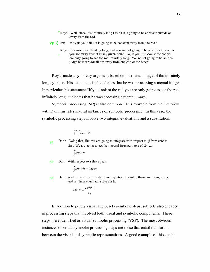
58

Royal: Well, since it is infinitely long I think it is going to be constant outside oraway from the rod.

Int: Why do you think it is going to be constant away from the rod?VP

Royal: Because it is infinitely long, and you are not going to be able to tell how faryou are away from it at any given point. So, if you just look at the rod youare only going to see the rod infinitely long. You're not going to be able tojudge how far you all are away from one end or the other.

Royal made a symmetry argument based on his mental image of the infinitely

long cylinder. His statements included cues that he was processing a mental image.

In particular, his statement “if you look at the rod you are only going to see the rod

infinitely long” indicates that he was accessing a mental image.

Symbolic processing (SP) is also common. This example from the interview

with Dan illustrates several instances of symbolic processing. In this case, the

symbolic processing steps involve two integral evaluations and a substitution.

Dan : Doing that, first we are going to integrate with respect to φ from zero toπ2 . We are going to get the integral from zero to z of π2 …

Dan: With respect to z that equals

SP

Dan: And if that's my left side of my equation, I want to throw in my right sideand set them equal and solve for E.

∫ ∫π

φ2

0 0

zErdzd

∫z

Erdz02π

EzrErdzz

ππ 220

=∫

0

2

2επρ

πrz

Ezr =

SP

SP

In addition to purely visual and purely symbolic steps, subjects also engaged

in processing steps that involved both visual and symbolic components. These

steps were identified as visual-symbolic processing (VSP). The most obvious

instances of visual-symbolic processing steps are those that entail translation

between the visual and symbolic representations. A good example of this can be

59

seen in the following excerpt from John’s interview. John realized that he needed

to find an expression for dV in his equation for Coulomb’s Law. To do this, he

drew diagrams of a complete cylinder and a small piece of a cylinder to represent

the dV, in essence, translating from a symbolic representation (dV) to a visual

representation (the diagrams). He then identified the sub-elements of the diagram

(the sides of the differential volume element) and associated these with their

symbolic counterparts ( , and )dr rd dzφ . In this instance, John’s objective was to

find a symbolic expression for dV.

John: Now, I'm going to use cylindrical coordinates system. Even though Iassigned xyz I'm going to go ahead and use cylindrical coordianates. Andmy volume element dV in cylindrical coordinates is a… Draw a cylinder…A chunk of it's going to be… And that's going to be wedged back in…This… The height will be z…err dz. This distance here…This is z. You'vegot r, φ. This is rdφ and this is dr…this distance here. So dV in spheric…incylindrical coordinates I'm thinking is rdrdφdz.

VSP

z

dz

rdφ

dr

dzrdrddV φ=

( )∫∫∫ ′−

′−=

304

1

rr

rrdVE ρπε

John achieved this by translating into the visual representation, extracting

information from a visual image and translating back to the symbolic

representation.

Some of the steps that subjects made during the interviews were difficult to

classify. This takes us back to the first example.

60

Dean: So I have a cylinder. This goes out like this. (drawing three horizontal linesat each end to indicate that the cylinder continues on) This is going to bealong the z-axis. And I want to use cylindrical coordinates, because itmakes sense. This is a cylinder.

VI

?P

Dean’s decision to use cylindrical coordinates based on the geometry of the

situation appears to be a good example of visual processing. However, it is not

clear what type of processing Dean was using here. It may be that he based his

decision to use cylindrical coordinates on a recognition of the symmetry of the

charge distribution. On the other hand, he may have associated the fact that he has

a cylinder with cylindrical coordinates based on memory or word similarity. In this

case, there are no clear cues to indicate that this is either visual or symbolic

processing. This ambiguity prompted us to assign a code of ?P to indicate that he

is doing some sort of processing, but that it is not clear what kind. The ? code was

assigned in a variety of cases where coding was ambiguous. This difficulty in

coding can arise from a variety of causes including:

• The student’s statements are confusing and or the student seems

confused.

• There is some indication that the student is not thinking aloud or that he is

not expressing what he is thinking as he works through the problem. This

may indicate that he is skipping steps or combining steps.

• The statement does not fit neatly into our coding scheme. This may

indicate that this coding scheme is not complete.

Table 6.2 contains a tabulation of the coding scheme described above.

61

SYMBOL TYPE OF STEP EXAMPLE

SI Symbolic Initialization A remembered or given equation, a known law (Coulomb's Law)

VI Visual Initialization A remembered picture or a picture drawn based on the statement of the problem.

SP Symbolic Processing

Algebraic simplification, substitution, or equation. General symbolic manipulation.

VP Visual Processing

Simplification using symmetry, generation of a diagram/picture or elements there of, rotation or translation of a diagram. General visual manipulation.

VSP Visual - Symbolic Processing

Includes statements that clearly involve visual and symbolic processes that are intertwined. These steps include translations between symbolic and visual representations as well as processing or manipulation of visual and symbolic elements.

? Unclear or Undecided Coding

It is not clear what code to apply. This could result from a variety of causes.

Table 6.2 - Tabulation of coding scheme

6.4.3 Visual Problem Solving Strategies

In solving the proposed problem, subjects routinely broke the problem down

into smaller sub-problems. These sub-problems were then attacked with a

combination of visual and symbolic problem solving strategies. In this section, we

will describe two prevalent visual strategies and explore the interplay of visual and

symbolic steps in the context of these strategies.

6.4.4 Visual Reconstruction

All of the subjects used visualization as a memory tool. In each case,

pictures were used to help recall the important elements of a problem solution. In

62

many instances, subjects used a combination of memory and reasoning to

reconstruct images and equations they needed.

Good examples of this occurred when subjects tried to find expressions for

the differential volume or area elements ( dV or da ). In these instances, subjects

often used simple diagrams to help them find expressions that reflect the geometry

of the problem.

In this example, John drew a diagram of a differential volume element to

help him find the expression for dV in his equation for Coulomb’s Law. In this

case, he was clearly reconstructing this image. First, he drew a cylinder. Then,

based on that drawing, he drew a “chunk” of the cylinder (a differential volume

element corresponding to dV). He then identified and labeled the sides of this

“chunk” and multiplied them together to get an expression for dV.

John: And my volume element dV in cylindrical coordinates is a… Draw acylinder… A chunk of it's going to be… And that's going to be wedgedback in… This… The height will be z…err dz. This distance here…This isz. You've got r, φ. This is rdφ and this is dr…this distance here. So dV inspheric…in cylindrical coordinates. I'm thinking is rdrdφdz.

VSP

z

dz

rdφ

dr

dzrdrddV φ=

In this instance, Royal remembered the equation for da, but used a diagram

to check his equation.

Royal: da for this rod is going to be in cylindrical coordinates rdφdx cause it's um...Where this is φ this is r and this is dx.

VP

rφ

dx

63

Another good example of visual reconstruction was when Royal used a

diagram to recover parts of Coulomb’s Law. Here, Royal recalled some of the

equation, but also used the diagram to identify some of the essential elements.

Royal: So we're going to have E=1/ (4 pi epsilon0) times some big ugly integralthat's going to have τρd over... then we will hang out right here and look ata point right there. This is r and this is r' and we know that the electric fieldthat you are going to see at this point from this whole thing is going to bedependent on this distance here which will be r minus r' (drawing the arrowfrom the r vector to the r' vector).

SPVP

VSP

∫ ′−=

τρπε 0

041 r

rrdE

ρ

r0

xr

r'

This is Royal’s second attempt to construct this equation. In the first

instance, he had not defined the and r r′ vectors. Instead he had loosely defined

the denominator in Coulomb’s Law with the statement, “the distance away can

be…I don’t know… k in the k direction.” While the details of this equation are still

not correct, he has used his drawing to define and identify the important

displacement in the problem.

Visual reconstruction as described here can involve symbolic as well as

visual processing. This strategy was often combined with pure symbolic

processing to find an expression for one of the pieces in a central equation. In this

example, Dean used a combination of visual and symbolic steps effectively to

develop an expression for dq. He began by writing a general equation he

remembered for the potential due to a charge distribution (1 SI). He then found a

value for dq using a simple two-dimensional diagram (2 VSP & 3 VSP). He then

realized that this equation was not correct and drew a three-dimensional diagram to

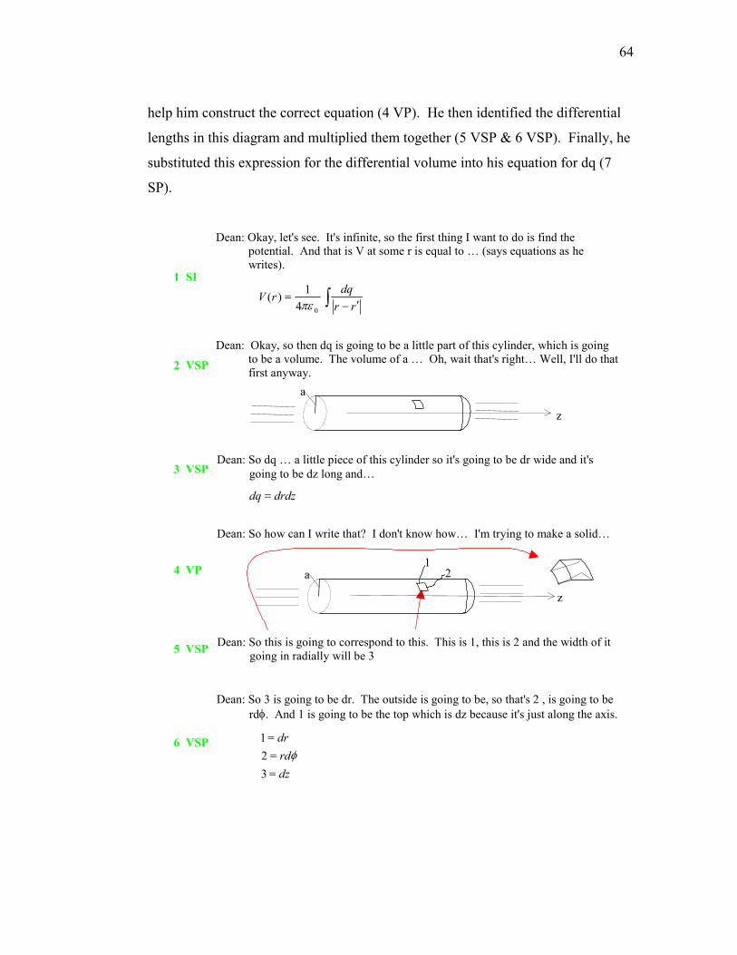
64

help him construct the correct equation (4 VP). He then identified the differential

lengths in this diagram and multiplied them together (5 VSP & 6 VSP). Finally, he

substituted this expression for the differential volume into his equation for dq (7

SP).

Dean: Okay, let's see. It's infinite, so the first thing I want to do is find thepotential. And that is V at some r is equal to … (says equations as hewrites).

∫ ′−=

rrdqrV

041)(

πε

1 SI

a

z

Dean: Okay, so then dq is going to be a little part of this cylinder, which is goingto be a volume. The volume of a … Oh, wait that's right… Well, I'll do thatfirst anyway.2 VSP

drdzdq =

Dean: So dq … a little piece of this cylinder so it's going to be dr wide and it'sgoing to be dz long and…3 VSP

a

z

12

Dean: So how can I write that? I don't know how… I'm trying to make a solid…

4 VP

Dean: So this is going to correspond to this. This is 1, this is 2 and the width of it

going in radially will be 35 VSP

dzrddr

===

321

φ

Dean: So 3 is going to be dr. The outside is going to be, so that's 2 , is going to berdφ. And 1 is going to be the top which is dz because it's just along the axis.

6 VSP

65

Dean: So, to find the volume, just multiply all those out. So it's going to be…

dV…dV times the constant. You said ρ… a constant charge of ρ.

ρdVdq =

( )ρφ zddrdrdq ′′′′=7 SP

In all of these cases, the resulting information is something that could have

been remembered or looked up. The students, however, chose to use a combination

of memory and reasoning to reconstruct this information. This is in sharp contrast

to the “plug and chug” problem-solving behavior typical of introductory courses.

These students exhibited behavior that is common to more advanced problem

solvers. That is, they derived or constructed pieces of their solution as opposed to

memorizing each of the parts. In these cases, visual processing seems to be an

integral part of this process.

6.4.5 Visual Simplification

Another common visual strategy was to try to simplify equations or quantities

with the aid of pictures. The use of images to identify symmetry was very common

in these problem solutions. In this example, Royal made symmetry arguments to

support his claim that the electric field was constant outside the cylinder. He used

a mental image of the rod to explore the consequences of the rod being infinitely

long. He made good arguments to suggest that the electric field was independent of

z, but overgeneralized and claimed that the field was constant.

66

Royal:Well, since it is infinitely long I think it is going to be constant outside oraway from the rod.

VP

Int: Why do you think it is going to be constant away from the rod?

Royal:Because it is infinitely long, and you are not going to be able to tell how faryou are away from it at any given point. So, if you just look at the rod youare only going to see the rod infinitely long. You're not going to be able tojudge how far you all are away from one end or the other.

VP

In another example, Dean made careful arguments that the field did not

depend on or z φ . Dean used explicit references to points in a picture he had

drawn to make his statements of symmetry clear. Early in his arguments, he

claimed that the electric field was constant, but by the end of this sequence, he

began to question this assertion.

Dean: So we are solving for this and since this is infinite, the electric field outsideof here (indicating in the region below the cylinders) is …is constant. It'sfelt the same here as it is here (drawing two dots on the board),because…because they don't know the relation with respect to z because thisis an infinite in the z direction.

L

VP

67

Dean: And like we said r…that represents r away from the z equals zero. That'sgoing to be a constant (writes r=constant) Okay, is that what I'm trying tosay. (Erases r=constant). Anyway, you know what I mean. I'm not going to…

Dean: And this is going to be radially symmetric like this. (moving his arm aroundin a circle with an axis parallel to the cylinders on the board.) So as long asthis is the same distance as here, they are going to feel the same as them soyou can do that all the way around.

L

VP

VP

In both of these cases, the subjects began with strong statements about the

behavior of the electric field. They then tried to justify these statements with

symmetry arguments. This was a common strategy in these interviews. Subjects

often used intuition to describe the electric field. They then used visual symmetry

arguments to justify these intuition-based assertions. In many cases, these attempts

to justify their intuitions were unsuccessful, often because these intuitions were

incorrect. Some of the subjects used this information to revise their description of

the electric field while others retained their intuitions in spite of information that

suggested they were flawed.

In some instances, subjects applied the results of visual simplification

arguments from earlier in the interview to help them with other parts of the

problem. A good example of this comes from Dean’s interview. Here, Dean was

trying to find the flux through the endcaps of his Gaussian surface. As this excerpt

begins, he had just found that the direction for the differential area element of the

endcaps was along the z direction

68

Dean: So we don't have to worry about the z component…err…the r componentor the φ component. We just want to worry about the z componentbecause we are going to be dotting it so the other parts are just going tobe falling out anyway. …The z component of the electric field is going tobe…

SP

Dean: My thought right now is that it's zero on those. But I'm trying to figureout why. Oh, because the electric field only points out radially. Andbecause of that, this (indicating the =E ) is going to be zero, becausethere is only a z component of the area. This is not going to be…notgoing to have a z component because the electric field only points outradially, because of the symmetry argument right here (pointing to thetwo small arrows at the top of the Gaussian surface diagram).

VSP

Dean indicated the drawing associated with a symmetry argument he made

earlier. In this argument, he justified his statement that the electric field pointed

radially outward.

Int: How do you know that?

Dean: I know this, so E …E's going to be constant. So rEE ˆ=

Dean: Because the electric field is pointing radially outward from thecylinder…the field.

VP

Dean: Because of this…because this is infinite. So, whatever…oh, because of thatsymmetry argument I was using. When…there's a piece over here andthere's a piece over here. So if you have a charge here, it's going to feel avector pointing this way and a vector pointing that way

VP

Int: How do you know that?

L

1 2 3

Dean: and these two components are going to…the horizontal components…the zcomponents are going to cancel out (puts bottoms of fists together withthumbs pointing out) and you are only going to feel a radial force or a radialfield vector. Okay.

VP

69

In other instances, subjects used visual simplification to find the properties of

the electric field, but then did not use the results of this simplification to help them

solve the main problem. This was particularly common with Tom. Tom obtained

useful information about the electric field from visual arguments but never utilized

this information. Here is an example where Tom explored the behavior of the

electric field far away from the charged cylinder. Tom began by acknowledging

that he wanted to use symmetry to simplify the problem. He made a variety of true

statements about the nature of the electric field but then did not use them to

perform the simplification he suggested.

Tom : I know that a lot of what I'm trying to remember, I'm not going to need. I'mgoing to be able to throw some of it away. I'll try to throw a lot of it awaywith symmetry arguments. With the density. I'm thinking hey, if I backway off of this thing…this cylinder, it's going to look just like a wire or aline if I get far enough away. It's only when I get really close that the factthat it has a diameter a is going to make a difference. So I'm expecting it tolook like…ummm…I'm expecting it to look like…like a wire. It's…So I'mthinking it's only going to depend on …r…call it r minus a. If it's infinitelylong, z right, then wherever I am, wherever my z component is doesn'tmatter, because wherever I'm at in z doesn’t matter. (waving hand up anddown along the z axis). So, that z symmetry drops out. The θ is the samestory. Whatever my angle is around…

VP

6.4.6 Summary of Analysis

The most striking result of these interviews is the degree to which student use

visual and non-visual methods in close conjunction. Admittedly, the interview

problem was chosen to provide students with an opportunity to use visual methods.

Still, nearly every student in the sample utilized a complex combination of visual

and non-visual steps and strategies. In many cases, it was difficult to identify steps

as visual or symbolic, since the subjects were using visual and symbolic

representations in such close connection. This result stands out against much of the

70

existing research, which has attempted to study students’ ability to visualize in

isolation from non-visual processing.

A second result of this research is the introduction of a new model that

promises to help us explore the interaction between visual and non-visual modes of

thinking in physics problem solving. In the preceding sections, we have illustrated

a new method for examining student use of visual and symbolic steps in problem

solving. Based on the V/A model (Zazkis, Dubinsky and Dautermann, 1996), this

method has several new features. First, the definitions and elements used here are

readily associated with observables from the interviews. The visual and symbolic

steps defined in Section 6.4.2 are generally easy to identify in the interview

transcripts. We have also accounted for steps involving visual and symbolic

processing as well as steps that are difficult to categorize.

Secondly, we explore the relationship between visual and symbolic steps as

opposed to acts of visualization and analysis. Analysis takes on a different role in

the method described here. Each visual or symbolic step contains within it some

acts of analysis in the sense described by Zazkis, Dubinsky and Dautermann. In

this study, we explicitly avoid trying to identify analysis independently of a visual

or symbolic representation. At best identifying purely analytical steps is a

subjective endeavor; at worst, it is impossible.

As it stands, this analysis presents a useful model for describing how upper-

division physics students use visualization in problem solving. We have provided

examples in which visual and symbolic steps are used in combination as part of a

complex problem solution. However, we have yet to synthesize a description of

how the steps described in Section 6.4.2 are used together in problem solving. In

other words, we have defined the elements of our model but still need to explore

how these elements work together in students’ problem solving. Our intent upon

the completion of this analysis was to explore the interaction of the model elements

described here in the context of another set of interviews. However, as we describe

in Section 7.4, our focus shifted after a preliminary analysis of thee final

interviews.

71

Chapter 7 Final Interviews

In the fall term of 2000, we conducted a set of think-aloud interviews in

which students were asked to solve a problem involving the calculation of electric

flux. The goal of these interviews was to gain an understanding of student problem

solving at this level and, in particular, their use of visualization in problem solving.

This chapter describes the administration of these interviews as well as their

analysis.

7.1 Sample

Fifteen volunteers from a class of 19 physics and engineering physics

students were interviewed. This sample consisted of 12 male and 3 female

students. The female/male ratio of 20% was typical of undergraduate physics

classes at Oregon State University, but considerably higher than the national

average of around 12% (Ivie & Stowe, 2000).

The class of 20 students was administered the PSVT (Guay, 1976) to

determine the general spatial ability of each subject. A tabulation of student scores

on the PSVT and incoming math and physics grade-point average (GPA) is listed

for each student in Table 7.1. The average PSVT scores for the sample (N=15) was

32.3 compared to a score of 31.9 for the entire class (N=20). The average

incoming math and physics GPA for the sample was 3.02 compared to 3.17 for the

entire class. The similarity of these statistics indicates that the voluntary sample

represents the entire class quite well, as well it should since the sample constitutes

over three quarters of the population.

A regression analysis measuring the relationship between PSVT score and

incoming GPA revealed that there was no significant correlation (R2= 0.033,

72

F=0.45, α=0.52) between these variables. This data agrees very closely with the

data from Section 4.5.1.

PseudonymPSVT (0-

36)Incoming GPA (0-4)

Enkidu 34 3.27

Tortuga 34 2.17

Sirius 28 1.99

Blue 34 3.61

Yellow 36 3.61

Shedder 28 2.42

Bravo 30 4.00

Jerry 31 2.49

Chameleon 35 3.40

Parsec 35 3.47

Penguin 31 2.53

Turtle 29 3.81

Q 34 2.62

Garfield 35 2.36

Scooby 31 3.58

Class Average 32.3 3.02

Table 7.1 - Tabulation of students’ PSVT scores and Incoming Math and Physics GPA

7.2 Data Collection and Interview Protocol

Subjects participated in think-aloud interviews in which they were asked to

solve an electrostatic flux problem. Each of the interviews was administered by the

author and lasted between 45 minutes and one hour. Subjects were not allowed

access to reference materials including books and notes except were noted. The

73

interviews were videotaped with the permission of the subjects and later

transcribed. Transcriptions were carried out by the author and included all

drawings, equations, etc… as well as notes on hand gestures and references to

items written on the board. A timeline for the interview protocol is shown in

Figure 7.1.

An infinitely long line charge generates

an electric field0

1 ˆ2

E rr

λπε

= where λ is

the uniform linear charge density and r isthe distance from the line charge. Theorange thread along the edge of themodel represents this infinitely long linecharge. Find the flux of electric fieldthrough the entire surface represented bythe model.

Introduction

Follow-upQuestions

Answer StudentQuestions

MainProblem

5 min.

25 min.

40 min.

Start

End

Figure 7.1 - Interview timeline and problem statement.

As in the preliminary study, the interviewer began by explaining the think-

aloud format of the interviews. The interviewer explained that the questions he

would ask were intended to elicit information about the subjects thinking process

and should not be taken as guiding questions. Subjects were asked to talk through

their thinking process as they worked and were encouraged to use the chalkboard.

The interviewer encouraged subjects to ask any questions that came to mind, but

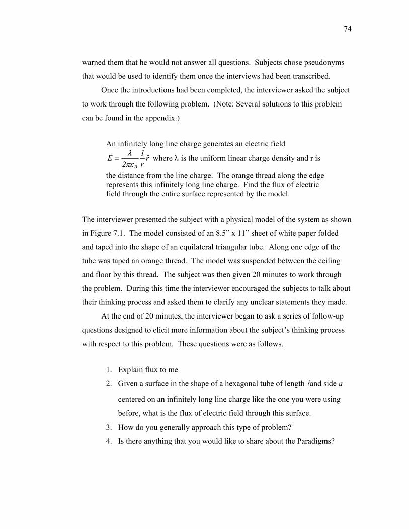
74

warned them that he would not answer all questions. Subjects chose pseudonyms

that would be used to identify them once the interviews had been transcribed.

Once the introductions had been completed, the interviewer asked the subject

to work through the following problem. (Note: Several solutions to this problem

can be found in the appendix.)

An infinitely long line charge generates an electric field

rr1

2E

0ˆ

πελ

= where λ is the uniform linear charge density and r is

the distance from the line charge. The orange thread along the edge represents this infinitely long line charge. Find the flux of electric field through the entire surface represented by the model.

The interviewer presented the subject with a physical model of the system as shown

in Figure 7.1. The model consisted of an 8.5” x 11” sheet of white paper folded

and taped into the shape of an equilateral triangular tube. Along one edge of the

tube was taped an orange thread. The model was suspended between the ceiling

and floor by this thread. The subject was then given 20 minutes to work through

the problem. During this time the interviewer encouraged the subjects to talk about

their thinking process and asked them to clarify any unclear statements they made.

At the end of 20 minutes, the interviewer began to ask a series of follow-up

questions designed to elicit more information about the subject’s thinking process

with respect to this problem. These questions were as follows.

1. Explain flux to me

2. Given a surface in the shape of a hexagonal tube of length l and side a

centered on an infinitely long line charge like the one you were using

before, what is the flux of electric field through this surface.

3. How do you generally approach this type of problem?

4. Is there anything that you would like to share about the Paradigms?

75

Subjects were allowed to return to their solution of the main problem at any

time during the administration of the follow-up questions. In some instances, the

follow-up questions were asked and answered in an uninterrupted sequence. In

others, the subjects returned to the main problem between follow-up questions.

The final follow-up question was asked to collect data for the evaluation of the

Paradigms in Physics program. Anonymous transcripts of student responses to this

question were submitted to the Paradigms in Physics evaluation team.

Upon completion of the interview, subjects were encouraged to ask questions

about the problems. These questions were answered and subjects were given the

option of discussing the interview questions with the interviewer off camera. The

length of time for each interview varied between 45 minutes and one hour

depending upon the speed with which subjects answered each question as well as

the amount of time spent on student questions at the end of the interview.

Significant deviations from this protocol occurred in two of the interviews.

Very early on in his interview, Blue became stumped and gave up. The interviewer

responded to this by asking the subject the first of the follow-up questions very

early in the interview. Following this question, the subject returned to the main

problem. Subsequent follow-up questions were asked in accord with the schedule

outlined above.

Shedder’s interview was affected by more substantial irregularities. Due to

an equipment malfunction, the first 15 minutes of the interview was not videotaped.

This was recognized during the interview and the malfunction corrected. At this

point, the interviewer asked the subject to review what she had done during the first

15 minutes of the interview. We considered dropping this interview from the

study, however, since the subject was one of only three women included in the

study the data from this interview was retained. Conclusions drawn from this

interview should be examined with extra scrutiny since the interview environment

was more reflective than the other interviews in this study.

76

7.3 Choice of the Interview Problem

Our goal in selecting the interview problem was to choose a problem that

would encourage students to demonstrate the use imagery and equations together

while solving problems. We chose a problem from electrostatics because it was

reasonably fresh in students’ minds. The particular problem used in the interviews

described here was chosen based on a number of other important criteria. First, it

was essential that the problem allow students’ many opportunities to use equations

and imagery together. Second, it was important that the problem be based on

recent course material but not be too closely related. We wanted students to be able

to make significant progress on the problem, but we did not want the problem to be

so similar to ones they had solved recently that they could remember large parts of

the problem solution.

In addition, there were several logistical requirements for the problem. First,

it was important that the entire interview last less than one hour. Taking into

account time for introductions, explanations and follow-up questions, this left

roughly 30 minutes for the main problem. The problem used in the preliminary

interviews was too long and too complicated to analyze easily. We chose what we

thought would be a shorter problem for these interviews. This shorter format also

allowed more students to be interviewed since the transcription and analysis time

for a single interview was decreased.

The problem we chose is described in Section 7.2 and several solutions to

this problem can be found in the appendix. In developing this problem we

considered several problems and conducted brief interviews to determine if each

problem had the potential to meet the above criteria. These interviews showed that

students used a rich variety of imagery together with equations in solving this

problem. We tested this problem in two formats. One that involved a purely verbal

explanation and one that involved the model described in Section 7.2. We found

that the students experienced difficulties understanding the verbal description of the

model and we were unable to concoct a satisfactory verbal description.

77

We chose electric flux as the topic for this problem because understanding

flux problems requires a combination of verbal and visual problem solving skills.

A successful solution to the problem described above can be achieved with the use

of primarily verbal or visual strategies; however, a complete understanding of the

problem utilizes a complex intertwining of the two.

This problem allowed several different avenues of solution. Students had the

opportunity to choose either rectangular or cylindrical coordinates, but in either

case, would have to translate some of the elements of the problem from one

coordinate system to the other. In addition, subjects could simplify the problem

using Gauss’s Law. Each of these possible solutions is described in the context of

student solutions below.

7.4 Results/Analysis

We began the analysis of this set of interviews by directly following up the

analysis of the Chapter 6. We coded the transcripts searching for visual strategies

and identifying visual and symbolic steps. Two results emerged from this analysis.

First, the most common strategies we identified were construction, as defined

above, and checking, a new strategy described in Section 7.4.2. In addition, we

noted that these two strategies were often found in conjunction. Second, we found

that most of the strategies we identified contained a mix of visual, symbolic and

verbal steps. This supported one of the most significant results of the research in

Chapter 6, that student’s use of visual representations in problem solving is

intertwined with their use of non-visual representations.

Based on these conclusions we adjusted the direction of our analysis. Section

7.4.1 describes the subjects’ overall performance in solving the interview problems.

In Section 7.4.2, we describe the pattern of construction and checking that we

observed and we outline a simple model for understanding this pattern. Finally, in

78

Section 7.4.3, we explore the subjects’ models of flux. In particular, we describe

the typical model students have and the difficulties that some students experience.

7.4.1 Overall Performance

Subjects’ performance on the main flux problem varied from one student who

solved the problem in a complete and thorough manner to a few students who were

only able to make small amounts of progress toward a solution. Table 7.2 shows

the subject groupings according to overall performance on the main flux problem.

Subjects in the high performance group produced a solution that was correct to

within simple algebraic errors. Both of the subjects in the high performance group

utilized some form of Gauss’s Law to simplify the problem.

Each of the subjects in the middle performance group was able to recall or

construct a correct equation for flux. In addition, they were able to use this

equation in a correct and productive manner, but were unable to produce a correct

solution. Each of the subjects in this group either did not produce a final solution

in the allowed time or expressed doubt about the correctness of their solution. In

general, individuals in the medium performance group were unable to solve the

problem due to difficulties translating between cylindrical and rectangular

coordinates.

Subjects in the low performance group made only minimal progress toward a

correct solution of the problem. Three of the subjects, Scooby, Sirius and Blue

were unable to recall or reconstruct a correct equation for flux. Garfield was able

to write the correct equation for flux, but thought that it was incorrect and promptly

erased it. Jerry recalled and used the proper equation for flux, but because his

model of flux was so flawed, he was unable to make significant progress toward a

solution.

79

Name Performance

Jerry

Sirius

Scooby

Blue

Garfield

Yellow

Parsec

Turtle

Tortuga

Chameleon

Enkidu

Bravo

Penguin

Shedder

Q

Low: Did not use the correct flux equation to make significant progress

Medium: Used the correct flux equation to make significant progress but were not able to obtain a solution. Most had problems with translation from rectangular to cylindrical coordinates.

High: Solution correct to within algebra errors. Used Gauss' Law.

Table 7.2 - Grouping of Subjects by Performance

In addition to performance groupings, we found that most of the students fell

into natural groups based on their method of solution and on the particular

difficulties they encountered. A tabulation of these groupings is presented in Table

7.3. Three of the subjects in the low performance group, Jerry, Sirius and Scooby,

were deemed the Poor Flux Model group, because they had poor or incomplete

models of flux. These were the only three students in the sample that did not

recognized that the flux through the sides of the surface adjacent to the line charge

would be zero. Students models of flux will be discussed more in Section 7.4.3

The other two students in the low performance group, Blue and Garfield, had

more complete models of flux but made very few quantitative statements. They

were called the Qualitative group because their entire interviews consisted of

qualitative and visual arguments. While this qualitative approach helped them to

80

gain some understanding of the problem, they did not make significant progress

toward a solution.

Five of the subjects in the middle performance group, Parsec, Turtle, Tortuga,

Chameleon and Enkidu, were grouped together because each of them experienced

difficulty defining the differential area element, da , for a flat side in cylindrical

coordinates. In general, these subjects had expected to write down some form of

ˆda rd dzrφ= in analogy to solutions they had seen before for electrostatics

problems in cylindrical coordinates. This group was deemed the Difficulties with

da group.

Name Solution Characteristics

Jerry

Sirius

Scooby

Blue

Garfield

Yellow Chose to use rectangular coordinates. Got stuck on integral.

Parsec

Turtle

Tortuga

Chameleon

Enkidu

Bravo

Penguin

Shedder Used Gauss' Law to argue that the flux through the given surface should be one sixth.

Q Used Gauss' Law to justify equating the flat side to an arced surface with constant radius.

Qualitative - Few Quantitative statements. Made lots of true statements but drew few conclusions and made few useful connections.

Difficulties with da - Had difficulty writing down da = dxdz. Expected to write rdφdx and got stumped. Confused because the surface and electric field are most easily represented in different coordinate systems.

Quantitative - Used few qualitative arguments. Didn't like and had difficulty with using images.

Poor Flux Models - Didn't recognize that the sides adjacent to the charge had no flux though them. Achieved very little progress toward solution.

Table 7.3 - Grouping of subjects by solution characteristics.

81

Bravo and Penguin, also middle performers, were grouped together because

they both approached the problem in a very quantitative manner. Both expressed

some discomfort or dislike of using pictures and noted that pictures often confused

them. While both of these subjects drew many pictures, they tended to draw the

same picture several times with only minor changes. In most cases, these pictures

were geometric representations they used to convert between rectangular and

cylindrical coordinates. In addition, Bravo and Penguin each had difficulty

extracting information from their pictures. Bravo and Penguin were regarded as the

Quantitative group.

The other three subjects did not fall neatly into any group. Yellow was the

only subject to try to solve the problem in rectangular coordinates. In general, his

solution proceeded along a productive path. However, his final integral was

impossible to evaluate because of a mistake he had made translating between

cylindrical and rectangular coordinates.

Both Shedder and Q produced a correct result using Gauss’s Law. However,

their methods of solution were somewhat different. Q and Shedder began by

equating the flat side opposite the line charge with an arced surface of constant

radius. Q justified this step using Gauss’s Law and proceeded to solve the simpler

arc problem in cylindrical coordinates. Shedder, on the other hand, abandoned this

idea when she was unable to justify it. After questioning the interviewer about the

exact position of the line charge, she argued that the flux through the triangular

tube would be one sixth of the total flux coming from the line charge over the

length of the triangular tube. She then used Gauss Law to calculate the flux.

7.4.2 A Model of Construction and Checking

In the pilot study, one of the problem-solving strategies identified was visual

construction. During the analysis of the final interviews, we looked closely at

students’ use of construction as a strategy. We found that instances where students

82

used construction were often followed by checking events. In these checking

events, subjects tested the conclusions drawn in construction against other

information they had. A cyclic pattern of construction and checking was observed

in most students’ problem solving behavior. This pattern served as the basis for a

model that has been useful in analyzing the similarities and differences in subjects’

problem solving behaviors. Here, we describe this model and provide several

examples of its variations throughout these interviews.

This model describes a process in which subjects draw together several

pieces of input information to construct a conclusion. This conclusion is then

checked. If the check fails, more information is brought in and the conclusion is

refined. In the ideal case, this process continues until the conclusion passes the

checking process. Once a conclusion has passed the checking process, it is passed

on to be used as an input for drawing later conclusions. The result is a cyclic

pattern in which early conclusions are used as the basis for later conclusions until a

final solution is achieved.

For simplicity in analysis, we relate excerpts from students’ interviews with

this model in a diagrammatic format. Figure 7.2 shows a prototypical diagram.

Here, several pieces of input information are used to draw a conclusion. This

conclusion fails a check and a revised conclusion is constructed from the original

conclusion, results of the check and some new information. This revised

conclusion then passes a final check.

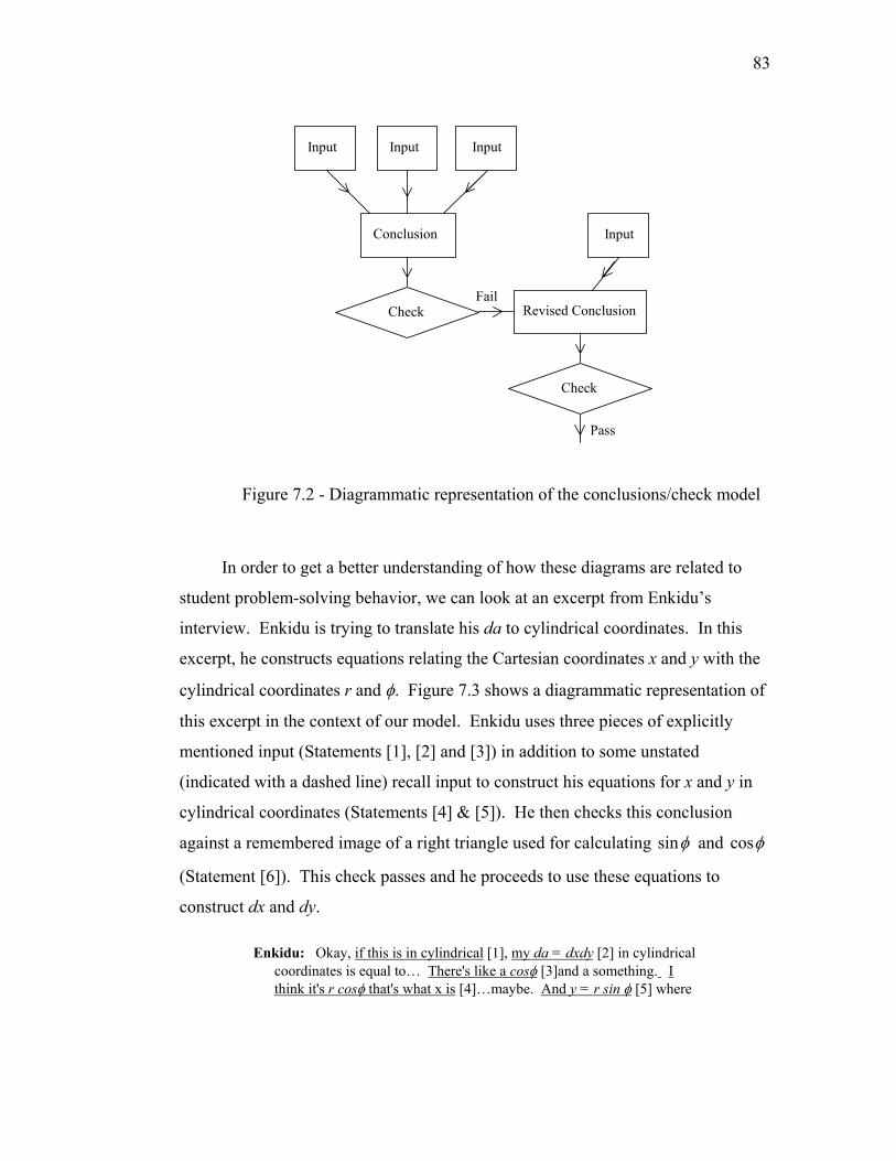
83

Input Input Input

Conclusion

CheckFail

Revised Conclusion

Input

Check

Pass

Figure 7.2 - Diagrammatic representation of the conclusions/check model

In order to get a better understanding of how these diagrams are related to

student problem-solving behavior, we can look at an excerpt from Enkidu’s

interview. Enkidu is trying to translate his da to cylindrical coordinates. In this

excerpt, he constructs equations relating the Cartesian coordinates x and y with the

cylindrical coordinates r and φ. Figure 7.3 shows a diagrammatic representation of

this excerpt in the context of our model. Enkidu uses three pieces of explicitly

mentioned input (Statements [1], [2] and [3]) in addition to some unstated

(indicated with a dashed line) recall input to construct his equations for x and y in

cylindrical coordinates (Statements [4] & [5]). He then checks this conclusion

against a remembered image of a right triangle used for calculating sinφ and cosφ

(Statement [6]). This check passes and he proceeds to use these equations to

construct dx and dy.

Enkidu: Okay, if this is in cylindrical [1], my da = dxdy [2] in cylindrical coordinates is equal to… There's like a cosφ [3]and a something. I think it's r cosφ that's what x is [4]…maybe. And y = r sin φ [5] where

84

this is cylindrical and this is φ (drawing and indication of the angle φ from the x axis) I should look at it and make sure that is right.

b

ac

z

y

x cosx r φ=

siny r φ=

da dxdy=

aac

12

a

φ

Enkidu: Is this right (draws a triangle around the φ in the drawing to check that he has defined it correctly) Cosine of the angle is x, sine of the angle is y. And r changes its length…multiplies it… So yeah [6]

1 Input 2 Input 3 Input

4 & 5 Conclusions

6 Check

Pass

Recall Input

Figure 7.3 - Diagrammatic representation of Enkidu's conclusion and checking process.

In the context of this model, inputs are pieces of knowledge students bring to

the part of the problem they are solving. Students obtain these pieces of knowledge

from a variety of sources including: recall, observation, construction, guessing,

reference sources and the problem statement. Students recall typically items like

85

facts, equations and images. However, they also recall more complex structures

like concepts and solution methods. In addition, students’ memory is often

incomplete. In some cases students may only remember part of an equation or a

single property of a complex concept. Students make observations of the physical

world, but also make more complex observations. For example, noting the

behavior of equations or observing the properties of a drawn image. In some

instances, students supplement recalled information with guessing. In some cases,

they automatically fill in missing pieces without realizing it. In other instances,

they are aware that their recall is incomplete and make a conscious guess. At this

educational level, many of the subjects rely heavily on reference materials. While

no references were provided in this interview, it was common for subjects to ask if

they could reference notes or a book.

In this study, we refer to information resulting from the construction process

described above as conclusions. For the purposes of this model, conclusions were

defined as information constructed from two or more pieces of input. However,

most of the conclusions we identified synthesized several pieces of information.

Conclusions served as another form of input information for most of the subjects.

In the ideal case, in which they have perfect recall and flawless reasoning,

subjects would build problem solutions by constructing a chain of these

conclusions each building upon previous conclusions until the final solution is

reached. In reality, both recall and reasoning have faults. To deal with these faults,

subjects employ a variety of checking procedures to test the validity of conclusions.

In some cases, it is a simple review to identify obvious errors. In others, it involves

comparison to other known information. In still others, it may involve complex

reasoning to test the plausibility of the conclusion

In the example from Enkidu’s interview above, he explicitly states three

pieces of input he uses to construct the equations for x and y in cylindrical

coordinates. He mentions cylindrical coordinates and the differential area element,

da = dxdy, he is trying to convert. Each of these is a conclusion resulting from

previous construction. He also utilizes a partially recalled equation, “There’s like a

86

cos φ and something.” The resulting conclusions are then checked against the

recalled image of a right triangle from introductory trigonometry.

7.4.2.1 Complex Structures

The thought structures students used to draw conclusions in these interviews

were not all as simple as the example given above. Some of the structures are quite

complex, involving several conclusions or repeated checking. The following

example from the interview with Q illustrates a more complex structure with

multiple checking and several conclusions. In this excerpt, Q constructed and

refined an equation for flux. In statement 2, he postulated a simple equation for

flux from memory. He then realized for himself that it is incomplete (Statement

[3]) and refined the equation utilizing several other recalled properties of flux

(Statements [4], [5], [6] and [7]). Next, Q refined the equation again, adding

information about the direction of the differential area element (Statements [8], [9]

and [10]). A diagrammatic representation of this excerpt is given in Figure 7.4

Q: And then I’m going to integrate the E-field. [1] Flux equals (φ = Ea) [2] and so. Is that the right equation for flux? [3] You can’t answer that.

Interviewer: I can’t really answer that. There are a lot of equations for flux.

Q: For the flux in the electric charge…err using the electric field is just the electric field going through an area…or the total electric field through an area. [4]

Q: Oh, e dot and then the normal is what it is. [5] Oh, yeah and you would integrate it. [6] ( E daφ = ⋅∫ ) [7] Where da equals…da [8] and

then the normal which is oops r. [9] (replacing the n with r to get ˆda dar= ). [10]

87

Q: What I just did was take the area and say that the flux was the field going through it in the perpendicular direction. (drawing an arrow on the side of the triangle opposite the charge) [11]

φ

r

r

7 Conclusion

4 Input 5 Input 6 Input

8 Input 9 Input

10 Conclusion

11 Check

Pass

3 Check

2 Conclusion

Fail

1 InputRecall Input

Figure 7.4 - Diagrammatic representation of Q's construction of the flux equation.

Most of the conclusions-checking structures identified in these interviews

were similar to those described above in that several pieces of information were

synthesized to draw a conclusion that was then checked for validity. In these cases,

most of the input information is used to draw or refine a conclusion.

88

Interestingly, we found that in some instances, the bulk of the input

information was applied at the checking stage. In such cases, the student would

draw a conclusion based on only a small amount of input information. Then upon

checking this conclusion the student would bring in several more pieces of

information supporting and enriching the conclusion. The following excerpt from

Parsec’s interview illustrates this behavior.

In this example, Parsec constructed an equation for flux. Comparing this

excerpt to Q’s construction of the flux equation above, it is clear that Parsec

generated the correct flux equation very quickly. Whereas Q refined his

construction from a simpler equation, Parsec produced the correct equation with no

explicit refining. In fact, Parsec noted that he was recalling the equation in

Statement [3]. In this case, the bulk of information about the flux equation was

brought in during the checking procedure (Statements [5], [6], [7] and [8]). The

checking process served as a constructive justification, both confirming and

expanding the original conclusion. In the checking step, Parsec established

connections between the equation and his qualitative/geometric understanding of

the problem.

Parsec: The flux being the amount of the vector going through a surface [1] …

Parsec: So, I’m thinking about this thing (mumbling)… (drawing a 3-D picture of the triangular tube and writing the equation for flux) [2]

Flux E da= ⋅∫

Interviewer: What are you writing?

Parsec: The flux integral.

89

Interviewer: Where did the equation come from? Are you just remembering it?

Parsec: Yeah, I’m trying to remember it. [3] I think that is correct, because it is the electric field. [4] And we are finding the flux of the electric field which is the amount of electric field through the surface. [5] It’s only the field that travels through the surface [6]…so the perpendicular field, [7] so the dot product (pointing to the dot product in the flux equation) would give that to you [8].

5 Input

1 Input3 Recall Input

7 Conclusion

4 Check

2 Conclusion6 Input

8 Conclusion

Pass

Figure 7.5 - Diagrammatic representation of Parsec's construction of the flux equation.

The excerpt from Q’s interview clearly shows an example of the student

constructing a quantitative representation from a qualitative representation. In

contrast, Parsec clearly used his equation as a basis for recalling/constructing his

qualitative understanding of the system. Observing these contrasting methods for

construction/recall brings to mind several interesting questions. Which of these

methods is most common? Are there any patterns in expert/novice use of these

methods? Do particular subjects prefer one method or another? If so, does this

90

preference change as the subject’s problem-solving abilities improve? While these

questions are beyond the scope of the present study, we intend to address them in

the future.

7.4.2.2 Difficult or Trivial?

Using this model as a framework, an interesting pattern was observed. We

noticed that students’ often engaged in elaborate thinking processes in order to

arrive at conclusions that seem trivial to the experienced problem solver. The

following excerpt from Turtle’s interview illustrates this point.

Turtle: I’m thinking if I had a line charge and then at some point that’s the e-field. [1] I’m concerned about the shape of what the flux is going through. [2] I am trying to decide what’s the best way to go about this.

Interviewer: Why are you concerned? What is your concern?

Turtle: It is an unusual shape. Because well the direction. [3] Do you want me to talk as I go through this or just solve…

Interviewer: Yes, talk to me and tell me what you are thinking. And I will remind you to do that.

Turtle: Well, if the e-field is directly…is radially outward from the line charge, [4] then… I would expect…at all points, the e-field would be radiating outward from the line charge (drawing arrows from the line charge). [5]

Turtle: So, if I were to use cylindrical coordinates, that would be best. [6]

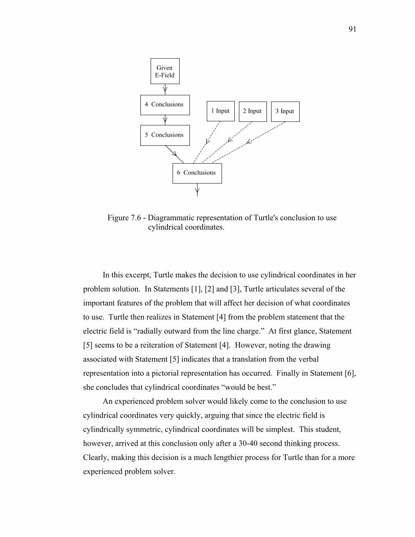
91

1 Input 2 Input 3 Input

5 Conclusions

6 Conclusions

GivenE-Field

4 Conclusions

Figure 7.6 - Diagrammatic representation of Turtle's conclusion to use cylindrical coordinates.

In this excerpt, Turtle makes the decision to use cylindrical coordinates in her

problem solution. In Statements [1], [2] and [3], Turtle articulates several of the

important features of the problem that will affect her decision of what coordinates

to use. Turtle then realizes in Statement [4] from the problem statement that the

electric field is “radially outward from the line charge.” At first glance, Statement

[5] seems to be a reiteration of Statement [4]. However, noting the drawing

associated with Statement [5] indicates that a translation from the verbal

representation into a pictorial representation has occurred. Finally in Statement [6],

she concludes that cylindrical coordinates “would be best.”

An experienced problem solver would likely come to the conclusion to use

cylindrical coordinates very quickly, arguing that since the electric field is

cylindrically symmetric, cylindrical coordinates will be simplest. This student,

however, arrived at this conclusion only after a 30-40 second thinking process.

Clearly, making this decision is a much lengthier process for Turtle than for a more

experienced problem solver.

92

This phenomenon was not isolated, but was common throughout the

interviews among all students, strong and weak. One of the strongest students in

the sample and the student who presented the most complete solution to this

problem, Q, also exhibited this behavior.

Q: So my da is rdrdφdz. [1] No, that is volume. [2] So the dr part is constant, [3] so dz… where dz is your length [4] (writing da = rdφdz).[5]

1 Input2 Input3 Input

5 Conclusion2 CheckFail

Figure 7.7 - Diagrammatic representation of Q's construction of da.

A number of possible explanations for this behavior exist. It is possible that

expert and novice problem solvers alike, utilize these complex thinking structures,

but that experts are so practiced that this type of thinking has become essentially

automatic. Another possibility is that experts are more willing to make tentative

decisions and move on knowing that they can reconsider the decision if the path

they have chosen is not fruitful.

In any case, these students clearly labor through problem solving tasks that

instructors tend to trivialize. This has serious implications for instructors. In

lectures, we tend to move very quickly through material they think will be easy for

students. This example shows that it is not always easy to know what material will

be difficult for students. Thus, it is very easy for students to fall behind in a

lecture. Even for those students who can keep up, the time constraints present in a

lecture make it unlikely that they are engaged in the decision-making processes that

93

characterize their problem solving. When discussing one of the more lecture-

oriented courses in the Paradigms, Turtle, herself noted,

Turtle: It made sense watching him draw the conclusions, but it’s things I probably would have run across on my own and stopped and thought about, but because of the… when you are just sitting there in lecture it just keeps going.

She also hinted that more student-controlled alternatives to the lecture mode

may yield some relief.

Turtle: …it is nice to be able to work in a group…you come across more problems when you are actually doing it yourself than just watching board work.

7.4.2.3 Moving on with the Aid of Terminating Statements

Throughout the interviews, some of the subjects were observed to end a train

of thought abruptly when it appeared to be unfruitful. In many of these instances,

the subject had engaged in a prolonged checking process that was not yielding

productive results. These abrupt terminations were often signaled by a frustrated

statement that indicated the subjects were willing to accept an answer in which they

had little confidence so that they could move on. These statements were denoted

terminating statements. In order to assess the importance of terminating

statements, we searched each of the interviews. Six of the 15 subjects used at least

one terminating statement.

Only two of the subjects, Chameleon and Enkidu, used a large number of

terminating statements (5 each). Both of these students were in the middle

performance group. In these two cases, most of the terminating statements came

after the subjects had tried and checked various avenues in an attempt to make

progress toward a problem solution. These terminating statements indicate some

level of frustration on the part of the subject. In essence, the subjects are saying,

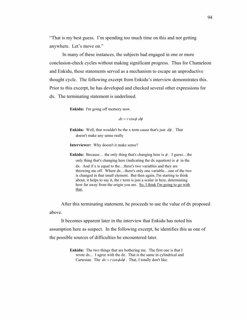
94

“That is my best guess. I’m spending too much time on this and not getting

anywhere. Let’s move on.”

In many of these instances, the subjects had engaged in one or more

conclusion-check cycles without making significant progress. Thus for Chameleon

and Enkidu, these statements served as a mechanism to escape an unproductive

thought cycle. The following excerpt from Enkidu’s interview demonstrates this.

Prior to this excerpt, he has developed and checked several other expressions for

dx. The terminating statement is underlined.

Enkidu: I'm going off memory now.

cos dx r dφ φ=

Enkidu: Well, that wouldn't be the x term cause that's just dφ . That doesn't make any sense really

Interviewer: Why doesn't it make sense?

Enkidu: Because… the only thing that's changing here is φ . I guess…the only thing that's changing here (indicating the dx equation) is φ in the dx. And if x is equal to the…there's two variables and they are throwing me off. Where dx…there's only one variable....one of the two is changed in that small element. But then again, I'm starting to think about, it helps to say it, the r term is just a scalar in here, determining how far away from the origin you are. So, I think I'm going to go with that.

After this terminating statement, he proceeds to use the value of dx proposed

above.

It becomes apparent later in the interview that Enkidu has noted his

assumption here as suspect. In the following excerpt, he identifies this as one of

the possible sources of difficulties he encountered later.

Enkidu: The two things that are bothering me. The first one is that I wrote dx... I agree with the dz. That is the same in cylindrical and Cartesian. The cosdx r dφ φ= . That, I totally don't like.

95

In Chameleon’s case, his terminating statements were mostly near the end of

his problem solution. They tended to indicate frustration and an unwillingness to

further justify his reasoning. In a sense, Chameleon’s terminating statements

signaled that he was giving up.

Chameleon: I’m probably way off, but that’s why partial credit is there.

…

Chameleon: Which is some number, so now there is no dependence on r. It’s just in the z direction now. Which completely baffles me. And that is the flux. I guess it would be a number because I said it wouldn’t have a direction, but who knows. So it equals some number, we know that. So that is as far as I can do here.

Initially we thought that subjects in the low performance group would use a

larger number of terminating statements. That is, they would make progress with

the aid of many unchecked statements. Upon examination of the data, we found

exactly the opposite result. Jerry was the only subject in the low performance

group to use even a single terminating statement.

This is not to say that subjects in the low performance group did not make

erroneous statements, only that they did not tend to use information that they

thought might be incorrect. Typically when these subjects encountered suspect

information they became stumped.

In general, the subjects in the low performance group experienced difficulty

deciding how to proceed. Where as some students in the middle and high

performance groups made terminating statements to allow them to proceed in what

they perceived as a fruitful direction, the subjects in the low performance group

were typically unable to choose a direction to proceed.

96

7.4.3 Student Understanding of Flux

The combination of the main interview problem and the follow-up question

asking students to explain flux has proved to be a powerful tool for exploring

students’ understanding of electric flux. Subjects understanding of electric flux

varied greatly throughout the sample. The interviews revealed that most of the

students had a reasonably complete model of flux. However, only two of the

subjects made the connection between flux and Gauss’s Law. In this section, we

will describe the models of electric flux used by students in this interview. First,

we will describe the features we feel constitute a reasonably complete model of

flux.

A simple but useful definition offered by many of the students interviewed is

that flux is “the total amount of field through a given area.” This basic definition

indicates several important properties of the concept of flux. First, it indicates that

flux is the summation of the field over a given area. Second, it suggests that the

only part of the field that is important is the component that passes through the

area. While this simple definition is useful, it is worded loosely enough that

students can easily misinterpret it. Thus, a complete model of flux needs to be

connected with a quantitative definition. The equation for electric flux,

E daΦ = ⋅∫ , provides this definition.

However, having the verbal and quantitative definitions described above is

not enough. In order to use the idea of flux, students need to be able to connect the

quantitative and qualitative representations of flux. In particular, students need to

understand that taking the dot product between the electric field and the normal

vector to the surface of interest gives them the component of the electric field

perpendicular to the surface. In addition, students must understand that the

component of the electric field perpendicular to the surface is what is meant by the

part of the electric field that goes through the area. It is also essential that students

understand that the integral in the flux equation corresponds to the summation of

97

the correct component of the field over the area of interest. Figure 7.8 contains a

pictorial representation of the connections between the verbal, symbolic and visual

representations of flux.

Flux is the total amount of electric field through a given area.

E daΦ = ⋅∫

PerpendicularComponent

NormalVector

da

E

over all rectangles∑

E da⋅

Figure 7.8 - Pictorial representation of connections between the verbal, symbolic and visual representations of flux.

7.4.3.1 Students’ Explanations of Electric Flux

We obtained information about students’ concepts of flux from three sources

in the interviews. First, as one of the follow-up questions, we asked each student to

explain flux. In addition, many of the students explained flux while they were

solving the main problem. Finally, we were able to learn something about

98

students’ understanding of flux based on their solution methods for the main

problem and the extension involving a hexagonal tube (see number 2 on page 74).

We examined each interview transcript to identify which elements of the above

model were present in each student’s explanation of flux. In addition to examining

students’ responses to the follow-up question about flux, we searched the entire

transcripts for statements about flux.

A tabulation of the results of this analysis is contained in Table 7.4. For each

subject we identified the number of pictorial and symbolic/verbal representations

used to explain flux. Any picture drawn or referenced in a subject’s explanation of

flux was counted as a pictorial representation. Symbolic/verbal representations

consisted of equations or verbal definitions the subjects used to describe flux. It

was also noted whether the subjects mentioned a concrete representation, e.g.,

water flow, in their explanation of flux. Whether the student produced all, part or

none of the equation for flux during the interview was recorded in the equation

column. In the three columns to the right of the equation column is recorded

whether the subject mentioned the dot product, the perpendicular component or

integration/summation. In each of these columns, yes indicates that the item was

mentioned in the subjects response to the follow-up question, cntxt indicates that

the item was mentioned in the context of the problem solution and no indicates that

the item was not mentioned during the interview. The final column lists a

categorization of each student’s definition of flux and a paraphrased definition from

each interview.

All of the subjects in the medium and high performance groups used a

reasonable model for flux. All but one of them explained flux as the Total Field

Through the Surface. Subjects who defined flux in this way were categorized

TFTS in the definition column. There was some variation in the definitions

provided by subjects in the TFTS category. Some described flux more generally,

referring to the “amount of stuff” or the “amount of quantity” that passes through a

given area. Penguin defined flux as, “the amount of charge that goes through a

surface.” Since Penguin used the concept of electric flux correctly in his problem

99

solution, it is likely that his mention of charge in the definition of electric flux

reflects carelessness in his choice of words rather than a fundamental

misconception.

Unlike the other subjects in the high and middle performance groups, Bravo

explained flux using the flux equation (Eqn) as a basis. Bravo noted most of the

important elements in his explanation of flux, but used the equation for flux as a

foundation for his explanation.

The definitions of flux proffered by each of the subjects in the low

performance group revealed that the subject’s model of flux was incomplete or

significantly flawed. Blue provided the most correct definition in the low

performance group, however his definition of flux was given in terms of field

Lines. He defined flux as, “the amount of field lines that pass through the area.”

Throughout Blue’s interview, he referred only to field, never mentioning field

vectors. Scooby’s and Garfield’s definitions of electric flux were connected to

models of rain and fluid flow. Both of these subjects presented a definition with a

Time component, e.g., “the amount of flow that passes over a given area in a

certain amount of time.” While this definition is correct in the case of fluid flow, it

is incorrect for electric flux. The definition given by Sirius refers to the flux

through a volume. In addition, his problem solution indicates that he thinks of flux

in terms of the amount of field passing through a three dimensional volume as

opposed to a two dimensional area. Sirius’s definition was labeled 3D. Finally,

Jerry provided a very loose definition of flux referring to “the varying of the field

on…or through a surface.” His solution to the main problem indicated that he had

no clear model for flux. Because his definition was so loosely constructed, it was

labeled ???.

100

Name

Pictorial R

epresentations

Symbolic/Verbal

Representations

Concrete

Representation

Equation

Dot Product

Perpendicular

Integral/Sum

Definition

Jerry 0 1 no part no no yes ??? - Flux would be the varying of the field on a surface or through a surface.

Sirius 0 1 no none no no no 3D - It measures how many electric field vectors enter a region vs. how many are pointing out

Scooby 0 1 yes all cntxt no cntxtTime: If I'm driving my car and it's raining. If I'm stopped… If I'm moving more rain hits the windshield.TFTS (cntxt) - It's just the amount of field that passes through this surface

Blue 3 1 yes part Yes Yes Yes Lines - The flux would be the amount fo field lines that pass through the area.

Garfield 1 2 yes all cntxt cntxt cntxt Time - Flux is the amount of flow that passes over a given area in a certain amount of time.

Yellow 2 1 no all no no no TFTS - Flux is the amount of vector field that goes through the surface. Mentions what is going in and what is going out.

Parsec 0 1 yes all cntxt cntxt cntxt TFTS - It's the amount of quantity in question that passes through a surface.

Turtle 0 1 no all yes cntxt no TFTS - The amount of electric field through a given area.

Tortuga 1 2 yes all yes yes yesTFTS - The amount of field that passes through a surface. You can integrate (the dot product of the vector and the da)…add them up and get the amount passing through the surface.

Chameleon 1 1 no all cntxt no no TFTS - The e-field that goes through the surface is the flux.

Enkidu 1 1 no all yes no yes TFTS - The total field passing through the given surface.

Bravo 3 1 no all yes yes yes Eqn - You write it like this (pointing to flux eq) You use this relation then you perform the dot product and then you integrate over the surface.

Penguin 3 1 no all no yes noTFTS - Flux is the amount of charge that goes through a surface normal to the surface. (Confuses charge and field in his definition. Also talks about the amount of "stuff")

Shedder 1 1 no all cntxt cntxt cntxt TFTS - Number of field lines coming out of this suface. Tries to resolve confusion between # of field lines and field line density models of flux.

Q 1 2 yes all cntxt cntxt cntxt TFTS - It's the amount of something going through an area…a surface area

Table 7.4 - Characterization of students' explanation and use of flux

The following two sections will describe in more detail the subjects’

particular models of flux. Students’ failure to correctly use Gauss’s Law and Field

lines will be discussed in Section 7.4.3.2. Then, in Section 7.4.3.3 we will describe

some of the incomplete and/or incorrect flux models that students used in these

interviews.

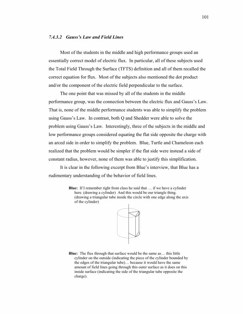
101

7.4.3.2 Gauss’s Law and Field Lines

Most of the students in the middle and high performance groups used an

essentially correct model of electric flux. In particular, all of these subjects used

the Total Field Through the Surface (TFTS) definition and all of them recalled the

correct equation for flux. Most of the subjects also mentioned the dot product

and/or the component of the electric field perpendicular to the surface.

The one point that was missed by all of the students in the middle

performance group, was the connection between the electric flux and Gauss’s Law.

That is, none of the middle performance students was able to simplify the problem

using Gauss’s Law. In contrast, both Q and Shedder were able to solve the

problem using Gauss’s Law. Interestingly, three of the subjects in the middle and

low performance groups considered equating the flat side opposite the charge with

an arced side in order to simplify the problem. Blue, Turtle and Chameleon each

realized that the problem would be simpler if the flat side were instead a side of

constant radius, however, none of them was able to justify this simplification.

It is clear in the following excerpt from Blue’s interview, that Blue has a

rudimentary understanding of the behavior of field lines.

Blue: If I remember right from class he said that … if we have a cylinder here. (drawing a cylinder) And this would be our triangle thing. (drawing a triangular tube inside the circle with one edge along the axis of the cylinder)

Blue: The flux through that surface would be the same as… this little cylinder on the outside (indicating the piece of the cylinder bounded by the edges of the triangular tube)… because it would have the same amount of field lines going through this outer surface as it does on this inside surface (indicating the side of the triangular tube opposite the charge).

102

Blue realizes that under some circumstances he can equate the flux through

one surface with the flux through another. He mentions that this is possible

because the same number of field lines pass through both surfaces. However, the

following excerpt illustrates the limitations in his understanding. Blue clearly

remembers pieces of something that was mentioned in lecture, but has not yet

assimilated this information into his understanding of electric flux.

Blue: All I remember is the diagram he was drawing. Something to the effect if you had some weird surface up here above the x-y plane. (draws axes and irregular surface). Like if this was all curved and odd (indicating the irregular surface) Then, it projected down onto the x-y plane, even though it was an odd shape out here, the same… (drawing a projection down onto a square in the x-y plane)

Blue: I guess that doesn’t really make sense, does it. Even though this was oddly shaped and curved up here, it would have the same amount of flux as the square… down here. So, what I got out of that was that the flux could be projected into a nice area even if it was an oddly shaped surface on the outside. So I was kind of trying to use that here. … because, this flat surface would be hard to describe in cylindrical coordinates … I was trying to apply what Professor Plum said in class and what I kind of remember to this problem.

Blue’s understanding of flux is in large part intuitive. While this allows him

to make many true statements about the nature of flux and helps him to identify

simplifications in the problem, it does not provide him with a means for making

quantitative statements. His explanation in this case is based on a picture he

remembers from class. Strangely, the picture he remembers lacks any reference to

field lines or vectors.

Before she solved the problem using Gauss’s Law, Shedder had similar

difficulties trying to justify equating the flat side to an arced side.

103

Shedder: I didn’t think, in the beginning… I thought that the field lines would depend upon the radius…because, I didn’t think that they would be as dense. But then, the number of field lines coming through would be the same for the angle that was cause, either having this flat surface or the curved surface. It’s just. No, I guess that wouldn’t. But then you would have more surface area. So, I guess I can’t do that.

Interviewer: Explain that again please.

Shedder: The flux is equal to the amount of field coming through the surface. I’m looking… the number of field lines coming out of this surface (indicating the surface opposite the charge in her 3-D drawing) would be equal to the number of field lines coming out of this surface (indicating the cylindrical arch surface bounded by the surface opposite the charge in her 3-D drawing) if I didn’t take the radius into account. Being different from here (indicating a radial line along one edge of the triangular tube) than it would be to here (indicating a radial line bisecting the triangular tube) I’d have more surface, but the same amount of field lines.

These two excerpts illustrate the difficulties students had with field lines.

These excerpts illustrate attempts to justify their proposal that the flux through an

arced surface subtending the same angle was equal to the flux through the flat

surface they were given. In each of these instances, the subjects relied heavily on

the concept of field lines to draw these conclusions. In the end however, these field

line models failed since they did not yield to quantitative analysis and were not

well connected to the students’ other models of flux.

While the utility of field lines is certainly limited (Wolf, Van Hook & Weeks,

1996), these interviews indicate that field lines are not entirely useless. In

particular, field lines are a simple way to illustrate the basic principles of Gauss’s

Law and provide a framework for explaining charges as sources and sinks for the

electric field. Unfortunately, any extension of the field line model beyond these

limited applications is fraught with obstacles. According to Wolf, Van Hook and

Weeks, there is no self-consistent, quantitative model of field lines. Moreover,

field lines cannot be simply connected to a symbolic representation. That is, the

process of drawing an individual field line from the equation for the electric field is

quite complex. In contrast, any electric field vector can be drawn simply by

104

determining the field magnitude and direction from the equation for electric field

and drawing the corresponding arrow.

Still, the concept of field lines is presented in most introductory courses and

is already in the minds of many of our students. Six of the 15 students in this study

mentioned field lines explicitly in either their definition of flux or their problem

solution. Another four of the subjects used field lines in one or more of the

drawings in their interview. Prior to this study, each of the subjects was engaged in

a three-week course on static vector fields. Even though this course utilized the

field vector model almost exclusively, two-thirds of the subjects used field lines as

part of their solution.

7.4.3.3 Incomplete and Incorrect Models of Flux

Subjects in the low performance group utilized a variety of incomplete and

incorrect models of flux. Garfield and Scooby both had models of flux based on

fluid flow. In each of these interviews, the subjects mention the amount of

substance that passes through an area per unit time. The following two excerpts

from Garfield’s and Scooby’s explanations of flux illustrate this.

Garfield: Flux is the amount of flow that passes through a given area over a specific amount of time. Can I use a picture?

Interviewer: Do whatever you need.

Garfield: It’s… Say this is like a ring in a pipe. (drawing a ring with arrows through it. It’s the amount of water that flows through this in a given amount of time. That’s what my understanding of flux is.

105

Here Scooby tries to use her model of flux to calculate the flux through the surfaces

of the triangular tube. When she is faced with a difficulty, she refers to a

description of flux presented to her by a graduate teaching assistant, Shaggy.

Scooby: To get the flux through, you need to know how much of the electric field is going through here (motioning upward)… going through…

Scooby: If it’s going in the r direction, out this way (indicating away from the string in the model) It’s moving in this direction. It’s not going up at all. There is no flux…no electric field going up, so I can’t integrate… That’s not what I’m concerned about. I need the flux this way, because that’s the way it’s moving. Because the flux… the best analogy I got was from Shaggy (a GTA) when he said that flux is like when you are driving your car and it is raining. When you speed up, more rain hits your car window. When you are stopped it is not going through there as much. So if I’m going this … if it’s going in the r direction, this is the way, I want to go for the flux. Right?

This example demonstrates the lack of coherence in Scooby’s model of flux. As

she solves the problem, Scooby utilizes a model of flux that is by all accounts

similar to the TFTS (Total Flux Through the Surface) model used by most of the

students in the middle and high performance categories. However, when she is

stumped she reverts to this rain model and its associated flow analogy.

Scooby: Flux is the amount of stuff that passes through a surface per unit of time. Right?

Interestingly, near the end of her interview, Scooby is able to reason her way out of

this time-flow representation of flux.

Scooby: But I don’t have a unit of time. I don’t have a unit of time obviously. It’s just the amount of the electric field that passes through this surface.

Sirius’s explanation of flux also showed serious inconsistencies in his model

of flux. In his explanation, he uses field lines and field vectors interchangeably.

Sirius: (Flux) is the measure of how much… how many electric field vectors enter a region compared to how many are pointing out of it…

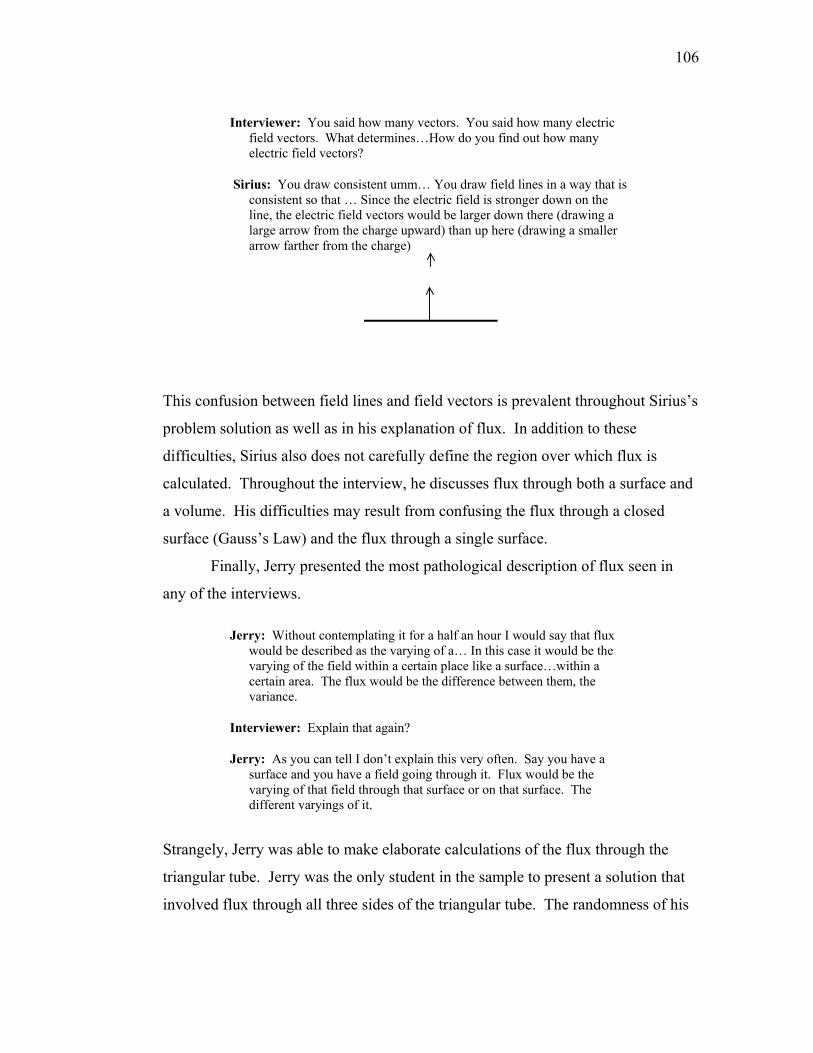
106

Interviewer: You said how many vectors. You said how many electric field vectors. What determines…How do you find out how many electric field vectors?

Sirius: You draw consistent umm… You draw field lines in a way that is consistent so that … Since the electric field is stronger down on the line, the electric field vectors would be larger down there (drawing a large arrow from the charge upward) than up here (drawing a smaller arrow farther from the charge)

This confusion between field lines and field vectors is prevalent throughout Sirius’s

problem solution as well as in his explanation of flux. In addition to these

difficulties, Sirius also does not carefully define the region over which flux is

calculated. Throughout the interview, he discusses flux through both a surface and

a volume. His difficulties may result from confusing the flux through a closed

surface (Gauss’s Law) and the flux through a single surface.

Finally, Jerry presented the most pathological description of flux seen in

any of the interviews.

Jerry: Without contemplating it for a half an hour I would say that flux would be described as the varying of a… In this case it would be the varying of the field within a certain place like a surface…within a certain area. The flux would be the difference between them, the variance.

Interviewer: Explain that again?

Jerry: As you can tell I don’t explain this very often. Say you have a surface and you have a field going through it. Flux would be the varying of that field through that surface or on that surface. The different varyings of it.

Strangely, Jerry was able to make elaborate calculations of the flux through the

triangular tube. Jerry was the only student in the sample to present a solution that

involved flux through all three sides of the triangular tube. The randomness of his

107

solution in conjunction with this definition of flux suggests that Jerry did not think

much about flux before this interview.

While each of these incomplete models was only utilized by one or two

student in the sample, they illustrate some of the misconceptions and confusions

that students encounter with the concept of flux.

108

Chapter 8 Discussion

In this chapter, we tie together the results from the three studies presented in

this thesis. We discuss the results and conclusions dealing with visualization and

construction in problem solving. Then, we summarize our findings with regard to

junior physics majors models of flux and concepts of electric field. We also

address the relevant findings regarding the transition defined in Section 3.3.

Finally, we provide a summary of the hypotheses and recommendations that have

resulted from the studies presented in this document.

8.1 The Role of Visualization in Problem Solving

In Chapters 6 and 7 we saw that visualization played a part in every student’s

problem solving. At first glance, this seems to contrast the results of Chapter 4,

which suggest that performance in physics classes is independent of spatial ability

as measured by the Purdue Spatial Visualization Test. However, a more careful

examination of these results tells a different story. First, the average PSVT scores

of the subjects interviewed was very high, greater than 31 out of 36 for both the

preliminary and final interview samples. In addition, the spread in these scores was

very low. This suggests that the spatial abilities of the students in this study are

quite high, and that the spread in their spatial abilities is quite low. In this light, the

results of Chapter 4 really tell us that the spread in spatial ability among the

students in that study did not account for very much of the spread in their grades.

This is not surprising considering that the spread in spatial ability was so small.

Hypothesis 1: The three dimensional spatial ability of junior physics majors is

very high and the variation in spatial ability is small.

109

Data from the interviews in Chapters 6 and 7 clearly show that visualization

is an integral part of students problem solving. It is also clear that students’ use of

visualization in problem solving is deeply connected to the non-visual aspects of

their problem solving. It appears that images are often a central part of students

understanding. Two-thirds of the students in the final interview sample used one or

more pictures in their explanation of flux. All of the subjects interviewed used

images in their problem solutions, but many of them experienced difficulty doing

so.

Teachers often assume students know how to use the visual representations

presented in lecture and in the text. The data presented here suggest that this

assumptions is invalid. In particular, we have seen that students often have

difficulty constructing/recalling information that we consider trivial. We have also

seen that students have difficulty incorporating visual representations associated

with Gauss’s Law and field lines into their model of flux. Several of the students

exhibited difficulty understanding the limitations of the field line representation,

while others were unable to muster the simplest Gauss’s Law arguments to simplify

their problem solution. Clearly, more research needs to be done in order to

improve our understanding of how students incorporate visual representations into

their models of physical systems.

In Section 7.4.2.1 we saw two excerpts in which students used extended

thinking processes to achieve what experienced physicists might consider trivial

conclusions. In each case the student experienced difficulty translating between

visual and symbolic representations. While based on only two instances, it is

reasonable to conjecture that student difficulty in translating between visual and

symbolic representations is responsible for a significant part of the problems

students encountered during the interviews described in Chapter 7.

Hypothesis 2: Many junior physics majors have difficulty translating between

visual and mathematical representations associated with complex

physical phenomena. In particular, they struggle to draw explicit

110

connections between standard visual representations and equations

in electrostatics.

It would be interesting to test this hypothesis in a future study. It would also

be worthwhile to explore how this varies with subjects’ problem solving

experience. This could be achieved by comparing junior physics majors’ ability to

translate between visual and symbolic representations with that of professional

physicists. However, we could obtain more relevant data by conducting a

longitudinal study in which we track students as they progress from novice to

expert problem solvers.

In addition to these translation studies, we would like to explore the particular

representations that students use in more detail. The present study is limited

because we did not ask students specific questions about their visualization, but

instead gave them the freedom to tell us what they chose with minimal direct

questioning. Consequently, we only have access to the information that students

thought was valuable or that they thought the interviewer would be interested in.

More directed questions about what visual representations the subjects were using

would likely provide more information about the particular visual representations

they have in their minds. We envision conducting interviews similar to those

described in Chapters 6 and 7, but directly probing students about the visual

representations they use; asking them if they have any pictures in their minds as

they are working through the problem and asking them to describe these mental

pictures. Conducting study with the interview question used in Chapter 7 would

allow us to use the current study as a check to see if the more direct questioning

had a significant impact on students’ problem solving behaviors.

One method for combating the difficulties students experience translating

between representation is to engage them in activities in which they explicitly draw

connections between various respresentations. For example, a simple activity

might involve presenting the three representations of flux shown in Figure 8.1.

One could then break the students into small groups and ask each group to identify

111

the connections between a pair of these representations. The groups would then

draw an arrow representing each connection. Finally, students would present and

explain the connections they identified in a class discussion.

1. Flux is the total amount of electric field through a given area.

E daΦ = ⋅∫2.

da

EE da⋅

3.

Figure 8.1 - Three representations of electric flux.

8.2 Construction in Problem Solving

In Section 7.4.2 we describe our observations of the construction-checking

behavior exhibited in these interviews. We found that a common method for

acquiring needed information while problem solving was to use several pieces of

known information to construct another piece. This process took many forms from

building an equation out of known properties to construction of differential area

elements from a recalled picture. Students in the high and middle performance

groups used this technique with some effectiveness. Subjects in the low

112

performance group tended to make more incorrect statements. In addition, these

subjects made fewer checking and construction statements.

Hypothesis 3: When dealing with complex physical concepts, junior physics

majors often employ a process of construction to recall/reconstruct

important details of the relevant physical models.

The observations made in this study were, however, only formative. A more

complete study exploring students’ ability and tendency to draw conclusions and

check these conclusions would provide a clearer picture of how these abilities

varied over our population. It would be particularly interesting to examine the

differences between expert and novice problem solvers in this respect.

The checking-construction process was also seen to have several variations.

In Section 7.4.2.1 we saw that in some instances, students constructed quantitative

conclusions from qualitative properties, while in others they recalled equations

from which they then extracted qualitative properties. Studying the extent to which

each of these strategies is used by experts and novices may provide some useful

insight into the differences between them.

We saw in Section 7.4.2.2 that some tasks we might view as simple recall

require more labored thinking for our students. In particular, the examples

presented there illustrate that in some instances students go through a laborious

process to construct seemingly trivial pieces of information from even simpler

elements. This behavior is reminiscent of the behavior of novice problem solvers

observed by Larkin (1979). In that study, it was found that the novice problem

solver verbalized her thinking process almost continuously while the expert

mentioned only the results of calculations. The authors argued that the novice had

to reason through every step of the problem solution while the expert could perform

certain procedures automatically. Still, the fact that subjects in this study

sometimes used construction to rebuild nontrivial images and equations indicates

113

that these students have developed knowledge structures that are more advanced

and connected than the simple fact lists common to novice physics students.

Hypothesis 4: Explicit construction activities, like those described above, are and

essential part of students’ development from novice to expert

problem solvers.

This strikingly common construction process is undoubtedly more time

consuming and more mentally taxing. This result has significant implications with

respect to the lecture format of most upper-division classes. In particular, since

most lecture based classes move quickly through material, it is often difficult for

students to process lecture information in a productive way. Turtle summed it up in

her interview when she noted of a lecture class that, “It made sense watching him

draw the conclusions, but it’s things I probably would have run across on my own

and stopped and thought about,” however, “in lecture it just keeps going.” Turtle’s

comment suggests that students recognize the advantages of being able to think

through the material rather than struggling to keep up. One possible solution to this

problem is to increase the degree of student control in the classroom. A common

method for achieving this is with student-centered activities like small group

activities or integrated labs.

Unfortunately, time constraints make it impractical to cover all course

materials in student-centered activities. However, it may be worthwhile to use this

type of activity to improve students’ understanding of key concepts. The results

described above suggest that students may have particular difficulty constructing

conclusions and drawing connections in the fast paced environment of the lecture.

Therefore, it may be particularly effective to use these activities when students are

supposed to draw connections or learn the reasoning behind conclusions.

One could study the effectiveness of such an activity by observing students as

they participated in the activity and conducting brief interviews to determine the

extent to which subjects incorporated these connections into their model for flux.

114

8.3 Students’ Models of Electric Flux

In Section 7.4.3, we described our observations of students understanding of

flux in the final interviews. We found that all of the students in the high and

middle performance groups had an essentially complete model of flux. Still, only

two students were able to successfully simplify the problem using Gauss’s Law.

This suggests that the ideas associated with Gauss’s Law are not thoroughly

incorporated into students’ models of flux.

Hypothesis 5: Many junior physics majors do not spontaneously connect the ideas

of flux and Gauss’s Law when solving problems.

Since the primary use of electric flux in an electrostatics course is in the

application of Gauss’s Law, it is essential that students make this connection. It

may be useful to explicitly emphasize the connection between Gauss’s Law and

flux. Focusing on the role of Gauss’s Law as a simplification technique in problem

solving may encourage students to utilize Gauss’s Law beyond the solutions to

standard problems (i.e., finding the electric field outside of highly symmetric

shapes). A particularly effective strategy might be to give students the opportunity

to work through a problem similar to the one used in the Chapter 7 interviews with

the aid of an instructor. By directing students to make explicit simplification

arguments, like those outlined in Solution 1 of the Appendix, an instructor can

force students to reason through simplification arguments based on Gauss’s Law.

We found, in Section 7.4.3.3, that all students in the low performance group

had either incorrect models of flux or serious deficiencies in their models. A full

one-third of the subjects interviewed fell in to this category. Therefore, teachers

should not be surprised to find that some of their students have erroneous models of

flux. Among the five people who had erroneous flux models, we identified four

distinct misconceptions. It would not be feasible for an instructor to try to address

each of these misconceptions in class. However, by being aware that these are still

115

common at the upper-division, instructors may be able to identify these pathologies

and address them one-on-one in office hours.

8.4 What to do About Field Lines

In Section 7.4.3.2 we draw a connection between students’ use of field lines

and their difficulties applying Gauss’s Law to flux problem. In particular, we

found that while the students were recently engaged in a course that used the

electric field vector representation almost exclusively, most of them persisted in

using electric field lines to some extent in their solutions. We found that several of

the students used electric field vectors and electric field lines interchangeably and

that others clearly confused the two concepts. Data from our interviews suggest

that students do not clearly delineate between the electric field vector and the

electric field line models.

Hypothesis 6: Many junior physics majors do not properly distinguish between the

field vector and field line representations of electric field.

The difficulties associated with electric field lines have been addressed in the

literature (Herrmann, Hauptmann, & Suleder, 2000; Törnkvist, Pettersson, &

Tranströmer, 1993; Wolf, Van Hook, & Weeks, 1996); however, teachers continue

to use this formalism. We argue in Section 7.4.3.2 that field lines have no simple

quantitative representation. We do not argue, however, that they have no value.

On the contrary, field lines can be a particularly useful part of our model since they

emphasize the role of sources in the concept of electric field. Field lines are

particularly useful when making qualitative arguments about the flux through a

region. The common pictures (See Figure 8.2) used in the formulation of the

integral formulation of Gauss’ Law are very powerful. Several students included

these pictures in their explanation of flux.

116

Figure 8.2 - Field line diagrams commonly used in the introduction of the integral formulation of Gauss's Law.

Whether or not we think they are useful, field lines are part of students’

understanding of electric field. These electric field line diagrams seem to be very

robust. That is, some students remember these images long after they have

forgotten the equations for flux and Gauss’s Law. Thus, the question is not how to

eradicate field line diagrams from our students’ minds, but how to incorporate the

concept of field lines appropriately into students’ models of electric field.

We propose that this might be achieved by having students observe the

properties of field vectors and field lines simultaneously. We feel that it is

important to include both field vectors and field lines in an upper-division

introduction to electrostatics, since students have already seen the field line model

in the lower division. If we introduce field vectors as if they are the only

representation then it is easy for students to confuse the new model of field vectors

with their previous model of field lines. We believe that it will also be important to

directly contrast the differences between the two models and to emphasize the fact

that these are only models of electric field and that each have certain advantages

and disadvantages.

A simple activity that would allow students to identify some of these

advantages and disadvantages would be to divide the class into groups. Give each

group a simple charge distribution, for example three pairs of charges, one with two

117

equal positive charges, one with two equal negative charges and one with equal but

opposite charges. Each group would be given a piece of graph paper on which they

would draw their charge distribution and the resulting electric field. Half of the

class would be assigned to draw representative field vectors, while the other half of

the class would draw representative field lines. Prior to the activity, subjects would

be given procedures for constructing both field vectors and field lines. After the

students have completed their representations of the electric field, they would be

asked to use their diagrams to estimate the magnitude and direction of the electric

field at several points chosen by the instructor. Finally, students would calculate

the magnitude and direction of the field at these points and compare to their

estimates. Students would then present their results to the class. Several important

issues are addressed by this type of activity. First, students learn that the methods

for constructing field lines and field vectors are very different. Second, when they

make their estimates of the field based on their diagrams, students using field line

diagrams will find that it is very difficult to make a quantitative estimate of the

magnitude of the electric field with field line diagrams. Finally, in the class

discussion students will participate in a direct comparison of the field line and field

vector models.

It would be very interesting to test this or a similar exercise in class to see if it

significantly affected students understanding of the relationship between field lines

and field vectors. In particular, it would be valuable to identify exercises that

would help students recognize the superiority of the field vector model while still

indicating the value of field line diagrams.

8.5 The Transition from Novice to Professional

We mentioned in Chapter 1 that visual/qualitative problem solving strategies

are an important ingredient in students’ transition from novice to professional

physicist. The models we developed in Chapters 6 and 7 will serve as a framework

118

for examining problem solving in this transition. However, before we can begin to

examine this transition, we, first, need to develop a clear description of the problem

solving characteristics of incoming junior physics majors.

In Section 2.5 we outline several characteristics identified in the literature

that differentiate between the problem-solving behaviors of experts and novices.

An important step in describing the problem solving of incoming juniors will be to

compare their problem solving characteristics to the characteristics of novices and

experts described in the literature. A rough characterization of student problem

solving behaviors from the interviews described in Chapters 6 and 7 suggests that

the subjects use a variety of problem solving techniques, some of which correspond

to novice problem solving behaviors and some of which correspond to expert

problem solving behaviors.

Hypothesis 7: Junior physics majors’ use some combination of novice and expert

problem solving techniques as opposed to a unique set of

transitional problem solving techniques.

In order to realize a good characterization, however, we would need to

conduct another study involving both junior physics majors and expert physicists.

Each group would be interviewed as they solved several problems. Ideally, the

problems used would be similar in complexity to those used in this study. In

addition, the ideal study would involve a sample at least the size of the one used

here. However, realizing this study would require a huge time commitment on the

parts of both the researchers and the subjects. A more realistic study would involve

fewer subjects and shorter problems. The transcripts obtained from the juniors

would be compared to those of the experts as well as to the existing literature, to

characterize the extent to which they resemble experts and novices.

This type of study will allow us to answer a variety of questions about our

students’ problem-solving characteristics. We will be able to draw comparisons

between the problem solving behaviors of our students and those of professional

119

physicists. In addition, we will be able to address questions about their use of

visualization in problem solving.

The answers to these questions will help us to better understand the ways that

incoming students make the transition from novice to expert physicists. Ultimately,

however, the most effective strategy for understanding this transition will require a

longitudinal study investigating how individual students change over the course of

their junior and senior year.

8.6 Closing

Looking back on my experience as an undergraduate physics student, I

realize that the way I thought about physics and indeed the world, changed

fundamentally between my introductory courses and graduation. Initially, I only

thought about physics in class and while I worked on homework. Like many

students, I tried to finish my homework in the quickest way possible. By the time I

graduated with my physics degree, I saw physics everywhere. To this day, I still

wonder how my perspective changed so dramatically. In many ways, the study

contained here was motivated by my own desire to understand how one could

develop such a drastically different view of the world in only a few short years

As a teaching assistant in the Paradigms in Physics program I saw other

students go through a similar metamorphosis. Corrine Manogue, my thesis advisor,

gave this period of rapid change a name, the junior year transition. The longer I

worked with students in the Paradigms, the more I became interested in exploring

how students make this transition. Developing a complete understanding of this

transition was clearly too big a task for a single Ph.D. thesis, so I focused my

efforts on understanding how students used visualization in problem solving. Over

the course of the three studies that make up this thesis, it became clear that

students’ use of visualization was not isolated, but instead was interwoven with

other aspects of their problem solving behavior.

120

Two key features of this mixing between visual and non-visual in students’

problem solving have emerged from the studies presented here. First, the fact that

students engaged in construction/checking procedures to recall information

suggests that they are building sophisticated knowledge structures rather than

relying simply on fact recall. What is really interesting is that these construction

procedures involve a mixture of visual, symbolic, and verbal representations. The

second instance in which students’ mixed visual and non-visual elements occurred

when they translate between representations. Translation between images and

equations was already an integral part of the problem solving method for many of

the students interviewed. While they did not always translate successfully, they did

attempt to make connections between visual and symbolic representation of the

problem. These two observations illustrate the natural tendency of students to draw

connections between various representations while learning.

Even though many of the students interviewed were not able to solve the

problem presented to them, they drew together a variety of models and

representations in their attempt. It is, in fact, these failed attempts that indicate a

transition is occurring. Casual observation of professional physicists reveals that

their understanding of a physical system stems from their facility with and ability to

connect multiple representations of the system. This is not necessarily the case

with introductory physics students. I can remember a time when I wanted to know

the one right way of thinking about things. It was only later that I recognized the

power of exploring a single physical system in a variety of representations. It is not

uncommon for introductory students to want to learn only a single method for

solving problems in physics. In contrast to this, students in nearly every interview

in this study made an attempt to solve their problem utilizing a combination of

representations for the electric field. This clearly suggests that their problem

solving strategies have evolved beyond that of the average introductory student.

When do students begin to see the importance of multiple representations in

understanding? How does this change in perception affect other aspects of the

transition from novice to professional physicist? What can teachers do to

121

encourage students to utilize and connect multiple representations in physics?

These questions will lead my research as I go on to explore the ways that students

change over the course of the upper division physics major.

122

REFERENCES

Adeyemo, S. A. (1994). Individual difference in thinking and problem solving. Personality and Individual Difference, 17(1), 117-124.

Antonietti, A. (1999). Can students predict when imagery will allow them to discover the problem solution? European Journal of Cognitive Psychology, 11(3), 407-428.

Blade, M., & Watson, W.S. (1955). Increase in spatial visualization test scores during engineering study. Psychological Monographs, 69(12, Whole No. 397).

Borich, G., & Bauman, P. (1972). Convergent and discriminant validation of the French and Guilford-Zimmerman Spatial Orientation and Spatial Visualization factors. Educational and Psychological Measurement, 32, 1029-1033.

Burnett, S., Lane, D., & Dratt, L. (1979). Spatial visualization and sex differences in quantitative ability. Intelligence, 3, 345-354.

Burnett, S., & Lane, D. (1980). Effects of academic instruction on spatial visualization. Intelligence, 4, 233-242.

Cataloglu, E. & Robinett, R. W. (2001). Testing the development of student conceptual and visualization understanding in quantum mechanics through the undergraduate career. [.pdf file] Available: http://www.phys.psu.edu/faculty/RobinettR/QM/ QMVI/QMVI_analysis.pdf

Chi, M. T. H, Glaser, R., & Rees, E. (1982). Expertise in problem solving. In R. J. Sternberg (Ed.), Advances in the psychology of human intelligence, (Vol. 1). Hillsdale, NJ: Erlbaum.

Cohen, J. & Cohen, P. (1975). Applied multiple regression/correlation analysis for the behavioral science. Hillsdale, NJ: Erlbaum.

Ekstrom, R.B., French, J. W., & Harman, H. H. (1976). Manual for kit of factor referenced cognitive tests. Princeton, NJ: Educational Testing Service.

Forman, A. E. & McPhail, J. (1993). Vygotskian Perspective on Children's Collaborative Problem-Solving Activities. In E. A. Forman, M. Norris & C. Addison Stone. Contexts for Learning (pp. 213-229). New York, NY: Oxford University Press.

123

Fuller, R. G., Karplus, R. & Lawson, A. E. (1977). Can physics develop reasoning? Physics Today, February, (23-28).

Gleick, J. (1992). Genius: The life and science of Richard Feynman. New York: Pantheon Books, 241-225.

Greca, I. M., & Moreira, M. A. (1997). The kinds of mental representations - models, propositions and images - used by college physics students regarding the concept of field. International Journal of Science Education, 19(6), 711-724.

Guay, R. (1976). Purdue spatial visualization test. Purdue, IN: Purdue Research Foundation. (ETS Test Collection No. TC009199)

Guay, R. (1980, April). Spatial ability measurements: A critique and an alternative. Paper presented at the annual meeting of the American Educational Research Association, Boston, MA.

Herrmann, F., Hauptmann, H. & Suleder, M. (2000) Representations of electric and magnetic fields. American Journal of Physics, 68 (2), 171-174.

Hestenes, D., Wells, M., & Swackhammer, G. (1992). Force concepts inventory. Physics Teacher, 30, 141-158.

Hestenes, D., & Wells, M. (1992). A mechanics baseline test. Physics Teacher, 30, 159-166.

Hortin, J. A., Ohlsen, R. L., & Newhouse, B. S. (1985). Research for teachers on visual thinking to solve verbal problems. Journal of Educational Technology Systems, 13(4), 299-303.

Ivie, R., & Stowe, K. (2000). Women in Physics, 2000. AIP publication number R430. [WWW page] Available: http://www.aip.org/statistics/trends/reports/wominphys.pdf

Inhelder, B. & Piaget, J. (1958). The growth of logical thinking from childhood to adolescence. New York, NY: Basic Books.

Jolly, P., Zollman, D., Dimitrova, A. & Rebello, S. (1998). Visualizing motion in potential wells. American Journal of Physics, 66 (1), 57-63.

Kovac, R. (1989). The validation of selected spatial ability tests via correlational assessment and analysis of user-processing strategy. Educational Research Quarterly, 13(2), 26-34.

124

Larkin, J. H., & Reif, F. (1979). Understanding and Teaching Problem-Solving in Physics. European Journal of Science Education, 1(2), 191-203.

Larkin, J., McDermott, J., Simon, D. P., & Simon, H. A. (1980). Expert and Novice Performance in Solving Physics Problems. Science, 208, 1335-1342.

Larkin, J. (1981). Cognition of Learning Physics. American Journal of Physics, 49(6), 534-541.

Lean, G., & Clements, M. A. (1981). Spatial ability, visual imagery and mathematical performance. Educational Studies in Mathematics, 12, 267-299.

Litowitz, B. E., (1993). Deconstruction in the Zone of Proximal Development. In E. A. Forman, M. Norris & C. Addison Stone. Contexts for Learning (pp. 184-196). New York, NY: Oxford University Press.

Manogue, C.A., Siemens, P. J., Tate, J., Browne, K., Niess, M. L. & Wolfer, A. J. (2001). Paradigms in physics: A new upper-division curriculum. American Journal of Physics, 69(9), 978-990.

McDermott, L. C., & Redish, E. F. (1999). Resource letter: PER-1: Physics education research. American Journal of Physics, 67(9), 755-767.

McMillan, C., & Swadener, M. (1991). Novice use of qualitative versus quantitative problem solving in electrostatics. Journal of Research in Science Teaching, 28(8), 661-670.

Moses, B. (April, 1980). The relationship between visual thinking tasks and problem-solving performance. Paper presented at the Annual Meeting of the American Educational Research Association, Boston, MA.

Mundy, J. (1987). Spatial training for calculus students: Sex differences in achievement and in visualization ability. Journal for Research in Mathematics Education, 18(2), 126-140.

Presmeg, N. (1986). Visualization in high school mathematics. For the Learning of Mathematics, 6(3), 42-46.

Presmeg, N. (1992). Prototypes, metaphors, metonymies and imaginative rationality in high school mathematics. Educational Studies in Mathematics, 23, 595-610.

Pribyl, J., & Bodner, G. (April, 1985). The role of spatial ability and achievement in organic chemistry. Paper presented at the annual meeting of the National Association for Research in Science Teaching, French Lick Springs, IN.

125

Redish, E. F., Steinberg, R. N., & Wittmann, M. C. (2001). A new model course in applied quantum physics. [WWW page] Available: http://www.physics.umd.edu /perg/qm/qmcourse/welcome.htm

Siemankowski, F., & MacKnight, F. (1971). Spatial cognition: Success prognostication in college science courses. Journal of College Science Teaching 1, 56-59.

Singh, C. (2001). Student understanding of quantum mechanics. American Journal of Physics, 69 (8), 885-895.

Small, M., & Morton M. (1983). Spatial visualization training improves performance in organic chemistry. Journal of College Science Teaching, 13(1), 41-43.

Stericker, A., & LeVesconte, S. (April, 1981). Effects of Brief Training on Sex-Related Differences in Spatial Visualization. Paper presented at the annual meeting of the Midwestern Psychological Association, Detroit, MI.

Törnkvist, S., Pettersson, K. A., & Tranströmer, G. (1993). Confusion by representation: On student’s comprehension of the electric field concept. American Journal of Physics, 61 (4), 335-338.

Van Heuvelen, A. (1991). Learning to think like a physicist: A review of research-based instructional strategies. American Journal of Physics, 59 (10), 891-907.

Van Heuvelen, A., & Zou, X. (1999). Multiple representations of work-energy processes. American Journal of Physics, 69 (2), 184-194.

Wertsch, J. V., (1985). Vygotsky and the Social Formation of Mind (pp. 58-76), Cambridge, MA: Harvard University Press.

Wolf, A., Van Hook, S. J, & Weeks, E. R. (1996) Electric field line diagrams don’t work. American Journal of Physics, 64 (6), 714-724.

Zazkis, R., Dubinsky, E., & Dautermann, J. (1996). Coordinating visual and analytic strategies: A study of students' understanding of the group D4. Journal for Research in Mathematics Education, 27(4), 435-457.

126

Appendix Problem Solutions

The Problem

An infinitely long line charge generates an electric

field0

1 ˆ2

E rr

λπε

= where λ is the uniform linear charge density and r is

the distance from the line charge. The orange thread along the edge

of the model represents this infinitely long line charge. Find the flux

of electric field through the entire surface represented by the model.

Solution 1

The electric flux can be written

S

E daΦ = ⋅∫ (A.1)

Where the integral is taken over the surface of interest, E is the electric field

and da is the differential area element associated with the surface over which the

integral is taken.

In this case, the surface we are integrating over is the triangular surface

defined by the paper model. We can break this surface up into three sides as shown,

find the flux through each side independently and add the individual fluxes together

to find the total flux.

127

Since the electric field E and the differential area element da are

perpendicular, the quantity E da⋅ is zero and the flux through the sides of the

surface adjacent to the line of electric charge (sides 1 and 2) is zero.

Thus, the problem reduces to finding the flux through the side opposite the

charge (Surface 3). Using Gauss’s Law, we can show that the flux through Surface

3 is equivalent to the flux through an arced surface sharing two edges with surface

3. This surface is shown below.

1 2

3

1

2

3

128

To show that the flux through the arced surface and surface 3 are equal, we

will define a Gaussian surface by these two surfaces and flat end caps. As shown

below.

Thus the total flux through this Gaussian (closed) surface is

3total arc endcapsΦ = Φ + Φ + Φ (A.2)

But the total flux is zero from Gauss’s Law since no charge is enclosed in the

Gaussian surface. Since the field points only in the radial direction, the field is

parallel to the end caps and the flux through the end caps ( )endcapsΦ is zero. Thus,

the magnitude of the flux through surface 3 and the flux through the arced surface

are equal

3

3

3

0total arc

arc

arc

Φ = = Φ + ΦΦ = −Φ

Φ = Φ

(A.3)

129

Note: The flux of surface 3 and the arced surface differ by a minus sign

because the flux of electric field is into the Gaussian surface for surface 3 and out

of the Gaussian surface for the arced surface.

The flux through the arced surface can be found by simple integration in

spherical coordinates.

3

0 0

ˆL

arc

E da E rd dzr

π

φΦ = ⋅ = ⋅∫ ∫ ∫ (A.4)

Where L is the length of the triangular tube (and thus the length of the arced

surface) and the φ variable is integrated from zero to 3π because the arc subtends

an angle of 60 . In this case, we have substituted the differential area element for

the arced surface ( ˆda rd dzrφ= ) into the integral. Next, we substitute the given

value of the electric field, simplify and evaluate the integral.

3

00 0

3

00 0

3

0 0 0

0 0

0

1 ˆ ˆ2

1 2

2

2 3

6

L

L

L

L

r rd dzrr

rd dzr

d dz

dz

L

π

π

π

λ φπε

λ φπε

λ φπε

λ ππε

λε

Φ = ⋅

=

=

=

Φ =

∫ ∫

∫ ∫

∫ ∫

∫

(A.5)

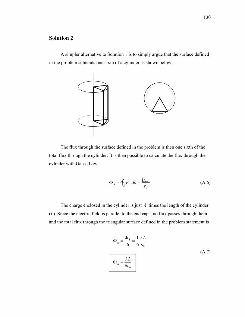
130

Solution 2

A simpler alternative to Solution 1 is to simply argue that the surface defined

in the problem subtends one sixth of a cylinder as shown below.

The flux through the surface defined in the problem is then one sixth of the

total flux through the cylinder. It is then possible to calculate the flux through the

cylinder with Gauss Law.

0

encS S

QE daε

Φ = ⋅ =∫ (A.6)

The charge enclosed in the cylinder is just λ times the length of the cylinder

(L). Since the electric field is parallel to the end caps, no flux passes through them

and the total flux through the triangular surface defined in the problem statement is

0

0

16 6

6

S L

L

λε

λε

∆

∆

ΦΦ = =

Φ =

(A.7)