Embed Size (px)
Citation preview
AN ABSTRACT OF A THESIS
THEORY AND APPLICATION OF TIME REVERSAL TECHNIQUE TO ULTRA WIDEBAND WIRELESS COMMUNICATIONS
Abiodun E. Akogun
Master of Science in Electrical Engineering
Inter symbol interference (ISI) is a major obstacle for achieving low bit error rates in wireless communications. Orthogonal frequency division multiplexing (OFDM) and equalization techniques such as zero forcing (ZF) and minimum mean square error (MMSE) have been employed in combating ISI in typical wireless channels. In this research, a technique called time reversal was investigated as a possible means for achieving higher data rate for a given bit error rate (BER) in ultra wideband (UWB) communications.
In this thesis work, time-reversal (TiR) technique was studied in detail and its application to UWB was fully evaluated. Different metrics for characterizing the space-time focusing properties of time reversal in UWB were proposed and evaluated. The technique employed used a time-domain sounding of the UWB channel to extract the channel impulse response (CIR). UWB channels are measured by sounding the channel with a sub-nanosecond pulse. CLEAN algorithm was then used to extract the CIR from the received waveform. From the observed channel impulse response, the leverages and applications of TiR in UWB were then demonstrated. In TiR, a signal is pre-filtered in such a way that it focuses in space and time at a particular receiver. This can be achieved by using a time-reversed complex conjugate of the CIR at the receiver as a transmitter pre-filter. This results in space-time focusing in TiR. Spatial focusing reduces co-channel interference in a multi-user system. Due to temporal focusing, the effective delay spread of the UWB channel is dramatically reduced and thus the complexity of the receiver is reduced. Using defined metrics for characterizing the amount of temporal focusing in UWB, it was observed that TiR works finer in a non-line-of-sight (NLOS) environment as compared with line of sight (LOS). In order to illustrate the principle of secured communications in UWB using TiR, the spatial focusing gain was studied and at a distance of approximately 6m from an intended receiver, this gain was at least 10dB. Also, to illustrate the advantage of TiR in UWB, the energy loss as a result of spatial focusing was studied against the energy loss without TiR and this gave relative information on the energy gain observed using TiR in UWB environments. Lastly, TiR was combined with equalization techniques as a means of compensation for the residual ISI in UWB channels after applying TiR, and a relative improvement was observed.

THEORY AND APPICATION OF TIME REVERSAL TECHNIQUE
TO ULTRA WIDEBAND WIRELESS COMMUNICATIONS
A Thesis
Presented to
The Faculty of the Graduate School
Tennessee Technological University
by
Abiodun Emmanuel Akogun
In Partial Fulfillment
Of the Requirements for the Degree
MASTER OF SCIENCE
Electrical Engineering
August 2005

ii
CERTIFICATE OF APPROVAL OF THESIS
THEORY AND APPLICATION OF TIME REVERSAL TECHNIQUE
TO ULTRA WIDEBAND WIRELESS COMMUNICATIONS
by
Abiodun Emmanuel Akogun
Graduate Advisory Committee:
R. C. Qiu, Chairperson date
P. K. Rajan date
X. B. He date
N. Ghani date
Approved for the Faculty:
Francis Otuonye Associate Vice President for Research and Graduate Studies
Date

iii
STATEMENT OF PERMISSION TO USE
In presenting this thesis in partial fulfillment of the requirements for a Master of
Science degree at Tennessee Technological University, I agree that the University
Library shall make it available to borrowers under rules of the Library. Brief quotations
from this thesis are allowable without special permission, provided that accurate
acknowledgement of the source is made.
Permission for extensive quotation from or reproduction of this thesis may be
granted by my major professor when the proposed use of the material is for scholarly
purposes. Any copying or use of the material in this thesis for financial gain shall not be
allowed without my written permission.
Signature
Date

iv
DEDICATION
This thesis is dedicated to my dad (Johnson) and my mum (Olufunmilayo)

v
ACKNOWLEDGEMENTS
I would like to express my sincere appreciation to my advisor, the chairperson of
my committee, Dr. R.C. Qiu, for his excellent guidance and patience throughout my
thesis work. He has been a great mentor, an excellent teacher, and a very senior colleague
and has made a very immense contribution towards the accomplishment of this task. I
would also like to thank Dr. P. K. Rajan, Dr. N. Ghani, and Dr. X. B. He for serving as
my committee members, reviewing my thesis work, and for patiently answering
questions and concerns as regards this work. Also, a very special thanks goes to Dr. Nan
Guo for all the long technical discussions and contributions he has made during the
course of this work. I will also like to thank Mr. J. Zhang of the Wireless Networking
Systems Laboratory for his help with the simulation work in this thesis. I also need to
thank Mr. C. Zhou of the Wireless Networking Systems Laboratory for his contributions
in some measurement work. All members of the Wireless Networking Systems
Laboratory have been very helpful in my accomplishment of this task and I would like to
express my special appreciation to every member of the group.
Again, I would like to thank all my friends, colleagues, and my family members
who have always been a source of encouragement throughout my life. Last but very
important I would like to thank the Graduate School for financial support provided during
my program of study. I would also like to thank the Center for Manufacturing Research
for summer financial support during my program of study. Finally, I would like to
express my profound gratitude to the almighty God who has constantly given me life and
has kept me through up to this moment in life.

vi
TABLE OF CONTENTS
Page LIST OF FIGURES…………………………………………………… .………………viii LIST OF TABLES.............................................................................................................. x CHAPTER 1. INTRODUCTION .......................................................................................................... 1
1.1 Motivation and Scope of Research ..................................................................... 1 1.2 Literature Survey of Time –Reversal Technique................................................ 3 1.3 Research Approach ............................................................................................. 5 1.4 Organization of the Thesis .................................................................................. 6
2. ULTRA WIDEBAND COMMUNICATION (UWB).................................................... 8
2.1 A Brief History of UWB Technology................................................................. 8 2.2 Definition ............................................................................................................ 9 2.3 UWB Signal Sources ........................................................................................ 10 2.4 UWB Modulation Techniques .......................................................................... 13
2.4.1 Pulse Position Modulation (PPM) ............................................................ 14 2.4.2 Pulse Amplitude Modulation (PAM)........................................................ 15 2.4.3 On-Off Keying (OOK).............................................................................. 15 2.4.4 Binary Phase Shift Keying (BPSK) .......................................................... 17
2.5 UWB Demodulation/Detection......................................................................... 17 2.6 UWB Multiple Access Techniques................................................................... 20
2.6.1 Direct Sequence, DS-UWB ...................................................................... 21 2.6.2 UWB DS-CDMA Basic Signal Model ..................................................... 21 2.6.3 Time Hopping UWB................................................................................. 22
2.6.3.1 Basic signal model for TH-WB………………………………………….23 2.7 Applications ...................................................................................................... 24
2.7.1 Through-wall Penetration ......................................................................... 24 2.7.2 UWB Radar............................................................................................... 25 2.7.3 Precision Location .................................................................................... 25 2.7.4 Sensor Networks (IEEE 802.15.4a) .......................................................... 25
2.8 Summary ........................................................................................................... 26 3. UWB CHANNEL MODELING AND CHARACTERIZATION................................ 27
3.1 Linear Filter-Based Small Scale Channel Modeling ........................................ 27 3.2 UWB Deterministic Channel Modeling............................................................ 30 3.3 UWB Channel Measurement and Modeling..................................................... 32
3.3.1. UWB Channel Measurement and Modeling Background ........................ 32 3.3.2 Measurement Apparatus and Setup .......................................................... 34
3.4 Deconvolution Techniques ............................................................................... 40 3.5 The Clean Algorithm ........................................................................................ 41
3.5.1 Limitations of the CLEAN Algorithm...................................................... 44

vii
CHAPTER Page 3.6 Summary ........................................................................................................... 44
4. TIME-REVERSAL COMMUNICATIONS................................................................. 46
4.1 Introduction....................................................................................................... 46 4.2 An Overview of Time-Reversal in UWB ......................................................... 46 4.3 Time-Reversal Theory ...................................................................................... 47 4.4 Time Reversal and UWB Systems Performance .............................................. 50
4.4.1 Rake Receivers.......................................................................................... 53 4.4.2 ISI Issues in UWB .................................................................................... 54 4.4.3 Equalization Techniques........................................................................... 56
4.4.3.1 Infinite length equalizers…………………………………………56 4.4.3.2 Finite length equalizers…………………………………………..59 4.4.3.2.1 Zero forcing equalizers………………………………………59 4.4.3.2.2 Minimum mean square error (MMSE) equalizer…………60
4.4.4 TiR System Structure................................................................................ 62 4.5 Summary ........................................................................................................... 63
5. SIMULATION RESULTS ........................................................................................... 65
5.1 Monte Carlo Simulation.................................................................................... 65 5.2 BER Simulation Results ................................................................................... 68
5.2.1 CM3 Simulation Results ........................................................................... 69 5.2.2 CM4 Simulation Results ........................................................................... 69 5.2.3 Foundry Simulation Result ....................................................................... 71 5.2.4 BER Results for Clement Hall 400 Hallway ............................................ 72
5.3 Results Illustrating Temporal Compression...................................................... 74 5.4 Results For Spatial Focusing Gain.................................................................... 81 5.5 Results for Time Reversal Loss Versus Distance ............................................. 83 5.6 Summary ........................................................................................................... 85
6. CONCLUSIONS AND FUTURE WORK ................................................................... 87
6.1 Conclusions....................................................................................................... 87 6.2 Recommendations for Future Work.................................................................. 88
APPENDICES A: IEEE CHANNEL MODEL P802.15.3A.…………………………………………….99 A. 1 Multipath Channel Model ……………………………………...100 A. 2 Channel characteristics desired to model………………………101 B: MATLAB CODE LIST …………………………………………………………….105 B. 1 List of Signal Processing/Simulation files……………………..106
VITA........................................................................................................................... 107

viii
LIST OF FIGURES
Page Figure 2.1 Comparison of UWB with traditional wireless technologies ................... 11 Figure 2.2 Spectral Mask for Indoor Applications..................................................... 11 Figure 2.3 Spectral Mask for outdoor Applications ................................................... 12 Figure 2.4 UWB Pulses .............................................................................................. 13 Figure 2.5 Spectrum of UWB pulses.......................................................................... 14 Figure 2.6 UWB Modulation schemes (a) OOK, (b) PAM, (c) PPM ........................ 16 Figure 2.7 BER Plot for UWB modulation schemes [19].......................................... 19 Figure 3.1 Classical ground bounce two-ray model................................................... 33 Figure 3.3 Pulser output with a differentiator ............................................................ 35 Figure 3.4 Time Domain UWB Channel Sounding ................................................... 36 Figure 3.5 UWB channel measurement setup ............................................................ 37 Figure 3.6 Received waveforms at distances 4m (LOS), 7m (NLOS), and 10m
(NLOS) from the transmitter .................................................................... 38 Figure 3.7 Received waveforms for LOS cases ......................................................... 39 Figure 3.8 Received waveform showing two back-to-back multipath profiles ......... 39 Figure 3.9 Clement Hall 400 Hallway........................................................................ 40 Figure 4.1 TiR experiment ......................................................................................... 48 Figure 4.2 Temporal compression illustrated using measured data ........................... 51 Figure 4.3 Temporal compression illustrated using IEEE 803.15.3a CM3 channel .. 51 Figure 4.4 Demonstrating spatial focusing in TiR ..................................................... 52 Figure 4.5 Rake receiver structure ............................................................................. 54 Figure 4.6 UWB Channel with equalizer ................................................................... 57 Figure 4.7 Discrete UWB channel with equalizer...................................................... 60 Figure 4.8 UWB systems with TiR ........................................................................... 63 Figure 5.1 Simulation setup........................................................................................ 67 Figure 5.2 TiR BER simulation result using CM3..................................................... 70 Figure 5.3 TiR BER simulation using CM4............................................................... 71 Figure 5.4 Foundry BER simulation results............................................................... 73 Figure 5.5 CMR Foundry ........................................................................................... 73 Figure 5.6 BER simulation result for Clement Hall 400 Hallway ............................ 74 Figure 5.7 Temporal compression in CM1 channel ................................................... 76 Figure 5.8 Temporal compression in CM3 channel ................................................... 77 Figure 5.9 Temporal compression in CM4 channel ................................................... 77 Figure 5.11 Temporal compression in CMR Foundry LOS........................................ 78 Figure 5.13 Clement Hall 400 Hallway LOS results showing temporal compression. 79 Figure 5.14 Clement Hall 400 Hallway NLOS showing temporal compression ........ 80 Figure 5.15 WNS lab result LOS results showing temporal compression................... 80 Figure 5.16 WNS laboratory NLOS result results showing temporal compression .... 81 Figure 5.17 Demonstrating spatial focusing gain in Clement Hall 400 Hallway......... 82 Figure 5.18 Demonstrating spatial focusing gain in CMR foundry ............................. 83 Figure 5.19 Foundry energy loss (TiR versus No TiR)................................................ 84

ix
Page Figure 5.20 Hallway energy loss (TiR versus No TiR)................................................ 84 Figure A.1 CM 1: LOS (0-4m).................................................................................. 103 Figure A.2 CM 2: NLOS (0-4m)............................................................................... 103 Figure A.3 CM 3: NLOS (4-10m)............................................................................. 104 Figure A.4 CM 4 : Extreme NLOS ........................................................................... 104

x
LIST OF TABLES
Page
Table 5.1 Temporal peak to channel energy ratio..................................................... 75 Table A.1 Channel model components and parameters........................................... 101 Table A.2 Typical Channel Characteristics and Model parameters ........................ 102
1
CHAPTER 1
INTRODUCTION
1.1 Motivation and Scope of Research
Ultra-wideband (UWB) has become a suitable candidate for high data rate, short-
range wireless communications [1]. According to Shannon’s law, the potential data rate
on a given radio frequency (RF) link is proportional to the channel bandwidth and the
logarithm of the signal-to-noise ratio. Existing narrowband and spread spectrum
technologies are regulated to operate in the unlicensed frequency bands that are provided
at 900MHz, 2.4GHz, and 5.1GHz occupying only a narrow band of frequencies relative
to that allowed for UWB. UWB is a usage of recently legalized spectrum with a
bandwidth of more than 7GHz wide and hence a higher data rate compared to
narrowband and spread spectrum systems. In 2002, the United States Federal
Communication Commission (FCC) allocated the 3.1 GHz to 10.6GHz spectrum for
UWB devices and after this, there has been sparkled interest in UWB research activities
in both academia and the industry.
To allow for such large operation bandwidth, the FCC has put in place strict
power limitations on UWB radios. With strict power limitations, it is therefore possible to
implement cost effective CMOS implementations of UWB radios. UWB radios therefore
have several advantages, which include low power consumption, low cost, and very high
data rate within a short range. Due to the large operation bandwidth, the resolution in
time domain is small for UWB radios. UWB involves transmitting ultra-short pulses. The

2
advantage of using short pulses is fine timing resolution thus more multipath channels
can be resolved [2]. The channel distorts these pulses so that per-path distortion is
encountered in UWB systems. References [3] and [4] address the designing of a reception
scheme as a key issue for UWB systems.
Despite the potential advantages of UWB, several drawbacks have been noted as
regards the application of UWB radios. Inter symbol interference (ISI) is a key
impediment for reliable high data rate transmission in wireless channels. Orthogonal
frequency division multiplexing (OFDM) and equalization techniques have been
employed in wireless systems as a means of compensation for ISI. OFDM uses a large
number of sub-bands chosen in such a way that each sub-band exhibits flat fading and
thus OFDM has the key property of mitigating ISI. Equalization is also an effective
means of combating ISI in frequency selective channels. The device, which equalizes the
dispersive effect of a channel with memory, is called an equalizer [5]. An approach called
time reversal (TiR) has been successfully applied to underwater acoustic channels and
narrowband channels as another means of combating ISI in such frequency dispersive
channels. When TiR is applied to a dispersive channel, a reduction is observed in the
effective channel length. With a reduction in the effective channel length, the effect of ISI
in the channel is reduced. This shows that TiR is an effective technique in reducing ISI in
frequency dispersive channels.
The objective of this project is to study critically the theory behind TiR and to
demonstrate several applications of TiR in a UWB channel using both statistical and
experimental data collected from different UWB environments. TiR has only recently
been applied to UWB [1, 6]. Two key applications that come with this technique are
3
spatial focusing and temporal compression. These two key applications are addressed in
details and metrics to characterize these two applications are defined in relation to UWB.
Spatial focusing is a concept that addresses security concerns in UWB channels. Due to a
focus of power at the intended UWB receiver, the probability of a nearby receiver
decoding the information on an intended receiver is greatly reduced. In TiR channels, the
effective channel impulse response is compressed with a temporal focus of the channel
energy being visible around the center of the compressed channel impulse response.
Metrics to characterize this temporal compression in UWB channels are defined in this
thesis work. Also, the use of TiR technique to compensate for ISI and thus improve UWB
receiver performance is addressed is this research work.
1.2 Literature Survey of Time –Reversal Technique
The concept of time reversal is not new in the world of telecommunications.
References [1, 6] show the first application of TiR to UWB. In [1], the concept is
combined with a minimum mean square error (MMSE) equalizer to improve receiver
performance in UWB. The channel data used are collected using a frequency domain
channel sounding technique and the number of taps of the TiR channel is varied to study
receiver performance in UWB. In [6], the space-time focusing properties of TiR in UWB
are demonstrated also using a frequency domain channel sounder with measurement
results from Intel Corporation. In [7], the concept is applied to electromagnetic waves
and the concept of spatial focusing and temporal compression is demonstrated using a 1
µs electromagnetic pulse at a central frequency of 2.45GHz. This is the first experimental

4
demonstration of TiR space-time focusing with electromagnetic waves. The spatial and
temporal focusing that comes with this technique has been demonstrated in ultra-sound
by Fink [8, 9].
In underwater acoustics, [10-13] details the application of the technique and the
issues of spatial and temporal compression are also addressed. Reference [14]
demonstrates the first application of TiR to wireless radio and proposes to convert an
available broadband multiple input multiple output (MIMO) channel sounder into a
device that can demonstrate the concept of TiR. In [15], the concept of multiple input
single output (MISO) is applied in conjunction with TiR as a possible means to reduce
the delay spread in a fixed wireless access channel and a delay spread reduction of a
factor of three was observed. In [16] the concept is applied to time reversed random fields
and the space-time focusing issues are addressed in relation to this field. Reference [17]
demonstrates the space-time focusing properties in TiR using a time domain channel
sounding technique and at a distance of 6m from the intended receiver, the spatial
focusing gain observed is at least 10dB. In [18], the basic principles of applying TiR to
underwater acoustic field are explained in details. Reference [19] applies the concept of
time reversal with a transmitted reference system and the new receiver structure called
time reversal and transmitted reference (TiR-TR) shows a relative improvement of about
9dB performance gain at a data rate of 19Mbps for a BER of 310− . In [20], the concept of
TiR is applied with MISO in an underwater acoustic channel and a zero forcing pre-
equalization is also applied in the channel to demonstrate the space-time focusing
features of TiR. Reference [20] shows that pre-equalization does not alter significantly
the spatial focusing properties of time reversal.

5
MIMO is a way of exploiting the rich scattering properties in frequency dispersive
narrowband channels. In [21], using outdoor measurements that mimic a typical 3G
WCDMA system, the feasibility of applying TiR with MIMO in single user wireless
systems is studied showing TiR-MIMO as a promising technique for wireless channels. It
also studied the feasibility of applying TiR with multi user MISO systems.
1.3 Research Approach
The methods employed in literature to demonstrate the application of TiR have all
employed a frequency domain channel sounder approach. With this approach, the real
time behavior of UWB channels cannot be observed. From the mathematical knowledge
of Fourier transforms, it is possible to transform a frequency domain signal into its
corresponding time domain equivalent. This shows that a time domain approach is also
possible to demonstrate the concept of TiR in UWB since a frequency domain approach
has already been used.
The received waveform in wireless channels is a convolution of the channel
impulse response with the transmitted waveform. In order to extract the channel impulse
response from the received waveform, deconvolution techniques are employed. UWB
channel data are collected for different UWB environments. From the collected data, a
signal processing algorithm, the CLEAN algorithm, is used to extract the channel impulse
response. The CLEAN algorithm is a deconvolution technique to extract the observed
channel impulse response from the received waveform. From the observed channel
impulse response, the space-time focusing properties of TiR in UWB are demonstrated

6
using defined metrics. Also, using IEEE channel models for 802.13.4a and 802.13.3a, the
concept of TiR is also illustrated. The use of TiR to compensate for ISI is also
demonstrated using IEEE 802.15.3a channel models and results from the collected data
for typical UWB environments. Bit error rate (BER) is used as the performance metric. It
is observed that with the use of TiR, ISI is greatly reduced and the equalization task in the
effective TiR channel is also greatly reduced. Equalization if needed for a TiR channel
has the complexity of the equalizer being tremendously reduced.
1.4 Organization of the Thesis
Chapter 2 details the concept behind UWB communication; a brief history of
UWB, UWB signal sources and the associated spectrum, UWB modulation
techniques, and the applications of UWB are discussed.
Chapter 3 presents the concept involved in time-domain sounding of UWB
channels. The principles involved in the use of the CLEAN algorithm as the signal-
processing algorithm used in this thesis are also addressed in this chapter.
Chapter 4 focuses on the theory and applications of TiR in UWB. This chapter
presents an overview of TiR and the proposed metrics for characterizing TiR in UWB
are discussed here. It also focuses on evaluating the performance of TiR channels in
UWB environments. It gives an overview of receiver types and signal models for
frequency selective channels. It also addresses the use of TiR to improve receiver
performance in UWB.

7
Chapter 5 presents the results on the applications of TiR in UWB channels. It gives
the relative improvement observed using TiR in BER simulation for UWB channels. It
also gives a comparison between the line-of sight (LOS) and non line of sight (NLOS)
UWB TIR channels.
Chapter 6 gives the conclusion from this thesis work. Recommendations for
future work are also presented in this chapter. Appendix A briefly introduces IEEE
802.15.3a and 802.15.4a channels. A Listing of the Matlab code is given in Appendix B.

8
CHAPTER 2
ULTRA WIDEBAND COMMUNICATION (UWB)
Ultra wideband (UWB) technology is well known for its use in ground penetrating
radar. UWB has also been of interest in communications and radar applications requiring
low probability of intercept and detection (LPI/D), high data throughput, precision
ranging and localization, and multipath immunity. In this chapter, the basic concept
behind UWB is presented. After a very brief history of UWB, the shapes and spectra of
UWB pulses are discussed; UWB modulation techniques and applications of UWB are
then discussed.
2.1 A Brief History of UWB Technology
The origin of ultra wideband stems from work in time-domain electromagnetic in
1962 [22]. The idea was to characterize linear, time invariant systems (LTI) using the
impulse response of such systems instead of using the conventional swept frequency
response. The output )(ty of an LTI system to an input excitation )(tx can be
determined using the well known convolution integral [23]:
∫∞
∞−
−= τττ dthxty )()()( (2.1)
where )(th is the impulse response of the system.
However, the impulse response of microwave networks could not be directly
observed and measured until the advent of the sampling oscilloscope by Hewlett Packard

9
in 1962 and the development of techniques for sub-nanosecond (base band) pulse
generation, providing suitable approximations to an impulse excitation. Once these
techniques were applied to the design of wideband, radiating antennae elements (Ross,
1968), it became obvious that they could also be applied to short pulse radar and
communications systems.
Throughout the late 1980’s, this technology was alternately called base band,
carrier-free, or impulse. The term ultra-wideband was not applied until 1989 by the U.S
Department of Defense (D.O.D). By that time, UWB had already experienced 30 years in
its development. Although, UWB is old, its application in communications is new.
2.2 Definition
UWB characterizes transmission systems with instantaneous spectral occupancy
in excess of 500MHz or a fractional bandwidth of more than 20%. Fractional bandwidth
( fB ) is defined as
c
f fBB = (2.2)
where LH ffB −= denotes the –10dB bandwidth and 2)( LH
cfff −= is the center
frequency with Hf being the –10dB emission point upper frequency and Lf is the –
10dB emission point lower frequency.
The huge bandwidth implies that UWB can provide high throughput required to
address the market for wireless personal area networks (WPAN). In order to co-exist with
existing traditional wireless technologies such as spread spectrum and narrowband

10
systems, the United States Federal Communication Commission (FCC) imposes strict
limitations on the power spectral density from UWB systems. Figure 2.1 shows a brief
comparison of UWB with existing wireless technologies in terms of bandwidth and the
emitted power expected from the devices. Figures 2.2 and 2.3 show the spectral density
mask for indoor and outdoor operations. UWB signals may be transmitted between 3.1
GHz and 10.6 GHz at power levels up to –41dBm/MHz. The primary difference between
indoor and outdoor operations is the higher degree of attenuation required for out of band
region for outdoors operation. This further protects GPS receivers, centered at 1.6 GHz.
2.3 UWB Signal Sources
UWB signals can be realized using sub-nanosecond pulses. Narrower pulses in
time domain correspond to an electromagnetic radiation of wide spectrum in frequency
domain. The frequency domain spectral content of a UWB signal depends on the pulse
waveform shape and the pulse width. The most common signals used to drive UWB
antennas include a Gaussian pulse, Gaussian monocycle, Gaussian doublet, Raleigh
monocycle and rectangular waveforms. Rectangular waveforms have large DC
components, which is not a desirable property. A generic Gaussian pulse can be
represented as [24]:
⎥⎥⎦
⎤
⎢⎢⎣
⎡⎟⎠⎞
⎜⎝⎛ −
−=2
21exp
21)(
σµ
πσttpg (2.3)

11
Figure 2.1 Comparison of UWB with traditional wireless technologies
Figure 2.2 Spectral Mask for Indoor Applications

12
Figure 2.3 Spectral Mask for outdoor Applications
where
t is the time in seconds
µ is the parameter that defines the center of the pulse
σ is the parameter that defines the width of the pulse.
A Raleigh monocycle is obtained by differentiating the Gaussian pulse once [25].
The second derivative of the Gaussian pulse gives a Gaussian monocycle while the
Gaussian doublet consists of two; amplitude reversed Gaussian pulse having a time gap
of wT between the pulses. Figures 2.4 and 2.5 show different UWB pulses and their
associated spectra.

13
2.4 UWB Modulation Techniques
In order to transmit information, it is necessary to modulate the pulse train. For
coherent detection several modulation schemes were initially employed for UWB
communication. The most common modulation schemes found in the literature include
Pulse Position Modulation (PPM), Pulse Amplitude Modulation (PAM), On-Off keying
(OOK), and Binary-phase shift keying (BPSK). BPSK has a 3dB performance
improvement over OOK and PPM.
0 0.5 1 1.5 2 2.5 3 3.5 4 4.5 5
x 10-9
-1
-0.8
-0.6
-0.4
-0.2
0
0.2
0.4
0.6
0.8
1
Time(ns)
Am
plitu
de
UWB pulses
Gaussian monocycle(2nd order differential)Rayleigh monocycle(1st order differential)Gaussian pulse
Figure 2.4 UWB Pulses

14
Figure 2.5 Spectrum of UWB pulses
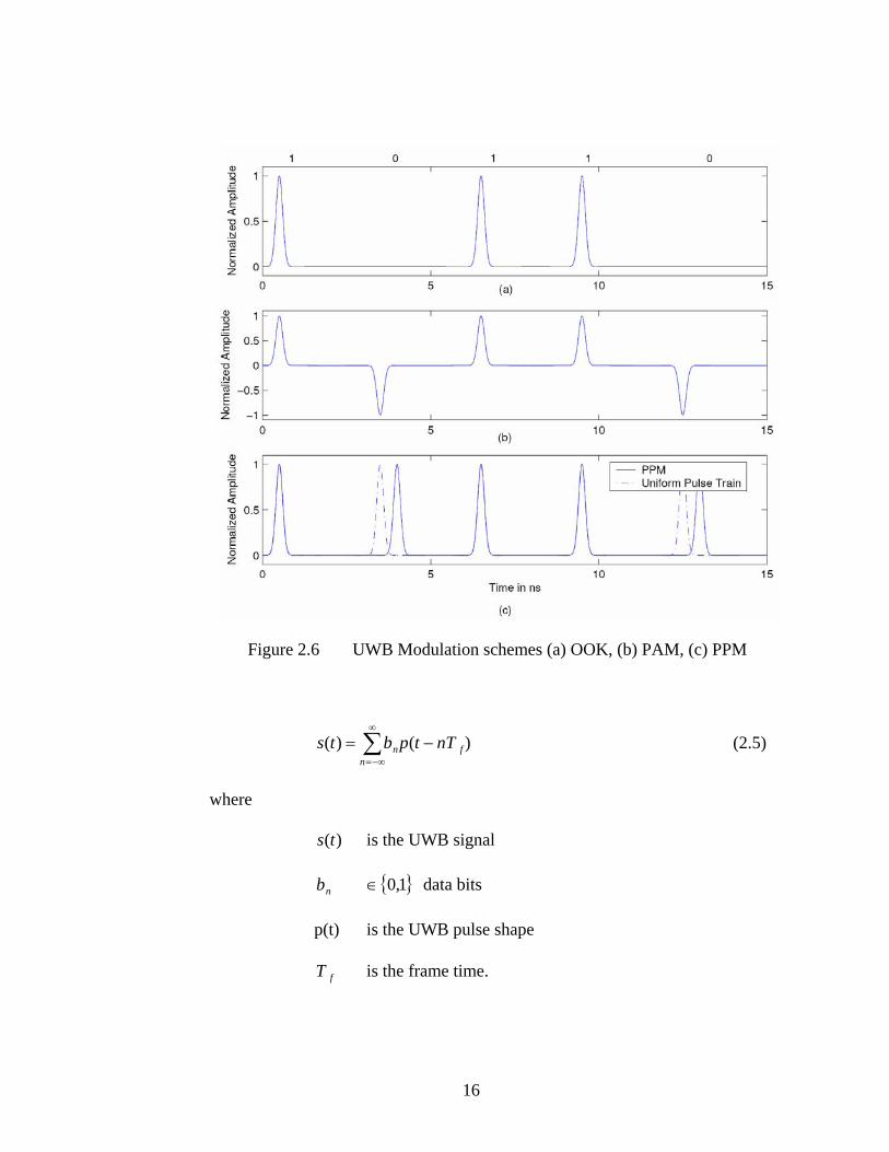
2.4.1 Pulse Position Modulation (PPM)
In PPM, the position of each pulse is varied in relation to the position of a
recurrent reference pulse according to the information data. A digital zero could be coded
by transmitting a pulse some picoseconds earlier than a reference position while a digital
one could be coded by transmitting at the same amount of time later as shown in Figure
2.6. Many positions can be used to increase the number of symbols and hence we can
have an M-ary PPM. PPM has the advantage of requiring constant transmitter power
since the pulses are of constant amplitude and duration. The periodicity of the pulse
repetition period (PRP) makes energy spikes to appear in the spectrum. In order to

15
smoothen the spectrum, pseudorandom sequence of delays could be added to the pulse
train. This is called time hopping. Binary PPM technique is given by
( )∑∞
=
−−=1
)(n
nf bnTtpts δ (2.4)
where
nb { }1,0∈ data bits
δ is the time shift
p(t) is the UWB pulse shape
fT is the frame time.
2.4.2 Pulse Amplitude Modulation (PAM)
In PAM, the information data are carried on a train of pulses with the information
being encoded in the amplitude of the pulses. Values are defined by changing the powers
of the pulses. An 8-ary PAM for example uses eight levels of the pulse amplitude to yield
four bits. The classic binary amplitude modulation (PAM) can be represented using for
example two antipodal Gaussian pulses [26] as shown in Figure 2.6.
2.4.3 On-Off Keying (OOK)
In On-Off keying, the presence of a pulse indicates a value of one while the
absence of a pulse indicates a value of zero. The following equation represents OOK
modulated UWB transmitted signal and the waveform is shown in Figure 2.6.
16
Figure 2.6 UWB Modulation schemes (a) OOK, (b) PAM, (c) PPM
∑∞
−∞=
−=n
fn nTtpbts )()( (2.5)
where
)(ts is the UWB signal
nb { }1,0∈ data bits
p(t) is the UWB pulse shape
fT is the frame time.
17
The main advantage of OOK over other modulation schemes is simplicity in its
implementation.
2.4.4 Binary Phase Shift Keying (BPSK)
In BPSK, a positive pulse is transmitted for a “1” and a negative pulse is
transmitted for a “0” as shown in Figure 2.6. BPSK can be mathematically represented
by
∑∞
−∞=
−=n
fn nTtpbts )()( (2.6)
where
nb { }1,1 −∈ data bits.
2.5 UWB Demodulation/Detection
The major criteria to evaluate the efficiency of a particular modulation scheme are
its BER performance, spectral shape, data rate, and transceiver complexity [27]. As seen
previously, modulation transmits the required data information. The main function of a
demodulator is to extract the original data information modulated on the monocycle train
from the distorted waveforms with the highest level of accuracy. A receiver generally
consists of a detection and decision device. The detector in ultra wideband systems is
different from that of existing narrowband systems since ultra wideband operates in a
carrier-less fashion. Typical UWB receiver implementations include autocorrelation
18
receivers and correlation or rake receivers. In the UWB correlator receiver, the first
operation to be carried out is the match filtering of the waveform. In order to do this, the
incoming signal is matched with a waveform template and the result is integrated. This
correlation operation between the received signal and the waveform template has to be
performed for each possible pulse position and the correlation results are then sent to the
base band for further processing.
The UWB correlator (matched) receiver already discussed is an optimum receiver
for the AWGN channel. For such a receiver, the received signal )(tr in the absence of
multiple access interference can be modeled as follows:
)()()( tntstr += (2.7)
where )(ts is the transmitted monocycle, )(tn is the zero mean white Gaussian noise
with power spectral density No/2. For binary modulation, the BER can be calculated
using the Euclidean distance d min between the two symbols.
⎟⎟
⎠
⎞
⎜⎜
⎝
⎛=
ob N
dQP2
2min (2.8)
The Euclidean distance between the two symbols can be evaluated for various
modulation options as
sEd 2min = for orthogonal PPM,
sEd 2min = for BPSK
sEad =min for OOK,
sEaad )( 21min −= for PAM
where

19
sE is the average energy per symbol (Joules)
a is the average transmitted pulse energy
Q is the Q function [28] which is the tail of the standard.
Gaussian density function (mean µ =0 and variance σ=1) and is defined by
dzexQ z
x
2/2
21)( −
∞
∫= π. (2.9)
The advantage of BPSK over OOK and PPM is the improvement in BER performance,
since it is 3dB more power efficient for the same probability of error. Figure 2.7 shows
the BER plots for different modulation schemes.
Figure 2.7 BER Plot for UWB modulation schemes [19]

20
2.6 UWB Multiple Access Techniques
Based on spreading, the two common multiple access schemes employed with
UWB are Time-Hopping UWB (TH-UWB) and Direct Sequence UWB (DS-UWB). In
TH-UWB, unique time hopping codes are used to position each of the UWB pulses
within a given time frame of a particular bit. In DS-UWB, no time gapping is left
between transmitted pulses. A multiple access scheme can either be synchronous or
asynchronous depending on whether the bits transmitted are in the same time interval or
not. Construction of asynchronous multi-user orthogonal codes is impossible as different
users arrive the receiver location with random time delays. TH/SS have spike problems
when compared with DS-SS. The co-existence of UWB systems using TH-SS and DS-SS
is important since UWB will co-exist with narrowband/wideband systems in the same
frequency spectrum. Narrowband/wideband systems include Global system for Mobile
Communications (GSM 900) and Universal Mobile for terminal service
(UMTS)/wideband code division multiple access (WCDMA) and the Global Positioning
system (GPS). In the GPS L1 and L2 channels, DS-SS introduces less interference than
TH-SS UWB. Both TH-SS UWB and DS-SS UWB generate similar level of interference
in GSM900 and UMTS/WCDMA bands. In the presence of degradation due to jamming
from narrowband systems, TH-SS UWB outperforms DS-SS UWB at a low interference
level and both TH-SS UWB and DS-SS UWB have similar performance at a high
jamming power level.

21
2.6.1 Direct Sequence, DS-UWB
The DS-UWB is similar to conventional CDMA carrier-based radios. The
spreading sequence is multiplied by an impulse sequence. The modulation technique
employed is the same as that employed in CDMA.
2.6.2 UWB DS-CDMA Basic Signal Model
The transmitted signal for a UWB DS-CDMA using PPM is defined as
∑∑∞
−∞=
−
=
−−−=i
N
nncr
kn
kikk
r
dnTiTtzabpts1
0)()( δ (2.10)
where
z(t) is the transmitted monocycle waveform,
k is the thk user,
kib are the modulated symbols for the thk user,
kna are the spreading chips,
Tr is the bit period,
Tc is the chip period,
c
rr T
TN = is the spread spectrum processing gain,
δ is the extra delay of monocycle for symbol 0,
nd is the information data sequence, and
kp is the transmitted power.

22
Correspondingly, for PAM the transmitted signal is given as
ni
N
ncr
kn
kikk dnTiTtzabpts
r
∑∑∞
−∞=
−
=
−−=1
0)()( . (2.11)
The information data sequence nd =0 for symbol “1” and =1 for symbol “0”in PPM while
nd =1 for symbol 1 in PAM and nd =-1 for symbol 0 in PAM. The received UWB signal
is represented as
)()()()()( tntItmtstr +++= (2.12)
where
)(ts is the transmitted signal,
)(tm is the multiple access interference,
)(tI is the narrowband interference,
)(tn is a white Gaussian noise process with two sided power spectral
density No/2, and the receiver is a correlator receiver.
2.6.3 Time Hopping UWB
Time Hopping is part of the original proposal for UWB communications.
Modulation of TH-SS UWB radio is achieved through shifting of pulses. The key
motivations for using TH-SS impulse radio are the ability to highly resolve multipath and
the availability of technology to implement and generate UWB signals with low
complexity [29]. In both TH-SS and DS-SS one information bit is spread over various
monocycles and the required processing gain is achieved in reception.
23
2.6.3.1 Basic signal model for TH-UWB. The transmitted signal from a user in
TH-SS using PPM is given by
)()( )(nc
kjf
jk dTcjTtwts δ−−−=∑ (2.13)
where
)(tsk is the kth transmitted signal,
w (t) is the transmitted monocycle waveform,
fT is the pulse repetition time or frame time,
j is the jth monocycle that sits at the beginning of each frame,
δ is the time shift that applies to the monocycle and such operation is
defined when 1 is transmitted,
cT is the additional time delay that associates with the time hopping code,
)(kjc are time hopping code (periodic pseudorandom codes), and
nd is the information data sequence.
For TH-PAM, the transmitted signal is represented as
nck
jfj
k dTcjTtwts )()( )(−−=∑ . (2.14)
The signal at the receiver is represented as
∑=
+−=Nu
kkkk tntsAtr
1)()()( τ (2.15)
where
kA models the attenuation at the transmitter signal,
n (t) is the additive white Gaussian noise, and

24
kτ represents the asynchronisms between the clock of the transmitter and the
receiver.
The correlator template signal is given by
y (t)=w (t)-w(t-δ ) (2.16)
where y (t) is the pulse shape defined as the difference between the two pulses shifted by
the modulation parameter δ . This will then be correlated with the received signal for the
required statistical decision test.
2.7 Applications
Typical applications of the UWB technology include through wall penetration,
precise location, UWB radar, and UWB sensor networks (IEEE 802.14.4a). UWB is
applicable in the above scenarios due to its popularity for multipath immunity, high data
throughput, better wall penetration, low power consumption, and low probability of
intercept and detection.
2.7.1 Through-wall Penetration
A high resolution is required to track the motion of persons or objects that are
placed on the other side of a wall. At longer ranges, precision time gating is required to
track multiple targets [30]. An UWB system is a very reliable solution in providing this
kind of through-wall penetration and resolution capabilities.

25
2.7.2 UWB Radar
An advantage of using UWB in radar applications is that due to UWB’s inherent
time resolution property, it reduces post detection signal processing required in
narrowband radars [30, 31]. UWB underground penetrating radars can be used to check if
any underground cables or pipes are present before digging. UWB ground penetrating
radars can also be used in numerous applications like target specific application,
geophysical location, and in civil engineering applications.
2.7.3 Precision Location
The use of differential GPS for outdoor applications can be used to improve errors
in modern day GPS and can also be used for precise estimation of location within 1-2
meters. Using UWB in addition with these technologies is a good solution for extending
the location finding capabilities to the indoor.
2.7.4 Sensor Networks (IEEE 802.15.4a)
Sensor networks are applicable for surveillance, automobiles, and medical
situations. The use of a wired network for these kinds of applications is expensive and
cumbersome. In these kinds of applications, UWB is a viable solution as a wireless
communication link. With UWB, the network is invisible and unnoticeable to others.
Sometimes, a UWB signal can even be used as a sensor.

26
2.8 Summary
This chapter focused on the fundamentals of UWB communications. UWB pulse
shapes and their associated spectra were discussed. The different modulation schemes
that can be used for UWB were also discussed. BPSK has a 3dB performance
improvement when compared to OOK and PPM. A discussion of UWB multiple access
techniques were also presented. TH-SS UWB and DS-SS UWB were discussed as two
popular methods of multiple accesses in UWB based on spreading. Finally, some
applications of UWB were also discussed.

27
CHAPTER 3
UWB CHANNEL MODELING AND CHARACTERIZATION
This chapter provides the foundation on which the thesis is based. It describes the
concept behind the modeling and characterization of UWB channels. It presents some of
the results obtained from the small-scale characterization of UWB channels. These results
are based on several measurement efforts conducted in different indoor environments.
The first half of the chapter addresses the issue of UWB channel modeling from a
deterministic and a statistical point of view. The second half of the chapter considers the
overall indoor channel impulse response, based on finite impulse response (FIR)
calculated using the CLEAN algorithm. The results obtained from the first half are
important towards validating some assumptions used in the second half. The observed
channel impulse responses from the second half of this chapter serve as the data on which
the applications of TiR are demonstrated in the later chapters of this thesis.
3.1 Linear Filter-Based Small Scale Channel Modeling
Accurate channel models are important in designing communication systems.
With adequate knowledge of the features that are unique to the channel,
communication engineers are able to predict the system performance for specific
modulation schemes. Propagation channels set fundamental limits on the performance
of UWB communication systems. Due to reflection, refraction, and diffraction, wireless
signals usually experience multipath propagation. In narrowband systems, this leads to

28
multipath fading. Various theoretical and empirical models have been employed in
studying the statistics of multipath fading in indoor environments. Turin’s point-
scattering model is widely used for amongst these models. In Turin’s model, the
channel is represented as
h(τ,t) = [ ]∑=
−L
lll tt
1)()( ττδα )(tj le θ (3.1)
where
δ represents the dirac function,
L is the number of resolvable multipaths,
)(tlα are the multipath amplitudes,
τ is the delay variable,
)(tlτ are the multipath arrival times, and
)(tlθ are the path phase values.
Distributions used to describe amplitude values are: Rayleigh, Rician, Nakagami
(m-distribution), Weibull, and Suzuki. Distributions used to describe the arrival times
are modified 2-state Poisson model (∆-K model), modified Poisson (Weibull Intervals),
and double Poisson (Saleh-Valenzuela). The initial phase is a uniformly distributed
random variable [0,2π]. Phase distribution can be incremented by a random Gaussian
variable and deterministic values calculated from the environment.
Certain parameters are useful as single number descriptions of the channel to
estimate the performance and the potential for inter symbol interference (ISI). The
parameters include the mean excess delay, RMS delay spread, and maximum excess
delay and they describe the time dispersive properties of the channel. These time

29
dispersive properties of the channel are measured relative to the time of arrival of the
first component.
The mean excess delay (X dB) of a power delay profile is the time required for
the energy to fall X dB below the maximum [32]. The mean excess delay is the first
moment of the power delay profile
∑∑
=
kk
kkk
a
a
2
2 ττ . (3.2)
The RMS delay spread is the square root of the second central moment of the power
delay profile [32]
( )22 ττσ τ −= (3.3)
where
∑∑
=
kk
kkk
a
a
2
22
2τ
τ . (3.4)
The ratio of the mean excess delay to the RMS delay spread can be used as a measure
of the time dispersion for UWB signals.
Channel models for UWB can either be physical models taking into account the
exact physics of the propagation environment or statistical models taking empirical
approach, measuring propagation characteristics of the environment and then
developing models based on measured statistics. In order to estimate the parameters
associated with a given channel impulse response, a channel sounder is used. A channel
sounder is a device that allows estimation of the parameters associated with the impulse

30
response of a radio channel namely: the number of multipath components and their
associated amplitudes, phases, and delays.
3.2 UWB Deterministic Channel Modeling
In UWB systems, the transmitted pulses have width much smaller than the
channel propagation delays and hence do not overlap. At the receiver, due to the
wideband nature of UWB signals, conventional models for characterizing narrowband
channels such as the Turin’s model are inadequate for UWB transmission. The Turin’s
point scattering models does not take into account the frequency dependency of the
individual path rays and hence it does not take into account the issue of waveform
distortion. In practice, when a waveform propagates through a medium, there are three
propagation mechanisms of interests: line of sight (LOS), reflection, and diffraction
[33]. Diffraction causes the strength of the diffraction field to be frequency dependent
with a term αω in the diffraction field expression. Including the frequency dependent
parameter to Turin’s model allows us to represent the wideband channel as
[ ] )(
1)()()(),( tj
L
llll
lethtth θττδτατ ∑=
−⊗= (3.5)
where
τ(lh ) is the per-path impulse response and ⊗ denotes convolution
operation.
The parameter τ(lh ) explains most of the practical diffraction phenomena occurring in
buildings, windows, cylinders, furniture, bottles, etc. In studying channel effects, the

31
effect of propagation phenomena on the received signal can be categorized as large-
scale effects and small-scale effects. Large-scale effects are important for predicting
service availability and coverage while small-scale effects are those that vary over a
short time and are important in designing modulation schemes for UWB systems.
UWB channel modeling with emphasis on pulse waveform distortion or
frequency dependency in frequency domain was first studied in [33]. The physical
foundation of pulse waveform distortion is based on Sommerfield’s exact solutions of
Maxwell’s equations. The study of time-domain or transient wave electromagnetics
was initiated by Sommerfield in 1902 on the diffraction of a pulse or a transient wave
by a wedge or half plane [34]. The frequency dependency of the path rays can be used
to trace, detect, and characterize a ray and is also useful in channel modeling. A ray
coming from the line of sight path or a reflected ray has no frequency dependency
while a ray from a diffracted path has frequency dependency. Ray tracing of the
individual path rays can be used in studying the propagation features of a UWB
channel. The concept of pulse waveform distortion or frequency dependency and its
impact on UWB transceiver design are studied extensively in [35-37]. The UWB
propagation mechanisms include the geometric optical (GO) rays and the diffracted
rays. The geometric theory of diffraction (GTD) framework can be used to model the
diffracted rays.
Mathematically,
GTDGOt EEE += (3.6)
where
tE represents the total electric field,
32
GOE represents the field component of the geometric optic rays, and
GTDE represents the diffracted rays.
In the deterministic modeling of UWB channels, a two-ray model shown in Figure 3.1
is the mostly used model for studying geometric optic (GO) rays
3.3 UWB Channel Measurement and Modeling
3.3.1. UWB Channel Measurement and Modeling Background
A limited number of measurement campaigns have been carried out by UWB
researchers to characterize UWB channels. Most proposed UWB channel models are
extensions of existing wideband channel models. There are many unresolved issues in
literature on the characterization of UWB channels and hence there is still a need for
more measurements to formulate a comprehensive model before designing UWB
simulators. Some proposed UWB channel models are based on empirical UWB results
while some are based on extrapolation from wideband measurement and models. The
characterization of a UWB channel can be carried out using two different approaches:
time domain approach and the frequency domain approach. The major piece of
equipment used in the frequency domain approach is a vector network analyzer (VNA).
The results obtained in frequency domain approach can then be converted into time
domain via inverse Fourier transform. The advantage of frequency domain approach is
that the sensitivity of narrowband measurement equipments such as the VNA is much
larger than that of oscilloscopes used in time domain measurements. However, extra data
processing is required for frequency domain measurements to get the time domain

33
Figure 3.1 Classical ground bounce two-ray model
channel impulse response of the UWB channel. This thesis has employed the time
domain approach for collecting the UWB channel data.
In this approach, a short duration pulse p(t) is transmitted as an excitation signal
for the propagation channel. This pulse approximates a delta function but in reality, it is
not and hence there is a need for a signal-processing algorithm to extract the actual
channel impulse response. Mathematically,
)()()( tpthty ⊗= (3.7)
when ),()( ttp δ= CIRthtpthty ==⊗= )()()()( .
However, in reality, ),()( ttp δ≠ and hence the need for deconvloution techniques to
extract the CIR from the measured )(ty .
34
3.3.2 Measurement Apparatus and Setup
The equipment used for collecting the UWB channel data involves a UWB pulser
that generates a Gaussian like pulse with root mean square (rms) pulse width of
approximately 250 ps as shown in Figure 3.2: a power amplifier with a gain of 34 dB, a
noise figure of 4.0dB, and a third order intercept point of 4.0dBm (for pulse
amplification): a Digital Sampling Oscilloscope (DSO) Tektronix TDS 8000E3 (with a
bandwidth of up to 20GHz), serving as the receiver: a wideband low noise amplifier
(LNA) with 23dB gain: a noise figure of 6.00dB: and a third order intercept point of
30dBm. It is possible to obtain other types of UWB pulses from the pulser for use in
sounding the UWB channel. Figure 3.3 shows another possible pulse obtained from the
pulser employing a differentiator to the pulser output to differentiate the Gaussian like
pulse and hence obtained a derivative of the Gaussian like pulse for use in sounding the
UWB channel. The pulser needs a triggering signal for operation. A 2MHz square wave-
clocking signal obtained from an Agilent 33220A function generator is used as the
triggering signal. To maintain synchronization, the same signal is employed in triggering
the DSO. To ensure some safety margin on DSO, some attenuator pads are placed at the
input to the DSO. The block diagram for the UWB channel sounding set up is shown in
Figure 3.4. Figure 3.5 shows a typical setup of the UWB channel sounder in the Wireless
Networking Systems Laboratory of Tennessee Technological University. With the 2
MHz square signal acting as a trigger, pulses are transmitted every 500 ns interval. This

35
Figure 3.2 Output pulse from the pulse generator used in UWB channel sounding
Figure 3.3 Pulser output with a differentiator

36
pulse repetition is slow enough to capture multipaths in the UWB channel. The DSO has
the capability to average received waveforms for noise reduction. About 64 or 32
sequentially measured profiles are averaged during the course of the UWB channel
sounding. The DSO is set in such a way that every 50 ns window measurement contains
4000 samples throughout the experiment. This implies a time of 12.5ps between samples
and a sampling rate of 80 GHz. Hence, according to sampling theorem, waveforms with
bandwidth of up to 40 GHz can be reconstructed from samples collected by the DSO
[39]-[42]. Antennas are omni-directional, linear in polarization, and span a bandwidth of
0.824-2.4GHz with a feed impedance of 50 ohms. The height of both transmit and
receive antenna is about 1.25 m above the floor. The antennas are fixed such that they
make an angle of 0 degrees with the vertical. This is because 0 degrees have been tested
to give the best received signal energy compared with other angles between zero degrees
Figure 3.4 Time Domain UWB Channel Sounding
37
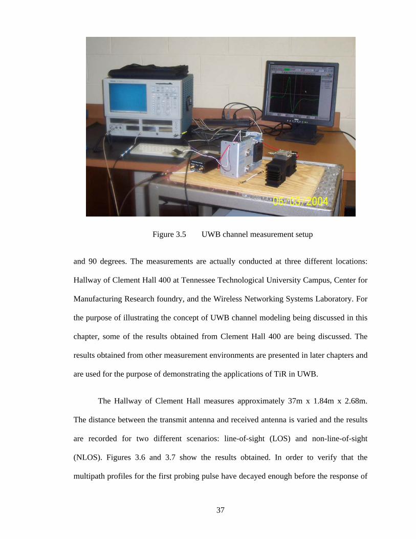
Figure 3.5 UWB channel measurement setup
and 90 degrees. The measurements are actually conducted at three different locations:
Hallway of Clement Hall 400 at Tennessee Technological University Campus, Center for
Manufacturing Research foundry, and the Wireless Networking Systems Laboratory. For
the purpose of illustrating the concept of UWB channel modeling being discussed in this
chapter, some of the results obtained from Clement Hall 400 are being discussed. The
results obtained from other measurement environments are presented in later chapters and
are used for the purpose of demonstrating the applications of TiR in UWB.
The Hallway of Clement Hall measures approximately 37m x 1.84m x 2.68m.
The distance between the transmit antenna and received antenna is varied and the results
are recorded for two different scenarios: line-of-sight (LOS) and non-line-of-sight
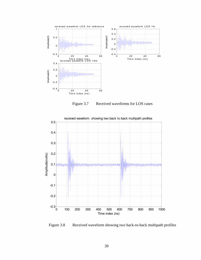
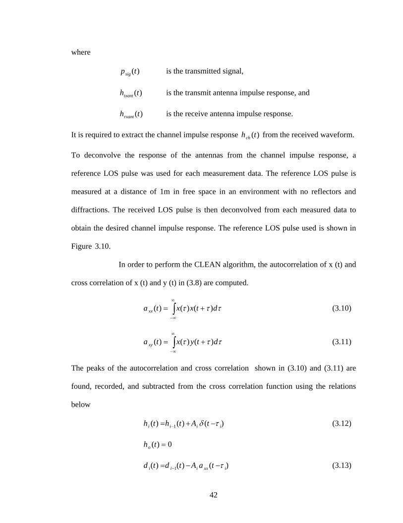
(NLOS). Figures 3.6 and 3.7 show the results obtained. In order to verify that the
multipath profiles for the first probing pulse have decayed enough before the response of
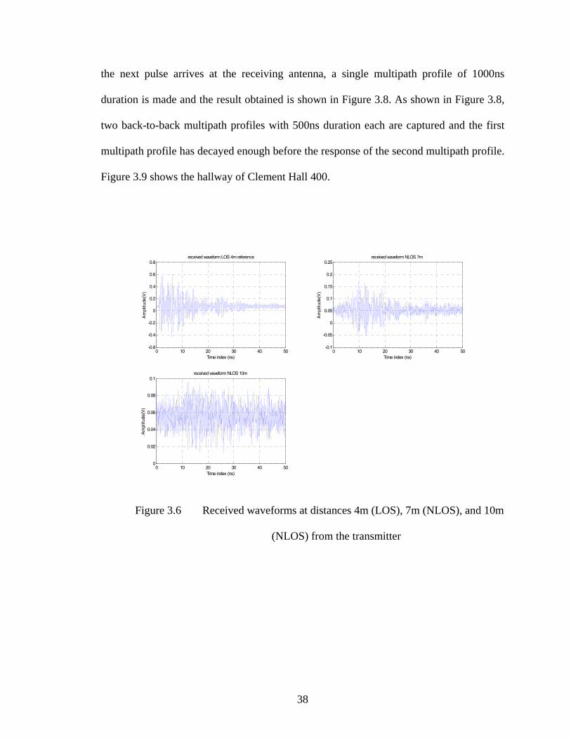
38
the next pulse arrives at the receiving antenna, a single multipath profile of 1000ns
duration is made and the result obtained is shown in Figure 3.8. As shown in Figure 3.8,
two back-to-back multipath profiles with 500ns duration each are captured and the first
multipath profile has decayed enough before the response of the second multipath profile.
Figure 3.9 shows the hallway of Clement Hall 400.
0 10 20 30 40 50-0.6
-0.4
-0.2
0
0.2
0.4
0.6
0.8
Time index (ns)
Am
plitu
de(V
)
received waveform LOS 4m reference
0 10 20 30 40 50-0.1
-0.05
0
0.05
0.1
0.15
0.2
0.25
Time index (ns)
Am
plitu
de(V
)
received waveform NLOS 7m
0 10 20 30 40 500
0.02
0.04
0.06
0.08
0.1
Time index (ns)
Am
plitu
de(V
)
received waveform NLOS 10m
Figure 3.6 Received waveforms at distances 4m (LOS), 7m (NLOS), and 10m
(NLOS) from the transmitter
39
0 2 0 4 0 6 0-0 .5
0
0 .5
1
Tim e in d e x (n s )
Am
plitu
de(V
)
re c e ive d w a ve fo rm L O S 4 m re fe re n c e
0 2 0 4 0 6 0-0 . 4
-0 . 2
0
0 . 2
0 . 4
0 . 6
Tim e in d e x (n s )
Am
plitu
de(V
)
re c e ive d w a ve fo rm L O S 7 m
0 2 0 4 0 6 0-0 .4
-0 .2
0
0 .2
0 .4
Tim e in d e x (n s )
Am
plitu
de(V
)
re c e ive d w a ve fo rm L O S 1 0 m
Figure 3.7 Received waveforms for LOS cases
0 100 200 300 400 500 600 700 800 900 1000-0.3
-0.2
-0.1
0
0.1
0.2
0.3
0.4
0.5
Time index (ns)
Am
plitu
de(v
olts
)
received waveform showing two back to back multipath profiles
Figure 3.8 Received waveform showing two back-to-back multipath profiles

40
Figure 3.9 Clement Hall 400 Hallway
3.4 Deconvolution Techniques
Deconvolution is the process of separating two signals that have been combined
by convolution. Several deconvolution techniques exist in literature often for specific
type of signal or for use with specific application. Deconvolution can be performed either
in frequency or time domain. In the frequency domain, the most straightforward
technique used is called inverse filtering. In time domain, the CLEAN algorithm is a
common technique used. The CLEAN algorithm is chosen as the method of determining
the CIR in this work. This is because the frequency domain techniques treat the CIR as
band limited while the indoor propagation channel is not expected to be band limited

41
relative to the bandwidth of the sounding pulse used. Since this work focuses on the time
domain characterization of the channel, the CLEAN algorithm is used as the primary
deconvolution technique in this work. The discrete nature of the CLEAN algorithm
makes the resulting impulse response more reasonable to characterize in time domain.
The CLEAN algorithm is discussed in details in the next section.
3.5 The CLEAN Algorithm
The approach to data analysis uses the CLEAN algorithm to extract the channel
impulse response from the observed data. Initially used in radio astronomy [43], it has
also been applied in the UWB communication channel characterization problems [44],
[45]. The CLEAN algorithm is used here because of its ability to produce discrete CIR in
time domain. The CLEAN algorithm assumes the channel to be a train of pulses, with the
well-known assumed tapped delay line channel model [46]. In order to use the CLEAN
algorithm to estimate the channel impulse response, it is assumed that there is no
significant pulse distortion caused to any of the multipaths1. The received signal at a
given receiver location is expressed as
)()()( thtxty ⊗= (3.8)
where )(tx and )(ty are known and h (t) is the signal to be determined. The received
signal from a given measurement location can be represented as
)()()()()( thththtptr rxantchtxantsig ⊗⊗⊗= (3.9)
1 If pulse distortion does exist, we can use a FIR filter to represent the pulse distortion.
42
where
)(tpsig is the transmitted signal,
)(thtxant is the transmit antenna impulse response, and
)(thrxant is the receive antenna impulse response.
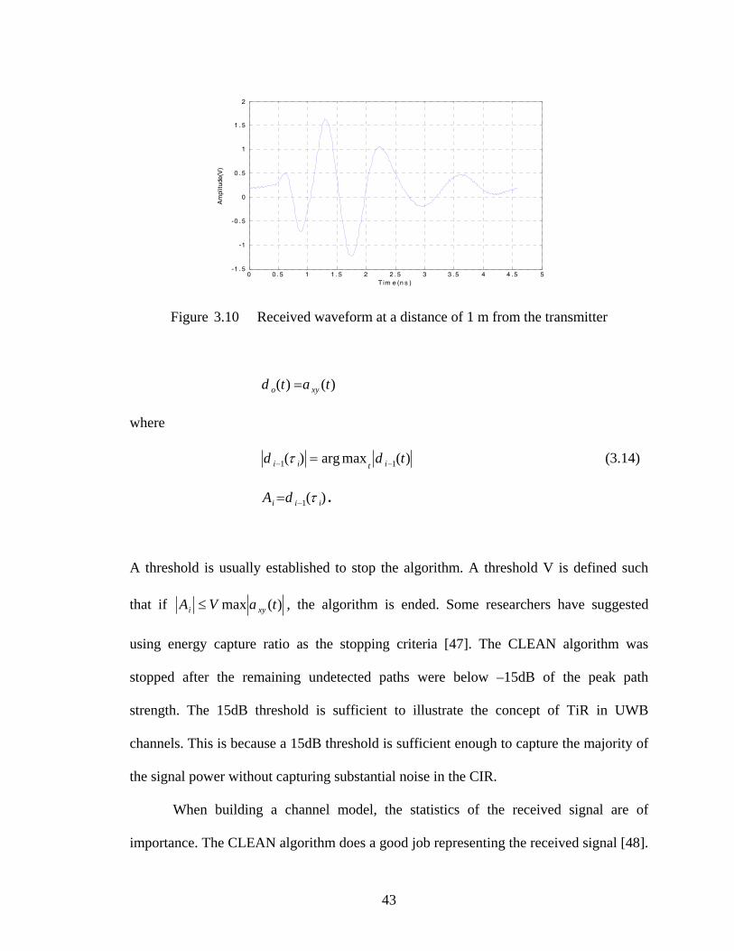
It is required to extract the channel impulse response )(thch from the received waveform.
To deconvolve the response of the antennas from the channel impulse response, a
reference LOS pulse was used for each measurement data. The reference LOS pulse is
measured at a distance of 1m in free space in an environment with no reflectors and
diffractions. The received LOS pulse is then deconvolved from each measured data to
obtain the desired channel impulse response. The reference LOS pulse used is shown in
Figure 3.10.
In order to perform the CLEAN algorithm, the autocorrelation of x (t) and
cross correlation of x (t) and y (t) in (3.8) are computed.
∫∞
∞−
+= τττ dtxxta xx )()()( (3.10)
∫∞
∞−
+= τττ dtyxta xy )()()( (3.11)
The peaks of the autocorrelation and cross correlation shown in (3.10) and (3.11) are
found, recorded, and subtracted from the cross correlation function using the relations
below
)()()( 1 iiii tAthth τδ −+= − (3.12)
0)( =tho
)()()( 1 ixxiii taAtdtd τ−−= − (3.13)
43
0 0 . 5 1 1 . 5 2 2 . 5 3 3 . 5 4 4 . 5 5-1 . 5
-1
-0 . 5
0
0 . 5
1
1 . 5
2
T im e (n s )
Am
plitu
de(V
)
Figure 3.10 Received waveform at a distance of 1 m from the transmitter
)()( tatd xyo =
where
)(maxarg)( 11 tdd itii −− =τ (3.14)
)(1 iii dA τ−= .
A threshold is usually established to stop the algorithm. A threshold V is defined such
that if )(max taVA xyi ≤ , the algorithm is ended. Some researchers have suggested
using energy capture ratio as the stopping criteria [47]. The CLEAN algorithm was
stopped after the remaining undetected paths were below –15dB of the peak path
strength. The 15dB threshold is sufficient to illustrate the concept of TiR in UWB
channels. This is because a 15dB threshold is sufficient enough to capture the majority of
the signal power without capturing substantial noise in the CIR.
When building a channel model, the statistics of the received signal are of
importance. The CLEAN algorithm does a good job representing the received signal [48].
44
The CLEAN algorithm is also robust to noise present in measured data where frequency
domain deconvolution techniques fail [49].
3.5.1 Limitations of the CLEAN Algorithm
The CLEAN algorithm has some limitations when employed in determining a
CIR. Below are some of the limitations of the algorithm.
• The CLEAN algorithm does not give a good estimate of the CIR when the paths
are very close and unresolveable.
• When different pulse shapes are associated with different paths, we only use the
LOS pulse as a template. In this case, The CLEAN algorithm cannot give a good
estimate of the CIR. Multiple taps are needed to represent distortion.
• The CLEAN algorithm is only fairly accurate in representing a signal at
moderately low SNR.
3.6 Summary
This chapter served as the foundation for this thesis work and it presented the
whole ideas on which research work is based. The concept of UWB channel modeling
was discussed and the UWB channel sounder employed in extracting the channel impulse
response was explained in details. The measurement setup and the measurement
procedure were discussed and the concept behind the CLEAN algorithm, which will be
used in the later chapters to extract the channel impulse response from the received
45
waveforms, was discussed in this chapter. The extracted UWB channel information will
then be used in the later chapters as the channel data on which the principle and
applications of TiR are demonstrated.

46
CHAPTER 4
TIME-REVERSAL COMMUNICATIONS
4.1 Introduction
In this chapter, the theory and the applications of time reversal in UWB are
discussed. Metrics are defined to characterize two key applications in TiR, namely:
spatial focusing and temporal compression. The concept of ISI in UWB systems is
discussed and the use of TiR to improve receiver performance in UWB ISI channels is
discussed. The chapter also studies some equalization techniques used in compensating
for ISI in UWB channels.
4.2 An Overview of Time-Reversal in UWB
Time-reversal (TiR) also known as phase conjugation in frequency domain is a
simple method of preparing a message such that it appears at a particular time at a
particular location in space and no where else. In TiR, a signal is prefiltered such that it
focuses in space and time at an intended receiver [17]. This can be achieved by using a
time-reversed complex conjugate of the channel impulse response at the receiver as a
transmitter prefilter. Several advantages come with this technique. Spatial focusing
reduces co-channel interference in a multi-user system. Due to temporal focusing, the
effective delay spread of the channel is dramatically reduced and thus ISI is also reduced
dramatically. This leads to a reduction in the equalization task at the receiver. For
47
example, the complexity of a maximum likelihood sequence estimator (MLSE) is
proportional to m L, where m is the size of the input alphabet and L is the length of the
channel impulse response in units of T with T being the symbol separation [50].
Temporal focusing in TiR reduces the equalization task by reducing the effective channel
length. In a TiR experiment, the intended receiver sends a training sequence to the
intended transmitter(s). The transmitter(s) time-reverses the estimated channel impulse
response (CIR), convolves it with the signal message that is now sent to the receiver. The
emitted time reversed waves propagates through the channel retracing their former paths
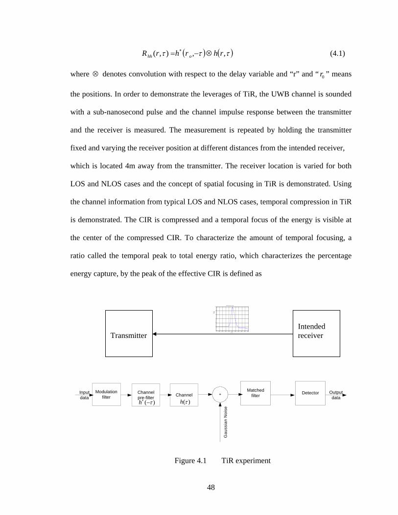
and this leads to a focus of power in space and time at the receiver. The concept of TiR
experiment is illustrated in Figure 4.1.
The concept has already been successfully applied in underwater acoustic
channels and in ultrasound applications. It has also been applied to narrowband systems
and has only recently been applied to UWB systems. Being newly applied to UWB
systems, further studies are necessary to demonstrate more feasibilities of applying TiR
to UWB and hence the reason for this research work.
4.3 Time-Reversal Theory
Consider a single user downlink scenario transmit-receive pair in a UWB channel.
In TiR, the transmitter uses the time-reversed complex conjugate of the CIR as a
transmitter prefilter. Let ( )τ,orh denote the impulse response at the intended receiver,
where or is the receiver location and τ is the delay variable. If the transmitter uses
( )τ−∗ ,orh as a transmit prefilter, the effective channel at a given location r is given by
48
( ) ( )τττ ,,),( rhrhrR ohh ⊗−= ∗ (4.1)
where ⊗ denotes convolution with respect to the delay variable and “r” and “ 0r ” means
the positions. In order to demonstrate the leverages of TiR, the UWB channel is sounded
with a sub-nanosecond pulse and the channel impulse response between the transmitter
and the receiver is measured. The measurement is repeated by holding the transmitter
fixed and varying the receiver position at different distances from the intended receiver,
which is located 4m away from the transmitter. The receiver location is varied for both
LOS and NLOS cases and the concept of spatial focusing in TiR is demonstrated. Using
the channel information from typical LOS and NLOS cases, temporal compression in TiR
is demonstrated. The CIR is compressed and a temporal focus of the energy is visible at
the center of the compressed CIR. To characterize the amount of temporal focusing, a
ratio called the temporal peak to total energy ratio, which characterizes the percentage
energy capture, by the peak of the effective CIR is defined as
0 200 400 600 800 1000 1200 1400 1600 1800 2000-2
0
2
4
6
8
10
differentiated gaussian output
Time(ps)
Amplitude(volts)
Modulationfilter
Channelpre-filter
DetectorMatchedfilter
Inputdata
+ Outputdata
Gau
ssia
n N
oise
Channel
)( τ−∗h )(τh
Figure 4.1 TiR experiment
Intended receiver
Transmitter

49
hhT
hhpTR
E
E=ϑ (4.2)
where
hhpE is the energy in the main peak of the received impulse response,
hhTE is the total energy in the received impulse response for the time-
reversed channel.
This ratio is expected to be as high as possible to illustrate good temporal
compression and is expected to approximate a fixed value. In order to illustrate spatial
focusing in TiR, a ratio called the spatial focusing gain is defined. The energy of
),( τrR hh at any point r in space at a given time oτ is given by
( ) 2),( ohhhh rRr τε = (4.3)
where oτ is defined such that ( , ) max { ( , )hh o o hh oR r R rττ τ= }. The spatial focusing
gain )(rhhη is the ratio of the energy at or to the energy at a given location away
from or .
( )( )r
rrhh
ohhhh ε
εη =)( (4.4)
This ratio gives relative information about security in TiR. A large value of this ratio
indicates a better spatial focusing gain and hence a low probability of intercept by a
receiver located near the intended receiver. )(rhhη can be computed with respect to time
delays other than oτ but oτ is chosen here, because at oτ , the effective time reversed
channel captures the largest amount of energy in the channel. Figures 4.2 and 4.3
illustrate the concept of temporal compression in TiR using measured data from Clement

50
Hall 400 of Tennessee Technological University campus and IEEE 802.15.3a data
respectively while Figure 4.4 illustrates spatial focusing.
In Figures 4.2 and 4.3, the temporal compression is visible at the center of the
channel impulse response and the amount of temporal compression is defined using
Equation 4.1. In Figure 4.4, oR is the intended receiver while receivers 1R and 2R are
users intending to steal the information from oR . From mathematical properties, it is
known that after normalizing the correlation functions with respect to energy,
autocorrelation is always stronger than cross-correlation. This implies that the receiver
power peaks at oR and is more compared to 1R and 2R . An intruder at 2R who tries to
steal user information at oR experiences some loss in received power and hence his
inability to decode the message signal. The results obtained by this concept are given in
details in the next chapter.
In order to illustrate the relative gain in UWB channels using TiR, the energy loss
due to prefilter is studied against energy loss without a prefilter. The relative information
obtained gives the amount of channel energy gain observed using TiR in UWB
environments and this is shown in the next chapter.
4.4 Time Reversal and UWB Systems Performance
Due to multipath propagation effects, the transmitted UWB waveform arrives at
the receiver distorted. The distorted waveforms arriving at the receivers are further
corrupted by multiple access interference and background noise. The function of a UWB

51
receiver is to extract the information bit sequence from the distorted and corrupted
received waveforms with a very high level of accuracy. The basic UWB receiver consists
0 10 20 30 40 50-0.3
-0.2
-0.1
0
0.1
0.2
0.3
0.4
0.5
Time index (ns)
Am
plitu
de
received waveform hallwayLOS 10m
0 10 20 30 40 50-0.1
-0.05
0
0.05
0.1
0.15 HallwayLOS 10m Estimated channel impulse response
Excess delay (ns)
Am
plitu
de
0 20 40 60 80 100-0.05
0
0.05
0.1
0.15
0.2
0.25
0.3Autocorrelation of channel impulse response(NLOS)
Excess delay (ns)
Am
plitu
de
Figure 4.2 Temporal compression illustrated using measured data
0 200 400 600 800 1000 1200 1400 1600-0.6
-0.4
-0.2
0
0.2
0.4CM3 Channel impulse response
excess delay(ns)
Am
plitu
de
0 500 1000 1500 2000 2500 3000 3500-1
0
1
2
3
4CM3 TiR channel
excess delay(ns)
Am
plitu
de
Figure 4.3 Temporal compression illustrated using IEEE 803.15.3a CM3
channel

52
Figure 4.4 Demonstrating spatial focusing in TiR
of a detector and a decision device. The detector is different from conventional
narrowband schemes because UWB can be carrier-less.
The most common implementations of UWB receivers are threshold detectors,
autocorrelation receivers, and correlation or rake receivers. Threshold detectors are
simple to implement and are also suitable for UWB radar systems [51]. In threshold
detectors, a threshold is usually set for establishing the presence of a radar target. An
autocorrelation receiver correlates the received waveform with a previously received
waveform [52-56]. This receiver can capture the entire received waveform energy for a
slowly varying channel without requiring channel estimation because the transmitter
transmits a pilot (reference waveform) to generate side information about the channel.
Some research on UWB receivers has been on the rake receiver [57-66].
R2
Ro)(τhTx
R1
).,(),(),( τττ ooohh rhrhrR ⊗= ∗
).,(),(),( 22 τττ rhrhrR ohh ⊗= ∗
).,(),(),( 11 τττ rhrhrR ohh ⊗= ∗

53
4.4.1 Rake Receivers
Rake receivers are used in time-hopping impulse radio systems and direct
sequence spread spectrum systems (DS-SS) for matched filtering of the received signal.
In theory, the receiver structure consists of a matched filter that is matched to the
transmitted waveform that represents one symbol, and a tapped delay line that matches
the channel impulse response. It is also possible to implement this structure as a number
of correlators that are sampled at the delays related to specific number of multipath
components; each of those correlators can be called “Rake finger.” A Rake receiver
structure is shown in Figure 4.5.
In UWB systems, frequency dependency is taking into consideration [3,34], the
receiver uses several rake fingers for each multipath component (MPC) spaced at the
nyquist sampling distance in order to collect the energy in the MPC. The number of rake
fingers in this case becomes very large [67]. Due to this problem of energy capture,
several simplified Rake structures have been proposed: selective Rake (Srake) and partial
rake (Prake). The Srake receiver collect energy from L strongest MPCs while the Prake
collects energy from the L first MPCs. The Srake structure has been adopted in this
research work. Srake outperforms Prake because Srake collects more channel energy than
the Prake [68].

54
Figure 4.5 Rake receiver structure
In Figure 4.5, the Rake structure consists of a parallel bank of L correlators
followed by a combiner that determines the variable to be used for the decision on the
symbol. Different approaches can be used to determine the rake weights: however,
maximal ratio combiner (MRC) is a traditional approach. Reference [69] proposes an
approach called minimum mean square error (MMSE) Rake combiner and it outperforms
MRC-Rake. As shown in [69], MMSE Rake receiver reduces the error floor observed
when MRC-Rake is receiver is employed in UWB systems.
4.4.2 ISI Issues in UWB
Inter symbol interference occurs when the effects of a transmitted pulse is not
allowed to die away completely before transmitting another pulse. If symbol duration is
given as Tb and the channel delay spread is given as Td, ISI occurs in a UWB channel if
db TT < . The received signal at the receiver in a frequency selective discrete ISI channel
can be represented as

55
∑−
≠=− ++=
1
,0
N
lnnlnlnll wxIIy (4.5)
where
ly represent the lth approximated bit at the receiver,
lI represent the desired information symbol at the lth sampling
time,
∑−
≠=−
1
,0
N
lnnnlnxI represent the ISI term, and
lw represent the additive Gaussian noise variable at the kth
sampling instant.
The ISI term makes it more likely for the decision device to have more decision
errors, as compared to a case without ISI because with ISI it is more likely to mix up
desired symbols with undesired symbols. In order to minimize the probability of error,
the optimum receiver in a mean-square error sense consists of a matched filter, an
equalizer, and a maximum likelihood detector. The maximum likelihood sequence
estimator (MLSE) is the optimum equalizer for use in wireless channel. The MLSE
searches for the information sequence that after convolution is closest in Euclidean
distance to the received signal sequence [70]. However, it has a complexity that grows
exponential with the channel length and it is thus not suitable for use in channels with
large delay spread such as UWB. Two sub-optimum equalization techniques for use in
frequency selective channels are the Zero forcing (ZF) and minimum mean square error
(MMSE) and are discussed in the next section.
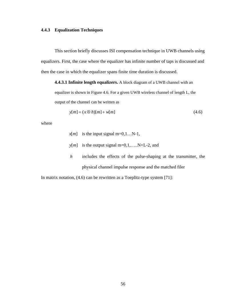
56
4.4.3 Equalization Techniques
This section briefly discusses ISI compensation technique in UWB channels using
equalizers. First, the case where the equalizer has infinite number of taps is discussed and
then the case in which the equalizer spans finite time duration is discussed.
4.4.3.1 Infinite length equalizers. A block diagram of a UWB channel with an
equalizer is shown in Figure 4.6. For a given UWB wireless channel of length L, the
output of the channel can be written as
][])[(][ mwmhxmy +⊗= (4.6)
where
][mx is the input signal m=0,1…N-1,
][my is the output signal m=0,1,…..N+L-2, and
h includes the effects of the pulse-shaping at the transmitter, the
physical channel impulse response and the matched filer
In matrix notation, (4.6) can be rewritten as a Toeplitz-type system [71]:
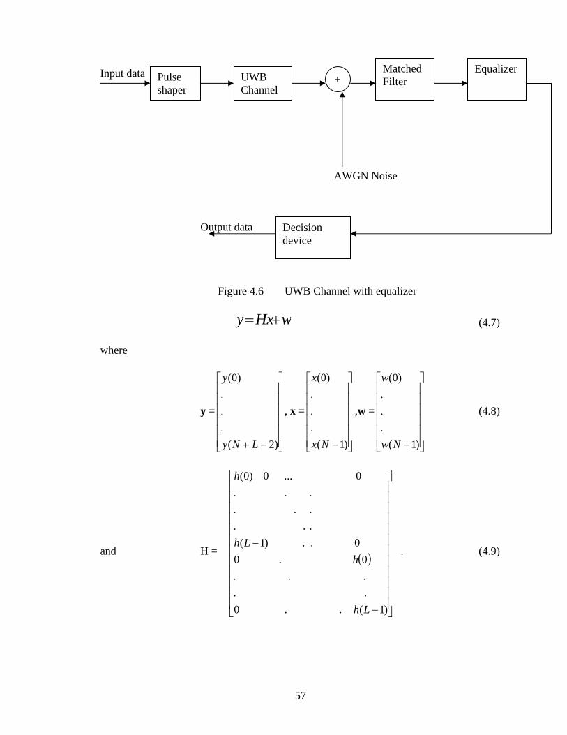
57
Input data AWGN Noise Output data
Figure 4.6 UWB Channel with equalizer
wHxy += (4.7)
where
y =
⎥⎥⎥⎥⎥⎥
⎦
⎤
⎢⎢⎢⎢⎢⎢
⎣
⎡
−+ )2(...
)0(
LNy
y
, x =
⎥⎥⎥⎥⎥⎥
⎦
⎤
⎢⎢⎢⎢⎢⎢
⎣
⎡
− )1(...
)0(
Nx
x
,w =
⎥⎥⎥⎥⎥⎥
⎦
⎤
⎢⎢⎢⎢⎢⎢
⎣
⎡
− )1(...
)0(
Nw
w
(4.8)
and H = ( )
⎥⎥⎥⎥⎥⎥⎥⎥⎥⎥⎥⎥
⎦
⎤
⎢⎢⎢⎢⎢⎢⎢⎢⎢⎢⎢⎢
⎣
⎡
−
−
)1(..0.....0.0
0..)1(.........
0...0)0(
Lh
hLh
h
. (4.9)
Pulse shaper
UWB Channel
Matched Filter +
Equalizer
Decision device

58
The MMSE estimate of x, x in Equation 4.6 gives the desired received information bit at
the output of the detector. In order to compute the bit error rate for the system, x is
compared with x . The basic idea of the MMSE estimator is to choose as the estimate the
function of the data that gives the smallest expected value of the square of the estimation
error [72].
It can be assumed that E (w) = 0 in Equation 4.7 without loss of generality.
Assuming x to be a linear function of y, i.e. x = By, where B is to be determined.
From (4.7):
wHxy += .
Since E (w) = 0,
K = E [ ] IwwT 2σ= (4.10)
where w is zero mean circularly symmetric complex Gaussian (ZMCSCG) noise with
variance oN .
To find x , let S be defined as
)ˆ()ˆ( xHyxHyS T −−≡ (4.11)
yHxHHxS TT 2ˆ][20ˆ
−==∂∂ (4.12)
x = yHHH TT 1)( − . (4.13)
Equation (4.13) is not optimal [73]. To make it optimal, the covariance of the noise w in
Equation (4.10) is added and hence the MMSE estimate of x is represented as
x = INyHHH oTT +−1)( (4.14)
where I represent a (1xN) identity matrix.
59
As observed in [74], the difference between an MMSE equalizer and a zero forcing
equalizer is the absence of the noise term in the ZF equalizer. Hence, (4.13) represents
the estimated data sequence for a zero forcing equalizer of infinite length.
4.4.3.2 Finite length equalizers. This section describes the cases in which the
equalizer spans finite time duration.
4.4.3.2.1 Zero forcing equalizer. The output of the equalizer in z-domain is given
by
Y (z) =R (z) B (z) (4.15)
where
Y (z) is the z-transform of the equalizer output,
R (z) is the z-transform of the effective channel output, and
B (z) is the z-transform of the equalizer coefficient.
In the absence of the additive noise introduced by the physical channel, the output of the
effective channel is given by
R (z) =X (z) H (z). (4.16)
Substituting 4.16 in 4.15, the output signal of the equalized system, can be expressed as
Y (z) =X (z) H (z) B (z). (4.17)
Figure 4.7 illustrates the equivalent discrete time representation of the equalized system.
Let C (z) denote the transfer function of the equalized system.

60
Figure 4.7 Discrete UWB channel with equalizer
Then
)()()()()( zBzH
zXzYzC == . (4.18)
In time-domain, this corresponds to
∑=
−=−=⊗=
Nk
Nkknknnn hbhbc . (4.19)
For ISI free transmission,
C (z) =1. (4.20)
In time domain, condition (4.20) means that
⎩⎨⎧
≠=
=0,00,1
nn
cn . (4.21)
With a finite number of taps (2N+1) in the equalizer, (4.21) becomes
⎩⎨⎧
±±±==
=Nn
nnc
,......2,1,00,1
)( . (4.22)
Equation (4.22) can be guaranteed by choosing the equalizer coefficients to satisfy the
following equation

61
[ ] [ ]TTNoN
oNNNN
NoN
NNNNo
bbbbb
hhhhh
hhhhh
hhhhh
0...010...0......
...................
.................
............
11
112
11
211
=
⎥⎥⎥⎥⎥⎥⎥⎥⎥⎥⎥
⎦
⎤
⎢⎢⎢⎢⎢⎢⎢⎢⎢⎢⎢
⎣
⎡
−−
−−+
−−
−−−−+−
(4.23)
where T denotes the transpose operation.
Equation (4.23) represents a finite length zero forcing equalizer.
4.4.3.2.2 Minimum mean square error (MMSE) equalizer. In reality the
noise component due to the physical channel cannot be ignored. In the presence of
additive Gaussian noise at the receiver input, the output of the equalizer at the nth
sampling instant is given by
∑−=
−=N
Nkknkn rby . (4.24)
The mean square error (MSE) for the equalizer having 2N+1 taps, denoted by J (N) is
⎥⎥⎦
⎤
⎢⎢⎣
⎡⎟⎠
⎞⎜⎝
⎛−=−= ∑
−=−
22ˆ)(
N
Nkknknnn rbxEyxENJ (4.25)
minimizing )(NJ with respect to the equalizer coefficients ( kb ) is obtained by the
following differentiation:
0)(=
∂∂
kbNJ . (4.26)
Equation 4.26 leads to the necessary condition for the minimum MSE given by
xrr RbR = (4.27)

62
or
xrr RRb 1−= (4.28)
where
b denotes the 2N+1 tap coefficient
xrR = ( )( )Txrxrxr NRRNR ..),........0(.),........(−
rR =
⎥⎥⎥⎥⎥⎥
⎦
⎤
⎢⎢⎢⎢⎢⎢
⎣
⎡
−−+−+−
)0()(........)2()1()1(.....)12(
.....
.....
)2(.....)(......)0(
2 rrNr
rr
rrrr
RNRNRRNRNR
NRNRR
.
4.4.4 TiR System Structure
Figure 4.8 gives a typical UWB channel with TiR. The major difference between
a system with TiR and a system with no TiR is the presence of the transmitter prefilter
( )( th −∗ in Figure 4.8.
The effective TiR channel impulse response is given by
)()()()()( tththtthTR −⊗⊗−⊗=− ∗∗ φφ (4.29)
where
)(tφ is the pulse shaping filter,
)( th −∗ is the transmitter prefilter,

63
Modulationfilter
Channelpre-filter
DetectorMatchedfilter
Inputdata
+ Outputdata
Gau
ssia
n N
oise
Channel
)( τ−∗h )(τh
Figure 4.8 UWB systems with TiR
)(th is the channel impulse response, and
)( t−∗φ is the filter matched to the transmitted pulse.
For a system with TiR, the equations for infinite length equalizers (MMSE and ZF) and
finite length equalizers (MMSE and ZF) still hold with the effective channel response
)(th in the previous equations being replaced by a new channel impulse response defined
in Equation 4.29.
For an infinite length equalizer, the received signal is therefore given by
][])[(][ mwmhxmy TR +⊗= . (4.30)
In matrix notation, this becomes
wxHy TR += . (4.31)
And the equation for an infinite length MMSE estimator is given by
x = INyHHH oT
TRTRT
TR +−1)( . (4.32)
4.5 Summary
In this chapter, a detailed study of TiR in UWB is presented. The theory behind
TiR is studied. The various applications of TiR in UWB are presented and ISI issues in
UWB are also presented. The various techniques for compensating ISI in UWB channels

64
are studied and the idea of combining these techniques with TiR to combat ISI in UWB
channels is also presented.

65
CHAPTER 5
SIMULATION RESULTS
The previous chapters provided a detailed study of UWB systems. The
motivations for applying TiR to UWB systems have been discussed in earlier chapters.
The signal-processing algorithm (CLEAN algorithm) used in this thesis to obtain the
channel information has also been discussed in Chapter 3. The extracted channel
information is the data on which the applications of TiR in UWB are demonstrated. In
this chapter, a simulation technique called Monte Carlo simulation is employed to
analyze the performance of UWB systems using the extracted channel impulse response.
MATLAB software package was used for simulating the complete UWB system from the
transmitter to the receiver. BER curves are generated for different cases using TiR and
equalizers as a means of compensation for ISI in the UWB channels. Also, in this
chapter, results for temporal compression, spatial focusing and TiR losses in UWB
channels are presented.
5.1 Monte Carlo Simulation
Monte Carlo (MC) simulation technique [75,76] is the most widely used
simulation technique for evaluating the performance of communication systems and it is
based on a game of chance. In the context of BER estimation for digital communication
systems, the MC simulation technique involves the following steps:

66
(1) Decide on the minimum target BER to be estimated. (In this thesis work, it is
310− .)
(2) Set the number of bits per simulation run to be at least 10 times the inverse of
the minimum target BER to be estimated. (Here, it is .)104 bits
(3) Set up the base band modulators, demodulators, transmit/receive filters, and
channel simulators. (Here, the channel information is known from the CLEAN
algorithm.)
(4) Run the BER simulation until 100 errors are counted and estimate the BER.
(5) Iterate the simulation for some specified number of iterations and compute the
average of the BERs obtained in these iterations (Here, the number of
simulation runs was chosen to be 40.)
The block diagram for the simulation setup is illustrated in Figure 5.1.
A 5th order Gaussian pulse width a pulse width bT of 0.625ns is used as the pulse-
shaping filter and is represented by
2
2
25
5
5
3
2 1015)( σ
σσσφ
t
etttkt−
⎟⎟⎠
⎞⎜⎜⎝
⎛−+−= (5.1)
where 111028.5 −×=σ is a parameter that controls the width of the pulse.
The spread waveform can be obtained from the pulse-shaping filter by
∑=
−=7
0)()(
kbk kTtstp φ . (5.2)
The spreading sequence, { } { }1,1,1,1,1,1,1,1 −−++−++−=ks . (5.3)
The symbol duration is thus given by
sec58 nTT bs == . (5.4)

67
Figure 5.1 Simulation setup
If kb is a sequence to be transmitted, the modulated signal is given as
∑∞
∞−
−= )()( sk kTtpbts . (5.5)
If the UWB CIR is represented as )(th , then the output of the channel is
)()()()( twtsthtx +⊗= . (5.6)
After matched filtering, the output of the matched filter can be expressed as
)()()( tptxty −⊗= . (5.7)
The outputs of the matched filter are then combined using MMSE rake combiner
discussed in Chapter 4. A MMSE equalizer is then employed for further receiver
performance improvement. The choice of modulation used is BPSK, i.e. { }1,1 −+=kb , a
channel data information for several cases is used: IEEE 802.15.3a (CM3 and CM4)
models and the extracted channel data using CLEAN algorithm from the received
waveform for several UWB channel environments. The major aim here is to demonstrate
improvement in receiver performance using TiR in UWB channels.
68
5.2 BER Simulation Results
Performance of TiR systems already discussed is evaluated via simulations in this
section. In order to verify the simulation, the setup is evaluated for an AWGN channel
and the result obtained is compared with the channel situation in which there is no ISI.
These results are expected to be as close as possible. In each BER simulation, different
scenarios of UWB receivers are considered. The following cases are considered in the
simulation:
• A Rake receiver with an estimate of the largest 20 channel fingers,
• MMSE equalizer (with 5 taps),
• MMSE-TiR,
• TiR-Rake,
• No ISI, and
• AWGN channel.
The MMSE-TiR combines MMSE equalization with TiR while TiR-Rake employs TiR
channel with a rake receiver also estimating the largest 20 channel taps. The No-ISI case
is that in which the bit duration (Tb) is chosen such that rmsb TT > , where rmsT is the rms
delay spread of the channel.
69
5.2.1 CM3 Simulation Results
The BER simulation results obtained using CM3 channel data is shown in Figure
5.2. As expected, using an MMSE equalizer to compensate for ISI, a relative
improvement is observed. The major comparison lies in the TiR channel versus the Rake
receiver. Using the TiR channel information as the channel impulse response and
estimating the 20 largest channel taps, at a BER of 310− , TiR-Rake channel has around
1.8dB performance improvement compared to a channel with rake receivers for CM3
channel. Also employing a 5-tap MMSE equalizer to the TiR channel shows a very slight
performance improvement (around 0.3 dB). After TiR, a very minimum number of taps
for the equalizer is employed. This demonstrates that with TiR, the equalization task if
needed is reduced to a minimum to achieve a reasonable BER. This is better illustrated
using the CM4 channel because the CM4 represents an extreme case of NLOS of site and
hence we expect a very intense ISI channel for this case. As a reference, the No-ISI case
is compared with a standard AWGN curve and a close result shown in Figure 5.2 is
obtained as expected.
5.2.2 CM4 Simulation Results
Using CM4 channel data, the simulation results obtained are shown in Figure 5.3.
Using a 5-tap MMSE equalizer as a means of compensation for the ISI, a 1 dB
improvement in BER is observed at around 310− . With 31 channel taps, a performance
improvement of about 2.2 dB is observed. Using TiR-Rake, i.e. TiR and a rake receiver

70
0 2 4 6 8 10 12 14 1610
-5
10-4
10-3
10-2
10-1
100
Eb/No(dB)
BE
R
CM3 channel
5-taps MMSERakeMMSE-TiRTiR-RakeAWGNNo ISI
Figure 5.2 TiR BER simulation result using CM3
with no equalization, a gain of around 4dB is observed. This shows that a relative
improvement in terms of cost for the equalization task. A TiR channel with no
equalization outperforms a channel with 31 taps equalizer. To further improve the
performance of the UWB channel, an equalizer is combined with the TiR channel and a
gain of 0.5 dB is observed compared to the TiR-Rake channel. As a reference, the No-
ISI case is compared with a standard AWGN curve and a close result shown in Figure 5.3
is obtained as expected.
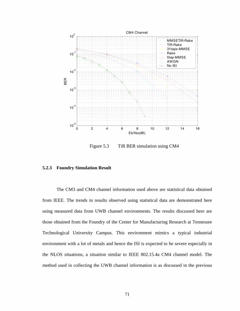
71
0 2 4 6 8 10 12 14 1610
-5
10-4
10-3
10-2
10-1
100
Eb/No(dB)
BE
R
CM4 Channel
MMSETiR-RakeTiR-Rake31taps-MMSERake5tap-MMSEAWGNNo ISI
Figure 5.3 TiR BER simulation using CM4
5.2.3 Foundry Simulation Result
The CM3 and CM4 channel information used above are statistical data obtained
from IEEE. The trends in results observed using statistical data are demonstrated here
using measured data from UWB channel environments. The results discussed here are
those obtained from the Foundry of the Center for Manufacturing Research at Tennessee
Technological University Campus. This environment mimics a typical industrial
environment with a lot of metals and hence the ISI is expected to be severe especially in
the NLOS situations, a situation similar to IEEE 802.15.4a CM4 channel model. The
method used in collecting the UWB channel information is as discussed in the previous
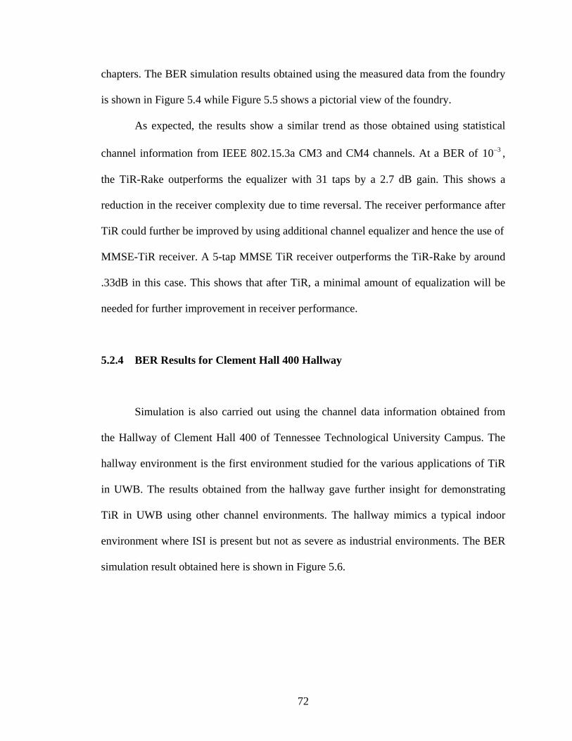
72
chapters. The BER simulation results obtained using the measured data from the foundry
is shown in Figure 5.4 while Figure 5.5 shows a pictorial view of the foundry.
As expected, the results show a similar trend as those obtained using statistical
channel information from IEEE 802.15.3a CM3 and CM4 channels. At a BER of 310− ,
the TiR-Rake outperforms the equalizer with 31 taps by a 2.7 dB gain. This shows a
reduction in the receiver complexity due to time reversal. The receiver performance after
TiR could further be improved by using additional channel equalizer and hence the use of
MMSE-TiR receiver. A 5-tap MMSE TiR receiver outperforms the TiR-Rake by around
.33dB in this case. This shows that after TiR, a minimal amount of equalization will be
needed for further improvement in receiver performance.
5.2.4 BER Results for Clement Hall 400 Hallway
Simulation is also carried out using the channel data information obtained from
the Hallway of Clement Hall 400 of Tennessee Technological University Campus. The
hallway environment is the first environment studied for the various applications of TiR
in UWB. The results obtained from the hallway gave further insight for demonstrating
TiR in UWB using other channel environments. The hallway mimics a typical indoor
environment where ISI is present but not as severe as industrial environments. The BER
simulation result obtained here is shown in Figure 5.6.
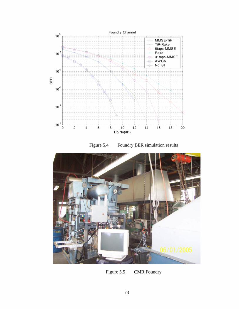
73
0 2 4 6 8 10 12 14 16 18 2010
-5
10-4
10-3
10-2
10-1
100
Eb/No(dB)
BE
R
Foundry Channel
MMSE-TiRTiR-Rake5taps-MMSERake31taps-MMSEAWGNNo ISI
Figure 5.4 Foundry BER simulation results
Figure 5.5 CMR Foundry

74
0 2 4 6 8 10 12 14 16 1810
-5
10-4
10-3
10-2
10-1
100
Eb/No(dB)
BE
R
Hallway
MMSE-TIRTIR-Rake5taps-MMSERakeAWGNNo ISI
Figure 5.6 BER simulation result for Clement Hall 400 Hallway
As shown in Figure 5.6, the ISI condition here is not that severe. This is seen by an
energy bit per noise (Eb/No) of around 13.7dB at a BER of 310− . However, the TiR –
Rake receiver still outperforms the Rake receiver by a 1 dB gain in Eb/No for a BER of
310− . The trend in receiver performance previously obtained is also shown in here as the
MMSE-TiR shows the best performance as expected.
5.3 Results Illustrating Temporal Compression
In this section, temporal compression is demonstrated using both statistical and
measured channel data in order to study the performance trend in UWB channels. CM1,
CM3, and CM4 channel information are used where CM1 is a typical LOS situation;
CM3 and CM4 are NLOS situations. Also, measured data for Clement Hall 400 Hallway,
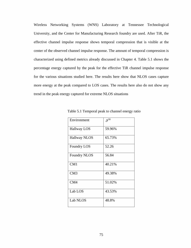
75
Wireless Networking Systems (WNS) Laboratory at Tennessee Technological
University, and the Center for Manufacturing Research foundry are used. After TiR, the
effective channel impulse response shows temporal compression that is visible at the
center of the observed channel impulse response. The amount of temporal compression is
characterized using defined metrics already discussed in Chapter 4. Table 5.1 shows the
percentage energy captured by the peak for the effective TiR channel impulse response
for the various situations studied here. The results here show that NLOS cases capture
more energy at the peak compared to LOS cases. The results here also do not show any
trend in the peak energy captured for extreme NLOS situations
Table 5.1 Temporal peak to channel energy ratio
Environment
TRϑ
Hallway LOS
59.96%
Hallway NLOS
65.73%
Foundry LOS
52.26
Foundry NLOS 56.84
CM1 40.21%
CM3 49.38%
CM4 51.02%
Lab LOS 43.53%
Lab NLOS 48.8%
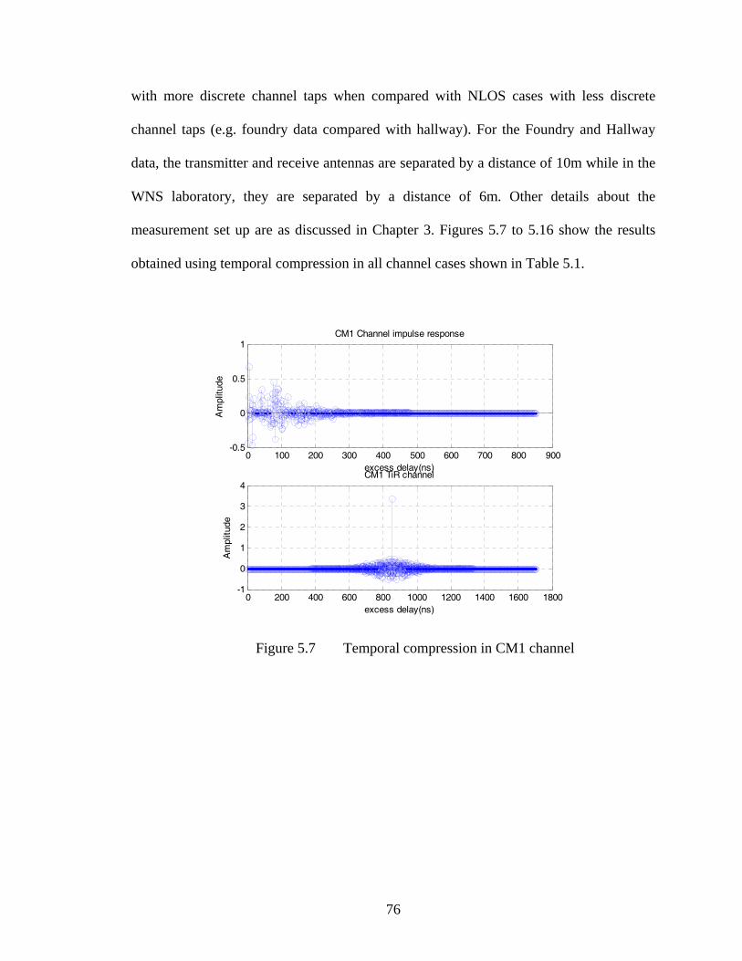
76
with more discrete channel taps when compared with NLOS cases with less discrete
channel taps (e.g. foundry data compared with hallway). For the Foundry and Hallway
data, the transmitter and receive antennas are separated by a distance of 10m while in the
WNS laboratory, they are separated by a distance of 6m. Other details about the
measurement set up are as discussed in Chapter 3. Figures 5.7 to 5.16 show the results
obtained using temporal compression in all channel cases shown in Table 5.1.
0 100 200 300 400 500 600 700 800 900-0.5
0
0.5
1CM1 Channel impulse response
excess delay(ns)
Am
plitu
de
0 200 400 600 800 1000 1200 1400 1600 1800-1
0
1
2
3
4CM1 TiR channel
excess delay(ns)
Am
plitu
de
Figure 5.7 Temporal compression in CM1 channel
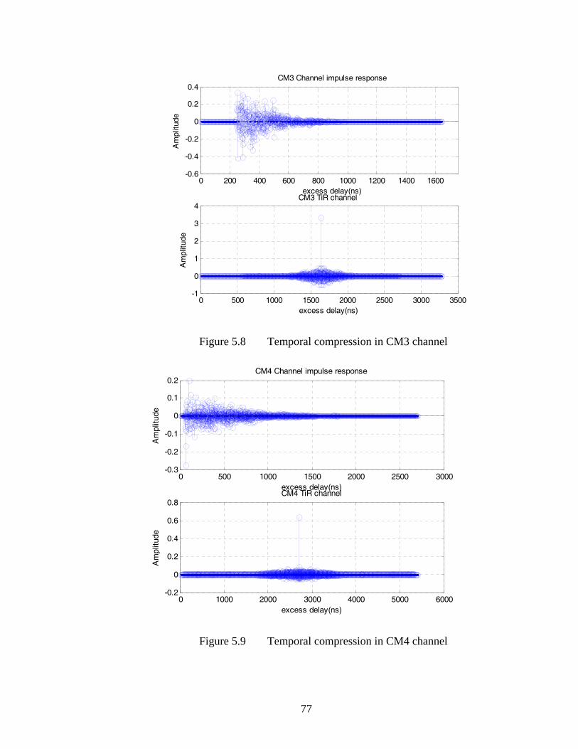
77
0 200 400 600 800 1000 1200 1400 1600-0.6
-0.4
-0.2
0
0.2
0.4CM3 Channel impulse response
excess delay(ns)
Am
plitu
de
0 500 1000 1500 2000 2500 3000 3500-1
0
1
2
3
4CM3 TiR channel
excess delay(ns)
Am
plitu
de
Figure 5.8 Temporal compression in CM3 channel
0 500 1000 1500 2000 2500 3000-0.3
-0.2
-0.1
0
0.1
0.2CM4 Channel impulse response
excess delay(ns)
Am
plitu
de
0 1000 2000 3000 4000 5000 6000-0.2
0
0.2
0.4
0.6
0.8CM4 TiR channel
excess delay(ns)
Am
plitu
de
Figure 5.9 Temporal compression in CM4 channel

78
0 100 200 300 400 500 600 700 800 900 10000
0.02
0.04
0.06
0.08
0.1
0.12
0.14
0.16
0.18Impulse response realizations
Time (nS)
0 2000 4000 6000 8000 10000 12000 14000 160000
0.2
0.4
0.6
0.8
1
1.2
1.4Autocorrelation of Impulse response
Time(ns)
Figure 5.10 Temporal compression in IEEE 802.15.4a Outdoor channel
0 10 20 30 40 50-0.2
-0.1
0
0.1
0.2
0.3
0.4
0.5
Time index (ns)
Am
plitu
de
received waveform foundryLOS 10m
0 10 20 30 40 50-0.1
-0.05
0
0.05
0.1
0.15Estimated channel impulse response foundryLOS10m
excess delay (ns)
Am
plitu
de
0 20 40 60 80 100-0.05
0
0.05
0.1
0.15
0.2
0.25
0.3
0.35Autocorrelation of channel impulse response foundryLOS10m
Excess delay (ns)
Am
plitu
de
Figure 5.11 Temporal compression in CMR Foundry LOS

79
0 10 20 30 40 500
0.02
0.04
0.06
0.08
0.1
0.12
0.14
0.16
Time index (ns)
Am
plitu
de
received waveform foundryNLOS 10m
0 10 20 30 40 50-0.04
-0.02
0
0.02
0.04
0.06
0.08
0.1Estimated channel impulse response foundry NLOS10m
Excess delay (ns)
Am
plitu
de
0 20 40 60 80 100-0.05
0
0.05
0.1
0.15
0.2
0.25
0.3Autocorrelation of channel impulse response foundyNLOS 10m
Excess delay (ns)
Am
plitu
de
Figure 5.12 CMR Foundry NLOS result showing temporal compression
0 10 20 30 40 50-0.3
-0.2
-0.1
0
0.1
0.2
0.3
0.4
0.5
Time index (ns)
Am
plitu
de
received waveform hallwayLOS 10m
0 10 20 30 40 50-0.1
-0.05
0
0.05
0.1
0.15 HallwayLOS 10m Estimated channel impulse response
Excess delay (ns)
Am
plitu
de
0 20 40 60 80 100-0.05
0
0.05
0.1
0.15
0.2
0.25
0.3Autocorrelation of channel impulse response(LOS)
Excess delay (ns)
Am
plitu
de
Figure 5.13 Clement Hall 400 Hallway LOS results showing temporal
compression

80
0 10 20 30 40 50-0.1
-0.05
0
0.05
0.1
0.15
0.2
0.25
Time index (ns)
Am
plitu
de
received waveform hallwayNLOS 10m
0 10 20 30 40 50-0.02
0
0.02
0.04
0.06
0.08Estimated channel impulse response hallway NLOS10m
Excess delay (ns)
Am
plitu
de
0 20 40 60 80 100-0.02
0
0.02
0.04
0.06
0.08
0.1
0.12Autocorrelation of channel impulse response NLOS10m
Excess delay (ns)
Am
plitu
de
Figure 5.14 Clement Hall 400 Hallway NLOS showing temporal compression
0 10 20 30 40 50-0.3
-0.2
-0.1
0
0.1
0.2
0.3
0.4
0.5
Time index (ns)
Am
plitu
de
LOS received waveform WNS lab
0 10 20 30 40 50-0.1
-0.05
0
0.05
0.1
0.15
0.2
0.25 WNS lab LOS Estimated channel impulse response
Excess delay (ns)
Am
plitu
de
0 20 40 60 80 100-0.1
0
0.1
0.2
0.3
0.4
0.5
0.6Autocorrelation of channel impulse response(WNS lab LOS)
Excess delay (ns)
Am
plitu
de
Figure 5.15 WNS lab result LOS results showing temporal compression

81
0 10 20 30 40 50-0.05
0
0.05
0.1
0.15
0.2
0.25
0.3
Time index (ns)
Am
plitu
de
received waveform WNS lab NLOS
0 10 20 30 40 50-0.04
-0.02
0
0.02
0.04
0.06
0.08
0.1Estimated channel impulse response WNS lab NLOS
Excess delay (ns)
Am
plitu
de
0 20 40 60 80 100-0.05
0
0.05
0.1
0.15
0.2
0.25
0.3Autocorrelation of channel impulse response WNS lab NLOS
Excess delay (ns)
Am
plitu
de
Figure 5.16 WNS laboratory NLOS result results showing temporal
compression
5.4 Results For Spatial Focusing Gain
One of the key advantages and applications of TiR is the concept of security in
UWB systems. Secured communications means the inability of a nearby receiver to
successfully decode the information in the TiR channel and this is of particular interest to
DoD applications. To demonstrate this concept in UWB using TiR, the channel impulse
response is measured and obtained between the transmit antenna and the intended
receiver. The receiver antenna is then moved to various locations and the channel impulse
response is also obtained using CLEAN algorithm. The aim of this demonstration is to
observe the approximate distance at which the spatial focusing gain )(rhhη discussed in
the previous chapter is at least 10dB for typical UWB environments. The Foundry
channel data and the Hallway channel data are used for the purpose of this demonstration.

82
Both LOS and NLOS cases are studied in both environments and the results here show
that at a transmitter-receiver antenna separation of 6m is sufficient to obtain a spatial
focusing gain )(rhhη of at least 10dB. Figures 5.17 and 5.18 show the results obtained for
both the Hallway and Foundry channels.
0 1 2 3 4 5 60
2
4
6
8
10
12
14LOS and NLOS gain vs distance
distance from intended receiver(m)
spa
ce-t
ime
focu
sing
gai
n(dB
)
LOSNLOS
Figure 5.17 Demonstrating spatial focusing gain in Clement Hall 400 Hallway

83
0 1 2 3 4 5 60
2
4
6
8
10
12
14Spatial focusing gain in foundry
distance from intended receiver(m)
spat
ial f
ocus
ing
gain
(dB
)
LOSNLOS
Figure 5.18 Demonstrating spatial focusing gain in CMR foundry
5.5 Results for Time Reversal Loss Versus Distance
Lastly, as suggested by Dr. Nan Guo of the Wireless Networking Systems
Laboratory [77], in order to have information about the gain or loss in channel energy due
to TiR, the energy loss due to TiR can be studied against the channel energy loss for each
distance without TiR. A distance of 7m from the intended receiver is chosen as a
reference distance for studying the energy loss due to TiR. Two cases were studied:
NLOS channel scenario in the Foundry and NLOS channel scenario in the Hallway of
Clement Hall 400. Figures 5.19 and 5.20 show the results obtained. A similar study is
carried out via simulation by Mr. Chenming (Jim) Zhou [78] also of the Wireless
Networking System Laboratory. His simulation models a typical Hallway and the results

84
4 5 6 7 8 9 10-25
-20
-15
-10
-5
0
5
distance(m)
ener
gylo
ss(d
B)
foundry energyLOSS
energyloss with prefilterenergyloss without prefilter
Figure 5.19 Foundry energy loss (TiR versus No TiR)
4 5 6 7 8 9 10-25
-20
-15
-10
-5
0
5
distance(m)
ener
gylo
ss(d
B)
Hallway energyLOSS
energyloss with prefilterenergyloss without prefilter
Figure 5.20 Hallway energy loss (TiR versus No TiR)

85
obtained is shown to have a similar trend as the experimental result. The experiments
result however shows a slightly better performance.
For the Foundry environment, the energy loss at a distance of 4m from the
transmitter, taking the 7m distance as a reference is shown to be around 3dB. Also, at a
distance of 4m, the energy loss by the TiR channel is shown to be around -19dB. The
channel energy gain due to TiR is approximately 22dB in this case. This shows that a
channel with TiR at this distance will have a 22dB gain in channel energy when
compared to that with no TiR. This also demonstrates that TiR energy has more channel
gain compared to non-TiR channel and hence the reason for a better receiver performance
also illustrated in the BER studies previously discussed. The results for other distances
are as shown in Figure 5.19. At a distance of about 1m from the reference location (7m),
the TiR channel shows a loss of around 19-20 dB.
For the Hallway, a gain of around 21dB is observed at a distance of 4m and other
gains due to TiR in the channel are as shown in Figure 5.20.
5.6 Summary
In this chapter, the performance analysis of UWB systems with TiR has been
analyzed and performance improvement was achieved using TiR for UWB channels
when compared to channels without TiR. Also, the concept of temporal compression was
discussed. Using defined metrics, temporal compression was characterized and the results
shown here show temporal compression to work finer for NLOS channels in UWB.

86
To demonstrate the concept of secured communications in UWB using TiR, the
spatial focusing gain was studied for UWB channels and at a distance of at least 6m,a
gain of 10dB was observed. This shows TiR to be a valuable concept in UWB systems
and this is of particular interest to the D.O.D.
Lastly, knowledge of the amount of channel energy gain using TiR was
demonstrated by studying the channel energy loss due to TiR with the channel energy
loss by distance. Using a 4m distance from the transmitter as an example, a gain of at
least 19dB was observed for both UWB channels studied here.
These results show TiR to be a promising technique in UWB. The results also
show that TiR, which has successfully been demonstrated in narrowband systems and
underwater acoustic channels could be applied to UWB systems.

87
CHAPTER 6
CONCLUSIONS AND FUTURE WORK
The objective of this thesis was to study and investigate the theory and
applications of time reversal in UWB using measurement and statistical data. Various
applications of TiR to UWB have been studied and analyzed using different UWB
channel data. BER performance using TiR was studied and evaluated and results show
TiR to be a promising technique for improving the performance of UWB systems when
ISI is present. TiR was also combined with conventional equalization techniques.
Temporal compression and spatial focusing in TiR were also studied in details and
knowledge of the amount of channel gain observed using TiR in UWB channels was
studied.
6.1 Conclusions
Performance results showed that the application of a transmitter prefilter
))(( th −∗ in a UWB channel with impulse response )(th results in performance
improvement and this technique shows a promising technique for reducing the effect of
ISI in UWB channels. Different UWB channel situations were studied and different
scenarios at the receiver were used. All channel cases studied here show that TiR reduces
the cost of equalization in UWB channels and hence one of the basic aims in any system
designs: cost versus performance has been met using TiR.

88
Two key applications of time reversal are temporal compression and spatial
focusing. These two concepts have been studied in details and results here obtained show
that TiR should work fine in NLOS UWB channels when compared with LOS channels.
This is because in the presence of ISI, there are more multipath and hence temporal
compression works finer because the more the number of multipaths, the better the
concept of TiR.
For spatial focusing, the aim of the study was to get a minimum distance at which
the spatial focusing gain is at least 10dB. A distance of 6m was sufficient for the cases
studied in this thesis.
Lastly, it is essential to have knowledge of the gain in channel energy by TiR.
This was studied comparing the energy losses due to TiR to that with no TiR and plots
showing this information were given. Using a typical 4m distance here, it was observed
that TiR results in a gain of at least 19dB for all channel situations studied here. This
gives an insight why TiR results in better performance in UWB system performance.
6.2 Recommendations for Future Work
This thesis gives a study of the applications of TiR in UWB systems and has
opened a lot of areas for future work, which could be done to better understand the theory
and applications of TiR in UWB systems. Some of the areas are as follows:
1. TiR uses a prefilter at the transmitter which is a time reversed complex
conjugate the of the channel impulse response. Other possible prefilter techniques need to
be studied and see if possible improvement in performance could be observed e.g. [77].
89
2. Performance of TiR in outdoor channels could also be evaluated (IEEE channel
model IEEE 802.15.4a).
3. Single user case has been addressed in work. The performance of UWB
systems with TiR for multi-user scenario should be studied when the receiver is not only
corrupted by ISI but also multi-user interference (MUI).
4. Hardware implementations issues related to the prefilter in TiR UWB systems
should be addressed in future work.

90
REFERENCES
91
[1] T. Strohmer, M. Emami, J. Hansen, G. Papanicolaou, and A. J. Paulraj, “Application of time-reversal with MMSE equalizer to UWB Communications,” Proc. IEEE Global Telecommunications Conference, Dallas, Texas, Nov.29-Dec.3, 2004.
[2] M. Z. Win and R. A. Scholtz, “On the robustness of ultra-wide bandwidth signals
in dense multipath environments,” IEEE Communications Letters, Vol. 2, pp. 51-53, Feb. 1998.
[3] R. C. Qiu, “A Generalized Time Domain Multipath Channel and its Applications
in Ultra-Wideband (UWB) Wireless Optimal Receiver Design: System Performance Analysis,” Proc. IEEE Wireless Comm. Network Conf.,2004, Atlanta, Georgia, March 21-23, 2004.
[4] R. C. Qiu, “A Theoretical study of the Ultra-wideband Wireless Propagation
Channel and Optimum UWB Receiver Design, ” IEEE Journal on Selected Areas in Communications, special issue on UWB multiple access communications, Vol. 20, No. 12, Dec. 2002.
[5] J. W. Mark and W. Zhang, Wireless Communications and Networking, Pearson
Education, Inc., 2003. [6] S. M. Emami, J. Hansen, A .D. Kim, G. Papanicolaou, A. J. Paulraj, D. Cheung,
and C. Prettie, “Predicted time reversal performance in wireless communications using channel measurements,” IEEE Communication Letters, to be published.
[7] G. Lerosey, J. de Rosny, A. Tourin, A. Deroude, G. Montaldo, and M. Fink
“Time reversal of electromagnetic waves” Physical Review Letters, Vol. 92, No. 19, May 2004.
[8] A. Derode, P. Roux, and M. Fink, “Robust acoustic time reversal with high –order
multiple scattering,” Phys. Rev. Letters, Vol. 75, pp. 4206-4209, 1995. [9] A. Derode, A. Tourin, J. de Rosny, M. Tanter, S. Yon, and M. Fink, “Taking
advantage of multiple scattering to communicate with time-reversal antennas,” Phys. Rev. Letters, Vol.90, No.1, Jan. 2003.
[10] D. Rouseff, et al., “Underwater acoustic communication by passive-phase
conjugation: Theory and experimental results,” IEEE Journal of Oceanic Engineering, Vol. 26, pp.821-831, 2001.
[11] G. F Edelmann, et al., “An initial demonstration of underwater acoustic
communication using time reversal,” IEEE Journal of Oceanic Engineering Vol. 27, pp. 602-609,2002.
92
[12] W. A. Kuperman, et al., “Phase Conjugation in the ocean: Experimental demonstration of an acoustic time –reversal mirror,” J. Acoust. Soc. Amer., Vol.103 , No. 6, pp. 25-40,1998.
[13] M. G. Heinemann, A. Larazza, and K. B. Smith, “Acoustic communications in an
enclosure using single-channel time-reversal acoustics,” Appl.Phys. Lett. ,Vol. 80, pp. 694-696, 2002.
[14] J. Hansen, D. S. Baun, and A. Paulraj, “Equipment for time-reversal in wireless
communications,” Special session on MIMO prototyping, Swiss Federal Institute of Technology, Date Accessed Dec. 8, 2004. http:// www.nari.ee.ethz.ch/commth/pubs/files/habp2004.pdf
[15] P. Kyritsi, G. Papanicolaou, P. Eggers, and A. Oprea, “MISO time reversal and delay spread compression for FWA channels at 5 GHz,” IEEE Antennas and Wireless Propagation Letters, Vol. 3, pp. 96-99, 2004.
[16] C. Oestges, A.D. Kim, G. Papanicolaou, and A. Paulraj “Characterization of
Space Time Focusing in Time reversed random fields”IEEE Transactions on Antennas and Propagation, Vol. 53, No. 1, Jan. 2005.
[17] A. Akogun, R .C. Qiu, and N. Guo, “Demonstrating time-reversal in ultra-
wideband communications using time domain measurements, The Instrumentation, Systems and Automation (ISA) 51st International Instrumentation Symposium, Knoxville, Tennessee, May 8-12, 2005.
[18] M. Fink, “Time reversal of ultrasonic fields-Part 1: Basic Principles,” IEEE
Transactions on Ultrasonics, Ferro Electronics and Frequency Control, Vol. 39, No 5, pp. 555-566, Sept. 1992.
[19] S. Kaza, “Performance analysis of ultra-wideband transmitted reference system
and enhancement techniques,” M.S. thesis, Tennessee Technological University, Cookeville, Tennessee, 2004.
[20] A. D. Kim, P. Kyritsi, P. Blomgren, and G. Papanicolaou, “Low probability of
intercept and intersymbol interference in multiple-input/single-output time reversal communication systems,” IEEE Journal of Oceanic Engineering, 2005.
[21] H. T. Nguyen, J. B. Andersen, and G. F. Pedersen, “The potential use of time
reversal techniques in multiple element antennae systems,” IEEE Communication Letters, Vol.9 No1, January 2005.
[22] R. J. Fontana, “A brief History of UWB Communications,” Mulitpsectral
Solutions, Inc. (MSSI), Germantown, MD, Date accessed Aug. 16, 2004. http:// www.multispectral.com/history.html

93
[23] A. Papoulis and S.U. Pillai, Probability, Random Variables and Stochastic Processes, McGrawHill, 2002.
[24] W. Zhuang, X. Shen, and Q. Bi, “Ultra-wideband wireless Communications,”
Wireless Communications and Mobile Computing, Vol. 3, No. 6, pp. 663-685, 2003.
[25] H. Stark and J. W. Woods, Probability and Random Processes with Applications
to Signal Processing, Upper Saddle River, NJ: Prentice Hall, 3rd Edition, 2002. [26] I. Oppermann, M. I. Hamaleinen, and J. Iinatti, UWB Theory and Applications,
John Wiley and Sons, Ltd, 2004. [27] I. Guvenc and H. Arslan, “On the Modulation Options for UWB systems.” Proc.
IEEE MILCOM, Boston, Massachusetts October13-16, 2003. [28] S. G. Wilson, Digital Modulation and Coding, Prentice Hall, 1996. [29] M. Z. Win and R. A. Scholtz, “Ultra-widebandwidth Time Hopping Spread
Spectrum Impulse Radio for wireless Multiple Access Communications,” IEEE Transactions on Communications, Vol. 48, No. 4, April 2000.
[30] Time Domain Corporation, “PULSON Time Modulated Ultra-Wideband For
Wireless Applications,” May 2000 Rev 2. http://www.timedomain.com/Files/downloads/techpapers/PulsONoverview.html
[31] “Bandwidth from thin air, Two main ways of transmitting data by wireless exploit unconventional approaches to create valuable additional capacity,” The Economist, Nov. 6, 1999, p. 85. http://www.timedomain.com/Files/HTML/news/The Economist.html
[32] T. S. Rappaport, Wireless Communications: Principles and Practice. Upper Saddle River, NJ: Prentice Hall, 2nd Edition, 2002.
[33] R. C. Qiu, “ Time/ frequency dispersion of digital transmission media:
wideband wireless channel, chiral optical fiber, and superconducting mimic,” Ph.D. Dissertation, Polytechnic University, Brooklyn, New York, 1996.
[34] R. C. Qiu, “A generalized time domain multipath channel and its applications in
ultra-wideband (uwb) wireless optimal receiver design: Wave-based system analysis,” IEEE Transactions on Wireless Communications, pp. 2312-2324, 2004.
[35] R. C. Qiu, “A theoretic study of the Ultra-wideband wireless Propagation
channel based on the scattering centers,” Proc. IEEE VTC’98, Ottawa, Canada, May 1998.

94
[36] R. C. Qiu and I. T. Lu, “A Novel High-Resolution Algorithm for Ray Resolving and Wireless Channel Modeling,” IEEE Princeton/Central Jersey Sarnoff Symposium, Princeton, NJ, April 28,1995.
[37] R. C. Qiu and I. T. Lu, “ Wideband Wireless Multipath Channel Modeling with
Path Frequency Dependence,” IEEE Conference on Communications (ICC’96), Dallas, TX, June 23-27,1996.
[38] E. T. Whittaker, “On the functions which are represented by expansions of the
interpolation theory,” Proc. Roy. Soc. Edinburgh, Vol.35, 1915, pp. 181-194. [39] J. M. Whittaker, “The Fourier theory of cardinal functions, “ Proc. Math. Soc.
Edinburgh, Vol. 1, 1929, pp.181-194. [40] H. Nyquist, “Certain topics in telegraph transmission theory,” AIEE Trans.,
Vol.47, pp. 617-644, Apr. 1928. [41] C. E. Shannon, “Communications in the presence of noise, ” Proc. IRE, Vol.37,
pp. 10-21, Jan. 1949. [42] A. J. Jerri, “The Shannon sampling theorem-Its various extensions and
applications: A tutorial review,” proc. IEEE, Vol. 65, pp.1565-1596, Nov.1977. [43] R. G. Vaughan and N. L Scott, “Super-Resolution of Pulsed Multipath
Channels for Delay Spread Characterization,” IEEE Trans. Commun. , Vol. 47, no. 3, March 1999.
[44] R. J. Cramer, R. A. Scholtz, and M. Z. Win, “Evaluation of an Ultra-Wide-Band
Propagation Channel,” IEEE Trans. Ant. Prop., Vol. 50, No. 5, pp. 561-570, May 2002.
[45] J. Foester, “Channel Modeling Sub-Committee Report Final (doc: IEEE 802-15-
02/490r1-SG3a),” submitted to IEEE P802.15 Working Group for Wireless Personal Area Networks (WPANs), Feb.2002.
[46] R. C. Qiu, H. P. Liu, X. Shen, and M. Guizani, “Ultra-Wideband for Multiple
Access,” IEEE Communications Magazine, pp. 80-87, Feb. 2005. [47] S. M. Yano, “Investigating the Ultra-wideband Wireless Channel,” Proc. IEEE
VTC 2002 , May 7-9 2002,Birmingham, AL, pp. 1200-1204. [48] R. M Buehrer, A. Safaai-Jazi, W. Davis, and D. Sweeney, “Ultra-wideband
propagation measurement and modeling final report,” DARPA NETEX program Virginia Tech University, 2004.

95
[49] R. J. M. Cramer, R. A. Scholtz, and M. Z Win, “Spatio-Temporal Diversity in Ultra-wideband Radio,” IEEE Wireless Communication and Networking Conference, 1999, Vol. 2, pp. 888-892.
[50] G. D. Forney, “Maximum-Likelihood Sequence Estimation of Digital Sequences
in the Presence of Intersymbol Interference,” IEEE Transactions on Information theory, Vol. IT-18, No 3,May 1972.
[51] C. L. Bennett and G.F. Ross, “Time-domain electromagnetics and its
applications,” Proc. IEEE , Vol.66,No 3, March 1978, pp. 299-318. [52] J. D. Choi and W. E Stark, “Performance of ultra-wideband communications
with sub optimal receivers in multipath channels,” IEEE J. Select. Areas Comm., 2002; Vol.20, No9, pp.1754-1766, Dec. 2002.
[53] R. T. Hoctor and T. W Tomlinson, “Delayed-hopped transmitted reference RF
communications,” proc. IEEE Conf. Of Ultra Wideband systems and Technologies 2002, pp.59-66.
[54] J. D. Taylor, Ultra-Wideband Radar Technology, New York: CRC press, 2001. [55] J. D. Taylor, An introduction to Ultra-Wideband Radar Technology. Boca
Raton, FL: CRC, 1995. [56] N. V. Stralen, A. Dentinger, K. Welless II, R. Gaus Jr., and R. T. Hoctor,
“Delayed hopped transmitted reference experimental results” Proc. IEEE Conf. Ultra Wideband Systems and Technologies 2002,pp. 93-98.
[57] D. Cassioli, et al., “Performance of low-complexity rake reception in a realistic
UWB channel,” Proc. IEEE ICC 2002,pp. 763-767. [58] J. R. Foester, “Performance of a direct sequence spread spectrum ultra
wideband system in the presence of multipath, narrowband interference, and multi user interference. Proc. IEEE Conf. Ultra Wideband Systems and Technologies, 2002,pp. 87-92.
[59] J. R. Foester, “The effect of multipath interference on the performance of UWB
systems in an indoor wireless channel,” Proc. IEEE VTC, Spring 2001,pp. 1176-1180.
[60] F. Ramirez-Mireles, “On performance of ultra wideband signals in Gausssian
noise and dense multipath,” IEEE Trans, Veh. Technol. 2001,Vol. 50, No 1, pp. 244-249.
96
[61] F. Ramirez-Mireles, “Performance of ultra wideband SSMA using time hopping and M-ary PPM,”IEEE J. Select. Areas Commun. 2001,Vol. 19,No. 6,pp.1186-1196.
[62] A. Taha and K. Chugg, “Multipath diversity reception of wireless multiple
access time-hopping digital impulse radio,” Proc. IEEE Conf. Ultra Wideband Systems and Technologies 2002. pp. 283-288.
[63] M. Z Win and R.A. Scholtz, “Ultra-wide bandwidth time-hopping spread-
spectrum impulse radio for wireless communications,” IEEE Trans. Communications 2000, Vol. 48,No.4,pp. 679-691.
[64] M. Z Win and R. A. Scholtz, “Impulse radio: how it works,” IEEE
Communication Lett. 1998. Vol.2, No.2, pp. 36-38. [65] M. Z. Win and R. A. Scholtz, “On robustness of ultra-wide bandwidth signals
in dense multipath environments,” IEEE Communications Lett. 1998.Vol.2, No.2, pp.51-53.
[66] Y. C. Yoon and R. Kohno, “Optimum multi-user detection in ultra wideband
(UWB) multiple access communication systems,” Proc. IEEE ICC 2002. Vol 2, pp. 812-816.
[67] A. F. Molisch, “Ultra wideband propagation channels-theory, measurement, and
modeling,” IEEE Transactions on Vehicular Technology, to appear Sept. 2005. [68] M. G. D. Benedetto and G. Giancola , Understanding Ultra Wide Band Radio
Fundamentals, Upper Saddle River, NJ: Prentice Hall, 2004. [69] Y. G. Li, A. F. Molisch, and J. Zhang, “ Channel Estimation and Signal
Detection for UWB,” Mitsubishi Electric Research Laboratory, Broadway, Cambridge, Massachusetts
http://www.merl.com/reports/docs/TR2003-74 [70] A. Paulraj, R. Nabar, and D. Gore, Introduction to Space-Time Wireless
Communications, Cambridge University Press, NY, 2003. [71] J. G. Proakis and M. Salehi, Contemporary Communication Systems Using
MATLAB, PWS Publishing Company, 1998. [72] X. Rong Li, Probability, Random Signals and Statistics, CRC Press LLC, 1999. [73] T.O. Lewis and P.L. Odell, Estimation in Linear Models, Upper Saddle River,
NJ: Prentice Hall, 1971. [74] J. G. Proakis, Digital Communications, McGraw-Hill, New York, 1995.
97
[75] R. Y. Rubinstein, Simulation and the Monte Carlo Method, John Wiley & Sons, Inc., 1981.
[76] W. H. Tranter, K. S. Shanmugan, T.S. Rappaport, and K. L. Kosbar, Principles
of Communication Systems Simulation with Wireless Applications, Upper Saddle River, New Jersey: Prentice-Hall, Inc., 2004.
[77] N. Guo, Private Communications on time reversal technique, Tennessee Tech.
Univ., Jan. 2005. [78] C. J. Zhou, Private Communications on time reversal technique, Tennessee
Tech Univ., March 2005.

98
APPENDICES

99
APPENDIX A: IEEE CHANNEL MODEL P802.15.3A

100
A.1 Multipath Channel Model
Clustering phenomenon was observed in several channel measurements.Based on this
clustering, IEEE proposed a UWB multipath channel model called IEEE P802.15.3a [45] derived
from the model by Saleh-Valenzuela with some slight modifications. Instead of a Rayleigh
distribution for the multipath gain magnitude, a log-normal distribution is employed . Log-normal
means that the logarithm of the random variable has a normal distribution. Additionally, for each
cluster as well as each ray within the cluster independent fading is assumed. Taking these
modifications into considerations, the multipath channel model can be represented by the
following discrete time channel response:
)()( ,0 0
, lki
li
L
l
Kk
klk
iii TtXth τδα −−= ∑∑
=
=
=
(A.1)
where :
iX represent the log normal fading
lki
,α are the multipath gain coefficients
liT is the decay of the lth cluster
lki
,τ is the delay of the kth multipath component relative to the thl
cluster arrival time Tl
i refers to the thi c realization
The proposed IEEE model uses the parameters in table A.1:
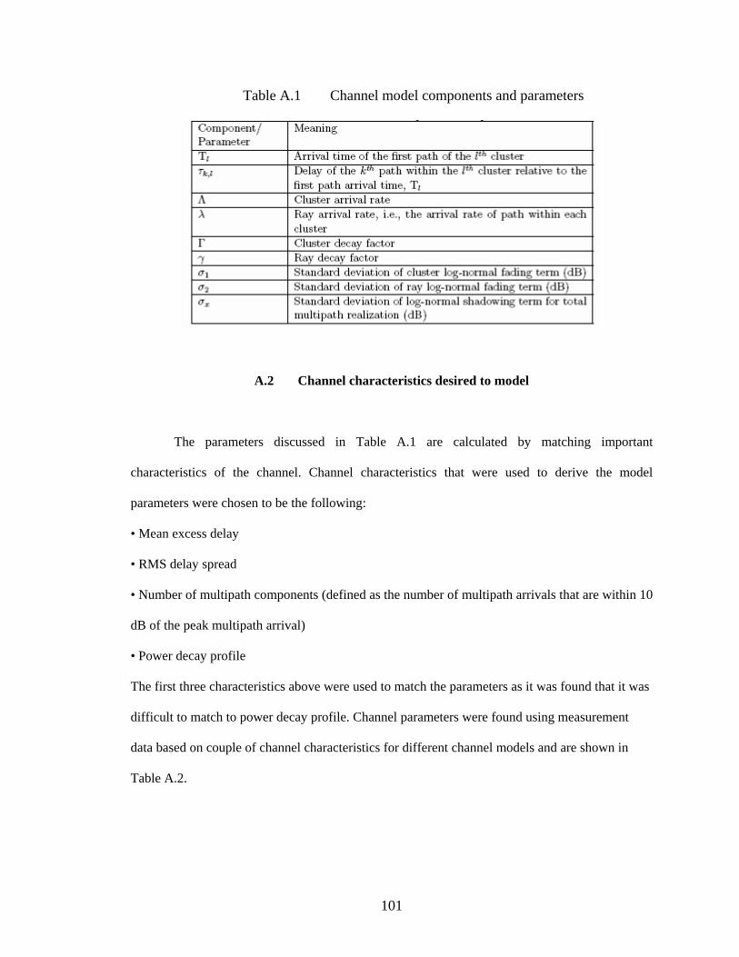
101
Table A.1 Channel model components and parameters
A.2 Channel characteristics desired to model
The parameters discussed in Table A.1 are calculated by matching important
characteristics of the channel. Channel characteristics that were used to derive the model
parameters were chosen to be the following:
• Mean excess delay
• RMS delay spread
• Number of multipath components (defined as the number of multipath arrivals that are within 10
dB of the peak multipath arrival)
• Power decay profile
The first three characteristics above were used to match the parameters as it was found that it was
difficult to match to power decay profile. Channel parameters were found using measurement
data based on couple of channel characteristics for different channel models and are shown in
Table A.2.

102
Table A.2 Typical Channel Characteristics and Model parameters
• 1 Based on LOS (0-4 m) channel measurements reported by Pandegrass.
• 2 Based on NLOS (0-4 m) channel measurements reported by Pandegrass.
• 3 Based on NLOS (4-10 m) channel measurements reported by Pandegrass and Forester.
• 4 Represents an extreme NLOS multipath channel to fit a 25 ns RMS delay spread.
• 5 Sampling time for these characteristic is 167 ps.
One hundred actual realizations for each channel model were derived from the model above and
the channel that was obtained is as shown in Figure A.1-A.4.
Channel shown in Figure A.1 is one realization of channel CM 1. This channel model is of a line
of sight (LOS) case with the transmitter and the receiver antenna being separated by a distance in
the range (0-4 m).
Figure A.2 shows single realization of the channel model CM 2. This channel is a model for a non
line of sight (NLOS) case with antenna separation being in the range (0-4 m). FigureA.3 and A.4
represent channel models CM 3 and CM 4 for NLOS case with antenna separation being in the
range (4-10 m) and an extreme case respectively.
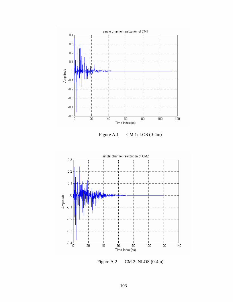
103
Figure A.1 CM 1: LOS (0-4m)
Figure A.2 CM 2: NLOS (0-4m)
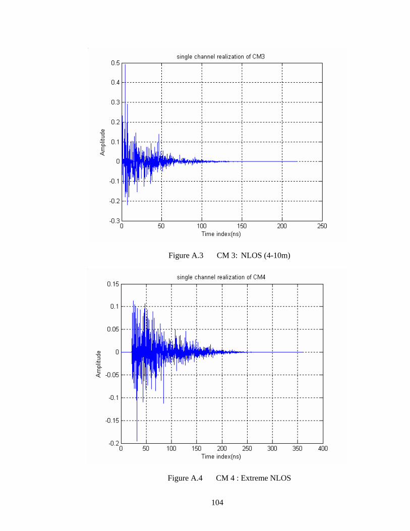
104
Figure A.3 CM 3: NLOS (4-10m)
Figure A.4 CM 4 : Extreme NLOS

105
APPENDIX B: MATLAB CODE LIST
106
B 1 List of Signal Processing/Simulation files
The following is a list of m files used for the signal processing and simulation in this thesis. The
files beranalysis and bertranalysis are modified files from those written by Mr. John Zhang of the
Wireless Networking Systems Laboratory. These files can be found on the CD attached to this
thesis.
Uwb_sv_cnvrt_ct.m
Uwb_sv_eval_ct.m
Uwb_sv_model_ct.m
Uwb_sv_params.m
Channelmodel.m
Cleanalgorithm.m
beranalysis.m
bertranalysis.m
uwbpulses.m
Comparetr.m

107
VITA
Abiodun Emmanuel Akogun graduated with a First Class Honors degree in
Electronic/Electrical Engineering from Obafemi Awolowo Universty, Ile-Ife, Nigeria, in
February 2000. From August 2000 to August 2003, he worked with GS Telecom/Spar
Aerospace, Nigeria Limited as Field Service Engineer. GS Telecom/Spar Aerospace is
the leading integrator of satellite and wireless systems in West Africa.
While at GS Telecom/Spar Aerospace, his key responsibilities include
designing/planning, installation, maintenance, and testing of radio frequency
(RF)/microwave and satellite systems and frame relay/ATM multiplexers for conveying
voice, data, and video over these RF systems. From August 2000 untill date, he served as
an active member of the Wireless Networking Systems Laboratory at Tennessee
Technological University.
Part of the results of his thesis work has been presented at the Instrumentation,
Systems and Automation Society (ISA) 51st International Instrumentation Symposium in
Knoxville, Tennessee. He is a member of the Eta Kappa Nu academic honor society and
also a recipient of the 2005 National Society of Black Engineers (NSBE) board of
corporate affiliates (BCA) award and the 2005 NSBE Torchbearer awards.