An-006 USD RIG Gyroscope Brief

USD-AN-006 Page 1 of 6

www.usdynamicscorp.com

US Dynamics Model 446 Series

Rate Integrating Gyroscope (RIG)

The RIG, Revisited (Part I) Scope: This applications note discusses the US Dynamics Rate Integrating Gyroscope (RIG) typical of the Model 446 design. Moreover, it attempts to expose those unfamiliar with the RIG to its operation. The RIG is functionally an elegantly simple analog device. Presented herein, is a simple method for modeling the RIG as a purely electrical analog, ideally suited for simulations in a typical electronics simulation (SPICE based) software program. The note therefore, focuses on RIG modeling for purposes of simulation within an application, rather than RIG design. A Brief Review The gyroscope is an instrument where the input is a rate of turn (angular rate). Any gyroscope is a torque-in, torque-out device. Therefore, the output of the gyro is a change in the gimbal angle (the gimbal turns) in response to the rate of turn input, due to gyroscopic precession. The input is a turn about the input axis (IA). The output is a turn about the output axis (OA). The precession of the gimbal takes place only when the rotor is spinning, of course. Conversely, a rotation imparted to the gimbal in its freedom axis (the OA), will cause a torque about the input axis (IA). Gyroscopes, therefore, will only provide an output response to a turn or spinning (angular) input motion, and will not respond to a linear input. Figure 1 depicts a RIG in simplistic form. It is what is known as a single degree of freedom type gyroscope. If the case is firmly tied to a structure, the freedom is in the output axis (OA), as the gimbal rolls in response to an input. The gyroscope requires a power input to the (typically) 2 phase AC spinmotor which drives the rotor. In addition, the output instrument, or the pickoff, requires an AC excitation signal. The output of the pickoff is a variable AC signal which tracks the movement of the gimbal. The direction of the gimbal is resolved by comparing the AC voltage phase of the output to that of the primary. More detail on gyroscope interfacing and excitation, etc., can be found in USD-AN’s 002, 003, and 004.

Input Axis

Figure 1 - View of a Single Axis RIG

Torque Generator

Pickoff

Viscous

Rotor(Inertia Wheel)

Case

DampingMechanism

Gimbal(Float)Output Axis

(IA)

Spin Axis (SA)

(OA)

US Dynamics Corp. Revision 09/2007 425 Bayview Avenue Amityville, NY 11701 631-842-5600


Rates vs. RIGs (or Rate Gyroscopes vs. Rate Integrating Gyroscopes, What’s the difference?) In the field of single axis miniature (approx 1” diameter, 2.6” length) gyroscopes, two types generally exist. First is the Rate gyroscope, where the gimbal is restrained by spring and lightly damped, directly measures a rate of turn. That is, the gyroscope output is calibrated “per degree per second”. Second is the RIG gyroscope, where the gimbal is un-restrained but heavily damped. The RIG measures either the rate of turn or the angle through which a turn was made during some period of time. Which measurement, depends on the operating mode of the RIG. Since there is no spring restraint, the gimbal is free to rotate through a small angle (typically ±2.0°). The gimbal must however, move against viscous damping. This damping provides for the smooth integrating action of the gimbal. The RIG includes a component not found in the rate gyroscopes (except for self testing rate gyros). A gimbal torque motor is present to allow for the intentional positioning of the gimbal. Typically, these are permanent magnet ‘torquers’ where a small input current will cause the gimbal to turn in one direction or the other. The measure of this input current is known as the torquer scale factor (T.S.F.) and is given in degrees per second per milliamp. The torquer essentially provides a gradient to either push (re-position) the gimbal, if there is no angular rate input, or to provide a nulling resistance to gimbal movement if there is an angular rate input. Thus, in the RIG, the rate of turn sensed by the gyro is integrated by the gimbal precession through the heavy viscous damping. The first integration of angular rate yields angular displacement. Therefore, the accumulating gimbal angle over time is the integrated gyro input rate. As such, the pickoff output is given in mV per degree, also known as the RIG transfer function (T.F.). Lastly, the Rate gyro is a second order system, which must be described by a natural frequency and a damping ratio. The RIG is a single order system, which may be described simply by its time constant (its characteristic time). RIG Operating Modes The RIG is a versatile gyroscope, in that it has two basic modes of operation. A ‘closed’ loop mode, where the torquer/pickoff loop is closed around the gyro itself, allows for the RIG to operate as an essentially hysteresis-free, high dynamic-range, high bandwidth, low drift Rate gyroscope (when compared to a conventional Rate gyroscope). In this mode, as the gyroscope senses an angular rate input and the gimbal begins to precess away from its center or null position. The gimbal angle, hence pickoff voltage, serves as feedback to a servo amplifier which then feeds the RIG’s torquer just the right amount of current to bring the gimbal back to its AC null position. A measure of the current multiplied by the torquer scale factor yields the angular rate in degrees per second sensed by the RIG. An ‘open-loop’ mode, where the RIG’s gimbal can be commanded via the torquer, and an outside loop, such as a velocity loop, (or a position loop) is closed via the RIG pickoff. This mode uses the RIG as both a command and feedback device.

NOTE for clarity. Both modes are closed servo loops. The torquer capture loop is commonly referred to as the RIG’s closed loop mode. A loop closed by driving some other structure in response to an RIG torquer input command is commonly referred to as a RIG open loop mode. Here, the torquer is fed a current corresponding to the rate of turn required of the structure to which the RIG is mounted (such as an antenna platform) to return the RIG’s gimbal to its null position. The rate feedback, which is actually the angular displacement of the gimbal, is given to the servo by the RIG’s pickoff, is the integrated angular rate. Visualizing an imaginary servo, the greater the gimbal angle from null, the higher the energy is fed into the motor controlling the turning function of the “platform”, to produce a rate to return the RIG’s gimbal to null. (Practically speaking, the gimbal stays where

www.usdynamicscorp.com US Dynamics Corp. Revision 09/2007 425 Bayview Avenue Amityville, NY 11701 631-842-5600


it is in inertial space, and the case of the RIG, the pickoff’s reference, turns around the inertially stabilized gimbal, essentially washing-out the precession.) Note that the gimbal action upon being commanded by the torquer is that of an integrator. That is, for a constant input, (after the relatively short time constant delay) the gimbal begins to roll at a controlled rate. If left long enough without correction, the gimbal will run into its stop. This is analogous to an op-amp integrator where upon given an input, no matter how small, the output will continue to accumulate until the amp saturates at the supply rail. In the RIG, the correction to the torquer induced gimbal roll is to roll the structure that supports the gyro at the correct compensating rate, which will “freeze” the gimbal in some angular position at that instant in time. Of course, that angle ideally serves as an error signal to the actuator (motor) controlling the structure. Therefore in a velocity loop servo, when the RIG is commanded via torquer current, the torquer scale factor will determine the angular rate at which the servo is ideally satisfied. This driven angular rate then exactly tracks the commanded RIG gimbal. In a properly tuned servo, zero velocity error is achieved between the command (the RIG gimbal) and the controlled element (the antenna, platform, etc.). In a position loop servo, the output of the RIG pickoff must be differentiated (a 90° phase shift). This mode assures that the angle of the structure onto which the gyro is mounted, follows the angle of the gimbal. A properly tuned and compensated system will deliver zero position error.

A Simple Electrical Analog Model of the RIG

NOTE: This section attempts to describe the RIG simply as an electrical analog to the actual RIG electro-mechanical system. In the actual system, the time constant (characteristic time) is determined by the gimbal moment of inertia (J) divided by the damping factor (B). The pickoff output gain, or transfer function, is determined by the angular momentum of the spinning mass (H) divided by the damping factor (B). By converting the electro-mechanical system into a purely electrical analog, a SPICE analysis tool can be used to analyze and model the system. In order to analyze or design an angular rate velocity loop, for example, it is helpful to conceptualize a simple model of the RIG. One such simple model can be assembled from op-amp integrators. Doing such allows one to make use of an analog circuit simulator (such as SPICE) to design a loop. The RIG is characterized (theoretically) by a single time constant. It is useful in an analog simulation of the RIG to use a lossy integrator in series with an ‘ideal’ integrator. This splits the RIG’s basic functions of the gimbal torquer (represented by the lossy integrator) and the gimbal precession-pickoff output (the ideal integrator). A schematic as described above is shown in figure 2.

R fb C Lossy

C

R in R


LOSSY INTEGRATOR IDEAL INTEGRATOR Figure 2 - Schematic of RIG Model

The first op-amp represents the lossy integrator, where a ‘bleed’ is placed on the capacitor. This section sets the time constant of the system, as well as plays some part in the gain of the model. The equations below describe the lossy integrator section.



1 f (Hz) =

2π(Rfb x C Lossy)


1

where: V out = V in x gain The above equations are also useful to describe the torquer function of the RIG. For example, a RIG is typically described by its time constant, T.S.F. and T.F. Then using the above equations for time constant and frequency, component selection can begin. It is helpful to set R_fb and R_in to the same value when selecting components to obtain the time constant. If for example, the time constant is known to be .0013 sec., the components selected may be 1300 Ohms for the R’s, and 1uF for C. The second op-amp represents the ‘ideal’ integrator. This section contributes to the gain of the model, which directly impacts the T.F. The equations below pertain to the ‘ideal’ integrator.

where: V in = V out from the lossy integrator, and V out of the ideal integrator is ‘per second’ Therefore, if V out of the lossy integrator is .03V, the using the R and C values from above in the ‘ideal’ integrator as well, the output will be 23V/sec. Using a hypothetical example, a RIG model may have the following specifications: T.S.F. = 1 deg/sec/mA Time Constant = .0013 sec T.F. = 175mV/deg If it is desired to have a gimbal roll rate of 30 deg/sec, then an appropriate input to the torquer would be 30mA. In the simple electrical model it is useful to deal in volts only. Therefore, equating mV to mA at the model’s input allows the use of volts only in the simple model. Then, the input to the lossy integrator will be 30mV. Using a first-pass set of component values which give the proper time constant of 1.3msec (all R’s = 1300 Ohms, all C’s = 1uF), the gain of the lossy integrator is 1. Using the lossy integrator output of 30mV as the input to the ‘ideal’ integrator, the result is 23.05V/sec. For the input of 30 deg/sec, the T.F. becomes 23.05/30 = 768mV/deg. This is higher than the specified 175mV/deg, so a gain adjustment is necessary. In order to retain the proper time constant, it is necessary only to reduce the gain of the lossy integrator by increasing R_in. Lowering the gain to approximately .23 (from 1) gives a T.F of 178mV/deg. The schematic of the electrical analog RIG model now appears as shown in figure 3.

((Rfb x C Lossy)+1)gain = (Rfb / Rin) x

1time constant (tau) =

2πf

1V out = V in xR x C(s)



1.3K

1.0 uF

1.3K

5.6K

LOSSY INTEGRATOR IDEAL INTEGRATOR

1.0 uF

Figure 3 - Model with component values

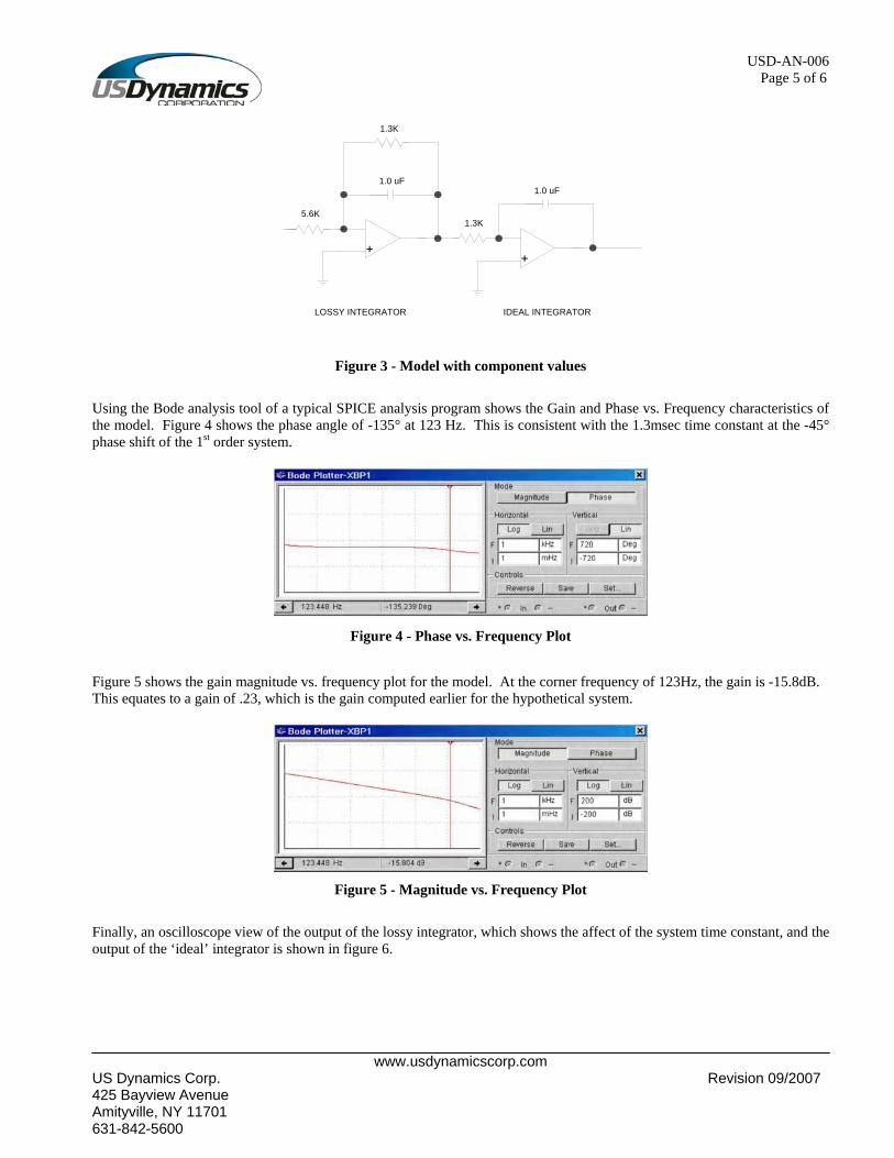
Using the Bode analysis tool of a typical SPICE analysis program shows the Gain and Phase vs. Frequency characteristics of the model. Figure 4 shows the phase angle of -135° at 123 Hz. This is consistent with the 1.3msec time constant at the -45° phase shift of the 1st order system.

Figure 4 - Phase vs. Frequency Plot

Figure 5 shows the gain magnitude vs. frequency plot for the model. At the corner frequency of 123Hz, the gain is -15.8dB. This equates to a gain of .23, which is the gain computed earlier for the hypothetical system.

Figure 5 - Magnitude vs. Frequency Plot

Finally, an oscilloscope view of the output of the lossy integrator, which shows the affect of the system time constant, and the output of the ‘ideal’ integrator is shown in figure 6.



Figure 6 - Scope View

Note that in the top trace of the oscilloscope, the leading edge of each positive and negative going pulse is slightly rounded. This is the effect of the gimbal time constant when the torquer is fed a step input. The ramp of the ‘ideal’ integrator shows a characteristic of 180mV/33.4msec as measured on the oscilloscope. A 33.4msec movement of the gimbal via the torquer provides approximately 1 deg/sec. Therefore, .0334deg/sec gives a calculated output of the pickoff of approximately 178mV/deg. This is consistent with the specification of the hypothetical system. The ramp output of the ideal integrator represents the pickoff output as the gimbal rolls in response to the torquer’s step input. [Note that the RIG is in an open loop mode here, and that the op-amp integrators are both inverting. Therefore, the input step into the lossy integrator is high when the output is low, and likewise the low input to the ideal integrator outputs a high.] The constant voltage input step represents a rate. The ramp output of the ideal integrator is the accumulated angle (the integrated rate, over some time). Again, at any given measured rate, this angle would appear as a constant angle when the system is servo lock. As a point of gyro design, the rate of roll of the gimbal should be equivalent to the torquer scale factor rate. That is, if the RIG has a torquer scale factor of 1°/sec/mA, then for a 30mA step input, the gimbal should roll at a rate of 30°/sec. Practically, however, this is possible only for a total freedom of ±2° typically. Therefore, the gimbal will roll its full 4° travel in approximately .13 seconds, or at about 7.5Hz. Closing Summary Using analog simulation techniques such as those shown above, system design engineers can gain a clearer understanding of the RIG’s function when represented as a circuit building block. Representing such electro-mechanical devices as purely analog electronics allows ease and flexibility in modeling and analysis due to the many SPICE based simulation tools already in use by engineers, particularly design engineers tasked with control circuitry design. In Part II to this series, a simulation of an angular rate velocity loop is presented. The loop contains the RIG as modeled herein, as well as a simple model of a prime mover, such as the sweeping function of an antenna platform. It is shown that a simple analog electronics model can simulate such a system, allowing engineers to test different system characteristics and conditions in order to gain a good basic understanding of angular velocity systems.

The RIG, of course, is the ideal instrument to issue the velocity rate command through its gimbal torquer and to close the loop via its gimbal precession in response to an angular rate sensed. The pickoff instrument output therefore gives rate feedback as the angle of the gimbal (the integrated angular rate). The RIG represents the simpler analog approach to angular rate measurement and control.


Documents

An-006 USD RIG Gyroscope Brief