Embed Size (px)
Citation preview

C.1
This appendix presents the principal syntactic rules of AMPL needed for the develop-ment and solution of complex mathematical programming models. For additionaldetails, you may consult the basic language reference given at the end of this appendix(Fourer and Associates, 2003). You may also consult www.ampl.com for additionalresources as well as the latest news and updates.
C.1 RUDIMENTARY AMPL MODEL
AMPL provides a facility for modeling mathematical programs (linear, integer, andnonlinear) in a longhand format. Figure C.1 gives the (self-explanatory) LP code forthe Reddy Mikks model (file RM1.txt). All reserved words are in bold. The remainingsymbols, other than the special operators , are generated by the user.
AMPL uses command lines and operates in a DOS environment. A recent betaversion of a Windows interface can be found in www.OptiRisk-Systems.com.
1+ - *, ; : 7 6 =2
APPENDIX C
AMPL Modeling Language1
1Folder AppenCFiles on the website includes all the files for this appendix.
var x1 >= 0;var x2 >= 0;maximize z: 5*x1 + 4*x2;subject toc1: 6*x1 + 4*x2 <= 24;c2: x1 + 2*x2 <= 6;c3: -x1 + x2 <= 1;c4: x2 <= 2;
solve;display z,x1,x2;
FIGURE C.1
Rudimentary AMPL model (file RM1.txt)
Z03_TAHA5937_09_SE_APPC.QXD 7/24/10 3:45 AM Page C.1

C.2 Appendix C AMPL Modeling Language
You can execute a model by clicking on ampl.exe in the AMPL folder and, at theampl prompt, typing the following command followed by Return:
ampl: model RM1.txt;
The output will be displayed on the screen as2
MINOS 5.5: Optimal solution found.2 iterationsz = 21x1 = 3x2 = 1.5
The rudimentary longhand format given here is not recommended for solvingpractical problems because it is problem specific. The remainder of this appendix pro-vides the details of how AMPL is used in practice.
C.2 COMPONENTS OF AMPL MODEL
Figure C.2 specifies the general structure of an AMPL model. The model is comprisedof two basic segments: The top segment (elements 1 through 4) is the algebraic repre-sentation of the model, and the bottom segment (elements 5 through 7) supplies thedata that drive the algebraic model. Thus, in LP, the algebraic representation in AMPLexactly parallels the following mathematical model:
Maximize z = an
j = 1cjxj
Algebraic Representation 1. Sets definitions.
2. Parameters definitions.
3. Variables definitions.
4. Model representation (objective and constraints).
Model implementation 4. Input data.
5. Solution of the model.
6. Output results.
2Every version of AMPL has a default solver that carries out the computations needed to optimize theAMPL model. In the student version, MINOS is the default solver, and it can handle linear and nonlinearproblems. The website includes other solvers: CPLEX, KNITRO, LPSOLVE, and LOQO. CPLEX handleslinear, integer, and quadratic problems. LPSOLVE handles linear and integer problems. KNITRO andLOQO handle linear and nonlinear problems.
FIGURE C.2
Basic structure of an AMPL model
Z03_TAHA5937_09_SE_APPC.QXD 7/24/10 3:45 AM Page C.2

C.2 Components of AMPL Model C.3
subject to
The advantage of this arrangement is that the same algebraic model can be used tosolve a problem of any size simply by changing the input data: , , and .
A number of syntax rules apply to the development of an AMPL model:
1. AMPL files must be plain text (Windows Notepad editor creates plain text).2. Commented text may appear anywhere in the model preceded with #.3. Each AMPL statement, comments excluded, must terminate with a semicolon (;).4. An AMPL statement may occupy more than one line. Breakpoints occur at a
proper separator, such as a blank space, colon, comma, parenthesis, brace,bracket, or mathematical operator. An exception to this rule occurs with strings(enclosed in quotes ' ' or " ") where a breakpoint is designated by adding abackslash ( \).
5. All keywords (with few exceptions) are in lower case.6. User-generated names are case sensitive. A name must be alphanumeric, inter-
spersed with underscores, if desired. No other special characters are allowed.
We will use the Reddy Mikks problem of Section 2.1 to show how AMPL works.Figure C.3 gives the corresponding model (file RM2.txt). For convenience, key (orreserved) words are emphasized in bold.
The algebraic model starts with the sets that define the indices of the general LPmodel.The user-generated names resource and paint each preceded by the keywordset correspond to the sets { and { in the general LP model. The specific elements ofthe sets resource and paint that define the Reddy Mikks model are given in theinput data section of the model.
The parameters are user-generated names preceded by the keyword param thatdefine the coefficients of the objective function and the constraints as a function of thevariable and constraint sets. The parameters unitprofit{paint}, aij{resource,paint}, and rhs{resource} correspond, respectively, to the mathematical symbols
, , and in the general LP model. The subscripts and are represented by AMPLsets resource and paint, respectively. The input data provide specific values of theparameters.
The variables of the model, , are given the name product preceded by the key-word var. Again, product is a function of the set paint. We can add the nonnegativitycondition ( ) in the same statement. Else, the default is that the variables areunrestricted in sign.
Having defined the sets, parameters, and variables of the model, the next stepis to express the optimization problem in terms of these elements. The objective-function statement specifies the sense of optimization using the keyword maximizeor minimize. The objective value z is given the user name profit followed by a
7 =0
xj
jibiaijcj
j}i}
biaijm, n, cj
an
j = 1aijxj … bi, i = 1, 2, . . . , m
Z03_TAHA5937_09_SE_APPC.QXD 7/24/10 3:45 AM Page C.3

C.4 Appendix C AMPL Modeling Language
colon (:), and its AMPL statement is a direct translation of the mathematicalexpression
sum{j in paint} unitprofit[j]*product[j];
The index j is user specified. Note the use of braces in {j in paint} to indicate thatj is a member of the set paint, and the use of brackets in [j] to represent a subscript.
aj
cjxj:
#********************ALGEBRAIC MODEL*******************#--------------------------------------------------setsset paint;set resource;#--------------------------------------------parametersparam unitprofit{paint};param rhs {resource};param aij {resource,paint};#---------------------------------------------variablesvar product{paint} >= 0#---------------------------------------------modelmaximize profit: sum{j in paint} unitprofit[j]*product[j];subject to limit{i in resource}:
sum{j in paint} aij[i,j]*product[j]<=rhs[i];#************************DATA**************************data;set paint : exterior interior;set resource : m1 m2 demand market;param unitprofit :
exterior 5interior 4;
param rhs:m1 24m2 6demand 1market 2;
param aij: exterior interior :m1 6 4m2 1 2demand -1 1market 0 1;
#**********************SOLUTION************************solve;#----------------------------------------output resultsdisplay profit, product, limit.dual, product.rc;
=
=
=
=
=
FIGURE C.3
AMPL model for the Reddy Mikks problem (file RM2.txt)
Z03_TAHA5937_09_SE_APPC.QXD 7/24/10 3:45 AM Page C.4

C.2 Components of AMPL Model C.5
A model may include one or more constraint statements, and each such statementcan be preceded by the keywords subject to or simply s.t. Actually, s.t. andsubject to are optional, and AMPL assumes that any statement that does not startwith a keyword is a constraint. The Reddy Mikks model has only one set of constraintsnamed limit and indexed over the set resource:
limit{i in resource}:sum{j in paint} aij[i,j]*product[j] <= rhs[i];
The statement is a direct translation of constraint ,
The idea of declaring variables as nonnegative can be generalized to allow estab-lishing upper and lower bounds on the variables, thus eliminating the need to declarethese bounds as explicit constraints. First, the two bounds are declared with the user-generated names lowerbound and upperbound as
param lowerbound{paint};param upperbound{paint};
Next, the variables are defined as
var product{j in paint}>=lowerbound[j],<=upperbound[j];
Notice that the syntax does not allow comparing “vectors.” Thus, an error is generatedif we use
var product{paint}>=lowerbound{paint},<=upperbound{paint};
We can use the same syntax to set conditions on parameters as well. For example,the statement
param upperbound{j in paint}>=lowerbound[j];
will guarantee that upperbound is never less than lowerbound. Else AMPL will issuean error. The main purpose of using bounds on parameters is to prevent entering con-flicting data inadvertently. Another instance where such checks may be used is when aparameter is required to assume nonnegative values only.
The algebraic model in Figure C.3 is general in the sense that it applies to any numberof variables and constraints. It can be tailored to the Reddy Mikks situation by specifyingthe data of the problem. Following the statement data; we first define the members of thesets, and then use these definitions to assign numeric values to the different parameters.
The set paint includes the names of two variables, which we suggestively callexterior and interior. Members of the set resource are given the names m1, m2,demand, and market. The associated statements in the data section are thus given as
set paint := exterior interior;set resource := m1 m2 demand market;
aj
aijxij … bi.i
Z03_TAHA5937_09_SE_APPC.QXD 7/24/10 3:45 AM Page C.5

C.6 Appendix C AMPL Modeling Language
Members of each set appear to the right of the reserved operator := separated by ablank space (or a comma). String indices must be enclosed in double quotes when usedoutside the data segment—that is, paint["exterior"], paint["interior"],limit["m1"], limit["m2"], limit["demand"], and limit["market"]. Otherwise,the string index will be incorrectly interpreted as a (numeric) parameter.
We could have defined the sets at the start of the algebraic model (instead of inthe data segment) as
set resource ={"m1", "m2", "demand", "market"};set paint ={"exterior", "interior"};
(Note the mandatory use of the double quotes " ", the separating commas, and thebraces.) This convention is not advisable in general because it is problem specific,which may limit tailoring the model to different input data scenarios. When this con-vention is used, AMPL will not allow modifying the set members in the data segment.
The use of alphanumeric names for the members of the sets resource and paintcan be cumbersome in large problems. For this reason, AMPL allows the use of purelynumeric sets—that is, we can use
set paint:= 1 2;set resource:= 1..4;
The range 1..4 replaces the explicit 1 2 3 4 representation and is useful for sets witha large number of members. For example, 1..1000 is a set with 1000 members startingwith 1 and ending with 1000 in increments of 1.
The range representation can be made more general by first defining m and n asparameters
param m;param n;
In this case, the sets 1..m and 1..n can be used directly throughout the entire model asshown in Figure C.4 (file RM2a.txt), eliminating altogether the need to use the setnames resource and paint.
Actually, the syntax 1..m (or 1..n) has the general format
start..end by step
where start, end, and step are defined AMPL parameters whose values are specifiedunder data. If start < end and step > 0, then members of the set begin with startand advance by the amount step to the highest value less than or equal to end. Theopposite occurs if start > end and step <0. For example, 3..10 by 2 producesthe members 3, 5, 7, and 9, and 10..3 by -2 produces the members 10, 8, 6, and 4. Thedefault for step is 1, which means that start..end by 1 is the same as start..end.
Actually, the parameters start, end, and step can be any legitimate AMPLmathematical expressions computed during execution. For example, given the parame-ters m and n, the set j in 2*n..m n^2 by n/2 is perfectly legal. Note, however, that+
Z03_TAHA5937_09_SE_APPC.QXD 7/24/10 3:45 AM Page C.6

C.2 Components of AMPL Model C.7
a fractional step is used directly to create the members of the set. For example, for m = , n = 13, the members of the set m..n step m/2 are 5, 7.5, 10, and 12.5.
The Reddy Mikks model includes single- and two-dimensional parameters. Theparameters unitprofit and rhs fall in the first category and the parameter aij in thesecond. In the first category, data are specified by listing each set member followed bya numeric value, as the following statements show:
param unitprofit :=exterior 5interior 4;
param rhs:=m1 24m2 6demand 1market 2;
The elements of the list may be “strung” into one line, if desired. The only requirementis a separation of at least one blank space. The format given here promotes betterreadability.
5
FIGURE C.4
AMPL model for the Reddy Mikks problem (file RM2a.txt)
param m;param n;param unitprofit{1..n};param rhs{1..m};param aij{1..m,1..n};#---------------------------------------------variablesvar product{1..n}>=0;#-------------------------------------------------modelmaximize profit:sum{j in 1..n}unitprofit[j]*product[j];subject to limit{i in 1..m}:
sum{j in 1..n}aij[i,j]*product[j]<=rhs[i];data;param m:=4;param n:=2;param unitprofit := 1 5 2 4;param rhs:=1 24 2 6 3 1 4 2;param aij: 1 2:=
1 6 42 1 23 -1 14 0 1;
solve;display profit, product, limit.dual, product.rc;
Z03_TAHA5937_09_SE_APPC.QXD 7/24/10 3:45 AM Page C.7
C.8 Appendix C AMPL Modeling Language
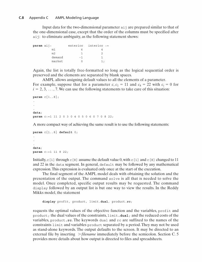
Input data for the two-dimensional parameter aij are prepared similar to that ofthe one-dimensional case, except that the order of the columns must be specified afteraij: to eliminate ambiguity, as the following statement shows:
param aij: exterior interior :=m1 6 4m2 1 2demand -1 1market 0 1;
Again, the list is totally free-formatted so long as the logical sequential order ispreserved and the elements are separated by blank spaces.
AMPL allows assigning default values to all the elements of a parameter.For example, suppose that for a parameter and with for
. We can use the following statements to take care of this situation:
param c{1..8};...data;param c:=1 11 2 0 3 0 4 0 5 0 6 0 7 0 8 22;
A more compact way of achieving the same result is to use the following statements:
param c{1..8} default 0;...data;param c:=1 11 8 22;
Initially,c[1] through c[8] assume the default value 0, with c[1] and c[8] changed to 11and 22 in the data segment. In general, default may be followed by any mathematicalexpression.This expression is evaluated only once at the start of the execution.
The final segment of the AMPL model deals with obtaining the solution and thepresentation of the output. The command solve is all that is needed to solve themodel. Once completed, specific output results may be requested. The commanddisplay followed by an output list is but one way to view the results. In the ReddyMikks model, the statement
display profit, product, limit.dual, product.rc;
requests the optimal values of the objective function and the variables, profit andproduct; the dual values of the constraints, limit.dual; and the reduced costs of thevariables, product.rc. The keywords dual and rc are suffixed to the names of theconstraints limit and variables product separated by a period. They may not be usedas stand-alone keywords. The output defaults to the screen. It may be directed to anexternal file by inserting filename immediately before the semicolon. Section C. 5provides more details about how output is directed to files and spreadsheets.
7
i = 2, 3, Á , 7ci = 0c8 = 22c, c1 = 11
Z03_TAHA5937_09_SE_APPC.QXD 7/24/10 3:45 AM Page C.8

C.2 Components of AMPL Model C.9
The execution command in DOS is
ampl: model RM2.txt;
The associated output is displayed on the screen, as the snapshot in Figure C.5 shows.The layout of the output in Figure C.5 is a bit “cluttered” because it mixes the
indices of the constraints and the variables. We can streamline the output by placing itselements in groups of the same dimension using the following two display statements:
display profit, product, product.rc;display limit.dual;
In a typical AMPL model, such as the one in Figure C.3, the segment associatedwith the logic of the model preferably should remain static. The data and output seg-ments are changed as needed to match specific LP scenarios. For this purpose, theAMPL model is represented by two separate files: RM2b.txt providing the logic of themodel and RM2b.dat accounting for the input data and the output results.3 In this case,the DOS line commands are entered sequentially as:
ampl: model RM2b.txt;ampl: data RM2b.dat;
We will see in Section C.7 how commands such as solve and display can be issuedinteractively rather than being hard-coded in the model.
The Reddy Mikks model provides only a “glimpse” of the capabilities of AMPL.We will show later how input data may be read from external files and spreadsheet
3Actually, the output command may be processed separately instead of being included in the .dat file, as willbe explained in Section C.7
FIGURE C.5
AMPL output using display profit, product, limit.dual. product.rc; in the Reddy Mikks model
MINOS 5.5: optimal solution found.2 iterations. objective 21
profit = 21
: product limit.dual product.rc :demand . 0 .exterior 3 . 6.66134e-16interior 1.5 . 0m1 . 0.75 .m2 . 0.5 .market . 0 .;
=
Z03_TAHA5937_09_SE_APPC.QXD 7/24/10 3:45 AM Page C.9

C.10 Appendix C AMPL Modeling Language
tables. We will also show how tailored (formatted) output can be sent to these media.Also, AMPL interactive commands are important debugging and execution tools, aswill be explained in Section C.7.
PROBLEM SET C.2A
1. Modify the Reddy Mikks AMPL model of Figure C.3 (file RM2.txt) to account for a thirdtype of paint named “marine.” Requirements per ton of raw materials m1 and m2 are .5 and.75 ton, respectively. The daily demand for the new paint lies between .5 ton and 1.5 tons.The revenue per ton is $3.5 (thousand). No other restrictions apply to this product.
2. In the Reddy Mikks model of Figure C.3 (file RM2.txt), rewrite the AMPL code using thefollowing set definitions:(a) paint and {1..m}.(b) {1..n} and resource.(c) {1..m} and {1..n}.
3. Modify the definition of the variables in the Reddy Mikks model of Figure C.3(file RM2.txt) to include a minimum demand of 1 ton of exterior paint and maximum demands of 2 and 2.5 tons of exterior and interior paints, respectively.
4. In the Reddy Mikks model of Figure C.3, the command
display profit;
provides the value of the objective function. We can use the same command to display thecontribution of each variable to the total profit as follows:
display profit, {j in paint} unitprofit[j]*product[j];
Another convenient way to accomplish the same result is to use defined variablestatements as follows:
var extProfit=unitprofit["exterior"]*product["exterior"]var intProfit=unitprofit["interior"]*product["interior"]
In this case, the objective function and display statements may be written in a less compli-cated form as
maximize profit: extProfit + intProfit;display profit, extProfit, intProfit;
In fact, defined variables can be in indexed form as:
var varProfit{j in paint} = unitprofit[j]*product[j];
The resulting objective function and display statement will then read as
maximize profit: sum {j in paint} varProfit[j];display profit, varProfit;
Use defined variables with the Reddy Mikks model to allow displaying each variable’sprofit contribution and resource consumption of raw materials m1 and m2.
5. Develop and solve an AMPL model for the diet problem of Example 2.2-2, and find theoptimum solution. Determine and interpret the associated dual values and the reduced costs.
Z03_TAHA5937_09_SE_APPC.QXD 7/24/10 3:45 AM Page C.10

C.3 Mathematical Expressions and Computed Parameters C.11
C.3 MATHEMATICAL EXPRESSIONS AND COMPUTED PARAMETERS
We have seen that AMPL allows placing upper and lower bounds on parameters.Actually, the language affords more flexibility in defining parameters as complexmathematical expressions, modified conditionally, if desired.
To illustrate the use of computed parameters, consider the case of a bank offeringtypes of loans that charges an interest rate for loan , .
Unrecoverable bad debt, both principal and interest, for loan equals of the amountof loan . The objective is to determine the amount the bank allocates to loan tomaximize the total return subject to a set of restrictions.
The use of computed parameters will be demonstrated by concentrating on theobjective function. Algebraically, the objective function is expressed as
A direct translation of into AMPL is the following:
param r{1..n}>0, <1;param v{1..n}>0, <1;var x{1..n}>=0;
maximize z: sum{i in 1..n}(r[i]-v[i]*(r[i]+1))*x[i];
(constraints)
Another way to handle the bank situation is to use a computed parameter torepresent the objective function coefficients in the following manner:
param r{1..n}>0, <1;param v{1..n}>0, <1;param c{i in 1..n}=(r[i]-v[i]*(r[i]+1));var x{1..n}>=0;
maximize z: sum{i in 1..n}c[i]*x[i];
(constraints)
AMPL will compute the parameter c[i] and use its value in the objective statement .The new formulation enhances readability. But in some cases the use of computedparameters may be essential.
In general, the expression defining the value of a computed parameter can be ofany complexity and may include any of the built-in arithmetic functions familiar to anyprogramming language (e.g., sin, max, log, sqrt, exp). An important requirement isthat the expression evaluate to a numeric value.4
Computed parameters may also be evaluated conditionally using the construct
parameter = if condition then expression1 else expression2;
z
z
Maximize z = an
i = 1ri(1 - vi)xi - a
n
i = 1vixi = a
n
i = 1[ri - vi(ri + 1)]xi
ixiivii
0 6 ri 6 1, i = 1, 2, Á , nirin
4AMPL manual provides an “exception” when a parameter is declared binary, in which case it can also betreated as logical.This distinction is artificial, because treating such a parameter as numeric still produces thesame result.
Z03_TAHA5937_09_SE_APPC.QXD 7/24/10 3:45 AM Page C.11

C.12 Appendix C AMPL Modeling Language
The condition compares arithmetic quantities and strings using the familiar operatorsand (together with and/or). Note that nonlinearity will result
if condition is a function of the model variables. As in other programming languages,the construct may be used without else expression2. Nested if is also allowed follow-ing then and else.
The if-then-else construct gives the computed parameters the numeric valueof either expression1 or expression2. This is the reason the if-then-else presentedhere is an expression and not a statement. (Section C.7 introduces the if-then-elsestatement together with the loop statements for{}, repeat while{}, and repeatuntil{}. These statements are used mainly for automating solution scenarios andformatting output.)
We will use a simple case to demonstrate the use of the if expression. In a multi-period manufacturing situation, units of a certain item are produced to meet variabledemand. Unit production cost is estimated at dollars for the first periods, andincreases by 10% for the next periods and by 20% for the following periods.
The constraints of this model deal with capacity restrictions for each period andthe balance equations that relate inventory, production, and demand. To demonstratethe use of the if expression, we will concentrate on the objective function. Let
The objective function is given asMinimize
We can model this function in AMPL as
param p;var x{1..3*m}>=0;
minimize cost: p*(sum{j in 1..m}x[j]+1.1*sum{j in m+1..2*m}x[j]+ 1.2*sum{j in 2*m+1..3*m}x[j]);
(constraints)
A more compact way that also enhances readability is to use if-then-else torepresent the objective-function parameter c[j]:
param m;param n=3*m;param p;param c{j in 1..n}= if j<=m then p else
(if j>m and j<=2*m then 1.1*p else 1.2*p);
var x{j in 1..n};
minimize z: sum{j in 1..n}c[j]*x[j];
(constraints)
+ 1.2p1x2m + 1 + x2m + 2 +Á
+ x3m2
z = p1x1 + x2 +Á
+ xm2 + 1.1p1xm + 1 + xm + 2 +Á
+ x2m2
xj = units produced in period j, j = 1, 2, Á , 3m
mmmp
6 7= , 6 , 7 , 6 = , 7 = ,
Z03_TAHA5937_09_SE_APPC.QXD 7/24/10 3:45 AM Page C.12

C.4 Subsets and Indexed Sets C.13
Note the nesting of the conditions. The parentheses () enclosing the second if are notnecessary and are used to enhance readability. Observe that then and else are alwaysfollowed by what must evaluate to numeric values. Note also that c can be defined as
param c{j in 1..n}=p*( if j<=m then 1 else(if j>m and j<=2*m then 1.1 else 1.2));
A particularly useful implementation of if-then-else occurs in the situationwhere parameters or variables are defined recursively. A typical example of such aparameter occurs in determining the inventory level in period , withinitial zero inventory. The production amount and demand in period are and ,respectively. Thus, the inventory level is
The amount can be computed recursively in AMPL as follows:
param p{1..n};param d{1..n};var I{t in 1..n}= if i=1 then 0 else I[t-1])+p[t]-d[t];
Notice that it would be somewhat cumbersome to compute were it not for the use ofthe if-then-else expression (see also Set C.3a).
The bus scheduling problem (Example 2.4-5) demonstrates the use of if . . .then . . . else within the context of a complete model.These two models are detailedin Section C.9.
PROBLEM SET C.3A
*1. Consider the following set of constraints:
Use if-then-else to develop a single set of constraints that represents all inequalities.2. In a multiperiod production-inventory problem, let , and be, respectively, the amount
of entering inventory, production quantity, and demand for period . Thebalance equation associated with period is . In a specific situation,
and .Write the AMPL constraints corresponding to the balance equa-tions using if-then-else to account for and .
3. Consider the parameters and and . Define and as AMPLparameters.
C.4 SUBSETS AND INDEXED SETS
Subsets. Suppose that we have the following constraint:
x1 + x2 + x5 + x6 + x7 … 15
bjaij e {1, ai}bi, j, i e {1, n}ai
xT + 1 = 0x1 = cxT + 1 = 0(70)x1 = c
xt + zt - dt - xt + 1 = 0tt, t = 1, 2, Á , T
dtxt, zt
n
x1 + xn Ú cn
xi + xi + 1 Ú ci, i = 1, 2, Á , n - 1
It
It
It = It - 1 + pt - dt, t = 1, 2, . . . , n
I0 = 0
dtpttt, t = 1, 2, Á , nIt
Z03_TAHA5937_09_SE_APPC.QXD 7/24/10 3:45 AM Page C.13

C.14 Appendix C AMPL Modeling Language
There are 7 variables in the model, and this particular constraint does not include thevariables and .
We can model this constraint by using subsets in a number of ways (all newkeywords are in bold):
#–––––––––––––––––––––– method 1 –––––––––––––––––––--—––––––––––––var x{1..7}>=0;subject to lim: sum{j in 1..7: j<=2 or j>=5}x[j]<=15;#–––––––––––––––––––––– method 2 –––––––––––––––––––--—––––––––––––var x{1..7}>=0;subject to lim: sum{j in 1..2 union 5..7}x[j]<=15;#–––––––––––––––––––––– method 3 –––––––––––––––––––--—––––––––––––var x{1..7}>=0;subject to lim: sum{j in 1..7 diff 3..4}x[j]<=15;#–––––––––––––––––––––– method 4 –––––––––––––––––––--—––––––––––––var x{1..7}>=0;subject to lim: sum{j in 1..7 diff (1..4 inter 3..7)}x[j]<=15;#–––––––––––––––––––––––––––––––––--—–––––––––––––––––––--—–––––––-
In method 1, the set {j in 1..7} deletes the elements 3 and 4 by imposingrestrictions on j. A colon separates the modified set from the condition(s). Keywordsunion, diff, and inter play the roles of and respectively.Method 4 is a convoluted set representation. Nevertheless, it serves to represent theuse of the operator inter.
Indexed sets. A powerful feature of AMPL allows indexing sets over the elements ofa regular set. Suppose that two components and are used to produce products 1, 2,3, 4, and 5. Component is used in products 1, 3, and 5, and component is used inproducts 1, 2, 4, and 5. Each product requires one unit of the specified components.Themaximum availabilities of components and are 200 and 300 units, respectively.Theproblem deals with determining the number of assembly units of each product. Otherpertinent data will be needed to complete the description of the problem, but we willconcentrate only on the constraints dealing with the components’ availability.
Let be the production quantity of product . Then the con-straints for components and can be expressed mathematically as
Component
The AMPL representation of the constraints can be achieved using indexed sets asfollows:
set comp;set prod{comp};param d{comp};var x{1..5}>=0;#-————objective function here
B: x1 + x2 + x4 + x5 … 300
Component A: x1 + x3 + x5 … 200
BAi, i = 1, 2, Á , 5xi
BA
BABA
A ¨ B,A ´ B, A - B,
x4x3
Z03_TAHA5937_09_SE_APPC.QXD 7/24/10 3:45 AM Page C.14

C.4 Subsets and Indexed Sets C.15
subject toC{i in comp}:sum{j in prod[i]}x[j]<=d[i];
#-————other constraints heredata;set comp:= A B;set prod[A]:=1 3 5;set prod[B]:=1 2 4 5;param d:= A 200 B 300;
The indices of set prod are the elements A and B of set comp, thus defining thetwo indexed sets prod[A] and prod[B]. Next, the data of the problem define theelements of prod[A] and prod[B]. With these data, the constraints of the components(regardless of how many there are) are defined by the single statement:
C{i in comp}:sum{j in prod[i]}x[j]]<=d[i];
The applications of indexed sets are demonstrated aptly in the AMPL momentsfollowing Examples 6.6-4 and 9.1-2.
PROBLEM SET C.4A
1. Use subsets to express the left-hand side by means of a single sum{} function:
(a)
(b)
*2. Suppose that 5 components (one unit per product unit) are used in the production of10 products according to the following schedule:
an
i = mxi + a
2n + k
i = n + kxi … c, k 7 1
am
j = 1xj + a
n
j = m + kxj + a
q
j = n + pxj Ú c
Component Products that use the component Minimum availability
1 1, 2, 5, 10 5002 3, 6, 7, 8, 9 4003 1, 2, 3, 5, 6, 7, 9 9004 2, 4, 6, 8, 10 7005 1, 3 4, 5, 6, 7, 9, 10 100
The unit assembly cost of each product is a function of the component used: $9, $4, $6, $5,and $8 for components 1 through 5, respectively. The maximum demand for any of theproducts is 300 units. Use AMPL indexed sets to determine the optimal product mix thatminimizes the installation cost. (Hint: Let be the number of units of product that usecomponent .)
3. Repeat Problem 2 assuming that the unit installation cost of the components is a functionof the assembled product: $1, $3, $2, $6, $4, $9, $2, $5, $10, and $7 for products 1 through 10,respectively.
jixij
Z03_TAHA5937_09_SE_APPC.QXD 7/24/10 3:45 AM Page C.15

C.16 Appendix C AMPL Modeling Language
C.5 ACCESSING EXTERNAL FILES
So far, we have used “hard-coded” data to drive AMPL models. Actually, AMPL datamay be accessed from external files, spreadsheets, and/or databases.The same is true forretrieving output results. This section deals with reading data from or writing output to
1. External files, including screen and keyboard.2. Spreadsheets.
More details can be found in Fourer and Associates, 2003, Chapter 10.
C.5.1 Simple read files
The statement for reading data from an unformatted external file is
read item-list <filename;
The item-list is a comma-separated list of nonindexed or indexed parameters. In theindexed case, the syntax is {indexing}paramName[index].The list can include parametersonly. This means that any set members must be accounted for under data prior toinvoking the read statement. (We will see in Sections C.5.3 and C.5.4 how set membersare read from formatted files and spreadsheets.)
To illustrate the use of read, consider the Reddy Mikks model where all the datafor the parameters unitprofit, rhs, and aij are read from a file named RM3.dat perthe model in file RM3.txt. The associated read statement is:
read {j in paint}unitprofit[j],{i in resource}rhs[i],{i in resource, j in paint}aij[i,j]<RM3.dat;
File RM3.dat lists the data in the exact order in which the items appear in theread list—that is,
5 424 6 1 26 41 2-1 10 1
The multiple-row organization of the data enhances readability, in the sense that wecould have had all the elements on one line (separated by blank spaces).5 Note that thisfile happens to be all numeric. For convenience, nonnumeric data (such as parameter
5Hidden codes in .dat files (and in .tab files, which will be presented later in this section) can triggerAMPL errors such as “too few elements in line xx” or “unexpected end of file” (xx stands for a numericvalue) even though the text file may appear perfectly legal. To get rid of these hidden codes, click immedi-ately to the right of the last data element in the file, then press the following keys in succession: Return,Backspace, and Return.
Z03_TAHA5937_09_SE_APPC.QXD 7/24/10 3:45 AM Page C.16

C.5 Accessing External Files C.17
names) can appear in the data file provided that they are declared symbolic (fordetails, see Sections 7.8 and 9.5 in Fourer and Associates, 2003).
The read statement allows accessing data from the keyboard. In this case, thefilename is replaced with a minus sign—that is, using . The execution of read in thiscase will produce the DOS prompt ampl?, and it will be repeated until all the data re-quested by read have been accounted for.
PROBLEM SET C.5A
1. Prepare the input file RM3x.dat for the Reddy Mikks model (file RM3.txt), assuming thatthe read statement is given as
read {j in paint}{i in resource}(rhs[i],{j in paint}aij[i,j])<RM3x.dat;
*2. For the Reddy Mikks model, explain why the following read statement is cumbersome:
read {i in resource}(rhs[i],{j in paint}(unitprofit[j],aij[i,j]))<RM3xx.dat;
C.5.2 Using print or printf to retrieve output
A simple way to retrieve output data in AMPL is to use preformatted print or for-matted printf. As an illustration, in the Reddy Mikks model we can use the followingstatements to send output data to a file we name file.out (output defaults to thescreen if a file is not designated):
printf "Objective value is %6.2f\n",profit >file.out;printf {j in paint}:
"%8s%8.2f%8.3f\n",j,product[j],product[j].rc >file.out;
The output format always precedes the output list and must be enclosed in doublequotes.The same statement can be used with print simply by removing the format code.
In the first printf statement, the format includes the optional descriptive textObjective value is and mandatory specifications of how the output list is printed.The code %6.2f says that the value of profit is printed in a field of length 6 with twodecimal points. The code \n moves printing to the next line in the file. These formatcodes are the same as in C programming.
In the second print statement, the output list includes j, product[j],product[j].rc, where j is one of the members (exterior, interior) in the AMPLset paint. The code %8s reserves the first eight fields for printing the name exterior
6 -
Z03_TAHA5937_09_SE_APPC.QXD 7/24/10 3:45 AM Page C.17

C.18 Appendix C AMPL Modeling Language
or interior. If j were numeric (e.g., {j in 1..2}), then the format specificationwould have to be integer, for example, %3i.
The format specifications in this section are limited to %s, %i, %f, and \n. AMPLprovides other specifications (see Table A-10 in Fourer and Associates, 2003).
PROBLEM SET C.5B
1. Use printf statements to present the optimal solution of the Reddy Mikks model (fileRM2.txt) in the following format where the suffixes .slack and .dual are used toretrieve slack amount and the dual price:
Objective value =
Product Quantity Profit($)
.
.
.
.
.
.
.
.
.Constraint Slack amount Dual price
.
.
.
.
.
.
.
.
.
C.5.3 Input table files
The read statement in Section C.5.1 does not allow reading set members.This situationis accounted for using table statements.
In table files, the data are presented as tables with properly labeled rows andcolumns using the members of the defining sets. Access to table files requires a com-panion read statement.The table statement formats the data, and the read statementmakes the data available to the model.
The syntax of table and read statements is as follows:
table tableName IN "fileName":SetName<-[SetColHdng], parameters~ParamColHdng;read table tableName;
This syntax allows reading both the members of AMPL sets and the parameters fromtableName in fileName.
The default fileName where the text table is stored is tableName.tab. It may beoverridden by explicitly specifying fileName (in double quotes) with mandatory.tab extension following the keyword IN. IN (in caps) means INput (as contrastedwith OUT, which, as shown later, is used to OUTput data to a table file). SetColHdngmay be an arbitrary heading name in the table which is cross-referenced to theelements of SetName using <-. Similarly, AMPL parameters are cross-referenced tothe arbitrary names ParamColHdng using~. If SetColHdng happens to be the sameas SetName, the syntax SetName<- [SetColHdng] may be replaced with [SetName]IN. In the case of parameters, ~ParamColHdng is deleted from the statement.
To illustrate the use of tables, Figure C.6 gives the contents of the files namedRM4profit.tab, RM4rhs.tab, and RM4aij.tab for inputting the parameters unitprofit,
Z03_TAHA5937_09_SE_APPC.QXD 7/24/10 3:45 AM Page C.18

C.5 Accessing External Files C.19
rhs, and aij of the Reddy Mikks model. The first line in each file must always followthe format
ampl.tab nbr_indexing_sets nbr_read_parameters
The first element, ampl.tab, identifies the table as a .tab file, with the succeeding twoelements providing the number of indexing sets of the parameters that will be readfrom the table. In RMprofit.tab and RMrhs.tab, only one set is needed to define theparameters unitprofit and rhs, and for this reason ampl.tab 1 1 is used as theheader line in these two files. For the parameter aij, two sets are needed, whichrequires the use of the header line ampl.tab 2 1.
The header line is followed by a list of the exact or substitute names of the sets andthe parameters. The succeeding rows in the respective file list the values of the inputparameter as an explicit function of its indexing set(s) using blank space(s) as separa-tors. For unitprofit and rhs, the listing is straightforward. For the double-indexedparameter aij, each parameter list is identified by two explicit indices, even at theexpense of redundancy.
For the Reddy Mikks model, the associated tables are defined as follows:
table RM4profit IN: paint <- [COL1], unitprofit~COL2;table RM4rhs IN: [resource] IN, rhs;table RM4aij IN: [resource, paint], aij;
FIGURE C.6
Contents of the table files for inputting the parameters unitprofit, rhs, and aij of the Reddy Mikks model
File RM4profit.tab:ampl.tab 1 1COL1 COL2exterior 5interior 4
File RM4rhs.tab:ampl.tab 1 1resource rhsm1 24m2 6demand 1market 2
File RM4aij.tab:ampl.tab 2 1resource paint aijm1 exterior 6m1 interior 4m2 exterior 1m2 interior 2demand exterior -1demand interior 1market exterior 0market interior 1
Z03_TAHA5937_09_SE_APPC.QXD 7/24/10 3:45 AM Page C.19
C.20 Appendix C AMPL Modeling Language
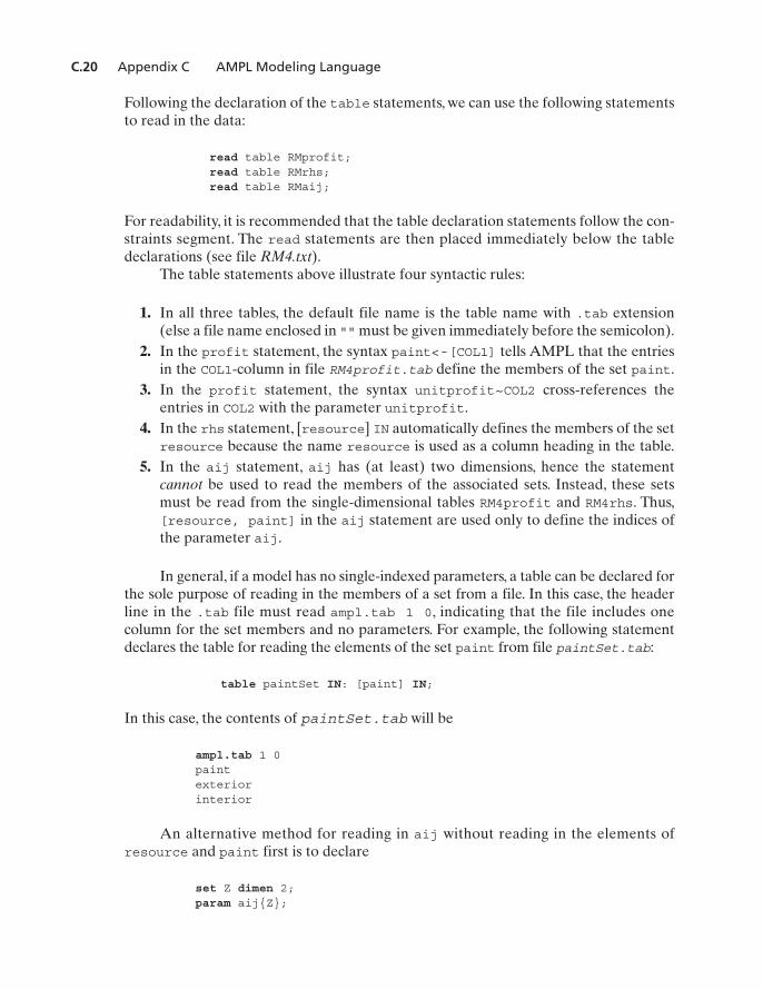
Following the declaration of the table statements, we can use the following statementsto read in the data:
read table RMprofit;read table RMrhs;read table RMaij;
For readability, it is recommended that the table declaration statements follow the con-straints segment. The read statements are then placed immediately below the tabledeclarations (see file RM4.txt).
The table statements above illustrate four syntactic rules:
1. In all three tables, the default file name is the table name with .tab extension(else a file name enclosed in "" must be given immediately before the semicolon).
2. In the profit statement, the syntax paint<-[COL1] tells AMPL that the entriesin the COL1-column in file RM4profit.tab define the members of the set paint.
3. In the profit statement, the syntax unitprofit~COL2 cross-references theentries in COL2 with the parameter unitprofit.
4. In the rhs statement, [resource] IN automatically defines the members of the setresource because the name resource is used as a column heading in the table.
5. In the aij statement, aij has (at least) two dimensions, hence the statementcannot be used to read the members of the associated sets. Instead, these setsmust be read from the single-dimensional tables RM4profit and RM4rhs. Thus,[resource, paint] in the aij statement are used only to define the indices ofthe parameter aij.
In general, if a model has no single-indexed parameters, a table can be declared forthe sole purpose of reading in the members of a set from a file. In this case, the headerline in the .tab file must read ampl.tab 1 0, indicating that the file includes onecolumn for the set members and no parameters. For example, the following statementdeclares the table for reading the elements of the set paint from file paintSet.tab:
table paintSet IN: [paint] IN;
In this case, the contents of paintSet.tab will be
ampl.tab 1 0paintexteriorinterior
An alternative method for reading in aij without reading in the elements ofresource and paint first is to declare
set Z dimen 2;param aij{Z};
Z03_TAHA5937_09_SE_APPC.QXD 7/24/10 3:45 AM Page C.20

C.5 Accessing External Files C.21
In this case, we can read in aij from table RM4aij in the following manner
table RM4aij IN: Z<-[resource, paint], aij;read table RM4aij;
Keep in mind that these statements do not define the elements of the setsresource and paint. To define the elements of the sets resource and paint
set resource=setof{(i, j) in Z} i;set paint=setoff{(i, j) in Z} j;
File RM4x.txt implements these ideas. It should be clear, however, that this is a convo-luted way for defining the sets resource and paint. The use of the two-dimensionalset Z as given above is advisable only if the sets resource and paint are not neededto define variables or parameters in the model. In such a case, we can use dummy setsX and Y to define the two-dimensional set z; that is,z<-[X, Y].
In some cases it may be convenient to read the data of a two-dimensionalparameter as an array in place of two indexed single elements, as given above foraij. AMPL allows this by changing the definition of the table to:
table RM4arrayAij IN:[i~resource], {j in paint}<aij[i, j]~(j)>;
(The new table definition is somewhat “overcoded” in the sense that ~(j) appearsredundant. Nevertheless, it gets the job done.) In this case, the file RM4arrayAij.tabmust appear as
ampl.tab 1 2resource exterior interiorm1 6 4m2 1 2demand -1 1market 0 1
Note that the header ampl.tab 1 2 indicates that table RM4arrayAij hasone key index (namely, [i~resource]) and two data columns with the headingsexterior and interior. The new table, RM4arrayAij, does not permit readingthe members of the sets resource and paint, the same restriction table RM4aijhas. (See file RM4.txt.)
C.5.4 Output table files
Table files may also receive output from AMPL after the solve command has beenexecuted. The syntax is similar to that of the input files, except that in the table decla-ration, IN is replaced with OUT. For example, in the Reddy Mikks model, suppose thatwe are interested in retrieving the following information:
1. Values of the variables and their reduced costs.2. Slack and dual values associated with the constraints.
Z03_TAHA5937_09_SE_APPC.QXD 7/24/10 3:45 AM Page C.21

C.22 Appendix C AMPL Modeling Language
This information requires the use of two tables because the two item are functions ofdistinct sets: paint and resource:
table varData OUT:[paint], product, product.rc;table conData OUT:
[resource], limit.slack~slack, limit.dual~Dual;
The OUT-table declaration statements should be placed after the constraints segmentto ensure that names of variables and constraints used in these statements havealready been defined (see file RM4.txt). The syntax limit.slack~slack andlimit.dual~Dual assign the descriptive header names slack and Dual to thecolumns where the corresponding data are written in the file. Otherwise, the defaultheader names will be limit.slack and limit.dual.
To retrieve the output, we need to issue the command solve and then follow itwith the following write statements:
write table varData;write table conData;
The output will be sent to files varData.tab and conData.tab, respectively. As withthe input case, we can override the default file name by entering (in double quotes) aspecific name (with .tab extension) following the keyword OUT and immediately beforethe colon.
Output tables can also be used to send two-dimensional arrays to a file. Forexample, either one of the following two definitions can be used to send the array aijto a .tab file:
table AijMatrix OUT: [resource, paint], aij;table Aijout OUT:{i in resource}->[RESOURCES], {j in paint}<aij[i, j]~(j)>;
In the first definition, file AijMatrix.tab lists each element of aij with its two indices onthe same row. In the second, file Aijout.tab lists aij in an array format, with the user-specified name RESOURCES being the heading of the first (key) column.
PROBLEM SET C.5C
*1. In RM4.txt, suppose the statements
read table RM4profit;read table RM4rhs;read table RM4aij;
are replaced with
read table RM4aij;data;param unitprofit:= exterior 5 interior 4;param rhs:=m1 24 m2 6 demand 1 market 2;
Z03_TAHA5937_09_SE_APPC.QXD 7/24/10 3:45 AM Page C.22

C.5 Accessing External Files C.23
Explain why AMPL will not execute properly with the proposed change. (Hint: The bestway to find out the answer is to experiment with the model.)
2. Suppose that the contents of file RM4rhs.tab read as
ampl.tab 1 1constrName Availabilitym1 24m2 6demand 1market 2
Make the necessary changes in RM4.txt, and execute the model.
C.5.5 Spreadsheet input/output tables
Accessing data from and sending data to a spreadsheet uses syntax similar to that of thetable files presented in Section C.5.4. The following statements show how the input data ofthe Reddy Mikks model can be accessed from an Excel spreadsheet file named RM5.xls:
table profitVector IN "ODBC" "RM5.xls":paint<-[COL1], unitprofit~COL2;table rhsVector IN "ODBC" "RM5.xls":[resource] IN, rhs;table aijMatrix IN "ODBC" "RM5.xls":[resource, paint], aij;
The user-generated names profitVector, rhsVector, and aijMatrix are those ofthe tables within the spreadsheet RM5.xls. These names define the ranges in thespreadsheet that correspond to the respective data tables.6 "ODBC" is the standarddata-handling interface for the spreadsheet. A read table then inputs the data to themodel (see file RM5.txt). Note the use of COL1 and COL2 in table profitVector,which correspond to the (arbitrary) column names in the spreadsheet.The syntax is thesame as in input tables (Section C.5.3). Each data table of the model may be stored ina separate sheet, if desired.
As in Section C.5.3, two-dimensional data can be read in an array format usingthe following table definition:
table aijArray IN "ODBC" "RM5.xls":[i~resource], {j in paint}<aij[i, j]~(j)>;
In this case, the array aij appears in the range aijArray of RM5.xls and must include theproper row and column headings. It is also important to remember that numeric columnheadings when used in the table must be converted to strings by using Excel TEXT function,else AMPL will issue some undecipherable error messages.
The same table declaration can be used to export output data to a spreadsheet.The only difference is to replace IN with OUT, exactly as in the case of table files. In thiscase, a write table command (following the solve command) will send the outputto the spreadsheet. The following examples demonstrate the use of OUT tables:
table variables OUT "ODBC" "RM5a.xls":
[paint], product~solution, product.rc~reducedCost;
6To name a range, highlight it and type its name in the “name box” to the left of the Excel formula bar, thenclick Enter, or use Excel’s Insert/Names/Define.
Z03_TAHA5937_09_SE_APPC.QXD 7/24/10 3:45 AM Page C.23

C.24 Appendix C AMPL Modeling Language
table constraints OUT "ODBC" "RM5a.xls":[resource], limit.slack~slack, limit.dual~dual;
The output tables variables and constraints will go to Excel file RM5a.xls follow-ing the execution of the write table command, each appearing automatically in thenorthwest corner of a separate sheet.
C.6 INTERACTIVE COMMANDS
AMPL allows the user to solve the model interactively and to check/modify data andretrieve output to the screen or to a file. The following is a partial list of a number ofuseful commands:
delete comma-separated names of objective function and constraints;drop comma-separated names of objective function and constraints;restore comma-separated names of objective function and constraints;display comma-separated item_list;print/printf unformatted/formatted item_list;expand comma-separated names of objective function and constraints;let parameter or variable (indexed or nonindexed):= value;fix variable (indexed or nonindexed):= value;unfix variable (indexed or noindexed);reset;
reset data;
solve;
Such commands are entered interactively at the ampl: prompt. Some, such as displayand print, may appropriately be hard-coded in the model, if desired.
The delete command completely removes the listed objective function and/orconstraints, whereas drop temporarily yanks them out of the model.The drop commandmay be annulled by the restore command. A new objective function or constraint maybe added to the model by entering it from the keyboard, exactly as we do in a hard-codedmodel. (See Example 9.2-1 for an application to the B&B algorithm.)
We have used display with the Reddy Mikks model.The output may be directedto an external file using filename immediately before the terminating semicolon. Else,the output defaults to the screen.
The print/printf command has been discussed earlier in Section C.5.2. Theoutput defaults to the screen, or it may be directed to an output file as in display.
The expand command provides a longhand representation of the objective functionand the constraints. For example, in the Reddy Mikks model, the command
expand profit;
prints out the objective function as
maximize profit:5*product["exterior"]+4*product["interior"];
7
Z03_TAHA5937_09_SE_APPC.QXD 7/24/10 3:45 AM Page C.24

C.6 Interactive Commands C.25
In this manner, the user can see if the model has retrieved the input data correctly. In asimilar manner, the command
expand limit;
will expand all the constraints of the model. If you are interested in a specific constraint,then limit must be properly indexed. For example,
expand limit["m1"];
will display the first constraint of the model.The let command allows entering new values of parameters and variables
(using : as assignment operator). The right-hand side may be a simple numericvalue or a mathematical expression. It is used to test different solution scenarios as wewill show in Section C.7.
The fix command is used to assign a specific value to a variable prior to solvingthe model. For example, suppose that the following statements are issued interactivelyprior to solving the Reddy Mikks model.
ampl: fix product["exterior"]:=1.5;ampl: solve;
With these commands, AMPL solves the problem with the added restrictionproduct["exterior"] .The change caused by fix can be undone by issuing theunfix command as
ampl: unfix product["exterior"];
The fix/unfix commands can be useful in experimenting with the model when someof the variables are either eliminated ( ) or held constant. (See AMPL momentfollowing Example 9.3-4 for an application to the traveling salesperson problem.)
The command reset removes all reference to the current model from AMPL.A fresh model command will thus be necessary to restart the model.Also, the commandreset data; will delete all the data of the model. Specific data elements may beselectively removed by listing them after the command. For example, reset data a bc; will delete the values of the parameters a, b, and c.
It is important to note that when two AMPL models are executed in the samesession, the command reset; must separate the execution of successive models. Forexample, the two AMPL models a1.txt and a2.txt are executed as follows:
ampl: model a1.txt;ampl: reset; model a2.txt;
If reset; is not used, AMPL will spew an enormous list of undecipherable errors.There is a large number of useful interactive commands in AMP, but their detailed
presentation is beyond the scope of this abridged presentation.
= 0
= 1.5
=
Z03_TAHA5937_09_SE_APPC.QXD 7/24/10 3:45 AM Page C.25

C.26 Appendix C AMPL Modeling Language
C.7 ITERATIVE AND CONDITIONAL EXECUTION OF AMPL COMMANDS
Suppose in the Reddy Mikks model we are interested in studying the sensitivity of theoptimal solution to changes in specific parameters. For example, in file RM2.txt, how isthe optimal solution affected when the availability of raw material m1 (=rhs["m1"]) ischanged from its current value of 24 tons to the new values of 27 and 30 tons? Afterexecuting RM2.txt and getting the solution for rhs["m1"]=24, we can enter the followingstatements interactively:
ampl: let rhs["m1"]:=27;ampl: solve;ampl: display profit, product;
The output will be displayed on the screen (it can also be sent to a file, if desired, as weexplained earlier). To secure results for rhs["m1"]=30, the same statements arerepeated with the let statement specifying the new value. This, however, is not themost efficient way to do the task.
AMPL allows building convenient commands files that will eliminate the unneces-sary chore of retyping commands. Specifically, for the present example, a command file(which we arbitrarily name cmd.txt) may have the following statements:
for (i in 1..2}{let rhs["m1"]:=rhs["m1"]+3;solve;display profit, product;}
Following the execution of the model (with rhs["m1"]=24), we can execute theremaining two cases by entering
ampl: commands cmd.txt;
Of course,we can modify cmd.txt to include rhs["m1"]=24 as well.See Problem 1,Set C.7a.We can use the statement repeat while condition{...}; or repeat until
condition{...}; to replace for{...} as follows:
repeat while rhs["m1"]<=30{let rhs["m1"]:=rhs["m1"] +3;solve;display profit, product;};
Alternatively, we may use
repeat until rhs["m1"]>30{let rhs["m1"]:=rhs["m1"]+3;
Z03_TAHA5937_09_SE_APPC.QXD 7/24/10 3:45 AM Page C.26

C.8 Sensitivity Analysis Using AMPL C.27
solve;display profit, rhs["m1"], product;};
Note that repeat while will loop so long as the condition is true, whereas repeat untilwill loop so long as the condition is false.
Another useful statement in commands file is if-then-else. In this case,if maybe followed by any legitimate condition, whereas then and else can be followed onlyby command statements. With the if statement, AMPL commands continue; andbreak; may be used within the loop construct to either skip to the next index of theloop or exit the loop altogether.
Example 9.3-5 (Figure 9.14) provides a good illustration of the use of the loopand conditional statements to print formatted output.
PROBLEM SET C.7A
1. Modify RM2.txt so that rhs["m1"] will assume the values 20 to 35 tons in steps of 5 tons.All solve commands must be executed from within the command file cmd.txt in thefollowing manner:
ampl: model RM2.txt;ampl: commands cmd.txt;
The command file cmd.txt is developed using the three different versions to construct the loop:
(a) for{}.(b) repeat while{};.(c) repeat until{};.
C.8 SENSITIVITY ANALYSIS USING AMPL
We have seen previously how the dual values and the reduced costs can be determinedin an AMPL LP model by using the ConstraintName .dual and VariableName .rc inthe display command.To complete the standard LP sensitivity analysis report,AMPLadditionally provides facilities for the determination of the optimality ranges for theobjective-function coefficients and the feasibility ranges for the (constant) right-handsides of the constraints. We will use file RM2.txt (see Figure C.3) to demonstrate howAMPL generates the sensitivity analysis report.
In the model in Figure C.3, replace the solve and display statements with
option solver cplex;option cplex_options ’sensitivity’;solve;display limit.down, limit.current, limit.up, limit.dual;display product.down, product.current, product.up, product.rc;
The output can be directed to a file if desired (see file RM6.txt). The two option state-ments must precede the solve command. The first display command provides the
Z03_TAHA5937_09_SE_APPC.QXD 7/24/10 3:45 AM Page C.27
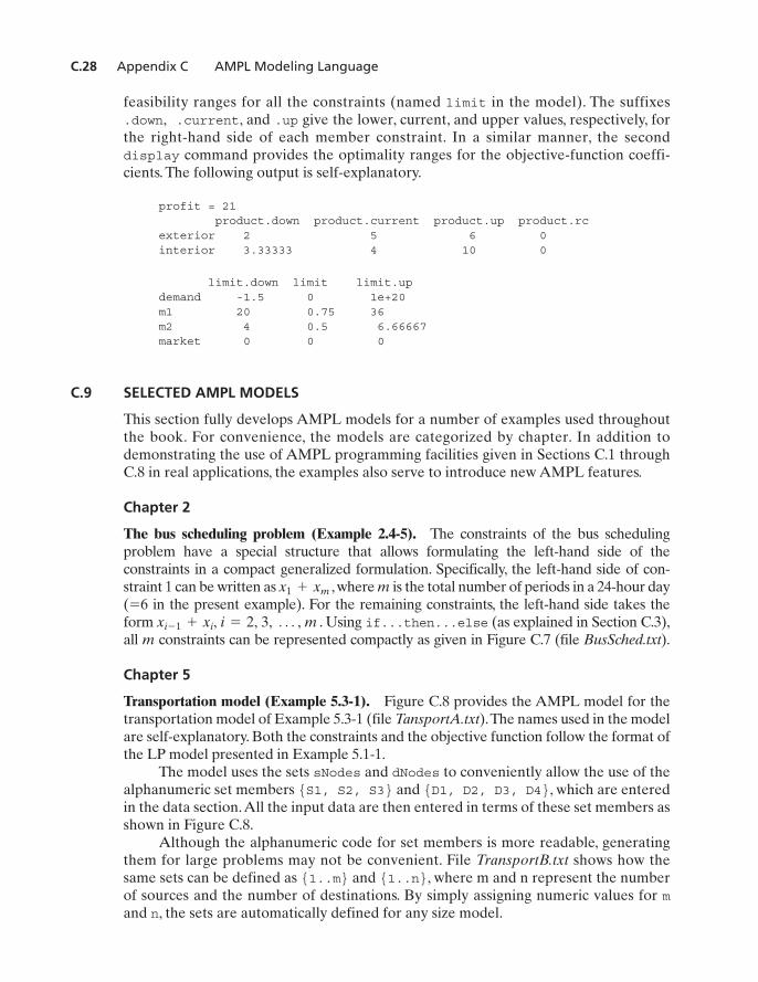
C.28 Appendix C AMPL Modeling Language
feasibility ranges for all the constraints (named limit in the model). The suffixes.down, .current, and .up give the lower, current, and upper values, respectively, forthe right-hand side of each member constraint. In a similar manner, the seconddisplay command provides the optimality ranges for the objective-function coeffi-cients. The following output is self-explanatory.
profit = 21product.down product.current product.up product.rc
exterior 2 5 6 0interior 3.33333 4 10 0
limit.down limit limit.updemand -1.5 0 1e+20m1 20 0.75 36m2 4 0.5 6.66667market 0 0 0
C.9 SELECTED AMPL MODELS
This section fully develops AMPL models for a number of examples used throughoutthe book. For convenience, the models are categorized by chapter. In addition todemonstrating the use of AMPL programming facilities given in Sections C.1 throughC.8 in real applications, the examples also serve to introduce new AMPL features.
Chapter 2
The bus scheduling problem (Example 2.4-5). The constraints of the bus schedulingproblem have a special structure that allows formulating the left-hand side of theconstraints in a compact generalized formulation. Specifically, the left-hand side of con-straint 1 can be written as ,where is the total number of periods in a 24-hour day( in the present example). For the remaining constraints, the left-hand side takes theform . Using if...then...else (as explained in Section C.3),all constraints can be represented compactly as given in Figure C.7 (file BusSched.txt).
Chapter 5
Transportation model (Example 5.3-1). Figure C.8 provides the AMPL model for thetransportation model of Example 5.3-1 (file TansportA.txt).The names used in the modelare self-explanatory. Both the constraints and the objective function follow the format ofthe LP model presented in Example 5.1-1.
The model uses the sets sNodes and dNodes to conveniently allow the use of thealphanumeric set members {S1, S2, S3} and {D1, D2, D3, D4}, which are enteredin the data section.All the input data are then entered in terms of these set members asshown in Figure C.8.
Although the alphanumeric code for set members is more readable, generatingthem for large problems may not be convenient. File TransportB.txt shows how thesame sets can be defined as {1..m} and {1..n}, where m and n represent the numberof sources and the number of destinations. By simply assigning numeric values for mand n, the sets are automatically defined for any size model.
mxi - 1 + xi, i = 2, 3, Á , m
=6mx1 + xm
Z03_TAHA5937_09_SE_APPC.QXD 7/24/10 3:45 AM Page C.28

C.9 Selected AMPL Models C.29
FIGURE C.7
AMPL model of the bus scheduling problem of Example 2.4-5 (file BusSched.txt)
param m;param min_nbr_buses{1..m};var x_nbr_buses{1..m} >= 0;minimize tot_nbr_buses: sum {i in 1..m} x_nbr_buses[i];subject to constr_nbr{i in 1..m}:
if i=1 thenx_nbr_buses[i]+x_nbr_buses[m]
elsex_nbr_buses[i-1]+x_nbr_buses[i] >= min_nbr_buses[i];
data;param m:=6;param min_nbr_buses:= 1 4 2 8 3 10 4 7 5 12 6 4;
solve;display tot_nbr_buses, x_nbr_buses;
FIGURE C.8
AMPL model of the transportation model of Example 5.3-1 (File TransportA.txt)
#----- Transporation model (Example 5.3-1)-----set sNodes;set dNodes;param c{sNodes,dNodes};param supply{sNodes};param demand{dNodes};var x{sNodes,dNodes}>=0;minimize z:sum {i in sNodes,j indNodes}c[i,j]*x[i,j];subject tosource{i in sNodes}:sum{j in dNodes}x[i,j]=supply[i];dest{j in dNodes}:sum{i in sNodes}x[i,j]=demand[j];data;set sNodes:=S1 S2 S3;set dNodes:=D1 D2 D3 D4;param c:D1 D2 D3 D4 :=S1 10 2 20 11S2 12 7 9 20S3 4 14 16 18;param supply:= S1 15 S2 25 S3 10;param demand:= D1 5 D2 15 D3 15 D4 15;solve;display z, x;
Z03_TAHA5937_09_SE_APPC.QXD 7/24/10 3:45 AM Page C.29

C.30 Appendix C AMPL Modeling Language
The data of the transportation model can be retrieved from a spreadsheet (fileTM.xls) using the AMPL table statement. File TansportC.txt provides the details. Tostudy this model, you will need to review the material in Section C.5.5.
Chapter 6
Figure C.9 provides the AMPL model for solving Example 6.3-6 (file ShortestRouteA.txt).The variable x[i, j] assumes the value 1 if arc [i, j] is on the shortest route and 0otherwise. The model is general in the sense that it can be used to find the shortest routebetween any two nodes in a problem of any size.
As explained in Example 6.3-6, AMPL treats the problem as a network in whichan external flow unit enters and exits at specified start and end nodes.The main input
FIGURE C.9
AMPL shortest route model (file ShortestRouteA.txt)
#--------- shortest route model (Example 6.3-6)---------param n;param start;param end;param M=999999; #infinityparam d{i in 1..n, j in 1..n} default M;param rhs{i in 1..n}=if i=start then 1
else (if i=end then -1 else 0);var x{i in 1..n,j in 1..n}>=0;var outFlow{i in 1..n}=sum{j in 1..n}x[i,j];var inFlow{j in 1..n}=sum{i in 1..n}x[i,j];
minimize z: sum{i in 1..n, j in 1..n}d[i,j]*x[i,j];subject to limit{i in 1..n}:outFlow[i]-inFlow[i]=rhs[i];
data;param n:=5;param start:=1;param end:=2;param d:
1 2 3 4 5:=1 . 100 30 . .2 . . 20 . .3 . . . 10 604 . 15 . . 505 . . . . .;solve;print "Shortest length from",start,"to",end,"=",z;printf "Associated route: %2i",start;for {i in 1..n-1} for {j in 2..n}{if x[i,j]=1 then printf" - %2i",j;} print;
Z03_TAHA5937_09_SE_APPC.QXD 7/24/10 3:45 AM Page C.30

C.9 Selected AMPL Models C.31
data of the model is an matrix representing the distance d[i, j] of the arc join-ing nodes i and j. Per AMPL syntax, a dot entry in d[i, j] is a placeholder thatsignifies that no distance is specified for the corresponding arc. In the model, the dotentry is overridden by the infinite distance M ( ) in
param d{i in 1..n, j in 1..n}default M;
The constraints represent flow conservation through each node:
From x[i, j], we can define the input and output flow for node using the statements
var inFlow{j in 1..n}=sum{i in 1..n}x[i, j];var outFlow{i in 1..n}=sum{j in 1..n}x[i, j];
The left-hand side of the constraint is thus given as outFlow[i]-inFlow[i].The right-hand side of constraint (external flow at node ) is defined as
param rhs{i in 1..n}=if i=start then 1 else(if i=end then -1 else 0);
(See Section C.3 for details of if...then...else.) With this statement, specifyingstart and end nodes automatically assigns 1, -1, or 0 to rhs, the right-hand sideof the constraints. This statement allows finding the shortest distance between any twonodes in the network.
The objective function seeks the minimization of the sum of d[i, j]*x[i, j]overall i and j.
In the present example, start=1 and end=2, meaning that we want to determinethe shortest route from node 1 to node 2. The associated output is
Shortest length from 1 to 2 =55Associated route: 1 - 3 - 4 - 2
Remarks. The AMPL model as given in Figure C.9 has one flaw: The number ofactive variables is , which could be significantly much larger than the actual num-ber of (positive-distance) arcs in the network, thus resulting in a much larger LP. Thereason is that the model accounts for the nonexisting arcs by assigning them an infinitedistance M ( ) to guarantee that they will be zero in the optimum solution.
The situation can be remedied by using a subset of {i in 1..n, j in 1..n}
that excludes nonexisiting arcs, as the following statement shows:
var x{i in 1..n, j in 1..n:d[i, j]<M}>=0;
(See Section C.4 for the use of conditions to define subsets.) The same logic must beapplied to the constraints as well by using the following statements:
var inFlow{j in 1..n}=sum{i in 1..n:d[i, j]<M}x[i, j];var outFlow{i in 1..n}=sum{j in 1..n:d[i, j]<M}x[i, j];
File ShortestRouteB.txt gives the complete model.
= 999999
n2xij
iii
i
(Input flow) - (Output flow) = (External flow)
= 999999
n * n
Z03_TAHA5937_09_SE_APPC.QXD 7/24/10 3:45 AM Page C.31

C.32 Appendix C AMPL Modeling Language
Maximal flow model (Example 6.4-2). Figure C.10 provides the AMPL model for themaximal flow problem.The data applies to Example 6.4-2 (file MaxFlow.txt).The overallidea of determining the input and output flows at a node is similar to the one detailed forthe shortest-route model. However, because the model is designed to find the maximumflow between any two nodes, start and end, two additional constraints are needed toensure that no external flow enters start and no external flow leaves end. ConstraintsinStart and outEnd in the model ensure this result. These two constraints are notneeded when start=1 and end=5 because the nature of the data guarantees the desired
FIGURE C.10
AMPL model of the maximal flow problem of Example 6.4-2 (file MaxFlow.txt)
#---------- Maximal Flow model (Example 6.4-2)----------param n;param start;param end;param c{i in 1..n, j in 1..n} default 0;
var x{i in 1..n,j in 1..n:c[i,j]>0}>=0,<=c[i,j];var outFlow{i in 1..n}=sum{j in 1..n:c[i,j]>0}x[i,j];var inFlow{i in 1..n}=sum{j in 1..n:c[j,i]>0}x[j,i];
maximize z: sum {j in 1..n:c[start,j]>0}x[start,j];subject tolimit{i in 1..n:
i<>start and i<>end}:outFlow[i]-inFlow[i]=0;inStart:sum{i in 1..n:c[i,start]>0}x[i,start]=0;outEnd:sum{j in 1..n:c[end,j]>0}x[end,j]=0;
data;param n:=5;param start:=1;param end:=5;param c:
1 2 3 4 5 :=1 . 20 30 10 02 . . 40 0 303 . . 0 10 204 . . 5 . 205 . . . . .;
solve;print "MaxFlow between nodes",start,"and",end, "=",z;printf "Associated flows:\n";for {i in 1..n-1} for {j in 2..n:c[i,j]>0}
{if x[i,j]>0 thenprintf"(%2i-%2i)=%5.2f\n",i,j,x[i,j];} print;
Z03_TAHA5937_09_SE_APPC.QXD 7/24/10 3:45 AM Page C.32

C.9 Selected AMPL Models C.33
result. However, for start =3, node 3 allows both input and output flow (arcs 4-3 and3-4) and, hence, constraint inStart is needed (try the model without inStart!).
The objective function maximizes the sum of the output flow at node start.Equivalently, we can choose to maximize the sum of the input flow at node end.
CPM model (Example 6.5-2). Figure C.11 provides the AMPL model for any CPMnetwork (file CPM.txt).The model is driven by the data of Example 6.5-2. It makes use
FIGURE C.11
------------------------ CPM (Example 6.5-2)------------------------param n;param D{1..n,1..n} default -1;set into{1..n};set from{1..n};var x{i in 1..n,j in from[i]}>=0;var ET{i in 1..n};var LT{i in 1..n};var TF{i in 1..n, j in from[i]};var FF{i in 1..n, j in from[i]};data;param n:=6;param D: 1 2 3 4 5 6:=1 . 5 6 . . .2 . . . 3 8 .3 . . . . 2 114 . . . . 0 15 . . . . . 126 . . . . . .;for {i in 1..n} {let from[i]:={j in 1..n:D[i,j]>=0}};for {j in 1..n} {let into[j]:={i in 1..n:D[i,j]>=0}};------------nodes earliest and latest times and floatslet ET[1]:=0; #earliest node timefor {i in 2..n}let ET[i]:=max{j in into[i]}(ET[j]+D[j,i]);let LT[n]:=ET[n]; #latest node timefor {i in n-1..1 by -1}let LT[i]:=min{j in from[i]}(LT[j]-D[i,j]);printf "%1s-%1s %5s %5s %5s %5s %5s %5s %5s \n\n",
"i","j","D","ES","EC","LS","LC","TF","FF" >Ex6.6-2out.txt;for {i in 1..n, j in from[i]}{let TF[i,j]:=LT[j]-ET[i]-D[i,j];let FF[i,j]:=ET[j]-ET[i]-D[i,j];printf "%1i-%1i %5i %5i %5i %5i %5i %5i %5i %3s\n",
i,j,D[i,j],ET[i],ET[i]+D[i,j],LT[j]-D[i,j],LT[j],TF[i,j],FF[i,j],if TF[i,j]=0 then "c" else "" >Ex6.6-2out.txt;
}
AMPL model for Example 6.6-2 (file CPM.txt)
Z03_TAHA5937_09_SE_APPC.QXD 7/24/10 3:45 AM Page C.33

C.34 Appendix C AMPL Modeling Language
of indexed sets (see Section C.4) and requires no optimization. In essence, no solvecommand is needed, and AMPL is implemented as a pure programming languagesimilar to Basic or C.
The nature of the computations in CPM requires representing the network byassociating two indexed sets with each node: into and from. For node i, the setinto[i] defines all the input nodes that feed into node i, and the set from[i] definesall the output nodes that are reached from node i (recall that in CPM all the arcs aredirectional, hence it makes sense to speak of input and output nodes). For example, inExample 6.5-2, from[1]={2, 3}, and into[1] is empty.
The determination of subsets from and into is achieved in the model as follows:Because D[i, j] can be zero when a CPM network uses dummy activities, the defaultvalue for D[i, j] is -1 for all nonexisting arcs. Thus, the set from[i] represents all thenodes j in the set {1..n} that can be reached from node i, which can happen only ifD[i, j]>=0.This says that from[i] is defined by the subset {j in 1..n:D[i, j]>=0}.Similar reasoning applies to the determination of subsets into[i].The following AMPLstatements automate the determination of these sets and must follow the D[i, j] data,as shown in Figure 6.48:
for {i in 1..n} {let from[i]:={j in 1..n:D[i, j]>=0}};for {j in 1..n} {let into[j]:={i in 1..n:D[i, j]>=0}};
Once the sets from and into have been determined, the model goes through theforward pass to compute the earliest time, ET[i]. With the completion of this pass, wecan initiate the backward pass by using
let LT[n]:=ET[n];
The rest of the model is needed to obtain the output shown in Figure C.12. This outputdetermines all the data needed to construct the CPM chart.The logic of this segment isbased on the computations given in Examples 6.5-2 and 6.5-4.
FIGURE C.12
Output of AMPL model for Example 6.5-2 (file CPM.txt)
i-j D ES EC LS LC TF FF1-2 5 0 5 0 5 0 0 c1-3 6 0 6 5 11 5 22-3 3 5 8 8 11 3 02-4 8 5 13 5 13 0 0 c3-5 2 8 10 11 13 3 33-6 11 8 19 14 25 6 64-5 0 13 13 13 13 0 0 c4-6 1 13 14 24 25 11 115-6 12 13 25 13 25 0 0 c
Z03_TAHA5937_09_SE_APPC.QXD 7/24/10 3:45 AM Page C.34
C.9 Selected AMPL Models C.35
Chapter 8
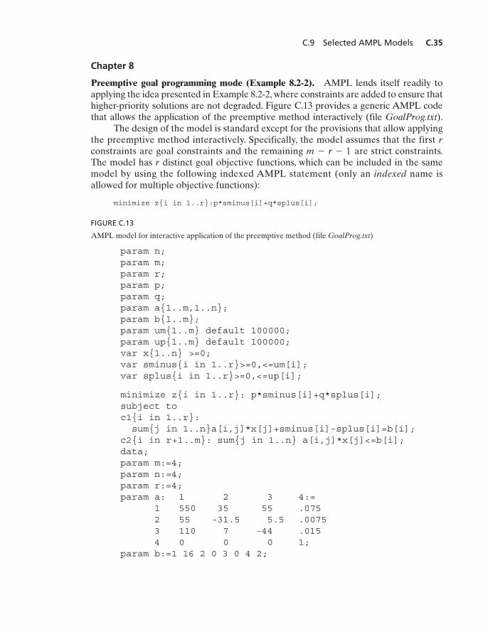
Preemptive goal programming mode (Example 8.2-2). AMPL lends itself readily toapplying the idea presented in Example 8.2-2, where constraints are added to ensure thathigher-priority solutions are not degraded. Figure C.13 provides a generic AMPL codethat allows the application of the preemptive method interactively (file GoalProg.txt).
The design of the model is standard except for the provisions that allow applyingthe preemptive method interactively. Specifically, the model assumes that the first constraints are goal constraints and the remaining are strict constraints.The model has distinct goal objective functions, which can be included in the samemodel by using the following indexed AMPL statement (only an indexed name isallowed for multiple objective functions):
minimize z{i in 1..r}:p*sminus[i]+q*splus[i];
rm - r - 1
r
FIGURE C.13
AMPL model for interactive application of the preemptive method (file GoalProg.txt)
param n;param m;param r;param p;param q;param a{1..m,1..n};param b{1..m};param um{1..m} default 100000;param up{1..m} default 100000;var x{1..n} >=0;var sminus{i in 1..r}>=0,<=um[i];var splus{i in 1..r}>=0,<=up[i];
minimize z{i in 1..r}: p*sminus[i]+q*splus[i];subject toc1{i in 1..r}:sum{j in 1..n}a[i,j]*x[j]+sminus[i]-splus[i]=b[i];
c2{i in r+1..m}: sum{j in 1..n} a[i,j]*x[j]<=b[i];data;param m:=4;param n:=4;param r:=4;param a: 1 2 3 4:=
1 550 35 55 .0752 55 -31.5 5.5 .00753 110 7 -44 .0154 0 0 0 1;
param b:=1 16 2 0 3 0 4 2;
Z03_TAHA5937_09_SE_APPC.QXD 7/24/10 3:45 AM Page C.35
C.36 Appendix C AMPL Modeling Language
The given definition of the objective function accounts for minimizing and by setting ( , ) and ( , ), respectively.
Instead of adding a new constraint each time we move from one prioritylevel to the next, we use a programming trick that allows modifying the upperbounds on the deviational variables.The parameters um[i] and up[i] representthe upper bounds on sminus[i] ( ) and splus[i] ( ), respectively.These parameters are modified to impose implicit constraints of the typessminus[i]<=um[i] and splus[i]<=up[i], respectively. The values of um andup in priority goal are determined from the solutions of the problems ofpriority goals 1, 2, and .The initial (default) value for um and up is infinity.
We will show shortly how AMPL activates any of the r objective func-tions, specifies the values of p and q, and sets the upper limits on and , allinteractively, which makes AMPL ideal for carrying out goal programmingcomputations.
Using the data of Example 8.1-1, the goals of the model are
Suppose that the goals are prioritized as
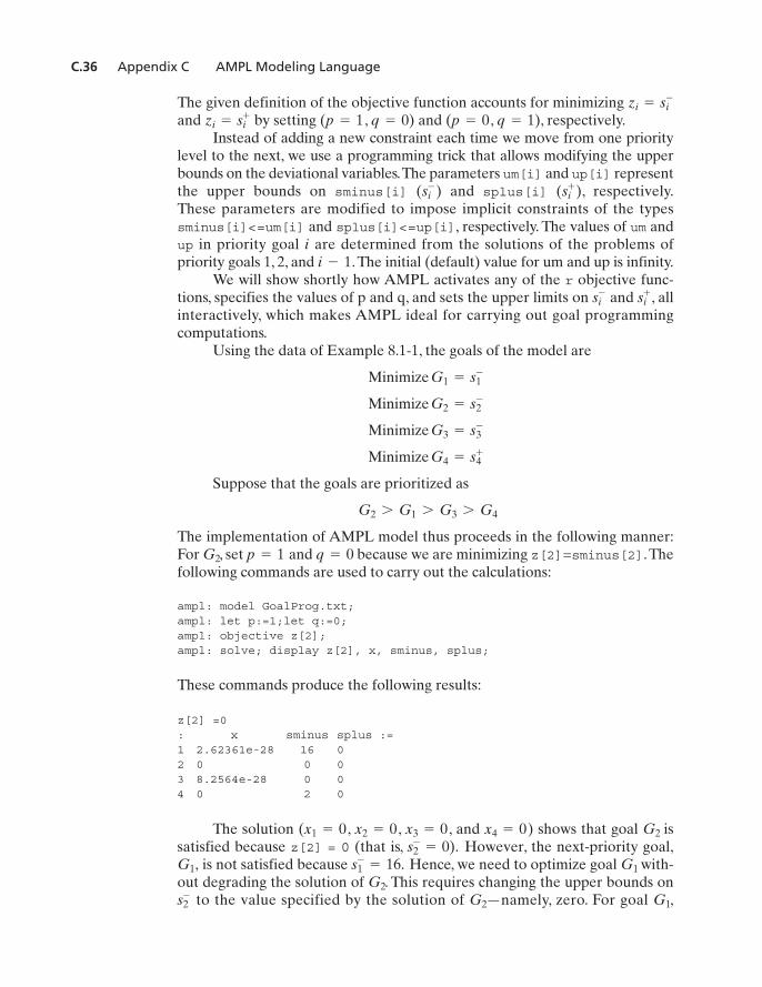
The implementation of AMPL model thus proceeds in the following manner:For , set and because we are minimizing z[2]=sminus[2].Thefollowing commands are used to carry out the calculations:
ampl: model GoalProg.txt;ampl: let p:=1;let q:=0;ampl: objective z[2];ampl: solve; display z[2], x, sminus, splus;
These commands produce the following results:
z[2] =0: x sminus splus :=1 2.62361e-28 16 02 0 0 03 8.2564e-28 0 04 0 2 0
The solution ( , , , and ) shows that goal issatisfied because z[2] = 0 (that is, However, the next-priority goal,
is not satisfied because Hence, we need to optimize goal with-out degrading the solution of . This requires changing the upper bounds on
to the value specified by the solution of —namely, zero. For goal ,G1G2s2-
G2
G1s1-
= 16.G1,s2
-
= 0).G2x4 = 0x3 = 0x2 = 0x1 = 0
q = 0p = 1G2
G2 7 G1 7 G3 7 G4
Minimize G4 = s4+
Minimize G3 = s3-
Minimize G2 = s2-
Minimize G1 = s1-
si+si
-
i - 1i
si+si
-
q = 1p = 0q = 0p = 1zi = si+
zi = si-
Z03_TAHA5937_09_SE_APPC.QXD 7/24/10 3:45 AM Page C.36

C.9 Selected AMPL Models C.37
current and from remain unchanged because we are minimizing The following interactive AMPL commands achieve this result:
ampl: let um[2]:=0;ampl: objective z[1]; solve; display z[1], x, sminus, splus;
The ouput is
z[1] =0: x sminus splus :=1 0.0203636 0 02 0.0457143 0 03 0.0581818 0 04 0 2 0
The solution shows that all the remaining goals are satisfied. Hence, no furtheroptimization is needed.The goal programming solution is , ,
, and .
Remarks.
1. We can replace let um[2]:=0; with either fix sminus[2]:=0; or let
sminus[2]:=0; with equal end result.2. The interactive session can be totally automated using a commands file that
automatically selects the current goal to be optimized and imposes the properrestrictions before solving the next priority goal. The use of this file (namedamplCmds.txt) requires making some modifications in the original model asshown in file GolaProgA.txt. To be completely versatile, the data of the modelare stored in a separate file named amplData.txt. In this case, the execution of themodel requires issuing two command lines:
ampl: model amplEx8.1-1A.txt;ampl: data amplData.txt;ampl: commands amplCmds.txt;
See Section C.7 for more information about the use of commands.
Chapter 9
Set covering model (Example 9.1-2). Figure C.14 presents a general AMPL model forany set-covering problem (file SetCovering.txt). The formulation is straightforward,once the use of indexed set is understood (see Section C.4).The model defines street asa (regular) set whose elements are A through K. Next, the indexed set corner{street}defines the corners as a function of street. With these two sets, the constraints of themodel can be formulated directly. The data of the model give the elements of theindexed sets that are specific to the situation in Example 9.1-2. Any other situation ishandled by changing the data of the model.
xg = 0xs = .0581818xf = .0457143xp = .0203636
s1-.G2q = 0p = 1
Z03_TAHA5937_09_SE_APPC.QXD 7/24/10 3:45 AM Page C.37

C.38 Appendix C AMPL Modeling Language
Job sequencing model (Example 9.1-4). File JobSeq.txt provides the AMPL modelfor the problem of Example 9.1-4.The model in Figure C.15 is self-explanatory becauseit is a direct translation of the general mathematical model. It can handle any numberof jobs by changing the input data. Note that the model is a direct function of the rawdata: processing time p, due date d, and delay penalty perDayPenalty.
Chapter 13
General multi-item EOQ (Example 13.3-3). The AMPL nonlinear model for the gen-eral multi-item EOQ with storage limitation is given in Figure C.16 (file ConstrEOQ.txt).The model follows the same rules used in solving linear programs. However, AMPLnonlinear models exhibit peculiarities that may impede reaching a solution. In particular,“judicious” initial values must be specified for the variables. In Figure C.16, the definitionstatement
var y{1..n}>=0, :=10; #initial trial value = 10;
FIGURE C.14
General AMPL model for the set covering problem of Example 9.1-2 (file SetCovering.txt)
#------------------ Example 9.1-2------------------param n; #maximum number of cornersset street;set corner{street};var x{1..n}binary;minimize z: sum {j in 1..n} x[j];subject to limit {i in street}:
sum {j in corner[i]} x[j]>=1;data;param n:=8;set street:=A B C D E F G H I J K;set corner[A]:=1 2;set corner[B]:=2 3;set corner[C]:=4 5;set corner[D]:=7 8;set corner[E]:=6 7;set corner[F]:=2 6;set corner[G]:=1 6;set corner[H]:=4 7;set corner[I]:=2 4;set corner[J]:=5 8;set corner[K]:=3 5;
option solver cplex;solve;display z,x;
Z03_TAHA5937_09_SE_APPC.QXD 7/24/10 3:45 AM Page C.38

C.9 Selected AMPL Models C.39
includes the code :=10 that assigns the initial value 10 to all the variables. If you use aninitial value of 1 in the present example, division by zero will result during the itera-tions. Thus, you may need to replace and very small,to prevent division by zero during the iterative process. Indeed, Problems 1 and 4,Set 13.3c, could not be solved with AMPL without invoking this trick.
Chapter 21
Modeling nonlinear problems (Example 21.2-2). Figure C.17 gives the AMPL model(file NLP.txt).The only deviation from LP (other than the nonlinearity, of course) is thatyou may need to specify “appropriate” initial values for the variables to get the solutioniteration to converge. In Figure C.17, the arbitrary initial values and arespecified by appending :=10 and :=10 to the definition of the two variables. If you donot specify initial values at all,AMPL will not reach the optimum solution and will printthe message “too many major iterations.” Although a solution is given in this case, it
x2 = 10x1 = 10
KiDi/yi with KiDi/(yi + ¢), ¢ 7 0
FIGURE C.15
AMPL model of the job sequencing problem of Example 9.1-4 (file JobSeq.txt)
#------------------ Example 9.1-4------------------param n;set I={1..n};set J={1..n}; #I is the same as Jparam p{I};param d{I};param perDayPenalty{I};param M=1000;var x{J}>=0; #continuousvar y{I,J} binary; #0-1var sMinus{J}>=0; # s=sMinus-sPlusvar sPlus{J}>=0;minimize penalty: sum {j in J}
perDayPenalty[j]*sPlus[j];subject toeitherOr1{i in I,j in J:i<>j}:
M*y[i,j]+x[i]-x[j]>=p[j];eitherOr2{i in I,j in J:i<>j}:
M*(1-y[i,j])+x[j]-x[i]>=p[i];dueDate{j in J}:x[j]+sMinus[j]-sPlus[j]=d[j]-p[j];data;param n:=3;param p:= 1 5 2 20 3 15;param d:= 1 25 2 22 3 35;param perDayPenalty := 1 19 2 12 3 34;option solver cplex; solve;display penalty,x;
Z03_TAHA5937_09_SE_APPC.QXD 7/24/10 3:45 AM Page C.39

C.40 Appendix C AMPL Modeling Language
usually is not correct. In essence, the most logical way to deal with a nonlinear problemis to specify different initial values for the variables and then decide if a consensus canbe reached regarding the optimum solution.
BIBLIOGRAPHY
Fourer, R., D. Gay, and B. Kernighan, AMPL, A Modeling Language for MathematicalProgramming, 2nd ed., Brooks/Cole-Thomson, Pacific Grove, CA, 2003.
FIGURE C.16
AMPL model for Example 13.3-3 (file ConstrEOQ.txt)
param n;param K{1..n};param D{1..n};param h{1..n};param a{1..n};param A;var y{1..n}>=0, :=10; #initial trial value = 10minimize z: sum{j in 1..n}(K[j]*D[j]/y[j]+h[j]*y[j]/2);subject to storage:sum{j in 1..n}a[j]*y[j]<=A;data;param n:=3;param K:= 1 10 2 5 3 15;param D:=1 2 2 4 3 4;param h:=1 .3 2 .1 3 .2;param a:=1 1 2 1 3 1;param A:=25;solve;display z,y;printf{"SOLUTION:\n"}>a.out;printf{" Total cost = %4.2\n"},z>a.out;for {i in 1..n}
printf{" y%1i = %4.2f\n"},i,y[i]>a.out;
FIGURE C.17
AMPL model of Example 21.2-2 (fileNLP.txt)
var x1>=0 :=10; #inital value = 10var x2>=0 :=10; #initial value = 10
maximize z: x1-x2;subject to c1: 3*x1^4+x2<=243;subject to c2: x1+2*x2^2<=32;subject to c3: x1>=2.1;subject to c4: x2>=3.5;
solve;display z,x1,x2;
Z03_TAHA5937_09_SE_APPC.QXD 7/24/10 3:45 AM Page C.40