Amphibian assemblages in zero-order basins in the Oregon ...andrewsforest.oregonstate.edu/pubs/pdf/pub3099.pdf · Amphibian assemblages in zero-order basins in the Oregon Coast Range1

Amphibian assemblages in zero-order basins inthe Oregon Coast Range1

Chris D. Sheridan and Deanna H. Olson

Abstract: Zero-order basins, extending from ridgelines to the initiation of first-order streams, were sampled in theCoast Range of Oregon to (i) characterize spatial distribution patterns of amphibian species and assemblages along lon-gitudinal and lateral gradients, and relative to three geomorphic surfaces (valleys, headmost areas, and slopes); and(ii) develop empirical species–habitat models. Unmanaged zero-order basins were hotspots for amphibian diversity, withsignificant differences across geomorphic gradients. Captures of riparian-associated amphibians were higher in valleyareas, usually within 2 m of basin center. Upland-associated amphibians were captured two times farther from basincenters than riparian-associated species, but highest densities occurred only 2–5 m from basin center. The most usefulempirical models related captures of individual amphibian species to geomorphic, disturbance, moisture, and overstoryvariables. Ordination and indicator species analysis characterized geomorphic and other environmental gradients in am-phibian assemblages and suggested spatial compression of fluvial habitats and riparian-associated species in zero-orderbasins, in comparison with downstream areas. Our findings have implications for headwater areas managed to hedgerisk to and uncertainty in amphibian persistence, namely in the delineation of zones with species management priority,and in the maintenance of natural fluvial and hillslope disturbance regimes, along with the microhabitat features cre-ated by these regimes.

Résumé : Des bassins d’ordre zéro, s’étendant des lignes de crête jusqu’à l’origine des ruisseaux de premier ordre, ontété échantillonnés dans la chaîne côtière de l’Oregon pour (i) caractériser les patrons de répartition spatiale des espèceset des assemblages d’amphibiens le long de gradients longitudinaux et latéraux et en regard de trois entités géomorpho-logiques (vallées, sommets et versants); et (ii) développer des modèles empiriques espèces–habitats. Les bassins d’ordrezéro non aménagés étaient des points chauds pour la diversité des amphibiens, avec des différences significatives entreles gradients géomorphologiques. Les captures d’amphibiens associés au milieu riverain ont été plus nombreuses dansles vallées, habituellement à moins de 2 m du centre du bassin. Les amphibiens associés aux milieux non riverains ontété capturés deux fois plus loin du centre des bassins que les espèces riveraines, mais c’est seulement à 2–5 m ducentre des bassins que leur densité était la plus forte. Les modèles empiriques les plus utiles sont ceux qui mettent enrelation les espèces individuelles d’amphibiens avec les variables géomorphologiques, les perturbations, l’humidité et lavoûte forestière. L’ordination et l’analyse d’espèces indicatrices ont fait ressortir des gradients d’assemblagesd’amphibiens selon la géomorphologie et d’autres variables environnementales et elles montrent une compression spa-tiale des habitats fluviaux et des espèces riveraines dans les bassins d’ordre zéro en comparaison avec les milieux enaval. Nos résultats ont des implications en regard des têtes de bassins aménagées pour limiter le risque et l’incertitudeentourant la persistance des amphibiens, allant de la délimitation de zones prioritaires d’aménagement d’espèces aumaintien des régimes de perturbations naturelles des versants et des secteurs fluviaux, ainsi qu’aux caractéristiques desmicrohabitats créés par ces régimes.

[Traduit par la Rédaction] Sheridan and Olson 1477

Introduction

In western North America, headwater drainages make upa large proportion of the forested landscape (Hack andGoodlett 1960; Benda 1990; USDA and USDI 1994, Appen-dix V-G). Portions of the central Coast Range in Oregonhave a drainage density of 2.9 km of streams/km2 (USDI

2000). Because of their frequency and areal extent in moun-tainous forested landscapes, role in transport of materialsdown-gradient to higher-order systems (Benda 1990; Mayand Greswell 2003), and influence on downstream waterquality (Forest Ecosystem Management Team 1993; Beschtaet al. 1987), it is probable that small headwater drainages areimportant in the maintenance of ecosystem integrity, a com-

Can. J. For. Res. 33: 1452–1477 (2003) doi: 10.1139/X03-038 © 2003 NRC Canada

1452

Received 11 June 2002. Accepted 3 February 2003. Published on the NRC Research Press Web site at http://cjfr.nrc.ca on7 July 2003.

C.D. Sheridan.2 USDI Bureau of Land Management, Coos Bay District, 1300 Airport Lane, North Bend, OR 97420, U.S.A.D.H. Olson. Pacific Northwest Research Station, USDA Forest Service, 3200 SW Jefferson Way, Corvallis, OR 97331, U.S.A.

1This paper was presented at the symposium Small Stream Channels and Riparian Zones: Their Form, Function and EcologicalImportance in a Watershed Context held 19–21 February 2002, The University of British Columbia, Vancouver, B.C., and hasundergone the Journal’s usual peer review process.

2Corresponding author (e-mail: [email protected]).

I:\cjfr\cjfr3308\X03-038.vpJuly 2, 2003 11:51:34 AM

Color profile: Generic CMYK printer profileComposite Default screen

mon objective for forestry practices in the Pacific North-west.

Biodiversity policies on U.S. federal lands necessitatemaintenance and restoration of habitat to support well-distributed populations of native species within autonomousgeophysical landscape units, such as riparian areas (ForestEcosystem Management Team 1993). A significant compo-nent of ecosystem management in drainage basins in the Pa-cific Northwest has involved the installation of riparianbuffers, areas where disturbance from forest management isreduced to minimize impact to riparian species. Buffers havetraditionally been established based on stream size and fishusage (Belt and O’Laughlin 1994), extending some predeter-mined distance laterally from fluvial centers. Differences inmanagement practices across landownerships in the PacificNorthwest (Gregory 1997), particularly in headwater areas(Table 1), have resulted in scrutiny of resources in headwaterareas and in reassessment of ecological values warrantingprotection. For basins supporting ephemeral streams in par-ticular, protection of native ecosystem resources is negligiblein current management guidelines, while installation ofdownstream protections has left these headwater areas opento continued anthropogenic disturbances (Welsh 2000).

Ephemeral systems, also called zero-order basins, domi-nate the drainage area of most soil-mantled hillslopes (Hackand Goodlett 1960; Benda 1990; Kikuchi and Miura 1993).Zero-order basins are hillslope units where flow lines con-verge on a hollow (Tsukamoto et al. 1982), and they includecatchment areas above sustained scour and deposition aswell as intermittent scour areas. Zero-order basins extendfrom ridgelines down to the initiation of first-order streamsand may include areas defined as hollows (Montgomery andDietrich 1989; Benda 1990) and ephemeral or intermittentstreams (USDA and USDI 1994). These basins have beenstudied for their unique physical characteristics, includingtheir disturbance regimes (Reneau and Dietrich 1990; Mayand Greswell 2003) and moisture relations (Dietrich et al.1987).

Although studies have characterized vertebrate (McCombet al. 1993) and plant (Pabst and Spies 1998; Nierenberg and

Hibbs 2000) presence in larger unmanaged headwaterriparian drainages, few studies have characterized speciesassemblages in unmanaged zero-order basins (Waters et al.2002). The upper limits of riparian species in drainage bas-ins have not been well defined. Biotic patterns in largerheadwater areas are organized by geomorphic and otherabiotic processes (Kovalchik and Chitwood 1990; Hack andGoodlet 1960; Gregory et al. 1991; Pabst and Spies 1998).In particular, the spatial arrangement of amphibians in largerheadwater drainages reflects shaping by these abiotic pro-cesses (e.g., Dupuis and Bunnel 2000; Wilkins and Peterson2000; Waters et al. 2002). It is unclear whether the spatialpatterning of amphibians in zero-order basins follows simi-lar patterns.

Amphibian species may be key components of forestmanagement in zero-order basins. Amphibians have rela-tively high biomass in headwater stream systems (Bury1988; Vesely 1997) and have been proposed as environmen-tal indicator species (Welsh and Olivier 1998; Welsh andDroege 2001), owing, in part, to their associations with late-successional forests and sensitivity to management activities(Corn and Bury 1989; Welsh 1990; Blaustein et al. 1995).The low vagility and peripatry of many forest-associated am-phibians lead to a tight coupling of densities to habitat ele-ments commonly influenced by forest management, such asdown wood volumes and overstory conditions (Corn andBury 1989; Forest 1993).

Amphibian assemblages have been characterized in bothmanaged (Vesely 1997; Wilkins and Peterson 2000; Olson etal. 2000; Stoddard 2001) and unmanaged (Bury et al. 1991;Welsh and Lind 2002; Welsh and Olivier 1998; Adams andBury 2002) headwater streams. Preliminary results of Olsonet al. (2000) showed changes in amphibian assemblagesfrom aquatic and splash-zone species to species favoringdrier habitat elements concomitant with changes in streamsfrom perennial systems to channels “above water”. However,Olson et al. (2000) did not consider unmanaged systems,and they did not clearly define species assemblages associ-ated with zero-order basins and their geomorphic surfaces.Studies of amphibian fauna in unmanaged systems can pro-

© 2003 NRC Canada

Sheridan and Olson 1453

Basin type

Perennial Intermittent

Governmentjurisdiction >Second-order

First- and second-order Zero-order Species of concerna

British Columbia 20-m buffer; 20-mmanagement zone

No buffer; 20-mmanagement zone

None Tailed frog, Pacific giant salamander

U.S. federal landsb 1–2 site-potential treeheights

1 site-potential treeheight

Variable by slopeand geology

Tailed frog, southern torrent salamander,Dunn’s salamander, clouded salamander

Washington Stateand private

No buffer; 7.5–30 mmanagement zone

None None Dunn’s salamander

Oregon State andprivate

6-m buffer; 30-mmanagement zone

6-m buffer; 15-mmanagement zone

None Tailed frog, southern torrent salamander,clouded salamander

California Stateand private

45-m management zone 15-m managementzone

None Tailed frog, southern torrent salamander

aSpecies designated sensitive or threatened by provincial, state, or federal governments.bLands covered by the Northwest Forest Plan.

Table 1. Comparison of riparian zone management practices in forested mountain streams of the Pacific Northwest (adapted fromYoung 2000), and amphibian species of concern in zero-order basins.



vide a baseline for evaluating species composition and eco-system integrity in contexts where disturbance may masksubtle environmental gradients (Adams and Bury 2002).

Our study examines the spatial arrangement and habitatassociations of amphibians in unmanaged zero-order basinsin the Oregon Coast Range. Specifically, we investigate(i) spatial distribution patterns of individual amphibian spe-cies along longitudinal and lateral gradients, and relative tothree geomorphic surfaces (valleys, headmost areas, andslopes); (ii) amphibian species-specific associations with en-vironmental variables; and (iii) composition of amphibianassemblages in zero-order basins, and their associations withenvironmental gradients. Finally, we discuss forest manage-ment implications of the resulting amphibian species – habi-tat relationships and amphibian assemblage compositions inzero-order basins.

Materials and methods

Study areaThe study area was chosen based on landownership, the

presence of large unmanaged areas, a relatively high densityof first-order systems (over 13 first-order streams/km2), andsimilarities in landscape attributes, including vegetation, ge-ology, elevation, and marine influence. Work was conductedon U.S. federal lands administered by the Coos Bay Districtof the Bureau of Land Management (BLM) in the centralOregon Coast Range (Fig. 1). The study area encompassedapproximately 850 km2 of the headwaters of the CoquilleRiver basin (4767N to 4798N, 418E to 445E UniversalTransverse Mercator). The area is underlain by uplifted seafloor sediment and basalt, with geologic formations com-posed of sandstone and sandy siltstone (USDI 2000). Soilsin study sites included principally series in the Preacher–Bohannon and Umpcoos – Rock Outcrop units. Within theCoast Range physiographic province, maximum air tempera-tures seldom exceed 30°C, and minimum air temperaturesrarely fall below freezing (USDI 2000). Most precipitationoccurs as rainfall, ranging from 1397 to over 3810 mmannually (Oregon State University Extension Service 1982).The area is deeply dissected by stream networks and has adrainage density of 2.9 km of streams/km2, ca. 76% ofwhich are first- and second-order systems (USDI 2000).

This area is in the western hemlock (Tsuga heterophylla(Raf.) Sarg.) zone (Franklin and Dyrness 1973). Forested up-land areas are dominated by Douglas-fir (Pseudotsugamenziesii (Mirb.) Franco) and western hemlock. Forest floorspecies include evergreen huckleberry (Vaccinium ovatumPursh), salal (Gaultheria shallon Pursh), sword fern(Polystichum munitum (Kaulf.) Presl), and oxalis (Oxalisoregana Nutt.). Riparian areas support principally hardwoodoverstory trees including red alder (Alnus rubra Bong.). Ri-parian terrace species include salmonberry (Rubus specta-bilis Pursh) and stinking black currant (Ribes bracteosumDougl.).

Study sitesA set of criteria was applied a priori to all zero-order bas-

ins within the study area to identify suitable sites. Sites dis-turbed by management activities, sites >0.8 km from atransportation corridor, and zero-order basins that did not

contribute to the initiation of a first-order channel (Dietrichet al. 1987) were eliminated. Using geographic informationsystem maps of landownership, stand ages, roads, first-orderstreams, and contour crenulations (produced by 10-m digitalelevation models), we identified 222 zero-order basins fit-ting these criteria. Preliminary observations suggested thatzero-order basin habitat variables varied with differences inslope and aspect. We therefore stratified zero-order basinsinto high (≥39°) and low (<39°) slope classes, and intosouth- and west-facing (120–300°) and north- and east-facing(301–119°) aspect classes. All 222 systems were numbered,and a random-number generator was used to determine theorder of sites visited, alternating by slope and aspect class.The sample population includes the first 63 randomly se-lected zero-order basins from the inference population of222 zero-order basins.

Data collectionIn the field, we delineated the extent of each zero-order

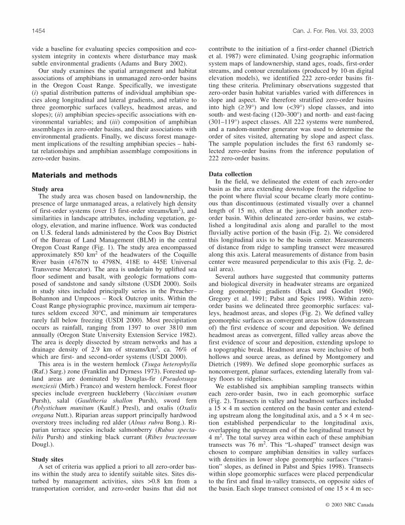
basin as the area extending downslope from the ridgeline tothe point where fluvial scour became clearly more continu-ous than discontinuous (estimated visually over a channellength of 15 m), often at the junction with another zero-order basin. Within delineated zero-order basins, we estab-lished a longitudinal axis along and parallel to the mostfluvially active portion of the basin (Fig. 2). We consideredthis longitudinal axis to be the basin center. Measurementsof distance from ridge to sampling transect were measuredalong this axis. Lateral measurements of distance from basincenter were measured perpendicular to this axis (Fig. 2, de-tail area).

Several authors have suggested that community patternsand biological diversity in headwater streams are organizedalong geomorphic gradients (Hack and Goodlet 1960;Gregory et al. 1991; Pabst and Spies 1998). Within zero-order basins we delineated three geomorphic surfaces: val-leys, headmost areas, and slopes (Fig. 2). We defined valleygeomorphic surfaces as convergent areas below (downstreamof) the first evidence of scour and deposition. We definedheadmost areas as convergent, filled valley areas above thefirst evidence of scour and deposition, extending upslope toa topographic break. Headmost areas were inclusive of bothhollows and source areas, as defined by Montgomery andDietrich (1989). We defined slope geomorphic surfaces asnonconvergent, planar surfaces, extending laterally from val-ley floors to ridgelines.

We established six amphibian sampling transects withineach zero-order basin, two in each geomorphic surface(Fig. 2). Transects in valley and headmost surfaces includeda 15 × 4 m section centered on the basin center and extend-ing upstream along the longitudinal axis, and a 5 × 4 m sec-tion established perpendicular to the longitudinal axis,overlapping the upstream end of the longitudinal transect by4 m2. The total survey area within each of these amphibiantransects was 76 m2. This “L-shaped” transect design waschosen to compare amphibian densities in valley surfaceswith densities in lower slope geomorphic surfaces (“transi-tion” slopes, as defined in Pabst and Spies 1998). Transectswithin slope geomorphic surfaces were placed perpendicularto the first and final in-valley transects, on opposite sides ofthe basin. Each slope transect consisted of one 15 × 4 m sec-

© 2003 NRC Canada

1454 Can. J. For. Res. Vol. 33, 2003



tion (60 m2). Where the lateral distance from basin center toridgeline was >30 m, the start point of slope transects wasestablished halfway between basin center and ridgelines,perpendicular to the longitudinal axis. Where total slopelength was <30 m, the start points of slope transects wereplaced 5.0 m from basin center.

We surveyed for amphibians from March through June in2000 and 2001. Amphibians were sampled once per basin.We sampled amphibians in each transect using time-constrained searches of all cover objects and litter (Bury andCorn 1991) for a maximum of 30 min, not including animalprocessing time. All cover objects were removed and litterwas combed systematically, from the downstream end oftransects. If 30 min elapsed before we could search all coverobjects in a transect, the searched area was reduced and re-corded accordingly.

We measured 31 environmental variables (Table 2) thatmay be important in structuring amphibian assemblages

within zero-order basins. These data were collected at plot,transect, and zero-order basin spatial scales. Plots were es-tablished within geomorphic surfaces within basins, follow-ing a stratified random design described in Sheridan (2002).Plots were 2 m2 in size, and 17 were placed in each basin.At the plot scale, data were collected for three substrate, twodown wood, and nine overstory variables. Binary variablesfor the presence–absence of saturation, scour, deposition,and stability in individual plots became proportions whenaveraged for geomorphic surfaces. Overstory variables weremeasured using variable-radius sampling in one plot pergeomorphic surface. At the amphibian transect scale, datawere collected on two positional, one surface moisture, andfour scour and deposition variables. At the zero-order basinlevel, we collected data on geomorphic surface, basin gradi-ent, basin depth, heat load index (a cosine transformation ofbasin aspect), and flow area above the initiation of scour anddeposition. Data collected on covariates were date of survey,

© 2003 NRC Canada


Fig. 1. Location of the study area and the 63 study sites within the Coquille Basin, southwestern Oregon.



relative humidity, temperature, stand age, and distance fromocean.

Statistical analyses

Spatial distribution patternsWe used several analyses to examine longitudinal and lat-

eral distribution patterns of amphibians. First, between spe-cies, we compared proximity to ridgeline to determine therelative longitudinal extent of amphibians in zero-order bas-ins. We considered the shortest slope distance along the lon-gitudinal axis from ridgeline to a species capture in a zero-order basin as that species’ proximity to ridgeline. We madebetween-species comparisons of proximity to ridgeline, us-ing a general linear model (PROC GLM, SAS Institute Inc.1999) with log10 of proximity to ridgeline as the responsevariable and species as the explanatory variable. We esti-mated the size of differences in first detection between spe-cies using pairwise means comparisons with a Tukey–Kramer adjustment to account for the large number of un-planned comparisons (Ramsey and Schafer 1997).

Similarly, we contrasted species’ use of areas along lateralaxes using between-species comparisons of maximum dis-tance from basin center for each zero-order basin. We ana-lyzed differences using a general linear model with the log10of maximum distance from basin center to capture as the re-sponse variable and species as the explanatory variable. Weestimated the size of differences in lateral extent betweenspecies using pairwise means comparisons with a Tukey–Kramer adjustment for unplanned comparisons.

Within species, we compared differences in captures be-tween lateral zones to examine species-specific penetrationof “dry” and “moist” habitats. We estimated differences inamphibian capture rates associated with lateral distance frombasin center, using log–linear regression models (PROCGENMOD, SAS Institute Inc. 1999), because amphibian

species captures were collected as count data. For this analy-sis we summed species captures for each of three lateralzones: 0–2, 2–5, and >5 m (slope transect data) from basincenter. Lateral zone was the explanatory variable and cap-tures was the response variable for each model, for each spe-cies. We used a compound symmetry model (SAS InstituteInc. 1999), which assumes constant variance and covariance,to model spatial autocorrelation between lateral zones withinzero-order basins. We included an offset to account for dif-ferent sampling effort between lateral zones.

Geomorphic surfaces integrate longitudinal and lateralenvironmental gradients in zero-order basins, and we hy-pothesized that species’ densities would differ between geo-morphic surfaces. Within species, we estimated differencesin captures between geomorphic surfaces using log–linearregression models (PROC GENMOD, SAS Institute Inc.1999). For this analysis, we summed transect capture datafor each geomorphic surface (valley, headmost, and slope) ineach zero-order basin. Geomorphic surface was the explana-tory variable and number of captures per geomorphic surfacewas the response variable, for each species. As in within-species lateral analyses, we used a compound symmetry cor-relation structure to model spatial autocorrelation betweengeomorphic surfaces within a zero-order basin and includedan offset to account for different sampling effort. For bothlateral zone and geomorphic surface models, we assessedgoodness of fit using estimated deviance/degrees of freedom(df), examination of residuals for outliers, and comparisonof model predicted values with actual values.

Amphibian associations with environmental variablesWe developed sets of empirical log–linear regression

models (PROC GENMOD, SAS Institute Inc. 1999) describ-ing amphibian capture rates in unmanaged zero-order basinsas a function of geomorphic, surface moisture, substrate,canopy cover, down wood, and overstory variables. We con-

© 2003 NRC Canada

1456 Can. J. For. Res. Vol. 33, 2003

Fig. 2. Schematic of geomorphic surfaces and amphibian transect set up within zero-order basins.



© 2003 NRC Canada


Para

met

erC

ode

Des

crip

tion

Ref

eren

cesa

Spe

cies

b

Plo

tsc

ale

Lar

gesu

bstr

ate

(%)

LR

GS

UB

Vis

ual

esti

mat

eof

%pl

otsu

rfac

eob

scur

edby

grav

el,

cobb

le,

boul

ders

,or

bedr

ock

(sub

stra

tes

>5

mm

)

Bla

uste

inet

al.

1995

;C

orn

and

Bur

y19

91S

outh

ern

torr

ent

sala

man

der,

Dun

n’s

sala

man

-de

r,w

este

rnre

d-ba

cked

sala

man

der,

clou

ded

sala

man

der

(–),

ensa

tina

(–)

Org

anic

subs

trat

e(%

)O

RG

SU

BV

isua

les

tim

ate

of%

plot

surf

ace

obsc

ured

byli

tter

,or

gani

cm

ater

ial,

bark

,or

dow

nw

ood

Cor

nan

dB

ury

1991

;B

laus

tein

etal

.19

95W

este

rnre

d-ba

cked

sala

man

der,

clou

ded

sala

-m

ande

r(–

),en

sati

naL

itte

rde

pth

(cm

)L

ITT

ER

Lit

ter

dept

hav

erag

edfr

omfi

vepo

ints

/plo

tB

laus

tein

etal

.19

95;

Cor

nan

dB

ury

1991

Sou

ther

nto

rren

tsa

lam

ande

r(–

),D

unn’

ssa

la-

man

der

(–),

wes

tern

red-

back

edsa

lam

ande

r(–

),cl

oude

dsa

lam

ande

r(–

),en

sati

naT

rans

ect

scal

eR

idge

dist

ance

(m)

DIS

TR

IDG

Rid

geli

neto

plot

slop

edi

stan

ce,

divi

ded

bydi

s-ta

nce

from

ridg

elin

eto

init

iati

onof

scou

rS

outh

ern

torr

ent

sala

man

der,

Dun

n’s

sala

man

-de

r,w

este

rnre

d-ba

cked

sala

man

der,

clou

ded

sala

man

der

(–),

ensa

tina

(–)

Dis

tanc

efr

omce

nter

(m)

DIS

TC

Per

pend

icul

arsl

ope

dist

ance

from

basi

nce

nter

topl

otlo

cati

onL

eona

rdet

al.

1993

;B

laus

tein

etal

.19

95;

Ves

ely

1997

;B

ury

etal

.19

91

Wes

tern

red-

back

edsa

lam

ande

r(–

),cl

oude

dsa

lam

ande

r,en

sati

na

Sur

face

moi

stur

eM

OIS

TR

Inte

ger

inde

xof

plot

moi

stur

eba

sed

onca

tego

ries

desc

ribe

din

Ols

onet

al.

1999

;va

lues

rang

efr

om1

(dry

)to

7(f

low

ing)

Bur

yet

al.

1991

Sou

ther

nto

rren

tsa

lam

ande

r,w

este

rnre

d-ba

cked

sala

man

der

Sat

urat

ion

SA

TU

RP

rese

nce–

abse

nce

offi

eld-

esti

mat

ed“s

atur

ated

”co

ndit

ions

Bur

yet

al.

1991

Sou

ther

nto

rren

tsa

lam

ande

r,D

unn’

ssa

lam

an-

der,

wes

tern

red-

back

edsa

lam

ande

r,cl

oude

dsa

lam

ande

r(–

),en

sati

na(–

)S

cour

SC

OU

RP

rese

nce–

abse

nce

ofsc

our

(rem

oval

ofab

ove-

grou

ndve

geta

tion

and

litt

er)

Bur

yet

al.

1991

Sou

ther

nto

rren

tsa

lam

ande

r,D

unn’

ssa

lam

an-

der,

wes

tern

red-

back

edsa

lam

ande

rD

epos

itio

nD

EP

OS

ITP

rese

nce–

abse

nce

ofde

posi

tion

(mat

eria

lfr

omou

tsid

eof

the

plot

mob

iliz

edby

fluv

ial

orhi

llsl

ope

dist

urba

nce

Sou

ther

nto

rren

tsa

lam

ande

r,D

unn’

ssa

lam

an-

der,

wes

tern

red-

back

edsa

lam

ande

r

Sta

bili

tyS

TAB

LE

Pre

senc

e–ab

senc

eof

stab

leco

ndit

ions

(no

scou

ror

depo

siti

on)

Wes

tern

red-

back

edsa

lam

ande

r(–

),cl

oude

dsa

lam

ande

r(–

),en

sati

naD

own

woo

dvo

lum

e(m

3 /ha)

CW

DM

3HA

Vol

ume

ofdo

wn

woo

d,ca

lcul

ated

from

visu

ally

esti

mat

eddo

wn

woo

dL

eona

rdet

al.

1993

;B

laus

tein

etal

.19

95;

Cor

nan

dB

ury

1991

Sou

ther

nto

rren

tsa

lam

ande

r,D

unn’

ssa

lam

an-

der,

wes

tern

red-

back

edsa

lam

ande

r,cl

oude

dsa

lam

ande

r,en

sati

naD

own

woo

dfr

eque

ncy

WO

OD

FR

EQ

Pre

senc

e–ab

senc

eof

dow

nw

ood

Leo

nard

etal

.19

93;

Bla

uste

inet

al.

1995

;C

orn

and

Bur

y19

91

Clo

uded

sala

man

der

Can

opy

cove

r(%

)C

CT

OT

%of

view

scre

enob

scur

edin

aca

nopy

view

er(M

uell

er-D

ombo

isan

dE

llen

burg

1974

)C

orn

and

Bur

y19

91S

outh

ern

torr

ent

sala

man

der,

Dun

n’s

sala

man

-de

r,w

este

rnre

d-ba

cked

sala

man

der,

clou

ded

sala

man

der,

ensa

tina

Lar

geov

erst

ory

(m2 /h

a)B

A70

Bas

alar

eaof

tree

sov

er70

cmin

diam

eter

Bla

uste

inet

al.

1995

;C

orn

and

Bur

y19

91S

outh

ern

torr

ent

sala

man

der,

Dun

n’s

sala

man

-de

r,w

este

rnre

d-ba

cked

sala

man

der,

clou

ded

sala

man

der,

ensa

tina

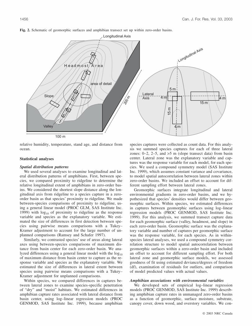
Tab

le2.

Des

crip

tion

ofha

bita

tpa

ram

eter

sco

llec

ted

atth

epl

ot,

tran

sect

,or

zero

-ord

er-b

asin

scal

e,co

vari

ates

,pa

ram

eter

code

s(u

sed

inem

piri

cal

mod

els)

,re

fere

nces

for

impo

r-ta

nce

ofec

olog

ical

vari

able

s,an

dsp

ecie

shy

poth

esiz

edto

beas

soci

ated

wit

hva

riab

les.



© 2003 NRC Canada

1458 Can. J. For. Res. Vol. 33, 2003

Para

met

erC

ode

Des

crip

tion

Ref

eren

cesa

Spe

cies

b

Rel

ativ

ede

nsit

yR

DT

ree

dens

ity

met

ric

calc

ulat

edfr

omba

sal

area

and

quad

rati

cm

ean

diam

eter

(Cur

tis

1982

),us

ing

basa

lar

eafr

omva

riab

le-r

adiu

sov

erst

ory

plot

san

dvi

sual

lyes

tim

ated

diam

eter

s

Ves

ely

1997

Wes

tern

red-

back

edsa

lam

ande

r

Rel

ativ

ede

nsit

yw

ithi

nge

omor

phic

surf

aces

RD

INR

elat

ive

dens

ity

(sim

ilar

toC

urti

s19

82),

calc

u-la

ted

usin

gon

lytr

ees

root

edin

the

sam

ege

omor

phic

surf

ace

asth

eva

riab

le-r

adiu

spl

ot

Sou

ther

nto

rren

tsa

lam

ande

r(–

),D

unn’

ssa

la-

man

der

(–),

wes

tern

red-

back

edsa

lam

ande

r,cl

oude

dsa

lam

ande

r,en

sati

naR

elat

ive

dens

ity

ofhe

mlo

ckR

DT

SH

ER

elat

ive

dens

ity

(sim

ilar

toC

urti

s19

82),

calc

u-la

ted

usin

gon

lyw

este

rnhe

mlo

cktr

ees

inva

riab

le-r

adiu

sov

erst

ory

plot

s

Sou

ther

nto

rren

tsa

lam

ande

r(–

),D

unn’

ssa

la-

man

der

(–),

wes

tern

red-

back

edsa

lam

an-

der

(–),

clou

ded

sala

man

der,

ensa

tina

Rel

ativ

ede

nsit

yof

hard

woo

dsR

DH

WR

elat

ive

dens

ity

(sim

ilar

toC

urti

s19

82),

calc

u-la

ted

usin

gon

lyha

rdw

ood

spec

ies

inva

riab

le-

radi

usov

erst

ory

plot

s

Sou

ther

nto

rren

tsa

lam

ande

r,D

unn’

ssa

lam

an-

der,

wes

tern

red-

back

edsa

lam

ande

r,cl

oude

dsa

lam

ande

r(–

),en

sati

na(–

)S

nag

dens

ity

(no.

/ha)

SN

AG

SS

nags

per

hect

are,

calc

ulat

edfr

omva

riab

le-r

adiu

sov

erst

ory

plot

sC

orn

and

Bur

y19

91C

loud

edsa

lam

ande

r

Fer

nco

ver

(%)

FE

RN

S%

plot

surf

ace

obsc

ured

byfe

rns

Bla

uste

inet

al.

1995

;C

orn

and

Bur

y19

91S

outh

ern

torr

ent

sala

man

der,

Dun

n’s

sala

man

-de

r,cl

oude

dsa

lam

ande

rS

hrub

cove

rS

HR

UB

S%

plot

surf

ace

obsc

ured

bysh

rubs

Ves

ely

1997

Sou

ther

nto

rren

tsa

lam

ande

r(–

),D

unn’

ssa

la-

man

der

(–),

wes

tern

red-

back

edsa

lam

an-

der

(–),

clou

ded

sala

man

der

(–)

Zer

o-or

der-

basi

nsc

ale

Geo

mor

phic

surf

ace

GE

OS

RF

Thr

eecl

asse

s:va

lley

,he

adm

ost

area

,an

dsl

ope

Wes

tern

red-

back

edsa

lam

ande

r,cl

oude

dsa

la-

man

der,

ensa

tina

Bas

ingr

adie

nt(d

egre

es)

GR

AD

EG

radi

ent

(slo

pe)

ofze

ro-o

rder

basi

n,ca

lcul

ated

usin

gdi

ffer

ence

inel

evat

ion

and

mea

sure

dle

ngth

ofba

sin

Bla

uste

inet

al.

1995

;C

orn

and

Bur

y19

91S

outh

ern

torr

ent

sala

man

der,

Dun

n’s

sala

man

-de

r,w

este

rnre

d-ba

cked

sala

man

der,

clou

ded

sala

man

der,

ensa

tina

Fea

ture

dept

h(m

)D

EP

TH

Dif

fere

nce

inel

evat

ion

betw

een

the

mid

poin

tof

the

geom

orph

icsu

rfac

ean

dth

esu

rrou

ndin

gri

dgel

ine

Sou

ther

nto

rren

tsa

lam

ande

r,D

unn’

ssa

lam

an-

der,

ensa

tina

(–)

Hea

tlo

adin

dex

HE

AT

ND

XR

elat

ive

mea

sure

ofso

lar

gain

,ca

lcul

ated

usin

gth

efo

rmul

a:1

–co

s(as

pect

-45)

/2(B

eers

etal

.19

66);

0re

pres

ents

cool

(45°

)as

pect

s,1.

0re

p-re

sent

sw

arm

(225

°)as

pect

s

Bla

uste

inet

al.

1995

;C

orn

and

Bur

y19

91S

outh

ern

torr

ent

sala

man

der

(–),

Dun

n’s

sala

-m

ande

r(–

),w

este

rnre

d-ba

cked

sala

man

-de

r(–

),cl

oude

dsa

lam

ande

r(–

),en

sati

na(–

)

Bas

inar

ea(h

a)A

RE

AA

rea

pote

ntia

lly

cont

ribu

ting

surf

ace

flow

toth

epo

int

ofin

itia

tion

ofsc

our

and

depo

siti

onin

aze

ro-o

rder

basi

n;ge

nera

ted

inA

RC

/IN

FO

,us

ing

flow

dire

ctio

nan

dac

cum

ulat

ion

algo

-ri

thm

san

da

10-m

digi

tal

elev

atio

nm

odel

Sou

ther

nto

rren

tsa

lam

ande

r,D

unn’

ssa

lam

an-

der,

wes

tern

red-

back

edsa

lam

ande

r,cl

oude

dsa

lam

ande

r(–

),en

sati

na(–

)

Cov

aria

tes

Day

num

ber

DA

YN

umbe

rof

days

from

Janu

ary

1to

surv

eyda

teS

outh

ern

torr

ent

sala

man

der

(–),

Dun

n’s

sala

-m

ande

r(–

),w

este

rnre

d-ba

cked

sala

man

-de

r(–

),cl

oude

dsa

lam

ande

r(–

),en

sati

na(–

)

Tab

le2

(con

tinu

ed).



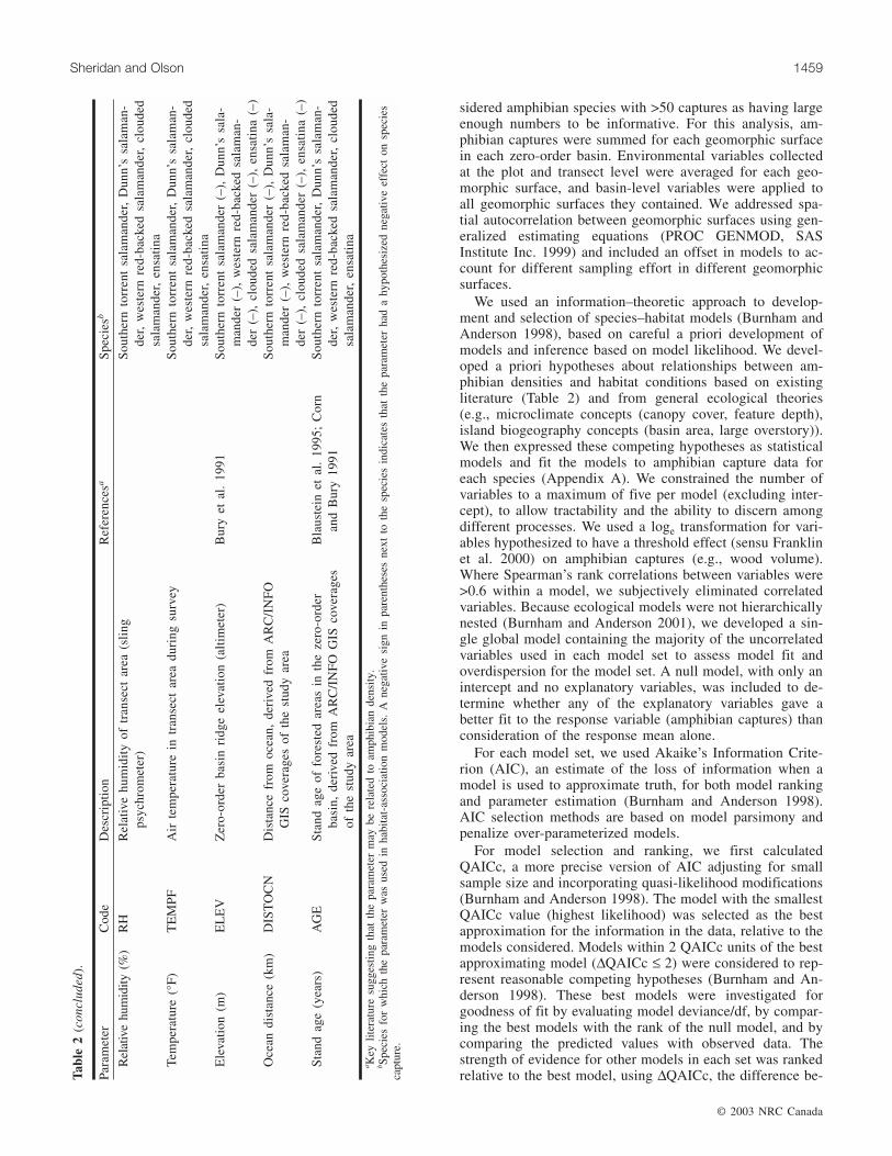
sidered amphibian species with >50 captures as having largeenough numbers to be informative. For this analysis, am-phibian captures were summed for each geomorphic surfacein each zero-order basin. Environmental variables collectedat the plot and transect level were averaged for each geo-morphic surface, and basin-level variables were applied toall geomorphic surfaces they contained. We addressed spa-tial autocorrelation between geomorphic surfaces using gen-eralized estimating equations (PROC GENMOD, SASInstitute Inc. 1999) and included an offset in models to ac-count for different sampling effort in different geomorphicsurfaces.

We used an information–theoretic approach to develop-ment and selection of species–habitat models (Burnham andAnderson 1998), based on careful a priori development ofmodels and inference based on model likelihood. We devel-oped a priori hypotheses about relationships between am-phibian densities and habitat conditions based on existingliterature (Table 2) and from general ecological theories(e.g., microclimate concepts (canopy cover, feature depth),island biogeography concepts (basin area, large overstory)).We then expressed these competing hypotheses as statisticalmodels and fit the models to amphibian capture data foreach species (Appendix A). We constrained the number ofvariables to a maximum of five per model (excluding inter-cept), to allow tractability and the ability to discern amongdifferent processes. We used a loge transformation for vari-ables hypothesized to have a threshold effect (sensu Franklinet al. 2000) on amphibian captures (e.g., wood volume).Where Spearman’s rank correlations between variables were>0.6 within a model, we subjectively eliminated correlatedvariables. Because ecological models were not hierarchicallynested (Burnham and Anderson 2001), we developed a sin-gle global model containing the majority of the uncorrelatedvariables used in each model set to assess model fit andoverdispersion for the model set. A null model, with only anintercept and no explanatory variables, was included to de-termine whether any of the explanatory variables gave abetter fit to the response variable (amphibian captures) thanconsideration of the response mean alone.

For each model set, we used Akaike’s Information Crite-rion (AIC), an estimate of the loss of information when amodel is used to approximate truth, for both model rankingand parameter estimation (Burnham and Anderson 1998).AIC selection methods are based on model parsimony andpenalize over-parameterized models.

For model selection and ranking, we first calculatedQAICc, a more precise version of AIC adjusting for smallsample size and incorporating quasi-likelihood modifications(Burnham and Anderson 1998). The model with the smallestQAICc value (highest likelihood) was selected as the bestapproximation for the information in the data, relative to themodels considered. Models within 2 QAICc units of the bestapproximating model (∆QAICc ≤ 2) were considered to rep-resent reasonable competing hypotheses (Burnham and An-derson 1998). These best models were investigated forgoodness of fit by evaluating model deviance/df, by compar-ing the best models with the rank of the null model, and bycomparing the predicted values with observed data. Thestrength of evidence for other models in each set was rankedrelative to the best model, using ∆QAICc, the difference be-

© 2003 NRC Canada


Para

met

erC

ode

Des

crip

tion

Ref

eren

cesa

Spe

cies

b

Rel

ativ

ehu

mid

ity(%

)R

HR

elat

ive

hum

idit

yof

tran

sect

area

(sli

ngps

ychr

omet

er)

Sou

ther

nto

rren

tsa

lam

ande

r,D

unn’

ssa

lam

an-

der,

wes

tern

red-

back

edsa

lam

ande

r,cl

oude

dsa

lam

ande

r,en

sati

naTe

mpe

ratu

re(°

F)

TE

MP

FA

irte

mpe

ratu

rein

tran

sect

area

duri

ngsu

rvey

Sou

ther

nto

rren

tsa

lam

ande

r,D

unn’

ssa

lam

an-

der,

wes

tern

red-

back

edsa

lam

ande

r,cl

oude

dsa

lam

ande

r,en

sati

naE

leva

tion

(m)

EL

EV

Zer

o-or

der

basi

nri

dge

elev

atio

n(a

ltim

eter

)B

ury

etal

.19

91S

outh

ern

torr

ent

sala

man

der

(–),

Dun

n’s

sala

-m

ande

r(–

),w

este

rnre

d-ba

cked

sala

man

-de

r(–

),cl

oude

dsa

lam

ande

r(–

),en

sati

na(–

)O

cean

dist

ance

(km

)D

IST

OC

ND

ista

nce

from

ocea

n,de

rive

dfr

omA

RC

/IN

FO

GIS

cove

rage

sof

the

stud

yar

eaS

outh

ern

torr

ent

sala

man

der

(–),

Dun

n’s

sala

-m

ande

r(–

),w

este

rnre

d-ba

cked

sala

man

-de

r(–

),cl

oude

dsa

lam

ande

r(–

),en

sati

na(–

)S

tand

age

(yea

rs)

AG

ES

tand

age

offo

rest

edar

eas

inth

eze

ro-o

rder

basi

n,de

rive

dfr

omA

RC

/IN

FO

GIS

cove

rage

sof

the

stud

yar

ea

Bla

uste

inet

al.

1995

;C

orn

and

Bur

y19

91S

outh

ern

torr

ent

sala

man

der,

Dun

n’s

sala

man

-de

r,w

este

rnre

d-ba

cked

sala

man

der,

clou

ded

sala

man

der,

ensa

tina

a Key

liter

atur

esu

gges

ting

that

the

para

met

erm

aybe

rela

ted

toam

phib

ian

dens

ity.

b Spec

ies

for

whi

chth

epa

ram

eter

was

used

inha

bita

t-as

soci

atio

nm

odel

s.A

nega

tive

sign

inpa

rent

hese

sne

xtto

the

spec

ies

indi

cate

sth

atth

epa

ram

eter

had

ahy

poth

esiz

edne

gativ

eef

fect

onsp

ecie

sca

ptur

e.

Tab

le2

(con

clud

ed).



tween the QAICc value for a given model and the modelwith the lowest QAICc value in the set. ∆QAICc valueswere used to compute Akaike weights (w), estimates of therelative likelihood of each model, given the likelihood of thefull set of candidate models (Burnham and Anderson 2001).

We investigated the relationship between amphibian cap-ture rates and individual environmental variables using ad-justed confidence intervals and parameter predictor weights.For models with ∆QAICc ≤ 2, we developed estimates of theunconditional sampling variation of model variables andused it to adjust 95% confidence intervals for model vari-ables (Burnham and Anderson 1998). We only interpretedadjusted confidence intervals for variables that had consis-tent and strong relationships with amphibian captures in thebest models (models with ∆QAICc ≤ 2). We compared therelative importance of variables in each model set by com-puting parameter predictor weights (Burnham and Anderson2001), an indicator of the importance of individual variablesin predicting response, considering the entire model set. Pre-dictor weights were calculated by summing the adjustedAkaike weights (w) for all the models in which a parameteroccurred. Akaike model weights (w) were adjusted followingStoddard (2001), using the formula:

adj. w

= (no. models/no. models with the variable)

× (1/no. variables) × w

This adjustment was made to account for large differences inthe numbers of models associated with individual variables.

Composition of amphibian assemblagesWe examined the compositions of amphibian assemblages

in zero-order basins and their relationships to environmentalgradients using nonmetric multidimensional scaling (NMS)and indicator species analysis. We used NMS (May 1976),an ordination technique in PC-ORD (McCune and Mefford1999), to depict relationships between experimental units(geomorphic surfaces), in terms of amphibian composition.We used a Sorenson distance measure (McCune and Grace2002) and detrended correspondence analysis (Hill andGauch 1980) to establish starting coordinates for the ordi-nation. Interpretation of ordination axes was facilitated byconsideration of Spearman’s rank correlations between envi-ronmental variables and axis scores. The final ordinationwas rotated to maximize correlations between axis 1 and theenvironmental variable with the single highest correlationwith the ordination space. Ellipses were drawn around areasin ordination space with the highest density of each species.

We used indicator species analysis (Dufrene and Legendre1997) to characterize amphibian assemblages associatedwith both geomorphic surfaces and lateral zones in zero-order basins. This analysis compared species abundance andconsistency in individual geomorphic surfaces or lateralzones with their abundance and consistency in all surfaces orzones to provide an indicator value. Indicator values repre-sented the percentage of perfect indication of a species for aparticular surface or zone, with 100% representing perfectindication (a species always being associated with that sur-face or zone, in relatively high numbers). Maximum indica-tor values represented the indicator value of a species for the

surface or zone with which it was most strongly associated.We developed amphibian assemblages associated with eachgeomorphic surface and lateral zone, considering only spe-cies whose maximum indicator values were significantlyhigher than values from Monte Carlo simulations (2000 iter-ations, α = 0.05).

We compared the effectiveness of geomorphic surfacesand lateral zones in explaining amphibian species distribu-tions using three techniques. We compared the total numberof significant indicator species associated with each geo-morphic surface and lateral zone. We used the sum of allspecies indicator values for each surface or zone as an addi-tional criterion to compare geomorphic surfaces and lateralzones for their ability to explain species distributions(Dufrene and Legendre 1997). Finally, we used a multi-response permutation procedure (MRPP, Biondini et al.1988) to test the hypothesis of no difference between indi-vidual geomorphic surfaces and between individual lateralzones. We used MRPP in PC-ORD (McCune and Mefford1999) with Sorenson distance and rank transformation of thedistance matrix to address loss of sensitivity due to commu-nity heterogeneity. We estimated effect size using chance-corrected within-group agreement (A) as an estimate ofwithin-group homogeneity compared with random expecta-tion.

Results

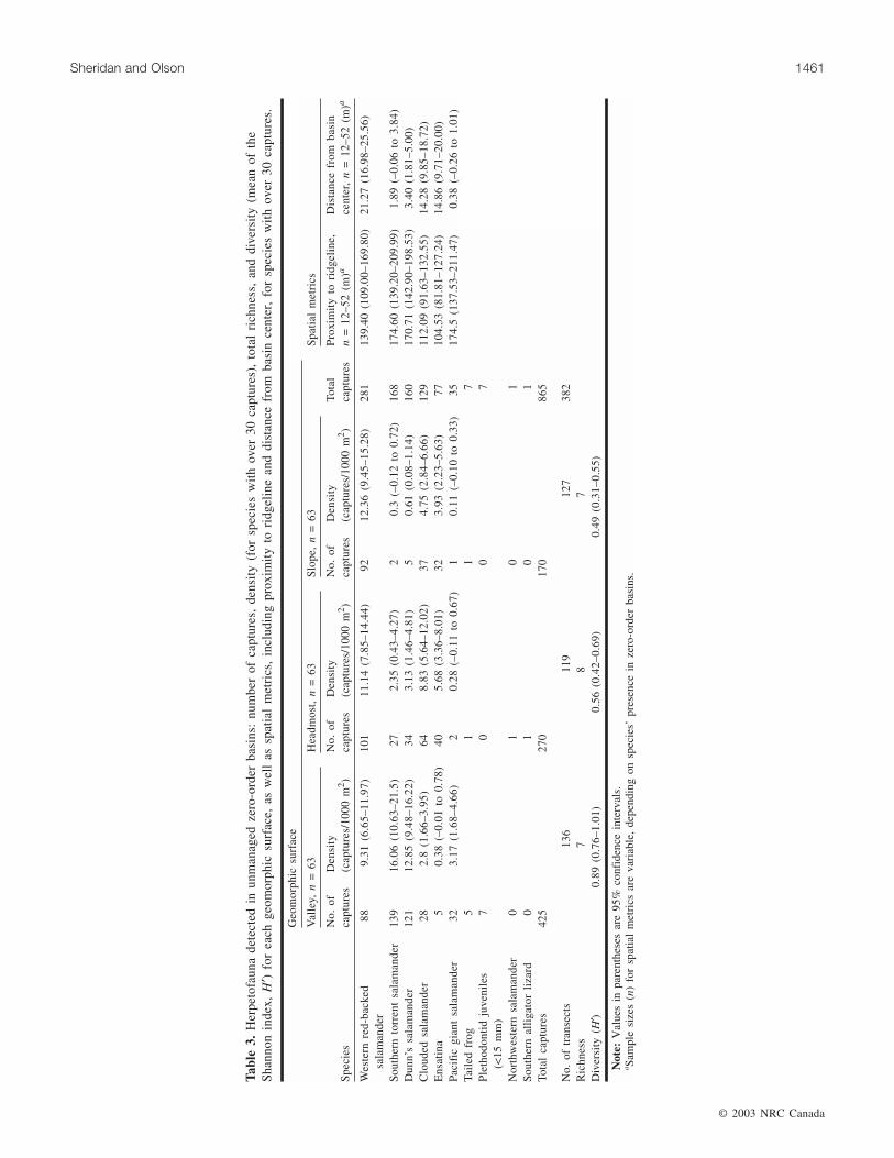
We surveyed 382 transects in 63 unmanaged zero-orderbasins and captured a total of 865 amphibians belonging toeight species (Table 3): western red-backed salamander(Plethodon vehiculum (Cooper)), southern torrent salaman-der (Rhyacotriton variegatus Stebbins and Lowe), Dunn’ssalamander (Plethodon dunni Bishop), clouded salamander(Aneides ferreus Strauch), ensatina (Ensatina eschscholtziiGray), Pacific giant salamander (Dicamptodon tenebrosusGood), tailed frog (Ascaphus truei Stejneger), and north-western salamander (Ambystoma gracile (Baird)). Only ter-restrial (adult) forms of tailed frog and northwesternsalamander were observed. Adult and juvenile forms ofother species were encountered, including both terrestrialand aquatic forms of the Pacific giant salamander. Four ofthe eight amphibian species identified have a status of con-cern in all or parts of their ranges (Table 1). Captures aver-aged over 6.3 detections/surveyor-hour (95% CI, 5.48–7.26).Amphibian densities were highly variable by species andgeomorphic surface (Table 3). Mean amphibian diversity(Shannon index, H ′) in zero-order basins was low (range, 0–1.77) and varied by geomorphic surface (Table 3). Amphib-ian diversity in valley geomorphic surfaces was 0.33 unitshigher (95% CI, 0.16–0.50) than that in headmost surfaces.Amphibian diversity in headmost areas was 0.13 units higherthan that in slope areas. This trend was not statistically sig-nificant (95% CI, –0.05 to 0.30), but may be important bio-logically, as the amphibian fauna of headmost areasappeared distinct from that of slope and surrounding uplandareas.

Amphibian abundances in zero-order basins restrictedtheir use in analyses. Pacific giant salamander, southern tor-rent salamander, Dunn’s salamander, western red-backed sal-amander, clouded salamander, and ensatina were used in

© 2003 NRC Canada

1460 Can. J. For. Res. Vol. 33, 2003



© 2003 NRC Canada


Geo

mor

phic

surf

ace

Val

ley,

n=

63H

eadm

ost,

n=

63S

lope

,n

=63

Spa

tial

met

rics

Spe

cies

No.

ofca

ptur

esD

ensi

ty(c

aptu

res/

1000

m2 )

No.

ofca

ptur

esD

ensi

ty(c

aptu

res/

1000

m2 )

No.

ofca

ptur

esD

ensi

ty(c

aptu

res/

1000

m2 )

Tota

lca

ptur

esP

roxi

mit

yto

ridg

elin

e,n

=12

–52

(m)a

Dis

tanc

efr

omba

sin

cent

er,

n=

12–5

2(m

)a

Wes

tern

red-

back

edsa

lam

ande

r88

9.31

(6.6

5–11

.97)

101

11.1

4(7

.85–

14.4

4)92

12.3

6(9

.45–

15.2

8)28

113

9.40

(109

.00–

169.

80)

21.2

7(1

6.98

–25.

56)

Sou

ther

nto

rren

tsa

lam

ande

r13

916

.06

(10.

63–2

1.5)

272.

35(0

.43–

4.27

)2

0.3

(–0.

12to

0.72

)16

817

4.60

(139

.20–

209.

99)

1.89

(–0.

06to

3.84

)D

unn’

ssa

lam

ande

r12

112

.85

(9.4

8–16

.22)

343.

13(1

.46–

4.81

)5

0.61

(0.0

8–1.

14)

160

170.

71(1

42.9

0–19

8.53

)3.

40(1

.81–

5.00

)C

loud

edsa

lam

ande

r28

2.8

(1.6

6–3.

95)

648.

83(5

.64–

12.0

2)37

4.75

(2.8

4–6.

66)

129

112.

09(9

1.63

–132

.55)

14.2

8(9

.85–

18.7

2)E

nsat

ina

50.

38(–

0.01

to0.

78)

405.

68(3

.36–

8.01

)32

3.93

(2.2

3–5.

63)

7710

4.53

(81.

81–1

27.2

4)14

.86

(9.7

1–20

.00)

Paci

fic

gian

tsa

lam

ande

r32

3.17

(1.6

8–4.

66)

20.

28(–

0.11

to0.

67)

10.

11(–

0.10

to0.

33)

3517

4.5

(137

.53–

211.

47)

0.38

(–0.

26to

1.01

)Ta

iled

frog

51

17

Ple

thod

onti

dju

veni

les

(<15

mm

)7

00

7

Nor

thw

este

rnsa

lam

ande

r0

10

1S

outh

ern

alli

gato

rli

zard

01

01

Tota

lca

ptur

es42

527

017

086

5

No.

oftr

anse

cts

136

119

127

382

Ric

hnes

s7

87

Div

ersi

ty(H

′)0.

89(0

.76–

1.01

)0.

56(0

.42–

0.69

)0.

49(0

.31–

0.55

)

Not

e:V

alue

sin

pare

nthe

ses

are

95%

conf

iden

cein

terv

als.

a Sam

ple

size

s(n

)fo

rsp

atia

lm

etri

csar

eva

riab

le,

depe

ndin

gon

spec

ies’

pres

ence

inze

ro-o

rder

basi

ns.

Tab

le3.

Her

peto

faun

ade

tect

edin

unm

anag

edze

ro-o

rder

basi

ns:

num

ber

ofca

ptur

es,

dens

ity

(for

spec

ies

wit

hov

er30

capt

ures

),to

tal

rich

ness

,an

ddi

vers

ity

(mea

nof

the

Sha

nnon

inde

x,H

′)fo

rea

chge

omor

phic

surf

ace,

asw

ell

assp

atia

lm

etri

cs,

incl

udin

gpr

oxim

ity

tori

dgel

ine

and

dist

ance

from

basi

nce

nter

,fo

rsp

ecie

sw

ith

over

30ca

ptur

es.



comparisons of proximity to ridgeline and distance from ba-sin center, as well as in ordination (NMS). Five of these spe-cies, all except Pacific giant salamander, were used in testsof differences in capture rates between geomorphic surfacesand between lateral zones, as well as in log–linear modeling.Indicator species analysis used all amphibians captured ex-cept northwestern salamander.

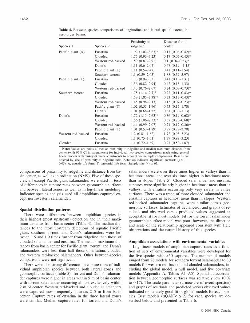
Spatial distribution patternsThere were differences between amphibian species in

their highest (most upstream) detection and in their maxi-mum distance from basin center (Table 4). The median dis-tances to the most upstream detections of aquatic Pacificgiant, southern torrent, and Dunn’s salamanders were be-tween 1.5 and 1.9 times further from ridgeline than those ofclouded salamander and ensatina. The median maximum dis-tances from basin center for Pacific giant, torrent, and Dunn’ssalamanders were less than half those of ensatina, clouded,and western red-backed salamanders. Other between-speciescomparisons were not significant.

There were also strong differences in capture rates of indi-vidual amphibian species between both lateral zones andgeomorphic surfaces (Table 5). Torrent and Dunn’s salaman-der captures were higher in areas within 5 m of basin center,with torrent salamander occurring almost exclusively within2 m of center. Western red-backed and clouded salamanderswere captured most frequently in areas 2–5 m from basincenter. Capture rates of ensatina in the three lateral zoneswere similar. Median capture rates for torrent and Dunn’s

salamanders were over three times higher in valleys than inheadmost areas, and over six times higher in headmost areasthan in slopes (Table 5). Clouded salamander and ensatinacaptures were significantly higher in headmost areas than invalleys, with ensatina occurring only very rarely in valleysurfaces. There was a trend of more clouded salamander andensatina captures in headmost areas than in slopes. Westernred-backed salamander captures were similar across geo-morphic surfaces. Estimates of deviance/df and graphs of re-siduals and observed versus predicted values suggested anacceptable fit for most models. Fit for the torrent salamandergeomorphic surface model was poor; however, the directionand scale of the relationship appeared consistent with fieldobservations and the natural history of this species.

Amphibian associations with environmental variablesLog–linear models of amphibian capture rates as a func-

tion of sets of environmental variables were developed forthe five species with >50 captures. The number of modelsranged from 28 models for southern torrent salamander to 30models for western red-backed and clouded salamanders, in-cluding the global model, a null model, and five covariatemodels (Appendix A, Tables A1–A5). Spatial autocorrela-tion between geomorphic surfaces was relatively low (0.02to 0.17). The scale parameter (a measure of overdispersion)and graphs of residuals and predicted versus observed valuesindicated moderately good fit of global models for each spe-cies. Best models (∆QAICc ≤ 2) for each species are de-scribed below and presented in Table 6.

© 2003 NRC Canada

1462 Can. J. For. Res. Vol. 33, 2003

Species 1 Species 2Proximity toridgeline

Distance fromcenter

Pacific giant (A) Ensatina 1.92 (1.02–3.63)* 0.17 (0.06–0.42)*Clouded 1.75 (0.93–3.23) 0.17 (0.07–0.43)*Western red-backed 1.59 (0.87–2.91) 0.1 (0.04–0.23)*Dunn’s 1.11 (0.6–2.04) 0.47 (0.19 –1.15)Pacific giant (T) 1.11 (0.5–2.47) 0.41 (0.11–1.54)Southern torrent 1.1 (0.59–2.05) 1.88 (0.59–5.97)

Pacific giant (T) Ensatina 1.73 (0.9–3.33) 0.41 (0.13–1.31)Clouded 1.56 (0.82–2.94) 0.42 (0.13–1.33)Western red-backed 1.43 (0.76–2.67) 0.24 (0.08–0.73)*

Southern torrent Ensatina 1.75 (1.14–2.7)* 0.22 (0.11–0.43)*Clouded 1.59 (1.05–2.38)* 0.23 (0.12–0.43)*Western red-backed 1.45 (0.98–2.13) 0.13 (0.07–0.23)*Pacific giant (T) 1.02 (0.53–1.96) 0.53 (0.17–1.70)Dunn’s 1.01 (0.68–1.52) 0.61 (0.33–1.13)

Dunn’s Ensatina 1.72 (1.15–2.63)* 0.36 (0.19–0.68)*Clouded 1.56 (1.06–2.33)* 0.37 (0.20–0.68)*Western red-backed 1.44 (0.99–2.07) 0.21 (0.12–0.36)*Pacific giant (T) 1.01 (0.53–1.89) 0.87 (0.28–2.70)

Western red-backed Ensatina 1.2 (0.81–1.82) 1.72 (0.93–3.23)Clouded 1.1 (0.75–1.61) 1.79 (0.99–3.23)

Clouded Ensatina 1.1 (0.72–1.69) 0.97 (0.50–1.87)

Note: Values are ratios of median proximity to ridgeline and median maximum distance fromcenter (with 95% CI in parentheses) for individual two-species comparisons made using generallinear models with Tukey–Kramer adjustments to account for multiple comparisons. Results areordered by size of proximity to ridgeline ratio. Asterisks indicates significant contrasts (p ≤0.05). A, aquatic life form; T, terrestrial life form. Sample size (n) is 63.

Table 4. Between-species comparisons of longitudinal and lateral spatial extents inzero-order basins.



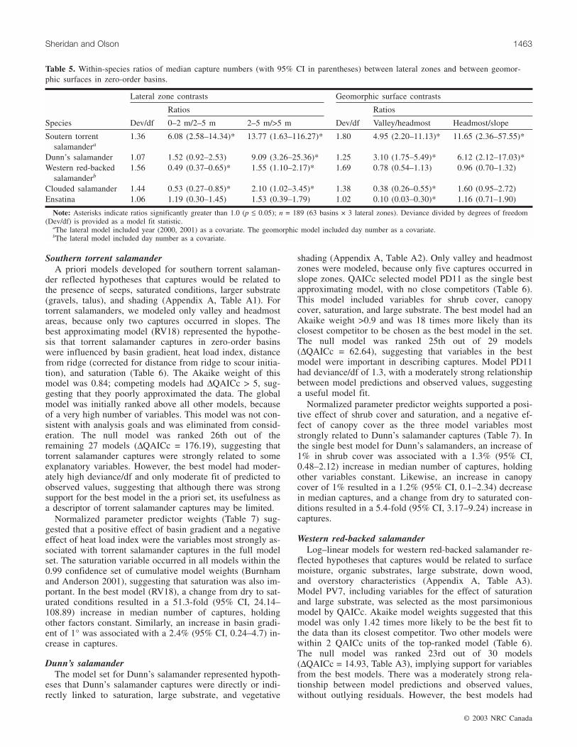
Southern torrent salamanderA priori models developed for southern torrent salaman-

der reflected hypotheses that captures would be related tothe presence of seeps, saturated conditions, larger substrate(gravels, talus), and shading (Appendix A, Table A1). Fortorrent salamanders, we modeled only valley and headmostareas, because only two captures occurred in slopes. Thebest approximating model (RV18) represented the hypothe-sis that torrent salamander captures in zero-order basinswere influenced by basin gradient, heat load index, distancefrom ridge (corrected for distance from ridge to scour initia-tion), and saturation (Table 6). The Akaike weight of thismodel was 0.84; competing models had ∆QAICc > 5, sug-gesting that they poorly approximated the data. The globalmodel was initially ranked above all other models, becauseof a very high number of variables. This model was not con-sistent with analysis goals and was eliminated from consid-eration. The null model was ranked 26th out of theremaining 27 models (∆QAICc = 176.19), suggesting thattorrent salamander captures were strongly related to someexplanatory variables. However, the best model had moder-ately high deviance/df and only moderate fit of predicted toobserved values, suggesting that although there was strongsupport for the best model in the a priori set, its usefulness asa descriptor of torrent salamander captures may be limited.

Normalized parameter predictor weights (Table 7) sug-gested that a positive effect of basin gradient and a negativeeffect of heat load index were the variables most strongly as-sociated with torrent salamander captures in the full modelset. The saturation variable occurred in all models within the0.99 confidence set of cumulative model weights (Burnhamand Anderson 2001), suggesting that saturation was also im-portant. In the best model (RV18), a change from dry to sat-urated conditions resulted in a 51.3-fold (95% CI, 24.14–108.89) increase in median number of captures, holdingother factors constant. Similarly, an increase in basin gradi-ent of 1° was associated with a 2.4% (95% CI, 0.24–4.7) in-crease in captures.

Dunn’s salamanderThe model set for Dunn’s salamander represented hypoth-

eses that Dunn’s salamander captures were directly or indi-rectly linked to saturation, large substrate, and vegetative

shading (Appendix A, Table A2). Only valley and headmostzones were modeled, because only five captures occurred inslope zones. QAICc selected model PD11 as the single bestapproximating model, with no close competitors (Table 6).This model included variables for shrub cover, canopycover, saturation, and large substrate. The best model had anAkaike weight >0.9 and was 18 times more likely than itsclosest competitor to be chosen as the best model in the set.The null model was ranked 25th out of 29 models(∆QAICc = 62.64), suggesting that variables in the bestmodel were important in describing captures. Model PD11had deviance/df of 1.3, with a moderately strong relationshipbetween model predictions and observed values, suggestinga useful model fit.

Normalized parameter predictor weights supported a posi-tive effect of shrub cover and saturation, and a negative ef-fect of canopy cover as the three model variables moststrongly related to Dunn’s salamander captures (Table 7). Inthe single best model for Dunn’s salamanders, an increase of1% in shrub cover was associated with a 1.3% (95% CI,0.48–2.12) increase in median number of captures, holdingother variables constant. Likewise, an increase in canopycover of 1% resulted in a 1.2% (95% CI, 0.1–2.34) decreasein median captures, and a change from dry to saturated con-ditions resulted in a 5.4-fold (95% CI, 3.17–9.24) increase incaptures.

Western red-backed salamanderLog–linear models for western red-backed salamander re-

flected hypotheses that captures would be related to surfacemoisture, organic substrates, large substrate, down wood,and overstory characteristics (Appendix A, Table A3).Model PV7, including variables for the effect of saturationand large substrate, was selected as the most parsimoniousmodel by QAICc. Akaike model weights suggested that thismodel was only 1.42 times more likely to be the best fit tothe data than its closest competitor. Two other models werewithin 2 QAICc units of the top-ranked model (Table 6).The null model was ranked 23rd out of 30 models(∆QAICc = 14.93, Table A3), implying support for variablesfrom the best models. There was a moderately strong rela-tionship between model predictions and observed values,without outlying residuals. However, the best models had

© 2003 NRC Canada


Lateral zone contrasts Geomorphic surface contrasts

Ratios Ratios

Species Dev/df 0–2 m/2–5 m 2–5 m/>5 m Dev/df Valley/headmost Headmost/slope

Soutern torrentsalamandera

1.36 6.08 (2.58–14.34)* 13.77 (1.63–116.27)* 1.80 4.95 (2.20–11.13)* 11.65 (2.36–57.55)*

Dunn’s salamander 1.07 1.52 (0.92–2.53) 9.09 (3.26–25.36)* 1.25 3.10 (1.75–5.49)* 6.12 (2.12–17.03)*Western red-backed

salamanderb1.56 0.49 (0.37–0.65)* 1.55 (1.10–2.17)* 1.69 0.78 (0.54–1.13) 0.96 (0.70–1.32)

Clouded salamander 1.44 0.53 (0.27–0.85)* 2.10 (1.02–3.45)* 1.38 0.38 (0.26–0.55)* 1.60 (0.95–2.72)Ensatina 1.06 1.19 (0.30–1.45) 1.53 (0.39–1.79) 1.02 0.10 (0.03–0.30)* 1.16 (0.71–1.90)

Note: Asterisks indicate ratios significantly greater than 1.0 (p ≤ 0.05); n = 189 (63 basins × 3 lateral zones). Deviance divided by degrees of freedom(Dev/df) is provided as a model fit statistic.

aThe lateral model included year (2000, 2001) as a covariate. The geomorphic model included day number as a covariate.bThe lateral model included day number as a covariate.

Table 5. Within-species ratios of median capture numbers (with 95% CI in parentheses) between lateral zones and between geomor-phic surfaces in zero-order basins.



© 2003 NRC Canada

1464 Can. J. For. Res. Vol. 33, 2003

ModelNo. Model k ∆QAICc w Dev/df

Estimated slope parameters(95% CI)

Southern torrent salamanderRV18 GRADE* + HEATNDX + DISTRIDG +

SATUR*5 0 0.844 1.48 β1 = –7.543 (–8.607 to –6.502)

β2 = 0.024 (0.002–0.046)*

β3 = –0.469 (–0.977 to 0.039)

β4 = –0.094 (–0.532 to 0.345)

β5 = 3.937 (3.184–4.69)*

Dunn’s salamanderPD11 SHRUBS* + CCTOT* + SATUR* +

LRGSUB5 0 0.903 1.33 β1 = –5.375 (–6.484 to –4.306)

β2 = 0.013 (0.005–0.021)*

β3 = –0.012 (–0.024 to –0.001)*

β4 = 1.689 (1.154–2.224)*

β5 = 0.006 (–0.004 to 0.016)

Western red-backed salamanderPV7 SATUR* + LRGSUB* 3 0 0.337 1.63 β1 = –4.63 (–4.872 to –4.391)

β2 = –0.892 (–1.366 to –0.440)*

β3 = 0.013 (0.006–0.021)*

PV19 GRADE* + AREA* + HEATINDEX +DISTC + LN(DISTRIDG)

6 0.708 0.237 1.62 β1 = –5.127 (–5.648 to –4.615)

β2 = 0.036 (0.017–0.055)*

β3 = –0.307 (–0.51 to –0.103)*

β4 = 0.127 (–0.4 to 0.655)

β5 = 0.006 (–0.009 to 0.021)

β6 = 0.006 (–0.325 to 0.337)

PV15 LRGSUB* + SATUR* + RDHW +CCTOT

5 1.729 0.142 1.63 β1 = –5.078 (–6.081 to –4.132)

β2 = 0.016 (0.006–0.024)*

β3 = –0.946 (–1.432 to –0.460)*

β4 = –0.008 (–0.022 to 0.005)

β5 = 0.006 (–0.005 to 0.018)

Clouded salamanderAF16 GEOSRF* 3 0 0.31 1.38 β1 = –5.33 (–5.784 to –4.942)

β2 = categorical*

AF19 GEOSRF* + SATUR + LN(BA70)* +WOODFREQ + LRGSUB

7 0.840 0.204 1.34 β1 = –7.004 (–8.84 to –5.299)

β2 = categorical*

β3 = 0.806 (–0.119 to 1.731)

β4 = 0.437 (0.01–0.864)*

β5 = 0.094 (–0.748 to 0.936)

β6 = –0.006 (–0.021 to 0.01)

AF17 GEOSRF* + AREA + GRADIENT +HEATINDX

6 1.811 0.125 1.36 β1 = –4.526 (–5.39 to –3.684)

β2 = categorical*

β3 = –0.047 (–0.252 to 0.158)

β4 = –0.024 (–0.054 to 0.006)

β5 = –0.523 (–1.191 to 0.144)

EnsatinaEE4 RDIN* + CCTOT 3 0 0.194 1.21 β1 = –8.348 (–10.686 to –6.32)

β2 = 0.019 (0.006–0.031)*

β3 = 0.025 (–0.002 to 0.052)

Table 6. QAICc model selection and ranking results for sets of log–linear regression models (with ∆QAICc ≤ 2) predict-ing amphibian captures as a function of environmental variables for five species.



moderately high deviance/df, and there was no clearly supe-rior single model or variables. Thus although there wasstrong support for several individual variables, the modelstested may be only moderately useful in describing relation-ships between western red-backed salamander captures andenvironmental variables.

Normalized parameter predictor weights supported posi-tive relationships between western red-backed captures andlarge substrate, basin gradient, and heat load index, and neg-ative relationships with saturation and basin area as the fivemost important variables in the model set (Table 7). Two ofthree models with ∆QAICc < 2 had a negative relationshipbetween captures and saturation, and a positive relationshipwith large substrates (Table 6). In the highest ranked model(PV7), a change from dry to saturated conditions was associ-ated with a 2.44-fold decrease (95% CI, 1.55–3.92) in me-dian number of captures, holding large substrate constant.For model PV7, an increase of 1% in large substrate coverwas associated with a 1.5% (95% CI, 0.6–2.1) increase inmedian captures, holding saturation constant. For modelPV19 (Table A3), an increase in basin gradient of 1° was as-sociated with a 3.67% (95% CI, 1.71–5.65) increase in me-dian captures, holding other variables constant. Similarly, a1 ha increase in basin area was associated with a 35.9%(95% CI, 10.88–66.55) decrease in median captures.

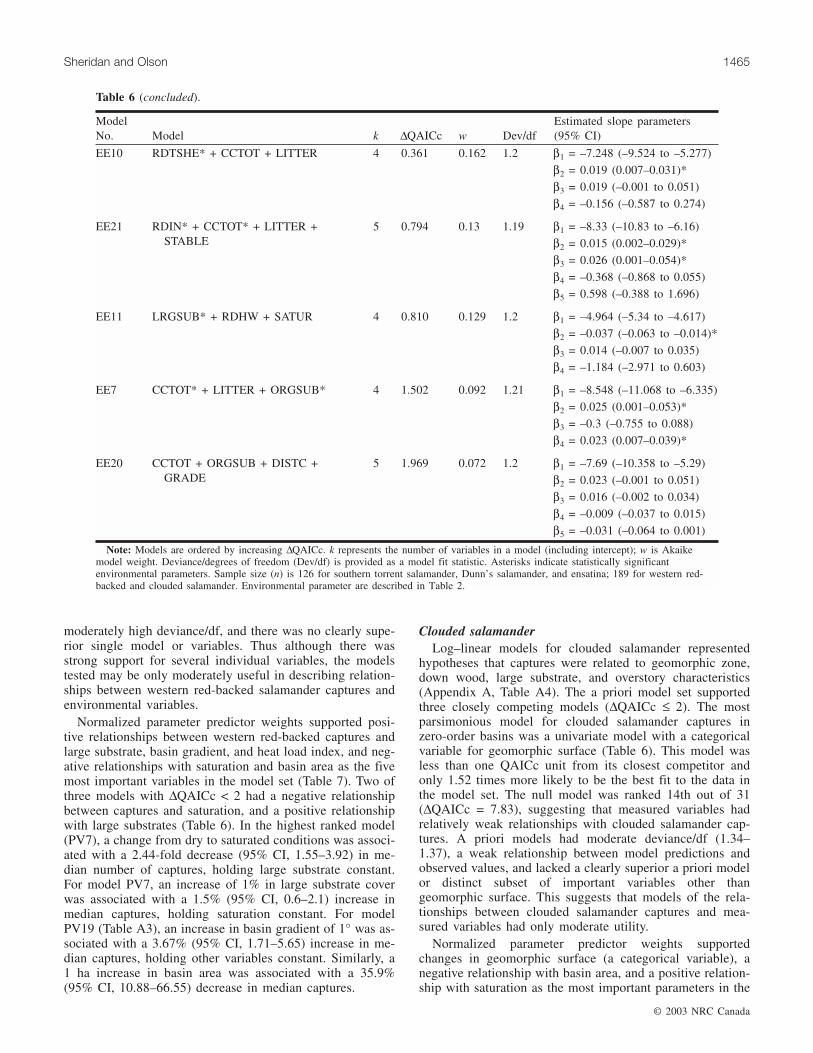
Clouded salamanderLog–linear models for clouded salamander represented

hypotheses that captures were related to geomorphic zone,down wood, large substrate, and overstory characteristics(Appendix A, Table A4). The a priori model set supportedthree closely competing models (∆QAICc ≤ 2). The mostparsimonious model for clouded salamander captures inzero-order basins was a univariate model with a categoricalvariable for geomorphic surface (Table 6). This model wasless than one QAICc unit from its closest competitor andonly 1.52 times more likely to be the best fit to the data inthe model set. The null model was ranked 14th out of 31(∆QAICc = 7.83), suggesting that measured variables hadrelatively weak relationships with clouded salamander cap-tures. A priori models had moderate deviance/df (1.34–1.37), a weak relationship between model predictions andobserved values, and lacked a clearly superior a priori modelor distinct subset of important variables other thangeomorphic surface. This suggests that models of the rela-tionships between clouded salamander captures and mea-sured variables had only moderate utility.

Normalized parameter predictor weights supportedchanges in geomorphic surface (a categorical variable), anegative relationship with basin area, and a positive relation-ship with saturation as the most important parameters in the

© 2003 NRC Canada


ModelNo. Model k ∆QAICc w Dev/df

Estimated slope parameters(95% CI)

EE10 RDTSHE* + CCTOT + LITTER 4 0.361 0.162 1.2 β1 = –7.248 (–9.524 to –5.277)

β2 = 0.019 (0.007–0.031)*

β3 = 0.019 (–0.001 to 0.051)

β4 = –0.156 (–0.587 to 0.274)

EE21 RDIN* + CCTOT* + LITTER +STABLE

5 0.794 0.13 1.19 β1 = –8.33 (–10.83 to –6.16)

β2 = 0.015 (0.002–0.029)*

β3 = 0.026 (0.001–0.054)*

β4 = –0.368 (–0.868 to 0.055)

β5 = 0.598 (–0.388 to 1.696)

EE11 LRGSUB* + RDHW + SATUR 4 0.810 0.129 1.2 β1 = –4.964 (–5.34 to –4.617)

β2 = –0.037 (–0.063 to –0.014)*

β3 = 0.014 (–0.007 to 0.035)

β4 = –1.184 (–2.971 to 0.603)

EE7 CCTOT* + LITTER + ORGSUB* 4 1.502 0.092 1.21 β1 = –8.548 (–11.068 to –6.335)

β2 = 0.025 (0.001–0.053)*

β3 = –0.3 (–0.755 to 0.088)

β4 = 0.023 (0.007–0.039)*

EE20 CCTOT + ORGSUB + DISTC +GRADE

5 1.969 0.072 1.2 β1 = –7.69 (–10.358 to –5.29)

β2 = 0.023 (–0.001 to 0.051)

β3 = 0.016 (–0.002 to 0.034)

β4 = –0.009 (–0.037 to 0.015)

β5 = –0.031 (–0.064 to 0.001)

Note: Models are ordered by increasing ∆QAICc. k represents the number of variables in a model (including intercept); w is Akaikemodel weight. Deviance/degrees of freedom (Dev/df) is provided as a model fit statistic. Asterisks indicate statistically significantenvironmental parameters. Sample size (n) is 126 for southern torrent salamander, Dunn’s salamander, and ensatina; 189 for western red-backed and clouded salamander. Environmental parameter are described in Table 2.

Table 6 (concluded).



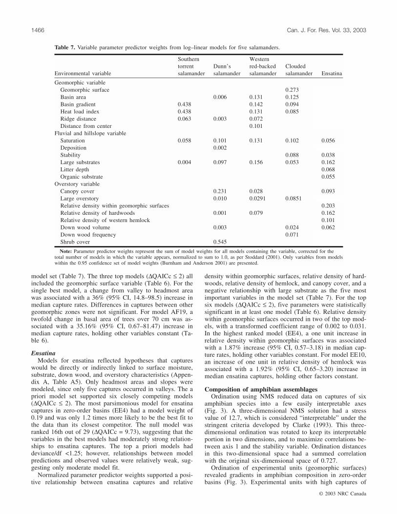
model set (Table 7). The three top models (∆QAICc ≤ 2) allincluded the geomorphic surface variable (Table 6). For thesingle best model, a change from valley to headmost areawas associated with a 36% (95% CI, 14.8–98.5) increase inmedian capture rates. Differences in captures between othergeomorphic zones were not significant. For model AF19, atwofold change in basal area of trees over 70 cm was as-sociated with a 35.16% (95% CI, 0.67–81.47) increase inmedian capture rates, holding other variables constant (Ta-ble 6).

EnsatinaModels for ensatina reflected hypotheses that captures

would be directly or indirectly linked to surface moisture,substrate, down wood, and overstory characteristics (Appen-dix A, Table A5). Only headmost areas and slopes weremodeled, since only five captures occurred in valleys. The apriori model set supported six closely competing models(∆QAICc ≤ 2). The most parsimonious model for ensatinacaptures in zero-order basins (EE4) had a model weight of0.19 and was only 1.2 times more likely to be the best fit tothe data than its closest competitor. The null model wasranked 16th out of 29 (∆QAICc = 9.73), suggesting that thevariables in the best models had moderately strong relation-ships to ensatina captures. The top a priori models haddeviance/df <1.25; however, relationships between modelpredictions and observed values were relatively weak, sug-gesting only moderate model fit.

Normalized parameter predictor weights supported a posi-tive relationship between ensatina captures and relative

density within geomorphic surfaces, relative density of hard-woods, relative density of hemlock, and canopy cover, and anegative relationship with large substrate as the five mostimportant variables in the model set (Table 7). For the topsix models (∆QAICc ≤ 2), five parameters were statisticallysignificant in at least one model (Table 6). Relative densitywithin geomorphic surfaces occurred in two of the top mod-els, with a transformed coefficient range of 0.002 to 0.031.In the highest ranked model (EE4), a one unit increase inrelative density within geomorphic surfaces was associatedwith a 1.87% increase (95% CI, 0.57–3.18) in median cap-ture rates, holding other variables constant. For model EE10,an increase of one unit in relative density of hemlock wasassociated with a 1.92% (95% CI, 0.65–3.20) increase inmedian ensatina captures, holding other factors constant.

Composition of amphibian assemblagesOrdination using NMS reduced data on captures of six

amphibian species into a few easily interpretable axes(Fig. 3). A three-dimensional NMS solution had a stressvalue of 12.7, which is considered “interpretable” under thestringent criteria developed by Clarke (1993). This three-dimensional ordination was rotated to keep its interpretableportion in two dimensions, and to maximize correlations be-tween axis 1 and the stability variable. Ordination distancesin this two-dimensional space had a summed correlationwith the original six-dimensional space of 0.727.

Ordination of experimental units (geomorphic surfaces)revealed gradients in amphibian composition in zero-orderbasins (Fig. 3). Experimental units with high captures of

© 2003 NRC Canada

1466 Can. J. For. Res. Vol. 33, 2003

Environmental variable

Southerntorrentsalamander

Dunn’ssalamander

Westernred-backedsalamander

Cloudedsalamander Ensatina

Geomorphic variableGeomorphic surface 0.273Basin area 0.006 0.131 0.125Basin gradient 0.438 0.142 0.094Heat load index 0.438 0.131 0.085Ridge distance 0.063 0.003 0.072Distance from center 0.101

Fluvial and hillslope variableSaturation 0.058 0.101 0.131 0.102 0.056Deposition 0.002Stability 0.088 0.038Large substrates 0.004 0.097 0.156 0.053 0.162Litter depth 0.068Organic substrate 0.055

Overstory variableCanopy cover 0.231 0.028 0.093Large overstory 0.010 0.0291 0.0851Relative density within geomorphic surfaces 0.203Relative density of hardwoods 0.001 0.079 0.162Relative density of western hemlock 0.101Down wood volume 0.003 0.024 0.062Down wood frequency 0.071Shrub cover 0.545

Note: Parameter predictor weights represent the sum of model weights for all models containing the variable, corrected for thetotal number of models in which the variable appears, normalized to sum to 1.0, as per Stoddard (2001). Only variables from modelswithin the 0.95 confidence set of model weights (Burnham and Anderson 2001) are presented.

Table 7. Variable parameter predictor weights from log–linear models for five salamanders.



southern torrent, Dunn’s, and Pacific giant salamander weretightly coupled in ordination space. Units with mostlyclouded salamander and ensatina captures were situated atthe opposite end of the dominant gradient (axis 1). Unitswith high captures of western red-backed salamander wereperipheral in ordination space.

Overlay of environmental variable values on the ordina-tion allowed interpretation of axis gradients and illustratedthe relationships between species composition and environ-mental and geomorphic conditions (Fig. 3). Axis 1 score waspositively correlated with stability (r = 0.611), relative den-sity within geomorphic surfaces (r = 0.618), and overstorybasal area (r = 0.47), and it was negatively correlated withsurface moisture (r = –0.550), scour (r = –0.574), and largesubstrate cover (r = –0.477). Axis 2 score was weakly posi-tively correlated with basin gradient (r = 0.284) and distancefrom center (r = 0.199), and it was negatively correlatedwith relative density of hemlock (r = –0.212). These correla-tions were all significant (p < 0.001). Units with highcaptures of southern torrent, Dunn’s, and Pacific giant sala-mander occurred in areas of the ordination associated withfluvial and (or) hillslope disturbance and surface moisture,usually in valleys and headmost areas. Units with high cap-tures of clouded and ensatina generally had higher stabilityand dense overstory, mostly in slope and headmost areas.Units with high western red-backed salamander captures oc-curred in steep areas far from fluvial center, mostly in slopeand headmost areas.

Indicator species analysis supported the importance ofgeomorphic surfaces in structuring amphibian assemblages

in zero-order basins and clarified the hierarchical importanceof lateral zones within geomorphic surfaces (Table 8). Forthe geomorphic surface classification scheme, three specieswere significant indicators for valleys: Pacific giant (aquaticand terrestrial forms), southern torrent, and Dunn’s salaman-ders. Clouded salamander and ensatina were significant indi-cators for headmost areas. These species had higherdensities in and fidelity to headmost areas than to othergeomorphic surfaces, and formed a distinct assemblage asso-ciated with this area. Western red-backed salamander wasmost strongly associated with slopes; however, it had highdensities in all three geomorphic surfaces.

Indicator species analysis for the lateral zone classifica-tion scheme clarified the hierarchical nesting of lateral dif-ferences in amphibian composition within geomorphicsurfaces (Table 8). Four species were significant indicatorsfor the 0–2 m lateral zone: Pacific giant (aquatic form),southern torrent, and Dunn’s salamanders, and tailed frog.Clouded salamander, ensatina, and western red-backed sala-mander were not significant indicators for any lateral zone,implying that these species were present across lateral zonesin zero-order basins. These results were comparable tocontrasts from log–linear models and suggest that theseterrestrial-breeding amphibians sort more by geomorphicsurface than by proximity to fluvial center.

The geomorphic surface classification had higher summedindicator values than the most similar lateral zone, for eachsurface and zone compared (Table 8). Multi-response permu-tation procedure (MRPP) confirmed this result. Amphibianspecies distributions differed among classes in both classifi-

© 2003 NRC Canada


Fig. 3. Ordination of experimental units in amphibian species-space. Experimental units (points) represent the average of amphibiantransects for each geomorphic surface in a basin. Geomorphic surface membership is shown, overlain on points. Ellipses are drawnaround points with highest densities of respective species. Directional arrows indicate important environmental gradients identifiedthrough correlation analysis. For geomorphic surfaces, n = 176. TSHE, relative density of western hemlock.



cation schemes (T values: –20.98 and –27.85, p < 0.0001).The geomorphic surface classification scheme had a slightlyhigher chance-corrected within-group agreement (A = 0.153)than the lateral zone scheme (A = 0.116). The results of indi-cator species analysis and MRPP suggest that differences ingeomorphic surface may be slightly more important than lat-eral zone distinctions in structuring amphibian assemblagesin zero-order basins.

Discussion

The implementation of buffer protection in western NorthAmerican riparian areas (Table 1) since the 1950s (Gregory1997) has modified management in forested landscapes.However, zero-order basins have traditionally been treated asupland forest. If zero-order basins provide unique resources,such as critical habitats for riparian species, management ac-tivities in these areas could have adverse effects on biotic re-sources. Within zero-order basins, our observational studydetermined the upper limits and spatial patterning of am-phibians as well as habitat features associated with their oc-currence. These results suggest that amphibians may haveunique ties to this portion of the forested landscape. Resultsfrom this study may be considered as reference conditions

against which findings from basins with forest managementcan be weighed. Although the scope of inference for thesefindings is limited to unmanaged zero-order basins withinthe study area, our results suggest hypotheses to be tested re-garding the role of geomorphic gradients in structuring zero-order basin amphibian assemblages that likely extend fromthe western portions of northern California to British Co-lumbia. Because models have not been cross validated andbecause this was an observational study, models should beconsidered as hypotheses for further testing, not as predic-tive tools.

Zero-order basins may be important for sensitive amphibi-ans. Although the amphibian species we detected are foundthroughout the Coast Range of Oregon, four of eight specieswe observed have a status of concern in all or parts of theirranges in the Pacific Northwest (Table 1). All eight specieshave been found to have some associations with componentsof older forest ecosystems, and all but ensatina have beenrated to have medium to high viability risk regionally (re-viewed in Blaustein et al. 1995).

This study extends the longitudinal range of aquatic andriparian species higher into headwater areas. Zero-order bas-ins were found to support four species traditionally associ-ated with aquatic and riparian habitats: southern torrent,Pacific giant, and Dunn’s salamanders, and adult tailed frogs(Nussbaum et al. 1983; Bury et al. 1991; McComb et al.1993). We observed two amphibian species traditionally as-sociated with upland areas in zero-order basins: clouded sal-amander and ensatina (Corn and Bury 1991; Welsh and Lind2002). Information regarding clouded salamander is of par-ticular interest because the habitat relationships of this spe-cies are poorly understood. Western red-backed salamanderhas been found in both upland (McComb et al. 1993) and ri-parian (Vesely 1997) areas. In our study of zero-order bas-ins, western red-backed salamander had the highest densitiesof any amphibian in headmost and slope geomorphic sur-faces (drier portions of zero-order basins) and did not appearto be a riparian obligate. Pond breeding amphibians such asred-legged frog (Rana aurora Baird and Girard), roughskinned newt (Taricha granulosa (Skilton)), and (except forone capture) northwestern salamander were not observed inthe zero-order basins we studied, although they were ob-served in the surrounding landscape.

Amphibian detection frequencies in this study suggest thatzero-order basins may represent important habitat for semi-aquatic and riparian amphibians, but less important habitatsfor aquatic and upland species. Estimated densities forsouthern torrent, Dunn’s, western red-backed, clouded, andensatina salamanders (Table 3) in zero-order basins werehigher than captures reported by Vesely (1997) for unman-aged riparian buffers in perennial reaches in the OregonCoast Range. In contrast, densities of upland amphibians inzero-order basins, particularly western red-backed salaman-ders, were lower than densities reported by others (Corn andBury 1991; Davis 1996). Densities for aquatic species (Pa-cific giant salamander and tailed frog) in zero-order basinswere also lower than those suggested for downstream habi-tats in the Pacific Northwest (Bury et al. 1991). However,caution should be exercised in comparing density resultsamong studies, because of differences in effort, methodology,and sampling design. In our study, capture rates, the response

© 2003 NRC Canada

1468 Can. J. For. Res. Vol. 33, 2003

Species Max. indicator valuea pb

Geomorphic surfacesValley

Dunn’s salamander 56.7 0.001Southern torrent salamander 52.7 0.001Pacific giant salamander (A) 19.4 0.001Pacific giant salamander (T) 11.3 0.004Sum of all speciesc 184

HeadmostClouded salamander 29.8 0.002Ensatina 24.4 0.003Sum of all species 87

SlopeWestern red-backed salamander 31.4 0.055Sum of all species 70

Lateral zones0–2 m

Southern torrent salamander 57.3 0.001Dunn’ salamander 49.4 0.001Pacific giant salamander (A) 15.3 0.005Tailed frog 7.1 0.035Sum of all species 174

2–5 m No significant speciesSum of all species 62

>5 m No significant speciesSum of all species 55aMaximum indicator value is the percentage of perfect indication of a

species for the group it was most strongly associated with.bThe proportion of shuffled data matrices having maximum indicator

values as high as or higher than the original data (Monte Carlo test).cSum of indicator values for all species for each class. For geomorphic

surfaces, n = 176; and for lateral zones, n = 166.

Table 8. Amphibian assemblages associated with geomorphicsurface zones and lateral zones developed using indicator speciesanalysis.



in most analyses, reflected surface abundance, detectability,and search effort. These components cannot be separated.Thus, our results may overemphasize response of easily cap-tured species and undercount difficult to capture species.

Spatial patterning of amphibians in zero-order basinsThe densities of riparian- and upland-associated amphib-

ian species in zero-order basins followed spatial gradientsconsistent with species natural history and with the restrictednature of microhabitats in these basins. Species with life-history ties to fluvial conditions (Pacific giant, southern tor-rent, and Dunn’s salamanders) occurred farther from ridges(i.e., downstream) than other amphibians. Amphibians re-quiring perennial flow were restricted to the extreme lowerends of zero-order basins, while southern torrent salaman-ders occurred in seep habitat above the initiation of fluvialscour and deposition. Pacific giant, southern torrent, andDunn’s salamanders occurred significantly closer to the cen-ter of basins than western red-backed and clouded salaman-ders and ensatinas. Southern torrent salamander, an aquaticspecies associated with oxygenated flowing systems (Welshand Lind 1996), was strongly associated with the 0–2 m lat-eral zone. Dunn’s salamander occurred almost exclusively invalleys but had little difference in captures within the first5 m from basin center, consistent with current understandingregarding its splash-zone life history. Both clouded andwestern red-backed salamanders had their highest densitiesin areas 2–5 m from basin center, but indicator species anal-ysis found no significant indicator species for the 2–5 m or>5 m zones. These results suggest that the highest amphib-ian diversity in zero-order basins occurs in areas close to thefluvial center, at least during the time period in which wesurveyed. Areas >5 m from basin centers supported amphib-ian faunas similar to those in surrounding upland areas.These results are comparable to preliminary findings ofOlson et al. (2000), who found strong reductions in relativehumidity and changes in other environmental variables out-side of a zone 15 m from center in headwater stream innergorges. These cool, moist zones appear to be amphibian di-versity hotspots.

Geomorphic surfaces integrate longitudinal (valley vs.headmost areas) and lateral (valley and headmost areas vs.slopes) differences in amphibian composition. Log–linear re-gression models showed that southern torrent and Dunn’ssalamander were much more common in valley floors, lessso in headmost areas, and functionally absent from slopes.Indicator species analysis supported riparian species (south-ern torrent, Dunn’s, Pacific giant) as strong indicators forvalley geomorphic surfaces, particularly in the 0–2 m lateralzone. Western red-backed salamander was a marginallysignificant indicator species for slope areas, but there werenegligible differences in western red-backed salamandercaptures among the three geomorphic surfaces. No otherspecies were uniquely associated with slope surfaces.

Indicator species analysis supported clouded and ensatinasalamanders as strong indicators for headmost areas. Bothclouded salamander and ensatina achieved their highest den-sities in headmost areas. Headmost areas had the highestamphibian richness and higher densities of riparian speciesthan slope areas. Amphibian diversity in headmost geo-morphic surfaces was lower than that in valley surfaces, and

not significantly higher than that in slope areas. These re-sults suggest that headmost areas, drainage areas abovescour and deposition, support a marginally distinct, patchilydistributed (Gregory et al. 1991) amphibian assemblage,comparable in richness to higher-order riparian systemsdownstream, inclusive of both riparian and upland species.

Amphibian associations with habitat variables in zero-order basins

Several species–habitat models supported relationshipsbetween amphibian taxa and abiotic conditions, while othersindicated the importance of late-successional forest charac-teristics, such as large trees. Southern torrent salamanderswere strongly associated with saturation and basin gradient,and weakly positively associated with distance from ridgeand large substrate. Welsh and Lind (1996) suggested that ata microhabitat scale, southern torrent salamanders are asso-ciated with seep habitats and a mix of coarse substrates.Such conditions occur both above and below the initiation offluvial scour and deposition in zero-order basins.

Captures of Dunn’s salamander were positively associatedwith saturation, shrub cover, and large substrates, and nega-tively associated with overstory cover. Vesely (1997) alsofound positive associations between shrub cover and Dunn’ssalamander densities, and both Lee (1997) and Vesely(1997) found negative correlations between Dunn’s salaman-der density and coniferous overstory cover in headwaterstreams. In forested zero-order basins, higher cover ofshrubs and low canopy cover may be associated with scarpsand recent slumps. These open areas are often associatedwith fluvial disturbance and moist talus (Naiman et al.2000).

Clouded salamanders were positively associated withchanges from valley to headmost surfaces. Others havefound positive association between clouded salamander andtalus (Corn and Bury 1991) and down wood (Corn and Bury1991; Butts and McComb 2000). Although there was not astrong relationship between the volume or frequency of downwood and clouded salamander captures in our study, 108 of129 captures of clouded salamander were made in, on, or un-der down wood. Levels of down wood in the unmanagedzero-order basins we investigated were relatively high com-pared with the range investigated by Butts and McComb(2000); thus, amounts of down wood may not have limitedclouded salamander densities in any of the sites studied.

Captures of ensatina were positively associated with or-ganic substrates, overstory density (particularly westernhemlock), and distance from fluvial center. These findingsare comparable to other studies that showed ensatina was as-sociated with fine woody debris (Nussbaum et al. 1983;Vesely 1997), tree density (Welsh and Lind 2002; Vesely1997), and upland conditions (Corn and Bury 1989;McComb et al. 1993). The presence of an upland associatedspecies like ensatina in zero-order basins, including moder-ate densities in areas <5 m from fluvial center, reinforces theintermediate position of zero-order basins between riparianand upland systems.

The relationships we found between individual amphibianspecies and environmental variables in zero-order basinswere consistent with amphibian studies conducted in othergeomorphic contexts. However, in zero-order basins, fluvial

© 2003 NRC Canada




and upslope habitat elements were more spatially com-pressed, closely juxtaposed, and patchy (Gregory et al. 1991;Pabst and Spies 1998), at both small and intermediate scales.This appeared to lead to closely juxtaposed and less distinctamphibian assemblages. The effects of this juxtaposition areclear in ordination results, with the overlap in species com-position in slope and headmost area units, and in the indis-tinct lateral assemblages produced using indicator speciesanalysis.

ConclusionsThe role of headwater drainages, including zero-order

basins, in forest ecosystems is under investigation in westernNorth America. These areas are important in the transport ofinorganic substrate and large wood down gradient to higher-order systems, principally through debris flows (Benda1990; May and Greswell 2003). Headwater systems influ-ence downstream water quality (Beschta et al. 1987; ForestEcosystem Management Team 1993) and support distinct in-vertebrate (Dietrich 1992) and fish (Hubble 1994) faunas.Preliminary studies have shown distinct amphibian faunas inmanaged headwater Oregon Coast Range streams (Olson etal. 2000; Stoddard 2001) and intermittent Oregon CascadeRanges streams (Lee 1997). This study is the first to docu-ment the composition and habitat associations of amphibianassemblages in unmanaged zero-order basins.

In considering the results of log–linear regression modelsand indicator species analysis, unmanaged zero-order basinsin the south-central Oregon Coast Range appeared to supportthree amphibian assemblages: (i) a valley assemblage con-sisting of seep, splash-zone, and aquatic species (southerntorrent, Dunn’s, and Pacific giant salamander), associatedwith fluvially disturbed areas 0–5 m from the basin center;(ii) a headmost assemblage, composed of clouded salaman-der (especially in areas 2–5 m from center) and ensatina (indrier areas); and (iii) a slope assemblage, consisting of west-ern red-backed salamander in transition slope areas (2–5 mlateral zone) and ensatina in midslope, drier areas (>5 m lat-eral zone). However, although there were distinct differencesin the densities of amphibian species across geomorphic sur-faces, each species was observed in each of the surfaces.Western red-backed salamander, for example, was ubiqui-tous. Also, the distinctness of these assemblages may de-pend on season. During sustained periods of high relativehumidity and moderate temperature, or during potential dis-persal seasons of the species’ life history, these assemblagesmay become indistinct. During summer months, amphibianassemblages may become more compressed if species movecloser to fluvial centers. Finally, habitat use may vary duringthe life history of most forest amphibians in the PacificNorthwest, and potential dependencies on portions of theforest landscape for particular life-history functions (e.g.,breeding, foraging, dispersal, summer–winter refugia) areunknown.

Although amphibian usage of basin areas above sustainedfluvial scour and deposition has been considered (Olson etal. 2000), the upper limits of riparian species in drainagebasins have not been well defined. From this study, it ap-pears that at least two fluvially dependent species, southerntorrent and Dunn’s salamanders, penetrate drainage basins

above the start of scour and deposition and higher into head-water areas than previously known. These species had meanproximity to ridgelines of approximately 170 m and minimaof 36 and 46 m from ridgelines (respectively), whereas thedistance to start of flow averaged over 180 m in zero-orderbasins.

Geomorphic surfaces in zero-order basins are unique,shaped by distinct fluvial and hillslope disturbance regimes.These landforms provide a unique patch size and spatial ar-rangement of habitat features on the forested landscapes ofthe Pacific Northwest. The spatially compressed, closelyjuxtaposed, and patchy habitat features associated with geo-morphic surfaces in zero-order basins may lead to amphibianassemblages that are less distinct but comparable in richnessand abundances to those of larger riparian drainages.

Forest management applicationsBuffers have been suggested as techniques to minimize

impact to stream-dependent (Kelsey 1995) and terrestrial(Vesely 1997) riparian amphibians. Currently, buffers are notrequired in zero-order basins. The results of this study showthat riparian-associated amphibians (e.g., southern torrentsalamander) and sensitive amphibians (e.g., clouded sala-mander) utilize zero-order basins, and that the densities ofthese species are related to habitat variables, including bothrelatively invariant parameters (e.g., basin gradient and as-pect) and parameters affected by management such as largesubstrates and overstory conditions. Management activitiesthat affect substrate and overstory composition in headwaterareas have been shown to have negative effects on amphib-ian densities (Corn and Bury 1989; Kelsey 1995). Consid-ering these findings, where protection of amphibian speciesin zero-order basins is a priority, we suggest that develop-ment of reserved areas within a landscape context might bean effective approach to ensure maintenance of amphibianspecies in forested landscapes. Cissel et al. (1998, 1999)have developed landscape-level (subdrainage-level) reserveconcepts, but without considering zero-order basins as spe-cific design elements.

If zero-order basins were included in subdrainage re-serves, both patch reserves (including entire zero-order bas-ins) and linear buffers might be useful in minimizing theeffects of management activities on amphibian species.Patch reserves, encompassing entire zero-order basins andhaving species objectives as a key priority, would minimizeimpacts from timber harvest and road installation on (i) spe-cies associated with headmost areas (clouded salamander);(ii) amphibian species utilizing drier portions of zero-orderbasins (ensatina); and (iii) species associated with fluvial en-vironments (southern torrent, Dunn’s, and Pacific giant sala-manders). Patch reserves could also provide connectivitybetween zero-order basins across ridgelines. Linear buffersestablished along the longitudinal axes of zero-order basinscould provide refugia and aquatic connectivity for amphib-ian species associated with fluvial environments, and uplandspecies distributed across zero-order basins, but having dis-tinct peaks in density in the lower transition slope (westernred-backed and clouded salamanders). The dimensions ofreserved areas in zero-order basins could be designed tominimize management effects on fluvial and hillslope distur-

© 2003 NRC Canada

1470 Can. J. For. Res. Vol. 33, 2003



bance regimes and associated microhabitat features such asseeps, talus piles (Welsh and Lind 2002), and down woodaggregations. Consideration of microclimatic gradients asso-ciated with zero-order basin geomorphology and edge ef-fects associated with adjacent forest management also maybe needed. Zero-order basins are much smaller than the ri-parian systems downstream, and they occur in steep areasfrequently not amenable to forestry; thus, establishment ofzero-order basin refugia likely would require a smaller mod-ification of management activities than traditional riparianmanagement.

AcknowledgementsSupport for this research was provided by the U.S. Bureau

of Land Management (BLM) and the USDA Forest ServicePacific Northwest Research Station. Tom Spies and JohnHayes provided technical advice on the study design. TheBLM Coos Bay District provided logistic support. We thankManuela Huso and Lisa Ganio for statistical assistance,Kathryn Ronnenburg for graphics, and David Rundio, MargoStoddard, Maureen Duane, Rich Nauman, and BruceMcCune for valuable comments and assistance during studyand implementation. We are grateful to David Rundio,Margo Stoddard, Mike Adams, Mary Jane Bergener, and twoanonymous reviewers for helpful comments on earlier draftsof this paper.

References

Adams, M.J., and Bury, R.B. 2002. The endemic headwater streamamphibians of the American Northwest: associations with envi-ronmental gradients in a large forested preserve. Glob. Ecol.Biogeogr. 11: 169–178.

Beers, T.W., Dress, P.E., and Wensel, L.C. 1966. Aspect transfor-mation in site productivity research. J. For. 64: 691.

Belt, G.H., and O’Laughlin, J.O. 1994. Buffer strip design for protect-ing water quality and fish habitat. West. J. Appl. For. 9: 41–45.

Benda, L. 1990. The influence of debris flows on channels and val-ley floors in the Oregon Coast Range, U.S.A. Earth Surf. Pro-cesses Landforms, 15: 457–466.

Beschta, R.L., Bilby, R.E., Brown, G.W., Holtby, L.B., andHofstra, T.L. 1987. Stream temperature and aquatic habitat: fish-eries and forestry interactions. In Streamside management: for-estry and fisheries interactions. Edited by E.O. Salo and T.W.Cundy. University of Washington, Seattle, Wash. pp. 192–232.

Biondini, M.E., Mielke, P.W., and Berry, K.J. 1988. Data-dependent permutation techniques for analysis of ecologicaldata. Vegetatio, 75: 161–168.

Blaustein, A.R., Beatty, J.J., Olson, D.H., and Storm, R.M. 1995.The biology of amphibians and reptiles in old-growth forests inthe Pacific Northwest. USDA For. Serv. Gen. Tech. Rep. PNW-GTR-337.

Burnham, K.P., and Anderson, D.R. 1998. Model selection and in-ference: a practical information–theoretic approach. Springer-Verlag, New York.

Burnham, K.P., and Anderson, D.R. 2001. Kullback–Leibler infor-mation as a basis for strong inference in ecological studies.Wildl. Res. 28: 111–119.

Bury, R.B. 1988. Habitat relationships and ecological importance ofamphibians and reptiles. In Proceedings: Streamside Management:Riparian Wildlife and Forestry Interactions, 11–13 February 1987,

Seattle, Wash. Edited by K.J. Raedeke. Institute of Forest Re-search, University of Washington, Seattle, Wash. pp. 61–76.

Bury, R.B., and Corn, P.S. 1991. Sampling methods for amphibiansin streams in the Pacific Northwest. USDA For. Serv. Gen. Tech.Rep. PNW-GTR-275.

Bury, R., Corn, P.S., and Aubry, K.B. 1991. Regional patterns ofterrestrial amphibian communities in Oregon and Washington.In Wildlife and vegetation of unmanaged Douglas-fir forests.Edited by L.F. Ruggerio, K.B. Aubry, A.B. Carey, and M.H.Huff. USDA For. Serv. Gen. Tech. Rep. PNW-GTR-285.pp. 353–362.

Butts, S.R., and McComb, W.C. 2000. Association of forest-floorvertebrates with coarse woody debris in managed forests ofwestern Oregon. J. Wildl. Manage. 64: 95–104.

Cissel, J.H. 1998. A landscape plan based on historical fire regimesfor a managed forest ecosystem: the Augusta Creek study.USDA For. Serv. Gen. Tech. Rep. PNW-GTR-422.

Cissel, J.H., Swanson, F.J., and Weisberg, P.J. 1999. Landscapemanagement using historical fire regimes: Blue River, Oregon.Ecol. Appl. 9: 1217–1231.

Clarke, K.R. 1993. Non-parametric multivariate analysis ofchanges in community structure. Aust. J. Ecol. 18: 117–143.

Corn, P.S., and Bury, R.B. 1989. Logging in western Oregon: re-sponses of headwater habitats and stream amphibians. For. Ecol.Manage. 29: 39–57.

Corn, P.S., and Bury, R.B. 1991. Terrestrial amphibian communi-ties in the Oregon Coast Range. In Wildlife and vegetation ofunmanaged Douglas-fir forests. Edited by L.F. Ruggerio, K.B.Aubry, A.B. Carey, and M.H. Huff. USDA For. Serv. Gen. Tech.Rep. PNW-GTR-285. pp. 305–318.

Curtis, R.O. 1982. A simple index of stand density for Douglas-fir.For. Sci. 28: 92–94.

Davis, T.M. 1996. Distribution, abundance, microhabitat use andinterspecific relationships among terrestrial salamanders on Van-couver Island, British Columbia. Ph.D. dissertation, Universityof Victoria, Victoria, B.C.

Dietrich, M. 1992. Insect community composition and physico-chemical processes in summer-dry headwater streams of westernOregon. Ph.D. dissertation, Oregon State University, Corvallis, Ore.

Dietrich, W.E., Reneau, S.L., and Wilson, C.J. 1987. Overview:“zero-order basins” and problems of drainage density, sedimenttransport and hillslope morphology. IAHS Publ. 165. pp. 49–59.

Dufrene, M., and Legendre, P. 1997. Species assemblages and indi-cator species: the need for a flexible asymmetrical approach.Ecol. Monogr. 67: 345–366.

Forest Ecosystem Management Team. 1993. Forest ecosystemmanagement: an ecological, economic, and social assessment.U.S. Department of Agriculture, U.S. Department of Commerce,U.S. Department of Interior, U.S. Environmental ProtectionAgency, Portland, Ore.

Franklin, A.B., Anderson, D.R., Gutierrez, R.J., and Burnham, K.P.2000. Climate, habitat quality, and fitness in northern spottedowl populations in northwestern California. Ecol. Monogr. 70:539–590.

Franklin, J.F., and Dyrness, C.T. 1973. Natural vegetation of Ore-gon and Washington. USDA For. Serv. Gen. Tech. Rep. PNW-GTR-8.

Gregory, S.V. 1997. Riparian management in the 21st century. InCreating forestry in the 21st century. Edited by K.A. Kohm andJ.F. Franklin. Island Press, Washington, D.C. pp. 69–85.

Gregory, S.V., Swanson, F.J., and McKee, W.A. 1991. An ecosys-tem perspective of riparian zones. Bioscience, 40: 540–551.

© 2003 NRC Canada




Hack, J.T., and Goodlet, J.C. 1960. Geomorphology and forestecology of a mountain region in the central Appalachians. U.S.Geol. Surv. Prof. Pap. 347. pp. 1–66.

Hill, M.O., and Gauch, H.G. 1980. Detrended correspondence anal-ysis, an improved ordination technique. Vegetatio, 42: 47–58.

Hubble, J.D. 1994. A study of summer steelhead, Oncorhyncusmykiss, in several intermittent tributaries in the Satus Creek ba-sin, Washington. Northwest Sci. 68: 131.

Kelsey, K.A. 1995. Responses of headwater stream amphibians toforest practices in western Washington. Ph.D. dissertation, Uni-versity of Seattle, Seattle, Wash.

Kikuchi, T., and Miura, O. 1993. Vegetation patterns in relation tomicro-scale landforms in hilly land regions. Vegetatio, 106:147–154.

Lee, Y.M. 1997. Amphibian communities and physical characteris-tics of intermittent streams in old-growth and young foreststands in western Oregon. M.S. thesis, Oregon State University,Corvallis, Ore.

Leonard, W.P., Brown, H.A., Jones, L.L.C., McAllister, K.R., andStorm, R.M. 1993. Amphibians of Washington and Oregon. Se-attle Audubon Society, Seattle, Wash.

May, P.M. 1976. Computational methods of multivariate analysisin physical geography. John Wiley and Sons, London.

May, C.L., and Gresswell, R.E. 2003. Processes and rates of sedi-ment and wood accumulation in headwater streams of the Ore-gon Coast Range, USA. Earth Surf. Processes Landforms. 28:409–424.

McComb, W.C., McGarigal, K., and Anthony, R.G. 1993. Smallmammal and amphibian abundance in streamside and upslopehabitats of mature Douglas-fir stands, western Oregon. North-west Sci. 67: 7–15.

McCune, B., and Grace, J.B. 2002. Analysis of ecological commu-nities. MJM Software Design, Gleneden Beach, Ore.

McCune, B., and Mefford, M.J. 1999. Multivariate analysis of eco-logical data. Version 4.02. MJM Software, Gleneden Beach, Ore.

Montgomery, D.R., and Dietrich, W.E. 1989. Source areas, drainagedensity and channel initiation. Water Resour. Res. 25: 1907–1918.

Mueller-Dombois, D., and Ellenberg, H. 1974. Aims and methodsof vegetation ecology. John Wiley & Sons, Inc., New York.

Naiman, R.J., Bilby, R.E., and Bisson, P.A. 2000. Riparian ecologyand management in the Pacific coastal rainforest. Bioscience,50: 996–1011.

Nussbaum, R.A., Brodie, E.D., Jr., and Storm, R.M. 1983. Am-phibians and reptiles of the Pacific Northwest. University ofIdaho Press, Moscow, Idaho.

Olson, D.H., Hansen, B., Chan, S.S., and Cunningham, P. 1999. Asynthesis of forested headwater habitats and species: a casestudy of the compatibility of resource production and protection.USDA Forest Service, Corvallis, Ore.

Olson, D.H., Chan, S., Weaver, G., Cunningham, P., Moldenke, A.,Progar, R., Muir, P., McCune, B., Rosso, A., and Peterson, E.2000. Characterizing stream, riparian, upslope habitats and spe-cies in Oregon managed headwater forests. In Proceedings: Ri-parian Ecology and Management in Multi-Land UseWatersheds, International Conference of the American WaterResources Association, 28–31 August 2000, Portland, Ore.Edited by J. Wiggington and R. Beschta. American Water Re-sources Association, Middleburg, Va. pp. 83–88.

Oregon State University Extension Service. 1982. Average dry-season precipitation in southwest Oregon, May through Septem-ber. Oregon State University Extension Service, Corvallis, Ore.Rep. EM 8226.

Pabst, R.J., and Spies, T.A. 1998. Distribution of herbs and shrubsin relation to landform and canopy cover in riparian forests ofcoastal Oregon. Can. J. Bot. 76: 298–315.

Ramsey, F.L., and Schafer, D.W. 1997. The statistical sleuth: a coursein methods of data analysis. Duxbury Press, Belmont, Calif.

Reneau, S.L., and Dietrich, W.E. 1990. Depositional history of hol-lows on steep hillslopes, coastal Oregon and Washington. NatlGeogr. Res. 6: 220–230.

SAS Institute Inc. 1999. SAS user’s guide. Statistics, version 8 ed.SAS Institute Inc., Cary, N.C.

Sheridan, C.D. 2002. Plant and amphibian assemblages in zero-order basins in the Oregon Coast Range. Masters thesis, OregonState University, Corvallis, Ore.

Stoddard, M. 2001. The influence of forest management on head-water stream amphibians at multiple spatial scales. M.S. thesis,Oregon State University, Corvallis, Ore.

Tsukamoto, Y., Ohta, T., and Noguchi, H. 1982. Hydrological andgeomorphological studies of debris slides on forested hillslopesin Japan. In Recent developments in the explanation and predic-tion of erosion and sediment yield. IAHS Publ. 137. pp. 89–98.

USDA Forest Service and USDI Bureau of Land Management.1994. Record of decision on management of habitat for late-successional and old-growth forest related species within therange of the northern spotted owl (Northwest Forest Plan).USDA Forest Service USDI Bureau of Land Management,Washington, D.C.

USDI. 2000. East Fork Coquille watershed analysis. U.S. Departmentof the Interior, Bureau of Land Management, North Bend, Ore.

Vesely, D.G. 1997. Terrestrial amphibian abundance and speciesrichness in headwater riparian buffer strips, Oregon CoastRange. M.S. thesis, Oregon State University, Corvallis, Ore.

Waters, J.R., Zabel, C.J., McKelvey, K.S., and Welsh, H.H. 2002.Vegetation patterns and abundances of amphibians and smallmammals along small streams in a northwestern California wa-tershed. Northwest Sci. 75: 37–52.

Welsh, H.H. 1990. Relictual amphibians and old-growth forests.Conserv. Biol. 4: 309–319.

Welsh, H.H. 2000. California forest management and aquatic/ripar-ian ecosystems in the redwoods. In The redwood forest; history,ecology and conservation of the coast redwoods. Edited by R.Noss. Island Press, Washington, D.C. pp. 255–261.

Welsh, H.H., and Droege, S. 2001. A case for using Plethodontidsalamanders for monitoring biodiversity and ecosystem integrityof North American forests. Conserv. Biol. 15: 558–569.

Welsh, H.H., and Lind, A.J. 1996. Habitat correlates of the south-ern torrent salamander, Rhyacotriton variegatus (Caudata:Rhyacotritonidae), in northwestern California. J. Herpetol. 30:385–398.

Welsh, H.H., and Lind, A.J. 2002. Multiscale habitat relationshipsof stream amphibians in the Klamath–Siskiyou region of Cali-fornia and Oregon. J. Wildl. Manage. 66: 581–602.

Welsh, H.H., and Olivier, L.M. 1998. Stream amphibians as indica-tors of ecosystem stress: a case study from California’s red-woods. Ecol. Appl. 8: 1118–1132.

Wilkins, R.N., and Peterson, N.P. 2000. Factors related to amphib-ian occurrence and abundance in headwater streams drainingsecond-growth Douglas-fir forests in southwestern Washington.For. Ecol. Manage. 139: 79–91.

Young, A.K. 2000. Riparian management in the Pacific Northwest:Who’s cutting what? Environ. Manage. 26: 131–144.

© 2003 NRC Canada

1472 Can. J. For. Res. Vol. 33, 2003



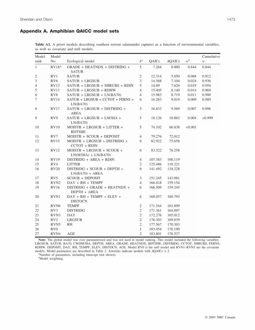
Appendix A. Amphibian QAICC model sets

© 2003 NRC Canada


Modelrank

ModelNo. Ecological model ka QAICc ∆QAICc wb

Cumulativew

1 RV18* GRADE + HEATNDX + DISTRIDG +SATUR

5 7.264 0.000 0.844 0.844

2 RV1 SATUR 2 12.314 5.050 0.068 0.9123 RV6 SATUR + LRGSUB 3 14.368 7.104 0.024 0.9364 RV13 SATUR + LRGSUB + SHRUBS + RDIN 5 14.89 7.626 0.019 0.9545 RV11 SATUR + LRGSUB + RDHW 4 15.405 8.140 0.014 0.9696 RV8 SATUR + LRGSUB + LN(BA70) 4 15.983 8.719 0.011 0.9807 RV14 SATUR + LRGSUB + CCTOT + FERNS +

LN(BA70)6 16.283 9.019 0.009 0.989

8 RV17 SATUR + LRGSUB + DISTRIDG +AREA

5 16.833 9.569 0.007 0.996

9 RV9 SATUR + LRGSUB + LM3HA +LN(BA70)

5 18.126 10.862 0.004 >0.999

10 RV10 MOISTR + LRGSUB + LITTER +RDTSHE

5 74.102 66.838 <0.001

11 RV7 MOISTR + SCOUR + DEPOSIT 4 79.276 72.01212 RV15 MOISTR + LRGSUB + DISTRIDG +

CCTOT + RDIN6 82.922 75.658

13 RV12 MOISTR + LRGSUB + SCOUR +LN(M3HA) + LN(BA70)

6 83.522 76.258

14 RV19 DISTRIDG + AREA + RDIN 4 107.383 100.11915 RV4 LITTER 2 125.486 118.22116 RV20 DISTRIDG + SCOUR + DEPTH +

LN(BA70) + AREA6 141.492 134.228

17 RV5 SCOUR + DEPOSIT 3 151.245 143.98118 RVN2 DAY + RH + TEMPF 4 166.418 159.15419 RV16 DISTRIDG + GRADE + HEATNDX +

DEPTH + AREA6 166.509 159.245

20 RVN1 DAY + RH + TEMPF + ELEV +DISTOCN

6 168.057 160.793

21 RVN6 TEMPF 2 171.164 163.89922 RV3 DISTRIDG 2 171.361 164.09723 RVN3 DAY 2 172.276 165.01224 RV2 LRGSUB 2 176.303 169.03925 RVN5 RH 2 177.567 170.30326 RV0 1 183.454 176.19027 RVN4 AGE 2 183.801 176.537

Note: The global model was over parameterized and was not used in model ranking. This model included the following variables:LRGSUB, SATUR, BA70, CWDM3HA, DEPTH, AREA, GRADE, HEATNDX, RDTSHE, DISTRIDG, CCTOT, SHRUBS, FERNS,RDHW, DEPOSIT, DAY, RH, TEMPF, ELEV, DISTOCN, AGE. Model RV0 is the null model and RVN1–RVN5 are the covariatemodels. Model parameters are described in Table 2. Asterisks indicate models with ∆QAICc ≤ 2.

aNumber of parameters, including intercept (not shown).bModel weighting.

Table A1. A priori models describing southern torrent salamander captures as a function of environmental variables,as well as covariate and null models.



© 2003 NRC Canada

1474 Can. J. For. Res. Vol. 33, 2003

Modelrank


Cumulativew

1 PD11* SHRUBS + CCTOT + SATUR + LRGSUB 5 112.43 0.000 0.903 0.9032 PD8 SATUR + LRGSUB + CCTOT + LN(BA70) 5 118.24 5.806 0.050 0.9533 PD21 LN(DISTRIDG) + SATUR + LN(BA70) +

AREA5 120.08 7.644 0.020 0.973

4 PD6 SATUR + DEPOSIT 3 121.99 9.555 0.008 0.9805 PD10 SATUR + LRGSUB + LN(BA70) +

LN(M3HA)5 123.05 10.621 0.004 0.985

6 PD1 SATUR 2 123.44 11.002 0.004 0.9887 PD13 SATUR + LRGSUB + LN(DISTRIDG) +

DEPOSIT + LN(BA70)6 123.77 11.340 0.003 0.992

8 PD7 SATUR + LRGSUB 3 123.87 11.432 0.003 0.9949 PD22 SATUR + LRGSUB + LN(DISTRIDG) +

CCTOT + RDHW6 124.39 11.951 0.002 0.997

10 PD9 SATUR + LRGSUB + FERNS + CCTOT +LN(M3HA)

6 124.67 12.234 0.002 0.999

11 PD14 SATUR + LRGSUB + DEPOSIT + RDHW 5 125.73 13.301 0.001 >0.99912 PD23 SATUR + LRGSUB + LN(DISTRIDG) +

DEPOSIT + LN(M3HA) + LN(BA70) +AREA + GRADE

20 132.06 19.623 <0.001

13 PD5 SCOUR + DEPOSIT 3 135.76 23.32914 PD15 LITTER + LN(BA70) + RDTSHE 4 139.56 27.13115 PD16 DEPOSIT + LN(BA70) + RDIN 4 140.31 27.87716 PD12 LRGSUB + DEPOSIT + LITTER + RDIN 5 141.35 28.92017 PD4 LITTER 2 147.25 34.81918 PD18 LN(DISTRIDG) + SCOUR + GRADE +

HEATNDX5 149.57 37.136

19 PD20 LN(DISTRIDG) + GRADE + LRGSUB +LN(BA70)

5 162.12 49.691

20 PD2 LRGSUB 2 166.64 54.20521 PD3 LN(DISTRIDG) 2 166.68 54.24422 PD17 LN(DISTRIDG) + GRADE + HEATNDX +

DEPTH + AREA6 170.80 58.364

23 PD19 LN(DISTRIDG) + GRADE + HEATNDX +DEPTH + AREA

6 170.80 58.364

24 PDN1 DAY + RH + TEMPF + ELEV + DISTOCN 6 171.78 59.34625 PD0 1 175.07 62.63726 PDN5 TEMPF 2 175.19 62.75327 PDN3 DAY 2 175.39 62.95428 PDN4 RH 2 175.68 63.24829 PDN2 DAY + RH + TEMPF 4 178.15 65.714

Note: Model PD0 is the null model, models PDN1–PDN5 are the covariate models, and model PD23 is the global model. Modelparameters are described in Table 2. Asterisks indicate models with ∆QAICc ≤ 2.


Table A2. A priori models describing Dunn’s salamander captures as a function of environmental variables.



© 2003 NRC Canada


Modelrank


Cumulativew

1 PV7* SATUR + LRGSUB 3 202.669 0.000 0.337 0.3372 PV19* GRADE + AREA + HEATNDX +

DISTC + LN(DISTRIDG)6 203.377 0.708 0.237 0.574

3 PV15* LRGSUB + SATUR + RDHW +CCTOT

5 204.398 1.729 0.142 0.716

4 PV18 LRGSUB + DISTC + GRADE +LN(BA70)

5 204.913 2.244 0.110 0.826

5 PV14 SATUR + LRGSUB + LN(M3HA) +LN(RD)

5 205.56 2.892 0.079 0.905

6 PV23 SATUR + LN(DISTRIDG) + DISTC +LRGSUB + CCTOT

6 207.986 5.317 0.024 0.929

7 PV24 SATUR + LRGSUB + LN(DISTRIDG) 20 209.065 6.397 0.014 0.9438 PV9 MOISTR + ORGSUB + CCTOT +

RDTSHE5 209.191 6.523 0.013 0.956

9 PVN3 DAY 2 209.595 6.926 0.011 0.96610 PV21 GEOMSRF + ORGSUB + CCTOT +

LN(BA70)6 209.922 7.253 0.009 0.975

11 PV16 MOISTR + ORGSUB + CCTOT +LITTER

5 210.276 7.607 0.008 0.983

12 PVN2 DAY + RH + TEMPF 4 211.633 8.964 0.004 0.98713 PV2 SATUR 2 212.034 9.365 0.003 0.99014 PV8 ORGSUB + CCTOT + LN(BA70) +

LITTER5 212.749 10.080 0.002 0.992

15 PV3 ORGSUB + LITTER 3 212.781 10.112 0.002 0.99416 PV11 ORGSUB + SCOUR + CCTOT 4 213.269 10.601 0.002 0.99617 PV6 ORGSUB + LRD 3 214.161 11.492 0.001 0.99718 PV1 MOISTR 2 214.416 11.747 0.001 0.99819 PVN1 DAY + RH + TEMPF + ELEV +

DISTOCN6 215.301 12.632 0.001 0.998

20 PVN5 TEMPF 2 215.448 12.779 0.001 0.99921 PV10 SATUR + SHRUBS + CCTOT + RD 5 217.225 14.556 <0.001 >0.99922 PVN4 RH 2 217.262 14.59323 PV0 1 217.598 14.92924 PV17 GEOMSRF 3 218.449 15.78125 PV13 LITTER + LN(BA70) 3 218.514 15.84526 PV12 STABLE + LN(BA70) 3 219.085 16.41627 PV5 LN(RD) + CCTOT 3 220.131 17.46228 PV4 LN(DISTRIDG) + DISTC 3 220.913 18.24529 PV22 GEOMSRF + MOISTR + LN(M3HA) +

CCTOT6 221.106 18.437

30 PV20 LN(DISTRIDG) + SCOUR + DEPOSIT 4 222.911 20.242

Note: Model PV0 is the null model, models PVN1–PVN5 are the covariate models, and model PV24 is the global model. Modelparameters are described in Table 2. Asterisks indicate models with ∆QAICc ≤ 2.


Table A3. A priori models describing western red-backed salamander captures as a function of environmental vari-ables.



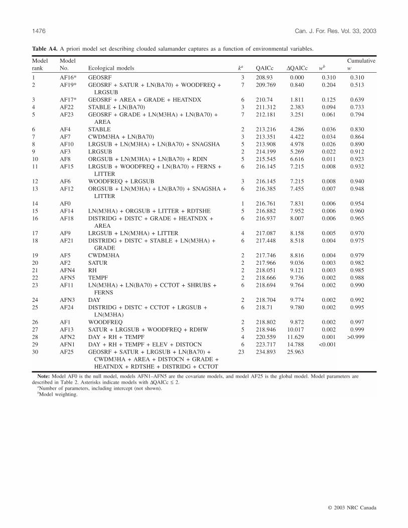
© 2003 NRC Canada

1476 Can. J. For. Res. Vol. 33, 2003

Modelrank

ModelNo. Ecological models ka QAICc ∆QAICc wb

Cumulativew

1 AF16* GEOSRF 3 208.93 0.000 0.310 0.3102 AF19* GEOSRF + SATUR + LN(BA70) + WOODFREQ +

LRGSUB7 209.769 0.840 0.204 0.513

3 AF17* GEOSRF + AREA + GRADE + HEATNDX 6 210.74 1.811 0.125 0.6394 AF22 STABLE + LN(BA70) 3 211.312 2.383 0.094 0.7335 AF23 GEOSRF + GRADE + LN(M3HA) + LN(BA70) +

AREA7 212.181 3.251 0.061 0.794

6 AF4 STABLE 2 213.216 4.286 0.036 0.8307 AF7 CWDM3HA + LN(BA70) 3 213.351 4.422 0.034 0.8648 AF10 LRGSUB + LN(M3HA) + LN(BA70) + SNAGSHA 5 213.908 4.978 0.026 0.8909 AF3 LRGSUB 2 214.199 5.269 0.022 0.91210 AF8 ORGSUB + LN(M3HA) + LN(BA70) + RDIN 5 215.545 6.616 0.011 0.92311 AF15 LRGSUB + WOODFREQ + LN(BA70) + FERNS +

LITTER6 216.145 7.215 0.008 0.932

12 AF6 WOODFREQ + LRGSUB 3 216.145 7.215 0.008 0.94013 AF12 ORGSUB + LN(M3HA) + LN(BA70) + SNAGSHA +

LITTER6 216.385 7.455 0.007 0.948

14 AF0 1 216.761 7.831 0.006 0.95415 AF14 LN(M3HA) + ORGSUB + LITTER + RDTSHE 5 216.882 7.952 0.006 0.96016 AF18 DISTRIDG + DISTC + GRADE + HEATNDX +

AREA6 216.937 8.007 0.006 0.965

17 AF9 LRGSUB + LN(M3HA) + LITTER 4 217.087 8.158 0.005 0.97018 AF21 DISTRIDG + DISTC + STABLE + LN(M3HA) +

GRADE6 217.448 8.518 0.004 0.975

19 AF5 CWDM3HA 2 217.746 8.816 0.004 0.97920 AF2 SATUR 2 217.966 9.036 0.003 0.98221 AFN4 RH 2 218.051 9.121 0.003 0.98522 AFN5 TEMPF 2 218.666 9.736 0.002 0.98823 AF11 LN(M3HA) + LN(BA70) + CCTOT + SHRUBS +

FERNS6 218.694 9.764 0.002 0.990

24 AFN3 DAY 2 218.704 9.774 0.002 0.99225 AF24 DISTRIDG + DISTC + CCTOT + LRGSUB +

LN(M3HA)6 218.71 9.780 0.002 0.995

26 AF1 WOODFREQ 2 218.802 9.872 0.002 0.99727 AF13 SATUR + LRGSUB + WOODFREQ + RDHW 5 218.946 10.017 0.002 0.99928 AFN2 DAY + RH + TEMPF 4 220.559 11.629 0.001 >0.99929 AFN1 DAY + RH + TEMPF + ELEV + DISTOCN 6 223.717 14.788 <0.00130 AF25 GEOSRF + SATUR + LRGSUB + LN(BA70) +

CWDM3HA + AREA + DISTOCN + GRADE +HEATNDX + RDTSHE + DISTRIDG + CCTOT

23 234.893 25.963

Note: Model AF0 is the null model, models AFN1–AFN5 are the covariate models, and model AF25 is the global model. Model parameters aredescribed in Table 2. Asterisks indicate models with ∆QAICc ≤ 2.


Table A4. A priori model set describing clouded salamander captures as a function of environmental variables.



© 2003 NRC Canada


Modelrank


Cumulativew

1 EE4* RDIN + CCTOT 3 180.503 0.000 0.194 0.1942 EE10* RDTSHE + CCTOT + LITTER 4 180.864 0.361 0.162 0.3563 EE21* RDIN + CCTOT + LITTER + STABLE 5 181.297 0.794 0.130 0.4864 EE11* LRGSUB + RDHW + SATUR 4 181.312 0.810 0.129 0.6165 EE7* CCTOT + LITTER + ORGSUB 4 182.005 1.502 0.092 0.7076 EE20* CCTOT + ORGSUB + DISTC + GRADE 5 182.472 1.969 0.072 0.7807 EE2 ORGSUB 2 183.562 3.059 0.042 0.8228 EE6 ORGSUB + LITTER 3 183.805 3.303 0.037 0.8599 EE9 ORGSUB + LITTER + DISTC + CCTOT 5 183.964 3.462 0.034 0.89310 EE8 ORGSUB + LITTER + CCTOT + LN(M3HA) 5 184.084 3.581 0.032 0.92611 EE17 DISTC + STABLE + GRADE 4 184.213 3.710 0.030 0.95612 EE16 DISTC + ORGSUB + LN(M3HA) + CCTOT +

GRADE6 184.66 4.157 0.024 0.980

13 EE3 SATUR 2 187.554 7.051 0.006 0.98614 EE12 GEOSRF + GRADE + HEATNDX 4 188.263 7.760 0.004 0.99015 EE18 LITTER + LN(BA70) 3 190.094 9.591 0.002 0.99216 EE0 1 190.23 9.727 0.002 0.99317 EE1 LITTER 2 191.049 10.546 0.001 0.99418 EE22 DISTRIDG + DISTC + CCTOT + LITTER 5 191.072 10.570 0.001 0.99519 EE15 DISTRIDG + DISTC + GRADE + HEATNDX +

AREA6 191.386 10.883 0.001 0.996

20 EE19 DISTC + DEPTH + AREA + CCTOT 5 191.936 11.433 0.001 0.99621 EEN5 TEMPF 2 191.952 11.449 0.001 0.99722 EEN3 DAY 2 191.989 11.486 0.001 0.99823 EE14 GEOSRF 2 192.064 11.561 0.001 0.99824 EEN4 RH 2 192.208 11.706 0.001 0.99925 EE23 ORGSUB + LN(M3HA) + AREA + GRADE 19 193.004 12.501 <0.000 >0.99926 EE5 DISTRIDG + DISTC 3 193.792 13.28927 EEN1 DAY + RH + TEMPF + ELEV + DISTOCN 6 194.126 13.62328 EEN2 DAY + RH + TEMPF 4 194.387 13.88529 EE13 GEOSRF + DEPTH + HEATNDX + AREA 5 196.788 16.285

Note: Model EE0 is the null model, models EEN1–EEN5 are the covariate models, and model EE23 is the global model. Modelparameters are described in Table 2. Asterisks indicate models with ∆QAICc ≤ 2.


Table A5. A priori model set describing ensatina captures as a function of environmental variables.



Documents

Amphibian assemblages in zero-order basins in the Oregon ...andrewsforest.oregonstate.edu/pubs/pdf/pub3099.pdf · Amphibian assemblages in zero-order basins in the Oregon Coast Range1