Embed Size (px)
DESCRIPTION
AMMBR II. Gerrit Rooks 8-2-10. Suppose I have a data-set with 100 observations. A graphic representation. Age groups. Logistics of logistic regression. Estimate the coefficients Assess model fit Interpret coefficients Check regression assumptions. Maximum likelihood estimation. - PowerPoint PPT Presentation
Citation preview

AMMBR II
Gerrit Rooks8-2-10

Suppose I have a data-set with 100 observations
ID age CHD
1 20 02 23 03 24 04 25 1…98 64 099 65 1
100 69 1

A graphic representation
0.2
.4.6
.81
chd
20 30 40 50 60 70age

Agegroup
Count Absent Present Proport-ion
1 10 9 1 .12 15 13 2 .133 12 9 3 .254 15 10 5 .335 13 7 6 .466 8 3 5 .637 17 4 13 .768 64 10 2 .8
Age groups


)( 11101
1)|( Xbbe
XYE

Logistics of logistic regression
• Estimate the coefficients • Assess model fit• Interpret coefficients • Check regression assumptions

Maximum likelihood estimation
• Method of maximum likelihood yields values for the unknown parameters whichi maximize te probability of obtaining the observed set of data.
• First we have to construct the likelihood function.– Expresses the probability of the observed data as
a function of the unknown parameters.

• The probability of a given observation
)( 11101
1)|1( Xbbe
Xpr
)( 11101
11)|0( Xbbe
Xpr

• Since the observations are assumed to be independent the likelihood function can be written as
• For technical reasons the likelihood is transformed in the log-likelihood
Likelihood = pr(obs1)*pr(obs2)*pr(obs3)…*pr(obsn)
LL= ln[pr(obs1)]+ln[pr(obs2)]+ln[pr(obs3)]…+ln[pr(obsn)]

_cons -5.309453 1.133655 -4.68 0.000 -7.531376 -3.087531 age .1109211 .0240598 4.61 0.000 .0637647 .1580776 chd Coef. Std. Err. z P>|z| [95% Conf. Interval]
Log likelihood = -53.676546 Pseudo R2 = 0.2145 Prob > chi2 = 0.0000 LR chi2(1) = 29.31Logistic regression Number of obs = 100
. logistic chd age, coef

)11.3.5( 11
1)|(
XeXYE

)05.3.5( 11
1)|(
XeXYE

)40.3.5( 11
1)|(
XeXYE

)11.3.5( 11
1)|(
XeXYE

Logistics of logistic regression
• Estimate the coefficients • Assess model fit• Interpret coefficients • Check regression assumptions

Assessing model fit
a) Between model comparisons
b) Pseudo R2 (similar to multiple regression)
c) Predictive accuracy per group
_cons -.2818512 .2019893 -1.40 0.163 -.6777429 .1140406 chd Coef. Std. Err. z P>|z| [95% Conf. Interval]
Log likelihood = -68.331491 Pseudo R2 = -0.0000 Prob > chi2 = . LR chi2(0) = -0.00Logistic regression Number of obs = 100
. logistic chd, coef
_cons -5.309453 1.133655 -4.68 0.000 -7.531376 -3.087531 age .1109211 .0240598 4.61 0.000 .0637647 .1580776 chd Coef. Std. Err. z P>|z| [95% Conf. Interval]
Log likelihood = -53.676546 Pseudo R2 = 0.2145 Prob > chi2 = 0.0000 LR chi2(1) = 29.31Logistic regression Number of obs = 100
. logistic chd age, coef
)]baseline()New([22 LLLL
2[-53.69-(-68.33)] = 29.31

Predictive accuracy
Correctly classified 57.00% False - rate for classified - Pr( D| -) 43.00%False + rate for classified + Pr(~D| +) .%False - rate for true D Pr( -| D) 100.00%False + rate for true ~D Pr( +|~D) 0.00% Negative predictive value Pr(~D| -) 57.00%Positive predictive value Pr( D| +) .%Specificity Pr( -|~D) 100.00%Sensitivity Pr( +| D) 0.00% True D defined as chd != 0Classified + if predicted Pr(D) >= .5
Total 43 57 100 - 43 57 100 + 0 0 0 Classified D ~D Total True
Logistic model for chd
. estat class

Logistics of logistic regression
• Estimate the coefficients • Assess model fit• Interpret coefficients • Check regression assumptions

21
3. Interpreting coefficients: direction
• original b reflects changes in logit: b>0 -> positive relationship
• exponentiated b reflects the changes in odds: exp(b) > 1 -> positive relationship
nnxbxbxbbyp
yp
...
)(1
)(lnlogit 22110
nnxbxbxbb eeeeyp
yp
...
)(1
)(Odds 22110

Interpreting coefficients: significance
• How statistically significant is the estimation?
• Logistic regression uses Wald statistics (instead of t-values)
• However, the Wald is sometimes underestimated (you are more likely to make a Type II error)
bSE
b Wald
Note: This is not the Wald Statistic SPSS presents!!!

23
3. Interpreting coefficients: magnitude
• The slope coefficient (b) is interpreted as the rate of change in the "log odds" as X changes … not very useful.
• exp(b) is the effect of the independent variable on the odds, more useful for calculating the size of an effect
nnxbxbxbbyp
yp
...
)(1
)(lnlogit 22110
nnxbxbxbb eeeeyp
yp
...
)(1
)(Odds 22110

Magnitude of association
• Percentage change in odds:
• (Exponentiated coefficienti - 1.0) * 100
event
event
prob1
probOddsi
Probability Odds
25% 0.33
50% 1
75% 3

25
• For variable ’previous’:– Percentage change in odds = (exponentiated coefficient – 1) * 100 = 6.7– A one unit increase in previous will result in 6,7% increase in the odds– So if a soccer player has a 10% higher scoring percentage, the odds that (s)he will score is 67%
higher • For variable ‘pswq’ (worrying)
– Percentage change in odds = (exponentiated coefficient – 1) * 100 = -20.6– A one unit increase in pswq will result in 20,6% decrease in the odds– So if a soccer player scores 1 on the pswq test instead of 0, the odds that (s)he will score is
20.6% lower
Variables in the Equation
-,230 ,080 8,309 1 ,004 ,794
,065 ,022 8,609 1 ,003 1,067
1,280 1,670 ,588 1 ,443 3,598
pswq
previous
Constant
Step1
a
B S.E. Wald df Sig. Exp(B)
Variable(s) entered on step 1: pswq, previous.a.
Magnitude of association

Calculating probabilities
)-.23pswqPrevious065.28.1(1
1)|(
eXYE
%831
1)|(
)15.6*-.2350*065.28.1(
e
XYE

Checking assumptions
• Influential data points & Residuals– Follow Samanthas tips
• Hosmer & Lemeshow– Divides sample in subgroups– Checks whether there are differences between
observed and predicted between subgroups– Test should not be significant, if so: indication of
lack of fit

Stata file types
• .ado – programs that add commands to Stata
• .do– Batch files that execute a set of Stata commands
• .dta– Data file in Stata’s format
• .log– Output saved as plain text by the log using
command

The working directory
• The working directory is the default directory for any file operations such as using & saving data, or logging output
• cd “d:\my work\”

Saving output to log files
• Syntax for the log command– log using filename [, append replace [smcl|text]]
• To close a log file– log close

Using and saving datasets
• Load a Stata dataset – use d:\myproject\data.dta, clear
• Save – save d:\myproject\data, replace
• Using change directory– cd d:\myproject– Use data, clear– save data, replace

Entering data
• Data in other formats– You can use SPSS to convert data– You can use the infile and insheet commands to
import data in ASCII format• Entering data by hand
– Type edit or just click on the data-editor button

Do-files
• You can create a text file that contains a series of commands
• Use the do-editor to work with do-files • Example I

Adding comments
• // or * denote comments stata should ignore• Stata ignores whatever follows after /// and
treats the next line as a continuation • Example II
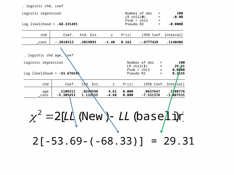
A recommended structure//if a log file is open, close itcapture log close//dont'pause when output scrolls off the pageset more off//change directory to your working directorycd d:\myproject//log results to file myfile.loglog using myfile, replace text// * myfile.do-written 7 feb 2010 to illustrate do-files//
your commands here
//close the log filelog close

Serious data analysis
• Ensure replicability use do+log files• Document your do-files
– What is obvious today, is baffling in six months• Keep a research log
– Diary that includes a description of every program you run
• Develop a system for naming files

Serious data analysis
• New variables should be given new names• Use labels and notes• Double check every new variable• ARCHIVE

The Stata syntax• Command
– What action do you want to performed• Names of variables, files or other objects
– On what things is the command performed• Qualifier on observations
– On which observations should the command be performed
• Options– What special things should be done in executing
the command

Example
• tabulate smoking race if agemother > 30, row
• Example of the if qualifier– sum agemother if smoking == 1 & weightmother < 100

Elements used for logical statements
Operator Definition Example
== Equal to If male == 1
!= Not equal to If male !=1
> Greater than If age > 20
>= Greater than or equal to If age >=21
< Less than If age<66
<= Less than or equal to If age<=65
& And If age==21&male ==1
| or If age<=21|age>=65
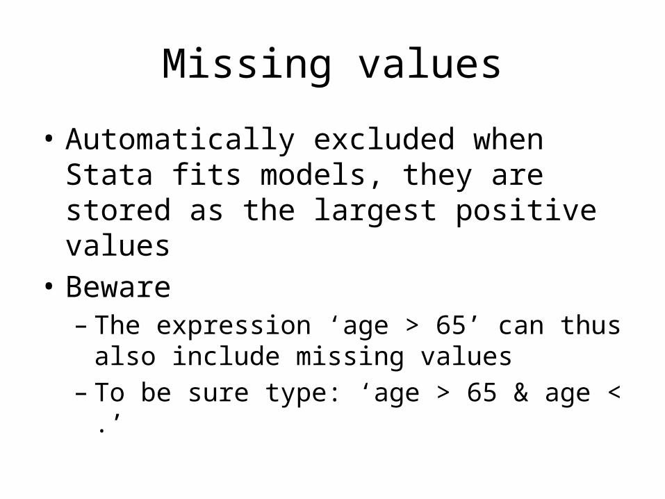
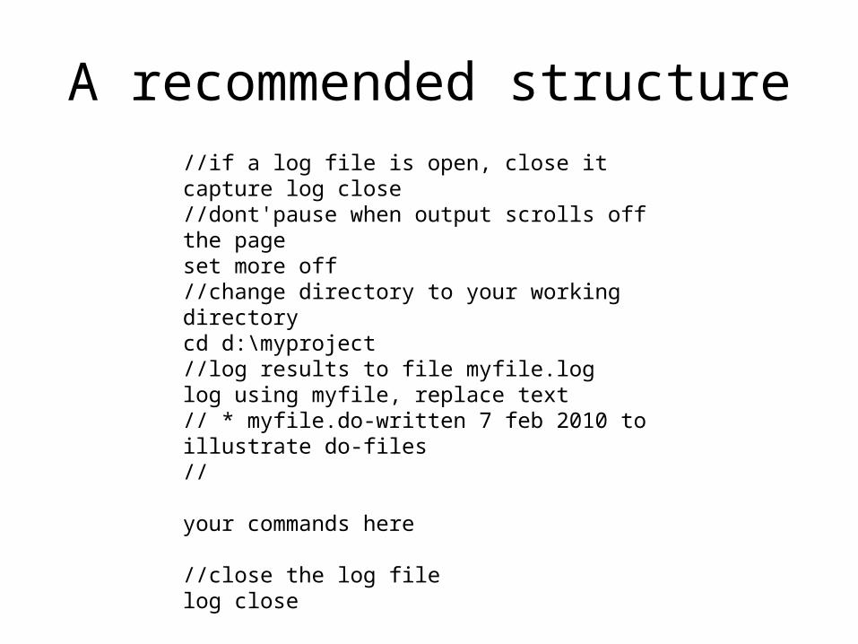
Missing values
• Automatically excluded when Stata fits models, they are stored as the largest positive values
• Beware – The expression ‘age > 65’ can thus also include
missing values– To be sure type: ‘age > 65 & age < .’

Selecting observations
• drop variable list• Keep variable list
• drop age if age < 65

Creating new variables
• generate command– generate age2 = age * age– generate – see help function
– !!sometimes the command egen is a useful alternative, f.i.
– gen meanage = mean(age)

Useful functionsFunction Definition Example
+ addition gen y = a+b
- subtraction gen y = a-b
/ Division gen density=population/area
* Multiplication gen y = a*b
^ Take to a power gen y = a^3
ln Natural log gen lnwage = ln(wage)
exp exponential gen y = exp(b)
sqrt Square root Gen agesqrt = sqrt(age)

Replace command
• replace has the same syntax as generate but is used to change values of a variable that already exists
• gen age_dum = .• replace age = 0 if age < 5• replace age = 1 if age >=5

Recode
• Change values of exisiting variables– Change 1 to 2 and 3 to 4– recode origvar (1=2)(3=4), gen(myvar1)
– Change missings to 1– recode origvar (.=1), gen(origvar)

Now a little exercise
• Using the clslowbwt data• give summaray statistics of the weight of the
mother• Give the frequency of the number of mothers
that smoked during pregnacy• compute a dummy variable indicating whether
mother is older than 30 • Recode the race variable – join category 2 and
3

• Regress the weight of the mother on race, smoking and age
• regress dep var indep varlist

• Logistic regression– Logit or logistic– estat class– estat gof
• Example III

• Use the `clslowbwt` data• Perform a logistic regression analysis of low vs
normal birth weight. How can you predict this?– Estimate the coefficients – Assess model fit– Interpret coefficients – Check regression assumptions