www.oeaw.ac.at

www.ricam.oeaw.ac.at

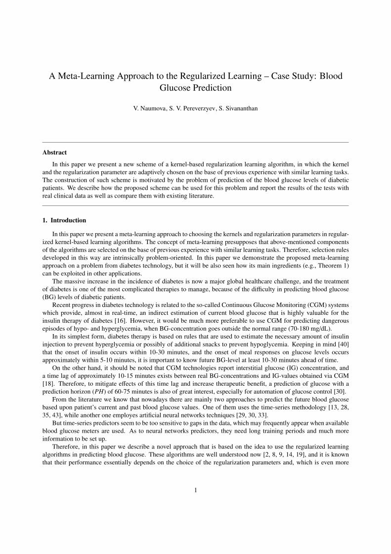
A Meta-Learning Approach tothe Regularized Learning –Case Study: Blood Glucose

Prediction

V. Naumova, S. Pereverzyev, S. Sampath

RICAM-Report 2011-31

A Meta-Learning Approach to the Regularized Learning – Case Study: BloodGlucose Prediction

V. Naumova, S. V. Pereverzyev, S. Sivananthan

Abstract

In this paper we present a new scheme of a kernel-based regularization learning algorithm, in which the kerneland the regularization parameter are adaptively chosen on the base of previous experience with similar learning tasks.The construction of such scheme is motivated by the problem of prediction of the blood glucose levels of diabeticpatients. We describe how the proposed scheme can be used for this problem and report the results of the tests withreal clinical data as well as compare them with existing literature.

1. Introduction

In this paper we present a meta-learning approach to choosing the kernels and regularization parameters in regular-ized kernel-based learning algorithms. The concept of meta-learning presupposes that above-mentioned componentsof the algorithms are selected on the base of previous experience with similar learning tasks. Therefore, selection rulesdeveloped in this way are intrinsically problem-oriented. In this paper we demonstrate the proposed meta-learningapproach on a problem from diabetes technology, but it will be also seen how its main ingredients (e.g., Theorem 1)can be exploited in other applications.

The massive increase in the incidence of diabetes is now a major global healthcare challenge, and the treatmentof diabetes is one of the most complicated therapies to manage, because of the difficulty in predicting blood glucose(BG) levels of diabetic patients.

Recent progress in diabetes technology is related to the so-called Continuous Glucose Monitoring (CGM) systemswhich provide, almost in real-time, an indirect estimation of current blood glucose that is highly valuable for theinsulin therapy of diabetes [16]. However, it would be much more preferable to use CGM for predicting dangerousepisodes of hypo- and hyperglycemia, when BG-concentration goes outside the normal range (70-180 mg/dL).

In its simplest form, diabetes therapy is based on rules that are used to estimate the necessary amount of insulininjection to prevent hyperglycemia or possibly of additional snacks to prevent hypoglycemia. Keeping in mind [40]that the onset of insulin occurs within 10-30 minutes, and the onset of meal responses on glucose levels occursapproximately within 5-10 minutes, it is important to know future BG-level at least 10-30 minutes ahead of time.

On the other hand, it should be noted that CGM technologies report interstitial glucose (IG) concentration, anda time lag of approximately 10-15 minutes exists between real BG-concentrations and IG-values obtained via CGM[18]. Therefore, to mitigate effects of this time lag and increase therapeutic benefit, a prediction of glucose with aprediction horizon (PH) of 60-75 minutes is also of great interest, especially for automation of glucose control [30].

From the literature we know that nowadays there are mainly two approaches to predict the future blood glucosebased upon patient’s current and past blood glucose values. One of them uses the time-series methodology [13, 28,35, 43], while another one employes artificial neural networks techniques [29, 30, 33].

But time-series predictors seem to be too sensitive to gaps in the data, which may frequently appear when availableblood glucose meters are used. As to neural networks predictors, they need long training periods and much moreinformation to be set up.

Therefore, in this paper we describe a novel approach that is based on the idea to use the regularized learningalgorithms in predicting blood glucose. These algorithms are well understood now [2, 8, 9, 14, 19], and it is knownthat their performance essentially depends on the choice of the regularization parameters and, which is even more

1

important, on the choice of the kernels generating Reproducing Kernel Hilbert Spaces (RKHS), in which the regu-larization is performed [5, 10, 22, 26, 42]. As it was realized [31], in the context of blood glucose prediction thesealgorithmic instances cannot be a priori fixed, but need to be adjusted to each particular prediction input.

Thus, a regularized learning based predictor should learn how to learn kernels and regularization parameters frominput. Such a predictor is constructed as a result of a process of learning to learn, or “meta-learning” [37]. In thisway we have developed the Fully Adaptive Regularized Learning (FARL) approach to the blood glucose prediction.This approach is described in the patent application [32] filed jointly by Austrian Academy of Sciences and NovoNordisk A/S (Denmark). The developed approach allows the construction of blood glucose predictors which, as ithas been demonstrated in the extensive clinical trials, outperform the state-of-the-art algorithms. Moreover, it turnsout that in the context of the blood glucose prediction the FARL approach is more advanced than other meta-learningtechnologies such as k-Nearest Neighbors (k-NN) ranking [41].

To facilitate further discussion, this paper is structured into 4 additional sections. Section 2 explains the detailsof the regularized learning approach to BG-prediction and indicates its issues and concerns. Section 3 specifies theframework of meta-learning for kernel-based regularized learning algorithms and three different types of operationsrequired for performing meta-learning, in particular, how these operations are processed within the proposed FARLapproach. In Section 4 we present a performance comparison of the FARL-based predictors with the current state-of-the-art BG-prediction methods and k-NN meta-learning. The paper concludes with Section 5 on current and futuredevelopments.

2. A Traditional Learning Theory Approach: Issues and Concerns

Throughout this paper we consider the problem of blood glucose prediction. Mathematically this problem can beformulated as follows. Assume that at the time moment t = t0 we are given m preceding estimates g0, g−1, g−2, . . . ,g−m+1 of a patient’s BG-concentration sampled correspondingly at the time moments t0 > t−1 > t−2 > . . . > t−m+1within the sampling horizon S H = t0 − t−m+1. The goal is to construct a predictor that uses these past measurementsto predict BG-concentration as a function of time g = g(t) for n subsequent future time moments t j

nj=1 within the

prediction horizon PH = tn − t0 such that t0 < t1 < t2 < . . . < tn.At this point, it is noteworthy to mention that CGM systems provide estimations gi of BG-values every 5 or 10

minutes, such that ti = t0 + i∆t, i = −1,−2, . . . , where ∆t = 5 (min) or ∆t = 10 (min). For mathematical details see[26].

Thus, the promising concept in the diabetes therapy management is the prediction of the future BG-evolutionusing CGM data [39]. The importance of such prediction has been shown by several applications [4, 28].

From the above discussion, one can see that the CGM technology allows us to form a training set z = (xµ, yµ), µ =1, 2, . . . ,M, |z| = M, where

xµ = ((tµ−m+1, g

µ−m+1), . . . , (tµ0 , g

µ0)) ∈ (R2

+)m,

yµ = ((tµ1 , gµ1), . . . , (tµn , g

µn)) ∈ (R2

+)n, (1)and tµ

−m+1 < tµ−m+2 < . . . < tµ0 < tµ1 < . . . < tµn

are the moments at which patient’s BG-concentrations were estimated by CGM system as gµ−m+1, . . . , g

µ0, . . . , g

µn. More-

over, for any µ = 1, 2, . . . ,M the moments tµj nj=−m+1 can be chosen such that tµ0 − tµ

−m+1 = S H, tµn − tµ0 = PH, whereS H and PH are the sampling and prediction horizons of interest respectively.

Given a training set it is rather natural to consider our problem in the framework of supervised learning [8, 14,19, 38, 45], where the available input-output samples (xµ, yµ) are assumed to be drawn independently and identicallydistributed (i.i.d.) according to an unknown probability distribution. Originally, in [17] it is stated that the consecutiveCGM readings gi taken from the same subject within a relatively short time are highly interdependent. At the sametime, CGM readings that are separated by more than 1 hour in time could be considered as (linearly) independent.Therefore, using the supervised learning framework we are forced to consider vector-valued input-output relationsxµ → yµ instead of scalar-valued ones tµi → gµi . Moreover, we will assume that (tµi , g

µi ), µ = 1, 2, . . . ,M, are sampled

in such a way that |tµi − tµ+1i | > 1 (hour).

2

In this setting, a set z is used to find (a vector-valued) function fz : (R2+)m → (R2

+)n such that for any newBG-observations

x = ((t−m+1, g−m+1), . . . , (t0, g0)) ∈ (R2+)m (2)

with t−m+1 < t−m+2 < . . . < t0, t0 − t−m+1 = S H, the value fz(x) ∈ (R2+)n is a good prediction of the future BG-sample

y = ((t1, g1), . . . , (tn, gn)) ∈ (R2+)n, (3)

where t0 < t1 < . . . < tn, tn − t0 = PH.Note that in such vector-valued formulation the problem still can be studied with the use of the standard scheme

of supervised learning [9, 23], where it is assumed that fz belongs to an RKHSHK generated by a kernel K.Then fz = f λz ∈ HK is constructed as the minimizer of the functional

1|z|

|z|∑µ=1

|| f (xµ) − yµ||2(R2)n + λ|| f ||2HK, (4)

where λ is a regularization parameter.Recall [9, 23] that a Hilbert space H of vector-valued functions f : X → (R2)n, X ⊂ (R2)m, is called an RKHS

if for any x ∈ X the value f (x) admits a representation f (x) = K∗x f , where K∗x : H → (R2)n is a Hilbert-Schmidtoperator, which is the adjoint of Kx : (R2)n → H . Similar to the scalar case the inner product 〈·, ·〉 = 〈·, ·〉K can bedefined in terms of the kernel K(x, t) = K∗x Kt for every x, t ∈ X.

The standard scheme (4) raises two main issues that should be clarified before its usage. One of them is how tochoose a regularization parameter λ and another one, which is even more important, is how to choose the space HK ,where the regularization should be performed, or, which is the same thing, the kernel K that generates this space.Several approaches to address these issues have been proposed in the past few years [5, 10, 20, 22, 36, 47].

All of them attempt to choose a kernel K “globally” for the whole given training set z, but they do not account forparticular features of input xµ. As the result, if some new input-output pair (xµ, yµ) is added to the training set z, then,in accordance with known approaches, a kernel selection procedure should be started from scratch, which is rathercostly. In essence, known techniques [5, 10, 20, 22, 47] do not learn how to select a kernel K and a regularizationparameter λ for each new input x in question.

In the next section we introduce a meta-learning approach which is free from the above-mentioned shortcomingand allows us to adjust K and λ “locally” to each new input x on the basis of the previous learning experience withthe examples (xµ, yµ) from a given training set z.

3. Meta-Learning Approach to Choosing a Kernel and a Regularization Parameter

First of all, let us note that the choice of the regularization parameter λ is completely depends on the choice of thekernel. For the fixed kernel K, there is a variety of strategies that can be used to select a regularization parameter λ.Among them are the discrepancy principle [24, 25, 34], balancing principle [10, 21], heuristically motivated quasi-optimality criterion [15, 44]. Thus, keeping in mind this remark, we will think about λ as a functional of K, i.e.λ = λ(K).

This observation motivates us to focus mainly on the choice of the kernel K as it can make significant differencein performance [3, Section 2.4].

As we already mentioned in the previous section, in most of the known approaches [5, 10, 20, 22, 47] the chosenkernel K and the regularization parameter λ are “reasonable,” in some sense, for the whole training set z = (xµ, yµ),but they are not necessarily optimal for a particular pair (xµ, yµ) ∈ z. In this section, as a way to overcome thisdrawback, we describe our approach to the kernel choice problem, which is based on the concept of meta-learning.

According to this approach, the meta-learning process can be divided into three phases / operations.In the first phase, which can be called optimization, the aim is to find for each input-output pair (xµ, yµ), µ =

1, 2, . . . ,M, a favorite kernel K = Kµ and a regularization parameter λ = λµ,which in some sense optimize a predictionof yµ from xµ. This operation can be cast as the set of M search problems, where for each pair (xµ, yµ) we are searchingover some set of admissible kernels.

3

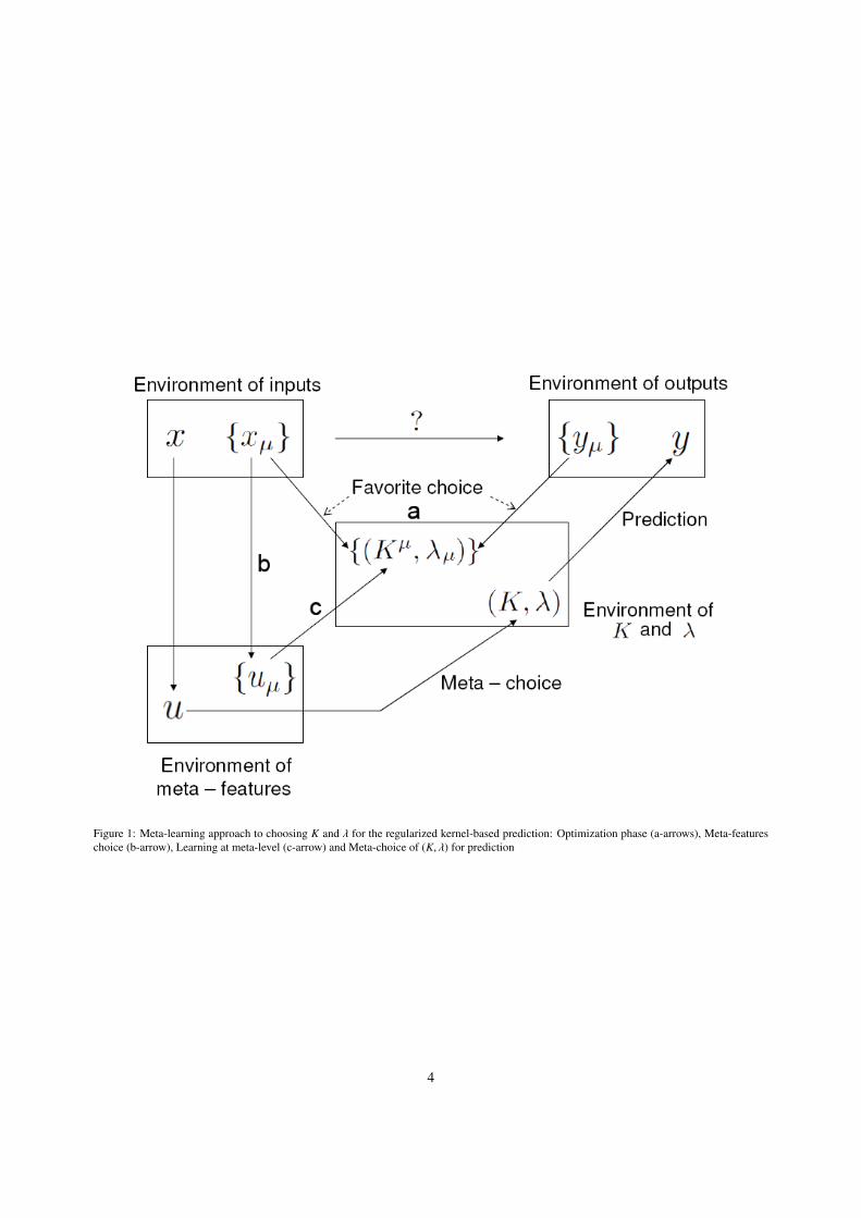
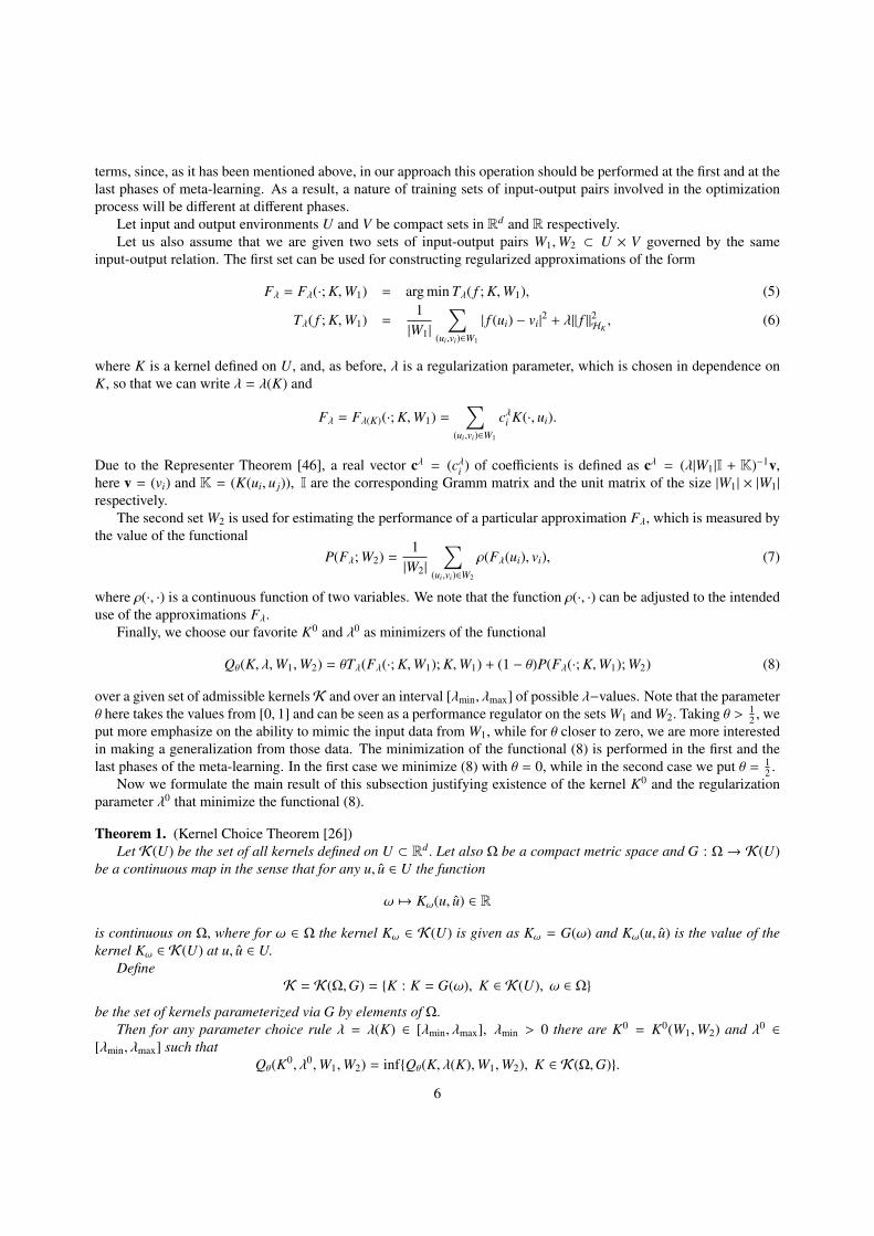
Figure 1: Meta-learning approach to choosing K and λ for the regularized kernel-based prediction: Optimization phase (a-arrows), Meta-featureschoice (b-arrow), Learning at meta-level (c-arrow) and Meta-choice of (K, λ) for prediction

4

Note that in the usual learning setting a kernel is also sometimes found as the solution of some optimizationoperation [5, 10, 20, 22, 47], but in contrast to our meta-learning based approach, the problem is formulated for thewhole training set. As a result, such a kernel choice should be executed from scratch each time when a new input-output pair (xµ, yµ) is added to the training set. Moreover, as it was already mentioned several times, the kernel chosenin this way is not necessarily optimal for a particular input-output pair.

The second phase of our meta-learning based approach consists in choosing and computing the so-called meta-features uµ of inputs xµ from the training set. The design of adequate meta-features should capture and representthe properties of an input xµ that influence the choice of a favorite kernel Kµ used for predicting yµ from xµ. Thissecond phase of meta-learning is often driven by heuristics [3, Section 3.3]. In [41] the authors discuss a set of 14possible input characteristics, which can be used as meta-features. In our approach, we use one of them, namely atwo-dimensional vector uµ = (u(1)

µ , u(2)µ ) of the coefficients of “least squares regression line” glin = u(1)

µ t + u(2)µ that

produces the “best linear fit” linking the components t = (tµ−m+1, t

µ−m+2, . . . , t

µ0) and g = (gµ

−m+1, gµ−m+2, . . . , g

µ0), which

form the input xµ. Heuristic reason for choosing such a meta-feature will be given below.Note that in the present context one may, in principle, choose an input xµ itself as a meta-feature. But, as it will be

seen below, such a choice would essentially increase the dimensionality of the optimization problem in the final phaseof the meta-learning. Moreover, since the inputs xµ are formed by potentially noisy measurements (tµi , g

µi ), the use of

low dimensional meta-features uµ = (u(1)µ , u

(2)µ ) can be seen as a regularization (denoising) by dimension reduction and

as an overfitting prevention.The final phase of the meta-learning consists of constructing the so-called meta-choice rule that explains the

relation between the set of meta-features of inputs and the parameters of favorite algorithms found in the first phaseof the meta-learning (optimization). This phase is sometimes called learning at meta-level. If above mentioned meta-choice rule is constructed, then for any given input x the parameters of a favorite prediction algorithm can be easilyfound by applying this rule to the meta-feature u calculated for the input x in question.

Recall that in the present context, the first two phases of the meta-learning result in the transformation of theoriginal training set z = (xµ, yµ) into new ones, where the meta-features uµ are paired with the parameters of favoritekernels Kµ and λµ = λ(Kµ).

Then, in principle, any learning algorithm can be employed on these new training sets to predict the parametersof the favorite kernel K and λ = λ(K) for the input x in question. For example, in [36] these parameters are predictedby means of least squares method that is performed in RKHS generated by the so-called histogram kernel. Note thatsuch approach can be used only for sufficiently simple sets of admissible kernelsK (only linear combinations of somea priori fixed kernels are considered in [36]). Moreover, as it has been also noted by the authors [36], in general, thehistogram kernel does not take into account specific knowledge about the problem at hand. So, the approach [36] canonly loosely be considered as a meta-learning.

At the same time, one of the most popular algorithm suggested in the meta-learning literature for learning at meta-level is the so-called k-Nearest Neighbors (k-NN) ranking [3, 41]. The algorithm can be interpreted as a learning inthe space of piecewise constant functions.

One of the novelties of our approach is that a regularization in RKHS is used not only in the first phase, but alsoin learning at meta-level. Of course, in this case the kernel choice issue arises again, and it will be addressed in thesame manner as in the first phase. But, what is important, the corresponding optimization needs to be performed onlyonce and only with the transformed training set (uµ,Kµ) from just one patient. This means that the blood glucosepredictor based on our approach can be transported from patient to patient without any additional re-adjustment.Such a portability is desirable and will be demonstrated in experiments with real clinical data. Moreover, it will beshown that the use of k-NN ranking at meta-level results in the blood glucose predictor, which is outperformed by thepredictor based on our approach.

In general, the meta-learning approach is schematically illustrated in Figure 1. The following subsections containdetailed description of all the operations needed to install and set our meta-learning based predictor.

3.1. Optimization operationThe ultimate goal of the optimization operation is to select such kernel K and regularization parameter λ that

allow to achieve good performance for given data. To describe the choice of favorite K and λ for each input-outputpair (xµ, yµ) ∈ (R2

+)m × (R2+)n from the training set z we rephrase vector-valued formalism in terms of ordinary scalar-

valued functions similar to how it was done in [9]. Moreover, we will describe the optimization operation in general

5

terms, since, as it has been mentioned above, in our approach this operation should be performed at the first and at thelast phases of meta-learning. As a result, a nature of training sets of input-output pairs involved in the optimizationprocess will be different at different phases.

Let input and output environments U and V be compact sets in Rd and R respectively.Let us also assume that we are given two sets of input-output pairs W1,W2 ⊂ U × V governed by the same

input-output relation. The first set can be used for constructing regularized approximations of the form

Fλ = Fλ(·; K,W1) = arg min Tλ( f ; K,W1), (5)

Tλ( f ; K,W1) =1|W1|

∑(ui,vi)∈W1

| f (ui) − vi|2 + λ|| f ||2

HK, (6)

where K is a kernel defined on U, and, as before, λ is a regularization parameter, which is chosen in dependence onK, so that we can write λ = λ(K) and

Fλ = Fλ(K)(·; K,W1) =∑

(ui,vi)∈W1

cλi K(·, ui).

Due to the Representer Theorem [46], a real vector cλ = (cλi ) of coefficients is defined as cλ = (λ|W1|I + K)−1v,here v = (vi) and K = (K(ui, u j)), I are the corresponding Gramm matrix and the unit matrix of the size |W1| × |W1|

respectively.The second set W2 is used for estimating the performance of a particular approximation Fλ, which is measured by

the value of the functionalP(Fλ; W2) =

1|W2|

∑(ui,vi)∈W2

ρ(Fλ(ui), vi), (7)

where ρ(·, ·) is a continuous function of two variables. We note that the function ρ(·, ·) can be adjusted to the intendeduse of the approximations Fλ.

Finally, we choose our favorite K0 and λ0 as minimizers of the functional

Qθ(K, λ,W1,W2) = θTλ(Fλ(·; K,W1); K,W1) + (1 − θ)P(Fλ(·; K,W1); W2) (8)

over a given set of admissible kernelsK and over an interval [λmin, λmax] of possible λ−values. Note that the parameterθ here takes the values from [0, 1] and can be seen as a performance regulator on the sets W1 and W2. Taking θ > 1

2 , weput more emphasize on the ability to mimic the input data from W1, while for θ closer to zero, we are more interestedin making a generalization from those data. The minimization of the functional (8) is performed in the first and thelast phases of the meta-learning. In the first case we minimize (8) with θ = 0, while in the second case we put θ = 1

2 .Now we formulate the main result of this subsection justifying existence of the kernel K0 and the regularization

parameter λ0 that minimize the functional (8).

Theorem 1. (Kernel Choice Theorem [26])Let K(U) be the set of all kernels defined on U ⊂ Rd. Let also Ω be a compact metric space and G : Ω → K(U)

be a continuous map in the sense that for any u, u ∈ U the function

ω 7→ Kω(u, u) ∈ R

is continuous on Ω, where for ω ∈ Ω the kernel Kω ∈ K(U) is given as Kω = G(ω) and Kω(u, u) is the value of thekernel Kω ∈ K(U) at u, u ∈ U.

DefineK = K(Ω,G) = K : K = G(ω), K ∈ K(U), ω ∈ Ω

be the set of kernels parameterized via G by elements of Ω.Then for any parameter choice rule λ = λ(K) ∈ [λmin, λmax], λmin > 0 there are K0 = K0(W1,W2) and λ0 ∈

[λmin, λmax] such thatQθ(K0, λ0,W1,W2) = infQθ(K, λ(K),W1,W2), K ∈ K(Ω,G).

6

Note that, as it has been pointed out in [26], in contrast to usual approaches, the technique described by theTheorem 1 is more oriented towards the prediction of the value of unknown function outside of the scope of availabledata. For example, in [22] it has been suggested to choose the kernel K = K(W, λ) as the minimizer of the functionalTλ(Fλ(·; K,W); K,W), where W = W1 ∪W2 and λ is given a priori.

Thus, the idea of [22] is to recover the kernel K generating the space where the unknown function of interest livesfrom given data, and then use this kernel for constructing the predictor Fλ(·; K,W).

Although feasible, this approach may fail in the prediction outside of the scope of available data as it was shownin [26]. In contrast, the approximant Fλ based on the kernel chosen in accordance with the Theorem 1 exhibits goodprediction properties, see [26] for more details.

To illustrate the assumptions of the Kernel Choice Theorem 1, we consider two cases, which are needed to setup our meta-learning predictor. In both cases the quasi-balancing principle [10] is used as a parameter choice ruleλ = λ(K) ∈ [10−4, 1].

In the first case, we use the data (1), and for any µ = 1, 2, . . . ,M define the sets

W1 = W1,µ = xµ = ((tµ−m+1, g

µ−m+1), . . . , (tµ0 , g

µ0)), tµ0 − tµ

−m+1 = S H,

W2 = W2,µ = yµ = ((tµ1 , gµ1), . . . , (tµn , g

µn)), tµn − tµ0 = PH.

In this case, the input environment U is assumed to be a time interval, i.e. U ⊂ (0,∞), while the output environ-ment V = [0, 450] is the range of possible BG-values (in mg/dL).

For this case, we choose Ω = ω = (ω1, ω2, ω3) ∈ R3, ωi ∈ [10−4, 3], i = 1, 2, 3, and the set of admissible kernelsis chosen as

K(Ω,G) = K : K(t, τ) = (tτ)ω1 + ω2e−ω3(t−τ)2, (ω1, ω2, ω3) ∈ Ω. (9)

For such a choice, the continuous map G parametrizing the admissible kernels is defined as G : ω = (ω1, ω2, ω3)→Kω(t, τ) = (tτ)ω1 + ω2e−ω3(t−τ)2

, where t, τ ∈ U. It is easy to see that for any ω = (ω1, ω2, ω3) ∈ [10−4, 3]3, the kernelKω(t, τ) = G(ω)(t, τ) is positive definite and for any fixed t, τ ∈ U its value continuously depends on ω.

To apply the Theorem 1 in this case, we modify the functional P(·,W2,µ) involved in the representation of (8) as in[27] with the idea to penalize heavily the failure in detection of dangerous glycemic levels.

As a result of the application of the Theorem 1, we relate input-output BG-observations (xµ, yµ) to the parametersω0 = ω0

µ = (ω01,µ, ω

02,µ, ω

03,µ) of our favorite kernels K0 = K0,µ = Kω0

µand λµ = λ0

µ. As we already mentioned, thecorresponding optimization is executed only for the data set of one particular patient. Thus, the operation in this casedoes not require considerable computational effort and time.

The second case of the use of the Theorem 1 corresponds to the optimization, that should be performed at thefinal phase of the meta-learning. We consider the transformed data sets zi = (uµ, ω0

i,µ), µ = 1, 2, . . . ,M, i = 1, 2, 3,obtained after performing the first two meta-learning operations.

In this case the input environment U is formed by two-dimensional meta-features vectors uµ ∈ R2 computed forthe inputs xµ, i.e. U ⊂ R2, whereas the output environment V = [10−4, 3] is the range of parameters ωi of the kernelsfrom (9).

Recall that at the final meta-learning phase the goal is to assign the parameters ω0 = (ω01, ω

02, ω

03), λ0 of favorite

algorithm to each particular input x, and such assignment should be made by comparing the meta-feature u calculatedfor x with the meta-features uµ of inputs xµ, for which the favorite parameters have been already found at the firstmeta-learning phase.

In the meta-learning literature one usually makes the above mentioned comparison by using some distance be-tween meta-feature vectors u and uµ. For two-dimensional meta-features u = (u(1), u(2)), uµ = (u(1)

µ , u(2)µ ) one of the

natural distances is the weighted Euclidean distance

|u − uµ|γ := (γ1(u(1) − u(1)µ )2 + γ2(u(2) − u(2)

µ )2)12

that potentially may be used in the meta-learning ranking methods in the same way as the distance suggested in [41](see also Section 3.3 below). Here we refine this approach by learning the dependence of parameters λ0, ω0

i , i = 1, 2, 3,on the meta-feature u in the form of functions

F(u) =M∑µ=1

cµϕω(|u − uµ|γ),

7

where ω = (ω1, ω2, ω3, ω4) ∈ Ω = [0, 2] × [0, 15] × [0, 2] × [0, 15], ϕω(τ) = τω1 + ω2e−ω3τω4 , and corresponding

coefficients cµ for λ0, ω0i , i = 1, 2, 3, are defined in accordance with the formula (15) below.

It means that the final meta-learning phase can be implemented as the optimization procedure described in theTheorem 1, where the set of admissible kernels is chosen as follows

K = Kγ(Ω,G) = K : Kω,γ(u, u) = M−1M∑µ=1

ϕω(|u − uµ|γ)ϕω(|u − uµ|γ), ω ∈ Ω. (10)

It is clear that the conditions of the Theorem 1 are satisfied with this choice.To apply the optimization procedure above, we rearrange the sets zi, so that zi = (uµk , ω

0i,µk

), where ω0i,µk<

ω0i,µk+1, k = 1, 2 . . . ,M − 1, and define the sets W1,W2 as follows:

W1 = W1,i = (uµk , ω0i,µk

), k = 3, . . . ,M − 2, W2 = W2,i = zi \W1,i,

so that the performance estimation sets W2 = W2,i contain two smallest and two largest values of the correspondingparameters.

Moreover, for the considered case we use the functional (7) with ρ( f , v) = | f − v|2.Then for i = 1, 2, 3, using the optimization procedure described in the Theorem 1 one can find the kernels K0 =

K0i ∈ Kγ(Ω,G) determined by the values of parameters that are presented in Table 1. In addition, using in the same

way the set (uµ, λ0µ) one can obtain the kernel K0

4 ∈ Kγ(Ω,G) which parameters are also given in Table 1.

Table1. The parameters of the kernels from (10), which are selected for learning at meta-level

γ1 γ2 ω1 ω2 ω3 ω4

K01 1 0 1.6 5 0.001 0.0160

K02 001.00 000.00 11.201 0.0010 3 0.01

K03 1 0 0 1 0.001 0.003

K04 1 1 0.2 0.02 0.1 0.2

Summing up, as the result of the optimization operations we, at first, find for each input-output pair (xµ, yµ), µ =1, 2, . . . ,M, the parameters of the favorite kernel K0 = K0,µ from (9) and λ0 = λ0

µ ∈ [10−4, 1]. Then using these foundparameters we construct the kernels K0 = K0

i , i = 1, 2, 3, 4, from (10) that will relate (K0,µ, λ0µ) with corresponding

meta-features uµ.In both cases the minimization of the corresponding functionals (8) was performed by a full search over grids

of parameters ω determining the kernels from (9) and (10). Of course, the application of the full search method iscomputationally intensive, but, as we already mentioned, in our application this minimization procedure should beperformed only once and only for one particular patient.

Remark 1. From the above discussion, it is obvious that the approach described in the Theorem 1 requires to splitavailable data into two sets of input-output pairs W1,W2 ⊂ U × V. Note that in the recent paper [36] data splittinghas been also used for identifying the favorite kernel from the set of admissible ones. In our terms, the approach [36]suggests to choose the kernel as follows

K0 = arg minK∈K

Tλ(Fλ(·; K,W1); K,W1 ∪W2), (11)

where in contrast to the Theorem 1, the value of the regularization parameter λ is assumed to be a priori given.

8

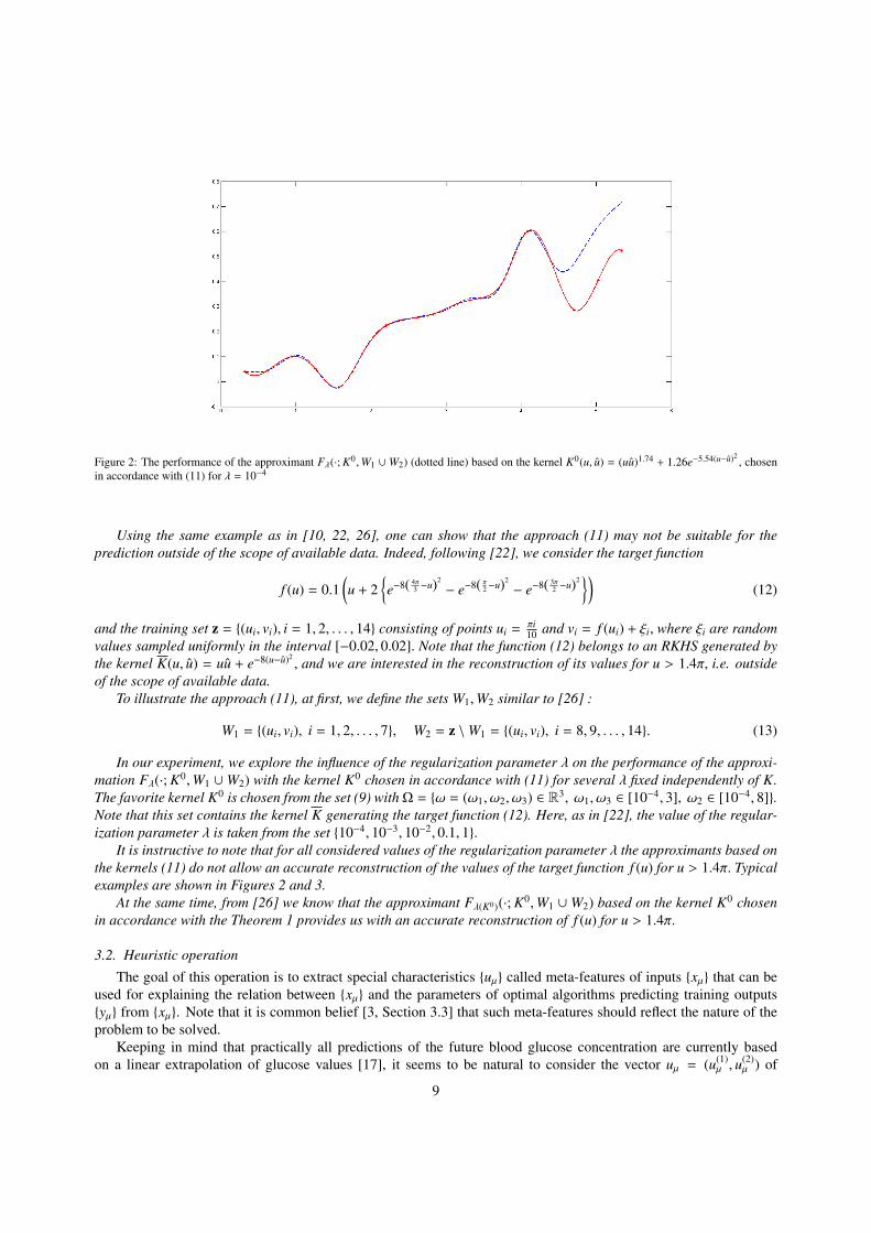
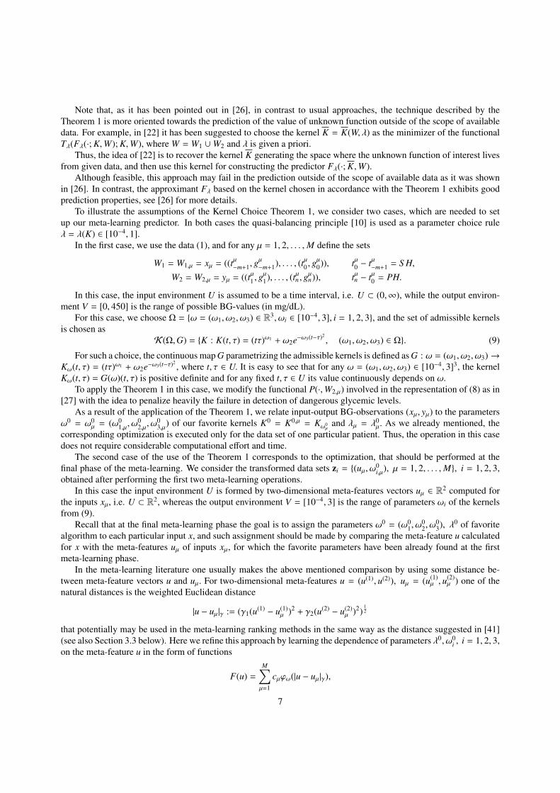
Figure 2: The performance of the approximant Fλ(·; K0,W1 ∪W2) (dotted line) based on the kernel K0(u, u) = (uu)1.74 + 1.26e−5.54(u−u)2, chosen

in accordance with (11) for λ = 10−4

Using the same example as in [10, 22, 26], one can show that the approach (11) may not be suitable for theprediction outside of the scope of available data. Indeed, following [22], we consider the target function

f (u) = 0.1(u + 2

e−8( 4π

3 −u)2

− e−8( π2−u)2

− e−8( 3π2 −u)2)

(12)

and the training set z = (ui, vi), i = 1, 2, . . . , 14 consisting of points ui =πi10 and vi = f (ui) + ξi, where ξi are random

values sampled uniformly in the interval [−0.02, 0.02]. Note that the function (12) belongs to an RKHS generated bythe kernel K(u, u) = uu + e−8(u−u)2

, and we are interested in the reconstruction of its values for u > 1.4π, i.e. outsideof the scope of available data.

To illustrate the approach (11), at first, we define the sets W1,W2 similar to [26] :

W1 = (ui, vi), i = 1, 2, . . . , 7, W2 = z \W1 = (ui, vi), i = 8, 9, . . . , 14. (13)

In our experiment, we explore the influence of the regularization parameter λ on the performance of the approxi-mation Fλ(·; K0,W1 ∪W2) with the kernel K0 chosen in accordance with (11) for several λ fixed independently of K.The favorite kernel K0 is chosen from the set (9) withΩ = ω = (ω1, ω2, ω3) ∈ R3, ω1, ω3 ∈ [10−4, 3], ω2 ∈ [10−4, 8].Note that this set contains the kernel K generating the target function (12). Here, as in [22], the value of the regular-ization parameter λ is taken from the set 10−4, 10−3, 10−2, 0.1, 1.

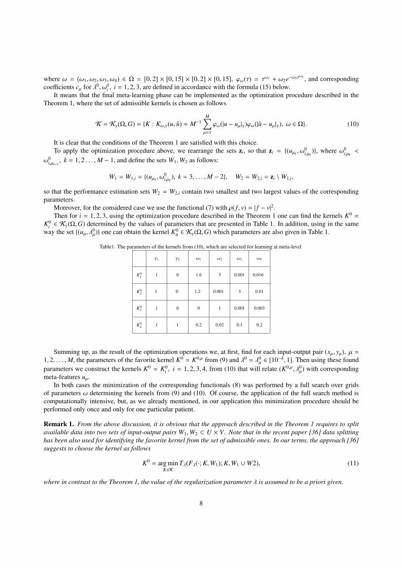
It is instructive to note that for all considered values of the regularization parameter λ the approximants based onthe kernels (11) do not allow an accurate reconstruction of the values of the target function f (u) for u > 1.4π. Typicalexamples are shown in Figures 2 and 3.

At the same time, from [26] we know that the approximant Fλ(K0)(·; K0,W1 ∪W2) based on the kernel K0 chosenin accordance with the Theorem 1 provides us with an accurate reconstruction of f (u) for u > 1.4π.

3.2. Heuristic operation

The goal of this operation is to extract special characteristics uµ called meta-features of inputs xµ that can beused for explaining the relation between xµ and the parameters of optimal algorithms predicting training outputsyµ from xµ. Note that it is common belief [3, Section 3.3] that such meta-features should reflect the nature of theproblem to be solved.

Keeping in mind that practically all predictions of the future blood glucose concentration are currently basedon a linear extrapolation of glucose values [17], it seems to be natural to consider the vector uµ = (u(1)

µ , u(2)µ ) of

9

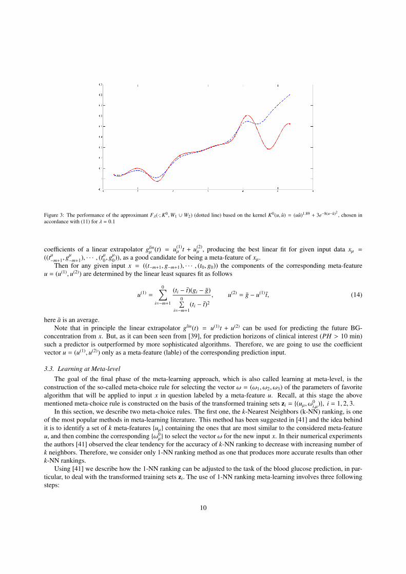
Figure 3: The performance of the approximant Fλ(·; K0,W1 ∪ W2) (dotted line) based on the kernel K0(u, u) = (uu)1.89 + 3e−8(u−u)2, chosen in

accordance with (11) for λ = 0.1

coefficients of a linear extrapolator glinµ (t) = u(1)

µ t + u(2)µ , producing the best linear fit for given input data xµ =

((tµ−m+1, g

µ−m+1), · · · , (tµ0 , g

µ0)), as a good candidate for being a meta-feature of xµ.

Then for any given input x = ((t−m+1, g−m+1), · · · , (t0, g0)) the components of the corresponding meta-featureu = (u(1), u(2)) are determined by the linear least squares fit as follows

u(1) =

0∑i=−m+1

(ti − t)(gi − g)0∑

i=−m+1(ti − t)2

, u(2) = g − u(1) t, (14)

here a is an average.Note that in principle the linear extrapolator glin(t) = u(1)t + u(2) can be used for predicting the future BG-

concentration from x. But, as it can been seen from [39], for prediction horizons of clinical interest (PH > 10 min)such a predictor is outperformed by more sophisticated algorithms. Therefore, we are going to use the coefficientvector u = (u(1), u(2)) only as a meta-feature (lable) of the corresponding prediction input.

3.3. Learning at Meta-level

The goal of the final phase of the meta-learning approach, which is also called learning at meta-level, is theconstruction of the so-called meta-choice rule for selecting the vector ω = (ω1, ω2, ω3) of the parameters of favoritealgorithm that will be applied to input x in question labeled by a meta-feature u. Recall, at this stage the abovementioned meta-choice rule is constructed on the basis of the transformed training sets zi = (uµ, ω0

i,µ), i = 1, 2, 3.In this section, we describe two meta-choice rules. The first one, the k-Nearest Neighbors (k-NN) ranking, is one

of the most popular methods in meta-learning literature. This method has been suggested in [41] and the idea behindit is to identify a set of k meta-features uµ containing the ones that are most similar to the considered meta-featureu, and then combine the corresponding ω0

µ to select the vector ω for the new input x. In their numerical experimentsthe authors [41] observed the clear tendency for the accuracy of k-NN ranking to decrease with increasing number ofk neighbors. Therefore, we consider only 1-NN ranking method as one that produces more accurate results than otherk-NN rankings.

Using [41] we describe how the 1-NN ranking can be adjusted to the task of the blood glucose prediction, in par-ticular, to deal with the transformed training sets zi. The use of 1-NN ranking meta-learning involves three followingsteps:

10

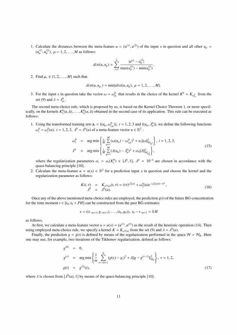
1. Calculate the distances between the meta-feature u = (u(1), u(2)) of the input x in question and all other uµ =(u(1)µ , u

(2)µ ), µ = 1, 2, . . . ,M as follows:

dist(u, uµ) =2∑

i=1

|u(i) − u(i)µ |

max(u(i)µ ) −min(u(i)

µ ).

2. Find µ∗ ∈ 1, 2, . . . ,M such that

dist(u, uµ∗ ) = mindist(u, uµ), µ = 1, 2, . . . ,M.

3. For the input x in question take the vector ω = ω0µ∗

that results in the choice of the kernel K0 = Kω0µ∗

from theset (9) and λ = λ0

µ∗.

The second meta-choice rule, which is proposed by us, is based on the Kernel Choice Theorem 1, or more specif-ically, on the kernels K0

1 (u, u), . . . ,K04 (u, u) obtained in the second case of its application. This rule can be executed as

follows:

1. Using the transformed training sets zi = (uµ, ω0i,µ), i = 1, 2, 3 and (uµ, λ0

µ), we define the following functionsω0

i = ω0i (u), i = 1, 2, 3, λ0 = λ0(u) of a meta-feature vector u ∈ R2 :

ω0i = arg min

1M

M∑µ=1

(ω(uµ) − ω0i,µ)

2 + αi||ω||2HK0

i

, i = 1, 2, 3,

λ0 = arg min

1M

M∑µ=1

(λ(uµ) − λ0µ)

2 + α4||λ||2HK0

4

,

(15)

where the regularization parameters αi = αi(K0i ) ∈ [λ0, 1], λ0 = 10−4 are chosen in accordance with the

quasi-balancing principle [10].2. Calculate the meta-feature u = u(x) ∈ R2 for a prediction input x in question and choose the kernel and the

regularization parameter as follows:

K(t, τ) = Kω0(u)(t, τ) = (tτ)ω01(u) + ω0

2(u)e−ω03(u)(t−τ)2

,

λ0 = λ0(u).(16)

Once any of the above mentioned meta-choice rules are employed, the prediction g(t) of the future BG-concentrationfor the time moment t ∈ [t0, t0 + PH] can be constructed from the past BG-estimates

x = ((t−m+1, g−m+1), . . . , (t0, g0)), t0 − t−m+1 = S H

as follows.At first, we calculate a meta-feature vector u = u(x) = (u(1), u(2)) as the result of the heuristic operation (14). Then

using employed meta-choice rule, we specify a kernel K = Kω0(u) from the set (9) and λ = λ0(u).Finally, the prediction g = g(t) is defined by means of the regularization performed in the space H = HK . Here

one may use, for example, two iterations of the Tikhonov regularization, defined as follows:

g(0) = 0,

g(ν) = arg min

1m

0∑i=−m+1

(g(ti) − gi)2 + λ||g − g(ν−1)||2HK

, ν = 1, 2,

g(t) = g(2)(t), (17)

where λ is chosen from [λ0(u), 1] by means of the quasi-balancing principle [10].

11

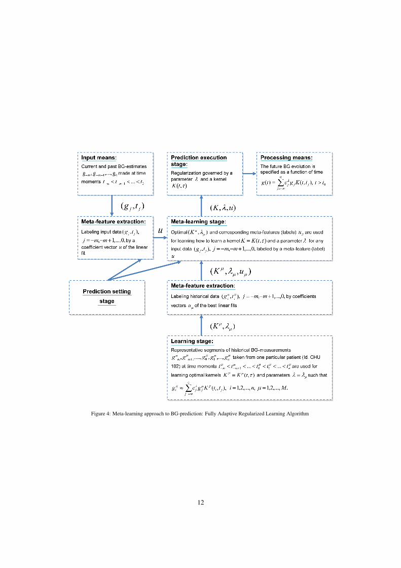
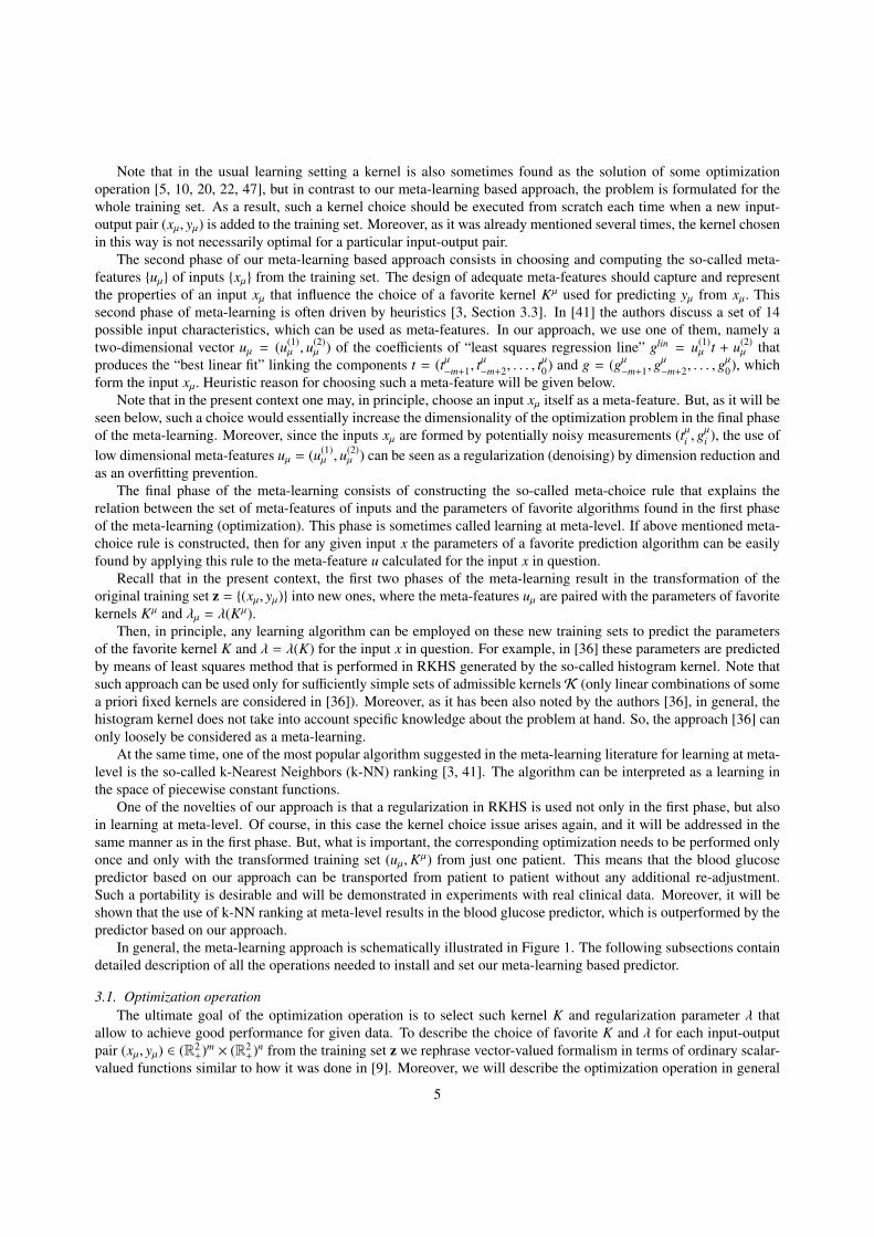
Figure 4: Meta-learning approach to BG-prediction: Fully Adaptive Regularized Learning Algorithm

12

4. Case-Study: Blood Glucose Prediction

In this section, we compare the performance of the state-of-the-art BG-predictors [30, 35] with that of meta-learning based predictors described in Section 3. It is remarkable, in retrospect, that in all cases the meta-learningbased predictors outperform their counterparts in terms of clinical accuracy. Even more, for some prediction horizonsBG-predictors based on the FARL approach perform at the level of the clinical accuracy achieved by CGM systems,providing the prediction input. Clearly, in general such accuracy cannot be beaten by CGM-based predictors.

The performance assessment has been made with the use of two different assessment metrics known from theliterature. One of them is the classical Point Error Grid Analysis (EGA) [7]. It uses a Cartesian diagram, in which thepredicted values are displayed on the y-axis, whereas the reference values are presented on the x-axis. This diagram issubdivided into 5 zones: A, B, C, D and E. The points that fall within zones A and B represent sufficiently accurate oracceptable glucose results, points in zone C may prompt unnecessary corrections, points in zones D and E representerroneous and incorrect treatment.

Another assessment metric is the Prediction Error Grid Analysis (PRED-EGA) [39] that has been designed espe-cially for BG-prediction assessment. PRED-EGA uses the same format as the Continuous Glucose Error Grid Analy-sis (CG-EGA)[6], which was originally developed for an assessment of the clinical accuracy of CGM systems. To beprecise, PRED-EGA records reference glucose estimates paired with the estimates predicted for the same momentsand look at two essential aspects of the clinical accuracy: rate error grid analysis and point error grid analyses. As aresult, it calculates combined accuracy in three clinically relevant regions, hypoglycemia (<70 mg/dL), euglycemia(70-180 mg/dL), and hyperglycemia (>180 mg/dL). In short, it provides three estimates of the predictor performancein each of the three regions: Accurate (Acc.), Benign (Benign) and Erroneous (Error). In contrast to the originalCG-EGA, PRED-EGA takes into account that predictors provide a BG-estimation ahead of time, and it paves a newway to estimating the rates of glucose changes.

The performance tests have been made with the use of clinical data from two trials executed within EU-project“DIAdvisor”[12] at the Montpellier University Hospital Center (CHU), France, and at the Institute of Clinical ofExperimental Medicine (IKEM), Prague, Czech Republic.

In the first trial (DAQ-trial), each clinical record of a diabetic patient contains nearly 10 days of CGM datacollected with the use of CGM system Abbott’s Freestyle Navigator R© [1], having a sampling frequency ∆t = 10(min), while in the second trial CGM data were collected during three days with the use of the system DexCom R©

SEVEN R© PLUS [11] that has a sampling frequency ∆t = 5 (min).For comparison with the state-of-the-art, we consider two BG-predictors described in the literature, such as data-

driven autoregressive model-based predictor (AR-predictor) proposed in [35] and neural network model-based pre-dictor (NNM-predictor) presented in [30].

It is instructive to see that these predictors require more information to produce a BG-prediction than is necessaryfor our approach. More precisely, AR-predictors use as an input past CGM-measurements sampled every minute.As to NNM-predictors, their inputs consist of CGM-measurements sampled every 5 minutes, as well as meal intake,insulin dosage, patient symptoms and emotional factors.

On the other hand, the FARL-based predictor uses as an input only CGM-measurements from the past 25 min-utes (in case of DexCom devices), or 30 minutes (in case of Abbott sensors) and, what is more important, thesemeasurements do not need to be equi-sampled.

Recall that in Section 3 we already mentioned such important feature of our algorithm as portability from indi-vidual to individual. To be more specific, for learning at meta-level we use CGM-measurements performed only withone patient (patient ID: CHU102). These measurements were collected during one day of the DAQ-trial with the useof Abbott sensor.

The training data set z = (xµ, yµ), µ = 1, 2, . . . ,M, M = 24, was formed from the data of the patient CHU102with the sampling horizon S H = 30 minutes and the training prediction horizon PH = 30 minutes. The applicationof the procedure described in the Theorem 1 in the first case transforms the training set z into the values ω0

µ =

(ω01,µ, ω

02,µ, ω

03,µ), λ

0µ, µ = 1, 2, . . . ,M, defining the favorite kernel and regularization parameters.

Then, the transformed training sets (xµ, yµ) → (uµ, ω0µ), (uµ, λ

0µ), µ = 1, 2, . . . , 24, were used for learning at

meta-level with FARL method, as well as with 1-NN ranking method.At first, the obtained fully trained BG-predictors have been tested without any readjustment on the data that were

collected during 8 days from other 10 patients taking part in DAQ-trial.

13

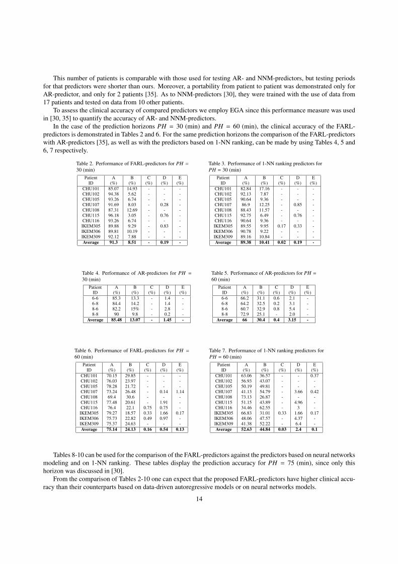
This number of patients is comparable with those used for testing AR- and NNM-predictors, but testing periodsfor that predictors were shorter than ours. Moreover, a portability from patient to patient was demonstrated only forAR-predictor, and only for 2 patients [35]. As to NNM-predictors [30], they were trained with the use of data from17 patients and tested on data from 10 other patients.

To assess the clinical accuracy of compared predictors we employ EGA since this performance measure was usedin [30, 35] to quantify the accuracy of AR- and NNM-predictors.

In the case of the prediction horizons PH = 30 (min) and PH = 60 (min), the clinical accuracy of the FARL-predictors is demonstrated in Tables 2 and 6. For the same prediction horizons the comparison of the FARL-predictorswith AR-predictors [35], as well as with the predictors based on 1-NN ranking, can be made by using Tables 4, 5 and6, 7 respectively.

Table 2. Performance of FARL-predictors for PH =30 (min)

Patient A B C D EID (%) (%) (%) (%) (%)

CHU101 85.07 14.93 - - -CHU102 94.38 5.62 - - -CHU105 93.26 6.74 - - -CHU107 91.69 8.03 - 0.28 -CHU108 87.31 12.69 - - -CHU115 96.18 3.05 - 0.76 -CHU116 93.26 6.74 - - -IKEM305 89.88 9.29 - 0.83 -IKEM306 89.81 10.19 - - -IKEM309 92.12 7.88 - - -Average 91.3 8.51 - 0.19 -

Table 3. Performance of 1-NN ranking predictors forPH = 30 (min)

Patient A B C D EID (%) (%) (%) (%) (%)

CHU101 82.84 17.16 - - -CHU102 92.13 7.87 - - -CHU105 90.64 9.36 - - -CHU107 86.9 12.25 - 0.85 -CHU108 88.43 11.57 - - -CHU115 92.75 6.49 - 0.76 -CHU116 90.64 9.36 - - -IKEM305 89.55 9.95 0.17 0.33 -IKEM306 90.78 9.22 - - -IKEM309 89.16 10.84 - - -Average 89.38 10.41 0.02 0.19 -

Table 4. Performance of AR-predictors for PH =30 (min)

Patient A B C D EID (%) (%) (%) (%) (%)6-6 85.3 13.3 - 1.4 -6-8 84.4 14.2 - 1.4 -8-6 82.2 15% - 2.8 -8-8 90 9.8 - 0.2 -

Average 85.48 13.07 - 1.45 -

Table 5. Performance of AR-predictors for PH =60 (min)

Patient A B C D EID (%) (%) (%) (%) (%)6-6 66.2 31.1 0.6 2.1 -6-8 64.2 32.5 0.2 3.1 -8-6 60.7 32.9 0.8 5.4 -8-8 72.9 25.1 - 2.0 -

Average 66 30.4 0.4 3.15 -

Table 6. Performance of FARL-predictors for PH =60 (min)

Patient A B C D EID (%) (%) (%) (%) (%)

CHU101 70.15 29.85 - - -CHU102 76.03 23.97 - - -CHU105 78.28 21.72 - - -CHU107 73.24 26.48 - 0.14 1.14CHU108 69.4 30.6 - - -CHU115 77.48 20.61 - 1.91 -CHU116 76.4 22.1 0.75 0.75 -IKEM305 79.27 18.57 0.33 1.66 0.17IKEM306 75.73 22.82 0.49 0.97 -IKEM309 75.37 24.63 - - -Average 75.14 24.13 0.16 0.54 0.13

Table 7. Performance of 1-NN ranking predictors forPH = 60 (min)

Patient A B C D EID (%) (%) (%) (%) (%)

CHU101 63.06 36.57 - - 0.37CHU102 56.93 43.07 - - -CHU105 50.19 49.81 - - -CHU107 41.13 54.79 - 3.66 0.42CHU108 73.13 26.87 - - -CHU115 51.15 43.89 - 4.96 -CHU116 34.46 62.55 - 3 -IKEM305 66.83 31.01 0.33 1.66 0.17IKEM306 48.06 47.57 - 4.37 -IKEM309 41.38 52.22 - 6.4 -Average 52.63 44.84 0.03 2.4 0.1

Tables 8-10 can be used for the comparison of the FARL-predictors against the predictors based on neural networksmodeling and on 1-NN ranking. These tables display the prediction accuracy for PH = 75 (min), since only thishorizon was discussed in [30].

From the comparison of Tables 2-10 one can expect that the proposed FARL-predictors have higher clinical accu-racy than their counterparts based on data-driven autoregressive models or on neural networks models.

14

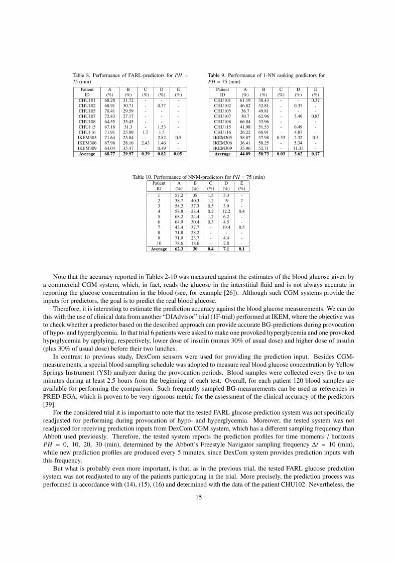
Table 8. Performance of FARL-predictors for PH =75 (min)

Patient A B C D EID (%) (%) (%) (%) (%)

CHU101 68.28 31.72 - - -CHU102 68.91 30.71 - 0.37 -CHU105 70.41 29.59 - - -CHU107 72.83 27.17 - - -CHU108 64.55 35.45 - - -CHU115 67.18 31.3 - 1.53 -CHU116 71.91 25.09 1.5 1.5 -IKEM305 71.64 25.04 - 2.82 0.5IKEM306 67.96 28.16 2.43 1.46 -IKEM309 64.04 35.47 - 0.49 -Average 68.77 29.97 0.39 0.82 0.05

Table 9. Performance of 1-NN ranking predictors forPH = 75 (min)

Patient A B C D EID (%) (%) (%) (%) (%)

CHU101 61.19 38.43 - - 0.37CHU102 46.82 52.81 - 0.37 -CHU105 36.7 49.81 - - -CHU107 30.7 62.96 - 5.49 0.85CHU108 66.04 33.96 - - -CHU115 41.98 51.53 - 6.49 -CHU116 26.22 68.91 - 4.87 -IKEM305 58.87 37.98 0.33 2.32 0.5IKEM306 36.41 58.25 - 5.34 -IKEM309 35.96 52.71 - 11.33 -Average 44.09 50.73 0.03 3.62 0.17

Table 10. Performance of NNM-predictors for PH = 75 (min)Patient A B C D E

ID (%) (%) (%) (%) (%)1 57.2 38 1.5 3.3 -2 38.7 40.3 1.2 19 73 58.2 37.3 0.5 3.9 -4 58.8 28.4 0.2 12.2 0.45 68.2 24.4 1.2 6.2 -6 64.9 30.4 0.3 4.5 -7 42.4 37.7 - 19.4 0.58 71.8 28.2 - - -9 71.9 23.7 - 4.4 -

10 78.6 18.6 - 2.8 -Average 62.3 30 0.4 7.1 0.1

Note that the accuracy reported in Tables 2-10 was measured against the estimates of the blood glucose given bya commercial CGM system, which, in fact, reads the glucose in the interstitial fluid and is not always accurate inreporting the glucose concentration in the blood (see, for example [26]). Although such CGM systems provide theinputs for predictors, the goal is to predict the real blood glucose.

Therefore, it is interesting to estimate the prediction accuracy against the blood glucose measurements. We can dothis with the use of clinical data from another “DIAdvisor” trial (1F-trial) performed at IKEM, where the objective wasto check whether a predictor based on the described approach can provide accurate BG-predictions during provocationof hypo- and hyperglycemia. In that trial 6 patients were asked to make one provoked hyperglycemia and one provokedhypoglycemia by applying, respectively, lower dose of insulin (minus 30% of usual dose) and higher dose of insulin(plus 30% of usual dose) before their two lunches.

In contrast to previous study, DexCom sensors were used for providing the prediction input. Besides CGM-measurements, a special blood sampling schedule was adopted to measure real blood glucose concentration by YellowSprings Instrument (YSI) analyzer during the provocation periods. Blood samples were collected every five to tenminutes during at least 2.5 hours from the beginning of each test. Overall, for each patient 120 blood samples areavailable for performing the comparison. Such frequently sampled BG-measurements can be used as references inPRED-EGA, which is proven to be very rigorous metric for the assessment of the clinical accuracy of the predictors[39].

For the considered trial it is important to note that the tested FARL glucose prediction system was not specificallyreadjusted for performing during provocation of hypo- and hyperglycemia. Moreover, the tested system was notreadjusted for receiving prediction inputs from DexCom CGM system, which has a different sampling frequency thanAbbott used previously. Therefore, the tested system reports the prediction profiles for time moments / horizonsPH = 0, 10, 20, 30 (min), determined by the Abbott’s Freestyle Navigator sampling frequency ∆t = 10 (min),while new prediction profiles are produced every 5 minutes, since DexCom system provides prediction inputs withthis frequency.

But what is probably even more important, is that, as in the previous trial, the tested FARL glucose predictionsystem was not readjusted to any of the patients participating in the trial. More precisely, the prediction process wasperformed in accordance with (14), (15), (16) and determined with the data of the patient CHU102. Nevertheless, the

15

tested prediction system performed quite well, as it can be seen in Tables 11, 12 and 13, displaying the assessmentresults produced by PRED-EGA with reference to YSI blood glucose values. The assessment has been made forpredictions with the horizons PH = 0, 10, 20 (min) respectively.

Table 11. Performance of FARL-predictors with reference to YSI for PH = 0 (min)Patient BG ≤ 70 (mg/dL) (%) BG 70-180 (mg/dL) (%) BG > 180 (mg/dL) (%)

ID Acc. Benign Error Acc. Benign Error Acc. Benign Error305 75 - 25 98.61 1.39 - 94.44 5.56 -308 100 - - 92.65 5.88 1.47 100 - -310 100 - - 91.67 3.33 5 95.56 2.22 2.22311 84.62 15.38 - 69.84 20.63 9.52 70.97 16.13 12.9320 85.71 14.29 - 75.68 18.92 5.41 87.1 3.23 9.68308 100 - - 93.2 5.83 0.97 100 - -Avg. 90.89 4.94 4.17 86.94 9.33 3.73 91.35 4.52 4.13

Table 12. Performance of FARL-predictors with reference to YSI for PH = 10 (min)Patient BG ≤ 70 (mg/dL) (%) BG 70-180 (mg/dL) (%) BG > 180 (mg/dL) (%)

ID Acc. Benign Error Acc. Benign Error Acc. Benign Error305 84.21 - 15.79 100 - - 96.97 - 3.03308 100 - - 81.82 13.64 4.55 93.94 6.06 -310 100 - - 91.38 3.45 5.17 95.74 2.13 2.13311 75 16.67 8.33 58.33 31.25 10.42 75 16.67 8.33320 85.71 14.29 - 72.97 24.32 2.7 81.48 - 18.52308 100 - - 93.26 5.62 1.12 100 - -Avg. 90.82 5.16 4.02 82.96 13.05 3.99 90.52 4.14 5.34

Table 13. Performance of FARL-predictors with reference to YSI for PH = 20 (min)Patient BG ≤ 70 (mg/dL) (%) BG 70-180 (mg/dL) (%) BG > 180 (mg/dL) (%)

ID Acc. Benign Error Acc. Benign Error Acc. Benign Error305 78.95 - 21.05 91.3 8.7 - 96.77 - 3.23308 81.82 - 18.18 80.65 19.35 - 100 - -310 100 - - 92.45 7.55 - 96.08 - 3.92311 58.33 16.67 25 60.42 31.25 8.33 68 8 24320 71.43 14.29 14.29 76.92 20.51 2.56 84 - 16308 100 - - 90.91 9.09 - 100 - -Avg. 81.75 5.16 13.09 82.11 16.08 1.81 90.81 1.33 7.86

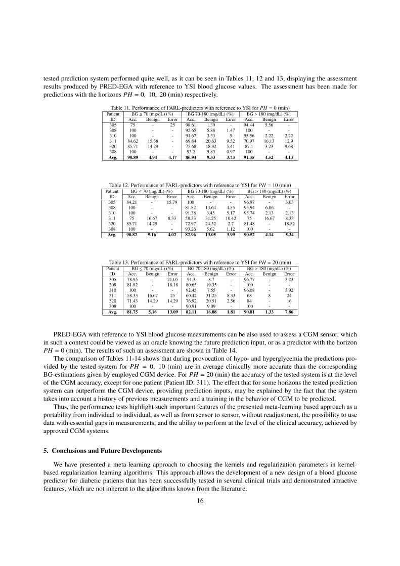
PRED-EGA with reference to YSI blood glucose measurements can be also used to assess a CGM sensor, whichin such a context could be viewed as an oracle knowing the future prediction input, or as a predictor with the horizonPH = 0 (min). The results of such an assessment are shown in Table 14.

The comparison of Tables 11-14 shows that during provocation of hypo- and hyperglycemia the predictions pro-vided by the tested system for PH = 0, 10 (min) are in average clinically more accurate than the correspondingBG-estimations given by employed CGM device. For PH = 20 (min) the accuracy of the tested system is at the levelof the CGM accuracy, except for one patient (Patient ID: 311). The effect that for some horizons the tested predictionsystem can outperform the CGM device, providing prediction inputs, may be explained by the fact that the systemtakes into account a history of previous measurements and a training in the behavior of CGM to be predicted.

Thus, the performance tests highlight such important features of the presented meta-learning based approach as aportability from individual to individual, as well as from sensor to sensor, without readjustment, the possibility to usedata with essential gaps in measurements, and the ability to perform at the level of the clinical accuracy, achieved byapproved CGM systems.

5. Conclusions and Future Developments

We have presented a meta-learning approach to choosing the kernels and regularization parameters in kernel-based regularization learning algorithms. This approach allows the development of a new design of a blood glucosepredictor for diabetic patients that has been successfully tested in several clinical trials and demonstrated attractivefeatures, which are not inherent to the algorithms known from the literature.

16

Table 14. Performance of DexCom sensors with reference to YSIPatient BG ≤ 70 (mg/dL) (%) BG 70-180 (mg/dL) (%) BG > 180 (mg/dL) (%)

ID Acc. Benign Error Acc. Benign Error Acc. Benign Error305 75 - 25 100 - - 89.19 2.7 8.11308 91.67 8.33 - 91.78 8.22 - 94.74 5.26 -310 100 - - 86.57 11.94 1.49 95.74 - 4.26311 85.71 14.29 - 86.57 11.94 1.49 77.14 20 2.86320 85.71 14.29 - 78.95 15.79 5.26 76.47 5.88 17.65308 100 - - 91.89 6.31 1.8 100 - -Avg. 89.68 6.15 4.17 89.29 9.03 1.67 88.88 5.64 5.48

Moreover, in [32] it has been described how the new design can be naturally extended to the prediction from othertypes of inputs containing not only past BG-estimations but also information about special events, such as meals orphysical activities. The predictors based on the extended design also perform quite well, and it gives a hint that themain ingredients of the proposed approach can be exploited in other applications.

More specifically, the optimization procedure described in the Theorem 1 can at first transform a given trainingdata set into a set of parameters defining the favorite kernels, and then the analogous procedure can be performed forlearning at meta-level to construct a rule that allows the choice of a favorite kernel for any prediction input in question.

The present paper shows that the meta-learning approach based on this two-steps optimization is rather promisingand deserves further development.

Acknowledgment

This research has been performed in the course of the project “DIAdvisor” [12] funded by the European Com-mission within 7-th Framework Programme. The authors gratefully acknowledge the support of the “DIAdvisor” –consortium.

References

[1] Abbott Diabetes Care, http://www.abbottdiabetescare.com, 2010.[2] F. Bauer, S. Pereverzev, L. Rosasco, On regularization algorithms in learning theory, J. Complexity 23 (2007) 52–72.[3] P. Brazdil, C. Giraud-Carrier, C. Soares, R. Vilalta, Metalearning: Applications to Data Mining, Springer-Verlag, Berlin Heidelberg, 2009.[4] B. Buckingham, H.P. Chase, E. Dassau, E. Cobry, P. Clinton, V. Gage, K. Caswell, J. Wilkinson, F. Cameron, H. Lee, B.W. Bequette, F.J.

Doyle III, Prevention of nocturnal hypoglycemia using predictive alarm algorithms and insulin pump suspension, Diabetes Care 33 (2010)1013–1018.

[5] O. Chapelle, V. Vapnik, O. Bousquet, S. Mukherjee, Choosing multiple parameters for support vector machines, Machine Learning 46 (2002)131159.

[6] W.L. Clarke, S. Anderson, L. Farhy, M. Breton, L. Gonder-Frederick, D. Cox, B. Kovatchev, Evaluating the clinical accuracy of two contin-uous glucose sensors using Continuous glucose–error grid analysis, Diabetes Care 28 (2005) 2412–2417.

[7] W.L. Clarke, D. Cox, L.A. Gonder-Frederick, W. Carter, S.L. Pohl, Evaluating clinical accuracy of systems for self-monitoring of bloodglucose, Diabetes Care 10 (1987) 622–628.

[8] F. Cucker, S. Smale, On the mathematical foundations of learning, Bull. Amer.Math. Soc. (N.S.) 39 (2002) 1–49 (electronic).[9] E. De Vito, A. Caponnetto, Optimal rates for the regularized least-squares algorithm, Foundations of Computational Mathematics 7 (2007)

331–368.[10] E. De Vito, S.V. Pereverzyev, L. Rosasco, Adaptive kernel methods using the balancing principle, Foundations of Computational Mathematics

10 (2010) 455–479.[11] DexCom: Continuous Glucose Meter, http://www.dexcom.com, 2011.[12] DIAdvisor: personal glucose predictive diabetes advisor, http://www.diadvisor.eu, 2008.[13] M. Eren-Oruklu, A. Cinar, L. Quinn, D. Smith, Estimation of future glucose concentrations with subject-specific recursive linear models,

Diabetes Technol Ther 11 (2009) 243–253.[14] T. Evgeniou, M. Pontil, T. Poggio, Regularization networks and support vector machines, Adv. Comp. Math. 13 (2000) 1–50.[15] S. Kindermann, A. Neubauer, On the convergence of the quasi-optimality criterion for (iterated) Tikhonov regularization, Inverse Problems

and Imaging 2 (2008) 291–299.[16] D.W. Klonoff, Continuous glucose monitoring: roadmap for 21-st diabetes therapy, Diabetes Care 28 (2005) 1231–1239.[17] B. Kovatchev, W. Clarke, Peculiarities of the continuous glucose monitoring data stream and their impact on developing closed-loop control

technology, J. Diabetes Sci Technol. 2 (2008) 158–163.[18] B. Kovatchev, D. Shields, M. Breton, Graphical and numerical evaluation of continuous glucose sensing time lag, Diabetes Technol Ther 11

(2009) 139–143.[19] V. Kurkova, M. Sanguineti, Approximate minimization of the regularized expected error over kernel models, Mathematics of Operations

Research 33 (2008) 747–756.

17

[20] G.R.G. Lanckriet, N. Christianini, L. Ghaoui, P. Bartlett, M. Jordan, Learning the kernel matrix with semidefinite programming, J. Mach.Learn. Res. 5 (2004) 2772.

[21] O. Lepskij, On a problem of adaptive estimation in Gaussian white noise, Theor. Probab. Appl. 35 (1990) 454–466.[22] C.A. Micchelli, M. Pontil, Learning the kernel function via regularization, J. Mach. Learn. Res. 6 (2005) 1099–1125.[23] C.A. Micchelli, M. Pontil, On learning vector-valued functions, Neural Computation 17 (2005) 177–204.[24] V. Morozov, On the solution of functional equations by the method of regularization, Soviet Math. Dokl. 7 (1966) 414–417.[25] V. Morozov, Methods for Solving Incorrectly Posed Problems, Springer-Verlag, New York, 1984.[26] V. Naumova, S.V. Pereverzyev, S. Sivananthan, Extrapolation in variable RKHSs with application to the blood glucose reading, Inverse

Problems 27 (2011) 075010, 13 pp.[27] V. Naumova, S.V. Pereverzyev, S. Sivananthan, Reading blood glucose from subcutaneous electric current by means of a regularization in

variable Reproducing Kernel Hilbert Spaces, in: 50th IEEE Conference on Decision and Control and European Control Conference, Orlando,Florida, USA, pp. 5158–5163.

[28] C. Palerm, B.W. Bequette, Hypoglycemia detection and prediction using continuous glucose monitoring - a study on hypoglycemic clampdata, J Diabetes Sci Technol. 1 (2007) 624–629.

[29] S. Pappada, B. Cameron, P. Rosman, Development of neural network for prediction of glucose concentration in Type 1 diabetes patients, JDiabetes Sci Technol. 2 (2008) 792–801.

[30] S. Pappada, B. Cameron, P. Rosman, R. Bourey, T. Papadimos, W. Olorunto, M. Borst, Neural networks-based real-time prediction of glucosein patients with insulin-dependent diabetes, Diabetes Technol Ther 13 (2011) 135–141.

[31] S. Pereverzev, S. Sivananthan, Regularized learning algorithm for prediction of blood glucose concentration in “no action period”, in: 1stInternational Conference on Mathematical and Computational Biomedical Engineering – CMBE2009, Swansea, UK, pp. 395–398.

[32] S. Pereverzyev, S. Sivananthan, J. Randløv, S. McKennoch, Glucose predictor based on regularization networks with adaptively chosenkernels and regularization parameters, EP 11163219.6, 2011.

[33] C. Perez-Gandia, A. Facchinetti, G. Sparacino, C. Cobelli, E.J. Gomez, M. Rigla, A. deLeiva, M.E. Hernando, Artificial neural networkalgorithm for online glucose prediction from continuous glucose monitoring, Diabetes Technol Ther 12 (2010) 81–88.

[34] D. Phillips, A technique for the numerical solution of certain integral equations of the first kind, J. Assoc. Comput. Mach. 9 (1962) 84–97.[35] J. Reifman, S. Rajaraman, A. Gribok, W.K. Ward, Predictive monitoring for improved management of glucose levels, J Diabetes Sci Technol.

1 (2007) 478–486.[36] U. Ruckert, S. Kramer, Kernel-based inductive transfer, in: W. Daelemans, B. Goethals, K. Morik (Eds.), Machine Learning and Knowledge

Discovery in Databases, volume 5212 of Lecture Notes in Computer Science, Springer Berlin / Heidelberg, 2008, pp. 220–233.[37] T. Schaul, J. Schmidhuber, Metalearning, Scholarpedia 5 (2010) 4650.[38] B. Scholkopf, A. Smola, Learning with Kernels, The MIT Press, Cambridge, Massachusetts, 2002.[39] S. Sivananthan, V. Naumova, C. Dalla Man, A. Facchinetti, E. Renard, C. Cobelli, S. Pereverzyev, Assessment of blood glucose predictors:

The Prediction-Error Grid Analysis, Diabetes Technol Ther 13 (2011) 787–796.[40] L. Snetselaar, Nutrition counseling skills for the nutrition care process, Jones and Bartlett Publishers, 2009.[41] C. Soares, P.B. Brazdil, P. Kuba, A Meta-Learning Approach to Select the Kernel Width in Support Vector Regression, Machine Learning 54

(2004) 195–209.[42] V. Solo, Selection of tuning parameters for support vector machine, in: IEEE ICASSP, Philadelphia, PA, pp. 237–240.[43] G. Sparacino, F. Zanderigo, S. Corazza, A. Maran, Glucose concentration can be predicted ahead in time from continuous glucose monitoring

sensor time-series, IEEE Trans Biomed Eng 54 (2007) 931–937.[44] A.N. Tikhonov, V.B. Glasko, Use of the regularization methods in non-linear problems, volume 5, USSR Comput. Math. Phys., 1965.[45] V.N. Vapnik, Statistical learning theory. Adaptive and Learning Systems for Signal Processing, Communications, and Control, A Wiley-

Interscience Publication, John Wiley & Sons Inc., New York, 1998.[46] G. Wahba, Spline Models for Observational Data, volume 59 of Series in Applied Mathematics, CBMS-NSF Regional Conf., SIAM, 1990.[47] Y. Xu, H. Zhang, J. Zhang, Reproducing kernel Banach spaces for machine learning, J. Mach. Learn. Res. 10 (2009) 27412775.

18