AMERICAN OPTION VALUATION UNDER …spiral.imperial.ac.uk/bitstream/10044/1/19226/2/14946_final.pdf · The value-function of an American option in this settingis characterised as the

Applied Probability Trust (May 1, 2014)

AMERICAN OPTION VALUATION UNDERCONTINUOUS TIME MARKOV CHAINS

B. ERIKSSON,∗ and

M. R. PISTORIUS,∗ Imperial College London

Abstract

This paper is concerned with the solution of the optimal stopping problemassociated to the value of American options driven by continuous time Markovchains. The value-function of an American option in this setting is characterisedas the unique solution (in distributional sense) of a system of variationalinequalities. Furthermore, with continuous and smooth fit principles notapplicable in this discrete state space setting, a novel explicit characterisationis provided of the optimal stopping boundary in terms of the generator ofthe underlying Markov chain. Subsequently an algorithm is presented for thevaluation of American options under Markov chain models. By applicationto a suitably chosen sequence of Markov chains the algorithm providesan approximate valuation of an American option under a class of Markovmodels, that includes diffusion models, exponential Levy models and stochasticdifferential equations driven by Levy processes. Numerical experiments for arange of different models suggest that the approximation algorithm is flexibleand accurate. A proof of convergence is also provided.

Keywords: Markov chain; American option; free-boundary problem; optimalstopping; Feller process; numerical approximation

2010 Mathematics Subject Classification: Primary 91G20Secondary 60J27, 65C40

1. Introduction

American options. The valuation of American options is an active research topic thathas received a good deal of attention in the literature. Related American-type optimalstopping problems turn up in the modeling of trading and investment decisions, andreal options (see e.g. Boyarchenko & Levendorskiı [6]). The theoretical and numericalaspects of American option valuation have been investigated using a diverse collectionof tools, methods and techniques, in several different settings—see Detemple [15] foran overview and references. It was early on understood that, as a consequence ofthe embedded optionality of the time of exercise, the value of an American option isequal to the value of an optimal stopping problem. For instance, under Samuelson’sgeometric Brownian motion model, which is considered to be the benchmark modelfor the evolution of the price of a risky stock, the optimal policy in the case of an

∗ Postal address: Department of Mathematics, Imperial College London, South Kensington Campus,London SW7 2AZ.Email addresses: eriksson [email protected], [email protected]

1

2 B. Eriksson and M.R. Pistorius

American put is to exercise at the first moment the stock price falls below a certainboundary. In this setting it was first observed by McKean [28] that the value-functionof an American option solves a free-boundary problem. Jacka [17] and Peskir [30]established this exercise boundary to be the unique solution of an integral equation.Motivated by the observed features of empirical returns data the focus in modeling hassubsequently shifted to more general classes of Markov processes, such as diffusionsand jump processes. In the setting of Levy processes the analytical characterisation ofthe value-function and optimal boundary of an American put was investigated amongothers by Boyarchenko & Levendorskiı [5] and Lamberton & Mikou [25]. In anotherline of research, going back at least as far as Cox et al. [13], a discrete-time and discrete-space approach has been developed for the valuation of American options in the settingof a binomial tree. In later years many extensions and refinements of the discrete timeapproach have been developed e.g. to tri- and multinomial trees. The connectionbetween the two approaches was investigated in e.g. Lamberton [23], Ahn & Song [2]and Szimayer & Maller [33] where (rates of) convergence of the values of Americanoptions under binomial and trinomial, and finite state models were established tothose under the limiting Brownian or Levy model, respectively. Kushner & Dupuis [22]propose numerical methods for the solution of stochastic control problems in diffusionsettings based on an approximation of the state process by Markov chains.

American options under Markov chains. In this paper we consider the optimalstopping problem associated to an American option in the setting of a continuoustime Markov chain with discrete state-space. Stochastic processes from this class haveserved as models for the evolution of random quantities that take values in lattices.Models from this class, which contains the classical birth-death processes, have recentlyalso been deployed to model the state of the order book or the limit price—see e.g. [1]and references therein. Furthermore, Markov chains have been deployed as modelson a discrete state-space that closely approximate continuous space diffusions, jump-diffusions and general Feller processes. In a continuous-time Markov chain settingwe solve the optimal stopping problem associated to the valuation of an Americanoption with a pay-off that is a function of the Markov chain. While it follows fromthe general theory of optimal stopping that the optimal stopping time is given bythe first passage time into a certain set (see [31]), the characterisation of the valuefunction as solution of a corresponding free-boundary problem and the identificationof the optimal boundary involve non-standard arguments. Taking advantage of theexplicit form of the semi-group we demonstrate that the value-function of such anAmerican option is the unique solution in distributional sense of an associated free-boundary problem, and deduce that the value function is in fact a classical solutionby showing that it is continuously differentiable as function of time (see Theorem 3.1below). In cases when the pay-off and Markov process are sufficiently regular, pastingprinciples have been used to identify and characterise the optimal boundary. In thecase that the payoff function is continuously differentiable in a neighbourhood of theboundary and the underlying is a real-valued Feller process, the general theory ofoptimal stopping (see [31]) suggests that it can be expected that, at the boundary, thevalue function is continuously differentiable if, for the Feller process, the boundary isregular for itself, while the value function can be expected to be merely continuous atthe boundary if, for the Feller process, the boundary is irregular for itself. These twoheuristics are known as smooth pasting and continuous pasting principles, respectively.

American option valuation under continuous time Markov chains 3

See Peskir & Shiryaev [31] for a general treatment of pasting principles, and refer toAlili & Kyprianou [3] and Lamberton & Mikou [24] for an investigation of the validityof pasting principles in the case of the optimal stopping problem associated to anAmerican put option under a Levy process. However, in the case of a discrete state-space with finite transition rates the smooth- and continuous-pasting principles nolonger apply due to the lack of smoothness that is a result of the discrete state-space.In the absence of pasting principles, we derive an explicit characterisation of the optimalstopping boundary directly in terms of the infinitesimal generator of the Markov chain,in the case that the optimal stopping boundary is monotone (see Theorem 4.1 below).

Algorithm. Deploying this characterisation, we design an algorithm for the computa-tion of the value function of an American option under a continuous time Markov chainmodel. By constructing the Markov chain such that it closely follows the evolution of agiven Feller process (e.g., by using the construction from [29]), this algorithm, with theconstructed Markov chain as input, provides a method for the valuation of Americanoptions under the Feller process in question. An advantage of the Markov chain modelis its computational tractability: We demonstrate in this paper that the describedalgorithm provides an efficient and accurate method for the valuation of Americanoptions, and the computation of the optimal boundary, using the powerful tools ofmatrix-based computations. The idea of valuation using Markov chain approximationgoes back at least as far as Kushner [21] in the case of diffusions, and was furtherdeveloped in e.g. [29]. To illustrate its effectiveness, we implemented the algorithm fora local-volatility model with jumps, and report results (such as estimates of the errors)in Section 7. We also give a proof of convergence of the approximation method.

Contents. The remainder of the paper is organised as follows. Section 2 containspreliminaries and notation that is used throughout the paper. Section 3 is devoted tothe free-boundary problem associated to the American option driven by a continuoustime Markov chain and contains a characterisation of the optimal boundary, and in Sec-tion 5 an algorithm is presented for solving this free boundary problem. Convergenceof the algorithm is established in Section 6, and a number of numerical examples areanalysed in Section 7. Appendix A and B contain the dynamic programming algorithmfor valuing American options using Markov chains and the proof of Lemma 2.1 below.

2. Preliminaries

2.1. Setting: Markov chains

We next set the notation that will be used throughout the paper. LetX be a continuoustime time-homogeneous Markov chain with discrete state space G = xi, i ∈ N andgenerator matrix Λ, defined on some filtered probability space (Ω,G,G,P) where G =Gtt∈[0,T ] denotes the completed right-continuous filtration generated by X . Assumethat X is a Feller process with cadlag paths (see [14, §2.2] for background), and denotethe infinitesimal generator of X by Λ. To avoid explosion of the chain X in finite timewe assume that Λ has uniformly bounded elements:

Assumption 1. The infinitesimal generator Λ of X satisfies the condition

supx∈G

|Λ(x, x)| <∞.


Denoting by l∞(G) the collection of bounded real-valued functions with domain G,we recall that the semi-group of X is equal to the collection (Pt, t ∈ R+) of mapsPt : l∞(G) → l∞(G), that is expressed in terms of the infinitesimal generator Λ :l∞(G)→ l∞(G) of X by

(Ptf)(x) =∑

y∈G

Pt(x, y)f(y), t ∈ R+, x ∈ G, f ∈ l∞(G),

Pt(x, y) = P(Xt = y|X0 = x) =: Px(Xt = y), x, y ∈ G,

with Pt = exp(tΛ) =

∞∑

n=0

tn

n!Λn

with Λn = Λn−1 Λ, i.e., Λnf = Λn−1(Λf) for any f ∈ l∞(G). The infinitesimalgenerator Λ is given by

Λf(x) =∑

y∈G

Λ(x, y)f(y), Λ(x, y) = (Λδy)(x), x ∈ G, f ∈ l∞(G),

with (1− δy(x)) · Λ(x, y) ≥ 0 and∑

z∈G

Λ(x, z) = 0, x, y ∈ G,

where δy is the Kronecker delta, which is the map on G that is equal to 1 if x and yare equal and zero otherwise. In particular, it follows that the expected value of thepay-off φ(XT ) at time T , where φ is an arbitrary map from the set l∞(G), is given by

Et,x[φ(XT )] = E0,x[φ(XT−t)] = (exp((T − t)Λ)φ)(x), x ∈ G, t ∈ [0, T ], (2.1)

where Et,x[·] = E[·|Xt = x] denotes the conditional expectation under the measure Pconditioned on Xt = x. For a bounded function f : [0, T ]× G → R we also use thenotation

(Puf)(t, x) = (Puft)(x), t, u ∈ [0, T ],

where ft is the map ft : G→ R given by ft(x) = f(t, x). Discounting at rate r ≥ 0 canbe incorporated by replacing the infinitesimal generator Λ by the sub-generator Λ(r)

given by

Λ(r) = Λ− rI,

where I : l∞(G)→ l∞(G) is the identity map, so that (2.1) generalizes to

Et,x[e−rTφ(XT )] = (exp((T − t)Λ(r))φ)(x), x ∈ G, t ∈ [0, T ]. (2.2)

Remark 2.1. The Markov property of the chain X together with the identity in (2.2)imply that the discounted process e−rtXt, t ∈ R+ is a martingale precisely if we have

E0,x[e−rtXt] = x for all x ∈ G.

2.2. Dynkin’s Lemma

In the sequel the following version of Dynkin’s lemma will be frequently deployed inthe analysis.


Lemma 2.1. Assume that the function F : [0, T ]× G → R is bounded and that, forany x ∈ G, the map t 7→ F (t, x) is continuous with density f(t, x) that is non-negativefor almost every t ∈ [0, T ]. Then we have for any t ∈ [0, T ] and any G-stopping timeτ taking values in the interval [t, T ]

Et,x[e−r(τ−t)F (τ,Xτ )] = F (t, x) +Et,x

[∫ τ

t

e−r(s−t)(ΛF )(s,Xs)ds

]. (2.3)

with the map ΛF : [0, T ]×G→ R defined by

(ΛF )(t, x) = f(t, x) + (Λ(r)F )(t, x), t ∈ [0, T ], x ∈ G. (2.4)

A proof is provided in Appendix B.

3. Markov chain free boundary problem

An American option with pay-off function given by φ and maturity T > 0, on anunderlying with price process denoted by X = Xt, t ∈ [0, T ], is a derivative securitythat entitles its holder to receive the pay-off φ(Xt) at any time t prior to the maturity Tthat she wishes to exercise the contract. The most common type of American optionsare the American call option with strike K, which has payoff φ(s) = (s −K)+ (withx+ = maxx, 0 for x ∈ R), and the American put option with strike K, which haspayoff given by φ(s) = (K − s)+. We assume that the pay-off function φ : G→ R+ isnon-negative and satisfies the integrability condition

E0,x

[sup

t∈[0,T ]

φ(Xt)

]<∞, x ∈ G. (3.1)

The value V ∗t of the American option at time t ∈ [0, T ] with pay-off function φ is given

byV ∗t = ess. sup

τ∈Tt,T

E[e−rτφ(Xτ )|Gt],

where Tt,T denotes the set of G-stopping times taking values between t and T . Theprocess V ∗ = V ∗

t , t ∈ [0, T ] is called the Snell-envelope of the collection of discountedpay-offs Π = e−rtφ(Xt), t ∈ [0, T ]: it is the smallest G-supermartingale that isbounded below by Π. The Markov property of X implies V ∗

t = V (t,Xt) where thevalue-function of the American option V = V (t, x), t ∈ [0, T ], x ∈ G is given by

V (t, x) = supτ∈Tt,T

Et,x

[e−r(τ−t)φ(Xτ )

](3.2)

= supτ∈T0,T−t

E0,x

[e−rτφ(Xτ )

], (t, x) ∈ [0, T ]×G, (3.3)

where the second line is a consequence of the homogeneity of the Markov process X .According to the general theory of optimal stopping (see [31]), we have that the solutionof the optimal stopping problem in (3.2) is expressed in terms of a stopping region S

and a continuation region C given by

S =(s, x) ∈ [0, T ]×G : V (s, x) = φ(x), (3.4)

C =(s, x) ∈ [0, T ]×G : V (s, x) > φ(x). (3.5)


In particular, τS(t) given by

τS(t) = infs ∈ [t, T ] : Xs ∈ S

is a G-stopping time in the set Tt,T that achieves the supremum in (3.2). By combiningwith the strong Markov property of X it follows

e−r(t∧τ)V (t ∧ τ,Xt∧τ ), t ∈ [0, T ] is a martingale for τ = τS(0). (3.6)

We can decompose S as follows

S =⋃

x∈G

S(x) × x, S(x) = s ∈ [t, T ] : V (s, x) = φ(x).

In the following result two properties of the value function and its generator arerecorded that will be used later:

Proposition 3.1. The following hold for the value function V :

(i) For each x ∈ G, the map t 7→ V (t, x) is decreasing and continuous.

(ii) For each x ∈ G, the map Λ(r) : [0, T ]→ R given by t 7→ [Λ(r)ft](x) with ft(x) =V (t, x) is continuous and is decreasing when restricted to S(x).

Proof of Proposition 3.1. (i) Since for any s, t ∈ [0, T ] with t < s we have T0,T−t ⊇T0,T−s it follows from the representation in (3.3) that we have V (t, x) ≥ V (s, x) foreach x ∈ G. Lebesgue’s Dominated Convergence Theorem, the fact that φ satisfiesthe integrability condition in (3.1) and the triangle inequality imply that V (t, x) iscontinuous as a function of t, for any fixed x ∈ G.

(ii) Since Λ(r) is a sub-generator we have

Λ(r)(h, g) ≥ 0, g 6= h, Λ(r)(g, g) ≤ 0, g, h ∈ G,

so that it follows that for any function f satisfying

∀x ∈ G : f(x) ≥ 0, ∃h ∈ G : f(h) = 0, (3.7)

we have that (Λ(r)f)(h) is non-negative.

For any t1, t2 ∈ [0, T ], t2 ≥ t1, and g ∈ G such that (t1, g) and (t2, g) are element ofS, the function f : G → R given by f(x) = V (t1, x) − V (t2, x) satisfies the conditionsin (3.7), by virtue of the facts that t 7→ V (t, x) is decreasing (by part (i)) and thatwe have V (t1, g) = V (t2, g) = φ(g) (by the definition of S). Hence we deduce thatΛ(r)(V (t1, g)− V (t2, g)) is nonnegative, which shows the stated monotonicity.

Since, for each h ∈ G, we have Λ(r)V (t, h) =∑

g∈GΛ(r)(h, g)V (t, g), it follows from the

continuity of t 7→ V (t, g) [shown in part (i)], the boundedness of V [by (3.1)], Assump-tion 1 and Lebesgue’s Dominated Convergence Theorem that also t 7→ Λ(r)V (t, h) iscontinuous.


The monotonicity of t 7→ V (t, x) stated in Proposition 3.1(i) implies that if a point(t, x) lies in S then also any point of the form (s, x) for s > t lies in S. Thus, sincet 7→ V (t, x) is continuous, the set S(x) is closed and is of the form

S(x) = [τ(x), T ] for some τ(x) ∈ [0, T ].

Associated to the value function of the American option is the system of variationalinequalities given by

ΛtV (t, x) ≤ 0 for (t, x) ∈ [0, T ]×G, (3.8)

ΛtV (t, x) = 0 for (t, x) ∈ C, (3.9)

V (t, x) = φ(x) for (t, x) ∈ S, (3.10)

V (t, x) > φ(x) for (t, x) ∈ C. (3.11)

where Λt denotes the infinitesimal generator of the time-space process (t,Xt), whichacts on functions F in the set C1([0, T ]× G) [the set of functions F : [0, T ]× G → R

that are continuously differentiable as function of the first argument], as follows:

ΛtF =∂F

∂t+ Λ(r)F. (3.12)

Since a priori we only know that the value-function V is continuous and decreasingas function of t, V may not be a classical solution of the system in (3.8)—(3.11)of variational inequalities. A function V : [0, T ] × G → R is called a solution indistributional sense of the system in (3.8)—(3.11) if V satisfies (3.8)—(3.11) with themap ΛtV replaced by the map ΛV that was defined in (2.4).

We have the following existence and uniqueness result:

Theorem 3.1. The function V defined in (3.2) is the unique continuous decreasingfunction that solves the system of variational inequalities in (3.8)–(3.11) in distribu-tional sense.

Furthermore, we have

(Λ(r)V )(τ(x), x) = 0 for any x ∈ G satisfying τ(x) < T , (3.13)

(Λ(r)V )(t, x) ≤ 0 for any x ∈ G and t ∈ [0, T ] with t > τ(x). (3.14)

In particular, the value-function V is a classical solution of the system in (3.8)–(3.11).

Proof of Theorem 3.1. (Existence) That V is decreasing and continuous follows fromProposition 3.1. We show that V satisfies the equations (3.10)—(3.11) and satisfies(3.8)—(3.9) in distributional sense. Note that (3.10) and (3.11) hold true by definitionof the stopping and continuation regions S and C. Next we verify that (3.8) holds true.Since t 7→ V (t, x) is decreasing and continuous, V (·, x) admits a density that is almosteverywhere non-positive. For any x ∈ G and any t ∈ [0, T ] and any stopping timeτ ∈ Tt,T we have, by Lemma 2.1 (Dynkin’s lemma)

Et,x

[e−r(τ−t)V (τ,Xτ )

]= V (t, x) +Et,x

[∫ τ

t

e−r(s−t)(ΛtV )(s,Xs)ds

], (3.15)


where ΛtV is defined in (2.4). As the discounted value-process e−rtV (t,Xt) is asupermartingale, we have for any pair t1, t2 ∈ [0, T ] with t1 < t2 and any x ∈ G

the inequality Et1,x [e−rt2V (t2, Xt2)] ≤ e−rt1V (t1, x) which yields in view of (3.15) the

relation

B(t1, t2, x1) := Et1,x

[∫ t2

t1

e−r(s−t1)ΛtV (s,Xs)ds

]≤ 0. (3.16)

To see that (3.16) implies that (3.8) is satisfied (in distributional sense), note that theleft-hand side of (3.16) is equal to

B(t1, t2, x1) =∑

y∈G

∫ t2

t1

e−r(s−t1)ΛtV (s, y)Px,t1(Xs = y)ds.

Since we have Px,t1(Xs 6= x) = −Λ(x, x)(s − t1) + o(t2 − t1) (t2 ց t1) for all s ≤ t2(as X is a continuous time Markov chain), it follows that ΛtV (s, y) is non-positive foralmost every t ∈ [0, T ] and for all y ∈ G. Thus, the claim follows from (3.16).

Finally, we check that (3.9) is satisfied. Since the stopped process e−r(t∧τS)V (t ∧τS, Xt∧τS) is a Pt,x-martingale for any (t, x) ∈ C (cf. (3.6)), it follows that we have forany t1, t2 ∈ [0, T ] with t1 < t2

Et1,x

[e−r(t2∧τS)V (t2 ∧ τS, Xt2∧τS)

]= Et1,x

[e−r(t1∧τS)V (t1 ∧ τS, Xt1∧τS)

],

which is equal to e−rt1V (t1, x) so that, in view of the equality in (3.15), we have theequality

Et1,x

[∫ t2∧τS

t1

e−r(s−t1)ΛtV (s,Xs)ds

]= 0.

A line of reasoning that is similar to the one used in the previous paragraph showsΛtV (t, x) = 0 for almost every t ∈ [0, T ] and every x ∈ G with (t, x) ∈ C, so that wededuce that (3.9) holds (in distributional sense).

(Uniqueness) Assume that V is a continuous decreasing function that solves the systemin (3.8)—(3.11) in distributional sense. An application of Lemma 2.1 shows that forany stopping time τ ∈ Tt,T we have

Et,x[e−r(τ−t)φ(Xτ )] ≤ Et,x[e

−r(τ−t)V (τ,Xτ )] ≤ V (t, x) (3.17)

where we used (3.8), (3.10) and (3.11). Taking the supremum in (3.17) over τ ∈ Tt,Tshows V (t, x) ≤ V (t, x). Similarly, an application of Dynkin’s Lemma shows that if

the function V solves the system in (3.9)—(3.10) in distributional sense, then we have

Et,x[e−r(τS−t)φ(XτS)] = V (t, x), (t, x) ∈ [0, T ]×G.

Hence, choosing τ = τS in (3.17) turns the inequalities into equalities and it follows

V (t, x) = V (t, x). We deduce that the solution of the system in (3.8)—(3.11) is uniquein distributional sense.

(Eqns.(3.13) and (3.14)) Since t 7→ V (t, x) is decreasing (Proposition 3.1), we have thatV (·, x) admits a density that is non-positive for almost every t ∈ [0, T ] and any x ∈ G


with (t, x) ∈ C. Hence, in combination with the equality in (3.9) and the continuity oft 7→ Λ(r)V (t, x), we have

Λ(r)V (t, x) ≥ 0 for all (t, x) ∈ C.

Observing that the map t 7→ V (t, x) restricted to the interval S(x) = [τ(x), T ] isconstant equal to φ(x), we see that the density of V (·, x) is equal to zero for almostevery t ∈ [τ(x), T ] and x ∈ G for which τ(x) is strictly smaller than T . Thus, in viewof the relation in (3.8) and the continuity of the map t 7→ Λ(r)V (t, x) we have

0 ≥ Λ(r)V (t, x) for any t ∈ [τ(x), T ] and x ∈ G with τ(x) < T.

Since the map t 7→ Λ(r)V (t, x) is continuous, non-negative for t < τ(x) and non-positivefor t > τ(x), the intermediate value theorem implies Λ(r)V (τ(x), x) is equal to zero,and the proof of (3.13) and (3.14) is complete. The proof of the fact that V is aclassical solution is given in the next section.

4. Characterisation of the optimal boundary

In this section we present a characterisation of the stopping region S. To simplify thepresentation we will make the following assumption throughout this section and thenext:

Assumption 2. The stopping region is of the form

S = (t, x) ∈ [0, T ]×G : x ≤ B(t),

where the optimal boundary t 7→ B(t) is increasing as a function of time t with B(T )taking a finite value.

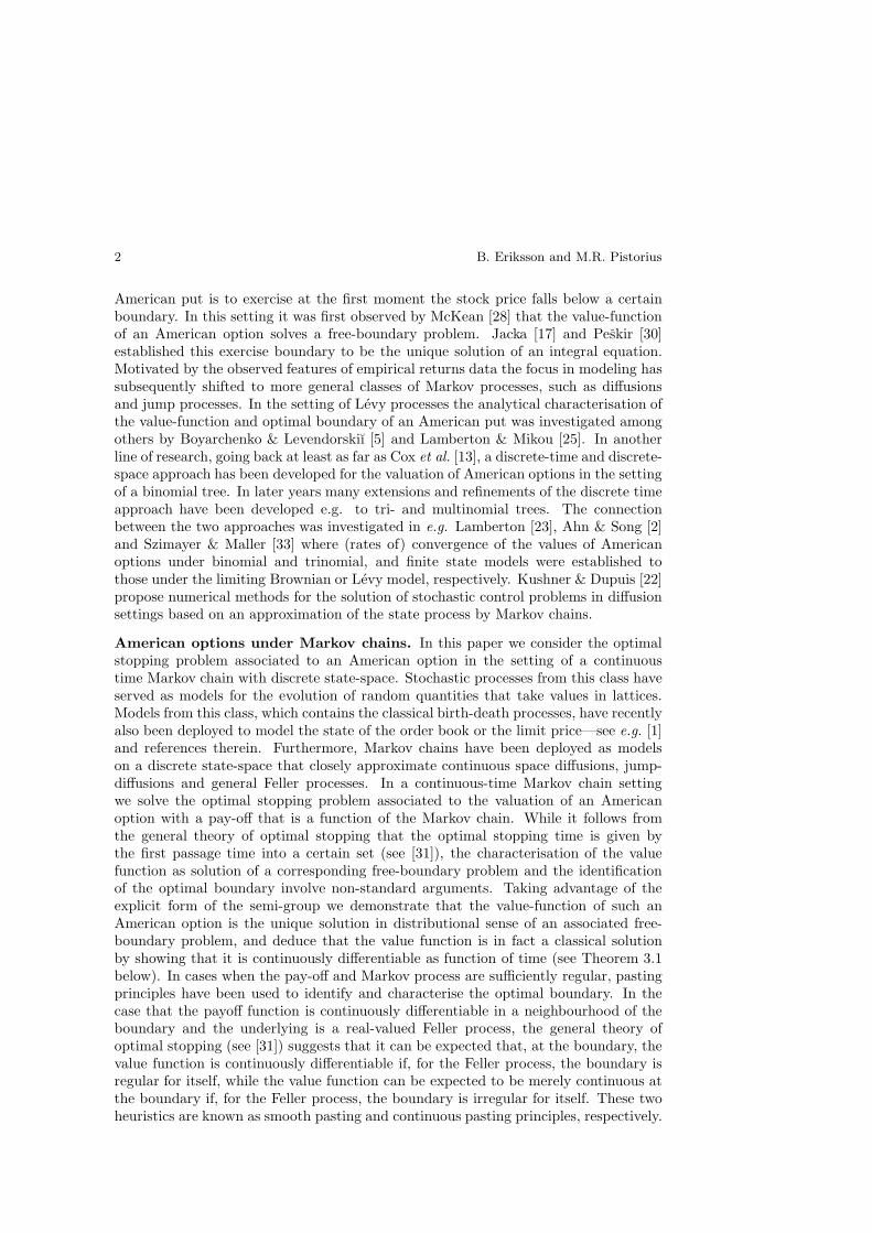
If the sequences X = x1, x2, . . . and τ(x1), τ(x2), . . . are non-decreasing, then theoptimal boundary is given by B(t) = supxi ∈ X : t ∈ [τ(xi), T ]. This form of Bis for example encountered in the case of an American put option under a continuoustime Markov chain model that is spatially homogeneous (see Figure 1).

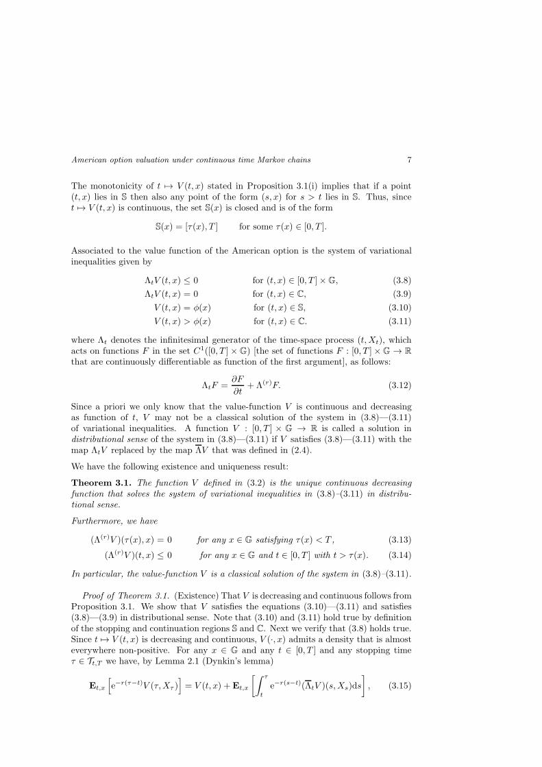
Denote byB = B(τ(x)), x ∈ G = bii, bi > bi+1,

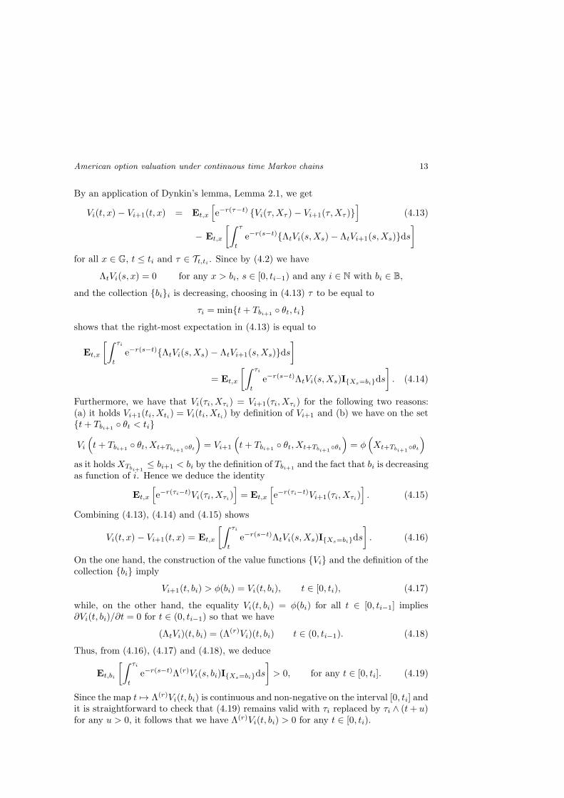
the set of distinct elements in B(τ(x)), x ∈ G that the optimal boundary takes(in order of decreasing magnitude or, equivalently, increasing time to maturity T ; seeFigure 2) and by

ti = τ(bi), i = 1, 2, . . . ,

the first epoch t in the interval [0, T ] that the optimal boundary B(t) is equal to bi. Atthis point we note that (i) the sequence tii is decreasing and (ii) the boundary B isconstant in between the epochs ti and has a discontinuity at the epochs ti. Given thetimes ti and the optimal barrier levels bi the American option can be valued recursively:The value-function V of the American option is equal to the value-function of a barrieroption contract with time-dependent barrier B that entitles the holder to a rebatepayment φ(XτB ) if the epoch τB = inft ≥ 0 : Xt ≤ B(t) is strictly smaller than T


Figure 1: The optimal boundary corresponding to an at-the-money American put option with strikeS0 = K = 100 and maturity T = 1 when interest rate and dividend yield are given by r = 0.1 andδ = 0 and the underlying is given by a Markov chain that closely approximates a geometric Brownianmotion with volatility σ = 0.3. The chain has a state-space of size 200 and was constructed bymatching the instantaneous moments of the Markov chain with those of the Brownian motion, usingthe procedure described in [29].

and to a payment φ(XT ) in the case that the epoch τB is larger or equal to T . Fromthe Markov property of X applied at the epochs ti that the barrier B has jumps itfollows that the function V is equal to the final value VN∗ of the following recursion:

Vi(t, x) = Et,x

[e−rTbi

θtφ(Xt+Tbi

θt

)ITbi

θt<ti−1−t+ e−r(ti−1−t)Vi−1(ti−1, Xti−1

)ITbiθt>ti−1−t

]

= Et,x

[e−r(Tbi

θt∧(ti−1−t))Vi−1

(ti−1, X(t+Tbi

θt)∧ti−1

)], (4.1)

for t ∈ [0, ti−1] and all i ≥ 1 and x ∈ G, with V0(t, x) = φ(x) for t ∈ [0, T ], whereTbi = infs ≥ 0 : Xs ≤ bi and θt denotes the shift-operator (defined by θt(ω) = ω(t+·)for all ω ∈ Ω), so that it holds Tbi θt = infs ≥ 0 : Xt+s ≤ bi. Note that we have

V (t, x) = Vi(t, x) = φ(x) for any pair (x, t) with x ∈ S and t ≤ ti−1

V (t, x) = Vi(t, x) for any t ∈ [ti, ti−1] and x ∈ G.

Thus, the optimal value function V is equal to Vi on the time interval [ti, ti−1].

We will next characterise the collection of epochs tii in terms of the value of thetime-space generator Λt applied to the functions Vi.

Theorem 4.1. Let Vi be defined by (4.1). For any i ∈ N with bi ∈ B and ti < T , itholds

ΛtVi(t, x) = 0 for x > bi, t ∈ [0, ti−1), (4.2)

ΛtVi(t, x) = Λ(r)Vi(t, x) = 0 for x = bi, t = ti, (4.3)

ΛtVi(t, x) = Λ(r)Vi(t, x) ≤ 0 for x ≤ bi, ti < t. (4.4)

ΛtVi(t, x) = Λ(r)Vi(t, x) > 0 for x = bi, t < ti, (4.5)

The proof is based on the following auxiliary result:


bi+1

bi

bi−1

ti ti−1

S

C

Figure 2: A close-up of the optimal boundary, illustrating the values bi and ti.

Lemma 4.1. For any i ∈ N with bi ∈ B and any x ∈ G, the function Vi(·, x) :[0, ti−1] → R given by t 7→ Vi(t, x) is decreasing and continuous. As a consequence,the function Λ(r)Vi(·, bi) : [0, ti−1] → R given by t 7→ (Λ(r)Vi)(t, bi) is continuous anddecreasing on [0, ti−1].

Proof of Lemma 4.1. Let x ∈ G and i with bi ∈ B be arbitrary and given. Thefunction t 7→ Vi(t, x) restricted to the interval (ti, ti−1) is equal to the function t 7→V (t, x), which was shown to be decreasing in Proposition 3.1. We next turn to thecase t ≤ ti. Note that for any t ∈ [0, ti−1] we have that Vi(t, x) is equal to

Et,x

[e−r(Tbi

θt∧(ti−1−t))Vi−1

(ti−1, X(t+Tbi

θt)∧ti−1

)]=

(exp[(ti−1 − t)Λ(i)

r ]φi−1

)(x),

(4.6)

where φi−1 : G → R is given by φi−1(x) = Vi−1(ti−1, x) and Λ(i)r is the sub-generator

of X , discounted at rate r and stopped upon first entrance into the set x ∈ G : x ≤ bi(see (5.1) below).

Thus, for any t, s ∈ [0, ti−1] with t > s we have

Vi(s, x) − Vi(t, x) =[exp[(ti−1 − t)Λ(i)

r ](exp[(t− s)Λ(i)

r ]− I)φi−1

](x), (4.7)

where I denotes the identity. Since t 7→ Vi(t, x) is decreasing for t ∈ [ti, ti−1] we deducefrom (4.6) and (4.7)

Vi(t, x)− Vi(ti−1, x) =[(

exp[(ti−1 − t)Λ(i)r ]− I

)φi−1

](x) ≥ 0 (4.8)

for any t ∈ [ti, ti−1] and x ∈ G. In view of (4.7) and (4.8) it follows

Vi(t, x)− Vi(s, x) ≤ 0 for any s, t ∈ [0, ti−1] with t− s ∈ [0, ti−1 − ti]. (4.9)

As the difference ti−1 − ti is strictly positive, the statement in (4.9) implies Vi(t, x) −Vi(s, x) ≤ 0 for any s, t ∈ [0, ti−1] with t ≥ s. The proof of the monotonicity ofVi(·, x) is complete. The continuity of t 7→ Vi(t, x) for any x ∈ G follows from the

continuity of the semi-group associated to the sub-generator Λ(i)r , while the continuity

of t 7→ (Λ(r)Vi)(t, bi) follows by an application of Lebesgue’s Dominated Convergence


Theorem, which is justified in view of the continuity of t 7→ Vi(t, x), the boundednessof Vi, and Assumption 1.

By an argument that is analogous to the one deployed in the proof of Proposition 3.1(ii)(noting that Vi(t, bi) = φ(bi) for any t ∈ [0, ti−1]), it follows that the monotonicity ofVi(·, x) implies the monotonicity of t 7→ (Λ(r)Vi)(t, bi) on the interval [0, ti−1].

Proof of Theorem 3.1, continued. (Classical solution) We start with noting that As-sumption 2 does not play any other role in the proof than simplifying the notation anddefinitions (of e.g. the functions Vi), and the proof in the general case is obtained by astraightforward adaptation of the proof that follows below. To show that V is a classicalsolution it suffices to show that at every t in [0, T ] and x in G the map t 7→ V (t, x)is continuously differentiable. Noting that the restrictions of the functions V and Vi

to the interval (ti, ti−1) are equal, we deduce that V is continuously differentiable atevery t in (ti, ti−1) with derivative given by

∂V

∂t(t, x) =

∂Vi

∂t(t, x) = −(Λ(i)

r V )(t, x), t ∈ (ti, ti−1), (t, x) ∈ C. (4.10)

Furthermore, since the function V is a solution of the system of variational equalitiesin (3.8)–(3.11) and is constant as function of t in the stopping region S it follows

∂V

∂t(t, x) = −(Λ(r)V )(t, x) for any t ∈ (ti, ti−1) with (t, x) ∈ C, (4.11)

∂V

∂t(t, x) = 0 for any pair (t, x) with t ∈ [ti, ti−1] with (t, x) ∈ S. (4.12)

Here we used that, for any x ∈ G, the definition of the sequence (ti)i implies that ifthere exists a t ∈ (ti, ti−1) with (t, x) ∈ S then we have (t, x) ∈ S for all t ∈ [ti, ti−1].To complete the proof of the continuous differentiability of V we finally consider thecase t = ti. If ti is such that (ti, x) is an element of the continuation region C then itfollows from the expression in (4.11) and the fact that the continuation region is openthat the left-limit and right-limit of ∂V

∂t (t, x) at ti are equal. If ti is such that (ti, x)is element of the stopping region S then we have that τ(x) is smaller or equal to ti.In the case τ(x) < ti it follows from (4.12) that the right- and left-limit of ∂V

∂t (t, x)at ti are equal to zero. In the case τ(x) = ti we note that the right-limit is equal tozero, while the left-limit of ∂V

∂t (t, x) at ti is equal to (Λ(r)V )(τ(x), x) which, in viewof (3.13), is also equal to zero. Thus, we deduce that at all t ∈ [0, T ] and x ∈ G thefunction V is continuously differentiable and the proof is complete.

Proof of Theorem 4.1. Since Vi(t, x) = V (t, x) for t ∈ [ti, ti−1], (4.3) and (4.4) holdin view of Theorem 3.1.

The function Vi is the value function of a down-and-out barrier option with matu-rity ti−1 rebate φ(x) and terminal payoff function Vi−1(ti−1, x). Since the processe−r(t∧ti−1∧Tbi

)Vi(t ∧ ti−1 ∧ Tbi , Xt∧ti−1∧Tbi) is a martingale, it follows by an analogous

reasoning as the one that was used in the proof of Theorem 3.1 that we have ΛtVi(t, x) =0 for x > bi and t < ti−1. Hence, (4.2) holds true.

Finally, we turn to the proof of (4.5). We start with observing that (Λ(r)Vi)(t, bi) isnon-negative on the interval t ∈ [0, ti] in view of Lemma 4.1 and (4.3). We next showthat (Λ(r)Vi)(t, bi) is in fact strictly positive on the interval [0, ti).


By an application of Dynkin’s lemma, Lemma 2.1, we get

Vi(t, x)− Vi+1(t, x) = Et,x

[e−r(τ−t) Vi(τ,Xτ )− Vi+1(τ,Xτ )

](4.13)

− Et,x

[∫ τ

t

e−r(s−t)ΛtVi(s,Xs)− ΛtVi+1(s,Xs)ds]

for all x ∈ G, t ≤ ti and τ ∈ Tt,ti . Since by (4.2) we have

ΛtVi(s, x) = 0 for any x > bi, s ∈ [0, ti−1) and any i ∈ N with bi ∈ B,

and the collection bii is decreasing, choosing in (4.13) τ to be equal to

τi = mint+ Tbi+1 θt, ti

shows that the right-most expectation in (4.13) is equal to

Et,x

[∫ τi

t

e−r(s−t)ΛtVi(s,Xs)− ΛtVi+1(s,Xs)ds]

= Et,x

[∫ τi

t

e−r(s−t)ΛtVi(s,Xs)IXs=bids

]. (4.14)

Furthermore, we have that Vi(τi, Xτi) = Vi+1(τi, Xτi) for the following two reasons:(a) it holds Vi+1(ti, Xti) = Vi(ti, Xti) by definition of Vi+1 and (b) we have on the sett+ Tbi+1

θt < ti

Vi

(t+ Tbi+1

θt, Xt+Tbi+1θt

)= Vi+1

(t+ Tbi+1

θt, Xt+Tbi+1θt

)= φ

(Xt+Tbi+1

θt

)

as it holdsXTbi+1≤ bi+1 < bi by the definition of Tbi+1

and the fact that bi is decreasingas function of i. Hence we deduce the identity

Et,x

[e−r(τi−t)Vi(τi, Xτi)

]= Et,x

[e−r(τi−t)Vi+1(τi, Xτi)

]. (4.15)

Combining (4.13), (4.14) and (4.15) shows

Vi(t, x) − Vi+1(t, x) = Et,x

[∫ τi

t

e−r(s−t)ΛtVi(s,Xs)IXs=bids

]. (4.16)

On the one hand, the construction of the value functions Vi and the definition of thecollection bi imply

Vi+1(t, bi) > φ(bi) = Vi(t, bi), t ∈ [0, ti), (4.17)

while, on the other hand, the equality Vi(t, bi) = φ(bi) for all t ∈ [0, ti−1] implies∂Vi(t, bi)/∂t = 0 for t ∈ (0, ti−1) so that we have

(ΛtVi)(t, bi) = (Λ(r)Vi)(t, bi) t ∈ (0, ti−1). (4.18)

Thus, from (4.16), (4.17) and (4.18), we deduce

Et,bi

[∫ τi

t

e−r(s−t)Λ(r)Vi(s, bi)IXs=bids

]> 0, for any t ∈ [0, ti]. (4.19)

Since the map t 7→ Λ(r)Vi(t, bi) is continuous and non-negative on the interval [0, ti] andit is straightforward to check that (4.19) remains valid with τi replaced by τi ∧ (t+ u)for any u > 0, it follows that we have Λ(r)Vi(t, bi) > 0 for any t ∈ [0, ti).


5. Valuation algorithm

The characterisation of the free boundary given in Theorem 4.1 can be deployed tocompute the optimal boundary and the corresponding value of an American optionunder the Markov chain model. For the presentation of a valuation algorithm we willrestrict ourselves in this section to Markov chains with a finite state-space (of size N ,say).

To identify the epochs ti a numerical method has to be deployed since the equations

ΛtVi(t, bi) = 0,

are highly non-linear in t. Except in degenerate cases, one may expect the maps 7→ ΛtVi(s, bi) to be strictly decreasing, in which case the equation (ΛtVi)(t, bi) =0 admits a unique solution and it is efficient to use a solver such as the Newton-Raphson method (which is the method that was used in the examples in Section 7).(Note that although we could have attempted to compute ti as root of the functions 7→ Λ(r)Vi(s, bi) we found that working with s 7→ ΛtVi(s, bi) yielded a more efficientnumerical implementation). A procedure for computation of the value function of anAmerican option under a Markov chain model based on a solution of the correspondingfree-boundary problem that was outlined in the previous paragraph is described inAlgorithm 1 below. In order to be able to formulate the algorithm we fix some extranotation. After relabeling we may assume without loss of generality that the elementsof the state-space G = xi, i = 1, . . . , N, where N is the number of states, are orderedin decreasing order

xN < xN−1 < . . . < x2 < x1,

and we denote by

Gi:j = xk, k ∈ i, . . . , j i < j, i, j = 1, . . . , N,

the slice of the state-space consisting of the elements xi, . . . , xj . Furthermore, for any

i = 1, . . . , N , denote by Λ(i)r and Λ

(i)

r the (sub-)generator matrices that can be obtaineddirectly from the generator matrix Λ(r) as follows: (i) the pair satisfies

Λ(i)r + Λ

(i)

r = Λ(r)

where we recall that Λ(r) = Λ−rI, and (ii) Λ(i)r (x, y) is equal to Λ(r)(x, y) for x, y ∈ G1:i

and zero for x, y ∈ Gi+1:N :

Λ(i)r (x, y) =

Λ(x, y)− r for x ∈ G, x ≥ xi, x = y,Λ(x, y) for x, y ∈ G, x ≥ xi, x 6= y,0 for x ≤ xi+1, x, y ∈ G.

(5.1)

The matrix Λ(i)r is the generator matrix of a Markov chain that has the same law as

the chain X that is stopped upon the first entrance into the set Gi+1:N . The roleof these matrices in barrier option valuation in Markov chain models is reviewed inRemark 5.1(ii) below.


Algorithm 1: Markov chain free-boundary algorithm

f i nd index i o f l a r g e s t g r id po int xi ∈ G such that (Λ(r)φ)(xi) < 0s e t t∗ ← Twhi le t∗ > 0

f i nd s < t∗ such that Λ(i)

r

[exp

((t∗ − s)Λ

(i)r

)φ](xi) = 0 ;

i f s > 0

s e t φ← exp((t∗ − s)Λ

(i)r

)φ ;

e l s e i f s ≤ 0

s e t φ← exp(t∗Λ

(i)r

)φ ;

s e t i← i+ 1 ; s e t t∗ ← s ;endreturn φ

Remark 5.1. In Algorithm 1 we used the following two facts:

(i) In view of the definition of the matrix Λ(i)

r and the relation ddt exp(tA) = A exp(tA)

that holds for any square matrix A we have the equality

(Λt exp

((t∗ − t)Λ(i)

r

))∣∣∣t=s

= O ⇔ Λ(r) exp((t∗ − s)Λ(i)

r

)= Λ(i)

r exp((t∗ − s)Λ(i)

r

),

where O denotes a zero matrix of appropriate size.

(ii) The value of the knock-out option Uξ(t, x) = Et,x[e−r(T∧τ)ξ(XT∧τ )] with maturity

T , pay-off function ξ : G→ R+ and knock-out set Gc, with

τ = inft ∈ R+ : Xt /∈ G,

is given by (as shown in [29])

Uξ(t, x) =[exp

((T − t)Λr

)ξ](x),

where we denote by Λr the (sub)-generator matrix

Λr(x, y) =

Λ(x, y)− r, if x ∈ G, x = y,

Λ(x, y), if x ∈ G, y ∈ G, x 6= y,

0, if x ∈ Gc, y ∈ G.

To see that this is the case the key observation is that the barrier option in question isa European-type option with the underlying given by the stopped process X·∧τ whichis itself a Markov chain with generator Λ0 (the (sub-)generator Λr is obtained whenalso the discounting rate r is included). Note that since t → exp(tX) is smooth, thevalue function Uξ(t, x) is smooth as a function of t.


6. Convergence

We next show that the convergence of a sequence of Markov chains carries over toconvergence of the corresponding American option values. We will assume that theprice process S is a Markov process with state-space R+ that is defined on some filteredprobability space (Ω,F ,F,P), where F = Ftt≥0 denotes the standard filtrationgenerated by S and Ω denotes the Skorokhod space of right-continuous functions withleft-hand limits that map R+ to R. We take the interest rate and dividend yield to beconstant equal to r and d, and assume in this section that the discounted price processe−γtStt≥0 with γ = r − d is a square-integrable martingale. We assume in additionthat S is a Feller process that solves the stochastic differential equation given by

dSt

St−= γdt+ σ(St−)dWt + p(dt× dx), t > 0,

with S0 = s > 0, where W denotes a Wiener process and p denotes a compensatedrandom measure with compensator given by the random measure ν(St−, dz)dt, where,for every x ∈ R+, ν(x, dy) is a measure with support in (−1,∞) satisfying theintegrability condition

∫

(−1,∞)

|y|2ν(x, dy) <∞. (6.1)

The value-function v : [0, T ]×R+ → R+ of the American option with payoff φ : R+ →R+ on the underlying process S is denoted by

v(t, x) = supτ∈Tt,T (F)

Et,x

[e−r(τ−t)φ(Sτ )

], (t, x) ∈ [0, T ]× R+, (6.2)

with Et,x[ · ] = E[ · |St = x] and the set Tt,T (F) equal to the collection of F-stoppingtimes taking values in between t and T . The Bermudan option, which is an American-type option for which the epoch of exercise is restricted to take values in the grid T

given byT = i∆ : i = 0, . . . ,M with ∆ = T/M, (6.3)

is a closely related derivative security, with value function vM : [0, T ]×R+ → R+ givenby

vM (t, x) = supτ∈T M

t,T(F)

Et,x

[e−r(τ−t)φ(Sτ )

], (t, x) ∈ [0, T ]× R+, (6.4)

where T Mt,T (F) denotes the collection of F-stopping times taking values in the grid T

intersected with the interval [t, T ].

LetX(n) denote a sequence of Markov chains such that e−γ·X(n)· are square-integrable

martingales, that is defined on the measurable space (Ω,F) and converges weakly tothe Feller process S, where the weak convergence is in the Skorokhod J1 topology(see e.g. [18]). Let V (n),M and V (n) denote the value functions of a Bermudan optionwith M equidistant exercise times and an American option, both with underlying priceprocess given by the Markov chain X(n). Below we show that as n and M tend to


infinity then both V (n)(0, x) and V (n),M (0, x) tend to the value v(x) of the Americanoption when the spot S0 is equal to x. More precisely, we assume that the subsequentgrids (G(n))n∈N are all nested (i.e., G(n) is contained in G(n+1) for any positive integern) and that the union ∪n∈NG

(n) is dense in R, and consider the following convergenceof a sequence of functions f (n) : G(n) → R to a function f : R→ R:

f (n) G−→ f ⇔ ∀m ∈ N ∀x ∈ G(m) : lim

n→∞,n≥mf (n)(x)→ f(x).

Convergence is established under the condition that the functions

t 7→ E0,x

[〈e−γ·S·〉t

], t 7→ E0,x

[〈e−γ·X

(n)· 〉t

](6.5)

are Lipschitz-continuous on [0, T ] with Lipschitz constants given by C2 (c1x + c2)2

and D(n)2 (d1x + d2)2 for some C,D(n), c1, c2, d1, d2 ∈ R+, such that supn∈N D(n) is

finite, where, for any square-integrable martingale M ′, 〈M ′〉· denotes its predictablequadratic variation. These conditions are satisfied by many of the Markov processesS used in financial modelling, and appropriately chosen approximating Markov chainsX(n).

Theorem 6.1. Assume that φ is Lipschitz continuous and that the functions in (6.5)are Lipschitz continuous with respective Lipschitz constants given by C2 (c1x+c2)

2 andD(n)2 (d1x + d2)

2 for some C,D(n), c1, c2, d1, d2 ∈ R+, where supn∈N D(n) is finite.The following hold true:

(i) V (n),M (0, ·) G−→ vM (0, ·), as n→∞ for any M ∈ N.

(ii) V (n),M (0, ·) G−→ v(0, ·) as minn,M → ∞.

(iii) V (n)(0, ·) G−→ v(0, ·) if n→∞.

Proof of Theorem 6.1. We first prove the following claim: For any n ∈ N, thereexist constants C(x) and D(n, x) such that for all M ∈ N

|vM (0, x)− v(0, x)| ≤ C(x)√M

, |V (n),M (0, x)− V (n)(0, x)| ≤ D(n, x)√M

. (6.6)

We will only prove this claim when the underlying is given by S as the proof of thecase that the underlying is a Markov chain is analogous.

Observe that the collection of stopping times of the form τM = infs ≥ τ : s ∈ T forτ ∈ T0,T (F) is equal to the set T M

0,T (F). By an application of the triangle inequalitywe find

|v(0, x)− vM (0, x)| ≤ supτ

E0,x

[∣∣e−rτφ(Sτ )− e−rτMφ(SτM )∣∣]

≤ supτ

E0,x

[∣∣(e−rτ − e−rτM )φ(Sτ )|+ |e−rτM (φ(Sτ )− φ(SτM ))∣∣]

≤ 1

M· c(x) +K · sup

τE0,x [|Sτ − SτM |] ,


where the suprema are taken over the set Tt,T (F) of (F)-stopping times taking values inthe interval [t, T ] and we used that by the triangle inequality and Lipschitz continuityof φ

supτ

E0,x[T re−rτ |φ(Sτ )|] ≤ T r(φ(x) + 2Kx) := c(x),

whereK is the Lipschitz constant. By the strong Markov property of S and the triangleinequality the expectation on the right-hand side can be estimated by

E0,x [|Sτ − SτM |] ≤ E0,x [E0,Sτ[|S0 − SτMθτ |]] . (6.7)

Another application of the triangle-inequality yields the estimate

E0,s [|S0 − SτMθτ |] (6.8)

≤ E0,s

[|S0 − e−γ(τMθτ )SτMθτ |

]+E0,s

[|e−γ(τMθτ ) − 1|SτMθτ

]:= e1(s) + e2(s),

for any non-negative s. An application of Doob’s Optional Stopping Theorem to thecadlag martingale M ′ = M ′

t = e−γtStt∈[0,T ] implies that e2(s) can be bounded by

e2(s) ≤|γT |eγ+T/M

M· E0,s

[e−γ(τMθτ )SτMθτ

]=|γT |eγ+T/M

M· s.

Another application of Doob’s Optional Stopping Theorem implies that the followingbound holds for any s ∈ R+:

E0,s [e2 (Sτ )] ≤|γT |eγ+T/M

M· eγ+T ·E0,s

[e−γτSτ

]

=|γT |eγ+T/M

M· eγ+T · s. (6.9)

By an application of Doob’s L2-inequality to the martingale M ′ and the Lipschitzcontinuity, we find

e1(s) ≤ E0,s

[sup

s:s< TM

∣∣e−γsSs − S0

∣∣]≤ 4E0,s

[∣∣∣e−γT/MST/M − S0

∣∣∣2]1/2

= 4(E0,s

[〈e−γ·S·〉T/M

])1/2 ≤ 4T 1/2

M1/2· C (c1 · s+ c2),

for s ∈ R+. Since M ′ is a martingale we have

E0,s[e1(Sτ )] ≤4T 1/2

M1/2· C (c1e

γ+T · s+ c2), (6.10)

for any s ∈ R+. By combining (6.7), (6.8), (6.9) and (6.10), it follows that (6.6) holds

with C(x) = 4KT 1/2C(c1eγ+T · x+ c2) +K|γT |e2γ+T · x+ c(x).

Next we turn to the proof of the three assertions. (i) By extending the probabilityspace if necessary, we may assume that the processes S and (X(n))n are all defined ona single probability space.


Denote by H the filtration generated by the process S,X(n), n ∈ N and by T Mt,T the

collection of H-stopping times taking values in the set [t, T ] intersected with the gridT. We may write

vM (0, x) = supτ∈T M

0,T

E0,x

[e−rτφ (Sτ )

], V (n),M (0, x) = sup

τ∈T M0,T

E0,x

[e−rτφ

(X(n)

τ

)].

We have by the triangle inequality and the Lipschitz continuity of φ (with Lipschitzconstant K)

∣∣∣vM (0, x)− V (n),M (0, x)∣∣∣ ≤ sup

τ∈T M0,T

E0,x

[e−rτ

∣∣∣φ(X(n)

τ

)− φ (Sτ )

∣∣∣]

(6.11)

≤ K supτ∈T M

0,T

E0,x

[∣∣∣Sτ −X(n)τ

∣∣∣]≤ KE0,x

[supt∈T

∣∣∣X(n)t − St

∣∣∣], (6.12)

where in the last line we used that any stopping time τ in the set T M0,T takes values in the

grid T. As, by assumption, X(n) converges weakly to S in the Skorokhod topology as

n→∞, it follows thatX(n)t converges to St in distribution as n tends to infinity, for any

fixed t ∈ T. The Skorokhod representation theorem implies that, for any given t ∈ T,

there exists a probability space carrying random variables X(n)t , n ∈ N, and St that

have the same distribution as X(n)t and St, respectively, such that X

(n)t converges a.s.

to St as n → ∞. The uniform integrability of the collection (X(n)t , St, t ∈ T, n ∈ N)

(which is in turn a consequence of the fact that C(x) + supn D(n, x) is finite) thusimplies

Ex

[∣∣∣St −X(n)t

∣∣∣]→ 0 as n→∞, for any t ∈ T, (6.13)

which implies that also the supremum in (6.12) converges to zero as T contains Melements. The proof of part (i) is completed by combining (6.12) and (6.13).

(ii), (iii) The triangle inequality implies that the differences between V (n)(0, x) andv(0, x) and V (n),M (0, x) and v(0, x) can be estimated as

∣∣∣V (n)(0, x)− v(0, x)∣∣∣ ≤

∣∣∣V (n)(0, x)− V (n),M (0, x)∣∣∣+

∣∣∣V (n),M (0, x)− v(0, x)∣∣∣

∣∣∣V (n),M (0, x)− v(0, x)∣∣∣ ≤

∣∣∣V (n),M (0, x)− vM (0, x)∣∣∣ +

∣∣vM (0, x)− v(0, x)∣∣ . (6.14)

Let ǫ > 0 be arbitrary. By virtue of (6.6) and the fact that supn D(n, x) is finite itfollows that there exists an Mǫ such that, for all M ≥Mǫ and for all n ∈ N,

max

∣∣vM (0, x)− v(0, x)∣∣ , sup

n∈N

∣∣∣V (n)(0, x)− V (n),M (0, x)∣∣∣≤ ǫ. (6.15)

Fixing an M larger than Mǫ, part (i) implies that there exists an Nǫ such that we have∣∣∣V (n),M (0, x)− vM (0, x)

∣∣∣ ≤ ǫ for all n ≥ Nǫ.

Combining this estimate with (6.14) and (6.15) yields the estimates |V (n)(0, x) −v(0, x)| ≤ 3ǫ and |V (n)(0, x)−V (n),M (0, x)| ≤ 2ǫ. Since ǫ was arbitrary the statementsin (ii) and (iii) follow.


7. Numerical illustrations

To provide an illustration of the effectiveness of the method we report in this sectionthe results of the approximation of the value of the American put option by the freeboundary approach (Algorithm 1, which we shall refer to as ‘FB’). The algorithmfor the pricing of American options takes as input a Markov chain X that closelyapproximates the Feller process S which is constructed by suitably specifying its state-space and generator matrix: the state-space will be taken non-uniform with higherdensity in relevant areas (e.g. around the spot value S0 and the strike K, in the caseof a put option) and the generator matrix is chosen so as to match the first twoinstantaneous moments of S. The smallest and largest points of the state-space aretaken sufficiently small and large respectively to guarantee that the truncation erroris negligible at the level of accuracy that is considered in the examples below (theselevels were determined after some numerical experimentation). Along these lines, analgorithm for the construction of a Markov chain was developed in [29] which we willdeploy in the numerical illustrations below. By way of comparison we also report theresults of the dynamic programming algorithm that proceeds by first approximatingthe American option by a Bermudan option, by restricting the possible exercise timesto a finite set, and subsequently valuing the Bermudan option under the Markov chainX according to the well-known dynamic programming procedure. (This algrithmis referred to as the ‘DP’ algorithm and a description in the current Markov chainsetting is presented in Appendix A). Additional numerical examples can be found inEriksson [16].

7.1. CEV-Kou model

We consider the valuation of the American put option under the jump diffusion thatevolves according to the SDE

dSt

St−= (r − d− λξ(St−/S0)

β)dt+ (St−/S0)βdLt,

Lt = σWt +

Nt∑

i=1

(eKi − 1), t > 0, S0 = s > 0,

where W is a Brownian motion, N a Poisson process and the Ki are independentrandom variables following a double exponential distribution, given by

fK(k) = pλpe−λpkI(0,∞)(k) + (1− p)λmeλmkI(−∞,0)(k), k ∈ R,

with λp > 0, λm > 0 and p ∈ [0, 1]. The parameter ξ is given by

ξ = E[eK1 − 1] =pλp

λp − 1+

(1− p)λm

λm + 1− 1.

The processesW andN and the collection of random variables Ki, i ∈ N are assumedto be mutually independent.

The model under consideration is a combination of the Kou model [19], a geometricLevy process with double exponential jumps, [obtained by setting β = 0] and the


Size N 200 400 200 400β = −1 β = −3

DP M = 3200 6.6926 6.6957 6.6576 6.6609M = 6400 6.6926 6.6958 6.6577 6.6610

FB 6.6927 6.6958 6.6578 6.6611

Table 1: The values of American put options under the CEV-Kou model with model parametersr = 0.05, σ = 0.2, p = 0.3, λp = 50, λm = 25 and λ = 3, obtained by using the Free Boundary andDynamic Programming methods. The parameter β is given in the table, and the option parametersare K = 100, S0 = 100 and T = 1.

Constant Elasticity of Variance model [12], a diffusion with local volatility functiongiven by a power [obtained by taking λ = 0]. In particular, taking λ = β = 0, yieldsthe geometric Brownian motion (GBM) model. This model, which we refer to as theCEV-Kou model, has an infinitesimal generator that acts on f ∈ C2

c (R+) as

Lf(x) = LDf(x) + LJf(x), x ∈ R+,

LDf(x) = (r − d)xf ′(x) +σ2

2

(x

S0

)2β

x2f ′′(x),

LJf(x) =∫

(−1,∞)

[f(x(1 + y))− f(x)− f ′(x)xy]fK(log y)dy

y.

The results obtained by deploying the DP and FB algorithms are reported in Figures 3and 4 and Table 1. Figure 3(a) shows the absolute error for the dynamic programmingproblem for a varying number of exercise times with fixed size of the state-space.The slope of the line in Figure 3(a) is approximately −1, which corresponds to alinear decay of the error of the dynamic programming method (DP) in 1/M if thenumber of states is fixed where M is the number of time-steps. Figure 3(b) shows theabsolute error for the FB and DP methods with a fixed number of exercise times. Weobserved that the outcomes of the FB method appear to converge slightly faster thanthose of the DP method, but at the expense of longer execution times. Figure 3(b)appears to show a quadratic speed of convergence in 1/N with N the cardinality ofthe state-space G. Figure 4 contains the execution times for the outcomes obtainedby the FB and DP algorithms for a varying number of states N of the approximatingMarkov chain, showing the DP algorithm is the faster of the two. We observed thatthe change in execution time when varying the number of exercise times is very small.One explanation for this small change is that the bulk of the computational effort is incalculating the matrix exponential exp(∆Λ), and it appears that the time to calculateexp(∆Λ) is only marginally affected by the size of ∆, and decreasing ∆ often results inslightly faster calculations. For β = 0 the CEV-Kou model reduces to the Kou model.We compare the results obtained using the dynamic programming and free boundarymethods in the case β = 0 with those reported in [20] in Table 3. Note that, althoughthe results are reported in [20] for an interest rate equal to r = 0.05, we match thenumbers in [20] by using the value r = 0.06. We believe that this is a misprint in [20].For λ = 0 the CEV-Kou model reduces to the CEV model and in Table 2 we reportthe outcomes of the free-boundary and dynamic programming methods in the casesβ = 0, β = −1/3 and the results obtained in [35] using a finite difference method.


4.5 5 5.5 6 6.5 7 7.5−8.5

−8

−7.5

−7

−6.5

−6

−5.5

−5

log(M)

LOG

AR

ITH

M O

F A

BS

OLU

TE

ER

RO

R

(a)

4.5 5 5.5 6 6.5 7 7.5−10

−9

−8

−7

−6

−5

−4

log(N)

LOG

AR

ITH

M O

F A

BS

OLU

TE

ER

RO

R

Free BoundaryDynamic Programming

(b)

Figure 3: (a) The absolute error of the American put option values generated by the DynamicProgramming method for varying number of exercise times M using a Markov chain with state-spaceof fixed size N = 1600. As reference value is taken the outcome of the DP method for M = 12800exercise times. The Markov chain is an approximation to the CEV-Kou model with model parametersgiven by r = 0.05, d = 0, σ = 0.2, β = −1, p = 0.3, λp = 50, λm = 25 and λ = 3. The optionparameters are fixed to be equal to K = 100 (strike), S0 = 100 (spot) and T = 1 (maturity). (b) Theabsolute error of the American put option prices with the same parameters under the same modelas in (a), for varying sizes N of the state-space of the Markov chain for the FB method and DPmethod with M = 6400. In the figure the reference values for the computation of the errors of thevalues generated by the FB and DP methods are taken equal to the outcomes generated by these twomethods with N = 800 and N = 3200 states, respectively.

β = 0 N = 200 N = 400 N = 800DP M = 3200 8.3316 8.3359 8.3370

M = 6400 8.3318 8.3361 8.3371FB 8.3320 8.3363 8.3373CR 8.3371

Binomial 8.3378

β = −1/3 N = 400 N = 600 N = 800DP M = 1600 4.6488 4.6490 4.6491

M = 3200 4.6488 4.6491 4.6491FB 4.6489 4.6491 4.6492WZ 4.6489

Binomial 4.6491

Table 2: Value of the at the money American put option with strike S0 = K = 100. In theupper part of the table the underlying is a geometric Brownian motion (β = 0) with parametervalues taken from [9] (r = 0.1, δ = 0, σ = 0.3 and maturity T = 1). The row CR refers toCarr [9]’s randomization algorithm with the number of randomization steps taken equal to 15 (usingRichardson’s extrapolation). In the bottom part of the table the underlying is given by the CEV modelwith parameters taken from [35] (r = 0.05, q = 0, σ = 0.2 and β = −1/3, and maturity T = 0.5).The row “WZ” refers to results obtained by [35] using a finite difference scheme. The row “Binomial”refers to the outcomes of a binomial tree algorithm with 2000 time steps (top) and 5000 time steps(bottom). For the Markov chain methods DP (dynamic programming) and FB (free boundary) “Size”denotes the size of the state-space of the Markov chain.


4.5 5 5.5 6 6.5 7 7.5−8.5

−8

−7.5

−7

−6.5

−6

−5.5

−5

log(M)

LOG

AR

ITH

M O

F A

BS

OLU

TE

ER

RO

R

Figure 4: Displayed are the execution times for the computation of the American put optiondeploying the free boundary and the dynamic programming (M = 6400 exercise times) methodsfor various sizes N of the approximating Markov chain. The option parameters are fixed and takento be K = 100 (strike), S0 = 100 (spot) and T = 1 (maturity). The underlying price process followsa CEV-Kou model with parameters r = 0.05, d = 0, σ = 0.2, β = −1, p = 0.3, λp = 50, λm = 25 andλ = 3. Computations were carried out in Matlab on a laptop with Intel Core Duo T2500 2GHz.

K λ λp λm FB DP Kou Binomial Kou Approximation90 3 50 25 2.6709 2.6707 2.66 2.7290 3 50 50 2.4568 2.4566 2.46 2.5190 7 25 50 3.2282 3.2280 3.24 3.2990 7 50 50 2.6662 2.6660 2.66 2.72100 3 50 25 6.2700 6.2698 6.26 6.29100 3 50 50 6.0120 6.0118 6.01 6.03100 7 25 50 7.0524 7.0522 7.07 7.09100 7 50 50 6.2891 6.2889 6.28 6.31110 3 50 25 12.0559 12.0557 12.04 12.00110 3 50 50 11.8442 11.8440 11.84 11.78110 7 25 50 12.8296 12.8294 12.85 12.79110 7 50 50 12.0928 12.0926 12.08 12.03

Table 3: Displayed are American put option prices under the Kou model (which is equal to theCEV-Kou model with β = 0). The final two columns are obtained from [20]. In all cases it is assumedthat the spot is S0 = 100, the maturity is T = 1, the interest rate is r = 0.06, the volatility is σ = 0.2and the probability of an upward jump is p = 0.6, with the remaining parameters as given in the table.We employ a Markov chain with state-space of size N = 400, and for the dynamical programmingalgorithm we used M = 3200 exercise times.

Appendix A. Dynamic Programming algorithm

A Bermudan option with pay-off function φ and finite set of admissible exercise timesT ⊂ [0, T ] is a derivative security that may be exercised at any time τ ∈ T yieldingpay-off φ(Xτ ). For the ease of presentation we restrict ourselves to the case of anequidistant grid given in (6.3) with mesh size ∆ = T/M . The value V (t, x) of theBermudan option at time t ∈ T in case we have Xt = x is given by

V (t, x) = maxτ∈T

t,T(∆,G)

Et,x[e−r(τ−t)φ(Xτ )], (A.1)

for t ∈ T, and x ∈ G, where Tt,T (∆,G) is the set of G-stopping times τ takingvalues in [t, T ] ∩ T, where G = Gt, t ∈ [0, T ] denotes the filtration generated by theMarkov chain X . At any time t ∈ T, the holder of the Bermudan option has the choicebetween immediately exercising or continuing to wait. The former results in a pay-off of


φ(Xt), while in the latter case, the expected reward of postponing exercise, assumingthat the holder continues to follow an optimal strategy from time t to maturity, isEt,Xt

[e−r∆V (t+∆, X∆)]. Thus, for any t ∈ T, the value V (t, x) is at least equal to thelarger of φ(x) and Et,x[e

−r∆Vt+∆(X∆)]. The Dynamic Programming principle statesthat in fact equality holds: with Vi(x) = V (i∆, x), we have

Vi(x) = max(φ(x),Ei∆,x

[e−r∆Vi+1(X(i+1)∆)

]), (A.2)

for i = 0, . . . ,M − 1, and x ∈ G. Noting that in view of the form of the semigroup in(2.1) we have

Et,x

[e−r∆Vi+1(X∆)

]=

[exp

(∆Λ(r)

)Vi+1

](x).

By deploying the Dynamic Programming Principle, we obtain the following recursiveprocedure to compute the values of Vi(x) ranging over all initial values x ∈ G and alltime-steps i = 0, . . . ,M .

Algorithm 2: Procedure to compute the value of a Bermudan option

s e t ← TM

s e t V ← O ∈ RN×(M+1)

s e t V ( : , M + 1)← φ( : )

eva lua te A = exp(Λ(r))f o r i = M to 1

V ( : , i)← A[V ( : , i+ 1)] ;V ( : , i)← max(φ( : ), V ( : , i)) ;i← i− 1 ;

endreturn V

Remark A.1. (i) The algorithm returns the matrix (Vi(x), (i∆, x) ∈ T × G) ofvalues of the Bermudan option on the time-space grid T × G, where V ( : , i)denotes the ith column of the matrix V and contains the values Vi+1(x) forx ∈ G.

(ii) Note that when, as assumed above, the time-grid T is equidistant, the expo-nentiation of the matrix ∆Λ only needs to be computed once. If the time-gridT is chosen non-equidistant, the above algorithm will computationally be a gooddeal more expensive, since a costly exponentiation would need to be carried outat every iteration of the recursive procedure.

Appendix B. Proof of Dynkin’s Lemma (Lemma 2.1)

Proof. Assume first in addition that the map F (·, x) : [0, T ] → R is continuouslydifferentiable for every x ∈ G. An application of Ito’s lemma to the semi-martingalee−rtF (t,Xt)t∈[0,T ] shows that the process Mtt∈[0,T ] with

Mt = e−rtF (t,Xt)− F (0, X0)−∫ t

0

e−rs

[∂F

∂t+ (ΛF )− rF

](s,Xs)ds


is a local martingale. In view of the assumptions on F and Λ it follows that M is infact a uniformly integrable martingale. An application of Doob’s Optional StoppingTheorem implies that for every G-stopping time τ taking values in [t, T ] we haveEt,x[Mτ ] = 0, so that (2.3) holds true.

Assume next that F is as stated in the Lemma, with density f . Since the set G offunctions G : [0, T ]× G → R that is continuously differentiable at t ∈ [0, T ] for everyx ∈ G is dense in the set of continuous real-valued functions with domain [0, T ]× G,there exists a sequence of functions (Gn)n in G that almost everywhere converges toF . An application of Lebesgue’s Dominated Convergence Theorem which is justifiedby the facts that F is bounded and Λ has uniformly bounded diagonal (cf. Remark 1)shows that (2.3) is true under the stated assumptions.

Acknowledgements

Research supported by EPSRC grant EP/D039053. We thank Aleksandar Mijatovicfor useful conversations.

References

[1] Abergel, F. and Jedidi, A. (2011). A Mathematical Approach to Order Book Modeling. InEconophysics of Order-driven Markets, pp 93-107.

[2] Ahn, J. and Song, M. (2007) Convergence of the trinomial tree method for pricingEuropean/American options. Appl. Math. Comp., 189, 575–582.

[3] Alili, L. and Kyprianou, A.E. (2005). Some remarks on first passage of Levy process, theAmerican put and pasting principles. Ann. Appl. Prob. 15, 2062–2080.

[4] Almendral, A. and Oosterlee, C.W. (2007). Accurate Evaluation of European and AmericanOptions under the CGMY process. SIAM J. Scient. Comp. 29, 93–117.

[5] Boyarchenko, S.I. and Levendorskii, S.Z. (2002). Perpetual American options under Levyprocesses. SIAM J. Control Optim. 40, 1663–1696.

[6] Boyarchenko, S.I. and Levendorskii, S.Z. (2007). Irreversible Decisions under Uncertainty:

Optimal Stopping Made Easy. Springer.

[7] Boyarchenko, S.I. and Levendorskii, S.Z. (2002). Option pricing for truncated Levy processesInt. J. Theor. Appl. Finance 3, 549-552.

[8] Boyarchenko, S.I. and Levendorskii, S.Z. (2002). Non-Gaussian Merton-Black-Scholes

Theory. World Scientific.

[9] Carr, P. (1998). Randomization and the American Put. The Review of Financial Studies 11,597–626.

[10] Carr, P., Madan, D., Geman, H. and Yor, M. (2002). The fine structure of asset returns: anempirical investigation. Journal of Business 75, 305–332.

[11] Cont, R. and Tankov, P. (2003). Financial Modelling With Jump Processes. Chapman & Hall.

[12] Cox, J. (1996). Notes on option pricing I: Constant elasticity of variance diffusions. J. PortfolioManagement 22, 15–17.

[13] Cox, J.C , Ross, S.A. and Rubinstein, M. (1979). Options pricing: A simplified approach. J.

Fin. Economics 3, 125–144.

[14] Chung, K.L. and Walsh, J.B. (2005) Markov Processes, Brownian Motion and Time Symmetry.2nd Ed., Springer.

[15] Detemple, J. (2006). American-style Derivatives. Chapman & Hall/CRC Financial MathematicsSeries: Valuation and Computation, Boca Raton, FL: Chapman & Hall/CRC.


[16] Eriksson, B. (2013). On the valuation of barrier and American options in local volatility models

with jumps. PhD thesis, Imperial College London.

[17] Jacka, S.D. (1991). Optimal Stopping and the American Put. Math. Finance 1, 1–14.

[18] Jacod, J. and Shiryaev, A.N. (1987). Limit theorems for stochastic processes. Springer.

[19] Kou, S.G. (2002). A jump-diffusion model for option pricing. Management Sci. 48, 1086–1101.

[20] Kou, S.G. and Wang, H. (2004). Option Pricing Under a Double Exponential Jump DiffusionModel. Management Sci. 50, 1178–1192.

[21] Kushner, H.J. (1997). Numerical methods for stochastic control problems in finance. InMathematics of Derivative Securities, Publications of the Newton Institute 15, pp. 504–527.Cambridge University Press.

[22] Kushner, H.J. and Dupuis, P.G. (2000). Numerical Methods for Stochastic Control Problems

in Continuous Time. Springer, 2nd ed.

[23] Lamberton, D. (1998). Error Estimates for the Binomial Approximation of American putoptions. Ann. Appl. Prob. 8, 206–233.

[24] Lamberton, D. and Mikou, M. (2012). The smooth-fit property in an exponential Levy model.J. Appl. Prob. 49, 137–149.

[25] Lamberton, D. and Mikou, M. (2013). Exercise boundary of the American put near maturityin an exponential Levy model. Fin. Stoch. 17, 355–394.

[26] Lipton, A. (2001). Mathematical Methods for Foreign Exchange. World Scientific.

[27] Madan, D. and Yor, M. (2008). CGMY and Meixner subordinators are absolutely continuouswith respect to one sided stable subordinators. J. Comp. Finance 12, 27–47.

[28] McKean Jr, H.P. (1965). Appendix: A free boundary problem for the heat equation arisingfrom a problem of mathematical economics. Ind. Management Rev. 6, 32–39.

[29] Mijatovic, A. and Pistorius, M.R. (2013). Continuously Monitored Barrier Options underMarkov Processes. Math. Finance 23, 1–38.

[30] Peskir, G. (2005). On the American option problem. Math. Finance 15, 169–181.

[31] Peskir, G. and Shiryaev, A.N. (2006). Optimal stopping and free-boundary problems.Birkhauser.

[32] Sato, K. (1999). Levy processes and infinitely divisible distributions. Cambridge UniversityPress.

[33] Szimayer, A. and Maller, R.A. (2007). Finite approximation schemes for Levy processes andtheir application to optimal stopping problems. Stoch. Proc. Appl.117, 1422–1447.

[34] Wang, I.R., Wan, J.W.L. and Forsyth, P.A. (2007). Robust numerical valuation of Europeanand American options under the CGMY process. J. Comp. Finance 10, 31–69.

[35] Wong, H.Y. and Zhao, J. (2008). An Artificial Boundary Method for American Option Pricingunder the CEV Model. SIAM J. Num. Anal. 46, 2183–2209.

Documents

AMERICAN OPTION VALUATION UNDER …spiral.imperial.ac.uk/bitstream/10044/1/19226/2/14946_final.pdf · The value-function of an American option in this settingis characterised as the