Embed Size (px)
Citation preview

Bulletin of the American Meteorological Society
EARLY ONLINE RELEASE
This is a preliminary PDF of the author-produced manuscript that has been peer-reviewed and accepted for publication. Since it is being posted so soon after acceptance, it has not yet been copyedited, formatted, or processed by AMS Publications. This preliminary version of the manuscript may be downloaded, distributed, and cited, but please be aware that there will be visual differences and possibly some content differences between this version and the final published version.
The DOI for this manuscript is doi: 10.1175/BAMS-D-16-0230.1 The final published version of this manuscript will replace the preliminary version at the above DOI once it is available. If you would like to cite this EOR in a separate work, please use the following full citation: Vinayachandran, P., A. Matthews, K. Vijay Kumar, A. Sanchez-Franks, V. Thushara, J. George, V. Vijith, B. Webber, B. Queste, R. Roy, A. Sarkar, D. Baranowski, G. Bhat, N. Klingaman, C. Parida, K. Heywood, R. Hall, B. King, E. Kent, A. Nayak, C. Neema, P. Amol, A. Lotliker, A. Kankonkar, D. Gracias, S.
AMERICAN METEOROLOGICAL
SOCIETY
Vernekar, A. D.Souza, G. Valluvan, S. Pargaonkar, K. Dinesh, J. Giddings, and M. Joshi, 2018: BoBBLE (Bay of Bengal Boundary Layer Experiment): Ocean–atmosphere interaction and its impact on the South Asian monsoon. Bull. Amer. Meteor. Soc. doi:10.1175/BAMS-D-16-0230.1, in press. © 2018 American Meteorological Society

BoBBLE (Bay of Bengal Boundary Layer Experiment): Ocean–atmosphere1
interaction and its impact on the South Asian monsoon2
P. N. Vinayachandran∗3
Centre for Atmospheric and Oceanic Sciences, Indian Institute of Science, Bangalore 560 012,
India
4
5
Adrian J. Matthews6
Centre for Ocean and Atmospheric Sciences, School of Environmental Sciences and School of
Mathematics, University of East Anglia, Norwich, UK
7
8
K. Vijay Kumar9
CSIR-National Institute of Oceanography, Goa, India10
Alejandra Sanchez-Franks11
National Oceanography Centre, Southampton, UK12
V. Thushara, Jenson George13
Centre for Atmospheric and Oceanic Sciences, Indian Institute of Science, Bangalore, India14
V. Vijith15
Generated using v4.3.2 of the AMS LATEX template 1
LaTeX File (.tex, .sty, .cls, .bst, .bib)
Centre for Atmospheric and Oceanic Sciences, Indian Institute of Science, Bangalore, India,
Present affiliation: School of Marine Sciences, Cochin University of Science and Technology,
Kochi, India
16
17
18
Benjamin G. M. Webber, Bastien Y. Queste19
Centre for Ocean and Atmospheric Sciences, School of Environmental Sciences, University of
East Anglia, Norwich, UK
20
21
Rajdeep Roy22
Indian Space Research Organisation, National Remote Sensing Centre, Hyderabad, India23
Amit Sarkar24
ESSO-National Centre for Antarctic and Ocean Research, Goa, India25
Dariusz B. Baranowski26
Institute of Geophysics, Faculty of Physics, University of Warsaw, Poland27
G. S. Bhat28
Centre for Atmospheric and Oceanic Sciences, Indian Institute of Science, Bangalore, India29
Nicholas P. Klingaman, Simon C. Peatman30
National Centre for Atmospheric Science – Climate, University of Reading, UK31
C. Parida32
Berhampur University, Odisha, India33
Karen J. Heywood, Robert Hall34
2
Centre for Ocean and Atmospheric Sciences, School of Environmental Sciences, University of
East Anglia, Norwich, UK
35
36
Brian King, Elizabeth C. Kent37
National Oceanography Centre, Southampton, UK38
Anoop A. Nayak, C. P. Neema39
Centre for Atmospheric and Oceanic Sciences, Indian Institute of Science, Bangalore, India40
P. Amol41
CSIR-National Institute of Oceanography, Visakhapatnam, India42
A. Lotliker43
ESSO-Indian National Centre for Ocean Information Services, Hyderabad, India44
A. Kankonkar, D. G. Gracias, S. Vernekar, A. C. D.Souza45
CSIR-National Institute of Oceanography, Goa, India46
G. Valluvan47
ESSO-National Institute of Ocean Technology, Chennai, India48
Shrikant M. Pargaonkar49
Centre for Atmospheric and Oceanic Sciences, Indian Institute of Science, Bangalore, India50
K. Dinesh51
ESSO-Indian National Centre for Ocean Information Services, Hyderabad, India52
Jack Giddings, Manoj Joshi53
3

Centre for Ocean and Atmospheric Sciences, School of Environmental Sciences, University of
East Anglia, Norwich, UK
54
55
∗Corresponding author address: P. N. Vinayachandran, Centre for Atmospheric and Oceanic Sci-
ences, Indian Institute of Science, Bangalore 560 012, India
56
57
E-mail: [email protected]
4

ABSTRACT
5
The Bay of Bengal (BoB) plays a fundamental role in controlling the
weather systems that make up the South Asian summer monsoon system. In
particular, the southern BoB has cooler sea surface temperature (SST) that in-
fluence ocean–atmosphere interaction and impact on the monsoon. Compared
to the southeast, the southwestern BoB is cooler, more saline, receives much
less rain, and is influenced by the Summer Monsoon Current (SMC). To exam-
ine the impact of these features on the monsoon, the BoB Boundary Layer Ex-
periment (BoBBLE) was jointly undertaken by India and the UK during June
– July 2016. Physical and bio-geochemical observations were made using a
CTD, five ocean gliders, a uCTD, a VMP, two ADCPs, Argo floats, drifting
buoys, meteorological sensors and upper air radiosonde balloons. The obser-
vations were made along a zonal section at 8◦N between 85.3◦E and 89◦E
with a 10-day time series at 89◦E, 8◦N. This paper presents the new observed
features of the southern BoB from the BoBBLE field program, supported by
satellite data. Key results from the BoBBLE field campaign show the Sri
Lanka Dome and the SMC in different stages of their seasonal evolution and
two freshening events during which salinity decreased in the upper layer lead-
ing to the formation of thick barrier layers. BoBBLE observations were taken
during a suppressed phase of the intraseasonal oscillation; they captured in
detail the warming of the ocean mixed layer and preconditioning of the atmo-
sphere to convection.
Capsule Summary: A field experiment in the southern Bay of Bengal to
generate new high-quality in situ observational data sets of the ocean, air–sea
interface and atmosphere during the summer monsoon.
59
60
61
62
63
64
65
66
67
68
69
70
71
72
73
74
75
76
77
78
79
80
81
82
6

1. Introduction83
The Bay of Bengal (BoB) holds a prominent place in the science of monsoons owing to its84
impacts on the South Asian summer monsoon rainfall and its variability over the countries located85
along the rim of the BoB, which is home to over a billion people. Maximum rainfall during the86
summer monsoon is received in the northeastern BoB and the adjoining land area (Xie et al. 2006).87
Weather systems that form over the BoB contribute substantially to rainfall over central India88
(Gadgil 2003). Several such systems breed over the BoB during each monsoon season because of89
the capacity of the BoB to recharge its sea surface temperature (SST) quickly in the short sunny90
spells after the passage of each disturbance (Shenoi et al. 2002; Bhat et al. 2001). This rapid SST91
warming is facilitated by the thin mixed layer maintained by freshwater input from rainfall and92
river runoff into the BoB (Vinayachandran et al. 2002). These general features characterise the93
BoB north of about 15◦N.94
Further south, features of the ocean-atmosphere system are somewhat different (Mathews et al.,95
2015, CLIVAR Exchanges, 19(3), 38-42), yet intriguing. Climatologically, both the ocean and96
atmosphere show contrasts between east and west. The SST is marked by a cold pool (Joseph97
et al. 2005; Das et al. 2016) around Sri Lanka (Fig. 1a) compared to the warmer water in the east.98
The sea surface salinity (SSS; Fig. 1b) is higher in the west than in the east (Vinayachandran et al.99
2013). Most remarkably, the western part of the southern BoB is marked by the intense monsoon100
current that flows into the BoB carrying higher salinity Arabian Sea water. The atmosphere above101
the cold pool is characterized by a minimum in seasonal total rainfall (Fig. 1a) and has the lowest102
amount of low level clouds in the region (Shankar et al. 2007; Nair et al. 2011). The role of ocean103
dynamics and air–sea interaction processes in defining these large zonal and meridional variations,104
and the impact of these on monsoon rainfall elsewhere, have received little attention.105
7

Several field experiments have been conducted in the BoB to understand the response of the106
BoB to monsoons and its possible feedbacks (Bhat and Narasimha 2007). Among the recent107
experiments, BOBMEX (Bay of Bengal Monsoon Experiment; Bhat et al. (2001)) focused on the108
coupled ocean–atmosphere system in the northern BoB during the peak monsoon months of July–109
September. The JASMINE (Joint AirSea Monsoon Interaction Experiment ) sampled the eastern110
Indian Ocean and southern BoB during May and September, 1997 (Webster et al. 2002). The111
CTCZ (Continental Tropical Convergence Zone) experiment carried out under the Indian Climate112
Research Program made observations of both the southern and northern BoB during 2009 and 2012113
(Rao et al. 2011; Vinayachandran et al. 2013; Jain et al. 2016). The ASIRI (Air-Sea Interactions114
Research Initiative) campaign covered both summer and winter monsoons and combined data sets115
from multiple platforms and model simulations (Wijesekera et al. 2016b). These experiments have116
contributed significantly towards our understanding of the processes at work during monsoons,117
but a large gap exists in our knowledge base about the physical processes in the southern BoB.118
BoBBLE focuses on the less known, yet important, southern BoB and combines observations from119
multiple instruments including five ocean gliders to obtain high-quality time series observations of120
the ocean, air–sea interface and atmosphere during the peak period of the 2016 summer monsoon.121
The first set of measurements in the region was carried out by Schott et al. (1994) using current122
meter moorings and ship sections in the early nineties, which provided a description of the annual123
cycle and intraseasonal variation of monsoon currents. Earlier hydrographic surveys (Murty et al.124
1992) indicated the flow of high salinity water into the southern BoB. The intrusion of the Summer125
Monsoon Current (SMC) into the BoB was described using geostrophic currents derived from126
Expendable bathythermograph (XBT) data sets (Vinayachandran et al. 1999). The seasonal cycle127
and interannual variability of the thermocline along 6◦N was explored using the XBT data (Yu128
2003). Using ship-board observations made during the CTCZ field campaign, Vinayachandran129
8

et al. (2013) described the existence of a salt pump in the southern BoB. Using ADCP moorings,130
Wijesekera et al. (2016c) obtained current measurements from east of Sri Lanka for nearly two131
years. Lee et al. (2016) reported observations using multiple platforms, towards understanding132
the circulation and transport around Sri Lanka. Sustained ocean observation systems, RAMA133
McPhaden et al. (2009) in particular, have also contributed to the data base in this region. However,134
there is a major gap in the observations that are relevant to understanding the complete ocean–135
atmosphere system during the summer monsoon.136
The primary objective of the BoBBLE field program was to characterize the ocean–atmosphere137
system in the southern BoB, which is marked by contrasting features in its east and west. One of138
the major aims is to generate new high-quality in situ observational data sets of the ocean, air–139
sea interface and atmosphere during the peak phase of the summer monsoon. The overarching140
objectives of BoBBLE are to evaluate the role of ocean–atmosphere interactions in the simulation141
and prediction of the summer monsoon, to combine data and models to investigate the physical142
and bio-geochemical processes under the monsoon forcing, and to determine the role of the above143
mentioned processes in causing the synoptic-scale variability of the south Asian monsoon system.144
The aim of this paper is to make the community aware of the new data set that has been acquired,145
and to present a preliminary analysis of the observations collected during the BoBBLE field pro-146
gram, the details of which are given in section 2. Sections 3 and 4 describe air–sea interaction, and147
the oceanographic features of the southern BoB, respectively. We conclude with a summary and148
outlook in section 5.149
2. BoBBLE field program150
The research vessel RV Sindhu Sadhana (Fig. 2), sailed from the port of Chennai on 24 June and151
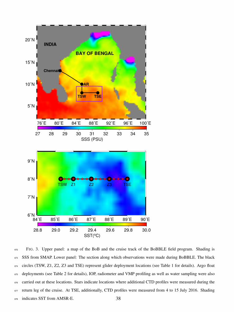
returned on 23 July 2016. The BoBBLE cruise was conducted along the track shown in Fig. 3.152
9

Ship-board observations can be classified into two types: observations made along the 8◦N section153
from 85.3◦E to 89◦E, in the international waters of the southern BoB and time series observations154
were at 89◦E, 8◦N (hereafter referred to as TSE) for a period of 10 days, 4–15 July 2016. Ocean155
glider deployments provided similar time series at locations marked as black circles in Fig. 3.156
Two ship-board Acoustic Doppler Current Profilers (ADCP, operating at frequencies of 38 kHz157
and 150 kHz), an autonomous weather station (AWS) and a thermo-salinograph recorded data con-158
tinuously during the cruise period. A SeaBird Electronics (SBE) 9/11+ Conductivity-Temperature-159
Depth profiler (CTD) measured vertical profiles and collected water samples at all points marked160
as stars in Fig. 3. Nominally, the casts were to a depth of 1000 m. At selected stations, additional161
CTD casts extended all the way to the deep ocean floor. At TSE, CTD observations were carried162
out to a depth of 500 m at approximately 3-hourly intervals, with a once-daily profile to 1000 m.163
Four standard MetOcean drifting buoys were also deployed during the BoBBLE field program.164
Five ocean gliders were deployed during 1-19 July 2016 along the 8◦N transect (Table 1). All165
gliders were equipped with a CTD package, enabling measurements of temperature and salinity166
with 0.5–1 m vertical resolution from the surface to 1000 m depth. Four gliders were equipped with167
dissolved oxygen (dO2), chlorophyll fluorescence (Chl) and optical backscatter sensors. Addition-168
ally, one glider (SG579) was equipped with a photosynthetically active radiation (PAR) sensor, and169
another (SG613) with microstructure shear and temperature sensors. Individual dives lasted 3–4170
hours. In total, 462 dives were made. Optimally interpolated (OI) two-dimensional (depth, time)171
gridded data sets (Matthews et al. 2014) were produced for each glider. The radii of influence in172
the Gaussian weighting functions were 2 m and 3 hr, respectively. The five depth–time OI data173
sets were then further combined into a single three-dimensional longitude–depth–time data set, by174
linear interpolation in longitude, taking account of the movement of the gliders with time.175
10

Seven Argo floats were deployed in the BoB along 8◦N, between 85.3◦E and 89◦E (Table 2). As176
BoBBLE is designed to target surface processes, all floats were programed to provide daily high-177
resolution profiles of the top 500 m in a region where in situ surface data are scarce. A second178
OI data set was created using profiles from core Argo floats from the international Argo program,179
BoBBLE Argo floats, glider profiles and the shipboard CTD. These OI data were mapped using180
World Ocean Atlas climatology (Boyer et al. 2013) and gridded at 25 longitude grid points at 8◦N,181
from 83◦E to 95◦E at 0.5◦ intervals. The time grid ran from 1 June 2016, before the BoBBLE182
field campaign started, to 30 September 2016, with data from each day gridded separately. This183
combined OI data set covers a longer time period than the BoBBLE field program, as there was184
a continuous Argo float presence in the BoB, before BoBBLE campaign which was then signifi-185
cantly enhanced by the seven floats deployed during BoBBLE.186
To map mesoscale and sub-mesoscale features, an Ocean Sciences–Teledyne underway CTD187
(uCTD), fitted with SBE CT sensors, was used for measuring temperature and salinity profiles188
while the ship was sailing at a speed of 6 knots. Nominally, the uCTD probe was allowed to189
profile vertically for 2 minutes in order to achieve a drop rate of about 1.5–2.5 m s−1 covering a190
depth range of approximately 250 m and the data was binned at 1m depth intervals.191
A vertical microstructure profiler (Rockland Scientific VMP-250) comprising two shear probes,192
one set of high-resolution micro-temperature and conductivity sensors and another set of standard193
CTD sensors was operated at all glider stations along the transect as well as at TSE. At each194
station, 2–3 profiles were measured. At TSE, profiles were measured at 0000, 0400, 0800, 1200,195
and 1700 UTC each day. In total, 138 casts were made, including that at TSE.196
To characterize the surface and sub-surface light field, bio-optical measurements were carried197
out with a Satlantic HyperProII hyperspectral underwater radiometer (HUR) equipped with three198
sensors for light, ECO triplet for fluorescence and colored dissolved organic matter (CDOM), and199
11

CTD sensors. The light sensors measured downwelling, upwelling and total solar irradiance. The200
HUR was operated for 17 days under cloud-free conditions between 0600 and 0700 hrs UTC at201
TSE, and along the 8◦N transect between 0530 and 0800 hrs UTC. A total of 37 profiles were col-202
lected during BoBBLE. An inherent optical profiler (IOP) was used for the measurement of light203
absorption and scattering coefficients, backscattering coefficient, chlorophyll-a, CDOM, turbidity204
and photosynthetically available radiation (PAR) along with a CTD sensor. The IOP was operated205
at TSE at 0130 and 0830 UTC each day.206
The meteorological measurements included an AWS, air-sea flux observing system (Table 3),207
and radiosondes. A LI-COR, infrared gas analyzer in conjunction with the 3D sonic anemome-208
ter based eddy covariance system, along with high-frequency response ship motion sensors were209
installed at the bow, at a height of approximately 15 m above sea surface and 6 m above the210
forecastle deck. Sensible and latent turbulent heat fluxes are estimated using the eddy covariance211
method (Fairall et al. 1997; Edson et al. 1998; Dupuis et al. 2003). Upper air observations of212
temperature, pressure, humidity, and wind were taken with Vaisala RS92 radiosondes, launched213
nominally at 0000 UTC and 1200 UTC every day. Additional launches were also made on some214
days to capture the diurnal cycle.215
3. Meteorology and air–sea interaction216
a. Large-scale conditions over the BoB during summer 2016217
The all-India rainfall for 2016 was 3% deficit relative to climatology (www.imd.gov.in), ENSO218
conditions were near neutral and SST anomalies in the tropical Pacific and Indian oceans were219
modest (www.ospo.noaa.gov). The Indian Ocean dipole (Saji et al. 1999) was in a negative state,220
with slightly warmer than usual conditions in the eastern Indian Ocean and cooler than usual con-221
12

ditions in the west, representing an intensification of the usual cross-basin gradient. Despite this,222
the 2016 can be seen as a representative monsoon and is therefore ideally suited for investigating223
its link with conditions in the BoB.224
The mean monsoon winds during the observation period were steady southwesterlies (Fig. 1d)225
and the SMC was intense with an axis oriented in the SW–NE direction, to the east of Sri Lanka226
(Fig. 1c). The mean SST was relatively cooler around the SMC with warmer water farther in the227
west and east. The east-west SST contrast that is typically seen in the climatology (Fig. 1a) was228
not as well developed during the period of observations (Fig. 1c). The mean SSS pattern was229
comparable to climatology (Fig. 1b,d).230
Intraseasonal variability had a significant effect on the conditions observed during the BoBBLE231
campaign. In June 2016, the southern BoB was under the influence of a convectively active phase232
(Fig. 4) of the Boreal Summer Intraseasonal Oscillation (BSISO) (Lee et al. 2013). This propa-233
gated northward (dashed blue line in Fig. 4) and was replaced by a convectively suppressed phase234
of the BSISO during July 2016. Toward the end of the deployment, conditions returned to convec-235
tively active phase, with the incursion of the next cycle of the BSISO. Hence, the main BoBBLE236
deployment sampled the transition between the end of one active BSISO event, the subsequent237
suppressed phase and the initiation of the active phase in the following BSISO event. This is an238
ideal framework for analyzing the high-resolution in situ observations made during the BoBBLE239
cruise.240
b. In situ measurements of air–sea interaction241
The time series of surface fluxes and atmospheric and ocean surface conditions observed from242
the ship are described here, within the large-scale context of the suppressed phase of the BSISO in243
the southern BoB. The focus is on the 4–15 July 2016 period when the ship was at TSE location244
13

at 89◦E, 8◦N (Fig. 5a). During this period, no precipitation was observed. Cloud conditions were245
characterized by broken layers of middle and high-level clouds and scattered small cumulus, with246
generally high surface solar radiation flux. The surface wind speeds during the first half of the247
period were 8–10 m s−1 (Fig. 5d), typical for the southern BoB during the summer monsoon.248
However, in the latter half of the period, they decreased to 5 m s−1 or below, with an associated249
reduction in the (cooling) surface latent heat flux.250
The high solar radiation flux and relatively low latent heat flux are consistent with conditions that251
prevail during the suppressed (calm, clear) phase of the BSISO (Lee et al., 2013). Consequently,252
the net heat flux into the ocean was positive (Fig. 5e). This led to a steady increase in SST, from253
28.0 to 29.5◦C (Fig. 5b), again consistent with the developing oceanic conditions typically found254
in the suppressed BSISO phase. Surface atmospheric temperature (Fig. 5c) increased in pace with255
the SST.256
Deep atmospheric convection broke out at the end of the TSE period. From 16 July 2016 on-257
wards, deep convective cloud systems with intense precipitation, associated with the next active258
BSISO phase, were observed from the ship. It should be noted that at this time, the ship had de-259
parted TSE and was cruising westwards on the return leg of the 8◦N section (Fig. 5a), hence the260
sampling of these precipitating systems was not at a fixed location. This deep convection was part261
of the next active BSISO phase (Fig. 4).262
The change in atmospheric characteristics from suppressed to active convection can clearly be263
seen in the shipboard AWS time series. The most notable change is that air temperature dropped on264
15 July and remained significantly lower than SST from then on (Fig. 5b,c). The air temperature265
was much more variable, with spikes of low temperature followed by gradual recovery. Low266
temperature spikes are due to the evaporation from falling rain drops in the sub-cloud layer and267
formation of a pool of cold air near the surface (i.e., wet bulb effect). Surface wind speed increases268
14

from its minimum on 15 July (Fig. 5d), and shows large variability. These are also likely due to269
gusts of cold, dry air originating from the convective systems associated with the transition to an270
active phase of BSISO.271
Overall, the shipboard measurements comprehensively captured the transition from the atmo-272
spheric convectively suppressed phase of the BSISO during 4–15 July to the following convec-273
tively active phase.274
Glider measurements extend the analysis of air-sea interaction along the entire 8◦N section.275
The longitude–time section of ocean temperature at 1 m depth (Fig. 6a) clearly shows the gradual276
warming across the whole section from approximately 28.5◦C on 3 July to up to 30.5◦C on 13 July.277
Superimposed on this are strong diurnal fluctuations, especially at the westernmost glider (SG579)278
and 88◦E (SG532). These represent the formation of surface diurnal warm layers (Fig. 6b), previ-279
ously diagnosed in the Indian Ocean by an ocean glider (Matthews et al. 2014).280
Argo floats extend the analysis even further to the end of the season. With the onset of the281
next active phase of BSISO in mid July, the temperature rapidly decreased (Fig. 6c) followed by a282
weaker warming from mid-August to mid-September and a further cooling.283
4. Oceanographic features of the southern BoB284
The deployment of multiple platforms has yielded an unprecedented description of the oceano-285
graphic features of the southern BoB during the summer monsoon. In particular, a nearly one-286
month time series of physical and bio-geochemical variables along a zonal section at 8◦N has287
been obtained. This section describes these features briefly.288
15

a. Sri Lanka Dome (SLD)289
The cyclonic circulation feature located to the east of Sri Lanka, caused by cyclonic wind stress290
curl above the SLD (Fig7a), associated with doming of the thermocline is known as the SLD291
(Vinayachandran and Yamagata (1998); Wijesekera et al. (2016a)). The SLD during BoBBLE is292
seen as a patch of negative mean sea level anomalies (MSLA; Fig. 7a), enclosed by the zero MSLA293
contour (thick line). The SLD was well developed during the survey with cyclonic circulation294
and cooler SST around it (Fig 7b). The CTD profiles measured during BoBBLE captured the295
doming of the thermocline with respect to its exterior. On 28 and 30 June 2016, CTD profiles296
were measured at locations within the SLD, and on 01 July 2016, on its outer edge. A comparison297
of these profiles shows that the thermocline (taken as the depth of the 20◦C isotherm; D20) within298
the dome is about 30 m shallower compared to its exterior (Fig. 7c). The dome also shows distinct299
salinity characteristics (Fig. 7d). The sub-surface high salinity core that exists along with the SMC300
(section 4c) does not penetrate into the SLD. The near-surface salinity within the SLD is higher301
compared to the north but lower than that in the east, confirming its isolation from the influence of302
the SMC.303
Along 8◦N (Fig. 8), the thermocline (D20) within the dome is elevated relative to the region to304
the east. The CTD and glider sections in early July (Fig. 8a,b) corresponds well during the season.305
The SLD moves westward as the season progresses (Fig. 8c). It has been possible to delineate the306
changes in the east–west slope of the thermocline from early to mid July because of these data sets307
generated by multiple instrumentation (Fig. 8d).308
b. The Summer Monsoon Current309
The SMC flows eastward to the south of India (Schott et al. 1994) and then turns to flow into310
the BoB (Murty et al. 1992; Vinayachandran et al. 1999, 2013). The SMC was fully developed311
16

during the observation period with near-surface speeds of 0.5–1 m s−1 (Fig. 9a,b). The circulation312
was characterized by a large cyclonic gyre to the east of Sri Lanka, that was fully developed by313
the last week of June (Fig. 9a). The main axis of the SMC that flows northeastward into the314
BoB weakened and moved westwards by mid-July; in the process, the gyre elongated and shrank.315
Multiple filaments emanated from the SMC in different directions (Fig. 9b). One of them flowed316
towards the equator, another towards the east, one towards the northeast and another continued to317
the southeast. One of the drifting buoys deployed during the cruise at TSW (Fig. 3) on 29 June318
traversed along the cyclonic gyre (Fig. 9c) but two drifters continued towards India. The drifter319
deployed in the east (147132; Fig. 9c) moved southeast.320
The BoBBLE section cut across the main branch of the SMC, and the TSE location was lo-321
cated on the outer edge of the filament flowing to the northeast. Geostrophic currents (Fig. 9d)322
showed high speeds (> 0.5 m s−1) near the surface and the northward flow was restricted to323
depths shallower than 200 m in agreement with previous observations (Wijesekera et al. 2016a).324
ADCP profiles confirm the shallow nature of the SMC (Fig. 9e,f). Between the two visits, the325
SMC weakened and shifted westwards, the latter being consistent with the well-known process of326
Rossby wave propagation across the BoB (McCreary et al. 1996; Shankar et al. 2002). There is a327
remarkable agreement between the ADCP data and geostrophic currents. The time-depth section328
of the geostrophic component of the SMC derived from glider data (Fig. 9e,g)show decreasing329
velocities, consistent with the weakening and westward propagation of the SMC.330
c. The high salinity core331
The SMC carries high salinity water (> 35.2 psu) from the Arabian Sea into the BoB. On332
encountering the lighter water of lower salinity, the Arabian Sea water subducts beneath the latter.333
The intrusion of high salinity (35 to 35.6 psu) water occurs below the mixed layer, to a maximum334
17

depth of about 200 m (Fig. 10). During 30 June to 4 July (Fig. 10a), the high salinity core was335
confined to 86–89◦E, between 25–175 m depth. At the eastern end (at 89◦E), the core thinned to336
about 25 m thickness. In contrast, at the western end, the profiles measured inside the SLD did337
not show the presence of Arabian Sea water (Fig. 7d). At TSE, (Fig. 10b) the core thickened from338
about 25 m on 4 July to about 100 m on 15 July suggesting a steady supply of high salinity water339
during the observation period. Glider (Fig. 10d) and Argo (Fig. 10e) observations reveal temporal340
variations of the high salinity core along the 8◦N section.341
d. Freshening events and barrier layer formation342
The 10-day time series at TSE captured two freshening events, one during 4–6 July and the other343
during 8–9 July (Fig. 10c). These events led barrier layers to form between the base of the upper344
isohaline layer and the base of the isothermal layer. The barrier layer formed rapidly during the345
first event. The SSS on 4 July dropped by 0.3 in 2 hours, decreasing from 34.3 psu at 0530 UTC to346
33.9 psu by 0730 UTC (Fig. 11). Since there was no rain locally, this drop in salinity is attributed347
to horizontal advection. The mixed layer depth (MLD) decreased from 70 m to 18 m leading to the348
formation of a barrier layer that was about 50 m thick and had a temperature of 29◦C. The upper349
layer warmed by about 0.3◦C relative to the barrier layer below, during the following diurnal cycle.350
The second event occurred more gradually; the SSS (MLD) decreased from 34.40 psu (75m) on351
07 July to 33.57 psu (35m) on 13 July (Fig. 11). Consequently, a new barrier layer formed that was352
about 40 m thick. Periods of low SST coincided with higher salinity and the SST increased after353
both freshening events. There was also a distinct increase in the diurnal warming of SST after the354
freshening.355
The barrier layer formation at TSE is comparable to that in the northern bay where the influence356
of river runoff and rainfall is more intense. Subsequent to the arrival of a fresh plume, the MLD357
18
decreased from 30 to 10 m during the 1999 summer monsoon (Vinayachandran et al. 2002), as a358
result of the decrease in SSS by about 4 psu over a period of 7 days. Observations during 2009359
(Rao et al. 2011) also showed a similar decrease of SSS and MLD in one day. It is quite remarkable360
that even in the southern bay, where the direct influence of fresh water is much weaker compared361
to that in the north, the mixed layer shallowing and barrier layer formation occur to a comparable362
degree, suggesting that the behavior of the southern BoB mixed layer is comparable to that of the363
north during the summer monsoon.364
e. Sub-mesoscale observations365
A uCTD was used for measuring vertical profiles of temperature and salinity, while the ship was366
in transit (details in section 2). A uCTD section measured just after a spell of rain near TSE on367
15 July 2016 (Fig. 12a) captured the spatial scale of a low salinity pool formed due to the rain368
event. The salinity within the fresh pool was lower by 0.1 psu compared to the region outside,369
and the impact of rain was seen to a depth of 12 m. The width of this pool was 7 km. There was370
no apparent change in the temperature (Fig. 12b) and the isothermal layer extended all the way to371
about 40 m despite the isohaline layer being confined to the upper 10 m.372
f. Microstructure measurements373
Previous indirect dissipation measurements inferred from Argo floats in the central BoB sug-374
gested very low dissipation rates in the 250–500 m depth range (Whalen et al. 2012). Recent375
direct dissipation measurements in the northern and central BoB (Jinadasa et al. 2016) show that376
the pycnocline is mostly decoupled from the low salinity surface layer, with low turbulence in the377
deeper layer. Profiles from simultaneous casts of the VMP-250 (Fig. 13a-c) and the microstruc-378
ture glider (Fig. 13d-f) at locations separated by a few kilometre suggest a shallow mixed layer379
19

(approximately 20 m thick) and a freshened upper layer (33.5 psu) compared to the thermocline380
region where salinity is 35.25 psu, confirming that the two platforms are sampling similar water381
columns. The 3 m binned profiles of turbulent kinetic energy dissipation rate (ε ) and vertical dif-382
fusivity (Kz) from the VMP (Fig. 13c) and the microstructure glider (Fig. 13f) suggest a sporadic383
and intermittent nature of the mixing in the water column. Within the mixed layer, the ε and Kz384
were greater than 10−8 W kg−1 and 10−4 m2s−1, respectively. Below the mixed layer, ε decreased385
to 10−10 W kg−1, and Kz reduced to 10−6 m2s−1. The microstructure data are consistent with the386
observations of Jinadasa et al. (2016) and Whalen et al. (2012).387
g. Biogeochemical observations388
Light Penetration and Chlorophyll389
The glider SG579 (Table 1.) equipped with a PAR sensor provides a proxy for the shortwave390
radiation flux. A sample profile (Fig. 14) shows a rapid decrease in radiation flux in the top 1–391
2 m, associated with the absorption of the red light part of the spectrum. Below this level, PAR392
decreases much more slowly, associated with absorption of the blue light part of the spectrum.393
A double exponential curve was fitted, producing a scale depth of 0.3 m for red light, and 18 m394
for blue light. Co-located measurements of chlorophyll concentration (Table 1.) show a layer of395
chlorophyll below 30 m (green line in Fig. 14), with near zero values above this. The effects of396
chlorophyll absorption of solar radiation, and any subsequent effect on SST, and through ocean–397
atmosphere interactions, a feedback onto precipitation, will be examined during the project.398
O2 and pCO2399
The dissolved oxygen at the surface ranged between 199–212 µM/Kg with the eastern part of400
the transect showing relatively higher values (Fig. 15a). The surface pH (Fig. 15b), total alkalinity401
(Fig. 15c) and pCO2(Fig. 15e) exhibited a similar distribution. The pH had a range of 8.071–402
20

8.168 units, whereas total alkalinity varied between 2172–2295 µmol kg−1. Atmospheric CO2403
(pCO2air) ranged between 386–409 µatm (Fig. 15d), where higher concentrations were associated404
with the AR station at 85.3◦E, 10◦N (Fig. 3). This station also exhibited high pCO2 (sea water)405
with a range of 467–554 µatm. The low surface pH in tandem with low alkalinity and high406
pCO2 at this station suggest upwelled waters, presumably associated with the SMC. Overall, all407
sampling stations exhibited high pCO2 compared to the atmospheric mixing ratios, suggesting that408
the southern BoB is a possible source of CO2 to the atmosphere during summer.409
5. Summary and outlook410
During a typical summer monsoon season, discrete cloud bands periodically form over the In-411
dian Ocean and then migrate over the Asian land mass, culminating in rainfall there. Such cloud412
bands can be embedded in large-scale intraseasonal oscillations or manifest as synoptic monsoon413
depressions. The BoB is a key region for the formation and propagation of these atmospheric414
systems. Thus, the variability of rainfall over the Asian land mass during the monsoon is closely415
linked to the exchange of heat and moisture taking place over the Indian Ocean. Hence, under-416
standing the detailed physical processes of ocean–atmosphere interaction over the Indian Ocean,417
and the BoB in particular, is crucial for understanding and successful modeling and prediction of418
monsoon variability.419
BoBBLE was motivated by this need and designed to investigate oceanographic conditions and420
air–sea interaction over the hitherto little known southern BoB during the summer monsoon. This421
paper outlines the preliminary results from the BoBBLE field program, which was aimed at col-422
lecting high-quality in situ observations from multiple platforms, including an ocean research ship,423
five ocean gliders, and seven specially configured Argo floats.424
21

The BoBBLE observations were made during July 2016, during a suppressed phase of the425
BSISO when the ocean and atmosphere were being pre-conditioned for an impending active stage426
of the monsoon. During this period, which was characterized by intense solar radiation, the ocean427
warmed, and exhibited strong diurnal variability. At the end of the BoBBLE observation period,428
atmospheric convection broke out over the southern BoB as part of the next, active phase of a429
northward-propagating BSISO. This active phase subsequently led to rainfall over India and the430
Asian land mass.431
The BoBBLE campaign has also made detailed observations of the major oceanographic fea-432
tures of the southern BoB. Using multiple in situ platforms, the spatial and temporal evolution of433
features such as the SLD Dome and the high salinity core in the SMC have been delineated using434
in situ data sets. Other observations include the formation of barrier layers in the southern BoB,435
and details of the associated changes in the mixed layer. The physical processes involved in barrier436
layer formation in the southern BoB contrast with those at work in the north.437
The next challenge for the BoBBLE program is to incorporate the observational knowledge438
gained by the field program into physical process models, and to determine the sensitivity of the439
monsoon system to ocean–atmosphere interactions in the southern BoB.440
Acknowledgments. BoBBLE is a joint MoES, India–NERC, UK program. The BoBBLE441
field program on board RV Sindhu Sadhana was funded by Ministry of Earth Sciences, Govt.442
of India under its Monsoon Mission program administered by Indian Institute of Tropical443
Meteorology, Pune. We are indebted to CSIR-National Institute of Oceanography, Goa for444
providing their research ship RV Sindhu Sadhana for BoBBLE. Encouragements by Dr M.445
Rajeevan, Secretary, MoES and Dr S. S. C. Shenoi, Director INCOIS are greatly appreciated.446
The support and co-operation of Dr P. S. Rao (NIO), the Captain, officers and crew of RV Sindhu447
22

Sadhana are greatly appreciated. We thank Dr. D. Shankar (NIO) Dr. R. Venkatesan (NIOT),448
Dr Tata Sudhakar (NIOT), Dr. Anil Kumar (NCOAR), Dr. M. Ravichandran (INCOIS) and449
their team, for their support for the field program. ASCAT winds were obtained from IFRE-450
MER (http://www.ifremer.fr/cersat/en/data/data.htm), NCEP from http://www.esrl.noaa.gov/psd/451
(Kalney et al, 1996), CERES downward long wave and short wave from https://ceres.larc.nasa.gov,452
OSCAR from https://podaac.jpl.nasa.gov/CitingPODAAC, AMSR-E products from453
http://www.remss.com/missions/amsr, KALPANA-OLR from http://www.tropmet.res.in, TRMM-454
rainfall from http://daac.gsfc.nasa.gov/precipitation, MSLA from Copernicus Marine and Environ-455
ment Monitoring Service (CMEMS) (http://www.marine.copernicus.eu), gridded Argo data from456
from Global Data Assembly Centre (Argo GDAC), SEANOE and ERA winds, fluxes and meteo-457
rological parameters from http://www.ecmwf.int/en/research/climate-reanalysis/era-interim. The458
core Argo profiles were collected and made freely available by the international Argo program and459
the national programmes that contribute to it (http://www.argo.ucsd.edu,http://argo.jcommops.org)460
NPK was supported by NERC (NE/L010976/1). ASF, BGMW and SCP were supported by the461
NERC BoBBLE project (NE/L013835/1, NE/L013827/1, NE/L013800/1).462
463
.464
References465
Bhat, G. S., and R. Narasimha, 2007: Indian summer monsoon experiments. Curr. Sci., 93 (2),466
153–164.467
Bhat, G. S., and Coauthors, 2001: BOBMEX: The Bay of Bengal monsoon experiment. Bull. Am.468
Meteorol. Soc., 82 (10), 2217–2243.469
23

Boyer, T. P., and Coauthors, 2013: Noaa atlas nesdis 72. World Ocean Database.470
Das, U., P. N. Vinayachandran, and A. Behara, 2016: Formation of the southern Bay of Bengal471
cold pool. Clim. Dyn., 47 (5-6), 2009–2023.472
Dupuis, H., C. Guerin, D. Hauser, A. Weill, P. Nacass, W. M. Drennan, S. Cloche, and H. C.473
Graber, 2003: Impact of flow distortion corrections on turbulent fluxes estimated by the iner-474
tial dissipation method during the FETCH experiment on R/V L’Atalante. J. Geophys. Res.:475
Oceans, 108 (C3).476
Edson, J. B., A. A. Hinton, K. E. Prada, J. E. Hare, and C. W. Fairall, 1998: Direct covariance flux477
estimates from mobile platforms at sea. J. Atmos. Oceanic Technol., 15 (2), 547–562.478
Fairall, C., A. White, J. Edson, and J. Hare, 1997: Integrated shipboard measurements of the479
marine boundary layer. J. Atmos. Oceanic Technol., 14 (3), 338–359.480
Gadgil, S., 2003: The Indian monsoon and its variability. Annu. Rev. Earth Planet. Sci., 31 (1),481
429–467.482
Jain, V., and Coauthors, 2016: Evidence for the existence of Persian Gulf Water and Red Sea483
Water in the Bay of Bengal. Clim. Dyn., 1–20.484
Jinadasa, S. U. P., I. Lozovatsky, J. Planella-Morato, J. D. Nash, J. A. MacKinnon, A. J. Lucas,485
H. W. Wijesekera, and H. J. S. Fernando, 2016: Ocean turbulence and mixing around Sri Lanka486
and in adjacent waters of the northern Bay of Bengal. Oceanography, 29 (2), 170–179.487
Joseph, P. V., K. P. Sooraj, C. A. Babu, and T. P. Sabin, 2005: A Cold Pool in the Bay of Bengal and488
its interaction With The Active-Break Cycle of Monsoon. CLIVAR Exchanges, 10 (3), 10–12.489
24
Lee, C. M., and Coauthors, 2016: Collaborative observations of boundary currents, water mass490
variability, and monsoon response in the southern Bay of Bengal. Oceanography, 29 (2), 102–491
111.492
Lee, J.-Y., B. Wang, M. C. Wheeler, X. Fu, D. E. Waliser, and I.-S. Kang, 2013: Real-time multi-493
variate indices for the boreal summer intraseasonal oscillation over the Asian summer monsoon494
region. Clim. Dyn., 40 (1-2), 493–509.495
Matthews, A. J., D. B. Baranowski, K. J. Heywood, P. J. Flatau, and S. Schmidtko, 2014: The496
surface diurnal warm layer in the Indian Ocean during CINDY/DYNAMO. J. Climate, 27 (24),497
9101–9122.498
McCreary, J. P., W. Han, D. Shankar, and S. R. Shetye, 1996: Dynamics of the East India Coastal499
Current: 2. Numerical solutions. J. Geophys. Res.: Oceans, 101 (C6), 13 993–14 010.500
McPhaden, M. J., and Coauthors, 2009: RAMA: The Research Moored Array for African-Asian-501
Australian Monsoon Analysis and Prediction. Bull. Am. Meteorol. Soc., 90, 459–480.502
Moum, J. N., M. C. Gregg, R. C. Lien, and M. E. Carr, 1995: Comparison of turbulence kinetic503
energy dissipation rate estimates from two ocean microstructure profilers. J. Atmos. Oceanic504
Tech., 12 (2), 346–366.505
Murty, V. S. N., Y. V. B. Sarma, D. P. Rao, and C. S. Murty, 1992: Water characteristics, mixing506
and circulation in the Bay of Bengal during southwest monsoon. J. Mar. Res., 50 (2), 207–228.507
Nair, A. K. M., K. Rajeev, S. Sijikumar, and S. Meenu, 2011: Characteristics of a persistent pool508
of inhibited cloudiness and its genesis over the Bay of Bengal associated with the Asian summer509
monsoon. Ann. Geophys., 29 (7), 1247–1252.510
25
Osborn, T. R., 1980: Estimates of the local rate of vertical diffusion from dissipation measure-511
ments. J. Phys. Oceanogr., 10 (1), 83–89.512
Rao, S. A., and Coauthors, 2011: Modulation of SST, SSS over northern Bay of Bengal on ISO513
time scale. J. Geophys. Res., 116 (C9).514
Saji, N. H., B. N. Goswami, P. N. Vinayachandran, and T. Yamagata, 1999: A dipole mode in the515
tropical Indian Ocean. Nature, 401 (6751), 360–363.516
Schott, F., J. Reppin, J. Fischer, and D. Quadfasel, 1994: Currents and transports of the Monsoon517
Current south of Sri Lanka. J. Geophys. Res., 99 (C12), 25 127–25 141.518
Shankar, D., S. R. Shetye, and P. V. Joseph., 2007: Link between convection and meridional519
gradient of sea surface temperature in the Bay of Bengal. J. Earth. Syst. Sci., 116 (5), 385–406.520
Shankar, D., P. N. Vinayachandran, and A. S. Unnikrishnan, 2002: The Monsoon current in the521
north Indian ocean. Prog. Oceanogr., 52, 63–120.522
Shenoi, S. S. C., D. Shankar, and S. R. Shetye, 2002: Differences in heat budgets of the near-523
surface Arabian Sea and Bay of Bengal: Implications for the summer monsoon. J. Geophys.524
Res., 107 (C6), 5–1.525
Vinayachandran, P. N., Y. Masumoto, T. Mikawa, and T. Yamagata, 1999: Intrusion of the south-526
west monsoon current into the Bay of Bengal. J. Geophys. Res., 104 (C5), 77–85.527
Vinayachandran, P. N., V. S. N. Murty, and V. Ramesh Babu, 2002: Observations of barrier layer528
formation in the Bay of Bengal during summer monsoon. J. Geophys. Res.: Oceans, 107 (C12).529
Vinayachandran, P. N., D. Shankar, S. Vernekar, K. K. Sandeep, P. Amol, C. P. Neema, and530
A. Chatterjee, 2013: A summer monsoon pump to keep the Bay of Bengal salty. Geophys.531
Res. Lett., 40, 1–6.532
26

Vinayachandran, P. N., and T. Yamagata, 1998: Monsoon response of the sea around Sri Lanka:533
generation of thermal domesand anticyclonic vortices. J. Phys. Oceanogr., 28 (10), 1946–1960.534
Webster, P. J., and Coauthors, 2002: The JASMINE pilot study. Bull. Am. Meteorol. Soc., 83 (11),535
1603–1630.536
Weller, R. A., E. F. Bradley, J. B. Edson, C. W. Fairall, I. M. Brooks, M. J. Yelland, and W. Pascal,537
Robin, 2008: Sensors for physical fluxes at the sea surface: energy, heat, water, salt. Copernicus538
Publications on behalf of the European Geosciences Union.539
Whalen, C. B., L. D. Talley, and J. A. MacKinnon, 2012: Spatial and temporal variability of global540
ocean mixing inferred from Argo profiles. Geophys. Res. Lett., 39 (18).541
Wijesekera, H. W., W. J. Teague, D. W. Wang, E. Jarosz, T. G. Jensen, S. U. P. Jinadasa, H. J. S.542
Fernando, and Z. R. Hallock, 2016a: Low-frequency currents from deep moorings in the south-543
ern bay of bengal. J. Phys. Oceanogr., 46 (10), 3209–3238.544
Wijesekera, H. W., and Coauthors, 2016b: ASIRI: An Ocean–Atmosphere Initiative for Bay of545
Bengal. Bull. Am. Meteorol. Soc., 97 (10), 1859–1884.546
Wijesekera, H. W., and Coauthors, 2016c: Observations of currents over the deep southern Bay of547
Bengalwith a little luck. Oceanography, 29 (2), 112–123.548
Xie, S.-P., H. Xu, N. H. Saji, Y. Wang, and W. T. Liu, 2006: Role of narrow mountains in large-549
scale organization of Asian monsoon convection. J. Climate, 19 (14), 3420–3429.550
Yu, L., 2003: Variability of the depth of the 20◦C isotherm along 6◦N in the Bay of Bengal: Its551
response to remote and local forcing and its relation to satellite SSH variability. Deep-Sea Res.552
II: Topical Studies in Oceanography, 50 (12), 2285–2304.553
27

554
555
556
28
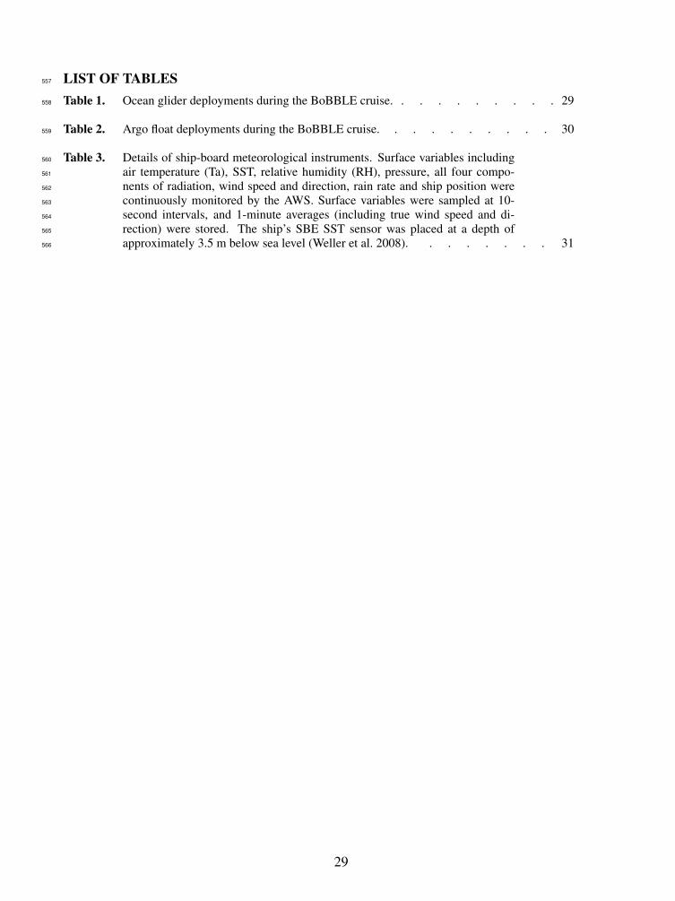
LIST OF TABLES557
Table 1. Ocean glider deployments during the BoBBLE cruise. . . . . . . . . . 29558
Table 2. Argo float deployments during the BoBBLE cruise. . . . . . . . . . 30559
Table 3. Details of ship-board meteorological instruments. Surface variables including560
air temperature (Ta), SST, relative humidity (RH), pressure, all four compo-561
nents of radiation, wind speed and direction, rain rate and ship position were562
continuously monitored by the AWS. Surface variables were sampled at 10-563
second intervals, and 1-minute averages (including true wind speed and di-564
rection) were stored. The ship’s SBE SST sensor was placed at a depth of565
approximately 3.5 m below sea level (Weller et al. 2008). . . . . . . . 31566
29

TABLE 1. Ocean glider deployments during the BoBBLE cruise.
Glider ID Waypoint Deployed Recovered Instrumentation
SG579 8◦N,86◦E then 8◦N,85◦20′E 30 Jun 20 Jul CTD, dO2, Chl,
backscatter, PAR
SG534 8◦N,87◦E 1 Jul 17 Jul CTD, dO2, Chl,
backscatter
SG532 8◦N,88◦E 2 Jul 16 Jul CTD, dO2, Chl,
backscatter
SG620 8◦N,88◦54′E 3 Jul 14 Jul CTD, dO2, Chl,
backscatter
SG613 8◦N,89◦06′E 4 Jul 15 Jul CTD, microstructure shear
and temperature
30
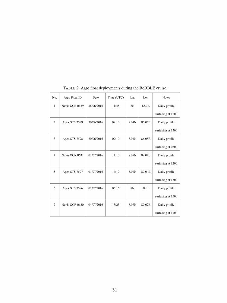
TABLE 2. Argo float deployments during the BoBBLE cruise.
No. Argo Float ID Date Time (UTC) Lat Lon Notes
1 Navis OCR 0629 28/06/2016 11:45 8N 85.3E Daily profile
surfacing at 1200
2 Apex STS 7599 30/06/2016 09:10 8.04N 86.05E Daily profile
surfacing at 1500
3 Apex STS 7598 30/06/2016 09:10 8.04N 86.05E Daily profile
surfacing at 0300
4 Navis OCR 0631 01/07/2016 14:10 8.07N 87.04E Daily profile
surfacing at 1200
5 Apex STS 7597 01/07/2016 14:10 8.07N 87.04E Daily profile
surfacing at 1500
6 Apex STS 7596 02/07/2016 06:15 8N 88E Daily profile
surfacing at 1500
7 Navis OCR 0630 04/07/2016 13:23 8.06N 89.02E Daily profile
surfacing at 1200
31
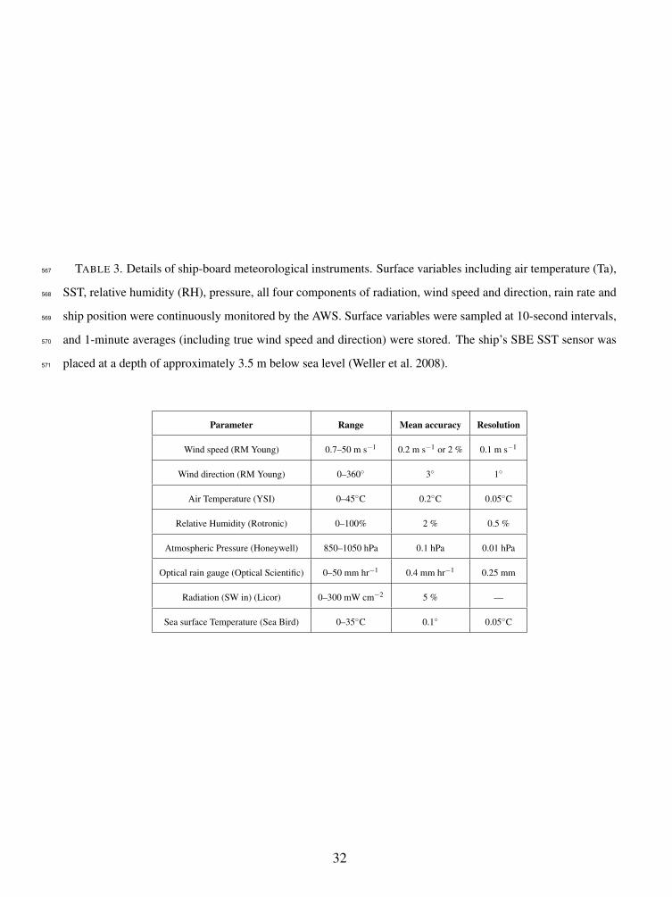
TABLE 3. Details of ship-board meteorological instruments. Surface variables including air temperature (Ta),
SST, relative humidity (RH), pressure, all four components of radiation, wind speed and direction, rain rate and
ship position were continuously monitored by the AWS. Surface variables were sampled at 10-second intervals,
and 1-minute averages (including true wind speed and direction) were stored. The ship’s SBE SST sensor was
placed at a depth of approximately 3.5 m below sea level (Weller et al. 2008).
567
568
569
570
571
Parameter Range Mean accuracy Resolution
Wind speed (RM Young) 0.7–50 m s−1 0.2 m s−1 or 2 % 0.1 m s−1
Wind direction (RM Young) 0–360◦ 3◦ 1◦
Air Temperature (YSI) 0–45◦C 0.2◦C 0.05◦C
Relative Humidity (Rotronic) 0–100% 2 % 0.5 %
Atmospheric Pressure (Honeywell) 850–1050 hPa 0.1 hPa 0.01 hPa
Optical rain gauge (Optical Scientific) 0–50 mm hr−1 0.4 mm hr−1 0.25 mm
Radiation (SW in) (Licor) 0–300 mW cm−2 5 % —
Sea surface Temperature (Sea Bird) 0–35◦C 0.1◦ 0.05◦C
32
LIST OF FIGURES572
Fig. 1. Climatology for the period 23 June – 24 July. (a)TMI SST (1998–2014, shading in ◦C),573
TRMM rainfall (1998–2015, contours) OSCAR (1993–2015, vector arrows); (b) AVISO574
MSLA (1993–2015, shading in cm), salinity from Argo (2005–2015, contours) ASCAT575
surface winds (2008–2015, vector arrows). Fields in panels (c) and (d) are the same as in576
panels (a) and (b), respectively, except that they are for the period 23 June - 24 July, 2016 . . 35577
Fig. 2. RV Sindhu Sadhana of CSIR-National Institute of Oceanography, Goa, India which was578
used for the BoBBLE field program. . . . . . . . . . . . . . . . . 36579
Fig. 3. Upper panel: a map of the BoB and the cruise track of the BoBBLE field program. Shading580
is SSS from SMAP. Lower panel: The section along which observations were made dur-581
ing BoBBLE. The black circles (TSW, Z1, Z2, Z3 and TSE) represent glider deployment582
locations (see Table 1 for details). Argo float deployments (see Table 2 for details), IOP,583
radiometer and VMP profiling as well as water sampling were also carried out at these lo-584
cations. Stars indicate locations where additional CTD profiles were measured during the585
return leg of the cruise. At TSE, additionally, CTD profiles were measured from 4 to 15 July586
2016. Shading indicates SST from AMSR-E. . . . . . . . . . . . . . . 37587
Fig. 4. Hovmoller diagram (averaged from 80◦-95◦E) for anomalous 5-day running mean OLR588
(shading interval 25 W m−2), SST (line contour interval 0.2◦C; negative contours dashed589
purple, zero contour solid black, positive contours solid red). The solid black line at 8◦N590
shows the timing of the BoBBLE ship and glider and Argo float deployments. Negative591
(positive) OLR anomalies indicate convectively active (suppressed) phase of BSISO. The592
dashed blue (red) lines are shown to subjectively indicate the main axis of northward prop-593
agation of the active (suppressed) phases of the BSISO during June-July 2016. . . . . . 38594
Fig. 5. (a) Ship position as a function of time. Red and dark blue lines correspond to latitude and595
longitude respectively. The double-headed arrow shows the time series observation period596
at TSE (89◦E, 8◦N). (b) SST from AWS and CTD at 3.4 m depth. (c) Air temperature.597
(d) Surface (approximately 10 m) wind speed (red line,) and radiosonde wind speed (black598
squares) at 975 hPa. (e) Surface net heat flux into the ocean. The text in the legends cor-599
responds to: AWS - automatic weather system; CTD - conductivity, temperature and depth600
probe; RS - radiosonde; Ta sonic - sonic anemometer temperature corrected for water va-601
por; ECM and BM refer to turbulent fluxes calculated using the eddy covariance and bulk602
methods, respectively. . . . . . . . . . . . . . . . . . . . . 39603
Fig. 6. (a) Longitude–time section of OI glider temperature at 1 m depth. The longitudes of the604
five gliders are shown by the coloured lines. (b) Average diurnal cycle of temperature for605
glider SG579 at the western end of the 8◦N section. Time of day is in local solar time (LST).606
(c) Longitude–time section of temperature at 1 m depth for the July–September months of607
2016, based on OI Argo data. A three day moving mean has been applied to the Argo data. . . 40608
Fig. 7. Sri Lanka dome. (a) AVISO MSLA (cm) for 30 June 2016 (contours) and wind stress curl609
(shading, N m−3) from ASCAT averaged for the period 20 June - 1 July 2016. (b) AMSR-E610
SST (shading, ◦C) averaged for the period 27 - 30 June 2016 overlayed on current vectors611
(m s−1) from OSCAR for 2 July 2016. (c) Temperature and (d) salinity profiles that contrasts612
the spatial structure of the SLD. Profiles in black and green were measured at a location to613
the north and east of the SLD respectively, and those in blue and red were measured inside614
the SLD. Refer to Fig. 3 for the locations. Salinity profiles shows that the high salinity core615
of the SMC (green curve) is absent in the regions of SLD (blue and red). . . . . . . . 41616
33
Fig. 8. Longitude–depth sections of temperature along 8◦N using (a) CTD section during 30 June617
– 4 July 2016, (b) glider data on 8 July 2016, (c) CTD section observed during 15–20 July618
2016, (d) OI Argo data on 24 July 2016. . . . . . . . . . . . . . . . 42619
Fig. 9. The SMC. Surface currents from OSCAR (vector, m s−1) overlaid on current speed (shad-620
ing) on (a) 26 June, (b) 17 July 2016. (c) Trajectories of 4 drifting buoys deployed during621
the cruise. (d) Meridional geostrophic current referenced to 500 dbar, calculated using ship622
CTD temperature and salinity measured at every quarter degree longitude along 8◦N during623
15 – 20 July 2016. (e) Meridional current measured using the ADCP during 30 June - 4624
July, and (f) 15–20 July 2016. (g) Time-depth meridional geostrophic current referenced to625
500 dbar, at a nominal longitude of 87.5◦E, calculated using SG534 and SG532 glider data626
(Table 1). . . . . . . . . . . . . . . . . . . . . . . . 43627
Fig. 10. High Salinity Core. (a) Vertical section of CTD salinity along 8◦N, measured during 30 June628
- 4 July 2016, at stations located one degree apart between 85.3◦E and 89◦E. (b) Same sec-629
tion as in (a) profiled during 15-20 July 2016 at stations located a quarter degree longitudes630
apart. (c) Time-depth section of salinity measured at TSE during 4–15 July 2016. High631
Salinity (>35) core is highlighted using contours in (a), (b) and (c). (d) Time–longitude sec-632
tion of salinity averaged between 90–130 m using glider data. (e) Time–longitude section633
of salinity averaged between 90–130 m using Argo data. . . . . . . . . . . . 44634
Fig. 11. Changes in the temperature and salinity characteristics of the upper layer due to freshening.635
The three upper panels correspond to the first freshening event (4–6 July 2016) described636
in the text and the three bottom panels correspond to the second (7–13 July 2016). Red,637
blue, black and gray curves in all panels indicate temperature, salinity, density and MLD638
respectively. The date and time (UTC) of each profile is given above the respective panel.639
The left, middle and right panels correspond to the situation before and during the freshening640
event. The right panel roughly corresponds to the peak of the freshening event. . . . . . 45641
Fig. 12. uCTD observations of a rain-formed low salinity pool. (a) Salinity along a 14 km section642
over which 21 vertical profiles were measured just after a spell of rain. Locations of uCTD643
profiles are indicated using asterisks marked at a depth of 55 m. Along the depth axis, the644
raw data is averaged into 1m bins before plotting.(b) Vertical profiles of temperature (black)645
and salinity (blue) measured outside the low salinity pool (at x = 2 km, thick lines) and646
inside (at x = 6 km, thin lines). . . . . . . . . . . . . . . . . . . 46647
Fig. 13. Data from VMP-250 at 7◦54’N and 89◦06’E on 15 July 2016 : (a) Temperature (blue) and648
salinity (red). (b) Squared Brunt Vaisala Frequency (N2, blue) and density (red). (c) log10649
of turbulent kinetic energy dissipation rate (ε , blue) and log10 of eddy diffusivity coefficient650
(Kz, red). Near-simultaneous data from glider SG613: (d) Temperature (blue) and salinity651
(red). (e) N2 (blue) and density (red). (f) log10 of ε (blue) and log10 of Kz (red). The noise652
threshold of ε = 10−10.5 W kg−1. The measured microstructure shear was used to infer653
ε and Kz in the water column by assuming isotropic turbulence (Moum et al. 1995) and a654
mixing efficiency of 0.2 (Osborn 1980). The upper 10 m of the VMP-250 data has been655
removed to avoid contamination by the ship’s wake. . . . . . . . . . . . . 47656
Fig. 14. PAR profile (black dots) from a sample dive from glider SG579, near midday on 6 July 2016.657
The best fit double exponential curve is shown by the black line. Chlorophyll concentration658
is shown by the green crosses and line. . . . . . . . . . . . . . . . 48659
Fig. 15. Spatial variation of surface biogeochemical properties during BoBBLE: (a) dissolved oxy-660
gen, (b) pH, (c) total alkalinity, (d) atmospheric pCO2air, pCO2
sw in sea water and the dif-661
ference in air-sea pCO2 concentration. Water sampling was carried out using a Seabird662
34

CTD–rosette system fitted with 10 L Niskin bottles. Samples were collected along the 8◦N663
transect at locations denoted by the red stars in Fig. 3. . . . . . . . . . . . . 49664
35

FIG. 1. Climatology for the period 23 June – 24 July. (a)TMI SST (1998–2014, shading in ◦C), TRMM
rainfall (1998–2015, contours) OSCAR (1993–2015, vector arrows); (b) AVISO MSLA (1993–2015, shading
in cm), salinity from Argo (2005–2015, contours) ASCAT surface winds (2008–2015, vector arrows). Fields in
panels (c) and (d) are the same as in panels (a) and (b), respectively, except that they are for the period 23 June -
24 July, 2016
665
666
667
668
66936

FIG. 2. RV Sindhu Sadhana of CSIR-National Institute of Oceanography, Goa, India which was used for the
BoBBLE field program.
670
671
37
84˚E 85˚E 86˚E 87˚E 88˚E 89˚E 90˚E6˚N
7˚N
8˚N
9˚N
TSW TSEZ1 Z2 Z3
28.8 29.0 29.2 29.4 29.6 29.8 30.0
SST(oC)
76˚E 80˚E 84˚E 88˚E 92˚E 96˚E 100˚E
5˚N
10˚N
15˚N
20˚N
Chennai
AR
TSW TSE
INDIA
BAY OF BENGAL
27 28 29 30 31 32 33 34 35
SSS (PSU)
FIG. 3. Upper panel: a map of the BoB and the cruise track of the BoBBLE field program. Shading is
SSS from SMAP. Lower panel: The section along which observations were made during BoBBLE. The black
circles (TSW, Z1, Z2, Z3 and TSE) represent glider deployment locations (see Table 1 for details). Argo float
deployments (see Table 2 for details), IOP, radiometer and VMP profiling as well as water sampling were also
carried out at these locations. Stars indicate locations where additional CTD profiles were measured during the
return leg of the cruise. At TSE, additionally, CTD profiles were measured from 4 to 15 July 2016. Shading
indicates SST from AMSR-E.
672
673
674
675
676
677
678 38

FIG. 4. Hovmoller diagram (averaged from 80◦-95◦E) for anomalous 5-day running mean OLR (shading
interval 25 W m−2), SST (line contour interval 0.2◦C; negative contours dashed purple, zero contour solid
black, positive contours solid red). The solid black line at 8◦N shows the timing of the BoBBLE ship and glider
and Argo float deployments. Negative (positive) OLR anomalies indicate convectively active (suppressed) phase
of BSISO. The dashed blue (red) lines are shown to subjectively indicate the main axis of northward propagation
of the active (suppressed) phases of the BSISO during June-July 2016.
679
680
681
682
683
684
39
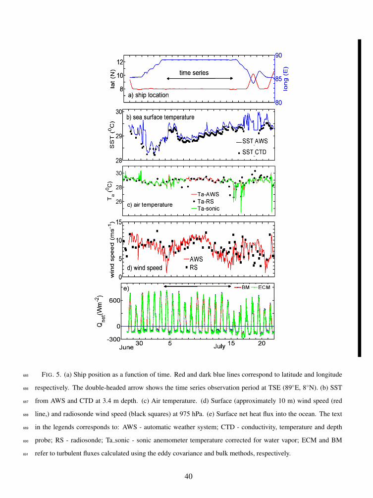
FIG. 5. (a) Ship position as a function of time. Red and dark blue lines correspond to latitude and longitude
respectively. The double-headed arrow shows the time series observation period at TSE (89◦E, 8◦N). (b) SST
from AWS and CTD at 3.4 m depth. (c) Air temperature. (d) Surface (approximately 10 m) wind speed (red
line,) and radiosonde wind speed (black squares) at 975 hPa. (e) Surface net heat flux into the ocean. The text
in the legends corresponds to: AWS - automatic weather system; CTD - conductivity, temperature and depth
probe; RS - radiosonde; Ta sonic - sonic anemometer temperature corrected for water vapor; ECM and BM
refer to turbulent fluxes calculated using the eddy covariance and bulk methods, respectively.
685
686
687
688
689
690
691
40

FIG. 6. (a) Longitude–time section of OI glider temperature at 1 m depth. The longitudes of the five gliders
are shown by the coloured lines. (b) Average diurnal cycle of temperature for glider SG579 at the western end
of the 8◦N section. Time of day is in local solar time (LST). (c) Longitude–time section of temperature at 1
m depth for the July–September months of 2016, based on OI Argo data. A three day moving mean has been
applied to the Argo data.
692
693
694
695
696 41

FIG. 7. Sri Lanka dome. (a) AVISO MSLA (cm) for 30 June 2016 (contours) and wind stress curl (shading, N
m−3) from ASCAT averaged for the period 20 June - 1 July 2016. (b) AMSR-E SST (shading, ◦C) averaged for
the period 27 - 30 June 2016 overlayed on current vectors (m s−1) from OSCAR for 2 July 2016. (c) Temperature
and (d) salinity profiles that contrasts the spatial structure of the SLD. Profiles in black and green were measured
at a location to the north and east of the SLD respectively, and those in blue and red were measured inside the
SLD. Refer to Fig. 3 for the locations. Salinity profiles shows that the high salinity core of the SMC (green
curve) is absent in the regions of SLD (blue and red).
697
698
699
700
701
702
703
42

FIG. 8. Longitude–depth sections of temperature along 8◦N using (a) CTD section during 30 June – 4 July
2016, (b) glider data on 8 July 2016, (c) CTD section observed during 15–20 July 2016, (d) OI Argo data on 24
July 2016.
704
705
706
43

80˚E 85˚E 90˚E 95˚E0˚
5˚N
10˚N
15˚N
1.0 ms−1a
26 June 2016
80˚E 85˚E 90˚E 95˚E
17 July 2016
b
0.0 0.2 0.4 0.6 0.8 1.0 1.2 1.4
OSCAR current (m s−1)
80˚E 85˚E 90˚E 95˚E
27/06
02/08
29/06
31/10
14/07
31/10
01/07
31/10
24/0724/07
01/08
11/08
25/08
03/09
09/09
15/09
24/07
24/07
135779147132147133147134
c Drifter trajectory
80˚E 90˚E 100˚E
0˚
10˚N
20˚N
0
50
100
150
200
250
300
De
pth
(m
)
0
0
86 87 88 89
Longitude (oE)
CTD−Geostrophyd
0
0
0
ADCP−Onwarde
86 87 88 89
Longitude (oE)
−1.0 −0.8 −0.6 −0.4 −0.2 0.0 0.2 0.4 0.6 0.8 1.0
V−Current (m s−1)
0
0
ADCP−Returnf
86 87 88 89
Longitude (oE)
2 4 6 8 10 12 14 16
July 2016
Glider−Geostrophyg
FIG. 9. The SMC. Surface currents from OSCAR (vector, m s−1) overlaid on current speed (shading) on (a) 26
June, (b) 17 July 2016. (c) Trajectories of 4 drifting buoys deployed during the cruise. (d) Meridional geostrophic
current referenced to 500 dbar, calculated using ship CTD temperature and salinity measured at every quarter
degree longitude along 8◦N during 15 – 20 July 2016. (e) Meridional current measured using the ADCP during
30 June - 4 July, and (f) 15–20 July 2016. (g) Time-depth meridional geostrophic current referenced to 500 dbar,
at a nominal longitude of 87.5◦E, calculated using SG534 and SG532 glider data (Table 1).
707
708
709
710
711
712
44

FIG. 10. High Salinity Core. (a) Vertical section of CTD salinity along 8◦N, measured during 30 June - 4
July 2016, at stations located one degree apart between 85.3◦E and 89◦E. (b) Same section as in (a) profiled
during 15-20 July 2016 at stations located a quarter degree longitudes apart. (c) Time-depth section of salinity
measured at TSE during 4–15 July 2016. High Salinity (>35) core is highlighted using contours in (a), (b) and
(c). (d) Time–longitude section of salinity averaged between 90–130 m using glider data. (e) Time–longitude
section of salinity averaged between 90–130 m using Argo data.
713
714
715
716
717
718
45

FIG. 11. Changes in the temperature and salinity characteristics of the upper layer due to freshening. The
three upper panels correspond to the first freshening event (4–6 July 2016) described in the text and the three
bottom panels correspond to the second (7–13 July 2016). Red, blue, black and gray curves in all panels indicate
temperature, salinity, density and MLD respectively. The date and time (UTC) of each profile is given above the
respective panel. The left, middle and right panels correspond to the situation before and during the freshening
event. The right panel roughly corresponds to the peak of the freshening event.
719
720
721
722
723
724
46
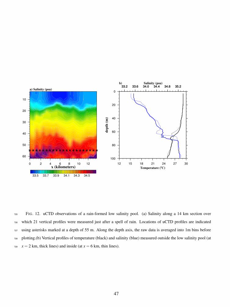
FIG. 12. uCTD observations of a rain-formed low salinity pool. (a) Salinity along a 14 km section over
which 21 vertical profiles were measured just after a spell of rain. Locations of uCTD profiles are indicated
using asterisks marked at a depth of 55 m. Along the depth axis, the raw data is averaged into 1m bins before
plotting.(b) Vertical profiles of temperature (black) and salinity (blue) measured outside the low salinity pool (at
x = 2 km, thick lines) and inside (at x = 6 km, thin lines).
725
726
727
728
729
47

FIG. 13. Data from VMP-250 at 7◦54’N and 89◦06’E on 15 July 2016 : (a) Temperature (blue) and salinity
(red). (b) Squared Brunt Vaisala Frequency (N2, blue) and density (red). (c) log10 of turbulent kinetic energy
dissipation rate (ε , blue) and log10 of eddy diffusivity coefficient (Kz, red). Near-simultaneous data from glider
SG613: (d) Temperature (blue) and salinity (red). (e) N2 (blue) and density (red). (f) log10 of ε (blue) and log10
of Kz (red). The noise threshold of ε = 10−10.5 W kg−1. The measured microstructure shear was used to infer ε
and Kz in the water column by assuming isotropic turbulence (Moum et al. 1995) and a mixing efficiency of 0.2
(Osborn 1980). The upper 10 m of the VMP-250 data has been removed to avoid contamination by the ship’s
wake.
730
731
732
733
734
735
736
737
48
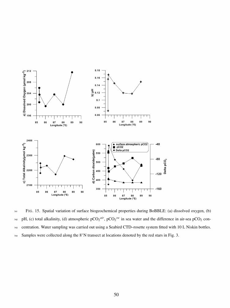
FIG. 15. Spatial variation of surface biogeochemical properties during BoBBLE: (a) dissolved oxygen, (b)
pH, (c) total alkalinity, (d) atmospheric pCO2air, pCO2
sw in sea water and the difference in air-sea pCO2 con-
centration. Water sampling was carried out using a Seabird CTD–rosette system fitted with 10 L Niskin bottles.
Samples were collected along the 8◦N transect at locations denoted by the red stars in Fig. 3.
741
742
743
744
50

FIG. 14. PAR profile (black dots) from a sample dive from glider SG579, near midday on 6 July 2016. The
best fit double exponential curve is shown by the black line. Chlorophyll concentration is shown by the green
crosses and line.
738
739
740
49