Embed Size (px)
Citation preview
TRANSACTIONS OF THEAMERICAN MATHEMATICAL SOCIETYVolume 359, Number 8, August 2007, Pages 3733–3768S 0002-9947(07)04087-1Article electronically published on March 7, 2007
MODULI OF ROOTS OF LINE BUNDLES ON CURVES
LUCIA CAPORASO, CINZIA CASAGRANDE, AND MAURIZIO CORNALBA
Abstract. We treat the problem of completing the moduli space for rootsof line bundles on curves. Special attention is devoted to higher spin curveswithin the universal Picard scheme. Two new different constructions, bothusing line bundles on nodal curves as boundary points, are carried out andcompared with pre-existing ones.
1. Introduction
The problem of compactifying the moduli space for roots of line bundles oncurves is the object of this paper.
More precisely, consider a family of nodal curves f : C → B, with nonsingularfibers over an open subset U of B; let N be a line bundle on C, viewed as a familyof line bundles on the fibers of f . Assume that the relative degree of N is divisibleby some positive integer r. Then the family of r-th roots1 of the restriction of Nto the nonsingular fibers is an etale covering of U .
The issue is how to compactify over B such a covering, in a modular way. Wedefine and explore two different approaches, and compare our resulting modulispaces between themselves and with pre-existing ones.
One of the first cases in which such a question was considered is the one of 2-torsion points in the Jacobian, that is, the case N = O, r = 2. This was solved byA. Beauville [4] by means of admissible coverings.
Another remarkable, well-known instance is the one of the so-called “higher spincurves”, which corresponds to N = ωf and, more generally, to N = ω⊗l
f .The case of genuine “spin curves”, that is, r = 2 (and l = 1), was solved by
Cornalba in [8], where a geometrically meaningful compactification was constructedover the moduli space Mg of Deligne-Mumford stable curves. The boundary pointsare certain line bundles on nodal curves.
Later T. J. Jarvis (in [14] and [15]) used rank 1 torsion-free sheaves to approachthe problem (over stable curves) for all r and l. In particular, he constructed twostack compactifications S and Root, the first of which is the normalization ofthe second, and turns out to be smooth. For r = 2 his compactifications are allisomorphic to the one of [8].
Other methods have recently been used by D. Abramovich and T. J. Jarvis [1]and by A. Chiodo [7]. Both employ (differently) “twisted curves”, which, roughlyspeaking, are nodal curves with a stack structure at some nodes. The resultingcompactifications are isomorphic to Jarvis’s S.
Received by the editors April 12, 2005 and, in revised form, May 25, 2005.2000 Mathematics Subject Classification. Primary 14H10, 14H60; Secondary 14K30.1If L and N are line bundles on X such that L⊗r = N , we call L an r-th root of N .
c©2007 American Mathematical Society3733
License or copyright restrictions may apply to redistribution; see https://www.ams.org/journal-terms-of-use
3734 LUCIA CAPORASO, CINZIA CASAGRANDE, AND MAURIZIO CORNALBA
Over the last decade, interest in higher spin curves has been revived by thegeneralized Witten conjecture, which predicts that the intersection theory on theirmoduli spaces is governed by the Gelfand-Dikiı (also known as higher KdV) hier-archy. This conjecture is open;2 see [18] for more details and some recent progress.
The first part of our paper presents a solution of the general problem in thesame spirit as [8]; we complete the r-th root functor (and its moduli scheme) forany family and any line bundle N as above, by means of line bundles on nodalcurves. For clarity (and to distinguish it from other approaches) we name theresulting space the moduli space for limit roots. Some of the results in this partcan already be found, in one form or another, in the existing literature; however,it seemed worthwhile to present a coherent account of the subject based on theideas of [8]. In order to limit the length of the paper, we work in the contextof schemes and coarse moduli spaces, although it is quite clear that our methodslend themselves to the construction of stacks which are fine moduli spaces for theproblem at hand. We plan to return to the question in a future paper.
As in the case r = 2 (see [6]), the combinatorial aspects of our constructionplay a significant role, and enable us to offer a fairly explicit description of ourcompactification.
We prove in Theorem 4.2.3 that, in the special case of higher spin curves, ourmoduli space is isomorphic to the coarse space underlying Jarvis’s Root.
The last section is devoted to our second approach, whose goal is to obtain acompletion within the compactified Picard scheme, where, obviously, r-th rootson smooth curves naturally live. Because of the relative newness of this method,we only apply it to higher spin curves over Mg. A modular compactification ofthe universal Picard scheme was constructed in [5] by Caporaso, by means of linebundles on semistable curves. This space was later given a description in terms ofrank 1 torsion-free sheaves by R. Pandharipande [20], as a special case of a moregeneral result, valid for all ranks.
The question on whether the existing compactifications of higher spin curvesembed in the universal Picard scheme seemed, at least to us, irresistible. All themore so because of the strong similarities between the boundary points used by thevarious authors: (analogous) line bundles in [8] and [5] on the one hand, and rank1 torsion-free sheaves in [14] and [20] on the other.
Therefore we construct and study a new modular compactification of higher spincurves, S r, l
g , sitting inside the universal Picard scheme, and whose main new featureis that it is not finite over Mg, as soon as r ≥ 3.
We then prove that, for r ≥ 3, the previously constructed moduli spaces of limitroots, which we denote by S
r, l
g , as well as those constructed in [14], [15], [1] and[7], do not embed in the universal Picard scheme. More precisely, neither is thenatural birational map χ : S
r, l
g ��� S r, lg regular, nor is its inverse (Theorem 5.4.2
and its corollary). The case r = 2, treated by C. Fontanari in [12], is an exception,as χ is regular and bijective.
For higher rank, in the same spirit as ours, a compactification of the modulispace of vector bundles over curves using, instead of torsion-free sheaves, vectorbundles over semistable curves, has recently been constructed by A. Schmitt [22],
2Added in proof. The generalized Witten conjecture has recently been proved by C. Faber,S. Shadrin and D. Zvonkine in Faber, Shadrin, Zvonkine: Tautological relations and the r-spinWitten conjecture. Preprint math.AG/0612510.
License or copyright restrictions may apply to redistribution; see https://www.ams.org/journal-terms-of-use
MODULI OF ROOTS OF LINE BUNDLES ON CURVES 3735
continuing upon the work of C. S. Seshadri and others (see [23] and referencestherein).
1.1. Notation. Throughout the paper we work over the field of complex numbers.We shall use the words “line bundle” as a synonym of “invertible sheaf”.
For any scheme Z, we denote by ν = νZ : Zν → Z the normalization morphism.C will always be a connected, nodal, projective curve of (arithmetic) genus g.
We denote by gν the genus of its normalization.To C we associate a dual graph ΓC , as follows. The set of vertices of ΓC is the
set of components of Cν . The set of half-edges is the set of all points of Cν mappingto a node of C. Two half-edges form an edge of ΓC when the two correspondingpoints map to the same node of C. Recall that g = gν + b1(ΓC), where b1(ΓC)is the first Betti number. Let ∆ be a set of nodes of C, i.e., of edges of ΓC . Wedenote by ∆ the subgraph of ΓC consisting of ∆ plus the abutting vertices.
We say that a nodal curve X is obtained from C by blowing-up ∆ if there existsπ : X → C such that π−1(ni) = Ei � P
1 for any ni ∈ ∆, and π : X �⋃
i Ei → C �∆is an isomorphism. We call π : X → C a blow-up of C and Ei an exceptionalcomponent. Set X = X �
⋃i Ei. Then π : = π|X : X → C is the normalization of
C at ∆. For any ni ∈ ∆, set {pi, qi} = Ei ∩ X = π−1(ni); the points pi and qi arecalled exceptional nodes.
For families of curves, we use the same letters but different styles to denote thetotal space and a special fiber, and a star superscript to indicate restriction to thecomplement of the special fiber. For instance, C → B will denote a family of curveswith special fiber C, while C∗ will stand for C � C.
Let C → B be a family of nodal curves. We denote by Cb the fiber over b ∈ B. Wesay that a family of nodal curves X → B, endowed with a B-morphism π : X → C,is a family of blow-ups of C, if for any b ∈ B the restriction π|Xb
: Xb → Cb is ablow-up of Cb. If N ∈ Pic C, we set Nb := N|Cb
and, as above, N ∗ = N|C∗ .We denote by S a smooth, connected 1-dimensional scheme, not necessarily
complete, with a fixed point s0 ∈ S, and we set S∗ = S � {s0}.We shall attach to X a second graph ΣX , whose vertices are the connected
components of X and whose edges are the exceptional components of X. Note thatΣX is obtained from ΓC by contracting all edges corresponding to nodes which arenot blown up in X.
For any graph Γ and commutative group G, we denote by C0(Γ, G) and C1(Γ, G)the groups of formal linear combinations, respectively, of vertices and edges ofΓ with coefficients in G. When we fix an orientation for Γ, the boundary andcoboundary operators ∂ : C1(Γ, G) → C0(Γ, G) and δ : C0(Γ, G) → C1(Γ, G) aredefined in the usual way. Then H1(Γ, G) := ker ∂ ⊂ C1(Γ, G).
For any positive integer r, µr is group of r-th roots of unity.
2. Limit roots of line bundles
Let C be a nodal curve, r a positive integer, and N a line bundle on C whosedegree is divisible by r.
2.1. The main definition.
Definition 2.1.1. Consider a triple (X, L, α), where X is a blow-up of C, L is aline bundle on X, and α is a homomorphism α : L⊗r → π∗(N) (π : X → C is the
License or copyright restrictions may apply to redistribution; see https://www.ams.org/journal-terms-of-use
3736 LUCIA CAPORASO, CINZIA CASAGRANDE, AND MAURIZIO CORNALBA
natural map). We say that (X, L, α) is a limit r-th root of (C, N) if the followingproperties are satisfied:
(i) the restriction of L to every exceptional component of X has degree 1;(ii) the map α is an isomorphism at all points of X not belonging to an exceptional
component;(iii) for every exceptional component Ei of X, the orders of vanishing of α at pi
and qi add up to r.
The following is an analogue, for roots of line bundles, of the stable reductiontheorem.
Proposition 2.1.2. Let C → S be a family of nodal curves, smooth over S∗.Consider line bundles N ∈ Pic C and L ∈ Pic C∗ with an isomorphism α : L⊗r ∼→N|C∗ . Then there exist:
1) A diagram X
h
����
�����
����
� C′ ��
��
C
��S′ �� S
where S′ is a smooth curve; S′ → S is
a finite morphism of degree r, etale over S∗; C′ := C ×S S′; X → C′ is anisomorphism outside the central fiber; X is a blow-up of C ′.
2) A line bundle L′ ∈ PicX such that L′|X∗ = h∗(L).
3) An isomorphism α′ : (L′)⊗r ∼→ h∗(N )(−D), where D is an effective Cartierdivisor supported on the exceptional components of the central fiber, suchthat α′
|X∗ = h∗(α) and (X,L′|X , α′
|X) is a limit r-th root of (C,N|C).
Moreover, for any (X1 → C′,L′1, α
′1, D1) and (X2 → C′,L′
2, α′2, D2) satisfying the
above conditions, there exists an isomorphism σ : X1∼→ X2 over C′ such that
σ∗(D2) = D1, σ∗(L′2) � L′
1, and this last isomorphism is compatible with α′1 and
α′2.
The proof is in [14], section §4.2.2. For more details on the work of Jarvis onthe subject, see section 4.2.
The notion of a limit root generalizes to families in a natural way. Let C → Tbe a family of nodal curves and N ∈ Pic C. A limit r-th root (X ,L, α) of (C,N )is the datum of a family π : X → C of blow-ups of C, a line bundle L ∈ PicX anda homomorphism α : L⊗r → π∗(N ), such that for all t ∈ T , (Xt, Lt, αt) is a limitr-th root of (Ct, Nt).
We can restate Proposition 2.1.2 by saying that if C → S is a family of nodalcurves, N ∈ Pic C and (C∗,L, α) is an r-th root of N|C∗ , then for some finite coveringS′ → S of degree r there exists a limit r-th root (X ,L′, α′) of the pull-back of Nto the base-changed family C′ → S′ which extends over all of S′ the pull-back of(C∗ → S∗,L, α).
2.2. Weighted graphs. To a limit r-th root (X, L, α) we shall attach a weightedsubgraph of the dual graph ΓC of C. The underlying graph is the subgraph ∆corresponding to the set ∆ of nodes which are blown up in π : X → C. The weightfunction w is defined on the exceptional nodes (or, equivalently, on the half-edgesof ∆), takes values in {1, . . . , r − 1}, and is given by w(pi) = ui, w(qi) = vi, where
License or copyright restrictions may apply to redistribution; see https://www.ams.org/journal-terms-of-use
MODULI OF ROOTS OF LINE BUNDLES ON CURVES 3737
ui, vi are the orders of vanishing of α at the points pi, qi respectively. We denotethis weighted graph by ∆w. Clearly, the following conditions are satisfied:(C1) ui + vi = r for any i;(C2) for every irreducible component Cj of C, the sum of all weights assigned to
the vertex corresponding Cj is congruent to degCjN modulo r.
Conversely, for any assignment of a weighted subgraph ∆w of ΓC satisfying condi-tions (C1) and (C2), there is a limit r-th root of N whose graph is ∆w. In fact,let π : X → C be the partial normalization of C at ∆. By (C2), the line bundleπ∗(N)(−
∑ni∈∆(uipi + viqi)) on X admits an r-th root L ∈ Pic X. Let X be the
blow-up of C at ∆. We obtain a limit root (X, L, α) of N by gluing to L (how-ever we wish) the degree one line bundle on each exceptional component; the mapα : L⊗r → π∗(N) is defined to agree with (L)⊗r = π∗(N)(−
∑i(uipi + viqi)) ↪→
π∗(N) on X, and to be zero on all exceptional components.
Remark 2.2.1. The multidegree d = deg N of N is the set of the degrees degCjN
for all irreducible components Cj of C. Its class modulo r can be viewed as anelement [ d ]r of C0(ΓC , Z/r) defined naturally as
[ d ]r :=∑
j
(degCj
N (mod r))[Cj ].
Of course, condition (C2) above only depends on [ d ]r.Now fix an orientation for ΓC ; then there is a natural bijection between
C1(ΓC , Z/r) and the set of weighted subgraphs of ΓC satisfying (C1): to a weightedsubgraph ∆w we associate the 1-chain
∑i ui[ni] with the convention that the edge
ni is oriented entering the vertex corresponding to ui.In this set-up, the boundary operator ∂ : C1(ΓC , Z/r) → C0(ΓC , Z/r) can be
viewed as a map from weighted subgraphs of ΓC satisfying (C1) to multidegrees re-duced modulo r. Then ∆w satisfies (C2) with respect to [ d ]r if and only if ∂(∆w) =[ d ]r. Since the cardinality of ∂−1([ d ]r) equals that of ker ∂ = H1(ΓC , Z/r), we seethat:
• for every N as above, there exist rb1(ΓC) weighted subgraphs of ΓC satisfying(C1) and (C2) with respect to N .
2.3. Automorphisms of limit roots.
Definition 2.3.1. An isomorphism of limit r-th roots (X → T,L, α) and (X ′ →T,L′, α′) of (C,N ) is the datum of:(a) an isomorphism σ : X → X ′ over C,(b) an isomorphism τ : σ∗L′ → L that makes the following diagram commute:
σ∗(L′)⊗r
σ∗(α′)
��
τ⊗r�� L⊗r
α
��σ∗(π′)∗(N ) ∼ �� π∗(N )
This notion of isomorphism agrees with the one of [9], rather than with theone of [8]. At the level of automorphisms, for instance, the difference is that herefiber multiplication in L by a nontrivial root of unity is viewed as a nontrivial au-tomorphism of the limit root. To make contact with the terminology of [8] and
License or copyright restrictions may apply to redistribution; see https://www.ams.org/journal-terms-of-use
3738 LUCIA CAPORASO, CINZIA CASAGRANDE, AND MAURIZIO CORNALBA
[9], an isomorphism between X and X ′ over C will sometimes be referred to asan inessential isomorphism. Likewise, automorphisms of X over C will sometimesbe called inessential automorphisms of X . As customary, the group of these auto-morphism will be denoted AutC(X ). Given a limit root (X → T,L, α), we denoteby Aut(X → T,L, α) the group of its automorphisms. Clearly, Aut(X → T,L, α)maps to AutC(X ); the kernel is naturally isomorphic to a product of copies of µr,one for each connected component of T .
We now state and prove some of the basic properties of automorphisms of limitroots. Let X be a blow-up of C, and let E1, . . . , Em be its exceptional components.View each Ei as a copy of the Riemann sphere, with the origin placed at qi andthe point at infinity placed at pi. Then any inessential automorphism of X actson each Ei as multiplication by a nonzero constant li, and any assignment of theli corresponds to an inessential automorphism. This proves the first part of thefollowing result.
Lemma 2.3.2. Let (X, L, α) be a limit root of (C, N), and fix an orientation onthe graph ΣX . Then:
(i) There is a natural identification AutC(X) � C1(ΣX , C∗).(ii) There is a natural identification Aut(X, L, α) � C0(ΣX , µr), and the ho-
momorphism Aut(X, L, α) → AutC(X) corresponds to the compositionof the coboundary map δ : C0(ΣX , µr) → C1(ΣX , µr) with the inclusionC1(ΣX , µr) → C1(ΣX , C∗).
Proof. We have already proved (i). To prove (ii), it is convenient to work withthe geometric bundles V(L) and V(L⊗r) rather than with L and L⊗r. In termsof these, an automorphism of (X, L, α) is a pair (σ, τ ), where σ is an inessentialautomorphism of X and τ is an automorphism of V(L) which is compatible withσ, is linear on the fibers of V(L) → X, and is such that α ◦ τ⊗r = α. This lastcondition means that, above each connected component Xj of X, τ⊗r is the identity,and hence τ must be the fiberwise multiplication by an r-th root of unity lj . If Ei
is an exceptional component connecting Xj and Xk, the restrictions of τ and σ toV(L)|Ei
→ Ei can thus be viewed as an automorphism pair of V(O(1)) → P1 which
is the multiplication by lj on the fiber above the origin and the multiplication by lkon the fiber above the point at infinity. These pairs are easy to describe. View P1
as the projective space PV constructed on a two-dimensional vector space V , andits origin and point at infinity as [v0] and [v1], where v0, v1 is a basis of V . ThenV(O(1)) is the set of all pairs (�, ϕ), where � is a one-dimensional subspace of V andϕ an element of its dual. An automorphism pair as above then acts on V(O(1)) via(�, ϕ) �→ (f(�), ϕ◦f−1), where f is the automorphism of V such that f(v0) = l−1
j v0,f(v1) = l−1
k v0, and on PV via � �→ f(�). Thus σ acts on Ei as multiplication bylj/lk. This means that giving an automorphism of (X, L, α) is the same as givingan r-th root of unity for each connected component of X, that is, an element ofC0(ΣX , µr), and that the map Aut(X, L, α) → AutC(X) is as claimed. �
It follows from Lemma 2.3.2 that Aut(X, L, α) has cardinality rγ , where γ is thenumber of connected components of X.
Fix (C, N) and π : X → C as usual. We need to further investigate the actionof AutC(X) on certain line bundles on X. Consider pairs (M, β), where M is aline bundle on X, β : M → π∗(N) is a homomorphism which is an isomorphism on
License or copyright restrictions may apply to redistribution; see https://www.ams.org/journal-terms-of-use
MODULI OF ROOTS OF LINE BUNDLES ON CURVES 3739
the complement of the exceptional components of X, and M is assumed to havedegree r on each exceptional component. This degree condition forces β to vanishidentically on each exceptional component
An example of this situation is provided by α : L⊗r → π∗(N), where (X, L, α) isa limit r-th root.
Lemma 2.3.3. Let (M, β) and (M ′, β′) be two pairs as above. Then:
(i) There exist σ ∈ AutC(X) and an isomorphism ϑ : M → σ∗(M ′) such thatβ = σ∗(β′) ◦ ϑ if and only if, for any exceptional node q, the orders ofvanishing of β and β′ at q are the same.
(ii) Under the identification (i) of Lemma 2.3.2, the set of those σ ∈ AutC(X)such that there is an isomorphism ϑ : M → σ∗(M) with the property thatβ = σ∗(β) ◦ ϑ corresponds to C1(ΣX , µr).
Proof. The proof is similar to the one of Lemma 2.3.2. The “only if” part of (i) isclear. To prove the converse, denote by ui (resp., vi) the order of vanishing of β andβ′ at pi (resp., qi). The homomorphisms β and β′ determine isomorphisms M|X �π∗(N)(−
∑(uipi + viqi)) � M ′
|X , hence there is a unique isomorphism ϑ′ : M|X →M ′
|X such that β|X = β′|X ◦ ϑ′. Clearly, ϑ must restrict to ϑ′ on X. It remains to
construct σ and ϑ on the exceptional components. If Ei is one of these, we identifythe restrictions to Ei of V(M) → X and V(M ′) → X to V(O(r)) → P(V ), where Vis a two-dimensional vector space. We also think of P(V ) as being attached to therest of X at [v0] and [v1], where v0, v1 is a basis of V . The isomorphisms ϑ and σ, ifthey exist, restrict on V(O(r)) → P(V ) to an automorphism pair fixing [v0] and [v1].Now, V(O(r)) is the set of all pairs (�, ϕ⊗r), where � is a one-dimensional subspaceof V and ϕ an element of its dual. Any automorphism pair fixing [v0] and [v1] thenacts on V(O(r)) via (�, ϕ⊗r) �→ (f(�), (ϕ ◦ f−1)⊗r), where f is an automorphism ofV such that f(v0) = b0v0, f(v1) = b1v0, b0, b1 ∈ C∗, and on PV via � �→ f(�). Theaction of such an automorphism pair on the fiber above [vi], i = 0, 1, correspondsto multiplication by b−r
i , hence we can choose b0 and b1 so that it matches the oneof ϑ′; the choices are unique up to multiplication by r-th roots of unity. This provesthe existence of σ and ϑ. It also proves (ii). In fact, σ acts on Ei as multiplicationby b1/b0. In the setup of (ii), both b0 and b1 are (arbitrary) roots of unity. Theconclusion is that σ acts on each exceptional component as multiplication by anr-th root of unity, and conversely that any element of C1(ΣX , µr) comes from anautomorphism σ as in (ii). �
2.4. The general moduli problem. Let B be a scheme, f : C → B a family ofnodal curves, and N ∈ Pic C a line bundle of relative degree divisible by r. We shalluse the following notation: for any B-scheme T with structure map p : T → B weset
CT := C ×B Tp ��
��
Cf
��T
p �� B
where p : CT → C is the projection. The pull-back of N to CT is denoted by
NT := p∗N .
License or copyright restrictions may apply to redistribution; see https://www.ams.org/journal-terms-of-use
3740 LUCIA CAPORASO, CINZIA CASAGRANDE, AND MAURIZIO CORNALBA
Having fixed B, f : C → B and N as above, we introduce a contravariant functor
S r
f (N ) : {B-schemes} −→ {sets},
encoding the moduli problem for limit r-th roots of N , as follows. For every B-scheme T , the set S r
f (N )(T ) is the set of all limit r-th roots of NT (which is, withthe above notation, a line bundle on the total space of the family CT → T ), moduloisomorphisms of limit roots.
For every morphism of B-schemes ρ : T → T ′, the corresponding map
S r
f (N )(ρ) : S r
f (N )(T ′) −→ S r
f (N )(T )
sends a limit r-th root (X ′,L′, α′) of NT ′ to the limit root (X ,L, α) of NT definedby X := X ′ ×T ′ T and L := ρ∗L′, where ρ : X → X ′ is the projection. Finally, themorphism α′ is the natural pull-back of α.
We shall prove
Theorem 2.4.1. Let f : C → B be a family of nodal curves, with B a quasi-projective scheme. Let N ∈ Pic C be a line bundle on C of relative degree divisibleby r.
Then the functor S r
f (N ) is coarsely represented by a quasiprojective schemeS
r
f (N ), finite over B. If B is projective, then Sr
f (N ) is projective.
We shall denote by S rf (N ) the open subscheme of S
r
f (N ) parametrizing (closed)points whose underlying curve has no exceptional components.
Proposition 2.4.2. Let ξ = (X, L, α) ∈ Sr
f (N ). The morphism p : Sr
f (N ) → B issmooth at ξ if and only if b1(ΣX) = 0.
In particular, if B is smooth, Sr
f (N ) is smooth at all points ξ such that X hasno exceptional components, or is of compact type.
The proofs of these results are in section 3.4.
Remark 2.4.3. A purely formal consequence of Theorem 2.4.1 is the following usefulfact. Let B′ be a B-scheme, and denote by
f ′ : C′ = C ×B B′ −→ B′
the family obtained by base change, and by N ′ the pull-back of N to C′. Then wenaturally have
Sr
f ′(N ′) � Sr
f (N ) ×B B′.
Remark 2.4.4. Let f : C → B and N ∈ Pic C be as above. For any L0 ∈ Pic C,the functors S r
f (N ) and S r
f (N ⊗ L⊗r0 ) are isomorphic, so the same holds for the
corresponding moduli spaces Sr
f (N ) and Sr
f (N ⊗ L⊗r0 ). This is because for any
limit r-th root (X ,L) of N , (X ,L ⊗ π∗(L0)) is a limit r-th root of N ⊗L⊗r0 .
Remark 2.4.5. Let f : C → B and N ∈ Pic C be as above. For any positive integers, there is a natural injective morphism
J : Sr
f (N ) −→ Srs
f (N⊗s)
over B. Indeed for any limit r-th root (X ,L, α) of N , (X ,L, α⊗s) is a limit (rs)-throot of N⊗s. The image of J is a union of irreducible components of S
rs
f (N⊗s).
License or copyright restrictions may apply to redistribution; see https://www.ams.org/journal-terms-of-use
MODULI OF ROOTS OF LINE BUNDLES ON CURVES 3741
3. Proof of the existence theorem
We shall now construct Sr
f (N ), and prove Theorem 2.4.1. First of all, workingin the analytic category, we construct the universal deformation of a limit root.Then we glue together the bases of the universal deformations, in order to give acomplex algebraic structure to S
r
f (N ).We will make use of the following simple results. The first one is well known,
while the second is Lemma 1.1 of [8].
Remark 3.0.6. Let Y → T be a family of nodal curves, t0 a point of T , and let Ybe the fiber over t0. Consider two line bundles P ∈ PicY and L ∈ Pic Y such thatthere exists an isomorphism ι0 : L⊗r → P|Y . Then, up to shrinking T , there exista line bundle L ∈ PicY extending L and an isomorphism ι : L⊗r → P extendingι0. Moreover, this extension is unique up to isomorphism, meaning that if (L′, ι′)is another extension, then there is an isomorphism χ : L → L′ on a neighbourhoodof Y which restricts to the identity on L and is such that ι = ι′ ◦ χ⊗r.
Remark 3.0.7. Let Y → T be a family of nodal curves, and let E be a smoothrational component of one of its fibers. If L is a line bundle on Y whose restrictionto E has zero degree, then L is trivial on a neighbourhood of E in Y .
3.1. Local structure near exceptional curves. Let C → T be a family of nodalcurves, N ∈ Pic C and (X → T,L, α) a limit r-th root of (C,N ). Fix an exceptionalcomponent E ⊂ X lying over a point t0 ∈ T , let u, v be the corresponding weights,and denote by n the point of C to which E contracts. As usual, π : X → C is thenatural map; recall that π∗N is trivial on a neighbourhood of E. We shall describethe geometry of X → T near E.
The prototype is the following family: for the base, consider the affine planecurve Cu,v ⊂ A
2w,z
3 given by the equation wu = zv. The total space is the surface
Su,v = {xs0 = ws1, ys1 = zs0, wu = zv} ⊂ A4x,y,w,z × P
1s0:s1
.
The projection to A2w,z yields a family of open curves
fu,v : Su,v −→ Cu,v
whose only singular fiber lies over the point (0, 0) ∈ Cu,v and contains an exceptionalcomponent, i.e., the locus of all points of Su,v for which x = y = w = z = 0.
Note that Su,v has d = (u, v) irreducible components, each one isomorphic toSu/d, v/d. For instance, when d = 1, Su,v is smooth if and only if u = v = 1 (inwhich case it is a resolution of an A1-singularity); it is normal if and only if u = 1 orv = 1 (in which case it has an isolated Av−1 or Au−1 singularity in one exceptionalnode). If u > 1 and v > 1, Su,v is singular along the whole special fiber of fu,v (thecurve w = z = 0).
We now show that the morphism fu,v : Su,v → Cu,v is a model for X → T nearE. To set up, recall that a neighbourhood V of n in C is of the form {xy = �},where � is a regular function on a neighbourhood T0 of t0. In other terms, there is
3The notation A2w,z means, here and similarly below, that w, z are the coordinate functions
on A2.
License or copyright restrictions may apply to redistribution; see https://www.ams.org/journal-terms-of-use
3742 LUCIA CAPORASO, CINZIA CASAGRANDE, AND MAURIZIO CORNALBA
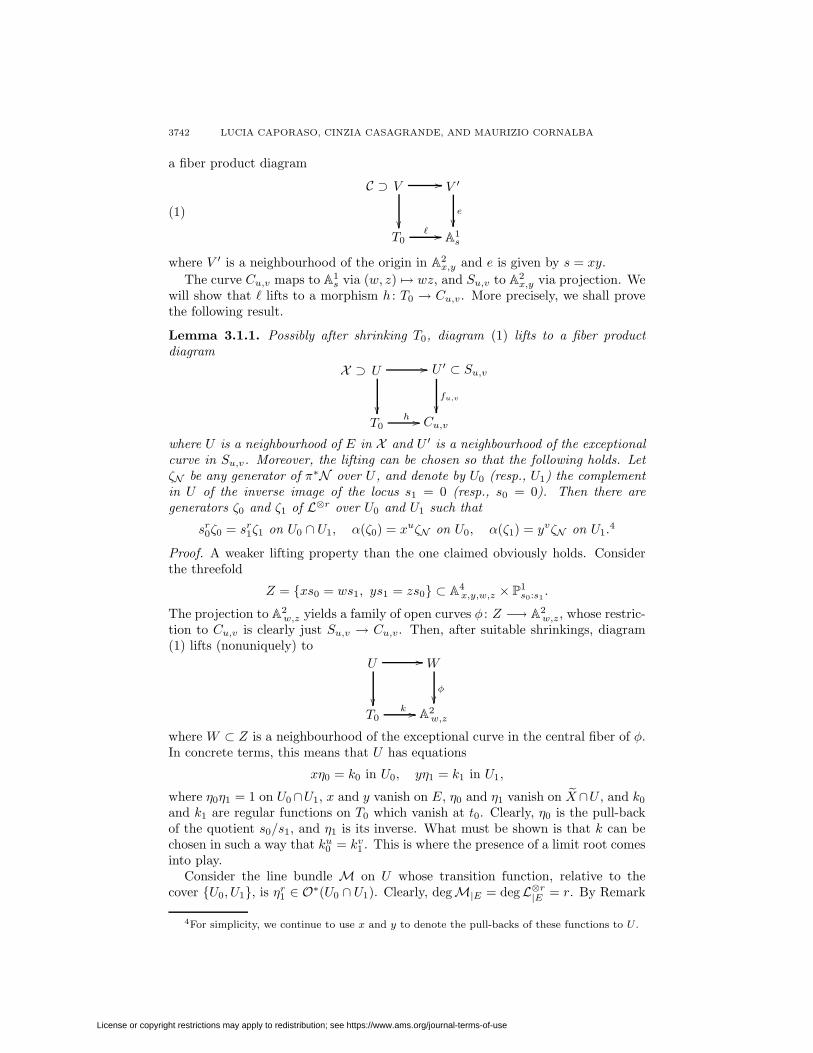
a fiber product diagram
C ⊃ V ��
��
V ′
e
��T0
� �� A1s
(1)
where V ′ is a neighbourhood of the origin in A2x,y and e is given by s = xy.
The curve Cu,v maps to A1s via (w, z) �→ wz, and Su,v to A
2x,y via projection. We
will show that � lifts to a morphism h : T0 → Cu,v. More precisely, we shall provethe following result.
Lemma 3.1.1. Possibly after shrinking T0, diagram (1) lifts to a fiber productdiagram
X ⊃ U ��
��fu,v
��
U ′ ⊂ Su,v
T0h �� Cu,v
where U is a neighbourhood of E in X and U ′ is a neighbourhood of the exceptionalcurve in Su,v. Moreover, the lifting can be chosen so that the following holds. LetζN be any generator of π∗N over U , and denote by U0 (resp., U1) the complementin U of the inverse image of the locus s1 = 0 (resp., s0 = 0). Then there aregenerators ζ0 and ζ1 of L⊗r over U0 and U1 such that
sr0ζ0 = sr
1ζ1 on U0 ∩ U1, α(ζ0) = xuζN on U0, α(ζ1) = yvζN on U1.4
Proof. A weaker lifting property than the one claimed obviously holds. Considerthe threefold
Z = {xs0 = ws1, ys1 = zs0} ⊂ A4x,y,w,z × P
1s0:s1
.
The projection to A2w,z yields a family of open curves φ : Z −→ A
2w,z, whose restric-
tion to Cu,v is clearly just Su,v → Cu,v. Then, after suitable shrinkings, diagram(1) lifts (nonuniquely) to
U ��
��
W
φ
��T0
k �� A2w,z
where W ⊂ Z is a neighbourhood of the exceptional curve in the central fiber of φ.In concrete terms, this means that U has equations
xη0 = k0 in U0, yη1 = k1 in U1,
where η0η1 = 1 on U0∩U1, x and y vanish on E, η0 and η1 vanish on X∩U , and k0
and k1 are regular functions on T0 which vanish at t0. Clearly, η0 is the pull-backof the quotient s0/s1, and η1 is its inverse. What must be shown is that k can bechosen in such a way that ku
0 = kv1 . This is where the presence of a limit root comes
into play.Consider the line bundle M on U whose transition function, relative to the
cover {U0, U1}, is ηr1 ∈ O∗(U0 ∩ U1). Clearly, degM|E = degL⊗r
|E = r. By Remark
4For simplicity, we continue to use x and y to denote the pull-backs of these functions to U .
License or copyright restrictions may apply to redistribution; see https://www.ams.org/journal-terms-of-use
MODULI OF ROOTS OF LINE BUNDLES ON CURVES 3743
3.0.7, we may assume that L⊗r|U � M, possibly after shrinking U . Thus there are
generators ζ ′0, ζ ′1 of L⊗r, over U0 and U1, respectively, such that ζ ′0 = ηr1ζ
′1 on
U0 ∩ U1.Let ζN be a generator of π∗(N ) over U . We have α(ζ ′i) = ciζN on Ui, i = 0, 1,
where c0 and c1 are regular functions on U0 and U1, respectively. Consider theexpressions of c0 and c1 as power series
(2) c0 =∑i≥0
aixi +
∑i<0
aiη−i0 in U0, c1 =
∑i≥0
biyi +
∑i<0
biη−i1 in U1,
where the ai and the bi are regular functions on T0. Since π∗(N ) has degree zero onE while L⊗r has degree r, α is identically zero on E, which gives ai(t0) = bi(t0) = 0for all i ≤ 0. On the other hand, by definition, the order of vanishing of (c0)|X∩U0
at p is u and that of (c1)|X∩U1 at q is v, so au(t0) �= 0 and bv(t0) �= 0. Up toshrinking T0, we may thus assume that au and bv are units.
On U0 ∩ U1 we have α(ζ ′0) = ηr1α(ζ ′1), so c0 = ηr
1c1. We also have η0 = η−11 ,
x = k0η1, y = k1η−11 . Substituting, we get
(3)∑i≥0
aiki0η
i1 +
∑i<0
aiηi1 =
∑i≥0
biki1η
r−i1 +
∑i<0
biηr−i1 in U0 ∩ U1.
Comparing terms of degree u in η1, we get auku0 = bvkv
1 . This is not exactly whatwe are asking for, but we may proceed as follows. Let δ be an r-th root of bv/au
(a unit), and define a morphism h : T0 → A2w,z by setting h0 = δ−1k0, h1 = δk1.
Clearly, hu0 = hv
1, and h is a lifting of �, since h0h1 = k0k1 = �. A compatible liftingof V → A
2x,y to a morphism U → Su,v is given by
(x, η0, t) �→ (x, η0k1(t), h0(t), h1(t), [δ−1η0 : 1]) on U0,
(y, η1, t) �→ (η1k0(t), y, h0(t), h1(t), [1 : δη1]) on U1,
where t stands for a variable point in T0.It remains to find the local generators ζ0 and ζ1. What we have done so far
amounts to showing that, replacing η0 with δ−1η0 and η1 with δη1, we may assumethat U is defined by equations xη0 = h0 on U0 and yη1 = h1 on U1, where η0η1 = 1on U0 ∩ U1 and hu
0 = hv1. Moreover, replacing ζ ′0 with δuζ ′0 and ζ ′1 with δ−vζ ′1, we
may also assume that the coefficients au and bv in the power series developments(2) are equal, while conserving the property that ζ ′0 = ηr
1ζ′1. Now, comparing terms
of all degrees in identity (3), we conclude that
c0 = xuρ, c1 = yvρ,
where
ρ = au +∑i>0
au+ixi +
∑i>0
bv+iyi = bv +
∑i>0
au+ixi +
∑i>0
bv+iyi.
Since ρ is a unit on a neighbourhood of E, possibly after shrinking U it makes senseto set
ζi = ζ ′i/ρ, i = 0, 1,
and these local generators of L⊗r have all the required properties. �
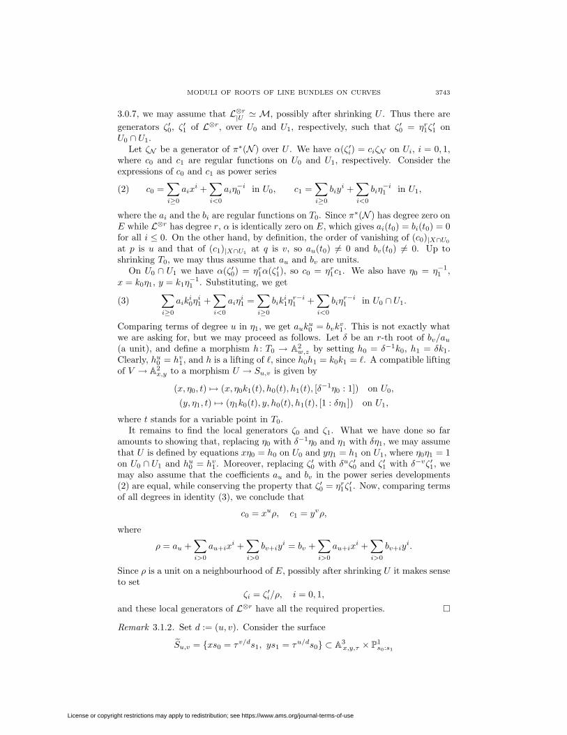
Remark 3.1.2. Set d := (u, v). Consider the surface
Su,v = {xs0 = τv/ds1, ys1 = τu/ds0} ⊂ A3x,y,τ × P
1s0:s1
License or copyright restrictions may apply to redistribution; see https://www.ams.org/journal-terms-of-use
3744 LUCIA CAPORASO, CINZIA CASAGRANDE, AND MAURIZIO CORNALBA
and the family of curves fu,v : Su,v → A1τ induced by the projection. Note that if
d = 1, this is the normalization of fu,v : Su,v → Cu,v.If the base T is normal, then X has the following stronger property:(P) There exist neighbourhoods T0 of t0 in T and U of E in X , and a regular
map h : T0 → A1τ , such that h(t0) = 0 and U is isomorphic to a neighbour-
hood of the exceptional curve in the base change of the surface Su/d, v/d viah.
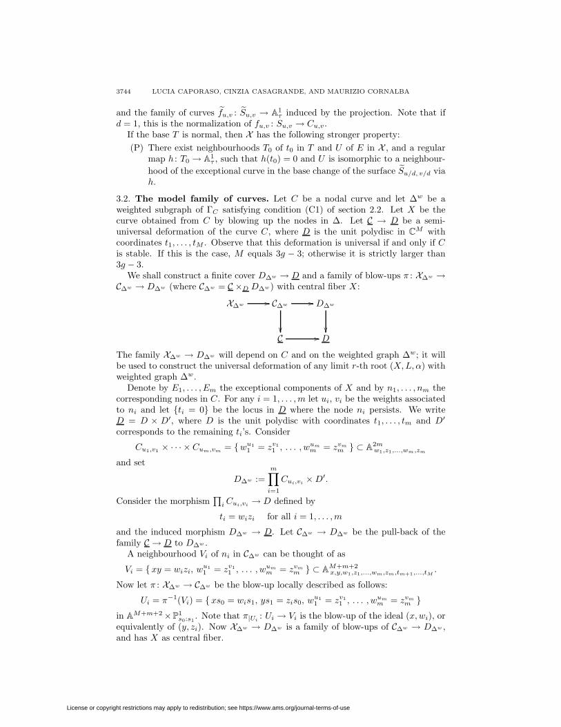
3.2. The model family of curves. Let C be a nodal curve and let ∆w be aweighted subgraph of ΓC satisfying condition (C1) of section 2.2. Let X be thecurve obtained from C by blowing up the nodes in ∆. Let C → D be a semi-universal deformation of the curve C, where D is the unit polydisc in CM withcoordinates t1, . . . , tM . Observe that this deformation is universal if and only if Cis stable. If this is the case, M equals 3g − 3; otherwise it is strictly larger than3g − 3.
We shall construct a finite cover D∆w → D and a family of blow-ups π : X∆w →C∆w → D∆w (where C∆w = C ×D D∆w) with central fiber X:
X∆w �� C∆w ��
��
D∆w
��C �� D
The family X∆w → D∆w will depend on C and on the weighted graph ∆w; it willbe used to construct the universal deformation of any limit r-th root (X, L, α) withweighted graph ∆w.
Denote by E1, . . . , Em the exceptional components of X and by n1, . . . , nm thecorresponding nodes in C. For any i = 1, . . . , m let ui, vi be the weights associatedto ni and let {ti = 0} be the locus in D where the node ni persists. We writeD = D × D′, where D is the unit polydisc with coordinates t1, . . . , tm and D′
corresponds to the remaining ti’s. Consider
Cu1,v1 × · · · × Cum,vm= {wu1
1 = zv11 , . . . , wum
m = zvmm } ⊂ A
2mw1,z1,...,wm,zm
and set
D∆w :=m∏
i=1
Cui,vi× D′.
Consider the morphism∏
i Cui,vi→ D defined by
ti = wizi for all i = 1, . . . , m
and the induced morphism D∆w → D. Let C∆w → D∆w be the pull-back of thefamily C → D to D∆w .
A neighbourhood Vi of ni in C∆w can be thought of as
Vi = {xy = wizi, wu11 = zv1
1 , . . . , wumm = zvm
m } ⊂ AM+m+2x,y,w1,z1,...,wm,zm,tm+1,...,tM
.
Now let π : X∆w → C∆w be the blow-up locally described as follows:
Ui = π−1(Vi) = {xs0 = wis1, ys1 = zis0, wu11 = zv1
1 , . . . , wumm = zvm
m }in A
M+m+2 ×P1s0:s1
. Note that π|Ui: Ui → Vi is the blow-up of the ideal (x, wi), or
equivalently of (y, zi). Now X∆w → D∆w is a family of blow-ups of C∆w → D∆w ,and has X as central fiber.
License or copyright restrictions may apply to redistribution; see https://www.ams.org/journal-terms-of-use
MODULI OF ROOTS OF LINE BUNDLES ON CURVES 3745
Cover each Ui by the two affine open subsets Ui0 = {s1 �= 0} and Ui1 = {s0 �= 0}.Set η0 := s0/s1 and η1 := s1/s0. Then the total space X∆w has equations
(4) wu11 = zv1
1 , . . . , wumm = zvm
m ,
{xη0 = wi in Ui0,yη1 = zi in Ui1,
and η0η1 = 1 on Ui0 ∩ Ui1. Let E be the Cartier divisor given by
(5) xui on Ui0 and yvi on Ui1, for i = 1, . . . , m.
On Ui0 ∩ Ui1 we have xui/yvi = ηr1 ∈ O∗
X∆w(Ui0 ∩ Ui1). Note that:
◦ E is effective; its support in each Ui is the inverse image via π of the locusof the i-th node {x = y = wi = zi} in Vi ⊂ C∆w ;
◦ E|X =∑m
i=1(uipi + viqi);◦ OX∆w (−E)|Ei
has degree r for any i = 1, . . . , m.The following result is a global version of Lemma 3.1.1.
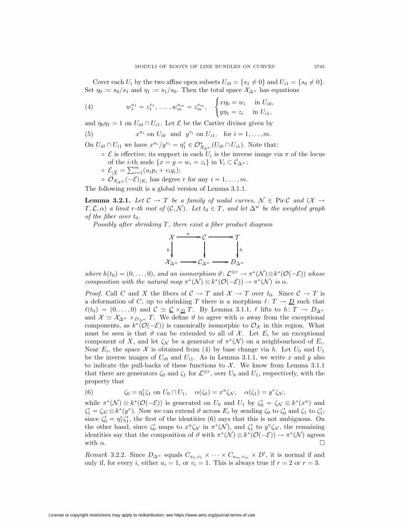
Lemma 3.2.1. Let C → T be a family of nodal curves, N ∈ Pic C and (X →T,L, α) a limit r-th root of (C,N ). Let t0 ∈ T , and let ∆w be the weighted graphof the fiber over t0.
Possibly after shrinking T , there exist a fiber product diagram
X π ��
k
��
C ��
��
T
h
��X∆w �� C∆w �� D∆w
where h(t0) = (0, . . . , 0), and an isomorphism ϑ : L⊗r → π∗(N )⊗k∗(O(−E)) whosecomposition with the natural map π∗(N ) ⊗ k∗(O(−E)) → π∗(N ) is α.
Proof. Call C and X the fibers of C → T and X → T over t0. Since C → T isa deformation of C, up to shrinking T there is a morphism � : T → D such that�(t0) = (0, . . . , 0) and C � C ×D T . By Lemma 3.1.1, � lifts to h : T → D∆w
and X � X∆w ×D∆w T . We define ϑ to agree with α away from the exceptionalcomponents, as k∗(O(−E)) is canonically isomorphic to OX in this region. Whatmust be seen is that ϑ can be extended to all of X . Let Ei be an exceptionalcomponent of X, and let ζN be a generator of π∗(N ) on a neighbourhood of Ei.Near Ei, the space X is obtained from (4) by base change via h. Let U0 and U1
be the inverse images of Ui0 and Ui1. As in Lemma 3.1.1, we write x and y alsoto indicate the pull-backs of these functions to X . We know from Lemma 3.1.1that there are generators ζ0 and ζ1 for L⊗r, over U0 and U1, respectively, with theproperty that
(6) ζ0 = ηr1ζ1 on U0 ∩ U1, α(ζ0) = xuζN , α(ζ1) = yvζN ,
while π∗(N ) ⊗ k∗(O(−E)) is generated on U0 and U1 by ζ ′0 = ζN ⊗ k∗(xu) andζ ′1 = ζN ⊗ k∗(yv). Now we can extend ϑ across Ei by sending ζ0 to ζ ′0 and ζ1 to ζ ′1;since ζ ′0 = ηr
1ζ′1, the first of the identities (6) says that this is not ambiguous. On
the other hand, since ζ ′0 maps to xuζN in π∗(N ), and ζ ′1 to yvζN , the remainingidentities say that the composition of ϑ with π∗(N ) ⊗ k∗(O(−E)) → π∗(N ) agreeswith α. �Remark 3.2.2. Since D∆w equals Cu1,v1 × · · · × Cum,vm
× D′, it is normal if andonly if, for every i, either ui = 1, or vi = 1. This is always true if r = 2 or r = 3.
License or copyright restrictions may apply to redistribution; see https://www.ams.org/journal-terms-of-use
3746 LUCIA CAPORASO, CINZIA CASAGRANDE, AND MAURIZIO CORNALBA
3.3. Construction of universal deformations. We are now in a position toconstruct the universal deformation of a limit root. We place ourselves in the set-up of section 2.4. Let B be a scheme, f : C → B a family of nodal curves andN ∈ Pic C a line bundle of relative degree divisible by r.
Fix b0 ∈ B, set C = f−1(b0) and let C → D be a semi-universal deformationof C. There exist a neighbourhood B0 of b0 in B and a morphism B0 → D,b0 �→ (0, . . . , 0), such that CB0 � C ×D B0.
Let ξ := (X, L, α) be a limit r-th root of (C, Nb0) and let ∆w be the associatedweighted subgraph of ΓC . Let X∆w → D∆w be the deformation of X constructedabove. Set
Uξ := B0 ×D D∆w ,
let u0 ∈ Uξ be the point that maps to b0 ∈ B0 and define Cξ, Xξ in the natural way.We denote by Nξ the pull-back of N under Cξ → CB0 ; observe that in general Nξ
is not the pull-back of a line bundle on C∆w :
Nξ
��X
� � �� Xξπξ ��
��
Cξ ��
��
Uξ ��
��
B0
��X∆w �� C∆w �� D∆w �� D
Our goal is to prove that L extends to a line bundle on Xξ, giving a family of limitr-th roots of Nξ.
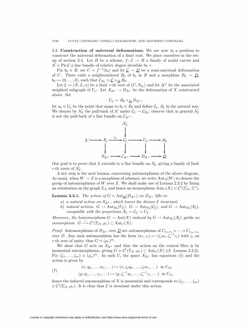
A key step is the next lemma, concerning automorphisms of the above diagram.As usual, when W → Z is a morphism of schemes, we write AutZ(W ) to denote thegroup of automorphisms of W over Z. We shall make use of Lemma 2.3.2 by fixingan orientation on the graph ΣX and hence an isomorphism AutC(X) � C1(ΣX , C∗).
Lemma 3.3.1. The action of G = AutD(D∆w) on D∆w lifts to:a) a natural action on X∆w , which leaves the divisor E invariant;b) natural actions G → AutB0(Uξ), G → AutB0(Cξ), and G → AutB0(Xξ),
compatible with the projections Xξ → Cξ → Uξ.Moreover, the homomorphism G → Aut(X) induced by G → AutB0(Xξ) yields anisomorphism G
∼−→ C1(ΣX , µr) ⊂ AutC(X).
Proof. Automorphisms of D∆w over D are automorphisms of Cu1,v1 ×· · ·×Cum,vm
over D. Any such automorphism has the form (wi, zi) �→ (ζiwi, ζ−1i zi) with ζi an
r-th root of unity; thus G � (µr)m.We show that G acts on X∆w and that the action on the central fiber is by
inessential automorphisms, giving G � C1(ΣX , µr) ⊂ AutC(X) (cf. Lemma 2.3.2).Fix (ζ1, . . . , ζm) ∈ (µr)m. In each Ui the space X∆w has equations (4) and theaction is given by
(7)(x, η0, . . . , wi, . . . ) �→ (x, ζiη0, . . . , ζiwi, . . . ) in Ui0,
(y, η1, . . . , zi, . . . ) �→ (y, ζ−1i η1, . . . , ζ
−1i zi, . . . ) in Ui1,
hence the induced automorphism of X is inessential and corresponds to (ζ1, . . . , ζm)∈ C1(ΣX , µr). It is clear that E is invariant under this action.
License or copyright restrictions may apply to redistribution; see https://www.ams.org/journal-terms-of-use
MODULI OF ROOTS OF LINE BUNDLES ON CURVES 3747
Now, using the universal property of fiber products, it is immediate to see thatthe action of G lifts to Uξ, Cξ, and Xξ with the desired properties. �
In what follows, if σ ∈ G, we shall denote by σUξ, σCξ
, and σXξthe corresponding
automorphisms of Uξ, Cξ, and Xξ.We now address the problem of extending L. Recall that there exists an effective
Cartier divisor E on X∆w such that E|X =∑m
i=1(uipi + viqi) and OX∆w (−E)|Eihas
degree r for any i = 1, . . . , m. Denote by Gξ the pull-back of OX∆w (−E) to Xξ.Then part (i) of Lemma 2.3.3 implies that there are an inessential automorphismσ of X and an isomorphism ϑ : L⊗r → σ∗(π∗
ξ (Nξ) ⊗ Gξ ⊗ OX) such that α is thecomposition of ϑ with the pull-back of π∗
ξ (Nξ)⊗Gξ ⊗OX → π∗ξ (Nξ)⊗OX . Hence,
up to modifying via σ the identification of X with the central fiber of Xξ, we canassume that α : L⊗r → π∗
b0(Nb0) agrees with the restriction to X of the natural
map π∗ξ (Nξ) ⊗ Gξ → π∗
ξ (Nξ).Shrinking Uξ and B0, if necessary, we can extend L to Lξ ∈ PicXξ so that
L⊗rξ � π∗
ξ (Nξ) ⊗ Gξ ,
by Remark 3.0.6. Let αξ be the composition of this isomorphism with π∗ξ (Nξ)⊗Gξ →
π∗ξ (Nξ). Now (Xξ → Uξ,Lξ, αξ) is a limit r-th root of Nξ. Moreover, there is an
isomorphism ψ of limit roots between ξ and the fiber of the family (Xξ → Uξ,Lξ, αξ)over u0 ∈ Uξ. The pair ((Xξ → Uξ,Lξ, αξ), ψ) is a universal deformation for ξ.
Proposition 3.3.2. Let p : T → B be a morphism of schemes, and (X → T,L, β) alimit r-th root of NT . Let t0 ∈ T be such that p(t0) = b0, and assume that there is anisomorphism φ of limit roots between ξ = (X, L, α) and the fiber of (X → T,L, β)over t0. Then, possibly after shrinking T , the deformation ((X → T,L, β), φ) isisomorphic to the pull-back of ((Xξ → Uξ,Lξ, αξ), ψ) via a unique morphism ofB-schemes γ : T → Uξ such that γ(t0) = u0; moreover, the isomorphism is unique.
Proof of existence. We know by Lemma 3.2.1 that, up to shrinking T , there existsh : T → D∆w such that CT � C∆w ×D∆w T and X � X∆w ×D∆w T . Recall thatUξ = B0 ×D D∆w , and set γ = p × h. Then γ : T → Uξ has the property thatγ(t0) = u0 and that there is a commutative diagram with fiber product squares
X π ��
δ
��
CT��
κ
��
T
γ
��
p
������
����
��
Xξπξ �� Cξ �� Uξ �� B0 ⊂ B
(8)
Let L′ and β′ be the line bundle and the homomorphism obtained by pulling backLξ and αξ via δ. Note that (X ,L′, β′) is a limit r-th root of NT , since κ∗(Nξ) = NT
by the commutativity of (8). Moreover, it follows from Lemma 3.2.1 and from thedefinition of Lξ that there is an isomorphism ϑ : L⊗r → L′⊗r such that β′ ◦ ϑ = β.
Now let φ : X → Xt0 and ψ : X → (Xξ)u0 be the isomorphisms of schemesunderlying φ and ψ, and set L′ = φ∗(L′). Then σ := ψ−1 ◦ δ ◦ φ is an inessentialautomorphism of X with the property that σ∗(L) = L′, and ϑ yields an isomorphismχ : L⊗r → σ∗(L)⊗r such that α = σ∗(α) ◦ χ. Then part ii) of Lemma 2.3.3 saysthat σ belongs to C1(ΣX , µr) which, by Lemma 3.3.1, can be identified with G =AutD(D∆w). Moreover, Lemma 3.3.1, suitably interpreted, implies that ψ ◦ σ =
License or copyright restrictions may apply to redistribution; see https://www.ams.org/journal-terms-of-use
3748 LUCIA CAPORASO, CINZIA CASAGRANDE, AND MAURIZIO CORNALBA
σXξ◦ ψ. Thus, replacing γ with σ−1
Uξ◦ γ, κ with σ−1
Cξ◦ κ, and δ with σ−1
Xξ◦ δ, we
may suppose that ψ = δ ◦φ (recall that, always by Lemma 3.3.1, E is G-invariant).A consequence is that L and L′ agree at t0. On the other hand, L⊗r and L′⊗r areisomorphic via ϑ, so Remark 3.0.6 implies that there is an isomorphism between Land L′ whose r-th tensor power is ϑ. At this point we are almost done: (X ,L, β) iscertainly the pull-back of (Xξ,Lξ, αξ). Moreover, φ is the pull-back of ψ, except forone little detail, namely that the corresponding isomorphisms between L and thepull-back of L might not be equal. However, since the r-th tensor powers of theseisomorphisms are equal, the ratio between the two is an r-th root of unity. To fixthis it suffices to multiply the isomorphism between L and L′ by a suitable root ofunity. �
Proof of uniqueness. Assume that the morphism p : T → B0 has another liftingγ′ : T → Uξ such that ((X ,L, β), φ) is isomorphic to the pull-back of ((Xξ,Lξ, αξ), ψ)via γ′, and let
X π ��
δ′
��
CT��
κ′
��
T
γ′
��
p
������
����
��
Xξπξ �� Cξ �� Uξ �� B0 ⊂ B
(9)
be the corresponding commutative diagram. Call h and h′ the morphisms T → D∆w
induced, respectively, by γ and γ′. Then h and h′ are both liftings of T → D, sothere exists σ ∈ G such that h′ = σ ◦ h. As p is fixed, this yields that γ′ = σUξ
◦ γ,and hence also that κ′ = σCξ
◦ κ. If we compose the vertical arrows of (9) withthe actions of the inverse of σ on the respective target spaces, we get anothercommutative diagram whose vertical arrows are δ′′ := σ−1
Xξ◦ δ′, κ, and γ. Clearly,
δ′′ and δ differ at most by an automorphism of X over CT ; in other words, thereis ι ∈ AutCT
(X ) such that δ′′ = δ ◦ ι. Moreover, there is an isomorphism betweenL⊗r and ι∗(L⊗r) which is compatible with β. We need an auxiliary lemma.
Lemma 3.3.3. Let ι ∈ AutCT(X ). Suppose that there exists an isomorphism
ϑ : L⊗r → ι∗(L⊗r) such that β = ι∗(β) ◦ ϑ. Then there exists τ ∈ G such that,possibly after shrinking T , δ ◦ ι = τXξ
◦ δ.
Proof of the lemma. This is essentially a version “with parameters” of part (ii) ofLemma 2.3.3. Let E be an exceptional component of Xt0 . Recall from Lemma3.1.1 that there are open sets U0 and U1 covering E such that X is of the formxη0 = h0 in U0 and of the form xη1 = h1 in U1, where η0η1 = 1 and h0, h1 arefunctions on a neighbourhood of t0 such that hu
0 = hv1. Since ι is an automorphism
over CT , ι∗(x) = x and ι∗(y) = y. Write
ι∗(η0) =∑i≥0
aixi +
∑i<0
aiη−i0 , ι∗(η1) =
∑i≥0
biyi +
∑i<0
biη−i1 .
From ι∗(x)ι∗(η0) = h0 we get in particular that ai = 0 for i ≥ 0. Similarly,bi = 0 for i ≥ 0. On the other hand, a−1 and b−1 are both different from zero,since ι restricts to an automorphism of E. Starting from ι∗(η0)ι∗(η1) = 1, anothersimple power series computation then yields that ai = bi = 0 for i < −1, and thata−1b−1 = 1. Thus ι∗(η0) = k−1η0 and ι∗(η1) = kη1, where k = b−1 is a unit on aneighbourhood of t0. To prove the lemma it suffices to show that k is an r-th root of
License or copyright restrictions may apply to redistribution; see https://www.ams.org/journal-terms-of-use
MODULI OF ROOTS OF LINE BUNDLES ON CURVES 3749
unity. Now, Lemma 3.1.1 says that there are generators ζi for L⊗r on Ui, i = 0, 1,and ζN for π∗(NT ) on U0
⋃U1, with the property that ζ0 = ηr
1ζ1, β(ζ0) = xuζN ,and β(ζ1) = yvζN . Write ϑ(ζi) = fiι
∗(ζi), i = 0, 1, where
f0 =∑i≥0
cixi +
∑i<0
ciη−i0 , f1 =
∑i≥0
diyi +
∑i<0
diη−i1 .
From β(ζ0) = xuζN and β = ι∗(β) ◦ ϑ we then get that xu = xuf0; this yields thatci = 0 for i > 0 and that c0 = 1. Similarly, di = 0 for i > 0, and d0 = 1. On theother hand,
ηr1f1ι
∗(ζ1) = ηr1ϑ(ζ1) = ϑ(ζ0) = f0ι
∗(ζ0) = f0ι∗(ηr
1ζ1) = krηr1f0ι
∗(ζ1).
This gives that d0ηr1 + d−1η
r−11 + · · · = kr(c0η
r1 + c−1η
r+11 + · · · ), and hence in
particular that kr = 1, as desired. �We return to the proof of uniqueness in Proposition 3.3.2. Lemma 3.3.3 implies
that δ′ = σXξ◦ τXξ
◦ δ. On the other hand, τCξ◦ κ = κ and τUξ
◦ γ = γ, since τXξ
corresponds, via δ, to an automorphism of X over CT . Thus, replacing the originalσ with στ , we may in fact suppose that not only γ′ = σUξ
◦ γ and κ′ = σCξ◦ κ, but
also δ′ = σXξ◦ δ. In particular, σXξ
◦ δ ◦φ = ψ. However, by the proof of existence,ψ is also equal to δ◦φ, so σXξ
acts trivially on the fiber of Xξ → Uξ at u0. Since thisaction corresponds via ψ to the action of σ on X, it follows that σ = Id, γ′ = γ, andδ′ = δ. That there is a unique isomorphism L � δ∗(Lξ) which is compatible withβ and δ∗(αξ) and agrees with the given one on the fibers above t0 follows from theuniqueness part of Remark 3.0.6. This finishes the proof of Proposition 3.3.2. �Remark 3.3.4. It follows from the construction of (Xξ → Uξ,Lξ, αξ) that this familyis a universal deformation for any one of its fibers.
3.4. The moduli scheme of limit roots. We are ready to prove Theorem 2.4.1.Consider the set
Sr
f (N ) =∐b∈B
{limit r-th roots of (Cb, Nb)}/
∼,
where ∼ is the equivalence relation given by isomorphism of limit roots.Fix b0 ∈ B and a limit r-th root ξ = (X, L, α) of (Cb0 , Nb0). Let (Xξ →
Uξ,Lξ, αξ) be the universal deformation of ξ and B0 ⊂ B the open subset of Bdominated by Uξ.
Recall that, by Lemmas 2.3.2 and 3.3.1, there are natural identifications andmaps:
Aut(ξ) = C0(ΣX , µr) → C1(ΣX , µr) = G.
Via this homomorphism, the group Aut(ξ) acts on Uξ, Cξ, and Xξ; if σ ∈ Aut(ξ), wewill denote by σUξ
, σCξ, and σXξ
the corresponding automorphisms of these spaces.The universality of the family (Xξ,Lξ, αξ) shown in Proposition 3.3.2 implies that,if σ ∈ Aut(ξ), then σ ∗
Xξ(Lξ) � Lξ and σ ∗
Xξ(αξ) � αξ.
Lemma 3.4.1. Let b∈B0, let u1, u2∈Uξ be points lying over b, and let (X1, L1, α1),(X2, L2, α2) be the corresponding limit r-th roots of (Cb, Nb). The following areequivalent:
(i) there exists σ ∈ Aut(ξ) such that σUξ(u1) = u2;
(ii) there exists an isomorphism of limit roots between (X1, L1, α1) and(X2, L2, α2).
License or copyright restrictions may apply to redistribution; see https://www.ams.org/journal-terms-of-use
3750 LUCIA CAPORASO, CINZIA CASAGRANDE, AND MAURIZIO CORNALBA
Proof. The implication (i) ⇒ (ii) is an immediate consequence of what we observedabove: if there exists σ ∈ Aut(ξ) such that σUξ
(u1) = u2, then (σXξ)|X1 : X1 → X2
is an inessential isomorphism which induces an isomorphism of limit roots.Conversely, assume that there is an inessential isomorphism φ : X1 → X2 that
induces an isomorphism between the corresponding limit roots. We are going toshow first of all that φ = (σXξ
)|X1 for some σ ∈ G, and then that σ belongs to theimage of Aut(ξ) in G. Let d ∈ D be the image of b, and d1, d2 ∈ D∆w the imagesof u1, u2. Recall that G is the group of automorphisms of D∆w over D, and thatD = D∆w/G. Choose τ ∈ G such that τ (d1) = d2. Then τUξ
(u1) = u2 and
ρ := φ−1 ◦ (τXξ)|X1 : X1 −→ X1
is an inessential automorphism of X1. Note that ρ ∈ C1(ΣX1 , µr) ⊂ AutCb(X1) by
construction.Set ξ1 := (X1, L1, α1). The universal deformation (Xξ1 → Uξ1 ,Lξ1 , αξ1) of ξ1
is naturally an open subfamily of (Xξ → Uξ,Lξ, αξ) (see Remark 3.3.4). ApplyingLemma 3.3.1 with respect to ξ1, we see that there is a subgroup G1 of G whichis naturally identified with C1(ΣX1 , µr) ⊂ AutCb
(X1). If {j1, . . . , jk} ⊂ {1, . . . , m}are the indices for which the exceptional component Ei of X does not deform to X1
(namely, in Cb the i-th node is smoothed), then under the isomorphism G � (µr)m,G1 is the subgroup of (ζ1, . . . , ζm) with ζj1 = · · · = ζjk
= 1.Let τ ′ ∈ G1 be such that (τ ′
Xξ)|X1 = ρ, and set σ := τ◦(τ ′)−1. Then (σXξ
)|X1 = φ.Note that σ∗
Xξ(Gξ) � Gξ and σ∗
Xξ(π∗
ξ (Nξ)) � π∗ξ (Nξ) (this is true for all elements of
G). In fact, the first property is easily deduced from (5) and (7); for the secondproperty, it is enough to observe that σ∗
Cξ(Nξ) � Nξ and that πξ ◦ σXξ
= σCξ◦ πξ,
so σ∗Xξ
(π∗ξ (Nξ)) � π∗
ξ (σ∗Cξ
(Nξ)) � π∗ξ (Nξ).
Now, since L⊗rξ � π∗
ξ (Nξ) ⊗ Gξ, we get σ∗Xξ
(L⊗rξ ) � L⊗r
ξ . By construction
σ∗Xξ
(Lξ)|X1 = φ∗(L2) � L1 = Lξ|X1 ,
so we get σ∗Xξ
(Lξ) � Lξ by Remark 3.0.6, and σ comes from Aut(ξ). �
Proof of Theorem 2.4.1. For every r-th root ξ as above we have a well-defined,injective map between B-sets:
βξ : Uξ/ Aut(ξ) −→ Sr
f (N ),
and the image of βξ inherits a complex structure from Uξ/ Aut(ξ). Since Sr
f (N ) iscovered by subsets of the form Im βξ, in order for these “charts” to define a complexstructure on S
r
f (N ), the following must hold: if ξ1 and ξ2 are limit roots such thatIm βξ1 and Imβξ2 intersect, then β−1
ξ2(Imβξ1) is open and the composition β−1
ξ2◦βξ1
is holomorphic. That this is true follows easily from Proposition 3.3.2, Remark3.3.4, and Lemma 3.4.1. In fact, choose a limit root η corresponding to a pointin the intersection of Imβξ1 and Imβξ2 . Then there are natural (and canonicallydetermined) open immersions Ji : Uη ↪→ Uξi
, compatible with the actions of Aut(η)and Aut(ξi). Thus Ji induces a morphism J i : Uη/ Aut(η) ↪→ Uξi
/ Aut(ξi), whichis an embedding by Lemma 3.4.1. Finally, we have βη = βξi
◦ J i.The analytic morphism p : S
r
f (N ) → B has finite fibers. Proposition 2.1.2 impliesthat p is proper, hence it is a finite projective morphism. As B is quasiprojective,so is S
r
f (N ).
License or copyright restrictions may apply to redistribution; see https://www.ams.org/journal-terms-of-use
MODULI OF ROOTS OF LINE BUNDLES ON CURVES 3751
Finally, the scheme Sr
f (N ) is a coarse moduli space for the functor S r
f (N ). Infact, for any B-scheme T , the map S r
f (N )(T ) → HomB(T, Sr
f (N )) is naturallydefined as follows. To any limit r-th root (X → T,L, α) of NT , we associate themorphism T → S
r
f (N ) which is locally given by Proposition 3.3.2. Clearly, thismorphism depends only on the isomorphism class of (X → T,L, α). �
Proof of Proposition 2.4.2. The morphism p is smooth at a point ξ if and onlyif Uξ/ Aut(ξ) � B0, that is, if and only if Aut(ξ) = G. This is equivalent tob1(ΣX) = 0. �
4. Geometry of the moduli space of limit roots
4.1. Limit roots for a fixed curve: examples. Let C be a nodal curve andN ∈ PicC. We denote by S
r
C(N) the zero-dimensional scheme Sr
fC(N), where
fC : C → {pt} is the trivial family. Note that, by Remark 2.4.3, for any familyf : C → B whose fiber over b0 ∈ B is C and for any N ∈ Pic C such that N|C =N , the scheme-theoretical fiber over b0 of the finite morphism S
r
f (N ) → B isisomorphic to S
r
C(N).We have seen in Remark 2.2.1 that there are rb1(ΓC) weighted subgraphs of ΓC
satisfying conditions (C1) and (C2). Let ∆w be one of them. Recall that ∆w carriesthe weights ui, vi on each edge, and that its supporting graph ∆ is a subgraph ofΓC . As usual, denote by gν the genus of the normalization of C. The set of nodes∆ determines a partial normalization π : X → C of C, and the weights determinea line bundle π∗(N)(−
∑i(uipi + viqi)) on X. The dual graph of X coincides
with ΓC � ∆, so we have r2gν+b1(ΓC�∆) choices for a line bundle L ∈ Pic X suchthat L⊗r � π∗(N)(−
∑i(uipi + viqi)) (r2gν
choices for the pull-back of L to thenormalization of X, and rb1(ΓC�∆) choices for the gluings at the nodes). Eachchoice of L gives a point (X, L, α) in S
r
C(N) with weighted graph ∆w.
Lemma 4.1.1. The geometric multiplicity of the connected component of Sr
C(N)supported on (X, L, α) is rb1(ΣX) = rb1(ΓC)−b1(ΓC�∆).
Proof. Recall that ΣX is the graph whose vertices are the connected components ofX and whose edges are the exceptional components of X. The connected componentof S
r
C(N) corresponding to (X, L, α) is isomorphic to the fiber over the origin ofthe morphism D∆w/ Aut(X, L, α) → D (see section 3). If X has m exceptionalcomponents and γ is the number of connected components of X, then the orderof ramification of D∆w/ Aut(X, L, α) → D over the origin is rm/rγ−1 = rb1(ΣX).Now note that ΣX is obtained from ΓC by contracting all edges in ΓC � ∆, thusb1(ΣX) = b1(ΓC) − b1(ΓC � ∆). �
In conclusion, using Remark 2.2.1, we have that the length of Sr
C(N) is∑∆w∈∂−1([ d ]r)
r2gν+b1(ΓC�∆) · rb1(ΓC)−b1(ΓC�∆) = rb1(ΓC) · r2gν+b1(ΓC) = r2g,
as expected. Here, as usual, [ d ]r stands for the modulo r multidegree of N .
Remark 4.1.2. Consider a limit root (C, L) having C itself as an underlying curve;then the scheme S
r
C(N) is reduced at the point (C, L).
License or copyright restrictions may apply to redistribution; see https://www.ams.org/journal-terms-of-use
3752 LUCIA CAPORASO, CINZIA CASAGRANDE, AND MAURIZIO CORNALBA
Remark 4.1.3. By construction D∆w → D depends only on C and on ∆w, whileAut(X, L, α) depends only on ΣX and r, by Lemma 2.3.2. Thus
• the scheme structure on Sr
C(N) depends only on [ d ]r.
Example 4.1.4 (Compact type). Let C =⋃
j Cj be a curve of compact type.Then b1(ΓC) = 0, hence there is a unique weighted subgraph of ΓC satisfying (C1)and (C2) (which depends on [ d ]r by the previous remark). So there is a uniqueblow-up X of C (X is of compact type) with a divisor D =
∑i(uipi + viqi), such
that every limit root in Sr
C(N) is of type (X, L, α) with L⊗r
|X� π∗(N)(−D). In
particular, X = C if and only if [ d ]r = 0. Note also that Sr
C(N) is reduced.
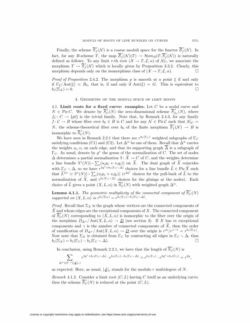
Example 4.1.5. Let C be a curve of genus g with two smooth components C1, C2
and three nodes n1, n2, n3:
C
C1
C2n3
n1
n2
C1
C2
n3n2
ΓC
n1
We describe S3
C(OC). Since b1(ΓC) = 2, ΓC must have 32 = 9 weighted sub-graphs satisfying (C1) and (C2). One is ∅. This choice corresponds to points oftype (C, L) with L⊗3 � OC ; there are 9 ·32gν
of them (with gν = g−2), all reducedpoints in S
3
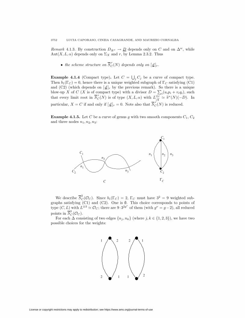
C(OC).For each ∆ consisting of two edges {nj , nk} (where j, k ∈ {1, 2, 3}), we have two
possible choices for the weights:
2
22
1
1
2
1
1
License or copyright restrictions may apply to redistribution; see https://www.ams.org/journal-terms-of-use
MODULI OF ROOTS OF LINE BUNDLES ON CURVES 3753
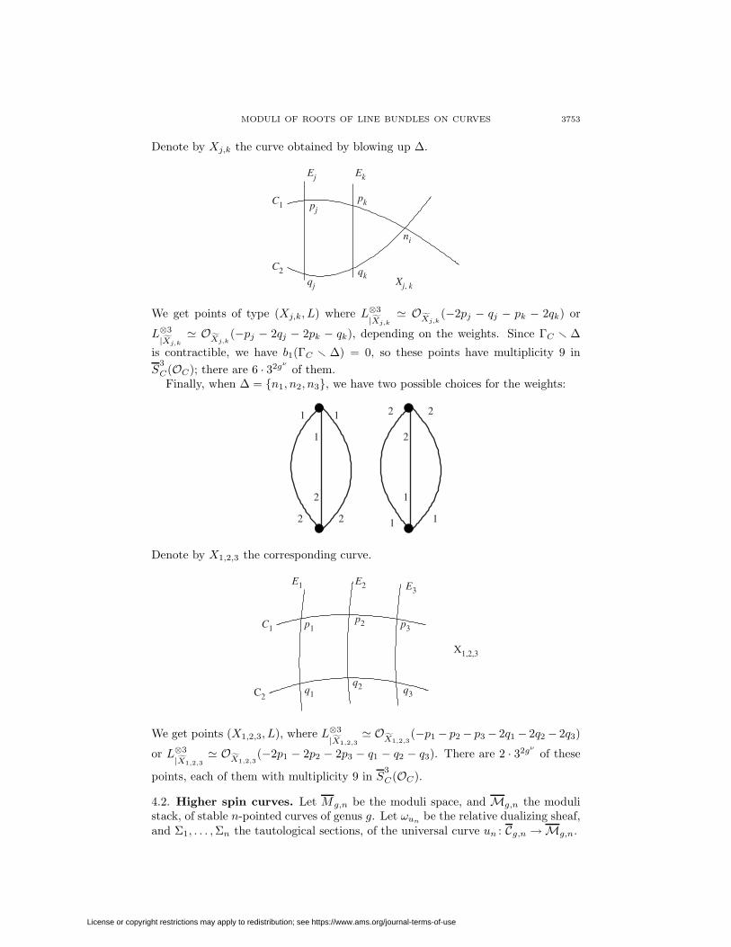
Denote by Xj,k the curve obtained by blowing up ∆.
Ej
qj
ni
Xj, k
C2
C1pk
qk
pj
Ek
We get points of type (Xj,k, L) where L⊗3
|Xj,k
� OXj,k
(−2pj − qj − pk − 2qk) or
L⊗3
|Xj,k
� OXj,k
(−pj − 2qj − 2pk − qk), depending on the weights. Since ΓC � ∆
is contractible, we have b1(ΓC � ∆) = 0, so these points have multiplicity 9 inS
3
C(OC); there are 6 · 32gν
of them.Finally, when ∆ = {n1, n2, n3}, we have two possible choices for the weights:
Denote by X1,2,3 the corresponding curve.
p1p2 p3
q2 q3
C1
C2q1
X1,2,3
E3E1 E2
We get points (X1,2,3, L), where L⊗3
|X1,2,3� O
X1,2,3(−p1 − p2 − p3 − 2q1 − 2q2 − 2q3)
or L⊗3
|X1,2,3� O
X1,2,3(−2p1 − 2p2 − 2p3 − q1 − q2 − q3). There are 2 · 32gν
of these
points, each of them with multiplicity 9 in S3
C(OC).
4.2. Higher spin curves. Let Mg,n be the moduli space, and Mg,n the modulistack, of stable n-pointed curves of genus g. Let ωun
be the relative dualizing sheaf,and Σ1, . . . , Σn the tautological sections, of the universal curve un : Cg,n → Mg,n.
License or copyright restrictions may apply to redistribution; see https://www.ams.org/journal-terms-of-use
3754 LUCIA CAPORASO, CINZIA CASAGRANDE, AND MAURIZIO CORNALBA
Fix integers l, m1, . . . , mn such that r | l(2g − 2) + m1 + · · · + mn, and set m :={m1, . . . , mn} and
ωlm := ω⊗l
un( m1Σ1 + · · · + mnΣn ) ∈ Pic Cg,n .
We introduce a contravariant functor
S r, l, m
g,n : {schemes} −→ {sets},
encoding the moduli problem for limit r-th roots of ωlm over Mg,n, as follows. Look
at pairs (f : C → B, ξ) consisting of a family f : C → B of n-pointed genus g curvesand a limit root ξ of (C, ω⊗l
f (∑
miσi)), where σ1, . . . , σn are the tautological sectionsof f and ωf is the relative dualizing sheaf. Two such pairs (f : C → B, ξ) and(f ′ : C′ → B, ξ′) are considered equivalent if there is an isomorphism κ : C → C′ offamilies of n-pointed curves and an isomorphism, as limit roots of (C, ω⊗l
f (∑
miσi)),between ξ and κ∗(ξ′) (observe that, if σ′
1, . . . , σ′n are the tautological sections of f ′,
then ω⊗lf (
∑miσi) and κ∗(ω⊗l
f ′ (∑
miσ′i)) are canonically isomorphic). Note that
this is clearly a coarser equivalence relation than the one given by isomorphism oflimit roots over a fixed family of curves.
Then, for every scheme B, we define S r, l, m
g,n (B) to be the set of all equivalenceclasses of pairs (f : C → B, ξ) as above. Arguing exactly as in the proof of Theorem2.4.1 we obtain:
Theorem 4.2.1. The functor S r, l, m
g,n is coarsely represented by a projective scheme
Sr, l, m
g,n , finite over Mg,n.
We call ϕ : Sr, l, m
g,n → Mg,n the structure morphism. For any stable n-pointedcurve (C, σ1, . . . , σn), the fiber of ϕ over [C] is
Sr
C(ω⊗lC (m1σ1 + · · · + mnσn)) / Aut(C, σ1, . . . , σn).
When we consider stable curves without markings (i.e., when n = 0), we denoteby S
r, l
g the corresponding moduli space, and by Sr, l
C the fiber of ϕ over [C] ∈ Mg.
The scheme S2,1
g is the moduli space of spin curves, constructed in [8].
Denote by S r, l, mg,n the open subscheme of S
r, l, m
g,n parametrizing points (C, L)with C stable, and let ϕ : S r, l, m
g,n → Mg,n be the natural morphism.Pairs (C, L) with C a smooth curve and L ∈ Pic C such that L⊗r � ωC are gener-
ally called r-spin curves. Their moduli space admits a natural stratification by lociparametrising line bundles L with increasing h0(C, L), so that the largest locus cor-responds to “effective r-spin curves”; we refer to the recent paper of A. Polishchuk[21] for more details and open problems related to this interesting aspect.
Several modular compactifications of the moduli space of r-spin curves, and moregenerally of S r, l, m
g,n , have been introduced by T. J. Jarvis [14, 15, 16], by means ofrank 1, torsion-free sheaves.
The next statement summarizes well-known results relating line bundles andtorsion-free sheaves of rank 1.
Proposition 4.2.2. Let B be an integral scheme and f : C → B a family of nodalcurves.
License or copyright restrictions may apply to redistribution; see https://www.ams.org/journal-terms-of-use
MODULI OF ROOTS OF LINE BUNDLES ON CURVES 3755
(I) Let π : X → C be a family of blow-ups of C and let L ∈ PicX be a linebundle having degree 1 on every exceptional component. Then π∗(L) is arelatively torsion-free sheaf of rank 1, flat over B.
(II) Conversely, suppose that F is a relatively torsion-free sheaf of rank 1 on C,flat over B. Then there exist a family π : X → C of blow-ups of C and aline bundle L ∈ PicX having degree 1 on all exceptional components, suchthat F � π∗(L).
(III) Let π : X → C, π′ : X ′ → C be families of blow-ups of C and L ∈ PicX ,L′ ∈ PicX ′ line bundles having degree 1 on every exceptional component.Then π∗(L) � π′
∗(L′) if and only if there exists an isomorphism σ : X ∼→ X ′
over C such that L � σ∗(L′).
Proof. (I) is a local property, see [14], Proposition 3.1.2.(II) is a consequence of G. Faltings’ local characterization of torsion-free sheaves
[11]; see [14], §3.1 and 3.2, in particular Theorem 3.2.2.(III) The “if” part is clear. To prove the converse, it suffices to note that there
is an isomorphism τ : X → Proj(⊕
k≥0 Symk(π∗(L))) of spaces over C, with theproperty that τ∗(O(1)) is isomorphic to L, and similarly for X ′ and L′. �
Jarvis introduces the notion of an r-th root sheaf of a line bundle N ∈ PicC,which is a rank 1, torsion-free sheaf F on C together with a homomorphismβ : F⊗r → N with the following properties (see [16], Definition 2.3):
◦ r degF = deg N ;◦ β is an isomorphism on the locus where F is locally free;◦ at any node of C where F is not locally free, the length of the cokernel of
β is r − 1.
Such an r-th root sheaf is always of the form π∗(L), where X is the curve obtainedfrom C by blowing-up the nodes where F is not locally free, π : X → C is thenatural morphism and (X, L, β) is a limit r-th root of (C, N). It is easy to see,using Proposition 4.2.2, that the moduli functor of r-th root sheaves of ωl
m over
Mg,n is isomorphic to S r, l, m
g,n (see [14], 3.1 and 4.2.2, and [16], 2.2.2 and page 38).Hence we have the following:
Theorem 4.2.3. The scheme Sr, l, m
g,n is isomorphic over Mg,n to the coarse modulispace of the stack Root
1/rg,n(ωl
m) (in the notation of [15]) of r-th root sheaves of ωlm.
Observe that, exactly as in [15], one could construct different (less singular)compactifications of S r, l, m
g,n (and more generally of S rf (N )) in two ways:
(a) requiring, in the definition of a family of limit roots, that property (P) ofRemark 3.1.2 holds; this amounts to considering only “not too singular” familiesof limit roots;
(b) attaching to a limit r-th root the data of a set of limit d-th roots for any positived dividing r, i.e., considering “coherent nets of roots”. Set-theoretically, thisamounts to attaching to a limit r-th root ξ = (X, L, α) the data of the gluingsfor ξm for any integer m dividing r.
License or copyright restrictions may apply to redistribution; see https://www.ams.org/journal-terms-of-use
3756 LUCIA CAPORASO, CINZIA CASAGRANDE, AND MAURIZIO CORNALBA
5. Higher spin curves in the universal Picard scheme
5.1. Compactifying the Picard functor. Assume g ≥ 3 and let P d,g → M0g be
the degree d universal Picard variety5 whose fiber over a smooth curve C is Picd C,the variety of line bundles of degree d on C. Let P d, g → Mg be the modularcompactification constructed in [5]; P d, g is an integral, normal projective scheme.Its fiber over C ∈ M
0
g is denoted by Pd
C and gives a compactification of (a finitenumber of copies of) the generalized Jacobian of C. The moduli properties of P d, g
are described in [5], section 8. Its boundary points are of the same nature as limitroots: they correspond to line bundles on quasistable curves6 having degree 1 onexceptional components.
The moduli space of higher spin curves over M0g naturally embeds in P d,g (see
Lemma-Definition 5.2.1); its projective closure in P d, g is thus a new compactifica-tion which we shall now study.
We recall from [5] a few basic properties of P d, g, which, as Mg, is constructedby means of Geometric Invariant Theory (see [13]; in this section we freely use thelanguage of [19]). We begin with some useful conventions and numerical prelimi-naries. Let d be an integer; we denote by d an element of Zγ whose entries add upto d, that is, d = {d1, . . . , dγ} and
∑di = d. We say that d is divisible by some
integer r if all of its entries are; if that is the case, we write d ≡ 0 (mod r). If q isa rational number, we set qd = {qd1, . . . , qdγ}, and we say that qd is integer if qdi
is integer for every i.For any nodal curve X, we denote by X1, . . . , Xγ its irreducible components and
set ki = #Xi ∩ X � Xi. Let M be a line bundle of degree d on X; denote byd = deg M = {d1, . . . , dγ} its multidegree, where di := degXi
M . For the dualizingsheaf of X we use the special notation wi := degXi
ωX = 2g(Xi) − 2 + ki and
wX := deg ωX = {w1, . . . , wγ}.
Similarly, for a subcurve Z of X, we set kZ := #Z ∩ X � Z, wZ := degZ ωX =2g(Z) − 2 + kZ and dZ := degZ M .
Let X be a quasistable curve. As usual, we denote by Ei its exceptional compo-nents and set X = X �
⋃i Ei (thus X is a partial normalization of C).
Definition 5.1.1. Let X be a quasistable curve and M ∈ PicX. We shall say thatthe multidegree d of M is balanced if degE M = 1 on every exceptional componentE of X and if, for every subcurve Z of X, the following inequality (known as BasicInequality) holds: ∣∣∣∣dZ − d
wZ
2g − 2
∣∣∣∣ ≤ kZ
2.
We shall say that d is stably balanced if it is balanced and if for every subcurve Zof X such that
dZ − dwZ
2g − 2= −kZ
2,
we have that Z contains X.Similarly, we shall say that the line bundle M is balanced (or stably balanced) if
its multidegree is.
5M0g (and likewise M
0g) stands for the locus of curves with a trivial automorphism group.
6A quasistable curve X is a blow-up of a stable curve C. We call C the stable model of X.
License or copyright restrictions may apply to redistribution; see https://www.ams.org/journal-terms-of-use
MODULI OF ROOTS OF LINE BUNDLES ON CURVES 3757
It is easy to see that if d is balanced and Z is a connected component of X, thendZ − d wZ
2g−2 = −kZ
2 . Hence if d is stably balanced, X is connected.We shall need the following elementary
Lemma 5.1.2. Let X be a quasistable curve.(i) Let M ∈ Pic X be such that M⊗r � ω⊗l
X for some integers r and l; then Mis stably balanced.
(ii) M ∈ PicX is balanced (stably balanced) if and only if M ⊗ ω⊗tX is balanced
(stably balanced) for some integer t.(iii) Assume that the stable model of X is irreducible and let M ∈ PicX be
a line bundle having degree 1 on all exceptional components. Then M isstably balanced.
The goal of the following definitions is to measure the nonseparatedness of thePicard functor.
Definition 5.1.3. Let X be a nodal curve and T ∈ PicX; we say that T is atwister if there exists a one-parameter smoothing X → S of X such that
T � OX (γ∑
i=1
aiXi) ⊗OX
for some Cartier divisor∑γ
i=1 aiXi on X (where ai ∈ Z). The set of all twisters ofX is denoted by Tw(X).
Definition 5.1.4. Consider two balanced line bundles M ∈ Pic X and M ′ ∈Pic X ′, where X and X ′ are quasistable curves.
We say that M and M ′ are equivalent if there exists a semistable curve Y dom-inating7 both X and X ′ and a twister T ∈ Tw(Y ) such that, denoting by MY andM ′
Y the pull-backs of M and M ′ to Y , we have
M ′Y � MY ⊗ T.
In particular, for any automorphism σ of X, σ∗(M) is equivalent to M .
To say that M and M ′ are equivalent is to say that their pull-backs to Y areboth limits of the same family of line bundles. More precisely, let Y −→ S bea one-parameter smoothing of Y such that the twister T of Definition 5.1.4 isT = OY(D) ⊗ OY , with Supp D ⊂ Y . Let M ∈ PicY be such that M|Y � MY ;then M⊗OY(D) ⊗ OY � M ′
Y so that MY and M ′Y are both limits of the family
corresponding to M∗ (recall that the “∗” denotes restriction away from the centralfiber). Therefore, the line bundles MY and M ′
Y (and likewise M and M ′) must beidentified in any proper completion of the Picard scheme over Mg.
Remark 5.1.5. Let M, M ′ ∈ PicX be stably balanced. Then a simple numericalchecking shows that they are equivalent if and only if there exists an automor-phism σ of X such that M ′ � σ∗(M). If the stable model of X has no nontrivialautomorphisms, then M and M ′ are equivalent if and only if M|X � M ′
|X .
Fix a large d (d ≥ 20(g − 1) would work), set s = d − g and consider theHilbert scheme Hilbd,g
Ps of connected curves of degree d and genus g in Ps; the group
7We say that a semistable curve Y dominates a nodal curve X if it can be obtained from Xby a finite sequence of blow-ups.
License or copyright restrictions may apply to redistribution; see https://www.ams.org/journal-terms-of-use
3758 LUCIA CAPORASO, CINZIA CASAGRANDE, AND MAURIZIO CORNALBA
SL(s + 1) naturally acts on Hilbd,gPs . Recall that there exist linearizations for such
an action such that the following facts hold.
Theorem 5.1.6 ([5]). Let X ⊂ Ps be a connected curve of genus g.
(1) The Hilbert point of X is GIT-semistable if and only if X is quasistableand OX(1) is balanced.
(2) The Hilbert point of X is GIT-stable if and only if X is quasistable andOX(1) is stably balanced.
(3) Assume that the Hilbert points of X and X ′ ⊂ Ps are GIT-semistable. Thenthey are GIT-equivalent if and only if OX(1) and OX′(1) are equivalent.
Proof. We have assembled together, for convenience, various results from [5]: for (1)see Propositions 3.1 and 6.1 (the “only if” part is due to D. Gieseker [13]); for (2) seeLemma 6.1. The “only if” of part (3) is Lemma 5.2; the “if” is a direct consequenceof the existence of the GIT quotient as a projective scheme (see below). �
Then let P d, g be the GIT-quotient of the locus of all GIT-semistable points inHilbd,g
Ps ; it is a normal, integral scheme, flat over M0
g (Theorem 6.1 in [5]).The above result permits a modular interpretation of P d, g as a modular com-
pactification of the universal Picard variety. Let X be a quasistable curve andlet M ∈ PicX be very ample of degree d. By Theorem 5.1.6, if we embed X inPs by M , the Hilbert point of X is GIT-semistable if and only if M is balanced.Thus P d, g parametrizes equivalence classes of balanced line bundles on quasistablecurves.
Associating to M ∈ Pic X the stable model C of X yields the natural morphismP d, g → Mg; P
d
C denotes its fiber over [C] ∈ Mg.Recall (Theorem 6.1 in [5]) that P
d
C is a finite union of g-dimensional irreduciblecomponents, one for each stably balanced multidegree (of degree d) on C:
Pd
C =⋃
dstably
balanced
Pd
C .
Moreover, if C has no nontrivial automorphisms, every component of Pd
C containsa copy of the generalized Jacobian of C as a dense open subscheme:
Pic d C ⊂ Pd
C ,
where Pic d C is the variety of line bundles on C having multidegree d. If C isirreducible or of compact type, then P
d
C is irreducible.
Remark 5.1.7. By [5], Lemma 8.1, for any integer t, P d, g and P d+t(2g−2), g areisomorphic over Mg via the morphism M �→ M ⊗ ω⊗t
X for any M ∈ Pic X. Hencewe can assume that P d, g exists for any d ∈ Z, even if it is constructed only ford � 0. Moreover, M is balanced, or stably balanced, if and only if M ⊗ ω⊗t
X is (bypart (ii) of Lemma 5.1.2).
5.2. A new compactification of higher spin curves. Let C be a stable curveand L ∈ Pic C an r-th root of ω⊗l
C ; then, by part (ii) of Lemma 5.1.2, L is stably
License or copyright restrictions may apply to redistribution; see https://www.ams.org/journal-terms-of-use
MODULI OF ROOTS OF LINE BUNDLES ON CURVES 3759
balanced, therefore, by part (2) of 5.1.6, it is identified with a point of P l(2g−2)/r, g.More precisely, consistently with section 4.2, we denote by S r, l
g the open subscheme
of Sr, l
g corresponding to pairs (C, L) as above. Obviously, S r, lg is the coarse moduli
space for the similarly defined functor S r, lg . We have:
Lemma-Definition 5.2.1. There is a natural embedding
χ : S r, lg ↪→ P l(2g−2)/r, g.
We define S r, lg to be the closure, in the projective variety P l(2g−2)/r, g, of the image
of χ, andϕ : S r, l
g −→ Mg
to be the natural morphism.
Proof. The set-theoretic inclusion has already been defined before the statement.To complete the proof, note that there is an obvious inclusion of functors
S r, lg ↪→ P l(2g−2)/r, g,
and hence the desired embedding follows from [5], Proposition 8.1(1). �
This defines a new compactification of the moduli space of higher spin curves,which we shall compare with the previously constructed S
r, l
g . As for Sr, l
g , theboundary points of S r, l
g correspond to line bundles on quasistable curves, havingdegree 1 on exceptional components. Here is a more precise description.
Proposition 5.2.2. The points of S r, lg are in bijective correspondence with equiva-
lence classes of balanced line bundles M ∈ Pic X such that X is a quasistable curveof genus g and there exists a twister T on X for which the following relation holds:
M⊗r � ω⊗lX ⊗ T.
Proof. Let λ ∈ S r, lg . Since λ belongs to the closure of (smooth) r-spin curves, there
exist a representative M ∈ Pic X of λ, a one-parameter smoothing f : X → S of X,and a line bundle M on X , such that M⊗OX � M and such that
(M∗)⊗r � (ω∗f )⊗l.
Then we haveM⊗r � ω⊗l
f ⊗OX (D),
where D is a Cartier divisor supported on the central fiber. Finally, the line bundleT = OX (D) ⊗OX is a twister of X; therefore, restricting the above relation to X,we are done.
Now we prove the converse: let X be a quasistable curve of genus g and letT ∈ Tw(X) be such that (deg T + lwX)r−1 is integer and balanced. Observe thatω⊗l
X ⊗T has degree divisible by r on each irreducible component of X, so it admitssome r-th root M ∈ Pic X. Let us show that M ∈ S r, l
g .M is balanced, so it defines a point in P d, g. Moreover, by the definition of
twister, there exist a 1-parameter smoothing f : X → S of X and a Cartier divisorD, supported on the central fiber, such that
OX (D) ⊗OX = T.
License or copyright restrictions may apply to redistribution; see https://www.ams.org/journal-terms-of-use
3760 LUCIA CAPORASO, CINZIA CASAGRANDE, AND MAURIZIO CORNALBA
Then M is an r-th root of (ω⊗lf ⊗ OX (D)) ⊗ OX , and by Remark 3.0.6 it has a
(unique) extension to M ∈ PicX such that
M⊗r � ω⊗lf ⊗OX (D).
Hence M is a limit of smooth r-spin curves, and, as such, it lies in S r, lg . �
Remark 5.2.3. The proposition highlights the combinatorial nature of S r, lg by
saying that the points of S r, lg are determined by all twisters T on X such that
r−1deg (T ⊗ω⊗lX ) is an integer and balanced. It is easy to see that this is equivalent
to the following properties of deg T :
(i) degEiT = r for every exceptional component Ei of X;
(ii) degXjT ≡ (−lwj) (mod r) for every nonexceptional component Xj of X;
(iii) | degZ T | ≤ kZr2 for every subcurve Z of X.
5.3. Fiberwise description. Consider again the embedding χ defined in Lemma-Definition 5.2.1. As S r, l
g is dense in Sr, l
g (and in S r, lg by definition), χ will be
viewed as a birational map
χ : Sr, l
g ��� S r, lg .
For any stable curve C of genus g, we denote by S r, lC the fiber of ϕ : S r, l
g → Mg
over [C]. Throughout this section we assume that the automorphism group of C istrivial. If C is smooth, then S r, l
C = Sr, l
C is the reduced, zero-dimensional schemeparametrizing r-th roots of ω⊗l
C .We have a first, easy result relating the two above moduli spaces.
Lemma 5.3.1. Let (X, L, α) ∈ Sr, l
g be a limit root and let C be a stable curve.
(i) The map χ is regular at every point (X, L, α) such that L is balanced.(ii) If every limit root in S
r, l
C is balanced (for instance, if C is irreducible), thenthe restriction χ|S r, l
C: S
r, l
C → S r, lC is surjective. In particular, dim S r, l
C =0.
Proof. The argument for (i) is analogous to the one proving Theorem 5.1.6. Therequirement that L be balanced naturally defines a subfunctor of S r, l
g , which hasa natural inclusion in the functor P l(2g−2)/r, g. Hence the statement follows fromProposition 8.1 of [5].
Now (ii). We just proved that χ is defined on Sr, l
C and that, for any ξ ∈ Sr, l
C
with ξ = (X, L, α), the image χ(ξ) is the class defined by L in S r, lC . Let λ ∈ S r, l
C
and choose a representative M ∈ Pic X for λ, where X is some blow-up of C; picka one-parameter smoothing of X, f : X → S, and M ∈ PicX such that
(M∗)⊗r � (ωf∗)⊗l
(“∗” means away from the special fiber). Then by Proposition 2.1.2, up to replacingS by a finite (ramified) covering, the family (f∗ : X ∗ → S∗,M∗) determines aunique limit root ξ ∈ S
r, l
C . By continuity, χ(ξ) = λ, hence surjectivity. The factthat (ii) applies to irreducible curves descends from Lemma 5.1.2, (iii). �
License or copyright restrictions may apply to redistribution; see https://www.ams.org/journal-terms-of-use
MODULI OF ROOTS OF LINE BUNDLES ON CURVES 3761
Observe that, if (X, L, α) and (X, L, β) are two balanced limit roots of ω⊗lC ,
then they are identified by χ to the same point in S r, lg , regardless of their being
isomorphic or not as limits roots (cf. Lemma 2.3.3, part (ii)).The main difference between S r, l
g and Sr, l
g is that, if r ≥ 3, the morphism ϕ isnot finite. First we have
Lemma 5.3.2. Let Z be an irreducible component of S r, lC . Then
dim Z ≤ b1(ΓC).
In particular, if C is of compact type, then dim S r, lC = 0.
Proof. Let Z be an irreducible component of S r, lC and let λ ∈ Z. By Proposi-
tion 5.2.2, there exists a representative L ∈ Pic X for λ such that L⊗r � ω⊗lX ⊗ T
for a twister T ∈ Tw(X). For every given T there are obviously finitely manyL ∈ Pic X satisfying this relation. We claim that the twisters T vary in algebraicvarieties of dimension at most b1(ΓC).
Let ν : Xν → X be the normalization, T a twister, and set G := ν∗T ∈ PicXν .Then every T ′ ∈ Tw(X) such that ν∗T ′ = G has the same multidegree as T , andhence all the r-th roots of ω⊗l
X ⊗ T ′ lie in S r, lC (see Remark 5.2.3). Under the map
ν∗ : PicX → Pic Xν the fiber of G is a (C∗)b, where
b = b1(ΓX) = b1(ΓC);
now, T ′ moves in such a fiber, and hence in a variety of dimension at most b1(ΓC).On the other hand, the varying of G does not contribute to the dimension of Z: itis in fact easy to see that the set ν∗(Tw X) (where G ranges) is a discrete subsetof Pic Xν . Therefore we are done.
Finally, if C is of compact type, then b1(ΓC) = 0, so the last statement is aspecial case of the first. �
Proposition 5.3.3. Let C = C1 ∪ C2 with Ci smooth and #C1 ∩ C2 = k ≥ 2.Then dim S r, l
C = k − 1, with the following list of exceptions, where dim S r, lC = 0:
(i) r = 2;(ii) k = 2, lwC ≡ 0 (mod r);(iii) k = 3, r = 4, lwC ≡ (2, 2) (mod 4);(iv) k = 4, r = 3, lwC ≡ 0 (mod 3).
Proof. In the four exceptional cases listed in the statement, it is easy to checkthat all limit roots in S
r, l
C are balanced, hence by Lemma 5.3.1, part (ii), we havedim S r, l
C = 0.Denote by n1, . . . , nk the nodes of C, and by ν : Cν → C the normalization. We
divide the proof into three steps.Step 1. Fix a twister T on C. Let T ′ ∈ PicC be such that ν∗(T ′) = ν∗(T ); then
T ′ is a twister.Let C → S be such that T = OC(
∑i aiCi) ⊗ OC , and suppose that C has an
Ahj−1 singularity in nj . Introduce the universal deformation C → D of C, where Dis a smooth polydisc. Assume, as usual, that the locus where the nodes n1, . . . , nk
are preserved is defined by the vanishing of the first k coordinates on D. Consider
License or copyright restrictions may apply to redistribution; see https://www.ams.org/journal-terms-of-use
3762 LUCIA CAPORASO, CINZIA CASAGRANDE, AND MAURIZIO CORNALBA
the family C′ → S obtained by pulling back C via the morphism
S −→ D,
t �→ (c1th1 , . . . , ckthk , 0, . . . , 0),
where t is the local coordinate on S and the cj ∈ C∗ are arbitrary. Then C′, justlike C, has an Ahj−1 singularity at nj ; therefore T ′ := OC′(
∑i aiCi) ⊗OC is a line
bundle and thus a twister. Finally, it is easy to see that T ′ has gluing datum cj
over nj . The conclusion is that, for any gluing assignment of ν∗T over the nodesof C, we obtain a twister, as desired.
From now on we exclude cases (i), . . . , (iv) above.Step 2. There exists a nonzero twister T0 on C such that the r-th roots of
ω⊗lC ⊗ T0 are stably balanced and, in particular, correspond to points of S r, l
C .Pick k nonzero integers b1, . . . , bk having the same sign. As usual, denote by
p1, . . . , pk (respectively, q1, . . . , qk) the inverse images in C1 (respectively, in C2) ofthe nodes. Define G ∈ Pic Cν by
G|C1 = OC1(k∑
i=1
bipi), G|C2 = OC2(−k∑
i=1
biqi).
Then there exists a twister T on C such that ν∗T = G. In fact, set h :=lcm(|b1|, . . . , |bk|) and hi := h/|bi|. Consider a one-parameter smoothing C → S ofC having an Ahi−1 singularity in ni for i = 1, . . . , k. Set D := hC2 if the bi are posi-tive, D := −hC2 if the bi are negative. Then D is Cartier and T := OC(D)⊗OC is atwister such that T|C1 = OC1(b1p1 + · · ·+bkpk) and T|C2 = OC2(−b1q1−· · ·−bkqk),that is, ν∗T = G.
Now set s =∑
bi; obviously |s| ≥ k. By Proposition 5.2.2, Step 2 will be provedby solving the following numerical problem.
Find an integer s such that(1) |s| ≥ k,(2) lw1 + s ≡ 0 (mod r) and lw2 − s ≡ 0 (mod r),(3) |s| < kr
2 ,where (2) and (3) are parts (ii) and (iii) of Remark 5.2.3, and we ask for strictinequality in (3) because we want the degree to be stably balanced.
Write s = rj − lw1 for some integer j. It finally suffices to find an integer j sothat (1) and (3) above are satisfied, that is, k ≤ |rj − lw1| < kr
2 . In other words,we are reduced to showing that the set(
−k
2+
lw1
r, −k
r+
lw1
r
]∪
[k
r+
lw1
r,
k
2+
lw1
r
)contains an integer j (provided that cases (i), . . . , (iv) are excluded). The proof ofthis fact is elementary and easy, therefore we omit it.
Step 3. Steps 1 and 2 imply the proposition.Pick a twister T0 as in Step 2. By Proposition 5.2.2 and Remark 5.2.3, the set
of all such T0 is characterized by some numerical conditions on their multidegree,hence on the multidegree of their pull-back to the normalization of C. Therefore,by Step 1, if there exists one T0, then there exists a b1(ΓC)-dimensional family Fof them: F � (C∗)b1(ΓC) is the entire fiber of ν∗ over ν∗(T0). This yields that forevery T ∈ F the r-th roots of ω⊗l
C ⊗T lie in S r, lC , and correspond to different points,
License or copyright restrictions may apply to redistribution; see https://www.ams.org/journal-terms-of-use
MODULI OF ROOTS OF LINE BUNDLES ON CURVES 3763
because they are stably balanced. We conclude that S r, lC contains subvarieties of
dimension b1(ΓC) = k − 1; by Lemma 5.3.2 we are done. �
5.4. Comparison results. We begin with the case r = 2, which is essentiallyalready known, as we will explain. Under this condition limit roots are alwaysbalanced.
Lemma 5.4.1. Assume that r = 2. Let C be a stable curve and let (X, L, α) ∈S
2, l
g be a limit square root of (C, ω⊗lC ). Then L is balanced, and the orbit of the
corresponding Hilbert point is closed in the GIT-semistable locus.
Proof. Fix a subcurve Z of X, let kZ and wZ be as usual, and let k′Z be the number
of exceptional components of X intersecting Z and not contained in Z. Then wehave
k′Z ≡ lkZ (mod 2),
k′Z ≤ kZ and 2dZ = lwZ − k′
Z . The Basic Inequality (see Definition 5.1.1) for Zsimplifies to k′
Z ≤ kZ , which is always satisfied, thus L is balanced and the Hilbertpoint is GIT-semistable (Theorem 5.1.6). Moreover, if equality holds, every nodeon Z∩X � Z is exceptional. Then Lemma 6.1 of [5] applies, giving that the Hilbertpoint has closed orbit, as stated. �
In view of Lemma 5.3.1, one obtains that χ : S2, l
g ��� S 2, lg is regular for all l;
moreover, χ is bijective because of the last assertion of the previous lemma (cf.[12]).
When r ≥ 3 the situation is quite different, for, in general, neither the birationalmap χ : S
r, l
g ��� S r, lg nor its inverse are regular, as we shall presently see.
Theorem 5.4.2. Let r ≥ 3.
(i) χ is regular in codimension 1.(ii) If r does not divide 2l, then χ is not regular in codimension 2.
If r divides 2l, then χ is not regular in codimension 3, unless r = 4 andl ≡ 2 (mod 4).
If r = 4 and l ≡ 2 (mod 4), then χ is not regular in codimension 4.(iii) If r ≥ 5 and g ≥ 7, or r = 3, 4 and g ≥ 10, then χ−1 is not regular in
codimension 1.
Proof. First of all, recall that ϕ : Sr, l
g → Mg is finite. By Lemma 5.3.1, χ is regular
over the locus of irreducible curves in Mg. Let U ⊂ Sr, l
g be the inverse image ofthe locus of curves of compact type in Mg. Then, by Proposition 2.4.2 applied toB = Mg, U is normal, so χ is regular in codimension 1 on U , hence regular incodimension 1 on S
r, l
g . This settles (i).For (ii) we use Proposition 5.3.3, which describes boundary strata in Mg over
which ϕ : S r, lg → Mg is not finite. Since ϕ is finite, χ, being dominant, cannot be
regular over such strata.In case r does not divide 2l we consider the locus of curves C = C1 ∪ C2 with
Ci smooth, #C1 ∩ C2 = 2 and C1 of genus 1 (hence C2 of genus g − 2). ThenlwC = (2l, 2l(g − 2)) �≡ 0 (mod r), so by Proposition 5.3.3 ϕ is not finite over thislocus.
License or copyright restrictions may apply to redistribution; see https://www.ams.org/journal-terms-of-use

3764 LUCIA CAPORASO, CINZIA CASAGRANDE, AND MAURIZIO CORNALBA
If r divides 2l and (r, l) �= (4, 2 + 4j), again by Proposition 5.3.3, ϕ is not finiteover all codimension 3 loci whose general curve is a union of 2 smooth componentsmeeting at 3 points.
Finally, if r = 4 and l ≡ 2 (mod 4), ϕ is not finite over all codimension 4 lociwhose general curve is a union of 2 smooth components meeting at 4 points.
(iii) Consider ξ = (X, L, α) ∈ Sr, l
C and a one-parameter smoothing (f : X →S,L) of ξ. Then the moduli morphism S∗ → S r, l
g completes to a morphism S →S r, l
g . Denote by λ ∈ S r, lC the image of s0 ∈ S. Clearly, if χ−1 is defined at λ,
then χ−1(λ) = ξ. We shall exhibit, for a suitable choice of C, r distinct pointsξ1, . . . , ξr ∈ S
r, l
C and one-parameter deformations f1, . . . , fr as above, such thatthe associated λi all lie in the same irreducible component of S r, l
C . This impliesthat χ−1 is not defined at λi, as the ξi are irreducible components of S
r, l
C .Let C = C1 ∪ C2 with Ci smooth, C1 � P1 and #C1 ∩ C2 = k (hence C has
genus g ≥ k − 1 and w1 = k − 2).We treat the case r ≥ 5, g ≥ 7 and l = 1, the remaining cases being similar. Let
k = 7, fix 5 nodes n1, . . . , n5 of C and consider the weighted subgraph of ΓC givenby these five nodes with weights u1 = · · · = u5 = 1 and v1 = · · · = v5 = r − 1.This weighted graph satisfies conditions (C1) and (C2) of section 2.2 with respectto ωC .
Let X be the blow-up of C at n1, . . . , n5. Fix Li ∈ PicCi such that
L⊗r1 � (ωX)|C1 ⊗OC1(−
5∑j=1
pj) and L⊗r2 � (ωX)|C2 ⊗OC2(−
5∑j=1
(r − 1)qj).
The choices for the gluings of L1 and L2 over n6 and n7 yield r distinct limit rootsξi = (X, Li) of (C, ωC), i = {1, . . . , r}. Now consider a general one-parametersmoothing (fi : X → S,Li) of (X, Li). The surface X is smooth at q1, . . . , q5, n6, n7
and has Ar−2 singularities at p1, . . . , p5; therefore C2 is a Cartier divisor. The linebundle Mi := Li ⊗OX (−C2) has degree zero on all exceptional components of X,hence it descends to M′
i ∈ Pic C, where C → S is the stable model of X → S. Nowset Mi := (M′
i)|C . Then Mi is stably balanced and determines a point λi ∈ S r, 1C .
Observe that M⊗ri � ωC ⊗ Ti, where Ti is a twister on C and
(Ti)|C1 � OC1(−5∑
j=1
pj), (Ti)|C2 � OC2(5∑
j=1
qj).
Then, as in the proof of Proposition 5.3.3, we see that there is a 6-dimensionalirreducible component Z of S r, 1
C containing λ1, . . . , λr. Moreover, as we vary thefamilies fi, the points λi cover an open subset of Z. This shows that Z is entirelycontained in the subscheme where χ−1 is not defined. Since the curve C itselfvaries in a codimension 7 stratum of Mg, we obtain that χ−1 is not regular over acodimension 1 subscheme of S r, 1
g . �
Our comparison results extend easily to torsion-free sheaves compactifications.More precisely, recall that Pandharipande constructs in [20] a compactificationUg(d, 1) of P d,g over Mg, by means of rank 1 torsion-free sheaves, and showsthat this compactification is isomorphic to P d, g under the correspondence givenby Proposition 4.2.2. Let R
1/rg (ω⊗l) be the coarse moduli space of Jarvis’s stack
License or copyright restrictions may apply to redistribution; see https://www.ams.org/journal-terms-of-use
MODULI OF ROOTS OF LINE BUNDLES ON CURVES 3765
Root1/rg (ω⊗l) of r-th root sheaves of ω⊗l over Mg (see section 4.2). Set d =
l(2g − 2)/r. Then we have a commutative diagram:
Sr, l
g
∼ ��
χ
�����
R1/rg (ω⊗l)
χ′
�����
P d, g∼ �� Ug(d, 1)
Therefore all results about χ hold equally for χ′. In particular, we have:
Corollary 5.4.3. The coarse moduli spaces of the stacks Root1/rg (ω⊗l) and
S1/r
g (ω⊗l) (in the notation of [15]) do not embed in Ug(d, 1).
Proof. For R1/rg (ω⊗l), the statement is an immediate consequence of Theorem 4.2.3
and Theorem 5.4.2 (ii). Let T1/rg (ω⊗l) be the coarse moduli space of the stack
S1/r
g (ω⊗l). Then T1/rg (ω⊗l) is the normalization of R
1/rg (ω⊗l), so it is finite over
Mg. The statement follows. �
The literature on compactified Picard varieties is quite rich and varied, so thatit would be worthwhile to study the same issue with respect to other compactifi-cations, such as those of [24], [10], [17], for example. This naturally leads to theproblem of comparing among each other various constructions of the compactifiedjacobian; the general situation is not as clear-cut as it is for the two compactifica-tions ([5] and [20]) used in our paper. Recent results in [2] show that, under suitablehypotheses, the spaces of [5] and [24] coincide; other correlation results are, at leastto us, not known.
We conclude with a detailed example.
Example 5.4.4. Let C be as in Example 4.1.5. Assume also, for simplicity, thatCi �� P
1 for i = 1, 2. Under this assumption, two limit third roots are isomorphic ifand only if the underlying line bundles are isomorphic off the exceptional compo-nents. The quasistable curves having stable model C are Xi, obtained blowing upthe node ni for i = 1, 2, 3, and Xj,k and X1,2,3, described in Example 4.1.5. Thebalanced multidegrees are:
◦ d = (dC1 , dC2) = (1,−1), (0, 0) and (−1, 1) on C;◦ d = (dC1 , dC2 , dEi
) = (0,−1, 1) and (−1, 0, 1) on Xi;◦ d = (dC1 , dC2 , dEj
, dEk) = (−1,−1, 1, 1) on Xj,k.
All these degrees are stably balanced; no multidegree on X1,2,3 is balanced.Let P
0
C be the compactified jacobian of C. Recall from [5], §7.3, that P0
C is theunion of strata V d
I parametrized by the balanced multidegrees listed above. Eachstratum V d
I is isomorphic to the variety of line bundles of multidegree d on thequasistable curve obtained blowing-up the nodes {ni}i∈I of C (we denote by V d
the strata V d∅ ). The three open strata V (1,−1), V (0,0) and V (−1,1) are (C∗)2-bundles
over Pic1 C1×Pic−1 C2, Pic0 C1×Pic0 C2 and Pic−1 C1×Pic1 C2 respectively; theirclosures are the irreducible components of P
0
C . In V(1,−1)
and V(−1,1)
, the fibers arecompactified by P2; in V
(0,0)they are compactified by P2 blown-up in three points.
License or copyright restrictions may apply to redistribution; see https://www.ams.org/journal-terms-of-use
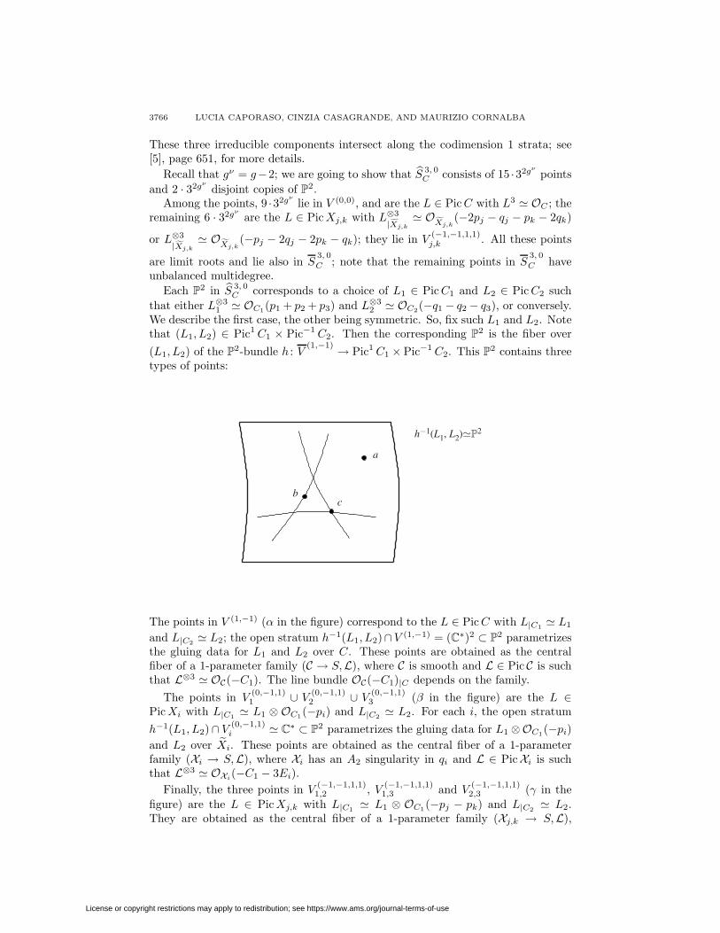
3766 LUCIA CAPORASO, CINZIA CASAGRANDE, AND MAURIZIO CORNALBA
These three irreducible components intersect along the codimension 1 strata; see[5], page 651, for more details.
Recall that gν = g−2; we are going to show that S 3, 0C consists of 15 ·32gν
pointsand 2 · 32gν
disjoint copies of P2.Among the points, 9 ·32gν
lie in V (0,0), and are the L ∈ Pic C with L3 � OC ; theremaining 6 · 32gν
are the L ∈ Pic Xj,k with L⊗3
|Xj,k
� OXj,k
(−2pj − qj − pk − 2qk)
or L⊗3
|Xj,k
� OXj,k
(−pj − 2qj − 2pk − qk); they lie in V(−1,−1,1,1)j,k . All these points
are limit roots and lie also in S3, 0
C ; note that the remaining points in S3, 0
C haveunbalanced multidegree.
Each P2 in S 3, 0C corresponds to a choice of L1 ∈ PicC1 and L2 ∈ Pic C2 such
that either L⊗31 � OC1(p1 + p2 + p3) and L⊗3
2 � OC2(−q1 − q2 − q3), or conversely.We describe the first case, the other being symmetric. So, fix such L1 and L2. Notethat (L1, L2) ∈ Pic1 C1 × Pic−1 C2. Then the corresponding P2 is the fiber over(L1, L2) of the P2-bundle h : V
(1,−1) → Pic1 C1 ×Pic−1 C2. This P2 contains threetypes of points:
a
h−1(L1, L2)�P2
bc
The points in V (1,−1) (α in the figure) correspond to the L ∈ Pic C with L|C1 � L1
and L|C2 � L2; the open stratum h−1(L1, L2)∩V (1,−1) = (C∗)2 ⊂ P2 parametrizesthe gluing data for L1 and L2 over C. These points are obtained as the centralfiber of a 1-parameter family (C → S,L), where C is smooth and L ∈ Pic C is suchthat L⊗3 � OC(−C1). The line bundle OC(−C1)|C depends on the family.
The points in V(0,−1,1)1 ∪ V
(0,−1,1)2 ∪ V
(0,−1,1)3 (β in the figure) are the L ∈
Pic Xi with L|C1 � L1 ⊗ OC1(−pi) and L|C2 � L2. For each i, the open stratumh−1(L1, L2)∩ V
(0,−1,1)i � C∗ ⊂ P2 parametrizes the gluing data for L1 ⊗OC1(−pi)
and L2 over Xi. These points are obtained as the central fiber of a 1-parameterfamily (Xi → S,L), where Xi has an A2 singularity in qi and L ∈ PicXi is suchthat L⊗3 � OXi
(−C1 − 3Ei).Finally, the three points in V
(−1,−1,1,1)1,2 , V
(−1,−1,1,1)1,3 and V
(−1,−1,1,1)2,3 (γ in the
figure) are the L ∈ PicXj,k with L|C1 � L1 ⊗ OC1(−pj − pk) and L|C2 � L2.They are obtained as the central fiber of a 1-parameter family (Xj,k → S,L),
License or copyright restrictions may apply to redistribution; see https://www.ams.org/journal-terms-of-use
MODULI OF ROOTS OF LINE BUNDLES ON CURVES 3767
where Xj,k has A2 singularities in qj and qk, and L ∈ PicXj,k is such that L⊗3 �OXj,k
(−C1 − 3Ej − 3Ek).
References
[1] Dan Abramovich and Tyler J. Jarvis. Moduli of twisted spin curves. Proceedings of the Amer-ican Mathematical Society, 131(3):685–699, 2002. MR1937405 (2003k:14027)
[2] Valery Alexeev. Compactified Jacobians and Torelli map. Publ. RIMS, Kyoto University40:1241-1265, 2004. MR2105707 (2006a:14016)
[3] Edoardo Ballico, Cinzia Casagrande, and Claudio Fontanari. Moduli of Prym curves. Docu-menta Mathematica, 9:265–281, 2004. MR2117416 (2006e:14031)
[4] Arnaud Beauville. Prym varieties and the Schottky problem. Inventiones Mathematicae,41:149–196, 1977. MR0572974 (58:27995)
[5] Lucia Caporaso. A compactification of the universal Picard variety over the moduli spaceof stable curves. Journal of the American Mathematical Society, 7(3):589–660, 1994.MR1254134 (95d:14014)
[6] Lucia Caporaso and Cinzia Casagrande. Combinatorial properties of stable spin curves. Com-munications in Algebra, 31(8):3653–3672, 2003. Special Issue in Honor of Steven L. Kleiman.MR2007379 (2004i:14026)
[7] Alessandro Chiodo. Higher Spin curves and Witten’s top Chern class. Ph.D. thesis, Universityof Cambridge, 2003.
[8] Maurizio Cornalba. Moduli of curves and theta-characteristics. In Lectures on Riemann Sur-
faces: Proceedings of the College on Riemann Surfaces, International Centre for TheoreticalPhysics, Trieste, 1987, pages 560–589. World Scientific, 1989. MR1082361 (91m:14037)
[9] Maurizio Cornalba. A remark on the Picard group of spin moduli space. Rendiconti Lincei.Matematica e Applicazioni, 2:211–217, 1991. MR1135424 (92k:14007)
[10] Eduardo Esteves. Compactifying the relative Jacobian over families of reduced curves.Transactions of the American Mathematical Society, 353(8):3045–3095, 2001. MR1828599(2003b:14036)
[11] Gerd Faltings. Moduli-stacks for bundles on semistable curves. Mathematische Annalen,304:489–515, 1996. MR1375622 (97d:14016)
[12] Claudio Fontanari. On the geometry of the compactification of the universal Picard variety.To appear in Rendiconti Lincei. Matematica e Applicazioni, 2005.
[13] David Gieseker. Lectures on moduli of curves. Tata Institute of Fundamental Research Lec-tures on Mathematics and Physics, 69. Springer-Verlag, Berlin, New York, 1982. MR0691308(84h:14035)
[14] Tyler J. Jarvis. Torsion-free sheaves and moduli of generalized spin curves. Compositio Math-ematica, 110:291–333, 1998. MR1602060 (99b:14026)
[15] Tyler J. Jarvis. Geometry of the moduli of higher spin curves. International Journal ofMathematics, 11(5):637–663, 2000. MR1780734 (2001f:14050)
[16] Tyler J. Jarvis. The Picard group of the moduli of higher spin curves. New York Journal ofMathematics, 7:23–47, 2001. MR1838471 (2002j:14032)
[17] Tyler J. Jarvis. Compactification of the universal Picard over the moduli of stable curves.Math. Z., 235(1):123–149, 2001. MR1785075 (2001m:14040)
[18] Yuan-Pin Lee. Witten’s conjecture and Virasoro conjecture for genus up to two. Preprint
math.AG/0310442.[19] David Mumford, John Fogarty, and Frances Clare Kirwan. Geometric Invariant Theory, vol-
ume 34 of Ergebnisse der Mathematik und ihrer Grenzgebiete. Springer-Verlag, third edition,1994. First edition 1965. MR1304906 (95m:14012)
[20] Rahul Pandharipande. A compactification over Mg of the universal moduli space of slope-semistable vector bundles. Journal of the American Mathematical Society, 9(2):425–471,1996. MR1308406 (96f:14014)
[21] Alexander Polishchuk. Moduli spaces of curves with effective r-spin structures. Preprintmath.AG/0309217
[22] Alexander Schmitt. The Hilbert compactification of the universal moduli space of semistablevector bundles over smooth curves. Journal of Differential Geometry, 66:169–209, 2004.MR2106123 (2005j:14044)
License or copyright restrictions may apply to redistribution; see https://www.ams.org/journal-terms-of-use
3768 LUCIA CAPORASO, CINZIA CASAGRANDE, AND MAURIZIO CORNALBA
[23] Conjeeveram S. Seshadri. Degenerations of the moduli spaces of vector bundles on curves.In Moduli Spaces in Algebraic Geometry - School on Algebraic Geometry (Trieste, 1999),volume 1 of ICTP Lecture Notes Series, pages 205–265, 2000. MR1795864 (2001i:14044)
[24] Carlos T. Simpson. Moduli of representations of the fundamental group of a smooth projective
variety. Inst. Hautes Etudes Sci. Publ. Math., 80:5–79, 1994. MR1320603 (96e:14013)
Dipartimento di Matematica, Universita Roma Tre, Largo S. L. Murialdo, 1, 00146
Roma, Italy
E-mail address: [email protected]
Dipartimento di Matematica “L. Tonelli”, Universita di Pisa, Largo B. Pontecorvo,
5, 56127 Pisa, Italy
E-mail address: [email protected]
Dipartimento di Matematica “F. Casorati”, Universita di Pavia, Via Ferrata, 1, 27100
Pavia, Italy
E-mail address: [email protected]
License or copyright restrictions may apply to redistribution; see https://www.ams.org/journal-terms-of-use