[American Institute of Aeronautics and Astronautics 48th AIAA/ASME/ASCE/AHS/ASC Structures, Structural Dynamics, and Materials Conference - Honolulu, Hawaii (23 April 2007 - 26 April

Cryo Magnetic Damping: Material Characterization and Damping Demonstration

Sarah M. Brennan1, Allen J. Bronowicki2, and Stepan S. Simonian3

Northrop Grumman Space Technology, Redondo Beach, CA, 90278, USA

The aim of this research is to develop analytical techniques that are supported by experimental data to predict the behavior of a passive magnetic damper in a cryogenic environment. The applications are far reaching--projects with high precision pointing requirements, such as JWST, operate in harsh environments where traditional damping techniques may be limited or ineffective. Therefore, we are interested in developing new technologies that can be used passively to isolate vibration disturbances effectively at a temperature of 40 K, under conditions that offer only a few nanometers of relative motion. Magnetic damping relies on the principle of motional EMF. As a conductor passes through a magnetic field, eddy currents form to produce a force that opposes the direction of motion. The magnitude of this force depends on several factors including the characteristics of the conductor and the magnetic field, which may be highly dependent on temperature. Current research is focused on material characterization, and a simple test cell has been designed to evaluate the damping, quantify the temperature effects, and expand our predictive capabilities. Several material combinations have been successfully cycled from 295K to 15 K, and the results, which illustrate damping from 1% to 100% critical damping, will be presented and compared to model predictions.

Nomenclature B = magnetic flux density v = velocity i = current

emfF = damping force from the electromotive force m = mass k = spring stiffness

emfc = damping coefficient related to electromotive force t = time

)(tf = time varying forcing function x = direction of motion in 1DOF system ζ = damping ratio

nω = natural frequency of the undamped oscillation ρ = electrical resistivity

ct = thickness of the conductor

dB = remenance induction

magL = dimension of magnet length

magW = dimension of magnet width

magT = dimension of magnet thickness ε = electromotive force, EMF

1 Staff Engineer, System Dynamics Design, One Space Park Blvd/MS R4-1112D 2 Technical Fellow, Integrated Modeling, One Space Park Blvd/MS R8-2781

1 American Institute of Aeronautics and Astronautics

3 Senior Staff Engineer, System Dynamics Design, One Space Park Blvd/MS R4-1104E

48th AIAA/ASME/ASCE/AHS/ASC Structures, Structural Dynamics, and Materials Conference<br> 15th23 - 26 April 2007, Honolulu, Hawaii

AIAA 2007-2154

Copyright © 2007 by Northrop Grumman Space Technology. Published by the American Institute of Aeronautics and Astronautics, Inc., with permission.

gapd = gap distance between magnets

R = electrical resistance of the conductor

cV = volume of the conductor

cl = dimension of conductor length

cw = dimension of conductor length

cl = dimension of conductor length Φ = magnetic flux

cl = dimension of conductor length

dω = frequency of the damped oscillation

K = constant associated with non-uniform magnetic flux distribution

I. Introduction HE magnetic damper is a viscous damper that operates on the principle of motional EMF (see Figure 1). As an

electrically conductive plate enters a magnetic field, the changing magnetic flux creates an induced electromotive force (EMF) in the conductor that leads free electrons in the metal to move, producing eddy currents that create effective poles on the conductor, thus generating a force to oppose the motion [1, page 889]. Maxwell’s equations describe this electromagnetic behavior and may be coupled with Newton’s second law to predict the behavior of a spring-mass-damper system with a magnetic element. While some passive damping techniques become ineffective at low temperatures (e.g. the dissipation capacity of viscoelastic material falls precipitously as temperatures drop [2]), other dampers are ineffectual at small amplitudes (e.g. particle dampers are non-linear and have less dissipation at lower excitation levels). However, the parameters influencing the efficacy of a magnetic damper indicate that performance remains linear and the behavior is not adversely affected at low temperature. This research studied the temperature dependence of a passive magnetic damper at cryogenic temperatures down to 15 K, and observed system response over a large range of amplitudes, from centimeter to micron levels.

T

Here damping relies on relative motion, so a test cell was devised to demonstrate the dynamic response of a predictable system to support characterization of different materials over a wide temperature range. Both magnet and conductor properties are temperature dependent, so tests were conceived to quantify both magnetic induction and electrical resistivity as functions of temperature. A single-axis spring-mass-damper concept (see Figure 2) was developed to measure damping. Obvious challenges accompany any attempt to cycle a system over a temperature range from 295 K to 15 K. All tests were conducted in a cryogenic chamber, shown in Figure 3, an environment that is physically restrictive and difficult to instrument. It is an ultra-high vacuum chamber that limits the types of devices that can be employed to excite a dynamic system, e.g. standard solenoids will outgas, thus contaminating MLI blankets and obscuring any optics. Standard measurement devices are not intended, designed, or calibrated for use over such extreme temperature ranges, so alternative instrumentation methods were utilized in this study. While force transducers and accelerometers are traditionally used to extract transfer functions that represent a dynamic system, under these conditions log-decrement observations proved most effective for characterizing the inherent damping of this simple, single-degree-of-freedom (1 DOF) dynamic system. To monitor the displacement of the system a laser interferometer was employed, introducing a non-contact method of measurement with very high resolution. Analyzing the data proved challenging as damping levels for certain material combinations yielded near-critical damping, limiting the ability of log-decrement analysis to produce useful results. The details of the design, the prediction techniques and analytical models, as well as the experimental results of extensive material and damper tests are presented below and indicate that cryo magnetic damping is an emerging and enabling technology.


v

1B

i eddy currents

magnets

2BemfF

gap

conductor plate v

Figure 1. A simple magnetic damper. The conductor moves relative to the magnetic material ( and represent the magnetic fields) with velocity, , and as a result eddy currents, i , form within the conductive material. This generates a damping force, , that acts opposite the direction of motion.

1B 2Bv

emfF

m

k emfc

)(tf

x

Figure 2. A simple single-degree-of-freedom system with mass , spring stiffness , damping coefficient ,

driven by a time varying force .

m k emfc( )tf

Figure 3. The cryo chamber used for testing consisting of a CTI-cryogenics Model 350CP, with a two stage Gifford-McMahon coldhead that is mounted in a 12” diameter, turbo-pumped, vacuum chamber.

II. Objective and Scope The objective of this research is to characterize the material behavior and dissipation of a passive magnetic damper at

cryogenic temperatures through experiment, and to develop prediction capabilities for a simple 1 DOF system. The damping


coefficient, , is a representative measure of the amount of damping in a system. It is related to the force generated from

the eddy currents, , and the velocity at which the conductor moves through the magnetic field, , such that emfc

emfF v

v

Fc emf

emf = (1)

The damping coefficient appears in the equation of motion describing the dynamic behavior of a single-degree-of-freedom system (as shown in Figure 2) [3, page 59]

)()()()( tftkxtxctxm emf =++ &&& (2)

And alternately may be expressed [4, page 24] as

nemf mc ζω2= (3)

In the equations above, is the oscillating mass in the spring-mass-damper system, and is the stiffness of the spring. The displacement,

m kx , and forcing function, , are functions that vary with time, . The damping ratio, f t ζ , is a non-

dimensional quantity that expresses the amount of damping relative to a critically damped system, and nω is the natural frequency of the undamped oscillation.

A magnetic damper consists of three key material elements: 1) the conductor, 2) the permanent magnets, and 3) the soft

magnetic material (i.e. a high permeability material such as iron) which serves as the back plate used to create the magnetic circuit (see Figure 4). Others have documented the effect of temperature variations on these individual components [5, 6, 7, 8, 9, 10, 11, 12, 13, 14], but no studies were found that were dedicated to a coupled system designed for damping purposes. The damping is dependent on several parameters including the electrical resistivity of the conductive material, ρ , the thickness

of the conductor, , the properties of the magnets (in particular magnetic flux density, , also known as magnetic

induction), the orientation of the magnets, the dimensions of the magnets (length, , width , thickness, ), the

use of soft magnetic materials to boost magnetic flux, and the gap distance, , between the opposing magnets. Maxwell’s

equations may be used to predict the damping coefficient, , assuming a uniform distribution of flux in the gap

ct dB

magL magW magT

gapd

emfc

ρ

cmagmagdemf

tWLBc

2

= (4)

A. Modeling a 1DOF Magnetic Damper

Two models are presented to calculate the damping coefficient of a dynamic system with a magnetic damper. The first approach considers the motion of an electrical conductor through a uniform magnetic field, while the alternate method assumes a variable flux distribution through the length and width of the conductive element as shown in Figure 5.

Power may be expressed in terms of induced EMF, ε , and resistance, R . It may also be defined in terms of force,

, and velocity, , therefore the following equation [1, page 880] holds emfF v

vFR

P emf==2ε

(5)



For a uniform magnetic field, the damping force generated by the formation of eddy currents is [15, page 5]

ρ

where dB is the remenance induction, V is the volume of the conductor, and

vVBF cd

emf

2

= (6)

c ρ is the resist ty of the conduct r.

Alternatively the resist

ivi o

ance of the conductor, R , may be expressed in terms of the leng , width, , and thickness, of the conductor

th, cl cw ct ,

cctwclR

ρ= (7)

In this case the volume of the conductor is related to the surface area

of the magnet

cmagmagcccc tWLtwlV == (8)

Here is the length of the magnet, he width, and he thickness of the conductor, such that Eqn. 6 becomes

magL magW t ct t

ρvtWLB

F cmagmagdemf

2

= (9)

The damping coefficient may then be expressed as

ρemf v

cmagmagdemf tWLBFc

2

== (10)

Alternatively this result may be derived from Faraday’s Law [1, page 877] which relates the induced EMF ,ε , to the time rate of change of magnetic flux through a circuit

Φ

dtdΦ

−=ε (11)

Magnetic flux may be expressed in terms of the magnetic field Br

and the surface perpendicular to the field, Ar

( ) ∫ ⋅=Φ AdByxrr

, (12)

thus, considering uniform flux through the conductor perpendicular to

(13)

the magnet surface

( ) dxdyByx magW

∫ ∫=Φ0

,

( ) ( ) dxdyBtt

yy magW

∫ ∫∂∂

=∂Φ∂

=0

ε (14)

{ } ∫∫ ∂∂

= dyt

dxB mag

0

W (15)

{ } ∫∂∂

= dyt

WB mag (16)

t

BWmag ∂y∂

= (17)

vBWmag=ε (18)

Therefore, when the area of the conductor is assumed equivalent to the surface of the magnet:

vtLWB

F cmagmagemf ρ

2

= (19)

Finally, the damping coefficient is

ρ

cmagmagemf

tLWBc

2

= (20)

However, in practice it is difficult to produce a truly uniform flux distribution. We used Maxwell3D, a commercially available electromagnetic design simulation tool, to model a realistic magnetic damper system. We were able to simulate the results observed during test: the assumption of uniform flux distribution overestimates the amount of damping in the system. Therefore, a sinusoidal distribution was considered and the derivation is shown below, considering the flux through the conductor perpendicular to the magnet surface

( ) dxdyL

yW

xByxmag

W

mag

mag

⎟⎟⎠

⎞⎜⎜⎝

⎛⎟⎟⎠

⎞⎜⎜⎝

⎛=Φ ∫ ∫

ππ sinsin,0

(21)

( ) ( ) dxdyL

yW

xBtt

yymag

W

mag

mag

⎟⎟⎠

⎜⎜⎝

⎟⎟⎠

⎜⎜⎝∂

∂=

∂Φ∂

= ∫ ∫ππε sinsin

0

⎞⎛⎞⎛ (22)

∫∫ ⎟⎟⎠

⎞⎜⎜⎝

⎛

∂∂

⎪⎭

⎪⎬⎫

⎪⎩

⎪⎨⎧

⎟⎟⎠

⎞⎜⎜⎝

⎛= dy

Ly

tdx

WxB

mag

W

mag

mag ππ sinsin0

(23)

∫ ⎟⎟⎠

⎞⎜⎜⎝

⎛

∂∂

⎭⎬⎫

⎩⎨⎧−= dy

Ly

tWB

mag

ππ

sin2 (24)


⎭⎬⎫

⎩⎨⎧

⎟⎠⎞

⎜⎝⎛−

∂∂

⎭⎬⎫

⎩⎨⎧−=

LyL

tWB π

ππcos2

(25)

⎭⎬⎫

⎩⎨⎧

∂∂

⎟⎠⎞

⎜⎝⎛

⎭⎬⎫

⎩⎨⎧−=

ty

LyWB π

πsin2

(26)

vmag

πε =

BW2 (27)

Therefore, when the area of the resistor is assumed equivalent to the surface of the magnet, and the magnetic flux is assumed to have a sinusoidal distribution:

vtLWB

F cmagmagemf ρπ

2

2

4= (28)

When evaluating the damping ratio for a highly damped system using Prony’s method, the following relationship between damped and undamped frequency applies

2

1 ⎟⎟⎠

⎞⎜⎜⎝

⎛−=

n

d

ωω

ζ (29)

Figure 4. The magnet assembly consists of an aluminum housing that supports an iron back plate (soft magnetic material) that enhances that magnetic flux through the gap. The magnets are affixed to the back plate and are aligned in attracting positions across the gap; the two magnets on each back plate have reverse polarity to encourage the flux pattern illustrated on the right. The conductor is supported such that it is suspended at the mid-plane of the gap.

B. Magnetic Damper Properties in Low Temperature Environments The behavior of the magnetic damper described above is well understood and predictable under nominal conditions.

However, both electrical and magnetic properties are functions of temperature that can vary dramatically when the system is exposed to a cryogenic environment. An experimental setup was designed to support damping measurements in which the effects of the electrical and magnetic properties could be quantified over temperature range of 15K – 300K. These results were then compared to analytical models for validation and verification. It should be noted that these room temperature tests were quite enlightening and led to modification and refinement of both the test cell and the analytical tools and models. The test the effect of temperature on material properties was measured independently, including resistivity versus temperature for


the conductor and magnetic flux density versus temperature for the magnet assembly.

B w

y l

y x

Figure 5. Left, the uniform distribution of flux through a conductor. Right, a sinusoidal distribution of flux.

III. Material Properties An extensive material survey explored the behavior of electrical conductors and magnetic materials in low temperature

environments. Initial experiments were performed at room temperature where material properties are well understood and documented. Under these conditions the test setup could be modified and tuned, and alternate measurement systems exercised to guarantee measurement repeatability.

A. Conductors The effects of temperature on electrical resistivity vary drastically for different metals as shown in Figure 6 [5,8]. Many

pure metals experience a significant reduction in electrical resistivity as temperature falls that suggests damping behavior will improve at lower temperatures because damping is inversely proportional to electrical resistivity, ρ (Eqn. 20). Pure copper and aluminum are good conductor candidates if maximum damping is desired, while manganese or CuBe would be preferred if consistent performance is desired over a broad temperature range. It should be noted that alloy composition and treatments (annealing, age hardening) have a marked effect on resistivity values and care should be taken to correctly identify the material in use.


Figure 6. Electrical resistivity of metals plotted as a function of temperature.

B. Rare Earth Permanent Magnets Lterature review indicates that rare earth magnets, such as neodymium iron boron (NdFeB) and samarium cobalt (SmCo)

exhibit the most attractive magnetic properties. Both possess high values of residual induction, , a measure of the strength

of the magnetic field, and equally high values of intrinsic coercive force, , which indicate a magnets resistance to demagnetization [9]. However, while all publications agree that SmCo is thermally stable, there is some disagreement as to the behavior of NdFeB in a cryogenic environment [12, 13]. The degradation of magnetic field strength is attributed to easy-cone anisotropy, which is marked by a spin reorientation (dipole realignment) [12]. Additionally, the nature of the application, be it AC or DC, will determine what combination of magnetic properties offer the most attractive BH-curve. Because the passive magnetic damper is a DC application, the residual induction is deemed most important and magnetic material grade selection should be made to maximize this quantity, after factoring in availability and cost, NdFeB(53) and SmCo(27H) were identified as viable candidates for the magnetic damper application. The configuration of the magnetic circuit is also crucial to maximizing the magnetic field strength. The horseshoe configuration shown in Figure 4 offers a good flux path and is well designed to concentrate the field in the gap. However, it should be noted that this does not produce a truly uniform distribution in the gap because in reality flux varies along the surface of the conductor, so attempts were made both analytically and experimentally to quantify this discrepancy. It should be noted that increasing magnetic field strength in the gap is the most effective method for increasing the damping of the system, as the damping coefficient is proportional to the square of the magnetic induction, (Eqn. 20).

rB

ciH

dB

C. Soft Magnetic Materials To fully understand the magnetic system the influence of the soft magnetic back plate must be evaluated. High

permeability materials such as Fe, SiFe, NiFe, and CoFe alloys have been used for various magnetic applications as shown in Table 1 [14]. Here the goal is to direct as much flux as possible through the gap in the magnet assembly. The magnets high flux, so it is necessary to select a back plate material with a high saturation limit. This eliminates nickel-iron alloys which are good for shielding because of their extremely high permeability values, but which have relatively low saturation limits (0.8 T). In this DC case, the high resistivity of silicon-iron offers no benefit over pure iron as both have similar saturation (~1.7 T) levels. Cobalt-iron alloys (trade name Hiperco50A) are best suited for this application because of the high saturation limits (2.4 T), though the cost of these materials is a consideration. However, in a weight critical situation they offer a potential weight savings compared to Fe or SiFe, so for a technology with space applications this is an attractive option. Permeability



can vary significantly with temperature, the saturation levels are relatively stable, therefore the choice of back plate material is not expected to have significant influence in the values of measured magnetic induction as temperature varies [14].

Table 1. Summary of magnetic properties for select soft-magnetic materials [14].

Material Fe SiFe Hiperco50 Permalloy Permeability Ratio 6000 40,000 10,000 100,000

Magnetic Saturation (295K) 1.78 1.72 2.40 0.76

Benefits & Applications

Increased magnet effect at low cost; best for most DC applications.

High resistivity for low eddy current losses; good for AC applications.

High saturation; less material needed to carry flux.

High permeability reduces leakage; good for shielding.

The magnetic damper considered in this research is a passive and completely non-contact. All literature reviews and

material characteristics indicate that this system behavior is truly linear. In the following section, the results of thermal tests offer system material characterization, and the dynamic behavior of a 1 DOF spring-mass-damper system is observed and a rigorous quantitative analysis of the damping is presented.

IV. Testing An initial prototype was built to illustrate the potential of eddy current damping is shown in Figure 7. A test cell was

designed to capture the damping characteristics of the magnet damper with a twang test. The 1 DOF oscillator has a conductor that is suspended by springs that permit only axial motion as it travels through the magnetic field created by four opposing permanent magnets. The magnet assembly consisted of 4 NdFeB magnets (0.75” x 0.75” x 0.25”) mounted to a soft-magnetic back plate that was attached by 4-40 fasteners to an aluminum housing. To address cryo compatibility issues, Hysol EA-9321 epoxy was used to fix the magnets to the backplate, and micro-beads were used to insure an even bond. The conductor was interchangeable and supported on by diaphragm springs to constrain response to the axial direction and avoid contact with the magnets.

An early concept is illustrated in Figure 8 and the actual test cell hardware is shown in Figure 9. The system is designed with a solenoid exciter that can either be driven to specified displacement and released or used as a striker (Figure 10). Displacement of the system is measured using and interferometer by placing a retroreflector (Figure 11) on the top of the oscillating mass. The damping coefficient is calculated using log decrement. This test cell may be mounted to an optical table for room temperature tests, or fixed to the second stage of the coldhead for testing at cryogenic temperatures.

A. The Cryo Chamber The tests were designed to characterize the damping behavior of a passive magnetic damper in a cryogenic environment

and the setup imposed technical and logistical issues as we sought to measure the damping performance of a 1DOF system over a temperature range from 295 K to 15 K. All tests were conducted in a cryogenic chamber located in the NGST Cryogenics Lab that consisted of a CTI-cryogenics Model 350CP with a two stage Gifford-McMahon coldhead that is mounted in a 12” diameter, turbo-pumped, vacuum chamber. Under operating conditions the first stage of the coldhead is maintained at 80 K and it is here that the shroud that shields the test cell from the outer dome is attached. The test cell was mounted directly to the coldhead second stage that reaches approximately 15 K during operation. This cryo chamber (shown in Figure 3) is an environment that is physically restricted and difficult to instrument with only a limited number of pin connections for electrical signals to record conditions inside. It is an ultra-high vacuum chamber that limits the types of devices that can be employed to excite a dynamic system, e.g. standard solenoids will outgas, thus contaminating MLI blankets and obscuring any optics. Similarly, standard measurement devices are not intended, designed, or calibrated for use over such extreme temperature ranges, and thus alternative instrumentation methods were utilized in this study. A Zygo laser interferometer was employed to monitor displacement, introducing a non-contact method of measurement with very high resolution. The basic test configuration is shown in Figure 12.

B. The Instrumentation An interferometer is an optical device comprised of several elements that selectively splits a dual frequency laser beam

into two separate frequencies. When used to measure linear displacement, the beam of Frequency A is sent to a moving reflector while the beam of Frequency B is sent to a stationary reflector, and the two beams are then combined at the exit aperture of the interferometer to produce an optical reference signal [16, page 1-4, Rev. J]. The Zygo laser interferometer system consists of a ZMI Laser Head using a Helium-Neon frequency stabilized laser that produces a laser beam with two orthogonally polarized frequency components [16, page 1-2. Rev. B], a 2-pass High Stability Plane Mirror Interferometer [16, page 1-5, Rev. J], a retroreflector that mounts to the moving target, a fiber optic pickup, and a ZMI 1000A measurement

board that connects to a Windows PC via a GPIB interface card. Complementary software allows the user to interact with the system, collecting samples the displacement over time, and presenting the results in graphical form, as well in ASCII form that is later imported into matlab for analysis. The measured displacement of the damped system is recorded over a 30 second period at a sampling rate of 100 Hz. While the optical resolution of such a system is nanometers (1.24 nm for the High Stability Plane Mirror Interferometer used in these experiments), the environment in the laboratory produced a noise floor that averaged ± 0.4 microns.

The temperature of the system within the chamber was monitored at three discrete locations using Lakeshore DT-4701SD silicon diodes. Lakeshore QT-36 cryogenic wire (phosphor bronze, 26 gauge) was used for all sensor wiring, in addition to providing power to the non-contact actuator. Initially two sensors were mounted to the aluminum housing of both magnet plates as shown in Figure 13, and one was attached to the shroud. It was feared that attaching anything to the conductor would be obtrusive and adversely affect the behavior of the system, however this led to uncertainties in the temperature of the conductor, a parameter of high sensitivity for certain metals (i.e. pure Cu). For example, the first tests were conducted with CuBe, an alloy with near constant resistivity values over the temperature cycle, and the results correlated well with model predictions. However, when we tested a sample of pure Cu our predictions varied drastically from the observed damping values. After allowing the system to sit overnight another measurement was taken, and while the magnet and shroud temperature readings were identical to the previous run, the results were very different. The system was now critically damped. It identified two problems 1) the conductor was thermally isolated from the system 2) the temperature of the conductor was unknown. We went back and instrumented the conductor with a diode, and the undamped tests were repeated. There was no appreciable change in the response of the system maintaining the integrity of the test, but tremendous knowledge was gained be explicitly monitoring conductor temperature. At this time additional effort was invested to improve the thermal conductivity of the system. A thin layer of grease (Apeizon N) was applied to all contacting surfaces improving connectivity and significantly reducing the cool down time. Because the conductor relied almost entirely on radiation to cool down (the only thermal path to the conductor was the thin elements of the titanium diaphragm springs), a thin copper foil was affixed to the base plate of the assembly and connected to the base of the conductor at the diode interface to improve thermal conductivity. In a further attempt to keep the conductor cold, a copper shield was placed around the conductor as shown in Figure 14. The added stiffness of the copper foil did cause a slight frequency shift in the undamped system that was noted, but no change in the damping was observed under vacuum.

A separate test was performed to verify the resistivity of the CuBe alloy. The sample strip of similar dimension to the conductor used in testing ( 0.040 thickness) was machined into an I beam, and holes were punched in the outer corners of the top and bottom flanges. Voltage and current sources were attached mechanically using screw mounts. The top and bottom surfaces of the sample were covered with kapton tape to avoid a short circuit when the sample was sandwiched between two aluminum plates and affixed to the second stage of the coldhead. Then as the sample was cycled down to 25K, a controlled 1 Amp current was supplied and voltage was read off a multi-meter with micro-volt sensitivity. The data was so well correlated to existing NIST data, that it was possible to identify the treatment of the alloy [8].

In all, over 200 interferometer datasets were collected (each consisting of 2500 position samples at a rate of 100 Hz), each containing multiple impulses. A typical data set contained three to five impulses that would be characterized by a decaying oscillation. A sample dataset is shown if Figure 15. A complete summary of the results follows.


Figure 7. The original prototype magnetic damper assembly. Soft iron back plate with NdFeB magnets are mounted to the aluminum housing using epoxy.

Figure 8. Illustration of the cryogenic damper test cell. The conductor plate is suspended from springs that allow only one axial degree of freedom. The conductor passes through the magnetic field generated by a configuration of rare earth permanent magnets.

.


Figure 9. Pictures of the cryogenic damper test cell. At left, a side view with the magnet assembly in place. At right, a front view without the magnets as natural frequency data is collected.


Figure 10. These figures illustrate the original “striker” concept (left) and the final “non-contact” impulse source (right). In situations with very high levels of damping, the noise from the striker proved difficult to filter out of the data, because frequency associated with the retraction spring was very close to the conductor oscillation. So instead of hitting the middle plate, a 1 inch long ferrous screw was threaded into the center plate aligning with the hole in the bobbin. Thus, when a pulse of current is sent through the coil, the middle plate is pulled upwards providing an initial displacement. The plate is then free to oscillate free of any unrelated motion.

Ti ring

retroreflector

chamfered washer

wave spring

Al spacer

CRES pin

recycled composite tube

Figure 11. A cryo compatible retroreflector and the assembly stack that supports it to maintain fit over large temperature changes. The retroreflector sits in a chamfered washer that sits upon a wave spring. An aluminum disk lies below that. The carbon mount on the right has a thin titanium ring at the top opening that catches the edge of the retroreflector. The remaining stack is then loads into place and held in place, under slight compression, by two steel pins.


unistrut platform

laser head mirror interferometer

fiber optic pickup

view port

shroud

vacuum chamber

coldhead

laser beam

Figure 12. The cryo test setup in which the test cell is mounted to the second stage of the coldhead, and a laser interferometer is used to measure the displacement of the oscillating spring-mass-damper.

diode diode

Figure 13. The magnet assembly. Silicon diodes were mechanically clamped to the outer surfaces of the aluminum plate supporting the back plate. The kapton tape seen on the inner surface serves to protect the tool from impact during assembly (hex drivers, screws, etc. are easily and forcefully attracted).


Figure 14. Improvements made to the thermal path of the system. At left the thin copper strip used to tie the conductor to the base plate of the assembly. At right, the copper shield adding further insulation of the conductor from the radiation of the warmer 80 K shroud.

Figure 15. Data collected during one collection cycle.

V. Results

The results of the tests are presented below and illustrate the sensitivity of damping to both material combination and temperature. While the apparent success of a response measurement could be immediately monitored by reviewing the graphical data from the ZMI software, complete analysis was performed in matlab. Raw data files were imported and evaluated to determine the damping behavior.

A. Room Temperature and Undamped Tests Initial assessment of the effectiveness of the test cell design was observed during room temperature testing. An example

of the data is shown in Figure 16 (undamped) and Figure 17 (damped). Figure 18 illustrates the “ringing” of the striker that threatened to contaminate our data, as the spring loaded stinger continued to oscillate after the conductor motion had fallen below the noise level. This problem was averted by replacing the striker with a ferrous screw that was attached to the mid- 16 American Institute of Aeronautics and Astronautics

plate, which was then “plucked” by running a pulse of current through the bobbin coil, creating a non-contact exciter. The analytical model prediction is compared to the experimental results in Figure 19.

B. Cryo Tests After an extensive series of room temperature tests, tests moved to the cryo chamber and the test cell was cycled from 295

K to 15 K. This was a learning process. We gathered results for SmCo, CuBe, and Fe combinations. The results are shown in Figure 20. During an early test, after 48 hours in the chamber, the temperature never fell below 60 K, so Apeizon N grease was applied at all of the mechanical interfaces to improve conduction, and the next test dropped to 15 K in 8 hours. Eventually the CuBe conductor was exchanged for a pure copper sample. The results were perplexing. After 8 hours of cool down, magnet temperature was recorded at 15 K, and damping was observed at approximately 55% critical. However, the system was allowed to sit for 48 hours. Upon return, the damping ratio was now 1.0 as shown in Figure 21. This highlighted the need to tie the conductor to the rest of the system thermally, as well as the need to monitor the temperature of the conductor to get a precise reading. This was done as described in Section 4, and tests were repeated yielding much better results Figure 22. After the conductor was instrumented we were able to gather independent data on the conductor and magnets. In Figure 23 the remenance induction is presented as a function of temperature, normalized to the room temperature value, thus removing the uncertainty factor associated with the flux distribution

ρ

ζωLWtB

m dn

2

2 = (30)

Here the mass, , damping ratio, m ζ , and natural frequency, nω , are all measured quantities, the magnet and conductor

dimensions are known, as well as the resistivity values of CuBe as a function of temperature, T . Therefore we can calculate . This allowed the characterization of two combinations of magnet and back plate materials. This is valuable data as

literature reviews presented ambiguous and conflicting results. With these values in hand, we continued with the tests and observed very good correlation between model predictions and experimental data (see Figure 24). With decoupled temperature data for the magnetic properties, it was possible to experiment with the conductor, and a cycle was performed with a laminated conductor. The 0.040” thick CuBe sample was laminated with two pure Cu facesheets, each 0.06mm thick. The resistivity value was back calculated from experimental results and compared to the resisitivity of the homogeneous samples.

( )TBd

The only parameter that remained to be defined was temperature independent, and it was related to the flux distribution. Having decoupled the thermal properties of the system, it was possible to determine a knockdown factor K ; it was observed that the response was less than that predicted by uniform flux, but greater than the sinusoidal prediction. Therefore, because all quanities could be explicitly defined, the knockdown factor could be explicitly defined at room temperature and constant (independent of temperature) such that

ρLWtB

cK demf

2

57.057.0 =⇒= (31)

After obtaining the temperature behavior of both NdFeB magnets of Fe, and measuring the damping of the system with Cu and CuBe conductors, tests were run with Hiperco50A back plates. In this case the material was 0.25” thick, similar to the Fe back plates. The results shown with model predictions are found in Figure 25. Results for as highly damped system, illustrating the low resistivity value of pure copper at 15 K is shown in Figure 26.

This successful damping demonstration illustrated the effectiveness of this magnetic damping in a cryogenic environment, and it provided a complete material characterization of different magnetic materials and conductive materials over a temperature range from 295 K to 15 K.


Figure 16. Results from an undamped test at room temperature with a 0.040” thick CuBe conductor (no magnets). The black line represents the displacement sampled at 100 Hz using the interferometer. Each asterisk denotes a peak used in log-decrement calculations. The red line shows the exponential decay, 18.9=nω Hz, and .44.5 −= eζ The

mass of the system was measured independently to be 7.629=m g.


Figure 17. Damped test at room temperature with 0.040” thick CuBe conductor and NdFeB magnets with a 6.5mm gap. The black line represents the displacement sampled at 100 Hz using the interferometer. Each asterisk denotes a peak used in log-decrement calculations. The red line shows the exponential decay, 0300.0=ζ .


Figure 18. A plot of experimental results with a combination of pure copper and NdFeB with high damping levels. The Prony Method was used to fit the data, but it should be noted that the data on the left (green) shows the “ringing” of the striker, while the clean data on the right (red) is the response using the non-contact pulse.

modellog-dec fit data


Figure 19. On the left are the damping results of SmCo; on the right, NdFeB at room temperature compared to model predictions.


model log-dec fit data

295 K


159 K


16 K

Figure 20. Results at various temperatures for a combination of SmCo, CuBe, and Fe vs. temperature. Note that as temperature decreases, the model representation degrades slightly. This may be attributed to the unknown temperature of the conductor. However, for this material combination the effect is very slight, both magnets and conductor are relatively insensitive.


Figure 21. This figure illustrates the large discrepancy between conductive materials. Clusters in the 1-3% range are CuBe results, while the pure Cu sample approaches critical damping. It should be noted that there is a one inconsistent, but telling, data point recorded during the Cu test that led to a re-evaluation of the test design. After 8 hours of cool down, magnet temperature was recorded at 15 K, and damping was observed at approximately 55%. However, the system was allowed to sit for 48 hour. Upon return, the damping level was now 100%. This highlighted the need to tie the conductor to the rest of the system thermally, as well as the need to monitor the temperature of the conductor to get a precise reading. It should also be noted that of the tests using the CuBe sample, greater damping values were always observed using NdFeB rather than SmCo. In fact, in one case the SmCo magnet showed slight non-reversible loses, while all NdFeB cycles suggested all losses were completely reversible.

American Institute of Aeronautics and Astronautics

22

Damping Coefficients for Cryo Magnetic Damper

0

10

20

30

40

50

60

70

80

0 50 100 150 200 250 300

Magnet Temperature, T[K]

Dam

ping

Coe

ffici

ent,

c [N

/(m/s

) CuBe Laminat e

CuBe

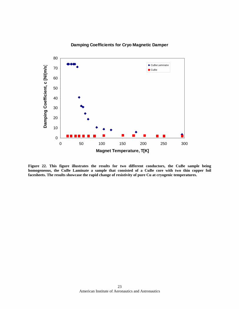
Figure 22. This figure illustrates the results for two different conductors, the CuBe sample being homogeneous, the CuBe Laminate a sample that consisted of a CuBe core with two thin copper foil facesheets. The results showcase the rapid change of resistivity of pure Cu at cryogenic temperatures.


23

Figure 23. This figure presents two combinations of magnetic material and back plates (NdFeB with Fe, NdFeB with Hiperco50A) as a function of temperature. The results have been normalized to the room temperature value.


24


294 K


125 K


15 K

Figure 24. After grounding the conductor and quantifying the temperature dependence of the magnetic materials, the following measurements were made for a combination of NdFeB, CuBe, and Fe. The model shows excellent comparison to experimental results.

295 K

100 K

16 K

Figure 25. Results from tests of NdFeB of Hiperco50A back plates. The conductor was 0.040” thick CuBe. The model predictions show excellent agreement with experimental results at all temperatures. The only surprise was a slightly lower damping value than that observed with the Fe back plates. This could be explained by a slight offset of the magnets in the magnet assembly that may have caused a change in flux density through the conductor.


25

20 K

Figure 26. This illustrates the response of a system consisting of NdFeB magnets, Fe back plates, and a C101 conductor. Damping levels are near critical dictating the use of Prony’s Method to fit data. It also illustrates the sensitive nature of the interferometer with the stepping of response (most likely due to a velocity limit that exceeded the range of the system on the initial displacement, but an effect that does not affect the damping measurement).

VI. Conclusion This research demonstrated that a passive magnetic damper is fully functional in a cryogenic environment, and

by testing different material combinations we were able to fully characterize and compare two conductors (CuBe, Cu), two permanent magnets (NdFeB, SmCo), and two soft magnetic materials (Fe, Hiperco50A). The results were very encouraging with damping observed between 1% to 100% critical damping. Examination of these results indicates that cryo magnetic damping is an emerging and enabling technology, and we have used these results to aid in the design and development of several magnetic damping devices to address challenging vibration requirements.

VII. References [1] Serway, R.A. (1990) PHYSICS For Scientists and Engineers. 3rd ed. Saunders College Publishing,

Philadelphia, PA, USA. [2] 3M Data Sheets on Viscoelastic Damping Polymers 110, 242, 94XX. (2003) Technical Bulletin. St. Paul, MN,

USA. [3] Meirovitch, L. (1986) Elements of Vibration Analysis. McGraw-Hill, Inc. New York, NY, USA. [4] Meirovitch, L. (1997) Principles and Techniques of Vibration. Prentice-Hall, Inc. Upper Saddle River, NJ,

USA. [5] Hall, L.A.(1968) “Survey of Electrical Resistivity Measurements of 16 Pure Metals in the Temperature Range

of 0 to 273 K.” National Bureau of Standards, Technical Note 365. [6] Meaden, G.T. (1965) “Electrical Resistance of Metals.” Plenum Press, New York, USA. [7] Hundley, M.F.& Hoffer, J.K. “Thermal Conductivity and Electrical Resistivity of Copper-Beryllium Alloys.”

Los Alamos. http://www.lanl.gov/ICF/documents/MA199705.pdf. [8] Simon, N.J., Drexler, E.S., and R.P. Reed. (1992) Properties of Copper and Copper Alloys at Cryogenic

Temperatures. NIST/MN-177, Springfield, VA, USA.


26

http://www.lanl.gov/ICF/documents/MA199705.pdf

[9] Magnet Sales and Manufacturing, Inc. (1995) High Performance Permanent Magnets 7. Catalog Culver City, CA, USA.

[10] Strnat, K.J., Li, D., & Mildrum, H. (1985) “High and Low Temperature Properties of Sintered NdFeB Magnets.” 8th International Workshop on Rare Earth Magnets and Their Properties.

[11] Kumada, M., Iwashita, Y., & Antokhin, E.A. “Issues with Permanent Magnets.” [12] TECHNotes, Arnold Magnetics. (2003) “Using Permanent Magnets at Low Temperatures.” TN 0302 June

2003, p.1-3

[13] Gonzalez, J.M., de Julian, C., Cebollada, F. (1995) “Phase Segregation and Interactions in Dy-substituted Melt Spun Nd-Fe-B Alloys.” IEEE Transactions on Magnetics, Vol. 31, No. 6.

[14] Ackermann, F.W. & Klawitter, W.A. (1971) “Magnetic Properties of Commercial Soft Magnetic Alloys at

Cryogenic Temperatures.” Advances in Cryogenic Engineering, Ed. K.D. Timmerhaus, Vol. 16, pp. 46-50. [15] Ghaby, R.A. (1987) “Magnetic Damping Report” TRW L122.3.87-032. June 19, 1987.

[16] Zygo Corporation. ZMI 1000 Operating Manual OMP-0411D. Middlefield, CT, USA.


27

Documents

[American Institute of Aeronautics and Astronautics 48th AIAA/ASME/ASCE/AHS/ASC Structures, Structural Dynamics, and Materials Conference - Honolulu, Hawaii (23 April 2007 - 26 April