AM274 Final Project: Continuous GalerkinNavier-Stokes in 2D

Dylan Nelson, Ariana Minot, Philip Mocz, Pengfei Liu

May 10, 2012

1

Abstract

We describe the implementation of the continuous Galerkin (CG) method to solvethe Navier-Stokes equations on a finite element mesh. We demonstrate the success ofthe method by solving several 2D model problems, including the backward-facing step,flow past cylinder, and the bifurcated pipe problem. We also post-process simulatedflows to study pressure and viscous forces.

1 Introduction

The Navier-Stokes equations are a set of partial differential equations describing the flow ofa viscous, incompressible fluid. They represent one of the most physically motivated modelsin the field of computational fluid dynamics (CFD) and are widely used to model both liq-uids and gases in various regimes. Use is widespread in such research fields as astrophysicsand geophysics as well as in industries including aeronautical, biomedical, chemical, and me-chanical. The Navier-Stokes equations are developed in several commercial software packageswhich are then used to design mechanical machines such as airplanes, boats, bicycles, andcars. In this context the model has been shown to reproduce accurate models of real worldfluid problems of practical importance.

Solutions to the Navier-Stokes equations are in general difficult to obtain. Exact analyt-ical solutions exist typically only for problems where the non-linear terms vanish, such asPoiseuille and Couette flow. Mathematical theory of general solutions to N-S in 3D is anopen problem and one of the Clay Millennium Prize Problems.

In general, solutions to the time-dependent equations are computed using numericalmethods designed to be both highly accurate and highly efficient. We discuss in this paperthe implementation of a Navier-Stokes solver using a continuous Galerkin (CG) methodfor the time-dependent, incompressible fluid flow problem in 2D. We focus on numericalcorrectness and clarity of algorithmic implementation over any speed considerations. In § 2we review the mathematical model, while § 3 discusses the numerical implementation. In § 4we present results on several test problems – the backward-facing step, flow past a cylinder,and bifurcated pipe problem – at various Reynolds numbers and verify the correctness of thecode.

2 Mathematical Background

The dimensionless steady-state Navier-Stokes equations are:

Re ~u · ~∇~u + ~∇p = ∆~u (1)

~∇ · ~u = 0 (2)

where the relations to dimensionful units are:

u = uunits/U0 (3)

x = xunits/L0 (4)

p = punits/P0 (5)

P0 ≡ µU0/L0 (6)

Re ≡ ρU0L0/µ (7)

where µ is the dynamic viscosity. Note that if Re = 0 then we have simple Stokes flow.Re > 0 makes the above equations non-linear.

The dimensionless time-dependent Navier-Stokes equations are:

∂~u

∂t+ Re ~u · ~∇~u + ~∇p = ∆~u (8)

~∇ · ~u = 0 (9)

We do not experiment with any additional body forces which could be included as asource term. As before, the relations to dimensionful units are:

t = tunits/[ReL0/U0] (10)

u = uunits/U0 (11)

x = xunits/L0 (12)

p = punits/P0 (13)

P0 ≡ µU0/L0 (14)

Re ≡ ρU0L0/µ (15)

3 Numerical Method

Our numerical technique for solving the Navier-Stokes equations is based on the finite elementmethod, where we search for the solutions of the velocity and pressure fields over an arbitrarycomputational domain. All code was written in Matlab. The approach is described below.

3.1 Steady-State Incompressible Navier-Stokes Flow

The steady-state Navier Stokes equations given in (1-2) have a weak-formulation form:

∫

Ω

~∇~u : ~∇~w dx + Re

∫

Ω

(~u · ~∇~u) · ~w dx−∫

Ω

p~∇ · ~w dx =

∫

∂ΩN

(gN,1, gN,2) · ~w ds (16)

∫

Ω

q~∇ · ~u = 0 (17)

where the Neumann boundary conditions on ∂ΩN are given by (gN,1, gN,2), and the weakformulation must also satisfy the Dirichlet boundary conditions: ~u|∂ΩD

= (gD,1, gD,2). The

2

test functions are ~w ∈ V0 × V0 and q ∈ Π. We can set ~w = (w1, 0), ~w = (0, w2) to obtain aset of scalar equations.

The above has the following simplified weak formulation: we seek uh, vh ∈ Vh and ph ∈ Πh

such that ~uh|∂ΩD= (uD, vD) and

∫

Ω

~∇uh · ~∇w1,h dx + Re

∫

Ω

(uh∂uh

∂x1

+ vh∂uh

∂x2

)w1,h dx−∫

Ω

ph∂w1,h

∂x1

dx−∫

∂ΩN

gN,1w1,h ds = 0

(18)∫

Ω

~∇vh·~∇w2,h dx+Re

∫

Ω

(uh∂vh

∂x1

+vh∂vh

∂x2

)w2,h dx−∫

Ω

ph∂w2,h

∂x2

dx−∫

∂ΩN

gN,2w2,h ds = 0 (19)

∫

Ω

qh~∇ · ~uh = 0 (20)

for all w1,h, w2,h ∈ Vh, qh ∈ Πh.The discretization is:

uh =

Nvel∑j=1

Ujφj (21)

vh =

Nvel∑j=1

Vjφj (22)

ph =

Npres∑j=1

Pjψj (23)

where U ∈ RNvel , V ∈ RNvel , P ∈ RNpres are the coefficient vectors we want to solve for.The test functions are set to:

w1,h = φi, i = 1, . . . ,Nvel (24)

w2,h = φi, i = 1, . . . ,Nvel (25)

qh = ψi, i = 1, . . . ,Npres (26)

(27)

This finite element discretization gives us a nonlinear system of algebraic equations:

FNS(U, V, P ) = 0 (28)

where FNS : R2Nvel+Npres → R2Nvel+Npres .We solve for FNS(U, V, P ) = 0 using Newton’s method. We require an initial guess

(U0, V0, P0) ∈ R2Nvel+Npres , which can typically be the solution to the corresponding Stokesproblem (Re = 0). Then for each iterative step k find the update vector δk ∈ R2Nvel+Npres ,which satisfies:

JFNS(Uk, Vk, Pk)δk = −FNS(Uk, Vk, Pk) (29)

where JFNS(Uk, Vk, Pk) ∈ R(2Nvel+Npres)×(2Nvel+Npres) is the Jacobian of FNS. We give its explicit

formulation in Section 3.2.

3

The solution is updated after each iteration:

(Uk+1, Vk+1, Pk+1) ← (Uk, Vk, Pk) + δk (30)

until ‖δk‖ falls below a designated tolerance.

3.2 Jacobian of the Steady-State Navier-Stokes Flow, JFNS

The Jacobian JFNS(Uk, Vk, Pk) ∈ R(2Nvel+Npres)×(2Nvel+Npres) has the block form:

JFNS=

Auu Auv Bup

Avu Avv Bvp

BTup BT

vp 0

(31)

where:

[Auu]ij =

∫

Ω

~∇φj · ~∇φi dx + Re

∫

Ω

(uh

∂φj

∂x1

+ φj∂uh

∂x1

+ vh∂φj

∂x2

)φi dx (32)

[Avv]ij =

∫

Ω

~∇φj · ~∇φi dx + Re

∫

Ω

(vh

∂φj

∂x2

+ φj∂vh

∂x2

+ uh∂φj

∂x1

)φi dx (33)

[Auv]ij = Re

∫

Ω

(φj

∂uh

∂x2

)φi dx (34)

[Avu]ij = Re

∫

Ω

(φj

∂vh

∂x1

)φi dx (35)

[Bup]ij = −∫

Ω

ψj∂φi

∂x1

dx (36)

[Bvp]ij = −∫

Ω

ψj∂φi

∂x2

dx (37)

3.3 Time-Dependent Incompressible Navier-Stokes Flow

The time-dependent Navier Stokes equations given in (8-9) have a weak-formulation form:

FNS,TD(U ′, V ′, Un, V n, P n) = 0 (38)

A simple way to solve this is with a backward-Euler method:

FNS,TD(Un − Un−1

∆t,V n − V n−1

∆t, U, V, P ) = 0 (39)

which makes FNS,TD a map from R2Nvel+Npres to R2Nvel+Npres if we apply discretization ofU, V, P . The map FNS,TD is closely related to the steady-state map FNS and just has theadditional terms:

1

∆t

∫

Ω

Nvel∑j=1

(Unj − Un−1

j )φjφi dx i = 1, . . .Nvel (40)

4

in the first Nvel entries and

1

∆t

∫

Ω

Nvel∑j=1

(V nj − V n−1

j )φjφi dx i = 1, . . .Nvel (41)

in the next Nvel entries of the output.The Jacobian JFNS,TD

is also closely related to the steady-state Jacobian JFNSand just

has the additional contribution:

1

∆t

M 0 00 M 00 0 0

(42)

where

Mij =

∫

Ω

φjφi dx i, j = 1, . . .Nvel (43)

The equations can be numerically solved by employing Newton’s method at each timestep and taking as an initial guess the solution of the previous time step.

The accuracy of the method can be improved easily by using a higher-order backwarddifferentiation formula (BDF). In our implementation, we use a second-order BDF:

FNS,TD(1.5Un − 2Un−1 + 0.5Un−2

∆t,V n − V n−1

∆t, U, V, P ) = 0 (44)

3.4 Domain and Solution Space

We subdivide the computational domain Ω of interest in R2 for each model problem usingthe distmesh package. The vertex (node) locations are placed randomly to achieve a typicalspatial resolution within the domain specified by a signed distance functions. A Delaunaytriangulation is iteratively regularized until each triangle is roughly equilateral. This leadsto better numerical performance when compared to an arbitrary triangulation with a widerange of edge lengths. Note that the distmesh package only produces 3-nodes per triangularelement, and so we post-process the output to add midpoint nodes, since we require aNvel = 2basis.

We identify boundaries in our mesh by testing whether the physical location of a nodeis within a tolerance error of where we expect the boundary to be. We specify inflowboundary conditions by fixing the values of uh and vh on the boundary at each time step.We specify no-slip boundary conditions by fixing uh and vh to 0. We specify outflow by using(gN,1, gN,2) = (0, 0) Neumann boundary conditions.

We discretize the weak formulation of the Navier-Stokes equation in Equation (38) usingthe classic Taylor-Hood basis family where the pressure is approximated by linear polyno-mials (Πh ∈ P1) and the velocity is approximated by quadratic polynomials (Vh ∈ P2). Bothare continuous across element boundaries. This approach satisfies the constraint that theorder of basis of the pressure must be less than that of the velocity in order to avoid singularmatrices during the solution step.

5

4 Model Problems

In this section, we apply the numerical methods discussed above to several 2D model prob-lems.

4.1 Backward-Facing Step

step

height

outowinow

Figure 1: Domain geometry for the backward-facing step problem and a representative low-resolution mesh. The inflow and outflow boundaries on the left and right faces are indicated,while the top and bottom faces have no-slip enforced.

This case examines turbulent fluid flow past a “backward-facing step” at increasingReynolds number. The geometry of the domain and a representative low-resolution mesh isshown in Figure (1). We take the rectangular domain Ω such that 0 < x < 2, 0 < y < 1 withthe step vertex at x = 1, y = 0.5 (a step height of 0.5). We specify a parabolic inflow velocityon the left boundary (peak velocity 1), no-slip on the top and bottom, and outflow on theright. Characteristic solutions of the steady-state at low Re = 10 for both velocity compo-nents and the pressure are shown in Figures (2)-(4). The velocity-field is post-processed tovisualize streamlines of the flow in Figure (5) where the laminar turbulent boundary pastthe step can be seen in the circulation region.

The size of the turbulent region increases with higher Reynolds number, as expected.The flow demonstrates the same behavior as in the AM 274 chapter II.5 slides. We considerthis qualitative verification of the correctness of our code.

6

0 0.2 0.4 0.6 0.8 1 1.2 1.4 1.6 1.8 2

−0.4

−0.2

0

0.2

0.4

0.6

0.8

1

1.2

1.4

x

yu

0

0.1

0.2

0.3

0.4

0.5

0.6

0.7

0.8

0.9

Figure 2: Backward-facingstep u solution at Re = 10.

0 0.2 0.4 0.6 0.8 1 1.2 1.4 1.6 1.8 2

−0.4

−0.2

0

0.2

0.4

0.6

0.8

1

1.2

1.4

x

y

v

−0.3

−0.25

−0.2

−0.15

−0.1

−0.05

0

Figure 3: Same as previous,for v solution.

0 0.2 0.4 0.6 0.8 1 1.2 1.4 1.6 1.8 2

−0.4

−0.2

0

0.2

0.4

0.6

0.8

1

1.2

1.4

x

y

p

−5

0

5

10

15

20

25

30

35

40

Figure 4: Same as previous,for p solution.

0 0.5 1 1.5 20

0.1

0.2

0.3

0.4

0.5

0.6

0.7

0.8

0.9

1

x

y

Streamlines

Figure 5: Backward-facingstep streamlines for Re = 10.

0 0.5 1 1.5 20

0.1

0.2

0.3

0.4

0.5

0.6

0.7

0.8

0.9

1

x

y

Streamlines

Figure 6: Same as previous,for Re = 50.

0 0.5 1 1.5 20

0.1

0.2

0.3

0.4

0.5

0.6

0.7

0.8

0.9

1

x

y

Streamlines

Figure 7: Same as previous,for Re = 100.

4.2 Flow Past a Cylinder

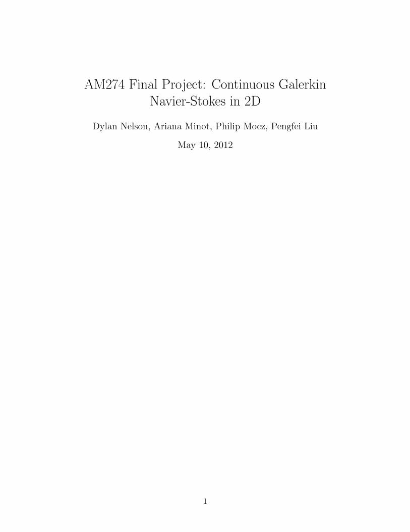
In this test problem, we look at the 2D cross-section flow past a cylinder. We create a mesh asshown in Figure 8. The domain is [0, 4]× [0, 2] with a circle of radius 0.2 centered at (1.5, 1).The mesh has higher resolution in regions we expect the flow to be more complicated, suchas around the cylinder and behind it. The left boundary has parabolic inflow (max velocity1). No-slip boundary conditions are imposed on the top, bottom, and cylinder. Outflow isimposed on the right boundary.

First, we test the time-dependent Navier Stokes solver. We investigate a Reynolds number40 flow. We use the Stokes solution as the initial condition and show the evolution of thefluid (u is plotted) in Figures 9. The fluid adjusts to a steady wake behind the cylinder onthe order of the viscous timescale. The flow is the same as would be obtained by solving thesteady-state Navier Stokes equations with Reynolds number 40. Plots of the pressure andvelocity in the final state are shown in Figures (10)-(12)

We also investigate the forces on the cylinder due to pressure and viscosity as a functionof Reynolds number. Here we consider the forces due to steady state (time-independent)flow. We investigate Reynolds numbers of in the range 0.1–100. The viscous and pressureforces on the cylinder (boundary ∂C) are:

7

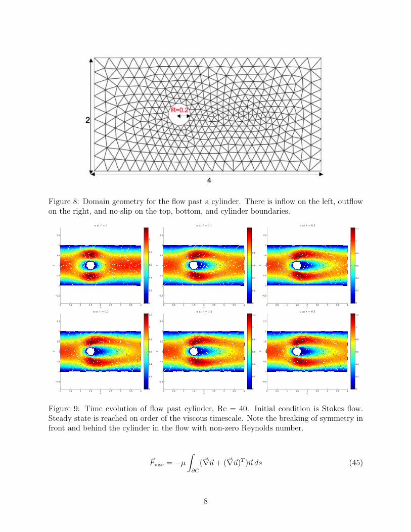
Figure 8: Domain geometry for the flow past a cylinder. There is inflow on the left, outflowon the right, and no-slip on the top, bottom, and cylinder boundaries.

0 0.5 1 1.5 2 2.5 3 3.5 4

−0.5

0

0.5

1

1.5

2

2.5

x

y

u at t = 0

0

0.2

0.4

0.6

0.8

1

0 0.5 1 1.5 2 2.5 3 3.5 4

−0.5

0

0.5

1

1.5

2

2.5

x

y

u at t = 0.1

0

0.2

0.4

0.6

0.8

1

0 0.5 1 1.5 2 2.5 3 3.5 4

−0.5

0

0.5

1

1.5

2

2.5

x

y

u at t = 0.2

0

0.2

0.4

0.6

0.8

1

1.2

0 0.5 1 1.5 2 2.5 3 3.5 4

−0.5

0

0.5

1

1.5

2

2.5

x

y

u at t = 0.3

0

0.2

0.4

0.6

0.8

1

1.2

0 0.5 1 1.5 2 2.5 3 3.5 4

−0.5

0

0.5

1

1.5

2

2.5

x

y

u at t = 0.4

0

0.2

0.4

0.6

0.8

1

1.2

0 0.5 1 1.5 2 2.5 3 3.5 4

−0.5

0

0.5

1

1.5

2

2.5

x

y

u at t = 0.5

0

0.2

0.4

0.6

0.8

1

1.2

Figure 9: Time evolution of flow past cylinder, Re = 40. Initial condition is Stokes flow.Steady state is reached on order of the viscous timescale. Note the breaking of symmetry infront and behind the cylinder in the flow with non-zero Reynolds number.

~Fvisc = −µ

∫

∂C

(~∇~u + (~∇~u)T )~n ds (45)

8

0 0.5 1 1.5 2 2.5 3 3.5 4

−0.5

0

0.5

1

1.5

2

2.5

x

yu

0

0.2

0.4

0.6

0.8

1

1.2

Figure 10: Flow past cylin-der, u solution at Re = 40.

0 0.5 1 1.5 2 2.5 3 3.5 4

−0.5

0

0.5

1

1.5

2

2.5

x

y

v

−0.5

−0.4

−0.3

−0.2

−0.1

0

0.1

0.2

0.3

0.4

0.5

Figure 11: Same as previous,for v solution.

0 0.5 1 1.5 2 2.5 3 3.5 4

−0.5

0

0.5

1

1.5

2

2.5

x

y

p

−10

0

10

20

30

40

Figure 12: Same as previous,for p solution.

~Fpres =

∫

∂C

p(s)~n ds (46)

where ~n is the outward unit normal to the cylinder.These forces can be normalized by the dynamic pressure Pdynamic ∼ 1

2ρV 2

0 . This turns

out to be equivalent to dividing the unitless ~Fvisc and ~Fpres by the global Reynolds number.These normalized values are called drag coefficients, CD.

The pressure and viscous forces are shown in Figure 13 (compare with Figure 1 of Hender-son [1995]). As expected, the pressure force is larger, and both forces decrease with Reynoldsnumber relative to the dynamic pressure. In addition, the drag coefficient CD ∝ Re−1 forRe < 100, shows excellent quantitative agreement with theoretical expectations for a steadywake.

At high Reynolds numbers of Re & 100, instabilities are expected which lead to vortexshedding. This will result in the drag coefficient flattening to ∼ 1. In general this phe-nomenon can be captured by solving the time-dependent flow instead on a high resolutiongrid. We attempted to reproduce this interesting effect with uniform “windtunnel” type flowpast both circular and rectangular obstructions but did not immediately see vortex shedding.The relatively slow performance of our time dependent code prevented any more exhaustiveexploration of the parameter space within which vortex shedding takes place.

4.3 Bifurcated Pipe

In this test problem, we examine flow in symmetric and asymmetric bifurcated pipes. Thegeometries of the two domains are shown in Figures (14) and (15). We specify a parabolicinflow velocity on the left boundary (peak velocity 1), outflow on the right boundaries, andno-slip boundary conditions elsewhere. We compare the steady-state solutions at Re = 10for the symmetric and antisymmetric pipes. Both velocity components and the pressureare plotted in Figures (16)-(21). The outflow boundary conditions enforce that the meanpressure across the outflow boundary is zero, causing the pressure gradient of the shorterpipe branch to be greater [Rannacher,1999]. This results in greater flow going throughthe shorter pipe branch than through the longer pipe branch. Our results reproduce thisexpected behavior. The streamlines are shown for the symmetric pipe at Reynolds number

9

10−2

10−1

100

101

102

103

10−2

10−1

100

101

102

103

Re

Fpres/visc/R

e

Pressure and Viscous Forces vs Reynolds Number

presvisctotaltheory

Figure 13: Steady-wake pressure and viscous forces normalized by the dynamic force on thecylinder as a function of Reynolds number. For Reynolds numbers less than ∼ 100, thesedrag coefficients are expected to be inversely proportional to the Reynolds number.

10 and 100 in Figures (22) and (23). The size of the turbulent region again increases withReynolds number as expected.

5 Concluding Remarks

We have successfully created a CG solver for the Navier-Stokes equations and applied it toseveral test problems. We deliberately looked at problems that are fairly simple and not toocomputationally intensive. Our method can easily be extended to 3D, but would require morecomputational resources. Higher Reynolds number flows require greater mesh resolutiondue to thin-boundary layers that can form, thus requiring more computational power andmemory as well. In addition, a stabilization method such as Streamline Upwind Petrov-Galerkin (SUPG), which introduce extra terms into the weak form to minimize spuriousoscillations in convection-dominated flows, may need to be employed for higher Reynoldsnumber flows.

10

Figure 14: Dimensions of the bifurcated pipesetup.

Figure 15: Dimensions of the asymmetric bi-furcated pipe setup.

0 0.5 1 1.5 2

−0.2

0

0.2

0.4

0.6

0.8

1

1.2

1.4

x

y

0

0.1

0.2

0.3

0.4

0.5

0.6

0.7

0.8

0.9

1

Figure 16: Bifurcated pipeflow u solution at Re = 10.

0 0.5 1 1.5 2

−0.2

0

0.2

0.4

0.6

0.8

1

1.2

1.4

x

y

−0.3

−0.2

−0.1

0

0.1

0.2

0.3

Figure 17: Bifurcated pipeflow v solution at Re = 10.

0 0.5 1 1.5 2

−0.2

0

0.2

0.4

0.6

0.8

1

1.2

1.4

x

y

0

10

20

30

40

50

60

Figure 18: Bifurcated pipeflow p solution at Re = 10.

0 0.5 1 1.5 2 2.5 3

−0.5

0

0.5

1

1.5

2

x

y

0

0.1

0.2

0.3

0.4

0.5

0.6

0.7

0.8

0.9

1

Figure 19: Asymmetric bifur-cated pipe flow u solution atRe = 10.

0 0.5 1 1.5 2 2.5 3

−0.5

0

0.5

1

1.5

2

x

y

−0.2

−0.1

0

0.1

0.2

0.3

0.4

Figure 20: Asymmetric bifur-cated pipe flow v solution atRe = 10.

0 0.5 1 1.5 2 2.5 3

−0.5

0

0.5

1

1.5

2

x

y

0

10

20

30

40

50

60

70

Figure 21: Asymmetric bifur-cated pipe flow p solution atRe = 10.

References

R.D. Henderson. Details of the drag curve near the onset of vortex shedding. Phys. Fluids,7:2102–2104, 1995.

11

0 0.5 1 1.5 20

0.2

0.4

0.6

0.8

1

1.2

1.4

x

y

Figure 22: Backward-facing step streamlinesfor Re = 10.

0 0.5 1 1.5 20

0.2

0.4

0.6

0.8

1

1.2

1.4

x

y

Figure 23: Same as previous, for Re = 100.

Rannacher R. Finite element methods for the incompressible navier-stokes equation, 1999.URL http://numerik.iwr.uni-heidelberg.de/Oberwolfach-Seminar/CFD-Course.pdf.

12