Altimetry and Coastal Currents Ted Strub, John Wilkin, Jerome Bouffard Kristine Madsen, Bill Emery, Luciana Fenoglio And Countless Others

Altimetry and Coastal Currents

Ted Strub, John Wilkin, Jerome Bouffard Kristine Madsen, Bill Emery, Luciana Fenoglio

And Countless Others

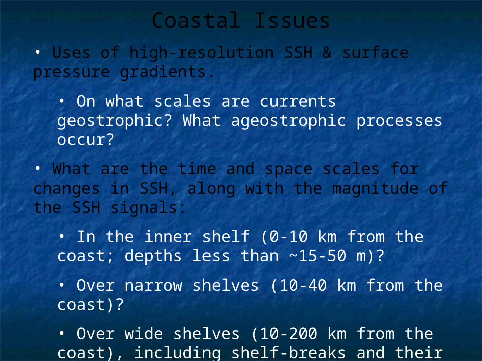
Coastal Issues• Uses of high-resolution SSH & surface pressure gradients.

• On what scales are currents geostrophic? What ageostrophic processes occur?

• What are the time and space scales for changes in SSH, along with the magnitude of the SSH signals:

• In the inner shelf (0-10 km from the coast; depths less than ~15-50 m)?

• Over narrow shelves (10-40 km from the coast)?

• Over wide shelves (10-200 km from the coast), including shelf-breaks and their associated fronts?

• In the “Coastal Transition Zone” (30-500 km from the coast)?

J. Barth

J. Barth

J. Barth

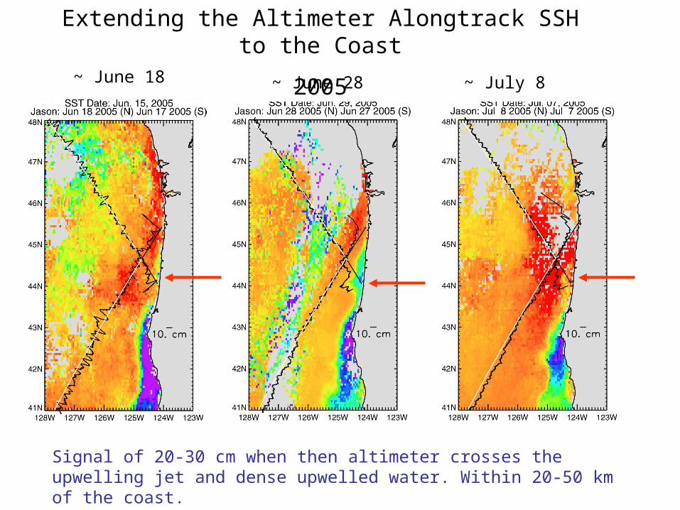
~ June 18 ~ June 28 ~ July 8

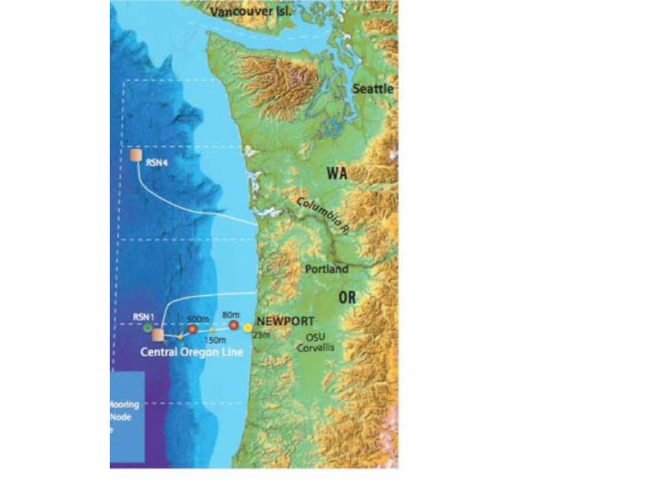
Extending the Altimeter Alongtrack SSH to the Coast

2005

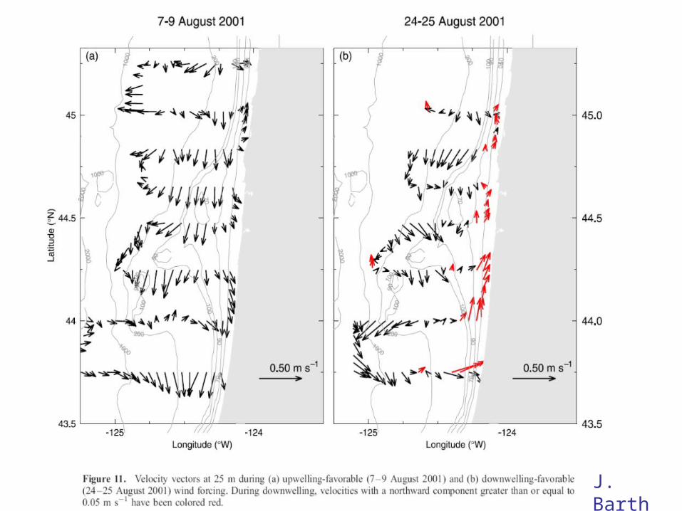
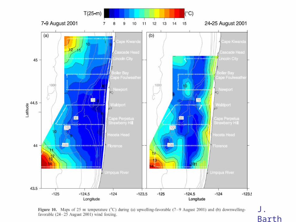
Signal of 20-30 cm when then altimeter crosses the upwelling jet and dense upwelled water. Within 20-50 km of the coast.

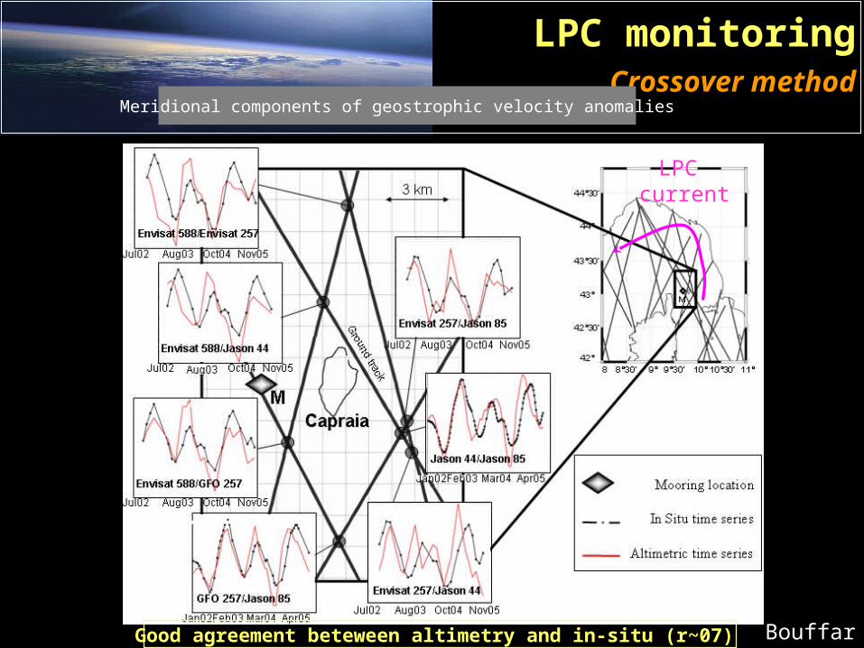
LPC monitoringCrossover method

Meridional components of geostrophic velocity anomalies

LPC current

Good agreement beteween altimetry and in-situ (r~07) Bouffard

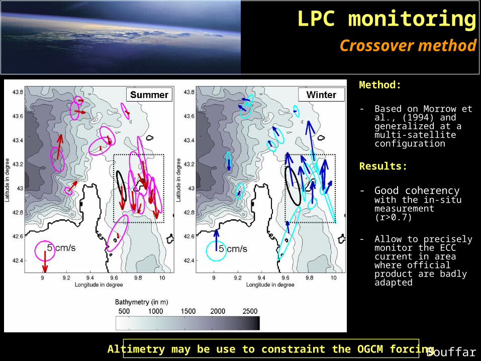
LPC monitoringCrossover method

Currentmeter

Method:

- Based on Morrow et al., (1994) and generalized at a multi-satellite configuration

Results:

- Good coherency with the in-situ measurement (r>0.7)

- Allow to precisely monitor the ECC current in area where official product are badly adapted

Altimetry may be use to constraint the OGCM forcing

Xtrack AVISO

Bouffard

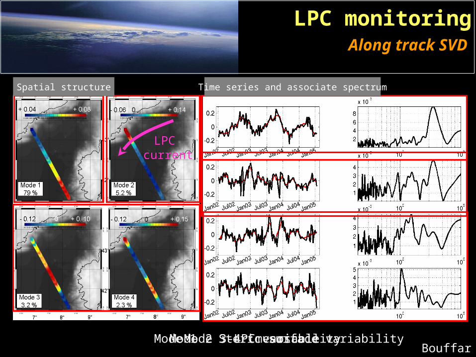
Mode 1 : Steric surface variabilityMode 3-4 :mesoscaleMode 2 : LPC variability

LPC monitoringAlong track SVD

LPC current

Spatial structure Time series and associate spectrum

Bouffard

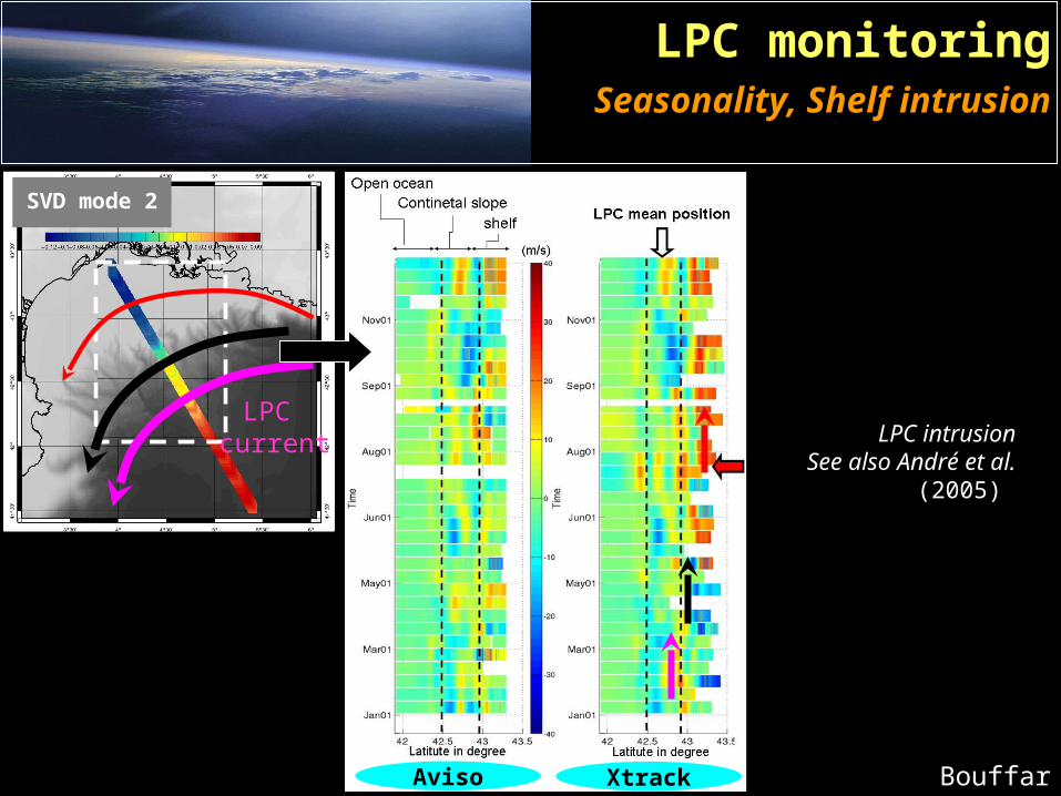
Aviso Xtrack

LPC intrusionSee also André et al.

(2005)

Seasonality, Shelf intrusion

SVD mode 2

LPC monitoring

LPC current

Bouffard

cm/s

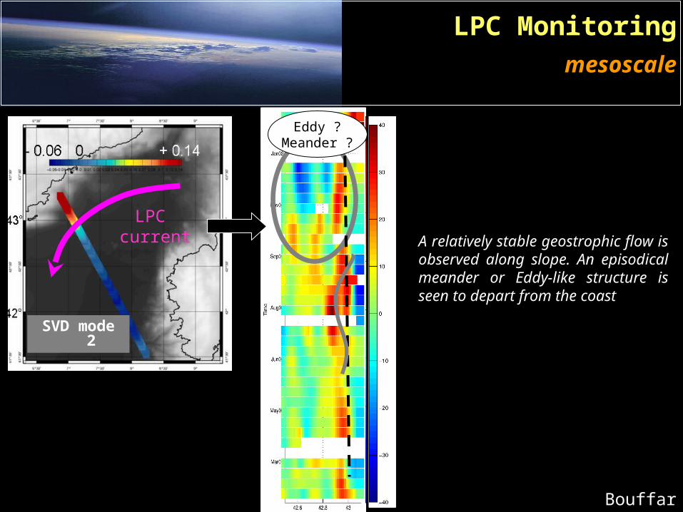
Eddy ?Meander ?

A relatively stable geostrophic flow is observed along slope. An episodical meander or Eddy-like structure is seen to depart from the coast

LPC Monitoringmesoscale

SVD mode 2

LPC current

Bouffard

NIELS BOHR INSTITUTEUNIVERSITY OF COPENHAGEN

Kristine S. Madsen, J. L. Høyer, and C. C. TscherningCenter for Ocean and Ice, Danish Meteorological Institute Niels Bohr Institute, University of Copenhagen


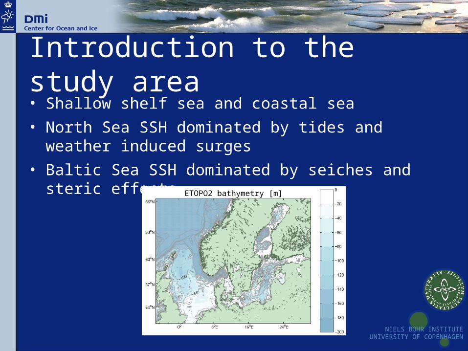
Introduction to the study area• Shallow shelf sea and coastal sea

• North Sea SSH dominated by tides and weather induced surges

• Baltic Sea SSH dominated by seiches and steric effectsETOPO2 bathymetry [m]


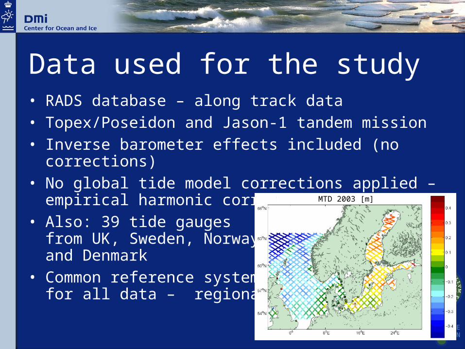
Data used for the study• RADS database – along track data • Topex/Poseidon and Jason-1 tandem mission• Inverse barometer effects included (no corrections)• No global tide model corrections applied – empirical

harmonic correction in North Sea• Also: 39 tide gauges

from UK, Sweden, Norway and Denmark

• Common reference system for all data – regional geoid

MTD 2003 [m]


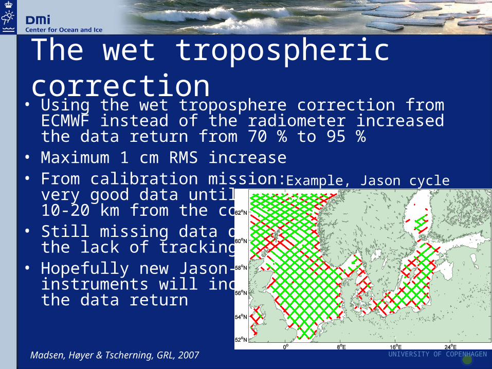
The wet tropospheric correction• Using the wet troposphere correction from ECMWF

instead of the radiometer increased the data return from 70 % to 95 %

• Maximum 1 cm RMS increase• From calibration mission:

very good data until 10-20 km from the coast

• Still missing data due to the lack of tracking

• Hopefully new Jason-2 instruments will increase the data return

Example, Jason cycle 37

Madsen, Høyer & Tscherning, GRL, 2007


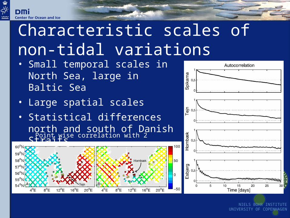
Characteristic scales of non-tidal variations• Small temporal scales in North

Sea, large in Baltic Sea

• Large spatial scales

• Statistical differences north and south of Danish Straits

Point wise correlation with 2 tide gauges


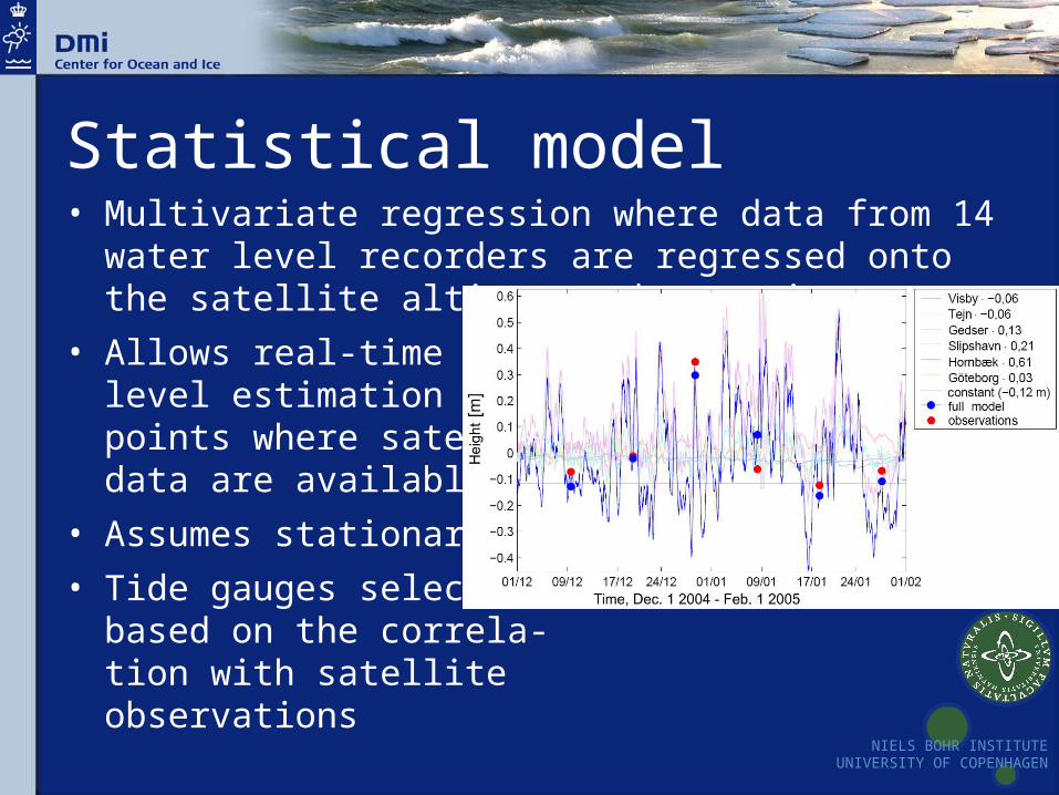
Statistical model• Multivariate regression where data from 14 water level

recorders are regressed onto the satellite altimetry observations

• Allows real-time sea level estimation in points where satellite data are available

• Assumes stationarity

• Tide gauges selected based on the correla-tion with satellite observations


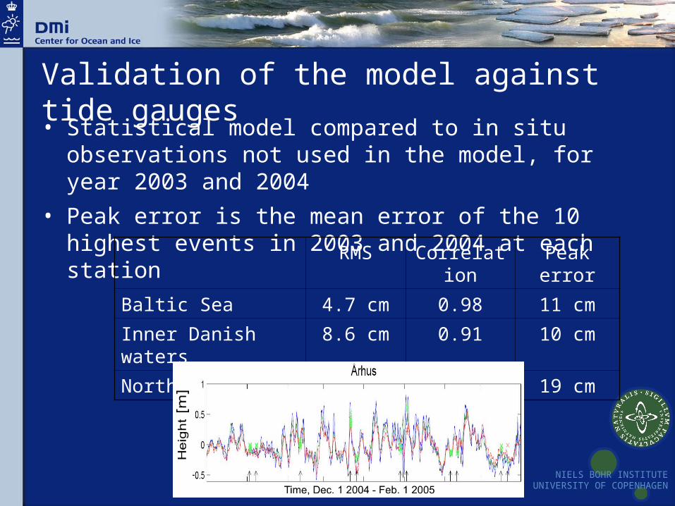
Validation of the model against tide gauges• Statistical model compared to in situ observations not

used in the model, for year 2003 and 2004

• Peak error is the mean error of the 10 highest events in 2003 and 2004 at each station

RMS Correlation Peak error

Baltic Sea 4.7 cm 0.98 11 cm

Inner Danish waters 8.6 cm 0.91 10 cm

North Sea 8.9 cm 0.94 19 cm


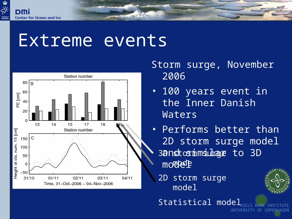
Extreme eventsStorm surge, November 2006

• 100 years event in the Inner Danish Waters

• Performs better than 2D storm surge model and similar to 3D model

3D storm surge mode

2D storm surge model

Statistical model


Summary• We can obtain high quality SSH satellite observations in

the coastal seas of our region.• The use of a model wet tropospheric correction is

important for data return in coastal regions. Still data loss close to the coast (~10-20 km).

• Combination of satellite and tide gauge observations through a statistical model performs well for real time estimation of sea level in the region, even in extreme cases.

• An operational version will be set up at DMI to complement our storm surge models.

• Jason-2 data will hopefully give better data return closer to the coast.

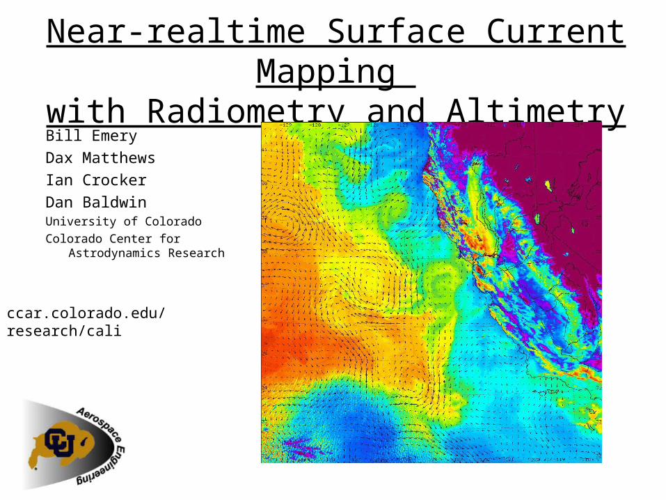
Near-realtime Surface Current Mapping with Radiometry and Altimetry

Bill Emery

Dax Matthews

Ian Crocker

Dan BaldwinUniversity of Colorado

Colorado Center for Astrodynamics Research

ccar.colorado.edu/research/cali

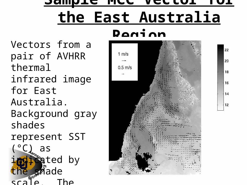
Sample MCC Vector for the East Australia Region

Vectors from a pair of AVHRR thermal infrared image for East Australia. Background gray shades represent SST (°C) as indicated by the shade scale. The vector scale is shown in m/s.

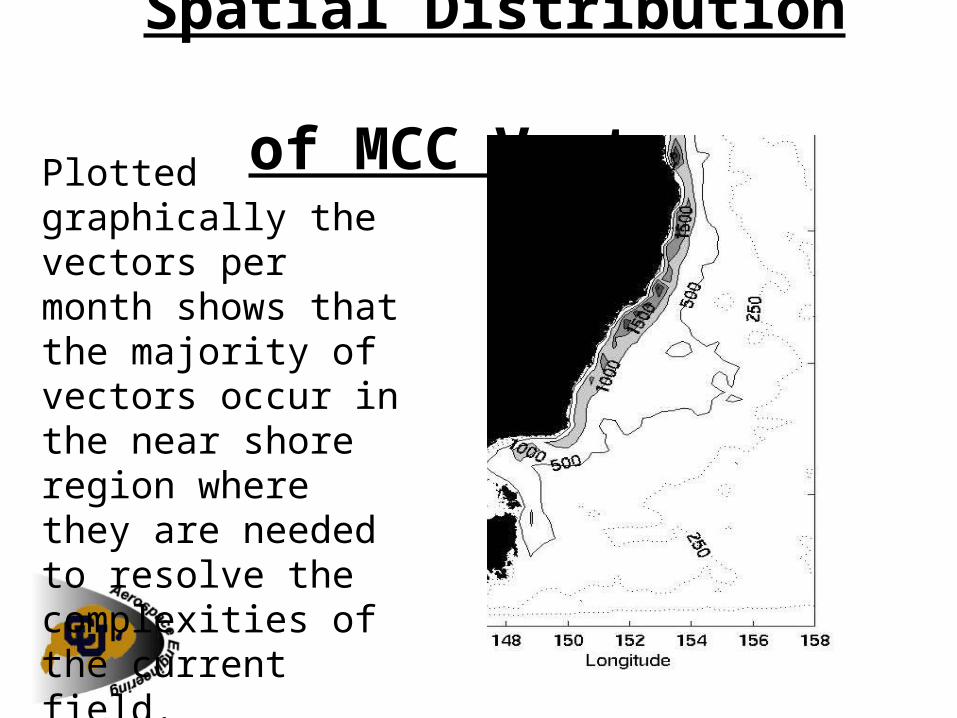
Spatial Distribution of MCC Vectors

Plotted graphically the vectors per month shows that the majority of vectors occur in the near shore region where they are needed to resolve the complexities of the current field.

Blending MCC Vectors and Satellite Altimeter Data

• There are many reasons to merge MCC vectors and geostrophic currents computed from satellite altimetry:

– At present altimeter currents are computed with the mean removed taking out the mean surface current.

– Near the coast where dramatic topography changes occur altimeter data are compromised by gravity and tidal changes.

– The wide track spacing in altimeter data requires a lot of spatial interpolation that can now be replaced with real surface currents.

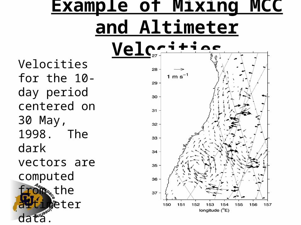
Example of Mixing MCC and Altimeter Velocities

Velocities for the 10-day period centered on 30 May, 1998. The dark vectors are computed from the altimeter data.

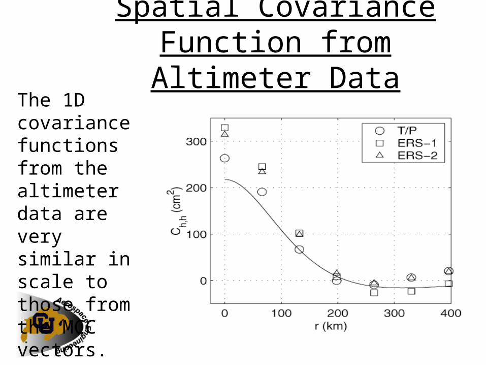
Spatial Covariance Function from Altimeter Data

The 1D covariance functions from the altimeter data are very similar in scale to those from the MCC vectors.

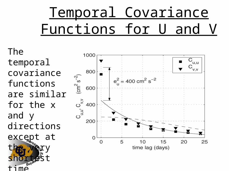
Temporal Covariance Functions for U and V

The temporal covariance functions are similar for the x and y directions except at the very shortest time scales.

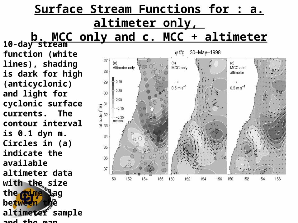
Surface Stream Functions for : a. altimeter only, b. MCC only and c. MCC + altimeter

10-day stream function (white lines), shading is dark for high (anticyclonic) and light for cyclonic surface currents. The contour interval is 0.1 dyn m. Circles in (a) indicate the available altimeter data with the size the time lag between the altimeter sample and the map time.

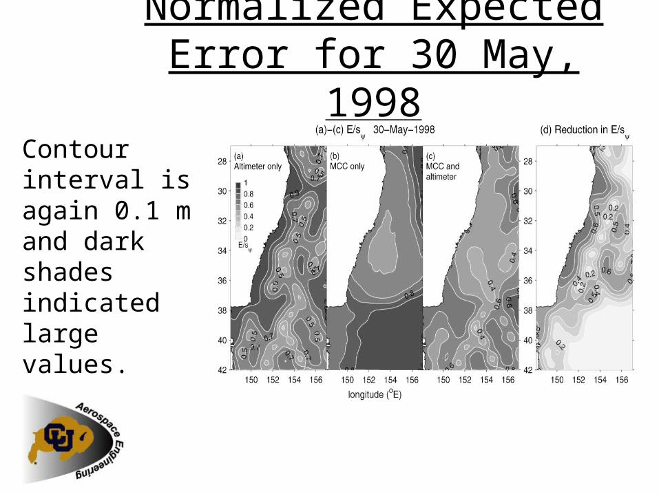
Normalized Expected Error for 30 May, 1998

Contour interval is again 0.1 m and dark shades indicated large values.

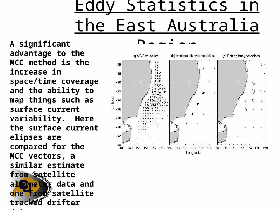
Eddy Statistics in the East Australia Region

A significant advantage to the MCC method is the increase in space/time coverage and the ability to map things such as surface current variability. Here the surface current elipses are compared for the MCC vectors, a similar estimate from satellite altimeter data and one from satellite tracked drifter data.

Coastal currents, eddies and frontal systems

in the Mediterranean Sea and Black Sea

L. Fenoglio, M. Becker Institut für Physikalische Geodäsie, TU

Darmstadt

S. Grayek, E. StanevICBM Universität Oldenburg

Motivation Data Method Results Conclusions

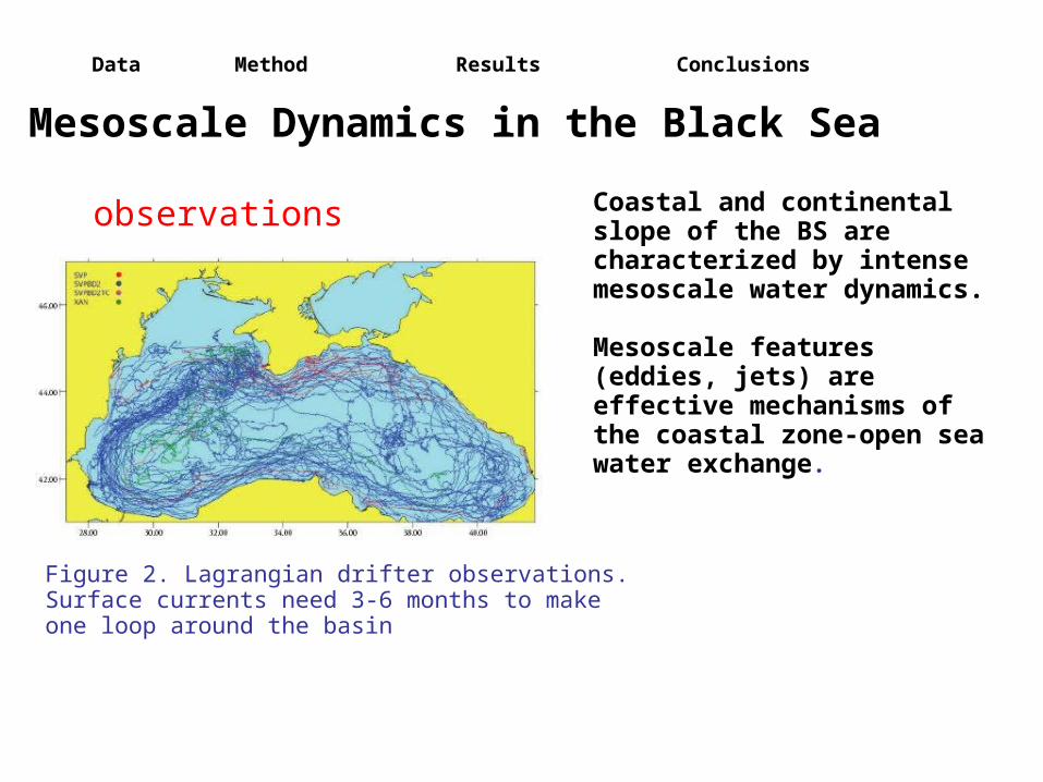
Mesoscale Dynamics in the Black Sea

Coastal and continental slope of the BS are characterized by intense mesoscale water dynamics.

Mesoscale features (eddies, jets) are effective mechanisms of the coastal zone-open sea water exchange.

Figure 2. Lagrangian drifter observations. Surface currents need 3-6 months to make one loop around the basin

observations


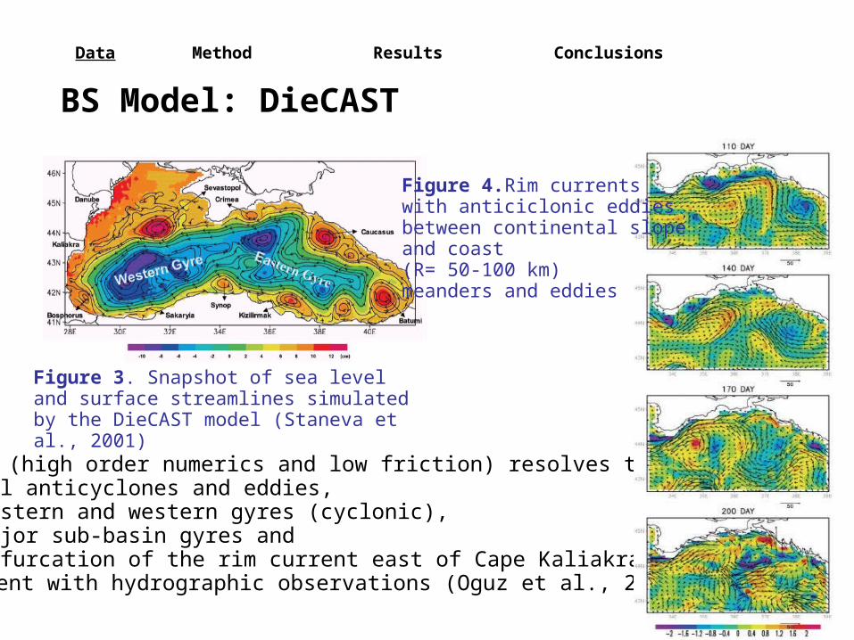
BS Model: DieCAST

The model (high order numerics and low friction) resolves the (1) coastal anticyclones and eddies, (2) the eastern and western gyres (cyclonic), (3) the major sub-basin gyres and (4) the bifurcation of the rim current east of Cape Kaliakra in agreement with hydrographic observations (Oguz et al., 2003).

Figure 3. Snapshot of sea level and surface streamlines simulated by the DieCAST model (Staneva et al., 2001)

Figure 4.Rim currentswith anticiclonic eddies between continental slope and coast(R= 50-100 km)meanders and eddies


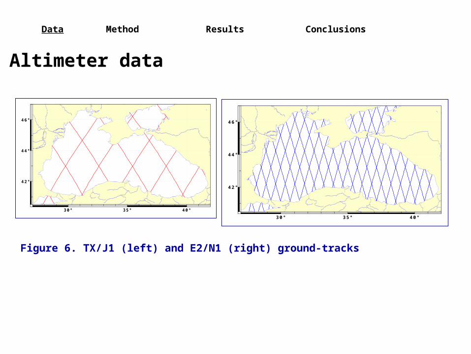
Altimeter data

Figure 6. TX/J1 (left) and E2/N1 (right) ground-tracks

30° 35° 40°

42°

44°

46°

30° 35° 40°

42°

44°

46°


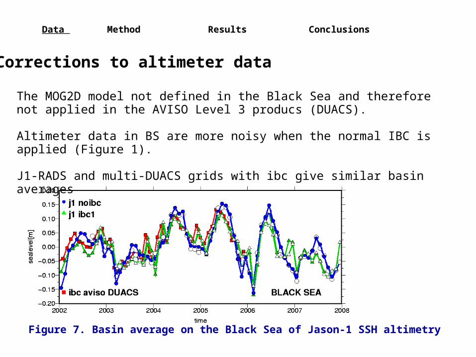
Corrections to altimeter data

Figure 7. Basin average on the Black Sea of Jason-1 SSH altimetry

The MOG2D model not defined in the Black Sea and therefore not applied in the AVISO Level 3 producs (DUACS).

Altimeter data in BS are more noisy when the normal IBC is applied (Figure 1).

J1-RADS and multi-DUACS grids with ibc give similar basin averages


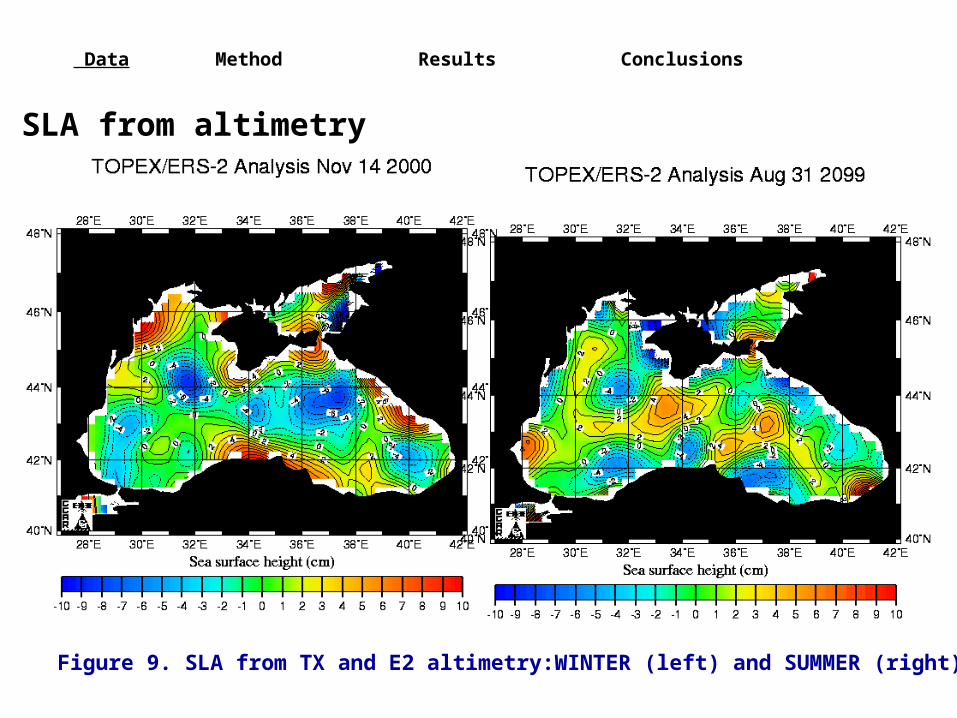
SLA from altimetry

Figure 9. SLA from TX and E2 altimetry:WINTER (left) and SUMMER (right)

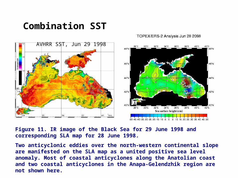
Figure 11. IR image of the Black Sea for 29 June 1998 and corresponding SLA map for 28 June 1998.

Two anticyclonic eddies over the north-western continental slope are manifested on the SLA map as a united positive sea level anomaly. Most of coastal anticyclones along the Anatolian coast and two coastal anticyclones in the Anapa-Gelendzhik region are not shown here.

AVHRR SST, Jun 29 1998

Combination SST

• Large-scale (D= 60-80 km) and closely-spaced coastal anticyclonic eddies in BS

• Ocean models (without altimetry assimilation) distinguish the winter/summer situations

• Coastal large-scale (about 60-80 km in diameter) and closely-spaced anticyclonic eddies not distinguished on the SLA maps as individual features.

• Coastal currents and small-scale eddy features are not manifested on the SLA

• In the deep-sea basin, the SLA maps provide reliable information on large and intense anticyclonic eddies


CONCLUSION

• OPEN points:

• Corrections : Ibc correction im BS is not optimal. Has it an effect on model results that assimilate altimeter data?

I.e. which altimetry data should be assimilated in ocean models

(with or without IBC if IBC is correct)?

• Resolution of altimeter grids. Which is the minimum required?

• Data near coast: lack of altimeter data near to coast

Overall:

• Coastal altimetry


OUTLOOK

Documents

Altimetry and Coastal Currents Ted Strub, John Wilkin, Jerome Bouffard Kristine Madsen, Bill Emery, Luciana Fenoglio And Countless Others