1

Alternatives to Subjective Expected Utility:

Ambiguity Aversion (MEU), Capacities (CEU), and Smooth Ambiguity Aversion (SAA)

The observed behavior in the Ellsberg paradox led many scholars to suggest that individuals have ambiguous (unclear) beliefs, rather than objective or subjective beliefs as previous theories considered. In order to allow for such ambiguity, and to explain the Ellsberg paradox, the literature has offered alternative theories. Given their importance and subsequent use in applications, we next present three of them: expected utility theory with multiple priors (also referred to as maxmin expected utility, MEU), rank-dependent expected utility (or Choquet expected utility, CEU), and smooth ambiguity aversion (SAA). In our discussion, we let F denote an act :F S X→ from the set of states to the set of outcomes (which can be monetary payoffs or any other prize).

1.1 Maxmin Expected Utility (MEU)

Following Gilboa and Schmeidler (1989), consider a setting where subjects have too little information to form their priors, and allow the subjects to consider a set of priors. Now, if an individual is uncertainty averse (to be defined below), he will choose lottery F over another lottery G if the former provides a higher expected utility than the latter according to a worst possible prior. In this context, Gilboa and Schmeidler replaced the IA with their “uncertainty aversion” axiom and their “certainty-independence” axiom, which we define next.

Uncertainty Aversion. Consider an individual who is indifferent between two lotteries F and G . Then he is uncertainty averse if he weakly prefers the compound lottery (1 )F Gα α+ − to simple lottery G , where

(0,1)α ∈ .

Intuitively, a decision maker who is uncertainty averse has a preference for mixing (or hedging), since the compound lottery becomes at least as valuable as either of the two lotteries alone.1 In particular, that may occur when the two acts have negatively correlated payoffs, so their mixture yields a more even payoff distribution across states.2 Let us next define the second axiom, certainty independence, which weakens the IA.

Certainty Independence. For any two lotteries F and G and a constant act K (e.g., a certain outcome, or a lottery that remains constant across all states), the decision maker weakly prefers lottery F to G if and only if he prefers (1 )F Kα α+ − to (1 )G Kα α+ − , where (0,1)α ∈ .

1 The standard IA is actually a special case of the uncertainty aversion axiom if we restrict the decision maker to exhibit indifference between the compound lottery and the simple lotteries. Indeed, if the individual is indifferent between F and G, then by the IA he is also indifferent between (1 )F Gα α+ − and (1 )G Gα α+ − , that is, between

(1 )F Gα α+ − and G ; thus becoming a special case of the above definition of uncertainty aversion. 2 Intuitively, think about two investments, one being attractive when the economy grows (e.g., shares of a diamond company, or luxury cars) and another when the economy enters a crisis (e.g., shares of a dollar store). If you are indifferent between both of them, you might prefer their mixture rather than one of the two shares alone.

2

Note that the certainty-independence axiom relaxes the IA as it only requires that preferences over two lotteries F and G be unaffected when each lottery is mixed with a certain outcome K (rather than when mixed with a third lottery, as required by the IA). In other words, certainty independence can be understood as a special case of the IA, where the third lottery has degenerate probability distribution, thus describing an outcome that occurs with certainty. Importantly, when we replace the IA with uncertainty aversion and certainty independence, we obtain a nice utility representation of preferences that allows for the possibility of the individual decision maker sustaining multiple prior beliefs. In particular, a decision maker weakly prefers lottery F to G if and only if (i.e., it is equivalent to)

( )( ) ( ) ( )( )min min ( )p C p C

S S

u F s dp s u G s dp s∈ ∈

≥ ∫∫ .

That is to say, the individual decision maker first evaluates the expected utility of lotteries F and G according to each of his multiple priors p C∈ ; he then identifies the prior that yields the lowest expected utility when playing lottery F , and similarly for lottery G ; last, he selects the lottery with the highest expected utility. Intuitively, he separately evaluates each lottery at his worst possible prior, and then chooses the lottery yielding the highest expected utility, which explains why this approach is also referred to as “maxmin expected utility,” or MEU. (For a proof of this expected utility representation result, see Gilboa and Schmeidler (1989), pp. 145–49); or the more didactic presentation in Ok (2007)’s textbook, pp. 513–19).

Example 1: Ambiguity aversion Consider a decision maker with Bernouilli utility function ( )u x x= ,

where 0x ≥ denotes monetary amounts. Assume that he faces two lotteries ($1, $100)AL = and

($3, $5)BL = , and allow the decision maker to hold priors ( ),1A Ap p− for lottery AL , and ( ),1B Bp p−

for lottery BL . According to MEU, he chooses lottery BL if

min 3 (1 ) 5 min 1 (1 ) 100B A

B B A Ap pp p p p + − ≥ + − .

For instance, priors are left unrestricted if the decision maker does not have any available information with which to update his priors, so they can take values , [0,1]A Bp p ∈ . In this setting, it is possible that his most pessimistic belief is that by which he receives the lowest monetary amount with probability one in both lotteries, implying that in lottery BL ,

min 3 (1 ) 5 3B

B Bpp p + − =

with argmin 1Bp = , and similarly for lottery AL ,

min 1 (1 ) 100 1A

A App p + − =

3

with argmin 1Ap = . Hence a decision maker with MEU preferences selects lottery BL because 3 1> . Note that such a choice is somewhat extreme, as the decision maker first focuses on the worst-case scenario within each lottery, and then selects the lottery that provides the best worst-case scenario. Next we will show that the Ellsberg paradox, despite not being rationalized by subjective probability theory, can be explained if the decision maker exhibits MEU preferences. Recall from the Ellsberg paradox that gamble A (B) rewards the individual with $1,000 if the ball he extracts is red (blue, respectively). While the proportion of red balls in the urn is known, 1/3, the decision maker does not receive any information about the number of blue balls. Hence an individual with MEU preferences finds

( ) 1 ($1,000)3

U A u= and ( ) min ($1,000)Blue

BluepU B p u= .

Thus, if the individual selects gamble A, as required by the Ellsberg paradox, he reveals that pBlue satisfies

1 min 3 Blue

Bluepp> , (1)

where the right-hand side indicates the worst possible prior among all those considered by the decision maker. A similar argument applies for gamble C (extracting a ball that is not red) and gamble D (extracting a ball that is not blue), where

( ) 2 ($1,000)3

U C u= and ( )

min ($1,000)Not Blue

Not BluepU D p u= .

Hence, if the decision maker selects gamble C, as described in the Ellsberg paradox, he reveals that

2 min 3 Not Blue

Not Bluepp> . (2)

Conditions (1) and (2) are compatible, since

min 1 min

Blue Not BlueBlue Not Bluep p

p p≠ − ,

can easily occur. For instance, if the decision maker has two possible priors (pBlue, pNot Blue)=(0.1,0.9) and (0.4,0.6), the lowest prior pBlue is min{0.1,0.4min } 0 1 .

BlueBluep

p = = , while the lowest for pNot Blue is

min{0.9,0.6} 0.min 6

Not BlueNot Bluep

p = = , entailing that

min 1 min Blue Not Blue

Blue Not Bluep pp p≠ − since 0.1 0.6≠ .

Hence the Ellsberg paradox can be explained according to MEU.

4

1.2 Choquet Expected Utility (CEU)

Schmeidler (1989) provided an alternative theory to account for the anomaly in the Ellsberg paradox by defining beliefs with the use of capacities. Specifically, a capacity is defined as a real-valued function ( )v ⋅

from a subset of the state space S to [0, 1], with the normalization ( ) 0v ∅ = and ( ) 1v S = . In addition, we say that capacity ( )v ⋅ satisfies comonotonicity if ( ) ( )v A v B≥ , where A is a superset of ;B in words, the probability weight assigned to the larger set A cannot be smaller than that assigned to its subset B . While a probability distribution assigns weights that are additive across two mutually exclusive events, such as

,a b S∈ (their probabilities are additive), their capacities allow for nonadditivity. For instance, if

{ },S a b= , then an example of a capacity is ( ) 0v ∅ = , ( ) 0.4v a = , ( ) 0.5v b = , and ( ), 1v a b = , where

( ) ( ) ( ),v a v b v a b+ ≠ . In this context, we cannot simply use a standard integral over states, since capacity ( )v ⋅ does not correspond to our notion of beliefs. However, Choquet (1953) developed integrals specifically for capacities, which Schmeidler (1989) used in his representation result. In particular, a decision maker weakly prefers F to G if the Choquet integrals satisfy

( )( ) ( ) ( )( ) ( )S S

u F S dv S u G S dv S≥∫ ∫ .

Moreover the CEU and MEU models are connected if we impose the uncertainty aversion axiom in this CEU context. In order to do that, we first need that capacity ( )v ⋅ satisfies supermodularity (also referred to as complementarity in this context), in the sense that the marginal contribution of a subset of events B is larger when it joins a large set of events A than when it joins a small set C . To see this, let us take two sets A and C , where C is a subset of A , that is, C A⊂ . In this context, the marginal contribution of B to the large set A is larger than its marginal contribution to the small group C :

( ) ( )( ) ( )v A B v A v C B v B− ≥ −∪ ∪ ,

where A and B do not intersect, 𝐴𝐴⋂𝐵𝐵 = ∅. 3

Example 2: Simple capacities While the use of Choquet integrals is involved, the literature often uses “simple” capacities. Intuitively, a simple capacity on state space S can be understood as a convex combination between two extreme capacities: (1) a standard probability weight on A , ( ) [0,1]p A ∈ , which

3 Schmeidler (1986) showed that CEU and MEU are mathematically related. In particular, the Choquet integral of 𝐹𝐹 with respect to a supermodular capacity v coincides with the evaluation of F according to MEU when the decision maker’s priors belong to the core of capacity v.

5

is a capacity with additive probabilities; and (2) the “complete ignorance” capacity w , which assigns ( ) 1w S = and ( ) 0w A = for every A S⊆ . (In other words, in w the decision maker assigns a zero

probability weight to all events, except to the entire state space S .) Formally, simple capacities are then defined as

( ) ( ) (1 ) ( )v A p A w Aλ λ= + −

for every A S⊆ and where [0,1]λ∈ . In this context, parameter λ denotes the individual’s degree of

confidence on ( )p A , while 1 λ− captures his “degree of ambiguity” about ( )p A (also referred to as his “degree of uncertainty aversion”). For applications of simple capacities to noncooperative games, see Haller (2000), and to common pool resources, see Aflaki (2013).

1.3 Smooth Ambiguity Aversion (SAA)

Klibanoff (2005) offered a framework that accounts for observed behavior in the Ellsberg paradox while achieving separation between ambiguity (defined as the decision maker considering multiple priors) and his ambiguity attitude (a reflection of the decision maker’s taste).4 A decision maker weakly prefers lottery F to G if and only if

( )( ) ( ) ( )( ) ( )( ) ( )p S p S

u F s dp s d p u G s dp s d pφ µ φ µ

≥

∫ ∫ ∫ ∫ .

That is to say, the individual decision maker, first, evaluates the expected utility of lottery F for each prior p C∈ ; and second, he aggregates using prior µ over each of his multiple priors p C∈ given the

increasing function ( )φ ⋅ . Performing a similar calculation for lottery G , he can choose the lottery with the highest expected value. Intuitively, priors µ capture the ambiguity the decision maker faces, as a more concentrated support of µ indicates that he does not face much ambiguity on the possible priors p C∈ . In the extreme, when µ is degenerate on a single prior p , the SAA model reduces to the standard EU model.

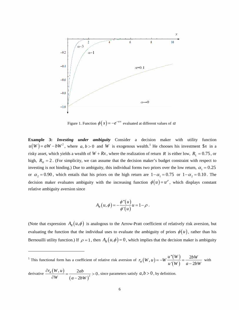
Moreover the shape of function ( )φ ⋅ captures his attitude toward ambiguity. For example, if ( ) xx e αφ −= − ,

parameter α describes the concavity of the function, as depicted in figure 1. When 0α → , function ( ) 1xφ → − for every prior p , assigning the same weight on all priors. However, when α increases, so

does the concavity of function ( )xφ , assigning a zero probability weight on a larger support of priors. In the

limit, when α →∞ , function ( ) 0xφ → for all priors, expect for the lowest (i.e., the prior corresponding to the worst case scenario); indicating that in such limiting case SAA collapses to the MEU model we discussed above.

4 Thanks to PhD candidate Casey Bolt for his suggestions in this subsection, especially in example 3.

6

Figure 1. Function ( ) xx e αφ −= − evaluated at different values of α

Example 3: Investing under ambiguity Consider a decision maker with utility function ( ) 2u W aW bW= − , where , 0a b > and W is exogenous wealth.5 He chooses his investment $x in a

risky asset, which yields a wealth of W Rx+ , where the realization of return R is either low, 0.75LR = , or high, 2HR = . (For simplicity, we can assume that the decision maker’s budget constraint with respect to investing is not binding.) Due to ambiguity, this individual forms two priors over the low return, 1 0.25α = or 2 0.90α = , which entails that his priors on the high return are 11 0.75α− = or 21 0.10α− = . The

decision maker evaluates ambiguity with the increasing function ( )u uρφ = , which displays constant relative ambiguity aversion since

( ) ( )( )

'', 1

'R

uA u u

uφ

φ ρφ

= − = − .

(Note that expression ( ),RA u φ is analogous to the Arrow-Pratt coefficient of relatively risk aversion, but

evaluating the function that the individual uses to evaluate the ambiguity of priors ( )uφ , rather than his

Bernouilli utility function.) If 1ρ = , then ( ), 0RA u φ = , which implies that the decision maker is ambiguity

5 This functional form has a coefficient of relative risk aversion of ( ) ( )

( )'' 2,' 2R

u W bWr W u Wu W a bW

= − =−

with

derivative ( )( )2

, 2 02

Rr W u abW a bW

∂= >

∂ −, since parameters satisfy , 0a b > , by definition.

7

neutral while he can still exhibit risk aversion. As ρ decreases, relative ambiguity aversion increases, so for 1ρ < the individual is ambiguity averse. If instead 1ρ > , the decision maker is ambiguity loving.

Assuming that the individual places equal weight on his priors 1α or 2α being correct, his problem becomes

( ) ( ) ( ) ( )1 1 2 2max 0.5 ; (1 ) ; 0.5 ; (1 ) ;L H L Hxu x R u x R u x R u x R

ρ ρα α α α + − + + − .

We can now plug in parameters 1, α 2 ,α and utility function ( )u ⋅ . For simplicity, we also consider

parameters 10, 1, 0.5a b ρ= = = , and wealth 1W = (so that the low return 0.75LR = entails a 25 percent loss on every dollar invested in the asset). The above problem becomes

( ) ( ) ( ) ( )0.52 2max 0.5 2.5 1 0.75 0.25 1 0.75 75 1 2 0.75 1 2

xx x x x + − + + + − +

( ) ( ) ( ) ( )0.52 20.5 9 1 0.75 0.9 1 0.75 1 2 0.1 1 2x x x x + + − + + + − + .

Taking first-order condition with respect to x yields

[ ] [ ]( ) ( ) 0.519.375 0.125 1.5 1.125 7.5 0.375 4 8 ;x x Eu x α −− + + − +

[ ] [ ]( ) ( ) 0.5233.75 0.45 1.5 1.125 1 0.05 4 8 ; 0x x Eu x α −+ − + + − + = .

And solving for x , we obtain an investment of 2.3.x ≈ If we replicate this problem for a ambiguity neutral individual, where 1ρ = , we find a higher investment of 2.53.x ≈ Thus ambiguity aversion reduces his investment in the risky asset.

Further reading The preceding two models have been used in many applications. Dow and Werlang (1992) consider individuals with supermodular capacities in the CEU framework analyzed above to show that individuals do not have incentives to buy or sell assets for a potentially large range of prices. A similar finding emerged in variations on the model developed by Epstein and Wang (1994) and Uppal and Wang (2003). The multiple priors model in MEU has also been applied to labor economics by Nishimura and Ozaki (2004), and to macroeconomic policy by Hansen et al. (1999) and Hansen and Sargent (2001, 2008). For a detailed review of the different models proposed in this literature that build on MEU and CEU, see Machina and Siniscalchi (2014), and for an extensive survey of applications of these models to economics and finance, see Mukenji and Tallon (2004). Last, the preceding models have been recently tested in experimental labs, providing evidence of support for MEU and CEU in certain contexts, but relatively more consistent evidence that supports prospect theory; see Abdellaoui et al. (2014), Baillon, and Bleichrodt (2015), and Dimmock et al. (2015).