Alternative Measures of Replacement Rates

Michael D. Hurd RAND and NBER

Susann Rohwedder RAND

We gratefully acknowledge research support from the Social Security Administration via the Michigan Retirement Research Center, and additional support from the National Institute on Aging.

2

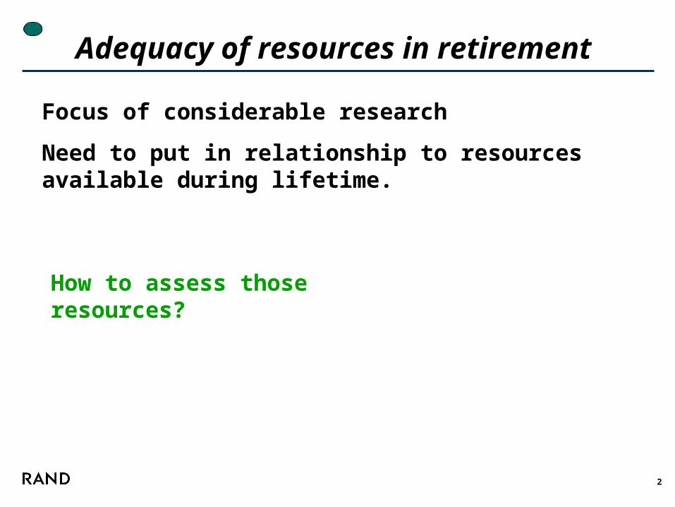
Adequacy of resources in retirement

Focus of considerable research

Need to put in relationship to resources available during lifetime.

How to assess those resources?

3

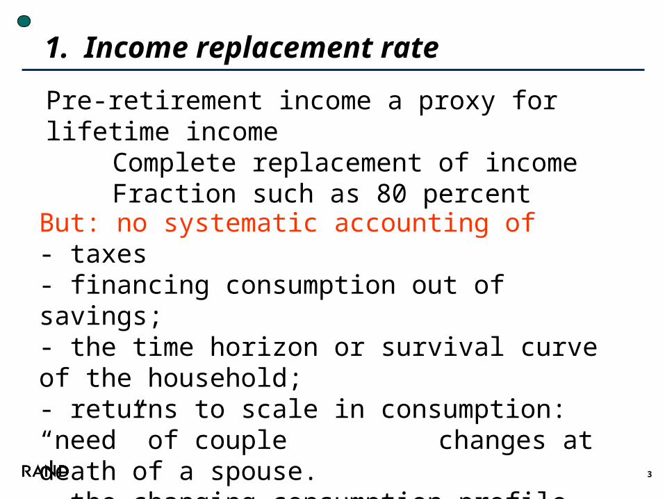
1. Income replacement rate

Pre-retirement income a proxy for lifetime incomeComplete replacement of income Fraction such as 80 percent

But: no systematic accounting of - taxes - financing consumption out of savings; - the time horizon or survival curve of the household; - returns to scale in consumption: “need” of couple

changes at death of a spouse.- the changing consumption profile with age;

4

How to assess adequacy?

2. Estimate lifetime income. Compare accumulated wealth with “optimal” wealth

Hard to do

3. Can resources at retirement maintain consumption?

or consumption path…consumption not necessarily constant

5

- Observe someone at 65 consuming at some initial level

- Have theoretically or empirically derived consumption path

- Ask: can resources support that path?

Examples

Our Method

6

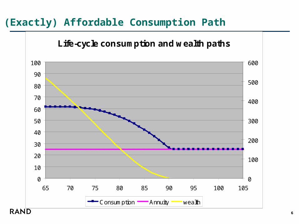
(Exactly) Affordable Consumption Path

Life-cycle consumption and wealth paths

0

10

20

30

40

50

60

70

80

90

100

65 70 75 80 85 90 95 100 105

0

100

200

300

400

500

600

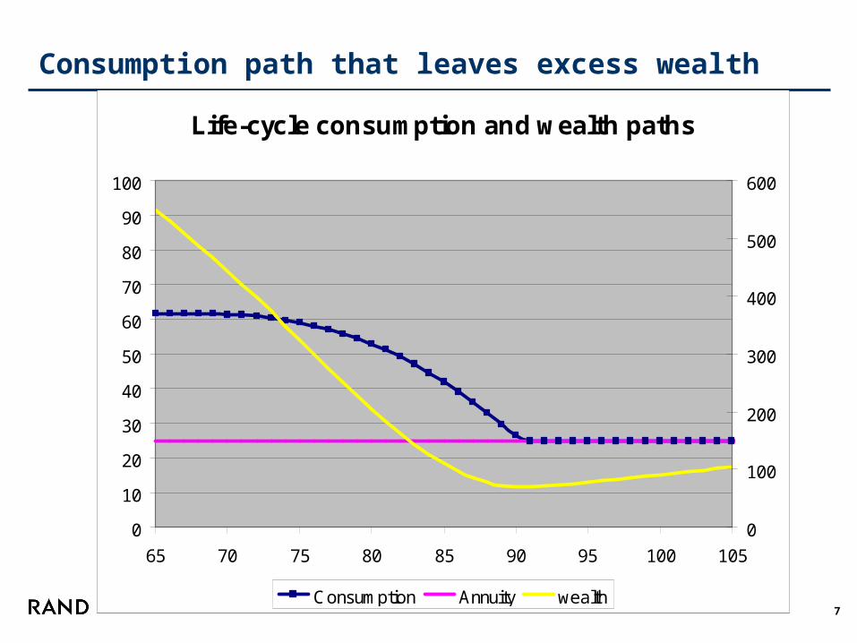
Consumption Annuity wealth

7

Consumption path that leaves excess wealth

Life-cycle consumption and wealth paths

0

10

20

30

40

50

60

70

80

90

100

65 70 75 80 85 90 95 100 105

0

100

200

300

400

500

600

Consumption Annuity wealth

8

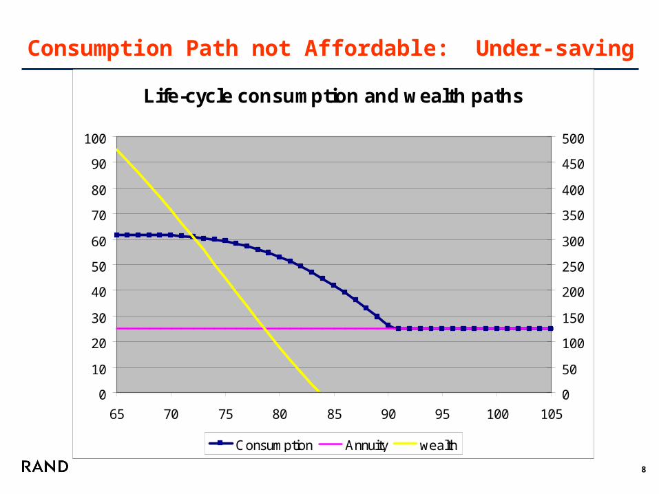
Consumption Path not Affordable: Under-saving

Life-cycle consumption and wealth paths

0

10

20

30

40

50

60

70

80

90

100

65 70 75 80 85 90 95 100 105

0

50

100

150

200

250

300

350

400

450

500

Consumption Annuity wealth

9

Consumption and Activities Mail Survey (CAMS)

October, 2001, CAMS wave 1 5,000 HRS households (random selection)Couples: one of two spouses at random.3,866 returned questionnaires:

unit response rate of 77.3 percent.Low rate of item nonresponseSpending measure close to spending in Consumer Expenditure Survey

October, 2003, CAMS wave 1Sent to same householdsSubstantially same as CAMS wave 1

Use change in consumption to generate life-cycle paths

10

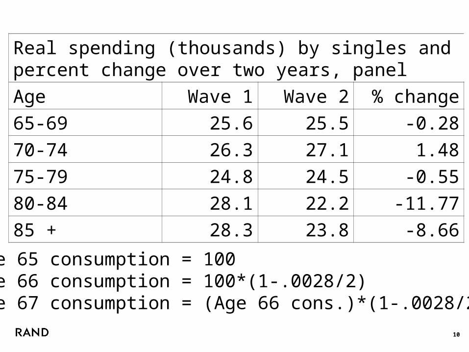
Real spending (thousands) by singles and percent change over two years, panel

Age Wave 1 Wave 2 % change

65-69 25.6 25.5 -0.28

70-74 26.3 27.1 1.48

75-79 24.8 24.5 -0.55

80-84 28.1 22.2 -11.77

85 + 28.3 23.8 -8.66

Age 65 consumption = 100Age 66 consumption = 100*(1-.0028/2)Age 67 consumption = (Age 66 cons.)*(1-.0028/2)

11

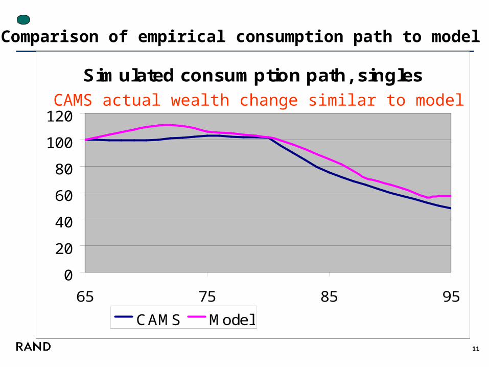
Comparison of empirical consumption path to model

Simulated consumption path, singles

0

20

40

60

80

100

120

65 75 85 95

CAMS Model

CAMS actual wealth change similar to model

12

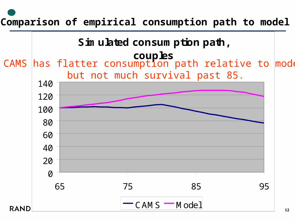
Comparison of empirical consumption path to model

Simulated consumption path, couples

0

20

40

60

80

100

120

140

65 75 85 95

CAMS Model

CAMS has flatter consumption path relative to model;but not much survival past 85.

13

Add data from Health and Retirement Study core

Waves 2000, 2002 & 2004- work status- wealth- Social Security and pension income

14

Choice of sample

Want:Observe all resources

bequeathable wealthSocial SecurityPension income(Future earnings)

Singles 66-69, N = 210

Couples 66-69, not working, and spouse 62 or olderN = 282.

15

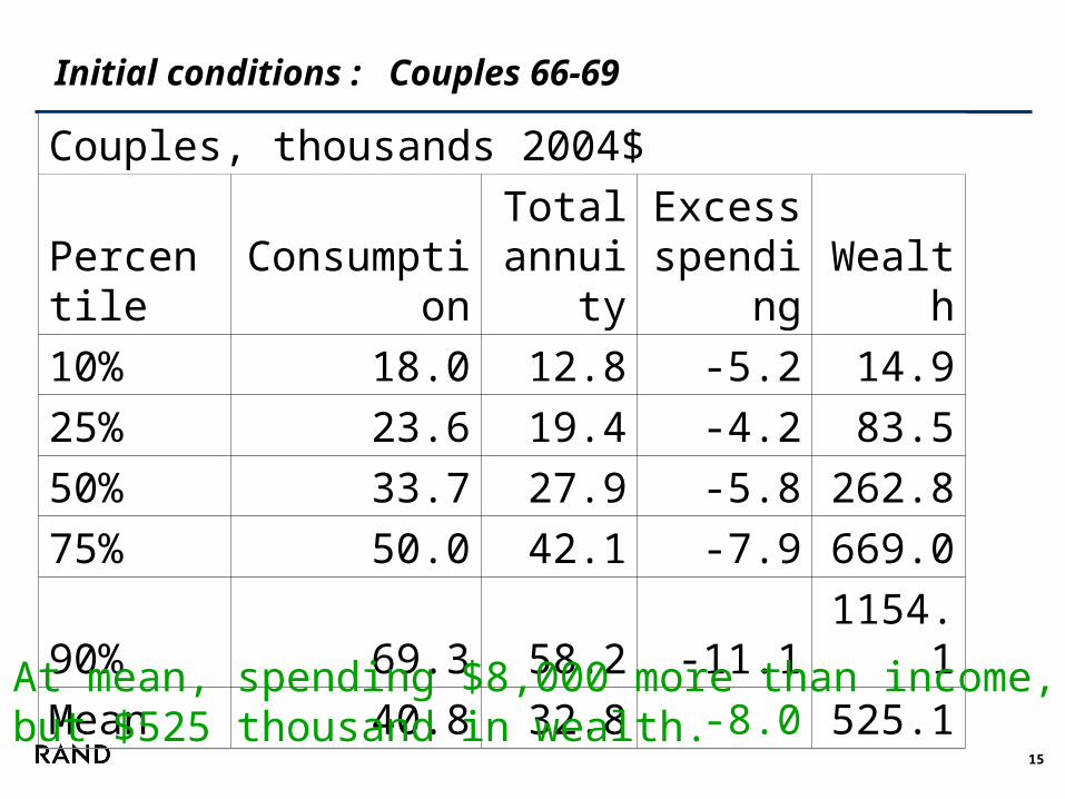
Initial conditions : Couples 66-69

Couples, thousands 2004$

Percentile ConsumptionTotal

annuityExcess

spending Wealth

10% 18.0 12.8 -5.2 14.9

25% 23.6 19.4 -4.2 83.5

50% 33.7 27.9 -5.8 262.8

75% 50.0 42.1 -7.9 669.0

90% 69.3 58.2 -11.1 1154.1

Mean 40.8 32.8 -8.0 525.1At mean, spending $8,000 more than income, but $525 thousand in wealth.

16

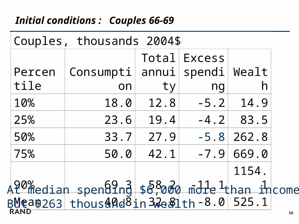
Initial conditions : Couples 66-69

Couples, thousands 2004$

Percentile ConsumptionTotal

annuityExcess

spending Wealth

10% 18.0 12.8 -5.2 14.9

25% 23.6 19.4 -4.2 83.5

50% 33.7 27.9 -5.8 262.8

75% 50.0 42.1 -7.9 669.0

90% 69.3 58.2 -11.1 1154.1

Mean 40.8 32.8 -8.0 525.1At median spending $6,000 more than incomeBut $263 thousand in wealth

17

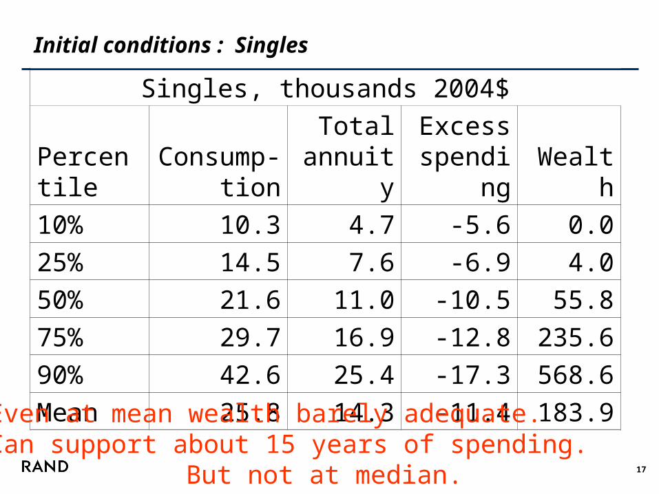
Initial conditions : Singles

Singles, thousands 2004$

PercentileConsump-

tionTotal

annuityExcess

spending Wealth

10% 10.3 4.7 -5.6 0.0

25% 14.5 7.6 -6.9 4.0

50% 21.6 11.0 -10.5 55.8

75% 29.7 16.9 -12.8 235.6

90% 42.6 25.4 -17.3 568.6

Mean 25.8 14.3 -11.4 183.9Even at mean wealth barely adequate. Can support about 15 years of spending.

But not at median.

18

Simulations from initial conditions

Singles

Begin with observed consumption

Follow consumption path of singles

Real annuities (Social Security) and nominal annuities (pension income)

Random mortality from life-table.

Importance: don’t need resources to last forever

Example…

19

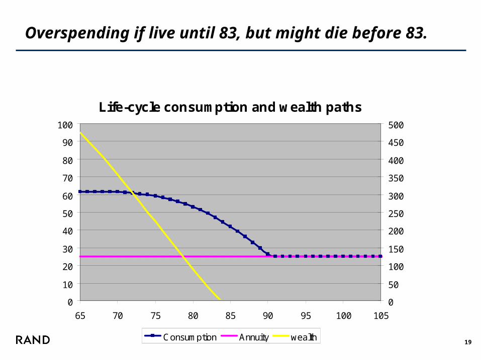
Life-cycle consumption and wealth paths

0

10

20

30

40

50

60

70

80

90

100

65 70 75 80 85 90 95 100 105

0

50

100

150

200

250

300

350

400

450

500

Consumption Annuity wealth

Overspending if live until 83, but might die before 83.

20

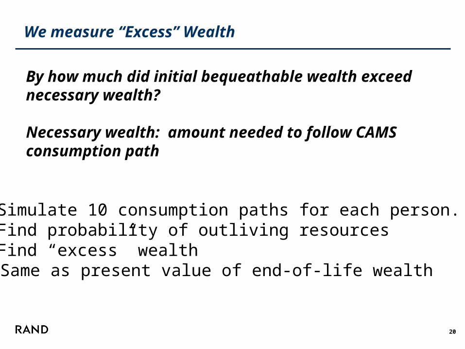
We measure “Excess” Wealth

By how much did initial bequeathable wealth exceed necessary wealth?

Necessary wealth: amount needed to follow CAMS consumption path

- Simulate 10 consumption paths for each person.- Find probability of outliving resources- Find “excess” wealth

Same as present value of end-of-life wealth

21

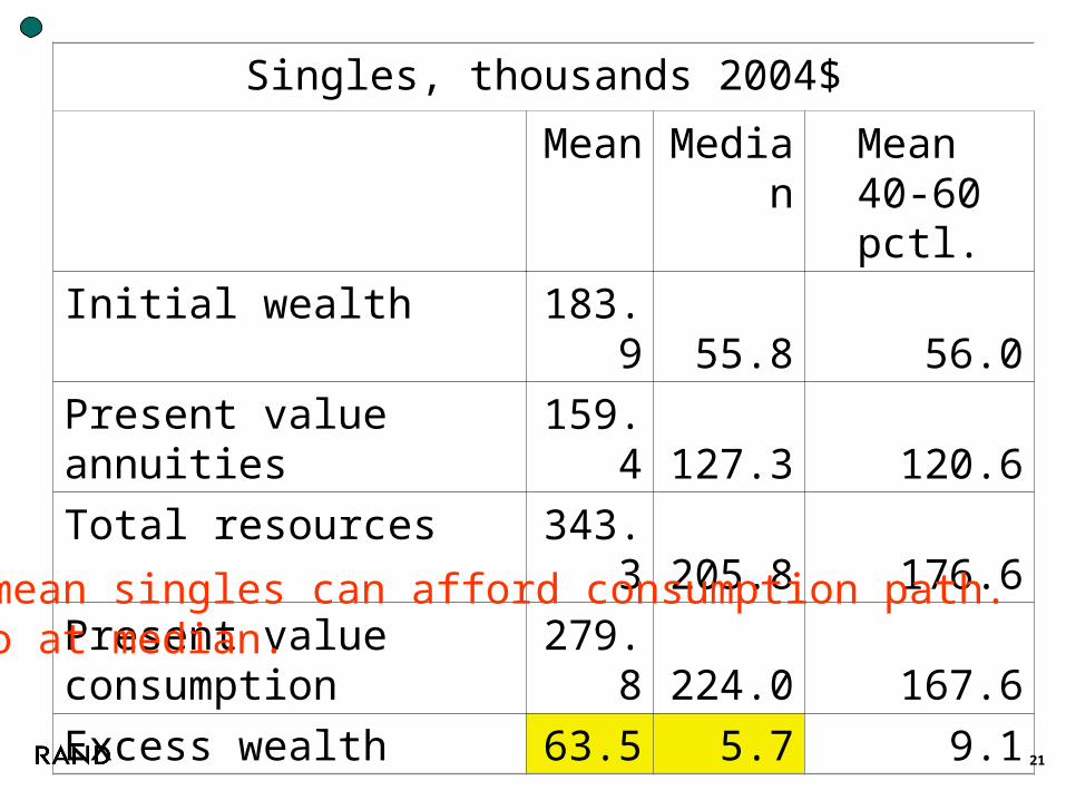
Singles, thousands 2004$

Mean Median Mean 40-60 pctl.

Initial wealth 183.9 55.8 56.0

Present value annuities 159.4 127.3 120.6

Total resources 343.3 205.8 176.6

Present value consumption 279.8 224.0 167.6

Excess wealth 63.5 5.7 9.1

At mean singles can afford consumption path.Also at median.

22

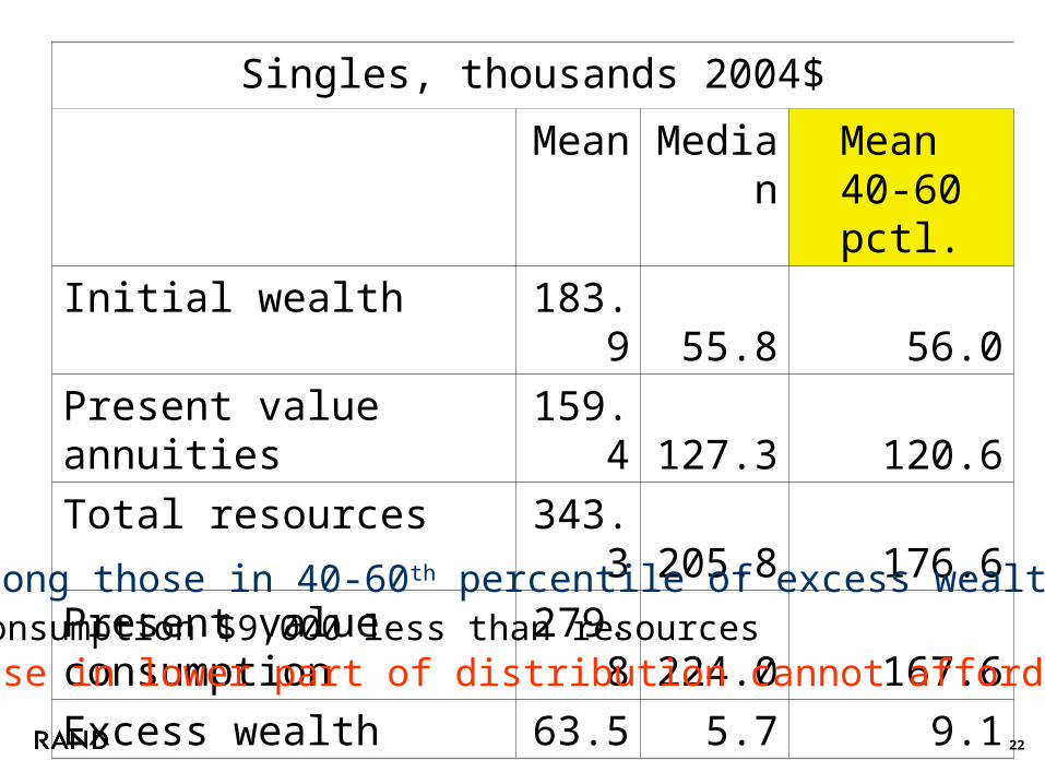
Singles, thousands 2004$

Mean Median Mean 40-60 pctl.

Initial wealth 183.9 55.8 56.0

Present value annuities 159.4 127.3 120.6

Total resources 343.3 205.8 176.6

Present value consumption 279.8 224.0 167.6

Excess wealth 63.5 5.7 9.1

Mean among those in 40-60th percentile of excess wealth Consumption $9,000 less than resources But those in lower part of distribution cannot afford path.

23

Couples

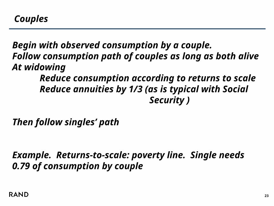
Begin with observed consumption by a couple.Follow consumption path of couples as long as both aliveAt widowing

Reduce consumption according to returns to scaleReduce annuities by 1/3 (as is typical with Social

Security )

Then follow singles’ path

Example. Returns-to-scale: poverty line. Single needs 0.79 of consumption by couple

24

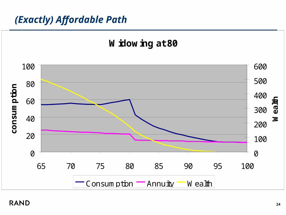
(Exactly) Affordable Path

Widowing at 80

0

20

40

60

80

100

65 70 75 80 85 90 95 100

con

sum

pti

on

0

100

200

300

400

500

600

Wea

lth

Consumption Annuity Wealth

25

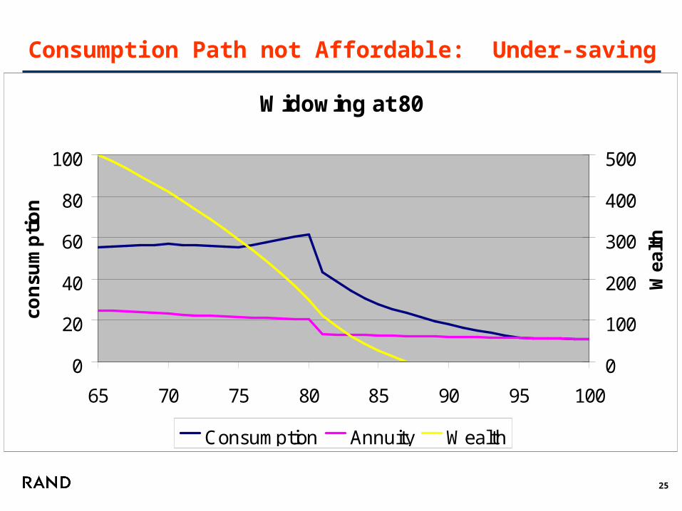
Consumption Path not Affordable: Under-saving

Widowing at 80

0

20

40

60

80

100

65 70 75 80 85 90 95 100

con

sum

pti

on

0

100

200

300

400

500

Wea

lth

Consumption Annuity Wealth

26

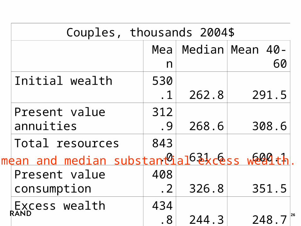
Couples, thousands 2004$

Mean Median Mean 40-60

Initial wealth 530.1 262.8 291.5

Present value annuities 312.9 268.6 308.6

Total resources 843.0 631.6 600.1

Present value consumption 408.2 326.8 351.5

Excess wealth 434.8 244.3 248.7At mean and median substantial excess wealth.

27

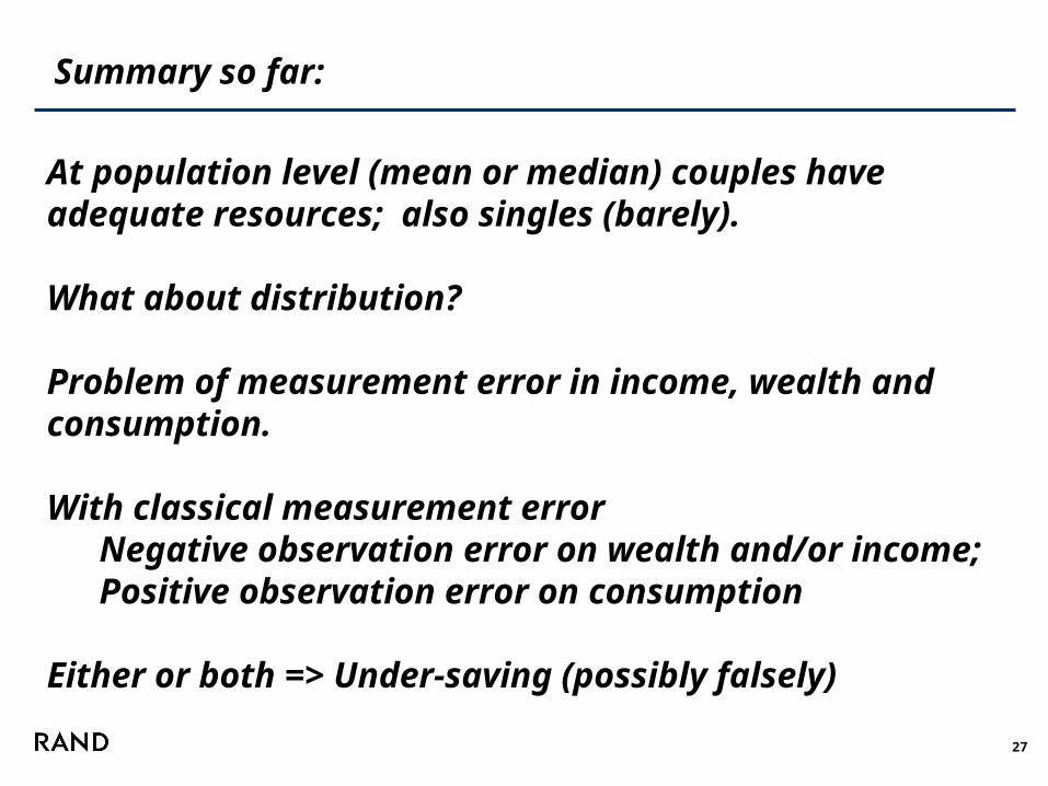
Summary so far:

At population level (mean or median) couples have adequate resources; also singles (barely).

What about distribution?

Problem of measurement error in income, wealth and consumption.

With classical measurement errorNegative observation error on wealth and/or income; Positive observation error on consumption

Either or both => Under-saving (possibly falsely)

28

Group by characteristics such as education

29

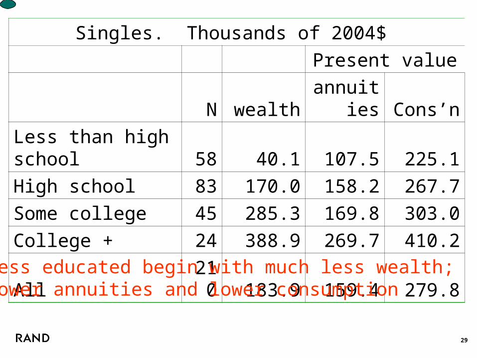
Singles. Thousands of 2004$

Present value

N wealth annuities Cons’n

Less than high school 58 40.1 107.5 225.1

High school 83 170.0 158.2 267.7

Some college 45 285.3 169.8 303.0

College + 24 388.9 269.7 410.2

All 210 183.9 159.4 279.8

Less educated begin with much less wealth; lower annuities and lower consumption

30

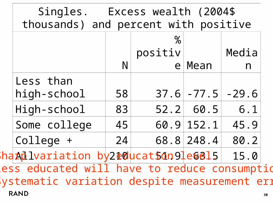
Singles. Excess wealth (2004$ thousands) and percent with positive

N % positive Mean Median

Less than high-school 58 37.6 -77.5 -29.6

High-school 83 52.2 60.5 6.1

Some college 45 60.9 152.1 45.9

College + 24 68.8 248.4 80.2

All 210 51.9 63.5 15.0

Sharp variation by education level.Less educated will have to reduce consumptionSystematic variation despite measurement error

31

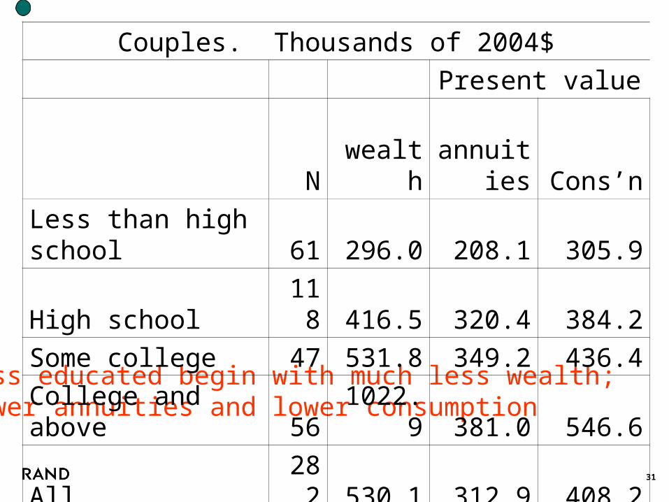
Less educated begin with much less wealth; lower annuities and lower consumption

Couples. Thousands of 2004$

Present value

N wealth

annuities Cons’n

Less than high school 61 296.0 208.1 305.9

High school 118 416.5 320.4 384.2

Some college 47 531.8 349.2 436.4

College and above 56 1022.9 381.0 546.6

All 282 530.1 312.9 408.2

32

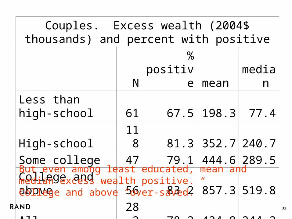
Couples. Excess wealth (2004$ thousands) and percent with positive

N % positive mean median

Less than high-school 61 67.5 198.3 77.4

High-school 118 81.3 352.7 240.7

Some college 47 79.1 444.6 289.5

College and above 56 83.2 857.3 519.8

All 282 78.3 434.8 244.3

But even among least educated, mean and median excess wealth positive.College and above “over-saved.”

33

Still to be done

Differential mortality:Poor tend to die earlier than well-to-do.

Will reduce difference between least educated and most educated

Wider sample

Better treatment of housing wealth

34

Conclusions

Preparation for retirement adequate at population level.

Some have under-saved but with measurement error; hard to say how many.

But less educated have under-saved on average

Have used observed spending levels and age-patterns: a good guide to future?

Obvious question: future out-of-pocket health care costs. So far not a big problem

35

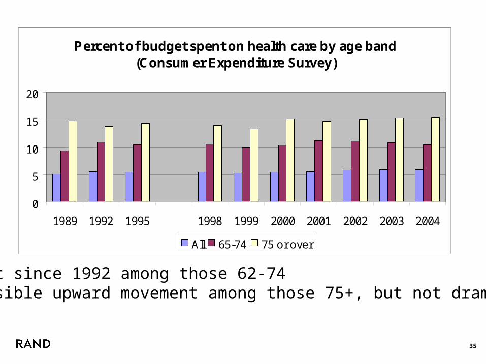
Percent of budget spent on health care by age band(Consumer Expenditure Survey)

0

5

10

15

20

1989 1992 1995 1998 1999 2000 2001 2002 2003 2004

All 65-74 75 or over

Flat since 1992 among those 62-74Possible upward movement among those 75+, but not dramatic.

36

Next Steps