Alternative Approaches to the Analysis of Economic Growth

(Based on Lectures given at the National University of Mexico, September 2000)

Contents

Preface Chapter 1 Growth Theory in the History of Thought Chapter 2 Neoclassical and ‘New’ Growth Theory: A Critique Chapter 3 Manufacturing Industry as the Engine of Growth Chapter 4 A Demand-Oriented Approach to Economic Growth: Export-Led

Growth Models Chapter 5 Balance of Payments Constrained Growth: Theory and Evidence Chapter 6 The Endogeneity of the Natural Rate of Growth

2

Preface

This short book has arisen out of a series of lectures and seminars that I gave at the

National University of Mexico in September 2000. They, in turn, were based on a selection

of lectures I have been giving for a long time at the University of Kent to students studying

for a Master's degree in development economics. The fact that the lectures were given to

graduate students, however, does not mean that the book will not be intelligible to others,

including undergraduates and practitioners in the development field. First of all, the basic

principles of growth and development theory are not that difficult to grasp by anyone with a

willingness and interest to learn, and secondly, following the dictum of Alfred Marshall (the

great 19th century Cambridge economist), I have tried to translate theoretical models

expressed in mathematics into words.

The subject matter of why some countries are rich and others are poor, and why some

countries grow faster than others over long periods of time (although not necessarily

continuously), has always fascinated me as an economist, and in the chapters to follow I try

to present the conventional wisdom, as it has evolved historically, but with a critical eye,

from Adam Smith, the author of an Inquiry into the Nature and Causes of the Wealth of

Nations (1776) to ‘new’ or endogenous growth theory. I am critical of the latter, and its

predecessor, neoclassical growth theory, and my own contribution is to try and put (back)

demand into growth theory as a driving force. In my view, neoclassical and ‘new’ growth

theory is far too supply-oriented in its approach, not recognising sufficiently the various

constraints on demand long before supply constraints bite. In an open, developing economy

one of the major constraints is the availability of foreign exchange to pay for imports, so that

export growth which relaxes a balance of payments constraint on demand becomes a crucial

determinant of overall growth performance. This is entirely missing from ‘new’ growth

3

theory, but is a central feature of my own thinking and research. There are not many

developing countries in the world that could not utilise resources more fully, and grow faster,

given the greater the availability of foreign exchange. Within this framework, the main

factors of production – labour and capital – are considered to be elastic to demand, and so too

is productivity growth based on static and dynamic returns to scale, captured by Verdoorn’s

Law. Demand creating its own supply (within limits) in a growth context (as well as in a

static context), rather than the pre-Keynesian view of supply creating its own demand,

provides an alternative framework to the neoclassical one for understanding the differential

growth performance of nations.

4

Chapter 1 Growth Theory in the History of Thought

Growth and development theory is at least as old as Adam Smith’s famous book

published in 1776 entitled An Inquiry into the Nature and Causes of the Wealth of Nations.

The macro issues of growth, and the distribution of income between wages and profits, were

the major preoccupation of all the great classical economists including Adam Smith, Thomas

Malthus, John Stuart Mill, David Ricardo, and Karl Marx.

One of Smith’s most important contributions was to introduce into economics the

notion of increasing returns – a concept that ‘new’ growth theory (or endogenous growth

theory) has recently rediscovered (see chapter 2). In Smith, increasing returns is based on the

division of labour. He saw the division of labour, or gains from specialisation, as the very

basis of a social economy, otherwise everybody might as well be their own Robinson Crusoe

doing everything for themselves. And it is the notion of increasing returns, based on the

division of labour, that lay at the heart of Smith’s optimistic vision of economic progress as a

self-generating process, in contrast to the later classical economists, such as Ricardo and Mill,

who believed that economies would end up in a stationary state due to diminishing returns in

agriculture; and also in contrast to Marx who believed that capitalism would collapse through

its own ‘inner contradictions’ (competition between capitalists reducing the rate of profit; a

failure of effective demand as capital is substituted for labour, and the alienation of workers).

The notion of increasing returns may sound a trivial one but it is of profound

significance for the way we view economic processes. It is not possible to understand

divisions in the world economy, and so-called ‘centre-periphery’ models of growth and

development (between North and South and rich and poor countries), without distinguishing

between activities subject to increasing returns on the one hand and diminishing returns on

the other. Increasing returns means rising labour productivity and per capita income, and no

5

limits to the employment of labour set by the (subsistence) wage, whereas diminishing

returns implies the opposite. Industry is, by and large, an increasing returns activity, while

land-based activities, such as agriculture and mining, are diminishing returns activities. Rich,

developed countries tend to specialise in increasing returns activities, while poor developing

countries tend to specialise in diminishing returns activities. It is almost as simple as that, but

not quite!

Adam Smith

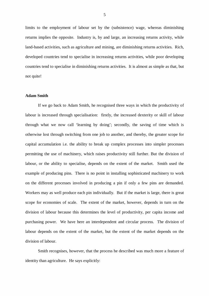
If we go back to Adam Smith, he recognised three ways in which the productivity of

labour is increased through specialisation: firstly, the increased dexterity or skill of labour

through what we now call ‘learning by doing’; secondly, the saving of time which is

otherwise lost through switching from one job to another, and thereby, the greater scope for

capital accumulation i.e. the ability to break up complex processes into simpler processes

permitting the use of machinery, which raises productivity still further. But the division of

labour, or the ability to specialise, depends on the extent of the market. Smith used the

example of producing pins. There is no point in installing sophisticated machinery to work

on the different processes involved in producing a pin if only a few pins are demanded.

Workers may as well produce each pin individually. But if the market is large, there is great

scope for economies of scale. The extent of the market, however, depends in turn on the

division of labour because this determines the level of productivity, per capita income and

purchasing power. We have here an interdependent and circular process. The division of

labour depends on the extent of the market, but the extent of the market depends on the

division of labour.

Smith recognises, however, that the process he described was much more a feature of

identity than agriculture. He says explicitly:

6

the nature of agriculture, indeed, does not admit of so many subdivisions of labour, nor of so complete a separation of

one business from another, as manufactures. It is impossible to separate so entirely the business of the grazier from that of the corn farmer, as the trade of the carpenter is commonly separated from that of the smith (p.16).

There is not the scope for increasing returns in agriculture. Indeed, if land is a fixed factor of

production, there will be diminishing returns to labour – one of the few incontrovertible laws

of economics, as Keynes once said.

As far as the extent of the market is concerned, Smith also recognised the importance

of exports, as we do today particularly for small countries. Exports provide a ‘vent for

surplus’; that is, an outlet for surplus commodities that otherwise would go unsold. There is

a limit to which indigenous populations can consume fish, bananas and coconuts, or can use

copper, diamonds and oil:

without an extensive foreign market, [manufacturers] could not well flourish, either in countries so moderately extensive as to afford but a narrow home market; or in countries where the communication between one province and another [is] so difficult as to render it impossible for the goods of any particular place to enjoy the whole of that home market which the country can afford (p.680).

This vision of Smith of growth and development as a cumulative interactive process

based on the division of labour and increasing returns in industry lay effectively dormant

until the American economist, Allyn Young, based at the London School of Economics,

revived it in a neglected but profound paper in 1928 entitled ‘Increasing Returns and

Economic Progress’ (another paper rediscovered by ‘new’ growth theory). As Young

observed:

Adam Smith’s famous theorem amounts to saying that the division of labour depends in large part on the division of labour. [But] this is more than mere tautology. It means that the counter forces which are continually defeating the forces which make for equilibrium are more pervasive and more deeply rooted than we commonly realise – change

7

becomes progressive and propagates itself in a cumulative way.

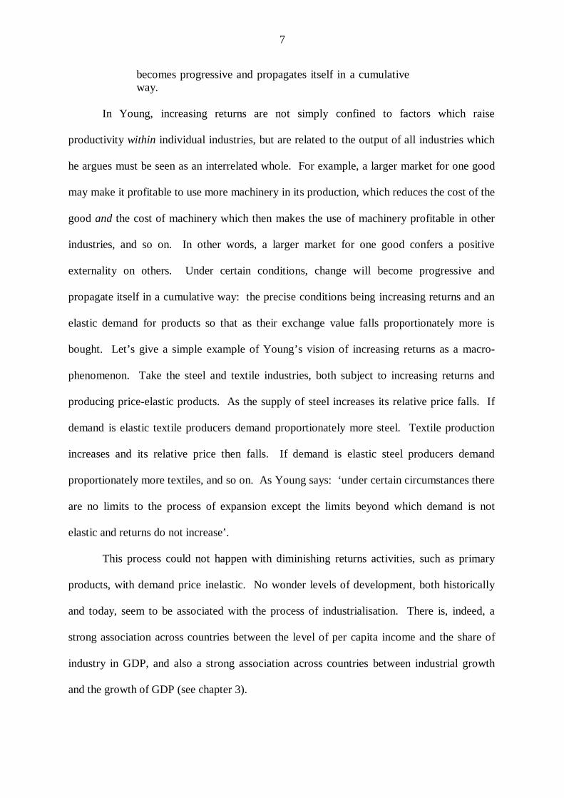
In Young, increasing returns are not simply confined to factors which raise

productivity within individual industries, but are related to the output of all industries which

he argues must be seen as an interrelated whole. For example, a larger market for one good

may make it profitable to use more machinery in its production, which reduces the cost of the

good and the cost of machinery which then makes the use of machinery profitable in other

industries, and so on. In other words, a larger market for one good confers a positive

externality on others. Under certain conditions, change will become progressive and

propagate itself in a cumulative way: the precise conditions being increasing returns and an

elastic demand for products so that as their exchange value falls proportionately more is

bought. Let’s give a simple example of Young’s vision of increasing returns as a macro-

phenomenon. Take the steel and textile industries, both subject to increasing returns and

producing price-elastic products. As the supply of steel increases its relative price falls. If

demand is elastic textile producers demand proportionately more steel. Textile production

increases and its relative price then falls. If demand is elastic steel producers demand

proportionately more textiles, and so on. As Young says: ‘under certain circumstances there

are no limits to the process of expansion except the limits beyond which demand is not

elastic and returns do not increase’.

This process could not happen with diminishing returns activities, such as primary

products, with demand price inelastic. No wonder levels of development, both historically

and today, seem to be associated with the process of industrialisation. There is, indeed, a

strong association across countries between the level of per capita income and the share of

industry in GDP, and also a strong association across countries between industrial growth

and the growth of GDP (see chapter 3).

8

Allyn Young’s 1928 vision also got lost until economists such as Gunnar Myrdal

(Swedish nobel-prize winner in economics), Albert Hirschman and Nicholas Kaldor (a pupil

of Young at the LSE, and later joint-architect of the Cambridge post-Keynesian school of

economists) started to develop non-equilibrium models of the development process in such

books as Economic Theory and Underdeveloped Regions (Myrdal, 1957); Strategy of

Economic Development (Hirschman, 1958), and Economics without Equilibrium (Kaldor,

1985). Kaldor used to joke that economics went wrong after Chapter 4 of Book I of the

Wealth of Nations 1776 when Adam Smith abandoned the assumption of increasing returns

in favour of constant returns, and the foundations for general equilibrium theory were laid;

but foundations totally inappropriate for analysing the dynamics of growth and change.

The Classical Pessimists

The prevailing classical view after Smith was very pessimistic about the process of

economic development which led the historian, Thomas Carlyle, to describe economics as

the dismal science – not a view shared by present readers, I hope! The first of the pessimists

was Thomas Malthus who wrote his famous Essay on Population in 1798 in which he

claimed that there is a “tendency in all animated life to increase beyond the nourishment

prepared for it”. According to Malthus “population, when unchecked, goes on doubling

itself every 25 years, or increases in a geometric ratio [whereas] it may be fairly said – that

the means of subsistence increases in an arithmetical ratio”. Taking the world as a whole,

therefore, Malthus concludes that “the human species would increase (if unchecked) as the

numbers 1, 2, 4, 8, 16, 32, 64, 128, 256 and subsistence as 1, 2, 3, 4, 5, 6, 7, 8, 9”. This

implies, of course, a diminishing proportional rate of increase of food production, or

diminishing returns to agriculture. The result of this imbalance between food supply and

9

population will be that living standards oscillate around a subsistence level, with rising living

standards leading to more children which then reduces living standards again.

This Malthusian vision forms the basis in the development literature of models of the

low-level equilibrium trap associated originally with Nelson (1956) and Leibenstein (1957),

and models of the big push to escape from it. The ghost of Malthus does, indeed, still haunt

many Third World countries, although it has to be said that for the world as a whole, food

production has grown much faster than population for at least the last century. The reason is

that technical progress, always underestimated by the classical pessimists, has offset

diminishing returns leading to substantial increases in productivity, particularly in Europe

and North America, but also in developing countries that experienced a ‘green revolution’.

Another of the great classical pessimists was David Ricardo. In 1817 he published

his Principles of Political Economy and Taxation in which he predicted that capitalist

economies would end up in a stationary state with no capital accumulation and therefore no

growth, also due to diminishing returns in agriculture. In Ricardo’s model, capital

accumulation is determined by profits, but profits get squeezed between subsistence wages

and the payment of rent to landowners which increases as the price of food increases owing

to diminishing returns to land and rising marginal cost. As the profit rate in agriculture falls,

capital shifts to industry causing the profit rate to decline there too. In industry, profits also

get squeezed because the subsistence wage rises in terms of food. As profits fall to zero,

capital accumulation ceases, heralding the stationary state. Ricardo recognised that the cheap

import of food could delay the stationary state, and as an industrialist and politician, as well

as an economist, he campaigned vigorously for the repeal of the Corn Laws in England

which protected British farmers. Arthur Lewis’s famous model economic development with

unlimited supplies of labour (Lewis, 1954) is a classical Ricardian model, but where the

industrial wage stays the same as long as surplus labour exists. Ricardo’s pessimism has also

10

been confounded by technical progress, and the stationary state has never appeared on the

horizon, except, perhaps, in Africa in recent times, but the causes there are different and

complex related to political failure.

Karl Marx in his famous book, Das Kapital (1867) also predicted crisis due to falling

profits, but through a different mechanism related to competition between capitalists,

overproduction and social upheaval. The wages of labour are determined institutionally, and

profit (or surplus value, which only labour can create) is the difference between output per

man and the wage rate. The rate of profit is given by s/(v+c) or (s/v)/(1+c/v), where s is

surplus value, c is 'constant' capital, v is 'variable' capital (the wage bill), and c/v is defined as

the organic composition of capital. The latter is assumed to rise through time, and as it does

so, the rate of profit will fall unless the rate of surplus value rises. As long as surplus labour

exists (or what Marx called a ‘reserve army of unemployed’) there is no problem, but Marx

predicted that as capital accumulation takes place, the reserve army will disappear, driving

wages up and profits down. The capitalists’ response is either to attempt to keep wages

down (the immiseration of workers) leading to social conflict, or to substitute more capital

for labour which raises the organic composition of capital and worsens the problem of a

falling profit rate. Moreover, as labour is substituted, it cannot consume all the goods

produced, and there is a failure of effective demand, or a ‘realisation crisis’ as Marx called it.

Capitalism collapses through its own ‘inner contradictions’, and power passes to the working

classes.

Classical models of growth and distribution still form an integral part of growth and

development theory, particularly the emphasis on the capitalist surplus for investment, but

the gloomy prognostications of the classical economists have not materialised, at least for the

capitalist world as a whole. As said before, what is wrong with Malthus and Ricardo is that

they both underestimated the strength of technical progress in agriculture as an offset to

11

diminishing returns. What is wrong with Marx is that he first of all confused money and real

wages, and secondly underestimated the effect of technical progress in industry on the

productivity of labour. A rise in money wages as labour becomes scarcer does not

necessarily mean a rise in real wages; and a rise in real wages could be offset by a rise in

productivity, leaving the rate of profit unchanged. In other words, in a growing economy,

there is no necessary conflict between wages and the rate of profit.

For nearly sixty years after Marx’s death in 1883, growth and development theory lay

virtually dormant until it was revived by the British economist (Sir) Roy Harrod in 1939 in a

classic article ‘An Essay in Dynamic Theory’. In the late 19th and early 20th centuries,

economics was dominated by neoclassical value theory under the influence of Jevons, Walras

and particularly Alfred Marshall’s Principles of Economics published in 1890. Growth and

development was regarded as an evolutionary natural process akin to biological

developments in the natural world. All this changed in 1939 with Harrod’s article, which led

to the development of what came to be called the Harrod-Domar growth model (named after

Evesey Domar as well who derived independently Harrod’s fundamental result in 1947 but in

a different way (Domar, 1947).) The model has played a major part in thinking about

development issues ever since, and is still widely used as a planning framework in

developing countries. Neoclassical growth theory was born as a reaction to the Harrod-

Domar model, and ‘new’ growth theory developed as a reaction to neoclassical growth

theory.

Harrod-Domar Growth Model

Harrod was one of the most original and versatile economists of the twentieth

century. He was the inventor of the marginal revenue product curve in micro theory; the life-

cycle hypothesis of saving and the absorption approach to the balance of payments in macro

12

theory; the biographer of Keynes; the author of a book on inductive logic, as well as the

originator of modern growth theory.

Harrod’s 1939 model was an extension of Keynes’s static equilibrium analysis of The

General Theory. The question Harrod asked was: if the condition for a static equilibrium is

that plans to invest must equal plans to save, what must be the rate of growth of income for

this equilibrium condition to hold in a growing economy through time? Moreover, is there

any guarantee that this required rate of growth will prevail?

Harrod introduced three different growth concepts: the actual growth rate (ga); the

warranted growth rate (gw) and the natural growth rate (gn). The actual growth rate is defined

as ga = s/c, where s is the savings ratio and c is the actual incremental capital-output ratio (i.e.

the amount of extra capital accumulation or investment associated with a unit increase in

output). This expression is definitionally true because in the national accounts, savings and

investment are equal. Thus s/c = (S/Y)/(I/Y) = (Y/Y), where S is saving, I is investment,

Y is output, and Y/Y is the growth rate (ga).

This rate of growth, however, does not necessarily guarantee a moving equilibrium

through time in the sense that it induces just enough investment to match planned saving.

Harrod called this rate the warranted growth rate. Formally, it is the rate that keeps capital

fully employed, so that there is no overproduction or underproduction, and manufacturers are

therefore willing to carry on investment in the future at the same rate as in the past. How is

this rate determined? The demand for investment is given by an accelerator mechanism (or

what Harrod called ‘the relation’) with planned investment (Ip) a function of the change in

output, so that Ip = crY, where cr is the required incremental capital-output ratio at a given

rate of interest, determined by technological conditions. Planned saving (Sp) is a function of

income so that Sp = sY where s is the propensity to save. Setting planned investment equal to

planned saving gives crY = sY or Y/Y = s/cr, which equals the warranted growth rate (gw).

13

For dynamic equilibrium, output must grow at the rate s/cr. If not, the economic system will

be cumulatively unstable. If actual growth exceeds the warranted growth rate, plans to invest

will exceed plans to save; and the actual growth rate is pushed even further above the

warranted rate. Contrawise, if actual growth is less than the warranted rate, plans to invest

will be less than plans to save and growth will fall further below the warranted rate. This is

the Harrod instability problem. Economies appeared to be poised on a ‘knife-edge’. Any

departure from equilibrium, instead of being self-righting, will be self-aggravating.

The American economist, Evesey Domar, working independently of Harrod, also

arrived at Harrod’s central conclusion by a different route – hence the linking of their two

names. What Domar realised was that investment both increases demand via the Keynesian

multiplier, and also increases supply by expanding capacity. So the question he posed was:

what is the rate of growth of investment that will guarantee that demand matches supply?

The crucial rate of growth of investment can be derived in the following way. A change in

the level of investment increases demand by Yd = I/s, and investment itself increases

supply by Ys = I, where is the productivity of capital (Y/I). Therefore, for Yd = Ys

we must have I/s = I, or I/I = s. That is to say, investment must grow at a rate equal to

the product of the savings ratio and the productivity of investment. With a constant savings-

investment ratio, this implies output growth at the rate s. Since = 1/cr (at full

employment), then the Harrod and Domar result for equilibrium growth is the same.

Even if the actual and warranted growth rates are equal, however, guaranteeing the

full utilisation of capital, this does not guarantee the full utilisation of labour which depends

on the natural rate of growth (gn) made up of two components: the growth of the labour

force (l) and the growth of labour productivity (t), both exogenously given. The sum of the

two gives the growth of the labour force in efficiency units. If all labour is to be employed,

14

the actual growth rate must match the natural rate. If the actual growth rate falls below the

natural rate there will be growing unemployment of the structural variety.

It should be clear that the full employment of both capital and labour requires that ga

= gw = gn; a happy coincidental state of affairs that Joan Robinson once coined ‘the golden

age’ to emphasise its mythical nature.

Where do the developing countries fit into this story? The short-run (trade cycle)

problem is the relation between ga and gw, and we won’t say more about this here. The long

run problem is the relation between gw and gn, or the relation between the growth of capital

and the growth of the labour force in efficiency units. Almost certainly, in most developing

countries, gn exceeds gw. Labour force growth (determined by population growth) may be 2

percent per annum, and productivity growth 3 percent per annum, giving a natural growth

rate of 5 percent. If the net savings ratio is 9 percent and the required incremental capital-

output ratio is 3, the warranted growth rate is only 3 percent. Therefore gn > gw. This has

two main consequences. Firstly, it means that the effective labour force is growing faster

than capital accumulation so that with fixed coefficients of production there will be

unemployment of the structural variety. Secondly, it means that plans to invest will exceed

plans to save, because if the economy could grow at 5 percent there are profitable investment

opportunities for more than 9 percent saving, and there will be inflationary pressure. Hence,

the simultaneous existence of unemployment and inflation in developing countries is not a

paradox; it is the outcome of an inequality between the natural and warranted growth rates.

A good deal of development policy can be understood and considered within this

Harrod framework. The task is to bring gn and gw closer together; to reduce gn and to

increase gw. The only feasible way to reduce the growth of the labour force is to reduce

population growth. The Harrod model provides a rationale for population control. A second

way to reduce gn is to reduce the rate of labour saving technical progress, but this has the

15

serious drawback of reducing the growth of living standards. A rise in gw could be brought

about by increases in the savings ratio. This is what monetary and fiscal policy programmes

are designed to do, with emphasis on tax reform and policies of financial liberalisation. A

rise in gw could also come about if the capital-output ratio was reduced by countries using

more labour intensive techniques of production. There is an on-going debate on the choice

of appropriate techniques in developing countries, and whether more labour intensive

techniques could be employed without the sacrifice of output or saving.

The Harrod (and Domar) model provided the starting point for the great debates in

growth economics that preoccupied large sections of the economics profession for at least

three decades between the mid-1950s and the 1980s. The battle-lines were drawn up

between the neoclassical growth school on the one hand based in Cambridge, Massachusetts,

USA with the major protagonists being Robert Solow, Paul Samuelson and Franco

Modigliani, and the Keynesian growth school on the other based in Cambridge, England with

the major protagonists being Nicholas Kaldor, Joan Robinson, Richard Kahn and Luigi

Pasinetti. What was immediately apparent to both camps was that if the Harrod-Domar

model was a representation of the real world, all economies, rich and poor, capitalist and

communist, would be in for a bumpy ride. The variables and parameters determining gn and

gw were all independently given, and there were apparently no automatic mechanisms for

bringing the two rates of growth into line to provide the basis for steady long run growth at

the natural rate. The task that both conflicting camps set themselves was to develop

mechanisms to reconcile divergences between gn and gw.

The Cambridge, England camp focussed on the savings ratio, making it a function of

the distribution of income between wages and profits which in turn was assumed to be

related to whether the economy was in boom or slump. Specifically in their model the

propensity to save out of profits is assumed to be higher than out of wages, and the share of

16

profits in national income is assumed to rise during booms and fall during slumps.

Therefore, if gn exceeds gw, generating a boom, the share of profits rises and the savings ratio

will rise raising gw towards gn. The only constraint might be an ‘inflation barrier’ caused by

workers not being willing to see the share of wages fall below a certain minimum.

Conversely, if gn is less than gw, generating a slump, the share of profits falls and the savings

ratio falls lowering gw towards gn. The only limit here might be a minimum rate of profit

acceptable to entrepreneurs which sets a limit to the fall in the share of profits.

The Cambridge, Massachusetts camp focussed on the capital-output ratio arguing that

if the labour force grows faster than capital, the price mechanism will operate in such a way

as to induce the use of more labour intensive techniques, and vice versa. Thus if gn exceeds

gw, the capital-output ratio will fall raising gw to gn. If gn is less than gw, the capital-output

ratio will rise lowering gw to gn. This neoclassical adjustment mechanism, however,

presupposes two things. Firstly, that the relative price of labour and capital are flexible

enough, and secondly that there is a spectrum of techniques to choose from so that

economies can move easily and smoothly along a continuous production function relating

output to the factor inputs, capital and labour. If this is true, economies can achieve a growth

equilibrium at the natural rate (see chapter 2).

Out of the neoclassical model, however, came the extraordinary counterintuitive

conclusion that investment does not matter for long run growth because the natural rate

depends on the growth of the labour force and labour productivity (determined by technical

progress) and both are exogenously determined. Any increase in a country’s saving or

investment ratio would be offset by an increase in the capital-output ratio leaving the long

run growth rate unchanged. The argument depends crucially, however, on the productivity

of capital falling as the capital to labour ratio rises. In other words, it depends on the

assumption of diminishing returns to capital. This is the neoclassical story that ‘new’

17

endogenous growth theory objects to. If there are mechanisms which keep the productivity

of capital from falling as more investment takes place, then the investment ratio will matter

for long run growth, and growth is endogenous in this sense i.e. growth is not simply

determined by the exogenous growth of the labour force in efficiency units.

In the next chapter we consider in more detail the assumptions and predictions of the

neoclassical model; and the criticisms made of it. We then look at the challenge of ‘new’

growth theory, and we are critical of this too.

18

Chapter 2 Neoclassical and ‘New’ Growth Theory: A Critique

Our task in this chapter is to formally outline the assumptions and predictions of

neoclassical growth theory as a background to showing: firstly, how the neoclassical

production function is used for analysing growth rate differences between countries, and its

weaknesses; and secondly, how neoclassical growth theory forms the basis for ‘new’

endogenous growth theory – the only major difference being that the assumption of

diminishing returns to capital is relaxed, so that ‘new’ growth theory is subject to the same

major criticisms as conventional neoclassical theory as far as analysing and understanding

growth rate differences between countries is concerned.

The Neoclassical Model

The neoclassical growth model is based on three key assumptions. The first is that

the labour force (l) and labour saving technical progress (t) grow at a constant exogenous

rate. The second assumption is that all saving is invested, S = I = sY. There is no

independent investment function. The third assumption is that output is a function of capital

and labour, where the production function exhibits constant returns to scale, and diminishing

returns to individual factors of production. The most commonly used neoclassical

production function, with constant returns to scale, is the so-called Cobb-Douglas production

function, named after Charles Cobb, a mathematician, and Paul Douglas, a well-known

Chicago economist before world-war II (who later became a US senator). The function takes

the form:

Y = TKL1- (2.1)

where Y is output, K is capital, L is labour, T is the level of technology, is the elasticity of

output with respect to capital and 1- is the elasticity of output with respect to labour.

19

Obviously + (1-) = 1 (the assumption of constant returns to scale), so that a one percent

increase in capital and labour leads to a one percent increase in output.

To consider the predictions of the model, it is convenient to transform equation (2.1)

into its ‘labour-intensive’ form by dividing both sides by L, so that the dependent variable is

output per head, and the independent variables are the level of technology and capital per

head.

Y/L = (TKL1-)/L = T(K/L)

or q = T(k) (2.2)

where q is output per head and k is capital per head.

The basic predictions of the neoclassical model, which can be shown diagramatically

(see below) are as follows:

(i) firstly, in the steady state, the level of output per head (q) is positively related to the

savings-investment ratio and negatively related to the growth of population (or labour

force).

(ii) secondly, the growth of output is independent of the savings-investment ratio and is

determined by the exogenously given rate of growth of the labour force in efficiency

units (l + t). This is because a higher savings-investment ratio is offset by a higher

capital-output ratio (or a lower productivity of capital) owing to the assumption of

diminishing returns to capital.

(iii) thirdly, given identical tastes and preferences (i.e. the same savings ratio) and

technology (i.e. production function), there will be an inverse relation across

countries between the capital-labour ratio and the productivity of capital, so that poor

countries should grow faster than rich countries leading to the convergence of per

capita incomes across the world.

20

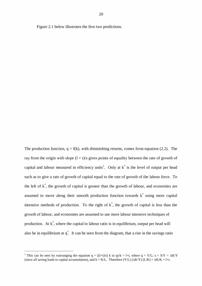
Figure 2.1 below illustrates the first two predictions.

The production function, q = f(k), with diminishing returns, comes from equation (2.2). The

ray from the origin with slope (l + t)/s gives points of equality between the rate of growth of

capital and labour measured in efficiency units1. Only at k* is the level of output per head

such as to give a rate of growth of capital equal to the rate of growth of the labour force. To

the left of k*, the growth of capital is greater than the growth of labour, and economies are

assumed to move along their smooth production function towards k* using more capital

intensive methods of production. To the right of k*, the growth of capital is less than the

growth of labour, and economies are assumed to use more labour intensive techniques of

production. At k*, where the capital to labour ratio is in equilibrium, output per head will

also be in equilibrium at q*. It can be seen from the diagram, that a rise in the savings ratio

1 This can be seen by rearranging the equation q = [(l+t)/s] k to qs/k = l+t, where q = Y/L; s = S/Y = K/Y (since all saving leads to capital accumulation), and k = K/L. Therefore (Y/L) (K/Y) (L/K) = K/K = l+t.

21

(s) pivots downwards the ray from the origin and raises the equilibrium k and raises the level

of q, but does not affect the growth rate of the economy. It can also be seen that the level of

q will be inversely related to the rate of growth of the labour force because a rise in l pivots

upwards the ray from the origin.

The explanation for convergence of per capita income across countries can be seen

from the formula for the capital-output ratio.

K/Y = (K/L) (L/Y) (2.3)

If there is diminishing returns to capital , a higher K/L will not be offset by a higher Y/L

ratio, and therefore K/Y will be higher. Thus, if the savings-investment ratio is the same

across countries, rich countries with a higher K/L ratio should grow slower than poor

countries with a lower K/L because the productivity of capital is lower in the former case

than the latter.

What major criticisms can be made of this model, apart from the empirical fact that

across the world we do not observe the convergence of living standards? The fundamental

point to be made at this stage is that the neoclassical model is a supply-oriented model par

excellence. First, demand never enters the picture. Saving leads to investment, so that

supply creates its own demand. The neoclassical model of growth takes us back to a pre-

Keynesian world where demand does not matter for an understanding of the determination of

the level of output (and by implication, the growth of output). Secondly, factors of

production and technical progress are treated as exogenously determined, unresponsive to

demand. But, by and large, the demand for factors of production is a derived demand,

derived from the growth of output itself. Much technical progress and labour productivity

growth is also induced by the growth of output itself (see later).

The assumption of exogeneity of factor supplies is no more apparent than in the

studies that use the aggregate production function for analysing growth rate differences

22

between countries; an approach pioneered by Abramovitz (1956) and Solow (1957) and still

widely utilised. Let us consider this approach and comment on its limitations.

Using the Production Function for Analysing Growth Differences

If we go back to the Cobb-Douglas production function in equation (2.1), it is easy to

see how it can be used for analysing the sources of growth; that is, decomposing a country’s

growth rate into the contribution of capital, labour and technical progress. The question is,

how useful is it for a proper understanding of the growth performance of countries if the

main inputs into the growth process are not exogenous but endogenous?

The function in equation (2.1) is made operational by taking logarithms of the

variables and differentiating with respect to time which gives:

y = t + (k) + (1 – )l , (2.4)

or in labour intensive form:

y – l = t + (k – l) (2.5)

where lower-case letters represent rates of growth of the variables.

Given estimates of and (1 – ), the contribution of capital growth and labour force

growth to any measured growth rate can be estimated, leaving the contribution of technical

progress as a residual. For example, suppose y = 5%, k = 5%, l = 2%, = 0.3 and (1 - ) =

0.7. The contribution of capital to growth is then (0.3) (5%) = 1.5 percentage points or 30

percent; the contribution of labour is (0.7) (2%) = 1.4 percentage points or 28 percent,

leaving the contribution of technical progress as 5% - 2.9% = 2.1% or 42 percent.

Solow (1957) was the first to use the labour intensive form of the Cobb-Douglas

production function in analysing the growth performance of the US economy over the

previous fifty years, and concluded that only 10 percent of the growth of output per man

could be ‘explained’ by the growth of capital per man leaving 90 percent of growth to be

23

‘explained’ by various forms of technical progress. Denison (1962, 1967) used the same

production function approach, or growth accounting framework, to study growth

performance in the US and between the countries of Europe, disaggregating the technical

progress term (or residual) into various component parts. Maddison (1970) used the

approach to study growth rate differences between developing countries. Since this early

research, there has been a mass of other studies too extensive to survey here (but see Felipe,

1998), but two recent studies may be mentioned as illustrative. The World Bank (1991) did a

study of 68 countries showing capital accumulation to be of prime importance, with technical

progress minimal. This seems to be the central conclusion for developing countries in

contrast to developed countries. Secondly, there is the controversial study by Alwyn Young

(1995) of the four East Asian ‘dragons’ of Hong Kong, Singapore, South Korea and Taiwan

which also shows that most of the growth in these countries can be explained by the growth

of factor inputs and not technical progress, so that according to Young there has been no

growth miracle in these countries – contrary to the conventional wisdom. Before accepting

this conclusion, however, the observer still has to explain why there was such a rapid growth

of factor inputs, and it is this point which exposes the fundamental weakness of the

production function approach to the analysis of growth performance. Inputs are not manna

from heaven dropped by God. Something ‘miraculous’ must have been driving these

economies, to which input growth responded. On closer inspection, what distinguishes these

countries is their outward orientation and relentless search for export markets, and their

remarkable growth of exports which confers benefits on an economy from both the demand

and supply side (see chapter 4). This exposes another weakness of neoclassical growth

theory and that is that the models are closed. There is no trade in these simple models, and

no balance of payments to worry about. They are supply-oriented, supply-driven, closed

economy models unsuitable for the analysis of open economies in which foreign exchange is

24

invariably a scarce resource acting to constrain the growth process. We return to this topic in

chapters 4 and 5, but first we must look at the challenge of ‘new’ growth theory.

‘New’ Endogenous Growth Theory

Since the mid-1980s there has been an outpouring of literature and research on the

applied economies of growth attempting to understand and explain differences in output

growth and living standards across countries of the world – most inspired by so-called ‘new’

growth theory or endogenous growth theory. This spate of studies seems to have been

prompted by a number of factors: firstly, by the increased concern with the economic

performance of poorer parts of the world, and particularly major differences between

continents and between countries, with South East Asia forging ahead, Africa left behind and

South America somewhere in the middle; secondly, by the increased availability of

standardised data on which to do research (Summers and Heston, 1991), and thirdly, studies

showing no convergence of per capita incomes in the world economy (e.g. Baumol, 1986),

contrary to the prediction of neoclassical growth theory based on the assumption of

diminishing returns to capital.

If there are not diminishing returns to capital – but, say, constant returns – a higher

capital-labour ratio will be exactly offset by a higher output per head2, and the capital-output

ratio will not be higher in capital-rich countries than in capital-poor countries, and the

savings-investment ratio will therefore matter for long run growth. Growth is endogenously

determined in this sense and not simply determined by the exogenous rate of growth of the

labour force and technical progress. This is the starting point for ‘new’, endogenous growth

theory which seeks an explanation of why there has not been a convergence of living

standards in the world economy.

2 Remember K/Y = (K/L)/(Y/L).

25

The explanation of ‘new’ growth theory is that there are forces at work which prevent

the marginal product of capital from falling (and the capital-output ratio from rising) as more

investment takes place as countries get richer. Paul Romer (1986) first suggested

externalities to research and development (R+D) expenditure. Robert Lucas (1988) focuses

on externalities to human capital formation (education). Grossman and Helpman (1991)

concentrate on technological spillovers from trade and foreign direct investment (FDI).

Other economists have stressed the role of infrastructure investment and its complementarity

with other types of investment. In fact, it can be seen from the formula for the capital-output

ratio that increasing returns to labour for all sorts of reasons could keep the capital-output

ratio from rising.

So now let us turn to ‘new’ growth theory; see what it has to say; see whether it is

saying anything new, and consider some of the problems of interpreting the empirical results

from testing new growth theory.

The first crude test of new growth theory is to observe whether or not there is an

inverse relation across countries between the growth of output per head and the initial level

of per capita income of countries. If there is, this would be supportive of the neoclassical

prediction of convergence. If not, it would be supportive of ‘new’ growth theory that the

marginal product of capital does not decline. This is referred to as the test for beta ()

convergence. It can be said straight away that no global studies find evidence of

unconditional beta convergence. Virtually all studies find evidence of divergence. The

coefficient linking the growth of output per head to the initial level of per capita income is

positive not negative.

Before jumping to the conclusion that this is unequivocal support for ‘new’ growth

theory, however, it must be remembered that the neoclassical prediction of convergence

assumes all other things the same across countries i.e. population growth; tastes and

26

preferences (e.g. the savings ratio); technology etc. Since these assumptions are manifestly

false, there can never be the presumption of unconditional convergence – only conditional

convergence controlling for differences in all other factors that affect the growth of living

standards, including differences in the ratio of investment to GDP and variables that affect

the productivity of capital and labour such as education and training; R+D expenditure; trade;

macroeconomic performance, and political stability. The question is what happens to the

sign on the initial per capita income variable when these control variables are introduced into

the equation? If the sign on initial per capita income turns negative, this is supposed to

represent a rehabilitation of the neoclassical model. In other words, living standards would

converge if only levels of investment, education, R+D expenditure etc. were the same in poor

countries as rich countries, but they aren’t! The argument is reminiscent of the way

neoclassical economists continue to work with fictitious models of competitive equilibrium

in the presence of increasing returns, by treating the latter as externalities (the device

originally adopted by Alfred Marshall in 1890). Indeed, most ‘new’ growth theorists, and

particularly Robert Barro (1991), are clearly neoclassical economists in disguise. We will

look at the work of Barro and others later, but first let us consider the ‘newness’ of ‘new’

growth theory and the interpretation of results.

First, I find it amusing that it seems to have come as a surprise to many members of

the economics profession that living standards in the world have not been converging

according to the prediction of neoclassical growth theory. Long before the advent of ‘new’

growth theory, many ‘non-orthodox’ economists had been pointing to widening divisions in

the world economy, and developed models to explain divergence. There is what the centre-

periphery models of Prebisch (1950), Myrdal (1957), Hirschman (1958), Seers (1962), and

the neo-Marxist school (e.g. Emmanuel, 1972; Frank 1967) were all about, many based on a

combination of international trade and increasing returns.

27

Secondly, it has to be said that many of the ideas of ‘new’ growth theory are not new

at all. Who, apart from strict adherents to the neoclassical model, ever believed that

investment did not matter for long run growth? Kaldor (1957), with his technical progress

function, precisely anticipated new growth theory by arguing that technical progress requires

capital accumulation and capital accumulation requires technical progress (it is impossible to

have one without the other), and his model of growth gives an explanation of why the

capital-output ratio stays constant through time despite a rising ratio of capital to labour (see

later). On the origins of increasing returns, we could mention Adam Smith and the division

of labour (see chapter 1); Allyn Young and the idea of increasing returns as a

macroeconomic phenomenon related to the interaction between activities (see chapter 1);

Kenneth Arrow’s model of learning by doing (Arrow, 1962), and the work of Schultz (1961)

and Denison (1962) on the social returns to education, and the work of Griliches (1958) on

the social returns to R+D. We have an endearing tendency in economics to reinvent the

wheel.

Thirdly, when it comes to interpreting the empirical results from testing models of

new growth theory and convergence, some care needs to be taken. In particular, great care

needs to be exercised in interpreting the negative sign on the initial level of per capita income

as necessarily rehabilitating the neoclassical model of growth, as for example, Barro (1991)

does, because there are other conceptually distinct reasons for expecting a negative sign.

Firstly, outside the neoclassical paradigm, there is a whole body of literature that argues that

economic growth should be inversely related to the initial level of per capita income because

the more backward a country, the greater the scope for catch-up; that is, for absorbing a

backlog of technology, which represents a shift in the whole production function. Is

conditional convergence picking up diminishing returns to capital in the neoclassical sense,

or catch-up? The two concepts are conceptually distinct, but not easy to disentangle

28

empirically. Secondly, the negative term could simply be picking up structural change, with

poor countries growing faster than rich countries (controlling for other variables) because of

a more rapid shift of resources from low productivity to high productivity sectors (e.g. from

agriculture to industry). How do we discriminate between these hypotheses?

A fourth point concerns the specification of ‘new’ growth theory in its simplest form

as the so-called AK model i.e.

Y = AK (2.6)

where A is a constant, which implies a constant proportional relation between output (Y) and

capital (K), or constant returns to capital. On close inspection, this specification is none

other than the Harrod growth equation g = s/c (see chapter 1). This can be seen by taking

changes in Y and K and dividing by Y, which gives:

Y/Y = A K/Y = A (I/Y) (2.7)

where Y/Y is the growth rate (g); I/Y is the savings-investment ratio (s), and A is the

productivity of investment, Y/I = 1/c or the reciprocal of the incremental capital-output

ratio. What this means is that if the productivity of investment (A) was the same across all

countries, there would be a perfect correlation between growth and the investment ratio. If

there is not a perfect correlation, then definitionally there must be differences across

countries in the productivity of capital. All that empirical studies of ‘new’ growth theory are

really doing is trying to explain differences in the productivity of capital across countries

(provided the investment ratio is in the equation) in terms of differences in education, R+D

expenditure, trade etc., and initial endowments (see Hussein and Thirlwall, 2000, for further

elaboration of this point).

As far as the constancy of the capital-output ratio is concerned, it was pointed out by

Kaldor (1957) many years ago, as one of his six stylised facts of economic growth, that

despite capital accumulation and increases in capital per head through time, the capital-

29

output ratio has remained broadly unchanged, implying some form of externalities or

increasing returns. It is worth quoting Kaldor in full:

“As regards the process of economic change and development in capitalist societies, I suggest the following ‘stylised facts’ as a starting point for the construction of theoretical models --- (4) steady capital-output ratios over long periods; at least there are no clear long-term trends, either rising or falling, if differences in the degree of capital utilisation are allowed for. This implies, or reflects, the near identity in the percentage growth of production and of the capital stock i.e. for the economy as a whole, and over long periods, income and capital tend to grow at the same rate.”

Kaldor’s explanation lay in his innovation of the Technical Progress Function (TPF) relating

the growth of output per man (q) to the growth of capital per man (k), as in figure 2.2

30

The position of the (linear) TPF drawn in figure 2.2 depends on the exogenous rate of

technical progress, and the slope of the function depends on the extent to which technical

progress is embodied in capital. Along the 45 line, the capital-output ratio is constant, and

the equilibrium growth of output per head is q*

1. An upward shift of the function associated

with new discoveries, technological breakthroughs etc. will cause the growth of output to

exceed the growth of capital, raising the rate of profit and inducing more investment to give a

new equilibrium growth of output per head at q*

2 (follow the arrows). An increase in capital

accumulation not accompanied by technical progress will simply cause the capital-output

ratio to rise. If the capital-output ratio is observed to be constant there must be technological

forces at work shifting the function upwards. ‘New’ growth theory is precisely anticipated.

What applies to countries through time applies pari passu to different countries at a

point in time, with differences in country growth rates at the same capital-output ratio

associated with different technical progress functions. To quote Kaldor again:

“A lower capital-labour ratio does not necessarily imply a lower capital-output ratio – indeed, the reverse is often the case. The countries with the most highly mechanised industries, such as the United States, do not require a higher ratio of capital to output. The capital-output ratio in the United States has been falling over the past 50 years whilst the capital-labour ratio has been steadily rising; and it is lower in the United States today than in the manufacturing industries of many underdeveloped countries” (Kaldor, 1972).

In other words, rich and poor countries are simply not on the same production function.

A final point concerns the way that new growth theory models trade. First of all,

some of the models and empirical studies do not consider the role of trade at all, as if

economies are completely closed. It is hard to imagine how it is possible to explain growth

rate differences between countries without reference to trade, and particularly without

reference to the balance of payments of countries which constitutes for many developing

31

countries the major constraint on the growth of demand and output (which will reduce the

productivity of capital). When a trade variable is included in the model, it is invariably

insignificant, or loses its significance when combined with other variables. On the surface,

this is a puzzle. It would conflict with the rich historical literature that exists on the relation

between trade and growth (Thirlwall, 2000). It would conflict with the voluminous work of

the World Bank and other organisations showing the beneficial effects of trade liberalisation,

and it would undermine the whole thrust of international policy-making since the second

world war, which has been to free-up markets and to promote trade in the interests of

economic development.

There may be several explanations for the weak results, but I believe the major one is

that the trade variable normally takes is the share of exports in GDP as a measure of

‘openness’ which may pick up the static gains from trade and technological spillovers, but

not the dynamic effects of trade which can only be properly captured by the growth of

exports which affects demand, both directly and indirectly (by relaxing a balance of

payments constraint on demand), and also the supply side of the economy by permitting a

faster growth of imports. This point relates to my general criticism of 'new' growth theory

that it neglects demand-side variables. When an export growth variable is included in a

‘new’ growth theory equation, it is highly significant (see Thirlwall and Sanna,1996).

When it comes to evaluating the empirical evidence, only four variables in ‘new’

growth theory equations appear to be robust (see Levine and Renelt, 1992): the initial level

of per capita income; the savings-investment ratio; investment in human capital, and

population growth (usually). All other variables are fragile in the sense that when they are

combined with other variables, they lose their significance. The robust variables are ones

that growth analysts have stressed for many years, long before the advent of ‘new’ growth

theory. Plus cà change, plus cà la même chose.

32

Chapter 3 Manufacturing Industry as the ‘Engine’ of Growth

The neoclassical approach to economic growth, and its offspring ‘new’ growth

theory, are not only very supply oriented, treating factor supplies as exogenously given, but

are also very aggregative. They treat all sectors of the economy as if they are alike. They

don’t explicitly pick out any one sector as more important than another. In practice,

however, aggregate growth will naturally be related to the rate of expansion of the sector

with the most favourable growth characteristics.

There is a lot of historical, empirical evidence to suggest that there is something

special about industrial activity, and particularly manufacturing. There seems to be a close

association across countries between the level of per capita income and the degree of

industrialisation, and there also seems to be a close association across countries between the

growth of GDP and the growth of manufacturing industry. Countries which are growing fast

tend to be those where the share of industry in GDP is rising most rapidly; the so-called

newly industrialising countries (the NICs). Is this an accident?

One of the first economists to have seriously addressed this issue is the late Nicholas

Kaldor who argued in many of his writings (see Targetti and Thirlwall, 1989) that it is

impossible to understand the growth and development process without taking a sectoral

approach, distinguishing between increasing returns activities on the one hand (which he

associated with industry) and diminishing returns activities on the other (which he associated

with the land-based activities of agriculture and mining). Kaldor first articulated his theory

about why growth rates differ in two lectures: one in Cambridge in 1966 entitled Causes of

the Slow Rate of Economic Growth of the United Kingdom (Kaldor, 1966); the other at

Cornell University in the same year entitled Strategic Factors in Economic Development

(Kaldor, 1967). In these lectures he presented a series of ‘laws’ or empirical generalisations

33

which attempted to account for growth rate differences between advanced capitalist

countries, but which also have applicability to developing countries as well.

There are three laws to focus on, plus a number of subsidiary propositions. The first

law is that there exists a strong causal relation between the growth of manufacturing output

and the growth of GDP. The second law states that there exists a strong positive causal

relation between the growth of manufacturing output and the growth of productivity in

manufacturing as a result of static and dynamic returns to scale. This is also known as

Verdoorn’s Law (see chapter 1 and later). The third law states that there exists a strong

positive causal relation between the rate at which the manufacturing sector expands and the

growth of productivity outside of the manufacturing sector because of diminishing returns in

agriculture and many petty service activities which supply labour to the industrial sector. If

the marginal product of labour is below the average product in these sectors, the average

product (productivity) will rise as employment is depleted. For this reason, overall GDP

growth will tend to slow up as the scope for absorbing labour from diminishing returns

activities dries up. Given these ‘laws’, the question remains of what determines the growth

of the manufacturing sector in the first place? Kaldor’s answer is demand coming from

agriculture in the early stages of development and export growth in the later stages. These

are the two fundamental sources of autonomous demand to match the leakages of income

from the industrial sector of food imports from agriculture on the one hand and imports from

abroad on the other. A fast growth of exports and output may then set up a virtuous circle of

growth with rapid export growth leading to rapid output growth, and rapid output growth

leading to fast export growth through the favourable impact of output growth on

competitiveness. Other countries find it difficult to break in to such virtuous circles, and this

is why the polarisation between countries occurs. The present north-south divide in the

world economy has its origins in the fact that the ‘north’ contains the first set of countries to

34

industrialise, and only a handful of countries since have managed to challenge their industrial

supremacy and to match their living standards.

Kaldor’s growth laws can be tested across countries; across regions within countries;

across regions and countries using panel data (e.g. across the regions of the European Union),

and for individual countries using time series data (although care has to be taken with the

second law not to confuse Verdoorn’s Law with Okun’s Law which relates to pro-cyclical

variations in productivity over the trade cycle). (see McCombie and Thirlwall, 1994)

The first test of the first law is to run a regression of the rate of growth of GDP

against the rate of growth of manufacturing output and to test for statistical significance.

When this is done across countries or regions, the relation is invariably highly significant, but

this could be a spurious relation due to the fact that manufacturing output constitutes a

sizeable fraction of total output. Side tests therefore need to be undertaken. One is to regress

the growth of GDP on the excess of the growth of manufacturing output over the growth of

non-manufacturing output; another is to regress the growth of non-manufacturing output on

the growth of manufacturing output. When these side tests are performed, the first law is

generally confirmed. A recent interesting study across the regions of China strongly supports

Kaldor’s first law (Hansen and Zhang, 1996). For manufacturing to be regarded as special,

however, it needs to be shown that GDP growth is not closely related to the growth of other

sectors such as agriculture, mining or services. It is hard to find any cross section relations

between the growth of GDP and the growth of the agricultural sector. The relation between

the growth of GDP and the growth of services is stronger but there is reason to believe that

the direction of causation may be the other way round from GDP growth to service growth

since the demand for many services is derived from the demand for manufacturing output

itself. The question is to what extent service activities have an ‘autonomous’ existence, and

35

whether they have the production characteristics (e.g. static and dynamic scale economies) to

induce fast growth? This is still an open question, ripe for further research.

If the first law is accepted, what accounts for the fact that the faster manufacturing

output grows relatively to GDP, the faster GDP seems to grow? Since differences in growth

rates are largely accounted for by differences in labour productivity growth (rather than the

growth of the labour force), there must be some relationship between the growth of the

manufacturing sector and productivity growth in the economy as a whole. This is to be

expected for two main reasons. The first is that wherever industrial production and

employment expand, labour resources are drawn from sectors which have open or disguised

unemployment (that is, where there is no relation between employment and output), so that

labour transference to manufacturing will not cause a diminution in the output of these

sectors, and productivity growth increases outside of manufacturing (the third law – see

below). The second reason is the existence of increasing returns within industry, both static

and dynamic. Static returns relate to the size and scale of production units and are a

characteristic largely of manufacturing where, for example, in the process of doubling the

linear dimensions of equipment, the surface increases by the square and the volume by the

cube (the so-called cube rule). Dynamic economies refer to increasing returns brought about

by ‘induced’ technical progress, learning by doing, external economies in production and so

on. Kaldor draws inspiration here from Allyn Young’s pioneering paper of 1928 ‘Increasing

Returns and Economic Progress’ with its emphasis on increasing returns as a macroeconomic

phenomenon resulting from the interaction between activities in the process of general

industrial expansion; ideas now taken up by ‘new’ growth theory (see chapter 1). For those

interested in the history of economic thought and the inter-generational transmission of ideas

(which sometimes take a long time to resurface!), Kaldor was a pupil of Allyn Young at the

36

London School of Economics in 1928 and took a full set of lecture notes from him including

his thoughts on increasing returns (see Thirlwall 1987, Sandilands, 1990).

The empirical relation between productivity growth and output growth in

manufacturing is known as Verdoorn’s Law, following Verdoorn’s (1949) paper published in

Italian entitled ‘Fattori che Regolano lo Sviluppo della Produttivita del Lavoro’.

Interestingly, at the time of publication, Verdoorn was working for Kaldor in the Research

and Planning Division of the Economic Commission for Europe in Geneva, of which Kaldor

was Director. It was Kaldor who revived Verdoorn’s Law in 1966, and it is also known as

Kaldor’s second law; that is, there is a strong positive causal relation between the growth of

manufacturing output and the growth of productivity in manufacturing. In recent years, the

relation has been extensively tested across countries (Kaldor, 1966; Michl, 1985); across

regions within countries for both developed and developing countries (McCombie and de

Ridder, 1983; Fingleton and McCombie, 1998; Leon-Ledesma, 2000; Hansen and Zhang,

1996), and across industries (McCombie, 1985). Typically, the estimated Verdoorn

coefficient is 0.5 which means that manufacturing output growth is split evenly between

induced productivity growth on the one hand and employment growth on the other. The

relation is always robust for manufacturing and industry more broadly. The primary sector

of agriculture and mining reveals no such relationship, but some studies (e.g. Leon-Ledesma,

2000) find evidence of a Verdoorn relation also operating in service activities, although not

so strongly.

There are a number of ways in which the Verdoorn relation can be generated.

Verdoorn himself derived it from a static Cobb-Douglas production function where the

coefficient linking output growth and productivity growth depends on the parameters of the

production function; the exogenous rate of technical progress, and the rate at which capital is

growing relative to the labour force. The Verdoorn coefficient can also be thought of,

37

however, as a much more dynamic relation linked to Kaldor’s technical progress function

(see chapter 2) where the coefficient depends on the rate at which capital accumulation is

induced by output growth (the accelerator effect), the extent to which technical progress is

embodied in capital (reflected in the slope of the technical progress function), and the rate of

disembodied technical progress induced by growth (learning by doing).

The estimation of the Verdoorn relation, by regressing productivity growth on output

growth, is not without its critics, however, because the question has been raised, quite rightly,

of what is cause and what is effect? Some argue that the direction of causation could be from

fast productivity growth to fast output growth because fast productivity growth causes

demand to expand faster through improved competitiveness. In this (opposite) view, all

productivity growth would be autonomous; none induced by output growth itself. Also, for

the mechanism to work, the price elasticities of demand would have to be relatively high and

wage growth would have to lag behind productivity growth for relative prices to fall. Kaldor

did not deny the reverse causation argument – indeed it is part of his export-led growth

model (see chapter 4) – but his argument was always that it would be very difficult to explain

such large differences in productivity growth in the same industry over the same time period

in different countries without reference to the growth of output itself. To assume all

productivity growth is autonomous would be a denial of the existence of dynamic scale

economies and increasing returns. The two-way relation between output growth and

productivity growth does mean, however, that the Verdoorn relation should be estimated

using simultaneous equation methods to avoid biased estimates of the Verdoorn coefficient.

Whether or not Verdoorn’s Law holds, it is not, contrary to the popular view, an

indispensable element of the complete Kaldor model. Even in the absence of induced

productivity growth in the manufacturing sector (which is difficult to believe) the growth of

industry would still be the governing factor determining overall output growth as long as

38

resources used by industry represent a net addition to output either because they would

otherwise have been unused or because of diminishing returns elsewhere, or because industry

generates its own resources in a way that other sectors do not by the reinvestment of profits.

This leads on to Kaldor’s third law which states that the faster the growth of manufacturing

output the faster the rate of labour transference from non-manufacturing so that productivity

growth in non-manufacturing is negatively associated with the growth of employment

outside of manufacturing. In practice, it is difficult to measure productivity growth in many

non-manufacturing activities because output can only be measured by inputs. But it is

possible to relate the overall rate of productivity growth in the economy as a whole to

employment growth in non-manufacturing controlling for differences in the growth of

manufacturing employment or output. When this is done, Kaldor’s third law is generally

supported. The study referred to earlier across the regions of China by Hansen and Zhang

estimates the following equation:

p = 0.02 + 0.49 (gm) – 0.82 (enm) (3.1) (16.4) (5.4)

where p is overall productivity growth; gm is the growth of manufacturing output and enm is

the growth of employment in non-manufacturing. The sign on enm is negative and

significant, as hypothesised, and the sign on gm is positive and significant (bracketed terms

are t values).

There are a number of subsidiary propositions which complete Kaldor’s wide vision

of the growth and development process. Following on from the third law, as surplus labour

becomes exhausted in the non-manufacturing sector, and productivity levels tend to equalize

across sectors, the degree of overall productivity growth induced by manufacturing output

growth is likely to diminish. This is why country growth rates tend to be fastest in the take-

off stage of development and decelerate in maturity (to use Rostow’s terminology). It is in

this sense that countries at a high level of development may suffer from a ‘labour shortage’,

39

not in the sense that manufacturing output growth itself is constrained by a shortage of labour

because labour is a very elastic factor of production as we shall argue in chapter 6. The

manufacturing sector can always get the labour it wants, although it may have to pay a higher

real wage which eats into profits and investment (à la Lewis and Marx). What may constrain

manufacturing output growth is not a shortage of labour but demand from agriculture in the

early stages of development and exports in the later stages. A nascent industrial sector needs

a market to sell to. In the pre-take-off stage of development, agriculture is by far the largest

‘external’ sector; hence the importance of rising agricultural productivity to provide the

purchasing power and growing market for industrial goods. Kaldor’s two sector model of

agriculture and industry (Kaldor 1996, Thirlwall 1986) shows the importance of establishing

an equilibrium terms of trade between the two sectors if the growth of the economy is to be

maximised, so that industrial growth is neither supply constrained because agricultural prices

are too high relative to industrial prices or demand constrained because they are too low.

Through time, however, the importance of agriculture as an autonomous market for industrial

goods will diminish and exports will take over, and a fast growth of exports and industrial

output will tend to set up a virtuous circle of growth working through Verdoorn’s Law and

other feed-back, reinforcing mechanisms. Fast export growth leads to fast output growth;

fast export growth depends on competitiveness and the growth of world income;

competitiveness depends on the relationship between wage growth and productivity growth,

and fast productivity growth depends on fast output growth. The circle is complete. I shall

outline this model more fully in the next chapter. Suffice it to say at this point, that a country

ignores the performance of its manufacturing sector at its peril, but the foundations must first

be laid for the manufacturing sector to prosper. Balanced growth is required between

industry and agriculture, and between internal growth and the traded goods sector if balance

40

of payments problems are to be avoided. It is to the role of exports and the balance of

payments that we now turn.

41

Chapter 4 A Demand Oriented Approach to Economic Growth: Export-Led Growth Models

In chapter 2 it was argued that ‘new’ growth theory is an improvement on old

(neoclassical) growth theory in the sense that it can explain why we do not observe

convergence in the world economy, but ‘new’ growth theory is still open to the same

criticism as old growth theory, that it is supply-oriented. Moreover, ‘new’ growth theory is

not the only model in town to explain divergent trends in the world economy. In neoclassical

theory, output growth is a function of factor inputs and factor productivity with no

recognition that factor inputs are endogenous, and that factor productivity growth may also

be a function of the pressure of demand in an economy. In practice, labour is a derived

demand, derived from the demand for output itself. Capital is a produced means of

production, and is therefore as much a consequence of the growth of output as its cause.

Factor productivity growth will be endogenous if there are static and dynamic returns to

scale.

As a starting point for the analysis of growth, therefore, it would seem just as

sensible, if not more so, to take a (Keynesian) demand-oriented approach to growth and ask

what are the major constraints on demand, and assume that demand constraints generally bite

long before supply constraints become operative. In static macro theory, students are taught

that national income (or output) is the sum of consumption expenditure, investment and

exports, minus imports. In growth analysis, why not teach that national income growth is the

weighted sum of the growth of consumption, investment and the balance between exports

and imports, and proceed from there? If we take this approach, the role of exports is

immediately apparent. Exports differ from other components of demand in three important

respects. Firstly, exports are the only true component of autonomous demand in an

42

economic system, in the sense of demand emanating from outside the system. This is very

important to bear in mind. The major part of consumption and investment demand is

dependent on the growth of income itself. Secondly, exports are the only component of

demand that can pay for the import requirements for growth. It may be possible to initiate

consumption-led growth; investment-led growth, or government expenditure-led growth for a

short time, but each of these components of demand has an import content (that is why

imports are subtracted in the national income equation). If there are not export earnings to

pay for the import content of other components of expenditure, then demand will have to be

constrained. In this respect, exports are of great significance if balance of payments

equilibrium on current account is a long-run requirement. What it means is that exports not

only have a direct effect on demand, but also an indirect effect by allowing all other

components of demand to rise faster than otherwise would be the case. This is the idea of the

Hicks’ supermultiplier (Hicks, 1950, McCombie 1985) in which the rate of growth of an

economy becomes attuned to the rate of growth of the dominant component of autonomous

demand, which in the case of the open economy is exports. The third importance of exports

is that imports (permitted by exports) may be more productive than domestic resources

because certain crucial goods necessary for development (e.g. capital goods) are not

produced domestically. This is the supply-side argument for export-led growth.

It can then be shown that if there are increasing returns and induced productivity

growth, export growth can set up a virtuous circle of growth which leads into centre-

periphery models of growth and development which, on certain conditions, predict

divergence between regions and countries in the world economy. In this chapter I develop

this demand oriented export-led growth model and consider the conditions under which

divergence is likely to take place, but without imposing a balance of payments constraint.

This is done in chapter 5.

43

The Model

As mentioned already, the main idea behind the model is that export demand is the

most important component of autonomous demand in an open economy, so that the growth

of exports will govern the long run growth of output to which other components of demand

adapt. Thus we may write:

gt = (xt) (4.1)

where gt is the growth of output at time t and xt is the growth of exports. But what

determines the growth of exports? We can use a conventional multiplicative (constant

elasticity) export demand function which makes export demand a function of relative prices

measured in a common currency (competitiveness), and income outside the country:

Xt = A (Pdt/Pft) Zt (4.2)

so that taking rates of change (lower case letters):

xt = (pdt – pft) + (zt) (4.3)

where Pd is domestic prices; Pf is competitors’ prices measured in a common currency; Z is

income outside the country; (< 0) is the price elasticity of demand for exports; and (> 0)

is the income elasticity of demand for exports.

The growth of income outside the economy and foreign prices may be taken as

exogenous, but the growth of domestic prices is assumed to be endogenous derived from a

mark-up pricing equation in which prices are based on labour costs per unit of output plus a

percentage markup:

Pdt = (Wt/Rt) (t) (4.4)

where W is the money wage rate; R is the average product of labour, and is 1 + % markup

on unit labour costs. Taking rates of change gives:

pdt = wt – rt + t (4.5)

44

Productivity growth, however, is partly dependent on the growth of output itself

through static and dynamic returns to scale – Verdoorn’s Law (see chapter 3):

rt = rat + (gt) (4.6)

where rat is autonomous productivity growth, and is the Verdoorn coefficient.

The Verdoorn relation opens up the possibility of a virtuous circle of export-led

growth. The model becomes circular because the faster the growth of output the faster the

growth of productivity; and the faster the growth of productivity the slower the growth of

unit labour costs, and hence the faster the growth of exports and output. The model also

implies that once a country obtains a growth advantage, it will tend to sustain it. Suppose,

for example, that an economy acquires an advantage in the production of goods with a high

income elasticity of demand in world markets (technology-based activities) which raises its

growth rate above that of other economies. Owing to the Verdoorn effect, productivity

growth will be higher and the competitive advantage of the economy in these goods will be

reinforced making it difficult for other economies to produce the same commodities except

through protection or exceptional industrial enterprise. In centre-periphery models of growth

and development, it is differences between the income elasticity characteristics of exports

and imports which lies at the core of the problem for the periphery and at the heart of the

success of the centre (Thirlwall, 1983).

The equilibrium solution of the model is obtained by successive substitution of (4.6)

into (4.5), the result into (4.3) and this into (4.1) which gives:

gt = [ (wt – rat + t – pft + (zt)] (4.7) 1 +

Remembering that < 0, the equilibrium growth rate is shown to vary positively with

autonomous productivity growth, the rate of growth of foreign prices and the growth of

world income, and negatively with domestic wage growth and an increase in the mark-up.

45

The Verdoorn coefficient () serves to exaggerate growth rate differences between

economies arising from differences in other parameters and variables (i.e. the higher , the

smaller the denominator since < 0). If = 0, there is no exaggeration of differences.

Now it is an interesting question whether country growth rates will tend to diverge

through time. This depends on the behaviour of the model out of equilibrium. In a two-

country model, a necessary condition for divergence is that the growth rate of one of the

countries diverges from its own equilibrium rate. One way to consider a model in

disequilibrium, and to examine its dynamics, is to put lags into the equation. If we put a one-

period lag into the export growth equation (4.2), we obtain a first-order difference equation,

the solution to which is:

gt = A (- )t + particular (equilibrium) solution (4.8)

Since < 0, (- ) > 0, so there are no cycles. If > 1, there will be explosive growth

as t increases. If < 1, there will be convergence to equilibrium. If, for the moment, it

is assumed that = 1, this would mean there would be cumulative divergence away from

equilibrium if - > 1. Given a Verdoorn coefficient of 0.5, this would imply a price

elasticity of demand for exports greater than 2. This is possible.

In practice, however, it is not usual to observe growth rates between countries

diverging through time. Levels of per capita income diverge, but not the growth of output.

Growth rates between countries differ not because we observe countries in the process of

divergence but because the equilibrium growth rates differ, associated mainly with

differences in the income elasticity of demand for exports (). What keeps growth on its

equilibrium path is likely to be a balance of payments equilibrium requirement. Typically,

imports grow faster than output. This means that exports must also grow faster than output.

This implies that in equation (4.1) will be substantially less than unity. If relative price

changes are ruled out as a balance of payments adjustment mechanism, will be the

46

reciprocal of the income elasticity of demand for imports. For example, if the import

elasticity is 2, then = 0.5. This means (from equation 4.8) that the price elasticity of

demand for exports would have to be greater than 4 for divergence from equilibrium to

occur. Such a high elasticity for aggregate exports is highly unusual.3

If the above model is simply treated as an export-led growth model with no feedback

mechanism through the Verdoorn effect, and relative prices are held constant, equation (4.7)

reduces to:

gt = (zt) (4.9)

If a balance of payments constraint is imposed, = 1/, where is the income elasticity of

demand for imports. Therefore:

gt = (zt)/ (4.10)

or gt / zt = / (4.11)

This says that one country’s growth rate relative to all others (z) is equiproportional to the

ratio of the income elasticity of demand for exports and imports. I discovered this rule in

1979 (Thirlwall, 1979), which turns out to be the dynamic analogue of the static Harrod trade

multiplier (Harrod, 1933), and I elaborate it and its implications more fully in the next

chapter. Paul Krugman (1989) discovered it ten years later and for obvious reasons called it

the 45-degree rule, (relative growth rates are equiproportional to relative income elasticities).

However, he reverses the direction of causation, which makes him an orthodox neoclassical

economist as far as growth theory is concerned. In his model, the growth of the labour force

determines output growth, and fast output growth leads to fast export growth – hence an

3 Recently more sophisticated models have been developed (e.g. Leon Ledesma, 2000) containing elements of both divergence and convergence. Specifically, the export growth equation is augmented to include a technology variable which depends on cumulative output, education and the productivity gap between a country and the technological leader. The productivity growth equation also depends on the level of technology and the technological gap. Whether there is divergence or convergence becomes an empirical matter depending on the parameters of the model.

47

apparently higher income elasticity of demand for exports. The direction of causation is

therefore from growth to export elasticities, not from elasticities to growth. It is

tautologically true, of course, that if faster growing countries manage to sell more exports,

they will be observed to have a higher elasticity, but the model does not explain how fast

growth arises in the first place (except by the assumption of a faster growth of the labour

force), or why a faster growing country will necessarily export more independent of the

characteristics of the goods it produces. Greater supply availability and/or variety is not

sufficient if demand is relatively lacking.

In the final analysis, it is a question of to what extent income elasticities can be

considered as exogenously determined and to what extent they are endogenously determined

by the growth of output itself. In this respect, it should not be forgotten that in many

instances, countries’ income elasticities are largely determined by natural resource

endowments and the characteristics of the goods produced which are the product of history

and independent of the growth of output. An obvious example is the contrast between

primary product production and industrial production, where primary products tend to have

an income elasticity of demand less than unity (Engel’s Law) while most industrial products

have an income elasticity greater than unity. In my model, where the direction of causation

is from elasticities to growth, the elasticities reflect the structure of production. This is the

basic assumption of all the classic centre-periphery models including those of Prebisch,

Myrdal and Seers and also Kaldor (1970). Even between industrial countries (with which

Krugman is primarily concerned), feedback mechanisms of the type already described

(associated with Verdoorn’s Law) will tend to perpetuate initial differences in income

elasticities associated with ‘inferior’ industrial structures on the one hand and ‘superior’

industrial structures on the other.

48

Empirical Evidence on Exports and Growth

Let us now consider the interpretation of the empirical evidence that exists on the

relationship between export growth and GDP growth. There has been a massive amount of

research in recent years showing a link between export and output growth (see Thirlwall,

2000 for a survey). In fact, output growth probably correlates more closely with export

growth than any other variable introduced into growth equations. The causal mechanism by

which export growth affects output growth is often not specified, however, and where it is, it

is normally a neoclassical supply-side argument. It is assumed that the export sector has a

higher level of productivity than the non-export sector, and that because of exposure to

foreign competition, the export sector confers externalities on the non-export sector.

Therefore, both the share of exports in GDP and the growth of exports matters for overall

growth performance.

Feder (1983) was the first to develop a formal model on these lines which fits neatly

into mainstream neoclassical growth theory, where the conventional production function is

augmented by three terms: the growth of exports, the share of exports in GDP, and a

coefficient combining the differential productivity and externality effects. The equation

derived is:

g = a(I/Y) + b(dL/L) + [ (1 + ) + Fx] (X/Y) (dX/X) (4.12)

where I/Y is the investment ratio as a proxy for capital accumulation; dL/L is the growth of

the labour force; X/Y is the share of exports in GDP; dX/X is the growth of exports; (1 + )

measures the differential productivity effect between the two sectors and Fx measures the

externality effect. Feder tests the model across 31 countries over the period 1964-73 first

without export growth and then with. The inclusion of dX/X improves considerably the

explanatory power. Then the export share term is excluded to isolate the externality effect.

The difference between the total export effect on growth and the externality effect is the

49

differential productivity effect. There is evidence of both externality and differential

productivity effects.

The model certainly has plausibility, but it is a pure supply-side argument, and not the

only possible one. There are other possible supply-side arguments, and also demand side

arguments, consistent with a strong correlation between export and output growth. For

example, as we argued at the beginning, fast export growth permits fast import growth.

Imports, particularly of capital goods and intermediate inputs, are a vehicle for the transfer of

technology which can have spillover effects on output (Grossman and Helpman, 1991).

Also, if countries are short of foreign exchange, and domestic and foreign resources are not

fully substitutable, more imports permit a fuller use of domestic resources. Esfahani (1991)

recognises this latter point and reestimates Feder’s equation for 31 countries, including

import growth as well as export growth. The export growth variable now loses its

significance, while the import growth variable is significant. The regression equation is also

run without export growth, and it is found that once the import supply side effect of exports

is taken into account, there is apparently no significant externality effect of exports left to

explain. Esfahani concludes “even though exports do not appear to have had much direct

externality effect on GDP --- export promotion policies in these countries can be quite

valuable in supplying foreign exchange which relieves import shortages and permits output

expansion”.

But even the Esfahani argument does not go far enough because, as argued at the

beginning, there are equally (if not more) important demand-side considerations to take into

account which would also be consistent with finding a positive relation between export

growth and GDP growth, but these considerations are rarely articulated in the mainstream

trade and growth literature. Specifically, export growth is a major component of aggregate

demand, and may set up a virtuous circle of growth. But even more important, in most

50

developing countries at least, the major constraint on the growth of demand is the current

balance of payments and a shortage of foreign exchange. Export growth relaxes this

constraint and is unique in allowing all other components of demand to grow faster without

balance of payments difficulties arising. This is the simplest of all explanations of the

relationship between export and output growth, and leads on to the modelling of balance of

payments constrained growth models.

51

Chapter 5 Balance of Payments Constrained Growth: Theory and Evidence

It has been a central feature of most of my own work on growth to try and put

demand back into growth theory, and to argue that for most countries demand constraints bite

long before supply constraints operate, and that to understand growth rate differences

between countries over the long run, the analysis and understanding of demand constraints

cannot be ignored. In an open economy, the major constraint on the growth of demand (and

therefore growth performance) is likely to be its balance of payments. At a theoretical level,

it can be stated as a fundamental proposition that no country can grow faster than that rate

consistent with balance of payments equilibrium on current account unless it can finance

ever-growing deficits which, in general, it cannot. There is a limit to the deficit to GDP ratio,

(Moreno Brid 1998), and a limit to the debt to GDP rates beyond which the financial markets

become nervous and a country is unable to borrow more. If capital flows are included in the

model, every country must have a growth rate consistent with its overall balance of payments

because, by definition, the total balance of payments must balance.

At the empirical (observational) level, the evidence for the proposition I am making is

that many countries find themselves in balance of payments difficulties, and have to

constrain growth, while the economy still has surplus capacity and surplus labour. There are

certainly not many developing countries in the world that could not grow faster given the

greater availability of foreign exchange. Obviously, not every country in the world can be

balance of payments constrained simultaneously, since the world itself is a closed trading

system, but it only requires one country or group of countries not to be constrained for all the

rest to be so. Constrainers in the past have been countries such as Japan, Germany,

Switzerland and many of the oil producing countries of the Middle East. Keynes at Bretton

Woods recognised the deflationary consequences of persistent balance of payments

52

surpluses, and would have penalised surplus countries in the same way that deficit countries

are penalised, but his proposal was rejected (see Thirlwall, 1987 where the Keynes Plan

‘Proposals for an International Clearing Union’ is reprinted).

Below, I develop a model of balance of payments constrained growth, first without

capital flows, and then including capital flows. I will then discuss tests of the model, and

examine some of the more recent empirical evidence. The inspiration for developing this

class of model came in the 1970s when I was working with a Ph.D student (R.J. Dixon) on

regional export-led growth models (of the type outlined in Chapter 4), but where balance of

payments problems are not apparent in the normal sense of regions within a country having

to defend an exchange rate, since they are part of a common currency area. It occurred to

me, however, that in these regional export-led growth models, when applied to countries, it

cannot be assumed that there are no demand constraints at all. Suppose, for example, that the

growth rate determined by the parameters of the model (as in equation (4.7)) leads to a faster

growth of imports than exports. The growth rate would not be sustainable. In other words,

imports need modelling in export-led growth models, and the obvious approach is to model

starting with the condition of current account equilibrium.

The Model

The structure of the model is very simple. We start with the balance of payments

equilibrium condition. We then specify export and import demand functions (as in Chapter

4). Since import growth is a function of income growth, we can then solve for the growth of

income consistent with balance of payments equilibrium.

Current account equilibrium is given by:

PdX = PfME (5.1)

where X is the quantity of exports; Pd is the price of exports in domestic currency; M is the

53

quantity of imports; Pf is the price of imports in foreign currency, and E is the exchange rate

measured as the domestic price of foreign currency. Taking rates of growth gives:

pd + x = pf + m + e (5.2)

The growth of exports (as in chapter 4, but with the exchange rate included) is given as:

x = (pd – pf – e) + (z) (5.3)

But now imports need modelling. The import demand function may be specified in the same

way as the export demand function; as a multiplicative (constant elasticity) function in which

imports are related to competitiveness and to domestic income as a proxy for expenditure.

Thus:

M = B (Pf E / Pd) Y (5.4)

where (< 0) is the price elasticity of demand for imports; Y is domestic income, and (>

0) is the income elasticity of demand for imports. Taking rates of change gives:

m = (pf + e – pd) + (y) (5.5)

Substituting equation (5.3) and (5.5) into (5.2) gives the rate of growth of income consistent

with balance of payments equilibrium (yB):

yB = [(1 + + ) (pd – pf – e) + z] / (5.6)

Equation (5.6) expresses a number of interesting and familiar economic propositions:

(i) an improvement in the real terms of trade, (pd – pf – e) > 0, will improve a country’s

growth rate consistent with balance of payments equilibrium. This is the pure terms

of trade effect on real income growth.

(ii) one country’s prices rising faster than another measured in a common currency will

lower a country’s balance of payments equilibrium growth rate if the sum of the

(negative) price elasticities is greater than unity i.e. (1 + + ) < 0.

(iii) currency depreciation (e > 0) will raise the balance of payments equilibrium growth

rate if the sum of the price elasticities is greater than unity. This is the dynamic

54

analogue of the static Marshall-Lerner condition for an improvement in the balance of

payments following currency depreciation. Note, however, that a once-for-all

depreciation or devaluation of the currency cannot put a country on a permanently

higher growth path consistent with balance of payments equilibrium since in the

period after the devaluation e = 0, and the growth rate would revert to its former

level. Using constant elasticity demand functions, the currency depreciation would

have to be continuous, but this would soon feed through to domestic prices, nullifying

the exchange rate advantage.

(iv) the equation shows the mutual interdependence of countries because one country’s

growth performance (y) is linked to all others (z). But how fast one country can grow

relative to all others, while preserving its balance of payments, depends crucially on

, the income elasticity of demand for exports. For some countries, is very high (in

the range 3 to 4); in other countries it is very low (less than unity).

(v) the balance of payments equilibrium growth rate is inversely related to its appetite for

imports, measured by .

If it is now assumed that relative prices measured in a common currency remain unchanged,

equation (5.6) reduces to:

yB = (z) / = x/ (5.7)

This is the dynamic analogue of the static Harrod trade multiplier result Y = X/m (where Y is

the level of income, X is the level of exports and m is the marginal propensity to import),

which Harrod derived in his book International Economics in 1933 on the same assumptions

as above, namely balance of payments equilibrium and no change in the real terms of trade. I

had not read Harrod before I derived the result in equation (5.7), but when I did I realised I

had reinvented the wheel, although it should be emphasised that Harrod never derived the

growth implications of his result. The Harrod trade multiplier of 1/m was eclipsed by the

55

closed economy Keynesian multiplier of 1/s (where s is the propensity to save), but in the

open economy it is probably more difficult to plug an import-export gap than it is to bridge a

savings-investment gap and therefore the foreign trade multiplier has more relevance for

understanding the macroeconomic performance of countries. If relative prices do not adjust

in international trade, or trade flows are relatively insensitive to price changes, it is output

and growth that adjusts to bring imports and exports into line.

The test of this model is to see how close the long run growth of countries

approximates to the predicted growth rate x/. If it is equal, or slightly above with countries

running deficits, and there exist unemployed domestic resources, this is pretty convincing

evidence (to me at least) that growth is balance of payments constrained. When I first

applied this simple model in 1979 to a series of developed countries, I did not perform any

formal parametric tests. I simply observed how close the actual growth rate was to the

predicted rate and estimated rank correlations. The actual and predicted rates were

remarkably close, and I rather pompously remarked “it might almost be stated as a

fundamental law that --- the rate of growth of a country will approximate to the ratio of its

rate of growth of exports and its income elasticity of demand for imports. The

approximation itself vindicates the assumptions used to arrive at the simple rule”. Ever

since, this result has come to be known in the literature as Thirlwall’s Law: not as powerful

as e = mc2(!), but a powerful predictor, nonetheless, of inter-country growth performance (for

surveys, see Journal of Post Keynesian Economics (1997) and McCombie and Thirlwall

(1997).

There are parametric tests of the model. The two main ones are as follows: The first

is to run a regression of actual growth (y) on yB for a series of countries and test whether the

constant term is zero and the regression coefficient is equal to unity. If so, yB will be a good

predictor of y. This test has been performed by some investigators with mixed results, but

56

there are at least two major problems with the test. The first is that there will be bias if a

sample of countries is taken in which the balance of payments deficits and surpluses do not

cancel out i.e. if there is a systematic tendency for y > yB or y < yB. Secondly, there may

well be outliers where y yB (e.g. Japan) which gives a regression coefficient significantly

different from unity, leading to a rejection of the theory for all other countries.

A second (alternative) test which avoids the above problems is to take each country

separately and to estimate the income elasticity of demand for imports (say ) that would

make y = yB, and then to compare this with the estimated from time series regression

analysis of the import demand function. If is not significantly different from , y and yB

will not differ significantly either. When this test is done, the model is supported in the vast

majority of cases. The cases where it is not are typically countries that have either run large

balance of payments surpluses for a long period of time, or large deficits financed by capital

inflows. This leads on to the extension of the basic model to include the capital account of

the balance of payments.

The Model with Capital Flows

With capital flows, equation (5.1) becomes:

PdX + C = Pf ME (5.8)

where C > 0 is capital inflows measured in domestic currency. This is an identity because

the balance of payments must balance in total. Taking rates of change of (5.8), and

substituting (5.3) and (5.5), gives the rate of growth of income consistent with the total

balance of payments:

yBT = [(pd – pf – e) + + ) (pd – pf – e) + z + (1 - ) (c – pd)]/ (5.9)

where c is the growth of nominal capital inflows; is the share of exports in total receipts to

pay for imports, and (1 - ) is the share of capital inflows in total receipts. The first term in

57

equation (5.9) gives the pure terms of trade effect on real income growth. The second term

gives the volume effect of relative price changes. The third term gives the effect of

exogenous changes in income growth abroad, and the fourth term gives the effect of the

growth of real capital inflows which ‘finance’ growth in excess of the rate of growth

consistent with equilibrium on current account.

Since equation (5.9) is derived from an identity, it is possible to disaggregate any

country’s growth rate into the above four components, and to compare countries or groups of

countries. One of the latest studies to do this is by Nureldin-Hussain (1999). He takes a

sample of 29 African countries which grew on average at 3.66 percent per annum and 11

Asian countries which grew on average at 6.60 percent, and analyses differences between

them in terms of equation (5.9). There is not much difference between the two sets of

countries as far as the terms of trade movements are concerned. The effect of capital inflows

on growth is slightly lower in Asia than in Africa. The big difference comes through the

growth in the volume of exports which in Asia gives a growth rate of 5.91 percent while in

Africa produces a growth rate of only 2.45 percent – less than half. This highlights once

again the importance of differences in the structure of production and income elasticities of

demand for exports in contributing to differences in growth performance between countries.

Africa is still dominated by the export of primary products while Asia has diversified into

manufactures.

Policy Implications

The simple policy implication for most countries is that if they wish to grow faster,

they must first raise the balance of payments constraint on demand. The challenge for

economic policy making is how to do this effectively. The IMF prescription is normally

liberalisation and currency depreciation. While trade liberalisation may improve export

58

performance, it may also lead to a faster growth of imports which worsens the balance of

payments. Among international organisations, only UNCTAD (1999) seems to recognise

this possibility. Liberalisation of the capital account of the balance of payments is also

fraught with problems without internal macroeconomic stability. Domestic interest rates

which are too high will lead to capital inflows and overvalued currencies which damage the

tradeable goods sector. Equally, domestic crisis may lead to rapid capital outflows,

depreciating the currency excessively leading to inflation.

As far as devaluation is concerned, we have shown that currency depreciation cannot

raise a country’s growth rate on a permanent basis unless it is continuous, or it changes

favourably other parameters of the model. The exchange rate, however, is not an efficient

instrument for structural change because it simply makes countries more competitive

(temporarily) in the goods that cause the balance of payments problems in the first place.

Countries can try and make their goods more price competitive by other means, but many of

the goods developing countries produce (at least collectively) are price inelastic (e.g. primary

commodities). It is the non-price characteristics of goods such as their quality, technical

sophistication, marketing etc which seem to be the most important factor in determining

trade performance.

Countries can impose import controls to reduce the income elasticity of demand for

imports () but this can breed serious inefficiency. It is true, however, and worth

remembering in debates over protection, that no country in the world, apart from the United

Kingdom, has ever industrialised without protection of one form or another. Export

promotion and import substitution are not incompatible strategies, as Japan and South Korea

have demonstrated in the post-war years. The distinguished development economist Ajit

Singh tells the story of when he first went to Cambridge to study economics that Nicholas

Kaldor taught him three things: first, the only way for a country to develop is to

59

industrialise; second, the only way for a country to industrialise is to protect itself, and third,

anyone who says otherwise is being dishonest! The developed economies do preach double

standards. They preach free trade for developing countries, yet protect their own markets.

There is an economic case for protection to alter the structure of protection and to improve

the balance of payments, but it needs to be implemented with prudence and skill to avoid the

protection of high-cost inefficient industries and the pursuit of rent-seeking.

Countries can encourage greater capital inflows to finance import growth in excess of

export growth, but care needs to be taken with the type of capital inflow. Long term direct

investment is probably the most stable and beneficial, but foreign investment can also cause

problems relating to the nature of the goods produced, the techniques of production

employed and the outflow of profits. Most other types of inflow, apart from pure aid,

involve debt-service repayments, and debt problems can arise if the inflows are not translated

into improved export performance which earn the foreign exchange to pay interest and

amortisation. Even if the borrowing is invested in the tradeable goods sector, foreign

exchange is not guaranteed because the growth of exports is outside of the control of the

countries concerned. The export growth of developing countries depends largely on the

health of the world economy, which became dramatically apparent during the debt crisis of

the early 1980s.

The only sure and long term solution to raising a country’s growth rate consistent

with balance of payments equilibrium on current account in structural change to raise and

to reduce . We are back to the ideas of Raul Prebisch and the question of the most

appropriate industrial policy for countries and the role of protection.

60

Chapter 6 The Endogeneity of the Natural Rate of Growth

It was Harrod who first formally introduced the concept of the natural rate of growth

into economic theory in his paper ‘An Essay in Dynamic Theory’ (Harrod 1939), which was

discussed in chapter 1. The natural rate of growth refers to the rate of growth of productive

potential of an economy, or the ‘social optimum’ rate of growth as Harrod called it. In all of

mainstream growth theory, the natural rate of growth (composed of labour force growth and

labour productivity growth) is treated as exogenously determined, unresponsive to the actual

rate of growth or the pressure of demand in an economy. It is exogenous in Harrod’s original

model, which is why Harrod’s growth model is not really a growth model at all, but a trade

cycle model, because it does not explain growth. It is treated as exogenous in the

neoclassical response to Harrod, as in the original model of Solow (1956), for example, as

discussed in chapter 2. It is treated as exogenous (by and large) in the post-Keynesian

response to the neoclassicals, as in the original models of Kaldor (1957) and Joan Robinson

(1958). Paradoxically it is even treated as exogenous in ‘new’ endogenous growth theory. In

‘new’ growth theory, growth is endogenous in the sense that investment matters for growth,

because the assumption of diminishing returns to capital is relaxed, not in the sense that

labour force growth and productivity growth respond to demand and the growth of output

itself. Demand is entirely missing from ‘new’ endogenous growth theory.

Then when it comes to empirical studies of growth rate differences between

countries, we find that exogeneity of factor supplies and productivity growth permeates the

whole of the mainstream literature on the sources of growth, as in the pioneer studies of

Abramovitz (1956), Solow (1957), Denison (1967), Maddison (1970) etc, and the recent

work of Alwyn Young (1995) on South East Asia and Hu and Khan (1997) on China as

discussed in chapter 2.

61

But the question arises, suppose the natural rate of growth, or a country’s growth of

productive potential, is not exogenous, but endogenous to demand or the actual rate of

growth? What implications does this have? It has two major implications. First at the

theoretical level, it has implications for the efficiency and speed of the adjustment process

between the warranted and natural rates of growth in the Harrod model. Secondly, and more

important, it has implications for the way we view the growth process, and why growth rates

differ between countries: whether we view growth as supply determined, or whether we

view growth as demand determined or by constraints on demand before supply constraints

become operative. The view taken here is that it is a mistake to think of the natural rate of

growth as exogenously determined. In other words, there is nothing natural about the natural

rate of growth, just as there is nothing natural about the natural rate of unemployment (but

that is another story). Both the growth of the labour force and productivity growth are

positively related to demand or the actual rate of growth.

The view that growth is primarily demand driven to which supply responds does not

mean, of course, that demand growth determines supply growth without limit; rather that

aggregate demand determines aggregate supply over a range of full employment growth

rates, and that in most countries demand constraints tend to bite long before supply

constraints are ever reached.

Later, I will suggest a simple technique for testing the endogeneity of the natural rate

of growth and give some empirical results for a sample of 15 OECD countries over the

period 1961 to 1995. First, however, let us discuss the theoretical consequences of the

natural rate being endogenous.

Although it was Harrod in 1939 who first coined the term ‘the natural rate of growth’,

as a matter of historical interest, Keynes had effectively anticipated Harrod’s idea two years

earlier in his Galton Lecture to the Eugenics Society in 1937 on ‘Some Economic

62

Consequences of a Declining Population’ (Keynes, 1937), where he expressed the worry that

because of a falling population there would not be enough demand to absorb full

employment saving. Consider, he says, an economy with a savings ratio of 8-15 percent of

national income, and a capital-output ratio of 4, giving a rate of capital accumulation which

will absorb saving of approximately 2-4 percent. With a constant capital-output ratio, this is

the required growth of output, but can this rate be guaranteed? Historically, it appeared to

Keynes that one-half of the increase in capital accumulation (or demand for investment)

could be attributed to increased population; the other half to increased living standards

(productivity growth). Now suppose population growth falls to zero. Since the standard of

life cannot be expected to grow by more than one percent per annum, this means that the

demand for capital will only grow at one percent while the supply grows at between 2-4

percent – a clear and worrying imbalance which would have to be rectified either by reducing

saving or by reducing the rate of interest to lengthen the average period of production (i.e. to

raise the capital-output ratio). This discussion is exactly analogous to Harrod’s discussion of

divergence between the warranted and natural rates of growth. The required rate of growth

to absorb saving is the warranted rate of growth, and the long run growth rate determined by

population (labour force) growth and rising living standards (productivity growth through

technical progress) is the natural rate of growth. Harrod’s dynamic theory is precisely

anticipated by Keynes; and Keynes, like Harrod, treats the natural growth rate as exogenous.

Given the definition of the natural rate of growth as the sum of the rate of growth of

the labour force and the rate of growth of labour productivity, it follows that the measured

natural rate must be that rate of growth that keeps the unemployment rate constant.

Otherwise, if the actual growth rate is above the natural rate, the unemployment rate will fall;

and if the actual growth is below the natural rate, the unemployment rate will rise. For the

63

purposes here, I define and measure the natural growth rate of countries as the rate which

keeps the rate of unemployment constant.

The natural growth rate fulfils two functions in the Harrod model. Firstly, it sets the

ceiling to the divergence between the actual and warranted growth rates and turns cyclical

booms into slumps. Secondly, as implied earlier, it gives the long run potential growth rate

to which economies might gravitate given the right conditions. But there was no mechanism

in the original Harrod model to bring the warranted and natural rates of growth in line with

one another, with the consequence that economies might experience perpetual secular

stagnation (if the warranted rate exceeds the natural rate) or permanent inflation and

structural unemployment (if the natural rate exceeds the warranted rate, as in most

developing countries where population growth is high and savings low). Mechanisms that

might achieve equilibrium, however, were soon invented. The Cambridge, Massachusetts

School, represented by Robert Solow, Paul Samuelson and Franco Modigliani used the

neoclassical production function and variations in the capital-output ratio to show that the

warranted growth rate would adjust to the natural rate (assuming, of course, appropriate

factor price adjustment and a spectrum of production techniques to choose from). The

Cambridge, England school, represented by Nicholas Kaldor, Joan Robinson, Richard Kahn

and Luigi Pasinetti used variations in the savings ratio brought about by changes in the

functional distribution of income between wages and profits as the mechanism to bring about

equilibrium. But both schools have equilibrium growth proceeding at the exogenously given

natural rate.

What happens, however, if the natural rate of growth is not exogenous? This has

interesting consequences both for the short-run trade cycle model of Harrod, as well as the

long run equilibrium growth model. Recall that in the trade cycle model (see chapter 1), if

the actual growth rate diverges from the warranted growth rate in either direction, forces

64

come into play which widen the divergence – but divergence is bounded by ceilings and

floors. The ceiling is the natural rate of growth because the level of output cannot exceed the

full employment ceiling. But suppose the natural rate increases with the actual rate of

growth (because labour force growth and productivity growth are induced), this will

perpetuate the cyclical upturn. One interesting conjecture is that this increases the possibility

that the cyclical upturn is not brought to an end by an absolute ceiling, but by demand

constraints associated with inflation and balance of payments problems due to bottlenecks in

the system. This may explain why cyclical peaks are often accompanied by excess capacity.

In any case, the endogeneity of the natural rate will surely lengthen the cycle.

In the long period model of divergence between the warranted and natural growth

rate, the endogeneity of the natural rate will impede adjustment to equilibrium. If the

warranted rate exceeds the natural rate, it means that the growth of capital exceeds the

growth of the labour force in efficiency units and the warranted rate must fall for equilibrium.

In conditions of recession, however, the natural rate is also likely to fall as workers leave the

labour force and productivity growth slows, impeding adjustment. Similarly, if the natural

rate exceeds the warranted rate, this implies that the growth of the effective labour force

exceeds the growth of capital and the warranted rate must rise for equilibrium. In booms,

however, the natural rate is also likely to rise as workers are attracted into the labour force

and productivity growth accelerates, also impeding adjustment.

In general, the endogeneity of the natural rate of growth has serious implications for

the notion of a given full employment production frontier which economies will gravitate

towards. In practice, the frontier will continually shift with the actual growth rate.

65

In What Ways is the Natural Rate Endogenous?

There are many mechanisms through which the natural rate of growth is likely to be

endogenous to the actual rate of growth. Consider first the growth of the labour force or

labour supply. Labour supply is extremely elastic to demand. When the demand for labour

is strong, labour input responds in a number of ways. Firstly, participation rates rise.

Workers previously out of the labour force decide to join the labour force. The participation

rates of the young, the old, and married women are particularly flexible. Secondly, hours

worked increase. Part-time workers become full-time workers, and overtime work increases.

Thirdly, and significantly for many countries across the world, labour migration takes place

in response to booming labour markets. If countries are short of labour, they import it.

Cornwall (1977) and Kindleberger (1967) document the important role that immigrant labour

played in Europe during the ‘golden age’ of economic growth between 1950 and 1973. The

migration of labour from Portugal, Spain, Greece and Turkey into Germany, France,

Switzerland and northern Italy was not an exogenous movement but fuelled by an excess

demand for labour in the receiving countries because the growth of demand for output was so

high (largely due to rapid export growth). Similar stories could be told for other parts of the

world.

Now consider the growth of labour productivity. There are several mechanisms

through which labour productivity growth is endogenous to demand, and well documented.

First, there are static and dynamic returns to scale associated with increases in the volume of

output and the technical progress incorporated in capital accumulation. Some technical

progress is autonomous, but a great deal is demand-driven, particularly process innovation.

Necessity is the mother of invention! Secondly there are macro increasing returns in the

Allyn Young (1928) sense associated with the interrelated expansion of all activities. If the

market for a good expands, it makes it profitable to use more sophisticated machinery, which

66

cuts costs. This not only reduces the price of the good (leading to further expansion of

demand) but will also reduce the price of machinery if there are economies of scale in its

production which makes it profitable to use machinery in other activities. The initial demand

expansion leads to a series of changes which propagate themselves in a cumulative way

causing labour productivity to rise. Thirdly there is the well known phenomenon of learning

by doing whereby the efficiency or productivity of labour is an increasing function of a

learning process related to cumulative output. The more output produced, the more adept

labour becomes at producing it. Clearly the impact of learning will gradually diminish with

successive amounts of the same output, but as long as product ranges change over time, the

effect of learning on productivity growth will be a continuous process related to the

expansion of output. All the phenomena mentioned above are captured by the Verdoorn

relation, or Verdoorn’s Law, discussed in chapter 3. Given this relationship between the

growth of output and induced productivity growth, it is no accident that when growth slows

down, productivity growth also slows down. The productivity growth slow-down after the

shocks to the world economy in the 1970s was regarded as a puzzle by some economists, but

can be readily understood in the context of models in which productivity growth is

endogenous.

Estimating the Natural Rate and Testing its Endogeneity

Let us now turn to the question of how the natural rate of growth of a country may be

estimated, and to test whether it is endogenous. Many years ago (Thirlwall, 1969), I

suggested a simple technique for estimating the natural rate of growth based on a

modification of the equations used for testing Okun’s Law (Okun, 1962) relating to the

relation between changes in unemployment and the gap between actual and potential output.

We saw earlier that, by definition, the natural rate must be the growth rate which keeps the

67

rate of unemployment constant. If we therefore relate changes in unemployment in a country

to its growth rate, we can solve for the growth of output that keeps unemployment constant.

In other words, let

% U = a – b (g) (6.1)

where % U is the percentage rate of unemployment and g is the growth rate. Solving for g

when % U = 0 gives an expression for the natural rate of growth of gn = a/b. The technique

is simple, but there are certain problems. The estimate of the coefficient ‘b’ may be biased

downwards because of labour hoarding which would exaggerate the estimate of gn. Equally,

however, the constant term ‘a’ may be biased downwards through workers leaving the labour

force where g is low depressing the estimate of gn. It is difficult to know a priori what the

relative strengths of the (offsetting) biases are likely to be.

An alternative procedure is to reverse the variables in equation (6.1) to give:

g = a1 – b1 (% U) (6.2)

Solving for g when % U = 0 now gives an estimate for the natural rate of growth of gn = a1.

This also has statistical problems since the change in unemployment is an endogenous

variable, although it transpires empirically that this does not affect the results obtained from

fitting (6.2). Originally, I tested both ways for the United States and the United Kingdom

using (6.1) and (6.2) and obtained the same results for the period 1950 to 1967; a natural rate

for the UK of 2.9 percent and for the US of 3.3 percent, which seemed eminently reasonable

estimates.

To my knowledge, the technique has not been subsequently used, but if this simple

way of estimating the natural rate of growth is accepted, the obvious way to test for

endogeneity is to include a dummy variable into (say) equation (6.2) in periods when the

actual growth rate is above the estimated natural rate and test for its significance i.e.

g = a2 + b2D – c2 (% U) (6.3)

68

where D takes the value of 1 when actual growth is greater than the natural rate and zero

otherwise. If the dummy is significant, this must mean that the rate of growth in periods of

boom to keep unemployment constant has risen. The actual growth rate must have been

puling more workers into the labour force and inducing productivity growth. The constant

term ‘a2’ plus b2 gives the natural rate of growth in boom periods. The interesting question is

then how this estimate of the natural rate in boom periods compares with the estimate of the

natural rate which does not distinguish between boom and slump. What is the elasticity of

the natural rate in periods of boom?

The procedures described above can be illustrated by means of a simple diagram

(Figure 6.1).

69

The growth of output is measured on the vertical axis and the change in the percentage level

of unemployment on the horizontal axis. The scatter points relate to the time series relation

between the two variables. Since the natural rate of growth is defined as that rate which

keeps unemployment constant, a1 is the estimated natural rate over the whole sample period

not distinguishing between periods of boom and slump. If we then distinguish between

periods when g > gn and g < gn, the question is whether the intercept is the same for both

regimes, or do they share the common intercept a1? Note that in practice not all observations

will lie where they should theoretically in the top left and bottom right quadrants of the

diagram (with % U > 0 when g < gn and % U < 0 when g > gn) because the relation

between g and % U is stochastic. Some observations may lie in the top right and bottom

left quadrants which could bias estimates of the intercepts between the two regimes. This is

tested for, and it is found that ‘rogue’ observations make no statistical difference to the

results to be presented below.

Empirical Results

To test the model a sample of 15 OECD countries is taken over the period 1961 to

1995. Both equations (6.1) and (6.2) were fitted to estimate the natural rate of growth over

the whole period. In general, equation (6.2) gave the best results in terms of goodness of fit

of the equations and the reasonableness of the results. In equation (6.2), the estimate of the

natural rate of growth is given by the constant term (a1), and this is reported for all countries

in the first column of Table 6.1. The constant term was estimated as statistically significant

in all 15 countries. The estimates of the natural rate all look reasonable for the countries

concerned, and range from 2.5 percent in the UK (the lowest) to 4.6 percent in Japan (the

highest). The average natural growth rate for the 15 OECD countries as a whole is 3.5

percent.

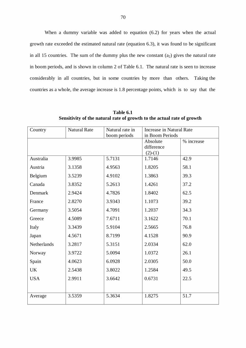
70

When a dummy variable was added to equation (6.2) for years when the actual

growth rate exceeded the estimated natural rate (equation 6.3), it was found to be significant

in all 15 countries. The sum of the dummy plus the new constant (a2) gives the natural rate

in boom periods, and is shown in column 2 of Table 6.1. The natural rate is seen to increase

considerably in all countries, but in some countries by more than others. Taking the

countries as a whole, the average increase is 1.8 percentage points, which is to say that the

Table 6.1 Sensitivity of the natural rate of growth to the actual rate of growth

Country Natural Rate Natural rate in

boom periods Increase in Natural Rate in Boom Periods

Absolute difference (2)-(1)

% increase

Australia

Austria

Belgium

Canada

Denmark

France

Germany

Greece

Italy

Japan

Netherlands

Norway

Spain

UK

USA

3.9985

3.1358

3.5239

3.8352

2.9424

2.8270

3.5054

4.5089

3.3439

4.5671

3.2817

3.9722

4.0623

2.5438

2.9911

5.7131

4.9563

4.9102

5.2613

4.7826

3.9343

4.7091

7.6711

5.9104

8.7199

5.3151

5.0094

6.0928

3.8022

3.6642

1.7146

1.8205

1.3863

1.4261

1.8402

1.1073

1.2037

3.1622

2.5665

4.1528

2.0334

1.0372

2.0305

1.2584

0.6731

42.9

58.1

39.3

37.2

62.5

39.2

34.3

70.1

76.8

90.9

62.0

26.1

50.0

49.5

22.5

Average 3.5359 5.3634 1.8275 51.7

71

actual rate of growth in boom periods has induced labour force growth and productivity

growth by that amount. The countries where the sensitivity of the natural rate seems to be

greatest are those where the reserves of labour are known to be highest such as Greece and

Italy (due to surplus labour in the south), and where output growth has induced impressive

technical progress through learning and sectoral rationalisation, such as Japan. In general,

the results show substantial elasticity of the labour force and productivity growth with

respect to the pressure of demand in the economy, and it is important to stress that these

results are not measuring simply the cyclical effect of demand on output growth because this

is captured by the coefficient, c2, in equation (6.3). The results are capturing the longer-

lasting effects that sustained demand expansion has had on the growth of productive potential

over the cycle.

Conclusion

The conclusion to this chapter can provide a fitting conclusion to the book as a whole.

In mainstream growth theory, including ‘new’ growth theory, the natural rate of growth is

treated as exogenously determined, unrelated to demand or the actual rate of growth. If

supply or output potential responds to demand, however, this raises the crucial question of

what does it mean to say that output growth is supply determined, or constrained by supply?

Of course, it is true in a trivial sense that capital and labour are required to produce output,

and how much output is produced will also depend on the level of technical efficiency, but

the really important question is why does the growth of capital, and technical progress differ

so much between countries? The supply-oriented, neoclassical production function approach

to the analysis of growth cannot answer this question, and for the most part never asks it!

72

What has been shown in this last chapter is that it is a mistake to regard the natural

rate of growth as exogenously given. The rate of growth necessary to keep the percentage

level of unemployment constant rises in boom periods and falls in recession because the

labour force and productivity growth are elastic to demand and output growth. This is also

confirmed using causality tests between input and output growth (not reported here, but see

Leon-Ledesma and Thirlwall, 2001). The orthodox and ‘new’ growth theories that assume

that it is input growth that unidirectionally causes output growth funds no support from the

evidence. The implication for growth theory and policy is that it makes little economic sense

to think of growth as supply constrained if demand, within limits, creates its own supply. If

factor inputs (including productivity growth) react endogenously, the process of growth, and

growth rate difference between countries can only be properly understood in terms of

differences in the strength of demand, and constraints on demand. For most countries, and

particularly developing countries, demand constraints operate long before capacity is

reached. Demand constraints are likely to be related to supply bottlenecks which cause

inflation and balance of payments difficulties for countries. It is this aspect of supply, and

not the growth of inputs in a production function, that should be the main focus of enquiry in

any supply-oriented theory of economic growth.

73

Bibliography

M. Abramovitz (1956), Resource and Output Trends in the United States since 1870,

American Economic Review Papers and Proceedings, May. K. Arrow (1962), The Economic Implications of Learning by Doing, Review of Economic

Studies, June. R. Barro (1991), Economic Growth in a Cross Section of Countries, Quarterly Journal of

Economics, May. W. Baumol (1986), Productivity Growth, Convergence and Welfare, American Economic

Review, December. J. Cornwall (1977), Modern Capitalism: Its Growth and Transformation (London: Martin

Robertson). E. Denison (1962), The Sources of Economic Growth in the US and the Alternatives before

Us, (New York: Committee for Economic Development, Library of Congress). E. Denison (1967), Why Growth Rates Differ: Post-war Experience in Nine Western

Countries (Washington DC: Brookings Institution). E. Domar (1947), Expansion and Employment, American Economic Review, March. A. Emmanuel (1972), Unequal Exchange: A Study of the Imperialism of Trade (New York:

Monthly Review Press). H. Esfahani (1991), Exports, Imports and Economic Growth in Semi-Industrialised

Countries, Journal of Development Economics, January. G. Feder (1983), On Exports and Economic Growth, Journal of Development Economics,

February/April. J. Felipe (1999), Total Factor Productivity Growth in East Asia: A Critical Survey, Journal

of Development Studies, April. B. Fingleton and J. McCombie (1996), Increasing Returns and Economic Growth: Some

Evidence from the European Union Regions, Oxford Economic Papers, January G. Frank (1967), Capitalism and Underdevelopment in Latin America (New York: Monthly

Review Press). Z. Griliches (1958), Research Costs and Social Returns: Hybrid Corn and Related

Innovations, Journal of Political Economy, October. G. Grossman and E. Helpman (1991), Innovation and Growth in the Global Economy

(Cambridge, Mass: MIT Press).

74

J.D. Hansen and J. Zhang (1996), A Kaldorian Approach to Regional Economic Growth in

China, Applied Economics, June. R. Harrod (1933), International Economics (Cambridge: Cambridge University Press). R. Harrod (1939), An Essay in Dynamic Theory, Economic Journal, March. J. Hicks (1950), The Trade Cycle (Oxford: Clarendon Press). A. Hirschman (1958), Strategy of Economic Development (New Haven: Yale University

Press). Z.F. Hu and M.S. Khan (1997), Why is China Growing so Fast?, IMF Staff Papers, March. K. Hussein and A.P. Thirlwall (2000), The AK Model of ‘New’ Growth Theory is the

Harrod-Domar Growth Equation: Investment and Growth Revisited, Journal of Post Keynsian Economics, Spring.

Journal of Post Keynesian Economics (1997), Symposium on Thirlwall’s Law, Spring. N. Kaldor (1957), A Model of Economic Growth, Economic Journal, December. N. Kaldor (1966), Causes of the Slow Rate of Economic Growth of the United Kingdom

(Cambridge: Cambridge University Press). N. Kaldor (1967), Strategic Factors in Economic Development (New York, Ithaca: New

York State School of Industrial and Labour Relations, Cornell University). N. Kaldor (1970), The Case for Regional Policies, Scottish Journal of Political Economy,

November. N. Kaldor (1972), ‘Advanced Technology in a Strategy for Development: Some Lessons

from Britain’s Experience’, in Automation and Developing Countries (Geneva: ILO). N. Kaldor (1985), Economics without Equilibrium (University College Cardiff Press). N. Kaldor (1996), Causes of Growth and Stagnation in the World Economy (The Raffaele

Lectures, Cambridge University Press). J.M. Keynes (1937), Some Economic Consequences of a Declining Population, Eugenics

Review, April. Kindleberger (1967), Europe’s Postwar Growth: the Role of the Labour Supply (Cambridge,

Mass: Harvard University Press). P. Krugman (1989), Differences in Income Elasticities and Trends in Real Exchange Rates,

European Economic Review, May. H. Leibenstein (1957), Economic Backwardness and Economic Growth (New York: Wiley).

75

M. Leon-Ledesma (2000), Economic Growth and Verdoorn’s Law in the Spanish Regions

1962-91, International Review of Applied Economics, January. M. Leon-Ledesma (2000), Accumulation, Innovation and Catching-Up: an Extended

Cumulative Growth Model, Cambridge Journal of Economics. M. Leon-Ledesma and A.P. Thirlwall (2001), The Endogeneity of the Natural Rate of

Growth, Cambridge Journal of Economics, R. Levine and D. Renelt (1992), A Sensitivity Analysis of Cross-Country Growth

Regressions, American Economic Review, September. A. Lewis (1954), Economic Development with Unlimited Supplies of Labour, Manchester

School, May. J. Lopez G. and A. Cruz B. (2000), “Thirlwall’s Law” and Beyond: the Latin American

Experience, Journal of Post Keynesian Economics, Spring R. Lucas (1988), On the Mechanics of Economic Development, Journal of Monetary

Economics, Vol 22. J. McCombie and A.P. Thirlwall (1994), Economic Growth and the Balance of Payments

Constraint (London: Macmillan). J. McCombie and J.R. de Ridder (1983), Increasing Returns, Productivity and Output

Growth: The Case of the United States, Journal of Post Keynesian Economics, Spring

J. McCombie (1985), Increasing Returns and the Manufacturing Industries: Some Empirical

Issues, The Manchester School, March J. McCombie (1985), Economic Growth, the Harrod Foreign Trade Multiplier and the Hicks’

Super Multiplier, Applied Economics, February. J. McCombie and A.P. Thirlwall (1997), The Dynamic Harrod Foreign Trade Multiplier and

the Demand Oriented Approach to Economic Growth: An Evaluation, International Review of Applied Economics, January.

A. Maddison (1970), Economic Progress and Policy in Developing Countries (London:

Allen and Unwin). T. Malthus (1798), Essay on the Principle of Population (London: Penguin, 1983). K. Marx (1867), Capital: A Critique of Political Economy, Vol.1 (New York: International

Publishers, 1967). T.R. Michl (1985), International Comparisons of Productivity Growth: Verdoorn’s Law

Revisited, Journal of Post Keynesian Economics, Summer

76

J.C. Moreno-Brid (1999), Mexico’s Economic Growth and the Balance of Payments Constraint: A Cointegration Analysis, International Review of Applied Economics Vol.13 No 2.

J.C. Moreno-Brid (1998), Balance of Payments Constrained Economic Growth: The Case of

Mexico, Banca Nazionale del Lavoro Quarterly Review, December. G. Myrdal (1957), Economic Theory and Underdeveloped Regions (London: Duckworth). R. Nelson (1956), A Theory of the Low Level Equilibrium Trap in Underdeveloped

Countries, American Economic Review, December. M. Nureldin-Hussain (1999), The Balance of Payments Constraint and Growth Rate

Differences among African and East Asian Economies, African Development Review, June.

Okun (1962), Potential GNP: Its Measurement and Significance, Proceedings of the Business

and Finance Statistics Section of the American Statistical Association. R. Prebisch (1950), The Economic Development of Latin America and its Principal Problems

(New York: ECLA, UN Dept. of Economic Affairs). D. Ricardo (1817), Principles of Political Economy and Taxation (London: Everyman,

1992). J. Robinson (1956), The Accumulation of Capital (London: Macmillan). P. Romer (1986), Increasing Returns and Long Run Growth, Journal of Political Economy,

October. R. Sandilands (1990), Nicholas Kaldor’s Notes on Allyn Young’s LSE Lectures, 1927-29,

Journal of Economic Studies, Vol.17 No 3/4/ T.W. Schultz (1961), Investment in Human Capital, American Economic Review, March. D. Seers (1962), A Model of Comparative Rates of Growth of the World Economy,

Economic Journal, March. A. Smith (1776), An Inquiry into the Nature and Causes of the Wealth of Nations (London:

Straham and Caddell). R. Solow (1956), A Contribution to the Theory of Economic Growth, Quarterly Journal of

Economics, February. R. Solow (1957), Technical Change and the Aggregate Production Function, Review of

Economics and Statistics, August. R. Summers and A. Heston (1991), The Penn World Table (Mark 5): An Expanded Set of

International Comparisons 1950-1966, Quarterly Journal of Economics, May.

77

F. Targetti and A.P. Thirlwall (1989), The Essential Kaldor (London: Duckworth). A.P. Thirlwall (1969), Okun’s Law and the Natural Rate of Growth, Southern Economic

Journal, July. A.P. Thirlwall (1979), The Balance of Payments Constraint as an Explanation of

International Growth Rate Differences, Banca Nazionale del Lavoro Quarterly Review, March.

A.P. Thirlwall (1983), Foreign Trade Elasticities in Centre-Periphery Models of Growth and

Development, Banca Nazionale del Lavoro Quarterly Review, September. A.P. Thirlwall (1986), A General Model of Growth and Development on Kaldorian Lines,

Oxford Economic Papers, July. A.P. Thirlwall (1987), Nicholas Kaldor (Brighton: Harvester Wheatsheaf Press). A.P. Thirlwall (1987), Keynes and Economic Development (London: Macmillan). A.P. Thirlwall and G. Sanna (1996), ‘”New” Growth Theory and the Macrodeterminants of

Growth: An Evaluation and Further Evidence’ in P. Arestis (ed), Employment, Economic Growth and the Tyranny of the Market: Essays in Honour of Paul Davidson Vol.2 (Aldershot: Edward Elgar).

A.P. Thirlwall (1999), Growth and Development: with Special Reference to Developing

Economies (London: Macmillan). A.P. Thirlwall (2000), Trade Agreements, Trade Liberalisation and Economic Growth: A

Selective Survey, African Development Review, December. UNCTAD (1999), Trade and Development Report (Geneva: UNCTAD). P.J. Verdoorn (1949), Fattori che Regolano lo Sviluppo della Produttivita del Lavoro,

L’Industria, No 1. English translation by A.P. Thirlwall in L. Pasinetti (ed), Italian Economic Papers Vol II (Oxford University Press, 1993).

World Bank (1991), World Development Report (Washington: World Bank). Allyn Young (1928), Increasing Returns and Economic Progress, Economic Journal,

December. Alwyn Young (1995), The Tyranny of Numbers: Confronting the Statistical Realities of the

East Asian Growth Experience, Quarterly Journal of Economics, August. Mexico Book

78

79