Alpine Peatlands of the Andes, Cajamarca, Peru - Sites · Cajamarca, Peru Abstract An ecological analysis of wetlands in the high mountain jalca above 3700 m elevation in the Andes

Alpine Peatlands of the Andes, Cajamarca, Peru

David J. Cooper*{Evan C. Wolf*{Christopher Colson1

Walter Vering1

Arturo Granda" and

Michael Meyer#

*Department of Forest, Rangeland and

Watershed Stewardship, Colorado State

University, Fort Collins, Colorado

80305, U.S.A.

{Corresponding author:

[email protected]

{Present address: Department of

Environmental Science, University of

California, Davis, California 95616,

U.S.A.

1Tetra Tech Inc., Boise, Idaho 83706,

U.S.A.

"Herbario de la Facultad de Ciencias

(MOL), Universidad Nacional Agraria

La Molina, Apdo. 456, Lima, Peru

#Minera Yanacocha S.R.L.,

Cajamarca, Peru

Abstract

An ecological analysis of wetlands in the high mountain jalca above 3700 m elevation

in the Andes near Cajamarca, Peru, indicated that most wetlands are groundwater-

supported peat-accumulating fens. The floristic composition of fen communities was

controlled largely by groundwater chemistry, which was highly variable and

influenced by watershed bedrock composition. Watersheds with highly mineralized

rock discharged water as acidic as pH 3.7, which was high in CaSO4, while

watersheds with limestone, marble, and skarn produced groundwater as basic as

pH 8.2 and high in CaHCO3. Of the 125 plots sampled in 36 wetland complexes,

.50% of plots had at least 3 m of peat, and 21 plots had peat thicker than 7 m. Most

soil horizons analyzed had 18 to 35% organic carbon, indicating high C storage. A

total of 102 vascular plants, 69 bryophytes, and 10 lichens were identified. Study

plots were classified using TWINSPAN into 20 plant communities, which were

grouped into four broad categories by dominant life form: (1) cushion plant

communities, (2) sedge- and rush-dominated communities, (3) bryophyte and lichen

communities, and (4) tussock grass communities. Direct gradient analysis using

canonical correspondence analysis indicated that Axis 1 was largely a water

chemistry gradient, while Axis 2 was a complex hydrology and peat thickness

gradient. Bryophytes and lichens were more strongly separated in the ordination

space than vascular plants and were better indicators of specific environmental

characteristics.

DOI: 10.1657/1938-4246-42.1.19

Introduction

In the world’s tropical regions, the largest area of alpine

vegetation above the limit of closed canopy forest and below the

permanent snowline is in the Andes Mountains of northern South

America (Smith and Young, 1994). This landscape includes broad

continuous highlands and isolated peaks that rise to elevations of

3500 m to over 6000 m. The northern Andes in Venezuela, Colombia,

and Ecuador receive abundant rainfall, and their alpine ecosystems

are termed paramo (Troll, 1968; Walter, 1985). From central Peru

south to central Chile the climate is drier, and the alpine ecosystems

are termed puna (Smith and Young, 1994). The transition between

paramo and puna occurs in northern Peru, between 4.5 and 8uSlatitude, and is termed jalca (Rundel et al., 1994; Luteyn, 1992).

Cloud forest forms the upper treeline in the east, while deep valleys

on the Andes’ western slopes are in rain shadows and support thorn

scrub and desert below the montane vegetation. In the jalca, tree-

sized Polylepis (Rosaceae) and Lupinus (Fabaceae) occur in scattered

patches within a high-elevation steppe.

The alpine flora of South America is the most species-rich of

all high mountain regions in the tropics (Smith and Cleef, 1988). It

contains the smallest number of boreal and temperate zone species

and the greatest proportion of endemics (Luteyn and Churchill,

2000). There have been analyses of regional biota, endemism, and

historical and biogeographic relationships of the flora (Young and

Reynel, 1997; Weigend, 2002; Young et al., 2002). However,

relatively little is known about factors controlling vegetation

composition (Squeo et al., 2006; Ginocchio et al., 2008).

Uplands in the jalca, paramo, and puna are dominated by

grass species in the genera Calamagrostis, Poa, and Festuca. Taller

rosette plants including species of Puya are common, along with

woody species of Senecio and other genera, particularly in

Asteraceae. Most areas are cultural landscapes (Young and

Reynel, 1997) heavily grazed by domestic livestock and burned

annually (Suarez and Medina, 2001).

Seasonally abundant precipitation has allowed the develop-

ment of numerous wetlands in the jalca, which have been

referred to as cushion mires (Bosman et al., 1993), highland bogs

(Wilcox et al., 1986), and soligenous (formed on slopes)

peatlands (Earle et al., 2003), and are locally and regionally

known as bofedales (Squeo et al., 2006). Ombrogenous (rain-fed)

bogs are known to occur in southern Chile (Kleinebecker et al.,

2008) but are unlikely to occur in the seasonally wet jalca. Few

wetlands in the jalca are known to be Sphagnum-dominated

(Earle et al., 2003), and not all are soligenous or dominated by

cushion plants (Squeo et al., 2006). It is unclear what proportion

of wetlands have accumulated peat and should be termed mires,

bogs, or peatlands. Little is known about the physical factors

controlling wetland distribution, wetland types, and their floristic

composition in the jalca. The goals of this study were to (1)

characterize the types of wetlands and the plant communities

occurring within them in a region of jalca in northern Peru, (2)

compile a list of species occurring in the wetlands, (3) determine

the proportion of wetlands that are peat-accumulating, and (4)

identify the physical factors controlling the floristic composition

of vegetation.

Arctic, Antarctic, and Alpine Research, Vol. 42, No. 1, 2010, pp. 19–33

E 2010 Regents of the University of Colorado D. J. COOPER ET AL. / 191523-0430/10 $7.00

Study Area

LANDSCAPES, LANDFORMS, AND HYDROLOGY

The study area is approximately 150 km2, located in

Cajamarca Department, in the Andean Cordillera of northern

Peru at elevations ranging from 3700 m to 4200 m (Fig. 1). Four

rivers originate in the study area: Chirimayo to the east,

Challhuagon to the south, Rio Grande to the north, and

Mamacocha to the west. Most wetlands occur on slopes or at

the toe of slopes and appear to be supported by groundwater

discharging from relatively localized and small hillslope aquifers.

Terminal moraines deposited perpendicular to valley bottoms

retard runoff and have created the hydrologic template for

wetland formation in many areas. Other wetlands occur up-

gradient from and adjacent to lakes or pond basins that had filled

with peat.

GEOLOGY

Bedrock in the study area is complex and highly variable,

consisting of five major rock types: Cretaceous sedimentary rocks

including limestone, Pliocene volcanic rocks, Eocene/Miocene

intrusive igneous rocks, metamorphic rocks where the original

parent material has been altered, and surficial Pleistocene

sediments (Davies, 2002).

Cation and anion concentrations, and acidity, differ in

groundwater originating in each bedrock type. Water emerging

from highly mineralized metamorphic rock is acidic due to the

formation of sulfuric acid from pyrite weathering (Cooper et al.,

2002; Verplank et al., 2006), while the dissolution of calcium

carbonate from limestone or marble (metamorphosed limestone)

produces alkaline water (Macpherson et al., 2008). Because of the

numerous lithologic contact zones, where two or more rock types

are adjacent to each other, a single wetland may straddle bedrock

types and receive runoff and groundwater from more than one

chemically distinct water source (Fig. 2)

CLIMATE

The rainy season in the jalca occurs from October to April,

contrasting strongly with the dry season from May through

September. Precipitation arrives from northeasterly winds that

bring warm and humid air masses from the Amazon Basin. Mean

annual precipitation is 1180 mm at Brillantana and 1400 mm at

Minas Sipan, both privately operated weather stations located

near the study area, and is highly variable from year to year. Sites

that are saturated to the surface with water-filled pools during the

rainy season may have dry pools and water tables .40 cm below

the soil surface during the dry season. Monthly temperatures are

relatively consistent year round, with January being the warmest

month with a mean temperature of 7.8 uC.

Methods

FIELD METHODS AND SPECIES NOMENCLATURE

We sampled all 36 major wetland complexes in the study area

(Fig. 1). In each complex we identified homogeneous stands of

vegetation and collected data on the physical environment and

floristic composition of each stand. The number of stands

analyzed in each wetland depended upon its size and heterogene-

ity, and varied from one to seven. One 20 m2 plot was analyzed in

each stand for plant species composition, and we visually

estimated percent canopy coverage by species. A total of 125

plots were analyzed. All data were collected in September and

October 2005. Collections of unknown vascular plants were

identified at Herbario de la Facultad de Ciencias (MOL),

Universidad Nacional Agraria La Molina, Lima, Peru, where all

vouchers are housed. We used the APG II (Angiosperm Phylogeny

Group) system of plant classification (Stevens, 2001; Angiosperm

Phylogeny Group, 2003; http://www.mobot.org/MOBOT/re-

search/APweb/) for species nomenclature. The geographic distri-

FIGURE 1. Location of studysites (dots on left panel) in theDepartment Cajamarca (middlepanel) in Peru, South America.The study area is centered at6u549S, 78u229W.

FIGURE 2. View of wetland Cocanes 3 looking southeast,illustrating its three major groundwater flow systems indicated byarrows. The water flowing from the near side of the wetland (twoblack arrows) has pH ranging from 6.4 to 6.7, while that from thefar side (white arrow) is highly acid with pH ranging from 4.3 to 4.7.The two areas support different plant species and plant communities.

20 / ARCTIC, ANTARCTIC, AND ALPINE RESEARCH

bution of vascular plant taxa were investigated using the U.S.

Department of Agriculture PLANTS database ,http://plants.

usda.gov. and The Missouri Botanical Garden’s website database

TROPICOS ,http://www.tropicos.org..

In each plot we measured the pH of groundwater that filled a

20- to 40-cm-deep soil pit using an Orion model 250A pH meter

with combination electrode. We measured the wetland’s slope

using a Suunto clinometer, aspect with a compass, peat thickness

with a tile probe pushed until rock or dense mineral soil was

encountered, groundwater level in the open soil pit after it had

equilibrated for 1 h, and soil temperature at 13 and 28 cm depth

with thermometers.

Lichens were identified by Dr. S. Will-Wolf, Sphagnum by Dr.

Richard Andrus, other mosses and liverworts were identified by

Dr. W. Weber with the exception of Scorpidium and Drepanocla-

dus (L. Hedenas), Breutelia and Philonotis (Dana Griffin III),

Campylopus (Jan-Peter Frahm), Leptodontium (Richard Zander),

and Dicranum (Robert Ireland). Voucher specimens of all

cryptogams are at the University of Colorado at Boulder (COLO).

LABORATORY ANALYSIS OF WATER AND SOIL SAMPLES

Water was collected from 32 wetland complexes for analysis of

dissolved ions, metals, and nutrients. The lack of shallow

groundwater made it impossible to collect water from 4 wetlands.

Two 1 L sample bottles were filled from the 40-cm-deep soil pit after

it filled with fresh clean groundwater. Samples were stored on ice in

the field and for transport, and in a refrigerator until analyzed by

ALS Environmental in Lima, Peru. One sample bottle from each

site was acidified in the field to stabilize the metals. All samples were

filtered in the laboratory. We used standard analytical procedures

recommended by the American Public Health Association (APHA,

2005) for analysis: Ca, Cu, Mg, and Fe using direct nitrous oxide-

acetylene flame method (APHA 3111-D), Na and K using flame

photometric method (APHA 3500-K-B), HCO3 and CO3 using

titration (APHA 2320-B), SO4 using turbidimetric method (APHA

4500-SO4 E), and total P using persulfate digestion method (APHA

4500-P-E). Total N was determined using the Kjeldahl method,

following ASTM method D5176-91 (standard method for total

chemically bound N, http://amaec.kicet.re.kr/cd_astm/PAGES/

D5176.htm). Percent organic carbon (OC) for one soil sample in

each stand was collected at ,30–40 cm depth from a soil pit and

analyzed using a LECO soil analyzer.

SOIL CLASSIFICATION

Soils in the upper 40 cm horizon were analyzed for % OC and

organic horizon thickness. Soils containing ,18% OC were

classified as mineral horizons, while those with .18% OC were

classed as organic horizons following USDA Soil Taxonomy

(USDA, 1999). If organic horizons were .40 cm thick, the soils

were considered to be peat, and wetlands with peat soils to be

peatland ecosystems. Sloping wetlands that lacked peat soils were

classified as wet meadows, while those on lake shores that flooded

deeply were classified as marshes.

DATA ANALYSIS

Divisive cluster analysis using Two Way Indicator Species

Analysis (TWINSPAN) was performed with the computer

program PC Ord (McCune and Mefford, 1999) to sort plots into

groups based upon their floristic composition. Braun-Blanquet

table sorting methods (Mueller-Dombois and Ellenberg, 1975)

were used to further refine the plot groupings and produce a

vegetation classification.

Direct gradient analysis was used to identify the major

environmental gradients controlling the floristic composition of

study stands. Canonical correspondence analysis (CCA) was

performed using the default settings in the computer program

CANOCO (ter Braak, 1986, 1992; ter Braak and Prentice, 1988).

Forward selection was used to test the main environmental

variables. Variables were tested for their significance using a Monte

Carlo permutation test (499 permutations), and significant vari-

ables (P , 0.05, except Cu which was accepted at P , 0.01) were

included in the analysis and are shown on the canonical ordination

diagrams. A Monte Carlo permutation test (499 runs) was

performed to evaluate the significance of the environmental

variables and the first ordination axis in explaining the vegetation

composition (P , 0.05). In addition, a Monte Carlo permutation

test (499 runs) was used to test the significance of all canonical

eigenvalues. Raw data were not transformed prior to analysis. Two

CCA diagrams are presented, one for vegetation composition of

plots, and a second for plant species.

Results

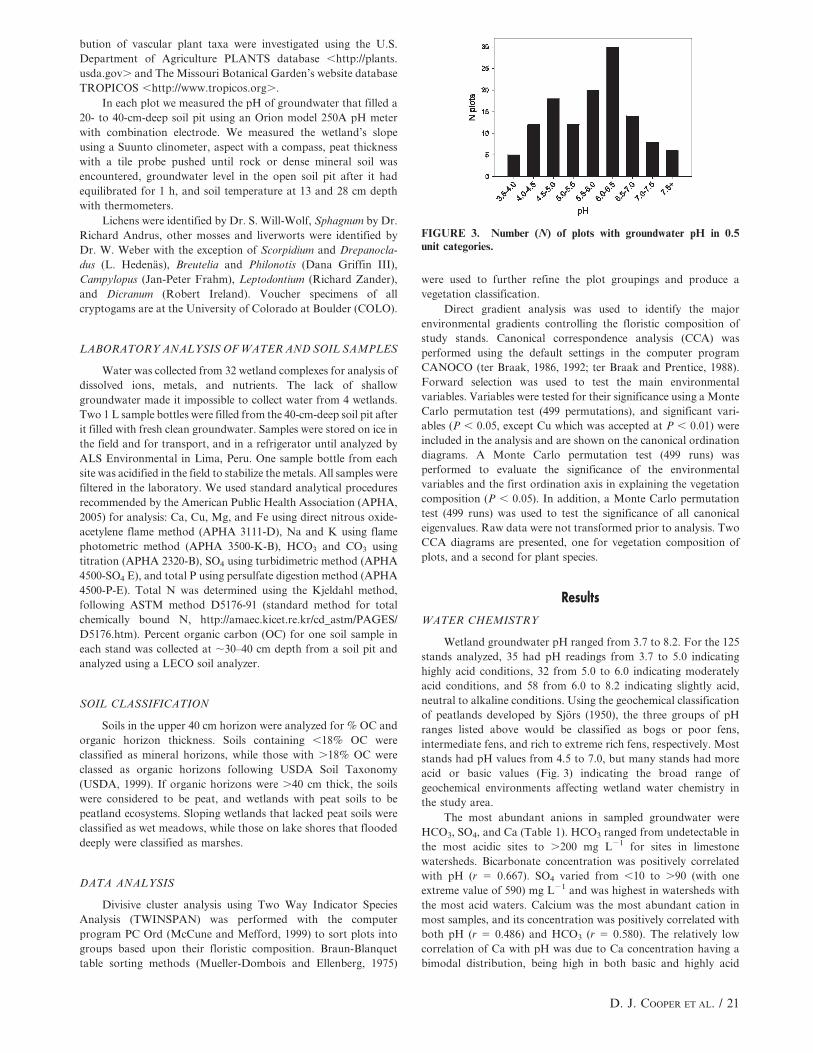
WATER CHEMISTRY

Wetland groundwater pH ranged from 3.7 to 8.2. For the 125

stands analyzed, 35 had pH readings from 3.7 to 5.0 indicating

highly acid conditions, 32 from 5.0 to 6.0 indicating moderately

acid conditions, and 58 from 6.0 to 8.2 indicating slightly acid,

neutral to alkaline conditions. Using the geochemical classification

of peatlands developed by Sjors (1950), the three groups of pH

ranges listed above would be classified as bogs or poor fens,

intermediate fens, and rich to extreme rich fens, respectively. Most

stands had pH values from 4.5 to 7.0, but many stands had more

acid or basic values (Fig. 3) indicating the broad range of

geochemical environments affecting wetland water chemistry in

the study area.

The most abundant anions in sampled groundwater were

HCO3, SO4, and Ca (Table 1). HCO3 ranged from undetectable in

the most acidic sites to .200 mg L21 for sites in limestone

watersheds. Bicarbonate concentration was positively correlated

with pH (r 5 0.667). SO4 varied from ,10 to .90 (with one

extreme value of 590) mg L21 and was highest in watersheds with

the most acid waters. Calcium was the most abundant cation in

most samples, and its concentration was positively correlated with

both pH (r 5 0.486) and HCO3 (r 5 0.580). The relatively low

correlation of Ca with pH was due to Ca concentration having a

bimodal distribution, being high in both basic and highly acid

FIGURE 3. Number (N) of plots with groundwater pH in 0.5unit categories.

D. J. COOPER ET AL. / 21

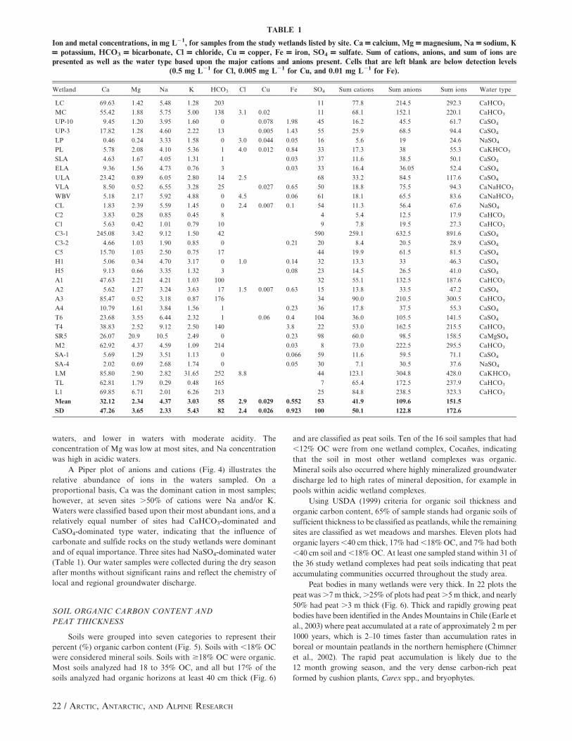
waters, and lower in waters with moderate acidity. The

concentration of Mg was low at most sites, and Na concentration

was high in acidic waters.

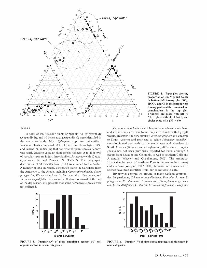
A Piper plot of anions and cations (Fig. 4) illustrates the

relative abundance of ions in the waters sampled. On a

proportional basis, Ca was the dominant cation in most samples;

however, at seven sites .50% of cations were Na and/or K.

Waters were classified based upon their most abundant ions, and a

relatively equal number of sites had CaHCO3-dominated and

CaSO4-dominated type water, indicating that the influence of

carbonate and sulfide rocks on the study wetlands were dominant

and of equal importance. Three sites had NaSO4-dominated water

(Table 1). Our water samples were collected during the dry season

after months without significant rains and reflect the chemistry of

local and regional groundwater discharge.

SOIL ORGANIC CARBON CONTENT AND

PEAT THICKNESS

Soils were grouped into seven categories to represent their

percent (%) organic carbon content (Fig. 5). Soils with ,18% OC

were considered mineral soils. Soils with $18% OC were organic.

Most soils analyzed had 18 to 35% OC, and all but 17% of the

soils analyzed had organic horizons at least 40 cm thick (Fig. 6)

and are classified as peat soils. Ten of the 16 soil samples that had

,12% OC were from one wetland complex, Cocanes, indicating

that the soil in most other wetland complexes was organic.

Mineral soils also occurred where highly mineralized groundwater

discharge led to high rates of mineral deposition, for example in

pools within acidic wetland complexes.

Using USDA (1999) criteria for organic soil thickness and

organic carbon content, 65% of sample stands had organic soils of

sufficient thickness to be classified as peatlands, while the remaining

sites are classified as wet meadows and marshes. Eleven plots had

organic layers ,40 cm thick, 17% had ,18% OC, and 7% had both

,40 cm soil and ,18% OC. At least one sampled stand within 31 of

the 36 study wetland complexes had peat soils indicating that peat

accumulating communities occurred throughout the study area.

Peat bodies in many wetlands were very thick. In 22 plots the

peat was .7 m thick, .25% of plots had peat .5 m thick, and nearly

50% had peat .3 m thick (Fig. 6). Thick and rapidly growing peat

bodies have been identified in the Andes Mountains in Chile (Earle et

al., 2003) where peat accumulated at a rate of approximately 2 m per

1000 years, which is 2–10 times faster than accumulation rates in

boreal or mountain peatlands in the northern hemisphere (Chimner

et al., 2002). The rapid peat accumulation is likely due to the

12 month growing season, and the very dense carbon-rich peat

formed by cushion plants, Carex spp., and bryophytes.

TABLE 1

Ion and metal concentrations, in mg L21, for samples from the study wetlands listed by site. Ca = calcium, Mg = magnesium, Na = sodium, K= potassium, HCO3 = bicarbonate, Cl = chloride, Cu = copper, Fe = iron, SO4 = sulfate. Sum of cations, anions, and sum of ions arepresented as well as the water type based upon the major cations and anions present. Cells that are left blank are below detection levels

(0.5 mg L21 for Cl, 0.005 mg L21 for Cu, and 0.01 mg L21 for Fe).

Wetland Ca Mg Na K HCO3 Cl Cu Fe SO4 Sum cations Sum anions Sum ions Water type

LC 69.63 1.42 5.48 1.28 203 11 77.8 214.5 292.3 CaHCO3

MC 55.42 1.88 5.75 5.00 138 3.1 0.02 11 68.1 152.1 220.1 CaHCO3

UP-10 9.45 1.20 3.95 1.60 0 0.078 1.98 45 16.2 45.5 61.7 CaSO4

UP-3 17.82 1.28 4.60 2.22 13 0.005 1.43 55 25.9 68.5 94.4 CaSO4

LP 0.46 0.24 3.33 1.58 0 3.0 0.044 0.05 16 5.6 19 24.6 NaSO4

PL 5.78 2.08 4.10 5.36 1 4.0 0.012 0.84 33 17.3 38 55.3 CaKHCO3

SLA 4.63 1.67 4.05 1.31 1 0.03 37 11.6 38.5 50.1 CaSO4

ELA 9.36 1.56 4.73 0.76 3 0.03 33 16.4 36.05 52.4 CaSO4

ULA 23.42 0.89 6.05 2.80 14 2.5 68 33.2 84.5 117.6 CaSO4

VLA 8.50 0.52 6.55 3.28 25 0.027 0.65 50 18.8 75.5 94.3 CaNaHCO3

WBV 5.18 2.17 5.92 4.88 0 4.5 0.06 61 18.1 65.5 83.6 CaNaHCO3

CL 1.83 2.39 5.59 1.45 0 2.4 0.007 0.1 54 11.3 56.4 67.6 NaSO4

C2 3.83 0.28 0.85 0.45 8 4 5.4 12.5 17.9 CaHCO3

C1 5.63 0.42 1.01 0.79 10 9 7.8 19.5 27.3 CaHCO3

C3-1 245.08 3.42 9.12 1.50 42 590 259.1 632.5 891.6 CaSO4

C3-2 4.66 1.03 1.90 0.85 0 0.21 20 8.4 20.5 28.9 CaSO4

C5 15.70 1.03 2.50 0.75 17 44 19.9 61.5 81.5 CaSO4

H1 5.06 0.34 4.70 3.17 0 1.0 0.14 32 13.3 33 46.3 CaSO4

H5 9.13 0.66 3.35 1.32 3 0.08 23 14.5 26.5 41.0 CaSO4

A1 47.63 2.21 4.21 1.03 100 32 55.1 132.5 187.6 CaHCO3

A2 5.62 1.27 3.24 3.63 17 1.5 0.007 0.63 15 13.8 33.5 47.2 CaSO4

A3 85.47 0.52 3.18 0.87 176 34 90.0 210.5 300.5 CaHCO3

A4 10.79 1.61 3.84 1.56 1 0.23 36 17.8 37.5 55.3 CaSO4

T6 23.68 3.55 6.44 2.32 1 0.06 0.4 104 36.0 105.5 141.5 CaSO4

T4 38.83 2.52 9.12 2.50 140 3.8 22 53.0 162.5 215.5 CaHCO3

SR5 26.07 20.9 10.5 2.49 0 0.23 98 60.0 98.5 158.5 CaMgSO4

M2 62.92 4.37 4.59 1.09 214 0.03 8 73.0 222.5 295.5 CaHCO3

SA-1 5.69 1.29 3.51 1.13 0 0.066 59 11.6 59.5 71.1 CaSO4

SA-4 2.02 0.69 2.68 1.74 0 0.05 30 7.1 30.5 37.6 NaSO4

LM 85.80 2.90 2.82 31.65 252 8.8 44 123.1 304.8 428.0 CaKHCO3

TL 62.81 1.79 0.29 0.48 165 7 65.4 172.5 237.9 CaHCO3

L1 69.85 6.71 2.01 6.26 213 25 84.8 238.5 323.3 CaHCO3

Mean 32.12 2.34 4.37 3.03 55 2.9 0.029 0.552 53 41.9 109.6 151.5

SD 47.26 3.65 2.33 5.43 82 2.4 0.026 0.923 100 50.1 122.8 172.6


FLORA

A total of 102 vascular plants (Appendix A), 69 bryophyte

(Appendix B), and 10 lichen taxa (Appendix C) were identified in

the study wetlands. Most Sphagnum spp. are unidentified.

Vascular plants comprised 56% of the flora, bryophytes 38%,

and lichens 6%, indicating that non-vascular plant species richness

was nearly equal to vascular plant species richness. A total of 49%

of vascular taxa are in just three families, Asteraceae with 12 taxa,

Cyperaceae 14, and Poaceae 24 (Table 2). The geographic

distribution of 54 vascular taxa (53%) was limited to the Andes.

A number of taxa are widely distributed along the Cordillera from

the Antarctic to the Arctic, including Carex microglochin, Carex

praegracilis, Eleocharis acicularis, Juncus arcticus, Poa annua, and

Veronica serpyllifolia. Because our collections occurred at the end

of the dry season, it is possible that some herbaceous species were

not collected.

Carex microglochin is a calciphile in the northern hemisphere,

and in the study area was found only in wetlands with high pH

waters. However, the very similar Carex camptoglochin is endemic

to South America and restricted to acidic Sphagnum magellani-

cum–dominated peatlands in the study area and elsewhere in

South America (Wheeler and Guaglianone, 2003). Carex campto-

glochin has not been previously reported for Peru, although it

occurs from Ecuador and Colombia, as well as southern Chile and

Argentina (Wheeler and Guaglianone, 2003). The Amotape-

Huancabamba zone of northern Peru is known to have many

endemic taxa (Weigend, 2002, 2004); however, no species new to

science have been identified from our collections to date.

Bryophytes covered the ground in many wetland communi-

ties. In particular, Sphagnum magellanicum, Breutelia chrysea, B.

polygastria, B. subarcuata, B. tomentosa, Campylopus argyrocau-

lon, C. cucullatifolius, C. sharpii, Cratoneuron filicinum, Drepano-

FIGURE 4. Piper plot showingproportion of Ca, Mg, and Na+Kin bottom left ternary plot; SO4,HCO3, and Cl in the bottom rightternary plot; and the combined ioncombinations in the top plot.Triangles are plots with pH ,

5.0, x plots with pH 5.0–6.0, andcircles plots with pH . 6.0.

FIGURE 5. Number (N) of plots containing percent (%) soilorganic carbon in seven categories.

FIGURE 6. Number (N) of plots containing peat soil thickness innine categories.


cladus longifolius, Hamatocaulis vernicosus, Polytrichum juniper-

inum, Scorpidium cossonii, S. scorpioides, and Warnstorfia

exannulata had high canopy coverage in many stands and

characterized some wetland community types. Bryophytes, be-

cause they lack roots, are highly sensitive indicators of environ-

mental conditions at the soil surface, particularly water pH and

chemical content, and water table depth and duration of soil

saturation (Vitt and Chee, 1990; Cooper and Andrus, 1994).

Because bryophytes and lichens comprise .40% of the flora

and dominate the vegetation at many sites, they are essential to

include in wetland classification and characterization studies. This

is particularly important in the study area where many vascular

plant species—for example Carex pichinchensis, C. bonplandii,

Werneria nubigena, and some species of Calamagrostis—occurred

in both acid and alkaline wetlands, making them poor indicators

of specific environmental conditions. Classifications based solely

upon vascular plant taxa could miss even the most important

environmental differences among communities.

The bryophytes Straminergon stramineum, Scorpidium cosso-

nii, Scorpidium scorpioides, Warnstorfia exannulata, Drepanocladus

longifolius, Drepanocladus polygamus, Drepanocladus sordidus, and

Meesia uliginosa are characteristic of basic to slightly acid

peatlands throughout the northern hemisphere, and occupy

similar environments in the study area. Species of Sphagnum,

Polytrichium, and many Campylopus and Breutelia were indicative

of acidic waters in the study area. Lichens were common only in

acid peatlands, and the fruticose species Cladina confusa, C.

arbuscula, and Cladia aggregata formed dense patches.

VEGETATION

Plant communities of the study area were placed into four

broad categories based upon the dominant life form: (1) cushion

plant, (2) sedge and rush, (3) bryophyte and lichen, and (4) tussock

grasses. Within these broad categories 20 plant communities were

identified from the 125 plots using TWINSPAN, and are briefly

described below.

Cushion Plant Communities

Wetlands with cushion-forming vascular plants have been

reported only for the southern hemisphere including the Andes,

New Zealand (Wardle, 1991), and Africa (Hedberg, 1964, 1979,

1992). Typically termed cushion bogs (Bosman et al., 1993), these

wetlands are fens supported by groundwater discharge, not solely

by direct precipitation. The most common cushion-forming species

were Plantago tubulosa, Oreobolus obtusangulus, Werneria pygmaea,

Distichia acicularis, Aciachne pulvinata, and D. muscoides, with the

first two species being most abundant. Cushion communities

dominated by species of Oreobolus occur in many other regions;

for example O. pectinatus in New Zealand (Wardle, 1991) and O.

cleefii in Ecuador (Bosman et al., 1993). Distichia muscoides,

Plantago rigida, and Oreobolus cleefii dominate cushion wetlands in

the Andes of Colombia (Cleef, 1981) and D. muscoides dominates

similar wetlands in Chile (Squeo et al., 2006). Donatia fascicularis

and Astelia pumila dominate cushion plant communities in southern

Chile (Kleinebecker et al., 2008). Cushion community soils had the

highest organic carbon content of any community type, ranging

from 30 to 40%. The high organic content, and nearly year-round

growth of the dense cushions has produced peat deposits .7 m

thick in many sites. These communities are heavily used for

livestock forage, are deeply hummocked by cattle trampling, and

sod has been cut from many sites for use as a building material and

for fuel, and in some areas all of the vegetation and peat has been

removed. Three cushion plant communities were identified:

(1) Plantago tubulosa–Oreobolus obtusangulus–Werneria pyg-

maea–Distichia acicularis: This cushion community is common

and widespread in the study area. The vegetation can be

dominated by any species for which the community is named,

but all stands have prostrate forms and most have thick peat

accumulations (Fig. 7A).

(2) Distichia muscoides–Breutelia polygastria: This cushion-

forming community is rare in the study area and characterized by

dense turfs of Distichia muscoides.

(3) Werneria nubigena–Campylopus spp.: This is one of the

most characteristic communities in many wetlands because the

leaves and flowers of Werneria nubigena are distinctive.

Sedge- and Rush-dominated Communities

Species of Cyperaceae and Juncaceae dominate wetlands on

the margins of lakes and ponds where seasonal standing water

occurs, and in some sloping wetlands. Stands of Schoenoplectus

californicus and Juncus arcticus form dense stands bordering many

lakes and ponds (Fig. 8). Stands of short stature Carex crinalis

dominated pool margins in acid wetlands. The most common

sedge was Carex pichinchensis but Carex bonplandii, C. hebetata,

C. praegracilis, C. camptoglochin, Uncinia hamata, and Eleocharis

albibracteata were also common. Fourteen sedge and rush

community types are described, indicating the high diversity of

this type of wetland.

(4) Carex pichinchensis–Scorpidium scorpioides–Cratoneuron

filicinum: This community is dominated by the tall sedge Carex

TABLE 2

Number of vascular plant taxa and proportion of flora by family.

Family N Taxa % Flora

Apiaceae 1 0.98

Araliaceae 1 0.98

Asteraceae 12 11.76

Brassicaceae 2 1.96

Bromeliaceae 1 0.98

Campanulaceae 1 0.98

Caryophyllaceae 2 1.96

Cyperaceae 14 13.73

Ericaceae 2 1.96

Fabaceae 2 1.96

Gentianaceae 5 4.90

Geraniaceae 1 0.98

Hypericaceae 1 0.98

Isoetaceae 1 0.98

Juncaceae 5 4.90

Lamiaceae 1 0.98

Lentibulariaceae 1 0.98

Lycopodiaceae 1 0.98

Melastomataceae 1 0.98

Onagraceae 1 0.98

Orchidaceae 2 1.96

Orobanchaceae 2 1.96

Phrymaceae 1 0.98

Plantaginaceae 3 2.94

Poaceae 24 23.53

Polygonaceae 1 0.98

Ranunculaceae 4 3.92

Rosaceae 5 4.90

Rubiaceae 1 0.98

Salviniaceae 1 0.98

Valerianaceae 1 0.98

Violaceae 1 0.98

Total 102 100


pichinchensis and forms dense vegetation in shallow flooded basins

with water that has a pH . 6.0. The mosses Scorpidium scorpioides

and/or Cratoneuron filicinum are common in this alkaline wetland

type (Fig. 7B).

(5) Carex pichinchensis–Werneria nubigena: Sloping wetlands

dominated by the tall sedge Carex pichinchensis are common in

acid sites and have an understory of Werneria nubigena.

(6) Schoenoplectus californicus: This tall bulrush marsh

community occurred on the margins of lakes in the study area.

(7) Juncus arcticus–Scorpidium scorpioides–Brachythecium

stereopoma: This community dominates flooded marshes on pond

margins in alkaline environments where it has an understory of

Scorpidium scorpioides and other bryophytes.

(8) Juncus arcticus–Campylopus nivalis: This community

occurs in seasonally or perennially flooded marsh basins with an

understory of Campylopus nivalis and other bryophytes.

(9) Carex hebetata–Cratoneuron filicinum. This tall sedge

community occurred in sloping alkaline fens.

(10) Carex praegracilis–Cratoneuron filicinum: This community

occupies seasonally flooded sloping lake shorelines. Carex praegra-

cilis is common in wet meadows and fens in North America.

(11) Hypsela reniformis–Drepanocladus longifolius: This com-

munity was found in seasonally flooded but sloping lake shorelines.

(12) Carex camptoglochin–Jensenia erythropus: This commu-

nity occurred on sloping acid sites, and has an open canopy of

Carex camptoglochin and an understory of the liverwort Jensenia

erythropus and other mosses.

(13) Carex crinalis–Sphagnum pylaesii: This community

occurred in and around pools in the larger acidic wetlands, with

Sphagnum pylaesii submerged in pools.

(14) Carex bonplandii: Stands dominated by Carex bonplandii

occurred in several acid wetlands.

(15) Carex bonplandii–Drepanocladus longifolius: This highly

productive sedge community occurs in areas with a plentiful

supply of alkaline water, and nearly constant saturation to the soil

surface.

(16) Uncinia hamata–Puya fastuosa: A community dominated

by the distinctive sedge Uncinia hamata was sampled once, but

may be regionally common.

(17) Eleocharis albibracteata–Scorpidium cossonii: This is the

characteristic community of sloping fens in limestone watersheds.

The spike rush Eleocharis albibracteata has high fidelity to this

community type, and the ground layer is covered by mosses that

occur only in alkaline substrates, particularly Scorpidium cossonii.

Bryophyte- and Lichen-dominated Community

Sphagnum spp. and Cladina spp. are characteristic of acidic

fens throughout the study area. These wetlands have complex

topography with pools and hummocks, although submerged

aquatic vascular plants were not seen.

(18) Sphagnum magellanicum–Cladina confusa–Loricaria ly-

copodinea: This is the common and distinctive fen community in

acid wetlands. The ground layer is dominated by Sphagnum spp.,

most commonly S. magellanicum, several unidentified Sphagnum

taxa, and the fruticose lichens Cladina confusa, C. arbuscula ssp.

Boliviana, and Cladia aggregata. Loricaria lycopodinea is also

distinctive (Fig. 7C).

Tussock Grass Communities

Tussock grass-dominated communities were present in every

wetland complex investigated, and are dominated by two genera,

Calamagrostis and Cortadaria. Calamagrostis tarmensis, C. rigida,

FIGURE 7. Photographs of four of the major vegetation types. (A) Cushion plant community heavily damaged by livestock tramplingshowing the Plantago tubulosa–Oreobolus obtusangulus–Werneria pygmaea–Distichia acicularis community. (B) Sedge vegetation in plotshowing the Carex pichinchensis–Scorpidium scorpioides–Cratoneuron filicinum community. (C) Bryophyte- and lichen-dominated vegetationshowing the Sphagnum magellanicum–Cladina confusa–Loricaria lycopodinea community. The dark plant is Loricaria lycopodinea. (D)Tussock grass community showing the Cortaderia hapalotricha–Cortaderia sericantha community.


and C. recta were abundant, as were Cortaderia hapalotricha and

C. sericantha. In the Ecuadorian paramo C. sericantha dominates

wetland communities (Bosman et al., 1993).

(19) Cortaderia hapalotricha–Cortaderia sericantha: Stands

dominated by Cortaderia were typical of wetlands with acid soils.

This community occurred on sites with deeper water tables, some

of which lacked peat soils (Fig. 7D).

(20) Calamagrostis tarmensis–Campylopus cucullatifolius–

Scorpidium cossonii: Bunch grass communities dominated by

Calamagrostis tarmensis, and other species of Calamagrostis, are

characteristic of many wetlands, with acid and alkaline soils.

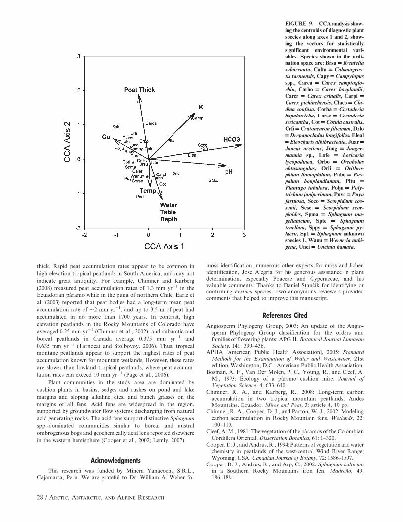
DIRECT GRADIENT ANALYSIS OF THE VEGETATION

AND SPECIES DATA

The eigenvalue of the first canonical axis is 0.507 (Table 3),

and it was statistically significant at P , 0.01 using a Monte Carlo

permutation test. The sum of all canonical eigenvalues was also

significant at P , 0.01, demonstrating that the relation between

the species and the environmental variables is highly significant (P

, 0.01). The canonical coefficients and intra-set correlations of

environmental variables from the CCA analyses (Table 3) indicate

that Axis 1 is driven by water chemistry, particularly HCO3

content and pH. Sites with high HCO3 have low SO4 concentra-

tions, high pH, and are plotted on the right side of the canonical

ordination diagram (Fig. 8), while those with low HCO3 and low

pH are on the left. Acidic wetlands form a relatively tight cluster

along Axis 1 between 0 and 21, indicating that these communities

are abundant and have relatively similar floristic composition.

Most acid waters had detectable concentrations of copper and

iron, and other metals are likely present as well.

CCA axis 2 is a complex hydrologic, soil temperature, and

peat thickness gradient. Sites with deeper water tables during 2005

had warmer soil temperatures and thinner peat deposits, and

plotted at the bottom of the canonical ordination diagram. Sites

near the top of the diagram have thicker peat, cooler soil

temperatures at 28 cm, and a water table closer to the soil surface.

On the right side of the species canonical ordination diagram

(Fig. 9), the mosses Cratoneuron filicinum, Scorpidium scorpioides,

S. cossonii, and Drepanocladus longifolius along with the vascular

plant species Eleocharis albibracteata and Carex praegracilis are

diagnostic of alkaline waters. On the acidic (left) side of the

gradient are species of Sphagnum, Polytrichum juniperinum, and

the fruticose lichens Cladina confusa, C. arbuscula, and Cladia

aggregata. Among the vascular plants, Loricaria lycopodinea,

Cortaderia hapalotricha, C. sericantha, Carex crinalis, and

Werneria nubigena are most abundant in acid wetlands. Juncus

arcticus and Carex pichinchensis are plotted near the center of the

ordination space indicating their occurrence in acid and basic

wetlands, and those with thick and thin peat deposits. Bryophyte

and lichen species were more closely tied to specific hydrological

and geochemical environments than vascular plants.

Discussion

Geologically complex mountain systems, such as the northern

Andes, are composed of a range of bedrock types, including highly

mineralized igneous and metamorphic rocks as well as limestone

and other sedimentary rocks. Groundwater contacting each rock

type is geochemically distinct, and along with landforms produced

by glaciers and hillslope processes form heterogeneous environ-

ments that support a diversity of wetlands. Direct gradient

analysis indicated that wetland floristic composition is controlled

primarily by groundwater geochemistry, which explained more of

the total variation in species composition than all other

environmental variables combined. Similar controlling gradients

occur in boreal (Vitt and Chee, 1990; Nicholson et al., 1996) and

mountain wetlands (Gignac et al., 1991; Cooper and Andrus,

FIGURE 8. CCA analysis ofall plots along axes 1 and 2,showing the vectors for statisti-cally significant environmentalvariables. Eigenvalue of the firstcanonical axis is 0.507 and isstatistically significant at P ,

0.01 using a Monte Carlo permu-tation test. The sum of all canon-ical eigenvalues was also signifi-cant at P , 0.01, demonstratingthat the relation between thespecies and the environmentalvariables is highly significant (P, 0.01). Numbers are plots as-signed to each community type.


1994) in Canada and the U.S.A., where biogeochemical variables,

more than climate, explain the most floristic variation. In the

study area, acid and alkaline sloping wetlands have few species in

common. This acidic to alkaline gradient is typically referred to as

the ‘‘rich to poor’’ gradient (Sjors, 1950; Malmer, 1986) and

provides a conceptual understanding of peatland vegetation

variation throughout the world.

Poor fens and bogs are typically dominated by species of

Sphagnum whose ion exchange capacity acidifies water and soil.

However, acidic waters in the study area are produced by the

oxidation of mineral sulfides to form sulfuric acid. This water

discharges from hillslopes and its pH is little altered during its flow

path through the wetland or apparently by ion exchange by

Sphagnum species. The acid water may leach cations and metals

from watershed rock producing acidic and ion-rich water which

have been termed iron fens or acid geothermal fens in the Rocky

Mountains of the U.S.A. (Cooper et al., 2002; Lemly, 2007). Iron

fens occur in watersheds with iron pyrite, which results in

precipitation of iron and the formation of iron rich peat, mineral

terraces, and bog iron ore formation, similar to those in the study

area. Acid geothermal fens occur in volcanic landscapes where

sulfur vents produce mineral sulfides. These fens are distinct from

poor fens or bogs, which are saturated largely by precipitation and

have mineral ion poor waters. The acid fens in our study area were

dominated by S. magellanicum, which also dominates ombro-

trophic (rain fed) bogs in hypermaritime regions of south

Patagonia (Kleinebecker et al., 2008) and southeastern Alaska

(Klinger, 1996), indicating that water acidity more than climate

variables control the distribution and abundance of many peat-

land species. The alkaline portion of the rich-poor gradient

supports Scorpidium scorpioides and other brown mosses in the

family Amblystegiaceae which dominate rich and extreme rich

fens around the world.

Axis 2 of our CCA analysis (Fig. 9) represents a complex

hydrologic gradient. Wetlands with perennial discharge of cool

groundwater maintained the lowest temperatures, highest water

tables, and formed the thickest peat bodies. The hydrologic

characteristics of wetlands that formed in basins vs. slopes also

produce floristic differences. Basin wetlands dominated by Carex

pichinchensis, Juncus balticus, and Schoenoplectus californicus were

floristically similar in both alkaline and acid waters because deep

flooding limited the species that could occur in these marsh

communities, while slope wetland communities were distinctly

different in each water type.

Most wetland complexes had at least one area with organic

soils of sufficient thickness to be classed as peatlands. Because of

the strongly seasonal precipitation regime, peatlands formed only

where perennial groundwater discharge occurs, and all peatlands

sampled were fens. Previous researchers have termed alpine

Andean wetlands cushion mires (Bosman et al., 1993), highland

bogs (Wilcox et al., 1986), and soligenous peatlands (Earle et al.,

2003). However, communities in the study area are dominated by

a wide range of vascular plants, not solely cushion plants. Bogs are

ombrogenous (rain-fed) peatland ecosystems (Rydin and Jeglum,

2006) and do not exist in the study area. Peatlands were not all

soligenous and many basins with nearly level surfaces supported

well developed peat. Our study sites included cushion plant

communities, a range of soligenous peatland community types,

and topogenous peatlands that had formed in basins. While

communities dominated by Sphagnum spp. and cushion plants

were common, most communities sampled were dominated by

species in Cyperaceae.

Biogeographically 53% of vascular plant taxa in the study

area are Andean endemics, although no narrow endemics were

found. Several species of Carex that occur along the Cordillera

from the Arctic to Antarctic, such as Carex microglochin (Hulten,

1968), were present. In addition, several ruderal taxa, such as Poa

annua, were found. More than 20% of the bryophyte species are

common in the southern and northern hemisphere, and many are

worldwide dominants in fens, for example Scorpidium scorpioides

and Warnstorfia exannulata. Of the Sphagnum taxa, three occur in

the northern hemisphere, and S. magellanicum is common in

oceanic regions throughout the world.

CONCLUSIONS

A wide diversity of wetland plant communities occur in the

study area supported by complex geological and geochemical

gradients that produce widely varied groundwater pH and ion

concentrations and hydrogeologic settings. Most study wetlands

were peat-accumulating fens, and many had peat bodies .5 m

TABLE 3

Results of the canonical correspondence analysis showing eigenval-ues for the first four axes, as well as the species environmentcorrelations, and cumulative variance in species and speciesenvironment relation data and the total inertia in the data set. Thelower portion of the table includes the canonical coefficients, andintraset correlation coefficients of environmental variables with thefirst two ordination axes are also shown. Axis variables are pH, WT(water table depth), peat thickness (Peat), % organic carbon(%OC), soil temperature at 13 and 28 cm depth (13 cm and28 cm), wetland slope, aspect, and dissolved HCO3, total N, total P,Cl, SO4, Cu, Fe, Mg, K, and Na. Variables in bold explained astatistically significant proportion of the variance as determined

using a Monte Carlo permutation test (499 runs) (P , 0.05).

Axes 1 2 3 4

Total

inertia

Eigenvalues: 0.507 0.323 0.244 0.207 15.149

Species-environment correlations: 0.858 0.773 0.727 0.716

Cumulative percentage variance

of species data: 3.3 5.5 7.1 8.5

of species-environment relation: 18.2 29.9 38.7 46.1

Sum of all unconstrained eigenvalues 15.149

Sum of all canonical eigenvalues 2.779

Axis variable

Canonical correlations Correlation coefficients

AX1 AX2 AX1 AX2

pH 0.1895 20.0563 0.6257 20.0480

WT 20.0027 20.2778 0.0722 20.3432

Peat 20.0410 0.2631 20.0866 0.4580

% OC 0.1451 0.0626 0.0775 20.0104

13 cm 0.1054 20.0827 20.0427 0.1263

28 cm 20.0683 0.6221 20.0606 0.2464

Slope 0.0741 20.0173 20.0312 20.1880

Aspect 20.0847 0.1738 20.0633 20.0676

HCO3 0.7878 0.7290 0.7767 0.1336

Total N 0.0766 20.6476 20.0357 20.1650

Total P 0.1072 0.4237 20.0128 20.1028

Cl 20.0906 0.3401 0.1477 0.2217

SO4 0.1406 0.8201 0.0215 20.1064

Ca 0.0278 20.9716 0.5537 20.0232

Cu 20.1229 0.1965 20.2867 0.1656

Fe 20.2004 0.4619 20.2525 0.0399

Mg 20.0136 0.4518 0.0414 0.1280

K 20.0442 0.1184 0.3375 0.2667

Na 20.1900 20.5706 20.2073 20.1905


thick. Rapid peat accumulation rates appear to be common in

high elevation tropical peatlands in South America, and may not

indicate great antiquity. For example, Chimner and Karberg

(2008) measured peat accumulation rates of 1.3 mm yr21 in the

Ecuadorian paramo while in the puna of northern Chile, Earle et

al. (2003) reported that peat bodies had a long-term mean peat

accumulation rate of ,2 mm yr21, and up to 3.5 m of peat had

accumulated in no more than 1700 years. In contrast, high

elevation peatlands in the Rocky Mountains of Colorado have

averaged 0.25 mm yr21 (Chimner et al., 2002), and subarctic and

boreal peatlands in Canada average 0.375 mm yr21 and

0.635 mm yr21 (Tarnocai and Stolbovoy, 2006). Thus, tropical

montane peatlands appear to support the highest rates of peat

accumulation known for mountain wetlands. However, these rates

are slower than lowland tropical peatlands, where peat accumu-

lation rates can exceed 10 mm yr21 (Page et al., 2006).

Plant communities in the study area are dominated by

cushion plants in basins, sedges and rushes on pond and lake

margins and sloping alkaline sites, and bunch grasses on the

margins of all fens. Acid fens are widespread in the region,

supported by groundwater flow systems discharging from natural

acid generating rocks. The acid fens support distinctive Sphagnum

spp.-dominated communities similar to boreal and austral

ombrogenous bogs and geochemically acid fens reported elsewhere

in the western hemisphere (Cooper et al., 2002; Lemly, 2007).

Acknowledgments

This research was funded by Minera Yanacocha S.R.L.,Cajamarca, Peru. We are grateful to Dr. William A. Weber for

moss identification, numerous other experts for moss and lichenidentification, Jose Alegrıa for his generous assistance in plantdetermination, especially Poaceae and Cyperaceae, and hisvaluable comments. Thanks to Daniel Stancık for identifying orconfirming Festuca species. Two anonymous reviewers providedcomments that helped to improve this manuscript.

References Cited

Angiosperm Phylogeny Group, 2003: An update of the Angio-sperm Phylogeny Group classification for the orders andfamilies of flowering plants: APG II. Botanical Journal LinnaeanSociety, 141: 399–436.

APHA [American Public Health Association], 2005: StandardMethods for the Examination of Water and Wastewater. 21stedition. Washington, D.C.: American Public Health Association.

Bosman, A. F., Van Der Molen, P. C., Young, R., and Cleef, A.M., 1993: Ecology of a paramo cushion mire. Journal ofVegetation Science, 4: 633–640.

Chimner, R. A., and Karberg, R., 2008: Long-term carbonaccumulation in two tropical mountain peatlands, AndesMountains, Ecuador. Mires and Peat, 3: article 4, 10 pp.

Chimner, R. A., Cooper, D. J., and Parton, W. J., 2002: Modelingcarbon accumulation in Rocky Mountain fens. Wetlands, 22:100–110.

Cleef, A. M., 1981: The vegetation of the paramos of the ColombianCordillera Oriental. Dissertation Botanica, 61: 1–320.

Cooper, D. J., and Andrus, R., 1994: Patterns of vegetation and waterchemistry in peatlands of the west-central Wind River Range,Wyoming, USA. Canadian Journal of Botany, 72: 1586–1597.

Cooper, D. J., Andrus, R., and Arp, C., 2002: Sphagnum balticumin a Southern Rocky Mountains iron fen. Madrono, 49:186–188.

FIGURE 9. CCA analysis show-ing the centroids of diagnostic plantspecies along axes 1 and 2, show-ing the vectors for statisticallysignificant environmental vari-ables. Species shown in the ordi-nation space are: Brsu = Breuteliasubarcuata, Calta = Calamagros-tis tarmensis, Capy = Campylopusspp., Carca = Carex camptoglo-chin, Carbo = Carex bonplandii,Carcr = Carex crinalis, Carpi =Carex pichinchensis, Claco = Cla-dina confusa, Corha = Cortaderiahapalotricha, Corse = Cortaderiasericantha, Cot = Cotula australis,Crfi = Cratoneuron filicinum, Drlo= Drepanocladus longifolius, Eleal= Eleocharis albibracteata, Juar =Juncus arcticus, Jung = Junger-mannia sp., Lofe = Loricarialycopodinea, Orbo = Oreobolusobtusangulus, Orli = Orithro-phium limnophilum, Pabo = Pas-palum bonplandianum, Pltu =Plantago tubulosa, Polju = Poly-trichum juniperinum, Puya = Puyafastuosa, Scco = Scorpidium cos-sonii, Scsc = Scorpidium scor-pioides, Spma = Sphagnum ma-gellanicum, Spte = Sphagnumtenellum, Sppy = Sphagnum py-laesii, Sp1 = Sphagnum unknownspecies 1, Wanu = Werneria nubi-gena, Unci = Uncinia hamata.


Davies, R. J., 2002: Tectonic, magmatic, and metallogenic evolutionof the Cajamarca mining district, northern Peru. PhD dissertation.James Cook University, Townsville, Queensland, Australia.

Earle, L. R., Warner, B. G., and Aravena, R., 2003: Rapiddevelopment of an unusual peat-accumulating ecosystem in theChilean Altiplano. Quaternary Research, 59: 2–11.

Gignac, L. D., Vitt, D., Zoltai, S. C., and Bayley, S. E., 1991:Bryophyte response surfaces along climatic, chemical, andphysical gradients in peatlands of western Canada. Nova

Hedwigia, 53: 27–71.

Ginocchio, R., Hepp, J., Bustamante, E., Silva, Y., de la Fuente, L.M., Casale, J. F., de la Harpe, J. P., Urrestarazu, P., Anic, V.,and Montenegro, G., 2008: Importance of water quality onplant abundance and diversity in high-alpine meadows of theYerba Loca Natural Sanctuary at the Andes of north-centralChile. Revista Chilena de Historia Natural, 81: 469–488.

Hedberg, O., 1964: Features of Afroalpine plant ecology. Acta

Phytogeographica Suecica, 49: 1–144.

Hedberg, O., 1979: Tropical-alpine life-forms of vascular plants.Oikos, 33: 297–307.

Hedberg, O., 1992: Afroalpine vegetation compared to paramo:convergent adaptations and divergent differentiation. In

Balslev, H., and Luteyn, J. L. (eds.), Paramo. An Andean Ecosystem

under Human Influence. London: Academic Press, 15–29.

Hulten, E., 1968: Flora of Alaska and Neighboring Territories.Stanford, California: Stanford University Press, 1008 pp.

Kleinebecker, T., Holzel, N., and Vogel, A., 2008: SouthPatagonian bog vegetation reflects biogeochemical gradients atthe landscape level. Journal of Vegetation Science, 19: 151–160.

Klinger, L., 1996: Coupling of soils and vegetation in peatlandsuccession. Arctic and Alpine Research, 28: 380–387.

Lemly, J., 2007: Fens of Yellowstone National Park, USA: regionaland local controls over plant species distribution. MS thesis.Colorado State University, Fort Collins, Colorado, 134 pp.

Luteyn, J. L., 1992: Paramos: why study them? In Balslev, H., andLuteyn, J. L. (eds.), Paramo: an Andean Ecosystem under Human

Influence. London: Academic Press, 1–14.

Luteyn, J. L., and Churchill, S. P., 2000: Vegetation of the tropicalAndes. In Lentz, D. L. (ed.), An Imperfect Balance: Landscape

Transformations in the Precolumbian Americas. New York:Columbia University Press, 281–310.

Malmer, N., 1986: Vegetational gradients in relation to environ-mental-conditions in northwestern European mires. Canadian

Journal of Botany, 64: 375–383.

Macpherson, G. L., Roberts, J. A., Blair, J. M., Townsend, M. A.,Fowle, D. A., and Beisner, K. R., 2008: Increasing shallowgroundwater CO2 and limestone weathering, Konza Prairie,USA. Geochimica et Cosmochimica Acta, 72: 5581–5599.

McCune, B., and Mefford, M. J., 1999: PC-ORD. Multivariate

Analysis of Ecological Data, Version 4. Gleneden Beach,Oregon: MjM Software Design, 237 pp.

Mueller-Dombois, D., and Ellenberg, H., 1975: Aims and Methods

of Vegetation Ecology. New York: John Wiley & Sons, 547 pp.

Nicholson, B., Gignac, L., and Bayley, S., 1996: Peatlanddistribution along a north-south transect in the MackenzieRiver Basin in relation to climatic and environmental gradients.Vegetatio, 126: 119–133.

Page, S. E., Rieley, J. O., and Wust, R., 2006: Lowland tropicalpeatlands of Southeast Asia. In Martini, I. P., MartınezCortizas, A., and Chesworth, W. (eds.), Peatlands: Evolution

and Records of Environmental and Climate Changes. Amster-dam/Oxford: Elsevier, 145–172.

Rundel, P. W., Smith, A. P., and Meinzer, F. C., 1994: Tropical

Alpine Environments: Plant Form and Function. Cambridge,U.K.: Cambridge University Press, 375 pp.

Rydin, H., and Jeglum, J., 2006: The Biology of Peatlands. Oxford,England: Oxford University Press, 343 pp.

Sjors, H., 1950: On the relation between vegetation andelectrolytes in north Swedish mire waters. Oikos, 2: 241–258.

Smith, A. P., and Young, T., 1994: Tropical alpine plant ecology.Annual Review of Ecology and Systematics, 18: 137–158.

Smith, J.M.B., andCleef, A.M.,1988:Compositionand origins of theworld’s tropic-alpine floras. Journal of Biogeography, 15: 631–645.

Squeo, F. A., Warner, B. G., Aravena, R., and Espinoza, D., 2006:

Bofedales: high altitude peatlands of the central Andes. Revista

Chilena de Historia Natural, 79: 245–255.

Stevens, P. F., 2001 and onwards: Angiosperm PhylogenyWebsite. Version 9, June 2008 ,http://www.mobot.org/MO-BOT/research/APweb..

Suarez, E., and Medina, G., 2001: Vegetation structure and soilproperties in Ecuadorian paramo grasslands with differenthistories of burning and grazing. Arctic, Antarctic, and Alpine

Research, 33: 158–164.

Tarnocai, C., and Stolbovoy, V., 2006: Northern peatlands: theircharacteristics, development and sensitivity to climate change.In Martini, I. P., Martınez Cortizas, A., and Chesworth, W.(eds.), Peatlands: Evolution and Records of Environmental and

Climate Changes. Amsterdam/Oxford: Elsevier, 17–51.

ter Braak, C. J. F., 1986: Canonical correspondence analysis: a

new eigenvector technique for multivariate direct gradientanalysis. Ecology, 67: 1167–1179.

ter Braak, C. J. F., 1992: CANOCO—A Fortran program for

canonical community ordination, Version 3.2. Ithaca, NewYork: Microcomputer Power.

ter Braak, C. J. F., and Prentice, I. C., 1988: A theory of gradientanalysis. Advances in Ecological Research, 18: 271–317.

Troll, C., 1968: The cordilleras of the tropical Americas: aspects of

climatic, phytogeographical and agrarian ecology. In Troll, C.(ed.), Geoecology of the Mountainous Regions of the Tropical

Americas. Bonn: Colloquium Geographica, 9: 15–56.

USDA [U.S. Department Of Agriculture], 1999: Soil Taxonomy.

Second edition. Washington, D.C.: Agriculture Handbook,Number 436, 871 pp.

Verplank, P. L., Nordstrom, D. K., Plumice, G. S., Wanty, R. B.,Bove, D. J., and Caine, J. S., 2006: Hydrogeochemical controlson surface and groundwater chemistry in naturally acidic,porphyry-related mineralized areas, Southern Rocky Moun-

tains. Chinese Journal of Geochemistry, 25: 231.

Vitt, D. H., and Chee, W. L., 1990: The relationships of vegetationto surface-water chemistry and peat chemistry in fens of

Alberta, Canada. Vegetatio, 89: 87–106.

Walter, H., 1985: Vegetation of the Earth, and Ecological Systems of

the Geo-biosphere. 5th edition. New York: Springer-Verlag, 318 pp.

Wardle, P., 1991: Vegetation of New Zealand. Cambridge,England: Cambridge University Press, 672 pp.

Weigend, M., 2002: Observations on the biogeography of theAmotape-Huancabamba zone in northern Peru. Botanical

Review, 68: 38–54.

Weigend, M., 2004: Additional observations on the biogeography of

the Amotape-Huancabamba zone in northern Peru: defining thesoutheastern limits. Revista Peruana de Biologia, 11: 127–134.

Wheeler, G. A., and Guaglianone, E. R., 2003: Notes on South

American Carex (Cyperaceae): C. camptoglochin and C.

microglochin. Darwinia, 41: 193–206.

Wilcox, B. P., Wood, M. K., Tromble, J. T., and Ward, T. J.,1986: Grassland communities and soils on a high elevationgrassland of central Peru. Phytologia, 61: 231–250.

Young, D. R., Ulloa, C. U., Leteyn, J. L., and Knapp, S., 2002:Plant evolution and endemism in Andean South America: anintroduction. Botanical Review, 68: 4–21.

Young, K. R., and Reynel, C., 1997: Huancabamba Region, Peruand Ecuador. In Davis, S. D., Heywood, V. H., andHamilton, A. C. (eds.), Centres of Plant Diversity, a Guide and

Strategy for Their Conservation. Vol. 3, The Americas. Cam-bridge, England: IUCN Publications Unit, 465–469.

MS accepted August 2009


APPENDIX AVascular plant taxa found in study plots. N is the number of stands in which the taxon was recorded. Mean is the mean canopy cover in all

plots, and SD is the standard deviation of mean canopy cover. Distribution is the known geographic distribution of the taxon.

Taxon N Mean SD Distribution

APIACEAE

Lilaeopsis macloviana (Gand.) A. W. Hill 5 0.05 0.45 South America, Falkland Islands

ARALIACEAE

Hydrocotyle pusilla A. Rich. USA; Mexico, Caribbean to Andes; Brazil; Paraguay; Uruguay

ASTERACEAE

Baccharis genistelloides (Lam.) Pers. 1 0 0.01 Andes: Colombia to N Chile and central Bolivia

Cotula australis (Sieber ex Spreng.) Hook. f. 19 1.72 6.78 New Zealand. Cosmopolitan

Loricaria lycopodinea Cuatrec. 35 4.1 10.2 Andes: Peru

Luciliocline piptolepis (Wedd.) M.O. Dillon & Sagast. Andes: Venezuela to Argentina (Chile)

Oritrophium limnophilum (Sch. Bip.) Cuatrec. Andes: Venezuela to Bolivia

Oritrophium peruvianum (Lam.) Cuatrec. 10 0.13 0.55 Andes: Venezuela to Peru

Paranephelius uniflorus Poepp. vel aff. 1 0.04 0.45 Andes: Peru and N Bolivia

Pentacalia andicola (Turcz.) Cuatrec. 4 0.03 0.2 Andes: Venezuela to Peru; Costa Rica; Panama

Senecio canescens (Bonpl.) Cuatrec. 15 0.47 2.1 Andes: Colombia to Bolivia

Werneria nubigena Kunth 55 6.37 11 Andes: Colombia to Bolivia; S Mexico and N Guatemala

Werneria pygmaea Gillies ex Hook. & Arn. 10 1 4.5 Andes: Venezuela to Patagonia

Xenophyllum humile (Kunth) V.A. Funk 7 0.15 0.79 Andes: Colombia to N Peru (and Bolivia)

BRASSICACEAE

Cardamine bonariensis Pers. 8 0.1 0.45 Andes: Venezuela to Argentina; Uruguay; Mexico to Panama

Rorippa nana (Schltdl.) J.F. Macbr. vel aff. 1 0 0.01 Andes: Colombia to Argentina; Brazil (TROPICOS)

BROMELIACEAE

Puya fastuosa Mez 24 1.34 4.38 Andes: Ecuador and Peru

CAMPANULACEAE

Hypsela reniformis (Kunth) C. Presl 1 0.48 5.35 Andes: Colombia to Bolivia and Chile

CARYOPHYLLACEAE

Arenaria orbignyana Wedd. vel aff. 7 0.2 1.12 Andes: Peru and Bolivia

Cerastium imbricatum Kunth vel aff. 2 0.01 0.09 Andes: Colombia to Bolivia

CYPERACEAE

Carex bonplandii Kunth 8 0.1 0.45 Andes: Venezuela to Argentina; USA; C America

Carex camptoglochin V.I. Krecz. 15 1.33 5.83 Andes: Colombia to Peru; Argentina-Chile (Falkland Islands)

Carex crinalis Boott vel aff. 22 3.57 12.5 Andes: Colombia to Peru

Carex hebetata Boot 2 0.56 6.24 Andes: Peru

Carex microglochin Wahlenb. 4 0.08 0.52 Canada; USA; South America (Andes); Europe; Asia

Carex pichinchensis Kunth 39 12.12 25.7 Andes: Colombia to Bolivia; Guatemala (TROPICOS)

Carex praegracilis W. Boott 1 0.48 5.35 America

Eleocharis acicularis (L.) Roem. & Schult. 1 0 0.01 America

Eleocharis albibracteata Nees & Meyen ex Kunth 9 1.58 8.06 Andes: Ecuador to Argentina (Chile); Guatemala

Eleocharis radicans (Poir.) Kunth vel aff. 1 0.02 0.27 USA; Mexico; C America; South America (Andes, Brazil, Uruguay)

Isolepis inundata R. Br. 2 0.05 0.45 C America; South America, Oceania

Oreobolus obtusangulus Gaudich. 21 2.35 8.51 Andes: Colombia to Peru; S Chile, Argentina

Schoenoplectus californicus (C.A. Mey.) Sojak 2 0.64 7.13 USA (Hawaii); Mexico, C America; South America

Uncinia hamata (Sw.) Urb. 13 1.45 7.06 USA; Mexico; Caribbean; C America; South America (Andes)

ERICACEAE

Pernettya prostrata (Cav.) DC. 34 0.85 1.81 Central Mexico south through Central America, Andes to NW

Argentina

Vaccinium floribundum Kunth Andes. Venezuela to Argentina; USA; Costa Rica, Panama

FABACEAE

Trifolium amabile Kunth 3 0.06 0.63 Andes: Ecuador to Argentina (Chile); USA to Guatemala, and Costa

Rica

Vicia graminea Sm. 3 0.01 0.09 Andes: Colombia to Argentina (Chile); Brazil and Uruguay; Mexico

GENTIANACEAE

Gentiana sedifolia Kunth 21 0.05 0.2 Andes: Venezuela to Argentina (Chile); Guatemala to Panama

Gentianella limoselloides (Kunth) Fabris vel aff. 6 0.15 1.09 Andes: Ecuador and Peru

Gentianella stuebelii (Gilg) T.N. Ho & S.W. Liu vel aff. Andes: Peru

Halenia phyteumoides Gilg vel aff. 3 0.02 0.2 Andes: Peru

Halenia stuebelii Gilg 6 0.07 0.63 Andes: Peru


APPENDIX

Continued.


GERANIACEAE

Geranium sibbaldioides Benth. 27 0.22 0.69 Andes: Venezuela to Bolivia

HYPERICACEAE

Hypericum laricifolium Juss. 12 0.2 0.81 Andes: Venezuela to Bolivia

ISOETACEAE

Isoetes dispora Hickey vel aff. 3 0.01 0.09 Andes: Peru

JUNCACEAE

Distichia acicularis Balslev & Laegaard 2 0.44 4.47 Andes: Ecuador and Peru

Distichia muscoides Nees & Meyen 5 0.71 5.54 Andes: Colombia to N Argentina

Juncus arcticus Willd. 10 4.35 17 Circumboreal and along the Pacific coast of America to Patagonia

Juncus ebracteatus E. Mey. vel aff. 2 0.02 0.13 Andes: Peru and Bolivia; Mexico and Guatemala

Luzula racemosa Desv. 8 0.06 0.34 Andes: Colombia to Chile

LAMIACEAE

Stachys pusilla (Wedd.) Briquet Andes: Colombia to Bolivia

LENTIBULARIACEAE

Pinguicula calyptrata Kunth vel aff. Andes: Colombia to Peru

LYCOPODIACEAE

Huperzia crassa (Humb. & Bonpl. ex Willd.) Rothm. vel

aff.

19 0.22 0.6 Andes: Venezuela to Bolivia; Mexico to Panama and Hispaniola

MELASTOMATACEAE

Miconia chionophila Naudin 4 0 0.02 Andes: Venezuela to Bolivia

ONAGRACEAE

Epilobium fragile Sam. vel aff. 6 0.1 0.7 Andes: Peru, Bolivia, and Chile

ORCHIDACEAE

Aa paleacea (Kunth) Rchb. f. Andes: Venezuela to Bolivia; Costa Rica

Myrosmodes paludosum (Rchb. f.) Ortiz vel aff. 4 0.02 0.13 Andes: Venezuela to Bolivia (Ecuador is a gap)

OROBANCHACEAE

Castilleja pumila (Benth.) Wedd. 2 0 0.01 Andes: Colombia to Argentina

Bartsia pedicularoides Benth. 2 0 0.01 Andes: Venezuela to N Bolivia

PHRYMACEAE

Mimulus glabratus Kunth 3 0.14 1.36 Andes: Venezuela to Argentina (Chile); Canada to Central America

PLANTAGINACEAE

Plantago australis Lam. 2 0.03 0.28 S Arizona, Mexico, C America and most of South America

Plantago tubulosa Decne. 16 3.55 12.6 Andes: Ecuador to Argentina; Mexico and Guatemala

Veronica serpyllifolia L. America; Africa; temp. Asia; Europe

POACEAE

Aciachne pulvinata Benth. Andes: Venezuela, Ecuador to Bolivia; Costa Rica

Agrostis breviculmis Hitchc. 1 0.01 0.09 Andes: Venezuela to Argentina (Chile); Brazil

Agrostis tolucensis Kunth 9 0.81 4.08 Andes: Ecuador to Argentina (Chile); Mexico, Guatemala, Panama

Bromus pitensis Kunth 6 0.05 0.25 Andes: Venezuela to Bolivia

Calamagrostis bogotensis (Vahl) P. Royen vel aff. 2 0.12 0.99 Andes: Venezuela to Ecuador; Costa Rica, Panama

Calamagrostis eminens (J. Presl) Steud. 6 0.53 2.98 Andes: Colombia to Argentina (Chile)

Calamagrostis ligulata (Kunth) Hitchc. 5 0.17 1.12 Andes: Venezuela to Bolivia

Calamagrostis recta (Kunth) Trin. ex Steud. 18 1.74 6.52 Andes: Colombia to Argentina

Calamagrostis rigescens (J. Presl) Scribn. 7 0.28 1.6 Andes: Ecuador to Argentina (Chile); Mexico

Calamagrostis rigida (Kunth) Trin. ex Steud. 17 1.46 5.88 Andes: Ecuador to Argentina (Chile)

Calamagrostis spicigera (J. Presl) Steud. vel aff. Andes: Peru to Argentina

Calamagrostis tarmensis Pilg. 41 5.42 11.5 Andes: Ecuador to Argentina

Calamagrostis vicunarum (Wedd.) Pilg. 4 0.15 0.93 Andes: Ecuador to Argentina (Chile)

Cortaderia hapalotricha (Pilg.) Conert 22 2.6 8.12 Andes: Venezuela to Bolivia; Costa Rica

Cortaderia sericantha (Steud.) Hitchc. 16 0.86 3.85 Andes: Colombia to Peru

Festuca asplundii E.B. Alexeev 5 0.11 0.68 Andes: Colombia to Peru

Festuca rigescens (J. Presl) Kunth 1 0.01 0.68 Andes: Peru to Argentina

Festuca subulifolia Benth. 4 0.25 1.66 Andes: Colombia to Ecuador

Muhlenbergia ligularis (Hack.) Hitchc. 6 0.14 1.34 Andes: Venezuela to Argentina; Guatemala

APPENDIX AContinued.


APPENDIX

Continued.


Paspalum bonplandianum Flugg 32 3.15 8.27 Andes: Colombia to Peru

Poa annua L. 9 0.07 0.33 Andes; Brazil and Uruguay; Canada to Panama; Caribbean;

Greenland

Poa cucullata Hack. vel aff. Andes: Colombia and Ecuador (to Peru?)

Poa pauciflora Roem. & Schult. Andes: Venezuela to Peru

Poa subspicata (J. Presl) Kunth Andes: Venezuela to Bolivia

POLYGONACEAE

Rumex peruanus Rech. f. 2 0.02 0.2 Andes: Ecuador to Bolivia

RANUNCULACEAE

Caltha sagittata Cav. 1 0.12 1.34 Andes: Ecuador to Argentina (Chile)

Ranunculus flagelliformis Sm. 4 0.03 0.28 Andes: Venezuela to Argentina; Paraguay; Uruguay; Mexico;

Caribbean;

Ranunculus peruvianus Pers. Andes: Colombia to Peru; Mexico; Central America

Ranunculus praemorsus Kunth ex DC. 9 0.44 2.59 Andes: Venezuela to Argentina; Mexico; Central America

ROSACEAE

Lachemilla aphanoides (Mutis ex L. f.) Rothm. 1 0.02 0.18 California to Bolivia

Lachemilla erodiifolia (Wedd.) Rothm. vel aff. Andes: Ecuador and Peru

Lachemilla orbiculata (Ruiz & Pav.) Rydb. 3 0.24 1.66 Andes: Colombia to Peru

Lachemilla pinnata (Ruiz & Pav.) Rothm. 12 0.46 1.97 Andes; Mexico to Panama

Lachemilla verticillata (Fielding & Gardner) Rothm. vel

aff.

2 0.03 0.28 Andes: Venezuela to Peru; Costa Rica

RUBIACEAE

Nertera granadensis (Mutis ex L. f.) Druce 7 0.05 0.25 Andes; Mexico; Caribbean; Central America

SALVINIACEAE

Azolla filiculoides Lam. vel aff. 1 0.04 0.45 S South America to W North America to Alaska; Europe, Asia,

Australia

VALERIANACEAE

Valeriana hirtella Kunth vel aff. 1 0 0.01 Andes: Ecuador and Peru

VIOLACEAE

Viola pygmaea Juss. ex Poir. 4 0.04 0.29 Andes: Ecuador to Argentina

APPENDIX AContinued.


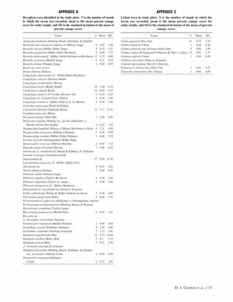
Taxon N Mean SD

Amblyodon dealbatus (Hedwig) Bruch, Schimper, & Gumbel

Brachythecium stereopoma (Spruce ex Mitten) Jaeger 9 0.45 1.89

Breutelia chrysea (Muller Halle) Jaeger 4 0.52 3.21

Breutelia polygastria (Muller Halle) Brotherus 5 0.99 7.13

Breutelia subarcuata (C. Muller, Halle) Schimper ex Brotherus 12 1.23 4.68

Breutelia tomentosa (Bridel) Jaeger 5 0.71 4.23

Breutelia trianae (Hampe) Jaeger 1 0.08 0.89

Bryum sp. sensu stricto

Bryum filiforme Dickson

Campylopus argyrocaulon (C. Muller-Halle) Brotherus

Campylopus concolor (Hooker) Bridel

Campylopus cucullatifolius Herzog

Campylopus nivalis (Bridel) Bridel 19 1.48 4.19

Campylopus richardii Bridel 10 0.85 3.15

Campylopus sharpii J.-P. Frahm, Horton, Vitt 5 0.83 4.55

Campylopus cf. trichophylloides Theriot 2 0.16 1.41

Campylopus trivialis C. Muller Halle ex E. G. Britton 5 0.34 1.89

Ceratodon stenocarpus Bruch & Schimp.

Cratoneuron filicinum (Hedwig) Spruce 12 3.17 13.21

Ctenidium malacodes Mitten

Dicranum frigidum Mull. Hal. 1 0.04 0.45

Didymodon rigidulus Hedwig var. gracilis (Schleicher ex

Hooker & Greville) Zander 3 0.25 1.93

Drepanocladuslongifolius (Wilson ex Mitten) Brotherus ex Paris 6 1.31 6.88

Drepanocladus polygamus (Schimp.) Hedenas 1 0.08 0.89

Drepanocladus sordidus (Muller Halle) Hedenas 1 0.48 5.35

Entodon beyrichii (Schwagrichen) Muller Halle

Hamatocaulis vernicosus (Mitten) Hedenas 1 0.63 7.13

Hygrodicranum bolivianum Herzog 1 0.06 0.62

Imbribryum cf. muehlenbeckii (Bruch & Schimp.) N. Pedersen

Jensenia erythropus (Gottsche) Grolle

Jungermannia sp. 27 3.92 10.36

Leptodontium araucarieti (C. Muller, Halle) Paris

Marchantia sp. 4 0.47 3.26

Meesia uliginosa Hedwig 1 0.04 0.45

Philonotis andina (Mitten) Jaeger

Philonotis angulata (Taylor) Brotherus 3 0.18 1.43

Philonotis elegantula (Taylor) A. Jaeger 1 0.04 0.45

Philonotis polygastrica (C. Muller) Brotherus

Plagiomnium cf. rhynchophorum (Hooker) Koponen

Pohlia wahlenbergii (Weber & Mohr) Andrews in Grout 1 0.04 0.45

Polytrichum juniperinum Hedw. 5 0.64 5.51

Ptychostomum cf. pallescens (Schleicher ex Schwagrichen.) Spence

Ptychostomum pseudotriquetrum (Hedwig) Spence & Ramsay

Racomitrium crispipilum (Taylor) Jaeger

Rhacocarpus purpurascens (Bridel) Paris 2 0.16 1.41

Riccardia sp.

cf. Ruizanthus venezuelanus Schuster

Straminergon stramineum (Bridel) Hedenas 1 0.08 0.89

Scorpidium cossonii (Schimper) Hedenas 8 1.09 6.66

Scorpidium scorpioides (Hedwig) Limpricht 7 1.13 5.41

Sphagnum magellanicum Brid. 11 2.74 10.84

Sphagnum tenellum (Brid.) Brid. 3 0.2 1.33

Sphagnum pylaesii Brid. 3 0.31 2.38

cf. Temnoma chaetophylla Schuster

Thuidium delicatulum (Hedwig) Bruch, Schimper, & Gumbel

var. peruvianum (Mitten) Crum 1 0.08 0.89

Warnstorfia exannulata (Schimp.)

Loeske 2 0.32 2.81

Taxon N Mean SD

Cladia aggregata (Sw.) Nyl. 11 0.72 2.78

Cladina fuliginosa Filson 1 0.04 0.45

Cladina arbuscula ssp. boliviana (Ahti) Ahti 9 0.82 3.49

Cladina confusa (R.Santesson) Follmann & Ahti f. confusa 12 0.91 3.32

Cladonia andesita Vainio 1 0.08 0.89

Cladonia calycantha Delise ex Nylander

Cladonia leprocephala Ahti & S. Stenroos

Peltigera cf. dolichorrhiza (Nyl.) Nyl. 1 0.02 0.27

Thamnolia vermicularis (Sw.) Schaer. 1 0.01 0.09

APPENDIX BBryophyte taxa identified in the study plots. N is the number of standsin which the taxon was recorded, mean is the mean percent canopycover for study stands, and SD is the standard deviation of the mean of

percent canopy cover.

APPENDIX CLichen taxa in study plots. N is the number of stands in which thetaxon was recorded, mean is the mean percent canopy cover forstudy stands, and SD is the standard deviation of the mean of percent

canopy cover.


Documents

Alpine Peatlands of the Andes, Cajamarca, Peru - Sites · Cajamarca, Peru Abstract An ecological analysis of wetlands in the high mountain jalca above 3700 m elevation in the Andes