Alpha Shapes — a Survey - Computer graphicsgraphics.stanford.edu/courses/cs268-14-fall/Handouts/AlphaShapes/... · Alpha Shapes — a Survey 3 such as calling a sequence of three

Alpha Shapes — a Survey

Herbert Edelsbrunner1

Departments of Computer Science and of Mathematics, Duke University, Durham,North Carolina, USA, Geomagic, Research Triangle Park, North Carolina, USA,and IST Austria (Institute of Science and Technology Austria)[email protected]

Alpha shapes have been conceived in 1981 as an attempt to define the shapeof a finite set of point in the plane. Since then, connections to diverse areas inthe sciences and engineering have developed, including to pattern recognition,digital shape sampling and processing, and structural molecular biology. Thissurvey begins with a historical account and discusses geometric, algorithmic,topological, and combinatorial aspects of alpha shapes in this sequence.

1 History

The history of alpha shapes started in 1981 during my first trip to the Amer-ican continent. Studying mathematics and computer science in Austria, I vis-ited David Kirkpatrick at the University of British Columbia in Vancouverand spent a few months of intense research with him and with Raimund Seidel.

Conceptualization

In the late 1970s, Jarvis published a paper in which he generalized his planarconvex hull algorithm to a method that generates something like the shapeof a finite point set. We recall that this algorithm computes the convex hullone edge at a time, pivoting a line about one endpoint until it hits the otherendpoint of the edge [34]. If we replace the line by a line segment of fixed lengththen we again walk around the point set but venture into sufficiently largecavities [35]. The size requirement on the cavities depends on the chosen lengthfor the pivoting line segment. Sometimes it happens that the line segment getslost in what we might reasonably call the interior of the shape and does notproduce a reasonable description of the boundary.

The idea of alpha shapes was a response to the shortcomings of definingthe outline of the shape by a pivoting line segment. Instead we imagined adisk of given radius to define the outline of the shape [24]. We call this the

2 Herbert Edelsbrunner

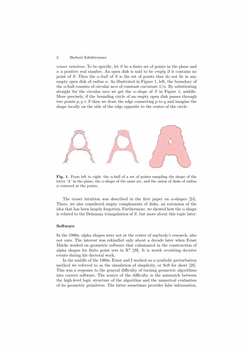
eraser intuition. To be specific, let S be a finite set of points in the plane andα a positive real number. An open disk is said to be empty if it contains nopoint of S. Then the α-hull of S is the set of points that do not lie in anyempty open disk of radius α. As illustrated in Figure 1, left, the boundary ofthe α-hull consists of circular arcs of constant curvature 1/α. By substitutingstraight for the circular arcs we get the α-shape of S in Figure 1, middle.More precisely, if the bounding circle of an empty open disk passes throughtwo points p, q ∈ S then we draw the edge connecting p to q and imagine theshape locally on the side of the edge opposite to the center of the circle.

Fig. 1. From left to right: the α-hull of a set of points sampling the shape of theletter ‘A’ in the plane, the α-shape of the same set, and the union of disks of radiusα centered at the points.

The eraser intuition was described in the first paper on α-shapes [24].There, we also considered empty complements of disks, an extension of theidea that has been largely forgotten. Furthermore, we showed how the α-shapeis related to the Delaunay triangulation of S, but more about this topic later.

Software

In the 1980s, alpha shapes were not at the center of anybody’s research, alsonot ours. The interest was rekindled only about a decade later when ErnstMucke worked on geometric software that culminated in the construction ofalpha shapes for finite point sets in R

3 [29]. It is worth revisiting decisiveevents during his doctoral work.

In the middle of the 1980s, Ernst and I worked on a symbolic perturbationmethod we referred to as the simulation of simplicity, or SoS for short [28].This was a response to the general difficulty of turning geometric algorithmsinto correct software. The source of the difficulty is the mismatch betweenthe high-level logic structure of the algorithm and the numerical evaluationof its geometric primitives. The latter sometimes provides false information,

Alpha Shapes — a Survey 3

such as calling a sequence of three almost collinear points a left-turn whilethey actually turn right. The logic structure can be unforgiving for even slightmistakes because they send it to geometrically impossible configurations forwhich nobody is prepared. Making the logic structure more tolerant provedto be difficult and incompatible with the desire to retain the efficiency of thealgorithm. Alternatively, we can make sure that all primitives give correctinformation no matter how ambiguous the situation may be. This leads tothe use of exact arithmetic and the need to resolve degenerate cases, such asthree points collinear or worse. To finesse the latter question, SoS simulates aperturbation and thus reduces every degenerate to a generic case. Importantly,this reduction is done in a consistent manner so that the collection of alldecisions made by the algorithm corresponds to a geometrically valid input.

At the time, SoS was a contentious proposal and there was intense com-petition between proponents of the two schools distinguished from each otherby basing all numerical decisions on either inexact or on exact arithmetic.Ernst and I were therefore looking for interesting challenges to demonstratethe utility of SoS in creating geometric software. Three-dimensional Delaunaytriangulations and alpha shapes seemed like perfect candidates. More aboutthis later.

Applications

Generalizing the two-dimensional algorithms to three dimensions and turningtheoretical algorithms into working code is one thing, then making the soft-ware available to the public is another. At the time, there was no world-wide-web but we worked with Ping Fu at the National Center for SupercomputingApplications and Ernst put his software on an ftp server for people to down-load. The high volume of interest surprised us. Apparently, the alpha shapessoftware tabbed into a common need. An important factor was the three-dimensionality of the computation, a relevant as well as challenging space towork in. Through these activities we learned something significant, namelythe application community’s wants. Looking back, I see three categories, eachtaking alpha shapes in its own interesting direction.

Pattern recognition. How can we characterize point distributions in space,such as galaxies in the universe and the like?

Digital shape sampling and processing. How can we reconstruct a shape froma finite point sample on its surface?

Structural molecular biology. How can we model the structural aspects of pro-teins and other biomolecules relevant for the functioning of life?

The applications motivated the research that unfolded. While they posed dif-ferent challenges, they were based on common fundamental mathematicalquestions. It seemed most productive to address those and build solutions tothe applications on answers to the mathematical questions. This is also howwe structure this survey.


Geometry. What are the different guises of alpha shapes and how do theyrelate to each other?

Algorithms. How do we turn the mathematics into working software usableby non-specialists?

Topology. How do we approach the multi-resolution reality of data and howdo we define and extract features?

Combinatorics. How do we exploit the rich combinatorial structure of alphashapes to measure space?

This survey can only scratch the surface of each topic. While there is a lotknown that will remain untouched here, we hasten to point out that there areentire fields that are yet unexplored.

2 Geometry

In this section, we describe alternatives to the eraser intuition and generalizealpha shapes beyond two dimensions and to points with weights.

Union of disks

The eraser intuition has a dual view that arises when we take the union ofdisks centered at the given points. To be specific, let z1 to zn be the pointsin S ⊆ R

2, write Bi(α) for the closed disk with center zi and radius α > 0,and let U(α) =

⋃ni=1

Bi(α) be the union of the disks. In other words, U(α)is the set of points x ∈ R

2 that are at distance at most α from the set S.This invites an alternative interpretation as a sublevel set of the Euclideandistance function S : R

2 → R defined by S(x) = min1≤i≤n ‖x − zi‖, namelyU(α) = −1

S [0, α]. This interpretation will be useful later. At the time being,we focus on the connection to the eraser intuition. For this, we consider a pointx ∈ R

2 and let Bx(α) be the closed disk with center x and radius α. Clearly,its interior is empty (of points in S) iff x does not belong to the interior ofU(α). The boundary of the α-hull consists of points that lie on circles of radiusα centered at points x that lie on the boundary of U(α). Generically, thereare only two cases:

Type 1: there is a unique closest point zi at distance α from x;Type 2: there are two closest points at distance α from x.

Points of Type 1 lie in the interior of the circular arcs that make up theboundary of the union of disks. Points of Type 2 are the endpoints of thesearcs. Imagine a point x moving continuously along such an arc, from oneendpoint to the other. As x moves, the disk Bx(α) rotates about a point onits boundary, namely the point zi at the center of the circle that carries thearc. At the endpoints, we get dual arcs in the α-hull, one ending at zi and theother starting at zi. The arcs of the α-hull may intersect and in the process


decompose each other into shorter arcs. It follows that a single circle maycontribute more than one arc to the boundary of the α-hull or no arc at all.The latter case arises when the pair of points in S define two empty disksof radius α, one centered on each side of the line passing through the twopoints. In this case, the edge connecting the two points in the α-shape doesnot bound area on either side.

Voronoi and Delaunay

It is time to introduce the Voronoi diagram and the Delaunay triangulation,named after two Russian mathematicians [51, 12]. The two structures areintimately related to the α-shape. As before, let z1 to zn be the points in Sand let the Voronoi cell of zi consist of all points for which zi is the closest,

Vi = {x ∈ R2 | ‖x − zi‖ ≤ ‖x − zj‖, ∀j}.

The points x that satisfy ‖x − zi‖ ≤ ‖x − zj‖ for a fixed j 6= i define aclosed half-plane. Hence Vi is the intersection of n − 1 half-planes, a closedand possibly unbounded convex polygon. By construction, any two Voronoicells have disjoint interiors but they may intersect along shared pieces oftheir boundaries. Generically, there is only one possible case, namely thatVi and Vj share a common side. Indeed, they cannot share more than oneside and to share just a corner would require four points of S on a commoncircle around that corner, a non-generic case. Together, the n Voronoi cellscover the entire plane. The Voronoi diagram of S is the set of Voronoi cells,VorS = {Vi | 1 ≤ i ≤ n}.

The Delaunay triangulation, Del S, is dual to the Voronoi diagram. Specif-ically, whenever two Voronoi cells share a common side then the edge connect-ing the two corresponding points belongs to the Delaunay triangulation, andwhenever three Voronoi cells share a common corner the triangle spanned bythe three corresponding points belongs to the Delaunay triangulation. A moreformal way of saying the same uses the concept of the nerve of the Voronoidiagram, that is, the collection of subsets whose cells have non-empty commonintersection,

Nrv (VorS) = {X ⊆ VorS |⋂

X 6= ∅}.

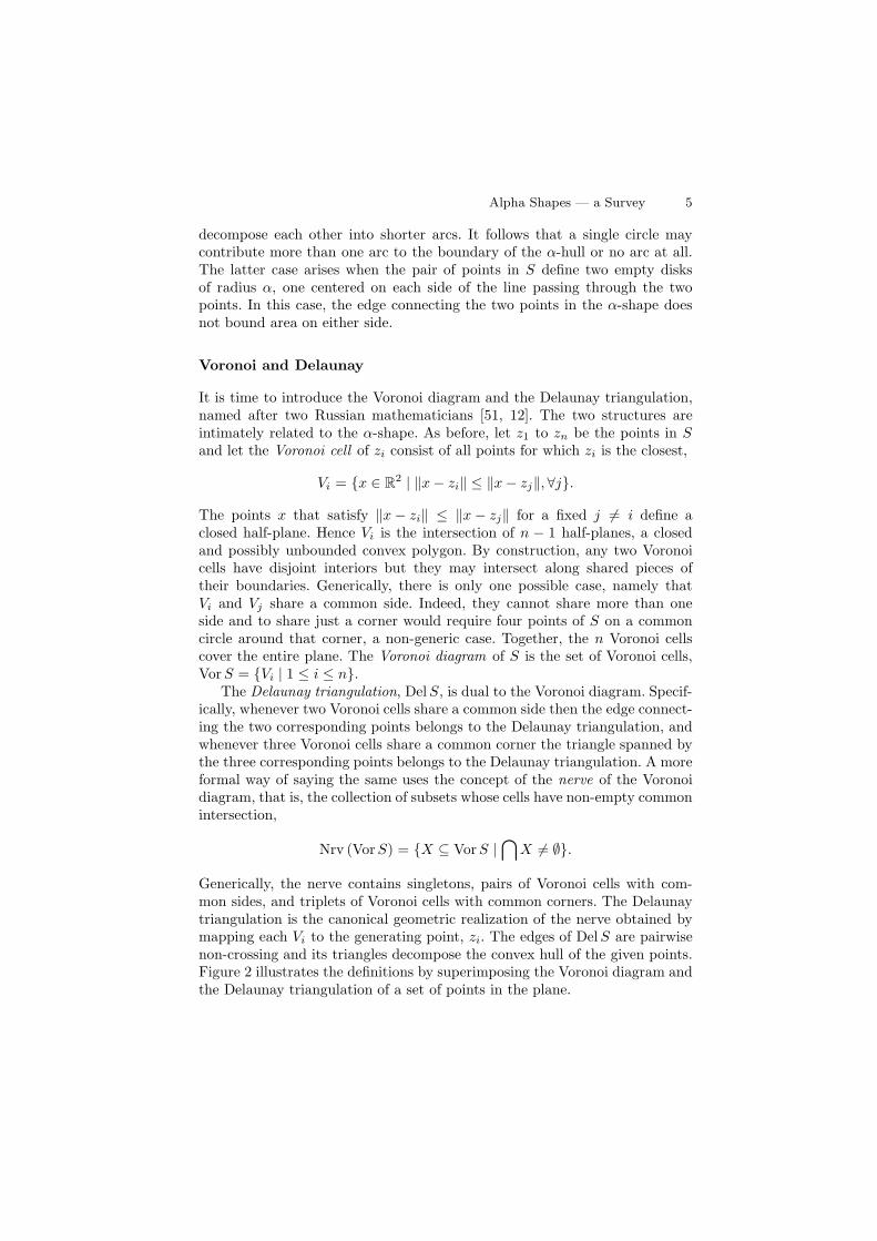
Generically, the nerve contains singletons, pairs of Voronoi cells with com-mon sides, and triplets of Voronoi cells with common corners. The Delaunaytriangulation is the canonical geometric realization of the nerve obtained bymapping each Vi to the generating point, zi. The edges of Del S are pairwisenon-crossing and its triangles decompose the convex hull of the given points.Figure 2 illustrates the definitions by superimposing the Voronoi diagram andthe Delaunay triangulation of a set of points in the plane.


Fig. 2. The points mark trees in the Allerton Park in Monticello, Illinois. Each treeis associated with the region of points for which it is the nearest. Close inspectionof the drawing shows that the Voronoi edges are sometimes not exactly halfwaybetween the points. This is because we really see the weighted Voronoi diagram andthe weighted Delaunay triangulation in which weights quantify sizes of the trees.

Alpha complex

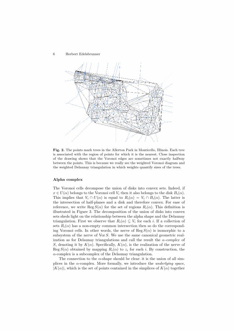
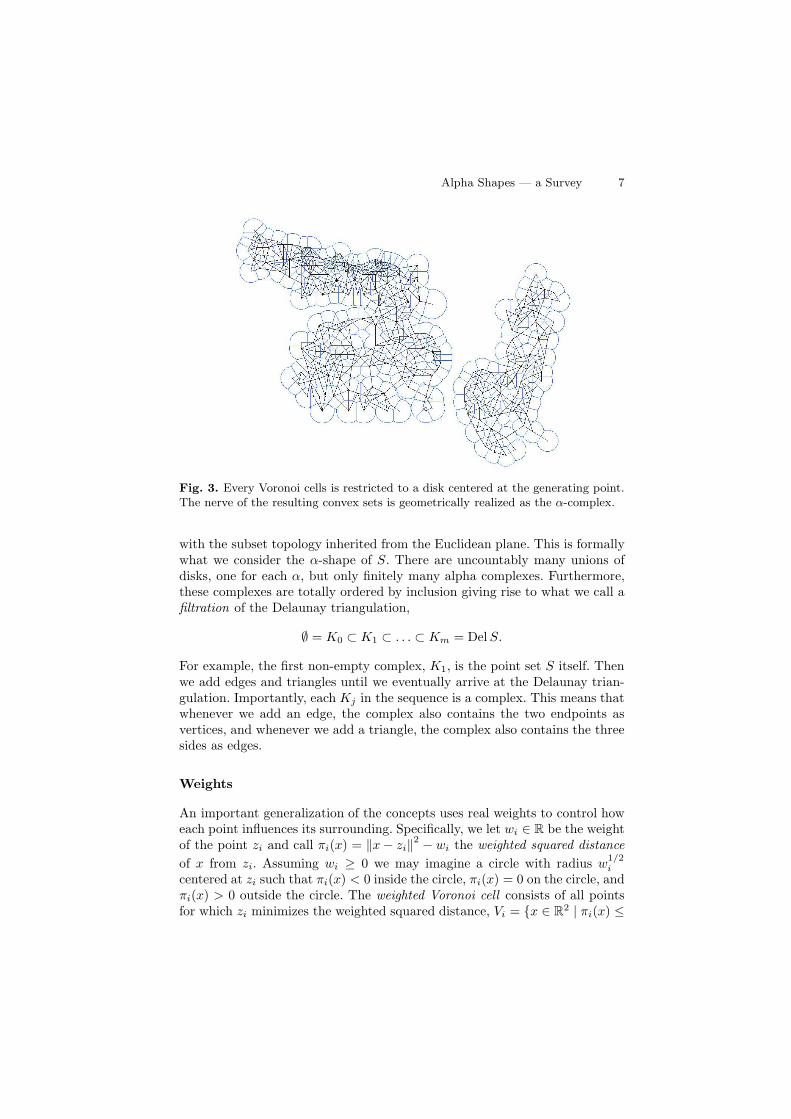
The Voronoi cells decompose the union of disks into convex sets. Indeed, ifx ∈ U(α) belongs to the Voronoi cell Vi then it also belongs to the disk Bi(α).This implies that Vi ∩ U(α) is equal to Ri(α) = Vi ∩ Bi(α). The latter isthe intersection of half-planes and a disk and therefore convex. For ease ofreference, we write Reg S(α) for the set of regions Ri(α). This definition isillustrated in Figure 3. The decomposition of the union of disks into convexsets sheds light on the relationship between the alpha shape and the Delaunaytriangulation. First we observe that Ri(α) ⊆ Vi for each i. If a collection ofsets Ri(α) has a non-empty common intersection then so do the correspond-ing Voronoi cells. In other words, the nerve of Reg S(α) is isomorphic to asubsystem of the nerve of Vor S. We use the same canonical geometric real-ization as for Delaunay triangulations and call the result the α-complex ofS, denoting it by K(α). Specifically, K(α), is the realization of the nerve ofReg S(α) obtained by mapping Ri(α) to zi for each i. By construction, theα-complex is a subcomplex of the Delaunay triangulation.

The connection to the α-shape should be clear: it is the union of all sim-plices in the α-complex. More formally, we introduce the underlying space,|K(α)|, which is the set of points contained in the simplices of K(α) together


Fig. 3. Every Voronoi cells is restricted to a disk centered at the generating point.The nerve of the resulting convex sets is geometrically realized as the α-complex.

with the subset topology inherited from the Euclidean plane. This is formallywhat we consider the α-shape of S. There are uncountably many unions ofdisks, one for each α, but only finitely many alpha complexes. Furthermore,these complexes are totally ordered by inclusion giving rise to what we call afiltration of the Delaunay triangulation,

∅ = K0 ⊂ K1 ⊂ . . . ⊂ Km = Del S.

For example, the first non-empty complex, K1, is the point set S itself. Thenwe add edges and triangles until we eventually arrive at the Delaunay trian-gulation. Importantly, each Kj in the sequence is a complex. This means thatwhenever we add an edge, the complex also contains the two endpoints asvertices, and whenever we add a triangle, the complex also contains the threesides as edges.

Weights

An important generalization of the concepts uses real weights to control howeach point influences its surrounding. Specifically, we let wi ∈ R be the weightof the point zi and call πi(x) = ‖x − zi‖

2 − wi the weighted squared distance

of x from zi. Assuming wi ≥ 0 we may imagine a circle with radius w1/2

i

centered at zi such that πi(x) < 0 inside the circle, πi(x) = 0 on the circle, andπi(x) > 0 outside the circle. The weighted Voronoi cell consists of all pointsfor which zi minimizes the weighted squared distance, Vi = {x ∈ R

2 | πi(x) ≤


πj(x), ∀j}. The weighted Voronoi diagram is the set of weighted Voronoi cells,VorS = {Vi | 1 ≤ i ≤ n}. We use the same notation in the weighted case asin the unweighted case.

The weighted Delaunay triangulation should be clear. It is the canonicalgeometric realization of Nrv (Vor S) obtained by mapping each Vi to the gen-erating point, zi. Some caution is in order: not every point zi generates anon-empty weighted Voronoi cell. To describe how a cell can end up beingempty, we say a point z with weight w is orthogonal to another point y withweight v if ‖y − z‖2

= w+v. If v, w > 0 this indeed corresponds to two circlesthat cross at two right angles. Generically, three weighted points have a uniqueweighted point that is orthogonal to all three. Now consider weighted pointszi, zj , zk, zℓ such that zi is in the triangle spanned by the other three and let

the point y with weight v be orthogonal to zj, zk, zℓ. If ‖zi − y‖2> wi + v

then Vi is empty and zi is not a vertex of Del S.Finally, we generalize alpha complexes to the weighted case. Given α ∈ R,

we let Bi(α) be the closed disk with center zi and radius (α2 + wi)1/2. If

α2 +wi < 0 then the root is imaginary and Bi(α) is empty, by definition. Theunion of the disks is U(α) =

⋃ni=1

Bi(α). Similar to the unweighted case, wehave Vi ∩ U(α) = Vi ∩ Bi(α). Hence, the sets Ri(α) = Vi ∩ Bi(α) form againa convex decomposition of the union. The weighted α-complex, K(α), is thecanonical geometric realization of the nerve of the collection of sets Ri(α).

Weighted Voronoi diagrams are known under various names, includingpower diagrams and Dirichlet tessellations; see e.g. [4]. Similarly, weightedDelaunay triangulations are known under different names, including regular

triangulations and coherent triangulations ; see e.g. [31]. We prefer to use theadjective ‘weighted’, which we drop when it is convenient to blur the differencebetween the weighted and the special, unweighted case.

Convex polyhedra

Voronoi diagrams and Delaunay triangulation can also be viewed as convexpolyhedra in R

3. This view is sometimes more natural and high-lights a fun-damental symmetry between the two concepts.

Let S be the set of points zi ∈ R2 with weights wi ∈ R for 1 ≤ i ≤ n.

Consider the function π : R2 → R defined by π(x) = min1≤i≤n πi(x). This is a

piecewise quadratic function, one piece for each non-empty weighted Voronoicell. Its restriction to Vi is ‖x − zi‖

2 − wi and subtracting the squared normof x turns this into a linear function. Hence, f : R

2 → R defined by f(x) =

π(x) − ‖x‖2is piecewise linear, again a piece for each non-empty weighted

Voronoi cell. Specifically,

f(x) =

(

min1≤i≤n

πi(x)

)

− ‖x‖2= min

1≤i≤n

(

πi(x) − ‖x‖2)

,

which shows that f is concave. It is best visualized by its graph. For each i,the graph of πi(x)−‖x‖2

is a plane in R3, and if wi ≥ 0 it intersects the graph


of −‖x‖2in a curve whose vertical projection to R

2 is the circle with center

zi and radius w1/2

i . The graph of f is the lower envelope of these n planes. Itis thus the boundary of a convex polyhedron that projects vertically to theweighted Voronoi diagram of S.

There is a similar dual view of the Delaunay triangulation. Specifically,(zi, wi−‖zi‖

2) in R

3 is the polar point of the plane that is the graph of πi(x)−

‖x‖2. We collect all n polar points, add the point (0,−∞), and construct theconvex hull in R

3. This is again a convex polyhedron. We obtain the weightedDelaunay triangulation by taking its boundary, removing all faces incident tothe point (0,−∞), and projecting the rest vertically to R

2.In the unweighted case, we get a circumscribed polyhedron for the Voronoi

diagram and an inscribe polyhedron for the Delaunay triangulation. Specif-ically, the face planes of the first polyhedron are all tangent to the graphof −‖x‖2

and the vertices of the second polyhedron all lie on this graph. Inthe weighted case, we relax the circumscribed/inscribed condition and allowfor general convex polytopes. Generically, the polyhedra defined as lower en-velopes of planes are simple and the polyhedra defined as convex hulls aresimplicial. It is instructive to describe the α-complex in terms of how thesetwo convex polyhedra interact with the graph of α2 − ‖x‖2

. We leave this asan exercise to the reader.

Beyond two dimensions

The above definitions are easily extended to weighted points in Rd, for any

positive integer d. The Voronoi diagram consists of cells that are convex poly-hedra of dimension d. Generically, the common intersection of any i+1 ≤ d+1cells is either empty or a (d − i)-dimensional convex polyhedron. The nervethus consists of (i+1)-tuplets of Voronoi cells, for 0 ≤ i ≤ d. Correspondingly,the Delaunay triangulation consists of simplices of dimension 0 ≤ i ≤ d. Fora given α ∈ R, the α-complex is a subcomplex of the Delaunay triangulation.Finally, all diagrams can be viewed as convex polyhedra in R

d+1 or as theinteraction of such a polyhedron with the graph of the function that mapseach point x ∈ R

d to α2 − ‖x‖2.

3 Algorithms

There are many different strategies to construct the α-complex of a finite pointset and most are based on the Delaunay triangulation. We focus on the mostcommon method which computes the Delaunay triangulation incrementally,adding one point at a time, and then selects the α-complex as a subcomplex.Before we agonize about how fast we can do the computation we ask how biga structure we can expect.


Number of simplices

Assume first that S is a set of n weighted points in R2. The edges of the De-

launay triangulation form a planar graph, that is, they can be drawn withoutany two crossing each other. Euler’s formula for the Euclidean plane statesthat #vertices − #edges + #faces = #components + 1. For generic inputwe have #vertices ≤ n, #faces = #triangles + 1, and #components = 1.Hence, #edges − #triangles ≤ n − 1. But every triangle has three edgesand every edge belongs to two faces, either two triangles or one triangleand the outer face. Letting k be the number of edges of the outer face wethus get 2#edges = 3#triangles + k. This implies #edges ≤ 3n − 3 − k and#triangles ≤ 2n − 2 − k. In short, the entire Delaunay triangulation hasfewer than 6n simplices and so has every α-complex. This is true both in theweighted case and in the unweighted case.

The situation is a lot more subtle in d ≥ 3 dimensions because the numberof simplices in the Delaunay triangulation heavily depends on how the pointsare distributed. The worst case corresponds to so-called cyclic polytopes inR

d+1. These are polytopes with n vertices for which every subset of i + 1vertices spans a face of dimension i, for 0 ≤ i ≤ (d − 1)/2, see e.g. [33].For example, there are polytopes in R

4 that have an edge between everypair of vertices and similarly there are Delaunay triangulations in R

3 whoseedges form the complete graph on n vertices. According to the Upper BoundTheorem, the cyclic polytopes are indeed the worst case [53] and the weightedDelaunay triangulation for n points in R

d has at most some constant timesn⌈d/2⌉ simplices. This is not to say that Delaunay triangulations of this largesize are typical. Quite the opposite, large Delaunay triangulations seem veryrare but to say anything concrete we would have to decide upon the pointdistributions we consider. If we pick n points uniformly at random within theunit cube, the expected number of simplices is only some constant times n,where the constant depends exponentially on the dimension [15]. If the pointsare well distributed on a generic smooth surface in R

3 then the number ofsimplices is bounded from above by a constant times n log2 n [2]. To complicatematters further, it is of course possible that the Delaunay triangulation is largebut the α-complex is small. For example, suppose the points are unweightedand no two are closer to each other than some constant times α. Then wecan use a packing argument to prove a linear upper bound on the number ofsimplices in the α-complex while the Delaunay triangulation can still reachworst-case size. This assumption is realistic for the data that describes proteinsand other biomolecules in R

3.

Incremental construction

The most popular method for constructing a Delaunay triangulation adds onepoint at a time. Early versions of this algorithm have been studied in the con-vex polytope literature [33] and described for Voronoi diagrams and Delaunay


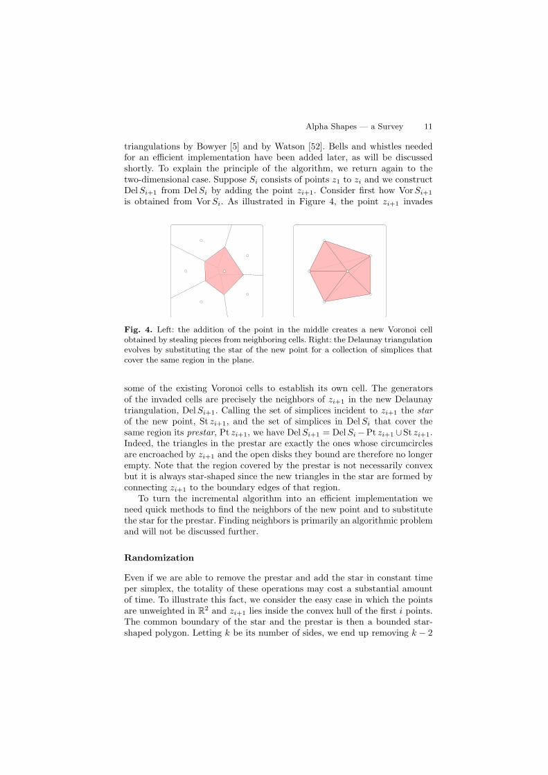
triangulations by Bowyer [5] and by Watson [52]. Bells and whistles neededfor an efficient implementation have been added later, as will be discussedshortly. To explain the principle of the algorithm, we return again to thetwo-dimensional case. Suppose Si consists of points z1 to zi and we constructDel Si+1 from Del Si by adding the point zi+1. Consider first how VorSi+1

is obtained from VorSi. As illustrated in Figure 4, the point zi+1 invades

Fig. 4. Left: the addition of the point in the middle creates a new Voronoi cellobtained by stealing pieces from neighboring cells. Right: the Delaunay triangulationevolves by substituting the star of the new point for a collection of simplices thatcover the same region in the plane.

some of the existing Voronoi cells to establish its own cell. The generatorsof the invaded cells are precisely the neighbors of zi+1 in the new Delaunaytriangulation, DelSi+1. Calling the set of simplices incident to zi+1 the star

of the new point, St zi+1, and the set of simplices in Del Si that cover thesame region its prestar, Pt zi+1, we have Del Si+1 = Del Si −Pt zi+1 ∪St zi+1.Indeed, the triangles in the prestar are exactly the ones whose circumcirclesare encroached by zi+1 and the open disks they bound are therefore no longerempty. Note that the region covered by the prestar is not necessarily convexbut it is always star-shaped since the new triangles in the star are formed byconnecting zi+1 to the boundary edges of that region.

To turn the incremental algorithm into an efficient implementation weneed quick methods to find the neighbors of the new point and to substitutethe star for the prestar. Finding neighbors is primarily an algorithmic problemand will not be discussed further.

Randomization

Even if we are able to remove the prestar and add the star in constant timeper simplex, the totality of these operations may cost a substantial amountof time. To illustrate this fact, we consider the easy case in which the pointsare unweighted in R

2 and zi+1 lies inside the convex hull of the first i points.The common boundary of the star and the prestar is then a bounded star-shaped polygon. Letting k be its number of sides, we end up removing k − 2


triangles in the prestar and adding k triangles in the star. In other words, wespend time proportional to 2k− 2 with a net plus of only two triangles in thetriangulation. The number of sides, k, can be as large as i, so the total effortmay be as large as 2

∑

(i−1), which is roughly n2, while the final triangulationhas fewer than 2n triangles.

It is indeed possible that the algorithm creates and destroys about n2 tri-angles, but this is not very likely. A useful perspective is the randomizationover all input sequences. Specifically, we consider all n! permutations of then points, compute the effort for each, and divide the sum by n! to get theexpected effort. This has been advocated as a general strategy in computa-tional geometry by Clarkson and Shor [10]. The analysis has been simplifiedby Seidel [49], who suggests we look at the entire process going backwards.Indeed, each point is equally likely to be the last one in the input sequence.Since the average number of triangles in the star of a vertex in Del Sn = Del Sis less than 6, this implies that the combined effort for the respective lastpoints of the n! permutations is less than 6n!. The same is true for all theother points, so the total effort is less than 6n · n!. The expected effort for asingle input sequence is therefore less than 6n. In other words, chances arethat the algorithm constructs only three times as many triangles as necessary.

As always, the situation is more subtle in three and higher dimensions andwe refer to the relevant literature as cited e.g. in [19]. It should be mentionedthat randomizing the input sequence has also undesired effects. In particular,the access pattern to the representation of the evolving Delaunay triangulationin memory tends to be non-local, which goes against the grain of currentcomputer hardware which uses fast cache to take advantage of locality in thecomputation. A compromise between the benefits of random input sequencesand locality in computation has been described in [1].

Flipping

Instead of first removing the entire prestar and then adding the entire star,we may prefer to modify Del Si one simplex at a time, eventually turning itinto Del Si+1 while preserving that we have a triangulation during the entireprocess. This can be done using flips, also known as bi-stellar operations. Weagain simplify the situation by restricting ourselves to the unweighted planarcase. An edge flip replaces two triangles sharing an edge by the other twotriangles decomposing the same quadrangle. More generally, we define a flipin R

2 in terms of the boundary of a tetrahedron in R3. Its projection to R

2 iseither a quadrangle or a triangle and its upper and lower boundaries providetwo triangulations of this projection. Flipping refers to substituting one localtriangulation for the other.

The first use of flipping to construct Delaunay triangulations can be foundin a paper by Lawson [40]. He starts with an arbitrary triangulation of aset S of unweighted points in R

2 and constructs Del S in a sequence of edgeflips. Each flip is directed in the sense that the two new triangles belong to


the Delaunay triangulation of the four points involved. Although there areconfigurations that require a quadratic number of such flips, the algorithm isgenerally quite efficient. There are, however, serious obstacles to generalizingthis algorithm to three and higher dimensions. Specifically, there are triangu-lations of a set of n points in R

3 that are not Delaunay and that do not permita single flip to bring them closer to the Delaunay triangulation [36]. However,such obstacles do not exist if we add one point at a time, flipping to the De-launay triangulation before adding the next point. This has first been provedfor unweighted points in R

3 [37] and then generalized to weighted points inR

d [30]. If applied as part of the incremental algorithm, each flip removes oneof the d-simplices in the prestar. Hence the number of flips is directly relatedto the total number of simplices created and destroyed in the process.

Sorting simplices

Given the Delaunay triangulation, we construct the α-complex by selectingthe simplices whose Voronoi cells have a non-empty common intersection withthe union of balls. To expedite this process, we use the fact that each simplexσj ∈ Del S has a threshold αj such that σj ∈ K(α) iff αj ≤ α. This suggestswe sort the simplices in a non-decreasing order of the thresholds and retrievethe α-complex as a prefix of this sequence. For some of the simplices, thethreshold is the radius of the smallest circumsphere and for others it is thethreshold of another simplex in its star. A case analysis complete with analyticformulas for weighted points in R

d can be found in [16]. Here we illustrate thesituation for a set of unweighted points in R

2. The threshold of every vertex iszero and that of every triangle in the Delaunay triangulation is the radius ofits circumcircle. For an edge σj = conv {a, b}, there are two cases which canbe distinguished by considering the smallest circumcircle, the circle centeredat the midpoint and passing through the endpoints of the edge. If the thirdvertex of each incident triangle lies outside this circle then the threshold isthe radius of the circle, αj = ‖a − b‖/2. Otherwise the third vertex of onetriangle lies inside the circle and the threshold of the edge is the same as thatof this triangle.

After computing all thresholds, we sort the simplices into a sequenceσ1, σ2, . . . , σm such that αj ≤ αj+1 for all j. Calling this sequence a filter,we get the filtration of the Delaunay triangulation by considering all prefixesof simplices with thresholds smaller than or equal to a real number α. Fortechnical reasons, we require that all prefixes of the filter are complexes, notjust those defined by real numbers α. This can be achieved by sorting sim-plices with equal thresholds by dimension. Guaranteeing this property canbe challenging numerically but the advantages are simpler and more efficientalgorithms for topological properties of the α-complexes, as we will see later.


Implementation

We aim for an implementation that is robust and reflects the structure ofthe abstract algorithm without cluttering it with the treatment of specialcases. By robust we mean provably correct for all possible inputs. To achievethese two goals, we advocate a disciplined approach in which the numericalaspects are clearly separated from the control flow. We illustrate what wemean by considering the in-circle test for a sequence of four points a = (a1, a2),b = (b1, b2), c = (c1, c2), x = (x1, x2) in the plane. The point x lies on thecircle defined by a, b, c iff the matrix

Λ =

1 a1 a2 a21 + a2

2

1 b1 b2 b21 + b2

2

1 c1 c2 c21 + c2

2

1 x1 x2 x21 + x2

2

has vanishing determinant. If a, b, c form a left-turn then the point x lies insidethe circle iff detΛ < 0. Finally, a, b, c form a left-turn iff the upper left 3-by-3submatrix ∆ of Λ has positive determinant. We thus get the following booleanfunction that recognizes when x lies inside the circle defined by a, b, c:

boolean isInCircle (a, b, c, x):return det∆ · detΛ < 0.

The test is simple but numerically instable if one or both matrices are notclearly full rank. Using exact arithmetic, we can get the correct sign in allcases. It remains to describe how we can think of the non-generic situationsdefined by det∆·det Λ = 0. We propose to disambiguate the many possibilitiesusing a symbolic perturbation that turns every input configuration into ageneric configuration nearby. The perturbation is only simulated and doesnot affect the data. Following [28], we make use of the indices of the inputpoints, writing a = zi and so forth, and of a sufficiently small but positivereal number ε. The perturbation is smaller for larger indices and we definezi,j(ε) = zi,j +ε2

3i−j

for 1 ≤ i ≤ n and 1 ≤ j ≤ 3, where zi,3 = z2i,1 +z2

i,2. Note

that zi,3(ε) is not equal to zi,1(ε)2 + zi,2(ε)

2, which is what Knuth suggestedto use [38]. Instead, we perturb an unweighted to a weighted point and thisway avoid unnecessary algebraic complications. To see that the method works,we verify that for sufficiently small ε the product of determinants is non-zerono matter how non-generic the input points are chosen. An extreme test caseis a = b = c = x = (0, 0). We also note that the perturbation is easy toimplement and compute, despite the fact that finding an appropriate ε isprohibitively expensive. Indeed the determinants themselves are polynomialsin ε and finding the first non-zero coefficient suffices to decide the sign.


4 Topology

In this section, we focus on how the α-shape is connected and how its con-nectivity is measured.

Homotopy type

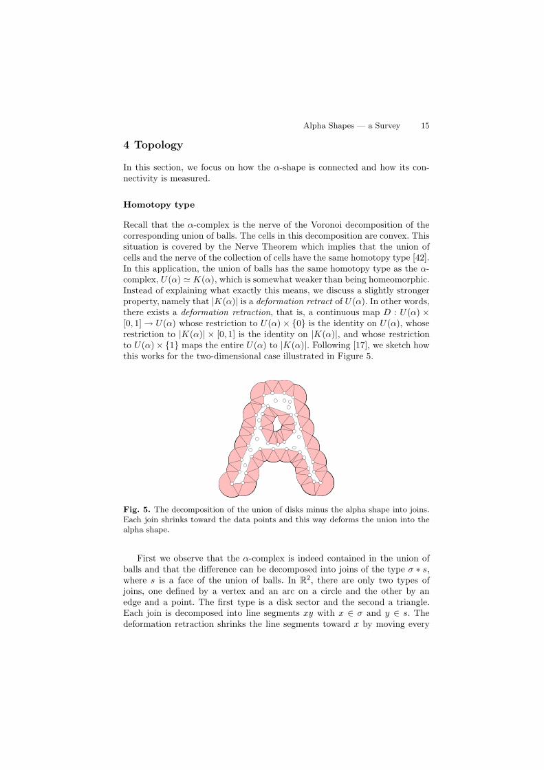
Recall that the α-complex is the nerve of the Voronoi decomposition of thecorresponding union of balls. The cells in this decomposition are convex. Thissituation is covered by the Nerve Theorem which implies that the union ofcells and the nerve of the collection of cells have the same homotopy type [42].In this application, the union of balls has the same homotopy type as the α-complex, U(α) ≃ K(α), which is somewhat weaker than being homeomorphic.Instead of explaining what exactly this means, we discuss a slightly strongerproperty, namely that |K(α)| is a deformation retract of U(α). In other words,there exists a deformation retraction, that is, a continuous map D : U(α) ×[0, 1] → U(α) whose restriction to U(α) × {0} is the identity on U(α), whoserestriction to |K(α)| × [0, 1] is the identity on |K(α)|, and whose restrictionto U(α)× {1} maps the entire U(α) to |K(α)|. Following [17], we sketch howthis works for the two-dimensional case illustrated in Figure 5.

Fig. 5. The decomposition of the union of disks minus the alpha shape into joins.Each join shrinks toward the data points and this way deforms the union into thealpha shape.

First we observe that the α-complex is indeed contained in the union ofballs and that the difference can be decomposed into joins of the type σ ∗ s,where s is a face of the union of balls. In R

2, there are only two types ofjoins, one defined by a vertex and an arc on a circle and the other by anedge and a point. The first type is a disk sector and the second a triangle.Each join is decomposed into line segments xy with x ∈ σ and y ∈ s. Thedeformation retraction shrinks the line segments toward x by moving every


point xλ = (1 − λ)x + λy to xλ(t) = (1 − t)xλ + tx. There are complicationsbecause this map is noncontinuous for some points on the boundary of theunion but these can be finessed.

Voids and pockets

The deformation retraction does more than deforming the union of balls intothe alpha shape, it also deforms the holes of the union into the holes of theshape. For the time being, we only consider two types of holes, voids that arethe bounded components of the complement, and pockets that are not holesat all, at least not to a topologist. Interestingly, this kind of non-hole arises inimportant everyday phenomena such as ditches in which cars get stuck [7]. Asa consequence of U(α) and K(α) having the same homotopy type, they alsohave the same number of voids. In other words, R

d − U(α) and Rd − |K(α)|

have the same number of connected components. Moreover, the existence ofthe deformation retraction implies that each void of U(α) is contained in aunique void of |K(α)| into which is expands during the deformation. We willcome back to this topic shortly when we count holes of all dimensions.

As mentioned earlier, pockets are not really holes. They are cavities ordepressions near the boundary. The reason we bother in spite of the difficultyto define them topologically is their importance in applications. Indeed, theoriginal motivation for the concept was the interest in proteins and how theyinteract by partial shape complementarity [21]. In order to produce a well-defined concept, we make use of the filtration instead of considering a singlealpha shape. Doing so, we can trace the development of a region in the com-plement. In a nutshell, a pocket is a region in R

d − |K(α)| that turns into avoid before it disappears [22]. To make this more concrete, we consider thevector field, v : R

d → Rd, that assigns to each point x the outward normal

of ∂U(α) at x for the value of α at which x does lie on the boundary. Thisis well-defined in the interior of each Voronoi cell and can be extended to allpoints by letting N(x) ⊆ S be the collection of closest points and mapping xto v(x) = Z(x)− x, where Z(x) is the center of the smallest enclosing ball ofN(x) [43]. We note that in the interior of the Voronoi cells, 2v(x) is the gra-

dient of the squared distance function that maps x to 2S(x) = mini ‖x − zi‖

2.

Similarly, in the interior of an intersection of Voronoi cells, 2v(x) is the gradi-ent of 2

S(x) restricted to that intersection. If x = Z(x) we call x is a critical

point of 2S . We get d + 1 types of critical points conveniently indexed from

0 to d, just like in conventional Morse Theory [45]. A point x may flow alongthis discrete vector field until it ends up at infinity or at a critical point. Asink, y, is a critical point of index d. It has a neighborhood in which all pointsflow toward y. The set of points x whose flow lines ends at y is the catchment

region, Cy, of the sink. If Cy −U(α) is not yet a void then it has the propertythat classifies it as a pocket, namely it will become a void before it disappears.

We note that the actual situation is somewhat more complicated but alsomore interesting than we made it appear. Specifically, the sets Cy − U(α)


decompose the complement of the union, except for the outer region whosepoints flow to infinity. We call a component of this decomposition a pocket.As α increases, the pocket shrinks and breaks up into pieces which are even-tually swallowed up by the union. In other words, the pockets are organizedhierarchically, which smaller pockets being part of larger pockets. We skip thediscussion of how the discrete gradient flow translates into an acyclic relationon the simplices of the Delaunay triangulation and refer instead to [20, 32]where it is used for the purpose of reconstructing the surface from a sampledpoint set.

Betti numbers

We now expand our interest from voids to holes of all dimensions, basing ourapproach on homology groups [46]. There is one group, Hp, per dimension p.The rank of Hp is called the p-th Betti number and can be considered thenumber of p-dimensional holes of the space. We say “can” because there is anambiguity what exactly one may consider a p-dimensional hole and turning thesituation around we use the homology group to make the concept concrete. Wenote that even settling on homology groups leaves an ambiguity since they canbe defined for different coefficient groups. We find it convenient to use additionmodulo 2 since this leads to simple interpretations and fast algorithms.

We now return to the specific case of interest in this paper, namely a finiteset of points, S, the Delaunay triangulation, DelS, and the filter σ1, σ2, . . . , σm

of the simplices in Del S. As mentioned earlier, we may assume that the faces ofa simplex precede the simplex in the filter. If follows that Kj = {σ1, σ2, . . . , σj}is a complex for every j. Let Hp(Kj) be the dimension p homology groupand βp(Kj) = rankHp(Kj) the dimension p Betti number of Kj . We areinterested in computing the Betti numbers incrementally. For this, we need tounderstand how βp(Kj+1) differs from βp(Kj). There are two cases dependingon whether or not σj+1 belongs to a q-dimensional cycle in Kj+1, where q isthe dimension of σj+1. For modulo 2 arithmetic, a p-cycle is a set of p-simpliceswhose boundary vanishes, that is, every (p − 1)-simplex belongs to an evennumber of p-simplices in the set.

1. If σj+1 belongs to a non-zero q-cycle in Kj+1 then βq(Kj+1) = βq(Kj)+1.2. Otherwise, βq−1(Kj+1) = βq−1(Kj) − 1.

The Betti numbers not affected by the rule remain unchanged. In the firstcase, we say σj+1 gives birth to a q-dimensional homology class. In the sec-ond case, we say σj+1 gives death to a (q − 1)-dimensional homology class.Algorithmically, the two cases can be distinguished by reducing the incidencematrices of the complex [46]. For modulo 2 arithmetic, this leads to a cubictime algorithm. For a complex in R

3, there is an alternative method that dis-tinguishes the two cases in almost constant time using the union-find datastructure [13]. This leads to an algorithm that computes the Betti numbers


of all m complexes Kj in time proportional to mA−1(m), where A−1 is thenotoriously slow growing inverse of the Ackermann function [50].

Persistence

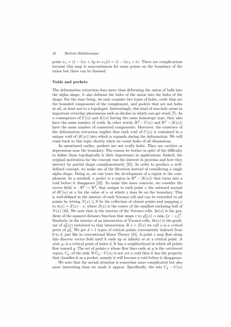
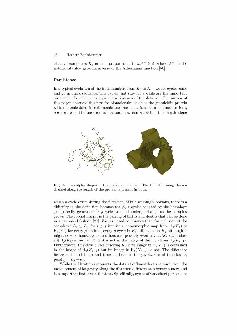
In a typical evolution of the Betti numbers from K0 to Km, we see cycles comeand go in quick sequence. The cycles that stay for a while are the importantones since they capture major shape features of the data set. The author ofthis paper observed this first for biomolecules, such as the gramicidin proteinwhich is embedded in cell membranes and functions as a channel for ions;see Figure 6. The question is obvious: how can we define the length along

Fig. 6. Two alpha shapes of the gramicidin protein. The tunnel forming the ionchannel along the length of the protein is present in both.

which a cycle exists during the filtration. While seemingly obvious, there is adifficulty in the definition because the βp p-cycles counted by the homologygroup really generate 2βp p-cycles and all undergo change as the complexgrows. The crucial insight is the pairing of births and deaths that can be donein a canonical fashion [27]. We just need to observe that the inclusion of thecomplexes Ki ⊆ Kj for i ≤ j implies a homomorphic map from Hp(Ki) toHp(Kj) for every p. Indeed, every p-cycle in Ki still exists in Kj although itmight now be homologous to others and possibly even trivial. We say a classc ∈ Hp(Ki) is born at Ki if it is not in the image of the map from Hp(Ki−1).Furthermore, this class c dies entering Kj if its image in Hp(Kj) is containedin the image of Hp(Ki−1) but its image in Hp(Kj−1) is not. The differencebetween time of birth and time of death is the persistence of the class c,pers(c) = αj − αi.

While the filtration represents the data at different levels of resolution, themeasurement of longevity along the filtration differentiates between more andless important features in the data. Specifically, cycles of very short persistence


may be discarded as noise and suppressed in the analysis of the data. Sinceour arch-enemy, noise, is ever present, the possibility to filter it out withoutchanging the data is significant. We refer to [23] and [8] for further details.

5 Combinatorics

In this section, we discuss the use of the α-complex to measure the correspond-ing union of balls. The motivation comes from biochemistry where proteinsand other biomolecules are routinely modeled as unions of balls in three dimen-sions. The method of choice is inclusion-exclusion which we use to computethe volume and surface area as well as their derivatives.

Inclusion-exclusion

Given a collection S of sets in Rd, the d-dimensional volume of the union can

be expressed as an alternating sum of volumes of common intersections ofsubcollections,

vol(⋃

S) =∑

∅6=σ⊆S

(−1)dim σvol(⋂

σ), (1)

where dimσ = cardσ − 1. This notation is convenient as it suggests we thinkof a collection as an abstract simplex whose dimension is one less than itsnumber of elements. Note that a region contained in k +1 of the sets is addedk + 1 times, once for each set, subtracted

(

k+1

2

)

times, once for each pair,

added(

k+1

3

)

times, etc. The equation follows because∑k

i=0(−1)i

(

k+1

i+1

)

= 1.This is known as the principle of inclusion-exclusion.

The trouble with the formula is its length which is exponential in thenumber of sets. For general sets, we cannot do better but in special situationswe sometimes have shorter formulas. Call σ independent if every face τ ⊆ σ hasits own region, that is,

⋂

τ −⋃

(σ − τ) 6= ∅. If all independent subcollectionshave dimension k or less then there is a formula with integer coefficientswhose terms are common intersections of at most k + 1 sets. To see this,take an abstract simplex of dimension dimσ ≥ k +1. By assumption, σ is notindependent and has therefore faces τ ⊆ σ with

⋂

τ ⊆⋃

(σ−τ). Choosing τ tobe maximal with this property implies that each set u in σ−τ has a non-emptyintersection with

⋂

τ . If τ = σ then⋂

σ = ∅ and we drop the correspondingterm from (1). Else we apply the principle of inclusion-exclusion to the sets⋂

τ ∩ u, where u ∈ σ − τ . The union of these sets is⋂

τ , so (1) gives

vol(⋂

τ ) =∑

∅6=υ⊆σ−τ

(−1)dim υvol(⋂

(τ ∪ υ)).

One of the terms on the right hand side is vol(⋂

σ) and all other terms arevolumes of intersections of strictly fewer than k + 1 sets. Hence, vol(

⋂

σ)


can be written as an alternating sum of volumes of common intersections ofstrictly fewer that cardσ sets. Starting with the exponential size formula, wecan drop terms for non-independent simplices or replace them by integer sumsof terms for independent simplices. The claim follows.

The maximum number of independent balls in Rd is d+1 which implies the

existence of formulas with terms of at most d+1 balls. This has been observedby Kratky in low dimensions [39] and used by Scheraga and collaborators tocompute the surface area of proteins [48].

Minimal formulas

Instead of going through a possibly lengthy substitution process, we can usethe α-complex to get a short formula directly. To explain how this works,we let S be a finite collection of balls in R

d and K = K(0) the weighted α-complex for α = 0. Recall that the Euler characteristic of K is the alternatingsum of simplices,

χ(K) =∑

∅6=σ∈K

(−1)dim σ.

More than in K itself, we are interested in certain subcomplexes of K. Specif-ically, for each point x ∈ R

d, we consider the simplices σ ∈ K defined byballs that contain x. The set of such simplices forms a full subcomplex F (x)of K. As it turns out, F (x) is either empty or contractible. In the formercase the Euler characteristic vanishes while in the latter case it is one. Inother words, χ(F (x)) = 0 if x 6∈

⋃

S and χ(F (x)) = 1 if x ∈⋃

S. We cantherefore integrate and get vol(

⋃

S) =∫

χ(F (x)) dx. A simplex σ ∈ K con-tributes (−1)dim σ for all points x ∈

⋂

σ and 0 for all other points. Its overallcontribution is therefore (−1)dim σvol(

⋂

σ). Summing over all simplices in theα-complex gives the anticipated result, namely

vol(⋃

S) =∑

∅6=σ∈K

(−1)dim σvol(⋂

σ). (2)

In words, we get the correct volume if we restrict the inclusion-exclusion for-mula (1) to subcollections that form simplices in the α-complex, for α = 0.A complete proof of (2) and of similar formulas for surface area and othermeasures of a union of balls can be found in [17]. As proved in [3], (2) isminimal in the sense that no terms can be removed, but there are also otherminimal formulas corresponding to other complexes made up of independentsimplices. To put the result in perspective, we mention that just truncating(1) to terms of dimension d or less does generally not give the correct volume.Nevertheless, truncating it to the simplices of the Delaunay triangulation ofS does give the correct result [47].


Voids

The voids in a protein structure and their sizes are of some interest in bio-chemistry. We thus modify (2) in such a way that the sum can be decomposedinto geometrically meaningful portions. A key ingredient is the notion of an-gle inside a d-simplex σ in R

d. Given a sufficiently small ball centered at aninterior point of a face τ of σ, we call the fraction of the ball that lies inside σthe angle of σ at τ , denoted as µσ,τ . This agrees with the usual notion of angleexcept that it is normalized to 1. To make a connection to (2), we considera k-simplex τ in the interior of |K|. The spheres bounding the k + 1 ballsdefining τ intersect in a sphere of dimension d− k − 1. The d-simplices in thestar of τ define a decomposition of this (d− k− 1)-sphere into as many piecesas there are d-simplices and the (d − k − 1)-dimensional volume of the piecethat corresponds to σ ∈ St τ is µσ,τ times the volume of the entire sphere.

We now return to the question of measuring a void in the union of balls,that is, a bounded component V of R

d −⋃

S. As suggested by Figure 5,we compute the volume of the corresponding void in the α-shape, V ′, andsubtract the volume of the fringe, the part of the union that reaches into it.However, we decompose the fringe in a way that is different than suggestedin the figure, using angles and inclusion-exclusion. To state the formula welet L ⊆ Del S − K be the set of simplices that define V ′. The d-dimensionalvolume of that void is simply the sum of volumes of the d-simplices in L. Someof the faces τ of a d-simplex σ ∈ L belong to L and others belong to K. Weuse the latter to compute the volume of the fringe and get

vol(V ) = vol(V ′) −∑

σ

∑

τ

(−1)dim τµσ,τvol(⋂

τ), (3)

where the outer sum is over all d-simplices σ in L and the inner sum is overall faces τ of σ that belong to K. A formal proof of (3) and of similar formulasfor surface area and other measures of voids can be found in [17].

Derivatives

An important concern in biochemistry is the dynamics of molecules, how theymove and change their shape. A natural approach to this question models theforces and solves the classical equation of motion for all atoms. Some of theforces are related to area and volume [26] which motivates our interest in thederivatives of these measures. The alpha complex is again useful because itgives ready access to geometric quantities that figure in the expression of thederivatives. The details for the volume derivative can be found in [25] andthose for the area derivative in [6]. Here we focus on the latter since it isgeometrically more interesting. Letting S be a set of n balls in R

3, we write zi

for the center and ri for the radius of the ball Bi, for 1 ≤ i ≤ n. In formulatingthe derivative, we concatenate the centers to get a vector z ∈ R

3n representingthe set S. The surface area of the union is then a map A : R

3n → R. Its


derivative at the point z is a linear map dAz : R3n → R. The gradient at

a point z is defined such that dAz(x) = 〈x,∇Az〉 for every motion vectorx. The derivative, dA : R

3n × R3n → R, can therefore be represented by

∇A : R3n → R

3n defined by mapping z to the gradient of A at z. To get ahandle on the gradient at z, we decompose the motion vector x ∈ R

3n intothree-dimensional vectors xi, where xi moves the center of the i-th ball tozi+xi. Since dAz is a linear function, we can focus on the infinitesimal changecaused by the motion of Bi along xi and add up the results for different indicesi. Similarly, we can focus on the impact of that motion on the interaction ofBi with individual other balls and add up the results to get the infinitesimalchange caused by Bi. Here it turns out that we need the interaction of Bi withindividual other balls Bj and with pairs of other balls Bj and Bk. The latteris interesting as it induces rotational forces on individual atoms which seemto be consistent with the type of motion typically observed in initial stages ofprotein folding.

Beginning with the case of two balls, Bi and Bj , we further decomposexi into a component uij along the direction defined by the two centers andanother component vij orthogonal to that direction. The magnitude of thecontribution of the motion along uij depends on the circle in which the twospheres bounding Bi and Bj intersect and more specifically the fraction sij

that belongs to the boundary of the union. This fraction can be computedwith inclusion-exclusion as explained above. Even though the motion of Bi

along vij keeps the surface area of Bi ∪Bj to first order unchanged, there is anon-zero contribution to the derivative if there in an interaction with a thirdball, Bk. To see this, we consider the caps Cij and Ckj in which Bi and Bk

intersect the sphere bounding Bj . The cap Ckj stays of course fixed but Cij

moves while its size remains to first order unchanged. The picture is similarto the two-ball case except one dimension lower. Again we decompose vij intoa component uijk inside the plane spanned by the three centers and anothercomponent vijk orthogonal to that plane. The magnitude of the contributionof the motion along uijk depends on the line segment connecting the two pointsat which the circles bounding the two caps intersect and more specifically onthe fraction bijk that forms an edge in the Voronoi decomposition of

⋃

S.This fraction can again be computed with inclusion-exclusion. Combining allcontributions, we write the i-th coordinate triplet of the gradient as

a3i−2

a3i−1

a3i

=∑

j

(sij · aij +∑

k

bijk · aijk), (4)

for 1 ≤ i ≤ n. Here the sums are over all boundary edges connecting pointszi and zj in K = K(0) and all triangles connecting this edge to furthervertices zk. The aij and aijk are vectors in R

3 that depend on straightforwardgeometric quantities such as the radii of the balls, the distances between thecenters, and the components of the motion vector introduced above. For detailswe refer to [6].


6 Discussion

In Section 1, we state that the interest in alpha shapes is driven by threeapplication areas: pattern recognition, digital shape sampling and processing,and structural molecular biology. All three require that the theory surveyed inthe paper be turned into widely available software. This has indeed been donethrough a combination of not-for-profit efforts at Universities and commercialsoftware development in industries. There is a place for both since they sat-isfy complementary needs. As the main contribution to Patton recognition,we see the fast Betti number algorithms and the introduction of persistent ho-mology. The main impact in digital shape sampling and processing has beenachieved by the surface reconstruction algorithm based on the idea of discreteflow [20]. The impact in structural molecular biology is based primarily onfast computation of measures and derivatives but we should also mention theconstruction of surface representations, such as the solvent accessible surface[41], the molecular surface [11], and the molecular skin [18].

The more we know the more we know we don’t know. Indeed there aremajor directions that remain largely unexplored. Work beyond three dimen-sions has only started and we mention the Cech, Vietoris-Rips, and witnesscomplexes that have been used to study high-dimensional data sets with per-sistent homology [14]. Probabilistic studies of alpha complexes and persistenthomology are also still in their infancy [44]. Finally, there are ideas of creatingshape spaces from alpha complexes which have yet unrealized potential [9].

References

1. N. Amenta, S. Choi and G. Rote. Incremental constructions con BRIO. In “Proc.19th Ann. Sympos. Comput. Geom., 2003”, 211–219.

2. D. Attali, J.-D. Boissonnat and A. Lieutier. Complexity of the Delaunay trian-gulation of points on surfaces: the smooth case. In “Proc. 19th Ann. Sympos.Comput. Geom., 2003”, 201–210.

3. D. Attali and H. Edelsbrunner. Inclusion-exclusion formulas from independentcomplexes. Discrete Comput. Geom. 37 (2007), 59–77.

4. F. Aurenhammer. Voronoi diagrams — a study of a fundamental geometric datastructure. ACM Comput. Surveys 23 (1991), 345–405.

5. A. Bowyer. Computing Dirichlet tessellations. Computer J. 24 (1981), 162–166.6. R. Bryant, H. Edelsbrunner, P. Koehl and M. Levitt. The area derivative of a

space-filling diagram. Discrete Comput. Geom. 32 (2004), 293–308.7. R. Casati and A. C. Varzi. Holes and Other Superficialities. MIT Press, Cam-

bridge, Massachusetts, 1994.8. F. Chazal and D. Cohen-Steiner. Geometric inference. This volume, 2008.9. H.-L. Cheng, H. Edelsbrunner and P. Fu. Shape space from deformation. Com-

put. Geom. Theory Appl. 19 (2001), 191-204.10. K. L. Clarkson and P. W. Shor. Applications of random sampling in computa-

tional geometry. Discrete Comput. Geom. 4 (1989), 387–421.


11. T. H. Connolly. Analytical molecular surface calculation. J. Appl. Cryst. 16

(1983), 548–558.12. B. Delaunay. Sur la sphere vide. Izv. Akad. Nauk SSSR, Otdelenie Matematich-

eskii i Estestvennyka Nauk 7 (1934), 793–800.13. C. J. A. Delfinado and H. Edelsbrunner. An incremental algorithm for Betti

numbers of simplicial complexes on the 3-sphere. Comput. Aided Geom. Design

12 (1995), 771–784.14. V. de Silva and G. Carlsson. Topological estimation using witness complexes.

In “Proc. Sympos. Point-Based Graphics, 2004”, 157–166.15. R. A. Dwyer. Average-case analysis of algorithms for convex hulls and Voronoi

diagrams. Ph. D. thesis, Report CMU-CS-88-132, Carnegie-Mellon Univ., Pitts-burgh, Pennsylvania, 1988.

16. H. Edelsbrunner. Weighted alpha shapes. Rept. UIUCDCS-R-92-1760, Dept.Comput. Sci., Univ. Illinois at Urbana-Champaign, Illinois, 1992.

17. H. Edelsbrunner. The union of balls and its dual shape. Discrete Comput. Geom.

13 (1995), 415–440.18. H. Edelsbrunner. Deformable smooth surface design. Discrete Comput. Geom.

21 (1999), 87–115.19. H. Edelsbrunner. Geometry and Topology for Mesh Generation. Cambridge

Univ. Press, England, 2001.20. H. Edelsbrunner. Surface reconstruction by wrapping finite sets in space. Dis-

crete and Computational Geometry — The Goodman-Pollack Festschrift, 379–404, eds. B. Aronov, S. Basu, J. Pach and M. Sharir, Springer-Verlag, Berlin,2003.

21. H. Edelsbrunner. Biological applications of computational topology. In Hand-

book of Discrete and Computational Geometry, 1395–1412, eds. J. E. Goodmanand J. O’Rourke, CRC Press, Boca Raton, Florida, 2004.

22. H. Edelsbrunner, M. Facello and J. Liang. On the definition and the constructionof pockets in macromolecules. Discrete Appl. Math. 88 (1998), 83–102.

23. H. Edelsbrunner and J. Harer. Persistent homology — a survey. Surveys on Dis-

crete and Computational Geometry. Twenty Years Later, eds. J. E. Goodman, J.Pach and R. Pollack, Contemporary Mathematics 453, 257–282, Amer. Math.Soc., Providence, Rhode Island, 2008.

24. H. Edelsbrunner, D. G. Kirkpatrick and R. Seidel. On the shape of a set ofpoints in the plane. IEEE Trans. Inform. Theory IT-29 (1983), 551–559.

25. H. Edelsbrunner and P. Koehl. The weighted volume derivative of a space-fillingdiagram. Proc. Natl. Acad. Sci. 100 (2003), 2203–2208.

26. H. Edelsbrunner and P. Koehl. The geometry of biomolecular solvation. Com-

binatorial and Computational Geometry, 243–275, eds. J. E. Goodman, J. Pachand E. Welzl, MSRI Publ. 52, Cambridge Univ. Press, England, 2005.

27. H. Edelsbrunner, D. Letscher and A. Zomorodian. Topological persistence andsimplification. Discrete Comput. Geom. 28 (2002), 511–533.

28. H. Edelsbrunner and E. P. Mucke. Simulation of simplicity: a technique to copewith degenerate cases in geometric algorithms. ACM Trans. Graphics 9 (1990),66–104.

29. H. Edelsbrunner and E. P. Mucke. Three-dimensional alpha shapes. ACM Trans.

Graphics 13 (1994), 43–72.30. H. Edelsbrunner and N. R. Shah. Incremental topological flipping works for

regular triangulations. Algorithmica 15 (1996), 223–241.


31. I. M. Gelfand, M. M. Kapranov and A. V. Zelevinsky. Discriminants, Resultants

and Multidimensional Determinants. Birkhauser, Boston, 1994.32. J. Giesen and M. John. The flow complex: a data structure for geometric mod-

eling. In “Proc. 14th Ann. ACM-SIAM Sympos. Discrete Alg., 2003”, 285–294.33. B. Grunbaum. Convex Polytopes. Second edition, Springer-Verlag, New York,

2003.34. R. A. Jarvis. On the identification of the convex hull of a finite set of points in

the plane. Inform. Process. Lett. 2 (1973), 18–21.35. R. A. Jarvis. Computing the shape hull of points in the plane. In “Comput.

Soc. Conf. Pattern Recognition and Image Processing, 1977”, 231–241.36. B. Joe. Three-dimensional triangulations from local transformations. SIAM J.

Sci. Statist. Comput. 10 (1989), 718–741.37. B. Joe. Construction of three-dimensional Delaunay triangulations from local

transformations. Comput. Aided Geom. Design 8 (1991), 123–142.38. D. E. Knuth. Axioms and Hulls. Springer-Verlag, Heidelberg, Germany, 1992.39. K. W. Kratky. The area of intersection of n equal circular disks. J. Phys. A:

Math. Gen. 11 (1978), 1017–1024.40. C. L. Lawson. Software for C

1 surface interpolation. In Mathematical Software

III, Academic Press, New York, 161–194.41. B. Lee and F. M. Richards. The interpretation of protein structures: estimation

of static accessibility. J. Mol. Biol. 55 (1971), 379-400.42. J. Leray. Sur la forme des espaces topologiques et sur les points fixes des

representations. J. Math. Pures Appl. 24 (1945), 95–167.43. A. Lieutier. Any open bounded subset of R

n has the same homotopy type as itsmedial axis. In “Proc. 8th ACM Sympos. Solid Modeling Appl., 2003”, 65–75.

44. D. J. Marchette. Random Graphs for Statistical Pattern Recognition. John Wiley& Sons, Hoboken, New Jersey, 2004.

45. J. Milnor. Morse Theory. Princeton Univ. Press, New Jersey, 1963.46. J. R. Munkres. Elements of Algebraic Topology. Perseus, Cambridge, Mas-

sachusetts, 1984.47. D. Q. Naiman and H. P. Wynn. Inclusion-exclusion-Bonferroni identities and in-

equalities for discrete tube-like problems via Euler characteristics. Ann. Statist.

20 (1992), 43–76.48. G. Perrot, B. Cheng, K. D. Gibson, J. Vila, A. Palmer, A. Nayeem, B. Maigret

and H. A. Scheraga. MSEED: a program for rapid determination of accessiblesurface areas and their derivatives. J. Comput. Chem. 13 (1992), 1–11.

49. R. Seidel. Backwards analysis of randomized geometric algorithms. In New

Trends in Discrete and Computational Geometry, J. Pach (ed.), Springer-Verlag,Berlin, 1993, 37–67.

50. R. E. Tarjan. Data Structures and Network Algorithms. SIAM, Philadelphia,Pennsylvania, 1983.

51. G. Voronoi. Nouvelles applications des parametres continus a la theorie desformes quadratiques. J. Reine Angew. Math. 133 (1907), 97–178 and 134 (1908),198–287.

52. D. F. Watson. Computing the n-dimensional Delaunay tessellation with appli-cation to Voronoi polytopes. Computer J. 24 (1981), 167–172.

53. G. M. Ziegler. Lectures on Polytopes. Springer-Verlag, New York, 1995.

Documents

Alpha Shapes — a Survey - Computer graphicsgraphics.stanford.edu/courses/cs268-14-fall/Handouts/AlphaShapes/... · Alpha Shapes — a Survey 3 such as calling a sequence of three