Embed Size (px)
Citation preview
ALOS-2 PALSAR-2 Support
1
ALOS-2 PALSAR-2 support in GAMMA Software Urs Wegmüller, Charles Werner, Andreas Wiesmann, Gamma Remote Sensing AG
CH-3073 Gümligen, http://www.gamma-rs.ch
11-Sep-2014, updated with InSAR example on 30-Nov-2014
1. Introduction
JAXA has made available sample data acquired by the ALOS-2 PALSAR-2 instrument [1]. The
products made available include SLC data (level 1.1) and geocoded backscatter data (level 1.5) for
the following data takes:
Table 1: Sample data from JAXA (http://www.eorc.jaxa.jp/ALOS-2/en/doc/sam_index.htm)
Nr. Site Date Mode Resolution Pol.
1 Tokyo, Japan June 19, 2014 Stripmap 3m HH+HV
2 Mt. Fuji, Japan June 20, 2014 Stripmap 3m HH+HV
3 Amazon, Brazil June 20, 2014 Stripmap 10m HH+HV
One of the data sets (Amazon) is acquired in left-looking geometry.
These sample data sets were downloaded by GAMMA and used to conduct an initial adaptation of
the GAMMA Software to ALOS-2 PALSAR-2 data processing. Apart from the software adaptation
the characteristics of these PALSAR data were assessed – knowing that these data are preliminary
and not corresponding entirely to standard PALSAR-2 data.
2. PALSAR-2 SLC data import
The sample data included SLC acquisitions in dual-polarization (HH+HV) strip-map mode. To read
the data the updated version of the program par_EORC_PALSAR is used. This program supports
reading both PALSAR-1 and PALSAR-2 SLC data in CEOS format. Some of the parameters of the
resulting SLC parameter file for the Tokyo data on 20140619 are listed in Table 2.
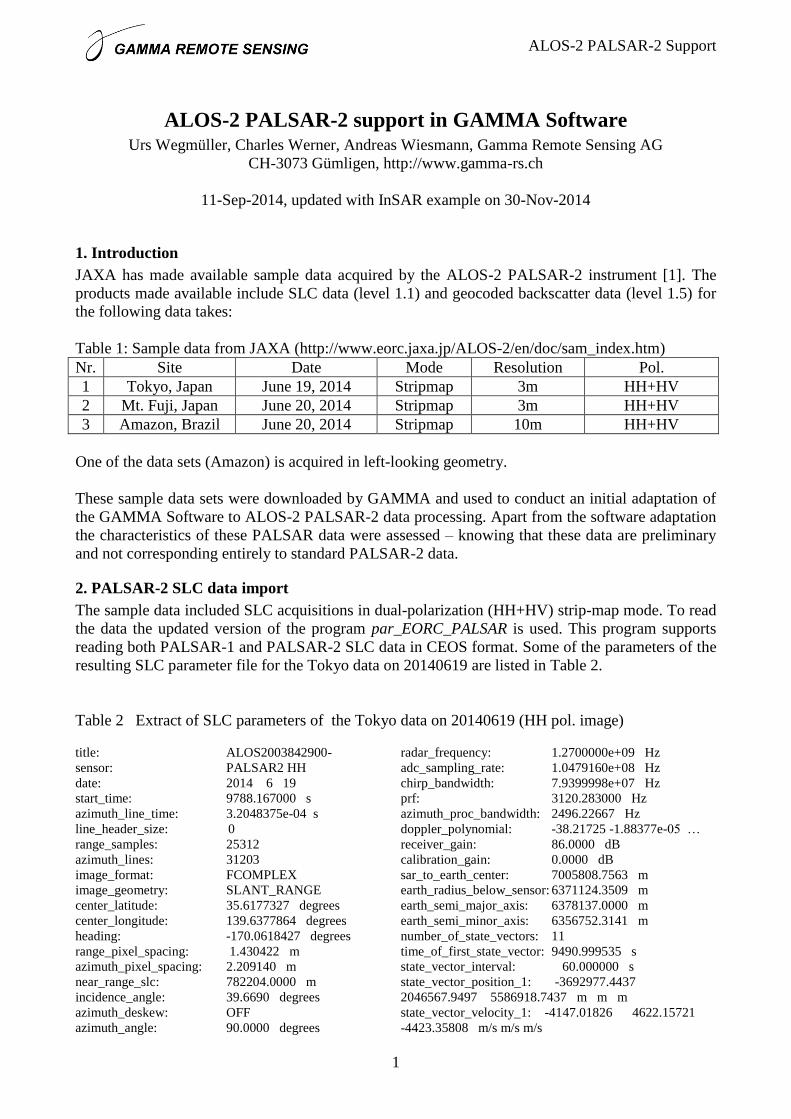
Table 2 Extract of SLC parameters of the Tokyo data on 20140619 (HH pol. image)
title: ALOS2003842900-
sensor: PALSAR2 HH
date: 2014 6 19
start_time: 9788.167000 s
azimuth_line_time: 3.2048375e-04 s
line_header_size: 0
range_samples: 25312
azimuth_lines: 31203
image_format: FCOMPLEX
image_geometry: SLANT_RANGE
center_latitude: 35.6177327 degrees
center_longitude: 139.6377864 degrees
heading: -170.0618427 degrees
range_pixel_spacing: 1.430422 m
azimuth_pixel_spacing: 2.209140 m
near_range_slc: 782204.0000 m
incidence_angle: 39.6690 degrees
azimuth_deskew: OFF
azimuth_angle: 90.0000 degrees
radar_frequency: 1.2700000e+09 Hz
adc_sampling_rate: 1.0479160e+08 Hz
chirp_bandwidth: 7.9399998e+07 Hz
prf: 3120.283000 Hz
azimuth_proc_bandwidth: 2496.22667 Hz
doppler_polynomial: -38.21725 -1.88377e-05 …
receiver_gain: 86.0000 dB
calibration_gain: 0.0000 dB
sar_to_earth_center: 7005808.7563 m
earth_radius_below_sensor: 6371124.3509 m
earth_semi_major_axis: 6378137.0000 m
earth_semi_minor_axis: 6356752.3141 m
number_of_state_vectors: 11
time_of_first_state_vector: 9490.999535 s
state_vector_interval: 60.000000 s
state_vector_position_1: -3692977.4437
2046567.9497 5586918.7437 m m m
state_vector_velocity_1: -4147.01826 4622.15721
-4423.35808 m/s m/s m/s

ALOS-2 PALSAR-2 Support
2
An overview in the entire Tokyo scene and a small section are shown in Figure 1. For the small
section shown a 2x2 multi-looking in range and azimuth was used. The Equivalent Number of
Looks (ENL) we determined for the section was around 3.8.
Figure 1 PALSAR-2 data over Tokyo. Full frame (left) showing the wide coverage and small section
(right) showing the high spatial resolution of this data set. Both images are in slant-range geometry.
3. PALSAR-2 SLC data characteristics
The sample product data were used to assess some characteristics of PALSAR-2.
3.1 Range and azimuth spectra
The program dismph_fft was used to visualize the range and azimuth spectra of the SLC data over
Tokyo (Figure 2).
Figure 2 Spectrum of SLC data over Tokyo as visualized by the program dismph_fft.
ALOS-2 PALSAR-2 Support
3
Then we also determined the azimuth spectrum using the program az_spec_SLC. The resulting plot
is shown in Figure 3.
Figure 3. Azimuth spectrum of PALSAR-2 SLC data over Tokyo.
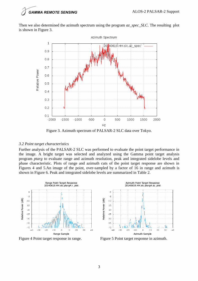
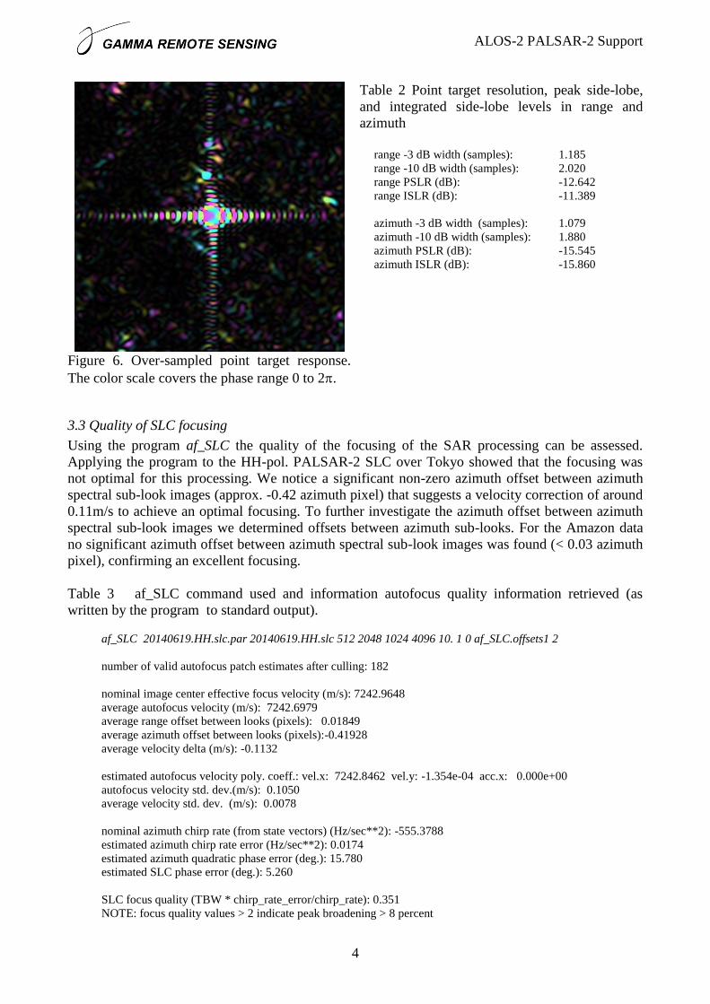
3.2 Point target characteristics
Further analysis of the PALSAR-2 SLC was performed to evaluate the point target performance in
the image. A bright target was selected and analyzed using the Gamma point target analysis
program ptarg to evaluate range and azimuth resolution, peak and integrated sidelobe levels and
phase characteristic. Plots of range and azimuth cuts of the point target response are shown in
Figures 4 and 5.An image of the point, over-sampled by a factor of 16 in range and azimuth is
shown in Figure 6. Peak and integrated sidelobe levels are summarized in Table 2.
Figure 4 Point target response in range.
Figure 5 Point target response in azimuth.
ALOS-2 PALSAR-2 Support
4
Table 2 Point target resolution, peak side-lobe,
and integrated side-lobe levels in range and
azimuth
range -3 dB width (samples): 1.185
range -10 dB width (samples): 2.020
range PSLR (dB): -12.642
range ISLR (dB): -11.389
azimuth -3 dB width (samples): 1.079
azimuth -10 dB width (samples): 1.880
azimuth PSLR (dB): -15.545
azimuth ISLR (dB): -15.860
Figure 6. Over-sampled point target response.
The color scale covers the phase range 0 to 2.
3.3 Quality of SLC focusing
Using the program af_SLC the quality of the focusing of the SAR processing can be assessed.
Applying the program to the HH-pol. PALSAR-2 SLC over Tokyo showed that the focusing was
not optimal for this processing. We notice a significant non-zero azimuth offset between azimuth
spectral sub-look images (approx. -0.42 azimuth pixel) that suggests a velocity correction of around
0.11m/s to achieve an optimal focusing. To further investigate the azimuth offset between azimuth
spectral sub-look images we determined offsets between azimuth sub-looks. For the Amazon data
no significant azimuth offset between azimuth spectral sub-look images was found (< 0.03 azimuth
pixel), confirming an excellent focusing.
Table 3 af_SLC command used and information autofocus quality information retrieved (as
written by the program to standard output).
af_SLC 20140619.HH.slc.par 20140619.HH.slc 512 2048 1024 4096 10. 1 0 af_SLC.offsets1 2
number of valid autofocus patch estimates after culling: 182
nominal image center effective focus velocity (m/s): 7242.9648
average autofocus velocity (m/s): 7242.6979
average range offset between looks (pixels): 0.01849
average azimuth offset between looks (pixels):-0.41928
average velocity delta (m/s): -0.1132
estimated autofocus velocity poly. coeff.: vel.x: 7242.8462 vel.y: -1.354e-04 acc.x: 0.000e+00
autofocus velocity std. dev.(m/s): 0.1050
average velocity std. dev. (m/s): 0.0078
nominal azimuth chirp rate (from state vectors) (Hz/sec**2): -555.3788
estimated azimuth chirp rate error (Hz/sec**2): 0.0174
estimated azimuth quadratic phase error (deg.): 15.780
estimated SLC phase error (deg.): 5.260
SLC focus quality (TBW * chirp_rate_error/chirp_rate): 0.351
NOTE: focus quality values > 2 indicate peak broadening > 8 percent

ALOS-2 PALSAR-2 Support
5
3.4 Split-beam positional offsets
Azimuth offsets between azimuth spectral sub-band images can relate to imperfect focusing or to
along-track variations in the ionospheric path delay [2]. To determine the azimuth offset field for
the SLC data over Tokyo we first applied band-pass filtering to the SLC data to determine 2
azimuth sub-band SLC with center frequencies shifted plus and minus a quarter of the prf and with
a filtered bandwidth of 0.4 of the prf
bpf 20140619.HH.slc 20140619.HH.slc.lf 25312 0.0 1.0 -0.25 0.4 0 0 - - 0 0 1.0 128
bpf 20140619.HH.slc 20140619.HH.slc.hf 25312 0.0 1.0 0.25 0.4 0 0 - - 0 0 1.0 128
Then we determined the offsets between the lower and upper azimuth band SLC using
create_offset 20140619.HH.slc.par 20140619.HH.slc.par 20140619.off 1 50 50 0
followed by
offset_pwr_tracking 20140619.HH.slc.lf 20140619.HH.slc.hf 20140619.HH.slc.par
20140619.HH.slc.par 20140619.off 20140619.sb_offs 20140619.sb_snr 256 128 - 2 3. 50 50 -
- - - 4 0
We determined then the bi-linear offset polynomial and rejected offset estimate outliers using
offset_fit 20140619.sb_offs 20140619.sb_snr 20140619.off 20140619.sb_coffs - 3.0 1 0
final range offset poly. coeff.: -0.00136
final range offset poly. coeff. errors: 1.55117e-05
final azimuth offset poly. coeff.: -0.20470
final azimuth offset poly. coeff. errors: 3.78543e-05
final model fit std. dev. (samples) range: 0.0395 azimuth: 0.0964
which indicates a significant non-zero average azimuth offset of around -0.2 azimuth pixels (of the
SLC). No significant non-zero range offset was observed.
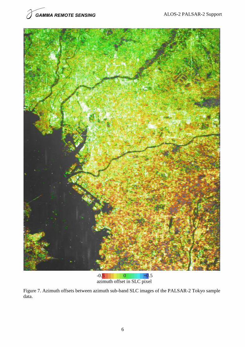
To display the azimuth offset field we extract the imaginary part of the culled offset field (program
cpx_to_real) and visualize the values using a color scale between offsets of -0.5 pixel (red) and +0.5
pixel (blue, see Figure 7. Based on the data alone it is difficult to judge if the reason for the azimuth
offsets observed relate to the processing or to ionospheric effects as there is no obvious azimuth
striping in the offsets but mainly an overall trend.
For the Amazon data no significant azimuth offsets between azimuth spectral sub-look images were
found.
For the Mt Fuji data an azimuth offset between azimuth spectral sub-look images similar to the one
for the Tokyo data was found (-0.25 pixel), with a spatial variation that might relate to ionospheric
effects.
ALOS-2 PALSAR-2 Support
6
Figure 7. Azimuth offsets between azimuth sub-band SLC images of the PALSAR-2 Tokyo sample
data.
-0.5 0 +0.5
azimuth offset in SLC pixel
ALOS-2 PALSAR-2 Support
7
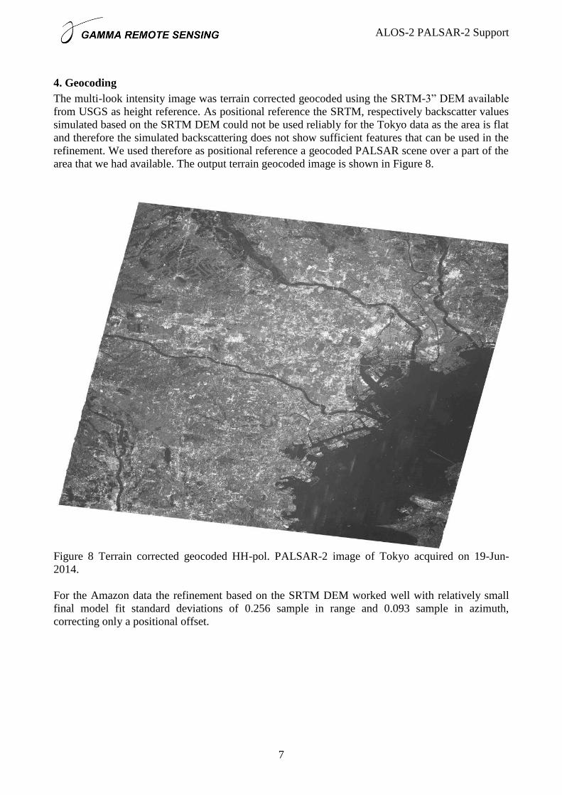
4. Geocoding
The multi-look intensity image was terrain corrected geocoded using the SRTM-3” DEM available
from USGS as height reference. As positional reference the SRTM, respectively backscatter values
simulated based on the SRTM DEM could not be used reliably for the Tokyo data as the area is flat
and therefore the simulated backscattering does not show sufficient features that can be used in the
refinement. We used therefore as positional reference a geocoded PALSAR scene over a part of the
area that we had available. The output terrain geocoded image is shown in Figure 8.
Figure 8 Terrain corrected geocoded HH-pol. PALSAR-2 image of Tokyo acquired on 19-Jun-
2014.
For the Amazon data the refinement based on the SRTM DEM worked well with relatively small
final model fit standard deviations of 0.256 sample in range and 0.093 sample in azimuth,
correcting only a positional offset.
ALOS-2 PALSAR-2 Support
8
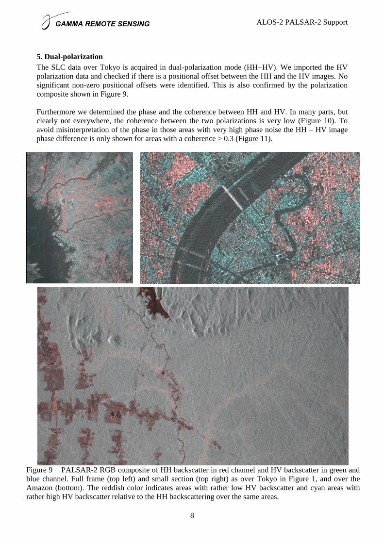
5. Dual-polarization
The SLC data over Tokyo is acquired in dual-polarization mode (HH+HV). We imported the HV
polarization data and checked if there is a positional offset between the HH and the HV images. No
significant non-zero positional offsets were identified. This is also confirmed by the polarization
composite shown in Figure 9.
Furthermore we determined the phase and the coherence between HH and HV. In many parts, but
clearly not everywhere, the coherence between the two polarizations is very low (Figure 10). To
avoid misinterpretation of the phase in those areas with very high phase noise the HH – HV image
phase difference is only shown for areas with a coherence > 0.3 (Figure 11).
Figure 9 PALSAR-2 RGB composite of HH backscatter in red channel and HV backscatter in green and
blue channel. Full frame (top left) and small section (top right) as over Tokyo in Figure 1, and over the
Amazon (bottom). The reddish color indicates areas with rather low HV backscatter and cyan areas with
rather high HV backscatter relative to the HH backscattering over the same areas.
ALOS-2 PALSAR-2 Support
9
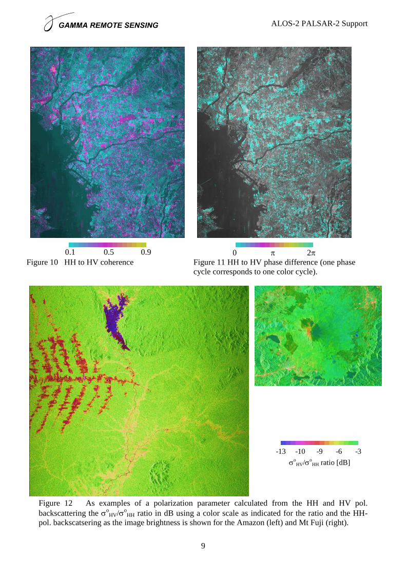
0.1 0.5 0.9
0 2
Figure 10 HH to HV coherence
Figure 11 HH to HV phase difference (one phase
cycle corresponds to one color cycle).
Figure 12 As examples of a polarization parameter calculated from the HH and HV pol.
backscattering the oHV/
oHH ratio in dB using a color scale as indicated for the ratio and the HH-
pol. backscatsering as the image brightness is shown for the Amazon (left) and Mt Fuji (right).
-13 -10 -9 -6 -3
o
HV/o
HH ratio [dB]
ALOS-2 PALSAR-2 Support
10
Another composite based on the HH and HV pol. backscattering shown over the Amazon and over
Mt. Fuji is the polarization ratio (Figure 12). The polarization ratio clearly discriminates deforested
areas from undisturbed forest. Over areas with very low backscattering we observe clear indications
that the noise equivalent sigma zero (NESZ) is affecting the observed HV backscatter. Over smooth
water surfaces (as present in the Mt Fuji data) a very low HV/HH ratio would be expected.
Nevertheless, the NESZ increases the HV image value resulting in values comparable to forest!
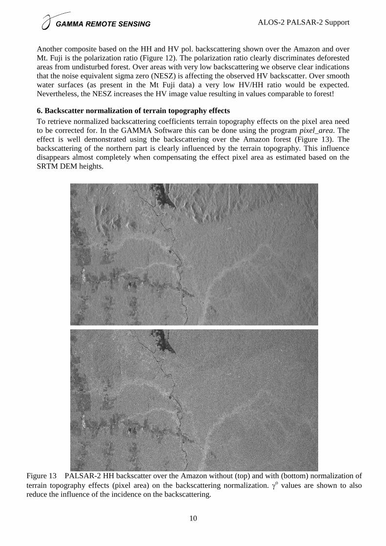
6. Backscatter normalization of terrain topography effects
To retrieve normalized backscattering coefficients terrain topography effects on the pixel area need
to be corrected for. In the GAMMA Software this can be done using the program pixel_area. The
effect is well demonstrated using the backscattering over the Amazon forest (Figure 13). The
backscattering of the northern part is clearly influenced by the terrain topography. This influence
disappears almost completely when compensating the effect pixel area as estimated based on the
SRTM DEM heights.
Figure 13 PALSAR-2 HH backscatter over the Amazon without (top) and with (bottom) normalization of
terrain topography effects (pixel area) on the backscattering normalization. o values are shown to also
reduce the influence of the incidence on the backscattering.
ALOS-2 PALSAR-2 Support
11
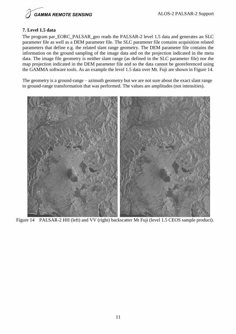
7. Level 1.5 data
The program par_EORC_PALSAR_geo reads the PALSAR-2 level 1.5 data and generates an SLC
parameter file as well as a DEM parameter file. The SLC parameter file contains acquisition related
parameters that define e.g. the related slant range geometry. The DEM parameter file contains the
information on the ground sampling of the image data and on the projection indicated in the meta
data. The image file geometry is neither slant range (as defined in the SLC parameter file) nor the
map projection indicated in the DEM parameter file and so the data cannot be georeferenced using
the GAMMA software tools. As an example the level 1.5 data over Mt. Fuji are shown in Figure 14.
The geometry is a ground-range – azimuth geometry but we are not sure about the exact slant range
to ground-range transformation that was performed. The values are amplitudes (not intensities).
Figure 14 PALSAR-2 HH (left) and VV (right) backscatter Mt Fuji (level 1.5 CEOS sample product).

ALOS-2 PALSAR-2 Support
12
8. Interferometry using PALSAR-2 strip-map mode data
For PALSAR-2 strip-map mode data SAR interferometry is supported in the same way as for
PALSAR-1. Figure 15 shows a differential interferogram generated using two HH-pol acquisitions
acquired in dual-polarization mode over the Swiss alps on 20140906 and 20141115 with a spatial
baseline of about 147 m (perpendicular component). Over the higher elevations the coherence is
very low because of changing snow conditions.
Figure 15: PALSAR-2 differential interferogram using HH-pol acquisitions acquired in dual-
polarization mode over the Swiss alps on 20140906 and 20141115 (Bperp 147m, dt 98 days). One
color cycle corresponds to one phase cycle. The full frame is shown, geocoded to Swiss national
coordinates.
ALOS-2 PALSAR-2 Support
13
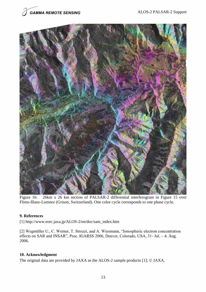
Figure 16: 26km x 26 km section of PALSAR-2 differential interferogram in Figure 15 over
Flims-Illanz-Lumnez (Grison, Switzerland). One color cycle corresponds to one phase cycle.
9. References
[1] http://www.eorc.jaxa.jp/ALOS-2/en/doc/sam_index.htm
[2] Wegmüller U., C. Werner, T. Strozzi, and A. Wiesmann, “Ionospheric electron concentration
effects on SAR and INSAR”, Proc. IGARSS 2006, Denver, Colorado, USA, 31- Jul. – 4. Aug.
2006.
10. Acknowledgment
The original data are provided by JAXA as the ALOS-2 sample products [1]; © JAXA.