Embed Size (px)
Citation preview
Almost None of the Theory of Stochastic
Processes
A Course on Random Processes, for Students of Measure-Theoretic
Probability, with a View to Applications in Dynamics and Statistics
Cosma Rohilla Shalizi with Aryeh Kontorovich
version 0.1.1, last LATEX’d July 3, 2010
Contents
Table of Contents i
Comprehensive List of Definitions, Lemmas, Propositions, Theo-rems, Corollaries, Examples and Exercises xxv
Preface xxvi
I Stochastic Processes in General 2
1 Basics 31.1 So, What Is a Stochastic Process? . . . . . . . . . . . . . . . . . 31.2 Random Functions . . . . . . . . . . . . . . . . . . . . . . . . . . 51.3 Exercises . . . . . . . . . . . . . . . . . . . . . . . . . . . . . . . 7
2 Building Processes 152.1 Finite-Dimensional Distributions . . . . . . . . . . . . . . . . . . 152.2 Consistency and Extension . . . . . . . . . . . . . . . . . . . . . 16
3 Building Processes by Conditioning 213.1 Probability Kernels . . . . . . . . . . . . . . . . . . . . . . . . . . 213.2 Extension via Recursive Conditioning . . . . . . . . . . . . . . . 223.3 Exercises . . . . . . . . . . . . . . . . . . . . . . . . . . . . . . . 25
II One-Parameter Processes in General 26
4 One-Parameter Processes 274.1 One-Parameter Processes . . . . . . . . . . . . . . . . . . . . . . 274.2 Operator Representations of One-Parameter Processes . . . . . . 314.3 Exercises . . . . . . . . . . . . . . . . . . . . . . . . . . . . . . . 31
5 Stationary Processes 345.1 Kinds of Stationarity . . . . . . . . . . . . . . . . . . . . . . . . . 34
i
CONTENTS ii
5.2 Strictly Stationary Processes and Measure-Preserving Transfor-mations . . . . . . . . . . . . . . . . . . . . . . . . . . . . . . . . 35
5.3 Exercises . . . . . . . . . . . . . . . . . . . . . . . . . . . . . . . 37
6 Random Times 386.1 Reminders about Filtrations and Stopping Times . . . . . . . . . 386.2 Waiting Times . . . . . . . . . . . . . . . . . . . . . . . . . . . . 396.3 Kac’s Recurrence Theorem . . . . . . . . . . . . . . . . . . . . . 416.4 Exercises . . . . . . . . . . . . . . . . . . . . . . . . . . . . . . . 45
7 Continuity 467.1 Kinds of Continuity for Processes . . . . . . . . . . . . . . . . . . 477.2 Why Continuity Is an Issue . . . . . . . . . . . . . . . . . . . . . 487.3 Separable Random Functions . . . . . . . . . . . . . . . . . . . . 507.4 Separable Versions . . . . . . . . . . . . . . . . . . . . . . . . . . 517.5 Measurable Versions . . . . . . . . . . . . . . . . . . . . . . . . . 567.6 Cadlag Versions . . . . . . . . . . . . . . . . . . . . . . . . . . . . 577.7 Continuous Modifications . . . . . . . . . . . . . . . . . . . . . . 577.8 Exercises . . . . . . . . . . . . . . . . . . . . . . . . . . . . . . . 59
III Markov Processes 60
8 Markov Processes 618.1 The Correct Line on the Markov Property . . . . . . . . . . . . . 618.2 Transition Probability Kernels . . . . . . . . . . . . . . . . . . . 628.3 The Markov Property Under Multiple Filtrations . . . . . . . . . 658.4 Exercises . . . . . . . . . . . . . . . . . . . . . . . . . . . . . . . 67
9 Markov Characterizations 709.1 Markov Sequences as Transduced Noise . . . . . . . . . . . . . . 709.2 Time-Evolution (Markov) Operators . . . . . . . . . . . . . . . . 729.3 Exercises . . . . . . . . . . . . . . . . . . . . . . . . . . . . . . . 76
10 Markov Examples 7810.1 Probability Densities in the Logistic Map . . . . . . . . . . . . . 7810.2 Transition Kernels and Evolution Operators for the Wiener Process 8010.3 Levy Processes and Limit Laws . . . . . . . . . . . . . . . . . . . 8210.4 Exercises . . . . . . . . . . . . . . . . . . . . . . . . . . . . . . . 86
11 Generators 8811.1 Exercises . . . . . . . . . . . . . . . . . . . . . . . . . . . . . . . 93
12 Strong Markov, Martingales 9512.1 The Strong Markov Property . . . . . . . . . . . . . . . . . . . . 9512.2 Martingale Problems . . . . . . . . . . . . . . . . . . . . . . . . . 9612.3 Exercises . . . . . . . . . . . . . . . . . . . . . . . . . . . . . . . 98
CONTENTS iii
13 Feller Processes 9913.1 Markov Families . . . . . . . . . . . . . . . . . . . . . . . . . . . 9913.2 Feller Processes . . . . . . . . . . . . . . . . . . . . . . . . . . . . 10013.3 Exercises . . . . . . . . . . . . . . . . . . . . . . . . . . . . . . . 106
14 Convergence of Feller Processes 10714.1 Weak Convergence of Processes with Cadlag Paths (The Sko-
rokhod Topology) . . . . . . . . . . . . . . . . . . . . . . . . . . . 10714.2 Convergence of Feller Processes . . . . . . . . . . . . . . . . . . . 10914.3 Approximation of Ordinary Differential Equations by Markov
Processes . . . . . . . . . . . . . . . . . . . . . . . . . . . . . . . 11114.4 Exercises . . . . . . . . . . . . . . . . . . . . . . . . . . . . . . . 113
15 Convergence of Random Walks 11415.1 The Wiener Process is Feller . . . . . . . . . . . . . . . . . . . . 11415.2 Convergence of Random Walks . . . . . . . . . . . . . . . . . . . 116
15.2.1 Approach Through Feller Processes . . . . . . . . . . . . . 11715.2.2 Direct Approach . . . . . . . . . . . . . . . . . . . . . . . 11915.2.3 Consequences of the Functional Central Limit Theorem . 120
15.3 Exercises . . . . . . . . . . . . . . . . . . . . . . . . . . . . . . . 121
IV Diffusions and Stochastic Calculus 123
16 Diffusions and the Wiener Process 12416.1 Diffusions and Stochastic Calculus . . . . . . . . . . . . . . . . . 12416.2 Once More with the Wiener Process and Its Properties . . . . . . 12616.3 Wiener Measure; Most Continuous Curves Are Not Differentiable 127
17 Stochastic Integrals 13017.1 A Heuristic Introduction to Stochastic Integrals . . . . . . . . . . 13017.2 Integrals with Respect to the Wiener Process . . . . . . . . . . . 13117.3 Some Easy Stochastic Integrals, with a Moral . . . . . . . . . . . 136
17.3.1∫dW . . . . . . . . . . . . . . . . . . . . . . . . . . . . . 136
17.3.2∫WdW . . . . . . . . . . . . . . . . . . . . . . . . . . . . 137
17.4 Ito’s Formula . . . . . . . . . . . . . . . . . . . . . . . . . . . . . 13917.4.1 Stratonovich Integrals . . . . . . . . . . . . . . . . . . . . 14417.4.2 Martingale Characterization of the Wiener Process . . . . 14417.4.3 Martingale Representation . . . . . . . . . . . . . . . . . . 145
17.5 Exercises . . . . . . . . . . . . . . . . . . . . . . . . . . . . . . . 146
18 Stochastic Differential Equations 14818.1 Brownian Motion, the Langevin Equation, and Ornstein-Uhlenbeck
Processes . . . . . . . . . . . . . . . . . . . . . . . . . . . . . . . 15418.2 Solutions of SDEs are Diffusions . . . . . . . . . . . . . . . . . . 15618.3 Forward and Backward Equations . . . . . . . . . . . . . . . . . 158
CONTENTS iv
18.4 Exercises . . . . . . . . . . . . . . . . . . . . . . . . . . . . . . . 161
19 Spectral Analysis and White Noise Integrals 16319.1 Spectral Representation of Weakly Stationary Procesess . . . . . 16419.2 White Noise . . . . . . . . . . . . . . . . . . . . . . . . . . . . . . 171
19.2.1 How the White Noise Lost Its Color . . . . . . . . . . . . 173
20 Small-Noise SDEs 17420.1 Convergence in Probability of SDEs to ODEs . . . . . . . . . . . 17520.2 Rate of Convergence; Probability of Large Deviations . . . . . . 176
V Ergodic Theory 180
21 The Mean-Square Ergodic Theorem 18121.1 Mean-Square Ergodicity Based on the Autocovariance . . . . . . 18221.2 Mean-Square Ergodicity Based on the Spectrum . . . . . . . . . 18421.3 Exercises . . . . . . . . . . . . . . . . . . . . . . . . . . . . . . . 186
22 Ergodic Properties and Ergodic Limits 18722.1 General Remarks . . . . . . . . . . . . . . . . . . . . . . . . . . . 18722.2 Dynamical Systems and Their Invariants . . . . . . . . . . . . . . 18822.3 Time Averages and Ergodic Properties . . . . . . . . . . . . . . . 19122.4 Asymptotic Mean Stationarity . . . . . . . . . . . . . . . . . . . 19422.5 Exercises . . . . . . . . . . . . . . . . . . . . . . . . . . . . . . . 197
23 The Almost-Sure Ergodic Theorem 198
24 Ergodicity and Metric Transitivity 20424.1 Metric Transitivity . . . . . . . . . . . . . . . . . . . . . . . . . . 20424.2 Examples of Ergodicity . . . . . . . . . . . . . . . . . . . . . . . 20624.3 Consequences of Ergodicity . . . . . . . . . . . . . . . . . . . . . 207
24.3.1 Deterministic Limits for Time Averages . . . . . . . . . . 20824.3.2 Ergodicity and the approach to independence . . . . . . . 208
24.4 Exercises . . . . . . . . . . . . . . . . . . . . . . . . . . . . . . . 209
25 Ergodic Decomposition 21025.1 Preliminaries to Ergodic Decompositions . . . . . . . . . . . . . . 21025.2 Construction of the Ergodic Decomposition . . . . . . . . . . . . 21225.3 Statistical Aspects . . . . . . . . . . . . . . . . . . . . . . . . . . 216
25.3.1 Ergodic Components as Minimal Sufficient Statistics . . . 21625.3.2 Testing Ergodic Hypotheses . . . . . . . . . . . . . . . . . 218
25.4 Exercises . . . . . . . . . . . . . . . . . . . . . . . . . . . . . . . 219
CONTENTS v
26 Mixing 22026.1 Definition and Measurement of Mixing . . . . . . . . . . . . . . . 22126.2 Examples of Mixing Processes . . . . . . . . . . . . . . . . . . . . 22326.3 Convergence of Distributions Under Mixing . . . . . . . . . . . . 22326.4 A Central Limit Theorem for Mixing Sequences . . . . . . . . . . 225
27 Asymptotic Distributions [[w]] 227
VI Information Theory 228
28 Entropy and Divergence 22928.1 Shannon Entropy . . . . . . . . . . . . . . . . . . . . . . . . . . . 23028.2 Relative Entropy or Kullback-Leibler Divergence . . . . . . . . . 232
28.2.1 Statistical Aspects of Relative Entropy . . . . . . . . . . . 23328.3 Mutual Information . . . . . . . . . . . . . . . . . . . . . . . . . 235
28.3.1 Mutual Information Function . . . . . . . . . . . . . . . . 235
29 Rates and Equipartition 23729.1 Information-Theoretic Rates . . . . . . . . . . . . . . . . . . . . . 23729.2 Asymptotic Equipartition . . . . . . . . . . . . . . . . . . . . . . 240
29.2.1 Typical Sequences . . . . . . . . . . . . . . . . . . . . . . 24329.3 Asymptotic Likelihood . . . . . . . . . . . . . . . . . . . . . . . . 244
29.3.1 Asymptotic Equipartition for Divergence . . . . . . . . . 24429.3.2 Likelihood Results . . . . . . . . . . . . . . . . . . . . . . 244
29.4 Exercises . . . . . . . . . . . . . . . . . . . . . . . . . . . . . . . 244
30 Information Theory and Statistics [[w]] 246
VII Large Deviations 247
31 Large Deviations: Basics 24831.1 Large Deviation Principles: Main Definitions and Generalities . . 24831.2 Breeding Large Deviations . . . . . . . . . . . . . . . . . . . . . . 252
32 IID Large Deviations 25832.1 Cumulant Generating Functions and Relative Entropy . . . . . . 25932.2 Large Deviations of the Empirical Mean in Rd . . . . . . . . . . . 26232.3 Large Deviations of the Empirical Measure in Polish Spaces . . . 26532.4 Large Deviations of the Empirical Process in Polish Spaces . . . 266
33 Large Deviations for Markov Sequences 26833.1 Large Deviations for Pair Measure of Markov Sequences . . . . . 26833.2 Higher LDPs for Markov Sequences . . . . . . . . . . . . . . . . . 272
CONTENTS vi
34 The Gartner-Ellis Theorem 27334.1 The Gartner-Ellis Theorem . . . . . . . . . . . . . . . . . . . . . 27334.2 Exercises . . . . . . . . . . . . . . . . . . . . . . . . . . . . . . . 277
35 Large Deviations for Stationary Sequences [[w]] 278
36 Large Deviations in Inference [[w]] 279
37 Freidlin-Wentzell Theory 28037.1 Large Deviations of the Wiener Process . . . . . . . . . . . . . . 28137.2 Large Deviations for SDEs with State-Independent Noise . . . . 28637.3 Large Deviations for State-Dependent Noise . . . . . . . . . . . . 28737.4 Exercises . . . . . . . . . . . . . . . . . . . . . . . . . . . . . . . 288
VIII Measure Concentration [Kontorovich/w] 289
IX Partially-Observable Processes [[w]] 290
38 Hidden Markov Models [[w]] 291
39 Stochastic Automata [[w]] 292
40 Predictive Representations [[w]] 293
X Applications [[w]] 294
XI Appendices [[w]] 296
A Real and Complex Analysis [[w]] 298A.1 Real Analysis . . . . . . . . . . . . . . . . . . . . . . . . . . . . . 298A.2 Complex Analysis . . . . . . . . . . . . . . . . . . . . . . . . . . 298
B General Vector Spaces and Operators [[w]] 299
C Laplace Transforms [[w]] 303
D Topological Notions [[w]] 305
E Measure-Theoretic Probability [[w]] 306
F Fourier Transforms [[w]] 308
G Filtrations and Optional Times [[w]] 309

CONTENTS vii
H Martingales [[w]] 311
Bibliography 312
Definitions, Lemmas,Propositions, Theorems,Corollaries, Examples andExercises
Chapter 1 Basic Definitions: Indexed Collections and RandomFunctions 3
Definition 1 A Stochastic Process Is a Collection of Random Vari-ables . . . . . . . . . . . . . . . . . . . . . . . . . . . . . . 3
Example 2 Random variables . . . . . . . . . . . . . . . . . . . . 4Example 3 Random vector . . . . . . . . . . . . . . . . . . . . . . 4Example 4 One-sided random sequences . . . . . . . . . . . . . . 4Example 5 Two-sided random sequences . . . . . . . . . . . . . . 4Example 6 Spatially-discrete random fields . . . . . . . . . . . . . 4Example 7 Continuous-time random processes . . . . . . . . . . . 4Example 8 Random set functions . . . . . . . . . . . . . . . . . . 4Example 9 One-sided random sequences of set functions . . . . . 4Example 10 Empirical distributions . . . . . . . . . . . . . . . . . 5Definition 11 Cylinder Set . . . . . . . . . . . . . . . . . . . . . . 5Definition 12 Product σ-field . . . . . . . . . . . . . . . . . . . . 6Definition 13 Random Function; Sample Path . . . . . . . . . . . 6Definition 14 Functional of the Sample Path . . . . . . . . . . . . 6Definition 15 Projection Operator, Coordinate Map . . . . . . . . 6Theorem 16 Product σ-field-measurability is equvialent to mea-
surability of all coordinates . . . . . . . . . . . . . . . . . 6Definition 17 A Stochastic Process Is a Random Function . . . . 7Corollary 18 Measurability of constrained sample paths . . . . . 7Example 19 Random Measures . . . . . . . . . . . . . . . . . . . 7Example 20 Point Processes . . . . . . . . . . . . . . . . . . . . . 7Example 21 Continuous random processes . . . . . . . . . . . . . 7Exercise 1 The product σ-field answers countable questions . . . 7
viii
CONTENTS ix
Exercise 2 The product σ-field constrained to a given set of paths 7
Chapter 2 Building Infinite Processes from Finite-DimensionalDistributions 15
Definition 22 Finite-dimensional distributions . . . . . . . . . . . 15Theorem 23 Finite-dimensional distributions determine process
distributions . . . . . . . . . . . . . . . . . . . . . . . . . 16Definition 24 Projective Family of Distributions . . . . . . . . . . 17Lemma 25 FDDs Form Projective Families . . . . . . . . . . . . 17Proposition 26 Randomization, transfer . . . . . . . . . . . . . . 18Theorem 27 Daniell Extension Theorem . . . . . . . . . . . . . . 18Proposition 28 Caratheodory Extension Theorem . . . . . . . . . 19Theorem 29 Kolmogorov Extension Theorem . . . . . . . . . . . 19
Chapter 3 Building Infinite Processes from Regular ConditionalProbability Distributions 21
Definition 30 Probability Kernel . . . . . . . . . . . . . . . . . . 21Definition 31 Composition of probability kernels . . . . . . . . . 22Proposition 32 Set functions continuous at ∅ . . . . . . . . . . . . 23Theorem 33 Ionescu Tulcea Extension Theorem . . . . . . . . . . 23Exercise 3 Lomnick-Ulam Theorem on infinite product measures 25Exercise 4 Measures of cylinder sets . . . . . . . . . . . . . . . . 25
Chapter 4 One-Parameter Processes, Usually Functions of Time 27Definition 34 One-Parameter Process . . . . . . . . . . . . . . . . 28Example 35 Bernoulli process . . . . . . . . . . . . . . . . . . . . 28Example 36 Markov models . . . . . . . . . . . . . . . . . . . . . 28Example 37 “White Noise” (Not Really) . . . . . . . . . . . . . . 28Example 38 Wiener Process . . . . . . . . . . . . . . . . . . . . . 29Example 39 Logistic Map . . . . . . . . . . . . . . . . . . . . . . 29Example 40 Symbolic Dynamics of the Logistic Map . . . . . . . 29Example 41 IID Samples . . . . . . . . . . . . . . . . . . . . . . . 30Example 42 Non-IID Samples . . . . . . . . . . . . . . . . . . . . 30Example 43 Estimating Distributions . . . . . . . . . . . . . . . . 30Example 44 Doob’s Martingale . . . . . . . . . . . . . . . . . . . 30Example 45 The One-Dimensional Ising Model . . . . . . . . . . 30Example 46 Text . . . . . . . . . . . . . . . . . . . . . . . . . . . 31Example 47 Polymer Sequences . . . . . . . . . . . . . . . . . . . 31Definition 48 Shift Operators . . . . . . . . . . . . . . . . . . . . 31Exercise 5 Existence of proto-Wiener processes . . . . . . . . . . 32Exercise 6 Time-Evolution Semi-Group . . . . . . . . . . . . . . . 32
Chapter 5 Stationary One-Parameter Processes 34Definition 49 Strong Stationarity . . . . . . . . . . . . . . . . . . 34Definition 50 Weak Stationarity . . . . . . . . . . . . . . . . . . . 35Definition 51 Conditional (Strong) Stationarity . . . . . . . . . . 35
CONTENTS x
Theorem 52 Stationarity is Shift-Invariance . . . . . . . . . . . . 35Definition 53 Measure-Preserving Transformation . . . . . . . . . 36Corollary 54 Measure-preservation implies stationarity . . . . . . 36Exercise 7 Functions of Stationary Processes . . . . . . . . . . . . 37Exercise 8 Continuous Measure-Preserving Families of Transfor-
mations . . . . . . . . . . . . . . . . . . . . . . . . . . . . 37Exercise 9 The Logistic Map as a Measure-Preserving Transfor-
mation . . . . . . . . . . . . . . . . . . . . . . . . . . . . . 37
Chapter 6 Random Times and Their Properties 38Definition 55 Filtration . . . . . . . . . . . . . . . . . . . . . . . . 38Definition 56 Adapted Process . . . . . . . . . . . . . . . . . . . 39Definition 57 Stopping Time, Optional Time . . . . . . . . . . . 39Definition 58 Fτ for a Stopping Time τ . . . . . . . . . . . . . . 39Definition 59 Hitting Time . . . . . . . . . . . . . . . . . . . . . . 40Example 60 Fixation through Genetic Drift . . . . . . . . . . . . 40Example 61 Stock Options . . . . . . . . . . . . . . . . . . . . . . 40Definition 62 First Passage Time . . . . . . . . . . . . . . . . . . 40Definition 63 Return Time, Recurrence Time . . . . . . . . . . . 41Proposition 64 Some Sufficient Conditions for Waiting Times to
be Weakly Optional . . . . . . . . . . . . . . . . . . . . . 41Lemma 65 Some Recurrence Relations for Kac’s Theorem . . . . 42Theorem 66 Recurrence in Stationary Processes . . . . . . . . . . 42Corollary 67 Poincare Recurrence Theorem . . . . . . . . . . . . 43Corollary 68 “Nietzsche” . . . . . . . . . . . . . . . . . . . . . . . 43Theorem 69 Kac’s Recurrence Theorem . . . . . . . . . . . . . . 44Example 70 Counter-example for Kac’s Recurrence Theorem . . 45Exercise 10 Weakly Optional Times and Right-Continuous Fil-
trations . . . . . . . . . . . . . . . . . . . . . . . . . . . . 45Exercise 11 Discrete Stopping Times and Their σ-Algebras . . . 45Exercise 12 Kac’s Theorem for the Logistic Map . . . . . . . . . 45
Chapter 7 Continuity of Stochastic Processes 46Definition 71 Continuity in Mean . . . . . . . . . . . . . . . . . . 47Definition 72 Continuity in Probability, Stochastic Continuity . . 47Definition 73 Continuous Sample Paths . . . . . . . . . . . . . . 47Definition 74 Cadlag . . . . . . . . . . . . . . . . . . . . . . . . . 47Definition 75 Versions of a Stochastic Process, Stochastically Equiv-
alent Processes . . . . . . . . . . . . . . . . . . . . . . . . 48Lemma 76 Versions Have Identical FDDs . . . . . . . . . . . . . 48Definition 77 Indistinguishable Processes . . . . . . . . . . . . . . 48Proposition 78 Continuous Sample Paths Have Measurable Extrema 49Example 79 A Horrible Version of the proto-Wiener Process . . . 50Definition 80 Separable Function . . . . . . . . . . . . . . . . . . 51Lemma 81 Some Sufficient Conditions for Separability . . . . . . 51Definition 82 Separable Process . . . . . . . . . . . . . . . . . . . 51
CONTENTS xi
Definition 83 Compactness, Compactification . . . . . . . . . . . 52Proposition 84 Compact Spaces are Separable . . . . . . . . . . . 52Proposition 85 Compactification is Possible . . . . . . . . . . . . 52Example 86 Compactifying the Reals . . . . . . . . . . . . . . . . 52Lemma 87 Alternative Characterization of Separability . . . . . . 52Lemma 88 Confining Bad Behavior to a Measure Zero Event . . 53Lemma 89 A Null Exceptional Set . . . . . . . . . . . . . . . . . 54Theorem 90 Separable Versions, Separable Modification . . . . . 55Corollary 91 Separable Modifications in Compactified Spaces . . 56Corollary 92 Separable Versions with Prescribed Distributions Exist 56Definition 93 Measurable random function . . . . . . . . . . . . . 57Theorem 94 Exchanging Expectations and Time Integrals . . . . 57Theorem 95 Measurable Separable Modifications . . . . . . . . . 57Theorem 96 Cadlag Versions . . . . . . . . . . . . . . . . . . . . 57Theorem 97 Continuous Versions . . . . . . . . . . . . . . . . . . 58Definition 98 Modulus of continuity . . . . . . . . . . . . . . . . . 58Lemma 99 Modulus of continuity and uniform continuity . . . . . 58Definition 100 Holder continuity . . . . . . . . . . . . . . . . . . 58Theorem 101 Holder-continuous versions . . . . . . . . . . . . . . 58Exercise 13 Piecewise Linear Paths Not in the Product σ-Field . 59Exercise 14 Indistinguishability of Right-Continuous Versions . . 59
Chapter 8 Markov Processes 61Definition 102 Markov Property . . . . . . . . . . . . . . . . . . . 61Lemma 103 The Markov Property Extends to the Whole Future 61Definition 104 Product of Probability Kernels . . . . . . . . . . . 62Definition 105 Transition Semi-Group . . . . . . . . . . . . . . . 63Theorem 106 Existence of Markov Process with Given Transition
Kernels . . . . . . . . . . . . . . . . . . . . . . . . . . . . 63Definition 107 Invariant Distribution . . . . . . . . . . . . . . . . 64Theorem 108 Stationarity and Invariance for Homogeneous Markov
Processes . . . . . . . . . . . . . . . . . . . . . . . . . . . 65Definition 109 Natural Filtration . . . . . . . . . . . . . . . . . . 65Definition 110 Comparison of Filtrations . . . . . . . . . . . . . . 65Lemma 111 The Natural Filtration Is the Coarsest One to Which
a Process Is Adapted . . . . . . . . . . . . . . . . . . . . . 65Theorem 112 Markovianity Is Preserved Under Coarsening . . . . 66Example 113 The Logistic Map Shows That Markovianity Is Not
Preserved Under Refinement . . . . . . . . . . . . . . . . 66Exercise 15 Extension of the Markov Property to the Whole Future 67Exercise 16 Futures of Markov Processes Are One-Sided Markov
Processes . . . . . . . . . . . . . . . . . . . . . . . . . . . 67Exercise 17 Discrete-Time Sampling of Continuous-Time Markov
Processes . . . . . . . . . . . . . . . . . . . . . . . . . . . 67Exercise 18 Stationarity and Invariance for Homogeneous Markov
Processes . . . . . . . . . . . . . . . . . . . . . . . . . . . 67
CONTENTS xii
Exercise 19 Rudiments of Likelihood-Based Inference for MarkovChains . . . . . . . . . . . . . . . . . . . . . . . . . . . . . 68
Exercise 20 Implementing the MLE for a Simple Markov Chain . 68Exercise 21 The Markov Property and Conditional Independence
from the Immediate Past . . . . . . . . . . . . . . . . . . 68Exercise 22 Higher-Order Markov Processes . . . . . . . . . . . . 69Exercise 23 AR(1) Models . . . . . . . . . . . . . . . . . . . . . . 69
Chapter 9 Alternative Characterizations of Markov Processes 70Theorem 114 Markov Sequences as Transduced Noise . . . . . . . 70Definition 115 Transducer . . . . . . . . . . . . . . . . . . . . . . 71Definition 116 Markov Operator on Measures . . . . . . . . . . . 72Definition 117 Markov Operator on Densities . . . . . . . . . . . 72Lemma 118 Markov Operators on Measures Induce Those on
Densities . . . . . . . . . . . . . . . . . . . . . . . . . . . 72Definition 119 Transition Operators . . . . . . . . . . . . . . . . 73Definition 120 L∞ Transition Operators . . . . . . . . . . . . . . 73Lemma 121 Kernels and Operators . . . . . . . . . . . . . . . . . 74Definition 122 Functional . . . . . . . . . . . . . . . . . . . . . . 74Definition 123 Conjugate or Adjoint Space . . . . . . . . . . . . . 74Proposition 124 Conjugate Spaces are Vector Spaces . . . . . . . 74Proposition 125 Inner Product is Bilinear . . . . . . . . . . . . . 74Example 126 Vectors in Rn . . . . . . . . . . . . . . . . . . . . . 74Example 127 Row and Column Vectors . . . . . . . . . . . . . . 74Example 128 Lp spaces . . . . . . . . . . . . . . . . . . . . . . . . 75Example 129 Measures and Functions . . . . . . . . . . . . . . . 75Definition 130 Adjoint Operator . . . . . . . . . . . . . . . . . . 75Proposition 131 Adjoint of a Linear Operator . . . . . . . . . . . 75Lemma 132 Markov Operators on Densities and L∞ Transition
Operators . . . . . . . . . . . . . . . . . . . . . . . . . . . 75Theorem 133 Transition operator semi-groups and Markov pro-
cesses . . . . . . . . . . . . . . . . . . . . . . . . . . . . . 76Lemma 134 Markov Operators are Contractions . . . . . . . . . . 76Lemma 135 Markov Operators Bring Distributions Closer . . . . 76Theorem 136 Invariant Measures Are Fixed Points . . . . . . . . 76Exercise 24 Kernels and Operators . . . . . . . . . . . . . . . . . 76Exercise 25 L1 and L∞ . . . . . . . . . . . . . . . . . . . . . . . 77Exercise 26 Operators and Expectations . . . . . . . . . . . . . . 77Exercise 27 Bayesian Updating as a Markov Process . . . . . . . 77Exercise 28 More on Bayesian Updating . . . . . . . . . . . . . . 77
Chapter 10 Examples of Markov Processes 78Definition 137 Processes with Stationary and Independent Incre-
ments . . . . . . . . . . . . . . . . . . . . . . . . . . . . . 82Definition 138 Levy Processes . . . . . . . . . . . . . . . . . . . . 82Example 139 Wiener Process is Levy . . . . . . . . . . . . . . . . 82
CONTENTS xiii
Example 140 Poisson Counting Process . . . . . . . . . . . . . . 82Theorem 141 Processes with Stationary Independent Increments
are Markovian . . . . . . . . . . . . . . . . . . . . . . . . 83Theorem 142 Time-Evolution Operators of Processes with Sta-
tionary, Independent Increments . . . . . . . . . . . . . . 83Definition 143 Infinitely-Divisible Distributions and Random Vari-
ables . . . . . . . . . . . . . . . . . . . . . . . . . . . . . . 84Proposition 144 Limiting Distributions Are Infinitely Divisible . 84Theorem 145 Infinitely Divisible Distributions and Stationary In-
dependent Increments . . . . . . . . . . . . . . . . . . . . 84Corollary 146 Infinitely Divisible Distributions and Levy Processes 84Definition 147 Self-similarity . . . . . . . . . . . . . . . . . . . . . 85Definition 148 Stable Distributions . . . . . . . . . . . . . . . . . 86Theorem 149 Scaling in Stable Levy Processes . . . . . . . . . . . 86Exercise 29 Wiener Process with Constant Drift . . . . . . . . . . 86Exercise 30 Perron-Frobenius Operators . . . . . . . . . . . . . . 86Exercise 31 Continuity of the Wiener Process . . . . . . . . . . . 86Exercise 32 Independent Increments with Respect to a Filtration 86Exercise 33 Poisson Counting Process . . . . . . . . . . . . . . . 86Exercise 34 Poisson Distribution is Infinitely Divisible . . . . . . 87Exercise 35 Self-Similarity in Levy Processes . . . . . . . . . . . 87Exercise 36 Gaussian Stability . . . . . . . . . . . . . . . . . . . . 87Exercise 37 Poissonian Stability? . . . . . . . . . . . . . . . . . . 87Exercise 38 Lamperti Transformation . . . . . . . . . . . . . . . . 87
Chapter 11 Generators of Markov Processes 88Definition 150 Infinitessimal Generator . . . . . . . . . . . . . . . 89Definition 151 Limit in the L-norm sense . . . . . . . . . . . . . . 89Lemma 152 Generators are Linear . . . . . . . . . . . . . . . . . 89Lemma 153 Invariant Distributions of a Semi-group Belong to
the Null Space of Its Generator . . . . . . . . . . . . . . . 89Lemma 154 Invariant Distributions and the Generator of the
Time-Evolution Semigroup . . . . . . . . . . . . . . . . . 89Lemma 155 Operators in a Semi-group Commute with Its Generator 90Definition 156 Time Derivative in Function Space . . . . . . . . . 90Lemma 157 Generators and Derivatives at Zero . . . . . . . . . . 90Theorem 158 The Derivative of a Function Evolved by a Semi-
Group . . . . . . . . . . . . . . . . . . . . . . . . . . . . . 90Corollary 159 Initial Value Problems in Function Space . . . . . 91Corollary 160 Derivative of Conditional Expectations of a Markov
Process . . . . . . . . . . . . . . . . . . . . . . . . . . . . 91Definition 161 Resolvents . . . . . . . . . . . . . . . . . . . . . . 92Definition 162 Yosida Approximation of Operators . . . . . . . . 92Theorem 163 Hille-Yosida Theorem . . . . . . . . . . . . . . . . . 93Corollary 164 Stochastic Approximation of Initial Value Problems 93Exercise 39 Generators are Linear . . . . . . . . . . . . . . . . . . 93
CONTENTS xiv
Exercise 40 Semi-Groups Commute with Their Generators . . . . 94Exercise 41 Generator of the Poisson Counting Process . . . . . . 94
Chapter 12 The Strong Markov Property and Martingale Prob-lems 95
Definition 165 Strongly Markovian at a Random Time . . . . . . 96Definition 166 Strong Markov Property . . . . . . . . . . . . . . 96Example 167 A Markov Process Which Is Not Strongly Markovian 96Definition 168 Martingale Problem . . . . . . . . . . . . . . . . . 97Proposition 169 Cadlag Nature of Functions in Martingale Problems 97Lemma 170 Alternate Formulation of Martingale Problem . . . . 97Theorem 171 Markov Processes Solve Martingale Problems . . . 97Theorem 172 Solutions to the Martingale Problem are Strongly
Markovian . . . . . . . . . . . . . . . . . . . . . . . . . . . 97Exercise 42 Strongly Markov at Discrete Times . . . . . . . . . . 98Exercise 43 Markovian Solutions of the Martingale Problem . . . 98Exercise 44 Martingale Solutions are Strongly Markovian . . . . 98
Chapter 13 Feller Processes 99Definition 173 Initial Distribution, Initial State . . . . . . . . . . 99Lemma 174 Kernel from Initial States to Paths . . . . . . . . . . 100Definition 175 Markov Family . . . . . . . . . . . . . . . . . . . . 100Definition 176 Mixtures of Path Distributions (Mixed States) . . 100Definition 177 Feller Process . . . . . . . . . . . . . . . . . . . . . 101Definition 178 Contraction Operator . . . . . . . . . . . . . . . . 101Definition 179 Strongly Continuous Semigroup . . . . . . . . . . 101Definition 180 Positive Operator . . . . . . . . . . . . . . . . . . 101Definition 181 Conservative Operator . . . . . . . . . . . . . . . . 102Lemma 182 Continuous semi-groups produce continuous paths in
function space . . . . . . . . . . . . . . . . . . . . . . . . 102Definition 183 Continuous Functions Vanishing at Infinity . . . . 102Definition 184 Feller Semigroup . . . . . . . . . . . . . . . . . . . 102Lemma 185 The First Pair of Feller Properties . . . . . . . . . . 103Lemma 186 The Second Pair of Feller Properties . . . . . . . . . 103Theorem 187 Feller Processes and Feller Semigroups . . . . . . . 103Theorem 188 Generator of a Feller Semigroup . . . . . . . . . . . 103Theorem 189 Feller Semigroups are Strongly Continuous . . . . . 103Proposition 190 Cadlag Modifications Implied by a Kind of Mod-
ulus of Continuity . . . . . . . . . . . . . . . . . . . . . . 104Lemma 191 Markov Processes Have Cadlag Versions When They
Don’t Move Too Fast (in Probability) . . . . . . . . . . . 104Lemma 192 Markov Processes Have Cadlag Versions If They
Don’t Move Too Fast (in Expectation) . . . . . . . . . . . 104Theorem 193 Feller Implies Cadlag . . . . . . . . . . . . . . . . . 105Theorem 194 Feller Processes are Strongly Markovian . . . . . . 105Theorem 195 Dynkin’s Formula . . . . . . . . . . . . . . . . . . . 106
CONTENTS xv
Exercise 45 Yet Another Interpretation of the Resolvents . . . . . 106Exercise 46 The First Pair of Feller Properties . . . . . . . . . . . 106Exercise 47 The Second Pair of Feller Properties . . . . . . . . . 106Exercise 48 Dynkin’s Formula . . . . . . . . . . . . . . . . . . . . 106Exercise 49 Levy and Feller Processes . . . . . . . . . . . . . . . 106
Chapter 14 Convergence of Feller Processes 107Definition 196 Convergence in Finite-Dimensional Distribution . 107Lemma 197 Finite and Infinite Dimensional Distributional Con-
vergence . . . . . . . . . . . . . . . . . . . . . . . . . . . . 108Definition 198 The Space D . . . . . . . . . . . . . . . . . . . . . 108Definition 199 Modified Modulus of Continuity . . . . . . . . . . 108Proposition 200 Weak Convergence in D(R+,Ξ) . . . . . . . . . 108Proposition 201 Sufficient Condition for Weak Convergence . . . 109Definition 202 Closed and Closable Generators, Closures . . . . . 109Definition 203 Core of an Operator . . . . . . . . . . . . . . . . . 109Lemma 204 Feller Generators Are Closed . . . . . . . . . . . . . 109Theorem 205 Convergence of Feller Processes . . . . . . . . . . . 110Corollary 206 Convergence of Discret-Time Markov Processes on
Feller Processes . . . . . . . . . . . . . . . . . . . . . . . . 111Definition 207 Pure Jump Markov Process . . . . . . . . . . . . . 111Proposition 208 Pure-Jump Markov Processea and ODEs . . . . 112Exercise 50 Poisson Counting Process . . . . . . . . . . . . . . . 113Exercise 51 Exponential Holding Times in Pure-Jump Processes 113Exercise 52 Solutions of ODEs are Feller Processes . . . . . . . . 113
Chapter 15 Convergence of Random Walks 114Definition 209 Continuous-Time Random Walk (Cadlag) . . . . . 117Lemma 210 Increments of Random Walks . . . . . . . . . . . . . 117Lemma 211 Continuous-Time Random Walks are Pseudo-Feller . 117Lemma 212 Evolution Operators of Random Walks . . . . . . . . 118Theorem 213 Functional Central Limit Theorem (I) . . . . . . . 118Lemma 214 Convergence of Random Walks in Finite-Dimensional
Distribution . . . . . . . . . . . . . . . . . . . . . . . . . . 119Theorem 215 Functional Central Limit Theorem (II) . . . . . . . 119Corollary 216 The Invariance Principle . . . . . . . . . . . . . . . 120Corollary 217 Donsker’s Theorem . . . . . . . . . . . . . . . . . . 121Exercise 53 Example 167 Revisited . . . . . . . . . . . . . . . . . 121Exercise 54 Generator of the d-dimensional Wiener Process . . . 121Exercise 55 Continuous-time random walks are Markovian . . . . 121Exercise 56 Donsker’s Theorem . . . . . . . . . . . . . . . . . . . 121Exercise 57 Diffusion equation . . . . . . . . . . . . . . . . . . . . 122Exercise 58 Functional CLT for Dependent Variables . . . . . . . 122
CONTENTS xvi
Chapter 16 Diffusions and the Wiener Process 124Definition 218 Diffusion . . . . . . . . . . . . . . . . . . . . . . . 124Lemma 219 The Wiener Process Is a Martingale . . . . . . . . . 126Definition 220 Wiener Processes with Respect to Filtrations . . . 127Definition 221 Gaussian Process . . . . . . . . . . . . . . . . . . . 127Lemma 222 Wiener Process Is Gaussian . . . . . . . . . . . . . . 127Theorem 223 Almost All Continuous Curves Are Non-Differentiable128
Chapter 17 Stochastic Integrals 130Definition 224 Progressive Process . . . . . . . . . . . . . . . . . 132Definition 225 Non-anticipating filtrations, processes . . . . . . . 132Definition 226 Elementary process . . . . . . . . . . . . . . . . . 132Definition 227 Mean square integrable . . . . . . . . . . . . . . . 132Definition 228 S2 norm . . . . . . . . . . . . . . . . . . . . . . . . 132Proposition 229 ‖·‖S2
is a norm . . . . . . . . . . . . . . . . . . . 133Definition 230 Ito integral of an elementary process . . . . . . . . 133Lemma 231 Approximation of Bounded, Continuous Processes
by Elementary Processes . . . . . . . . . . . . . . . . . . . 133Lemma 232 Approximation by of Bounded Processes by Bounded,
Continuous Processes . . . . . . . . . . . . . . . . . . . . 134Lemma 233 Approximation of Square-Integrable Processes by
Bounded Processes . . . . . . . . . . . . . . . . . . . . . . 134Lemma 234 Approximation of Square-Integrable Processes by El-
ementary Processes . . . . . . . . . . . . . . . . . . . . . . 134Lemma 235 Ito Isometry for Elementary Processes . . . . . . . . 135Theorem 236 Ito Integrals of Approximating Elementary Pro-
cesses Converge . . . . . . . . . . . . . . . . . . . . . . . . 135Definition 237 Ito integral . . . . . . . . . . . . . . . . . . . . . . 136Corollary 238 The Ito isometry . . . . . . . . . . . . . . . . . . . 136Definition 239 Ito Process . . . . . . . . . . . . . . . . . . . . . . 139Lemma 240 Ito processes are non-anticipating . . . . . . . . . . . 139Theorem 241 Ito’s Formula in One Dimension . . . . . . . . . . . 139Example 242 Section 17.3.2 summarized . . . . . . . . . . . . . . 143Definition 243 Multidimensional Ito Process . . . . . . . . . . . . 143Theorem 244 Ito’s Formula in Multiple Dimensions . . . . . . . . 144Theorem 245 Martingale Characterization of the Wiener Process 144Theorem 246 Representation of Martingales as Stochastic Inte-
grals (Martingale Representation Theorem) . . . . . . . . 145Theorem 247 Martingale Characterization of the Wiener Process 145Exercise 59 Basic Properties of the Ito Integral . . . . . . . . . . 146Exercise 60 Martingale Properties of the Ito Integral . . . . . . . 146Exercise 61 Continuity of the Ito Integral . . . . . . . . . . . . . 146Exercise 62 “The square of dW” . . . . . . . . . . . . . . . . . . 146Exercise 63 Ito integrals of elementary processes do not depend
on the break-points . . . . . . . . . . . . . . . . . . . . . . 146Exercise 64 Ito integrals are Gaussian processes . . . . . . . . . . 147
CONTENTS xvii
Exercise 65 Again with the martingale characterization of theWiener process . . . . . . . . . . . . . . . . . . . . . . . . 147
Chapter 18 Stochastic Differential Equations 148Definition 248 Stochastic Differential Equation, Solutions . . . . 148Lemma 249 A Quadratic Inequality . . . . . . . . . . . . . . . . . 149Definition 250 Maximum Process . . . . . . . . . . . . . . . . . . 150Definition 251 The Space QM(T ) . . . . . . . . . . . . . . . . . 150Lemma 252 Completeness of QM(T ) . . . . . . . . . . . . . . . . 150Proposition 253 Doob’s Martingale Inequalities . . . . . . . . . . 150Lemma 254 A Maximal Inequality for Ito Processes . . . . . . . . 150Definition 255 Picard operator . . . . . . . . . . . . . . . . . . . 151Lemma 256 Solutions are fixed points of the Picard operator . . 151Lemma 257 A maximal inequality for Picard iterates . . . . . . . 151Lemma 258 Gronwall’s Inequality . . . . . . . . . . . . . . . . . . 152Theorem 259 Existence and Uniquness of Solutions to SDEs in
One Dimension . . . . . . . . . . . . . . . . . . . . . . . . 152Theorem 260 Existence and Uniqueness for Multidimensional SDEs154Theorem 261 Solutions of SDEs are Non-Anticipating and Con-
tinuous . . . . . . . . . . . . . . . . . . . . . . . . . . . . 156Theorem 262 Solutions of SDEs are Strongly Markov . . . . . . . 157Theorem 263 SDEs and Feller Diffusions . . . . . . . . . . . . . . 157Corollary 264 Convergence of Initial Conditions and of Processes 158Example 265 Wiener process, heat equation . . . . . . . . . . . . 160Example 266 Ornstein-Uhlenbeck process . . . . . . . . . . . . . 161Exercise 66 A Solvable SDE . . . . . . . . . . . . . . . . . . . . . 161Exercise 67 Building Martingales from SDEs . . . . . . . . . . . 161Exercise 68 Brownian Motion and the Ornstein-Uhlenbeck Process161Exercise 69 Langevin equation with a conservative force . . . . . 162
Chapter 19 Spectral Analysis and White Noise Integrals 163Definition 267 Autocovariance Function . . . . . . . . . . . . . . 164Lemma 268 Autocovariance and Time Reversal . . . . . . . . . . 164Definition 269 Second-Order Process . . . . . . . . . . . . . . . . 165Definition 270 Spectral Representation, Cramer Representation,
Power Spectrum . . . . . . . . . . . . . . . . . . . . . . . 165Lemma 271 Regularity of the Spectral Process . . . . . . . . . . 166Definition 272 Jump of the Spectral Process . . . . . . . . . . . . 166Proposition 273 Spectral Representations of Weakly Stationary
Processes . . . . . . . . . . . . . . . . . . . . . . . . . . . 166Definition 274 Orthogonal Increments . . . . . . . . . . . . . . . 166Lemma 275 Orthogonal Spectral Increments and Weak Stationarity166Definition 276 Spectral Function, Spectral Density . . . . . . . . 167Theorem 277 Weakly Stationary Processes Have Spectral Functions167Theorem 278 Existence of Weakly Stationary Processes with Given
Spectral Functions . . . . . . . . . . . . . . . . . . . . . . 169
CONTENTS xviii
Definition 279 Jump of the Spectral Function . . . . . . . . . . . 170Lemma 280 Spectral Function Has Non-Negative Jumps . . . . . 170Theorem 281 Wiener-Khinchin Theorem . . . . . . . . . . . . . . 170Proposition 282 Linearity of White Noise Integrals . . . . . . . . 171Proposition 283 White Noise Has Mean Zero . . . . . . . . . . . 172Proposition 284 White Noise and Ito Integrals . . . . . . . . . . . 172Proposition 285 White Noise is Uncorrelated . . . . . . . . . . . 172Proposition 286 White Noise is Gaussian and Stationary . . . . . 173
Chapter 20 Large Deviations for Small-Noise Stochastic Differen-tial Equations 174
Theorem 287 Small-Noise SDEs Converge in Probability on No-Noise ODEs . . . . . . . . . . . . . . . . . . . . . . . . . . 176
Lemma 288 A Maximal Inequality for the Wiener Process . . . . 177Lemma 289 A Tail Bound for Maxwell-Boltzmann Distributions . 177Theorem 290 Upper Bound on the Rate of Convergence of Small-
Noise SDEs . . . . . . . . . . . . . . . . . . . . . . . . . . 178
Chapter 21 The Mean-Square Ergodic Theorem 181Definition 291 Time Averages . . . . . . . . . . . . . . . . . . . . 182Definition 292 Integral Time Scale . . . . . . . . . . . . . . . . . 182Theorem 293 Mean-Square Ergodic Theorem (Finite Autocovari-
ance Time) . . . . . . . . . . . . . . . . . . . . . . . . . . 182Corollary 294 Convergence Rate in the Mean-Square Ergodic
Theorem . . . . . . . . . . . . . . . . . . . . . . . . . . . 183Lemma 295 Mean-Square Jumps in the Spectral Process . . . . . 184Lemma 296 The Jump in the Spectral Function . . . . . . . . . . 184Lemma 297 Existence of L2 Limits for Time Averages . . . . . . 184Theorem 298 The Mean-Square Ergodic Theorem . . . . . . . . . 185Exercise 70 Mean-Square Ergodicity in Discrete Time . . . . . . 186Exercise 71 Mean-Square Ergodicity with Non-Zero Mean . . . . 186Exercise 72 Functions of Weakly Stationary Processes . . . . . . 186Exercise 73 Ergodicity of the Ornstein-Uhlenbeck Process? . . . . 186Exercise 74 Long-Memory Processes . . . . . . . . . . . . . . . . 186
Chapter 22 Ergodic Properties and Ergodic Limits 187Definition 299 Dynamical System . . . . . . . . . . . . . . . . . . 189Lemma 300 Dynamical Systems are Markov Processes . . . . . . 189Definition 301 Observable . . . . . . . . . . . . . . . . . . . . . . 189Definition 302 Invariant Functions, Sets and Measures . . . . . . 189Lemma 303 Invariant Sets are a σ-Algebra . . . . . . . . . . . . . 189Lemma 304 Invariant Sets and Observables . . . . . . . . . . . . 190Definition 305 Infinitely Often, i.o. . . . . . . . . . . . . . . . . . 190Lemma 306 “Infinitely often” implies invariance . . . . . . . . . . 190Definition 307 Invariance Almost Everywhere . . . . . . . . . . . 190Lemma 308 Almost-invariant sets form a σ-algebra . . . . . . . . 190
CONTENTS xix
Lemma 309 Invariance for simple functions . . . . . . . . . . . . 190Definition 310 Time Averages . . . . . . . . . . . . . . . . . . . . 191Lemma 311 Time averages are observables . . . . . . . . . . . . . 191Definition 312 Ergodic Property . . . . . . . . . . . . . . . . . . . 191Definition 313 Ergodic Limit . . . . . . . . . . . . . . . . . . . . 191Lemma 314 Linearity of Ergodic Limits . . . . . . . . . . . . . . 192Lemma 315 Non-negativity of ergodic limits . . . . . . . . . . . . 192Lemma 316 Constant functions have the ergodic property . . . . 192Lemma 317 Ergodic limits are invariantifying . . . . . . . . . . . 192Lemma 318 Ergodic limits are invariant functions . . . . . . . . . 193Lemma 319 Ergodic limits and invariant indicator functions . . . 193Lemma 320 Ergodic properties of sets and observables . . . . . . 193Lemma 321 Expectations of ergodic limits . . . . . . . . . . . . . 193Lemma 322 Convergence of Ergodic Limits . . . . . . . . . . . . 194Lemma 323 Cesaro Mean of Expectations . . . . . . . . . . . . . 194Corollary 324 Replacing Boundedness with Uniform Integrability 194Definition 325 Asymptotically Mean Stationary . . . . . . . . . . 195Lemma 326 Stationary Implies Asymptotically Mean Stationary 195Proposition 327 Vitali-Hahn Theorem . . . . . . . . . . . . . . . 195Theorem 328 Stationary Means are Invariant Measures . . . . . . 195Lemma 329 Expectations of Almost-Invariant Functions . . . . . 196Lemma 330 Limit of Cesaro Means of Expectations . . . . . . . . 196Lemma 331 Expectation of the Ergodic Limit is the AMS Expec-
tation . . . . . . . . . . . . . . . . . . . . . . . . . . . . . 196Corollary 332 Replacing Boundedness with Uniform Integrability 197Theorem 333 Ergodic Limits of Bounded Observables are Condi-
tional Expectations . . . . . . . . . . . . . . . . . . . . . . 197Corollary 334 Ergodic Limits of Integrable Observables are Con-
ditional Expectations . . . . . . . . . . . . . . . . . . . . 197Exercise 75 “Infinitely often” implies invariant . . . . . . . . . . 197Exercise 76 Invariant simple functions . . . . . . . . . . . . . . . 197Exercise 77 Ergodic limits of integrable observables . . . . . . . . 197Exercise 78 Vitali-Hahn Theorem . . . . . . . . . . . . . . . . . . 197
Chapter 23 The Almost-Sure Ergodic Theorem 198Definition 335 Lower and Upper Limiting Time Averages . . . . 199Lemma 336 Lower and Upper Limiting Time Averages are Invariant199Lemma 337 “Limits Coincide” is an Invariant Event . . . . . . . 199Lemma 338 Ergodic properties under AMS measures . . . . . . . 199Theorem 339 Birkhoff’s Almost-Sure Ergodic Theorem . . . . . . 199Corollary 340 Birkhoff’s Ergodic Theorem for Integrable Observ-
ables . . . . . . . . . . . . . . . . . . . . . . . . . . . . . . 203
CONTENTS xx
Chapter 24 Ergodicity and Metric Transitivity 204Definition 341 Ergodic Systems, Processes, Measures and Trans-
formations . . . . . . . . . . . . . . . . . . . . . . . . . . . 204Definition 342 Metric Transitivity . . . . . . . . . . . . . . . . . . 205Lemma 343 Metric transitivity implies ergodicity . . . . . . . . . 205Lemma 344 Stationary Ergodic Systems are Metrically Transitive 205Example 345 IID Sequences, Strong Law of Large Numbers . . . 206Example 346 Markov Chains . . . . . . . . . . . . . . . . . . . . 206Example 347 Deterministic Ergodicity: The Logistic Map . . . . 206Example 348 Invertible Ergodicity: Rotations . . . . . . . . . . . 207Example 349 Ergodicity when the Distribution Does Not Converge207Theorem 350 Ergodicity and the Triviality of Invariant Functions 207Theorem 351 The Ergodic Theorem for Ergodic Processes . . . . 208Lemma 352 Ergodicity Implies Approach to Independence . . . . 208Theorem 353 Approach to Independence Implies Ergodicity . . . 208Exercise 79 Ergodicity implies an approach to independence . . . 209Exercise 80 Approach to independence implies ergodicity . . . . . 209Exercise 81 Invariant events and tail events . . . . . . . . . . . . 209Exercise 82 Ergodicity of ergodic Markov chains . . . . . . . . . 209
Chapter 25 Decomposition of Stationary Processes into ErgodicComponents 210
Proposition 354 . . . . . . . . . . . . . . . . . . . . . . . . . . . . 211Proposition 355 . . . . . . . . . . . . . . . . . . . . . . . . . . . . 211Proposition 356 . . . . . . . . . . . . . . . . . . . . . . . . . . . . 211Definition 357 . . . . . . . . . . . . . . . . . . . . . . . . . . . . . 212Proposition 358 . . . . . . . . . . . . . . . . . . . . . . . . . . . . 212Proposition 359 . . . . . . . . . . . . . . . . . . . . . . . . . . . . 212Proposition 360 . . . . . . . . . . . . . . . . . . . . . . . . . . . . 213Proposition 361 . . . . . . . . . . . . . . . . . . . . . . . . . . . . 213Proposition 362 . . . . . . . . . . . . . . . . . . . . . . . . . . . . 213Definition 363 . . . . . . . . . . . . . . . . . . . . . . . . . . . . . 213Proposition 364 . . . . . . . . . . . . . . . . . . . . . . . . . . . . 213Definition 365 . . . . . . . . . . . . . . . . . . . . . . . . . . . . . 214Proposition 366 . . . . . . . . . . . . . . . . . . . . . . . . . . . . 214Proposition 367 . . . . . . . . . . . . . . . . . . . . . . . . . . . . 214Proposition 368 . . . . . . . . . . . . . . . . . . . . . . . . . . . . 215Lemma 369 . . . . . . . . . . . . . . . . . . . . . . . . . . . . . . 215Lemma 370 . . . . . . . . . . . . . . . . . . . . . . . . . . . . . . 215Lemma 371 . . . . . . . . . . . . . . . . . . . . . . . . . . . . . . 215Theorem 372 . . . . . . . . . . . . . . . . . . . . . . . . . . . . . 216Definition 373 . . . . . . . . . . . . . . . . . . . . . . . . . . . . . 216Lemma 374 . . . . . . . . . . . . . . . . . . . . . . . . . . . . . . 217Theorem 375 . . . . . . . . . . . . . . . . . . . . . . . . . . . . . 217Theorem 376 . . . . . . . . . . . . . . . . . . . . . . . . . . . . . 218Corollary 377 . . . . . . . . . . . . . . . . . . . . . . . . . . . . . 218
CONTENTS xxi
Corollary 378 . . . . . . . . . . . . . . . . . . . . . . . . . . . . . 218Exericse 83 . . . . . . . . . . . . . . . . . . . . . . . . . . . . . . 219
Chapter 26 Mixing 220Definition 379 . . . . . . . . . . . . . . . . . . . . . . . . . . . . . 221Lemma 380 . . . . . . . . . . . . . . . . . . . . . . . . . . . . . . 221Theorem 381 . . . . . . . . . . . . . . . . . . . . . . . . . . . . . 221Definition 382 . . . . . . . . . . . . . . . . . . . . . . . . . . . . . 221Lemma 383 . . . . . . . . . . . . . . . . . . . . . . . . . . . . . . 221Theorem 384 . . . . . . . . . . . . . . . . . . . . . . . . . . . . . 222Example 385 . . . . . . . . . . . . . . . . . . . . . . . . . . . . . 223Example 386 . . . . . . . . . . . . . . . . . . . . . . . . . . . . . 223Example 387 . . . . . . . . . . . . . . . . . . . . . . . . . . . . . 223Example 388 . . . . . . . . . . . . . . . . . . . . . . . . . . . . . 223Lemma 389 . . . . . . . . . . . . . . . . . . . . . . . . . . . . . . 224Theorem 390 . . . . . . . . . . . . . . . . . . . . . . . . . . . . . 224Theorem 391 . . . . . . . . . . . . . . . . . . . . . . . . . . . . . 224Definition 392 . . . . . . . . . . . . . . . . . . . . . . . . . . . . . 225Lemma 393 . . . . . . . . . . . . . . . . . . . . . . . . . . . . . . 225Definition 394 . . . . . . . . . . . . . . . . . . . . . . . . . . . . . 226Definition 395 . . . . . . . . . . . . . . . . . . . . . . . . . . . . . 226Theorem 396 . . . . . . . . . . . . . . . . . . . . . . . . . . . . . 226
Chapter 27 Asymptotic Distributions 227
Chapter 28 Shannon Entropy and Kullback-Leibler Divergence 229Definition 397 . . . . . . . . . . . . . . . . . . . . . . . . . . . . . 230Lemma 398 . . . . . . . . . . . . . . . . . . . . . . . . . . . . . . 231Definition 399 . . . . . . . . . . . . . . . . . . . . . . . . . . . . . 232Definition 400 . . . . . . . . . . . . . . . . . . . . . . . . . . . . . 232Lemma 401 . . . . . . . . . . . . . . . . . . . . . . . . . . . . . . 232Lemma 402 . . . . . . . . . . . . . . . . . . . . . . . . . . . . . . 232Definition 403 . . . . . . . . . . . . . . . . . . . . . . . . . . . . . 232Lemma 404 . . . . . . . . . . . . . . . . . . . . . . . . . . . . . . 233Lemma 405 . . . . . . . . . . . . . . . . . . . . . . . . . . . . . . 233Definition 406 . . . . . . . . . . . . . . . . . . . . . . . . . . . . . 233Lemma 407 . . . . . . . . . . . . . . . . . . . . . . . . . . . . . . 234Lemma 408 . . . . . . . . . . . . . . . . . . . . . . . . . . . . . . 234Corollary 409 . . . . . . . . . . . . . . . . . . . . . . . . . . . . . 234Definition 410 . . . . . . . . . . . . . . . . . . . . . . . . . . . . . 234Corollary 411 . . . . . . . . . . . . . . . . . . . . . . . . . . . . . 235Definition 412 . . . . . . . . . . . . . . . . . . . . . . . . . . . . . 235Proposition 413 . . . . . . . . . . . . . . . . . . . . . . . . . . . . 235Proposition 414 . . . . . . . . . . . . . . . . . . . . . . . . . . . . 235Definition 415 . . . . . . . . . . . . . . . . . . . . . . . . . . . . . 236Theorem 416 . . . . . . . . . . . . . . . . . . . . . . . . . . . . . 236
CONTENTS xxii
Chapter 29 Entropy Rates and Asymptotic Equipartition 237Definition 417 . . . . . . . . . . . . . . . . . . . . . . . . . . . . . 237Definition 418 . . . . . . . . . . . . . . . . . . . . . . . . . . . . . 237Lemma 419 . . . . . . . . . . . . . . . . . . . . . . . . . . . . . . 238Theorem 420 . . . . . . . . . . . . . . . . . . . . . . . . . . . . . 238Theorem 421 . . . . . . . . . . . . . . . . . . . . . . . . . . . . . 238Lemma 422 . . . . . . . . . . . . . . . . . . . . . . . . . . . . . . 239Example 423 . . . . . . . . . . . . . . . . . . . . . . . . . . . . . 239Example 424 . . . . . . . . . . . . . . . . . . . . . . . . . . . . . 239Definition 425 . . . . . . . . . . . . . . . . . . . . . . . . . . . . . 239Definition 426 . . . . . . . . . . . . . . . . . . . . . . . . . . . . . 240Lemma 427 . . . . . . . . . . . . . . . . . . . . . . . . . . . . . . 241Lemma 428 . . . . . . . . . . . . . . . . . . . . . . . . . . . . . . 241Lemma 429 . . . . . . . . . . . . . . . . . . . . . . . . . . . . . . 241Definition 430 . . . . . . . . . . . . . . . . . . . . . . . . . . . . . 242Lemma 431 . . . . . . . . . . . . . . . . . . . . . . . . . . . . . . 242Lemma 432 . . . . . . . . . . . . . . . . . . . . . . . . . . . . . . 242Lemma 433 . . . . . . . . . . . . . . . . . . . . . . . . . . . . . . 242Lemma 434 . . . . . . . . . . . . . . . . . . . . . . . . . . . . . . 242Theorem 435 . . . . . . . . . . . . . . . . . . . . . . . . . . . . . 243Theorem 436 . . . . . . . . . . . . . . . . . . . . . . . . . . . . . 244Theorem 437 . . . . . . . . . . . . . . . . . . . . . . . . . . . . . 244Exercise 84 . . . . . . . . . . . . . . . . . . . . . . . . . . . . . . 245Exercise 85 . . . . . . . . . . . . . . . . . . . . . . . . . . . . . . 245
Chapter 30 Information Theory and Statistics 246
Chapter 31 General Theory of Large Deviations 248Definition 438 . . . . . . . . . . . . . . . . . . . . . . . . . . . . . 248Definition 439 . . . . . . . . . . . . . . . . . . . . . . . . . . . . . 248Lemma 440 . . . . . . . . . . . . . . . . . . . . . . . . . . . . . . 249Lemma 441 . . . . . . . . . . . . . . . . . . . . . . . . . . . . . . 249Definition 442 . . . . . . . . . . . . . . . . . . . . . . . . . . . . . 249Lemma 443 . . . . . . . . . . . . . . . . . . . . . . . . . . . . . . 249Definition 444 . . . . . . . . . . . . . . . . . . . . . . . . . . . . . 250Lemma 445 . . . . . . . . . . . . . . . . . . . . . . . . . . . . . . 250Lemma 446 . . . . . . . . . . . . . . . . . . . . . . . . . . . . . . 250Definition 447 . . . . . . . . . . . . . . . . . . . . . . . . . . . . . 250Lemma 448 . . . . . . . . . . . . . . . . . . . . . . . . . . . . . . 250Lemma 449 . . . . . . . . . . . . . . . . . . . . . . . . . . . . . . 251Theorem 450 . . . . . . . . . . . . . . . . . . . . . . . . . . . . . 251Theorem 451 . . . . . . . . . . . . . . . . . . . . . . . . . . . . . 252Definition 452 . . . . . . . . . . . . . . . . . . . . . . . . . . . . . 253Definition 453 . . . . . . . . . . . . . . . . . . . . . . . . . . . . . 253Definition 454 . . . . . . . . . . . . . . . . . . . . . . . . . . . . . 254Definition 455 Empirical Process Distribution . . . . . . . . . . . 254
CONTENTS xxiii
Corollary 456 . . . . . . . . . . . . . . . . . . . . . . . . . . . . . 254Corollary 457 . . . . . . . . . . . . . . . . . . . . . . . . . . . . . 255Definition 458 . . . . . . . . . . . . . . . . . . . . . . . . . . . . . 255Theorem 459 . . . . . . . . . . . . . . . . . . . . . . . . . . . . . 255Theorem 460 . . . . . . . . . . . . . . . . . . . . . . . . . . . . . 256Theorem 461 . . . . . . . . . . . . . . . . . . . . . . . . . . . . . 256Definition 462 Exponentially Equivalent Random Variables . . . 256Lemma 463 . . . . . . . . . . . . . . . . . . . . . . . . . . . . . . 256
Chapter 32 Large Deviations for IID Sequences: The Return ofRelative Entropy 258
Definition 464 . . . . . . . . . . . . . . . . . . . . . . . . . . . . . 259Definition 465 . . . . . . . . . . . . . . . . . . . . . . . . . . . . . 259Lemma 466 . . . . . . . . . . . . . . . . . . . . . . . . . . . . . . 260Definition 467 . . . . . . . . . . . . . . . . . . . . . . . . . . . . . 260Definition 468 . . . . . . . . . . . . . . . . . . . . . . . . . . . . . 260Lemma 469 . . . . . . . . . . . . . . . . . . . . . . . . . . . . . . 261Theorem 470 . . . . . . . . . . . . . . . . . . . . . . . . . . . . . 262Proposition 471 . . . . . . . . . . . . . . . . . . . . . . . . . . . . 265Proposition 472 . . . . . . . . . . . . . . . . . . . . . . . . . . . . 265Lemma 473 . . . . . . . . . . . . . . . . . . . . . . . . . . . . . . 265Lemma 474 . . . . . . . . . . . . . . . . . . . . . . . . . . . . . . 265Theorem 475 . . . . . . . . . . . . . . . . . . . . . . . . . . . . . 266Corollary 476 . . . . . . . . . . . . . . . . . . . . . . . . . . . . . 267Theorem 477 . . . . . . . . . . . . . . . . . . . . . . . . . . . . . 267
Chapter 33 Large Deviations for Markov Sequences 268Theorem 478 . . . . . . . . . . . . . . . . . . . . . . . . . . . . . 269Corollary 479 . . . . . . . . . . . . . . . . . . . . . . . . . . . . . 271Corollary 480 . . . . . . . . . . . . . . . . . . . . . . . . . . . . . 271Corollary 481 . . . . . . . . . . . . . . . . . . . . . . . . . . . . . 271Corollary 482 . . . . . . . . . . . . . . . . . . . . . . . . . . . . . 272Theorem 483 . . . . . . . . . . . . . . . . . . . . . . . . . . . . . 272Theorem 484 . . . . . . . . . . . . . . . . . . . . . . . . . . . . . 272
Chapter 34 Large Deviations for Weakly Dependent Sequences viathe Gartner-Ellis Theorem 273
Definition 485 . . . . . . . . . . . . . . . . . . . . . . . . . . . . . 274Lemma 486 . . . . . . . . . . . . . . . . . . . . . . . . . . . . . . 274Lemma 487 Upper Bound in the Gartner-Ellis Theorem for Com-
pact Sets . . . . . . . . . . . . . . . . . . . . . . . . . . . 274Lemma 488 Upper Bound in the Gartner-Ellis Theorem for Closed
Sets . . . . . . . . . . . . . . . . . . . . . . . . . . . . . . 274Definition 489 . . . . . . . . . . . . . . . . . . . . . . . . . . . . . 275Lemma 490 . . . . . . . . . . . . . . . . . . . . . . . . . . . . . . 275Lemma 491 . . . . . . . . . . . . . . . . . . . . . . . . . . . . . . 275
CONTENTS xxiv
Definition 492 Exposed Point . . . . . . . . . . . . . . . . . . . . 275Definition 493 . . . . . . . . . . . . . . . . . . . . . . . . . . . . . 275Lemma 494 Lower Bound in the Gartner-Ellis Theorem for Open
Sets . . . . . . . . . . . . . . . . . . . . . . . . . . . . . . 276Theorem 495 Abstract Gartner-Ellis Theorem . . . . . . . . . . . 276Definition 496 Relative Interior . . . . . . . . . . . . . . . . . . . 276Definition 497 Essentially Smooth . . . . . . . . . . . . . . . . . 276Proposition 498 . . . . . . . . . . . . . . . . . . . . . . . . . . . . 276Theorem 499 Euclidean Gartner-Ellis Theorem . . . . . . . . . . 276Exercise 86 . . . . . . . . . . . . . . . . . . . . . . . . . . . . . . 277Exercise 87 . . . . . . . . . . . . . . . . . . . . . . . . . . . . . . 277Exercise 88 . . . . . . . . . . . . . . . . . . . . . . . . . . . . . . 277Exercise 89 . . . . . . . . . . . . . . . . . . . . . . . . . . . . . . 277Exercise 90 . . . . . . . . . . . . . . . . . . . . . . . . . . . . . . 277
Chapter 35 Large Deviations for Stationary Sequences 278
Chapter 36 Large Deviations in Inference 279
Chapter 37 Large Deviations for Stochastic Differential Equations280Definition 500 Cameron-Martin Spaces . . . . . . . . . . . . . . . 281Lemma 501 Cameron-Martin Spaces are Hilbert . . . . . . . . . . 281Definition 502 Effective Wiener Action . . . . . . . . . . . . . . . 282Proposition 503 Girsanov Formula for Deterministic Drift . . . . 282Lemma 504 Exponential Bound on the Probability of Tubes Around
Given Trajectories . . . . . . . . . . . . . . . . . . . . . . 282Lemma 505 Trajectories are Rarely Far from Action Minima . . 283Proposition 506 Compact Level Sets of the Wiener Action . . . . 284Theorem 507 Schilder’s Theorem on Large Deviations of the Wiener
Process on the Unit Interval . . . . . . . . . . . . . . . . . 284Corollary 508 Extension of Schilder’s Theorem to [0, T ] . . . . . 285Corollary 509 Schilder’s Theorem on R+ . . . . . . . . . . . . . . 285Definition 510 SDE with Small State-Independent Noise . . . . . 286Definition 511 Effective Action under State-Independent Noise . 286Lemma 512 Continuous Mapping from Wiener Process to SDE
Solutions . . . . . . . . . . . . . . . . . . . . . . . . . . . 286Lemma 513 Mapping Cameron-Martin Spaces Into Themselves . 287Theorem 514 Freidlin-Wentzell Theorem with State-Independent
Noise . . . . . . . . . . . . . . . . . . . . . . . . . . . . . 287Definition 515 SDE with Small State-Dependent Noise . . . . . . 287Definition 516 Effective Action under State-Dependent Noise . . 288Theorem 517 Freidlin-Wentzell Theorem for State-Dependent Noise288Exercise 91 Cameron-Martin Spaces are Hilbert Spaces . . . . . . 288Exercise 92 Lower Bound in Schilder’s Theorem . . . . . . . . . . 288Exercise 93 Mapping Cameron-Martin Spaces Into Themselves . 288
CONTENTS xxv
Chapter 38 Hidden Markov Models 291
Chapter 39 Stochastic Automata 292
Chapter 40 Predictive Representations 293
Appendix A Real and Complex Analysis 298
Appendix B General Vector Spaces and Operators 299Definition 518 Functional . . . . . . . . . . . . . . . . . . . . . . 299Definition 519 Conjugate or Adjoint Space . . . . . . . . . . . . . 300Proposition 520 Conjugate Spaces are Vector Spaces . . . . . . . 300Proposition 521 Inner Product is Bilinear . . . . . . . . . . . . . 300Example 522 Vectors in Rn . . . . . . . . . . . . . . . . . . . . . 300Example 523 Row and Column Vectors . . . . . . . . . . . . . . 300Example 524 Lp spaces . . . . . . . . . . . . . . . . . . . . . . . . 300Example 525 Measures and Functions . . . . . . . . . . . . . . . 300Definition 526 Adjoint Operator . . . . . . . . . . . . . . . . . . 300Proposition 527 Adjoint of a Linear Operator . . . . . . . . . . . 301Definition 528 Contraction Operator . . . . . . . . . . . . . . . . 301Definition 529 Strongly Continuous Semigroup . . . . . . . . . . 301Definition 530 Positive Operator . . . . . . . . . . . . . . . . . . 301Definition 531 Conservative Operator . . . . . . . . . . . . . . . . 301Lemma 532 Continuous semi-groups produce continuous paths in
function space . . . . . . . . . . . . . . . . . . . . . . . . 301Definition 533 Continuous Functions Vanishing at Infinity . . . . 302
Appendix C Laplace Transforms 303
Appendix D Topological Notions 305
Appendix E Measure-Theoretic Probability 306
Appendix F Fourier Transforms 308
Appendix G Filtrations and Optional Times 309Definition 534 Filtration . . . . . . . . . . . . . . . . . . . . . . . 309Definition 535 Adapted Process . . . . . . . . . . . . . . . . . . . 309Definition 536 Stopping Time, Optional Time . . . . . . . . . . . 310Definition 537 Fτ for a Stopping Time τ . . . . . . . . . . . . . . 310
Appendix H Martingales 311
Preface: StochasticProcesses inMeasure-TheoreticProbability
This is intended to be a second course in stochastic processes (at least!); I amgoing to assume you have all had a first course on stochastic processes, usingelementary probability theory. You might then ask what the added benefit isof taking this course, of re-studying stochastic processes within the frameworkof measure-theoretic probability, a framework I am going to assume that youalready know. There are a number of reasons to do this.
First, the measure-theoretic framework allows us to greatly generalize therange of processes we can consider. Topics like empirical process theory andstochastic calculus are basically incomprehensible without the measure-theoreticframework. Much of the impetus for developing measure-theoretic probabilityin the first place came from the impossibility of properly handling continuousrandom motion, especially the Wiener process, with only the tools of elementaryprobability.
Second, even topics like Markov processes and ergodic theory, which can bediscussed without it, greatly benefit from measure-theoretic probability, becauseit lets us establish important results which are beyond the reach of elementarymethods.
Third, many of the greatest names in twentieth century mathematics haveworked in this area, and the theories they have developed are profound, usefuland beautiful. Knowing them will make you a better person.
This manuscript grew out of lecture notes for a course in the statistics de-partment at Carnegie Mellon, 36-754. It was a sequel to the measure-theoreticprobability theory course, 36-752, so when you see references to that you shouldthink of your own favorite measure-theory course. References to “Kallenberg”mean Kallenberg (2002), the official textbook. These are being eliminated, tomake this manuscript self-contained, but that book is excellent and strongly
xxvi
CONTENTS 1
recommended.Definitions, lemmas, theorems, corollaries, examples, etc., are all numbered
together, consecutively across lectures. Exercises are separately numbered withinlectures.
Double brackets, [[like these]], mark notes for later changes or improvements.Chapters and sections marked “[[w]]” are ones which need to be written.
Comments, suggestions and (especially) corrections are most welcome. Thelatest version of the manuscript, and contact information, should be found at
http://www.stat.cmu.edu/~cshalizi/almost-none/
Part I
Stochastic Processes inGeneral
2
Chapter 1
Basic Definitions: IndexedCollections and RandomFunctions
Section 1.1 introduces stochastic processes as indexed collectionsof random variables.
Section 1.2 builds the necessary machinery to consider randomfunctions, especially the product σ-field and the notion of samplepaths, and then re-defines stochastic processes as random functionswhose sample paths lie in nice sets.
This first chapter begins at the beginning, by defining stochastic processes.Even if you have seen this definition before, it will be useful to review it.
We will flip back and forth between two ways of thinking about stochasticprocesses: as indexed collections of random variables, and as random functions.
As always, assume we have a nice base probability space (Ω,F , P ), which isrich enough that all the random variables we need exist.
1.1 So, What Is a Stochastic Process?
Definition 1 (A Stochastic Process Is a Collection of Random Vari-ables) A stochastic process Xtt∈T is a collection of random variables Xt,taking values in a common measure space (Ξ,X ), indexed by a set T .
That is, for each t ∈ T , Xt(ω) is an F/X -measurable function from Ω to Ξ,which induces a probability measure on Ξ in the usual way.
It’s sometimes more convenient to write X(t) in place of Xt. Also, whenS ⊂ T , Xs or X(S) refers to that sub-collection of random variables.
Example 2 (Random variables) Any single random variable is a (trivial)stochastic process. (Take T = 1, say.)
3
CHAPTER 1. BASICS 4
Example 3 (Random vector) Let T = 1, 2, . . . k and Ξ = R. Then Xtt∈Tis a random vector in Rk.
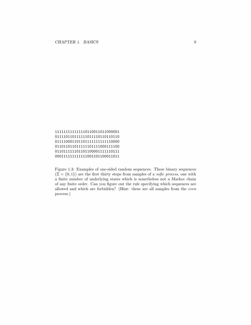
Example 4 (One-sided random sequences) Let T = 1, 2, . . . and Ξ besome finite set (or R or C or Rk. . . ). Then Xtt∈T is a one-sided discrete(real, complex, vector-valued, . . . ) random sequence. Most of the stochas-tic processes you have encountered are probably of this sort: Markov chains,discrete-parameter martingales, etc. Figures 1.2, 1.3, 1.4 and 1.5 illustratesome one-sided random sequences.
Example 5 (Two-sided random sequences) Let T = Z and Ξ be as inExample 4. Then Xtt∈T is a two-sided random sequence.
Example 6 (Spatially-discrete random fields) Let T = Zd and Ξ be as inExample 4. Then Xtt∈T is a d-dimensional spatially-discrete random field.
Example 7 (Continuous-time random processes) Let T = R and Ξ = R.Then Xtt∈T is a real-valued, continuous-time random process (or random mo-tion or random signal). Figures 1.6 and 1.7 illustrate some of the possibilities.
Vector-valued processes are an obvious generalization.
Example 8 (Random set functions) Let T = B, the Borel field on the reals,and Ξ = R+
, the non-negative extended reals. Then Xtt∈T is a random setfunction on the reals.
The definition of random set functions on Rd is entirely parallel. Notice thatif we want not just a set function, but a measure or a probability measure,this will imply various forms of dependence among the random variables in thecollection, e.g., a measure must respect countable additivity over disjoint sets.We will return to this topic in the next section.
Example 9 (One-sided random sequences of set functions) Let T =B × N and Ξ = R+
. Then Xtt∈T is a one-sided random sequence of setfunctions.
Example 10 (Empirical distributions) Suppose Zi, = 1, 2, . . . are indepen-dent, identically-distributed real-valued random variables. (We can see from Ex-ample 4 that this is a one-sided real-valued random sequence.) For each Borelset B and each n, define
Pn(B) =1n
n∑i=1
1B(Zi)
CHAPTER 1. BASICS 5
i.e., the fraction of the samples up to time n which fall into that set. This isthe empirical measure. Pn(B) is a one-sided random sequence of set functions— in fact, of probability measures. We would like to be able to say somethingabout how it behaves. It would be very reassuring, for instance, to be able toshow that it converges to the common distribution of the Zi (Figure 1.8).
1.2 Random Functions
X(t, ω) has two arguments, t and ω. For each fixed value of t, Xt(ω) is straight-forward random variable. For each fixed value of ω, however, X(t) is a functionfrom T to Ξ — a random function. The advantage of the random functionperspective is that it lets us consider the realizations of stochastic processes assingle objects, rather than large collections. This isn’t just tidier; we will needto talk about relations among the variables in the collection or their realiza-tions, rather than just properties of individual variables, and this will help usdo so. In Example 10, it’s important that we’ve got random probability mea-sures, rather than just random set functions, so we need to require that, e.g.,Pn(A ∪B) = Pn(A) + Pn(B) when A and B are disjoint Borel sets, and this isa relationship among the three random variables Pn(A), Pn(B) and Pn(A∪B).Plainly, working out all the dependencies involved here is going to get rathertedious, so we’d like a way to talk about acceptable realizations of the wholestochastic process. This is what the random functions notion will let us do.
We’ll make this more precise by defining a random function as a function-valued random variable. To do this, we need a measure space of functions, anda measurable mapping from (Ω,F , P ) to that function space. To get a measurespace, we need a carrier set and a σ-field on it. The natural set to use is ΞT ,the set of all functions from T to Ξ. (We’ll see how to restrict this to just thefunctions we want presently.) Now, how about the σ-field?
Definition 11 (Cylinder Set) Given an index set T and a collection of σ-fields Xt on spaces Ξt, t ∈ T . Pick any t ∈ T and any At ∈ Xt. Then At ×∏s6=t Ξs is a one-dimensional cylinder set.
For any finite k, k−dimensional cylinder sets are defined similarly, andclearly are the intersections of k different one-dimensional cylinder sets. Tosee why they have this name, notice a cylinder, in Euclidean geometry, con-sists of all the points where the x and y coordinates fall into a certain set(the base), leaving the z coordinate unconstrained. Similarly, a cylinder setlike At ×
∏s 6=t Ξs consists of all the functions in ΞT where f(t) ∈ At, and are
otherwise unconstrained.
Definition 12 (Product σ-field) The product σ-field, ⊗t∈TXt, is the σ-fieldover ΞT generated by all the one-dimensional cylinder sets. If all the Xt are thesame, X , we write the product σ-field as X T .
CHAPTER 1. BASICS 6
The product σ-field is enough to let us define a random function, and isgoing to prove to be almost enough for all our purposes.
Definition 13 (Random Function; Sample Path) A Ξ-valued random func-tion on T is a map X : Ω 7→ ΞT which is F/X T -measurable. The realizationsof X are functions x(t) taking values in Ξ, called its sample paths.
N.B., it has become common to apply the term “sample path” or even just“path” even in situations where the geometric analogy it suggests may be some-what misleading. For instance, for the empirical distributions of Example 10,the “sample path” is the measure Pn, not the curves shown in Figure 1.8.
Definition 14 (Functional of the Sample Path) Let E, E be a measure-space. A functional of the sample path is a mapping f : ΞT 7→ E which isX T /E-measurable.
Examples of useful and common functionals include maxima, minima, sam-ple averages, etc. Notice that none of these are functions of any one randomvariable, and in fact their value cannot be determined from any part of thesample path smaller than the whole thing.
Definition 15 (Projection Operator, Coordinate Map) A projection op-erator or coordinate map πt is a map from ΞT to Ξ such that πtX = X(t).
The projection operators are a convenient device for recovering the individ-ual coordinates — the random variables in the collection — from the randomfunction. Obviously, as t ranges over T , πtX gives us a collection of random vari-ables, i.e., a stochastic process in the sense of our first definition. The followinglemma lets us go back and forth between the collection-of-variables, coordinateview, and the entire-function, sample-path view.
Theorem 16 (Product σ-field-measurability is equvialent to measur-ability of all coordinates) X is F/ ⊗t∈T Xt-measurable iff πtX is F/Xt-measurable for every t.
Proof: This follows from the fact that the one-dimensional cylinder setsgenerate the product σ-field.
We have said before that we will want to constrain our stochastic processesto have certain properties — to be probability measures, rather than just setfunctions, or to be continuous, or twice differentiable, etc. Write the set of allsuch functions in ΞT as U . Notice that U does not have to be an element of theproduct σ-field, and in general is not. (We will consider some of the reasons forthis later.) As usual, by U ∩ X T we will mean the collection of all sets of theform U ∩C, where C ∈ X T . Notice that (U,U ∩X T ) is a measure space. Whatwe want is to ensure that the sample path of our random function lies in U .
Definition 17 (A Stochastic Process Is a Random Function) A Ξ-valuedstochastic process on T with paths in U , U ⊆ ΞT , is a random function X : Ω 7→U which is F/U ∩ X T -measurable.
CHAPTER 1. BASICS 7
Corollary 18 (Measurability of constrained sample paths) A functionX from Ω to U is F/U ∩ X T -measurable iff Xt is F/X -measurable for all t.
Proof: Because X(ω) ∈ U , F/U ∩ X T measurability works just the sameway as F/X T measurability (Exercise 2). So imitate the proof of Theorem 16.
Example 19 (Random Measures) Let T = Bd, the Borel field on Rd, and letΞ = R+
, the non-negative extended reals. Then ΞT is the class of set functionson Rd. Let M be the class of such set functions which are also measures (i.e.,which are countably additive and give zero on the null set). Then a random setfunction X with realizations in M is a random measure.
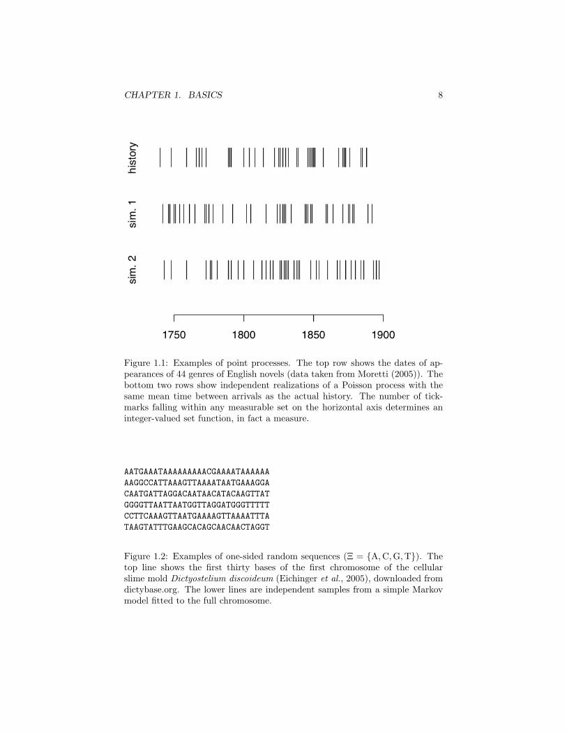
Example 20 (Point Processes) Let X be a random measure, as in the previ-ous example. If X(B) is a finite integer for every bounded Borel set B, then Xis a point process. If in addition X(r) ≤ 1 for every r ∈ Rd, then X is simple.The Poisson process is a simple point process. See Figure 1.1.
Example 21 (Continuous random processes) Let T = R+, Ξ = Rd, andC(T ) the class of continuous functions from T to Ξ (in the usual topology). Thena Ξ-valued random process on T with paths in C(T ) is a continuous randomprocess. The Wiener process, or Brownian motion, is an example. We will seethat most sample paths in C(T ) are not differentiable.
1.3 Exercises
Exercise 1 (The product σ-field answers countable questions) Let D =⋃S XS, where the union ranges over all countable subsets S of the index set T .
For any event D ∈ D, whether or not a sample path x ∈ D depends on the valueof xt at only a countable number of indices t.
1. Show that D is a σ-field.
2. Show that if A ∈ X T , then A ∈ XS for some countable subset S of T .
Exercise 2 (The product σ-field constrained to a given set of paths)Let U ⊂ X T be a set of allowed paths. Show that
1. U ∩ X T is a σ-field on U ;
2. U ∩ X T is generated by sets of the form U ∩ B, where B ∈ XS for somefinite subset S of T .
CHAPTER 1. BASICS 8
Figure 1.1: Examples of point processes. The top row shows the dates of ap-pearances of 44 genres of English novels (data taken from Moretti (2005)). Thebottom two rows show independent realizations of a Poisson process with thesame mean time between arrivals as the actual history. The number of tick-marks falling within any measurable set on the horizontal axis determines aninteger-valued set function, in fact a measure.
AATGAAATAAAAAAAAACGAAAATAAAAAAAAGGCCATTAAAGTTAAAATAATGAAAGGACAATGATTAGGACAATAACATACAAGTTATGGGGTTAATTAATGGTTAGGATGGGTTTTTCCTTCAAAGTTAATGAAAAGTTAAAATTTATAAGTATTTGAAGCACAGCAACAACTAGGT
Figure 1.2: Examples of one-sided random sequences (Ξ = A,C,G,T). Thetop line shows the first thirty bases of the first chromosome of the cellularslime mold Dictyostelium discoideum (Eichinger et al., 2005), downloaded fromdictybase.org. The lower lines are independent samples from a simple Markovmodel fitted to the full chromosome.
CHAPTER 1. BASICS 9
111111111111110110011011000001011110110111111011110110110110011110001101101111111111110000011011011011111101111000111100011011111101101100001111110111000111111111111001101100011011
Figure 1.3: Examples of one-sided random sequences. These binary sequences(Ξ = 0, 1) are the first thirty steps from samples of a sofic process, one witha finite number of underlying states which is nonetheless not a Markov chainof any finite order. Can you figure out the rule specifying which sequences areallowed and which are forbidden? (Hint: these are all samples from the evenprocess.)
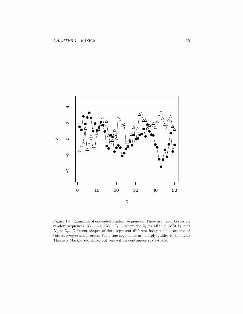
CHAPTER 1. BASICS 10
0 10 20 30 40 50
−4
−2
02
4
t
z
Figure 1.4: Examples of one-sided random sequences. These are linear Gaussianrandom sequences, Xt+1 = 0.8Xt+Zt+1, where the Zt are all i.i.d. N (0, 1), andX1 = Z0. Different shapes of dots represent different independent samples ofthis autoregressive process. (The line segements are simply guides to the eye.)This is a Markov sequence, but one with a continuous state-space.
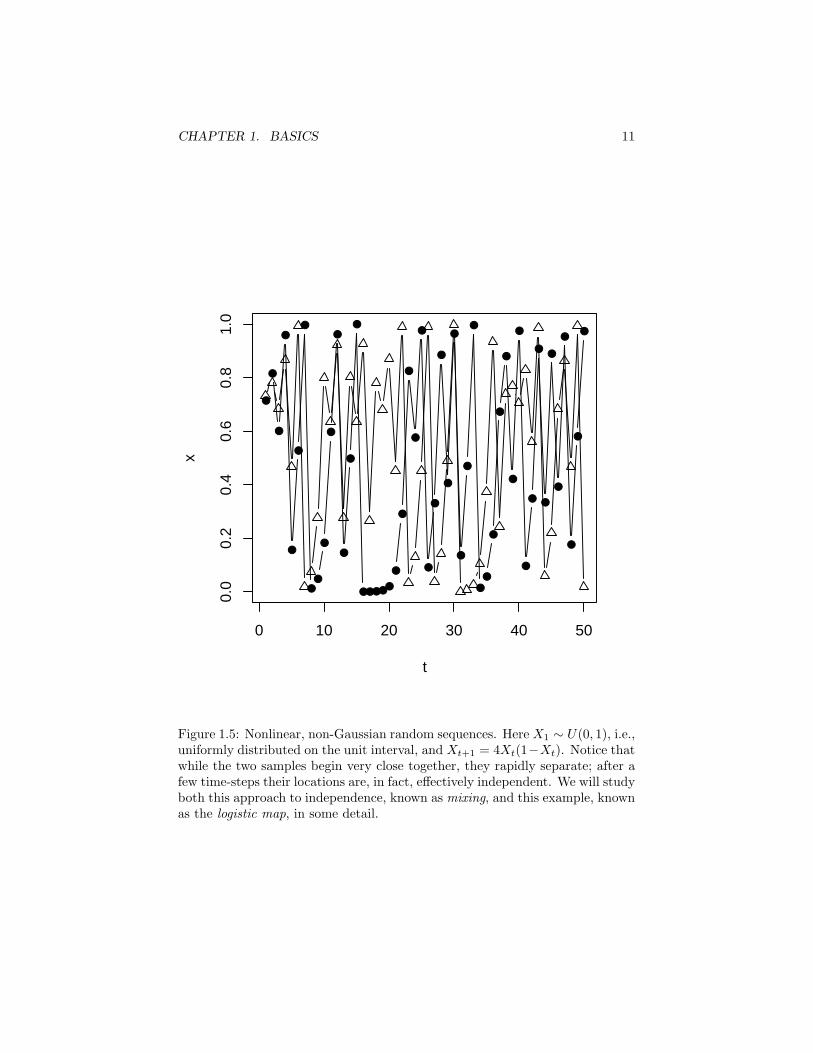
CHAPTER 1. BASICS 11
0 10 20 30 40 50
0.0
0.2
0.4
0.6
0.8
1.0
t
x
Figure 1.5: Nonlinear, non-Gaussian random sequences. Here X1 ∼ U(0, 1), i.e.,uniformly distributed on the unit interval, and Xt+1 = 4Xt(1−Xt). Notice thatwhile the two samples begin very close together, they rapidly separate; after afew time-steps their locations are, in fact, effectively independent. We will studyboth this approach to independence, known as mixing, and this example, knownas the logistic map, in some detail.
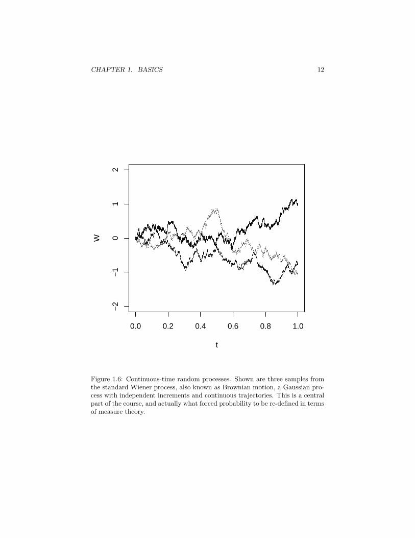
CHAPTER 1. BASICS 12
0.0 0.2 0.4 0.6 0.8 1.0
−2
−1
01
2
t
W
Figure 1.6: Continuous-time random processes. Shown are three samples fromthe standard Wiener process, also known as Brownian motion, a Gaussian pro-cess with independent increments and continuous trajectories. This is a centralpart of the course, and actually what forced probability to be re-defined in termsof measure theory.
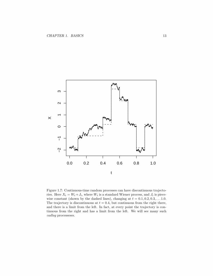
CHAPTER 1. BASICS 13
0.0 0.2 0.4 0.6 0.8 1.0
−2
−1
01
23
t
X
Figure 1.7: Continuous-time random processes can have discontinuous trajecto-ries. Here Xt = Wt+Jt, where Wt is a standard Wiener process, and Jt is piece-wise constant (shown by the dashed lines), changing at t = 0.1, 0.2, 0.3, . . . 1.0.The trajectory is discontinuous at t = 0.4, but continuous from the right there,and there is a limit from the left. In fact, at every point the trajectory is con-tinuous from the right and has a limit from the left. We will see many suchcadlag processeses.
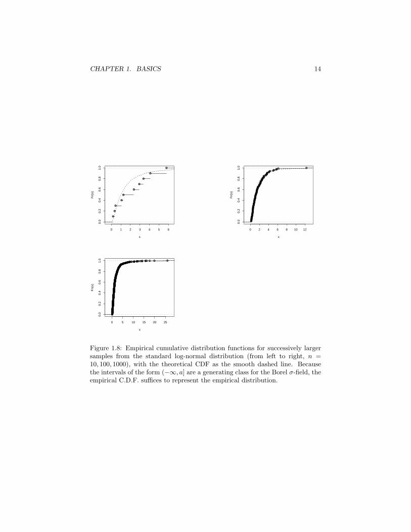
CHAPTER 1. BASICS 14
0 1 2 3 4 5 6
0.0
0.2
0.4
0.6
0.8
1.0
x
Fn(
x)
0 2 4 6 8 10 12
0.0
0.2
0.4
0.6
0.8
1.0
x
Fn(
x)
0 5 10 15 20 25
0.0
0.2
0.4
0.6
0.8
1.0
x
Fn(
x)
Figure 1.8: Empirical cumulative distribution functions for successively largersamples from the standard log-normal distribution (from left to right, n =10, 100, 1000), with the theoretical CDF as the smooth dashed line. Becausethe intervals of the form (−∞, a] are a generating class for the Borel σ-field, theempirical C.D.F. suffices to represent the empirical distribution.
Chapter 2
Building Infinite Processesfrom Finite-DimensionalDistributions
Section 2.1 introduces the finite-dimensional distributions of astochastic process, and shows how they determine its infinite-dimensionaldistribution.
Section 2.2 considers the consistency conditions satisfied by thefinite-dimensional distributions of a stochastic process, and the ex-tension theorems (due to Daniell and Kolmogorov) which prove theexistence of stochastic processes with specified, consistent finite-dimensional distributions.
2.1 Finite-Dimensional Distributions
So, we now have X, our favorite Ξ-valued stochastic process on T with pathsin U . Like any other random variable, it has a probability law or distribution,which is defined over the entire set U . Generally, this is infinite-dimensional.Since it is inconvenient to specify distributions over infinite-dimensional spacesall in a block, we consider the finite-dimensional distributions.
Definition 22 (Finite-dimensional distributions) The finite-dimensionaldistributions of X are the the joint distributions of Xt1 , Xt2 , . . . Xtn , t1, t2, . . . tn ∈T , n ∈ N.
You will sometimes see “FDDs” and “fidis” as abbreviations for “finite-dimensional distributions”. Please do not use “fidis”.
We can at least hope to specify the finite-dimensional distributions. But weare going to want to ask a lot of questions about asymptotics, and global proper-ties of sample paths, which go beyond any finite dimension, so you might worry
15
CHAPTER 2. BUILDING PROCESSES 16
that we’ll still need to deal directly with the infinite-dimensional distribution.The next theorem says that this worry is unfounded; the finite-dimensional dis-tributions specify the infinite-dimensional distribution (pretty much) uniquely.
Theorem 23 (Finite-dimensional distributions determine process dis-tributions) Let X and Y be two Ξ-valued processes on T with paths in U . ThenX and Y have the same distribution iff all their finite-dimensional distributionsagree.
Proof: “Only if”: Since X and Y have the same distribution, applyingthe any given set of coordinate mappings will result in identically-distributedrandom vectors, hence all the finite-dimensional distributions will agree.
“If”: We’ll use the π-λ theorem.Let C be the finite cylinder sets, i.e., all sets of the form
C =x ∈ ΞT |(xt1 , xt2 , . . . xtn) ∈ B
where n ∈ N, B ∈ Xn, t1, t2, . . . tn ∈ T . Clearly, this is a π-system, since it isclosed under intersection.
Now let L consist of all the sets L ∈ X T where P (X ∈ L) = P (Y ∈ L).We need to show that this is a λ-system, i.e., that it (i) includes ΞT , (ii) isclosed under complementation, and (iii) is closed under monotone increasinglimits. (i) is clearly true: P
(X ∈ ΞT
)= P
(Y ∈ ΞT
)= 1. (ii) is true because
we’re looking at a probability: if L ∈ L, then P (X ∈ Lc) = 1 − P (X ∈ L) =1 − P (Y ∈ L) = P (Y ∈ Lc). To see (iii), let Ln ↑ L be a monotone-increasingsequence of sets in L, and recall that, for any measure, Ln ↑ L implies µLn ↑ µL.So P (X ∈ Ln) ↑ P (X ∈ L), P (Y ∈ Ln) ↑ P (Y ∈ L), and (since P (X ∈ Ln) =P (Y ∈ Ln)), P (X ∈ Ln) ↑ P (Y ∈ L) as well. A sequence cannot have twolimits, so P (X ∈ L) = P (Y ∈ L), and L ∈ L.
Since the finite-dimensional distributions match, P (X ∈ C) = P (Y ∈ C) forall C ∈ C, which means that C ⊂ L. Also, from the definition of the productσ-field, σ(C) = X T . Hence, by the π-λ theorem, X T ⊆ L.
A note of caution is in order here. If X is a Ξ-valued process on T whosepaths are constrained to line in U , and Y is a similar process that is not soconstrained, it is nonetheless possible that X and Y agree in all their finite-dimensional distributions. The trick comes if U is not, itself, an element of X T .The most prominent instance of this is when Ξ = R, T = R, and the constraintis continuity of the sample paths: we will see that U 6∈ BR. (This is the pointof Exercise 1.)
2.2 Consistency and Extension
The finite-dimensional distributions of a given stochastic process are relatedto one another in the usual way of joint and marginal distributions. Takesome collection of indices t1, t2 . . . tn ∈ T , and corresponding measurable sets
CHAPTER 2. BUILDING PROCESSES 17
B1 ∈ X1, B2 ∈ X2, . . . Bn ∈ Xn. Then, for any m > n, and any further indicestn+1, tn2 , . . . tm, it must be the case that
P (Xt1 ∈ B1, Xt2 ∈ B2, . . . Xtn ∈ Bn) (2.1)= P
(Xt1 ∈ B1, Xt2 ∈ B2, . . . Xtn ∈ Bn, Xtn+1 ∈ Ξ, Xtn+2 ∈ Ξ, . . . Xtm ∈ Ξ
)This is going to get really awkward to write over and over, so let’s introducesome simplifying notation. Fin(T ) will denote the class of all finite sub-setsof our index set T , and likewise Denum(T ) all denumerable sub-sets. We’llindicate such sub-sets, for the moment, by capital letters like J , K, etc., andextend the definition of coordinate maps (Definition 15) so that πJ maps fromΞT to ΞJ in the obvious way, and πKJ maps from ΞK to ΞJ , if J ⊂ K. If µ isthe measure for the whole process, then the finite-dimensional distributions areµJ |J ∈ Fin(T ). Clearly, µJ = µ πJ−1.
Definition 24 (Projective Family of Distributions) A family of distri-butions µJ , J ∈ Denum(T ), is projective when for every J,K ∈ Denum(T ),J ⊂ K implies
µJ = µK (πKJ)−1
(2.2)
Such a family is also said to be consistent or compatible (with one another).
Lemma 25 (FDDs Form Projective Families) The finite-dimensional dis-tributions of a stochastic process always form a projective family.
Proof: This is just the fact that we get marginal distributions by integratingout some variables from the joint distribution. But, to proceed formally: LettingJ and K be finite sets of indices, J ⊂ K, we know that µK = µ πK−1, thatµJ = µ πJ−1 and that πJ = πKJ πK . Hence
µJ = µ (πKJ πK
)−1(2.3)
= µ π−1K
(πKJ)−1
(2.4)
= µK (πKJ)−1
(2.5)
as required. I claimed that the reason to care about finite-dimensional distributions is
that if we specify them, we specify the distribution of the whole process. Lemma25 says that a putative family of finite dimensional distributions must be consis-tent, if they are to let us specify a stochastic process. Theorem 23 says that therecan’t be more than one process distribution with all the same finite-dimensionalmarginals, but it doesn’t guarantee that a given collection of consistent finite-dimensional distributions can be extended to a process distribution — it givesuniqueness but not existence. Proving the existence of an extension requiressome extra assumptions. Either we need to impose topological conditions on Ξ,
CHAPTER 2. BUILDING PROCESSES 18
or we need to ensure that all the finite-dimensional distributions can be relatedthrough conditional probabilities. The first approach is due to Daniell and Kol-mogorov, and will finish this lecture; the second is due to Ionescu-Tulcea, andwill begin the next.
We’ll start with Daniell’s theorem on the existence of random sequences, i.e.,where the index set is the natural numbers, which uses mathematical inductionto extend the finite-dimensional family. To get there, we need a useful proposi-tion about our ability to represent non-trivial random variables as functions ofuniform random variables on the unit interval.
Proposition 26 (Randomization, transfer) Let X and X ′ be identically-distributed random variables in a measurable space Ξ and Y a random variablein a Borel space Υ. Then there exists a measurable function f : Ξ× [0, 1] 7→ Υsuch that L (X ′, f(X ′, Z)) = L (X,Y ), when Z is uniformly distributed on theunit interval and independent of X ′.
Proof: See Kallenberg, Theorem 6.10 (p. 112–113). Basically what this says is that if we have two random variables with a
certain joint distribution, we can always represent the pair by a copy of one ofthe variables (X), and a transformation of an independent random number. It isimportant that Υ be a Borel space here; the result, while very natural-sounding,does not hold for arbitrary measurable spaces, because the proof relies on havinga regular conditional probability.
Theorem 27 (Daniell Extension Theorem) For each n ∈ N, let Ξn be aBorel space, and µn be a probability measure on
∏ni=1 Ξi. If the µn form a
projective family, then there exist random variables Xi : Ω 7→ Ξi, i ∈ N, suchthat L (X1, X2, . . . Xn) = µn for all n, and a measure µ on
∏∞i=1 Ξi such that
µn is equal to the projection of µ onto∏i = 1nΞi.
Proof: For any fixed n, X1, X2, . . . Xn is just a random vector with distri-bution µn, and we can always construct such an object. The delicate part here isshowing that, when we go to n+1, we can use the same random elements for thefirst n coordinates. We’ll do this by using the representation-by-randomizationproposition just introduced, starting with an IID sequence of uniform randomvariables on the unit interval, and then transforming them to get a sequenceof variables in the Ξi which have the right joint distribution. (This is like thequantile transform trick for generating random variates.) The proof will goinductively, so first we’ll take care of the induction step, and then go back toreassure ourselves about the starting point.
Induction: Assume we already haveX1, X2, . . . Xn such that L (X1, X2, . . . Xn) =µn, and that we have a Zn+1 ∼ U(0, 1) and independent of all the Xi to date.As remarked, we can always get Y1, Y2, . . . Yn+1 such that L (Y1, Y2, . . . Yn+1) =µn+1. Because the µn form a projective family, L (Y1, Y2, . . . Yn) = L (X1, X2, . . . Xn).Hence, by Proposition 26, there is a measurable f such that, if we set Xn+1 =f(X1, X2, . . . Xn, Zn+1), then L (X1, X2, . . . Xn, Xn+1) = µn+1.
CHAPTER 2. BUILDING PROCESSES 19
First step: We need there to be an X1 with distribution µ1, and we need a(countably!) unlimited supply of IID variables Z2, Z3, . . . all ∼ U(0, 1). But theexistence of X1 is just the existence of a random variable with a well-defineddistribution, which is unproblematic, and the existence of an infinite sequence ofIID uniform random variates is too. (See 36-752, or Lemma 3.21 in Kallenberg,or Exercise 3.)
Finally, to convince yourself of the existence of the measure µ on the productspace, recall Theoerem 16.
Remark: Kallenberg, Corollary 6.15, gives a somewhat more abstract versionof this theorem.
Daniell’s extension theorem works fine for one-sided random sequences, butwe often want to work with larger and more interesting index sets. For thiswe need the full Kolmogorov extension theorem, where the index set T can becompletely arbitrary. This in turn needs the Caratheodory Extension Theorem,which I re-state here for convenience.
Proposition 28 (Caratheodory Extension Theorem) Let µ be a non-negative, finitely additive set function on a field C of subsets of some spaceΩ. If µ is also countably additive, then it extends to a measure on σ(C), and, ifµ(Ω) <∞, the extension is unique.
Proof: See 36-752 lecture notes (Theorem 50, Exercise 51), or Kallenberg,Theorem 2.5, pp. 26–27. Note that “extension” here means extending from amere field to a σ-field, not from finite to infinite index sets.
Theorem 29 (Kolmogorov Extension Theorem) Let Ξt, t ∈ T , be a col-lection of Borel spaces, with σ-fields Xi, and let µJ , J ∈ Fin(T ), be a projectivefamily of finite-dimensional distributions on those spaces. Then there exist Ξt-valued random variables Xt such that L (XJ) = µJ for all J ∈ Fin(T ).
Proof: This will be easier to follow if we first consider the case there Tis countable, which is basically Theorem 27 again, and then the general case,where we need Proposition 28.
Countable T : We can, by definition, put the elements of T in 1−1 correspon-dence with the elements of N. This in turn establishes a bijection between theproduct space
⊗t∈T Ξt = ΞT and the sequence space
⊗∞i=1 Ξt. This bijection
also induces a projective family of distributions on finite sequences. The DaniellExtension Theorem (27) gives us a measure on the sequence space, which thebijection takes back to a measure on ΞT . To see that this µ does not depend onthe order in which we arranged T , notice that any two arrangements must giveidentical results for any finite set J , and then use Theorem 23.
Uncountable T : For each countable K ⊂ T , the argument of the precedingparagraph gives us a measure µK on ΞK . And, clearly, these µK themselves forma projective family. Now let’s define a set function µ on the countable cylindersets, i.e., on the class D of sets of the form A×ΞT\K , for some K ∈ Denum(T )and some A ∈ XK . Specifically, µ : D 7→ [0, 1], and µ(A × ΞT\K) = µK(A).We would like to use Caratheodory’s theorem to extend this set function to
CHAPTER 2. BUILDING PROCESSES 20
a measure on the product σ-algebra XT . First, let’s check that the countablecylinder sets form a field: (i) ΞT ∈ D, clearly. (ii) The complement, in ΞT , ofa countable cylinder A× ΞT\K is another countable cylinder, Ac × ΞT\K . (iii)The union of two countable cylinders B1 = A1 × ΞT\K1 and B2 = A2 × ΞT\K2
is another countable cylinder, since we can always write it as A × ΞT\K forsome A ∈ XK , where K = K1 ∪ K2. Clearly, µ(∅) = 0, so we just need tocheck that µ is countably additive. So consider any sequence of disjoint cylindersets B1, B2, . . .. Because they’re cylinder sets, each i, Bi = Ai × ΞT\Ki , forsome Ki ∈ Denum(T ), and some Ai ∈ XKi . Now set K =
⋃iKi; this is a
countable union of countable sets, and so itself countable. Furthermore, sayCi = Ai × ΞK\Ki , so we can say that
⋃iBi = (
⋃i Ci) × ΞT\K . With this
notation in place,
µ⋃i
Bi = µK⋃i
Ci (2.6)
=∑i
µKCi (2.7)
=∑i
µKiAi (2.8)
=∑i
µBi (2.9)
where in the second line we’ve used the fact that µK is a probability measureon ΞK , and so countably additive on sets like the Ci. This proves that µ iscountably additive, so by Proposition 28 it extends to a measure on σ(D), theσ-field generated by the countable cylinder sets. But we know from Definition12 that this σ-field is the product σ-field. Since µ(ΞT ) = 1, Proposition 28further tells us that the extension is unique.
Borel spaces are good enough for most of the situations we find ourselvesmodeling, so the Daniell-Kolmogorov Extension Theorem (as it’s often known)see a lot of work. Still, some people dislike having to make topological assump-tions to solve probabilistic problems; it seems inelegant. The Ionescu-TulceaExtension Theorem provides a purely probabilistic solution, available if we canwrite down the FDDs recursively, in terms of regular conditional probabilitydistributions, even if the spaces where the process has its coordinates are notnice and Borel. Doing this properly will involve our revisiting and extendingsome ideas about conditional probability, which you will have seen in 36-752, soit will be deferred to the next lecture.
Chapter 3
Building Infinite Processesfrom Regular ConditionalProbability Distributions
Section 3.1 introduces the notion of a probability kernel, whichis a useful way of systematizing and extending the treatment ofconditional probability distributions you will have seen in 36-752.
Section 3.2 gives an extension theorem (due to Ionescu Tulcea)which lets us build infinite-dimensional distributions from a familyof finite-dimensional distributions. Rather than assuming topolog-ical regularity of the space, as in Section 2.2, we assume that theFDDs can be derived from one another recursively, through applyingprobability kernels. This is the same as assuming regularity of theappropriate conditional probabilities.
3.1 Probability Kernels
Definition 30 (Probability Kernel) A measure kernel from a measurablespace Ξ,X to another measurable space Υ,Y is a function κ : Ξ×Y 7→ R+
suchthat
1. for any Y ∈ Y, κ(x, Y ) is X -measurable; and
2. for any x ∈ Ξ, κ(x, Y ) ≡ κx(Y ) is a measure on Υ,Y. We will writethe integral of a function f : Υ 7→ R, with respect to this measure, as∫f(y)κ(x, dy),
∫f(y)κx(dy), or, most compactly, κf(x).
If, in addition, κx is a probability measure on Υ,Y for all x, then κ is a prob-ability kernel.
21
CHAPTER 3. BUILDING PROCESSES BY CONDITIONING 22
(Some authors use “kernel”, unmodified, to mean a probability kernel, andsome a measure kernel; read carefully.)
Notice that we can represent any distribution on Υ as a kernel where the firstargument is irrelevant: κ(x1, Y ) = κ(x2, Y ) for all x1, x2 ∈ Ξ. The “kernels” inkernel density estimation are probability kernels, as are the stochastic transitionmatrices of Markov chains. (The kernels in support vector machines, however,generally are not.)
From a previous probability course, like 36-752, you will remember themeasure-theoretic definition of the conditional probability of a set A, as theconditional expectation of 1A, i.e., P (A|G) = E [1A(ω)|G]. (I have explicitlyincluded the dependence on ω to make it plain that this is a random set func-tion.) You may also recall a potential bit of trouble, which is that even whenthese conditional expectations exist for all measurable sets A, it’s not necessarilytrue that they give us a measure, i.e., that P (
⋃∞i=1Ai|G) =
∑∞i=1 P (Ai|G) and
all the rest of it. A version of the conditional probabilities for which they doform a measure is said to be a regular conditional probability. Clearly, regularconditional probabilities are all probability kernels. The ordinary rules for ma-nipulating conditional probabilities suggest how we can define the compositionof kernels.
Definition 31 (Composition of probability kernels) Let κ1 be a kernelfrom Ξ to Υ, and κ2 a kernel from Ξ×Υ to Γ. Then we define κ1 ⊗ κ2 as thekernel from Ξ to Υ× Γ such that
(κ1 ⊗ κ2)(x,B) =∫κ1(x, dy)
∫κ2(x, y, dz)1B(y, z)
for every measurable B ⊆ Υ× Γ (where z ranges over the space Γ).
Verbally, κ1 gives us a distribution on Υ, from any starting point x ∈ Ξ.Given a pair of points (x, y) ∈ Ξ × Υ, κ2 gives a distribution on Γ. So theircomposition says, basically, how to chain together conditional distributions,given a starting point.
3.2 Extension via Recursive Conditioning
With the machinery of probability kernels in place, we are in a position to givean alternative extension theorem, i.e., a different way of proving the existence ofstochastic processes with specified finite-dimensional marginal distributions. InSection 2.2, we assumed some topological niceness in the sample spaces, namelythat they were Borel spaces. Here, instead, we will assume probabilistic nicenessin the FDDs themselves, namely that they can be obtained through composingprobability kernels. This is the same as assuming that they can be obtainedby chaining together regular conditional probabilities. The general form of thisresult is attributed in the literature to Ionescu Tulcea.
Just as proving the Kolmogorov Extension Theorem needed a measure-theoretic result, the Caratheodory Extension Theorem, our proof of the Ionescu
CHAPTER 3. BUILDING PROCESSES BY CONDITIONING 23
Tulcea Extension Theorem will require a different measure-theoretic result,which is not, so far as I know, named after anyone. (It re-appears in the theoryof Markov operators, beginning in Section 9.2.)
Proposition 32 (Set functions continuous at ∅) Suppose µ is a finite, non-negative, additive set function on a field A. If, for any sequence of sets An ∈ A,An ↓ ∅ =⇒ µAn → 0, then
1. µ is countably additive on A, and
2. µ extends uniquely to a measure on σ(A).
Proof: Part (1) is a weaker version of Theorem F in Chapter 2, §9 ofHalmos (1950, p. 39). (When reading his proof, remember that every field ofsets is also a ring of sets.) Part (2) follows from part (1) and the CaratheodoryExtension Theorem (Proposition 28).
With this preliminary out of the way, let’s turn to the main event.
Theorem 33 (Ionescu Tulcea Extension Theorem) Consider a sequenceof measurable spaces Ξn,Xn, n ∈ N. Suppose that for each n, there exists aprobability kernel κn from
∏n−1i=1 Ξi to Ξn (taking κ1 to be a kernel insensitive
to its first argument, i.e., a probability measure). Then there exists a sequenceof random variables Xn, n ∈ N, taking values in the corresponding Ξn, suchthat L (X1, X2, . . . Xn) =
⊗ni=1 κi.
Proof: As before, we’ll be working with the cylinder sets, but now we’llmake our life simpler if we consider cylinders where the base set rests in thefirst n spaces Ξ1, ...Ξn. More specifically, set Bn =
⊗ni=1 Xi (these are the base
sets), and Cn = Bn ×∏∞i=n+1 Ξi (these are the cylinder sets), and C =
⋃n Cn.
C clearly contains all the finite cylinders, so it generates the product σ-field oninfinite sequences. We will use it as the field in Proposition 32. (Checking thatC is a field is entirely parallel to checking that the D appearing in the proof ofTheorem 29 was a field.)
For each base set A ∈ Bn, let [A] be the corresponding cylinder, [A] =A×
∏∞i=n+1 Ξi. Notice that for every set C ∈ C, there is at least one A, in some
Bn, such that C = [A]. Now we define a set function µ on C.
µ([A]) =
(n⊗i=1
κi
)A (3.1)
(Checking that this is well-defined is left as an exercise, 4.) Clearly, this is afinite, and finitely-additive, set function defined on a field. So to use Proposition32, we just need to check continuity from above at ∅. Let An be any sequenceof sets such that [An] ↓ ∅ and An ∈ Bn. (Any sequence of sets in C ↓ ∅ can bemassaged into this form.) We wish to show that µ([An]) ↓ 0. We’ll get this to
CHAPTER 3. BUILDING PROCESSES BY CONDITIONING 24
work by considering functions which are (pretty much) conditional probabilitiesfor these sets:
pn|k =
(n⊗
i=k+1
κi
)1An , k ≤ n (3.2)
pn|n = 1An (3.3)
Two facts follow immediately from the definitions:
pn|0 =
(n⊗i=1
κi
)1An = µ([An]) (3.4)
pn|k = κk+1pn|k+1 (3.5)
From the fact that the [An] ↓ ∅, we know that pn+1|k ≤ pn|k, for all k. Thisimplies that limn pn|k = mk exists, for each k, and is approached from above.Applied to pn|0, we see from 3.5 that µ([An]) → m0. We would like m0 = 0.Assume the contrary, that m0 > 0. From 3.5 and the dominated convergencetheorem, we can see that mk = κk+1mk+1. Hence if m0 > 0, κ1m1 > 0, whichmeans (since that last expression is really an integral) that there is at least onepoint x1 ∈ Ξ1 such that m1(s1) > 0. Recursing our way down the line, we geta sequence x = x1, x2, . . . ∈ ΞN such that mn(x1, . . . xn) > 0 for all n. But nowlook what we’ve done: for each n,
0 < mn(x1, . . . xn) (3.6)≤ pn|n(x1, . . . xn) (3.7)= 1An(x1, . . . xn) (3.8)= 1[An](x) (3.9)
x ∈ [An] (3.10)
This is the same as saying that x ∈⋂n [An]. But [An] ↓ ∅, so there can be no
such x. Hence m0 = 0, meaning that µ([An]) → 0, and µ is continuous at theempty set.
Since µ is finite, finitely-additive, non-negative and continuous at ∅, byProposition 32 it extends uniquely to a measure on the product σ-field.
Notes on the proof: It would seem natural that one could show m0 = 0directly, rather than by contradiction, but I can’t think of a way to do it, andevery book I’ve consulted does it in exactly this way.
To appreciate the simplification made possible by the notion of probabilitykernels, compare this proof to the one given by Fristedt and Gray (1997, §22.1).
Notice that the Daniell, Kolmogorov and Ionescu Tulcea Extension Theo-rems all give sufficient conditions for the existence of stochastic processes, notnecessary ones. The necessary and sufficient condition for extending the FDDsto a process probability measure is something called σ-smoothness. (See Pollard(2002) for details.) Generally speaking, we will deal with processes which satisfyboth the Kolmogorov and the Ionescu Tulcea type conditions, e.g., real-valuedMarkov process.
CHAPTER 3. BUILDING PROCESSES BY CONDITIONING 25
3.3 Exercises
Exercise 3 ( Lomnick-Ulam Theorem on infinite product measures)Let T be an uncountable index set, and (Ξt,Xt, µt) a collection of probabilityspaces. Show that there exist independent random variables Xt in Ξt with dis-tributions µt. Hint: use the Ionescu Tulcea theorem on countable subsets of T ,and then imitate the proof of the Kolmogorov extension theorem.
Exercise 4 (Measures of cylinder sets) In the proof of the Ionescu TulceaTheorem, we employed a set function on the finite cylinder sets, where the mea-sure of an infinite-dimensional cylinder set [A] is taken to be the measure of itsfinite-dimensional base set A. However, the same cylinder set can be specifiedby different base sets, so it is necessary to show that Equation 3.1 has a uniquevalue on its right-hand side. In what follows, C is an arbitrary member of theclass C.
1. Show that, when A,B ∈ Bn, [A] = [B] iff A = B. That is, two cylindersgenerated by bases of equal dimensionality are equal iff their bases areequal.
2. Show that there is a smallest n such that C = [A] for an A ∈ Bn. Concludethat the right-hand side of Equation 3.1 could be made well-defined if wetook n there to be this least possible n.
3. Suppose that m < n, A ∈ Bm, B ∈ Bn, and [A] = [B]. Show thatB = A×
∏ni=m+1 Ξi.
4. Continuing the situation in (iii), show that(m⊗i=1
κi
)A =
(n⊗i=1
κi
)B
Conclude that the right-hand side of Equation 3.1 is well-defined, as promised.
Part II
One-Parameter Processes inGeneral
26
Chapter 4
One-Parameter Processes,Usually Functions of Time
Section 4.1 defines one-parameter processes, and their variations(discrete or continuous parameter, one- or two- sided parameter),including many examples.
Section 4.2 shows how to represent one-parameter processes interms of “shift” operators.
We’ve been doing a lot of pretty abstract stuff, but the point of this is toestablish a common set of tools we can use across many different concrete situa-tions, rather than having to build very similar, specialized tools for each distinctcase. Today we’re going to go over some examples of the kind of situation ourtools are supposed to let us handle, and begin to see how they let us do so. Inparticular, the two classic areas of application for stochastic processes are dy-namics (systems changing over time) and inference (conclusions changing as weacquire more and more data). Both of these can be treated as “one-parameter”processes, where the parameter is time in the first case and sample size in thesecond.
4.1 One-Parameter Processes
The index set T isn’t, usually, an amorphous abstract set, but generally some-thing with some kind of topological or geometrical structure. The number of(topological) dimensions of this structure is the number of parameters of theprocess.
Definition 34 (One-Parameter Process) A process whose index set T hasone dimension is a one-parameter process. A process whose index set has morethan one dimension is a multi-parameter process. A one-parameter process is
27
CHAPTER 4. ONE-PARAMETER PROCESSES 28
discrete or continuous depending on whether its index set is countable or un-countable. A one-parameter process where the index set has a minimal elementit is one-sided, otherwise it is two-sided.
N is a one-sided discrete index set, Z a two-sided discrete index set, R+ (in-cluding zero!) is a one-sided continuous index set, and R a two-sided continuousindex set.
Most of this course will be concerned with one-parameter processes, whichare intensely important in applications. This is because the one-dimensionalparameter is usually either time (when we’re doing dynamics) or sample size(when we’re doing inference), or both at once. There are also some importantcases where the single parameter is space.
Example 35 (Bernoulli process) You all know this one: a one-sided infinitesequence of independent, identically-distributed binary variables, where, for allt, Xt = 1 with probability p.
Example 36 (Markov models) Markov chains are discrete-parameter stochas-tic processes. They may be either one-sided or two-sided. So are Markov modelsof order k, and hidden Markov models. Continuous-time Markov processes are,naturally enough, continuous-parameter stochastic processes, and again may beeither one-sided or two-sided.
Instances of physical processes that may be represented by Markov modelsinclude: the positions and velocities of the planets; the positions and velocitiesof molecules in a gas; the pressure, temperature and volume of the gas (Keizer,1987); the position and velocity of a tracer particle in a turbulent fluid flow; thethree-dimensional velocity field of a turbulent fluid (Frisch, 1995); the gene poolof an evolving population (Fisher, 1958; Haldane, 1932; Gillespie, 1998). In-stances of physical processes that may be represented by hidden Markov modelsinclude: the spike trains of neurons (Tuckwell, 1989); the sonic wave-forms ofhuman speech (Rabiner, 1989); many economic and social time-series (Durbinand Koopman, 2001); etc.
Example 37 (“White Noise” (Not Really)) For each t ∈ R+, let Xt ∼N (0, 1), all mutually independent of one another. This is a process with a one-sided continuous parameter.
It would be character building, at this point, to convince yourself that theprocess just described exists. (You will need the Kolmogorov Extension Theo-rem, 29).
Example 38 (Wiener Process) Here T = R+ and Ξ = R. The Wienerprocess is the continuous-parameter random process where
1. W (0) = 0,
CHAPTER 4. ONE-PARAMETER PROCESSES 29
2. for any three times, t1 < t2 < t3, W (t2)−W (t1) and W (t3)−W (t2) areindependent (the “independent increments” property),
3. W (t2)−W (t1) ∼ N (0, t2 − t1) and
4. W (t, ω) is a continuous function of t for almost all ω.
We will spend a lot of time with the Wiener process, because it turns out toplay a role in the theory of stochastic processes analogous to that played bythe Gaussian distribution in elementary probability — the easily-manipulated,formally-nice distribution delivered by limit theorems.
When we examine the Wiener process in more detail, we will see that italmost never has a derivative. Nonetheless, in a sense which will be madeclearer when we come to stochastic calculus, the Wiener process can be regardedas the integral over time of something very like white noise, as described in thepreceding example.
Example 39 (Logistic Map) Let T = N, Ξ = [0, 1], X(0) ∼ U(0, 1), andX(t + 1) = aX(t)(1 −X(t)), a ∈ [0, 4]. This is called the logistic map. Noticethat all the randomness is in the initial value X(0); given the initial condition,all later values X(t) are fixed. Nonetheless, this is a Markov process, and we willsee that, at least for certain values of a, it satisfies versions of the laws of largenumbers and the central limit theorem. In fact, large classes of deterministicdynamical systems have such stochastic properties.
Example 40 (Symbolic Dynamics of the Logistic Map) Let X(t) be thelogistic map, as in the previous example, and let S(t) = 0 if X(t) ∈ [0, 0.5) andS(t) = 1 if X(t) = [0.5, 1]. That is, we partition the state space of the logisticmap, and record which cell of the partition the original process finds itself in.X(t) is a Markov process, but these “symbolic” dynamics are not necessarilyMarkovian. We will want to know when functions of Markov processes arethemselves Markov. We will also see that there is a sense in which, Markovianor not, this partition is exactly as informative as the original, continuous state— that it is generating. Finally, when a = 4 in the logistic map, the symbolsequence is actually a Bernoulli process, so that a deterministic function of acompletely deterministic dynamical system provides a model of IID randomness.
Here are some examples where the parameter is sample size.
Example 41 (IID Samples) Let Xi, i ∈ N be samples from an IID distribu-tion, and Zn = 1
n
∑ni=1Xi be the sample mean. Then Zn is a one-parameter
stochastic process. The point of the ordinary law of large numbers is to reassureus that Zn → E [Xn] a.s. The point of the central limit theorem is to reassure usthat
√n(Zn−E [X]) has constant average size, so that the sampling fluctuation
Zn −E [X] must be shrinking as√n grows.
If Xi is the indicator of a set, this convergence means that the relative fre-quency with which the set is occupied will converge on its true probability.
CHAPTER 4. ONE-PARAMETER PROCESSES 30
Example 42 (Non-IID Samples) Let Xi be a non-IID one-sided discrete-parameter process, say a Markov chain, and again let Zn be its sample mean,now often called its “time average”. The usual machinery of the law of largenumbers and the central limit theorem are now inapplicable, and someone whohas just taken 36-752 has, strictly speaking, no idea as to whether or not theirtime averages will converge on expectations. Under the heading of ergodic theory,we will see when this will happen. Since this is the situation with all interestingtime series, the application of statistical methods to situations where we cannotcontrive to randomize depends crucially on ergodic considerations.
Example 43 (Estimating Distributions) Recall Example 10, where we lookedat the sequence of empirical distributions Pn for samples from an IID data-source. We would like to be able to say that Pn converges on P . The usual wayto do this, if our samples are of a real-valued random variable, is to consider theempirical cumulative distribution function, Fn. For each n, this may be regardedas a one-parameter random process (T = R, Ξ = [0, 1]), and the difficulty is toshow that this sequence of random processes converges to F . The usual way is toshow that En ≡
√n(Fn−F ), the empirical process, converges to a fixed process,
related to the Wiener process, depending only on the true distribution F . (SeeFigure 4.1.) Since the magnitude of the limiting process is constant, and
√n
grows, it follows that Fn − F must shrink. So theorizing even this elementarybit of statistical inference really requires two doses of stochastic process theory,one to get a grip on Fn at each n, and the other to get a grip on what happensto Fn as n grows.
Example 44 (Doob’s Martingale) Let X be a random variable, and Fi,i ∈ N, a sequence of increasing σ-algebras (i.e. a filtration). Then Yi = E [X|Fi]is a one-sided discrete-parameter stochastic process, and in fact a martingale.Martingales in general are one-parameter stochastic processes. Note that poste-rior mean parameter estimates, in Bayesian inference, are instances of Doob’smartingale.
Here are some examples where the one-dimensional parameter is neither timenor sample size.
Example 45 (The One-Dimensional Ising Model) This system serves asa toy model of magnetism in theoretical physics. Atoms sit evenly spaced on thepoints of a regular, infinite, one-dimensional crystalline lattice. Each atom hasa magnetic moment, which is either pointing north (+1) or south (−1). Atomsare more likely to point north if their neighbors point north, and vice-versa. Thenatural index here is Z, so the parameter is discrete and two-sided.
Example 46 (Text) Text (at least in most writing systems!) can be repre-sented by a sequence of discrete values at discrete, ordered locations. Since textscan be arbitrarily long, but they all start somewhere, they are discrete-parameter,one-sided processes. Or, more exactly, once we specify a distribution over se-quences from the appropriate alphabet, we will have such a process.
CHAPTER 4. ONE-PARAMETER PROCESSES 31
Example 47 (Polymer Sequences) Similarly, DNA, RNA and proteins areall heteropolymers — compounds in which distinct constituent chemicals (themonomers) are joined in a sequence. Position along the sequence (chromosome,protein) provides the index, and the nature of the monomer at that position thevalue.
Linguists believe that no Markovian model (with finitely many states) cancapture human language (Chomsky, 1957; Pullum, 1991). Whether this is trueof DNA sequences is not known. In both cases, hidden Markov models are usedextensively Baldi and Brunak (2001); Charniak (1993), even if they can only beapproximately true of language.
4.2 Operator Representations of One-ParameterProcesses
Consider our favorite discrete-parameter process, say Xt. If we try to relate Xt
to its history, i.e., to the preceding values from the process, we will often get ahorribly complicated probabilistic expression. There is however an alternative,which represents the dynamical part of any process as a remarkably simplesemi-group of operators.
Definition 48 (Shift Operators) Consider ΞT , T = N, = Z, = R+ or = R.The shift-by-τ operator Στ , τ ≥ 0, maps ΞT into itself by shifting forward intime: (Στ )x(t) = x(t + τ). The collection of all shift operators is the shiftsemi-group or time-evolution semi-group.
(A semi-group does not need to have an identity element, and one whichdoes is technically called a “monoid”. No one talks about the shift monoid ortime-evolution monoid, however.)
Before we had a Ξ-valued stochastic process X on T , i.e., our process wasa random function from T to Ξ. To extract individual random variables, weused the projection operators πt, which took X to Xt. With the shift operators,we simply have πt = π0 Σt. To represent the passage of time, then, we justapply elements of this semi-group to the function space. Rather than havingcomplicated dynamics which gets us from one value to the next, by working withshifts on function space, all of the complexity is shifted to the initial distribution.This will prove to be extremely useful when we consider stationary processes inthe next lecture, and even more useful when, later on, we want to extend thelimit theorems from IID sequences to dependent processes.
4.3 Exercises
Exercise 5 (Existence of proto-Wiener processes) Use Theorem 29 andthe properties of Gaussian distributions to show that processes exist which satisfy
CHAPTER 4. ONE-PARAMETER PROCESSES 32
points (1)–(3) of Example 38 (but not necessarily continuity). You will want tobegin by finding a way to write down the FDDs recursively.
Exercise 6 (Time-Evolution Semi-Group) These are all very easy, butworth the practice.
1. Verify that the time-evolution semi-group, as described, is a monoid, i.e.,that it is closed under composition, that composition is associative, andthat there is an identity element. What, in fact, is the identity?
2. Can a one-sided process have a shift group, rather than just a semi-group?
3. Verify that πτ = π0 Στ .
4. Verify that, for a discrete-parameter process, Σt = (Σ1)t, and so Σ1 gen-erates the semi-group. (For this reason it is often abbreviated to Σ.)
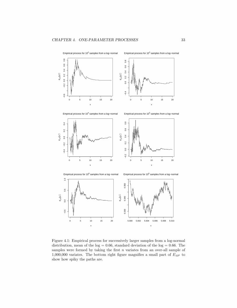
CHAPTER 4. ONE-PARAMETER PROCESSES 33
0 5 10 15 20
−0.
6−
0.2
0.0
0.2
0.4
0.6
0.8
Empirical process for 102 samples from a log−normal
x
E10
2 (x)
0 5 10 15 20
−0.
40.
00.
20.
40.
60.
8
Empirical process for 103 samples from a log−normal
x
E10
3 (x)
0 5 10 15 20
−0.
4−
0.2
0.0
0.2
0.4
Empirical process for 104 samples from a log−normal
x
E10
4 (x)
0 5 10 15 20
−0.
20.
00.
20.
40.
60.
8
Empirical process for 105 samples from a log−normal
x
E10
5 (x)
0 5 10 15 20
−0.
50.
00.
51.
0
Empirical process for 106 samples from a log−normal
x
E10
6 (x)
5.000 5.002 5.004 5.006 5.008 5.010
0.33
00.
340
0.35
0
Empirical process for 106 samples from a log−normal
x
E10
6 (x)
Figure 4.1: Empirical process for successively larger samples from a log-normaldistribution, mean of the log = 0.66, standard deviation of the log = 0.66. Thesamples were formed by taking the first n variates from an over-all sample of1,000,000 variates. The bottom right figure magnifies a small part of E106 toshow how spiky the paths are.
Chapter 5
Stationary One-ParameterProcesses
Section 5.1 describes the three main kinds of stationarity: strong,weak, and conditional.
Section 5.2 relates stationary processes to the shift operators in-troduced in the last chapter, and to measure-preserving transforma-tions more generally.
5.1 Kinds of Stationarity
Stationary processes are those which are, in some sense, the same at differenttimes — slightly more formally, which are invariant under translation in time.There are three particularly important forms of stationarity: strong or strict,weak, and conditional.
Definition 49 (Strong Stationarity) A one-parameter process is stronglystationary or strictly stationary when all its finite-dimensional distributions areinvariant under translation of the indices. That is, for all τ ∈ T , and allJ ∈ Fin(T ),
L (XJ) = L (XJ+τ ) (5.1)
Notice that when the parameter is discrete, we can get away with just check-ing the distributions of blocks of consecutive indices.
Definition 50 (Weak Stationarity) A one-parameter process is weakly sta-tionary or second-order stationary when, for all t ∈ T ,
E [Xt] = E [X0] (5.2)
and for all t, τ ∈ T ,E [XτXτ+t] = E [X0Xt] (5.3)
34
CHAPTER 5. STATIONARY PROCESSES 35
At this point, you should check that a weakly stationary process has time-invariant correlations. (We will say much more about this later.) You shouldalso check that strong stationarity implies weak stationarity. It will turn outthat weak and strong stationarity coincide for Gaussian processes, but not ingeneral.
Definition 51 (Conditional (Strong) Stationarity) A one-parameter pro-cess is conditionally stationary if its conditional distributions are invariant un-der time-translation: ∀n ∈ N, for every set of n + 1 indices t1, . . . tn+1 ∈ T ,ti < ti+1, and every shift τ ,
L(Xtn+1 |Xt1 , Xt2 . . . Xtn
)= L
(Xtn+1+τ |Xt1+τ , Xt2+τ . . . Xtn+τ
)(5.4)
(a.s.).
Strict stationarity implies conditional stationarity, but the converse is nottrue, in general. (Homogeneous Markov processes, for instance, are all con-ditionally stationary, but most are not stationary.) Many methods which arenormally presented using strong stationarity can be adapted to processes whichare merely conditionally stationary.1
Strong stationarity will play an important role in what follows, because itis the natural generaliation of the IID assumption to situations with dependentvariables — we allow for dependence, but the probabilistic set-up remains, in asense, unchanging. This will turn out to be enough to let us learn a great dealabout the process from observation, just as in the IID case.
5.2 Strictly Stationary Processes and Measure-Preserving Transformations
The shift-operator representation of Section 4.2 is particularly useful for stronglystationary processes.
Theorem 52 (Stationarity is Shift-Invariance) A process X with measureµ is strongly stationary if and only if µ is shift-invariant, i.e., µ = µ Σ−1
τ forall Στ in the time-evolution semi-group.
Proof: “If” (invariant distributions imply stationarity): For any finite col-lection of indices J , L (XJ) = µ π−1
J (Lemma 25), and similarly L (XJ+τ ) =µ π−1
J+τ .
πJ+τ = πJ Στ (5.5)π−1J+τ = Σ−1
τ π−1J (5.6)
µ π−1J+τ = µ Σ−1
τ π−1J (5.7)
L (XJ+τ ) = µ π−1J (5.8)
= L (XJ) (5.9)1For more on conditional stationarity, see Caires and Ferreira (2005).
CHAPTER 5. STATIONARY PROCESSES 36
“Only if”: The statement that µ = µ Σ−1τ really means that, for any
set A ∈ X T , µ(A) = µ(Σ−1τ A). Suppose A is a finite-dimensional cylinder
set. Then the equality holds, because all the finite-dimensional distributionsagree (by hypothesis). But this means that X and ΣτX are two processeswith the same finite-dimensional distributions, and so their infinite-dimensionaldistributions agree (Theorem 23), and the equality holds on all measurable setsA.
This can be generalized somewhat.
Definition 53 (Measure-Preserving Transformation) A measurable map-ping F from a measurable space Ξ,X into itself preserves measure µ iff, ∀A ∈ X ,µ(A) = µ(F−1A), i.e., iff µ = µF−1. This is true just when F (X) d= X, whenX is a Ξ-valued random variable with distribution µ. We will often say thatF is measure-preserving, without qualification, when the context makes it clearwhich measure is meant.
Remark on the definition. It is natural to wonder why we write the definingproperty as µ = µ F−1, rather than µ = µ F . There is actually a subtledifference, and the former is stronger than the latter. To see this, unpack thestatements, yielding respectively
∀A ∈ X , µ(A) = µ(F−1(A)) (5.10)∀A ∈ X , µ(A) = µ(F (A)) (5.11)
To see that Eq. 5.10 implies Eq. 5.11, pick any measurable set B, and thenapply 5.10 to F (B) (which is ∈ X , because F is measurable). To go the otherway, from 5.11 to 5.10, it would have to be the case that, ∀A ∈ X , ∃B ∈ X suchthat A = F (B), i.e., every measurable set would have to be the image, underF , of another measurable set. This is not necessarily the case; it would require,for starters, that F be onto (surjective).
Theorem 52 says that every stationary process can be represented by ameasure-preserving transformation, namely the shift. Since measure-preservingtransformations arise in many other ways, however, it is useful to know aboutthe processes they generate.
Corollary 54 (Measure-preservation implies stationarity) If F is a measure-preserving transformation on Ξ with invariant measure µ, and X is a Ξ-valuedrandom variable, L (X) = µ, then the sequence Fn(X), n ∈ N is strongly sta-tionary.
Proof: Consider shifting the sequence Fn(X) by one: the nth term in theshifted sequence is Fn+1(X) = Fn(F (X)). But since L (F (X)) = L (X), byhypothesis, L
(Fn+1(X)
)= L (Fn(X)), and the measure is shift-invariant. So,
by Theorem 52, the process Fn(X) is stationary.
CHAPTER 5. STATIONARY PROCESSES 37
5.3 Exercises
Exercise 7 (Functions of Stationary Processes) Use Corollary 54 to showthat if g is any measurable function on Ξ, then the sequence g(Fn(X)) is alsostationary.
Exercise 8 (Continuous Measure-Preserving Families of Transforma-tions) Let Ft, t ∈ R+, be a semi-group of measure-preserving transformations,with F0 being the identity. Prove the analog of Corollary 54, i.e., that Ft(X),t ∈ R+, is a stationary process.
Exercise 9 (The Logistic Map as a Measure-Preserving Transforma-tion) The logistic map with a = 4 is a measure-preserving transformation, andthe measure it preserves has the density 1/π
√x(1− x) (on the unit interval).
1. Verify that this density is invariant under the action of the logistic map.
2. Simulate the logistic map with uniformly distributed X0. What happens tothe density of Xt as t→∞?
Chapter 6
Random Times and TheirProperties
Section 6.1 recalls the definition of a filtration (a growing col-lection of σ-fields) and of “stopping times” (basically, measurablerandom times).
Section 6.2 defines various sort of “waiting” times, including hit-ting, first-passage, and return or recurrence times.
Section 6.3 proves the Kac recurrence theorem, which relates thefinite-dimensional distributions of a stationary process to its meanrecurrence times.
6.1 Reminders about Filtrations and StoppingTimes
You will have seen these in 36-752 as part of martingale theory, though theirapplication is more general, as we’ll see.
Definition 55 (Filtration) Let T be an ordered index set. A collection Ft, t ∈T of σ-algebras is a filtration (with respect to this order) if it is non-decreasing,i.e., f ∈ Ft implies f ∈ Fs for all s > t. We generally abbreviate this filtrationby Ft. Define Ft+ as
⋂s>t Fs. If Ft+ = Ft, then Ft is right-
continuous.
Recall that we generally think of a σ-algebra as representing available infor-mation — for any event f ∈ F , we can answer the question “did f happen?”A filtration is a way of representing our information about a system growingover time. To see what right-continuity is about, imagine it failed, which wouldmean Ft ⊂
⋂s>t Fs. Then there would have to be events which were detectable
at all times after t, but not at t itself, i.e., some sudden jump in our informationright after t. This is what right-continuity rules out.
38
CHAPTER 6. RANDOM TIMES 39
Definition 56 (Adapted Process) A stochastic process X on T is adaptedto a filtration Ft if ∀t, Xt is Ft-measurable. Any process is adapted to thefiltration it induces, σ Xs : s ≤ t. This natural filtration is written
FXt
.
A process being adapted to a filtration just means that, at every time, thefiltration gives us enough information to find the value of the process.
Definition 57 (Stopping Time, Optional Time) An optional time or astopping time, with respect to a filtration Ft, is a T -valued random variableτ such that, for all t,
ω ∈ Ω : τ(ω) ≤ t ∈ Ft (6.1)
If Eq. G.1 holds with < instead of ≤, then τ is weakly optional or a weakstopping time.
Basically, all we’re doing here is defining what we mean by “a random timeat which something detectable happens”. That being the case, it is natural toask what information we have when that detectable thing happens.
Definition 58 (Fτ for a Stopping Time τ) If τ is a Ft stopping time,then the σ-algebra Fτ is given by
Fτ ≡ A ∈ F : ∀t, A ∩ ω : τ(ω) ≤ t ∈ Ft (6.2)
I admit that the definition of Fτ looks bizarre, and I won’t blame you if youhave to read it a few times to convince yourself it isn’t circular. Here is a simplecase where it makes sense. Let X be a one-sided process, and τ a discrete
FXt
stopping time. Then
FXτ = σ (X(t ∧ τ) : t ≥ 0) (6.3)
That is, FXτ is everything we know from observing X up to time τ . (Thisis Exercise 11.) The convoluted-looking definition of Fτ carries this idea overto the more general situation where τ is continuous and we don’t necessarilyhave a single variable generating the filtration. A filtration lets us tell whethersome event A happened by the random time τ if simultaneously gives us enoughinformation to notice τ and A.
The process Y (t) = X(t ∧ τ) is follows along with X up until τ , at whichpoint it becomes fixed in place. It is accordingly called an arrested, halted orstopped version of the process. This seems to be the origin of the name “stoppingtime”.
6.2 Waiting Times
“Waiting times” are particular kinds of optional kinds: how much time mustelapse before a given event happens, either from a particular starting point,or averaging over all trajectories? Often, these are of particular interest inthemselves, and some of them can be related to other quantities of interest.
CHAPTER 6. RANDOM TIMES 40
Definition 59 (Hitting Time) Given a one-sided Ξ-valued process X, thehitting time τB of a measurable set B ⊂ Ξ is the first time at which X(t) ∈ B;
τB = inf t > 0 : Xt ∈ B (6.4)
Example 60 (Fixation through Genetic Drift) Consider the variation ina given locus (roughly, gene) in an evolving population. If there are k differentversions of the gene (“alleles”), the state of the population can be represented bya vector X(t) ∈ Rk, where at each time Xi(t) ≥ 0 and
∑iXi(t) = 1. This set
is known as the k-dimensional probability simplex Sk. We say that a certainallele has been fixed in the population or gone to fixation at t if Xi(t) = 1 forsome i, meaning that all members of the population have that version of thegene. Fixation corresponds to X(t) ∈ V , where V consists of the vertices ofthe simplex. An important question in evolutionary theory is how long it takesthe population to go to fixation. By comparing the actual rate of fixation tothat expected under a model of adaptively-neutral genetic drift, it is possible toestablish that some genes are under the influence of natural selection.
Gillespie (1998) is a nice introduction to population genetics, including thisproblem among many others, using only elementary probability. More sophis-ticated models treat populations as measure-valued stochastic processes.
Example 61 (Stock Options) A stock option1 is a legal instrument givingthe holder the right to buy a stock at a specified price (the strike price, c) beforea certain expiration date te. The point of the option is that, if you exercise it ata time t when the price of the stock p(t) is above c, you can turn around and sellthe stock to someone else, making a profit of p(t)−c. When p(t) > c, the optionis said to be in money or above water. Options can themselves be sold, and thevalue of an option depends on how much money it could be used to make, whichin turn depends on the probability that it will be “in money” before time te. Animportant part of mathematical finance thus consists of problems of the form“assuming prices p(t) follow a process distribution µ, what is the distribution ofhitting times of the set p(t) > c?”
While the financial industry is a major consumer of stochastics, and it hasa legitimate role to play in capitalist society, I do hope you will find somethingmore interesting to do with your new-found mastery of random processes, so Iwill not give many examples of this sort. If you want much, much more, readShiryaev (1999).
Definition 62 (First Passage Time) When Ξ = R or Z, we call the hittingtime of the origin the time of first passage through the origin, and similarly forother points.
1Actually, this is just one variety of option (an “American call”), out of a huge variety. Iwill not go into details.
CHAPTER 6. RANDOM TIMES 41
Definition 63 (Return Time, Recurrence Time) Fix a set B ∈ Ξ. Sup-pose that X(t0) ∈ B. Then the return time or first return time of B is recur-rence time of B is inf t > t0 : X(t) ∈ B, and the recurrence time θB is thedifference between the first return time and t0.
Note 1: If I’m to be honest with you, I should admit that “return time”and “recurrence time” are used more or less interchangeably in the literature torefer to either the time coordinate of the first return (what I’m calling the returntime) or the time interval which elapses before that return (what I’m callingthe recurrence time). I will try to keep these straight here. Check definitionscarefully when reading papers!
Note 2: Observe that if we have a discrete-parameter process, and are in-terested in recurrences of a finite-length sequence of observations w ∈ Ξk, wecan handle this situation by the device of working with the shift operator insequence space.
The question of whether any of these waiting times is optional (i.e., mea-surable) must, sadly, be raised. The following result is generally enough for ourpurposes.
Proposition 64 (Some Sufficient Conditions for Waiting Times to beWeakly Optional) Let X be a Ξ-valued process on a one-sided parameter T ,adapted to a filtration Ft, and let B be an arbitrary measurable set in Ξ. ThenτB is weakly Ft-optional under any of the following (sufficient) conditions,and Ft-optional under the first two:
1. T is discrete.
2. T is R+, Ξ is a metric space, B is closed, and X(t) is a continuousfunction of t.
3. T is R+, Ξ is a topological space, B is open, and X(t) is right-continuousas a function of t.
Proof: See, for instance, Kallenberg, Lemma 7.6, p. 123.
6.3 Kac’s Recurrence Theorem
For strictly stationary, discrete-parameter sequences, a very pretty theorem,due to Mark Kac (1947), relates the probability of seeing a particular event tothe mean time between recurrences of the event. Throughout, we consider anarbitrary Ξ-valued process X, subject only to the requirements of stationarityand a discrete parameter.
Fix an arbitrary measurable set A ∈ Ξ with P (X1 ∈ A) > 0, and considera new process Y (t), where Yt = 1 if Xt ∈ A and Yt = 0 otherwise. By Ex-ercise 7, Yt is also stationary. Thus P (X1 ∈ A,X2 6∈ A) = P (Y1 = 1, Y2 = 0).Let us abbreviate P (Y1 = 0, Y2 = 0, . . . Yn1 = 0, Yn = 0) as wn; this is the prob-ability of making n consecutive observations, none of which belong to the event
CHAPTER 6. RANDOM TIMES 42
A. Clearly, wn ≥ wn+1. Similarly, let en = P (Y1 = 1, Y2 = 0, . . . Yn = 0) andrn = P (Y1 = 1, Y2 = 0, . . . Yn = 1) — these are, respectively, the probabilitiesof starting in A and not returning within n − 1 steps, and of starting in Aand returning for the first time after n − 2 steps. (Set e1 to P (Y1 = 1), andw0 = e0 = 1.)
Lemma 65 (Some Recurrence Relations for Kac’s Theorem) The fol-lowing recurrence relations hold among the probabilities wn, en and rn:
en = wn−1 − wn, n ≥ 1 (6.5)rn = en−1 − en, n ≥ 2 (6.6)rn = wn−2 − 2wn−1 + wn, n ≥ 2 (6.7)
Proof: To see the first equality, notice that
P (Y1 = 0, Y2 = 0, . . . Yn−1 = 0) (6.8)= P (Y2 = 0, Y3 = 0, . . . Yn = 0)= P (Y1 = 1, Y2 = 0, . . . Yn = 0) + P (Y1 = 0, Y2 = 0, . . . Yn = 0) (6.9)
using first stationarity and then total probability. To see the second equality,notice that, by total probability,
P (Y1 = 1, Y2 = 0, . . . Yn−1 = 0) (6.10)= P (Y1 = 1, Y2 = 0, . . . Yn−1 = 0, Yn = 0) + P (Y1 = 1, Y2 = 0, . . . Yn−1 = 0, Yn = 1)
The third relationship follows from the first two.
Theorem 66 (Recurrence in Stationary Processes) Let X be a Ξ-valueddiscrete-parameter stationary process. For any set A with P (X1 ∈ A) > 0, foralmost all ω such that X1(ω) ∈ A, there exists a τ for which Xτ (ω) ∈ A.
∞∑k=1
P (θA = k|X1 ∈ A) = 1 (6.11)
Proof: The event θA = k,X1 ∈ A is the same as the event Y1 = 1, Y2 = 0, . . . Yk+1 = 1.Since P (X1 ∈ A) > 0, we can handle the conditional probabilities in an elemen-tary fashion:
P (θA = k|X1 ∈ A) =P (θA = k,X1 ∈ A)
P (X1 ∈ A)(6.12)
=P (Y1 = 1, Y2 = 0, . . . Yk+1 = 1)
P (Y1 = 1)(6.13)
∞∑k=1
P (θA = k|X1 ∈ A) =∑∞k=1 P (Y1 = 1, Y2 = 0, . . . Yk+1 = 1)
P (Y1 = 1)(6.14)
=∑∞k=2 rke1
(6.15)
CHAPTER 6. RANDOM TIMES 43
Now consider the finite sums, and apply Eq. 6.7.
n∑k=2
rk =n∑k=2
wk−2 − 2wk−1 + wk (6.16)
=n−2∑k=0
wk +n∑k=2
wk − 2n−1∑k=1
wk (6.17)
= w0 + wn − w1 − wn−1 (6.18)= (w0 − w1)− (wn−1 − wn) (6.19)= e1 − (wn−1 − wn) (6.20)
where the last line uses Eq. 6.6. Since wn−1 ≥ wn, there exists a limn wn, whichis ≥ 0 since every individual wn is. Hence limn wn−1 − wn = 0.
∞∑k=1
P (θA = k|X1 ∈ A) =∑∞k=2 rke1
(6.21)
= limn→∞
e1 − (wn−1 − wn)e1
(6.22)
=e1
e1(6.23)
= 1 (6.24)
which was to be shown.
Corollary 67 (Poincare Recurrence Theorem) Let F be a transformationwhich preserves measure µ. Then for any set A of positive µ measure, for µ-almost-all x ∈ A, ∃n ≥ 1 such that Fn(x) ∈ A.
Proof: A direct application of the theorem, given the relationship betweenstationary processes and measure-preserving transformations we established byCorollary 54.
Corollary 68 (“Nietzsche”) In the set-up of the previous theorem, if X1(ω) ∈A, then Xt ∈ A for infinitely many t (a.s.).
Proof: Repeated application of the theorem yields an infinite sequence oftimes τ1, τ2, τ3, . . . such that Xτi(ω) ∈ A, for almost all ω such that X1(ω) ∈ Ain the first place.
Now that we’ve established that once something happens, it will happenagain and again, we would like to know how long we have to wait betweenrecurrences.
Theorem 69 (Kac’s Recurrence Theorem) Continuing the previous nota-tion, E [θA|X1 ∈ A] = 1/P (X1 ∈ A) if and only if limn wn = 0.
CHAPTER 6. RANDOM TIMES 44
Proof: “If”: Unpack the expectation:
E [θA|X1 ∈ A] =∞∑k=1
kP (Y1 = 1, Y2 = 0, . . . Yk+1 = 1)
P (Y1 = 1)(6.25)
=1
P (X1 ∈ A)
∞∑k=1
krk+1 (6.26)
so we just need to show that the last series above sums to 1. Using Eq. 6.7again,
n∑k=1
krk+1 =n∑k=1
k(wk−1 − 2wk + wk+1) (6.27)
=n∑k=1
kwk−1 +n∑k=1
kwk+1 − 2n∑k=1
kwk (6.28)
=n−1∑k=0
(k + 1)wk +n+1∑k=2
(k − 1)wk − 2n∑k=1
kwk (6.29)
= w0 + nwn+1 − (n+ 1)wn (6.30)= 1− wn − n(wn − wn+1) (6.31)
We therefore wish to show that limn wn = 0 implies limn wn + n(wn − wn+1) =0. By hypothesis, it is enough to show that limn n(wn − wn+1) = 0. The partialsums on the left-hand side of Eq. 6.27 are non-decreasing, so wn+n(wn−wn+1)is non-increasing. Since it is also ≥ 0, the limit limn wn + n(wn − wn+1) exists.Since wn → 0, wn − wn+1 ≤ wn must also go to zero; the only question iswhether it goes to zero fast enough. So consider
limn
n∑k=1
wk −n∑k=1
wk+1 (6.32)
Telescoping the sums again, this is limn w1 − wn+1. Since limn+1 wn+1 =limn wn = 0, the limit exists. But we can equally re-write Eq. 6.32 as
limn
n∑k=1
wk − wk+1 =∞∑n=1
wn − wn+1 (6.33)
Since the sum converges, the individual terms wn−wn+1 must be o(n−1). Hencelimn n(wn − wn+1) = 0, as was to be shown.
“Only if”: From Eq. 6.31 in the “if” part, we see that the hypothesis isequivalent to
1 = limn
(1− wn − n(wn − wn+1)) (6.34)
Since wn ≥ wn+1, 1−wn−n(wn−wn+1) ≤ 1−wn. We know from the proof ofTheorem 66 that limn wn exists, whether or not it is zero. If it is not zero, thenlimn (1− wn − n(wn − wn+1)) ≤ 1− limn wn < 1. Hence wn → 0 is a necessarycondition.
CHAPTER 6. RANDOM TIMES 45
Example 70 (Counter-example for Kac’s Recurrence Theorem) Onemight imagine that the condition wn → 0 in Kac’s Theorem is redundant, giventhe assumption of stationarity. Here is a counter-example. Consider a ho-mogeneous Markov chain on a finite space Ξ, which is partitioned into twonon-communicating components, Ξ1 and Ξ2. Each component is, internally,irreducible and aperiodic, so there will be an invariant measure µ1 supportedon Ξ1, and another invariant measure µ2 supported on Ξ2. But then, for anys ∈ [0, 1], sµ1 + (1− s)µ2 will also be invariant. (Why?) Picking A ⊂ Ξ2 giveslimn wn = s, the probability that the chain begins in the wrong component toever reach A.
Kac’s Theorem turns out to be the foundation for a fascinating class ofmethods for learning the distributions of stationary processes, and for “univer-sal” prediction and data compression. There is also an interesting interactionwith large deviations theory. This subject is one possibility for further discus-sion at the end of the course. Whether or not we get there, let me recommendsome papers in a footnote.2
6.4 Exercises
Exercise 10 (Weakly Optional Times and Right-Continuous Filtra-tions) Show that a random time τ is weakly Ft-optional iff it is Ft+-optional.
Exercise 11 (Discrete Stopping Times and Their σ-Algebras) ProveEq. G.3. Does the corresponding statement hold for two-sided processes?
Exercise 12 (Kac’s Theorem for the Logistic Map) First, do Exercise 9.Then, using the same code, suitably modified, numerically check Kac’s Theoremfor the logistic map with a = 4. Pick any interval I ⊂ [0, 1] you like, but be surenot to make it too small.
1. Generate n initial points in I, according to the invariant measure 1
π√x(1−x)
.
For each point xi, find the first t such that F t(xi) ∈ I, and take the meanover the sample. What happens to this space average as n grows?
2. Generate a single point x0 in I, according to the invariant measure. Iterateit T times. Record the successive times t1, t2, . . . at which F t(x0) ∈ I, andfind the mean of ti − ti−1 (taking t0 = 0). What happens to this timeaverage as T grows?
2 “How Sampling Reveals a Process” (Ornstein and Weiss, 1990); Algoet (1992); Kon-toyiannis et al. (1998).
Chapter 7
Continuity of StochasticProcesses
Section 7.1 describes the leading kinds of continuity for stochasticprocesses, which derive from the modes of convergence of randomvariables. It also defines the idea of versions of a stochastic process.
Section 7.2 explains why continuity of sample paths is often prob-lematic, and why we need the whole “paths in U” song-and-dance.As an illustration, we consider a Gausssian process which is close tothe Wiener process, except that it’s got a nasty non-measurability.
Section 7.3 introduces separable random functions.Section 7.4 constructs separable modifications of reasonable but
non-separable random functions, and explains how separability re-lates to non-denumerable properties like continuity.
Section 7.5 constructs versions of our favorite one-parameter pro-cesses where the sample paths are measurable functions of the pa-rameter.
Section 7.6 gives conditions for the existence of cadlag versions.Section 7.7 gives some criteria for continuity, and for the existence
of “continuous modifications” of discontinuous processes.
The existence of processes with given finite-dimensional distributions doesnot guarantee that they have desirable and natural properties, like continuity,and in fact that one can construct discontinuous versions of processes whichought to be continuous. We therefore need extra theorems to guarantee theexistence of continuous versions of processes with specified FDDs. To get there,we will first prove the existence of versions with a weaker regularity propertycalled “separability”. This will require various topological conditions on boththe index set T and the value space Ξ.
In the interest of space (or is it time?), Section 7.4 will provide complete anddetailed proofs. The other sections will simply state results, and refer proofs tostandard sources, mostly Gikhman and Skorokhod (1965/1969).
46
CHAPTER 7. CONTINUITY 47
7.1 Kinds of Continuity for Processes
Continuity is a convergence property: a continuous function is one where con-vergence of the inputs implies convergence of the outputs. But we have severalkinds of convergence for random variables, so we may expect to encounter severalkinds of continuity for random processes. Note that the following definitions arestated broadly enough that the index set T does not have to be one-dimensional.
Definition 71 (Continuity in Mean) A stochastic process X is continuousin the mean at t0 if t → t0 implies E
[|X(t)−X(t0)|2
]→ 0. X is continuous
in the mean if this holds for all t0.
It would, of course, be more natural to refer to this as “continuity in meansquare”, or even “continuity in L2”, and one can define continuity in Lp forarbitrary p.
Definition 72 (Continuity in Probability, Stochastic Continuity) X iscontinuous in probability at t0 if t→ t0 implies X(t) P→ X(t0). X is continuousin probability or stochastically continuous if this holds for all t0.
Note that neither Lp-continuity nor stochastic continuity says that the indi-vidual sample paths, themselves, are continuous.
Definition 73 (Continuous Sample Paths) A process X is continuous at t0if, for almost all ω, t→ t0 implies X(t, ω)→ X(t0, ω). A process is continuousif, for almost all ω, X(·, ω) is a continuous function.
Obviously, continuity of sample paths implies stochastic continuity and Lp-continuity.
A weaker pathwise property than strict continuity, frequently used in prac-tice, is the combination of continuity from the right with limits from the left.This is usually known by the term “cadlag”, abbreviating the French phrase“continues a droite, limites a gauche”; “rcll” is an unpronounceable synonym.
Definition 74 (Cadlag) A sample function x on a well-ordered set T is cadlagif it is continuous from the right and limited from the left at every point. Thatis, for every t0 ∈ T , t ↓ t0 implies x(t) → x(t0), and for t ↑ t0, limt↑t0 x(t)exists, but need not be x(t0). A stochastic process X is cadlag if almost all itssample paths are cadlag.
As we will see, it will not be easy to show that our favorite random processeshave any of these desirable properties. What will be easy will be to show thatthey are, in some sense, easily modified into ones which do have good regularityproperties, without loss of probabilistic content. This is made more preciseby the notion of versions of a stochastic process, related to that of versions ofconditional probabilities.
CHAPTER 7. CONTINUITY 48
Definition 75 (Versions of a Stochastic Process, Stochastically Equiv-alent Processes) Two stochastic processes X and Y with a common index setT are called versions of one another if
∀t ∈ T, P (ω : X(t, ω) = Y (t, ω)) = 1
Such processes are also said to be stochastically equivalent.
Lemma 76 (Versions Have Identical FDDs) If X and Y are versions ofone another, they have the same finite-dimensional distributions.
Proof: Clearly it will be enough to show that P (XJ = YJ) = 1 for arbitraryfinite collections of indices J . Pick any such collection J = t1, t2, . . . tj. Then
P (XJ = YJ) = P(Xt1 = Yt1 , . . . Xtj = Ytj
)(7.1)
= 1− P
(⋃ti∈J
Xti 6= Yti
)(7.2)
≥ 1−∑ti∈J
P (Xti 6= Yti) (7.3)
= 1 (7.4)
using only finite sub-additivity. There is a stronger notion of similarity between processes than that of ver-
sions, which will sometimes be useful.
Definition 77 (Indistinguishable Processes) Two stochastic processes Xand Y are indistinguishable, or equivalent up to evanescence, when
P (ω : ∀t,X(t, ω) = Y (t, ω)) = 1
Notice that saying X and Y are indistinguishable means that their samplepaths are equal almost surely, while saying they are versions of one anothermeans that, at any time, they are almost surely equal. Indistinguishable pro-cesses are versions of one another, but not necessarily the reverse. (Look atwhere the quantifier and the probability statements go.) However, if T = Rd,then any two right-continuous versions of the same process are indistinguishable(Exercise 14).
7.2 Why Continuity Is an Issue
In many situations, we want to use stochastic processes to model dynamicalsystems, where we know that the dynamics are continuous in time (i.e. theindex set is R, or maybe R+ or [0, T ] for some real T ).1 This means that we
1Strictly speaking, we don’t really know that space-time is a continuum, but the discretiza-tion, if there is one, is so fine that it might as well be.
CHAPTER 7. CONTINUITY 49
ought to restrict the sample paths to be continuous functions; in some cases we’deven want them to be differentiable, or yet more smooth. As well as being amatter of physical plausibility or realism, it is also a considerable mathematicalconvenience, as the following shows.
Proposition 78 (Continuous Sample Paths Have Measurable Extrema)Let X(t, ω) be a real-valued continuous-parameter process with continuous sam-ple paths. Then on any finite interval I, M(ω) ≡ supt∈I X(t, ω) and m(ω) ≡inft∈I X(t, ω) are measurable random variables.
Proof: It’ll be enough to prove this for the supremum function M ; the prooffor m is entirely parallel. First, notice that M(ω) must be finite, because thesample paths X(·, ω) are continuous functions, and continuous functions arebounded on bounded intervals. Next, notice that M(ω) > a if and only ifX(t, ω) > a for some t ∈ I. But then, by continuity, there will be some rationalt′ ∈ I ∩Q such that X(t′, ω) > a; countably many, in fact.2 Hence
ω : M(ω) > a =⋃
t∈I∩Q
ω : X(t, ω) > a
Since, for each t, X(t, ω) is a random variable, the sets in the union on theright-hand side are all measurable, and the union of a countable collection ofmeasurable sets is itself measurable. Since intervals of the form (a,∞) generatethe Borel σ-field on the reals, we have shown that M(ω) is a measurable functionfrom Ω to the reals, i.e., a random variable.
Continuity raises some very tricky technical issues. The product σ-field isthe usual way of formalizing the notion that what we know about a stochas-tic process are values observed at certain particular times. What we saw inExercise 1 is that “the product σ-field answers countable questions”: for anymeasurable set A, whether x(·, ω) ∈ A depends only on the value of x(t, ω) atcountably many indices t. It follows that the class of all continuous samplepaths is not product-σ-field measurable, because x(·, ω) is continuous at t iffx(tn, ω)→ x(t, ω) along every sequence tn → t, and this is involves the value ofthe function at uncountably many coordinates. It is further true that the classof differentiable functions is not product σ-field measurable. For that matter,neither is the class of piecewise linear functions! (See Exercise 13.)
You might think that, on the basis of Theorem 23, this should not really bemuch of an issue: that even if the class of continuous sample paths (say) isn’tstrictly measurable, it could be well-approximated by measurable sets, and sogetting the finite-dimensional distributions right is all that matters. This wouldmake the theory of stochastic processes in continuous time much simpler, butunfortunately it’s not quite the case. Here is an example to show just how badthings can get, even when all the finite-dimensional distributions agree.3
2Continuity means that we can pick a δ such that, for all t′ within δ of t, X(t′, ω) is within12
(X(t, ω) − a) of X(t, ω). And there are countably many rational numbers within any realinterval. — There is nothing special about the rational numbers here; any countable, densesubset of the real numbers would work as well.
3I stole this example from Pollard (2002, p. 214).
CHAPTER 7. CONTINUITY 50
Example 79 (A Horrible Version of the proto-Wiener Process) Exam-ple 38 defined the Wiener process by four requirements: starting at the origin,independent increments, a Gaussian distribution of increments, and continu-ity of sample paths. Take a Wiener process W (t, ω) and consider M(ω) ≡supt∈[0,1]W (t, ω), its supremum over the unit interval. By the preceding propo-sition, we know that M is a measurable random variable. But we can constructa version of W for which the supremum is not measurable.
For starters, assume that Ω can be partitioned into an uncountable collectionof disjoint measurable sets, one for each t ∈ [0, 1]. (This can be shown as anexercise in real analysis.) Select any non-measurable real-valued function B(ω),so long as B(ω) > M(ω) for all ω. (There are uncountably many suitablefunctions.) Set W ∗(t, ω) = W (t, ω) if ω 6∈ Ωt, and = B(ω) if ω ∈ Ωt. Now,at every t, P (W (t, ω) = W ∗(t, ω)) = 1. W ∗ is a version of W , and all theirfinite-dimensional distributions agree. But, for every ω, there is a t such thatW ∗(t, ω) = B(ω) > suptW (t, ω), so suptW ∗(t, ω) = B(ω), which by design isnon-measurable.
Why care about this example? Two reasons. First, and technically, we’regoing to want to take suprema of the Wiener process a lot when we deal withlarge deviations theory, and with the approximation of discrete processes bycontinuous ones. Second, nothing in the example really depended on startingfrom the Wiener process; any process with continuous sample paths would haveworked as well. So controlling the finite-dimensional distributions is not enoughto guarantee that a process has measurable extrema, which would lead to allkinds of embarrassments. We could set up what would look like a reasonablestochastic model, and then be unable to say things like “with probability p, the temperature/ demand for electricity/ tracking error/ interest rate will notexceed r over the course of the year”.
Fundamentally, the issues with continuity are symptoms of a deeper problem.The reason the supremum function is non-measurable in the example is that itinvolves uncountably many indices. A countable collection of ill-behaved sets ofmeasure zero is a set of measure zero, and may be ignored, but an uncountablecollection of them can have probability 1. Fortunately, there are standard waysof evading these measure-theoretic issues, by showing that one can always findrandom functions which not only have prescribed finite-dimensional distribu-tions (what we did in Lectures 2 and 3), but also are regular enough that wecan take suprema, or integrate over time, or force them to be continuous. Thishinges on the notion of separability for random functions.
7.3 Separable Random Functions
The basic idea of a separable random function is one whose properties can behandled by dealing only with a countable, dense subset, just as, in the proofof Proposition 78, we were able to get away with only looking at X(t) at onlyrational values of t. Because a space with a countable, dense subset is called a“separable” space, we will call such functions “separable functions”.
CHAPTER 7. CONTINUITY 51
Definition 80 (Separable Function) Let Ξ and T be metric spaces, and Dbe a countable, dense subset of T . A function x : T 7→ Ξ is D-separable orseparable with respect to D if, forallt ∈ T , there exists a sequence ti ∈ D suchthat ti → t and x(ti)→ x(t).
Lemma 81 (Some Sufficient Conditions for Separability) The followingconditions are sufficient for separability:
1. T is countable.
2. x is continuous.
3. T is well-ordered and x is right-continuous.
Proof: (1) Take the separating set to be T itself. (2) Pick any countabledense D. By density, for every t there will be a sequence ti ∈ D such that ti → t.By continuity, along any sequence converging to t, x(ti) → t. (3) Just like (2),only be sure to pick the ti > t. (You can do this, again, for any countable denseD.)
Definition 82 (Separable Process) A Ξ-valued process X on T is separablewith respect to D if D is a countable, dense subset of T , and there is a measure-zero set N ⊂ Ω such that for every ω 6∈ N , X(·, ω) is D-separable. That is,X(·, ω) is almost surely D-separable.
We cannot easily guarantee that a process is separable. What we can easilydo is go from one process, which may or may not be separable, to a separa-ble process with the same finite-dimensional distributions. This is known asa separable modification of the original process. Combined with the extensiontheorems (Theorems 27, 29 and 33), this tells that we can always construct aseparable process with desired finite-dimensional distributions. We shall thenfeel entitled to assume that our processes are separable. The proofs of the ex-istence of separable and continuous versions of general processes are, however,somewhat involved.
7.4 Separable Versions
We can show that separable versions of our favorite stochastic processes existunder quite general conditions, but first we will need some preliminary results,living at the border between topology and measure theory. This starts by re-calling some facts about compact spaces.
Definition 83 (Compactness, Compactification) A set A in a topologicalspace Ξ is compact if every covering of A by open sets contains a finite sub-cover.Ξ is a compact space if it is itself a compact set. If Ξ is not compact, but is asub-space of a compact topological space Ξ, the super-space is a compactificationof Ξ.
CHAPTER 7. CONTINUITY 52
Proposition 84 (Compact Spaces are Separable) Every compact space isseparable.
Proof: A standard result of analysis. Interestingly, it relies on the axiomof choice.
Proposition 85 (Compactification is Possible) Every non-compact topo-logical space Ξ is a sub-space of some compact topological space Ξ, i.e., everynon-compact topological space can be compactified.
Example 86 (Compactifying the Reals) The real numbers R are not com-pact: they have no finite covering by open intervals (or other open sets). Theextended reals, R ≡ R ∪ +∞ ∪ −∞, are compact, since intervals of the form(a,∞] and [−∞, a) are open. This is a two-point compactification of the reals.There is also a one-point compactification, with a single point at ±∞, but thishas the undesirable property of making big negative and positive numbers closeto each other.
Recall that a random function is separable if its value at any arbitrary in-dex can be determined almost surely by examining its values on some fixed,countable collection of indices. The next lemma states an alternative charac-terization of separability. The lemma after that gives conditions under which aweaker property holds — the almost-sure determination of whether X(t, ω) ∈ B,for a specific t and set B, by the behavior of X(tn, ω) at countably many tn.The final lemma extends this to large collections of sets, and then the proof ofthe theorem puts all the parts together.
Lemma 87 (Alternative Characterization of Separability) Let T be aseparable set, Ξ a compact metric space, and D a countable dense subset of T .Define V as the class of all open balls in T centered at points in D and withrational radii. For any G ⊂ T , let
R(G,ω) ≡ closure
( ⋃t∈G∩D
X(t, ω)
)(7.5)
R(t, ω) ≡⋂
S: S∈V, t∈SR(S, ω) (7.6)
Then X(t, ω) is D-separable if and only if there exists a set N ⊂ Ω such that
ω 6∈ N ⇒ ∀t, X(t, ω) ∈ R(t, ω) (7.7)
and P (N) = 0.
Proof: Roughly speaking, R(t, ω) is what we’d think the range of thefunction would be, in the vicinity of t, if it we went just by what it did at pointsin the separating set D. The actual value of the function falling into this range
CHAPTER 7. CONTINUITY 53
(almost surely) is necessary and sufficient for the function to be separable. Butlet’s speak less roughly.
“Only if”: Since X(t, ω) is D-separable, for almost all ω, for any t thereis some sequence tn ∈ D such that tn → t and X(tn, ω) → X(t, ω). For anyball S centered at t, there is some N such that tn ∈ S if n ≥ N . Hence thevalues of x(tn) are eventually confined to the set
⋃t∈S∩DX(t, ω). Recall that
the closure of a set A consists of the points x such that, for some sequencexn ∈ A, xn → x. As X(tn, ω) → X(t, ω), it must be the case that X(t, ω) ∈closure
(⋃t∈S∩DX(t, ω)
). Since this applies to all S, X(t, ω) must be in the
intersection of all those closures, hence X(t, ω) ∈ R(t, ω) — unless we are onone of the probability-zero bad sample paths, i.e., unless ω ∈ N .
“If”: Assume that, with probability 1, X(t, ω) ∈ R(t, ω). Thus, for anyS ∈ V , we know that there exists a sequence of points tn ∈ S ∩ D such thatX(tn, ω) → X(t, ω). However, this doesn’t say that tn → t, which is what weneed for separability. We will now build such a sequence. Consider a seriesof spheres Sk ∈ V such that (i) every point in Sk is within a distance 2−k oft and (ii) Sk+1 ⊂ Sk. For each Sk, there is a sequence t
(k)n ∈ Sk such that
X(t(k)n , ω) → X(t, ω). In fact, for any m > 0, |X(t(k)
n , ω) − X(t, ω)| < 2−m ifn ≥ N(k,m), for some N(k,m). Our final sequence of indices ti then consists ofthe following points: t(1)
n for n from N(1, 1) to N(1, 2); t(2)n for n from N(2, 2)
to N(2, 3); and in general t(k)n for n from N(k, k) to N(k, k+1). Clearly, ti → t,
and X(ti, ω) → X(t, ω). Since every ti ∈ D, we have shown that X(t, ω) isD-separable.
Lemma 88 (Confining Bad Behavior to a Measure Zero Event) Let Tbe a separable index set, Ξ a compact space, X a random function from T to Ξ,and B be an arbitrary Borel set of Ξ. Then there exists a denumerable set ofpoints tn ∈ T such that, for any t ∈ T , the set
N(t, B) ≡ ω : X(t, ω) 6∈ B ∩
( ∞⋂n=1
ω : X(tn, ω) ∈ B
)(7.8)
has probability 0.
Proof: We proceed recursively. The first point, t1, can be whatever welike. Suppose t1, t2, . . . tn are already found, and define the following:
Mn ≡n⋂k=1
ω : X(tk, ω) ∈ B (7.9)
Ln(t) ≡ Mn ∩ ω : X(t, ω) 6∈ B (7.10)pn ≡ sup
tP (Ln(t)) (7.11)
Mn is the set where the random function, evaluated at the first n indices, gives avalue in our favorite set; it’s clearly measurable. Ln(t), also clearly measurable,gives the collection of points in Ω where, if we chose t for the next point in
CHAPTER 7. CONTINUITY 54
the collection, this will break down. pn is the worst-case probability of thishappening. For each t, Ln+1(t) ⊆ Ln(t), so pn+1 ≤ pn. Suppose pn = 0;then we’ve found the promised denumerable sequence, and we’re done. Supposeinstead that pn > 0. Pick any t such that P (Ln(t)) ≥ 1
2pn, and call it tn+1.(There has to be such a point, or else pn wouldn’t be the supremum.) Now noticethat L1(t2), L2(t3), . . . Ln(tn+1) are all mutually exclusive, but not necessarilyjointly exhaustive. So
1 = P (Ω) (7.12)
≥ P
(⋃n
Ln(tn+1)
)(7.13)
=∑n
P (Ln(tn+1)) (7.14)
≥∑n
12pn > 0 (7.15)
so pn → 0 as n→∞.We saw that Ln(t) is a monotone-decreasing sequence of sets, for each t,
so a limiting set exists, and in fact limn Ln(t) = N(t, B). So, by monotoneconvergence,
P (N(t, B)) = P(
limnLn(t)
)(7.16)
= limn
P (Ln(t)) (7.17)
≤ limnpn (7.18)
= 0 (7.19)
as was to be shown.
Lemma 89 (A Null Exceptional Set) Let B0 be any countable class of Borelsets in Ξ, and B the closure of B0 under countable intersection. Under thehypotheses of the previous lemma, there is a denumerable sequence tn such that,for every t ∈ T , there exists a set N(t) ⊂ Ω with P (N(t)) = 0, and, for allB ∈ B,
ω : X(t, ω) 6∈ A ∩
( ∞⋂n=1
ω : X(tn, ω) ∈ A
)⊆ N(t) (7.20)
Proof: For each B ∈ B0, construct the sequence of indices as in the previouslemma. Since there only countably many sets in B, if we take the union of all ofthese sequences, we will get another countable sequence, call it tn. Then we havethat, ∀B ∈ B0, ∀t ∈ T , P (X(tn, ω) ∈ B,n ≥ 1, X(t, ω) 6∈ B) = 0. Take this setto be N(t, B), and define N(t) ≡
⋃B∈B0
N(t, B). Since N(t) is a countableunion of probability-zero events, it is itself a probability-zero event. Now, take
CHAPTER 7. CONTINUITY 55
any B ∈ B, and any B0 ∈ B0 such that B ⊆ B0. Then
X(t, ω) 6∈ B0 ∩
( ∞⋂n=1
X(tn, ω) ∈ B
)(7.21)
⊆ X(t, ω) 6∈ B0 ∩
( ∞⋂n=1
X(tn, ω) ∈ B0
)⊆ N(t) (7.22)
Since B =⋂k B
(k)0 for some sequence of sets B(k)
0 ∈ B0, it follows (via DeMorgan’s laws and the distributive law) that
X(t, ω) 6∈ B =∞⋃k=1
X(t, ω) 6∈ B(k)
0
(7.23)
X(t, ω) 6∈ B ∩
( ∞⋂n=1
X(tn, ω) ∈ B
)
=∞⋃k=1
X(t, ω) 6∈ B(k)
0
∩
( ∞⋂n=1
X(tn, ω) ∈ B
)(7.24)
⊆∞⋃n=1
N(t) (7.25)
= N(t) (7.26)
which was to be shown.
Theorem 90 (Separable Versions, Separable Modification) Suppose thatΞ is a compact metric space and T is a separable metric space. Then, for anyΞ-valued stochastic process X on T , there exists a separable version X. This iscalled a separable modification of X.
Proof: Let D be a countable dense subset of T , and V the class of openspheres of rational radius centered at points in D. Any open subset of T isa union of countably many sets from V , which is itself countable. Similarly,let C be a countable dense subset of Ξ, and let B0 consist of the complementsof spheres centers at points in D with rational radii, and (as in the previouslemma) let B be the closure of B0 under countable intersection. Every closedset in Ξ belongs to B.4 For every S ∈ V , consider the restriction of X(t, ω) tot ∈ S, and apply Lemma 89 to the random function X(t, ω) to get a sequenceof indices I(S) ⊂ T , and, for every t ∈ S, a measure-zero set NS(t) ⊂ Ω wherethings can go wrong. Set I =
⋃S∈V I(S) and N(t) =
⋃S∈V NS(t). Because
V is countable, I is still a countable set of indices, and N(t) is still of measure
4You show this.
CHAPTER 7. CONTINUITY 56
zero. I is going to be our separating set, and we’re going to show that we haveuncountably many sets N(t) won’t be a problem.
Define X(t, ω) = X(t, ω) if t ∈ I or ω 6∈ N(t) — if we’re at a time in theseparating set, or we’re at some other time but have avoided the bad set, we’lljust copy our original random function. What to do otherwise, when t 6∈ I andω ∈ N(t)? Construct R(t, ω), as in the proof of Lemma 87, and let X(t, ω) takeany value in this set. Since R(t, ω) depends only on the value of the functionat indices in the separating set, it doesn’t matter whether we build it fromX or from X. In fact, for all t and ω, X(t, ω) ∈ R(t, ω), so, by Lemma 87,X(t, ω) is separable. Finally, for every t,
X(t, ω) = X(t, ω)
⊆ N(t), so ∀t,
P(X(t) = X(t)
), and X is a version of X (Definition 75).
Corollary 91 (Separable Modifications in Compactified Spaces) If thesituation is as in the previous theorem, but Ξ is not compact, there exists aseparable version of X in any compactification Ξ of Ξ.
Proof: Because Ξ is a sub-space of any of its compactifications Ξ, X is alsoa process with values in Ξ.5 Since Ξ is compact, X has a separable modificationX with values in Ξ, but (with probability 1) X(t) ∈ Ξ.
Corollary 92 (Separable Versions with Prescribed Distributions Ex-ist) Let Ξ be a complete, compact metric space, T a separable index set, andµJ , J ∈ Fin(T ) a projective family of probability distributions. Then there is aseparable stochastic process with finite-dimensional distributions given by µJ .
Proof: Combine Theorem 90 with the Kolmogorov Extension Theorem 29.(By Proposition 84, a complete, compact metric space is a complete, separablemetric space.)
7.5 Measurable Versions
It would be nice for us if X(t) is a measurable function of t, because we aregoing to want to write down things like∫ t=b
t=a
X(t)dt
and have them mean something. Irritatingly, this will require another modifi-cation.
Definition 93 (Measurable random function) Let T, T , τ be a measurablespace, its σ-field and a measure defined thereon. A random function X on T
with values in Ξ,X is measurable if X : T × Ω 7→ Ξ is T × F/X measurable,where T × F is the product σ-field on T × Ω, and T × F its completion by thenull sets of the product measure τ × P.
5If you want to be really picky, define a 1-1 function h : Ξ 7→ Ξ taking points to theircounterparts. Then X and h−1(X) are indistinguishable. Do I need to go on?
CHAPTER 7. CONTINUITY 57
It would seem more natural to simply define measurable processes by sayingthat the sample paths are measurable, that X(·, ω) is a T -measurable function oft for P-almost-all ω. This would be like our definition of almost-sure continuity.However, Definition 93 implies this version, via Fubini’s Theorem, and facilitatesthe proofs of the two following theorems.
Theorem 94 (Exchanging Expectations and Time Integrals) If X(t) ismeasurable, and E [X(t)] is integrable (with respect to the measure τ on T ), thenfor any set I ∈ T , ∫
I
E [X(t)] τ(dt) = E[∫
I
X(t)τ(dt)]
(7.27)
Proof: This is just Fubini’s Theorem!
Theorem 95 (Measurable Separable Modifications) Suppose that T andΞ are both compact. If X(t, ω) is continuous in probability at τ -almost-all t,then it has a version which is both separable and measurable, its measurableseparable modification.
Proof: See Gikhman and Skorokhod (1965/1969, ch. IV, sec. 3, thm. 1,p. 157).
7.6 Cadlag Versions
Theorem 96 (Cadlag Versions) Let X be a separable random process withT = [a, b] ⊆ R, and Ξ a complete metric space with metric ρ. Suppose that X(t)is continuous in probability on T , and there are real constants p, q, C ≥ 0, r > 1such that, for any three indices t1 < t2 < t3 ∈ T ,
E [ρp(X(t1), X(t2))ρq(X(t2), X(t3))] ≤ C|t3 − t1|r (7.28)
Then there is a version of X whose sample paths are cadlag (a.s.).
Proof: Combine Theorem 1 and Theorem 3 of Gikhman and Skorokhod(1965/1969, ch. IV, sec. 4, pp. 159–169).
7.7 Continuous Modifications
Theorem 97 (Continuous Versions) Let X be a separable stochastic processwith T = [a, b] ⊆ R, and Ξ a complete metric space with metric ρ. Suppose thatthere are constants C, p > 0, r > 1 such that, for any t1 < t2 ∈ T ,
E [ρp(X(t1), X(t2))] ≤ C|t2 − t1|r (7.29)
Then X(t) has a continuous version.
CHAPTER 7. CONTINUITY 58
Proof: See Gikhman and Skorokhod (1965/1969, ch. IV, sec. 5, thm. 2,p. 170), and the first remark following the theorem.
A slightly more refined result requires two preliminary definitions.
Definition 98 (Modulus of continuity) For any function x from a metricspace T, d to a metric space Ξ, ρ, the modulus of continuity is the functionmx(r) : R+ 7→ R+ given by
mx(r) = sup ρ(x(s), x(t)) : s, t ∈ T, d(s, t) ≤ r (7.30)
Lemma 99 (Modulus of continuity and uniform continuity) x is uni-formly continuous if and only if its modulus of continuity → 0 as r → 0.
Proof: Obvious from Definition 98 and the definition of uniform continuity.
Definition 100 (Holder continuity) Continuing the notation of Definition98, we say that x is Holder-continuous with exponent c if there are positiveconstants c, γ such that mx(r) ≤ γrc for all sufficiently small r; i.e., mx(r) =O(rc). If this holds on every bounded subset of T , then the function is locallyHolder-continuous.
Theorem 101 (Holder-continuous versions) Let T be Rd and Ξ a completemetric space with metric ρ. If there are constants p, q, γ > 0, such that, for anyt1, t2 ∈ T ,
E [ρp(X(t1), X(t2))] ≤ γ|t1 − t2|d+q (7.31)
then X has a continuous version X, and almost all sample paths of X are locallyHolder-continuous for any exponent between 0 and q/p exclusive.
Proof: See Kallenberg, theorem 3.23 (pp. 57–58). Note that part of Kallen-berg’s proof is a restricted case of what we’ve already done in proving the exis-tence of a separable version!
This chapter has been pretty hard and abstract. As a reward for our la-bor, however, we now have a collection of very important tools — operatorrepresentations, filtrations and optional times, recurrence times, and finally ex-istence theorems for continuous processes. These are the devices which willlet us take the familiar theory of elementary Markov chains, with finitely manystates in discrete time, and produce the general theory of Markov processes withcontinuously-many states and/or continuous time. The next lecture will beginthis work, starting with the operators.
CHAPTER 7. CONTINUITY 59
7.8 Exercises
Exercise 13 (Piecewise Linear Paths Not in the Product σ-Field) Con-sider real-valued functions on the unit interval (i.e., Ξ = R, T = [0, 1], X = B).The product σ-field is thus B[0,1]. In many circumstances, it would be usefulto constrain sample paths to be piece-wise linear functions of the index. LetPL([0, 1]) denote this class of functions. Use the argument of Exercise 1 toshow that PL([0, 1]) 6∈ B[0,1].
Exercise 14 (Indistinguishability of Right-Continuous Versions) Showthat, if X and Y are versions of one another, with index set Rd, and both areright-continuous, then they are indistinguishable.
Part III
Markov Processes
60
Chapter 8
Markov Processes
This chapter begins our study of Markov processes.Section 8.1 is mainly “ideological”: it formally defines the Markov
property for one-parameter processes, and explains why it is a nat-ural generalization of both complete determinism and complete sta-tistical independence.
Section 8.2 introduces the description of Markov processes interms of their transition probabilities and proves the existence ofsuch processes.
Section 8.3 deals with the question of when being Markovianrelative to one filtration implies being Markov relative to another.
8.1 The Correct Line on the Markov Property
The Markov property is the independence of the future from the past, given thepresent. Let us be more formal.
Definition 102 (Markov Property) A one-parameter process X is a Markovprocess with respect to a filtration Ft when Xt is adapted to the filtration, and,for any s > t, Xs is independent of Ft given Xt, Xs |= Ft|Xt. If no filtration ismentioned, it may be assumed to be the natural one generated by X. If X is alsoconditionally stationary, then it is a time-homogeneous (or just homogeneous)Markov process.
Lemma 103 (The Markov Property Extends to the Whole Future) LetX+t stand for the collection of Xu, u > t. If X is Markov, then X+
t |= Ft|Xt.
Proof: See Exercise 15. There are two routes to the Markov property. One is the path followed by
Markov himself, of desiring to weaken the assumption of strict statistical inde-pendence between variables to mere conditional independence. In fact, Markov
61
CHAPTER 8. MARKOV PROCESSES 62
specifically wanted to show that independence was not a necessary condition forthe law of large numbers to hold, because his arch-enemy claimed that it was,and used that as grounds for believing in free will and Christianity.1 It turnsout that all the key limit theorems of probability — the weak and strong laws oflarge numbers, the central limit theorem, etc. — work perfectly well for Markovprocesses, as well as for IID variables.
The other route to the Markov property begins with completely deterministicsystems in physics and dynamics. The state of a deterministic dynamical systemis some variable which fixes the value of all present and future observables.As a consequence, the present state determines the state at all future times.However, strictly deterministic systems are rather thin on the ground, so anatural generalization is to say that the present state determines the distributionof future states. This is precisely the Markov property.
Remarkably enough, it is possible to represent any one-parameter stochasticprocess X as a noisy function of a Markov process Z. The shift operators givea trivial way of doing this, where the Z process is not just homogeneous butactually fully deterministic. An equally trivial, but slightly more probabilistic,approach is to set Zt = X−t , the complete past up to and including time t. (Thisis not necessarily homogeneous.) It turns out that, subject to mild topologicalconditions on the space X lives in, there is a unique non-trivial representationwhere Zt = ε(X−t ) for some function ε, Zt is a homogeneous Markov process,and Xu |= σ(Xt, t ≤ u)|Zt. (See Knight (1975, 1992); Shalizi and Crutchfield(2001).) We may explore such predictive Markovian representations at the endof the course, if time permits.
8.2 Transition Probability Kernels
The most obvious way to specify a Markov process is to say what its transitionprobabilities are. That is, we want to know P (Xs ∈ B|Xt = x) for every s > t,x ∈ Ξ, and B ∈ X . Probability kernels (Definition 30) were invented to let usdo just this. We have already seen how to compose such kernels; we also needto know how to take their product.
Definition 104 (Product of Probability Kernels) Let µ and ν be two prob-ability kernels from Ξ to Ξ. Then their product µν is a kernel from Ξ to Ξ,defined by
(µν)(x,B) ≡∫µ(x, dy)ν(y,B) (8.1)
= (µ⊗ ν)(x,Ξ×B) (8.2)
1I am not making this up. See Basharin et al. (2004) for a nice discussion of the origin ofMarkov chains and of Markov’s original, highly elegant, work on them. There is a translationof Markov’s original paper in an appendix to Howard (1971), and I dare say other places aswell.
CHAPTER 8. MARKOV PROCESSES 63
Intuitively, all the product does is say that the probability of starting atthe point x and landing in the set B is equal the probability of first going toy and then ending in B, integrated over all intermediate points y. (Strictlyspeaking, there is an abuse of notation in Eq. 8.2, since the second kernel in acomposition ⊗ should be defined over a product space, here Ξ× Ξ. So supposewe have such a kernel ν′, only ν′((x, y), B) = ν(y,B).) Finally, observe that ifµ(x, ·) = δx, the delta function at x, then (µν)(x,B) = ν(x,B), and similarlythat (νµ)(x,B) = ν(x,B).
Definition 105 (Transition Semi-Group) For every (t, s) ∈ T × T , s ≥ t,let µt,s be a probability kernel from Ξ to Ξ. These probability kernels form atransition semi-group when
1. For all t, µt,t(x, ·) = δx.
2. For any t ≤ s ≤ u ∈ T , µt,u = µt,sµs,u.
A transition semi-group for which ∀t ≤ s ∈ T , µt,s = µ0,s−t ≡ µs−t is homoge-neous.
As with the shift semi-group, this is really a monoid (because µt,t acts asthe identity).
The major theorem is the existence of Markov processes with specified tran-sition kernels.
Theorem 106 (Existence of Markov Process with Given TransitionKernels) Let µt,s be a transition semi-group and νt a collection of distributionson a Borel space Ξ. If
νs = νtµt,s (8.3)
then there exists a Markov process X such that ∀t,
L (Xt) = νt (8.4)
and ∀t1 ≤ t2 ≤ . . . ≤ tn,
L (Xt1 , Xt2 . . . Xtn) = νt1 ⊗ µt1,t2 ⊗ . . .⊗ µtn−1,tn (8.5)
Conversely, if X is a Markov process with values in Ξ, then there exist distri-butions νt and a transition kernel semi-group µt,s such that Equations 8.4 and8.3 hold, and
P (Xs ∈ B|Ft) = µt,s a.s. (8.6)
Proof: (From transition kernels to a Markov process.) For any finite set oftimes J = t1, . . . tn (in ascending order), define a distribution on ΞJ as
νJ ≡ νt1 ⊗ µt1,t2 ⊗ . . .⊗ µtn−1,tn (8.7)
CHAPTER 8. MARKOV PROCESSES 64
It is easily checked, using point (2) in the definition of a transition kernel semi-group (Definition 105), that the νJ form a projective family of distributions.Thus, by the Kolmogorov Extension Theorem (Theorem 29), there exists astochastic process whose finite-dimensional distributions are the νJ . Now picka J of size n, and two sets, B ∈ Xn−1 and C ∈ X .
P (XJ ∈ B × C) = νJ(B × C) (8.8)= E [1B×C(XJ)] (8.9)= E
[1B(XJ\tn)µtn−1,tn(Xtn−1 , C)
](8.10)
Set Ft to be the natural filtration, σ(Xu, u ≤ s). If A ∈ Fs for some s ≤ t,then by the usual generating class arguments we have
P(Xt ∈ C,X−s ∈ A
)= E [1Aµs,t(Xs, C)] (8.11)
P (Xt ∈ C|Fs) = µs,t(Xs, C) (8.12)
i.e., Xt |= Fs|Xs, as was to be shown.(From the Markov property to the transition kernels.) From the Markov
property, for any measurable set C ∈ X , P (Xt ∈ C|Fs) is a function of Xs
alone. So define the kernel µs,t by µs,t(x,C) = P (Xt ∈ C|Xs = x), with a pos-sible measure-0 exceptional set from (ultimately) the Radon-Nikodym theorem.(The fact that Ξ is Borel guarantees the existence of a regular version of thisconditional probability.) We get the semi-group property for these kernels thus:pick any three times t ≤ s ≤ u, and a measurable set C ⊆ Ξ. Then
µt,u(Xt, C) = P (Xu ∈ C|Ft) (8.13)= P (Xu ∈ C,Xs ∈ Ξ|Ft) (8.14)= (µt,s ⊗ µs,u)(Xt,Ξ× C) (8.15)= (µt,sµs,u)(Xt, C) (8.16)
The argument to get Eq. 8.3 is similar. Note: For one-sided discrete-parameter processes, we could use the Ionescu-
Tulcea Extension Theorem 33 to go from a transition kernel semi-group to aMarkov process, even if Ξ is not a Borel space.
Definition 107 (Invariant Distribution) Let X be a homogeneous Markovprocess with transition kernels µt. A distribution ν on Ξ is invariant when, ∀t,ν = νµt, i.e.,
(νµt)(B) ≡∫ν(dx)µt(x,B) (8.17)
= ν(B) (8.18)
ν is also called an equilibrium distribution.
CHAPTER 8. MARKOV PROCESSES 65
The term “equilibrium” comes from statistical physics, where however itsmeaning is a bit more strict, in that “detailed balance” must also be satisified:for any two sets A,B ∈ X ,∫
ν(dx)1Aµt(x,B) =∫ν(dx)1Bµt(x,A) (8.19)
i.e., the flow of probability from A to B must equal the flow in the oppositedirection. Much confusion has resulted from neglecting the distinction betweenequilibrium in the strict sense of detailed balance and equilibrium in the weakersense of invariance.
Theorem 108 (Stationarity and Invariance for Homogeneous MarkovProcesses) Suppose X is homogeneous, and L (Xt) = ν, where ν is an invari-ant distribution. Then the process X+
t is stationary.
Proof: Exercise 18.
8.3 The Markov Property Under Multiple Fil-trations
Definition 102 specifies what it is for a process to be Markovian relative to agiven filtration Ft. The question arises of when knowing that X Markov withrespect to one filtration Ft will allow us to deduce that it is Markov withrespect to another, say Gt.
To begin with, let’s introduce a little notation.
Definition 109 (Natural Filtration) The natural filtration for a stochasticprocess X is
FXt≡ σ(Xu, u ≤ t). Every process X is adapted to its natural
filtration.
Definition 110 (Comparison of Filtrations) A filtration Gt is finer thanor more refined than or a refinement of Ft, Ft ≺ Gt, if, for all t, Ft ⊆ Gt,and at least sometimes the inequality is strict. Ft is coarser or less fine thanGt. If Ft ≺ Gt or Ft = Gt, we write Ft Gt.
Lemma 111 (The Natural Filtration Is the Coarsest One to Which aProcess Is Adapted) If X is adapted to Gt, then
FXt Gt.
Proof: For each t, Xt is Gt measurable. But FXt is, by construction,the smallest σ-algebra with respect to which Xt is measurable, so, for every t,FXt ⊆ Gt, and the result follows.
Theorem 112 (Markovianity Is Preserved Under Coarsening) If X isMarkovian with respect to Gt, then it is Markovian with respect to any coarserfiltration to which it is adapted, and in particular with respect to its naturalfiltration.
CHAPTER 8. MARKOV PROCESSES 66
Proof: Use the smoothing property of conditional expectations: For anytwo σ-fields H ⊂ K and random variable Y , E [Y |H] = E [E [Y |K] |H] a.s. So,if Ft is coarser than Gt, and X is Markovian with respect to the latter, forany function f ∈ L1 and time s > t,
E [f(Xs)|Ft] = E [E [f(Xs)|Gt] |Ft] a.s. (8.20)= E [E [f(Xs)|Xt] |Ft] (8.21)= E [f(Xs)|Xt] (8.22)
The next-to-last line uses the fact that Xs |= Gt|Xt, because X is Markovianwith respect to Gt, and this in turn implies that conditioning Xs, or anyfunction thereof, on Gt is equivalent to conditioning on Xt alone. (Recall thatXt is Gt-measurable.) The last line uses the facts that (i) E [f(Xs)|Xt] is afunction Xt, (ii) X is adapted to Ft, so Xt is Ft-measurable, and (iii) if Yis F-measurable, then E [Y |F ] = Y . Since this holds for all f ∈ L1, it holdsin particular for 1A, where A is any measurable set, and this established theconditional independence which constitutes the Markov property. Since (Lemma111) the natural filtration is the coarsest filtration to which X is adapted, theremainder of the theorem follows.
The converse is false, as the following example shows.
Example 113 (The Logistic Map Shows That Markovianity Is NotPreserved Under Refinement) We revert to the symbolic dynamics of thelogistic map, Examples 39 and 40. Let S1 be distributed on the unit inter-val with density 1/π
√s(1− s), and let Sn = 4Sn−1(1 − Sn−1). Finally, let
Xn = 1[0.5,1.0](Sn). It can be shown that the Xn are a Markov process withrespect to their natural filtration; in fact, with respect to that filtration, they areindependent and identically distributed Bernoulli variables with probability ofsuccess 1/2. However, P
(Xn+1|FSn , Xn
)6= P (Xn+1|Xn), since Xn+1 is a deter-
ministic function of Sn. But, clearly, FXn ⊂ FSn for each n, soFXt≺FSt
.
The issue can be illustrated with graphical models (Spirtes et al., 2001; Pearl,1988). A discrete-time Markov process looks like Figure 8.1a. Xn blocks all thepasts from the past to the future (in the diagram, from left to right), so itproduces the desired conditional independence. Now let’s add another variablewhich actually drives the Xn (Figure 8.1b). If we can’t measure the Sn variables,just the Xn ones, then it can still be the case that we’ve got the conditionalindependence among what we can see. But if we can see Xn as well as Sn —which is what refining the filtration amounts to — then simply conditioning onXn does not block all the paths from the past of X to its future, and, generallyspeaking, we will lose the Markov property. Note that knowing Sn does block allpaths from past to future — so this remains a hidden Markov model. Markovianrepresentation theory is about finding conditions under which we can get thingsto look like Figure 8.1b, even if we can’t get them to look like Figure 8.1a.
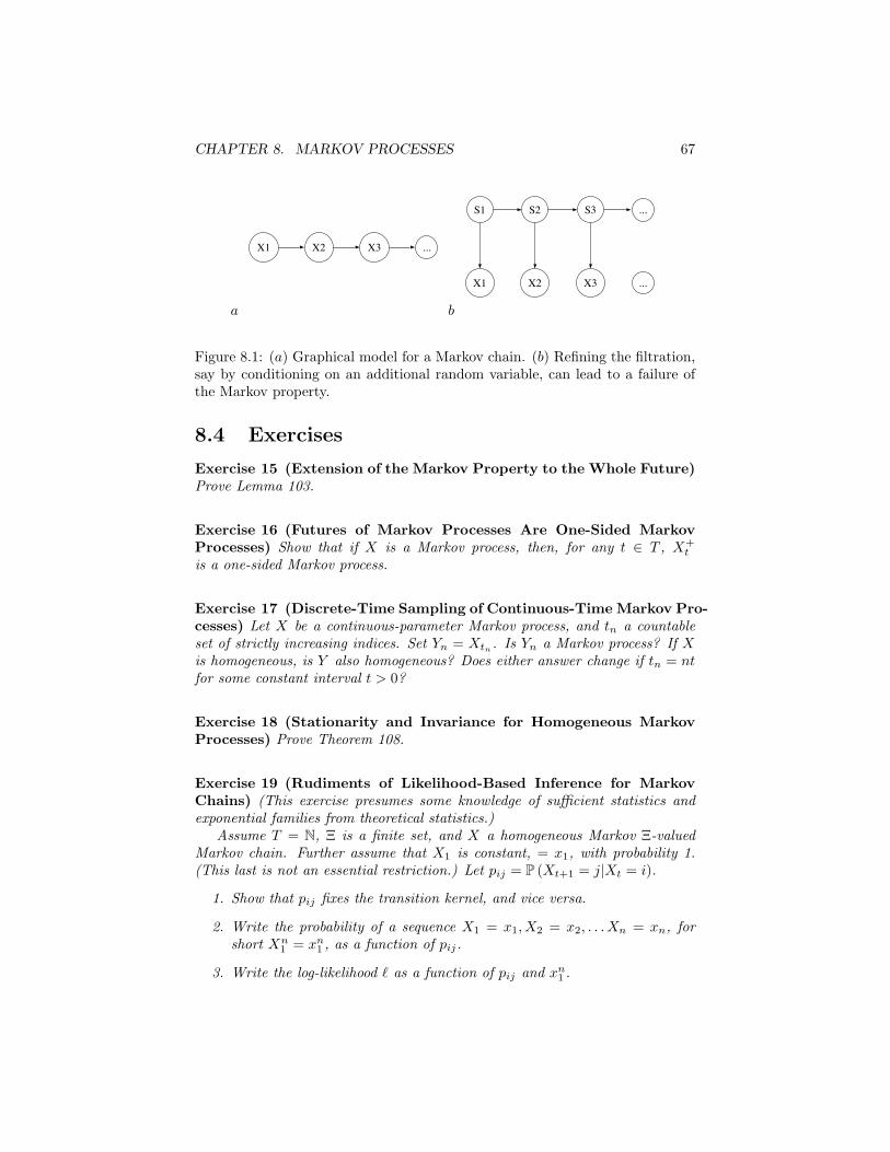
CHAPTER 8. MARKOV PROCESSES 67
a
X1 X2 X3 ...
b
S1
X1
S2
X2
S3
X3
...
...
Figure 8.1: (a) Graphical model for a Markov chain. (b) Refining the filtration,say by conditioning on an additional random variable, can lead to a failure ofthe Markov property.
8.4 Exercises
Exercise 15 (Extension of the Markov Property to the Whole Future)Prove Lemma 103.
Exercise 16 (Futures of Markov Processes Are One-Sided MarkovProcesses) Show that if X is a Markov process, then, for any t ∈ T , X+
t
is a one-sided Markov process.
Exercise 17 (Discrete-Time Sampling of Continuous-Time Markov Pro-cesses) Let X be a continuous-parameter Markov process, and tn a countableset of strictly increasing indices. Set Yn = Xtn . Is Yn a Markov process? If Xis homogeneous, is Y also homogeneous? Does either answer change if tn = ntfor some constant interval t > 0?
Exercise 18 (Stationarity and Invariance for Homogeneous MarkovProcesses) Prove Theorem 108.
Exercise 19 (Rudiments of Likelihood-Based Inference for MarkovChains) (This exercise presumes some knowledge of sufficient statistics andexponential families from theoretical statistics.)
Assume T = N, Ξ is a finite set, and X a homogeneous Markov Ξ-valuedMarkov chain. Further assume that X1 is constant, = x1, with probability 1.(This last is not an essential restriction.) Let pij = P (Xt+1 = j|Xt = i).
1. Show that pij fixes the transition kernel, and vice versa.
2. Write the probability of a sequence X1 = x1, X2 = x2, . . . Xn = xn, forshort Xn
1 = xn1 , as a function of pij.
3. Write the log-likelihood ` as a function of pij and xn1 .
CHAPTER 8. MARKOV PROCESSES 68
4. Define nij to be the number of times t such that xt = i and xt+1 = j.Similarly define ni as the number of times t such that xt = i. Write thelog-likelihood as a function of pij and nij.
5. Show that the nij are sufficient statistics for the parameters pij.
6. Show that the distribution has the form of a canonical exponential family,with sufficient statistics nij, by finding the natural parameters. (Hint: thenatural parameters are transformations of the pij.) Is the family of fullrank?
7. Find the maximum likelihood estimators, for either the pij parameters orfor the natural parameters. (Hint: Use Lagrange multipliers to enforce theconstraint
∑j nij = ni.)
The classic book by Billingsley (1961) remains an excellent source on statisticalinference for Markov chains and related processes.
Exercise 20 (Implementing the MLE for a Simple Markov Chain)(This exercise continues the previous one.)
Set Ξ = 0, 1, x1 = 0, and
p0 =[
0.75 0.250.25 0.75
]1. Write a program to simulate sample paths from this Markov chain.
2. Write a program to calculate the maximum likelihood estimate p of thetransition matrix from a sample path.
3. Calculate 2(`(p) − `(p0)) for many independent sample paths of lengthn. What happens to the distribution as n → ∞? (Hint: see Billingsley(1961), Theorem 2.2.)
Exercise 21 (The Markov Property and Conditional Independencefrom the Immediate Past) Let X be a Ξ-valued discrete-parameter randomprocess. Suppose that, for all t, Xt−1 |= Xt+1|Xt. Either prove that X is aMarkov process, or provide a counter-example. You may assume that Ξ is aBorel space if you find that helpful.
Exercise 22 (Higher-Order Markov Processes) A discrete-time process Xis a kth order Markov process with respect to a filtration Ft when
Xt+1 |= Ft|σ(Xt, Xt−1, . . . Xt−k+1) (8.23)
for some finite integer k. For any Ξ-valued discrete-time process X, define the k-block process Y (k) as the Ξk-valued process where Y (k)
t = (Xt, Xt+1, . . . Xt+k−1).
CHAPTER 8. MARKOV PROCESSES 69
1. Prove that if X is Markovian to order k, it is Markovian to any orderl > k. (For this reason, saying that X is a kth order Markov processconventionally means that k is the smallest order at which Eq. 8.23 holds.)
2. Prove that X is kth-order Markovian if and only if Y (k) is Markovian.
The second result shows that studying on the theory of first-order Markov pro-cesses involves no essential loss of generality. For a test of the hypothesis thatX is Markovian of order k against the alternative that is Markovian of orderl > k, see Billingsley (1961). For recent work on estimating the order of aMarkov process, assuming it is Markovian to some finite order, see the elegantpaper by Peres and Shields (2005).
Exercise 23 (AR(1) Models) A first-order autoregressive model, or AR(1)model, is a real-valued discrete-time process defined by an evolution equation ofthe form
X(t) = a0 + a1X(t− 1) + ε(t)
where the innovations ε(t) are independent and identically distributed, and in-dependent of X(0). A pth-order autoregressive model, or AR(p) model, is cor-respondingly defined by
X(t) = a0 +p∑i=1
aiX(t− i) + ε(t)
Finally an AR(p) model in state-space form is an Rp-valued process defined by
~Y (t) = a0~e1 +
a1 a2 . . . ap−1 ap1 0 . . . 0 00 1 . . . 0 0...
......
......
0 0 . . . 1 0
~Y (t− 1) + ε(t)~e1
where ~e1 is the unit vector along the first coordinate axis.
1. Prove that AR(1) models are Markov for all choices of a0 and a1, and alldistributions of X(0) and ε.
2. Give an explicit form for the transition kernel of an AR(1) in terms ofthe distribution of ε.
3. Are AR(p) models Markovian when p > 1? Prove or give a counter-example.
4. Prove that ~Y is a Markov process, without using Exercise 22. (Hint: Whatis the relationship between Yi(t) and X(t− i+ 1)?)
Chapter 9
AlternativeCharacterizations ofMarkov Processes
This lecture introduces two ways of characterizing Markov pro-cesses other than through their transition probabilities.
Section 9.1 describes discrete-parameter Markov processes as trans-formations of sequences of IID uniform variables.
Section 9.2 describes Markov processes in terms of measure-preserving transformations (Markov operators), and shows this isequivalent to the transition-probability view.
9.1 Markov Sequences as Transduced Noise
A key theorem says that discrete-time Markov processes can be viewed as theresult of applying a certain kind of filter to pure noise.
Theorem 114 (Markov Sequences as Transduced Noise) Let X be a one-sided discrete-parameter process taking values in a Borel space Ξ. X is Markoviff there are measurable functions fn : Ξ× [0, 1] 7→ Ξ such that, for IID randomvariables Zn ∼ U(0, 1), all independent of X1, Xn+1 = fn(Xn, Zn) almostsurely. X is homogeneous iff fn = f for all n.
Proof: Kallenberg, Proposition 8.6, p. 145. Notice that, in order to get the“only if” direction to work, Kallenberg invokes what we have as Proposition 26,which is where the assumptions that Ξ is a Borel space comes in. You shouldverify that the “if” direction does not require this assumption.
Let us stick to the homogeneous case, and consider the function f in some-what more detail.
70
CHAPTER 9. MARKOV CHARACTERIZATIONS 71
In engineering or computer science, a transducer is an apparatus — really, afunction — which takes a stream of inputs of one kind and produces a streamof outputs of another kind.
Definition 115 (Transducer) A (deterministic) transducer is a sextuple 〈Σ,Υ,Ξ, f, h, s0〉where Σ, Υ and Ξ are, respectively, the state, input and output spaces, f : Σ×Ξ 7→ Σ is the state update function or state transition function, h : Σ×Υ 7→ Ξis the measurement or observation function, and s0 ∈ Σ is the starting state.(We shall assume both f and h are always measurable.) If h does not dependon its state argument, the transducer is memoryless. If f does not depend onits state argument, the transducer is without after-effect.
It should be clear that if a memoryless transducer is presented with IIDinputs, its output will be IID as well. What Theorem 114 says is that, ifwe have a transducer with memory (so that h depends on the state) but iswithout after-effect (so that f does not depend on the state), IID inputs willproduce Markovian outputs, and conversely any reasonable Markov process canbe represented in this way. Notice that if a transducer is without memory,we can replace it with an equivalent with a single state, and if it is withoutafter-effect, we can identify Σ and Ξ.
Notice also that the two functions f and h determine a transition func-tion where we use the input to update the state: g : Σ × Υ 7→ Σ, whereg(s, y) = f(s, h(s, y)). Thus, if the inputs are IID and uniformly distributed,then (Theorem 114) the successive states of the transducer are always Marko-vian. The question of which processes can be produced by noise-driven transduc-ers is this intimately bound up with the question of Markovian representations.While, as mentioned, quite general stochastic processes can be put in this form(Knight, 1975, 1992), it is not necessarily possible to do this with a finite in-ternal state space Σ, even when Ξ is finite. The distinction between finite andinfinite Σ is crucial to theoretical computer science, and we might come back toit later, but
Two issues suggest themselves in connection with this material. One iswhether, given a two-sided process, we can pull the same trick, and represent aMarkovian X as a transformation of an IID sequence extending into the infinitepast. (Remember that the theorem is for one-sided processes, and starts withan initial X1.) This is more subtle than it seems at first glance, or even than itseemed to Norbert Wiener when he first posed the question (Wiener, 1958); fora detailed discussion, see Rosenblatt (1971), and, for recent set of applications,Wu (2005). The other question is whether the same trick can be pulled incontinuous time; here much less is known.
CHAPTER 9. MARKOV CHARACTERIZATIONS 72
9.2 Time-Evolution (Markov) Operators
Let’s look again at the evolution of the one-dimensional distributions for aMarkov process:
νs = νtµt,s (9.1)
νs(B) =∫νt(dx)µt,s(x,B) (9.2)
The transition kernels define linear operators taking probability measures on Ξto probability measures on Ξ. This can be abstracted.
Definition 116 (Markov Operator on Measures) Take any measurablespace Ξ,X . A Markov operator on measures is an operator M which takesfinite measures on this space to other finite measures on this space such that
1. M is linear, i.e., for any a1, a2 ∈ [0, 1] and any two measures µ1, µ2,
M(a1µ1 + a2µ2) = a1Mµ1 + a2Mµ2 (9.3)
2. M is norm-preserving, i.e., Mµ(Ξ) = µ(Ξ).
(In particular P must take probability measures to probability measures.)
Definition 117 (Markov Operator on Densities) Take any probability spaceΞ,X , µ, and let L1 be as usual the class of all µ-integrable generalized functionson Ξ. A linear operator P : L1 7→ L1 is a Markov operator on densities when:
1. If f ≥ 0 (a.e. µ), Pf ≥ 0 (a.e. µ).
2. If f ≥ 0 (a.e. µ), ‖Pf‖ = ‖f‖.
By “a Markov operator” I will often mean a Markov operator on densities,with the reference measure µ being some suitable uniform distribution on Ξ.However, the general theory applies to operators on measures.
Lemma 118 (Markov Operators on Measures Induce Those on Densi-ties) Let M be a Markov operator on measures. If M takes measures absolutelycontinuous with respect to µ to measures absolutely continuous with respect toµ, i.e., it preserves domination by µ, then it induces an almost-unique Markovoperator P on densities with respect to µ.
Proof: Let f be a function which is in L1(µ) and is non-negative (µ-a.e.).If f ≥ 0 µ a.e., the set function νf (A) =
∫Af(x)dµ is a finite measure which
is absolutely continuous with respect to µ. (Why is it finite?) By hypothesis,then, Mνf is another finite measure which is absolutely continuous with respectto µ, and νf (Ξ) = Mνf (Ξ). Hence, by the Radon-Nikodym theorem, there is anL1(µ) function, call it Pf , such that Mνf (A) =
∫APf(x)dµ. (“Almost unique”
CHAPTER 9. MARKOV CHARACTERIZATIONS 73
refers to the possibility of replacing Pf with another version of dMνf/dµ.)In particular, Pf(x) ≥ 0 for µ-almost-all x, and so ‖Pf‖ =
∫Ξ|Pf(x)|dµ =
Mνf (Ξ) = νf (Ξ) =∫
Ξ|f(x)|dµ = ‖f‖. Finally, the linearity of the operator on
densities follows directly from the linearity of the operator on measures and thelinearity of integration. If f is sometimes negative, apply the reasoning aboveto f+ and f−, its positive and negative parts, and then use linearity again.
Recall from Definition 30 that, for an arbitrary kernel κ, κf(x) is defined as∫f(y)κ(x, dy). Applied to our transition kernels, this suggests another kind of
operator.
Definition 119 (Transition Operators) Take any measurable space Ξ,X ,and let B(Ξ) be the class of bounded measurable functions. An operator K :B(Ξ) 7→ B(Ξ) is a transition operator when:
1. K is linear
2. If f ≥ 0 (a.e. µ), Kf ≥ 0 (a.e. µ)
3. K1Ξ = 1Ξ.
4. If fn ↓ 0, then Kfn ↓ 0.
Definition 120 (L∞ Transition Operators) For a probability space Ξ,X , µ,an L∞-transition operator is an operator on L∞(µ) satisfying points (1)–(4) ofDefinition 119.
Note that every function in B(Ξ) is in L∞(µ) for each µ, so the definitionof an L∞ transition operator is actually stricter than that of a plain transitionoperator. This is unlike the case with Markov operators, where the L1 versionis weaker than the unrestricted version.
Lemma 121 (Kernels and Operators) Every probability kernel κ from Ξ toΞ induces a Markov operator M on measures,
Mν = νκ (9.4)
and every Markov operator M on measures induces a probability kernel κ,
κ(x,B) = Mδx(B) (9.5)
Similarly, every transition probability kernel induces a transition operator K onfunctions,
Kf(x) = κf(x) (9.6)
and every transition operator K induces a transition probability kernel,
κ(x,B) = K1B(x) (9.7)
CHAPTER 9. MARKOV CHARACTERIZATIONS 74
Proof: Exercise 24. Now we need some basic concepts from functional analysis; see, e.g., Kol-
mogorov and Fomin (1975) for background.
Definition 122 (Functional) A functional is a map g : V 7→ R, that is, areal-valued function of a function. A functional g is
• linear when g(af1 + bf2) = ag(f1) + bg(f2);
• continuous when fn → f implies g(fn)→ f ;
• bounded by M when |g(f)| ≤M for all f ∈ V ;
• bounded when it is bounded by M for some M ;
• non-negative when g(f) ≥ 0 for all f ;
etc.
Definition 123 (Conjugate or Adjoint Space) The conjugate space or ad-joint space of a vector space V is the space V † of its continuous linear function-als. For f ∈ V and g ∈ V †, 〈f, g〉 denotes g(f). This is sometimes called theinner product.
Proposition 124 (Conjugate Spaces are Vector Spaces) For every V , V †
is also a vector space.
Proposition 125 (Inner Product is Bilinear) For any a, b, c, d ∈ R, anyf1, f2 ∈ V and any g1, g2 ∈ V †,
〈af1 + bf2, cg1 + dg2〉 = ac〈f1, g1〉+ ad〈f1, g2〉+ bc〈f2, g1〉+ bd〈f2, g2〉 (9.8)
Proof: Follows from the fact that V † is a vector space, and each gi is alinear operator.
You are already familiar with an example of a conjugate space.
Example 126 (Vectors in Rn) The vector space Rn is self-conjugate. If g(~x)is a continuous linear function of ~x, then g(~x) =
∑ni=1 yixi for some real con-
stants yi, which means g(~x) = ~y · ~x.
Here is the simplest example where the conjugate space is not equal to theoriginal space.
Example 127 (Row and Column Vectors) The space of row vectors is con-jugate to the space of column vectors, since every continuous linear functionalof a column vector x takes the form of yTx for some other column vector y.
CHAPTER 9. MARKOV CHARACTERIZATIONS 75
Example 128 (Lp spaces) The function spaces Lp(µ) and Lq(µ) are conjugateto each other, when 1/p+ 1/q = 1, and the inner product is defined through
〈f, g〉 ≡∫fgdµ (9.9)
In particular, L1 and L∞ are conjugates.
Example 129 (Measures and Functions) The space of Cb(Ξ) of bounded,continuous functions on Ξ and the spaces M(Ξ,X ) of finite measures on Ξ areconjugates, with inner product
〈µ, f〉 =∫fdµ (9.10)
Definition 130 (Adjoint Operator) For conjugate spaces V and V †, theadjoint operator, O†, to an operator O on V is an operator on V † such that
〈Of, g〉 = 〈f,O†g〉 (9.11)
for all f ∈ V, g ∈ V †.
Proposition 131 (Adjoint of a Linear Operator) If O is a continuouslinear operator on V , then its adjoint O† exists and is linear.
Lemma 132 (Markov Operators on Densities and L∞ Transition Op-erators) Every Markov operator P on densities induces an L∞ transition op-erator U on essentially-bounded functions, and vice versa.
Proof: Exercise 25. Clearly, if κ is part of a transition kernel semi-group, then the collection of
induced Markov operators and transition operators also form semi-groups.
Theorem 133 (Transition operator semi-groups and Markov processes)Let X be a Markov process with transition kernels µt,s, and let Kt,s be the cor-responding semi-group of transition operators. Then for any f ∈ B(Ξ),
E [f(Xs)|Ft] = (Kt,sf)(Xt) (9.12)
Conversely, let X be any stochastic process, and let Kt,s be a semi-group oftransition operators such that Equation 9.12 is valid (a.s.). Then X is a Markovprocess.
CHAPTER 9. MARKOV CHARACTERIZATIONS 76
Proof: Exercise 26. Remark. The proof works because the expectations of all B(Ξ) functions
together determine a probability measure. (Recall that P (B) = E [1B ], andindicators are bounded everywhere.) If we knew of another collection of func-tions which also sufficed to determine a measure, then linear operators on thatcollection would work just as well, in the theorem, as do the transition oper-ators, which by definition apply to all of B(Ξ). In particular, it is sometimespossible to define operators only on much smaller, more restricted collections offunctions, which can have technical advantages. See Ethier and Kurtz (1986,ch. 4, sec. 1) for details.
The next two lemmas are useful in establishing asymptotic results.
Lemma 134 (Markov Operators are Contractions) For any Markov op-erator P and f ∈ L1,
‖Pf‖ ≤ ‖f‖ (9.13)
Proof (after Lasota and Mackey (1994, prop. 3.1.1, pp. 38–39)): First,notice that (Pf(x))+ ≤ Pf+(x), because
(Pf(x))+ = (Pf+ − Pf−)+ = max (0, Pf+ − Pf−) ≤ max (0, Pf+) = Pf+
Similarly (Pf(x))− ≤ Pf−(x). Therefore |Pf | ≤ P |f |, and then the statementfollows by integration.
Lemma 135 (Markov Operators Bring Distributions Closer) For anyMarkov operator, and any f, g ∈ L1, ‖Pnf − Png‖ is non-increasing.
Proof: By linearity, ‖Pnf −Png‖ = ‖Pn(f − g)‖. By the definition of Pn,‖Pn(f − g)‖ = ‖PPn−1(f − g)‖. By the contraction property (Lemma 134),‖PPn−1(f − g)‖ ≤ ‖Pn−1(f − g)‖ = ‖Pn−1f − Pn−1g‖ (by linearity again).
Theorem 136 (Invariant Measures Are Fixed Points) A probability mea-sure ν is invariant for a homogeneous Markov process iff it is a fixed point ofall the Markov operators, Mtν = ν.
Proof: Clear from the definitions!
9.3 Exercises
Exercise 24 (Kernels and Operators) Prove Lemma 121. Hints: 1. Youwill want to use the fact that 1A ∈ B(Ξ) for all measurable sets A. 2. In goingback and forth between transition kernels and transition operators, you may findProposition 32 helpful.
Exercise 25 (L1 and L∞) Prove Lemma 132.
CHAPTER 9. MARKOV CHARACTERIZATIONS 77
Exercise 26 (Operators and Expectations) Prove Theorem 133. Hint: inshowing that a collection of operators determines a Markov process, try usingmathematical induction on the finite-dimensional distributions.
Exercise 27 (Bayesian Updating as a Markov Process) Consider a sim-ple version of Bayesian learning, where the set of hypotheses Θ is finite, and,for each θ ∈ Θ, fθ(x) is a probability density on Ξ with respect to a commondominating measure, µ say, and the Ξ-valued data X1, X2, . . . are all IID, bothunder the hypotheses and in reality. Given a prior probability vector π0 on Θ,the posterior πn is defined via Bayes’s rule:
πn(θ) =π0(θ)
∏ni=1 fθ(Xi)∑
θ∈Θ π0(θ)∏ni=1 fθ(Xi)
1. Prove that the random sequence π1, π2, . . . is adapted to Ft if X isadapted.
2. Prove that the sequence of posterior distributions is Markovian with respectto its natural filtration.
3. Is this still a Markov process if X is not IID? If the hypotheses θ do notmodel X as IID?
4. When, if ever, is the Markov process homogeneous? (If it is sometimeshomogeneous, you may give either necessary or sufficient conditions, asyou find easier.)
Exercise 28 (More on Bayesian Updating) Consider a more complicatedversion of Bayesian updating. Let T be one-sided, H be a Θ-valued randomvariable, and Gt be any filtration. Assume that πt = L (H|Gt) is a regularconditional probability distribution on Θ for all t and all ω. As before, π0 is theprior. Prove that πt is Markovian with respect to Gt. (Hint: E [E [Y |Gt] |Gs] =E [X|Gs] a.s., when s ≤ t and Y ∈ L1 so the expectations exist.)
Chapter 10
Examples of MarkovProcesses
Section 10.1 looks at the evolution of densities under the actionof the logistic map; this shows how deterministic dynamical systemscan be brought under the sway of the theory we’ve developed forMarkov processes.
Section 10.2 finds the transition kernels for the Wiener process,as an example of how to manipulate such things.
Section 10.3 generalizes the Wiener process example to otherprocesses with stationary and independent increments, and in doingso uncovers connections to limits of sums of IID random variablesand to self-similarity.
10.1 Probability Densities in the Logistic Map
Let’s revisit the first part of Exercise 9, from the point of view of what we nowknow about Markov processes. The exercise asks us to show that the density
1
π√x(1−x)
is invariant under the action of the logistic map with a = 4.
Let’s write the mapping as F (x) = 4x (1− x). Solving a simple quadraticequation gives us the fact that F−1 (x) is the set
12
(1−√
1− x), 1
2
(1 +√
1− x)
.Notice, for later use, that the two solutions add up to 1. Notice also thatF−1 ([0, x]) =
[0, 1
2
(1−√
1− x)]∪[
12
(1 +√
1− x), 1]. Now we consider the
78
CHAPTER 10. MARKOV EXAMPLES 79
cumulative distribution function of Xn+1, P (Xn+1 ≤ x).
P (Xn+1 ≤ x)= P (Xn+1 ∈ [0, x]) (10.1)= P
(Xn ∈ F−1 ([0, x])
)(10.2)
= P(Xn ∈
[0,
12(1−√
1− x)]∪[
12(1 +√
1− x), 1])
(10.3)
=∫ 1
2 (1−√
1−x)
0
ρn (y) dy +∫ 1
12 (1+
√1−x)
ρn (y) dy (10.4)
where ρn is the density of Xn. So we have an integral equation for the evolutionof the density,∫ x
0
ρn+1 (y) dy =∫ 1
2 (1−√
1−x)
0
ρn (y) dy +∫ 1
12 (1+
√1−x)
ρn (y) dy (10.5)
This sort of integral equation is complicated to solve directly. Instead, takethe derivative of both sides with respect to x; we can do this through thefundamental theorem of calculus. On the left hand side, this will just giveρn+1 (x), the density we want.
ρn+1 (x) (10.6)
=d
dx
∫ 12 (1−
√1−x)
0
ρn (y) dy +d
dx
∫ 1
12 (1+
√1−x)
ρn (y) dy
= ρn
(12(1−√
1− x)) d
dx
(12(1−√
1− x))
(10.7)
−ρn(
12(1 +√
1− x)) d
dx
(12(1 +√
1− x))
=1
4√
1− x
(ρn
(12(1−√
1− x))
+ ρn
(12(1 +√
1− x)))
(10.8)
Notice that this defines a linear operator taking densities to densities. (Youshould verify the linearity.) In fact, this is a Markov operator, by the terms ofDefinition 117. Markov operators of this sort, derived from deterministic maps,are called Perron-Frobenius or Frobenius-Perron operators, and accordingly de-noted by P . Thus an invariant density is a ρ∗ such that ρ∗ = Pρ∗. All the
CHAPTER 10. MARKOV EXAMPLES 80
problem asks us to do is to verify that 1
π√x(1−x)
is such a solution.
ρ∗(
12(1−√
1− x))
(10.9)
=1π
(12(1−√
1− x)(
1−(
12(1−√
1− x))))−1/2
=1π
(12(1−√
1− x) 1
2(1 +√
1− x))−1/2
(10.10)
=2
π√x
(10.11)
Since ρ∗ (x) = ρ∗ (1− x), it follows that
Pρ∗ = 21
4√
1− xρ∗(
12(1−√
1− x))
(10.12)
=1
π√x (1− x)
(10.13)
= ρ∗ (10.14)
as desired.By Lemma 135, for any distribution ρ, ‖Pnρ − Pnρ∗‖ is a non-increasing
function of n. However, Pnρ∗ = ρ∗, so the iterates of any distribution, underthe map, approach the invariant distribution monotonically. It would be veryhandy if we could show that any initial distribution ρ eventually converged onρ∗, i.e. that ‖Pnρ − ρ∗‖ → 0. When we come to ergodic theory, we will seeconditions under which such distributional convergence holds, as it does for thelogistic map, and learn how such convergence in distribution is connected toboth pathwise convergence properties, and to the decay of correlations.
10.2 Transition Kernels and Evolution Opera-tors for the Wiener Process
We have previously defined the Wiener process (Examples 38 and 79) as thereal-valued process on R+ with the following properties:
1. W (0) = 0;
2. For any three times t1 ≤ t2 ≤ t3, W (t3) −W (t2) |= W (t2) −W (t1) (inde-pendent increments);
3. For any two times t1 ≤ t2, W (t2) − W (t1) ∼ N (0, t2 − t1) (Gaussianincrements);
4. Continuous sample paths (in the sense of Definition 73).
CHAPTER 10. MARKOV EXAMPLES 81
In Exercise 5, you showed that a process satisfying points (1)–(3) aboveexists. To show that any such process has a version with continuous samplepaths, invoke Theorem 97 (Exercise 31). Here, however, we will show that itis a homogeneous Markov process, and find both the transition kernels andthe evolution operators. Markovianity follows from the independent incrementsproperty (2), while homogeneity and the form of the transition operators comesfrom the Gaussian assumption (3).
First, here’s how the Gaussian increments property gives us the transitionprobabilities:
P (W (t2) ∈ B|W (t1) = w1) = P (W (t2)−W (t1) ∈ B − w1) (10.15)
=∫B−w1
du1√
2π(t2 − t1)e− u2
2(t2−t1)(10.16)
=∫B
dw21√
2π(t2 − t1)e− (w2−w1)2
2(t2−t1) (10.17)
≡ µt1,t2(w1, B) (10.18)
Since this evidently depends only on t2 − t1, and not the individual times, theprocess is homogeneous. Now, assuming homogeneity, we can find the time-evolution operators for well-behaved observables:
Ktf(w) = E [f(Wt + s)|Ws = w] (10.19)
=∫f(u)µt(w, du) (10.20)
=∫f(u)
1√2πt
e−(u−w)2
2t du (10.21)
= E[f(w +
√tZ)]
(10.22)
where Z is a standard Gaussian random variable independent of Ws.To show that W (t) is a Markov process, we must show that, for any finite
collection of times t1 ≤ t2 ≤ . . . ≤ tk,
L (Wt1 ,Wt2 , . . .Wtk) = µt1,t2µt2,t3 . . . µtk−1,tk (10.23)
Let’s just go through the k = 3 case, as the others are fundamentally similar,but with more notation. Notice that W (t3) − W (t1) = (W (t3) − W (t2)) +(W (t2)−W (t1)). Because increments are independent, then, W (t3)−W (t1) isthe sum of two independent random variables, W (t3)−W (t2) andW (t2)−W (t1).The distribution of W (t3) −W (t1) is then the convolution of distributions ofW (t3) −W (t2) and W (t2) −W (t1). Those are N (0, t3 − t2) and N (0, t2 − t1)respectively. The convolution of two Gaussian distributions is a third Gaus-sian, summing their parameters, so according to this argument, we must haveW (t3) −W (t1) ∼ N (0, t3 − t1). But this is precisely what we should have, bythe Gaussian-increments property. Since the trick we used above to get thetransition kernel from the increment distribution can be applied again, we con-clude that µt1,t2µt2,t3 = µt1,t3 . The same trick applies when k > 3. Therefore(Theorem 106), W (t) is a Markov process, with respect to its natural filtration.
CHAPTER 10. MARKOV EXAMPLES 82
10.3 Levy Processes and Limit Laws
Let’s think a bit more about the trick we’ve just pulled with the Wiener process.We wrote the time evolution operators in terms of a random variable,
Ktf(w) = E[f(w +
√tZ)]
(10.24)
Notice that√tZ ∼ N (0, t), i.e., it is the increment of the process over an interval
of time t. This can be generalized to other processes of a similar sort. Theseare one natural way of generalizing the idea of a sum of IID random variables.
Definition 137 (Processes with Stationary and Independent Incre-ments) A stochastic process X is a stationary, independent-increments process,or has stationary, independent increments when
1. The increments are independent; for any collection of indices t1 ≤ t2 ≤. . . ≤ tk, with k finite, the increments X(ti) − X(ti−1) are all jointlyindependent.
2. The increments are stationary; for any τ > 0,
L (X(t2)−X(t1), X(t3)−X(t2), . . . X(tk)−X(tk−1)) (10.25)= L (X(t2 + τ)−X(t1 + τ), X(t3 + τ)−X(t2 + τ), . . . X(tk + τ)−X(tk−1 + τ))
Definition 138 (Levy Processes) A Levy process is a process with station-ary and independent increments and cadlag sample paths, which start at zero,X(0) = 0.
Example 139 (Wiener Process is Levy) The Wiener process is a Levyprocess (since it has not just cadlag but continuous sample paths).
Example 140 (Poisson Counting Process) The Poisson counting processwith intensity λ is the integer-valued process N on R+ where N(0) = 0, N(t) ∼Poisson(λt), and independent increments. It defines a Poisson point process(in the sense of Example 20) by assigning the interval [0, t] the measure N(t),the measure extending to other Borel sets in the usual way. Conversely, anyPoisson process defines a counting process in this sense. N can be shown to becontinuous in probability, and so, via Theorem 96, to have a cadlag modification.(Exercise 33.) This is a Levy process.
It is not uncommon to see people writing just “processes with independentincrements” when they mean “stationary and independent increments”.
Theorem 141 (Processes with Stationary Independent Increments areMarkovian) Any process with stationary, independent increments is Markovianwith respect to its natural filtration, and homogeneous in time.
CHAPTER 10. MARKOV EXAMPLES 83
Proof: The joint distribution for any finite collection of times factors intoa product of incremental distributions:
L (X(t1), X(t2), . . . X(tk)) (10.26)= L (X(t1))L (X(t2)−X(t1)) . . .L (X(tk)−X(tk−1))
Define µt(x,B) = P (X(t1 + t)−X(t1) + x ∈ B). This is a probability ker-nel. Moreover, it satisfies the semi-group property, since X(t3) − X(t1) =X(t3) − X(t2) + X(t2) + X(t1) (and similarly for more indices). Thus theµt, so defined, are transition probability kernels (Definition 105). By Theorem106, X is Markovian with respect to its natural filtration.
Remark: The assumption that the increments are stationary is not necessaryto prove Markovianity. What property of X does it then deliver?
Theorem 142 (Time-Evolution Operators of Processes with Station-ary, Independent Increments) If X has stationary and independent incre-ments, then its time-evolution operators Kt are given by
Ktf(x) = E [f(x+ Zt)] (10.27)
where L (Zt) = L (X(t)−X(0)), the increment from 0 to t.
Proof: Exactly parallel to the Wiener process case.
Ktf(x) = E [f(Xt)|F0] (10.28)= E [f(Xt)|X0 = x] (10.29)
=∫f(y)µt(x, dy) (10.30)
Since µt(x,B) = P (X(t1 + t)−X(t1) + x ∈ B), the theorem follows. Notice that so far everything has applied equally to discrete or to continuous
time. For discrete time, we can chose the distribution of increments over a singletime-step, L (X(1)−X(0)), to be essentially whatever we like; stationarity andindependence then determine the distribution of all other increments. For con-tinuous time, however, our choices are more constrained, and in an interestingway.
By the semi-group property of the time-evolution operators, we must haveKsKt = Kt+s for all times s and t. Applying Theorem 142, it must be the casethat
Kt+sf(x) = E [f(x+ Zt+s)] (10.31)= KsE [f(x+ Zt)] (10.32)= E [f(x+ Zs + Zt)] (10.33)
where Zs |= Zt. That is, the distribution of Zt+s must be the convolution ofthe distributions of Zt and Zs. Let us in particular pick s = t; this impliesL (Z2t) = L (Zt) ? L (Zt), where ? indicates convolution. Writing νt for L (Zt),
CHAPTER 10. MARKOV EXAMPLES 84
another way to phrase our conclusion is that νt = νt/2 ? νt/2. Clearly, thisargument could be generalized to relate νt to νt/n for any n:
νt = ν?nt/n (10.34)
where the superscript ?n indicates the n-fold convolution of the distributionwith itself. Equivalently, for each t, and for all n,
Ztd=
n∑i=1
Di (10.35)
where the IID Di ∼ νt/n. This is a very curious-looking property with a name.
Definition 143 (Infinitely-Divisible Distributions and Random Vari-ables) A probability distribution ν is infinitely divisible when, for each n, thereexists a νn such that ν = ν?nn . A random variable Z is infinitely divisible when,for each n, there are n IID random variables D(n)
i such that Z d=∑iD
(n)i , i.e.,
when its distribution is infinitely divisible.
Clearly, if ν is an infinitely divisible distribution, then it can be obtained asthe limiting distribution of a sum of IID random variables D(n)
i . (To converge,the individual terms must be going to zero in probability as n grows.) Moreremarkably, the converse is also true:
Proposition 144 (Limiting Distributions Are Infinitely Divisible) If νis the limiting distribution of a sequence of IID sums, then it is an infinitely-divisible distribution.
Proof: See, for instance, Kallenberg (2002, Theorem 15.12). Remark: This should not be obvious. If we take larger and larger sums of
(centered, standardized) IID Bernoulli variables, we obtain a Gaussian as thelimiting distribution, but at no time is the Gaussian the distribution of any ofthe finite sums. That is, the IID sums in the definition of infinite divisibilityare not necessarily at all the same as those in the proposition.
Theorem 145 (Infinitely Divisible Distributions and Stationary In-dependent Increments) If X is a process with stationary and independentincrements, then for all t, X(t)−X(0) is infinitely divisible.
Proof: See the remarks before the definition of infinite divisibility.
Corollary 146 (Infinitely Divisible Distributions and Levy Processes)If ν is an infinitely divisible distribution, there exists a Levy process whereX(1) ∼ ν, and this determines the other distributions.
Proof: If X(1) ∼ ν, then by Eq. 10.34, X(n) ∼ ν∗n for all integer n.Conversely, the distribution of X(1/n) is also fixed, since ν = L (X(1/n))∗n,which means that the characteristic function of ν is equal to the nth power of
CHAPTER 10. MARKOV EXAMPLES 85
that of X(1/n); inverting the latter then gives the desired distribution. Becauseincrements are independent, X(n+1/m) d= X(n)+X(1/m), hence L (X(1)) fixesthe increment distribution for all rational time-intervals. By continuity, however,this also fixes it for time intervals of any length. Since the distribution ofincrements and the conditionX(0) = 0 fix the finite-dimensional distributions, itremains only to show that the process is cadlag, which can be done by observingthat it is continuous in probability, and then using Theorem 96.
We have established a correspondence between the limiting distributions ofIID sums, and processes with stationary independent increments. There aremany possible applications of this correspondence; one is to reduce problemsabout limits of IID sums to problems about certain sorts of Markov process,and vice versa. Another is to relate discrete and continuous time processes. For0 ≤ t ≤ 1, set
X(n)t =
1√n
bntc∑i=0
Yi (10.36)
where Y0 = 0 but otherwise the Yi are IID with mean 0 and variance 1. Theneach X(n) is a Markov process in discrete time, with stationary, independentincrements, and its time-evolution operator is
Knf(x) = E
fx+
1√n
[nt]∑i=1
Yi
(10.37)
As n grows, the normalized sum approaches√tZ, with Z a standard Gaussian
random variable. (Where does the√t come from?) Since the time-evolution
operators determine the finite-dimensional distributions of a Markov process(Theorem 133), this suggests that in some sense X(n) should be convergingin distribution on the Wiener process W . This is in fact true, but we willhave to go deeper into the structure of the operators concerned before we canmake it precise, as a first form of the functional central limit theorem. Justas the infinitely divisible distributions are the limits of IID sums, processeswith stationary and independent increments are the limits of the correspondingrandom walks.
There is a yet further sense which the Gaussian distribution is a special kindof limiting distribution, which is reflected in another curious property of theWiener process. Gaussian random variables are not only infinitely divisible, butthey can be additively decomposed into more Gaussians. Distributions whichcan be infinitely divided into others of the same kind will be called “stable”(under convolution or averaging). “Of the same kind” isn’t very mathematical;here is a more precise expression of the idea.
Definition 147 (Self-similarity) A process is self-similar if, for all t, thereexists a measurable h(t), the scaling function, such that h(t)X(1) d= X(t).
CHAPTER 10. MARKOV EXAMPLES 86
Definition 148 (Stable Distributions) A distribution ν is stable if, for anyLevy process X where X(1) ∼ ν, X is self-similar.
Theorem 149 (Scaling in Stable Levy Processes) In a self-similar Levyprocess, the scaling function h(t) must take the form tα for some real α, theindex of stability.
Proof: Exercise 35. It turns out that there are analogs to the functional central limit theorem
for a broad range of self-similar processes, especially ones with stable incrementdistributions; Embrechts and Maejima (2002) is a good short introduction tothis topic, and some of its statistical implications.
10.4 Exercises
Exercise 29 (Wiener Process with Constant Drift) Consider a processX(0) which, like the Wiener process, has X(0) = 0 and independent increments,but where X(t2) −X(t1) ∼ N (a(t2 − t1), σ2(t2 − t1)). a is called the drift rateand σ2 the diffusion constant. Show that X(t) is a Markov process, followingthe argument for the standard Wiener process (a = 0, σ2 = 1) above. Do suchprocesses have continuous modifications for all (finite) choices of a and σ2? Ifso, prove it; if not, give at least one counter-example.
Exercise 30 (Perron-Frobenius Operators) Verify that P defined in thesection on the logistic map above is a Markov operator.
Exercise 31 (Continuity of the Wiener Process) Show that the Wienerprocess has continuous sample paths, using its finite-dimensional distributionsand Theorem 97.
Exercise 32 (Independent Increments with Respect to a Filtration)Let X be adapted to a filtration Ft. Then X has independent incrementswith respect to Ft when Xt − Xs is independent of Fs for all s ≤ t. Showthat X is Markovian with respect to Ft, by analogy with Theorem 141.
Exercise 33 (Poisson Counting Process) Consider the Poisson countingprocess N of Example 140.
1. Prove that N is continuous in probability.
2. Prove that N has a cadlag modification. Hint: Theorem 96 is one way,but there are others.
CHAPTER 10. MARKOV EXAMPLES 87
Exercise 34 (Poisson Distribution is Infinitely Divisible) Prove, directlyfrom the definition, that every Poisson distribution is infinitely divisible. Whatis the corresponding stationary, independent-increment process?
Exercise 35 (Self-Similarity in Levy Processes) Prove Theorem 149.
Exercise 36 (Gaussian Stability) Find the index of stability a standard Gaus-sian distribution.
Exercise 37 (Poissonian Stability?) Is the standard Poisson distributionstable? If so, prove it, and find the index of stability. If not, prove that it isnot.
Exercise 38 (Lamperti Transformation) Prove Lamperti’s Theorem: If Yis a strictly stationary process and α > 0, then X(t) = tαY (log t) is self-similar,and if X is self-similar with index of stability α, then Y (t) = e−αtX(et) isstrictly stationary. These operations are called the Lamperti transformations,after Lamperti (1962).
Chapter 11
Generators of MarkovProcesses
This lecture is concerned with the infinitessimal generator of aMarkov process, and the sense in which we are able to write the evo-lution operators of a homogeneous Markov process as exponentialsof their generator.
Take our favorite continuous-time homogeneous Markov process, and con-sider its semi-group of time-evolution operators Kt. They obey the relationshipKt+s = KtKs. That is, composition of the operators corresponds to addition oftheir parameters, and vice versa. This is reminiscent of the exponential func-tions on the reals, where, for any k ∈ R, k(t+s) = ktks. In the discrete-parametercase, in fact, Kt = (K1)t, where integer powers of operators are defined in theobvious way, through iterated composition, i.e., K2f = K (Kf). It wouldbe nice if we could extend this analogy to continuous-parameter Markov pro-cesses. One approach which suggests itself is to notice that, for any k, there’sanother real number g such that kt = etg, and that etg has a nice representationinvolving integer powers of g:
etg =∞∑i=0
(tg)i
i!
The strategy this suggests is to look for some other operator G such that
Kt = etG ≡∞∑i=0
tiGi
i!
Such an operator G is called the generator of the process, and the purpose of thischapter is to work out the conditions under which this analogy can be carriedthrough.
In the exponential function case, we notice that g can be extracted by takingthe derivative at zero: d
dtetg∣∣t=0
= g. This suggests the following definition.
88
CHAPTER 11. GENERATORS 89
Definition 150 (Infinitessimal Generator) Let Kt be a continuous-parametersemi-group of linear operators on L, where L is a normed linear vector space,e.g., Lp for some 1 ≤ p ≤ ∞. Say that a function f ∈ L belongs to Dom(G) ifthe limit
limh↓0
Khf −K0f
h≡ Gf (11.1)
exists in an L-norm sense (Definition 151). The operator G defined through Eq.11.1 is called the infinitessimal generator of the semi-group Kt.
Definition 151 (Limit in the L-norm sense) Let L be a normed vectorspace. We say that a sequence of elements fn ∈ L has a limit f in L when
limn→∞
‖fn − f‖ = 0 (11.2)
This definition extends in the natural way to continuously-indexed collections ofelements.
Lemma 152 (Generators are Linear) For every semi-group of homogeneoustransition operators Kt, the generator G is a linear operator.
Proof: Exercise 39.
Lemma 153 (Invariant Distributions of a Semi-group Belong to theNull Space of Its Generator) If ν is an invariant distribution of a semi-groupof Markov operators Mt with generator G, then Gν = 0.
Proof: Since ν is invariant, Mtν = ν for all t (Theorem 136). HenceMtν − ν = Mtν −M0ν = 0, so, applying the definition of the generator (Eq.11.1), Gν = 0.
Remark: The converse assertion, that Gν = 0 implies ν is invariant underMt, requires extra conditions.
There is a conjugate version of this lemma.
Lemma 154 (Invariant Distributions and the Generator of the Time-Evolution Semigroup) If ν is an invariant distribution of a Markov process,and the time-evolution semi-group Kt is generated by G, then, ∀f ∈ Dom(G),νGf = 0.
Proof: Since ν is invariant, νKt = ν for all t, hence νKtf = νf for allt ≥ 0 and all f . Since taking expectations with respect to a measure is a linearoperator, ν(Ktf − f) = 0, and obviously then (Eq. 11.1) νGf = 0.
Remark: Once again, νGf = 0 for all f is not enough, in itself, to show thatν is an invariant measure.
You will usually see the definition of the generator written with f insteadof K0f , but I chose this way of doing it to emphasize that G is, basically,
CHAPTER 11. GENERATORS 90
the derivative at zero, that G = dK/dt|t=0. Recall, from calculus, that theexponential function can kt be defined by the fact that d
dtkt ∝ kt (and e can
be defined as the k such that the constant of proportionality is 1). As part ofour program, we will want to extend this differential point of view. The nextlemma builds towards it, by showing that if f ∈ Dom(G), then Ktf is too.
Lemma 155 (Operators in a Semi-group Commute with Its Genera-tor) If G is the generator of the semi-group Kt, and f is in the domain of G,then Kt and G commute, for all t:
KtGf = limt′→t
Kt′f −Ktf
t′ − t(11.3)
= GKtf (11.4)
Proof: Exercise 40.
Definition 156 (Time Derivative in Function Space) For every t ∈ T , letu(t, x) be a function in L. When the limit
u′(t0, x) = limt→t0
u(t, x)− u(t0, x)t− t0
(11.5)
exists in the L sense, then we say that u′(t0) is the time derivative or strongderivative of u(t) at t0.
Lemma 157 (Generators and Derivatives at Zero) Let Kt be a homo-geneous semi-group of operators with generator G. Let u(t) = Ktf for somef ∈ Dom(G). Then u(t) is differentiable at t = 0, and its derivative there isGf .
Proof: Obvious from the definitions.
Theorem 158 (The Derivative of a Function Evolved by a Semi-Group)Let Kt be a homogeneous semi-group of operators with generator G, and letu(t, x) = (Ktf)(x), for fixed f ∈ Dom(G). Then u′(t) exists for all t, and isequal to Gu(t).
Proof: Since f ∈ Dom(G), KtGf exists, but then, by Lemma 155, KtGf =GKtf = Gu(t), so u(t) ∈ Dom(G) for all t. Now let’s consider the time deriva-tive of u(t) at some arbitrary t0, working from above:
(u(t)− u(t0)t− t0
=Kt−t0u(t0)− u(t0)
t− t0(11.6)
=Khu(t0)− u(t0)
h(11.7)
Taking the limit as h ↓ 0, we get that u′(t0) = Gu(t0), which exists, becauseu(t0) ∈ Dom(G).
CHAPTER 11. GENERATORS 91
Corollary 159 (Initial Value Problems in Function Space) u(t) = Ktf ,f ∈ Dom(G), solves the initial value problem u(0) = f , u′(t) = Gu(t).
Proof: Immediate from the theorem. Remark: Such initial value problems are sometimes called Cauchy problems,
especially when G takes the form of a differential operator.
Corollary 160 (Derivative of Conditional Expectations of a MarkovProcess) Let X be a homogeneous Markov process whose time-evolution op-erators are Kt, with generator G. If fDom(G), then its condition expectationE [f(Xs)|Xt] has strong derivative Gu(t).
Proof: An immediate application of the theorem.We are now almost ready to state the sense in which Kt is the result of
exponentiating G. This is given by the remarkable Hille-Yosida theorem, whichin turn involves a family of operators related to the time-evolution operators,the “resolvents”, again built by analogy to the exponential functions, and toLaplace transforms.
Recall that the Laplace transform of a function f : R 7→ R is another func-tion, f , defined by
f(λ) ≡∫ ∞
0
e−λtf(t)dt
for positive λ. Laplace transforms arise in many contexts (linear systems theory,integral equations, etc.), one of which is moment-generating functions in basicprobability theory. If Y is a real-valued random variable with probability lawP , then the moment-generating function is
MY (λ) ≡ E[eλY
]=∫eλydP =
∫eλyp(y)dy
when the density in the last expression exists. You may recall, from this context,that the distributions of well-behaved random variables are completely specifiedby their moment-generating functions; this is actually a special case of a moregeneral result about when functions are uniquely described by their Laplacetransforms, i.e., when f can be expressed uniquely in terms of f . This is im-portant to us, because it turns out that the Laplace transform, so to speak, of asemi-group of operators is better-behaved than the semi-group itself, and we’llwant to say when we can use the Laplace transform to recover the semi-group.
The analogy with exponential functions, again, is a key. Notice that, for anypositive constant λ, ∫ ∞
t=0
e−λtetgdt =1
λ− g(11.8)
from which we could recover g, as that value of λ for which the Laplace transformis singular. In our analogy, we will want to take the Laplace transform of thesemi-group. Just as f(λ) is another real number, the Laplace transform of asemi-group of operators is going to be another operator. We will want that tobe the inverse operator to λ−G.
CHAPTER 11. GENERATORS 92
Definition 161 (Resolvents) Given a continuous-parameter homogeneous semi-group Kt, for each λ > 0, the resolvent operator or resolvent Rλ is the Laplacetransform of Kt: for every f ∈ L,
(Rλf)(x) ≡∫ ∞t=0
e−λt(Ktf)(x)dt (11.9)
Remark 1: Think of Kt as a function from the real numbers to the linearoperators on L. Symbolically, its Laplace transform would be
∫∞0e−λtKtdt.
The equation above just fills in the content of that symbolic expression.Remark 2: The name “resolvent”, like some of the other ideas an termi-
nology of operator semi-groups, comes from the theory of integral equations;invariant densities (when they exist) are solutions of homogeneous linear Fred-holm integral equations of the second kind. Rather than pursue this connection,or even explain what that phrase means, I will refer you to the classic treatmentof integral equations by Courant and Hilbert (1953, ch. 3), which everyone elseseems to follow very closely.
Remark 3: When the function f is a value (loss, benefit, utility, ...) function,(Ktf)(x) is the expected value at time t when starting the process in state x.(Rλf)(x) can be thought of as the net present expected value when starting atx and applying a discount rate λ.
Definition 162 (Yosida Approximation of Operators) The Yosida ap-proximation to a semi-group Kt with generator G is given by
K(λ)t ≡ etG
(λ)(11.10)
G(λ) ≡ λ(λRλ − I) = λGRλ (11.11)
The domain of G(λ) is all of L, not just Dom(G).
Theorem 163 (Hille-Yosida Theorem) Let G be a linear operator on somelinear subspace D of L. G is the generator of a continuous semi-group of con-tractions Kt if and only if
1. D is dense in L;
2. For every f ∈ L and λ > 0, there exists a unique g ∈ D such that λg−Gg =f ;
3. For every g ∈ D and positive λ, ‖λg −Gg‖ ≥ λ‖g‖.
Under these conditions, the resolvents of Kt are given by Rλ = (λI−G)−1, andKt is the limit of the Yosida approximations as λ→∞:
Ktf = limλ→∞
Kλt f, ∀f ∈ L (11.12)
CHAPTER 11. GENERATORS 93
Proof: See Kallenberg, Theorem 19.11. Remark 1: Other good sources on the Hille-Yosida theorem include Ethier
and Kurtz (1986, sec. 1.2), and of course Hille’s own book (Hille, 1948, ch. XII).I have not read Yosida’s original work.
Remark 2: The point of condition (1) in the theorem is that for any f ∈ L,we can chose fn ∈ D such that fn → f . Then, even if Gf is not directly defined,Gfn exists for each n. Because G is linear and therefore continuous, Gfn goesto a limit, which we can chose to write as Gf . Similarly for G2, G3, etc. Thuswe can define etGf as
limn→∞
∞∑j=0
tjGjfnj!
assuming all of the sums inside the limit converge, which is yet to be shown.Remark 3: The point of condition (2) in the theorem is that, when it holds,
(λI −G)−1 is well-defined, i.e., there is an inverse to the operator λI−G. Thisis, recall, what we would like the resolvent to be, if the analogy with exponentialfunctions is to hold good.
Remark 4: If we start from the semi-group Kt and obtain its generator G, thetheorem tells us that it satisfies properties (1)–(3). If we start from an operatorG and see that it satsifies (1)–(3), the theorem tells us that it generates somesemi-group. It might seem, however, that it doesn’t tell us how to construct thatsemi-group, since the Yosida approximation involves the resolvent Rλ, which isdefined in terms of the semi-group, creating an air of circularity. In fact, whenwe start from G, we decree Rλ to be (λI −G)−1. The Yosida approximationsthen is defined in terms of G and λ alone.
Corollary 164 (Stochastic Approximation of Initial Value Problems)Let u(0) = f , u′(t) = Gu(t) be an initial value problem in L. Then a stochasticapproximation to u(t) can be founded by taking
u(t) =1n
n∑i=1
f(Xi(t)) (11.13)
where the Xi are independent copies of the Markov process corresponding to thesemi-group Kt generated by G, with initial condition Xi(0) = x.
Proof: Combine corollaries.
11.1 Exercises
Exercise 39 (Generators are Linear) Prove Lemma 152.
Exercise 40 (Semi-Groups Commute with Their Generators) ProveLemma 155.
CHAPTER 11. GENERATORS 94
1. Prove Equation 11.3, restricted to t′ ↓ t instead of t′ → t. Hint: Write Ttin terms of an integral over the corresponding transition kernel, and finda reason to exchange integration and limits.
2. Show that the limit as t′ ↑ t also exists, and is equal to the limit fromabove. Hint: Re-write the quotient inside the limit so it only involvespositive time-differences.
3. Prove Equation 11.4.
Exercise 41 (Generator of the Poisson Counting Process) Find the gen-erator of the time-evolution operators of the Poisson counting process (Example140).
Chapter 12
The Strong MarkovProperty and MartingaleProblems
Section 12.1 introduces the strong Markov property — indepen-dence of the past and future conditional on the state at random(optional) times. It includes an example of a Markov process whichis not strongly Markovian.
Section 12.2 describes “the martingale problem for Markov pro-cesses”, explains why it would be nice to solve the martingale prob-lem, and how solutions are strong Markov processes.
12.1 The Strong Markov Property
A process is Markovian, with respect to a filtration Ft, if for any fixed time t,the future of the process is independent of Ft given Xt. This is not necessarilythe case for a random time τ , because there could be subtle linkages betweenthe random time and the evolution of the process. If these can be ruled out, wehave a strong Markov process.
Definition 165 (Strongly Markovian at a Random Time) Let X be aMarkov process with respect to a filtration Ft, with transition kernels µt,s andevolution operators Kt,s. Let τ be an Ft-optional time which is almost surelyfinite. Then X is strongly Markovian at τ when either of the two following(equivalent) conditions hold
P (Xt+τ ∈ B|Fτ ) = µτ,τ+t(Xτ , B) (12.1)E [f(Xτ+t)|Fτ ] = (Kτ,τ+tf)(Xτ ) (12.2)
for all t ≥ 0, B ∈ X and bounded measurable functions f .
95
CHAPTER 12. STRONG MARKOV, MARTINGALES 96
Definition 166 (Strong Markov Property) If X is Markovian with respectto Ft, and strongly Markovian at every Ft-optional time which is almostsurely finite, then it is a strong Markov process with respect to Ft.
If the index set T is discrete, then the strong Markov property is implied bythe ordinary Markov property (Definition 102). If time is continuous, this is notnecessarily the case. It is generally true that, if X is Markov and τ takes on onlycountably many values, X is strongly Markov at τ (Exercise 42). In continuoustime, however, the Markov property does not imply the strong Markov property.
Example 167 (A Markov Process Which Is Not Strongly Markovian)(After Fristedt and Gray (1997, pp. 626–627).) We will construct an R2-valuedMarkov process on [0,∞) which is not strongly Markovian. Begin by definingthe following map from R to R2:
f(w) =
(w, 0) w ≤ 0(sinw, 1− cosw) 0 < w < 2π(w − 2π, 0) w ≥ 2π
(12.3)
When w is less than zero or above 2π, f(w) moves along the x axis of the plane;in between, it moves along a circle of radius 1, centered at (0, 1), which it entersand leaves at the origin. Notice that f is invertible everywhere except at theorigin, which is ambiguous between w = 0 and w = 2π.
Let X(t) = f(W (t) + π), where W (t) is a standard Wiener process. Atall t, P (W (t) + π = 0) = P (W (t) + π = 2π) = 0, so, with probability 1, X(t)can be inverted to get W (t). Since W (t) is a Markov process, it follows thatP (X(t+ h) ∈ B|X(t) = x) = P
(X(t+ h) ∈ B|FXt
)almost surely, i.e., X is
Markov. Now consider τ = inftX(t) = (0, 0), the hitting time of the origin.This is clearly an FX-optional time, and equally clearly almost surely finite,because, with probability 1, W (t) will leave the interval (−π, π) within a finitetime. But, equally clearly, the future behavior of X will be very different if it hitsthe origin because W = π or because W = −π, which cannot be determined justfrom X. Hence, there is at least one optional time at which X is not stronglyMarkovian, so X is not a strong Markov process.
Since we often want to condition on the state of the process at random times,we would like to find conditions under which a process is strongly Markovianfor all optional times.
12.2 Martingale Problems
One approach to getting strong Markov processes is through martingales, andmore specifically through what is known as the martingale problem.
Notice the following consequence of Theorem 158:
Ktf(x)− f(x) =∫ t
0
KsGf(x)ds (12.4)
CHAPTER 12. STRONG MARKOV, MARTINGALES 97
for any t ≥ 0 and f ∈ Dom(G). The relationship between Ktf and the condi-tional expectation of f suggests the following definition.
Definition 168 (Martingale Problem) Let Ξ be a Polish space, D a classof bounded, continuous, real-valued functions on Ξ, and G an operator from Dto bounded, measurable functions on Ξ. A Ξ-valued stochastic process on R+ isa solution to the martingale problem for G and D if, for all f ∈ D,
f(Xt)−∫ t
0
Gf(Xs)ds (12.5)
is a martingale with respect toFXt
, the natural filtration of X.
Proposition 169 (Cadlag Nature of Functions in Martingale Prob-lems) Suppose X is a cadlag solution to the martingale problem for G,D. Thenfor any f ∈ D, the stochastic process given by Eq. 12.5 is also cadlag.
Proof: Follows from the assumption that f is continuous.
Lemma 170 (Alternate Formulation of Martingale Problem) X is asolution to the martingale problem for G,D if and only if, for all t, s ≥ 0,
E[f(Xt+s)|FXt
]−E
[∫ t+s
t
Gf(Xu)du|FXt]
= f(Xt) (12.6)
Proof: Take the definition of a martingale and re-arrange the terms in Eq.12.5.
Martingale problems are important because of the two following theorems(which can both be refined considerably).
Theorem 171 (Markov Processes Solve Martingale Problems) Let Xbe a homogeneous Markov process with generator G and cadlag sample paths,and let D be the continuous functions in Dom(G). Then X solves the martingaleproblem for G,D.
Proof: Exercise 43.
Theorem 172 (Solutions to the Martingale Problem are Strongly Marko-vian) Suppose that for each x ∈ Ξ, there is a unique cadlag solution to themartingale problem for G,D such that X0 = x. Then the collection of thesesolutions is a homogeneous strong Markov family X, and the generator is equalto G on D.
Proof: Exercise 44. The main use of Theorem 171 is that it lets us prove convergence of some
functions of Markov processes, by showing that they can be cast into the form ofEq. 12.5, and then applying the martingale convergence devices. The other useis in conjunction with Theorem 172. We will often want to show that a sequence
CHAPTER 12. STRONG MARKOV, MARTINGALES 98
of Markov processes converges on a limit which is, itself, a Markov process. Oneapproach is to show that the terms in the sequence solve martingale problems(via Theorem 171), argue that then the limiting process does too, and finallyinvoke Theorem 172 to argue that the limiting process must itself be stronglyMarkovian. This is often much easier than showing directly that the limitingprocess is Markovian, much less strongly Markovian. Theorem 172 itself is oftena convenient way of showing that the strong Markov property holds.
12.3 Exercises
Exercise 42 (Strongly Markov at Discrete Times) Let X be a homoge-neous Markov process with respect to a filtration Ft and τ be an Ft-optionaltime. Prove that if P (τ <∞) = 1, and τ takes on only countably many values,then X is strongly Markovian at τ . (Note: the requirement that X be homo-geneous can be lifted, but requires some more technical machinery I want toavoid.)
Exercise 43 (Markovian Solutions of the Martingale Problem) ProveTheorem 171. Hints: Use Lemma 170, bounded convergence, and Theorem 158.
Exercise 44 (Martingale Solutions are Strongly Markovian) Prove The-orem 172. Hint: use the Optional Sampling Theorem (from 36-752, or fromchapter 7 of Kallenberg).
Chapter 13
Feller Processes
Section 13.1 makes explicit the idea that the transition kernelsof a Markov process induce a kernel over sample paths, mostly tofix notation for later use.
Section 13.2 defines Feller processes, which link the cadlag andstrong Markov properties.
13.1 Markov Families
We have been fairly cavalier about the idea of a Markov process having a par-ticular initial state or initial distribution, basically relying on our familiaritywith these ideas from elementary courses on stochastic processes. For futurepurposes, however, it is helpful to bring this notions formally within our generalframework, and to fix some notation.
Definition 173 (Initial Distribution, Initial State) Let Ξ be a Borel spacewith σ-field X , T be a one-sided index set, and µt,s be a collection of Markoviantransition kernels on Ξ. Then the Markov process with initial distribution ν,Xν , is the Markov process whose finite-dimensional distributions are given bythe action of µt,s on ν. That is, for all 0 ≤ t1 ≤ t2 ≤ . . . ≤ tn,
Xν(0), Xν(t1), Xν(t2), . . . Xν(tn) ∼ ν ⊗ µ0,t1 ⊗ µt1,t2 ⊗ . . .⊗ µtn−1,tn(13.1)
If ν = δ(x − a), the delta distribution at a, then we write Xa and call it theMarkov process with initial state a.
The existence of processes with given initial distributions and initial statesis a trivial consequence of Theorem 106, our general existence result for Markovprocesses.
Lemma 174 (Kernel from Initial States to Paths) For every initial statex, there is a probability distribution Px on ΞT ,X T . The function Px(A) : Ξ ×X T → [0, 1] is a probability kernel.
99
CHAPTER 13. FELLER PROCESSES 100
Proof: The initial state fixes all the finite-dimensional distributions, sothe existence of the probability distribution follows from Theorem 23. The factthat Px(A) is a kernel is a straightforward application of the definition of kernels(Definition 30).
Definition 175 (Markov Family) The Markov family corresponding to agiven set of transition kernels µt,s is the collection of all Px.
That is, rather than thinking of a different stochastic process for each initialstate, we can simply think of different distributions over the path space ΞT .This suggests the following definition.
Definition 176 (Mixtures of Path Distributions (Mixed States)) Fora given initial distribution ν on Ξ, we define a distribution on the paths in aMarkov family as, ∀A ∈ X T ,
Pν(A) ≡∫
Ξ
Px(A)ν(dx) (13.2)
In physical contexts, we sometimes refer to distributions ν as mixed states,as opposed to the pure states x, because the path-space distributions induced bythe former are mixtures of the distributions induced by the latter. You shouldcheck that the distribution over paths given by a Markov process with initialdistribution ν, according to Definition 173, agrees with that given by Definition176.
13.2 Feller Processes
Working in the early 1950s, Feller showed that, by imposing very reasonableconditions on the semi-group of evolution operators corresponding to a homo-geneous Markov process, one could obtain very powerful results about the near-continuity of sample paths (namely, the existence of cadlag versions), about thestrong Markov property, etc. Ever since, processes with such nice semi-groupshave been known as Feller processes, or sometimes as Feller-Dynkin processes,in recognition of Dynkin’s work in extending Feller’s original approach. (Thisis also recognized in the name of Dynkin’s Formula, Theorem 195 below.) Un-fortunately, to first order there are as many definitions of a Feller semi-group asthere are books on Markov processes. I am going to try to follow Kallenberg asclosely as possible, because his version is pretty clearly motivated, and you’vealready got it.
Definition 177 (Feller Process) A continuous-time homogeneous Markovfamily X is a Feller process when, for all x ∈ Ξ,
∀t, y → x ⇒ Xy(t) d→ Xx(t) (13.3)
t→ 0 ⇒ Xx(t) P→ x (13.4)
CHAPTER 13. FELLER PROCESSES 101
Remark 1: The first property basically says that the dynamics are a smoothfunction of the initial state. Recall1 that if we have an ordinary differentialequation, dx/dt = f(x), and the function f is reasonably well-behaved, the ex-istence and uniqueness theorem tells us that there is a function x(t, x0) satisfyingthe equation, and such that x(0, x0) = x0. Moreover, x(t, x0) is a continuousfunction of x0 for all t. The first Feller property is one counterpart of this forstochastic processes. This is a very natural assumption to make in physical orsocial modeling, that very similar initial conditions should lead to very similardevelopments.
Remark 2: The second property imposes a certain amount of smoothnesson the trajectories themselves, and not just how they depend on the initialstate. It’s a pretty well-attested fact about the world that teleportation doesnot take place, and that its state changes in a reasonably continuous manner(“natura non facit saltum”, as they used to say). However, the second Fellerproperty does not require that the sample paths actually be continuous. Wewill see below that they are, in general, merely cadlag. So a certain limitedamount of teleportation, or salti, is allowed after all. We do not think thisactually happens, but it is a convenience when using a discrete set of states toapproximate a continuous variable.
In developing the theory of Feller processes, we will work mostly with thetime-evolution operators, acting on observables, rather than the Markov oper-ators, acting on distributions. This is traditional in this part of the theory, asit seems to let us get away with less technical machinery, in effect because thenorm supx |f(x)| is stronger than the norm
∫|f(x)|dx. Of course, because the
two kinds of operators are adjoint, you can work out everything for the Markovoperators, if you want to.
As usual, we warm up with some definitions. The first two apply to operatorson any normed linear space L, which norm we generically write as ‖ · ‖. Thesecond two apply specifically when L is a space of real-valued functions on someΞ, such as Lp, p from 1 to ∞ inclusive.
Definition 178 (Contraction Operator) An operator A is an L-contractionwhen ‖Af‖ ≤ ‖f‖.
Definition 179 (Strongly Continuous Semigroup) A semigroup of oper-ators At is strongly continuous in the L sense on a set of functions D when,∀f ∈ D
limt→0‖Atf − f‖ = 0 (13.5)
Definition 180 (Positive Operator) An operator A on a function space Lis positive when f ≥ 0 a.e. implies Af ≥ 0 a.e.
1Or read Arnol’d (1973), if memory fails you.
CHAPTER 13. FELLER PROCESSES 102
Definition 181 (Conservative Operator) An operator A is conservativewhen A1Ξ = 1Ξ.
In these terms, our earlier Markov operators are linear, positive, conservativecontractions, either on L1(µ) (for densities) or M(Ξ) (for measures).
Lemma 182 (Continuous semi-groups produce continuous paths infunction space) If At is a strongly continuous semigroup of linear contrac-tions on L, then, for each f ∈ L, Atf is a continuous function of t.
Proof: Continuity here means that limt′→t ‖At′f −At‖ = 0 — we are usingthe norm ‖ · ‖ to define our metric in function space. Consider first the limitfrom above:
‖At+hf −Atf‖ = ‖At(Ahf − f)‖ (13.6)≤ ‖|Ohf − f‖ (13.7)
since the operators are contractions. Because they are strongly continuous,‖Ahf − f‖ can be made smaller than any ε > 0 by taking h sufficiently small.Hence limh↓0At+hf exists and is Atf . Similarly, for the limit from below,
‖At−hf −Atf‖ = ‖Atf −At−hf‖ (13.8)= ‖At−h(Ahf − f)‖ (13.9)≤ ‖Ahf − f‖ (13.10)
using the contraction property again. So limh↓0At−hf = Atf , also, and we canjust say that limt′→tAt′f = Atf .
Remark: The result actually holds if we just assume strong continuity, with-out contraction, but the proof isn’t so pretty; see Ethier and Kurtz (1986, ch.1, corollary 1.2, p. 7).
There is one particular function space L we will find especially interesting.
Definition 183 (Continuous Functions Vanishing at Infinity) Let Ξ bea locally compact and separable metric space. The class of functions C0 willconsist of functions f : Ξ 7→ R which are continuous and for which ‖x‖ → ∞implies f(x)→ 0. The norm on C0 is supx |f(x)|.
Definition 184 (Feller Semigroup) A semigroup of linear, positive, conser-vative contraction operators Kt is a Feller semigroup if, for every f ∈ C0 andx ∈ Ξ, (Definition 533),
Ktf ∈ C0 (13.11)limt→0
Ktf(x) = f(x) (13.12)
Remark: Some authors omit the requirement that Kt be conservative. Also,this is just the homogeneous case, and one can define inhomogeneous Fellersemigroups. However, the homogeneous case will be plenty of work enough forus!
You can guess how Feller semi-groups relate to Feller processes.
CHAPTER 13. FELLER PROCESSES 103
Lemma 185 (The First Pair of Feller Properties) Eq. 13.11 holds if andonly if Eq. 13.3 does.
Proof: Exercise 46.
Lemma 186 (The Second Pair of Feller Properties) Eq. 13.12 holds ifand only if Eq. 13.4 does.
Proof: Exercise 47.
Theorem 187 (Feller Processes and Feller Semigroups) A Markov pro-cess is a Feller process if and only if its evolution operators form a Feller semi-group.
Proof: Combine Lemmas 185 and 186. Feller semigroups in continuous time have generators, as in Chapter 11. In
fact, the generator is especially useful for Feller semigroups, as seen by thistheorem.
Theorem 188 (Generator of a Feller Semigroup) If Kt and Ht are Fellersemigroups with generator G, then Kt = Ht.
Proof: Because Feller semigroups consist of contractions, the Hille-YosidaTheorem 163 applies, and, for every positive λ, the resolvent Rλ = (λI −G)−1.Hence, if Kt and Ht have the same generator, they have the same resolventoperators. But this means that, for every f ∈ C0 and x, Ktf(x) andHtf(x) havethe same Laplace transforms. Since, by Eq. 13.12 Ktf(x) and Htf(x) are bothright-continuous, their Laplace transforms are unique, so Ktf(x) = Htf(x).
Theorem 189 (Feller Semigroups are Strongly Continuous) Every Fellersemigroup Kt with generator G is strongly continuous on Dom(G).
Proof: From Corollary 159, we have, as seen in Chapter 12, for all t ≥ 0,
Ktf − f =∫ t
0
KsGfds (13.13)
Clearly, the right-hand side goes to zero as t→ 0. The two most important properties of Feller processes is that they are cadlag
(or, rather, always have cadlag versions), and that they are strongly Markovian.First, let’s look at the cadlag property. We need a result which I really shouldhave put in Chapter 7.
Proposition 190 (Cadlag Modifications Implied by a Kind of Modulusof Continuity) Let Ξ be a locally compact, separable metric space with metricρ, and let X be a separable Ξ-valued stochastic process on T . For given ε, δ > 0,define α(ε, δ) to be
infΓ∈FXs : P(Γ)=1
sups,t∈T : s≤t≤s+δ
P(ω : ρ(X(s, ω), X(t, ω)) ≥ ε, ω ∈ Γ|FXs
)(13.14)
CHAPTER 13. FELLER PROCESSES 104
If, for all ε,
limδ→0
α(ε, δ) = 0 (13.15)
then X has a cadlag version.
Proof: Combine Theorem 2 and Theorem 3 of Gikhman and Skorokhod(1965/1969, Chapter IV, Section 4).
Lemma 191 (Markov Processes Have Cadlag Versions When TheyDon’t Move Too Fast (in Probability)) Let X be a separable homogeneousMarkov process. Define
α(ε, δ) = supt∈T : 0≤t≤δ; x∈Ξ
P (ρ(Xx(t), x) ≥ ε) (13.16)
If, for every ε > 0,
limδ→0
α(ε, δ) = 0 (13.17)
then X has a cadlag version.
Proof: The α in this lemma is clearly the α in the preceding proposition(190), using the fact that X is Markovian with respect to its natural filtration(Theorem 112) and homogeneous.
Lemma 192 (Markov Processes Have Cadlag Versions If They Don’tMove Too Fast (in Expectation)) A separable homogeneous Markov processX has a cadlag version if
limδ↓0
supx∈Ξ, 0≤t≤δ
E [ρ(Xx(t), x)] = 0 (13.18)
Proof: Start with the Markov inequality.
∀x, t > 0, ε > 0, P (ρ(Xx(t), x) ≥ ε) ≤ E [ρ(Xx(t), x)]ε
(13.19)
∀x, δ > 0, ε > 0, sup0≤t≤δ
P (ρ(Xx(t), x) ≥ ε) ≤ sup0≤t≤δ
E [ρ(Xx(t), x)]ε
(13.20)
∀δ > 0, ε > 0, supx, 0≤t≤δ
P (ρ(Xx(δ), x) ≥ ε) ≤ 1ε
supx, 0≤t≤δ
E [ρ(Xx(δ), x)](13.21)
Taking the limit as δ ↓ 0, we have, for all ε > 0,
limδ→0
α(ε, δ) ≤ 1ε
limδ↓0
supx, 0≤t≤δ
E [ρ(Xx(δ), x)] = 0 (13.22)
So the preceding lemma (191) applies.
CHAPTER 13. FELLER PROCESSES 105
Theorem 193 (Feller Implies Cadlag) Every Feller process X has a cadlagversion.
Proof: First, by the usual arguments, we can get a separable version of X.Next, we want to show that the last lemma is satisfied. Notice that, because Ξis compact, limx ρ(xn, x) = 0 if and only if fk(xn) → fk(x), for all fk in somecountable dense subset of the continuous functions on the state space.2 Since theFeller semigroup is strongly continuous on the domain of its generator (Theorem189), and that domain is dense in C0 by the Hille-Yosida Theorem (163), we canpick our fk to be in this class. The strong continuity is with respect to the C0
norm, so supx |Ktf(x)−Ksf(x)| = supx |Ks(Kt−sf(x)− f(x))| → 0 as t−s→0, for every f ∈ C0. But supx |Ktf(x)−Ksf(x)| = supx E [|f(Xx(t))− f(Xx(s))|].So supx, 0≤t≤δ E [|f(Xx(t))− f(x)|]→ 0 as δ → 0. Now Lemma 192 applies.
Remark: Kallenberg (Theorem 19.15, p. 379) gives a different proof, usingthe existence of cadlag paths for certain kinds of supermartingales, which hebuilds using the resolvent operator. This seems to be the favored approachamong modern authors, but obscures, somewhat, the work which the Fellerproperties do in getting the conclusion.
Theorem 194 (Feller Processes are Strongly Markovian) Any Fellerprocess X is strongly Markovian with respect to FX+, the right-continuous ver-sion of its natural filtration.
Proof: The strong Markov property holds if and only if, for all bounded,continuous functions f , t ≥ 0 and FX+-optional times τ ,
E[f(X(τ + t))|FX+
τ
]= Ktf(X(τ)) (13.23)
We’ll show this holds for arbitrary, fixed choices of f , t and τ . First, we discretizetime, to exploit the fact that the Markov and strong Markov properties coincidefor discrete parameter processes. For every h > 0, set
τh ≡ infuu ≥ τ : u = kh, k ∈ N (13.24)
Now τh is almost surely finite (because τ is), and τh → τ a.s. as h → 0. Weconstruct the discrete-parameter sequence Xh(n) = X(nh), n ∈ N. This is aMarkov sequence with respect to the natural filtration, i.e., for every boundedcontinuous f and m ∈ N,
E[f(Xh(n+m))|FXn
]= Kmhf(Xh(n)) (13.25)
Since the Markov and strong Markov properties coincide for Markov sequences,we can now assert that
E[f(X(τh +mh))|FXτh
]= Kmhf(X(τh)) (13.26)
2Roughly speaking, if f(xn) → f(x) for all continuous functions f , it should be obviousthat there is no way to avoid having xn → x. Picking a countable dense subset of functionsis still enough.
CHAPTER 13. FELLER PROCESSES 106
Since τh ≥ τ , FXτ ⊆ FXτh . Now pick any set B ∈ FX+τ and use smoothing:
E [f(X(τh + t))1B ] = E [Ktf(X(τh))1B ] (13.27)E [f(X(τ + t))1B ] = E [Ktf(X(τ))1B ] (13.28)
where we let h ↓ 0, and invoke the fact that X(t) is right-continuous (Theorem193) and Ktf is continuous. Since this holds for arbitrary B ∈ FX+
τ , andKtf(X(τ)) has to be FX+
τ -measurable, we have that
E[f(X(τ + t))|FX+
τ
]= Ktf(X(τ)) (13.29)
as required. Here is a useful consequence of Feller property, related to the martingale-
problem properties we saw last time.
Theorem 195 (Dynkin’s Formula) Let X be a Feller process with generatorG. Let α and β be two almost-surely-finite F-optional times, α ≤ β. Then, forevery continuous f ∈ Dom(G),
E [f(X(β))− f(X(α))] = E
[∫ β
α
Gf(X(t))dt
](13.30)
Proof: Exercise 48. Remark: A large number of results very similar to Eq. 13.30 are also called
“Dynkin’s formula”. For instance, Rogers and Williams (1994, ch. III, sec. 10,pp. 253–254) give that name to three different equations. Be careful about whatpeople mean!
13.3 Exercises
Exercise 45 (Yet Another Interpretation of the Resolvents) Consideragain a homogeneous Markov process with transition kernel µt. Let τ be anexponentially-distributed random variable with rate λ, independent of X. Showthat E [Kτf(x)] = λRλf(x).
Exercise 46 (The First Pair of Feller Properties) Prove Lemma 185.Hint: you may use the fact that, for measures, νt → ν if and only if νtf → νf ,for every bounded, continuous f .
Exercise 47 (The Second Pair of Feller Properties) Prove Lemma 186.
Exercise 48 (Dynkin’s Formula) Prove Theorem 195.
Exercise 49 (Levy and Feller Processes) Is every Levy process a Fellerprocess? If yes, prove it. If not, provide a counter-example, and try to find asufficient condition for a Levy process to be Feller.

Chapter 14
Convergence of FellerProcesses
This chapter looks at the convergence of sequences of Feller pro-cesses to a limiting process.
Section 14.1 lays some ground work concerning weak convergenceof processes with cadlag sample paths.
Section 14.2 states and proves the central theorem about theconvergence of sequences of Feller processes.
Section 14.3 examines a particularly important special case, theapproximation of ordinary differential equations by pure-jump Markovprocesses.
14.1 Weak Convergence of Processes with Cad-lag Paths (The Skorokhod Topology)
Recall that a sequence of random variables X1, X2, . . . converges in distributionon X, or weakly converges on X, Xn
d→ X, if and only if E [f(Xn)]→ E [f(X)],for all bounded, continuous functions f . This is still true when Xn are ran-dom functions, i.e., stochastic processes, only now the relevant functions f arefunctionals of the sample paths.
Definition 196 (Convergence in Finite-Dimensional Distribution) Ran-
dom processes Xn on T converge in finite-dimensional distribution on X, Xnfd→
X, when, ∀J ∈ Fin(T ), Xn(J) d→ X(J).
Lemma 197 (Finite and Infinite Dimensional Distributional Conver-gence) Convergence in finite-dimensional distribution is necessary but not suf-ficient for convergence in distribution.
107

CHAPTER 14. CONVERGENCE OF FELLER PROCESSES 108
Proof: Necessity is obvious: the coordinate projections πt are continuousfunctionals of the sample path, so they must converge if the distributions con-verge. Insufficiency stems from the problem that, even if a sequence of Xn allhave sample paths in some set U , the limiting process might not: recall ourexample (79) of the version of the Wiener process with unmeasurable suprema.
Definition 198 (The Space D) By D(T,Ξ) we denote the space of all cadlagfunctions from T to Ξ. By default, D will mean D(R+,Ξ).
D admits of multiple topologies. For most purposes, the most convenient oneis the Skorokhod topology, a.k.a. the J1 topology or the Skorokhod J1 topology,which makes D(Ξ) a complete separable metric space when Ξ is itself completeand separable. (See Appendix A2 of Kallenberg.) For our purposes, we needonly the following notion and propositions.
Definition 199 (Modified Modulus of Continuity) The modified modulusof continuity of a function x ∈ D(T,Ξ) at time t ∈ T and scale h > 0 is givenby
w(x, t, h) ≡ inf(Ik)
maxk
supr,s∈Ik
ρ(x(s), x(r)) (14.1)
where the infimum is over partitions of [0, t) into half-open intervals whose lengthis at least h (except possibly for the last one). Because x is cadlag, for fixed xand t, w(x, t, h)→ 0 as h→ 0.
Proposition 200 (Weak Convergence in D(R+,Ξ)) Let Ξ be a complete,separable metric space. Then a sequence of random functions X1, X2, . . . ∈D(R+,Ξ) converges in distribution to X ∈ D if and only if
i The set Tc = t ∈ T : X(t) = X(t−) has a countable dense subset T0,and the finite-dimensional distributions of the Xn converge on those of Xon T0.
ii For every t,
limh→0
lim supn→∞
E [w(Xn, t, h) ∧ 1] = 0 (14.2)
Proof: See Kallenberg, Theorem 16.10, pp. 313–314.
Proposition 201 (Sufficient Condition for Weak Convergence) The fol-lowing three conditions are all equivalent, and all imply condition (ii) in Propo-sition 200.
1. For any sequence of a.s.-finite FXn-optional times τn and positive con-stants hn → 0,
ρ(Xn(τn), Xn(τn + hn)) P→ 0 (14.3)
CHAPTER 14. CONVERGENCE OF FELLER PROCESSES 109
2. For all t > 0, for all
limh→0
lim supn→∞
supσ,τ
E [ρ(Xn(σ), Xn(τ)) ∧ 1] = 0 (14.4)
where σ and τ are FXn-optional times σ, τ ≤ t, with σ ≤ τ ≤ τ + h.
3. For all t > 0,
limδ→0
lim supn→∞
supτ≤t
sup0≤h≤δ
E [ρ(Xn(τ), Xn(τ + h)) ∧ 1] = 0 (14.5)
where the supremum in τ runs over all FXn-optional times ≤ t.
Proof: See Kallenberg, Theorem 16.11, pp. 314–315.
14.2 Convergence of Feller Processes
We need some technical notions about generators.
Definition 202 (Closed and Closable Generators, Closures) A linear op-erator A on a Banach space B is closed if its graph —
f, g ∈ B2 : f ∈ Dom(A), g = Af
— is a closed set. An operator is closable if the closure of its graph is a function(and not just a relation). The closure of a closable operator is that function.
Notice, by the way, that because A is linear, it is closable iff fn → 0 andAfn → g implies g = 0.
Definition 203 (Core of an Operator) Let A be a closed linear operator ona Banach space B. A linear subspace D ⊆ Dom(A) is a core of A if the closureof A restricted to D is, again A.
The idea of a core is that we can get away with knowing how the operatorworks on a linear subspace, which is often much easier to deal with, rather thancontrolling how it acts on its whole domain.
Lemma 204 (Feller Generators Are Closed) The generator of every Fellersemigroup is closed.
Proof: We need to show that the graph of G contains all of its limit points,that is, if fn ∈ Dom(G) converges (in L∞) on f , andGfn → g, then f ∈ Dom(G)and Gf = g. First we show that f ∈ Dom(G).
limn→∞
(I −G)fn = limnfn − lim
nGfn (14.6)
= f − g (14.7)
CHAPTER 14. CONVERGENCE OF FELLER PROCESSES 110
But (I −G)−1 = R1. Since this is a bounded linear operator, we can exchangeapplying the inverse and taking the limit, i.e.,
R1 limn
(I −G)fn = R1(f − g) (14.8)
limnR1(I −G)fn = R1(f − g) (14.9)
limnfn = R1(f − g) (14.10)
f = R1(f − g) (14.11)
Since the range of the resolvents is contained in the domain of the generator,f ∈ Dom(G). We can therefore say that f − g = (I −G)f , which implies thatGf = g. Hence, the graph of G contains all its limit points, and G is closed.
Theorem 205 (Convergence of Feller Processes) Let Xn be a sequenceof Feller processes with semigroups Kn,t and generators Gn, and X be anotherFeller process with semigroup Kt and a generator G containing a core D. Thenthe following are equivalent.
1. If f ∈ D, there exists a sequence of fn ∈ Dom(Gn) such that ‖fn − f‖∞ →0 and ‖Anfn −Af‖∞ → 0.
2. For every t > 0, Kn,tf → Ktf for every f ∈ C0
3. ‖Kn,tf −Ktf‖∞ → 0 for each f ∈ C0, uniformly in t for bounded positivet
4. If Xn(0) d→ X(0) in Ξ, then Xnd→ X in D.
Proof: See Kallenberg, Theorem 19.25, p. 385. Remark: The important versions of the property above are the second —
convergence of the semigroups — and the fourth — converge in distributionof the processes. The other two are there to simplify the proof. The way theproof works is to first show that conditions (1)–(3) are all equvialent, i.e., thatconvergence of the operators in the semi-group implies the apparently-strongerconditions about uniform convergence as well as convergence on the core. Thenone establishes the equivalence between the second condition and the fourth. Togo from convergence in distribution to convergence of conditional expectationsis fairly straightforward; to go the other way involves using both the first andthird condition, and the first part of Proposition 201. This last step uses theFeller proporties to bound, in expectation, the amount by which the process canmove in a small amount of time.
Corollary 206 (Convergence of Discret-Time Markov Processes onFeller Processes) Let X be a Feller process with semigroup Kt, generatorG and core D as in Theorem 205. Let hn be a sequence of positive real con-stants converging (not necessarily monotonically) to zero. Let Yn be a sequenceof discrete-time Markov processes with evolution operators Hn. Finally, let
CHAPTER 14. CONVERGENCE OF FELLER PROCESSES 111
Xn(t) ≡ Yn(bt/hnc), with corresponding semigroup Kn,t = Hbt/hncn , and gener-
ator An = (1/hn)(Hn − I). Even though Xn is not in general a homogeneousMarkov process, the conclusions of Theorem 205 remain valid.
Proof: Kalleneberg, Theorem 19.28, pp. 387–388. Remark 1: The basic idea is to show that the process Xn is close (in the
Skorokhod-topology sense) to a Feller process Xn, whose generator is An. Onethen shows that Xn converges on X, using Theorem 205, and that Xn
d→ Xn.Remark 2: Even though Kn,t in the corollary above is not, strictly speaking,
the time-evolution operator of Xn, because Xn is not a Markov process, it is aconditional expectation operator. Much more general theorems can be provedon when non-Markov processes converge on Markov processes, using the ideathat Kn,t → Kt. See Kurtz (1975).
14.3 Approximation of Ordinary Differential Equa-tions by Markov Processes
The following result, due to Kurtz (1970, 1971), is essentially an application ofTheorem 205.
First, recall that continuous-time, discrete-state Markov processes work es-sentially like a combination of a Poisson process (giving the time of transitions)with a Markov chain (giving the state moved to on transitions). This can begeneralized to continuous-time, continuous-state processes, of what are called“pure jump” type.
Definition 207 (Pure Jump Markov Process) A continuous-parameterMarkov process is a pure jump process when its sample paths are piece-wiseconstant. For each state, there is an exponential distribution of times spent inthat state, whose parameter is denoted λ(x), and a transition probability kernelor exit distribution µ(x,B).
Observe that pure-jump Markov processes always have cadlag sample paths.Also observe that the average amount of time the process spends in state x, onceit jumps there, is 1/λ(x). So the time-average “velocity”, i.e., rate of change,starting from x,
λ(x)∫
Ξ
(y − x)µ(x, dy)
Proposition 208 (Pure-Jump Markov Processea and ODEs) Let Xn bea sequence of pure-jump Markov processes with state spaces Ξn, holding timeparameters λn and transition probabilities µn. Suppose that, for all n Ξn is aBorel-measurable subset of Rk for some k. Let Ξ be another measurable subsetof Rk, on which there exists a function F (x) such that |F (x)−F (y)| ≤M |x−y|for some constant M . Suppose all of the following conditions holds.
CHAPTER 14. CONVERGENCE OF FELLER PROCESSES 112
1. The time-averaged rate of change is always finite:
supn
supx∈Ξn∩Ξ
λn(x)∫
Ξn
|y − x|µn(x, dy) < ∞ (14.12)
2. There exists a positive sequence εn → 0 such that
limn→∞
supx∈Ξn∩Ξ
λn(x)∫|y−x|>ε
|y − x|µn(x, dy) = 0 (14.13)
3. The worst-case difference between F (x) and the time-averaged rates ofchange goes to zero:
limn→∞
supx∈Ξn∩Ξ
∣∣∣∣F (x)− λn(x)∫
(y − x)µn(x, dy)∣∣∣∣ = 0 (14.14)
Let X(s, x0) be the solution to the initial-value problem where the differential isgiven by F , i.e., for each 0 ≤ s ≤ t,
∂
∂sX(s, x0) = F (X(s, x0)) (14.15)
X(0, x0) = x0 (14.16)
and suppose there exists an η > 0 such that, for all n,
Ξn ∩y ∈ Rk : inf
0≤s≤t|y −X(s, x0)| ≤ η
⊆ Ξ (14.17)
Then limXn(0) = x0 implies that, for every δ > 0,
limn→∞
P(
sup0≤s≤t
|Xn(s)−X(s, x0)| > δ
)= 0 (14.18)
The first conditions on the Xn basically make sure that they are Fellerprocesses. The subsequent ones make sure that the mean time-averaged rate ofchange of the jump processes converges on the instantaneous rate of change ofthe differential equation, and that, if we’re sufficiently close to the solution ofthe differential equation in Rk, we’re not in some weird way outside the relevantdomains of definition. Even though Theorem 205 is about weak convergence,converging in distribution on a non-random object is the same as converging inprobability, which is how we get uniform-in-time convergence in probability fora conclusion.
There are, broadly speaking, two kinds of uses for this result. One kind ispractical, and has to do with justifying convenient approximations. If n is large,we can get away with using an ODE instead of the noisy stochastic scheme, oralternately we can use stochastic simulation to approximate the solutions of uglyODEs. The other kind is theoretical, about showing that the large-populationlimit behaves deterministically, even when the individual behavior is stochasticand strongly dependent over time.
CHAPTER 14. CONVERGENCE OF FELLER PROCESSES 113
14.4 Exercises
Exercise 50 (Poisson Counting Process) Show that the Poisson countingprocess is a pure jump Markov process.
Exercise 51 (Exponential Holding Times in Pure-Jump Processes)Prove that pure-jump Markov processes have exponentially-distributed holdingtimes, i.e., that if X is a Markov process with piecewise-constant sample paths,and εx = inf t > 0X(t) 6= x, that εx|X(0) = x is exponentially distributed.
Exercise 52 (Solutions of ODEs are Feller Processes) Let F : Rd 7→Rd be a sufficiently smooth vector field that the ordinary differential equationdx/dt = F (x) as a unique solution for every initial condition x0. Prove that theset of solutions forms a Feller process.
Chapter 15
Convergence of RandomWalks
This lecture examines the convergence of random walks to theWiener process. This is very important both physically and statis-tically, and illustrates the utility of the theory of Feller processes.
Section 15.1 finds the semi-group of the Wiener process, showsit satisfies the Feller properties, and finds its generator.
Section 15.2 turns random walks into cadlag processes, and givesa fairly easy proof that they converge on the Wiener process.
15.1 The Wiener Process is Feller
Recall that the Wiener process W (t) is defined by starting at the origin, byindependent increments over non-overlapping intervals, by the Gaussian distri-bution of increments, and by continuity of sample paths (Examples 38 and 79).The process is homogeneous, and the transition kernels are (Section 10.2)
µt(w1, B) =∫B
dw21√2πt
e−(w2−w1)2
2t (15.1)
dµt(w1, w2)dλ
=1√2πt
e−(w2−w1)2
2t (15.2)
where the second line gives the density of the transition kernel with respect toLebesgue measure.
Since the kernels are known, we can write down the corresponding evolutionoperators:
Ktf(w1) =∫dw2f(w2)
1√2πt
e−(w2−w1)2
2t (15.3)
We saw in Section 10.2 that the kernels have the semi-group property, so(Lemma 121) the evolution operators do too.
114
CHAPTER 15. CONVERGENCE OF RANDOM WALKS 115
Let’s check that Kt , t ≥ 0 is a Feller semi-group. The first Feller propertyis easier to check in its probabilistic form, that, for all t, y → x implies Wy(t) d→Wx(t). The distribution of Wx(t) is just N (x, t), and it is indeed true that y → ximplies N (y, t) → N (x, t). The second Feller property can be checked in itssemi-group form: as t→ 0, µt(w1, B) approaches δ(w−w1), so limt→0Ktf(x) =f(x). Thus, the Wiener process is a Feller process. This implies that it hascadlag sample paths (Theorem 193), but we already knew that, since we knowit’s continuous. What we did not know was that the Wiener process is not justMarkov but strong Markov, which follows from Theorem 194.
To find the generator of Kt , t ≥ 0, it will help to re-write it in an equivalentform, as
Ktf(w) = E[f(w + Z
√t)]
(15.4)
where Z is an independent N (0, 1) random variable. (We saw that this wasequivalent in Section 10.2.) Now let’s pick an f ∈ C0 which is also twicecontinuously differentiable, i.e., f ∈ C0 ∩ C2. Look at Ktf(w) − f(w), andapply Taylor’s theorem, expanding around w:
Ktf(w)− f(w) = E[f(w + Z
√t)]− f(w) (15.5)
= E[f(w + Z
√t)− f(w)
](15.6)
= E[Z√tf ′(w) +
12tZ2f ′′(w) +R(Z
√t)]
(15.7)
=√tf ′(w)E [Z] + t
f ′′(w)2
E[Z2]
+ E[R(Z√t)](15.8)
Recalling that E [Z] = 0, E[Z2]
= 1,
limt↓0
Ktf(w)− f(w)t
=12f ′′(w) + lim
t↓0
E[R(Z√t)]
t(15.9)
So, we need to investigate the behavior of the remainder term R(Z√t).
We know from Taylor’s theorem that
R(Z√t) =
tZ2
2
∫ 1
0
du f ′′(w + uZ√t)− f ′′(w) (15.10)
(15.11)
Since f ∈ C0∩C2, we know that f ′′ ∈ C0. Therefore, f ′′ is uniformly continuous,and has a modulus of continuity,
m(f ′′, h) = supx,y: |x−y|≤h
|f ′′(x)− f ′′(y)| (15.12)
CHAPTER 15. CONVERGENCE OF RANDOM WALKS 116
which goes to 0 as h ↓ 0. Thus∣∣∣R(Z√t)∣∣∣ ≤ tZ2
2m(f ′′, Z
√t) (15.13)
limt→0
∣∣R(Z√t)∣∣
t≤ lim
t→0
Z2m(f ′′, Z√t)
2(15.14)
= 0 (15.15)
Plugging back in to Equation 15.9,
Gf(w) =12f ′′(w) + lim
t↓0
E[R(Z√t)]
t(15.16)
=12f ′′(w) (15.17)
That is, G = 12d2
dw2 , one half of the Laplacian. We have shown this only forC0 ∩ C2, but this is clearly a linear subspace of C0, and, since C2 is dense inC, it is dense in C0, i.e., this is a core for the generator. Hence the generator isreally the extension of 1
2d2
dw2 to the whole of C0, but this is too cumbersome torepeat all the time, so we just say it’s the Laplacian.
15.2 Convergence of Random Walks
Let X1, X2, . . . be a sequence of IID variables with mean 0 and variance 1. Therandom walk process Sn is then just
∑ni=1Xi. It is a discrete-time Markov
process, and consequently also a strong Markov process. Imagine each step ofthe walk takes some time h, and imagine this time interval becoming smallerand smaller. Then, between any two times t1 and t2, the number of steps ofthe random walk will be about t2−t1
h , which will go to infinity. The incrementof the random walk from t1 to t2 will then be a sum of an increasingly largenumber of IID random variables, and by the central limit theorem will approacha Gaussian distribution. Moreover, if we look at the interval of time from t2 tot3, we will see another Gaussian, but all of the random-walk steps going intoit will be independent of those going into our first interval. So, we expect thatthe random walk will in some sense come to look like the Wiener process, nomatter what the exact distribution of the X1. (We saw some of this in Section10.3.) Let’s consider this in more detail.
Definition 209 (Continuous-Time Random Walk (Cadlag)) Let X1, X2, . . .be an IID sequence of real-valued random variables with mean 0 and variance 1.Define S(m) as X1 +X2 . . .+Xm, and X0 = 0. The corresponding continuous-time random walks (CTRWs) are the processes
Yn(t) ≡ 1n1/2
bntc∑i=0
Xi (15.18)
= n−1/2S(bntc) (15.19)
CHAPTER 15. CONVERGENCE OF RANDOM WALKS 117
Remark 1: You should verify (Exercise 55) that continuous-time randomwalks are inhomogeneous Markov processes with cadlag sample paths.
Remark 2: We will later see CTRWs with continuous sample paths, obtainedby linear interpolation, but these, with their piece-wise constant sample paths,will do for now.
As has been hinted at repeatedly, random walks converge in distribution onthe Wiener process. There are, broadly speaking, two ways to show this. One isto use the Feller process machinery of Chapter 14, and apply Corollary 206. Theother is to directly manipulate the criteria for convergence of cadlag processes.Both lead to the same conclusion.
15.2.1 Approach Through Feller Processes
The processes Yn are not homogeneously Markovian, though the discrete-timeprocesses n−1/2S(m) are. Nonetheless, we can find the equivalent of their evo-lution operators, and show that they converge on the evolution operators of theWiener process. First, let’s establish a nice property of the increments of Yn.
Lemma 210 (Increments of Random Walks) For a continuous-time ran-dom walk, for all n,
Yn(t+ h)− Yn(t) = n−1/2S′(bn(t+ h)c − bntc) (15.20)
where S′(m) ≡∑mi=0X
′i and the IID sequence X ′ is an independent copy of X.
Proof: By explicit calculation. For any n, for any t and any h > 0,
Yn(t+ h) =1
n1/2
bn(t+h)c∑i=0
Xi (15.21)
= Yn(t) + n−1/2
bn(t+h)c∑i=bntc+1
Xi (15.22)
= Yn(t) + n−1/2
bn(t+h)c−bntc∑i=0
X ′i (15.23)
using, in the last line, the fact that the Xi are IID. Eq. 15.20 follows from thedefinition of S(m).
Lemma 211 (Continuous-Time Random Walks are Pseudo-Feller) Ev-ery continuous-time random walk has the Feller properties (but is not a homo-geneous Markov process).
Proof: This is easiest using the process/probabilistic forms (Definition 177)of the Feller properties.
CHAPTER 15. CONVERGENCE OF RANDOM WALKS 118
To see that the first property (Eq. 13.3) holds, we need the distribution ofYn,y(t), that is, the distribution of the state of Yn at time t, when started fromstate y (rather than 0). By Lemma 210,
Yn,y(t) d= y + n−1/2S′(bntc) (15.24)
Clearly, as y → x, y + n−1/2S′(bntc) d→ x + n−1/2S′(bntc), so the first Fellerproperty holds.
To see that the second Feller property holds, observe that, for each n, for allt, and for all ω, Yn(t + h, ω) = Yn(t, ω) if 0 ≥ h < 1/n. This sure convergenceimplies almost-sure convergence, which implies convergence in probability.
Lemma 212 (Evolution Operators of Random Walks) The “evolution”(i.e., conditional expectation) operators of the random walk Yn, Kn,t, are givenby
Kn,tf(y) = E [f(y + Y ′n(t))] (15.25)
where Y ′n is an independent copy of Yn.
Proof: Substitute Lemma 210 into the definition of the evolution operator.
Kn,hf(y) ≡ E [f(Yn(t+ h))|Yn(t) = y] (15.26)= E [f (Yn(t+ h) + Yn(t)− Yn(t)) |Yn(t) = y] (15.27)
= E[f(n−1/2S′(bntc)
)+ Yn(t)|Yn(t) = y
](15.28)
= E[f(y + n−1/2S′(bntc))
](15.29)
In words, the transition operator simply takes the expectation over the incre-ments of the random walk, just as with the Wiener process. Finally, substitutionof Y ′n(t) for n−1/2S′(bntc) is licensed by Eq. 15.19.
Theorem 213 (Functional Central Limit Theorem (I)) Ynd→W in D.
Proof: Apply Theorem 206. Clause (4) of the theorem says that if any ofthe other three clauses are satisfied, and Yn(0) d→ W (0) in R, then Yn
d→ Win D. Clause (2) is that Kn,t → Kt for all t > 0. That is, for any t > 0, andf ∈ C0, Kn,tf → Ktf as n → ∞. Pick any such t and f and consider Kn,tf .By Lemma 212,
Kn,tf(y) = E[f(y + n−1/2S′(bntc))
](15.30)
As n→∞, n−1/2 → t1/2bntc−1/2. Since the Xi (and so the X ′i) have variance1, the central limit theorem applies, and bntc−1/2
S′(bntc) d→ N (0, 1), say Z.Consequently n−1/2S′(bntc d→
√tZ. Since f ∈ C0, it is continuous and bounded,
hence, by the definition of convergence in distribution,
E[f(y + n−1/2S′(bntc)
)]→ E
[f(y +√tZ)]
(15.31)
CHAPTER 15. CONVERGENCE OF RANDOM WALKS 119
But E[f(y +
√tZ)]
= Ktf(y), the time-evolution operator of the Wiener pro-cess applied to f at y. Since the evolution operators of the random walks con-verge on those of the Wiener process, and since their initial conditions match,by the theorem Yn
d→W in D.
15.2.2 Direct Approach
The alternate approach to the convergence of random walks works directly withthe distributions, avoiding the Feller properties. It is not quite so slick, butprovides a comparatively tractable example of how general results about con-vergence of stochastic processes go.
We want to find the limiting distribution of Yn as n → ∞. First of all,we should convince ourselves that a limit distribution exists. But this is nottoo hard. For any fixed t, Yn(t) approaches a Gaussian distribution by thecentral limit theorem. For any fixed finite collection of times t1 ≤ t2 . . . ≤ tk,Yn(t1), Yn(t2), . . . Yn(tk) approaches a limiting distribution if Yn(t1), Yn(t2) −Yn(t1), . . . Yn(tk)−Yn(tk−1) does, but that again will be true by the (multivari-ate) central limit theorem. Since the limiting finite-dimensional distributionsexist, some limiting distribution exists (via Theorem 23). It remains to convinceourselves that this limit is in D, and to identify it.
Lemma 214 (Convergence of Random Walks in Finite-Dimensional
Distribution) Ynfd→W .
Proof: For all n, Yn(0) = 0 = W (0). For any t2 > t1,
L (Yn(t2)− Yn(t1)) = L
1√n
bnt2c∑i=bnt1c
Xi
(15.32)
d→ N (0, t2 − t1) (15.33)= L (W (t2)−W (t1)) (15.34)
Finally, for any three times t1 < t2 < t3, Yn(t3) − Yn(t2) and Yn(t2) − Yn(t1)are independent for sufficiently large n, because they become sums of disjointcollections of independent random variables. The same applies to large groupsof times. Thus, the limiting distribution of Yn starts at the origin and hasindependent Gaussian increments. Since these properties determine the finite-dimensional distributions of the Wiener process, Yn
fd→W .
Theorem 215 (Functional Central Limit Theorem (II)) Ynd→W .
Proof: By Proposition 200, it is enough to show that Ynfd→ W , and that
any of the properties in Proposition 201 hold. The lemma took care of thefinite-dimensional convergence, so we can turn to the second part. A sufficient
CHAPTER 15. CONVERGENCE OF RANDOM WALKS 120
condition is property (1) in the latter theorem, that |Yn(τn +hn)−Yn(τn)| P→ 0for all finite optional times τn and any sequence of positive constants hn → 0.
|Yn(τn + hn)− Yn(τn)| = n−1/2 |S(bnτn + nhnc)− S(bnτnc)| (15.35)d= n−1/2 |S(bnhnc)− S(0)| (15.36)= n−1/2 |S(bnhnc)| (15.37)
= n−1/2
∣∣∣∣∣∣bnhnc∑i=0
Xi
∣∣∣∣∣∣ (15.38)
To see that this converges in probability to zero, we will appeal to Chebyshev’sinequality: if Zi have common mean 0 and variance σ2, then, for every positiveε,
P
(∣∣∣∣∣m∑i=1
Zi
∣∣∣∣∣ > ε
)≤ mσ2
ε2(15.39)
Here we have Zi = Xi/√n, so σ2 = 1/n, and m = bnhnc. Thus
P(n−1/2 |S(bnhnc)| > ε
)≤ bnhnc
nε2(15.40)
As 0 ≤ bnhnc /n ≤ hn, and hn → 0, the bounding probability must go to zerofor every fixed ε. Hence n−1/2 |S(bnhnc)|
P→ 0.
15.2.3 Consequences of the Functional Central Limit The-orem
Corollary 216 (The Invariance Principle) Let X1, X2, . . . be IID randomvariables with mean µ and variance σ2. Then
Yn(t) ≡ 1√n
bntc∑i=0
Xi − µσ
d→ W (t) (15.41)
Proof: (Xi − µ)/σ has mean 0 and variance 1, so Theorem 215 applies. This result is called “the invariance principle”, because it says that the
limiting distribution of the sequences of sums depends only on the mean andvariance of the individual terms, and is consequently invariant under changeswhich leave those alone. Both this result and the previous one are known as the“functional central limit theorem”, because convergence in distribution is thesame as convergence of all bounded continuous functionals of the sample path.Another name is “Donsker’s Theorem”, which is sometimes associated howeverwith the following corollary of Theorem 215.
Corollary 217 (Donsker’s Theorem) Let Yn(t) and W (t) be as before, butrestrict the index set T to the unit interval [0, 1]. Let f be any function fromD([0, 1]) to R which is measurable and a.s. continuous at W . Then f(Yn) d→f(W ).
CHAPTER 15. CONVERGENCE OF RANDOM WALKS 121
Proof: Exercise. This version is especially important for statistical purposes, as we’ll see a
bit later.
15.3 Exercises
Exercise 53 (Example 167 Revisited) Go through all the details of Example167.
1. Show that FXt ⊆ FWt for all t, and thatFXt⊂FWt
.
2. Show that τ = inftX(t) = (0, 0) is aFXt
-optional time, and that it isfinite with probability 1.
3. Show that X is Markov with respect to both its natural filtration and thenatural filtration of the driving Wiener process.
4. Show that X is not strongly Markov at τ .
5. Which, if either, of the Feller properties does X have?
Exercise 54 (Generator of the d-dimensional Wiener Process) Con-sider a d-dimensional Wiener process, i.e., an Rd-valued process where eachcoordinate is an independent Wiener process. Find the generator.
Exercise 55 (Continuous-time random walks are Markovian) Show thatevery continuous-time random walk (as per Definition 209) is an inhomogeneousMarkov process, with cadlag sample paths.
Exercise 56 (Donsker’s Theorem) Prove Donsker’s Theorem (Corollary 217).
Exercise 57 (Diffusion equation) The partial differential equation
12∂2f(x, t)∂x2
=∂f(x, t)∂t
is called the diffusion equation. From our discussion of initial value problemsin Chapter 12 (Corollary 159 and related material), it is clear that the functionf(x, t) solves the diffusion equation with initial condition f(x, 0) if and only iff(x, t) = Ktf(x, 0), where Kt is the evolution operator of the Wiener process.
1. Take f(x, 0) = (2π10−4)−1/2e−
x2
2·10−4 . f(x, t) can be found analytically;do so.
CHAPTER 15. CONVERGENCE OF RANDOM WALKS 122
2. Estimate f(x, 10) over the interval [−5, 5] stochastically. Use the fact thatKtf(x) = E [f(W (t))|W (0) = x], and that random walks converge on theWiener process. (Be careful that you scale your random walks the rightway!) Give an indication of the error in this estimate.
3. Can you find an analytical form for f(x, t) if f(x, 0) = 1[−0.5,0.5](x)?
4. Find f(x, 10), with the new initial conditions, by numerical integration onthe domain [−10, 10], and compare it to a stochastic estimate.
Exercise 58 (Functional CLT for Dependent Variables) Let Xi, i =1, 2, . . ., be a weakly stationary but dependent sequence of real-valued randomvariables, with mean 0 and standard deviation 1. (Note that any weakly-stationarysequence with finite variance can be normalized into this form.) Let Yn be thecorresponding continuous-time random walk, i.e.,
Yn(t) =1
n1/2
bntc∑i=0
Xi
Suppose that, despite their interdependence, the Xi still obey the central limittheorem,
1n1/2
n∑i=1
Xid→ N (0, 1)
Are these conditions enough to prove a functional central limit theorem, thatYn
d→ W? If so, prove it. If not, explain what the problem is, and suggest anadditional sufficient condition on the Xi.
Part IV
Diffusions and StochasticCalculus
123
Chapter 16
Diffusions and the WienerProcess
Section 16.1 introduces the ideas which will occupy us for thenext few lectures, the continuous Markov processes known as diffu-sions, and their description in terms of stochastic calculus.
Section 16.2 collects some useful properties of the most importantdiffusion, the Wiener process.
Section 16.3 shows, first heuristically and then more rigorously,that almost all sample paths of the Wiener process don’t have deriva-tives.
16.1 Diffusions and Stochastic Calculus
So far, we have looked at Markov processes in general, and then paid particularattention to Feller processes, because the Feller properties are very natural con-tinuity assumptions to make about stochastic models and have very importantconsequences, especially the strong Markov property and cadlag sample paths.The natural next step is to go to Markov processes with continuous samplepaths. The most important case, overwhelmingly dominating the literature, isthat of diffusions.
Definition 218 (Diffusion) A stochastic process X adapted to a filtration Fis a diffusion when it is a strong Markov process with respect to F , homogeneousin time, and has continuous sample paths.
Remark: Having said that, I should confess that some authors don’t insistthat diffusions be homogeneous, and some even don’t insist that they be strongMarkov processes. But this is the general sense in which the term is used.
Diffusions matter to us for several reasons. First, they are very naturalmodels of many important systems — the motion of physical particles (the
124
CHAPTER 16. DIFFUSIONS AND THE WIENER PROCESS 125
source of the term “diffusion”), fluid flows, noise in communication systems,financial time series, etc. Probabilistic and statistical studies of time-series datathus need to understand diffusions. Second, many discrete Markov models havelarge-scale limits which are diffusion processes: these are important in physicsand chemistry, population genetics, queueing and network theory, certain as-pects of learning theory1, etc. These limits are often more tractable than moreexact finite-size models. (We saw a hint of this in Section 14.3.) Third, manystatistical-inferential problems can be described in terms of diffusions, mostprominently ones which concern goodness of fit, the convergence of empiricaldistributions to true probabilities, and nonparametric estimation problems ofmany kinds.
The easiest way to get at diffusions is to through the theory of stochas-tic differential equations; the most important diffusions can be thought of as,roughly speaking, the result of adding a noise term to the right-hand side of adifferential equation. A more exact statement is that, just as an autonomousordinary differential equation
dx
dt= f(x), x(t0) = x0 (16.1)
has the solution
x(t) = x0 +∫ t
t0
f(x(s))ds (16.2)
a stochastic differential equation
dX
dt= f(X) + g(X)
dY
dt, X(t0) = x0 a.s. (16.3)
where X and Y are stochastic processes, is solved by
X(t) = x0 +∫f(X(s))ds+
∫g(X(s))dY (16.4)
where∫g(X, t)dY is a stochastic integral. It turns out that, properly con-
structed, this sort of integral, and so this sort of stochastic differential equation,makes sense even when dY/dt does not make sense as any sort of ordinaryderivative, so that the more usual way of writing an SDE is
dX = f(X)dt+ g(X)dY, X(t0) = x0 a.s. (16.5)
even though this seems to invoke infinitessimals, which don’t exist.2
1Specifically, discrete-time reinforcement learning converges to the continuous-time repli-cator equation of evolutionary theory.
2Some people, like Ethier and Kurtz (1986), prefer to talk about stochastic integral equa-tions, rather than stochastic differential equations, because things like 16.5 are really short-hands for “find an X such that Eq. 16.4 holds”, and objects like dX don’t really make muchsense on their own. There’s a certain logic to this, but custom is overwhelmingly againstthem.
CHAPTER 16. DIFFUSIONS AND THE WIENER PROCESS 126
The fully general theory of stochastic calculus considers integration with re-spect to a very broad range of stochastic processes, but the original case, whichis still the most important, is integration with respect to the Wiener process,which corresponds to driving a system with white noise. In addition to itsmany applications in all the areas which use diffusions, the theory of integra-tion against the Wiener process occupies a central place in modern probabilitytheory; I simply would not be doing my job if this course did not cover it.We therefore begin our study of diffusions and stochastic calculus by reviewingsome of the properties of the Wiener process — which is also the most importantdiffusion process.
16.2 Once More with the Wiener Process andIts Properties
To review, the standard Wiener process W (t) is defined by
1. W (0) = 0,
2. centered Gaussian increments with linearly-growing variance, L (W (t2)−W (t1)) =N (0, t2 − t1),
3. independent increments and
4. continuity of sample paths.
We have seen that it is a homogeneous Markov process (Section 10.2), andin fact (Section 15.1) a Feller process, and therefore a strong Markov process,whose generator (Equation 15.16) is 1
2∇2. By Definition 218, W is a diffusion.
This section proves a few more useful properties.
Lemma 219 (The Wiener Process Is a Martingale) The Wiener processis a martingale with respect to its natural filtration.
Proof: This follows directly from the Gaussian increment property:
E[W (t+ h)|FXt
]= E [W (t+ h)|W (t)] (16.6)= E [W (t+ h)−W (t) +W (t)|W (t)] (16.7)= E [W (t+ h)−W (t)|W (t)] +W (t) (16.8)= 0 +W (t) = W (t) (16.9)
where the first line uses the Markov property ofW , and the last line the Gaussianincrements property.
Definition 220 (Wiener Processes with Respect to Filtrations) If W (t, ω)is adapted to a filtration Ft and is an Ft-filtration, it is an Ft Wienerprocess or Ft Brownian motion.
CHAPTER 16. DIFFUSIONS AND THE WIENER PROCESS 127
It seems natural to speak of the Wiener process as a Gaussian process. Thismotivates the following definition.
Definition 221 (Gaussian Process) A real-valued stochastic process is Gaus-sian when all its finite-dimensional distributions are multivariate Gaussian dis-tributions.
Lemma 222 (Wiener Process Is Gaussian) The Wiener process is a Gaus-sian process.
Proof: Pick any k times t1 < t2 < . . . < tk. Then the incrementsW (t1) −W (0), W (t2) −W (t1), W (t3) −W (t2), . . . W (tk) −W (tk−1) are in-dependent Gaussian random variables. If X and Y are independent Gaus-sians, then X,X + Y is a multivariate Gausssian, so (recursively) W (t1) −W (0),W (t2)−W (0), . . .W (tk)−W (0) has a multivariate Gaussian distribution.Since W (0) = 0, the Gaussian distribution property follows. Since t1, . . . tk werearbitrary, as was k, all the finite-dimensional distributions are Gaussian.
Just as the distribution of a Gaussian random variable is determined byits mean and covariance, the distribution of a Gaussian process is determinedby its mean over time, E [X(t)], and its covariance function, cov (X(s), X(t)).(You might find it instructive to prove this without looking at Lemma 13.1 inKallenberg.) Clearly, E [W (t)] = 0, and, taking s ≤ t without loss of generality,
cov (W (s),W (t)) = E [W (s)W (t)]−E [W (s)] E [W (t)] (16.10)= E [(W (t)−W (s) +W (s))W (s)] (16.11)= E [(W (t)−W (s))W (s)] + E [W (s)W (s)] (16.12)= E [W (t)−W (s)] E [W (s)] + s (16.13)= s (16.14)
Because the Wiener process is a Levy process (Example 139), it is self-similarin the sense of Definition 147. That is, for any a > 0, W (at) d= a1/2W (t). Infact, if we define a new process Wa through Wa(t, ω) = a−1/2W (at, ω), thenWa is itself a Wiener process. Thus the whole process is self-similar. This isonly one of several sorts of self-similarities in the Wiener process. Another issometimes called spatial homogeneity: Wτ , defined through Wτ (t, ω) = W (t +τ, ω) −W (τ, omega) is also a Wiener process. That is, if we “re-zero” to thestate of the Wiener process W (τ) at an arbitrary time τ , the new process looksjust like the old process. −W (t), obviously, is also a Wiener process.
16.3 Wiener Measure; Most Continuous CurvesAre Not Differentiable
We can regard the Wiener process as establishing a measure on the space C(R+)of continuous real-valued functions; this is one of the considerations which led
CHAPTER 16. DIFFUSIONS AND THE WIENER PROCESS 128
Wiener to it (Wiener, 1958)3. This will be important when we want to dostatistical inference for stochastic processes. All Bayesian methods, and mostfrequentist ones, will require us to have a likelihood for the model θ given datax, fθ(x), but likelihoods are really Radon-Nikodym derivatives, fθ(x) = dνθ
dµ (x)with respect to some reference measure µ. When our sample space is Rd, wegenerally use Lebesgue measure as our reference measure, since its support isthe whole space, it treats all points uniformly, and it’s reasonably normalizable.Wiener measure will turn out to play a similar role when our sample space isC.
A mathematically important question, which will also turn out to matterto us very greatly when we try to set up stochastic differential equations, iswhether, under this Wiener measure, most curves are differentiable. If, say,almost all curves were differentiable, then it would be easy to define dW/dt.Unfortunately, this is not the case; almost all curves are nowhere differentiable.
There is an easy heuristic argument to this conclusion. W (t) is a Gaussian,whose variance is t. If we look at the ratio in a derivative
W (t+ h)−W (t)(t+ h)− t
the numerator has variance h and the denominator is the constant h, so theratio has variance 1/h, which goes to infinity as h → 0. In other words, as welook at the curve of W (t) on smaller and smaller scales, it becomes more andmore erratic, and the slope finally blows up into a completely unpredictablequantity. This is basically the shape of the more rigorous argument as well.
Theorem 223 (Almost All Continuous Curves Are Non-Differentiable)With probability 1, W (t) is nowhere-differentiable.
Proof: Assume, by way of contradiction, that W (t) is differentiable at t0.Then
limt→t0
W (t, ω)−W (t0, ω)t− t0
(16.15)
must exist, for some set of ω of positive measure. Call its supposed valueW ′(t0, ω). That is, for every ε > 0, we must have some δ such that t0− δ ≤ t ≤t0 + δ implies ∣∣∣∣W (t, ω)−W (t0, ω)
t− t0−W ′(t0, ω)
∣∣∣∣ ≤ ε (16.16)
Without loss of generality, take t > t0. Then W (t, ω)−W (t0, ω) is independentof W (t0, ω) and has a Gaussian distribution with mean zero and variance t− t0.Therefore the differential ratio is N (0, 1
t−t0 ). The quantity inside the absolutevalue sign in Eq. 16.16 is thus Gaussian with distribution N (−W ′(t0), 1
t−t0 ).The probability that it exceeds any ε is therefore always positive, and in fact
3The early chapters of this book form a wonderfully clear introduction to Wiener measure,starting from prescriptions on the measures of finite-dimensional cylinders and building fromthere, deriving the incremental properties we’ve started with as consequences.
CHAPTER 16. DIFFUSIONS AND THE WIENER PROCESS 129
can be made arbitrarily large by taking t sufficiently close to t0. Hence, withprobability 1, there is no point of differentiability.
Continuous curves which are nowhere differentiable are odd-looking beasts,but we’ve just established that such “pathological” cases are in fact typical, andnon-pathological ones vanishingly rare in C. What’s worse, in the functionalcentral limit theorem (215), we obtained W as the limit of piecewise constant,and so piecewise differentiable, random functions. We could even have linearlyinterpolated between the points of the random walk, and those random functionswould also have converged in distribution on W .4 The continuous, almost-everywhere-differentiable curves form a subset of C, and now we have a sequenceof measures which give them probability 1, converging on Wiener measure, whichgives them probability 0. This sounds like trouble, especially if we want to useWiener measure as a reference measure in likelihoods, because it sounds likelots of interesting measures, which do produce differentiable curves, will not beabsolutely continuous...5
4Could we have used quadratic spline interpolation to get sample paths with continuous
first derivatives, and still have hadd→W?
5Doing Exercises 1 and 13, if you haven’t already, should help you resolve this paradox.
Chapter 17
Stochastic Integrals
17.1 A Heuristic Introduction to Stochastic In-tegrals
Euler’s method is perhaps the most basic method for numerically approximatingintegrals. If we want to evaluate I(x) ≡
∫ bax(t)dt, then we pick n intervals of
time, with boundaries a = t0 < t1 < . . . tn = b, and set
In(x) =n∑i=1
x (ti−1) (ti − ti−1)
Then In(x) → I(x), if x is well-behaved and the length of the largest interval→ 0. If we want to evaluate
∫ t=bt=a
x(t)dw, where w is another function of t, thenatural thing to do is to get the derivative of w, w′, replace the integrand byx(t)w′(t), and perform the integral with respect to t. The approximating sumsare then
n∑i=1
x (ti−1)w′ (ti−1) (ti − ti−1) (17.1)
Alternately, we could, if w(t) is nice enough, approximate the integral byn∑i=1
x (ti−1) (w (ti)− w (ti−1)) (17.2)
even if w′ doesn’t exist.(You may be more familiar with using Euler’s method to solve ODEs, dx/dt =
f(x). Then one generally picks a ∆t, and iterates
x(t+ ∆t) = x(t) + f(x)∆t (17.3)
from the initial condition x(t0) = x0, and uses linear interpolation to get acontinuous, almost-everywhere-differentiable curve. Remarkably enough, thisconverges on the actual solution as ∆t shrinks (Arnol’d, 1973).)
130
CHAPTER 17. STOCHASTIC INTEGRALS 131
Let’s try to carry all this over to random functions of time X(t) and W (t).The integral
∫X(t)dt is generally not a problem — we just find a version of X
with measurable sample paths (Section 7.5).∫X(t)dW is also comprehensible
if dW/dt exists (almost surely). Unfortunately, we’ve seen that this is not thecase for the Wiener process, which (as you can tell from the W ) is what we’dreally like to use here. So we can’t approximate the integral with a sum like Eq.17.1. But there’s nothing preventing us from using one like Eq. 17.2, since thatonly demands increments of W . So what we would like to say is that∫ t=b
t=a
X(t)dW ≡ limn→∞
n∑i=1
X (ti−1) (W (ti)−W (ti−1)) (17.4)
This is a crude-but-workable approach to numerically evaluating stochastic in-tegrals, and apparently how the first stochastic integrals were defined, back inthe 1920s. Notice that it is going to make the integral a random variable, i.e.,a measurable function of ω. Notice also that I haven’t said anything yet whichshould lead you to believe that the limit on the right-hand side exists, in anysense, or that it is independent of the choice of partitions a = t0 < t1 < . . . tn b.The next chapter will attempt to rectify this.
(When it comes to the SDE dX = f(X)dt + g(X)dW , the counterpart ofEq. 17.3 is
X(t+ ∆t) = X(t) + f(X(t))∆t+ g(X(t))∆W (17.5)
where ∆W = W (t+∆t)−W (t), and again we use linear interpolation in betweenthe points, starting from X(t0) = x0.)
Section 17.1 gives a heuristic introduction to stochastic integrals,via Euler’s method for approximating ordinary integrals.
Section 17.2 gives a rigorous construction for the Ito integral ofa function with respect to a Wiener process.
Section 17.3 gives two easy examples of Ito integrals. The secondone shows that there’s something funny about change of variables,or if you like about the chain rule.
Section 17.4 explains how to do change of variables in a stochasticintegral, also known as “Ito’s formula”.
Section 18 defines stochastic differential equations.Section 18.1 sets up a more realistic model of Brownian motion,
leading to an SDE called the Langevin equation, and solves it to getOrnstein-Uhlenbeck processes.
17.2 Integrals with Respect to the Wiener Pro-cess
The drill by now should be familiar: first we define integrals of step functions,then we approximate more general classes of functions by these elementaryfunctions. We need some preliminary technicalities.
CHAPTER 17. STOCHASTIC INTEGRALS 132
Definition 224 (Progressive Process) A continuous-parameter stochasticprocess X adapted to a filtration Gt is progressively measurable or progressivewhen X(s, ω), 0 ≤ s ≤ t, is always measurable with respect to Bt×Gt, where Btis the Borel σ-field on [0, t].
If X has continuous sample paths, for instance, then it is progressive.
Definition 225 (Non-anticipating filtrations, processes) Let W be a stan-dard Wiener process, Ft the right-continuous completion of the natural filtra-tion of W , and G any σ-field independent of Ft. Then the non-anticipatingfiltrations are the ones of the form σ(Ft ∪ G), 0 ≤ t <∞. A stochastic processX is non-anticipating if it is adapted to some non-anticipating filtration.
The idea of the definition is that if X is non-anticipating, we allow it todepend on the history of W , and possibly some extra, independent randomstuff, but none of that extra information is of any use in predicting the futuredevelopment of W , since it’s independent.
Definition 226 (Elementary process) A progressive, non-anticipating pro-cess X is elementary if there exist an increasing sequence of times ti, startingat zero and tending to infinity, such that X(t) = X(tn) if t ∈ [tn, tn+1), i.e., ifX is a step-function of time.
Remark: It is sometimes convenient to allow the break-points of the elemen-tary process to be optional random times. We won’t need this for our purposes,however.
Definition 227 (Mean square integrable) A random process X is mean-square-integrable from a to b if E
[∫ baX2(t)dt
]is finite. The class of all such
processes will be written S2[a, b].
Notice that if X is bounded on [a, b], in the sense that |X(t)| ≤ M withprobability 1 for all a ≤ t ≤ b, then X is square-integrable from a to b.
Definition 228 (S2 norm) The norm of a process X ∈ S2[a, b] is its root-mean-square time integral:
‖X‖S2≡
∣∣∣∣∣E[∫ b
a
X2(t)dt
]∣∣∣∣∣1/2
(17.6)
Proposition 229 (‖·‖S2is a norm) ‖·‖S2
is a semi-norm on S2[a, b]; it is afull norm if processes such that X(t)− Y (t) = 0 a.s., for Lebesgue-almost-all t,are identified. Like any norm, it induces a metric on S2[a, b], and by “a limitin S2” we will mean a limit with respect to this metric. As a normed space, itis complete, i.e. every Cauchy-convergent sequence has a limit in the S2 sense.
CHAPTER 17. STOCHASTIC INTEGRALS 133
Proof: Recall that a semi-norm is a function from a vector space to the realnumbers such that, for any vector X and any scalar a, ‖aX‖ = |a|‖X‖, and,for any two vectors X and Y , ‖X + Y ‖ ≤ ‖X‖ + ‖Y ‖. The root-mean-squaretime integral ‖X‖S2
clearly has both properties. To be a norm and not just asemi-norm, we need in addition that ‖X‖ = 0 if and only if X = 0. This is nottrue for random processes, because the process which is zero at irrational timest ∈ [a, b] but 1 at rational times in the interval also has semi-norm 0. However,by identifying two processes X and Y if X(t) − Y (t) = 0 a.s. for almost all t,we get a norm. This is exactly analogous to the way the L2 norm for randomvariables is really only a norm on equivalence classes of variables which are equalalmost always. The proof that the space with this norm is complete is exactlyanalogous to the proof that the L2 space of random variables is complete, seee.g. Lemma 1.31 in Kallenberg (2002, p. 15).
Definition 230 (Ito integral of an elementary process) If X is an el-ementary, progressive, non-anticipative process, square-integrable from a to b,then its Ito integral from a to b is∫ b
a
X(t)dW ≡∑i≥0
X(ti) (W (ti+1)−W (ti)) (17.7)
where the ti are as in Definition 226, truncated below by a and above by b.
Notice that this is basically a Riemann-Stieltjes integral. It’s a randomvariable, but we don’t have to worry about the existence of a limit. Now we setabout approximating more general sorts of processes by elementary processes.
Lemma 231 (Approximation of Bounded, Continuous Processes byElementary Processes) Suppose X is progressive, non-anticipative, boundedon [a, b], and has continuous sample paths. Then there exist bounded elementaryprocesses Xn, Ito-integrable on [a, b], such that X is the S2[a, b] limit of Xn, i.e.,
limn→∞
‖X −Xn‖S2= 0 (17.8)
limn→∞
E
[∫ b
a
(X −Xn)2dt
]= 0 (17.9)
Proof: Set
Xn(t) ≡∞∑i=0
X(i2−n)1[i/2n,(i+1)/2n)(t) (17.10)
This is clearly elementary, bounded and square-integrable on [a, b]. Moreover,for fixed ω,
∫ ba
(X(t, ω)−Xn(t, ω))2dt→ 0, since X(t, ω) is continuous. So the
expectation of the time-integral goes to zero by bounded convergence. Remark: There is nothing special about using intervals of length 2−n. Any
division of [a, b] into sub-intervals would do, provided the width of the largestsub-interval shrinks to zero.
CHAPTER 17. STOCHASTIC INTEGRALS 134
Lemma 232 (Approximation by of Bounded Processes by Bounded,Continuous Processes) Suppose X is progressive, non-anticipative, and boundedon [a, b]. Then there exist progressive, non-anticipative processes Xn which arebounded and continuous on [a, b], and have X as their S2 limit,
limn→∞
‖X −Xn‖S2= 0 (17.11)
Proof: Let M be the bound on the absolute value of X. For each n,pick a probability density fn(t) on R whose support is confined to the interval(−1/n, 0). Set
Xn(t) ≡∫ t
0
fn(s− t)X(s)ds (17.12)
Xn(t) is then a sort of moving average of X, over the interval (t−1/n, t). Clearly,it’s continuous, bounded, progressively measurable, and non-anticipative. More-over, for each ω,
limn→∞
∫ b
a
(Xn(t, ω)−X(t, ω))2dt = 0 (17.13)
because of the way we’ve set up fn and Xn. By bounded convergence, thisimplies
limn→∞
E
[∫ b
a
(X −Xn)2dt
]= 0 (17.14)
which is equivalent to Eq. 17.11.
Lemma 233 (Approximation of Square-Integrable Processes by BoundedProcesses) Suppose X is progressive, non-anticipative, and square-integrableon [a, b]. Then there exist a sequence of random processes Xn which are pro-gressive, non-anticipative and bounded on [a, b], which have X as their limit inS2.
Proof: Set Xn(t) = (−n ∨X(t)) ∧ n. This has the desired properties, andthe result follows from dominated (not bounded!) convergence.
Lemma 234 (Approximation of Square-Integrable Processes by Ele-mentary Processes) Suppose X is progressive, non-anticipative, and square-integrable on [a, b]. Then there exist a sequence of bounded elementary processesXn with X as their limit in S2.
Proof: Combine Lemmas 231, 232 and 233. This lemma gets its force from the following result.
Lemma 235 (Ito Isometry for Elementary Processes) Suppose X is asin Definition 230, and in addition bounded on [a, b]. Then
E
(∫ b
a
X(t)dW
)2 = E
[∫ b
a
X2(t)dt
]= ‖X‖2S2
(17.15)
CHAPTER 17. STOCHASTIC INTEGRALS 135
Proof: Set ∆Wi = W (ti+1) −W (ti). Notice that ∆Wj is independent ofX(ti)X(tj)∆Wi if i < j, because of the non-anticipation properties of X. On
the other hand, E[(∆Wi)
2]
= ti+1− ti, by the linear variance of the incrementsof W . So
E [X(ti)X(tj)∆Wj∆Wi] = E[X2(ti)
](ti+1 − ti)δij (17.16)
Substituting Eq. 17.7 into the left-hand side of Eq. 17.15,
E
(∫ b
a
X(t)dW
)2 = E
∑i,j
X(ti)X(tj)∆Wj∆Wi
(17.17)
=∑i,j
E [X(ti)X(tj)∆Wj∆Wi] (17.18)
=∑i
E[X2(ti)
](ti+1 − ti) (17.19)
= E
[∑i
X2(ti)(ti+1 − ti)
](17.20)
= E
[∫ b
a
X2(t)dt
](17.21)
where the last step uses the fact that X2 must also be elementary.
Theorem 236 (Ito Integrals of Approximating Elementary ProcessesConverge) Let X and Xn be as in Lemma 234. Then the sequence In(X) ≡∫ b
a
Xn(t)dW (17.22)
has a limit in L2. Moreover, this limit is the same for any such approximatingsequence Xn.
Proof: For each Xn, In(X(ω)) is an S2 function of ω, by the fact that Xn
is square-integrable and Lemma 235. Now, the Xn are converging on X, in thesense that
‖X −Xn‖S2→ 0 (17.23)
Since (Proposition 229) the space S2[a, b] is complete, every convergent sequenceis also Cauchy, and so, for every ε > 0, there exists an n such that
‖Xn+k −Xn‖S2< ε (17.24)
for every positive k. Since Xn and Xn+k are both elementary processes, theirdifference is also elementary, and we can apply Lemma 235 to it. That is, forevery ε > 0, there is an n such that
E
(∫ b
a
(Xn+k(t)−Xn(t))dW
)2 < ε (17.25)
CHAPTER 17. STOCHASTIC INTEGRALS 136
for all k. (Chose the ε in Eq. 17.24 to be the square root of the ε in Eq. 17.25.)But this is to say that In(X) is a Cauchy sequence in L2, therefore it has alimit, which is also in L2 (because L2 is complete). If Yn is another sequenceof approximations of X by elementary processes, parallel arguments show thatthe Ito integrals of Yn are a Cauchy sequence, and that for every ε > 0, thereexist m and n such that ‖Xn+k − Ym+l‖S2
≤ ε, hence the integrals of Yn mustbe converging on the same limit as the integrals of Xn.
Definition 237 (Ito integral) Let X be progressive, non-anticipative and square-integrable on [a, b]. Then its Ito integral is∫ b
a
X(t)dW ≡ limn
∫ b
a
Xn(t)dW (17.26)
taking the limit in L2, with Xn as in Lemma 234. We will say that X is Ito-integrable on [a, b].
Corollary 238 (The Ito isometry) Eq. 17.15 holds for all Ito-integrable X.
Proof: Obvious from the approximation by elementary processes and Lemma235.
This would be a good time to do Exercises 59, 60 and 61.
17.3 Some Easy Stochastic Integrals, with a Moral
17.3.1∫
dW
Let’s start with the easiest possible stochastic integral:∫ b
a
dW (17.27)
i.e., the Ito integral of the function which is always 1, 1R+(t). If this is anykind of integral at all, it should be W — more exactly, because this is a definiteintegral, we want
∫ badW = W (b) −W (a). Mercifully, this works. Pick any set
of time-points ti we like, and treat 1 as an elementary function with those timesas its break-points. Then, using our definition of the Ito integral for elementaryfunctions, ∫ b
a
dW =∑ti
W (ti+1)−W (ti) (17.28)
= W (b)−W (a) (17.29)
as required. (This would be a good time to convince yourself that adding extrabreak-points to an elementary function doesn’t change its integral (Exercise 63.)
CHAPTER 17. STOCHASTIC INTEGRALS 137
17.3.2∫
WdW
Tradition dictates that the next example be∫WdW . First, we should con-
vince ourselves that W (t) is Ito-integrable: it’s clearly measurable and non-anticipative, but is it square-integrable? Yes; by Fubini’s theorem,
E[∫ t
0
W 2(s)ds]
=∫ t
0
E[W 2(s)
]ds (17.30)
=∫ t
0
sds (17.31)
which is clearly finite on finite intervals [0, t]. So, this integral should exist.Now, if the ordinary rules for change of variables held — equivalent, if thechain-rule worked the usual way — we could say that WdW = 1
2d(W 2), so∫WdW = 1
2
∫dW 2, and we’d expect
∫ t0WdW = 1
2W2(t). But, alas, this can’t
be right. To see why, take the expectation: it’d be 12 t. But we know that it has
to be zero, and it has to be a martingale in t, and this is neither. A bone-headwould try to fix this by subtracting off the non-martingale part, i.e., a bone-head would guess that
∫ t0WdW = 1
2W2(t) − t/2. Annoyingly, in this case the
bone-head is correct. The demonstration is fundamentally straightforward, ifsomewhat long-winded.
To begin, we need to approximate W by elementary functions. For each n,let ti = i t2n , 0 ≤ i ≤ 2n− 1. Set φn(t) =
∑2n−1i=0 W (ti)1[ti,ti+1). Let’s check that
this converges to W (t) as n→∞:
E[∫ t
0
(φn(s)−W (s))2ds
]= E
[2n−1∑i=0
∫ ti+1
ti
(W (ti)−W (s))2ds
](17.32)
=2n−1∑i=0
E[∫ ti+1
ti
(W (ti)−W (s))2ds
](17.33)
=2n−1∑i=0
∫ ti+1
ti
E[(W (ti)−W (s))2
]ds(17.34)
=2n−1∑i=0
∫ ti+1
ti
(s− ti)ds (17.35)
=2n−1∑i=0
∫ 2−n
0
sds (17.36)
=2n−1∑i=0
[t2
2
]2−n
0
(17.37)
=2n−1∑i=0
2−2n−1 (17.38)
= 2−n−1 (17.39)
CHAPTER 17. STOCHASTIC INTEGRALS 138
which → 0 as n→∞. Hence∫ t
0
W (s)dW = limn
∫ t
0
φn(s)dW (17.40)
= limn
2n−1∑i=0
W (ti)(W (ti+1)−W (ti)) (17.41)
= limn
2n−1∑i=0
W (ti)∆W (ti) (17.42)
where ∆W (ti) ≡ W (ti+1) −W (ti), because I’m getting tired of writing bothsubscripts. Define ∆W 2(ti) similarly. Since W (0) = 0 = W 2(0), we have that
W (t) =∑i
∆W (ti) (17.43)
W 2(t) =∑i
∆W 2(ti) (17.44)
Now let’s re-write ∆W 2 in such a way that we get a W∆W term, which is whatwe want to evaluate our integral.
∆W 2(ti) = W 2(ti+1)−W 2(ti) (17.45)
= (∆W (ti) +W (ti))2 −W 2(ti) (17.46)
= (∆W (ti))2 + 2W (ti)∆W (ti) +W 2(ti)−W 2(ti) (17.47)
= (∆W (ti))2 + 2W (ti)∆W (ti) (17.48)
This looks promising, because it’s got W∆W in it. Plugging in to Eq. 17.44,
W 2(t) =∑i
(∆W (ti))2 + 2W (ti)∆W (ti) (17.49)
∑i
W (ti)∆W (ti) =12W 2(t)− 1
2
∑i
(∆W (ti))2 (17.50)
Now, it is possible to show (Exercise 62) that
limn
2n−1∑i=0
(∆W (ti))2 = t (17.51)
in L2, so we have that∫ t
0
W (s)dW = limn
2n−1∑i=0
W (ti)∆W (ti) (17.52)
=12W 2(t)− lim
n
2n−1∑i=0
(∆W (ti))2 (17.53)
=12W 2(t)− t
2(17.54)
CHAPTER 17. STOCHASTIC INTEGRALS 139
as required.Clearly, something weird is going on here, and it would be good to get to the
bottom of this. At the very least, we’d like to be able to use change of variables,so that we can find functions of stochastic integrals.
17.4 Ito’s Formula
Integrating∫WdW has taught us two things: first, we want to avoid evaluating
Ito integrals directly from the definition; and, second, there’s something funnyabout change of variables in Ito integrals. A central result of stochastic calculus,known as Ito’s formula, gets us around both difficulties, by showing how to writefunctions of stochastic integrals as, themselves, stochastic integrals.
Definition 239 (Ito Process) If A is a non-anticipating measurable process,B is Ito-integrable, and X0 is an L2 random variable independent of W , thenX(t) = X0 +
∫ t0A(s)ds +
∫ t0B(s)dW is an Ito process. This is equivalently
written dX = Adt+BdW .
Lemma 240 (Ito processes are non-anticipating) Every Ito process isnon-anticipating.
Proof: Clearly, the non-anticipating processes are closed under linear oper-ations, so it’s enough to show that the three components of any Ito process arenon-anticipating. But a process which is always equal to X0 |= W (t) is clearlynon-anticipating. Similarly, since A(t) is non-anticipating,
∫A(s)ds is too: its
natural filtration is smaller than that of A, so it cannot provide more infor-mation about W (t), and A is, by assumption, non-anticipating. Finally, Itointegrals are always non-anticipating, so
∫B(s)dW is non-anticipating.
Theorem 241 (Ito’s Formula in One Dimension) Suppose X is an Itoprocess with dX = Adt + BdW . Let f(t, x) : R+ × R 7→ R be a functionwith continuous partial time derivative ∂f
∂t , and continuous second partial spacederivative, ∂2f
∂x2 . Then F (t) = f(t,X(t)) is an Ito process, and
dF =∂f
∂t(t,X(t))dt+
∂f
∂x(t,X(t))dX +
12B2(t)
∂2f
dx2(t,X(t))dt (17.55)
That is,
F (t)− F (0) = (17.56)∫ t
0
[∂f
∂t(s,X(s)) +A(s)
∂f
∂x(s,X(s)) +
12B2(s)
∂2f
∂x2(s,X(s))
]dt+
∫ t
0
B(s)∂f
∂x(s,X(s))dW
Proof: I will suppose first of all that f , and its partial derivatives appear-ing in Eq. 17.55, are all bounded. (You can show that the general case of C2
CHAPTER 17. STOCHASTIC INTEGRALS 140
functions can be uniformly approximated by functions with bounded deriva-tives.) I will further suppose that A and B are elementary processes, since inthe last chapter we saw how to use them to approximate general Ito-integrablefunctions. (If you are worried about the interaction of all these approximationsand simplifications, I commend your caution, and suggest you step through theproof in the general case.)
For each n, let ti = i t2n , as in the last section. Define ∆ti ≡ ti+1 − ti,∆X(ti) = X(ti+1)−X(ti), etc. Thus
F (t) = f(t,X(t)) = f(0, X(0)) +2n−1∑i=0
∆f(ti, X(ti)) (17.57)
Now we’ll approximate the increments of F by a Taylor expansion:
F (t) = f(0, X(0)) +2n−1∑i=0
∂f
∂t∆ti (17.58)
+2n−1∑i=0
∂f
∂x∆X(ti)
+12
2n−1∑i=0
∂2f
∂t2(∆ti)
2
+2n−1∑i=0
∂2f
∂t∂x∆ti∆X(ti)
+12
2n−1∑i=0
∂2f
∂x2(∆X(ti))
2
+2n−1∑i=0
Ri
Because the derivatives are bounded, all the remainder terms Ri are of thirdorder,
Ri = O(
(∆ti)3 + ∆X(ti)(∆ti)
2 + (∆X(ti))2∆ti + (∆X(ti))
3)
(17.59)
We will come back to showing that the remainders are harmless, but for nowlet’s concentrate on the leading-order components of the Taylor expansion.
First, as n→∞,2n−1∑i=0
∂f
∂t∆ti →
∫ t
0
∂f
∂tds (17.60)
2n−1∑i=0
∂f
∂x∆X(ti) →
∫ t
0
∂f
∂xdX (17.61)
≡∫ t
0
∂f
∂xA(s)dt+
∫ t
0
∂f
∂xB(s)dW (17.62)
CHAPTER 17. STOCHASTIC INTEGRALS 141
[You can use the definition in the last line to build up a theory of stochasticintegrals with respect to arbitrary Ito processes, not just Wiener processes.]
2n−1∑i=0
∂2f
∂t2(∆ti)
2 → 0∫ t
0
∂2f
∂t2ds = 0 (17.63)
Next, since A and B are (by assumption) elementary,
2n−1∑i=0
∂2f
∂x2(∆X(ti))
2 =2n−1∑i=0
∂2f
∂x2A2(ti) (∆ti)
2(17.64)
+22n−1∑i=0
∂2f
∂x2A(ti)B(ti)∆ti∆W (ti)
+2n−1∑i=0
∂2f
∂x2B2(ti)(∆W (ti))
2
The first term on the right-hand side, in (∆t)2, goes to zero as n increases.Since A is square-integrable and ∂2f
∂x2 is bounded,∑ ∂2f
∂x2A2(ti)∆ti converges to
a finite value as ∆t→ 0, so multiplying by another factor ∆t, as n→∞, giveszero. (This is the same argument as the one for Eq. 17.63.) Similarly for thesecond term, in ∆t∆X:
limn
2n−1∑i=0
∂2f
∂x2A(ti)B(ti)∆ti∆W (ti) = lim
n
t
2n
∫ t
0
∂2f
∂x2A(s)B(s)dW (17.65)
because A and B are elementary and the partial derivative is bounded. Nowapply the Ito isometry:
E
[(t
2n
∫ t
0
∂2f
∂x2A(s)B(s)dW
)2]
=t2
22nE
[∫ t
0
(∂2f
∂x2
)2
A2(s)B2(s)ds
]
The time-integral on the right-hand side is finite, since A and B are square-integrable and the partial derivative is bounded, and so, as n grows, both sidesgo to zero. But this means that, in L2,
2n−1∑i=0
∂2f
∂x2A(ti)B(ti)∆ti∆W (ti) → 0 (17.66)
The third term, in (∆X)2, does not vanish, but rather converges in L2 to a timeintegral:
2n−1∑i=0
∂2f
∂x2B2(ti)(∆W (ti))
2 →∫ t
0
∂2f
∂x2B2(s)ds (17.67)
CHAPTER 17. STOCHASTIC INTEGRALS 142
You will prove this in Exercise 62.The mixed partial derivative term has no counterpart in Ito’s formula, so it
needs to go away.
2n−1∑i=0
∂2f
∂t∂x∆ti∆X(ti) =
2n−1∑i=0
∂2f
∂t∂x
[A(ti)(∆ti)
2 +B(ti)∆ti∆W (ti)]
(17.68)
2n−1∑i=0
∂2f
∂t∂xA(ti)(∆ti)
2 → 0 (17.69)
2n−1∑i=0
∂2f
∂t∂xB(ti)∆ti∆W (ti) → 0 (17.70)
where the argument for Eq. 17.70 is the same as that for Eq. 17.63, while thatfor Eq. 17.70 follows the pattern of Eq. 17.66.
Let us, as promised, dispose of the remainder terms, given by Eq. 17.59,re-stated here for convenience:
Ri = O(
(∆t)3 + ∆X(∆t)2 + (∆X)2∆t+ (∆X)3)
(17.71)
Taking ∆X = A∆t + B∆W , expanding the powers of ∆X, and using the factthat everything is inside a big O to let us group together terms with the samepowers of ∆t and ∆W , we get
Ri = O(
(∆t)3 + ∆W (∆t)2 + (∆W )2∆t+ (∆W )3)
(17.72)
From our previous uses of Exercise 62, it’s clear that in the limit (∆W )2 termswill behave like ∆t terms, so
Ri = O(
(∆t)3 + ∆W (∆t)2 + (∆t)2 + ∆W∆t)
(17.73)
Now, by our previous arguments, the sum of terms which are O((∆t)2)→ 0, sothe first three terms all go to zero; similarly we have seen that a sum of termswhich are O(∆W∆T ) → 0. We may conclude that the sum of the remainderterms goes to 0, in L2, as n increases.
Putting everything together, we have that
F (t)− F (0) =∫ t
0
[∂f
∂t+∂f
∂xA+
12B2 ∂
2f
∂x2
]dt+
∫ t
0
∂f
∂xBdW (17.74)
exactly as required. This completes the proof, under the stated restrictions onf , A and B; approximation arguments extend the result to the general case.
Remark 1. Our manipulations in the course of the proof are often summa-rized in the following multiplication rules for differentials: dtdt = 0, dWdt = 0,dtdW = 0, and, most important of all,
dWdW = dt
CHAPTER 17. STOCHASTIC INTEGRALS 143
This last is of course related to the linear growth of the variance of the incrementsof the Wiener process. If we used a different driving noise term, it would bereplaced by the corresponding rule for the growth of that noise’s variance.
Remark 2. Re-arranging Ito’s formula a little yields
dF =∂f
∂tdt+
∂f
∂xdX +
12B2 ∂
2f
∂x2dt (17.75)
The first two terms are what we expect from the ordinary rules of calculus; it’sthe third term which is new and strange. Notice that it disappears if ∂2f
∂x2 = 0.When we come to stochastic differential equations, this will correspond to state-independent noise.
Remark 3. One implication of Ito’s formula is that Ito processes are closedunder the application of C2 mappings.
Example 242 (Section 17.3.2 summarized) The integral∫WdW is now
trivial. Let X(t) = W (t) (by setting A = 0, B = 1 in the definition of an Itoprocess), and f(t, x) = x2/2. Applying Ito’s formula,
dF =∂f
∂tdt+
∂f
∂xdW +
12∂2f
∂x2dt (17.76)
12dW 2 = WdW +
12dt (17.77)
12
∫dW 2 =
∫WdW +
12
∫dt (17.78)∫ t
0
W (s)dW =12W 2(t)− t
2(17.79)
All of this extends naturally to higher dimensions.
Definition 243 (Multidimensional Ito Process) Let A by an n-dimensionalvector of non-anticipating processes, B an n ×m matrix of Ito-integrable pro-cesses, and W an m-dimensional Wiener process. Then
X(t) = X(0) +∫ t
0
A(s)ds+∫ t
0
B(s)dW (17.80)
dX = A(t)dt+B(t)dW (17.81)
is an n-dimensional Ito process.
Theorem 244 (Ito’s Formula in Multiple Dimensions) Let X(t) be ann-dimensional Ito process, and let f(t, x) : R+ × Rn 7→ Rm have a continuouspartial time derivative and continuous second partial space derivatives. ThenF (t) = f(t,X(t)) is an m-dimensional Ito process, whose kth component Fk isgiven by
dFk =∂gk∂t
dt+∂gk∂xi
dXi +12
∂2gk∂Xi∂Xj
dXidXj (17.82)
CHAPTER 17. STOCHASTIC INTEGRALS 144
summing over repeated indices, with the understanding that dWidWj = δijdt,dWidt = dtdWi = dtdt = 0.
Proof: Entirely parallel to the one-dimensional case, only with even morealgebra.
It is also possible to define Wiener processes and stochastic integrals onarbitrary curved manifolds, but this would take us way, way too far afield.
17.4.1 Stratonovich Integrals
It is possible to make the extra term in Eq. 17.75 go away, and have stochasticdifferentials which work just like the ordinary ones. This corresponds to makingstochastic integrals limits of sums of the form∑
i
X
(ti+1 + ti
2
)∆W (ti)
rather than the Ito sums we are using,∑i
X(ti)∆W (ti)
That is, we could evade the Ito formula if we evaluated our test function inthe middle of intervals, rather than at their beginnning. This leads to what arecalled Stratonovich integrals. However, while Stratonovich integrals give simplerchange-of-variable formulas, they have many other inconveniences: they are notmartingales, for instance, and the nice connections between the form of an SDEand its generator, which we will see and use in the next chapter, go away.Fortunately, every Stratonovich SDE can be converted into an Ito SDE, andvice versa, by adding or subtracting the appropriate noise term.
17.4.2 Martingale Characterization of the Wiener Process
Related to these properties is the fact that W 2(t)−t is a martingale with respecttoFWt
. (This is easily shown with a little algebra.) What is more surprising
is that this is enough to characterize the Wiener process.
Theorem 245 (Martingale Characterization of the Wiener Process) IfM(t) is a continuous martingale, and M2(t)− t is also a martingale, then M(t)is a Wiener process.
There are some very clean proofs of this theorem1 — but they require us touse stochastic calculus! Doob (1953, pp. 384ff) gives a proof which does not,however. The details of his proof are messy, but the basic idea is to get thecentral limit theorem to apply, using the martingale property of M2(t) − t toget the variance to grow linearly with time and to get independent increments,
1See especially Ethier and Kurtz (1986, Theorem 5.2.12, p. 290).
CHAPTER 17. STOCHASTIC INTEGRALS 145
and then seeing that between any two times t1 and t2, we can fit arbitrarilymany little increments so we can use the CLT.
We will return to this result as an illustration of the stochastic calculus(Theorem 247).
17.4.3 Martingale Representation
One property of the Ito integral is that it is always a continuous square-integrablemartingale. Remarkably enough, the converse is also true. In the interest oftime, I omit the proof of the following theorem; there is one using only toolswe’ve seen so far in Øksendal (1995, ch. 4), but it builds up from some auxiliaryresults.
Theorem 246 (Representation of Martingales as Stochastic Integrals(Martingale Representation Theorem)) Let M(t) be a continuous martin-gale, with E
[M2(t)
]< ∞ for all t ≥ 0. Then there exists a unique process
M ′(t), Ito-integrable for all finite positive t, such that
M(t) = E [M(0)] +∫ t
0
M ′(t)dW a.s. (17.83)
A direct consequence of this and Ito’s formula is the promised martingalecharacterization of the Wiener process.
Theorem 247 (Martingale Characterization of the Wiener Process)If M is continuous martingale, and M2 − t is also a martingale, then M is aWiener process.
Proof: Since M is a continuous martingale, by Theorem 246 there is aunique process M ′ such that dM = M ′dw. That is, M is an Ito process withA = 0, B = M ′. Now define f(t, x) = x2 − t. Clearly, M2(t) − t = f(t,M) ≡Y (t). Since f is smooth, we can apply Ito’s formula (Theorem 241):
dY =∂f
∂tdt+
∂f
∂xdM +
12B2 ∂
2f
∂x2dt (17.84)
= −dt+ 2MM ′dW + (M ′)2dt (17.85)
Since Y is itself a martingale, dY = Y ′dW , and this is the unique representationas an Ito process, hence the dt terms must cancel. Therefore
0 = −1 + (M ′(t))2 (17.86)±1 = M ′(t) (17.87)
Since −W is also a Wiener process, it follows that M d= W (plus a possibleadditive).
CHAPTER 17. STOCHASTIC INTEGRALS 146
17.5 Exercises
Exercise 59 (Basic Properties of the Ito Integral) Prove the following,first for elementary Ito-integrable processes, and then in general.
1. ∫ c
a
X(t)dW =∫ b
a
X(t)dW +∫ c
b
X(t)dW (17.88)
almost surely.
2. If c is any real constant, then, almost surely,∫ b
a
(cX(t) + Y (t))dW = c
∫ b
a
XdW +∫ b
a
Y (t)dW (17.89)
Exercise 60 (Martingale Properties of the Ito Integral) Suppose X isIto-integrable on [a, b]. Show that
Ix(t) ≡∫ t
a
X(s)dW (17.90)
a ≤ t ≤ b, is a martingale. What is E[Ix(t)]?
Exercise 61 (Continuity of the Ito Integral) Show that Ix(t) has (a mod-ification with) continuous sample paths.
Exercise 62 (“The square of dW”) Use the notation of Section 17.3 here.
1. Show that∑i (∆W (ti))
2 converges on t (in L2) as n grows. Hint: Showthat the terms in the sum are IID, and that their variance shrinks suffi-ciently fast as n grows. (You will need the fourth moment of a Gaussiandistribution.)
2. If X(t) is measurable and non-anticipating, show that
limn
2n−1∑i=0
X(ti)(∆W (ti))2 =
∫ t
0
X(s)ds (17.91)
in L2.
Exercise 63 (Ito integrals of elementary processes do not depend onthe break-points) Let X and Y be two elementary processes which are versionsof each other. Show that
∫ baXdW =
∫ baY dW a.s.
CHAPTER 17. STOCHASTIC INTEGRALS 147
Exercise 64 (Ito integrals are Gaussian processes) For any fixed, non-random cadlag function f on R+, let If (t) =
∫ t0f(s)dW .
1. Show that E [If (t)] = 0 for all t.
2. Show cov (If (t), If (s)) =∫ t∧s
0f2(u)du.
3. Show that If (t) is a Gaussian process.
Exercise 65 (Again with the martingale characterization of the Wienerprocess) Try to prove Theorem 247, starting from the integral representationof M2 − t and using Ito’s lemma to get the integral representation of M .
Chapter 18
Stochastic DifferentialEquations
Section 18 defines stochastic differential equations.Section 18.1 sets up a more realistic model of Brownian motion,
leading to an SDE called the Langevin equation, and solves it to getOrnstein-Uhlenbeck processes.
Section 18.2 shows that the solutions of SDEs are diffusions, andhow to find their generators. Our previous work on Feller processesand martingale problems pays off here. Some other basic propertiesof solutions are sketched, too.
Section 18.3 explains the “forward” and “backward” equationsassociated with a diffusion (or other Feller process). We get ourfirst taste of finding invariant distributions by looking for stationarysolutions of the forward equation.
Definition 248 (Stochastic Differential Equation, Solutions) Let a(x) :Rn 7→ Rn and b(x) : Rn 7→ Rnm be measurable functions (vector and matrix val-ued, respectively), W an m-dimensional Wiener process, and X0 an L2 randomvariable in Rn, independent of W . Then an Rn-valued stochastic process X onR+ is a solution to the autonomous stochastic differential equation
dX = a(X)dt+ b(X)dW, X(0) = X0 (18.1)
when, with probability 1, it is equal to the corresponding Ito process,
X(t) = X0 +∫ t
0
a(X(s))ds+∫ s
0
b(X(s))dW a.s. (18.2)
The a term is called the drift, and the b term the diffusion.
Remark 1: A given process X can fail to be a solution either because ithappens not to agree with Eq. 18.2, or, perhaps more seriously, because the
148
CHAPTER 18. STOCHASTIC DIFFERENTIAL EQUATIONS 149
integrals on the right-hand side don’t even exist. This can, in particular, hap-pen if b(X(t)) is anticipating. For a fixed choice of Wiener process, there arecircumstances where otherwise reasonable SDEs have no solution, for basicallythis reason — the Wiener process is constructed in such a way that the class ofIto processes is impoverished. This leads to the idea of a weak solution to Eq.18.1, which is a pair X,W such that W is a Wiener process, with respect tothe appropriate filtration, and X then is given by Eq. 18.2. I will avoid weaksolutions in what follows.
Remark 2: In a non-autonomous SDE, the coefficients would be explicitfunctions of time, a(t,X)dt + b(t,X)dW . The usual trick for dealing withnon-autonomous n-dimensional ODEs is turn them into autonomous n + 1-dimensional ODEs, making xn+1 = t by decreeing that xn+1(t0) = t0, x′n+1 = 1(Arnol’d, 1973). This works for SDEs, too: add time as an extra variable withconstant drift 1 and constant diffusion 0. Without loss of generality, therefore,I’ll only consider autonomous SDEs.
Let’s now prove the existence of unique solutions to SDEs. First, recall howwe do this for ordinary differential equations. There are several approaches,most of which carry over to SDEs, but one of the most elegant is the “methodof successive approximations”, or “Picard’s method” (Arnol’d, 1973, SS30–31)).To construct a solution to dx/dt = f(x), x(0) = x0, this approach uses functionsxn(t), with xn+1(t) = x0+
∫ t0f(xn(s)ds, starting with x0(t) = x0. That is, there
is an operator P such that xn+1 = Pxn, and x solves the ODE iff it is a fixedpoint of the operator. Step 1 is to show that the sequence xn is Cauchy on finiteintervals [0, T ]. Step 2 uses the fact that the space of continuous functions iscomplete, with the topology of uniform convergence of compact sets — which,for R+, is the same as uniform convergence on finite intervals. So, xn has alimit. Step 3 is to show that the limit point must be a fixed point of P , thatis, a solution. Uniqueness is proved by showing that there cannot be more thanone fixed point.
Before plunging in to the proof, we need some lemmas: an algebraic triviality,a maximal inequality for martingales, a consequent maximal inequality for Itoprocesses, and an inequality from real analysis about integral equations.
Lemma 249 (A Quadratic Inequality) For any real numbers a and b, (a+ b)2 ≤2a2 + 2b2.
Proof: No matter what a and b are, a2, b2, and (a− b)2 are non-negative,so
(a− b)2 ≥ 0 (18.3)a2 + b2 − 2ab ≥ 0 (18.4)
a2 + b2 ≥ 2ab (18.5)
2a2 + 2b2 ≥ a2 + 2ab+ b2 = (a+ b)2 (18.6)
CHAPTER 18. STOCHASTIC DIFFERENTIAL EQUATIONS 150
Definition 250 (Maximum Process) Given a stochastic process X(t), wedefine its maximum process X∗(t) as sup0≤s≤t |X(s)|.
Remark: Example 79 was of course designed with malice aforethought.
Definition 251 (The Space QM(T )) Let QM(T ), T > 0, be the space of allnon-anticipating processes, square-integrable on [0, T ], with norm ‖X‖QM(T ) ≡‖X∗(T )‖2.
Technically, this is only a norm on equivalence classes of processes, wherethe equivalence relation is “is a version of”. You may make that amendmentmentally as you read what follows.
Lemma 252 (Completeness of QM(T )) QM(T ) is a complete normed spacefor each T .
Proof: Identical to the usual proof that Lp spaces are complete, see, e.g.,Lemma 1.31 of Kallenberg (2002, p. 15).
Proposition 253 (Doob’s Martingale Inequalities) If M(t) is a continu-ous martingale, then, for all p ≥ 1, t ≥ 0 and ε > 0,
P (M∗(t) ≥ ε) ≤ E [|M(t)|p]εp
(18.7)
‖M∗(t)‖p ≤ q‖M(t)‖p (18.8)
where q−1 + p−1 = 1. In particular, for p = q = 2,
E[(M∗(t))2
]≤ 4E
[M2(t)
]Proof: See Propositions 7.15 and 7.16 in Kallenberg (pp. 128 and 129). These can be thought of as versions of the Markov inequality, only for mar-
tingales. They accordingly get used all the time.
Lemma 254 (A Maximal Inequality for Ito Processes) Let X(t) be anIto process, X(t) = X0 +
∫ t0A(s)ds+
∫ t0B(s)dW . Then there exists a constant
C, depending only on T , such that, for all t ∈ [0, T ],
‖X‖2QM(t) ≤ C
(E[X2
0
]+ E
[∫ t
0
A2(s) +B2(s)ds])
(18.9)
Proof: Clearly,
X∗(t) ≤ |X0|+∫ t
0
|A(s)|ds+ sup0≤s≤t
∣∣∣∣∫ s
0
B(s)dW∣∣∣∣ (18.10)
(X∗(t))2 ≤ 2X20 + 2
(∫ t
0
|A(s)|ds)2
+ 2(
sup0≤s≤t
∣∣∣∣∫ s
0
B(s′)dW∣∣∣∣)2
(18.11)
CHAPTER 18. STOCHASTIC DIFFERENTIAL EQUATIONS 151
by Lemma 249. By Jensen’s inequality1,(∫ t
0
|A(s)|ds)2
≤ t
∫ t
0
A2(s)ds (18.12)
Writing I(t) for∫ t
0B(s)dW , and noticing that it is a martingale, we have, from
Doob’s inequality (Proposition 253), E[(I∗(t))2
]≤ 4E
[I2(t)
]. But, from Ito’s
isometry (Corollary 238), E[I2(t)
]= E
[∫ t0B2(s)ds
]. Putting all the parts
together, then,
E[(X∗(t))2
]≤ 2E
[X2
0
]+ 2E
[t
∫ t
0
A2(s)ds+∫ t
0
B2(s)ds]
(18.13)
and the conclusion follows, since t ≤ T . Remark: The lemma also holds for multidimensional Ito processes, and for
powers greater than two (though then the Doob inequality needs to be replacedby a different one: see Rogers and Williams (2000, Ch. V, Lemma 11.5, p. 129)).
Definition 255 (Picard operator) Given an SDE dX = a(X)dt + b(X)dWwith initial condition X0, the corresponding integral operator PX0,a,b is definedfor all Ito processes Y as
PX0,a,bY (t) = X0 +∫ t
0
a(Y (s))ds+∫ t
0
b(Y (s))dW (18.14)
Lemma 256 (Solutions are fixed points of the Picard operator) Y is asolution of dX = a(X)dt + b(X)dW , X(0) = X0, if and only if PX0,a,bY = Ya.s.
Proof: Obvious from the definitions.
Lemma 257 (A maximal inequality for Picard iterates) If a and b areuniformly Lipschitz continuous, with constants Ka and KB, then, for somepositive D depending only on T , Ka and Kb,
‖PX0,a,bX − PX0,a,bY ‖2QM(t) ≤ D
∫ t
0
‖X − Y ‖2QM(s)ds (18.15)
Proof: Since the SDE is understood to be fixed, abbreviate PX0,a,b by P .Let X and Y be any two Ito processes. We want to find the QM(t) norm of
1Remember that Lebesgue measure isn’t a probability measure on [0, t], but 1tds is a
probability measure, so we can apply Jensen’s inequality to that. This is where the t on theright-hand side will come from.
CHAPTER 18. STOCHASTIC DIFFERENTIAL EQUATIONS 152
PX − PY .
|PX(t)− PY (t)| (18.16)
=∣∣∣∣∫ t
0
a(X(s))− a(Y (s))dt+∫ t
0
b(X(s))− b(Y (s))dW∣∣∣∣
≤∫ t
0
|a(X(s))− a(Y (s))| ds+∫ t
0
|b(X(s))− b(Y (s))| dW (18.17)
≤∫ t
0
Ka |X(s)− Y (s)| ds+∫ t
0
Kb |X(s)− Y (s)| dW (18.18)
‖PX − PY ‖2QM(t) (18.19)
≤ C(K2a +K2
b )E[∫ t
0
|X(s)− Y (s)|2ds]
≤ C(K2a +K2
b )t∫ t
0
‖X − Y ‖2QM(s)ds (18.20)
which, as t ≤ T , completes the proof.
Lemma 258 (Gronwall’s Inequality) If f is continuous function on [0, T ]such that f(t) ≤ c1 + c2
∫ t0f(s)ds, then f(t) ≤ c1ec2t.
Proof: See Kallenberg, Lemma 21.4, p. 415.
Theorem 259 (Existence and Uniquness of Solutions to SDEs in OneDimension) Let X0, a, b and W be as in Definition 248, and let a and bbe uniformly Lipschitz continuous. Then there exists a square-integrable, non-anticipating X(t) which solves dX = a(X)dt + b(X)dW with initial conditionX0, and this solution is unique (almost surely).
Proof: I’ll first prove existence, along with square-integrability, and thenuniqueness. That X is non-anticipating follows from the fact that it is an Itoprocess (Lemma 240). For concision, abbreviate PX0,a,b by P .
As with ODEs, iteratively construct approximate solutions. Fix a T > 0,and, for t ∈ [0, T ], set
X0(t) = X0 (18.21)Xn+1(t) = PXn(t) (18.22)
The first step is showing that Xn is Cauchy in QM(T ). Define φn(t) ≡‖Xn+1 −Xn‖2QM(t). Notice that φn(t) = ‖PXn − PXn−1‖2QM(t), and that,for each n, φn(t) is non-decreasing in t (because of the supremum embedded in
CHAPTER 18. STOCHASTIC DIFFERENTIAL EQUATIONS 153
its definition). So, using Lemma 257,
φn(t) ≤ D
∫ t
0
‖Xn −Xn−1‖2QM(s)ds (18.23)
≤ D
∫ t
0
φn−1(s)ds (18.24)
≤ D
∫ t
0
φn−1(t)ds (18.25)
= Dtφn−1(0) (18.26)
≤ Dntn
n!φ0(t) (18.27)
≤ Dntn
n!φ0(T ) (18.28)
Since, for any constant c, cn/n!→ 0, to get the successive approximations to beCauchy, we just need to show that φ0(T ) is finite, using Lemma 254.
φ0(T ) = ‖PX0,a,b,X0 −X0‖2QM(T ) (18.29)
=∥∥∥∥∫ t
0
a(X0)ds+∫ t
0
b(X0)dW∥∥∥∥2
QM(T )
(18.30)
≤ CE
[∫ T
0
a2(X0) + b2(X0)ds
](18.31)
≤ CTE[a2(X0) + b2(X0)
](18.32)
Because a and b are Lipschitz, this will be finite ifX0 has a finite second moment,which, by assumption, it does. So Xn is a Cauchy sequence in QM(T ), whichis a complete space, so Xn has a limit in QM(T ), call it X:
limn→∞
‖X −Xn‖QM(T ) = 0 (18.33)
The next step is to show that X is a fixed point of the operator P . This istrue because PX is also a limit of the sequence Xn.
‖PX −Xn+1‖2QM(T ) = ‖PX − PXn‖2QM(T ) (18.34)
≤ DT‖X −Xn‖2QM(T ) (18.35)
which → 0 as n→∞ (by Eq. 18.33). So PX is the limit of Xn+1, which meansit is the limit of Xn, and, since X is also a limit of Xn and limits are unique,PX = X. Thus, by Lemma 256, X is a solution.
To prove uniqueness, suppose that there were another solution, Y . ByLemma 256, PY = Y as well. So, with Lemma 257,
‖X − Y ‖2QM(t) = ‖PX − PY ‖2QM(t) (18.36)
≤ D
∫ t
0
‖X − Y ‖2QM(s)ds (18.37)
CHAPTER 18. STOCHASTIC DIFFERENTIAL EQUATIONS 154
So, from Gronwall’s inequality (Lemma 258), we have that ‖X − Y ‖QM(t) ≤ 0for all t, implying that X(t) = Y (t) a.s.
Remark: For an alternative approach, based on Euler’s method (rather thanPicard’s), see Fristedt and Gray (1997, §33.4). It has a certain appeal, but italso involves some uglier calculations. For a side-by-side comparison of the twomethods, see Lasota and Mackey (1994).
Theorem 260 (Existence and Uniqueness for Multidimensional SDEs)Theorem 259 also holds for multi-dimensional stochastic differential equations,provided a and b are uniformly Lipschitz in the appropriate Euclidean norms.
Proof: Entirely parallel to the one-dimensional case, only with more alge-bra.
The conditions on the coefficients can be reduced to something like “locallyLipschitz up to a stopping time”, but it does not seem profitable to pursue thishere. See Rogers and Williams (2000, Ch. V, Sec. 12).
18.1 Brownian Motion, the Langevin Equation,and Ornstein-Uhlenbeck Processes
The Wiener process is not a realistic model of Brownian motion, because itimplies that Brownian particles do not have well-defined velocities, which isabsurd. Setting up a more realistic model will eliminate this absurdity, andillustrate how SDEs can be used as models.2 I will first need to summarizeclassical mechanics in one paragraph.
Classical mechanics starts with Newton’s laws of motion. The zeroth law,implicit in everything, is that the laws of nature are differential equations inposition variables with respect to time. The first law says that they are notfirst-order differential equations. The second law says that they are second-orderdifferential equations. The usual trick for higher-order differential equations isto introduce supplementary variables, so that we have a higher-dimensionalsystem of first-order differential equations. The supplementary variable here ismomentum. Thus, for particle i, with mass mi,
d~xidt
=~pimi
(18.38)
d~pidt
=F (x,p, t)
mi(18.39)
constitute the laws of motion. All the physical content comes from specifyingthe force function F (x,p, t). We will consider only autonomous systems, so wedo not need to deal with forces which are explicit functions of time. Newton’s
2See Selmeczi et al. (2006) for an account of the physicalm theory of Brownian motion,including some of its history and some fascinating biophysical applications. Wax (1954)collects classic papers on this and related subjects, still very much worth reading.
CHAPTER 18. STOCHASTIC DIFFERENTIAL EQUATIONS 155
third law says that total momentum is conserved, when all bodies are taken intoaccount.
Consider a large particle of (without loss of generality) mass 1, such as apollen grain, sitting in a still fluid at thermal equilibrium. What forces act onit? One is drag. At a molecular level, this is due to the particle colliding withthe molecules (mass m) of the fluid, whose average momentum is zero. Thistypically results in momentum being transferred from the pollen to the fluidmolecules, and the amount of momentum lost by the pollen is proportional towhat it had, i.e., one term in d~p/dt is −γ~p. In addition, however, there will befluctuations, which will be due to the fact that the fluid molecules are not all atrest. In fact, because the fluid is at equilibrium, the momenta of the moleculeswill follow a Maxwell-Boltzmann distribution,
f(~pmolec) = (2πmkBT )−3/2e− 1
2p2molecmkBT
where which is a zero-mean Gaussian with variancemkBT . Tracing this through,we expect that, over short time intervals in which the pollen grain nonethelesscollides with a large number of molecules, there will be a random impulse (i.e.,random change in momentum) which is Gaussian, but uncorrelated over shortersub-intervals (by the functional CLT). That is, we would like to write
d~p = −γ~pdt+DIdW (18.40)
where D is the diffusion constant, I is the 3 × 3 identity matrix, and W ofcourse is the standard three-dimensional Wiener process. This is known as theLangevin equation in the physics literature, as this model was introduced byLangevin in 1907 as a correction to Einstein’s 1905 model of Brownian motion.(Of course, Langevin didn’t use Wiener processes and Ito integrals, which camemuch later, but the spirit was the same.) If you like time-series models, youmight recognize this as a continuous-time version of an mean-reverting AR(1)model, which explains why it also shows up as an interest rate model in financialtheory.
We can consider each component of the Langevin equation separately, be-cause they decouple, and solve them easily with Ito’s formula:
d(eγtp) = DeγtdW (18.41)
eγtp(t) = p0 +D
∫ t
0
eγsdW (18.42)
p(t) = p0e−γt +D
∫ t
0
e−γ(t−s)dW (18.43)
We will see in the next chapter a general method of proving that solutions ofequations like 18.40 are Markov processes; for now, you can either take that onfaith, or try to prove it yourself.
Assuming p0 is itself Gaussian, with mean 0 and variance σ2, then (usingExercise 64), ~p always has mean zero, and the covariance is
cov (~p(t), ~p(s)) = σ2e−γ(s+t) +D2
2γ
(e−γ|s−t| − e−γ(s+t)
)(18.44)
CHAPTER 18. STOCHASTIC DIFFERENTIAL EQUATIONS 156
If σ2 = D2/2γ, then the covariance is a function of |s − t| alone, and the pro-cess is weakly stationary. Such a solution of Eq. 18.40 is known as a stationaryOrnstein-Uhlenbeck process. (Ornstein and Uhlenbeck provided the Wiener pro-cesses and Ito integrals.)
Weak stationarity, and the fact that the Ornstein-Uhlenbeck process is Marko-vian, allow us to say that the distribution N (0, D2/2γ) is invariant. Now, ifthe Brownian particle began in equilibrium, we expect its energy to have aMaxwell-Boltzmann distribution, which means that its momentum has a Gaus-sian distribution, and the variance is (as with the fluid molecules) kBT . Thus,kBT = D2/2γ, orD2 = 2γkbT . This is an example of what the physics literaturecalls a fluctuation-dissipation relation, since one side of the equation involvesthe magnitude of fluctuations (the diffusion coefficient D) and the other the re-sponse to fluctuations (the frictional damping coefficient γ). Such relationshipsturn out to hold quite generally at or near equilibrium, and are often summa-rized by the saying that “systems respond to forcing just like fluctuations”. (Cf.18.43.)
Oh, and that story I told you before about Brownian particles followingWiener processes? It’s something of a lie told to children, or at least to proba-bility theorists, but see Exercise 68.
For more on the physical picture of Brownian motion, fluctuation-dissipationrelations, and connections to more general thermodynamic processes in and outof equilibrium, see Keizer (1987).3
18.2 Solutions of SDEs are Diffusions
For the rest of this lecture, whenever I say “an SDE”, I mean “an SDE satisfyingthe requirements of the existence and uniqueness theorem”, either Theorem 259(in one dimension) or Theorem 260 (in multiple dimensions). And when I say“a solution”, I mean “a strong solution”. If you are really curious about whathas to be changed to accommodate weak solutions, see Rogers and Williams(2000, ch. V, sec. 16–18).
Solutions of SDEs are diffusions: i.e., continuous, homogeneous strong Markovprocesses.
Theorem 261 (Solutions of SDEs are Non-Anticipating and Contin-uous) The solution of an SDE is non-anticipating, and has a version withcontinuous sample paths. If X(0) = x is fixed, then X(t) is FWt -adapted.
Proof: Every solution is an Ito process, so it is non-anticipating by Lemma240. The adaptation for non-random initial conditions follows similarly. (Infor-mally: there’s nothing else for it to depend on.) In the proof of the existenceof solutions, each of the successive approximations is continuous, and we boundthe maximum deviation over time, so the solution must be continuous too.
3Be warned that he perversely writes the probability of event A conditional on event B asP (B|A), not P (A|B).
CHAPTER 18. STOCHASTIC DIFFERENTIAL EQUATIONS 157
Theorem 262 (Solutions of SDEs are Strongly Markov) Let Xx be theprocess solving a one-dimensional SDE with non-random initial condition X(0) =x. Then Xx forms a homogeneous strong Markov family.
Proof: By Exercise 67, for every C2 function f ,
f(X(t))− f(X(0))−∫ t
0
[a(X(s))
∂f
∂x(X(s)) +
12b2(X(s))
∂2f
∂x2(X(s))
]ds
(18.45)is a martingale. Hence, for every x0, there is a unique, continuous solution tothe martingale problem with operator G = a(x) ∂
∂x + 12b
2(x) ∂2
∂x2 and functionclass D = C2. Since the process is continuous, it is also cadlag. Therefore,by Theorem 172, X is a homogeneous strong Markov family, whose generatorequals G on C2.
Similarly, for a multi-dimensional SDE, where a is a vector and b is a matrix,the generator extends4 ai(x)∂i+ 1
2 (bbT )ij(x)∂2ij . Notice that the coefficients are
outside the differential operators.Remark: To see what it is like to try to prove this without using our more
general approach, read pp. 103–114 in Øksendal (1995).
Theorem 263 (SDEs and Feller Diffusions) The processes which solveSDEs are all Feller diffusions.
Proof: Theorem 262 shows that solutions are homogeneous strong Markovprocesses, the previous theorem shows that they are continuous (or can be madeso), and so by Definition 218, solutions are diffusions. For them to be Feller,we need (i) for every t > 0, Xy(t) d→ Xx(t) as y → x, and (ii) Xx(t) P→ x ast → 0. But, since solutions are a.s. continuous, Xx(t) → x with probability 1,automatically implying convergence in probability, so (ii) is automatic.
To get (i), prove convergence in mean square (i.e. in L2), which implies
4Here, and elsewhere, I am going to freely use the Einstein conventions for vector calculus:repeated indices in a term indicate that you should sum over those indices, ∂i abbreviates∂∂xi
, ∂2ij means ∂2
∂xi∂xj, etc. Also, ∂t ≡ ∂
∂t.
CHAPTER 18. STOCHASTIC DIFFERENTIAL EQUATIONS 158
convergence in distribution.
E[|Xx(t)−Xy(t)|2
](18.46)
= E
[∣∣∣∣x− y +∫ t
0
a(Xx(s))− a(Xy(s))ds+∫ t
0
b(Xx(s))− b(Xy(s))dW∣∣∣∣2]
≤ |x− y|2 + E
[∣∣∣∣∫ t
0
a(Xx(s))− a(Xy(s))ds∣∣∣∣2]
(18.47)
+E
[∣∣∣∣∫ t
0
b(Xx(s))− b(Xy(s))dW∣∣∣∣2]
= |x− y|2 + E
[∣∣∣∣∫ t
0
a(Xx(s))− a(Xy(s))ds∣∣∣∣2]
(18.48)
+∫ t
0
E[|b(Xx(s))− b(Xy(s))|2
]ds
≤ |x− y|2 +K
∫ t
0
E[|Xx(s)−Xy(s)|2
]ds (18.49)
for some K ≥ 0, using the Lipschitz properties of a and b. So, by Gronwall’sInequality (Lemma 258),
E[|Xx(t)−Xy(t)|2
]≤ |x− y|2eKt (18.50)
This clearly goes to zero as y → x, so Xy(t) → Xx(t) in L2, which impliesconvergence in distribution.
Corollary 264 (Convergence of Initial Conditions and of Processes)For a given SDE, convergence in distribution of the initial condition impliesconvergence in distribution of the trajectories: if Y d→ X0, then XY
d→ XX0 .
Proof: For every initial condition, the generator of the semi-group is thesame (Theorem 262, proof). Since the process is Feller for every initial condition(Theorem 263), and a Feller semi-group is determined by its generator (Theorem188), the process has the same evolution operator for every initial condition.Hence, condition (ii) of Theorem 205 holds. This implies condition (iv) of thattheorem, which is the stated convergence.
18.3 Forward and Backward Equations
You will often seen probabilists, and applied stochastics people, write about“forward” and “backward” equations for Markov processes, sometimes withthe eponym “Kolmogorov” attached. We have already seen a version of the
CHAPTER 18. STOCHASTIC DIFFERENTIAL EQUATIONS 159
“backward” equation for Markov processes, with semi-group Kt and generatorG, in Theorem 158:
∂tKtf(x) = GKtf(x) (18.51)
Let’s unpack this a little, which will help see where the “backwards” comes from.First, remember that the operators Kt are really just conditional expectation:
∂tE [f(Xt)|X0 = x] = GE [f(Xt)|X0 = x] (18.52)
Next, turn the expectations into integrals with respect to the transition proba-bility kernels:
∂t
∫µt(x, dy)f(y) = G
∫µt(x, dy)f(y) (18.53)
Finally, assume that there is some reference measure λ µt(x, ·), for all t ∈ Tand x ∈ Ξ. Denote the corresponding transition densities by κt(x, y).
∂t
∫dλκt(x, y)f(y) = G
∫dλκt(x, y)f(y) (18.54)∫
dλf(y)∂tκt(x, y) =∫dλf(y)Gκt(x, y) (18.55)∫
dλf(y) [∂tκt(x, y)−Gκt(x, y)] = 0 (18.56)
Since this holds for arbitrary nice test functions f ,
∂tκt(x, y) = Gκt(x, y) (18.57)
The operator G alters the way a function depends on x, the initial state. That is,this equation is about how the transition density κ depends on the starting point,“backwards” in time. Generally, we’re in a position to know κ0(x, y) = δ(x−y);what we want, rather, is κt(x, y) for some positive value of t. To get this, weneed the “forward” equation.
We obtain this from Lemma 155, which asserts that GKt = KtG.
∂t
∫dλκt(x, y)f(y) = KtGf(x) (18.58)
=∫dλκt(x, y)Gf(y) (18.59)
Notice that here, G is altering the dependence on the y coordinate, i.e. the stateat time t, not the initial state at time 0. Writing the adjoint5 operator as G†,
∂t
∫dλκt(x, y)f(y) =
∫dλG†κt(x, y)f(y) (18.60)
∂tκt(x, y) = G†κt(x, y) (18.61)5Recall that, in a vector space with an inner product, such as L2, the adjoint of an operator
A is another operator, defined through 〈f,Ag〉 = 〈A†f, g〉. Further recall that L2 is an inner-product space, where 〈f, g〉 = E [f(X)g(X)].
CHAPTER 18. STOCHASTIC DIFFERENTIAL EQUATIONS 160
N.B., G† is acting on the y-dependence of the transition density, i.e., it sayshow the probability density is going to change going forward from t.
In the physics literature, this is called the Fokker-Planck equation, becauseFokker and Planck discovered it, at least in the special case of Langevin-typeequations, in 1913, about 20 years before Kolmogorov’s work on Markov pro-cesses. Notice that, writing νt for the distribution of Xt, νt = ν0µt. Assumingνt has density ρt w.r.t. λ, one can get, by integrating the forward equation overspace,
∂tρt(x) = G†ρt(x) (18.62)
and this, too, is sometimes called the “Fokker-Planck equation”.We saw, in the last section, that a diffusion process solving an equation with
drift terms ai(x) and diffusion terms bij(x) has the generator
Gf(x) = ai(x)∂if(x) +12
(bbT )ij(x)∂2ijf(x) (18.63)
You can show — it’s an exercise in vector calculus, integration by parts, etc. —that the adjoint to G is the differential operator
G†f(x) = −∂iai(x)f(x) +12∂2ij(bb
T )ij(x)f(x) (18.64)
Notice that the space-dependence of the SDE’s coefficients now appears insidethe derivatives. Of course, if a and b are independent of x, then they simplypull outside the derivatives, giving us, in that special case,
G†f(x) = −ai∂if(x) +12
(bbT )ij∂2ijf(x) (18.65)
Let’s interpret this physically, imagining a large population of independenttracer particles wandering around the state space Ξ, following independentcopies of the diffusion process. The second derivative term is easy: diffusiontends to smooth out the probability density, taking probability mass away frommaxima (where f ′′ < 0) and adding it to minima. (Remember that bbT is posi-tive semi-definite.) If ai is positive, then particles tend to move in the positivedirection along the ith axis. If ∂iρ is also positive, this means that, on average,the point x sends more particles up along the axis than wander down, againstthe gradient, so the density at x will tend to decline.
Example 265 (Wiener process, heat equation) Notice that (for diffusionsproduced by SDEs) G† = G when a = 0 and b is constant over the state space.This is the case with Wiener processes, where G = G† = 1
2∇2. Thus, the heat
equation holds both for the evolution of observable functions of the Wiener pro-cess, and for the evolution of the Wiener process’s density. You should convinceyourself that there is no non-negative integrable ρ such that Gρ(x) = 0.
CHAPTER 18. STOCHASTIC DIFFERENTIAL EQUATIONS 161
Example 266 (Ornstein-Uhlenbeck process) For the one-dimensional Ornstein-Uhlenbeck process, the generator may be read off from the Langevin equation,
Gf(p) = −γp∂pf(p) +12D2∂2
ppf(p)
and the Fokker-Planck equation becomes
∂tρ(p) = γ∂p(pρ(p)) +D2 12∂2ppf(p)
It’s easily checked that ρ(p) = N (0, D2/2γ) gives ∂tρ = 0. That is, the long-runinvariant distribution can be found as a stationary solution of the Fokker-Planckequation. See also Exercise 69.
18.4 Exercises
Exercise 66 (A Solvable SDE) Consider
dX =12Xdt+
√1 +X2dW (18.66)
1. Show that there is a unique solution for every initial value X(0) = x0.
2. It happens (you do not have to show this) that, for fixed x0, the the solutionhas the form X(t) = φ(W (t)), where φ is a C2 function. Use Ito’s formulato find the first two derivatives of φ, and then solve the resulting second-order ODE to get φ.
3. Verify that, with the φ you found in the previous part, φ(W (t)) solves Eq.18.66 with initial condition X(0) = x0.
Exercise 67 (Building Martingales from SDEs) Let X be an Ito processgiven by dX = Adt+BdW , and f any C2 function. Use Ito’s formula to provethat
f(X(t))− f(X(0))−∫ t
0
[A∂f
∂x+
12B2 ∂
2f
∂x2
]dt
is a martingale.
Exercise 68 (Brownian Motion and the Ornstein-Uhlenbeck Process)Consider a Brownian particle whose momentum follows a stationary Ornstein-Uhlenbeck process, in one spatial dimension (for simplicity). Assume that itsinitial position x(0) is fixed at the origin, and then x(t) =
∫ t0p(t)dt. Show that
as D → ∞ and D/γ → 1, the distribution of x(t) converges to a standardWiener process. Explain why this limit is a physically reasonable one.
CHAPTER 18. STOCHASTIC DIFFERENTIAL EQUATIONS 162
Exercise 69 (Langevin equation with a conservative force) A conserva-tive force is one derived from an external potential, i.e., there is a function φ(x)giving energy, and F (x) = −dφ/dx. The equations of motion for a body subjectto a conservative force, drag, and noise read
dx =p
mdt (18.67)
dp = −γpdt+ F (x)dt+ σdW (18.68)
1. Find the corresponding forward (Fokker-Planck) equation.
2. Find a stationary density for this equation, at least up to normalizationconstants. Hint: use separation of variables, i.e., ρ(x, p) = u(x)v(p).You should be able to find the normalizing constant for the momentumdensity v(p), but not for the position density u(x). (Its general form shouldhowever be familiar from theoretical statistics: what is it?)
3. Show that your stationary solution reduces to that of the Ornstein-Uhlenbeckprocess, if F (x) = 0.
Chapter 19
Spectral Analysis andWhite Noise Integrals
Section 19.1 introduces the spectral representation of weakly sta-tionary processes, and the central Wiener-Khinchin theorem con-necting autocovariance to the power spectrum.
Section 19.2 makes sense of the idea of white noise. The first partdevelops it as a random linear functional, which can be regarded asthe generalized time derivative of the Wiener process. Subsection19.2.1 explains why white noise is “white”, making the link to spec-tral theory.
Any reasonable real-valued function x(t) of time, t ∈ R, has a Fourier trans-form, that is, we can write
x(ν) =1
2π
∫ ∞−∞
dteiνtx(t)
which can usually be inverted to recover the original function,
x(t) =∫ ∞−∞
dνe−iνtx(ν)
This one example of an “analysis”, in the original sense of resolving into parts,of a function into a collection of orthogonal basis functions. (You can find thedetails in any book on Fourier analysis, as well as the varying conventions onwhere the 2π goes, which side gets the e−iνt, the constraints on x which arisefrom the fact that x is real, etc.)
There are various reasons to prefer the trigonometric basis functions eiνt
over other possible choices. One is that they are invariant under translationin time, which just changes phases1. This suggests that the Fourier basis will
1If t 7→ t+ τ , then x(ν) 7→ eiντ x(ν).
163
CHAPTER 19. SPECTRAL ANALYSIS AND WHITE NOISE INTEGRALS164
be particularly useful when dealing with time-invariant systems. For stochas-tic processes, however, time-invariance is stationarity. This suggests that thereshould be some useful way of doing Fourier analysis on stationary random func-tions. In fact, it turns out that stationary and even weakly-stationary processescan be productively Fourier-transformed. This is potentially a huge topic, es-pecially when it’s expanded to include representing random functions in termsof (countable) series of orthogonal functions. The spectral theory of randomfunctions connects Fourier analysis, disintegration of measures, Hilbert spacesand ergodicity. This lecture will do no more than scratch the surface, covering,in succession, white noise, the basics of the spectral representation of weakly-stationary random functions and the fundamental Wiener-Khinchin theoremlinking covariance functions to power spectra, why white noise is called “white”,and the mean-square ergodic theorem.
Good sources, if you want to go further, are the books of Bartlett (1955,ch. 6) (from whom I’ve stolen shamelessly), the historically important and in-spiring Wiener (1949, 1961), and of course Doob (1953). Loeve (1955, ch. X) ishighly edifying, particular his discussion of Karhunen-Loeve transforms, and theassociated construction of the Wiener process as a Fourier series with randomphases.
19.1 Spectral Representation of Weakly Station-ary Procesess
This section will only handle spectral representations of real- and complex-valued one-parameter processes in continuous time. Generalizations to vector-valued and multi-parameter processes are straightforward; handling discretetime is actually in some ways more irritating, because of limitations on allowablefrequencies of Fourier components (to the range from −π to π).
Definition 267 (Autocovariance Function) Suppose that, for all t ∈ T , Xis real and E
[X2(t)
]is finite. Then Γ(t1, t2) ≡ E [X(t1)X(t2)]−E [X(t1)] E [X(t2)]
is the autocovariance function of the process. If the process is weakly station-ary, so that Γ(t, t + τ) = Γ(0, τ) for all t, τ , write Γ(τ). If X(t) ∈ C, thenΓ(t1, t2) ≡ E
[X†(t1)X(t2)
]−E
[X†(t1)
]E [X(t2)], where † is complex conjuga-
tion.
Lemma 268 (Autocovariance and Time Reversal) If X is real and weaklystationary, then Γ(τ) = Γ(−τ); if X is complex and weakly stationary, thenΓ(τ) = Γ†(−τ).
Proof: Direct substitution into the definitions. Remarks on terminology. It is common, when only dealing with one stochas-
tic process, to drop the qualifying “auto” and just speak of the covariance func-tion; I probably will myself. It is also common (especially in the time seriesliterature) to switch to the (auto)correlation function, i.e., to normalize by the
CHAPTER 19. SPECTRAL ANALYSIS AND WHITE NOISE INTEGRALS165
standard deviations. Finally, be warned that the statistical physics literature(e.g. Forster, 1975) uses “correlation function” to mean E [X(t1)X(t2)], i.e., theuncentered mixed second moment. This is a matter of tradition, not (despiteappearances) ignorance.
Definition 269 (Second-Order Process) A complex-valued process X is sec-ond order when E
[|X|2(t)
]<∞ for all t.
Definition 270 (Spectral Representation, Cramer Representation, PowerSpectrum) A real-valued process X on T has a complex-valued spectral processX, if it has a spectral representation or Cramer representation:
X(t) ≡∫ ∞−∞
e−iνtdX(ν) (19.1)
The power spectrum V (ν) ≡ E[∣∣∣X(ν)
∣∣∣2].
Remark 1. The name “power spectrum” arises because this is proportional tothe amount of power (energy per unit time) carried by oscillations of frequency≤ ν, at least in a linear system.
Remark 2. Notice that the only part of the right-hand side of Equation 19.1which depends on t is the integrand, e−iνt, which just changes the phase ofeach Fourier component deterministically. Roughly speaking, for a fixed ω theamplitudes of the different Fourier components in X(t, ω) are fixed, and shiftingforward in time just involves changing their phases. (Making this simple is whywe have to allow X to have complex values.)
The spectral representation is another stochastic integral, like the Ito integralwe saw in Section 17.2. There, the measure of the time interval [t1, t2] was givenby the increment of the Wiener process, W (t2)−W (t1). Here, for any frequencyinterval [ν1, ν2], the increment X(ν2) − X(ν1) defines a random set function(admittedly, a complex-valued one). Since those intervals are a generating classfor the Borel σ-field, the usual arguments extend this set function uniquely to arandom complex measure on R,B. When we write something like
∫G(ν)dX(ν),
we mean an integral with respect to this measure.Rather than dealing directly with this measure, we can, as with the Ito inte-
gral, use approximation by elementary processes. That is, we should interpret∫ ∞−∞
G(t, ν)dX(ν)
as the L2 limit of sums
∞∑νi=−∞
G(t, ν1)(X(νi+1)− X(νi))
CHAPTER 19. SPECTRAL ANALYSIS AND WHITE NOISE INTEGRALS166
as sup νi+1 − νi goes to zero. This limit can be shown to exist in pretty muchexactly the same way we showed the corresponding limit for Ito integrals toexist.2
Lemma 271 (Regularity of the Spectral Process) When it exists, X(ν)has right and left limits at every point ν, and limits as ν → ±∞.
Proof: See Loeve (1955, §34.4). You can prove this yourself, however, usingthe material on characteristic functions in 36-752.
Definition 272 (Jump of the Spectral Process) The jump of the spec-tral process at ν is the difference between the right- and left- hand limits at ν,∆X(ν) ≡ X(ν + 0)− X(ν − 0).
Remark 1: As usual, X(ν+0) ≡ limh↓0 X(ν + h), and X(ν−0) ≡ limh↓0 X(ν − h).Remark 2: Some people call the set of points at which the jump is non-
zero the “spectrum”. This usage comes from functional analysis, but seemsneedlessly confusing in the present context.
Proposition 273 (Spectral Representations of Weakly Stationary Pro-cesses) Every weakly-stationary process has a spectral representation.
Proof: See Loeve (1955, §34.4), or Bartlett (1955, §6.2). The following property will be very important for us, since when the spectral
process has it, many nice consequences follow.
Definition 274 (Orthogonal Increments) A one-parameter random func-tion (real or complex) has orthogonal increments if, for t1 ≤ t2 ≤ t3 ≤ t4 ∈ T ,the covariance of the increment from t1 to t2 and the increment from t3 to t4 isalways zero:
E[(X(ν4)− X(ν3)
)(X(ν2)− X(ν1)
)†]= 0 (19.2)
Lemma 275 (Orthogonal Spectral Increments and Weak Stationarity)The spectral process of a second-order process has orthogonal increments if andonly if the process is weakly stationary.
Sketch Proof: Assume, without loss of generality, that E [X(t)] = 0, soE[X(ν)
]= 0. “If”: Pick any arbitrary t. We can write, using the fact that
2There is a really excellent discussion of such stochastic integrals, and L2 stochastic calculusmore generally, in Loeve (1955, §34).
CHAPTER 19. SPECTRAL ANALYSIS AND WHITE NOISE INTEGRALS167
X(t) = X†(t) for real-valued processes,
Γ(τ) = Γ(t, t+ τ) (19.3)= E
[X†(t)X(t+ τ)
](19.4)
= E[∫ ∞−∞
∫ ∞−∞
eiν1te−iν2(t+τ)dX†ν1dXν2
](19.5)
= E
[lim
∆ν→0
∑ν1
∑ν2
eit(ν1−ν2)e−iν2τ∆X†(ν1)∆X(ν2)
](19.6)
= lim∆ν→0
∑ν1
∑ν2
eit(ν1−ν2)e−iν2τE[∆X†(ν1)∆X(ν2)
](19.7)
where ∆X(ν) = X(ν+∆ν)−X(ν). Since t was arbitrary, every term on the rightmust be independent of t. When ν1 = ν2, eit(ν1−ν2) = 1, so E
[∆X†(ν)∆X(ν)
]is unconstrained. If ν1 6= ν2, however, we must have E
[∆X†(ν1)∆X(ν2)
]= 0,
which is to say (Definition 274) we must have orthogonal increments.“Only if”: if the increments are orthogonal, then clearly the steps of the
argument can be reversed to conclude that Γ(t1, t2) depends only on t2 − t1.
Definition 276 (Spectral Function, Spectral Density) The spectral func-tion of a weakly stationary process is the function S(ν) appearing in the spectralrepresentation of its autocovariance:
Γ(τ) =∫ ∞−∞
e−iντdSν (19.8)
Remark. Some people prefer to talk about the spectral function as theFourier transform of the autocorrelation function, rather than of the autoco-variance. This has the advantage that the spectral function turns out to bea normalized cumulative distribution function (see Theorem 277 immediatelybelow), but is otherwise inconsequential.
Theorem 277 (Weakly Stationary Processes Have Spectral Functions)The spectral function exists for every weakly stationary process, if Γ(τ) is con-tinuous. Moreover, S(ν) ≥ 0, S is non-decreasing, S(−∞) = 0, S(∞) = Γ(0),and limh↓0S(ν + h) and limh↓0 S(ν − h) exist for every ν.
Proof: Usually, by an otherwise-obscure result in Fourier analysis calledBochner’s theorem. A more direct proof is due to Loeve. Assume, without lossof generality, that E [X(t)] = 0.
Start by defining
HT (ν) ≡ 1√T
∫ T/2
−T/2eiνtX(t)dt (19.9)
CHAPTER 19. SPECTRAL ANALYSIS AND WHITE NOISE INTEGRALS168
and define fT (ν) through H:
2πfT (ν) ≡ E[HT (ν)H†T (ν)
](19.10)
= E
[1T
∫ T/2
−T/2
∫ T/2
−T/2eiνt1X(t1)e−iνt2X†(t2)dt1dt2
](19.11)
=1T
∫ T/2
−T/2
∫ T/2
−T/2eiν(t1−t2)E [X(t1)X(t2)] dt1dt2 (19.12)
=1T
∫ T/2
−T/2
∫ T/2
−T/2eiν(t1−t2)Γ(t1 − t2)dt1dt2 (19.13)
=∫ T
−T
(1− |τ |
T
)Γ(τ)eiντdτ (19.14)
Recall that Γ(τ) defines a non-negative quadratic form, meaning that∑s,t
a†satΓ(t− s) ≥ 0
for any sets of times and any complex numbers at. This will in particular work ifthe complex numbers lie on the unit circle and can be written eiνt. This meansthat integrals ∫ ∫
eiν(t1−t2)Γ(t1 − t2)dt1dt2 ≥ 0 (19.15)
so fT (ν) ≥ 0.Define φT (τ) as the integrand in Eq. 19.14, so that
fT (ν) =1
2π
∫ ∞−∞
φT (τ)eiντdτ (19.16)
which is recognizable as a proper Fourier transform. Now pick some N > 0 andmassage the equation so it starts to look like an inverse transform.
fT (ν)e−iνt =1
2π
∫ ∞−∞
φT (τ)eiντe−iνtdτ (19.17)(1− |ν|
N
)fT (ν)e−iνt =
12π
∫ ∞−∞
φT (τ)eiντe−iνt(
1− |ν|N
)dτ (19.18)
Integrating over frequencies,∫ N
−N
(1− |ν|
N
)fT (ν)e−iνtdν (19.19)
=∫ N
−N
12π
∫ ∞−∞
φT (τ)eiντe−iνt(
1− |ν|N
)dτdν
=1
2π
∫ ∞−∞
φT (τ)(
sinN(τ − t)/2N(τ − t)/2
)2
Ndτ (19.20)
CHAPTER 19. SPECTRAL ANALYSIS AND WHITE NOISE INTEGRALS169
For fixed N , it is easy to verify that∫ ∞−∞
N
(sinN(τ − t)/2N(τ − t)/2
)2
dt = 1
and that
limt→τ
N
(sinN(τ − t)/2N(τ − t)/2
)2
= N
On the other hand, if τ 6= t,
limN→∞
N
(sinN(τ − t)/2N(τ − t)/2
)2
= 0
uniformly over any bounded interval in t. (You might find it instructive to tryplotting this function; you will need to be careful near the origin!) In otherwords, this is a representation of the Dirac delta function, so that
limN→∞
∫ ∞−∞
φT (τ)(
sinN(τ − t)/2N(τ − t)/2
)2
Ndτ = φT (τ)
and in fact the convergence is uniform.Turning to the other side of Equation 19.20,
(1− |ν|N
)fT (ν) ≥ 0, so
∫ N
−N
(1− |ν|
N
)fT (ν)e−iνtdν
is like a characteristic function of a distribution, up to, perhaps, an over-allnormalizing factor, which will be (given the right-hand side) φT (0) = Γ(0) > 0.Since Γ(τ) is continuous, φT (τ) is too, and so, as N → ∞, the right-handside converges uniformly on φT (t), but a uniform limit of characteristic func-tions is still a characteristic function. Thus φT (t), too, can be obtained froma characteristic function. Finally, since Γ(t) is the uniform limit of φT (t) onevery bounded interval, Γ(t) has a characteristic-function representation of thestated form. This allows us to further conclude that S(ν) is real-valued, non-decreasing, S(−∞) = 0 and S(∞) = Γ(0), and has both right and left limitseverywhere.
There is a converse, with a cute constructive proof.
Theorem 278 (Existence of Weakly Stationary Processes with GivenSpectral Functions) Let S(ν) be any function with the properties describedat the end of Theorem 277. Then there is a weakly stationary process whoseautocovariance is of the form given in Eq. 19.8.
Proof: Define σ2 = Γ(0), F (ν) = S(ν)/σ2. Now F (ν) is a properly normal-ized cumulative distribution function. Let N be a random variable distributed
CHAPTER 19. SPECTRAL ANALYSIS AND WHITE NOISE INTEGRALS170
according to F , and Φ ∼ U(0, 2π) be independent of N . Set X(t) ≡ σei(Φ−Nt).Then E [X(t)] = σE
[eiΦ]E[e−iNt
]= 0. Moreover,
E[X†(t1)X(t2)
]= σ2E
[e−i(Φ−Nt1)ei(Φ−Nt2)
](19.21)
= σ2E[e−iN(t1−t2)
](19.22)
= σ2
∫ ∞−∞
e−iν(t1−t2)dFν (19.23)
= Γ(t1 − t2) (19.24)
Definition 279 (Jump of the Spectral Function) The jump of the spectralfunction at ν, ∆S(ν), is S(ν + 0)− S(ν − 0).
Lemma 280 (Spectral Function Has Non-Negative Jumps) ∆S(ν) ≥ 0.
Proof: Obvious from the fact that S(ν) is non-decreasing.
Theorem 281 (Wiener-Khinchin Theorem) If X is a weakly stationaryprocess, then its power spectrum is equal to its spectral function.
V (ν) ≡ E[∣∣∣X(ν)
∣∣∣2] = S(ν) (19.25)
Proof: Assume, without loss of generality, that E [X(t)] = 0. Substitutethe spectral representation of X into the autocovariance, using Fubini’s theoremto turn a product of integrals into a double integral.
Γ(τ) = E [X(t)X(t+ τ)] (19.26)= E
[X†(t)X(t+ τ)
](19.27)
= E[∫ ∞−∞
∫ ∞−∞
e−i(t+τ)ν1eitν2dXν1dXν2
](19.28)
= E[∫ ∞−∞
∫ ∞−∞
e−it(ν1−ν2)e−iτν2dXν1dXν2
](19.29)
=∫ ∞−∞
∫ ∞−∞
e−it(ν1−ν2)e−iτν2E[dXν1dXν2
](19.30)
using the fact that integration and expectation commute to (formally) bring theexpectation inside the integral. Since X has orthogonal increments, E
[dX†ν1
dXν2
]=
0 unless ν1 = ν2. This turns the double integral into a single integral, and killsthe e−it(ν1−ν2) factor, which had to go away because t was arbitrary.
Γ(τ) =∫ ∞−∞
e−iτνE[d(X†νXν)
](19.31)
=∫ ∞−∞
e−iτνdVν (19.32)
CHAPTER 19. SPECTRAL ANALYSIS AND WHITE NOISE INTEGRALS171
using the definition of the power spectrum. Since Γ(τ) =∫∞−∞ e−iτνdVν , it
follows that Sν and Vν differ by a constant, namely the value of V (−∞), whichcan be chosen to be zero without affecting the spectral representation of X.
19.2 White Noise
Scientists and engineers are often uncomfortable with the SDEs in the wayprobabilists write them, because they want to divide through by dt and havethe result mean something. The trouble, of course, is that dW/dt does not,in any ordinary sense, exist. They, however, are often happier ignoring thisinconvenient fact, and talking about “white noise” as what dW/dt ought to be.This is not totally crazy. Rather, one can define ξ ≡ dW/dt as a generalizedderivative, one whose value at any given time is a random real linear functional,rather than a random real number. Consequently, it only really makes sense inintegral expressions (like the solutions of SDEs!), but it can, in many ways, beformally manipulated like an ordinary function.
One way to begin to make sense of this is to start with a standard Wienerprocess W (t), and a C1 non-random function u(t), and to use integration byparts:
d
dt(uW ) = u
dW
dt+du
dtW (19.33)
= u(t)ξ(t) + u(t)W (t) (19.34)∫ t
0
d
dt(uW )ds =
∫ t
0
u(s)W (s) + u(s)ξ(s)ds (19.35)
u(t)W (t)− u(0)W (0) =∫ t
0
u(s)W (s)ds+∫ t
0
u(s)ξ(s)ds (19.36)∫ t
0
u(s)ξ(s)ds ≡ u(t)W (t)−∫ t
0
u(s)W (s)ds (19.37)
We can take the last line to define ξ, and time-integrals within which it appears.Notice that the terms on the RHS are well-defined without the Ito calculus: oneis just a product of two measurable random variables, and the other is the time-integral of a continuous random function. With this definition, we can establishsome properties of ξ.
Proposition 282 (Linearity of White Noise Integrals) ξ(t) is a linearfunctional:∫ t
0
(a1u1(s) + a2u2(s))ξ(s)ds = a1
∫ t
0
u1(s)ξ(s)ds+a2
∫ t
0
u2(s)ξ(s)ds (19.38)
CHAPTER 19. SPECTRAL ANALYSIS AND WHITE NOISE INTEGRALS172
Proof:∫ t
0
(a1u1(s) + a2u2(s))ξ(s)ds (19.39)
= (a1u1(t) + a2u2(t))W (t)−∫ t
0
(a1u1(s) + a2u2(s))W (s)ds
= a1
∫ t
0
u1(s)ξ(s)ds+ a2
∫ t
0
u2(s)ξ(s)ds (19.40)
Proposition 283 (White Noise Has Mean Zero) For all t, E [ξ(t)] = 0.
Proof:∫ t
0
u(s)E [ξ(s)] ds = E[∫ t
0
u(s)ξ(s)ds]
(19.41)
= E[u(t)W (t)−
∫ t
0
u(s)W (s)ds]
(19.42)
= E [u(t)W (t)]−∫ t
0
u(s)E [W (t)] ds (19.43)
= 0− 0 = 0 (19.44)
Proposition 284 (White Noise and Ito Integrals) For all u ∈ C1,∫ t
0u(s)ξ(s)ds =∫ t
0u(s)dW .
Proof: Apply Ito’s formula to the function f(t,W ) = u(t)W (t):
d(uW ) = W (t)u(t)dt+ u(t)dW (19.45)
u(t)W (t) =∫ t
0
u(s)W (s)ds+∫ t
0
u(t)dW (19.46)∫ t
0
u(t)dW = u(t)W (t)−∫ t
0
u(s)W (s)ds (19.47)
=∫ t
0
u(s)ξ(s)ds (19.48)
This could be used to extend the definition of white-noise integrals to any
Ito-integrable process.
Proposition 285 (White Noise is Uncorrelated) ξ has delta-function co-variance: cov (ξ(t1), ξ(t2)) = δ(t1 − t2).
CHAPTER 19. SPECTRAL ANALYSIS AND WHITE NOISE INTEGRALS173
Proof: Since E [ξ(t)] = 0, we just need to show that E [ξ(t1)ξ(t2)] = δ(t1−t2). Remember (Eq. 16.14 on p. 127) that E [W (t1)W (t2)] = t1 ∧ t2.∫ t
0
∫ t
0
u(t1)u(t2)E [ξ(t1)ξ(t2)] dt1dt2 (19.49)
= E[∫ t
0
u(t1)ξ(t1)dt1∫ t
0
u(t2)ξ(t2)dt2
](19.50)
= E
[(∫ t
0
u(t1)ξ(t1)dt1
)2]
(19.51)
=∫ t
0
E[u2(t1)
]dt1 =
∫ t
0
u2(t1)dt1 (19.52)
using the preceding proposition, the Ito isometry, and the fact that u is non-random. But ∫ t
0
∫ t
0
u(t1)u(t2)δ(t1 − t2)dt1dt2 =∫ t
0
u2(t1)dt1 (19.53)
so δ(t1 − t2) = E [ξ(t1)ξ(t2)] = cov (ξ(t1), ξ(t2)).
Proposition 286 (White Noise is Gaussian and Stationary) ξ is a stronglystationary Gaussian process.
Proof: To show that it is Gaussian, use Exercise 64. The mean is constantfor all times, and the covariance depends only on |t1−t2|, so it satisfies Definition50 and is weakly stationary. But a weakly stationary Gaussian process is alsostrongly stationary.
19.2.1 How the White Noise Lost Its Color
Why is white noise, as defined in Section 19.2, called “white”? The answer iseasy, given the Wiener-Khinchin relation in Theorem 281.
Recall from Proposition 285 that the autocovariance function of white noiseis δ(t1 − t2). Recall from general analysis that one representation of the deltafunction is the following Fourier integral:
δ(t) =1
2π
∫ ∞−∞
dνeiνt
(This can be “derived” from inserting the definition of the Fourier transforminto the inverse Fourier transform, among other, more respectable routes.) Ap-pealing then to the theorem, S(ν) = 1
2π for all ν. That is, there is equal power atall frequencies, just as white light is composed of light of all colors (frequencies),mixed with equal intensity.
Relying on this analogy, there is an elaborate taxonomy red, pink, black,brown, and other variously-colored noises, depending on the shape of their powerspectra. The value of this terminology has honestly never been very clear tome, but the curious reader is referred to the (very fun) book of Schroeder (1991)and references therein.
Chapter 20
Large Deviations forSmall-Noise StochasticDifferential Equations
This lecture is at once the end of our main consideration of dif-fusions and stochastic calculus, and a first taste of large deviationstheory. Here we study the divergence between the trajectories pro-duced by an ordinary differential equation, and the trajectories of thesame system perturbed by a small amount of uncorrelated Gaussiannoise (“white noise”; see Sections 19.2 and 19.2.1).
Section 20.1 establishes that, in the small noise limit, the SDE’strajectories converge in probability on the ODE’s trajectory. Thisuses Feller-process convergence.
Section 20.2 upper bounds the rate at which the probability oflarge deviations goes to zero as the noise vanishes. The methods areelementary, but illustrate deeper themes to which we will recur oncewe have the tools of ergodic and information theory.
In this chapter, we will use the results we have already obtained aboutSDEs to give a rough estimate of a basic problem, frequently arising in practice1
namely taking a system governed by an ordinary differential equation and seeinghow much effect injecting a small amount of white noise has. More exactly,we will put an upper bound on the probability that the perturbed trajectorygoes very far from the unperturbed trajectory, and see the rate at which this
1For applications in statistical physics and chemistry, see Keizer (1987). For applicationsin signal processing and systems theory, see Kushner (1984). For applications in nonparamet-ric regression and estimation, and also radio engineering (!) see Ibragimov and Has’minskii(1979/1981). The last book is especially recommended for those who care about the connec-tions between stochastic process theory and statistical inference, but unfortunately expound-ing the results, or even just the problems, would require a too-long detour through asymptoticstatistical theory.
174
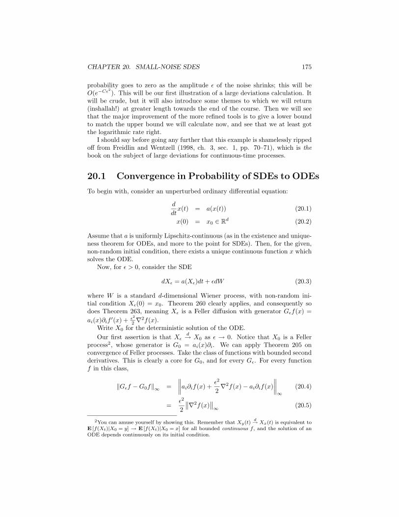
CHAPTER 20. SMALL-NOISE SDES 175
probability goes to zero as the amplitude ε of the noise shrinks; this will beO(e−Cε
2). This will be our first illustration of a large deviations calculation. It
will be crude, but it will also introduce some themes to which we will return(inshallah!) at greater length towards the end of the course. Then we will seethat the major improvement of the more refined tools is to give a lower boundto match the upper bound we will calculate now, and see that we at least gotthe logarithmic rate right.
I should say before going any further that this example is shamelessly rippedoff from Freidlin and Wentzell (1998, ch. 3, sec. 1, pp. 70–71), which is thebook on the subject of large deviations for continuous-time processes.
20.1 Convergence in Probability of SDEs to ODEs
To begin with, consider an unperturbed ordinary differential equation:
d
dtx(t) = a(x(t)) (20.1)
x(0) = x0 ∈ Rd (20.2)
Assume that a is uniformly Lipschitz-continuous (as in the existence and unique-ness theorem for ODEs, and more to the point for SDEs). Then, for the given,non-random initial condition, there exists a unique continuous function x whichsolves the ODE.
Now, for ε > 0, consider the SDE
dXε = a(Xε)dt+ εdW (20.3)
where W is a standard d-dimensional Wiener process, with non-random ini-tial condition Xε(0) = x0. Theorem 260 clearly applies, and consequently sodoes Theorem 263, meaning Xε is a Feller diffusion with generator Gεf(x) =ai(x)∂if ′(x) + ε2
2 ∇2f(x).
Write X0 for the deterministic solution of the ODE.Our first assertion is that Xε
d→ X0 as ε → 0. Notice that X0 is a Fellerprocess2, whose generator is G0 = ai(x)∂i. We can apply Theorem 205 onconvergence of Feller processes. Take the class of functions with bounded secondderivatives. This is clearly a core for G0, and for every Gε. For every functionf in this class,
‖Gεf −G0f‖∞ =∥∥∥∥ai∂if(x) +
ε2
2∇2f(x)− ai∂if(x)
∥∥∥∥∞
(20.4)
=ε2
2
∥∥∇2f(x)∥∥∞ (20.5)
2You can amuse yourself by showing this. Remember that Xy(t)d→ Xx(t) is equivalent to
E [f(Xt)|X0 = y] → E [f(Xt)|X0 = x] for all bounded continuous f , and the solution of anODE depends continuously on its initial condition.
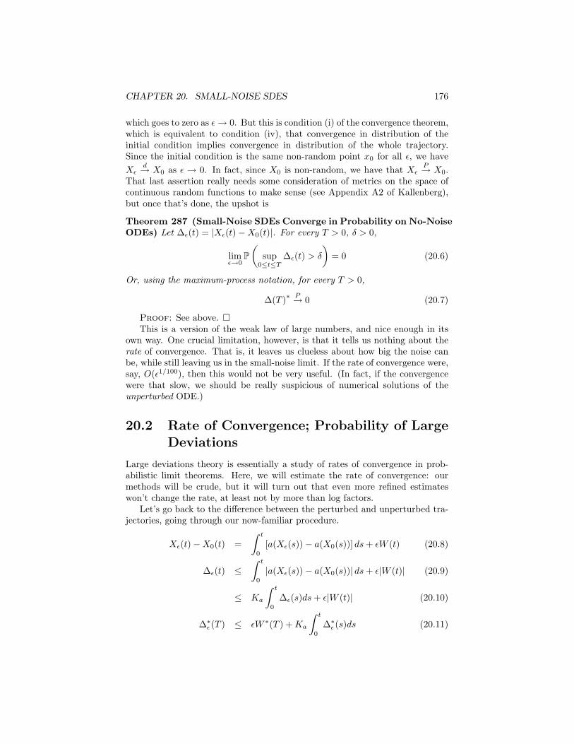
CHAPTER 20. SMALL-NOISE SDES 176
which goes to zero as ε→ 0. But this is condition (i) of the convergence theorem,which is equivalent to condition (iv), that convergence in distribution of theinitial condition implies convergence in distribution of the whole trajectory.Since the initial condition is the same non-random point x0 for all ε, we haveXε
d→ X0 as ε → 0. In fact, since X0 is non-random, we have that XεP→ X0.
That last assertion really needs some consideration of metrics on the space ofcontinuous random functions to make sense (see Appendix A2 of Kallenberg),but once that’s done, the upshot is
Theorem 287 (Small-Noise SDEs Converge in Probability on No-NoiseODEs) Let ∆ε(t) = |Xε(t)−X0(t)|. For every T > 0, δ > 0,
limε→0
P(
sup0≤t≤T
∆ε(t) > δ
)= 0 (20.6)
Or, using the maximum-process notation, for every T > 0,
∆(T )∗ P→ 0 (20.7)
Proof: See above. This is a version of the weak law of large numbers, and nice enough in its
own way. One crucial limitation, however, is that it tells us nothing about therate of convergence. That is, it leaves us clueless about how big the noise canbe, while still leaving us in the small-noise limit. If the rate of convergence were,say, O(ε1/100), then this would not be very useful. (In fact, if the convergencewere that slow, we should be really suspicious of numerical solutions of theunperturbed ODE.)
20.2 Rate of Convergence; Probability of LargeDeviations
Large deviations theory is essentially a study of rates of convergence in prob-abilistic limit theorems. Here, we will estimate the rate of convergence: ourmethods will be crude, but it will turn out that even more refined estimateswon’t change the rate, at least not by more than log factors.
Let’s go back to the difference between the perturbed and unperturbed tra-jectories, going through our now-familiar procedure.
Xε(t)−X0(t) =∫ t
0
[a(Xε(s))− a(X0(s))] ds+ εW (t) (20.8)
∆ε(t) ≤∫ t
0
|a(Xε(s))− a(X0(s))| ds+ ε|W (t)| (20.9)
≤ Ka
∫ t
0
∆ε(s)ds+ ε|W (t)| (20.10)
∆∗ε (T ) ≤ εW ∗(T ) +Ka
∫ t
0
∆∗ε (s)ds (20.11)
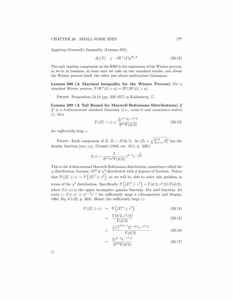
CHAPTER 20. SMALL-NOISE SDES 177
Applying Gronwall’s Inequality (Lemma 258),
∆∗ε (T ) ≤ εW ∗(T )eKaT (20.12)
The only random component on the RHS is the supremum of the Wiener process,so we’re in business, at least once we take on two standard results, one aboutthe Wiener process itself, the other just about multivariate Gaussians.
Lemma 288 (A Maximal Inequality for the Wiener Process) For astandard Wiener process, P (W ∗(t) > a) = 2P (|W (t)| > a).
Proof: Proposition 13.13 (pp. 256–257) in Kallenberg.
Lemma 289 (A Tail Bound for Maxwell-Boltzmann Distributions) IfZ is a d-dimensional standard Gaussian (i.e., mean 0 and covariance matrixI), then
P (|Z| > z) ≤ 2zd−2e−z2/2
2d/2Γ(d/2)(20.13)
for sufficiently large z.
Proof: Each component of Z, Zi ∼ N (0, 1). So |Z| =√∑d
i=1 Z2i has the
density function (see, e.g., Cramer (1945, sec. 18.1, p. 236))
f(z) =2
2d/2σdΓ(d/2)zd−1e−
z2
2σ2
This is the d-dimensional Maxwell-Boltzmann distribution, sometimes called theχ-distribution, because |Z|2 is χ2-distributed with d degrees of freedom. Noticethat P (|Z| ≥ z) = P
(|Z|2 ≥ z2
), so we will be able to solve this problem in
terms of the χ2 distribution. Specifically, P(|Z|2 ≥ z2
)= Γ(d/2, z2/2)/Γ(d/2),
where Γ(r, a) is the upper incomplete gamma function. For said function, forevery r, Γ(r, a) ≤ ar−1e−a for sufficiently large a (Abramowitz and Stegun,1964, Eq. 6.5.32, p. 263). Hence (for sufficiently large z)
P (|Z| ≥ z) = P(|Z|2 ≥ z2
)(20.14)
=Γ(d/2, z2/2)
Γ(d/2)(20.15)
≤(z2)d/2−121−d/2e−z
2/2
Γ(d/2)(20.16)
=2zd−2e−z
2/2
2d/2Γ(d/2)(20.17)
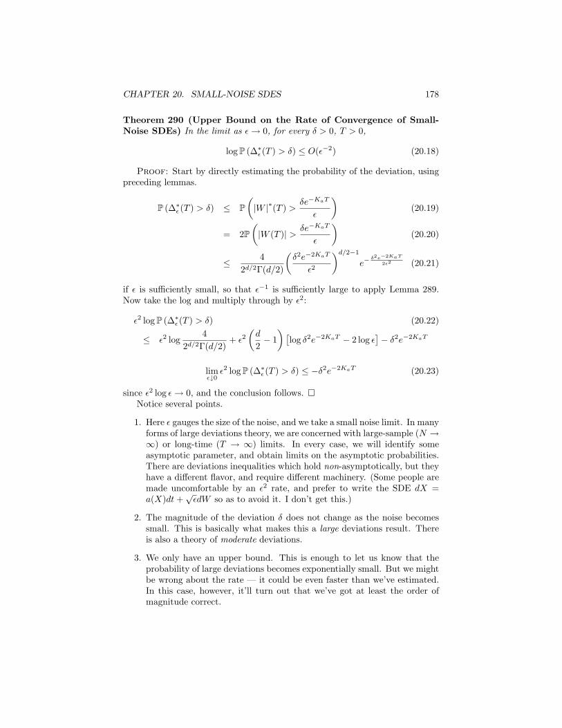
CHAPTER 20. SMALL-NOISE SDES 178
Theorem 290 (Upper Bound on the Rate of Convergence of Small-Noise SDEs) In the limit as ε→ 0, for every δ > 0, T > 0,
log P (∆∗ε (T ) > δ) ≤ O(ε−2) (20.18)
Proof: Start by directly estimating the probability of the deviation, usingpreceding lemmas.
P (∆∗ε (T ) > δ) ≤ P(|W |∗(T ) >
δe−KaT
ε
)(20.19)
= 2P(|W (T )| > δe−KaT
ε
)(20.20)
≤ 42d/2Γ(d/2)
(δ2e−2KaT
ε2
)d/2−1
e−δ2e−2KaT
2ε2 (20.21)
if ε is sufficiently small, so that ε−1 is sufficiently large to apply Lemma 289.Now take the log and multiply through by ε2:
ε2 log P (∆∗ε (T ) > δ) (20.22)
≤ ε2 log4
2d/2Γ(d/2)+ ε2
(d
2− 1)[
log δ2e−2KaT − 2 log ε]− δ2e−2KaT
limε↓0
ε2 log P (∆∗ε (T ) > δ) ≤ −δ2e−2KaT (20.23)
since ε2 log ε→ 0, and the conclusion follows. Notice several points.
1. Here ε gauges the size of the noise, and we take a small noise limit. In manyforms of large deviations theory, we are concerned with large-sample (N →∞) or long-time (T → ∞) limits. In every case, we will identify someasymptotic parameter, and obtain limits on the asymptotic probabilities.There are deviations inequalities which hold non-asymptotically, but theyhave a different flavor, and require different machinery. (Some people aremade uncomfortable by an ε2 rate, and prefer to write the SDE dX =a(X)dt+
√εdW so as to avoid it. I don’t get this.)
2. The magnitude of the deviation δ does not change as the noise becomessmall. This is basically what makes this a large deviations result. Thereis also a theory of moderate deviations.
3. We only have an upper bound. This is enough to let us know that theprobability of large deviations becomes exponentially small. But we mightbe wrong about the rate — it could be even faster than we’ve estimated.In this case, however, it’ll turn out that we’ve got at least the order ofmagnitude correct.
CHAPTER 20. SMALL-NOISE SDES 179
4. We also don’t have a lower bound on the probability, which is somethingthat would be very useful in doing reliability analyses. It will turn outthat, under many circumstances, one can obtain a lower bound on theprobability of large deviations, which has the same asymptotic dependenceon ε as the upper bound.
5. Suppose we’re right about the rate (which, it will turn out, we are), andit holds both from above and below. It would be nice to be able to saysomething like
P (∆∗ε (T ) > δ)→ C1(δ, T )e−C2(δ,T )ε−2(20.24)
rather thanε2 log P (∆∗ε (T ) > δ)→ −C2(δ, T ) (20.25)
The difficulty with making an assertion like 20.24 is that the large devia-tion probability actually converges on any function which goes to asymp-totically to zero! So, to extract the actual rate of dependence, we need toget a result like 20.25.
More generally, one consequence of Theorem 290 is that SDE trajectorieswhich are far from the trajectory of the ODE have exponentially small proba-bilities. The vast majority of the probability will be concentrated around theunperturbed trajectory. Reasonable sample-path functionals can therefore bewell-approximated by averaging their value over some small (δ) neighborhood ofthe unperturbed trajectory. This should sound very similar to Laplace’s methodfor the evaluate of asymptotic integrals in Euclidean space, and in fact one ofthe key parts of large deviations theory is an extension of Laplace’s method toinfinite-dimensional function spaces.
In addition to this mathematical content, there is also a close connectionto the principle of least action in physics. In classical mechanics, the systemfollows the trajectory of least action, the “action” of a trajectory being theintegral of the kinetic minus potential energy along that path. In quantummechanics, this is no longer an axiom but a consequence of the dynamics: theaction-minimizing trajectory is the most probable one, and large deviations fromit have exponentially small probability. Similarly, the theory of large deviationscan be used to establish quite general stochastic principles of least action forMarkovian systems.3
3For a fuller discussion, see Eyink (1996),Freidlin and Wentzell (1998, ch. 3).
Part V
Ergodic Theory
180
Chapter 21
The Mean-Square ErgodicTheorem
This chapter gives our first classical ergodic result, the “meansquare” ergodic theorem for weakly stationary processes. This as-serts that time averages converge in L2 on expectations.
Section 21.1 gives an easy proof of a sufficient condition, justusing the autocovariance. It even provides a lower bound on therate of convergence. But the sufficient condition is rather strong.
Section 21.2 gives a necessary and sufficient condition, using thespectral representation, and an interpretation of why this works inthis terms.
Ergodic theorems relate functionals calculated along individual sample paths(say, the time average, T−1
∫ T0dtX(t), or the maximum attained value) to func-
tionals calculated over the whole distribution (say, the expectation, E [X(t)], orthe expected maximum). The basic idea is that the two should be close, and theyshould get closer the longer the trajectory we use, because in some sense anyone sample path, carried far enough, is representative of the whole distribution.Since there are many different kinds of functionals, and many different modes ofstochastic convergence, there are many different kinds of ergodic theorem. Theclassical ergodic theorems say that time averages converge on expectations1, ei-ther in Lp or a.s. (both implying convergence in distribution or in probability).The traditional centerpiece of ergodic theorem is Birkhoff’s “individual” ergodictheorem, asserting a.s. convergence. We will see its proof, but it will need a lotof preparatory work, and it requires strict stationarity. By contrast, the L2, or“mean square”, ergodic theorem, attributed to von Neumann2 is already in our
1Proverbially: “time averages converge on space averages”, the space in question beingthe state space Ξ; or “converge on phase averages”, since physicists call certain kinds of statespace “phase space”.
2See von Plato (1994, ch. 3) for a fascinating history of the development of ergodic theorythrough the 1930s, and its place in the history of mathematical probability.
181
CHAPTER 21. THE MEAN-SQUARE ERGODIC THEOREM 182
grasp, and holds for weakly stationary processes.We will actually prove it twice, once with a fairly transparent sufficient condi-
tion, and then again with a more complicated necessary-and-sufficient condition.The more complicated proof will wait until next lecture.
21.1 Mean-Square Ergodicity Based on the Au-tocovariance
First, the easy version, which gives an estimate of the rate of convergence.(What I say here is ripped off from the illuminating discussion in (Frisch, 1995,sec. 4.4, especially pp. 49–50).)
Definition 291 (Time Averages) When X is a one-sided, continuous-parameterrandom process, we say that its time average between times T1 and T2 is 〈X(t)〉T1,T2
≡(T2 − T1)−1 ∫ T2
T1dtX(t). When we only mention one time argument, by default
the time average is from 0 to T , 〈X(t)〉T ≡ 〈X(t)〉0,T .
(Only considering time averages starting from zero involves no loss of gen-erality for weakly stationary processes: why?)
Definition 292 (Integral Time Scale) The integral time scale of a weakly-stationary random process is
τint ≡∫∞
0dτ |Γ(τ)|Γ(0)
(21.1)
Notice that τint does, indeed, have units of time.As a particular example, suppose that Γ(τ) = Γ(0)e−τ/A, where the constant
A is known as the autocorrelation time. Then simple calculus shows that τint =A.
Theorem 293 (Mean-Square Ergodic Theorem (Finite AutocovarianceTime)) Let X(t) be a weakly stationary process with E [X(t)] = 0. If τint <∞,then 〈X(t)〉T
L2→ 0 as T →∞.
CHAPTER 21. THE MEAN-SQUARE ERGODIC THEOREM 183
Proof: Use Fubini’s theorem to to the square of the integral into a doubleintegral, and then bring the expectation inside it:
E
( 1T
∫ T
0
dtX(t)
)2 = E
[1T 2
∫ T
0
∫ T
0
dt1dt2X(t1)X(t2)
](21.2)
=1T 2
∫ T
0
∫ T
0
dt1dt2E [X(t1)X(t2)] (21.3)
=1T 2
∫ T
0
∫ T
0
dt1dt2Γ(t1 − t2) (21.4)
=2T 2
∫ T
0
dt1
∫ t1
0
dτΓ(τ) (21.5)
≤ 2T 2
∫ T
0
dt1
∫ ∞0
dτ |Γ(τ)| (21.6)
=2T
∫ ∞0
dτ |Γ(τ)| (21.7)
Since the integral in the final inequality is Γ(0)τint, which is finite, everythingmust go to zero as T →∞.
Remark. From the proof, we can see that the rate of convergence of the mean-square of ‖〈X(t)〉T ‖2
2 is (at least) O(1/T ). This would give a root-mean-square(rms) convergence rate of O(1/
√T ), which is what the naive statistician who
ignored inter-temporal dependence would expect from the central limit theorem.(This ergodic theorem says nothing about the form of the distribution of 〈X(t)〉Tfor large T . We will see that, under some circumstances, it is Gaussian, but thatneeds stronger assumptions [forms of “mixing”] than we have imposed.) Thenaive statistician would expect that the mean-square time average would go likeΓ(0)/T , since Γ(0) = E
[X2(t)
]= Var [X(t)]. The proportionality constant is
instead∫∞
0dτ |Γ(τ)|. This is equal to the naive guess for white noise, and for
other collections of IID variables, but not in the general case. This leads to thefollowing
Corollary 294 (Convergence Rate in the Mean-Square Ergodic The-orem) Under the conditions of Theorem 293,
Var [〈X(t)〉T ] ≤ 2Var [X(0)]τint
T(21.8)
Proof: SinceX(t) is centered, E [〈X(t)〉T ] = 0, and ‖〈X(t)〉T ‖22 = Var [〈X(t)〉T ].
Everything else follows from re-arranging the bound in the proof of Theorem293, Definition 292, and the fact that Γ(0) = Var [X(0)].
As a consequence of the corollary, if T τint, then the variance of the timeaverage is negigible compared to the variance at any one time.
CHAPTER 21. THE MEAN-SQUARE ERGODIC THEOREM 184
21.2 Mean-Square Ergodicity Based on the Spec-trum
Let’s warm up with some lemmas of a technical nature. The first relates thejumps of the spectral process X(ν) to the jumps of the spectral function S(ν).
Lemma 295 (Mean-Square Jumps in the Spectral Process) For a weakly
stationary process, E[∣∣∣∆X(ν)
∣∣∣2] = ∆S(ν).
Proof: This follows directly from the Wiener-Khinchin relation (Theorem281).
Lemma 296 (The Jump in the Spectral Function) The jump of the spec-tral function at ν is given by
∆S(ν) = limT→∞
1T
∫ T
0
Γ(τ)eiντdτ (21.9)
Proof: This is a basic inversion result for characteristic functions. It shouldbecome plausible by thinking of this as getting the Fourier transform of Γ as Tgrows.
Lemma 297 (Existence of L2 Limits for Time Averages) If X is weaklystationary, then for any real f ,
⟨eiftX(t)
⟩T
converges in L2 to ∆X(f).
Proof: Start by looking at the squared modulus of the time average forfinite time.∣∣∣∣∣ 1
T
∫ T
0
eiftX(t)dt
∣∣∣∣∣2
(21.10)
=1T 2
∫ T
0
∫ T
0
e−if(t1−t2)X†(t1)X(t2)dt1dt2
=1T 2
∫ T
0
∫ T
0
e−if(t1−t2)
∫ ∞−∞
eiν1t1dXν1
∫ ∞−∞
e−iν2t2dXν2 (21.11)
=1T 2
∫ T
0
∫ ∞−∞
dt1dXν1eit1(f−ν1)
∫ T
0
∫ ∞−∞
dt2dXν2e−it2(f−ν2) (21.12)
As T → ∞, these integrals pick out ∆X(f) and ∆X†(f). So,⟨eiftX(t)
⟩T
L2→∆X(f).
Notice that the limit provided by the lemma is a random quantity. What’sreally desired, in most applications, is convergence to a deterministic limit,which here would mean convergence (in L2) to zero.
CHAPTER 21. THE MEAN-SQUARE ERGODIC THEOREM 185
Theorem 298 (The Mean-Square Ergodic Theorem) If X is weakly sta-tionary, and E [X(t)] = 0, then 〈X(t)〉T converges in L2 to 0 iff
limT−1
∫ T
0
dτΓ(τ) = 0 (21.13)
Proof: Taking f = 0 in Lemma 297, 〈X(t)〉TL2→ ∆X(0), the jump in the
spectral function at zero. Let’s show that the (i) expectation of this jump iszero, and that (ii) its variance is given by the integral expression on the LHS ofEq. 21.13. For (i), because 〈X(t)〉T
L2→ Y , we know that E [〈X(t)〉T ] → E [Y ].
But E [〈X(t)〉T ] = 〈E [X(t)]〉T = 0. So E[∆X(0)
]= 0. For (ii), Lemma 295,
plus the fact that E[∆X(0)
]= 0, shows that the variance is equal to the jump
in the spectrum at 0. But, by Lemma 296 with ν = 0, that jump is exactly theLHS of Eq. 21.13.
Remark 1: Notice that if the integral time is finite, then the integral condi-tion on the autocovariance is automatically satisfied, but not vice versa, so thehypotheses here are strictly weaker than in Theorem 293.
Remark 2: One interpretation of the theorem is that the time-average isconverging on the zero-frequency component of the spectral process. Intuitively,all the other components are being killed off by the time-averaging, because thebecause time-integral of a sinusoidal function is bounded, but the denominatorin a time average is unbounded:
∀ν 6= 0, limT→∞
1T
∫ T
0
e−iνtdt = limT→∞
e−iνT − 1−iνT
= 0
The only part left is the zero-frequency component, whose time integral can alsogrow linearly with time. If there is a jump in the spectral process at 0, thenthis has finite variance; if not, not.
limT→∞
〈X(t)〉T = limT→∞
1T
∫ T
0
X(t)dt
= limT→∞
1T
∫ T
0
∫ ∞−∞
e−iνtdX(ν)
=∫ ∞−∞
dX(ν) limT→∞
1T
∫ T
0
e−iνtdt
Exchanging the order of the time and frequency integrals is justified by Fubini’stheorem, but bringing the limit inside the integral needs justification, and that’sbasically what the proof provides.
Remark 3: Lemma 297 establishes the L2 convergence of time-averages ofthe form
1T
∫ T
0
eiftX(t)dt
CHAPTER 21. THE MEAN-SQUARE ERGODIC THEOREM 186
for any real f . Specifically, from Lemma 295, the mean-square of this variableis converging on the jump in the spectrum at f . Multiplying X(t) by eift makesthe old frequency f component the new frequency zero component, so it is thesurviving term. While the ergodic theorem itself only needs the f = 0 case, thisresult is useful in connection with estimating spectra from time series (Doob,1953, ch. X, §7).
21.3 Exercises
Exercise 70 (Mean-Square Ergodicity in Discrete Time) It is often con-venient to have a mean-square ergodic theorem for discrete-time sequences ratherthan continuous-time processes. If the dt in the definition of 〈X(t)〉T is re-interpreted as counting measure on N, rather than Lebesgue measure on R+,does the proof of Theorem 293 remain valid? (If yes, say why; if no, explainwhere the argument fails.)
Exercise 71 (Mean-Square Ergodicity with Non-Zero Mean) State andprove a version of Theorem 293 which does not assume that E [X(t)] = 0.
Exercise 72 (Functions of Weakly Stationary Processes) Suppose X is aweakly stationary process, and f is a measurable function such that ‖f(X0)‖2 <∞. Is f(X) a weakly stationary process? (If yes, prove it; if not, give a counter-example.)
Exercise 73 (Ergodicity of the Ornstein-Uhlenbeck Process?) Supposethe Ornstein-Uhlenbeck process is has its invariant distribution as its initialdistribution, and is therefore weakly stationary. Does Theorem 293 apply?
Exercise 74 (Long-Memory Processes) A weakly stationary process is some-times said to have a “long memory” if there is some α > 0 such that Γ(τ) ∝ τ−α,at least for large τ . For what values of α is τint finite? For what values of αdoes Theorem 298 hold?
Chapter 22
Ergodic Properties andErgodic Limits
Section 22.1 gives a general orientation to ergodic theory, whichwe will study in discrete time.
Section 22.2 introduces dynamical systems and their invariants,the setting in which we will prove our ergodic theorems.
Section 22.3 considers time averages, defines what we mean fora function to have an ergodic property (its time average converges),and derives some consequences.
Section 22.4 defines asymptotic mean stationarity, and showsthat, with AMS dynamics, the limiting time average is equivalent toconditioning on the invariant sets.
22.1 General Remarks
To begin our study of ergodic theory, let us consider a famous1 line from Gne-denko and Kolmogorov (1954, p. 1):
In fact, all epistemological value of the theory of probability isbased on this: that large-scale random phenomena in their collectiveaction create strict, nonrandom regularity.
Now, this is how Gnedenko and Kolmogorov introduced their classic study of thelimit laws for independent random variables, but most of the random phenomenawe encounter around us are not independent. Ergodic theory is a study ofhow large-scale dependent random phenomena nonetheless create nonrandomregularity. The classical limit laws for IID variables X1, X2, . . . assert that,
1Among mathematical scientists, anyway.
187
CHAPTER 22. ERGODIC PROPERTIES AND ERGODIC LIMITS 188
under the right conditions, sample averages converge on expectations,
1n
n∑i=1
Xi → E [Xi]
where the sense of convergence can be “almost sure” (strong law of large num-bers), “Lp” (pth mean), “in probability” (weak law), etc., depending on thehypotheses we put on the Xi. One meaning of this convergence is that suffi-ciently large random samples are representative of the entire population — thatthe sample mean makes a good estimate of E [X].
The ergodic theorems, likewise, assert that for dependent sequencesX1, X2, . . .,time averages converge on expectations
1t
t∑i=1
Xi → E [X∞|I]
where X∞ is some limiting random variable, or in the most useful cases a non-random variable, and I is a σ-field representing some sort of asymptotic in-formation. Once again, the mode of convergence will depend on the kind ofhypotheses we make about the random sequence X. Once again, the interpre-tation is that a single sample path is representative of an entire distributionover sample paths, if it goes on long enough. The IID laws of large numbersare, in fact, special cases of the corresponding ergodic theorems.
Section 21 proved a mean-square (L2) ergodic theorem for weakly stationarycontinuous-parameter processes.2 The next few chapters, by contrast, will de-velop ergodic theorems for non-stationary discrete-parameter processes.3 Thisis a little unusual, compared to most probability books, so let me say a word ortwo about why. (1) Results we get will include stationary processes as specialcases, but stationarity fails for many applications where ergodicity (in a suit-able sense) holds. So this is more general and more broadly applicable. (2) Ourresults will all have continuous-time analogs, but the algebra is a lot cleanerin discrete time. (3) Some of the most important applications (for people likeyou!) are to statistical inference and learning with dependent samples, and toMarkov chain Monte Carlo, and both of those are naturally discrete-parameterprocesses. We will, however, stick to continuous state spaces.
22.2 Dynamical Systems and Their Invariants
It is a very remarkable fact — but one with deep historical roots (von Plato,1994, ch. 3) — that the way to get regular limits for stochastic processes isto first turn them into irregular deterministic dynamical systems, and then letaveraging smooth away the irregularity. This section will begin by laying outdynamical systems, and their invariant sets and functions, which will be thefoundation for what follows.
2Can you identify X∞ and I for this case?3In doing so, I’m ripping off Gray (1988), especially chapters 6 and 7.
CHAPTER 22. ERGODIC PROPERTIES AND ERGODIC LIMITS 189
Definition 299 (Dynamical System) A dynamical system consists of a mea-surable space Ξ, a σ-field X on Ξ, a probability measure µ defined on X , and amapping T : Ξ 7→ Ξ which is X/X -measurable.
Remark: Measure-preserving transformations (Definition 53) are special casesof dynamical systems. Since (Theorem 52) every strongly stationary process canbe represented by a measure-preserving transformation, namely the shift (Def-inition 48), the theory of ergodicity for dynamical systems which we’ll developis easily seen to include the usual ergodic theory of strictly-stationary processesas a special case. Thus, at the cost of going to the infinite-dimensional space ofsample paths, we can always make it the case that the time-evolution is com-pletely deterministic, and the only stochastic component to the process is itsinitial condition.
Lemma 300 (Dynamical Systems are Markov Processes) Let Ξ,X , µ, Tbe a dynamical system. Let L (X1) = µ, and define Xt = T t−1X1. Then theXt form a Markov process, with evolution operator K defined through Kf(x) =f(Tx).
Proof: For every x ∈ Ξ and B ∈ X , define κ(x,B) ≡ 1B(Tx). For fixedx, this is clearly a probability measure (specifically, the δ measure at Tx).For fixed B, this is a measurable function of x, because T is a measurablemapping. Hence, κ(x,B) is a probability kernel. So, by Theorem 106, the Xt
form a Markov process. By definition, E [f(X1)|X0 = x] = Kf(x). But theexpectation is in this case just f(Tx).
Notice that, as a consequence, there is a corresponding operator, call it U ,which takes signed measures (defined over X ) to signed measures, and specifi-cally takes probability measures to probability measures.
Definition 301 (Observable) A function f : Ξ 7→ R which is B/X measurableis an observable of the dynamical system Ξ,X , µ, T .
Pretty much all of what follows would work if the observables took values inany real or complex vector space, but that situation can be built up from thisone.
Definition 302 (Invariant Functions, Sets and Measures) A function isinvariant, under the action of a dynamical system, if f(Tx) = f(x) for allx ∈ Ξ, or equivalently if Kf = f everywhere. An event B ∈ X is invariant ifits indicator function is an invariant function. A measure ν is invariant if it ispreserved by T , i.e. if ν(C) = ν(T−1C) for all C ∈ X , equivalently if Uν = ν.
Lemma 303 (Invariant Sets are a σ-Algebra) The class I of all measurableinvariant sets in Ξ forms a σ-algebra.
Proof: Clearly, Ξ is invariant. The other properties of a σ-algebra followbecause set-theoretic operations (union, complementation, etc.) commute withtaking inverse images.
CHAPTER 22. ERGODIC PROPERTIES AND ERGODIC LIMITS 190
Lemma 304 (Invariant Sets and Observables) An observable is invariantif and only if it is I-measurable. Consequently, I is the σ-field generated by theinvariant observables.
Proof: “If”: Pick any Borel setB. Since f = fT , f−1(B) = (f T )−1(B) =T−1f−1B. Hence f−1(B) ∈ I. Since the inverse image of every Borel set isin I, f is I-measurable. “Only if”: Again, pick any Borel set B. By assump-tion, f−1(B) ∈ I, so f−1(B) = T−1f−1(B) = (f T )−1(B), so the inverseimage of under Tf of any Borel set is an invariant set, implying that f Tis I-measurable. Since, for every B, f−1(B) = (f T )−1(B), we must havef T = f . The consequence follows.
Definition 305 (Infinitely Often, i.o.) For any set C ∈ X , the set C in-finitely often, Ci.o., consists of all those points in Ξ whose trajectories visit Cinfinitely often, Ci.o. ≡ lim supt T−tC.
Lemma 306 (“Infinitely often” implies invariance) For every C ∈ X ,Ci.o. is invariant.
Proof: Exercise 75.
Definition 307 (Invariance Almost Everywhere) A measurable functionis invariant µ-a.e., or almost invariant, when
µ x ∈ Ξ|∀n, f(x) = Knf(x) = 1 (22.1)
A measurable set is invariant µ-a.e., when its indicator function is almost in-variant.
Remark 1: Some of the older literature annoyingly calls these objects totallyinvariant.
Remark 2: Invariance implies invariance µ-almost everywhere, for any µ.
Lemma 308 (Almost-invariant sets form a σ-algebra) The almost-invariantsets form a σ-field, I ′, and an observable is almost invariant if and only if it ismeasurable with respect to this field.
Proof: Entirely parallel to that for the strict invariants. Let’s close this section with a simple lemma, which will however be useful
in approximation-by-simple-function arguments in building up expectations.
Lemma 309 (Invariance for simple functions) A simple function, f(x) =∑mk=1 am1Ck(x), is invariant if and only if all the sets Ck ∈ I. Similarly, a
simple function is almost invariant iff all the defining sets are almost invariant.
Proof: Exercise 76.
CHAPTER 22. ERGODIC PROPERTIES AND ERGODIC LIMITS 191
22.3 Time Averages and Ergodic Properties
For convenience, let’s re-iterate the definition of a time average. The notationdiffers here a little from that given earlier, in a way which helps with discretetime.
Definition 310 (Time Averages) The time-average of an observable f is thereal-valued function
Atf(x) ≡ 1t
t−1∑i=0
f(T ix) (22.2)
where At is the operator taking functions to their time-averages.
Lemma 311 (Time averages are observables) For every t, the time-averageof an observable is an observable.
Proof: The class of measurable functions is closed under finite iterationsof arithmetic operations.
Definition 312 (Ergodic Property) An observable f has the ergodic prop-erty when Atf(x) converges as t → ∞ for µ-almost-all x. An observable hasthe mean ergodic property when Atf(x) converges in L1(µ), and similarly forthe other Lp ergodic properties. If for some class of functions D, every f ∈ Dhas an ergodic property, then the class D has that ergodic property.
Remark. Notice that what is required for f to have the ergodic property isthat almost every initial point has some limit for its time average,
µx ∈ Ξ
∣∣∣∃r ∈ R : limt→∞
Atf(x) = r
= 1 (22.3)
This does not mean that there is some common limit for almost every initialpoint,
∃r ∈ R : µx ∈ Ξ
∣∣∣ limt→∞
Atf(x) = r
= 1 (22.4)
Similarly, a class of functions has the ergodic property if all of their time averagesconverge; they do not have to converge uniformly.
Definition 313 (Ergodic Limit) If an observable f has the ergodic property,define Af(x) to be the limit of Atf(x) where that exists, and 0 elsewhere. Thedomain of A consists of all and only the functions with ergodic properties.
Observe that
Af(x) = limt→∞
1t
t∑n=0
Knf(x) (22.5)
That is, A is the limit of an arithmetic mean of conditional expectations. Thissuggests that it should itself have many of the properties of conditional expec-tations. In fact, under a reasonable condition, we will see that Af = E [f |I],expectation conditional on the σ-algebra of invariant sets. We’ll check first thatA has the properties we’d want from a conditional expectation.
CHAPTER 22. ERGODIC PROPERTIES AND ERGODIC LIMITS 192
Lemma 314 (Linearity of Ergodic Limits) A is a linear operator, and itsdomain is a linear space.
Proof: If c is any real number, then Atcf(x) = cAtf(x), and so clearly, ifthe limit exists, Acf(x) = cAf(x). Similarly, At(f + g)(x) = Atf(x) + Atg(x),so if f and g both have ergodic properties, then so does f+g, and A(f+g)(x) =Af(x) +Ag(x).
Lemma 315 (Non-negativity of ergodic limits) If f ∈ DomA, and, for alln ≥ 0, fTn ≥ 0 a.e., then Af(x) ≥ 0 a.e.
Proof: The event Af(x) < 0 is a sub-event of⋃n f(Tn(x)) < 0. Since
the union of a countable collection of measure zero events has measure zero,Af(x) ≥ 0 almost everywhere.
Notice that our hypothesis is that fTn ≥ 0 a.e. for all n, not just that f ≥ 0.The reason we need the stronger assumption is that the transformation T mightmap every point to the bad set of f ; the lemma guards against that. Of course,if f(x) ≥ 0 for all, and not just almost all, x, then the bad set is non-existent,and Af ≥ 0 follows automatically.
Lemma 316 (Constant functions have the ergodic property) The con-stant function 1 has the ergodic property. Consequently, so does every otherconstant function.
Proof: For every n, 1(Tnx) = 1. Hence At1(x) = 1 for all t, and soA1(x) = 1. Extension to other constants follows by linearity (Lemma 314).
Remember that for any time-evolution operator K, K1 = 1.
Lemma 317 (Ergodic limits are invariantifying) If f ∈ Dom(A), then,for all n, f Tn is too, and Af(x) = Af Tn(x). Or, AKnf(x) = Af(x).
Proof: Start with n = 1, and show that the discrepancy goes to zero.
AKf(x)−Af(x) = limt
1t
t∑i=0
(Ki+1f(x)−Kif(x)
)(22.6)
= limt
1t
(Ktf(x)− f(x)
)(22.7)
Since Af(x) exists a.e., we know that the series t−1∑t−1i=0 K
if(x) convergesa.e., implying that (t+ 1)−1
Ktf(x) → 0 a.e.. But t−1 = t+1t (t+ 1)−1, and for
large t, t+ 1/t < 2. Hence (t+ 1)−1Ktf(x) ≤ t−1Ktf(x) ≤ 2(t+ 1)−1
Ktf(x),implying that t−1Ktf(x) itself goes to zero (a.e.). Similarly, t−1f(x) must goto zero. Thus, overall, we have AKf(x) = Af(x) a.e., and Kf(x) ∈ Dom(A).
Lemma 318 (Ergodic limits are invariant functions) If f ∈ Dom(A),then Af is an invariant, and I-measurable.
CHAPTER 22. ERGODIC PROPERTIES AND ERGODIC LIMITS 193
Proof: Af exists, so (previous lemma) AKf exists and is equal to Af (al-most everywhere). But AKf(x) = Af(Tx), by definition, hence Af is invariant,i.e., KAf = AKf = Af . Measurability follows from Lemma 304.
Lemma 319 (Ergodic limits and invariant indicator functions) If f ∈Dom(A), and B is any set in I, then A(1B(x)f(x)) = 1B(x)Af(x).
Proof: For every n, 1B(Tnx)f(Tnx) = 1B(x)f(Tnx), since x ∈ B iffTnx ∈ B. So, for all finite t, At(1B(x)f(x)) = 1B(x)Atf(x), and the lemmafollows by taking the limit.
Lemma 320 (Ergodic properties of sets and observables) All indicatorfunctions of measurable sets have ergodic properties if and only if all boundedobservables have ergodic properties.
Proof: A standard approximation-by-simple-functions argument, as in theconstruction of Lebesgue integrals.
Lemma 321 (Expectations of ergodic limits) Let f be bounded and havethe ergodic property. Then Af is µ-integrable, and E [Af(X)] = E [f(X)], whereL (X) = µ.
Proof: Since f is bounded, it is integrable. Hence Atf is bounded, too,for all t, and Atf(X) is an integrable random variable. A sequence of bounded,integrable random variables is uniformly integrable. Uniform integrability, plusthe convergence Atf(x) → Af(x) for µ-almost-all x, gives us that E [Af(X)]exists and is equal to lim E [Atf(X)] via Fatou’s lemma. (See e.g., Theorem 117in the notes to 36-752.)
Now use the invariance of Af , i.e., the fact that Af(X) = Af(TX) µ-a.s.
0 = E [Af(TX)]−E [Af(X)] (22.8)
= lim1t
t−1∑n=0
E [Knf(TX)]− lim1t
t−1∑n=0
E [Knf(X)] (22.9)
= lim1t
t−1∑n=0
E [Knf(TX)]−E [Knf(X)] (22.10)
= lim1t
t−1∑n=0
E[Kn+1f(X)
]−E [Knf(X)] (22.11)
= lim1t
(E[Ktf(X)
]−E [f(X))
](22.12)
Hence
E [Af ] = lim1t
t−1∑n=0
E [Knf(X)] = E [f(X)] (22.13)
as was to be shown.
CHAPTER 22. ERGODIC PROPERTIES AND ERGODIC LIMITS 194
Lemma 322 (Convergence of Ergodic Limits) If f is as in Lemma 321,then Atf → f in L1(µ).
Proof: From Lemma 321, lim E [Atf(X)] = E [f(X)]. Since the variablesAtf(X) are uniformly integrable (as we saw in the proof of that lemma), itfollows (Proposition 4.12 in Kallenberg, p. 68) that they also converge in L1(µ).
Lemma 323 (Cesaro Mean of Expectations) Let f be as in Lemmas 321and 322, and B ∈ X be an arbitrary measurable set. Then
limt→∞
1t
t−1∑n=0
E [1B(X)Knf(X)] = E [1B(X)f(X)] (22.14)
where L (X) = µ.
Proof: Let’s write out the expectations explicitly as integrals.∣∣∣∣∣∫B
f(x)dµ− 1t
t−1∑n=0
∫B
Knf(x)dµ
∣∣∣∣∣ (22.15)
=
∣∣∣∣∣∫B
f(x)− 1t
t−1∑n=0
Knf(x)dµ
∣∣∣∣∣=
∣∣∣∣∫B
f(x)−Atf(x)dµ∣∣∣∣ (22.16)
≤∫B
|f(x)−Atf(x)| dµ (22.17)
≤∫|f(x)−Atf(x)| dµ (22.18)
= ‖f −Atf‖L1(µ) (22.19)
But (previous lemma) these functions converge in L1(µ), so the limit of thenorm of their difference is zero.
Boundedness is not essential.
Corollary 324 (Replacing Boundedness with Uniform Integrability)Lemmas 321, 322 and 323 hold for any integrable observable f ∈ Dom(A),bounded or not, provided that Atf is a uniformly integrable sequence.
Proof: Examining the proofs shows that the boundedness of f was impor-tant only to establish the uniform integrability of Atf .
22.4 Asymptotic Mean Stationarity
Next, we come to an important concept which will prove to be necessary andsufficient for the most important ergodic properties to hold.
CHAPTER 22. ERGODIC PROPERTIES AND ERGODIC LIMITS 195
Definition 325 (Asymptotically Mean Stationary) A dynamical systemis asymptotically mean stationary when, for every C ∈ X , the limit
m(C) ≡ limt→∞
1t
t−1∑n=0
µ(T−nC) (22.20)
exists, and the set function m is its stationary mean.
Remark 1: It might’ve been more logical to call this “asymptotically measurestationary”, or something, but I didn’t make up the names...
Remark 2: Symbolically, we can write
m = limt→∞
1t
t−1∑n=0
Unµ
where U is the operator taking measures to measures. This leads us to the nextproposition.
Lemma 326 (Stationary Implies Asymptotically Mean Stationary) Ifa dynamical system is stationary, i.e., T is preserves the measure µ, then it isasymptotically mean stationary, with stationary mean µ.
Proof: If T preserves µ, then for every measurable set, µ(C) = µ(T−1C).Hence every term in the sum in Eq. 22.20 is µ(C), and consequently the limitexists and is equal to µ(C).
Proposition 327 (Vitali-Hahn Theorem) If mt are a sequence of probabil-ity measures on a common σ-algebra X , and m(C) is a set function such thatlimtmt(C) = m(C) for all C ∈ X , then m is a probability measure on X .
Proof: This is a standard result from measure theory.
Theorem 328 (Stationary Means are Invariant Measures) If a dynam-ical system is asymptotically mean stationary, then its stationary mean is aninvariant probability measure.
Proof: For every t, let mt(C) = 1t
∑t−1n=0 µ(T−n(C)). Then mt is a convex
combination of probability measures, hence a probability measure itself. Since,for every C ∈ X , limmt(C) = m(C), by Definition 325, Proposition 327 saysthat m(C) is also a probability measure. It remains to check invariance.
m(C)−m(T−1C) (22.21)
= lim1t
t−1∑n=0
µ(T−n(C))− lim1t
t−1∑n=0
µ(T−n(T−1C))
= lim1t
t−1∑n=0
µ(T−n−1C)− µ(T−nC) (22.22)
= lim1t
(µ(T−tC)− µ(C)
)(22.23)
CHAPTER 22. ERGODIC PROPERTIES AND ERGODIC LIMITS 196
Since the probability measure of any set is at most 1, the difference betweentwo probabilities is at most 1, and so m(C) = m(T−1C), for all C ∈ X . Butthis means that m is invariant under T (Definition 53).
Remark: Returning to the symbolic manipulations, if µ is AMS with sta-tionary mean m, then Um = m (because m is invariant), and so we can writeµ = m+ (µ−m), knowing that µ−m goes to zero under averaging. Speakingloosely (this can be made precise, at the cost of a fairly long excursion) m isan eigenvector of U (with eigenvalue 1), and µ − m lies in an orthogonal di-rection, along which U is contracting, so that, under averaging, it goes away,leaving only m, which is like the projection of the original measure µ on to theinvariant manifold of U .
The relationship between an AMS measure µ and its stationary mean mis particularly simple on invariant sets: they are equal there. A slightly moregeneral theorem is actually just as easy to prove, however, so we’ll do that.
Lemma 329 (Expectations of Almost-Invariant Functions) If µ is AMSwith limit m, and f is an observable which is invariant µ-a.e., then Eµ [f ] =Em [f ].
Proof: Let C be any almost invariant set. Then, for any t, C and T−tCdiffer by, at most, a set of µ-measure 0, so that µ(C) = µ(T−tC). The definitionof the stationary mean (Equation 22.20) then gives µ(C) = m(C), or Eµ [1C ] =Em [1C ], i.e., the result holds for indicator functions. By Lemma 309, this thenextends to simple functions. The usual arguments then take us to all functionswhich are measurable with respect to I ′, the σ-field of almost-invariant sets,but this (Lemma 308) is the class of all almost-invariant functions.
Lemma 330 (Limit of Cesaro Means of Expectations) If µ is AMS withstationary mean m, and f is a bounded observable,
limt→∞
Eµ [Atf ] = Em [f ] (22.24)
Proof: By Eq. 22.20, this must hold when f is an indicator function. Bythe linearity of At and of expectations, it thus holds for simple functions, andso for general measurable functions, using boundedness to exchange limits andexpectations where necessary.
Lemma 331 (Expectation of the Ergodic Limit is the AMS Expecta-tion) If f is a bounded observable in Dom(A), and µ is AMS with stationarymean m, then Eµ [Af ] = Em [f ].
Proof: From Lemma 323, Eµ [Af ] = limt→∞Eµ [Atf ]. From Lemma 330,the latter is Em [f ].
Remark: Since Af is invariant, we’ve got Eµ [Af ] = Em [Af ], from Lemma329, but that’s not the same.
Corollary 332 (Replacing Boundedness with Uniform Integrability)Lemmas 330 and 331 continue to hold if f is not bounded, but Atf is uniformlyintegrable (µ).
CHAPTER 22. ERGODIC PROPERTIES AND ERGODIC LIMITS 197
Proof: As in Corollary 324.
Theorem 333 (Ergodic Limits of Bounded Observables are Condi-tional Expectations) If µ is AMS, with stationary mean m, and the dynamicshave ergodic properties for all the indicator functions, then, for any bounded ob-servable f ,
Af = Em [f |I] (22.25)
with probability 1 under both µ and m.
Proof: Begin by showing this holds for the indicator functions of measur-able sets, i.e., when f = 1C for arbitrary measurable C. By assumption, thisfunction has the ergodic property.
By Lemma 318, A1C is an invariant function. Pick any set B ∈ I, so that1B is also invariant. By Lemma 319, A(1B1C) = 1BA1C , which is invariant(as a product of invariant functions). So Lemma 329 gives
Eµ [1BA1C ] = Em [1BA1C ] (22.26)
while Lemma 331 says
Eµ [A(1B1C)] = Em [1B1C ] (22.27)
Since the left-hand sides are equal, the right-hand sides must be equal as well,so
m(B ∩ C) = Em [1B1C ] (22.28)= Em [1BA1C ] (22.29)
Since this holds for all invariant sets B ∈ I, we conclude that A1C must be aversion of the conditional probability m(C|I).
From Lemma 320, every bounded observable has the ergodic property. Theproof above then extends naturally to arbitrary bounded f .
Corollary 334 (Ergodic Limits of Integrable Observables are Condi-tional Expectations) Equation 22.25 continues to hold if Atf are uniformlyµ-integrable, or f is m-integrable.
Proof: Exercise 77.
22.5 Exercises
Exercise 75 (“Infinitely often” implies invariant) Prove Lemma 306.
Exercise 76 (Invariant simple functions) Prove Lemma 309.
Exercise 77 (Ergodic limits of integrable observables) Prove Corollary334.
Exercise 78 (Vitali-Hahn Theorem) Prove the Vitali-Hahn Theorem (Propo-sition 327).
Chapter 23
The Almost-Sure ErgodicTheorem
This chapter proves Birkhoff’s ergodic theorem, on the almost-sure convergence of time averages to expectations, under the as-sumption that the dynamics are asymptotically mean stationary.
This is not the usual proof of the ergodic theorem, as you will find in e.g.Kallenberg. Rather, it uses the AMS machinery developed in the last lecture,following Gray (1988, sec. 7.2), in turn following Katznelson and Weiss (1982).The central idea is that of “blocking”: break the infinite sequence up into non-overlapping blocks, show that each block is well-behaved, and conclude thatthe whole sequence is too. This is a very common technique in modern ergodictheory, especially among information theorists. In pure probability theory, theusual proof of the ergodic theorem uses a result called the “maximal ergodiclemma”, which is clever but somewhat obscure, and doesn’t seem to generalizewell to non-stationary processes: see Kallenberg, ch. 10.
We saw, at the end of the last chapter, that if time-averages converge in thelong run, they converge on conditional expectations. Our work here is showingthat they (almost always) converge. We’ll do this by showing that their lim infsand lim sups are (almost always) equal. This calls for some preliminary resultsabout the upper and lower limits of time-averages.
Definition 335 (Lower and Upper Limiting Time Averages) For anyobservable f , define the lower and upper limits of its time averages as, respec-tively,
Af(x) ≡ lim inft→∞
Atf(x) (23.1)
Af(x) ≡ lim supt→∞
Atf(x) (23.2)
Define Lf as the set of x where the limits coincide:
Lf ≡x∣∣Af(x) = Af(x)
(23.3)
198
CHAPTER 23. THE ALMOST-SURE ERGODIC THEOREM 199
Lemma 336 (Lower and Upper Limiting Time Averages are Invari-ant) For each obsevable f , Af and Af are invariant functions.
Proof: Use our favorite trick, and write Atf(Tx) = t+1t At+1f(x)− f(x)/t.
Clearly, the lim sup and lim inf of this expression will equal the lim sup andlim inf of At+1f(x), which is the same as that of Atf(x).
Lemma 337 (“Limits Coincide” is an Invariant Event) For each f , theset Lf is invariant.
Proof: Since Af and Af are both invariant, they are both measurable withrespect to I (Lemma 304), so the set of x such that Af(x) = Af(x) is in I,therefore it is invariant (Definition 303).
Lemma 338 (Ergodic properties under AMS measures) An observablef has the ergodic property with respect to an AMS measure µ if and only if ithas it with respect to the stationary limit m.
Proof: By Lemma 337, Lf is an invariant set. But then, by Lemma 329,m(Lf ) = µ(Lf ). (Take f = 1Lf in the lemma.) f has the ergodic property withrespect to µ iff µ(Lf ) = 1, so f has the ergodic property with respect to µ iff ithas it with respect to m.
Theorem 339 (Birkhoff’s Almost-Sure Ergodic Theorem) If a dynam-ical system is AMS with stationary mean m, then all bounded observables havethe ergodic property, and with probability 1 (under both µ and m),
Af = Em [f |I] (23.4)
for all f ∈ L1(m).
Proof: From Theorem 333 and its corollaries, it is enough to prove that allL1(m) observables have ergodic properties to get Eq. 23.4. From Lemma 338, itis enough to show that the observables have ergodic properties in the stationarysystem Ξ,X ,m, T . (Accordingly, all expectations in the rest of this proof willbe with respect to m.) Since any observable can be decomposed into its positiveand negative parts, f = f+ − f−, assume, without loss of generality, that f ispositive. Since Af ≥ Af everywhere, it suffices to show that E
[Af −Af
]≤ 0.
This in turn will follow from E[Af]≤ E [f ] ≤ E [Af ]. (Since f is bounded, the
integrals exist.)We’ll prove that E
[Af]≤ E [f ], by showing that the time average comes
close to its lim sup, but from above (in the mean). Proving that E [Af ] ≥ E [f ]will be entirely parallel.
Since f is bounded, we may assume that f ≤M everywhere.For every ε > 0, for every x there exists a finite t such that
Atf(x) ≥ f(x)− ε (23.5)

CHAPTER 23. THE ALMOST-SURE ERGODIC THEOREM 200
This is because f is the limit of the least upper bounds. (You can see wherethis is going already — the time-average has to be close to its lim sup, but closefrom above.)
Define t(x, ε) to be the smallest t such that f(x) ≤ ε+Atf(x). Then, sincef is invariant, we can add from from time 0 to time t(x, ε)− 1 and get:
t(x,ε)−1∑n=0
Knf(x) + εt(x, ε) ≥t(x,ε)−1∑n=0
Knf(x) (23.6)
Define BN ≡ x|t(x, ε) ≥ N, the set of “bad” x, where the sample average failsto reach a reasonable (ε) distance of the lim sup before time N . Because t(x, ε)is finite, m(BN ) goes to zero as N →∞. Chose a N such that m(BN ) ≤ ε/M ,and, for the corresponding bad set, drop the subscript. (We’ll see why this levelis important presently.)
We’ll find it convenient to not deal directly with f , but with a related func-tion which is better-behaved on the bad set B. Set f(x) = M when x ∈ B,and = f(x) elsewhere. Similarly, define t(x, ε) to be 1 if x ∈ B, and t(x, ε)elsewhere. Notice that t(x, ε) ≤ N for all x. Something like Eq. 23.6 still holdsfor the nice-ified function f , specifically,
t(x,ε)−1∑n=0
Knf(x) ≤t(x,ε)−1∑n=0
Knf(x) + εt(x, ε) (23.7)
If x ∈ B, this reduces to f(x) ≤M + ε, which is certainly true because f(x) ≤M . If x 6∈ B, it will follow from Eq. 23.6, provided that Tnx 6∈ B, for alln ≤ t(x, ε)− 1. To see that this, in turn, must be true, suppose that Tnx ∈ Bfor some such n. Because (we’re assuming) n < t(x, ε), it must be the case that
Anf(x) < f(x)− ε (23.8)
Otherwise, t(x, ε) would not be the first time at which Eq. 23.5 held true. Sim-ilarly, because Tnx ∈ B, while x 6∈ B, t(Tnx, ε) > N ≥ t(x, ε), and so
At(x,ε)−nf(Tnx) < f(x)− ε (23.9)
Combining the last two displayed equations,
At(x,ε)f(x) < f(x)− ε (23.10)
contradicting the definition of t(x, ε). Consequently, there can be no n < t(x, ε)such that Tnx ∈ B.
We are now ready to consider the time average ALf over a stretch of timeof some considerable length L. We’ll break the time indices over which we’reaveraging into blocks, each block ending when T tx hits B again. We need tomake sure that L is sufficiently large, and it will turn out that L ≥ N/(ε/M)suffices, so that NM/L ≤ ε. The end-points of the blocks are defined recursively,
CHAPTER 23. THE ALMOST-SURE ERGODIC THEOREM 201
starting with b0 = 0, bk+1 = bk + t(T bkx, ε). (Of course the bk are implicitlydependent on x and ε and N , but suppress that for now, since these are constantthrough the argument.) The number of completed blocks, C, is the largest ksuch that L − 1 ≥ bk. Notice that L − bC ≤ N , because t(x, ε) ≤ N , so ifL − bC > N , we could squeeze in another block after bC , contradicting itsdefinition.
Now let’s examine the sum of the lim sup over the trajectory of length L.
L−1∑n=0
Knf(x) =C∑k=1
bk∑n=bk−1
Knf(x) +L−1∑n=bC
Knf(x) (23.11)
For each term in the inner sum, we may assert that
t(T bkx,ε)−1∑n=0
Knf(T bkx) ≤t(T bkx,ε)−1∑
n=0
Knf(T bkx) + εt(T bkx, ε) (23.12)
on the strength of Equation 23.7, so, returning to the over-all sum,
L−1∑n=0
Knf(x) ≤C∑k=1
bk−1∑n=bk−1
Knf(x) + ε(bk − bk−1) +L−1∑n=bC
Knf(x)(23.13)
= εbC +bC−1∑n=0
Knf(x) +L−1∑n=bC
Knf(x) (23.14)
≤ εbC +bC−1∑n=0
Knf(x) +L−1∑n=bC
M (23.15)
≤ εbC +M(L− 1− bC) +bC−1∑n=0
Knf(x) (23.16)
≤ εbC +M(N − 1) +bC−1∑n=0
Knf(x) (23.17)
≤ εL+M(N − 1) +L−1∑n=0
Knf(x) (23.18)
where the last step, going from bC to L, uses the fact that both ε and f arenon-negative. Taking expectations of both sides,
E
[L−1∑n=0
Knf(X)
]≤ E
[εL+M(N − 1) +
L−1∑n=0
Knf(X)
](23.19)
L−1∑n=0
E[Knf(X)
]≤ εL+M(N − 1) +
L−1∑n=0
E[Knf(X)
](23.20)
LE[f(x)
]≤ εL+M(N − 1) + LE
[f(X)
](23.21)
CHAPTER 23. THE ALMOST-SURE ERGODIC THEOREM 202
using the fact that f is invariant on the left-hand side, and that m is stationaryon the other. Now divide both sides by L.
E[f(x)
]≤ ε+
M(N − 1)L
+ E[f(X)
](23.22)
≤ 2ε+ E[f(X)
](23.23)
since MN/L ≤ ε. Now let’s bound E[f(X)
]in terms of E [f ]:
E[f]
=∫f(x)dm (23.24)
=∫Bcf(x)dm+
∫B
f(x)dm (23.25)
=∫Bcf(x)dm+
∫B
Mdm (23.26)
≤ E [f ] +∫B
Mdm (23.27)
= E [f ] +Mm(B) (23.28)
≤ E [f ] +Mε
M(23.29)
= E [f ] + ε (23.30)
using the definition of f in Eq. 23.26, the non-negativity of f in Eq. 23.27, andthe bound on m(B) in Eq. 23.29. Substituting into Eq. 23.23,
E[f]≤ E [f ] + 3ε (23.31)
Since ε can be made arbitrarily small, we conclude that
E[f]≤ E [f ] (23.32)
as was to be shown.The proof of E
[f]≥ E [f ] proceeds in parallel, only the nice-ified function
f is set equal to 0 on the bad set.Since E
[f]≥ E [f ] ≥ E
[f], we have that E
[f − f
]≥ 0. Since however it is
always true that f−f ≥ 0, we may conclude that f−f = 0m-almost everywhere.Thus m(Lf ) = 1, i.e., the time average converges m-almost everywhere. Sincethis is an invariant event, it has the same measure under µ and its stationarylimit m, and so the time average converges µ-almost-everywhere as well. ByCorollary 334, Af = Em [f |I], as promised.
Corollary 340 (Birkhoff’s Ergodic Theorem for Integrable Observ-ables) Under the assumptions of Theorem 339, all L1(m) functions have ergodicproperties, and Eq. 23.4 holds a.e. m and µ.
CHAPTER 23. THE ALMOST-SURE ERGODIC THEOREM 203
Proof: We need merely show that the ergodic properties hold, and thenthe equation follows. To do so, define fM (x) ≡ f(x) ∧M , an upper-limitedversion of the lim sup. Reasoning entirely parallel to the proof of Theorem 339leads to the conclusion that E
[fM]≤ E [f ]. Then let M → ∞, and apply the
monotone convergence theorem to conclude that E[f]≤ E [f ]; the rest of the
proof goes through as before.
Chapter 24
Ergodicity and MetricTransitivity
Section 24.1 explains the ideas of ergodicity (roughly, there isonly one invariant set of positive measure) and metric transivity(roughly, the system has a positive probability of going from any-where to anywhere), and why they are (almost) the same.
Section 24.2 gives some examples of ergodic systems.Section 24.3 deduces some consequences of ergodicity, most im-
portantly that time averages have deterministic limits (§24.3.1), andan asymptotic approach to independence between events at widelyseparated times (§24.3.2), admittedly in a very weak sense.
24.1 Metric Transitivity
Definition 341 (Ergodic Systems, Processes, Measures and Transfor-mations) A dynamical system Ξ,X , µ, T is ergodic, or an ergodic system or anergodic process when µ(C) = 0 or µ(C) = 1 for every T -invariant set C. µ iscalled a T -ergodic measure, and T is called a µ-ergodic transformation, or justan ergodic measure and ergodic transformation, respectively.
Remark: Most authorities require a µ-ergodic transformation to also bemeasure-preserving for µ. But (Corollary 54) measure-preserving transforma-tions are necessarily stationary, and we want to minimize our stationarity as-sumptions. So what most books call “ergodic”, we have to qualify as “stationaryand ergodic”. (Conversely, when other people talk about processes being “sta-tionary and ergodic”, they mean “stationary with only one ergodic component”;but of that, more later.
Definition 342 (Metric Transitivity) A dynamical system is metrically tran-sitive, metrically indecomposable, or irreducible when, for any two sets A,B ∈X , if µ(A), µ(B) > 0, there exists an n such that µ(T−nA ∩B) > 0.
204
CHAPTER 24. ERGODICITY AND METRIC TRANSITIVITY 205
Remark: In dynamical systems theory, metric transitivity is contrasted withtopological transitivity: T is topologically transitive on a domain D if for anytwo open sets U, V ⊆ D, the images of U and V remain in D, and there isan n such that TnU ∩ V 6= ∅. (See, e.g., Devaney (1992).) The “metric”in “metric transitivity” refers not to a distance function, but to the fact thata measure is involved. Under certain conditions, metric transitivity in factimplies topological transitivity: e.g., if D is a subset of a Euclidean space andµ has a positive density with respect to Lebesgue measure. The converse is notgenerally true, however: there are systems which are transitive topologically butnot metrically.
A dynamical system is chaotic if it is topologically transitive, and it containsdense periodic orbits (Banks et al., 1992). The two facts together imply that atrajectory can start out arbitrarily close to a periodic orbit, and so remain nearit for some time, only to eventually find itself arbitrarily close to a differentperiodic orbit. This is the source of the fabled “sensitive dependence on ini-tial conditions”, which paradoxically manifests itself in the fact that all typicaltrajectories look pretty much the same, at least in the long run. Since metrictransitivity generally implies topological transitivity, there is a close connectionbetween ergodicity and chaos; in fact, most of the well-studied chaotic systemsare also ergodic (Eckmann and Ruelle, 1985), including the logistic map. How-ever, it is possible to be ergodic without being chaotic: the one-dimensionalrotations with irrational shifts are, because there periodic orbits do not exist,and a fortiori are not dense.
Lemma 343 (Metric transitivity implies ergodicity) If a dynamical sys-tem is metrically transitive, then it is ergodic.
Proof: By contradiction. Suppose there was an invariant set A whose µ-measure was neither 0 nor 1; then Ac is also invariant, and has strictly positivemeasure. By metric transitivity, for some n, µ(T−nA∩Ac) > 0. But T−nA = A,and µ(A ∩Ac) = 0. So metrically transitive systems are ergodic.
There is a partial converse.
Lemma 344 (Stationary Ergodic Systems are Metrically Transitive)If a dynamical system is ergodic and stationary, then it is metrically transitive.
Proof: Take any µ(A), µ(B) > 0. Let Aever ≡⋃∞n=0 T
−nA — the union ofA with all its pre-images. This set contains its pre-images, T−1Aever ⊆ Aever,since if x ∈ T−nA, T−1x ∈ T−n−1A. The sequence of pre-images is thus non-increasing, and so tends to a limiting set,
⋂∞n=1
⋃∞k=n T
−kA = Ai.o., the set ofpoints which not only visit A eventually, but visit A infinitely often. This is aninvariant set (Lemma 306), so by ergodicity it has either measure 0 or measure1. By the Poincare recurrence theorem (Corollaries 67 and 68), since µ(A) > 0,µ(Ai.o.) = 1. Hence, for any B, µ(Ai.o. ∩ B) = µ(B). But this means that, forsome n, µ(T−nA ∩B) > 0, and the process is metrically transitive.
CHAPTER 24. ERGODICITY AND METRIC TRANSITIVITY 206
24.2 Examples of Ergodicity
Example 345 (IID Sequences, Strong Law of Large Numbers) EveryIID sequence is ergodic. This is because the Kolmogorov 0-1 law states that everytail event has either probability 0 or 1, and (Exercise 81) every invariant eventis a tail event. The strong law of large numbers is thus a two-line corollary ofthe Birkhoff ergodic theorem.
Example 346 (Markov Chains) In the elementary theory of Markov chains,an ergodic chain is one which is irreducible, aperiodic and positive recurrent.To see that such a chain corresponds to an ergodic process in the present sense,look at the shift operator on the sequence space. For consistency of notation, letS1, S2, . . . be the values of the Markov chain in Σ, and X be the semi-infinitesequence in sequence space Ξ, with shift operator T , and distribution µ oversequences. µ is the product of an initial distribution ν ∼ S1 and the Markov-family kernel. Now, “irreducible” means that one goes from every state to everyother state with positive probability at some lag, i.e., for every s1, s2 ∈ Σ, thereis an n such that P (Sn = s2|S1 = s1) > 0. But, writing [s] for the cylinder set inΞ with base s, this means that, for every [s1], [s2], µ(T−n[s2]∩[s1]) > 0, providedµ([s1]) > 0. The Markov property of the S chain, along with positive recurrence,can be used to extend this to all finite-dimensional cylinder sets (Exercise 82),and so, by a generating-class argument, to all measurable sets.
Example 347 (Deterministic Ergodicity: The Logistic Map) We haveseen that the logistic map, Tx = 4x(1−x), has an invariant density (with respectto Lebesgue measure). It has an infinite collection of invariant sets, but the onlyinvariant interval is the whole state space [0, 1] — any smaller interval is notinvariant. From this, it is easy to show that all the invariant sets either havemeasure 0 or measure 1 — they differ from ∅ or from [0, 1] by only a countablecollection of points. Hence, the invariant measure is ergodic. Notice, too, thatthe Lebesgue measure on [0, 1] is ergodic, but not invariant.
Example 348 (Invertible Ergodicity: Rotations) Let Ξ = [0, 1), Tx =x + φ mod 1, and let µ be the Lebesgue measure on Ξ. (This corresponds toa rotation, where the angle advances by 2πφ radians per unit time.) Clearly,T preserve µ. If φ is rational, then, for any x, the sequence of iterates willvisit only finitely many points, and the process is not ergodic, because one canconstruct invariant sets whose measure is neither 0 nor 1. (You may constructsuch a set by taking any one of the periodic orbits, and surrounding its pointsby internals of sufficiently small, yet positive, width.) If, on the other hand, φis irrational, then Tnx never repeats, and it is easy to show that the process isergodic, because it is metrically transitive. Nonetheless, T is invertible.
This example (suitably generalized to multiple coordinates) is very importantin physics, because many mechanical systems can be represented in terms of
CHAPTER 24. ERGODICITY AND METRIC TRANSITIVITY 207
“action-angle” variables, the speed of rotation of the angular variables being setby the actions, which are conserved, energy-like quantities. See Mackey (1992);Arnol’d and Avez (1968) for the ergodicity of rotations and its limitations, andArnol’d (1978) for action-angle variables. Astonishingly, the result for the one-dimensional case was proved by Nicholas Oresme in the 14th century (von Plato,1994).
Example 349 (Ergodicity when the Distribution Does Not Converge)Ergodicity does not ensure a uni-directional evolution of the distribution. (Somepeople (Mackey, 1992) believe this has great bearing on the foundations of ther-modynamics.) For a particularly extreme example, which also illustrates whyelementary Markov chain theory insists on aperiodicity, consider the period-twodeterministic chain, where state A goes to state B with probability 1, and viceversa. Every sample path spends just much time in state A as in state B, soevery time average will converge on Em [f ], where m puts equal probability onboth states. It doesn’t matter what initial distribution we use, because they areall ergodic (the only invariant sets are the whole space and the empty set, andevery distribution gives them probability 1 and 0, respectively). The uniformdistribution is the unique stationary distribution, but other distributions do notapproch it, since U2nν = ν for every integer n. So, Atf → Em [f ] a.s., butL (Xn) 6→ m. We will see later that aperiodicity of Markov chains connects to“mixing” properties, which do guarantee stronger forms of distributional con-vergence.
24.3 Consequences of Ergodicity
The most basic consequence of ergodicity is that all invariant functions areconstant almost everywhere; this in fact characterizes ergodicity. This in turnimplies that time-averages converge to deterministic, rather than random, limits.Another important consequence is that events widely separated in time becomenearly independent, in a somewhat funny-looking sense.
Theorem 350 (Ergodicity and the Triviality of Invariant Functions)A T transformation is µ-ergodic if and only if all T -invariant observables areconstant µ-almost-everywhere.
Proof: “Only if”: Because invariant observables are I-measurable (Lemma304), the pre-image under an invariant observable f of any Borel set B is aninvariant set. Since every invariant set has µ-probability 0 or 1, the probabilitythat f(x) ∈ B is either 0 or 1, hence f is constant with probability 1. “If”: Theindicator function of an invariant set is an invariant function. If all invariantfunctions are constant µ-a.s., then for any A ∈ I, either 1A(x) = 0 or 1A(x) = 1for µ-almost all x, which is the same as saying that either µ(A) = 0 or µ(A) = 1,as required.
CHAPTER 24. ERGODICITY AND METRIC TRANSITIVITY 208
24.3.1 Deterministic Limits for Time Averages
Theorem 351 (The Ergodic Theorem for Ergodic Processes) Supposeµ is AMS, with stationary mean m, and T -ergodic. Then, almost surely,
limt→∞
Atf(x) = Em [f ] (24.1)
for µ- and m- almost all x, for any L1(m) observable f .
Proof: Because every invariant set has µ-probability 0 or 1, it likewise hasm-probability 0 or 1 (Lemma 329). Hence, Em [f ] is a version of Em [f |I]. SinceAtf is also a version of Em [f |I] (Corollary 340), they are equal almost surely.
An important consequence is the following. Suppose St is a strictly sta-tionary random sequence. Let Φt(S) = f(St+τ1 , St+τ2 , . . . St+τn) for some fixedcollection of shifts τn. Then Φt is another strictly stationary random sequence.Every strictly stationary random sequence can be represented by a measure-preserving transformation (Theorem 52), where X is the sequence S1, S2, . . ., themapping T is just the shift, and the measure µ is the infinite-dimensional mea-sure of the original stochastic process. Thus Φt = φ(Xt), for some measurablefunction φ. If the measure is ergodic, and E [Φ] is finite, then the time-averageof Φ converges almost surely to its expectation. In particular, let Φt = StSt+τ .Then, assuming the mixed moments are finite, t−1
∑∞t=1 StSt+τ → E [StSt+τ ]
almost surely, and so the sample covariance converges on the true covariance.More generally, for a stationary ergodic process, if the n-point correlation func-tions exist, the sample correlation functions converge a.s. on the true correlationfunctions.
24.3.2 Ergodicity and the approach to independence
Lemma 352 (Ergodicity Implies Approach to Independence) If µ isT -ergodic, and µ is AMS with stationary mean m, then
limt→∞
1t
t−1∑n=0
µ(B ∩ T−nC) = µ(B)m(C) (24.2)
for any measurable events B,C.
Proof: Exercise 79.
Theorem 353 (Approach to Independence Implies Ergodicity) SupposeX is generated by a field F . Then an AMS measure µ, with stationary meanm, is ergodic if and only if, for all F ∈ F ,
limt→∞
1t
t−1∑n=0
µ(F ∩ T−nF ) = µ(F )m(F ) (24.3)
i.e., iff Eq. 24.2 holds, taking B = C = F ∈ F .
Proof: “Only if”: Lemma 352. “If”: Exercise 80.
CHAPTER 24. ERGODICITY AND METRIC TRANSITIVITY 209
24.4 Exercises
Exercise 79 (Ergodicity implies an approach to independence) ProveLemma 352.
Exercise 80 (Approach to independence implies ergodicity) Prove the“if” part of Theorem 353.
Exercise 81 (Invariant events and tail events) Prove that every invariantevent is a tail event. Does the converse hold?
Exercise 82 (Ergodicity of ergodic Markov chains) Complete the argu-ment in Example 346, proving that ergodic Markov chains are ergodic processes(in the sense of Definition 341).
Chapter 25
Decomposition ofStationary Processes intoErgodic Components
This chapter is concerned with the decomposition of asymptotically-mean-stationary processes into ergodic components.
Section 25.1 introduces some preliminary ideas about convexmixtures of invariant distributions, and in particular characterizesergodic distributions as extremal points.
Section 25.2 shows how to write the stationary distribution as amixture of distributions, each of which is stationary and ergodic, andeach of which is supported on a distinct part of the state space. Thisis connected to ideas in nonlinear dynamics, each ergodic componentbeing a different basin of attraction.
Section 25.3 lays out some connections to statistical inference:ergodic components can be seen as minimal sufficient statistics, andlead to powerful tests.
25.1 Preliminaries to Ergodic Decompositions
It is always the case, with a dynamical system, that if x lies within some invariantset A, then all its future iterates stay within A as well. In general, therefore, onemight expect to be able to make some predictions about the future trajectoryby knowing which invariant sets the initial condition lies within. An ergodicprocess is one where this is actually not possible. Because all invariants setshave probability 0 or 1, they are all independent of each other, and indeed ofevery other set. Therefore, knowing which invariant sets x falls into is completelyuninformative about its future behavior. In the more general non-ergodic case,a limited amount of prediction is however possible on this basis, the limitations
210
CHAPTER 25. ERGODIC DECOMPOSITION 211
being set by the way the state space breaks up into invariant sets of points withthe same long-run average behavior — the ergodic components. Put slightlydifferently, the long-run behavior of an AMS system can be represented as amixture of stationary, ergodic distributions, and the ergodic components are, ina sense, a minimal parametrically sufficient statistic for this distribution. (Theyare not in generally predictively sufficient.)
The idea of an ergodic decomposition goes back to von Neumann, but wasconsiderably refined subsequently, especially by the Soviet school, who seem tohave introduced most of the talk of predictions, and all of the talk of ergodiccomponents as minimal sufficient statistics. Our treatment will follow Gray(1988, ch. 7), and Dynkin (1978).
Proposition 354 Any convex combination of invariant probability measures isan invariant probability measure.
Proof: Let µ1 and µ2 be two invariant probability measures. It is elementarythat for every 0 ≤ a ≤ 1, ν ≡ aµ1 + (1 − a)µ2 is a probability measure. Nowconsider the measure under ν of the pre-image of an arbitrary measurable setB ∈ X :
ν(T−1B) = aµ1(T−1B) + (1− a)µ2(T−1B) (25.1)= aµ1(B) + (1− a)µ2(B) (25.2)= ν(B) (25.3)
so ν is also invariant.
Proposition 355 If µ1 and µ2 are invariant ergodic measures, then either µ1 =µ2, or they are singular, meaning that there is a set B on which µ1(B) = 0,µ2(B) = 1.
Proof: Suppose µ1 6= µ2. Then there is at least one set C where µ1(C) 6=µ2(C). Because both µi are stationary and ergodic, At1C(x) converges to µi(C)for µi-almost-all x. So the set
x| limtAt1C(x) = µ2(C)
has a µ2 measure of 1, and a µ1 measure of 0 (since, by hypothesis, µ1(C) 6=µ2(C).
Proposition 356 Ergodic invariant measures are extremal points of the convexset of invariant measures, i.e., they cannot be written as combinations of otherinvariant measures.
Proof: By contradiction. That is, suppose µ is ergodic and invariant, andthat there were invariant measures ν and λ, and an a ∈ (0, 1), such that µ =aν + (1 − a)λ. Let C be any invariant set; then µ(C) = 0 or µ(C) = 1.Suppose µ(C) = 0. Then, because a is strictly positive, it must be the case that
CHAPTER 25. ERGODIC DECOMPOSITION 212
ν(C) = λ(C) = 0. If µ(C) = 1, then Cc is also invariant and has µ-measure 0,so ν(Cc) = λ(Cc) = 0, i.e., ν(C) = λ(C) = 1. So ν and λ would both have tobe ergodic, with the same support as µ. But then (Proposition 355 preceeding)λ = ν = µ.
Remark: The converse is left as an exercise (83).
25.2 Construction of the Ergodic Decomposi-tion
In the last section, we saw that the stationary distributions of a given dynamicalsystem form a convex set, with the ergodic distributions as the extremal points.A standard result in convex analysis is that any point in a convex set canbe represented as a convex combination of the extremal points. Thus, anystationary distribution can be represented as a mixture of stationary and ergodicdistributions. We would like to be able to determine the weights used in themixture, and even more to give them some meaningful stochastic interpretation.
Let’s begin by thinking about the effective distribution we get from takingtime-averages starting from a given point. For every measurable set B, andevery finite t, At1B(x) is a well-defined measurable function. As B ranges overthe σ-field X , holding x and t fixed, we get a set function, and one which,moreover, meets the requirements for being a probability measure. Suppose wego further and pass to the limit.
Definition 357 (Long-Run Distribution) The long-run distribution start-ing from the point x is the set function λ(x), defined through λ(x,B) = limtAt1B(x),when the limit exists for all B ∈ X . If λ(x) exists, x is an ergodic point. Theset of all ergodic points is E.
Notice that whether or not λ(x) exists depends only on x (and T and X );the initial distribution has nothing to do with it. Let’s look at some propertiesof the long-run distributions. (The name “ergodic point” is justified by one ofthem, Proposition 359.)
Proposition 358 If x ∈ E, then λ(x) is a probability distribution.
Proof: For every t, the set function given by At1B(x) is clearly a probabilitymeasure. Since λ(x) is defined by passage to the limit, the Vitali-Hahn Theorem(Proposition 327) says λ(x) must be as well.
Proposition 359 If x ∈ E, then λ(x) is an ergodic distribution.
Proof: For every invariant set I, 1I(Tnx) = 1I(x) for all n. Hence A1I(x)exists and is either 0 or 1. This means λ(x) assigns every invariant set eitherprobability 0 or probability 1, so by Definition 341 it is ergodic.
Proposition 360 If x ∈ E, then λ(x) is an invariant function of x, i.e., λ(x) =λ(Tx).
CHAPTER 25. ERGODIC DECOMPOSITION 213
Proof: By Lemma 317, A1B(x) = A1B(Tx), when the appropriate limit exists.Since, by assumption, it does in this case, for every measurable set λ(x,B) =λ(Tx,B), and the set functions are thus equal.
Proposition 361 If x ∈ E, then λ(x) is a stationary distribution.
Proof: For all B and x, 1T−1B(x) = 1B(Tx). So λ(x, T−1B) = λ(Tx,B).Since, by Proposition 360, λ(Tx,B) = λ(x,B), it finally follows that λ(x,B) =λ(x, T−1B), which proves that λ(x) is an invariant distribution.
Proposition 362 If x ∈ E and f ∈ L1(λ(x)), then limtAtf(x) exists, and isequal to Eλ(x) [f ].
Proof: This is true, by the definition of λ(x), for the indicator functions ofall measurable sets. Thus, by linearity of At and of expectation, it is true forall simple functions. Standard arguments then let us pass to all the functionsintegrable with respect to the long-run distribution.
At this point, you should be tempted to argue as follows. If µ is an AMSdistribution with stationary mean m, then Af(x) = Em [f |I] for almost all x.So, it’s reasonable to hope that m is a combination of the λ(x), and yet furtherthat
Af(x) = Eλ(x) [f ]
for µ-almost-all x. This is basically true, but will take some extra assumptionsto get it to work.
Definition 363 (Ergodic Component) Two ergodic points x, y ∈ E belongto the same ergodic component when λ(x) = λ(y). We will write the ergodiccomponents as Ci, and the function mapping x to its ergodic component as φ(x).φ(x) is not defined if x is not an ergodic point. By a slight abuse of notation,we will write λ(Ci, B) for the common long-run distribution of all points in Ci.
Obviously, the ergodic components partition the set of ergodic points. (Thepartition is not necessarily countable, and in some important cases, such asthat of Hamiltonian dynamical systems in statistical mechanics, it must beuncountable (Khinchin, 1949).) Intuitively, they form the coarsest partitionwhich is still fully informative about the long-run distribution. It’s also prettyclear that the partition is left alone with the dynamics.
Proposition 364 For all ergodic points x, φ(x) = φ(Tx).
Proof: By Lemma 360, λ(x) = λ(Tx), and the result follows. Notice that I have been careful not to say that the ergodic components are
invariant sets, because we’ve been using that to mean sets which are both leftalong by the dynamics and are measurable, i.e. members of the σ-field X , andwe have not established that any ergodic component is measurable, which inturn is because we have not established that λ(x) is a measurable function.
CHAPTER 25. ERGODIC DECOMPOSITION 214
Let’s look a little more closely at the difficulty. If B is a measurable set,then At1B(x) is a measurable function. If the limit exists, then A1B(x) is alsoa measurable function, and consequently the set y : A1B(y) = A1B(x) is ameasurable set. Then
φ(x) =⋂B∈X
y : A1B(x) = A1B(y) (25.4)
gives the ergodic component to which x belongs. The difficulty is that theintersection is over all measurable sets B, and there are generally an uncountablenumber of them (even if Ξ is countable!), so we have no guarantee that theintersection of uncountably many measurable sets is measurable. Consequently,we can’t say that any of the ergodic components is measurable.
The way out, as so often in mathematics, is to cheat; or, more politely,to make an assumption which is strong enough to force open an exit, but notso strong that we can’t support it or verify it1 What we will assume is thatthere is a countable collection of sets G such that λ(x) = λ(y) if and only ifλ(x,G) = λ(y,G) for every G ∈ G. Then the intersection in Eq. 25.4 need onlyrun over the countable class G, rather than all of X , which will be enough toreassure us that φ(x) is a measurable set.
Definition 365 (Countable Extension Space) A measurable space Ω,F isa countable extension space when there is a countable field G of sets in Ω suchthat F = σ(G), i.e., G is the generating field of the σ-field, and any normalized,non-negative, finitely-additive set function on G has a unique extension to aprobability measure on F .
The reason the countable extension property is important is that it lets usget away with just checking properties of measures on a countable class (thegenerating field G). Here are a few important facts about countable extensionspaces; proofs, along with a much more detailed treatment of the general theory,are given by Gray (1988, chs. 2 and 3), who however calls them “standard”spaces.
Proposition 366 Every countable space is a countable extension space.
Proposition 367 Every Borel space is a countable extension space.
Remember that finite-dimensional Euclidean spaces are Borel spaces.
Proposition 368 A countable product of countable extension spaces is a count-able extension space.
1For instance, we could just assume that uncountable intersections of measurable setsare measurable, but you will find it instructive to try to work out the consequences of thisassumption, and to examine whether it holds for the Borel σ-field B— say on the unit interval,to keep things easy.
CHAPTER 25. ERGODIC DECOMPOSITION 215
The last proposition is important for us: if Σ is a countable extension space,it means that Ξ ≡ ΣN is too. So if we have a discrete- or Euclidean- valuedrandom sequence, we can switch to the sequence space, and still appeal togenerating-class arguments based on countable fields. Without further ado,then, let’s assume that Ξ, the state space of our dynamical system, is a countableextension space, with countable generating field G.
Lemma 369 x ∈ E iff limtAt1G(x) converges for every G ∈ G.
Proof: “If”: A direct consequence of Definition 365, since the set functionA1G(x) extends to a unique measure. “Only if”: a direct consequence of Defi-nition 357, since every member of the generating field is a measurable set.
Lemma 370 The set of ergodic points is measurable: E ∈ X .
Proof: For each G ∈ G, the set of x where At1G(x) converges is measurable,because G is a measurable set. The set where those relative frequencies convergefor all G ∈ G is the intersection of countably many measurable sets, hence itselfmeasurable. This set is, exactly, the set of ergodic points (Lemma 369).
Lemma 371 All the ergodic components are measurable sets, and φ(x) is ameasurable function. Thus, all Ci ∈ I.
Proof: For each G, the set y : λ(y,G) = λ(x,G) is measurable. So theirintersection over all G ∈ G is also measurable. But, by the countable extensionproperty, this intersection is precisely the set y : λ(y) = λ(x). So the ergodiccomponents are measurable sets, and, since φ−1(Ci) = Ci, φ is measurable.Since we have already seen that T−1Ci = Ci, and now that Ci ∈ X , we maysay that Ci ∈ I.
Remark: Because Ci is a (measurable) invariant set, λ(x,Ci) = 1 for everyx ∈ Ci. However, it does not follow that there might not be a smaller set, alsowith long-run measure 1, i.e., there might be a B ⊂ Ci such that λ(x,B) = 1.For an extreme example, consider the uniform contraction on R, with Tx = axfor some 0 ≤ a ≤ 1. Every trajectory converges on the origin. The only ergodicinvariant measure the the Dirac delta function. Every point belongs to a singleergodic component.
More generally, if a little roughly2, the ergodic components correspond tothe dynamical systems idea of basins of attraction, while the support of thelong-run distributions corresponds to the actual attractors. Basins of attractiontypically contain points which are not actually parts of the attractor.
Theorem 372 (Ergodic Decomposition of AMS Processes) Suppose Ξ,Xis a countable extension space. If µ is an asymptotically mean stationary mea-sure on Ξ, with stationary mean m, then µ(E) = m(E) = 1, and, for anyf ∈ L1(m), and µ- and m- almost all x,
Af(x) = Eλ(x) [f ] = Em [f |I] (25.5)
2I don’t want to get into subtleties arising from the dynamicists tendency to define thingstopologically, rather than measure-theoretically.
CHAPTER 25. ERGODIC DECOMPOSITION 216
so thatm(B) =
∫λ(x,B)dµ(x) (25.6)
Proof: For every set G ∈ G, At1G(x) converges for µ- and m- almost allx (Theorem 339). Since there are only countably many G, the set on whichthey all converge also has probability 1; this set is E. Since (Proposition 362)Af(x) = Eλ(x) [f ], and (Theorem 339 again) Af(x) = Em [f |I] a.s., we havethat Eλ(x) [f ] = Em [f |I] a.s.
Now let f = 1B . As we know (Lemma 331), Eµ [A1B(X)] = Em [1B(X)] =m(B). But, for each x, A1B(x) = λ(x,B), so m(B) = Eµ [λ(X,B)].
In words, we have decomposed the stationary mean m into the long-rundistributions of the ergodic components, with weights given by the fraction ofthe initial measure µ falling into each component. Because of Propositions 354and 356, we may be sure that by mixing stationary ergodic measures, we obtainan ergodic measure, and that our decomposition is unique.
25.3 Statistical Aspects
25.3.1 Ergodic Components as Minimal Sufficient Statis-tics
The connection between sufficient statistics and ergodic decompositions is a verypretty one. First, recall the idea of parametric statistical sufficiency.3
Definition 373 (Sufficiency, Necessity) Let P be a class of probability mea-sures on a common measurable space Ω,F , indexed by a parameter θ. A σ-fieldS ⊆ F is parametrically sufficient for θ, or just sufficient, when Pθ (A|S) =Pθ′ (A|S) for all θ, θ′. That is, all the distributions in P have the same distri-bution, conditional on S. A random variable such that S = σ(S) is called asufficient statistic. A σ-field is necessary (for the parameter θ) if it is a sub-σ-field of every sufficient σ-field; a necessary statistic is defined similarly. Aσ-field which is both necessary and sufficient is minimal sufficient.
Remark: The idea of sufficiency originates with Fisher; that of necessity, sofar as I can work out, with Dynkin. This definition (after Dynkin (1978)) isbased on what ordinary theoretical statistics texts call the “Neyman factoriza-tion criterion” for sufficiency. We will see all these concepts again when we doinformation theory.
3There is also a related idea of predictive statistical sufficiency, which we unfortunatelywill not be able to get to. Also, note that most textbooks on theoretical statistics state thingsin terms of random variables and measurable functions thereof, rather than σ-fields, but thisis the more general case (Blackwell and Girshick, 1954).
CHAPTER 25. ERGODIC DECOMPOSITION 217
Lemma 374 S is sufficient for θ if and only if there exists an F-measurablefunction λ(ω,A) such that
Pθ (A|S) = λ(ω,A) (25.7)
almost surely, for all θ.
Proof: Nearly obvious. “Only if”: since the conditional probability exists,there must be some such function (it’s a version of the conditional probabil-ity), and since all the conditional probabilities are versions of one another, thefunction cannot depend on θ. “If”: In this case, we have a single functionwhich is a version of all the conditional probabilities, so it must be true thatPθ (A|S) = Pθ′ (A|S).
Theorem 375 If a process on a countable extension space is asymptoticallymean stationary, then φ is a minimal sufficient statistic for its long-run distri-bution.
Proof: The set of distributions P is now the set of all long-run distributionsgenerated by the dynamics, and θ is an index which tracks them all unambigu-ously. We need to show both sufficiency and necessity. Sufficiency: The σ-fieldgenerated by φ is the one generated by the ergodic components, σ(Ci). (Be-cause the Ci are mutually exclusive, this is a particularly simple σ-field.) Clearly,Pθ (A|σ(Ci)) = λ(φ(x), A) for all x and θ, so (Lemma 374), φ is a sufficientstatistic. Necessity: Follows from the fact that a given ergodic component con-tains all the points with a given long-run distribution. Coarser σ-fields will not,therefore, preserve conditional probabilities.
This theorem may not seem particularly exciting, because there isn’t, neces-sarily, anything whose distribution matches the long-run distribution. However,it has deeper meaning under two circumstances when λ(x) really is the asymp-totic distribution of random variables.
1. If Ξ is really a sequence space, so that X = S1, S2, S3, . . ., then λ(x)really is the asymptotic marginal distribution of the St, conditional onthe starting point.
2. Even if Ξ is not a sequence space, if stronger conditions than ergodicityknown as “mixing”, “asymptotic stability”, etc., hold, there are reason-able senses in which L (Xt) does converge, and converges on the long-rundistribution.4
In both these cases, knowing the ergodic component thus turns out to be neces-sary and sufficient for knowing the asymptotic distribution of the observables.(Cf. Corollary 378 below.)
4Lemma 352 already gave us a kind of distributional convergence, but it is of a veryweak sort, known as “convergence in Cesaro mean”, which was specially invented to handlesequences which are not convergent in normal senses! We will see that there is a directcorrespondence between levels of distributional convergence and levels of decay of correlations.
CHAPTER 25. ERGODIC DECOMPOSITION 218
25.3.2 Testing Ergodic Hypotheses
Finally, let’s close with an application to hypothesis testing, inspired by Badino(2004).
Theorem 376 Let Ξ,X be a measurable space, and let µ0 and µ1 be two infinite-dimensional distributions of one-sided, discrete-parameter strictly-stationary Σ-valued stochastic processes, i.e., µ0 and µ1 are distributions on ΞN,XN, andthey are invariant under the shift operator. If they are also ergodic under theshift, then there exists a sequence of sets Rt ∈ X t such that µ0(Rt) → 0 whileµ1(Rt)→ 1.
Proof: By Proposition 355, there exists a set R ∈ XN such that µ0(R) = 0,µ1(R) = 1. So we just need to approximate B by sets which are defined onthe first t observations in such a way that µi(Rt) → µi(R). If Rt ↓ R, thenmonotone convergence will give us the necessary convergence of probabilities.Here is a construction with cylinder sets5 that gives us the necessary sequenceof approximations. Let
Rt ≡ R ∪∞∏
n=t+1
Ξt (25.8)
Clearly, Rt forms a non-increasing sequence, so it converges to a limit, whichequally clearly must be R. Hence µi(Rt)→ µi(R) = i.
Remark: “R” is for “rejection”. Notice that the regions Rt will in generaldepend on the actual sequence X1, X2, . . . Xt ≡ Xt
1, and not necessarily bepermutation-invariant. When we come to the asymptotic equipartition theoremin information theory, we will see a more explicit way of constructing such tests.
Corollary 377 Let H0 be “Xi are IID with distribution p0” and H1 be “Xi areIID with distribution p1”. Then, as t → ∞, there exists a sequence of tests ofH0 against H1 whose size goes to 0 while their power goes to 1.
Proof: Let µ0 be the product measure induced by p0, and µ1 the productmeasure induced p1, and apply the previous theorem.
Corollary 378 If X is a strictly stationary (one-sided) random sequence whoseshift representation has countably-many ergodic components, then there exists asequence of functions φt, each Xt-measurable, such that φt(Xt
1) converges on theergodic component with probability 1.
Proof: From Theorem 52, we can write Xt1 = π1:tU , for a sequence-valued
random variable U , using the projection operators of Chapter 2. For eachergodic component, by Theorem 376, there exists a sequence of sets Rt,i suchthat P (Xt
1 ∈ Rt,i)→ 1 if U ∈ Ci, and goes to zero otherwise. Let φ(Xt1) be the
5Introduced in Chapters 2 and 3. It’s possible to give an alternative construction using theHilbert space of all square-integrable random variables, and then projecting onto the subspaceof those which are X t measurable.
CHAPTER 25. ERGODIC DECOMPOSITION 219
set of all Ci for which Xt1 ∈ Rt,i. By Theorem 372, U is in some component with
probability 1, and, since there are only countably many ergodic components,with probability 1 Xt
1 will eventually leave all but one of the Rt,i. The remainingone is the ergodic component.
25.4 Exercises
Exercise 83 Prove the converse to Proposition 356: every extermal point ofthe convex set of invariant measures is an ergodic measure.
Chapter 26
Mixing
A stochastic process is mixing if its values at widely-separatedtimes are asymptotically independent.
Section 26.1 defines mixing, and shows that it implies ergodicity.Section 26.2 gives some examples of mixing processes, both de-
terministic and non-deterministic.Section 26.3 looks at the weak convergence of distributions pro-
duced by mixing, and the resulting decay of correlations.Section 26.4 defines strong mixing, and the “mixing coefficient”
which measures it. It then states, but does not prove, a central limittheorem for strongly mixing sequences. (The proof would demandfirst working through the central limit theorem for martingales.)
For stochastic processes, “mixing” means “asymptotically independent”:that is, the statistical dependence between X(t1) and X(t2) goes to zero as|t1− t2| increases. To make this precise, we need to specify how we measure thedependence between X(t1) and X(t2). The most common and natural choice(first used by Rosenblatt, 1956) is the total variation distance between theirjoint distribution and the product of their marginal distributions, but there areother ways of measuring such “decay of correlations”1. Under all reasonablechoices, IID processes are, naturally enough, special cases of mixing processes.This suggests that many of the properties of IID processes, such as laws oflarge numbers and central limit theorems, should continue to hold for mixingprocesses, at least if the approach to independence is sufficiently rapid. This inturn means that many statistical methods originally developed for the IID casewill continue to work when the data-generating process is mixing; this is trueboth of parametric methods, such as linear regression, ARMA models beingmixing (Doukhan, 1995, sec. 2.4.1), and of nonparametric methods like kernelprediction (Bosq, 1998). Considerations of time will prevent us from going into
1The term is common, but slightly misleading: lack of correlation, in the ordinarycovariance-normalized-by-standard-deviations sense, implies independence only in specialcases, like Gaussian processes. Nonetheless, see Theorem 391.
220
CHAPTER 26. MIXING 221
the purely statistical aspects of mixing processes, but the central limit theoremat the end of this chapter will give some idea of the flavor of results in this area:much like IID results, only with the true sample size replaced by an effectivesample size, with a smaller discount the faster the rate of decay of correlations.
26.1 Definition and Measurement of Mixing
Definition 379 (Mixing) A dynamical system Ξ,X , µ, T is mixing when, forany A,B ∈ X ,
limt→∞
|µ(A ∩ T−tB)− µ(A)µ(T−tB)| = 0 (26.1)
Lemma 380 If µ is T -invariant, mixing is equivalent to
limt→∞
µ(A ∩ T−tB) = µ(A)µ(B) (26.2)
Proof: By stationarity, µ(T−tB) = µ(B), so µ(A)µ(T−tB) = µ(A)µ(B). Theresult follows.
Theorem 381 Mixing implies ergodicity.
Proof: LetA be any invariant set. By mixing, limt µ(T−tA ∩A) = µ(T−tA)µ(A).But T−tA = A for every t, so we have limµ(A) = µ2(A), or µ(A) = µ2(A). Thiscan only be true if µ(A) = 0 ormu(A) = 1, i.e., only if µ is T -ergodic.
Everything we have established about ergodic processes, then, applies tomixing processes.
Definition 382 A dynamical system is asymptotically stationary, with station-ary limit m, when limt µ(T−tA) = m(A) for all A ∈ X .
Lemma 383 An asymptotically stationary system is mixing iff
limt→∞
µ(A ∩ T−tB) = µ(A)m(B) (26.3)
for all A,B ∈ X .
Proof: Directly from the fact that in this case m(B) = limt T−tB.
Theorem 384 Suppose G is a π-system, and µ is an asymptotically stationarymeasure. If
limt
∣∣µ(A ∩ T−tB)− µ(A)µ(T−tB)∣∣ = 0 (26.4)
for all A,B ∈ G, then it holds for all pairs of sets in σ(G). If σ(G) = X , thenthe process is mixing.
CHAPTER 26. MIXING 222
Proof(after Durrett, 1991, Lemma 6.4.3): Via the π-λ theorem, of course. LetΛA be the class of all B such that the equation holds, for a given A ∈ G. Weneed to show that ΛA really is a λ-system.
Ξ ∈ ΛA is obvious. T−tΞ = Ξ so µ(A ∩ Ξ) = µ(A) = µ(A)µ(Ξ).Closure under complements. Let B1 and B2 be two sets in ΛA, and assume
B1 ⊂ B2. Because set-theoretic operations commute with taking inverse images,T−t (B2 \B1) = T−tB2 \ T−tB1. Thus
0 ≤ |µ(A ∩ T−t (B2 \B1)
)− µ(A)µ(T−t (B2 \B1))| (26.5)
= |µ(A ∩ T−tB2)− µ(A ∩ T−tB1)− µ(A)µ(T−tB2) + µ(A)µ(T−tB1)|≤ |µ(A ∩ T−tB2)− µ(A)µ(T−tB2)| (26.6)
+|µ(A ∩ T−tB1)− µ(A)µ(T−tB1)|
Taking limits of both sides, we get that lim |µ (A ∩ T−t (B2 \B1))− µ(A)µ(T−t (B2 \B1))| =0, so that B2 \B1 ∈ ΛA.
Closure under monotone limits: LetBn be any monotone increasing sequencein ΛA, with limit B. Thus, µ(Bn) ↑ µ(B), and at the same time m(Bn) ↑ m(B),where m is the stationary limit of µ. Using Lemma 383, it is enough to showthat
limtµ(A ∩ T−tB) = µ(A)m(B) (26.7)
Since Bn ⊂ B, we can always use the following trick:
µ(A ∩ T−tB) = µ(A ∩ T−tBn) + µ(A ∩ T−t(B \Bn)) (26.8)limtµ(A ∩ T−tB) = µ(A)m(Bn) + lim
tµ(A ∩ T−t(B \Bn)) (26.9)
For any ε > 0, µ(A)m(Bn) can be made to come within ε of µ(A)m(B) bytaking n sufficiently large. Let us now turn our attention to the second term.
0 ≤ limtµ(A ∩ T−t(B \Bn)) = lim
tµ(T−t(B \Bn)) (26.10)
= limtµ(T−tB \ T−tBn) (26.11)
= limtµ(T−tB)− lim
tµ(T−tBn) (26.12)
= m(B)−m(Bn) (26.13)
which again can be made less than any positive ε by taking n large. So, forsufficiently large n, limt µ(A ∩ T−tB) is always within 2ε of µ(A)m(B). Since εcan be made arbitrarily small, we conclude that limt µ(A ∩ T−tB) = µ(A)m(B).Hence, B ∈ ΛA.
We conclude, from the π− λ theorem, that Eq. 26.4 holds for all A ∈ G andall B ∈ σ(G). The same argument can be turned around for A, to show thatEq. 26.4 holds for all pairs A,B ∈ σ(G). If G generates the whole σ-field X ,then clearly Definition 379 is satisfied and the process is mixing.
CHAPTER 26. MIXING 223
26.2 Examples of Mixing Processes
Example 385 (IID Sequences) IID sequences are mixing from Theorem 384,applied to finite-dimensional cylinder sets.
Example 386 (Ergodic Markov Chains) Another application of Theorem384 shows that ergodic Markov chains are mixing.
Example 387 (Irrational Rotations of the Circle are Not Mixing) Irrationalrotations of the circle, Tx = x + φ mod 1, φ irrational, are ergodic (Example348), and stationary under the Lebesgue measure. They are not, however, mix-ing. Recall that T tx is dense in the unit interval, for arbitrary initial x. Becauseit is dense, there is a sequence tn such that tnφ mod 1 goes to 1/2. Now letA = [0, 1/4]. Because T maps intervals to intervals (of equal length), it followsthat T−tnA becomes an interval disjoint from A, i.e., µ(A ∩ T−tnA) = 0. Butmixing would imply that µ(A∩T−tnA)→ 1/16 > 0, so the process is not mixing.
Example 388 (Deterministic, Reversible Mixing: The Cat Map) HereΞ = [0, 1)2, X are the appropriate Borel sets, µ is Lebesgue measure on thesquare, and Tx = (x1 + x2, x1 + 2x2) mod 1. This is known as the cat map. Itis a deterministic, invertible transformation, but it can be shown that it is actu-ally mixing. (For a proof, which uses Theorem 390, the Fibonacci numbers anda clever trick with Fourier transforms, see Lasota and Mackey (1994, example4.4.3, pp. 77–78).) The origins of the name lie with a figure in Arnol’d andAvez (1968), illustrating the mixing action of the map by successively distortingan image of a cat.
26.3 Convergence of Distributions Under Mix-ing
To show how distributions converge (weakly) under mixing, we need to recallsome properties of Markov operators. Remember that, for a Markov process,the time-evolution operator for observables, K, was defined through Kf(x) =E [f(X1)|X0 = x]. Remember also that it induces an adjoint operator for theevolution of distributions, taking signed measures to signed measures, throughthe intermediary of the transition kernel. We can view the measure-updatingoperator U as a linear operator on L1(µ), which takes non-negative µ-integrablefunctions to non-negative µ-integrable functions, and probability densities toprobability densities. Since dynamical systems are Markov processes, all of thisremains valid; we have K defined through Kf(x) = f(Tx), and U through theadjoint relationship, Eµ [f(X)Kg(X)] = E [Uf(X)g(X)]µ, where g ∈ L∞ andf ∈ L1(µ). These relations continue to remain valid for powers of the operators.
CHAPTER 26. MIXING 224
Lemma 389 In any Markov process, Und converges weakly to 1, for all initialprobability densities d, if and only if Unf converges weakly to Eµ [f ], for allinitial L1 functions f , i.e. Eµ [Unf(X)g(X)] → Eµ [f(X)] Eµ [g(X)] for allbounded, measurable g.
Proof: “If”: If d is a probability density with respect to µ, then Eµ [d] = 1.“Only if”: Re-write an arbitrary f ∈ L1(µ) as the difference of its positiveand negative parts, f = f+ − f−. A positive f is a re-scaling of some density,f = cd for constant c = Eµ [f ] and a density d. Through the linearity of U andits powers,
limU tf = limU tf+ − limU tf− (26.14)= Eµ
[f+]
limU td+ −Eµ
[f−]
limU td− (26.15)
= Eµ
[f+]−Eµ
[f−]
(26.16)
= Eµ
[f+ − f−
]= Eµ [f ] (26.17)
using the linearity of expectations at the last step.
Theorem 390 A T -invariant probability measure µ is T -mixing if and only ifany initial probability measure ν << µ converges weakly to µ under the actionof T , i.e., iff, for all bounded, measurable f ,
EUtν [f(X)]→ Eµ [f(X)] (26.18)
Proof: Exercise. The way to go is to use the previous lemma, of course. Withthat tool, one can prove that the convergence holds for indicator functions, andthen for simple functions, and finally, through the usual arguments, for all L1
densities.
Theorem 391 (Decay of Correlations) A stationary system is mixing if andonly if
limt→∞
cov (f(X0), g(Xt)) = 0 (26.19)
for all bounded observables f , g.
Proof: Exercise, from the fact that convergence in distribution implies con-vergence of expectations of all bounded measurable functions.
It is natural to ask what happens if U tν → µ not weakly but strongly. Thisis known as asymptotic stability or (especially in the nonlinear dynamics liter-ature) exactness. Remarkably enough, it is equivalent to the requirement thatµ(T tA) → 1 whenever µ(A) > 0. (Notice that for once the expression involvesimages rather than pre-images.) There is a kind of hierarchy here, where differ-ent levels of convergence of distribution (Cesaro, weak, strong) match differentsorts of ergodicity (metric transitivity, mixing, exactness). For more details, seeLasota and Mackey (1994).
CHAPTER 26. MIXING 225
26.4 A Central Limit Theorem for Mixing Se-quences
Notice that I say “a central limit theorem”, rather than “the central limit the-orem”. In the IID case, the necessary and sufficient condition for the CLT iswell-known (you saw it in 36-752) and reasonably comprehensible. In the mixingcase, a necessary and sufficient condition is known2, but not commonly used,because quite opaque and hard to check. Rather, the common practice is torely upon a large set of distinct sufficient conditions. Some of these, it must besaid, are pretty ugly, but they are more susceptible of verification.
Recall the notation that X−t consists of the entire past of the process, in-cluding Xt, and X+
t its entire future.
Definition 392 (Mixing Coefficients) For a stochastic process Xt, definethe strong-, Rosenblatt- or α- mixing coefficients as
α(t1, t2) = sup|P (A ∩B)− P (A) P (B)| : A ∈ σ(X−t1), B ∈ σ(X+
t2)
(26.20)
If the system is conditionally stationary, then α(t1, t2) = α(t2, t1) = α(|t1 −t2|) ≡ α(τ). If α(τ) → 0, then the process is strong-mixing or α-mixing. Ifα(τ) = O(e−bτ ) for some b > 0, the process is exponentially mixing, b is themixing rate, and 1/b is the mixing time. If α(τ) = O(τ−k) for some k > 0,then the process is polynomially mixing.
Notice that α(t1, t2) is just the total variation distance between the joint distri-bution, L
(X−t1 , X
+t2
), and the product of the marginal distributions, L
(X−t1)×
L(X+t2
). Thus, it is a natural measure of the degree to which the future of
the system depends on its past. However, there are at least four other mixingcoefficients (β, φ, ψ and ρ) regularly used in the literature. Since any of theseothers going to zero implies that α goes to zero, we will stick with α-mixing, asin Rosenblatt (1956).
Also notice that if Xt is a Markov process (e.g., a dynamical system) thenthe Markov property tells us that we only need to let the supremum run overmeasurable sets in σ(Xt1) and σ(Xt2).
Lemma 393 If a dynamical system is α-mixing, then it is mixing.
Proof: α is the supremum of the quantity appearing in the definition of mixing.
Notation: For the remainder of this section,
Sn ≡n∑k=1
Xn (26.21)
σ2n ≡ Var [Sn] (26.22)
Yn(t) ≡S[nt]
σn(26.23)
2Doukhan (1995, p. 47) cites Jakubowski and Szewczak (1990) as the source, but I havenot verified the reference.
CHAPTER 26. MIXING 226
where n is any positive integer, and t ∈ [0, 1].
Definition 394 Xt obeys the central limit theorem when
Snσ√n
d→ N (0, 1) (26.24)
for some positive σ.
Definition 395 Xt obeys the functional central limit theorem or the invarianceprinciple when
Ynd→W (26.25)
where W is a standard Wiener process on [0, 1], and the convergence is in theSkorokhod topology of Sec. 14.1.
Theorem 396 (Central Limit Theorem for α-Mixing Sequences) Let Xt
be a stationary sequence with E [Xt] = 0. Suppose X is α-mixing, and that forsome δ > 0
E[|Xt|2+δ
]≤ ∞ (26.26)
∞∑n=0
αδ
2+δ (n) ≤ ∞ (26.27)
Then
limn→∞
σ2n
n= E
[|X1|2
]+ 2
∞∑k=1
E [X1Xk] ≡ σ2 (26.28)
If σ2 > 0, moreover, Xt obeys both the central limit theorem with variance σ2,and the functional central limit theorem.
Proof: Complicated, and based on a rather technical central limit theorem formartingale difference arrays. See Doukhan (1995, sec. 1.5), or, for a simplifiedpresentation, Durrett (1991, sec. 7.7).
For the rate of convergence of of L (Sn/√n) to a Gaussian distribution, in
the total variation metric, see Doukhan (1995, sec. 1.5.2), summarizing sev-eral works. Polynomially-mixing sequences converge polynomially in n, andexponentially-mixing sequences converge exponentially.
There are a number of results on central limit theorems and functional cen-tral limit theorems for deterministic dynamical systems. A particularly strongone was recently proved by Tyran-Kaminska (2005), in a friendly paper whichshould be accessible to anyone who’s followed along this far, but it’s too longfor us to do more than note its existence.
Chapter 27
Asymptotic Distributions[[w]]
To follow
227
Part VI
Information Theory
228
Chapter 28
Shannon Entropy andKullback-LeiblerDivergence
Section 28.1 introduces Shannon entropy and its most basic prop-erties, including the way it measures how close a random variable isto being uniformly distributed.
Section 28.2 describes relative entropy, or Kullback-Leibler di-vergence, which measures the discrepancy between two probabilitydistributions, and from which Shannon entropy can be constructed.Section 28.2.1 describes some statistical aspects of relative entropy,especially its relationship to expected log-likelihood and to Fisherinformation.
Section 28.3 introduces the idea of the mutual information sharedby two random variables, and shows how to use it as a measure ofserial dependence, like a nonlinear version of autocovariance (Section28.3.1).
Information theory studies stochastic processes as sources of information,or as models of communication channels. It appeared in essentially its modernform with Shannon (1948), and rapidly proved to be an extremely useful mathe-matical tool, not only for the study of “communication and control in the animaland the machine” (Wiener, 1961), but more technically as a vital part of prob-ability theory, with deep connections to statistical inference (Kullback, 1968),to ergodic theory, and to large deviations theory. In an introduction that’s solimited it’s almost a crime, we will do little more than build enough theory tosee how it can fit in with the theory of inference, and then get what we needto progress to large deviations. If you want to learn more (and you should!),the deservedly-standard modern textbook is Cover and Thomas (1991), and agood treatment, at something more like our level of mathematical rigor, is Gray
229
CHAPTER 28. ENTROPY AND DIVERGENCE 230
(1990).1
28.1 Shannon Entropy
The most basic concept of information theory is that of the entropy of a randomvariable, or its distribution, often called Shannon entropy to distinguish it fromthe many other sorts. This is a measure of the uncertainty or variability asso-ciated with the random variable. Let’s start with the discrete case, where thevariable takes on only a finite or countable number of values, and everything iseasier.
Definition 397 (Shannon Entropy (Discrete Case)) The Shannon entropy,or just entropy, of a discrete random variable X is
H[X] ≡ −∑x
P (X = x) log P (X = x) = −E [log P (X)] (28.1)
when the sum exists. Entropy has units of bits when the logarithm has base 2,and nats when it has base e.
The joint entropy of two random variables, H[X,Y ], is the entropy of theirjoint distribution.
The conditional entropy of X given Y , H[X|Y ] is
H[X|Y ] ≡∑y
P (Y = y)∑x
P (X = x|Y = y) log P (X = x|Y = y)(28.2)
= −E [log P (X|Y )] (28.3)= H[X,Y ]−H[Y ] (28.4)
Here are some important properties of the Shannon entropy, presented with-out proofs (which are not hard).
1. H[X] ≥ 0
2. H[X] = 0 iff ∃x0 : X = x0 a.s.
3. If X can take on n <∞ different values (with positive probability), thenH[X] ≤ log n. H[X] = log n iff X is uniformly distributed.
4. H[X]+H[Y ] ≥ H[X,Y ], with equality iff X and Y are independent. (Thiscomes from the logarithm in the definition.)
1Remarkably, almost all of the post-1948 development has been either amplifying or refiningthemes first sounded by Shannon. For example, one of the fundamental results, which wewill see in the next chapter, is the “Shannon-McMillan-Breiman theorem”, or “asymptoticequipartition property”, which says roughly that the log-likelihood per unit time of a randomsequence converges to a constant, characteristic of the data-generating process. Shannon’soriginal version was convergence in probability for ergodic Markov chains; the modern formis almost sure convergence for any stationary and ergodic process. Pessimistically, this sayssomething about the decadence of modern mathematical science; optimistically, somethingabout the value of getting it right the first time.
CHAPTER 28. ENTROPY AND DIVERGENCE 231
5. H[X,Y ] ≥ H[X].
6. H[X|Y ] ≥ 0, with equality iff X is a.s. constant given Y , for almost allY .
7. H[X|Y ] ≤ H[X], with equality iff X is independent of Y . (“Conditioningreduces entropy”.)
8. H[f(X)] ≤ H[X], for any measurable function f , with equality iff f isinvertible.
The first three properties can be summarized by saying that H[X] is max-imized by a uniform distribution, and minimized, to zero, by a degenerate onewhich is a.s. constant. We can then think of H[X] as the variability of X,something like the log of the effective number of values it can take on. We canalso think of it as how uncertain we are about X’s value.2 H[X,Y ] is then howmuch variability or uncertainty is associated with the pair variable X,Y , andH[Y |X] is how much uncertainty remains about Y once X is known, averag-ing over Y . Similarly interpretations follow for the other properties. The factthat H[f(X)] = H[X] if f is invertible is nice, because then f just relabels thepossible values, meshing nicely with this interpretation.
A simple consequence of the above results is particularly important for lateruse.
Lemma 398 (Chain Rule for Shannon Entropy) Let X1, X2, . . . Xn be discrete-valued random variables on a common probability space. Then
H[X1, X2, . . . Xn] = H[X1] +n∑i=2
H[Xi|X1, . . . Xi−1] (28.5)
Proof: From the definitions, it is easily seen that H[X2|X1] = H[X2, X1] −H[X1]. This establishes the chain rule for n = 2. An argument by inductiondoes the rest.
For non-discrete random variables, it is necessary to introduce a referencemeasure, and many of the nice properties go away.
Definition 399 (Shannon Entropy (General Case)) The Shannon entropyof a random variable X with distribution µ, with respect to a reference measureρ, is
Hρ[X] ≡ −Eµ
[log
dµ
dρ
](28.6)
2This line of reasoning is sometimes supplemented by saying that we are more “surprised”to find that X = x the less probable that event is, supposing that surprise should go as thelog of one over that probability, and defining entropy as expected surprise. The choice ofthe logarithm, rather than any other increasing function, is of course retroactive, though onemight cobble together some kind of psychophysical justification, since the perceived intensityof a sensation often grows logarithmically with the physical magnitude of the stimulus. Moredubious, to my mind, is the idea that there is any surprise at all when a fair coin coming upheads.
CHAPTER 28. ENTROPY AND DIVERGENCE 232
when µ << ρ. Joint and conditional entropies are defined similarly. We willalso write Hρ[µ], with the same meaning. This is sometimes called differentialentropy when ρ is Lebesgue measure on Euclidean space, especially R, and thenis written h(X) or h[X].
It remains true, in the general case, that Hρ[X|Y ] = Hρ[X,Y ]−Hρ[Y ], pro-vided all of the entropies are finite. The chain rule remains valid, conditioningstill reduces entropy, and the joint entropy is still ≤ the sum of the marginalentropies, with equality iff the variables are independent. However, dependingon the reference measure, Hρ[X] can be negative; e.g., if ρ is Lebesgue measureand L (X) = δ(x), then Hρ[X] = −∞.
28.2 Relative Entropy or Kullback-Leibler Di-vergence
Some of the difficulties associated with Shannon entropy, in the general case,can be evaded by using relative entropy.
Definition 400 (Relative Entropy, Kullback-Leibler Divergence) Giventwo probability distributions, ν << µ, the relative entropy of ν with respect toµ, or the Kullback-Leibler divergence of ν from µ, is
D(µ‖ν) = −Eµ
[log
dν
dµ
](28.7)
If ν is not absolutely continuous with respect to µ, then D(µ‖ν) =∞.
Lemma 401 D(µ‖ν) ≥ 0, with equality iff ν = µ almost everywhere (µ).
Proof: From Jensen’s inequality, Eµ
[log dν
dµ
]≤ log Eµ
[dνdµ
]= log 1 = 0. The
second part follows from the conditions for equality in Jensen’s inequality.
Lemma 402 (Divergence and Total Variation) For any two distributions,D(µ‖ν) ≥ 1
2 ln 2‖µ− ν‖21.
Proof: Algebra. See, e.g., Cover and Thomas (1991, Lemma 12.6.1, pp. 300–301).
Definition 403 The conditional relative entropy, D(µ(Y |X)‖ν(Y |X)) is
D(µ(Y |X)‖ν(Y |X)) ≡ −Eµ
[log
dν(Y |X)dµ(Y |X)
](28.8)
Lemma 404 (Chain Rule for Relative Entropy) D(µ(X,Y )‖ν(X,Y )) =D(µ(X)‖ν(X)) +D(µ(Y |X)‖ν(Y |X))
CHAPTER 28. ENTROPY AND DIVERGENCE 233
Proof: Algebra. Shannon entropy can be constructed from the relative entropy.
Lemma 405 The Shannon entropy of a discrete-valued random variable X,with distribution µ, is
H[X] = log n−D(µ‖υ) (28.9)
where n is the number of values X can take on (with positive probability), andυ is the uniform distribution over those values.
Proof: Algebra. A similar result holds for the entropy of a variable which takes values in a
finite subset, of volume V , of a Euclidean space, i.e., Hλ[X] = log V −D(µ‖υ),where λ is Lebesgue measure and υ is the uniform probability measure on therange of X.
28.2.1 Statistical Aspects of Relative Entropy
From Lemma 402, “convergence in relative entropy”, D(µ‖νn)→ 0 as n→∞,implies convergence in the total variation (L1) metric. Because of Lemma 401,we can say that KL divergence has some of the properties of a metric on thespace of probability distribution: it’s non-negative, with equality only when thetwo distributions are equal (a.e.). Unfortunately, however, it is not symmetric,and it does not obey the triangle inequality. (This is why it’s the KL divergencerather than the KL distance.) Nonetheless, it’s enough like a metric that it canbe used to construct a kind of geometry on the space of probability distributions,and so of statistical models, which can be extremely useful. While we will notbe able to go very far into this information geometry3, it will be important toindicate a few of the connections between information-theoretic notions, andthe more usual ones of statistical theory.
Definition 406 (Cross-entropy) The cross-entropy of ν and µ, Q(µ‖ν), is
Qρ(µ‖ν) ≡ −Eµ
[log
dν
dρ
](28.10)
where ν is absolutely continuous with respect to the reference measure ρ. If thedomain is discrete, we will take the reference measure to be uniform and dropthe subscript, unless otherwise noted.
Lemma 407 Suppose ν and µ are the distributions of two probability models,and ν << µ. Then the cross-entropy is the expected negative log-likelihood ofthe model corresponding to ν, when the actual distribution is µ. The actualor empirical negative log-likelihood of the model corresponding to ν is Qρ(ν‖η),where η is the empirical distribution.
3See Kass and Vos (1997) or Amari and Nagaoka (1993/2000). For applications to sta-tistical inference for stochastic processes, see Taniguchi and Kakizawa (2000). For an easiergeneral introduction, Kulhavy (1996) is hard to beat.
CHAPTER 28. ENTROPY AND DIVERGENCE 234
Proof: Obvious from the definitions.
Lemma 408 If ν << µ << ρ, then Qρ(µ‖ν) = Hρ[µ] +D(µ‖ν).
Proof: By the chain rule for densities,
dν
dρ=
dµ
dρ
dν
dµ(28.11)
logdν
dρ= log
dµ
dρ+ log
dν
dµ(28.12)
Eµ
[log
dν
dρ
]= Eµ
[log
dµ
dρ
]+ Eµ
[log
dν
dµ
](28.13)
The result follows by applying the definitions.
Corollary 409 (Gibbs’s Inequality) Qρ(µ‖ν) ≥ Hρ[µ], with equality iff ν =µ a.e.
Proof: Insert the result of Lemma 401 into the preceding proposition. The statistical interpretation of the proposition is this: The log-likelihood
of a model, leading to distribution ν, can be broken into two parts. One is thedivergence of ν from µ; the other just the entropy of µ, i.e., it is the same for allmodels. If we are considering the expected log-likelihood, then µ is the actualdata-generating distribution. If we are considering the empirical log-likelihood,then µ is the empirical distribution. In either case, to maximize the likelihoodis to minimize the relative entropy, or divergence. What we would like to do, asstatisticians, is minimize the divergence from the data-generating distribution,since that will let us predict future values. What we can do is minimize diver-gence from the empirical distribution. The consistency of maximum likelihoodmethods comes down, then, to finding conditions under which a shrinking di-vergence from the empirical distribution guarantees a shrinking divergence fromthe true distribution.4
Definition 410 Let θ ∈ Rk, k < ∞, be the parameter indexing a set M ofstatistical models, where for every θ, νθ << ρ, with densities pθ. Then theFisher information matrix is
Iij(θ) ≡ Eνθ
[(∂ log pθdθi
)(∂ log pθdθj
)](28.14)
Corollary 411 The Fisher information matrix is equal to the Hessian (secondpartial derivative) matrix of the relative entropy:
Iij(θ0) =∂2
∂θi∂θjD(νθ0‖νθ) (28.15)
4If we did have a triangle inequality, then we could say D(µ‖ν) ≤ D(µ‖η) + D(η‖ν), andit would be enough to make sure that both the terms on the RHS went to zero, say by somecombination of maximizing the likelihood in-sample, so D(η‖ν) is small, and ergodicity, sothat D(µ‖η) is small. While, as noted, there is no triangle inequality, under some conditionsthis idea is roughly right; there are nice diagrams in Kulhavy (1996).
CHAPTER 28. ENTROPY AND DIVERGENCE 235
Proof: It is a classical result (see, e.g., Lehmann and Casella (1998, sec. 2.6.1))that Iij(θ) = −Eνθ
[∂2
∂θi∂θjlog pθ
]. The present result follows from this, Lemma
407, Lemma 408, and the fact that Hρ[νθ0 ] is independent of θ.
28.3 Mutual Information
Definition 412 (Mutual Information) The mutual information between tworandom variables, X and Y , is the divergence of the product of their marginaldistributions from their actual joint distribution:
I[X;Y ] ≡ D(L (X,Y ) ‖L (X)× L (Y )) (28.16)
Similarly, the mutual information among n random variables X1, X2, . . . Xn is
I[X1;X2; . . . ;Xn] ≡ D(L (X1, X2, . . . Xn) ‖n∏i=1
L (Xi)) (28.17)
the divergence of the product distribution from the joint distribution.
Proposition 413 I[X;Y ] ≥ 0, with equality iff X and Y are independent.
Proof: Directly from Lemma 401.
Proposition 414 If all the entropies involved are finite,
I[X;Y ] = H[X] +H[Y ]−H[X,Y ] (28.18)= H[X]−H[X|Y ] (28.19)= H[Y ]−H[Y |X] (28.20)
so I[X;Y ] ≤ H[X] ∧H[Y ].
Proof: Calculation. This leads to the interpretation of the mutual information as the reduction
in uncertainty or effective variability of X when Y is known, averaging over theirjoint distribution. Notice that in the discrete case, we can say H[X] = I[X;X],which is why H[X] is sometimes known as the self-information.
28.3.1 Mutual Information Function
Just as with the autocovariance function, we can define a mutual informationfunction for one-parameter processes, to serve as a measure of serial dependence.
Definition 415 (Mutual Information Function) The mutual informationfunction of a one-parameter stochastic process X is
ι(t1, t2) ≡ I[Xt1 ;Xt2 ] (28.21)
which is symmetric in its arguments. If the process is stationary, it is a functionof |t1 − t2| alone.
CHAPTER 28. ENTROPY AND DIVERGENCE 236
Notice that, unlike the autocovariance function, ι includes nonlinear depen-dencies between Xt1 and Xt2 . Also notice that ι(τ) = 0 means that the twovariables are strictly independent, not just uncorrelated.
Theorem 416 A stationary process is mixing if ι(τ)→ 0.
Proof: Because then the total variation distance between the joint distribution,L (Xt1Xt2), and the product of the marginal distributions, L (Xt1)L (Xt2), isbeing forced down towards zero, which implies mixing (Definition 379).
Chapter 29
Entropy Rates andAsymptotic Equipartition
Section 29.1 introduces the entropy rate — the asymptotic en-tropy per time-step of a stochastic process — and shows that it iswell-defined; and similarly for information, divergence, etc. rates.
Section 29.2 proves the Shannon-MacMillan-Breiman theorem,a.k.a. the asymptotic equipartition property, a.k.a. the entropyergodic theorem: asymptotically, almost all sample paths of a sta-tionary ergodic process have the same log-probability per time-step,namely the entropy rate. This leads to the idea of “typical” se-quences, in Section 29.2.1.
Section 29.3 discusses some aspects of asymptotic likelihood, us-ing the asymptotic equipartition property, and allied results for thedivergence rate.
29.1 Information-Theoretic Rates
Definition 417 (Entropy Rate) The entropy rate of a random sequence Xis
h(X) ≡ limnHρ[Xn
1 ]n (29.1)
when the limit exists.
Definition 418 (Limiting Conditional Entropy) The limiting conditionalentropy of a random sequence X is
h′(X) ≡ limnHρ[Xn|Xn−1
1 ] (29.2)
when the limit exists.
237
CHAPTER 29. RATES AND EQUIPARTITION 238
Lemma 419 For a stationary sequence, Hρ[Xn|Xn−11 ] is non-increasing in n.
Moreover, its limit exists if X takes values in a discrete space.
Proof: Because “conditioning reduces entropy”, Hρ[Xn+1|Xn1 ] ≤ H[Xn+1|Xn
2 ].By stationarity, Hρ[Xn+1|Xn
2 ] = Hρ[Xn|Xn−11 ]. If X takes discrete values,
then conditional entropy is non-negative, and a non-increasing sequence of non-negative real numbers always has a limit.
Remark: Discrete values are a sufficient condition for the existence of thelimit, not a necessary one.
We now need a natural-looking, but slightly technical, result from real anal-ysis.
Theorem 420 (Cesaro) For any sequence of real numbers an → a, the se-quence bn = n−1
∑ni=1 an also converges to a.
Proof: For every ε > 0, there is an N(ε) such that |an − a| < ε whenevern > N(ε). Now take bn and break it up into two parts, one summing the termsbelow N(ε), and the other the terms above.
limn|bn − a| = lim
n
∣∣∣∣∣n−1n∑i=1
ai − a
∣∣∣∣∣ (29.3)
≤ limnn−1
n∑i=1
|ai − a| (29.4)
≤ limnn−1
N(ε)∑i=1
|ai − a|+ (n−N(ε))ε
(29.5)
≤ limnn−1
N(ε)∑i=1
|ai − a|+ nε
(29.6)
= ε+ limnn−1
N(ε)∑i=1
|ai − a| (29.7)
= ε (29.8)
Since ε was arbitrary, lim bn = a.
Theorem 421 (Entropy Rate) For a stationary sequence, if the limiting con-ditional entropy exists, then it is equal to the entropy rate, h(X) = h′(X).
Proof: Start with the chain rule to break the joint entropy into a sum ofconditional entropies, use Lemma 419 to identify their limit as h]prime(X), and
CHAPTER 29. RATES AND EQUIPARTITION 239
then use Cesaro’s theorem:
h(X) = limn
1nHρ[Xn
1 ] (29.9)
= limn
1n
n∑i=1
Hρ[Xi|Xi−11 ] (29.10)
= h′(X) (29.11)
as required. Because h(X) = h′(X) for stationary processes (when both limits exist), it is
not uncommon to find what I’ve called the limiting conditional entropy referredto as the entropy rate.
Lemma 422 For a stationary sequence h(X) ≤ H[X1], with equality iff thesequence is IID.
Proof: Conditioning reduces entropy, unless the variables are independent, soH[Xn|Xn−1
1 ] < H[Xn], unless Xn |= Xn−11 . For this to be true of all n, which
is what’s needed for h(X) = H[X1], all the values of the sequence must beindependent of each other; since the sequence is stationary, this would implythat it’s IID.
Example 423 (Markov Sequences) If X is a stationary Markov sequence,then h(X) = Hρ[X2|X1], because, by the chain rule, Hρ[Xn
1 ] = Hρ[X1] +∑nt=2Hρ[Xt|Xt−1
1 ]. By the Markov property, however, Hρ[Xt|Xt−11 ] = Hρ[Xt|Xt−1],
which by stationarity is Hρ[X2|X1]. Thus, Hρ[Xn1 ] = Hρ[X1]+(n−1)Hρ[X2|X1].
Dividing by n and taking the limit, we get Hρ[Xn1 ] = Hρ[X2|X1].
Example 424 (Higher-Order Markov Sequences) If X is a kth order Markovsequence, then the same reasoning as before shows that h(X) = Hρ[Xk+1|Xk
1 ]when X is stationary.
Definition 425 (Divergence Rate) The divergence rate or relative entropyrate of the infinite-dimensional distribution Q from the infinite-dimensional dis-tribution P , d(P‖Q), is
d(P‖Q) = limn
EP
[log
(dP
dQ
∣∣∣∣σ(X0
−n)
)](29.12)
if all the finite-dimensional distributions of Q dominate all the finite-dimensionaldistributions of P . If P and Q have densities, respectively p and q, with respectto a common reference measure, then
d(P‖Q) = limn
EP
[log
p(X0|X−1−n)
q(X0|X−1−n)
](29.13)
CHAPTER 29. RATES AND EQUIPARTITION 240
29.2 The Shannon-McMillan-Breiman Theoremor Asymptotic Equipartition Property
This is a central result in information theory, acting as a kind of ergodic theoremfor the entropy. That is, we want to say that, for almost all ω,
− 1n
log P (Xn1 (ω))→ lim
n
1n
E [− log P (Xn1 )] = h(X)
At first, it looks like we should be able to make a nice time-averaging argument.We can always factor the joint probability,
1n
log P (Xn1 ) =
1n
n∑t=1
log P(Xt|Xt−1
1
)with the understanding that P
(X1|X0
1
)= P (X1). This looks rather like the
sort of Cesaro average that we became familiar with in ergodic theory. Theproblem is, there we were averaging f(T tω) for a fixed function f . This is notthe case here, because we are conditioning on long and longer stretches of thepast. There’s no problem if the sequence is Markovian, because then the remotepast is irrelevant, by the Markov property, and we can just condition on a fixed-length stretch of the past, so we’re averaging a fixed function shifted in time.(This is why Shannon’s original argument was for Markov chains.) The resultnonetheless more broadly, but requires more subtlety than might otherwise bethought. Breiman’s original proof of the general case was fairly involved1, re-quiring both martingale theory, and a sort of dominated convergence theoremfor ergodic time averages. (You can find a simplified version of his argumentin Kallenberg, at the end of chapter 11.) We will go over the “sandwiching”argument of Algoet and Cover (1988), which is, to my mind, more transparent.
The idea of the sandwich argument is to show that, for large n, −n−1 log P (Xn1 )
must lie between an upper bound, hk, obtained by approximating the sequenceby a Markov process of order k, and a lower bound, which will be shown to beh. Once we establish that hk ↓ h, we will be done.
Definition 426 (Markov Approximation) For each k, define the order kMarkov approximation to X by
µk(Xn1 ) = P
(Xk
1
) n∏t=k+1
P(Xt|Xt−1
t−k)
(29.14)
µk is the distribution of a stationary Markov process of order k, where thedistribution of Xk+1
1 matches that of the original process.
1Notoriously, the proof in his original paper was actually invalid, forcing him to publish acorrection.
CHAPTER 29. RATES AND EQUIPARTITION 241
Lemma 427 For each k, the entropy rate of the order k Markov approximationis is equal to H[Xk+1|Xk
1 ].
Proof: Under the approximation (but not under the original distribution ofX),H[Xn
1 ] = H[Xk1 ]+(n−k)H[Xk+1|Xk
1 ], by the Markov property and stationarity(as in Examples 423 and 424). Dividing by n and taking the limit as n → ∞gives the result.
Lemma 428 If X is a stationary two-sided sequence, then Yt = f(Xt−∞) de-
fines a stationary sequence, for any measurable f . If X is also ergodic, then Yis ergodic too.
Proof: Because X is stationary, it can be represented as a measure-preservingshift on sequence space. Because it is measure-preserving, θXt
−∞d= Xt
−∞, so
Y (t) d= Y (t+ 1), and similarly for all finite-length blocks of Y . Thus, all of thefinite-dimensional distributions of Y are shift-invariant, and these determine theinfinite-dimensional distribution, so Y itself must be stationary.
To see that Y must be ergodic if X is ergodic, recall that a random sequenceis ergodic iff its corresponding shift dynamical system is ergodic. A dynamicalsystem is ergodic iff all invariant functions are a.e. constant (Theorem 350).Because the Y sequence is obtained by applying a measurable function to theX sequence, a shift-invariant function of the Y sequence is a shift-invariantfunction of the X sequence. Since the latter are all constant a.e., the former aretoo, and Y is ergodic.
Lemma 429 If X is stationary and ergodic, then, for every k,
P(
limn− 1n
logµk(Xn1 (ω)) = hk
)= 1 (29.15)
i.e., − 1n logµk(Xn
1 (ω)) converges a.s. to hk.
Proof: Start by factoring the approximating Markov measure in the way sug-gested by its definition:
− 1n
logµk(Xn1 ) = − 1
nlog P
(Xk
1
)− 1n
n∑t=k+1
log P(Xt|Xt−1
t−k)
(29.16)
As n grows, 1n log P
(Xk
1
)→ 0, for every fixed k. On the other hand, − log P
(Xt|Xt−1
t−k)
is a measurable function of the past of the process, and since X is stationaryand ergodic, it, too, is stationary and ergodic (Lemma 428). So
− 1n
logµk(Xn1 ) → − 1
n
n∑t=k+1
log P(Xt|Xt−1
t−k)
(29.17)
a.s.→ E[− log P
(Xk+1|Xk
1
)](29.18)
= hk (29.19)
by Theorem 351.
CHAPTER 29. RATES AND EQUIPARTITION 242
Definition 430 The infinite-order approximation to the entropy rate of a discrete-valued stationary process X is
h∞(X) ≡ E[− log P
(X0|X−1
−∞)]
(29.20)
Lemma 431 If X is stationary and ergodic, then
limn− 1n
log P(Xn
1 |X0−∞)
= h∞ (29.21)
almost surely.
Proof: Via Theorem 351 again, as in Lemma 429.
Lemma 432 For a stationary, ergodic, finite-valued random sequence, hk(X) ↓h∞(X).
Proof: By the martingale convergence theorem, for every x0 ∈ Ξ,
P(X0 = x0|X−1
n
) a.s.→ P(X0 = x0|X−1
∞)
(29.22)
Since Ξ is finite, the probability of any point in Ξ is between 0 and 1 inclusive,and p log p is bounded and continuous. So we can apply bounded convergenceto get that
hk = E
[−∑x0
P(X0 = x0|X−1
−k)
log P(X0 = x0|X−1
−k)]
(29.23)
→ E
[−∑x0
P(X0 = x0|X−1
−∞)
log P(X0 = x0|X−1
−∞)]
(29.24)
= h∞ (29.25)
Lemma 433 h∞(X) is the entropy rate of X, i.e. h∞(X) = h(X).
Proof: Clear from Theorem 421 and the definition of conditional entropy. We are almost ready for the proof, but need one technical lemma first.
Lemma 434 If Rn ≥ 0, E [Rn] ≤ 1 for all n, then
lim supn
1n
logRn ≤ 0 (29.26)
almost surely.
Proof: Pick any ε > 0.
P(
1n
logRn ≥ ε)
= P (Rn ≥ enε) (29.27)
≤ E [Rn]enε
(29.28)
≤ e−nε (29.29)
by Markov’s inequality. Since∑n e−nε ≤ ∞, by the Borel-Cantelli lemma,
lim supn n−1 logRn ≤ ε. Since ε was arbitrary, this concludes the proof.
CHAPTER 29. RATES AND EQUIPARTITION 243
Theorem 435 (Asymptotic Equipartition Property) For a stationary, er-godic, finite-valued random sequence X,
− 1n
log P (Xn1 )→ h(X) a.s. (29.30)
Proof: For every k, µk(Xn1 )/P (Xn
1 ) ≥ 0, and E [µk(Xn1 )/P (Xn
1 )] ≤ 1. Hence,by Lemma 434,
lim supn
1n
logµk(Xn
1 )P (Xn
1 )≤ 0 (29.31)
a.s. Manipulating the logarithm,
lim supn
1n
logµk(Xn1 ) ≤ − lim sup
n− 1n
log P (Xn1 ) (29.32)
From Lemma 429, lim supn1n logµk(Xn
1 ) = limn1n logµk(Xn
1 ) = −hk(X), a.s.Hence, for each k,
hk(X) ≥ lim supn− 1n
log P (Xn1 ) (29.33)
almost surely.A similar manipulation of P (Xn
1 ) /P(Xn
1 |X0−∞)
gives
h∞(X) ≤ lim infn− 1n
log P (Xn1 ) (29.34)
a.s.As hk ↓ h∞, it follows that the liminf and the limsup of the normalized log
likelihood must be equal almost surely, and so equal to h∞, which is to say toh(X).
Why is this called the AEP? Because, to within an o(n) term, all sequencesof length n have the same log-likelihood (to within factors of o(n), if they havepositive probability at all. In this sense, the likelihood is “equally partitioned”over those sequences.
29.2.1 Typical Sequences
Let’s turn the result of the AEP around. For large n, the probability of agiven sequence is either approximately 2−nh or approximately zero2. To getthe total probability to sum up to one, there need to be about 2nh sequenceswith positive probability. If the size of the alphabet is s, then the fractionof sequences which are actually exhibited is 2n(h−log s), an increasingly smallfraction (as h ≤ log s). Roughly speaking, these are the typical sequences, anyone of which, via ergodicity, can act as a representative of the complete process.
2Of course that assumes using base-2 logarithms in the definition of entropy.
CHAPTER 29. RATES AND EQUIPARTITION 244
29.3 Asymptotic Likelihood
29.3.1 Asymptotic Equipartition for Divergence
Using methods analogous to those we employed on the AEP for entropy, it ispossible to prove the following.
Theorem 436 Let P be an asymptotically mean-stationary distribution, withstationary mean P , with ergodic component function φ. Let M be a homoge-neous finite-order Markov process, whose finite-dimensional distributions dom-inate those of P and P ; denote the densities with respect to M by p and p,respectively. If limn n
−1 log p(Xn1 ) is an invariant function P -a.e., then
− 1n
log p(Xn1 (ω)) a.s.→ d(Pφ(ω)‖M) (29.35)
where Pφ(ω) is the stationary, ergodic distribution of the ergodic component.
Proof: See Algoet and Cover (1988, theorem 4), Gray (1990, corollary 8.4.1).Remark. The usual AEP is in fact a consequence of this result, with the
appropriate reference measure. (Which?)
29.3.2 Likelihood Results
It is left as an exercise for you to obtain the following result, from the AEP forrelative entropy, Lemma 408 and the chain rules.
Theorem 437 Let P be a stationary and ergodic data-generating process, whoseentropy rate, with respect to some reference measure ρ, is h. Further let M be afinite-order Markov process which dominates P , whose density, with respect tothe reference measure, is m. Then
− 1n
logm(Xn1 )→ h+ d(P‖M) (29.36)
P -almost surely.
29.4 Exercises
Exercise 84 Markov approximations are maximum-entropy approximations. (Youmay assume that the process X takes values in a finite set.)
a Prove that µk, as defined in Definition 426, gets the distribution of se-quences of length k + 1 correct, i.e., for any set A ∈ X k+1, ν(A) =P(Xk+1
1 ∈ A).
b Prove that µk′ , for any any k′ > k, also gets the distribution of lengthk + 1 sequences right.
CHAPTER 29. RATES AND EQUIPARTITION 245
c In a slight abuse of notation, let H[ν(Xn1 )] stand for the entropy of a se-
quence of length n when distributed according to ν. Show that H[µk(Xn1 )] ≥
H[µk′(Xn1 )] if k′ > k. (Note that the n ≤ k case is easy!)
d Is it true that that if ν is any other measure which gets the distributionof sequences of length k + 1 right, then H[µk(Xn
1 )] ≥ H[ν(Xn1 )]? If yes,
prove it; if not, find a counter-example.
Exercise 85 Prove Theorem 437.
Chapter 30
Information Theory andStatistics [[w]]
To follow
246
Part VII
Large Deviations
247
Chapter 31
General Theory of LargeDeviations
A family of random variables follows the large deviations princi-ple if the probability of the variables falling into “bad” sets, repre-senting large deviations from expectations, declines exponentially insome appropriate limit. Section 31.1 makes this precise, using someassociated technical machinery, and explores a few consequences.The central one is Varadhan’s Lemma, for the asymptotic evalua-tion of exponential integrals in infinite-dimensional spaces.
Having found one family of random variables which satisfy thelarge deviations principle, many other, related families do too. Sec-tion 31.2 lays out some ways in which this can happen.
As the great forensic statistician C. Chan once remarked, “Improbable eventspermit themselves the luxury of occurring” (reported in Biggers, 1928). Largedeviations theory, as I have said, studies these little luxuries.
31.1 Large Deviation Principles: Main Defini-tions and Generalities
Some technicalities:
Definition 438 (Level Sets) For any real-valued function f : Ξ 7→ R, thelevel sets are the inverse images of intervals from −∞ to c inclusive, i.e., allsets of the form x ∈ Ξ : f(x) ≤ c.
Definition 439 (Lower Semi-Continuity) A real-valued function f : Ξ 7→R is lower semi-continuous if xn → x implies lim inf f(xn) ≥ f(x).
248
CHAPTER 31. LARGE DEVIATIONS: BASICS 249
Lemma 440 A function is lower semi-continuous iff either of the followingequivalent properties hold.
i For all x ∈ Ξ, the infimum of f over increasingly small open balls centeredat x approaches f(x):
limδ→0
infy: d(y,x)<δ
f(y) = f(x) (31.1)
ii f has closed level sets.
Proof: A character-building exercise in real analysis, left to the reader.
Lemma 441 A lower semi-continuous function attains its minimum on everynon-empty compact set, i.e., if C is compact and 6= ∅, there is an x ∈ C suchthat f(x) = infy∈C f(y).
Proof: Another character-building exercise in real analysis.
Definition 442 (Logarithmic Equivalence) Two sequences of positive realnumbers an and bn are logarithmically equivalent, an ' bn, when
limn→∞
1n
(log an − log bn) = 0 (31.2)
Similarly, for continuous parameterizations by ε > 0, aε ' bε when
limε→0
ε (log aε − log bε) = 0 (31.3)
Lemma 443 (“Fastest rate wins”) For any two sequences of positive num-bers, (an + bn) ' an ∨ bn.
Proof: A character-building exercise in elementary analysis.
Definition 444 (Large Deviation Principle) A parameterized family of ran-dom variables, Xε, ε > 0, taking values in a metric space Ξ with Borel σ-fieldX , obeys a large deviation principle with rate 1/ε, or just obeys an LDP, when,for any set B ∈ X ,
− infx∈intB
J(x) ≤ lim infε→0
ε log P (Xε ∈ B) ≤ lim supε→0
ε log P (Xε ∈ B) ≤ − infx∈clB
J(x)
(31.4)for some non-negative function J : Ξ 7→ [0,∞], its raw rate function. If J islower semi-continuous, it is just a rate function. If J is lower semi-continuousand has compact level sets, it is a good rate function.1 By a slight abuse ofnotation, we will write J(B) = infx∈B J(x).
1Sometimes what Kallenberg and I are calling a “good rate function” is just “a rate func-tion”, and our “rate function” gets demoted to “weak rate function”.

CHAPTER 31. LARGE DEVIATIONS: BASICS 250
Remark: The most common choices of ε are 1/n, in sample-size or discretesequence problems, or ε2, in small-noise problems (as in Chapter 20).
Lemma 445 (Uniqueness of Rate Functions) If Xε obeys the LDP withraw rate function J , then it obeys the LDP with a unique rate function J ′.
Proof: First, show that a raw rate function can always be replaced by a lowersemi-continuous function, i.e. a non-raw (cooked?) rate function. Then, showthat non-raw rate functions are unique.
For any raw rate function J , define J ′(x) = lim infy→x J(x). This is clearlylower semi-continuous, and J ′(x) ≤ J(x). However, for any open setB, infx∈B J ′(x) =infx∈B J(x), so J and J ′ are equivalent for purposes of the LDP.
Now assume that J is a lower semi-continuous rate function, and supposethat K 6= J was too; without loss of generality, assume that J(x) > K(x) atsome point x. We can use semi-continuity to find an open neighborhood Bof x such that J(clB) > K(x). But, substituting into Eq. 31.4, we obtain acontradiction:
−K(x) ≤ −K(B) (31.5)≤ lim inf
ε→0ε log P (Xε ∈ B) (31.6)
≤ −J(clB) (31.7)≤ −K(x) (31.8)
Hence there can be no such rate function K, and J is the unique rate function.
Lemma 446 If Xε obeys an LDP with rate function J , then J(x) = 0 for somex.
Proof: Because P (Xε ∈ Ξ) = 1, we must have J(Ξ) = 0, and rate functionsattain their infima.
Definition 447 A Borel set B is J-continuous, for some rate function J , whenJ(intB) = J(clB).
Lemma 448 If Xε satisfies the LDP with rate function J , then for every J-continuous set B,
limε→0
ε log P (Xε ∈ B) = −J(B) (31.9)
Proof: By J-continuity, the right and left hand extremes of Eq. 31.4 are equal,so the limsup and the liminf sandwiched between them are equal; consequentlythe limit exists.
Remark: The obvious implication is that, for small ε, P (Xε ∈ B) ≈ ce−J(B)/ε,which explains why we say that the LDP has rate 1/ε. (Actually, c need not beconstant, but it must be at least o(ε), i.e., it must go to zero faster than ε itselfdoes.)
There are several equivalent ways of defining the large deviation principle.The following is especially important, because it is often simplifies proofs.
CHAPTER 31. LARGE DEVIATIONS: BASICS 251
Lemma 449 Xε obeys the LDP with rate 1/ε and rate function J(x) if andonly if
lim supε→0
ε log P (Xε ∈ C) ≤ −J(C) (31.10)
lim infε→0
ε log P (Xε ∈ O) ≥ −J(O) (31.11)
for every closed Borel set C and every open Borel set O ⊂ Ξ.
Proof: “If”: The closure of any set is closed, and the interior of any set isopen, so Eqs. 31.10 and 31.11 imply
lim supε→0
ε log P (Xε ∈ clB) ≤ −J(clB) (31.12)
lim infε→0
ε log P (Xε ∈ intB) ≥ −J(intB) (31.13)
but P (Xε ∈ B) ≤ P (Xε ∈ clB) and P (Xε ∈ B) ≥ P (Xε ∈ intB), so the LDPholds. “Only if”: every closed set is equal to its own closure, and every open setis equal to its own interior, so the upper bound in Eq. 31.4 implies Eq. 31.10,and the lower bound Eq. 31.11.
A deeply important consequence of the LDP is the following, which can bethought of as a version of Laplace’s method for infinite-dimensional spaces.
Theorem 450 (Varadhan’s Lemma) If Xε are random variables in a metricspace Ξ, obeying an LDP with rate 1/ε and rate function J , and f : Ξ 7→ R iscontinuous and bounded from above, then
Λf ≡ limε→0
ε log E[ef(Xε)/ε
]= supx∈Ξ
f(x)− J(x) (31.14)
Proof: We’ll find the limsup and the liminf, and show that they are bothsup f(x)− J(x).
First the limsup. Pick an arbitrary positive integer n. Because f is contin-uous and bounded above, there exist finitely closed sets, call them B1, . . . Bm,such that f ≤ −n on the complement of
⋃iBi, and within each Bi, f varies by
at most 1/n. Now
lim sup ε log E[ef(Xε)/ε
](31.15)
≤ (−n) ∨maxi≤m
lim sup ε log E[ef(Xε)/ε1Bi(Xε)
]≤ (−n) ∨max
i≤msupx∈Bi
f(x)− infx∈Bi
J(x) (31.16)
≤ (−n) ∨maxi≤m
supx∈Bi
f(x)− J(x) + 1/n (31.17)
≤ (−n) ∨ supx∈Ξ
f(x)− J(x) + 1/n (31.18)
CHAPTER 31. LARGE DEVIATIONS: BASICS 252
Letting n→∞, we get lim sup ε log E[ef(Xε)/ε
]= sup f(x)− J(x).
To get the liminf, pick any x ∈ Xi and an arbitrary ball of radius δ aroundit, Bδ,x. We have
lim inf ε log E[ef(Xε)/ε
]≥ lim inf ε log E
[ef(Xε)/ε1Bδ,x(Xε)
](31.19)
≥ infy∈Bδ,x
f(y)− infy∈Bδ,x
J(y) (31.20)
≥ infy∈Bδ,x
f(y)− J(x) (31.21)
Since δ was arbitrary, we can let it go to zero, so (by continuity of f) infy∈Bδ,x f(y)→f(x), or
lim inf ε log E[ef(Xε)/ε
]≥ f(x)− J(x) (31.22)
Since this holds for arbitrary x, we can replace the right-hand side by a supre-mum over all x. Hence sup f(x)− J(x) is both the liminf and the limsup.
Remark: The implication of Varadhan’s lemma is that, for small ε, E[ef(Xε)/ε
]≈
c(ε)eε−1(supx∈Ξ f(x)−J(x)), where c(ε) = o(ε). So, we can replace the exponential
integral with its value at the extremal points, at least to within a multiplicativefactor and to first order in the exponent.
An important, if heuristic, consequence of the LDP is that “Highly im-probable events tend to happen in the least improbable way”. Let us con-sider two events B ⊂ A, and suppose that P (Xε ∈ A) > 0 for all ε. ThenP (Xε ∈ B|Xε ∈ A) = P (Xε ∈ B) /P (Xε ∈ A). Roughly speaking, then, thisconditional probability will vanish exponentially, with rate J(A)− J(B). Thatis, even if we are looking at an exponentially-unlikely large deviation, the vastmajority of the probability is concentrated around the least unlikely part of theevent. More formal statements of this idea are sometimes known as “conditionallimit theorems” or “the Gibbs conditioning principle”.
31.2 Breeding Large Deviations
Often, the easiest way to prove that one family of random variables obeys alarge deviations principle is to prove that another, related family does.
Theorem 451 (Contraction Principle) If Xε, taking values in a metric spaceΞ, obeys an LDP, with rate ε and rate function J , and f : Ξ 7→ Υ is a continu-ous function from that metric space to another, then Yε = f(Xε) also obeys anLDP, with rate ε and raw rate function K(y) = J(f−1(y)). If J is a good ratefunction, then so is K.
CHAPTER 31. LARGE DEVIATIONS: BASICS 253
Proof: Since f is continuous, f−1 takes open sets to open sets, and closed setsto closed sets. Pick any closed C ⊂ Υ. Then
lim supε→0
ε log P (f(Xε) ∈ C) (31.23)
= lim supε→0
ε log P(Xε ∈ f−1(C)
)≤ −J(f−1(C)) (31.24)= − inf
x∈f−1(C)J(x) (31.25)
= − infy∈C
infx∈f−1(y)
J(x) (31.26)
= − infy∈C
K(y) (31.27)
as required. The argument for open sets in Υ is entirely parallel, establishingthat K, as defined, is a raw rate function. By Lemma 445, K can be modifiedto be lower semi-continuous without affecting the LDP, i.e., we can make a ratefunction from it. If J is a good rate function, then it has compact level sets.But continuous functions take compact sets to compact sets, so K = J f−1
will also have compact level sets, i.e., it will also be a good rate function. There are a bunch of really common applications of the contraction principle,
relating the large deviations at one level of description to those at coarser levels.To make the most frequent set of implications precise, let’s recall a couple ofdefinitions.
Definition 452 (Empirical Mean) If X1, . . . Xn are random variables in acommon vector space Ξ, their empirical mean is Xn ≡ 1
n
∑ni=1Xi.
We have already encountered this as the sample average or, in ergodic theory,the finite time average. (Notice that nothing is said about the Xi being IID, oreven having a common expectation.)
Definition 453 (Empirical Distribution) Let X1, . . . Xn be random variablesin a common measurable space Ξ (not necessarily a vector or metric space). Theempirical distribution is Pn ≡ 1
n
∑ni=1 δXi , where δx is the probability measure
that puts all its probability on the point x, i.e., δx(B) = 1B(x). Pn is a ran-dom variable taking values in P (Ξ), the space of all probability measures on Ξ.(Cf. Example 10 in chapter 1 and Example 43 in chapter 4.) P (Ξ) is a met-ric space under any of several distances, and a complete separable metric space(i.e., Polish) under, for instance, the total variation metric.
Definition 454 (Finite-Dimensional Empirical Distributions) For eachk, the k-dimensional empirical distribution is
P kn ≡1n
n∑i=1
δ(Xi,Xi+1,...Xi+k) (31.28)
where the addition of indices for the delta function is to be done modulo n, i.e.,P 2
3 = 13
(δ(X1,X2) + δ(X2,X3) + δ(X3,X1)
). P kn takes values in P
(Ξk).
CHAPTER 31. LARGE DEVIATIONS: BASICS 254
Definition 455 (Empirical Process Distribution) With a finite sequenceof random variables X1, . . . Xn, the empirical process is the periodic, infiniterandom sequence Xn as the repetition of the sample without limit, i.e., Xn(i) =Xi mod n. If T is the shift operator on the sequence space, then the empiricalprocess distribution is
P∞n ≡1n
n−1∑i−0
δT iXn (31.29)
P∞n takes values in the space of infinite-dimensional distributions for one-sidedsequences, P
(ΞN). (In fact, it is always a stationary distribution, because by
construction it is invariant under the shift T .)
Be careful not to confuse this “empirical process” with the quite distinct“empirical process” of Example 43.
Corollary 456 The following chain of implications hold:
i If the empirical process distribution obeys an LDP, so do all the finite-dimensional distributions.
ii If the n-dimensional distribution obeys an LDP, all m < n dimensionaldistributions do.
iii If any finite-dimensional distribution obeys an LDP, the empirical distri-bution does.
iv If the empirical distribution obeys an LDP, the empirical mean does.
Proof: In each case, we obtain the lower-level statistic from the higher-levelone by applying a continuous function, hence the contraction principle applies.For the distributions, the continuous functions are the projection operators ofChapter 2.
Corollary 457 (“Tilted” LDP) In set-up of Theorem 450, let µε = L (Xε).Define the probability measures µf,ε via
µf,ε(B) ≡E[ef(Xε)/ε1B(Xε)
]E[ef(Xε)/ε
] (31.30)
Then Yε ∼ µf,ε obeys an LDP with rate 1/ε and rate function
JF (x) = −(f(x)− J(x)) + supy∈Ξ
f(y)− J(y) (31.31)
CHAPTER 31. LARGE DEVIATIONS: BASICS 255
Proof: Define a set function Fε(B) = E[ef(Xε)/ε1B(Xε)
]; then µf,ε(B) =
Fε(B)/Fε(Ξ). From Varadhan’s Lemma, we know that Fε(Ξ) has asymptoticlogarithm supy∈Ξ f(y)− J(y), so it is just necessary to show that
lim supε
ε logFε(B) ≤ supx∈clB
f(x)− J(x) (31.32)
lim infε
ε logFε(B) ≥ supx∈intB
f(x)− J(x) (31.33)
which can be done by imitating the proof of Varadhan’s Lemma itself. Remark: “Tilting” here refers to some geometrical analogy which, in all
honesty, has never made any sense to me.Because the LDP is about exponential decay of probabilities, it is not sur-
prising that several ways of obtaining it require a sort of exponential bound onthe dispersion of the probability measure.
Definition 458 (Exponentially Tight) The parameterized family of randomvariables Xε, ε > 0, is exponentially tight if, for every finite real M , there existsa compact set C ⊂ Ξ such that
lim supε→0
ε log P (Xε 6∈ C) ≤ −M (31.34)
The first use of exponential tightness is a converse to the contraction prin-ciple: a high-level LDP is implied by the combination of a low-level LDP andhigh-level exponential tightness.
Theorem 459 (Inverse Contraction Principle) If Xε are exponentially tight,f is continuous and injective, and Yε = f(Xε) obeys an LDP with rate functionK, then Xε obeys an LDP with a good rate function J(x) = K(f(x)).
Proof: See Kallenberg, Theorem 27.11 (ii). Notice, by the way, that the proofof the upper bound on probabilities (i.e. that lim sup ε log P (Xε ∈ B) ≤ −J(B)for closed B ⊆ Ξ) does not depend on exponential tightness, just the continuityof f . Exponential tightness is only needed for the lower bound.
Theorem 460 (Bryc’s Theorem) If Xε are exponentially tight, and, for allbounded continuous f , the limit
Λf ≡ limε→0
ε log E[ef(Xε/ε)
](31.35)
exists, then Xε obeys the LDP with good rate function
J(x) ≡ supff(x)− Λf (31.36)
where the supremum extends over all bounded, continuous functions.
CHAPTER 31. LARGE DEVIATIONS: BASICS 256
Proof: See Kallenberg, Theorem 27.10, part (ii). Remark: This is a converse to Varadhan’s Lemma.
Theorem 461 (Projective Limit Theorem (Dawson-Gartner)) Let Ξ1,Ξ2, . . .be a countable sequence of metric spaces, and let Xε be a random sequence fromthis space. If, for every n, Xn
ε = πnXε obeys the LDP with good rate functionJn, then Xε obeys the LDP with good rate function
J(x) ≡ supnJn(πnx) (31.37)
Proof: See Kallenberg, Theorem 27.12.
Definition 462 (Exponentially Equivalent Random Variables) Two fam-ilies of random variables, Xε and Yε, taking values in a common metric space,are exponentially equivalent when, for all positive δ,
limε→0
ε log P (d(Xε, Yε) > δ) = −∞ (31.38)
Lemma 463 If Xε and Yε are exponentially equivalent, one of them obeys theLDP with a good rate function J iff the other does as well.
Proof: It is enough to prove that the LDP for Xε implies the LDP for Yε, withthe same rate function. (Draw a truth-table if you don’t believe me!) As usual,first we’ll get the upper bound, and then the lower.
Pick any closed set C, and let Cδ be its closed δ neighborhood, i.e., Cδ =x : ∃y ∈ C, d(x, y) ≤ δ. Now
P (Yε ∈ Cδ) ≤ P (Xε ∈ Cδ) + P (d(Xε, Yε) > δ) (31.39)
Using Eq. 31.38 from Definition 462, the LDP for Xε, and Lemma 443
lim sup ε log P (Yε ∈ C) (31.40)≤ lim sup ε log P (Xε ∈ Cδ) + ε log P (d(Xε, Yε) > δ)≤ lim sup ε log P (Xε ∈ Cδ) ∨ lim sup ε log P (d(Xε, Yε) > δ) (31.41)≤ −J(Cδ) ∨ −∞ (31.42)= −J(Cδ) (31.43)
Since J is a good rate function, we have J(Cδ) ↑ J(C) as δ ↓ 0; since δ wasarbitrary to start with,
lim sup ε log P (Yε ∈ C) ≤ −J(C) (31.44)
As usual, to obtain the lower bound on open sets, pick any open set O and anypoint x ∈ O. Because O is open, there is a δ > 0 such that, for some open
CHAPTER 31. LARGE DEVIATIONS: BASICS 257
neighborhood U of x, not only is U ⊂ O, but Uδ ⊂ O. In which case, we cansay that
P (Xε ∈ U) ≤ P (Yε ∈ O) + P (d(Xε, Yε) > h) (31.45)
Proceeding as for the upper bound,
− J(x) ≤ −J(U) (31.46)≤ lim inf ε log P (Xε ∈ U) (31.47)≤ lim inf ε log P (Yε ∈ O) ∨ lim sup ε log P (d(Xε, Yε) > δ)(31.48)= lim inf ε log P (Yε ∈ O) (31.49)
(Notice that the initial arbitrary choice of δ has dropped out.) Taking thesupremum over all x gives −J(O) ≤ lim inf ε log P (Yε ∈ O), as required.
Chapter 32
Large Deviations for IIDSequences: The Return ofRelative Entropy
Section 32.1 introduces the exponential version of the Markov in-equality, which will be our major calculating device, and shows howit naturally leads to both the cumulant generating function and theLegendre transform, which we should suspect (correctly) of being thelarge deviations rate function. We also see the reappearance of rela-tive entropy, as the Legendre transform of the cumulant generatingfunctional of distributions.
Section 32.2 proves the large deviations principle for the empir-ical mean of IID sequences in finite-dimensional Euclidean spaces(Cramer’s Theorem).
Section 32.3 proves the large deviations principle for the empiri-cal distribution of IID sequences in Polish spaces (Sanov’s Theorem),using Cramer’s Theorem for a well-chosen collection of bounded con-tinuous functions on the Polish space, and the tools of Section 31.2.Here the rate function is the relative entropy.
Section 32.4 proves that even the infinite-dimensional empiricalprocess distribution of an IID sequence in a Polish space obeys theLDP, with the rate function given by the relative entropy rate.
The usual approach in large deviations theory is to establish an LDP forsome comparatively tractable basic case through explicit calculations, and thenuse the machinery of Section 31.2 to extend it to LDPs for more complicatedcases. This chapter applies this strategy to IID sequences.
258
CHAPTER 32. IID LARGE DEVIATIONS 259
32.1 Cumulant Generating Functions and Rela-tive Entropy
Suppose the only inequality we knew in probability theory was Markov’s inequal-ity, P (X ≥ a) ≤ E [X] /a when X ≥ 0. How might we extract an exponentialprobability bound from it? Well, for any real-valued variable, etX is positive, sowe can say that P (X ≥ a) = P
(etX ≥ eta
)≤ E
[etX]/eta. E
[etX]
is of coursethe moment generating function of X. It has the nice property that addition ofindependent random variables leads to multiplication of their moment generat-ing functions, as E
[et(X1+X2)
]= E
[etX1etX2
]= E
[etX1
]E[etX2
]if X1 |= X2.
If X1, X2, . . . are IID, then we can get a deviation bound for their sample meanXn through the moment generating function:
P(Xn ≥ a
)= P
(n∑i=1
Xi ≥ na
)P(Xn ≥ a
)≤ e−nta
(E[etX1
])n1n
log P(Xn ≥ a
)≤ −ta+ log E
[etX1
]≤ inf
t−ta+ log E
[etX1
]≤ − sup
tta− log E
[etX1
]This suggests that the functions log E
[etX]
and sup ta− log E[etX]
will beuseful to us. Accordingly, we encapsulate them in a pair of definitions.
Definition 464 (Cumulant Generating Function) The cumulant generat-ing function of a random variable X in Rd is a function Λ : Rd 7→ R,
Λ(t) ≡ log E[et·X
](32.1)
Definition 465 (Legendre Transform) The Legendre transform of a real-valued function f on Rd is another real-valued function on Rd,
f∗(x) ≡ supt∈Rd
t · x− f(t) (32.2)
The definition of cumulant generating functions and their Legendre trans-forms can be extended to arbitrary spaces where some equivalent of the innerproduct (a real-valued form, bilinear in its two arguments) makes sense; f andf∗ then must take arguments from the complementary spaces.
Legendre transforms are particularly important in convex analysis1, sinceconvexity is preserved by taking Legendre transforms. If f is not convex initially,
1See Rockafellar (1970), or, more concisely, Ellis (1985, ch. VI).
CHAPTER 32. IID LARGE DEVIATIONS 260
then f∗∗ is (in one dimension) something like the greatest convex lower boundon f ; made precise, this statement even remains true in higher dimensions. Imake these remarks because of the following fact:
Lemma 466 The cumulant generating function Λ(t) is convex.
Proof: Simple calculation, using Holder’s inequality in one step:
Λ(at+ bu) = log E[e(at+bu)X
](32.3)
= log E[eatXebuX
](32.4)
= log E[(etX)a(
euX)b]
(32.5)
≤ log(E[etX])a(
E[ebuX
])b(32.6)
= aΛ(t) + bΛ(u) (32.7)
which proves convexity. Our previous result, then, is easily stated: if the Xi are IID in R, then
P(Xn ≥ a
)≤ Λ∗(a) (32.8)
where Λ∗(a) is the Legendre transform of the cumulant generating function ofthe Xi. This elementary fact is, surprisingly enough, the foundation of the largedeviations principle for empirical means.
The notion of cumulant generating functions can be extended to probabilitymeasures, and this will be useful when dealing with large deviations of empiri-cal distributions. The definitions follow the pattern one would expect from thecomplementarity between probability measures and bounded continuous func-tions.
Definition 467 (Cumulant Generating Functional) Let X be a randomvariable on a metric space Ξ, with distribution µ, and let Cb(Ξ) be the class of allbounded, continuous, real-valued functions on Ξ. Then the cumulant-generatingfunctional Λ : Cb(Ξ) 7→ R is
Λ(f) ≡ log E[ef(X)
](32.9)
Definition 468 The Legendre transform of a real-valued functional F on Cb(Ξ)is
F ∗(ν) ≡ supf∈Cb(Ξ)
Eν [f ]− Λ(f) (32.10)
where ν ∈ P (Ξ), the set of all probability measures on Ξ.
Lemma 469 (Donsker and Varadhan) The Legendre transform of the cu-mulant generating functional is the relative entropy:
Λ∗(ν) = D (ν‖µ) (32.11)
CHAPTER 32. IID LARGE DEVIATIONS 261
Proof: First of all, notice that the supremum in Eq. 32.10 can be taken overall bounded measurable functions, not just functions in Cb, since Cb is dense.This will let us use indicator functions and simple functions in the subsequentargument.
If ν 6 µ, then D (ν‖µ) = ∞. But then there is also a set, call it B, withµ(B) = 0, ν(B) > 0. Take fn = n1B . Then Eν [fn]−Λ(fn) = nν(B)−0, whichcan be made arbitrarily large by taking n arbitrarily large, hence the supremumin Eq. 32.10 is ∞.
If ν µ, then show that D (ν‖µ) ≤ Λ∗(ν) and D (ν‖µ) ≥ Λ∗(ν), so theymust be equal. To get the first inequality, start with the observation thendνdµ exists, so set f = log dν
dµ , which is measurable. Then D (ν‖µ) is Eν [f ] −log Eµ
[ef]. If f is bounded, this shows that D (ν‖µ) ≤ Λ∗(ν). If f is not
bounded, approximate it by a sequence of bounded, measurable functions fnwith Eµ
[efn]→ 1 and Eν [fn] → Eν [fn], again concluding that D (ν‖µ) ≤
Λ∗(ν).To go the other way, first consider the special case where X is finite, and so
generated by a partition, with cells B1, . . . Bn. Then all measurable functionsare simple functions, and Eν [f ]− Λ(f) is
g(f) =n∑i=1
fiν(Bi)− logn∑i=1
efiµ(Bi) (32.12)
Now, g(f) is concave on all the fi, and
∂g(f)∂fi
= ν(Bi)−1∑n
i=1 efiµ(Bi)
µ(Bi)efi (32.13)
Setting this equal to zero,
ν(Bi)µ(Bi)
=1∑n
i=1 µ(Bi)efiefi (32.14)
logν(Bi)µ(Bi)
= fi (32.15)
gives the maximum value of g(f). (Remember that 0 log 0 = 0.) But theng(f) = D (ν‖µ). So Λ∗(ν) ≤ D (ν‖µ) when the σ-algebra is finite. In thegeneral case, consider the case where f is a simple function. Then σ(f) is finite,and Eν [f ] − log Eµ
[ef]≤ D (ν‖µ) follows by the finite case and smoothing.
Finally, if f is not simple, but is bounded and measurable, there is a simple hsuch that Eν [f ]− log Eµ
[ef]≤ Eν [h]− log Eµ
[eh], so
supf∈Cb(Ξ)
Eν [f ]− log Eµ
[ef]≤ D (ν‖µ) (32.16)
which completes the proof.
CHAPTER 32. IID LARGE DEVIATIONS 262
32.2 Large Deviations of the Empirical Mean inRd
Historically, the oldest and most important result in large deviations is that theempirical mean of an IID sequence of real-valued random variables obeys a largedeviations principle with rate n; the oldest version of this proposition goes backto Harald Cramer in the 1930s, and so it is known as Cramer’s theorem, eventhough the modern version, which is both more refined technically and works inarbitrary finite-dimensional Euclidean spaces, is due to Varadhan in the 1960s.
Theorem 470 (Cramer’s Theorem) If Xi are IID random variables in Rd,and Λ(t) <∞ for all t ∈ Rd, then their empirical mean obeys an LDP with raten and good rate function Λ∗(x).
Proof: The proof has three parts. First, the upper bound for closed sets;second, the lower bound for open sets, under an additional assumption on Λ(t);third and finally, lifting of the assumption on Λ by means of a perturbationargument (related to Lemma 463).
To prove the upper bound for closed sets, we first prove the upper boundfor sufficiently small balls around arbitrary points. Then, we take our favoriteclosed set, and divide it into a compact part close to the origin, which we cancover by a finite number of closed balls, and a remainder which is far from theorigin and of low probability.
First the small balls of low probability. Because Λ∗(x) = supu u · x− Λ(u),for any ε > 0, we can find some u such that u · x − Λ(x) > min 1/ε,Λ∗(x)− ε.(Otherwise, Λ∗(x) would not be the least upper bound.) Since u · x is contin-uous in x, it follows that there exists some open ball B of positive radius,centered on x, within which u · y − Λ(x) > min 1/ε,Λ∗(x)− ε, or u · y >Λ(x) + min 1/ε,Λ∗(x)− ε. Now use the exponential Markov inequality to get
P(Xn ∈ B
)≤ E
[eu·nXn−n infy∈B u·y
](32.17)
≤ e−n(min 1ε ,Λ∗(x)−ε) (32.18)
which is small. To get the the compact set near the origin of high probability,use the exponential decay of the probability at large ‖x‖. Since Λ(t) < ∞ forall t, Λ∗(x) →∞ as ‖x‖ → ∞. So, using (once again) the exponential Markovinequality, for every ε > 0, there must exist an r > 0 such that
1n
log P(∥∥Xn
∥∥ > r)≤ −1
ε(32.19)
for all n.Now pick your favorite closed measurable set C ∈ Bd. Then C∩x : ‖x‖ ≤ r
is compact, and I can cover it by m balls B1, . . . Bm, with centers x1, . . . xm,of the sort built in the previous paragraph. So I can apply a union bound to
CHAPTER 32. IID LARGE DEVIATIONS 263
P(Xn ∈ C
), as follows.
P(Xn ∈ C
)(32.20)
= P(Xn ∈ C ∩ x : ‖x‖ ≤ r
)+ P
(Xn ∈ C ∩ x : ‖x‖ > r
)≤ P
(Xn ∈
m⋃i=1
Bi
)+ P
(∥∥Xn
∥∥ > r)
(32.21)
≤
(m∑i=1
P(Xn ∈ Bi
))+ P
(∥∥Xn
∥∥ > r)
(32.22)
≤
(m∑i=1
e−n(min 1ε ,Λ∗(xi)−ε)
)+ e−n
1ε (32.23)
≤ (m+ 1)e−n(min 1ε ,Λ∗(C)−ε) (32.24)
with Λ∗(C) = infx∈C Λ∗(x), as usual. So if I take the log, normalize, and go tothe limit, I have
lim supn
1n
log P(Xn ∈ C
)≤ −min
1ε,Λ∗(C)− ε (32.25)
≤ −Λ∗(C) (32.26)
since ε was arbitrary to start with, and I’ve got the upper bound for closed sets.To get the lower bound for open sets, pick your favorite open set O ∈ Bd,
and your favorite x ∈ O. Suppose, for the moment, that Λ(t)/‖t‖ → ∞ as‖t‖ → ∞. (This is the growth condition mentioned earlier, which we will left atthe end of the proof.) Then, because Λ(t) is smooth, there is some u such that∇Λ(u) = x. (You will find it instructive to draw the geometry here.) Now letYi be a sequence of IID random variables, whose probability law is given by
P (Yi ∈ B) =E[euX1B(X)
]E [euX ]
= e−Λ(u)E[euX1B(X)
](32.27)
It is not hard to show, by manipulating the cumulant generating functions, thatΛY (t) = ΛX(t+u)−ΛX(u), and consequently that E [Yi] = x. I construct theseY to allow me to pull the following trick, which works if ε > 0 is sufficientlysmall that the first inequality holds (and I can always chose small enough ε):
P(Xn ∈ O
)≥ P
(∥∥Xn − x∥∥ < ε
)(32.28)
= enΛ(u)E[e−nuY n1y : ‖y − x‖ < ε(Y n)
](32.29)
≥ enΛ(u)−nu·x−nε‖u‖P(∥∥Y n − x∥∥ < ε
)(32.30)
CHAPTER 32. IID LARGE DEVIATIONS 264
By the strong law of large numbers, P(∥∥Y n − x∥∥ < ε
)→ 1 for all ε, so
lim inf1n
log P(Xn ∈ O
)≥ Λ(u)− u · x− ε‖u‖ (32.31)
≥ −Λ∗(x)− ε‖u‖ (32.32)≥ −Λ∗(x) (32.33)≥ − inf
x∈OΛ∗(x) = −Λ(O) (32.34)
as required. This proves the LDP, as required, if Λ(t)/‖t‖ → ∞ as ‖t‖ → ∞.Finally, to lift the last-named restriction (which, remember, only affected the
lower bound for open sets), introduce a sequence Zi of IID standard Gaussianvariables, i.e. Zi ∼ N (0, I), which are completely independent of the Xi. It iseasily calculated that the cumulant generating function of the Zi is ‖t‖2/2, sothat Zn satisfies the LDP. Another easy calculation shows that Xi + σZi hascumulant generating function ΛX(t)+ σ2
2 ‖t‖2, which again satisfies the previous
condition. Since ΛX+σZ ≥ ΛX , Λ∗X ≥ Λ∗X+σZ . Now, once again pick any openset O, and any point x ∈ O, and an ε sufficiently small that all points within adistance 2ε of x are also in O. Since the LDP applies to X + σZ,
P(∥∥Xn + σZn − x
∥∥ ≤ ε) ≥ −Λ∗X+σZ(x) (32.35)≥ −Λ∗X(x) (32.36)
On the other hand, basic probability manipulations give
P(∥∥Xn + σZn − x
∥∥ ≤ ε) ≤ P(Xn ∈ O
)+ P
(σ∥∥Zn∥∥ ≥ ε) (32.37)
≤ 2 max P(Xn ∈ O
),P(σ∥∥Zn∥∥ ≥ ε)(32.38)
Taking the liminf of the normalized log of both sides,
lim inf1n
log P(∥∥Xn + σZn − x
∥∥ ≤ ε) (32.39)
≤ lim inf1n
log(max P
(Xn ∈ O
),P(σ∥∥Zn∥∥ ≥ ε))
≤ lim inf1n
log P(Xn ∈ O
)∨(− ε2
2σ2
)(32.40)
(32.41)
Since σ was arbitrary, we can let it go to zero, and obtain
lim inf1n
log P(Xn ∈ O
)≥ −Λ∗X(x) (32.42)
≥ −Λ∗X(O) (32.43)
as required.
CHAPTER 32. IID LARGE DEVIATIONS 265
32.3 Large Deviations of the Empirical Measurein Polish Spaces
The Polish space setting is, apparently, more general than Rd, but we willrepresent distributions on the Polish space in terms of the expectation of aseparating set of functions, and then appeal to the Euclidean result.
Proposition 471 Any Polish space S can be represented as a Borel subset ofa compact metric space, namely [0, 1]N ≡M .
Proof: See, for instance, Appendix A of Kallenberg. Strictly speaking, there should be a function mapping points from S to
points in M . However, since this is an embedding, I will silently omit it in whatfollows.
Proposition 472 Cb(M) has a countable dense separating set F = f1, f2, . . ..
Proof: See Kallenberg again. Because F is separating, to specify a probability distribution on K is equiv-
alent to specifying the expectation value of all the functions in F . Write fd1 (X)to abbreviate the d-dimensional vector (f1(X), f2(X), . . . fd(X)), and f∞1 (X)to abbreviate the corresponding infinite-dimensional vector.
Lemma 473 Empirical means are expectations with respect to empirical mea-sure. That is, let f be a real-valued measurable function and Yi = f(Xi). ThenY n = EPn
[f(X)].
Proof: Direct calculation.
Y n ≡ 1n
n∑i=1
f(Xi) (32.44)
=1n
n∑i=1
EδXi[f(X)] (32.45)
≡ EPn[f(X)] (32.46)
Lemma 474 Let Xi be a sequence of IID random variables in a Polish spaceΞ. For each d, the sequence of vectors (EPn
[f1] , . . .EPn[fd]) obeys the LDP
with rate n and good rate function Jd.
Proof: For each d, the sequence of vectors (f1(Xi), . . . fd(Xi)) are IID, so, byCramer’s Theorem (470), their empirical mean obeys the LDP with rate n andgood rate function
Jd(x) = supt∈Rd
t · x− log E[et·f
d1 (X)
](32.47)
CHAPTER 32. IID LARGE DEVIATIONS 266
But, by Lemma 473, the empirical means are expectations over the empiricaldistributions, so the latter must also obey the LDP, with the same rate and ratefunction.
Notice, incidentally, that the fact that the fi ∈ F isn’t relevant for the proofof the lemma; it will however be relevant for the proof of the theorem.
Theorem 475 (Sanov’s Theorem) Let Xi, i ∈ N, be IID random variablesin a Polish space Ξ, with common probability measure µ. Then the empirical dis-tributions Pn obey an LDP with rate n and good rate function J(ν) = D (ν‖µ).
Proof: Combining Lemma 474 and Theorem 461, we see that EPn[f∞1 (X)]
obeys the LDP with rate n and good rate function
J(x) = supdJd(πdx) (32.48)
= supd
supt∈Rd
t · πdx− log E[et·f
d1 (X)
](32.49)
Since P (M) is compact (so all random sequences in it are exponentiallytight), and the mapping from ν ∈ P (M) to Eν [f∞1 ] ∈ RN is continuous, applythe inverse contraction principle (Theorem 459) to get that Pn satisfies the LDPwith good rate function
J(ν) = J(Eν [f∞1 ]) (32.50)
= supd
supt∈Rd
t ·Eν
[fd1]− log Eµ
[et·f
d1 (X)
](32.51)
= supf∈spanF
Eν [f ]− Λ(f) (32.52)
= supf∈Cb(M)
Eν [f ]− Λ(f) (32.53)
= D (ν‖µ) (32.54)
Notice however that this is an LDP in the space P (M), not in P (Ξ). However,the embedding taking P (Ξ) to P (M) is continuous, and it is easily verified (seeLemma 27.17 in Kallenberg) that Pn is exponentially tight in P (Ξ), so anotherapplication of the inverse contraction principle says that Pn must obey the LDPin the restricted space P (Ξ), and with the same rate.
32.4 Large Deviations of the Empirical Processin Polish Spaces
A fairly straightforward modification of the proof for Sanov’s theorem estab-lishes a large deviations principle for the finite-dimensional empirical distribu-tions of an IID sequence.
CHAPTER 32. IID LARGE DEVIATIONS 267
Corollary 476 Let Xi be an IID sequence in a Polish space Ξ, with commonmeasure µ. Then, for every finite positive integer k, the k-dimensional empiricaldistribution P kn , obeys an LDP with rate n and good rate function Jk(ν) =D (ν‖πk−1ν ⊗ µ) if ν ∈ P
(Ξk)
is shift invariant, and J(ν) =∞ otherwise.
This leads to the following important generalization.
Theorem 477 If Xi are IID in a Polish space, with a common measure µ, thenthe empirical process distribution P∞n obeys an LDP with rate n and good ratefunction J∞(ν) = d(ν‖µ∞), the relative entropy rate, if ν is a shift-invariantprobability measure, and =∞ otherwise.
Proof: By Corollary 476 and the projective limit theorem 461, P∞n obeys anLDP with rate n and good rate function
J∞(ν) = supkJk(πkν) = sup
kD (πkν‖πk−1ν ⊗ µ) (32.55)
But, applying the chain rule for relative entropy (Lemma 404),
D (πnν‖µn) = D (πnν‖πn−1ν ⊗ µ) +D(πn−1ν‖µn−1
)(32.56)
=n∑k=1
D (πkν‖πk−1ν ⊗ µ) (32.57)
lim1nD (πnν‖µn) = lim
1n
n∑k=1
D (πkν‖πk−1ν ⊗ µ) (32.58)
= supkD (πkν‖πk−1ν ⊗ µ) (32.59)
But limn−1D (πnν‖µn) is the relative entropy rate, d(ν‖µ∞), and we’ve alreadyidentified the right-hand side as the rate function.
The strength of Theorem 477 lies in the fact that, via the contraction prin-ciple (Theorem 451), it implies that the LDP holds for any continuous functionof the empirical process distribution. This in particular includes the finite-dimensional distributions, the empirical mean, functions of finite-length trajec-tories, etc. Moreover, Theorem 451 also provides a means to calculate the ratefunction for all these quantities.
Chapter 33
Large Deviations forMarkov Sequences
This chapter establishes large deviations principles for Markovsequences as natural consequences of the large deviations principlesfor IID sequences in Chapter 32. (LDPs for continuous-time Markovprocesses will be treated in the chapter on Freidlin-Wentzell theory.)
Section 33.1 uses the exponential-family representation of Markovsequences to establish an LDP for the two-dimensional empirical dis-tribution (“pair measure”). The rate function is a relative entropy.
Section 33.2 extends the results of Section 33.1 to other observ-ables for Markov sequences, such as the empirical process and timeaverages of functions of the state.
For the whole of this chapter, let X1, X2, . . . be a homogeneous Markov se-quence, taking values in a Polish space Ξ, with transition probability kernel µ,and initial distribution ν and invariant distribution ρ. If Ξ is not discrete, wewill assume that ν and ρ have densities n and r with respect to some referencemeasure, and that µ(x, dy) has density m(x, y) with respect to that same ref-erence measure, for all x. (LDPs can be proved for Markov sequences withoutsuch density assumptions — see, e.g., Ellis (1988) — but the argument is morecomplicated.)
33.1 Large Deviations for Pair Measure of MarkovSequences
It is perhaps not sufficiently appreciated that Markov sequences form expo-nential families (Billingsley, 1961; Kuchler and Sørensen, 1997). Suppose Ξ is
268
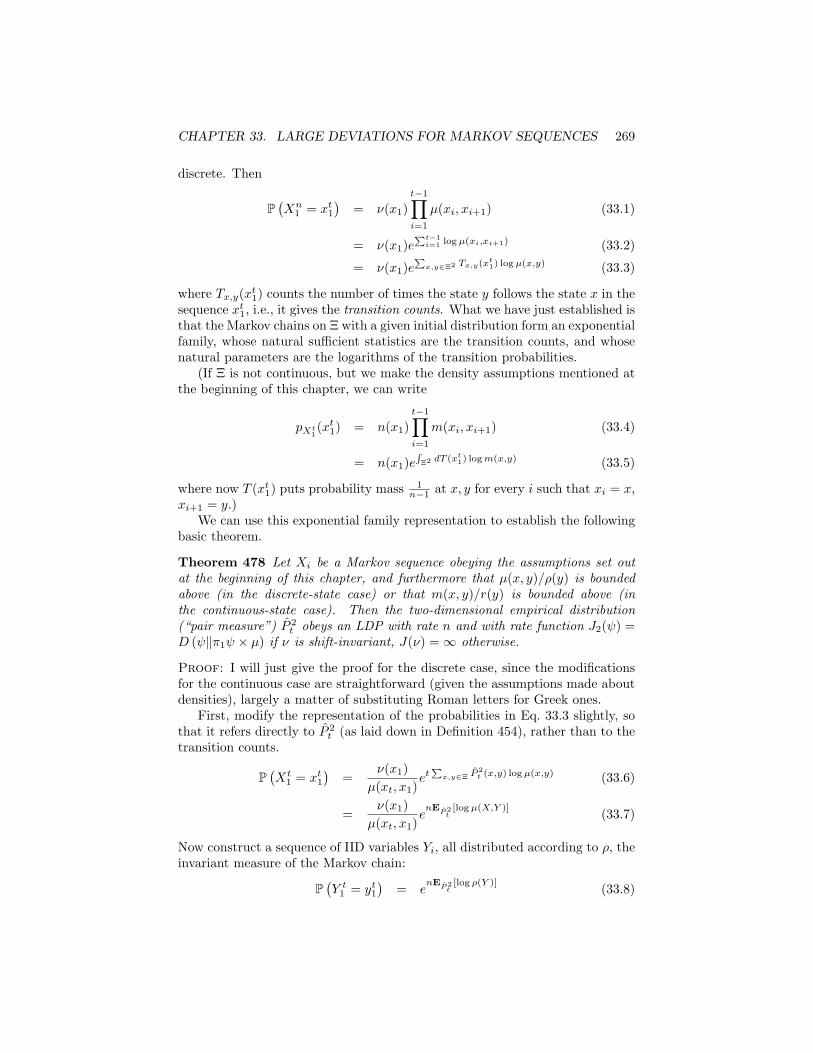
CHAPTER 33. LARGE DEVIATIONS FOR MARKOV SEQUENCES 269
discrete. Then
P(Xn
1 = xt1)
= ν(x1)t−1∏i=1
µ(xi, xi+1) (33.1)
= ν(x1)ePt−1i=1 log µ(xi,xi+1) (33.2)
= ν(x1)ePx,y∈Ξ2 Tx,y(xt1) log µ(x,y) (33.3)
where Tx,y(xt1) counts the number of times the state y follows the state x in thesequence xt1, i.e., it gives the transition counts. What we have just established isthat the Markov chains on Ξ with a given initial distribution form an exponentialfamily, whose natural sufficient statistics are the transition counts, and whosenatural parameters are the logarithms of the transition probabilities.
(If Ξ is not continuous, but we make the density assumptions mentioned atthe beginning of this chapter, we can write
pXt1(xt1) = n(x1)t−1∏i=1
m(xi, xi+1) (33.4)
= n(x1)eRΞ2 dT (xt1) logm(x,y) (33.5)
where now T (xt1) puts probability mass 1n−1 at x, y for every i such that xi = x,
xi+1 = y.)We can use this exponential family representation to establish the following
basic theorem.
Theorem 478 Let Xi be a Markov sequence obeying the assumptions set outat the beginning of this chapter, and furthermore that µ(x, y)/ρ(y) is boundedabove (in the discrete-state case) or that m(x, y)/r(y) is bounded above (inthe continuous-state case). Then the two-dimensional empirical distribution(“pair measure”) P 2
t obeys an LDP with rate n and with rate function J2(ψ) =D (ψ‖π1ψ × µ) if ν is shift-invariant, J(ν) =∞ otherwise.
Proof: I will just give the proof for the discrete case, since the modificationsfor the continuous case are straightforward (given the assumptions made aboutdensities), largely a matter of substituting Roman letters for Greek ones.
First, modify the representation of the probabilities in Eq. 33.3 slightly, sothat it refers directly to P 2
t (as laid down in Definition 454), rather than to thetransition counts.
P(Xt
1 = xt1)
=ν(x1)
µ(xt, x1)et
Px,y∈Ξ P
2t (x,y) log µ(x,y) (33.6)
=ν(x1)
µ(xt, x1)enE
P2t
[log µ(X,Y )] (33.7)
Now construct a sequence of IID variables Yi, all distributed according to ρ, theinvariant measure of the Markov chain:
P(Y t1 = yt1
)= e
nEP2t
[log ρ(Y )] (33.8)
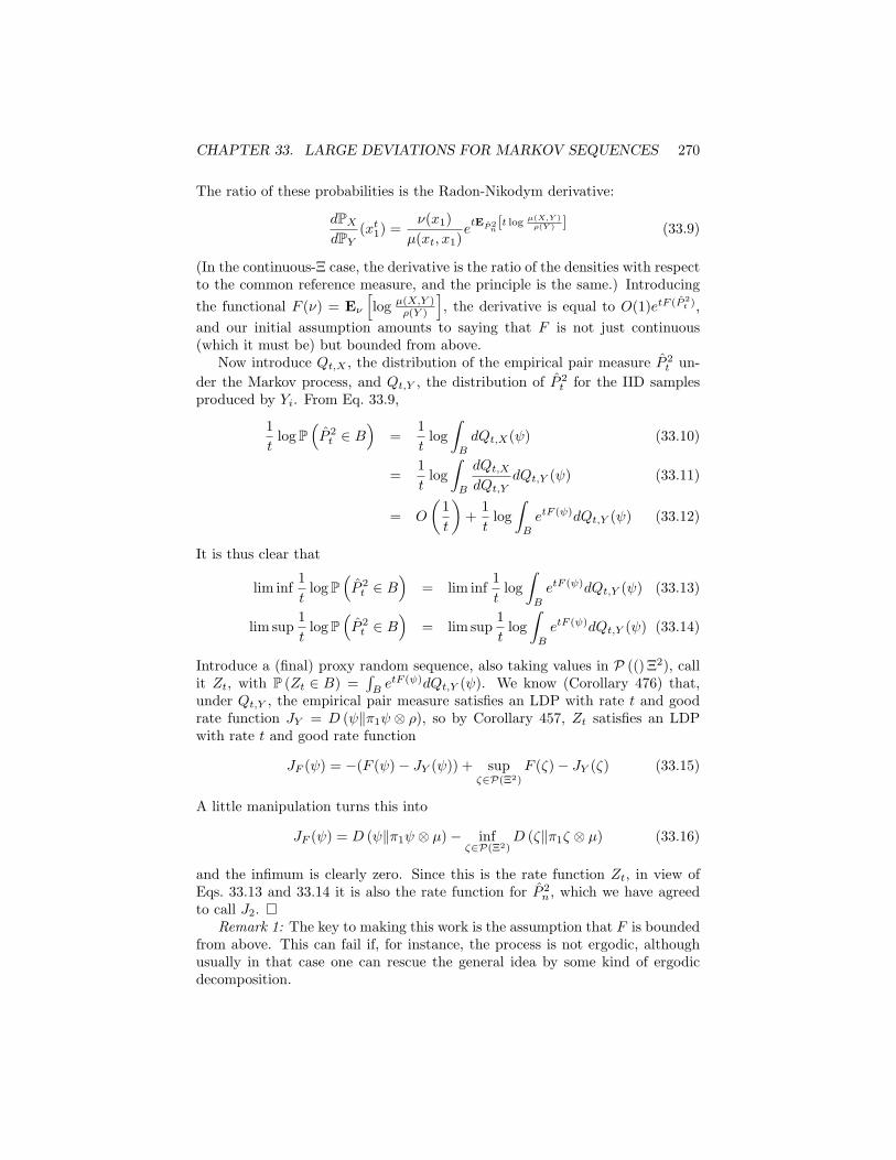
CHAPTER 33. LARGE DEVIATIONS FOR MARKOV SEQUENCES 270
The ratio of these probabilities is the Radon-Nikodym derivative:
dPXdPY
(xt1) =ν(x1)
µ(xt, x1)etEP2
n[t log
µ(X,Y )ρ(Y ) ] (33.9)
(In the continuous-Ξ case, the derivative is the ratio of the densities with respectto the common reference measure, and the principle is the same.) Introducingthe functional F (ν) = Eν
[log µ(X,Y )
ρ(Y )
], the derivative is equal to O(1)etF (P 2
t ),and our initial assumption amounts to saying that F is not just continuous(which it must be) but bounded from above.
Now introduce Qt,X , the distribution of the empirical pair measure P 2t un-
der the Markov process, and Qt,Y , the distribution of P 2t for the IID samples
produced by Yi. From Eq. 33.9,
1t
log P(P 2t ∈ B
)=
1t
log∫B
dQt,X(ψ) (33.10)
=1t
log∫B
dQt,XdQt,Y
dQt,Y (ψ) (33.11)
= O
(1t
)+
1t
log∫B
etF (ψ)dQt,Y (ψ) (33.12)
It is thus clear that
lim inf1t
log P(P 2t ∈ B
)= lim inf
1t
log∫B
etF (ψ)dQt,Y (ψ) (33.13)
lim sup1t
log P(P 2t ∈ B
)= lim sup
1t
log∫B
etF (ψ)dQt,Y (ψ) (33.14)
Introduce a (final) proxy random sequence, also taking values in P (() Ξ2), callit Zt, with P (Zt ∈ B) =
∫BetF (ψ)dQt,Y (ψ). We know (Corollary 476) that,
under Qt,Y , the empirical pair measure satisfies an LDP with rate t and goodrate function JY = D (ψ‖π1ψ ⊗ ρ), so by Corollary 457, Zt satisfies an LDPwith rate t and good rate function
JF (ψ) = −(F (ψ)− JY (ψ)) + supζ∈P(Ξ2)
F (ζ)− JY (ζ) (33.15)
A little manipulation turns this into
JF (ψ) = D (ψ‖π1ψ ⊗ µ)− infζ∈P(Ξ2)
D (ζ‖π1ζ ⊗ µ) (33.16)
and the infimum is clearly zero. Since this is the rate function Zt, in view ofEqs. 33.13 and 33.14 it is also the rate function for P 2
n , which we have agreedto call J2.
Remark 1: The key to making this work is the assumption that F is boundedfrom above. This can fail if, for instance, the process is not ergodic, althoughusually in that case one can rescue the general idea by some kind of ergodicdecomposition.
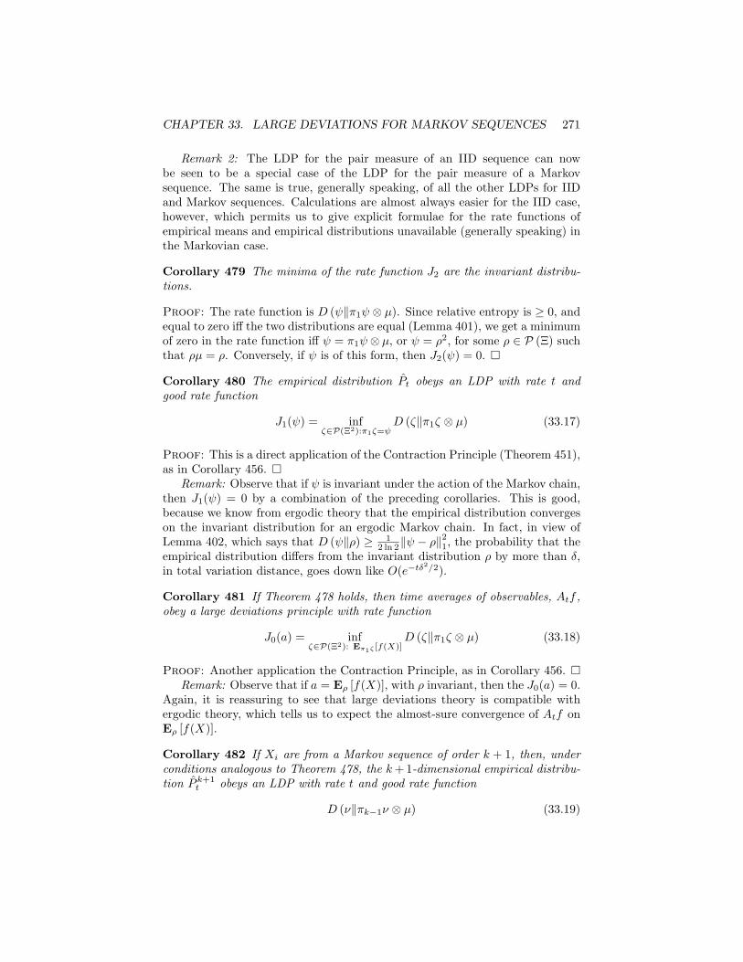
CHAPTER 33. LARGE DEVIATIONS FOR MARKOV SEQUENCES 271
Remark 2: The LDP for the pair measure of an IID sequence can nowbe seen to be a special case of the LDP for the pair measure of a Markovsequence. The same is true, generally speaking, of all the other LDPs for IIDand Markov sequences. Calculations are almost always easier for the IID case,however, which permits us to give explicit formulae for the rate functions ofempirical means and empirical distributions unavailable (generally speaking) inthe Markovian case.
Corollary 479 The minima of the rate function J2 are the invariant distribu-tions.
Proof: The rate function is D (ψ‖π1ψ ⊗ µ). Since relative entropy is ≥ 0, andequal to zero iff the two distributions are equal (Lemma 401), we get a minimumof zero in the rate function iff ψ = π1ψ⊗ µ, or ψ = ρ2, for some ρ ∈ P (Ξ) suchthat ρµ = ρ. Conversely, if ψ is of this form, then J2(ψ) = 0.
Corollary 480 The empirical distribution Pt obeys an LDP with rate t andgood rate function
J1(ψ) = infζ∈P(Ξ2):π1ζ=ψ
D (ζ‖π1ζ ⊗ µ) (33.17)
Proof: This is a direct application of the Contraction Principle (Theorem 451),as in Corollary 456.
Remark: Observe that if ψ is invariant under the action of the Markov chain,then J1(ψ) = 0 by a combination of the preceding corollaries. This is good,because we know from ergodic theory that the empirical distribution convergeson the invariant distribution for an ergodic Markov chain. In fact, in view ofLemma 402, which says that D (ψ‖ρ) ≥ 1
2 ln 2‖ψ − ρ‖21, the probability that the
empirical distribution differs from the invariant distribution ρ by more than δ,in total variation distance, goes down like O(e−tδ
2/2).
Corollary 481 If Theorem 478 holds, then time averages of observables, Atf ,obey a large deviations principle with rate function
J0(a) = infζ∈P(Ξ2): Eπ1ζ [f(X)]
D (ζ‖π1ζ ⊗ µ) (33.18)
Proof: Another application the Contraction Principle, as in Corollary 456. Remark: Observe that if a = Eρ [f(X)], with ρ invariant, then the J0(a) = 0.
Again, it is reassuring to see that large deviations theory is compatible withergodic theory, which tells us to expect the almost-sure convergence of Atf onEρ [f(X)].
Corollary 482 If Xi are from a Markov sequence of order k + 1, then, underconditions analogous to Theorem 478, the k+ 1-dimensional empirical distribu-tion P k+1
t obeys an LDP with rate t and good rate function
D (ν‖πk−1ν ⊗ µ) (33.19)
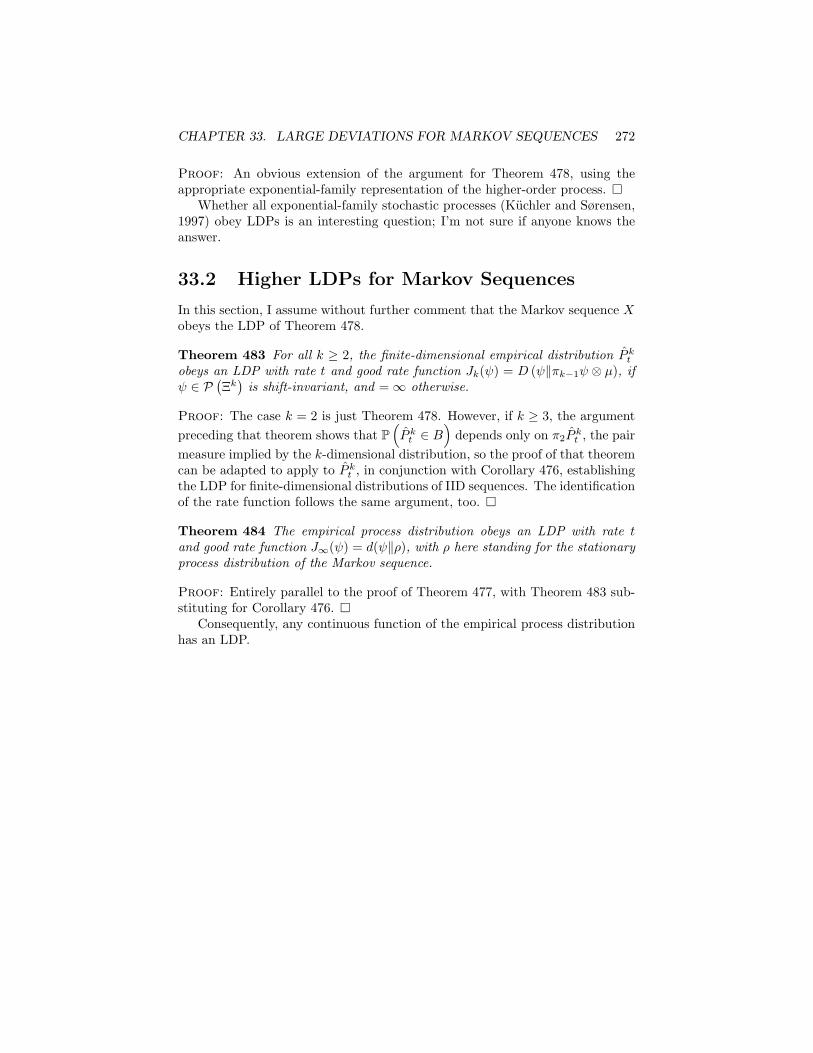
CHAPTER 33. LARGE DEVIATIONS FOR MARKOV SEQUENCES 272
Proof: An obvious extension of the argument for Theorem 478, using theappropriate exponential-family representation of the higher-order process.
Whether all exponential-family stochastic processes (Kuchler and Sørensen,1997) obey LDPs is an interesting question; I’m not sure if anyone knows theanswer.
33.2 Higher LDPs for Markov Sequences
In this section, I assume without further comment that the Markov sequence Xobeys the LDP of Theorem 478.
Theorem 483 For all k ≥ 2, the finite-dimensional empirical distribution P ktobeys an LDP with rate t and good rate function Jk(ψ) = D (ψ‖πk−1ψ ⊗ µ), ifψ ∈ P
(Ξk)
is shift-invariant, and =∞ otherwise.
Proof: The case k = 2 is just Theorem 478. However, if k ≥ 3, the argumentpreceding that theorem shows that P
(P kt ∈ B
)depends only on π2P
kt , the pair
measure implied by the k-dimensional distribution, so the proof of that theoremcan be adapted to apply to P kt , in conjunction with Corollary 476, establishingthe LDP for finite-dimensional distributions of IID sequences. The identificationof the rate function follows the same argument, too.
Theorem 484 The empirical process distribution obeys an LDP with rate tand good rate function J∞(ψ) = d(ψ‖ρ), with ρ here standing for the stationaryprocess distribution of the Markov sequence.
Proof: Entirely parallel to the proof of Theorem 477, with Theorem 483 sub-stituting for Corollary 476.
Consequently, any continuous function of the empirical process distributionhas an LDP.
Chapter 34
Large Deviations forWeakly DependentSequences via theGartner-Ellis Theorem
This chapter proves the Gartner-Ellis theorem, establishing anLDP for not-too-dependent processes taking values in topologicalvector spaces. Most of our earlier LDP results can be seen as con-sequences of this theorem.
34.1 The Gartner-Ellis Theorem
The Gartner-Ellis theorem is a powerful result which establishes the existenceof a large deviation principle for processes where the cumulant generating func-tion tends towards a well-behaved limit, implying not-too-strong dependencebetween successive values. (Exercise 90 clarifies the meaning of “too strong”.)It will imply our LDPs for IID and Markovian sequences. I could have startedwith it, but its proof, as you’ll see, is pretty technical, and so it seemed betterto use the more elementary arguments of the preceding chapters.
To fix notation, Ξ will be a real topological vector space, and Ξ∗ will be itsdual space, of continuous linear functions Ξ 7→ R. (If Ξ = Rd, we can identifyΞ and Ξ∗ by means of the inner product. In differential geometry, on the otherhand, Ξ might be a space of tangent vectors, and Ξ∗ the corresponding one-forms.) Xε will be a family of Ξ-valued random variables, parameterized byε > 0. Refer to Definitions 464 and 465 in Section 32.1 for the definition of thecumulant generating function and its Legendre transform (respectively), whichI will denote by Λε : Ξ∗ 7→ R and Λ∗ε : Ξ 7→ R.
The proof of the Gartner-Ellis theorem goes through a number of lemmas.
273
CHAPTER 34. THE GARTNER-ELLIS THEOREM 274
Basically, the upper large deviation bound holds under substantially weakerconditions than the lower bound does, and it’s worthwhile having the partialresults available to use in estimates even if the full large deviations principledoes not apply.
Definition 485 The upper-limiting cumulant generating function is
Λ (t) ≡ lim supε→0
εΛε(t/ε) (34.1)
and its Legendre transform is written Λ∗
(x).
The point of this is that the limsup always exists, whereas the limit doesn’t,necessarily. But we can show that the limsup has some reasonable properties,and in fact it’s enough to give us an upper bound.
Lemma 486 Λ (t) is convex, and Λ∗
(x) is a convex rate function.
Proof: The proof of the convexity of Λε(t) follows the proof in Lemma 466,and the convexity of Λ (t) by passing to the limit. To etablish Λ
∗(x) as a
rate function, we need it to be non-negative and lower semi-continuous. SinceΛε(0) = 0 for all ε, Λ (0) = 0. This in turn implies that Λ
∗(x) ≥ 0. Since the
latter is the supremum of a class of continuous functions, namely t(x) − Λ (t),it must be lower semi-continuous. Finally, its convexity is implied by its beinga Legendre transform.
Lemma 487 (Upper Bound in Gartner-Ellis Theorem: Compact Sets)For any compact set K ⊂ Ξ,
lim supε→0
ε log P (Xε ∈ K) ≤ −Λ∗
(K) (34.2)
Proof: Entirely parallel to the proof of the upper bound in Cramer’s Theorem(470), up through the point where closed sets are divided into a compact partand a remainder far from the origin, of exponentially-small probability. BecauseK is compact, we can proceed as though the remainder is empty.
Lemma 488 (Upper Bound in Gartner-Ellis Theorem: Closed Sets) Ifthe family of distributions L (Xε) are exponentially tight, then for all closedC ⊂ Ξ,
lim supε→0
ε log P (Xε ∈ C) ≤ −Λ∗
(C) (34.3)
Proof: Exponential tightness, by definition (458), will let us repeat Theorem470 trick of dividing closed sets into a compact part, and an exponentially-vanishing non-compact part.
CHAPTER 34. THE GARTNER-ELLIS THEOREM 275
Definition 489 The limiting cumulant generating function is
Λ(t) ≡ limε→0
εΛε(t/ε) (34.4)
when the limit exists. Its domain of finiteness D ≡ t ∈ Ξ∗ : Λ(t) < infty. Itslimiting Legendre transform is Λ∗, with domain of finiteness D∗.
Lemma 490 If Λ(t) exists, then it is convex, Λ∗(x) is a convex rate function,and Eq. 34.2 applies to the latter. If in addition the process is exponentiallytight, then Eq. 34.3 holds for Λ∗(x).
Proof: Because, if a limit exists, it is equal to the limsup.
Lemma 491 If Ξ = Rd, then 0 ∈ intD is sufficient for exponential tightness.
Proof: Exercise. Unfortunately, this is not good enough to get exponential tightness in arbi-
trary vector spaces.
Definition 492 (Exposed Point) A point x ∈ Ξ is exposed for Λ∗
(·) whenthere is a t ∈ Ξ∗ such that Λ
∗(y) − Λ
∗(x) > t(y − x) for all y 6= x. t is the
exposing hyper-plane for x.
In R1, a point x is exposed if the curve Λ∗
(y) lies strictly above the line of slopet through the point (x,Λ
∗(x)). Similarly, in Rd, the Λ
∗(y) surface must lie
strictly above the hyper-plane passing through (x,Λ∗
(x)) with surface normalt. Since Λ
∗(y) is convex, we could generally arrange this by making this the
tangent hyper-plane, but we do not, yet, have any reason to think that thetangent is well-defined. — Obviously, if Λ(t) exists, we can replace Λ
∗(·) by
Λ∗(·) in the definition and the rest of this paragraph.
Definition 493 An exposed point x ∈ Ξ with exposing hyper-plane t is nice,x ∈ N , if
limε→0
εΛε(t/ε) (34.5)
exists, and, for some r > 1,Λ (rt) <∞ (34.6)
Note: Most books on large deviations do not give this property any particularname.
Lemma 494 (Lower Bound in Gartner-Ellis Theorem) If the Xε are ex-ponentially tight, then, for any open set O ⊆ Ξ,
lim infε→0
ε log P (Xε ∈ O) ≥ −Λ∗
(O ∩N) (34.7)
CHAPTER 34. THE GARTNER-ELLIS THEOREM 276
Proof: If we pick any nice, exposed point x ∈ O, we can repeat the proof ofthe lower bound from Cramer’s Theorem (470). In fact, the point of Definition493 is to ensure this. Taking the supremum over all such x gives the lemma.
Theorem 495 (Abstract Gartner-Ellis Theorem) If the Xε are exponen-tially tight, and Λ
∗(O ∩ E) = Λ
∗(O) for all open sets O ⊆ Ξ, then Xε obey an
LDP with rate 1/ε and good rate function Λ∗
(x).
Proof: The large deviations upper bound is Lemma 488. The large deviationslower bound is implied by Lemma 494 and the additional hypothesis of thetheorem.
Matters can be made a bit more concrete in Euclidean space (the originalhome of the theorem), using, however, one or two more bits of convex analysis.
Definition 496 (Relative Interior) The relative interior of a non-empty andconvex set A is
rintA ≡ x ∈ A : ∀y ∈ A,∃δ > 0, x− δ(y − x) ∈ A (34.8)
Notice that intA ⊆ rintA, since the latter, in some sense, doesn’t care aboutpoints outside of A.
Definition 497 (Essentially Smooth) Λ is essentially smooth if (i) intD 6=∅, (ii) Λ is differentiable on intD, and (iii) Λ is “steep”, meaning that if D hasa boundary, ∂D, then limt→∂D ‖∇Λ(t)‖ =∞.
This definition was introduced to exploit the following theorem of convexanalysis.
Proposition 498 If Λ is essentially smooth, then Λ∗ is continuous on rintD∗,and rintD∗ ⊆ N , the set of exposed, nice points.
Proof: D∗ is non-empty, because there is at least one point x0 where Λ∗(x0) =0. Moreover, it is a convex set, because Λ∗ is a convex function (Lemma 490),so it has a relative interior. Now appeal to Rockafellar (1970, Corollary 26.4.1).
Remark: You might want to try to prove that Λ∗ is continuous on rintD∗.
Theorem 499 (Euclidean Gartner-Ellis Theorem) Suppose Xε, taking val-ues in Rd, are exponentially tight, and that Λ(t) exists and is essentially smooth.Then Xε obey an LDP with rate 1/ε and good rate function Λ∗(x).
Proof: From the abstract Gartner-Ellis Theorem 495, it is enough to showthat Λ∗(O ∩N) = Λ∗(O), for any open set O. That is, we want
infx∈O∩N
Λ∗(x) = infx∈O
Λ∗(x) (34.9)
CHAPTER 34. THE GARTNER-ELLIS THEOREM 277
Since it’s automatic that
infx∈O∩N
Λ∗(x) ≥ infx∈O
Λ∗(x) (34.10)
what we need to show is that
infx∈O∩N
Λ∗(x) ≤ infx∈O
Λ∗(x) (34.11)
In view of Proposition 498, it’s really just enough to show that Λ∗(O∩rintD∗) ≤Λ∗(O). This is trivial when the intersection O ∩ D∗ is empty, so assume itisn’t, and pick any x in that intersection. Because O is open, and becauseof the definition of the relative interior, we can pick any point y ∈ rintD∗,and, for sufficiently small δ, δy + (1 − δ)x ∈ O ∩ rintD∗. Since Λ∗ is convex,Λ∗(δy + (1− δ)x) ≤ δΛ∗(y) + (1− δ)Λ∗(x). Taking the limit as δ → 0,
Λ∗(O ∩ rintD∗) ≤ Λ∗(x) (34.12)
and the claim follows by taking the infimum over x.
34.2 Exercises
Exercise 86 Show that Cramer’s Theorem (470), is a special case of the Eu-clidean Gartner-Ellis Theorem (499).
Exercise 87 Let Z1, Z2, . . . be IID random variables in a discrete space, and letX1, X2, . . . be the empirical distributions they generate. Use the Gartner-EllisTheorem to re-prove Sanov’s Theorem (475). Can you extend this to the casewhere the Zi take values in an arbitrary Polish space?
Exercise 88 Let Z1, Z2, . . . be values from a stationary ergodic Markov chain(i.e. the state space is discrete). Repeat the previous exercise for the pair mea-sure. Again, can the result be extended to arbitrary Polish state spaces?
Exercise 89 Let Zi be real-valued mean-zero stationary Gaussian variables,with
∑∞i=−∞ |cov (Z0, Zi) | < ∞. Let Xt = t−1
∑ti=1 Zi. Show that these
time averages obey an LDP with rate t and rate function x2/2Γ, where Γ =∑∞i=−∞ cov (Z0, Zi). (Cf. the mean-square ergodic theorem 293 of chapter 19.)
If Zi are not Gaussian but are weakly stationary, find an additional hypothesissuch that the time averages still obey an LDP.
Exercise 90 (Too-Strong Dependence) Let Xi = X, a random variable inR, for all i. Show that the Gartner-Ellis Theorem fails, unless X is degenerate.
Chapter 35
Large Deviations forStationary Sequences [[w]]
To follow
278
Chapter 36
Large Deviations inInference [[w]]
279
Chapter 37
Large Deviations forStochastic DifferentialEquations
This last chapter revisits large deviations for stochastic differen-tial equations in the small-noise limit, first raised in Chapter 20.
Section 37.1 establishes the LDP for the Wiener process (Schilder’sTheorem).
Section 37.2 proves the LDP for stochastic differential equationswhere the driving noise is independent of the state of the process.
Section 37.3 states the corresponding result for SDEs when thenoise is state-dependent, and gestures in the direction of the proof.
In Chapter 20, we looked at how the diffusions Xε which solve the SDE
dXε = a(Xε)dt+ εdW, Xε(0) = x0 (37.1)
converge on the trajectory x0(t) solving the ODE
dx
dt= a(x(t)), x(0) = x0 (37.2)
in the “small noise” limit, ε→ 0. Specifically, Theorem 290 gave a (fairly crude)upper bound on the probability of deviations:
limε→0
ε2 log P(
sup0≤t≤T
∆ε(t) > δ
)≤ −δ2e−2KaT (37.3)
where Ka depends on the Lipschitz coefficient of the drift function a. The the-ory of large deviations for stochastic differential equations, known as Freidlin-Wentzell theory for its original developers, shows that, using the metric implicit
280
CHAPTER 37. FREIDLIN-WENTZELL THEORY 281
in the left-hand side of Eq. 37.3, the family of processes Xε obey a large devia-tions principle with rate ε−2, and a good rate function.
(The full Freidlin-Wentzell theory actually goes somewhat further than justSDEs, to consider small-noise perturbations of dynamical systems of many sorts,perturbations by Markov processes (rather than just white noise), etc. Timedoes not allow us to consider the full theory (Freidlin and Wentzell, 1998), orits many applications to nonparametric estimation (Ibragimov and Has’minskii,1979/1981), systems analysis and signal processing (Kushner, 1984), statisticalmechanics (Olivieri and Vares, 2005), etc.)
As in Chapter 32, the strategy is to first prove a large deviations principlefor a comparatively simple case, and then transfer it to more subtle processeswhich can be represented as appropriate functionals of the basic case. Here,the basic case is the Wiener process W (t), with t restricted to the unit interval[0, 1].
37.1 Large Deviations of the Wiener Process
We start with a standard d-dimensional Wiener process W , and consider its di-lation by a factor ε, Xε(t) = εW (t). There are a number of ways of establishingthat Xε obeys a large deviation principle as ε → 0. One approach (see Demboand Zeitouni (1998, ch. 5) starts with establishing an LDP for continuous-timerandom walks, ultimately based on the Gartner-Ellis Theorem, and then show-ing that the convergence of such processes to the Wiener process (the FunctionalCentral Limit Theorem, Theorem 215 of Chapter 15) is sufficiently fast that theLDP carries over. However, this approach involves a number of surprisinglytricky topological issues, so I will avoid it, in favor of a more probabilistic path,marked out by Freidlin and Wentzell (Freidlin and Wentzell, 1998, sec. 3.2).
Until further notice, ‖w‖∞ will denote the supremum norm in the space ofcontinuous curves over the unit interval, C([0, 1],Rd).
Definition 500 (Cameron-Martin Spaces) The Cameron-Martin space HT
consists of all continuous sample paths x ∈ C([0, T ],Rd) where x(0) = 0, x isabsolutely continuous, and its Radon-Nikodym derivative x is square-integrable.
Lemma 501 (Cameron-Martin Spaces are Hilbert) Cameron-Martin spacesare Hilbert spaces, with norm ‖x‖CM =
∫ T0|x(t)|2dt.
Proof: An exercise (91) in verifying that the axioms of a Hilbert space aresatisfied.
Definition 502 (Effective Wiener Action) The effective Wiener action ofan continuous function x ∈ C([0, t],Rd) is
JT (x) ≡ 12‖x‖2CM (37.4)
CHAPTER 37. FREIDLIN-WENTZELL THEORY 282
if x ∈ HT , and ∞ otherwise. In particular,
J1(x) ≡ 12
∫ 1
0
|x(t)|2dt (37.5)
For every j > 0, let LT (j) = x : JT (x) ≤ j.
Proposition 503 (Girsanov Formula for Deterministic Drift) Fix a func-tion f ∈ H1, and let Yε = Xε − f . Then L (Yε) = νε is absolutely continuouswith respect to L (Xε) = µε, and the Radon-Nikodym derivative is
dνεdµε
(εw) = exp−1ε
∫ 1
0
w(t) · dW − 12ε2
∫ 1
0
|w(t)|2dt
(37.6)
Proof: This is a special case of Girsanov’s Theorem. See Corollary 18.25on p. 365 of Kallenberg, or, more transparently perhaps, the relevant parts ofLiptser and Shiryaev (2001, vol. I).
Lemma 504 (Exponential Bound on the Probability of Tubes AroundGiven Trajectories) For any δ, γ,K > 0, there exists an ε0 > 0 such that, ifε < ε0,
P (‖Xε − x‖∞ ≤ δ) ≥ e− J1(x)+γ
ε2 (37.7)
provided x(0) = 0 and J1(x) < K.
Proof: Using Proposition 503,
P (‖Xε − x‖∞ ≤ δ) = P (‖Yε − 0‖∞ ≤ δ) (37.8)
=∫‖εw‖∞<δ
dνεdµε
(εw)dµε(εw) (37.9)
= e−J1(x)ε2
∫‖εw‖∞<δ
e−1ε
R 10 x·dW dµε(w) (37.10)
From Lemma 288 in Chapter 20, we can see that P (‖εW‖∞ < δ)→ 1 as ε→ 0.So, if ε is sufficiently small, P (‖εW‖∞ < δ) ≥ 3/4. Now, applying Chebyshev’sinequality to the integrand,
P
(−1ε
∫ 1
0
x · dW ≤ −2√
2ε
√J1(x)
)(37.11)
≤ P
(∣∣∣∣1ε∫ 1
0
x · dW∣∣∣∣ ≤ 2
√2ε
√J1(x)
)(37.12)
≤ε2E
[(∫ 1
0x · dW
)2]
8ε2J1(x)(37.13)
=
∫ 1
0|x|2dt
8J1(x)=
14
(37.14)
CHAPTER 37. FREIDLIN-WENTZELL THEORY 283
using the Ito isometry (Corollary 238). Thus
P(e−
1ε
R 10 x·dW ≥ e−
2√
2ε
√J1(x)
)≥ 3
4(37.15)
∫‖εw‖∞<δ
e−1ε
R 10 x·dW dµε(w) >
12e−
2√
2ε
√J1(x) (37.16)
P (‖Xε − x‖∞ ≤ δ) >12e−
J1(x)ε2− 2√
2ε
√J1(x) (37.17)
where the second term in the exponent can be made less than any desired γ bytaking ε small enough.
Lemma 505 (Trajectories are Rarely Far from Action Minima) Forevery j > 0, δ > 0, let U(j, δ) be the open δ neighborhood of L1(j), i.e., all thetrajectories coming within δ of a trajectory whose action is less than or equal toj. Then for any γ > 0, there is an ε0 > 0 such that, if ε < ε0 and
P (Xε 6∈ U(j, δ)) ≤ e−s−γε2 (37.18)
Proof: Basically, approximating the Wiener process by a continuous piecewise-linear function, and showing that the approximation is sufficiently fine-grained.Chose a natural number n, and let Yn,ε(t) be the piecewise linear random func-tion which coincides with Xε at times 0, 1/n, 2/n, . . . 1, i.e.,
Yn,ε(t) = Xε([tn]/n) +(t− [tn]
n
)Xε([tn+ 1]/n) (37.19)
We will see that, for large enough n, this is exponentially close to Xε. First,though, let’s bound the probability in Eq. 37.18.
P (Xε 6∈ U(j, δ))= P
(Xε 6∈ U(j, δ), ‖Xε − Yn,ε‖∞ < δ
)+P(Xε 6∈ U(j, δ), ‖Xε − Yn,ε‖∞ ≥ δ
)(37.20)
≤ P(Xε 6∈ U(j, δ), ‖Xε − Yn,ε‖∞ < δ
)+ P
(‖Xε − Yn,ε‖∞ ≥ δ
)(37.21)
≤ P (J1(Yn,ε) > j) + P(‖Xε − Yn,ε‖∞ ≥ δ
)(37.22)
J1(Yn,ε) can be gotten at from the increments of the Wiener process:
J1(Yn,ε) = nε2
2
n∑i=1
|W (i/n)−W ((i− 1)/n)|2 (37.23)
=ε2
2
dn∑i=1
ξi (37.24)
CHAPTER 37. FREIDLIN-WENTZELL THEORY 284
where the ξi have the χ2 distribution with one degree of freedom. Using ourresults on such distributions and their sums in Ch. 20, it is not hard to showthat, for sufficiently small ε,
P (J1(Yn,ε) > j) ≤ 12e−
j−γε2 (37.25)
To estimate the probability that the distance between Xε and Yn,ε reaches orexceeds δ, start with the independent-increments property of Xε, and the factthat the two processes coincide when t = i/n.
P(‖Xε − Yn,ε‖∞ ≥ δ
)≤
n∑i=1
P(
max(i−1)/n≤t≤i/n
|Xε(t)− Yn,ε(t)| ≥ δ)
(37.26)
= nP(
max0≤t≤1/n
|Xε(t)− Yn,ε(t)| ≥ δ)
(37.27)
= nP(
max0≤t≤1/n
|εW (t)− nεW (1/n)| ≥ δ)
(37.28)
≤ nP(
max0≤t≤1/n
|εW (t)| ≥ δ
2
)(37.29)
≤ 4dnP(W1(1/n) ≥ δ
2dε
)(37.30)
≤ 4dn2dε
δ√
2πne−
nδ2
8d2ε2 (37.31)
again freely using our calculations from Ch. 20. If n > 4d2j/δ2, then P(‖Xε − Yn,ε‖∞
)≤
12e− j−γ
ε2 , and we have overall
P (Xε 6∈ U(j, δ)) ≤ e−j−γε2 (37.32)
as required.
Proposition 506 (Compact Level Sets of the Wiener Action) The Cameron-Martin norm has compact level sets.
Proof: See Kallenberg, Lemma 27.7, p. 543.
Theorem 507 (Schilder’s Theorem on Large Deviations of the WienerProcess on the Unit Interval) If W is a d-dimensional Wiener process onthe unit interval, then Xε = εW obeys an LDP on C([0, 1],Rd), with rate ε−2
and good rate function J1(x), the effective Wiener action over [0, 1].
Proof: It is easy to show that Lemma 504 implies the large deviation lowerbound for open sets. (Exercise 92.) The tricky part is the upper bound. Pickany closed set C and any γ > 0. Let s = J1(C) − γ. By Lemma 506, the set
CHAPTER 37. FREIDLIN-WENTZELL THEORY 285
K = L1(s) = x : J1(x) ≤ s is compact. By construction, C ∩ K = ∅. Soδ = infx∈C,y∈K ‖x− y‖∞ > 0. Let U be the closed δ-neighborhood of K. Thenuse Lemma 505
P (Xε ∈ C) ≤ P (Xε 6∈ U) (37.33)
≤ e−s−γε2 (37.34)
≤ e−J1(C)−2γ
ε2 (37.35)
log P (Xε ∈ C) ≤ −J1(C)− 2γε2
(37.36)
ε2 log P (Xε ∈ C) ≤ −J1(C)− 2γ (37.37)lim supε→0
ε2 log P (Xε ∈ C) ≤ −J1(C)− 2γ (37.38)
Since γ was arbitrary, this completes the proof. Remark: The trick used here, about establishing results like Lemmas 505
and 504, and then using compact level sets to prove large deviations, worksmore generally. See Theorem 3.3 in Freidlin and Wentzell (1998, sec. 3.3).
Corollary 508 (Extension of Schilder’s Theorem to [0, T ]) Schilder’s the-orem remains true for Wiener processes on [0, T ], for all T > 0, with ratefunction JT , the effective Wiener action on [0, T ].
Proof: If W is a Wiener process on [0, 1], then, for every T , S(W ) =√TW (t/T ) is a Wiener process on [0, T ]. (Show this!) Since the mapping S
is continuous from C([0, 1],Rd) to C([0, T ],Rd), by the Contraction Principle(Theorem 451) the family εS(W ) obey an LDP with rate ε−2 and good ratefunction JT (x) = J1(S−1(x)). (Notice that S is invertible, so S−1(x) is afunction, not a set of functions.) Since x ∈ H1 iff y = S(x) ∈ HT , it’s easy tocheck that for such, y(t) = T−1/2x(t/T ), meaning that
‖y‖CM =∫ T
0
|y(t)|2dt =∫ T
0
|x(t/T )|2 dtT
= ‖x‖CM (37.39)
which completes the proof.
Corollary 509 (Schilder’s Theorem on R+) Schilder’s theorem remainstrue for Wiener processes on R+, with good rate function J∞ given by the ef-fective Wiener action on R+,
J∞(x) ≡ 12
∫ ∞0
|x(t)|2dt (37.40)
if x ∈ H∞, J∞(x) =∞ otherwise.
Proof: For each natural number n, let πnx be the restriction of x to theinterval [0, n]. By Corollary 508, each of them obeys an LDP with rate function12
∫ n0|x(t)|2dt. Now apply the projective limit theorem (461) to get that J∞(x) =
supn Jn(x), which is clearly Eq. 37.40, as the integrand is non-negative.
CHAPTER 37. FREIDLIN-WENTZELL THEORY 286
37.2 Large Deviations for SDEs with State-IndependentNoise
Having established an LDP for the Wiener process, it is fairly straightforwardto get an LDP for stochastic differential equations where the driving noise isindependent of the state of the diffusion process.
Definition 510 (SDE with Small State-Independent Noise) An SDEwith small state-independent noise is a stochastic differential equation of theform
dXε = a(Xε)dt+ εdW (37.41)Xε(0) = 0 (37.42)
where a : Rd 7→ Rd is uniformly Lipschitz continuous.
Notice that any non-random initial condition x0 can be handled by a simplechange of coordinates.
Definition 511 (Effective Action under State-Independent Noise) Theeffective action of a trajectory x ∈ H∞ is
J(x) ≡ 12
∫ t
0
|x(t)− a(x(t))|2dt (37.43)
and =∞ if x ∈ C \H∞.
Lemma 512 (Continuous Mapping from Wiener Process to SDE So-lutions) The map F : C(R+,Rd) 7→ C(R+,Rd) given by
x(t) = w(t) +∫ t
0
a(x(s))ds (37.44)
when x = F (w) is continuous.
Proof: This goes rather in the same manner as the proof of existenceand uniqueness for SDEs (Theorem 260). For any w1, w2 ∈ C(R+,Rd), setx1 = F (w1), x2 = F (w2). From the Lipschitz property of a,
|x1(t)− x2(t)| ≤ ‖w1 − w2‖+Ka
∫ t
0
|x1(s)− x2(s)| ds (37.45)
(writing |y(t)| for the norm of Euclidean vectors y, and ‖x‖ for the supremumnorm of continuous curves). By Gronwall’s Inequality (Lemma 258), then,
‖x1 − x2‖ ≤ ‖w1 − w2‖ eKaT (37.46)
on every interval [0, T ]. So we can make sure that ‖x1 − x2‖ is less than anydesired amount by making sure that ‖w1 − w2‖ is sufficiently small, and so Fis continuous.
CHAPTER 37. FREIDLIN-WENTZELL THEORY 287
Lemma 513 (Mapping Cameron-Martin Spaces Into Themselves) Ifw ∈ H∞, then x = F (w) is in H∞.
Proof: Exercise 93.
Theorem 514 (Freidlin-Wentzell Theorem with State-Independent Noise)The Ito processes Xε of Definition 510 obey the large deviations principle withrate ε−2 and good rate function given by the effective action J(x).
Proof: For every ε, Xε = F (εW ). Corollary 509 tells us that εW obeysthe large deviation principle with rate ε−2 and good rate function J∞. Since(Lemma 512) F is continuous, by the Contraction Principle (Theorem 451) Xε
also obeys the LDP, with rate given by J∞(F−1(x)). If F−1(x) ∩ H∞ = ∅,this is ∞. On the other hand, if F−1(x) does contain curves in H∞, thenJ∞(F−1(x)) = J∞(F−1(x) ∩H∞). By Lemma 513, this implies that x ∈ H∞,too. For any curve w ∈ F−1(x) ∩ H∞, x = w + a(x), or w = x − a(x).J∞(w) =
∫∞0|x− a(x)|2dt is however the effective action of the trajectory x
(Definition 511).
37.3 Large Deviations for State-Dependent Noise
If the diffusion term in the SDE does depend on the state of the process, oneobtains a very similar LDP to the results in the previous section. However, theapproach must be modified: the mapping from W to Xε, while still measurable,is no longer necessarily continuous, so we can’t use the contraction principle asbefore.
Definition 515 (SDE with Small State-Dependent Noise) An SDE withsmall state-dependent noise is a stochastic differential equation of the form
dXε = a(Xε)dt+ εb(Xε)dW (37.47)Xε(0) = 0 (37.48)
where a and b are uniformly Lipschitz continuous, and b is non-singular.
Definition 516 (Effective Action under State-Dependent Noise) Theeffective action of a trajectory x ∈ H∞ is given by
J(x) ≡∫ ∞
0
L(x(t), x(t))dt (37.49)
whereL(q, p) =
12
(pi − ai(q))B−1ij (q) (pj − aj(q)) (37.50)
andB(q) = b(q)bT (q) (37.51)
with J(x) =∞ if x ∈ C \H∞.
CHAPTER 37. FREIDLIN-WENTZELL THEORY 288
Theorem 517 (Freidlin-Wentzell Theorem for State-Dependent Noise)The processes Xε obey a large deviations principle with rate ε−2 and good ratefunction equal to the effective action.
Proof: Considerably more complicated. (See, e.g., Dembo and Zeitouni(1998, sec. 5.6, pp. 213–220).) The essence, however, is to consider an approx-imating Ito process Xn, where a(Xt) and b(Xt) are replaced in Eq. 37.47 bya(Xn([tn]/n)) and b(Xn([tn]/n)). Here the mapping from W to Xn is continu-ous, so it’s not too hard to show that the latter obey an LDP with a reasonablerate function, and also that they’re exponentially equivalent (in n) to Xε.
37.4 Exercises
Exercise 91 (Cameron-Martin Spaces are Hilbert Spaces) Prove Lemma501.
Exercise 92 (Lower Bound in Schilder’s Theorem) Prove that Lemma504 implies the large deviations lower bound for open sets.
Exercise 93 (Mapping Cameron-Martin Spaces Into Themselves) ProveLemma 513. Hint: Use Gronwall’s Inequality (Lemma 258) again to show thatF maps HT into HT , and then show that H∞ =
⋂∞n=1Hn.
Part VIII
Measure Concentration[Kontorovich/w]
289
Part IX
Partially-ObservableProcesses [[w]]
290

Chapter 38
Hidden Markov Models[[w]]
to follow
291
Chapter 39
Stochastic Automata [[w]]
to follow
292
Chapter 40
Predictive Representations[[w]]
to follow
293
Part X
Applications [[w]]
294
295
Topics TBD. Possibilities: principles of least action; generalized H-theorems;diffusion approximations for branching processes; nonlinear filtering; “how sam-pling reveals a process”; Bayesian learning as a stochastic dynamical system;convergence of empirical distributions; large deviations of recurrence times andentropies; invariance principles for maps; likelihood inference for diffusions
Part XI
Appendices [[w]]
296
297
Reminders about math the reader should already know, or at least havealready forgotten.
Appendix A
Real and Complex Analysis[[w]]
Section A.1 collects some useful facts from real analysis and ele-mentary calculus, especially concerned with different kinds of conti-nuity.
Section A.2 collects useful facts from complex analysis.
A.1 Real Analysis
Sums, convergence on series (e.g. Cesaro), differentiation of series [[really nec-essary?]]
Continuity, uniform continuity, Lipschitz continuity, Holder continuity, mod-ulus of continuity
Taylor theorem, bounding the remainder
A.2 Complex Analysis
I’m sure we used some results that need to be collected here!
298
Appendix B
General Vector Spaces andOperators [[w]]
This appendix collects essential facts about operators (largelylinear ones) on linear spaces (largely function spaces), and semi-groups of such operators.
[[Define: vector space, norm, Banach space, Hilbert space, other spaces?]][[Give elementary vector spaces, matrices, function spaces as ezamples]][[Explain an operator]][[Explain operators correspond to matrices in finite-dimensional case]][[This material is copied-and-pasted from chapters 10, 14; delete there when
revising]]
Definition 518 (Functional) A functional is a map g : V 7→ R, that is, areal-valued function of a function. A functional g is
• linear when g(af1 + bf2) = ag(f1) + bg(f2);
• continuous when fn → f implies g(fn)→ f ;
• bounded by M when |g(f)| ≤M for all f ∈ V ;
• bounded when it is bounded by M for some M ;
• non-negative when g(f) ≥ 0 for all f ;
etc.
Definition 519 (Conjugate or Adjoint Space) The conjugate space or ad-joint space of a vector space V is the space V † of its continuous linear function-als. For f ∈ V and g ∈ V †, 〈f, g〉 denotes g(f). This is sometimes called theinner product.
299
APPENDIX B. GENERAL VECTOR SPACES AND OPERATORS [[W]]300
Proposition 520 (Conjugate Spaces are Vector Spaces) For every V , V †
is also a vector space.
Proposition 521 (Inner Product is Bilinear) For any a, b, c, d ∈ R, anyf1, f2 ∈ V and any g1, g2 ∈ V †,
〈af1 + bf2, cg1 + dg2〉 = ac〈f1, g1〉+ ad〈f1, g2〉+ bc〈f2, g1〉+ bd〈f2, g2〉 (B.1)
Proof: Follows from the fact that V † is a vector space, and each gi is alinear operator.
You are already familiar with an example of a conjugate space.
Example 522 (Vectors in Rn) The vector space Rn is self-conjugate. If g(~x)is a continuous linear function of ~x, then g(~x) =
∑ni=1 yixi for some real con-
stants yi, which means g(~x) = ~y · ~x.
Here is the simplest example where the conjugate space is not equal to theoriginal space.
Example 523 (Row and Column Vectors) The space of row vectors is con-jugate to the space of column vectors, since every continuous linear functionalof a column vector x takes the form of yTx for some other column vector y.
Example 524 (Lp spaces) The function spaces Lp(µ) and Lq(µ) are conjugateto each other, when 1/p+ 1/q = 1, and the inner product is defined through
〈f, g〉 ≡∫fgdµ (B.2)
In particular, L1 and L∞ are conjugates.
Example 525 (Measures and Functions) The space of Cb(Ξ) of bounded,continuous functions on Ξ and the spaces M(Ξ,X ) of finite measures on Ξ areconjugates, with inner product
〈µ, f〉 =∫fdµ (B.3)
Definition 526 (Adjoint Operator) For conjugate spaces V and V †, theadjoint operator, O†, to an operator O on V is an operator on V † such that
〈Of, g〉 = 〈f,O†g〉 (B.4)
for all f ∈ V, g ∈ V †.
APPENDIX B. GENERAL VECTOR SPACES AND OPERATORS [[W]]301
Proposition 527 (Adjoint of a Linear Operator) If O is a continuouslinear operator on V , then its adjoint O† exists and is linear.
Definition 528 (Contraction Operator) An operator A is an L-contractionwhen ‖Af‖ ≤ ‖f‖.
Definition 529 (Strongly Continuous Semigroup) A semigroup of oper-ators At is strongly continuous in the L sense on a set of functions D when,∀f ∈ D
limt→0‖Atf − f‖ = 0 (B.5)
Definition 530 (Positive Operator) An operator A on a function space Lis positive when f ≥ 0 a.e. implies Af ≥ 0 a.e.
Definition 531 (Conservative Operator) An operator A is conservativewhen A1Ξ = 1Ξ.
In these terms, our earlier Markov operators are linear, positive, conservativecontractions, either on L1(µ) (for densities) or M(Ξ) (for measures).
Lemma 532 (Continuous semi-groups produce continuous paths infunction space) If At is a strongly continuous semigroup of linear contrac-tions on L, then, for each f ∈ L, Atf is a continuous function of t.
Proof: Continuity here means that limt′→t ‖At′f −At‖ = 0 — we are usingthe norm ‖ · ‖ to define our metric in function space. Consider first the limitfrom above:
‖At+hf −Atf‖ = ‖At(Ahf − f)‖ (B.6)≤ ‖|Ohf − f‖ (B.7)
since the operators are contractions. Because they are strongly continuous,‖Ahf − f‖ can be made smaller than any ε > 0 by taking h sufficiently small.Hence limh↓0At+hf exists and is Atf . Similarly, for the limit from below,
‖At−hf −Atf‖ = ‖Atf −At−hf‖ (B.8)= ‖At−h(Ahf − f)‖ (B.9)≤ ‖Ahf − f‖ (B.10)
using the contraction property again. So limh↓0At−hf = Atf , also, and we canjust say that limt′→tAt′f = Atf .
Remark: The result actually holds if we just assume strong continuity, with-out contraction, but the proof isn’t so pretty; see Ethier and Kurtz (1986, ch.1, corollary 1.2, p. 7).
There is one particular function space L we will find especially interesting.
APPENDIX B. GENERAL VECTOR SPACES AND OPERATORS [[W]]302
Definition 533 (Continuous Functions Vanishing at Infinity) Let Ξ bea locally compact and separable metric space. The class of functions C0 willconsist of functions f : Ξ 7→ R which are continuous and for which ‖x‖ → ∞implies f(x)→ 0. The norm on C0 is supx |f(x)|.
Appendix C
Laplace Transforms [[w]]
This appendix collects some basic facts about Laplace transformsof real functions, including inversion theorems. It is useful in con-nection with the generators of Markov processes (Chapter 11) andsome aspects of Feller processes (Chapter 13).
[[Text taken from chapter on generators, smooth out]]Recall that the Laplace transform of a function f : R 7→ R is another func-
tion, f , defined by
f(λ) ≡∫ ∞
0
e−λtf(t)dt
for positive λ. Laplace transforms arise in many contexts (linear systems theory,integral equations, etc.), one of which is moment-generating functions in basicprobability theory. If Y is a real-valued random variable with probability lawP , then the moment-generating function is
MY (λ) ≡ E[eλY
]=∫eλydP =
∫eλyp(y)dy
when the density in the last expression exists. You may recall, from this context,that the distributions of well-behaved random variables are completely specifiedby their moment-generating functions; this is actually a special case of a moregeneral result about when functions are uniquely described by their Laplacetransforms, i.e., when f can be expressed uniquely in terms of f . This is im-portant to us, because it turns out that the Laplace transform, so to speak, of asemi-group of operators is better-behaved than the semi-group itself, and we’llwant to say when we can use the Laplace transform to recover the semi-group.
The analogy with exponential functions, again, is a key. Notice that, for anypositive constant λ, ∫ ∞
t=0
e−λtetgdt =1
λ− g(C.1)
303
APPENDIX C. LAPLACE TRANSFORMS [[W]] 304
from which we could recover g, as that value of λ for which the Laplace transformis singular. In our analogy, we will want to take the Laplace transform of thesemi-group. Just as f(λ) is another real number, the Laplace transform of asemi-group of operators is going to be another operator. We will want that tobe the inverse operator to λ−G.
Appendix D
Topological Notions [[w]]
This appendix collects, without proofs, basic definitions and re-sults from topology. It is used in connection with establishing con-tinuity of processes, and with the convergence in dstribution ofcontinuous-time processes.
Topology, what it isExamplesClosed setsConvergenceCoversCompactness, compactaCompactness, relative compactness, convergenceCompletenessSeparabilityMetric spaces (cf. norms in appendix on vector spaces and operators)“Complete, separable metric space”Relation between a topology and a σ-algebraBorel spaces
305
Appendix E
Measure-TheoreticProbability [[w]]
This appendix collects, for the most part without even a sketch ofa proof, the essential facts and concepts of measure-theoretic prob-ability. It is intended solely to serve as a REMINDER of materialthe student has already encoutnered, as well as to point to a fewresults which, while long-established in the literature and useful forour purposes, may have been skipped in an introductory course.
Set functionField of sets, set function on fieldSigma-field, set function on sigma fieldMeasureProbabilityExtension of a set-function on a field to a measure: Caratheodory, continuity
at the empty set, etc., Hahn-Vitali, etc.Borel-CantelliMeasurable functions, random variablesAbsolute continuity, Radon-Nikodym theoremIntegral/expectationThe standard machineryThe Lp(µ) function spacesConditional expectationModes of convergenceProduct fields, product measure, FubiniIndependenceStrong, weak laws of large numbersConvergence in distribution: conjugacy approach, Riesz representation the-
oremCharacteristic functions
306
APPENDIX E. MEASURE-THEORETIC PROBABILITY [[W]] 307
The central limit theorem for IID variables with finite varianceThe central limit theorem for IID variables with non-finite variance
Appendix F
Fourier Transforms [[w]]
This appendix collects, without proof, the bare essentials of Fourieranalysis, for use in connection with characteristic functions [[cross-refs]] and spectral analysis [[cross-refs]]
Fourier transform, elementary caseExistencce, uniqueness, inversionFourier transform as basis selection in L2
Possibility of other bases, wavelets
308
Appendix G
Filtrations and OptionalTimes [[w]]
This appendix collects basics about filtrations — growing familiesof σ-algebras — and about optional times — random times whichcan be detected via filtrations.
[[All of the following stolen from 6.1, so re-write there]]You will have seen these in 36-752 as part of martingale theory, though their
application is more general, as we’ll see.
Definition 534 (Filtration) Let T be an ordered index set. A collection Ft,t ∈ T of σ-algebras is a filtration (with respect to this order) if it is non-decreasing, i.e., f ∈ Ft implies f ∈ Fs for all s > t. We generally abbreviatethis filtration by Ft. Define Ft+ as
⋂s>t Fs. If Ft+ = Ft, then Ft
is right-continuous.
Recall that we generally think of a σ-algebra as representing available infor-mation — for any event f ∈ F , we can answer the question “did f happen?”A filtration is a way of representing our information about a system growingover time. To see what right-continuity is about, imagine it failed, which wouldmean Ft ⊂
⋂s>t Fs. Then there would have to be events which were detectable
at all times after t, but not at t itself, i.e., some sudden jump in our informationright after t. This is what right-continuity rules out.
Definition 535 (Adapted Process) A stochastic process X on T is adaptedto a filtration Ft if ∀t, Xt is Ft-measurable. Any process is adapted to thefiltration it induces, σ Xs : s ≤ t. This natural filtration is written
FXt
.
A process being adapted to a filtration just means that, at every time, thefiltration gives us enough information to find the value of the process.
309
APPENDIX G. FILTRATIONS AND OPTIONAL TIMES [[W]] 310
Definition 536 (Stopping Time, Optional Time) An optional time or astopping time, with respect to a filtration Ft, is a T -valued random variableτ such that, for all t,
ω ∈ Ω : τ(ω) ≤ t ∈ Ft (G.1)
If Eq. G.1 holds with < instead of ≤, then τ is weakly optional or a weakstopping time.
Basically, all we’re doing here is defining what we mean by “a random timeat which something detectable happens”. That being the case, it is natural toask what information we have when that detectable thing happens.
Definition 537 (Fτ for a Stopping Time τ) If τ is a Ft stopping time,then the σ-algebra Fτ is given by
Fτ ≡ A ∈ F : ∀t, A ∩ ω : τ(ω) ≤ t ∈ Ft (G.2)
I admit that the definition of Fτ looks bizarre, and I won’t blame you if youhave to read it a few times to convince yourself it isn’t circular. Here is a simplecase where it makes sense. Let X be a one-sided process, and τ a discrete
FXt
stopping time. Then
FXτ = σ (X(t ∧ τ) : t ≥ 0) (G.3)
That is, FXτ is everything we know from observing X up to time τ . (Thisis Exercise 11.) The convoluted-looking definition of Fτ carries this idea overto the more general situation where τ is continuous and we don’t necessarilyhave a single variable generating the filtration. A filtration lets us tell whethersome event A happened by the random time τ if simultaneously gives us enoughinformation to notice τ and A.
The process Y (t) = X(t ∧ τ) is follows along with X up until τ , at whichpoint it becomes fixed in place. It is accordingly called an arrested, halted orstopped version of the process. This seems to be the origin of the name “stoppingtime”.
Appendix H
Martingales [[w]]
This appendix collects the essentials of martingale theory, at leastfor our purposes.
Martingales w.r.t. filtrations, martingale differencesElementary martingales with discrete parameter as an exampleDoob’s martingaleOptional sampling/optional stoppingMartingale convergenceStrong law of large numbers of martingalesCentral limit theorem for martingales
311
Acknowledgments
All the students in 36-754 for their patience and comments; Kristina Klinkner,for many things; Maynard Handley and Danny Yee, for detailed comments onchapters of the first draft; Alex Frankel for typo-spotting.
312
Bibliography
Abramowitz, Milton and Irene A. Stegun (eds.) (1964). Handbook of Mathe-matical Functions. Washington, D.C.: National Bureau of Standards. URLhttp://www.math.sfu.ca/~cbm/aands/.
Algoet, Paul (1992). “Universal Schemes for Prediction, Gambling andPortfolio Selection.” Annals of Probability , 20: 901–941. URL http://projecteuclid.org/euclid.aop/1176988396.
Algoet, Paul H. and Thomas M. Cover (1988). “A Sandwich Proof of theShannon-McMillan-Breiman Theorem.” Annals of Probability , 16: 899–909.URL http://projecteuclid.org/euclid.aop/1176991794.
Amari, Shun-ichi and Hiroshi Nagaoka (1993/2000). Methods of Informa-tion Geometry . Providence, Rhode Island: American Mathematical Society.Translated by Daishi Harada. As Joho Kika no Hoho, Tokyo: Iwanami ShotenPublishers.
Arnol’d, V. I. (1973). Ordinary Differential Equations. Cambridge, Mas-sachusetts: MIT Press. Trans. Richard A. Silverman from Obyknovennyedifferentsial’nye Uravneniya.
— (1978). Mathematical Methods of Classical Mechanics. Berlin: Springer-Verlag. First published as Matematicheskie metody klassicheskoi mekhaniki,Moscow: Nauka, 1974.
Arnol’d, V. I. and A. Avez (1968). Ergodic Problems of Classical Mechanics.Mathematical Physics Monograph Series. New York: W. A. Benjamin.
Badino, Massimiliano (2004). “An Application of Information Theory to theProblem of the Scientific Experiment.” Synthese, 140: 355–389. URL http://philsci-archive.pitt.edu/archive/00001830/.
Baldi, Pierre and Søren Brunak (2001). Bioinformatics: The Machine LearningApproach. Cambridge, Massachusetts: MIT Press, 2nd edn.
Banks, J., J. Brooks, G. Cairns, G. Davis and P. Stacy (1992). “On Devaney’sDefinition of Chaos.” American Mathematical Monthly , 99: 332–334.
313
BIBLIOGRAPHY 314
Bartlett, M. S. (1955). An Introduction to Stochastic Processes, with SpecialReference to Methods and Applications. Cambridge, England: CambridgeUniversity Press.
Basharin, Gely P., Amy N. Langville and Valeriy A. Naumov (2004). “TheLife and Work of A. A. Markov.” Linear Algebra and its Applica-tions, 386: 3–26. URL http://decision.csl.uiuc.edu/~meyn/pages/Markov-Work-and-life.pdf.
Biggers, Earl Derr (1928). Behind That Curtain. New York: Grosset andDunlap.
Billingsley, Patrick (1961). Statistical Inference for Markov Processes. Chicago:University of Chicago Press.
Blackwell, David and M. A. Girshick (1954). Theory of Games and StatisticalDecisions. New York: Wiley.
Bosq, Denis (1998). Nonparametric Statistics for Stochastic Processes: Estima-tion and Prediction. Berlin: Springer-Verlag, 2nd edn.
Caires, S. and J. A. Ferreira (2005). “On the Non-parametric Prediction ofConditionally Stationary Sequences.” Statistical Inference for Stochastic Pro-cesses, 8: 151–184. Correction, vol. 9 (2006), pp. 109–110.
Charniak, Eugene (1993). Statistical Language Learning . Cambridge, Mas-sachusetts: MIT Press.
Chomsky, Noam (1957). Syntactic Structures. The Hauge: Mouton.
Courant, Richard and David Hilbert (1953). Methods of Mathematical Physics.New York: Wiley.
Cover, Thomas M. and Joy A. Thomas (1991). Elements of Information Theory .New York: Wiley.
Cramer, Harald (1945). Mathematical Methods of Statistics. Uppsala: Almqvistand Wiksells.
Dembo, Amir and Ofer Zeitouni (1998). Large Deviations Techniques and Ap-plications. New York: Springer Verlag, 2nd edn.
Devaney, Robert L. (1992). A First Course in Chaotic Dynamical Systems:Theory and Experiment . Reading, Mass.: Addison-Wesley.
Doob, Joseph L. (1953). Stochastic Processes. New York: Wiley.
Doukhan, Paul (1995). Mixing: Properties and Examples. New York: Springer-Verlag.
Durbin, James and Siem Jam Koopman (2001). Time Series Analysis by StateSpace Methods. Oxford: Oxford University Press.
BIBLIOGRAPHY 315
Durrett, Richard (1991). Probability: Theory and Examples. Belmont, Califor-nia: Duxbury.
Dynkin, E. B. (1978). “Sufficient statistics and extreme points.” Annals ofProbability , 6: 705–730. URL http://projecteuclid.org/euclid.aop/1176995424.
Eckmann, Jean-Pierre and David Ruelle (1985). “Ergodic Theory of Chaosand Strange Attractors.” Reviews of Modern Physics, 57: 617–656. URLhttp://dx.doi.org/10.1103/RevModPhys.57.617.
Eichinger, L., J. A. Pachebat, G. Glockner et al. (2005). “The genome of thesocial amoeba Dictyostelium discoideum.” Nature, 435: 43–57.
Ellis, Richard S. (1985). Entropy, Large Deviations, and Statistical Mechanics.Berlin: Springer-Verlag.
— (1988). “Large Deviations for the Empirical Measure of a Markov Chainwith an Application to the Multivariate Empirical Measure.” Annals ofProbability , 16: 1496–1508. URL http://projecteuclid.org/euclid.aop/1176991580.
Embrechts, Paul and Makoto Maejima (2002). Selfsimilar processes. Princeton,New Jersey: Princeton University Press.
Ethier, Stewart N. and Thomas G. Kurtz (1986). Markov Processes: Charac-terization and Convergence. New York: Wiley.
Eyink, Gregory L. (1996). “Action principle in nonequilbrium statistical dy-namics.” Physical Review E , 54: 3419–3435.
Fisher, Ronald Aylmer (1958). The Genetical Theory of Natural Selection. NewYork: Dover, 2nd edn. First edition published Oxford: Clarendon Press, 1930.
Forster, Dieter (1975). Hydrodynamic Fluctuations, Broken Symmetry, andCorrelation Functions. Reading, Massachusetts: Benjamin Cummings.
Freidlin, M. I. and A. D. Wentzell (1998). Random Perturbations of Dynami-cal Systems. Berlin: Springer-Verlag, 2nd edn. First edition first publishedas Fluktuatsii v dinamicheskikh sistemakh pod deistviem malykh sluchainykhvozmushchenii, Moscow: Nauka, 1979.
Frisch, Uriel (1995). Turbulence: The Legacy of A. N. Kolmogorov . Cambridge,England: Cambridge University Press.
Fristedt, Bert and Lawrence Gray (1997). A Modern Approach to ProbabilityTheory . Probability Theory and Its Applications. Boston: Birkhauser.
Gikhman, I. I. and A. V. Skorokhod (1965/1969). Introduction to the Theoryof Random Processes. Philadelphia: W. B. Saunders. Trans. Richard Silver-man from Vvedenie v teoriiu slucainikh protessov, Moscow: Nauka; reprintedMineola, New York: Dover, 1996.
BIBLIOGRAPHY 316
Gillespie, John H. (1998). Population Genetics: A Concise Guide. Baltimore:Johns Hopkins University Press.
Gnedenko, B. V. and A. N. Kolmogorov (1954). Limit Distributions for Sums ofIndependent Random Variables. Cambridge, Massachusetts: Addison-Wesley.Translated from the Russian and annotated by K. L. Chung, with an Ap-pendix by J. L. Doob.
Gray, Robert M. (1988). Probability, Random Processes, and Ergodic Properties.New York: Springer-Verlag. URL http://ee.stanford.edu/~gray/arp.html.
— (1990). Entropy and Information Theory . New York: Springer-Verlag. URLhttp://ee.stanford.edu/~gray/it.html.
Haldane, J. B. S. (1932). The Causes of Evolution. Longmans, Green and Co.Reprinted Princeton: Princeton University Press, 1990.
Halmos, Paul R. (1950). Measure Theory . New York: Van Nostrand.
Hille, Einer (1948). Functional Analysis and Semi-Groups. New York: AmericanMathematical Society.
Howard, Ronald A. (1971). Markov Models, vol. 1 of Dynamic ProbabilisticSystems. New York: Wiley.
Ibragimov, I. A. and R. Z. Has’minskii (1979/1981). Statistical Estimation:Asymptotic Theory . New York: Springer-Verlag. Tranlated by Samuel Kotzfrom Asimptoticheskaia teoriia ostsenivaniia, Moscow: Nauka.
Jakubowski, A. and Z. S. Szewczak (1990). “A normal convergence criterionfor strongly mixing stationary sequences.” In Limit Theorems in Probabil-ity and Statistics (I. Berkes and Endre Csaki and Pal Revesz, eds.), vol. 57of Colloquia mathematica Societatis Janos Bolyai , pp. 281–292. New York:North-Holland. Proceedings of the Third Hungarian Colloquium on LimitTheorems in Probability and Statistics, held in Pecs, Hungary, July 3-7, 1989and sponsored by the Bolyai Janos Mathematical Society.
Kac, Mark (1947). “On the Notion of Recurrence in Discrete Stochastic Pro-cesses.” Bulletin of the American Mathematical Society , 53: 1002–1010.Reprinted in Kac (1979), pp. 231–239.
— (1979). Probability, Number Theory, and Statistical Physics: Selected Papers.Cambridge, Massachusetts: MIT Press. Edited by K. Baclawski and M. D.Donsker.
Kallenberg, Olav (2002). Foundations of Modern Probability . New York:Springer-Verlag, 2nd edn.
Kass, Robert E. and Paul W. Vos (1997). Geometrical Foundations of Asymp-totic Inference. New York: Wiley.
BIBLIOGRAPHY 317
Katznelson, I. and B. Weiss (1982). “A simple proof of some ergodic theorems.”Israel Journal of Mathematics, 42: 291–296.
Keizer, Joel (1987). Statistical Thermodynamics of Nonequilibrium Processes.New York: Springer-Verlag.
Khinchin, Aleksandr Iakovlevich (1949). Mathematical Foundations of Statisti-cal Mechanics. New York: Dover Publications. Translated from the Russianby G. Gamow.
Knight, Frank B. (1975). “A Predictive View of Continuous Time Pro-cesses.” Annals of Probability , 3: 573–596. URL http://projecteuclid.org/euclid.aop/1176996302.
— (1992). Foundations of the Prediction Process. Oxford: Clarendon Press.
Kolmogorov, A. N. and S. V. Fomin (1975). Introductory Real Analysis. NewYork: Dover. Translated and edited by Richard A. Silverman.
Kontoyiannis, I., P. H. Algoet, Yu. M. Suhov and A. J. Wyner (1998). “Non-parametric entropy estimation for stationary processes and random fields,with applications to English text.” IEEE Transactions on Information The-ory , 44: 1319–1327. URL http://www.dam.brown.edu/people/yiannis/PAPERS/suhov2.pdf.
Kuchler, Uwe and Michael Sørensen (1997). Exponential Families of StochasticProcesses. Berlin: Springer-Verlag.
Kulhavy, Rudolf (1996). Recursive Nonlinear Estimation: A Geometric Ap-proach, vol. 216 of Lecture Notes in Control and Information Sciences. Berlin:Springer-Verlag.
Kullback, Solomon (1968). Information Theory and Statistics. New York: DoverBooks, 2nd edn.
Kurtz, Thomas G. (1970). “Solutions of Ordinary Differential Equations asLimits of Pure Jump Markov Processes.” Journal of Applied Probability , 7:49–58. URL http://www.jstor.org/pss/3212147.
— (1971). “Limit Theorems for Sequences of Jump Markov Processes Approx-imating Ordinary Differential Processes.” Journal of Applied Probability , 8:344–356. URL http://www.jstor.org/pss/3211904.
— (1975). “Semigroups of Conditioned Shifts and Approximation of MarkovProcesses.” Annals of Probability , 3: 618–642. URL http://projecteuclid.org/euclid.aop/1176996305.
Kushner, Harold J. (1984). Approximation and Weak Convergence Methods forRandom Processes, with Applications to Stochastic Systems Theory . Cam-bridge, Massachusetts: MIT Press.
BIBLIOGRAPHY 318
Lamperti, John (1962). “Semi-Stable Stochastic Processes.” Transactions ofthe American Mathematical Society , 104: 62–78. URL http://www.jstor.org/pss/1993933.
Lasota, Andrzej and Michael C. Mackey (1994). Chaos, Fractals, and Noise:Stochastic Aspects of Dynamics. Berlin: Springer-Verlag. First edition, Prob-abilistic Properties of Deterministic Systems, Cambridge University Press,1985.
Lehmann, E. L. and George Casella (1998). Theory of Point Estimation.Springer Texts in Statistics. Berlin: Springer-Verlag, 2nd edn.
Liptser, Robert S. and Albert N. Shiryaev (2001). Statistics of Random Pro-cesses. Berlin: Springer-Verlag, 2nd edn. Two volumes. Trans. A. B. Aries.First English edition 1977–1978. First published as Statistika sluchainykhprotessov, Moscow: Nauka, 1974.
Loeve, Michel (1955). Probability Theory . New York: D. Van Nostrand Com-pany, 1st edn.
Mackey, Michael C. (1992). Time’s Arrow: The Origins of ThermodynamicBehavior . Berlin: Springer-Verlag.
Moretti, Franco (2005). Graphs, Maps, Trees: Abstract Models for a LiteraryHistory . London: Verso.
Øksendal, Bernt (1995). Stochastic Differential Equations: An Introduction withApplications. Berlin: Springer-Verlag, 4th edn.
Olivieri, Enzo and Maria Eulalia Vares (2005). Large Deviations and Metasta-bility . Cambridge, England: Cambridge University Press.
Ornstein, Donald S. and Benjamin Weiss (1990). “How Sampling Reveals aProcess.” Annals of Probability , 18: 905–930. URL http://projecteuclid.org/euclid.aop/1176990729.
Pearl, Judea (1988). Probabilistic Reasoning in Intelligent Systems. New York:Morgan Kaufmann.
Peres, Yuval and Paul Shields (2005). “Two New Markov Order Estimators.”E-print, arxiv.org. URL http://arxiv.org/abs/math.ST/0506080.
Pollard, David (2002). A User’s Guide to Measure Theoretic Probability . Cam-bridge, England: Cambridge University Press.
Pullum, Geoffrey K. (1991). The Great Eskimo Vocabulary Hoax, and OtherIrreverent Essays on the Study of Language. Chicago: University of ChicagoPress.
BIBLIOGRAPHY 319
Rabiner, Lawrence R. (1989). “A Tutorial on Hidden Markov Models and Se-lected Applications in Speech Recognition.” Proceedings of the IEEE , 77:257–286.
Rockafellar, R. T. (1970). Convex Analysis. Princeton: Princeton UniversityPress.
Rogers, L. C. G. and David Williams (1994). Foundations, vol. 1 of Diffu-sions, Markov Processes and Martingales. New York: John Wiley, 2nd edn.Reprinted Cambridge, England: Cambridge University Press, 2000.
— (2000). Ito Calculus, vol. 2 of Diffusions, Markov Processes and Martingales.Cambridge, England: Cambridge University Press, 2nd edn.
Rosenblatt, Murray (1956). “A Central Limit Theorem and a Strong MixingCondition.” Proceedings of the National Academy of Sciences (USA), 42:43–47. URL http://www.pnas.org/cgi/reprint/42/1/43.
— (1971). Markov Processes. Structure and Asymptotic Behavior . Berlin:Springer-Verlag.
Schroeder, Manfred (1991). Fractals, Chaos, Power Laws: Minutes from anInfinite Paradise. San Francisco: W. H. Freeman.
Selmeczi, David, Simon F. Tolic-Norrelykke, Erik Schaeffer, Peter H. Hage-dorn, Stephan Mosler, Kirstine Berg-Sorensen, Niels B. Larsen and HenrikFlyvbjerg (2006). “Brownian Motion after Einstein: Some new applica-tions and new experiments.” In Controlled Nanoscale Motion in Biologicaland Artificial Systems (H. Linke and A. Mansson, eds.), vol. 131 of Pro-ceedings of the Nobel Symposium, p. forthcoming. Berlin: Springer. URLhttp://arxiv.org/abs/physics/0603142.
Shalizi, Cosma Rohilla and James P. Crutchfield (2001). “Computational Me-chanics: Pattern and Prediction, Structure and Simplicity.” Journal of Sta-tistical Physics, 104: 817–879. URL http://arxiv.org/abs/cond-mat/9907176.
Shannon, Claude E. (1948). “A Mathematical Theory of Communication.” BellSystem Technical Journal , 27: 379–423. URL http://cm.bell-labs.com/cm/ms/what/shannonday/paper.html. Reprinted in Shannon and Weaver(1963).
Shannon, Claude E. and Warren Weaver (1963). The Mathematical Theory ofCommunication. Urbana, Illinois: University of Illinois Press.
Shiryaev, Albert N. (1999). Essentials of Stochastic Finance: Facts, Models,Theory . Singapore: World Scientific. Trans. N. Kruzhilin.
Spirtes, Peter, Clark Glymour and Richard Scheines (2001). Causation, Predic-tion, and Search. Cambridge, Massachusetts: MIT Press, 2nd edn.
BIBLIOGRAPHY 320
Taniguchi, Masanobu and Yoshihide Kakizawa (2000). Asymptotic Theory ofStatistical Inference for Time Series. Berlin: Springer-Verlag.
Tuckwell, Henry C. (1989). Stochastic Processes in the Neurosciences. Philadel-phia: SIAM.
Tyran-Kaminska, Marta (2005). “An Invariance Principle for Maps with Poly-nomial Decay of Correlations.” Communications in Mathematical Physics,260: 1–15. URL http://arxiv.org/abs/math.DS/0408185.
von Plato, Jan (1994). Creating Modern Probability: Its Mathematics, Physicsand Philosophy in Historical Perspective. Cambridge, England: CambridgeUniversity Press.
Wax, Nelson (ed.) (1954). Selected Papers on Noise and Stochastic Processes.Dover.
Wiener, Norbert (1949). Extrapolation, Interpolation, and Smoothing of Station-ary Time Series: With Engineering Applications. Cambridge, Massachusetts:The Technology Press of the Massachusetts Institute of Technology.
— (1958). Nonlinear Problems in Random Theory . Cambridge, Massachusetts:The Technology Press of the Massachusetts Institute of Technology.
— (1961). Cybernetics: Or, Control and Communication in the Animal and theMachine. Cambridge, Massachusetts: MIT Press, 2nd edn. First edition NewYork: Wiley, 1948.
Wu, Wei Biao (2005). “Nonlinear system theory: Another look at dependence.”Proceedings of the National Academy of Sciences (USA), 102: 14150–14154.