Embed Size (px)
Citation preview

Alma Mater Studiorum – Università di Bologna
Scuola di Ingegneria e Architettura
D.I.C.A.M.
Dipartimento di Ingegneria Civile, Chimica, Ambientale e dei Materiali
Corso di Laurea Magistrale in Ingegneria Civile
In collaboration with:
Norwegian Geotechnical Institute
Offshore Geotechnics Section
Tesi di Laurea in Coastal Engineering
Offshore tower or platform foundations: numerical analysis of a laterally
loaded single pile or pile group in soft clay and analysis of actions on a
jacket structure
Candidato: Relatore:
Giacomo Tedesco Prof.Ing. Alberto Lamberti
Correlatore:
Dott.Ing. Laura Tonni
Anno Accademico 2012-2013
Sessione III

-This page intentionally left blank-

Abstract MSc student Giacomo Tedesco
I
ABSTRACT Laterally loaded piles are a typical situation for a large number of cases in which deep foundations
are used. Dissertation herein reported, is a focus upon the numerical simulation of laterally loaded
piles. In the first chapter the best model settings are largely discussed, so a clear idea about the
effects of interface adoption, model dimension, refinement cluster and mesh coarseness is reached.
At a second stage, there are three distinct parametric analyses, in which the model response
sensibility is studied for variation of interface reduction factor, Eps50 and tensile cut-off. In addition,
the adoption of an advanced soil model is analysed (NGI-ADP). This was done in order to use the
complex behaviour (different undrained shear strengths are involved) that governs the resisting
process of clay under short time static loads. Once set a definitive model, a series of analyses has
been carried out with the objective of defining the resistance-deflection (P-y) curves for Plaxis3D
(2013) data. Major results of a large number of comparisons made with curves from API (America
Petroleum Institute) recommendation are that the empirical curves have almost the same ultimate
resistance but a bigger initial stiffness. In the second part of the thesis a simplified structural
preliminary design of a jacket structure has been carried out to evaluate the environmental forces
that act on it and on its piles foundation. Finally, pile lateral response is studied using the empirical
curves.
Key words P-y curves, offshore foundation, pile foundation, jacket structures, Plaxis3D 2013
SOMMARIO I pali caricati lateralmente sono situazioni comuni ove siano adottate fondazioni profonde.
L’elaborato che segue tratta specificatamente di analisi numeriche di pali nelle citate condizioni di
carico. Nel primo capitolo le impostazioni più performanti del modello sono esaustivamente trattate,
con riguardo agli effetti dell’adozione dell’interfaccia, alla dimensione del modello e a quella della
discretizzazione. Seguono tre analisi parametriche al fine di individuare la sensibilità del modello alle
variazioni di: coefficiente riduttivo d’interfaccia, Eps50 e cut-off in estensione. In seguito è introdotto
un modello avanzato di terreno (NGI-ADP), al fine di simulare al meglio il reale comportamento
(diverse resistenze non drenate a taglio coinvolte secondo il regime tensionale, quindi del tipo di
rottura, locale) di argille soggette a carichi statici impulsivi. Stabilito il modello definitivo, varie analisi
hanno portato alla definizione delle curve resistenza-deflessione ottenute da Plaxis3D (2013).
Risultati principali dei confronti tra curve sperimentali e curve da raccomandazioni API (American
Petroleum Institute) sono: l’osservazione della medesima resistenza ultima e un’iniziale maggior
rigidezza delle curve empiriche ottenute da simulazioni numeriche.
Nella seconda parte della tesi, è stata predimensionata una struttura jacket semplificata, valutando le
sollecitazioni ambientali, quindi le azioni su jacket e fondazione. Infine, la verifica a caricamento
laterale dei pali è stata eseguita con l’utilizzo delle curve P-y sperimentali.
Parole chiave curve P-y, fondazioni offshore, pali di fondazione, strutture jacket, Plaxis3D 2013
Bologna, 11.03.2014
Giacomo Tedesco

Abstract MSc student Giacomo Tedesco
II
-This page intentionally left blank-

Acknowledgments MSc student Giacomo Tedesco
III
ACKNOWLEDGMENTS I would like to thank Senior Engineer Pasquale Carotenuto for his endless patience and help during my
four months of permanence at the Norwegian Geotehnical Institute. A special thank must be listed to
Thomas Langford, Head of Offshore Geotechnics Section at NGI; his positive response in June 2013
allowed me to do this amazing experience. These results have been made possible only after a series of
gigantic helps constantly guaranteed to me by Khoa D.V.Huynh (Computational Geomechanics Division–
NGI) and Professor Alberto Lamberti (DICAM-University of Bologna).
Professor Lamberti followed me during the development of this dissertation with attention and
punctuality that must be highlighted.
A dedicated line must be written to my former flatmate, friend and (unaware) personal English teacher,
Dr. Jürgen Sheibz.
No words can describe the mental support I have received from Angela, thanks for your presence fully
alive.
I would like to thank my parents because they allowed me to benefit from these years of education and
much more, something that only a loved son can understand. A dedication to my brother and to my
grandparents for all the (unaware) relief valves that they constantly represented to me.
Giovanni and Alessandro played two important roles for this academic goal, relatively software and
English grammar consulting. Mathias instead helped me with five years of pleasant conversations and
cohabitation. In the end, a thought to all my friends, be they engineers, referees, scouts or simply
Bortoloti’.
Dulcis in fundo Miani, I cannot forget the period passed with such a good friend. Bologna was ours.
RINGRAZIAMENTI Voglio ringraziare l’Ingegner Pasquale Carotenuto per la sua infinita pazienza e aiuto fornitomi durante i
quattro mesi della mia permanenza presso il Norwegian Geotechnical Institute. Un ringraziamento
speciale va a Thomas Langford, capo della Divisione Offshore Geotechnics del NGI, che, col suo accettarmi
come ospite, ha reso possibile questa formidabile esperienza. Questi risultati sono stati possibili solo
grazie al costante consiglio di Khoa D.V.Huynh (Compuational Geomechanics Division–NGI) e del
Professor Alberto Lamberti (DICAM-Università of Bologna).
Il Professor Lamberti durante lo sviluppo di questo elaborato è stato in grado di seguirmi con
un’attenzione e una puntualità davvero encomiabili.
Una riga deve essere dedicata al mio ex coinquilino e amico, nonché (inconsapevole) insegnante d’inglese,
Dr. Jürgen Sheibz.
Non ci sono parole che possano descrivere il supporto mentale e affettivo datomi da Angela, grazie per la
tua presenza così piena di vita.
Voglio dire grazie ai miei genitori per avermi garantito questi anni di formazione e molto di più, qualcosa
che solo un figlio amato può capire. Una dedica a mio fratello e ai nostri nonni, per la loro (inconsapevole)
capacità di farmi sfogare.
Giovanni e Alessandro hanno giocato due ruoli chiave in questa tesi, relativamente per consulenze
inerenti software e linguistiche. Mathias invece mi ha aiutato con cinque anni di convivenza e parlate.
Infine un pensiero a tutti i miei amici, siano essi ingegneri, arbitri, scout o più semplicemente Bortoloti.
Dulcis in fundo Miani, non posso scordare il tempo passato con un così buon amico. Bologna era nostra.

Acknowledgments MSc student Giacomo Tedesco
IV
-This page intentionally left blank

Index MSc student Giacomo Tedesco
V
Index
ABSTRACT ................................................................................................................................................. I
Key words ............................................................................................................................................. I
SOMMARIO .............................................................................................................................................. I
Parole chiave ........................................................................................................................................ I
ACKNOWLEDGMENTS ............................................................................................................................ III
RINGRAZIAMENTI ................................................................................................................................... III
MODEL CONSTRUCTION .......................................................................................................................... 5
Modelling a solid pile .......................................................................................................................... 5
Cantilever verification ......................................................................................................................... 7
Solid section .................................................................................................................................... 7
Hollow section ............................................................................................................................... 10
Young modulus of the beam effect ............................................................................................... 12
Model dimension effect for the cantilever ................................................................................... 14
Beam inertial moment effect ........................................................................................................ 15
Full and half model ............................................................................................................................ 17
Beam position .................................................................................................................................... 20
Mesh dimension ................................................................................................................................ 21
Refinement clusters .......................................................................................................................... 26
Interface adoption ............................................................................................................................. 30
Model dimensions ............................................................................................................................. 34
PARAMETRIC ANALYSIS ......................................................................................................................... 37
Unexpected shear fluctuation ........................................................................................................... 37
Eps50 (EpsC) ...................................................................................................................................... 39
Tensile cut-off adoption .................................................................................................................... 45
Interface reduction factor ................................................................................................................. 49
P-Y CURVES ............................................................................................................................................ 55
Matlock (1970) .................................................................................................................................. 55
Definition and use of the P-y curves ................................................................................................. 58
Lateral pressure calculation in Plaxis3D ............................................................................................ 60
Isotropic NGI-ADP soil model ............................................................................................................ 71

Index MSc student Giacomo Tedesco
VI
Anisotropic NGI-ADP soil model ........................................................................................................ 82
Experimental P-y curves .................................................................................................................... 95
SIMPLFIED ANALYSIS OF A REAL JACKET STRUCTURE ........................................................................... 99
International Standard ISO 19902 ................................................................................................... 103
Actions calculation .......................................................................................................................... 106
Piles foundation and P-y curves use ................................................................................................ 117
CONCLUSIONS AND OBSERVATIONS ................................................................................................... 123
REFERENCE .......................................................................................................................................... 127
APPENDIX A – ANALYSIS OF GROUPS OF PILES ................................................................................... 129
Head isplacements .......................................................................................................................... 129
Normalized head displacements using the maximum interaxis cases (F4-G4) ............................... 132
Normalized head displacements using SPLICE or Plaxis3D results ................................................. 135
Head displacements grouped by load ............................................................................................. 138

MSc student Giacomo Tedesco
“Foundations can appropriately be described as a necessary evil.
If a building is to be constructed on an outcrop of sound rock, no foundation is required.
Hence, in contrast to the building itself which satisfies specific needs, appeals to the aesthetic sense,
and fills its matters with pride, the foundations merely serve as a remedy for the deficiencies of whatever
whimsical nature has provided for the support of the structure at the site which has been selected.
On account of the fact that there is no glory attached to the foundations,
and that the sources of success or failures are hidden deep in the ground,
building foundations have always been treated as step children;
and their acts of revenge for the lack of attention can be very embarrassing”
Karl Terzaghi

MSc student Giacomo Tedesco
-This page intentionally left blank

Introduction MSc student Giacomo Tedesco
1
INTRODUCTION
Since the beginning of the offshore activities, in the first half of the past century, piles have been the
more diffuse technique to fix the steel structure to the seabed.
Nowadays, piles are largely used in relative shallow conditions of water depth.
Fixing towers and jacket structures to the seabed is the principal role played by piling engineering
today.
Development of a new type of foundation has become necessary in order to exploit oil reserves in
very deep water. So, with the diffusion of floating producing system, other types of foundation have
been introduced as bucket foundation or suction pile.
In the picture below the main offshore structure are shown, relatively from right: jacket, rig, semi-
submersible, FPSO and TLP. Different types of foundation mean different peculiarities and analyses.
In the following master thesis a special attention is put upon the problem represented by laterally
loaded piles in soft clay.
In order to run more realistic simulations, an advanced soil model is used. The final simulations are
run adopting the NGI-ADP soil model on the optimized numerical model. The NGI-ADP soil model has
been created to perform the real behaviour of clays in undrained conditions, which is the effective
condition for a static short term load of a pile in cohesive soils.

Introduction MSc student Giacomo Tedesco
2
In the picture on the right, it is easy to recognize
the importance of identifying clearly which
resistance is interested by the resisting process.
The picture reports the different tests able to
furnish the correct shear strength zone by zone.
Peculiarity of the NGI-ADP soil model is its
capability of using all these three undrained strength in relation to the local stress regime.
Numerical simulation probably represents the future of advanced pile design but since the early 70es
the most common procedure for designing laterally loaded piles has used the P-y curves. They are
representative of a simple concept of non-linearity defined by Hudson Matlock into his paper of ‘70.
The result of this master thesis is exactly the P-y curves, calculated by Plaxis3D simulations.
The expected failure mechanism for the pile has been only partially confirmed, because the moment
of a wedge of soil behind the pile is confirmed, but the displacement vectors of the integration point
of the mesh do not allow defining clearly a soil flowing around the pile.
Different sensibility analysis will give an idea about the model behaviour for several parameters
changing into their respective engineering range.
Defined the P-y curves, a real case is analysed; it has been possible doing that thanks to metocean
data furnished by Kvaerner, a Norwegian contractor.
Performance of the pile foundation of a simplified jacket structure will be the test bench for the
results just obtained.
Furthermore the preliminary structural design put in evidence a large number of aspects that must
be accurately evaluated in order to guarantee a margin of safety for the platform.
Calculation of waves, wind and current actions on the structure has the indispensable passage to
obtain the load acting on the foundation.

Introduction MSc student Giacomo Tedesco
3
Known actions and empirical P-y curves, a comparison with curves from API recommendation is done
in order to get the reliability of the method proposed.
Results will confirm some observations just found in the specific papers.
INPORTANT: No space is assigned to software description, in order to report uniquely the real work
personally developed. For the same reason only the indispensable theoretical concepts are listed,
where strictly necessary.

Introduction MSc student Giacomo Tedesco
4
-This page intentionally left blank-

Model Construction MSc student Giacomo Tedesco
5
MODEL CONSTRUCTION
In order to allow a comparison between SPLICE and Plaxis3D, it becomes necessary to define the
same soil and the same pile. This objective presents the simple problem that those softwares need in
input of different setting to model a soil because SPLICE works with non-linear springs while Plaxis3D
is a finite element solver, so it needs a more advaced and complicated setting.
Validation of the soil model used has been made by a soil test simulation (available in Material
Setting window of Plaxis3D), confirming that the soil defined in Plaxis3D is equivalent to SPLICE soil.
In the FEA input was defined a shear modulus obtained by the following relationship:
The value of shear modulus defined above from undrained strength and (also defined as EpsC in
SPLICE, it's the strain at half the maximum stress from laboratory compression tests on clay samples.
Typical values range from 0.005 to 0.02 (from 0.5% to 2%) leads to correct results, for instance below
is shown a soil test run with Plaxis3D for an undrained shear strength equal to 80 kPa and Eps50
equal to 0.5%; this simple test confirm the expectation.
Modelling a solid pile
SPLICE gives in output directly the values of the variables of interest, while there is a different
situation in Plaxis3D.
Plaxis3D is a commercial software for finite element analysis of problems concerning soils and
interaction soil-structure.

Model Construction MSc student Giacomo Tedesco
6
Normally it is not necessary to know the pressure in the contact surface pile-structure, but for the
purpose of this study it is indispensable.
In order to do that, a strategy is developed to obtain the lateral pressure directly from the Plaxis3D
output.
Plaxis3D has elements “embedded pile” but they are not suitable for this function because they give
in output bending moment, shear and displacement with a good approximation, but they are
represented by a line without thickness which means losing the soil behavior around the pile, for
instance using embedded pile is not possible to observe the soil movements all around the pile shaft.
For this reason, it was decided to model the pile using soil elements with assigned properties for the
pile (in the next two paragraphs the properties to use for the pile setting are largely discussed).
This solution gives more representative results, of the interaction pile-soil, but presents a gigantic
problem like the impossibility to obtain the structural action for each pile section.
To solve this unfriendly problem there are two solutions: the first one is merely theoretical because it
consists in a numerical integration of the tension on the volume elements that represent a section
while the second one is the more realistic use of a “false” beam only for post-processing use.
The position for this beam is naturally the pile axis in case of full pile modeled. A different
consideration about the beam position will be done in the paragraph dedicated to this problem for
only half pile modeled, using the symmetric condition of the situation modeled.
Using a beam leads to obtain directly in output by Plaxis3D the displacement, bending moment and
shear.
The beam must not influence the pile stiffness, but
it must be representative of the pile behavior. For
this reason, and in order to avoid problem related to
results scaled of strange value, the beam is set with
a Young modulus equal to the pile scaled one
thousand times.
In the end, the calculation of lateral pressure will be
treat in a specific section of the next chapter.

Model Construction MSc student Giacomo Tedesco
7
Cantilever verification
Solid section
This first numerical simulation has been carried out with the objective of focus on the problem that
affects the model developed to performe the behavior of a pile laterally loaded, because initially,
during the first period of simulations, there were several incongruity within the results.
To validate our own model, it was chosen to do a comparison between it and a note case, so the
cantilever case has been chosen for the evaluation. It was chosen to work with a steel full section pile
to avoid doubts about the behavior of the FE software.
The restrain condition is reached using two different tricks: very stiff soil and restrained sections; this
second condition is due to the need of zero displacements and rotations at the ground level.
In Plaxis3D two fixed sections has been used to model the restrain, one at the pile tip and the other
at the ground level whereas in SPLICE six springs have been adopted, each one having been set with
very stiff properties in order not to allow movements or rotations in the relative direction.
FE analysis (Plaxix3D model) is composed by soil (set very stiff), solid equivalent pile, beam (to get
easy the post processing phase), restrained sections and point force.
In the table below the main characteristics of Plaxis3D model are shown.
PLAXIS3D
LOAD SOLID PILE (hollow pile equivalent) X-direction Point Force 10 MN Length 80 m (40+40)
SOIL Outside Diameter 2,134 m (84 inches) Material Model Mohr-Coulomb Material Model Linear Elastic – Non
Porous Drainage Type Undrained (C) Young Modulus E_steel (210E6 kPa)
Undrained Young Modulus
self-compute from G_50 BEAM
G_50 Su/(2*1,5*Eps_C) Young Modulus (E_beam)
(E_solid_pile)E-6
Su 9E9 kPa Section Area (A_beam)
A_solid_pile
Interface Rigid Inertia Moment (J_beam)
J_solid_pile
SPLICE
LOAD SPRINGS STIFFNESS X-direction Point Force 10 MN K trasl. (rotat) 9E9 m/kN (deg/kN)
HOLLOW PILE SOIL Outside Diameter 2,134 m (84 inches) Z_bottom 50 m
Wall Thickness 1,067 m Su 9E3 kPa Length 80 m (40+40) Eps_C 0,005 (-)

Model Construction MSc student Giacomo Tedesco
8

Model Construction MSc student Giacomo Tedesco
9
The comparison between the results obtained by SPLICE and Plaxis3D is herein done through bending
moments, horizontal displacements and shear forces trends.
Due to zero constant value, the graphs don't show the trends between -10 and -38 meters.
For displacements and bending moments the fitting is perfect and agrees with theoretical results.
A little difference can be noted at ground level for the bending moment value, probably tied to some
computational "problems" of FE and it should reduce itself increasing the discretization.
Different reasons must be done for the shear forces trend, where a great dispersion affected
Plaxis3D results. This behavior could be linked to beam elements Plaxis3D that compute the shear
force by the bending moment derivative. An attempt to increase the shear quality was carried out by
changing the modulus of elasticity of the beam. This attempt is presented in the next pages.
Next validation step is to repeat cantilever simulation for the hollow pile, in order to get possible
problems connected with the new geometry of the section.

Model Construction MSc student Giacomo Tedesco
10
Hollow section
Objective of this series of numerical simulation is to focus on the problem that affects the model
developed to perform the behavior of a pile laterally loaded. To validate our own model, it has been
chosen to do a comparison between it and a cantilever (known case).
As just explained in the last paragraph, the condition of restrain is reached using very stiff soil and
restrained sections; this second adoption guarantee zero displacements and rotations at the ground
level.
In the picture in the next page, the restrained section is represented by a green crown around the
pile, at the pile tip and at ground level.
Equivalent parameters for hollow pile are calculated in the following way:
( ) ( )
In the table below, the main setting of Plaxis3D and SPLICE models are presented.
PLAXIS3D
LOAD Model Type Linear Elastic – Non porous
X-direction Point Force Young Modolus Young Modulus 43E6 kPa BEAM SOIL
Young Modulus (E_beam)
(E_solid_pile)E-6 Model Mohr-Coulomb
Section Area (A_beam) A_solid_pile Drainage Type Undrained (C) Inertia Moment
(J_beam) J_solid_pile Undrained Young
Modulus self-compute from
G_50 SOLID PILE (hollow pile equivalent) G_50 Su/(2*1,5*Eps_C)
Length 80 m (40+40) Su 9E9 kPa Outside Diameter 2,134 m (84 inches) Interface Rigid
SPLICE
LOAD SPRINGS STIFFNESS X-direction Point Force 1 MN K trasl. (rotat) 9E9 m/kN (deg/kN)
HOLLOW PILE SOIL Outside Diameter 2,134 m (84 inches) Z_bottom 50 m
Wall Thickness 6 cm Su 9E3 kPa Length 80 m (40+40) Eps_C 0,005 (-)

Model Construction MSc student Giacomo Tedesco
11

Model Construction MSc student Giacomo Tedesco
12
Young modulus of the beam effect
Herein, the comparison of the results came out from Splice and Plaxis3D is done through bending
moments, horizontal displacements and shear forces trends. Beam Young modulus is set small in
order to avoid a false stiffness increase.
As in the last chapters, the graphs do not show the curve trends between -10 and -38 meters.
For displacements and bending moments, the fitting is perfect and it agrees with theoretical results
calculated by hand.
A little difference can be noted at ground level for the bending moment value, probably tied to some
computational "problems" of FE, a behavior just observed into others numerical simulations.
Different reasons must be elaborated for the shear forces trends, where a great dispersion affects
Plaxis3D results.
This behavior could be linked to the one for beam elements Plaxis3D that computes the shear forces
by the bending moment derivative. We obtained moment data from the false beam for post
processing; we had assigned to it a very small Young Modulus (reduced by a million times). This
means that bending moments computed by Plaxis3D, shown in the graphs herein reported, have
multiplied by about one million times from the original output data, meaning that a very little
fluctuation of moment can involve a strong shear variation.
This problem is partially reduced adopting the beam Young modulus scaled only E-3 times.
Furthermore, this is a great help for the engineer, because the Plaxis3D output values are along these
lines just in MN and MNm (output in kN and kNm but scaled E-3 times means that the value is just in
mega Newton).
With this Young modulus increasing, the stiffness of the system pile-beam is governed by the pile
stiffness, so a beam modulus of elasticity scaled a thousand times from the true value (pile modulus
of elasticity) gives absolutely negligible effects.

Model Construction MSc student Giacomo Tedesco
13

Model Construction MSc student Giacomo Tedesco
14
Model dimension effect for the cantilever
Down below here, the results comparison is presented, by Splice and Plaxis3D, for the same problem,
i.e. hollow pile cantilever, with different base dimensions for Plaxis3D model.
In agreement with our own previsions, there are not differences. Indeed, the cantilever is used in
order to investigate the pile behavior and the soil must not influence the results. The restrained
sections block the pile into the soil in order to obtain a cantilever.

Model Construction MSc student Giacomo Tedesco
15
Beam inertial moment effect
It’s interesting to note that the model response for the beam inertial moment is set equal to the
inertial moment for a hollow section: results obtained for bending moment and shear force are
completely wrong (blue curves into below). It is explained by the simple reason that those trends do
not respect the equilibrium condition (bending moment and shear must be equal to 40MNm and
1MN respectively at the first restrained section). Instead, the displacements are correct.
The motivation of that erroneous behavior could be due to a kind of surplus of "information" about
section properties, because they are just “included” into the displacement value where
displacements are function of E*, i.e. Ebeam, is function of inertial moment of hollow real pile section.
Displacements calculation does not use Ebeam, so displacements are not affected by this kind of
information redundancy.
This means that assigning to the beam an inertial moment of hollow section (real pile) produces a
superabundance of information, in facts bending moment and shear trends are scaled of the ratio
between hollow section and solid section inertial moments. For the bending moment:
( )
( ) but

Model Construction MSc student Giacomo Tedesco
16

Model Construction MSc student Giacomo Tedesco
17
Full and half model
In order to reduce the computational costs for FEA, it was decided to work with only a half model.
This means a substantial time reduction for each PLAXIS3D run for an equivalent fine discretization.
Using this trick it became possible to spend the same time for a run with a finer mesh in the correct
place. It has to be kept in mind that a "surface load against a point load" adjustment has already
been used to reduce the local effects on the highest beam elements. This has been done in order to
reduce local effects related to tension diffusion on the pile head, but the results showed that the
problem is only reduced but not avoided. This will be discussed in a specific section of the next
chapter.
PLAXIS3D
FULL MESH HALF MESH DIMENSIONS (x/y/z)
40m/40m/50m 40m/20m/50m LOAD
X-direction force (surface load)
10 MN (2796 kN/m^3) X-direction force (surface load)
5 MN (2796 kN/m^3)
POST PROCESSING BEAM Position (in plan) Pile Axis Position (in plan, from pile
axis) Y_beam/Radius=0,2804
Young Modulus (E_beam)
(E_solid_pile)E-3 Young Modulus (E_beam)
((E_solid_pile)E-3)/2
Section Area (A_beam) A_solid_pile Section Area (A_beam) A_solid_pile/2 Inertia Moment
(J_beam) J_solid_pile Inertia Moment
(J_beam) J_solid_pile/2
SOIL Model Mohr-Coulomb Model Mohr-Coulomb
Drainage Type Undrained (C) Drainage Type Undrained (C) Undrained Young
Modulus self-compute from G_50 Undrained Young
Modulus self-compute from G_50
G_50 Su/(2*1,5*Eps_C) G_50 Su/(2*1,5*Eps_C) Su 80 kPa Su 80 kPa
Interface NO Interface NO SOLID PILE (hollow pile equivalent)
Section Circular Section Semicircular Length 40 m Length 40 m
Outside Diameter 2,14 m (84 inches) Outside Radius 1,07 m (42 inches) Model Type Linear Elastic – Non
porous Model Type Linear Elastic – Non
porous Young Modolus 43E6 kPa Young Modolus 43E6 kPa
SPLICE
LOAD X-direction Point Force 10 MN
HOLLOW PILE SOIL Outside Diameter 2,134 m (84 inches) Z_bottom 50 m
Wall Thickness 6 cm Su 80 kPa Length 40 m Eps_C 0,005 (-)
Model Construction MSc student Giacomo Tedesco
18
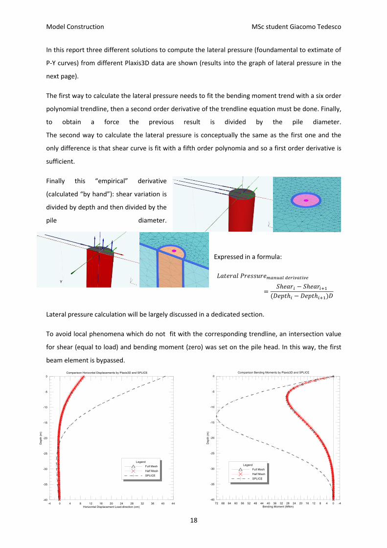
In this report three different solutions to compute the lateral pressure (foundamental to extimate of
P-Y curves) from different Plaxis3D data are shown (results into the graph of lateral pressure in the
next page).
The first way to calculate the lateral pressure needs to fit the bending moment trend with a six order
polynomial trendline, then a second order derivative of the trendline equation must be done. Finally,
to obtain a force the previous result is divided by the pile diameter.
The second way to calculate the lateral pressure is conceptually the same as the first one and the
only difference is that shear curve is fit with a fifth order polynomia and so a first order derivative is
sufficient.
Finally this “empirical” derivative
(calculated “by hand”): shear variation is
divided by depth and then divided by the
pile diameter.
Expressed in a formula:
( )
Lateral pressure calculation will be largely discussed in a dedicated section.
To avoid local phenomena which do not fit with the corresponding trendline, an intersection value
for shear (equal to load) and bending moment (zero) was set on the pile head. In this way, the first
beam element is bypassed.
Model Construction MSc student Giacomo Tedesco
19
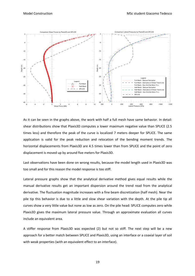
As it can be seen in the graphs above, the work with half a full mesh have same behavior. In detail:
shear distributions show that Plaxis3D computes a lower maximum negative value than SPLICE (2.5
times less) and therefore the peak of the curve is localized 7 meters deeper for SPLICE. The same
application is valid for the peak reduction and relocation of the bending moment trends. The
horizontal displacements from Plaxis3D are 4.5 times lower than from SPLICE and the point of zero
displacement is moved up by around five meters for Plaxis3D.
Last observations have been done on wrong results, because the model length used in Plaxis3D was
too small and for this reason the model response is too stiff.
Lateral pressure graphs show that the analytical derivative method gives equal results while the
manual derivative results get an important dispersion around the trend read from the analytical
derivative. The fluctuation magnitude increases with a fine beam discretization (half mesh). Near the
pile tip this behavior is due to a little and slow shear variation with the depth. At the pile tip all
curves show a very little value but none as low as zero. On the pile head: SPLICE computes zero while
Plaxis3D gives the maximum lateral pressure value. Through an approximate evaluation all curves
include an equivalent area.
A stiffer response from Plaxis3D was expected (2) but not so stiff. The next step will be a new
approach for a better match between SPLICE and Plaxis3D, using an interface or a coaxial layer of soil
with weak properties (with an equivalent effect to an interface).

Model Construction MSc student Giacomo Tedesco
20
Beam position
The use of half a mesh has entailed a sensible time reduction for each run but at the same time a
problem's started due to the beam position.
The beam is used only for helping the engineer during the post processing phase i.e. against several
difficult volume integrations on the equivalent pile volume, using the beam became possible to
obtain all the interesting variables (mainly bending moment and horizontal displacement than shear)
directly from Plaxis3D. Below are shown results for different beam positions: coinciding with the pile
axis (that for half mesh used model is part of the mesh border).
Herein are reported only bending moment data, for the simple reason that is the unique trend with a
sensible variation with the beam position.
For exam cases the maximum bending moment
variation peak has been found in the order of 3,4%
(against full mesh value). In case of horizontal
displacement analysis (not reported herein) this error
is halved.
Different changing beam positions run give a clear result: the best match between a half and a full
mesh is found for a beam position equal to the sectional barycenter. In this case, there is a relevant
reduction against full mesh value (2%). This could be due to some effect in the solid pile related with
the tangential stresses diffusion,
maybe something like a torsional
effect.

Model Construction MSc student Giacomo Tedesco
21
Mesh dimension
Objective of the study herein reported is to show the trend changing for bending moments, shear
force and horizontal displacements computed for different coarse of mesh elements.
Adopting the best compromise for the element size in a finite elements analysis is the main choice
for the engineer.
Mesh Type Approx. Time
TOTAL BEAM Max.Diplacements Max.Shear Max.Moment
Elements
Nodes Elements
Nodes
Value Rel.Err.
Value
Rel.Err. Value Rel.Err.
(min) (-) (-) (-) (-) (cm) (%) (MN) (%) (MNm)
(%)
Very Coarse
1 7659 11206 60 180 8,664 13,038 9,96 3,2318 27,06 11,4528
Coarse 2 11799 17298 74 222 9,076 8,9029 9,73 0,8493 28,18 7,78795
Medium 5 22575 32829 74 222 9,258 7,0761 9,63 0,1657 28,66 6,21727
Fine 18 44586 64460 74 222 9,725 2,3888 9,72 0,7250 29,9 2,15968
Very Fine 67 87143 124307 74 222 9,963 0 9,65 0 30,56 0
it’s noticeable that the known error in the first beam element (a wrong value for bending moment
and shear force) hasn't been corrected in order to evaluate the behavior of that element in different
mesh condition.
On the left are shown nodes and
elements number for each global
coarseness adopted.
In the graphs below it can be noted that
for a very coarse discretization the shear
behavior has several skips around the
(supposed) correct value.
The number of the beam elements (and
node) increase only between "very
coarse" and "coarse". After that, it is
constant although the model precision
continues to grow, so different mesh coarseness increase only the soil discretization.
It has been supposed that results are more precise when computed by very fine mesh coarse.

Model Construction MSc student Giacomo Tedesco
22
In line with this assumption, the relative error for each
coarse condition and each variable has been calculated
referred to very fine results.
On the right a Plaxis3D soil element detailed (10-nodes
tetrahedrons):

Model Construction MSc student Giacomo Tedesco
23
For a mesh elements dimension bigger or equal to "coarse", shear trends show a very small variation,
less than 1%.
Bending moments and horizontal displacements exhibit an equal trend: a relative error reduction as
finest mesh and an variation minor than 2% between "fine" and "very fine" elements.
In the next two pages are plotted three sketches for each coarse condition in order to allow an easy
visual recognition for the engineer.

Model Construction MSc student Giacomo Tedesco
24
Mesh coarse
Prostective view Mesh coarse
Prospective view
Very coarse
Coarse
Medium
Fine
Very fine

Model Construction MSc student Giacomo Tedesco
25
Mesh coarse
Top view Pile detail (top view)
Very coarse
Coarse
Medium
Fine
Very fine

Model Construction MSc student Giacomo Tedesco
26
Refinement clusters
In this section, Plaxis3D results are shown for different cluster shapes around the pile. These proves
are done in order to increase locally the mesh refinement, consequently to the results quality, in a
defined zone of interest, as the upper half pile subjected to great displacements and stress.
It had been chosen to use a "coarse" mesh setting for the global model and to refine every cluster of
interest with different fitness factors. A simple model properties summary is shown in the table
below:
Curve ID
Mesh coarse Cluster Pile
Type re Dimensions (m) Fitness
Factor
Fitness
Factor
Very fine very fine 0,7 - - 1
Coaxial cylinder coarse 1,5 R5,3 L20 Z20 0,2 0,5 (0,2 up)
Parallelepiped coarse 1,5 L10,6 B5,3 Z20 0,2 0,5 (0,2 up)
Eccentric
parallelepiped coarse 1,5
L10,5 B5,3 Z20 (2,05 ecc.X-
dir.) 0,2 0,5 (0,2 up)
Two coaxial cilinders coarse 1,5 R5,3 Z20 (R10 Z13) 0,2 (0,5) 0,5 (0,2 up)
Where the Fitness factor (FF) is a coefficient of reduction for the target element dimension,
calculated with this formula:
√( )
( ) ( )
( )
During the meshing phase, when each element dimension is lower than the value of the target
element dimension, the subdivision process is stopped. The fitness factor role is ever the same:
reducing for a single cluster or structural element the target element dimension.
In this way it becomes possible to lighten the model discretization in zones where a low precision is
required.

Model Construction MSc student Giacomo Tedesco
27
Coaxial cylinder Parallelepiped
Eccentric parallelepiped Two coaxial cylinders
Here below is shown the relative error for each variable and for each refinement cluster shape
adopted.
The model with the smallest difference with the very fine mesh condition, is the model with two
coaxial cylinder.
Moreover, it's clear that each shape of refinement cluster gives good results, with only a little
percentage variation to each other.

Model Construction MSc student Giacomo Tedesco
28

Model Construction MSc student Giacomo Tedesco
29
Herein are shown the trends for the interest variables computed by a very fine element subdivision
and a coarse mesh with two coaxial cylinder of refinement around the pile.
It's simple to check an equal behavior for each variable in both cases. Only the bending moment peak
is reduced of 2%, and this is perfectly acceptable in reason of an important computational time
reduction.

Model Construction MSc student Giacomo Tedesco
30
Interface adoption
The following paragraph treats a sequence of analyses run in order to: understand the real need for
adopting an interface, its usefulness and then (next chapter) the results depending from its
parameter R, a kind of reduction coefficient with a clear role stated by the name itself: interface
reduction factor.
In input, Plaxis3D demands to create a positive
or negative interface; the sign is subjected to
the local Z-axis for the original surface, so it
does not have to change behavior and
therefore the results.
After meshing process interface is composed
by 12-node elements, each element consists of
6 couple of nodes (compatible with the 6-
noded triangular side of a soil element or plate
element). On the monitor, and then on the plot, the interface has a finite thickness, but in the finite
elements formulation, each nodes pair has the same coordinates, which means that the element has
zero thickness.
However, Plaxis3D assigns a virtual thickness in order to calculate the stiffness properties of the
interface. This virtual thickness is calculated on the average elements size that surrounds the
interface (check "target element dimension" in next chapter) scaled by a virtual thickness factor. This
factor is set at a value of 0,1 and the user cannot modify it.
In this chapter the model behavior is analyzed in relation with different load steps of a model both
with and without interface.
It could be interesting to note that at the interface ends every interface element nodes pair
"degenerates" to a single node.
In this section, the simulation run with the interface reduction factor
equal to one is used as benchmark for the calculation of the variables
variation. For the interface reduction factor equal to one is common to
use the definition: rigid interface, in that case only the Poisson coefficient
change (automatically set equal to 0.45).
Above two image to explain the interface position, first during input
phase and then after the mesh construction.
Model Construction MSc student Giacomo Tedesco
31
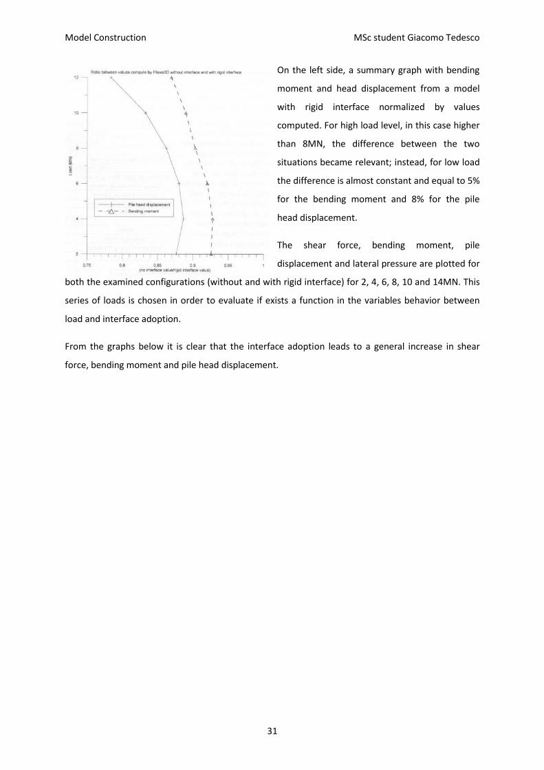
On the left side, a summary graph with bending
moment and head displacement from a model
with rigid interface normalized by values
computed. For high load level, in this case higher
than 8MN, the difference between the two
situations became relevant; instead, for low load
the difference is almost constant and equal to 5%
for the bending moment and 8% for the pile
head displacement.
The shear force, bending moment, pile
displacement and lateral pressure are plotted for
both the examined configurations (without and with rigid interface) for 2, 4, 6, 8, 10 and 14MN. This
series of loads is chosen in order to evaluate if exists a function in the variables behavior between
load and interface adoption.
From the graphs below it is clear that the interface adoption leads to a general increase in shear
force, bending moment and pile head displacement.

Model Construction MSc student Giacomo Tedesco
32

Model Construction MSc student Giacomo Tedesco
33

Model Construction MSc student Giacomo Tedesco
34
Model dimensions
Herein, the results of simulations run for three different model (mesh) dimension are presented.
It was chosen to investigate the mesh dimension effects in order to adopt the best engineering
solution for the analysis on the definitive model.
It has been changed only the dimension parallel to the load, which means the main direction of
displacement and deformation.
The model dimensions adopted are 100m, 120m and 150m.
Above, the table presents the maximum values of the main variables of interesting i.e. bending
moment and horizontal displacement. In the same table are presented the same data described
above but normalized by the value assumed as final i.e. from D1C_150m; this is done in order to
show clearly the variables' variation.
Bending moment is absolutely constant (fluctuation of 0.1% between 100m and 150m).
Horizontal displacement instead, has a little variation: 2.4% (less) between 100m and 150m and 1.1%
between 120m and 150m.
The conclusion of this tests is that 100m as model side is a good assumption, because it adopts a
larger side length. This means better results but it also means adopting a larger number of elements
in order to maintain the indispensable relatively small element coarseness.
Briefly: a little bit better results do not justify such a large increase of time consumption.
In the following pages, are shown trends for shear, bending moment and horizontal displacement for
pile with and without a surrounding interface.
Model ID u_x max %u_x max M_3 max %M_3 max
D1A_100m 1,7643 0,9760 60,1186 1,0010
D1B_120m 1,7881 0,9893 60,0966 1,0007
D1C_150m 1,8076 1,0000 60,0562 1,0000

Model Construction MSc student Giacomo Tedesco
35
-40
-35
-30
-25
-20
-15
-10
-5
0
-6 -4 -2 0 2 4 6
Dep
th (
m)
Shear force (MN)
Load: 10 MN
D1A_100m
D1B_120m
D1C_150m
-40
-35
-30
-25
-20
-15
-10
-5
0
-0,5 0 0,5 1 1,5 2
Dep
th (
m)
Horizontal displacement (cm)
Load: 10MN
D1A_100m
D1B_120m
D1C_150m
-40
-35
-30
-25
-20
-15
-10
-5
0
-20 0 20 40 60 80
Dep
th (
m)
Bending moment (MNm)
Load: 10MN
D1A_100m
D1B_120m
D1C_150m

Model Construction MSc student Giacomo Tedesco
36
-This page intentionally left blank-

Parametric Analysis MSc student Giacomo Tedesco
37
PARAMETRIC ANALYSIS
In the following paragraphs, a parametric study of the model defined in the last chapter is presented.
These sensibility analyses cover three variables of primary importance that must be defined in the
input phase for each numerical model representative of soil behavior.
The model construction has just been described in the previous chapter, where each choice and
assumption is largely explained. Now it has become necessary to know which input parameter has
major effect on the behavior of numerical model of a pile laterally loaded in soft clay.
In order to evaluate the major capability of influence on the model, it is tested:
Eps50 (EpsC in SPLICE), because it is the unique parameter that allows us to set an equivalent
material into Plaxis3D and SPLICE, so both analyses are run with the software;
Tensile cut-off, it is investigated the effect of its global adoption and then some configuration
with activation localized. This second series of simulation is run in order to evaluate which
possible layer subdivision best match the real soil behavior, especially back the pile. It’s
important to know that SPLICE allows gap opening, so only Plaxis3D results changing during
these tests;
Interface reduction factor, the model response for this parameter is studied in reason to get
the sensibility of the model in relation with this variable that can be seen like arbitrary in
some case, especially in merely academic exercise where none field or laboratory data are
available.
If the interface role and operation in Plaxis3D are clear, not so clear is the correct value to
assign to it. The presence of a highly reworked layer all around the pile is demonstrated and
intuitive, but a unique theory-rule does not exist to define the correct value of the interface
reduction factor. So in several scientific papers it is possible to find different values for it, but
everyone it is representative of a specific site condition only. From literature the unique
indication that crops out is that the interface reduction factor depends essentially on the soil
type and pile type (technology used to construct or drive it) i.e. on the level of the coaxial
layer material reworking with the pile.
Unexpected shear fluctuation In each analysis done up to now exists a large fluctuation that affects the shear distribution
calculated by Plaxis3D on the pile top, at seabed level.

Parametric Analysis MSc student Giacomo Tedesco
38
This problem could come from: numerical problem due to the great difference of stiffness between
pile and soil or numerical problem connected with the load application on the deformed structure
(top section rotated but load defined only in horizontal direction).
In order to try to remove this annoying problem it has been attempted to:
change the beam Young's modulus (E-6 and E-3 than pile elasticity modulus);
decrease the single elements size near the top part of the pile;
use different ways of loading, like point force, line load and surface load;
maintain the load on the seabed pile section increasing the pile length above the seabed.
Every test carried out has been affected by the same inconvenience.
For the models later used, two tricks have been adopted in order to reduce the shear fluctuation:
adopting a stiff plate on the pile head (Young modulus is a thousand times stiffer than pile Young
modulus) and increasing the pile length above the seabed. Load was applied upon the rigid plate with
a couple of forces that balance the residual bending moment in order to have zero moment at the
seabed pile section (like in the original situation).
Several tests were run to find out the best solution (none of these are reported) and eventually it
was chosen to work with: plate activated and the pile length increased two meters above the seabed
(four meters) led to even better results. But it had a problem too: a too large number of elements
were needed for a good discretization and in that case it became too important the bending moment
effect connected with the arm of the load.
Disturbing phenomena were also present but reduced, which meant an increased lateral pressure
study quality.
The next chapter presents a possible explanation for the strange behavior of lateral pressure in the
top part of the pile; moreover, the problem due to the shear variation has been briefly explained
above.

Parametric Analysis MSc student Giacomo Tedesco
39
Eps50 (EpsC)
In this section are presented the effects of Eps50 on the soil response for our model of single pile in
soft clay.
It has been chosen to run these series of analyses for 2 and 8 MN because 8 MN is the maximum load
allowed by SPLICE solution for Eps50 equal to 1% and 2% (for 0,5% it's a little bit more: 9MN), so a
comparison with SPLICE is possible.
Calculation results by Plaxis3D are compared with SPLICE output. This has been done in order to
investigate a possible law in the relationship between variables of interesting and Eps50.
It's important to know that the Eps50 definition, also here adopted, is: the strain at half of the
maximum stress from laboratory compression test on clay.
Below are shown the results for different Eps50. SPLICE results are normalized by Plaxis3D values in
order to estimate the percentage variation.
It seems clear to observe that for a low load like 2 MN exists a fluctuation of every variable larger
than for 8 MN. For the highest load condition each variable is grouped by type (maximum bending
moment, horizontal displacement and lateral pressure), and the elements of this whole "family" stay
in a range of 5% or less (approximately 2% for the maximum bending moment).

Parametric Analysis MSc student Giacomo Tedesco
40
For 8 MN the difference between SPLICE and Plaxis3D results are set on: around 30% for the pile
head displacement, 15% for the maximum bending moment and 4% for the maximum lateral
pressure.
This behavior of the lateral pressure is very “friendly” because confirm us that once reached the
maximum strength (undrained), the soil can only increase the involved (plasticized) volume i.e.
bearing capacity factors are almost the same.

Parametric Analysis MSc student Giacomo Tedesco
41

Parametric Analysis MSc student Giacomo Tedesco
42

Parametric Analysis MSc student Giacomo Tedesco
43

Parametric Analysis MSc student Giacomo Tedesco
44

Parametric Analysis MSc student Giacomo Tedesco
45
Tensile cut-off adoption
It has been decided to run analyses with different extension of tension cut-off zone.
These were done in order to investigate the effects of tension cut-off activated in different
configurations of the shallow layer to find the best compromise between tension cut-off adoption
and computational time required per each analysis.
Model case with tension cut-off deactivated is used as benchmark for the following results
comparison, in order to present clearly the effects concerning this study.
From the model with tension cut-off completely activated, it has been possible to figure out that
around 30 meters is the maximum extension of the zone in tensile cut-off condition, which means
that every test has to be carried out for a layer with tension cut-off shallower than 30 meters depth.
It was chosen to test the following cut-off zone depth: 5-10-15-20 meters and furthermore, the
“extreme” cases with tension cut-off completely activated and deactivated.
Each model needs to re-run its meshing phase; this was caused by the new layering conditions i.e.
new geometry. Anyway, elements and nodes numbers are only subjected to a slight variation and the
extreme situations, both with a unique layer, have lower elements and nodes number.
It was run only the load condition of 10 MN, which means a high load i.e. near failure condition. It
was established that a lower load would not bring more information than that severe load. For these
sensibility analyses were defined two soil
materials: equal in all their properties except
for the tension cut-off activation and set equal
to zero for one of these.
The graph on the left side clearly presents the
percentage variation of the maximum bending
moment and pile head displacement for
different cut-off zones normalized by the case
results with tension cut-off completely
deactivated. Maximum bending moment
presents a variation by about 25% between 5m
and all activated; for the pile head
displacement this variation is lower, around

Parametric Analysis MSc student Giacomo Tedesco
46
10% complexly.
The largest difference is in the passage through 5
and 10 meter of cut-off zone.
This fact confirms the logic thinking that the cut-
off effect is more important in that region
subjected to a great tensile stress like the soil in
the pile backward.
Above, the effects of different cut-off zones have
been explained but it was also found that each
layer subdivision means an increase of the
computational time requested by Plaxis3D to run
each model phase.
Finally, it is possible to declare that the best solution for our purpose will be using the tension cut-off
completely activated this in order to consider the tension cut-off effects because none of the
proposed solutions showed a computational time reduction or at least an increase of it.
Anyway, some uncertainties about a real physical meaning of tension cut-off adoption remains,
because a gap opening of 30 meters depth is not real.
Bending moment, horizontal displacement, shear force and lateral pressure trends have shown the
same behavior for every different condition tested.
Correctly, the case with only the top layer of 5m presents a trend similar to the situation with tension
cut-off deactivated. 10 and 15 meters have very similar results both converging to the "all activated"
value. The best match with "all activated" has been found for 20 meters depth of cut-off zone; in
that case, the results are almost equivalent.
Below are plotted the trends of every variable object of this study.

Parametric Analysis MSc student Giacomo Tedesco
47

Parametric Analysis MSc student Giacomo Tedesco
48

Parametric Analysis MSc student Giacomo Tedesco
49
Interface reduction factor
The important role played by the interface reduction factor has been just explained in the intro part
of this chapter.
Adopt and interface in a Mohr-Coulomb soil model require to define a value for the interface
reduction factor, which is the setting that define the interface behaviour.
For two load conditions are tested different values of the parameter object of study in order to
define clearly the relation between model responses and interface. It is used a load of 2 and 10 MN.
Below the maximum value for each variable is plotted for different interface reduction factor, these
graphs allow to write that for a reduction of the interface parameters between 0.90 and 0.33, the
shears are linear and the same behaviour is shown by the bending moment.
Above summary graphs with the maximum values for each R tested. Below the same graph
normalised.

Parametric Analysis MSc student Giacomo Tedesco
50
Below are reported graphs of displacement, bending moment, shear and later pressure for both the
load conditions tested for different interface reduction factor.
From the graphs below it is clear that the interface adoption leads to a general increase of the
variables of interest.
For a value of the interface reduction factor between 1 and 0.33, the results give a similar linear
trend to each other, and only for the extreme value of 0.10 (black dashed curve) there are very
important variations from the original trends. An extremely low value of the interface reduction
factor means that both the interface surfaces are “free” to move. That behaviour is reached thanks
to a great reduction of resistance and stiffness between each pair of nodes that compose the
interface (of course, caused by 0.10 like reduction factor).
A decrease of the reduction factor leads to a shift of the bending moment peak and at the same time
an increase of the maximum value; the same shift is shown by shear force trend.
Pile displacement increases with the reduction of the interface reduction factor.

Parametric Analysis MSc student Giacomo Tedesco
51

Parametric Analysis MSc student Giacomo Tedesco
52

Parametric Analysis MSc student Giacomo Tedesco
53

Parametric Analysis MSc student Giacomo Tedesco
54

P-y curves MSc student Giacomo Tedesco
55
P-Y CURVES
The ability to do a reasonable estimate of the behaviour of laterally loaded piles is an important
consideration in the design of many offshore installations.
To perform an analysis for the design, it must be possible to reduce the soil behaviour at each depth
to a simple p-y curve.
Matlock (1970)
In the paper “correlation for design of laterally loaded piles in soft clay” published in 1970, Hudson
Matlock wrote the most widespread approach for that typology of problems. Below, parts of that
paper are reported.
He ran three load conditions pertinent with laterally loaded pile design: short-time static load, cyclic
loading (like a storm) and reloading with a force less than the previous maximum.
Some problematic effects were
present but Matlock neglected it
explaining his choice with its low final
effect.
Matlock studied the behaviour of
laterally loaded piles in the Gulf of
Mexico, where, like other seas, large
lateral forces are produced by wind
and waves associated with hurricanes
and where the foundation materials in
the critical zone near the mudline are
often weakly clayey.
The structural analysis problem
consists of a complex beam-column on
an inelastic base. For piles separated
by spacing of several diameters or
more, the Winkler assumption is useful

P-y curves MSc student Giacomo Tedesco
56
to facilitate the analysis.
Soil is considered as a series of independent layers in providing resistance (p) to the pile deflection
(y).
Soil resistance may be a highly non-linear function of the deflection. Only few versions of this
problem, with simple configurations and elastic behaviours, can be solved by closed-form
mathematics. Somewhat more complicated cases may be handled by non-dimensional curves or
tables.
The steel tested pile presents a diameter of 12.75 inches and a length of 42 foot. The pile was
calibrated in order to provide extremely accurate determinations of the bending moment.

P-y curves MSc student Giacomo Tedesco
57
Free-head tests were done with only lateral applied to the mudline. Fixed-head tests were done
using a framework to simulate the effect of jacket structure. The load from the hydraulic rams was
transferred to the pile by a walking beam and a loading strut.
Precise determination of the pile bending moment, during the static loading, allows differentiation to
obtain curves of the soil reaction along the pile to a high degree of precision. Integration of the
bending moment diagram provides the deflected shape of the pile. Load were increased by
increments and for any selected depth the soil reaction (p) mat be plotted as a function of the pile
deflection (y).
These experimental p-y curves are the main basis for the development of this design procedure.
Principal conclusion from Sabine River and Lake Austin (Matlock, 1970) were:
The resistance-deflection (p-y) characteristics of the soil are highly non-linear and inelastic;
Within practical ranges, the fundamental resistance-deflection characteristics of the soil
appear to be independent of the degree of pile head restrain;
A principal effect of cyclic loading appears to be permanent physical displacement of the soil
away from the pile in the direction of loading. It is not clear what contribution to this effect
was provided by loss in strength within the soil volume;
The cyclic shear reversals in the soil mass may have caused some structural deterioration in
the clay;
Permanent displacement of the soil created a slack zone in the resistance-deflection
characteristics;
Although significant changes occurred with continued repetitions of load cycles, at any given
magnitude of lateral load (except for the highest) the behavior of the pile-soil system tended
to stabilize.
Then it becomes possible to define a static ultimate resistance.
In soft clay soil is confined so that plastic flow around a pile occurs only in horizontal planes, the
ultimate resistance per unit of length of pile may be expressed as:
Where c is the soil strength (Su), d is he pile diameter and Np is a non-dimensional ultimate
resistance coefficient. For soft clay soils flowing around a cylindrical pile at a considerable depth
below the surface, the Np factor should be 9. Very near the surface the soils in front of the pile will

P-y curves MSc student Giacomo Tedesco
58
fail by forward and upward and so the corresponding value of Np reduces to the range of 2 to 4.
For a cylindrical pile a value of 3 is believed appropriate.
The resistance increase with the distance from the free soil surface. The following equation describes
this variation:
Where the first term expresses the resistance at the surface, the second term gives the increase with
depth due to overburden pressure, and third term may be thought of as geometrically related
restrain that even a weightless soil around the pile would provide against upward flow of the soil.
J is an empirical factor obtained by field data, for instance on Sabine River is approximately 0.5
Definition and use of the P-y curves
P-y curve is the most widespread relation adopted to design laterally loaded piles. The curve
represents the non-linear behaviour of the soil at a certain depth. Each curve is representative of a
spring at a specific depth.
Exist several correlations to improve the quality of original p-y curves thought by Matlock or to
define a relation resistance-deflection for cyclic load, also in the original paper this design is
considered.
P-y curves for static and cyclic loading is part of American Petroleum Institute standard today.
The proper form of the p-y relation is influenced by many factors:
Natural variations of soil properties with depth;
General form of the pile deflection;

P-y curves MSc student Giacomo Tedesco
59
Corresponding state of stress and strain throughout the affected soil zone;
Rate, sequence and history of the cyclic wave loadings.
To perform an analysis for the design, it must be possible to reduce the soil behavior at each depth
to a simple p-y curve.
The curves are in non-dimensional form with the ordinates normalized according to the static
ultimate resistance Pu determined like above descripted for each average depth of the sub-layer.
The horizontal coordinate is the pile deflection divided by the deflection at the point where the static
resistance is one-half of the ultimate.
The form of the pre-plastic portion of the static resistance curve is based on semi-logarithmic plots of
the experimental p-y curves, which fall roughly along straight lines at slope yielding the exponent of
one-third.
Equation of the resistance-deflection curve by Matlock is:
(
)
The value of the deflection at the point where the static resistance is one-half of the ultimate, is
based on concepts given by Skempton by which he combines elasticity theory, ultimate strength
methods and laboratory soil properties to estimate the short-time load-settlement characteristics of
buried strip footings in clay soils. The strain Eps50 (EpsC in the original paper) is defined like the
strain that occurs at one-half of the maximum stress on a laboratory stress-strain curve. It may be
determined by dividing the shear strength c (Su for us) by an estimated secant modulus of elasticity
(Ec) or it may be taken directly from stress-strain curves.
Using the relation proposed by Skempton, the deflection sought is defined like:
Complete loss in resistance is assumed to occur at the soil surface when deflections at the point
reaches 15yC.
P-y curves for cyclic load and re-load, are not part of this study.

P-y curves MSc student Giacomo Tedesco
60
Lateral pressure calculation in Plaxis3D
Since the first analysis, there was the problem of choosing the most accurate way to calculate the
lateral pressure i.e. the contact pressure between soil and laterally loaded pile.
A real and accurate value of lateral pressure is essential to build the p-y curves that is the objective of
these series of analysis.
In the first part of this section are presented the lateral pressure obtained for two different degree of
fitting polynomial (5th and 6th order), then are tested different intersection values for those curves at
seabed level (depth equal to zero).
For both, the polynomial degrees are tested by the following intersection values: the load applied
(like boundary condition), the value of Plaxis3D shear at seabed and without fixing an intercept.
In the graph below, lateral pressure trends are shown; it is clear that below 5 meters depth all these
different polynomials compute the same lateral pressure.
Problems are localized on the pile tip and, more dangerously, on the top 5 meters.
Lateral pressure has been calculated like the first order derivative of the shear. Note that it was
chosen to fit the trend of Plaxis3D shear with a polynomial to obtain a continuous function, then it
was done the analytical derivative of first order of that function. In order to calculate the lateral

P-y curves MSc student Giacomo Tedesco
61
pressure, the shear derivative is also divided by pile diameter, this to obtain dimensionally a
pressure.
In the end, it was done also a test with the lateral pressure calculated by a trend line with intercept
set equal to the average of load applied and Plaxis3D shear at the seabed section.
In all this proves were obtained too variable results in the shallows (5 meter depth).
For this reason, it has been decided to "solve" the problem by hand calculation based on the simple
and, at the same time, sure concept of force equilibrium.
It’s important to highlight that this method modifies the lateral pressure, on the top part of the pile,
working on the lateral pressure trend computed like above explained.
The first step consists in choosing a depth where the results are assumed as correct so in this case it
is chosen a depth of 5 meters. In these pages the expression "sure depth" is used with reference to
the depth just above defined. Known the shear variation (calculated like the difference between
Plaxis3D shear at the sure depth and the load applied on the pile head), this value is divided by the
corresponding depth variation (sure depth subtracted seabed level) and divided by pile diameter.
The pressure, in this way calculated, is the constant pressure value able to guarantee the force
equilibrium on the top part of the pile.
Note that the lateral pressure value at sure depth it's known, which means the possibility of create a
linear trend between that point and the seabed level, this because it's already known the constant
value of lateral pressure that equilibrates the system. Now, fixed one point more, to create a linear
trend becomes simple, i.e. same area (force) but linear distribution of pressure against constant.
With this method are obtained approximate but plausible results for the shallow part of the problem
that alternatively is affected by problems connected with the weakness of adopting a fitting curve.
The idea of using a polynomial fitting curve (trend line) was found in several technical papers.
Using the "manual" derivative (shear variation divided by depth variation and diameter, point by
point) was left aside because every typical (little) shear fluctuation into Plaxis3D data output
produces a gigantic and senseless variation of lateral pressure.
In the end, the pile tip problem, i.e. in some case a value slightly negative related with the pile
displacement, it should be connected with a kind of boundary condition for the pile shear with the
pile tip friction against the soil that produces a resistance force able to restrict the pile tip
movement. In order to reduce it, a rigid interface is adopted on the pile tip. Another solution consists

P-y curves MSc student Giacomo Tedesco
62
in defining a thin layer at the pile tip level, where a very fine discretization must be set in order to
allow the tip movement and to evaluate it with an acceptable precision.
Note that only for the definitive model the lateral pressure at shallow depth will be calculated by
equilibrium like above described.
From the graphs below, it is clear that using a trend line is a comfortable way of working, but at the
same time it is a weak solving methods.
A negative value for the lateral pressure has not sense near the pile tip, or positive near the pile
head. Where it happens, it is due to some numerical wrong approximations of the fitting curve, that
is amplified by the second order derivative.

P-y curves MSc student Giacomo Tedesco
63
0
5
10
15
20
25
30
35
40
-10 0 10 20 30 40 50 60
Dep
th (
m)
(Lat.Pres./Su)
N 6-10
N 6-noN 6-9,69
N 5-10N 5-no
N 5-9,69N 5-Av.
Load: 6MN 0
5
10
15
20
25
30
35
40
-400 -300 -200 -100 0 100 200 300 400 500 600D
epth
(m
)
Lateral Pressure (kPa)
6-int10-LP6-no int-LP6-int 9,69-LP5-int10-LP5-no int-LP5-int 9,69-LP5-int Av.-LP
Load: 10MN
Load: 10MN
Load: 10MN
Load: 10MN

P-y curves MSc student Giacomo Tedesco
64
0
5
10
15
20
25
30
35
40
-400 -300 -200 -100 0 100 200 300 400 500 600
Dep
th (
m)
Lateral Pressure (kPa)
6-int10-LP
6-no int-LP
6-int 9,69-LP
5-int10-LP
5-no int-LP
5-int 9,69-LP
5-int Av.-LP
0
5
10
15
20
25
30
35
40
-10 -5 0 5 10 15 20 25 30 35 40 45
Dep
th (
m)
(Lat.Pres./Su)
N 6-10
N 6-no
N 6-9,69
N 5-10
N 5-no
N 5-9,69
N 5-Av.
Load: 6MN
Load: 6MN

P-y curves MSc student Giacomo Tedesco
65
Model (series ID: D1) with lateral pressure corrected by equilibrium above the node at a 4,88m
depth:
0
5
10
15
20
25
30
35
40
-60 -40 -20 0 20 40 60 80 100
Dep
th (
m)
Lateral Pressure (kPa)
2MN-Eps50=0,02
ADP with anisotropy
LP_by eq
0
5
10
15
20
25
30
35
40
-3 -2 -1 0 1 2 3 4 5
Dep
th (
m)
(Lateral Pressure / Su)
2MN-Eps50=0,02
ADP with anisotropy
(LP_by eq/Su)

P-y curves MSc student Giacomo Tedesco
66
0
5
10
15
20
25
30
35
40
-300 -200 -100 0 100 200 300
Dep
th (
m)
Lateral Pressure (kPa)
6MN-Eps50=0,02
ADP with anisotropy
LP_by eq
0
5
10
15
20
25
30
35
40
-4 -2 0 2 4 6 8
Dep
th (
m)
(Lateral Pressure / Su)
6MN-Eps50=0,02
ADP with anisotropy
(LP_by eq/Su)

P-y curves MSc student Giacomo Tedesco
67
0
5
10
15
20
25
30
35
40
-10 -5 0 5 10 15
Dep
th (
m)
(Lateral Pressure / Su)
9MN-Eps50=0,02
ADP with anisotropy
(LP_by eq/Su)
0
5
10
15
20
25
30
35
40
-800 -600 -400 -200 0 200 400 600
Dep
th (
m)
Lateral Pressure (kPa)
9MN-Eps50=0,02
ADP with anisotropy
LP_by eq

P-y curves MSc student Giacomo Tedesco
68
0
5
10
15
20
25
30
35
40
-15 -10 -5 0 5 10 15
Dep
th (
m)
(Lateral Pressure / Su)
12MN-Eps50=0,02
ADP with anisotropy
(LP_by eq/Su)
0
5
10
15
20
25
30
35
40
-2000 -1500 -1000 -500 0 500 1000
Dep
th (
m)
Lateral Pressure (kPa)
12MN-Eps50=0,02
ADP with anisotropy
LP_by eq

P-y curves MSc student Giacomo Tedesco
69
0
5
10
15
20
25
30
35
40
-2500 -2000 -1500 -1000 -500 0 500 1000
Dep
th (
m)
Lateral Pressure (kPa)
13MN-Eps50=0,02
ADP with anisotropy
LP_by eq
0
5
10
15
20
25
30
35
40
-20 -15 -10 -5 0 5 10 15
Dep
th (
m)
(Lateral Pressure / Su)
13MN-Eps50=0,02
ADP with anisotropy
(LP_by eq/Su)

P-y curves MSc student Giacomo Tedesco
70
0
5
10
15
20
25
30
35
40
-3000 -2500 -2000 -1500 -1000 -500 0 500 1000
Dep
th (
m)
Lateral Pressure (kPa)
14MN-Eps50=0,02
ADP with anisotropy
LP_by eq
0
5
10
15
20
25
30
35
40
-25 -20 -15 -10 -5 0 5 10 15
Dep
th (
m)
(Lateral Pressure / Su)
14MN-Eps50=0,02
ADP with anisotropy
(LP_by eq/Su)

P-y curves MSc student Giacomo Tedesco
71
In the last pages, for each load step is presented a couple of graphs: lateral pressure and ratio
between it and undrained shear strength. This ratio is comparable with the Matlock N factor, but
only in the areas where the soil is totally plasticized i.e. where the ultimate pressure is reached. This
parameter for the heaviest load condition presents a good trend. It starts around 4 and it reaches a
maximum of 10. Matlock range of values starts from a minimum of 3 to a maximum of 9 (other
papers propose different values of the bearing factor, but in any case no more than 12).
Isotropic NGI-ADP soil model
After all, the sensibility analysis for the soil, just run for different variables, that adopts a Mohr-
Coulomb model was chosen to pass at ADP soil model.
This new model increases the quality of the numerical simulation response thanks to its affinity
observed to perform the real behavior of clay in undrained condition.
Using ADP soil model means defining a larger range of parameters than Mohr-Coulomb, like the
ratios between SuDSS and SuAVERAGE, SuTX-COMPRESSION and SuAVERAGE, SuTX-EXTENSION and SuAVERAGE.
-6
-4
-2
0
2
4
6
-0,1-0,08-0,06-0,04-0,0200,020,040,060,080,1
(sig
1-s
ig3
)/2
Eps1
EpsC=0,005
EpsC=0,005

P-y curves MSc student Giacomo Tedesco
72
Note that in the use of ADP soil model, the assignation of a different interface material has been
preferred to the definition of the interface reduction factor (Rinter) in the surrounding soil (adopting
ADP). The interface adopts Mohr-Coulomb as soil constitutive model and 0.67 is the value set for the
interface reduction factor in agreement with the value suggested by Plaxis3D manual for situations
without specific indication or available test data.
It is very important to note that until now it has been used a very low Young's elasticity modulus,
something which cannot be now changed or the comparison with older data will not be correct. This
is a problem because, in Plaxis3D, the minimum acceptable value of the ratio between Gur and
SuAVERAGE is 100 whereas unfortunately the real values are 66.7 for Eps50=0.5%, 33.3 for 1% and 16.7
for Eps50=2%. Therefore,n it has been chose to work adopting 100 (minimum input recognized) for
that ratio.
Note that also the definition of shear modulus is different through ADP and Mohr-Coulomb.
Indeed, Mohr-Coulomb defines in input G50 at half of the maximum stress instead in ADP soil model
Gur is defined like the shear modulus of the initial part of stress-strain curve.
Note that NGI-ADP is adoptable only in Plaxis3D 2013 VIP package, but it is not possible to run soil
tests in the 3D input phase. Fortunately, it is possible to do them in 2D input phase.
It has been found a matching between ADP and Mohr-Coulomb changing the failure strain in ADP
model (failure strain is equal to 1.5 times Eps50).
It was also chosen to work with two extreme values of the typical Eps50 strain at half of the ultimate
stress range, relatively 0.5% and 2%.
These analyses were run in reason to investigate essentially the response differences using ADP
compared with a soil model elastic perfectly plastic until now used.
It’s fundamental to know that to obtain an ADP soil equivalent to Mohr-Coulomb it has been
necessary to set every Su equal to SuAVERAGE. It means every Su ratio equal to 1. In order to avoid
annoying numerical problems it was preferred to adopt 0.99 as ratio between SuCOMPRESSION-TX and
SuAVERAGE.
For Eps50 equal to 0.5% and 2.0% it was set the failure strain relatively equal to 2% and 22% into ADP
soil model (input phase).
Below, the ratios between SPLICE and Plaxis3D results are plotted (Mohr-Coulomb and isotropic
ADP), then: shear force, lateral pressure, bending moment and horizontal displacement, only for the

P-y curves MSc student Giacomo Tedesco
73
case with Eps50 set equal to 0.5% in three load conditions (2/6/10 MN, where 10 MN is the
maximum value able to guarantee convergence in SPLICE for this Eps50 value.
Below, in recapitulative graphs, the values are normalized with isotropic ADP results.
In blue are plotted the maximum bending moment trends, instead in red the displacement trends of
the pile head. Dark tones are adopted for SPLICE, soft for Mohr-Coulomb.
It’s interesting to note that for a low load like 2 MN, SPLICE gives a displacement trend very similar to
isotropic ADP results, but the bending moment peak for ADP is substantially different from SPLICE
peak (15% ca).
For low load, the differences between ADP and Mohr-Coulomb are considerable, increasing the load,
especially near the failure, that behavior change, so ADP and Mohr-Coulomb give approximately the
same results.
This trend could be explained by the fact that the soil behavior is governed by the soil stiffness for
low load, instead for high load the ultimate strength governs the problem.
Indeed, looking at the strain-stress curve it is simple to note that the difference between isotropic
ADP and Mohr-Coulomb behavior is localized in the first part of that curves, i.e. the stiffness, then,
for large strain, both the curves converge to the assigned Su.
0,8
0,9
1
1,1
1,2
1,3
1,4
1 2 3 4 5 6 7 8 9 10 11
(MC
or
SPLI
CE
valu
e/ A
DP
val
ue)
Load (MN)
Eps50=0,5% MC/ADP_iso MC/ADP_iso
SPLICE/ADP_iso SPLICE/ADP_iso

P-y curves MSc student Giacomo Tedesco
74
Finally, it's important to highlight that for a load near the failure (10 MN) the ratio between lateral
pressure and undrained strength has a maximum of 9 in SPLICE (in agree with Matlock paper, where
this ratio is named Np) instead Plaxis3D leads to a value near to 10.5.
Consideration just done for SPLICE and Plaxis3D result differences, are also now working.
Results for Eps50=2% are reported in the next paragraph, in order to avoid repetitions.
All new parameters are reported in the table below.
NGI-ADP (C2A) Mohr-Coulomb (C1C)
Identification Soil ADP EpsC 0,5%
Identification Interface EpsC 0,02
Identification Soil
Identification number
4 Identification number
1 Identification number
1
Material model User-defined Material model Mohr-Coulomb
Material model Mohr-Coulomb
Drainage type Drained Drainage type Undrained (C)
Drainage type Undrained (C)
Colour RGB 134, 234, 162
Colour RGB 161, 226, 232
Colour RGB 161, 226, 232
Comments Comments Comments
γ_unsat
kN/m^3
10 γ_unsat kN/m^3
10 γ_unsat kN/m^3
10
γ_sat kN/m^3
10 γ_sat kN/m^3
10 γ_sat kN/m^3
10
Dilatancy cut-off No Dilatancy cut-off No Dilatancy cut-off No
e_init 0,5 e_init 0,5 e_init 0,5
e_min 0 e_min 0 e_min 0
e_max 999 e_max 999 e_max 999
Rayleigh α 0 Rayleigh α 0 Rayleigh α 0
Rayleigh β 0 Rayleigh β 0 Rayleigh β 0
DLL file usrmod_adp.dll
E kN/m^2
249,1 E kN/m^2
996,6
Model in DLL NGI-ADP ν (nu) 0,495 ν (nu) 0,495
G_ur/s_u^A 100 G kN/m^2
83,3 G kN/m^2
333,3
s_u^C,TX/s_u^A(,PS)
0,99 E_oed kN/m^2
8413 E_oed kN/m^2
3,37E+04
y_ref m 0 c_ref kN/m^2
5 c_ref kN/m^2
5
Δs_u^A/Δy
kN/m^2/m
3 φ (phi) ° 0 φ (phi) ° 0
s_u^A_ref
kN/m^2
5 ψ (psi) ° 0 ψ (psi) ° 0
s_u^DSS/s_u^A 1 V_s m/s 9,035 V_s m/s 18,07
s_u^P/s_u^A 1 V_p m/s 90,8 V_p m/s 181,6
τ_0/s_u^A 0 Set to default values
No Set to default values
No
ε_1_f^C,TX 4 E_inc kN/m^2/m
152,8 E_inc kN/m^2/m
598

P-y curves MSc student Giacomo Tedesco
75
γ_f^DSS
6 z_ref m 0 z_ref m 0
ε_1_f^E,TX 4 c_inc kN/m^2/m
3 c_inc kN/m^2/m
3
ν 0,495 z_ref m 0 z_ref m 0
ν_u 0,495 Tension cut-off Yes Tension cut-off Yes
a_2 0 Tensile strength
kN/m^2
0 Tensile strength
kN/m^2
0
Check input? Y=0, N=1
1 C_v,ref m^2/day
0 C_v,ref m^2/day
0
tom 0 Strength Manual Strength Manual
tom 0 R_inter 0,67 R_inter 0,67
tom 0 Consider gap closure
Yes Consider gap closure
Yes
tom 0 δ_inter 0 δ_inter 0
tom 0 K_0 determination Automatic K_0 determination Automatic
tom 0 K_0,x = K_0,y Yes K_0,x = K_0,y Yes
tom 0 K_0,x 1 K_0,x 1
tom 0 K_0,y 1 K_0,y 1
tom 0 k_x m/day 0 k_x m/day 0
tom 0 k_y m/day 0 k_y m/day 0
tom 0 k_z m/day 0 k_z m/day 0
tom 0 e_init 0,5 e_init 0,5
DEBUG 0 c_k 1,00E+15 c_k 1,00E+15
Strength
Rigid
R_inter
1
Consider gap closure
Yes
δ_inter 0
E_oed^ref
kN/m^2
10
c_ref kN/m^2
1
φ (phi) ° 0
ψ (psi) ° 0
UD-Power 0
UD-P^ref
kN/m^2
100
K_0 determination
Automatic
K_0,x = K_0,y Yes
K_0,x 1
K_0,y 1
k_x m/day 0
k_y m/day 0
k_z m/day 0
e_init 0,5
c_k 1,00E+15

P-y curves MSc student Giacomo Tedesco
76
0
5
10
15
20
25
30
35
40
-2 0 2 4 6 8 10
Dep
th (
m)
Displacement (cm)
2MN-Eps50=0,005
MC
ADP
SPLICE
0
5
10
15
20
25
30
35
40
-505101520
Dep
th (
m)
Bending moment (MNm)
2MN-Eps50=0,005
MC
ADP
SPLICE

P-y curves MSc student Giacomo Tedesco
77
0
5
10
15
20
25
30
35
40
-1,5 -1 -0,5 0 0,5 1 1,5 2 2,5
Dep
th (
m)
Shear (MN)
2MN-Eps50=0,005
MC
ADP
SPLICE
0
5
10
15
20
25
30
35
40
-50 0 50 100 150
Dep
th (
m)
Lateral Pressure (kPa)
2MN-Eps50=0,005
MC
ADP
SPLICE

P-y curves MSc student Giacomo Tedesco
78
0
5
10
15
20
25
30
35
40
-3 -2 -1 0 1 2 3 4 5 6
Dep
th (
m)
(Lateral Pressure / Su)
2MN-Eps50=0,005
MC
ADP
SPLICE

P-y curves MSc student Giacomo Tedesco
79
0
5
10
15
20
25
30
35
40
010203040506070
Dep
th (
m)
Bending moment (MNm)
6MN-Eps50=0,005
ADP
MC
SPLICE
0
5
10
15
20
25
30
35
40
-10 0 10 20 30 40 50
Dep
th (
m)
Displacement (cm)
6MN-Eps50=0,005
ADP
MC
SPLICE

P-y curves MSc student Giacomo Tedesco
80
0
5
10
15
20
25
30
35
40
-6 -4 -2 0 2 4 6 8
Dep
th (
m)
Shear (MN)
6MN-Eps50=0,005
ADP
MC
SPLICE
0
5
10
15
20
25
30
35
40
-300 -200 -100 0 100 200 300 400
Dep
th (
m)
Lateral Pressure (kPa)
6MN-Eps50=0,005
ADP
MC
SPLICE

P-y curves MSc student Giacomo Tedesco
81
0
5
10
15
20
25
30
35
40
-4 -2 0 2 4 6 8 10
Dep
th (
m)
(Lateral Pressure / Su)
6MN-Eps50=0,005
ADP
MC
SPLICE

P-y curves MSc student Giacomo Tedesco
82
Anisotropic NGI-ADP soil model
Herein, the results of finite elements simulation done with anisotropic ADP soil model are presented.
In the last paragraph was presented a comparison between SPLICE and Plaxis3D data in reason to
highlight the different behavior of the same problem simulated with different soil models.
in this paragraph instead is presented a simulation that use the ADP capability of describing an
anisotropic behavior, typical for a soil.
In order to define the anisotropy the following parameters are defined: SuDSS/SuAVERAGE=0.75, SuTX-
EXTENSION=0.60 and SuTX-COMPRESSION/SuAVERAGE=0.99 (0.99 is used instead of 1 to avoid numerical
problem).
Soil tests have been carried out with Plaxis3D, in 2D input phase and the results are plotted below.
The above graph presents a series of triaxial tests simulated with the specific Plaxis3D function, tests
run for ADP soil with and without anisotropy; the soil has been tested in compression and extension
both.
The second graph below instead shows the results of a direct simple shear test.
These graphs confirm that the input parameters, used in order to define anisotropy, effectively give
the expected behavior.
-6
-4
-2
0
2
4
6
-0,25-0,2-0,15-0,1-0,0500,050,10,150,20,25
(sig
1-s
ig3
)/2
(
kPa)
EpsAX (-)
ADP with anisotropy
ADP with isotropry
Mohr-Coulomb

P-y curves MSc student Giacomo Tedesco
83
Then, are presented trends of: horizontal displacement, bending moment, shear force, lateral
pressure and ratio between lateral pressure and undrained shear strength.
These analyses are carried out for different load condition (2, 6, 9 and 12 MN) in reason to put on
evidence every possible different relation between load level and variables of interest (especially
bending moment and horizontal displacement).
For Eps50 bigger than 0.5%, in SPLICE ultimate load is 9 MN, for a load larger than this there is not
convergence, i.e. solution. Instead, with Plaxis3d has been carried out an analysis for 12 MN also in
reason to be sure that the failure is reached into the pile model simulation.
0
0,5
1
1,5
2
2,5
3
3,5
4
0 0,02 0,04 0,06 0,08 0,1 0,12 0,14 0,16 0,18 0,2 0,22 0,24 0,26 0,28 0,3
Tao
_xy
(kP
a)
Gamma_xy (-)
Direct Simple Shear Test - Eps50=2%
ADP with anysotropy

P-y curves MSc student Giacomo Tedesco
84
0
5
10
15
20
25
30
35
40
-100 -50 0 50 100 150
Dep
th (
m)
Lateral Pressure (kPa)
2MN
MC C2C EpsC=0,02
ADP C1D EpsC=0,02
SLICE
ADP with anisotropy
0
5
10
15
20
25
30
35
40
-4 -2 0 2 4 6
Dep
th (
m)
(Lateral Pressure / Su)
2MN
ADP C1D EpsC=0,02
MC C2C EpsC=0,02
SLICE
ADP with anisotropy

P-y curves MSc student Giacomo Tedesco
85
0
5
10
15
20
25
30
35
40
-5 0 5 10 15 20
Dep
th (
m)
Displacement (cm)
2MN
ADP C1D EpsC=0,02
MC C2C EpsC=0,02
SLICE
ADP with anisotropy
0
5
10
15
20
25
30
35
40
-505101520
Dep
th (
m)
Bending moment (MNm)
2MN
ADP C1D EpsC=0,02
MC C2C EpsC=0,02
SLICE
ADP with anisotropy

P-y curves MSc student Giacomo Tedesco
86
0
5
10
15
20
25
30
35
40
-1,5 -1 -0,5 0 0,5 1 1,5 2 2,5
Dep
th (
m)
Shear (MN)
2MN
ADP C1D EpsC=0,02
MC C2C EpsC=0,02
SLICE
ADP with anisotropy

P-y curves MSc student Giacomo Tedesco
87
0
5
10
15
20
25
30
35
40
-400 -200 0 200 400
Dep
th (
m)
Lateral Pressure (kPa)
6MN
MC C2C EpsC=0,02
ADP C1D EpsC=0,02
SLICE
ADP with anisotropy
0
5
10
15
20
25
30
35
40
-10 -5 0 5 10
Dep
th (
m)
(Lateral Pressure / Su)
6MN
ADP C1D EpsC=0,02
MC C2C EpsC=0,02
SLICE
ADP with anisotropy
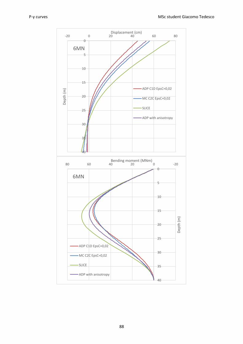
P-y curves MSc student Giacomo Tedesco
88
0
5
10
15
20
25
30
35
40
-20 0 20 40 60 80
Dep
th (
m)
Displacement (cm)
6MN
ADP C1D EpsC=0,02
MC C2C EpsC=0,02
SLICE
ADP with anisotropy
0
5
10
15
20
25
30
35
40
-20020406080
Dep
th (
m)
Bending moment (MNm)
6MN
ADP C1D EpsC=0,02
MC C2C EpsC=0,02
SLICE
ADP with anisotropy

P-y curves MSc student Giacomo Tedesco
89
0
5
10
15
20
25
30
35
40
-6 -4 -2 0 2 4 6 8
Dep
th (
m)
Shear (MN)
6MN
ADP C1D EpsC=0,02
MC C2C EpsC=0,02
SLICE
ADP with anisotropy

P-y curves MSc student Giacomo Tedesco
90
0
5
10
15
20
25
30
35
40
-800 -600 -400 -200 0 200 400 600
Dep
th (
m)
Lateral Pressure (kPa)
9MN
SLICE
ADP with anisotropy
0
5
10
15
20
25
30
35
40
-10 -5 0 5 10
Dep
th (
m)
(Lateral Pressure / Su)
9MN
SLICE
ADP with anisotropy

P-y curves MSc student Giacomo Tedesco
91
0
5
10
15
20
25
30
35
40
-50 0 50 100 150 200
Dep
th (
m)
Displacement (cm)
9MN
SLICE
ADP with anisotropy
0
5
10
15
20
25
30
35
40
020406080100120
Dep
th (
m)
Bending moment (MNm)
9MN
SLICE
ADP with anisotropy

P-y curves MSc student Giacomo Tedesco
92
0
5
10
15
20
25
30
35
40
-10 -5 0 5 10
Dep
th (
m)
Shear (MN)
9MN
SLICE
ADP with anisotropy

P-y curves MSc student Giacomo Tedesco
93
In the first dimensionless graph are plotted the maximum bending moment and the pile head
displacement at the seabed. Both these trends are normalized by results calculated by Plaxis3D with
isotropic ADP. The normalized results are calculated by SPLICE and Plaxis3D with Mohr-Coulomb and
ADP anisotropic output.
Below are presented the same variables calculated with ADP isotropic but normalized by values
obtained adopting anisotropic ADP.
0,9
1
1,1
1,2
1,3
1,4
1,5
1,6
1,7
1,8
1 2 3 4 5 6 7 8 9 10 11
(MC
or
SPLI
CE
valu
e/ A
DP
val
ue)
Load (MN)
Eps50=2%
SPLICE/ADP_iso
MC/ADP_iso
ADP_ani/ADP_iso
SPLICE/ADP_iso
MC/ADP_iso
ADP_ani/ADP_iso
0,50,520,540,560,58
0,60,620,640,660,68
0,70,720,740,760,78
0,80,820,840,860,88
0,90,920,940,96
1 2 3 4 5 6 7 8 9 10 11 12 13 14 15
(MC
or
SPLI
CE
valu
e/ A
DP
val
ue)
Load (MN)
Eps50=2%
ADP_iso/ADP_ani
ADP_iso/ADP_ani

P-y curves MSc student Giacomo Tedesco
94
A Very relevant consideration could be that the difference shown at 14 MN for the maximum
displacement into the second normalized graph, leads to an interception in the first graph between
the curves representative of SPLICE and anisotropic ADP, both normalized by isotropic ADP.
However, the consideration above remains a merely theoretical consideration due to the fact that
SPLICE does not calculate a solution for such a high load condition.

P-y curves MSc student Giacomo Tedesco
95
Experimental P-y curves
Several points are necessary to draw a curve resistance-deflection. For a certain depth and so for a
certain p-y curve, each point is representative of a couple of lateral pressure-deflection. Each point is
distinctive of a load, for this reason when a large number of load level is tested it becomes possible
to define with good precision the specific p-y curve, representative of a certain soil at a certain
depth.
In the next pages are plotted the p-y curves for 5.5-8.5-11.5-14.5-18.5-21.5 meters depth.
In each graph, three curves are shown: two calculated by Plaxis3D data, from simulations adopting
the ADP soil model, relatively with isotropy and anisotropy; and a third curve obtained by SPLICE
using the API recommendations i.e. Matlock equation.
The graphs representative of 2.5 and 4.5 meters depth, present the API curve and a second
experimental curve obtained with the lateral pressure corrected by equilibrium, as explained in the
last paragraph.
It is clear that the APD soil model gives curves more suitable with the curves calculated from API
recommendation if an anisotropic behaviour is defined, this in comparison an isotropic material
adopting the ADP soil model.
P-y curves calculated from Plaxis3D data (adopting ADP soil model with isotropy) present two main
characteristic:
The ultimate resistance from Plaxis3D
data is a little bit higher (+5%) than the
ultimate resistance defined by API
recommendations i.e. the flat-horizontal
part of the curves obtained by Plaxis3D is
a little bit higher than the same curve by
SPLICE;
The initial slope of the curve, i.e. the
stiffness, is higher for Plaxis3D (detail of
the initial different stiffness on the
picture at right side).
0
10
20
30
40
50
60
70
80
90
0 2 4 6 8 10
P (
kN)
y (cm)
8,5m depth API(Matlock)_SPLICE
D1A_Plaxis3D

P-y curves MSc student Giacomo Tedesco
96
0
10
20
30
40
50
60
70
80
90
100
0 100 200 300 400 500
P (
kPa)
y (cm)
2,5m depth
Plaxis3D (ADP with anisotropy) -D1Lat.Pres._corrected above 4,88m
SPLICE (GENSOD)
0
20
40
60
80
100
120
140
160
0 100 200 300 400 500
P (
kPa)
y (cm)
4,5m depth
Plaxis3D (ADP with anisotropy) -D1Lat.Pres._corrected above 4,88m
SPLICE (GENSOD)

P-y curves MSc student Giacomo Tedesco
97
0
20
40
60
80
100
120
140
160
0 20 40 60 80 100 120 140
P (
kN)
y (cm)
5,5m depth
API (Matlock)_SPLICE
D1A_Plaxis3D
0
50
100
150
200
250
0 20 40 60 80 100 120 140
P (
kN)
y (cm)
8,5m depth
API (Matlock)_SPLICE
D1A_Plaxis3D
0
50
100
150
200
250
300
350
400
0 20 40 60 80 100 120 140
P (
kN)
y (cm)
11,5m depth
API (Matlock)_SPLICE
D1A_Plaxis3D

P-y curves MSc student Giacomo Tedesco
98
0
50
100
150
200
250
300
350
400
450
500
0 20 40 60 80 100 120 140
P (
kN)
y (cm)
14,5m depth
API (Matlock)_SPLICE
D1A_Plaxis3D
0
100
200
300
400
500
600
0 20 40 60 80 100 120 140
P (
kN)
y (cm)
18,5m depth
API (Matlock)_SPLICE
D1A_Plaxis3D
0
100
200
300
400
500
600
700
0 20 40 60 80 100 120 140
P (
kN)
y (cm)
21,5m depth
API (Matlock)_SPLICE
D1A_Plaxis3D

Jacket Structure Example MSc student Giacomo Tedesco
99
SIMPLFIED ANALYSIS OF A REAL JACKET STRUCTURE
To close this master thesis, it was chosen to develop a real case, but simplified, in order to test the
obtained p-y curves (during the period, August-December 2013, at Norwegian Geotechnical Institute,
in Oslo).
The merely academic use of the following exercise, allows to do very strong assumptions and
simplifications.
Objective of this chapter is evaluating the actions on the foundation of a Jacket structure.
The actions calculated are used to verify the piles used to fix the jacket on the seabed.
Little importance is assigned to the structural design of the jacket. Also the fatigue behaviour for the
structure and the structural elements have been considered in the simplest way possible: using
uniquely a factor on the material resistance. International standard allows this calculation only for
inspectable elements, and in the jacket structure herein studied every element is inspectable
because it is found in relatively shallow water (for ISO an element below 200 meters depth it is not
inspectable with regularity; in this case the mudline is at a depth of 28,7 meter).
To compute the forces acting on the foundation a finite elements software for structural analysis is
used (Straus 7). In order to simplify the problem it is used a quasi-static approach for wave and
current actions. This procedure is defined into international standard ISO 19902.
The use of this methodology attributes the cyclic action due to wave passage on a system of static
forces on the fixed structure.
Metocean design data and a soil profile are furnished by a senior engineering working in Kvaerner, a
Norwegian contractor company.
The soil profile adopted is clay characterized by linear undrained strength, as the soil profile largely
used into the parametric analysis run at NGI and was explained in the initial part of this master
thesis.
This in order to use the p-y curves above obtained using ADP soil model with anisotropy.

Jacket Structure Example MSc student Giacomo Tedesco
100
It is modelled a not existing jacket structure, but in order to define an “credible” framework it is used
as model the Gudrun jacket (Gudrun is an oil ring between Scotland and Norway, it is property of
Statoil company and it was built by Kvaerner Industry).
The original framework of legs, horizontal beams and braces has been largely modified in order to
adopt that structure to a relatively shallow seabed.
Once calculated the sum vector for each leg it is supposed an equal subdivision of the force between
the three piles that compose the leg foundation.
No specific verifies are done on the leg-pile connection, because normally this part is characterized
by very high resistance due to its shape and thickness.
In the picture below are clearly represented the leg-piles connector, with the pile heads housing.

Jacket Structure Example MSc student Giacomo Tedesco
101
In these pages, it is developed uniquely the in-situ action on the structure, caused by extreme wave
plus current and wind conditions.
Dynamic situation is not part of this study.
Also the temporary situations like transport, installation, etc., are not studied, for two reason:
without a definitive structure geometry is not possible to study correctly these phase of the structure
life and, more important to me, these verifies do not concern the use of P-y curves, objective of this
exercise-chapter.
Standard ISO 19902 treats the fixed steel offshore structure and it furnishes a definition of jacket
structure: a jacket is a welded tubular space frame with three or more vertical (or near vertical)
tubular chords (the legs) and a bracing system between the legs.
The jacket provides support for the foundation piles, conductors, risers and other appurtenances.
The sketch on the left side presents the most
simple evaluation of the loads on a jacket
structure and the reactions of the foundation. In
the case herein treated these forces on the
structure base are guaranteed by a pile
foundation.
The following example adopts the jacket
structure above descripted and a foundation of
three pile for each leg (globally twelve piles).
Each pile is embedded for 40 meters with an
outside diameter of 84 inches (2,14 meters) and
a wall thickness of 60 mm.
It is used the same piles and the same soil
profile used in Norway to define the P-y curves
from Plaxis 3D and API-recommendation in order to simplify the comparison on a real case.
In the Straus numerical model, the desk is simulated like a concentrated mass (of 500 ton) and this
point is placed on the top of the structure and it is connected by four rigid links (defined in the plain
XR) at the highest columns.
Contact points between legs and seabed are represented by a fixed restrain below each leg.

Jacket Structure Example MSc student Giacomo Tedesco
102
Obviously, this is a very strong assumption but it leads to precautionary results, which means high
actions on the foundation due to the high stiffness of the restrains.
In the reality, the pile settlement reduces a little bit the stiffness of the jacket foundation, also scour
and subsidence play an important role in the real behaviour of the pile foundation.
The deck elevation from the water sea level is verified in order to guarantee a safety margin:
√ √(
)
( )
Where: is the abnormal wave crest height, is the extreme storme surge, is the maximum tide
relative to the main sea level and is the is the expected sum of subsidence, settlement and sea
level rise over the design life of the structure.
In order to avoid to recalculate the structure because of an element too much stressed, it is
preferred to define a jacket a little bit over dimensioned.
The steel framework is composed of three levels with equal dimension 13x13x13 (base x width x
height) meters, two levels of horizontal beam are located on the base on the top of the highest
framework level (26 and 39 meters).

Jacket Structure Example MSc student Giacomo Tedesco
103
It is supposed a quasi-static action in the same direction of the x-axis of the jacket structure. This
assumption helps me during the force calculation because it reduces the components in two
directions and not three for the main part of the braces, this thanks to theme “friendly” orientation.
The assumption of the wave current direction (directed like a jacket axis) simplify the hand-made
calculation done with the Morrison equation, because this equation calculate the force setting on a
cylindrical member perpendicular to its axis; for the generic brace the axis orientation it has
components in X, Y and Z direction.
An oblique beam is put on the plane parallel to the seabed, between second and third level, in order
to guarantee sufficient resistance of the jacket framework of actions directed along the diagonal of
the structure, so objective of this truss is to avoid the trellis crushing.
International Standard ISO 19902 In this paragraph parts of standard ISO 19902 are reported and briefly analysed in order to explain
clearly the passages that lead to the final action on the structure for the exercise presented in these
pages. The main concepts are listed below:
Selecting design metocean parameters and action factors. The reliability of a structure
depends on the combination of design actions and design resistances. Design in accordance
with ISO 19902 shall be based on a return period of 100 years. Where the data are available
and sufficient, the 100 years return period may apply to responses (action effect) of the
structure instead of to metocean (meteorological and oceanographic) parameters of design.
Design action are the product of selected representative actions and associated partial action
factors. The recurrence interval for metocean design parameters should be several times the
design service life of the structure.
Aspects to be considered in selecting partial action factors are: use of the structure; structure
design service life; time of construction, installation and actions due to environmental
condition during operation; earthquakes; ice; exposure level; requirements of regulations
and uncertainty of actions associated with metocean parameters.
Structure can be categorized by various levels of exposure to determine criteria that are
appropriate for the intended service of the structure. The levels are determined by
consideration of life-safety and of environmental and economic consequences. The structure
herein used for the analysis is supposed to be L3 of exposure level (platform unmanned with
low consequence in case of collapse).

Jacket Structure Example MSc student Giacomo Tedesco
104
Open-ended piles are normally used in foundations for offshore structure. These piles are
usually driven into the seabed with impact hammers, which use steam, diesel fuel or
hydraulic power as source of energy.
The foundation shall be designed to carry static, cyclic and transient actions without
excessive deformations or vibrations in the structure.
Special attention shall be given to the effect of cyclic and transient actions on the structural
behaviour of the piles, as well as on the strength of the supporting soils.
The ultimate pile pull out capacity is less than or equal to the total skin friction resistance.
The pile foundation shall be designed to resist static and cyclic lateral actions. The lateral
resistance of the soil near the surface is significant to pile design, and the possible effects of
scour on this resistance shall be considered.
For static lateral actions, the representative unit lateral capacity of soft clay, in unit of fource
per unit of length has been found to vary between 8 cu D and 12 cu D, except at shallow
depths where failure occurs in a different mode due to low overburden stress.
Cyclic actions cause deterioration of the lateral capacity below that for static actions.
Pile group behaviour: for piles embedded in clays, the group axial capacity can be less than
the single isolated pile capacity multiplied by the number of piles in the group. The group
settlement in either clay or sand is normally larger than of a single pile subjected to the
average action per pile of the pile group.
Pile group lateral behaviour: for pile with the same pile head fixity conditions and which are
embedded in either cohesive or cohesionless soils, the pile group normally experiences
greater lateral displacement than those undergone by a single pile subjected to the average
action per pile of the corresponding group. The major factors influencing the group
displacements and distribution of actions over the piles are the piles spacing, the ratio of the
pile penetration to the pile diameter, the pile flexibility relative to the soil, the dimension of
the group, and the variations in the shear strength and stiffness modulus of the soil with
depth.
Pile lateral failure: this occurs when the applied actions produce a shear force in a pile that
cannot be resisted by the lateral P-y resistance of the upper layers of soil. This results in
excessive lateral movement of the piles and, therefore, additional bending moments, which
combine with the existing pile axial forces to cause yielding and plastic hinges in the piles.
This type of failure will occur if the steel framework is sufficiently stiff and strong against
lateral movement and the upper layers of soil are relatively weak.
Fatigue damage design factors for fatigue of steel components primarily depend on failure
consequence and in-service inspectability. A structure with redundancy, capability for in-

Jacket Structure Example MSc student Giacomo Tedesco
105
service inspection and the possibility for repair/strengthening is preferred, especially for the
design of a new structural concept or a conventional structure for new environmental
conditions.
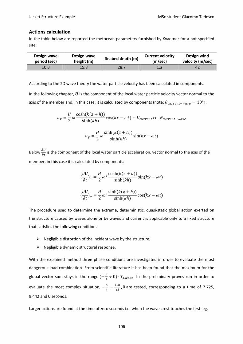
Jacket Structure Example MSc student Giacomo Tedesco
106
Actions calculation
In the table below are reported the metocean parameters furnished by Kvaerner for a not specified
site.
Design wave period (sec)
Design wave height (m)
Seabed depth (m) Current velocity
(m/sec) Design wind
velocity (m/sec)
10.3 15.8 28.7 1.2 42
According to the 2D wave theory the water particle velocity has been calculated in components.
In the following chapter, is the component of the local water particle velocity vector normal to the
axis of the member and, in this case, it is calculated by components (note: ):
( ( ))
( ) ( )
( ( ))
( ) ( )
Below
is the component of the local water particle acceleration, vector normal to the axis of the
member, in this case it is calculated by components:
(
)
( ( ))
( ) ( )
(
)
( ( ))
( ) ( )
The procedure used to determine the extreme, deterministic, quasi-static global action exerted on
the structure caused by waves alone or by waves and current is applicable only to a fixed structure
that satisfies the following conditions:
Negligible distortion of the incident wave by the structure;
Negligible dynamic structural response.
With the explained method three phase conditions are investigated in order to evaluate the most
dangerous load combination. From scientific literature it has been found that the maximum for the
global vector sum stays in the range (
) . In the preliminary proves run in order to
evaluate the most complex situation,
are tested, corresponding to a time of 7.725,
9.442 and 0 seconds.
Larger actions are found at the time of zero seconds i.e. when the wave crest touches the first leg.

Jacket Structure Example MSc student Giacomo Tedesco
107
In this page it is reported the scheme, from ISO 19902, representative of the procedure for
calculating the quasi-static action caused by wave plus current.
The computation of the action on a cylindrical object (a member) caused by waves, current or a
combination of waves and current depends on the ratio of the waves length to the member
diameter. When this ratio is large (>5), the member does not significantly modify the incident wave.
The action can then be computed as the sum of a hydrodynamic drag action and a hydrodynamic
inertia action, as given in following equation:
| |
Where:
is the local action vector per unit length acting normal to the axis of the member;
is the vector for the drag action per unit length acting normal to the axis of the member in the
plane of the member axis and U;
is the vector for the inertia action per unit length action normal to the axis of the member in the
plane of the member axis and

Jacket Structure Example MSc student Giacomo Tedesco
108
is the hydrodynamic drag coefficient;
is the mass density of water;
is the effective dimension of the cross-sectional area normal to the member axis per unit length
(=D for circular cylinder);
is the displaced volume of the member per unit length
is the effective diameter of a member ( a circular cylinder), including marine growth;
is the component of the local water particle velocity vector (due to waves and/or current) normal
to the axis of the member;
| | is the modulus ( the absolute value) of ;
is the hydrodynamic inertia coefficient;
is the component of the local water particle acceleration vector normal to the axis of the
member.
Suggested value of drag and inertia coefficients furnished by international standard, for typical
situations of smooth and rough member surface.
Surface of the component
smooth 0.65 1.6
rough 1.05 1.2
On the sketch below a member section affected by marine growth is presented.

Jacket Structure Example MSc student Giacomo Tedesco
109
The components affected by marine growth is classified as “rough”, otherwise “smooth”.
In this exercise are considered the smooth elements lower than the water sea level minus half of the
design wave height. Above this level, every member is supposed to be affected by marine growth, so
the related family of coefficients must be used during the forces calculation i.e. into the Morison
equation.
Supposed a platform with vertical walls in normal direction of wind, it is calculated the wind force by
the equation:
Where the shape coefficients is set equal to 1.5; like suggested by international standard for flat wall.
The load due to wind results equal to 120 kN, because it is considered a platform with wall dimension
of 15x6 meters (15x15 meters of base).
For the finite elements simulation, the deck weight is set equal to 500 tons.
In the picture on the right, the deck is
represented by a translation mass on the top
of the jacket (blue sphere) connected by rigid
link (also blue) to the edge of the column-legs.
Design wind is modelled by a concentrated
force on the deck i.e. the translational mass.
The green arrows are representative of the
wave plus current action and they are defined
for each member into the components along
X,Y and Z-axis.
Brace and horizontal beam (outside diameter:
1m, wall thickness: 1inc, steel) are in blue.
Legs (outside diameter: 2m, wall thickness:
1inc, steel) are in red.
The white and purple crosses on the legs foot
are the fixed restrain imposed.

Jacket Structure Example MSc student Giacomo Tedesco
110
The forces calculated by quasi-static approach are modelled like concentrated forces in the middle of
each member.
By hand calculation it is evaluated an acceptable leg and brace dimension (outside diameters and
wall thickness).
It’s important to know that the vertical axis, normally defined like Z-axis also into the equation of this
chapter, is named Y-axis instead in Straus 7.
A 3D structure is modelled, but to be clear below are reported only the view into the XY-plain,
because it has been supposed that current and wave stays into this plain.
In the picture below are presented the displacements for the nodes.

Jacket Structure Example MSc student Giacomo Tedesco
111
The forces calculated by quasi-static approach are modelled like concentrated forces in the middle of
each member.
This is the reason of the shear shape and moment diagrams.

Jacket Structure Example MSc student Giacomo Tedesco
112
In the next pages are shown the distribution of the maximum and the minimum principal stress.
Observing the maximum stress distribution is possible to define the areas subjected to highest tensile
stress, while the members in compression are highlighted into the minimum principal stress
distribution.

Jacket Structure Example MSc student Giacomo Tedesco
113

Jacket Structure Example MSc student Giacomo Tedesco
114
The picture above is representative of the fibre stress for the part of the structure in the XY-plain.
In order to add more information to get the real distribution of stress into the jacket structure, below
are reported the fibre stress per each level.
The pictures below confirm the expectative about the more stressed parts of the structure.
The moment, in which the wave crest passes the legs on the YZ-plain, the most stressed elements in
tension are the section near the mudline of these legs and the lower braces. In compression, others
legs are more stressed.
Concentrations of stress are visible around each node and in the middle of the highest part of the
legs into the YZ-plain.

Jacket Structure Example MSc student Giacomo Tedesco
115

Jacket Structure Example MSc student Giacomo Tedesco
116
From the level subdivision above reported it is clear shown that the most stressed elements of this
jacket are the lower parts of the legs, because they are very tensioned and compressed depending
on the position.
The maximum fibre stress is approximately 94 MPa, using the most simplified approach defined by
ISO 19902; the yielding stress (500 MPa) reduced by a safety factor (see table below) must be major
of the maximum stress found.
⇒
ISO 1990 coefficients table for simplified fatigue approach is below reported.
Failure critical component Inspectable Not Inspectable
No 2 5
Yes 5 10
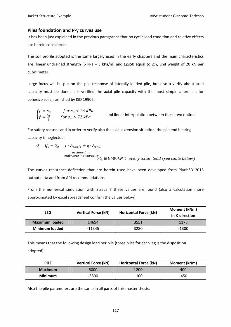
Jacket Structure Example MSc student Giacomo Tedesco
117
Piles foundation and P-y curves use
It has been just explained in the previous paragraphs that no cyclic load condition and relative effects
are herein considered.
The soil profile adopted is the same largely used in the early chapters and the main characteristics
are: linear undrained strength (5 kPa + 3 kPa/m) and Eps50 equal to 2%, unit weight of 20 kN per
cubic meter.
Large focus will be put on the pile response of laterally loaded pile, but also a verify about axial
capacity must be done. It is verified the axial pile capacity with the most simple approach, for
cohesive soils, furnished by ISO 19902:
{
and linear interpolation between these two option
For safety reasons and in order to verify also the axial extension situation, the pile end bearing
capacity is neglected:
⇒ ( )
The curves resistance-deflection that are herein used have been developed from Plaxis3D 2013
output data and from API recommendations.
From the numerical simulation with Straus 7 these values are found (also a calculation more
approximated by excel spreadsheet confirm the values below):
LEG Vertical Force (kN) Horizontal Force (kN) Moment (kNm)
in X-direction
Maximum loaded 14694 3551 1178
Minimum loaded -11345 3280 -1300
This means that the following design load per pile (three piles for each leg is the disposition
adopted):
PILE Vertical Force (kN) Horizontal Force (kN) Moment (kNm)
Maximum 5000 1200 400
Minimum -3800 1100 -450
Also the pile parameters are the same in all parts of this master thesis:

Jacket Structure Example MSc student Giacomo Tedesco
118
PILE Length (m)
Outside
Diameter
(inc/m)
Wall Thickness
(mm) Esteel (GPa)
E* for the
solid section
equivalent
to real (GPa)
40 84/2.14 60 210 43
The spreadsheet used to implement the P-y curves and run the simulation comes from a US
company, so each input parameter must be converted from the International System of Units into
the imperial unit system and vice versa.
In this spreadsheet the curves characteristic of the examined soil profile are defined one by one.
In order to do a comparison of results are run calculations also with curves from API standard.
It seems clear to evaluate that the results from both these methods are very similar and that like
expected using the curves obtained by API recommendations conservative results are obtained.
This last observation confirms the prediction done watching Plaxis3D results, just largely commented
in the early part of this thesis.
For each variable plotted the trend is almost the same: API curves furnish values larger than Plaxis3D
curves, but the curves have the same shape of each other.
In the table below are summarized the maximum values of bending moments and deflection for the
pile.
Curves
Leg max loaded Leg min loaded
Head
deflection (cm)
Max bending
moment (kNm)
Head
deflection (cm)
Max bending
moment (kNm)
Plaxis3D 28 8589 23 6834
API
recommendati
on
39 10437 31 8206
percentage variation
37% 22% 36% 20%
Pile deflection presents a large variation, approximately 35%, than the bending moment, 20% ca.
This confirms the observation already done in the initial chapters i.e. Plaxis3D furnishes values
smaller than API recommendation for pile deflection and maximum bending moment. It’s also
confirmed that the signalized trend according to the pile deflection is more variable than the bending
moment.

Jacket Structure Example MSc student Giacomo Tedesco
119
The variation between legs, in the table reported above, shown a very little difference into the
percentage variations, so it is possible to observe an increase of the results spreading with the load
level reached. Also the last one is an tendency already observed above.
Below are report the pile deflection, shear and bending moment, for the most and the less stressed
legs.

Jacket Structure Example MSc student Giacomo Tedesco
120
0
5
10
15
20
25
30
35
40
-10 0 10 20 30 40 50D
ep
th (
m)
y (cm)
Pile deflection (leg max loaded)
using P-y curves by Plaxis3D
using P-y curves by API recommendation
0
5
10
15
20
25
30
35
40
-5 0 5 10 15 20 25 30 35
De
pth
(m
)
y (cm)
Pile deflection (leg min loaded)
using P-y curves by Plaxis3D
using P-y curves by API recommendation

Jacket Structure Example MSc student Giacomo Tedesco
121
0
5
10
15
20
25
30
35
40
-2000 0 2000 4000 6000 8000 10000 12000
De
pth
(m
) Momemt (kNm)
Pile bending moment (leg max loaded)
using P-y curves by Plaxis3D
using P-y curves by API recommendation
0
5
10
15
20
25
30
35
40
-2000 0 2000 4000 6000 8000 10000
De
pth
(m
)
Momemt (kNm)
Pile bending moment (leg min loaded)
using P-y curves by Plaxis3D
using P-y curves by API recommendation

Jacket Structure Example MSc student Giacomo Tedesco
122
0
5
10
15
20
25
30
35
40
-750 -250 250 750 1250
De
pth
(m
)
Shear (kN)
Pile shear (leg max loaded)
using P-y curves by Plaxis3D
using P-y curves by APIrecommendation
0
5
10
15
20
25
30
35
40
-750 -250 250 750 1250
De
pth
(m
)
Shear (kN)
Pile shear (leg min loaded)
using P-y curves by Plaxis3D
using P-y curves by APIrecommendation

Conclusions and Observations MSc student Giacomo Tedesco
123
CONCLUSIONS AND OBSERVATIONS
During this dissertation, the behaviour of the laterally loaded pile in soft clay has been largely
treated.
In addition, the behaviour of groups of two pile (free and fixed) heads has been investigated. These
data are put in the appendix in order to avoid simple or wrong interpretations due to the few weeks
used to develop these simulations.
To conduct these analyses, the software Plaxis3D 2013 has been used. Several different settings are
tested in order to evaluate the sensibility of the model at the parameters variation.
Settings tested have been the interface reduction factor, tensile cut-off and Esp50. It is simple to
observe that only Esp50 is a pure geotechnical parameter while the two other parameters listed are
more related to the numerical model.
Moreover, a large number of “pure” model settings are analysed. These include model dimension,
interface adoption, pile validation and the soil model adopted.
Main result of the huge amount of analysis is a scale of importance for the tested parameters; it is
made evaluating the model response related to the parameter variation.
Primary importance must be assigned to soil model adopted and Esp50 value; because changing
Esp50 into its typical range of values caused a result fluctuation of almost 30% for each variable of
interest.
In the problem treated (short term static lateral load of a pile in soft clay), it has been demonstrated
that the best performances are reached adopting NGI-ADP soil model. The best solution for this
simulation has been reached defining an ADP soil with anisotropic behaviour. This is the most
realistic situation, instead, using an elastic-perfectly plastic soil model, the results are not easy to
comment, because the model response becomes stiff.
A secondary influence is observed for the interface reduction factor parameter if it is assumed in its
typical engineering range because, for a value between 1 and 0.4, the fluctuation is less than 15%.
To complete the part of the model setting is indispensable to touch two points of fundamental
importance: the model dimension along the load direction has a great influence on the result so it

Conclusions and Observations MSc student Giacomo Tedesco
124
must be set sufficiently large, in order to avoid stiff behaviour of the complex soil-structure.
At last, the mesh coarseness must be fine in the zone with high gradients of displacement and stress.
The adoption of the tensile cut-off can affect the result of large variation, but its physical meaning
must be evaluated with attention case by case, in reason to avoid “friendly” but wrong results. This
because it is not certain a large opening gap behind the pile.
The second part of the dissertation, and declared objective of my working period spent at the
Norwegian Geotechnical Institute, has been obtaining the resistance-deflection curves from finite
elements analysis (a laterally loaded pile is modelled in Plaxis3D).
Some problems have been found and fixed using Plaxis3D for the case above described. One of them
was a shear trend with unrealistic fluctuation along the shallow three meters of the pile (problem
attenuated increasing the pile of two meters, one diameter, above the seabed and adopting a rigid
plate on the pile head, where the load is applied).
Proving a comparison between displacement field obtained by Plaxis3D and the theoretical failure
mechanism of the soil around the pile it is possible to evaluate a correct movement of the soil wedge
behind the pile, but it is not possible to highlight a real flow of soil around the pile section, probably
because it can be reached only for very high displacements of the pile section, indeed several papers
test this behaviour defining a circular disc with imposed (high) displacement into the soil; in that case
the soil flow around the pile section is reached.
Indispensable steps to compute the P-y curves from Plaxis3D simulation have been discussed in the
specific chapter, but it must be highlighted again that the resistance-deflection curves obtained in
this way are stiffer than API standard curves even if they lead to almost the same ultimate resistance.
The last exercise reported in this thesis is representative of a jacket structure under environmental
loads.
Wave and current actions are evaluated following the quasi-static approach furnished by
international standard ISO 19902. Also wind and structural weight are taken into count.
Once calculated the load acting per each pile, it becomes possible to study the lateral response of the
foundation. This analyses are run with a specific spreadsheet.
The axial capacity is largely sufficient to accept the loads transmitted by the legs.
The result obtained by using Plaxis3D or API P-y curves shown the same trends but by 20%-30%
bigger adopting the curves recommended by American Petroleum Institute.

Conclusions and Observations MSc student Giacomo Tedesco
125
This confirms the observation done during the model construction and use.
The method used to obtain the resistance-deflection curves has demonstrated wide possibility for
future developments related to the generalization of other soil profiles and to the comparison of
curves from field tests of laterally loaded piles with curves obtained by numerical simulations.

Conclusions and Observations MSc student Giacomo Tedesco
126
-This page intentionally left blank-

Reference MSc student Giacomo Tedesco
127
REFERENCE
Hudson M.(1970). Correlations for design of laterally loaded piles in soft clay. The U. of Texas
at Austin.
Gustav G., Lars A. and Hans P.J. (2010). NGI-ADP: Anisotropic shear strength model for clay.
John B. Herbich, Editor. Handbook of Coastal and Ocean Engineering, Volume 2.
R. G. Bea, Fellow, ASCE, Z. Jin, C. Valle and R. Ramos (1999). Evaluation of reliability of
platform pile foundations.
Hudson M., Wayne B. Ingram, Allen E. Kelley, Dewaine B. (1980). Field tests of the lateral-
load behavior of pile groups in soft clay.
Robert G. Dean, Robert A. Dalrymple. Water wave mechanics for engineers and scientists.
V. Padmavathi, E.Saibaba Reddy and M.R. Madhav (2008). Behaviour of laterally loaded rigid
piles in cohesive soils based on kinematic approach.
SPLICE manual. NGI, Oslo, Norway.
Summary report of NGI Strategic Research Project SP2 2011-2013. Offshore wind turbine
foundations. No.20110001-R-01.
John A.F. and Kenneth J.K. (1973). Rational Analysis of the Lateral Performance of Offshore
Pile Group.
NGI project report No.20092244-00-8-R. Summary and recommendation practice. Lateral
capacity of piles in soft clay. 2013-01-08.
Plaxis3D 2013 scientific manual. Plaxis, Delft, Nederland.
H.Y. Qin, E.Y.N. Oh, W.D. Guo and P.F. Dai (2013). Upper bound limit analysis of lateral pile
capacity.
ISO 19901-1. Petroleum and natural gas industries - Specific requirements for offshore
structure. Part 1: Metocean design and operating considerations. First edition 2005-11-15.
ISO 19902. Petroleum and natural gas industries – Fixed steel offshore structure. First edition
2007-12-01.
V. Zania and O. Hededal (2011).The effect of soil-pile interface behaviour on laterally loaded
piles (paper 1). Department of Civil Engineering, Technical University of Denmark.
V. Zania and O. Hededal (2012). Friction effects on lateral loading behavior of rigid piles.
Department of Civil Engineering, Technical University of Denmark.
George G. and Ricardo D., Members, ASCE (1984). Horizontal response of piles in layered
soils.

Reference MSc student Giacomo Tedesco
128
Yit-Jin C., Associate Member, ASCE, Fellow and Fred H.K. (1993). Undrained strength
interrelationships among CIUC, UU, and UC Tests.
Youngho K., Sangseom J., Sooil K. (2009). Characteristics of lateral rigidity of offshore piles in
Incheon marine clay. Department of Civil Engineering, Yonsei University, Seoul, 120-749,
Korea.
L.J. Zhu, Y.M. Cheng and D.B. Yang (2007). The analysis of instrumented piles under lateral
load. Department of Hydraulic Engineering, Tsinghua University, Beijing, China; Department
of civil and Structural Engineering, Hong Kong Polytechnic University, Hong Kong.
Ke Yang and Robert Liang (2006). Methods for Deriving p-y Curves from Instrumented Lateral
Load Tests.
F. Rosquoet, L. Thorel, J. Garnier and M. Khemakhem (2010). P-y curves on model piles:
Uncertainty identification.
Todd W. Dunnavant, Associate Member, ASCE, and Michael W. O’Neill (1989). Experimental
p-y Model for Submerged Stiff Clay.
James D.Murff, and Jed M. Hamilton, Members, ASCE (1993). P-Ultimate for Undrained
Analysis of Laterally Loaded Piles.
P.Jeanjean, BP America Inc. (2009). Re-Assessment of P-Y Curves for Soft Clays from
Centrifuge Testing and Finite Element Modeling.
K. Georgiadis, S.W. Sloan, and A.V. Lyamin (2013). Effect of loading direction on the ultimate
lateral soil pressure of two piles in clay. Georgiadis, K. et al. (2013). Geotechnique 63, No. 13,
1170-1175 (http://dx.doi.org/10.1680/geot.13.T.003).
Harry G. Poulos, M. ASCE and Mark F. Randolph (1983). Pile Group Analysis: A Study of Two
Methods.
Wei Dong Guo, M. ASCE (2013). Simple Model for Nonlinear Response of 52 Laterally Loaded
Piles.
http://newtonexcelbach.wordpress.com/.
WWW.INTERACTIVEDS.COM.AU.

Appendix A – Groups of Piles MSc student Giacomo Tedesco
129
APPENDIX A – ANALYSIS OF GROUPS OF PILES
In this appendix are reported the results of numerical simulations run with Plaxi3D and compared
with SPLICE results.
Both fixed and free heads condition are tested. The fixed head condition has been reached
connecting the piles heads with a stiff plate.
Several series of analysis are run for models with different piles spacing. Interaxis of 2,3,4,5
diameters are tested. These tests are done for both the restrain condition descripted above.
Below the displacements trends and two series of five graphs with two different normalizations are
reported.
In the end also a third series is presented. The results are grouped by restrain heads conditions and
by the load condition acting on the piles heads.
Head isplacements
0
0,1
0,2
0,3
0,4
0,5
0,6
0,7
0,8
0,9
1
1,1
1,2
1,3
1,4
1,5
1,6
1,7
1,8
1,9
2
2 3 4 5 6 7 8
Ho
rizo
nta
l dis
pla
cem
ent
(m)
Load (MN)
Displacement of pile section at seabed level Group of two pile for differente spacing in fixed head condition
SPLICE and Plaxis3D G1-interaxis 1D
G2-interaxis 2D
G3-interaxis 3D
G4-interaxis 4D
splice1-interaxis 2D-interaction activated
splice2-interaxis 3D-interaction activated
splice3-interaxis 4D-interaction activated
splice4-interaxis 5D-interaction activated

Appendix A – Groups of Piles MSc student Giacomo Tedesco
130
0
0,1
0,2
0,3
0,4
0,5
0,6
0,7
0,8
0,9
1
1,1
1,2
1,3
1,4
1,5
1,6
2 3 4 5 6 7 8
Ho
rizo
nta
l dis
pla
cem
ent
(m)
Load (MN)
Average displacement of pile section at seabed level Group of two pile for differente spacing in free head condition
SPLICE and Plaxis3D F1-interaxis 2D
F2-interaxis 3D
F3-interaxis 4D
F4-interaxis 5D
splice1-interaxis 2D-interaction activated
splice2-interaxis 3D-interaction activated
splice3-interaxis 4D-interaction activated
splice4-interaxis 5D-interaction activated
splice-interaction deactivated (single pile)
0
0,1
0,2
0,3
0,4
0,5
0,6
0,7
0,8
0,9
1
1,1
1,2
1,3
1,4
1,5
1,6
1,7
1,8
1,9
2
2 3 4 5 6 7 8
Ho
rizo
nta
l dis
pla
cem
ent
(m)
Load (MN)
Displacement of pile section at seabed level Group of two pile for differente spacing in fixed and free head condition
Plaxis3D F series: free heads (it's used the average displacement of the piles)
G series: fixed heads F1-interaxis 2D
F2-interaxis 3D
F3-interaxis 4D
F4-interaxis 5D
G1-interaxis 1D
G2-interaxis 2D
G3-interaxis 3D
G4-interaxis 4D

Appendix A – Groups of Piles MSc student Giacomo Tedesco
131
0
0,1
0,2
0,3
0,4
0,5
0,6
0,7
0,8
0,9
1
1,1
1,2
1,3
1,4
1,5
1,6
1,7
1,8
1,9
2
2 3 4 5 6 7 8
Ho
rizo
nta
l dis
pla
cem
ent
(m)
Load (MN)
Displacement of pile section at seabed level of the first pile in load direction of
two piles group for differente spacing (free head condition) SPLICE and Plaxis3D F1-interaxis 2D
F2-interaxis 3D
F3-interaxis 4D
F4-interaxis 5D
splice1-interaxis 2D-interaction activated
splice2-interaxis 3D-interaction activated
splice3-interaxis 4D-interaction activated
F4-interaxis 5D-interaction activated
0
0,1
0,2
0,3
0,4
0,5
0,6
0,7
0,8
0,9
1
1,1
1,2
1,3
1,4
1,5
1,6
1,7
1,8
1,9
2
2 3 4 5 6 7 8
Ho
rizo
nta
l dis
pla
cem
ent
(m)
Load (MN)
Displacement of pile section at seabed level of the second pile in load direction of
two piles groups for differente spacing (free head condition) SPLICE and Plaxis3D F1-interaxis 2D
F2-interaxis 3DF3-interaxis 4DF4-interaxis 5Dsplice2-interaxis 3D-interaction activatedsplice1-interaxis 2D-interaction activatedsplice3-interaxis 4D-interaction activatedF4-interaxis 5D-interaction activated

Appendix A – Groups of Piles MSc student Giacomo Tedesco
132
Normalized head displacements using the maximum interaxis cases (F4-G4)
0,9
1
1,1
1,2
1,3
1,4
1,5
1,6
1,7
1,8
1,9
2
2,1
2,2
2,3
2,4
2,5
2,6
2,7
2,8
2,9
2 3 4 5 6 7 8
No
rmal
ized
dis
pla
cem
ent
(-)
Load (MN)
Normalized displacement (by G4 and splice4) of pile section at seabed level
Group of two pile for differente spacing in fixed head condition SPLICE and Plaxis3D
G1-interaxis 1D
G2-interaxis 2D
G3-interaxis 3D
G4-interaxis 4D
splice1-interaxis 2D-interaction activated
splice2-interaxis 3D-interaction activated
splice3-interaxis 4D-interaction activated
splice4-interaxis 5D-interaction activated
0,7
0,8
0,9
1
1,1
1,2
1,3
1,4
1,5
1,6
1,7
1,8
1,9
2
2,1
2,2
2 3 4 5 6 7 8
No
rmal
ized
dis
pla
cem
ent
(-)
Load (MN)
Normalized average displacement (by F4 and splice4) of pile section at seabed level
Group of two pile for differente spacing in free head condition SPLICE and Plaxis3D
F1-interaxis 2D
F2-interaxis 3D
F3-interaxis 4D
F4-interaxis 5D
splice1-interaxis 2D-interaction activated
splice2-interaxis 3D-interaction activated
splice3-interaxis 4D-interaction activated
splice4-interaxis 5D-interaction activated
splice-interaction deactivated (single pile)

Appendix A – Groups of Piles MSc student Giacomo Tedesco
133
0,9
1
1,1
1,2
1,3
1,4
1,5
1,6
1,7
1,8
1,9
2
2,1
2,2
2 3 4 5 6 7 8
No
rmal
ized
dis
pla
cem
ent
(-)
Load (MN)
Normalized displacement (by F4 and G4) of pile section at seabed level Group of two pile for differente spacing in fixed and free head condition
Plaxis3D F series: free heads (it's used the average displacement of the piles)
G series: fixed heads F1-interaxis 2D
F2-interaxis 3D
F3-interaxis 4D
F4-interaxis 5D
G1-interaxis 1D
G2-interaxis 2D
G3-interaxis 3D
G4-interaxis 4D
0,9
1
1,1
1,2
1,3
1,4
1,5
1,6
1,7
1,8
2 3 4 5 6 7 8
No
rmal
ized
dis
pla
cem
ent
(-)
Load (MN)
Normalized displacement (by F4 and splice4) of pile section at seabed level
of the first pile in load direction of two piles group for differente spacing (free head condition)
SPLICE and Plaxis3D F1-interaxis 2D
F2-interaxis 3D
F3-interaxis 4D
F4-interaxis 5D
splice1-interaxis 2D-interaction activated
splice2-interaxis 3D-interaction activated
splice3-interaxis 4D-interaction activated
splice4-interaxis 5D-interaction activated

Appendix A – Groups of Piles MSc student Giacomo Tedesco
134
0,9
1
1,1
1,2
1,3
1,4
1,5
1,6
1,7
1,8
2 3 4 5 6 7 8
No
rmal
ized
dis
pla
cem
ent
(-)
Load (MN)
Normalized displacement (by F4 and splice4) of pile section at seabed level
of the second pile in load direction of two piles groups for differente spacing (free head condition)
SPLICE and Plaxis3D
F1-interaxis 2D
F2-interaxis 3D
F3-interaxis 4D
F4-interaxis 5D
splice1-interaxis 2D-interaction activated
splice2-interaxis 3D-interaction activated
splice3-interaxis 4D-interaction activated
splice4-interaxis 5D-interaction activated

Appendix A – Groups of Piles MSc student Giacomo Tedesco
135
Normalized head displacements using SPLICE or Plaxis3D results
0,9
1
1,1
1,2
1,3
1,4
1,5
1,6
1,7
1,8
1,9
2
2,1
2,2
2,3
2,4
2,5
2,6
2,7
2,8
2,9
2 3 4 5 6 7 8
No
rmal
ized
dis
pla
cem
ent
(-)
Load (MN)
Normalized displacement (by splice results) of pile section at seabed level
Group of two pile for differente spacing in fixed head condition SPLICE and Plaxis3D G1-interaxis 1D
G2-interaxis 2D
G3-interaxis 3D
G4-interaxis 4D
splice1-interaxis 2D-interaction activated
splice2-interaxis 3D-interaction activated
splice3-interaxis 4D-interaction activated
splice4-interaxis 5D-interaction activated
0,8
0,9
1
1,1
1,2
1,3
1,4
1,5
2 3 4 5 6 7 8
No
rmal
ized
dis
pla
cem
ent
(-)
Load (MN)
Normalized average displacement (by F series) of pile section at seabed level
Group of two pile for differente spacing in free head condition SPLICE and Plaxis3D
F1-interaxis 2D
F2-interaxis 3D
F3-interaxis 4D
F4-interaxis 5D
splice1-interaxis 2D-interaction activated
splice2-interaxis 3D-interaction activated
splice3-interaxis 4D-interaction activated
splice4-interaxis 5D-interaction activated
splice-interaction deactivated (single pile)

Appendix A – Groups of Piles MSc student Giacomo Tedesco
136
0,9
1
1,1
1,2
1,3
1,4
1,5
1,6
1,7
1,8
1,9
2 3 4 5 6 7 8
No
rmal
ized
dis
pla
cem
ent
(-)
Load (MN)
Normalized displacement (by G series) of pile section at seabed level Group of two pile for differente spacing in fixed and free head condition
Plaxis3D F series: free heads (it's used the average displacement of the piles)
G series: fixed heads F1-interaxis 2D
F2-interaxis 3D
F3-interaxis 4D
F4-interaxis 5D
G1-interaxis 1D
G2-interaxis 2D
G3-interaxis 3D
G4-interaxis 4D
0,7
0,8
0,9
1
1,1
1,2
1,3
1,4
1,5
2 3 4 5 6 7 8
No
rmal
ized
dis
pla
cem
ent
(-)
Load (MN)
Normalized displacement (by F series) of pile section at seabed level of the first pile in load direction of
two piles group for differente spacing (free head condition) SPLICE and Plaxis3D
F1-interaxis 2D
F2-interaxis 3D
F3-interaxis 4D
F4-interaxis 5D
splice1-interaxis 2D-interaction activated
splice2-interaxis 3D-interaction activated
splice3-interaxis 4D-interaction activated
splice4-interaxis 5D-interaction activated

Appendix A – Groups of Piles MSc student Giacomo Tedesco
137
0,8
0,9
1
1,1
1,2
1,3
1,4
1,5
2 3 4 5 6 7 8
No
rmal
ized
dis
pla
cem
ent
(-)
Load (MN)
Normalized displacement (by F series) of pile section at seabed level of the second pile in load direction of
two piles groups for differente spacing (free head condition) SPLICE and Plaxis3D
F1-interaxis 2D
F2-interaxis 3D
F3-interaxis 4D
F4-interaxis 5D
splice1-interaxis 2D-interaction activated
splice2-interaxis 3D-interaction activated
splice3-interaxis 4D-interaction activated
splice4-interaxis 5D-interaction activated

Appendix A – Groups of Piles MSc student Giacomo Tedesco
138
Head displacements grouped by load
0
5
10
15
20
25
30
35
40
45
50
55
60
65
1,5 2 2,5 3 3,5 4 4,5 5 5,5
Dif
fere
nce
fro
m la
rge
st s
pac
ing
(%)
Interaxis (Diameters)
Free Heads
2MN
4MN
6MN
8MN
0
10
20
30
40
50
60
70
80
90
100
110
120
1,5 2 2,5 3 3,5 4 4,5 5 5,5
Dif
fere
nce
fro
m la
rge
st s
pac
ing
(%)
Interaxis (Diameters)
Fixed Heads
2MN
4MN
6MN
8MN

Appendix A – Groups of Piles MSc student Giacomo Tedesco
139
0
5
10
15
20
25
30
1,5 2 2,5 3 3,5 4 4,5 5 5,5
Dif
fere
nce
fro
m la
rge
st s
pac
ing
(%)
Interaxis (Diameters)
Free and Fixed Heads for 2MN on each pile head
Free Heads
Fixed Heads
0
5
10
15
20
25
30
35
40
45
1,5 2 2,5 3 3,5 4 4,5 5 5,5
Dif
fere
nce
fro
m la
rge
st s
pac
ing
(%)
Interaxis (Diameters)
Free and Fixed Heads for 4MN on each pile head
Free Heads
Fixed Heads

Appendix A – Groups of Piles MSc student Giacomo Tedesco
140
0
5
10
15
20
25
30
35
40
45
50
55
60
65
1,5 2 2,5 3 3,5 4 4,5 5 5,5
Dif
fere
nce
fro
m la
rge
st s
pac
ing
(%)
Interaxis (Diameters)
Free and Fixed Heads for 6MN on each pile head
Free Heads
Fixed Heads
0
10
20
30
40
50
60
70
80
90
100
110
120
1,5 2 2,5 3 3,5 4 4,5 5 5,5
Dif
fere
nce
fro
m la
rge
st s
pac
ing
(%)
Interaxis (Diameters)
Free and Fixed Heads for 8MN on each pile head
Free Heads
Fixed Heads

Appendix A – Groups of Piles MSc student Giacomo Tedesco
141
0
0,2
0,4
0,6
0,8
1
1,2
1,4
1,6
1,8
2
1,5 2 2,5 3 3,5 4 4,5 5 5,5
Dis
pla
cem
en
t (m
)
Interaxis (Diameters)
Free Heads 2MN
4MN
6MN
8MN
0
0,2
0,4
0,6
0,8
1
1,2
1,4
1,6
1,8
2
1,5 2 2,5 3 3,5 4 4,5 5 5,5
Dis
pla
cem
en
t (m
)
Interaxis (Diameters)
Fixed Heads 2MN
4MN
6MN
8MN

Appendix A – Groups of Piles MSc student Giacomo Tedesco
142
0
0,02
0,04
0,06
0,08
0,1
0,12
0,14
0,16
0,18
1,5 2 2,5 3 3,5 4 4,5 5 5,5
Dis
pla
cem
en
t (m
)
Interaxis (Diameters)
Free and Fixed Heads for 2MN on each pile head
Free Heads
Fixed Heads
0
0,05
0,1
0,15
0,2
0,25
0,3
0,35
0,4
0,45
0,5
1,5 2 2,5 3 3,5 4 4,5 5 5,5
Dis
pla
cem
en
t (m
)
Interaxis (Diameters)
Free and Fixed Heads for 4MN on each pile head
Free Heads
Fixed Heads

Appendix A – Groups of Piles MSc student Giacomo Tedesco
143
0
0,1
0,2
0,3
0,4
0,5
0,6
0,7
0,8
0,9
1
1,5 2 2,5 3 3,5 4 4,5 5 5,5
Dis
pla
cem
en
t (m
)
Interaxis (Diameters)
Free and Fixed Heads for 6MN on each pile head
Free Heads
Fixed Heads
0
0,2
0,4
0,6
0,8
1
1,2
1,4
1,6
1,8
2
1,5 2 2,5 3 3,5 4 4,5 5 5,5
Dis
pla
cem
en
t (m
)
Interaxis (Diameters)
Free and Fixed Heads for 8MN on each pile head
Free Heads
Fixed Heads

Appendix A – Groups of Piles MSc student Giacomo Tedesco
144
-This page intentionally left blank-


![Abstract - pure.qub.ac.uk · Web view[47]Tedesco, G. and Aickelin, U., “Adaptive Alert Throttling for Intrusion Detection Systems”. Journal of Intelligent Information Systems,](https://img.pdfslide.us/doc/110x75/5c68e4f209d3f25c6a8c3683/abstract-purequbacuk-web-view47tedesco-g-and-aickelin-u-adaptive.jpg)