Embed Size (px)
Citation preview
i
Allometry, biomass and litter decomposition of the New Zealand
mangrove Avicennia marina var. australasica
Phan Tran
A thesis submitted to Auckland University of Technology
in partial fulfilment of the requirements for the degree
of
Masters of Science (MSc)
2014
School of Applied Sciences
i
Table of contents
______________________________________________________________
Table of contents ..................................................................................................................... i
List of Figures ....................................................................................................................... iii
List of tables .......................................................................................................................... vi
Attestation of authorship ...................................................................................................... vii
Co-Authored Works ............................................................................................................ viii
Acknowledgements ............................................................................................................... ix
Abstract .................................................................................................................................. x
Chapter 1. Introduction .......................................................................................................... 1
1.1 Mangrove ecosystems ................................................................................................... 2
1.2 Global patterns of mangrove forests ............................................................................. 3
1.3 Mangrove ecosystem services ...................................................................................... 4
1.4 Mangrove carbon studies .............................................................................................. 6
1.5 New Zealand mangroves .............................................................................................. 7
1.6 Research questions:....................................................................................................... 9
1.7 Outline of chapters: ....................................................................................................... 9
Chapter 2. Allometry and biomass allocation ...................................................................... 10
2.1 Introduction ................................................................................................................. 11
2.2 Methods and Materials................................................................................................ 14
Study areas .................................................................................................................... 14
Allometry and Leaf Area Index (LAI) ............................................................................ 15
Above-ground biomass: ................................................................................................. 16
Below-ground biomass .................................................................................................. 19
2.3 Results ......................................................................................................................... 20
Allometry and LAI of mangrove stands ......................................................................... 20
Biomass partitioning ..................................................................................................... 21
Vertical distribution of biomass .................................................................................... 23
2.4 Discussion ................................................................................................................... 24
ii
Above-ground biomass .................................................................................................. 24
Belowground biomass ................................................................................................... 26
Allometric equation: ...................................................................................................... 27
Limitations ..................................................................................................................... 28
Chapter 3: Litter production and decomposition .............................................................. 30
3.1 Introduction ................................................................................................................. 31
Litterfall ......................................................................................................................... 31
Litterfall in mangrove forests ........................................................................................ 32
Litter decomposition ...................................................................................................... 33
Mangrove litter decomposition...................................................................................... 33
3.2 Methodology ............................................................................................................... 35
Site selection .................................................................................................................. 35
Litterfall ......................................................................................................................... 35
Decomposition ............................................................................................................... 37
3.3 Results ......................................................................................................................... 37
3.3.1 Litterfall ................................................................................................................ 37
3.3.2 Litter decomposition ............................................................................................. 42
3.4 Discussion ................................................................................................................... 45
Litterfall ......................................................................................................................... 45
Litter decomposition ...................................................................................................... 48
3.5 Conclusions ................................................................................................................. 49
Chapter 4. General discussion and implications for conservation and management ........... 51
4.1 Summary of main results ............................................................................................ 52
Allometry and LAI ......................................................................................................... 52
Biomass distribution ...................................................................................................... 52
Litterfall production ...................................................................................................... 52
Litter decomposition ...................................................................................................... 53
4.2 Conclusions and implication for conservation and management ............................... 53
References ............................................................................................................................ 56
iii
List of Figures ______________________________________________________________
Figure 1. Major components of (mangrove) forest carbon pool and its cycle among
ecosystems. Figure modified from Bouillon et al.(2008). ....................................... 6
Figure 2. Mangawhai Heads with five study sub-sites of Jack Boyd (JB), Molesworth
(MO), Island (IS), Insley (IN) and Black Swamp (BS). ....................................... 15
Figure 3. Basal area against dry wood and leaf mass at Black Swamp, Mangawhai Harbour
Estuary. The linear model Y = x * ba was used, with Y the wood / leaf dry weight
and ba the basal area. R-squared is 0.94 for both plots. ........................................ 18
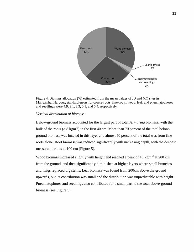
Figure 4. Biomass allocation (%) estimated from the mean values of JB and MO sites in
Mangawhai Harbour. ............................................................................................. 23
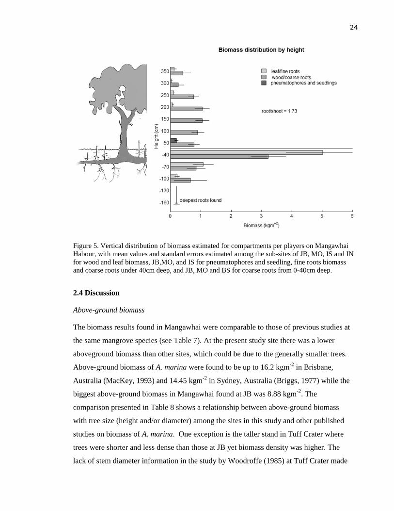
Figure 5. Vertical distribution of biomass estimated for compartments per players on
Mangawhai Habour, with mean values and standard errors estimated among the
sub-sites of JB, MO, IS and IN for wood and leaf biomass, JB,MO, and IS for
pneumatophores and seedling, fine roots biomass and coarse roots under 40cm
deep, and JB, MO and BS for coarse roots from 0-40cm deep. ............................ 24
Figure 6. Quadratic model Y = x * ba2 used for the regression of dry wood on basal area,
with Y the dry wood mass, ba the basal area. Data from the Black Swamp site at
Mangawhai Harbour Estuary. ................................................................................ 27
Figure 7. Basal area against total leaf mass (a) and leaf mass by height (b) at Black Swamp,
Mangawhai Harbour Estuary. The linear model Y = x * ba was used, with Y the
leaf dry weight and ba the basal area. R-squared is 0.94 for the relationship
between ba and total leaf dry weight, and are 0.34, 0.54, 0.52, and 0.79 for the
relationship between ba and leaf dry weight at 150-200cm, 200-250cm, 250-
300cm, and 300-350cm respectively. .................................................................... 28
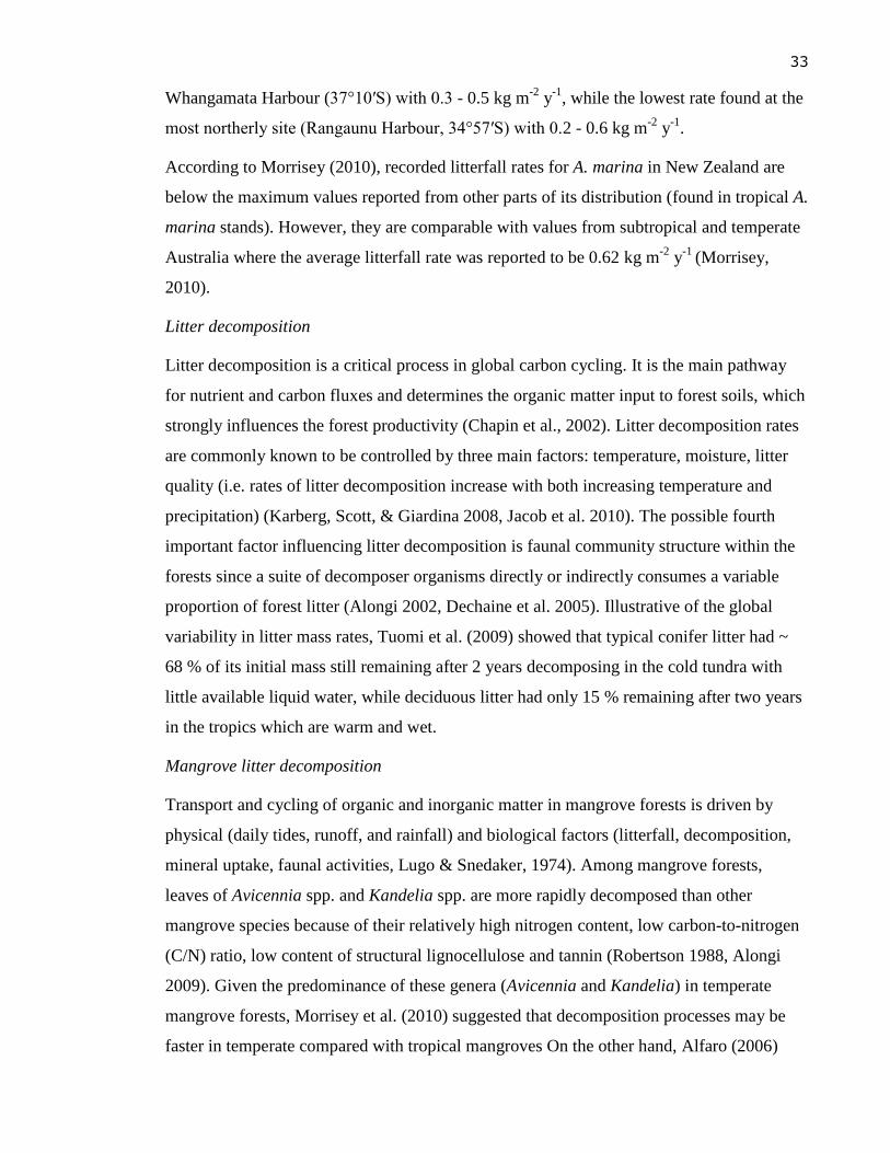
Figure 8. Locations of litter traps and litter bags at JB (a), MO (b), and IS (c) at the
Mangawhai Habour study area. ............................................................................. 36
iv
Figure 9. Seasonal litter production at Mangawhai Harbour (gm-2
day-1
), with the mean
values for each litter component calculated from thirty traps across all sites. Error
bars represent one standard error (n=30). .............................................................. 39
Figure 10. Site-specific seasonal litter production and monthly mean temperature (0C)
measured at Mangawhai Harbour. Error bars represent the standard errors for the
mean values of litter from ten traps (n=10) for each site Jack Boyd (JB),
Molesworth (MO) and Island (IS). ........................................................................ 40
Figure 11. Site-specific seasonal litter production and monthly max wind speed (kmh-1
)
measured at Mangawhai Harbour. Error bars represent the standard errors for the
mean values of litter from ten traps (n=10) for each site Jack Boyd (JB),
Molesworth (MO) and Island (IS). ........................................................................ 41
Figure 12. Site-specific seasonal litter production and monthly total rainfall (mm) measured
at Mangawhai Harbour. Error bars represent the standard errors for the mean
values of litter from ten traps (n=10) for each site Jack Boyd (JB), Molesworth
(MO) and Island (IS). ............................................................................................. 42
Figure 13. Mangrove leaf litter decomposition measured at Mangawhai Harbour, expressed
as the percentage of initial dry weight remaining over time. Error bars represent
the standard errors for the mean values twelve litter bags (n=10) collected each site
Jack Boyd (JB), Molesworth (MO) and Island (IS). .............................................. 43
Figure 14. Asymptotic model fit y = Asym + (R0 - Asym) * exp(-exp(lrc) * x) with y the
remaining weight over time), R0 the estimated intercept on the y-axis, Asym the
asymptote parallel to the x-axis, and lrc is the estimated logarithm of the rate
constant, applied generally for litter decomposition process at Mangawhai
Harbour. ................................................................................................................. 44
Figure 15. Asymptotic fit model ysite = Asym + (R0 - Asym) * exp(-exp(lrcsite) * x, with y the
the percentage of remaining weight over time, R0 the estimated intercept on the y-
axis, Asym the asymptote parallel to the x-axis, and lrc the estimated logarithm of
the rate constant applied site-specifically for IS (a), MO (b), and JB (c) at
Mangawhai Harbour. ............................................................................................. 45
v
Figure 16. Carbon pools (kg C m-2
) and fluxes (kg C m-2
y-1
) of A.marina with study results
at Mangawhai Harbour ( black text) and assumed figures (red text) based on data
from Suwa et al. (2006), Ray et al. (2011), and Alongi (2014). ............................ 54
vi
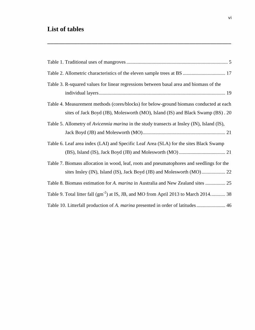
List of tables
______________________________________________________________
Table 1. Traditional uses of mangroves ................................................................................. 5
Table 2. Allometric characteristics of the eleven sample trees at BS .................................. 17
Table 3. R-squared values for linear regressions between basal area and biomass of the
individual layers ..................................................................................................... 19
Table 4. Measurement methods (cores/blocks) for below-ground biomass conducted at each
sites of Jack Boyd (JB), Molesworth (MO), Island (IS) and Black Swamp (BS) . 20
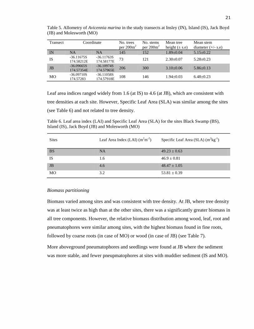
Table 5. Allometry of Avicennia marina in the study transects at Insley (IN), Island (IS),
Jack Boyd (JB) and Molesworth (MO) .................................................................. 21
Table 6. Leaf area index (LAI) and Specific Leaf Area (SLA) for the sites Black Swamp
(BS), Island (IS), Jack Boyd (JB) and Molesworth (MO) ..................................... 21
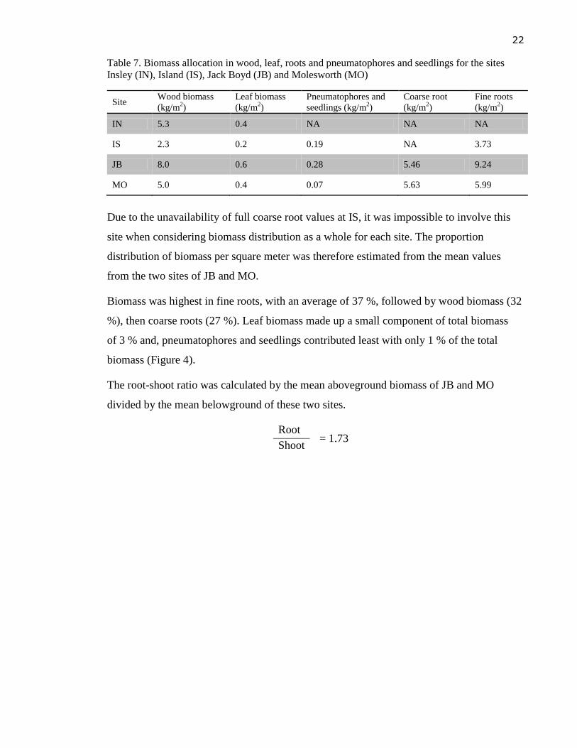
Table 7. Biomass allocation in wood, leaf, roots and pneumatophores and seedlings for the
sites Insley (IN), Island (IS), Jack Boyd (JB) and Molesworth (MO) ................... 22
Table 8. Biomass estimation for A. marina in Australia and New Zealand sites ................ 25
Table 9. Total litter fall (gm-2
) at IS, JB, and MO from April 2013 to March 2014. ........... 38
Table 10. Litterfall production of A. marina presented in order of latitudes ....................... 46

vii
Attestation of authorship
______________________________________________________________
“I hereby declare that this submission is my own work and that, to best of my
knowledge and belief, contains no material previously published or written by
another person (except where explicitly defined in the acknowledgements), nor
material which to a substantial extent has been submitted to the award of any other
degree or diploma of university or other institution of higher learning.”
Signed Date: Aug 22, 2014

viii
Co-Authored Works
______________________________________________________________________
The two main chapters of this thesis are in preparation to be submitted to the New Zealand
Journal of Marine and Freshwater Research. To this work, although I am the principal
author, I have received intellectual contribution from my supervisors through their valuable
advice, which can hardly weigh. I identify authorship contribution as 85 % from myself, 10
% from Sebastian Leuzinger (primary supervisor), and 5 % from Andrea Alfaro (secondary
supervisor).
Signatures:
Principal author: Phan Tran
Co-Author Sebastian Leuzinger
Co-Author Andrea C. Alfaro

ix
Acknowledgements ______________________________________________________________
I would like to express my deepest gratitude to my primary supervisor, Dr. Sebastian
Leuzinger, for giving me the opportunity to complete this thesis. I could hardly have done
without his devoted guidance and valuable advice. My sincere thanks are also to my
secondary supervisor, Prof. Andrea C. Alfaro and my senior Jarrod Cusens for their helpful
comments to make this study much better.
I owe the Mangrove research team, especially Iana Gritcan, and other student peers for their
dedicated help during my field work, which were highly labour-intensive. I also found
myself indebted to the New Zealand Ministry of Foreign Affairs and Trade for their
sponsorship for my study with AUT under New Zealand ASEAN Scholars Awards
program.
It would be difficult for me to finish this study without supports and encouragement from
my family and especially my husband, Jobi George, for his sharing of family
responsibilities during my academic years.
Last but not least, I would like to reserve my thankfulness to AUT Applied Sciences LAB
staff for their supports, which is also much important for me to complete my study.
x
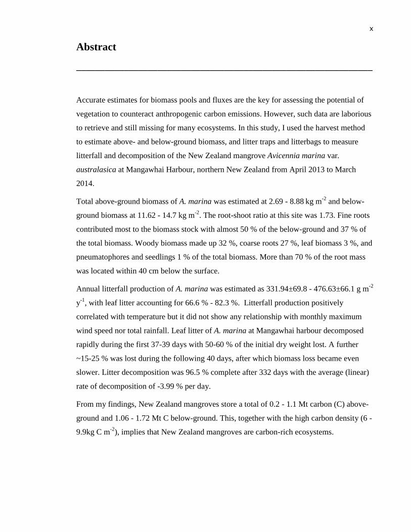
Abstract
______________________________________________________________
Accurate estimates for biomass pools and fluxes are the key for assessing the potential of
vegetation to counteract anthropogenic carbon emissions. However, such data are laborious
to retrieve and still missing for many ecosystems. In this study, I used the harvest method
to estimate above- and below-ground biomass, and litter traps and litterbags to measure
litterfall and decomposition of the New Zealand mangrove Avicennia marina var.
australasica at Mangawhai Harbour, northern New Zealand from April 2013 to March
2014.
Total above-ground biomass of A. marina was estimated at 2.69 - 8.88 kg m-2
and below-
ground biomass at 11.62 - 14.7 kg m-2
. The root-shoot ratio at this site was 1.73. Fine roots
contributed most to the biomass stock with almost 50 % of the below-ground and 37 % of
the total biomass. Woody biomass made up 32 %, coarse roots 27 %, leaf biomass 3 %, and
pneumatophores and seedlings 1 % of the total biomass. More than 70 % of the root mass
was located within 40 cm below the surface.
Annual litterfall production of A. marina was estimated as 331.94±69.8 - 476.63±66.1 g m-2
y-1
, with leaf litter accounting for 66.6 % - 82.3 %. Litterfall production positively
correlated with temperature but it did not show any relationship with monthly maximum
wind speed nor total rainfall. Leaf litter of A. marina at Mangawhai harbour decomposed
rapidly during the first 37-39 days with 50-60 % of the initial dry weight lost. A further
~15-25 % was lost during the following 40 days, after which biomass loss became even
slower. Litter decomposition was 96.5 % complete after 332 days with the average (linear)
rate of decomposition of -3.99 % per day.
From my findings, New Zealand mangroves store a total of 0.2 - 1.1 Mt carbon (C) above-
ground and 1.06 - 1.72 Mt C below-ground. This, together with the high carbon density (6 -
9.9kg C m-2
), implies that New Zealand mangroves are carbon-rich ecosystems.

1
Chapter 1. Introduction
______________________________________________________________
2
1.1 Mangrove ecosystems
Mangroves are salt-tolerant plants that are well adapted to intertidal areas within estuaries
and protected coastlines. According to Alongi (2002), there are about 70 species of
mangroves belonging to 27 genera, 20 families and 9 orders; while Spalding et al. (2010)
considered 73 species and hybrids as ‘true mangroves’ – the species that ‘have adapted to
this environment and are rarely, if ever, found elsewhere’. Among these, Spalding et al.
(2010) also highlighted 38 ‘core’ species, which dominate in most locations. The uncertain
classification of mangrove species is due to hybridization commonly observed in
mangroves (Clough, 2013).
Mangrove plants are tolerant to high salinity, long periods of inundation and soil anoxia
(Saenger, 2002). Paliyavuth et al. (2004) showed that many species of mangrove can grow
well in salinity of up to 40 ‰ and exclude from 85 % up to 99 % of the external salt
(sodium and chloride) during water uptake, although the mechanisms involved in salt
exclusion are still not fully understood.
To cope with the inundated and anaerobic condition of the ground, most mangrove species
have specialised aerial roots that extend above the ground for oxygen. In addition, since
mangroves occur at places which are often exposed to high winds and strong waves or
near-shore ocean currents, their root systems are adapted to keep them upright and stable in
soft, unstable soils (Saenger, 2002).
Mangroves have a range of leaf adaptations that can help to reduce water loss, including
sunken stomata, leaf hairs that cover the surface of the leaf, thick cuticles and waxy
coatings. Their propagules are often dispersed by water currents, and may survive in the
water column while dispersed as far as fifty kilometres away from their parent trees
(Clarke, 1993).
Mangroves act as a natural boundary between terrestrial and marine environments,
providing habitats and resources, including spawning grounds, nurseries and nutrients
(FAO, 2007), for a variety of faunal communities from mammals, reptiles, birds,
crustaceans, molluscs, fish, insects, worms, to microscopic organisms such as nematodes,
fungi and bacteria (Clough, 2013).
3
1.2 Global patterns of mangrove forests
The total area of mangrove forests was estimated to be 157,050 km2 (FAO, 2007), which
made up less than 1 per cent of tropical forests worldwide, and less than 0.4 per cent of the
global total forest estate area (Spalding et al., 2010). Mangroves are mainly distributed in
the warm climate of the tropics and subtropics with a few species extending to temperate
regions. In the northern hemisphere, they extend to 35°68 N (Japan) and their
southernmost limit is 38003'S (Australia and New Zealand) (FAO, 2007).
The global occurrence of mangroves were categorised differently, either in six distinct
zones from east to west separated by land or oceanic barriers that prevent migration from
one zone to another (Clough, 2013), or the ten regions with major breaks by latitudinal
limitation, distance and temperature condition (Spalding et al., 2010). FAO (2007),
however, divided mangrove ecosystems into five regions corresponding to continental
division with Asia showing the largest extent of mangroves (almost 40 %) followed by
Africa and North and Central America.
The region comprising Southeast Asia and the western Pacific Islands (the Indo-Pacific) is
the global epicentre of mangroves and tropical forests (FAO 2007). Approximately 40 % of
the world’s mangroves, or 6 million ha, occur in this region alone. There, standing biomass
per unit surface area reaches higher values than in any other place (Komiyama et al. 2008).
Another study on mangroves in this region also showed that the total carbon pool (total
living biomass) in these tropical mangrove ecosystems, which ranged from 8.6 to 10.7 kg C
m-2
, was exceptionally high compared with most forest types (Murdiyarso et al., 2010).
This resulted from a combination of large-stature forest (with trees up to 2 m in diameter)
and organic-rich sediment to the depth of 5 metres or more (Murdiyarso et al., 2010) in
these forests.
Temperate mangroves comprise up to six species to their northern global limits and up to
three species at the southern limits (Morrissey et al., 2010). The genus Avicennia has most
common species that persist within temperate regions (marina and germinans). Small
xylem vessel diameters found in these species help prevent the formation of air bubbles
(cavitation) in the xylem at freezing temperatures but, at the same time, affects the rate of
water transport within stems, which in turn limits photosynthesis and carbon gain,
potentially reducing growth rates (Stuart et al., 2007).
4
Temperate mangroves provide different ecosystem services than their tropical counterparts.
Saenger & Snedaker (1993) suggested temperate mangroves had lower productivity and
biomass, although this was not true for shorter temperate mangrove communities, which
produced larger litter-fall relative to their biomass than tropical ones. Ellison (2002), by
considering the relationships between species richness and latitude, illustrated that
mangroves at higher latitudes had lower species richness. This pattern is actually common
for other terrestrial forests (Gaston, 2007) and a universal pattern among almost all plants
and animals (Hillebrand, 2004). Temperate mangroves were also found to have lower
faunal densities than their tropical counterparts (Ellis et al., 2004) and also support a lower
density and diversity of benthic fauna compared to adjacent estuarine habitats (Alfaro,
2006).
1.3 Mangrove ecosystem services
Mangrove products are traditionally used by many indigenous populations, especially in
developing countries where livelihoods still heavily depend on primary resources. Spalding
et al. (2010) reviewed the economic values of mangrove ecosystems, which were believed
to make up to a total of 2,060-9,270 USD/ha/year.
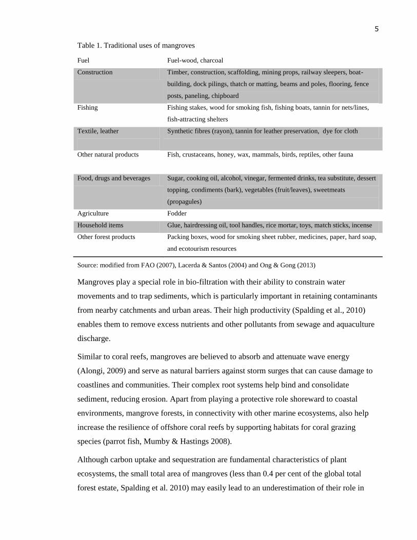
The uses of mangrove products are summarised in Table 1.
5
Table 1. Traditional uses of mangroves
Fuel Fuel-wood, charcoal
Construction Timber, construction, scaffolding, mining props, railway sleepers, boat-
building, dock pilings, thatch or matting, beams and poles, flooring, fence
posts, paneling, chipboard
Fishing
Fishing stakes, wood for smoking fish, fishing boats, tannin for nets/lines,
fish-attracting shelters
Textile, leather
Synthetic fibres (rayon), tannin for leather preservation, dye for cloth
Other natural products
Fish, crustaceans, honey, wax, mammals, birds, reptiles, other fauna
Food, drugs and beverages Sugar, cooking oil, alcohol, vinegar, fermented drinks, tea substitute, dessert
topping, condiments (bark), vegetables (fruit/leaves), sweetmeats
(propagules)
Agriculture Fodder
Household items Glue, hairdressing oil, tool handles, rice mortar, toys, match sticks, incense
Other forest products Packing boxes, wood for smoking sheet rubber, medicines, paper, hard soap,
and ecotourism resources
Source: modified from FAO (2007), Lacerda & Santos (2004) and Ong & Gong (2013)
Mangroves play a special role in bio-filtration with their ability to constrain water
movements and to trap sediments, which is particularly important in retaining contaminants
from nearby catchments and urban areas. Their high productivity (Spalding et al., 2010)
enables them to remove excess nutrients and other pollutants from sewage and aquaculture
discharge.
Similar to coral reefs, mangroves are believed to absorb and attenuate wave energy
(Alongi, 2009) and serve as natural barriers against storm surges that can cause damage to
coastlines and communities. Their complex root systems help bind and consolidate
sediment, reducing erosion. Apart from playing a protective role shoreward to coastal
environments, mangrove forests, in connectivity with other marine ecosystems, also help
increase the resilience of offshore coral reefs by supporting habitats for coral grazing
species (parrot fish, Mumby & Hastings 2008).
Although carbon uptake and sequestration are fundamental characteristics of plant
ecosystems, the small total area of mangroves (less than 0.4 per cent of the global total
forest estate, Spalding et al. 2010) may easily lead to an underestimation of their role in
6
mitigating carbon emission. In fact, their larger proportion of below-ground biomass
(compared to above-ground, Briggs,1977) makes their total biomass carbon per unit surface
area the higher (~21.8 kg C m-2
) than that of taller terrestrial forests (~14.5 kg C m-2
in
tropical rainforest and 12.4 kg C m-2
in tropical mountain systems) as reviewed by Pan et al.
(2013). Komiyama et al. (2008) also highlighted that mangrove forests are highly efficient
carbon sinks in the tropics. This motivates the investigation of the role mangroves may play
in global carbon budgets in the topical context of global warming.
1.4 Mangrove carbon studies
A carbon budget is the balance between carbon accumulation and release of a given
ecosystem. Forests are complex ecosystems, and good estimates for carbon uptake and
release are can be extremely difficult to achieve. The same is true for estimating carbon
pools, as particularly underground carbon pools are difficult to quantify.
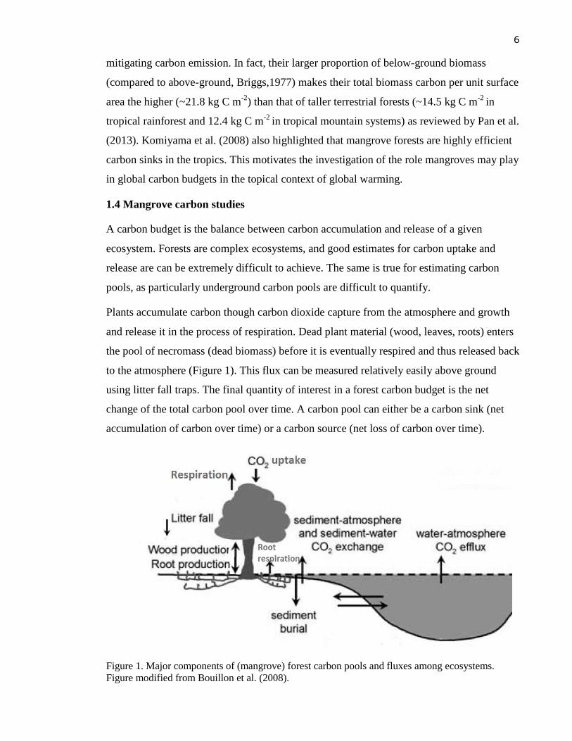
Plants accumulate carbon though carbon dioxide capture from the atmosphere and growth
and release it in the process of respiration. Dead plant material (wood, leaves, roots) enters
the pool of necromass (dead biomass) before it is eventually respired and thus released back
to the atmosphere (Figure 1). This flux can be measured relatively easily above ground
using litter fall traps. The final quantity of interest in a forest carbon budget is the net
change of the total carbon pool over time. A carbon pool can either be a carbon sink (net
accumulation of carbon over time) or a carbon source (net loss of carbon over time).
Figure 1. Major components of (mangrove) forest carbon pools and fluxes among ecosystems.
Figure modified from Bouillon et al. (2008).
7
Global studies/reviews of plant carbon stocks (Litton et al. 2007, Gorte 2009, Pan et al.
2013, Le Quere et al. 2013) have presented tropical forests as the biggest carbon pools,
followed by boreal forests, then temperate forests. Pan et al. (2013) have showed the
extremely high carbon density of mangrove forests compared to rest of the ecosystems.
Mangrove forests also appeared to be highly productive ecosystems with canopy net carbon
uptake estimated about 2.9 kg C m-2
y-1
(Clough, 1998) and gross primary productivity
(GPP) of 7.5 - 15 kg C m-2
y-1
(Eong, 1993). C fluxes from mangrove forests were, however,
also comparatively high with 80 % - 90 % of the GPP returned to the atmosphere as
respired carbon dioxide, leaving an estimated 0,7-1.8 kg C m-2
y-1
as net primary
productivity (NPP) (Eong, 1993). In another study, Bouillon et al.(2008) presented an
estimate of 218 ± 72 Tg C y-1
of global mangrove primary production, of which only about
45 % was reported as carbon burial, organic carbon export and CO2 emission from
sediments and the water column, leaving 112 ± 85 Tg C y-1
unaccounted for in current
budgets. In comparison to the total C flux of the world’s forests (900 Tg C y-1
) (Dixon,
1994), mangrove C fluxes are considerable especially considering that mangroves make up
less than 0.4 per cent of the global forest (Spalding, 2010). Donato et al. (2011) suggested
that high productivity and C flux rates in mangroves were indeed accompanied by high C
storage, especially below ground, implying mangroves are a globally important surface C
reserve.
The change in standing biomass as a result of imbalances between carbon in- and output is
a key variable for understanding forest carbon budgets. Direct measurement of changes in
biomass density helps indicate the magnitude and distribution of at least the largest carbon
sources (from land use change) and sinks (from woody growth). While litterfall, which
made up ~ 31 % of NPP (Bouillon et al 2008) is important for the study of mangrove
primary production, litter decomposition estimates how fast the accumulated biomass
dissolves back to other pools. This information is needed for our understanding of the
carbon cycle, including better information on the magnitude and mechanisms that make
forests sources or sinks of carbon.
1.5 New Zealand mangroves
New Zealand has only one mangrove species, Avicennia marina var. australasica and it
grows only in northern estuaries of the north island, ranging from Ohiwa Harbour (38003'S;
8
southern limit) to Northland (34027'S; Harty, 2009). This species is able to grow and
reproduce in variable conditions of tide, climate and edaphon. It occupies, therefore a
diverse range of coastal habitats and displays great variability of growth forms (Morrisey et
al., 2010). In contrast to tropical mangroves, there is evidence for the expansion of A.
marina var. australasica over the past decades in New Zealand (Morrisey et al, 2007). The
public view of mangroves also remains polarised, with some advocating for the
conservation of mangroves while others see mangroves as a nuisance and relate their
expansion to a loss of economic and aesthetic values of the harbours. Despite New
Zealand’s principal environmental legislation (the Resource Management Act 1991), which
allows governing bodies to uphold protection of mangroves against indiscriminate
destruction or reclamation, management initiatives have conflicted due to limited available
scientific information and diverging views of how mangrove expansion may affect the
various stakeholders’ interests.
A number of studies have been conducted on the benthic assemblages and species of
mangrove forests in New Zealand. Alfaro (2006) found mangrove forests have the lowest
faunal assemblages among six distinct habitats of mangrove stands, the pneumatophore
zones, seagrass, channels, banks and sand-flats. Ellis et al. (2004) studied the effects of
high sedimentation rates on mangrove communities and associated benthic community
composition and found sediment mudflats without mangroves had similar benthic
composition to mangrove sites, suggesting that increased silt/clay fraction from
sedimentation is more meaningful to the benthic composition than the presence or absence
of the mangroves themselves. These results contradict those in tropical mangroves
(Thailand), where impacts of mangrove forest development and maturity on benthic faunal
richness and diversity showed a tendency toward more diverse assemblages in undisturbed
and mature forests (Suzuki et al., 1997, 2002). Ongoing monitoring and research conducted
in New Zealand for both intact mangrove systems and those where mangroves have been
removed are contributing to answer the scientific and management question.
Although annual net primary production of temperate mangroves is known to be lower than
their tropical counterparts, knowledge of how they differ in other components of the carbon
budget is not well documented. A better understanding of mangrove carbon budgets and
their nutrient cycling will contribute to better management and conservation of mangrove
ecosystem in New Zealand.
9
In Mangawai Harbour Estuary, located 100 km northern of Auckland city, mangrove
removal is currently debated and partly approved by council permits (0.26-ha fringe of
mangrove trees for water access). This provides an opportunity to conduct studies on the
ecological importance of mangrove A. marina var. australasica in New Zealand.
1.6 Research questions:
- How much above- and belowground standing biomass is present A. marina var.
australasica stands in the Mangawhai Harbour estuary ?
- How much litterfall is produced by these stands and what are the rates of litter
decomposition ?
The specific aims include:
- To identify the basic allometric parameters (height, stem diameter distribution)
and leaf area index (LAI) of A. marina var. australasica in Mangawhai.
- To determine total biomass of mangrove forests in Mangwhai, layered
horizontally and as contribution from tree components.
- To determine litter production and decomposition rates, in relation to
sediment/substrate and hydrological conditions using litter traps and litter bags.
1.7 Outline of chapters:
Chapter 1 provides a general introduction about mangrove ecosystems and their position
in the global carbon budget.
Chapter 2 describes allometry and biomass of both above and below ground, layered
horizontally and partially (wood and leaf).
Chapter 3 describes the litter fall and litter decomposition process, relating to the function
of tidal immersion and substrate types, seasonal temperature and velocity.
Chapter 4 concludes the study results and implies conservation and management of
mangrove in New Zealand.

10
Chapter 2. Allometry and biomass allocation
______________________________________________________________
11
2.1 Introduction
The largest pool of terrestrial carbon is found in the woody biomass of forests (ca. 80 % of
terrestrial carbon; Saugier, Roy, & Mooney, 2001). In the context of global warming, the
study of tree biomass is helpful in the identification of important carbon pools for better
land use management. Biomass studies also provide the baseline for studies of the carbon
cycle (carbon fluxes). Biomass inventories therefore provide a comprehensive basis for
estimates on carbon pools and fluxes for climate change reports.
Biomass in plant science is defined as "the total weight of the living components
(producers, consumers, and decomposers) in an ecosystem at any given moment” (Albany,
2013) and usually expressed as dry weight per unit area. Biomass can be divided between
above-ground (all the living parts of the plants above the soil surface) and below-ground
biomass (the entire biomass of all live roots). Necromass, dead plants and the dead parts of
living plants, is not included in this definition.
The total biomass of the world was recently estimated at 363 Pg C, with a mean density of
9.4 kg C m-2
(Pan et al., 2013). Biomass is not evenly spread across biomes and values
range from less than 0.5 kg C m-2
in grasslands, croplands, and deserts to more than 30kg C
m-2
in some tropical forests (Houghton et al., 2009). The average biomass carbon density of
mangrove trees has been reported to be 21.8 ±17.3kg C m-2
(Pan et al., 2013), which puts
mangrove forests among the largest carbon pools per unit surface area on Earth.
With increasing latitudes, mangroves are ultimately limited by temperature and have a
trend of declining biomass (Morrisey et al., 2010). Mangrove biomass estimates have been
reported to range from 5.7–43.6 kgm-2
in the tropics between 23°N to 23°S, to 0.8–16.4
kgm-2
between 23 and 30° (Saenger & Snedaker, 1993). At smaller scales, waves, tides,
rivers and rainfall are major factors affecting the abundance and biomass of mangroves
because these factors affect water circulation, influencing the rate of erosion and deposition
of sediments on which mangroves grow (Alongi, 2002).
While aboveground terrestrial forest biomass accounts for 70–90 % of total forest biomass
(Cairns et al., 1997), mangroves maintain a bottom-heavy tree form, allocating the majority
of biomass to their roots (Ong et al., 2004). In fact, Pan et al. (2011) reported that tropical
evergreen forests have the highest root biomass densities of about 2.5 kg C m-2
, while
mangrove (Avicennia marina [Forsk.] Vierh) forests near Sydney (Australia) have been
12
estimated to have 14.73 (±0.19) - 16.03 (±0.41) kg m-2
of belowground biomass (Briggs,
1977), which is equivalent to an approximate of 7-8 kg C m-2
. This suggests that mangrove
forests may have much higher belowground biomass density than tropical terrestrial forests
and underlines the importance of mangrove forests as carbon stores.
However, there is limited research on belowground biomass as it is not always possible to
destructively harvest or measure belowground biomass or develop allometric equations,
especially in the estuarine environment. Very few allometric equations are available for
belowground biomass of forests, and mangroves in particular.
Small-flower mangrove species, Avicennia marina, has three varieties based on
morphology, electrophoretic patterns and carbohydrate composition; such as Avicennia
marina var. australasica, Avicennia marina var. marina, and Avicennia marina var.
eucalyptifolia (Duke, 1995). Avicennia marina var. australasica is the only mangrove
species of New Zealand. It also occurs in south-eastern Australia and in the tropics
(Duke,1990).
Saenger & Snedaker (1993) reviewed the trends in biomass of mangroves (incorporating 91
studies of litter-fall across species and locations, including New Zealand), which revealed
decreasing biomass with increasing latitude. This pattern suggests that mangroves in New
Zealand would be relatively small carbon pools compared to their tropical equivalents. To
my knowledge there has been only one study on New Zealand mangrove biomass
(Woodroffe 1985). Woodroffe (1985) reported above-ground biomass density of A. marina
of 7.6 t ha-1
(~0.7 kg m-2
) in Tuff Crater, Auckland. However, 94 % of the Tuff Crater basin
was covered sparsely by short trees (<1 m) and making it difficult to generalise other New
Zealand mangrove sites where trees reach up to five to six metres in height (Morrissey et
al., 2007).
Other studies of A. marina estimated aboveground biomass density to be 10.2 - 12.95 kg m-
2 (Briggs, 1977) and 11.0 - 34.1 kg m
-2 (Mackey, 1993). Belowground biomass was also
estimated at 15.4kgm-2
(Briggs,1977) and 10-12 kgm-2
(Mackey, 1993). Comley &
McGuinness (2005) also suggested an equation for root biomass estimation for A. marina
as Wr = 1.28DBH1.17
with root weight (Wr) and diameter at breast height (DBH). However,
these referred to either tropical A. marina or ones at lower latitudes with bigger mean tree
13
height (7-10 metres). This thesis contributes with a direct and detailed estimate of both
below and above ground biomass of a typical A. marina stand in northern New Zealand.
Common methods for estimating the biomass of forests include harvest method, satellite or
remote sensing, and modeling based on available equations (FAO 2009, Ravindranath &
Ostwald 2008). Harvest methods involve measuring directly the weight of the trees in the
sample plots, which gives the accurate estimate of biomass at the time of harvest. However,
this method is destructive, labour- intensive and may not be feasible due to local land use
regulations. Satellite or remote sensing methods involve the use of different techniques
such as aerial photography, optical parameters and radar to interpret the biomass stocks
based on relationship between the parameters of a forest stand and their spectral
representation. Although this method provides spatially explicit information and enables
repeated monitoring even in remote locations, it is usually not suitable as the only method.
Rather remote sensing methods are used to supplement other methods due to the high cost
and requirement of technical and institutional capacity. Modelling methods use the
available equations developed based on the relationship between biomass and allometric
parameters of specific species. This method is rapid and sometimes the only approach to
estimate the biomass stock of some forest stands. However, allometric equations are not
always available and even if they are, difference in the maturity and geographical locations
of the stands may lead to inaccuracy of the biomass estimation.
The total weight of an individual tree in tropical mangrove forests often reaches several
tons (Komiyama et al., 2005) making it almost impossible to use the harvest method. In
New Zealand, however, A. marina towards the southern limit of its occurrence rarely grow
to heights of greater than 6 m (Kuchler, 1972) making these trees more manageable for
harvest methods; the most accurate estimate of the biomass stocks. Therefore, a destructive
method was developed based partly on the technical paper by FAO (2002) for their UN-
REDD program, with modification to be more suitable for mangrove forests, to quantify
biomass stocks of mangrove stands in Mangawhai Harbour. This study aims to identify the
basic allometric parameters (height, stem diameter distribution), leaf area index (LAI), and
total biomass of A. marina var. australasica stands in Mangawhai, layered horizontally and
separated into different tree components.
14
2.2 Methods and Materials
Study areas
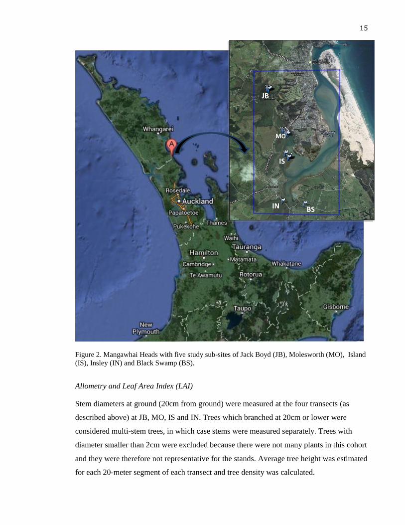
Mangawhai Harbour Estuary (36° 07' 00" S, 174° 36' 00" E) is located about100 km north-
east of Auckland, New Zealand (Figure 2). It is characterised as a typically deltaic estuary
with two main channels, Tara Creek that drains into the Tara volcanic area north of the
study area and Bob Creek that drains into the Waitemata sediments to the west. There is a
variety of wetlands including salt marshes, sand/mud flats, and about 87 ha of mangroves.
This site is the main field site for a larger estuarine ecosystem programme under the
Mangrove Research Group (Auckland University of Technology and the University of
Auckland).
Jack Boyd (JB) is situated at the upper tidal zone of Tara Creek, furthest from the shore
with more sandy substrate and shortest inundation. The Molesworth (MO) stand is located
in the middle of the waterway of Tara Creek, on the east side of Molesworth Drive, with
more muddy substrate and longer inundation. The Mangrove Island (IS) is located even
closer to shore but not too far away from MO, at the stream junction where Tara Creek and
Bob Creek meets. IS has a quite similar sediment although inundation was observed to be
shorter than MO.
For the allometry and biomass study, three sites JB, MO, IS were identified, plus Insley
(IN) located on Bob Creek stream on the side of Insley street. A transect (2 x 100 m) was
set up for each site, starting from the edge to the middle of each stand to be able to include
trees of different sizes; trees were usually taller at the edge and shorter towards the middle
of the stand. As felling trees were not legally possible at the public sites, sample trees were
harvested at a private site in Black Swamp (BS), located along Bob Creek and closer to IN.
Weight of sample tree at BS was combined with allometric measurements at JB, MO, IS
and IN for biomass estimation (see details of the method in the Above-ground biomass
section). Leaves were harvested from four sites JB, MO, IS, and IN for LAI calculation.
Figure 2 shows the locations of the sites on study area of Mangawhai Harbour.
15
Figure 2. Mangawhai Heads with five study sub-sites of Jack Boyd (JB), Molesworth (MO), Island
(IS), Insley (IN) and Black Swamp (BS).
Allometry and Leaf Area Index (LAI)
Stem diameters at ground (20cm from ground) were measured at the four transects (as
described above) at JB, MO, IS and IN. Trees which branched at 20cm or lower were
considered multi-stem trees, in which case stems were measured separately. Trees with
diameter smaller than 2cm were excluded because there were not many plants in this cohort
and they were therefore not representative for the stands. Average tree height was estimated
for each 20-meter segment of each transect and tree density was calculated.
JB
MO
IS
IN BS
16
Leaf area index (LAI) was measured directly by relating total leaf area of eleven
harvested trees at BS to stem diameter distributions at all three sites of JB, MO, and IS.
Fifty-five leaves from four sites of JB, MO, IS, and BS were randomly harvested,
including leaves of different ages from different tree layers. Leaf samples from each
collection were divided into groups of 1 to 10 leaves, weighed, scanned and total leaf area
was estimated using the software package ImageJ. Subsamples were then dried at 65°C to
constant weight and the relationship between leaf area and dry mass was used to calculate
specific leaf area (SLA). Mean leaf area was inferred by multiplying total dry mass of
leaves for all eleven harvested trees for which diameters were known. Finally, mean LAI
for each of the sites was estimated by relating tree diameters from the transects (200 m2
each) to leaf area and scaling to one square meter.
Regression analyses of the subsamples of 55 leaves for each of the four sites (JB, MO, IS
and BS) showed a significant linear relationship between leaf dry weight and leaf area,
with R-squared values >0.99 for all four sites. Leaf area is related to leaf dry weight by
the equation:
Y = Xβ
with leaf area Y, leaf dry weight X, and the coefficient β found to be 48.47±1.05,
53.81±0.39, 46.9±0.81 and 49.23±0.63 for JB, MO, IS, and BS, respectively.
To calculate the leaf area for each site, the basal area for each transect was estimated
using stem diameter information. The linear relationship between basal area and leaf dry
weight was also developed (R-squared = 0.93).
While leaf area sub samples are available for the site of BS, allometry data were not
collected for this site. LAI values were therefore estimated for the remaining three sites.
Above-ground biomass:
Biomass was estimated by the harvest method. For above-ground biomass, eleven trees
were felled at the BS site, layered in 50 cm height bands. Stem, branches and twigs were
then separated from leaves, weighed fresh at the site and sub-samples taken to the lab and
oven dried at 70°C to constant weight to get the ratio of fresh/dry weight. Total wood and
leaf biomass was then calculated for the eleven sample trees. One of the sample trees
differed from the other trees sampled having a crown that was lower and larger in
17
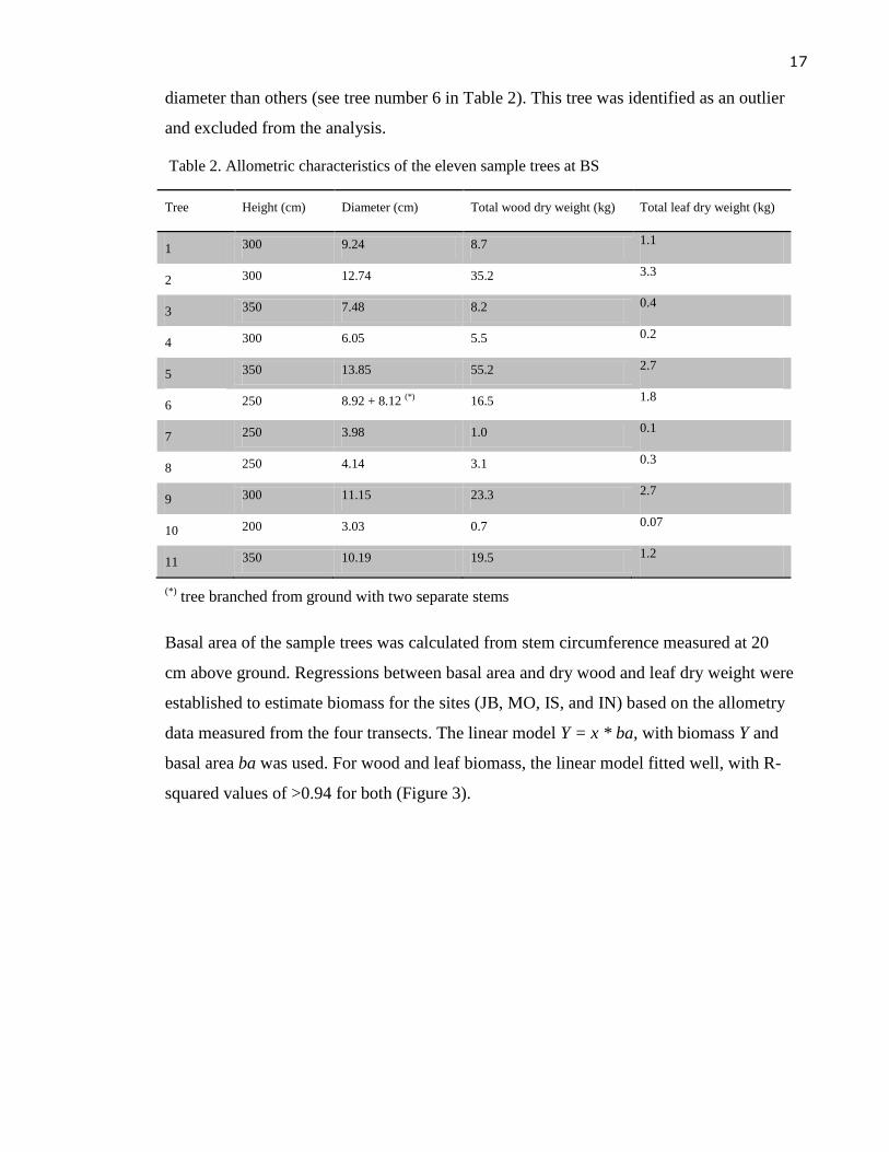
diameter than others (see tree number 6 in Table 2). This tree was identified as an outlier
and excluded from the analysis.
Table 2. Allometric characteristics of the eleven sample trees at BS
Tree Height (cm) Diameter (cm) Total wood dry weight (kg) Total leaf dry weight (kg)
1 300 9.24 8.7 1.1
2 300 12.74 35.2 3.3
3 350 7.48 8.2 0.4
4 300 6.05 5.5 0.2
5 350 13.85 55.2 2.7
6 250 8.92 + 8.12 (*) 16.5 1.8
7 250 3.98 1.0 0.1
8 250 4.14 3.1 0.3
9 300 11.15 23.3 2.7
10 200 3.03 0.7 0.07
11 350 10.19 19.5 1.2
(*) tree branched from ground with two separate stems
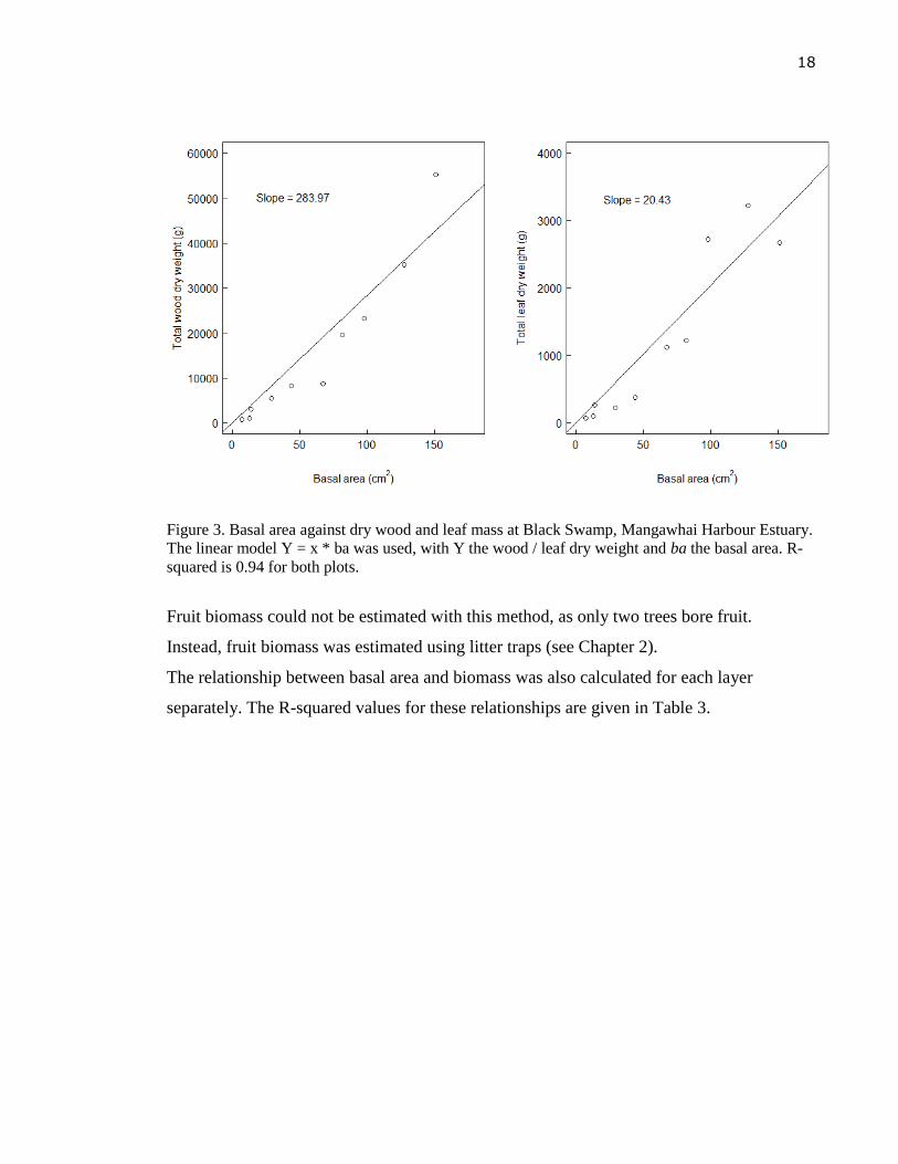
Basal area of the sample trees was calculated from stem circumference measured at 20
cm above ground. Regressions between basal area and dry wood and leaf dry weight were
established to estimate biomass for the sites (JB, MO, IS, and IN) based on the allometry
data measured from the four transects. The linear model Y = x * ba, with biomass Y and
basal area ba was used. For wood and leaf biomass, the linear model fitted well, with R-
squared values of >0.94 for both (Figure 3).
18
Figure 3. Basal area against dry wood and leaf mass at Black Swamp, Mangawhai Harbour Estuary.
The linear model Y = x * ba was used, with Y the wood / leaf dry weight and ba the basal area. R-
squared is 0.94 for both plots.
Fruit biomass could not be estimated with this method, as only two trees bore fruit.
Instead, fruit biomass was estimated using litter traps (see Chapter 2).
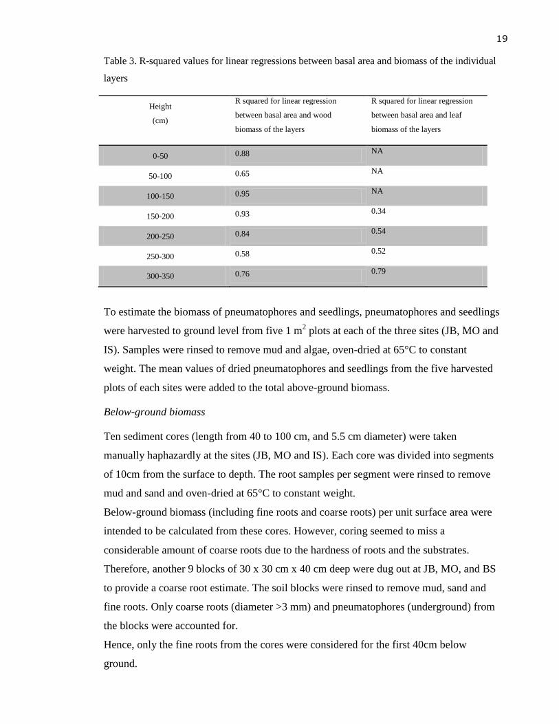
The relationship between basal area and biomass was also calculated for each layer
separately. The R-squared values for these relationships are given in Table 3.
19
Table 3. R-squared values for linear regressions between basal area and biomass of the individual
layers
Height
(cm)
R squared for linear regression
between basal area and wood
biomass of the layers
R squared for linear regression
between basal area and leaf
biomass of the layers
0-50 0.88 NA
50-100 0.65 NA
100-150 0.95 NA
150-200 0.93 0.34
200-250 0.84 0.54
250-300 0.58 0.52
300-350 0.76 0.79
To estimate the biomass of pneumatophores and seedlings, pneumatophores and seedlings
were harvested to ground level from five 1 m2 plots at each of the three sites (JB, MO and
IS). Samples were rinsed to remove mud and algae, oven-dried at 65°C to constant
weight. The mean values of dried pneumatophores and seedlings from the five harvested
plots of each sites were added to the total above-ground biomass.
Below-ground biomass
Ten sediment cores (length from 40 to 100 cm, and 5.5 cm diameter) were taken
manually haphazardly at the sites (JB, MO and IS). Each core was divided into segments
of 10cm from the surface to depth. The root samples per segment were rinsed to remove
mud and sand and oven-dried at 65°C to constant weight.
Below-ground biomass (including fine roots and coarse roots) per unit surface area were
intended to be calculated from these cores. However, coring seemed to miss a
considerable amount of coarse roots due to the hardness of roots and the substrates.
Therefore, another 9 blocks of 30 x 30 cm x 40 cm deep were dug out at JB, MO, and BS
to provide a coarse root estimate. The soil blocks were rinsed to remove mud, sand and
fine roots. Only coarse roots (diameter >3 mm) and pneumatophores (underground) from
the blocks were accounted for.
Hence, only the fine roots from the cores were considered for the first 40cm below
ground.
20
As the soil block samples were not available for the Island, coarse root biomass was
estimated by the mean of the three sites JB, MO and BS for the first layer belowground
(0-40 cm) while the deeper layers (coarse roots) were estimated from the core samples
taken three sites of JB, MO and IS. Therefore, only at JB and MO coarse root profile was
complete for all layers when considering the total biomass allocation by site.
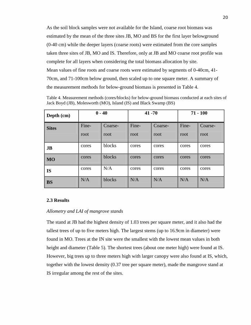
Mean values of fine roots and coarse roots were estimated by segments of 0-40cm, 41-
70cm, and 71-100cm below ground, then scaled up to one square meter. A summary of
the measurement methods for below-ground biomass is presented in Table 4.
Table 4. Measurement methods (cores/blocks) for below-ground biomass conducted at each sites of
Jack Boyd (JB), Molesworth (MO), Island (IS) and Black Swamp (BS)
Depth (cm) 0 - 40 41 -70 71 - 100
Sites Fine-
root
Coarse-
root
Fine-
root
Coarse-
root
Fine-
root
Coarse-
root
JB cores blocks cores cores cores cores
MO cores blocks cores cores cores cores
IS cores N/A cores cores cores cores
BS N/A blocks N/A N/A N/A N/A
2.3 Results
Allometry and LAI of mangrove stands
The stand at JB had the highest density of 1.03 trees per square meter, and it also had the
tallest trees of up to five meters high. The largest stems (up to 16.9cm in diameter) were
found in MO. Trees at the IN site were the smallest with the lowest mean values in both
height and diameter (Table 5). The shortest trees (about one meter high) were found at IS.
However, big trees up to three meters high with larger canopy were also found at IS, which,
together with the lowest density (0.37 tree per square meter), made the mangrove stand at
IS irregular among the rest of the sites.
21
Table 5. Allometry of Avicennia marina in the study transects at Insley (IN), Island (IS), Jack Boyd
(JB) and Molesworth (MO)
Transect Coordinate No. trees
per 200m2
No. stems
per 200m2
Mean tree
height (± s.e)
Mean stem
diameter (+/- s.e)
IN NA NA 145 152 1.89±0.04 5.15±0.22
IS -36.11675S
174.58212E
-36.11763S
174.58177E 73 121 2.30±0.07 5.28±0.23
JB -36.09665S
174.57354E
-36.10974S
174.57965E 206 300 3.10±0.06 5.86±0.13
MO -36.09710S
174.57283
-36.11058S
174.57918E 108 146 1.94±0.03 6.48±0.23
Leaf area indices ranged widely from 1.6 (at IS) to 4.6 (at JB), which are consistent with
tree densities at each site. However, Specific Leaf Area (SLA) was similar among the sites
(see Table 6) and not related to tree density.
Table 6. Leaf area index (LAI) and Specific Leaf Area (SLA) for the sites Black Swamp (BS),
Island (IS), Jack Boyd (JB) and Molesworth (MO)
Sites Leaf Area Index (LAI) (m2m
-2) Specific Leaf Area (SLA) (m
2kg
-1)
BS NA 49.23 ± 0.63
IS 1.6 46.9 ± 0.81
JB 4.6 48.47 ± 1.05
MO 3.2 53.81 ± 0.39
Biomass partitioning
Biomass varied among sites and was consistent with tree density. At JB, where tree density
was at least twice as high than at the other sites, there was a significantly greater biomass in
all tree components. However, the relative biomass distribution among wood, leaf, root and
pneumatophores were similar among sites, with the highest biomass found in fine roots,
followed by coarse roots (in case of MO) or wood (in case of JB) (see Table 7).
More aboveground pneumatophores and seedlings were found at JB where the sediment
was more stable, and fewer pneupmatophores at sites with muddier sediment (IS and MO).
22
Table 7. Biomass allocation in wood, leaf, roots and pneumatophores and seedlings for the sites
Insley (IN), Island (IS), Jack Boyd (JB) and Molesworth (MO)
Site Wood biomass
(kg/m2)
Leaf biomass
(kg/m2)
Pneumatophores and
seedlings (kg/m2)
Coarse root
(kg/m2)
Fine roots
(kg/m2)
IN 5.3 0.4 NA NA NA
IS 2.3 0.2 0.19 NA 3.73
JB 8.0 0.6 0.28 5.46 9.24
MO 5.0 0.4 0.07 5.63 5.99
Due to the unavailability of full coarse root values at IS, it was impossible to involve this
site when considering biomass distribution as a whole for each site. The proportion
distribution of biomass per square meter was therefore estimated from the mean values
from the two sites of JB and MO.
Biomass was highest in fine roots, with an average of 37 %, followed by wood biomass (32
%), then coarse roots (27 %). Leaf biomass made up a small component of total biomass
of 3 % and, pneumatophores and seedlings contributed least with only 1 % of the total
biomass (Figure 4).
The root-shoot ratio was calculated by the mean aboveground biomass of JB and MO
divided by the mean belowground of these two sites.
Root = 1.73
Shoot
23
Figure 4. Biomass allocation (%) estimated from the mean values of JB and MO sites in
Mangawhai Harbour, standard errors for coarse-roots, fine-roots, wood, leaf, and pneumatophores
and seedlings were 4.9, 2.1, 2.3, 0.1, and 0.4, respectively.
Vertical distribution of biomass
Below-ground biomass accounted for the largest part of total A. marina biomass, with the
bulk of the roots (> 8 kgm-2
) in the first 40 cm. More than 70 percent of the total below-
ground biomass was located in this layer and almost 50 percent of the total was from fine
roots alone. Root biomass was reduced significantly with increasing depth, with the deepest
measurable roots at 100 cm (Figure 5).
Wood biomass increased slightly with height and reached a peak of >1 kgm-2
at 200 cm
from the ground, and then significantly diminished at higher layers where small branches
and twigs replaced big stems. Leaf biomass was found from 200cm above the ground
upwards, but its contribution was small and the distribution was unpredictable with height.
Pneumatophores and seedlings also contributed for a small part to the total above-ground
biomass (see Figure 5).
Wood biomass 32%
Leaf biomass 3%
Pneumatophores and seedlings
1%
Coarse root 27%
Fine roots 37%
24
Figure 5. Vertical distribution of biomass estimated for compartments per players on Mangawhai
Habour, with mean values and standard errors estimated among the sub-sites of JB, MO, IS and IN
for wood and leaf biomass, JB,MO, and IS for pneumatophores and seedling, fine roots biomass
and coarse roots under 40cm deep, and JB, MO and BS for coarse roots from 0-40cm deep.
2.4 Discussion
Above-ground biomass
The biomass results found in Mangawhai were comparable to those of previous studies at
the same mangrove species (see Table 7). At the present study site there was a lower
aboveground biomass than other sites, which could be due to the generally smaller trees.
Above-ground biomass of A. marina were found to be up to 16.2 kgm-2
in Brisbane,
Australia (MacKey, 1993) and 14.45 kgm-2
in Sydney, Australia (Briggs, 1977) while the
biggest above-ground biomass in Mangawhai found at JB was 8.88 kgm-2
. The
comparison presented in Table 8 shows a relationship between above-ground biomass
with tree size (height and/or diameter) among the sites in this study and other published
studies on biomass of A. marina. One exception is the taller stand in Tuff Crater where
trees were shorter and less dense than those at JB yet biomass density was higher. The
lack of stem diameter information in the study by Woodroffe (1985) at Tuff Crater made
25
a closer look at this inconsistency difficult although it is important, especially when
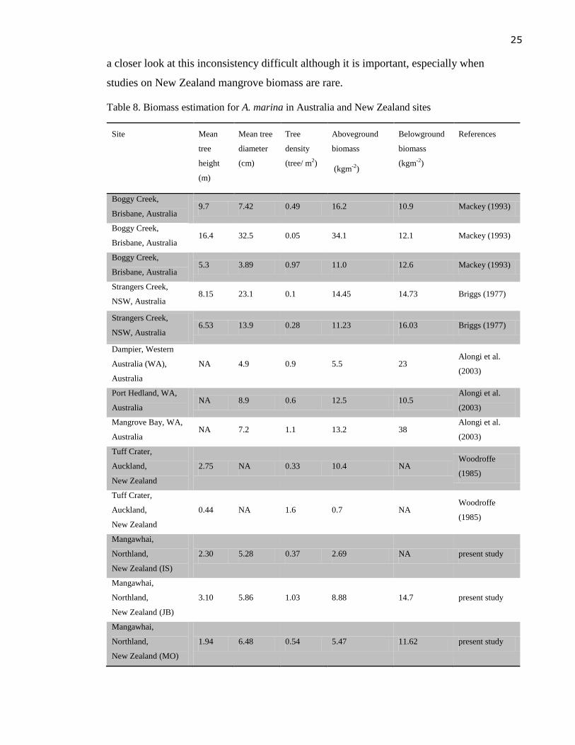
studies on New Zealand mangrove biomass are rare.
Table 8. Biomass estimation for A. marina in Australia and New Zealand sites
Site Mean
tree
height
(m)
Mean tree
diameter
(cm)
Tree
density
(tree/ m2)
Aboveground
biomass
(kgm-2)
Belowground
biomass
(kgm-2)
References
Boggy Creek,
Brisbane, Australia 9.7 7.42 0.49 16.2 10.9 Mackey (1993)
Boggy Creek,
Brisbane, Australia 16.4 32.5 0.05 34.1 12.1 Mackey (1993)
Boggy Creek,
Brisbane, Australia 5.3 3.89 0.97 11.0 12.6 Mackey (1993)
Strangers Creek,
NSW, Australia 8.15 23.1 0.1 14.45 14.73 Briggs (1977)
Strangers Creek,
NSW, Australia 6.53 13.9 0.28 11.23 16.03 Briggs (1977)
Dampier, Western
Australia (WA),
Australia
NA 4.9 0.9 5.5 23 Alongi et al.
(2003)
Port Hedland, WA,
Australia NA 8.9 0.6 12.5 10.5
Alongi et al.
(2003)
Mangrove Bay, WA,
Australia NA 7.2 1.1 13.2 38
Alongi et al.
(2003)
Tuff Crater,
Auckland,
New Zealand
2.75 NA 0.33 10.4 NA Woodroffe
(1985)
Tuff Crater,
Auckland,
New Zealand
0.44 NA 1.6 0.7 NA Woodroffe
(1985)
Mangawhai,
Northland,
New Zealand (IS)
2.30 5.28 0.37 2.69 NA present study
Mangawhai,
Northland,
New Zealand (JB)
3.10 5.86 1.03 8.88 14.7 present study
Mangawhai,
Northland,
New Zealand (MO)
1.94 6.48 0.54 5.47 11.62 present study
26
Biomass of pneumatophores and seedlings was very low at MO compared to other two
sites, although tree density was higher than that of IS. The muddy sediment and the tidal
current at MO may prevent the exposure of pneumatophores causing the low above-ground
pneumatophore and seedling biomass found at this site. Indeed, pneumatophores exposed
up to 20 - 30cm above ground at JB and IS, while at MO most of them were found shorter
than 5cm.
Belowground biomass
Below-ground biomass at Mangawhai, was similar to that of sites with bigger trees (Table
8), with exceptions from the sites studied by Alongi et al. (2003) where biomass
contributed from live and dead roots reached 38 kgm-2
. Small sampling size (three cores
per site) by Alongi et al. (2003) might have caused bias in estimating below-ground
biomass. Below-ground biomass at other sites in Australia ranged from 10.9 to 16.03
kgm-2
, while biomass at Mangawhai was 11.62 kgm-2
(at MO) and 14.7 kgm-2
(at JB).
This, together with the lower above-ground biomass, resulted in the root-shoot ratio in
Mangawhai to be among the highest recorded to date (1.73 compared to 1.20 at Strangers
Creek and in 0.58 at Boggy Creek; the ratio of 4.2 at Napier and 2.9 at Mangrove Bay,
Australia (Alongi et al, 2003) can be considered odd values). High accuracy is expected
in this measurement since belowground biomass was assessed by direct harvesting of root
samples at all sites with ten cores and three blocks per site. Further consideration of the
age and density of the stand in relation with root biomass is needed.
Although A. marina has a flat root system and no single tap root was expected for the trees,
the short "core" that supports cable roots was found to account for a considerable share of
total root weight. Only two of these "cores" (from trees with basal areas of 67 cm2 and
113.67 cm2) were collected from the sample trees, with dry weights of 0.85 kg and 0.89 kg
respectively. These samples were not adequate for extrapolating the biomass of these tap
roots. The absence of these plant parts (which were roughly estimated to be 0.07 - 0.27
kgm-2
, based on average dry weight of the taps per average basal area) from the total
biomass estimation may have led to a slight under-estimation of total belowground biomass
of A. marina in Mangawhai. Furthermore, taking root samples by manual coring limited the
measuring depth to one meter belowground, while the deepest fine roots were found at 1.6
meter belowground (Figure 4) from viber-core sampling by another study at the same study
site (Hulbert, 2014).
27
Allometric equation:
The linear model Y = x * ba, with ba is the basal area, gave satisfactory results for the
biomass of A. marina in Mangawhai, although this equation was not applied in any of the
previous studies. A. marina biomass was estimated using the relationship between stem
girth and tree volume (via wood density) (Briggs 1977, Mackay 1993), dry weight and
tree height (Woodroffe, 1985), and, closer to parameters used in our study, dry weight
and breast-height diameter (Comley & McGuinness, 2005) where dry weight is related to
diameter by a quadratic model (aboveground biomass = 0.0942*DBH2.54
). This quadratic
equation was also found in another study by Ong et al. (2004).
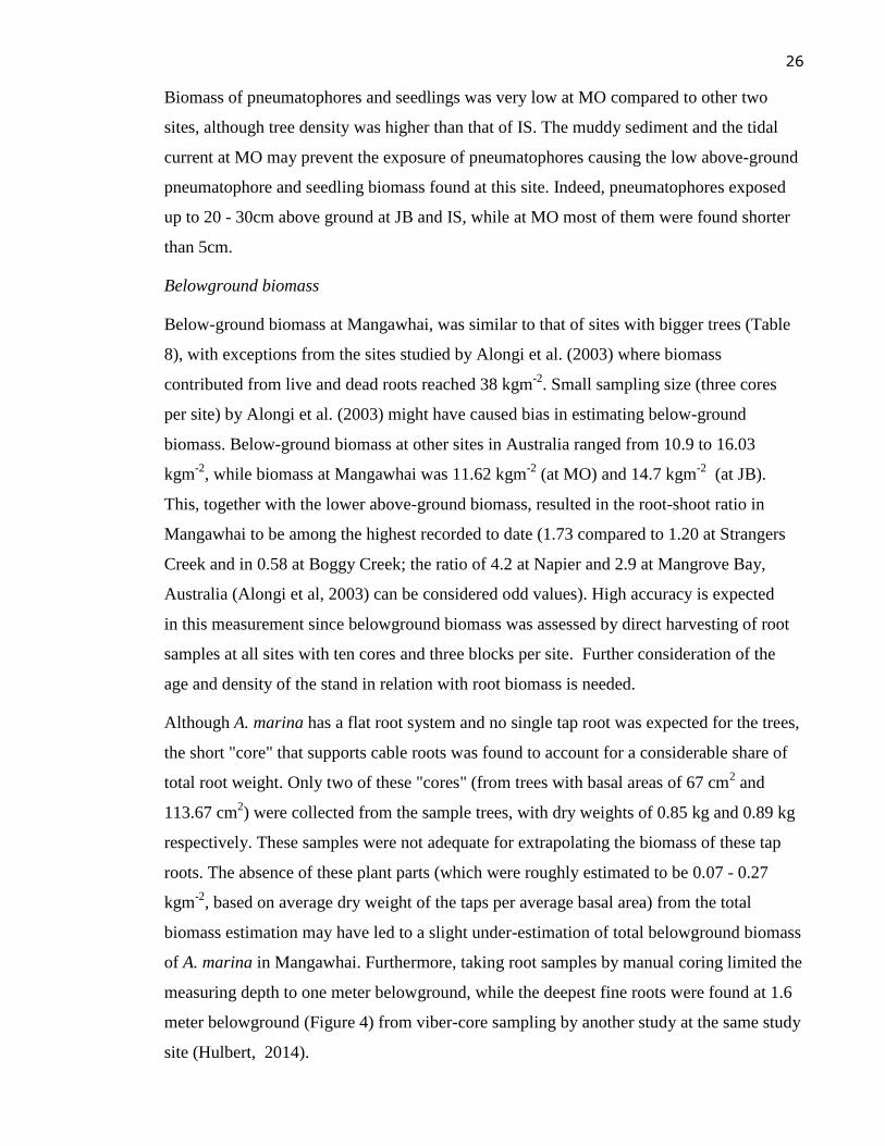
Fitting quadratic model (Y = x * ba2) was tried first in this study to relate basal area to dry
wood. This curve best described the variance with an R-squared value of 0.98 (see model
fit in Figure 6). However, this model underestimated biomass of small diameter trees.
Because almost 80 % of the trees at our site had a basal area of <50 cm2, this model gave
values that were too low compared to previous studies on similar stands.
Figure 6. Quadratic model Y = x * ba2 used for the regression of dry wood on basal area, with Y the
dry wood mass, ba the basal area. Data from the Black Swamp site at Mangawhai Harbour Estuary.
28
Limitations
The limitations in the samples of harvested trees for biomass quantification from a small
stand in a private farm (11 trees between 2 and 4 m high) may have introduced some bias,
because half of the trees found in the transects at IN, IS and MO were shorter than two
meters, and some trees at the JB site were taller than 4 meters. However, the mean basal
area was not significantly different between sites so this should help reduce the bias in
estimation of total biomass based on the basal area.
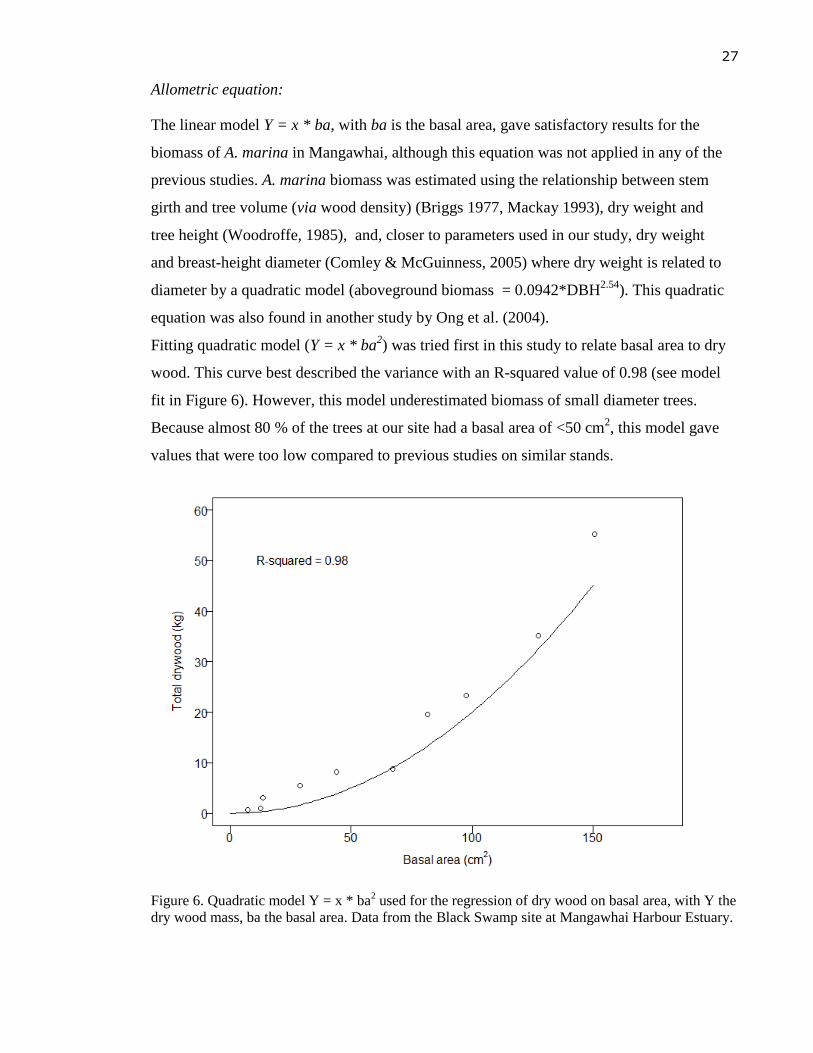
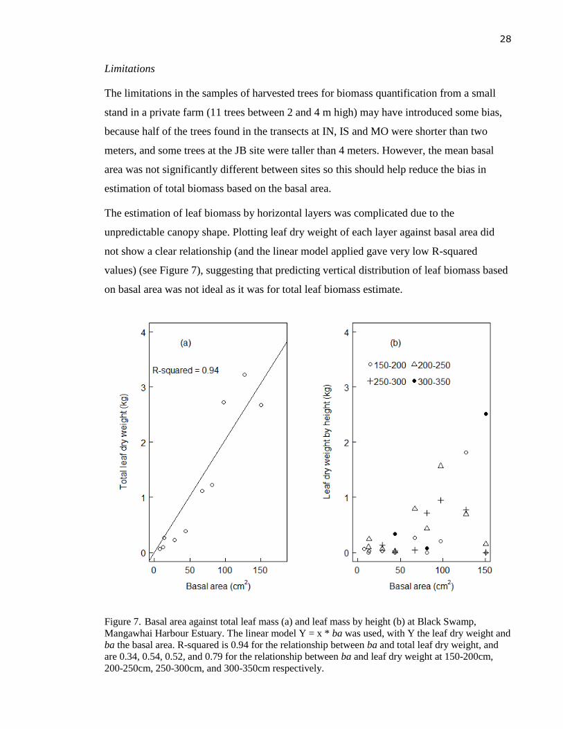
The estimation of leaf biomass by horizontal layers was complicated due to the
unpredictable canopy shape. Plotting leaf dry weight of each layer against basal area did
not show a clear relationship (and the linear model applied gave very low R-squared
values) (see Figure 7), suggesting that predicting vertical distribution of leaf biomass based
on basal area was not ideal as it was for total leaf biomass estimate.
Figure 7. Basal area against total leaf mass (a) and leaf mass by height (b) at Black Swamp,
Mangawhai Harbour Estuary. The linear model Y = x * ba was used, with Y the leaf dry weight and
ba the basal area. R-squared is 0.94 for the relationship between ba and total leaf dry weight, and
are 0.34, 0.54, 0.52, and 0.79 for the relationship between ba and leaf dry weight at 150-200cm,
200-250cm, 250-300cm, and 300-350cm respectively.
29
The stand canopy at IS was dissimilar from the rest of the sites with significantly bigger
crowns and highly variable tree height. Therefore, the estimation of biomass of trees at IS
based on the sample trees from BS may not give a satisfactory result, despite the fact that
the basal areas at the two sites were similar.
30
Chapter 3: Litter production and decomposition
______________________________________________________________
31
3.1 Introduction
Comprehensive characterisations carbon cycles require measurement of two key
components, namely the carbon pool and fluxes between the pools. A carbon pool is the
total amount of carbon stored in an ecosystem, where as carbon fluxes are the transfer of
carbon from one pool to another, usually expressed as a rate per time unit. In forest
ecosystems, carbon is transferred from the atmosphere to living plants through
photosynthesis and from plants to the soil/water mainly through litter production. Litter
production is the process in which dead plant materials are lost to the ground, where they
enter the process of decomposition.
Litterfall
Litterfall is a key parameter in the carbon cycle linking plant carbon to carbon in the soil
and, in the estuarine environment as in the case of mangroves, the ocean. Litter biomass
and its chemical contents are important in quantifying the annual return of elements and
organic matter to the soil (Chapin et al., 2002).
Litter production represents an important component of net primary production and is
usually measured as productivity. However, it is important to recognize that litterfal alone
does not completely represent net primary production (Bellot et al. 1992, Morrisey et al.
2010). Litterfall measurements are often an important component of general ecological
monitoring programs (Harrison et al., 2012) since changes in litterfall can be in response to
disturbance caused by biotic (e.g. insect pests) and/or environmental factors like frost,
drought, wind, or pollution. Monitoring litterfall provides temporal information about the
phenological development of a tree stand. Litterfall is commonly measured by litter traps,
which is time-consuming and laborious. The longest record of litterfall worldwide to date is
on-going in the Orangutan Tropical Peatland Project which started in 2005 (Harrison,
2012).
A comprehensive review of more than four hundred measurements of litterfall globally by
Zhang et al. (2014) showed that seasonal patterns of litterfall are diverse and are
determined by both physiological mechanisms and environmental variables (mostly
temperature, solar radiation and wind). Litterfall peaks differed in their temporal
occurrence among forest types: spring or winter for tropical forests, autumn for temperate
deciduous broadleaved and boreal evergreen needle-leaved forests, and various seasons for
32
temperate broadleaved and needle-leaved evergreen forests. The total annual litterfall
varied significantly by forest types, ranging from 0.3 - 1.1 kg dry mass m-2
y-1
(Zhang et al.,
2014).
Litterfall in mangrove forests
Mangrove forests, whose role in the carbon budget of the coastal zone has long been
debated, are highly productive with a global average primary production estimated to be
1.36 kg C m-2
y-1
(Bouillon et al., 2008). A review by Alongi (2002) stated that most inter-
annual variability in above-ground production and litterfall can be attributed to soil salinity,
minimum air temperature, and minimum rainfall.
Mangrove litterfall accounts for 31 % of overall mangrove production (Bouillon, 2008) and
decreases with increasing latitude (Saenger & Snedaker 1993, Bouillon et al. 2008). High
litterfall was found at latitudes between 0 and 10° with an average of 1.04 ± 0.46 kg m-2
y-1
,
which decreases with increasing latitudes and rather low production found at latitudes >30°
with 0.47 ± 0.21 kg m-2
y-1
(Bouillon et al.,2008).
The pattern of decreasing litterfall with increasing latitude suggests that mangroves in New
Zealand have relatively low litterfall rates compared to their tropical counterparts.
Published papers about New Zealand mangrove litterfall included studies at Tuff Crater by
Woodroffe (1982), Rangaunu Harbour by May (1999), and recently in Whangamata
Harbour by Gladstone-Gallagher et al. (2013). Litterfall production of A. marina in New
Zealand was found to be higher in stands closer to shore (0.39 - 0.81 kg m-2
y-1
) than further
inland (0.18 - 0.36 kg m-2
y-1
, May1999, Woodroffe 1982). Gladstone-Gallagher et al.
(2013) found that litterfall production 40 m within the mature stand (0.54±0.07 kg m-2
y-1
)
was significantly higher than under younger trees at the edge of the stand (0.32±0.04 kg m-2
y-1
). Leaf material contributed between 56 % and 86 % of the mangrove litter all year round
(Woodroffe 1982, May 1999, Gladstone-Gallagher et al. 2013). However, litterfall was
minimal during the colder months from March to October and as much as 77 % of the total
annual litterfall appeared during the warmer months of November to February (Gladstone-
Gallagher et al., 2013).
These data from New Zealand mangroves reveal that rates of litter production may vary
considerably among locations and were not related to latitude. Highest litterfall rates (0.7 -
0.8 kg m-2
y-1
) were recorded at the Tuff Crater site near Auckland (36°48′S) followed by
33
Whangamata Harbour (37°10′S) with 0.3 - 0.5 kg m-2
y-1
, while the lowest rate found at the
most northerly site (Rangaunu Harbour, 34°57′S) with 0.2 - 0.6 kg m-2
y-1
.
According to Morrisey (2010), recorded litterfall rates for A. marina in New Zealand are
below the maximum values reported from other parts of its distribution (found in tropical A.
marina stands). However, they are comparable with values from subtropical and temperate
Australia where the average litterfall rate was reported to be 0.62 kg m-2
y-1
(Morrisey,
2010).
Litter decomposition
Litter decomposition is a critical process in global carbon cycling. It is the main pathway
for nutrient and carbon fluxes and determines the organic matter input to forest soils, which
strongly influences the forest productivity (Chapin et al., 2002). Litter decomposition rates
are commonly known to be controlled by three main factors: temperature, moisture, litter
quality (i.e. rates of litter decomposition increase with both increasing temperature and
precipitation) (Karberg, Scott, & Giardina 2008, Jacob et al. 2010). The possible fourth
important factor influencing litter decomposition is faunal community structure within the
forests since a suite of decomposer organisms directly or indirectly consumes a variable
proportion of forest litter (Alongi 2002, Dechaine et al. 2005). Illustrative of the global
variability in litter mass rates, Tuomi et al. (2009) showed that typical conifer litter had ~
68 % of its initial mass still remaining after 2 years decomposing in the cold tundra with
little available liquid water, while deciduous litter had only 15 % remaining after two years
in the tropics which are warm and wet.
Mangrove litter decomposition
Transport and cycling of organic and inorganic matter in mangrove forests is driven by
physical (daily tides, runoff, and rainfall) and biological factors (litterfall, decomposition,
mineral uptake, faunal activities, Lugo & Snedaker, 1974). Among mangrove forests,
leaves of Avicennia spp. and Kandelia spp. are more rapidly decomposed than other
mangrove species because of their relatively high nitrogen content, low carbon-to-nitrogen
(C/N) ratio, low content of structural lignocellulose and tannin (Robertson 1988, Alongi
2009). Given the predominance of these genera (Avicennia and Kandelia) in temperate
mangrove forests, Morrisey et al. (2010) suggested that decomposition processes may be
faster in temperate compared with tropical mangroves On the other hand, Alfaro (2006)
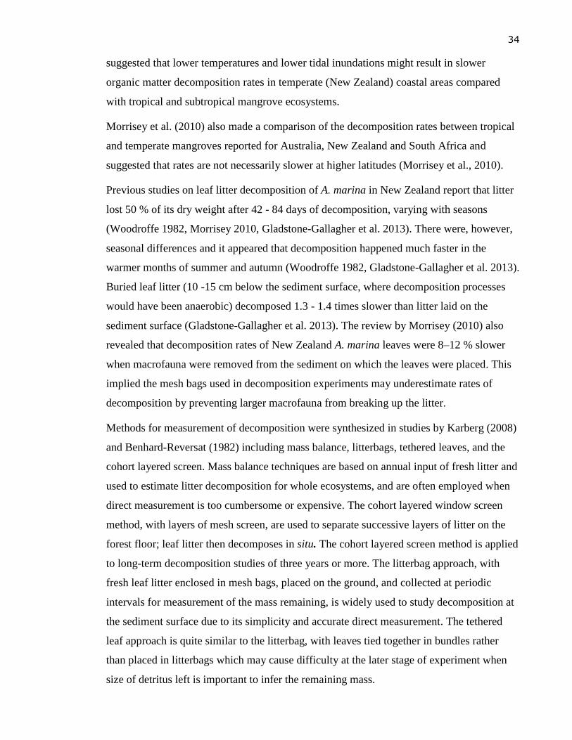
34
suggested that lower temperatures and lower tidal inundations might result in slower
organic matter decomposition rates in temperate (New Zealand) coastal areas compared
with tropical and subtropical mangrove ecosystems.
Morrisey et al. (2010) also made a comparison of the decomposition rates between tropical
and temperate mangroves reported for Australia, New Zealand and South Africa and
suggested that rates are not necessarily slower at higher latitudes (Morrisey et al., 2010).
Previous studies on leaf litter decomposition of A. marina in New Zealand report that litter
lost 50 % of its dry weight after 42 - 84 days of decomposition, varying with seasons
(Woodroffe 1982, Morrisey 2010, Gladstone-Gallagher et al. 2013). There were, however,
seasonal differences and it appeared that decomposition happened much faster in the
warmer months of summer and autumn (Woodroffe 1982, Gladstone-Gallagher et al. 2013).
Buried leaf litter (10 -15 cm below the sediment surface, where decomposition processes
would have been anaerobic) decomposed 1.3 - 1.4 times slower than litter laid on the
sediment surface (Gladstone-Gallagher et al. 2013). The review by Morrisey (2010) also
revealed that decomposition rates of New Zealand A. marina leaves were 8–12 % slower
when macrofauna were removed from the sediment on which the leaves were placed. This
implied the mesh bags used in decomposition experiments may underestimate rates of
decomposition by preventing larger macrofauna from breaking up the litter.
Methods for measurement of decomposition were synthesized in studies by Karberg (2008)
and Benhard-Reversat (1982) including mass balance, litterbags, tethered leaves, and the
cohort layered screen. Mass balance techniques are based on annual input of fresh litter and
used to estimate litter decomposition for whole ecosystems, and are often employed when
direct measurement is too cumbersome or expensive. The cohort layered window screen
method, with layers of mesh screen, are used to separate successive layers of litter on the
forest floor; leaf litter then decomposes in situ. The cohort layered screen method is applied
to long-term decomposition studies of three years or more. The litterbag approach, with
fresh leaf litter enclosed in mesh bags, placed on the ground, and collected at periodic
intervals for measurement of the mass remaining, is widely used to study decomposition at
the sediment surface due to its simplicity and accurate direct measurement. The tethered
leaf approach is quite similar to the litterbag, with leaves tied together in bundles rather
than placed in litterbags which may cause difficulty at the later stage of experiment when
size of detritus left is important to infer the remaining mass.
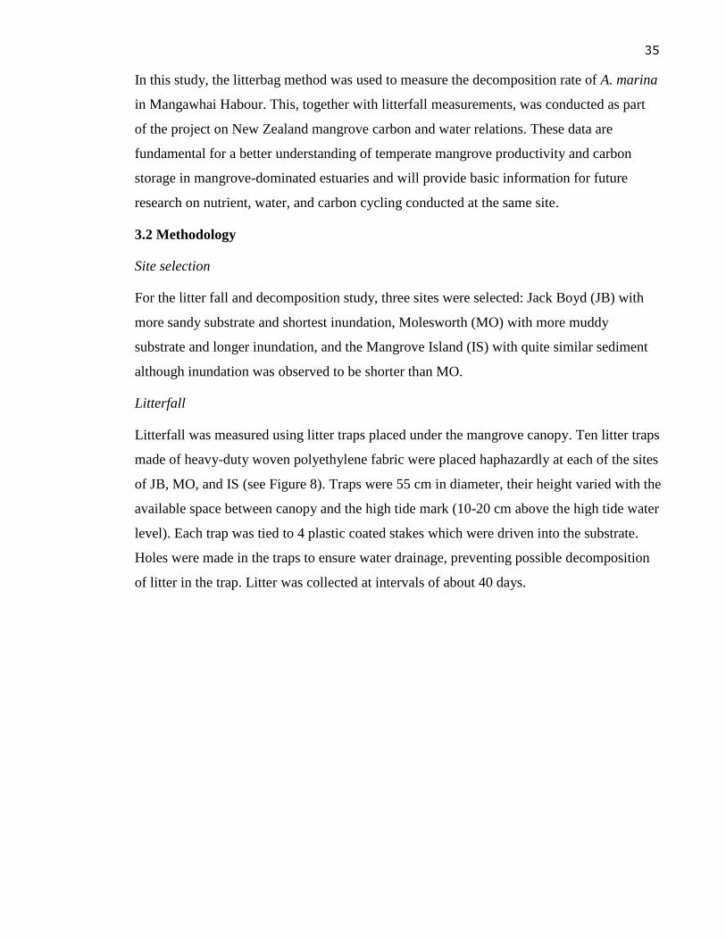
35
In this study, the litterbag method was used to measure the decomposition rate of A. marina
in Mangawhai Habour. This, together with litterfall measurements, was conducted as part
of the project on New Zealand mangrove carbon and water relations. These data are
fundamental for a better understanding of temperate mangrove productivity and carbon
storage in mangrove-dominated estuaries and will provide basic information for future
research on nutrient, water, and carbon cycling conducted at the same site.
3.2 Methodology
Site selection
For the litter fall and decomposition study, three sites were selected: Jack Boyd (JB) with
more sandy substrate and shortest inundation, Molesworth (MO) with more muddy
substrate and longer inundation, and the Mangrove Island (IS) with quite similar sediment
although inundation was observed to be shorter than MO.
Litterfall
Litterfall was measured using litter traps placed under the mangrove canopy. Ten litter traps
made of heavy-duty woven polyethylene fabric were placed haphazardly at each of the sites
of JB, MO, and IS (see Figure 8). Traps were 55 cm in diameter, their height varied with the
available space between canopy and the high tide mark (10-20 cm above the high tide water
level). Each trap was tied to 4 plastic coated stakes which were driven into the substrate.
Holes were made in the traps to ensure water drainage, preventing possible decomposition
of litter in the trap. Litter was collected at intervals of about 40 days.
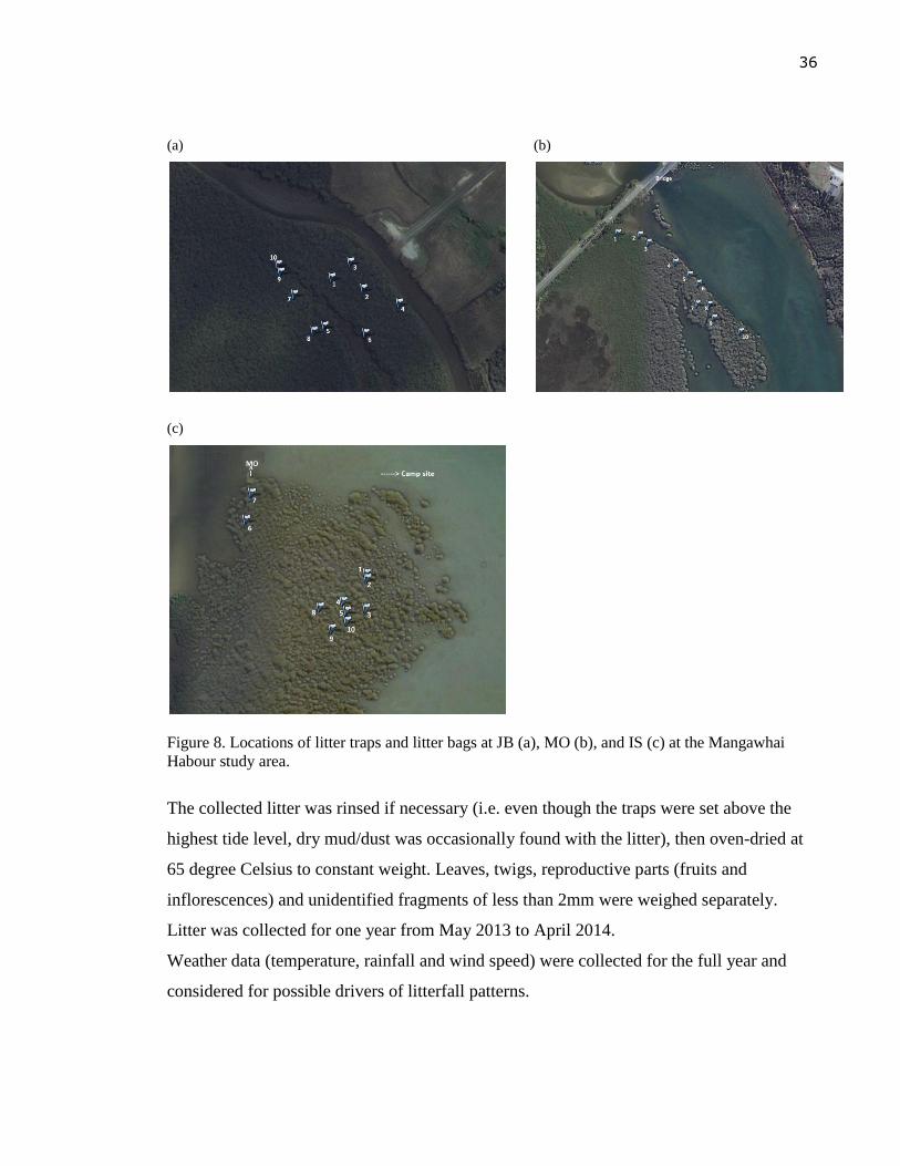
36
(a)
(b)
(c)
Figure 8. Locations of litter traps and litter bags at JB (a), MO (b), and IS (c) at the Mangawhai
Habour study area.
The collected litter was rinsed if necessary (i.e. even though the traps were set above the
highest tide level, dry mud/dust was occasionally found with the litter), then oven-dried at
65 degree Celsius to constant weight. Leaves, twigs, reproductive parts (fruits and
inflorescences) and unidentified fragments of less than 2mm were weighed separately.
Litter was collected for one year from May 2013 to April 2014.
Weather data (temperature, rainfall and wind speed) were collected for the full year and
considered for possible drivers of litterfall patterns.
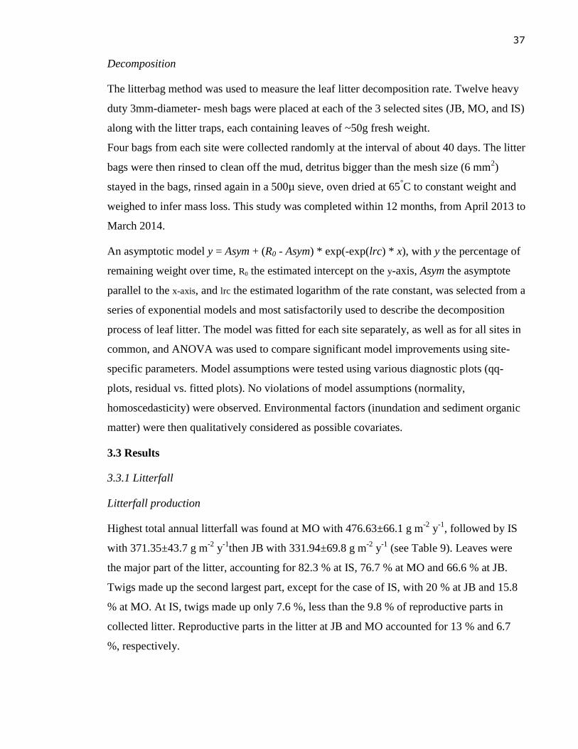
37
Decomposition
The litterbag method was used to measure the leaf litter decomposition rate. Twelve heavy
duty 3mm-diameter- mesh bags were placed at each of the 3 selected sites (JB, MO, and IS)
along with the litter traps, each containing leaves of ~50g fresh weight.
Four bags from each site were collected randomly at the interval of about 40 days. The litter
bags were then rinsed to clean off the mud, detritus bigger than the mesh size (6 mm2)
stayed in the bags, rinsed again in a 500µ sieve, oven dried at 65°C to constant weight and
weighed to infer mass loss. This study was completed within 12 months, from April 2013 to
March 2014.
An asymptotic model y = Asym + (R0 - Asym) * exp(-exp(lrc) * x), with y the percentage of
remaining weight over time, R0 the estimated intercept on the y-axis, Asym the asymptote
parallel to the x-axis, and lrc the estimated logarithm of the rate constant, was selected from a
series of exponential models and most satisfactorily used to describe the decomposition
process of leaf litter. The model was fitted for each site separately, as well as for all sites in
common, and ANOVA was used to compare significant model improvements using site-
specific parameters. Model assumptions were tested using various diagnostic plots (qq-
plots, residual vs. fitted plots). No violations of model assumptions (normality,
homoscedasticity) were observed. Environmental factors (inundation and sediment organic
matter) were then qualitatively considered as possible covariates.
3.3 Results
3.3.1 Litterfall
Litterfall production
Highest total annual litterfall was found at MO with 476.63±66.1 g m-2
y-1
, followed by IS
with 371.35±43.7 g m-2
y-1
then JB with 331.94±69.8 g m-2
y-1
(see Table 9). Leaves were
the major part of the litter, accounting for 82.3 % at IS, 76.7 % at MO and 66.6 % at JB.
Twigs made up the second largest part, except for the case of IS, with 20 % at JB and 15.8
% at MO. At IS, twigs made up only 7.6 %, less than the 9.8 % of reproductive parts in
collected litter. Reproductive parts in the litter at JB and MO accounted for 13 % and 6.7
%, respectively.
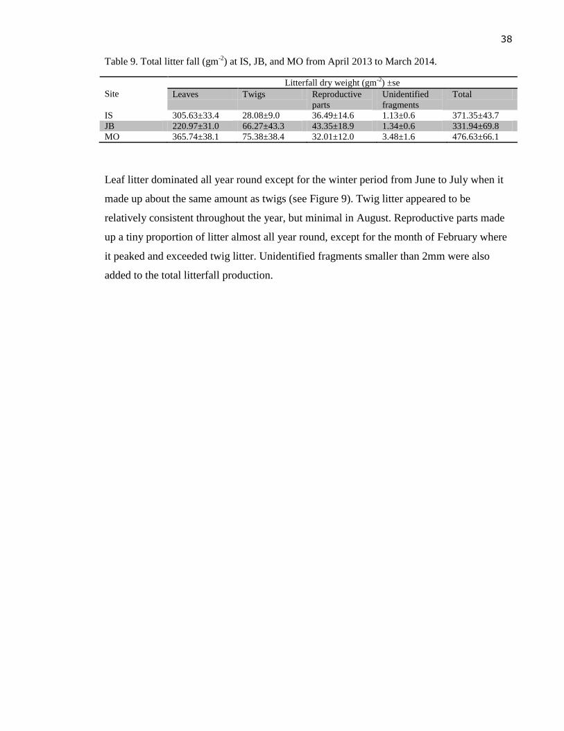
38
Table 9. Total litter fall (gm-2
) at IS, JB, and MO from April 2013 to March 2014.
Site
Litterfall dry weight (gm-2
) ±se
Leaves Twigs Reproductive
parts
Unidentified
fragments
Total
IS 305.63±33.4 28.08±9.0 36.49±14.6 1.13±0.6 371.35±43.7
JB 220.97±31.0 66.27±43.3 43.35±18.9 1.34±0.6 331.94±69.8
MO 365.74±38.1 75.38±38.4 32.01±12.0 3.48±1.6 476.63±66.1
Leaf litter dominated all year round except for the winter period from June to July when it
made up about the same amount as twigs (see Figure 9). Twig litter appeared to be
relatively consistent throughout the year, but minimal in August. Reproductive parts made
up a tiny proportion of litter almost all year round, except for the month of February where
it peaked and exceeded twig litter. Unidentified fragments smaller than 2mm were also
added to the total litterfall production.
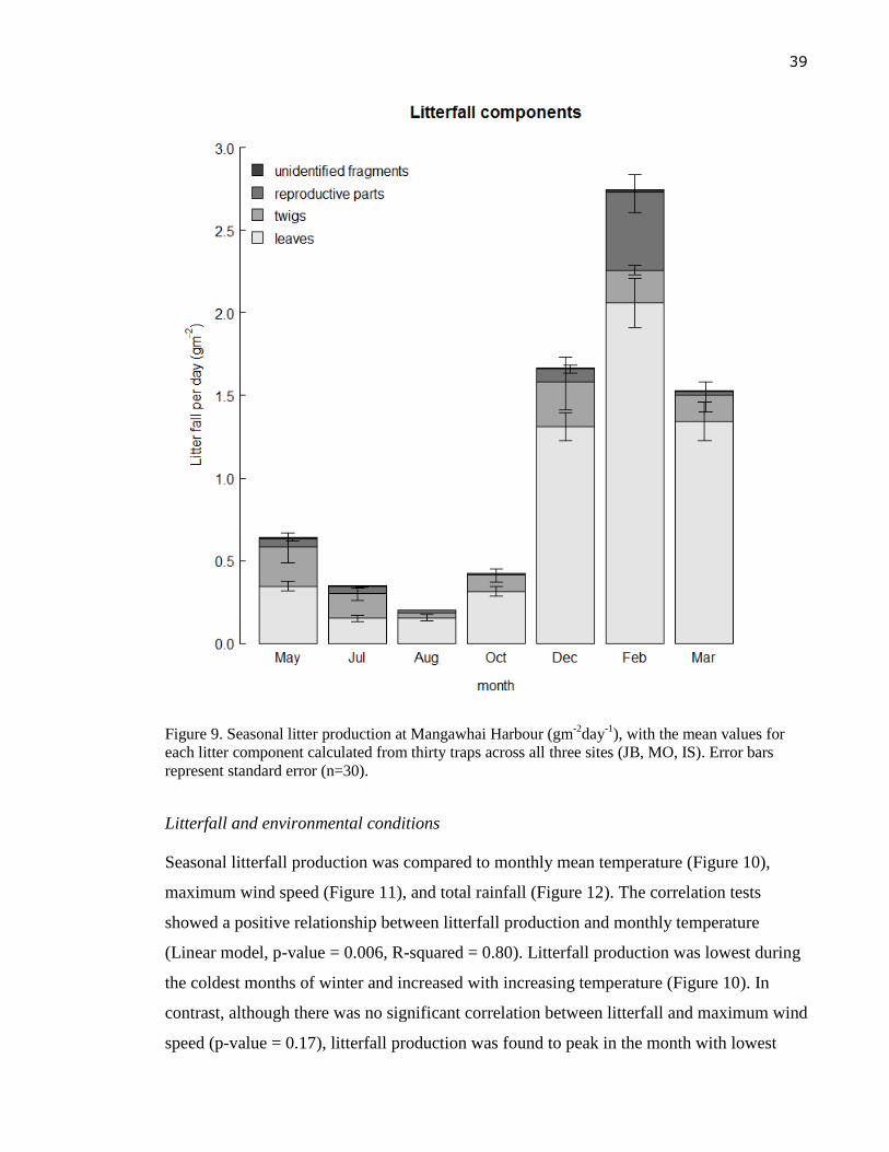
39
Figure 9. Seasonal litter production at Mangawhai Harbour (gm-2
day-1
), with the mean values for
each litter component calculated from thirty traps across all three sites (JB, MO, IS). Error bars
represent standard error (n=30).
Litterfall and environmental conditions
Seasonal litterfall production was compared to monthly mean temperature (Figure 10),
maximum wind speed (Figure 11), and total rainfall (Figure 12). The correlation tests
showed a positive relationship between litterfall production and monthly temperature
(Linear model, p-value = 0.006, R-squared = 0.80). Litterfall production was lowest during
the coldest months of winter and increased with increasing temperature (Figure 10). In
contrast, although there was no significant correlation between litterfall and maximum wind
speed (p-value = 0.17), litterfall production was found to peak in the month with lowest
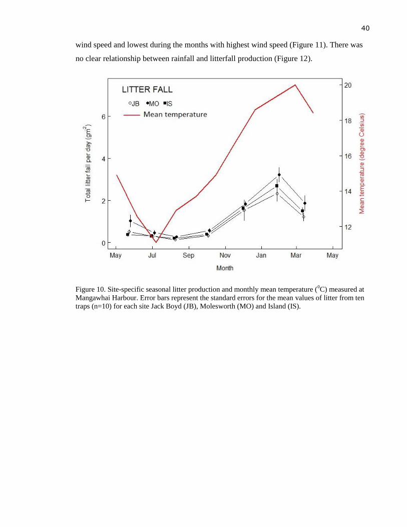
40
wind speed and lowest during the months with highest wind speed (Figure 11). There was
no clear relationship between rainfall and litterfall production (Figure 12).
Figure 10. Site-specific seasonal litter production and monthly mean temperature (0C) measured at
Mangawhai Harbour. Error bars represent the standard errors for the mean values of litter from ten
traps (n=10) for each site Jack Boyd (JB), Molesworth (MO) and Island (IS).
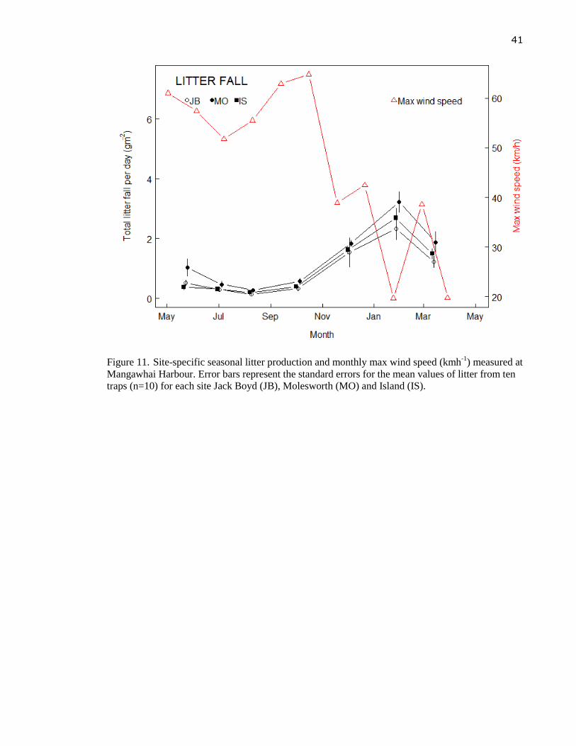
41
Figure 11. Site-specific seasonal litter production and monthly max wind speed (kmh-1
) measured at
Mangawhai Harbour. Error bars represent the standard errors for the mean values of litter from ten
traps (n=10) for each site Jack Boyd (JB), Molesworth (MO) and Island (IS).
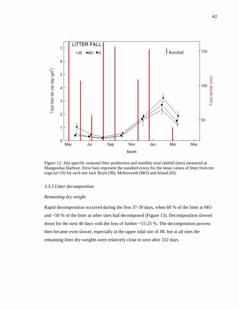
42
Figure 12. Site-specific seasonal litter production and monthly total rainfall (mm) measured at
Mangawhai Harbour. Error bars represent the standard errors for the mean values of litter from ten
traps (n=10) for each site Jack Boyd (JB), Molesworth (MO) and Island (IS).
3.3.2 Litter decomposition
Remaining dry weight
Rapid decomposition occurred during the first 37-39 days, when 60 % of the litter at MO
and ~50 % of the litter at other sites had decomposed (Figure 13). Decomposition slowed
down for the next 40 days with the loss of further ~15-25 %. The decomposition process
then became even slower, especially at the upper tidal site of JB, but at all sites the
remaining litter dry weights were relatively close to zero after 332 days.
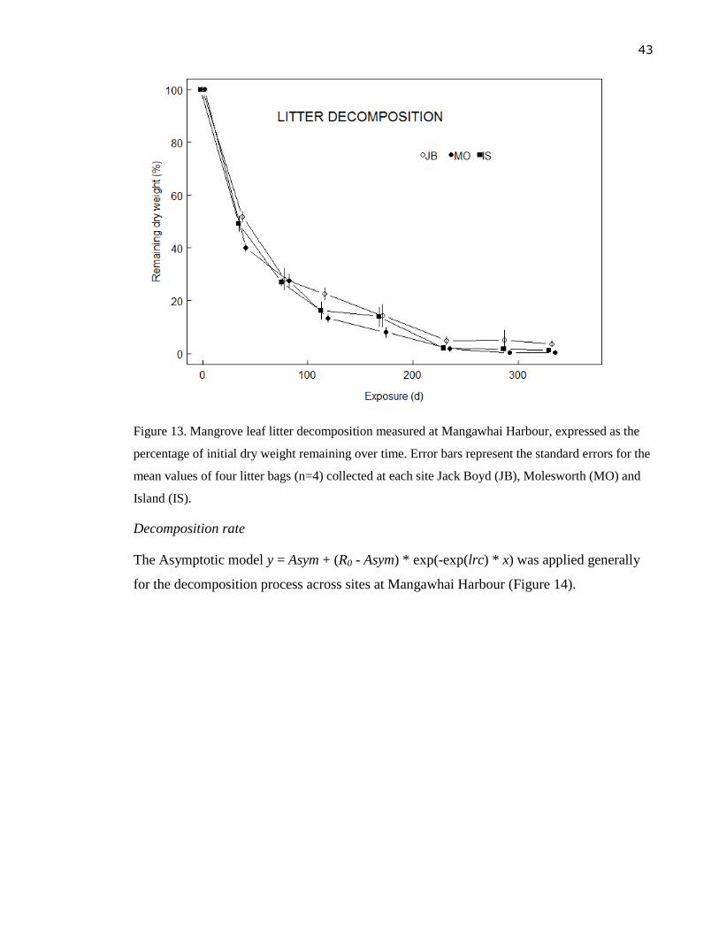
43
Figure 13. Mangrove leaf litter decomposition measured at Mangawhai Harbour, expressed as the
percentage of initial dry weight remaining over time. Error bars represent the standard errors for the
mean values of four litter bags (n=4) collected at each site Jack Boyd (JB), Molesworth (MO) and
Island (IS).
Decomposition rate
The Asymptotic model y = Asym + (R0 - Asym) * exp(-exp(lrc) * x) was applied generally
for the decomposition process across sites at Mangawhai Harbour (Figure 14).
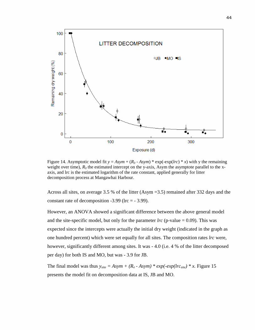
44
Figure 14. Asymptotic model fit y = Asym + (R0 - Asym) * exp(-exp(lrc) * x) with y the remaining
weight over time), R0 the estimated intercept on the y-axis, Asym the asymptote parallel to the x-
axis, and lrc is the estimated logarithm of the rate constant, applied generally for litter
decomposition process at Mangawhai Harbour.
Across all sites, on average 3.5 % of the litter (Asym =3.5) remained after 332 days and the
constant rate of decomposition -3.99 (lrc = - 3.99).
However, an ANOVA showed a significant difference between the above general model
and the site-specific model, but only for the parameter lrc (p-value = 0.09). This was
expected since the intercepts were actually the initial dry weight (indicated in the graph as
one hundred percent) which were set equally for all sites. The composition rates lrc were,
however, significantly different among sites. It was - 4.0 (i.e. 4 % of the litter decomposed
per day) for both IS and MO, but was - 3.9 for JB.
The final model was thus ysite = Asym + (R0 - Asym) * exp(-exp(lrcsite) * x. Figure 15
presents the model fit on decomposition data at IS, JB and MO.
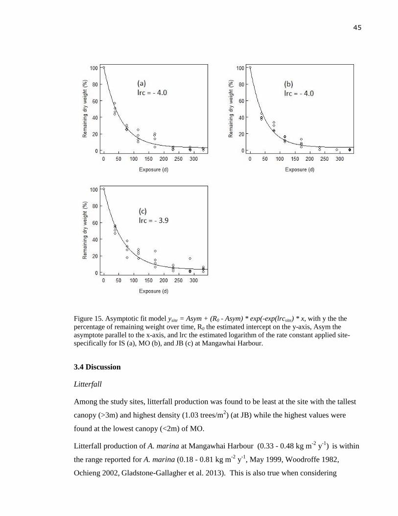
45
Figure 15. Asymptotic fit model ysite = Asym + (R0 - Asym) * exp(-exp(lrcsite) * x, with y the the
percentage of remaining weight over time, R0 the estimated intercept on the y-axis, Asym the
asymptote parallel to the x-axis, and lrc the estimated logarithm of the rate constant applied site-
specifically for IS (a), MO (b), and JB (c) at Mangawhai Harbour.
3.4 Discussion
Litterfall
Among the study sites, litterfall production was found to be least at the site with the tallest
canopy (>3m) and highest density (1.03 trees/m2) (at JB) while the highest values were
found at the lowest canopy (<2m) of MO.
Litterfall production of A. marina at Mangawhai Harbour (0.33 - 0.48 kg m-2
y-1
) is within
the range reported for A. marina (0.18 - 0.81 kg m-2
y-1
, May 1999, Woodroffe 1982,
Ochieng 2002, Gladstone-Gallagher et al. 2013). This is also true when considering
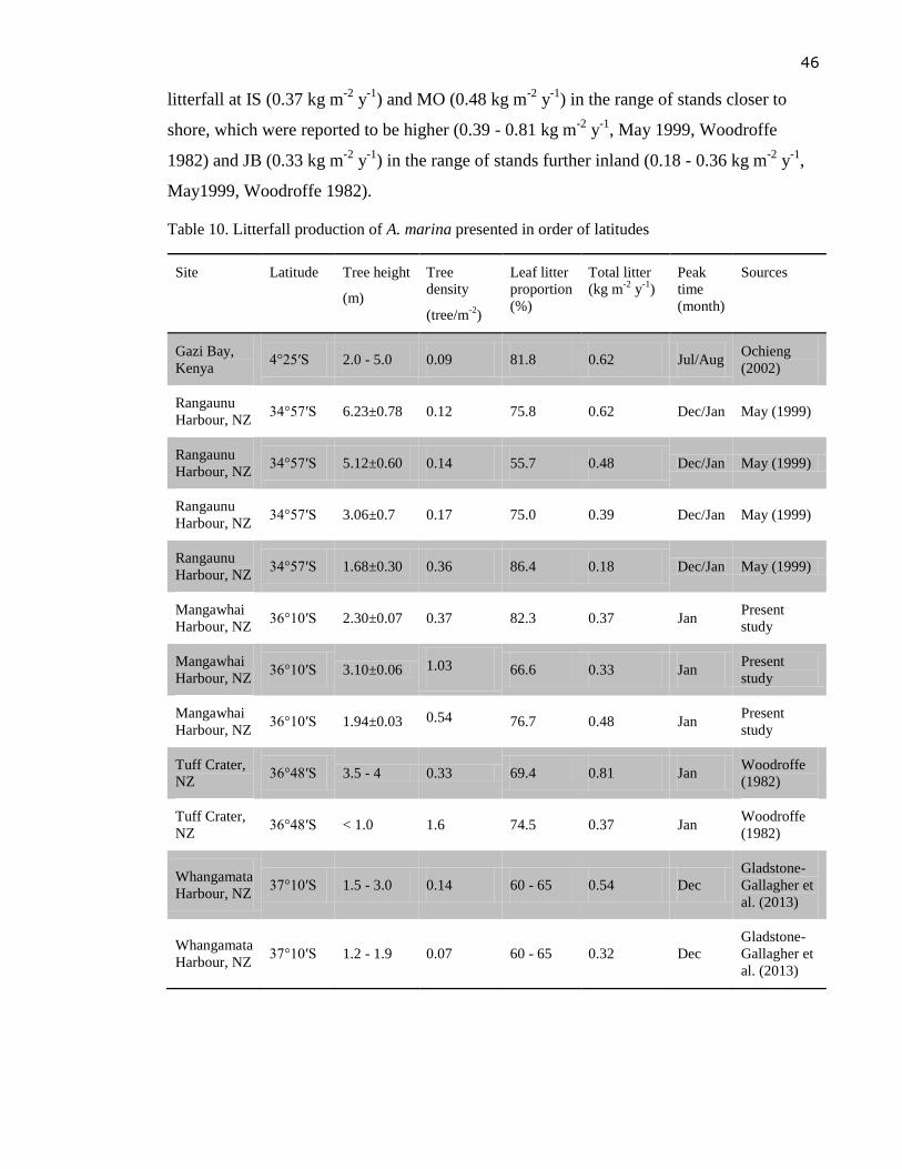
46
litterfall at IS (0.37 kg m-2
y-1
) and MO (0.48 kg m-2
y-1
) in the range of stands closer to
shore, which were reported to be higher (0.39 - 0.81 kg m-2
y-1
, May 1999, Woodroffe
1982) and JB (0.33 kg m-2
y-1
) in the range of stands further inland (0.18 - 0.36 kg m-2
y-1
,
May1999, Woodroffe 1982).
Table 10. Litterfall production of A. marina presented in order of latitudes
Site Latitude Tree height
(m)
Tree
density
(tree/m-2
)
Leaf litter
proportion
(%)
Total litter
(kg m-2
y-1
)
Peak
time
(month)
Sources
Gazi Bay,
Kenya 4°25′S 2.0 - 5.0 0.09 81.8 0.62 Jul/Aug
Ochieng
(2002)
Rangaunu
Harbour, NZ 34°57′S 6.23±0.78 0.12 75.8 0.62 Dec/Jan May (1999)
Rangaunu
Harbour, NZ 34°57′S 5.12±0.60 0.14 55.7 0.48 Dec/Jan May (1999)
Rangaunu
Harbour, NZ 34°57′S 3.06±0.7 0.17 75.0 0.39 Dec/Jan May (1999)
Rangaunu
Harbour, NZ 34°57′S 1.68±0.30 0.36 86.4 0.18 Dec/Jan May (1999)
Mangawhai
Harbour, NZ 36°10′S 2.30±0.07 0.37 82.3 0.37 Jan
Present
study
Mangawhai
Harbour, NZ 36°10′S 3.10±0.06 1.03 66.6 0.33 Jan
Present
study
Mangawhai
Harbour, NZ 36°10′S 1.94±0.03 0.54 76.7 0.48 Jan
Present
study
Tuff Crater,
NZ 36°48′S 3.5 - 4 0.33 69.4 0.81 Jan
Woodroffe
(1982)
Tuff Crater,
NZ 36°48′S < 1.0 1.6 74.5 0.37 Jan
Woodroffe
(1982)
Whangamata
Harbour, NZ 37°10′S 1.5 - 3.0 0.14 60 - 65 0.54 Dec
Gladstone-
Gallagher et
al. (2013)
Whangamata
Harbour, NZ 37°10′S 1.2 - 1.9 0.07 60 - 65 0.32 Dec
Gladstone-
Gallagher et
al. (2013)
47
Table 10 shows a comparison of A. marina litterfall production among New Zealand sites
and one tropical site. It is difficult to predict a specific pattern for litterfall of A. marina
since there was no relationship found between litterfall values with latitude, tree height, nor
tree density. Although it is reasonable to predict litterfall to be higher in taller and denser
stands, the tallest stand (>6m, Rangaunu Harbour) had a lower litterfall than that of Tuff
Crater where tree height was only 3.5 - 4m. Litterfall under lowest canopy (<1m, Tuff
Crater) was in the lower part of the reported ranges, but not the lowest. The densest stands
(1.3 tree/m2, Mangawhai Harbour and 1.6 tree/m
2, Tuff Crater) were in the lower part of the
litterfall range. Litterfall rates among locations were not proportional to latitude (Table 9).
Along the New Zealand coast, the highest litterfall rates (0.7 - 0.8 kg m-2
y-1
) were recorded
at the Tuff Crater site near Auckland (36°48′S) followed by Whangamata Harbour
(37°10′S) with 0.3 - 0.5 kg m-2
y-1
, while the lowest rate found at the most northerly site
(Rangaunu Harbour, 34°57′S) with 0.2 - 0.6 kg m-2
y-1
. However, this latitudinal range may
be insufficient to result in significant differences in environmental conditions, temperature
in particular, that affect litter production.
These results are not consistent with suggestion by Saenger and Snedaker (1993) that there
are positive relationships between temperate mangrove litterfall, tree height and latitude.
Morrisey (2010) also suggested that litterfall rates for A. marina in New Zealand are below
the maximum values reported for tropical A. marina while among the range of temperate
ones. The one tropical site reviewed (Kenya, 4°25′S) in this study had litterfall rates similar
to those reported here. However, this is only one tropical site and it had considerable lower
tree density compared to New Zealand sites. More tropical sites are needed to draw robust
conclusions about latitudinal patterns of A. marina litterfall at a larger scale.
The environmental factor that seemed to be correlated with litterfall was temperature.
Litterfall of A. marina at Mangawhai Harbour increased with increasing temperature, which
is highly consistent with May (1999), who suggested that leaf litter, the major part of
litterfall, was closely related to temperature. However, this is unlikely to be a causal
relationship, since litterfall of tropical A. marina in Gazi Bay (Kenya) peaked in Jul/Aug
and temperature for this site was stable between 25-300C year-round.
There was no clear relationship between litterfall and rainfall, although May (1999) found
that litterfall was negatively correlated with water availability (which was calculated by the
difference between total rainfall and total evaporation). Litterfall at Mangawhai Harbour
48
decreased, surprisingly, with increasing wind speed. Maximum litterfall was recorded
during the least rainfall and vice versa. There was no storm recorded for Mangawhai during
the study period, although strong wind (exceeding 60 kmh-1
) was recorded between
September and November 2013 but this did not have any effect on the litterfall pattern.
Litter decomposition
Although decomposition rates were similar for MO and IS (-4.0 % day-1
), decomposition
happened fastest at MO especially during the first 37-39 days when litter at MO lost as
much as 60 % of its weight while only 50 % at the IS site. Locations of the three sites were
different clearly in terms of inundation and distance from the shore. No inundation time
measurement was available, but MO was observed to have longer and higher inundation
than the other sites. In addition, although it is slightly further away from the shore
compared to IS, the site of MO is on the waterway during inundation, which may cause the
litter bags at MO being buried naturally by the mud. This may help speed up decomposition
rates at MO. Although the macrofauna was reported to have an impact on the
decomposition rates of mangrove leaves (Morrisey, 2010), this may not be an important
factor for the fast decomposition process at MO because the animals found in the litter bags
during sample collecting were not different between MO and IS (small mud crabs and
amphipod Orchestia) with similar frequency (1-2 crabs and 4-5 amphipods/bag).
Litter decomposition happened most slowly at JB, the site farthest inshore where
inundation time is shortest with sandier substrate. Litter bags collected from JB were
always in comparatively dry and clean conditions, compared to the bags heavily covered
with mud found at IS and especially MO. Together with the amphipod Orchestia,
abundance of scavenger snail Z. lutulentus was found at JB instead of mud crabs. In
addition, the slightly lower water content in the leaves at JB (fresh/dry weight ratio of 2.7
compared to 2.9 at MO and IS) may contribute to the slower decomposition process.
Sediment organic matter (OM) content was also collected (for another research project,
Hulbert 2014) and considered as a driving factor for the decomposition process. However,
the variation in OM among sites (4.9 - 8.8 % of sediment contents at MO, 2.6 - 3.4 % at IS,
and 20.47 % at JB) did not show any relationship with the decomposition patterns.
The decomposition rate of A. marina at Mangwhai Harbour is the fastest recorded in New
Zealand so far with >50 % of litter lost after 37-39 days. Other studies on leaf litter
49
decomposition of A. marina in New Zealand was reported to lose 50 % of its dry weight
after 42 - 84 days of decomposition (Woodroffe 1982, Morrisey 2010, Gladstone-Gallagher
et al. 2013), Although it was reported that decomposition happened much faster in the
warmer months of summer and autumn (Woodroffe 1982, Morrisey 2010), this does not
help explain the faster decomposition of mangrove litter at the initial stage in Mangawhai
Harbour compared to other New Zealand sites because the experiment at Mangawhai was
set up in April, when it was more likely to be colder than the study at Tuff Crater (in
March) and at Whangamata (in February).
Mesh size of the litter bags possibly influenced litter decomposition patterns in the present
study. The litter bag mesh size used here was bigger (6 mm2 compared to 4 mm
2 mesh size
used at Tuff Crater and Whangamata Harbour,Woodroffe 1982, Gladstone-Gallagher et al.
2013), which may have enhanced access from macrofauna to the litter and at the same time
this may have allowed bigger chunks of detritus to escape the bags while washed by tidal
inundation or when rinsed in the lab. The common benthic species found in New Zealand
mangroves are the mud crab Helice crassa, the amphipod Orchestia and the scavenger snail
Z. lutulentus (Woodroffe 1982, Alfaro 2006, Morrisey et al. 2010). Although their
abundance appeared to vary among locations (Woodroffe 1982, Alfaro 2006) and it was not
clear if they feed on mangrove leaves, their appearance was proven to be important to the
decomposition process (Morrisey, 2010).
The asymptotic model fit best described the decomposition process at Mangawhai Harbour,
although this model has not been used before for decomposition of leaf litter on the surface.
Woodroffe (1982) used a linear fit with R-squared of 56-83 %, which was acknowledged
not to be ideal to describe the decomposition process that happened rapidly at the beginning
but slower later on. A single exponential decay model was used by Gladstone-Gallagher et
al. (2013) to describe the decomposition of leaf litter on the sediment as an alternative to
the one used here.
3.5 Conclusions
Litterfall production of A. marina at Mangawhai Harbour is among the range reported for
New Zealand mangroves. However, when considering litterfall results among the sites at
Mangawhai Harbour and with other sites in New Zealand, there is no relationship between
litterfall production and stand size (tree height and density). Neither is there any specific
50
latitudinal pattern of litterfall production. There is a positive correlation between litterfall
and temperature. However, more studies of litterfall of A. marina at lower latitude and
tropical sites is needed to be able to draw any conclusion about the causal relationship
between temperature and litterfall. Rainfall and wind speed do not affect the litterfall
production.
Among the sites at Mangwhai Harbour, litter decomposition of A. marina happens faster at
sites with clearly longer inundation time and muddy substrate than sandy site with shorter
inundation. However, quantitative data of inundation time at the three sites should be
collected to confirm this possible relationship. OM of the sediment does not affect the
decomposition rate. Compared to other New Zealand sites, leaf litter at Mangawhai
decomposes faster, especially during the first 40 days, which is possibly because of the
bigger mesh size bags used in this study.
51
Chapter 4. General discussion and implications for conservation
and management ______________________________________________________________
52
4.1 Summary of main results
Allometry and LAI
A. marina stands at Mangawhai Harbour showed a density from 0.37-1.03 trees per square
metre, with tree height varying from 1-5 m. The tallest and densest stand was at Jack Boyd
(JB) but larger stems of up to 16.9 cm in diameter were found at Molesworth (MO). Mean
stem diameter varied from 5.15 ± 0.22 to 6.40 ± 0.23 cm. LAI ranged widely from 1.6 (at
IS) to 4.6 m2m
-2 (at JB) and SLA was 46.9 ± 0.81 to 53.81 ± 0.39 m
2kg
-1.
Biomass distribution
Total above-ground biomass of A. marina at Mangawhai Harbour was 2.69 - 8.88 kgm-2
,
which is lower than in other temperate A. marina stands in New Zealand and Australia.
Below-ground biomass ranged from 11.62 kgm-2
to 14.7 kgm-2
, which is similar to that of
sites with larger trees. The root-shoot ratio in Mangawhai was estimated at 1.73, which is
among the highest reported for A. marina.
More than 70 % of the total below-ground biomass was located within 40 cm below the
surface and almost 50 % of the total was from fine roots alone. The deepest fine roots were
found at 1.6 m. Fine roots contributed most to the total biomass with an average of 37 %,
followed by woody biomass (32 %), and then coarse roots (27 %). Leaf biomass
contributed a only 3 % and pneumatophores and seedlings contributed least, with only 1 %
of the total biomass.
The linear model Y = x * ba, with Y the biomass and ba the basal area, was used to
satisfactorily estimate the biomass of A. marina.
Litterfall production
Annual litterfall production of A. marina at Mangawhai Harbour was estimated to be from
331.94 ± 69.8 to 476.63 ± 66.1 gm-2
, with leaves as the major part of the litter accounting
for 66.6 % - 82.3 %. Litterfall production positively correlated with temperature,
suggesting a seasonal trend with more litterfall during late summer. There was no
relationship between litterfall and maximum wind speed although litterfall was found to
peak in the month with lowest wind speed and was minimal during the months with the
highest maxium wind speed. Monthly total rainfall did not affect the seasonal litterfall
pattern.
53
Litter decomposition
Leaf litter of A. marina at Mangawhai harbour decomposed rapidly during the first 37-39
days with 50-60 % of the initial dry weight lost. This was slowed down during the
following 40 days with the loss of further ~15-25 % of litter mass and then even slower.
After 332 days an average of 3.5 % of the initial litter mass remained. The average (linear)
rate of decomposition was -3.99 % per day.
Litter decomposition happened more rapidly at muddy sites with longer inundation,
although no quantitative data about inundation time was available. Sediment organic matter
(OM) did not affect the decomposition process. Because I only had three sites, my data are
not adequate for statistical tests of the correlation between litter decomposition and the site
characteristics.
The asymptotic model ysite = Asym + (R0 - Asym) * exp(-exp(lrcsite) * x, with y percentage
of remained litter, R0 the estimated intercept on the y-axis, Asym the asymptote parallel to
the x-axis, and lrc is the (site-specific) estimated logarithm of the rate constant, best
described the decomposition process of leaf litter at Mangwhai Harbour.
4.2 Conclusions and implication for conservation and management
Despite the shorter stands of A. marina at Mangawhai Harbour compared to other sites in
New Zealand and Australia, the total estimated biomass is within their range. Particularly
the very high below-ground biomass density makes A.marina stands important carbon
stores. With a carbon content of 44 % in wood, 41 % in roots, and 31 % in the leaf of A.
marina (Gritcan, unpublished data), mangrove stands at Mangawhai Harbour store 4.8 - 6
kg C m-2
below-ground, 1.2 - 3.9 kg C m-2
above-ground, and produce 0.1 - 0.2 kg C m-2
y-1
of litter, which takes around one year to completely decompose and transfer to other pools.
Assuming that A.marina at our site shows similar rates of growth, carbon fixation, canopy
respiration, and sediment burial as those reported for other mangrove forests (Suwa et al.
2006, Ray et al. 2011, Alongi 2014), the carbon cycle for New Zealand mangroves can be
roughly described as in Figure 16. Root respiration was not quantified in this study and are
generally difficult to measure. No study was found which would have allowed to assign a
value to this carbon flux. However, given that root biomass was significantly higher than
aboveground biomass it is reasonable to assume that root (or total soil) respiration is a
significant carbon flux from mangrove ecosystems.
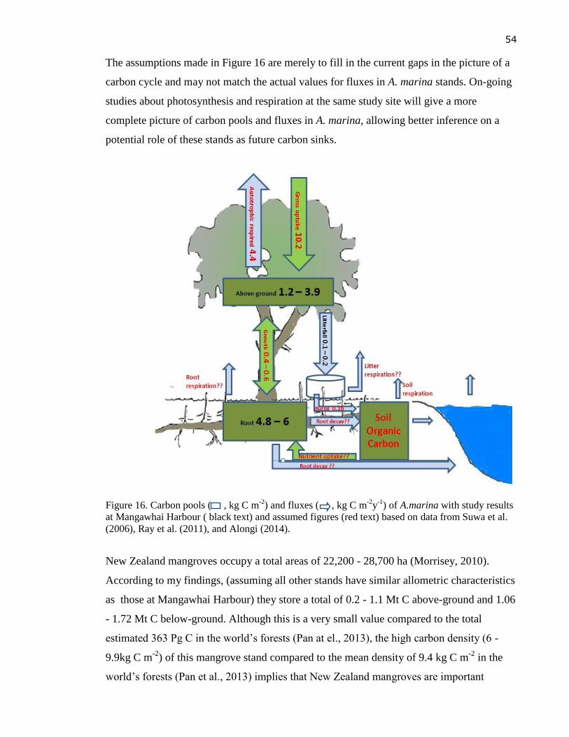
54
The assumptions made in Figure 16 are merely to fill in the current gaps in the picture of a
carbon cycle and may not match the actual values for fluxes in A. marina stands. On-going
studies about photosynthesis and respiration at the same study site will give a more
complete picture of carbon pools and fluxes in A. marina, allowing better inference on a
potential role of these stands as future carbon sinks.
Figure 16. Carbon pools ( , kg C m-2
) and fluxes ( , kg C m-2
y-1
) of A.marina with study results
at Mangawhai Harbour ( black text) and assumed figures (red text) based on data from Suwa et al.
(2006), Ray et al. (2011), and Alongi (2014).
New Zealand mangroves occupy a total areas of 22,200 - 28,700 ha (Morrisey, 2010).
According to my findings, (assuming all other stands have similar allometric characteristics
as those at Mangawhai Harbour) they store a total of 0.2 - 1.1 Mt C above-ground and 1.06
- 1.72 Mt C below-ground. Although this is a very small value compared to the total
estimated 363 Pg C in the world’s forests (Pan at el., 2013), the high carbon density (6 -
9.9kg C m-2
) of this mangrove stand compared to the mean density of 9.4 kg C m-2
in the
world’s forests (Pan et al., 2013) implies that New Zealand mangroves are important
55
carbon stores regarding land use management. This is an important point in the context of
the ongoing expansion of mangroves in New Zealand and the fact that the absence of any
industrial or commercial use of this vegetation have led to management initiatives that are
more likely to support their removal than their restoration.
The removal of all stands of A.marina in New Zealand when considering their above- and
below-ground biomass stocks, would remove at least 1-2 Mt of carbon from the current
pools. In contrast, if they remain undisturbed, their expansion with an average of 4.1 % y-1
in New Zealand (Morrisey et al., 2010) could even add up to 0.05 - 0.1 Mt C y-1
. This
amount of carbon of course only is sequestered once the stands are mature, which could
take decades. Given the fact that New Zealand's total greenhouse gas emissions reached 76
Mt CO2 equivalent (CO2-e) in 2012 (an increase by 25.4 % since 1990), while CO2 sinks
totalled 26.6 Mt CO2-e during the same time span (New Zealand Ministry of Environment,
2014), my results combined with their rate of mangrove expansion clearly supports their
protection in the current context of global warming.
However, data are incomplete to draw any final conclusions on the C fluxes of A.marina.
More studies on carbon uptake, canopy and root respiration, wood and root production are
needed to contribute to the full picture of the carbon cycle in New Zealand mangrove
ecosystems. The ongoing debate about the ecological role of New Zealand mangroves in
coastal ecosystems has highlighted the need for more comprehensive information than what
is available to date. This will be helpful not only for communities seeking guidance or
action on mangrove management, but also for the related governing agencies.
56
References
______________________________________________________________
Albany, M. (Ed.). (2013). A dictionary of plant sciences: Oxford University Press.
Alfaro, A. C. (2006). Benthic macro-invertebrate community composition within a
mangrove/seagrass estuary in northern New Zealand. Estuarine, Coastal and Shelf
Science, 66(1–2), 97-110. doi:http://dx.doi.org/10.1016/j.ecss.2005.07.024
Alongi, D. M. (2002). Present state and future of the world's mangrove forests.
Environmental Conservation, 29(03), 331-349. doi:doi:10.1017/S0376892902000231
Alongi, D., Clough, B., Dixon, P., & Tirendi, F. (2003). Nutrient partitioning and storage in
arid-zone forests of the mangroves Rhizophora stylosa and Avicennia marina. Trees,
17(1), 51-60. doi:10.1007/s00468-002-0206-2
Alongi, D.M. (2009) Paradigm shifts in mangrove biology. Coastal wetlands: an integrated
ecosystem approach (ed. by G.M.E. Perillo, E. Wolanski, D.R. Cahoon and M.M.
Brinson), pp. 615–640. Elsevier, Amsterdam.
Alongi, D. M. (2009). The energetics of mangrove forests: Springer Dordrecht.
Alongi, D. M. (2014). Carbon sequestration in mangrove forests. Carbon Management,
3(3), 313-322. doi:10.4155/cmt.12.20
Bandaranayake, W. M. (1998). Traditional and medicinal uses of mangroves. Mangroves
and Salt Marshes, 2(3), 133-148. doi:10.1023/a:1009988607044
Bellot, J., Sánchez, J. R., Lledó, M. J., Martínez, P., & Escarré, A. (1992). Litterfall as a
measure of primary production in Mediterranean holm-oak forest. Vegetatio, 99-
100(1), 69-76. doi:10.1007/bf00118211
Bouillon, S., Borges, A. V., Castañeda-Moya, E., Diele, K., Dittmar, T., Duke, N. C., ...
Twilley, R. R. (2008). Mangrove production and carbon sinks: A revision of global
budget estimates. Global Biogeochemical Cycles, 22(2), GB2013.
doi:10.1029/2007gb003052
Briggs, S. V. (1977). Estimates of biomass in a temperate mangrove community. Australian
Journal of Ecology, 2(3), 369-373. doi:10.1111/j.1442-9993.1977.tb01151.x
57
Burchett, M. D., Field, C. D., & Pulkownik, A. (1984). Salinity, growth and root respiration
in the grey mangrove, Avicennia marina. Physiologia Plantarum, 60(2), 113-118.
doi:10.1111/j.1399-3054.1984.tb04549.x
Cairns, M. A., Brown, S., Helmer, E. H., & Baumgardner, G. A. (1997). Root biomass
allocation in the world's upland forests. Oecologia, 111(1), 1-11.
doi:10.1007/s004420050201
Chapin, F. S. F. S., Matson, P. A. P. A., & Mooney, H. A. (2002). Principles of terrestrial
ecosystem ecology. New York: Springer.
Clarke, P. J. (1993). Dispersal of grey mangrove (Avicennia marina) propagules in
southeastern Australia. Aquatic Botany, 45(2–3), 195-204.
doi:http://dx.doi.org/10.1016/0304-3770(93)90021-N
Clough, B. (1998). Mangrove forest productivity and biomass accumulation in
Hinchinbrook Channel, Australia. Mangroves and Salt Marshes, 2(4), 191-198.
doi:10.1023/a:1009979610871
Clough, B. F. (2013). Continuing the Journey Amongst Mangroves: International Society
for Mangrove Ecosystems. Retrieved from
http://books.google.co.nz/books?id=9rchnwEACAAJ
Clough, B. F., & Sim, R. G. (1989). Changes in gas exchange characteristics and water use
efficiency of mangroves in response to salinity and vapour pressure deficit.
Oecologia, 79(1), 38-44. doi:10.1007/bf00378237
Comley, B. W. T., & McGuinness, K. A. (2005). Above- and below-ground biomass, and
allometry, of four common northern Australian mangroves. Australian Journal of
Botany, 53(5), 431-436. doi:http://dx.doi.org/10.1071/BT04162
Curran, Cole, & Allaway. (1986). Root Aeration and Respiration in Young Mangrove
Plants (Avicennia marina (Forsk.) Vierh.). Journal of Experimental Botany, 37(8),
1225-1233. doi:10.1093/jxb/37.8.1225
Dechaine, J., Ruan, H., Sanchez-de Leon, Y., & Zou, X. (2005). Correlation between
earthworms and plant litter decomposition in a tropical wet forest of Puerto Rico.
Pedobiologia, 49(6), 601-607. doi:http://dx.doi.org/10.1016/j.pedobi.2005.07.006
58
Donato, D. C., Kauffman, B. J., Murdiyarso, D., Kurnianto, S., Stidham, M., & Kanninen,
M. (2011). Mangroves among the most carbon-rich forests in the tropics. Nature
Geoscience, 4(5). doi:http://dx.doi.org/10.1038/ngeo1123
Duke, N. (1990). Phenological trends with latitude in the mangrove tree Avicennia marina.
The Journal of Ecology, 113-133.
Duke, N. C. (1995). Genetic diversity, distributional barriers and rafting continents—more
thoughts on the evolution of mangroves. Hydrobiologia, 295(1-3), 167-181.
Ellis, J., Nicholls, P., Craggs, R., Hofstra, D., & Hewitt, J. (2004). Effects of terrigenous
sedimentation on mangrove physiology and associated macrobenthic communities.
Marine Ecology Progress Series, 270, 71-82. doi:10.3354/meps270071
Ellison, A. (2002). Macroecology of mangroves: large-scale patterns and processes in
tropical coastal forests. Trees, 16(2-3), 181-194. doi:10.1007/s00468-001-0133-7
FAO. (2007). The world's mangrove 1980 – 2005
Gaston, K. J. (2007). Latitudinal gradient in species richness. Current Biology, 17(15),
R574. doi:10.1016/j.cub.2007.05.013
Gladstone-Gallagher, R. V., Lundquist, C. J., & Pilditch, C. A. (2013). Mangrove
(Avicennia marina subsp. australasica) litter production and decomposition in a
temperate estuary. New Zealand Journal of Marine and Freshwater Research, 48(1),
24-37. doi:10.1080/00288330.2013.827124
Gorte, R. W. (2009, August). Carbon sequestration in forests. US of Library of Congress,
Congressional Research Service.
Harrison, M. E., Marchant, N. C., and Husson, S. J. (2012) Ecological Monitoring to
Support Conservation in Kalimantan’s Forests: Concepts and Design. Orangutan
Tropical Peatland Project Report, Palangka Raya, Indonesia
Harty, C. (2009). Mangrove planning and management in New Zealand and South East
Australia – A reflection on approaches. Ocean & Coastal Management, 52(5), 278-
286. doi:http://dx.doi.org/10.1016/j.ocecoaman.2009.03.001
Hillebrand, H. (2004). On the Generality of the Latitudinal Diversity Gradient. The
American Naturalist, 163(2), 192-211
59
Hulbert, C. (2014). Modern estuarine habitats and organism-sediment interactions at
Mangawhai Estuary, North Island, New Zealand. The University of Auckland,
Auckland.
Jacob, M., Viedenz, K., Polle, A., & Thomas, F. (2010). Leaf litter decomposition in
temperate deciduous forest stands with a decreasing fraction of beech (Fagus
sylvatica). Oecologia, 164(4), 1083-1094. doi:10.1007/s00442-010-1699-9
Karberg, N., Scott, N., & Giardina, C. (2008). Methods for Estimating Litter
Decomposition. In C. Hoover (Ed.), Field Measurements for Forest Carbon
Monitoring (pp. 103-111): Springer Netherlands. Retrieved from
http://dx.doi.org/10.1007/978-1-4020-8506-2_8. doi:10.1007/978-1-4020-8506-2_8
Kauffman, J. B., & Donato, D. C. (2012). Protocols for the measurement, monitoring and
reporting of structure, biomass and carbon stocks in mangrove forests. Bogor,
Indonesia: CIFOR Working paper 86.
Knowledge. Auckland Regional Council Technical Publication Number 325
Komiyama, A., Ong, J. E., & Poungparn, S. (2008). Allometry, biomass, and productivity
of mangrove forests: A review. Aquatic Botany, 89(2), 128-137.
doi:http://dx.doi.org/10.1016/j.aquabot.2007.12.006
Kuchler, A. W. (1972). The mangrove in New Zealand. New Zealand Geoghraper, 28, 113
- 129.
Lacerda, L. D. d., & Santos, N. P. d. (May 2004). Mangroves and the Development of the
Chemical Industry in Brazil. 4.
Le Quéré, C., Peters, G. P., Andres, R. J., Andrew, R. M., Boden, T., Ciais, P., ... Yue, C.
(2013). Global carbon budget 2013. Earth Syst. Sci. Data Discuss., 6(2), 689-760.
doi:10.5194/essdd-6-689-2013
Leuzinger, S., & Hättenschwiler, S. (2013). Beyond global change: Lessons from 25 years
of CO2 research. Oecologia,171(3), 639-51. doi:http://dx.doi.org/10.1007/s00442-
012-2584-5
Litton, C. M., Raich, J. W., & Ryan, M. G. (2007). Carbon allocation in forest ecosystems.
Global Change Biology, 13(10), 2089-2109. doi:10.1111/j.1365-2486.2007.01420.x
60
Lugo, A. E., & Snedaker, S. C. (1974). The Ecology of Mangroves. Annual Review of
Ecology and Systematics, 5(ArticleType: research-article / Full publication date: 1974
/ Copyright © 1974 Annual Reviews), 39-64.
Mackey, A. (1993). Biomass of the mangrove <I>Avicennia marina</I> (Forsk.) Vierh.
Near Brisbane, South-eastern Queensland. Marine and Freshwater Research, 44(5),
721-725. doi:http://dx.doi.org/10.1071/MF9930721
May, J. D. (1999). Spatial variation in litter production by the mangrove Avicennia marina
var. australasica in Rangaunu harbour, Northland, New Zealand. New Zealand
Journal of Marine and Freshwater Research, 33(2), 163-172.
doi:10.1080/00288330.1999.9516866
Medeiros, T. C. C., & Sampaio, E. V. S. B. (2008). Allometry of aboveground biomasses in
mangrove species in Itamaracá, Pernambuco, Brazil. Wetlands Ecology and
Management, 16(4), 323-330. doi:10.1007/s11273-007-9069-z
Methods for Below-Ground Biomass. (2008). In Carbon Inventory Methods Handbook for
Greenhouse Gas Inventory, Carbon Mitigation and Roundwood Production Projects
(Vol. 29, pp. 149-156): Springer Netherlands. Retrieved from
http://dx.doi.org/10.1007/978-1-4020-6547-7_11. doi:10.1007/978-1-4020-6547-
7_11
Morrisey, D. et al. (2007). The New Zealand Mangrove: Review of the Current State Of
Morrisey, D., Swales, A., Dittmann, S., Morrison, M., Lovelock, C., & Beard, C. (2010).
The Ecology and Management of Temperate Mangroves. Oceanography and Marine
Biology, 48, 43-160. doi:doi:10.1201/EBK1439821169-c2
Mumby, P. J., & Hastings, A. (2008). The impact of ecosystem connectivity on coral reef
resilience. Journal of Applied Ecology, 45, 854–862. doi:10.1111/j.1365-
2664.2008.01459.x
Murdiyarso, D., Donato, D., Kauffman, J. B., Kurnianto, S., Stidham, M., & Kanninen, M.,
&. (2010). Carbon storage in mangrove and peatland ecosystems: a preliminary
account from plots in Indonesia Bogor, Indonesia: Center for International Forestry
Research (CIFOR).
61
New Zealand's Greenhouse Gas Inventory 1990–2012. (2014): New Zealand Ministry of
the Environment. Retrieved from
http://www.mfe.govt.nz/publications/climate/greenhouse-gas-inventory-2014-
snapshot/index.html
Ong, J.E. & Gong, W.K. (2013) Structure, Function and Management of Mangrove
Ecosystems. ISME Mangrove Educational Book Series No. 2. International Society
for Mangrove Ecosystems (ISME), Okinawa, Japan, and International Tropical
Timber Organization (ITTO), Yokohama, Japan
Paliyavuth, C., Clough, B., & Patanaponpaiboon, P. (2004). Salt uptake and shoot water
relations in mangroves. Aquatic Botany, 78(4).
doi:http://dx.doi.org/10.1016/j.aquabot.2004.01.002
Pan, Y., Birdsey, R. A., Fang, J., Houghton, R., Kauppi, P. E., Kurz, W. A., ... Hayes, D.
(2011). A Large and Persistent Carbon Sink in the World’s Forests. Science,
333(6045), 988-993. doi:10.1126/science.1201609
Pan, Y., Birdsey, R. A., Phillips, O. L., & Jackson, R. B. (2013). The Structure,
Distribution, and Biomass of the World's Forests. Annual Review of Ecology,
Evolution, and Systematics, 44(1), 593-622. doi:doi:10.1146/annurev-ecolsys-
110512-135914
Ravindranath N.H., & Ostwald, M. (2008). Carbon Inventory Methods (Vol. 29): Springer.
Ray, R., Ganguly, D., Chowdhury, C., Dey, M., Das, S., Dutta, M. K., ... Jana, T. K.
(2011). Carbon sequestration and annual increase of carbon stock in a mangrove
forest. Atmospheric Environment, 45(28), 5016-5024.
doi:http://dx.doi.org/10.1016/j.atmosenv.2011.04.074
Saenger, P. (2002). Mangrove Ecology, Silviculture and Conservation: Springer. Retrieved
from http://books.google.co.nz/books?id=FDXCLuG9ZCcC
Saenger, P., & Snedaker, S. (1993). Pantropical trends in mangrove above-ground biomass
and annual litterfall. Oecologia, 96(3), 293-299. doi:10.1007/bf00317496
Spalding, M., Kainuma, M., & Collins, L. (2010). World atlas of mangroves (M. Kainuma
& L. Collins, Trans)
62
Stuart, S. A., Choat, B., Martin, K. C., Holbrook, N. M., & Ball, M. C. (2007). The role of
freezing in setting the latitudinal limits of mangrove forests. New Phytologist, 173(3),
576-583. doi:10.1111/j.1469-8137.2006.01938.x
Suwa, R., Khan, M. N. I., & Hagihara, A. (2006). Canopy photosynthesis, canopy
respiration and surplus production in a subtropical mangrove Kandelia candel forest,
Okinawa Island, Japan. Marine Ecology Progress Series, 320, 131-139.
doi:10.3354/meps320131
Suzuki, T., Nishihira, M., & Paphavasit, N. (2002). Size structure and distribution of
Ovassiminea brevicula (Gastropoda) in a Thai mangrove swamp. Wetlands Ecology
and Management, 10(3), 265-271. doi:10.1023/a:1020115411316
Tackenberg, O. (2007). A New Method for Non-destructive Measurement of Biomass,
Growth Rates, Vertical Biomass Distribution and Dry Matter Content Based on
Digital Image Analysis. Annals of Botany, 99(4), 777-783. doi:10.1093/aob/mcm009
Tuomi, M., Thum, T., Järvinen, H., Fronzek, S., Berg, B., Harmon, M., Trofymow, J.A.,
Sevanto, S. & Liski, J. 2009. Leaf litter decomposition - Estimates of global
variability based on Yasso07 model. Ecological Modelling 220 (23), 3362-3371.
doi:10.1016/j.ecolmodel.2009.05.016
Woodroffe, C. D. (1982). Litter production and decomposition in the New Zealand
mangrove, Avicennia marina var. resinifera. New Zealand Journal of Marine and
Freshwater Research, 16(2), 179-188. doi:10.1080/00288330.1982.9515961
Woodroffe, C. D. (1985). Studies of a mangrove basin, Tuff Crater, New Zealand: I.
Mangrove biomass and production of detritus. Estuarine, Coastal and Shelf Science,
20(3), 265-280. doi:http://dx.doi.org/10.1016/0272-7714(85)90042-3
Zhang, H., et al. (2014) Seasonal patterns of litterfall in forest ecosystem worldwide. Ecol.
Complex. , http://dx.doi.org/10.1016/j.ecocom.2014.01.003