Embed Size (px)
Citation preview


FUNDAMENTAL PHYSICS FOR PROBING AND IMAGING

This page intentionally left blank

Fundamental Physicsfor Probing andImaging
WADE ALLISON
Department of Physics and Keble College,University of Oxford
1

3Great Clarendon Street, Oxford OX2 6DP
Oxford University Press is a department of the University of Oxford.It furthers the University’s objective of excellence in research, scholarship,and education by publishing worldwide in
Oxford New York
Auckland Cape Town Dar es Salaam Hong Kong KarachiKuala Lumpur Madrid Melbourne Mexico City NairobiNew Delhi Shanghai Taipei Toronto
With offices in
Argentina Austria Brazil Chile Czech Republic France GreeceGuatemala Hungary Italy Japan Poland Portugal SingaporeSouth Korea Switzerland Thailand Turkey Ukraine Vietnam
Oxford is a registered trade mark of Oxford University Pressin the UK and in certain other countries
Published in the United Statesby Oxford University Press Inc., New York
© Wade Allison 2006
The moral rights of the author have been assertedDatabase right Oxford University Press (maker)
First published 2006
All rights reserved. No part of this publication may be reproduced,stored in a retrieval system, or transmitted, in any form or by any means,without the prior permission in writing of Oxford University Press,or as expressly permitted by law, or under terms agreed with the appropriatereprographics rights organization. Enquiries concerning reproductionoutside the scope of the above should be sent to the Rights Department,Oxford University Press, at the address above
You must not circulate this book in any other binding or coverand you must impose the same condition on any acquirer
British Library Cataloguing in Publication Data
Data available
Library of Congress Cataloging in Publication Data
Data available
Printed in Great Britainon acid-free paper byAntony Rowe Ltd., Chippenham, Wiltshire
ISBN 0–19–920388–1 978–0–19–920388–8 (Hbk)ISBN 0–19–920389–X 978–0–19–920389–5 (Pbk)
10 9 8 7 6 5 4 3 2 1

For Alice, Joss and Alfie

This page intentionally left blank

Preface
Fear has dominated much of the experience of the human race fromearliest times. Fear of death, fear of natural disaster, fear of humanenemies and fear of deities: these were fused together beneath a denseshroud of the unseen and the unknown. The major impact of physicson civilisation has been to roll back this shroud. Physics explains. Itenables us to see inside the Earth and inside our own bodies. It gives usways to probe and to cure.
It has seemed to me that there are some big questions to ask, and adearth of books that ask them. Which aspects of physics are primarilyresponsible for this revolution? How do they work and how are theyused to provide the information and images? Are the dangers that sur-round applications of this physics understood? Are these safety mattersoverstated or understated, and is the public misinformed?
This book is written to answer these questions. It is written for allphysicists who wish to understand the physics basis. Its coverage isbroad but it is also quite demanding in places, for I have a deep dislikeof asking the reader to take statements on trust. Anyway, there are otherbooks that do just that, as they rush through the fundamentals in orderto reach the excitement of the applications at an early stage. I skip overmany experimental details of particular technical realisations but giveenough examples of applications for useful comparisons between differentmodalities to be made. I strongly believe that the widest understandingof the basic physics is essential if future advances in technology are toexploit the possibilities to the full.
The book developed from a short optional course entitled ‘Medical andEnvironmental Physics’ that I have given in recent years to third yearmainstream physics undergraduates at Oxford University, and assumessome familiarity with basic mathematical methods and the core physicsof optics, electromagnetism, quantum mechanics and elementary atomicstructure.
In the introduction we ask which aspects of pure physics have enabledmankind to delve into their environment by seeing into or through oth-erwise opaque objects. Successful solutions have centred on three areasof fundamental physics: firstly the physics of magnetism and low fre-quency radiation, secondly ionising radiation and the physics of nuclei,and thirdly the mechanical properties of matter and sound. Practicalexamples range from safe navigation to medical diagnosis, from findingminerals to border security.
The early chapters give a pedagogical development of the pure physics

viii Preface
of these three fundamental areas. The later chapters follow how theseideas have been developed in applications. They are concerned not justwith imaging, but with further questions of dating, function and prove-nance, and finally with intervention and therapy. The applications illus-trate both the principles at work and the comparison between differentpossibilities.
The pure physics concerned has changed slowly compared with therecent rapid development of applications. The necessary understandingof magnetism and electromagnetic radiation began in the mid nineteenthcentury and was completed a century later with the theory of magneticresonance. Similarly the relevant ionising radiation and nuclear physicswas understood within 75 years of the discovery of radioactivity in the1890s. The basic physics of sound is classical and the understandingof it dates back to the work of Lord Rayleigh, more than a centuryago. In every case what has changed recently is that developmentsand applications using modern materials, electronics and computationalpower have enabled this academic understanding to escape from the purephysics laboratory into the everyday world.
I have avoided the temptation to follow, logically and immediately,the discussion of each set of fundamental ideas with examples of its ap-plication. The subject of successive chapters switches back and forthto encourage parallel thinking about the choice of methods available.Chapter 5 in the middle gives an overview of information and methodsof data analysis which have been used in academic physics research fordecades. In the past these were too computationally intensive to be de-ployed in everyday analysis. Now, as the required computational powerhas become available, they are used routinely in the analysis of imagesand data.
Inevitably from such a broad field, the applications are selected andtheir discussion avoids experimental detail which may be found on theWeb and elsewhere. To have followed every idea raised in the early chap-ters would have lengthened this book beyond what could conceivably becovered in a single text. Therefore many fields of application have beenomitted entirely, or have only been mentioned in passing.
The concluding chapter takes a bird’s eye view of possible devel-opments and the ideas that might emerge from the cupboard of purephysics in the future. There is much in the physical world that we donot understand, and the book ends by looking at a few such cases. Forsome readers the book will open many questions that it does not answer,but it will not have failed in its aim if such omissions stimulate furtherstudy. Other readers will feel the need to rebalance completely society’sperception of the threats and dangers that surround it. Perhaps thebook may be a beginning to the process of turning public opinion anddecision making in the direction of a safer world.

ix
Structure of the book
The chapters are written in such a way that some may be omittedwithout affecting all of those that follow, and shorter courses may beconstructed by reading them selectively, albeit with some loss of theoverview. Thus one or more of the following sub-sets of chapters mightbe omitted:
chapters 2 and 7 on magnetism and magnetic resonance, andrelated imaging methods;
chapters 3, 6 and 8 on interactions of ionising radiation, anal-ysis and damage by irradiation, and medical imaging andtherapy with such radiation;
chapters 4 and 9 on mechanical waves and properties of mat-ter, and ultrasound for imaging and therapy.
Every chapter is divided into a number of sections, each of which startswith a summary. Some sections are more demanding and are markedwith a dagger (†). On a first reading of the book some readers may preferto study just the summary of these, returning to pick up the detail ofthe derivations at a second reading.
At the end of each chapter there is a short list of recommended booksand a list of references and searches for further material on the Web.These should enable the reader both to keep up to date and also tobroaden programmes of study based on this book. With its basic intro-duction I hope that the reader will be able to appreciate in context thetechnical details of applications, galleries of images, and yet wider linksthat may be found. Included is a link to the website for the book:
www.physics.ox.ac.uk/users/allison/booksite.htm
Some colour images and video related to the grey-scale material in thebook may be found there, together with later comments and news.
Because of the interdisciplinary nature of the material some clarity isneeded in the use of terms, abbreviations and conventions. These arelaid out for reference in two appendices. Each of the main chapters endswith a short selection of questions, and the final appendix gives hintsand answers to some of these.
Acknowledgements
In writing this book I have relied heavily on others to keep my balanceand perspective in a wide landscape. Those who have read large sec-tions of the manuscript and provided exactly the combination of crispcomment and encouragement that was most helpful were Richard Tuley,Daniel McGowan, Louis Lyons, John Mulvey and Peter Jezzard. Overthe years, Peter, with Stuart Clare, Steve Smith and other members ofhis group at the FMRIB at the John Radcliffe Hospital, has given memuch time and encouragement. More recently I have enjoyed the benefitof discussions with Chris Gibson, Andrew Nisbett and Fares Mayia at

x Preface
the Churchill Hospital on ultrasound and therapy, and stimulating ex-periments with Geoff Lewis, Chris Fursdon-Davis and students, LaurenMcDonald and Frances Lavender, on noise emission from the neck. Infact this book would not have been written without the interest andenthusiasm of many students, both those on the course and those whohave carried out medical physics projects. I am indebted especially toPeter Jezzard and Chris Gibson among the many people who have read-ily provided medical and other images that have brought this story tolife. I should like to thank Dieter Jaksch who shouldered my teachingresponsibilities at Keble College during my sabbatical year when muchof this work was done. Help from Ian Macarthur and his IT team inthe Oxford Physics Department is warmly acknowledged. And I thankSonke Adlung and his editorial team at OUP for their positive and wel-coming cooperation in this venture.
I have received ideas, stimulation and correction from many people butthe mistakes that remain are mine. Comments on these are welcomed.
Finally, thanks and love to Kate who has sustained and encouragedme throughout this absorbing task.
Wade AllisonOxford, August 2006

Contents
1 Physics for security 11.1 The task 1
1.1.1 Stimulation by fear and the search for security 11.1.2 Crucial physics for probing 51.1.3 Basic approaches to imaging 9
1.2 Value of images 101.2.1 Information from images 111.2.2 Comparing modalities 12
1.3 Safety, risk and education 161.3.1 Public apprehension of physics 161.3.2 Assessing safety 17
2 Magnetism and magnetic resonance 212.1 An elemental magnetic dipole 21
2.1.1 Laws of electromagnetism 212.1.2 Current loop as a magnetic dipole 222.1.3 The Larmor frequency 25
2.2 Magnetic materials 272.2.1 Magnetisation and microscopic dipoles 272.2.2 Hyperfine coupling in B-field 31
2.3 Electron spin resonance 342.3.1 Magnetic resonance 342.3.2 Detection and application 36
2.4 Nuclear magnetic resonance 372.4.1 Characteristics 382.4.2 Local field variations 392.4.3 Relaxation 422.4.4 Elements of an experiment 442.4.5 Measurement of relaxation times 45
2.5 Magnetic field measurement 472.5.1 Earth’s field 482.5.2 Measurement by electromagnetic induction 482.5.3 Measurement by magnetic resonance 50
3 Interactions of ionising radiation 553.1 Sources and phenomenology 55
3.1.1 Sources of radiation 553.1.2 Imaging with radiation 563.1.3 Single and multiple collisions 57

xii Contents
3.2 Kinematics of primary collisions 583.2.1 Kinematics and dynamics 593.2.2 Energy and momentum transfer 593.2.3 Recoil kinematics 603.2.4 Applications of recoil kinematics 61
3.3 Electromagnetic radiation in matter 653.3.1 Compton scattering 653.3.2 Photoabsorption 663.3.3 Pair production 68
3.4 Elastic scattering collisions of charged particles 683.4.1 Dynamics of scattering by a point charge † 693.4.2 Cross section for energy loss by recoil 73
3.5 Multiple collisions of charged particles 733.5.1 Cumulative energy loss of a charged particle 743.5.2 Range of charged particles 773.5.3 Multiple Coulomb scattering 78
3.6 Radiative energy loss by electrons 813.6.1 Classical, semi-classical and QED electromagnetism 813.6.2 Weissacker–Williams virtual photon picture 813.6.3 Radiation length 82
4 Mechanical waves and properties of matter 854.1 Stress, strain and waves in homogeneous materials 85
4.1.1 Relative displacements and internal forces 854.1.2 Elastic fluids 874.1.3 Longitudinal waves in fluids 884.1.4 Stress and strain in solids † 924.1.5 Polarisation of waves in solids † 96
4.2 Reflection and transmission of waves in bounded media 994.2.1 Reflection and transmission at normal incidence 994.2.2 Relative directions of waves at boundaries † 1004.2.3 Relative amplitudes of waves at boundaries † 103
4.3 Surface waves and normal modes 1114.3.1 General surface waves 1134.3.2 Rayleigh waves on free solid surfaces 1134.3.3 Waves at fluid–fluid interfaces 1154.3.4 Normal mode oscillations 119
4.4 Structured media 1204.4.1 Interatomic potential wells 1214.4.2 Linear absorption 126
5 Information and data analysis 1315.1 Conservation of information 1315.2 Linear transformations 135
5.2.1 Fourier transforms 1355.2.2 Wavelet transforms 142
5.3 Analysis of data using models 1435.3.1 General features 144

Contents xiii
5.3.2 Least squares and minimum χ2 methods 1455.3.3 Maximum likelihood method 149
6 Analysis and damage by irradiation 1576.1 Radiation detectors 157
6.1.1 Photons and ionisation generated by irradiation 1576.1.2 Task of radiation detection 1596.1.3 Charged particle detectors 1616.1.4 Electromagnetic radiation detectors 165
6.2 Analysis methods for elements and isotopes 1686.2.1 Element concentration analysis 1696.2.2 Isotope concentration analysis 1726.2.3 Radiation damage analysis 177
6.3 Radiation exposure of the population at large 1796.3.1 Measurement of human radiation exposure 1796.3.2 Sources of general radiation exposure 182
6.4 Radiation damage to biological tissue 1876.4.1 Hierarchy of damage in space and time 1876.4.2 Survival and recovery data 189
6.5 Nuclear energy and applications 1926.5.1 Fission and fusion 1926.5.2 Weapons and the environment 1936.5.3 Nuclear power and accidents 199
7 Imaging with magnetic resonance 2077.1 Magnetic resonance imaging 207
7.1.1 Spatial encoding with gradients 2077.1.2 Artefacts and imperfections in the image 2117.1.3 Pulse sequences 2137.1.4 Multiple detector coils 218
7.2 Functional magnetic resonance imaging 2217.2.1 Functional imaging 2217.2.2 Flow and diffusion 2237.2.3 Spectroscopic imaging 2257.2.4 Risks and limitations 227
8 Medical imaging and therapy with ionising radiation 2338.1 Projected X-ray absorption images 233
8.1.1 X-ray sources and detectors 2338.1.2 Optimisation of images 2368.1.3 Use of passive contrast agents 239
8.2 Computed tomography with X-rays 2418.2.1 Image reconstruction in space 2418.2.2 Patient exposure and image quality 245
8.3 Functional imaging with radioisotopes 2468.3.1 Single photon emission computed tomography 2468.3.2 Resolution and radiation exposure limitations 2528.3.3 Positron emission tomography 252

xiv Contents
8.4 Radiotherapy 2568.4.1 Irradiation of the tumour volume 2568.4.2 Sources of radiotherapy 2578.4.3 Treatment planning and delivery of RT 2598.4.4 Exploitation of non-linear effects 262
9 Ultrasound for imaging and therapy 2679.1 Imaging with ultrasound 267
9.1.1 Methods of imaging 2679.1.2 Material testing and medical imaging 270
9.2 Generation of ultrasound beams 2729.2.1 Ultrasound transducers 2729.2.2 Ultrasound beams 2769.2.3 Beam quality and related artefacts 278
9.3 Scattering in inhomogeneous materials 2809.3.1 A single small inhomogeneity 2819.3.2 Regions of inhomogeneity 2849.3.3 Measurement of motion using the Doppler effect 287
9.4 Non-linear behaviour 2909.4.1 Materials under non-linear conditions 2909.4.2 Harmonic imaging 2949.4.3 Constituent model of non-linearity 2979.4.4 Progressive non-linear waves 3009.4.5 Absorption of high intensity ultrasound 301
10 Forward look and conclusions 30710.1 Developments in imaging 30710.2 Revolutions in cancer therapy 31210.3 Safety concerns in ultrasound 31310.4 Rethinking the safety of ionising radiation 31510.5 New ideas, old truths and education 318
Appendices
A Conventions, nomenclature and units 321
B Glossary of terms and abbreviations 323
C Hints and answers to selected questions 327
Index 331

Physics for security 11.1 The task 1
1.2 Value of images 10
1.3 Safety, risk and education 16
Look on the Web 20
in which are discussed the ways in which physics is used to answer ques-tions, practical and cultural, that face human society. This sets theagenda for the rest of the book.
1.1 The task
By enabling us to know and understand what is happening in the physicalworld, physics has reduced our fear of it. Specifically, we consider areasof human activity where physics has made a real difference by providingadditions to our ability to see by probing and imaging. We identify fourpossible approaches in physics to seeing into and through material objects:high energy radiation, low frequency radiation (and magnetism), sound(and mechanical probing), and gravity. We mention gravity for complete-ness only, for it is effective on a different scale to the other three probingfields discussed in this book. There are five ways in which to gather datato make an image using a probing field. These differ according to whetherthe origin of signals is internal or external, natural or applied, pulsed orcontinuous.
1.1.1 Stimulation by fear and the search forsecurity
Science and the external world
Scientific progress is stimulated by the urge to understand and controlthe physical world. It starts quite simply. First we perceive the objectsaround us. Next we seek to develop an understanding of the laws thatdetermine their behaviour and how they work. Then we learn to applythis knowledge to predict their behaviour, to modify them, to conservethem and to use them for the common good. By doing this we havelearned to master the fear of the external world which oppressed previousgenerations.
It is no coincidence that, although the space of physics is isotropic inprinciple, the space of the humanities is not.1 Upwards we can see. There 1This divide was the substance of the
Copernican revolution.is light. It is ‘good’ and the symbolic direction of heaven. Downwards isdark, ‘bad’ and the supposed direction of hell. Our language is full of asymbolic fear of an underworld, both as used figuratively and in reality.Despite the light that physics has shed in the past five centuries on thephysical world in general, it was still from beneath our feet that theunpredicted tsunami struck on 26 December 2004. Physics has further

2 Physics for security
to go to protect humanity from danger and the related fear.Physics has generalised the idea of light and the act of seeing. We
often use the word ‘see’ to mean ‘understand’, and there is a degree ofconfidence implicit in all seeing and imaging. We ‘see’ when informationflows into the mind of the observer. Such information often arrivesrather indirectly through the intermediary of a display screen, a recordedpicture or an optical instrument.2 In such cases, with familiarity and2Or even through reading the pages of
a book! confidence observers come to think that they see ‘as with their owneyes’. Even the process of seeing itself is quite indirect, for an eye too isa physical instrument which works on the same principle as a telescopeor microscope.
Pictorial information
Pictorial information is stimulating, partly because pictures entering thebrain carry a thousand times the information content or bandwidth ofother senses, such as hearing or touch. Pictures of the night sky, forexample, have influenced humans from the earliest times. Their con-stancy, predictability and dramatic changes told them something thatthey could not understand. These pictures have been one of the great-est influences on our minds, and modern pictures from better telescopesenable us to see deeper and answer more questions about the Universe.
However, there are objects close at hand that we cannot see. Forexample, intervening opaque layers obscure the inside of our bodies andthe Earth beneath our feet. Screens can hide enemies, and packagingmay conceal dangerous drugs or weapons. With an understanding ofphysics we have found methods of seeing through these barriers for thefirst time.
Navigation
Navigation is a historic example of the stimulation of physics by the needto see. The Sun, Moon and stars provide an outstandingly precise basisfor navigation. Before the development of the chronometer by Harrisonin the eighteenth century, one dimension of information was still missing.But even after this longitude problem was solved, unpredictably overcastskies continued to frustrate navigation, and fog often rendered navigatorsquite blind. The resulting fear, loss of life and loss of goods seriouslyrestricted world trade.
The penetrating power of the Earth’s magnetic field and the mechan-ical probe of the lead line were the early solutions.3 Sound signals in the3In the base of the lead sounding weight
was placed a core of soft tallow to pickup a sample of the seabed. Charts ofthe composition of the seabed gave ad-ditional navigational information. Suchinformation may be found on nauticalcharts to this day.
form of fog horns were used in historic times, and the use of underwa-ter sound (or ultrasound) for navigation by simple depth determinationreplaced the lead line in the mid twentieth century.
These early techniques were all based on single channel probes, andno images were produced. With radar and the ability to see through fogcame the first multi-channel image. Recently, with modern electronicsand software other single channel probes have been extended to providepictures, such as the map of a whole area of the sea floor provided by a

1.1 The task 3
Fig. 1.1 An ultrasound image of a sunken boat on the sea floor. The image is taken in cylindrical coordinates, shown withthe z-axis horizontal and the r-axis downward. The transducer has scanned a fan-shaped beam horizontally along the z-axison the sea surface. The r-coordinate is the radial distance from the transducer, as determined by the ultrasound reflectiontime. There is no discrimination in angle. The signals at the top of the picture are from surface waves. In the centre can beseen signals scattered by fish. The sharp boundary is the sea floor immediately below. The mast and rigging are further awaysideways along the sea floor. The reflection of early signals therefore generates shadows on later image elements further away.[Image reproduced by kind permission of Humminbird, a Subsidiary of Johnson Outdoors, Inc.]

4 Physics for security
modern ultrasonic depth sounder.4 Figure 1.1 shows an example of such4These images, invaluable for locatingwrecks, are proving injurious to thesurvival of the fish population of theoceans that may now be easily locatedand caught by modern fishing fleets.
an image.
Geophysics and geology
The problem of imaging the interior of the Earth presents a major chal-lenge. Drilling wells and digging mines is invasive, expensive and verylimited. Sounding, including the use of signals generated naturally byearthquakes, is the preferred solution, both for mineral and oil prospect-ing, and for larger scale geophysics. Superficially, imaging with soundsignals in this way is similar to imaging with ultrasound in medicineor the oceans, although there are significant differences. The task ofimaging the geological structure sufficiently well to locate minerals andpredict major natural disasters is difficult.
Medicine
Medicine is the single most important field for the application of physicsprobes. Pictures of the inner workings of the human body are nowcommonplace, even in routine clinical examination. They are intriguingand exciting to everybody, and their interpretation is challenging. Thefirst pictures came a century ago following the discovery of X-rays. Anearly example, Figure 1.2a, shows the bones within a hand. A modernpicture using magnetic resonance imaging (MRI) is shown in Fig. 1.2b.As the ability to see more clearly has developed the need for invasiveexploratory surgery has declined.
In some cases the physics used to make an image of a tumour is relatedto the physics required to deliver a therapeutic energy dose. The taskfor therapy is to confine the damage to the contours of the malignanttumour, sparing the surrounding healthy tissue as far as possible. Thiscalls for alignment of scanned images in three dimensions with the coor-dinates of the treated volume and for quantitative planning of the effectof the dose. The alignment is termed registration. The mathematicalphysics tools of fiducial mark arrays, coordinate transformations andoverdetermined sets of measurements are needed.
Archaeology
Methods of imaging developed for medicine and geophysics are also suc-cessful in archaeology. Images of buried objects can highlight whereexcavations would be most effective. They also stimulate popular imag-ination and answer questions without the need to excavate.
Archaeological discoveries are followed by further questions, on datesof activities, on origins and on uses of artefacts. In many cases theanswers to these questions come from the application of fundamentalphysics, for instance by analysing and imaging the concentration of par-ticular elements or isotopes as discussed in chapter 6.

1.1 The task 5
a) b)
Fig. 1.2 a) An X-ray of a hand with ring (printed in McClures Magazine, April 1896). b) A recent MRI scan of the author’shead.
Transport security at railway stations, airports and ports
A challenging new problem is the task of transport security. Internalimages and information are needed in order to find hidden weapons andexplosives. The invasive opening of all luggage and personal strippingare time consuming, impractical and unpopular. The wider problem ofsearching freight for drugs, terrorists and illegal immigrants, on land orsea, is a large task. Its thoroughness is directly related to how fast, safelyand conveniently it can be done. The problem is that luggage, packagingand clothes are opaque to light. How can these be examined quickly andnon-invasively? What is the basis in physics for the possible probes thatmight be used? Can they be made specific enough to distinguish differentdrugs, for example? Or fast enough and definite enough to pick out asuicide bomber carrying explosives? Or sufficiently effective to help inthe clearance of land-mines.
1.1.2 Crucial physics for probing
Of the fundamental interactions known to physics only gravity and elec-tromagnetism have the necessary long range influence to provide thebasis of a macroscopic probing field. In addition, as we discuss later,there is the approach based on mechanical properties and sound. Thisis a second order interaction from the physics viewpoint, but nonethelesseffective.

6 Physics for security
21 21
22 22
20 20
19 19
18 18
17 17
16 16
15 15
14 14
13 13
12 12
1 11 1
10 10
9 9
8 8
7 7
6 6
5 5
3 3
2 2
1 1
0 0
-1 -1
-2 -2
-3 -3
-4 -4
-5 -5
-6 -6
-7 -7
-8 -8
-9 -9
-10 -10
-1 -11 1
-12 -12
-13 -13
-14 -14
(fre
qu
ency
/Hz)
log
10
(fre
qu
ency
/Hz)
log
10
(wav
elen
gth
/m)
log
10
(wav
elen
gth
/m)
log
10
Visible light
Terahertz
Infrared
Radar
Electromagneticinduction
Nuclear magneticresonanceNMR/MRI
FM radio
LW radio
e+e- pairproduction
Comp
Inner shellphotoelectric
effect
ton&
Thomson scattering
Absorption byE1 resonances
due tonuclear motion
Absorption byE1 resonances
M1 resonance
of nucleus in
Induction loop inresonant circuit
Electron spinresonance ESR/EPR
M1 resonance of electron
in external labB field
W band
X band
Radiotherapy
X-ray
γ-ray
imaging
due toelectron motion
external labB field
Low frequencyand static
magnetic survey
Absorbingprocesses
Probing & imagingprocesses
Radioisotopeimaging
1
2
3
4
5
6
7
8
(ener
gy/e
V)
log
10
Ultraviolet
Fig. 1.3 A diagrammatic plot of the spectrum of electromagnetic radiation with frequency and wavelength shown vertically onlogarithmic scales. The various phenomena shown to the right include the two main absorption regions due to electric dipole(E1) resonances. These are indicated by heavy arrows. The one in the ultraviolet region (UV) is associated with electronicmotion. The other in the infrared (IR) is due to the motion of nuclei and atoms.

1.1 The task 7
Gravity and dark matter
Gravity is a very weak probe and can only contribute information whenthe mass of the object concerned is very large. This is significant onlyat the geophysical scale and above.5 In the Universe at large, gravity 5Even there, the sensitivity of the grav-
itational field at short range to changesin mass density is reduced if the massesconcerned are floating. The reasonis that Archimedes’ principle ensuresthat, for example, the mass of a floatingcontinent is the same as the displacedmass of the mantle, where the two arein hydrostatic equilibrium. This givessome cancellation, depending on thedistance at which the field is measured.
has an important story to tell. Among other data, in our own and othergalaxies the dependence of rotation velocity on distance from the centreof the galaxy indicates that a large fraction of the mass is unobserved. Inthe next 50 years we may expect that the detection of this dark matteras well as gravitational waves will reveal much about the Universe ofwhich we are unaware.6 However, these important developments have
6These gravitational waves (concernedwith G) should be clearly distinguishedfrom water and tidal waves, discussedin chapter 4. These are sometimescalled gravity waves because of their de-pendence on g.
little in common with the rest of this book, and we do not pursue themfurther.
X-ray and RF methods
The different regions of the electromagnetic spectrum are shown inFig. 1.3 on a logarithmic scale. Half way up the page in the centreof the scale is visible light. This narrow range, called the optical region,lies between the ultraviolet (UV) and infrared (IR) absorption bands inmatter. The UV or soft X-ray band with shorter wavelength and greaterfrequency than optical is associated with electric dipole resonances (E1)involving electron transitions in atoms. The IR region involves simi-lar E1 resonances where the motion of nuclei rather than electrons isinvolved. Nuclei carry the inertia of whole atoms, so that the IR reso-nances are transitions in the rotational and vibrational states of atomswithin molecules. Typically the two regions are displaced from one an-other by just over three orders of magnitude in energy (or frequency),arising from the mass ratio of atoms and electrons.7 7It is a fortunate accident that the
narrow gap between the bands wheremany materials are transparent is alsothe region at which the 6000 K blackbody spectrum of the Sun is maximum.It is not surprising that animals withsight should have developed sensitivityto this region.
For the task of border security, for instance, we need to see throughall materials. If this is not possible with visible light, Fig. 1.3 suggeststhat either we should use frequencies above the UV region (3×10¹⁷ Hz)or below the IR absorption region (1012 Hz). We describe these as theX-ray and radiofrequency (RF) methods. The fundamental physics ofthese two options is explored in chapters 3 and 2. The X-rays extend toγ-rays with energies in the MeV range.8 Closely related to γ-rays are 8We shall often refer to photons over
this whole range as X-rays. Usuallyno distinction between the terms X-rayand γ-ray is intended.
the charged particle beams such as electrons (β-radiation) and protonswith similar energy. All such radiation is termed ionising radiation andits general applications are discussed in chapter 6 and its use for medicalimaging and therapy in chapter 8.
Although the high frequency or X-ray methods are quite distinct fromthe magnetic or radio frequency (RF) methods, they are competitivein many applications. Magnetic imaging applications are covered inchapter 7.
Mechanical probing
Both the X-ray and the RF methods are routinely used in airport se-curity. Luggage is scanned with X-rays and passengers walk through

8 Physics for security
RF magnetic induction loops. A third method of probing is also used.As soon as the RF induction loop indicates that a passenger might becarrying something magnetic or conductive, he or she is quickly takenaside and frisked by a security guard for signs of the bulk mechanicalproperties that might be expected of a gun or other weapon. We at-tempt a description in physics terms of this frisking process. It is usefulto think about how this is actually done! A large quasi-static mechanicaldeformation of the exterior surface, in this case the clothing, is appliedand variations in the magnitude and direction of the reactive force aresensed. These methods have none of the simplifying assumptions ofsmall amplitude, linearity, isotropy or homogeneity assumed in simplephysics problems. The response to the large amplitude probings are in-terpreted in the mind of the experienced airport security officer in termsof the possible density and elasticity variations that he or she wouldexpect of a concealed object, such as a weapon in a pocket.
The same technique is applied in the crucially important cancer screen-ing procedure of ‘feeling for lumps’, or palpation as it is termed med-ically. By applying large strains at the tissue surface, particularly inshear, and sensing the variation in the stress felt by the fingers as theymove around, it is possible to detect a hard mass that might be a tu-mour, for instance in the breast. This is the way in which many peoplebecome aware of a possible tumour before alerting their doctor. Deepertumours for which such simple early detection is not possible present agreater challenge.
The passive detection of sound emission from the body using a stetho-scope also relies on the simple mechanical interactions of matter. In thatcase the probe is a single channel probe without imaging.
This mechanical probing field is provided by the forces between neu-tral atoms and molecules that determine the properties of bulk material.99In fundamental terms this is a second
order electromagnetic process. The basic physics of these properties is discussed in chapter 4 with ex-tensions and applications, particularly to ultrasound, in chapter 9. Inthe linear limit the propagation of sound and ultrasound depends solelyon the density and elastic moduli of the material. When these change,the waves are reflected or scattered and an image may be formed. Sucha use of ultrasound is an alternative to palpation.
At sufficient power levels and with focusing, these waves behave non-linearly and their energy may be deposited in a small region for therapy.This is discussed at the end of chapter 9.
Weaker interactions
It is important that the items being imaged are not completely trans-parent to the probing field, otherwise the image would be blank. Forexample, in the application to border security, neither the case nor thegun that it might contain would be seen. So, for the two options that useelectromagnetic waves, the X-ray and RF methods, we need to identifythe weaker interactions that offer something short of total transparency.
For the solution using X-rays there are three such weaker phenom-

1.1 The task 9
ena: inner electron ionisation by the photoelectric effect, Thomson (orCompton) scattering, and pair production. These will be discussed inchapter 3.
For the low frequency or RF region the source of the required weakerinteraction is magnetic. As already stated the resonances responsible forthe strong absorption at UV and IR frequencies are the electric dipoleresonances. Magnetic effects involve currents or moving charges insteadof the static charges of electric interactions. They are relativistic correc-tions to the electric interaction and are weaker by factors of the orderof v2/c2 where v is the speed of the charge and c is the velocity of light.In atomic hydrogen, as an example, this ratio is α2, where α, the finestructure constant, is 0.00730. Therefore typical magnetic dipole (M1)resonances are weaker in energy than E1 resonances by a factor of order5×10−5. This means that the frequency of a typical magnetic resonanceis lower by the same factor. Just as for electric resonances, we expectmagnetic resonances to be divided into those associated with the motionof electrons and those associated with the motion of nuclei or atoms,the two separated from one another by a factor of several thousand infrequency on account of the mass ratio. The general frequency ranges ofthese are shown in the right hand column in Fig. 1.3. These ideas giveonly rough estimates. The actual numbers depend on whether externalas well as internal fields are involved and whether there are cancellationeffects in the details. The important conclusion is that magnetic dipoleresonances are likely to occur in the low frequency range where mate-rials are almost transparent and which is suitable for the imaging task.These resonances are the basis of the weaker interaction response thatwe need for imaging to avoid complete transparency.
Very low frequency magnetic fields (below 1 MHz) usually interactwith material by magnetic induction. Probing methods based on these,like the induction coil used in airport security, are important but willnot be discussed in detail.
The three principal imaging methods discussed above are distinguishedby their penetration. Other methods are subject to much stronger ab-sorption in general and discussion of these is omitted from the main text.The most important are IR absorption, IR fluorescent spectroscopy andterahertz imaging. These are noted briefly in the final chapter.
1.1.3 Basic approaches to imaging
We have identified three particular carriers of imaging information. Howmay they be utilised to image properties in space and time? We distin-guish five different ways in which this problem may be approached.
1. We can observe internal signals that are generated naturally.For example, we may attach sensors to the surface of thebody and record the electric and magnetic fields emitted inthe course of its normal function. Similarly an array of seis-mometers can be deployed to map and record earthquakevibrations as they occur. We can detect vibrations emitted
10 Physics for security
by the body with a classic stethoscope, or instrument it in amore modern way with accelerometers, as described in chap-ter 10. Such passive imaging methods are the least invasiveand most benign. Any risk is confined to the attachment ofsensors.
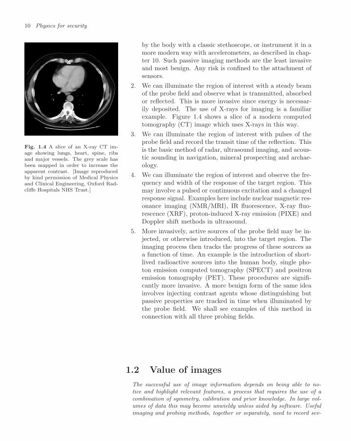
2. We can illuminate the region of interest with a steady beamof the probe field and observe what is transmitted, absorbedor reflected. This is more invasive since energy is necessar-ily deposited. The use of X-rays for imaging is a familiarexample. Figure 1.4 shows a slice of a modern computedtomography (CT) image which uses X-rays in this way.
Fig. 1.4 A slice of an X-ray CT im-age showing lungs, heart, spine, ribsand major vessels. The grey scale hasbeen mapped in order to increase theapparent contrast. [Image reproducedby kind permission of Medical Physicsand Clinical Engineering, Oxford Rad-cliffe Hospitals NHS Trust.]
3. We can illuminate the region of interest with pulses of theprobe field and record the transit time of the reflection. Thisis the basic method of radar, ultrasound imaging, and acous-tic sounding in navigation, mineral prospecting and archae-ology.
4. We can illuminate the region of interest and observe the fre-quency and width of the response of the target region. Thismay involve a pulsed or continuous excitation and a changedresponse signal. Examples here include nuclear magnetic res-onance imaging (NMR/MRI), IR fluorescence, X-ray fluo-rescence (XRF), proton-induced X-ray emission (PIXE) andDoppler shift methods in ultrasound.
5. More invasively, active sources of the probe field may be in-jected, or otherwise introduced, into the target region. Theimaging process then tracks the progress of these sources asa function of time. An example is the introduction of short-lived radioactive sources into the human body, single pho-ton emission computed tomography (SPECT) and positronemission tomography (PET). These procedures are signifi-cantly more invasive. A more benign form of the same ideainvolves injecting contrast agents whose distinguishing butpassive properties are tracked in time when illuminated bythe probe field. We shall see examples of this method inconnection with all three probing fields.
1.2 Value of images
The successful use of image information depends on being able to no-tice and highlight relevant features, a process that requires the use of acombination of symmetry, calibration and prior knowledge. In large vol-umes of data this may become unwieldy unless aided by software. Usefulimaging and probing methods, together or separately, need to record sev-

1.2 Value of images 11
eral properties so as to be able to optimise contrast or answer furtherquestions. In practice, techniques vary in their resolution in time andspace. Each is compromised to some extent and all fall short of whatis ultimately sought. There are further criteria that influence the choiceof method, namely contrast, registration, signal-to-noise ratio, artefacteffects, safety and calibration. In addition there are the socio-economiccriteria of availability of educated staff, patient throughput and accept-ability.
1.2.1 Information from images
Imaging and noticing
Having obtained an image the task is to notice whether it contains animportant message so that action can be taken. A security scan of air-port luggage which produces a good image of a gun inside a suitcase ora medical scan of the brain which shows a tumour is not effective unlessthe features are actually picked up by the security guard or the clinicianrespectively. Images may be formed from measurements of several dif-ferent properties in three dimensions, and the important message maybe hidden in the way in which these have changed with time. Such largedata sets in the four dimensions of space and time are not simple to lookat, and clear evidence may be missed.10
10The reader should note that the illus-trations in this book are all two dimen-sional. Although they may show goodexamples of what is being looked for inimages, they obscure the difficulties ofnoticing or finding it.
In the days when the information could be laid out as a number ofsimple pictures in black and white, the experienced eye of the profes-sional was a sufficiently reliable and quick way to notice and interpretthe evidence. With the vast increase in the volume and complexity ofdata that is no longer generally true. The time required can be too longto examine all by eye. Computer software can help by searching the datavery rapidly using agreed search rules, rules which emulate an initial ex-amination by a professional with all the data available. Features thatare possibly unusual can then be highlighted for the clinician’s atten-tion using colour enhancement and quantitative estimates. Ultimately ahuman, whether doctor or security officer, has to be alerted and actiontaken. This observer is often the slowest link in the chain and needs allthe help that can be given.
Fig. 1.5 A positron emission tomog-raphy (PET) scan of a patient diag-nosed with lung cancer. Because of theasymmetry of the signals from the twolungs, the diagnosis is strongly sugges-tive, even with the poor image reso-lution in the image. (The physics ofthis image is discussed further in chap-ter 8.) [Image reproduced by kind per-mission of Medical Physics and Clini-cal Engineering, Oxford Radcliffe Hos-pitals NHS Trust.]
Symmetry and calibration
It is instructive to think about how we look at pictures or plots of graph-ical information, even in two dimensions, and what we learn by doing so.Sometimes there is some symmetry to the image. From that symmetry,especially if it is slightly broken, we learn something, even starting froma point of complete ignorance. Thus in Fig. 1.5 we first note the sym-metry between the left and right sides of the body. The eye is drawnto the black area in the region of the right lung because of the incom-plete symmetry. One lung is different to the other. The human eye isgood at noticing tumours and other pathologies when they violate a nearsymmetry. The search for symmetry has been an essential item in thephysicist’s tool bag in the past century, and it has proved to be crucial
12 Physics for security
when attempting to unravel the physics of an unknown field, such asparticle physics in the 1960s.
The beauty of symmetry is that it is self-calibrating. Thus, even tosomeone who knows nothing of medicine, the sight of someone walkingwith a limp indicates prima facie that they have a medical problem. Butto go beyond the use of symmetry requires measurement and calibration,and a real quantitative understanding of what is going on. For example,the comparison of two medical images taken on different occasions re-quires calibration and position registration. Using symmetry we simplyneed to compare one part of the image with another.
Without symmetry clinicians compare an image qualitatively withtheir perception of cases they have seen previously. But to use all of theinformation requires a quantitative assessment of the measured valuesusing calibration information to register and compare scans of the pa-tient taken on other occasions. This is not a task for which the unaidedhuman eye was designed. Computer software is better matched to dothe detailed quantitative work for the clinician.
The actual detailed solutions to the technical problems of calibrationand registration depend on the particular modality and lie somewhatoutside the scope of this book. However, we note their importance.
Further investigation
When something unexpected does show up in an image we need to beable to answer more questions. In transport security these might beblunt questions to the traveller.11 In archaeology the questions might be11‘Where did you get this?’, ‘Why
do you have this in your possession?’,‘What is this for?’ or ‘How long haveyou had it?’
about use, provenance or date. In medical imaging the questions mightbe about function, blood flow or growth. Purely anatomical maps oftendo not provide the answer to the questions that the medical clinician isasking. Airport security is a privileged example, for the passenger is onhand to answer the questions. In clinical medicine the patient may tryto answer but have limited relevant sensory information which he or shefinds hard to articulate. In archaeology the witnesses are long gone, thehunter from his arrows or the mason from his stone tablets. Thereforewe need to study with what success it is possible to image the answersto the follow-up questions in addition to the initial purely compositionalor anatomical ones.
1.2.2 Comparing modalities
Space and time resolution
How should we assess different methods of imaging? There are a sig-nificant number of methods to choose from, their differences are oftencomplementary and they are frequently used together. In the following,since it presents the most ambitious list of objectives, we have takenthe example of medical imaging to discuss a basis on which to comparemethods.
Although great advances have been made, there is a long way to go.

1.2 Value of images 13
At best, current methods achieve millimetre spatial resolution in threedimensions and millisecond resolution in time, albeit with different tech-niques. But these fall seriously short of the ability to watch individualcells and detect the onset of pathological cell reproduction, which is thescale ultimately needed to master the medical condition.
Near-field and far-field imaging
In an imaging process a probe acts on an object through a probe field,and the reaction of the object is detected and used to form the image.The spatial resolution that may be achieved in an image of an object ata distance r from the detector using a probe at frequency ω depends onwhether the influence of the probe is near-field or far-field. Qualitativelyspeaking, in the near-field case the interaction between the probe andobject is intimate and involves no significant time delay. In the far-field case the probe field mediates an action at a distance with a delay.The significance of this delay is measured by the phase difference, rω/cradians, where c is the phase velocity of the probe field.
In the far-field region the object–detector distance is sufficient thatthis phase difference is larger than unity, say. The probe field φ is thengoverned in a non-trivial way by the wave equation,
∇2φ − 1c2
∂2φ
∂t2= 0. (1.1)
This determines the wavelength, λ = 2πc/ω. The spatial resolutionwhich comes from measurement of the phase is limited to a fraction12 of 12The actual value of this fraction de-
pends on the noise level but is notsmall.
λ/(2π). It follows that to improve the spatial resolution significantly, ashorter wavelength, that is to say a higher frequency probe field, mustbe used.
However, this dependence of resolution on frequency does not apply inthe near-field where the object–detector distance is not inferred from thisphase difference. In some cases the frequency may be effectively zero.A simple example is palpation, which we already mentioned. Therethe spatial resolution is determined by the size of the fingers of theindividual doing the examination. The dimension of time, and the waveequation, are not involved. Another near-field method is MRI, discussedin chapter 7. The wavelength of the RF used may be 3 m (100 MHz),but the spatial resolution achieved is about 1 mm. This is possiblebecause the probing field is not the radiative electromagnetic field butthe inductive magnetic near-field of NMR, discussed in chapter 2. Thespatial resolution derives from measurement of field signals as a functionof static B-field gradients, and the phase delay between source and objectis not involved. Radar is a far-field method which uses similar frequenciesto MRI but has far inferior spatial resolution. Mechanical probing, too,may be either near-field (palpation) or far-field (ultrasound). The twomethods provide quite different information, as discussed in chapter 9.

14 Physics for security
A list of criteria
We draw up a list against which different modalities may be judged.
1. The spatial resolution in three dimensions (3-D). This maybe described by a point spread function (PSF), the raw im-age shape generated by a point object.13 Alternatively the13We may describe the latter at the
origin by a 3-D Dirac delta function,δ3(r) = δ(x) × δ(y) × δ(z).
resolution may be described in harmonic rather than impulseterms. This is usually expressed in terms of the image con-trast of an object with full sine-wave modulation at a certainspacing, written reciprocally as the number of lines per mm.Thus an optical system whose quality would render an ob-ject of black lines on a white ground with 100 µm spacing asan image with valley-to-peak intensity ratio of 50% can bedescribed as having a spatial resolution of 10 lines per mm at50% contrast. In digital terms a distinguishable element ofa 2-D image is a pixel, a picture element with a certain size.An element of a 3-D image is called a voxel, an elementaryvolume element.
2. Time resolution. If time-resolved images are available, thencomplete images may be recorded for different times, andmovement and velocity may be derived by comparing them.In other modalities velocity itself can be measured and im-aged; an instance is the imaging of Doppler shifts in ultra-sound.
3. Contrast. The images derived from different modalities showup different properties of the bone and tissue, muscle and fat,blood and other fluids. Some tend to show fine detail withpoor contrast; others, strong contrast but poor resolution.For this reason progress has been made by combining datafrom different modalities.
4. Registration. During imaging a patient breathes, his or herheart beats and he or she may move. If optimum spatial res-olution is to be achieved, there is therefore a general problemof referencing images to a coordinate system that co-moveswith the body. Parts of the body that deform or move differ-entially according to the patient’s attitude or muscular ten-sion present the most challenging problem, for example thebreast. Registration between different examinations mustbe made so that changes over periods of weeks and monthscan be tracked. Even more important is the need to relateimages, possibly from different modalities, to the patient co-ordinate system at the point of delivery of therapy. Thebetter the intrinsic spatial resolution, the more demandingthe task of registration. The development of any technique,such as ultrasound, which can deliver images and therapywithin the same coordinate system in a short time interval,has an important advantage in this respect.

1.2 Value of images 15
5. Noise. Every technique is limited to some extent by signal-to-noise ratio (SNR). In some cases we shall find that thisis a compromise also involving spatial resolution, safety andthe rate at which data can be taken and patients scanned.
6. Artefacts. In addition to random noise there are system-atic effects that create features in the image which are notpresent in the object. The understanding, identification andminimisation of these requires the coordinated skills of clin-ician, engineer and physicist.
7. Safety. There are real risks that have to be weighed againstthe potential benefit of a procedure. There are additionalsafety concerns that arise from public perceptions. The pub-lic accepts risk in medicine, and therefore medical safetyneeds to be considered carefully. Regular maintenance, cali-bration and safety checks form a part of the disciplined wayof life with imaging and therapy equipment. A more generaldiscussion of risk follows later in this chapter.
8. Cost and expertise. The cost of making techniques, devel-oped in research laboratories, rapidly available in hospitalsis high. However, the limiting factor is expertise. With morequalified staff more use could be made of expensive equip-ment. The local education and knowledge base is important.
9. Throughput. The total time taken to prepare and execute ascan determines the patient throughput, but calibration andshimming procedures can be time consuming. In a clinicalcontext costs are directly related to throughput.
10. Acceptability. Some scanning modalities form an unpleas-ant or forbidding experience for the patient. They may benoisy, claustrophobic, uncomfortable and protracted. Oftenpatients are being scanned at a time when they are alreadyupset or afraid, such as after an accident or as part of adiagnosis for a cancerous tumour.
11. Calibration. As discussed above the first level of informa-tion in an image comes from comparing one part of an imagewith another. To learn more from an image we must be ableto calibrate the measurements. This will depend in part onmeasurements and images of known reference samples. Inmedicine these are termed ‘phantoms’, usually simple vol-umes of matter of known composition. In scientific archae-ology they are called ‘standards’.
To improve registration the patient may be asked to hold his or herbreath, but this is only possible for short scans. Alternatively, datamay be taken only during a selected phase of the respiratory cycle, butthen the time required to complete a scan is correspondingly increased,patient throughput decreased, unit costs raised and the unpleasant expe-rience for the patient lengthened. These points bear upon one another,and there is a continual need to compromise.

16 Physics for security
1.3 Safety, risk and education
The power of physics to provide information and to diminish real dangers,comes at some risk. This risk needs to be understood, monitored andopenly explained to the public at large. Otherwise physics itself generatesfear and apprehension. In the early days of a new application, whenexperience is fragmentary, monitoring poor, and there are no longtermrecords, safety standards need to be conservative. Later, as knowledge andexperience grow, safety standards may be lowered, so that decisions aremade in the light of the best information available at the time. Legislationand regulation do not make people feel safe. That only comes with theconfidence born of understanding, information, explanation and publiceducation. Unfortunately this is not what normally occurs. Consequently,wrong decisions are made, apprehensions may be increased, and futuredangers incurred.
1.3.1 Public apprehension of physics
The impact of physics on society became a public concern with theadvent of nuclear weapons. The threat of ionising radiation was usedduring the Cold War intentionally to frighten people. This fear was notforgotten, and remains to this day to be exploited as an instrument ofpolitical or terrorist blackmail, independent of the weight of risk actuallyinvolved. Rigid safety standards have not reassured, and the knowledgenow available is largely ignored by the media and the general public. Anobjective of this book is to provide a broad look at such knowledge.
Risks due to ionising radiation should be looked at in the same way asother types of damage, such as laceration and bruising, or tissue over-heating. An important psychological difference is in the ability to sensethe effect. Consider magnetic fields, for example. They carry no risks,but in the absence of education on the subject, the general population isnaturally frightened by that which is apparently influential, but whichcannot be seen or felt. So the popular perception of magnetism includes afear of the unknown, unrelated to any uncertainty in physics. Magnetismis sometimes seen alongside water-divining14 and other ‘mysteries’ that14Alias dowsing or witching in the
USA. lack a scientific basis.Nuclear radiation is associated in the public mind with the idea of
the run-away chain reaction.15 Then to the fear inherited from the era15In fact it is extremely difficult togenerate a chain reaction, as discussedbriefly in chapter 6.
of the Cold War were added concerns about accidents in the nuclearpower industry. Early accidents were hushed up. Later ones were exag-gerated in the media despite subsequent reliable international reports.Both outcomes had perverse effects on public trust that now discourageirresolute politicians from reaching clear policy decisions on the futureof nuclear power, in spite of the threat of global warming. The cur-rent state of knowledge of the effects of ionising radiation is discussed inchapters 3, 6 and 8. Some conclusions are drawn in chapter 10.
Unfortunately, it is in the earlier days of a new use of physics, whenenthusiasm is high, that there is the greatest danger, the least under-standing of risks and the least adequate technology available to monitor

1.3 Safety, risk and education 17
exposure.16 Later, when procedures for monitoring and control are fully 16An early example of a poorly moni-tored risk was the use of X-rays in theso-called pedoscope. This was used inchildren’s shoe shops in the 1940s and1950s. The author recalls his mother’senthusiastic reception of the display ona fluorescent screen showing that histoes and feet were well matched in sizeto the newly acquired pair of shoes. Itis interesting to note that:
1 the scan was applied regularly toall children, not just a minoritywith a serious problem;
2 the standard high street shoeshop would not have had any-one with the skill to calibrateor maintain the equipment reg-ularly;
3 in spite of the fact that the radi-ation levels involved would nowbe considered unsafe, there doesnot appear to be any evidencethat either he or any of his con-temporaries suffered any ill ef-fects.
developed, risks can be more precisely evaluated. This suggests thatsafety levels should be determined in the light of current knowledge, withthe implication that normally they may be relaxed subsequently ratherthan raised, assuming positive experience and improved knowledge. Inpractice the cumbersome machinery of safety legislation is usually to beobserved proceeding in the opposite direction.
There are other cultural pressures. The use of an RF induction loopfor surveillance at an airport, though sensitive to the presence of an elec-trical conductor or magnetic material carried by a passenger, does notprovide an image. Is this technically inferior solution chosen because ithas been decided that it would be dangerous to expose passengers toX-rays on a routine basis? Or is it because it is thought an unaccept-able invasion of privacy to take images of people through their clothes?Was this the right decision? Such broader questions arise in medicalphysics, archaeology and other areas where the choice between differenttechnologies has to be made in terms of risk, benefit and wider culturalsensitivities. Physicists should know what they are talking about, sothat they can contribute to such debates. The media and the publicin general have great difficulty in balancing matters of benefit, risk andacceptability. Consequently those charged with making decisions too of-ten prefer to conceal debate rather than discuss matters openly. Whenthis becomes known, faith in the science suffers unjustly. Ultimately,our ability to survive on this planet may depend on improving the con-fidence and communication that scientists have with the public aboutwhat science can do for everybody. The only solution is a combinationof education and open debate.
1.3.2 Assessing safety
Evolution of acceptable levels of risk
We take a fresh look at safety. This is a subject on which much is writtenand much assumed. What is important is what is known in principle,and what can be monitored in a particular instance. Procedures shouldevolve as knowledge and experience grow and as instrumentation im-proves. Regulation should follow such development, not lead it.
The exposure of the population to sources of energy, whether in thecourse of probing and imaging or otherwise, may be looked at objectivelyin terms of the following levels:
the detectable level at which dose may be reliably measuredand monitored;
the background level within which humans have lived andevolved naturally;
the damage level above which long-term damage is possi-ble as informed by reliable epidemiological study or currentknowledge of causative mechanisms;

18 Physics for security
the lethal level at which breakdown of the functioning of cellsand organisms causes their early death.
Doses at the background level carry no risk, but doses that cannotbe monitored reliably are of concern. Thus diagnostic doses below thedamage level can be considered safe provided that dose monitoring isreliable. Where this implies a narrow window, a significant safety prob-lem exists. As discussed in chapters 8 and 10 cancer therapy involvesthe delivery of localised lethal doses. The problem is to avoid damageto peripheral healthy tissue associated with the difference between thelethal level and the damage level, a window in which some cells will beseriously affected but not all.
The damage level includes special cases, such as metal implants inMRI patients, or the role of iodine in thyroid cancer in the radiationenvironment. Generally establishing confidence in a value for the dam-age level requires continuing high quality research, record keeping andvigilance over long periods.
Thus there should be an expectation that accepted safety levels maybe relaxed as knowledge increases, confidence builds and standards ofmonitoring and instrumentation improve. Often this is not what hap-pens. Safety legislation is often tardy and driven by the conservativeALARA principle, ‘as low as reasonably achievable’. This is ill-foundedfor the following reasons:
it does not relax with improving knowledge;
by concentrating only on achievable levels it ignores the needto balance absolute risks against one another;
it does not take account of the possibility that achievable lev-els may be inadequate, that is to say of questionable safety;
it does not take into account the possibility that achievablelevels may be factors of 10 lower than background levels, andtherefore irrelevant.
With ALARA, technical improvements tend to encourage ever tightersafety standards on the basis that ‘you cannot be too safe’. This state-ment is dangerous. Responsible living depends on a continually updatedbalance between benefits and risks. In an overcautious safety-legislatedsociety the largest and latest risks, for which knowledge is least devel-oped, are incurred preferentially, and older dangers, which may be wellunderstood and far less of a threat, are avoided. The result is that thegreater risk is incurred.
The relative threats of global warming and nuclear power are the primeexample. Another is the balance between the risks of ionising radiation,MRI and ultrasound in medicine. We return to these comparisons in thecourse of the book and again in the final chapter where conclusions aredrawn.

1.3 Safety, risk and education 19
Thermal, resonant and disruptive damage
By interacting with materials, all probing and imaging methods depositenergy to a greater or lesser extent. The most pervasive type of damagecaused by this energy is unspecific and thermal. However, it is alsopossible that the energy absorption is specific, that is associated with aresonance in a non-thermal way. A third possibility is that the energyis absorbed in a disruptive and inelastic fashion.
An unspecific thermal dose may be characterised by the local tis-sue temperature rise. In time, such an increase may be dispersed, forinstance by convection or evaporation. It is well established that anincrease of 1C in the local temperature of human tissue above its normcauses no serious damage, but that a rise of 2C or more can be harm-ful. Temperature excursions at this level occur in tissue as a result ofnormal exercise or a mild fever. The corresponding tolerable specificenergy absorption rate (SAR) that can be dispersed by tissue varies17 17These figures are quite high because
the body responds dynamically in vari-ous ways to reduce any temperature in-crease. They cover a range because ofthe variation in this cooling for differentparts of the body. For example, coolingis poor in the eyes and the testes.
between 2 and 10 W kg−1. At the other extreme a temperature increaseof 21C for a duration of 1 s causes coagulative necrosis.18 So for tem-
18This medical description means thecells are cooked or melted at 56C, aterminal condition for functioning tis-sue.
perature changes, referring to the levels defined above, we may say thatthe background level is 1C, the damage level is 2C and the lethal levelis 21C. The monitoring level presents a problem, for it is difficult tomeasure localised temperature excursions in vivo with precision.
To the extent that the rate of energy deposition or damage in tissue isa non-linear function of the incident energy flux, monitoring and safetylevels need to be more tightly defined. For example, if the damagedepends on the third power of the energy flux and the energy flux wasonly measured to a precision of 10%, the damage would be uncertain atthe level of 30%. So significant non-linearity in tissue response imposesa need for more carefully defined monitoring procedures.
There is always the question whether more serious damage might beinflicted if energy is delivered non-thermally, for instance via a particularlocal atomic or molecular resonance. Whether this is a problem dependson the strength of the coupling of the resonance to the probing field andto the other degrees of freedom of the tissue. These questions have tobe considered in the physics of each case.
The problem of high magnetic fields is exceptional, as no energy isdeposited unless the field changes or there is some movement.19 Because 19Strictly, this refers to movement of
conductors, currents or magnetic ma-terials, but all materials experience in-duced magnetisation or eddy currentsto some degree.
no firm evidence of damage by high steady fields has been reported, themaximum field considered safe in clinical use for MRI has been raisedto 4 tesla. This change has a direct benefit on the signal-to-noise ratiothat may be achieved in MRI, or, equivalently, on the speed with whichsuch scans can be made.20 This is an unusual case in which increased 20These are discussed in chapter 7.knowledge and experience has lead to an appropriate relaxation of safetylevels.
Distinct from either thermal or resonant energy deposition is the dam-age caused by disruption. An example is abrasion, or cuts and bruises.Given time such damage heals. In this case the questions are ‘Whatis the healing time?’ and ‘How much abrasion can be tolerated within
20 Physics for security
that time without incurring permanent damage?’. The energy depositedby ionising radiation causes such rupture of atoms, molecules and cells.The debris tends to be confined to the immediate local path followed bythe individual charged particles, including the secondary ones createdby the absorption of photons. The extent to which such damage getsrepaired, by cell and bio-molecule reproduction, is an important matteraddressed in chapter 6. This gives a risk of long-term damage that de-pends quite non-linearly on the dose integrated over repair time. Theprovision of effective cancer therapy turns on an appreciation of this.The naive assumption that the dependence is linear without a thresholdis called the linear no-threshold (LNT) model and is not credible.
There are also important risks of a more mundane variety. Exam-ples are burns caused through contact with metal probes which becomeoverheated during ultrasound scanning, and impacts by metal objectsaccelerated by the high fringe B-field of an MRI scanner.
The principal regulatory bodies are given below. Their websites maybe consulted for more details. The facts given there are usually reliable,but, regrettably, the ALARA principle and the discredited LNT modelremain deeply embedded in their application in some cases.
Look on the Web
Look at the book website atwww.physics.ox.ac.uk/users/allison/booksite.htm
Find links to simple ideas and developments on gravi-tational fields
gravitational waves LIGO LISAgravitational anomalies
Examine safety and other regulatory websites:
IAEA, the International Atomic Energy Agency
OECD NEA, the Nuclear Energy Agency isa specialised organisation within the internationalOrganisation for Economic Cooperation and De-velopment. Find recent reports on Chernobylat www.nea.fr/html/rp/chernobyl/chernobyl.html andlinks to World Health Organisation Reports
SRP The UK Society for Radiological Protection
NRPB UK National Radiological Protection Board(became part of HPA after April 2005), including thetext of Report, Vol. 14, No. 2 (2003) on RF fields.
HPA UK Health Protection Agency, including ultra-sound. Find Ionising Radiation Exposure of the UKPopulation: 2005 Review, and also search for referencesto ultrasound
ICNIRP International Commission on Non-ionisingRadiation, including the text of Magnetic Resonance2004, Health Physics, 87, 197
USFDA US Food and Drug Administration
NICE UK National Institute for Health and ClinicalExcellence
BMUS British Medical Ultrasound Society
RERF LSS Radiation Effects Research Foundation,Life Span Study, for more information on the studies ofHiroshima and Nagasaki survivors.
HPS The Health Physics Society, for examplehps.org/documents/radiationrisk.pdf

Magnetism and magneticresonance 2
2.1 An elemental magnetic dipole21
2.2 Magnetic materials 27
2.3 Electron spin resonance 34
2.4 Nuclear magnetic resonance37
2.5 Magnetic field measurement47
Read more in books 53
Look on the Web 53
Questions 54
in which are developed the fundamental physics of the single isolatedmagnetic dipole, materials as ensembles of such dipoles, their resonantbehaviour, and magnetic field measurements. This provides the under-lying physics for chapter 7.
2.1 An elemental magnetic dipole
Magnetic forces are weaker than electric ones to which they are a rel-ativistic correction. Current loops, both microscopic and macroscopic,form the basic source of magnetic flux B. The torque on a magneticdipole µ = IS due to a current I in a loop of area S in a field B isΓ = µ × B. A charge Q of mass m circulating in an orbit has botha magnetic moment and an angular momentum. The ratio of these isγ = gQ/2m, where the gyromagnetic ratio g in this case is unity. In aclassical view such a magnetic moment in a uniform B-field precesses withthe Larmor frequency, ωL = γB. In a quantum view the magnetic sub-states mj of an atom are split in energy from one another by hγ∆mjB.The dipole selection rule ∆mj = ±1 ensures that classical and quantumfrequencies are the same. Electron spins, nuclear spins and muon spinsbehave in similar ways to orbital motion but with values of g differentfrom 1. The effective value of g for an electron with both orbital and spinangular momentum is gj given by the Lande formula.
2.1.1 Laws of electromagnetism
Maxwell’s equations in the absence of materials
The basic laws of electromagnetism are known as Maxwell’s equations.In their differential form in the absence of materials these link the fieldsE and B to their sources, the charge and current densities ρ and J ,through the constants ε0 and µ0:
divE = ρ/ε0 (2.1)divB = 0 (2.2)
curlE = −∂B
∂t(2.3)
curlB = µ0J + ε0µ0∂E
∂t. (2.4)
22 Magnetism and magnetic resonance
Equations 2.1 and 2.2 are both known as Gauss’s law. Equation 2.3 isFaraday’s law of electromagnetic induction describing the electric fieldgenerated by a changing B-field. Equation 2.4 is Ampere’s law for the B-field generated by a current density J and displacement current densityε0∂E/∂t. The conservation of charge relates the current flowing out ofunit volume to the rate of change of charge density
divJ = −dρ
dt. (2.5)
Taking the divergence of both sides of equation 2.4 shows that the dis-placement current density term is necessary for the consistency of Am-pere’s law with the conservation of charge. As shown in books on elec-tromagnetism, in the absence of the source terms wave solutions to theseequations exist with velocity c = 1/
√ε0µ0, the velocity of light in vac-
uum.
2.1.2 Current loop as a magnetic dipole
Origin of magnetism
In the first observations of magnetism a sample of iron ore was suspendedin the magnetic field of the Earth. The torque on this ore formed acompass which indicated the direction of the Earth’s B-field, that is thedirection of the magnetic pole.1 This continues to be a very important
1A north (+) magnetic pole is attractedtowards the North. Since opposite signmagnetic poles attract, the North mag-netic pole of the Earth is actually asouth (−) magnetic pole. This is con-sistent with the direction of the B-fieldwhich by convention points from + to−, as for an electric field.
aid to navigation.22There are two conditions for a com-pass to work. Firstly the electron hasto have spin 1
2, so that the unpaired
electron spin of iron gives it spon-taneous magnetisation. Secondly thestatic B-field due to the Earth’s coremust have a long enough range to reachthe Earth’s surface. It may be shownthat this requires that the Comptonwavelength of the photon h/mγc be aslarge as an Earth radius. Thus, fora compass to work, mγ , the mass ofthe photon, must be less than about10−49 kg.
It has been suggested that the dis-covery of America depended on the spinof the electron and such an upper limitto the mass of the photon, althoughChristopher Columbus did not knowthat!
Equation 2.4 shows that the source of the magnetic B-field is the cur-rent density J ; that is, magnetism arises from the movement of electriccharges. Magnetic interactions are relativistic corrections to electric in-teractions and so magnetic energies and forces are expected to be smallerby a factor of order v2/c2. For atomic electrons this factor is typically10−4.
This expectation is rather misleading. Electric fields achieve rathercomplete cancellation except on an atomic scale, while magnetic effectsoften do not. There are two reasons why magnetic forces do not averageout as effectively as electric ones, namely thermodynamics and spin.
The density of electric charge is often balanced, although its flow maynot be. Any significant imbalance of charge density is suppressed by thelarge energy that this would generate. This contrasts with the smallermagnetic energy associated with a significant net charge flow. So ongeneral thermodynamic grounds magnetic forces and net current flowsare not suppressed by cancellation to the same extent as electric forcesand net charge densities.
The electron spin which is equivalent to a circulating charge or currentdoes not balance out effectively in certain kinds of atoms. Because theelectron spin is 1
2 , the net angular momentum cannot be zero unlesselectrons can pair their angular momenta.3
3Such lack of pairing occurs in partic-ular for the transition elements (suchas iron, cobalt, nickel or manganese),the lanthanides (such as cerium, lan-thanum or gadolinium) and the ac-tinides. These have partially filledshells of electrons with high angularmomentum.
Thus magnetism arises from materials that contain these microscopicatomic currents and spins, as well as from currents provided by macro-scopic current loops. However, these microscopic atomic magnets and

2.1 An elemental magnetic dipole 23
the macroscopic magnets of currents are fundamentally the same froman electromagnetic viewpoint.
Macroscopic current loop
The current in such a loop arises from a combination of any directlyapplied voltage source, such as a battery, and the effect of changing B-fields through Faraday’s law of electromagnetic induction, equation 2.3.In the absence of any applied voltage, the electromotive force V inducedin a loop of area S in an externally applied changing B-field is
V = −∂B
∂t· S. (2.6)
Such a loop can be described in terms of its equivalent componentsshown in Fig. 2.1a, a series resistance R, capacitance C and magneticinductance L. The current in the loop I obeys the differential equation
∂V
∂t= L
∂2I
∂t2+ R
∂I
∂t+ CI, (2.7)
where each term is the time derivative of the voltage across each compo-nent. Driven by a harmonic external B-field of frequency ω the currentin the steady state is then given by4
4The time development is assumed tobe of the form exp (j ωt), see the dis-cussion of the choice of complex signconvention in appendix A.
C
L
R
a)
b)
freq./ω ωreal
amp.
imag.amp.
phase
0
1.0 2.0
-π
0ω ω/
0
Fig. 2.1 a) An electrical circuit loop.b) The phase, real and imaginary partsof the induced current in the circuit asa function of the frequency of the ex-ternal applied B-field, in terms of theresonant frequency ω0 = 1/
√LC. The
value of Q is taken as 10 for purposesof illustration.
I = V/Z =−jωB · S
R + jωL + 1/(jωC). (2.8)
The electrical impedance Z is given by
Z = R + jωL +1
jωC. (2.9)
Resonant circuit
The dependence of the phase, the imaginary and real parts of this cur-rent on frequency are plotted out in Fig. 2.1b. They show the generalcharacteristics of a resonance, namely a peak in the imaginary part at theresonant frequency ω0, a phase that changes by π as the frequency passesthrough resonance, and a real part that changes sign at resonance.5 The
5The sign of this phase depends on thephase convention used.
resonant frequency isω0 =
1√LC
. (2.10)
The full width of the peak in the imaginary part at half-maximum energyis γr = R/L, and the Q of the resonance6 is ω0/γr. At resonance the real
6This may be derived from the defini-tion: 2π× the energy stored divided bythe energy lost per cycle.
part of the current amplitude passes through zero and the imaginary partis maximum. Note that below resonance the current produces a B-fieldthat opposes the applied field within the loop and increases it outsidethe loop. Above resonance the situation is reversed.
This may be described as a classical example of magnetic resonance.Next we consider the torque and force on such a small current loop in
a steady B-field.

24 Magnetism and magnetic resonance
Torque on a magnetic dipole in a B-field
Consider a small rectangular coil carrying a current I and placed in auniform field B parallel to the z-axis. The side of length a is parallelto the x-axis and the side of length b lies in the yz-plane at an angle θto the z-axis, as shown in Fig. 2.2. We calculate the force and torqueon this coil, and then express the result in general terms. The force perunit length on a conductor carrying a current I in a B-field is
xy
z θ
Fy
F
a
a
bb
B
y S
θ
Fig. 2.2 A rectangular coil carrying acurrent I placed in a uniform field B.
F = I × B. (2.11)
So the forces on the a sides of the coil are equal and opposite, Fy =±IaB. Although there is no net force along y, the two forces are dis-placed by a distance b cos θ along z. They therefore form a torque in thex-direction of magnitude IabB cos θ. So there is a net torque which canbe expressed with a cross product as7
7The forces Fx on the two b sides arealso equal and opposite with magnitudeIBzb sin θ but are not displaced and donot contribute a torque.
Γ = IS × B (2.12)
where S is equal in magnitude to the area ab and normal to it with aright hand sense determined by the direction of the current I as shown.This is a general result. The torque depends only on the vectors S andB, but not on other details of the geometry.
In SI units the magnetic dipole moment of the loop is defined as
µ = IS. (2.13)
The torque is thenΓ = µ × B. (2.14)
The potential energy of the magnetic dipole in the B-field is found byintegrating the torque over angle,
W =∫ θ
0
µB sin θ′dθ′ = µ · B. (2.15)
Gyromagnetic ratio
Such a current loop also possesses a mechanical angular momentum Lby virtue of the rotating charge carriers which have mass m and chargeQ. If the orbital velocity of the charge is v, then L = mv × r wherewe have now assumed that the loop is circular with radius r for ease ofcalculation. The ratio of the magnetic moment of the rotating chargeto the angular momentum of its orbiting mass is a constant as we nowshow.
The current I in a loop length 2πr is equivalent to a total circulatingcharge Q = 2πrI/v. From equation 2.13 the magnetic moment is thenµ = Qvr/2. The gyromagnetic ratio is then defined as
γ = µ/L = Q/2m. (2.16)
Since the angular momentum L is quantised in units of h, the size ofthe magnetic moment is fixed to be in multiples of hγ. This classical

2.1 An elemental magnetic dipole 25
derivation gives the correct answer for charges in orbital motion as de-termined by quantum mechanics. The magnetic moment of an electronwith L = lh and quantum number l = 1 by virtue of its orbiting motionis defined as the Bohr magneton,
µB = hγ = eh/(2me) = 5.788 × 10⁻⁵ eV T−1. (2.17)
Similarly the moment of a proton charge with l = 1 by virtue of itsorbiting motion is defined as the nuclear magneton,
µN = eh/(2mp) = 3.152× 10⁻⁸ eV T−1, (2.18)
which is three orders of magnitude smaller than the Bohr magneton.For magnetic moments arising from quantum spins the classical pic-
ture described above fails and the magnetic moment is different. Thefactor by which it differs is denoted by the g-factor. For the electron spin,g = 2 as determined by the Dirac equation for an elementary point-likespin- 1
2 fermion, ignoring a tiny correction given by quantum electrody-namics (QED). On the other hand a proton is a composite particle withan internal structure that is not described by the Dirac equation. In itscase the value of g = 5.59 comes from experiment.
Thus with a spin 12 and g = 2 the electron spin magnetic moment is
µB. The magnitude of the proton spin magnetic moment is µp = 2.79µN.
2.1.3 The Larmor frequency
Classical precession
Consider the motion of a current-carrying coil or magnetic moment µin a uniform B-field. As a result of the torque, equation 2.14, the rateof change of angular momentum L of the magnetic dipole is
dL
dt= µ × B. (2.19)
Using equation 2.16 this may be written more usefully as
dµ
dt= γµ × B. (2.20)
If B is constant then dµ/dt is always perpendicular to B. Being alsoperpendicular to µ, the length of µ is constant. So the end of the µ-vector executes circular motion in the plane perpendicular to B. Inother words, µ precesses about B with angular frequency ωL = γB asshown schematically in Fig. 2.3a. This is called the Larmor precession.
μ
B
m = +½
a)
b)
m = ½-
2 Bμ
Fig. 2.3 a) A classical view of a mag-netic moment µ precessing in a B-field.b) The energy of a spin-1/2 magneticmoment µ split by a B-field as seen inquantum mechanics.
Larmor precession in quantum mechanics
This picture of a magnetic moment with a well-defined direction in spaceis essentially classical, and incorrect. In the quantum description the di-rection of the angular momentum of a state, and therefore its magnetic
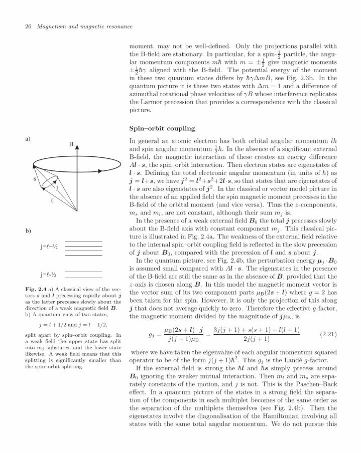
26 Magnetism and magnetic resonance
moment, may not be well-defined. Only the projections parallel withthe B-field are stationary. In particular, for a spin-1
2 particle, the angu-lar momentum components mh with m = ± 1
2 give magnetic moments± 1
2 hγ aligned with the B-field. The potential energy of the momentin these two quantum states differs by hγ∆mB, see Fig. 2.3b. In thequantum picture it is these two states with ∆m = 1 and a difference ofazimuthal rotational phase velocities of γB whose interference replicatesthe Larmor precession that provides a correspondence with the classicalpicture.
Spin–orbit coupling
In general an atomic electron has both orbital angular momentum lhand spin angular momentum 1
2 h. In the absence of a significant externalB-field, the magnetic interaction of these creates an energy differenceAl · s, the spin–orbit interaction. Then electron states are eigenstates ofl · s. Defining the total electronic angular momentum (in units of h) asj = l+s, we have j2 = l2+s2+2l·s, so that states that are eigenstates ofl · s are also eigenstates of j2. In the classical or vector model picture inthe absence of an applied field the spin magnetic moment precesses in theB-field of the orbital moment (and vice versa). Thus the z-components,ms and ml, are not constant, although their sum mj is.
B
j
s
ℓ
a)
b)
j= +½
j= -½
Fig. 2.4 a) A classical view of the vec-tors s and l precessing rapidly about jas the latter precesses slowly about thedirection of a weak magnetic field B.b) A quantum view of two states,
j = l + 1/2 and j = l − 1/2,
split apart by spin–orbit coupling. Ina weak field the upper state has splitinto mj substates, and the lower statelikewise. A weak field means that thissplitting is significantly smaller thanthe spin–orbit splitting.
In the presence of a weak external field B0 the total j precesses slowlyabout the B-field axis with constant component mj . This classical pic-ture is illustrated in Fig. 2.4a. The weakness of the external field relativeto the internal spin–orbit coupling field is reflected in the slow precessionof j about B0, compared with the precession of l and s about j.
In the quantum picture, see Fig. 2.4b, the perturbation energy µj ·B0
is assumed small compared with Al · s. The eigenstates in the presenceof the B-field are still the same as in the absence of B, provided that thez-axis is chosen along B. In this model the magnetic moment vector isthe vector sum of its two component parts µB(2s + l) where g = 2 hasbeen taken for the spin. However, it is only the projection of this alongj that does not average quickly to zero. Therefore the effective g-factor,the magnetic moment divided by the magnitude of jµB, is
gj =µB(2s + l) · jj(j + 1)µB
=3j(j + 1) + s(s + 1) − l(l + 1)
2j(j + 1)(2.21)
where we have taken the eigenvalue of each angular momentum squaredoperator to be of the form j(j + 1)h2. This gj is the Lande g-factor.
If the external field is strong the hl and hs simply precess aroundB0 ignoring the weaker mutual interaction. Then ml and ms are sepa-rately constants of the motion, and j is not. This is the Paschen–Backeffect. In a quantum picture of the states in a strong field the separa-tion of the components in each multiplet becomes of the same order asthe separation of the multiplets themselves (see Fig. 2.4b). Then theeigenstates involve the diagonalisation of the Hamiltonian involving allstates with the same total angular momentum. We do not pursue this

2.2 Magnetic materials 27
here because we shall not need it. However, for the analogous case ofhyperfine structure, the strong field case will be needed, as describedlater.
Precession by electrons, nuclei and muons
Frequency is a parameter which is easily and accurately measured. Manytechnologies depend on measurements of the precession frequency ofmagnetic moments in B-fields. The moments of most interest are thespin moments of the electron, the nucleus (especially the proton) andthe muon. Large parts of this book are concerned with the preces-sion frequency of electron spin as measured with electron spin resonance(ESR) and of nuclear spin as measured with nuclear magnetic resonance(NMR). Investigations with the muon spin resonance (µSR) are largelyof interest to academic research programmes outside the scope of thisbook.
2.2 Magnetic materials
Materials exhibit magnetic behaviour because of the moments of their con-stituent electrons and nuclei. These moments are influenced by the fieldand by their mutual interaction. They may exist without the field (elec-tronic paramagnetism and nuclear magnetism) or they may be induced bythe field (diamagnetism). Nuclear magnetic moments are strongly influ-enced by the electronic magnetic moments. Within the same atom this istermed hyperfine structure, but this influence is also important at muchlonger range.
2.2.1 Magnetisation and microscopic dipoles
Macroscopic magnetisation
Now we look at the magnetic behaviour of a whole ensemble of atomsand molecules in the form of a magnetic material. In this case thereare many magnetic dipoles in a unit volume. These do not all point inthe same direction. The net magnetic moment density M , the mag-netisation, is the vector sum of these. At finite temperature this vector,though composed of quantum vectors, behaves classically and may havesimultaneously well-defined projections on all three cartesian axes. Themagnetisation is both a source of B-field, call it B′, and is itself influ-enced to a greater or lesser extent by the net B-field. The net B-field ismade up of the externally applied field B0 and the field B′. These twosources of B-field are not different in principle. However, traditionallyB0 is written in terms of the H-field8 B0 = µ0H and then
8The H-field is only introduced here inorder to relate the discussion to stan-dard treatments of electromagnetism.We eliminate it and revert to a discus-sion in terms of B, M and the magneticsusceptibility χ.

28 Magnetism and magnetic resonance
B = B0 + B′ = µ0(H + M), (2.22)
where µ0 = 4π × 10−7.If the magnetisation of the medium is in thermal equilibrium, linear
and isotropic, then all three fields (B, H , M) are proportional andcollinear. This is usually written
B = µrµ0H = (1 + χ)µ0H . (2.23)
We can eliminate (and then ignore) the H-field and express µr the rela-tive magnetic permeability and χ the magnetic susceptibility of a mate-rial in terms of the magnitudes of B and M by
µr =(
1 − µ0M
B
)−1
and χ = µr − 1. (2.24)
Both χ and µr are properties of the material and dimensionless in SIunits. Alternatively susceptibility may be given per unit density or permole with consequential change of dimensions. Some examples of χ′
the magnetic susceptibility per mole are given in table 2.1. Often theseare small compared with unity.9 Materials with positive and negative9As a result µr is usually positive.
However, this is not required. If χis less than −1, µr may be negative.This unusual case is discussed in sec-tion 10.5.
values are called paramagnetic and diamagnetic, respectively. These arestatic values. As a function of frequency some materials show resonantbehaviour similar to the circuit shown in Fig. 2.1. We should emphasisethat the use of χ and µr is appropriate to linear isotropic materials inthermal equilibrium.
In the following applications we shall also be concerned with non-equilibrium magnetic states. In that case B and M , although influenc-ing one another, are to be thought of as independent fields which mayvary with time and may not be collinear. We may think in terms of
B = B0 + µ0M , (2.25)
while remembering that this is of limited use since the only B-field thatmay be sensed is the net B.
How does this magnetic response by matter to an applied B-field comeabout? There are three distinguishable effects which are due, in orderof decreasing magnitude, to pre-existing electronic magnetic dipoles, toinduced electronic magnetic dipoles and to pre-existing nuclear magneticdipoles.
Electronic paramagnetism and ferromagnetism
Pre-existing free electronic magnetic dipoles arise from the net angularmomenta of electrons. While the angular momentum of an even num-ber of electrons can pair up to give zero, an odd number of electronscan never do so on account of their intrinsic spin 1
2 . In some materials,although the number of electrons is even, pairing is not favoured. Thediatomic oxygen molecule is an important example of this. Generallytransition and rare earth elements with partially complete inner electron

2.2 Magnetic materials 29
Table 2.1 Values of the static magnetic susceptibility per mole χ′/10−6 cm3 mol−1
for various materials at room temperature, where χ′ = µ0M/B ×mw103/ρ with mw
the molecular weight and ρ the SI density.
Al +16.5 Ba +20.6 Be −9.0He −2.0 Ar −19.3 Xe −45.5F2 −9.6 Cl2 −40.4 I2 −90C −6.0 N2 −12 O2 +3449Cu −5.5 CuCl −40 CuSO4 +1330Cr +167 CrO3 +40 Cr2O3 +1960H2 −4.0 NH3 −16.3 H2O −12FeO 7200 Ge −11.6 Gd 185000
shells also have a net electronic angular momentum J , although this de-pends on the chemical state and degree of ionisation.10 In table 2.1 some 10We loosely follow the convention that
lower case j, l, s refer to the quan-tum state of single electrons and up-per case J, L, S refer to the net angu-lar momentum of several electrons inan atom. To be general in the follow-ing we frequently use upper case let-ters while giving simple single electronexamples. More complex examples ofelectron coupling would be out of placein this book.
examples are given. The first row is a selection of metals. The second,third and fourth rows show typical elements with paired electrons and adiamagnetic susceptibility rising steadily with Z, with the exception ofoxygen. The fifth and sixth rows show that the chemical form of tran-sition elements can affect their magnetic properties. The last two rowsinclude the exceptional behaviour of gadolinium and the large value forferrous oxide. Transition metals that are ferromagnetic, such as iron andcobalt, cannot be given a value because their magnetic behaviour is notlinear.
Unpaired electron angular momenta also occur in chemical radicalsand other non-equilibrium molecular states created by irradiation andother sources of excitation. In solids at room temperature these maybe metastable. The density of such free magnetic moments is impor-tant in archaeology and radiation dosimetry as a frozen record of pastirradiation.
In an applied B-field any pre-existing electronic moments are prefer-entially orientated, causing an increase in the net B-field and a positivevalue of χ. Atoms and molecules with net angular momentum Jh have2J + 1 states with different values of mJ . In a field B these are equallyspaced in energy as gJµBmJB. To make things simple we consider thecase j = 1
2 and g = 2 as an example. There are two states for each spinwith energies +µBB and −µBB in the B-field, so that the net energydifference is E12 = 2µBB.
According to Boltzmann’s theorem of classical statistical mechanicsthe ratio of populations of two states, N2 and N1, in thermal equilibriumat temperature T with an energy difference E12 is11
11With the exception of electrons inmetals quantum statistics is not rele-vant at room temperature in our con-text. It only matters whether the atomsare fermions or bosons if the tempera-ture is much lower and the density ishigh, as in liquid helium or in a Bose–Einstein condensate.
N2
N1= exp(−E12/kBT ), (2.26)
taking due account of any degeneracy, where kB is the Boltzmann con-

30 Magnetism and magnetic resonance
stant. Thus, if the spins do not interact the population ratio of thesestates depends on the temperature T as exp(−2µBB/kBT ). The frac-tion of spins aligned is only µBB/kBT = 2.3 × 10⁻³ in a B-field of 1.0T at room temperature. This shows that in the absence of cooperativeeffects the paramagnetic susceptibility is small and very dependent ontemperature.
The mutual interaction of the moments can be significant at finitedensity, and this can affect the relative population very dramatically.In these circumstances Boltzmann’s theorem is still applicable but theenergy has a large term depending on the mutual orientation of themoments. At a sufficiently low temperature the moments become orien-tated just by their own field. Then all the spins line up and ferromag-netism is observed. That is, a net macroscopic magnetic moment maybe observed, even in the absence of an externally imposed B-field. Thetemperature below which this cooperative behaviour occurs is known asthe Curie temperature.
Electronic diamagnetism
If there are no such pre-existing microscopic magnetic dipoles there isno such first order response and the magnetisation is determined by thesecond order effect known as diamagnetism. This response of materialsto a B-field comes from the current induced in the eigenstates of other-wise symmetrical atoms and molecules. By Faraday’s law this inducedcurrent opposes the applied field leading to a reduction of the net B-field.Since it affects the eigenstates themselves rather than their population,it does not depend on temperature and occurs for all materials, althoughobscured by the larger paramagnetic effect, if present.12 This is respon-12A very important exception is hydro-
gen in water. Because the hydrogen-bond structure of water changes contin-uously with temperature, the electronwavefunction varies also. Therefore theelectronic susceptibility of water, andwith it the NMR chemical shift, is tem-perature sensitive. The shift is 0.01ppm per degree C. This causes a tem-perature dependent phase shift whichis measurable in MRI. This is becom-ing important for thermal mapping inultrasound therapy, as noted in chap-ter 9.
sible for the negative values of χ given in table 2.1. These are usuallysmall although bismuth is an exception.
Metals do not conform to this simple picture. For some there is a smallparamagnetic response because the magnetic field generates an energydifference between the Fermi distributions for different spins. This re-sults in a small spin asymmetry in the population of the conduction bandwhich in turn is responsible for a small paramagnetic effect. This is ofthe same order as the diamagnetic response so that the net susceptibilityis small but varies in sign from one metal to another.
Nuclear paramagnetism
The contribution to magnetic properties made by atomic nuclei is ona much smaller scale. In a magnetic field the magnetic moment of anucleus with spin13 behaves in a similar way to an unpaired electron
13By ‘nuclear spin’ in this context wemean the total angular momentum ofa nucleus. Discussed in terms of nu-clear structure this angular momentummay be composed of a combination ofthe orbital motion of protons within thenucleus together with the intrinsic spinangular momenta of both protons andneutrons. However, we are not con-cerned here with these details of nuclearphysics.
magnetic moment. However, its gyromagnetic ratio is three orders ofmagnitude less, and this is reflected in its energy and Larmor frequency.But what is the value of the nuclear spin, I? All nuclei with an evennumber of protons and an even number of neutrons are known to havezero spin, a fact rationalised, if not explained, in the shell model of nu-clear structure. A majority of stable nuclei, 155 in fact, have such even

2.2 Magnetic materials 31
numbers and zero spin. With the exception of hydrogen, this includesalmost all those with a particularly high natural abundance, for exam-ple 16O, 4He, 12C, 40Ca, 56Fe, 28Si. The remaining 107 stable nucleihave non-zero spin14 and several of these are given in table 2.2 with 14It is found that these even–even nu-
clei have tighter binding than thosewith unpaired spins and lower nat-ural abundance. The fact that themore tightly bound nuclei are alsothe most abundant is witness to thefact that they were created in nuclearsynthesis under conditions of near-thermodynamic equilibrium. This isconsistent with the fact that the Earthis almost entirely composed of theresidue of stellar thermonuclear com-bustion.
the values of their Larmor precession frequency. Hydrogen is the mostimportant entry in this table, because it is abundant and its frequencyis highest. Hence hydrogen nuclei tend to give the strongest and mostuseful magnetic signals.
Table 2.2 Some common nuclei of inter-est with their spin I, value of precessionfrequency γ and relative isotopic percent-age abundance.
I γ AbundanceUnits h MHz T−1 %
1H 12
42.57 99.982D 1 6.54 0.015613C 1
210.71 1.1
14N 1 3.08 10019F 1
240.05 100
23Na 32
11.26 10031P 1
217.23 100
2.2.2 Hyperfine coupling in B-field
Atomic hydrogen in zero B-field
Because nuclear magnetic moments are so small their effect on one an-other is negligible, and there is no nuclear equivalent of ferromagnetism.However, the behaviour of nuclear spins is heavily influenced by nearbyelectrons. The B-field which the nucleus sees is composed of the vectorsum of the local magnetic field due to the electron angular momentaas well as the macroscopic applied field itself. This local field dependson position within the atom and also on the relative location of otheratoms. As an example and to simplify the discussion, we start with thecase of an isolated atom of neutral hydrogen far from any neighbours.
In the absence of an applied B-field the proton magnetic momentaligns either parallel or antiparallel to the B-field due to the electronmagnetic moment. This field is proportional to J and the magneticenergy splitting between these states is proportional to I · J , where Iis the nuclear spin vector and J is the electronic angular momentumvector.15
15In hydrogen we have I = J = 12. We
retain the notation for general I, J .
This is an example of hyperfine structure. In the classical or vectormodel the interaction causes I and J to precess around one another,just as the l and s do in electronic fine structure. The total angularmomentum F = I + J is a constant of the motion. So for atomichydrogen there are four states, a singlet F = 0 and a triplet F = 1 withMF = 0,±1. The three triplet states are degenerate and the singlet isseparated from them by 1.5 GHz, or 6.2 × 10⁻⁶ eV, see Fig. 2.5. Thetransition between the F = 1 and F = 0 states in zero external field isthe famous 21 cm line that makes it possible to observe the existence ofclouds of low density cold atomic hydrogen in interstellar space. This isa magnetic dipole transition and the energy is very small. As a resultthe radiative mean life is long, 11.4× 10⁶ years, but not long comparedwith the collision frequency in cold low density H clouds.
Atomic hydrogen in weak and strong B-fields
When a small magnetic field is applied to an isolated hydrogen atom,the net magnetic moment of the mutually coupled electron and protonprecesses about the applied field. The F=1 state splits into three equallyspaced levels, as shown to the left in Fig. 2.5. This is the Zeeman effect.At a slightly larger field the magnetic force on the electron moment due
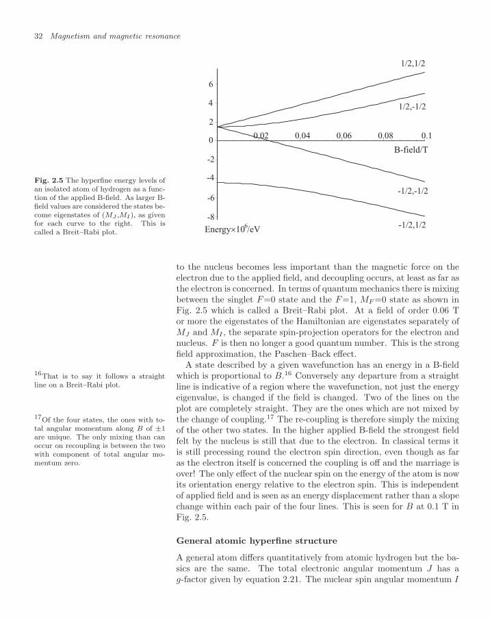
32 Magnetism and magnetic resonance
Fig. 2.5 The hyperfine energy levels ofan isolated atom of hydrogen as a func-tion of the applied B-field. As larger B-field values are considered the states be-come eigenstates of (MJ ,MI), as givenfor each curve to the right. This iscalled a Breit–Rabi plot.
-6
-4
-2
0
2
4
6
0.02 0.04 0.06 0.08 0.1
-8
Energy 10 /eV6
B-field/T
-1/2,-1/2
1/2,-1/2
-1/2,1/2
1/2,1/2
to the nucleus becomes less important than the magnetic force on theelectron due to the applied field, and decoupling occurs, at least as far asthe electron is concerned. In terms of quantum mechanics there is mixingbetween the singlet F=0 state and the F=1, MF =0 state as shown inFig. 2.5 which is called a Breit–Rabi plot. At a field of order 0.06 Tor more the eigenstates of the Hamiltonian are eigenstates separately ofMJ and MI , the separate spin-projection operators for the electron andnucleus. F is then no longer a good quantum number. This is the strongfield approximation, the Paschen–Back effect.
A state described by a given wavefunction has an energy in a B-fieldwhich is proportional to B.16 Conversely any departure from a straight16That is to say it follows a straight
line on a Breit–Rabi plot. line is indicative of a region where the wavefunction, not just the energyeigenvalue, is changed if the field is changed. Two of the lines on theplot are completely straight. They are the ones which are not mixed bythe change of coupling.17 The re-coupling is therefore simply the mixing17Of the four states, the ones with to-
tal angular momentum along B of ±1are unique. The only mixing than canoccur on recoupling is between the twowith component of total angular mo-mentum zero.
of the other two states. In the higher applied B-field the strongest fieldfelt by the nucleus is still that due to the electron. In classical terms itis still precessing round the electron spin direction, even though as faras the electron itself is concerned the coupling is off and the marriage isover! The only effect of the nuclear spin on the energy of the atom is nowits orientation energy relative to the electron spin. This is independentof applied field and is seen as an energy displacement rather than a slopechange within each pair of the four lines. This is seen for B at 0.1 T inFig. 2.5.
General atomic hyperfine structure
A general atom differs quantitatively from atomic hydrogen but the ba-sics are the same. The total electronic angular momentum J has ag-factor given by equation 2.21. The nuclear spin angular momentum I

2.2 Magnetic materials 33
4 8 12 16 20
r/a0
10
1
0.1
0.01
B/T
Fig. 2.6 The on-axis B-field due toan isolated unpaired electron spin as afunction of radial distance in units ofthe Bohr radius, a0.
may also be other than 12 and has its own gI-factor, so that µI = µNgII.
The coefficient of the coupling energy I · J is an independent variablewhich in the absence of an external B-field will split each atomic levelinto 2I + 1 or 2J + 1 hyperfine levels, whichever is the less. Each ofthese hyperfine levels has its own value of F and in the presence of aweak B-field splits into 2F + 1 components. As a result the number ofstates whose energies are tracked as a function of B-field in the Breit–Rabi plot is increased compared with atomic hydrogen. Qualitatively,however, the same type of behaviour occurs and we do not need to pursuedetails.
Range of the electronic paramagnetic B-field
The magnetic field of a non-zero electronic J has a significant influenceon the precession of nuclei over a long range. The B-field of an isolatedelectronic magnetic dipole with moment µ in units of µB at a distancer in the direction of unit vector n is given by
B =µ0µB
4πr3[3n(µ · n) − µ]. (2.27)
It is useful to consider the range at which this field would have influenceon a nuclear moment. The on-axis field is plotted out in Fig. 2.6. It isevident that within a range of about three atomic radii the electroniclocal field is large on the scale of 1 T. A nucleus sensitive to field vari-ations at the level of 100 ppm (parts per million) would be significantlyperturbed even at distances of 20 radii. As nuclei are sensitive to fieldvariations at the level of 1 ppm, it is clear that nuclear precession ishighly sensitive to small concentrations of unpaired electronic angularmomenta.

34 Magnetism and magnetic resonance
2.3 Electron spin resonance
Energy differences between electronic magnetic substates are small. Elec-tric dipole transitions between them are forbidden and the spontaneousrate of the allowed magnetic dipole transitions is negligible. Because theenergy differences are much less than thermal energies kBT , the popu-lation differences are small. For states with J = 0, transitions can beobserved between electronic states in magnetic resonant absorption. Suchstates have unpaired electron angular momenta and their observation mayyield information on the irradiation history or indicate the presence ofchemical radicals.
2.3.1 Magnetic resonance
Absence of spontaneous radiative relaxation in magneticresonance
Consider the states described in the Breit–Rabi plot, Fig. 2.5, as anexample. The only difference between them is the direction of the nu-clear and electronic spin angular momenta. They have the same orbitalangular momentum and therefore the same parity. An electric dipoletransition between any of them would require a change of orbital angu-lar momentum and parity, and is therefore forbidden. Magnetic dipoletransitions may be allowed but the spontaneous decay rate varies withE3. The transition energy E, even for the electronic magnetic splittingsis only of order µBB which is very small even in a high field.
Although spontaneous transition rates are negligible, induced transi-tions are important. The long spontaneous mean life τ implies that thestates are very narrow in resonant frequency, γr = 1/τ . An applied RFfield tuned to exactly the right frequency induces transitions. In fact theinduced transition rate describes both absorption or emission, becausethe matrix elements for these two processes are the same.1818If the RF field is sufficiently intense
the populations of the upper and lowerstates may become equal. Then therates of stimulated emission and ab-sorption are the same and the transi-tion is said to have been saturated.
In electron spin resonance (ESR), also called paramagnetic resonance,the electron spin is excited by an RF field in the presence of a B-field.The coupling environment of the electron spin has a significant effecton the resonant frequency as described by the gJ -factor, discussed insection 2.2.
ESR without orbital motion
For a simple isolated electron spin with g = 2 the resonant angularfrequency is 2µBB/h or 28 GHz T−1. If a B-field of 0.34 T is chosen,the frequency is 9.5 GHz with λ = 0.032 m, in the middle of the X-band microwave region. The energy difference E12 = 3.9 × 10⁻⁵ eV issmall compared with thermal energy, kBT = 2.5 × 10⁻² eV at roomtemperature. In thermal equilibrium the number of electrons with spinparallel N+ and antiparallel N− is given by equation 2.26, so that the

2.3 Electron spin resonance 35
excess fraction of parallel over antiparallel spins is
N+ − N−N+ + N−
≈ 12
[1 − N−
N+
]=
12
[1 − exp
(−2µBB
kBT
)]≈ µBB
kBT. (2.28)
At B = 0.34 T this fraction is 0.78 × 10⁻³. So that, although the num-ber of unpaired electrons in a sample may be large, the net macroscopicmagnetisation at thermal equilibrium is small. With N unpaired elec-tron spins per cubic metre the net magnetisation at a temperature Tis
M ≈ Nµ2BB
kBT. (2.29)
In general there is a factor gj compared with the pure electron sping = 2, and there is a multiplet of states with their Boltzmann factors,all close to unity. We do not need the detail here.
In any case there is a macroscopic magnetisation M which couplesto the RF field. The magnetic dipole selection rule ∆mj = 1 ensuresthat despite the multiplet there is only one resonant frequency, althoughthis will be proportional to gj and therefore depend on the atomic andmolecular coupling. The amplitude of the resonant absorption signalsdepends on M . It should therefore increase linearly with the B-field anddepend inversely on the temperature T .
This suggests that to enhance the signal a large value of B should beused. In practice there are difficulties in doing this effectively. A typicalexperimental arrangement is described below. The medium of interesthas to be placed in a microwave resonant cavity which is necessarily nomore than about one wavelength in size. The problem is that a higherfield implies a shorter wavelength and thence a smaller cavity. Thusbeyond a certain value the choice of a higher B-field does not result ina larger signal because the sample size is reduced.
Hyperfine structure in ESR
What role does nuclear spin play in ESR? Usually there is no role, be-cause most nuclei are spinless.
If the nucleus has spin, the frequency of ESR is determined by the en-ergy differences between the states at the value of the B-field on a Breit–Rabi plot. As an introductory example we consider again transitions inatomic hydrogen. In the weak B-field region to the left in the plot, M1resonance transitions occur between members of the triplet and the sin-glet (∆F = 1) and also between neighbouring members of the triplet(∆MF = ±1). At higher B-field to the right in the Breit–Rabi plot, the
M
M
M
M
M
M
M
M
,M
,M
,M
,M
,M
,M
,M
,M
,
,
,
,
,
,
,
,
J
J
J
J
J
J
J
J
I
I
I
I
I
I
I
I
=
=
+
+
=
=
=
=
+
+
=
=
+
+
+
+
_
_
_
_
_
_
_
_
1
1
1
1
1
1
1
1
1
1
1
1
1
1
1
1
2
2
2
2
2
2
2
2
2
2
2
2
2
2
2
2
_
_
_
_
_
_
_
_
_
_
_
_
_
_
_
_
NMR transitions
M = 0, M = ±1
ESR transitions
M = ,Δ ±1 M = 0
J
J
I
I
a)
b)
ΔΔ
ΔΔ
Fig. 2.7 The ESR and NMR transi-tions in an (I = 1
2, J = 1
2) atom, such
as atomic hydrogen, in a B-field largeenough to break the IJ coupling (e.g.0.1 T in atomic hydrogen).
ESR transitions are those that flip the electron spin. That is, betweenstates with ∆mJ = ±1 and ∆MI = 0, as shown in Fig. 2.7. The nuclearspin transitions with ∆mJ = 0 and ∆MI = ±1 are NMR transitions inthe strong paramagnetic environment in which the nuclear orientationenergy is determined by the electronic B-field, not the applied B-field.From Fig. 2.7 we see that there are two such ESR transitions, betweenthe highest and lowest states and between the two middle states. The

36 Magnetism and magnetic resonance
energy of the two transitions differs since I · J changes from parallel toantiparallel in one case, and from antiparallel to parallel in the other. Sothe gross dependence of the resonant frequency of the two transitions onthe B-field is determined by the electronic gj-factor. Their difference isan example of the hyperfine splitting of ESR spectra. When I and J aregreater than 1
2 there is an additional term in the Hamiltonian due to theelectric quadrupole moment of the nucleus. We shall not explore thisdetail here although it affects NMR (and MRI) for nuclei with I > 1
2 .
2.3.2 Detection and application
ESR apparatus
klystron
attenuator detector
sample incavity with
B-field
loada)
b)
Fig. 2.8 a) A schematic diagram of theelements of an ESR experiment con-nected by lengths of waveguide. b) Thecurve shows a trace of the RF ampli-tude detected as a function of the mod-ulating B-field with a minimum at res-onance.
Figure 2.8 shows a simplified diagram of the components of an ESR spec-trometer. The klystron microwave source is connected by a rectangularwaveguide to an attenuator, a cavity containing the sample of materialin a uniform B-field, a diode detector to measure the RF field amplitudeand a dump load. The radio frequency is constant and data are taken bymodulating the amplitude of the B-field very slightly, thereby sweepingthe value of the resonant frequency back and forth relative to the fixedvalue of the applied radio frequency. Data are recorded by observingthe phase of the modulation at which maximum absorption of the RFwave occurs, as shown by the trace in Fig. 2.8b. In fact the signal isusually shown differentiated with the curve passing through zero at reso-nance. The amplitude and phase of the signal seen by the diode detectorenables the frequency, width and amplitude of the resonant absorptionby the sample to be measured. The attenuator is required because theabsorption easily saturates. If a higher power level is employed, the pop-ulation difference between the upper and lower states which is alreadysmall falls towards zero. As the population of the upper state rises to-wards 50%, the energy emitted by stimulated emission becomes equalto the energy absorbed by excitation. This is the saturation conditiondiscussed earlier.
Applications of ESR
Studies of the frequency shifts in ESR are used extensively in research inchemistry and biochemistry. Molecular fragments or chemical radicalsfrequently have unpaired electron states with characteristic ESR spectra,values of gj in fact. These stand out in the presence of ground statechemical species with paired electron angular momenta and no ESRresponse. ESR is therefore a prime tool in the investigation of chemicalreaction mechanisms where short-lived molecular fragments with theirunpaired electrons are the interesting agents.
ESR is also used in other applications which give rise to unpairedelectrons. In particular the chemical debris that results from the ex-posure of material to ionising radiation includes a significant density ofunpaired electrons. Such unpaired electrons may migrate and pair upwith a relaxation time which may be fast in liquids and gases. In solids

2.4 Nuclear magnetic resonance 37
the relaxation times may be very slow indeed. Single electrons may betrapped by crystal dislocation and vacancy sites. Some of these sitesmay themselves have been created by irradiation. Relaxation times arereduced dramatically by heating or melting. Thus ESR has uses in mea-suring time-integrated radiation exposure and, thence, in archaeologicaldating. It is also important in the study of the effect of sterilisation offood by irradiation.
In general ESR has two big advantage over NMR at the same B-field.The larger energy splitting between the states gives a larger populationdifference. The magnetic moment associated with each member of thispopulation excess is also larger. In consequence signal-to-noise ratio isnot a problem in ESR. In addition the frequency shift associated withdifferent values of gJ is a large effect. So ESR frequencies have a firstorder dependence on the electron environment.
But ESR also has a number of significant disadvantages comparedwith NMR in addition to the short wavelength and limited sample size.The strong coupling of the resonances to the crystal lattice through theelectron wavefunction brings short electron spin relaxation times andtherefore broader resonances. In other words the Q of the resonances islower. If high B-fields are used the frequencies are much higher and thisbrings added technical problems. Advances are being made, and newapplications including spatially encoded ESR may be expected. Thesehave the prospect of fine resolution over small regions.
2.4 Nuclear magnetic resonance
NMR between nuclear states has lower frequency, higher Q-value butmuch smaller signal size than ESR. The motion of the net magnetisa-tion is given by the Bloch equations. The precise value of γ (the chemicalshift), and the relaxation rate caused by local variation in the magnitude(T2) or direction (T1) of the applied field, can all be measured. The ma-terial in a uniform steady field B0 may be excited by an RF pulse at theresonant frequency. The amplitude, phase, frequency and polarisation ofthe resulting free induction decay (FID) signal is measured over the pro-tracted period of the slow return to thermal equilibrium. By applying anRF pulse to invert the spin population during the decay, an echo signalmay be generated whose amplitude is insensitive to non-uniformities inthe applied B-field.

38 Magnetism and magnetic resonance
2.4.1 Characteristics
History
NMR was discovered in 1946 separately by Bloch and Purcell. Fromthose early days the small frequency shift determined by the electronicenvironment of the nucleus has been exploited in investigations in chem-istry and biochemistry. The extension of NMR to imaging, now de-scribed as magnetic resonance imaging (MRI), dates from a short paperby Lauterbur in 1973. In this chapter we discuss NMR. In chapter 7 weextend the treatment to MRI and spatially resolved magnetic resonancespectroscopy (MRS).
Energy and population differences
NMR depends on the relative energies of states with different nuclearspin orientation in an applied B-field. We saw in section 2.2.2 how ina paramagnetic material the local B-field seen by the nucleus is domi-nated by the effect of the unpaired electron moments. For diamagneticmaterials the effect of electronic moments is only a small correction tothe orientation energy of nuclei in an applied B-field. The orientationenergy difference between states is given by hγB where γ is given intable 2.2 for nuclei of interest. For instance, for hydrogen in water or fatwhere the electrons are diamagnetic, the energy splitting between thestates in a 1.5 T field is 2µpB = 2.6 × 10⁻⁷ eV.
According to the Boltzmann distribution, equation 2.26, it followsthat in thermal equilibrium the excess of protons with spin parallel tothis field compared with all protons is a fraction 5.3 × 10⁻⁶ at roomtemperature. Compared with ESR at the same field the fraction ofaligned spins is smaller by µp/µB and the magnetic moment per spin issmaller by the same factor. The net magnetic moment per unit volumeis
M =Nµ2
pB
kBT, (2.30)
where N is now the hydrogen concentration (m−3). This is six orders ofmagnitude smaller than the comparable figure for ESR and can only beenhanced by using the highest possible B-field and the lowest possibletemperature. In the chemistry or biochemistry research laboratory suchchoices may be made. However, for applications in clinical medicine themaximum B-field is limited on safety grounds, and the use of cryogenictemperatures is excluded, so that NMR signals are small and the signal-to-noise ratio is a limitation.
One way around this difficulty is to use spins that are not in ther-mal equilibrium. Such hyperpolarised states are discussed later in thischapter in connection with the measurement of magnetic fields. Recentwork has shown that the polarisation of hyperpolarised 129Xe may betransferred to the state of other nuclei such as 13C. This has opened upthe prospect of important new applications.

2.4 Nuclear magnetic resonance 39
Quality factor of resonance
Relaxation by spontaneous emission is effectively forbidden as discussedin section 2.3.1. Therefore once a distribution of nuclear spins becomesexcited from its equilibrium Boltzmann value, the only way that it canrelax back to equilibrium is through the interaction of the spins withapplied fields and with the atomic and molecular environment. However,such interaction is weak and relaxation mean lives τ are typically 100–1000 ms or even longer.
To be precise, we consider the energy of the excited state with fre-quency ωL to decay as exp (−t/τ). So the amplitude of such a wave hasa time dependence
exp[−i
(ωL − i
12τ
)t
].
Taking the Fourier transform gives the frequency dependence of thisresonance amplitude a(ω) in the form of a narrow peak at ωL. Theresonance width γr is defined as the full width at half maximum of thispeak plotted as intensity |a(ω)|2. Then γr = 1/τ as may be derived inanswer to question 2.4.
The quality factor Q is the dimensionless ratio of the energy of theresonance to its width,
Q = E/hγr = ωLτ. (2.31)
It follows that excitations with the above range of relaxation times havevalues of Q typically in excess of 108. This is a significant conclusion.19 19We may generalise. Any system in
physics that displays a high Q is fertileground for applications.
It is responsible for the fact that detection of NMR excitation is possi-ble despite the weak signal strength. Within the narrow bandwidth ofthe signal the random noise is reduced proportionally. Furthermore, anoscillator with such a high Q can act as a very precise probe because itoscillates coherently for a long time throughout which its phase accu-mulates sensitivity to small perturbations. It is technically convenientthat NMR resonances occur in the 100 MHz region. At such frequen-cies it is particularly straightforward to measure not only amplitude andfrequency, but also absolute phase and signal polarisation as well. Howmuch easier it would have been for the X-ray analysis of DNA and othermolecular structures, if it had been possible to measure the phase ofX-ray signals as simply!
2.4.2 Local field variations
The Bloch equations
The equations of motion of the net macroscopic magnetisation M areknown as the Bloch equations. We use a set of unit vectors i, j, k alongthe x, y, z axes. In the absence of an external RF field and with aconstant applied field B along k we have
dM
dt= γM × B − (Mxi + Myj)
T2− (Mz − M0)
T1k (2.32)

40 Magnetism and magnetic resonance
0
0.2
0.4
0.6
0.8
1
1 2 3 4 5
M(t
)/M
(t=
0)
(t)/
M(t
=0
)
t/T
-0.8
-0.4
0
0.4
0.8
1 2 3 4 5
Mz
z
t/T
a) b)
2
1
xy
xy
Fig. 2.9 a) The exponential decay of the transverse magnetisation with time constant T2 relative to its value at t = 0.b) The exponential recovery of the longitudinal magnetisation towards thermal equilibrium with time constant T1 relative toits value at t = 0.
where M0k is the longitudinal magnetisation at thermal equilibrium.The first term on the right hand side describes the precession of M aboutB, as derived in section 2.1.3. The second and third terms describe therelaxation of the transverse and longitudinal components of M withtime constants T2 and T1 respectively. These may appear similar at themacroscopic level but have a quite different microscopic interpretation.
The time T1 describes the rate at which the relative number of upand down spins relaxes towards the thermal equilibrium value discussedabove. It depends directly on the transition rate between the nuclearspin orientation states and is the relaxation connected with the actualresonance width γr = 1/T1.
The relaxation time T2 does not describe any changes in state or relax-ation at the microscopic level. It arises from a loss of agreement on thephase of the Larmor precession between different protons, a loss of syn-chronisation, caused by the variation in the B-field that they experienceat their various locations within the material.
Therefore in a steady applied B-field the Bloch equations describe amacroscopic magnetisation of two parts.
A transverse magnetisation which rotates in the xy-plane atthe Larmor frequency and has a magnitude that decays withtime constant T2, as illustrated in Fig. 2.9a.
A longitudinal magnetisation with a magnitude that relaxestowards its non-zero thermal equilibrium value with timeconstant T1, as illustrated in Fig. 2.9b.
The Bloch equations of motion apply equally to ESR and NMR, al-though the values of the various parameters are significantly different.20
20The coupling of ESR to the crystallattice is very much stronger than inNMR and the Larmor frequency higher.Consequently the relaxation times arequalitatively shorter.
They may also be used to describe the behaviour of spins in the B-fieldof an RF wave at resonance, as discussed later in section 2.4.4.

2.4 Nuclear magnetic resonance 41
Sources of local B-field variation
The behaviour of a non-equilibrium state of proton magnetisation withtime is affected by variations in the local B-field that each constituentproton experiences.21 Such a variation may be in the magnitude or in
21We refer to protons, but other nucleiwith spin behave in a similar way.
CH CH COCH
a
b
c
abc
33 2
012345
ppmchemical shift
O
Fig. 2.10 The high resolution NMRspectrum of methyl propionate. Hydro-gen atoms are in three types of posi-tions, a, b and c. Each has its own fre-quency in the spectrum separated by afew ppm with normalisation 3:2:3. Athigh resolution each peak is split inton + 1 sub-peaks where n is the numberof hydrogen atoms on the neighbouringcarbon atom. This sub-structure allowsidentification of radicals but it is not re-solved in imaging applications.[Spectrum sourced from SDBSWebat www.aist.go.jp/RIODB/SDBS/(National Institute of Advanced Indus-trial Science and Technology, 29 Jan06).]
the direction of this local field. The variation may be constant in time,depending only on the site, or it may be time dependent. In particular itmay be time dependent because the proton itself moves from one placeto another during the period between excitation and readout.
Table 2.3 The values of the chemical shiftfor a proton at certain molecular sites.
Molecular site Freq. shift (ppm)
Lactate 4.1Fat –CH2– 1.32
Water 4.7NAA (CH3) 2.0/2.48–2.64
Choline N(CH3)3 3.2Creatine N(CH3) 3.03/3.94
If the proton spin is coupled to a paramagnetic electronic J the NMRtransitions are those with ∆MJ = 0, ∆MI = ±1. For example, inatomic hydrogen these NMR transitions which are between the uppertwo states or between the lower two states shown in Fig. 2.5 are nearlyindependent of the B-field altogether except at the lowest fields. Thisis because the proton has an orientation energy determined by the fieldof the unpaired electron, not by the applied B-field. As described byequation 2.27 and plotted in Fig. 2.6, this influence will dominate withintwo or three atomic radii but also cause a change in the local B-field, andtherefore a significant shift in NMR precession frequency, at a distanceof many tens of atomic radii.
Far removed from any unpaired electron, a proton will still be influ-enced slightly by the medium through its diamagnetic properties. Ina uniform medium to a linear approximation, if χ is the magnetic sus-ceptibility of the macroscopic material then fractional NMR frequencyshifts of order χ are to be expected. For values of χ, see table 2.1.
Chemical shifts
However, this is not a satisfactory description of the microscopic B-fieldseen by a proton. Within a macroscopic medium in a uniform B-field,protons at different chemical sites will see different local fields unrelatedto the average macroscopic response described by χ. A proton in water,a proton in a saturated hydrocarbon chain, –CH2–, and a proton ina hydroxyl group, –OH, all have different local electron densities andslightly different local B-fields. A molecule placed in a uniform field willhave a discrete spectrum of such frequencies. Each peak is characteristicof a type of site, and the relative amplitude or peak area indicates thenumber of such sites. These discrete shifts, called chemical shifts, are atthe part-per-million (ppm) level. This is illustrated in Fig. 2.10 for thehydrogen atoms in the organic compound, methyl propionate. Examplesof proton chemical shifts which act as signatures in clinical studies ofmetabolism and its disorders are given in table 2.3. Zero shift is definedby the spectrum of tetra-methyl silane.22 On this scale the shift for water
22This molecule, Si(CH3)4, is chosenbecause it has 12 hydrogen atoms, allin identical chemical positions with noeffects due to hydrogen bonding.is 4.7 ppm and the shift for fat, –CH2–, is about 1.0 ppm.

42 Magnetism and magnetic resonance
2.4.3 Relaxation
Precession dephasing by variation of the field magnitude
The variation in NMR frequency is not limited to the discrete valuesassociated with particular chemical sites. Especially in liquids and gasesthere is a continuum of magnetic environments experienced by protonspins as they move about. Thus there is a spread of values of local B-field that depends in a continuous way on the position of molecules inthe neighbourhood, especially if any of these should contain an unpairedelectron moment. This implies that the magnetisation associated withindividual protons will precess at slightly different rates and that the netmacroscopic integrated transverse magnetisation will die away as contri-butions become progressively ‘dephased’, as sketched in Fig. 2.9a. Themean decay time of the transverse magnetisation is named T ∗
2 . Since thedecay is not primarily thermal in origin it does not depend significantlyon temperature. The component of magnetisation along the B-field re-mains unchanged because it is not affected by precession.
The variation in the magnitude of B-field responsible for T ∗2 has three
different contributions. These are the non-uniformity of the applied field,the position-dependent variation of the microscopic B-field experiencedby hydrogen at different sites and the effect of migration of hydrogenatoms for one site to another during the measurement period. Whilethe relaxation time T ∗
2 is used to describe all three, the time T2 is usedto describe the last only.
A variation of 1 part in 107 in the magnitude of the macroscopic ap-plied B-field generates a phase slip at 100 MHz of 2π in 100 ms. Thusapplied field uniformity at this level or better is a concern in NMR. How-ever such dephasing is reversible by the spin echo technique, discussedlater in section 2.4.5. The effect of microscopic site-dependent field vari-ations is also reversible. Only if the proton wanders about from onelocation to another during the signal decay time is the dephasing not re-versible. This irreversible part is T2. The importance of the distinctionbetween T2 and T ∗
2 will become more apparent in section 2.4.5. Somesample values of T2 are given in table 2.4 for various tissue materials.
Spin state population relaxation by variation of the fielddirection
The variation in the magnitude of the local B-field discussed above af-fects the transverse magnetisation through dephasing, but leaves thelongitudinal magnetisation unchanged. The longitudinal magnetisationis determined purely by the relative population of the spin states, notby their energy splitting. In the absence of spontaneous (or induced)transitions this population can only change if the spin states are mixed.In quantum mechanics that is only possible if the quantisation axis isrotated. Only changes in the direction (not the magnitude) of the localB-field will have this effect.
Changes in the B-field direction can arise from local fluctuating trans-

2.4 Nuclear magnetic resonance 43
Table 2.4 Values of T1 and T2 in milliseconds for hydrogen atoms in various tissuesand at various applied B-fields. These values are given without errors for illustration.
Tissue T1 (ms) T2 (ms)B = 0.2 T 1.0 T 1.5 T
Fat 182 241 259 85Muscle (skeletal) 372 732 868 45Brain – white matter 390 683 786 90Brain – grey matter 495 813 921 100Cerebral spinal fluid 1400 2500 3000 1400
verse magnetic moments, for instance from the thermal motion of mag-netic moments and charges. In liquids and gases the fluctuation is to beunderstood as occurring in the form of collisions for which the matrixelement includes a coupling between the nuclear moment and the trans-verse interacting magnetic field or electric field gradient. In consequencethere is a probability that the proton spin is flipped in a collision. Insolids there are no such collisions. In this case the time dependenceis to be seen as coming from the thermal vibrations of the ions of thelattice, acoustic waves or phonons, and their accompanying local mag-netic or electric field perturbations. It is found that the nuclear electricquadrupole moment (if present) with its coupling to electric field gra-dients is as important as the magnetic coupling to the spins. For bothfluids and solids the response of the electron wavefunctions to the per-turbation and its effect on the nucleus are complicated.
However, there are two simple conclusions.Firstly, fluctuations in B-field direction are intrinsically thermal, so
that T1 decreases with temperature. In fluids this is because a thermallydriven flux determines the relaxation rate via a spin-flip cross section.In solids a flux of phonons is thermally generated.
Secondly, T1 increases with the value of B0. This may be seen clas-sically as follows. The state mixing and the relaxation depend on theangle through which the quantisation axis is rotated during the collision,and this angle is roughly equal to the transitory local B-field divided bythe steady B0. More precisely, in a perturbation theory picture the mix-ing that occurs during a collision depends on the perturbation energydivided by the energy separation of the spin states. Since the latter isproportional to B0 we have the same result.
T1 is typically much larger than T2, while T ∗2 is even shorter. Some
values are included in table 2.4. In section 2.4.5 we discuss how thesedifferent time constants may be determined experimentally.

44 Magnetism and magnetic resonance
2.4.4 Elements of an experiment
Solenoid for the field B0
The basic apparatus needed for an NMR experiment starts with a sourceof the steady uniform field B0 which should be as high in strength assafety and resources permit. The most effective way to make a region ofuniform magnetic field is to employ a large solenoidal magnet and use arelatively small volume around its centre of symmetry. In addition shim-ming coils can be used to reduce further the field variations throughoutthis region. Because of the size and stability required, this magnet isusually chosen to be superconducting and powered continuously.
Coil for the RF field
a)
b)
c)
Fig. 2.11 a) A cylindrical birdcage coilwith N = 18 elements.b) A view of the current elements inthe same view as a). The currents areof equal magnitude, each with a phasedelay 2πn/N matching its geometricalazimuth in the structure. Thus In =I0 sin(ωLt + 2πn/N).c) A view looking along the coil axisand showing the resulting interior uni-form field B1, which rotates at the ra-dio frequency ωL. The dots representsections through the longitudinal con-ductors of the coil.
Around the uniform field volume and enclosing the sample is an RF ex-citation coil. This coil is fed with a short excitation pulse at the Larmorfrequency. A design commonly encountered is shown in Fig. 2.11 andconsists of a symmetric array of circuits forming longitudinal elements ofa structure that looks like a birdcage. The axis of the birdcage is alignedwith the field B0. The magnitude of the currents In in the n elementalcircuits are all equal but the phase of each is equal to its azimuthal an-gle in the structure. The polarisation of the resulting RF field takes theform of a near-uniform B-field rotating at the Larmor Frequency in theplane perpendicular to B0, as illustrated in Fig. 2.11c.
This circularly polarised field is called B1. To each proton spin pre-cessing at this same frequency, the field appears static.23 Thus for the
23This is a classical picture. In a quan-tum picture the matrix element mayhave a non-zero value only if the rateof azimuthal phase change of the prod-uct of initial and conjugate final wave-functions γ∆MB matches the rotationrate of the operator due to the RF field.The result is the same as the classicalone.
duration of the RF pulse the nuclear magnetisation precesses about thevector sum B0 + B1 instead of the vector B0 alone. As a result, at theend of such an RF pulse the magnetisation has been rotated, such thatit may now have a component in the xy-plane. The angle of rotationdepends on the integral of B1 over the duration of the pulse. Thus apulse that rotates the magnetisation through 60 is called ‘a 60 degreepulse’. A 90 pulse maximises the transverse magnetisation and reducesthe longitudinal magnetisation to zero. A 180 pulse actually invertsthe magnetisation relative to its previous orientation.
Coils to detect the free induction decay signal
As shown in Fig. 2.12, following a 90 RF pulse the excited transversemagnetisation starts to precess at the Larmor frequency with an am-plitude that decays due to dephasing. Such a rotating magnetisationgenerates a magnetic field which can be detected. In principle a pair ofpickup coils, one in the xz-plane and the other in the yz-plane, will seethe changing By and Bx fields respectively as an induced voltage givenby Faraday’s law of electromagnetic induction. So these two voltagesignals are sensitive to the precessing magnetisation with a 90 phasedifference. This signal is called the free induction decay (FID) signal. Itis a near-field inductive signal, not a far-field radiative signal. In prac-

2.4 Nuclear magnetic resonance 45
time
time M , detected FID signaldecaying with T*
x
90 degRF pulse
Mx
z
y
a)
b)
c)
2
Fig. 2.12 The effect of an RF excitation pulse on hydrogen in thermal equilibrium. a) A 90 circularly polarised RF pulse isapplied. b) This tips the magnetisation from the z- into the x-direction. c) The magnetisation Mx then starts to precess aboutthe z-direction inducing the FID signal detected by a pickup coil. A similar signal from My but 90 out of phase may also bedetected. Both decay exponentially with the constant T ∗
2 .
tice such a simple pair of coils at right angles is not used. Sometimes thebirdcage coil having been used to apply the RF pulse is used again to de-tect the FID output signals. Alternatively an array of smaller dedicatedpickup coils is used.24 24See section 7.1.4.
Electronics and signal processing
The analogue FID signals lie in a frequency bandwidth of between 2 and100 kHz centred around the nominal Larmor frequency. By mixing thissignal with a reference oscillator at the nominal Larmor frequency it isconverted to frequencies in the audio range. The amplitude of this audiosignal is recorded by digitising it at a rate to match the bandwidth ofinterest. From these measurements the initial amplitude, the frequencyshift and the decay rate 1/T ∗
2 can be found, and thence the number ofproton spins.25
25The choice of bandwidth in NMR de-pends on what is being encoded. If itis chemical shift information, the band-width is small. If it is spatial informa-tion using gradient coils, as discussedin chapter 7, it is much larger.
2.4.5 Measurement of relaxation times
Measurement of T1
The observed FID falls rather rapidly with time constant T ∗2 which de-
pends particularly on the uniformity of the applied B-field. There is nosignal attributable to Mz because it does not precess, and therefore theFID is not sensitive to the value of T1. What we want is to measure T1
and T2, which are characteristics of different media. How can this bedone?
Consider the pulse sequence shown in Fig. 2.13a. With the spinsinitially in thermal equilibrium there is a longitudinal magnetisationbut none in the transverse plane, so that no FID signal is observed. An
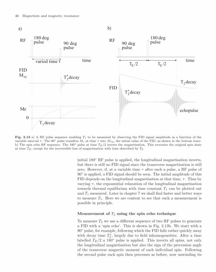
46 Magnetism and magnetic resonance
b)a)
RF RF
FIDM
Mz
time time
180 180deg degpulse pulse90 deg
pulse
0
varied time τ
90 degpulse
FID
T decay2
T decay2*
T /2E T /2E
echopulse
T decay2*xy
T decay1
Fig. 2.13 a) A RF pulse sequence enabling T1 to be measured by observing the FID signal amplitude as a function of thevariable interval τ . The 90 pulse transfers Mz at time τ into Mxy, the initial value of the FID, as shown in the bottom trace.b) The spin echo RF sequence. The 180 pulse at time TE/2 inverts the magnetisation. This recreates the original spin stateat time TE , except for the irreversible loss of magnetisation with time described by T2.
initial 180 RF pulse is applied, the longitudinal magnetisation inverts,but there is still no FID signal since the transverse magnetisation is stillzero. However, if, at a variable time τ after such a pulse, a RF pulse of90 is applied, a FID signal should be seen. The initial amplitude of thisFID depends on the longitudinal magnetisation at that time, τ . Thus byvarying τ , the exponential relaxation of the longitudinal magnetisationtowards thermal equilibrium with time constant T1 can be plotted outand T1 measured. Later in chapter 7 we shall find faster and better waysto measure T1. Here we are content to see that such a measurement ispossible in principle.
Measurement of T2 using the spin echo technique
To measure T2 we use a different sequence of two RF pulses to generatea FID with a ‘spin echo’. This is shown in Fig. 2.13b. We start with a90 pulse, for example, following which the FID falls rather quickly awaywith decay time T ∗
2 , largely due to field inhomogeneities. After a timelabelled TE/2 a 180 pulse is applied. This inverts all spins, not onlythe longitudinal magnetisation but also the sign of the precession angleof the transverse magnetic moment of each individual spin. Followingthe second pulse each spin then precesses as before, now unwinding its
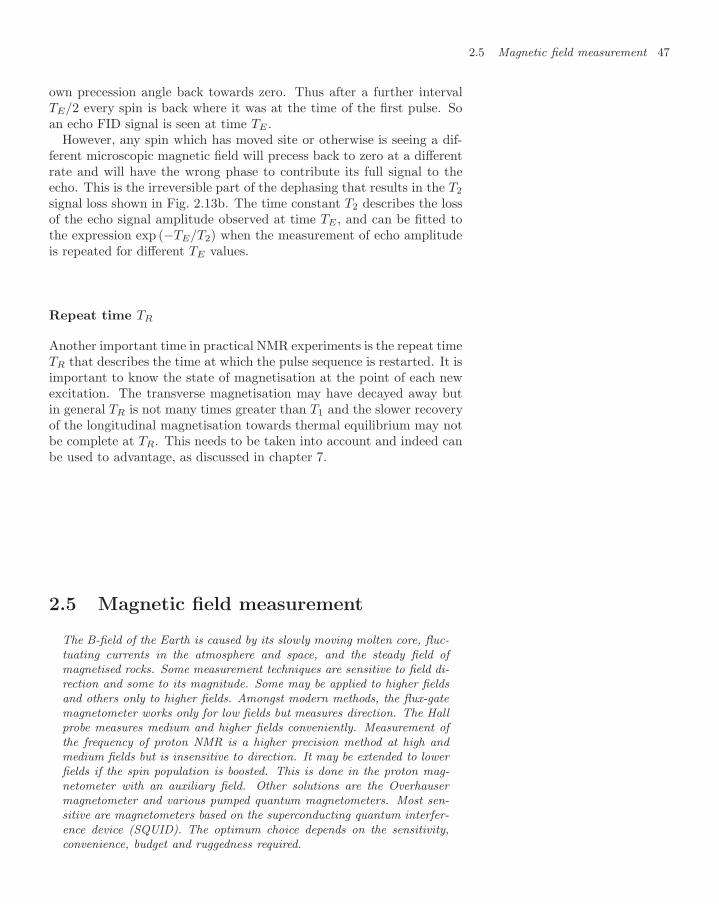
2.5 Magnetic field measurement 47
own precession angle back towards zero. Thus after a further intervalTE/2 every spin is back where it was at the time of the first pulse. Soan echo FID signal is seen at time TE .
However, any spin which has moved site or otherwise is seeing a dif-ferent microscopic magnetic field will precess back to zero at a differentrate and will have the wrong phase to contribute its full signal to theecho. This is the irreversible part of the dephasing that results in the T2
signal loss shown in Fig. 2.13b. The time constant T2 describes the lossof the echo signal amplitude observed at time TE , and can be fitted tothe expression exp (−TE/T2) when the measurement of echo amplitudeis repeated for different TE values.
Repeat time TR
Another important time in practical NMR experiments is the repeat timeTR that describes the time at which the pulse sequence is restarted. It isimportant to know the state of magnetisation at the point of each newexcitation. The transverse magnetisation may have decayed away butin general TR is not many times greater than T1 and the slower recoveryof the longitudinal magnetisation towards thermal equilibrium may notbe complete at TR. This needs to be taken into account and indeed canbe used to advantage, as discussed in chapter 7.
2.5 Magnetic field measurement
The B-field of the Earth is caused by its slowly moving molten core, fluc-tuating currents in the atmosphere and space, and the steady field ofmagnetised rocks. Some measurement techniques are sensitive to field di-rection and some to its magnitude. Some may be applied to higher fieldsand others only to higher fields. Amongst modern methods, the flux-gatemagnetometer works only for low fields but measures direction. The Hallprobe measures medium and higher fields conveniently. Measurement ofthe frequency of proton NMR is a higher precision method at high andmedium fields but is insensitive to direction. It may be extended to lowerfields if the spin population is boosted. This is done in the proton mag-netometer with an auxiliary field. Other solutions are the Overhausermagnetometer and various pumped quantum magnetometers. Most sen-sitive are magnetometers based on the superconducting quantum interfer-ence device (SQUID). The optimum choice depends on the sensitivity,convenience, budget and ruggedness required.

48 Magnetism and magnetic resonance
2.5.1 Earth’s field
Magnetic surveys
Three mechanisms contribute to the B-field of the Earth.Firstly there is the magnetohydrodynamic effect of the moving molten
core. The associated inertia of this is large enough to ensure that itchanges only with a long time constant. The change in direction of thefield is measured in minutes of arc per year.26 However, on geological or26This effect is large enough to require
significant correction to magnetic com-pass readings that depend on the year.
even archaeological timescales such changes are fast.Then there are the magnetic effects of currents of charged particles
in space and in the atmosphere. These vary on a daily timescale beingdriven by the weather, fluctuations in the solar wind and charged particleemission from the Sun.
Finally there is the magnetisation of local rocks, baked bricks or theremains of a hearth. Such magnetisation was fixed at the time thatthe material or its ferromagnetic constituent was deposited or cooledbelow its Curie point. It then becomes a frozen record of the Earth’sfield at the time of formation. The detection and measurement of thismagnetisation and its direction are of importance in geophysics, geologyand archaeology.
Surveys using very sensitive devices are required to map the effect ofthis last signal in the presence of the other two. Some other applicationsrequiring magnetic field maps call for even greater sensitivity, such asthe measurement of the magnetic fields emitted by the brain as part ofits neurological activity.
Measurement of the Earth’s field
Historically the Earth’s field direction was mapped in the horizontalplane using a compass, a pivoted magnetic needle. A similar instrumentin the vertical plane measured the dip angle. The magnitude of the fieldwas determined by measuring the oscillation frequency of such a needlesuspended by a torsional fibre, or by measuring the static torque with abalance. The torsion angle was read by observing the reflection of a pen-cil beam of light from a small mirror attached to the fibre. Work withsuch delicate devices was slow and laborious and belongs to a romanticbut bygone age when there was something heroic about recording scien-tific measurements in out-of-the-way places under conditions of extremehardship. Fortunately the days of this hair shirt school of experimentalphysics are passed! Today there are better and faster methods of tak-ing accurate readings of magnetic fields in satellites and other remotelocations and transmitting the data back.
2.5.2 Measurement by electromagnetic induction
Induction loop
The induction loop used for example in airport security is in the formof a resonant circuit as in Fig. 2.1. A change in the presence of the

2.5 Magnetic field measurement 49
susceptible or conductive material changes the inductance of the coil Lby a small fraction. This gives rise to a small shift in resonant frequencyω0 = 1/
√LC which may be sensed if Q is large.
As a method of sensing the presence of conductors and magnetic ma-terials at close range this is very effective. However, its sensitivity fallsoff rapidly if the distance to the material d is much larger than the di-mensions of the coil. The dipole field of the coil at the material falls asd−3. The flux linkage of the loop due to the material therefore falls asd−6. We conclude that magnetic measurements which rely on generatinga magnetising field and detecting its response are not useful except atclose range or with large coils.
Flux-gate magnetometer
Magnetic flux measurements are possible using Faraday’s law by simplyrotating a coil at constant speed in the field B and measuring the voltagegenerated. The orientation of the axis of the coil determines whichcomponent of B is measured.
A more sensitive device is the flux-gate magnetometer. This consistsof three separate transformers mutually at right angles to one another,each consisting of a cylindrical core of high permeability metal withstraight solenoidal primary and secondary windings. The primary wind-ing is driven with a 5 kHz pure sine wave and the signal induced inthe secondary winding is analysed. If there is no ambient B-field alongthe transformer axis, the output voltage of the secondary winding isamplified by the permeability of the core. Superimposed on the funda-mental 5 kHz waves are its even harmonics which are generated as themetal core saturates. In the absence of an external field the saturationis symmetric and frequency components at 15 kHz, 25 kHz and so onare detected.
However, if there is an ambient static field along the axis the highpermeability metal will saturate at lower values in one direction thanthe other. The magnetic response will then be asymmetric in direction,thereby generating odd harmonics, 10 kHz, 20 kHz and so on, in additionto the even ones. The B-field measurement comes from the amplitude ofthe odd harmonics. The flux-gate compass has a limited dynamic rangeof B-field (up to about 1 mT), good resolution (0.1 nT), but requirescalibration for absolute field values. Its directional properties are excel-lent and it can be used to measure low frequency as well as static fields(to about 1 kHz). It may be used together with a quantum magnetome-ter which has the complementary properties of accurate absolute fieldmeasurement but lacks directional information.
Hall probe
The measurement of large B-fields is not possible with a flux-gate com-pass as the high permeability metal saturates too readily. However, itis possible to use a Hall probe instead.
The Hall effect is illustrated in Fig. 2.14. When a charge q moves along
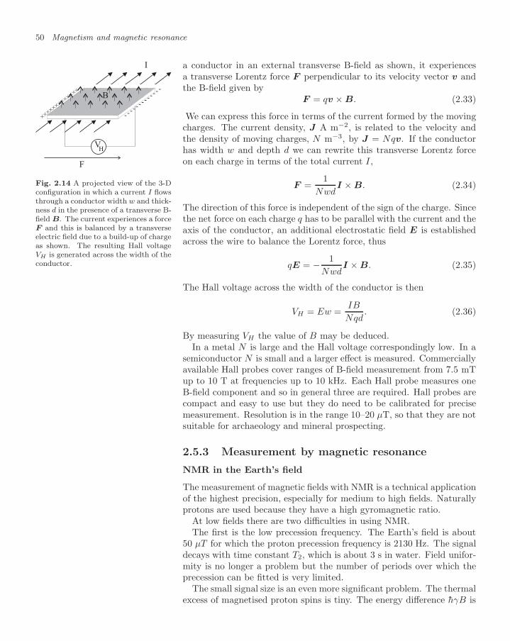
50 Magnetism and magnetic resonance
a conductor in an external transverse B-field as shown, it experiencesa transverse Lorentz force F perpendicular to its velocity vector v andthe B-field given by
F = qv × B. (2.33)
We can express this force in terms of the current formed by the moving
I
B
+++++++++++++
-------------
VH
F
Fig. 2.14 A projected view of the 3-Dconfiguration in which a current I flowsthrough a conductor width w and thick-ness d in the presence of a transverse B-field B. The current experiences a forceF and this is balanced by a transverseelectric field due to a build-up of chargeas shown. The resulting Hall voltageVH is generated across the width of theconductor.
charges. The current density, J A m−2, is related to the velocity andthe density of moving charges, N m−3, by J = Nqv. If the conductorhas width w and depth d we can rewrite this transverse Lorentz forceon each charge in terms of the total current I,
F =1
NwdI × B. (2.34)
The direction of this force is independent of the sign of the charge. Sincethe net force on each charge q has to be parallel with the current and theaxis of the conductor, an additional electrostatic field E is establishedacross the wire to balance the Lorentz force, thus
qE = − 1Nwd
I × B. (2.35)
The Hall voltage across the width of the conductor is then
VH = Ew =IB
Nqd. (2.36)
By measuring VH the value of B may be deduced.In a metal N is large and the Hall voltage correspondingly low. In a
semiconductor N is small and a larger effect is measured. Commerciallyavailable Hall probes cover ranges of B-field measurement from 7.5 mTup to 10 T at frequencies up to 10 kHz. Each Hall probe measures oneB-field component and so in general three are required. Hall probes arecompact and easy to use but they do need to be calibrated for precisemeasurement. Resolution is in the range 10–20 µT, so that they are notsuitable for archaeology and mineral prospecting.
2.5.3 Measurement by magnetic resonance
NMR in the Earth’s field
The measurement of magnetic fields with NMR is a technical applicationof the highest precision, especially for medium to high fields. Naturallyprotons are used because they have a high gyromagnetic ratio.
At low fields there are two difficulties in using NMR.The first is the low precession frequency. The Earth’s field is about
50 µT for which the proton precession frequency is 2130 Hz. The signaldecays with time constant T2, which is about 3 s in water. Field unifor-mity is no longer a problem but the number of periods over which theprecession can be fitted is very limited.
The small signal size is an even more significant problem. The thermalexcess of magnetised proton spins is tiny. The energy difference hγB is

2.5 Magnetic field measurement 51
8.8×10⁻¹² eV. The excess fraction of aligned proton spins is 1.8×10⁻¹⁰
at ambient temperature. To see how small this is, consider 1 cm3 ofwater. It contains n = 6 × 10²² protons. The root mean square (RMS)of the statistical fluctuation of the number of these protons with spinup rather than down27 is not much smaller than the number oriented 27This is about
√n/2 ≈ 2 × 10¹¹.
by the Earth’s field.The conclusion is clear. A method has to be found to increase the
magnetisation of the proton spins. The population difference must beraised from its thermal Boltzmann value. There are three different waysin which this may be done. The first uses a macroscopic auxiliary field,as in the proton magnetometer described below. The second uses theOverhauser effect in which a similar role is played by a microscopicauxiliary field. The third way is to use quantum pumping.
Proton magnetometer
The proton magnetometer is the simplest method of measuring a smallB-field by NMR since no RF generator is required. Protons are sup-plied in the form of a bottle of water or paraffin. This is placed insidea simple coil that can be fed with a steady current to provide a mag-netic field. Measurement with the proton magnetometer follows foursequential steps.
In the first the coil is powered to provide an auxiliary fieldB′ for a time of the order of T1.28 Thus with B′ of order 28To work, the orientation of B′ should
be at some angle to the Earth’s field,otherwise the coil will not give rise to alarge transverse magnetisation signal.
0.01 to 0.05 T and applied for several hundred milliseconds,the proton spins will be aligned along the axis of the coilwith 2–3 orders of magnitude greater magnetisation thanthe equilibrium alignment in the Earth’s field.
Next B′ is reduced to a value several times the Earth’s field,300 µT say. This does not have to be done very quicklybecause the net field direction does not change.
In the third step the residual value of B′ is reduced rapidly tozero in a time short compared with the precession period. At300µ T the latter is 80 µs. This step is done quickly so thatthe magnetisation does not have time to track the changein field direction. As a result a significantly large transversemagnetisation is available to precess in the Earth’s field.
In the fourth step the FID signal is read out and its frequencyanalysed. The precession can be observed for several timesT1 or the sequence can be repeated for another measurement.
Sensitivities of about 1 in 105 are reasonable. Commercially availableproton magnetometers quote sensitivities better than a nanotesla.
Overhauser magnetometer
An improvement on the proton magnetometer relies on the Overhausereffect to increase the magnetisation further and to provide a continuous

52 Magnetism and magnetic resonance
signal.A fluid medium is required containing protons and a low concentra-
tion of paramagnetic ions which are not bound to the protons. At anytime, with the fluid in thermal equilibrium, a proton may be either ina location magnetically influenced by the paramagnetic ion, or far fromsuch an ion. In a coupled location it is close enough for its spin to forma singlet or triplet state F = 0, 1 with the unpaired electron.29 As a29In reality it is more complicated, but
we have an atomic hydrogen couplingmodel in our mind for illustration.
result of thermal motion in the liquid protons may diffuse from being incoupled sites (under the influence of an ion in this way) to uncoupledsites (where they are influenced only by the Earth’s field) and then maydiffuse back again.
In the Earth’s field the F = 1 energy levels in a coupled locationare split. This magnetic splitting is dominated by the large effect of theelectron moment. Then the Boltzmann factors that determine the popu-lation densities in thermal equilibrium are characterised by the magneticmoment of the electron, to which the proton spin is aligned by the hyper-fine splitting.30 Therefore in thermal equilibrium protons in a coupled30The hyperfine coupling is weak
enough that the F = 1 level is popu-lated as well as the F = 0 one.
location have a polarisation enhanced by a factor of order the ratio ofmagnetic moments, µB/µp. The medium is a fluid and as the protonsdiffuse away from the paramagnetic ion they take their polarisation withthem. The result is that the free protons in the uncoupled state havea much higher magnetisation than they would have in thermal equi-librium. This is the Overhauser effect and is an example of dynamicnuclear polarisation (DNP).
To generate a precession signal the liquid is excited by a very broadband 90 RF pulse at around 2 kHz. This excites the magnetisationof the enlarged population of protons in uncoupled locations into thetransverse plane. An enhanced FID signal may be measured.
Pumped quantum and SQUID magnetometers
More sensitive magnetometers are available. Most are based on pumpedspin population states in potassium, rubidium or caesium vapour.
The most sensitive depend on the magnetic flux linkage of a supercon-ducting ring and the Josephson effect. These are called SQUID devices.Their sensitivity is required to detect the transient magnetic fields emit-ted by the brain. Such a procedure is called magnetic encephalography(MEG). These signals, though very weak, ∼ 10−13 T, are not attenu-ated by the conductivity of the skull. They have good time resolution oforder milliseconds, but very poor spatial resolution of order 10 cm. Assuch they are complementary to MRI and other modalities discussed inchapters 7 and 8.

2.5 Magnetic field measurement 53
Read more in books
Classical Electrodynamics, JD Jackson, Wiley, 3rd edn(1998), the authoritative text on electricity and mag-netism
Electricity and Magnetism, WJ Duffin, McGraw-Hill,3rd edn (1980), a standard text on electromagnetism
Electricity and Magnetism, BI Bleaney and B Bleaney,Oxford, 3rd edn (1976), a standard text on electromag-netism
Electromagnetic Fields and Waves, P Lorrain, DR Cor-son, and F Lorrain, Freeman, 3rd edn (1988), a stan-dard text on electromagnetism
Principles of Nuclear Magnetism, A Abragam, Oxford(1961), the classic reference work on magnetic reso-nance
Magnetism in Condensed Matter, SJ Blundell, Oxford(2001), a modern advanced text on magnetism
Look on the Web
Look at the book website atwww.physics.ox.ac.uk/users/allison/booksite.htm
Watch for further developments and experimental de-tails in ESR
electron spin resonance
Read about the related behaviour of muonsmuon spin resonance
Follow the story of the astrophysics revealed by obser-vations of the M1 transition in atomic hydrogen
neutral H 21 cm
Find out more about the information given by chemicalshifts and their splitting
chemical shift NMR
Read about developments in quantum magnetometersand their application
caesium, potassiumor rubidium quantum magnetometers
Follow current developments in hyperpolarisationNMR hyperpolarisation or DNP enhanced NMR
Learn about SQUID magnetometers and their usesSQUID magnetometers

54 Magnetism and magnetic resonance
Questions
2.1 Calculate the numerical value of the nuclear mag-neton in SI units from fundamental constants andthence the Larmor precession frequency in Hz forthe proton in hydrogen in a 3 T field using g = 5.59.
2.2 The radiative decay mean lifetime of the F = 1state of atomic hydrogen is 11.4 × 10⁶ years. Cal-culate the corresponding resonance width in eV.What determines the actual lifetime and measuredwidth, a) in the laboratory, and b) in interstellarspace.
2.3 A birdcage coil is formed from a ladder of 12 circuitseach of self-inductance L with parallel capacitanceC, of which 4 are shown:
L L L L
C outin CCC ZZ
The coil is to be driven at 120 MHz from a powersupply with output impedance Z. Suggest how thevalues of L and C should be chosen in first approx-imation.Explain in principle how a more realistic solution tothe problem that takes into account the interactionbetween the coils might be achieved.
2.4 Show that the full width at half maximum of theexcitation spectrum for a single resonance plottedas a function of frequency is the reciprocal of themean life of the resonant state, as suggested on sec-tion 2.4.1.
2.5 Calculate the magnetisation of pure water placed ina steady magnetic induction of B0 = 3 T in equi-librium at a temperature of 20C.Following a 90 RF pulse the maximum FID sig-nal amplitude that can be detected in a single turncoil from a container of water under the above con-ditions is 1.0 mV. Calculate the frequency of thesignal and the mass of the water. Discuss the geo-metrical position of the coil and the water that isrequired for this maximum signal.
2.6 Calculate the frequency of ESR for an isolated elec-tron in the Earth’s B-field, assumed to be 50 µT.Explain why ESR is not a practicable way accu-rately to measure a value for this field.
2.7 Explain carefully the distinction between the NMRrelaxation times T1, T2 and T ∗
2 . How are the phe-nomena behind these related to the chemical shift,the shift in NMR frequency determined by thechemical environment of a hydrogen atom?
2.8 A water phantom is at equilibrium at 20C in a B0
field of 1.5 T along the z-axis. A B1 field rotatingin the xy-plane with constant magnitude 78 µT isapplied for 50 µs. What is the condition for theproton magnetization vector to rotate? What is itsdirection immediately after the B1 field is turnedoff?
2.9 What are the longitudinal and transverse compo-nents of the magnetisation vector of the phantomin the previous question after a further delay of 100ms if the values of T1 and T ∗
2 are 500 ms and 50 msrespectively?

Interactions of ionisingradiation 3
3.1 Sources and phenomenology55
3.2 Kinematics of primary colli-sions 58
3.3 Electromagnetic radiation inmatter 65
3.4 Elastic scattering collisions ofcharged particles 68
3.5 Multiple collisions of chargedparticles 73
3.6 Radiative energy loss by elec-trons 81
Read more in books 83
Look on the Web 83
Questions 84
in which the fundamental physics of ionising radiation is developed inpreparation for general applications in chapter 6 and for the physics ofmedical imaging and therapy in chapter 8.
3.1 Sources and phenomenology
Ionising radiation comprises beams of charged particles, and photons withenergies above about 10 keV (X-rays and γ-rays). Primary sources ofsuch radiation include natural radioactivity, cosmic radiation from space,and beams of particles accelerated in the laboratory. Beams of secondaryphotons may be produced by the transverse acceleration of electron beamsin the atomic electric field of a heavy nucleus (bremsstrahlung) or inthe macroscopic B-field of a magnet (synchrotron radiation). Radiationin any of these forms interacts with matter through stochastic collisionevents. These collisions vary from single catastrophic events to multiplecollisions that progressively reduce the energy of the incident particle. Theprobability of a collision is described by its cross section.
3.1.1 Sources of radiation
History of ionising radiation
The history of ionising radiation starts in the four extraordinary years,1895–1898. In 1895 Wilhelm Rontgen discovered X-rays, in 1896 HenriBecquerel discovered natural radioactivity, in 1897 J.J. Thompson dis-covered the electron and in 1898 Marie Curie discovered Radium. Thebook by Mould gives a brief account supported by pictures of the pio-neers, their apparatus, data and contemporary reports in the press. Thefact that these discoveries were made in such a short time generated aeuphoria such that subsequently all sorts of claims were made and manybelieved, culminating in the fraudulent discovery of ‘N rays’ in 1903–1904. Radiation attracted immediate publicity as an extension of thefairground peepshow by recording pictures of otherwise hidden objects.However, its more serious use for medical imaging was also understoodand exploited from the earliest days. The damaging effects of radiationwere found when those working with radiation sources recorded burnsthat did not clear up. On the other hand in 1896 already ionising radi-ation was used to treat skin tumours experimentally.

56 Interactions of ionising radiation
Ionising radiation is normally understood to include beams of chargedparticles and photons of sufficient energy to create significant ionisation,about 10 keV and above. We discuss three primary sources of suchradiation. Natural sources of radioactivity are concentrated in certainminerals, but also present in most unrefined materials at the level of10−9 to 10−12. Then there is cosmic radiation incident on the Earth fromspace. We discuss both of these further in the context of the naturalradiation environment in chapter 6. Finally there are accelerated beamsof charged particles, both electrons and nuclei, derived from ion sourcesin the laboratory.
The ion source for an accelerated electron beam traditionally startswith a heated metal filament providing thermionic emission. However,the current that can be obtained in this way is limited. Modern elec-tron sources for pulsed beams use photoelectric emission from metalsilluminated by lasers.
X-ray sources
X-rays and γ-rays are usually generated by the acceleration of high en-ergy electrons as a secondary process. These electrons may be given en-ergy by a DC voltage or a linear accelerator with an RF energy source,see section 8.1. In either case the resulting electron beam is incident on ahigh Z metal target where the electrons suffer large transverse accelera-tions in the nuclear electric fields of the atoms. The resulting electromag-netic radiation is known as bremsstrahlung and is peaked in the forwarddirection. Additional X-rays are emitted by the target when atoms ra-diate following the ejection of an inner electron.1 The bremsstrahlung1Such photons are isotropic and have
a spectrum characteristic of the Z ofthe atom. They may also be initi-ated by a higher energy photon (X-rayfluorescence or XRF) or by a protonbeam (proton-induced X-ray emissionor PIXE).
spectrum when plotted as a function of energy is quite constant2 but
2The flatness of the spectrum is re-lated to the (near) point-like charges ofthe nucleus and electron, the frequencyspectrum of a delta function being flat.
cuts off at the energy of the incident electron energy. The higher theelectron beam energy, the higher the efficiency of photon production.The physics of bremsstrahlung is discussed further in section 3.6.2.
In the production of bremsstrahlung much energy is lost by th elec-trons through ionisation and excitation of the material. For the most ef-ficient generation of γ-rays the electron beam is accelerated transverselyby macroscopic magnetic fields in vacuum, instead of by the atomic nu-clear electric fields in matter. Such sources are called synchrotron lightsources and have only recently become available for use other than asresearch tools.
3.1.2 Imaging with radiation
Ionising radiation may be used to image structure in two modes, coher-ent and incoherent. Probing coherently, the scattered Huygens waveletsinterfere to reveal structure on scales down to λ/2π where λ is the wave-length of the radiation. The de Broglie wavelength λ is given in termsof the momentum P as λ = 2πh/P . By using radiation with enoughmomentum it is possible to ‘see’ down to the atomic scale at 10−10 m,or to the nuclear and quark scale at 10−15 m and below.

3.1 Sources and phenomenology 57
Practical applications of ionising radiation as discussed in this bookare not concerned with these scales, and radiation is used incoherently.Imaging structures on a macroscopic scale in this way, the wavelength ofthe radiation does not determine the spatial resolution. The radiation ismerely used to measure along penetrating straight lines. No use is madeof refraction, reflection or diffraction. It is the crude optics of the pointsource, the collimator, and the pinhole camera.
In addition to its use for imaging, X-ray and γ-radiation may be usedto modify the medium through which it passes. The most importantapplications of interest are in the areas of electronics, cancer therapy,sterilisation and the polymerisation of organic molecules.
3.1.3 Single and multiple collisions
Range and cross section
How does radiation interact with matter? At a microscopic level theradiation, whether particles or photons, suffers collisions with the ions,atoms or molecules of which the matter is composed. There are twoextreme kinds of such collision. An incident particle may suffer a catas-trophic collision such that it is effectively removed from the beam. Al-ternatively it may simply suffer a slight loss of energy but otherwisecontinue with a rather small change in direction.
N
Range
Fig. 3.1 Sketches of two examples ofrange distributions. An exponentialdistribution applies when the end ofthe range coincides with a single catas-trophic collision. A narrow peak ap-plies when the range is reached follow-ing attrition by a very large number ofsmall collisions.
An example of the first kind is the behaviour of photons in matterdue to the photoelectric effect. When a photoelectric collision occursthe photon is absorbed completely and an atomic electron is expelledfrom the atom. Therefore the range of photons under these conditionsfollows an exponential distribution (see Fig. 3.1) with mean range R,given by 1/R = Nσ, where N is the number of targets per m3 and σ isthe cross section in m2 per target.3
3Observe that it does not matter onwhat scale the ‘target’ is defined. Forexample, if N refers to the density ofatoms and σ refers to the cross sec-tion per atom, the result will be thesame as when N denotes the density ofmolecules and σ the cross section permolecule.
An example of the second kind is the range of charged particles.4 A
4This includes any charged particles,except electrons which are covered inthe next paragraph.
particle finally stops after a large number of small collisions, n, each ofwhich reduces its kinetic energy by a small amount. The mean rate ofthis energy loss with distance is called dE/dx. The range distribution isa sharp spike, broadened only by the effect of relatively small statisticalfluctuations in the occurrence of the n collisions (see Fig. 3.1).
The range distribution of electrons in matter is described neither bya spike nor by an exponential. Because of its small mass an electronaccelerates, and therefore radiates, in the nuclear electric field of atoms.Thus in addition to the gradual attrition of energy experienced by othercharged particles, electrons suffer the additional process of radiative en-ergy loss. The spectrum of this includes a significant cross section foremission of a photon carrying much of the electron energy. As a result,the electron range distribution includes the effect of a strong exponentialcomponent due to this bremsstrahlung process in addition to the usualdE/dx.

58 Interactions of ionising radiation
Differential cross section
Whether the phenomenology of the interaction involves a large numberof small collisions or a smaller number of significant collisions, the be-haviour is determined solely by the cross section and its dependence on,for example, energy transfer5 E and scattering angle θ. The probability5In this chapter E denotes the energy
of the incident charge and E the changeto this in a single collision.
per unit path of a given class of collision is
dP = Ndσ. (3.1)
So for a charged particle, the probability dP of a collision per unit pathwith an energy transfer between E and E + dE is
P (E) dE =dσ
dE N dE , (3.2)
where dσ/dE is called the differential cross section with respect to energy.
θ
dθ
dφ
dΩ
φ
Fig. 3.2 The relationship between anelement of solid angle dΩ and the po-lar scattering angle θ and the azimuthalscattering angle φ.
The dependence of the scattering on angle is described by the differ-ential cross section with respect to angle, dσ/dθ, or solid angle, dσ/dΩ.An element of solid angle
dΩ = sin θ dθ dφ (3.3)
in polar coordinates is shown in Fig. 3.2 with the incident beam as polaraxis. If the scattering is independent of azimuth φ, we may integrateover it6 so that dΩ = 2π sin θ dθ. Then the probability per unit path6This will be the case provided neither
beam nor target is polarised, and any fi-nal state polarisation is averaged. Thiswill always be so in the following.
length for a collision to occur with a scattering angle between θ andθ + dθ is
P (θ) dθ = Ndσ
dΩ2π sin θ dθ. (3.4)
3.2 Kinematics of primary collisions
In quantum mechanics the cross section is given by first order time-dependent perturbation theory as a product of two factors. These maybe described as a kinematics factor and a dynamics factor. Kinematicsinvolves the features that follow from energy–momentum conservation.Dynamics concerns the features arising from the matrix element of theinteraction itself. Many processes can be described rather simply by thekinematics of an elastic collision with a stationary constituent mass in themedium. This gives a useful quantitative description of a diverse rangeof applications.

3.2 Kinematics of primary collisions 59
3.2.1 Kinematics and dynamics
A collision between the incident particle and the medium is usually lo-calised to a particular constituent of that medium. The constituentinvolved may be an atom, a whole molecule or just an individual elec-tron. The rest of the medium is then not affected.7 Such a collision 7A counter example is the emission of
Cherenkov radiation where the interac-tion is with the material as a whole. Inthat case the emission is still linearlydependent on path length and nothingis lost by pretending that it is more orless localised.
process is subject to the kinematic constraints of energy and momen-tum conservation. Kinematics is unaffected by the detailed mechanismor interaction type and depends only on the masses involved. Otherfactors in the cross section are described as dynamics and depend onthe interaction type.
Reaction rate and cross section
How is the cross section related to the rate of the interaction W thatmay be calculated by quantum mechanics? W is the rate of the reactionper second when the wavefunctions of the target and incident charge arenormalised in a volume V . We imagine a single incident charge bouncingaround in this volume with velocity v and tracing out a volume σv persecond, in the sense that, if the target lies inside that volume σv, theinteraction happens in that second.8 So the average interaction rate is 8To include the possibility that the tar-
get is moving, we simply note that it isthe relative velocity that is relevant.
W = σv/V .In first order time-dependent perturbation theory the interaction rate
W is given by Fermi’s golden rule (FGR),99As derived in a standard text on quan-tum mechanics, such as one of thosegiven in the list for further reading atthe end of the chapter.
W =2π
h|M|2ρf . (3.5)
Thence the cross section,
σ =2πVhv
|M|2ρf . (3.6)
This comprises two factors, ρf the phase space factor which expresses thekinematics and the square of the matrix element |M|2 which expressesthe dynamics.10
10We shall derive what we can usingthe kinematics of energy and momen-tum conservation. Later in section 3.4we shall tackle the dynamics. We shallfind that the volume V cancels out andtherefore can be taken as large and ir-relevant.
The value of a cross section is unchanged by a Lorentz transformationalong the incident momentum. It may therefore be evaluated in thecentre-of-mass frame and transformed into the rest frame of the target.This is a useful picture. However, the transformation is not so trivialfor a differential cross section such as dσ/dΩ, because the solid angle Ωis not invariant under such a transformation.
materialmedium
E,Q
radiationradiation
Fig. 3.3 The energy and 3-momentumtransfer between the radiation and themedium as a result of a single collision.
3.2.2 Energy and momentum transfer
In a collision the material gets a kick and gains energy. The incidentparticle gets an opposite kick and loses energy. In Fig. 3.3 we illustratethis for a transfer of energy E and 3-vector momentum Q from theparticle to the target or medium. The E and Q form a 4-vector. Thelength of the vector is called the 4-momentum transfer Q4 and is given byQ2
4 = Q2−E2/c2. As such, it is a relativistic invariant.11 The differential11We have chosen a space-like defini-tion for the 4-momentum transfer.

60 Interactions of ionising radiation
cross sectiond2σ
dE dQ(3.7)
is a function of E , Q and the incident particle energy E. We mayeffectively ignore other variables.12 We write E = hω and the 3-vector
12The particles may have spin uponwhich the cross section may also de-pend. But, provided the incident par-ticles are not polarised and the polar-isation of the outgoing particles is notmeasured, the effect of spin on the crosssection is at most a constant, an overallstatistical factor.
momentum Q = hk.Before considering the general case involving both energy and momen-
tum transfer, we look at examples of collisions that are dominated byone or the other.
Example of momentum transfer
Consider the case of the elastic scattering of low energy photons in acrystal. This is Bragg scattering. The photon energy is unchanged andthere is no energy transfer to the medium, so that ω = 0. In scatteringthe incident momentum vector of the X-ray is simply rotated through asignificant angle, so that k = 0.
The analysis of the experimentally observed cross section as a functionof k for all sorts of crystals and molecules has enabled their structureto be deduced. The determination of the structure of DNA, the doublehelix, is the most famous historical example. The scattering depends onspatial structure, the electron density to be precise, and is not concernedwith the resonant or frequency response of the medium.
Example of energy transfer
In photoabsorption (photoelectric effect) there is no outgoing photon andthe whole incident energy and momentum are absorbed with |k| = ω/c.The energy transfer hω is now relatively large and the momentum trans-fer hk relatively small. For example, in the photoelectric effect at opticalfrequencies the value of k corresponds to a wavelength of 0.5 µm, farlarger than any atom. Therefore the EM wave is very uniform withinthe spatial dimension of any target atom or molecule.13 The interac-13The assumption that the electric field
is completely uniform over the atom ormolecule is called the dipole approxi-mation.
tion is not sensitive to where the electron density is within the atom ormolecule, only to what its frequency response is. Consequently the crosssection depends on ω rather than on the spatial structure.
3.2.3 Recoil kinematics
Elastic recoil
Generally collisions depend in a significant way separately on both Qand E (or k and ω). The exception is elastic scattering for which theyare related. Consider the kinematics of an elastic scatter of an inci-dent particle by a constituent of the medium, mass M , assumed to beinitially stationary.14 On these assumptions, the final kinetic energy of
14In an elastic scatter the identities ofthe incident particle and the struck par-ticle survive intact. This is the mean-ing of the term ‘elastic’ as used here.Their energies and momenta may be ex-changed but no new particles are pro-duced. We ignore the binding energyof any constituent involved in a hardcollision.
the constituent is equal to the energy transfer, and its final momentummust be the momentum transfer.15 But the constituent kinetic energy15We consider any kind of incident par-
ticle, including a photon. and momentum are related to its mass M . In the case of non-relativistic

3.2 Kinematics of primary collisions 61
motion by the constituent we have
E =Q2
2M, (3.8)
by elementary kinematics. In the relativistic case the relationship canbe shown to be16 16See question 3.4.
E =Q2
4
2M. (3.9)
In either case, for a given momentum transfer the energy loss to theincident particle is inversely proportional to the mass of the struck con-stituent.
P* P*
P*
P*
*
P
a) Laboratory frame b) Centre-of-mass frame
afterthe collision
beforethe collision
P-Q
Q
Fig. 3.4 Elastic scattering of incidentradiation of momentum P by a station-ary free constituent of a medium, a) asseen in the laboratory frame where the3-momentum transfer is Q, and b) asseen in the centre-of-mass frame wherethe length of the momentum vector P ∗is constant and the only variable is θ∗.
Transformation from the centre of mass
As shown in Fig. 3.4 the process looks particularly simple in the centre-of-mass frame, where the only variable is the scattering angle θ∗. Inthis frame the energy and modulus of the momentum are unchanged inthe scattering. In the laboratory frame there is seen to be an energytransfer. This is just a result of the Lorentz transformation from thecentre of mass. The smaller the constituent-to-projectile mass ratio,the bigger this transformation and the larger the energy transfer. Ifthe scatterer is heavy, the laboratory frame is almost the same as thecentre-of-mass frame, and consequently the energy loss is small.
Equation 3.8 (or 3.9) is a useful result with a number of interestingand important practical applications.
3.2.4 Applications of recoil kinematics
Energy loss by charged particles
In their passage through materials charged particles encounter electronsas well as nuclei. For small momentum transfers Q, electrons and nu-clei are not resolved from one another. But if the momentum transferQ = hk is such that λ/2π = 1/|k| is significantly smaller than the

62 Interactions of ionising radiation
atom, electrons and nuclei may be seen as independent constituents bythe incident charge. This value is about 25 keV/c for the whole atom.So separate constituent collisions with atomic electrons and nuclei areexpected to occur with values of momentum transfer Q > 25 keV/c.
In this range of Q the energy transfers E for collisions with electronsand with nuclei are Q2/2me and Q2/2MN, respectively, where me is themass of the electron and MN is the mass of the nucleus. It follows thatthe energy loss in collisions with electrons is more than three orders ofmagnitude larger than with nuclei at the same Q. The conclusion isthat constituent scattering by nuclei does not contribute to energy loss,which is dominated by scattering off atomic electrons.1717For incident electrons only, radiative
scattering by nuclei is a source of energyloss, as discussed in section 3.6.2.
We have made two simplifications that can be justified at large mo-mentum transfer. Firstly the electron binding energy was ignored. Im-plicitly we assumed the recoil energy to be well above this binding energy.Secondly we assumed the target atomic electron to be stationary, whichis not quite true. In atomic hydrogen the RMS speed of the ground stateelectron v = αc where α = 0.0073. This is typical for an outer electronand is negligible compared with the minimum electron recoil velocitydiscussed above, Q/me = 0.05c. We note that an inner atomic electronin an atom of higher Z is in a similar situation. It is bound in a smallervolume, has a greater RMS speed and a larger momentum transfer isrequired to resolve it.
An example of data is shown in Fig. 3.5. The calculation that showsthat the peak in the data represents elastic scattering by atomic electronsis left to question 3.2. The effect of the moving electron is a broadeningof the exact relation E = Q2/2me with some atomic electrons movingtowards the incident charge and some away from it.
Fig. 3.5 The cross section for 25 keVelectrons incident on helium, observedat 7 scattering angle and plottedagainst energy loss.
0 200 400 600 800 1000
energy loss /eV
cross section(arbitrary scale)

3.2 Kinematics of primary collisions 63
Rutherford back scattering
The scattering of an incident charged particle by the electric charge of astationary nucleus is known as Rutherford scattering. The actual crosssection will be discussed in section 3.4. However, using the kinematicrelation 3.8, we can discuss the consequences of the recoiling nucleuswithout knowing the cross section. If a collision is observed in whichthe incident particle suffers a change in momentum Q and a change inenergy E , then the mass of the struck nucleus is
MN =Q2
2E . (3.10)
This means that measurements of momentum and angle on the incidentand scattered particles alone give a measurement of the struck nuclearmass, even though this is not itself detected. This is an importanttechnique which can be used to analyse the concentration of nuclearmasses in a small thin sample of material without chemical or physicalpreparation. To reduce the measurement error, data are taken in thebackward direction where the changes in energy and momentum arelargest. Hence the technique is called Rutherford back scattering (RBS).As discussed in chapter 6 this has been developed into a 3-D analyticimaging capability for thin samples.
Compton effect
The scattering of photons by free constituent electrons also shows arecoil effect. This is the famous Compton effect which helped histori-cally to establish the semi-classical quantisation of the electromagneticfield. Because a photon carries momentum 2πh/λ, the momentum ofthe recoil electron depends on Planck’s constant and its observation isa confirmation of quantum theory. The calculation of the kinematics isleft to question 3.3.
Quark structure of hadrons
Often scattering data as a function of E and Q in an apparently inelasticprocess can be interpreted consistently in terms of elastic scatteringfrom a constituent within the target. Indeed such an analysis may showevidence for constituents which are not otherwise observable. This wasone of the principal pieces of evidence used to establish the existence ofquarks inside hadrons, such as protons and neutrons.18
18This is known as deep inelastic scat-tering (DIS); ‘deep’ means that it is athigh Q, just as was the case for scatter-ing from atoms.
Neutron moderator in a nuclear fission reactor
In a reactor the fission process results in two heavy, slowly moving nu-clear fragments and several free neutrons carrying away most of the en-ergy released.19 For this energy to reach the cooling circuits that power
19The fact that the neutrons get thelion’s share of the kinetic energy is itselfinteresting. In a reaction the share-outbetween products is largely on the basisof momentum. It follows that the neu-trons which are light carry away two or-ders of magnitude more kinetic energythan the fission fragments.
the turbines it needs to be thermalised, that is transmitted from theneutrons to the material of the reactor. This must be done quickly

64 Interactions of ionising radiation
by elastic collisions that do not absorb the neutrons, as some of theseat least are needed to maintain the chain reaction by inducing furtherfission processes. When successfully slowed to thermal energies the neu-trons encounter large cross sections for absorption by the fuel, 235U or239Pu. The resulting states of 236U or 240Pu are excited relative to theirground states by an energy equal to the pairing energy.20 Such excited20This is the binding energy difference
between a nucleus with an even numberof neutrons and an odd number of neu-trons. It is 0.5–1.0 MeV for high A nu-clei, as given roughly by the Weissackersemi-empirical mass formula.
states have a high rate of spontaneous fission, and the chain reaction canthen be maintained. Some other isotopes and impurities present, suchas 238U, absorb neutrons and do not lead to fission. This absorption isconcentrated at a number of sharp resonances at certain energies. If thereduction in neutron energy takes place in large steps, the absorptionwill not be important because many neutrons simply never have theright energy for resonant absorption.
A fission reactor therefore contains a neutron moderator whose func-tion is to reduce the neutron kinetic energy elastically in large steps. Itsconstituent nuclei suffer elastic collisions with high energy neutrons andlarge energy transfer.21 For this to be true, our discussion has shown21Neutron collisions with electrons
could only be magnetic. Electrons haveno strong nuclear interactions and neu-trons, with zero charge, no electricones. Consequently the cross section isnegligible.
that these moderator nuclei must have low mass. It is the ratio of nu-clear mass to neutron mass that is important. The usual choices arehydrogen (water), deuterium (heavy water), or carbon (graphite).
In the case of a solid moderator such as graphite, there is an importantsecondary effect of the large nuclear recoil energy. The struck nucleusmay be kicked out of its location in the crystal lattice. The potentialenergy stored in the crystal in the form of vacant sites and interstitialoccupation rises as the neutron irradiation continues. If the temperatureis raised, atoms may get enough kinetic energy to hop from interstitialsites back into vacancies, thereby releasing the potential energy involved.This means that in such a temperature range a heavily irradiated neu-tron moderator may exhibit a negative lattice heat capacity and give aspontaneous increase in temperature. Management of this problem callsfor frequent small excursions of temperature to anneal the lattice and toavoid the build-up of stored energy that can result in a runaway ‘fire’.The worst nuclear radiation accident in the UK, the Windscale fire of1956, was caused by mismanagement of this problem.
Radiation damage in materials
All solid materials are prone to radiation damage due to displaced atomsin the lattice, as discussed above. The effect is large when the momentumtransfer is high and the nuclear mass is low. Such lattice dislocations anddistortions give rise to donor and acceptor levels in the bandgaps of theelectronic structure. If occupied, such states can absorb or scatter lightfor energies at which, prior to irradiation, the crystal was transparent.As a result, after low levels of irradiation transparent materials are seento be coloured. At higher levels they become cloudy and opaque. Thismay be caused by the radiation populating existing metastable electronsites or by creating new ones as discussed above. In general there iscoupling between the problems of electrons being excited and the lattice

3.3 Electromagnetic radiation in matter 65
being excited by atoms being misplaced. In some cases transparencycan be annealed by heating.
For the same reason the electronic behaviour of materials is directlyaffected by irradiation. Semiconductors are particularly sensitive be-cause the density of carriers is low anyway. Radiation increases thecarrier density, either through the creation of extra interstitial and va-cancy sites in the lattice or through populating the resulting donor oracceptor levels with electrons. Neutron or high energy charged particleradiation are expected to have a larger effect than X-rays because ofthe higher momentum transfers. Generally after high levels of irradia-tion the characteristics of semiconductor components change and leakagecurrents rise because of the increased number of carriers.
3.3 Electromagnetic radiation in matter
Photons have three significant interactions in matter. Compton scatteringis a reaction with a small cross section, almost independent of energy andZ, in which the incident photon is scattered from an electron with reducedenergy. The nucleus is a spectator. Photoabsorption (photoelectric effect)has a large energy-dependent and Z-dependent cross section in which thephoton is completely absorbed by an atom. Pair production has a smallercross section rising with both energy and Z from a threshold at 2mec
2.The photon converts to an electron–positron pair in the nuclear Coulombfield and the atomic electron plays no role. .
3.3.1 Compton scattering
a)
b)
c)
e+
e-
e
e
e
Fig. 3.6 The three processes for theinteraction of electromagnetic radiationwith an atom, with time shown runningfrom left to right. The nucleus and elec-tron are shown as a double heavy andlight line, and photons as wavy lines.a) Compton or Thomson scattering.b) Photoabsorption, where the inter-nal photon lines indicate significant in-ternal momentum transfer by Coulombfields.c) Electron–positron pair production.
Compton scattering is constituent scattering by atomic electrons, asshown in Fig. 3.6a. Because there are two simple electromagnetic ver-tices involving charge e, the interaction is second order. Therefore it issmall compared with photoabsorption, a first order processes. The bind-ing energy of the electrons can always be ignored in Compton scatteringcompared with the incident photon energy in the wavelength range wherethe electron can be resolved within the atom. In the low energy limitCompton scattering is called Thomson scattering.
Classical Thomson scattering
If hω is much smaller than mc2, the energy change of the photon due tothe electron recoil is small and a classical picture of the interaction pro-vides an adequate description. The electric field of the incident photonforces the electron to oscillate, and this oscillating charge then emits adipole radiation field in its centre of mass. Electric dipole radiation isnot isotropic but has a sin2 θ angular distribution where θ is the angle

66 Interactions of ionising radiation
between the induced electron motion and the direction of the emittedphoton, that is between the electric vector of the incident wave andthe momentum vector of the outgoing wave.22 Integrated over angle the22The calculation is the subject of
question 3.5. Thomson cross section is,
σT =8π
3
(αh
mec
)2
. (3.11)
This is a constant, 0.665 barn, independent of photon energy. It de-pends on the inverse square of the electron mass because the radiationamplitude is proportional to the electron acceleration. The equivalentcross section due to scattering by nuclear charges is therefore smaller bysix or more orders of magnitude and can be ignored.
Relativistic corrections
Compton scattering is the name given to this process when it is no longertrue that hω is much less than mc2. The required relativistic correctionsto Thomson scattering arise for two reasons.
The first is purely kinematic. The centre of mass of the scattering ismoving in the laboratory frame. The Thomson scattering in the centreof mass, when transformed to the laboratory frame, gives an angulardistribution which peaks at an angle 1/γ with respect to the incidentphoton direction. The same Lorentz transformation creates a Dopplershift in the photon energy. The decrease in photon energy in the labo-ratory frame appears as electron recoil energy.
The second relativistic correction is dynamic. There is a magneticcontribution in addition to the electric term, not only because v/c isnow significant, but also because the magnetic moment associated withthe spin of the electron plays a role. Further details of the relativisticfield theory calculation need not concern us here. The resulting crosssection falls slowly with energy from σT as hω approaches mc2 andbecomes2323There are additional logarithmic
terms depending on spin.σ(ω) = σT × 3mec
2
4hω(3.12)
in the extreme relativistic region, hω mec2.
3.3.2 Photoabsorption
Energy and Z-dependence
At low energy the largest contribution to the interaction of photons inmaterials comes from resonant interaction with the atom as a whole,resulting either in atomic excitation or in photoelectric ionisation. Asshown in Fig. 3.6b there is only one external electromagnetic vertex inthe excitation of the resonant state (the internal vertices just representthe potential that binds the resonant state itself), so this is a first orderprocess. The cross section is typically three orders of magnitude largerthan the Compton cross section and shows a sharp edge at the ionisa-tion threshold of each electron energy shell. There are discrete bound

3.3 Electromagnetic radiation in matter 67
/Z
barn
2 5 10 20 50 100
H
C
OCa
Pb
Photon energy /keV
10
1
10
10
10
2
3
4
Fig. 3.7 The total photon cross section of hydrogen, carbon, oxygen, calcium and lead, divided by Z, as a function of photonenergy. At high energies the cross sections fall to the Thomson cross section, 0.665 barn per electron.
state resonances just below the edge.24 Above the edge the cross section 24These resonances when excited maydecay by photon emission. This isknown as resonance fluorescence.
falls roughly as E−5/2. This fall may be envisaged as arising from aprogressive loss of coherence between emitted Huygens wavelet ampli-tudes coming from different parts of the finite atomic volume involved.The pattern in energy of these thresholds or edges is a fingerprint of theatomic number of the element concerned. Important analytical applica-tions are explored in chapter 6.
Figure 3.7 shows the photon cross section per electron (the atomiccross section divided by Z) for some typical elements of interest betweenhydrogen and lead. It is dominated by the photoabsorption process.The Thomson cross section, the same for all elements and independentof energy, is 0.665 barn, just below the axis as drawn on this log–logplot.25 The edge for K-shell electrons in lead can be seen at 90 keV. The 25There is a difference between the
photoabsorption process and Comptonscattering. One gives rise to a scat-tered photon, whereas the other doesnot. They remain distinct. What isshown in the plot is the total cross sec-tion, the sum of the two.
K-shell edge for calcium at 4 keV is at about the same energy as theM-shell edge for lead. The edges for the lower Z elements are below theleft margin of this plot.
Sum rule
The photoabsorption cross section per electron (σγ/Z), when integratedover frequency, is a constant for all elements,
∫ ∞
0
σ
Zdω =
πe2
ε0mec. (3.13)

68 Interactions of ionising radiation
So, although not apparent in the log–log plot, Fig. 3.7, the area undereach curve is the same for all elements when plotted on a linear–linearscale and integrated down to low energy. This is known as the Thomas–Reiche–Kuhn sum rule. The photoabsorption spectra for all elementscan be found on the NIST website.
3.3.3 Pair production
At photon energies above 2mec2 pair production (e+e−) can occur. This
second order process involves the incoming photon interacting with theCoulomb field of the nucleus,26 as shown in Fig. 3.6c. As a result the26The atomic electrons provide a much
smaller source of field because it is notboosted by the Z2-factor and its centre-of-mass energy is much lower, if not ac-tually below pair threshold.
cross section involves a factor Z2α2. Since particle creation is involved,the derivation of the cross section depends on quantum electrodynamics(QED).
The QED matrix element involves the same second order process asboth Compton scattering
γ + e− → γ + e− (3.14)
and the annihilation process
e+ + e− → γ + γ. (3.15)
Pair creation is the inverse process to annihilation, with the incom-ing γ interacting with a virtual γ, a component of the static nuclearCoulomb field. The nuclear Coulomb field and its Fourier componentsare modified27 in the same way as in Coulomb scattering and brem-27The field is reduced at large distances
by the electron screening of the nucleus,and at short distances by the chargedistribution within the nucleus.
sstrahlung, described later in this chapter. The effect of this modifiedCoulomb field may be parametrised in terms of the radiation length ofthe material,28 X0, usually expressed as the length times the density in
28This is defined in section 3.6.3.g cm−2. If material thickness is expressed as a multiple of X0, all ma-terials of the same thickness have the same properties as regards e+e−
pair creation, bremsstrahlung and multiple scattering, ignoring smallthreshold effects. At photon energies well above 2mec
2 the mean rangefor a photon to create a pair is roughly equal to X0. Values of X0 fordifferent materials are given in table 3.1.
3.4 Elastic scattering collisions of charged
particles
Charged particles are scattered by point charges in a medium according tothe Rutherford scattering formula. This differential cross section may bederived in quantum mechanics and in classical mechanics with the sameresult. The cross section rises as cosec4(θ/2), limited in practice at the

3.4 Elastic scattering collisions of charged particles 69
smallest angles by the screening of the nuclear charge by atomic electrons.Energy loss of the incident charge occurs by Rutherford scattering ontarget electrons.
3.4.1 Dynamics of scattering by a point charge †History
We derive the cross section for Rutherford scattering, that is the scat-tering of a point charge by a stationary fixed point charge, both byquantum mechanics and by classical mechanics.29 The quantum deriva- 29It is a matter of extraordinary his-
torical importance that they give thesame result. If the potential were otherthan a 1/r, the classical calculation ofthe scattering cross section would givethe wrong result. In that case, histori-cally, the early shaky steps in the appli-cation of quantum ideas in the form ofthe Bohr atomic model would not havebeen made, and the theory of quantummechanics as we know it today mightnot have been established, certainly atthe time and in the way that it was.
tion is straightforward. The classical derivation takes a number of linesand a good diagram.
We express the cross section in terms of the fine structure constant,α = e2/(4πε0hc).
Quantum derivation of cross section. The matrix element
Consider the incident charge ze of mass µ. Its wavefunction ψ describesa plane wave of momentum P . The scattered wavefunction ψ′ describesan outgoing wave of momentum P ′. Let the two waves be normalisedin a large box of volume V .30 The wavefunctions are then
30Later this volume cancels, so thenformally we can let it go to infinity. Itis the same box that was introduced al-ready in equation 3.6.
Q
P'
P
θ
Fig. 3.8 The incident and scatteredmomentum vectors, P and P ′ with the3-momentum transfer Q.
ψ =exp(iP · r/h)√V and ψ′ =
exp(iP ′ · r/h)√V (3.16)
To use Fermi’s golden rule, equation 3.6, we need to evaluate the matrixelement of the Coulomb potential between these states,
M =∫ ∫ ∫
Vψ′∗(r)V (r)ψ(r) d3r. (3.17)
We take the nucleus to be the origin and the Coulomb potential
V (r) =zZe2
4πε0r=
zZαhc
r. (3.18)
We neglect the magnetic interaction of the charges and assume thatthe only force between them is electrostatic. We also neglect the recoilenergy and assume that M µ. The rest frame of M is then the centre-of-mass frame. Let P be the magnitude of P (and also of P ′). Thenthe momentum transfer Q is given in terms of the scattering angle θ by
Q = 2P sin(θ/2), (3.19)
as illustrated in Fig. 3.8.Now we can evaluate the integral, equation 3.17. Writing the element
of volume d3r = r2 dΩ dr = 2πr2 dη dr, where η is the cosine of thepolar angle31 between the momentum transfer Q and the vector r, 31The angles involved in this integra-
tion process should not be confusedwith the scattering angle θ.M =
2πzZαhc
V∫ ∞
0
[∫ 1
−1
exp (−iQrη/h) dη
]r dr. (3.20)

70 Interactions of ionising radiation
Evaluating the η integral,
M = −4πzZαhc
V∫ ∞
0
drsin(Qr/h)
Q/h. (3.21)
The potential will be screened such that, for values of r exceeding atomicdimensions, the potential falls to zero significantly faster than the 1/rof the pure Coulomb potential. Therefore the r integration converges,32
32The integral over r is formally takento infinity rather than the edge ofthe box as the integrand vanishes out-side the atomic volume because ofthe electron screening. This inte-gral involves the difference between− cos(Qr/h) evaluated at ∞ and atzero. Shielding at large r reduces thisfactor to unity. M = −4πzZαh3c
VQ2. (3.22)
Quantum derivation of cross section. The phase space factor
Next we evaluate the density of states factor in Fermi’s golden rule,ρf = dN/dE. According to statistical mechanics there are (2πh)−3
states per unit volume of phase space, ignoring spin. So the number offinal states in the scattering solid angle dΩ and momentum range dP is
dN =VP 2 dP dΩ
(2πh)3. (3.23)
The phase space factor is the density of states per unit energy dE, whereE2 = P 2c2 + µ2c4 and EdE = c2PdP . Thus
ρf =dN
dE=
VPE dΩc2(2πh)3
. (3.24)
Substituting in equation 3.6, the dependence on the volume V cancels,then
dσ
dΩ=
(2zZαh
βQ2P
)2
, (3.25)
where we have also used v = βc = Pc2/E. The only factor dependingon the scattering angle θ is Q = 2P sin(θ/2). The Rutherford scatteringformula with the explicit angular dependence is
dσ
dΩ=
(zZαh
2Pβ
)2
cosec4(θ/2). (3.26)
Classical derivation of cross section
In classical mechanics (including the effects of relativity) we may followthe trajectory of the charge as it is deflected by the Coulomb field. Thisdepends on knowing the position and momentum of the charge at alltimes, a state of knowledge forbidden in quantum mechanics. The fol-lowing derivation is therefore unacceptable, although it gives the correctanswer.
Figure 3.9 shows such a classical trajectory in the xy-plane with they-axis chosen as the axis of symmetry. The incoming charge has aninitial velocity βc at an angle θ/2 with respect to the x-axis and animpact parameter b with respect to the origin, that is the distance of
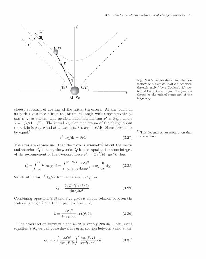
3.4 Elastic scattering collisions of charged particles 71
r
χ
/2 /2
b
ze
c
M Ze
y
x
Fig. 3.9 Variables describing the tra-jectory of a classical particle deflectedthrough angle θ by a Coulomb 1/r po-tential fixed at the origin. The y-axis ischosen as the axis of symmetry of thetrajectory.
closest approach of the line of the initial trajectory. At any point onits path a distance r from the origin, its angle with respect to the y-axis is χ, as shown. The incident linear momentum P is βγµc whereγ = 1/
√(1 − β2). The initial angular momentum of the charge about
the origin is βγµcb and at a later time t is µγr2 dχ/dt. Since these mustbe equal,33 33This depends on an assumption that
γ is constant.r2 dχ/dt = βcb. (3.27)
The axes are chosen such that the path is symmetric about the y-axisand therefore Q is along the y-axis. Q is also equal to the time integralof the y-component of the Coulomb force F = zZe2/(4πε0r
2); thus
Q =∫ ∞
−∞F cosχ dt =
∫ (π−θ)/2
−(π−θ)/2
zZe2
4πε0r2cosχ
dt
dχdχ. (3.28)
Substituting for r2 dχ/dt from equation 3.27 gives
Q =2zZe2cos(θ/2)
4πε0βcb. (3.29)
Combining equations 3.19 and 3.29 gives a unique relation between thescattering angle θ and the impact parameter b,
b =zZe2
4πε0Pβccot(θ/2). (3.30)
The cross section between b and b+db is simply 2πb db. Then, usingequation 3.30, we can write down the cross section between θ and θ+dθ,
dσ = π
(zZe2
4πε0Pβc
)2 cos(θ/2)sin3(θ/2)
dθ. (3.31)

72 Interactions of ionising radiation
Using the element of solid angle, dΩ = 2πsinθ dθ, the differential crosssection is then
dσ
dΩ=
12πsinθ
dσ
dθ. (3.32)
Thus
dσ
dΩ=
(zZe2
8πε0Pβc
)2
cosec4(θ/2). (3.33)
Expressed in terms of α we get the same expression as we found by thequantum route,
dσ
dΩ=
(zZαh
2βP
)2
cosec4(θ/2). (3.34)
Features of the Rutherford cross section
The cross section depends on the square of both charges and thereforethe scattering is independent of their signs. In quantum mechanics thisfollows from the use of first order perturbation theory. The cross sectioncould only depend on the sign of the charge if there were interferencebetween different orders. With the obvious exception of the sense of de-flection in a magnetic field, it is very unusual for the sign of the charge toaffect a scattering experiment.34 Because it depends on Z2 the scattering
34There are two other cases:
• If the incident particle moves ata velocity comparable with theatomic electrons (v ∼ αc);
• if it interacts coherently withcrystal planes (so-called chan-nelling), then first order pertur-bation theory breaks down and adependence on the sign of chargeis observed.
cross section by heavy nuclei is largest. For the same reason the contri-bution to scattering by atomic electrons with charge 1 is much smaller,although there are Z of them. Approximately their contribution may betaken into account by replacing the factor Z2 by Z(Z + 1).
The cross section contains the factor 1/β2. This means that the crosssection gets very large as charged particles slow down towards the endof their range. This feature is inherited by all results that depend onRutherford scattering, with important technical consequences.
10
10
10
1
2
3
4
5
40 800
100 140 180
angle
angle
2
4
6
1
a)
b)
Fig. 3.10 The Rutherford scatteringcross section as a function of angleshown relative to its value at 180.a) At forward angles (note the logarith-mic scale). b) At backward angles (notethe linear scale).
The angular distribution is rather flat in the backward hemisphere,Fig. 3.10b, but a very steep function of angle near the forward direction,Fig. 3.10a. The singularity at θ = 0 and zero momentum transfer doesnot actually happen because the nuclear Coulomb field is screened byatomic electrons at small momentum transfer (or large impact parame-ters). Still, in passing through even a thin sample of material, a chargedparticle suffers a very large number of very small scatters. Thus mostobservations relate to the effects of multiple scattering, rather than tothe single encounters described by the formula. Multiple scattering isdescribed in section 3.5.
In the scattering process the incident charge is accelerated, and suchan accelerating electric charge radiates. The acceleration is inverselyproportional to the mass µ and the radiated energy varies as 1/µ2. Con-sequently this is important for electrons and unimportant for heaviercharged particles. Radiative Rutherford scattering or bremsstrahlung isdescribed in section 3.6.2.
3.5 Multiple collisions of charged particles 73
3.4.2 Cross section for energy loss by recoil
Relativistic invariant cross section
We express the cross section in terms of the relativistic invariant Q24
instead of θ and Ω. Since M µ the cross section 3.26 refers to thecentre-of-mass frame. In this frame, there is no energy transfer and sothe 4-momentum transfer Q4 is equal to the 3-momentum transfer Q,
Q24 = Q2 = (2P sin (θ/2))2 , (3.35)
and also
dQ24 = 2P 2sinθ dθ =
P 2
πdΩ. (3.36)
Hence the Rutherford cross section 3.25 expressed in terms of relativisticinvariants is
dσ
dQ24
=4πz2Z2α2h2
β2Q44
. (3.37)
This cross section is the same in any Lorentz frame as Q4 and β, therelative speed of beam and target, are both Lorentz scalars.
Differential energy loss cross section
If the target mass M is finite then, as seen in the frame in which M isinitially stationary, it will recoil with a consequential loss of energy E forthe incident particle. To re-express the invariant cross section in termsof energy loss, we change variables using equation 3.9, Q2
4 = 2ME . Thus
dσ
dE =2πz2Z2α2h2
Mβ2E2. (3.38)
Note the inverse dependence on the target mass M . We expected thisfrom our study of kinematics and now we see it in the formula for theactual cross section. This factor shows why the most important appli-cation of this formula is to collisions with atomic electron targets withM = me and target charge Z = 1, rather than with nuclei for which theenergy transfer is 3–4 orders of magnitude smaller. This is in contrastto the relative importance of nuclei and electrons to scattering in Q2 orθ, where nuclei dominate because of the factor Z2 and the absence of aninverse mass dependence.
3.5 Multiple collisions of charged particles
Because of the large size of the Rutherford cross section, most practicalobservations relate to the effect of many collisions. The energy loss ofan incident charged particle by Rutherford scattering on electrons may be

74 Interactions of ionising radiation
integrated to get the mean accumulated energy loss in a finite thicknessof material. The formula so derived is close to the standard Bethe–Blochformula. This shows that energy loss is determined by the incident charge,its velocity and the target electron density, but is otherwise insensitive tothe medium. Thence universal relations between range, expressed in massper unit area, and energy may be derived which apply to all charged parti-cles incident on a material. Further, even the variation between differentmaterials is quite small. The cumulative effect of scattering (in angle)in finite thickness of material depends on the Rutherford scattering fromnuclei. The resulting formula for multiple scattering is characterised bythe radiation length of the material, a measure of the effectiveness of thescreened Coulomb field of the constituent nuclei and their density. Fluctu-ations in both the energy loss and the scattering angle may be significant.
3.5.1 Cumulative energy loss of a charged particle
Mean energy loss in thickness dx
We calculate the rate of energy loss of a charge due to the many colli-sions that it suffers as it passes through material containing N electronsm−3. From equation 3.38 the differential cross section due to constituentscattering by atomic electrons is
dσ
dE =2πz2α2h2
meβ2E2. (3.39)
To determine the average total loss dE of the incident energy E dueto all the collisions experienced by a charged particle in traversing alayer of material with thickness dx,35 we integrate the contribution of35So Ndx electrons m−2.
all collision energies from Emin to Emax. Thus
dE = −N dx
∫ Emax
Emin
E dσ
dE dE
= −N dx2πz2α2h2
meβ2
∫ Emax
Emin
dEE . (3.40)
The mean rate of energy loss with distance travelled x is then
dE
dx= −2πz2α2h2N
meβ2ln
(Emax
Emin
). (3.41)
That leaves the problem of how to handle this logarithmic factor.
Maximum and minimum energy transfers
The minimum energy transfer that can be given to each atomic electronis its binding energy and the maximum energy must be closely relatedto the incident energy. We refine these two statements later. But firstwe note that their ratio is large, often 106 and frequently more. Soits logarithm changes by about 1%, if either Emin or Emax is changedby 20%. Consequently we only need to estimate their dependence onatomic number Z and the parameters of the beam quite roughly.
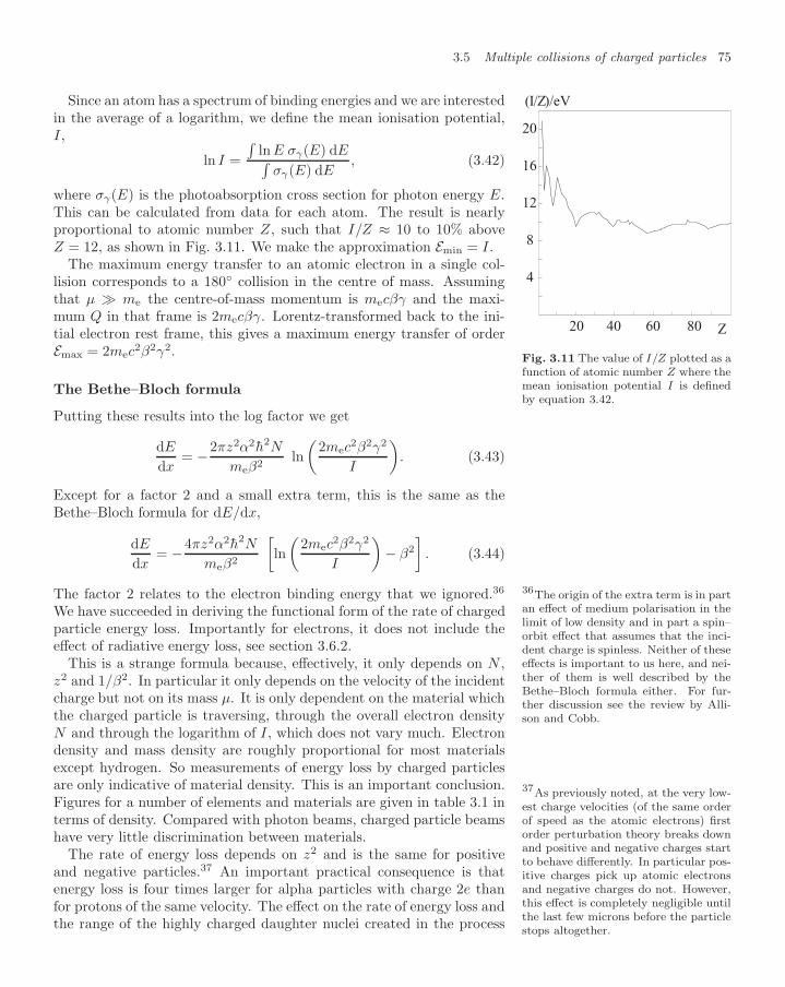
3.5 Multiple collisions of charged particles 75
Since an atom has a spectrum of binding energies and we are interestedin the average of a logarithm, we define the mean ionisation potential,I,
4
8
12
16
20
( / )/eVI Z
Z20 40 60 80
Fig. 3.11 The value of I/Z plotted as afunction of atomic number Z where themean ionisation potential I is definedby equation 3.42.
ln I =∫
lnE σγ(E) dE∫σγ(E) dE
, (3.42)
where σγ(E) is the photoabsorption cross section for photon energy E.This can be calculated from data for each atom. The result is nearlyproportional to atomic number Z, such that I/Z ≈ 10 to 10% aboveZ = 12, as shown in Fig. 3.11. We make the approximation Emin = I.
The maximum energy transfer to an atomic electron in a single col-lision corresponds to a 180 collision in the centre of mass. Assumingthat µ me the centre-of-mass momentum is mecβγ and the maxi-mum Q in that frame is 2mecβγ. Lorentz-transformed back to the ini-tial electron rest frame, this gives a maximum energy transfer of orderEmax = 2mec
2β2γ2.
The Bethe–Bloch formula
Putting these results into the log factor we get
dE
dx= −2πz2α2h2N
meβ2ln
(2mec
2β2γ2
I
). (3.43)
Except for a factor 2 and a small extra term, this is the same as theBethe–Bloch formula for dE/dx,
dE
dx= −4πz2α2h2N
meβ2
[ln
(2mec
2β2γ2
I
)− β2
]. (3.44)
The factor 2 relates to the electron binding energy that we ignored.36 36The origin of the extra term is in partan effect of medium polarisation in thelimit of low density and in part a spin–orbit effect that assumes that the inci-dent charge is spinless. Neither of theseeffects is important to us here, and nei-ther of them is well described by theBethe–Bloch formula either. For fur-ther discussion see the review by Alli-son and Cobb.
We have succeeded in deriving the functional form of the rate of chargedparticle energy loss. Importantly for electrons, it does not include theeffect of radiative energy loss, see section 3.6.2.
This is a strange formula because, effectively, it only depends on N ,z2 and 1/β2. In particular it only depends on the velocity of the incidentcharge but not on its mass µ. It is only dependent on the material whichthe charged particle is traversing, through the overall electron densityN and through the logarithm of I, which does not vary much. Electrondensity and mass density are roughly proportional for most materialsexcept hydrogen. So measurements of energy loss by charged particlesare only indicative of material density. This is an important conclusion.Figures for a number of elements and materials are given in table 3.1 interms of density. Compared with photon beams, charged particle beamshave very little discrimination between materials.
The rate of energy loss depends on z2 and is the same for positiveand negative particles.37 An important practical consequence is that
37As previously noted, at the very low-est charge velocities (of the same orderof speed as the atomic electrons) firstorder perturbation theory breaks downand positive and negative charges startto behave differently. In particular pos-itive charges pick up atomic electronsand negative charges do not. However,this effect is completely negligible untilthe last few microns before the particlestops altogether.
energy loss is four times larger for alpha particles with charge 2e thanfor protons of the same velocity. The effect on the rate of energy loss andthe range of the highly charged daughter nuclei created in the process

76 Interactions of ionising radiation
Table 3.1 The energy loss coefficient and radiation length, 1/ρ dE/dx and X0, for
some materials. The energy loss coefficient should be multiplied by z2ρ/β2 to getthe rate of energy loss with distance for a charge ze moving at velocity βc. Thevalue of X0 should be divided by ρ to get the radiation length in cm. The criticalelectron energy Ec at which dE/dx equals the radiative energy loss is given in thefinal column.
Material Z Z/A 1/ρ dE/dx X0 Density Ec
MeV cm2 g−1 g cm−2 g cm−3 MeV
H2 gas 1 0.992 4.103 61.28 0.089 × 10⁻³ 251Carbon 6 0.500 1.745 42.70 2.265 75N2 gas 7 0.500 1.825 37.99 1.250 × 10⁻³ 68O2 gas 8 0.500 1.801 34.24 1.428 × 10⁻³ 62Aluminium 13 0.482 1.615 24.01 2.70 38Silicon 14 0.498 1.664 21.82 2.33 36Argon gas 18 0.451 1.519 19.55 1.78 × 10⁻³ 30Iron 26 0.466 1.451 13.84 7.87 20Copper 29 0.456 1.371 12.25 8.96 17Germanium 32 0.441 1.264 8.82 5.32 11Xenon gas 54 0.411 1.255 8.48 5.86 × 10⁻³ 11Tungsten 74 0.403 1.145 6.76 19.3 8Lead 82 0.396 1.123 6.37 11.35 7Air 0.500 1.815 36.66 1.205 66Water 0.555 1.991 36.08 1.000 72Concrete 0.503 1.711 26.7 2.50 46SiO2 0.499 1.699 27.1 2.20 46Polystyrene scint. 0.538 1.936 43.7 1.03 85NaI 0.427 1.305 9.49 3.67 12BaF2 0.422 1.303 9.91 4.89 13BGO 0.421 1.251 7.97 7.1 10PbWO4 0.412 1.57 7.04 8.28 11
of nuclear fission is very pronounced. We return to this when we discussradiation damage by alpha particles and more highly charged ions inchapter 6 and again in the discussion of radiotherapy in chapter 8.
The energy loss varies as 1/β2 universally for all materials.38 As a
38The apparent dependence on ln (βγ)is usually suppressed in practice by thedensity effect, a material polarisationeffect not accounted for by the Bethe–Bloch formula.
charge passes through a material it loses energy and slows down. As βfalls, the factor 1/β2 rises sharply. Thus energy is deposited ever moredensely until the charge finally stops.
Because of the stochastic nature of the energy loss process, individ-ual charges experience different values of energy loss in the same ab-sorber under the same circumstances. These variations are called Lan-dau fluctuations.39 The effect of these fluctuations can be important
39With a computer it is quite simpleto calculate these fluctuations from aknowledge of the cross section. Whenattempting to derive results in a pre-computer age, Landau was obliged tomake approximations which are rarelyvalid. There is no need to use his ap-proximations in any calculation today.See the review by Allison and Cobb.
in very thin absorbers, and they generate variations in range, termedstraggling.
The mean rate of energy loss with distance, dE/dx, with its factor

3.5 Multiple collisions of charged particles 77
0.10.0 0.2
distance/cm
alpha particles
protons
electrons& muons
d /dMeV/cm
E x
0.10.0 0.2distance/cm
log d /d
MeV/cm
E x10
alpha particles
protons
muons
electrons
b)a)
200
400
600
800
1000
1
2
3
Fig. 3.12 The calculated rate of energy loss as a function of depth in water for various particles with initial kinetic energy 20MeV, ignoring straggling. a) On a linear scale; b) on a logarithmic scale.
z2/β2 and linear dependence on electron density is called the linear en-ergy transfer (LET) in the context of radiation damage. It is importantin determining the localisation of radiation damage in living tissue. Asdiscussed in chapters 6 and 8 this plays a major role in determining theprobability that living tissue recovers from a given radiation dose.
3.5.2 Range of charged particles
Dependence of range on mass for incident particles of knownenergy
The effect of the z2/β2 dependence of the energy loss is illustrated inFig. 3.12, neglecting Landau fluctuations. The rate of energy depositionwith depth is calculated for various charged particles of 20 MeV kineticenergy passing into water. The alpha particles lose energy so rapidlythat they stop within 150 µm. The protons go further and stop in about2.1 mm. There is a very sharp peak in the rate of energy deposition justbefore they stop. In Fig. 3.12b the same calculations are shown on alogarithmic scale. In practice fluctuations spread the values of β at eachdistance and have a blurring effect on the peaks of these distributionswhen averaged over a number of particles. Such distributions are knownas Bragg curves and the broadened peaks known as Bragg peaks.40 40In addition to fluctuations in its en-
ergy loss, each particle scatters so thatits path is not a straight line. Strictlyspeaking, the mean range is the tracklength along its path, rather than thestraight line to its stopping point. How-ever, the effect on the range is small,except for electrons.
How far do charged particles of a given energy E go? There is a certainmean range and because of straggling there is a narrow spread in thedistribution. Straggling is a relatively small effect because the numberof collisions involved is large. In fact the number of collisions that occuris on the scale of 105 to 106 for the 20 MeV particles considered inFig. 3.12. However, the fluctuations are dominated by a relatively smallnumber of rather energetic collisions.
If a proton beam of the right energy is used for radiotherapy, a large

78 Interactions of ionising radiation
highly localised dose can be delivered at the point where the protonsstop. Thus by locating the Bragg peak in a small target volume in atumour within healthy tissue the energy may be deposited preferentiallyjust where it is required as discussed in section 8.4.
Range–energy relations
In a given material the mean range R of any incident charged particleobeys the scaling relation
R =µ
z2Φ
(E
µ
)(3.45)
where E is the initial kinetic energy, µ is the mass and ze the charge.The function Φ(E/µ) is the same for all charges and is determined onlyby the medium, primarily through its electron density. This relation canbe proved from the Bethe–Bloch formula by observing that the rangeis the integral along the particle path from the point at which it haskinetic energy E to the point where this falls to zero:
R =∫
dx =∫ 0
E
1dE′/dx
dE′ (3.46)
The energy loss is a function of the velocity of the charge only, that isthere exists a function F characteristic of the medium such that
dE
dx= −z2F
(E
µ
)(3.47)
Then
R = − µ
z2
∫ 0
E/µ
d(E′/µ)F (E′/µ)
=µ
z2Φ(E/µ) (3.48)
where the integral Φ depends only on the medium and the ratio (E/µ).This is called the range–energy relation, sometimes expressed equiva-
lently as the range–momentum relation. It says that there is a universalcurve for a given material that applies for all particles. It is plotted forhydrogen, carbon and lead in Fig. 3.13. Actually, because of the relativeinsensitivity to parameters describing the medium, the universal curvesfor different materials are all rather similar when expressed in terms of(electron) density.
3.5.3 Multiple Coulomb scattering
Calculation of RMS scattering angle on passing through amaterial
When a parallel beam of charged particles passes through a slice of mate-rial of thickness , it exits with a symmetric distribution in net scatteringangle due to the cumulative effect of Rutherford scattering. Scatteringcollisions at large impact parameters with small angular deviations occurmany times while those at small impact parameters occur infrequently

3.5 Multiple collisions of charged particles 79
10
10
10
10
0.1 1 30.3P/mc
Proton range
density
kg m
H
Pb
C
2
3
4
-2
Fig. 3.13 Universal curves for hydro-gen, carbon and lead showing protonrange times density as a function ofthe dimensionless βγ = P/mc, for unitcharge. [Originally from the ParticleData Group website.]For particles of mass m = µ, the rangescales as mP /µ. For particles of chargez, the range scales as 1/z2.
but give large contributions to the mean scattering. If the beam is alongthe z-axis, there is scattering in both the xz- and yz-planes. These twodistributions are the same and symmetric. It is usual to refer to this pro-jected distribution and its RMS width, θMS. This introduces a factor of12 in the expression for the mean square scattering angle:
θ2MS =
12
∫θ2 N
dσ
dΩdΩ (3.49)
where N is the nuclear target density with cross section dσ/dΩ given byequation 3.26.41 41For simplicity we have assumed a ma-
terial composed of a single element withatomic number Z.
θ2MS =
N Z(Z + 1)2
(zαh
2Pβ
)2 ∫θ2cosec4(θ/2) 2π sin θ dθ (3.50)
We have included the scattering due to the atomic electrons. There areZ of these per atom but their cross section is smaller by factor 1/Z2. Sowe have replaced Z2 by Z(Z + 1).
Unfortunately this integral diverges when evaluated between 0 andπ. We need to consider the maximum and minimum scattering angles

80 Interactions of ionising radiation
for which equation 3.26 applies. The scattering is reduced by electronscreening of the nuclear charge at large distance a and by the spreadof the nuclear charge due to its finite size at small distance rN, that iswhen the momentum transfer is less than h/a or greater than h/rN.4242These are different, although similar,
to the considerations that applied inthe evaluation of dE/dx. The true re-lation is with the radiation length.
The mean charge radius of the atomic electron distribution is abouta = 0.5 × 10⁻¹⁰Z−1/3 m according to the Thomas–Fermi model of theatom. The nuclear radius is rN = 1.2× 10⁻¹⁵A1/3 m. So for momentumP we have as the limits of integration a lower limit of θ1 = 2πh/(Pa)and an upper limit θ2 = 2πh/(PrN). Then the result is
θ2MS =
Nz2Z(Z + 1)2
(αh
2Pβ
)2 ∫ θ2
θ1
θ2cosec4(θ/2)2π sin θ dθ (3.51)
Practical estimation of multiple scattering
Such calculations give fair agreement with accepted values for RMS mul-tiple scattering for all elements from hydrogen to lead within a few percent. The square root dependence of the mean net angle on the slicethickness is characteristic of the random walk nature of the scatteringprocess.
The distribution of projected scattering angles is not quite Gaussian.The distribution has a tail at very large angles.43 The distribution of43The observation of a small number of
large angle scatters was historically im-portant in establishing the evidence forthe existence of the very large concen-tration of mass and charge right at thecentre of the atom, the nuclear model.
these unusual single scatters is described by Poisson statistics. How-ever, they are rare in thin samples. From the point of view of the prac-tical applications referenced in this book, the distribution of projectedscattering angles may be taken to be a Gaussian distribution with thevariance calculated.
In practical applications most materials are composed of more thanone element. The scattering may be combined in quadrature, but it isusual to use tabulations of the radiation length X0 for the compositematerial concerned. Some figures are given in table 3.1. Thus
θMS =13.6βP
√ρ
X0, (3.52)
where ρ is the thickness multiplied by the density and X0 is the radi-ation length of the medium.44 The X0 conveniently encapsulates all of44Usually in this book we use SI units.
However, in table 3.1 we follow normalusage and give X0 in units of g cm−2.This makes no difference provided thethickness ρ is expressed in the sameunits.
the physics of the medium discussed above into a single number. Thevalue 13.6 and the momentum P are in units of MeV/c.
Question 3.7 provides a numerical example of the application of equa-tion 3.52. It concerns the scattering in the carbon ion ‘stripper’ channelof a radiocarbon accelerator mass spectrometer of the type shown inFig. 6.12.

3.6 Radiative energy loss by electrons 81
3.6 Radiative energy loss by electrons
Radiative Rutherford scattering in the nuclear field is important if theincident charges are electrons. Because of their low mass they accelerateand radiate readily. This bremsstrahlung process may be understood sim-ply in the centre-of-mass frame of the incident electron in terms of Comp-ton scattering of virtual photons. The energy loss due to bremsstrahlunginvolves the same screened nuclear field as in multiple scattering and pairproduction. The radiation length of different materials is defined in termsof bremsstrahlung production.
3.6.1 Classical, semi-classical and QEDelectromagnetism
An incident charge that scatters in the nuclear Coulomb field of a targetatom accelerates transversely. If it has low mass µ this acceleration maybe large and it is likely to radiate. In classical mechanics the radiatedenergy is uniquely determined by the acceleration; in quantum mechan-ics the acceleration only determines the probability of photon emission.This can be calculated by the Planck mechanism of equating the classi-cal radiated energy I(ω)∆ω in each frequency band ∆ω to the productof the probability, P (ω)∆ω, of emitting a photon in that band and theenergy per photon hω. Thus P (ω) = I(ω)/(hω). This is called the semi-classical approximation. If the particle radiates a significant fraction ofits kinetic energy, this approximation fails and a calculation in QED isrequired. Semi-classical methods are sufficient for most purposes and wepresent such a picture in the following.
3.6.2 Weissacker–Williams virtual photon picture
To a stationary observer a passing charged particle gives a pulse of elec-tric field. The pulses are sketched in Fig. 3.14. The longitudinal fieldforms an odd function of time, rising as the charge approaches and thenfalling rapidly to zero and reversing sign as the charge passes and re-treats away. The transverse field is an even function of time, rising to amaximum as the charge passes the observer and then falling again.
We can analyse this pulse into the frequency components seen by theobserver, and interpret the power spectrum in each frequency band asthe probability of detecting a photon. Under relativistic conditions thesephotons behave as if they were free.
a)
b)
time
time
E
E
L
T
Fig. 3.14 a) The longitudinal electricfield pulse, and b) the transverse fieldpulse, seen as a function of time byan observer close to the trajectory ofa passing charge.
Bremsstrahlung in the virtual photon picture
Consider the bremsstrahlung emitted by a high velocity electron passinga lead nucleus which is stationary in the laboratory. What understandingof the process can we derive from the virtual photon picture?
The heavy lead nucleus is not much affected by the passing of a singlycharged electron. However, consider the electron’s view of the process.It sees a charge of 82e passing at the same relativistic speed that the

82 Interactions of ionising radiation
electron has in the laboratory. According to the virtual photon picturethis rapidly moving charge of 82e is seen densely shrouded in photons.The situation is illustrated in cartoon form in Fig. 3.15. Because thecharges are point-like over the scale 10−15 to 10−10 m the Fourier analysisof the field determines that the spectrum of photons is flat over a broadrange of frequencies. The amplitude of the field depends on Z and theflux on Z2. These photons can be Thomson scattered by the electronwith4545In the unlikely event that the pho-
ton has energy > mec2 in the electronframe, the cross section is the Comptoncross section.
σT =8π
3
(αh
µc
)2
. (3.53)
The angular distribution of scattered photons in the electron rest frameis nearly isotropic. When this distribution is Lorentz-transformed fromthe electron to the laboratory frame, those photons that were scatteredinto the forward hemisphere in the electron frame become boosted tosmall angles θ ∼ 1/γ and Doppler blue-shifted.
a)
b)
c)
Ze
e
e
Ze
e
Fig. 3.15 a) Radiation by an electronin a beam passing a nucleus, as seenin the laboratory frame. b) The EMfield of the approaching charge Ze asseen by an observer co-travelling withthe beam electron. c) The resulting EMfield, scattered as a dipole field in therest frame of the electron.
3.6.3 Radiation length
The dependence of the bremsstrahlung cross section on 1/µ2 and γmeans that under normal circumstances such radiation is peculiar toelectron beams. The virtual photon flux (and thence the bremsstrahlung)is proportional to Z2, so that this is largest for high Z materials. Thusa typical X-ray tube consists of an electron beam hitting a heavy metaltarget such as copper or tungsten. Calculations of flux involve the sametype of integral that we encountered in the calculation of multiple scat-tering. There are the same limits on impact parameter associated withthe screening distance due to atomic electrons on the one hand and fi-nite nuclear size (or maximum energy) on the other. The same effectappears in the calculation of pair production by photons incident on ahigh Z target where the cross section also depends on Z2.
Because the charges are point-like, the cross section for the electronto lose a fraction η of its energy is independent of η. As a result thebremsstrahlung energy loss process scales, that is the energy loss is pro-portional to the incident energy. The energy loss is subject to largefluctuations, unlike the recoil and ionisation energy loss.46 Because of46Together, these two are often referred
to as the collisional energy loss as op-posed to the radiative energy loss.
the scaling, when bremsstrahlung dominates over the collisional energyloss, the mean energy E of an incident electron falls exponentially withdistance as
dE
dx= − E
X0. (3.54)
This is the definition of X0, the radiation length.The radiation length X0 for a material with atomic number Z is given
to a good approximation by
X0 =716.4A
Z(Z + 1) ln (287/√
Z)(3.55)
in units of g cm−2. Bremsstrahlung cross sections in mixtures of elementsbehave additively. In table 3.1 are given values of the radiation length

3.6 Radiative energy loss by electrons 83
and the magnitude of collisional dE/dx in the limit β = 1 for a widevariety of materials. According to equation 3.54, the radiative energyloss increases linearly with electron energy whereas the collisional energyloss is almost constant. The electron energy at which they are equal canbe determined directly from the table. The ratio of these processes inX-ray targets gives an estimate of the efficiency of photon productionand also the cooling required. It follows that a high Z target and ahigh energy electron beam are the most efficient. The energy of theelectron beam also determines the photon energy spectrum from thescaling argument.47
47In addition to the bremsstrahlungspectrum there are also the characteris-tic X-ray peaks generated by radiativerelaxation of inner shell vacancies.
Read more in books
A Century of X-rays and Radioactivity in Medicine,RF Mould, IOP (1993), a book of early pictures andinteresting authoritative history
Introduction to Nuclear Physics, DA Greenwood andWN Cottingham, CUP, 2nd edn (2001), a standardbook on the interaction of radiation in matter and onnuclear physics
Nuclear and Particle Physics, WSC Williams, OUP(1991), a standard book on the interaction of radiationin matter and on nuclear physics
Quantum Mechanics, F Mandl, Manchester Physics Se-ries, Wiley (1992), a standard book on quantum me-chanics including time-dependent perturbation theory
Quantum Physics, S Gasiorowicz, Wiley (1974), astandard book on quantum mechanics including timedependent-perturbation theory
Relativistic Charged Particle Identification by EnergyLoss, WWM Allison and JH Cobb, Annual Reviews ofNuclear and Particle Science, 30, 253 (1980), furtherdiscussion of energy loss
The Physics of Charged Particle Identification: dE/dx,Cherenkov and Transition Radiation, WWM Allisonand PRS Wright, Experimental Techniques in High En-ergy Nuclear and Particle Physics, ed. T Ferbel, 2ndedn, World Scientific (1991), further discussion of en-ergy loss
Look on the Web
Look at the book website atwww.physics.ox.ac.uk/users/allison/booksite.htm
Find information on coherent X-ray sources withFEL and synchrotron light source
Get data on the X-ray spectra of elements from theNIST site
NIST X-ray
Look at the Particle Data Group website for informa-tion on range–momentum, multiple scattering, radia-tion length, etc., for charged particles and photons inmatter
PDG, particle data group
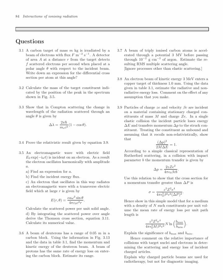
84 Interactions of ionising radiation
Questions
3.1 A carbon target of mass m kg is irradiated by abeam of electrons with flux F m−2 s−1. A detectorof area A at a distance r from the target detectsf scattered electrons per second when placed at apolar angle θ with respect to the incident beam.Write down an expression for the differential crosssection per atom at this angle?
3.2 Calculate the mass of the target constituent indi-cated by the position of the peak in the spectrumshown in Fig. 3.5.
3.3 Show that in Compton scattering the change inwavelength of the radiation scattered through anangle θ is given by
∆λ =2πh
mec2(1 − cos θ).
3.4 Prove the relativistic result given by equation 3.9.
3.5 An electromagnetic wave with electric fieldE0 exp(−iωt) is incident on an electron. As a resultthe electron oscillates harmonically with amplitudea.
a) Find an expression for a.
b) Find the incident energy flux.
c) An electron that oscillates in this way radiatesan electromagnetic wave with a transverse electricfield which at large r is given by
E(r, θ) =eaω2 sin θ
4πε0c2r.
Calculate the scattered power per unit solid angle.
d) By integrating the scattered power over anglederive the Thomson cross section, equation 3.11.Calculate its numerical value.
3.6 A beam of deuterons has a range of 0.05 m in acarbon block. Using the information in Fig. 3.13and the data in table 3.1, find the momentum andkinetic energy of the deuteron beam. A beam ofprotons has the same rate of energy loss on enter-ing the carbon block. Estimate its range.
3.7 A beam of triply ionised carbon atoms is accel-erated through a potential 3 MV before passingthrough 10−2 g cm−2 of argon. Estimate the re-sulting RMS multiple scattering angle.[Ignore processes other than elastic scattering.]
3.8 An electron beam of kinetic energy 3 MeV enters acopper target of thickness 1.0 mm. Using the datagiven in table 3.1, estimate the radiative and non-radiative energy loss. Comment on the effect of anyassumption that you make.
3.9 Particles of charge ze and velocity βc are incidenton a material containing stationary charged con-stituents of mass M and charge Ze. In a singleelastic collision the incident particle loses energy∆E and transfers momentum ∆p to the struck con-stituent. Treating the constituent as unbound andassuming that it recoils non-relativistically, showthat
(∆p)2
2M∆E= 1.
According to a simple classical representation ofRutherford scattering, in a collision with impactparameter b the momentum transfer is given by
∆p =2zZe2
4πε0βcb.
Use this relation to show that the cross section fora momentum transfer greater than ∆P is
σ =z2Z2e4
4πε20β2c2(∆P )2
.
Hence show in this simple model that for a mediumwith a density of N such constituents per unit vol-ume the mean rate of energy loss per unit pathlength is
z2Z2e4
4πε20Mβ2c2N ln
(bmax
bmin
).
Explain the significance of bmax and bmin.
Hence comment on the relative importance ofcollisions with target nuclei and electrons in deter-mining the scattering and energy loss of incidentcharged articles.
Explain why charged particle beams are used forradiotherapy, but not for diagnostic imaging.

Mechanical waves andproperties of matter 4
4.1 Stress, strain and waves in ho-mogeneous materials 85
4.2 Reflection and transmission ofwaves in bounded media 99
4.3 Surface waves and normalmodes 111
4.4 Structured media 120
Read more in books 129
Look on the Web 129
Questions 130
in which is derived the fundamental physics of sound. This provides anexplanation of many applications and an introduction to chapter 9.
4.1 Stress, strain and waves inhomogeneous materials
The internal forces in a material (stress) are determined by the relativedisplacement of its elements (strain). Two types of displacement giveinternal forces, expansion and distortion. Fluids are distinguished fromsolids by the fact that internal forces are not generated by distortion.For small changes forces and displacements are related linearly (Hooke’slaw). This law may fail due to non-linearity and inelasticity. In anideal fluid expansion and stress are related by the bulk modulus. Waveswith longitudinal displacement and isotropic pressure may propagate. Ina solid both stress and strain are described by second rank tensors. Eachtensor may be separated into irreducible parts, a scalar, a vector and a5-component symmetric traceless second-rank tensor. In an elastic linearisotropic solid the stress is related to the strain by two moduli. There arethree independent wave equations, two with transverse displacements andone with longitudinal displacement.
4.1.1 Relative displacements and internal forces
Every material has an equation of state that describes how it respondsto different externally imposed conditions. Under given thermodynamicconditions each individual element of that material acts on its neighbour-ing elements as their displacements change.1 These actions and reactions 1We start by thinking of simple isother-
mal conditions, correcting this laterwhere appropriate.
are the internal forces.To keep track of what happens to each element we choose a reference
state. Each part of the material is then labelled by its position (x, y, z)in that reference, and its displacement vector u = (ux, uy, uz) is the shiftbetween its actual position and its reference position.2 There are inter- 2Here we look at materials macroscop-
ically and treat u as a smooth andcontinuous function of position, ignor-ing the fact that at a microscopic levelconstituents may be moving about, asmolecules in a gas, for example.
nal forces in the reference state. The relations of interest are betweenthe changes in internal forces and the displacements, all relative to thereference state. Looking at the displacement of an elemental volume, itmay undergo a combination of the following:

86 Mechanical waves and properties of matter
displacement as a whole; rotation as a whole; expansion, so that its volume changes; distortion, such that it is squeezed in one direction and stretched
in another.
Some types of displacement field, u(r), within a material are resistedby internal forces and some are not. Displacement as a whole and ro-tation as a whole do not change the relative positions of neighbouringparts within a material and therefore are not associated with changes ofinternal forces. In a solid, expansion and distortion do generate changesin local separations and so are generally accompanied by changes to in-ternal forces. In a fluid, only changes in expansion generate changes ininternal forces.3
3Viscous forces oppose the rate ofchange of distortion, but there are nointernal forces associated with changesin static distortion.
B
A
-ΔF
-ΔF
Δℓ/ℓ
Δℓ/ℓ
a)
b)
Fig. 4.1 Illustrations of change in forceagainst relative displacement. a) Anelastic force, linear to point A but non-linear at B relative to A. Redefining thereference state at B, displacements nearB are seen to be linear. b) An inelasticforce which is not uniquely determinedby the displacement.
Linearity and elasticity
The archetype of the relation between displacement and the change inforce, Hooke’s law, assumes that these are small. For such displacementof the end of a spring of length there is a linear change in the force F ,
−∆F = F0 − F = K∆
, (4.1)
where F0 is the spring force in the reference state. The coefficient K isknown as the modulus and the force is always in the opposite directionto the displacement. This is required for mechanical stability.
Real springs do not quite obey Hooke’s law. Figure 4.1 illustrates thetwo ways in which the law can fail. The relation between extension andchange in force may be non-linear, and it may be inelastic.
The plot of force against extension is typically straight only locally.It may be linear near point A and also near point B. But relative toA as reference point, extensions near B are not linear. Mathematically,changing the reference point is doing no more than expanding the de-scription of the problem in a Taylor’s series about a closer point at whichthe series converges more rapidly, requiring no more than a linear term.So questions of non-linearity are intimately connected with the choice ofreference state.
Figure 4.1b illustrates what happens when the force is inelastic. If amaterial is inelastic the relation between force change and relative dis-placement is not unique. Net work is done when an inelastic material isdeformed and then returned to the original state of deformation. Theforce is not conservative.4 Everyday experience shows that such materi-
4In thermodynamic language, the in-ternal energy is not a function of state.
als get hot when repeatedly deformed in this way. This shows explicitlythat mechanical energy is not conserved, and that from a thermody-namic point of view such changes are irreversible. Then the relationbetween force change and relative displacement is typically described bya hysteresis loop.
Elasticity and linearity are essentially different. A deformation maybe elastic or inelastic, and linear or non-linear.

4.1 Stress, strain and waves in homogeneous materials 87
Stress and strain in a material
In a material an internal force is expressed as a force per unit area andknown as a component of stress. The generalisation of the ratio ∆/,displacement over distance, is known as a component of strain. Themodulus for expansion is known as the bulk modulus, KB. The modulusfor distortion is known as the shear modulus, µ. The shear modulus of afluid is zero.5 When subjected to distortion, fluids simply flow and relax. 5We ignore the effect of viscosity for the
time being.There are shear displacements, but no shear forces. Liquids and gasesmay be described to a fair approximation as ideal fluids. We discussfluids first. This is followed by a discussion of solids for which a moregeneral approach is required.
4.1.2 Elastic fluids
Stress and strain in a fluid
A fluid reacts in the simplest way to stress, deforming or flowing freelysuch that only isotropic stress is maintained. The stress T has threecomponents, in the x-direction on the plane x = 0, in the y-direction onthe plane y = 0, in the z-direction on the plane z = 0. Each is equal to−P , the pressure.6 Any change in stress is similarly constrained with all 6The use of the letter T for the stress
denotes the fact that it is convention-ally signed as a tensile stress, oppositein sign to pressure.
three diagonal components of ∆T equal to −∆P .A fluid can be subjected to many different elements of strain, ε.7 But
7When we study solids we shall need toworry more about the details of straincomponents. Here we only need thecomponents that contribute to a changeof volume.
only the expansion in x, in y and in z contribute to the volumetricexpansion,
ε =∆V
V0=
∂ux
∂x+
∂uy
∂y+
∂uz
∂z. (4.2)
This volumetric strain is related to the stress by the KB,
∆T = KB∆V/V0. (4.3)
Thence
KB = −V0∂P
∂V. (4.4)
The equation of state of the fluid relates the pressure to the volume atany given value of temperature, so that KB may be found.
Isothermal bulk modulus for a perfect gas
The equation of state of a perfect gas is
PV = nRT, (4.5)
where P is the pressure, V the volume, T the temperature,8 n the num-8We use T to denote temperature aswell as stress. In the following themeaning will usually be stress unlessnoted otherwise.
ber of moles and R the gas constant. In the reference state the volumeis V0 and the stress is T0 = −P0. This suggests that KB = P0.

88 Mechanical waves and properties of matter
Thermodynamic conditions on expansion or deformation
An important question is which thermodynamic parameters are to beheld constant in the partial differentiation involved in the definitionof the modulus. We have made the mistake, implicitly, of consideringchanges9 at constant temperature when differentiating equation 4.5. In9We are in good company for Newton
also made this mistake, as pointed outby Laplace.
general, no heat is supplied when materials are deformed or expanded.So the process takes place at constant entropy, not at constant tempera-ture. Therefore KB should be defined at constant entropy, and likewisefor other moduli.Table 4.1 Values of γ, the ratio
CP/CV, for some gases.
Argon 1.667Neon 1.642Mercury at 550 K 1.666Hydrogen 1.407Air 1.402Carbon monoxide 1.297Steam at 373 K 1.334Carbon dioxide 1.300Methane 1.313Ethane 1.22Propane 1.130Carbon tetrachloride 1.130
A constant entropy change in a perfect gas obeys the relation PV γ =constant where γ is the ratio of the specific heats, CP /CV . So for aperfect gas,
KB = γP0, (4.6)
instead of P0. The value of γ depends on n, the number of degrees offreedom of the gas, γ = (n+2)/n. For a monatomic gas there are only thethree translational motions and the expected value is γ = 5/3 = 1.667.For a diatomic gas rotation about two axes leads to the expectation7/5 = 1.400, unless the temperature is high enough for longitudinalvibrational excitation to occur. For polyatomic gases n is 6 or more andγ ≤ 1.333. Observed values, table 4.1, conform to these expectations.
4.1.3 Longitudinal waves in fluids
The stress change and the strain are also related by Newton’s secondlaw. The forces described by the change in stress generate accelerationswhich are related to the second time derivative of the strain. Theseresult in wave motion.
in referencestate
at time t
z z+dz
z+u z+u+dz(1+du/dz)
Fig. 4.2 The position of the bound-aries of a slice, defined as being at z andz+dz in the reference state, as seen attime t.
In the case of a plane wave moving along the z-axis, partial derivativeswith respect to x or y are zero. The only nonzero element of volumetricstrain is ∂uz/∂z. Therefore the displacement is along z. We trackthe displacement of a point defined by its reference position z in thematerial. At time t the displacement in the z-direction is uz(z, t). Atthe same time a neighbouring point with reference z+dz will be displacedby a distance uz+duz/dz×dz as illustrated in Fig. 4.2. The subsequentbehaviour of the medium is determined by Newton’s second law appliedin the z-direction on the element dz. If the reference density is ρ0 and anelement of the slice has unit area in the xy-plane, then the mass of theelement is ρ0dz, a constant. The force in the negative z-direction on theelement through the boundary at z is ∆T (z) and the force in the positivez-direction through the boundary at z+dz is ∆T (z)+ ∂∆T (z)/∂z dz.10
10Recall that T is positive for a tensilestress.
The mass times the acceleration is then equal to the net force in thepositive z-direction acting on the slice
ρ0dz∂2uz
∂t2=
∂∆T
∂zdz. (4.7)
Substituting
∆T = KB∂uz
∂z. (4.8)

4.1 Stress, strain and waves in homogeneous materials 89
The final differential equation is11 11Note that there are also changes intransverse stress because the pressureis isotropic. However, these are in equi-librium and so cause no motion.
∂2uz
∂t2=
(KB
ρ0
)∂2uz
∂z2. (4.9)
Comparing this equation with the standard form of the one dimen-sional linear wave equation
∂2φ
∂t2= c2 ∂2φ
∂z2, (4.10)
it is evident that uz(z, t) obeys a wave equation with wave velocity
c =
√KB
ρ0. (4.11)
Note that this is the velocity of the waves as they propagate in the z-direction and is a fixed property of the medium independent of waveamplitude. It should not be confused with the instantaneous velocityof elements of the medium vz = ∂uz/∂t, which is proportional to theamplitude and oscillates with time. This is called the particle velocity.For this longitudinal wave it is also in the z-direction.
D’Alembert solutions in one dimension
Since the relation between stress and strain does not depend explicitlyon time and Newton’s second law is symmetric in time, for every solutionto the wave equation in an unbounded material that involves t, there isanother in which the sign of t is reversed. These pairs of solutions in ±tare called progressive or travelling wave solutions.
Such pairs of solutions exist for all elastic media, even when the wavesare not linear. However, only in linear media does the principle of super-position apply, such that progressive wave solutions may be freely addedtogether. We return to consider the non-linear case in section 9.4.
In the linear case these pairs of solutions may be found by the d’Alem-bert method. We change variables in the wave equation 4.10 from zand t to ξ = z − ct and ζ = z + ct. Using the chain rule for partialdifferentiation
∂
∂t=
∂ξ
∂t
∂
∂ξ+
∂ζ
∂t
∂
∂ζ(4.12)
and a similar expression for the ∂/∂z operator, the wave equation re-duces to
∂2u
∂ξ∂ζ= 0. (4.13)
z-ct
z
z
z
1 2
2
2
2
1
1
1
3
3
3
3
at t=0
at t=1/c
at t=2/c
a)
b)
c)
d)
Fig. 4.3 A progressive wave f(z − ct)travelling in the positive z-direction: a)plotted as a function of z − ct, b) plot-ted at t = 0, c) plotted at t = 1/c, d)plotted at t = 2/c.
The general solution is found by integration to be
u = f(z − ct) + g(z + ct), (4.14)
where the arbitrary functions f and g arise from the two constants ofintegration for which ζ and ξ are, in turn, held constant.

90 Mechanical waves and properties of matter
To understand these solutions, consider first f(z − ct). Such a waveis illustrated in Fig. 4.3. The peak at z − ct = 1 appears at z = 1 whent = 0, z = 2 when t = 1/c, z = 3 when t = 2/c, and so on. The profile ofthe wave moves in the positive z-direction at wave velocity c. These arethe properties that we expect of an ideal travelling wave. It is ideal in thesense that it suffers neither distortion nor attenuation as it progresses.A wave of the form g(z + ct) behaves similarly but with the sign of timet reversed. It therefore describes an unattenuated distortion-free wavethat moves in the negative z direction.
Wave impedance of fluids
To complete the solution for a travelling wave we need to determinethe remaining variables. For a longitudinal wave in the z-direction theparticle velocity vz is the time derivative of uz
vz(z, t) =∂uz
∂t= −cf ′(z − ct) (4.15)
where f ′ is the derivative of f with respect to its argument, ξ = z − ct.The acceleration is c2f ′′(z − ct). Equation 4.8 gives
∆T = KBf ′(z − ct). (4.16)
This shows that in a travelling wave ∆T and vz are proportional, and
∆T = ∓Zvz, (4.17)
where the positive and negative signs apply for negative and positivegoing waves respectively. The impedance of the fluid is
Z = ρ0c =√
ρ0KB. (4.18)
The ratio of stress to particle velocity changes sign according to thedirection in which the progressive waves are moving. For a superpositionof waves in both directions the ratio ∆T/v varies in space and time andmay have any value.12
12The impedance is often written asthe ratio Z = P/v for a positive go-ing wave. Since the excess pressureP = −∆T , the signs are consistent.
Table 4.2 Values of density (ρ in kgm−3), wave velocity (cL and cS m s−1)for longitudinal and transversely po-larised waves for various materials attemperature T = 293 K (except at273 K for He, ice and water).
Material ρ cL cS
Be 1848 12800 8880Al 2700 6420 3040Steel 7870 5940 3220Lead 11350 1960 690Sandstone 2323 2920 1840SiO2 2200 5968 3764Ice 910 3760 2000Nylon 1140 2620 1070Polythene 930 1950 540Muscle 1040 1567 var.Bone 1940 3550 1970Blood 1060 1547 –Hg 13600 1450 –Water 1000 1401 –Air 1.29 344 –He 0.17 965 –
Values for moduli and impedances can be deduced from the tableof densities and velocities for longitudinal and shear waves for a widevariety of materials given in table 4.2. Notice that gases have both lowdensity and low elastic modulus compared with solids. The low soundvelocity indicates that the low elastic modulus is the dominant effect.13
13In fact, as discussed below, the inter-pretation for waves in solids is not sostraightforward. Specifically the mod-ulus for longitudinal waves differs fromthe bulk modulus.
Energy density
The energy density relative to the reference state in a linear mediumcan be expressed as the sum of the local kinetic and potential energydensities. The kinetic energy density is
UKE(x, t) =12ρ0v
2. (4.19)
4.1 Stress, strain and waves in homogeneous materials 91
The potential energy density can be expressed in a number of equivalentways using the relations ∆T = Kε and ε = ∆V/V0:
UPE(x, t) =12Kε2 =
12∆Tε. (4.20)
For a progressive wave ∆T = ±Zv. Therefore the kinetic energy andpotential energy densities are equal everywhere. In the absence of dis-persion, the energy flux N in a progressive wave is the sum of kineticand potential energy densities multiplied by the wave velocity,
N = ρ0v2c = Zv2 = ∆Tv = (∆T )2/Z. (4.21)
These are instantaneous values in SI units of W m−2. For the mean fluxthe RMS value of v or ∆T should be used. Note that the transverseforces present in a longitudinal compression wave are in equilibrium anddo no work. It is the longitudinal force that is relevant.
Dispersion for progressive waves
So far we have implicitly assumed that the bulk modulus KB is constant.At low frequencies this is a good approximation. At higher frequenciesit is not true and consequently the values of c and Z are functions offrequency. Then the different Fourier components in a signal travel atdifferent speeds.
The result is that the signal profile changes as it propagates. A Fouriercomponent (frequency ω and wavenumber k) has phase velocity c = ω/k.In general a study of the physical mechanics of the wave motion givesa relation between ω and k from which c may be determined. Such anequation is called a dispersion relation.
The envelope of a pulse composed of frequencies between ω and ω+dωand wavenumber between k and k+dk moves with velocity dω/dk, theslope of the dispersion curve, plotted as ω against k. This is called thegroup velocity. If the group velocity itself varies with frequency withinthe signal bandwidth then the pulse will distort and spread out in time,even if there is no actual absorption. If the dispersion relation hascomplex parts then there is energy absorption. The reason for this maybe understood by considering a progressive harmonic wave in the formexp [i(kx − ωt)]. Any imaginary part of k (or ω) implies an exponentiallydamped progression in x (or t). This describes a wave that is beingattenuated.
Absorption of harmonic linear waves may be described by consideringcomplex moduli. An imaginary part of KB describes a phase differ-ence between stress and strain. Of course this is just a formalism. Weshall need to dig deeper to understand what is happening in absorptiveprocesses.
We shall see later in section 4.4.2 that the absorption of sound waves isassociated with a delay in the strain relative to the causative stress. Ev-ery effect must follow its cause so that such a delay may not be negativewithout violating causality. There is a theorem called the Kramers–Kronig relation based on this causality principle. It has widespread

92 Mechanical waves and properties of matter
application in electromagnetism and electronics. It links the real andimaginary parts of the complex modulus of the material. We do notpursue this matter here beyond noting that dispersion and absorptionare linked and considering a qualitative example.
It is observed that the velocity of sound in diatomic and polyatomicgases,
√γP0/ρ, depends on frequency. This is understood in terms of
a frequency dependence of γ. At low frequency there is time to es-tablish thermal equilibrium between translational and other degrees offreedom during the cycle of the wave. At high frequency this is not so.The effective number of degrees of freedom, and therefore γ, dependson frequency. Further, any energy that flows into rotational modes istransferred under thermodynamically irreversible conditions, and so ab-sorption occurs. In this example it is seen how one mechanism canbe responsible for both dispersion and absorption. In fact this link isgeneral.
4.1.4 Stress and strain in solids †Stress tensor
The internal forces inside a material at a point x, y, z are defined relativeto the three planes, the yz-plane, the zx-plane and the xy-plane. Thematerial on one side of each of these imaginary planes acts on the mate-rial on the other side with a force (or rather a force per unit area) whichis balanced by an equal and opposite reaction on the other side. For eachplane the force per unit area may have components in the x-direction,in the y-direction and in the z-direction, making nine components in all,as shown in Fig. 4.4. Each of these components may be a function ofx,y,z)(
dy
dx
dz
Fig. 4.4 Three elemental orthogonalplanes in a material at point (x, y, z)upon each of which three forces per unitarea may act.
(x, y, z). The nine numbers at any point form a complete descriptionof the mechanical internal forces there. Together they form the secondrank stress tensor at that point, Tij where the subscripts i, j run from 1to 3, denoting x to z
T =
Txx Txy Txz
Tyx Tyy Tyz
Tzx Tzy Tzz
. (4.22)
Reduction of a second rank tensor
The concept of a tensor is an extension of the concept of a vector. Avector is identified by its transformation properties when referred tonew axes. A physical vector, such as position, has three componentsand may be described as a first rank tensor. Under changes of axes thethree components are transformed amongst themselves. A second ranktensor transforms under rotation like the outer product of two vectors.
The nine elements of a second rank tensor T referred to one set ofaxes may be written in terms of the elements of T ′ in a different primedset of axes as
Tij =3∑
l=1
3∑k=1
cilT′lkcjk (4.23)
4.1 Stress, strain and waves in homogeneous materials 93
where the cil are the cosines of the angles between directions i andprimed directions l. However, there are subsets of the nine compo-nents whose transformation is simpler and which only transform amongstthemselves: a singlet, a triplet and a subset of five.14 These subsets can- 14In terms of the outer product of two
vectors these subsets may be visualisedas the scalar product, the vector crossproduct and the five remaining ele-ments of the outer product.
not be simplified further and are termed irreducible tensors. Thus wewrite symbolically
9 = 1 ⊕ 3 ⊕ 5.
The scalar is the trace of the tensor (4.22), Txx + Tyy + Tzz. The threeantisymmetric elements of T , the combinations
Tyz − Tzy, Tzx − Txz, Txy − Tyx,
transform as a vector. The remaining five elements of the original nineform an irreducible symmetric traceless second-rank tensor, and trans-form amongst themselves with equation 4.23.
Not only mathematically but physically, the three subsets have theirown identity. In the case of stress there is the isotropic tension whichis just the bulk pressure with opposite sign. Then there are the partsof the stress tensor that describe body torque. This subset is a vector,or first rank tensor. The remaining five elements form the irreduciblestress tensor.
In the following, in order to simplify the discussion we minimise theuse of tensor algebra as far as possible by considering isotropic media.15
15The books by Nye and by Fano andRacah may be consulted to understandhow less symmetric materials may behandled.
Strain tensor
The displacement vector field u = (ux, uy, uz) which is a measure of howfar the point at (x, y, z) has moved generates nine first order stretcheswhich may oppose the elements of the stress change tensor in a general-isation of Hooke’s law for small displacements. These general stretchesare given locally by the nine gradients of u
E =
∂ux/∂x ∂ux/∂y ∂ux/∂z
∂uy/∂x ∂uy/∂y ∂uy/∂z∂uz/∂x ∂uz/∂y ∂uz/∂z
.
This is the strain tensor, defined relative to the reference state. Eachelement is a ratio of distances and is therefore physically dimensionless.As for the stress tensor we need to separate this into its irreducible parts.
To help understand tensor reduction, consider first a two dimensionalstrain tensor. Figure 4.5 illustrates the ideas in pictorial terms. In twodimensions the 2 × 2 strain tensor may be reduced to a compression, arotation and a two-component shear. In component terms this reductionmay be illustrated as[
r st u
]=
[a 00 a
]+
[0 θ−θ 0
]+
[b cc −b
]. (4.24)
In tensor terms we write
4 = 1 ⊕ 1 ⊕ 2.
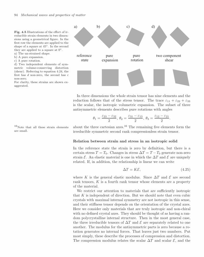
94 Mechanical waves and properties of matter
Fig. 4.5 Illustrations of the effect of ir-reducible strain elements in two dimen-sions using a geometrical figure. In thefirst row the elements are applied to theshape of a square at 45. In the secondthey are applied to a square at 0.a) The un-strained shape.b) A pure expansion.c) A pure rotation.d) Two independent elements of sym-metric volume-conserving distortion(shear). Referring to equation 4.24, thefirst has d non-zero, the second has cnon-zero.For clarity, these strains are shown ex-aggerated.
a) b) d)c)
referencestate
purerotation
two componentshear
pureexpansion
In three dimensions the whole strain tensor has nine elements and thereduction follows that of the stress tensor. The trace ε11 + ε22 + ε33
is the scalar, the isotropic volumetric expansion. The subset of threeantisymmetric elements describes pure rotations with angles
θ1 =ε23 − ε32
2, θ2 =
ε31 − ε13
2, θ3 =
ε12 − ε21
2.
about the three cartesian axes.16 The remaining five elements form the16Note that all these strain elementsare small. irreducible symmetric second rank compressionless strain tensor.
Relation between strain and stress in an isotropic solid
In the reference state the strain is zero by definition, but there is acertain stress T = T0. Changes in stress ∆T = T −T0 generate non-zerostrain E . An elastic material is one in which the ∆T and E are uniquelyrelated. If, in addition, the relationship is linear we can write
∆T = KE , (4.25)
where K is the general elastic modulus. Since ∆T and E are secondrank tensors, K is a fourth rank tensor whose elements are a propertyof the material.
We restrict our attention to materials that are sufficiently isotropicthat K is independent of direction. But we should note that even cubiccrystals with maximal internal symmetry are not isotropic in this sense,and their stiffness tensor depends on the orientation of the crystal axes.Here we consider only materials that are truly isotropic and non-chiralwith no defined crystal axes. They should be thought of as having a ran-dom polycrystalline internal structure. Then in the most general case,the three irreducible tensors of ∆T and E are separately related to oneanother. The modulus for the antisymmetric parts is zero because a ro-tation generates no internal forces. That leaves just two numbers. Putmost simply, these describe the processes of compression and distortion.The compression modulus relates the scalar ∆T and scalar E , and the

4.1 Stress, strain and waves in homogeneous materials 95
shear modulus relates the elements of the irreducible second rank ∆Tand the irreducible second rank E . For historical reasons these are writ-ten as 3λ + 2µ and 2µ, respectively. λ and µ are the Lame constants.Any more complex relation between stress and strain in a linear elas-tic medium would not be compatible with the assumed isotropy of thematerial.17 17This is a simple application of the
idea behind the Wigner–Eckart theo-rem (see the book by Fano and Racah).This theorem may be used to describerelations between stress and strainin anisotropic materials of a particu-lar symmetry class using further irre-ducible elements of the rank-4 stiffnesstensor.
In Fig. 4.6 we show how the stress associated with a single diagonalelement of strain is composed. The strain is analysed into its irreducibleparts, each of which is multiplied by the appropriate modulus. Thestress is found by recomposing the resulting elements.
Fig. 4.6 The calculation of the stress ina solid associated with a unit diagonalelement of strain. In the first row thestrain is decomposed into its irreducibleparts, a symmetric traceless strain anda uniform expansion. In the second roweach is related by its modulus to thecorresponding stress. The net stress isgiven by the addition of these.
This procedure is repeated for a single off-diagonal element of strainin Fig. 4.7.
Fig. 4.7 The calculation of the stressin a solid associated with a unit off-diagonal element of strain. The firstrow shows its irreducible parts, a sym-metric traceless part and an antisym-metric part. In the second row the sym-metric part is related by its modulus toa stress (third row). The antisymmet-ric part of the strain has modulus zero,because a pure rotation generates no in-ternal stress.
Uniform stress change and the bulk modulus
A material subjected to a uniform stress change,
∆T11 = ∆T22 = ∆T33 = −∆P,
experiences a strain which is also rank 0,
∆V
V=
∂ux
∂x+
∂uy
∂y+
∂uz
∂z.

96 Mechanical waves and properties of matter
Under these conditions only, the bulk modulus may be defined as KB =λ+ 2
3µ. In a fluid µ = 0 and the restriction to uniform compression goesaway.
4.1.5 Polarisation of waves in solids †Longitudinal and transverse polarisations
As in a fluid, the stress change and the strain in a solid are also relatedby Newton’s second law, and this results in wave motion. For a planewave moving along the z-axis all partial derivatives with respect to x ory are zero. So the only non-zero elements of strain are
E =
0 0 ∂ux/∂z
0 0 ∂uy/∂z0 0 ∂uz/∂z
.
These three elements are associated with three independent polarisa-tions: a transverse shear wave polarised along x, a transverse shearwave polarised along y, and a longitudinal compressive wave with mo-tion along z. We can write down the stress tensor for each using thedecompositions shown in Figs 4.6 and 4.7.
In a longitudinal wave the only strain component is εzz, andthis is accompanied by a longitudinal stress change,
∆Tzz = (λ + 2µ)εzz (4.26)
but also by stress changes in both orthogonal directions,
∆Txx = ∆Tyy = λεzz . (4.27)
In one transverse wave the only strain component is the off-diagonal element, εxz = ∂ux/∂z. The shear stress change isthen in the same xz-plane
∆Txz = ∆Tzx = µεxz. (4.28)
The other transverse wave involves the other independentoff-diagonal element εyz = ∂uy/∂z with stress change com-ponents
∆Tyz = ∆Tzy = µεyz. (4.29)
Longitudinal and transverse waves
For a wave with longitudinal polarisation the longitudinal strain is drivenby the longitudinal force described with the modulus λ+2µ. The velocityof longitudinal waves is therefore
cL =
√λ + 2µ
ρ0. (4.30)

4.1 Stress, strain and waves in homogeneous materials 97
The transverse forces present in the wave are in equilibrium and causeno oscillation. This does not mean that they do not matter. Where thewave meets a boundary at oblique incidence, the transverse forces donot balance and have to be taken into account. Indeed this is true evenin a fluid where there are also transverse forces present in a longitudinalwave.
For each of the two independent waves with transverse polarisationthe transverse strain is driven by the transverse force described with themodulus µ. The velocity of transverse waves is therefore
cS =√
µ
ρ0. (4.31)
The longitudinal force present in the wave is in equilibrium and causesno oscillation. Again, where the wave meets a boundary, this force hasto be taken into account in the boundary conditions. In a fluid µ = 0and there are no transverse waves.18 18In a viscous fluid the dissipative resis-
tance to shear motion can be describedfor harmonic motion by an imaginaryvalue of µ. Such motion is oscillatoryin time but decays exponential in space.
Table 4.2 shows that cS is always significantly smaller than cL. Sinceλ and µ are both positive, cL must be at least
√2 times cS . In a solid the
longitudinal impedance ZL = ρcL and the transverse or shear impedanceZS = ρcS can be defined also. However, the relation between stress andvelocity in a solid is more involved than in a fluid.
Stress and velocity for waves travelling in the z-direction
For a longitudinal wave the particle velocity vz is the time derivative ofuz
vz(z, t) =∂uz
∂t= −cLf ′(z − cLt) (4.32)
where f ′ is the derivative of f(ξ) with respect to ξ = z − cLt. Thecorresponding stress change is
∆TL =
λ 0 0
0 λ 00 0 λ + 2µ
× f ′(z − cLt). (4.33)
For a wave transversely polarised along y, we can write
∆TS1 =
0 0 0
0 0 µ0 µ 0
× f ′(z − cSt). (4.34)
For a wave transversely polarised along x we have
∆TS2 =
0 0 µ
0 0 0µ 0 0
× f ′(z − cSt). (4.35)
In a solid the kinetic energy density is 12ρv2 for each polarisation, as in
a fluid.19
19The potential energy density, equalto the kinetic energy density, is one halfthe contraction of the stress and straintensors, Σi,j
12εij∆Tij , but with only
one non-vanishing element of ε for eachpolarisation this is simple.

98 Mechanical waves and properties of matter
Stress and strain in a wave travelling at an angle
Because stress and strain are tensors we need to derive their componentsfor a wave travelling at an angle to the z-axis. In the following welabel the transverse wave with displacement in the x-direction with thesubscript S2. The orthogonal one is labelled S1.
θ
z
y
Fig. 4.8 A wave travels at an angle θto the z-axis in the yz-plane.
When a plane wave with one of these polarisations travels at an angleθ in the yz-plane instead of along the z-axis the displacement for eachpolarisation u is rotated through θ according to the transformation forvectors (Fig. 4.8). Thus for the wave f(ξ) where ξ = z cos θ+y sin θ−ct,the components of the displacement vector u is one of the followingvectors, depending on the polarisation,
uL = [ 0 sin θ cos θ ]f(ξ),
uS1 = [ 0 cos θ − sin θ ]f(ξ),
uS2 = [ 1 0 0 ]f(ξ).
(4.36)
The tensor ∆T for each polarisation transforms under rotations accord-ing to equation 4.23 with the following result:
∆TL =
1 0 0
0 1 00 0 1
× λf ′(ξ)
+
0 0 0
0 1 − cos 2θ − sin 2θ0 − sin 2θ 1 + cos 2θ
× µf ′(ξ), (4.37)
∆TS1 =
0 0 0
0 − sin 2θ cos 2θ0 cos 2θ sin 2θ
× µf ′(ξ),
∆TS2 =
0 − sin θ cos θ
− sin θ 0 0cos θ 0 0
× µf ′(ξ).
We shall need these results when we consider a wave incident on aplane boundary. The boundary conditions for force concern the threecomponents of the vector force transmitted through unit area of theboundary. For a boundary in the plane z = constant, for example, theseare given by just picking off the third column of the stress matrix forthe polarisation concerned,
FzL = [ 0 0 1 ] λf ′(ξ)+ [ 0 − sin 2θ 1 + cos 2θ ] µf ′(ξ),
FzS1 = [ 0 cos 2θ sin 2θ ] µf ′(ξ),
FzS2 = [ cos θ 0 0 ] µf ′(ξ).
(4.38)

4.2 Reflection and transmission of waves in bounded media 99
4.2 Reflection and transmission of waves
in bounded media
Reflection and transmission amplitudes for waves at normal incidence ona boundary are determined for each polarisation. At oblique incidencewave solutions in the two media must satisfy continuity of displacementand force on that boundary along all three axes. These six conditionsapply over the whole surface and for all time. They are sufficient todetermine the frequency and directions of the six waves that may be gen-erated by a single incident wave. Parity considerations determine thatno more than four outgoing waves are generated in any one case. Thedetailed conditions themselves determine the various reflection and trans-mission coefficients. In each case the component of energy flux normalto the boundary is found to satisfy the constraint that the energy carriedin by the incident wave is equal to the sum of the energies carried awayby the generated waves. If the velocity of the generated wave exceeds thevelocity of the incident wave, the generalised law of reflection or trans-mission can give a generated wave which is evanescent perpendicular tothe boundary. Reflection and transmission coefficients are calculated forinterfaces of water, air and rock. Typically large changes in polarisationare found and evanescent waves that travel parallel to the surface may begenerated.
4.2.1 Reflection and transmission at normalincidence
At normal incidence the reflected and transmitted waves are also normalto the boundary. As a result incident waves of any given polarisationgenerate reflected and transmitted waves of the same polarisation, andthere is no mixing of modes. The boundary conditions20 require conti- 20These will be examined more care-
fully later when we consider oblique in-cidence.
nuity of velocity and force. These conditions are sufficient to determinethat the amplitude reflection and transmission coefficients are
ur
ui=
Z1 − Z2
Z1 + Z2(4.39)
ut
ui=
2Z1
Z1 + Z2,
where Z1 and Z2 are the impedances of the first and second materialsfor the polarisation concerned. The demonstration of this result and thefact that it conserves energy flux is left to question 4.2.
These results cannot be extended simply to other angles of incidence.When all the force components in a given polarisation are taken into ac-count, the different polarisation modes become coupled. At a fluid–fluidinterface where no transverse waves are expected, there are difficultiesin satisfying boundary conditions for an incident longitudinal wave atoblique incidence.

100 Mechanical waves and properties of matter
4.2.2 Relative directions of waves at boundaries †Need to match waves at material boundaries
Consider two half-spaces, z < 0 occupied by one homogeneous material,and z > 0 occupied by a second homogeneous material. At the boundarythere is a change in the density (from ρ1 to ρ2) and elastic moduli,and thence in the wave velocity and impedance.21 When we derived21We use subscripts 1 and 2 to de-
note variables in the first and secondmedium respectively. Similarly we usesubscripts i, r and t to denote inci-dent, reflected and transmitted wavevariables.
the wave equation we wrote down the gradient of the stress change ∆Tin equation 4.7. In stepping from there to equation 4.9, we assumedthat the modulus K was not dependent on z. This is untrue on theboundary, and consequently the wave equation is invalid there. That isthe reason we have to solve for the waves in each half-space separately,and then impose the constraints at the boundary on those solutions,instead of solving the problem all at once. In each material progressivewaves with various directions of wave motion may propagate with variouspolarisations, longitudinal and transverse, some approaching the surfaceand some moving away. To determine the relation between the waveson either side of the boundary we need to consider the problem in threedimensions. In the first step we shall prove that two dimensions aresufficient. This will then make drawing diagrams and visualising thewaves easier.
We consider the case where one single plane wave moves towardsthe boundary with a specific polarisation, a single frequency ω andwavenumber k.22 This incident wave generates a number of waves in22The wavenumber vector points nor-
mal to the plane wavefront with mag-nitude 2π/λ where λ is the wavelength.
both materials which move away from the boundary. We have alreadychosen the z-axis as normal to the boundary. We choose the y-axis suchthat the incident k-vector of the incident wave lies in the yz-plane. Thusk = (0, ky, kz) with |k| = 2π/λ, and ω = |k|c. As we have seen, the wavevelocity c depends only on the choice of longitudinal or transverse polar-isation and the properties of the medium, assumed linear and isotropic.The polarisation indicates the displacement and particle velocity vec-tors, see equation 4.36. The stress is described by a tensor, but it is thecomponents of the force vector per unit area of the surface z = 0 whichwe shall need, see equation 4.38.
Boundary conditions for displacement and force
The displacement of material perpendicular to the boundary must becontinuous across the boundary, otherwise either a gap would open upor the two materials would coexist in the same space. If the former isconceivable under shock conditions, the latter is not.
This condition must be satisfied, not just at one point on the surfaceand one time, but over the whole surface and for all time. Continuity ofthe particle velocity perpendicular to the boundary is then also assured.
A discontinuity in either of the two components of particle velocityparallel to the boundary between two materials is imaginable, but afinite viscous friction between the materials would eliminate this. So allthree components of displacement at the boundary must be continuous

4.2 Reflection and transmission of waves in bounded media 101
at the boundary.23 23We argue that the parallel velocityis continuous across the boundary overthe whole boundary for all time. Thisis equivalent to continuity of displace-ment since the possibility of a constantparallel displacement of one materialrelative to the other is trivial.
Equation 4.38 describes the components of force in the x-, y- and z-directions per unit area of the boundary z = 0 due to an incident waveat angle θ. The z-component must be continuous to avoid a finite forceacting on the zero mass of a infinitesimal surface layer spanning theboundary. Similarly any discontinuity in the force acting parallel to theboundary would produce unacceptable angular acceleration.
In summary, when all of the incident, reflected and transmitted wavesare taken into account, the three components of displacement and threecomponents of force per unit area of the boundary must be continuousacross the boundary. These conditions apply, not just at one point inx, y and time t, but for all x, y and t together. As we now show,this requirement alone is sufficient to determine the relative directionsof each of the wavevectors in terms of the incident wavevector and toreduce the 3-D problem to 2-D. The detail of the six constraints in forceand displacement then determine the amplitudes of the outgoing wavesrelative to the incident one.
Footprint of all waves on the boundary plane
Each harmonic plane wave of amplitude A, wavenumber (kx, ky, kz) andangular frequency ω has the form24 24Later we shall need to include the ef-
fect of the polarisation, that is that A isa vector. However, that does not affectthe initial stages of the discussion.
A exp [i(kxx + kyy + kzz − ωt)]. (4.40)
In the plane z = 0 the incident wave looks like
A exp [i(kyy − ωt)] (4.41)
since kx = 0 by choice of axes. In this plane the various reflected andtransmitted waves could be of the form
A′ exp [i(k′xx + k′
yy − ω′t)]. (4.42)
In general the matching conditions for all x, y and t together wouldrepresent an infinite number of conditions to be satisfied. This is clearlynot possible with a finite number of wave amplitudes, A′, unless thedependence of every wave in each material on the plane z = 0 hasexactly the same dependence on x, y and t as the incident wave. Eachwave has to match the same footprint in x, y and t.
Then these phase factors are identical for all waves and simply can-cel when applying the boundary conditions. The consequence is thatthe values of kx, ky and ω must be the same for every wave, incident,reflected and transmitted, in the two materials.25 The conditions then 25Note that this matching does not ex-
tend to kz .reduce to relations between the different overall amplitudes A and A′.So the frequency of each generated wave is the same as the incident
wave. Then the value of kx is the same for each wave. However, theaxes were chosen such that kx = 0 for the incident wave. It follows thatkx = 0 for all the other waves also. This means that all the wavevectorsand the surface normal are perpendicular to the x-axis and lie in theyz-plane. This is called the plane of incidence. It makes it much easierto draw diagrams of the various wavevectors k for they are all coplanar.

102 Mechanical waves and properties of matter
y
z
incidentk
reflectedk
transmittedk
θ θ
θ
i hr
ht
Hi
i
Hr
Ht
ht
hr
c)
y
z
incidentk
reflectedk
transmittedk
θ θ
θ
i vr
vt
Vi
i
Vr
Vt
vt
vr
b)
y
z
incidentk
reflected
k
transmittedk
θ θ
θ
i pr
pt
Pi
i
Pr
Pt
pt
pr
a)
Fig. 4.9 Diagrams of wavevectors for each of the three polarisations of plane waves incident, reflected and transmitted at aplane boundary. The small arrows show the direction of the displacement vectors in each case: a) for compression waves (P),b) for shear waves (SV), c) for shear waves (SH). These diagrams simply describe the variables for the three polarisations. Asdiscussed later, polarisations are changed on reflection and transmission. Note that reflected angles here are defined in theconventional way, such that reflected wavevectors are at angles π − θr to the z-axis.
Polarisation of waves
Each wave, incident, reflected and transmitted, can have one of threepolarisations. A longitudinal or ‘compression’ wave is called a P-wavein geophysics. The two transverse shear waves are distinguished. Awave polarised with displacement in the plane of incidence is called anSV wave.26 A wave polarised perpendicular to the plane of incidence is26In geophysics the plane of incidence
is typically vertical, hence the choice oflabels, V for vertical and H for horizon-tal.
called an SH wave. Wavevector diagrams for each of the polarisationsare drawn in the plane of incidence in Figs. 4.9a–c. These simply de-scribe the variables. All three possible polarisations for the reflected andtransmitted waves have to be considered in principle for each polarisa-tion of the incident wave. Each generated wave has its own amplitudeand value for kz, but its values for ω, kx and ky are fixed, being thesame as the incident wave.
The value of kz is determined for each wave as follows. The phasevelocity is given by c =
√K/ρ with K = λ + 2µ for longitudinal waves,
and K = µ for shear waves. For each wave c = ω/k, so that
ω2 =K
ρ(k2
y + k2z). (4.43)
This fixes the value of kz, except for its sign, for each wave,
kz = ±√
ρω2
K− k2
y. (4.44)
The sign of kz is determined by whether the wave concerned is movingtowards the surface or away. Thus incident and transmitted waves havea positive sign, and reflected waves have a negative sign.

4.2 Reflection and transmission of waves in bounded media 103
General laws of reflection and transmission
From the geometry of the k-vector and the relation between ω, k and c,the angle of the wave vector with respect to the normal is given by
sin θ =ky
|k| = cky
ω. (4.45)
In particular the incident wave with phase velocity ci has an angle givenby
sin θi =
√Ki
ρ1
ky
ω. (4.46)
Similar expressions for θr and θt, the angle of each reflected and trans-mitted wave, can differ only by virtue of their phase velocities:
sin θr = crky
ω(4.47)
sin θt = ctky
ω. (4.48)
The general law of reflection is therefore
sin θi
sin θr=
ci
cr=
√Ki
Kr. (4.49)
This includes the case of a reflected wave with a different polarisation tothe incident wave. If the polarisation of the reflected wave is the sameas the incident wave we get the familiar law of reflection,
sin θi = sin θr. (4.50)
Applying the same argument to the transmitted wavevector, the gen-eral law of transmission is
sin θi
sin θt=
ci
ct=
√Ki
Kt
ρ2
ρ1. (4.51)
As we shall see below, an incident P wave gives rise both to a reflectedP wave and to a reflected SV wave, and the same is true of an incidentSV wave. Similarly there may be more than one transmitted wave, eachwith its own amplitude and polarisation, travelling at its own angle givenby the generalised law of transmission, equation 4.51. Snell’s law, wherethere is no change in polarisation on transmission, is a particular case.
4.2.3 Relative amplitudes of waves at boundaries †Possible polarisation changes on reflection and transmission
In the following we consider three cases separately: an incident SH wave,an incident P wave and an incident SV wave. In each case the waveamplitude is described by its displacement with a positive amplitude,

104 Mechanical waves and properties of matter
meaning that there is a positive component of the displacement alongthe positive x-axis (for SH waves) or positive y-axis (for SV or P waves).
There is an important difference between SH waves on the one hand,and SV and P waves on the other. They have different parities andtherefore do not mix. We explore this statement briefly. The x-axis isthe normal to the plane of incidence and, as such, is defined by a vectorcross product. This therefore changes sign if the waves are describedin a left-handed coordinate system instead of a right-handed one. Thedisplacement amplitude of SH waves is measured along this axis. Theamplitudes of SV and P waves lie in the plane of incidence and have asign defined by the direction of the y-axis, the direction of the incidentk on the xy-plane. This is independent of the choice of left- or right-handed axes. Therefore the relative sign of SH and SV/P waves dependson whether we use left- or right-handed axes. If they were to mix onreflection or transmission at the boundary, this relative sign would haveobservable consequences. Since the physics of sound does not depend onthe handedness of the axes, this may not happen.
The conclusion is that the problem simplifies. An incident SH wavegenerates only reflected and transmitted SH waves. An incident SV orP wave generates a superposition of reflected and transmitted SV andP waves, but no SH waves.
Calculations with geophysical examples
The reflection and transmission amplitude coefficients are calculated be-low for a solid–solid boundary. As examples, numerical values of thesecoefficients for the Earth’s mantle–crust boundary (table 4.3) are plottedas a function of angle of incidence for an incident SH wave, P wave andSV wave in Figs 4.12 and 4.14. For a solid–fluid interface we have usedrock–water and rock–air boundaries as examples, and the coefficientsare plotted in Figs 4.15–4.16.
Table 4.3 Material properties for theEarth’s mantle–crust interface used inthe calculation of Figs 4.12 and 4.14.
Units First Secondmaterial material
cP m s−1 8000 2920cS m s−1 4300 1840ρ kg m−3 4000 2700
We discuss the simpler incident SH wave first, followed by the incidentP wave and then the SV wave. We use a notation in which the subscriptsS and P refer to shear and compression waves respectively. The symbolused for the wave displacement amplitude, H , P or V denotes the polar-isation. The angle θ is subscripted h, p or v to indicate the polarisationof the wave to which it refers. Calculations of energy flux may be usedas a check that the boundary conditions have been satisfied correctly. Iffluxes are calculated per unit area normal to the boundary, the incidentflux towards the boundary should equal the sum of all of the outgoingfluxes away from it.
Incident shear wave polarised perpendicular to the plane ofincidence
The only components of displacement or force in the x-direction (per-pendicular to the plane of incidence) arise from SH waves, as shown inequations 4.36 and 4.38. Continuity of these two quantities across theboundary gives the two constraints that determine the two unknowns,

4.2 Reflection and transmission of waves in bounded media 105
the reflection amplitude coefficient Hr/Hi and the transmission ampli-tude coefficient Ht/Hi for the two outgoing SH waves.
y
z
θ θ
θ
hi hr
ht
HiHr
Ht
Fig. 4.10 A diagram for wave ampli-tudes generated by an incident shearwave polarised normal to the plane ofincidence (SH).
The displacement amplitudes indicated in Fig. 4.10 are to be under-stood as positive along the x-axis standing out of the paper. Then theconstraint of continuity of displacement is
Hi + Hr = Ht (4.52)
and the constraint of continuity of force is
Hi cos θhikiµ1 − Hr cos θhrkrµ1 = Ht cos θhtktµ2. (4.53)
The negative sign for the reflected ray comes from the fact that thereflected wave is travelling in a direction θ = π − θhr. The magnitudeof each k is ω/cS where cS is the wave velocity for shear waves in thematerial. The solutions for the amplitude transmission and reflectioncoefficients are
Ht
Hi=
2Z1S cos θhi
Z1S cos θhi + Z2S cos θht(4.54)
Hr
Hi=
Z1S cos θhi − Z2S cos θht
Z1S cos θhi + Z2S cos θht, (4.55)
where Z1S = ρ1c1S and Z2S = ρ2c2S . These solutions satisfy the con-servation of energy flux, as shown in Fig. 4.12b.
These coefficients are plotted in Figs 4.12a and 4.12b. They showthat for the mantle–crust boundary at most angles the amplitude of thetransmitted wave in the lighter and less rigid second medium is largerthan in the incident amplitude. However, the associated energy in thelower density of the second medium is seen to be smaller. This is ageneral feature. For example, the displacement amplitude of earthquakesis typically largest in regions of low density and rigidity, such as landfillsites. The large displacement does not carry large energy, although thismay be where the greatest damage occurs.
Incident compression wave
For an incident P wave there are both reflected and transmitted SVwaves as well as reflected and transmitted P waves, as shown in Fig. 4.11.To match the unknown amplitudes of the four outgoing waves there arefour constraints coming from the y- and z-components of displacementand force. The four constraint equations are linear in the amplitudes ofthe four generated waves, and can be written as the matrix equation
y
z
Vr
V Pt t
θ
θ
θθ
θ
p
p
vp
v
r
t
ri
t
P
P
r
i
Fig. 4.11 A diagram for wave ampli-tudes generated by an incident com-pression wave (P).
M × CP = IP , (4.56)
where the vector of the four amplitudes is
CP =
Pr/Pi
Vr/Pi
Pt/Pi
Vt/Pi
, (4.57)

106 Mechanical waves and properties of matter
-1
-0.5
0
0.5
1
1.5
0.2 0.4 0.6 0.8 1 1.2 1.4
0
0.2
0.4
0.6
0.8
1
0.2 0.4 0.6 0.8 1 1.2 1.4
angle of incidence/radians
angle of incidence/radians
a) Relative displacement b) Relative normal energy flux
-1
-0.5
0
0.5
1
1.5
0.2 0.4 0.6 0.8 1 1.2 1.4
0
0.2
0.4
0.6
0.8
1
0.2 0.4 0.6 0.8 1 1.2 1.4
angle of incidence/radians
angle of incidence/radians
c) Relative displacement d) Relative normal energy flux
Incident SH wave on mantle-crust boundary
Incident P wave on mantle-crust boundary
Fig. 4.12 Reflection and transmission coefficients as a function of the angle of incidence for the mantle–crust interface (table 4.3).a) and b) for incident SH wave: full curve = reflected SH, dash curve = transmitted SH, dotted line = calculated energy sum.c) and d) for an incident P wave: full thin curve = reflected P, full heavy curve = reflected SV, thin dashed curve = transmittedP, heavy dashed curve = transmitted SV, dotted line = calculated energy sum.

4.2 Reflection and transmission of waves in bounded media 107
the vector of displacements and forces due to the incident wave is
IP =
sin θi
cos θi
Z1S(c1S/c1P ) sin 2θi
Z1P − Z1S(c1S/c1P )(1 − cos 2θi)
(4.58)
and the matrix M =
− sin θpr cos θvr sin θpt cos θvt
cos θpr sin θvr cos θpt − sin θvt
Z1S(c1S/c1P ) sin 2θpr −Z1S cos 2θvr Z2S(c2S/c2P ) sin 2θpt Z2S cos 2θvt
−Z1P + Z1S(c1S/c1P )(1 − cos 2θpr) −Z1S sin 2θvr Z2P − Z2S(c2S/c2P )(1 − cos 2θpt) −Z2S sin 2θvt
(4.59)
By inverting the matrix the amplitude coefficients due to the incident Pwave may be found,
CP = M−1IP . (4.60)
The amplitude ratios and the corresponding energy fluxes are shownin Figs 4.12c and 4.12d for the mantle–crust boundary. While at normalincidence there is no change in polarisation,27 at other angles there are 27Such a change is forbidden by parity
conservation.significant amplitudes of shear as well as compressive waves. Becausein this case the phase velocities of these generated secondary waves arelower than the incident wave, their angles are real and less than theangle of incidence, whatever it is.
y
z
VV ri
V Pt t
θ
θ
θθ
θ
p
p
vv
v
r
t
ri
t
Pr
Fig. 4.13 A diagram for wave ampli-tudes generated by an incident shearwave polarised in the plane of incidence(SV).
Incident shear wave polarised in the plane of incidence
A similar analysis can be made for waves generated by an SV waveincident on the boundary with wavevectors as shown in Fig. 4.13. Thesame matrix (equation 4.59) links the generated wave amplitudes to theforces and displacements of the incident wave. The amplitudes
CV =
Pr/Vi
Vr/Vi
Pt/Vi
Vt/Vi
(4.61)
are given byCV = M−1IV , (4.62)
where
IV =
cos θi
− sin θi
Z1S cos 2θi
−Z1S sin 2θi
. (4.63)
As an example, the amplitudes are plotted in Fig. 4.14 for the samemantle–crust interface (table 4.3).
These show new features which do not arise for incident SH or P waveson this boundary. For angles of incidence greater than 0.56 all four
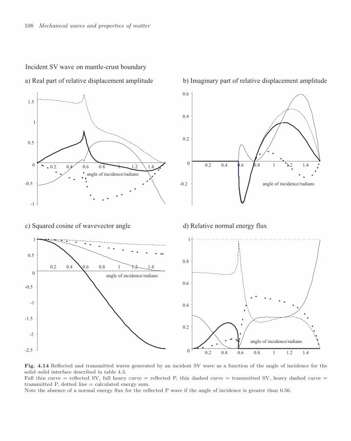
108 Mechanical waves and properties of matter
a) Real part of relative displacement amplitude
-2.5
-2
-1.5
-1
-0.5
0
0.5
1
0.2 0.4 0.6 0.8 1 1.2 1.4
-1
-0.5
0
0.5
1
1.5
0.2 0.4 0.6 0.8 1 1.2 1.4
-0.2
0
0.2
0.4
0.6
0.2 0.4 0.6 0.8 1 1.2 1.4
0
0.2
0.4
0.6
0.8
1
0.2 0.4 0.6 0.8 1 1.2 1.4
angle of incidence/radians
angle of incidence/radians
angle of incidence/radians
angle of incidence/radians
c) Squared cosine of wavevector angle
b) Imaginary part of relative displacement amplitude
d) Relative normal energy flux
Incident SV wave on mantle-crust boundary
Fig. 4.14 Reflected and transmitted waves generated by an incident SV wave as a function of the angle of incidence for thesolid–solid interface described in table 4.3.Full thin curve = reflected SV, full heavy curve = reflected P, thin dashed curve = transmitted SV, heavy dashed curve =transmitted P, dotted line = calculated energy sum.Note the absence of a normal energy flux for the reflected P wave if the angle of incidence is greater than 0.56.

4.2 Reflection and transmission of waves in bounded media 109
generated waves have a non-trivial phase angle relative to the incidentwave. Figures 4.14a and 4.14b show the imaginary as well as the realparts. For angles above 0.56 the reflected P wave has a negative value ofk2
z (Fig. 4.14c). In this region there is zero normal energy flow associatedwith the reflected P wave (Fig. 4.14d), although the calculated energyflux for the remaining three waves still adds up to the incoming flux.
Evanescent waves
If k2z is negative, then kz is pure imaginary. The phase factor exp[ikzz]
for the reflected P wave normally represents a harmonic dependence.However, when kz is imaginary this describes a real exponential of theform exp−z/z0 where the range is given by z0 = 1/
√−k2z . Such an
evanescent wave is familiar from other branches of physics, such as thetotal internal reflection of light and the exponential behaviour of quan-tum wavefunctions in regions where the classical kinetic energy wouldbe negative. These have important applications in the physics of fibreoptics and field effect transistors as well as describing the phenomenonof alpha radioactive decay.
As given by equations 4.49 and 4.51 whenever an incident wave gener-ates an outgoing wave with an increased wave velocity, the value of sin θfor that wave is greater than for the incident wave. So for some range ofthe angle of incidence, the sine of the angle of reflection or transmissionexceeds unity. Then its cosine is pure imaginary. Such a wave decays inz but oscillates in time and in x or y in the normal way. It propagatesalong the boundary with a finite amplitude but carries no energy awayfrom the surface. To match the boundary conditions the other wavesacquire phases and display threshold effects as shown in Fig. 4.14. Thethreshold is at an angle with sin θi = c1/c2. There may be up to threesuch thresholds, one for each generated wave whose phase velocity ex-ceeds the phase velocity of the incident wave. At the threshold anglethe exponential range z0 of the evanescent wave starts from infinity andfalls as the angle of incidence is increased further.
Solid–liquid interface
Table 4.4 Material properties for therock–water boundary used in the calcu-lation of Fig. 4.15.
Units First Secondmaterial material
cP m s−1 2920 1407cS m s−1 1840 0ρ kg m−3 2700 1000
Table 4.4 gives constants for a rock–water interface, such as might applyat the bottom of the oceans. As the second material is a fluid theimpedance Z2S = 0 and there can be no propagation of energy by shearwave in the second medium. Equations 4.54 and 4.55 show that anincident SH wave is totally reflected at all angles. Because the surface isunrestrained in shear, there is an antinode there. There is a transmittedSH wave. It has a displacement amplitude twice that of the incidentwave but transmits no force or energy because the modulus is zero.28
28Because this amplitude does not de-pend on the angle of incidence the plotis featureless and is not shown.
For an incident SV wave29 the reflection and transmission coefficients 29An incident P wave generates noevanescent wave as no wave has a phasevelocity faster than the incident wave.The reflection and transmission coef-ficients are all real and unremarkable.They are not plotted here.
are plotted out in Fig. 4.15. The amplitude and energy of the reflectedP wave is large away from normal incidence, showing again that polar-isation changes are first order effects, not just corrections. The largetransmitted SV wave amplitude has the same interpretation as for the

110 Mechanical waves and properties of matter
-1.5
-1
-0.5
0
0.5
1
0.2 0.4 0.6 0.8 1 1.2 1.4
0
0.2
0.4
0.6
0.8
1
0.2 0.4 0.6 0.8 1 1.2 1.4
-1
0
1
2
3
4
5
6
0.2 0.4 0.6 0.8 1 1.2 1.4
-3
-2
-1
0
0.2 0.4 0.6 0.8 1 1.2 1.4
a) Real part of relative displacement amplitude
c) Squared cosine of wavevector angle
b) Imaginary part of relative displacement amplitude
d) Relative normal energy flux
angle of incidence/radians
angle of incidence/radians
angle of incidence/radians
angle of incidence/radians
Incident SV wave on rock-water boundary
Fig. 4.15 Reflected and transmitted waves generated by an incident SV wave as a function of the angle of incidence for therock–water interface described in table 4.4.Full thin curve = reflected SV, full heavy curve = reflected P, dashed thin curve = transmitted SV, dashed heavy curve =transmitted P, dotted line = calculated energy sum.Note the absence of a normal energy flux for the reflected P wave for an angle of incidence of greater than 0.68.

4.3 Surface waves and normal modes 111
transmitted SH wave, amplitude but no velocity or impedance and there-fore no energy flux. The reflected P wave is evanescent for angles ofincidence above sin θi = c1S/c1P = 0.682. In this range only the trans-mitted P wave and the reflected SV wave can carry energy, althoughthe other two waves have amplitude. The transmitted SV wave has zeromodulus, and the reflected P wave is an evanescent wave. Neither carryenergy.
Solid–gas interface
Table 4.5 describes a rock–air interface, such as might apply at theEarth’s surface. Air not only is a fluid but also has a very low impedancefor transmitted P waves. For incident SH waves the situation is the sameas it was for the rock–water interface. For incident SV waves or P wavesthere is a near antinode at the surface and the large transmitted P waveamplitude carries negligible energy. Figure 4.16 shows curves for an
Table 4.5 Material properties for therock–air boundary used in the calcula-tion of Fig. 4.16.
Units First Secondmaterial material
cP m s−1 2920 330cS m s−1 1840 0ρ kg m−3 2700 1.2
incident SV wave. The energy is divided between the reflected P waveand SV wave, again with a large change in polarisation. With no energyin the transmitted P wave, above the critical angle for the reflected Pwave all the energy is reflected in the SV polarisation.
4.3 Surface waves and normal modes
We consider surface waves on the plane boundary between two homoge-neous materials and the three dimensional oscillation modes of bodies asa whole.
Under certain circumstances combinations of evanescent waves alonecan satisfy the boundary conditions. These combinations are known assurface waves although they penetrate the bulk material to an importantextent. At a solid–fluid interface a superposition of evanescent longitu-dinal and evanescent transverse waves can form a surface wave. This isa Rayleigh wave. Such waves have important applications in geophysics,geological prospecting and modern electronics. A different surface wavemay propagate along a fluid–fluid interface. Gravity or surface tensionallows a single evanescent longitudinal wave to satisfy the boundary con-ditions. Such waves describe a range of phenomena from short ripples tolong ocean tidal waves. Compared with free bulk waves they have low wavevelocity. Their properties are of considerable environmental importance.
In a medium bounded on all sides wave solutions form a set of discretemodes with well-defined frequencies. Such modes are realised in the tuneof musical instruments and in the bodily vibrations of the Earth and theSun.
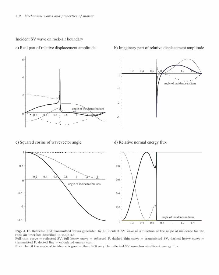
112 Mechanical waves and properties of matter
-1.5
-1
-0.5
0
0.5
1
0.2 0.4 0.6 0.8 1 1.2 1.4
0
2
4
6
0.2 0.4 0.6 0.8 1 1.2 1.4
0
0.2
0.4
0.6
0.8
1
0.2 0.4 0.6 0.8 1 1.2 1.4
-3
-2
-1
0
1
0.2 0.4 0.6 0.8 1 1.2 1.4
angle of incidence/radians
angle of incidence/radians
angle of incidence/radians
angle of incidence/radians
a) Real part of relative displacement amplitude
c) Squared cosine of wavevector angle
b) Imaginary part of relative displacement amplitude
d) Relative normal energy flux
Incident SV wave on rock-air boundary
Fig. 4.16 Reflected and transmitted waves generated by an incident SV wave as a function of the angle of incidence for therock–air interface described in table 4.5.Full thin curve = reflected SV, full heavy curve = reflected P, dashed thin curve = transmitted SV, dashed heavy curve =transmitted P, dotted line = calculated energy sum.Note that if the angle of incidence is greater than 0.68 only the reflected SV wave has significant energy flux.

4.3 Surface waves and normal modes 113
4.3.1 General surface waves
The evanescent waves discussed so far are generated by the incidence ofa bulk S or P wave on a surface. This happens whenever the angle ofincidence is large enough to satisfy equation 4.49 or 4.51 with sin θr >1 or sin θt > 1. In table 4.6 we list all the possible combinations ofpolarisation that can generate such evanescent waves. These evanescentwaves only persist as long as the incident bulk S or P waves are present.In that sense they are not free.
Table 4.6 The complete list of possiblecombinations of incident wave (i-wave)and evanescent wave (e-wave) polarisa-tions, transmitted or reflected, with thenecessary condition on the phase veloci-ties in the first and second media.
Polarisation necessaryi-wave e-wave condition
P P transmitted c1P < c2P
SV P transmitted c1S < c2P
SV SV transmitted c1S < c2S
SH SH transmitted c1S < c2S
P SV transmitted c1P < c2S
SV P reflected c1S < c1P
In addition there exist surface wave solutions which are freely prop-agating and which, though confined to the surface and the region closeto it, do not require incident free bulk waves. Such surface waves maybe formed by particular superpositions of evanescent S and P wavesfor which the boundary conditions can be matched. These are calledRayleigh waves and can be excited at a solid–light-fluid interface.30
30The light fluid implies that the solidhas an essentially free surface. Strictlythis couples to a P wave in the fluidwhich if sufficiently light carries awayno energy.
A quite different surface wave can be excited at a fluid–fluid interfacewhere a restoring force enables the boundary conditions to be satisfied.This force may be due either to gravity and a density difference betweenthe fluids or to the effect of surface tension.
4.3.2 Rayleigh waves on free solid surfaces
A Rayleigh wave is a particular linear combination of an evanescent SVwave and an evanescent P wave on the solid side of a free unloadedsurface. Consider a P wave with amplitude uP and wavevector kP , anda S wave with amplitude uS and wavevector kS . We choose axes with theinterface being the plane z = 0 and kP lying in the yz-plane, as before.To satisfy the boundary conditions for all (x, y, t), the ‘footprint’ of theSV wave and the P wave on the boundary must match as discussed insection 23. Therefore the frequencies of the two waves are the same, theirk-vectors lie in the yz-plane and they have the same value ky = kPy =kSy. The magnitudes of the k-vectors are kP = ω/cP and kS = ω/cS.So far all quantities are real. Defining angles θP and θS for the directionof the k-vectors relative to the interface normal, we deduce
ky =ω
cPsin θP =
ω
cSsin θS . (4.64)
Both of these sines are greater than 1 in a Rayleigh wave, and thecorresponding cosines pure imaginary. Because the two waves are onthe same side of the boundary, the signs of the two imaginary cosinesare the same.
The constraints for a free surface are that the components of stressthrough the surface in the z- and y-directions for the two waves shouldadd to zero. The forces per unit area, FzL and FzS1, may be read off fromequation 4.38 in terms of the moduli and angles. Defining the velocityω/ky = cR, these two constraints may be reduced to the equations
(2 − c2
R
c2S
)4
= 16(
1 − c2R
c2S
) (1 − c2
R
c2P
)(4.65)

114 Mechanical waves and properties of matter
Fig. 4.17 a) The ratio of the velocityof Rayleigh waves to free shear wavesplotted as a function of the ratio of thevelocities of free shear and longitudi-nal waves. b) The depth penetrationof Rayleigh waves in terms of the freeshear wavelength/2π plotted as a func-tion of the same ratio of the velocitiesof free shear and longitudinal waves.The upper curve is the penetration ofthe evanescent shear wave component.The lower curve is the penetration ofthe evanescent longitudinal wave com-ponent.
0.90
0.92
0.94
0.96
0.98
1.00
0.1 0.2 0.3 0.4 0.5 0.6 0.7
ratio c /c
ratio c /c
PS
R Sa)
0
0.5
1.0
1.5
2.0
2.5
3.0
0.1 0.2 0.3 0.4 0.5 0.6 0.7
depth ratio
ratio c /cPS
b)
uP
uS= −i
(2c2
S − c2R
2cP
√c2P − c2
R
). (4.66)
The velocity cR is the phase velocity of both evanescent waves along thesurface. These relations do not depend on ω, so that Rayleigh waves arenot dispersive, unless the free longitudinal and shear waves themselvesare.
Figure 4.17a shows a plot of the velocity of the ratio of the velocity ofRayleigh waves to free shear waves as a function of the ratio of the veloc-ity of free shear waves to longitudinal waves as given by equation 4.65.The velocity of Rayleigh waves is seen to be 0.92–0.95 of the free shearvelocity, more or less independent of the velocity of the longitudinalvelocity.
Equation 4.66 gives the relative amplitude of the two evanescent com-ponents at the surface. They are π/2 out of phase, and so combine togive an elliptical motion. The depth penetration of the two constituentevanescent waves is different. It may be calculated in each case as thereciprocal of kz , determined by Pythagoras’s theorem from k = ωc andky. The shear wave component is only just evanescent and so has a rel-atively deep penetration. The longitudinal component is more stronglyevanescent, and consequently has a short range. Both ranges are plot-ted in Fig. 4.17b. The consequence is that near the surface there is asignificant component of strain parallel to the surface and the motion iselliptical. Further from the surface the motion is more closely that of asimple shear wave with motion perpendicular to the surface.
In geophysics Rayleigh waves may be distinguished from bulk wavesby their slow speed and by their characteristic polarisation, involving anelliptical motion, both longitudinal and transverse.31 They are gener-31They are seen to be slow because
they follow the longer route along theEarth’s surface while the bulk wavesfollow a more direct route.
ated by earthquakes within a few wavelengths of the surface. Typicallyearthquakes involve sudden shear failure of structures over the area of afault. Geological seismometers are also sensitive to the signals emittedby underground nuclear weapon tests. These involve spherically sym-metric point-like P wave emission but no SH or SV waves. Such eventsdo not create Rayleigh waves. By measuring the polarisation of seis-

4.3 Surface waves and normal modes 115
mic signals and their relative timings, earthquakes and explosions fromnuclear weapon testing may be distinguished.
Rayleigh waves are of particular importance in modern seismologybecause their propagation is sensitive to density and modulus changesclose to the surface. As the shear modulus of any fluid vanishes, oilor gas bearing strata show up clearly. The change of shear modulus inregions of loose sand or landfill where they adjoin rigid compacted stratacan also be imaged.
In our analysis so far we have seen that evanescent waves (includingRayleigh waves) carry no energy compared with bulk waves. This is notthe whole story. There is a dimensional point here. Rayleigh waves aretwo dimensional while bulk waves are three dimensional. Bulk wavescarry an energy flux per square metre of wavefront, while a Rayleighwave carries energy per linear metre in the surface. Indeed there is a realenergy flux parallel to the surface but only within the depth penetrationof the wave. The energy from a localised source of such a two dimensionalwave spreads out with a circular wavefront and an intensity falling as1/r. This is in contrast to bulk waves that spread out from a source withan intensity falling as 1/r2. Therefore signals carried by surface waves,guided by the boundary, propagate effectively over longer distances.
Variants on Rayleigh waves as described above occur for thin sheets.The single evanescent wave in each polarisation is replaced by sinh andcosh waves built from the evanescent behaviour at the two surfaces.Such waves are dispersive. Further modifications also arise if the elasticproperties of the lighter medium are taken into account.
Surface waves of a different type may occur if the medium is layeredor graded in elasticity or density. Such layers may act as a waveguidethereby trapping the energy in two dimensions. In a geological contextsuch waves are known as Love waves.
Surface acoustic waves
On a different scale Rayleigh waves may be excited in the surface of thinwafers that form important components of modern electronics. A shearwave is launched on a thin piezoelectric wafer by an array of alternatingelectrodes laid down on the surface as illustrated in Fig. 4.18. In
~SAW
piezoelectric crystal
signal
Fig. 4.18 An electrode array depositedon the surface of a piezoelectric crys-tal to transmit a surface acoustic wave(SAW). It may also act as a receiver,transforming a SAW into a high fre-quency electrical signal.
this context thin-film Rayleigh waves are described as surface acousticwaves (SAW). In electronic engineering they are the basis of most highfrequency filters and delay lines in modern communication systems. Ithas been estimated that in 2005 annual production exceeded 109 suchdevices worldwide.
4.3.3 Waves at fluid–fluid interfaces
Shear motion in fluids
At solid–fluid interfaces the transmitted shear wave carries no energyas shown in Figs 4.15 and 4.16. However, the displacement amplitudeof the shear wave in the fluid required by the boundary conditions is

116 Mechanical waves and properties of matter
very large.32 The structural integrity of the surface depends essentially32The real part of the shear modu-lus of fluids is zero. The only shearforce generated by shear motion in afluid is viscous damping. This is pro-portional to the shear velocity, not theshear displacement to which it is π/2out of phase, and is therefore describedby a small imaginary value of µ pro-portional to ω. This small imaginaryvalue of µ gives small complex valuesfor the impedance and the wave veloc-ity for shear waves.
on the rigidity of the solid and the resulting reflected SV wave.The surface at a fluid–fluid interface does not have the structural
integrity of a solid on either side. When a P wave is incident at an obliqueangle interesting problems arise. In the absence of any other forces theboundary conditions cannot be met and the molecules of the two fluidswould simply mix and the surface dissolve.33 However, there are two
33These observations have an obviousconnection with the use of ultrasoundas a cleaning agent and emulsifyingtechnique.
other weaker forces, gravity and surface tension, that can maintain thesurface under these conditions. The most familiar manifestation is the‘water wave’. Analogous waves exist between all fluids including betweenlayers of different density in the atmosphere and between layers of waterof different temperature or salinity. However, these forces are weak, thevelocities are slow and there is generally a large displacement amplitudeat the interface.
Gravity and surface tension waves
Water waves travel so slowly compared with any free bulk P wave thatwater behaves as if it were incompressible. In other words, the associatedevanescent P wave that underlies a surface wave with real k in y has ak-vector with k2 ≈ 0, and thence k2
z = −k2y and kz = ±iky. The general
P wave solution is then a superposition of the solutions with these twosigns, each of which has k parallel to the displacement for all space andtime,
ψy = A exp[i(kyy − ωt)] exp(−kyz) + B exp[i(kyy − ωt)] exp(+kyz)ψz = iA exp[i(kyy − ωt)] exp(−kyz) − iB exp[i(kyy − ωt)] exp(+kyz).
(4.67)Each describes circular motion in the yz-plane, one decreasing exponen-tially with depth z and the other increasing. From this point we drop thesubscript y in ky, and describe the wave as a surface wave of wavenumberk. Note that the same value of k also describes the exponential depthbehaviour.
If the depth of water is z0 the bottom forms a rigid boundary wherethere is no vertical motion. This fixes B = A exp(−2kz0). Thence
ψy = A exp[i(ky − ωt)] × [exp(−kz) + exp(kz − 2kz0)] (4.68)ψz = iA exp[i(ky − ωt)] × [exp(−kz) − exp(kz − 2kz0)] .
At the surface z = 0 the difference between the zero pressure abovethe surface and the P wave pressure below the surface is balanced bythe hydrostatic weight of the surface wave amplitude. Figure 4.19
y y+dy
dh = dyyh
Fig. 4.19 The horizontal pressure gra-dient near the surface of a water wave isdue to the gradient of the wave height,multiplied by density and accelerationdue to gravity g.
illustrates how the horizontal pressure gradient depends on the waveheight h,
∂P
∂y= ρg
∂h
∂y. (4.69)
We substitute h = ψz at z = 0 and equate this horizontal pressuregradient to the product of density and acceleration in y,
−ρω2ψy = iρgkψz. (4.70)

4.3 Surface waves and normal modes 117
wavelength/mfrequency/Hz
frequency/Hz
100
10
0.1
100100.01 0.1
wavelength/m
10 10 103 4 5
10
1
10
10
10
10
-1
-2
-3
-4
a) b)
5
1
1
4
5
1
4
3
2
Fig. 4.20 The dispersion relation for water waves on Earth shown as plots of frequency against wavelength using T = 0.072 N
m−2. Curve 1, for ‘deep’ waves; curves 2–4 show the effects of a depth of 1000 m, 100 m and 10 m depth respectively. Curve5 shows the relation for free P waves, the velocity of sound in water. Plots a) and b) cover different logarithmic wavelengthscales.
This is satisfied provided
ω2 =(
gk +T
ρk3
) (1 − exp(−2kz0)1 + exp(−2kz0)
). (4.71)
To complete this dispersion relation we have added the term that de-scribes surface tension T . This gives a force proportional to surfacecurvature Tk2 where T is the surface tension in N m−1. This term ismuch smaller than the effect of gravity for water waves on Earth forwavelengths greater than 2 cm.
Properties of gravity and surface tension waves
For gravity waves in the deep water limit, z0 λ, the dispersion equa-tion 4.71 reduces to
ω2 = gk. (4.72)
The phase velocity is then
cgravity =
√gλ
2π(4.73)
which is dispersive. Long wavelength waves travel much faster than shortones. The group velocity is half the phase velocity. This dispersion isa dominant effect in naval architecture as it determines the maximumspeed of a non-planing ship’s hull. As a boat moves forward it displacesthe water in front and, if it is not to find itself trying to climb its ownbow wave, relies on this displaced water flowing round to the stern fastenough to fill the volume left by the retreating hull, hopefully nearlyreversibly. This requires water motion with wavelength not longer than
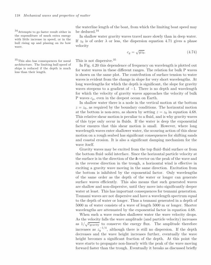
118 Mechanical waves and properties of matter
the waterline length of the boat, from which the limiting boat speed maybe deduced.3434Attempts to go faster result either in
the expenditure of much extra energywith little increase in speed, or in thehull rising up and planing on its bowwave.
In shallow water gravity waves travel more slowly than in deep water.If z0 is of order λ or less, the dispersion equation 4.71 gives a phasevelocity
cg =√
gz0. (4.74)
This is not dispersive.3535This also has consequences for navalarchitecture. The limiting hull speed ofships is reduced if the depth is muchless than their length.
In Fig. 4.20 this dependence of frequency on wavelength is plotted outfor water waves in these different ranges. The relation for bulk P wavesis shown on the same plot. The contribution of surface tension to waterwaves is evident from the change in slope for very short wavelengths. Atlong wavelengths for which the depth is significant, the slope for gravitywaves steepens to a gradient of −1. There is no depth and wavelengthfor which the velocity of gravity waves approaches the velocity of bulkP waves cp, even in the deepest ocean on Earth.
In shallow water there is a node in the vertical motion at the bottomz = z0, as required by the boundary conditions. The horizontal motionat the bottom is non-zero, as shown by setting z = z0 in equation 4.68.This relative shear motion is peculiar to a fluid, and is why gravity wavesof this type only occur in fluids. If the water is deep the exponentialfactor ensures that this shear motion is small. However, where longwavelength waves enter shallower water, the scouring action of this shearmotion on a rough seabed has significant consequences for shifting sandsand coastal erosion. It is also a significant damping mechanism for thewave itself.
Gravity waves may be excited from the top fluid–fluid surface or fromthe bottom fluid–solid interface. Since the horizontal particle velocity atthe surface is in the direction of the k-vector on the peak of the wave andin the reverse direction in the trough, a horizontal wind is effective inexciting a gravity wave moving in the same direction. Excitation fromthe bottom is inhibited by the exponential factor. Only wavelengthsof the same order as the depth of the water or longer can generatesurface waves efficiently. This also means that such generated wavesare shallow and non-dispersive, until they move into significantly deeperwater at least. This has important consequences for tsunami generation.Tsunami waves are not dispersive and have a wavelength spectrum equalto the depth of water or longer. Thus a tsunami generated in a depth of5000 m of water consists of a wave of length 5000 m or longer. Shorterwavelengths are attenuated by the exponential factor in equation 4.68.
When such a wave reaches shallower water the wave velocity drops.As the velocity falls the wave amplitude (and particle velocity) increasesas 1/
√cgravity to conserve the energy flux. The amplitude therefore
increases as z−1/40 , although there is still no dispersion. If the depth
decreases and the wave height increases further, eventually the waveheight becomes a significant fraction of the depth. At this point thewave starts to propagate non-linearly with the peak of the wave movingforward faster than the trough. Eventually it breaks as discussed briefly

4.3 Surface waves and normal modes 119
in section 9.4.On the other hand, if the tsunami wave propagates into deeper water
where the velocity is dispersive, the pulse spreads out. Non-linear ef-fects would then be reduced, if and when the wave subsequently reachedshallow water again.
Prospectively, the most dangerous tsunamis are associated with earth-quakes in shallow water, for these have no filtering of short wavelengthsby the exponential depth factor.
4.3.4 Normal mode oscillations
Waves in bounded volumes
If a space is enclosed by boundaries, there are too many conditions andthe propagation of waves in that space is overdetermined. This meansthat waves may propagate only at certain frequencies. This happens tothe sound waves in a musical instrument, or the vibrations on a finitestring. The surfaces may be constrained or free. If they are constrained,there is a node at the surface. If they are free, there is an antinode.The allowed states are defined in either case. Another possibility is thatthe space is joined to itself, so that it has periodic boundary conditions.The important examples are waves on a cylinder or circle, and also ona sphere. A string attached at both ends, a drum held at its periphery,or a cavity with well-defined surfaces are familiar eigenvalue problemsof this type. Other examples are the tune of musical instruments andthe bound state energies of atoms and molecules.
In a cartesian geometry for a volume of dimensions x by y by z thewave equation determines that
ω2/c2 = k2x + k2
y + k2z = 4π2
(1λ2
x
+1λ2
y
+1λ2
z
), (4.75)
where the boundary conditions require that x matches an integer (orhalf integer) number of wavelengths λx, with similar relations in y andz. This defines a spectrum of allowable values of ω. Such solutions arecalled normal modes. In spherical and other geometries the calculationof the spectrum of modes becomes more involved, although symmetrymay be used to classify and understand the results. The mathemat-ics is analogous, whether the waves are vibrational, electromagnetic orquantum mechanical.
Boundary conditions are not exact. For example, the point at theend of string of a musical instrument is not quite a node. It is a highimpedance point where the transverse tension is high and the displace-ment low. This small displacement is used to generate the sound via thesound box and causes damping of the resonance giving it a finite widthγr. In general a frequency spectrum of modes consists of sequence ofpeaks each with its particular width. The width for a given mode maybe described by the dimensionless ratio Q = ω/γr.

120 Mechanical waves and properties of matter
Vibrational modes of the Earth and Sun
Normal modes are important if the wavelengths of interest become asignificant fraction of the size of the region. On the other hand, atshort wavelengths and high frequencies the resonances become suffi-ciently close that they may be treated as a continuum. The solid Earthhas a spectrum of vibrational resonances. The lowest is at 468 µHz.Many such modes may be distinguished with Q between 350 and 900.Their identification is limited only when their spacing in frequency be-comes smaller than their widths.36 Some of these resonances are excited36The Earth’s oceans are too heavily
damped and obstructed by land massesto show any such worldwide resonancestructure. Isolated lakes and seas, suchas the Lake of Geneva, do show reso-nances, called seiches.
by large earthquakes and their subsequent oscillation has been followedfor significant times. Comparison of experimental data with the resultsof finite-element calculations of the frequency, width and symmetry ofsuch modes can be made to constrain our understanding of the elasticstructure of the Earth’s interior.
These are free oscillations. In addition there are data on forced os-cillations driven by lunar and solar tidal forces. The excitation of suchoff-resonance steady-state oscillations of the solid Earth have an ampli-tude of a some centimetres.3737Famously, when account was taken
of the effect on the geometry of theLEP electron–positron accelerator ringat CERN of this tidal dilation of thesurface of the Earth, the machine en-ergy calibration was improved by anorder of magnitude with considerablebenefit to our knowledge of fundamen-tal physics.
Similar observations and calculations have been made for a large num-ber of normal modes of oscillation of the Sun. They confirm that ourunderstanding of the density and elasticity structure of the Sun’s inte-rior is good enough to give agreement between calculated and observedfrequencies of better than 1%.
Normal modes of piezoelectric crystals
If a small piezoelectric crystal, typically a quartz crystal, is set up toresonate, the oscillator has a very high Q because of the low couplingwith its environment. Such quartz oscillators have generated a revolu-tion in cheap and accurate time-keeping that is now largely taken forgranted.
4.4 Structured media
The mechanical properties of materials derive from the potential betweenatoms and molecules, in the simplest model between nearest neighbours.This potential is hard and repulsive at short distance and softly attractiveat long distance. This asymmetry is not important for small changesrelative to a reference state for which materials behave linearly. Thediscreteness of the atomic chain is responsible for breaking the dispersioncurve of oscillations into energy bands. The usual low frequency bandis the acoustic band. In addition there may be higher frequency opticalbands. The heat capacity of a material body is largely associated with the
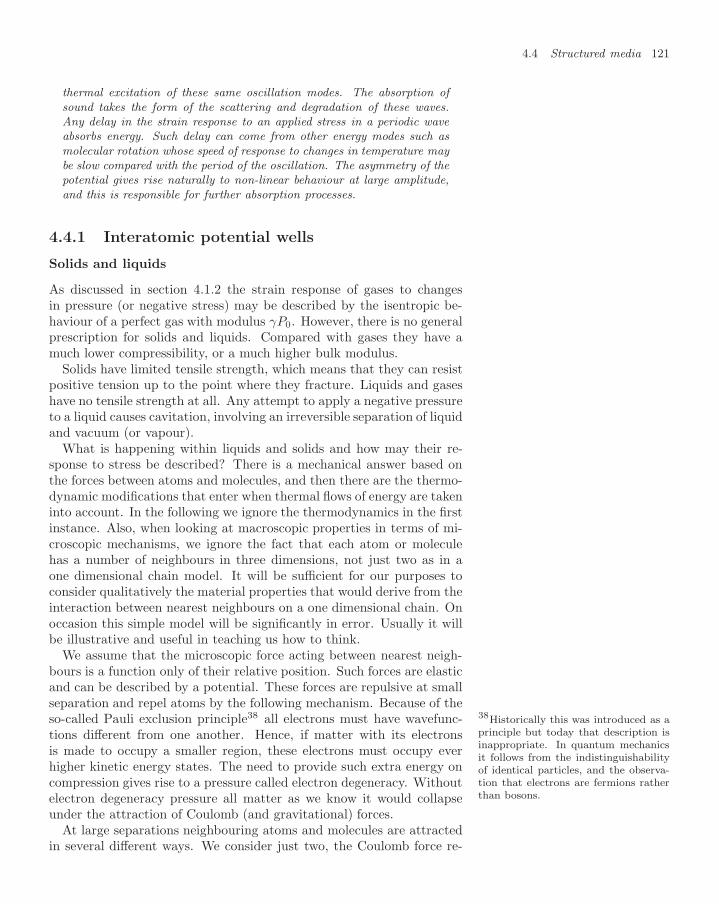
4.4 Structured media 121
thermal excitation of these same oscillation modes. The absorption ofsound takes the form of the scattering and degradation of these waves.Any delay in the strain response to an applied stress in a periodic waveabsorbs energy. Such delay can come from other energy modes such asmolecular rotation whose speed of response to changes in temperature maybe slow compared with the period of the oscillation. The asymmetry of thepotential gives rise naturally to non-linear behaviour at large amplitude,and this is responsible for further absorption processes.
4.4.1 Interatomic potential wells
Solids and liquids
As discussed in section 4.1.2 the strain response of gases to changesin pressure (or negative stress) may be described by the isentropic be-haviour of a perfect gas with modulus γP0. However, there is no generalprescription for solids and liquids. Compared with gases they have amuch lower compressibility, or a much higher bulk modulus.
Solids have limited tensile strength, which means that they can resistpositive tension up to the point where they fracture. Liquids and gaseshave no tensile strength at all. Any attempt to apply a negative pressureto a liquid causes cavitation, involving an irreversible separation of liquidand vacuum (or vapour).
What is happening within liquids and solids and how may their re-sponse to stress be described? There is a mechanical answer based onthe forces between atoms and molecules, and then there are the thermo-dynamic modifications that enter when thermal flows of energy are takeninto account. In the following we ignore the thermodynamics in the firstinstance. Also, when looking at macroscopic properties in terms of mi-croscopic mechanisms, we ignore the fact that each atom or moleculehas a number of neighbours in three dimensions, not just two as in aone dimensional chain model. It will be sufficient for our purposes toconsider qualitatively the material properties that would derive from theinteraction between nearest neighbours on a one dimensional chain. Onoccasion this simple model will be significantly in error. Usually it willbe illustrative and useful in teaching us how to think.
We assume that the microscopic force acting between nearest neigh-bours is a function only of their relative position. Such forces are elasticand can be described by a potential. These forces are repulsive at smallseparation and repel atoms by the following mechanism. Because of theso-called Pauli exclusion principle38 all electrons must have wavefunc- 38Historically this was introduced as a
principle but today that description isinappropriate. In quantum mechanicsit follows from the indistinguishabilityof identical particles, and the observa-tion that electrons are fermions ratherthan bosons.
tions different from one another. Hence, if matter with its electronsis made to occupy a smaller region, these electrons must occupy everhigher kinetic energy states. The need to provide such extra energy oncompression gives rise to a pressure called electron degeneracy. Withoutelectron degeneracy pressure all matter as we know it would collapseunder the attraction of Coulomb (and gravitational) forces.
At large separations neighbouring atoms and molecules are attractedin several different ways. We consider just two, the Coulomb force re-

122 Mechanical waves and properties of matter
Fig. 4.21 The Lennard–Jones inter-atomic potential described in the text,shown relative to its equilibrium depthE0 and equilibrium separation . -1.5
-1
-0.5
0
0.5
1
1.5
2
0.5 1 1.5 2
r/ℓ
φ/Eo
sponsible for the ionic solid, and the van der Waals force responsible formost other solids and liquids. An ionic solid is composed of ions, that isatoms or molecules that are charged. Between these positive and neg-ative ions there is a Coulomb potential with the basic 1/r dependence.This is strong and long range so that forces between next-to-nearestneighbours as well as nearest neighbours are important.
By contrast, in a van der Waals solid the force is weak and shorterrange, but acts between neutral atoms and molecules as well. It arisesin the following way.39 If, by fluctuation, a small electric dipole moment39This is a reasonably convincing clas-
sical justification for a second order per-turbation effect in quantum mechanics.
were to occur on one molecule, it would create a field proportional to1/r3 in a second neighbouring molecule. This field would induce a dipolemoment in the second molecule whose field at the first molecule wouldthen be proportional to 1/r6. The energy of the initial dipole in this fieldmakes the initial fluctuation energetically favourable. The consequenceis that such fluctuations occur and there is a weak attractive term in thepotential energy varying as 1/r6. Figure 4.21 shows such a potential,the Lennard–Jones potential,
φ(r) = E0
[(
r
)12
− 2(
r
)6]
. (4.76)
The short range repulsion is parametrised by the 1/r12 term. The depthof the potential is E0 at the equilibrium distance of .
The value of the binding energy E0 is of order 0.1 eV so that a typicalvan der Waals solid or liquid vaporises at a temperature not far removedfrom ambient. An ionic solid has a much deeper well and such mate-rials do not vaporise at normal temperatures. For a metal the shapeof the potential well is similar to the Lennard–Jones potential althoughthe binding is tighter because, qualitatively, electric dipole moments areeasily induced in conductors and so the effect of the dipole–dipole at-traction is enhanced.
The position of the potential minimum determines the separation ofatoms at low temperature. At higher temperature, T , classically the

4.4 Structured media 123
Displacement, u
n,reference position/
n
1 2 3 4 5
Fig. 4.22 A plot of displacementagainst reference position for a one di-mensional chain of identical masses.The reference position is given as a mul-tiple of the reference separation . Inthe model forces act between nearestneighbours. A possible solution is thatat any time the displacements follow asine wave as shown. However, the linesbetween the masses have no physicalsignificance and the wave exists only atthe reference position of the masses.
atoms bounce back and forth inside the well with energy of order kBT . Inquantum mechanics they occupy states of energy E within the well withprobabilities related to the Boltzmann factor, exp(−E/kBT ). Effectivelythe differences between the quantum and classical descriptions are small.In the following we use a classical description.
The asymmetry of the potential is such that the mean separationincreases with increased temperature, an effect familiar as the thermalexpansion of solids and liquids. This is a direct result of the non-linearityof the force, or equivalently the non-parabolic shape of the potential.In the following we neglect the effect of finite temperature in the firstinstance.
Motion of masses with nearest-neighbour potential
Such a constituent potential establishes the linear terms that determinethe mechanical properties for small amplitude distortions and the non-linear terms as well. It also determines the periodic structure that givesrise to the band structure at short wavelengths which distinguishes aconstituent model from a continuum model.40 40For a non-trivial band structure there
needs to be more than one kind of mass,but this is a modest elaboration of thechain.
The motion of two point masses, initially separated in x, can be de-scribed by six coordinates. If they do not interact, each can move inde-pendently in x, y and z. If they interact, there are still six modes andthese may be described as the relative motion and the combined motionof the centre of mass in each direction, x, y and z. By extension, thenormal modes of N identical masses along x-may be described by theirN different amplitudes, and the same for their transverse positions in yand z.
We consider a chain of atoms extended in x, for simplicity looking onlyat motion in the x-direction. Figure 4.22 shows such a line for whichthe reference separation of the masses is and the displacement of massn relative to its reference position is un where n is its integer label. Tosimplify the diagram the displacements are shown transversely, althoughin this case they are actually longitudinal. According to this model theforce on mass n due to mass n + 1 depends only on the strain in theirrelative positions εn+ = (un+1 − un)/ and may be written in terms of

124 Mechanical waves and properties of matter
the derivative of a potential function φ(ε),
Fn+ =dφ(ε)
dεεn+. (4.77)
The force due to the mass n − 1 is of opposite sign. They only fail tocancel exactly because the strain is different there. The difference instrain on the two sides is (un+1 +un−1−2un)/. Therefore the net forceon n from its two neighbours is
Fn =(un+1 + un−1 − 2un)
d2φ(ε)dε2
. (4.78)
For small strain ε relative to the reference state we may assume thatd2φ(ε)/dε2 is a constant41 evaluated at ε = 0. We call this φ′′
. Then41In section 9.4 we shall consider whathappens when the strain is large enoughthat this is not true.
the motion of mass n is found by applying Newton’s law,
m∂2un
∂t2=
(un+1 + un−1 − 2un)
φ′′ . (4.79)
Chain dynamics in the linear approximation
Equation 4.79 is linear in the displacements u. We try a solution of theform
un(t) = A exp [i(nk − ωt)]. (4.80)
Displacements for neighbouring masses that follow such a spatial depen-dence are sketched in Fig. 4.22. Substituting this into equation 4.79 weget
mω2 =2(1 − cos k)
φ′′
. (4.81)
This is the dispersion relation, the relation between k and ω, that mustbe satisfied for equation 4.80 to be a possible solution. We recall that itassumes that φ′′
is a constant.For long wavelengths (small k) the equation becomes mω2 = k2φ′′
,and in terms of the reference density per unit length ρ,
ρω2 =
k2
2φ′′
. (4.82)
Comparing this with the macroscopic dispersion relation in the formρω2 = k2K, we see that the macroscopic elastic modulus at the referencepoint ε = 0 is given by
K = φ′′ /2. (4.83)
For shorter wavelengths we use the full equation 4.81. This relationbetween ω and k is sketched out as curve 1 in Fig. 4.23. As k reaches±π/, the curve indicates a maximum value of ω. Beyond these valuesof k the curve turns down again. The ratio ω/k represents the phasevelocity of these sound waves, and the slope dω/dk is the group velocity.At long wavelengths compared with the atomic spacing, the curve is astraight line and the velocity of sound is constant. At shorter wave-lengths the phase velocity (ω/k) and the group velocity (dω/dk) both

4.4 Structured media 125
0 + /ℓπ- /ℓπwavenumber
frequency1
2
3
2
1
3
Fig. 4.23 Illustrative plots of disper-sion curves, ω against k. Curve 1 forlongitudinal acoustic modes; curve 2 fortransverse or shear modes; curve 3 foroptical modes.
start to fall. When k = ±π/, alternate atoms are π out of phase intheir relative motion, and curve 1 is flat. The group velocity is zero.
What does this mean? The amplitude of any wave in a discrete struc-ture only has meaning at the position of the elements. When the motionsof neighbouring atoms are exactly π out of phase, there is no physicaldifference between a wave travelling to the left and a wave travelling tothe right, or a standing wave. Such a solution cannot transmit energy.That is why the group velocity is zero. This is the maximum frequencythat is possible in this ‘band’. Higher frequencies incident on the ma-terial are attenuated. This means that the atoms are simply too heavyand the restoring forces too loose to respond fast enough.
These principles apply to shear waves just as to longitudinal waves.The dispersion of shear waves, illustrated as curve 2 in Fig. 4.23, issimilar although the frequency is lower because the restoring force isweaker. The shear wave frequency band is therefore narrower than thecompression frequency band.
If the single atoms in this simple model are replaced by bound pairsof atoms42 with their own mutual but stronger interaction, their inter- 42In condensed matter terms this is de-
scribed as having more than one atomper unit cell.
nal oscillation will be influenced by the phase of neighbouring pairs.The result is a spread of normal mode frequencies. The phase betweenneighbouring pairs can only vary between −π and π. This phase ad-vance is described by the wavenumber k, and the speed at which thephase moves is ω/k as before. An illustrative example is shown as curve3 in Fig. 4.23. Such modes may have much higher frequency than themodes which we have discussed previously, because the higher restoringforce within the bound pairs is excited. They are called optical modesand often have infrared frequencies. Consequently they have strong cou-pling to electromagnetic radiation in the infrared. This is a picture ofhow each single resonant frequency characteristic of an isolated individ-ual atom or molecule is spread into a band by mutual interaction withneighbours when it forms part of a condensed material of similar atomsor molecules.

126 Mechanical waves and properties of matter
Thermal excitation of chains
In the absence of a source of sound the atoms of a material are notstationary. The thermal behaviour may be described in terms of themean energy of each vibrational mode. This energy depends only onthe temperature T , the degeneracy n and the excitation energy of themode hω. The mean energy is given by the same Planck distributionthat describes the mean energy of electromagnetic radiation modes of abody or cavity,
E =nhω
exp(hω/kBT ) − 1. (4.84)
It follows that there are thermally induced sound waves criss-crossingall materials at finite temperature. In so far as the behaviour is linear,these waves do not interact with other sound waves, such as the oneswhich carry the information in which we may be interested.
However, materials are not exactly linear. The principle of superposi-tion is an approximation and waves do scatter off one another as a resultof anharmonic terms in the potential. Then in a further approximationthe frequency of normal modes may be shifted slightly if other modesare excited. This is most simply described by a temperature dependenceof φ′′ associated with a change in the reference state. These non-lineareffects are discussed further in chapter 9.
4.4.2 Linear absorption
Sound and thermal energy
Here we discuss linear absorption processes both macroscopically andmicroscopically. Later in section 9.4 we discuss non-linear processesthat lead to absorption. A macroscopic description of linear absorptionis phenomenological, but does not explain fully what is happening. Amicroscopic explanation discusses different mechanisms.
A wave may suffer absorption or scattering. By absorption it is under-stood that the energy is changed into another form. By scattering it isunderstood that the wave changes the direction in which it travels, pos-sibly with some frequency change also. In the case of sound waves at themicroscopic level there is a difficulty in making such a clear distinction.When sound waves are absorbed the energy becomes thermal. Thermalenergy in a material is itself largely composed of sound waves, althoughthere is a small contribution from the thermal excitation of electromag-netic waves also.43 So at a microscopic level at least, the processes of
43Such electromagnetic waves consti-tute the black body radiation whichpersists even in an empty cavity. Thesewaves have the same spatial modes assound but each mode has a frequencywhich is higher by the ratio of the phasevelocities, which is typically 106. Ineach case the net energy in the modeis given by equation 4.84. For wave-lengths greater than 100 µm the con-tributions of EM and acoustic wavesare similar. However, EM waves makea completely negligible contribution tothe integrated thermal energy of anymassive body.
absorption and scattering are not distinguishable in principle.In practice sound coherently scattered from large objects is described
as scattered. Energy incoherently scattered from small objects or otherthermal waves may be shared out and thermalised rather more quickly.This may therefore be counted as ‘absorbed’ though still vibrationalsound energy.

4.4 Structured media 127
Absorption through delayed strain
An absorptive medium is inelastic. In thermodynamic terms this im-plies that changes are irreversible and that the internal energy is not afunction of state. In a macroscopic description the components of stressof the material are not uniquely described by the strain and the materialshows hysteresis. For example, it is observed that many materials taketime to respond when deformed by a sudden change in stress. Such adelay causes absorption.
ΔT
ε
ε
a)
b)ΔT
Fig. 4.24 Illustrative plots of stressagainst strain: a) for stress and strainin phase, b) for strain lagging stress by0.1 radians.
Consider first the changes of stress and strain in an elastic material.Figure 4.24a shows a plot of stress change ∆T against strain ε. As aprogressive wave passes a small element of material, the stress and strainin that element run back and forth along this curve. This is a straightline of slope equal to the modulus if the material is elastic and linear.The work done per unit volume is the area under an element of thiscurve, ∆Tdε. If the curve is single valued, this integrates to zero over apulse.
If the contour is a loop as in Fig. 4.24b, there would be net workdone every cycle. This is what happens in a dynamic situation when thestrain lags the stress. This is an example of hysteresis.
As a simple model we consider a harmonic wave, which at the point zis given by ε = α exp(iωt) and ∆T = β exp(iωt). If the stress wave andthe strain wave are in phase, the contour encloses no area and no energyis lost, Fig. 4.24a. However, if the strain lags the stress in phase thecontour will be an ellipse. Mathematically this may be described as aphase difference between β and α, so that β/α is a complex number. Thisratio is the elasticity modulus concerned. Thus absorption in a linearmodel may be described in terms of a complex elastic modulus. Thusthe complex phase of the mechanical modulus applicable to Fig. 4.24bis 0.1 radians. The energy lost per unit volume per cycle is given by thearea enclosed by the ∆T –ε contour.
This is a linear picture of energy absorption in a medium showingdelayed response. The rate of loss of energy is proportional to the rateat which the material is taken round the loop. So for a given wavevelocity and hysteresis loop, the rate of energy loss of the wave is linearlyproportional to the frequency. A complex value of the modulus K meansthat the phase velocity c =
√K/ρ and the impedance Z =
√Kρ are
also complex numbers. The wave whose amplitude in space is of theform exp(iωx/c) therefore includes an attenuation factor that describesthe energy loss of the wave in a consistent way.
1.0
2.0
3.0
0 20 40 60 80
frequency/kHz
attenuation/dB/m
Fig. 4.25 Frequency dependence of theattenuation of sound in air at 293 K,dry air (lower curve) and 60% humidity(upper curve).
Figure 4.25 shows that sound attenuation in air is quite well describedby a linear frequency dependence. However, the observation that dampair has a much higher attenuation indicates that we need to understandthe cause of the delay and why it might be greater, for instance, in dampthan in dry air.

128 Mechanical waves and properties of matter
Microscopic mechanisms of delayed strain
When we considered the motion of a small volume of material to a changein stress in equation 4.7, we omitted the possibility of velocity-dependentforces. We assumed that the material was homogeneous. We ignoredthe effects of any time required to reach thermodynamic equilibrium andthe possibility of other thermal effects.
Velocity-dependent forces that act in material are described as vis-cosity. They contribute imaginary parts to both λ and µ. Viscosityarises from momentum diffusion by molecules within the wave. For ex-ample, shear wave viscosity arises when molecules transmit momentumforwards and backwards to neighbouring volumes with a different meantransverse velocity. Similar momentum transfer in the longitudinal di-rection for longitudinal waves also gives rise to viscosity.
The exchange of thermal energy within the wave is also important inthe attenuation of sound. Acoustic waves are isentropic not isothermal,and the various mechanical moduli concerned are defined at constant en-tropy. As a result there are temperature differences within the wave, andthe exchange of energy by thermal conduction between the peaks andtroughs with different temperatures is a significant dissipative process.This thermal conduction process is distinct from the viscous mechanismdiscussed above.
A related point concerns the internal energy of non-translational de-grees of freedom, such as the rotation or internal vibration of molecules.If acoustic waves had been isothermal, this energy would not have beeninvolved. However, because the temperature oscillates up and down inan acoustic wave, energy flows in and out of these otherwise transla-tionally irrelevant modes. This flow takes time because the coupling isweak. The time required for the translational energy to reach thermalequilibrium with rotational modes is often significant compared with theperiod of the acoustic waves. Such thermodynamic changes taking placeunder non-equilibrium conditions cannot be reversible. The delayed ex-change of this energy is a major cause of absorption in diatomic andpolyatomic gases, and in more complex solid and liquid materials also.This mechanism with the extra degrees of freedom of the water moleculeis responsible for the extra attenuation of damp compared with dry airshown in Fig. 4.25.
Sound attenuation by scattering and non-linearity
So far materials have been assumed homogeneous. Inhomogeneitiescause attenuation through scattering and changes in polarisation. Scat-tering from an inhomogeneity of size a depends critically on the ratioa/λ. If this is not too small, scattering is determined by the detailedboundary conditions at the inhomogeneity. If it is small, scattering ismore isotropic and the scattering cross section depends on λ−4, so thatthe scattering (and consequently the beam absorption) is much largerat short wavelengths. This is known as Rayleigh scattering.44 This is of
44Rayleigh scattering is unconnectedwith Rayleigh waves. Lord Rayleigh,like Gauss, belongs to that small bandof physicists whose contributions are soextensive that it is sometimes not easyto distinguish which eponymous effectis being referenced.
great technical importance in the use of ultrasound for industrial quality

4.4 Structured media 129
control, fish location and medical imaging. It is discussed in more detailin chapter 9.
Other mechanisms of energy absorption involve the non-linearity ofthe medium. In particular there is the scattering of sound waves byother acoustic waves, including thermally generated waves. This doesnot happen in a linear medium.
Read more in books
Waves, Berkeley Physics Course Vol. 3, FS Crawford,McGraw–Hill (1965), a student text on waves
The Physics of Vibrations and Waves, HJ Pain, Wiley(1999), a student text on waves
Properties of Matter, Manchester Physics Series, BHFlowers and E Mendoza, Wiley (1970), a student texton condensed matter
Introduction to Solid State Physics, C Kittel, Wiley(1971), a student text on condensed matter
Physical Properties of Crystals, JF Nye, Oxford (1957),a classic text on tensors
Irreducible Tensorial Sets, U Fano and G Racah, Aca-demic Press (1959), a classic text on tensors
Fundamentals of Acoustics, LE Kinsler, AR Frey, ABCoppens, JV Sanders, Wiley, 3rd edn (1982), a stan-dard textbook on sound
The Theory of Sound, Vols 1 and 2, JWS Rayleigh,reprinted Dover (1945), Rayleigh’s original texts onsound
The Solid Earth, CMR Fowler, Cambridge (1990), astandard textbook on geology and geophysics
Look on the Web
Look at the book website atwww.physics.ox.ac.uk/users/allison/booksite.htm
Discover how far geophysicists have progressed with thedifficulties of recording, analysing and understandingseismic waves with different polarisations
Geophysics SV SH P waves
Find out about the current state of knowledge of theEarth’s structure
USGS Earth structure
Study more about Rayleigh waves, high frequency sur-face waves and their applications
Rayleigh waves or surface acoustic waves
Get data on the normal vibration modes of the Earthand Sun
Earth normal modes and helioseismology

130 Mechanical waves and properties of matter
Questions
4.1 A material is subject to a general strain,[a b cd e fg h i
].
Separate this into the components of compressionstrain, shear strain and rotation.
The material has Lame constants, λ and µ. Deter-mine the related stress tensor.
4.2 Prove that at normal incidence the reflection andtransmission coefficients are given by equation 4.39for any polarisation.
Show that with these coefficients the energy flux isconserved.
4.3 A planet of uniform composition has a radius of5000 km. The velocity of compression waves is3.0 km s−1 and of shear waves is 1.9 km s−1. TheRayleigh wave generated by a quake arrives 500 safter the compression wave. When did the shearwave arrive and how far away was the quake?
4.4 A primitive musical instrument consists of an opensquare box section of side a. A piston closes off oneend to make a channel of length . What are thenormal modes of this cavity?At first sight the sides of width a do not appearto influence the displacement of this longitudinalwave. Why do they need to be there?
4.5 Prove that for a gravity wave of height h and wavenumber k travelling in fluid of depth z0 the dis-placement amplitude of the horizontal scouring mo-tion at the bottom is
h/ sinh (kz0).
Hence that, if the depth is small compared with thewavelength, the scouring velocity has amplitude
h√
g/z0.
Put in numbers for h = 1 m and depth z0 = 3 m.What happens as z0 gets even smaller?

Information and dataanalysis 5
5.1 Conservation of information131
5.2 Linear transformations 135
5.3 Analysis of data using models143
Read more in books 155
Look on the Web 156
Questions 156
in which the physics and mathematics of information and data analysisare discussed
5.1 Conservation of information
Information may be quantified in terms of the required number of binarybits, and is equivalent to negative entropy. The second law of thermody-namics requires that information may not increase in an isolated system.Imaging and other data are collected for a purpose, that is to answerspecific questions. The processing of data involves the transformation ofinformation available from collected data and previous knowledge. Thistransformation is intended to separate information related to the purpose(the signal) from the rest (the noise). The separation is uncertain and thecalculated signal depends on the estimated noise and the previous knowl-edge. Statistical errors derive from the effects of random noise and maybe reduced by taking further data. Systematic errors derive from uncer-tainties in the previous information and their effect on the signal. Theseare not reduced just by taking more data.
Information and thermodynamics
Information can be quantified by counting the number N of independentbinary bits required to store it. This definition of information makes noreference to any value judgement. The same quantity of informationmay be interesting, unintelligible, or dominated by noise. The definitionis, however, objective and of practical importance. The requirement thatthe state of the binary bits be independent is significant. For example,if a record of information is copied, the quantity of information is notthereby increased. If the vector of N bits is linearly transformed bymultiplying by a unitary N × N matrix, the quantity of information isalso unchanged. If the matrix is not unitary, the independence of thebinary bits is reduced and information reduced.
In statistical mechanics a system whose macroscopic state is equallyconsistent with any of W different microscopic quantum states has anentropy S given by
S = kB loge W, (5.1)
where kB is Boltzmann’s constant. To specify the microstate of the
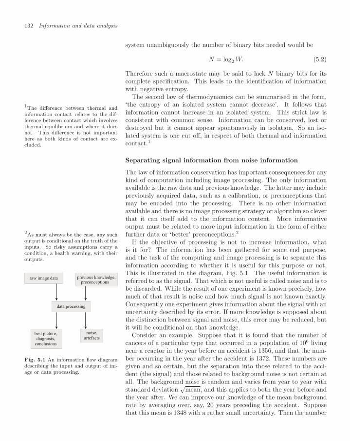
132 Information and data analysis
system unambiguously the number of binary bits needed would be
N = log2 W. (5.2)
Therefore such a macrostate may be said to lack N binary bits for itscomplete specification. This leads to the identification of informationwith negative entropy.
The second law of thermodynamics can be summarised in the form,‘the entropy of an isolated system cannot decrease’. It follows thatinformation cannot increase in an isolated system. This strict law isconsistent with common sense. Information can be conserved, lost ordestroyed but it cannot appear spontaneously in isolation. So an iso-lated system is one cut off, in respect of both thermal and informationcontact.1
1The difference between thermal andinformation contact relates to the dif-ference between contact which involvesthermal equilibrium and where it doesnot. This difference is not importanthere as both kinds of contact are ex-cluded.
Separating signal information from noise information
The law of information conservation has important consequences for anykind of computation including image processing. The only informationavailable is the raw data and previous knowledge. The latter may includepreviously acquired data, such as a calibration, or preconceptions thatmay be encoded into the processing. There is no other informationavailable and there is no image processing strategy or algorithm so cleverthat it can itself add to the information content. More informativeoutput must be related to more input information in the form of eitherfurther data or ‘better’ preconceptions.22As must always be the case, any such
output is conditional on the truth of theinputs. So risky assumptions carry acondition, a health warning, with theiroutputs.
If the objective of processing is not to increase information, whatis it for? The information has been gathered for some end purpose,and the task of the computing and image processing is to separate thisinformation according to whether it is useful for this purpose or not.This is illustrated in the diagram, Fig. 5.1. The useful information isreferred to as the signal. That which is not useful is called noise and is tobe discarded. While the result of one experiment is known precisely, howmuch of that result is noise and how much signal is not known exactly.Consequently one experiment gives information about the signal with anuncertainty described by its error. If more knowledge is supposed aboutthe distinction between signal and noise, this error may be reduced, butit will be conditional on that knowledge.
raw image data previous knowledge,preconceptions
data processing
best picture,diagnosis,
conclusions
noise,artefacts
Fig. 5.1 An information flow diagramdescribing the input and output of im-age or data processing.
Consider an example. Suppose that it is found that the number ofcancers of a particular type that occurred in a population of 106 livingnear a reactor in the year before an accident is 1356, and that the num-ber occurring in the year after the accident is 1372. These numbers aregiven and so certain, but the separation into those related to the acci-dent (the signal) and those related to background noise is not certain atall. The background noise is random and varies from year to year withstandard deviation
√mean, and this applies to both the year before and
the year after. We can improve our knowledge of the mean backgroundrate by averaging over, say, 20 years preceding the accident. Supposethat this mean is 1348 with a rather small uncertainty. Then the number

5.1 Conservation of information 133
of background cancers in the year in question that contribute to 1372 is1348±√
1348. Because the separation of signal from noise involves thislarge statistical error, the number of cancers that can be attributed tothe accident is consistent with zero at the one standard deviation level. Ifthe difference had been larger any conclusion would still have been con-ditional on implicit assumptions. For example, if the background counthad risen because of an increase in smoking-induced cancers caused bysocio-economic collapse triggered by the accident, the information alonecould not be used to relate cancer to radiation exposure.
If the number of possible outcomes of an experiment3 is W , then, 3For simplicity we assume that the apriori probabilities of all such outcomesare equal.
when that experiment is done and yields one result, by equation 5.2that experiment conveys information N = log2(W ). This allows thatsome of this information may be uninteresting, that is to say noise. Ifthe results of experiments were truly continuous variables then, by theabove definition, they would yield an infinite amount of information,almost all of which would be noise. This is not helpful. In practice,either by recording results with limited precision, or by explicitly binningreadings in discrete bins, we may reduce the number of possible outcomesof the experiment W to a finite, if large, number. When precision isdiscarded in this way, care is taken to ensure that signal information isnot lost, either by truncating significant figures too hard, or by digitisingor binning too coarsely. This might, for example, lead to a decision todigitise the square or the logarithm of an analogue signal. Anyway, therecording of the experiment or image in terms of limited informationand discrete variables is the first stage in the separation of signal andnoise.
Reproducible and non-reproducible noise
We distinguish two types of noise, random noise and artefactual noise,by their reproducibility. Random noise changes if the experiment isrepeated, and this is the way in which its separation from the signal maybe improved. Systematic effects and artefactual noise are reproducibleand causal. They differ from the signal only in that they are not wantedin the image or in answer to the question. Only previous knowledgecan separate these from the signal. For example, unwanted reflectionsand distortions may be subtracted from an image if previous knowledgeis available. However, if random noise is present as well, there may beuncertainty in such a separation. The error on the corrected signal wouldthen be increased by the artefact. In practice therefore information maybe correlated between types of noise as well as with signal.
In the absence of noise the result of the experiment is a certain sig-nal. In the presence of noise the result of the experiment is a certainoutcome. But the outcome for the signal alone is uncertain because it isnot resolved from the noise. This uncertainty is the error. Signal errorsassociated with random noise are called statistical errors; those asso-ciated with reproducible noise are called systematic errors. Statisticalerrors can be reduced by taking further data, at a cost in experimental

134 Information and data analysis
time and inconvenience. Because systematic errors relate to previousknowledge and not to the experiment at hand, they may only be re-duced with additional knowledge. If that comes from other observationssuch as data runs with different conditions, data from other modalities,calibration or registration information, then those may be repeated andthe previous information increased.4
4There is a semantic point here. If anexperiment is defined so as to include acalibration run, for example, then anystatistical errors in the calibration runbecome statistical errors in the experi-ment instead of systematic.
Noise filtering by transformation and modelling
Separation of the signal from the noise is only possible in so far asthe signal and noise are different. Information about this differencecomes from previous knowledge, and without this no progress is possible.There are two approaches, one based on transformation and the otheron modelling.
If the previous knowledge gives information about the characteristicsof the signal, the data are transformed into variables in which thesecharacteristics are most clear. The noise, too, will have characteristics.We consider two simple examples of such previous information.
If it is known that the signals are episodic pulses in time andthat the noise is not, a discriminator may be applied to thedata as a time sequence, as illustrated in Fig. 5.2a. Thenall elements in time below that level may be reset to zerowhich erases the noise signals. Such a filter makes two kindsof mistake. It discards some real signals that are very low,and it retains the contribution of the noise within the timewindow of a signal pulse. Its success depends on the differ-ence between the signal and noise, and on our knowledge ofthat difference.
time
amp
litu
de discriminator
level
y
x
a)
b)
0
Fig. 5.2 a) An illustration of signaland noise contributions in time, distin-guished by a discriminator in the lightof previous knowledge.b) Measurements of y for different xwhich are fitted by a model, given byprevious knowledge, that generates afamily of curves for different values ofthe physically interesting parameter α.
Perhaps it is known that the signals are waves with quitewell-defined frequency. In that case the data should be trans-formed to a frequency spectrum. A discriminator is thenapplied to this spectrum in the same way. The spectrumcleaned of low amplitude noise in this way may be reconsti-tuted in time by inverting the transformation.5
5This example applies to the recon-struction of music from a compactdisc. The noise arising from dirt andscratches on the surface is episodic intime, whereas the sound is harmonicand may be filtered.
In any case the success of the filter is only as good as the previousknowledge.
Similar considerations apply when the previous information comes inthe form of a model. A simple example is illustrated in Fig. 5.2b, wherethe data for a number of measurements of y for particular values of xare plotted. The experiment was carried out to measure a parameterα and a model y = f(α, x) relates this to y and x. The model, itselfprevious knowledge, represents a family of curves in the plot, each fora different value of α. On the assumption that the effect of the noiseis random, sometimes increasing a reading y and sometimes decreasingit, the best choice of α would be the curve that is closest to the pointswith some above and some below, although we need to specify exactlywhat is meant by ‘best’. All differences between the best model curve
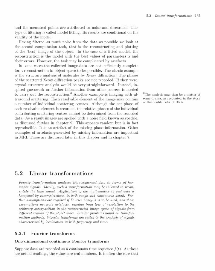
5.2 Linear transformations 135
and the measured points are attributed to noise and discarded. Thistype of filtering is called model fitting. Its results are conditional on thevalidity of the model.
Having filtered as much noise from the data as possible we look atthe second computation task, that is the reconstructing and plottingof the ‘best’ image of the object. In the case of a fitted model, thereconstruction is the model with the best values of parameters α andtheir errors. However, the task may be complicated by artefacts.
In some cases the collected image data are not sufficiently completefor a reconstruction in object space to be possible. The classic exampleis the structure analysis of molecules by X-ray diffraction. The phasesof the scattered X-ray diffraction peaks are not recorded. If they were,crystal structure analysis would be very straightforward. Instead, in-spired guesswork or further information from other sources is neededto carry out the reconstruction.6 Another example is imaging with ul- 6The analysis may then be a matter of
some drama, as recounted in the storyof the double helix of DNA.
trasound scattering. Each resolvable element of the image may containa number of individual scattering centres. Although the net phase ofeach resolvable element is recorded, the relative phases of the individualcontributing scattering centres cannot be determined from the recordeddata. As a result images are spoiled with a noise field known as speckle,as discussed further in chapter 9. This appears random but is in factreproducible. It is an artefact of the missing phase information. Otherexamples of artefacts generated by missing information are importantin MRI. These are discussed later in this chapter and in chapter 7.
5.2 Linear transformations
Fourier transformation analyses time-sequenced data in terms of har-monic signals. Ideally, such a transformation may be inverted to recon-stitute the time signal. Application of the mathematics to real data ishampered by incompleteness, in both range and continuous detail. Fur-ther assumptions are required if Fourier analysis is to be used, and theseassumptions generate artefacts, ranging from loss of resolution to thearbitrary superposition in the reconstructed image space of signals fromdifferent regions of the object space. Similar problems haunt all transfor-mation methods. Wavelet transforms are suited to the analysis of signalscharacterised by localisation in both frequency and time.
5.2.1 Fourier transforms
One dimensional continuous Fourier transforms
Suppose data are recorded as a continuous time sequence f(t). As theseare actual readings, the values are real numbers. It is often the case that

136 Information and data analysis
these data are to be interpreted in terms of a superposition of a numberof frequencies ω.7 Thus in general we can express7For example, such a decomposition is
applied by the brain to the pressure sig-nals detected by the ear so that musicmay be heard. In this decompositionlinearity is essential so that the signalheard at any time is a simple superpo-sition of each frequency present.
f(t) =1√2π
∫ +∞
−∞g(ω) exp(−iωt)dω, (5.3)
where g(ω), the amplitude of the angular frequency ω, is known as theFourier transform. (The choice of constant outside the integral is ex-plained below.)
The reason for extending the integral to negative frequencies deservesmore explanation. What do we mean by negative frequencies? Becausef(t) and ω are real, we may equate the right hand side of equation 5.3to its conjugate
1√2π
∫ +∞
−∞g∗(ω) exp(+iωt)dω
and deduce that g(−ω) = g∗(ω). So g for negative ω is determined wheng for positive ω is known, and negative frequencies are just a mathe-matical convenience. The real and imaginary parts of g(ω) form thecoefficients of cos(ωt) and sin(ωt) respectively in a real expansion usingcos and sin. We have chosen this complex exponential representationbecause it is the most concise.
But how may the g(ω) be determined? This is done with a standardtrick. We multiply both sides of equation 5.3 by exp(iωt) and integrateover all time t,8
8We have replaced the dummy variablein equation 5.3 by ω′.
∫ +∞
−∞f(t) exp(iωt)dt =
1√2π
∫ +∞
−∞g(ω′)
[∫ +∞
−∞exp[i(ω − ω′)t]dt
]dω′.
(5.4)The integral in square brackets is 2πδ(ω−ω′) where δ is the Dirac deltafunction. The proof of this is left to question 5.2.
h
1/h
0
0
x
x
h ∞→
a)
b)1.0
Fig. 5.3 a) The Dirac δ-function, δ(x),where h is taken to infinity. b) TheHeaviside function or unit stepfunctionis the integral of the Dirac function,H(x) =
∫ x
−∞ δ(x′)dx′.
The δ-function, δ(x − x0), may be described as a spike at x = x0
of infinite height, infinitesimal width but unit area, as illustrated inFig. 5.3a for x0 = 0. It has the important property for any functionf(x), ∫
f(x)δ(x − x0)dx = f(x0). (5.5)
The integral of δ(x) is the Heaviside unit stepfunction H(x) shown inFig. 5.3b.
Returning to equation 5.4 and using equation 5.5 to complete theintegration on the right hand side, we get
g(ω) =1√2π
∫ +∞
−∞f(t) exp(iωt)dt. (5.6)
The reason for choosing the factor in equation 5.3 is now seen to be tomake the pair of equations, 5.3 and 5.6, of the same form except for thechange in sign in the phase factor. These represent the Fourier transfor-mation and the inverse Fourier transformation. The general propertiesof Fourier transforms are treated in standard mathematical texts, and

5.2 Linear transformations 137
some are the subject of questions at the end of the chapter. In the follow-ing we highlight the physical interpretation as it affects the use of Fouriertransforms in imaging. It is important to note that the transformationis linear, possesses an inverse and therefore conserves information.
In many applications the variables are not time and frequency, buttheir spatial equivalents, distance x and wavenumber kx = 2π/λx. Asthese transforms are linear, the Fourier transformation may be taken inany cartesian dimensions, separately or simultaneously. Such wavenum-bers form a vector k = (kx, ky, kz). Any function of r = (x, y, z) maybe expressed as9 9In anticipation of the analysis of plane
waves in the following paragraph wechange the sign of the i in this spatialtransform. This will ensure that a wavewith positive k and ω travels forward inr with time, t.
f(r) =(
12π
)3/2 ∫ ∫ ∫g(k) exp(ik · r)d3k, (5.7)
with the three dimensional inverse transform given by
g(k) =(
12π
)3/2 ∫ ∫ ∫f(r) exp(−ik · r)d3r, (5.8)
where the integrals are over all three dimensional k and r space respec-tively.
A wave in space and time, f(r, t), may be expanded by Fourier anal-ysis into a superposition of elemental plane waves with direction andwavenumber k and frequency ω. A plane wave has a constant value of kindependent of r; its wavelength and direction of travel are independentof position. Loci of constant phase φ = k · r − ωt describe wavefronts,families of parallel flat planes. Such an expansion may be written
f(r, t) =(
12π
)2 ∫ ∫ ∫ ∫g(k, ω) exp[i(k · r − ωt)]d3kdω. (5.9)
Its transform is then given by
g(k, ω) =(
12π
)2 ∫ ∫ ∫ ∫f(r, t) exp[−i(k · r − ωt)]d3rdt. (5.10)
Convolution theorem
In the application of Fourier techniques to object distributions and re-lated image distributions we need to use the formalism of convolutions.
The convolution of two functions, h1(x) and h2(x), is defined by
h12(x) =∫ ∞
−∞h1(x′) × h2(x − x′)dx′. (5.11)
An important application is the use of the image of a point source, thepoint spread function (PSF).10 If the object distribution is u(x) and the 10In the following we describe the 1-D
problem. This may be extended simplyto 2-D and 3-D problems.
PSF is w(x), then the image v(x) is the convolution of the two,
v(x) =∫ ∞
−∞u(x′)w(x − x′)dx′. (5.12)

138 Information and data analysis
To prove this result consider first a unit point object at x = x0 withu(x) = δ(x − x0). By definition the image distribution is the PSF itselfin this case, and integration over the δ-function confirms that the imageis v(x) = w(x−x0). Next we verify equation 5.12 for a general extendedobject u(x). We can represent u by a superposition of such δ-functionsside by side, as illustrated in Fig. 5.4. Formally
u(x) =∫
u(x′)δ(x − x′)dx′. (5.13)
Since the relation between u and v is linear, the corresponding imageis the superposition of the image of each δ-function. Equation 5.12 istherefore true for any object function u(x). The image of any object isthe convolution of the object and the PSF.
u(x)
x
Fig. 5.4 The object distribution u(x)can be represented in terms of a se-quence of bar elements of width d. Asd tends to zero, the representation be-comes a sequence of δ-functions, eachmultiplied by its own u(x).
The Fourier transform (FT) of any image is therefore the transformof this convolution. The transform of a convolution of two functions isequal to the product of their transforms. The proof is left to question 5.3.So we deduce the relation,
FTimage(ω) = FTobject(ω) × FTPSF(ω). (5.14)
This is an important result. The FT of the image is determined by thedata. The PSF is known from previous knowledge. So the true FT ofthe object may be determined from the image FT using equation 5.14for any range of ω for which the FT of the PSF is non-zero. For valuesof ω for which the PSF is small, the image FT is multiplied by a largefactor to determine the object FT. In practice noise in the data limits theefficacy of this. Indeed to reduce noise the contribution at frequenciesfor which the PSF is small may be suppressed altogether. So for thereconstruction there is a choice between fine detail but amplified noise,and coarse resolution with reduced noise. A balance can be struck. Thisprocess is called filtering.
Shortcomings in the practical application of Fourier analysis
The formalism of Fourier transformations is symmetric, instructive andelegant. This is deceptive! The apparent symmetry between the twocanonical variables, say ω and t, is broken. In terms of one of them, sayt, the measurements are made, the values f(t). These measurementsare real, not complex, and there are a finite number of them, that is tosay the measurements are samples of f at certain values of t only. Theresulting g(ω) is complex in general, and is not sampled. So in practicalterms the symmetry is removed.11
11If the measurements are samples as afunction of ω, the roles are reversed butin no case is the symmetry maintained.
The problem is that finite data, whether recorded in ω or t, cannotprovide the infinite number of values required to carry out the integra-tion prescribed by the transformation. Whichever is recorded, both thetotal range of measurements and the step between successive measure-ments are finite. Data values at intermediate points simply do not exist,and the same is true for values outside the range.12 These limitations
12It is not the case that we just needto reconstruct the missing values fromthose that we have. Any such recon-struction depends on the model or pre-scription used. There is no way to checkwith the data whether the prescriptionused is correct, or even just sensible. Itis better to say that the data are unde-fined except at the points where theyare explicitly measured. Then we mayappreciate fully the artefacts generatedby using different prescriptions to forcethe application of a Fourier decomposi-tion.
have major effects on the application of Fourier techniques. To imple-ment the Fourier transformation at all, arbitrary decisions have to be

5.2 Linear transformations 139
made about the non-existent data, and the effect of these decisions isto create artefacts, the artificial differences between reconstruction andtrue object.
Formally we may say that the measurements in t are the product ofthe continuous function of possible measurements f(t) and a samplingfunction S(t). Thus the actual measurements are the non-zero values of
F (t) = S(t) × f(t). (5.15)
The sampling function has value 1 for values of t for which a measure-ment is made, and 0 otherwise. This provides a symmetry with equa-tion 5.14. However, this relation is singular, and is not much help. Itdoes not tell us the values of f(t) for which no measurement is available.
The problem of missing information is the same whichever of the twoconjugate variables, ω or t, is measured. Random noise enters sym-metrically between them. Noise power is constant with time. So thesquared noise amplitude increases linearly with the length of the mea-surement period, ∆t. This is a simple example of the random walk.13 13A coherent signal amplitude is not a
random walk. It integrates linearly overthe same time and is seen rising abovethe noise as ∆t increases. The differ-ence is that the signal is coherent withdefined phase, while the noise is not.
The squared noise amplitude is also linearly dependent on bandwidth,∆ω, in the same way.
Depending on the way in which the incomplete Fourier information iscircumvented, the artefacts generated are different. Thus understandingartefacts in images is largely a matter of understanding the effect of thesecircumventions. It is usual to simplify the discussion by distinguishingthe range of sampling from the intersampling spacing, assumed uniformwithin that range. Clearly similar artefacts would be generated by moregeneral sampling schemes.
In Fig. 5.5 we give a calculated graphical example where the functionf(t) is measured at the discrete values t = −2,−1, 0, 1, 2 and found tohave the values −4, 3,−2, 3,−4 respectively. Four different assumptions(in the left-hand column: a, c, e, g), all equally reasonable, are madeabout the values of the continuous function f(t) that might have beenfound at other values of t, if these had been measured. The four resultingtransforms g(ω) are very different (in the right-hand column: b, d, f, h).In the following paragraphs we discuss these differences and how theyrelate to previous knowledge, preconceptions or guesswork.14
14The measurements are symmetricabout t = 0 and the prescriptions illus-trated maintain this symmetry. Other-wise the FTs would have had an imagi-nary part. We have avoided this to sim-plify the example.
Circumvention of the limited range of measurement points
If data are only available for a limited range, ∆t = 5 in our example,it is often supposed that at other values of t the data would have beenperiodic, thus
f(t + n∆t) = f(t), (5.16)
for all integer n, Fig. 5.5a. The FT g(ω) of such a periodic functionis discrete, vanishing for all values of ω except 2πm/∆t for any integerm.15 This is illustrated in Fig. 5.5b; the FT is non-zero only at discrete 15See question 5.4.
values of ω. These spikes are artefacts created by the supposition.A more elementary assumption is that the function f(t) is zero outside
the measured range, Fig. 5.5c. Through the convolution theorem this

140 Information and data analysis
-40
40
-15 -10 -5 5 10 15
frequency
3
-3
time-8 -4 4 8
c) d)
-15 -10 -5 5 10 15
5
-15
frequency
3
-3
time-8 -4 4 8
g) h)
-15 -10 -5 5 10 15
6
-6
frequency
3
-3
time-8 -4 4 8
a) b)
-40
40
-15 -10 -5 5 10 15
frequency
3
-3
time-8 -4 4 8
e) f). .
Fig. 5.5 The four distributions f(t) shown in the left-hand column (a,c,e,g) have identical measured values (at times: t =−2,−1, 0, 1, 2). For a) the measured values of f(t) are assumed to be part of a infinitely repeated discrete sequence of values.For c) values of f(t) are assumed zero unless measured. Plot e) is like a) except that the sampled readings are assumed toapply over a range in t of ± 1
2units. Plot g) is like c) but with the local sampling of e). The right-hand column shows the
corresponding FTs (b,d,f,h).

5.2 Linear transformations 141
limited range of t measurements generates a PSF in ω given by
1√2π
∫ ∆t/2
−∆t/2
exp(−iωt)dt =
√2π
sin(ω∆t)∆t
. (5.17)
This is a sinc function of width 1/∆t. Convoluted with the discreteelements of plot c this gives rise to the rounded FT shown in plot d, inplace of the sharp spikes of plot b.
These two strategies for coping with a limited range of data in t arequite different and the results likewise, although the data are the same.
Circumvention of the discreteness of measurement points
Further artefacts are associated with assumptions about how f(t) inter-polates between measurements.
In general, if there are p measurements spaced ∆t/p apart, the sam-pling function is 1 at values of t = m∆t/p for integer m, and 0 otherwise.What happens to f(t) at the values of t between? The data say noth-ing but some assumption is required if a Fourier transformation is to becarried out at all. One extreme example has already been illustrated inFig. 5.5a–d where it is assumed that f(t) is zero in between the discretepoints. Alternatively, as shown in Fig. 5.5e–h, a rectangular wave in-terpolation might be chosen. These FTs are no longer periodic and arelocalised in ω. In fact the smoother the interpolation of f(t), the morecompact is the localisation of the FT in ω-space.
Further, any such smoothly varying function might be multiplied byany linear phase factor
exp[2πni
pt
∆t
]
with arbitrary integer n. Such factors are unity at the t of each datareading, and would therefore be entirely consistent with all recordedreadings.16 The effect of such factors on the FT is a shift in ω-space 16Artefacts generated by more gen-
eral sampling schemes may be under-stood by generalising this phase factorwhile maintaining the constraint that itpasses through +1 wherever a samplingoccurs.
by an arbitrary multiple of 2πp/∆t. The upshot is that the FT in ω-space is inherently ambiguous with cells of ambiguity forming a periodicstructure. Often the assumption is made that the contribution fromregions with higher values of ω may be neglected on the basis that detailis less important than gross features. However such an assumption isnot based on data.
If data are recorded as a function of ω the roles of t and ω are simplyreversed. The above phase ambiguity then generates artefacts in t-space.We shall see important examples of this in the context of MRI datain chapter 7. In spite of these difficulties Fourier analysis is widelyused especially where high Q oscillations are involved so that signals arelocalised in frequency.
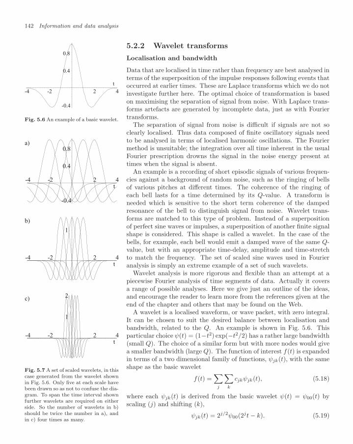
142 Information and data analysis
5.2.2 Wavelet transforms
Localisation and bandwidth
Data that are localised in time rather than frequency are best analysed interms of the superposition of the impulse responses following events thatoccurred at earlier times. These are Laplace transforms which we do not
-0.4
0.4
0.8
-4 -2 2 4
t
Fig. 5.6 An example of a basic wavelet.
investigate further here. The optimal choice of transformation is basedon maximising the separation of signal from noise. With Laplace trans-forms artefacts are generated by incomplete data, just as with Fouriertransforms.
The separation of signal from noise is difficult if signals are not soclearly localised. Thus data composed of finite oscillatory signals needto be analysed in terms of localised harmonic oscillations. The Fouriermethod is unsuitable; the integration over all time inherent in the usualFourier prescription drowns the signal in the noise energy present attimes when the signal is absent.
1
-4 -2 2 4t
-0.4
0.4
0.8
-4 -2 2 4t
2
-4 -2 2 4t
1
a)
b)
c)
Fig. 5.7 A set of scaled wavelets, in thiscase generated from the wavelet shownin Fig. 5.6. Only five at each scale havebeen drawn so as not to confuse the dia-gram. To span the time interval shownfurther wavelets are required on eitherside. So the number of wavelets in b)should be twice the number in a), andin c) four times as many.
An example is a recording of short episodic signals of various frequen-cies against a background of random noise, such as the ringing of bellsof various pitches at different times. The coherence of the ringing ofeach bell lasts for a time determined by its Q-value. A transform isneeded which is sensitive to the short term coherence of the dampedresonance of the bell to distinguish signal from noise. Wavelet trans-forms are matched to this type of problem. Instead of a superpositionof perfect sine waves or impulses, a superposition of another finite signalshape is considered. This shape is called a wavelet. In the case of thebells, for example, each bell would emit a damped wave of the same Q-value, but with an appropriate time-delay, amplitude and time-stretchto match the frequency. The set of scaled sine waves used in Fourieranalysis is simply an extreme example of a set of such wavelets.
Wavelet analysis is more rigorous and flexible than an attempt at apiecewise Fourier analysis of time segments of data. Actually it coversa range of possible analyses. Here we give just an outline of the ideas,and encourage the reader to learn more from the references given at theend of the chapter and others that may be found on the Web.
A wavelet is a localised waveform, or wave packet, with zero integral.It can be chosen to suit the desired balance between localisation andbandwidth, related to the Q. An example is shown in Fig. 5.6. Thisparticular choice ψ(t) = (1−t2) exp(−t2/2) has a rather large bandwidth(small Q). The choice of a similar form but with more nodes would givea smaller bandwidth (large Q). The function of interest f(t) is expandedin terms of a two dimensional family of functions, ψjk(t), with the sameshape as the basic wavelet
f(t) =∑
j
∑k
cjkψjk(t), (5.18)
where each ψjk(t) is derived from the basic wavelet ψ(t) = ψ00(t) byscaling (j) and shifting (k),
ψjk(t) = 2j/2ψ00(2jt − k). (5.19)

5.3 Analysis of data using models 143
linear time segments
frequency,increasingby a factor
two ineach row
Fig. 5.8 A diagram showing the rela-tion between the domains in frequencyand time of different members of awavelet family, such that frequency isproportional to the inverse scaling ofthe wavelet shape. Each rectangle de-scribes the domain in time and fre-quency of one wavelet in the expansion.
As an example, Fig. 5.7 shows some members of a wavelet ‘family’ forshifts k = −2,−1, 0, 1, 2 plotted out for scalings j = 0, 1, 2 generatedfrom the mother wavelet of Fig. 5.6. These scaled expansion functionshave the following properties:
each new scaling increases the frequency by a factor 2, andhalves the wavelet width in t;
the number of independent shifts in time increases by a factor2 with each scaling, as illustrated in Fig. 5.8;
fast algorithms which do not depend on the choice of waveletare available for implementing the decomposition;
they are normalised in such a way that their energies arerelated to c2
jk.
The reconstruction may be filtered of noise by inverting the decom-position omitting those time–frequency elements that show no evidenceof signal.
5.3 Analysis of data using models
Data may be analysed by building models based on previous knowledge.Parameters left free in the model may be determined from the data withsome error. Three methods are described: least squares, minimum χ2,and maximum likelihood. In the least squares method the fit is definedby minimising the summed squared differences between the model predic-tions and the measurements. In the χ2 method each element of the sumof squares is weighted with its known inverse error squared. This may begeneralised to include correlation or off-diagonal effects. Simulated datamay be generated according to the model by Monte Carlo, and then com-pared with real data. We discuss a simple historical example of its use,the analysis of an experiment to scan the Pyramids for hidden chambers.

144 Information and data analysis
The maximum likelihood method represents the most complete and flex-ible use of information. If the data are binned and the errors on thosebins are Gaussian, the likelihood method is equivalent to the χ2 method.The likelihood function enables the errors of potential experiments to beevaluated without the use of Monte Carlo. With the likelihood method,data from different sources can be combined in a rigorous single optimumanalysis. This use is important in medical imaging.
5.3.1 General features
Questions and models
At first sight, analysis by transformation and filtering removes noisefrom an image in a model-independent way, and should therefore beobjective. The filter, however, must be designed in the light of a knowndistinction between signal and noise. The alternative approach is toacknowledge the significance of what is already known and to build amodel of how we expect the data to look, and then to compare thatwith the observed data. Such an analysis attempts to answer two kindsof question. First there is the goodness of fit, ‘To what extent does themodel give a satisfactory match to the data?’ Then there is parameterdetermination, ‘If the model is correct, what are the best values of itsunknown parameters?’ Of course, if the goodness of fit is unacceptable,the values of the determined parameters are not meaningful.
To minimise dependence on preconceptions the model is given as manyfree parameters as reasonable.17 Finding the best values for these pa-17Relaxed fits with many free param-
eters give results with larger errors.Small errors are given by fits tightlyconstrained by preconceptions. Butsuch apparently accurate results areconditional on the assumptions made.
rameters is called fitting. With these values is the match to the data sat-isfactory? This is difficult to answer. The model cannot tell us whetherthere exists another quite different interpretation or model, of which weare unaware, but which matches the data better.18
18In an apparently different approachcalled neural networks, previous dataare used as previous knowledge to‘teach’ the model, and the soft-ware learns dynamically. Neverthelessthe overall relation between previousknowledge and data remains.
Noise enters the discussion in two ways. If the model is correct, itshould be solely responsible for the observed difference between dataand fitted model. Secondly it gives rise to the error on the estimatedparameters and their correlations.
The output of these calculations may be a series of simple fitted pa-rameters. Or it may consist of an array of such parameters which them-selves constitute the required image. The analysis principles are thesame.
Monte Carlo simulation
By combining the prescription of the model with the effect of randomnoise, artificial experiments may be simulated by Monte Carlo on a com-puter. The Monte Carlo ‘data’ generated in this way may be comparedwith the model, in the same way as real data, to find out how often suchcomparisons are less favourable than that found for the actual data.Such simulations may also be used to check the variation and value ofestimated parameters against their calculated errors. These simulationsmay be time consuming. Their statistical value improves only as the

5.3 Analysis of data using models 145
square root of the number of simulations. However, since they dependon the model, not the data, they may be used with care to optimise thedesign stage of equipment before any data are available. Blind relianceon Monte Carlo simulation is dangerous since any conclusion is negatedif the model is in error.
Noise and errors
An important type of noise derives from the Poisson fluctuations ofdiscrete events whose occurrence is uncorrelated. Other noise such asthermal noise is random but has a well-defined power spectrum whosebandwidth and amplitude need to be understood precisely.
In the model analysis of a set of data, the noise and fitted parametervalues become correlated. Thus the observation of extra counts withcertain values may be interpreted either as an upward chance noise fluc-tuation or as evidence for a stronger signal. A repeat data set would havedifferent noise and different estimated parameters. If the second dataset were available the uncertainty of interpretation would be resolved toan extent. Because of this correlation, when the noise information in thegiven data set is discarded, the information on the estimated parameterssuffers an increase in entropy. This negative information takes the formof the calculated statistical errors estimated during the fitting process,usually in the form of an error matrix relating to the uncertainties of allthe parameters.
The more free parameters that are included in the model, the looserwill be the constraint of the data on the model and the larger will be theestimated errors. Since a loose model may be preferred, this behaviourof calculated errors needs careful interpretation. Should the model bewrong in some respect, not only the parameter values but also theirerrors are compromised. Often the effect of fitting an inappropriatemodel is to generate smaller errors in the context of the model whereasa proper overall picture should acknowledge a larger uncertainty.
5.3.2 Least squares and minimum χ2 methods
Least squares
The least squares method is the simplest way in which data may befitted to a model. We suppose that we have a set of n data readings ofvalues y, yi for i = 1 to n, forming a set of measurements at values ofx = xi. In the absence of noise the model hypothesis is that
y = f(x, α, β), (5.20)
where α, β are unknown parameters to be determined.19 The residuals 19There may be a whole vector of suchquantities. We indicate just two for dis-cussion purposes.
are the n values, yi − f(xi, α, β), the differences between the measure-ment for x = xi and the value calculated by the model. In the least

146 Information and data analysis
squares method the sum of the squared residuals,
S =n∑
i=1
(yi − f(xi, α, β))2 , (5.21)
is formed and minimised with respect to variation of α and β. If this sumis stationary with respect to such variations, the derivatives of the sumwith respect to α and β are zero. This leads to the pair of simultaneousequations,
0 =n∑
i=1
(yi − f(xi, α, β))∂f(xi, α, β)
∂α(5.22)
0 =n∑
i=1
(yi − f(xi, α, β))∂f(xi, α, β)
∂β.
If f is linear in α and β, these equations may be solved for α andβ by linear algebra. If f is nearly linear, the solution may be founditeratively. Otherwise, by changing variable or even searching numeri-cally, the values α and β that give the smallest value of S are found.In this simple method there is no gauge of what is an acceptable sumof squares, and therefore no indication of whether the model fit is anadequate description or not.
Minimum χ2
The minimum χ2 method is an adaption of least squares in which themeasurement error σi of each measurement yi is known. Each elementof the sum of squares is now weighted with its inverse error squared,
χ2 =n∑
i=1
(yi − f(xi, α, β))2
σ2i
, (5.23)
and its contribution to equations 5.22 likewise. The error σi is thestandard deviation, such that, if the measurement of yi were repeated alarge number of times, the distribution of values would be given by theGaussian function
1√2πσi
exp(
(yi − yi)2
2σ2i
),
where yi is the mean. If the measurements are correlated, this distribu-tion may take a two dimensional form using the inverse of σ2, which isnow the error-squared matrix, including its off-diagonal terms. Thus
χ2 =∑i,j
(yi − f(xi, α, β))((σ2)−1
)ij
(yj − f(xj , α, β)). (5.24)
The process of minimisation of χ2 is then similar to the least squaresmethod except that the actual value of χ2 at the minimum is signifi-cant. Its interpretation depends on the number of degrees of freedomν, defined as the number of measurements (the number of values of i in

5.3 Analysis of data using models 147
the summation equation 5.23) less the number of parameters allowed tovary in the minimisation process. The errors on parameters are deter-mined by noting that when χ2 increases by one, the probability densityfalls from exp(−χ2/2) to exp(−χ2/2) × exp(−1/2), equivalent to onestandard deviation. So combinations of parameter values that lie withinthe surface ∆χ2 = 1 are within one standard deviation of the best fit.Acceptable fits, consistent with the errors used, have a distribution ofminimum χ2 with the mean value
⟨χ2
⟩= ν. The distribution of χ2
values becomes rather broad for values of ν less than about 8, but athigher ν acceptable fits have χ2 ∼ ν. The reader is referred to standardtexts on statistics for more details.
Sometimes data take the form of counts recorded in a number of bins.The index i is then taken as running over the total of n bins. The modelis used to integrate the probability flux within each bin pi, which maybe a function of the parameters α, β, etc., so that the mean numberof counts in bin i is expected to be pi. Then the actual number ofcounts mi observed in this bin for an ensemble of experiments should bedistributed according to the Poisson distribution,
f(mi) =pmi
i
mi!exp(−pi), (5.25)
with the fluctuations of the contents of different bins being uncorrelated.The standard deviation is expected to be
√pi. If pi is larger than about
8, the difference between a Poisson and Gaussian distribution becomessmall, and the latter may be used. The standard error for the bin con-tent is
√pi in either case and the contribution to χ2 is (mi − pi)2/pi.
However, the χ2 method does not take into account the skewness ofthe distribution that applies if Poisson statistics, rather than Gaussianstatistics, are required. To this extent χ2 is not quite right if pi is lessthan about 8.
Example: a survey of the Pyramids by cosmic rays
In the 1960s Luis Alvarez speculated how it might be possible to detectthe existence of a hidden chamber within the Pyramid of Chephren atGiza in Egypt. As Fig. 5.9 shows, the Pyramid of Cheops, Chephren’sfather, is well endowed with chambers and these were ransacked in earlytimes. However, the only known chamber in Chephren’s Pyramid is thesmall Belzoni Chamber at ground level near the centre. Alvarez andhis Egyptian collaborators built a wide-angle cosmic-ray telescope inthe Belzoni Chamber and analysed the cosmic-ray flux as a function ofangle in n = 750 bins of angle 3 × 3. The telescope was composed
a)
b)
Fig. 5.9 Sections through the Pyra-mids. a) The Pyramid of Cheops show-ing the Kings Chamber, the QueensChamber and the Underground cham-ber. b) The Pyramid of Chephrenshowing only the small Belzoni Cham-ber.
of layers of spark chambers and recorded the passage of nearly 1 milliontracks.
The way in which the data were analysed is a simple example of earlymodern data analysis and Fig. 5.10 indicates the stages. The hypothesisbeing tested is ‘Are the data consistent with the absence of chambers?’There are two sources of information that lead eventually down to the

148 Information and data analysis
Fig. 5.10 The analysis flow diagram ofthe search for hidden chambers in thePyramid
Datasimulation
Cosmic ray
flux ( )f ,E
Shape ofpyramid
Position ofdetector
Energy loss &scattering perkg of stone
Detectorangular
resolution
Detectorefficiency
Calculate
for bins n2
Simulatedcosmic rays
Rawdata
Internaldata checks
Cut datasample
Minimisefor unknowns
2 Plot residuals
in angle witherrors
Hiddenchambersrequired?
box that asks the question. The first source is the data of recorded tracksfrom the telescope. This is selected or ‘cut’ to ensure good data on thebasis of internal consistency, records of gas quality and so on. Therewere 650000 such tracks in the final sample. The result is a series ofcounts mi, one for each angular bin i. The second source of informationis the previous knowledge. This comprises the expected distributionof cosmic rays in energy and angle, their interaction in stone and thegeometry of the Pyramid assuming no hidden chambers. The dottedlines in Fig. 5.10 indicate the separation between the data sample andthe simulation. On the right of the diagram is shown the informationneeded to predict the observed distribution of cosmic-ray angles from:a knowledge of incident cosmic ray flux, the shape of the Pyramid, thedetector position, the dE/dx in stone. Thence were constructed theMonte Carlo simulated observations in the detector, pi(α, β, . . .), fordifferent values of the unknown free parameters (α, β, . . .).2020These parameters included the pre-
cise position of the chamber within thePyramid as discussed below.
These predictions awee combined with the observed data mi in theχ2:
χ2 =∑bins
[mi − pi(α, β, . . .)]2
pi. (5.26)
where the pi in the denominator is the square of the error on the pre-dicted count in each bin. The parameters α, β, . . . are determined byminimising χ2. If the simulation is acceptable, the mean value of χ2
should be approximately the number of degrees of freedom.When carried out the χ2 minimisation process confirmed the Belzoni
Chamber position to be within 2 m of the actual surveyed position.21
21This means that when the position ofthe chamber was left free, as α and β,the minimum χ2 was found when thechamber position was hypothesised tobe in its actual position. This is an ex-ample of the way in which confidencecan be built in the result of an experi-ment.
The extra stone cap at the apex of the Pyramid also showed up veryclearly in the residuals, as shown in the plots of Fig. 5.11.22 The final
22Originally the whole Pyramid wascovered with these blocks but in theMiddle Ages they were removed exceptat the top to supply stone to build thecity of Cairo.
value of χ2 for the 750 angular bins with useful sensitivity was 1100. Inthe final step of the analysis, the residuals were plotted as a function of

5.3 Analysis of data using models 149
angle to see whether the discrepancy in χ2 could not be related to anexcess flux in a small angular range, indicating a deficit in the Pyramidrock and a hidden chamber. It was concluded that no chamber in theChephren Pyramid like those in the Cheops Pyramid exists within 35
of the vertical.
a) N-S
b) E-W
2
2
0
0
-2
-2
m
m
Fig. 5.11 The stone thickness (m)as measured with cosmic rays less thestone thickness calculated for a perfectgeometrical pyramid. a) North–southscan through the zenith. b) East–westscan through the zenith. The smoothcurves are the simulated corrections forthe limestone cap.
This experiment was carried out 40 years ago. Today a better tele-scope could be constructed and the statistical analysis could be pursuedfurther. The minimum value of χ2 was not very good although thediscrepancies were not clustered in a particular direction to indicate achamber. Attempts were made to detect the edges of a hidden cham-ber by differentiating the flux as a function of angle but these weredominated by noise. If repeated today, emphasis would be placed onincreasing the number of counts recorded, improving the angular resolu-tion and using a maximum likelihood analysis instead of χ2, to avoid theneed to define angular bins. Otherwise the principles would be largelythe same. Perhaps a hidden chamber lies below the Belzoni Chamber.That would be harder to find!
5.3.3 Maximum likelihood method
The likelihood function
The χ2 method suffers from two difficulties. Firstly there is the needto bin the data. This is rather arbitrary in execution and discards in-formation within a bin. Secondly, as we already saw, it does not treatcorrectly bins containing few counts. Both of these shortcomings arehandled better in the maximum likelihood method which is used exten-sively in image analysis.
Consider N measurements of a parameter x. Suppose that we knowthat the probability distribution23 of measurements of x would be fα1(x) 23This is the distribution of observa-
tions in the limit N → ∞.if the unknown α were actually to have the value α1. Since the proba-bility of a measurement having some value of x is 100%, the distributionfα1(x) is normalised to unity. Then the probability of one measurementyielding a value of x between x1 and x1+dx1 is fα1(x1)dx1. And, sinceseparate measurements are independent and uncorrelated, the probabil-ity of N measurements with values of x between xi and xi+dxi (with irunning from 1 to N) is
Pα1 =N∏
i=1
fα1(xi)dxi. (5.27)
If on the other hand the true value of α were α2, the probability Pα2
would be different. The ratio of likelihoods is
Pα1
Pα2=
N∏i=1
fα1(xi)fα2(xi)
. (5.28)
This is as near as we can get to the relative probability of α having the

150 Information and data analysis
value α1 compared with the value α2. So
L(α) =N∏
i=1
fα(xi) (5.29)
is called the likelihood of α. But it is important to understand that itis not actually what we wanted. It is the likelihood of the data giventhe value of α, rather than the likelihood of the value of α given thedata. So it is sometimes called the inverse probability. The distinctionis emphasised by the fact that L(α) is not normalised.
This is all that is needed. The most likely value of α, labelled α∗,is the one with the highest likelihood L. This is found by setting thederivatives of L with respect to all parameters α simultaneously to zero.The solution to these simultaneous conditions gives us the best valueof the parameters. Previous knowledge enters either through the defini-tion of the problem as described by the likelihood function itself or byan additional factor, or factors, in the likelihood function, as discussedbelow. The latter method is appropriate if the information is qualifiedby errors.
The likelihood method may be used under different conditions. Givena set of available experimental data, it can be used to test a model andfind the best-fit values of parameters with their errors. In the absence ofreal data, it can be used to predict the errors of possible experiments byconsidering the probability function for an ensemble of such experiments.
Determination of parameters by maximum likelihood
General principles and previous knowledge are used to construct themodel f(α, x) where x is a quantity we can measure in an experimentand α is a parameter to be determined. Recall that f(α0, x)dx is theprobability of measuring x with a value between x and x+dx given thatα = α0. The integral or sum of f over x is unity, corresponding tothe fact that each measurement yields exactly one value. Real measure-ments or scans have many measured variables like x, continuous anddiscrete, and a large number of quantities like α to be determined. Inthe following, reference to x and α should be understood in each case todescribe such long vectors of variables.
In the experiment we make N measurements of x. L(α) constructedaccording to equation 5.29 involves the product of a significantly largenumber of factors, one for each of N measurements. Each is positiveand typically small compared with unity. Such a product can lead to anumerical underflow condition, even on a modern computer. It is easierto work with w(α), the natural logarithm of the likelihood function,instead of the likelihood function itself. This converts the awkwardproduct into a sum,
w(α) = log(L(α)) =N∑
i=1
log(f(α, xi)). (5.30)

5.3 Analysis of data using models 151
The procedures of maximising the likelihood and its logarithm are equiv-alent. Use of log likelihood also brings further theoretical insights as weshall see. Procedures for maximising functions in many variables arewell established. If the log likelihood is quadratic in the parametersα, its derivatives are linear and the solution may be found by matrixinversion.24 24This is the Gaussian case, discussed
next.In the general case we may consider a Taylor expansion of the loglikelihood surface in (α − α∗) about its peak value at α∗. This is com-posed of quadratic and higher terms. With a different choice of variableit may be possible to minimise these higher terms, thereby linearisingthe determination of the α∗. In the absence of higher terms the con-fidence levels on the estimation of α become symmetric about α∗ andwell describable in terms of Gaussian errors.
As a simple example consider observations of an exponential decayprocess. The data might consist of the observation of a set of decaytimes ti with i from 1 to N , confined within an accessible observationwindow between Ta and Tb. The normalised probability distribution forthe observed decay to occur between time t and time t+dt is
f(t)dt =exp(−t/τ)
τ [exp(−Ta/τ) − exp(−Tb/τ)]dt, (5.31)
if the state has a mean lifetime τ . The distribution f(t) is shown inFig. 5.12 for various values of τ . The log likelihood for the N observa-
0
0.1
0.2
0.3
0.4
0.5
2 4 6 8 10
f(t)
t
Fig. 5.12 The normalised decay prob-ability functions, equation 5.31, for val-ues of τ equal to 1, 2, 3, 5 and 10,each normalised between Ta = 1 andTb = 10.
tions is then
w(τ) = −∑N
i=1 tiτ
−N log τ −N log[exp(−Ta/τ)− exp(−Tb/τ)]. (5.32)
The most likely value of τ may be evaluated by setting the derivative ofw with respect to τ equal to zero.
Likelihood in the Gaussian approximation
As N becomes larger, the likelihood becomes asymptotically Gaussian,
L(α) =1√
2πσα
exp(− (α − α)2
2σ2α
), (5.33)
where σα is the standard error on the reconstructed value of α. This isa general statistical result known as the central limit theorem. In thisapproximation the logarithm of the likelihood is very simply
w(α) = − (α − α)2
2σ2α
− log(√
2πσα). (5.34)
Then the procedure of minimising χ2 is seen to be equivalent to that ofmaximising likelihood provided σα is independent of α.
Differentiating equation 5.34 twice with respect to α gives a relationbetween w(α) and σα, the error on α,
∂2w
∂α2= − 1
σ2α
. (5.35)

152 Information and data analysis
This result is only correct in the absence of correlations between α andother parameters. The generalisation to a vector of parameters, αk fork = 1 . . .m, is as follows. The elements of the inverse squared-errormatrix H are given by
Hij = − ∂2w
∂αi∂αj. (5.36)
The complete H-matrix must be inverted to get the matrix of squarederrors. The simple errors of interest are the roots of the diagonal termsof H−1. However, the presence of non-trivial correlation terms impliesthat
σ2α =
[−∂2w
∂α2
]−1
.
If the likelihood is not Gaussian, the surface of w is usually plotted andthe locus on which w has decreased by 1
2 relative to its value at α∗
interpreted as a standard deviation, and likewise with other confidence-level contours of interest. Such a log likelihood surface is sketched inFig. 5.13 for a case of two variables. Contours for n = 1, 2 and 3standard deviation are shown. These would be the loci where the loglikelihood is lower than the maximum by n2/2. The standard errorfor each parameter separately is shown by the heavy arrows. If thelikelihood surface were Gaussian, the contours would be ellipses andthe errors symmetrical. Elliptical contours with rotated axes describecorrelations that may be represented by error matrices with off-diagonalterms.
α
α
1
2
32
1
Fig. 5.13 A sketch of a log likeli-hood surface for two parameters, α1
and α2, showing the most probable val-ues marked by a star within contoursdescribing confidence levels.
Combining information from different experiments
Probability distributions that contain uncorrelated information are com-bined by simply multiplying them together. So if experiment A tells usthat the probability of a certain situation is pA and if a second quite in-dependent experiment B gives the probability pB, then the probability inthe light of both experiments is pA × pB. Thus the log likelihood basedon two experiments is the sum of the log likelihoods of each of themseparately. The inverse squared-error matrices H from each experimentjust add for the same reason.
Any other independent information on the relative probability of dif-ferent values of α can be added to the log likelihood function in the sameway.25 Thus25You may notice that log likelihood,
information and entropy are all addi-tive. Boltzmann factors, likelihoods,Gaussian distributions are multiplica-tive being described by negative ex-ponential quadratic forms. These areclosely related. However, this is not anappropriate text in which to mount anexpedition into the exciting world of in-formation theory and its recent quan-tum developments!
W (α) = w1(α) + w2(α) + w3(α) + . . . , (5.37)
where data from different experiments, different modalities, previousknowledge, etc., each make their own contribution to the combined loglikelihood function.
The best value of α is given by the peak of the combined W , andits second derivative gives the error. None of this should surprise. Inequation 5.30 the contribution of individual uncorrelated measurements

5.3 Analysis of data using models 153
within one experiment combined additively to the log likelihood func-tion. It is natural that information from different experiments or scanswhich are uncorrelated should combine in the same way.
Sometimes the number of readings N is predetermined. However, inother experiments the value of N is itself a measurement. For example,it may represent the number of occurrences in a predetermined timeinterval. In such cases the value of N contains information.26 The log 26The probability function f(x) for
each reading must be normalised tounity, as before.
likelihood associated purely with the number of readings is simply addedonto the log likelihood derived from the values of those readings.27 It may
27This is usually called the extendedmaximum likelihood method.
be added in this way because there is no correlation between fluctuationsin the value of readings and fluctuations in the number of readings. Theterm to be added comes from the Poisson distribution, equation 5.25.If the expected number is N (α), the log of the probability of getting Nreadings is
wnumber(α, N) = N log(N (α)) − log(N !) −N (α). (5.38)
In the limit of N and N large, this is given asymptotically by the Gaus-sian result,
wnumber(α, N) = − (N −N (α))2
2N , (5.39)
where constant terms independent of α have been dropped.
Simulation of experiments by maximum likelihood
Building equipment, optimising conditions and taking multiple data setsare expensive and time consuming. We have already seen that it is pos-sible to simulate experiments by the Monte Carlo technique. However,that brute force method generates data sets of increasingly unman-
x-1
-1
0
1
0
1
1
f
0
α
Fig. 5.14 The probability surface,equation 5.40.
0.1
0.2
0.3
0.4
0.5
0.6
0.7 f(x)
0-0.4-0.8-1 0.4 0.8 1x
Fig. 5.15 The normalised probabil-ity distribution for measurements of xfor the experiment in which the actualvalue of α is 0.3. This is the corre-sponding section though the surface ofFig. 5.14.
ageable size and comes with its own statistical errors. Such studiescan be time consuming and inconvenient. A more elegant simulationof experiments uses the maximum likelihood method. In this methodexperiments of any statistical precision can be simulated and studied atthe same speed.
We consider a very simple example. Suppose that we have a modelfor our experiment to determine the unknown α from measurements ofx between −1 and +1. The model is
f(α, x) =12
(1 + αx) (5.40)
and this two dimensional surface is shown in Fig. 5.14. The normali-sation requires that the integral of the curve of any section at constantα is unity. Let us suppose that the actual value of α is 0.3. Then theactual distribution of x-values would be given, in the limit of large N atleast, by the slice through the surface at α = 0.3, shown in Fig. 5.15.
We now ask what happens when the experiment is performed withoutknowing that α = 0.3. The likelihood function is used with α undeter-mined. For each measurement we know that the chance of the valueof x being between x and x+dx is f(0.3, x)dx. To that measurement

154 Information and data analysis
0-0.4-0.8-1 0.4 0.8 1
-1.0
-0.4
-0.8
-0.2
-0.6
α
0-0.4-0.8-1 0.4 0.8 1α
0.4
0.2
0.6
0.8
1.0
L
a) b)
w
N
N
Fig. 5.16 a) The mean log likelihood function wN , and b) the average likelihood curves LN , as a function of the hypothesisedvalue of α for experiments where the true value of α is 0.3. The curves describe experiments in which the number of events Nis 1,10,100,1000. [To ease comparison the likelihood functions have been shifted to unity at α=0.3 and the log likelihoods tozero.]
the program attaches a weight log(f(α, x)) in accordance with the pre-scription for constructing the log likelihood function. So the average loglikelihood function that would be found from a single measurement is
w1(α) =∫ 1
−1
log(f(α, x)) × f(0.3, x)dx. (5.41)
As the measurements are uncorrelated the average log likelihood func-tion found for N measurements will be just N times greater (and thelikelihood function itself raised to the Nth power),
wN (α) = N
∫ 1
−1
log(f(α, x)) × f(0.3, x)dx. (5.42)
This averaging will be poor when N is small, and this type of analy-sis will be a poor predictor of an actual experiment, but then such anexperiment will convey rather little information anyway. But for largerN , the average will become closer and closer to that found. The shapeof the average log likelihood function is shown in Fig. 5.16a for values ofN of 1, 10, 100 and 1000. For increased N the log likelihood functionsbecome more closely parabolic. This is equivalent to the central limittheorem which says that as N increases the probability distributionsbecome progressively Gaussian and follow the familiar bell shape. Theaverage error on α that would be found if such an experiment were done,may be read off for different N using the point at which the mean loglikelihood has fallen from its peak by 0.5, as in the analysis of an actualexperiment. Sometimes it is easier to calculate the second derivative ofw, equation 5.35. In Fig. 5.17 we have plotted out the mean error σα
as a function of the number of measurements N for the case when the

5.3 Analysis of data using models 155
0
0.02
0.04
0.06
0.08
0.10
0.12
0.14
0.16
0.18
0.20
200 400 600 800 1000N
σα
Fig. 5.17 The average error on α thatwould be found in the experiments dis-cussed in the text, assuming that thetrue value of α is 0.3, as a function ofthe number of measurements, N .
true value of α is 0.3. The shapes of the average likelihood functionsthemselves are shown in Fig. 5.16b.
This method enables us to calculate the average value of any otherquantity of interest in the same way. In particular, the average value ofthe second derivatives of w can be evaluated and then used to derive theelements of the inverse squared-error matrix H following equation 5.36.Thus
∂2w
∂αi∂αj= N
∫ 1
−1
∂2 log(f(α, x))∂αi∂αj
× f(α0, x)dx, (5.43)
where the known solution has been described by the vector of relationsα = α0. The linear dependence of all errors on 1/
√N is evident. The
effect of non-linearities and correlations can all be evaluated cheaply andrapidly in the same way.
It is important to note that these results have been calculated with-out doing the experiment at all, and without doing any Monte Carlosimulation either. These techniques enable errors to be simulated, ex-periments to be designed and optimised, and resolution performance tobe predicted before the apparatus is built. The only question that maxi-mum likelihood cannot address is the determination of the actual values.To do that, money must be spent and measurements actually made!
Read more in books
The Mathematical Theory of Communication, CEShannon and W Weaver, University of Illinois Press(1948) is the classical reference for information theory
Science and Information Theory, Leon Brillouin, Aca-demic Press (1962) is another classical reference
Mathematical methods in the physical sciences, Mary LBoas, Wiley, 2nd edn (1983) is a student text coveringFourier analysis
All you ever wanted to know about Mathematics, Vols 1& 2, L Lyons, Cambridge (1998) is a more basic studentreference

156 Information and data analysis
Notes on statistics for physicists, J Orear (1958, rev.1982) is a highly recommended reference on statisticsthat is classic, readable, concise, but unpublished. Itmay now be found on the Web, see below
Statistics for nuclear and particle physicists, L Lyons,Cambridge (1986) is a more gentle introduction tostatistics
Oxford users’ guide to mathematics, ed. E Zeidler, Ox-ford (2004) includes a section on wavelets
Discovering Alvarez, ed. WP Trower, Chicago (1987)includes a chapter that describes Alvarez’s experimentin the Pyramids
Fundamentals of Medical Imaging, P Suetens, Cam-bridge (2002) discusses the reconstruction of medicalimages and includes some excellent illustrations and aCD
Look on the Web
Look at the book website atwww.physics.ox.ac.uk/users/allison/booksite.htm
Read more about information theory by searching onwords such as
information theory, shannon, quantum
Look up a very helpful website that explains more aboutwavelets
wavelets clemens
Be sure to read Orear’s article on statistics which maybe found on a number of websites by searching for
orear statistics physicists
Questions
5.1 If the mean probability for each of N pixels beingblack rather than white is f , the mean informationcontent is given by
Neffective = Nf ln f + (1 − f) ln(1 − f)
ln(1/2).
Consider the implications of this expression for thecases f = 0.0, 0.5, 1.0. Hence prove the followingstatement: ‘A digital image with a certain num-ber of pixels or voxels which may be black or whitecontains maximum information when the illumina-tion is adjusted such that on average the expectedfraction of black pixels is 50%.’
5.2 Prove the property of the Dirac δ-function,∫ +∞
−∞exp[i(ω − ω′)t]dt = 2πδ(ω − ω′).
5.3 Prove that the transform of the convolution of twofunctions is equal to the product of their trans-forms, equation 5.14.
5.4 Consider a periodic function with f(x) = f(x+nL)for all integer values of n. Find its Fourier trans-form using the convolution theorem.
5.5 A measured in vivo NMR spectrum M(ω) is a su-perposition of the spectra of 5 metabolites, A(ω),B(ω), C(ω), D(ω), E(ω), with a background ofthe form X + ω × Y , where X and Y are free pa-rameters. The 5 spectra are known from in vitromeasurement of each separate metabolite of knownconcentration. Show how you would determine theconcentrations of the 5 metabolites by the leastsquares method while making allowance for thebackground. You should assume that each spec-trum consists of amplitudes measured at the sameset of 100 discrete frequencies.

Analysis and damage byirradiation 6
6.1 Radiation detectors 157
6.2 Analysis methods for ele-ments and isotopes 168
6.3 Radiation exposure of thepopulation at large 179
6.4 Radiation damage to biologi-cal tissue 187
6.5 Nuclear energy and applica-tions 192
Read more in books 204
Look on the Web 204
Questions 205
in which the detection, health effects, safety, uses and abuses of ionisingradiation are discussed.
6.1 Radiation detectors
Energy deposited by radiation in matter undergoes prompt changes ofform (secondary ionisation electrons, bremsstrahlung and electromagneticshowers) and further changes with some delay (fluorescence radiation andAuger electron emission). In addition to releasing photons and electrons,irradiation also leaves a trail of atomic ions and molecular fragments inexcited states. These are highly reactive and are responsible for longerterm radiation-induced effects. Charged particle detectors may be basedon the use of photographic emulsion, the detection of scintillation light,or the ionisation signal generated in gas-filled or solid state devices. Thedetection of electromagnetic radiation depends on the photon energy. Atthe lowest frequency, coherent waves, not photons, are detected. In themid range individual photons are detected but the signals are amplified ex-ternally using photomultipliers, gas or solid state devices. At the highestenergies, the self-powered avalanche of an electromagnetic shower gener-ated by the incident photon may be detected by its scintillation light.
6.1.1 Photons and ionisation generated byirradiation
Prompt processes
Much of the energy initially deposited by irradiation is in the form ofeither excited atoms and molecules, or free electrons and ions. Thelatter are called primary ionisation. The electrons may have substantialkinetic energy. Historically the most energetic are called δ-rays becausethey leave their own tracks in detectors.
n
1
log E
X rayUVoptical
Fig. 6.1 Sketch of the frequency de-pendence of the refractive index n dueto resonances in the ultraviolet region(shaded). In this region radiation is ab-sorbed and n is complex. With the typ-ical resonance shape n may only be realand greater than 1 below resonance inthe optical region.
Other prompt or primary processes include the bremsstrahlung radi-ation discussed in section 3.6.2 and Cherenkov radiation. In both casesthe radiation is coherent and highly directional. Cherenkov radiationis emitted by any charge moving faster than the speed of light in themedium, c/n, where n is the refractive index. Since the speed of thecharge is necessarily less than c, such emission is not possible unless nis greater than 1. Figure 6.1 shows the dependence of n on frequency

158 Analysis and damage by irradiation
for a typical material. Above the ultraviolet absorption region, n is lessthan 1. In the ultraviolet region itself, the medium is absorptive andno free Cherenkov radiation propagates. So only in the optical regionis Cherenkov emission possible. The flux in this modest bandwidth issmall, the spectrum is rather soft and in total accounts for no more thana per cent or so of the total energy loss.
a) b)
Fig. 6.2 Sketches illustrating how, fora given energy deposition, a) the evendistribution due to a large number ofrelativistic electron tracks (z=1, β=1)contrasts with b) the uneven distribu-tion due to a small number of ion trackswith z2/β2 of 10, for example.
Delayed processes
A
A
G
G
B
a)
b)
Fig. 6.3 Energy level diagrams show-ing modes of de-excitation of an atomor molecule in an excited state, A.a) This may occur on its own by theemission of a fluorescent photon leav-ing the atom or molecule in its groundstate, G.b) It may also occur by excitation toan ionised state B with emission of afree electron with the remaining kineticenergy. In each case vertical lines de-note internal energy changes, the exter-nal wavy line is an emitted photon andthe dashed line an emitted electron.
Many important applications in medical and environmental physics de-pend on what happens to the deposited energy subsequently and on thetimescale on which it evolves. The free electrons do not usually recom-bine with ions. This is unlikely because they are spatially separated,and recombination requires the involvement of a catalyst if energy andmomentum are to be conserved. Generally, primary and secondary ionscome to rest within a few tens of microns of the flight path of the orig-inal charge. Consequently, except in a gas, the debris or the radiationdamage is not evenly spread though the medium but is confined to nar-row cylinders along the flight paths of the individual incident charges.This is most pronounced when the density of the elemental energy lossprocess is high. The linear density of energy loss is given by the Bethe–Bloch formula, equation 3.44, and dE/dx ∼ z2/β2. So when the incidentparticle is highly charged (high z) or non-relativistic (low β), the energydeposition is highly concentrated. Figure 6.2 gives an impression of how,for the same total deposited energy in a material, many singly chargedrelativistic particles give a much more uniform distribution of irradiationthan a few multiply charged non-relativistic ions. The energy depositedalong the track is referred to as the linear energy transfer density (LET).It is the dE/dx discussed in chapter 3.
Excited atoms may begin the process of thermalisation by internaltransition, either by emitting a photon or by emitting an atomic elec-tron as illustrated in Fig. 6.3. The first process is called fluorescenceor scintillation and the second Auger emission.1 Scintillation emission
1We use the terms scintillation and flu-orescence interchangeably according tocontext.
is isotropic, being incoherent and having no memory of the directionof the incident radiation. However, the emission spectrum has sharplines characteristic of the atom or molecule. These two de-excitationprocesses usually compete with one another. A third possibility is thatthe atom or molecule, instead of de-exciting on its own, has a collisionwith another atom or molecule. (In condensed matter it may transferenergy to its neighbours by forming a mixed quantum state with themby level broadening, although this is actually equivalent.) No radia-tion is emitted in such collisions and the energy progresses to thermalequilibrium.
In some regions of the spectrum scintillation photons are not actuallyobserved, simply because they are reabsorbed by the medium withina short distance. Otherwise the radiation can travel away from thepoint where the initial energy deposition occurred and be detected. Inparticular scintillation light emitted in a transition to a state that is

6.1 Radiation detectors 159
not the ground state (or within an energy of kBT of it) will not sufferself-absorption.
Electromagnetic showers
a)
c)
b)
d)
e
e ee
e e
γ
γ
γ
γ
Fig. 6.4 The four processes contribut-ing to the build-up of a shower:a) emission of radiation by an electron,b) pair production by a photon,c) Compton scattering of a photon,d) multiple scattering of an electron.All processes except c) occur on a scaledetermined by the radiation length, asdiscussed in chapter 3.
The behaviour of high energy electrons and photons is a special case.Such photons create electron–positron pairs and also recoil Comptonelectrons. The electrons (and positrons) then create bremsstrahlung.These elemental processes are illustrated in Fig. 6.4. Starting eitherfrom an electron or from a photon, each of energy several times theelectron rest-mass energy mec
2, a cascade or shower builds up. As theshower develops the energy of the individual secondary photons eventu-ally falls below the threshold for pair production. Similarly the energyof each electron falls to the point below which non-radiative energy lossdominates over bremsstrahlung. Further statistical multiplication of theshower is then choked off.
Both pair production and bremsstrahlung depend on the radiationlength of the medium. In dense high Z materials with short radiationlengths electromagnetic showers are spatially compact. This is idealfor high energy electron and photon detection with containment of theshower and measurement of both the energy and the line of flight of theoriginal electron or photon.
Chemical radicals
In addition to these free electrons, ionised and excited atoms, irradiationleaves excited molecules and chemical fragments. These highly reactiveproducts are not found in normal materials at room temperature. Theymay migrate in the gaseous or liquid state and initiate reactions thatdo not normally occur. In a solid they may remain trapped for a longtime, depending on the temperature. Typically such radicals have un-paired electrons and therefore exhibit electron spin resonance with afrequency characteristic of the radical concerned. This offers a methodof diagnosing their presence.
One example of a chemical product of radiation is the creation ofunstable polymer film. This shrinks rapidly when exposed to heat andis used as a wrapping material in the electrical and food industries.Another example is the generation of a metastable image of a radiationexposure in a photographic emulsion, or analogue photography as wecommonly know it.
6.1.2 Task of radiation detection
The basic methods have changed little over the decades. What haschanged is the technology with which any method is implemented. De-tectors differ in the way in which the incident energy is amplified andrecorded. The amplification is important because the basic signals aretiny. A single electronic charge, even after acceleration through a mil-lion volts, only has an energy of 1.6 × 10⁻¹³ J. Nevertheless individual
160 Analysis and damage by irradiation
charged particles can be detected, and their energy, position and angledetermined.
The range of energy involved in photon detection is the most extreme.From Fig. 1.3 we see that the energy of a photon of visible light is about1 eV or 1.6× 10⁻¹⁹ J. The energy of harder photons is easier to detect.The detection of softer photons with energies falling by nine orders ofmagnitude below visible involves special consideration.
Detector resolution and efficiency
Some radiation detectors are sensitive to the number of electrons re-leased in the material. Others detect released photons and some detectphonons. In every case the statistics of these information carriers areimportant. The working assumption is that the average number of car-riers released is proportional to the deposited energy for a detector thatdoes not saturate. The number of carriers n will fluctuate as prescribedby Poisson statistics with standard deviation σn =
√n where n is the
mean. These fluctuations will be responsible for a fractional variation insignal size of order 1/
√n. In a linear detector this determines the energy
resolution. The larger the value of n, the better the energy resolution.Even for a detector that saturates, n determines the detector efficiency
in the absence of the effects of other sources of noise. The probabilityof getting zero carriers is given by P (0, n) = exp(−n). This is theirreducible inefficiency. So an efficient detector should have a suitablylarge value of n. If the energy deposited in the detector is E, then
E = W × n. (6.1)
The value of W , the average energy deposited per carrier, is an importantnumber for a detector technology. For a given value of E, a lower valueof W brings smaller signal fluctuations, higher statistical efficiency andbetter energy resolution.
In addition to the signal and its fluctuations there is random thermalnoise. The signal-to-noise ratio (SNR) is the amplitude ratio of thetwo. A discriminator level determines when a signal is considered tobe present. If it is set high, there will be a low ‘false positive’ rate butalso a decreased detection efficiency of real signals. If it is set low, realsignals will be detected efficiently but there will be a significant ratedue to noise. The SNR may be improved by increased amplificationif the noise is not also amplified. Understanding the sources of noise istherefore important if signals are to be detected efficiently and unaffectedby noise.
Acceptance and exposure
The largest factor in the efficient use of radiation is the acceptance ofthe detector array. Radiation that does not fall within the sensitivearea of the array is lost. In some methods the radiation flux is confinedto a narrow slice. In others it is isotropic. In the latter case an ideal

6.1 Radiation detectors 161
detector array would envelope the experiment, subtending a solid angleof 4π steradians. Large reductions in the radiation dose experiencedby patients are achieved by increasing the detector size and the solidangle to match the optics of the administered flux. Cheaper technologyis allowing significant improvements in efficiency to be made. However,methods that rely on collimators and pinhole optics within the detectorare by their nature inefficient.
As in solid angle, so also in time, the period of detection should bematched to the period of radiation exposure. This is a significant sourceof inefficiency in some current medical imaging procedures.
Precision and resolution in time and space
The error on the time (or position) of a recorded signal is limited by thesignal pulse shape and its statistical fluctuations. The pulse shape intime is the impulse response of the detector and its electronics2 folded 2Corresponding to the signal generated
by a single electron or photon at thedetector input.
with the distribution of electron arrival times to simulate the observedpulse shape. The actual value of the precision depends on the way inwhich the measured position is determined by the pulse. For example,it might be the peak, the mean or the leading edge of the pulse.
In practice the precision is not as important as the resolution givenby the pulse shape itself. The resolution is the ‘occupancy’ of the sig-nal. This determines how close a further signal can occur and still beresolved as being separate. Some detectors are disabled for a time fol-lowing a signal.3 In other detectors subsequent signals simply add on 3This is known as the dead time. For
example the Geiger–Muller tube hassuch a dead time of tens of millisecondsduring which the tube is insensitive.
top of one another generating ‘pile up’. A linear device would record asignal amplitude which was the sum of the unresolved signals. In mostapplications the resolution is the useful measure at the analogue levelin both time and space. The element of a digital sampling of the ana-logue image is typically matched in size to the resolution. Detectors mayrecord resolved data in one, two or three dimensions, and in time. Asingle digital element of a two dimensional picture is termed a pixel. Adigital element in a three dimensional image is called a voxel.
6.1.3 Charged particle detectors
It matters in what form detectors provide image data and how they arestored. Photographic data are cheap, of high quality and convenient ina low technology environment. Electronic methods are often preferredbecause they can be linked straight to a computer. Circumstances andresources determine which detector is used.
Photographic emulsion
Photographic emulsion was the first radiation detector of charged par-ticles. The photographic plates that Henri Becquerel left in a drawerrecorded the radiation emitted by the specimens of uranium sulphateplaced on top of them. A photographic emulsion contains fine grains ofsilver halide. These are metastable. The activation energy required to
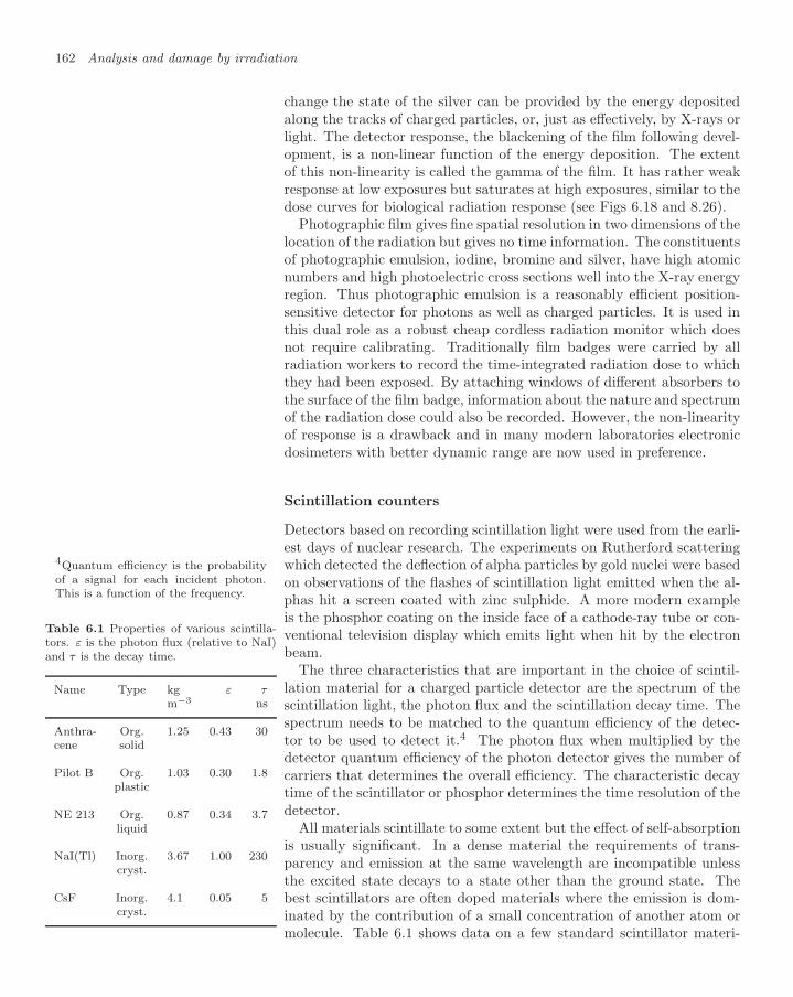
162 Analysis and damage by irradiation
change the state of the silver can be provided by the energy depositedalong the tracks of charged particles, or, just as effectively, by X-rays orlight. The detector response, the blackening of the film following devel-opment, is a non-linear function of the energy deposition. The extentof this non-linearity is called the gamma of the film. It has rather weakresponse at low exposures but saturates at high exposures, similar to thedose curves for biological radiation response (see Figs 6.18 and 8.26).
Photographic film gives fine spatial resolution in two dimensions of thelocation of the radiation but gives no time information. The constituentsof photographic emulsion, iodine, bromine and silver, have high atomicnumbers and high photoelectric cross sections well into the X-ray energyregion. Thus photographic emulsion is a reasonably efficient position-sensitive detector for photons as well as charged particles. It is used inthis dual role as a robust cheap cordless radiation monitor which doesnot require calibrating. Traditionally film badges were carried by allradiation workers to record the time-integrated radiation dose to whichthey had been exposed. By attaching windows of different absorbers tothe surface of the film badge, information about the nature and spectrumof the radiation dose could also be recorded. However, the non-linearityof response is a drawback and in many modern laboratories electronicdosimeters with better dynamic range are now used in preference.
Scintillation counters
Detectors based on recording scintillation light were used from the earli-est days of nuclear research. The experiments on Rutherford scatteringwhich detected the deflection of alpha particles by gold nuclei were basedon observations of the flashes of scintillation light emitted when the al-phas hit a screen coated with zinc sulphide. A more modern exampleis the phosphor coating on the inside face of a cathode-ray tube or con-ventional television display which emits light when hit by the electronbeam.
The three characteristics that are important in the choice of scintil-lation material for a charged particle detector are the spectrum of thescintillation light, the photon flux and the scintillation decay time. Thespectrum needs to be matched to the quantum efficiency of the detec-tor to be used to detect it.4 The photon flux when multiplied by the
4Quantum efficiency is the probabilityof a signal for each incident photon.This is a function of the frequency.
Table 6.1 Properties of various scintilla-tors. ε is the photon flux (relative to NaI)and τ is the decay time.
Name Type kg ε τm−3 ns
Anthra- Org. 1.25 0.43 30cene solid
Pilot B Org. 1.03 0.30 1.8plastic
NE 213 Org. 0.87 0.34 3.7liquid
NaI(Tl) Inorg. 3.67 1.00 230cryst.
CsF Inorg. 4.1 0.05 5cryst.
detector quantum efficiency of the photon detector gives the number ofcarriers that determines the overall efficiency. The characteristic decaytime of the scintillator or phosphor determines the time resolution of thedetector.
All materials scintillate to some extent but the effect of self-absorptionis usually significant. In a dense material the requirements of trans-parency and emission at the same wavelength are incompatible unlessthe excited state decays to a state other than the ground state. Thebest scintillators are often doped materials where the emission is dom-inated by the contribution of a small concentration of another atom ormolecule. Table 6.1 shows data on a few standard scintillator materi-

6.1 Radiation detectors 163
als. The fluxes are quoted relative to sodium iodide (NaI) doped withthallium (Tl).
Because the scintillation emission is incoherent and isotropic it is dif-ficult to extract fine spatial information from such detectors. A modernvariant of the scintillation detector uses bundles of optical fibres formedfrom scintillator. However, there are two difficulties. Scintillation lightis emitted isotropically and therefore the fraction of the flux trapped bythe narrow angular acceptance of the fibre is small. Further, such fibrescan only be of limited length because of the self-absorption problem.An advantage is that the signals may be matched into bundles of non-absorbing optical fibres which may be read out remotely with segmentedphotomultipliers or photodiodes.
Gas-filled detectors and the Geiger–Muller tube
The basic geometry of the classic gas-filled detector is shown in Fig. 6.5.A central fine anode in a cylinder of gas is enclosed by an outer cathode.It may be used in three different ways, depending on the gas with whichit is filled, the diameter of the central anode and the applied voltage.
V
R
CA
E
Fig. 6.5 A cylindrical gas counter withcentral anode at high voltage V andearthed outer cylinder E. The signalis readout by an amplifier A through adecoupling capacitor C.
Its most robust form is the Geiger–Muller tube. In this case the anodeis a stout wire of diameter ∼ 500µm raised to several hundred volts. Thecylinder is filled with a noble gas such as neon. There is no amplifierA. Charged particles passing through the gas create free electrons andpositive ions which move towards the central anode and outer cathoderespectively. The field rises as 1/r as the electrons converge on the an-ode. They therefore gain in energy as they move inwards. There areno soft vibrational or rotational modes for a neon atom and thereforethe electron energy continues to rise until it is high enough to ionisethe neon. Finally the electrons hit the anode with several electronvoltsof energy. This process is sufficient to generate a number of ultravio-let photons at the anode. This gas is transparent in the soft UV andthese photons generate fresh electrons by the photoelectric effect whenthey are absorbed by the surrounding cathode. For the UV dischargeto propagate, the number of UV photons multiplied by their conversionefficiency to create a fresh electron simply has to exceed unity. Theincreased number of new electrons is attracted by the anode and a dis-charge is built up which spreads through the whole volume. The entirestored energy 1
2CV 2 of the cylinder as a charged capacitor is dumped,and the signal saturates. It takes a significant time for the electronsand ions to clear and the external circuit to recharge the capacitor inreadiness for another signal. While such a detector gives little quantita-tive information, the Geiger–Muller tube is widely used as a cheap andrugged radiation monitor in the field.
Gas-filled ionisation detector
The ionisation detector is a variant of the gas-filled counter, Fig. 6.5.It is a linear and quantitative device. The pure noble gas is replacedby a mixture containing a molecular gas with UV absorption length

164 Analysis and damage by irradiation
which is short compared with the dimensions of the detector. Incidentradiation ionises the gas as before releasing free electrons of charge Q.The electrons drift in the radial electric field as before, but they now loseenergy in collisions with the molecular gas, keep cool and do not createfurther ionisation. The resulting current pulse in the external circuit isdetected by an amplifier through a decoupling capacitor. This pulse isproportional to the rate at which the electrons move down through thepotential difference V and begins as the electrons start to move. Thetotal energy of the pulse QV =
∫IV dt can be related directly to the
energy released in the gas QW/e where W is the value of the mean energyper ionised electron for the gas concerned.5 Ionisation counters play a key5This is not true if there is any elec-
tronegative component in the gas whichcan attach to free electrons and removetheir contribution to the signal. Suchnegatively charged ions, like the posi-tive ones, would contribute in the endto the signal. However, they arrive toolate to be seen as part of the pulse be-cause their mass and mobility in the gasare four orders of magnitude lower thanthe electrons. Oxygen is the main elec-tronegative gas of concern.
role in measuring absolute radiotherapy doses. The important point isthat the signal amplitude does not depend on an unknown detector gainrequiring calibration. However, because the signals are not amplifiedthey are not large. The integrated signal is only linearly dependent onthe choice of voltage V . The anode diameter should not be too smalland a value of 100–200 µm might be chosen.
The ionisation detector has no amplification. This is satisfactory whenthe signals are large and heavily integrated so that the bandwidth issmall and thermal noise is reduced. For measuring absolute radiother-apy doses these conditions are satisfied. However, for small fast signalsamplification is required.
Gas-filled proportional detectors
If the voltage V is increased substantially to 1000–2000 volts with theanode diameter small, 20–50 µm, amplification of the electrons by ion-ising collision occurs within a few diameters of the anode. Photons andmetastable ions play no part as they are quickly quenched by the molec-ular gas. The amplification of the signal can be up to 106 and remainlinear, which is why the detectors are named proportional counters.6
6At large energies and gains theavalanche amplifier becomes non-linearsimply because the magnitude of thecharge in the avalanche itself becomesa significant fraction of the staticcharge on the wire which is driving theavalanche.
The gas is typically 80–90% argon or xenon with an added polyatomicgas such as CO2 or hydrocarbons.
Fig. 6.6 A section through a multi-wireproportional chamber with thin alu-minised Mylar windows acting as cath-ode and an array of fine anode wires,each providing gas amplification and aseparate channel of electronic amplifi-cation (not shown).
Proportional counters can provide good spatial precision by deployingan array of separate anode wires with separation of a few millimetreswithin a chamber, as shown in Fig. 6.6. However, the energy resolutionis limited by fluctuations of the small number of carriers, that is by themodest energy loss and the large value of W , the energy deposited perionisation electron, which is about 20 eV.
Two reasons for the small signal from a gas-filled ionisation detectorare the low density and the large value of W . Liquid ionisation counterscan be used to increase the density by a factor of a thousand, but thepurity required to achieve the necessary free electron lifetime in liquidsis not practical outside a research laboratory.7
7Liquid argon calorimeters have beenused for many years but they requirecryogenic as well as high purity condi-tions.
Proportional counters may also be used as photon detectors. Suchphotons need to enter the counter and be absorbed. Thus the photonenergy range extends from the top of the absorption band of the chamberwindow to the top of the absorption band of the gas. This favours the

6.1 Radiation detectors 165
use of dense high Z gases such as xenon.
Solid state detectors
Detectors based on semiconductors provide improvements in both den-sity and W . The density is increased by a factor of a thousand, and themean energy per carrier which is closely related to the semiconductorbandgap is less by a factor of order 20, W ∼ 1 eV. Relative to a gas thisis an increase of 2 × 10⁴ in the number of carriers per unit volume. Onthe other hand there is no amplification like the cascade around the wire.There is some benefit in using germanium rather than silicon with itssmaller bandgap, although this is at the expense of running the detectorat liquid nitrogen temperatures. Like the liquid argon calorimeter, thegermanium counter has remained in the physics laboratory.
Detectors based on arrays of pixels in amorphous silicon are in wide-spread use not only to record images as such, but also for the moreexacting task of monitoring absolute radiation doses for radiotherapy.Such arrays are now used to provide a combination of good spatial res-olution with immediately available readout.
Other technologies exist with very much smaller values of W , andtherefore better energy resolution. However, like the germanium counter,these need to be operated at a temperature T , such that kBT W . Thesuperconducting tunnel junction technology (STJ) requires liquid heliumtemperatures but its resolution has already brought benefits in infraredastronomy.
6.1.4 Electromagnetic radiation detectors
The spectrum of electromagnetic radiation shown in Fig. 1.3 extendsover 17 orders of magnitude. It is instructive to discuss how radiationmay be detected over such a range. There is one consideration thatdivides the spectrum in two and causes a qualitative change in the wayin which electromagnetic radiation is treated experimentally. In the hardpart of the spectrum defined by
hω kBT (6.2)
thermal noise permits individual quanta to be detected. In the remainingsoft part individual quanta cannot be resolved above background noise.At room temperature kBT is 0.025 eV, which is in the infrared. Inresearch laboratories the boundary may be pushed substantially lower bythe use of cryogenic temperatures. An overview of the basis of detectionin each range is summarised in table 6.2.
Low energy photon detection
In the soft region the wavefunction of the photons behaves as a classicalfield because the number of photons is large. Signals may be filteredby selecting a very small range of direction (using an aerial or dish)

166 Analysis and damage by irradiation
Table 6.2 An overview of electromagnetic wave detection in different energy ranges.
Region Detector options
Radio aerial/dish and resonant circuitInfrared calorimeter, room temperature and cooled (STJ)Optical photoelectric (PMT), photoexcitation (Ge, Si),
photochemicalUltraviolet photoelectric (PMT, gas), photoexcitation (Si),
photochemicalSoft X-ray photoelectric (gas), photoexcitation (Si),
photochemicalHard X-ray shower with generation of secondary optical photonsγ-ray shower with generation of secondary optical photons
and a very small range of frequency (using a narrow band resonantcircuit or other filters). The brightness of any source within that smallacceptance is likely to exceed the thermal background, because the latteris reduced by both acceptance factors. If the bandwidth is large thesignal may be detected as a temperature rise in a cryogenic calorimeter oflow heat capacity.8 If the bandwidth is small the signal may be detected
8The heat capacity of all crystal lat-tices falls rapidly at cryogenic temper-atures. The benefit of cryogenic tem-peratures is both to reduce the thermalbackground and to increase the temper-ature excursion generated by the signalenergy input to the calorimeter. coherently as a normal radio signal amplitude.
Photon detection in the optical energy range and above
In the hard X-ray and γ-ray range each photon has enough energy togenerate a shower itself. In the optical to soft X-ray region individualphotons can be detected but an external energy source is required foramplification.
Hard photons may deposit energy, and thereby be detected, by any ofthe interaction processes discussed in section 3.3. Photoelectric emissionof an electron from an alkali metal surface has the lowest threshold andthis is combined with external amplification in the photomultiplier tube(PMT). This is the classic workhorse of photon detection in or near theoptical range. A schematic diagram of a PMT is shown in Fig. 6.7a. Theprimary photon enters the vacuum of a photomultiplier through a thinwindow (not shown) and strikes an alkali-coated electrode, emitting aphotoelectron. This electron is accelerated onto a second electrode (ordynode as it is called) by a positive voltage, where on impact more elec-trons are ejected because of the increased kinetic energy. With severalsuch stages a large amplification is built up. The dynodes are attached toa high voltage divider chain with high impedance elements R. Electronsare emitted in a cascade as they gain energy striking dynodes with morepositive voltages and releasing extra electrons. The final cascade currentgenerates a voltage pulse across the smaller input resistor r between the

6.1 Radiation detectors 167
rA
R
R
R
R
R
HT A
Mn
p
p+Electric
field
a) b)
Fig. 6.7 a) A diagram of a vacuum photomultiplier, showing on the left the ladder of dynodes (electrodes) and the developmentof the cascade, and on the right the voltage divider chain and signal readout discussed in the text.b) A schematic diagram of an avalanche photodiode. A photon enters from above through a thin metallised layer and isconverted in the thick absorber layer A. A modest electric field transports carriers to the amplification region M where furthercarriers are excited in the high electric field.
last dynode and ground. This pulse is detected by a decoupled amplifierA. With modest capacitance C and very high values of R, the bandwidthof the divider chain, ∆ν = 1/(RC), can be kept low. Consequently thenoise associated with this chain is absent at high frequencies, and thesignal can be looked at with very high bandwidth without loss of SNR.The photon energy threshold is low because the electron work functionof an alkali metal is lower than for other materials. In the absence ofsignal the current is small, and a gain of order 106 is normal. The ef-ficiency is high. The amplification is linear provided that the charge inthe avalanche is small compared with the stored charge on the dynodes.
PMTs are now commercially available with arrays of anodes (8 × 8)each affording spatial resolution on a scale of 6×6 mm2.
Available solid state photon detectors typically have p- and n-dopedsemiconductor layers separated by an intrinsic layer, a PIN device.9 Pho- 9The terms p-doped, n-doped and in-
trinsic are explained briefly in the glos-sary and in texts on electronics.
toexcitation of carriers in the thick intrinsic layer enables charge to flow.Devices are usually based on silicon and can be made in arrays with pix-els on the scale of a millimetre or two. Layers are biassed by a fewhundred volts. This is the avalanche photodiode (APD). Figure 6.7b isa generic diagram showing an absorber region and a multiplication re-gion. Gains of 20–100 are achieved. Noise levels are a consideration forthe APD, unlike the PMT. Sensitivity to wavelengths in the range 300to 1700 nm depends on the choice of semiconductor.10 Further materi- 10Si, Ge and InGaAs.
als such as CdTe are under development. Other developments include

168 Analysis and damage by irradiation
the hybrid photodiode (HPD) which combines vacuum and solid statetechnology. Up-to-date information on these may be found on the Web.
Table 6.3 Transparent electromag-netic shower calorimeter materials. X0
is the radiation length in m. ε is theintegrated light output relative to NaI(100%). The density ρ is in kg m−3.
Material X0 ε(%) ρ
NaI 0.0259 100 3670CsI 0.0185 45 4510Bi4GeO4 0.0112 15–20 7130(BGO)CdWO4 0.0106 35–40 7900PbWO4 0.0089 1 8280
Photon detection above pair production threshold
At the higher energies photon detectors work in two steps. In the firstan electromagnetic shower is produced. In the second the scintillationlight generated by this shower is detected by PMTs, APDs or HPDs.
The first stage calls for a dense high-Z transparent medium. By choos-ing a material with a sufficiently short radiation length the shower willbe compact and may be contained within a small segment of a fine-grained calorimeter.11 The segments may be isolated by reflective foil or
11The number of radiation lengths re-quired depends logarithmically on thephoton energy.
coatings.Some transparent materials with short radiation lengths that are avail-
able are given in table 6.3.
6.2 Analysis methods for elements and
isotopes
Imaging and analysis of element concentration rely on the characteristicspectrum of fluorescent (or scintillation) X-rays. These spectra may beexcited in several ways, by X-rays (XRF), electrons or protons (PIXE).Protons create less background than electrons. The scanning proton mi-croprobe (SPM) may also be used to identify nuclei by mass using Ruther-ford back scattering (RBS). Unlike the relative concentration of elements,the relative concentration of different isotopes has a long memory andmeasurements are sensitive to age and changes in climate that remainpreserved over long periods. Measurements of isotope concentration relyon differences in nuclear decay, differences in nuclear reaction cross sec-tions, and differences in mass. Such mass differences may be measuredby mass spectrometer. Specific examples discussed include 14C, the ratio40Ar/40K, the ratio 230Th/234U, and the oxygen isotopes of mass 17 and18. The legacy of the natural nuclear fission of 238U may also be usedto date materials. Generally the radiation damage which is preserved insolids may be used either as a clock or as an irradiation record. Age de-termination requires that a clear time-zero point is defined. Systematicand statistical errors have to be controlled, and this determines whichmethods are reliable.
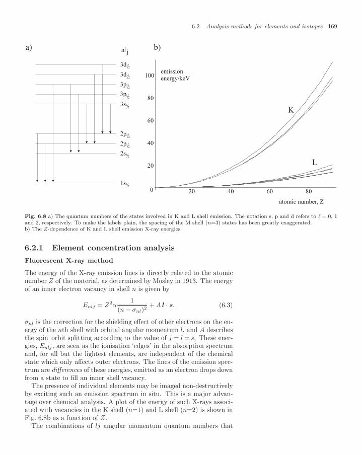
6.2 Analysis methods for elements and isotopes 169
0
20
40
60
80
100
20 40 60 80
atomic number, Z
emissionenergy/keV
nl j
1s
2s
2p
2p
3s
3p
3p
3d
3d5/2
1
1
1
1
1
/
/
/
/
/
2
2
2
2
2
3
3
3
/
/
/
2
2
2
K
L
a) b)
Fig. 6.8 a) The quantum numbers of the states involved in K and L shell emission. The notation s, p and d refers to = 0, 1and 2, respectively. To make the labels plain, the spacing of the M shell (n=3) states has been greatly exaggerated.b) The Z-dependence of K and L shell emission X-ray energies.
6.2.1 Element concentration analysis
Fluorescent X-ray method
The energy of the X-ray emission lines is directly related to the atomicnumber Z of the material, as determined by Mosley in 1913. The energyof an inner electron vacancy in shell n is given by
Enlj = Z2α1
(n − σnl)2+ A l · s. (6.3)
σnl is the correction for the shielding effect of other electrons on the en-ergy of the nth shell with orbital angular momentum l, and A describesthe spin–orbit splitting according to the value of j = l ± s. These ener-gies, Enlj , are seen as the ionisation ‘edges’ in the absorption spectrumand, for all but the lightest elements, are independent of the chemicalstate which only affects outer electrons. The lines of the emission spec-trum are differences of these energies, emitted as an electron drops downfrom a state to fill an inner shell vacancy.
The presence of individual elements may be imaged non-destructivelyby exciting such an emission spectrum in situ. This is a major advan-tage over chemical analysis. A plot of the energy of such X-rays associ-ated with vacancies in the K shell (n=1) and L shell (n=2) is shown inFig. 6.8b as a function of Z.
The combinations of lj angular momentum quantum numbers that

170 Analysis and damage by irradiation
arise for n=1,2,3 are shown in Fig. 6.8a. The resulting fine structure inthe spectra gives the three close K lines and five close L lines, as shown inFig. 6.8b. The dipole selection rules, ∆j = 0,±1 and ∆ = ±1, restrictthe transitions to those shown. Transitions from higher n states areallowed but the wavefunctions have smaller overlaps and so the matrixelements are small. Transitions from states with higher j appear strongeron account of the statistical weight 2j + 1.
Analysis with XRF
PMT
NaIRock
Lead
Rock
HT&signal cables
source
ray
Fig. 6.9 A γ-ray fluorescent detectordeployed to analyse rock in a bore hole.
For X-ray fluorescence a nuclear γ-source with energy above the K edgeof the elements of interest is required. These γ produce K and L shellvacancies in the elements of the target material which then emit theircharacteristic spectra. The energy resolution of the X-ray detector ismost important. In favourable cases element concentrations of a frac-tion of a part per million can be detected. The concentration value itselfis determined by comparing with standards, with care taken over absorp-tion and scattering. The overlap of the L lines of higher Z elements withK lines of lighter elements is simply handled by fitting a superpositionof the emission spectra of elements checked with standards.
XRF is routinely used for the analysis of elements from sodium touranium from the ppm up to the % level. Applications cover geology,forensics, planetary exploration, materials science, environmental sam-pling and industrial process monitoring. An example showing how therock in a geological bore hole may be analysed as a function of depthis shown in Fig. 6.9. In a forensic context firearms may be identifiedand explosives traced. Other materials can be matched, for instanceto those at a crime scene. No special sample preparation is required,the exposure can be carried out at ambient pressure and the analysis isimmediate.
The element discrimination of XRF is outstanding but the spatialimaging is limited. Although X-rays cannot be focused they can betightly collimated if the source is sufficiently bright. A synchrotronsource (SR) can be used to provide such brightness. Spatial resolutionsof order 1 mm square with high brightness and depth penetration can beachieved with SR. However, radioactive γ-ray sources are often cheaperand more convenient, as SR sources are still only available in specialisedlaboratories.
Ion source at 3MV
3MeV accelerator
Beam deflecting magnet
Slits
Lenses
Sample
Fig. 6.10 The scanning proton micro-probe.
Scanning proton microprobe (SPM)
Alternatively, the characteristic emission X-rays may be excited with abright spot from a finely focused proton beam. The beam can be focuseddown to a spot of 2–3 µm which can then be scanned across the sam-ple. Electron beams are less suitable as they scatter significantly. Theyalso generate bremsstrahlung which forms a background that swampsthe fluorescent signals from all elements except those with the high-est concentration. Figure 6.10 shows a diagram of the scanning protonmicroprobe. An electrostatic generator with terminal voltage of 3 MV
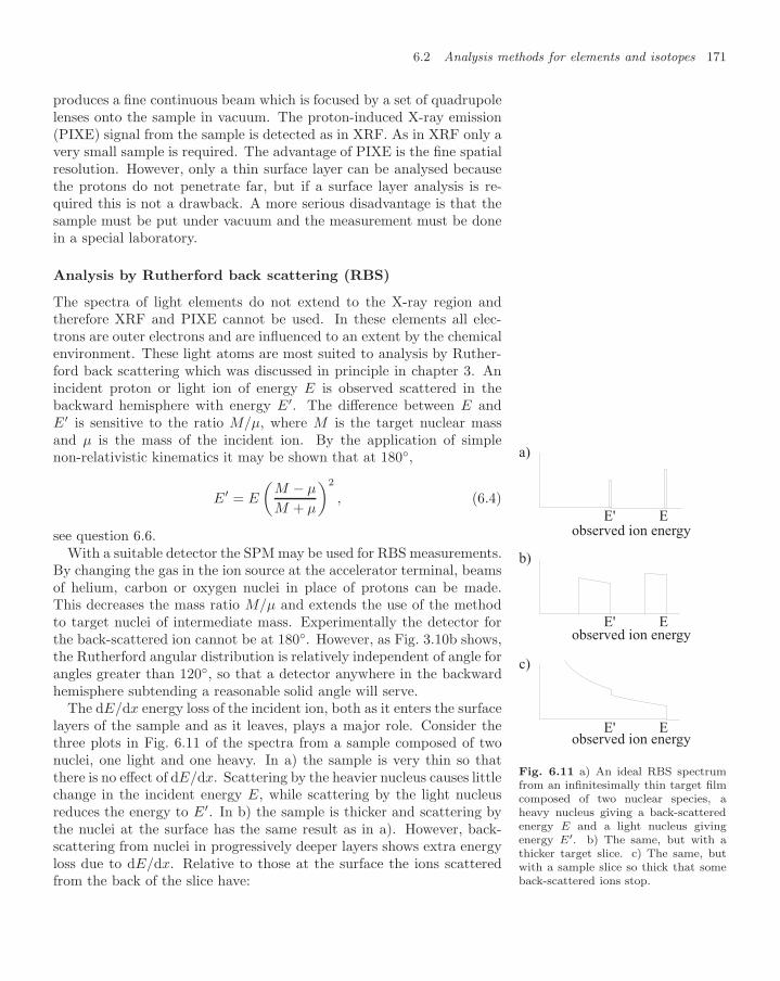
6.2 Analysis methods for elements and isotopes 171
produces a fine continuous beam which is focused by a set of quadrupolelenses onto the sample in vacuum. The proton-induced X-ray emission(PIXE) signal from the sample is detected as in XRF. As in XRF only avery small sample is required. The advantage of PIXE is the fine spatialresolution. However, only a thin surface layer can be analysed becausethe protons do not penetrate far, but if a surface layer analysis is re-quired this is not a drawback. A more serious disadvantage is that thesample must be put under vacuum and the measurement must be donein a special laboratory.
Analysis by Rutherford back scattering (RBS)
The spectra of light elements do not extend to the X-ray region andtherefore XRF and PIXE cannot be used. In these elements all elec-trons are outer electrons and are influenced to an extent by the chemicalenvironment. These light atoms are most suited to analysis by Ruther-ford back scattering which was discussed in principle in chapter 3. Anincident proton or light ion of energy E is observed scattered in thebackward hemisphere with energy E′. The difference between E andE′ is sensitive to the ratio M/µ, where M is the target nuclear massand µ is the mass of the incident ion. By the application of simplenon-relativistic kinematics it may be shown that at 180,
E′ = E
(M − µ
M + µ
)2
, (6.4)
see question 6.6.With a suitable detector the SPM may be used for RBS measurements.
By changing the gas in the ion source at the accelerator terminal, beamsof helium, carbon or oxygen nuclei in place of protons can be made.This decreases the mass ratio M/µ and extends the use of the methodto target nuclei of intermediate mass. Experimentally the detector forthe back-scattered ion cannot be at 180. However, as Fig. 3.10b shows,the Rutherford angular distribution is relatively independent of angle forangles greater than 120, so that a detector anywhere in the backwardhemisphere subtending a reasonable solid angle will serve.
a)
b)
c)
E
E
E
E'
E'
E'
observed ion energy
observed ion energy
observed ion energy
Fig. 6.11 a) An ideal RBS spectrumfrom an infinitesimally thin target filmcomposed of two nuclear species, aheavy nucleus giving a back-scatteredenergy E and a light nucleus givingenergy E′. b) The same, but with athicker target slice. c) The same, butwith a sample slice so thick that someback-scattered ions stop.
The dE/dx energy loss of the incident ion, both as it enters the surfacelayers of the sample and as it leaves, plays a major role. Consider thethree plots in Fig. 6.11 of the spectra from a sample composed of twonuclei, one light and one heavy. In a) the sample is very thin so thatthere is no effect of dE/dx. Scattering by the heavier nucleus causes littlechange in the incident energy E, while scattering by the light nucleusreduces the energy to E′. In b) the sample is thicker and scattering bythe nuclei at the surface has the same result as in a). However, back-scattering from nuclei in progressively deeper layers shows extra energyloss due to dE/dx. Relative to those at the surface the ions scatteredfrom the back of the slice have:

172 Analysis and damage by irradiation
loss of ion energy penetrating to the back; smaller recoil loss but with larger probability when they get
to the back, since the Rutherford cross section increases asthe incident energy falls;
extra loss of ion energy on the return to the surface, sincedE/dx increases as 1/v2 as v the ion velocity falls.
These effects are responsible for the energy-dependent profiles in b).The contributions of different nuclei can ride up on one another. In c)the sample is so thick, that some ions stop before they get back to thesurface.1212In Fig. 6.11 we have neglected the ef-
fect of fluctuations in dE/dx, the strag-gling, which round the sharper featuresin the spectra.
Because of the sharp depth dependence and fine focus, density distri-butions can be plotted in depth in thin layers with good resolution inall three dimensions.
6.2.2 Isotope concentration analysis
The previous section showed how the concentration of trace elementsmay be imaged or determined. The composition, the relative concentra-tion of different elements, is a clear indicator of origin. Archaeologicalartefacts can often be linked to the actual mine or quarry of origin,sometimes very far away. However, the relative abundance of differentelements is subject to change with every chemical or physical process.Elements and their compounds are separated from one another, not onlyby chemical change, but also by crystallisation and dissolution, by evapo-ration and condensation, by freezing, melting and boiling. Consequentlythe memory associated with the relative abundance of different elementsis rather volatile.
The relative abundance of different isotopes of the same element hasa much longer memory. These ratios can be measured precisely, andtheir variations in space and time form a record of valuable information.The relative isotopic abundance is only changed by nuclear reactionsor by rather small mass-dependent effects that affect isotopes slightlydifferently. Nuclear decay reduces the concentration of an isotope, andirradiation and nuclear reactions may increase it. The isotope concen-tration is a faithful record of the combined action of these effects, andin this section we give a few examples of such records, how they may bedetermined and how they have been interpreted.
Separation of isotopes by mass dependence
Heavier isotopes have smaller random velocities than lighter ones in ther-mal equilibrium in gas or liquid phases, and lower vibrational frequenciesin solids or in molecules. These differences give rise to slightly unequalchemical reaction rates, diffusion rates and concentration gradients in agravitational field. The effects are largest in light elements where thefractional difference in mass between isotopes is largest.
The most pronounced differences between isotopes are their nuclearproperties. Otherwise isotopes are analysed in the laboratory using con-

6.2 Analysis methods for elements and isotopes 173
ventional mass spectrometers, or special purpose ones for very smallconcentrations. Separation of isotopes in large quantities is based ongaseous diffusion, centrifuges or lasers that exploit the effect of massdependence.13 13See section 6.5.2.
Distribution of stable isotopes
In the natural world stable isotopes may change their relative concen-tration as a result of phase changes. In the process of crystal growth, forexample, the mass difference gives rise to a very slightly different rateof accretion. Biological activity can show a similar slight preference.
An important example is the concentration of oxygen isotopes in theoceans. Oxygen has three stable isotopes of mass 16, 17 and 18. Themajority of atoms are 16O. The concentration of 18O is about 0.2%.A notable variation in this ratio is said to be due to the preferentialfreezing of 16O, leaving a slightly higher concentration of 18O in theliquid phase.14 14We note that this effect is reported
to have the opposite sign to that whichmight have been expected.
During glacial epochs when a significant fraction of the water on Earthbecomes locked up in ice sheets the concentration of 18O in the oceanrises. Shell fish and new ice formed at this time then have a higher con-centration as shown by analysis of marine deposits and ice core samples.The difference in concentration between glacial and interglacial epochsis about 2 parts per million.15 The timing of these climatic changes has 15A change of 0.2 parts per million is
said to be just measurable and equiv-alent to a change in world-wide meansea level of 10m.
been compared with changes in the Earth’s magnetic field, the variousclocks associated with radioactive decay, pollen counts, and longtermchanges in the Earth’s solar orbit and the tilt of its axis. These allcontribute data to the discussion of the climatic history of our planet.
Neutron activation analysis
Isotope ratios may be determined by using their different nuclear proper-ties. If a sample is placed in a nuclear reactor isotopes behave differentlyaccording to their neutron absorption cross sections. Typically one iso-tope may absorb a neutron with a large cross section in a reaction
A(N, Z) + n → A(N + 1, Z) + γ, (6.5)
while other isotopes do not. Such differences tend to be large, sinceneutron affinity is influenced by a preference for paired nucleons. If thesample is now removed from the reactor the product nucleus A(N +1, Z)is typically unstable, with a characteristic and decay mode. Observationof the decay and its rate can be used to determine the concentration ofthat isotope. The measurement is most reliably calibrated by repeatingthe same procedure with a standard, a known quantity of the isotope ina similar physical form.
The scanning proton microprobe can also be used to distinguish iso-topes by proton-induced reactions. There are many variations involvingnuclear activation analysis which are described in some detail in thebook by Alfassi.

174 Analysis and damage by irradiation
Isotope detection by observation of decay
Isotope ratios may be determined by the detection of the radioactivedecay of one particular isotope. For a sufficient counting rate this re-quires a certain minimum mass of the isotope that is proportional tothe half-life. The errors of such measurements are usually dominated bythe statistics of the observed decays. With the exception of 14C mostnaturally occurring isotopes have far too long a half-life for this to be arealistic method.1616See question 6.2.
Carbon has two stable isotopes of mass 12 and 13, and one of mass 14with a mean life, τ = 8267±60 years. The value of this is fortunate as itgives good overlap with typical timespans of archaeological interest. Thepresence of 14C in the environment is entirely due to neutrons createdin the upper atmosphere by cosmic rays. These react with nitrogen,
n + 14N → p + 14C. (6.6)
This 14C then behaves almost indistinguishably from the other carbonisotopes. In particular it is present at a concentration, ρ0, of 10−12
relative to 12C in all living matter. As soon as matter dies and stopsexchanging carbon with the environment, this concentration starts tofall due to the decay1717The decay energy is only 160 keV.
This is sufficiently small that, for it tobe detected with reasonable efficiency,the carbon must be inside the detector.This may be done by filling a propor-tional counter with the carbon in theform of CO2 or CH4.
14C → 14N + e− + νe. (6.7)
At some time t later, the decay rate is measured, the current concentra-tion ρ determined, and the value of t deduced from
ρ(t) = ρ0 exp(−t/τ). (6.8)
The method assumes that the production rate of 14C has been constantin the past. This has been checked by measuring the 14C concentrationin tree rings whose sequence acts as a digital clock, phase locked to theseasonal year. The neutron flux is found to fluctuate slightly due tothe solar cycle and to have been seriously affected by the era of nuclearweapon testing. Otherwise the production rate has been rather constantuntil recently.1818The release of extra old carbon into
the atmosphere by industrial activity,the source of the global warming prob-lem, has tended to lower the 14C con-centration. The period of weapon test-ing has raised the production rate of14C in recent years, more than com-pensating for the release of old carbon.This makes dating easiest for modernmaterials. Indeed the successful iden-tification of fake bottles of ‘vintage’whisky or Armagnac has caught a fewscoundrels unawares!
Carbon dating by accelerator mass spectrometry (AMS)
The large statistical error associated with the small number of 14C nu-clei that decay in the counting time T can be reduced by a factor oforder
√T/τ . An accelerator mass spectrometer can detect all the 14C
atoms present, not just those that decay during the measurement. Aby-product is that the ratio 13C/12C can also be measured. This isindependent of date but forms a record of the fractionation effect, theextent to which the sample has been enriched or depleted of heavierisotopes by processes other than decay. The 14C ratio may then becorrected for this.19 Here we discuss the physics behind the accelerator19Further details are described in the
book by Aitken. mass spectrometer (AMS).

6.2 Analysis methods for elements and isotopes 175
+2MVgenerator
gas stripper bendingmagnet
analysingmagnet
HV terminal
C14
C12
C13
C C-+++
Cs ions
target C sample Fig. 6.12 The layout of an accelerator
specifically designed to measure 14C.
The mass spectrometer shown in Fig. 6.12 has particular features de-signed to enhance its sensitivity to 14C. Only a very small quantity ofcarbon is required, and the measurement for this is compared againstseveral samples of known age on a carousel.20 20Such known reference samples are
called standards.A conventional mass spectrometer would suffer from backgroundsof 14N and chemical fragments like 12CH2 that have nearly the samemass as 14C. This spectrometer reduces these backgrounds in two steps.Firstly it uses a negative ion C− in the initial acceleration stage. N doesnot form a stable negative ion. At the positive terminal four electronsare stripped off (on average) and the C3+ is accelerated back down toground potential.21 The second stage of background reduction occurs 21A stripper is a region of low
density gas which knocks off elec-trons. Roughly speaking, all looselybound electrons whose Fermi velocityis smaller than the ion velocity will beremoved.
because the chemical binding of a molecular ion such as CH−2 could not
survive such a stripping process intact. For each carbon isotope the re-lation between the kinetic energy given by the charge and potential, andthe momentum as it passes through the magnets, depends on the mass.The momentum and the B-field determine the angle of the trajectory,so that the three isotopes follow separate trajectories and are countedin separate counters. Further, the energy deposited in the counter iswell-defined for a carbon atom, but will be different for a backgroundatom that reaches the 14C counter spuriously.
These checks permit errors to be reduced such that samples as old as50,000 years may be dated provided that they have not been contami-nated. It is left to question 6.2 to calculate what this implies in termsof statistics and contamination tolerance.
Radiocarbon dating has become a mainstay of modern archaeology.This acceptance has been achieved by a particularly careful applicationof physics, including calibration techniques and consideration of statis-tical and systematic errors. Public relations have been well handled andthe technique has added to the popular perception of science.
Amongst well-known results the date of the Turin Shroud was deter-mined to be within AD1275–1290 at 68% confidence level, and within

176 Analysis and damage by irradiation
AD1260–1310 or AD1355–1385 at 95% confidence level. The two possi-ble ranges at 95% confidence level arise from an inflection in the calibra-tion curve that maps a single carbon measurement with Gaussian errorsinto a probability distribution in date with more than one peak. This isillustrated qualitatively in Fig. 6.13. Anyway these dates are consistentwith an origin not too long before the Shroud was brought to the Westby the Crusaders.
C"date"
14
+1σ
+2σ
-1σ
-2σ
historical date
Fig. 6.13 An illustration of how a nor-mally distributed 14C date is mappedby a calibration curve based on den-dochronology into probability bands onan axis of historical date.
Other results of interest are frequently reported. In 1991 a perfectlypreserved frozen body was discovered in the Alps, complete with clothes,tools, food and belongings. Accelerator mass spectrometry of 14C wasused to measure the age of this exciting find at 5300 years.
Dating by measurement of daughter concentration
There is another way in which the radioactive decay of an isotope maybe used as a clock. The integrated number of decays that have occurredin time t may be inferred from a measurement of the ratio of decayproduct to parent element concentrations. If the decay rate is known,this gives an estimate of the period t over which the daughter nucleushas been accumulating.
There are two questions: ‘What defines when the clock starts?’, and‘Are there any circumstances in which the daughter nuclei have left thesample, thereby reducing the apparent time and slowing the clock?’ Theanswers to these questions are related. The clock starts when the sampleis formed with no daughter nuclei present. The clock is slowed if daugh-ter nuclei diffuse away or are leached out of the rock sample. In somecases the daughter nuclei may themselves decay, but that is a knownprocess whose effects can be corrected precisely, statistics permitting.
A good example is the decay of 40K to 40Ar for which the branchingratio is 10.5%. 40K is widespread in nature and forms a fairly constant0.0118% of natural potassium, with a lifetime of 1.2×10⁹ years. Thisis sufficiently long that the rate of production of argon is effectivelyconstant. The clock is reset whenever the argon is released. This occurswhenever rock is formed, whether deposited in water as a sediment orcooled from a molten lava flow. In theory, once the rock is deposited orcooled from the liquid state, the argon is trapped. In practice allowancehas to be made for both a pre-existing concentration and losses of gasby diffusion, especially if the rock has been heated significantly since itwas formed.2222See the note in section 36 for further
discussion of this point. An effective experimental procedure is the argon-argon technique.The rock sample is placed in a nuclear reactor to convert a fractionof the normal 39K to 39Ar. The sample is then heated and the ratio40Ar/39Ar measured with time as the sample outgases. This methodcompensates for the speed of outgassing, gives a signal relative to the Kcontent and indicates samples which have lost Ar from surface layers inthe time since formation. Such samples give a ‘young’ reading as suchsurface layers outgas, but can give an asymptotically correct age as gasfrom deeper in the sample is released. Alternatively the trapped argon

6.2 Analysis methods for elements and isotopes 177
may be released from a single grain of a milligram or less with a laser.Errors vary with the K content. Age estimates with errors of ±103 yearsfor rocks with high K content have been confirmed by radiocarbon dat-ing for ages up to 3 × 10⁴ years. The dates of early hominid remainshave been determined at 1–2 million years with errors of 1–2% by thismethod.
Uranium series dating
Errors in dating based on parent and daughter isotopic concentrationsarise when concentrations are affected either by other processes or whenthe initial concentration is uncertain. The absence of a significant ini-tial argon concentration in rock is a good example where uncertainty isreduced small. Another is based on the low solubility of thorium saltscompared with those of uranium.
As shown in table 6.6 the naturally occurring and long lived isotope238U gives rise on decay to 234U with a half-life of 2.45 × 10⁵ years.This in turn decays to 230Th with a half-life of 7.7 × 10⁴ years. Itfollows that, starting with rock deposited from solution at time t = 0,the concentration ratio of 230Th/234U rises from zero as the daughterconcentration builds up. Thus the calcite of a stalagmite, for instance,has a ratio that is a direct measure of its age. The ratio eventuallysaturates after a number of lifetimes of 230Th as dynamic equilibrium isestablished.
The experimental method involves the chemical separation of U andTh, followed by the identification of the two isotopes of interest by theircharacteristic α-decay energies.23 Statistical errors may be reduced by 23This is actually not too easy as the
energies are close, 4.8 MeV and 4.7MeV respectively.
the use of mass spectrometry of the isotopes instead, and the age rangeextended back to 5 × 10⁵ years.
There are other methods too. The reader is referred to the book byAitken.
6.2.3 Radiation damage analysis
In solids the record of past radiation may be recorded in the form of thefrozen atomic, molecular and crystal-structure damage. Such a recordis ‘wiped’ by processes such as heating, melting or recrystallisation. Itmay be recorded in the form of visible lattice damage, electronic excitedstates or paramagnetic electrons, with some overlap between these.
Fission track dating
The decay of the naturally occurring 238U usually proceeds by α-decayto 234Th. However, in a fraction 0.5×10⁻⁶ the decay process is sponta-neous fission. The fission products are highly charged with a low velocity.Their dE/dx, or LET, is exceptionally high, and they stop in about 10µm. The locally disrupted crystal structure may be dissolved preferen-tially by etching a polished face, making the track location visible undera microscope. Because the half-life is so long, a count of the density

178 Analysis and damage by irradiation
of these pits relative to the 238U concentration is linearly dependent onthe time since the crystal was last annealed. The count is normalisedby observing the density of pits found on an identical sample which hasbeen annealed and irradiated with neutrons in a reactor. This processreveals the location of induced fission by 238U. Using the ratio of den-sities takes care of the parent uranium concentration and details of thecounting procedure used.
Only certain minerals are suitable and the counting procedure is te-dious. The technique is not practicable at densities below 100 cm−2.
Dating by thermoluminescence
Thermoluminescence depends on the density of excited electrons frozeninto a solid. These metastable excited electronic states are created by thegeneral flux of radiation incident on a sample, which includes the back-ground γ-rays from neighbouring rock and the external cosmic radiation,as well as local α- and β-activity. In a liquid or gas these do not persist,but in certain solids the relaxation time is very long, though a rapidlydecreasing function of temperature. The record may be ‘bleached’ bylight in surface layers as well as by heat. Below the surface the density oftrapped excited electrons may accumulate. If such samples are exposedand heated, the light emitted by de-excitation is a measure, either of theage of the sample if it has been held in a constant radiation environment,or of the integrated radiation flux if the sample is of known age.
As the temperature of the sample is raised very slowly, light is emittedby progressively more deeply bound electrons. The second stage of themeasurement requires the sample to be irradiated with a known dose,and then heated again slowly as in the original measurement. The ratioof thermoluminescent fluxes emitted indicates the ratio of the historicaldose to the calibration dose. If the annual dose can be estimated then theage may be deduced. Spurious effects may be eliminated by observingthe ratio as a function of the temperature. The details are described byAitken.
The technique is particularly important for dating pottery and kilns.The t = 0 event is the date when these were last fired and cooled.24 The
24This firing and then cooling gives riseto a further effect that is also used indating. The thermal cycling takes mag-netic grains in the clay above and thenbelow the Curie temperature, therebyfreezing information on the Earth’s B-field strength and direction at preciselythe same time. This has been usedto deduce information about dates andabout the behaviour of the Earth’sfield. Data from lava flows as well askilns and ceramics are discussed in thebook by Aitken.
dominant error tends to come from the uncertainty in the annual doseexperienced by the sample.
These radiation-induced electronic states also involve unpaired elec-trons which give rise to paramagnetic properties. A measurement ofthe amplitude of the electron spin resonance (ESR) is another techniquethat may be used to indicate radiation exposure or date.25
25ESR is sensitive to the integral ofradiation exposure. So if the date isknown, the radiation exposure can bededuced, as in Hiroshima studies andtests of food irradiation. Converselyif the rate of irradiation is known andsteady, a date may be determined.

6.3 Radiation exposure of the population at large 179
6.3 Radiation exposure of the population
at large
Radioactivity may be measured as the rate at which nuclei decay. Ra-diation exposure is measured as the absorption of energy per unit mass.The response of living tissue to a radiation dose is essentially non-linear.Doses that are local and of short duration are more damaging than thesame dose less densely distributed either in space or time. This may besimply understood in terms of healing processes. These are essential tothe successful use of radiotherapy. The linear no-threshold model (LNT)naively assumes that a given radiation dose spread over a large populationcauses the same damage as when concentrated on a few individuals; thismodel is not sustainable, though frequently quoted. Such quotations havegenerated significant public misunderstanding. We give the radiation ex-posure of the UK population and discuss its various sources, namely radongas, gammas from radioactive rocks, internal sources, secondary cosmicrays, medical doses and other human-made contributions.
6.3.1 Measurement of human radiation exposure
SI units
To discuss radiation in the environment we need first a basis of objectivemeasurements. In SI there are units for three different quantities thatmay be measured in radiation health physics.
The activity of a radioactive source is the number of disin-tegrations per second. One disintegration per second is 1becquerel (Bq). This is not the number detected or counted,but refers to the whole source. A earlier unit, the curie, wasequal to 3.7 × 10¹⁰ Bq.
The unit of absorbed dose or deposited energy is the gray(Gy). A radiation dose of 1 Gy is equal to 1 joule per kg. Aearlier unit, the rad, was equal to 0.01 Gy.
The unit of equivalent dose for biological damage is the siev-ert (Sv).26 For X-rays, γ-rays and electrons the equivalent
26An older unit is the rem where 100rem equals 1 Sv.
dose in sieverts is defined to be equal to the absorbed dosein grays. For other types of radiation the equivalent dosein sieverts is greater than the dose in grays by a factor, wR,the radiation weighting factor. Some values of this factor aregiven in table 6.4.
Biological equivalent dose
Table 6.4 Some values of the radiationweighting factor wR for different kinds ofradiation.
Radiation Energy wR
X-rays and γ-rays any 1Electrons any 1Muons and muons any 1Protons >2 MeV 5Alpha/light ions any 20Fission fragments any 20Neutrons <10 keV 5Neutrons 10–100 keV 10Neutrons 0.2–2 MeV 20Neutrons 2–20 MeV 10Neutrons >20 MeV 5
The operational definition of the sievert is that 1 Sv should represent thesame hazard to tissue whatever the form of the ionising radiation. Whatdetermines the factors in table 6.4? First we shall justify, qualitativelyat least, the use of these values. Later we shall come to see that actualbiological damage has a more complex relation with absorbed dose whichis not describable by a single factor.

180 Analysis and damage by irradiation
The response of biological tissue to radiation damage is non-linearand the reason for this may be understood as follows. Compare thefollowing situations in which two cells are exposed to a certain totalabsorbed radiation dose.
One cell receives all the energy and the other none, with theresult that one cell dies and the other survives.
Both cells receive half the dose each, with the result thateach has a fair chance of effecting a repair. As a result bothhave a better than even chance of survival.
With a non-linear response due to repair mechanisms and some biologicalredundancy, the question of the uniformity of a delivered dose is critical.
Now we examine the entries in the table. The energy loss associatedwith photons and β = 1 charged particles is thinly spread along the pathsof the individual charges or quanta. This maximises the opportunity forbiological repair.
However, a non-relativistic charge, whose rate of energy depositionalong its path is enhanced by a factor 1/β2, delivers energy much morelocally. Relative to irradiation by electrons, material irradiated with 1Gy by such charges is traversed by a smaller number of more denselyionising tracks. Those cells that lie near a track get a large dose, fromwhich recovery is unlikely, while those that are far removed are unaf-fected. Due to the non-linear effect of repair this radiation will do moredamage per gray than electrons or γ-radiation. In brief the damagedepends on the LET as well as the specific energy dose.2727This is particularly evident for multi-
ple charged ions such as alpha particlesor the highly ionised nuclear fragmentsemitted in the nuclear fission process.They get a very heavy rating in ta-ble 6.4 because they have a high LET.
Why do neutrons carry a heavy penalty per gray? A neutron, beinga neutral particle, does not deposit energy at all until it has a collision.It does not collide with electrons. It can only undergo nuclear collisions.Products of such collisions typically consist of slowly moving nuclei ornon-relativistic recoil protons. These have a high LET and a high wR.Very low energy neutrons are moving too slowly to create recoils thationise.28 They have a low wR. More energetic neutrons generate recoil
28This will occur for neutrons withless than atomic electron velocity,that is with energy less than about10 eV ×mN/me. This is about 10 keV,in broad agreement with the table en-tries. Neutrons with less energy de-posit it in the form of lattice vibrationsor phonons which represent heat andcause no damage.
protons of similar energy and therefore have similar wR.
Timing of radiation dose
Life on Earth has developed under conditions in which it has been contin-uously exposed to ionising radiation from a number of different sources.The average exposure of the population in the UK is 2.7 mSv per year.There are significant fluctuations on this figure depending on location.2929However, there is rather good infor-
mation that overall it has not changedmuch in the last 50,000 years. Look-ing back 109 years the radiation en-vironment due to radioactivity in theEarth would have been more intense bya small factor. Since that time radia-tion levels have been declining slowlywith a combination of the known expo-nential decay factors of the long-livedparent nuclei involved.
At the other end of the scale it has been found that a radiation dose tothe whole body of the order of 5 Sv is fatal to life in 50% of cases.
Life has evolved and thrived in the gap between these two extremes.However, there is an inconsistency here, for the dimensions of the back-ground rate and the fatal whole-body dose are not commensurable. Weneed a timescale. In other words, we have to answer the question ‘Overwhat time should we integrate the radiation dose rate in order to com-pare it with the fatal dose?’ Arguably, understanding the importance of

6.3 Radiation exposure of the population at large 181
this question and the question of non-linearity discussed earlier are thetwo most important questions for radiation health physics.
The brief answer is that the timescale that is important is the cellreplacement time or the repair time. This determines over what periodthe human body remembers radiation exposure. Over a longer timerepair and replacement can make good the damage of irradiation. Overa shorter time damage is integrated. From a century of experience withradiotherapy and studies of cell recovery in vitro this time is known tobe on the scale of days. It varies for different parts of the body anddifferent organs, and also varies with age. To be very conservative wetake this time to be a month. That is we assume that a radiation dosespread over a period of a month causes the same damage as if the doseis delivered in a single episode.30
30Clinical experience with radiother-apy treatment planning suggests thatthis may be an order of magnitude toolong. See chapter 8.
Collective dose and the linear no-threshold (LNT) model
In assessing the radiation hazard to a whole population it is a naturaltemptation to multiply the radiation dose by the size of the populationso exposed. This is what is known as the collective dose. Thus a millionpeople receiving an additional dose of 1 mSv makes an extra collectivedose of 1000 man Sv. The mistake is to suppose that the biologicaldamage, for instance the number of additional cancers, is linearly pro-portional to this collective dose with no constant term. This suppositionis called the linear no-threshold model (LNT). However, it is quite simpleit is wrong. Biological systems do not respond linearly in this way.31 31For any threat to which life has
evolved a protection or repair mech-anism the normal response is an S-shaped curve, as shown in Fig. 6.18.Such non-linearity provides complete,not proportional, protection providedthat the repair mechanism is not over-loaded, for example in space and time- hence, in the case of radiation, thedependence on LET and the exposureperiod. We should expect such non-linearity for any threat to which lifeis exposed in the natural environmentand has therefore had the opportunityto evolve some protection mechanism.This includes ionising radiation.
Laceration is another kind of biologically disruptive damage. If I cutmy finger badly, in the absence of any coagulation, blood would be lostto the point that death would follow. This does not happen becausethe blood does coagulate and seal the wound, and in due course the lossis replaced. For this reason, although a major amputation may causeloss of life, a large number of people losing even a moderate amount ofblood is not life-threatening. It makes no sense to represent the danger asproportional to the number of people multiplied by the loss of blood thateach suffers. Otherwise every blood-donor clinic would be responsiblefor a large number of deaths every day.
The same argument applies to the effect of a moderate dose of ionisingradiation on a large population. A whole body dose of 5 Sv deliveredto each of 100 people can be expected to result in about 50 mortalities.Because of the non-linearity an extra dose of 0.5 mSv delivered to amillion people results in no fatalities, although the collective dose is 500man Sv in both cases. Exposure of an individual within a factor ten of afatal level causes some permanent damage and results in scar tissue, ina radiation exposure just as it does in laceration. However, much largermargins of safety, the equivalent of avoiding pin pricks, make no sensein the real world. Life has evolved to recover completely from pin pricksand the effects of modest levels of radiation.
The effect of radiation doses on very large populations have been stud-ied to check whether there is any additional response to radiation damage

182 Analysis and damage by irradiation
that is linear. Table 6.5 lists some of these. In a group of a million peoplethere are about 2000 cancers that occur each year, predominantly fromill-advised life styles, but also naturally. Thus the statistical error on thenumber of cancer cases in a sample of this size is about 50. There aresystematic effects as well. The panic, social and economic upset that
Table 6.5 Some high statistics studiesof the effects of radiation.
Location Pop. Ref.
Hiroshima 120,000 p. 196and Nagasaki
Urals accident 30,000 p. 191Radon
in China 80,640 §§in Europe various p. 191
Chernobyl various p. 199
§§www.hps.org/publicinformation/ate/q1254.html
followed Chernobyl caused fatalities through family breakdown, drink,smoking and despair. These were not consequences of the physical effectsof radiation and contribute large systematic uncertainties. The variousreports on Chernobyl, and on Hiroshima and Nagasaki, may be foundon the NEA and RERF-LSS websites referenced at the end of chapter 1.A most readable account is given in the book by Henriksen and Maillie.The conclusion is that there is no evidence to support the LNT model.Use of the LNT model and collective dose is easy but dangerous. Ithas been the cause of the exaggeration of the threat posed by ionisingradiation.
6.3.2 Sources of general radiation exposure
Data for the UK population
The average annual radiation dose to the UK population is 2.7 mSv.Fig. 6.14 shows the various sources of this radiation and how they makeup this average. However, some sectors of the population receive morethan others.
The greatest source of radiation is from natural radioactivity in therocks of which the Earth is composed. Most materials, unless theyhave been very highly refined, also contain these radioactive nuclei inmeasurable quantities. All of the alpha radiation, most of the betaradiation and some of the gamma radiation is absorbed within the rockor other material and does not escape. The only products of theseradioactive sources that contribute to the human dose are radon gasand gamma rays. Together these make up 63% of the average dose, butthere are geographical locations where the exposure is five and moretimes greater than the average.
radon50%
medical15%
cosmic12%
gamma13%
internal9.5%
0.2% occupational0.2% fallout< 0.1% discharges< 0.1% products
Fig. 6.14 The composition of the aver-age radiation exposure of the UK popu-lation (2.7 mSv). Of this 84% is naturaland 16% is artificial. [Data from HPA-RPD-001(2005).]
Background radioactivity is also present within our own bodies. Inthis case the dose includes the alpha radiation with its high weight(shown in table 6.4). The internal source of exposure represents some9.5% of average dose. This is the only source for which little than can bedone to reduce the level. Cosmic radiation contributes 12% of the aver-age dose. This derives from the radiation that shines on the Earth fromouter space. However, its effects are by no means uniform. The largestsource of radiation over which we have substantial control is its use inmedicine where it forms 15% of the average. In the following we studyeach of these sources and also those that contribute to the remaining 1%of the average.
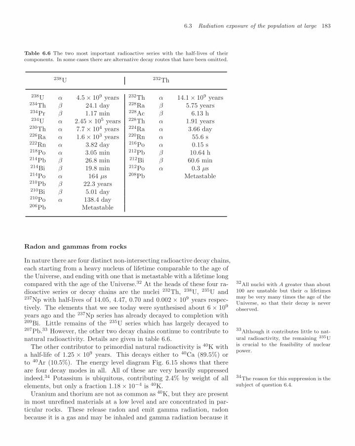
6.3 Radiation exposure of the population at large 183
Table 6.6 The two most important radioactive series with the half-lives of theircomponents. In some cases there are alternative decay routes that have been omitted.
238U 232Th
238U α 4.5 × 10⁹ years 232Th α 14.1 × 10⁹ years234Th β 24.1 day 228Ra β 5.75 years234Pr β 1.17 min 228Ac β 6.13 h234U α 2.45 × 10⁵ years 228Th α 1.91 years230Th α 7.7 × 10⁴ years 224Ra α 3.66 day226Ra α 1.6 × 10³ years 220Rn α 55.6 s222Rn α 3.82 day 216Po α 0.15 s218Po α 3.05 min 212Pb β 10.64 h214Pb β 26.8 min 212Bi β 60.6 min214Bi β 19.8 min 212Po α 0.3 µs214Po α 164 µs 208Pb Metastable210Pb β 22.3 years210Bi β 5.01 day210Po α 138.4 day206Pb Metastable
Radon and gammas from rocks
In nature there are four distinct non-intersecting radioactive decay chains,each starting from a heavy nucleus of lifetime comparable to the age ofthe Universe, and ending with one that is metastable with a lifetime longcompared with the age of the Universe.32 At the heads of these four ra- 32All nuclei with A greater than about
100 are unstable but their α lifetimesmay be very many times the age of theUniverse, so that their decay is neverobserved.
dioactive series or decay chains are the nuclei 232Th, 238U, 235U and237Np with half-lives of 14.05, 4.47, 0.70 and 0.002 × 10⁹ years respec-tively. The elements that we see today were synthesised about 6 × 10⁹
years ago and the 237Np series has already decayed to completion with209Bi. Little remains of the 235U series which has largely decayed to207Pb.33 However, the other two decay chains continue to contribute to 33Although it contributes little to nat-
ural radioactivity, the remaining 235Uis crucial to the feasibility of nuclearpower.
natural radioactivity. Details are given in table 6.6.The other contributor to primordial natural radioactivity is 40K with
a half-life of 1.25 × 10⁹ years. This decays either to 40Ca (89.5%) orto 40Ar (10.5%). The energy level diagram Fig. 6.15 shows that thereare four decay modes in all. All of these are very heavily suppressedindeed.34 Potassium is ubiquitous, contributing 2.4% by weight of all 34The reason for this suppression is the
subject of question 6.4.elements, but only a fraction 1.18 × 10⁻⁴ is 40K.Uranium and thorium are not as common as 40K, but they are present
in most unrefined materials at a low level and are concentrated in par-ticular rocks. These release radon and emit gamma radiation, radonbecause it is a gas and may be inhaled and gamma radiation because it

184 Analysis and damage by irradiation
Fig. 6.15 The states with their ener-
gies involved in the decay of 40K. Ca
K
Ar40
40
40
0+
0
2 4
+
+ -
0.0
1.4611.505
0.193
γ β β
electroncapture
Relativeatomicmass
MeV/c2
-+
e.c.
has a long range.Radon is the heaviest of the noble gases. Two isotopes are produced
in the radioactive decay chains, but the important one is 222Rn with a3.82 day half-life.35 This is long enough for it to diffuse out of the rock35The other one is sometimes called
thoron but has a half-life of only 55.6s. where it is produced, at least from sites with depth less than 100µm.36
36These statements seem at variance
with the observation that 40Ar pro-duced in the decay of 40K does not dif-fuse out of the rock over periods of 106
years, as quoted in section 22. The ra-tio, a factor 108, is related to the recoilenergy, see question 6.7.
Its geographical distribution is very uneven. More than two thirds ofhomes in England where the indoor radon radiation levels exceed 200 Bqm−3 are in Devon and Cornwall. On average this has the effect that theannual radiation dose for the population of Cornwall is 7.5 mSv ratherthan the average for the whole country of 2.7 mSv.
It is not difficult to minimise the exposure to radon. Because of itsvery high atomic weight of 222, it is some 15 times denser than airand accumulates on the floor.37 As a result the concentration at head
37In the same way that nitrogen from aliquid nitrogen dewar falls to the floor,although that is only four times denserthan air at ambient temperature.
height is much less. The half-life of radon is only 3.82 days and so ittends to establish an equilibrium concentration on such a timescale. Theradiation may be reduced by ventilating buildings, especially cellars, ona daily basis.
Internal sources
Potassium is present in the body as the main base ion of the intracellularfluid and therefore essential to the body’s electrochemistry. The 40Kcomponent is the main internal source of radiation, 70 Bq kg−1. Thecorresponding radiation dose of 0.18 mSv per year is not subject to muchvariation. Other internal sources, predominantly 210Pb and 14C, add tomake a total of 0.25 mSv per year.
Secondary cosmic rays
The Earth is illuminated by a wide variety of radiation from the Sunand elsewhere in space.
From the Sun we receive black body electromagnetic radiation whichpeaks in the optical region of the spectrum but extends down into theinfrared and upwards into the ultraviolet. Both of these are largelyabsorbed in the atmosphere, although in the latter case this depends onthe coverage of the ozone layer. Also emitted by the Sun are streams of
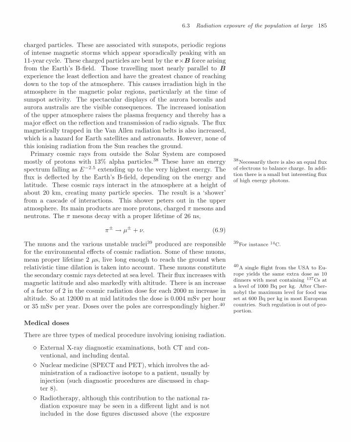
6.3 Radiation exposure of the population at large 185
charged particles. These are associated with sunspots, periodic regionsof intense magnetic storms which appear sporadically peaking with an11-year cycle. These charged particles are bent by the v×B force arisingfrom the Earth’s B-field. Those travelling most nearly parallel to Bexperience the least deflection and have the greatest chance of reachingdown to the top of the atmosphere. This causes irradiation high in theatmosphere in the magnetic polar regions, particularly at the time ofsunspot activity. The spectacular displays of the aurora borealis andaurora australis are the visible consequences. The increased ionisationof the upper atmosphere raises the plasma frequency and thereby has amajor effect on the reflection and transmission of radio signals. The fluxmagnetically trapped in the Van Allen radiation belts is also increased,which is a hazard for Earth satellites and astronauts. However, none ofthis ionising radiation from the Sun reaches the ground.
Primary cosmic rays from outside the Solar System are composedmostly of protons with 13% alpha particles.38 These have an energy 38Necessarily there is also an equal flux
of electrons to balance charge. In addi-tion there is a small but interesting fluxof high energy photons.
spectrum falling as E−2.5 extending up to the very highest energy. Theflux is deflected by the Earth’s B-field, depending on the energy andlatitude. These cosmic rays interact in the atmosphere at a height ofabout 20 km, creating many particle species. The result is a ‘shower’from a cascade of interactions. This shower peters out in the upperatmosphere. Its main products are more protons, charged π mesons andneutrons. The π mesons decay with a proper lifetime of 26 ns,
π± → µ± + ν. (6.9)
The muons and the various unstable nuclei39 produced are responsible 39For instance 14C.
for the environmental effects of cosmic radiation. Some of these muons,mean proper lifetime 2 µs, live long enough to reach the ground whenrelativistic time dilation is taken into account. These muons constitutethe secondary cosmic rays detected at sea level. Their flux increases withmagnetic latitude and also markedly with altitude. There is an increaseof a factor of 2 in the cosmic radiation dose for each 2000 m increase inaltitude. So at 12000 m at mid latitudes the dose is 0.004 mSv per houror 35 mSv per year. Doses over the poles are correspondingly higher.40
40A single flight from the USA to Eu-rope yields the same extra dose as 10dinners with meat containing 137Cs ata level of 1000 Bq per kg. After Cher-nobyl the maximum level for food wasset at 600 Bq per kg in most Europeancountries. Such regulation is out of pro-portion.
Medical doses
There are three types of medical procedure involving ionising radiation.
External X-ray diagnostic examinations, both CT and con-ventional, and including dental.
Nuclear medicine (SPECT and PET), which involves the ad-ministration of a radioactive isotope to a patient, usually byinjection (such diagnostic procedures are discussed in chap-ter 8).
Radiotherapy, although this contribution to the national ra-diation exposure may be seen in a different light and is notincluded in the dose figures discussed above (the exposure

186 Analysis and damage by irradiation
e X-ray dose by age
X-ray examinationse X-ray dose per
colon
angiography
X-ray CT
X-ray CT
other
other
interventional radiology
chest
mammography
mammography
abdomen
c) Proportion of dose, 0.33 Sv per person per yearm
a) Averagexamination, mSv
colonangiographyX-ray CTinterventional radiologyabdomenmammographyskullchestdentallimbs & joints
b) Proportion of total
dental
limbs &joints
7.26.05.55.00.700.270.0380.0200.0060.001
0
0.2
0.4
0.6
0.8
20 40 60 80
Averageannualdose
/ Svm
Age/years
d) Averag
Fig. 6.16 The composition of the X-ray diagnostic radiology dose to the UK population. a) Dose per examination by procedure.b) Fraction of all examinations. c) Fraction of total dose (ordered and classified as in b)). d) Average dose by age (indicative).[Data from Hart and Wall, NRPB-W4 (2002).]
of staff during radiotherapy procedures is properly includedwithin occupation-dependent doses).
The diagnostic X-ray dose accounts for an average of 0.33 mSv perhead of the population, and Fig. 6.16 shows how this is made up. Inaddition there is a mean dose of 0.024 mSv from nuclear medicine. Threequarters of the latter dose involved the administration of 99Tc. Thenumber of such examinations was 360K in the UK in 1998 with anaverage dose of 3.3 mSv each.
The distribution of dose is far from uniform: 93% of the populationreceive a dose of less than 1 mSv from diagnostic radiology; 7% of thepopulation receive 82% of the total collective dose. Dental examinations,chest and limb X-ray procedures involve very small doses. X-ray CTexaminations, like the nuclear medicine procedures, carry a higher dose,close to the recommended annual limit, or the annual dose acquired byliving in Cornwall. We shall consider the reasons for these higher dosesin chapter 8. Many of those who receive higher doses are older andbeyond child-bearing age. The age distribution, Fig. 6.16d, shows thatthose over 60 receive typically four times the dose of those under 20.

6.4 Radiation damage to biological tissue 187
Radioactive consumer products and occupational doses
In the 1950s and 1960s every schoolboy wanted a watch with a largeluminous dial. The radioactive constituent of the paint used on thedial and hands was a γ-emitter, such as radium. This gave an annualdose of about 1.3 mSv. The constituents now used are β-emitters whoseradiation is contained. These are now marketed as ‘beta-light’ sources.Another consumer product in which radioactive material is used is thethoriated gas mantle. An efficient gas mantle should act as a black bodyradiator throughout the optical spectrum and have a high melting point.When heated to a high temperature it then emits a good white light. Asa high Z material thorium has the required dense absorption spectrum.Thoriated gas mantles are still used, but gas lighting is very much theexception, and the dose is small. Smoke alarms are provided with aweak α-source (40 kBq 241Am). However, no radiation can be detectedoutside the ionisation chamber. In summary, consumer products are nolonger responsible for any significant dose.
The radiation exposure of certain occupations used to be significant.Now, carefully monitored and regulated on an individual basis, occu-pational doses are small compared with the variation of doses such asradon. Other contributions to the radiation exposure of the general pop-ulation including the effect of atmospheric nuclear weapon testing andChernobyl fallout are discussed later in this chapter.
6.4 Radiation damage to biological tissue
We discuss the range in scale of radiation damage to biological systems,and how such damage is related non-linearly to the radiation dose. Dataon survival from exposure to high doses, the effects of low doses and theincidence of radon-induced lung cancer show that the health risks of low-level radiation have been significantly overstated. High doses are usedto sterilise cell reproduction completely, and this has application to thesterilisation of hospital supplies and food.
6.4.1 Hierarchy of damage in space and time
On the left in Fig. 6.17 is shown a diagram of the structural hierarchy ofhealthy living tissue. On the right are shown the abnormal forms thatcan result from radiation exposure. This simplified picture is intended toshow the relative scale at which different pathological conditions occur.Because there is a very large number of each lower scale structure ineach higher scale form, there is significant redundancy in the system ateach level. With this redundancy goes an ability to replace and repairwhen radiation-induced abnormalities occur.
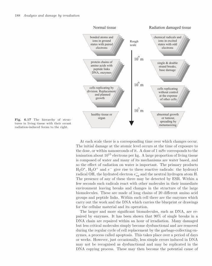
188 Analysis and damage by irradiation
Fig. 6.17 The hierarchy of struc-tures in living tissue with their errantradiation-induced forms to the right.
bonded atoms andions in ground
states with pairedelectrons
protein chains ofamino acids with
peptide linksDNA, enzymes
cells replicating bydivision. Replacement
and plannedgrowth
healthy tissue ororgan
chemical radicals andions in excitedstates with odd
electrons
single & doublestrand breaks,base damage
cells replicatingwithout controlat the expenseof other cells
abnormal growthor tumour,
spreading bymetastasizing
10 m
10 m
10 m
-9
-6
-3
Roughscale
Normal tissue Radiation damaged tissue
At each scale there is a corresponding time over which changes occur.The initial damage at the atomic level occurs at the time of exposure tothe dose, or within nanoseconds of it. A dose of 1 mSv corresponds to theionisation about 1015 electrons per kg. A large proportion of living tissueis composed of water and many of its mechanisms are water based, andso the effect of radiation on water is important. The primary productsH2O∗, H2O+ and e− give rise to three reactive radicals: the hydroxylradical OH, the hydrated electron e−aq and the neutral hydrogen atom H.The presence of any of these three may be detected by ESR. Within afew seconds such radicals react with other molecules in their immediateenvironment leaving breaks and changes in the structure of the largebiomolecules. These are made of long chains of 20 different amino acidgroups and peptide links. Within each cell there are the enzymes whichcarry out the work and the DNA which carries the blueprint or drawingsfor the cellular material and its operation.
The larger and more significant biomolecules, such as DNA, are re-paired by enzymes. It has been shown that 90% of single breaks in aDNA chain are repaired within an hour of irradiation. Many damagedbut less critical molecules simply become dysfunctional and are removedduring the regular cycle of cell replacement by the garbage-collecting en-zymes, a process called apoptosis. This takes place over a period of daysor weeks. However, just occasionally, less simple errors induced in DNAmay not be recognised as dysfunctional and may be replicated in theDNA copying process. These may then become the potential cause of

6.4 Radiation damage to biological tissue 189
longer term problems.
Factors affecting cell survival
Survival curves for cells show two marked effects that are important inradiotherapy.41 The first is the oxygen effect. A higher oxygen concen- 41This is discussed at greater length in
chapter 8.tration increases the mortality of cells by up to a factor 2. This is aproblem for radiotherapy because a malignant tumour in an advancestate is depleted of oxygen. However, with careful treatment planning,successive treatments can penetrate deeper into the tumour as normalmetabolism recovers and the oxygen level rises to its normal level. Thesecond effect relates to the timing of the cell reproduction cycle. A cellhas to double its DNA in order to divide. The division stage is calledmitosis. After mitosis there is the lowest redundancy in the DNA infor-mation in each cell and it is at this phase (1–2 hours in 24) that the cellis most radiation sensitive. In vivo cells are at different phases in theircycles. However, such questions may be studied with human cells grownin vitro in a tissue laboratory under controlled conditions.
6.4.2 Survival and recovery data
Damage at high doses
Very high whole-body doses cause catastrophic failure of biological mech-anisms and early death with high probability and without significant de-lay. Unequivocal data on this are available, largely from animal studiesbut supported by available human data. The response is very non-linear.An example is shown in Fig. 6.18, in this case for rats. When humans oranimals are irradiated the blood-forming organs in the bone marrow areimmediately affected. After doses of 1 to 2 Gy the white and red blood
4 6 8 10
25%
50%
75%
100%
Ratdeathrate
Dose/Gy
Fig. 6.18 The whole-body fatal dosecurve for rats.
cells decrease and the immune system deteriorates. If the dose is lessthan 4 to 5 Gy the bone marrow may recover after 3 to 4 weeks. Thelethal dose LD50 is the whole body dose that induces 50% death within30 days.42 For rats LD50 is 7.5 Gy, for humans it is 3–5 Gy, with similar
42This is called acute radiation death.
values for other higher mammals. Simpler organisms are more tolerant,for example for goldfish the figure is 23 Gy. Single cell organisms maysurvive much higher doses, such as 2000–3000 Gy. This is taken intoaccount in the radiation treatment of food and the sterilisation of hospi-tal supplies. Following exposure to a dose significantly above 5 Gy thereproduction of cells in humans shuts down. Systems with a high cellturnover fail first. Thus the gastrointestinal tract is an early casualtywith symptoms of vomiting and diarrhoea.
Effects of irradiation over long periods
The time lapse between the irradiation and the diagnosis of a cancer,called the latent period, may be many years. Our understanding of whathappens during this time is still poor. There is no in vivo imaging withthe required resolution and specificity, and the error rate itself is very

190 Analysis and damage by irradiation
small indeed. At a clinical level, the presence of cancer cells is often notdiagnosed with certainty until a tumour many millimetres in size hasdeveloped. This is an unfortunately late stage at which to give therapy.The large number of malignant cells to be killed means that considerabledamage is sustained by healthy tissue and there is also a significantchance that some malignant cells will survive and metastasize.43
43Metastasis is the stage at which ma-lignant cells spreads around the body,typically through the bloodstream.
Damage due to low doses
Low doses44 do not cause cell death, at least not on a scale that has44For example, below 100 mSv.
an impact on the survival of the organism as a whole. Low doses affectthe cell or organism through errors in the information carried by theDNA that are mis-repaired or not repaired. Such errors or mutationsalso occur naturally and are a necessary source of diversity in a biologi-cally competitive environment. Whether natural radiation is actually abeneficial and normal source of such mutations is unclear. The presenceof mutations, whether natural or radiation induced, is not injurious.4545Mis-repair also occurs in the case of
modest levels of laceration. In that casewe call it scar tissue, and it remains in-definitely as a source of imperfection.
Most mutations do not survive and are effectively sterile. However, theoccasional mutation may be viable and also involve instructions to cellsto divide and multiply without limit. This is a malignant cancer. It givesrise to tissue which drains resources and oxygen from the blood supplyand grows without reference to the host body. The tumour created hasan outer edge which grows anomalously fast and a centre which is starvedof oxygen and nutrients. This centre becomes necrotic or dead. Inlater development the tumour metastasizes. The malignant cells breakaway to start secondary tumours elsewhere in the body carried by thebloodstream.
Exceptionally, relatively low doses may be concentrated by the body.The significant case is the absorption of 131I by the thyroid. Followingan accident this iodine may be ingested from the atmosphere, unlessa simple treatment with regular iodine tablets is given. This was notdispensed at Chernobyl and there was a significant increase of thyroidcancer in consequence.4646See section 6.5.3.
Particular attention has been paid to the effect of radon. As a noblegas it is airborne and absorbed by the body. It is an α-particle emitter
Fig. 6.19 The incidence of lung cancerfor smokers and life-long non-smokersas a function of the radon count oftheir domestic environment. [Data andanalysis from a compilation of 13 sep-arate European case-controlled studiesby Darby et al.]
5
10
15
20
25
2000 400 600 800
life-long non-smoker
smoker
% mortalityfrom lungcancer byage 75
usual Radon/Bq m-3

6.4 Radiation damage to biological tissue 191
with high LET and in some regions dominates the background radiationin homes over long periods. Large scale studies of the effect of radon inthe lungs has been carried out in India, China and Europe. An increasedincidence of lung cancer with radon exposure was found to be confinedto heavy smokers. The European data on 13 studies in nine countries aredescribed in the paper by Darby et al published in the British MedicalJournal.47 The results are summarised in Fig. 6.19. Their conclusion, 47This study and others are to be found
on the websites given at the end of thechapter.
In the absence of other causes of death, the absolute risks of lung cancerby age 75 years at usual radon concentrations of 0, 100, and 400 Bq/m3
would be about 0.4%, 0.5%, and 0.7%, respectively, for lifelong non-smokers, and about 25 times greater (10%, 12%, and 16%) for cigarettesmokers.
So smokers have a high chance of lung cancer and this may be doubledif they have been living in homes with a high radon count. However,given the sample size, 7148 cases of lung cancer with 14208 controls,the statistical errors are of order 1% and the figures for non-smokers aretherefore consistent with zero.48 48This author’s observation.
Other studies have been made of large populations contaminated by,and exposed to, unusual doses of β and γ radiation. In 1957 an explosionat a fuel plant in the southern Urals exposed 270,000 people in 23,000km2 to doses of 90Sr. A recent IAEA study revealed no discernablechanges in the subsequent incidence of cancer and other causes of deathover more than three decades.49
49For details find the paper on the Webwith the search keywords given at theend of the chapter.
Sterilisation of bacteria and viruses
The use of radiation to sterilise hospital supplies and surgical instru-ments is an unqualified benefit that has been in use since 1958. Bacteriaand viruses are smaller biological structures that are more radiation re-sistant than higher biological forms. Doses of 20,000 to 40,000 Gy areused to ensure complete sterilisation. It is cheap and convenient to usea radioactive γ-source. It is essential that the irradiated material doesnot become radioactive as a result of the sterilisation process. Possiblenuclear reactions of the form
γ + A → n + (A − 1) (6.10)
have a threshold associated with the binding energy of the last neutron.This lies between 5 and 9 MeV. An exception is the deuteron with abinding energy of 2.2 MeV although naturally occurring materials donot effectively contain any deuterium. Other nuclear reactions leadingto radioactivity would require a charged particle to tunnel its way outthrough a Coulomb barrier and would be more unfavourable. Nuclearreactions of the form
γ + A → γ′ + A∗ (6.11)
may occur but these cannot make materials radioactive. Therefore ifthe γ energy is less than 2 MeV no radioactivity can be induced. Thesource that is usually used for sterilisation is 60Co which emits γ-rays ofenergy 1.17 MeV and 1.3 MeV. This cannot induce radioactivity in any

192 Analysis and damage by irradiation
material. With the advent of antibiotic-resistant organisms and evolvingviruses this method of sterilisation has become especially important.
Fresh food can be sterilised in the same way. Typically a dose of5,000 to 10,000 Gy is used. Both insect infestation and decay bacteriaare sterilised. An advantage is that chemical preservatives are thennot needed, and so the condition of the food is actually closer to itsnatural state. The chemical changes induced by irradiation are similarto those involved in the normal process of cooking although in most casesthere is no change in taste. ESR can be used to measure whether foodhas been irradiated. Food irradiation is permitted by the World HealthOrganization and it is established that it is both beneficial and harmless.Regulations vary considerably throughout the EU and in some countriesmatters appear to have been fudged, whether out of ignorance or fearof public opinion. For example, it is not permitted in the UK except inspecial cases, such as for spices.
6.5 Nuclear energy and applications
The basic physics involved in nuclear fission and fusion is introduced. Wethen review applications from the harmful to the benign. We explain theprinciples and difficulties involved in the construction of nuclear weapons.Recent data on radiation exposure and its consequences are summarised,including the bombing of Hiroshima and Nagasaki, the atmospheric test-ing of nuclear weapons in the 1960s and 1970s, contamination incidentsfrom the Soviet era, and nuclear power accidents such as Chernobyl. Theprinciples of nuclear surveillance, methods of tackling nuclear contami-nation and the storage of waste are explained.
6.5.1 Fission and fusion
We start with an account of the nuclear physics involved. The bindingenergy of a nucleus of A nucleons with atomic number Z arises froma balance between the attractive nuclear potential and the repulsiveCoulomb potential arising from the charge Ze. The attractive nuclearpotential is spherical with a constant depth in energy and a volumeproportional to the number of nucleons; thus the nuclear radius R variesas A1/3. The nuclear binding energy is proportional to A less a correctionterm for the nuclear surface proportional to A2/3. This is like a liquiddrop where there is a correction to the latent heat due to the moleculesat the surface, the surface tension energy. The dependence of the netenergy per nucleon is illustrated in Fig. 6.20 as a function of A. It shows
50 100 150 200
Pote
nti
alen
ergy
per
nucl
eon
mass number, A
A=56, Iron
Fig. 6.20 A sketch of the potential en-ergy per nucleon for a nucleus of massnumber A as function of A.
a broad minimum around A = 56 in the neighbourhood of iron betweenthe less stable low A nuclei and the increasingly disruptive effect of theCoulomb term Z(Z − 1)e2/(4πε0R) at high A and Z. This is only asketch because A and Z are separate variables. At a given A the lowestenergy state occurs when A ≈ 2Z. At least that would be the case were

6.5 Nuclear energy and applications 193
it not for the effect of the Coulomb energy which favours neutron-richproton-poor nuclei at high A. This excess number of neutrons has verysignificant consequences for nuclear fission.
Nuclei with A very much less than iron can release energy by increas-ing A by fusing. This is nuclear fusion. However, all nuclei have apositive charge and there is a high Coulomb barrier to be surmountedbefore the nuclei can get close enough to be affected by the extra attrac-tive nuclear potential. For hydrogen the height of this barrier must beon the scale of
V =e2
4πε0R. (6.12)
At a distance R = 10−15 m, the nuclear radius, this is about 1 MeV. Topenetrate such a barrier at a significant rate the hydrogen must be at atemperature much greater than 106 K with high density. Such conditionsobtain in the interior of the Sun and this is its source of energy, knownas thermonuclear fusion.
Nuclei with A much greater than iron can release energy by splitting.This is nuclear fission. The energy of nuclear fission comes from thereduction in electrostatic energy when a highly charged nucleus splitsinto two. This process absorbs nuclear energy by increasing the nuclearsurface area, but the released electrostatic energy associated with therepulsion between the two nuclear fragments is much larger. In principlemost heavy nuclei are unstable against fission. However, the increase insurface energy is large at small separations creating a potential barrierwhich inhibits the decay almost completely for all but the heaviest nuclei.
The spontaneous fission rate of any naturally occurring nucleus is verysmall. However, a thermal neutron reacting with an odd N nucleus suchas
n + 235U → 236U∗ (6.13)
creates a highly excited even N nucleus which prefers to decay by fission.The product nuclei cover a range in Z and are asymmetric in massnumber A. The heavy fragment might be an isotope of atomic numberin the range Z = 48 to 58, and the lighter fragment with correspondingmass between Z = 34 and 44. In each case the most stable isotopes havesignificantly fewer neutrons than the parent uranium. Some of the excessneutrons are emitted promptly at fission (about 2.5 on average), othersare emitted after a short delay (a few per cent), while the remainder areresponsible for the β-decay of the resulting neutron-rich isotopes.
Each of these processes has profound consequences. The initial fluxof 2.5 neutrons drives the nuclear chain reaction, the delayed neutronsmakes it possible to control a fission reactor, and the neutron-rich iso-topes are responsible for the longer living radioactive waste products.50
50The following elements are plentifulamong the heavy group, cerium, lan-thanum, barium, caesium, xenon, io-dine, tellurium. Among the light groupare bromine, krypton, rubidium, stron-tium, zirconium, niobium, molybde-num, technetium, ruthenium.
6.5.2 Weapons and the environment
Nuclear weapons were developed in the World War II and its aftermath,the Cold War. Some devices are based on nuclear fission and others

194 Analysis and damage by irradiation
on thermonuclear fusion. There follows a brief sketch of the principlesinvolved.
Nuclear fission bomb
A nuclear fission bomb relies on the rapid build-up of a neutron-inducedchain reaction. Each nucleus of the fissile fuel emits 2 or 3 more neu-trons when it fissions. These neutrons have a large cross section forinducing fission in further nuclei thereby releasing more neutrons andmore energy. If the mass of fuel is small too many neutrons leave thesurface for this build-up to diverge, a condition described as sub-critical.For an explosion to occur two or more subcritical masses have to be as-sembled into a critical mass for which the build-up does diverge. Thetechnical problem is to assemble the extra mass sufficiently quickly. Thismay be achieved with a chemically driven implosion. A physical devicecomprises a number of concentric elements illustrated symbolically inFig. 6.21 and listed below.
At the centre a neutron initiator with added tritium to trig-ger the rapid build-up of neutron flux just at the time ofmaximum compression of the fuel.
A core of fissile material that must be assembled or concen-trated very quickly into a critical mass. This critical massfor 235U is about 20 kg and for 239Pu about 6 kg.
A ‘tamper’ material to reflect neutrons back into the core.
A conventional chemical explosive to implode the fissile andtamper material with a physical shock wave.
A steel vessel.
a
bc
de
Fig. 6.21 A diagram illustrating therelation between the components of afission-based nuclear weapon:a, the neutron initiator;b, the fissile fuel;c, the tamper;d, the chemical explosive;e, the steel vessel.
Timing is crucial. The critical mass must be fully assembled before thechain reaction is fully developed otherwise the assembly would be blownapart without developing its full power. The problem is to avoid the ex-plosion starting prematurely, or ‘fizzle’ as it is known. The requirementis
assembly time < chain reaction < mechanical dispersal.
The chemical explosion is used to achieve assembly speeds in the range1000–7000 m s−1. Nuclear chain reactions that build up too quicklycannot be used for nuclear weapons. The start of the chain reactionbuild-up cannot be left to the rare spontaneous fission decay. The ini-tiator is a neutron source made of a mixture of 9Be and 241Am which isan α-source. Neutrons are then made by the reaction
α + 9Be → n + 12C. (6.14)
This neutron flux gives the chain reaction a ‘push start’ just at the righttime as the assembly comes together.

6.5 Nuclear energy and applications 195
Weapons-grade nuclear fission fuel
The main difficulty in making such a device, apart from the triggermechanism just discussed, is obtaining a sufficient mass of fissile fuel.The only naturally occurring nucleus with a significant fission decay rateis 235U. Its half-life is 7×10⁸ years, so that only about 0.1% of that whichexisted when the Earth was formed survives today. Natural uranium isalmost entirely composed of 238U, with only 0.71% of 235U. Any 238Uin a 235U device would absorb neutrons at the expense of the build-upof the chain reaction. If 235U is to be used, the 238U must be removed.Separating these isotopes that differ by only 1% in mass is difficult. Inprinciple it could be done in one of four ways:
By mass spectrometry. This was attempted but proved un-suitable for the quantities required.
By laser excitation. A tuned laser excites and ionises a chem-ical compound of one isotope but not the other. This isdifficult even today but was not available in the 1940s.
By centrifuge. Again this is a high technology solution whichis difficult today but was not realistic in the 1940s.
By diffusion. The compound uranium hexafluoride UF6 isa gas. By building many stages of diffusion the nimblermolecule 235UF6 can be separated from the slightly heav-ier and slower 238UF6. This requires a very large plant anda large amount of energy.
In principle the centrifuge method is the same as the diffusion methodbut with the equivalent of a vastly enhanced gravitational acceleration.Such centrifuges require late twentieth century materials technology ifthey are to withstand the forces involved. In the 1940s such technologywas not available and only the diffusion method was viable.
The other possible fissile material was 239Pu. At the start of the Man-hattan Project, as the bomb project was codenamed in the Second WorldWar, this artificial isotope had only been produced as single atoms. Toproduce several kilograms a 235U reactor had to be built as a source ofneutrons to make 239Pu by the reactions
n + 238U → 239U → 239Np (+β) → 239Pu (+β). (6.15)
The plutonium could then be extracted chemically. However, there wasa further problem. The cross section for 239Pu to capture a furtherneutron to make 240Pu is high. Even a second neutron can be capturedto make 241Pu. 240Pu fissions too readily and the presence of even a smallconcentration is sufficient to make a 239Pu device fizzle. Consequentlythe 239Pu has to be removed from the reactor rather frequently andbefore it has time to absorb further neutrons. This is a very inefficientuse of the reactor fuel and some 10 tonnes of uranium must be processedto extract a critical mass of 239Pu.
A plutonium test device called Trinity was detonated on 16 July 1945in the New Mexico Desert. Of the two bombs dropped on Japan on
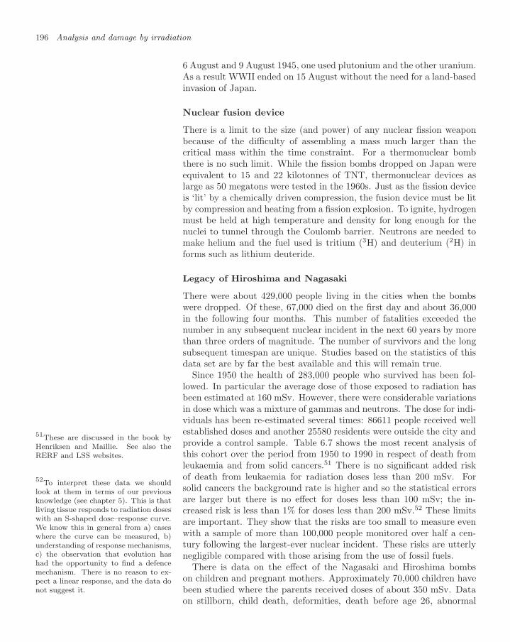
196 Analysis and damage by irradiation
6 August and 9 August 1945, one used plutonium and the other uranium.As a result WWII ended on 15 August without the need for a land-basedinvasion of Japan.
Nuclear fusion device
There is a limit to the size (and power) of any nuclear fission weaponbecause of the difficulty of assembling a mass much larger than thecritical mass within the time constraint. For a thermonuclear bombthere is no such limit. While the fission bombs dropped on Japan wereequivalent to 15 and 22 kilotonnes of TNT, thermonuclear devices aslarge as 50 megatons were tested in the 1960s. Just as the fission deviceis ‘lit’ by a chemically driven compression, the fusion device must be litby compression and heating from a fission explosion. To ignite, hydrogenmust be held at high temperature and density for long enough for thenuclei to tunnel through the Coulomb barrier. Neutrons are needed tomake helium and the fuel used is tritium (3H) and deuterium (2H) informs such as lithium deuteride.
Legacy of Hiroshima and Nagasaki
There were about 429,000 people living in the cities when the bombswere dropped. Of these, 67,000 died on the first day and about 36,000in the following four months. This number of fatalities exceeded thenumber in any subsequent nuclear incident in the next 60 years by morethan three orders of magnitude. The number of survivors and the longsubsequent timespan are unique. Studies based on the statistics of thisdata set are by far the best available and this will remain true.
Since 1950 the health of 283,000 people who survived has been fol-lowed. In particular the average dose of those exposed to radiation hasbeen estimated at 160 mSv. However, there were considerable variationsin dose which was a mixture of gammas and neutrons. The dose for indi-viduals has been re-estimated several times: 86611 people received wellestablished doses and another 25580 residents were outside the city andprovide a control sample. Table 6.7 shows the most recent analysis ofthis cohort over the period from 1950 to 1990 in respect of death fromleukaemia and from solid cancers.51 There is no significant added risk
51These are discussed in the book byHenriksen and Maillie. See also theRERF and LSS websites.
of death from leukaemia for radiation doses less than 200 mSv. Forsolid cancers the background rate is higher and so the statistical errorsare larger but there is no effect for doses less than 100 mSv; the in-creased risk is less than 1% for doses less than 200 mSv.52 These limits
52To interpret these data we shouldlook at them in terms of our previousknowledge (see chapter 5). This is thatliving tissue responds to radiation doseswith an S-shaped dose–response curve.We know this in general from a) caseswhere the curve can be measured, b)understanding of response mechanisms,c) the observation that evolution hashad the opportunity to find a defencemechanism. There is no reason to ex-pect a linear response, and the data donot suggest it.
are important. They show that the risks are too small to measure evenwith a sample of more than 100,000 people monitored over half a cen-tury following the largest-ever nuclear incident. These risks are utterlynegligible compared with those arising from the use of fossil fuels.
There is data on the effect of the Nagasaki and Hiroshima bombson children and pregnant mothers. Approximately 70,000 children havebeen studied where the parents received doses of about 350 mSv. Dataon stillborn, child death, deformities, death before age 26, abnormal
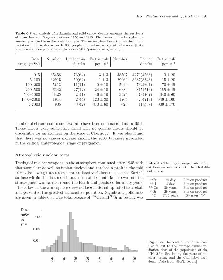
6.5 Nuclear energy and applications 197
Table 6.7 An analysis of leukaemia and solid cancer deaths amongst the survivorsof Hiroshima and Nagasaki between 1950 and 1990. The figures in brackets give thenumber predicted from the control sample. The excess gives the extra risk due to theradiation. This is shown per 10,000 people with estimated statistical errors. [Datafrom www.eh.doe.gov/radiation/workshop2005/presentations/neta.ppt]
Dose Number Leukaemia Extra risk Number Cancer Extra riskrange (mSv) deaths per 104 deaths per 104
0–5 35458 73(64) 3 ± 3 38507 4270(4268) 0 ± 205–100 32915 59(62) −1 ± 3 29960 3387(3343) 15 ± 20
100–200 5613 11(11) 0 ± 10 5949 732(691) 70 ± 45200–500 6342 27(12) 24 ± 10 6380 815(716) 155 ± 45
500–1000 3425 23(7) 46 ± 16 3426 378(262) 340 ± 601000–2000 1914 26(4) 120 ± 30 1764 326(213) 640 ± 100
>2000 905 30(2) 310 ± 60 625 114(58) 900 ± 170
number of chromosomes and sex ratio have been summarised up to 1991.These effects were sufficiently small that no genetic effects should bediscernible for an accident on the scale of Chernobyl. It was also foundthat there was no cancer increase among the 2000 Japanese irradiatedin the critical embryological stage of pregnancy.
Atmospheric nuclear tests
Testing of nuclear weapons in the atmosphere continued after 1945 withthermonuclear as well as fission devices and reached a peak in the mid1960s. Following such a test some radioactive fallout reached the Earth’ssurface within the first month but much of the material thrown into thestratosphere was carried round the Earth and persisted for many years.Tests low in the atmosphere drew surface material up into the fireball
Table 6.8 The major components of fall-out from nuclear tests with their half-lifeand source.
95Zr 64 day Fission product131I 8 day Fission product
137Cs 30 years Fission product90Sr 29 years Fission product14C 5730 years By n on 14N
and generated the greatest radioactive pollution. Significant pollutantsare given in table 6.8. The total release of 137Cs and 90Sr in testing was
0.04
0.08
0.12
1990
1985
1980
1975
1970
1965
1960
1955
Dose
/ Sv
per
year
m
Fig. 6.22 The contribution of radioac-tive fallout to the average annual ra-diation dose of the population of theUK, 2.5m Sv, during the years of nu-clear testing and the Chernobyl acci-dent. [Data from NRPB report]
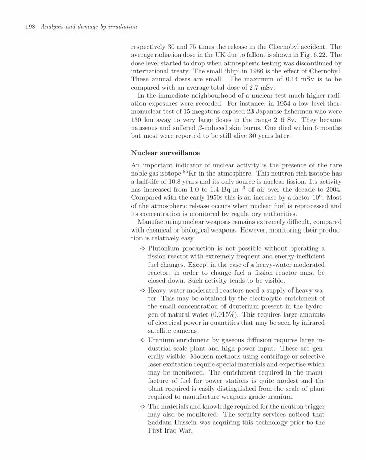
198 Analysis and damage by irradiation
respectively 30 and 75 times the release in the Chernobyl accident. Theaverage radiation dose in the UK due to fallout is shown in Fig. 6.22. Thedose level started to drop when atmospheric testing was discontinued byinternational treaty. The small ‘blip’ in 1986 is the effect of Chernobyl.These annual doses are small. The maximum of 0.14 mSv is to becompared with an average total dose of 2.7 mSv.
In the immediate neighbourhood of a nuclear test much higher radi-ation exposures were recorded. For instance, in 1954 a low level ther-monuclear test of 15 megatons exposed 23 Japanese fishermen who were130 km away to very large doses in the range 2–6 Sv. They becamenauseous and suffered β-induced skin burns. One died within 6 monthsbut most were reported to be still alive 30 years later.
Nuclear surveillance
An important indicator of nuclear activity is the presence of the rarenoble gas isotope 85Kr in the atmosphere. This neutron rich isotope hasa half-life of 10.8 years and its only source is nuclear fission. Its activityhas increased from 1.0 to 1.4 Bq m−3 of air over the decade to 2004.Compared with the early 1950s this is an increase by a factor 106. Mostof the atmospheric release occurs when nuclear fuel is reprocessed andits concentration is monitored by regulatory authorities.
Manufacturing nuclear weapons remains extremely difficult, comparedwith chemical or biological weapons. However, monitoring their produc-tion is relatively easy.
Plutonium production is not possible without operating afission reactor with extremely frequent and energy-inefficientfuel changes. Except in the case of a heavy-water moderatedreactor, in order to change fuel a fission reactor must beclosed down. Such activity tends to be visible.
Heavy-water moderated reactors need a supply of heavy wa-ter. This may be obtained by the electrolytic enrichment ofthe small concentration of deuterium present in the hydro-gen of natural water (0.015%). This requires large amountsof electrical power in quantities that may be seen by infraredsatellite cameras.
Uranium enrichment by gaseous diffusion requires large in-dustrial scale plant and high power input. These are gen-erally visible. Modern methods using centrifuge or selectivelaser excitation require special materials and expertise whichmay be monitored. The enrichment required in the manu-facture of fuel for power stations is quite modest and theplant required is easily distinguished from the scale of plantrequired to manufacture weapons grade uranium.
The materials and knowledge required for the neutron triggermay also be monitored. The security services noticed thatSaddam Hussein was acquiring this technology prior to theFirst Iraq War.

6.5 Nuclear energy and applications 199
These points have prevented the proliferation of weapons in the past inmany cases at least. However, when weapons production is detected,political decisiveness is required to act on this information.
6.5.3 Nuclear power and accidents
Windscale and Three Mile Island accidents
There have been rather few major nuclear accidents. We discuss thethree best known, Windscale (1957), Three Mile Island (1979) and Cher-nobyl (1986).
The Windscale case was caused by a build-up of unstable potentialenergy in the graphite moderator.53 The result was a chemical fire in the 53See section 3.2.4.
reactor core. Radioactive debris was released into the local environmentalthough the heat was not sufficiently intense to propel it into the upperatmosphere. The most serious immediate consequence was that 6 ×10¹⁴ Bq of 131I contaminated the atmosphere, food supplies and localagriculture. This caused 260 cases of thyroid cancer, 13 of them fatal.Children were particularly at risk because they absorb more iodine thanadults while they are growing. The highest thyroid dose was calculatedto be 160 mGy. The full extent of the disaster was covered up until 1983.When revealed, the fact that this cover-up occurred seriously damagedthe long-term credibility of official information about nuclear accidents.
The Three Mile Island accident was caused by human failure. Theoverheated and damaged reactor core did not release a significant quan-tity of radiation into the environment. However, there was a misunder-standing, a scare and a loss of public confidence in the nuclear industryto oversee the routine operation of nuclear power plants.
Chernobyl accident
The cause of the Chernobyl accident was a combination of human andmanagement failure with a seriously inadequate reactor design.54 An un- 54There is an authoritative interna-
tional OECD NEA report on the acci-dent which may be found on their web-site; see the list at the end of chapter 1.
regulated ‘test’ caused a loss of cooling water, then a fire of the graphitemoderator. This was followed by a chemical explosion which blew thetop off the reactor. The heat propelled the more volatile contents ofthe reactor high into the atmosphere. The accident occurred just asthe Soviet Union was itself becoming unstable, and contributed to thatdisintegration as well as being partly caused by it.
Table 6.9 gives details of the activity released. There are the neutron-rich fission product nuclei and also the transuranic elements, neptuniumplutonium and curium, formed by neutron absorption and β-decay fromthe uranium fuel. The volatile elements were all released into the en-vironment, the xenon and most of the iodine, caesium and tellurium.Most of the heavy transuranic elements remained in the reactor. Thehazard posed by each nuclide is determined by its lifetime as well asits initial activity. Chemical and biological affinity are also important.Thus xenon is not absorbed and decays in the atmosphere, but iodine isingested and taken up by the thyroid gland.
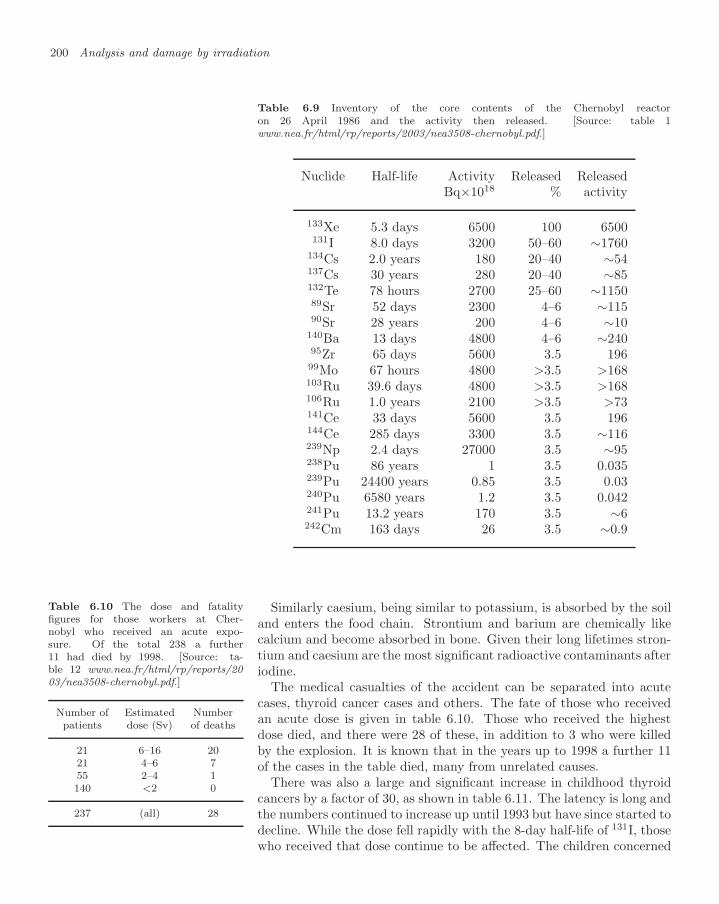
200 Analysis and damage by irradiation
Table 6.9 Inventory of the core contents of the Chernobyl reactoron 26 April 1986 and the activity then released. [Source: table 1www.nea.fr/html/rp/reports/2003/nea3508-chernobyl.pdf.]
Nuclide Half-life Activity Released ReleasedBq×1018 % activity
133Xe 5.3 days 6500 100 6500131I 8.0 days 3200 50–60 ∼1760
134Cs 2.0 years 180 20–40 ∼54137Cs 30 years 280 20–40 ∼85132Te 78 hours 2700 25–60 ∼115089Sr 52 days 2300 4–6 ∼11590Sr 28 years 200 4–6 ∼10
140Ba 13 days 4800 4–6 ∼24095Zr 65 days 5600 3.5 19699Mo 67 hours 4800 >3.5 >168103Ru 39.6 days 4800 >3.5 >168106Ru 1.0 years 2100 >3.5 >73141Ce 33 days 5600 3.5 196144Ce 285 days 3300 3.5 ∼116239Np 2.4 days 27000 3.5 ∼95238Pu 86 years 1 3.5 0.035239Pu 24400 years 0.85 3.5 0.03240Pu 6580 years 1.2 3.5 0.042241Pu 13.2 years 170 3.5 ∼6242Cm 163 days 26 3.5 ∼0.9
Similarly caesium, being similar to potassium, is absorbed by the soiland enters the food chain. Strontium and barium are chemically likecalcium and become absorbed in bone. Given their long lifetimes stron-tium and caesium are the most significant radioactive contaminants afteriodine.
Table 6.10 The dose and fatalityfigures for those workers at Cher-nobyl who received an acute expo-sure. Of the total 238 a further11 had died by 1998. [Source: ta-ble 12 www.nea.fr/html/rp/reports/2003/nea3508-chernobyl.pdf.]
Number of Estimated Numberpatients dose (Sv) of deaths
21 6–16 2021 4–6 755 2–4 1140 <2 0
237 (all) 28
The medical casualties of the accident can be separated into acutecases, thyroid cancer cases and others. The fate of those who receivedan acute dose is given in table 6.10. Those who received the highestdose died, and there were 28 of these, in addition to 3 who were killedby the explosion. It is known that in the years up to 1998 a further 11of the cases in the table died, many from unrelated causes.
There was also a large and significant increase in childhood thyroidcancers by a factor of 30, as shown in table 6.11. The latency is long andthe numbers continued to increase up until 1993 but have since started todecline. While the dose fell rapidly with the 8-day half-life of 131I, thosewho received that dose continue to be affected. The children concerned

6.5 Nuclear energy and applications 201
Table 6.11 Data on cases of child thyroid cancers by year, then aged up to 15,showing the steep rise from 1986 as a result of the Chernobyl accident. The upperrows show the number of cases. The lower rows show the numbers normalised per100,000 of the whole population. At the time the table was compiled 3 of these 1036children had died. [Source: table 13 www.nea.fr/html/rp/reports/2003/nea3508-chernobyl.pdf.]
Year 86 87 88 89 90 91 92 93 94 95 96 97 98
Belarus 3 4 6 5 31 62 62 87 77 82 67 73 48Ukraine 8 7 8 11 26 22 49 44 44 47 56 36 44Russia 0 1 0 0 1 1 3 1 6 7 2 5 0Total 11 12 14 16 58 85 114 132 127 136 125 114 92
Belarus 0.2 0.3 0.4 0.3 1.9 3.9 3.9 5.5 5.1 5.6 4.8 5.6 3.9Ukraine 0.2 0.1 0.1 0.1 0.2 0.2 0.5 0.4 0.4 0.5 0.6 0.4 0.5Russia 0.3 0.3 0.3 0.9 0.3 2.8 3.5 0.6 2.2
are now adult. Up to 1995, 3 out of 1036 children with thyroid cancerhad died. The incidence is high because the most elementary precautionswere not taken by the population in the days immediately following theaccident. There was also an increase of adult thyroid cancers.
Table 6.12 Distribution of estimated to-tal effective doses received by the pop-ulations of contaminated areas (1986–1995) excluding dose to thyroid [Source:table 10 www.nea.fr/html/rp/reports/2003/nea3508-chernobyl.pdf.]
Dose NumbermGy Belarus Russia Ukraine
<1 133053 1553015 1163490 1253130 33090020 439620 474176 80790050 113789 82876 148700100 25065 14580 7700200 5105 2979 400>200 790 333
Table 6.12 shows that the numbers of people receiving a dose of 100–200 mSv and more than 200 mSv are 1123 and 8124, respectively.55
55These dose profiles are coarselybinned but there are large errors onthe Hiroshima and Nagasaki data too.Whatever, the predicted fatalities arefew compared with risks associatedwith climate change.
Using the Hiroshima and Nagasaki data (the fourth and last columnsof table 6.7) we may estimate that an extra 40–120 of these may diefrom solid cancer caused by the radiation in the next 50 years; thenumber of extra deaths from leukaemia would be less than 5. In theChernobyl data themselves there is no clear evidence for anomalous ratesof leukaemia, genetic disorders or forms of cancer other than thyroid.Any such evidence would be buried by the statistical noise on the largerincidence of cancers that occur in any population. In addition there aresystematic effects arising from the social dislocation and panic causedby the accident itself.
As a result of the accident land became contaminated by 90Sr and137Cs. How can radioactive contamination over a large area be ‘cleanedup’? It can be concentrated, stored and managed; it can be diluted anddispersed into the wider environment; or it can be left where it is. Highlevels of radioactivity may best be concentrated and managed, but overwide areas the only practical solution is dispersal, ensuring as much aspossible that contamination does not enter the food chain. This meansdiluting the caesium with massive applications of potassium fertiliserto the land. This exploits the chemical similarity between caesium andpotassium. Similarly the agricultural uptake of strontium and bariumis minimised by a heavy application of calcium in the form of lime.
The same dilution technique should be used to minimise the incidence

202 Analysis and damage by irradiation
of thyroid cancer. Following a radiation accident those exposed shouldtake an excess of normal iodine for 2–3 weeks.56 This excess reduces the56It can be taken orally in the form of
tablets. uptake of radioactive 131I which has a half-life of 8 days. After a fewweeks the iodine has decayed and the thyroid risk is passed. Indeedthe best advice in the event of a nuclear accident is ‘don’t go out in therain’, for rain concentrates the fallout, and ‘take iodine tablets’. No suchadvice was given to the population affected by the Chernobyl incident.
Management of nuclear waste
High level nuclear waste is managed and concentrated while low levelwaste is dispersed. The dispersal should be to safe levels,57 so that57The expense of nuclear power de-
pends in large measure on just how lowsuch safe levels need to be. This is con-sidered critically in chapter 10.
there are no further cost, health or security implications. High level nu-clear waste comes from weapon stockpiles, spent fuel elements, decom-missioned reactors and used medical and industrial radioactive sources.Compared with high toxicity chemical waste the volumes of materialare small. It is difficult but technically possible to ‘burn up’ nuclearwaste. This is called transmutation and references to this may be foundon the Web. In the absence of such a process high level nuclear wastemust be stored securely and records maintained to avoid its inadvertentdispersal.
The scale of the problem of waste from nuclear power stations may bejudged from the following figures. In January 2005 there were reportedto be some 440 operating commercial nuclear power stations world-widewith generating capacity of some 364 GW. A typical light-water-reactorpower station generates 20 tonnes of spent fuel in the process of deliv-ering 6.6 × 10⁹ kWh of electricity.58 This waste occupies 11 m3. At full58This is about 1 GW-year. An equiv-
alent coal power station would burn2×106 tonnes of coal releasing 5.4×10⁶
tonnes of CO2 into the atmosphere(and 0.05×10⁶ tonnes of SO2, leaving0.12×106tonnes of ash). The mass ofnuclear waste is smaller by a factor of10,000. The environmental impact issmall compared with the effect of theCO2 on the climate.
capacity each year the world’s nuclear power stations would generate8000 tonnes of spent fuel with volume about 4000 m3. This is small.
The public perception is that the physical storage is a serious diffi-culty, and that no storage exists with an integrity on a sufficiently longtimescale. That this is not correct can be illustrated by the Oklo re-actor. In 1972 it was found that the ratio of 235U to 238U from thisuranium mine in Gabon, Africa, was only 50% of the value elsewhere.The fission products found there have been used to show that, about 1.7billion years ago when the isotope ratio was 3% and this rock was beingformed, the 235U went critical and induced fission occurred, moderatedby water bound in the minerals. The energy generated was about 15GW years, and over a considerable time a large fraction of the 235U wasburnt up, thus generating the anomalous uranium isotopic ratio foundtoday. The important point for the waste storage question is that thetell-tale waste fission products have not moved significantly in 1.7 billionyears. They remain quite secure. Indeed the Earth has always had asignificant content of radioactivity, more or less widely dispersed. A fewdeep dry storage locations built by humans will be a tiny addition. In afew locations natural radioactivity is leached out of the Earth by ground-water. Far from being shunned by the public, fashionable spas59 have59For instance, the Roman city of
Bath, popular to this day. been built at such places and have proved both popular and harmless.
6.5 Nuclear energy and applications 203
In total, by the middle of the twenty-first century the accumulated highlevel nuclear waste requiring long term storage would be about 0.1×10⁶
tonnes, or 5×10⁴ m3. This assumes nuclear power stations operating at150 GW, with realistic levels of recycling.60 60In January 2006 there were 10 nu-
clear power stations under constructionin OECD countries (Korea, Japan, Slo-vakia and Finland) with another 17 onorder.
Many incidents have arisen from poor record keeping, especially inthe less stable conditions that can occur in the Third World. In 1987 inBrazil a 137Cs source of 50 TBq from an abandoned radiation medicaltherapy unit was broken open in a scrap-metal yard: 244 people werecontaminated, 20 were taken seriously ill and 4 died.
In 1983 a radiotherapy device containing 15 TBq was taken from awarehouse where it had been stored. Two steel foundries in Mexico andone in the USA handled the scrap producing 4000 tonnes of radioactivesteel that was used to make table legs and building reinforcements. Over100 people received doses between 10–500 mSv, and some over 15 Sv overa period of several months. These instances show how nuclear materialputs a heavy burden on society in the areas of record keeping, labelling,expertise, education, regulation and political continuity.
Only about 50% of the available fissile nuclear fuel is ‘burnt’ in areactor before the fuel rods must be withdrawn, otherwise their chemicaland structural integrity would become dangerous. Natural uranium isenriched somewhat (0.7% to 3.5%) for a light water reactor; 100 tonnesof such fuel will keep a 1 GW power reactor running for three years.When such a reactor is shut down, the primary chain reaction is haltedand the fuel withdrawn. However, the daughter nuclear decay processescontinue. After 10 days the fuel emits 60 MW, after 1 year 1 MW,after 100 years 40 kW. For this reason, for a number of years spentfuel must be concentrated, stored, managed and cooled. It is usuallykept under water in large tanks. Since the mass is not that large this isquite practical. Currently 10% is reprocessed but this is only economicif the reprocessed fuel is needed. This may be carried out at Sellafieldin the UK or at two plants in France. The advantages of keeping wasteconcentrated in one place are that its history and location are known.However, it remains a responsibility and a security risk. When it nolonger needs active cooling it may be vitrified and set in concrete. Thenit may be stored in dry caverns. The task of reactor de-commissioningwill become somewhat easier with the advent of more advanced robotics.And significantly cheaper with more realistic safety assessments.
Modern nuclear power stations are much safer than the old Sovietdesign built at Chernobyl and ‘burn up’ a greater proportion of theirfuel. In addition there is the reassuring expectation that power fromcontrolled nuclear fusion will be available by the middle of the twenty-first century. Such power involves no chain reaction, no risk of explosion,and no creation of radioactive daughter products with long lifetimes.Making such power available to the Third World will be a challenge tofuture statesmen.

204 Analysis and damage by irradiation
Read more in books
Detectors for Particle Radiation, K Kleinknecht, Cam-bridge (1986), a text on radiation detectors
Nuclear Physics, Principles and Applications, Manch-ester Physics Series, J Lilley, Wiley (2001), a textbookcovering applications of nuclear physics
Chemical Analysis by Nuclear Methods, ed. ZB Alfassi,Wiley (1994), an edited compilation of articles on anal-ysis techniques using nuclear methods
Tracing Noble Gas Radionuclides in the Environment,P Collon et al, Annual Reviews of Nuclear and ParticleScience 54,39 (2004), a review exemplifying the infor-mation available from studies of isotope distributions
Medical Physics & Biomedical Engineering, BH Brownet al, IOP (1999), a standard text on medical physics
The Physics of Medical Imaging, ed. S Webb, IOP(1988), an edited compilation of useful articles, some-what out of date but still frequently referenced.
Radiation & Health, T Henriksen and HD Maillie, Tay-lor & Francis (2003), a highly readable general text onradiation and health
Radiation and Radioactivity on Earth and Beyond, IGDragonic, ZD Dragonic and J-P Adloff, CRC Press(1993), a wide-ranging descriptive book
Science-based Dating in Archaeology, MJ Aitken, Ad-dison Wesley Longman (1990), a readable physics texton scientific dating in archaeology
Archaeology: Theories, Methods and Practice, C Ren-frew and P Bahn, Thames & Hudson, 4th edn (2004),a textbook on scientific methods in archaeology
The Solid Earth, CMR Fowler, Cambridge (1990), atextbook on geology and geophysics
Look on the Web
Look at the book website atwww.physics.ox.ac.uk/users/allison/booksite.htm
Find out how radiation is used to manipulate thebehaviour of plastics, including shrink-wrap film, bysearching on
polymer memory electron beam
Keep abreast of developments in radiation detectortechnology
PMT, APD, CCD, HPD, amorphous silicon, CdTe
Follow further developments in analytical and datingtechniques
XRF, SPM, PIXE, RBS, NAA, AMS
Check for nuclei with specific decays, lifetimes and otherproperties by consulting
nuclear data BNL
Watch the growth in availability of synchrotron radia-tion sources (SR)
synchrotron light
Study the known data on Hiroshima and Nagasaki, andon Chernobyl, by searching the websites of the author-ities listed at the end of chapter 1
Take a look at papers on the incidence of radon-inducedlung cancers and other studies
bmj.com/cgi/content/full/330/7485/223www.hps.org/publicinformation/ate/q1254.htmlIAEA Urals soviet accident
Look up about the transmutation of nuclear wastetransmutation nuclear waste
Read about sterilisation with radiationsterilisation radiation medicalsterilisation radiation food
6.5 Nuclear energy and applications 205
Questions
6.1 Calculate the number of 14C atoms detected froma ‘modern’ 1 mg sample of carbon assuming 100%detection efficiency, (a) in an experiment countingthe beta decays over a period of four weeks, and (b)in an accelerator mass spectrometer measurement.
6.2 Calculate the statistical error on the measured ageof a 1 mg sample as determined by the methods ofquestion 6.1 if the age is about 3000 years, and if itis about 40000 years. Calculate the systematic biasof the age determination caused by a contaminationof 1% modern carbon.
6.3 The proportion of 14C in living tissue is about10−12 and its half-life is 5730 years. It decays to14N emitting an electron with maximum energy156 keV. Calculate the associated internal radia-tion dose to the body in Sv making appropriateassumptions where necessary.
6.4 In the decay of 40K, see Fig. 6.15, both possibledaughter nuclei, 40Ar and 40Ca, have an even num-ber of both neutrons and protons, and thereforeJ = 0. Consider the dominant decay mode
40K →40 Ca + e− + ν.
The parent 40K has angular momentum J = 4, so∆J = 4. Calculate the ratio of decay rates for thisβ-decay to that for the neutron (half-life 614 s, en-ergy 0.78 MeV with ∆J = 1),
n → p + e− + ν.
Compare the value of this suppression factor withthat for the EM decay of multipolarity ∆J = 4and wavelength λ of a nucleus of radius a,(2πa/λ)2∆J−2, discussed in section 8.3.1.[The same angular momentum effect is responsiblefor the suppression, although in one case it is aweak nuclear process and in the other an electro-magnetic one.]
6.5 A beam of 3 MeV alpha particles is incident ona flat surface. The energy spectrum of the back-scattered alpha particles consists of a continuousdistribution up to 1.693 MeV, and a sharp peak at2.766 MeV. What can be deduced about the struc-ture and composition of the surface?
6.6 Derive the non-relativistic RBS relation for themass ratio of target-to-beam
M
µ=
E + E′ − 2√
EE′ cos θ
E − E′
in terms of the incident energy E, the scattered en-ergy E′ and the laboratory scattering angle θ.Deduce the relation at 180 given by equation 6.4.For what range of θ is that an adequate approxi-mation for the determination of M to within 10%?
6.7 a) The decay of 40K to 40Ar has a Q-value of 1.5MeV. In most cases this energy is released as aγ-ray. Calculate the recoil kinetic energy of theresidual 40Ar nucleus.
b) In the α-decay of 226Ra to 222Rn the energyrelease is 4.87 MeV. Calculate the nuclear recoilenergy of the residual 222Rn nucleus.
Hence comment on the fact that the 40Ar productmay be trapped in rock for millions of years (allow-ing its formation to be dated) but that radon seepsout of rock on a timescale short compared with itshalf-life of 3.82 days.

This page intentionally left blank

Imaging with magneticresonance 7
7.1 Magnetic resonance imaging207
7.2 Functional magnetic reso-nance imaging 221
Read more in books 230
Look on the Web 230
Questions 231
in which the analysis, strengths and limitations of MRI methods inmedicine are explored.
7.1 Magnetic resonance imaging
In MRI field gradients are used to encode spatial information into NMR.The fields of the gradient coils select a slice by excitation, and label avoxel within that slice by its phase and frequency. Because the signalsare linear, a superposition from many voxels may be decoded by Fourierinversion. However, an image is never an exact copy of the related object.In MRI it may fall short in three ways: limited resolution, random noiseand the presence of artefacts. As in other applications of Fourier optics,artefacts are generated as a result of incomplete sampling in k-space. MRIdata acquisition, that is the sampling of k-space, can be made faster inthree ways: the interleaving of data acquisition from different slices, theuse of complete scans of kx, ky with a single excitation pulse, and the useof arrays of pickup coils. Each such method has its drawbacks. These arearguably the most important strategies, but there are others not discussedhere.
7.1.1 Spatial encoding with gradients
Gradient coils
By applying different gradients to the B0 field in the x-, y- and z- di-rections at different times, it is possible to determine a complete threedimensional map of the nuclear spin density in the region of interest.This region is called the field of view (FOV). Figure 7.1 shows how such
B0
Fig. 7.1 Gradient coils giving a gra-dient of B0 in the z direction, shownhorizontal. The coils and current floware shown with heavy lines. The B-fieldlines are shown lighter.
a uniform gradient may be applied along the z-axis with a pair of coils.If the current in the two coils is in the opposite sense to one another, thisgenerates a uniform gradient along z, the axis of symmetry. Departuresfrom uniformity are minimised by adjusting the ratio of coil diameter totheir separation, so that, on axis at least, departures are of order (z/a)4
where a is the coil size. Uniformity is improved by making the coilslarge, and by arranging the geometry of further windings to ensure thathigher polynomials contributing to the field variation are zero.
The coil geometry can conform easily to the bore of the NMR B0
solenoid. A finite field gradient in z (∂Bz/∂z) must still satisfy Gauss’s

208 Imaging with magnetic resonance
law,∂Bx
∂x+
∂By
∂y+
∂Bz
∂z= 0, (7.1)
and therefore unwanted radial B-field components must be present.B0
Fig. 7.2 Saddle-shaped gradient coilsgiving a gradient of B0 in the trans-verse vertical direction. The four coilswith their current flow are shown withheavy lines. The B-field lines areshown lighter. The geometry allowsunrestricted access in the horizontal z-direction.
However, although these will tip the direction of the field slightly as afunction of z, they have only a second order effect on the magnitude ofthe field, and it is the latter to which the FID is sensitive. It is importantto appreciate that the gradients are small. Typically the value of Bz isvaried by up to 1 part in 104, while the chemical shifts in precessionfrequency correspond to about a part in 106. The x- and y-terms inequation 7.1 are therefore negligible.
In the x- and y-directions gradients of Bz can provided by sets of coils.However, the coil design has to be different because access to the magnetvolume is required along the z-axis. So these coils have to conform tothe cylindrical geometry of the main static B0 solenoidal magnet. Therequired set of four saddle-shaped coils is shown in Fig. 7.2. The y-coilsare similar to those for x, being related by a 90 rotation about z.
RF pulse shape and slice selection
Consider a problem in which there is just one voxel containing spins atposition (x, y, z). How can we measure this position? The first step inposition encoding is to select a thin slice in z by applying the initial RFpulse with a frequency ω in the presence of a uniform z-gradient. Whenthis is done, only those nuclei in a narrow range of z will have the rightLarmor frequency to be excited by the pulse, and therefore to contributeto the subsequent FID signal. Thus
ω = γ
(B0 +
∂Bz
∂zz
). (7.2)
By applying an RF pulse of a different frequency in the presence of az-gradient field, different slices in z may be excited. If the observedamplitude of the FID is plotted out as a function of RF frequency, thez-value of the voxel occupied by the spins would be seen.
Δt
Δω
a)
b)
ω0
Fig. 7.3 a) The RF pulse in time show-ing the Larmor frequency modulated bya sinc function, as required to give b),the rectangular frequency distributionfor sharp slice selection in z in the pres-ence of a uniform B-field gradient in z.
Before moving on to measurements in x and y we need to be a little bitmore precise about this process for selecting spins in z. The thicknessof the selected slice depends on the field gradient and the bandwidth ofthe RF pulse. In a uniform field gradient there is a one-to-one relationbetween z and frequency ω. So, to excite spins in a sharply defined slicein z, a pulse with a rectangular frequency distribution is required, asshown in Fig. 7.3b. The corresponding time modulation of the amplitudeof the RF is shown in Fig. 7.3a. This is the Fourier transform of therectangular pulse, and the same problem mathematically that occurs inFraunhofer diffraction from a sharp slit. The functional form of the timemodulation is
sin(2πt/∆t)t
, (7.3)
where the main peak is bounded by ±∆t/2. The shorter the bunch mod-ulation ∆t, the larger the frequency slice ∆ω and therefore the thicker

7.1 Magnetic resonance imaging 209
the slice ∆z. Quantitatively
∆t−1 =∆ω
4π=
14π
γ∂Bz
∂z∆z. (7.4)
In this way, with a certain gradient the choice of central frequencyand bandwidth determine the excited slice position and thickness re-spectively.
RF
dB /dzz
dB /dxz
dB /dyz
FID1
FID2
time
A B C D
tC
< t >'
Fig. 7.4 A pulse sequence using allthree gradient coils to encode the x, y, zspin density into the two orthogonalFID signals.
Gradient refocus in slice
To measure the position in x and y as well as z, coils providing inde-pendent gradients along all three axes are required. Figure 7.4 shows asimple pulse sequence as a function of time from left to right. On thefirst line is shown the applied RF waveform, on the next three lines theswitched currents applied to the three gradient coils, and in the lowesttwo lines the detected FID signals picked up by coils in the xz- andyz-planes. Following the RF pulse, the spins within the slice will con-tribute towards a potential FID signal. However, the field varies withinthe slice because of the applied z-gradient. The spins in the differentdepths within the slice will get progressively dephased. To counteractthis, not only is the z-gradient switched off, but it is reversed for a time,such that afterwards, all spins within the slice have seen the same timeintegral of B-field; that is, they will have precessed through the sameangle, at least as far as the effect of the z-gradient is concerned. This isshown on the second trace of Fig. 7.4. This unwinding of gradient-relateddephasing is called gradient refocusing. Unlike the spin echo discussed

210 Imaging with magnetic resonance
in chapter 2, this only compensates for the field variation coming fromthe applied gradients.
Spatial encoding by frequency measurement
The two FID signals shown in Fig. 7.4 are digitised and read out inthe interval BD. During this readout time a steady gradient of Bz inthe x-direction is applied. Therefore, if the single occupied voxel thatwe are considering lies in the excited slice, it will give a FID signalwhose frequency indicates its x-position. The application of the reversegradient during the period AB is such that there is a gradient echo attime tc, in the middle of the readout interval.1 Within this gate the1In general at this time the FIDs of all
voxels in the slice are in phase. FID traces generated by the two orthogonal magnetic fluxes due to therotating spins in the particular voxel at x are
cos[γ
(B0 +
∂Bz
∂xx
)(t − tc)
]and sin
[γ
(B0 +
∂Bz
∂xx
)(t − tc)
].
(7.5)
Linear superposition of signals
Now we come to a small but important step in the argument. Since thecontribution of spins to the FID is linear, if we have a distribution ofspins f(x), the FIDs will be given by a simple linear superposition
F1(t) =∫
f(x) cos[γ
(B0 +
∂Bz
∂xx
)(t − tc)
]dx (7.6)
F2(t) =∫
f(x) sin[γ
(B0 +
∂Bz
∂xx
)(t − tc)
]dx.
We compare the equations (7.6) with the standard form for a Fouriertransform, equation 5.3, in the form
g1(kx) =1√2π
∫f(x) cos(kxx) dx (7.7)
g2(kx) =1√2π
∫f(x) sin(kxx) dx.
We observe that with a suitable normalisation and definition of kx thesetwo functions (7.6) represent the real and imaginary parts of the complexFourier transform of f(x). The role of kx in the trigonometric factorscos(kxx) and sin(kxx) is taken by γ(∂Bz/∂x)(t − tc). It is the spindensity f(x) that we want to determine. This is proportional to theinverse Fourier transform of the FID, F1 + iF2.
Spatial encoding by phase
With the pulse sequence as discussed so far, the relative phase of allvoxels at time tc is zero. The remaining unmeasured coordinate y canbe resolved by giving the signals from each voxel a phase shift between−π and π that depends linearly on its y-position. We therefore apply

7.1 Magnetic resonance imaging 211
a y-gradient ∂Bz/∂y for a fixed short length of time ∆t′ before thereadout gate as shown in Fig. 7.4. This results in an additional phaseγy∆t′(∂Bz/∂y), linearly dependent on y. The multiple lines shown forthe size of the y gradient in the figure are intended to indicate that FIDsare recorded for a whole sequence of different values of this gradient. Thetwo orthogonal FID signals are related to the spin density f(x, y) in theexcited slice by2 2The two independent FID signals
could be read by two coils at right an-gles. In practice they are deduced fromthe magnitude and phase of the signalsinduced in the birdcage coil or other de-tector coils used.
F1(t) =∫ ∫
f(x, y) cos[γ
(B0 +
∂Bz
∂xx
)(t − tc) + γ
∂Bz
∂yy∆t′
]dxdy
F2(t) =∫ ∫
f(x, y) sin[γ
(B0 +
∂Bz
∂xx
)(t − tc) + γ
∂Bz
∂yy∆t′
]dxdy.
(7.8)
Spatial reconstruction by Fourier transformation
These are the real and imaginary parts of the two dimensional complexFourier transform of the spin density f(x, y). To invert this transformand obtain f(x, y) it must be measured everywhere in k-space. Thenideally
f(x, y) =1
(2π)2
∫ ∫(F1 + iF2) exp[−i(kxx + kyy)] dkxdky (7.9)
with kx = γ(∂Bz/∂x)(t − tc) as before and ky = γ(∂Bz/∂y)∆t′.These two k-vector components differ only in that, for kx, the gradi-
ent is fixed and the time t varies, while for ky the gradient is varied insequential scans and the time interval ∆t′ is fixed. This distinction ispeculiar to the particular choice of simplified pulse sequence we intro-duced in Fig. 7.4. For a general pulse sequence the (kx, ky)-vector is the(x, y)-derivative of the phase accumulated between the excitation of thetransverse magnetisation and the read time,
kx =∫ read time
RF pulse time
γ∂Bz
∂xdt (7.10)
ky =∫ read time
RF pulse time
γ∂Bz
∂ydt.
Of course we cannot measure the transform at all values of (kx, ky).The best that we can do in practice is to sample the FID signal at asequence of nx discrete times in the interval BD and repeat the wholesequence for ny discrete values of ∂Bz/∂y. This restricted informationgenerates the artefacts discussed in general in chapter 5.
7.1.2 Artefacts and imperfections in the image
Limited resolution
The reconstructed image may not show the fine detail of the object.This is related to the values of the Fourier transform at high k. If the
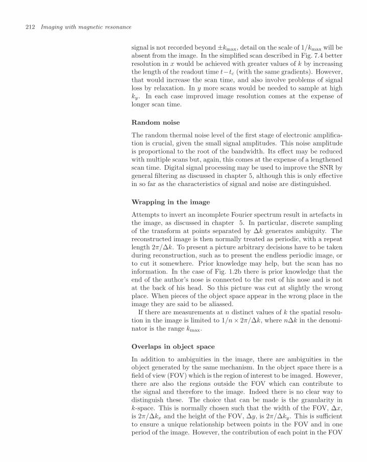
212 Imaging with magnetic resonance
signal is not recorded beyond ±kmax, detail on the scale of 1/kmax will beabsent from the image. In the simplified scan described in Fig. 7.4 betterresolution in x would be achieved with greater values of k by increasingthe length of the readout time t−tc (with the same gradients). However,that would increase the scan time, and also involve problems of signalloss by relaxation. In y more scans would be needed to sample at highky. In each case improved image resolution comes at the expense oflonger scan time.
Random noise
The random thermal noise level of the first stage of electronic amplifica-tion is crucial, given the small signal amplitudes. This noise amplitudeis proportional to the root of the bandwidth. Its effect may be reducedwith multiple scans but, again, this comes at the expense of a lengthenedscan time. Digital signal processing may be used to improve the SNR bygeneral filtering as discussed in chapter 5, although this is only effectivein so far as the characteristics of signal and noise are distinguished.
Wrapping in the image
Attempts to invert an incomplete Fourier spectrum result in artefacts inthe image, as discussed in chapter 5. In particular, discrete samplingof the transform at points separated by ∆k generates ambiguity. Thereconstructed image is then normally treated as periodic, with a repeatlength 2π/∆k. To present a picture arbitrary decisions have to be takenduring reconstruction, such as to present the endless periodic image, orto cut it somewhere. Prior knowledge may help, but the scan has noinformation. In the case of Fig. 1.2b there is prior knowledge that theend of the author’s nose is connected to the rest of his nose and is notat the back of his head. So this picture was cut at slightly the wrongplace. When pieces of the object space appear in the wrong place in theimage they are said to be aliassed.
If there are measurements at n distinct values of k the spatial resolu-tion in the image is limited to 1/n× 2π/∆k, where n∆k in the denomi-nator is the range kmax.
Overlaps in object space
In addition to ambiguities in the image, there are ambiguities in theobject generated by the same mechanism. In the object space there is afield of view (FOV) which is the region of interest to be imaged. However,there are also the regions outside the FOV which can contribute tothe signal and therefore to the image. Indeed there is no clear way todistinguish these. The choice that can be made is the granularity ink-space. This is normally chosen such that the width of the FOV, ∆x,is 2π/∆kx and the height of the FOV, ∆y, is 2π/∆ky. This is sufficientto ensure a unique relationship between points in the FOV and in oneperiod of the image. However, the contribution of each point in the FOV
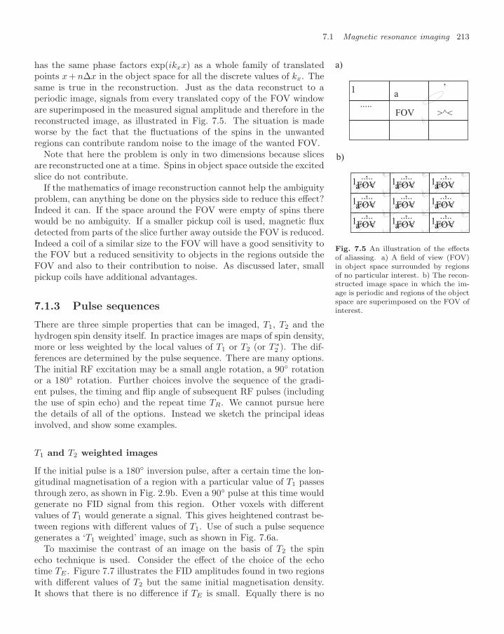
7.1 Magnetic resonance imaging 213
has the same phase factors exp(ikxx) as a whole family of translatedpoints x+ n∆x in the object space for all the discrete values of kx. Thesame is true in the reconstruction. Just as the data reconstruct to aperiodic image, signals from every translated copy of the FOV windoware superimposed in the measured signal amplitude and therefore in thereconstructed image, as illustrated in Fig. 7.5. The situation is madeworse by the fact that the fluctuations of the spins in the unwantedregions can contribute random noise to the image of the wanted FOV.
1
1
111
1 1 1
11
.....
.....
...............
..... ..... .....
..........
a
a
aaa
a a a
aa
FOV
FOV
FOVFOVFOV
FOV FOV FOV
FOVFOV
,
,
,,,
, , ,
,,
>^<
>^<
>^<>^<>^<
>^< >^< >^<
>^<>^<
a)
b)
Fig. 7.5 An illustration of the effectsof aliassing. a) A field of view (FOV)in object space surrounded by regionsof no particular interest. b) The recon-structed image space in which the im-age is periodic and regions of the objectspace are superimposed on the FOV ofinterest.
Note that here the problem is only in two dimensions because slicesare reconstructed one at a time. Spins in object space outside the excitedslice do not contribute.
If the mathematics of image reconstruction cannot help the ambiguityproblem, can anything be done on the physics side to reduce this effect?Indeed it can. If the space around the FOV were empty of spins therewould be no ambiguity. If a smaller pickup coil is used, magnetic fluxdetected from parts of the slice further away outside the FOV is reduced.Indeed a coil of a similar size to the FOV will have a good sensitivity tothe FOV but a reduced sensitivity to objects in the regions outside theFOV and also to their contribution to noise. As discussed later, smallpickup coils have additional advantages.
7.1.3 Pulse sequences
There are three simple properties that can be imaged, T1, T2 and thehydrogen spin density itself. In practice images are maps of spin density,more or less weighted by the local values of T1 or T2 (or T ∗
2 ). The dif-ferences are determined by the pulse sequence. There are many options.The initial RF excitation may be a small angle rotation, a 90 rotationor a 180 rotation. Further choices involve the sequence of the gradi-ent pulses, the timing and flip angle of subsequent RF pulses (includingthe use of spin echo) and the repeat time TR. We cannot pursue herethe details of all of the options. Instead we sketch the principal ideasinvolved, and show some examples.
T1 and T2 weighted images
If the initial pulse is a 180 inversion pulse, after a certain time the lon-gitudinal magnetisation of a region with a particular value of T1 passesthrough zero, as shown in Fig. 2.9b. Even a 90 pulse at this time wouldgenerate no FID signal from this region. Other voxels with differentvalues of T1 would generate a signal. This gives heightened contrast be-tween regions with different values of T1. Use of such a pulse sequencegenerates a ‘T1 weighted’ image, such as shown in Fig. 7.6a.
To maximise the contrast of an image on the basis of T2 the spinecho technique is used. Consider the effect of the choice of the echotime TE . Figure 7.7 illustrates the FID amplitudes found in two regionswith different values of T2 but the same initial magnetisation density.It shows that there is no difference if TE is small. Equally there is no

214 Imaging with magnetic resonance
c)
a) b)
Fig. 7.6 a) Conventional T1 weighted spin echo image, TE = 15 ms, TR = 400 ms, 1.5 tesla.b) Conventional T2 weighted spin echo image, TE = 80 ms, TR = 2000 ms, 1.5 tesla.c) 3-D spoiled ‘FLASH’ (T1 weighted) image, 625 µm in plane resolution, 1.5 mm slice thickness.[Images kindly provided by the FMRIB Centre, University of Oxford.]

7.1 Magnetic resonance imaging 215
difference at large TE because both signals have decayed away. If TE
is chosen between the two T2-values there is a broad maximum in thecontrast. This is illustrated as the curve of the difference between 50 and150 ms in Fig. 7.7. An example of such an image is shown in Fig. 7.6b.
Figure 7.6c shows a high resolution image taken with a sequence calledFLASH which uses a small flip angle.
0 50 100 150 200
T , msE
amplitude
Fig. 7.7 The effect of varying TE onthe contrast between two regions withdifferent T2. The two decaying curvesshow the spin echo amplitude decayingwith T2 = 50 ms and 150 ms. The dif-ference curve is shown assuming thatthe spin density in the two regions isthe same.
Spatial resolution and timing
Given time, data more finely divided in k-space could be taken. If ∆kis halved, the unique FOV is doubled in size, and the occurrence ofambiguities, ghosts or aliases correspondingly reduced. Alternativelythe range kmax may be extended by taking more measurements deeperinto k-space. Then the spatial resolution in the image is improved. Buteither of these options doubles the scan time required.
Scan time is valuable, and techniques that speed up scans are of thegreatest practical importance. They permit increased throughput, en-larged FOV or improved resolution. The pulse sequence Fig. 7.4 can beshortened in a simple way. Because the behaviour is linear, the gradientpulses in the time between the end of the RF pulse and the start of digiti-sation at time B may be applied simultaneously rather than sequentially.But much more can be done to speed up scanning.
Overlapping scans
The choice of TR determines the longitudinal magnetisation at the timeof the excitation pulse of the next scan. If TR is long the spins will havecompletely recovered their thermal distribution. However, this may bea poor choice. For a start, waiting for thermal equilibrium to be reachedtakes precious time, and anyway the memory of the previous scan canbe useful.
A different idea allows complete thermal recovery of the magnetisationof a slice without the penalty of lost time. As soon as the last remnantsof the transverse magnetisation of one slice have decayed away, the exci-tation of a different slice can begin. This is in spite of the fact that thelongitudinal magnetisation of the first slice is still recovering towardsthermal equilibrium. With the B-field tuned to be on resonance at adifferent z, the spins in the first slice will not contribute to the FID, willstill relax towards thermal equilibrium and will ignore off-resonance RFpulses. Later, after several further slices have been scanned, the pulsesequence can return to excite and scan the first slice again, by whichtime the longitudinal magnetisation will have reached thermal equilib-rium. Meanwhile all the other slices, now off resonance, can be quietlyrecovering in their turn.
Echo planar imaging (EPI)
Every scanning strategy is a compromise between speed of acquisitionand adequate signal-to-noise ratio. Having excited the magnetisation

216 Imaging with magnetic resonance
RF
dB /dzz
dB /dxz
dB /dyz
FID
time
BC
a)
b)ky
kx
A D E F G H I J K
C
E
G
I
K
D
F
H
J
B
A
Fig. 7.8 a) An EPI pulse sequence and b) the related sweep in kxky-space. The labels A, B,. . . indicate the k-values thatcorrelate to specific times in the pulse sequence.
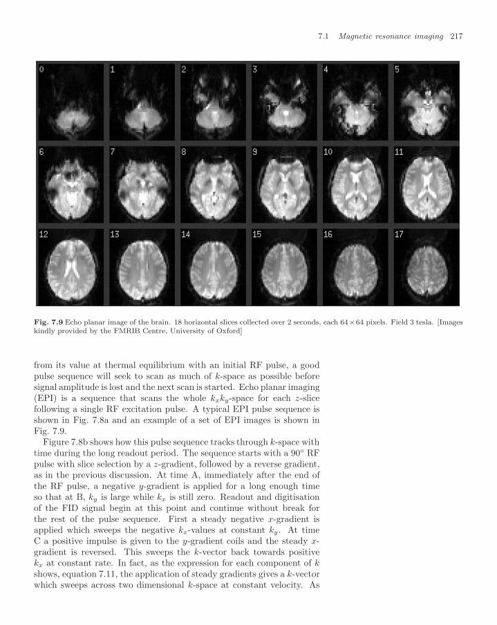
7.1 Magnetic resonance imaging 217
Fig. 7.9 Echo planar image of the brain. 18 horizontal slices collected over 2 seconds, each 64×64 pixels. Field 3 tesla. [Imageskindly provided by the FMRIB Centre, University of Oxford]
from its value at thermal equilibrium with an initial RF pulse, a goodpulse sequence will seek to scan as much of k-space as possible beforesignal amplitude is lost and the next scan is started. Echo planar imaging(EPI) is a sequence that scans the whole kxky-space for each z-slicefollowing a single RF excitation pulse. A typical EPI pulse sequence isshown in Fig. 7.8a and an example of a set of EPI images is shown inFig. 7.9.
Figure 7.8b shows how this pulse sequence tracks through k-space withtime during the long readout period. The sequence starts with a 90 RFpulse with slice selection by a z-gradient, followed by a reverse gradient,as in the previous discussion. At time A, immediately after the end ofthe RF pulse, a negative y-gradient is applied for a long enough timeso that at B, ky is large while kx is still zero. Readout and digitisationof the FID signal begin at this point and continue without break forthe rest of the pulse sequence. First a steady negative x-gradient isapplied which sweeps the negative kx-values at constant ky. At timeC a positive impulse is given to the y-gradient coils and the steady x-gradient is reversed. This sweeps the k-vector back towards positivekx at constant rate. In fact, as the expression for each component of kshows, equation 7.11, the application of steady gradients gives a k-vectorwhich sweeps across two dimensional k-space at constant velocity. As

218 Imaging with magnetic resonance
the Fig. 7.8 shows the regular sequence of small positive impulses on they-gradient coils and the long alternating pulses on the x-coils sweep thek-vector back and forth across the whole k-region. In the middle of eachkx-sweep, it passes through zero. At this point all of the spins are inphase, except for the effect of y which is phase encoded. Such a point isdescribed as a gradient echo or gradient refocus.
Many other rasters have been used for scanning k-space including aspiral sweep. However, the basic idea is the same and the benefits anddisadvantages similar.
Advantages and drawbacks of EPI
The advantage of an EPI scan is speed, as shown by Fig. 7.9. For thescan to be fast, k must change rapidly. This means that ∆k is large andthe spatial resolution is limited.
Another disadvantage is signal loss. The loss of amplitude due to fieldinhomogeneities accumulates throughout the pulse sequence. These arisefrom three sources.
Intrinsic inhomogeneities of the static B0 field. These can bemapped and vary slowly with distance. They are minimisedby shimming and by working at the centre of symmetry ofthe magnet.
Dynamic effects due to eddy currents induced by gradientfield changes. These can be reduced by shaping the pulsethat drives changes to the gradient coil currents.
Static distortion of the field due to the magnetic susceptibil-ity of the patient or sample. The longer range components ofthis effect may be reduced by adjusting the current in shim-ming coils. However, this is a time-consuming procedure andcannot compensate for local short range distortions.
The effect of a chemical shift is similar to a field distortion. Bothproduce a frequency change. Spins with a chemical shift will be displacedin the image depending on the phase shift that they accumulate duringa long scan. A simple calculation of this effect is left to question 7.5.
7.1.4 Multiple detector coils
Encoding with gradients and multiple pickup coils
The birdcage coil which is designed to generate a uniform RF excitationpulse can also be used later in the sequence as the pickup coil. However,significant improvements in scanning speed can be achieved by the useof a dedicated array of small pickup coils instead. This involves anadditional idea.
If the distance from a voxel to a coil is r and the coil is small, thecontribution to the FID from the precessing magnetic moment in thatvoxel will fall off with the 1/r3 dependence of a dipole field together with
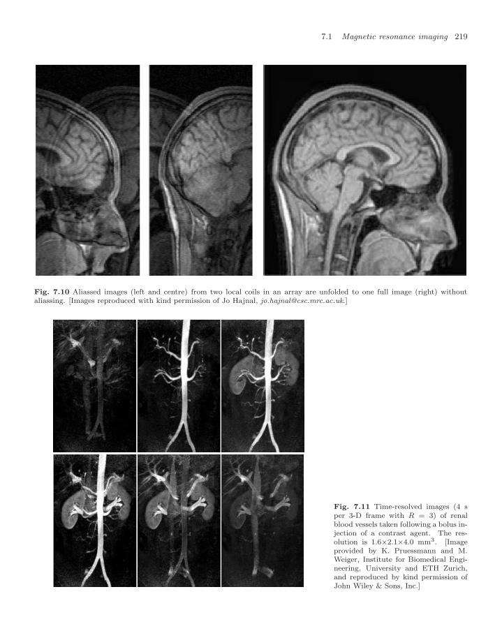
7.1 Magnetic resonance imaging 219
Fig. 7.10 Aliassed images (left and centre) from two local coils in an array are unfolded to one full image (right) withoutaliassing. [Images reproduced with kind permission of Jo Hajnal, [email protected].]
Fig. 7.11 Time-resolved images (4 sper 3-D frame with R = 3) of renalblood vessels taken following a bolus in-jection of a contrast agent. The res-olution is 1.6×2.1×4.0 mm3. [Imageprovided by K. Pruessmann and M.Weiger, Institute for Biomedical Engi-neering, University and ETH Zurich,and reproduced by kind permission ofJohn Wiley & Sons, Inc.]
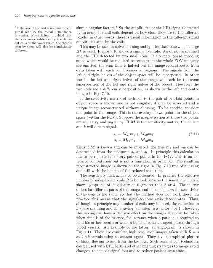
220 Imaging with magnetic resonance
simple angular factors.3 So the amplitudes of the FID signals detected3If the size of the coil is not small com-pared with r, the radial dependenceis weaker. Nevertheless, provided thatthe solid angle subtended by the differ-ent coils at the voxel varies, the signalsseen by them will also be significantlydifferent.
by an array of small coils depend on how close they are to the differentvoxels. In other words, there is useful information in the different signalamplitudes seen by the coils.
This may be used to solve aliassing ambiguities that arise when a large∆k is used. Figure 7.10 shows a simple example. An object is scannedand the FID detected by two small coils. If alternate phase encodingscans which would be required to reconstruct the whole FOV uniquelyare omitted, the scan time is halved but the image reconstructed fromdata taken with each coil becomes ambiguous. The signals from theleft and right halves of the object space will be superposed. In otherwords, the left and right halves of the image will each be the samesuperposition of the left and right halves of the object. However, thetwo coils see a different superposition, as shown in the left and centreimages in Fig. 7.10.
If the sensitivity matrix of each coil to the pair of overlaid points inobject space is known and is not singular, it may be inverted and aunique image reconstructed without aliassing. To be specific, considerone point in the image. This is the overlay of two points in the objectspace (within the FOV). Suppose the magnetisation at those two pointsare m1 at r1 and m2 at r2. If M is the sensitivity matrix, the coils aand b will detect signals
sa = Ma1m1 + Ma2m2 (7.11)sb = Mb1m1 + Mb2m2.
Thus if M is known and can be inverted, the true m1 and m2 can bedetermined from the measured sa and sb. In principle this calculationhas to be repeated for every pair of points in the FOV. This is an ex-tensive computation but is not a limitation in principle. The resultingreconstructed image is shown on the right in Fig. 7.10 free of aliassingand still with the benefit of the reduced scan time.
The sensitivity matrix has to be measured. In practice the effectivenumber of independent coils R is limited because the sensitivity matrixshows symptoms of singularity at R greater than 3 or 4. The matrixdiffers for different parts of the image, and in some places the sensitivityof the coils is the same, so that the method does not work there. Inpractice this means that the signal-to-noise ratio deteriorates. Thus,although in principle any number of coils may be used, the reduction ink-space scanning and time saving is limited to a factor 3 or 4. However,this saving can have a decisive effect on the images that can be takenwhen time is of the essence, for instance when a patient is required tohold his or her breath or when a bolus of contrast agent passes throughblood vessels. An example of the latter, an angiogram, is shown inFig. 7.11. These are complete high resolution images taken with R = 3at 4 s intervals using a contrast agent. They give a graphical pictureof blood flowing to and from the kidneys. Such parallel coil techniquescan be used with EPI, MRS and other imaging strategies to image rapidchanges, to combat signal loss and to reduce patient scan times.

7.2 Functional magnetic resonance imaging 221
7.2 Functional magnetic resonance
imaging
Functional imaging methods based on paramagnetic contrast agents andthe detection of blood oxygenation (BOLD) are described. It is explainedhow the flow and diffusion of proton spins may be measured. Such mea-surements relate to blood flow and the orientation and connectivity ofnerve fibres. MRI may be extended to spectroscopy, such that hydrogenatoms in specific metabolites may be imaged, albeit with inferior signal-to-noise ratio and spatial resolution. The concentration of other speciesof magnetic nuclei may also be imaged, also with poor signal conditions.The risks, safety and installation configuration of a clinical MRI scannerare summarised.
7.2.1 Functional imaging
Paramagnetic contrast agent
Anatomical images do not answer all the questions. Clinicians need toknow what the imaged tissue is doing. The simplest way to get datarelevant to such questions is to inject the patient with a weak solutioncontaining paramagnetic ions. The location of the ions is then observedthrough the large reduction in the relaxation time of all protons in theneighbourhood of any such ion. Such ions act as a contrast agent. Indeedwe already saw an example of this in Fig. 7.11.
From the point of view of MRI there is a wide range of possible transi-tion and rare earth ions. The usual choice is the gadolinium ion, Gd3+,which has a very large magnetic moment, 7.98µB. The larger the mag-netic moment chosen, the weaker is the solution with the required mag-netic properties. The use of a weak solution minimises any toxic sideeffects. A concentration of order 10−4 mole Gd3+ per kg is usuallysufficient.4 The ion is bound in a chelate such as DTPA.5 This chemical 4The SI unit mole in this instance is the
amount of contrast agent that containsthe same number of Gd atoms as thereare in 12 g of 12C. So 10−4 mole perkg means that the fractional mass ofGd ions in solution is 157/12 × 10−7,where 157 is the atomic weight of Gd.
5Di-ethylene-triamine-penta-aceticacid.
‘wrapper’ for the ion is chosen to minimise toxic effects, to have therequired selective uptake from the bloodstream in the different organsand tissue of interest, and to enable the effective fluctuation of localmagnetic field direction experienced by proton spins in water moleculesundergoing frequent interchange as part of the hydration state of thewrapped ion.
Images of tumours are often taken T1-weighted because of the effect ofparamagnetic ions on the local field direction. The abnormal vascularitycharacteristic of a tumour is seen as an enhanced accumulation of theagent relative to surrounding healthy tissue. In this way a tumour mayshow up with exceptional contrast, even when it is barely visible on asimple anatomical image.
To maximise the contrast an image is taken without the agent. Thecontrast agent is then injected into the bloodstream, and its distributionimaged as it is absorbed preferentially by pathological tissue. The agentwill often leak out of the blood vessels and persist in the tissue. Theseareas are bright in a T1-weighted image, as seen in Fig. 7.11.

222 Imaging with magnetic resonance
Fig. 7.12 The structural image on the left is also shown on the right with functional data overlaid. Black regions show brainareas responding to 40 s visual stimulation alternating with 40 s rest. White regions show brain areas responding to 30 sauditory stimulation alternating with 30 s rest. [Image kindly provided by the FMRIB Centre, University of Oxford.]
Blood oxygen level dependent (BOLD) scan
An ideal contrast agent is one that occurs naturally in the body, does nothave to be injected, is not toxic and does not have to be excreted. Mostfortunately such an agent exists. Red blood cells contain haemoglobin.As they carry out one of the functions of blood by transporting oxygen,the haemoglobin changes its form to de-oxyhaemoglobin at the pointwhere it delivers the oxygen, indicating thereby the location of metabolicactivity. Iron is a transition element and can change its valency. Asa component of haemoglobin in blood, it can switch the diamagneticoxygen-rich form (oxyhaemoglobin) to the paramagnetic oxygen-poorform (de-oxyhaemoglobin).
Muscular activity increases the return of venous de-oxyhaemoglobinto the heart. The vasculature of the muscle provides a reservoir of oxy-haemoglobin that is then replenished from the blood supply. However,in the brain this is not possible because there is inadequate muscle toprovide storage. To protect the supply of metabolites and oxygen neededfor brain function oxyhaemoglobin is therefore oversupplied by the bloodflow even in the resting state. As a result the venous flow is only partiallydeoxygenated. Mental activity at a site in the brain requires metabolicactivity there. Then, because of the poor storage, an increase in freshblood flow is stimulated which actually overcompensates for the use ofoxygen there. The result is to invert the expected effect. The return (ve-nous) blood flow is actually even more oxygenated than in the resting
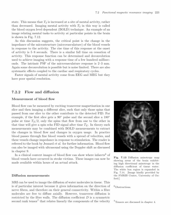
7.2 Functional magnetic resonance imaging 223
state. This means that T2 is increased at a site of mental activity, ratherthan decreased. Imaging mental activity with T2 in this way is calledthe blood oxygen level dependent (BOLD) technique. An example of animage relating mental tasks to activity at particular points in the brainis shown in Fig. 7.12.
As this discussion suggests, the critical point is the change in theimpedance of the microstructure (microvasculature) of the blood vesselsin response to the activity. The rise time of this response at the onsetof activity is 5–8 seconds. There is a similar fall time on cessation ofactivity. This response function can be determined and deconvolutionused to achieve imaging with a response time of a few hundred millisec-onds. The intrinsic PSF of the microvasculature response is 2–3 mm.Again some deconvolution is possible but is noise limited. There are alsosystematic effects coupled to the cardiac and respiratory cycles.
Faster signals of mental activity come from EEG and MEG but theyhave poor spatial resolution.
7.2.2 Flow and diffusion
Measurement of blood flow
Blood flow can be measured by exciting transverse magnetisation in oneslice and then imaging a different slice, such that only those spins thatpassed from one slice to the other contribute to the detected FID. Forexample, if the first slice gets a 90 pulse and the second slice a 180
pulse at time TE/2, only the spins that flow from one to the other inthat time will give a spin echo FID signal after time TE . In theory suchmeasurements may be combined with BOLD measurements to extractthe changes in blood flow and changes in oxygen usage. In practiceblood passes through fine blood vessels with a spread of velocities, andthese vessels change impedance in response to stimulation. The reader isreferred to the book by Jezzard et al. for further information. Blood flowcan also be imaged with ultrasound using the Doppler shift as discussedin chapter 9.
Fig. 7.13 Diffusion anisotropy mapshowing areas of the brain exhibit-ing high directional anisotropy in thediffusion coefficient of tissue water.The white box region is expanded inFig. 7.14. [Image kindly provided bythe FMRIB Centre, University of Ox-ford.]
In a clinical context images of blood flow can show where infarcts6 of
6Obstructions.
blood vessels have occurred in stroke victims. These images can now bemade available within hours of an actual attack.
Diffusion measurements
MRI can be used to image the diffusion of water molecules in tissue. Thisis of particular interest because it gives information on the direction ofnerve fibres, and therefore on their general connectivity. Within a fibremolecules are free to diffuse axially. However, transverse diffusion isrestricted by the fibre walls. The diffusion coefficient D is a symmetricsecond rank tensor7 that relates linearly the components of the velocity 7Tensors are discussed in chapter 4.

224 Imaging with magnetic resonance
Fig. 7.14 An expansion of the region within the white box of Fig. 7.13 showing anisotropic diffusion. The direction of theprincipal eigenvector of the diffusion tensor is shown as a small line within each pixel. [Image kindly provided by the FMRIBCentre, University of Oxford.]
vector v to the components of the concentration gradient vector g. Thus
vi =3∑
k=1
Dikgk. (7.12)
The anisotropy of D is described by its irreducible traceless part withfive independent components, like the stress or strain of a solid discussedin chapter 4. Diffusion measurements by MRI enable the eigenvaluesand eigenvectors of the matrix describing D to be determined. For acylindrical fibre this is axially symmetric with one large and two smalleigenvalues. These represent data on the size and orientation of nerve-fibre bundles. This is a crude first step along the road to understandinghow nerves are connected in the brain. A sample of data is shown inFig. 7.13, with further detail in Fig. 7.14.

7.2 Functional magnetic resonance imaging 225
7.2.3 Spectroscopic imaging
Combining imaging with spectroscopic measurement
The crude distinction between fat, water, etc., based on measurementsof T1 and T2 provides some contrast between different tissue types, aswe have seen. However, it is a long way from a chemical analysis ofwhat is occurring in the human body. What is really wanted is to im-age the density, not just of hydrogen atoms but of hydrogen atoms inspecific molecules, thereby recording the presence and concentration ofthose particular molecules. This approach is called magnetic resonancespectroscopy (MRS). It comes with the prospect of rather large voxelsor poor spatial information and is intrinsically slow and noisy. It coversnot only hydrogen atoms at sites in specific classes of molecules, butalso other NMR active nuclei with a workable NMR signal size and aspecific chemical or biochemical story to tell, particularly phosphorusand fluorine.
Difficulties of spectroscopic imaging
MRS enables a start to be made on the non-invasive in vivo study of thechemistry of the functioning human body and brain. What is needed isa spectrum for each voxel. This is made difficult for a number of relatedreasons.
Even in theory, to measure the frequency of a 100 MHz wavewith a resolution of 0.1 part per million (ppm) takes a timeof order 100 ms. Thus each spectrum must be digitised fora long time.
A chemical shift of 0.1 ppm cannot be distinguished from anon-uniformity of 0.1 ppm in the applied B-field. Uniformityof the B-field is therefore crucial, and extensive use has tobe made of shimming.
Since the frequency measured during readout is to be inter-preted as the chemical shift, no gradient field is applied dur-ing this time. Both x and y are measured by phase encodingwith an increased number of scans.8 Figure 7.15 shows such 8In some sequences x or y may be se-
lected by RF excitation with a gradientfield, like the z slice selection.
a pulse sequence. So, for example, an MRS image with 100pixels requires 100 scans, each with a different combinationof values of kx and ky.
While the hydrogen atoms of interest may have a modestconcentration, the spectrum is dominated by the very largepeak due to water. Special techniques are employed to pre-vent this overwhelming the dynamic range of the electronics.Here is an example. With no gradient fields applied, a longRF excitation with small bandwidth matched to the watersignal generates a 90 rotation. This is then dephased withlarge gradients, so that the magnetisation due to water issmall. Now the pulse sequence of interest is applied and,

226 Imaging with magnetic resonance
Fig. 7.15 An MRS pulse sequence.Both x and y are encoded by phase.The FID signal is digitised from timeB onward, when all gradients are off.
RF
dB /dzz
dB /dxz
dB /dyz
FID
time
A B
although the longitudinal magnetisation of the water will re-cover, it will generate no FID provided that the last RF pulseis applied within a time short compared with its T1.
The presence and concentrations of important metabolites in a samplecan be measured in vivo by fitting its NMR spectrum as a linear com-bination of the spectra of known solutions of metabolites prepared invitro. The spectra are even sensitive to the pH value, the acidity of themedium. An example is shown in Fig. 7.16 where peaks correspondingto some of the more important metabolites may be seen.
Few isotopes other than hydrogen generate a strong NMR signal. Eventhose with spin tend to have low concentrations in biological tissue,small isotopic ratios or small gyromagnetic ratios, as shown in table 2.2.Although there is no problem equivalent to the water peak, the magneticmoment at thermal energies is small on all counts. As a result dataare usually taken for a few large voxels to get sufficient signal-to-noiseratio. Imaging of these is also referred to as MRS. The elements mostfrequently studied are 31P and 19F.
Phosphorus plays an important role in metabolism as various metabo-lites incorporating phosphate bonds are used by organs for short termenergy storage. Fluorine, though not itself biologically interesting, hasa large magnetic moment and is used as a tracer to study drug action.Among other isotopes, sodium is used in the academic study of cellaction. Tracers labelled with the NMR-active isotopes 13C, 14N and17O are used in animal studies. Recent developments in hyperpolari-

7.2 Functional magnetic resonance imaging 227
NAA
Cr
Cho
GABA
+ Glu
+ Gln
GABA
+ Glu
+ Gln
mI
NAA
2.03.04.0 1.0
chemical shift, ppm
Fig. 7.16 Hydrogen metabolitespectrum collected using the PRESSsequence at 3 tesla. mI=myo-inositol, GABA=gamma butyric acid,Glu=glutamate, Gln=glutamine,Cho=choline, Cr=creatine, NAA=nacetyl aspartate. [Spectrum kindlyprovided by the FMRIB Centre,University of Oxford.]
sation have shown how signals from these isotopes may be significantlyenhanced by dynamic nuclear polarisation (DNP).
In summary, the various techniques of MRI and MRS permit the non-invasive mapping of the flow of fuel, oxygen and services within thepatient. This is the information that the clinician needs.
7.2.4 Risks and limitations
Benefits and resources
How effective is MRI as a clinical technique in terms of contrast, defi-nition, speed, safety and cost? Contrast can be achieved by generatingH-spin density images weighted by T1 or T2. This forms a rich andversatile basis for differentiation of tissue by anatomy or function. Con-trast based on more specific chemical information (MRS) comes at theexpense of a big increase in scan time and loss of spatial definition. Oth-erwise spatial definition is good to 1 mm and images may be obtainedwith a time resolution of a few seconds with some loss of definition inother respects. Although the cost of an MRI scanner is high, the avail-ability of staff and know-how is more critical. Expensive facilities maylie fallow much of the time. Society is prepared to keep supermarketsopen 24 hours a day, seven days a week. The need for scanners is morepressing. The availability of radiographers and clinicians would appearto be more critical than the availability of money to supply scanners,at least in the developed world. By the same argument, the widespreaddeployment of MRI in some parts of the Third World presents seriousdifficulties.

228 Imaging with magnetic resonance
Safety
MRI appears superficially safe and there is no history of accidents, pro-vided that standard safety precautions are followed. Nevertheless thereare a significant number of safety concerns.
The high static B-field itself is not responsible for any knownwell-defined physiological hazard. The current recommendedlimit is 4.0 T.9 However, such a field is dangerous for anyone9As discussed in chapter 1 and refer-
ences there. with a pacemaker or metal implants and MRI cannot beused at all for such patients.10 It is interesting to note that
10The accidents that have occurred asa result of MRI have been in connec-tion either with pacemakers or with themotion of ferromagnetic objects in thefringe field of the dipole magnet.
in connection with overhead power lines and mobile phonesthere is public concern over microtesla fields!
In the interest of speed the gradient fields would be switchedas fast as possible. However, rapid switches of magnetic fluxcreate large electric fields by Faraday’s law. These in turncause eddy currents which are felt as a tingling sensationin the skin and even give pain. This pain occurs at a lowerthreshold than any serious physiological effects. A maximumdB/dt of 20 T s−1 is permitted.
The rapidly changing magnetic forces on the gradient fieldcoils generate acoustic noise. They form a powerful loud-speaker system in a small volume. This noise and the claus-trophobic sensation of being confined in a small tube for anextended period make an MRI scan a disturbing, even un-pleasant, experience. Headphones with soothing music arenot sufficient to overcome this. Significantly, conclusions onpsychological research and clinical results are always quali-fied by the fact that, whatever else may have been experi-enced, the patient was being subjected to much noise in anoppressive environment. The noise level and spectrum de-pend on the pulse sequence and may be reduced by avoidingthe resonances of the scanner as an acoustic cavity. How-ever, much of the spectrum is around 1 kHz which is unfor-tunate for the human ear. Maximum permitted noise levelsare specified.
Fortunately most patients are not aware that they are lyingenveloped by a liquid helium cryostat. One may wonderwhether this would be allowed by the safety rules in a physicsresearch laboratory!
The maximum recommended level of RF heating in this fre-quency range for the general public is 0.08 W kg−1 to thewhole body, averaged over any 6 minute period.11 This is11See the references given at the end of
chapter 1. to ensure that no part of the body experiences a tempera-ture rise exceeding 1C. The maximum power that can beabsorbed in MRI under saturation conditions is in fact lessthan 0.01 W kg−1, safely below this level.1212See question 7.6.

7.2 Functional magnetic resonance imaging 229
Xgradcoil
Ygradcoil
Zgradcoil
RFpowersupply
Computerand electronics for
pulse sequencegeneration,
signal processingand analysis
Displaysignals
Solenoid Bfield power
supply
0
Fig. 7.17 A diagram of the components of a basic MRI scanner.
The fringe B-field in the neighbourhood of such a magnetextends for many times the solenoid diameter and presentsa serious hazard. Metal objects can be dragged by suchfield gradients with considerable force. In spite of the moresophisticated risks discussed above, the greatest danger fromMRI is that of being impaled by a flying screwdriver or otherloose metal object.13 13See question 7.7.
Summary of clinical equipment
In Fig. 7.17 we summarise schematically the various elements of equip-ment that make up an MRI clinical scanner.
There is the large bore static superconducting solenoidalmagnet with horizontal uniform B0 field in the range 1.5to 4.0 T.
Inside which there is a set of x-, y- and z-gradient coils. Inside which there is an RF excitation birdcage coil giving
42.58 MHz T−1. Inside which is the patient with an array of small detector
coils to detect the FID (if the birdcage coil is not used forthis purpose).
The power supplies for the gradient coils and RF are con-trolled by the computer and electronics. The electronics also

230 Imaging with magnetic resonance
amplifies and mixes the FID signals with the reference fre-quency to give an ‘audio’ output, which is then sampled anddigitised.
Not shown in the diagram are the B0 shimming coils, the software andthe team of people. The software is needed to control the pulse sequence,monitor the performance, carry out the calibrations, map the magneticfields, invert the Fourier transforms, extract T1, T2, spin density, MRSspectra and many other tasks. The integrated team includes physicists,clinicians, hardware and software engineers.
Read more in books
The Physics of Medical Imaging, ed. S Webb, IOP(1988), an edited compilation of useful articles, some-what out of date but still frequently referenced
Functional Brain Imaging, WW Orrison, JD Lewine,JA Sanders and MF Hartshorne, Mosby (1995), anedited volume by authors active in the field
Functional MRI, An Introduction to Methods, P Jez-zard, PM Matthews and SM Smith, OUP (2001), anedited compilation of articles written by researchers inthe field
Fundamentals of Medical Imaging, P Suetens, Cam-bridge (2002), a fully illustrated book with discussionof image processing
Look on the Web
Look at the book website atwww.physics.ox.ac.uk/users/allison/booksite.htm
Read about a wider range of MRI pulse sequences thanhave been discussed here
MRI pulse sequences
Follow the development of spatial encoding of MRI withmultiple pickup coils
MRI sense coil array
Find up-to-date examples of functional imaging usingblood oxygenation
BOLD imaging
Learn more about the use of MRI for diffusion, flow andperfusion measurements
MRI diffusion and MRI perfusion flow
Look at examples of the clinical use of magnetic reso-nance spectroscopy
proton MRS or phosphorus MRS
Consult the sites referenced at the end of chapter 1 onMRI safety matters, or search
MRI safety
Find out about MRI magnet optionsMRI magnets

7.2 Functional magnetic resonance imaging 231
Questions
7.1 A voxel at position r has a magnetic moment mperpendicular to a static B-field about which it pre-cesses with frequency ω. Show that the oscillatingvoltage induced in a small detector coil of area Aat the origin has an amplitude
V = µ0ωA · ∇(
m · R4πR3
).
7.2 Consider the signals induced by the magnetic mo-ments of a pair of voxels at A and B in a pair ofsmall detector coils at C and D where the four lieat the corners of a square ABCD. A uniform staticB0 field is perpendicular to the square. The normalof coil D points towards voxel A, and the normal ofcoil C points towards voxel B. Using the result ofquestion 7.1 show that the ratio of signals detectedin the two coils due to the precessing component ofthe magnetic moment of each voxel is 8
√2.
Hence discuss the spatial sensitivity matrix of coilsC and D with respect to the positions A and B.
7.3 A water droplet is suspended in the field of viewof an MRI scanner. The B0 field at the origin ofcoordinates, the centre of symmetry of the MRIscanner, is 2.998015 T in the z-direction. An RFpulse of frequency 127.5987 MHz is applied at thesame time as a z-gradient of B0 is present. A FIDsignal is not detected subsequently unless this z-gradient field is 7.81×10⁻³ T m−1. (After the RFpulse the z-gradient is reversed for a time such thatall hydrogen atoms that are excited have a preces-sion phase which is independent of z.) Two scansare made and two measurements of the FID signalare recorded, both in the presence of a y-gradient ofthe B0 field of −12.2× 10⁻³ T m−1. In both casesthe observed FID frequency is 127.5662 MHz. Inthe first scan no x-gradient field is applied; in thesecond an x-gradient field of −1.00 × 10⁻³ T m−1
is applied for a time of 100 µs before readout. Inthe second case the FID is measured to have anextra phase shift of 1.60 radians compared to thefirst case.Draw the pulse-sequence diagram and explain howit works.Determine (x, y, z), the position of the waterdroplet.[The Larmor precession frequency for protons inwater is 42.55747 MHz T−1.]
7.4 A close sequence of water droplets as described inquestion 7.3 form a steady drip falling parallel toy from a single point. Suggest ideas for a pulse se-quence to measure the mass of each drop, the spac-ing of drops and their vertical velocity with time.
7.5 If the hydrogen atoms of question 7.3 were subjectto a chemical shift of 4 ppm, how far would theyappear to be shifted in the image?
7.6 A paramagnetic salt is dissolved in water at 20C.The concentration is such that in a magnetic in-duction of 3 T the proton spin relaxation time T1
is 10 ms. Discuss the absorption of energy per kgof water in the steady state as a function of theaverage RF power level. Estimate the maximumpower per unit mass that can be absorbed in thisway. Comment on the relevance of this result toclinical safety considerations.
[A steady whole-body absorbed power level of4 W kg−1 generates a temperature rise of less than1C in a healthy patient.]
7.7 A long thin screwdriver lies outside a magnet ofcentral field B0. It is drawn point first by the fringefield towards the magnet centre. Its density is ρ andits relative magnetic permeability is µr. Ignoringgravity show that when it reaches the centre of themagnet it has a velocity of about B0
√µr/ρ. Put
in numbers to show that this might be on the scaleof 1 m s−1 in a typical case.
7.8 A phantom is composed of two materials, A andB, with T1 relaxation times 0.75 s and 1.3 s re-spectively. An NMR pulse sequence starts with a180 RF pulse which is followed by a 90 pulse aftertime T ′. Describe briefly the FID signals from Aand B seen as a function of t. Find the ratio of theFID signal for B to the FID signal for A at time T ′
as a function of T ′. For what choice of T ′ wouldthe MRI contrast between regions of A and B begreatest?

This page intentionally left blank

Medical imaging andtherapy with ionisingradiation 8
8.1 Projected X-ray absorptionimages 233
8.2 Computed tomography withX-rays 241
8.3 Functional imaging with ra-dioisotopes 246
8.4 Radiotherapy 256
Read more in books 264
Look on the Web 265
Questions 265
in which the uses of ionising radiation in medical imaging and radiother-apy are discussed and compared.
8.1 Projected X-ray absorption images
The source of X-rays generally used in imaging is bremsstrahlung emis-sion by electron beams incident on high Z metal targets. Electrons areaccelerated by a DC voltage or an RF linear accelerator. The efficiency,energy and angular distribution of X-ray production depend on the elec-tron energy and the Z of the target. The X-ray energy spectrum is hard-ened by passage through a high Z absorber. The quality of the pinholeoptics of the camera depends on beam source size, detector resolution andscattering. Image quality is affected by the statistical noise of the numberof detected photons. The image contrast depends on the photon energyspectrum and the absorption edges of the regions of different Z withinthe object. For images of blood vessels and the digestive tract contrast isenhanced by administering iodine and barium as passive high-Z contrastagents.
8.1.1 X-ray sources and detectors
Conventional X-ray tube
From the time of their discovery X-rays have been used for imaging.The conventional X-ray examination, as used in medicine and dentistry,with a simple photographic plate is safe, cheap and widely available.In addition to the photographic plate as detector, a source of X-raysis needed. The initial electron beam can be focused to a small brightspot. But because it is not possible to reflect, refract or focus an X-ray beam, the straight line optics of the pinhole camera must be usedto produce the image. Technically there are three possibilities. Intensehighly collimated beams of X-rays are produced by electron synchrotronsand X-ray lasers. However, as yet these are too large and expensive tobe available for clinical purposes. Secondly there is the production ofX-rays using the more manageable linear electron accelerator with anRF power supply. These are used to produce X-rays for radiotherapy

234 Medical imaging and therapy with ionising radiation
Fig. 8.1 The layout of a conventionalX-ray tube.
oil-cooled
copper anode
tungsten
target
heated cathode
thin window electron beam
focussed to spot
X ray beam
HV supply
where MeV X-ray energies are needed for their long range. For mostimaging purposes, however, this increased energy is not helpful. Forimages using the contrast between the X-ray absorption of elements ofmoderate Z, a source based on a simple DC electron beam is sufficient.The power supply with terminal voltage up to 150 kV for such a sourcemay use a diode array similar in principle to that in the Cockcroft–Walton accelerator with which they artificially split the nucleus in 1932.
A conventional low energy X-ray source of this kind is shown inFig. 8.1. Electrons emitted by a heated cathode are accelerated in vac-uum through a potential defined by the DC voltage supply (25–150 kV)and focused to a spot on the anode. The anode consists of a tungsten tar-get (W, Z=74) set into an oil-cooled copper holder designed to conductaway the heat. The high Z maximises the production of bremsstrahlungrelative to dE/dx energy loss which is responsible for the heat. The pro-cess is very inefficient; the efficiency is calculated in question 8.1 usinga simplified model and plotted in Fig. 8.2 for copper and tungsten. Aswell as having a high Z, tungsten has a very high melting point whichincreases the tolerance to the high thermal load. A rotating target canbe used to spread the local heat load due to a tightly focused beam spot.The X-rays generated leave the vacuum through a thin window.
6
4
2
0
efficiency %
efficiency %
incident energy/MeV
incident energy/MeV
0.2
2
0.4
4
0.6
6
0.8
8
1.0
10
W
Cu
0
10
20
30 W
Cu
Fig. 8.2 The efficiency with which theenergy of an electron beam generatesbremsstrahlung radiation in a thick tar-get as a function of the incident energy,calculated for tungsten (W) and cop-per (Cu). This simplified calculationtends to overestimate the efficiency, es-pecially at low energy; see question 8.1.
The raw spectrum emitted by such a target was discussed in chapter 3.It consists of a broad spectrum of bremsstrahlung with added emissionlines characteristic of the target. The upper limit of the bremsstrahlungis given by the maximum incident electron energy. For a tungsten targetthe discrete lines are Kα, Kβ , Lα and Lβ at 59.3, 67.2, 8.39 and 9.67keV respectively. For a lower energy source suitable for mammography amolybdenum target is used with a 30 kV terminal voltage. In either casethe broad spectrum that emerges includes a flux of low energy photonswhich will be absorbed in any case. These increase the radiation dose

8.1 Projected X-ray absorption images 235
0
0.1
0.2
0.3
0.4
0.5
0.6
10 15 20 25
Transmission
Photon energy/keV
Fig. 8.3 The energy dependence of theX-ray transmission of a 30 µm thick fil-ter of molybdenum. The arrows markthe position of the K emission lines ofmolybdenum.
without adding information to the image, and are therefore need to beabsorbed with a filter. Such a filter has a pass band. Figure 8.3 shows thetransmission for a 30 µm window of molybdenum which removes the softphotons and substantially reduces the hard ones using the molybdenumK edge. Used with a molybdenum target the K emission lines of Moare transmitted. The X-ray spectrum is therefore determined by theincident electron energy, the Z of the target and the Z of the filter(which may be different).
RF linear accelerator and synchrotron sources
RF waveguidedeflection
magnet
target
window
Fig. 8.4 An illustration of the compo-nents of an electron linac with steerablebeam and an optional target producinga photon beam in the forward direction.
As shown in Fig. 8.2 and discussed in question 8.1, raising the electronenergy increases both the radiation energy and the efficiency. However,high energy beams are less suitable for imaging because the contrastdisappears. The photoelectric cross section falls to zero for all elementsand attenuation becomes a function of electron density alone.
Higher energy beams are used for therapy and materials testing. Abovea few hundred kilovolts the use of a DC accelerating voltage becomesless practicable. Such electrons are accelerated in bunches in a linear ac-celerator (linac) with RF power in a waveguide. At energies above about500 keV the electrons become relativistic and the bremsstrahlung radi-ation that they create in the target becomes collimated in the forwarddirection1 in a cone with angle of order 1/γ radians, where γ = E/mec
2. 1This is because the radiation, whichis nearly isotropic in the electron restframe, is thrown forward by the Lorentztransformation to the laboratory frame.
Therefore the target geometry shown in Fig. 8.1 is not suitable and thebeam must be focused onto a thin transmission target which producesa bremsstrahlung beam in the forward direction as shown in Fig. 8.4.The spectrum is affected by the choice of target thickness as the electronbeam loses energy. If the target is removed, the focused electron beam

236 Medical imaging and therapy with ionising radiation
itself exits though the thin window2 and may be used for radiotherapy2The window is needed to maintain thevacuum and is made of a low Z materialto minimise scattering of the electrons.
as an electron beam, as discussed in section 8.4.2.In a synchrotron source the electrons radiate in the forward direction
as a result of transverse acceleration perpendicular to an applied mag-netic field. Because the radiation is produced in vacuum, there is nosource of heating. The beam ‘spot’ size is finer and more intense thancan be obtained in a bremsstrahlung beam. However, such sources arelarge, expensive and not yet generally available outside research labora-tories.
Detectors for projected X-ray images
For many purposes the simple two dimensional photographic plate pro-vides the resolution and ease of use that is required of a detector. Suchdata are not easily read electronically and have threshold and saturationeffects that limit their dynamic range. Increasingly X-ray images arerecorded electronically using CCD and other semiconductor technolo-gies as these become cheaper and more widely available. Such imagesare more easily calibrated, stored and used quantitatively. This is im-portant when relating images taken at different times or under differentconditions.
8.1.2 Optimisation of images
Photon energy
The projected image in the xy-plane is the flux3 I(x, y) that penetrates3This is assumed normal to the xy-plane for simplicity. the absorption density ρ(x, y, z) due to the object and is successfully
detected,
I(x, y) = Φ(x, y) exp(−
∫ρ(x, y, z)dz
)ε,
where Φ(x, y) is the flux of the incident parallel beam along z and ε is thedetection efficiency. However, this equation is too simple. The incidentflux, the absorption and the efficiency all depend on the photon energyE in an essential way. At each energy the absorption ρ(E, x, y, z) is thesum of the absorption due to each chemical element present, representedby the product of the cross section σi and number density Ni of each.Thus,
ρ(E, x, y, z) =∑
i,elements
σi(E) × Ni(x, y, z). (8.1)
A useful image gives information on the density Ni of elements of inter-est, albeit projected onto the xy-plane. For each element the dependenceof the cross section σi(E) on energy takes the form of absorption edgesfor different electron shells as discussed in section 6.2.1, and shown fora number of significant elements in Fig. 3.7. At an energy above theK edge the absorption cross section for each element falls progressivelyto zero, leaving only the Thomson scattering cross section4 which is
4The cross section per atom is Z timesthe Thomson (or Compton) cross sec-tion. the same for all elements. Images taken at such energies are degraded

8.1 Projected X-ray absorption images 237
0
0.5
1
1.5
2
2.5
20 30 40 50 60 70 80 90 100
/Zbarn
Photon energy /keV
Calcium
Carbon
Thomson cross section
Oxygen
Fig. 8.5 The total photon cross sectionof carbon, oxygen and calcium, dividedby Z, as a function of photon energy.All cross sections fall with energy to theThomson value, 0.665 barn.
Energy/keV
Atomic number
0
40
80
120
160
20 40 60 80
Fig. 8.6 The energy E1cm plottedagainst Z, where E1cm is defined in thetext. Points are plotted for various ele-ments and lie close to the plotted line,E1cm = 2.25 × Z keV.
by scattering and are only sensitive to electron density, not elementalcomposition. The energy range of interest for X-ray medical imaging isshown in Fig. 8.5 on a linear scale.
Imaging with X-rays is therefore a matter of making measurementsin an energy band in which the elements to be imaged have differentphotoelectric cross sections. Figure 8.5 shows that up to 70 keV thereis a very large difference in the absorption of calcium and the normalelements of which tissue is composed. At energies up to 35 keV thereis some discrimination between carbon and oxygen. We may ask atwhat energy each element becomes effectively transparent. In Fig. 8.6is plotted the energy at which the absorption length of each elementis 1 g cm−2 (in other words, 1 cm at the density of water) which fitswell to E1cm = 2.25 × Z keV. Assuming an energy dependence of the

238 Medical imaging and therapy with ionising radiation
Fig. 8.7 An X-ray image of the intes-tine with contrast by orally adminis-tered barium. The image is of a trans-verse slice, reconstructed by tomogra-phy. The contorted shape of the gutcan be picked out in the centre and up-per part of the image as it crosses backand forth across the plane of the slice.The whole is contained within the rib-cage which is seen in lower contrast dueto the calcium. [Image reproduced bykind permission of Medical Physics andClinical Engineering, Oxford RadcliffeHospitals NHS Trust.]
cross section E−2.5 in the region beyond the K edge, the energy at whichthe absorption length approximates the thickness of the scanned objectmay be estimated. Thus the need to penetrate thicker objects leads to achoice of higher energies. In this way the photon energies may be chosenin a range from 17 to 150 keV.
Noise
So much for the signal in an X-ray image, but what about the noise? Inthis case the dominant form of random noise is statistical. The numberof radiation quanta n detected in a pixel of the image fluctuates withstandard deviation
√n. In a relatively coarse-grained two dimensional
image the number of pixels is low and only a small radiation exposureis required to achieve an adequate image quality.
Sources of systematic imperfection of the image are the limited spatialresolution associated with the size of detector elements, the spot size ofthe X-ray source, and the background flux that comes from scatteringof the X-rays. At higher X-ray energy the Thomson scattering crosssection increases in size relative to the photoelectric cross section; thusscattering becomes more significant.
There is also an incoherent flux of scattered photons due to X-rayfluorescence and these photons are characteristic of the Z of the medium.However, in medical physics the fluorescence yields of low Z atoms aretoo small to be useful, but remain as a source of background.5
5Where higher Z atoms are imaged andhigher radiation doses are acceptablethese XRF signals are used, as dis-cussed in chapter 6.

8.1 Projected X-ray absorption images 239
8.1.3 Use of passive contrast agents
Limitations of simple X-ray images
A simple X-ray image exhibits contrast in terms of the atomic number ofthe absorbing medium. This is very good for distinguishing tissue fromhigher Z metals such as iron, copper and silver. The ring on a finger, acoin swallowed by a child, a metal splint – all these show up very clearly.So too do bones through the calcium content. The higher absorptioncomes not from the linear dependence on Z of the electron density inhigher Z atoms, as stated in some medical physics texts, but through theZ2 dependence of the binding energy of the inner electrons. Lungs andair passages form images with good contrast because of the significantdensity difference. The presence of a growth in the throat and otherairways is readily seen. Otherwise, foreign objects and bones apart, thecomposition of most tissue is a variable mix of carbon, hydrogen, oxygenwith some nitrogen with rather uniform density. Absorption of X-raysby tissue is therefore rather uniform. Additional methods are needed toincrease contrast, rather as the paramagnetic agents do for MRI.
Use of barium and iodine
The contrast agents most used with X-rays are iodine (Z = 53) andbarium (Z = 56).6 These are chosen for their high Z and low toxicity. 6These agents are the normal stable
isotopes of iodine and barium, not theradioisotopes used in other applicationsconsidered later in this chapter.
Iodine is used as a contrast agent for blood vessels,7 and barium for the
7Images of blood vessels obtained inthis way are called angiograms.
digestive tract.Barium is a divalent metal with a chemistry like calcium and stron-
tium. The patient swallows a so-called barium meal, or, if administeredthrough the rectum, receives a barium enema. The shape of features ofthe gut can be imaged as the barium gradually coats the stomach andthe intestinal tract with its X-ray absorbing properties. Ulcers, growthsand hernias can all be seen in high contrast. An example of such animage is shown in Fig. 8.7. The barium is inert and is excreted in thenormal way.
Iodine is introduced to the bloodstream by injection and is removedby the action of the kidneys and passes out with the urine. It maybe imaged as it spreads through blood vessels, but most examinationsinvolve simply taking images before and after the administration of theiodine.
Digital subtraction techniques
To image the finest blood vessels special techniques are used. The imagestaken before the contrast agent is administered are compared with thosetaken afterwards, and these images are digitally subtracted to bring theblood vessels into maximum relief. Examples of the results are shownin Figs 8.8 and 8.9. However, if spatial resolution is not to be lost, thetwo images have to be registered with one another. This is difficult sincesome movement is unavoidable.

240 Medical imaging and therapy with ionising radiation
Fig. 8.8 Angiographic images of the pelvis and lower spine. On the left, an initial image. In the centre, the same after injectionof iodine as a contrast agent. On the right, a digitally subtracted image formed from the other two and showing the right iliacartery (the main artery dividing from the aorta to supply the right leg). [Images reproduced by kind permission of MedicalPhysics and Clinical Engineering, Oxford Radcliffe Hospitals NHS Trust.]
Fig. 8.9 Digitally subtracted iodine contrast images of the iliac arteries, on the left for an abnormal patient, and on the rightfor a normal patient. The abnormal patient has virtually no left iliac artery. [Images reproduced by kind permission of MedicalPhysics and Clinical Engineering, Oxford Radcliffe Hospitals NHS Trust.]

8.2 Computed tomography with X-rays 241
An ideal solution to this problem is to take two images in the presenceof the contrast agent in rapid succession, one using X-rays just belowthe energy of the absorption edge of iodine, and the other just above theabsorption edge. Ideal monochromatic X-ray beams are available fromsynchrotron radiation sources but useful results may also be achievedwith filters. Similar studies have been carried out on the airways ofanimals using xenon as an inert contrast agent. The animals inhale thexenon and are illuminated by two monochromatic beams of SR, aboveand below the xenon K edge. As discussed above, such SR sources arenot clinically available under normal circumstances.
The use of contrast agents is limited to the imaging of fluid passages.Further ideas are needed to improve the contrast of general images. Thenext step is to establish how three dimensional images may be made,free from the superposition of the contribution of those objects whichlie above or below the plane of the object under study.
8.2 Computed tomography with X-rays
A three dimensional object distribution can be mapped as a series of twodimensional projections. With a sufficient number of projections thismapping process can be inverted and the three dimensional distributionreconstructed from the maps. The matrix to be inverted may be extremelylarge. If the projection axes lie in a plane, the reconstruction may be car-ried out one slice at a time. In this case the inversion is simpler and maybe done using a Fourier method. Otherwise, to avoid the large matrix, amaximum likelihood method is used and the solution found by iteration.
The statistical noise in such images depends on the number of photonsin each resolved image element. Consequently, for three dimensional im-age reconstruction the radiation exposure increases significantly with theimage quality required, specifically with the fineness of the spatial resolu-tion and with the statistical signal-to-noise ratio of each voxel.
8.2.1 Image reconstruction in space
Linear imaging by absorption or emission
When imaging by absorption the detected radiation flux depends ex-ponentially on the density of absorber. So expressed in terms of thelogarithm of the flux the behaviour of absorbers is additive.
In later sections we consider nuclear medicine, that is methods thatinvolve imaging the emissions from administered radioisotopes, namelysingle photon emission computed tomography (SPECT) and positronemission tomography (PET). Then the measured flux from different re-gions itself is additive, and the intensity, not its logarithm, is the linear

242 Medical imaging and therapy with ionising radiation
experimental measure.8 With such a difference understood, the following8In nuclear medicine absorption of theemitted radiation within the object isa second order effect. This is becausethe photon energy is in the range 100keV to 511 keV and the only process isThomson scattering for which the cor-rection required is small.
discussion of 3-D linear imaging applies equally in principle to a spatialdistribution of emitting sources as to a distribution of absorption.
Reconstruction in three dimensions by linear inversion
Consider an object described by the 3-D density ρ(x, y, z), defined rel-ative to axes (x, y, z). Data are taken relative to different sets of axes(s, v, t) at N different rotations labelled i relative to (x, y, z), such that,for each i, a 2-D projective density ζi(s, v) is measured integrated overt. We treat ρ as defined for a discrete set of voxels ρxyz and each ζi fora discrete set of pixels ζi sv. The two are linearly related thus99In an oversimplified visualisation an
element of matrix Cisv,xyz is equal to1 when the voxel at xyz projects ontothe pixel sv at the angle labelled by i,and 0 otherwise. Actual values includepartial overlaps.
ζi sv =∑
all xyz
Ci sv,xyzρxyz. (8.2)
The matrix C is very large indeed, but its elements are essentially geo-metric and known, and most of them are zero. In principle this linearrelation can be inverted provided that the matrix C is not singular,
ρxyz =∑
all isv
[Ci sv,xyz]−1ζi sv. (8.3)
This condition will not be satisfied if there are too few different projec-tions i or the granularity of the voxels in (x, y, z) is too fine relative tothe pixels in (s, v).
This is a general statement of principle. In practice the problem can-not be solved so simply. A relatively coarse image with projective data100×100, each recorded for 100 different projection angles, would requirethe inversion of a matrix with 106 × 106 elements to determine the 3-Dpicture. For data with finer resolution the numbers are correspondinglylarger. There are two solutions to this difficulty.
A simple solution is to take data projections in one plane only andthen reconstruct slice by slice. Fourier analysis can be used to performthe inversion10 as described in the paragraphs below.
10This use of Fourier transforms in im-age reconstruction is distinct from itsuse in MRI.
z,v
y
x
s1
s2
s3
t
t
t
1
2
3
Fig. 8.10 An illustration of a fam-ily of projection planes with normals(t1, t2, t3, . . .), all perpendicular to z.
For some imaging methods such a solution is not possible because theoption to take data by slice is unavailable. Then an iterative methodmust be used to work towards a best-fit solution by the maximum like-lihood method, described in outline in chapter 5.
Fourier inversion for slice images
Consider the family of projections ζi(s, v), restricted such that the v-axis is the same for all and is parallel to z, for instance. The planes ofprojection are illustrated in Fig. 8.10. Then the matrix C is partitionedinto submatrices for which the values v and z are equal. At each valueof z we have a 2-D transformation between (s, t) and (x, y) for eachprojection i at angle θi.
Figure 8.11 shows such a slice at constant z (and v) of an objectdensity µz(x, y). The data λi(s) are given as a series of projections onto

8.2 Computed tomography with X-rays 243
axes s(θi) integrated in the orthogonal direction t(θi) at different anglesθi relative to x. Thus
λi(s) =∫
constant s
µz(x, y) dt. (8.4)
To find µz(x, y) we form the 1-D Fourier transform of λi with respect
y
x
t
s
μ (x,y)z
i
Fig. 8.11 A 2-D diagram of axesand projection directions for the sliceµz(x, y) at constant z. The data forma series of projections onto the s-axisdefined for each θi.
to s,
Pi(k) =1√2π
∫λi(s) exp(−iks) ds
=1√2π
∫ ∫µz(x, y) exp(−iks) dt ds. (8.5)
But s = x cos θi + y sin θi and ds dt = dx dy, so that
Pi(k) =1√2π
∫ ∫µz(x, y) exp[−ik(x cos θi + y sin θi)] dx dy. (8.6)
We recognise this as√
2π times the 2-D Fourier transform of µz,
P (k) =1√2π
∫ ∫µz(r) exp(−ik · r) d2r, (8.7)
where k = (k cos θi, k sin θi). If data are taken at enough angles to spanthe k-space, P (k) is determined.
Then the transformation can be inverted to find the source density inthe slice µz(r), which is what we are trying to find,
µz(r) =(
12π
)3/2 ∫ ∫P (k) exp(ik · r) d2k. (8.8)
To reconstruct the full density in three dimensions this procedure mustbe repeated for each z-slice in turn. In practice each integral becomes asummation because the pixels and voxels are effectively discrete.
If the data projection axes do not lie in a plane this 2-D Fourier slice-by-slice method cannot be used. Then a maximum likelihood methodmust be used with a model using the principles described in chapter 5.This takes more computation but is more flexible in the use of scanninghardware and can incorporate the secondary effects of absorption.11 As 11In the Fourier method these have to
be treated as a correction.computational power becomes evermore easily available, such generalmethods become more attractive.
Reconstructed X-ray CT images
Examples of such reconstructed images free from the effect of overlyingand underlying layers are shown in Fig. 8.12. Of course the imagesthemselves are in three dimensions, and what is shown are just slices ofthe whole. Once the image of the whole has been constructed, whetherfrom a sequence of slices or not, sections or slices may be constructedand viewed in any orientation. In Fig. 8.12 the slices are seen framedin the software display environment with its options to scan through a

244 Medical imaging and therapy with ionising radiation
Fig. 8.12 Two sets of orthogonal slices (coronal, transverse and sagittal) from a complete 3-D tomographic X-ray whole-bodyimage. In each case the superimposed crossed hair-lines indicate the position of the section shown in the other two slices ofthe set. [Images reproduced by kind permission of Medical Physics and Clinical Engineering, Oxford Radcliffe Hospitals NHSTrust.]

8.2 Computed tomography with X-rays 245
progression of slices as a cine at a selected speed. The provision of such afacility is a reminder of the extensive and time-consuming task involvedin examining 3-D images and finding features that may be important.
The second row of slices shown in Fig. 8.12 are centred on a growthin the lungs of a patient which later images in this chapter will suggestis tumour. This growth is only visible in X-rays because it is seen incontrast to the air in the lungs. Tumours embedded in healthy tissueare not so simply seen with X-rays. This requires the functional imagingability of nuclear medicine.12 12See section 8.3.
8.2.2 Patient exposure and image quality
Noise, spatial resolution and radiation exposure
The statistical signal-to-noise ratio in a data element is 1/√
n where nis the number of counts in that data element. This noise is random anduncorrelated in different data elements. If an image is formed by takinglinear combinations of such elements, as in a tomographic reconstruction,the noise is not increased but does become correlated between differentvoxels.13 The SNR is still of the order of 1/
√n where n is the number of 13Such a linear transformation con-
serves information and therefore doesnot increase noise.
counts detected in the voxel. Thus a picture with SNR=10 and 100×100voxels in each of 20 slices requires 100 counts in each of 200,000 voxels.
The radiation dose is related to the number of quanta absorbed bythe patient rather than the number seen by the detector. However, as isgenerally true, the information per photon is maximal when, averagedover the exposure, the chance of absorption is 50%.14 Therefore the 14The proof of this statement is the
subject of question 5.1.radiation detected and the radiation absorbed by the patient should beof the same order.
The next question is ‘How does the radiation dose scale with thespatial resolution ∆x, when the same SNR is maintained?’ If the numberof voxels is increased, the radiation dose is increased in proportion. Thusif the resolution is improved by a factor two in all three dimensions, theradiation dose increases by a factor 8 to maintain the same statistics pervoxel.
Consider the step from a single projected 2-D image to a 3-D image.The latter is composed of 20–100 slices or 2-D images at different z. Soa 3-D image involves a dose increased by a factor 20–100 compared witha 2-D one.
It is not surprising then that recent improvements in image qualityhave tended to be accompanied by increases in the general medical ra-diation dose. However, this has been balanced by improved radiationdetection efficiency the effect of which has tended to reduce the dosesgiven.

246 Medical imaging and therapy with ionising radiation
8.3 Functional imaging with radioisotopes
By injecting a patient with a radioisotope, regions of high metabolic ac-tivity may be imaged by the anomalous concentration of the isotope there.For this to be effective most of the radiation from the decay should es-cape the body without attenuation or scatter, and the half-life of the decayshould be matched to the duration of the procedure. Such a long decaytime is only possible either with a highly suppressed electromagnetic de-cay or with a prompt electromagnetic process following a weak interactiondecay. This may be achieved with activity giving one or two high energyphotons. The procedure with single photon emission (SPECT) involvesrather high patient dose and poor spatial resolution, although the contrastis exceptional. With two photon emission (PET) the shortcomings ofSPECT are solved but the procedure is more expensive in resources andexpertise.
8.3.1 Single photon emission computedtomography
Contrast in radiation images
X-ray absorption can only generate contrast in terms of density andatomic number. Bones, teeth and most foreign objects such as coins,needles or artificial joints show up clearly against tissue. The contrastbetween air and tissue is also adequate. However, since tissue, healthyor otherwise, has a fairly uniform density and atomic composition, inter-tissue contrast is poor except in the few cases where simple passive con-trast agents can be used. As with MRI, the need is to find techniquesthat can generate contrast by activity. This allows functional imagesto be made, as opposed to purely anatomical ones. The simple solu-tion is to administer a radioactive isotope carried by a suitable chemicalwhich is absorbed differentially according to the local metabolic rate.In the region of a tumour where exceptional growth is occurring, theaccumulation rate will be high. The image is formed by recording thedistribution of the decay locations of the radioactive isotope. This tech-nique gives images of exceptional contrast although the spatial precisionis poor compared with CT or MRI.
Choice of radioisotope
There are severe constraints on the choice of a suitable radioactive iso-tope. The first requirement is that the radiation from the decay shouldescape from the patient without absorption. Also, in order to make agood image the radiation should suffer minimal scattering. Finally theenergy deposition in the patient should be minimised. These eliminateradiation from isotopes that involve any decay by alpha or beta emis-sion. Alpha radiation would be absorbed in a few millimetres. Betaradiation may penetrate a few centimetres but is subject to severe scat-tering. The same argument eliminates gamma emission with energy lessthan 70 keV which would be subject to significant absorption by cal-

8.3 Functional imaging with radioisotopes 247
cium. A secondary requirement is that the radioisotope in the chemicalform in which it is administered should not be toxic. This can be quiterestrictive since most elements in the periodic table are toxic to a greateror lesser extent.
However, the tightest constraint on the choice comes from a consid-eration of the acceptable range of half-life for the isotope. The half-lifemust be long enough for the isotope itself to be prepared, the requiredchemical solution of it to be made and administered to the patient, theisotope to circulate in the body and be absorbed by function and theimaging data to be collected. The half-life must be short enough thatthe patient does not suffer the radiation dose of being radioactive longafter the scan is over. The effect of a long half-life may be mitigated byexcretion or exhalation from the body. A radioisotope with a half-life inthe range between 10 minutes and a small number of hours is needed.
Generally lifetimes for gamma emission are much shorter than this.The rates of electromagnetic transitions depend on the energy of thetransition and the multipolarity of the decay. Other factors appearing inthe matrix element for the rate of the decay process given by equation 3.6seldom affect the rate by more than one or two orders of magnitude atmost.
The multipolarity of the decay categorises the decay rate accordingto the angular momentum and parity change of the nucleus, and thesuppression factor that this generates if angular momentum and parityare to be conserved. The change of angular momentum of the nucleus,∆J , is the vector difference between the angular momenta Ji and Jf ofthe initial and final nuclei. Thus
|Ji − Jf | ≤ ∆J ≤ Ji + Jf . (8.9)
Without orbital angular momentum the photon can only carry away∆J = 1 unit of angular momentum as the photon has spin 1. The restof the angular momentum change must be carried by the orbital motionof the recoil in the centre of mass. The field of the photon vanishes nearthe origin with an extra factor 1/r for every increase in this multipolarity,∆J .15 Because of the reduced amplitude of the wave near the nucleus
15This is a general property of anywavefunction with angular momentumabout the origin, and is familiar forthe electron wavefunction with orbitalangular momentum L in the hydrogenatom.
there is a suppression factor in the emission rate of order (2πa/λ)2∆J−2
where a is the radius of the nucleus emitting the radiation and λ isthe wavelength. Although such suppressed transitions occur, they aretermed forbidden, doubly forbidden, and so on.
We are looking for a radioisotope with a γ-decay half-life of order 103 sand an energy of about 105 eV. A decay with ∆J = 1 and a change inparity is termed an E1 or allowed transition and at this energy (100 keV)would have a half-life of about 10−13 s.16 So we want suppression by 16
16Since most of the story may be un-derstood in terms of the need for a large∆J , we do not dwell here on the effectof a parity change.
orders of magnitude relative to an allowed E1 transition. This suggestsa triply forbidden transition (∆J = 4).
Surprisingly there are transitions that satisfy these requirements.17
17There are no such transitions in theelectronic structure of atoms becausestates of high J have high energy, andlong-lifetime states are de-excited bycollision anyway. (The small spin–orbitcoupling effect raises the energy of highJ states.) But in nuclei the spin–orbitinteraction is large and negative giv-ing some high J states at low energies.Thus there are transitions with ∆J ashigh as 5. For example an excited stateof 192Ir∗ has J = 11 with a half-life of240 years for decay to another excitedstate (J = 6) with an energy of 155keV.
The best match is the excited state of an isotope of technetium, 99Tc, adaughter nucleus produced by the β-decay of molybdenum. The parent99Mo is produced in the neutron-induced fission of 235U or by neutron

248 Medical imaging and therapy with ionising radiation
absorption by 98Mo. Anyway it is readily made in a fission reactor. Thenuclear decay scheme is shown in Fig. 8.13. The ∆J = 2 β-decay to theexcited state 99Tc∗ predominates over the decay direct to the groundstate.18 The ∆J = 4 γ-decay to the ground state of 99Tc with energy of18Such long-lived γ-emitting nuclear
states are called isomers. Sometimesthey are distinguished from the groundstate with a superscript m. We use asuperscript ∗.
140 keV and a 6 hour half-life satisfies the requirements for the transitionthat we are looking for. Note that there are no accompanying emissionsthat would increase the dose to the patient.
TcMo
5/2 67hr
1/2 6hr
9/299 99
+
+
-
β 85%
β 15%
γ
Fig. 8.13 A simplified diagram of theenergy levels of 99Mo and 99Tc.
The parent 99Mo with its 67 hour half-life is manufactured at a reactorsite on a substrate of aluminium oxide and shipped to the hospital bynormal transport. The parent radioisotope and its substrate, both ofwhich are insoluble, are immersed in a solution within lead shielding andheld in the hospital radiation store. As it is formed, the daughter nucleus99Tc∗ dissolves in the solution. After 6 hours or so a concentration oftechnetium in dynamic equilibrium with the source is available and canbe drawn off in solution as needed.
There are other sources of delayed gamma emission that rely on anucleus that decays by electron capture (EC) with the required half-lifeleaving a daughter nucleus that decays promptly by emission of the γ ofinterest without suppression. The electron capture releases a neutrinobut deposits no energy except for the kinetic energy of the nuclear re-coil; 123I is an example. However, 99Tc∗ is the radioisotope used in themajority of clinical applications.
Camera and detector
The photons emitted from the patient have to be imaged in order todetermine where the active agent has been absorbed. Just as with con-ventional X-rays, the only available optical imaging technique is the pin-hole camera.19 At an energy of 140 keV most materials are transparent19This means that images depend on
the approximation of point sources andare defined by straight line trajectoriesas they pass through narrow collima-tors.
and the highest Z materials must be used for collimators. Figure 8.14ashows that the photon interaction length in lead is about 0.4 mm sothat a thickness of a few millimetres is needed in the construction of aneffective collimator. The way in which this may be used to constructa camera, known as the Anger camera, is shown in Fig. 8.14b. At agiven position of the camera only the decay γ-rays that pass throughthe collimator give a signal in the detector.
The detector itself consists of a large high-Z crystal to convert each γinto one or more electrons. The detection mechanism involves the cre-ation of a large number of scintillation photons in a transparent densecrystal following photoelectric absorption, possibly with Compton scat-tering. The traditional crystal used is NaI, which gives a large secondaryphoton flux. By using a single large crystal the probability of containingall the energy of a photon passing the collimator is maximised. Thescintillation light is detected by a number of PMTs around the crystal.The effect of scattered background signals may be reduced by recordingthe pulseheight of each photon and discarding those inconsistent with140 keV.
The collimator and detector assembly as a whole is moved and rotated,

8.3 Functional imaging with radioisotopes 249
PMT PMT PMT PMT PMT
Detector crystal
Focal plane
Resolution
0
1
2
3
4
100 200 300 400
mm
Energy/keV
a) b)
Fig. 8.14 a) The interaction length of photons in lead in mm as a function of photon energy in keV. b) The principle of aSPECT camera.
so as to scan the region of acceptance along and also around the patient.Referring to Fig. 8.14b, the patient lies in the focal plane perpendicularto the plane of the diagram. Each longitudinal slice is scanned by rotat-ing the camera in the plane of the diagram. Other geometries are alsoused. According to the geometry of the projections there are changes tothe reconstruction strategy as discussed in section 8.2. In more modernscanners the single large NaI crystal is replaced by an array of BGOcrystals each with their own slit geometry and PMT. This enables morechannels of data to be taken simultaneously.
The apparatus is necessarily heavy and has to be moved with precisionwhich requires a very substantial gantry. This creates a claustrophobicenvironment for the patient, similar to other scan modalities with theexception of ultrasound.
Among other difficulties there is the effect of scattering. At this en-ergy the scattering cross section of γ-rays is not small compared to pho-toabsorption. As a result typically 30% of the detected photons havescattered, and this represents a background flux in images.
The quality of SPECT data may be seen in Fig. 8.15. The strength andmessage of the functional signal given by SPECT is immediately evident.The MRI anatomical images shown in Fig. 8.16 show no significant signalin spite of their high spatial resolution. However the two modalities maybe combined to give a fused image, if adequately registered, as shown inthe bottom row of images in Fig. 8.15.

250 Medical imaging and therapy with ionising radiation
Fig. 8.15 Sets of coronal, transverse and sagittal image slices of a patient’s liver. The first row is MRI; the second and thirdrows are SPECT; the bottom row is a fused MRI/SPECT composite image. The cross-hairs and slices in the lowest two rowsintersect at the location of the strong SPECT signal indicating exceptional metabolic activity. This feature is not clear at thesame location in the MRI image shown in Fig. 8.16). [Images reproduced by kind permission of Medical Physics and ClinicalEngineering, Oxford Radcliffe Hospitals NHS Trust.]

8.3 Functional imaging with radioisotopes 251
Fig. 8.16 Sets of MRI coronal, transverse and sagittal slices of a patient’s liver. The inexperienced eye sees nothing untoward.The cross-hairs and slices in the lowest row are at the location of the high metabolic activity evident in the SPECT image,Fig. 8.15. [Images reproduced by kind permission of Medical Physics and Clinical Engineering, Oxford Radcliffe Hospitals NHSTrust.]
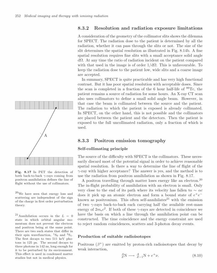
252 Medical imaging and therapy with ionising radiation
8.3.2 Resolution and radiation exposure limitations
A consideration of the geometry of the collimator slits shows the dilemmafor SPECT. The radiation dose to the patient is determined by all theradiation, whether it can pass through the slits or not. The size of theslit determines the spatial resolution as illustrated in Fig. 8.14b. A finespatial resolution requires fine slits with a small acceptance solid angledΩ. At any time the ratio of radiation incident on the patient comparedwith that used in the image is of order 1/dΩ. This is unfavourable. Tokeep the radiation dose to the patient low, wide slits and a coarse imageare accepted.
In summary, SPECT is quite practicable and has very high functionalcontrast. But it has poor spatial resolution with acceptable doses. Sincethe scan is completed in a fraction of the 6 hour half-life of 99Tc, thepatient remains a source of radiation for some hours. An X-ray CT scanalso uses collimators to define a small solid angle beam. However, inthat case the beam is collimated between the source and the patient.The radiation to which the patient is exposed is already collimated.In SPECT, on the other hand, this is not possible and the collimatorsare placed between the patient and the detectors. Then the patient isexposed to the full uncollimated radiation, only a fraction of which isused.
A
Fig. 8.17 In PET the detection ofboth back-to-back γ-rays coming frompositron annihilation defines the line offlight without the use of collimators.
8.3.3 Positron emission tomography
Self-collimating principle
The source of the difficulty with SPECT is the collimators. These neces-sarily discard most of the potential signal in order to achieve reasonablespatial resolution. Is there a way to determine the line of flight of theγ-ray with higher acceptance? The answer is yes, and the method is touse the radiation from positron annihilation as shown in Fig. 8.17.
A positron travelling through matter loses energy like an electron.20
20We have seen that energy loss andscattering are independent of the signof the charge in first order perturbationtheory.
The in-flight probability of annihilation with an electron is small. Onlyvery close to the end of its path where its velocity has fallen to ∼ αcdoes it pick up an atomic electron and form a bound state of e+e−
known as positronium. This often self-annihilates21 with the emission
21Annihilation occurs in the L = 0state in which orbital angular mo-mentum does not prevent the electronand positron being at the same point.There are two such states that differ intheir spin wavefunction, 1S0 and 3S1.The first decays to two 511 keV pho-tons in 125 ps. The second decays tothree photons in 142 ns, long enough forit to be perturbed by its environment.This effect is used in condensed matterstudies but not in medical physics.
of two γ-rays back-to-back each carrying half the available rest-massenergy of 2mec
2. If both of these γ-rays are detected in coincidence wehave the basis on which a line through the annihilation point can beconstructed. The time coincidence and the energy constraint are usedto reject random coincidences, scatters and 3-photon decay events.
Production of suitable radioisotopes
Positrons (β+) are emitted by proton-rich radioisotopes that decay byweak interaction,
AZN −→ A
Z−1N + e+ν. (8.10)

8.3 Functional imaging with radioisotopes 253
Table 8.1 The principal positron-emitting nuclei used in PET.
Nucleus Production Positron Half-lifeMax. energy Max. range
11C p+14N−→11C+α 1.0 MeV 2 mm 20 min13N p+13C−→13N+n 1.2 MeV 3 mm 10 min15O p+15N−→15O+n 1.7 MeV 4 mm 2 min18F p+18O−→18F+n 0.7 MeV 1.4 mm 110 min
Such nuclei are quite plentiful and are relatively easily made. Someuseful examples are given in table 8.1. This list shows immediately thatsuch isotopes can be substituted for the stable nuclei of C, N, O, etc.in any pharmaceutical agent of choice and the problem of toxicity doesnot arise. As the nuclei are of low Z and the Coulomb barrier whichforms an energy threshold for their production is low, protons from acyclotron of about 15 MeV have sufficient energy to drive the productionreactions given in the table. Because the β+-decay is a weak process,the half-lives are normally quite long. We no longer need to find a factor1016. The positron is emitted with a range of energies up to a maximumwhich determines how far it can go before it stops and annihilates.
Spatial resolution of PET
DA
Δθ
Fig. 8.18 The annihilation point (A) isa distance from the radioisotope decaypoint (D) depending on the positronrange. The line of flight of the γ-rays isnot quite back-to-back, angle ∆θ.
Figure 8.18 shows a little more detail. If the isotope decays at D, thepositron will have a range to its annihilation point A. The distanceDA represents an error in the image. As the table shows, the smallerthe positron energy, the shorter this range and the longer the half-life.For once the choices go the right way! We seek both a longer half-life and a shorter range.22 An additional position error comes from the
22Many PET images are taken with flu-orine. Fluorine is not normally presentin the body, but it can be incor-porated into glucose as fluoro-deoxy-glucose (FDG) without toxic side ef-fects. Since glucose has a high take-up at sites of metabolic activity, this ismost fortunate for clinical oncologicaluse.
fact that the two γ-rays are not quite back-to-back. At annihilationthe positronium is likely to have a velocity of the same magnitude as atypical atomic electron orbital velocity which is of order αc. So an angle∆θ ∼ 1/137 is to be expected. These two contributions to the spatialresolution are of order 2–3 mm.
The largest contribution to the spatial resolution of PET comes fromthe size of the detector elements. Detectors are composed of large arraysof small crystals, about 4×4 mm2, of BGO or calcium tungstate chosenfor their high Z and short radiation length. The segmented detectorneeds to record the position and contain the γ-ray energy, now 511 keV.The position of the photon may best be reconstructed as the centroidof the shower in the detector. Some of the practical problems may bejudged by noting that the photon mean free path in lead at 511 keV isabout 5 mm, greater by a factor 10–12 than at 140 keV.23 23See Fig. 8.14a.

254 Medical imaging and therapy with ionising radiation
Fig. 8.19 Two sets of slices from a complete 3-D tomographic PET whole-body image. In each case the superimposed crossedhair-lines indicate the position of the section shown in the other two slices of the set. The PET signal fits the position of theanomalous growth in the lung evident in the CT scan of the same patient shown in Fig. 8.12. [Images reproduced by kindpermission of Medical Physics and Clinical Engineering, Oxford Radcliffe Hospitals NHS Trust.]

8.3 Functional imaging with radioisotopes 255
Figure 8.19 shows an example of PET imaging. The effectiveness ofthe functional imaging is impressive. The spatial information is betterthan SPECT although worse than MRI or CT.
The major problem with PET is that the half-lives of the radioiso-topes involved are only a few minutes, as shown in table 8.1. The mostuseful isotope 18F has a mean life of 110 min. This makes it possible totransport an activated pharmaceutical from a hospital which has a cy-clotron facility to a neighbouring one that only has a PET scanner. Theshorter-lived isotopes have to be made on site at an accelerator adjacentto a highly automated hot chemistry laboratory. The reagents madein this laboratory are delivered to the patient by injection, circulatedin the bloodstream and absorbed in the region of interest. The wholeprocedure must be completed within a few half-lives of the radioisotopechosen. Such facilities are available at a small but growing number ofhospitals.24 24In 2003 there were 160 such sites in
USA and 120 in Europe. Notably therewere only 5 in the UK.
The principal benefit of PET with FDG is its sensitivity at flagginganomalous metabolic activity. The information that this brings to thetask of monitoring the progress of cancer is reported to outweigh its highcost. A need for more interdisciplinary skilled staff to run such facilitiespersists.
The strong signals from a SPECT or PET scan may be fused withMRI or CT scans with their precise anatomical detail. Provided thatthe registration of the two is sufficiently accurate the fused image maythen be used as a basis for therapy. In Fig. 8.15 fusion of MRI andSPECT images was shown for the liver. In Fig. 8.20 an instance offusion of CT and PET images is shown for a case of prostate cancerwith evidence for metastasis.
Fig. 8.20 PET–CT image fusion for a case of prostate cancer. Left, anatomical CT image. Centre, PET image showinganomalous take-up of FDG. Right, fused image showing precise locations of tumours. Note the increased glucose utilisationnear the right pelvic wall (1). Hermes Image Fusion reveals that this hot spot is in the right ilium directly lateral of the sacroiliacjoint. Lymph node metastasis right iliac region (2), with increased FDG-uptake. [Image reproduced by kind permission of DrRichard P Daum, [email protected] and www.zentralklinik-bad-berka.de.]

256 Medical imaging and therapy with ionising radiation
8.4 Radiotherapy
Ideally the task of therapy is to deposit energy uniformly within the volumeof a tumour and not to deposit energy outside in healthy tissue. The pre-cise shape and location of the tumour are established using one or moreof the imaging modalities. In radiotherapy the energy source may be ahigh energy collimated γ-ray or electron beam, an ion or proton beam, ora radioactive source. The radioactive source may be external or internal.Treatment by an implanted internal source is known as brachytherapy. Ingeneral it is not possible to match the radiation dose to the tumour vol-ume, but the best compromise maximises the uniform irradiation withinthe tumour volume and minimises the dose to the surrounding tissue. Thedependence of cell survival on dose is non-linear in both space and time.This is exploited to improve the effectiveness of treatment. Oxygenationand hydration also affect this dependence. Precise delivery of therapy rel-ative to a diagnostic image depends on registration, choice of energy andscattering. The use of ion beams has advantages over γ-ray or electronbeams in respect of focusing, scattering and the depth–dose profile.
8.4.1 Irradiation of the tumour volume
Fig. 8.21 A sketch of the problem ofthe radiotherapy of a deep-seated tu-mour. The volume to be irradiated uni-formly is shown as the heavily shadedregion within tissue which should bespared, shown lightly shaded.
incidentbeam
focussed?
beamabsorbedbefore?
beamabsorbedbeyond?
beamscattered
out?
beamscattered
out?
The objective of radiotherapy (RT) is to deliver a fatal dose of manyGy to the cells in the tumour while minimizing the damage to healthyperipheral tissue. The problem is illustrated in Fig. 8.21. Energy maybe absorbed by healthy tissue for any of the following reasons:
the radiation is not aimed at the target region, because ofinadequate focusing;
the radiation is not aimed at the target region, because ofalignment errors in registration;
the radiation is scattered out of the beam; the depth distribution is such that radiation is absorbed in
overlying tissue before it reaches the target; the depth distribution is such that radiation passes through
the target region and is absorbed in healthy tissue beyond.

8.4 Radiotherapy 257
The importance of these varies according to the therapy radiationsource. For example, the depth distributions sketched in Fig. 8.22 arequite different for a charged ion beam and a γ-ray beam. Whatevermethod is used the predicted deposited energy distribution is calculatedin 3-D; this process is called treatment planning. A
B
rate ofenergy
deposition
depth
Fig. 8.22 Sketch profiles of the depthdistribution from two sources of radio-therapy: A, a γ-ray beam, and B, acharged ion beam.
8.4.2 Sources of radiotherapy
Brachytherapy
A solution adopted in the early days and still used in certain casestoday is to implant a radioactive source at the site of the tumour. Lowenergy γ-sources, such as 192Ir, 125I (35 keV) or 103Pd (21 keV), areused. The strong attenuation and the simple geometric fall-off of the fluxwith distance from the implant delivers a highly localised dose. Sourcesmay be surgically implanted in accordance with the treatment planningprocedure to give a well-defined dose distribution. The relative locationsof the sources and tumour are imaged with ultrasound or MRI. Themethod is only in common use today in situations where the tumour isparticularly close to a radiation-sensitive region, such as in the treatmentof the prostate, which is very close to the rectum. Doses up to 100 Gyare given.
External radioactive sources
Beams of γ-rays from an external radioactive source may be used forRT. Usually 60Co is used. This emits γ-rays with energy 1.2 and 1.3MeV, and β-rays with 0.3 MeV. Such beams have drawbacks when com-pared with the high energy X-ray and γ-ray beams from acceleratorsdiscussed below. The radiation source cannot be turned off when notrequired. It has limited brightness as a point source providing irradia-tion in a narrow cone of interest. But it also has a high isotropic flux.This generates a high scattered background and requires extra shield-ing to protect staff. Such sources are used extensively for non-medicalapplications, but therapy with such sources is largely confined to ThirdWorld facilities.
Electron and photon beams
Most RT today is provided by photon or electron beams. The machinesto provide such beams were discussed in section 8.1.1. The energy ischosen to provide the penetration depth required, and this depends onwhether the tumour is on the surface or is deep seated. For surfacetumours RT with an electron beam may be used.25
25As shown in table 3.1, in low Zmaterials the energy loss of electronsis predominantly non-radiative up to70MeV. Therefore, for electrons of lessthan a few MeV, the contribution ofbremsstrahlung is small and they havea range of roughly 5 mm per MeV atthe density of water.
For deep-seated tumours RT is usually delivered by a beam of γ-rays of 1–20 MeV from an electron linear accelerator. Any low energycomponents of the spectrum would be absorbed rapidly in the surfacelayers and contribute no dose to the target volume. This effect is reducedby hardening the beam with high Z filters. In this range of photon

258 Medical imaging and therapy with ionising radiation
energy, Compton scattering is the dominant form of energy deposition.The recoil Compton electrons deposit their kinetic energy close to theline of flight of the beam, but the scattered photons travel away at anangle of order 1/γ radians where γ = E/mc2. Thus the effect of beamscatter reduces with energy. This angle is ∼ 1 at 20 MeV.
The transverse size of the irradiated volume depends on the beam size.The beam cannot be focused and its size is determined geometrically bythe electron spot size on the target anode and by the sets of collimatorswhich are shaped to match the tumour. The energy is deposited overa wider area than that defined by the collimators because of the finitespot size, the multiple scattering of the secondary electrons, and theeffect of the scattered secondary photons. The longitudinal size of theirradiated volume in a given orientation is poorly defined by the range ofthe radiation. In the simple terms of Fig. 3.1, this is dominated by theexponentially distributed point at which each photon interacts. It resultsin a rather featureless longitudinal distribution of energy deposition. Asa result substantial energy is deposited both in front of, and beyond,the target volume. By rotating and translating the beam relative tothe patient, the dose to healthy tissue may be spread out. Because ofthe non-linear relation between dose and cell damage, this spread in thedose distribution results in an important reduction in damage to healthytissue. But for this effect, photon beams would be quite unsuitable fordeep therapy.
Ion beams
Each of the shortcomings of photon RT may be addressed by the use ofion beams. Such a beam might be a proton beam of variable energy upto about 200 MeV, which would have a range in water of about 20 cm.2626The density of tissue and water are
almost the same. Since the range–energy relation for dE/dx is deter-mined by density, we may treat waterand tissue as equivalent.
As shown in chapter 3 the rate of energy loss, dE/dx or LET, of anion of charge Ze and velocity βc varies as Z2/β2. So for most of itstrajectory such an ion loses energy relatively slowly, but the energy lossrises rapidly as its velocity falls at the end of its range. The increaseddose, delivered to a small volume where the protons stop, is known asthe Bragg peak (see Fig. 3.12).27 By choosing the initial energy carefully27This is broadened somewhat by
straggling. to get the right range, most of the dose may be deposited at the requireddepth. No dose at all is deposited beyond the target region, and only asmall fraction in the overlying tissue.
The use of a charged ion beam brings the following improvements tothe transverse profile of the deposited dose.
Unlike a γ-ray beam, a charged ion beam may be focused intothe treatment volume very precisely using magnetic lenses.Spot sizes on the scale of 1 mm can be achieved.
An ion beam passing through matter creates negligible sec-ondary photons.
An ion beam does not itself scatter significantly and re-mains tightly collimated compared with an electron or pho-ton beam. In question 8.4 using equation 3.52 we calculate

8.4 Radiotherapy 259
that the RMS scattering angle for a proton beam passingthrough 10 cm of tissue is about 1. Its large mass ensuresthat each proton continues on an approximate straight patheven to the point where it stops.
Such therapy requires a substantial accelerator and there are alreadyseveral such clinical facilities with more under construction. If lightions such as carbon are used the LET may be increased further. Theenergy distribution of the Bragg curve is then amplified further by thenon-linearity. Such facilities are under development.
8.4.3 Treatment planning and delivery of RT
Inversion problem
k
O
s
r
u
u
z
z
radiationtrajectory
radiationtrajectory
s
a)
b)
Fig. 8.23 The geometry of a trajec-tory defined by the vector of its clos-est approach s to the origin at O andazimuthal angle φ in the plane normalto s. The vector r is the position ofan element of tissue on the trajectory.This geometry is seen a) as viewed ina general direction, and b) as viewedin the plane normal to s showing theazimuthal angle φ.
The radiation dose delivered in three dimensional space is the super-position of the radiation absorbed from a number of pencil rays. In asimplified picture we consider each such ray depositing energy with anabsorption coefficient µ per unit density ρ. The geometry of a ray isshown in Fig. 8.23. Relative to the origin at O and the z-axis, each suchray may be described by a vector s, the point of closest approach to theorigin, and φ, the azimuthal angle of the direction of the trajectory inthe plane perpendicular to that vector relative to the z-axis.
We write k as a unit vector along the z-axis, and the vector s in termsof its length s and unit vector s. Then a unit vector along the ray is
u =(s × k) sinφ + s × (s × k) cosφ
|s × k| . (8.11)
The equation of the line of the ray is then
r = s + λu, (8.12)
where λ is the distance along the ray from the point of closest approachto the origin. An element of flux may be written Φ(s, φ) d3s dφ. Thenthe energy deposition per unit volume of r-space is found by summingover all elements of flux and values of λ to give a dose
D(r) = µρ(r)∫ ∫ [∫ ∫ ∫
Φ(s, φ) δ3(r − s − λu) d3s
]dλ dφ. (8.13)
Looking at this relation we consider the task. The required dose dis-tribution D(r) is known. It is uniform over the volume of the tumourand zero outside.28 We want to find the distribution of flux Φ(s, φ) that
28In fact the irradiated volume is cho-sen to be slightly larger than the tu-mour itself to allow for imperfections ofalignment or registration between thetreatment and imaging coordinate sys-tems.
should be applied to achieve it. We have the relation 8.13 between thetwo.29 In fact it is rather more realistic to consider small discrete ele- 29The 3-D δ-function in equation 8.13
reduces this 5-D integral down to a 2-D one. These may be thought of asthe two angles, polar and azimuth forexample, of the radiation that depositsenergy in the voxel at r.
ments of volume and turn these integrals into summations. Then thelinear relation between the elements of flux Φ and the dose to voxels Dcan be expressed in matrices, as was the case for the general CT problemfor imaging, equation 8.2. Then, as in equation 8.3, the matrix has only

260 Medical imaging and therapy with ionising radiation
prostate
rectum
Fig. 8.24 A 2-D section of the dose contours (shown as a percentage of the peak value) calculated as part of the treatmentplan for RT of the prostate. The contours are shown superimposed on the anatomical section. Note the re-entrant contoursaround the rectum. Such doses are delivered in a number of fractions spread over several months, as discussed in the text.[Image reproduced by kind permission of Medical Physics and Clinical Engineering, Oxford Radcliffe Hospitals NHS Trust.]
to be inverted to derive the elements of flux Φ required to deliver the el-ements of dose D. Mathematically this is atraightforward; the inversionis not singular.
But this attractive conclusion is flawed. Common sense tells us thatwe cannot irradiate a volume deep inside the body with such a super-position of rays without also irradiating the overlying tissue to someextent. What is wrong with our calculation? The answer is that sucha computation describing a perfect treatment would require the use ofnegative as well as positive fluxes! With positive flux elements alone thedistribution of delivered dose includes irradiation of tissue elements thatwe do not wish to irradiate.30
30These ideas may be extended byconsidering µ to be a function of λto describe the range distribution inbrachytherapy or the Bragg curve in ionbeam therapy.
Intensity-modulated radiotherapy (IMRT)
We can still define the treatment planning task with the help of equa-tion 8.13. We need to determine the flux elements Φ(s, φ) that minimisethe irradiation of the rest of the tissue while maintaining the requireddose D(r) inside the tumour. With the constraint that flux elements bepositive this is no longer a linear problem and must be solved iteratively.
As available computational power has increased, the completeness andprecision of planning calculations have improved. The optimisation ofthe treatment plan in terms of the model is driven by the delineationof the region to be irradiated and the sensitive regions to be spared.Numerical optimisation procedures can be set to work to find by itera-tion the set of fluxes that come as close as possible to the desired dosedistribution.

8.4 Radiotherapy 261
Delivery of such elements of flux requires a beam that can be rotated,translated and modulated in intensity. In practice this involves irradia-tion at a number of angles with a parallel beam which can be modulatedin shape by a 2-D collimator composed of dynamically controlled ‘fin-gers’. The optimisation is then made in terms of the actual degrees offreedom of the particular therapy accelerator, its collimators and geom-etry. If there are restrictions on the beam angles available because ofthe position of the patient, these can be taken into account in the treat-ment planning. The irradiated volume may follow complex 3-D contourswith re-entrant regions that reduce exposure to sensitive organs. Thisprocedure is called intensity modulated radiotherapy (IMRT).
Because the plan is a 3-D problem it is not easy to visualise from2-D representations. An example of a set of 2-D dose contours is shownsuperimposed on an anatomical image in Fig. 8.24. This treatmentplan provided for the uniform irradiation of the prostate, minimisingthe irradiation of the rectum which is particularly sensitive and close by.This is achieved by five beam settings each with particular collimatorconfigurations. A 2-D sketch, Fig. 8.25, indicates the general directionsof the flux but it does not describe the 3-D nature of the problem andits solution, and does not show transverse shaping of the beam by thecollimator fingers.
Fig. 8.25 A rough 2-D sketch of thedirections of radiation flux required inthe IMRT plan, Fig. 8.24.
Figure 8.24 shows the difficulty rather clearly. A dose of many Gy isrequired to treat the tumour volume but the peripheral healthy tissuewould receive as much as 50% of that over a wide area. The actualvalue of the dose is determined by the tolerance of the peripheral healthytissue. Thus an improved plan would permit a higher peak dose to beapplied to the tumour with a higher probability of successful treatment.The treatment for the plan shown in Fig. 8.24 called for a total peakirradiation of 60 Gy. To permit the peripheral healthy tissue a chance torecover this is spread over 20 fractions, as discussed later. This meansthat the healthy tissue is subject to 1.5Gy for each fraction, a significantdose which will leave scar tissue.
The details of treatment planning differ depending on the method andenergy of irradiation. With γ-ray RT, the beam is attenuated slowly anda reduced flux reaches deeper layers. Compton scattering and electron–positron pair production must be included in the calculation of the dosedistribution map. For brachytherapy and ion beam therapy the effectsare different but a precise treatment plan is needed nonetheless. Inevery case allowance has to be made for systematic errors, particularlyin alignment.
Dose monitoring
During the delivery of RT the irradiated region should be preciselyaligned with the tumour concerned. This alignment depends on themapping of imaging information into the coordinate system of the plan-ning and therapy delivery system. Depending on the location of thetumour this may require

262 Medical imaging and therapy with ionising radiation
an RT delivery coordinate system defined with a set of lowpower laser beams relative to which the patient may bealigned;
a set of visual marks on the patient’s skin or implanted metaltargets that can be related directly to the coordinate systemof the scanned images and related treatment plan;
a number of tightly defined mechanical restraints to whichthe patient is attached;
a portal imaging system in which the transmitted RT flux isused to provide an image relating the treatment volume andto the physiology of the patient in real time.
The high photon energies used for RT show little contrast for any physiol-ogy properties apart from (electron) density.31 Consequently such portal31As discussed in chapter 3 such pho-
tons are far removed from any photo-electric absorption edge showing dis-crimination between elements.
images have poor contrast and are not ideal for aligning the patient’sphysiology with the treatment plan.
The good spatial definition of ion beam therapy puts extra demandson registration which must be matched to it. Real-time imaging duringtherapy becomes increasingly important. When the spatial resolution ofthe beam is finer than the volume to be treated, the dose distributionmay be delivered by scanning the beam on a raster. With such resolutionthe dose to the target volume can be increased, the dose to peripheraltissue reduced, and the success rate of the therapy increased.
The other monitoring function concerns the measurement of the deliv-ered flux. In the first instance this comes from the settings of the X-raysource and the exposure time. The portal imaging device monitors thisdose. Traditionally this was done with photographic plates and ionisa-tion chambers, the former for the position information and the latter forthe absolute calibration of dose. These are now replaced by amorphoussilicon pixel arrays that provide fast readout of the portal image withgood linearity.
8.4.4 Exploitation of non-linear effects
Cell repair
As discussed so far in this section it has been implicitly assumed thatthe effect of irradiation on the cells of a tumour is linear. However, wehave seen already in chapter 6 that this is not the case. This is becausecells can repair themselves if the DNA does not suffer multiple damage.
As a result, cell death is not a linear function of dose. The dependenceof cell mortality on dose is shown qualitatively as curve A in Fig. 8.26.Such behaviour follows if cells suffering single hits can survive by re-pair. If in a given treatment peripheral healthy tissue gets half the dose,the cell mortality would be described by curve B in the figure. For atreatment corresponding to the vertical line, the healthy tissue wouldthen suffer 10% cell mortality while the tumour cells would suffer morethan 80%. In this illustration the non-linearity brings the benefit thatthe tumour cells suffer eight times the mortality although the dose is
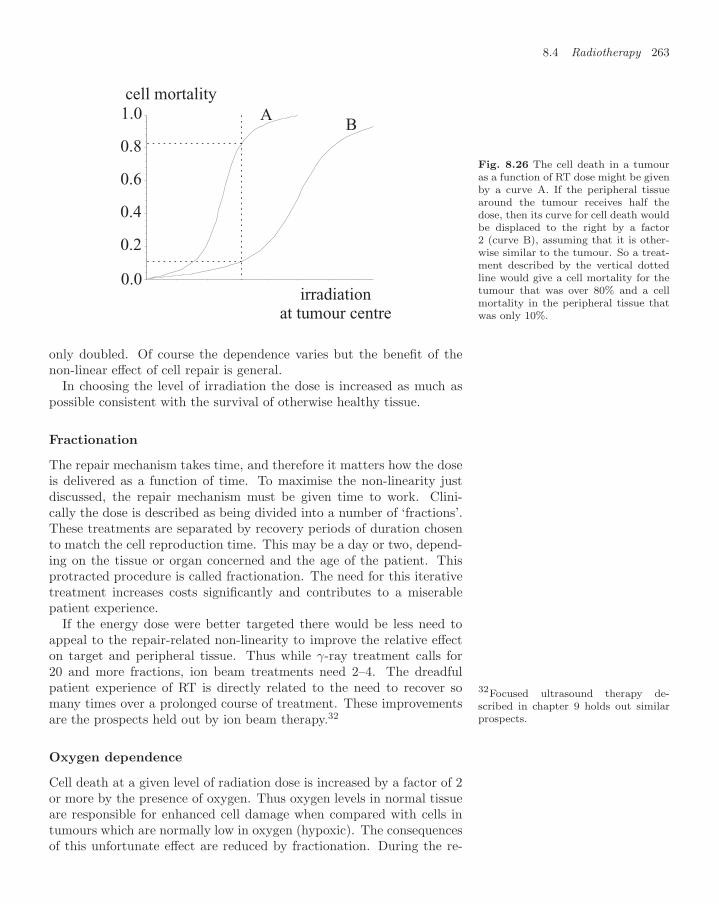
8.4 Radiotherapy 263
0.2
0.4
0.6
0.8
1.0 AB
irradiationat tumour centre
cell mortality
0.0
Fig. 8.26 The cell death in a tumouras a function of RT dose might be givenby a curve A. If the peripheral tissuearound the tumour receives half thedose, then its curve for cell death wouldbe displaced to the right by a factor2 (curve B), assuming that it is other-wise similar to the tumour. So a treat-ment described by the vertical dottedline would give a cell mortality for thetumour that was over 80% and a cellmortality in the peripheral tissue thatwas only 10%.
only doubled. Of course the dependence varies but the benefit of thenon-linear effect of cell repair is general.
In choosing the level of irradiation the dose is increased as much aspossible consistent with the survival of otherwise healthy tissue.
Fractionation
The repair mechanism takes time, and therefore it matters how the doseis delivered as a function of time. To maximise the non-linearity justdiscussed, the repair mechanism must be given time to work. Clini-cally the dose is described as being divided into a number of ‘fractions’.These treatments are separated by recovery periods of duration chosento match the cell reproduction time. This may be a day or two, depend-ing on the tissue or organ concerned and the age of the patient. Thisprotracted procedure is called fractionation. The need for this iterativetreatment increases costs significantly and contributes to a miserablepatient experience.
If the energy dose were better targeted there would be less need toappeal to the repair-related non-linearity to improve the relative effecton target and peripheral tissue. Thus while γ-ray treatment calls for20 and more fractions, ion beam treatments need 2–4. The dreadfulpatient experience of RT is directly related to the need to recover somany times over a prolonged course of treatment. These improvementsare the prospects held out by ion beam therapy.32
32Focused ultrasound therapy de-scribed in chapter 9 holds out similarprospects.
Oxygen dependence
Cell death at a given level of radiation dose is increased by a factor of 2or more by the presence of oxygen. Thus oxygen levels in normal tissueare responsible for enhanced cell damage when compared with cells intumours which are normally low in oxygen (hypoxic). The consequencesof this unfortunate effect are reduced by fractionation. During the re-

264 Medical imaging and therapy with ionising radiation
covery periods the oxygen levels in the tumour start to return to normalas the runaway metabolic activity slows. As a result, later fractionsbenefit from oxygen levels in the target tumour that were absent whenthe initial fractions were given.
Further sources of non-linearity
Any source of non-linearity can improve the separation of the survivalof peripheral tissue from the mortality of treated cells. The steeper thecurves sketched in Fig. 8.26, the better will be the result.
In chapter 6 the non-linear response of tissue to highly charged slowions was discussed. The biological damage caused with such ions isgreater than with γ-rays, joule for joule, by an order of magnitude andmore. This effect is crudely described by the radiation weighting factorswR in table 6.4. This effect depends on the LET. Consequently as anion slows and stops in tissue, not only does the deposited energy rise as1/β2 described by the Bragg peak but the damage rises even faster dueto wR. This extra non-linearity is such that the number of fractions maybe reduced and the dose to the tumour raised. The effect is expected tobe even more pronounced with multiply charged ions such as carbon.
Read more in books
A Century of X-rays and Radioactivity in Medicine,RF Mould, IOP (1993), a book of early pictures andinteresting authoritative history
The Physics of Medical Imaging, ed. S Webb, IOP(1988), an edited compilation of useful articles, some-what out of date but still frequently referenced
Contemporary IMRT: Developing Physics and ClinicalImplementation, S Webb, IOP (2004), a recent text onradiotherapy, see also earlier books on radiotherapy bythe same author

8.4 Radiotherapy 265
Look on the Web
Look at the book website atwww.physics.ox.ac.uk/users/allison/booksite.htm
Search for further examples of images including the useof contrast agents with combinations of
CT, angiography, SPECT, PET
Look at manufacturers’ websites and the images thatmay be downloaded, for example
GEhealthcare or Hermesmedical
Look on the Brookhaven database for nuclei that mightbe suitable for nuclear medicine
nuclear data BNL
For radiotherapy searching is a bit harder. Many web-sites are concerned simply to reassure patients and areshort on factual information. Try some of
brachytherapy, radiotherapy treatment planning,IMRT
For prospects in radiotherapyproton therapy, BASROC or carbon therapy
Questions
8.1 Consider the following simple calculation of the ef-ficiency of bremsstrahlung production by electrons.If it is assumed that electrons have β = 1, the rateof energy loss with distance is −E/X0 − b, where bis the rate of non-radiative energy loss. Show thatthe solution to this equation is
E(x) = (E1 + bX0) exp (−x/X0) − bX0
for an electron whose energy is E1 at x = 0.Hence show that its range is X0 ln(1 + E1/(bX0)),and that the efficiency, the fraction of energy emit-ted as bremsstrahlung, is
(E1 − Rb)/E1 = 1 − X0b ln(1 + E1/(bX0))/E1.
[This simple model neglects K shell emission, an-gular distributions, scattering and self-absorption.By assuming that β = 1 it over-estimates thebremsstrahlung efficiency, especially at low energy.]
8.2 When 99Tc∗ decays to 99Tc emitting a 140 keVγ-ray, the nucleus recoils. Calculate this recoil en-ergy.
8.3 A patient is irradiated with X-rays in a CT scan.The 3-D spatial resolution is 1 mm and the statis-tical noise is 1%. Make a reasoned estimate of theminimum dose that the patient receives.
8.4 A 175 MeV proton beam passes through 10 cm oftissue. Using data in table 3.1 show that the RMSscattering angle of the beam is just over 1.[Treat the tissue as equivalent to water and neglectthe effect of energy loss by the proton.]
8.5 A radiotherapy beam of carbon ions with charge6+ is to penetrate a depth of 20 cm in tissue andstop. Find the required incident beam energy.

This page intentionally left blank

Ultrasound for imaging andtherapy 9
9.1 Imaging with ultrasound 267
9.2 Generation of ultrasoundbeams 272
9.3 Scattering in inhomogeneousmaterials 280
9.4 Non-linear behaviour 290
Read more in books 305
Look on the Web 305
Questions 306
in which the use of ultrasound for medical imaging and therapy is ex-plored, and the important roles of scattering and non-linearity are em-phasised.
9.1 Imaging with ultrasound
The direction of objects that emit sound may be determined by passiveimaging. In active imaging the observer emits a sound wave that it is re-flected by the object. The detected signal is the convolution of the emittedwave train and the reflection coefficient as a function of radial distance.The resolution of the spatial imaging information depends on the wave-length used. In the non-destructive testing of materials both longitudinaland shear waves are used. Medical imaging uses longitudinal waves forwhich tissue materials differ little in mean properties (with the exceptionof bone, tooth and air). Contrast in images is made possible by differ-ences in scattering from inhomogeneities, contrast agents, Doppler shiftsby moving fluids, and harmonic generation.
9.1.1 Methods of imaging
Passive directional imaging
Sound is used for navigation and communication by humans and othercreatures over distances large compared with a wavelength. The fre-quency range of 100–20,000 Hz employed by humans corresponds to awavelength range in air of 3.3 m down to 20 mm for a sound velocity inair of 330 m s−1. In water the velocity is five times higher and the wave-length five time larger at the same frequency. Sounds in this range areeasily generated by bio-mechanical or electro-mechanical transducers.
In passive imaging the direction of sound emitted by an object issensed by using several detector elements. For example, the use of twoears is sufficient for animals to detect the direction of sound sources inthe horizontal plane.
If the wavelength is small compared with the size of the head, the headcasts a sound ‘shadow’ so that the ear furthest from the source hears aweaker signal. Thus for humans in air at frequencies above 1500 Hz therelative sound intensity is used to determine direction. If the wavelengthis large compared with the width of the head, the waves diffract around

268 Ultrasound for imaging and therapy
the head and there is no shadowing. However, the direction may thenbe detected by the difference in phase of the sound waves heard by thetwo ears. For the human head this phase difference gives directionalinformation in air at 500 Hz and below. At frequencies around 1000 Hzthere is little directional information. In water these frequencies wouldbe five times higher.
Directional information can be improved dramatically using parabolicmirrors to focus the sound.1 In espionage technology these principles1A parabolic shape is appropriate to a
source at infinity. For a single sourceat a finite distance the shape should bean ellipse. The Winston cone is a shapeoptimised for a distribution of distantsources. The intuitive conical horn orear trumpet is a qualitative solution.
are extended with large diaphragms and sensitive microphones. Similarpassive detection methods are used in the sea to detect ships, submarinesand creatures such as whales and porpoises. However, the passive useof sound gives little indication of range.
Active imaging and range by timing or frequency shift
In the active use of sound for imaging, a sound pulse is emitted and theecho of the reflected signal is detected. The timing of the echo givesthe range of an object. The directional information is added either byemitting the pulse in a specific direction or by sensing the direction ofthe echo. In practice both may be used. Such active imaging is used lessby humans than by other creatures, most famously bats who employ itto sense a complete 3-D image of their surroundings.
The traditional method is to emit a short pulse and to determine therange distribution of a number of objects by measuring the time-lapsespectrum of the reflected signals.2 An alternative is to emit a continuous2This is the type of scan used with RF
waves in radar. beam with a frequency that changes linearly with time. The difference infrequency between the transmitted beam and reflected signal at any timeis proportional to the delay since the received beam was emitted. Thisfrequency shift therefore encodes the radial distance to the reflectingsurface. The phase as well as the amplitude of the reflected signal ismeasured by interference with a reference beam. This approach is calledfrequency scanning interferometry (FSI). As in the traditional time-lapsemethod the waves add linearly so that a number of reflecting surfacesmay be imaged simultaneously. This method requires the source andimaging transducers to operate over a wide bandwidth. Probably fortechnical reasons FSI has not been used much in ultrasound imaging todate. However, it is used widely in laser metrology.33The Michelson interferometer is the
archetype. In FSI the frequency reflected by moving objects depends on theirrange and their velocity through the Doppler shift. By analysing signalswith the frequency ramping down as well as up, such objects may belocated in both range and radial velocity.
Range resolution
The spatial resolution is limited by the wavelength, both transversely inangle and radially in range. Using higher frequencies (20–100 kHz) batsachieve high resolution.4 They employ combinations of pulse emission
4This is about the highest frequencythat can be achieved with a transducerwithout the use of piezoelectric mate-rials which are not available in livingtissue, one presumes.
and FSI. In the technical and medical use of ultrasound, to get thebenefit of the best resolution and directional information frequencies

9.1 Imaging with ultrasound 269
–0.4
–0.2
0
0.2
0.4
2
2
4
4
6
6
8
8
10
10
12
12
ω/10 s -13
–0.4
–0.2
0
0.2
0.4
t/ms2 4 6 8 10 12 14 16 18 20
a) b)
–0.4
–0.2
0
0.2
0.4
–0.4
–0.2
0
0.2
0.4
t/ms2 4 6 8 10 12 14 16 18 20
c) d)
ω/10 s -13
/10 s -13
/10 s -13
Fig. 9.1 a) A broad Gaussian 1 kHz pulse with ∆t = 1.1 ms plotted in time t.b) The frequency spectrum of a) showing Q = ω/∆ω = 7.c) A narrower Gaussian pulse with ∆t = 0.55 ms plotted in time t.d) The frequency spectrum of c) showing Q = 3.5.
up to 10 MHz or beyond may be used. At 1 MHz the wavelength is1.5 mm in water and this sets the scale of spatial resolution in medicalapplications. The angular resolution is λ/D where D is the width ofthe transmitter (or receiver). Although the resolution improves if thefrequency is increased further, the range over which ultrasound can beused becomes shorter due to increased absorption.
Let us see how this works. For illustration, Fig. 9.1a shows a pulsef(t) of frequency 1 kHz emitted at time t = 10 ms with a width ∆t = 1.1ms.5 The reflected signal F (t′) observed at time t′ is the convolution of 5We show Gaussian pulses for which
the width ∆t is conveniently defined asthe standard deviation σ. Then, sincethe frequency spectrum, the Fouriertransform of the time pulse, is alsoGaussian, the width of the spectrum∆ω may be defined in the same way.
f with the reflection coefficient as a function of range, R(r),
F (t′) =∫
f(t′ − 2r/c)R(r)dr. (9.1)
By taking Fourier transforms the radial profile R(r) may be extractedfrom the observations. Using equation 5.14 the Fourier transform ofthe object can be written down. However, for frequencies for which

270 Ultrasound for imaging and therapy
the PSF is very small, the inversion becomes singular. In other words,spatial detail can only be imaged for those spatial frequencies k = 2ω/cfor which spectral components are present in the pulse. Figure 9.1bshows the values of ω for which this is the case. At other values of ω,and thence k, the reconstruction involves dividing by a small number,thereby amplifying noise in the image.
A pulse narrower in time may be used, as shown in Fig. 9.1c, giving abroader spread in frequency, Fig. 9.1d. The range of spatial information∆k = ∆ω/c is greater than with the pulse broader in time. So it isthe bandwidth and noise that determine spatial resolution. Deconvolu-tion may be used to boost resolution but noise ultimately prevents theamplification of signal at spatial frequencies that are effectively absent.
Imaging of objects in three dimensions
This treatment may be extended to imaging in three dimensions. As wellas the range information, the observed signal involves the convolutionof the angular distribution of the transmitted pulse, the reflectivity atdifferent angles and the response of the detector as a function of angle.Suppose that, when the detector is pointed at an angle θ′, the sensitivityto signals at angle θ is g(θ′ − θ). Then the observed signal
F (t′, θ′) =∫ ∫
f(t′ − 2r/c)g(θ′ − θ)R(r, θ)drdθ. (9.2)
As in optics, the angular pattern of a radiator or receiver with well-defined aperture d involves an angular resolution of λ/d with sidelobesat angles ±1.5×λ/d. A similar angular resolution is involved in passiveimaging. Angular resolution good at the level of a degree or so thereforerequires radiators or detectors with sizes on the scale of 50λ. At acous-tic frequencies in the animal kingdom this would be very cumbersome.Nature’s solution is to use an array of discrete detectors, a pair of ears.For ultrasound such arrays may be conveniently small.
In general the signal received is the convolution of the object and the3-D PSF. To reconstruct an image of the object, measurements are takenthat sample as much of k-space as possible, as with other modalities.This may be achieved by sweeping the centre spot of the PSF bothradially and azimuthally in time as discussed. To complete the 3-Dprocess it should be scanned in polar angle also.
9.1.2 Material testing and medical imaging
Non-destructive testing
The improved reliability of everyday items and technical products inthe second half of the twentieth century depended on the developmentand application of quality control testing of the integrity of materials.This is known as ‘non-destructive testing’. While other modalities inthis book such as X-rays are also used, sound is often the preferredmethod of searching for cracks, scratches and other hidden flaws. The

9.1 Imaging with ultrasound 271
changes in density and elastic properties at such discontinuities giverise to large reflection coefficients for ultrasound. For instance, majorimpedance changes occur at gaseous or liquid occlusions that do notsupport transverse waves. The high resolution required to resolve smallblemishes means that frequencies in excess of 10 MHz are usually used.This is because of the high velocity of sound in metallic and other rigidmaterials for which wavelengths are otherwise correspondingly longer.
Table 9.1 Values of the speed of longi-tudinal sound (cP , in m s−1) and lon-gitudinal impedance (ZP , in units of106 kg m−2 s−1) for various tissuesand substances. [Quoted from Evans &McDicken, table 3.1]
Material cP ZP
Air (NTP) 330 0.0004Amniotic fluid 1510Aqueous humour 1500 1.50Blood 1570 1.61Bone 3500 7.80Brain 1540 1.58Cartilage 1660Castor oil 1500 1.43Cerebral spinal fluid 1510Fat 1450 1.38Kidney 1560 1.62Eye lens 1620 1.84Liver 1550 1.65Muscle 1580 1.70Perspex 2680 3.20Polythene 2000 1.84Skin 1600Average soft tissue 1540 1.63Tendon 1750Tooth 3600Vitreous humour 1520 1.52Water 1480 1.48
Medical imaging
There are difficulties in applying ultrasound to medical imaging.The density and compressibility variations in biological tissue are
small. Table 9.1 shows the variations in longitudinal sound velocityand impedance. Apart from bone and tooth on the one hand, and airon the other, materials are rather similar. Table 9.2 shows that reflectedenergies are also small from most interfaces of possible interest. Tissuematerials vary in composition from sample to sample so that the num-bers in tables 9.1 and 9.2 are rather imprecise as well as being closein value to one another. Further, the tissue boundaries that exist arenot sharply defined and are not planar. One might conclude from thesearguments that ultrasound medical imaging would not show effectivecontrast.
Table 9.2 Calculated reflection coeffi-cients at normal incidence for the am-plitude RA and for the energy RE .[Quoted from Evans and McDicken, ta-ble 3.4]
Boundary RA RE
Fat/muscle 0.10 0.0108Fat/kidney 0.08 0.0064Muscle blood 0.03 0.0007Bone/fat 0.70 0.4891Bone/muscle 0.64 0.4123Lens/aqueous 0.10 0.0104
humourSoft tissue/water 0.05 0.0023Soft tissue/air 0.9995 0.999Soft tissue/PZT 0.89 0.800Soft tissue/poly- 0.47 0.0022
vinylidenedifluorideSoft tissue/ 0.07 0.0043
castor oil
There are six reasons why ultrasound is an effective imaging modalityin spite of these difficulties.
1. The random thermal noise level in ultrasound is low, so thatsmall signals can be detected. MRI is troubled by the lowsignal-to-noise ratio that accompanies the small signal from1 in 105 magnetised protons. Ionising radiation modalitiesare troubled by the large statistical fluctuations that accom-pany the use of large energy quanta. Relative to the compe-tition, ultrasound images have good signal-to-noise ratio, atleast in principle.
2. Reflected ultrasound signals come from incoherent scatter-ing, not from specular reflection by sharply defined planarsurfaces. Such scattering is caused by the fact that the ma-terials of living tissue are not homogeneous. Materials aredistinguished by the extent to which they are inhomogeneousand generate scattering, rather than by differences in theirmean properties. In fact some materials such as blood areremarkably inhomogeneous.
3. Inert contrast agents that increase scattering may be intro-duced. Because such agents do not rely for their efficacy onany chemical effect or biological action, they are non-toxicand present no hazard beyond their physical bulk.
4. If these inhomogeneities are moving longitudinally, ultra-sound can measure their velocity through the Doppler shiftin the frequency of the scattered waves.

272 Ultrasound for imaging and therapy
5. In addition to the small variations in longitudinal sound ve-locity and impedance shown in table 9.1, there are varia-tions in shear modulus between different tissues. At normalincidence these do not affect the reflection of longitudinal Pwaves. However, as seen in chapter 4, significant polarisa-tion changes in reflected and transmitted waves are to beexpected at other angles of incidence. The shear modulus issensitive to fluidity, muscle tension and other properties ofclinical interest. Indeed, in so far as palpation involves a lin-ear process, it is a procedure for sensing a local variation ofshear modulus, due for instance to a tumour felt as a lump.
6. Contrast may be generated through the non-linear responseof tissue materials. At moderate amplitudes this is seen asharmonic frequency generation, a process characteristic ofnon-linear phenomena in general. Materials differ more intheir non-linear properties than they do in their linear ones,specifically sound velocity and density. It follows that imag-ing by harmonic generation usually exhibits better contrastthan fundamental imaging. In addition contrast agents maybe introduced which enhance harmonic generation.
Because the mean acoustic properties of tissue do not vary much, imagedistortion through refraction is quite mild and can be corrected. In thisrespect at least the homogeneity of tissue materials represents a usefulbenefit.
9.2 Generation of ultrasound beams
The generation of ultrasound depends on the use of piezoelectric res-onators, made of a material with a non-centrosymmetric crystal struc-ture. Quartz with an internal tetrahedral structure is the classic example.A number of other materials are now commercially available. A resonatorconsists of a slice of thickness λ/2 so that the resonator has antinodes atfront and back boundaries. In the far-field region (distance > d2/λ) thewavefront from such a transducer of width d is approximately spherical. Afocusable and steerable ultrasound beam may be emitted by a phased arrayof such transducers. Such an array can also act as a receiver. The PSF ofthe beam is determined by the geometry of the array and the wavelength.
9.2.1 Ultrasound transducers
Problems at high frequency
The choice of high frequencies to optimise image resolution has two ma-jor drawbacks. Although there are a number of different mechanisms

9.2 Generation of ultrasound beams 273
of sound absorption, they all increase with frequency.6 Ultrasound sig- 6Low frequencies are often preferred forpassive imaging. Fog horns operate atthe lower limit of audible frequencies inorder to maximise the range of signalsunder foggy conditions. Fog scattersstrongly at short wavelengths.
nals have a short range, especially in materials of low rigidity such assoft tissue. Hence lower frequencies are used in medical imaging thanin non-destructive testing. The penetration depth of the required imagedetermines the choice of frequency.
The second disadvantage of the choice of high frequency concerns gen-eration and detection. Effective sources and detectors need to be highfrequency mechanical resonators. For a high frequency mechanical res-onance a low inertial mass and a high restoring force are required withstrong coupling to both electrical input and acoustic output. An ultra-sound detector can employ the same resonance as the generator, excitedby its coupling to the incident pressure wave and losing energy throughcoupling to an electrical output signal, instead of the other way around.
Thus for high frequencies we need materials that couple electricaland mechanical behaviour of matter directly and firmly. Piezoelectricmaterials have this property.
ultrasoundbeam energy
energy stored inresonant transducer
hysteresis lossesin resonator
electrical energyin external circuit
Fig. 9.2 The energy stored in a piezo-electric resonator is supplied by the ex-ternal circuit and transmitted to the ul-trasound beam. Acting as a detectorthe energy flow is reversed but is alsomuch smaller. The resonator also losesenergy to heat internally by hysteresis.
Piezoelectricity is the strain generated in a material by an appliedelectric field, or vice versa. If the material is constrained a stress will beinvolved also. The coupling between the stress and strain in the piezo-electric resonator and the stress and strain in the medium of propaga-tion depend on their respective impedances and the mechnical boundaryconditions. The coupling on the electrical side depends on the electricalinput impedance that the resonator presents to the external circuit. Anadditional process is that a medium can lose energy internally throughmechanical hysteresis. Together these couplings, shown schematicallyin Fig. 9.2, determine the Q of the resonator and the efficiency withwhich incident acoustic energy is transformed to electrical energy, andvice versa.
Ferroelectricity and piezoelectricity
An ultrasound transducer that produces acoustic output transforms avoltage signal, a longitudinal Ez, into ε33 = ∂uz/∂z, the longitudinalstrain. Such a transducer is shown in Fig. 9.3. The strain of the ac-tive element ε, assumed linear, depends on the third rank7 piezoelectric 7For a discussion of tensors see chap-
ter 4.tensor dijk . In general
εij = dkijEk + Slm
ij Tlm (9.3)
where Ek is the electric field, Slmij is the elastic compliance tensor, and
Tlm is the stress tensor. When coupled to a low impedance acousticmedium, the piezoelectric material is not subjected to a mechanicalstress and the second term nearly vanishes. This means that there is anantinode at the surfaces of the piezoelectric material.8 We write ‘nearly’ 8The surface is nearly free, hence the
material has a thickness λ/2.as a reminder that the medium driven by the transducer does have asmall impedance, otherwise no energy would be transmitted at all.
Only certain materials have the lack of a centre of symmetry in theircrystal structure required for a non-zero piezoelectric effect. There aretwo classes, those with pre-existing electric dipole moments, and those
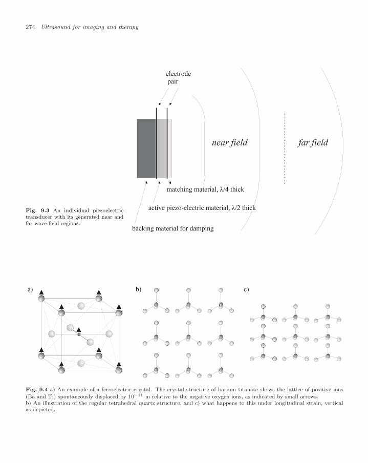
274 Ultrasound for imaging and therapy
Fig. 9.3 An individual piezoelectrictransducer with its generated near andfar wave field regions.
backing material for damping
active piezo-electric material, λ/2 thick
matching material, λ/4 thick
electrodepair
near field far field
b)a) c)
Fig. 9.4 a) An example of a ferroelectric crystal. The crystal structure of barium titanate shows the lattice of positive ions
(Ba and Ti) spontaneously displaced by 10−11 m relative to the negative oxygen ions, as indicated by small arrows.b) An illustration of the regular tetrahedral quartz structure, and c) what happens to this under longitudinal strain, verticalas depicted.

9.2 Generation of ultrasound beams 275
Table 9.3 Some values of piezoelectric properties for quartz and proprietary ceramicmaterials based on lead zirconium titanate (PZT) and barium titanate (BT). Thedissipation is the reciprocal of the electrical Q measured at 1 kHz. The density ρ in103 kg m−3. [Data from various websites.]
Material c ρ εr d333 Dissipationm s−1 10−12 m V−1 1/Q
Quartz 5660 6.82 4.5 −2.3K300 4060 7.7 1450 350 0.004PZT-4 4600 7.6 1470 315 0.003BT301 5640 5.8 1140 127 0.006PZT5J1 7.4 2600 500 0.02PZT5H1 4560 7.4 3250 620 0.018
without a centre of symmetry but no pre-existing inherent moment. Weconsider an example of each.
Ferroelectrics have an inherent charge asymmetry in the crystal unitcell. They include materials such as barium titanate, in which a latticeof barium and titanium ions is displaced with respect to the lattice ofoxygen ions by about 10−11 m, as illustrated in Fig. 9.4a. As with fer-romagnetism and paramagnetism, there is usually a temperature belowwhich the material is spontaneously polarized in this way. Above thistemperature the material appears symmetric but shows a large linearpolarisability. This is the para-electric state.9 Such a material exhibits 9In these materials the instability of the
unit cell may be described in terms ofan optical phonon band that reachesdown to zero frequency at k = 0, com-pare Fig. 4.23. However, such disper-sion curves do not tell the full underly-ing stories of non-linearity and temper-ature dependence.
first order piezoelectric behaviour.There are also materials that show a second order and weaker ef-
fect. Unlike ferroelectrics they have no spontaneous electric polarisa-tion, even at low temperature. An example is quartz. This has anon-centrosymmetric crystal, a regular tetrahedral structure which whenstrained develops a separation of charge in the direction of the longitu-dinal displacement gradient. This is illustrated in Figs 9.4b and c.
Some examples of piezoelectric materials are given in table 9.3. Aswell as quartz and barium titanate there are new composite materials.Other important properties are the velocity of sound, the density andthe hysteresis loss. The ferroelectric materials have the largest values ofεr and the piezoelectric coefficient d333. This is the coefficient of interestwhich relates the longitudinal strain along the polar axis and the electricfield in that same direction. Large amplitude behaviour is accompaniedby some hysteresis. This heating at high frequencies may be a concern.10
10In medical imaging, to avoid re-flective energy losses, transducers aresometimes used in direct contact withthe patient. This is a potential safetyhazard if the piezoelectric material hasa high hysteresis loss so that the trans-ducer runs hot.
Piezoelectric materials may also be used to generate transverse ul-trasound waves as shown in Fig. 4.18. These waves are particularlyimportant for non-destructive testing. They can also be generated usingthe transverse E-field of an RF wave.

276 Ultrasound for imaging and therapy
A typical longitudinal ultrasound transducer is shown in Fig. 9.3 withits longitudinal electric field and piezoelectric slice of thickness λ/2. Thebacking material is designed to give some damping to the resonance sothat short pulses can be generated.11 Once the ultrasound wave has
11Without backing material a trans-ducer would actually radiate a dipolefield with waves of opposite phase com-ing from the rear side. The backing ma-terial should also absorb these. been emitted by the transducer it is important that it proceeds to illu-
minate the object with as little reflection on the way as possible.12 This12Books and papers on ultrasound of-ten use words like insonate, meaning toilluminate with sound. To those out-side the field this may seem unfamiliarand unhelpful. In this book illuminateand similar words will be used in con-nection with sound where the analogywith light is unambiguous.
is achieved by eliminating impedance and density changes, for exampleby eliminating air gaps and by using water or gel between the transducerand the clinical patient.
9.2.2 Ultrasound beams
Ultrasound beams are generated by arrays of individual transducer ele-ments. As the wave leaves the flat surface,13 width d, of a transducer,
13Many transducer arrays are curvedrather than being flat. This gives acurved wavefront with default focusing.These shapes are formed for use as in-ternal probes or to follow body curva-ture.
it behaves as a plane wave parallel to the surface with cylindrical wavesat the edges. This is the near-field zone. As shown in Fig. 9.3, as itprogresses further the wave becomes indistinguishable from a spheri-cal wave. This is the far-field region. The far-field region begins at adistance where the phase difference between the plane wave and thespherical approximation becomes smaller than, say, π/4. From the ge-ometry of a circle the sagitta is d2/(8), as shown in Fig. 9.5. Equatingthis to λ/8 we get
≈ d2/λ. (9.4)
d/2
d/2
ℓ
d /8=λ/8
ℓ2
Fig. 9.5 The geometry of the wave-front at the boundary between the nearand far wave zones. At this distance the phase difference between the planewavefront width d and the sphericalwave approximation is π/4.
Individual transducers are small with d ≈ 1–3 mm, so that the far-fieldapproximation applies for distances greater than 10 mm, depending onthe wavelength.
An array of transducers may be used to steer a beam in a specificdirection by introducing a delay for each element of the array. This isshown in Fig. 9.6 in one dimension. If the delay varies linearly acrossthe array, a parallel beam is emitted. By adjusting the delays the beammay be swept in angle. This is faster and more robust than the earliermethod which involved mechanically rotating the array.14 By varying
14The same applies to radar aerialswhich are composed of an array of ele-ments that may both transmit and re-ceive. Earlier designs involved mechan-ical rotation and may still be seen atairports and on ships. These are be-ing replaced progressively by phased ar-rays.
the delay quadratically across the array the beam may be focused. Byusing a 2-D array the beam may be steered and focused in both planes.15
15The array may be curved or planar.If it is curved this acts as a focusingelement in the signal transit times.
When the array acts as a detector the signals reflected from material arecollected and summed, again using the delays so that signals from anobject in the desired direction and focal region add coherently to thesummed signal. This is illustrated in Fig. 9.6d.
The object of interest is scanned by sweeping a directed beam acrossit and recording the time of the reflected signals as a function of angle.The image data may then be plotted showing a spread of angle anddistance. An image is shown in Fig. 9.7 and a transducer in Fig. 9.8.Note how the resolution deteriorates and the signal becomes noisier atthe bottom of the image where the signals have suffered the greatestabsorption.
Many 3-D clinical images are recorded by mechanically scanning 1-D arrays over the patient’s skin. Then, one dimension comes from the

9.2 Generation of ultrasound beams 277
var
iable
del
ayin
tran
smit
var
iable
del
ayin
tran
smit
var
iable
del
ayin
tran
smit
focus
singleinputpulse
singleinputpulse
singleinputpulse
sum
med
afte
rvar
iable
del
ay
scatteringregion
outputvs. time
a)
c)
b)
d)
transducerarray
transducerarray
transducerarray
transducerarray
Fig. 9.6 A Huygens wavelet construction shows how different beams may be generated using an array of piezoelectric transducersdriven by inputs with variable delays. a) A parallel beam in the forward direction. b) A parallel beam at an angle.c) A beam focused onto a particular region. In the same way, when the array acts as a detector of ultrasound, the same delaysapplied to the received signals act to refocus the summed signal, as illustrated in d). [See the Duke University website given atthe end of the chapter.]

278 Ultrasound for imaging and therapy
Fig. 9.7 An ultrasound scan of the liver. Some reverberation artefacts are marked by arrows. Much of the image contrastderives from the variation in the density of scattering rather than reflection at boundaries. [Image used with kind permissionfrom GE Healthcare.]
echo time, one comes from the angle encoded by the phase betweenpiezoelectric elements, and one comes from the mechanical motion.
Fig. 9.8 A modern ultrasound trans-ducer for imaging and guided biopsy.The acoustic surface is 50mm × 4mm,the frequency range 5–12 MHz and itcan be used with Doppler and har-monic techniques. [Picture reproducedby kind permission of B-K Medical]
Since 2000 the availability of 2-D arrays has enabled other faster imagingmethods to be developed. In special cases data for volume images maybe recorded in times as short as 1 ms for off-line processing.
9.2.3 Beam quality and related artefacts
It is interesting to examine Fig. 9.7. Most of the features in the imageare delineated by a change in texture. In a few cases, such as the loweredge of the liver as shown, there is a reflection from a surface. Evenwhere that does occur it seems poorly defined.
In practice beams have significant imperfections which give rise toartefacts and signal loss of various kinds.

9.2 Generation of ultrasound beams 279
0.2
0.4
0.6
0.8
–0.05 –0.04 –0.03 –0.02 –0.01 0.01 0.02 0.03 0.04 0.05
A B
a) b)
A
B
C
angle/radians
Fig. 9.9 a) The energy diffraction pattern showing the angular distribution in one dimension, in this case for a detector of
width d = 128λ. The sidelobes at A and B at an angle 1.5λ/d have an intensity 4/(9π2) = 0.045 relative to the principal peak.b) Vector diagrams showing how the elements add up to give an amplitude maxima of 2/(3π) at A and B. The segmentationof the detector width into 128 elements has a negligible effect (C).
Effect of absorption
As discussed earlier, the frequency is chosen by considering the depthof material to be imaged and its absorption. To maximise spatial reso-lution the highest frequency that is consistent with achieving adequatesignal-to-noise ratio at the full depth of the image is chosen. Signalamplitudes from the shallow and deep regions of the image then differby a large factor. While this may be corrected by software in the im-age processing stage, optimal use of dynamic range is often achieved byramping the gain of the detector amplifiers in hardware. Then signalsfrom deeper layers that have suffered the greatest absorption arrive lateand get boosted by a larger amplification factor.
Sidelobe artefacts
With a linear array of a finite number of elements N and total width Dthe definition of the beam direction is limited. As well as the PSF peakin angle with a width at base of ±λ/D there are secondary peaks at±1.5λ/D. These are shown in Fig. 9.9 and arise from the sinc functionassociated with the top-hat-shaped position dependence of the sensi-tivity/brightness of the detector/emitter array. They are also seen inFig. 9.10 where an example of a complete 3-D PSF is plotted. Thesesecondary peaks form artefacts in raw data. However, these may be re-
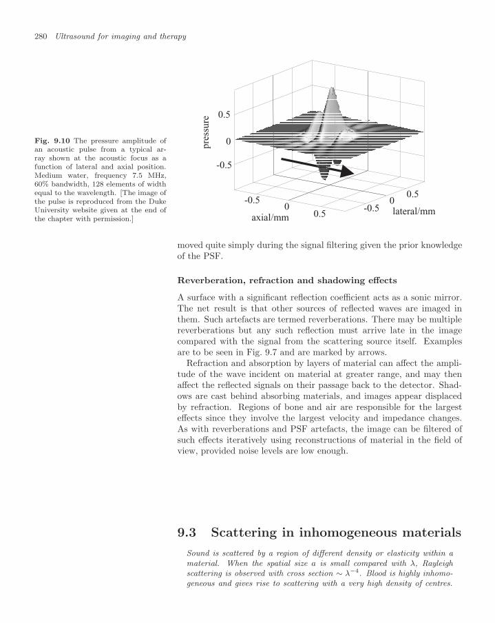
280 Ultrasound for imaging and therapy
Fig. 9.10 The pressure amplitude ofan acoustic pulse from a typical ar-ray shown at the acoustic focus as afunction of lateral and axial position.Medium water, frequency 7.5 MHz,60% bandwidth, 128 elements of widthequal to the wavelength. [The image ofthe pulse is reproduced from the DukeUniversity website given at the end ofthe chapter with permission.] axial/mm
lateral/mmpre
ssure
0.5
-0.50
0
0
0.5
0.5
-0.5
-0.5
moved quite simply during the signal filtering given the prior knowledgeof the PSF.
Reverberation, refraction and shadowing effects
A surface with a significant reflection coefficient acts as a sonic mirror.The net result is that other sources of reflected waves are imaged inthem. Such artefacts are termed reverberations. There may be multiplereverberations but any such reflection must arrive late in the imagecompared with the signal from the scattering source itself. Examplesare to be seen in Fig. 9.7 and are marked by arrows.
Refraction and absorption by layers of material can affect the ampli-tude of the wave incident on material at greater range, and may thenaffect the reflected signals on their passage back to the detector. Shad-ows are cast behind absorbing materials, and images appear displacedby refraction. Regions of bone and air are responsible for the largesteffects since they involve the largest velocity and impedance changes.As with reverberations and PSF artefacts, the image can be filtered ofsuch effects iteratively using reconstructions of material in the field ofview, provided noise levels are low enough.
9.3 Scattering in inhomogeneous materials
Sound is scattered by a region of different density or elasticity within amaterial. When the spatial size a is small compared with λ, Rayleighscattering is observed with cross section ∼ λ−4. Blood is highly inhomo-geneous and gives rise to scattering with a very high density of centres.

9.3 Scattering in inhomogeneous materials 281
The noise associated with the interference of amplitudes from a high den-sity of scatterers is termed ‘speckle’. This is responsible for the limitedeffective spatial resolution in ultrasound images. At short wavelengthsthere may be resonances with very large cross sections. Contrast agentsbased on tiny bubbles with resonant cross sections can be used. Movingscattering centres may be imaged by their Doppler shift. This is usedclinically to give blood-flow images with good time resolution.
9.3.1 A single small inhomogeneity
Source of scattering
Sound may be scattered by a localised inhomogeneity in a material.The inhomogeneity may concern the value of an elastic modulus or thedensity, or equivalently impedance or velocity. If a, the size of the in-homogeneous region, is large compared with a wavelength, the variousreflected and refracted waves are determined by matching boundary con-ditions, as discussed in chapter 4. If the region is small compared witha wavelength, there are simplifications which may be used to describethe scattering, and these are discussed below.
When a wave is incident on such a small inhomogeneity, in a firstapproximation each part of the scattering volume may be considered asemitting a secondary wave. The phase differences between these dependon a/λ and the scattering angle θ.16 The higher angular terms in the
16This is only true for a weak inhomo-geneity. For a stronger case these sec-ondary waves may be rescattered by theinhomogeneity. We keep to the sim-ple first order perturbation picture inwhich this is neglected. This is a Huy-gens secondary wave description of thescattering process.Today this is known as the Born ap-proximation, although it was intro-duced by Lord Rayleigh in 1871, elevenyears before Born was born.
angular distribution relate to higher powers of a/λ. Thus the scatteredamplitude ψ(θ) may be written as an expansion of the form
ψ(θ) =∑
A
(a
λ
)
P(cos θ), (9.5)
where P(cos θ) are the usual Legendre polynomials. The details neednot concern us because, if a λ, the power series converges rapidly andonly the first term, the scattering associated with an equivalent spher-ical inhomogeneity, is significant. In effect, all the scattered waveletsemanating from the region are then in phase with one another.
The weakness of the inhomogeneity implies that the phase shift suf-fered by the incident wave crossing the scattering volume must be small.If the density and the modulus of the region differ from the bulk materialby ∆ρ and ∆K respectively, we can write the conditions
a
λ 1,
a
λ
√∆ρ
ρ 1,
a
λ
√∆K
K 1. (9.6)
The scattering mechanisms relevant to density and elasticity varia-tions are quite different, as illustrated in Figs 9.11a and b respectively.
Small density inhomogeneity
a)
b)
.
Fig. 9.11 Exaggerated illustrations ofthe response of a small inhomogene-ity, assumed spherical, to an incidentwave. a) A density inhomogeneitywhich moves back and forth relativeto the bulk medium because its iner-tia is different to the bulk medium andtherefore has a different acceleration.b) An elasticity inhomogeneity whichexpands differently to the bulk for thesame stress or pressure change.
A density difference (in the absence of an elasticity change) implies thatthe inertia of the sphere is different from the spherical region of homo-geneous bulk matter that it displaces. In first order the forces acting on

282 Ultrasound for imaging and therapy
the sphere are the same as they would be acting on the equivalent homo-geneous bulk matter. This force is then either too large or two small toaccelerate the sphere in synchronism with its surroundings. The result isthat the sphere undergoes simple harmonic motion driven by the wave,as the bulk matter does, but with a different amplitude. The scatteringis caused by this difference in amplitude which is inversely proportionalto mass. The relative motion excites a longitudinal compression wavein the medium. As the diagram indicates, this P wave has opposite signin the forward and backward directions, and at 90 the wave vanishes.The scattered wave therefore has a factor cos θ in its amplitude. If theincident displacement amplitude is u0, the amplitude of the scatteredwave at large distances for each Huygens wavelet must be proportionalto factors u0 cos θ exp(ikr)/r and to ∆ρ/ρ. The integration over waveletsbrings in the volume of the sphere V = 4
3πa3. The scattered amplitudeis therefore the product of these factors and a constant, C:
CV × ∆ρ
ρ× u0 cos θ
exp(ikr)r
.
The differential cross section is the ratio of the scattered intensity mul-tiplied by r2 and divided by the incident intensity.17 This gives a cross17For a discussion of the meaning of a
differential cross section, see section 4. sectiondσ
dΩ= C2V 2
(∆ρ cos θ
ρ
)2
.
The left hand side of this equation has the dimensions of area. Thiscan only be reconciled with the factor V 2 if C has dimensions of inverselength squared. The only candidate length, not already accounted for,is the wavelength. So the final cross section is
dσ
dΩ=
π2V 2
λ4
(∆ρ cos θ
ρ
)2
, (9.7)
where we have slipped in a numerical factor π2 as revealed in a fullderivation.
Small elasticity inhomogeneity
The effect of a small change in elasticity is quite different. It causes thespherical region to expand and contract relative to the bulk medium asthe pressure wave passes, as illustrated in Fig. 9.11b. If the modulushad been the same, the rise in pressure would have matched the relativevolume change in the surrounding medium. So it is only the differencethat causes a change in volume relative to the volume that the spherewould have had under homogeneous conditions. This causes a furthercompression wave to be propagated, this time isotropic and determinedby ∆K/K. Similar general arguments as for the density variation givea differential cross section,
dσ
dΩ=
π2V 2
λ4
(∆K
K
)2
. (9.8)

9.3 Scattering in inhomogeneous materials 283
The two scattering effects are coherent and we need to consider theirrelative phase. In a travelling wave the pressure and the particle velocityare in phase and related by the impedance, assumed real. The pressureand displacement are therefore 90 out of phase. Since the scattering bydensity variation is synchronised to the displacement, and the scatteringby elasticity variation is synchronised to the pressure wave, the twoscattered waves are always 90 out of phase. At any value of θ thescattering amplitude is the sum of the two processes in quadrature. Thecombined scattering differential cross section is
dσ
dΩ=
π2V 2
λ4
[(∆K
K
)2
+(
∆ρ cos θ
ρ
)2]
. (9.9)
This scattering is responsible for many ultrasound signals. For ex-ample, the reflection of ultrasound by shoals of fish is not caused by adifference of the mean density or elasticity of the fish relative to water(see Fig. 1.1). The density of fish must be very close to the densityof water, otherwise fish would just float or sink! The signal detected infish-finder technology comes from scattering by small gas bubbles withinthe fish.
In medical imaging with ultrasound the highest frequencies are usedto maximise the scattering that comes from the 1/λ4 characteristic ofthe Rayleigh cross section, equation 9.9.
Progress in using and applying these results quantitatively, at leastin a medical context, has been slow. For many years the piezoelectrictechnology was not available to enable exploitation of the field. Re-cently the qualitative use of imaging by scattering has given satisfactoryresults without any need for quantitative study. The real problem im-peding rigorous study has been the intrinsic variability of tissue and itsinhomogeneities, and the lack of a clear method for obtaining and quan-tifying reliable measurements. But these variations are arguably thevery parameters likely to be of clinical interest. If he returned today,Lord Rayleigh might be surprised at the lack of progress in this area.
Shear waves and scattering
Such elemental motion also generates a shear S wave in a medium thatcan support it. The motion shown in Fig. 9.11b is purely radial andgenerates only outgoing P waves. However, that shown in Fig. 9.11a,while generating a outgoing P wave with a cos θ dependence, will alsocouple to a cylindrical outgoing S wave with a sin θ dependence. Theparticle velocity of such a transverse wave at θ = π/2 will be similar tothe longitudinal wave at θ = 0 or π. The energy density for this S waveis similar to the P wave, but the flux, and thence the cross section, willbe reduced by a factor cS/cP . This suggests a differential cross section
dσS
dΩ=
cS
cP
π2V 2
λ4
(sin θ
∆ρ
ρ
)2
. (9.10)

284 Ultrasound for imaging and therapy
The motion in this S wave is at right angles to the P wave, so that thereare no interference effects. The smaller the shear modulus, the smallerthe cross section. In a viscous fluid such waves are rapidly absorbed andthe mechanism is one of absorption rather than scattering.
For solid materials there is a difference between the modulus for lon-gitudinal plane waves K = λ + 2µ and the bulk modulus that describesthe spherical expansion at small r, KB = λ + 2
3µ. This shows that Pwaves should be scattered by inhomogeneities of either shear modulusor bulk modulus, or equivalently of either λ or µ. At small r a sphericalP wave involves a degree of distortion which is absent in a plane P wave.
Incident S waves are scattered by discontinuities in either densityor shear modulus. This makes them particularly suitable for the non-destructive testing of solids where the discontinuity in shear modulus ismost pronounced at microscopic bubbles or other fluid micro-inclusions.The choice of S waves also maximises specular reflection in solids atcracks and surfaces bounded by fluids.
Thermodynamics and scattering
Small bubbles of vapour in a liquid do not behave isentropically underthe influence of an incident P wave. In the expansion cycle energy isexchanged with the bulk medium as evaporation and condensation occur.These thermodynamic changes are driven fast, not necessarily underconditions of thermodynamic equilibrium. This is the kind of delayedresponse which gives attenuation of sound through irreversible cyclicchange, as discussed in section 43. The details depend critically on thethermodynamics and are not simply described. Similar considerationsapply to liquid drops in a vapour. The absorption and scattering ofsound in fog is an interesting application. It is common experience thatlow frequency sound penetrates fog most effectively and that, even at1 kHz, fog dampens general noise and gives an isolated eerie impressionexploited in many a ghost story.
9.3.2 Regions of inhomogeneity
Materials with a concentration of scatterers
Because in tissue the reflection of ultrasound at extended boundaries issmall and does not increase with frequency, the f4 frequency dependenceof scattering is important and determines the choice of high frequency.The limitation is absorption which increases at least linearly with fre-quency by any of the mechanisms discussed in section 4.4.2. The choicealso makes for high spatial resolution. Taking this a step further, thespectrum of the size of scattering centres can be measured by observ-ing the frequency dependence of the scattering cross section correctedfor absorption. At a ∼ λ this cross section changes over from a λ−4
dependence to being independent of λ.In a material composed of a large number of scatterers we need to
consider the interference between the waves from different centres. Scat-

9.3 Scattering in inhomogeneous materials 285
Table 9.4 Constituents of blood. [Quoted from Evans & McDicken.]
Number Size Density Compressibility Volumemm−3 µm ×103 kg m−3 m2 N−1 %
Plasma 1.021 4.09×10⁻¹⁰ ∼ 50Erythrocytes 5 × 10⁶ 7.2 × 2.2 1.091 3.41×10⁻¹⁰ 45Leukocytes 8 × 10³ 9–25 ∼ 0.8Platelets 2.5 × 10⁵ 2–3 ∼ 0.2
tered waves emitted by centres that are imaged into different spatiallyresolved pixels do not interfere. However, when the number of scatter-ing centres contributing to each spatially resolved pixel in the image isgreater than 1, there are interference effects.18 The relative phase comes 18If there are n such scatterers, then
there are n − 1 phases.from the fact that scattering centres are dispersed in depth. The depthprobability distribution is likely to be uniform within any depth slice ofthickness λ/2 so that the actual value of this phase for a given pixel isapparently random, though determined by the actual difference in depthof the scatterers for that pixel. The spatial resolution of the optics de-termines the effective pixel size and therefore which scattering centrescan interfere in this way. The result of this interference is called speckle.
Many biological tissues have such a high concentration of inhomo-geneities that their mutual interference has a large effect on scattering.An important example is blood. It consists of a dense suspension of cellsin a clear fluid, the plasma. The various constituents are enumeratedin table 9.4. The erythrocytes, or red blood cells, predominate. Theyconsist of flexible discs and their concentration is so high that their av-erage separation is only about 10% of their diameter. The conditionsfor pure Rayleigh scattering are therefore not met. Nevertheless it hasbeen shown experimentally that the f4 frequency dependence only startsto flatten off above 15 MHz. Note that blood may become anisotropicwhen the disc-shaped red blood cells become orientated for any reason.
Speckle noise
The amplitude R of an image pixel is the superposition of the scatteringamplitudes from a number of scattering centres within the object, eachwith a phase determined by the depth of the centre. The fluctuation inthe resultant R has two sources:
the number of scatterers, described by the mean and Poissonstatistics;
the phases of the amplitudes varying between 0 and 2π anddepending on the depth, as discussed above.

286 Ultrasound for imaging and therapy
The mean resultant R can be drawn as the summation of the con-tributing amplitudes in an Argand diagram. This increases as
√n, and
the mean energy as n. If the value of n in each pixel is less than orof order 1, phases are irrelevant and the signal and its fluctuations aredescribed by Poisson statistics. Otherwise the phase becomes importantand the SNR is determined by speckle noise.
This is simply studied. In Fig. 9.12 a numerical calculation of thedistribution of the resultant amplitude R with both Poisson and phasefluctuations is shown for a mean n = 6 scatterers per pixel. Some struc-ture associated with the contribution of small values of n remains but thedistribution is already quite close to the smooth Rayleigh distribution,
20 4 6resultant amplitude R
N
Fig. 9.12 A numerically calculated dis-tribution of the resultant amplitudewhen the mean number of unit vectorsis six. The curve is the correspondingRayleigh distribution, equation 9.11.
P (R) dR =πR dR
2nexp
(−πR2
4n
), (9.11)
which obtains for general large n. Note that this is a function of the ratioR2/n only. It is normalised, its mean is
√n and its standard deviation is√
n/1.91. The SNR is therefore 1.91 at large n. Results of the simulationare shown in Fig. 9.13 as curve c. As the mean number of scatterers perpixel is increased from 1 the value of the SNR rises from 1 towards 1.91.As Fig. 9.12 also shows, the Rayleigh distribution is applicable for nabove 6 or so.
So measurements of the scattered amplitude remain noisy and are notimproved as the number of scatterers increases. If the spatial resolutionis improved the resolved pixel gets smaller but the fluctuations persist,albeit on a smaller spatial scale. The same phenomenon also occursin the Rayleigh scattering of light. If the scattering centres move, thespeckle pattern changes. By measuring the rate of change of the specklepattern rates of diffusion or flow may be deduced.
0
1
2
4 8 12
a
b
c
mean, n
SNR
Fig. 9.13 The amplitude resolution,mean over standard deviation, plottedagainst the mean number of unit vec-tors n. Curve a, the value for a linearPoisson distribution which is relevantat n ∼ 1 when the phase is not impor-tant. Line b, constant value 1.91 inde-pendent of n for fluctuations describedby the Rayleigh distribution, valid atlarge n. Envelope of points c, the re-sult of a simple numerical simulation.
As a result of speckle, medical ultrasound images appear mottled. Atypical example is shown in Fig. 9.7. The apparent scale of the mottlingis related to the spatial resolution, that is to the transfer function ofthe imaging. It does not relate to a change in the scattering density inthe object. As shown, the amplitude of the mottling is half the meanscattered amplitude, or a quarter in terms of intensity. This has a seriouseffect on images. It has been shown19 that speckle causes a reduction in
19As discussed in the book by Hill etal.
lesion detectability of approximately a factor 8. This radical reductionin contrast resolution is responsible for the poor effective resolution ofultrasound compared with X-ray CT and MRI.
Resonant scattering
If larger values of the scattering phase shift are considered, there is thepossibility of resonance. For example, the fundamental oscillation modeof a bubble of perfect gas of radius a in a fluid of density ρ at ambientpressure p is
ωR =1a
√3γp
ρ. (9.12)
At resonance the cross section is of order λ2 in the absence of damping.Such a figure is many orders of magnitude above the Rayleigh value.

9.3 Scattering in inhomogeneous materials 287
Typically 4 µm bubbles resonate at 2 MHz with a cross section broad-ened and reduced by damping. At frequencies above resonance the crosssection of a bubble falls rapidly and tends towards its geometrical area.
Other inhomogeneities of the same size resonate at much higher fre-quencies because they have lower elasticity.
Streaming, mixing and shaking
By driving large amplitude mechanical waves through inhomogeneousmaterials, at low as well as high frequency, the differential motion causeshigh rates of shear and thence turbulence. Such irreversible behaviouris familiar in the everyday effects of shaking and mixing. These phe-nomena have important applications in ultrasonic cleaning baths andindustrial homogenisation. In ultrasound the localised flow around in-homogeneities is called streaming.
Ultrasound contrast agents
Contrast agents in ultrasound are provided by administering concentra-tions of artificial centres of inhomogeneity with large scattering crosssections. In practice these bubbles are small compared with a wave-length with large fractional changes in elasticity and density.
Small gas bubbles may be injected into the bloodstream but tend todissolve rather too quickly for clinical use. However, air-filled artificialencapsulated bubbles are commercially available with diameters in therange 2–5 µm. These are small enough to pass through the finest bloodvessels. These are non-toxic and may be excreted from the body withoutharmful side effects. They have a spectrum of sizes, and the quantifi-cation of this is important, given the size dependence of the resonantcross section. This is the main difficulty in the quantitative use of suchagents.
The presence of such contrast agents is detected by scattering andtheir motion determined using Doppler methods which are discussedbelow.
9.3.3 Measurement of motion using the Dopplereffect
source
source
scatterer, velocity V
scatterer, velocity V
observer
observer
θ
θ
φ
φ
a)
b)
Fig. 9.14 a) A source emits a wave to-wards a scatterer which is moving awayfrom it with speed v and angle θ.b) The scattered wave is detected by anobserver at an angle φ.
Doppler shift from a moving scatterer
Suppose that the scatterer is moving with a velocity v at angle θ relativeto the direction of the ultrasound waves emanating from the source, asdepicted in Fig. 9.14a. If the phase velocity of the wave is c, then therelative velocity of waves and scatterer is c − v cos θ. If the frequencyemitted by the stationary source is f , the frequency seen by the scattereris
f ′ = f × c − v cos θ
c. (9.13)
This is the usual Doppler shift for a moving detector.20
20It assumes implicitly that the (appar-ent) values of the angles do not changerapidly with time.

288 Ultrasound for imaging and therapy
T T/RRa) b)
Fig. 9.15 Doppler geometries. Target scattering centres in region illuminated by transmitter T and within the sensitivity ofreceiver R are detected with a frequency shift. a) Continuous wave (CW) with angular separation α. b) Pulsed wave (PW).
If this scattered echo signal is detected by a stationary observer in thedirection φ, as shown in Fig. 9.14b, the velocity of the reflected signalrelative to the scatterer (as source) is c + v cosφ. At the frequency f ′,that makes for a wavelength λ′ = (c + v cosφ)/f ′. The frequency of thesignal detected by the observer as a result of this double Doppler shiftis therefore
f ′′ = f × c − v cos θ
c + v cosφ. (9.14)
If the ratio v/c is small, the frequency shift may be approximated
∆f = −v
c(cos θ + cosφ). (9.15)
This is the double Doppler shift for the frequency of a stationary sourceseen by a stationary observer on reflection by a reflector or scatterermoving away at a velocity v.2121This is an approximation. Although
the relative velocity of the reflected im-age of the source and the observer isv(cos θ + cos φ), the observer would seeadditionally that half of the mediumbetween him or her and the image ofthe source is stationary and half is mov-ing. This breaks the mirror symmetryso that equation 9.15 is not the exactresult.
The value of α = θ + φ is determined by the geometry of the sourceand detector. The smaller the value of α, the larger the sensitivity toDoppler. In medical applications of ultrasound the ratio v/c is alwayssmall and the velocity c is effectively constant at 1540 m s−1.
Doppler detection
The Doppler signal from a specific region may be detected in two differ-ent ways, termed continuous wave (CW) and pulsed wave (PW). Theseare shown diagrammatically in Fig. 9.15. In CW the transmitter andreceiver are distinct and separated. Using its angular resolution thetransmitter illuminates a well-defined column of tissue with a contin-uous beam. The angular resolution of the detector is used to restrict

9.3 Scattering in inhomogeneous materials 289
Fig. 9.16 Data from a CW doppler scan of a vascular feature. The geometry is shown at the top. The trace at the bottomshows the velocity spectrum as a function of time. Thus the envelope of the spectra is the maximum blood velocity componentat any time. This shows a flow varying regularly from 20–70 cm s−1 during the cardiac cycle. [Image used with kind permissionfrom GE Healthcare]
recorded signals to those reflected by a short section of this column, asshown in Fig. 9.15a.
In the PW mode the transmitter and receiver are combined, as shownin Fig. 9.15b with α = 0. The position information comes from the echotime of the received signal relative to the transmitted pulse. In PW thelength of the transmitted pulse determines both the longitudinal spatialresolution and the bandwidth of the pulse frequency. If the pulse islengthened, the spatial resolution deteriorates and the velocity resolutionimproves. The spatial information may be improved but at the expenseof the velocity resolution.
In medical ultrasound Doppler signals are generated by scattering atsmall moving inhomogeneities. Thus the Doppler frequency shift forscattering from red blood corpuscles in the bloodstream is a measure ofthe longitudinal speed of the blood. Signals from a region are linearlysuperposed. Therefore by spectral analysis the spectrum of velocitywithin each image volume can be determined.22
22This can be applied also to the de-tection of natural gaseous bubbles andemboli. The latter are minute clots orcoagulations in the blood which are dif-ficult to detect by other means. It isof great clinical importance to detectthe presence of these before they pre-cipitate an actual embolism or blockagewith its serious consequences for the pa-tient.
Figure 9.16 shows an example of the detailed spectrum that may beobtained. In the upper part of the display is shown the anatomical

290 Ultrasound for imaging and therapy
scan indicating the CW geometry like Fig. 9.15a. The lower part of thediagram shows a plot of velocity (vertically) against time (horizontally).At each time there is a velocity spectrum. The peak velocity has beenpicked out by a line marking the envelope. This shows clear quantitativemeasurements of maximum radial blood velocity varying from 20 to70 m s−1 during the cardiac cycle in the targeted region.
Such Doppler measurements only refer to a component of the velocityvector. However, additional components of flow may be measured byadding further detectors R at different angles but aimed at the sameregion in the CW geometry. With three or more such detectors thecomplete velocity vector can be measured.
9.4 Non-linear behaviour
Strain and stress changes relative to a reference state may be relatedby a power series expansion. For small changes the relation is linear.For larger changes all materials show non-linearity and therefore expandwhen heated. A heated material behaves linearly relative to its quies-cent heated state. Non-linearity generates harmonics from an incidentmonochromatic wave, and a wave–wave interaction picture provides in-sight. Medical imaging with harmonics gives improved resolution, betterpenetration and less artefact. However the effects of high power levelsare not unpredictable with current knowledge. Higher order terms may bestudied only in constituent models. They show how large amplitude pro-gressive waves approach a singular state where harmonic generation andfrequency-dependent absorption give irreversible energy deposition; thishas applications to homogenising, ultrasonic cleaning and plastic weld-ing. These sound waves can give focussed energy deposition for cancertherapy and other clinical procedures. But constituent models are onlyillustrative and there is a lack of data for real biological tissue.
9.4.1 Materials under non-linear conditions
Phenomenology
Hooke’s law, equation 4.1, states that the change in internal stress isproportional to the strain in a material. This is a statement about twostates of the material, the initial or reference state and a changed state.The relation is only true for small strains, that is for pairs of statesrelated by a small strain and a small stress change. We may considerHooke’s law as the approximation involved in taking the first term of apower series which expresses a change in the stress as a Taylor expansionrelative to the reference state. Thus in one dimension generally we write

9.4 Non-linear behaviour 291
the stress change ∆T in terms of the strain ∂uz/∂z,
∆T = A∂uz
∂z− B
2!
(∂uz
∂z
)2
+C
3!
(∂uz
∂z
)3
. . . (9.16)
where A is the linear modulus that we have discussed previously.23 The 23When discussing 3-D materials wetake A to be the bulk modulus KB.Otherwise we discuss non-linear be-haviour in one dimension only, ignoringthe additional complexities that comewith three dimensions.
ratio B/A is a measure of the non-linearity of the relation, but higherorders are often important too. This non-linearity is not peculiar toparticular materials, as is the case for the non-linearity of magnetic orelectric properties. All materials exhibit mechanical non-linearity to agreater or lesser extent at large strains, and therefore it is a mistake torefer to ‘non-linear materials’. Rather one should speak of ‘non-linearstrains’.
Reference state
In chapter 4 the displacement of each point in the material ux, uy, uz wasdescribed by the difference between the actual position of the point andits reference position x, y, z as a function of this reference position. Thenthe strain was defined as the spatial derivatives of these displacementswith respect to the reference positions. Similarly the change in stress∆T (z) at each point was defined as the difference between the actualstress and the reference stress for that point in the material.24 Also the 24Some care is needed here. The ‘point’
co-moves with the material in the waythat we have described it. Thus thechange in stress is the difference in T atthe point that was at z in the referencestate.
density ρ0 was defined as the density in the reference state.The question of how this reference state should be chosen was not
discussed. It was implied perhaps that the reference state should bechosen as the quiescent state. The question of what happens if a differentreference state is chosen was not addressed.
Provided that linearity is maintained a different choice would changenothing substantial. All points would have a reference position stretchedrelative to other choices and the zero of energy would be shifted, butthere would be no consequences for waves or the elastic moduli on whichthey depend.
If, however, non-linear deformations are considered, that is no longertrue. In equation 9.16 if the coefficients B, C, . . . are non-zero, a differentselection of expansion point changes the coefficient A mathematically,and with it the elastic modulus, wave velocity, impedance and so on. Sothe choice of reference state matters when behaviour is non-linear butit does not in so far as the behaviour is linear.
Temperature and non-linearity
An important application of these ideas arises in considering the effectof a temperature rise. An atom subject to the interatomic potential suchas the Lennard–Jones potential, Fig. 4.21, would sit at the bottom ofthe well at 0 K. If the material were perfectly linear the curve would bea parabola. However, all such curves must be asymmetric on account ofthe ‘brick wall’ at a strain ε = −1 due to electron degeneracy, and theabsence of such a wall for positive strain.

292 Ultrasound for imaging and therapy
At a higher temperature an atom oscillating in such a potential willspend more time at larger separation and less at smaller. In conse-quence the material expands and the mean strain is positive. We candefine a new reference point, the thermal equilibrium state at the raisedtemperature. Strains will be redefined, there will be a new density anda different modulus related to the changed value of the second deriva-tive of the potential, φ′′
. The velocity of small amplitude sound wavesat that temperature will be described better by the new parameters atthe new reference point with respect to which typical strains are small.They would not be small and linear if referred to the original referencestate defined at the lower temperature. We conclude that by changingthe reference state to reduce the value of the strain, the appearance oflinear behaviour can be recovered.
Data for materials
How large is the dimensionless non-linearity parameter B/A for realmaterials? A perfect gas obeys the relation PV γ =constant for adiabaticchanges. This determines that the ratio2525See question 9.4.
B
A= 1 + γ. (9.17)
This ratio ranges from 2.67 to 2.11 depending on whether the gas ismonatomic or polyatomic.26 For an isothermal change B/A = 2. So the26See table 4.1 for values of γ.
adiabatic condition for a perfect gas increases both the non-linearity andthe bulk modulus KB = γP .
For liquids and solids the value of B/A may be derived from data onthermal expansion and the change of sound velocity with temperature.Values are shown in table 9.5 together with other parameters of interest.The table is divided into separate parts for solids, liquids and physio-logical materials. The characterisation of solids is more complicated asthere are more possible non-linear parameters. The value of B/A shownis derived from the coefficient of expansion and sound velocity shown.While there is a wide spread in sound velocity there is a smaller rangeof values for B/A from 4 to 10. Gases are less non-linear.
Since we suppose that the non-linear behaviour of all materials arisesfrom the underlying asymmetric potential curve between atoms andmolecules, it is not surprising to find similar values for B/A. Someincrease for elements with Z may be understandable in terms of an in-creasing electron degeneracy. But generally the various values for chem-ical compounds are harder to understand.
The data shown in table 9.5 include the linear parameters, sound ve-locity and density, as well as the non-linear ones. These illustrate animportant point for physiological materials. Many entries describe largevariations. This is because measurements are difficult to make, andconditions difficult to define precisely, particularly in vivo. But theremay be a genuine wide variation between samples according to the age,background and clinical condition of the patient. This variation is what
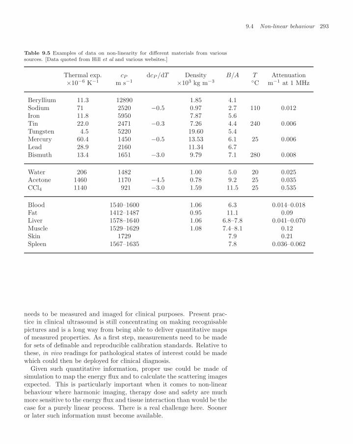
9.4 Non-linear behaviour 293
Table 9.5 Examples of data on non-linearity for different materials from varioussources. [Data quoted from Hill et al and various websites.]
Thermal exp. cP dcP /dT Density B/A T Attenuation×10−6 K−1 m s−1 ×10³ kg m−3 C m−1 at 1 MHz
Beryllium 11.3 12890 1.85 4.1Sodium 71 2520 −0.5 0.97 2.7 110 0.012Iron 11.8 5950 7.87 5.6Tin 22.0 2471 −0.3 7.26 4.4 240 0.006Tungsten 4.5 5220 19.60 5.4Mercury 60.4 1450 −0.5 13.53 6.1 25 0.006Lead 28.9 2160 11.34 6.7Bismuth 13.4 1651 −3.0 9.79 7.1 280 0.008
Water 206 1482 1.00 5.0 20 0.025Acetone 1460 1170 −4.5 0.78 9.2 25 0.035CCl4 1140 921 −3.0 1.59 11.5 25 0.535
Blood 1540–1600 1.06 6.3 0.014–0.018Fat 1412–1487 0.95 11.1 0.09Liver 1578–1640 1.06 6.8–7.8 0.041–0.070Muscle 1529–1629 1.08 7.4–8.1 0.12Skin 1729 7.9 0.21Spleen 1567–1635 7.8 0.036–0.062
needs to be measured and imaged for clinical purposes. Present prac-tice in clinical ultrasound is still concentrating on making recognisablepictures and is a long way from being able to deliver quantitative mapsof measured properties. As a first step, measurements need to be madefor sets of definable and reproducible calibration standards. Relative tothese, in vivo readings for pathological states of interest could be madewhich could then be deployed for clinical diagnosis.
Given such quantitative information, proper use could be made ofsimulation to map the energy flux and to calculate the scattering imagesexpected. This is particularly important when it comes to non-linearbehaviour where harmonic imaging, therapy dose and safety are muchmore sensitive to the energy flux and tissue interaction than would be thecase for a purely linear process. There is a real challenge here. Sooneror later such information must become available.
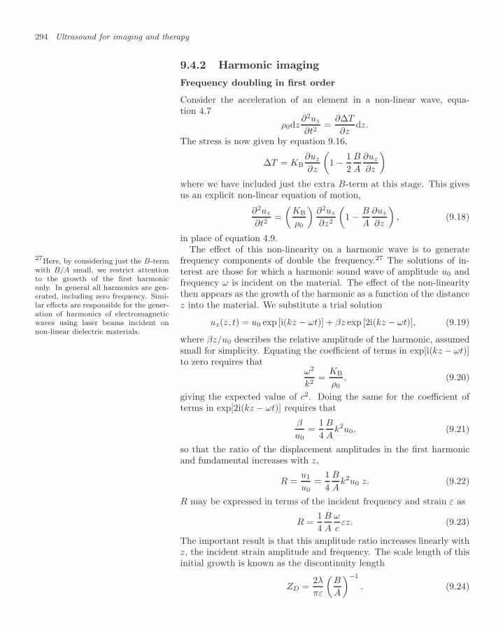
294 Ultrasound for imaging and therapy
9.4.2 Harmonic imaging
Frequency doubling in first order
Consider the acceleration of an element in a non-linear wave, equa-tion 4.7
ρ0dz∂2uz
∂t2=
∂∆T
∂zdz.
The stress is now given by equation 9.16,
∆T = KB∂uz
∂z
(1 − 1
2B
A
∂uz
∂z
)where we have included just the extra B-term at this stage. This givesus an explicit non-linear equation of motion,
∂2uz
∂t2=
(KB
ρ0
)∂2uz
∂z2
(1 − B
A
∂uz
∂z
), (9.18)
in place of equation 4.9.The effect of this non-linearity on a harmonic wave is to generate
frequency components of double the frequency.27 The solutions of in-27Here, by considering just the B-termwith B/A small, we restrict attentionto the growth of the first harmoniconly. In general all harmonics are gen-erated, including zero frequency. Simi-lar effects are responsible for the gener-ation of harmonics of electromagneticwaves using laser beams incident onnon-linear dielectric materials.
terest are those for which a harmonic sound wave of amplitude u0 andfrequency ω is incident on the material. The effect of the non-linearitythen appears as the growth of the harmonic as a function of the distancez into the material. We substitute a trial solution
uz(z, t) = u0 exp [i(kz − ωt)] + βz exp [2i(kz − ωt)], (9.19)
where βz/u0 describes the relative amplitude of the harmonic, assumedsmall for simplicity. Equating the coefficient of terms in exp[i(kz − ωt)]to zero requires that
ω2
k2=
KB
ρ0, (9.20)
giving the expected value of c2. Doing the same for the coefficient ofterms in exp[2i(kz − ωt)] requires that
β
u0=
14
B
Ak2u0, (9.21)
so that the ratio of the displacement amplitudes in the first harmonicand fundamental increases with z,
R =u1
u0=
14
B
Ak2u0 z. (9.22)
R may be expressed in terms of the incident frequency and strain ε as
R =14
B
A
ω
cεz. (9.23)
The important result is that this amplitude ratio increases linearly withz, the incident strain amplitude and frequency. The scale length of thisinitial growth is known as the discontinuity length
ZD =2λ
πε
(B
A
)−1
. (9.24)

9.4 Non-linear behaviour 295
The ratio for the particle velocity and strain of the harmonic wave tothe fundamental is 2R because the frequency and wavenumber in thefirst harmonic are double.
The fraction of energy flux in the first harmonic rises as 4R2, thatis proportional to z2 and ω2. This dependence, combined with the fre-quency dependence of absorption and the higher order terms in the ex-pansion 9.16 which have been neglected so far, suggest that as non-linearpropagation progresses energy is shifted on shorter distance scales intoever higher harmonics which are then rapidly absorbed.
Calculated rates of harmonic generation
In table 9.6 we show some estimated results for ZD for a number ofmaterials. The values are for an incident frequency of 1 MHz and
Table 9.6 Values of the dis-continuity length ZD (in me-tres) as calculated from B/Afor different substances at 1MHz for an ultrasound energyflux of 2 × 10⁵ W m−2. Thisvalue of energy flux is typicalof that in use in many diagnos-tic instruments. See also thebook by Hill et al.
B/A ZD m
Beryllium 4.1 99.60Sodium 2.7 1.85Iron 5.6 21.77Tin 4.4 2.96Tungsten 5.4 25.70Mercury 6.1 0.77Lead 6.7 1.73Bismuth 7.1 0.78
Water 5.0 0.25Acetone 9.2 0.07CCl4 9.0 0.06Benzene 9.0 0.10Blood 6.0 0.27Fat 10.0 0.12Muscle 7.8 0.21
a power flux 2 × 10⁵ W m−2. For values of z approaching ZD theassumptions we have made break down progressively.
Further terms in the Taylor expansion, equation 9.16, gener-ate higher harmonics direct from the fundamental.
As harmonics grow they start to generate their own harmon-ics. Since the harmonic pumping mechanism is proportionalto ω, these secondary harmonics grow faster proportionatelythan the parent process.
As more and more energy is transferred to higher harmonics,it is attenuated by the frequency-dependent absorption.
Energy conservation ensures that, as the energy flux in theharmonics rises, the strength of the incident fundamentalharmonic falls, thereby choking off this harmonic pumpingmechanism.
As the rate of energy deposition rises, local heating occurswhich gives rise to inhomogeneity in c and ρ that may thenfocus and reflect subsequent waves.
The values show that harmonic generation is particularly pronouncedin low density materials with low sound velocity. The length variesinversely with frequency and the square root of the power density.
Harmonic generation and wave–wave scattering
If conditions are linear there is no wave–wave interaction. Under non-linear conditions the wave–wave interaction can be calculated in firstorder by the Born approximation in terms of the anharmonicity of thepotential. The space and time integrals involved generate the momen-tum and energy conservation conditions on the incident and scatteredwavenumbers
k1 + k2 → k3 + k4 (9.25)
and frequenciesω1 + ω2 → ω3 + ω4. (9.26)

296 Ultrasound for imaging and therapy
Fig. 9.17 Two ultrasound images showing a large cyst in a breast. The image on the left, scanned with fundamental imaging,shows prominent reverberation echoes in the near field of the cyst (arrows). The harmonic image on the right shows a reductionin artefactual echoes, allowing a more confident diagnosis of a simple breast cyst. [Rapp and Stavros, Journal of DiagnosticMedical Sonography. Image downloaded from GEhealthcare website and reprinted by permission of Sage Publications, CorwinPress Inc.]
Such scattering may be seen as the mechanism of the thermalisationand absorption of an acoustic wave through scattering with low energywaves in thermal equilibrium in the material.
The same mechanism may be used to describe the scattering of anincident wave with itself. The momentum and energy constraints areonly satisfied in the forward direction, with
ω1 + ω1 → ω2 and k1 + k1 → k2, (9.27)
This provides another view of harmonic generation by an incidentmonochromatic wave, although still in a small amplitude and perturba-tive approximation.
Use of harmonic generation in diagnostic imaging
In the practical application of harmonic imaging the object is illumi-nated at one frequency, 5 MHz for example, and then imaged at twicethe frequency by filtering the received signal. This has a number ofadvantages over imaging at the fundamental frequency, as exemplifiedin Figs 9.17 and 9.18. The resolution is improved in depth and angle.By focusing the incident beam the illumination may be arranged to re-duce harmonic generation except within a small region at the depth ofinterest. As these images show, artefacts are also reduced.
There is an additional benefit of harmonic imaging connected withabsorption. The illuminating flux at the lower frequency suffers less ab-sorption on the outward journey. Only the scattered wave on the return

9.4 Non-linear behaviour 297
Fig. 9.18 On the left the fundamental image shows reverberation, scatter and clutter artefact in the near field of this siliconeimplant. This could be mistaken for a pathological condition. On the right in a harmonic image most of the artefactual signalsare suppressed, showing that there was no condition. [Rapp and Stavros, Journal of Diagnostic Medical Sonography. Imagedownloaded from GEhealthcare website and reprinted by permission of Sage Publications, Corwin Press Inc.]
journey suffers the attenuation characteristic of the higher frequency.Harmonic imaging is in widespread clinical use.
Safety and related concerns
To make harmonic images the power level has to be raised to the thresh-old of non-linear behaviour. With proper monitoring this should not bea cause for concern because images can be taken rapidly and exposuretimes kept short. However, the perception that ultrasound is a safemodality means that monitoring is taken, perhaps, less seriously andscanning beams may be left free-running. The physiological data andmodelling of energy deposition by ultrasound are not well developed.This is made more serious on account of the non-linearity of harmonicgeneration.28 What is the safety margin for ultrasound? Diagnostic 28In a non-linear process the sensi-
tivity to the conditions is increased.For example, in a quadratic process a10% error in the fundamental ampli-tude makes for a 20% change in the firstharmonic.
doses are considered acceptable if the thermal load raises the tempera-ture of the tissue by less than 1C, and this is well established. At theother extreme doses that raise the tissue temperature above 56C for 1second result in coagulative necrosis.29 These margins of safety for clin-
29Typical doses in ultrasound therapyraise the temperature of the targetedtissue to 80C.
ical diagnostic use might be acceptable if the local monitoring of tissuetemperature in tissue in vivo were more highly developed and if reliabledata were available as a basis for simulation and planning.
9.4.3 Constituent model of non-linearity
To understand what happens as higher order terms in the power series,equation 9.16, become important, we need accurate data that describe

298 Ultrasound for imaging and therapy
the materials involved. Since these are not available, we resort to the1-D constituent model with the Lennard–Jones potential discussed inchapter 4. This will help us understand the phenomena qualitatively,athough quite inadequate to predict actual responses. A feature of sucha model is that the higher order terms are all defined and there is noneed to consider a truncated series.
Reference state and non-linearity in a constituent model
The change in stress in a material described by the Lennard–Jones po-tential comes from differentiating twice the potential φ given by equa-tion 4.76. We may pick up the story from equation 4.79 where we tookthe derivative φ′′(ε) to be constant. Here in the non-linear regime wetake on board its dependence on the strain ε and on the choice of refer-ence state.
0.2
0.4
0.6
0.8
-0.1 0.1 0.2 0.3
strain
/E 0
X
Fig. 9.19 The Lennard–Jones inter-atomic potential of Fig. 4.21 replottedas a function of strain relative to thereference state chosen to be the equi-librium state at 0 K. Note that at thepoint marked ‘X’ the curvature of thepotential changes sign.
The absolute value of the potential φ is arbitrary. Only relative valuesare significant for dynamics. The first derivative is absorbed into thedefinition of T0, the stress at the reference point. It is only the secondderivative of the potential and its variation that need concern us. Thewave equation is
ρ∂2u
∂t2=
∂2u
∂z2
12
∂2φ
∂ε2(ε), (9.28)
where ρ is the density and the constituent separation in the referencestate. This equation is valid for all strains and any choice of referencepoint but is linear only within any small window of ε for which φ′′
is effectively constant. By centring the reference point on the chosenwindow, non-linear effects can be minimised.
At T = 0 K the Lennard–Jones potential model (Fig. 9.19) gives theratio B/A = 21 for the reference point at the bottom of the well, r = .3030See question 9.5.
Compared with real materials this is an overestimate by a factor between2 and 4. In the model at higher temperatures the equilibrium value ofr increases and the reference point moves. The ratio B/A increases andthe value of A falls, so that non-linearity becomes more significant andthe velocity of sound decreases. These effects are plotted in Fig. 9.20.3131This model calculated rate of de-
crease of sound velocity with tempera-ture may be compared with some actualvalues shown in table 9.5.
It is interesting to note that for a perfect gas the value32 of the mod-
32Given by γP0.
ulus A is positive for all strains. This cannot be the case for a solid or aliquid. The modulus is proportional to the curvature of the potential φ′′.There is always a value of positive strain at which the potential startsto flatten off and therefore its curvature passes through zero. For theLennard–Jones potential this occurs at the point marked ‘X’ in Fig. 9.19.
What happens at such a point, and what does it mean? The answeris shown illustratively in Fig. 9.21 for neighbouring atoms in one dimen-sion. At strains greater than ‘X’ the modulus K goes negative. An atombetween two others at such a strain as shown in Fig. 9.21c. Althoughthere is still tension on the atomic chain, it is energetically favourablefor an atom to move away from its median position between its neigh-bours. It gains more energy by being closer to one neighbour than itloses from moving away from the other. In other words, the chain is

9.4 Non-linear behaviour 299
-10 0 +10
100
80
60
40
20
B/A
Expansion, %-10 0 +10
Expansion, %
1.0
0.5
2.0
1.5
c/c0
a) b)
Fig. 9.20 Calculated non-linearity effects in the Lennard–Jones constituent model plotted as a function of the expansion ofthe reference state relative to the minimum of the potential curve.a) The first order non-linearity ratio B/A.b) The relative velocity of sound which reaches zero at a strain of just over 10%.
unstable. Under quasi-static conditions this implies some kind of phaseseparation. In dynamic conditions the material would suffer cavitationor fracture. With negative K sound waves have an imaginary velocity.Figure 9.20b indicates that this condition happens in a Lennard–Jonesmaterial at a strain of just over 10%. In a real material this happens ata much lower strain because of thermal excitation and imperfections inthe bonding structure. It is an instance of properties being determinedby the proverbial weakest link in the constituent chain.
Superposition principle and non-linear waves
An important aspect of linearity is the superposition principle. Thisallows that when waves propagate they maintain their identity and donot interact. We can retain some of this picture under certain circum-stances even when non-linearity is important. The trick is to redefinethe reference state.
a)
b)
c)
Fig. 9.21 a) At strains below X forcesbetween atoms maintain equal spacing.b) Below X unequal spacing stabilises.(Repulsion of close neighbour + at-traction of far neighbour > attractionof close neighbour + repulsion of farneighbour.)c) Above X unequal spacing is unsta-ble and ruptures. (Repulsion of closeneighbour + attraction of far neighbour< attraction of close neigbour + repul-sion of far neighbour.)
Consider two waves. If the strain represented by the first and largerwave defines a new local reference state, the effect of a smaller secondwave may be considered as propagating in the compressed (or rarefied)moving medium that the first has provided. The motion of the mediuminvolved is the particle velocity of the first medium, not the velocity ofsound. Thus a small wave will propagate quite linearly in a region wherethe particle velocity is u with a wave velocity, the vector sum, u + c.This wave velocity is determined by the compressed (or rarefied) stateof the first wave. This only provides a local and short term picture butone that is useful when the waves are moving in the same direction, sothat the changed reference state persists for a time.

300 Ultrasound for imaging and therapy
Fig. 9.22 The shape of a harmonicwave, initially a sine wave of frequency3 MHz, changes shape as it propagatesthrough a Lennard–Jones material atthe density of water.
9.4.4 Progressive non-linear waves
General harmonic generation
This view of the reference state gives a useful interpretation of harmonicgeneration. A small pulse (of either sign) on the peak of a large ampli-tude travelling wave will move forwards at a greater speed than the bulkof the wave because it is a wave in a more highly compressed mediumwhich is itself moving forward. And by the same argument a small pulsein the trough will move forward more slowly.
What is true for a pulse is true for the wave itself. One may thinkof each part of a large amplitude wave carrying its own reference statewith it. The peak of the wave propagates fast by reference to its owncompressed reference state, and the trough slowly. The conclusion isthat different parts of the wave propagate at different speeds accordingto their amplitude. This results in distortion and harmonic generation.
Can we calculate this? In the case of the Lennard–Jones potential,the second derivative of φ is known as a function of ε and we may goback to the original wave equation for which the wave velocity is
c(ε) =
√1ρ
12
∂2φ(ε)∂ε2
. (9.29)
Consider a wave that is monochromatic in time for all time at z = 0.As the wave progresses in z its rising edge becomes steadily steeper asshown in Fig. 9.22. At greater values of z it is still periodic in time butits harmonic content grows as z increases. The illustration is for a 3MHz wave of 4 W cm−2 in a material of the density of water assumed tobe described by the Lennard–Jones potential. The curves represent theevolution of the wave shape over a distance of 10–20 cm. The harmoniccontent grows rapidly as shown in Fig. 9.23. This qualitative illustra-tion obviously does not conserve energy as the harmonics build, but theimportant point is that a non-linear wave progresses the peaks catch upwith the troughs and something dramatic has to occur.
Energy flux
depth in H O2
3 MHz
6 MHz
9 MHz
Fig. 9.23 The growth in harmonic en-ergy as the wave of Fig. 9.22 propa-gates. As noted in the text, this sim-plified calculation does not conserve en-ergy.
One may see this phenomenon on the sea shore where the deep waterharmonic waves have a wave velocity proportional to the square root

9.4 Non-linear behaviour 301
of the depth for all frequencies.33 The wave pattern therefore is not 33See section 4.3.3.
dispersive and does not change shape. As the waves reach shallowerwater where the wave amplitude becomes a significant fraction of thedepth the crests gain on the troughs. Eventually the waves break in thefamiliar way. What happens when a sound wave ‘breaks’?
Non-linear absorption, delayed response and irreversibility
The above discussion suggests that at some value of z the wave catchesup with itself. For a transverse wave, such as an ocean wave at a beach,this is possible in some sense. For a longitudinal wave it cannot occurbecause of the implied density singularity. As the curve becomes steeperthe rate of change of strain becomes progressively larger at the risingedge of the wave. Eventually the assumption that strain responds with-out delay to applied stress must fail. A time-independent relation such asthe Lennard–Jones potential makes no allowance for response time. Thefinite delay in the change of strain associated with a very rapid changein stress becomes important. This causes absorption by hysteresis, asillustrated in Fig. 4.24. It is a mistake to try to think quantitativelyin terms of separate harmonics as the harmonic waves become stronglycoupled in non-linear conditions. It is better to visualise cycling roundthe stress–strain plot with a strain delayed in time which then generatessignificant hysteresis when the stress changes very rapidly.
In practice therefore the wave starts to suffer strong attenuation beforeit reaches the singular condition of catching up with itself. However, theenergy deposited by such localised absorption can raise the temperatureof the material sufficiently that the properties of the medium themselvesare changed, and a shock wave results. Alternatively the absolute stressmay be raised above the tensile strength of the material which may thenrupture. If the material is a liquid the absolute stress may rise to zero(or to minus the vapour pressure), such that phase separation or cavi-tation occurs.34 These processes are thermodynamically irreversible and 34Since the absolute stress in a fluid is
−P , the condition is that this rises toabout zero. The effects of the vapourpressure and the surface tension modifythe point at which separation occurs.
give rise to heating and absorption. The fracture, heating and cavita-tion or phase separation represent inhomogeneities that can build withtime and precipitate further scattering and absorption in a catastrophicprogression. The result is a region of highly localised energy deposition.The sharpness of the edge to the region of energy deposition is relatedto the high order of non-linearity.
9.4.5 Absorption of high intensity ultrasound
Welding of layered materials
Ultrasound is used for homogenising mixtures of materials and for clean-ing solid surfaces immersed in fluids. These are irreversible processesinvolving energy deposition which we discussed earlier in terms of shearmotion and streaming. More generally, ultrasound energy may be de-posited selectively at any loose boundary in a material, such as betweenthe layers of plastic polymer sheet in loose contact with one another. The

302 Ultrasound for imaging and therapy
resulting rise in temperature these may result in them being efficientlywelded together.
Let us visualise how this happens. If the density and modulus of thematerials at the boundary differ significantly there will be large reflec-tion, leading to standing wave patterns. To match the boundary condi-tions the displacement amplitudes in the less rigid low density materialwill be high relative to the rigid dense material. There will therefore beantinodes at the boundary in the more rigid material. These boundaryregions will therefore experience higher energy density, larger amplitudeand more non-linear absorption than other regions of the dense material.At suitable power levels these regions may fuse with other such layers.
Kidney stone ablation and acoustic surgery
Ultrasound is used to break up and disperse kidney and gall stones. Thisnon-invasive procedure is known as lithotripsy and is now in widespreaduse. The relative density and rigidity of the stone causes the surface toabsorb energy in the same way as discussed for ultrasonic welding. Asa result the stone breaks into pieces that may then be excreted in thenormal way.
Focused ultrasound may be used to stop bleeding and for minor sur-gical operations, simply by depositing highly localised energy. This iseffectively cauterising a wound. Sources of ultrasound are mobile, andsuch procedures are cheap and convenient in principle. This is describedas acoustic surgery but is not yet developed for general use. It might besuitable for use at the scene of an accident if sufficient monitoring andsafeguards are developed.
Cancer therapy
High intensity focused ultrasound (HIFU) has been used for cancer ther-apy, particularly for the prostate, liver and breast. Much of the clinicalwork has been pioneered in China. A schematic view of a treatmentprocedure is shown in Fig. 9.24. The patient is immersed in a waterbath to match the ultrasound field to the impedance of the tissue. Thetreatment plan must be designed so that the beam avoids bones thatwould disrupt the production of a clean focus. The first stage of theintegrated procedure is to provide an image of the organ and tumourwith a low power ultrasound beam. This provides registration of thetarget volume in real time. The therapeutic dose is delivered by a highpower beam from a transducer of 12–15 cm aperture and 9–15 cm focallength. A frequency of about 1 MHz is used depending on the tumourdepth. The beam is focused to a small cylindrical volume, typically 1.5mm wide by 15 mm long. The focus is stepped through the region of thetumour raising its temperature locally to more than 55C with resultingcoagulative necrosis.
Under these conditions the catastrophic non-linear absorption occursat the focus. As the temperature of the treated region rises, bubblesand cavities are formed and the general inhomogeneity increases. As a

9.4 Non-linear behaviour 303
degassed waterorgan
patientskin
transducer
Fig. 9.24 A schematic diagram of can-cer therapy treatment using high inten-sity focused ultrasound.
result the non-linear response and absorption of the region rise further.The location of the energy deposition then moves backwards upstreamtowards the source, and farther parts of the targeted volume becomeshadowed by the increased absorption of the nearer parts. Such effectsrequire monitoring and modelling. Outside the focal region there is noenergy deposition, and the edge of the region is very sharply definedbecause of the extreme steepness of the non-linearity at this high power.Such non-linearity may involve higher terms in the expansion 9.16, notjust B/A, the first term.35 35Alternatively a lower power thera-
peutic ultrasound beam may be usedto raise the temperature of the tumour,voxel by voxel, while imaging it withultrasound or MRI. In the latter casea temperature map in vivo may beproduced using the temperature depen-dence of the chemical shift of the NMRwater peak (this is called MRI ther-mometry, see page 30). Such instru-mentation enables effective doses to bedelivered with feedback, achieving co-agulative necrosis at 55C without cav-itation.
In principle such treatment does not require the small extra non-lineareffect of fractionation and is not sensitive to the tissue oxygen content.The only cause for further treatment would be regions of malignancythat were not swept effectively by the therapeutic focal volume. Thisputs high demands on monitoring and registration that are not easilyachieved in the treatment of deep-seated cancers.
Bubble contrast agents are under study as a means of increasing andtargeting the non-linear energy deposition of HIFU. In another devel-opment bubbles, preloaded with an appropriate chemotherapy pharma-ceutical, may be burst by the high intensity ultrasound field preciselyat the site of a tumour. This minimises the unfocused general damageand side effects typical of conventional chemotherapy. Figure 9.25 showsa microbubble rupturing in this way. The pulse consisted of one cycleof ultrasound with a frequency centred on 500 kHz. The peak negativeacoustic pressure at the region of interest was 0.85MPa. Each frameshows a region 45µm by 27µm at time intervals of 330 ns, except for thetime between frames e and f, which was 660 ns. The sequence shows themicrobubble: (a) the initial size, 17.6 µm, growing to (c) maximum size,22.9 µm; (d) shrinking to 20.2 µm before (e) rupture. The collapsed mi-crobubble gets pushed to the lower left side of the frame, apparently bywater propelled into the microbubble. A subframe shows the negativeof the region of interest. Finally, the deformed microbubble is left as anasymmetric shape (f). These and other ideas are under development.
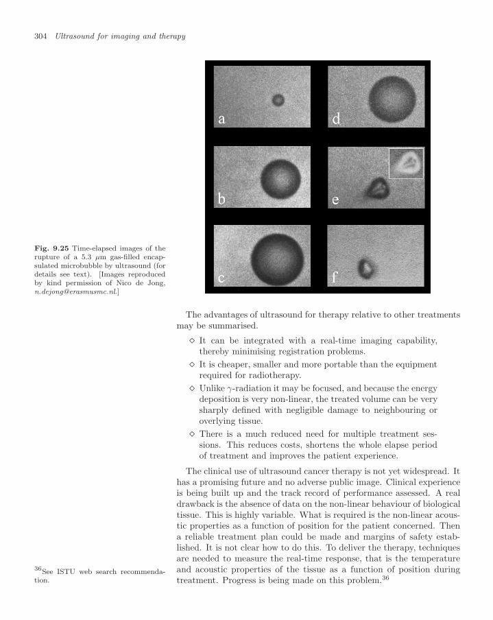
304 Ultrasound for imaging and therapy
Fig. 9.25 Time-elapsed images of therupture of a 5.3 µm gas-filled encap-sulated microbubble by ultrasound (fordetails see text). [Images reproducedby kind permission of Nico de Jong,[email protected].]
The advantages of ultrasound for therapy relative to other treatmentsmay be summarised.
It can be integrated with a real-time imaging capability,thereby minimising registration problems.
It is cheaper, smaller and more portable than the equipmentrequired for radiotherapy.
Unlike γ-radiation it may be focused, and because the energydeposition is very non-linear, the treated volume can be verysharply defined with negligible damage to neighbouring oroverlying tissue.
There is a much reduced need for multiple treatment ses-sions. This reduces costs, shortens the whole elapse periodof treatment and improves the patient experience.
The clinical use of ultrasound cancer therapy is not yet widespread. Ithas a promising future and no adverse public image. Clinical experienceis being built up and the track record of performance assessed. A realdrawback is the absence of data on the non-linear behaviour of biologicaltissue. This is highly variable. What is required is the non-linear acous-tic properties as a function of position for the patient concerned. Thena reliable treatment plan could be made and margins of safety estab-lished. It is not clear how to do this. To deliver the therapy, techniquesare needed to measure the real-time response, that is the temperatureand acoustic properties of the tissue as a function of position duringtreatment. Progress is being made on this problem.36
36See ISTU web search recommenda-tion.

9.4 Non-linear behaviour 305
Read more in books
The Theory of Sound, Vols 1 and 2, JWS Rayleigh,reprinted Dover (1945), Rayleigh’s original texts onsound
The Physics of Medical Imaging, ed. S Webb, IOP(1988), an edited compilation of useful articles, some-what out of date but still frequently referenced.
Doppler Ultrasound, DH Evans and WN McDicken,Wiley 2nd edn (2000), a useful recent text
Physical Principles of Medical Ultrasonics, ed. CR Hill,JC Bamber and GR ter Haar, Wiley, 2nd edn (2004),a recommended recent text
Look on the Web
Look up the book website atwww.physics.ox.ac.uk/users/allison/booksite.htm
Find ‘A seminar on k-space applied to medical ultra-sound’, Martin E. Anderson and Gregg E. Trahey, De-partment of Biomedical Engineering, Duke University,by searching on
duke ultrasound k-space
Consider the imaging option of using variable frequencysound waves in medical imaging
frequency scanning interferometry
Find out how ultrasound is used in NDTnon-destructive testing
Find out more about developments in piezoelectric ma-terials
piezoelectric
Read more about bloodblood composition
Learn about progress and prospects for ultrasound con-trast agents
ultrasound contrast agents
Follow developments in the use of harmonic imagingultrasound harmonic imaging
Monitor advances in ultrasound therapyISTU, MRI thermometry or hifu ter haar
Look at other uses of ultrasound for therapylithotripsy or acoustic surgery

306 Ultrasound for imaging and therapy
Questions
9.1 Consider a parallel ultrasound beam of 1 MHzand 100 W m−2 in water. The phase velocityis 1540 m s−1. Calculate the impedance, wave-length, pressure difference, particle velocity, dis-placement and acceleration.At what energy flux would the absolute pressurereach zero in the trough of the wave (assumed lin-ear)? Does this depend on frequency?
9.2 Estimate the Rayleigh scattering cross section froma red blood cell in plasma at 1 MHz using the datagiven in table 9.4. If the scattering in blood werecomplete incoherent, what would be the attenua-tion length? Compare with the observed value of0.21 m.Make a more realistic estimate by assuming thatthe scattering is completely coherent within a vol-ume of side λ/4, but incoherent between such vol-umes. How does this estimate scale with frequency?
9.3 Show that the mean and standard deviation of theRayleigh distribution, equation 9.11, are
√n and
√n(4/π − 1).
Evaluate the SNR due to speckle noise.
9.4 Show that the non-linearity ratio B/A = 1 + γ fora perfect gas under adiabatic conditions (PV γ =constant).
9.5 Show that in one dimension the Lennard–Jones po-tential, equation 4.76, gives a value of 21 for thenon-linearity ratio B/A at 0 K, equation 9.16.
9.6 Show that in the simple Lennard–Jones model theratio B/A increases when materials are heated andexpand. Is this generally true?

Forward look andconclusions 10
10.1 Developments in imaging307
10.2 Revolutions in cancer ther-apy 312
10.3 Safety concerns in ultra-sound 313
10.4 Rethinking the safety of ion-ising radiation 315
10.5 New ideas, old truths and ed-ucation 318
Look on the Web 320
in which we look forward to predictable improvements in imaging andsignificant revolutions in therapy. We conclude that the hazards of ionis-ing radiation have been significantly overestimated with important con-sequences for choices facing society. We have much yet to learn, notleast from the animal kingdom. Progress in ensuring the security of hu-man life continues to depend on knowledge of fundamental physics andinformed public education.
10.1 Developments in imaging
Influence of computational power
The advent of almost unlimited computational power and communica-tion is changing the methods that we use to carry out tasks, althoughthe fundamentals on which these are based are not changed. This revo-lution has only just begun. The timing of its progress is determined asmuch by the speed at which trust can be established in new proceduresas by the appearance of new technical opportunities. This trust growsas a result of positive experience and education.
Computational power itself will grow and new generations at all levelsof society will grow up with it. In decades to come confidence willgrow in the use of images in particular as quantitative measurementsthrough better analyses, better displays, optimised designs, improvedregistration, simulation and calibration. With education these longerterm benefits are within our grasp.
Combining data
Additional computing power has eased the task of combining data fromdifferent sources, thereby optimising both the contrast and the reso-lution. These are called fused images and examples1 were shown in 1Recall that these are only 2-D grey-
scale sections taken from the full 3-Dimage.
Figs 8.15 and 8.20. In the same way, with careful registration and cal-ibration, images taken on different occasions may be compared, andchanges with time monitored.

308 Forward look and conclusions
Modalities can be used together in other ways. Two examples are ul-trasound elastography and magnetic resonance elastography which com-bine palpation with ultrasound and MRI respectively. As limbs and mus-cles are flexed and other bodily tasks undertaken, the real-time motionand strain of constituent tissue is mapped in three dimensions usingultrasound or MRI. Such 3-D motion may be combined with calcula-tions using finite-element analysis to image the full elastic behaviour ofmuscles. Alternatively tissue may be subjected to externally appliedstress, and then the strain measured by MRI or ultrasound. Possibletumours may be detected as regions with anomalous elastic moduli, asin palpation.2 Such developments should bring better quantitative data,2The thesis by Revell gives some exam-
ples of the possibilities that are openedup.
monitoring procedures and simulations that will permit more quantita-tive uses of ultrasound.
Electro- and magneto-encephalography
Activity in muscles and the brain takes place on timescales of a millisec-ond or less. Ultrasound, MRI and PET have no resolution on such ascale. However, the electric and magnetic fields that are emitted can besensed at such speeds. The electric fields emitted by the heart have beenused clinically to monitor its activity for many years in the form of theelectro-cardiogram (ECG). Such signals are large, being associated withthe delivery of significant mechanical power. Electro-encephalography(EEG) concerns the measurement of electrical signals generated by ac-tivity in the brain. These are smaller and are partially screened by theconductivity of the skull. Time-varying potential differences on a scaleof 10 µV may be measured by an array of electrodes in contact with theskull. Modest spatial information comes from the 1/r2 dependence ofthe potential of an electric dipole.33The potential from any higher multi-
pole would fall off even faster. Magnetic fields generated by brain activity, though even smaller, arenot screened. The detected B-field depends on the orientation of the cur-rent elements which may be considered as magnetic dipoles. The mea-surement and study of these signals is called magneto-encephalography(MEG). As in EEG, spatial information is rudimentary. The necessarydetection sensitivity has been developed using superconducting quan-tum interference devices (SQUIDs). These are the most sensitive mag-netometers such devices are available commercially. The usefulness ofEEG and MEG may be enhanced by combining their time resolutionwith the spatial resolution of other modalities.
Passive acoustic imaging
The stethoscope is the icon of medical care and its use is the model ofnon-invasive clinical examination. Vibrations are emitted during anymotion of the human body, and every joint, every muscle, every bowelmovement emits sound. Some of the loudest are the low frequency emis-sions of heart, pulse and lung function. Diagnosis of their malfunctionin the doctor’s surgery is classic medicine in action. But a doctor hasonly a single pair of ears of limited frequency response, and the time for

10.1 Developments in imaging 309
(c)
(d)
Fig. 10.1 Vibrations emitted from the necks of two people as they move their heads gently from side to side. Traces (a) and(c) are from a person with a ‘noisy’ neck; traces (b) and (d) are from a person with a ‘quiet’ neck. Traces (a) and (b) wererecorded by a microphone in the person’s ear; traces (c) and (d) were recorded with an accelerometer taped to the skull behindthe ear. The signals recorded by the microphone show evidence of resonating in the acoustic cavity of the ear. [Waveformsrecorded by Lauren McDonald.]
an examination is short.4 Arrays of modern accelerometers, developed 4In addition, the doctor listens to sig-nals that have suffered a large reduc-tion in energy by reflection as they aretransmitted from the body into the air.
to record every movement of an engineering structure like a car engine,have superior sensitivity, higher frequency range and timing capabilitythan a stethoscope. They hold promise for a useful step forward in sim-ple, affordable and continuous clinical examination of joints and musclesin motion. Significant differences are observed between people. As anexample, Fig. 10.1 shows the acoustic signals emitted from the necksof two people, recorded with both a microphone and an accelerometer.The modernisation of the stethoscope is overdue and looks promising.
Non-medical developments
Measurement and simulation have much to offer non-invasive archae-ology. As the number and extent of archaeological sites and findingscontinues to expand, the need to investigate and preserve without ex-cavation becomes more important. Ground-penetrating radar, electricalimpedance tomography and acoustic sounding are used to image buriedsites and extended to underwater ones too. Ideas and technologies de-veloped for medicine are frequently taken up for geology and securityapplications.
In parts of the world that have recently experienced war, hidden land-mines are a major source of fear for the population, especially in thecountryside. These may be located safely by similar imaging and sens-ing technologies. Greater progress could be made in the development of

310 Forward look and conclusions
techniques for land-mine clearance.In the future other dangerous work such as the decommissioning of
nuclear reactors should be eased through the increased use of roboticsand autonomous probes on all scales.
Brighter sources and larger signals
The availability of brighter X-ray sources and large area detector arrayswith smaller elements gives the prospect of improved resolution with X-ray CT images and XRF. The new types of source, synchrotrons (SR)and X-ray lasers, are still in the physics laboratory. In the future suchsources and detectors will make possible cleaner images with reducedscattering and better energy discrimination.
In MRI the signal is limited by the number of spins in the voxel andthe small fractional polarisation. Applications are constrained by themaximum acceptable B-field, the small voxel size, the data acquisitiontime, and the frequency resolution required. Improvement in the ac-quisition time through further use of multiple detector coils is limitedbecause pickup coils are necessarily external. This suggests that MRIis a mature modality with little prospect of major improvement, butthis is not the case. Recent developments involve the use of noble gaseshyperpolarised by laser pumping techniques, and the generation of hy-perpolarised 13C (and other nuclei) using dynamic nuclear polarisation(DNP).5 Polarisation may also be enhanced by the use of B0 fields up5This is similar to the Overhauser effect
discussed in section 2.5.3. to 7T and beyond. Problems with the short wavelength at such fieldsmay be overcome by the use of segmented RF excitation coils. This isdifficult because of problems of field and flip-angle uniformity. Theseare developments to be watched.
For imaging with PET the statistical noise, SNR = 1/√
n in the num-ber of quanta per pixel n, limits the contrast. If the safety of ionisingradiation were treated in the same way as other hazards, as discussed be-low, much higher doses would be permitted in PET. If accepted, brighterPET scans with improved large detector arrays are a prospect. The lowrandom background and the high specificity of the take-up suggest atechnology for further development. But the spatial resolution of a fewmillimetres, related to the physics of positron production and annihila-tion, is a hard limit.
In ultrasound imaging the limit is speckle, and this ‘noise’ is deter-ministically related to the 3-D distribution of scatterers contributing toeach pixel. Although this looks to be a hard limit, much remains to bedone in ultrasound, and there may be surprises. In principle it is cheapand portable. The source technology is not a problem.
Terahertz imaging and infrared spectroscopy
In chapter 1 we dismissed the IR and UV regions of the spectrum asstrongly absorbing, and therefore unsuited to imaging in depth. How-ever, neither ultrasound nor ionising radiation is sensitive to the chemicalform of matter, and this is a requirement for imaging and probing, for

10.1 Developments in imaging 311
10
10
10
2
4
6
1
1
10
10
100
100
1000
1000
wavelength/ mμ
wavelength/ mμ
abso
rpti
on
coef
fici
ent
/mpow
erper
log
(arb
.sc
ale)
λ-1 1 freq./THz
1 freq./THz
10
10
100
100
1
2
0
a)
b)
Fig. 10.2 a) The absorption coefficientof liquid water as a function of log wave-length. Note that the vertical scale islogarithmic.b) The black body radiation spectrumas a function of log wavelength. Thelower curve is for T = 10C, the middlecurve is for T = 30C, and the uppercurve is for blood heat T = 35C. Notethat the vertical scale is linear.
example in security applications. Identification is possible exceptionallywith NMR by the chemical shift, but this is a second order marginaleffect.
In the far IR spectrum warm materials emit thermal radiation, es-pecially at wavelengths for which they are absorbing or black. Indeedthermodynamics requires that, if the absorption coefficient approachesunity, the emission spectrum approaches that of a black body. The blackbody spectrum at ambient temperatures peaks in the infrared as shownin Fig. 10.2b. Fig. 10.2a shows that water, and materials containingit, are particularly absorptive and black at these wavelengths. By con-trast, many dry materials (excluding metals) are quite transparent there.Consequently, by imaging in the terahertz region,6 the thermal radia- 6Figure 10.2a shows that absorption by
water is less than 103 m−1 at 1 THz.tion emitted by warm-blooded beings may be detected through colderdry material. Such principles may be used to image hidden survivors andbodies at disaster scenes, and also to find hidden cargoes of immigrantsat national ports of entry. The technique depends on the observationof a temperature difference in the field of view, and so, as the ambienttemperature approaches blood heat, the sensitivity is reduced.
The strong absorption in the IR is accompanied by strong reflection.In addition, following absorption atoms and molecules may emit charac-teristic fluorescent radiation. Although the reflected spectrum and thefluorescent radiation may come from a shallow depth, they are useful

312 Forward look and conclusions
in the recognition of materials. The same effect is used in everyday lifein the optical region when we distinguish things by their colour andreflectivity. In the X-ray region too, fluorescent emission by electronicresonance flags the presence of individual elements (XRF). Similarly, IRfluorescence spectra flag molecules by their individual rotational and vi-brational spectrum. When detected in a security context with sufficientresolution, these spectra may indicate the presence of specific drugs orexplosives, even through dry packaging in the mail. Technical advancesin IR technology suggest that further major developments are expected.For example, the presence of molecules specific to particular cancers maybe detected.
The difficulty is that other materials may absorb or reflect bandswithin the spectrum of interest. In particular the absorption spectrumof water is such that a search can easily be frustrated by a water thicknessof a few hundred microns. Materials wrapped in metal foil may escapedetection in the same way.
10.2 Revolutions in cancer therapy
Exploitation of non-linearity
Skin cancers can be treated with low energy γ-rays or electron beamswithout significant peripheral damage. This is because there is no over-lying healthy tissue to be damaged. Using a beam of low energy electronsstraight from the linac, few photons are created by bremsstrahlung andthe electrons do not penetrate much below the superficial volume to betreated.77In the discussion in section 8.1.1 the
inefficient production of photons byelectrons presented a problem, even ina high Z material like tungsten. In thiscase with the low Z of tissue, the in-efficiency of photon production by anelectron beam is beneficial.
For deep-seated cancers treatment by γ-ray therapy must be describedas primitive. As the dose contours on Fig. 8.24 show, the dose deliveredto the prostate tumour is less than twice as large as the dose deliveredto the healthy rectum. The death of the one and the survival of theother is attempted by putting the patient through 20 or more cyclesof treatment and recovery in order to exploit the related non-linearity.This is unsatisfactory on four levels.
The patient experience of this damage-and-recovery iterationis dreadful. The prolonged duration of the treatment is afurther element of the adverse patient experience.
The cost increases with the number of fractions and is there-fore high.
The success rate for the treatment of deep-seated cancersis not good. This is because it is not feasible to give therequired dose to the tumour and still ensure the survival ofperipheral tissue.
The healthy tissue is heavily scarred following such treatmentsuch that further courses of treatment may not be possible.
The consequence is that people are frightened. They speak in hushedtones of the ‘C word’. This should remind us of where this book started.

10.3 Safety concerns in ultrasound 313
In our discussion in chapter 1 we noted that physics has succeeded overthe decades and centuries in relieving society of its worst fears. Whatcan be done in this case?
There are two avenues.8 They are light ion beam therapy and focused 8We exclude developments inchemotherapy as such which lieoutside the physical methods discussedin this book.
ultrasound (HIFU). These were discussed in chapters 8 and 9. Thecurrent situation calls for a massive and concerted development in thesetwo areas over the next 20 years, such that in 2025 it can be said that2005–2025 was an era of great advances in therapy, as 1985–2005 hasbeen in imaging.
Both solutions promise a sharply defined therapeutic spot. Conse-quently the registration of the treatment with the position of the tumourbecomes exacting. This is made difficult by cardiac and respiratory cy-cles and other differential patient motion. The treatment plan calls forthe spot to be raster-scanned through the volume of the tumour. Thisdemands the development of feedback between a real-time image of thetumour and the position of therapeutic beam.
There are new prospects in the design of small high current acceler-ators that could make the beams of light ions needed for radiotherapymore readily available. Such facilities are already under developmentin a number of countries. The extension to carbon ions with the extranon-linearity should follow.9 9See for example the website of the
BASROC consortium.In the case of HIFU the application of the therapy is affected bythe degree of non-linearity, the early monitoring technology and theconsiderable variability of tissue properties. These represent a need forserious investment, not just of resources but also of ideas and data.As simulation and monitoring of such therapy develops, confidence willbuild. Currently prostate therapy is available on an out-patient basis ata number of centres. Much remains to be done before similar treatmentis available for other deeper cancers.10
10See websites for the InternationalSymposium on Therapeutic Ultrasound(ISTU).
10.3 Safety concerns in ultrasound
Sonoluminescence
The inadequate state of our knowledge of ultrasound in the non-linearregime is indicated by the phenomenon of sonoluminescence in which asmall bubble illuminated by ultrasound is observed to emit light consis-tent with a high temperature black body spectrum.
Figure 10.3 shows a glass vessel of diameter 6.4 cm filled with dem-ineralised water and illuminated by two ultrasound transducers at 25kHz. Their outline may be seen towards the edge of the picture. At thisfrequency there is a simple acoustic antinode at the centre of the vessel.An air-filled bubble of initial diameter 75 µm has been placed there bypipette. The observation is that under the influence of the ultrasoundfield this bubble emits white light in pulses 1 ns long at the point in timewhen the bubble collapses. This is known as sonoluminescence, whichwas first discussed in 1934. In the experiment shown here the bubble isthe bright point of light indicated by the arrow. The spectrum of the
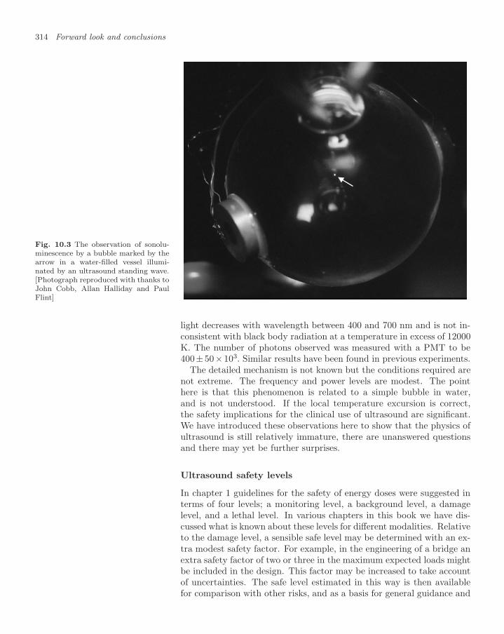
314 Forward look and conclusions
Fig. 10.3 The observation of sonolu-minescence by a bubble marked by thearrow in a water-filled vessel illumi-nated by an ultrasound standing wave.[Photograph reproduced with thanks toJohn Cobb, Allan Halliday and PaulFlint]
light decreases with wavelength between 400 and 700 nm and is not in-consistent with black body radiation at a temperature in excess of 12000K. The number of photons observed was measured with a PMT to be400±50×103. Similar results have been found in previous experiments.
The detailed mechanism is not known but the conditions required arenot extreme. The frequency and power levels are modest. The pointhere is that this phenomenon is related to a simple bubble in water,and is not understood. If the local temperature excursion is correct,the safety implications for the clinical use of ultrasound are significant.We have introduced these observations here to show that the physics ofultrasound is still relatively immature, there are unanswered questionsand there may yet be further surprises.
Ultrasound safety levels
In chapter 1 guidelines for the safety of energy doses were suggested interms of four levels; a monitoring level, a background level, a damagelevel, and a lethal level. In various chapters in this book we have dis-cussed what is known about these levels for different modalities. Relativeto the damage level, a sensible safe level may be determined with an ex-tra modest safety factor. For example, in the engineering of a bridge anextra safety factor of two or three in the maximum expected loads mightbe included in the design. This factor may be increased to take accountof uncertainties. The safe level estimated in this way is then availablefor comparison with other risks, and as a basis for general guidance and

10.4 Rethinking the safety of ionising radiation 315
regulation. We call the range from the safe level to the damage level thethreshold region.
For ultrasound the levels are summarised in Fig. 10.4a on a logarith-mic scale in terms of the tissue temperature rise. The threshold regionis ∆T = 1 − 2C; the damage region is ∆T = 20C. These levels arequite close considering that instrumentation suitable to monitor suchtemperature rises in vivo is a recent development and not yet widelyavailable. The degree of non-linear response of tissue to ultrasound andthe paucity of related data is a concern, especially as the advantagesof harmonic imaging encourage the use of sound at non-linear intensi-ties. Safety is not improved by the public perception that ultrasound isharmless and particularly suitable for scans of pregnancies. The currentunregulated situation is apparent from the website of the UK HealthProtection Agency (HPA) where it is stated:11 11A subgroup was set up at a meeting
on 7 December 2004 to consider theseconcerns. An initial report is expectedbefore the end of 2006.
There are no specific regulations in the UK for controlling exposure toultrasound (and infrasound). However, medical products are required tocomply with the Medical Devices Regulations 2002 (SI 618/2002). Theguidance for medical diagnostic exposures are based on limits specified bythe US Food and Drug Administration (FDA) but these do not appear to
have a solid scientific basis.12 Guidance is issued by the professional and 12The underlining emphasis has beenadded.membership bodies the British Medical Ultrasound Society, the European
Committee for Medical Ultrasound Safety, and the World Federation forUltrasound in Medicine and Biology.
We conclude that the situation is a matter of concern.
10.4 Rethinking the safety of ionising
radiation
What is a safe radiation dose?
The safety of ionising radiation and ultrasound could hardly be moredifferent. There is no difficulty in monitoring ionising radiation, evendown to the level of single photons or less per day. The data fromHiroshima and Nagasaki discussed in chapter 6 show that there is nosignificant risk of death from solid cancers or leukaemia for a single dosebelow 100 mSv.13 This is plotted in Fig. 10.4b. The fatal dose at about
13A recent report concludes that “Onaverage, assuming a sex and age dis-tribution similar to that of the entireU.S. population, the BEIR VII lifetimerisk model predicts that approximately1 person in 100 would be expected to de-velop cancer (solid cancer or leukemia)from a dose of 100 mSv above back-ground, while approximately 42 of the100 individuals would be expected todevelop solid cancer or leukemia fromother causes.” This refers to the whole-life risk and is based in part on a furtherre-calibration (2002) of the Hiroshimaand Nagasaki data. It is an upper limitbecause the report uses the LNT model.This comes from the Biological Effectsof Ionizing Radiation (BEIR) group ofthe US National Academies (19 June2005). This conclusion does not differgreatly from that reached in chapter 6.
5000 mSv is also shown. Interestingly, the factors that separate the safe,threshold, damage and fatal bands seem much the same as for thermaldamage, Fig. 10.4a (although no reason why this should be so is evident).
Also shown is a typical therapy dose per fraction. At 1500 mSv givento healthy tissue every day this dose is far from safe; the dose of 3000 mSvto the tumour is inadequately fatal. These figures vary somewhat butare typical of treatment provided in therapy departments on a regularroutine basis.
The average annual dose of background radiation in the UK is 2.7mSv/year.14 To make a comparison of this dose rate with the above
14As discussed in chapter 6.
single doses, we need to know the time over which tissue integratesdamage. This is the repair time, already known from in vitro and therapyexperience to vary between several hours and a few days. This is used in

316 Forward look and conclusions
1,000 3,000 10,0003001003010310.30.1
mSv
tumourtherapydose perfraction
CT
equivalent UKmean environmental
dose per monthscan
or PET
10 10030310.30.10.030.010.003
fever &exerciseunmeasurable
ultrasoundtherapydose
C above normal
a) tissue heated above normal temperature (35 C)°
b) tissue irradiation
completely safe threshold damage fatal
°
Fig. 10.4 A comparison on a logarithmic scale of ranges of dose separated by dotted lines that, (in turn from left to right) arecompletely safe, are at the threshold of damage, involve certain damage, and are fatal. These regions are shown for a) tissueheating generated by ultrasound or microwaves, and b) a single dose of ionising radiation. The rise in tissue temperature is inC and the radiation dose is in mSv.
radiotherapy to set the recovery time between fractions, typically a day.Even if we choose a conservative time of a month, typical environmentalradiation exposures are seen to be many orders of magnitude belowthreshold. With this choice the average UK background dose rate of 2.7mSv/year is equivalent to a single dose of 0.2 mSv. This is lower than thedamage threshold by a factor 1/500. Because of the non-linear repairmechanism this represents not just a proportionately small hazard, itrepresents no hazard, as was the case for the blood donation discussedearlier.
The dose from a typical PET or CT scan is an order of magnitudebelow the damage threshold level. This suggests that doses larger by afactor ten should be permitted in cases for which the resulting improvedimage resolution would give a better clinical diagnosis.
The current public safety limit for any steady extra dose of ionisingradiation is 1 mSv/year. This would be equivalent to a single dose of0.1 mSv, again using the conservative repair time of one month. This isseen to be over-cautious by a factor of about a thousand. Certainly thesenumbers can be argued up or down by factors of two but the factors often are rather firm. Of course room should be left for uncertainties.However, after 50 years these have become rather small.
This is an important conclusion. It means that all safety considera-

10.4 Rethinking the safety of ionising radiation 317
tions associated with nuclear radiation need to be revised by a factor ofat least 500. This includes the handling of nuclear material, the decom-missioning of reactors and the disposal of waste. The costs of nuclearpower should be very substantially reduced thereby. Given the threatof global warming this would be an important step. If it is acceptablefor a patient in therapy to risk receiving 15 times the safe dose of 100mSv every day, should not some risks be incurred for the health of theplanet?
Why have we over-reacted to nuclear risks in the past?
A related question is how society came to have the current stringentsafety thresholds for ionising radiation. There are a number of reasons,some political and some scientific.
As a result of the bombing of Hiroshima and Nagasaki thepublic were frightened by the power of nuclear weapons. Thepublic were told something of the compelling ideas of the fis-sion chain reaction and the power of Einstein’s conclusionthat E = mc2. This information did nothing to calm theirfear.15 Indeed there were political reasons to maintain the 15We note that neither of these aspects
is relevant to the safety of ionising ra-diation as such.
fear of radiation, providing, as it did, the basis for the deter-ence of the Cold War.
In 1945 and for some time after there was little understandingof how radiation affected living organisms. Knowledge ofgenetics was rudimentary. A cautious approach to safetyseemed wise at that stage.
There was no large scale data on the basis of which it waspossible to limit with confidence any long term damage dueto ionising radiation.
With ample supplies of oil and coal and with no evidentglobal warming there was no serious disadvantage to a tightcontrol of radiation safety.
As a result, in the decades that followed World War II wholly newcriteria were set up and applied to ionising radiation safety that were notapplied elsewhere. These became linked to a naive search for absolutenuclear safety, ignoring the need to balance radiation risks with otherhazards.
A safety regime was set up in which nuclear radiation was tobe set at the lowest possible level. This became the ALARAprinciple, discussed in section 1.3.2.
The linear no-threshold (LNT) model was introduced. Thisignored the experience of recovery from radiation dose andexpressed risk in terms of collective dose.
International studies of incidents and accidents (from Hi-roshima to Chernobyl) that indicated that risks were exag-gerated were ignored by the media. Pressure groups com-peted with one another in their state of alarm. Even the

318 Forward look and conclusions
label ‘nuclear’ was dropped from NMR when MRI was in-troduced. A polarised state of nuclear denial became thenorm. To settle practical matters most people followed theprevailing guidelines.
Public authorities confused the need to provide safety fromreal hazards with the need to make the population feel thatthey were safe. The latter is an important objective, buteducation, legislation and advice must be anchored to theformer. Politicians having no knowledge of their own andseeking short term advancement, tightened laws and regula-tions further.
Individual scientists who could have seen what was happen-ing did not have the time to do so.
And then the realisation of global warming dawned – and with it thequestion of the nuclear power option.
The hazards of global warming need to be weighed against those ofionising radiation. Physicists need to rewrite the description of nuclearsafety, for, not only is the current version of it unjustified, but it isobstructing the deployment of nuclear power which is the only largescale ‘green’ carbon-free solution to the world’s power needs. A safetyindustry entrenched in the old out-dated standards has been built up.It will not be easy to turn this around. Much public education is neededand time is short.
A stumbling block for popular perception is the invisibility of ionisingradiation, and it was from the ability to see and its effect on confidencefrom which this book started. But the public already accepts high levelsof ionising radiation16 in medicine; the need is to achieve an equivalent16Although in radiotherapy the levels
accepted by the public should be re-duced, as discussed in the previous sec-tion.
acceptance of relaxed environmental radiation standards. So the task ofpublic re-education and information should be possible.
Terrorists and rogue states will continue to try to create fear, whetherby biological, nuclear or any other means that comes to hand. However,as far as nuclear dangers are concerned the effect of more relaxed safetystandards will be to deflate the currency of their threats to some extent.That can only be to the good. However, nothing said here should beconstrued as suggesting that nuclear power is safe, but it is safer thanthe alternative and we need it.
10.5 New ideas, old truths and education
Nanotechnology probes
Contrast agents have played an important part in the development ofimaging. However, these agents have been more or less passive. In thefuture, miniature probes will become increasingly active. An importanttask will be the maintenance of communication and supply of powerto such probes if they are to undertake sophisticated tasks such as lo-cal measurement, surgery and targeted drug delivery. The design and

10.5 New ideas, old truths and education 319
engineering of such miniature devices would harness the tools of DNAself-replication.
Metamaterials and coherent optics
Nanotechnology presents the prospect of making wholly new classes ofmaterials. An example is a metamaterial with a negative refractiveindex. Samples have already been made. With a negative value of bothεr and µr an electromagnetic pulse may propagate forwards in respectof both group velocity and energy flow, while having a phase velocity inthe backward direction.17
17We saw in section 3 when discussingthe behaviour of a small circuit in aB-field that it may resonate and that,depending on the damping, the mag-netic moment that opposes the appliedB-field may be negative in the regionbelow resonance. The induced electricdipole moment is opposite to the ap-plied E-field at ω just above ωp, theplasma frequency. It has been pre-dicted, and recently confirmed, that anartificial material composed of an en-semble of such circuits and conductorson a lattice can be constructed whichdisplays negative values of relative per-meability µr and relative permeabilityεr in a region of frequency.
This negative refractive index causes the incident and transmittedrays at the interface to such a material to be on the same side of thenormal, as given by Snell’s law. The usual situation is illustrated inFig. 10.5a, compared with the unconventional result in Fig. 10.5b.
a)
b)
Fig. 10.5 The application of Snell’slaw. a) A conventional material withtransmitted ray on the opposite side ofthe normal to the incident ray. b) Acomposite metamaterial with transmit-ted ray on the same side of the normalto the incident ray.
A parallel-sided block of such material behaves as a converging lens inthe frequency range concerned. Conventional materials are too weaklymagnetic at a microscopic level to exhibit these effects. The range ofapplication of such ‘metamaterials’ remains to be determined, but itseems likely that interesting developments will follow, especially in theRF, microwave and terahertz bands.
Advances in the use of coherent optics, with or without the use ofmetamaterials, is likely to influence medical imaging in the years ahead.
Smell and spectroscopy
The extent to which dogs and other creatures can distinguish chemicalsby smell is surprising. They are able to distinguish different people andto find small quantities of narcotics and explosives on the basis of verylow vapour pressures. Substances of molecular weight greater than about340 cannot be distinguished in this way. Nevertheless dogs can diagnosemelanoma by smell. Recently the physiology of smell has been decodedby molecular techniques, and Buck and Axel were awarded the 2004Nobel Prize for Medicine for their work. Is there a future for animalswhose sense of smell has been genetically redesigned for a molecule ofinterest? Or can the same end be achieved by old-fashioned training?
Navigation in the animal kingdom
While many an ancient mariner could smell land and some birds areknown to navigate by following railway lines, on the whole animals,birds and fish have developed their own navigation systems. They areable to recall physical landmarks and features over long periods, theycan sense magnetic fields and the polarisation of sunlight, as well as usetheir powers of smell. Many of their skills appear to be inherited ratherthan learned. They combine different techniques to able to overcome lossof any one signal. Mankind has still much to learn from understandinghow they manage to do this.
320 Forward look and conclusions
Gravitational waves and the Universe
The observation of gravitational waves in the first decades of the twentyfirst century will permit the exploitation of the most penetrating probein the Universe. The information carried in the form of the polarisation,frequency and direction of gravitational waves will stimulate a whole newbranch of physics and astronomy. This new Copernican revolution willensure that mankind keeps thinking and wondering about new ideasin pure physics. Such stimulation will continue to pay dividends ineveryday life even though the benefits will be indirect.
Confidence and progress through open education in purescience
New technology makes further features in pure physics accessible. Tosurvive on the planet for further centuries mankind will need to investin responsible education and informed confidence. Then, if decisions aretaken by those who understand and consider the consequences, thereis plenty of scope for optimism. Otherwise, if decisions continue to bedriven by greed, secrecy, private gain and sectional interest, prospectsare bleak. The way forward relies on decisions being made that arebased on pure science and that command the informed confidence of thepublic. Only in this way may fear be reduced. This should be a majoritem on the world agenda for the twenty first century.
Look on the Web
Look up the book website atwww.physics.ox.ac.uk/users/allison/booksite.htm
Study the imaging methods of EEG and MEGEEG MEG
Read about infrared spectroscopyIR spectroscopy
Consider the competition to IR spectroscopy offered bysmell, and the small extent of our knowledge of it
smell and Buck Axel Nobel prize
Read about developments and prospects in radiother-apy (see also chapter 8)
protontherapy, carbontherapy, BASROC
For progress in ultrasound therapyinternational symposium on ultrasound therapy
Look up elastographyMRI elastography and ultrasound elastography
and find PhD thesis of James Revell, Bristol (2005)
Watch developments in nanotechnologynanotechnology probesDNA molecular engineering
Follow new possibilities in MRI using dynamic nuclearpolarisation
DNP enhanced MRI
Read further about sonoluminescence amd metamate-rials
sonoluminescence and metamaterials
Look at the links to animal navigation research on theRoyal Institute of Navigation website
animal navigation RIN

Conventions, nomenclatureand units AUnits and nomenclature
Generally we use conventional SI units. In this system the magneticfield is denoted properly by H and measured in A m−1. On the otherhand the magnetic flux density or magnetic induction is denoted by Band measured in tesla. In a sense H is fictitious and B is the measurablefield. In this book we avoid using H where possible and refer simply tothe ‘B-field’ measured in teslas. This is brief, clear and unambiguous.
In addition we use the following conventional nuclear or atomic units:
Quantity Unit SI equivalent Conversion factorCross section barn 10−28 m2
Energy eV e J 1.602× 10⁻¹⁹ JMass eV/c2 e/c2 kg 1.783× 10−36 kgMomentum eV/c e/c kg m s−1 5.344× 10⁻²⁸ kg m s−1
When we refer to ‘frequency’ we mean angular frequency measured inradians per second, often denoted by ω, unless the frequency is explicitlygiven in hertz (Hz), meaning cycles per second.
All logarithms are natural logarithms unless another base is explicitlystated.
Decibels
The decibel is used in two different ways in applied physics.First it is a measure of the ratio of signal energy fluxes on a base-
10 logarithmic scale. Thus 1 decibel represents an energy flux ratio of100.1. In general a signal of intensity I and amplitude A is described asn decibels relative to one of intensity I0 and amplitude A0, if
n = 10 × log10
(I
I0
)= 10 × log10
(A2
A20
)= 20 × log10
(A
A0
). (A.1)
In acoustics the decibel is also used to quantify an absolute level ofenergy flux relative to a just audible standard. This standard is definedin terms of pressure, and is different in air and water. The decibel is notused in this way in this book.

322 Appendix A Conventions, nomenclature and units
Lifetimes
The exponential decay of an unstable state may be described, either interms of a mean life τ such that the population or energy falls with timeas exp(−t/τ), or in terms of the half-life t1/2 such that the energy orpopulation falls by a factor 2 in each period of time t1/2. In environ-mental and radiation contexts the half-life is always used. In quantummechanics and most of the rest of physics the mean life is used. Weexplicitly use the terms ‘half-life’ and ‘mean life’ to remove ambiguity.The two are related as
t1/2 = ln 2 × τ. (A.2)
Square roots of −1 and time development
It is conventional in electrical circuit theory to denote the root of −1 byj, and to describe time development by exp(jωt). In quantum theory itis usual to use i for the square root, and to describe time developmentby exp(−iωt). It does not really matter which time development is usedprovided that there is consistency. By flagging the choice by the changeof symbol, ambiguity is avoided. In the quantum theory convention aforward-moving progressive wave has an exponent exp[i(k · r − ωt)].
Classical and quantum treatments
Many aspects of the physics that we discuss are adequately describedin terms of classical physics, meaning that a description in quantummechanics gives the same result. If it affords a deeper understandingof what is going on and it is straightforward to do so, we give bothquantum and classical descriptions. How it is that classical physics givesthe correct answer in the limit, the so-called correspondence principle,is a larger subject beyond the scope of this book.

Glossary of terms andabbreviations BThe letter in the second column denotes the field to which the termor abbreviation principally belongs: A=archaeology, C=chemistry,E=engineering, G=geology, M=medicine, P=physics, I=imaging.
Term Meaning
1-D, 2-D, 3-D one-, two- or three-dimensionalALARA as low as reasonably achievable, principle of safety standardsalias I an artificially displaced part of an imageangiogram M an X-ray image of blood vesselsAPD P avalanche photodiodeBASROC British Accelerator Science and Radiation Oncology ConsortiumB-field P magnetic flux density or magnetic induction, in teslabolus M concentrated charge of agent introduced into blood or digestive tractbrachytherapy M radiotherapy by implanted sourcesCCD E charge coupled device, a detector array as used in an electronic camerachiral P having handed symmetry, left or rightcoronal M face-on vertical section of body or head in the upright positionCT scan M an X-ray scan analysed in three dimensions by computed tomographydE/dx P mean energy loss with distance along a charged track, excluding bremsstrahlungDNP dynamic nuclear polarisationDTPA M di-ethylene-triamine-penta-acetic acid, a chemical ‘wrapper’ for Gd ions
when required as paramagnetic contrast agent in MRIE1 P electric dipole resonance. Similarly En, electric multipole resonancesECG M electro-cardiogramEEG M electro-encephalographyerythrocyte M red blood cellESR P electron spin resonance in a laboratory B-fieldFDG M Fluoro-deoxy-glucose, the carrier used for radioactive fluorine in PETFFAG P (non-scaling) Fixed Field Alternating Gradient, a potential design for a medical
therapy acceleratorFGR P Fermi’s golden rule for the calculation in quantum mechanics of the rate of
an interaction in first order time-dependent perturbation theoryFMRIB I Functional Magnetic Resonance Imaging of the Brain unit, Oxford UniversityFOV I field of view, the part of the object to be imagedfractionation C change in the relative concentration of isotopes by a mass-dependent processfractionation M delivery of therapy over a period to exploit the non-linearity of response

324 Appendix B Glossary of terms and abbreviations
Term Meaning
FSI P frequency scanning interferometryfused image I an image composed of data from two or more modalities combinedgradient echo I condition when all spins in a slice have the same phase due to field gradientsg-factor P factor relating a gyromagnetic ratio to its classical valueHPD P hybrid photodiodehypoxic M oxygen deficientinfarction M blockage, e.g. of a blood vesselIMRT M intensity-modulated radiotherapyintrinsic P pure semiconductor state with carriers arising from thermal excitation alonein vitro M an observation or experiment conducted in a test tubein vivo M a live observation or experimentIR P infra-red region of the spectrum with frequency less than that of lightLET I linear energy transfer (dE/dx) of a charge in tissuelinac P linear accelerator powered by RFLNT linear no-threshold model of radiation damageM1 P magnetic dipole resonance. Similarly Mn, magnetic multipole resonancesmagnetisation P magnetic dipole moment per unit volume (also called polarisation)mammography M imaging of the breastMEG M magneto-encephalographymetabolite M a chemical, an active ingredient of growth or functioning of the bodymetastasis M the migration of cancer cells from one organ to anothermodality M group of methods of medical imaging based on a common physical principleMRI I nuclear magnetic resonance imagingMRS I nuclear magnetic resonance spectroscopy with some spatial resolutionmuon P an unstable heavy version of the electron with 200 times the massn-type P a semiconductor with impurities so that most charge carriers are negativeNDT E non-destructive testingnecrosis M death of the cells of an organ or tissueNICE M UK National Institute for Health and Clinical ExcellenceNMR P nuclear magnetic resonancenon-linear P depending more (or less) steeply than the first powernuclear medicine M imaging using administered radioactive nuclei (SPECT and PET)palpation M examination by feeling with fingers and palmsp-type P a semiconductor with impurities so that most charge carriers are positivePET I positron emission tomographyphantom M a made-up reference sample of known compositionPIXE P proton-induced X-ray emissionpixel I a discrete element of a 2-D imagePMT P photomultiplier tubepolarisation P (of a wave) direction of the field vector (not the wavevector)polarisation P (of material) having net electric dipole moment (see also magnetisation)PSF I point spread functionP wave G compression wave with longitudinally polarised strainQ P 2π× ratio of resonance energy divided by energy lost per cycleQED P quantum electrodynamics

Appendix B Glossary of terms and abbreviations 325
Term Meaning
radar E RAdio Detection And RangingRBS P Rutherford back scattering with light ion beamregistration M matching of position information, both alignment and rotationRF P radiofrequencyRMS root mean square deviationRT M radiotherapysagittal M side-on vertical section of body or head in the upright positionSAR P specific energy absorption rateSH wave G shear wave with strain perpendicular to the plane of incidence (horiz.)SI the international system of metric unitsSNR E signal-to-noise ratiospeckle P a form of statistical noise arising from random phasesSPECT I single photon emission computed tomographyspin echo P condition in NMR when the precession phase of all spins returns to zeroSPM P scanning proton microprobeSQUID P superconducting quantum interference deviceSR P synchrotron radiation sourcestandard A a made-up reference sample of known compositionSV wave G shear wave with strain in the plane of incidence (vertical)T P temperature in K or stress in Newtons /m−2, according to contextT P Tesla, unit of B-field strengthterahertz P electromagnetic radiation of frequency around 1 THztomography I 3-D reconstruction of an imagetransverse M horizontal section of body or head in the upright positionUV P ultraviolet region of the spectrum with frequency greater than that of lightvasculature M form of the blood vesselsvoxel I a spatial element of a 3-D imagewavelets P a form of wave analysis combining localisation with frequency analysisXRF P X-ray fluorescenceZ P the atomic number of an element

This page intentionally left blank

Hints and answers toselected questions C2.2
Width 1.8 × 10⁻³⁰ eV.
In the laboratory the width and lifetime are domi-nated by collisional de-excitation and the Dopplershift. In inter-stellar space the Doppler shift stilldominates the width but the lifetime is the radia-tive lifetime.
2.3There are three considerations: a) L comes fromthe self inductance of the coil element but C canbe chosen freely; b) the phase change in each ele-ment should be 2π/12 at 120 MHz; c) the input,output and terminating impedances should matchfor efficiency and to prevent reflected waves gener-ating a field rotating the wrong way around. [Forfurther discussion of such filter circuits refer to thebook by Bleaney and Bleaney.]
This ignores the mutual inductances of the coil el-ements; this is described by a 12 × 12 inductancematrix. The back emfs are related to the flux link-ages of pairs of coil elements. The full set of 12simultaneous equations should be solved; a conse-quence is that the C values will not all be the same.
2.4Consider the Fourier transform of the decay of theresonance energy as a function of time.
2.5M = 0.02 Wb m−3. Frequency 128 MHz.Consider the maximum possible rate of change ofmagnetic flux linking the detector coil, and deducethat the mass of water is 0.05 kg.For the maximum voltage the coil should surroundthe sample closely so that no return flux passesthrough the coil. The plane of the coil should con-tain the B0 field.
2.6For an isolated electron the answer is 0.74 MHz.However, the ESR frequency varies too much withthe atomic environment of the electron and itsdamping is too large (Q too low) for this to bea good way to measure small fields.
2.8The frequency of B1 must be on resonance at 64MHz within ≈ 1/50 MHz. This tolerance is suchthat the phase will not slip significantly during the50 µs pulse. During the pulse the moment is ro-tating about B1 in its own frame at 2.1×10⁴ radi-ans s−1. [See the book by Bleaney and Bleaney forfurther discussion of this motion.] Answer 60.
2.9In units of 10−3 Wb m−3, initially M = 10 unitsin z direction. Immediately after the RF pulse, 5units in z and 8.7 tranversely. After 100 ms, 5.9units in z and 1.2 units transversely.
3.1
dσ
dΩ=
fr2
12 × 103 × FAmNam2 steradian−1,
where Na is Avogadro’s number.
3.2Calculate the transverse and longitudinal momen-tum transfer using the data given. Then use equa-tion 3.9 to show that the target mass is actuallythat of the electron.
3.4Form the Lorentz scalar product of the target 4-vector before scattering with that after. In the tar-get frame this is −mc2(E + mc2). In the centre-of-mass frame it is
−(mc2)2 + Q2/2 = −(mc2)2 + Q24/2.

328 Appendix C Hints and answers to selected questions
3.5a) Get amplitude a using Newton’s second law.b) Use the impedance Z to get the incident H-fieldand Poynting’s vector to get the incident energyflux, E2
0/2Z.c) Use Z again.d) The cross section is the scattered power dividedby the incident energy flux.Answer 6.65×10⁻²⁸ m2.
3.6Deuteron range is 11 g cm−2 = 110 kg m−2, equiv-alent to 220 kg m−2 for a proton.Read off from the curve βγ = P/mc = 0.4 so thatP = 800 MeV/c and KE = 155 MeV.At the same βγ, the proton range is 0.025 m.
3.7RMS angle 0.017 radians.
3.81 mm of copper is 0.896 g cm−2. Assuming thatthe energy loss is small and that β = 1, the non-radiative energy loss is 1.228 MeV. The radiativeloss is 3.0×0.896/12.25 = 0.22 MeV. If the incidentenergy were much less than 3 MeV, the fractionalenergy loss would not be small and the approxima-tion would fail.
4.1The isotropic, traceless symmetric and antisym-metric parts:
1
3
[a + e + i 0 0
0 a + e + i 00 0 a + e + i
],
1
6
[4a − 2(e + i) 3(b + d) 3(c + g)
3(d + b) 4e − 2(i + a) 3(f + h)3(g + c) 3(h + f) 4i − 2(a + e)
],
1
2
[0 b − d c − g
d − b 0 f − hg − c h − f 0
].
For the stress tensor multiply each by the respec-tive modulus (3λ + 2µ, 2µ, 0) and add back upagain.
4.3Read off cR from Fig. 4.17. The rest is geometry.Time = 383 s. Distance = 2000 km.
4.4The wavelengths at resonance are 2/(n + 1) forthe nth harmonic. The open end of the tube is anantinode so that odd n harmonics are missing.
But what are the walls doing? Nothing for the dis-placement which is longitudinal anyway. But con-sider the stress (pressure) and why a wave in thetube should be reflected from the open end. Whathappens if the width, a ∼ λ?
4.5Use equation 4.68 with h = ψz at z = 0. Damp-ing of the wave by scouring is clearly a large effect.This is the reason why seabeds are remarkably flat.In the non-linear range the peak of the waves form aforward flow of water which is balanced by a steadybackward scouring flow on the seabed. This is themechanism of coastal erosion under conditions ofhigh waves.
5.5Let concentrations relative to the references be a,b, c, d, e. The sum-of-squares,
S = Σ100i=1 (M(ωi) − aA(ωi) − bB(ωi)
−cC(ωi) − dD(ωi) − eE(ωi) − X − ωiY )2 .
Get 7 equations by setting to zero the differential ofS with respect to a, b, c, d, e, X, Y in turn. Theseequations are linear in the unknown concentrationsand could be solved by inverting the matrix. Acheck would then be made that the concentrationsand the background levels X +ωiY are everywherepositive for a reasonable fit.
[Such an analysis might also be used to find theconcentrations of elements contributing to an ob-served X-ray emission spectrum taken by XRF orPIXE techniques discussed in chapter 6.]
6.1a) 470. b) 50×106.
6.2Error on age = mean life × error on count / count.Statistical errors: a) 460 years, 4300 years. b) 1.4years, 13 years.Systematic errors due to 1% modern C: for 3000year old sample is 120 years, for 40,000 year oldsample is 10,000 years.
6.3Assume that 30% of tissue is carbon and that halfof the decay energy of 14C is carried away by theneutrino and half deposited by the electron. Sv andGy are the same for β-decay. This contributes 23µSv per year to internal dose.

Appendix C Hints and answers to selected questions 329
6.4Suppression of 40K decay relative to neutron decayis 1.6× 10⁻¹⁴, ignoring that the energy is 1.5 MeVwhereas it is only 0.8 MeV for the neutron.The λ of 1 MeV photon is 1.2×10⁻¹² m, and soa/λ ≈ 10−3. For ∆J = 4 the given EM suppres-sion factor comes out at 6×10⁻¹⁴, and this appliesapproximately to the γ-decay of 99Tc. Both thesehighly forbidden decays are of great importance,99Tc in medicine and 40K in the environment.
6.5Layer of gold (197) on a silicon (28) substrate.
6.6Apply energy conservation and momentum conser-vation, longitudinal and transverse.
6.7a) The KE of the argon is 28 eV.
b) The KE of the radon is 86 keV. Comment: theradon nucleus recoil energy is 3000 times larger andit is probably kicked out of its lattice site which isprobably interstitial anyway on account of earlierdecays in the radioactive decay sequence. The ar-gon with its small recoil and previously undisturbedlattice site has a good chance to remain trapped.However, I have found no analysis that comparesthis with the six orders of magnitude difference incontainment time.
7.1Consider the magnetostatic potential due to m andthence its B-field perpendicular to the coil.
7.2The sensitivity matrix has diagonal elements 8
√2
and off-diagonal elements 1. This would give clearnon-singular spatial discrimination.
7.3Answer: (x, y, z) = (-60, 42, 32) mm relative tothe isocentre (the centre of symmetry of the ap-plied gradient fields).
7.5This chemical shift amounts to increasing the valueof the Larmor frequency, 42.55747 MHz T−1, by 4ppm. The change in calculated position would be(0.0, 1.0, 1.5) mm.
7.6If the relaxation time is 10 ms, then the maximumpower at which energy can be deposited is the fullresonance energy every 10 ms. This is the magneti-sation energy of 1 in 105 protons which is 5.3×10⁻⁵
J kg−1. Maximum resonant power loading 5.3 mWkg−1. We may conclude that resonant power ab-sorption due to NMR cannot be a significant haz-ard. (The position is different for ESR.)
7.7Use energy conservation. The magnetic energy perunit volume is about − 1
2µrB
20 (depending somwhat
on the shape as well as the orientation of the screw-driver to the field) and its KE is + 1
2ρV 2. These add
to zero for a screwdriver starting from rest outsidethe magnet.
7.8Ignore any difference between the values of T2 forA and B, and also the distinction between T2 andT ∗
2 . Answer: Before time t = T ′ there will be noFID from A or B. After time t = T ′ the ratio of Bmagnetisation over A magnetisation will be
1 − 2 exp (t/1.3)
1 − 2 exp(t/0.75).
The contrast is a maximum at T ′ = 0.75/ ln 2 s,when the amplitude of the FID due to A will bezero.
8.2KE is 0.1 eV.
8.3Assume patient has density of water. Then 106 vox-els per kg and 104 counts per voxel. Taking eachcount to be 60 keV, that makes 6×10¹⁴ eV per kg.This equals 0.1 mSv at 100% efficiency. This is ob-viously a significant underestimate for a practicalcase.
8.5The range is 200 kg m−2. The range for protonsis read off Fig. 3.13; for another particle with thesame value of βγ but charge Z and mass µ the rangescales as Z−2 × µ/mp. A proton with the requiredincident value of βγ has a range 200× 62/12 = 600kg m−2. From the curve this βγ = 0.85 and themomentum is 9570 MeV/c. The (relativistic) ki-netic energy required is 3517 MeV.

330 Appendix C Hints and answers to selected questions
9.1Impedance 1.54 × 10⁶. Wavelength 1.54 mm.Pressure amplitude 2.48 × 10⁴ Pa.Particle velocity 16 × 10−3 m s−1.Particle displacement 2.6 × 10⁻⁹ m.Acceleration 1.0 × 10⁵ m s−2.At 1600 W m−2 the pressure amplitude would reachatmospheric pressure, 105 Pa, independent of fre-quency.
9.2Using an oblate ellipsoid for the red blood cell itsvolume is 6 × 10⁻¹⁷ m3. Putting this value of Vand the differences in density and elasticity from ta-ble 9.4 into equation 9.9 and integrating over cos θgives a total cross section for an isolated blood cellσ ∼ 2.2× 10⁻²¹ m2. Neglecting the effect of coher-ence the attenuation length would be 90 km.The cross section for each coherent volume wouldbe N2 × σ = 1.8 × 10⁻¹⁰ where N = 290, 000 isthe number of blood cells in a coherent volume.The attenuation length may be estimated from thenumber of such coherent volumes per unit volume.This estimate of the attenuation length is 0.3 m,varying as 1/frequency and with a fair uncertainty.The observed value is 0.21 m at 1 MHz. The orderof magnitude is correct so that we may concludethat the physics is understood.

Index
ablation, 302absorption
sound, 126, 301X-ray, 66
absorption edge, 236absorption image, 236accelerator mass spectrometry, 174acceptance, 160acoustic surgery, 302active sound imaging, 268acute radiation death, 200ALARA, 18, 317aliassing, 213, 220Alvarez, Luiz, 147Ampere’s law, 22Anger camera, 248angiogram, 239archaeology, 4, 309artefacts, 15, 139, 211, 212atmospheric nuclear tests, 197atomic hydrogen, 9, 31, 32, 35, 41, 54Auger emission, 158avalanche photodiode, 167
B-field, 321origin, 22safety, 19strong, 31weak, 31
bandwidth, 142barium titanate, 273becquerel, 179beta-light, 187Bethe–Bloch formula, 75biological equivalent dose, 179biological radiation damage, 181, 187birdcage coil, 44, 54black body radiation, 311Bloch equations, 39blood, 285, 306blood flow, 223, 287blood oxygen level dependent scan, 222body location, 311Bohr magneton, 25Boltzmann distribution, 29, 35, 38, 52,
122Born approximation, 281, 295boundary
fluid–fluid, 115rock–air, 111
rock–water, 109solid–solid, 104
boundary conditionsdisplacement, 100force, 100frequency, 101wavevector, 101
Bragg peak, 78, 258Breit–Rabi plot, 32bremsstrahlung, 56, 81, 157, 159, 265
calibration, 11camera, 248cancer, 197carbon dating, 174, 175, 205cavitation, 298cell reproductive cycle, 189CERN, 120chain model, 121, 298, 306charge conservation, 22chemical radicals, 29, 159chemical shift, 41, 218, 225, 231Cherenkov radiation, 157Chernobyl, 181, 190, 199, 317chi-squared method, 146clean up, 201clinical MRI scanner, 229coherent optics, 319collective dose, 181combining data, 152Compton scattering, 8, 65, 84computation, 307constituent model, 121constituent scattering, 60, 84continuous variables, 133contrast, 14, 231contrast agent, 10
barium and iodine, 239bubbles in ultrasound, 271, 287, 303paramagnetic, 221
convolution theorem, 137, 156Copernican revolution, 1coronal section, 244cosmic rays, 184cost, 15
MRI, 227nuclear power, 202, 316PET, 255radiotherapy, 263therapy, 304, 312
cross section, 57differential, 58, 84
CT scan, 10current loop, 22, 23
D’Alembert travelling wave, 89damage
biological, 179, 187disruptive, 19, 181resonant, 19thermal, 19
damping, 119dating, 37
argon, 176carbon-14, 174, 205fission track, 177thermoluminescence, 178uranium series, 177
dE/dx, 74, 76, 82decibels, 321deep inelastic scattering, 63delayed processes, 158delayed response, 127, 128, 301delta rays, 157dephase, 42, 209diamagnetism, 28, 30diffusion measurement, 223Dirac δ-function, 56, 136, 156discontinuity length, 294discrete variables, 133dispersion relation, 91
chain model, 124fluid–fluid waves, 117shallow water waves, 118
displacement, 85, 306distortion, 86Doppler shift, 10, 14, 271, 287dynamic nuclear polarisation, 52, 227,
310dynamics, 59, 69
EarthB-field, 22, 48crust, 104mantle, 104normal modes, 120
earthquake, 115echo planar imaging, 215, 218education, 16, 203, 307, 317, 318, 320elasticity, 86

332 Index
electricimpedance tomography, 309resonance, 9
electro-cardiogram, 308electro-encephalography, 308electron spin resonance, 27, 34, 159, 178,
188, 192element
analysis, 169EM radiation detectors, 165EM shower, 168energy in seismic waves, 90, 97
bulk waves, 115Rayleigh waves, 115
energy loss, 74energy per charge carrier, 160energy transfer, 59entropy, 88, 131errors, 145, 152evanescent wave, 109, 113
far-field imaging, 13Faraday’s law, 22Fermi Golden Rule, 59, 69ferroelectricity, 273ferromagnetism, 28field of view, 212filtering, 134, 138fission reactor, 63fitting, 144, 156flow measurement, 223fluid, 87fluorescence, 158flux-gate magnetometer, 49food sterilisation, 192forbidden transitions, 205, 247Fourier reconstruction, 211, 242Fourier transforms, 135fracture, 298frequency, 321frequency encoding, 210frequency scanning interferometry, 268functional imaging, 12
MRI, 221PET, 252SPECT, 246
fused image, 14, 152, 255, 307
g-factor, 25, 26, 36gadolinium, 221gamma-ray, 7gas-filled detectors, 163Gauss’s law, 22Gaussian distribution, 151Geiger–Muller, 163geology, 4, 309geophysics, 4, 102, 104, 130gradient coils, 207gradient echo, 324gradient refocus, 209
gravitational waves, 7, 320gravity waves, 7, 116, 130gray, 179ground penetrating radar, 309group velocity, 91, 125gyromagnetic ratio, 24
H-field, 28Hall probe, 49harmonic generation, 272, 294, 300Heaviside stepfunction, 136high intensity focused ultrasound, 302,
313Hiroshima and Nagasaki, 182, 196, 315Hooke’s law, 86, 93, 290hull speed, 118hybrid photodiode, 167hyperfine structure, 31, 32, 35
identical particles, 121incomplete data, 135, 139information, 11, 131, 156insonate, 276internal forces, 85inversion problem, 259ionisation detector, 163IR
absorption, 9, 311fluorescent spectroscopy, 9, 310
irreducible tensor, 93, 130irreversibility, 301isotope
analysis, 172separation, 172, 195, 198
isotropic solid, 94
k-space, 215, 217kinematics, 59Kramers–Kronig relation, 92
laceration, 16, 181, 190Lame constants, 95Landau fluctuations, 77Lande g-factor, 26landmines, 310Larmor precession, 25law of reflection, 103law of transmission, 103least squares method, 145Lennard–Jones potential, 122, 291, 297leukaemia, 197likelihood method, 149
extended, 153linear accelerator, 235linear energy transfer, 76, 158, 180linear no-threshold model, 181, 317linear reconstruction, 242linear superposition, 210linearity, 86, 126liquid drop model, 192
lithotripsy, 302localisation, 142Love waves, 115luminous dials, 187
magneticdipole, 22, 24
long range field, 33field, 47, 321induction, 9, 48resonance, 9, 23, 34torque, 24
magnetic dipole transition, 31, 34magnetic permeability, 28magnetic resonance spectroscopy, 225magnetic susceptibility, 28magnetisation, 27
rotation angle, 44, 54magneto-encephalography, 308malignant growth, 190materials testing, 270Maxwell’s equations, 21mean ionisation potential, 74mechanical probing, 7MEG, 52metabolites, 156, 226metamaterials, 319metastasis, 190microprobe, 170modelling, 134, 144moderator, 63modulus
bulk, 87, 95shear, 87
momentum transfer, 59, 69monitoring ionising radiation, 37Monte Carlo, 144, 148MRI, 4, 13, 207, 310
safety, 227, 228, 231thermometry, 30, 303
multiple collisions, 74multiple scattering, 78, 265muon spin resonance, 27mutations, 190
nanotechnology, 318navigation, 2, 319near-field imaging, 13nearest-neighbour potential, 123neutron activation analysis, 173NMR, 27, 30, 50
B0 solenoid, 44B1 RF field, 44FID pickup coil, 44, 231free induction decay, 44, 231
NMR relaxation timeT1, 40, 42, 45T2, 40, 42, 46T∗
2, 42noise, 15, 132, 160, 238, 245

Index 333
non-destructive testing, 270non-linearity, 19, 312
biological radiation damage, 187, 189,262, 263
sound, 128, 272, 290, 298normal modes, 119, 130
Earth, 120piezoelectric crystals, 120Sun, 120
nuclearabundance, 30binding, 192fallout, 197fission and fusion, 192fission products, 193fuel, 195Oklo reactor, 202power, 16, 202reactor decommissioning, 310record keeping, 203shell model, 30spin, 30surveillance, 198waste, 202weapon tests, 115, 197weapons, 194–196
nuclear EM lifetime, 205, 247nuclear magnetic resonance, 37nuclear magneton, 25nuclear medicine, 246nuclear-phobia, 318
occupational doses, 187Overhauser effect, 51overlapping scans, 215oxygen effect, 189, 263
P wave, 102, 105pair production, 8, 68, 159palpation, 8, 13paramagnetic resonance, 34paramagnetism, 28parity, 104Paschen–Back effect, 32passive sound imaging, 267, 308patient experience, 15
radiotherapy, 263, 312SPECT, 249ultrasound therapy, 304
Pauli exclusion principle, 121pedoscope, 16perfect gas, 87, 292, 306permitted annual dose, 316perturbation theory, 59PET, 10, 11, 310
with 18F, 255phase encoding, 210phase space, 70phase velocity, 125photoabsorption, 66, 74
photoelectric effect, 8photographic detector, 161, 236photomultiplier tube, 166pickup coils, 218, 231piezoelectric properties, 273pinhole optics, 57, 233, 248PIXE, 56pixel, 14, 161Planck distribution, 126point spread function, 14, 137, 270Poisson distribution, 147polarisation
longitudinal, 96transverse, 96
portal imaging, 262positron emission tomography, 252positron emitters, 253potassium-40, 183, 205potential
inter-atomic, 298proportional counter, 164proton magnetometer, 51pulse sequences, 213pulse shape, 208Pyramids, 147
Q, 37, 39, 119QED, 81quantisation, 119quantum magnetometers, 52quarks, 63quartz, 120, 273
radar, 10, 13, 268radiation
annual exposure, 182collective dose, 181damage, 20, 64, 189detectors, 159exposure, 245internal exposure, 182length, 68, 76, 80, 82linear no-threshold model, 181medical doses, 185, 265memory time, 180, 188, 315safety, 181, 314weighting factor, 179
radioactive contamination, 201radioactive decay series, 183radioactivity, natural, 55, 182radiotherapy, 181, 256, 315
brachytherapy, 257carbon beam, 258, 264, 265, 313cobalt source, 257dose monitoring, 261electron beam, 257, 312fractionation, 262, 263IMRT, 260oxygen dependence, 263photon beam, 257, 312
proton beam, 258, 264, 313treatment planning, 259
radon exposure, 184, 205radon-induced cancer, 182, 190range, 57, 77, 78, 84Rayleigh distribution, 286, 306Rayleigh scattering, 281, 306
shear motion, 283speckle noise, 284, 285
Rayleigh wave, 113, 130recoil kinematics, 60reconstruction, 135reference state, 85, 86, 90, 93, 94, 126,
291, 298reflection and transmission
normal incidence, 99, 130polarisation change, 103
reflection at biological boundaries, 271registration, 14regulatory websites, 20resonant circuit, 23risk levels, 17rupture, 298Rutherford back scattering, 63, 171, 205Rutherford scattering, 72
classical derivation, 70quantum derivation, 69
safety, 16, 17, 227, 228B-field, 19CT, 316ionising radiation, 181, 314, 315MRI, 231PET, 316ultrasound, 297, 314
sagittal section, 244sampling function, 139scanning proton microprobe, 170scattering of sound, 129, 271, 306scintillation, 158, 162security, 1, 5, 309, 312seiches, 120semi-classical electrodynamics, 81sensitivity matrix, 220SH wave, 102, 104shimming, 225sievert, 179signal, 132simulation of experiments, 144, 153single photon emission computed
tomography, 246slice selection, 208smell, 319smoke alarms, 187Snell’s law, 103, 319SNR, 15solid state detector, 165sonoluminescence, 313spatial encoding, 207, 210, 218spatial resolution, 12, 14, 161, 172, 215,
245, 253

334 Index
specific energy absorption rate, 19speckle, 135speckle noise, 285, 306, 310SPECT, 10spectroscopic imaging, 225spin echo, 46spin–orbit coupling, 26, 75, 247SQUID, 52, 308statistical errors, 133sterilisation, 191stethoscope, 8, 309straggling, 77strain, 85, 87
tensor, 93stress, 85, 87
tensor, 92structured media, 120, 297subtraction, 239sum rule, 67superposition principle, 89, 299surface acoustic waves, 115, 275surface tension waves, 116susceptibility, 30SV wave, 102, 107symmetry, 11systematic errors, 133
tensile strength, 121tensors, 92, 130, 223, 273terahertz imaging, 9, 310therapy, 4, 302, 312thermal conductivity, 128thermal emission, 311thermal expansion, 291thermodynamics, 88, 131, 132thermoluminescence, 178Thomas–Reiche–Kuhn sum rule, 67Thomson scattering, 8, 65, 84Three Mile Island, 199thyroid, 190, 200tides, 120time resolution, 12, 14, 161
time-lapse imaging, 10, 268tissue temperature rise, 19transition elements, 29transverse section, 244treatment planning, 257tsunami, 1, 118, 119Turin Shroud, 175
ultrasonic welding, 301ultrasound, 8, 267, 310
absorption, 279, 301angular resolution, 270artefacts, 278, 279beams, 276constituent model, 123, 124, 298contrast agent, 287, 303Doppler, 287harmonic generation, 294harmonic imaging, 296, 315impedance, 271, 306inhomogeneous materials, 284medical imaging, 271near and far field zones, 276non-linearity, 290, 293, 295, 306range resolution, 268refraction and shadowing, 280resonant scattering, 286reverberation, 280safety, 297scattering, 281, 306shear wave scattering, 283streaming, mixing and shaking, 287surgery, 302therapy, 302, 313thermodynamics, 284transducers, 272wave–wave scattering, 295with chemotherapy, 303
underworld, 1units, 321unpaired angular momenta, 22, 29, 30,
32–34, 36, 38, 41, 42, 51, 178
Urals accident, 182
van der Waal’s forces, 122virtual photons, 81viscosity, 128voxel, 14, 161
waveabsorption, 91dispersion, 91energy density, 90equation, 89impedance, 90, 271, 306longitudinal, 88, 96particle velocity, 90, 306plane, 88transverse, 90, 96velocity
compression, 90, 271shear, 90
water, 116, 117, 130wavelet transforms, 142weighted image, 213, 221Weissacker–Williams virtual photons, 81Wigner–Eckart theorem, 94Windscale, 199Winston cone, 268wrapping, 212
X-ray, 7bremsstrahlung source, 56CT image, 243filter, 234fluorescence, 169image, 4, 10source, 56synchrotron source, 56, 170, 236, 310tube, 233
XRF, 169
Zeeman effect, 31