Embed Size (px)
Citation preview

All you want to know about GPs:Applications of GPs
Raquel Urtasun and Neil Lawrence
TTI Chicago, University of Sheffield
June 16, 2012
Urtasun & Lawrence () GP tutorial June 16, 2012 1 / 38

Applications of Gaussian Process Regression
We will concentrate on a few successful applications in computer vision
1 Multiple kernel learning: object recognition
2 Active Learning: object recognition
3 GPs as an optimization tool: weakly supervised segmentation
4 Human pose estimation from single images
5 Flow Classification and ROI detection
6 Shape from shading
7 Online Shopping
Urtasun & Lawrence () GP tutorial June 16, 2012 2 / 38
1) Object Recognition
Task: Given an image x, predict the class of the object present in the imagey ∈ Y
y → {car , bus, bicycle}
Although this is a classification task, one can treat the categories as realvalues and formulate the problem as regression.
Urtasun & Lawrence () GP tutorial June 16, 2012 3 / 38
1) Object Recognition
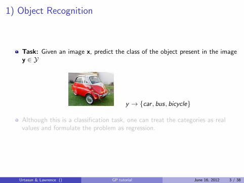
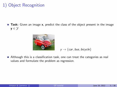
Task: Given an image x, predict the class of the object present in the imagey ∈ Y
y → {car , bus, bicycle}
Although this is a classification task, one can treat the categories as realvalues and formulate the problem as regression.
Urtasun & Lawrence () GP tutorial June 16, 2012 3 / 38

How do we do Object Recognition?
Given this two images, we will like to say if they are of the same class.
Choose a representation for the imagesI Global descriptor of the full imageI Local features: SIFT, SURF, etc.
We need to choose a way to compute similaritiesI Histograms of local features (i.e., bags of words), pyramids, etc.I Kernels on global descriptors, e.g., RBFI · · ·
Urtasun & Lawrence () GP tutorial June 16, 2012 4 / 38

Multiple Kernel Learning (MKL)
Why do we need to choose a single representation and a single similarityfunction?
Which one is the best among all possible ones?
Multiple kernel learning comes at our rescue, by learning which cues andsimilarities are more important for the prediction task.
Simplest form:
K =∑i
αiKi
This is just hyperparameter learning in GPs! No need for specialized SW!
Urtasun & Lawrence () GP tutorial June 16, 2012 5 / 38

Efficient Learning Using GPs for Multiclass Problems
Supposed we want to emulate a 1-vs-all strategy as |Y| > 2
We define y ∈ {−1, 1}|Y|
We can employ maximum likelihood and learn all the parameters for allclassifiers at once
minθ,α>0
−∑i
log p(y(i)|X,θ,α) + γ1||α||1 + γ2||α||2
with y(i) ∈ {−1, 1} each of the individual problems.
Efficient as we can share the covariance across all classes
Urtasun & Lawrence () GP tutorial June 16, 2012 6 / 38

Caltech 101 dataset
Urtasun & Lawrence () GP tutorial June 16, 2012 7 / 38

Results: Caltech 101
[A. Kapoor, K. Graumann, R. Urtasun and T. Darrell, IJCV 2009]
Comparison with SVM kernel combination: kernels based on Geometric Blur(with and without distortion), dense PMK and spatial PMK on SIFT, etc.
0 2 4 6 8 10 12 14 1630
40
50
60
70
80
90
Number of labeled images per class
Rec
ogni
tion
accu
racy
Statistical Efficiency (Caltech−101, 15 Examples per Class)
GP (6 kernels)Varma & Ray (6 kernels)
Figure: Average precision.
0 5 10 150
1000
2000
3000
4000
5000
6000
Number of labeled images per class
Tim
e in
sec
onds
Computational Efficiency (Caltech−101, 15 Examples per Class)
GP (6 kernels)Varma & Ray (6 kernels)
Figure: Time of computation.
Urtasun & Lawrence () GP tutorial June 16, 2012 8 / 38

Results: Caltech 101
[A. Kapoor, K. Graumann, R. Urtasun and T. Darrell, IJCV 2009]
0 5 10 15 20 25 300
10
20
30
40
50
60
70
80
90
number of training examples per class
mea
n re
cogn
ition
rat
e pe
r cl
ass
Caltech 101 Categories Data Set
GP−MultiBoiman et al. (CVPR08)Jain, Kulis, & Grauman (CVPR08)Frome, Singer, Sha, & Malik (ICCV07)Zhang, Berg, Maire, & Malik(CVPR06)Lazebnik, Schmid, & Ponce (CVPR06)Berg (thesis)Mutch, & Lowe(CVPR06)Grauman & Darrell(ICCV 2005)Berg, Berg, & Malik(CVPR05)Zhang, Marszalek, Lazebnik, & SchmidWang, Zhang, & Fei−Fei (CVPR06)Holub, Welling, & Perona(ICCV05)Serre, Wolf, & Poggio(CVPR05)Fei−Fei, Fergus, & PeronaSSD baseline
Figure: Comparison with the state of the art as in late 2008.
Urtasun & Lawrence () GP tutorial June 16, 2012 9 / 38

Other forms of MKL
Convex combination of kernels is too simple (not big boost reported), we needmore complex (non-linear) combinations
Localized comb. (the weighting varies locally) (Christioudias et al. 09)
K(v) = K(v)np �K(v)
p
use structure to define K(v)np , e.g., low-rank
Bayesian co-training (Yu et al. 07)
Kc =
∑j
(Kj + σ2j I)−1
−1
Heteroscedastic Bayesian Co-training: model noise with full covariance(Christoudias et al. 09)
Check out Mario Christoudias PhD thesis for more details
Urtasun & Lawrence () GP tutorial June 16, 2012 10 / 38

2) Active Learning: user in the loop
Labeling is typically an expensive process (now less with Mechanical Turk).
Label as little as possible to reach a certain performance level.
In active learning, we ask the human annotators to label not randomly, butwhere the classifier is more uncertain about a label.
Trade-off between exploration and exploitation
Urtasun & Lawrence () GP tutorial June 16, 2012 11 / 38

Active Learning Algorithm
repeatSelect xu to labeled using active learning criteriaAs the user to label xuRe-train classifier with previous labels + new label point
until budget reached
Urtasun & Lawrence () GP tutorial June 16, 2012 12 / 38

Active Learning Criteria
Let XU be the pool of unlabeled data, we could use
SVM-like criteria of distance to the margin
minxu∈YU
|y∗u |
Most uncertain point (i.e., variance)
maxxu∈YU
Σ∗u
Trade off between exploitation and exploration
minxu∈YU
|y∗u |√Σ∗u + σ2
Urtasun & Lawrence () GP tutorial June 16, 2012 13 / 38

Some examples on Caltech 101[A. Kapoor, K. Graumann, R. Urtasun and T. Darrell, ICCV 2007]
0 2 4 6 8 10 1270
75
80
85
90
95
100
Number of Examples Queried
Me
an
Re
co
gn
itio
n R
ate
pe
r C
lass
faces vs rest
GP ActiveGP Random
0 2 4 6 8 10 1260
65
70
75
80
85
90
Number of Examples Queried
Me
an
Re
co
gn
itio
n R
ate
pe
r C
lass
faces easy vs rest
GP ActiveGP Random
0 2 4 6 8 10 1275
80
85
90
95
100
Number of Examples Queried
Me
an
Re
co
gn
itio
n R
ate
pe
r C
lass
leopards vs rest
GP ActiveGP Random
0 2 4 6 8 10 1276
78
80
82
84
86
88
90
92
94
Number of Examples Queried
Me
an
Re
co
gn
itio
n R
ate
pe
r C
lass
motorbikes vs rest
GP ActiveGP Random
0 2 4 6 8 10 1252
53
54
55
56
57
58
59
60
Number of Examples Queried
Me
an
Re
co
gn
itio
n R
ate
pe
r C
lass
ketch vs rest
GP ActiveGP Random
0 2 4 6 8 10 1255
60
65
70
75
80
85
90
95
Number of Examples Queried
Me
an
Re
co
gn
itio
n R
ate
pe
r C
lass
airplanes vs rest
GP ActiveGP Random
0 2 4 6 8 10 1245
46
47
48
49
50
51
52
53
54
Number of Examples QueriedM
ea
n R
eco
gn
itio
n R
ate
pe
r C
lass
bass vs rest
GP ActiveGP Random
0 2 4 6 8 10 1260
65
70
75
80
85
90
95
Number of Examples Queried
Me
an
Re
co
gn
itio
n R
ate
pe
r C
lass
car side vs rest
GP ActiveGP Random
0 2 4 6 8 10 1242
44
46
48
50
52
54
Number of Examples Queried
Me
an
Re
co
gn
itio
n R
ate
pe
r C
lass
ceiling fan vs rest
GP ActiveGP Random
0 2 4 6 8 10 1245
46
47
48
49
50
51
52
53
54
55
Number of Examples Queried
Me
an
Re
co
gn
itio
n R
ate
pe
r C
lass
mandolin vs rest
GP ActiveGP Random
0 2 4 6 8 10 1260
65
70
75
80
85
90
95
Number of Examples Queried
Me
an
Re
co
gn
itio
n R
ate
pe
r C
lass
minaret vs rest
GP ActiveGP Random
0 2 4 6 8 10 1248
50
52
54
56
58
60
Number of Examples Queried
Me
an
Re
co
gn
itio
n R
ate
pe
r C
lass
electric guitar vs rest
GP ActiveGP Random
Urtasun & Lawrence () GP tutorial June 16, 2012 14 / 38

Does it always help?
[A. Kapoor, K. Graumann, R. Urtasun and T. Darrell, ICCV 2007]
Urtasun & Lawrence () GP tutorial June 16, 2012 15 / 38

3) Optimization non-differentiable functions
Supposed you have a function that you want to optimize, but it isnon-differentiable and also computationally expensive to evaluate, you can
Discretize your space and evaluate discretized values in a grid(combinatorial)
Randomly sample your parameters
Utilize ”active learning” style analysis and GPs to query where to look
Urtasun & Lawrence () GP tutorial June 16, 2012 16 / 38

GPs as an optimization tool[N. Srinivas, A. Krause, S. Kakade and M. Seeger, ICML 2010]
Suppose we want to compute max f (x), we can simply
repeatChoose xt = arg maxx∈D µt−1(x) +
√βtσt−1(x)
Evaluate yt = f (xt) + εtEvaluate µt and σt
until budget reached
−2 −1 1 2
−3
−2
−1
1
2
3
Urtasun & Lawrence () GP tutorial June 16, 2012 17 / 38

GPs as an optimization tool in vision
[A. Vezhnevets, V. Ferrari and J. Buhmann, CVPR 2012]
Image segmentation in the weakly supervised setting, where the only labelsare which classes are present in the scene.
y ∈ {sky , building , tree}
Train based on expected agreement, if I partition the dataset on two setsand I train on the first, it should predict the same as if I train on the second.
This function is sum of indicator functions and thus non-differentiable.
Urtasun & Lawrence () GP tutorial June 16, 2012 18 / 38

Examples of Good Segmentations and Results[A. Vezhnevets, V. Ferrari and J. Buhmann, CVPR 2012]
[Tighe 10] [Vezhnevets 11] GMIM
supervision fulll weak weakaverage accuracy 29 14 21
Urtasun & Lawrence () GP tutorial June 16, 2012 19 / 38

4) Discriminative Approaches to Human Pose Estimation
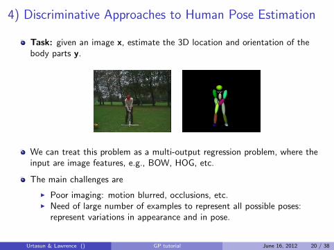
Task: given an image x, estimate the 3D location and orientation of thebody parts y.
We can treat this problem as a multi-output regression problem, where theinput are image features, e.g., BOW, HOG, etc.
The main challenges are
I Poor imaging: motion blurred, occlusions, etc.I Need of large number of examples to represent all possible poses:
represent variations in appearance and in pose.
Urtasun & Lawrence () GP tutorial June 16, 2012 20 / 38
4) Discriminative Approaches to Human Pose Estimation
Task: given an image x, estimate the 3D location and orientation of thebody parts y.
We can treat this problem as a multi-output regression problem, where theinput are image features, e.g., BOW, HOG, etc.
The main challenges are
I Poor imaging: motion blurred, occlusions, etc.I Need of large number of examples to represent all possible poses:
represent variations in appearance and in pose.
Urtasun & Lawrence () GP tutorial June 16, 2012 20 / 38

Challenges for GPs
GP have complexity O(n3), with n the number of examples, and cannot dealwith large datasets in their standard form.
This problem cannot be solved directly as a regression task, since themapping is multimodal: an image observation can represent more than onepose.
Urtasun & Lawrence () GP tutorial June 16, 2012 21 / 38

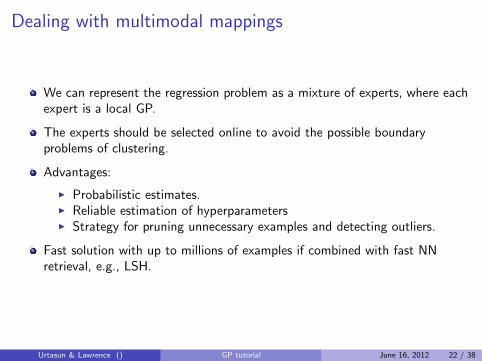
Dealing with multimodal mappings
We can represent the regression problem as a mixture of experts, where eachexpert is a local GP.
The experts should be selected online to avoid the possible boundaryproblems of clustering.
Advantages:
I Probabilistic estimates.I Reliable estimation of hyperparametersI Strategy for pruning unnecessary examples and detecting outliers.
Fast solution with up to millions of examples if combined with fast NNretrieval, e.g., LSH.
Urtasun & Lawrence () GP tutorial June 16, 2012 22 / 38

Online Algorithm
ONLINE: Inference of test point x∗T : number of experts, S : size of each expert
Find NN in x of x∗Find Modes in y of the NN retrievedfor i = 1 . . .T do
Create a local GP for each mode iRetrieve hyper-parametersCompute mean µ and variance σ
end forp(f∗|y) ≈
∑Ti=1 πiN (µi , σ
2i )
Urtasun & Lawrence () GP tutorial June 16, 2012 23 / 38

Online vs Clustering
−8 −6 −4 −2 0 2 4 6 8−3
−2.5
−2
−1.5
−1
−0.5
0
0.5
1
1.5
2
Full GP
−8 −6 −4 −2 0 2 4 6 8−3
−2.5
−2
−1.5
−1
−0.5
0
0.5
1
1.5
2
Local Offline GP
−8 −6 −4 −2 0 2 4 6 8−3
−2.5
−2
−1.5
−1
−0.5
0
0.5
1
1.5
2
Local online GP
3 3.5 4 4.5 5 5.5 6 6.5 7 7.5−1.8
−1.6
−1.4
−1.2
−1
−0.8
−0.6
−0.4
Full GP
3 3.5 4 4.5 5 5.5 6 6.5 7 7.5−1.8
−1.6
−1.4
−1.2
−1
−0.8
−0.6
−0.4
Local Offline GP
3 3.5 4 4.5 5 5.5 6 6.5 7 7.5−1.8
−1.6
−1.4
−1.2
−1
−0.8
−0.6
−0.4
Local online GP
Urtasun & Lawrence () GP tutorial June 16, 2012 24 / 38

Single GP vs Mixture of Online GPs
−8 −6 −4 −2 0 2 4 6 8−10
−5
0
5
10
15
20
25
Global GP
−8 −6 −4 −2 0 2 4 6 8−10
−5
0
5
10
15
20
25
Local Online GP
Urtasun & Lawrence () GP tutorial June 16, 2012 25 / 38

Results: Humaneva[R. Urtasun and T. Darrell, CVPR 2008]
walk jog box mono. discrim. dyn.Lee et al. I 3.4 – – yes no noLee et al. II 3.1 – – yes no yes
Pope 4.53 4.38 9.43 yes yes noMuendermann et al. 5.31 – 4.54 no no yes
Li et al. – – 20.0 yes no yesBrubaker et al. 10.4 – – yes no yesOur approach 3.27 3.12 3.85 yes yes no
Table: Comparison with state of the art (error in cm).
Caviat: Oracle has to select the optimal mixture component
Urtasun & Lawrence () GP tutorial June 16, 2012 26 / 38
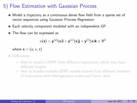
5) Flow Estimation with Gaussian Process
Model a trajectory as a continuous dense flow field from a sparse set ofvector sequences using Gaussian Process Regression
Each velocity component modeled with an independent GP
The flow can be expressed as
φ(x) = y(u)(x)i + y(v)(x)j + y(t)(x)k ∈ <3
where x = (u, v , t)
Difficulties:
I How to model a GPRF from different trajectories, which may havedifferent lengths
I How to handle multiple GPRF models trained from different numbersof trajectories with heterogeneous scales and frame rates
Solution: normalize the length of the tracks before modeling with a GP, aswell as the number of samples
Classification based on the likelihood for each class
Urtasun & Lawrence () GP tutorial June 16, 2012 27 / 38

Flow Classification and Anomaly Detection[K. Kim, D. Lee and I. Essa, ICCV 2011]
Urtasun & Lawrence () GP tutorial June 16, 2012 28 / 38

Detecting Regions of Interest
Detect the regions of interests in moving camera views of dynamic sceneswith multiple moving objects
Important for cheap streaming of events on the internet, e.g., NBA playoffson TNT
Extract a global motion tendency that reflects the scene context by trackingmovements of objects in the scene
Use GPs to represent the extracted motion tendency as a stochastic vectorfield.
Use the stochastic field for predicting important future regions of interest asthe scene evolves dynamically
Urtasun & Lawrence () GP tutorial June 16, 2012 29 / 38

Flow Classification and Anomaly Detection
[K. Kim, D. Lee and I. Essa, CVPR 2012]
Urtasun & Lawrence () GP tutorial June 16, 2012 30 / 38

6) Shape from Shading
3D shapes were obtained using a motion capture system and taking small5× 5 patches from the reconstructed shapes
Corresponding intensities were obtained using a Computer Graphics softwareand the calibrated lighting environment
To reduce the dimensionality, performed PCA on the 3D patch shapes andon the patch intensities separately.
Local intensities and shapes are then represented as
I = I0 +
NI∑i=1
xi Ii , D = D0 +
ND∑i=1
yiDi
Urtasun & Lawrence () GP tutorial June 16, 2012 31 / 38

Gaussian Process Mapping
We want to learn a mapping from intensity to 3D patch shape
This is equivalent to learn a mapping from x to y
Use GPs to learn this mapping
Illumination modeled as weighted sum of spherical harmonics
Illumination parameters estimated using a light probe
Urtasun & Lawrence () GP tutorial June 16, 2012 32 / 38

Handling MultimodalityUnfortunately, this mapping is multimodal (i.e., similar intensities maycorrespond to different 3D shapes)
These ambiguities are strongly related to the first two shape component,which define out-of-plane rotation
Use local GPs (Urtasun et al., 08) to handle multiple modes
Utilize an MRF to patch the local patches.
Urtasun & Lawrence () GP tutorial June 16, 2012 33 / 38
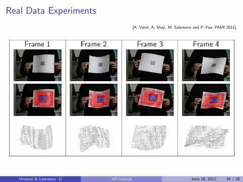
Real Data Experiments
[A. Varol, A. Shaji, M. Salzmann and P. Fua, PAMI 2011]
Urtasun & Lawrence () GP tutorial June 16, 2012 34 / 38

7) 3D Shape Recovery for Online Shopping
Interactive system for quickly modelling 3D body shapes from a single image
Obtain their 3D body shapes so as to try on virtual garments online
Interface for users to conveniently extract anthropometric measurementsfrom a single photo, while using readily available scene cues for automaticimage rectification
GPs to predict the body parameters from input measurements whilecorrecting the aspect ratio ambiguity resulting from photo rectification
Urtasun & Lawrence () GP tutorial June 16, 2012 35 / 38

Creating the 3D Shape from Single Images
Manually annotate a set of five 2D measurements
Well-defined by the anthropometric positions, easy to discern andunambiguous to users.
Good correlations with the corresponding tape measurements and conveyenough information for estimating the 3D body shape
User’s effort for annotation should be minimised
Urtasun & Lawrence () GP tutorial June 16, 2012 36 / 38

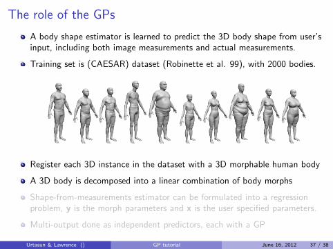
The role of the GPs
A body shape estimator is learned to predict the 3D body shape from user’sinput, including both image measurements and actual measurements.
Training set is (CAESAR) dataset (Robinette et al. 99), with 2000 bodies.
Register each 3D instance in the dataset with a 3D morphable human body
A 3D body is decomposed into a linear combination of body morphs
Shape-from-measurements estimator can be formulated into a regressionproblem, y is the morph parameters and x is the user specified parameters.
Multi-output done as independent predictors, each with a GP
Urtasun & Lawrence () GP tutorial June 16, 2012 37 / 38

Online Shopping
[Y. Chen and D. Robertson and R. Cipolla, BMVC 2011]
Chest Waist Hips Inner leg lengthError(cm) 1.52 ± 1.36 1.88 ± 1.06 3.10 ± 1.86 0.79 ± 0.90
Urtasun & Lawrence () GP tutorial June 16, 2012 38 / 38