Embed Size (px)
Citation preview

Copyright c©2011Edward Ashford Lee & Pravin Varaiya
All rights reserved
Second Edition, Version 2.04
ISBN 978-0-578-07719-2
Please cite this book as:
E. A. Lee and P. Varaiya,Structure and Interpretation of Signals and Systems,
Second Edition, LeeVaraiya.org, 2011.
First Edition was printed by:
Addison-Wesley, ISBN 0-201-74551-8, 2003, Pearson Education, Inc.

Contents
Preface ix
1 Signals and Systems 1
1.1 Signals . . . . . . . . . . . . . . . . . . . . . . . . . . . . . . . . . . . . 2
1.2 Systems . . . . . . . . . . . . . . . . . . . . . . . . . . . . . . . . . . . 27
1.3 Summary . . . . . . . . . . . . . . . . . . . . . . . . . . . . . . . . . . 42
Exercises . . . . . . . . . . . . . . . . . . . . . . . . . . . . . . . . . . . . . 45
2 Defining Signals and Systems 49
2.1 Defining functions . . . . . . . . . . . . . . . . . . . . . . . . . . . . . 50
2.2 Defining signals . . . . . . . . . . . . . . . . . . . . . . . . . . . . . . . 66
2.3 Defining systems . . . . . . . . . . . . . . . . . . . . . . . . . . . . . . 68
2.4 Summary . . . . . . . . . . . . . . . . . . . . . . . . . . . . . . . . . . 82
Exercises . . . . . . . . . . . . . . . . . . . . . . . . . . . . . . . . . . . . . 84
3 State Machines 933.1 Structure of state machines . . . . . . . . . . . . . . . . . . . . . . . . . 943.2 Finite state machines . . . . . . . . . . . . . . . . . . . . . . . . . . . . 983.3 Nondeterministic state machines . . . . . . . . . . . . . . . . . . . . . . 107
iii

3.4 Simulation relations . . . . . . . . . . . . . . . . . . . . . . . . . . . . . 1123.5 Summary . . . . . . . . . . . . . . . . . . . . . . . . . . . . . . . . . . 121
Exercises . . . . . . . . . . . . . . . . . . . . . . . . . . . . . . . . . . . . . 129
4 Composing State Machines 137
4.1 Synchrony . . . . . . . . . . . . . . . . . . . . . . . . . . . . . . . . . . 138
4.2 Side-by-side composition . . . . . . . . . . . . . . . . . . . . . . . . . . 139
4.3 Cascade composition . . . . . . . . . . . . . . . . . . . . . . . . . . . . 143
4.4 Product-form inputs and outputs . . . . . . . . . . . . . . . . . . . . . . 148
4.5 General feedforward composition . . . . . . . . . . . . . . . . . . . . . 151
4.6 Hierarchical composition . . . . . . . . . . . . . . . . . . . . . . . . . . 154
4.7 Feedback . . . . . . . . . . . . . . . . . . . . . . . . . . . . . . . . . . 1554.8 Summary . . . . . . . . . . . . . . . . . . . . . . . . . . . . . . . . . . 177
Exercises . . . . . . . . . . . . . . . . . . . . . . . . . . . . . . . . . . . . . 179
5 Linear Systems 187
5.1 Operation of an infinite state machine . . . . . . . . . . . . . . . . . . . 189
5.2 Linear functions . . . . . . . . . . . . . . . . . . . . . . . . . . . . . . . 192
5.3 The [A,B,C,D] representation of a system . . . . . . . . . . . . . . . . . 195
5.4 Continuous-time state-space models . . . . . . . . . . . . . . . . . . . . 218
5.5 Summary . . . . . . . . . . . . . . . . . . . . . . . . . . . . . . . . . . 219
Exercises . . . . . . . . . . . . . . . . . . . . . . . . . . . . . . . . . . . . . 227
6 Hybrid Systems 231
6.1 Mixed models . . . . . . . . . . . . . . . . . . . . . . . . . . . . . . . . 2336.2 Modal models . . . . . . . . . . . . . . . . . . . . . . . . . . . . . . . . 2356.3 Timed automata . . . . . . . . . . . . . . . . . . . . . . . . . . . . . . . 2406.4 More interesting dynamics . . . . . . . . . . . . . . . . . . . . . . . . . 250
6.5 Supervisory control . . . . . . . . . . . . . . . . . . . . . . . . . . . . . 260
6.6 Formal model . . . . . . . . . . . . . . . . . . . . . . . . . . . . . . . . 266
iv Lee & Varaiya, Signals and Systems

6.7 Summary . . . . . . . . . . . . . . . . . . . . . . . . . . . . . . . . . . 268
Exercises . . . . . . . . . . . . . . . . . . . . . . . . . . . . . . . . . . . . . 269
7 Frequency Domain 275
7.1 Frequency decomposition . . . . . . . . . . . . . . . . . . . . . . . . . . 277
7.2 Phase . . . . . . . . . . . . . . . . . . . . . . . . . . . . . . . . . . . . 2837.3 Spatial frequency . . . . . . . . . . . . . . . . . . . . . . . . . . . . . . 284
7.4 Periodic and finite signals . . . . . . . . . . . . . . . . . . . . . . . . . . 285
7.5 Fourier series . . . . . . . . . . . . . . . . . . . . . . . . . . . . . . . . 2897.6 Discrete-time signals . . . . . . . . . . . . . . . . . . . . . . . . . . . . 300
7.7 Summary . . . . . . . . . . . . . . . . . . . . . . . . . . . . . . . . . . 303
Exercises . . . . . . . . . . . . . . . . . . . . . . . . . . . . . . . . . . . . . 304
8 Frequency Response 311
8.1 LTI systems . . . . . . . . . . . . . . . . . . . . . . . . . . . . . . . . . 313
8.2 Finding and using the frequency response . . . . . . . . . . . . . . . . . 325
8.3 Determining the Fourier series coefficients . . . . . . . . . . . . . . . . . 339
8.4 Frequency response and the Fourier series . . . . . . . . . . . . . . . . . 340
8.5 Frequency response of composite systems . . . . . . . . . . . . . . . . . 342
8.6 Summary . . . . . . . . . . . . . . . . . . . . . . . . . . . . . . . . . . 346
Exercises . . . . . . . . . . . . . . . . . . . . . . . . . . . . . . . . . . . . . 355
9 Filtering 363
9.1 Convolution . . . . . . . . . . . . . . . . . . . . . . . . . . . . . . . . . 3659.2 Frequency response and impulse response . . . . . . . . . . . . . . . . . 378
9.3 Causality . . . . . . . . . . . . . . . . . . . . . . . . . . . . . . . . . . 382
9.4 Finite impulse response (FIR) filters . . . . . . . . . . . . . . . . . . . . 382
9.5 Infinite impulse response (IIR) filters . . . . . . . . . . . . . . . . . . . . 395
9.6 Implementation of filters . . . . . . . . . . . . . . . . . . . . . . . . . . 398
9.7 Summary . . . . . . . . . . . . . . . . . . . . . . . . . . . . . . . . . . 403
Lee & Varaiya, Signals and Systems v

Exercises . . . . . . . . . . . . . . . . . . . . . . . . . . . . . . . . . . . . . 406
10 The Four Fourier Transforms 41310.1 Notation . . . . . . . . . . . . . . . . . . . . . . . . . . . . . . . . . . . 41410.2 The Fourier series (FS) . . . . . . . . . . . . . . . . . . . . . . . . . . . 415
10.3 The discrete Fourier transform (DFT) . . . . . . . . . . . . . . . . . . . 421
10.4 The discrete-Time Fourier transform (DTFT) . . . . . . . . . . . . . . . 424
10.5 The continuous-time Fourier transform . . . . . . . . . . . . . . . . . . . 42810.6 Fourier transforms vs. Fourier series . . . . . . . . . . . . . . . . . . . . 43410.7 Properties of Fourier transforms . . . . . . . . . . . . . . . . . . . . . . 444
10.8 Summary . . . . . . . . . . . . . . . . . . . . . . . . . . . . . . . . . . 458
Exercises . . . . . . . . . . . . . . . . . . . . . . . . . . . . . . . . . . . . . 460
11 Sampling and Reconstruction 473
11.1 Sampling . . . . . . . . . . . . . . . . . . . . . . . . . . . . . . . . . . 474
11.2 Reconstruction . . . . . . . . . . . . . . . . . . . . . . . . . . . . . . . 48211.3 The Nyquist-Shannon sampling theorem . . . . . . . . . . . . . . . . . . 488
11.4 Summary . . . . . . . . . . . . . . . . . . . . . . . . . . . . . . . . . . 494
Exercises . . . . . . . . . . . . . . . . . . . . . . . . . . . . . . . . . . . . . 495
12 Stability 499
12.1 Boundedness and stability . . . . . . . . . . . . . . . . . . . . . . . . . 503
12.2 The Z transform . . . . . . . . . . . . . . . . . . . . . . . . . . . . . . . 50912.3 The Laplace transform . . . . . . . . . . . . . . . . . . . . . . . . . . . 521
12.4 Summary . . . . . . . . . . . . . . . . . . . . . . . . . . . . . . . . . . 530
Exercises . . . . . . . . . . . . . . . . . . . . . . . . . . . . . . . . . . . . . 532
13 Laplace and Z Transforms 537
13.1 Properties of the Z tranform . . . . . . . . . . . . . . . . . . . . . . . . 538
13.2 Frequency response and pole-zero plots . . . . . . . . . . . . . . . . . . 550
13.3 Properties of the Laplace transform . . . . . . . . . . . . . . . . . . . . . 552
vi Lee & Varaiya, Signals and Systems
13.4 Frequency response and pole-zero plots . . . . . . . . . . . . . . . . . . 557
13.5 The inverse transforms . . . . . . . . . . . . . . . . . . . . . . . . . . . 55913.6 Steady state response . . . . . . . . . . . . . . . . . . . . . . . . . . . . 570
13.7 Linear difference and differential equations . . . . . . . . . . . . . . . . 573
13.8 State-space models . . . . . . . . . . . . . . . . . . . . . . . . . . . . . 584
13.9 Summary . . . . . . . . . . . . . . . . . . . . . . . . . . . . . . . . . . 596
Exercises . . . . . . . . . . . . . . . . . . . . . . . . . . . . . . . . . . . . . 603
14 Composition and Feedback Control 611
14.1 Cascade composition . . . . . . . . . . . . . . . . . . . . . . . . . . . . 613
14.2 Parallel composition . . . . . . . . . . . . . . . . . . . . . . . . . . . . 620
14.3 Feedback composition . . . . . . . . . . . . . . . . . . . . . . . . . . . 626
14.4 PID controllers . . . . . . . . . . . . . . . . . . . . . . . . . . . . . . . 63914.5 Summary . . . . . . . . . . . . . . . . . . . . . . . . . . . . . . . . . . 647
Exercises . . . . . . . . . . . . . . . . . . . . . . . . . . . . . . . . . . . . . 648
A Sets and Functions 655A.1 Sets . . . . . . . . . . . . . . . . . . . . . . . . . . . . . . . . . . . . . 656A.2 Functions . . . . . . . . . . . . . . . . . . . . . . . . . . . . . . . . . . 677A.3 Summary . . . . . . . . . . . . . . . . . . . . . . . . . . . . . . . . . . 680
Exercises . . . . . . . . . . . . . . . . . . . . . . . . . . . . . . . . . . . . . 684
B Complex Numbers 689
B.1 Imaginary numbers . . . . . . . . . . . . . . . . . . . . . . . . . . . . . 690
B.2 Arithmetic of imaginary numbers . . . . . . . . . . . . . . . . . . . . . . 691
B.3 Complex numbers . . . . . . . . . . . . . . . . . . . . . . . . . . . . . . 692
B.4 Arithmetic of complex numbers . . . . . . . . . . . . . . . . . . . . . . 693
B.5 Exponentials . . . . . . . . . . . . . . . . . . . . . . . . . . . . . . . . 694
B.6 Polar coordinates . . . . . . . . . . . . . . . . . . . . . . . . . . . . . . 696Exercises . . . . . . . . . . . . . . . . . . . . . . . . . . . . . . . . . . . . . 701
Lee & Varaiya, Signals and Systems vii

Bibliography 703
Notation Index 704
Index 708
viii Lee & Varaiya, Signals and Systems

Preface
Signals convey information. Systems transform signals. This book introduces the mathe-matical models used to design and understand both. It is intended for students interestedin developing a deep understanding of how to digitally create and manipulate signals tomeasure and control the physical world and to enhance human experience and communi-cation.
The discipline known as “signals and systems” is rooted in the intellectual tradition ofelectrical engineering (EE). This tradition, however, has evolved in unexpected ways.EE has lost its tight coupling with the “electrical.” So although many of the techniquesintroduced in this book were first developed to analyze circuits, today they are widelyapplied in information processing, system biology, mechanical engineering, finance, andmany other disciplines.
This book approaches signals and systems from a computational point of view. A moretraditional introduction to signals and systems would be biased towards the historic ap-plication, analysis and design of circuits. It would focus almost exclusively on lineartime-invariant systems, and would develop continuous-time models first, with discrete-time models then treated as an advanced topic.
The approach in this book benefits students by showing from the start that the methods ofsignals and systems are applicable to software systems, and most interestingly, to systems
ix

Preface
that mix computers with physical devices and processes, including mechanical controlsystems, biological systems, chemical processes, transportation systems, and financialsystems. Such systems have become pervasive, and profoundly affect our daily lives.
The shift away from circuits implies some changes in the way the methodology of signalsand systems is presented. While it is still true that a voltage that varies over time isa signal, so is a packet sequence on a network. This text defines signals to cover both.While it is still true that an RLC circuit is a system, so is a computer program for decodingInternet audio. This text defines systems to cover both. While for some systems the stateis still captured adequately by variables in a differential equation, for many it is now thevalues in registers and memory of a computer. This text defines state to cover both.
The fundamental limits also change. Although we still face thermal noise and the speedof light, we are likely to encounter other limits–such as complexity, computability, chaos,and, most commonly, limits imposed by other human constructions–before we get tothese. The limitations imposed, for example, when transporting voice signals over the In-ternet, are not primarily physical limitations. They are instead limitations arising from thedesign and implementation of the Internet, and from the fact that transporting voice wasnever one of the original intentions of the design. Similarly, computer-based audio sys-tems face latency and jitter imposed by an operating system designed to time share scarcecomputing resources among data processing tasks. This text focuses on composition ofsystems so that the limits imposed by one system on another can be understood.
The mathematical basis for the discipline also changes with this new emphasis. Themathematical foundations of circuit analysis are calculus and differential equations. Al-though we still use calculus and differential equations, we frequently need discrete math,set theory, and mathematical logic. Whereas the mathematics of calculus and differentialequations evolved to describe the physical world, the world we face as system designersoften has nonphysical properties that are not such a good match for this mathematics.This text bases the entire study on a highly adaptable formalism rooted in elementary settheory.
Despite these fundamental changes in the medium with which we operate, the methodol-ogy of signals and systems remains robust and powerful. It is the methodology, not themedium, that defines the field.
The book is based on a course at Berkeley required of all majors in Electrical Engineer-ing and Computer Sciences (EECS). The experience developing the course is reflected incertain distinguished features of this book. First, no background in electrical engineer-
x Lee & Varaiya, Signals and Systems

Preface
ing or computer science is assumed. Readers should have some exposure to calculus,elementary set theory, series, first order linear differential equations, trigonometry, andelementary complex numbers. The appendices review set theory and complex numbers,so this background can be made up students.
Approach
This book is about mathematical modeling and analysis of signals and systems, appli-cations of these methods, and the connection between mathematical models and compu-tational realizations. We develop three themes. The first theme is the use of sets andfunctions as a universal language to describe diverse signals and systems. Signals—voice, images, bit sequences—are represented as functions with an appropriate domainand range. Systems are represented as functions whose domain and range are themselvessets of signals. Thus, for example, an Internet voice signal is represented as a functionthat maps voice-like signals into sequences of packets.
The second theme is that complex systems are constructed by connecting simpler sub-systems in standard ways—cascade, parallel, feedback. The connections determine thebehavior of the interconnected system from the behaviors of component subsystems. Theconnections place consistency requirements on the input and output signals of the systemsbeing connected.
Our third theme is to relate the declarative view (mathematical, “what is”) with the imper-ative view (procedural, “how to”). That is, we associate mathematical analysis of systemswith realizations of these systems. This is the heart of engineering. When electrical en-gineering was entirely about circuits, this was relatively easy, because it was the physicsof the circuits that was being described by the mathematics. Today we have to some-how associate the mathematical analysis with very different realizations of the systems,most especially software. We do this association through the study of state machines, andthrough the consideration of many real-world signals, which, unlike their mathematicalabstractions, have little discernable declarative structure. Speech signals, for instance, arefar more interesting than sinusoids, and yet many signals and systems textbooks talk onlyabout sinusoids.
Lee & Varaiya, Signals and Systems xi

Preface
Content
We begin in Chapter 1 by describing signals as functions, focusing on characterizing thedomain and the range for familiar signals that humans perceive, such as sound, images,video, trajectories of vehicles, as well as signals typically used by machines to store ormanipulate information, such as sequences of words or bits.
Systems, also introduced in Chapter 1, are described as functions, but now the domain andthe range are themselves sets of signals. Systems can be connected to form a more com-plex system, and the function describing these more complex systems is a composition offunctions describing the component systems.
Chapter 2 focuses on how to define the functions that we use to model both signals andsystems. It distinguishes declarative definitions (assertions of what a signal or system is)from imperative ones (descriptions of how a signal is produced or processed by a system).
The imperative approach is further developed in Chapter 3 using the notion of state, thestate transition function, and the output function, all in the context of finite state machines.In Chapter 4, state machines are composed in various ways (cascade, parallel, and feed-back) to make more interesting systems. Applications to feedback control illustrate thepower of the state machine model.
In Chapter 5, time-based systems are studied, first with discrete-time systems (which havesimpler mathematics), and then with continuous-time systems. We introduce the notionof a state machine and define linear time-invariant (LTI) systems as state machines withlinear state transition and output functions and zero initial state. The input-output behaviorof these systems is fully characterized by their impulse response.
Chapter 7 introduces frequency decomposition of signals, Chapter 8 introduces frequencyresponse of LTI systems, and Chapter 9 brings the two together by discussing filtering.The approach is to present frequency domain concepts as a complementary toolset, differ-ent from that of state machines, and much more powerful when applicable. Frequency de-composition of signals is motivated first using psychoacoustics, and gradually developeduntil all four Fourier transforms (the Fourier series, the Fourier transform, the discrete-time Fourier transform, and the discrete Fourier transform) have been described. Welinger on the first of these, the Fourier series, since it is conceptually the easiest, and thenmore quickly present the others as generalizations of the Fourier series. LTI systems yieldbest to frequency-domain analysis because of the property that complex exponentials areeigenfunctions (the output is a scaled version of the input). Consequently, they are fully
xii Lee & Varaiya, Signals and Systems

Preface
characterized by their frequency response—the main reason that frequency domain meth-ods are important in the analysis of filters and feedback control.
Chapter 10 covers classical Fourier transform material such as properties of the fourFourier transforms and transforms of basic signals. Chapter 11 applies frequency domainmethods to a study of sampling and aliasing.
Chapters 12, 13 and 14 extend frequency domain techniques to include the Z transformand the Laplace transform. Applications in signal processing and feedback control illus-trate the concepts and the utility of the techniques. Mathematically, the Z transform andthe Laplace transform are introduced as extensions of the discrete-time and continuous-time Fourier transforms to signals on which Fourier transforms do not work, specificallysignals that are not absolutely summable or integrable. Practically, the concern is forsystems that are not stable and for systems that consume unbounded amounts of energy.These chapters extend the intuition of previous chapters to cover such systems.
The unified modeling approach in this text is rich enough to describe a wide range ofsignals and systems, including those based on discrete events and those based on sig-nals in time, both continuous and discrete. The complementary tools of state machinesand frequency domain methods permit analysis and implementation of concrete signalsand systems. Hybrid systems and modal models offer systematic ways to combine thesecomplementary toolsets. The framework and the tools of this text provide a foundationon which to build later courses on digital systems, embedded systems, communications,signal processing, hybrid systems, and control.
Pedagogical features
This book has a number of highlights that make it well suited as a textbook for an intro-ductory course.
1. “Probing Further” sidebars briefly introduce the reader to interesting extensions ofthe subject, to applications, and to more advanced material. They serve to indicatedirections in which the subject can be explored.
2. “Basics” sidebars offer readers with less mathematical background some basic toolsand methods.
Lee & Varaiya, Signals and Systems xiii

Preface
3. Appendix A reviews basic set theory and helps establish the notation used through-out the book.
4. Appendix B reviews complex variables, making it unnecessary for students to havemuch background in this area.
5. Key equations are boxed to emphasize their importance. They can serve as theplaces to pause in a quick reading. In the index, the page numbers where key termsare defined are shown in bold.
6. The exercises at the end of each chapter are annotated with the letters E, T , orC to distinguish those exercises that are mechanical (E for excercise) from thoserequiring a plan of attack (T for thought) and those that generally have more thanone reasonable answer (C for conceptualization).
Notation
The notation in this text is unusual when compared to standard texts on signals and sys-tems. We explain our reasons for this as follows:
Domains and ranges. It is common in signals and systems texts to use the form of theargument of a function to define its domain. For example, x(n) is a discrete-time signal,while x(t) is a continuous-time signal; X( jω) is the continuous-time Fourier transformand X(e jω) is the discrete-time Fourier transform. This leads to apparent nonsense likex(n) = x(nT ) to define sampling, or to confusion like X( jω) 6= X(e jω) even when jω =e jω.
We treat the domain of a function as part of its definition. Thus a discrete-time, real-valued signal is a function x : Z→ R, which maps integers to real numbers. Its discrete-time Fourier transform (DTFT) is a function X : R→ C, which maps real numbers intocomplex numbers. The DTFT is found using a function whose domain and range are setsof functions,
DTFT : [Z→ R]→ [R→ C].
This function maps functions of the form x : Z→R into functions of the form X : R→C.The notation [Z→ R] means the set of all functions mapping integers into real numbers.Then we can unambiguously write X = DTFT(x).
xiv Lee & Varaiya, Signals and Systems

Preface
Functions as values. Most texts call the expression x(t) a function. A better interpretationis that x(t) is an element in the range of the function x. The difficulty with the formerinterpretation becomes obvious when talking about systems. Many texts pay lip serviceto the notion that a system is a function by introducing a notation like y(t) = T (x(t)). Thismakes it seem that T acts on the value x(t) rather than on the entire function x.
Our notation includes set of functions, allowing systems to be defined as functions withsuch sets as the domain and range. Continuous-time convolution, for example, becomes
Convolution : [R→ R]× [R→ R]→ [R→ R].
We then introduce the notation ∗ as a shorthand,
y = x∗h = Convolution(x,h),
and define the convolution function by
∀ t ∈ R, y(t) = (x∗h)(t) =∞∫−∞
x(τ)y(t− τ)dτ.
Note the careful parenthesization. The more traditional notation, y(t) = x(t)∗h(t), wouldseem to imply that y(t − T ) = x(t − T ) ∗ h(t − T ). But it is not so! Such notation un-dermines a student’s confidence in algebra, since substitution of a value for t does notwork!
A major advantage of our notation is that it easily extends beyond LTI systems to the sortsof systems that inevitably arise in any real world application, such as mixtures of discreteevent and continuous-time systems.
Names of functions. We use long names for functions and variables when they have aconcrete interpretation. Thus, instead of x we might use Sound. This follows a long-standing tradition in software, where readability is considerably improved by long names.By giving us a much richer set of names to use, this helps us avoid some of the precedingpitfalls. For example, to define sampling of an audio signal, we might write
SampledSound = SamplerT (Sound).
It also helps bridge the gap between realizations of systems (which are often software)and their mathematical models. How to manage and understand this gap is a major themeof our approach.
Lee & Varaiya, Signals and Systems xv
Preface
How to use this book
At Berkeley, the first 11 chapters of this book are covered in a 15-week, one-semestercourse. Even though it leaves Laplace transforms, Z transforms, and feedback controlsystems to a follow-up course, it remains a fairly intense experience. Each week consistsof three 50-minute lectures, a one-hour problem session, and one three-hour laboratory.The lectures and problem sessions are conducted by a faculty member while the laboratoryis led by teaching assistants, who are usually graduate students, but are also often talentedjuniors or seniors.
We have developed laboratory components based on MATLAB and Simulink, and a sep-arate set based on LabVIEW. In both cases, then lab content is closely coordinated withthe lectures. The text does not offer a tutorial on LabVIEW, MATLAB, or Simulink,although the labs include enough material so that, combined with on-line help, they aresufficient. Some examples in the text and some exercises at the ends of the chapters de-pend on MathScript, the mathematical expression language used by both MATLAB andLabVIEW.
At Berkeley, this course is taken by all electrical engineering and computer science stu-dents, and is followed by a more traditional signals and systems course. That coursecovers the material in the last three chapters plus applications of frequency-domain meth-ods to communications systems. The follow-up course is not taken by most computerscience students. In a program that is more purely electrical and computer engineeringthan ours, a better approach might be to spend two quarters or two semesters on the mate-rial in this text, since the unity of notation and approach would be better than having twodisjoint courses, the introductory one using a modern approach, and the follow-up courseusing a traditional one.
Acknowledgements
Many people have contributed to the content of this book. Dave Messerschmitt concep-tualized the first version of the course on which the book is based, and later committedconsiderable departmental resources to the development of the course while he was chairof the EECS department at Berkeley. Randy Katz, Richard Newton, and Shankar Sas-try continued to invest considerable resources in the course when they each took over aschair, and backed our efforts to establish the course as a cornerstone of our undergraduate
xvi Lee & Varaiya, Signals and Systems

Preface
curriculum. This took considerable courage, since the conceptual approach of the coursewas largely unproven.
Tom Henzinger probably had more intellectual influence over the approach than any otherindividual. The view of state machines, of composition of systems, and of hybrid systemsowe a great deal to Tom. Gerard Berry also contributed a great deal to our way of pre-senting synchronous composition.
We were impressed by the approach of Harold Abelson and and Gerald Jay Sussman,in Structure and Interpretation of Computer Programs (MIT Press, 1996), who con-fronted a similar transition in their discipline. The title of our book shows their influ-ence. Jim McLellan, Ron Shafer, and Mark Yoder influenced this book through theirpioneering departure from tradition in signals and systems, DSP First—A MultimediaApproach (Prentice-Hall, 1998). Ken Steiglitz greatly influenced the labs with his inspi-rational book, A DSP Primer: With Applications to Digital Audio and Computer Music(Addison-Wesley, 1996). Babak Ayazifar, with his visionary treatment of the course, hassignificantly influenced more recent versions of the book.
A number of people have been involved in the media applications, examples, the labo-ratory development, and the web content associated with the book. These include BrianEvans and Ferenc Kovac. We also owe gratitude for the superb technical support fromChristopher Brooks. Jie Liu contributed sticky masses example to the hybrid systemschapter, and Yuhong Xiong contributed the technical stock trading example. Other exam-ples and ideas were contributed by Steve Neuendorffer, Cory Sharp, and Tunc Simsek.
Over several years, students at Berkeley have taken the course that provided the impetusfor this book. They used successive versions of the book and the Web content. Theirvaried response to the course helped us define the structure of the book and the level ofdiscussion. The course is taught with the help of undergraduate teaching assistants. Theircomments helped shape the laboratory material.
Parts of this book were reviewed by more than 30 faculty members around the coun-try. Their criticisms helped us correct defects and inconsistencies in earlier versions.Of course, we alone are responsible for the opinions expressed in the book, and the er-rors that remain. We especially thank: Jack Kurzweil, San Jose State University; LeeSwindlehurst, Brigham Young University; Malur K. Sundareshan, University of Arizona;Stephane Lafortune, University of Michigan; Ronald E. Nelson, Arkansas Tech Univer-sity; Ravi Mazumdar, Purdue University; Ratnesh Kumar, University of Kentucky; RahulSingh, San Diego State University; Paul Neudorfer, Seattle University; R. Mark Nelms,
Lee & Varaiya, Signals and Systems xvii

Preface
Auburn University; Chen-Ching Liu, University of Washington; John H. Painter, TexasA&M University; T. Kirubarajan, University of Connecticut; James Harris, CaliforniaPolytechnic State University in San Luis Obispo; Frank B. Gross, Florida A&M Uni-versity; Donald L. Snyder, Washington University in St. Louis; Theodore E. Djaferis,University of Massachusetts in Amherst; Soura Dasgupta, University Iowa; Maurice Fe-lix Aburdene, Bucknell University; and Don H. Johnson, Rice University.
Many of these reviews were solicited by Heather Shelstad of Brooks/Cole, Denise Penroseof Morgan-Kaufmann, and Susan Hartman and Galia Shokry of Addison-Wesley, whohandled the publication of the first edition of this book. We are grateful to these editors fortheir interest and encouragement. To Susan Hartman, Galia Shokry and Nancy Lombardiwe owe a special thanks; their enthusiasm and managerial skills helped us and others keepthe deadlines in bringing the first edition of the book to print. Subsequent editions buildon this.
It took much longer to write this book than we expected when we embarked on thisproject. It has been a worthwhile effort nonetheless. Our friendship has deepened, andour mutual respect has grown as we learned from each other. Rhonda Righter and RuthVaraiya have been remarkably sympathetic and encouraging through the many hours atnights and on weekends that this project has demanded. To them we owe our immensegratitude.
xviii Lee & Varaiya, Signals and Systems

1Signals and Systems
Contents1.1 Signals . . . . . . . . . . . . . . . . . . . . . . . . . . . . . . . . . 2
1.1.1 Audio signals . . . . . . . . . . . . . . . . . . . . . . . . . . 5Probing Further: Household electrical power . . . . . . . . . . . . . 111.1.2 Images . . . . . . . . . . . . . . . . . . . . . . . . . . . . . 12Probing Further: Color and light . . . . . . . . . . . . . . . . . . . . 151.1.3 Video signals . . . . . . . . . . . . . . . . . . . . . . . . . . 161.1.4 Signals representing physical attributes . . . . . . . . . . . . 171.1.5 Sequences . . . . . . . . . . . . . . . . . . . . . . . . . . . . 201.1.6 Discrete signals and sampling . . . . . . . . . . . . . . . . . 22
1.2 Systems . . . . . . . . . . . . . . . . . . . . . . . . . . . . . . . . . 271.2.1 Systems as functions . . . . . . . . . . . . . . . . . . . . . . 281.2.2 Telecommunications systems . . . . . . . . . . . . . . . . . . 29Probing Further: Wireless communication . . . . . . . . . . . . . . . 32Probing Further: LEO telephony . . . . . . . . . . . . . . . . . . . . 331.2.3 Audio storage and retrieval . . . . . . . . . . . . . . . . . . . 361.2.4 Modem negotiation . . . . . . . . . . . . . . . . . . . . . . . 371.2.5 Feedback control systems . . . . . . . . . . . . . . . . . . . 38
1.3 Summary . . . . . . . . . . . . . . . . . . . . . . . . . . . . . . . . 42Probing Further: Modems and Encrypted speech . . . . . . . . . . . 43
Exercises . . . . . . . . . . . . . . . . . . . . . . . . . . . . . . . . . . . 45
1

1.1. SIGNALS
1.1 Signals
Broadly speaking, a signal is a means to convey information. This printed page, forexample, is a signal. So is the sound of someone reading the page aloud. In this text, asystem is a process that generates signals or transforms signals. A person reading thisbook aloud, for example, is a system that converts the printed page signal into a soundsignal. So is an electronic book reader for the blind. This book is about developing adeep enough understanding of signals and systems to be able to understand how such abook reader and many other systems work. We gain this understanding by dissecting thestructure of signals, examining their interpretation, and developing systematic ways toanalyze and synthesize them. Consider a few examples of signals and systems.
Example 1.1: A sound is a signal. A sequence of bits stored in a flash memory isalso a signal. An MP3 player is a system that converts such a sequence of bits intohigh-quality stereo sound. A sequence of commands issued to a computer is alsoa signal. An interactive voice response (IVR) system converts spoken words intocommands to a computer. IVR systems are commonly used today in call centers toefficiently handle high call volumes, for example in customer service centers.
Many mechanical machines produce sound as they operate. As they wear, the soundthat they produce may change. Automated analysis of the sound that they pro-duce can identify problems before the equipment fails. Such early detection isextremely valuable, particularly in safety-critical systems, such as jet engines orpower-generation turbines. This book can help understand how to design systemsfor such automated detection.
Sound signals can also be converted to images. The famous iTunes visualizer is abeautiful example; it generates aesthetically pleasing colorful patterns on a screenthat undulate synchronously with music. An ultrasound imaging system generatessounds with frequencies that are too high for humans to hear, and listens for theirreflections. The sounds are reflected in materials where two distinct materials meet.These reflections can be used to safely construct images of a baby in a womb, forexample, without exposing the baby to potentially harmful radiation.
2 Lee & Varaiya, Signals and Systems

1. SIGNALS AND SYSTEMS
Example 1.2: An image is a signal. A system that analyzes images, recogniz-ing objects, faces, animals, etc., might form the heart of an Internet image searchengine. A system that compares images might be used to enforce copyrights. Infactory automation, it is common to use imaging systems to detect manufacturingdefects. An image enhancement system might be used in a digital camera to, forexample, automatically remove red eye, a bright reflection from the back of theretina that occurs when a camera flash is close to the camera lens.
Example 1.3: A computer program, which is a sequence of commands, is alsoa signal. Malware, short for malicious software, is software that surreptitiouslyperforms undesired functions on your computer. A system that detects malwaretransforms the program signal into a simple yes or no answer. Either the programcontains malware or it does not. Although they are far from perfect, such sys-tems have gotten quite sophisticated, and they can often even detect obfuscatedprograms, programs that have been deliberately altered to attempt to hide their ma-licious intent.
Example 1.4: DNA molecules contain the genetic instructions used in the devel-opment and functioning of almost all known living organisms. A DNA molecule,therefore, is a signal, and a biological system uses the structure of the moleculeto synthesize other molecules. The structure of a DNA molecule can be relativelysimply represented as a sequence of one of four types of nucleotides denoted by theletters A, T, C, and G. A sequence of such letters, therefore, encodes the signal thatthe DNA molecule represents.
Example 1.5: Electromagnetic radiation can function as a signal. A radio broad-cast system, for example, converts sound signals into electromagnetic radiation,which is then picked up by a radio antenna and converted back to sound. A tele-vision broadcast system converts images into sequences of bits, and then converts
Lee & Varaiya, Signals and Systems 3

1.1. SIGNALS
the sequences of bits into radio signals. A TV receiver reverses these conversions.A radar system generates an electromagnetic signal, transmits it, listens for reflec-tions, and then converts the reflections into images. Radar signals are routinelyused in air traffic control systems, for example, and for collision avoidance systemsin high-end cars.
One way to get a deeper understanding of a subject is to formalize it, to develop mathemat-ical models. Such models admit manipulation with a level of confidence not achievablewith less formal models. We know that if we follow the rules of mathematics, then atransformed model still relates strongly to the original model. There is a sense in whichmathematical manipulation preserves “truth” in a way that is elusive with almost any otherintellectual manipulation of a subject. We can leverage this truth-preservation to gain con-fidence in the design of a system, to extract hidden information from a signal, or simplyto gain insight.
Mathematically, we model both signals and systems as functions. A signal is a functionthat maps a domain, often time or space, into a range, often a physical measure such as airpressure or light intensity. A system is a function that maps signals from its domain—itsinput signals—into signals in its range—its output signals. The domain and the range areboth sets of signals; we call a set of signals a signal space. Thus, systems are functionswhose domains and ranges are signal spaces.
We use the mathematical language of sets and functions to make our models unambigu-ous, precise, and manipulable. This language has its own notation and rules, which arereviewed in Appendix A. We begin to use this language in this chapter. Depending on thesituation, we represent physical quantities such as time, voltage, current, light intensity,air pressure, or the content of a memory location by variables that range over appropriatesets. A variable has a name, such as n or Intensity, and a set of values that can be assignedto the variable.
Example 1.6: Time may be represented by a variable n ∈ N, where N representsthe set of natural numbers 1,2,3, · · ·. We read the expression “n∈N” as “n in theset of natural numbers,” and it means that n is a variable that can have any value inN. For example, in Unix time or POSIX time, used by many computer systems tokeep track of the date and time, the value of n represents the number of seconds that
4 Lee & Varaiya, Signals and Systems
1. SIGNALS AND SYSTEMS
have elapsed since midnight on January 1, 1970. The time at which we are writingthis paragraph is n = 1290876962, a natural number.
Time may be represented many other ways. For example, the time of day maybe represented as h : m : s, where h ∈ 0,1, · · · ,23 represents the hour, m ∈0,1, · · · ,59 represents the minute, and s ∈ 0,1, · · · ,59 represents the second.Mathematically, these three numbers form a three-tuple,
(h,m,s) ∈ 0,1, · · · ,23×0,1, · · · ,59×0,1, · · · ,59,
where the × operator forms the Cartesian product of sets.
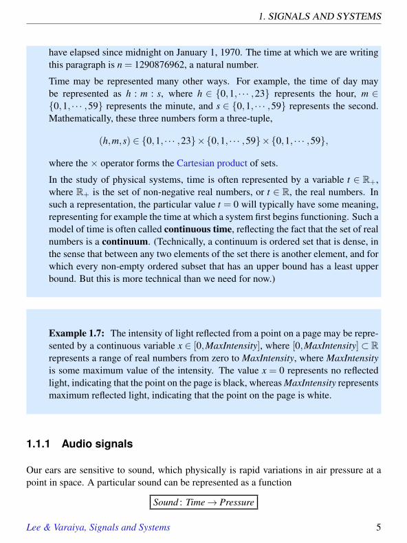
In the study of physical systems, time is often represented by a variable t ∈ R+,where R+ is the set of non-negative real numbers, or t ∈ R, the real numbers. Insuch a representation, the particular value t = 0 will typically have some meaning,representing for example the time at which a system first begins functioning. Such amodel of time is often called continuous time, reflecting the fact that the set of realnumbers is a continuum. (Technically, a continuum is ordered set that is dense, inthe sense that between any two elements of the set there is another element, and forwhich every non-empty ordered subset that has an upper bound has a least upperbound. But this is more technical than we need for now.)
Example 1.7: The intensity of light reflected from a point on a page may be repre-sented by a continuous variable x ∈ [0,MaxIntensity], where [0,MaxIntensity]⊂ Rrepresents a range of real numbers from zero to MaxIntensity, where MaxIntensityis some maximum value of the intensity. The value x = 0 represents no reflectedlight, indicating that the point on the page is black, whereas MaxIntensity representsmaximum reflected light, indicating that the point on the page is white.
1.1.1 Audio signals
Our ears are sensitive to sound, which physically is rapid variations in air pressure at apoint in space. A particular sound can be represented as a function
Sound : Time→ Pressure
Lee & Varaiya, Signals and Systems 5

1.1. SIGNALS
-2
-1
0
1
2
3x10⁴
0.0 0.1 0.2 0.3 0.4 0.5 0.6 0.7 0.8 0.9 1.0
Time in seconds
Figure 1.1: Waveform of a speech fragment.
where Time is the domain of the function, and Pressure is the codomain.∗ Pressure is aset consisting of possible values of air pressure, and Time is a set representing the timeinterval over which we wish to consider the signal.
Example 1.8: A one-second segment of a voice signal is a function of the form
Voice : [0,1]→ Pressure,
where [0,1] ⊂ R represents one second of time. An example of such a function isplotted in Figure 1.1. The horizontal axis represents times t ∈ [0,1], and the verticalaxis represents the values Voice(t)∈Pressure for each t ∈ [0,1]. Such a plot is oftencalled a waveform.
The signal in Figure 1.1 varies over positive and negative values, averaging ap-proximately zero. But air pressure cannot be negative, so the vertical axis does notdirectly represent air pressure. It is customary to normalize the representation of
∗For a review of the notation of sets and functions, see Appendix A.
6 Lee & Varaiya, Signals and Systems

1. SIGNALS AND SYSTEMS
sound by subtracting the ambient air pressure (which averages about 101,325 pas-cals, where one pascal (written Pa) equals one newton per square meter. Our ears,after all, are not sensitive to constant ambient air pressure (as we will see later, ourears are a highpass system). Thus, we take Pressure = R, the real numbers, wherenegative pressure means a drop in pressure relative to ambient air pressure.
As plotted, the vertical axis in Figure 1.1 ranges from approximately −32,768 to32,767 (notice the annotation ×104, which indicates that the values labeling theaxis should be multiplied by 10,000). This is because the voice signal that is plottedis actually the internal representation in a computer of the voice signal, and eachvalue of air pressure is represented by a 16-bit integer. Let us call the set of 16-bitintegers Integers16 = −32768, ...,32767. Then a more precise representation ofthe function would show that the codomain is Integers16,
Voice : [0,1]→ Integers16.
When a computer plays back an audio signal, the audio hardware of the computeris responsible for converting members of the set Integers16 into air pressure. Theactual air pressure at a human ear will depend on the audio hardware, its volumesetting, the distance to the listener, and the acoustic properties of the media betweenthe audio hardware and the listener.
The previous example models time as a continuum. However, a computer cannot directlyhandle such a continuum. In a computer, a sound is represented not as a continuouswaveform, but rather as a list of numbers. Each number is called a sample of the signal.To get audio quality that is sufficient to make speech signals intelligible (voice-qualityaudio), 8,000 samples for every second of speech are generally sufficient. This is whatis typically used for Internet voice signals. Voice transmission over the internet is calledvoice over IP or VoIP, where IP stands for Internet protocol. To get audio quality that issufficient for music, 44,100 samples for every second of sound are typically used. Thisis the standard rate for compact discs (CDs), and it is the most commonly used rate forMP3 files and other music encoding formats. The tradeoff between sound quality and thenumber of samples per second is considered in Chapter 11.
Example 1.9: A close-up of a section of the speech waveform of Figure 1.1 isshown in Figure 1.2. That plot shows 100 samples. For emphasis, that plot shows
Lee & Varaiya, Signals and Systems 7

1.1. SIGNALS
a dot for each sample rather than a continuous curve, with a stem connecting thedot to the horizontal axis. Such a plot is called a stem plot. Since there are 8,000samples per second, the 100 points in figure 1.2 represent 100/8,000 seconds, or12.5 milliseconds of speech.
Such signals are said to be discrete-time signals because they are defined only at discretepoints in time. A discrete-time one-second voice signal in a computer is a function
ComputerVoice : DiscreteTime→ Integers16,
where DiscreteTime = 0,1/8000,2/8000, . . . ,7999/8000 is the set of sampling times.By contrast, continuous-time signals are functions defined over a continuous intervalof time (technically, a continuum in the set R). The audio hardware of the computeris responsible for converting the ComputerVoice function into a function of the formSound : Time→ Pressure. That hardware, which converts an input signal into a differ-ent output signal, is a system.
-1.5
-1.0
-0.5
0.0
0.5
1.0
x104
0.188 0.190 0.192 0.194 0.196 0.198 0.200
Time in seconds
Figure 1.2: Discrete-time representation of a speech fragment.
8 Lee & Varaiya, Signals and Systems

1. SIGNALS AND SYSTEMS
The functions Voice and ComputerVoice of the previous examples are not easily definedby a mathematical expression that, given a value in the domain, provides a value in thecodomain. We now consider an example where there is such an expression.
Example 1.10: The sound emitted by a precisely tuned and idealized 440 Hztuning fork over the infinite time interval R= (−∞,∞) is the function
PureTone : R→ R,
where the time-to-(normalized) pressure assignment is
∀ t ∈ R, PureTone(t) = Psin(2π×440t).
(If the notation here is unfamiliar, see Appendix A.) Here, P is the amplitude ofthe sinusoidal signal PureTone. It is a real-valued constant. Figure 1.3 is a graph ofa portion of this pure tone (showing only a subset of the domain, R ). In the figure,P = 1.
The number 440 in this example is the frequency of the sinusoidal signal shown in Figure1.3, in units of cycles per second or Hertz, abbreviated Hz.† It simply asserts that thesinusoid completes 440 cycles per second. Alternatively, it completes one cycle in 1/440seconds or about 2.3 milliseconds. The time to complete one cycle, 2.3 milliseconds, iscalled the period.
The Voice signal in Figure 1.1 is much more irregular than PureTone in Figure 1.3. Animportant theorem, which we will study in subsequent chapters, says that, despite itsirregularity, a function like Voice is a sum of signals of the form of PureTone, but withdifferent frequencies. A sum of two pure tones of frequencies, say 440 Hz and 660 Hz, isthe function SumOfTones : R→ R given by
∀ t ∈ R, SumOfTones(t) = P1 sin(2π×440t)+P2 sin(2π×660t)
Notice that summing two signals amounts to adding the values of their functions at eachpoint in the domain. The two components are shown in Figure 1.4. At any point on
†The unit of frequency called Hertz is named after physicist Heinrich Rudolf Hertz (1857-94), for hisresearch in electromagnetic waves.
Lee & Varaiya, Signals and Systems 9

1.1. SIGNALS
the horizontal axis, the value of the sum is simply the addition of the values of the twocomponents.
0 1 2 3 4 5 6 7 8 1
0.5
0
0.5
1
time in milliseconds
Figure 1.3: Portion of the graph of a pure tone with frequency 440 Hz.
0 1 2 3 4 5 6 7 8 2
1
0
1
2
time in milliseconds
Figure 1.4: Sum of two pure tones (in bold), one at 440 Hz (dashed line) and theother at 660 Hz (solid line).
10 Lee & Varaiya, Signals and Systems

1. SIGNALS AND SYSTEMS
Probing Further: Household electrical power
In the U.S., household current is delivered on three wires, a neutral wire and two hotwires. The voltage between either hot wire and the neutral wire is around 110 to 120volts, RMS (root mean square, the square root of the average of the voltage squared).The voltage between the two hot wires is around 220 to 240 volts, RMS. The highervoltage is used for appliances that need more power, such as air conditioners. The volt-age between the hot wires and the neutral wire is sinusoidal with a frequency of 60 Hz.Thus, for one of the hot wires, it is a function x : R→ R where the domain representstime and the range represents voltage, and
∀ t ∈ R, x(t) = 170cos(60×2πt).
This 60 Hertz sinusoidal waveform completes one cycle in a period of T = 1/60 seconds.Why is the amplitude 170 volts, rather than 120? Because the 120 voltage is RMS (rootmean square). That is,
voltageRMS =
√1T
∫ T
0x2(t)dt volts = 120,
the square root of the average of the square of the voltage.The voltage between the second hot wire and the neutral wire is a function y : R→ R
where ∀ t ∈ R, y(t) =−170cos(60×2πt) =−x(t).
It is the negative of the other voltage at any time t. This sinusoidal signal is said to havea phase shift of 180 degrees, or π radians, compared to the first sinusoid. Equivalently,it is said to be 180 degrees out of phase. We can now see how to get the higher voltagefor power-hungry appliances. We simply use the two hot wires rather than one hot wireand the neutral wire. The voltage between the two hot wires is the difference, a functionz : R→ R where
∀ t ∈ R, z(t) = x(t)− y(t) = 340cos(60×2πt).
This corresponds to 240 volts RMS, as shown in figure 1.5.Note that the neutral wire should not be confused with the ground wire in a three-
prong plug. The ground wire is a safety feature to allow current to flow into the earthrather than through a person.
Lee & Varaiya, Signals and Systems 11

1.1. SIGNALS
1.1.2 Images
If an image is a grayscale picture on a 11× 8.5 inch sheet of paper, the picture is repre-sented by a function
Image : [0,11]× [0,8.5]→ [0,MaxIntensity], (1.1)
where MaxIntensity is the maximum grayscale value (0 is black and MaxIntensity iswhite). The set [0,11]× [0,8.5] defines the space of the sheet of paper. More generally, a
0 0.002 0.004 0.006 0.008 0.01 0.012 0.014 0.016 0.018
- 300
- 200
- 100
0
100
200
300
Phase 1 - Neutral
Phase 2 - Neutral
Phase 1 - Phase 2
Neutral
Figure 1.5: The voltages between the two hot wires and the neutral wire andbetween the two hot wires in household electrical power in the U.S.
12 Lee & Varaiya, Signals and Systems

1. SIGNALS AND SYSTEMS
grayscale image is a function
Image : VerticalSpace×HorizontalSpace→ Intensity,
where Intensity= [0,MaxIntensity] is the intensity range from black to white. An exampleis shown in Figure 1.6.
For a color picture, the reflected light is sometimes measured in terms of its RGB values(i.e. the magnitudes of the red, green, and blue colors), and so a color picture is repre-sented by a function
ColorImage : VerticalSpace×HorizontalSpace→ Intensity3.
The RGB values assigned by ColorImage at any point (x,y) in its domain is the triple(r,g,b) ∈ Intensity3 given by
(r,g,b) = ColorImage(x,y).
Different images will be represented by functions with different spatial domains (the sizeof the image might be different), different ranges (we may consider a more or less detailed
Figure 1.6: Grayscale image on the left, and its enlarged pixels on the right.
Lee & Varaiya, Signals and Systems 13

1.1. SIGNALS
way of representing light intensity and color than grayscale or RGB values), and differentassignments of color values to points in the domain.
Since a computer has finite memory and finite wordlength, an image is stored by dis-cretizing both the domain and the range, similarly to the ComputerVoice function. So, forexample, your computer may represent an image by storing a function of the form
ComputerImage :
DiscreteVerticalSpace×DiscreteHorizontalSpace→ Integers8
whereDiscreteVerticalSpace = 1,2, · · · ,300,
DiscreteHorizontalSpace = 1,2, · · · ,200,andIntegers8 = 0,1, · · · ,255.
It is customary to say that ComputerImage stores 300× 200 pixels, where a pixel is anindividual picture element. The value of a pixel is
ComputerImage(row,column) ∈ Integers8,
where row ∈ DiscreteVerticalSpace, column ∈ DiscreteHorizontalSpace. In this examplethe range Integers8 has 256 elements, so in the computer these elements can be repre-sented by an 8-bit integer (hence the name of the range, Integers8). An example of suchan image is shown in Figure 1.6, where the right-hand version of the image is magnifiedto show the discretization implied by the individual pixels.
A computer can store a color image in one of two ways. One way is to represent it as afunction
ColorComputerImage :
DiscreteVerticalSpace×DiscreteHorizontalSpace→ Integers83 (1.2)
so each pixel value is an element of 0,1, · · · ,2553. Such a pixel can be represented asthree 8-bit integers. A common method that saves memory is to use a colormap. Definethe set ColorMapIndexes = 0, · · · ,255, together with a Display function,
Display : ColorMapIndexes→ Intensity3. (1.3)
Display assigns to each element of ColorMapIndexes the three (r,g,b) color intensities.This is depicted in the block diagram in Figure 1.7. Use of a colormap reduces the re-quired memory to store an image by a factor of three because each pixel is now repre-sented by a single 8-bit number. But only 256 colors can be represented in any givenimage. The function Display is typically represented in the computer as a lookup table.
14 Lee & Varaiya, Signals and Systems

1. SIGNALS AND SYSTEMS
Probing Further: Color and light
The human eye is sensitive to electromagnetic waves of certain frequency. The frequencyf in Hertz of a purely sinusoidal electromagnetic wave is related to its wavelength λ inmeters by the formula, f = c/λ, where c is the speed of light (about 3×10⁸ meters/sec-ond). The wavelengths of visible light range from about 350-400 nm (nanometers or10−9 meters) to 750-800 nm. We experience light of different wavelengths as havingdifferent colors: violet (350 nm), indigo, blue, green, yellow, orange, red (800 nm).
The retina has three different groups of cones, each sensitive to one of the three pri-mary colors–red, green, and blue. Other colors are perceived when these three groupsare stimulated in different combinations, as shown below:
Red
BlueGreen
Magen
taYellow
Cyan
White
By combining its red, green, and blue light sources in different amounts, a computermonitor can create the perception of all colors. The color white is obtained by addingall three primary colors, and the absence of any light is perceived as black. This “ad-ditive” model of color perception was proposed in 1802 by Thomas Young and H.L.F.Helmholz.
In a computer, if the amount of each primary color is typically represented by an 8-bitword, and each color is represented by three 8-bit words, giving a total of 28×28×28 =224 = 16,777,216 different colors. An 8-bit colormap by contrast can only generate 256different colors.
Painting works by subtraction: different pigments of color absorb (subtract) light ofdifferent wavelengths. The primary subtractive colors are magenta, yellow, and cyan.
The ear and eye are quite different perceptual systems. If we listen to a sound con-sisting of the sum of two pure tones, we can distinguish the two tones. However, wecannot perceive the difference between, say, a yellow light source and an appropriatecombination of red and green sources. The ear can be modeled as a linear time-invariantsystem, see Chapter 5. The eye cannot.
Lee & Varaiya, Signals and Systems 15

1.1. SIGNALS
Display : ColorMapIndexes → Intensity3
(specified as a colormap table)image display device
(e.g. monitor)
red
green
bluecolormap index
Figure 1.7: In a computer representation of a color image that uses a colormap,pixel values are elements of the set ColorMapIndexes. The function Display con-verts these indexes to an RGB representation.
1.1.3 Video signals
A video is a sequence of still images displayed at a certain rate (frequency) ranging from25 frames per second to much higher (for specialty video). To the human visual system,a sequence of still images displayed at a high enough rate looks like continuous motion.
At 30 frames per second, the domain of a video signal is discrete time, FrameTimes =0,1/30,2/30, · · ·, and its range is a set of images, ImageSet. A video signal, therefore,is a function
Video : FrameTimes→ ImageSet. (1.4)
For any time t ∈ FrameTimes, the image Video(t) ∈ ImageSet is displayed. The signalVideo is illustrated in Figure 1.8.
An alternative way of specifying a video signal is by the function Video′ whose domain isa product set as follows:
Video′ : FrameTimes×DiscreteVerticalSpace×HorizontalSpace→ Intensity3.
Similarly to Figure 1.8, we can depict Video′ as in Figure 1.9. The RGB value assignedto a point (x,y) at time t is
(r,g,b) = Video′(t,x,y). (1.5)
If the signals specified in (1.4) and (1.5) represent the same video, then for all t ∈FrameTimesand (x,y) ∈ DiscreteVerticalSpace×HorizontalSpace,
(Video(t))(x,y) = Video′(t,x,y). (1.6)
16 Lee & Varaiya, Signals and Systems

1. SIGNALS AND SYSTEMS
It is worth pausing to understand the notation used in (1.6). Video is a function of t,so Video(t) is an element in its range ImageSet. Since elements in ImageSet them-selves are functions, Video(t) is a function. The domain of Video(t) is the product setDiscreteVerticalSpace×HorizontalSpace, so (Video(t))(x,y) is the value of this func-tion at the point (x,y) in its domain. This value is an element of Intensity3. On theright-hand side of (1.6), Video′ is a function of (t,x,y) and so Video′(t,x,y) is an ele-ment in its range, Intensity3. The equality (1.6) asserts that for all values of t,x,y thetwo sides are the same. On the left-hand side of (1.6) the parentheses enclosing Video(t)are not necessary; we could equally well write Video(t)(x,y). However, the parenthesesimprove readability.
1.1.4 Signals representing physical attributes
The change over time in the attributes of a physical object or device can be represented asfunctions of time or space.
Example 1.11: The position of an airplane can be expressed as
Position : Time→ R3,
0 1/30 2/30 3/30 n/30... ...
ImageSet
FrameTimes
Figure 1.8: Illustration of the function Video.
Lee & Varaiya, Signals and Systems 17

1.1. SIGNALS
0 1/30 2/30 n/30... ...
R
B
G(r,g,b)
(x,y)
red, green, blue values
Figure 1.9: Illustration of the function Video′.
where for all t ∈ Time,
Position(t) = (x(t),y(t),z(t))
is its position in 3-dimensional space at time t. The position and velocity of theairplane is a function
s : Time→ R6, (1.7)
wheres(t) = (x(t),y(t),z(t),vx(t),vy(t),vz(t)) (1.8)
gives its position and velocity at t ∈ Time.
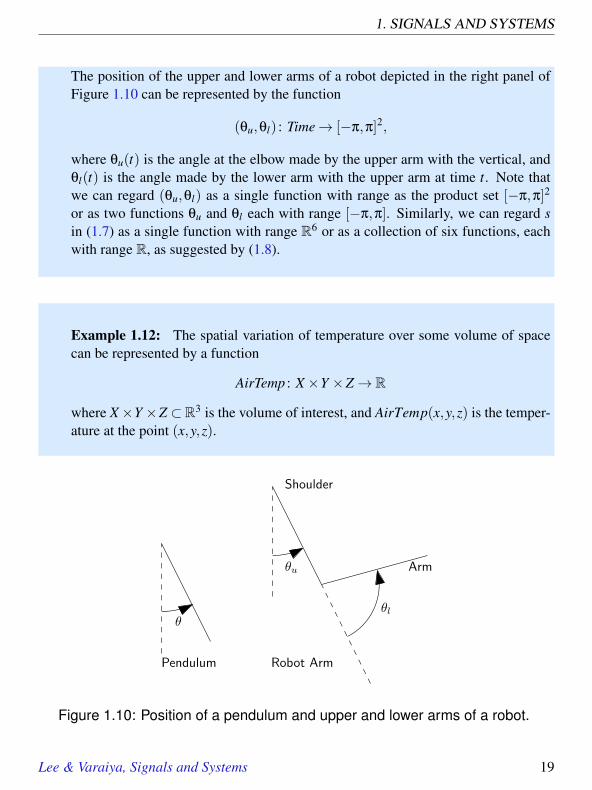
The position of the pendulum shown in the left panel of figure 1.10 is representedby the function
θ : Time→ [−π,π],
where θ(t) is the angle with the vertical made by the pendulum at time t.
18 Lee & Varaiya, Signals and Systems
1. SIGNALS AND SYSTEMS
The position of the upper and lower arms of a robot depicted in the right panel ofFigure 1.10 can be represented by the function
(θu,θl) : Time→ [−π,π]2,
where θu(t) is the angle at the elbow made by the upper arm with the vertical, andθl(t) is the angle made by the lower arm with the upper arm at time t. Note thatwe can regard (θu,θl) as a single function with range as the product set [−π,π]2
or as two functions θu and θl each with range [−π,π]. Similarly, we can regard sin (1.7) as a single function with range R6 or as a collection of six functions, eachwith range R, as suggested by (1.8).
Example 1.12: The spatial variation of temperature over some volume of spacecan be represented by a function
AirTemp : X×Y ×Z→ R
where X×Y ×Z ⊂R3 is the volume of interest, and AirTemp(x,y,z) is the temper-ature at the point (x,y,z).
Pendulum Robot Arm
θ
Shoulder
Armθu
θl
Figure 1.10: Position of a pendulum and upper and lower arms of a robot.
Lee & Varaiya, Signals and Systems 19

1.1. SIGNALS
1.1.5 Sequences
Above we studied examples in which temporal or spatial information is represented byfunctions of a variable representing time or space. The domain of time or space may becontinuous as in Voice and Image or discrete as in ComputerVoice and ComputerImage.
In many situations, information is represented as sequences of symbols rather than asfunctions of time or space. These sequences occur in two ways: as a representation ofdata or as a representation of an event stream. Sequences, in fact, are special sorts offunctions.
Examples of data represented by sequences are common. A file stored in a computer inbinary form is a sequence of bits, or binary symbols, i.e. a sequence of 0’s and 1’s. A textis a sequence of words. A sheet of music represents a sequence of notes.
Example 1.13: Consider an N-bit long binary file,
b1,b2, · · · ,bN ,
where each bi ∈ Binary = 0,1. We can regard this file as a function
File : 1,2, · · · ,N→ Binary,
with the assignment File(n) = bn for every n ∈ 1, · · · ,N.Sometimes we can give a mathematical expression for a binary signal. For instance,the N-bit long binary file Alt consisting of an alternating sequence of 0’s and 1’s isgiven by for all n,
Alt(n) =
0, n even1, n odd
If instead of Binary we take the range to be EnglishWords, then an N-word longEnglish text is a function
EnglishText : 1,2, · · · ,N→ EnglishWords.
20 Lee & Varaiya, Signals and Systems

1. SIGNALS AND SYSTEMS
In general, data sequences are functions of the form
Data : Indices→ Symbols, (1.9)
where Indices ⊂ N, where N is the set of natural numbers, is an appropriate index setsuch as 1,2, · · · ,N, and Symbols is an appropriate set of symbols such as Binary orEnglishWords.
One advantage of the representation (1.9) is that we can then interpret Data as a discrete-time signal, and so some of the techniques that we will develop in later chapters for thosesignals will automatically apply to data sequences. However, the domain Indices in (1.9)does not necessarily represent uniformly spaced instances of time. All we can say isthat if m and n are in Indices with m < n, then the m-th symbol Data(m) occurs in thedata sequence before the n-th symbol Data(n), but we cannot say how much time elapsesbetween the occurrence of those two symbols.
The second way in which sequences arise is as representations of event streams. An eventstream or event trace is a record or log of the significant events that occur in a system ofinterest. Here are some everyday examples.
Example 1.14: When you send a file to a printer, the normal trace of events is
CommandPrintFile, FilePrinting, PrintingComplete
but if the printer has run out of paper, the trace might be
CommandPrintFile, FilePrinting, MessageOutofPaper, InsertPaper, · · ·
When you enter your car the starting trace of events might be
StartEngine, SeatbeltSignOn, BuckleSeatbelt, SeatbeltSignOff, · · ·
Thus event streams are functions of the form
EventStream : Indices→ EventSet.
We will see in Chapter 3 that the behavior of finite state machines is best described interms of event traces, and that systems that operate on event streams are often best de-scribed as finite state machines.
Lee & Varaiya, Signals and Systems 21

1.1. SIGNALS
1.1.6 Discrete signals and sampling
Voice and PureTone are said to be continuous-time signals because their domain Time isa continuous interval of the form [α,β]⊂ R. The domain of Image, similarly, is a contin-uous 2-dimensional rectangle of the form [a,b]× [c,d]⊂ R2. The signals ComputerVoiceand ComputerImage have domains of time and space that are discrete sets. Video is alsoa discrete-time signal, but in principle it could be a function of a space continuum. Wecan define a function ComputerVideo where all three sets that are composed to form thedomain are discrete.
Discrete signals often arise from signals with continuous domains by sampling. Webriefly motivate sampling here, with a detailed discussion to be taken up later. Continuousdomains have an infinite number of elements. Even the domain [0,1]⊂ Time representinga finite time interval has an infinite number of elements. The signal assigns a value in itsrange to each of these infinitely many elements. Such a signal cannot be stored in a finitedigital memory device such as that in a computer. If we wish to store, say, Voice, we mustapproximate it by a signal with a finite domain.
A common way to approximate a function with a continuous domain like Voice and Imageby a function with a finite domain is by uniformly sampling its continuous domain.
Example 1.15: If we sample a 10-second long domain of Voice,
Voice : [0,10]→ Pressure,
10,000 times a second (i.e. at a frequency of 10 kHz) we get the signal
SampledVoice : 0,0.0001,0.0002, · · · ,9.9998,9.9999,10→ Pressure, (1.10)
with the assignment
SampledVoice(t) = Voice(t),
for all t ∈ 0,0.0001,0.0002, · · · ,9.9999,10. (1.11)
Notice from (1.10) that uniform sampling means picking a uniformly spaced subsetof points of the continuous domain [0,10].
22 Lee & Varaiya, Signals and Systems

1. SIGNALS AND SYSTEMS
In the example, the sampling interval or sampling period is 0.0001 sec, correspondingto a sampling frequency or sampling rate of 10,000 Hz. Since the continuous domain is10 seconds long, the domain of SampledVoice has 100,000 points. A sampling frequencyof 5,000 Hz would give the domain 0,0.0002, · · · ,9.9998,10, which has half as manypoints. The sampled domain is finite, and its elements are discrete values of time.
Figure 1.11 shows an exponential function Exp : [−1,1]→ R defined by
Exp(x) = ex.
SampledExp is obtained by sampling with a sampling interval of 0.2. So its domain is
−1,−0.8, · · · ,0.8,1.0.
The continuous domain of Image given by (1.1), which describes a grayscale image on an8.5 by 11 inch sheet of paper, is the rectangle [0,11]× [0,8.5], representing the space of
-1 - 0.5 0 0.5 10
0.5
1
1.5
2
2.5
3
-1 - 0.5 0 0.5 10
0.5
1
1.5
2
2.5
3
Figure 1.11: The exponential functions Exp and SampledExp, obtained by sam-pling with a sampling interval of 0.2.
Lee & Varaiya, Signals and Systems 23

1.1. SIGNALS
the page. In this case, too, a common way to approximate Image by a signal with finitedomain is to sample the rectangle. Uniform sampling with a spatial resolution of say, 100dots per inch, in each dimension, gives the finite domain D = 0,0.01, · · · ,8.49,8.5×0,0.01, · · · ,10.99,11.0. So the sampled grayscale picture is
SampledImage : D→ [0,MaxIntensity]
withSampledImage(x,y) = Image(x,y), for all (x,y) ∈ D.
As mentioned before, each sample of the image is called a pixel, and the size of the imageis often given in pixels. The size of your computer screen display, for example, may be600×800 or 768×1024 pixels.
Sampling and approximation
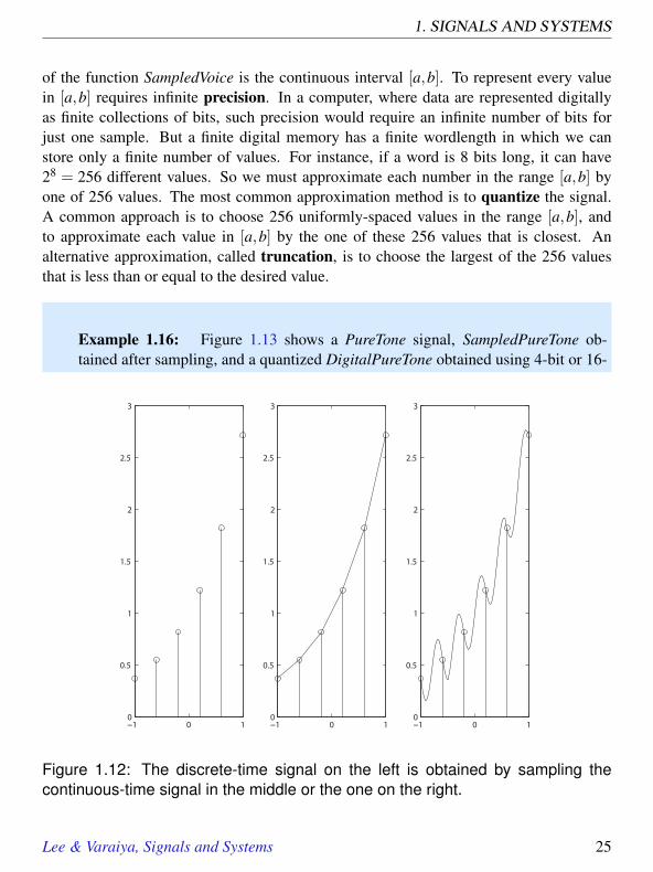
Let f be a continuous-time function, and let Sampledf be the discrete-time function ob-tained by sampling f . Suppose we are given Sampledf , as, for example, in the left panelof Figure 1.12. Can we reconstruct or recover f from Sampledf ? This question lies atthe heart of digital storage and communication technologies. The general answer to thisquestion tells us, for example, what audio quality we can obtain from a given discreterepresentation of a sound. The format for a compact disc is based on the answer to thisquestion. We will discuss it in much detail in later chapters.
For the moment, let us note that the short answer to the question above is no. For example,we cannot tell whether the discrete-time function in the left panel of Figure 1.12 wasobtained by sampling the continuous-time function in the middle panel or the functionin the right panel. Indeed there are infinitely many such functions, and one must make achoice. One option is to connect the sampled values by straight line segments, as shownin the middle panel. Another choice is shown in the right panel. The choice made by yourCD player is different from both of these, as explored further in Chapter 11.
Similarly, an image like Image cannot be uniquely recovered from its sampled versionSampledImage. Several different choices are commonly used.
Digital signals and quantization
Even though SampledVoice in example 1.15 has a finite domain, we may yet be unableto store it in a finite amount of memory. To see why, suppose that the range Pressure
24 Lee & Varaiya, Signals and Systems
1. SIGNALS AND SYSTEMS
of the function SampledVoice is the continuous interval [a,b]. To represent every valuein [a,b] requires infinite precision. In a computer, where data are represented digitallyas finite collections of bits, such precision would require an infinite number of bits forjust one sample. But a finite digital memory has a finite wordlength in which we canstore only a finite number of values. For instance, if a word is 8 bits long, it can have28 = 256 different values. So we must approximate each number in the range [a,b] byone of 256 values. The most common approximation method is to quantize the signal.A common approach is to choose 256 uniformly-spaced values in the range [a,b], andto approximate each value in [a,b] by the one of these 256 values that is closest. Analternative approximation, called truncation, is to choose the largest of the 256 valuesthat is less than or equal to the desired value.
Example 1.16: Figure 1.13 shows a PureTone signal, SampledPureTone ob-tained after sampling, and a quantized DigitalPureTone obtained using 4-bit or 16-
−1 0 10
0.5
1
1.5
2
2.5
3
−1 0 10
0.5
1
1.5
2
2.5
3
−1 0 10
0.5
1
1.5
2
2.5
3
Figure 1.12: The discrete-time signal on the left is obtained by sampling thecontinuous-time signal in the middle or the one on the right.
Lee & Varaiya, Signals and Systems 25

1.1. SIGNALS
level truncation. PureTone has continuous domain and continuous range, whileSampledPureTone (depicted with circles) has discrete domain and continuousrange, and DigitalPureTone (depicted with x’s) has discrete domain and discreterange. Only the last of these can be precisely represented on a computer.
It is customary to call a signal with continuous domain and continuous range like PureTonean analog signal, and a signal with discrete domain and range, like DigitalPureTone, adigital signal.
Example 1.17: In digital telephones, voice is sampled every 125µsec, or at asampling frequency of 8,000 Hz. Each sample is quantized into an 8-bit word, or256 levels. This gives an overall rate of 8,000× 8 = 64,000 bits per second. The
−4 −3 −2 −1 0 1 2 3 4−1
−0.8
−0.6
−0.4
−0.2
0
0.2
0.4
0.6
0.8
1
Figure 1.13: PureTone (continuous curve), SampledPureTone (circles), andDigitalPureTone signals (x’s).
26 Lee & Varaiya, Signals and Systems

1. SIGNALS AND SYSTEMS
worldwide digital telephony network, therefore, is composed primarily of channelscapable of carrying 64,000 bits per second, or multiples of this (so that multipletelephone channels can be carried together). In cellular phones, voice samples arefurther compressed to bit rates of 8,000 to 32,000 bits per second.
1.2 Systems
Systems are functions that transform signals. There are many reasons for transformingsignals. A signal carries information. A transformed signal may carry the same informa-tion in a different way. For example, in a live concert, music is represented as sound. Arecording system may convert that sound into a sequence of numbers stored on a magneticdisk drive. The original signal, the sound, is difficult to preserve for posterity. The diskhas a more persistent representation of the same information. Thus, storage is one of thetasks accomplished by systems.
A system may transform a signal into a form that is more convenient for transmission.Sound signals cannot be carried by the Internet. There is simply no physical mechanism inthe Internet for transporting rapid variations in air pressure. The Internet provides insteada mechanism for transporting sequences of bits. A system must convert a sound signalinto a sequence of bits. Such a system is called an encoder or coder. At the far end, adecoder is needed to convert the sequence back into sound. When a coder and a decoderare combined into the same physical device, the device is often called a codec.
A system may transform a signal to hide its information so that snoops do not have accessto it. This is called encryption. To be useful, we need matching decryption.
A system may enhance a signal by emphasizing some of the information it carries anddeemphasizing some other information. For example, an audio equalizer may compen-sate for poor room acoustics by reducing the magnitude of certain low frequencies thathappen to resonate in the room. In transmission, signals are often degraded by noise ordistorted by physical effects in the transmission medium. A system may attempt to reducethe noise or reverse the distortion. When the signal is carrying digital information overa physical channel, the extraction of the digital information from the degraded signal iscalled detection.
Lee & Varaiya, Signals and Systems 27

1.2. SYSTEMS
Systems are also designed to control physical processes such as the heating in a room,the ignition in an automobile engine, the flight of an aircraft. The state of the physicalprocess (room temperature, cylinder pressure, aircraft speed) is sensed. The sensed signalis processed to generate signals that drive actuators, such as motors or switches. Engineersdesign a system called the controller which, on the basis of the processed sensor signal,determines the signals that control the physical process (turn the heater on or off, adjustthe ignition timing, change the aircraft flaps) so that the process has the desired behavior(room temperature adjusts to the desired setting, engine delivers more torque, aircraftdescends smoothly).
Systems are also designed for translation from one format to another. For example, acommand sequence from a musician may be transformed into musical sounds. Or thedetection of risk of collision in an aircraft might be translated into control signals thatperform evasive maneuvers.
1.2.1 Systems as functions
Consider a system S that transforms input signal x into output signal y. The system is afunction, so y = S(x). Suppose x : D→ R is a signal with domain D and range R. Forexample, x might be a sound, x : R→ Pressure. The domain of S is the set X of all suchsounds, which we write
X = [D→ R] = x | x : D→ R (1.12)
This notation reads “X , also written [D→ R], is the set of all x such that x is a functionfrom D to R.” This set is called a signal space or function space. A signal or functionspace is a set of all functions with a given domain and range.
Example 1.18: The set of all sound segments with duration [0,1] and rangePressure is written
[[0,1]→ Pressure].
Notice that square brackets are used for both a subset of reals, as in [0,1], and fora function space, as in [D→ R], although obviously the meanings of these twonotations are very different.
28 Lee & Varaiya, Signals and Systems

1. SIGNALS AND SYSTEMS
The set ImageSet considered in section 1.1.3 is the function space
ImageSet = [DiscreteVerticalSpace×HorizontalSpace→ Intensity3].
Since this is a set, we can define functions that use it as a domain or range, as wehave done above with
Video : FrameTimes→ ImageSet.
Similarly, the set of all binary files of length N is
BinaryFiles = [Indices→ Binary].
where Indices = 1, · · · ,N.
A system S is a function mapping a signal space into a signal space,
S : [D→ R]→ [D′→ R′].
Systems, therefore, are much like signals, except that their domain and range are bothsignal spaces. Thus, if x ∈ [D→ R] and y = S(x), then it must be that y ∈ [D′ → R′].Furthermore, if z is an element of D′, z ∈ D′, then
y(z) = S(x)(z) = (S(x))(z) ∈ R′.
The parentheses around S(x) in (S(x))(z) are not necessary, but may improve readability.
1.2.2 Telecommunications systems
We give some examples of systems that occur in or interact with the global telecommu-nications network. This network is unquestionably one of the most remarkable accom-plishments of humankind. It is astonishingly complex, composed of hundreds of distinctcorporations and linking billions of people. It originated with a basic service, POTS, orplain-old telephone service, but the network has evolved into a global, high-speed, wire-less and wired digital network that carries not just voice, but also video, images, andcomputer data, including much of the traffic in the Internet.
Lee & Varaiya, Signals and Systems 29

1.2. SYSTEMS
Figure 1.14 depicts a small portion of the global telecommunications network. POTS ser-vice is represented at the upper right, where a twisted pair of copper wires connects acentral office to a home telephone. This twisted pair is called the local loop or subscriberline. At the central office, the twisted pair is connected to a line card, which usually con-verts the signal from the telephone immediately into digital form. The line card, in turn, is
The globaltelecommunications
network
Cable
Optical Fiber
Home Customer
Small Business/Home
Small Business/Home
Large Business Customer
ISDNModem Telephone
Computer
Modem
Fax
Telephone
Computer PBX
Satellite
Public Switch
T1 line
Line Card
Microwave Tower
DSL Card
ISDN card
Satellite dish
DSLModem Telephone
Computer
Twisted P
air
Twisted Pair
Twisted Pair
Coax Cable
Home Customer
Telephone
Line Card
Twisted P
air
Voiceband DataModem Computer
Figure 1.14: A portion of the global telecommunications network.
30 Lee & Varaiya, Signals and Systems

1. SIGNALS AND SYSTEMS
connected to a switch, which routes incoming and outgoing telephone connections. TheBerkeley central office is located on Bancroft, between Oxford and Shattuck.
The digital representation of a voice signal, a sequence of bits, is routed through thetelephone network. Usually it is combined with other bit sequences, which are othervoices or computer data, and sent over high-speed links implemented with optical fiber,microwave radio, coaxial cable, or satellites.
Of course, a telephone conversation usually involves two parties, so the network deliversto the same line card a digital sequence representing the far-end speaker. That digitalsequence is decoded and delivered to the telephone via the twisted pair. The line card,therefore, includes a codec.
The telephone itself, of course, is a system. It transforms the electrical signal that propa-gates down the twisted pair into a sound signal, and transforms a local sound signal intoan electrical signal that can propagate down the twisted pair.
POTS can be abstracted as shown in Figure 1.15. The entire network is reduced to a modelthat accepts an electrical representation of a voice signal and transports it to a remotetelephone. In this abstraction, the digital nature of the telephone network is irrelevant.The system simply transports (and degrades somewhat) a voice signal.
DTMF
Even in POTS, not all of the information transported is voice. At a minimum, the tele-phone needs to be able to convey to the central office a telephone number in order to
POTS
voice-like signal
TelephoneLine Card
voice-like signal
Network
Line CardTelephone
Figure 1.15: Abstraction of plain-old telephone service (POTS).
Lee & Varaiya, Signals and Systems 31

1.2. SYSTEMS
Probing Further: Wireless communication
The telephone network has been steadily freeing itself of its dependence on wires. Cel-lular telephones, which came into widespread use in the 1990s, use radio waves to con-nect a small, hand-held telephone to a nearby base station. The base station connectsdirectly to the telephone network.
There are three major challenges in the design of cellular networks. First, radio spec-trum is scarce. Frequencies are allocated by regulatory bodies, often constrained byinternational treaties. Finding frequencies for new technologies is difficult. Thus, wire-less communication devices have to be efficient in their use of the available frequencies.Second, the power available to drive a cellular phone is limited. Cellular phones mustoperate for long periods of time using only small batteries that fit easily within the hand-set. Although battery technology has been improving, the power that these batteries candeliver severely limits the range of a cellular phone (how far it can be from a base sta-tion) and the processing complexity (the microprocessors in a cellular phone consumeconsiderable power). Third, networking is complicated. In order to be able to route tele-phone calls to a cellular phone, the network needs to know where the phone is (whichbase station is closest). Moreover, the network needs to support phone calls in movingvehicles, which implies that a phone may move out of range of one base station and intothe range of another during the course of a telephone call. The network must hand offthe call seamlessly.
Although “radio telephones” have existed for a long time, particularly for maritimeapplications where wireline telephony is impossible, it was the cellular concept thatmade it possible to offer radio telephony to large numbers of users. Radio waves prop-agating along the surface of the earth lose power approximately proportionally to theinverse of the fourth power of distance. That is, if at distance d meters from a transmitteryour receive w watts of radio power, then at distance 2d you will receive approximatelyw/24 = w/16 watts of radio power. This fourth-power propagation loss was tradition-ally considered to be a hindrance to wireless communication. It had to be overcome byboosting the transmitted power. The cellular concept turns this hindrance into an ad-vantage. It observes that since the loss is so high, beyond a certain distance the samefrequencies can be re-used without significant interference. The service area is dividedinto cells. A second benefit is that the distance to base station is smaller than it wouldbe in a more centralized system, so less radio power is required.
32 Lee & Varaiya, Signals and Systems
1. SIGNALS AND SYSTEMS
establish a connection. A telephone number is not a voice signal. It is intrinsically dis-crete. Since the system is designed to carry voice signals, one option is to convert the
Probing Further: LEO telephony
Ideally, a cellular phone, with its one phone number, could be called anywhere in theworld, wherever it happens to be, without the caller needing to know where it is. Thetechnological and organizational infrastructure has evolved to make this possible in mostplaces. When a phone “roams” out of its primary service area, it negotiates with thelocal service provider in a new area for service. If that service provider has a businessagreement with the customer’s main service provider, then it provides service. Thisrequires complex networking so that telephone calls to the customer are routed to thecorrect locale.
However, digital cellular service is difficult to make universal, with many remote areasnot served. Providing such service by installing base stations is expensive. Moreover,marine service away from coastlines is technically impossible with cellular technology.
One candidate technology for truly global telephony services is based on low-earth-orbit (LEO) satellites. One such project (which failed in the marketplace) was the Irid-ium project, spearheaded by Motorola, and so named because in the initial conception,there would be 77 satellites. The iridium atom has 77 electrons. The idea is that enoughsatellites are put into orbit that one is always near enough to communicate with a hand-held telephone. When the orbit is low enough that a hand-held telephone can reach thesatellite (a few hundred kilometers above the surface of the earth), the satellites moveby fairly quickly. As a consequence, during the course of a telephone conversation, theconnection may have to be handed off from one satellite to another. In addition, in orderto be able to serve enough users simultaneously, each satellite has to re-use frequenciesaccording to the cellular concept. To do that, it focuses multiple beams on the surface ofthe earth using multi-element antenna arrays.
As of this writing, this approach has not yet proved economically viable. Theinvestment already has been huge, with at least one high-profile bankruptcy already,so the risks are high. Better networking of terrestrial cellular services may provideformidable competition, particularly as service improves to rural areas. The LEOapproach, however, has one advantage that terrestrial services cannot hope to matchanytime soon: truly worldwide service. The satellites provide service essentiallyeverywhere, even in remote wilderness areas and at sea.
Lee & Varaiya, Signals and Systems 33

1.2. SYSTEMS
telephone number into a voice-like signal. A system is needed with the structure shownin Figure 1.16. The block labeled “DTMF” is a system that transforms a sequence ofnumbers (coming from the keypad on the left) into a voice-like signal.
DTMFnumbers
voice-likesignal
1 2 3
4 5 6
7 8 9
* 0 #
697 Hz.
770 Hz.
852 Hz.
941 Hz.
1209
Hz.
1336
Hz.
1477
Hz.
Figure 1.16: DTMF converts numbers from a keypad into a voice-like signal.
0 0.001 0.002 0.003 0.004 0.005 0.006 0.007 0.008 0.009 0.01 2
1
0
1
2
time in seconds
Figure 1.17: Waveform representing the “0” key in DTMF.
34 Lee & Varaiya, Signals and Systems

1. SIGNALS AND SYSTEMS
The DTMF standard—dual-tone, multi-frequency—provides precisely such a mecha-nism. As indicated at the left in the figure, when the customer pushes one of the buttonson the telephone keypad, a sound is generated that is the sum of two sinusoidal signals.The frequencies of the two sinusoids are given by the row and column of the key. Forexample, a “0” is represented as a sum of two sinusoids with frequencies 941 Hz and1336 Hz. The waveform for such a sound is shown in Figure 1.17. The line card in thecentral office measures these frequencies to determine which digit was dialed.
Signal degradation
A voice received via the telephone network is different from the original in several re-spects. These differences can be modeled by a system that degrades the voice signal.
First, there is a loss of information because of sampling and quantization in the encoder,as discussed in the section 1.1.6. Moreover, the media that carry the signal, such as thetwisted pair, are not perfect. They distort the signal. One cause of distortion is addition ofnoise to the signal. Noise, by definition, is any undesired component in the signal. Noisein the telephone network is sometimes audible as background hiss, or as crosstalk, i.e.,leakage from other telephone channels into your own. Another degradation is that themedium attenuates the signal, and this attenuation depends on the signal frequency. Theline card, in particular, usually contains a bandlimiting filter that discards the high fre-quency components of the signal. This is why telephone channels do not transport musicwell. Finally, the signal propagates over a physical medium at a finite speed, bounded bythe speed of light, and so there is a delay between the time you say something and thetime when the person at the other end hears what you say. Light travels through 1 kmof optical fiber in approximately 5 µs, so the 5,000 km between Berkeley and New Yorkcauses a delay of about 25 ms, which is not easily perceptible.‡
‡ A phone conversation relayed by satellite has a much larger delay. Most satellites traditionally usedin the telecommunications network are geosynchronous, meaning that they hover at the same point overthe surface of the earth. To do that, they have to orbit at a height of 22,300 miles or 35,900 kilometers. Ittakes a radio signal about 120 ms to traverse that distance; since a signal has to go up and back, there is anend-to-end delay of at least 240 ms (not counting delays in the electronics). If you are using this channel fora telephone conversation, then the round-trip delay from when you say something to when you get a reactionis a minimum of 480 ms. This delay can be quite annoying, impeding your ability to converse until you gotused to it. If you use Internet telephony, the delays are even larger, and they can be irregular depending uponhow congested the Internet is when you call.
Lee & Varaiya, Signals and Systems 35
1.2. SYSTEMS
Communications engineering is concerned with how to minimize the degradation for allkinds of communication systems, including radio, TV, cellular phones, and computernetworks (such as the Internet).
1.2.3 Audio storage and retrieval
We have seen how audio signals can be represented as sequences of numbers. Digitalaudio storage and retrieval is all about finding a physical and persistent representation forthese numbers. These numbers can be converted into a single sequence of bits (binarydigits) and then “printed” onto some physical medium from which they can later be readback. The transformation of sound into its persistent representation can be modeled as asystem, as can the reverse or playback process.
Example 1.19: In the case of compact discs (CDs), the physical medium is a layerof aluminum on a platter into which tiny pits are etched. In the playback device, alaser aimed at the platter uses an interference pattern to determine whether or nota pit exists at a particular point in the platter. These pits, thus, naturally representbinary digits, since they can have two states (present or not present).
While a voiceband data modem converts bit sequences into voice-like signals, amusical recording studio does the reverse, creating a representation of the soundthat is a bit sequence,
RecordingStudio : Sounds→ BitStreams.
There is a great deal of engineering in the details, however. For instance, CDs arevulnerable to surface defects, which may arise in manufacturing or in the handsof the user. These defects may obscure some of the pits, or fool the reading laserinto detecting a pit where there is none. To guard against this, a very clever error-correcting code called a Reed-Solomon code is used. The coding process can beviewed as a function
Encoding : BitStreams→ RedundantBitStreams.
where RedundantBitStreams⊂ BitStreams is the set of all possible encoded bit se-quences. These bit sequences are redundant, in that they contain more bits than
36 Lee & Varaiya, Signals and Systems

1. SIGNALS AND SYSTEMS
are necessary to represent the original bit sequence. The extra bits are used to de-tect errors, and (sometimes) to correct them. Of course, if the surface of the CDis too badly damaged, even this clever scheme fails, and the audio data will not berecoverable.
CDs also contain meta data, which is extra information about the audio signal.This information allows the CD player to identify the start of a musical number andits length, and sometimes the title and the artist.
The CD format can also be used to contain purely digital data. Such a CD is called aCD ROM (read-only memory). It is called this because, like a computer memory,it contains digital information. But unlike a computer memory, that informationcannot be modified.
DVD (digital video discs) take this concept much further, including much moremeta data. They may eventually replace CDs. They are entirely compatible, in thatthey can contain exactly the same audio data that a CD can. DVD players can playCDs, but not the reverse, however. DVDs can also contain digital video informationand, in fact, any other digital data. DAT (digital audio tape) is also a competitorto CDs, but has failed to capture much of a market.
1.2.4 Modem negotiation
A very different kind of system is the one that manages the establishment of a connec-tion between two voiceband data modems. These two modems are at physically differentlocations, are probably manufactured by different manufacturers, and possibly use differ-ent communication standards. Both modems convert bit streams to and from voice-likesignals, but other than that, they do not have much in common.
When a connection is established through the telephone network, the answering modememits a tone that announces “I am a modem.” The initiating modem listens for this tone,and if it fails to detect it, assumes that no connection can be established and hangs up.If it does detect the tone, then it answers with a voice-like signal that announces “I am amodem that can communicate according to ITU standard x,” where x is one of the manymodem standard published by the International Telecommunication Union, or ITU.
The answering modem may or may not recognize the signal from the initiating modem.The initiating modem, for example, may be a newer modem using a standard that was
Lee & Varaiya, Signals and Systems 37

1.2. SYSTEMS
established after the answering modem was manufactured. If the answering modem doesrecognize the signal, then it responds with a signal that says “good, I too can communi-cation using standard x, so let’s get started.” Otherwise, it remains silent. The initiatingmodem, if it fails to get a response, tries another signal, announcing “I am a modem thatcan communicate according to ITU standard y,” where y is typically now an older (andslower) standard. This process continues until the two modems agree on a standard.
Once agreement is reached, the modems need to make measurements of the telephonechannel to compensate for its distortion. They do this by sending each other pre-agreedsignals called training signals, defined by the standard. The training signal is distortedby the channel, and, since the receiving modem knows the signal, it can measure thedistortion. It uses this measurement to set up a device called an adaptive equalizer.Once both modems have completed their setup, they begin to send data to one another.
As systems go, modem negotiation is fairly complex. It involves both event sequencesand voice-like signals. The voice like signals need to be analyzed in fairly sophisticatedways, sometimes producing events in the event sequences. It will take this entire bookto analyze all parts of this system. The handling of the event sequences will be treatedusing finite state machines, and the handling of the voice-like signals will be treated usingfrequency-domain concepts and filtering.
1.2.5 Feedback control systems
Feedback control systems are composite systems where a plant embodies a physical pro-cess whose behavior is guided by a control signal. A plant may be a mechanical device,such as the power train of a car, or a chemical process, or an aircraft with certain inertialand aerodynamic properties, for example. Sensors attached to the plant produce signalsthat are fed to the controller, which then generates the control signal. This arrangement,where the plant feeds the controller and the controller feeds the plant, is a complicatedsort of composite system called a feedback control system. It has extremely interestingproperties which we will explore in much more depth in subsequent chapters.
In this section, we construct a model of a feedback control system using the syntax ofblock diagrams. The model consists of several interconnected components. We will iden-tify the input and output signals of each component and how the components are inter-connected, and we will argue on the basis of a common-sense physics how the overallsystem will behave.
38 Lee & Varaiya, Signals and Systems

1. SIGNALS AND SYSTEMS
Example 1.20: Consider a forced air heating system, which heats a room in ahome or office to a desired temperature. Our first task is to identify the individualcomponents of the heating system. These are
• a furnace/blower unit (which we will simply call the heater) that heats air andblows the hot air through vents into a room,
• a temperature sensor that measures the temperature in a room, and
• the control system that compares the specified desired temperature with thesensed temperature and turns the furnace/blower unit on or off depending onwhether the sensed temperature is below or above the demanded temperature.
The interconnection of these components is shown in Figure 1.18.
Our second task is to specify the input and output signals of each component sys-tem (the domain and range of the function), ensuring the input-output matchingconditions. The heater produces hot air depending on whether it is turned on or off.So its input signal is simply a function of time which takes one of two values, Onor Off . We call input to the heater (a signal) OnOff ,
OnOff : Time→On,Off,
and we take Time = R+, the non-negative reals. So the input signal space is
OnOffProfiles = [R+→On,Off].
(Recall that the notation [D→ R] defines a function space, as explained in Section1.2.1.) When the heater is turned on it produces heat at some rate that depends onthe capacity of the furnace and blower. We measure this heating rate in BTUs perhour. So the output signal of the heater, which we name Heat is of the form
Heat : R+→0,Bc,
where Bc is the heater capacity measured in BTU/hour. If we name the output signalspace HeatProfiles, then
HeatProfiles = [R+→0,Bc].
Thus the Heater system is described by a function
Heater : OnOffProfiles→ HeatProfiles. (1.13)
Lee & Varaiya, Signals and Systems 39

1.2. SYSTEMS
Common-sense physics tells us that when the heater is turned on the room willbegin to warm up and when the heater is turned off the room temperature will falluntil it reaches the outside temperature. So the room temperature depends on boththe heat delivered by the heater and the outside temperature. Thus the input signalto the room is the pair (Heat,OutsideTemp). We can take OutsideTemp to be of theform
OutsideTemp : R+→ [min,max],
where [min,max] is the range of possible outside temperatures, measured in degreesCelsius, say. The output signal of the room is of course the room temperature,
RoomTemp : R+→ [min,max].
If we denoteOutsideTempProfiles = [R+→ [min,max]],
andRoomTempProfiles = [R+→ [min,max]],
then the behavior of the Room system is described by a function
Room : HeatProfiles×OutsideTempProfiles→ RoomTempProfiles (1.14)
In a similar manner, the Sensor system is described by a function
Sensor : RoomTempProfiles→ SensedTempProfiles (1.15)
with input signal space RoomTempProfiles and output signal space
SensedTempProfiles = [R+→ [min,max]].
The Controller is described by the function
Controller : DesiredTempProfile×SensedTempProfile→ OnOffProfile, (1.16)
whereDesiredTempProfiles = [R+→ [min,max]].
We have constructed a model where the input-output matching condition is satisfiedeverywhere.
40 Lee & Varaiya, Signals and Systems

1. SIGNALS AND SYSTEMS
The overall forced air heating system (the shaded part of Figure 1.18) has a pair ofinput signals, desired temperature and outside temperature, and one output signal,room temperature. So it is described by the function
ForcedHeat : DesiredTempProfiles×OutsideTempProfiles
→ RoomTempProfiles.
If we are given the input signal values x of desired temperature and the value y ofoutside temperature, we can compute the value z = ForcedHeat(x,y) by solving thefollowing four simultaneous equations
u = Controller(x,w)v = Heater(u)z = Room(y,v)w = Sensor(z)
(1.17)
Given x and y, we must solve these four equations to determine the four unknownfunctions u,v,w,z of which u,v,w are the internal signals, and z is the output signal.Of course to solve these simultaneous equations, we need to specify the four systemfunctions. So far we have simply given names to those functions and identifiedtheir domain and range. To complete the specification we must describe how thosefunctions assign output signals to input signals.
If the sensor is functioning properly we expect Sensor’s output signal to be theroom temperature, that is, for all z and for all t ∈ R+,
w(t) = Sensor(z)(t) = z(t).
A thermostatic controller has a simple behavior: it turns the heater on if the sensedtemperature falls below the desired temperature by a certain amount, say δ1, andit turns the heater off if the sensed temperature rises above the desired temperatureby, say δ2. That is, for all x,w and for all t ∈ R+,
u(t) = Controller(x,w)(t) =
On, if w(t)− x(t)≤−δ1Off , if w(t)− x(t)≥ δ2
Suppose finally that the desired temperature is set to some constant, say x∗, i.e. forall t ∈ R+,
x(t) = x∗.
Lee & Varaiya, Signals and Systems 41

1.3. SUMMARY
We can expect the behavior depicted in Figure 1.19. When w(t)− x∗ drops below−δ1, the controller will turn on the heater, the room temperature will increase untilw(t)− x∗ rises above δ2, and then the controller will turn off the heater. Thus theroom temperature will fluctuate around the desired temperature, x∗.
1.3 Summary
Signals are functions that represent information. We studied examples of three classes ofsignals. In the first class are functions of discrete or continuous time and space that occurin human perception and eletromechanical sensors. In the second class are functions oftime and space representing attributes of physical objects or devices. The third class ofsignals consist of sequences of symbols representing data or the occurrences of events. Ineach case, the domain and the range can be defined precisely.
Systems are functions that transform signals. We looked at telecommunication systems,where a network that was originally designed for carrying voice signals is used for manyother kinds of signals today. One way to accomplish this is to design systems such asmodems that transform signals so that they masquerade as voice-like signals. We alsolooked at system models for signal degradation and for storage of signals. We lookedat systems that are primarily concerned with discrete events and command sequences,and we examined a feedback control system. The telephone system and the forced airheating system were both described using block diagrams as interconnections of simplercomponent systems. In all cases, systems were given as functions where the domain andthe range are function spaces, or sets of functions.
42 Lee & Varaiya, Signals and Systems

1. SIGNALS AND SYSTEMS
Probing Further: Modems and Encrypted speech
POTS service is designed to carry speech signals. With proper encoding, however, it cancarry any signal that resembles speech in certain technical ways that we will discuss.Data can be transmitted over POTS networks using a voiceband data modem, shownjust below the upper right in Figure 1.14. This used to provide a routine way to connectto the Internet, but has since been supplanted (mostly) by broadband connections.
Data are represented by bit sequences, which are functions of the form
BitSequence : Indices→ Binary,
where Indices⊂N, the natural numbers, and Binary = 0,1. In order for a bit sequenceto traverse a POTS phone line, it has to be transformed into something that resemblesa voice signal. Furthermore, a system is needed to transform the voice-like signal backinto a bit sequence. A modem does this. The word modem is a contraction of modulator,demodulator. Pairs of modems are used at opposite ends of a POTS connection, eachwith a transmitter and a receiver to achieve bidirectional (called full duplex) communi-cation.
One of the strangest uses is to transmit digitally represented and encrypted voice sig-nals. Here is a depiction:
modulator bit sequence
telephone network
demodulator bit sequence
voice signal encoder
bit sequence encryption
voice signal decoder
bit sequence decryption
modem
voice-like signal
voice-like signal
What is actually sent through the telephone network sounds like hiss, which by itselfprovides a modicum of privacy. Casual eavesdroppers will be unable to understandthe encoded speech. However, this configuration also provides protection againstsophisticated listeners. A listener that is able to extract the bit sequence from thissound will still not be able to reconstruct the voice signal because the bit sequence isencrypted.
Lee & Varaiya, Signals and Systems 43

1.3. SUMMARY
Controller Heater DesiredTemp
x
OnOff
u
Heat
v Room RoomTemp
z
SensorSensedTemp
w
OutsideTempy
z
ForcedHeat
Figure 1.18: The interconnected components of a forced air heating system.
x* + d2
x* + d1
x*
offon
t
w
Figure 1.19: With a thermostatic controller the room temperature will fluctuatearound the desired temperature setting, x∗.
44 Lee & Varaiya, Signals and Systems

1. SIGNALS AND SYSTEMS
Exercises
Each problem is annotated with the letter E, T, C which stands for exercise, requires somethought, requires some conceptualization. Problems labeled E are usually mechanical,those labeled T require a plan of attack, those labeled C usually have more than onedefensible answer.
1. E The function x : R→ R given by
∀t ∈ R x(t) = sin(2π×440t)
is a mathematical example of a signal in the signal space [R→ R]. Give a mathe-matical example of a signal x in each of the following signal spaces.
(a) [Z→ R]
(b) [R→ R2]
(c) [0,1, · · · ,600×0,1, · · · ,400→ 0,1, · · · ,255](d) Describe a practical application for the signal space [0,1, · · · ,600×0,1, · · · ,400→0,1, · · · ,255]. That is, what might a function in this space represent?
2. C For each of the continuous-time signals below, represent the signal in the form off : X → Y and as a sketch like Figure 1.1. Carefully identify the range and domainin each case.
(a) The voltage across the terminals of a car battery.
(b) The closing prices on each day of a share of a company.
(c) The position of a moving vehicle on a straight one-lane road of length L.
(d) The simultaneous position of two moving vehicles on the same straight one-lane road of length L.
(e) The sound heard in both of your ears.
3. E In digital telephony, voice is sampled at a rate of 8,000 samples/second, so thesampling period is 1/8000 = 125 µs (microseconds). What is the sampling periodand the sampling frequency of sound in a compact disc (CD)?
Lee & Varaiya, Signals and Systems 45

EXERCISES
4. E Figure 1.4 displays the plots of two sinusoidal signals and their sum. Sketchby hand the plots of the four functions, Step,Triangle,Sum,Diff , all with domain[−1,1] and range R, where the four functions are defined by: ∀t ∈ [−1,1],
Triangle(t) = 1−|t|,Step(t) = 0 if t < 0, = 1 if t ≥ 0,
Sum(t) = Triangle(t)+Step(t),
Diff (t) = Triangle(t)−Step(t).
5. C The following examples of spatial information can be represented as a signal inthe form of f : X → Y . Specify a reasonable choice for the range and domain ineach case.
(a) An image impressed on photographic paper.
(b) An image stored in computer memory.
(c) The height of points on the surface of the earth.
(d) The location of the chairs in a room.
(e) The household voltage in Europe, which has frequency 50 Hz and is 210 voltsRMS.
6. C The image called Albers consists of an eight-inch yellow square in the center ofa white twelve-inch square background. Express Albers as a function, by choosingthe domain, range, and function assignment.
7. E How many bits are there in a 1024× 768 pixel image in which each pixel isrepresented as a 16-bit word? How long would it take to download this image overa 28 Kbps voice-band modem, a 384 Kbps DSL modem, a 10 Mbps Ethernet localarea network?
8. C Represent these examples as data or event sequences. Specify reasonable choicesfor the range and domain in each case.
(a) The result of 100 tosses of a coin,
(b) The sequence of button presses inside an elevator,
(c) The sequence of main events in a soda vending machine,
(d) Your response to a motorist who is asking directions,
(e) A play-by-play account of a game of chess.
46 Lee & Varaiya, Signals and Systems

1. SIGNALS AND SYSTEMS
9. C Formulate the following items of information as functions. Specify reasonablechoices for the domain and range in each case.
(a) The population of U.S. cities,
(b) The white pages in a phone book (careful: the white pages may list two iden-tical names, and may list the same phone number under two different names),
(c) The birth dates of students in class,
(d) The broadcast frequencies of AM radio stations,
(e) The broadcast frequencies of FM radio stations, (look at your radio dial, or atthe web page:
http://www.eecs.berkeley.edu/˜eal/eecs20/sidebars/radio/index.html.
10. E Use Matlab to plot the graph of the following continuous-time functions de-fined over [−1,1], and on the same plot display 11 uniformly spaced samples (0.2seconds apart) of these functions. Are these samples good representations of thewaveforms?
(a) f : [−1,1]→ R, where for all x ∈ [−1,1], f (x) = e−x sin(10πx).
(b) Chirp : [−1,1]→ R, where for all t ∈ [−1,1], Chirp(t) = cos(10πt2).
11. E Suppose the pendulum of Figure 1.10 is rotating counter-clockwise at a speedof one revolution per second over the five-second interval [0,5]. Sketch a plot ofthe resulting function: θ : [0,5]→ [−π,π). Assume θ(0) = 0. Also specify thisfunction mathematically. Your plot is discontinuous, but the pendulum’s motion iscontinuous. Explain this apparent inconsistency.
12. T There is a large difference between the sets X , Y , and [X → Y ]. This exerciseexplores some of that difference.
(a) Suppose X = a,b,c and Y = 0,1. List all the functions from X to Y , i.e.all the elements of [X→Y ]. Note that part of the problem here is to figure outhow to list all the functions.
(b) If X has m elements and Y has n elements, how many elements does [X → Y ]have?
Lee & Varaiya, Signals and Systems 47

EXERCISES
(c) Suppose
ColormapImages =
[DiscreteVerticalSpace×DiscreteHorizontalSpace
→ ColorMapIndexes].
Suppose the domain of each image in this set has 6,000 pixels and the rangehas 256 values. How many distinct images are there? Give an approximateanswer in the form of 10n. Hint: ab = 10b log10(a).
48 Lee & Varaiya, Signals and Systems

2Defining Signals and Systems
Contents2.1 Defining functions . . . . . . . . . . . . . . . . . . . . . . . . . . . 50
2.1.1 Declarative assignment . . . . . . . . . . . . . . . . . . . . . 522.1.2 Graphs . . . . . . . . . . . . . . . . . . . . . . . . . . . . . 54Probing Further: Relations . . . . . . . . . . . . . . . . . . . . . . . 562.1.3 Tables . . . . . . . . . . . . . . . . . . . . . . . . . . . . . . 572.1.4 Procedures . . . . . . . . . . . . . . . . . . . . . . . . . . . 582.1.5 Composition . . . . . . . . . . . . . . . . . . . . . . . . . . 582.1.6 Declarative vs. imperative . . . . . . . . . . . . . . . . . . . 62Probing Further: Declarative and imperative . . . . . . . . . . . . . 63
2.2 Defining signals . . . . . . . . . . . . . . . . . . . . . . . . . . . . 662.2.1 Declarative definitions . . . . . . . . . . . . . . . . . . . . . 662.2.2 Imperative definitions . . . . . . . . . . . . . . . . . . . . . 662.2.3 Physical modeling . . . . . . . . . . . . . . . . . . . . . . . 68
2.3 Defining systems . . . . . . . . . . . . . . . . . . . . . . . . . . . . 68Probing Further: Physics of a Tuning Fork . . . . . . . . . . . . . . 702.3.1 Memoryless systems and systems with memory . . . . . . . . 712.3.2 Differential equations . . . . . . . . . . . . . . . . . . . . . . 722.3.3 Difference equations . . . . . . . . . . . . . . . . . . . . . . 74Basics: Trigonometric Identities . . . . . . . . . . . . . . . . . . . . 76Basics: Summations . . . . . . . . . . . . . . . . . . . . . . . . . . . 772.3.4 Composing systems using block diagrams . . . . . . . . . . . 78Probing Further: Composition of graphs . . . . . . . . . . . . . . . . 80
2.4 Summary . . . . . . . . . . . . . . . . . . . . . . . . . . . . . . . . 82Exercises . . . . . . . . . . . . . . . . . . . . . . . . . . . . . . . . . . . 84
49
2.1. DEFINING FUNCTIONS
The previous chapter describes the representation of signals and systems as functions,concentrating on how to select the domain and range. This chapter is concerned with howto give more complete definitions of these functions. In particular, we need an assignmentrule, which specifies how to assign an element in the range to each element in the domain.
There are many ways to give an assignment rule. A theme of this chapter is that these dif-ferent ways have complementary uses. Procedural descriptions of the assignment rule, forexample, are more convenient for synthesizing signals or constructing implementations ofa system in software or hardware. Mathematical descriptions are more convenient for an-alyzing signals and systems and determining their properties.
In practice it is often necessary to use several descriptions of assignment rules in combi-nation, because of their complementary uses. In designing systems, a practicing engineeris often reconciling these diverse views to ensure, for instance, that a particular hardwaredevice or piece of software indeed implements a system that is specified mathematically.We begin with a discussion of functions in general, and then specialize to signals andsystems.
2.1 Defining functions
A function f : X → Y assigns to each element in X a single element in Y , as illustrated inFigure 2.1. This assignment can be defined by declaring the mathematical relationshipbetween the value in X and the value in Y , by graphing or enumerating the possibleassignments, by giving a procedure for determining the value in Y given a value in X , orby composing simpler functions. We go over each of these in more detail in this section.
Example 2.1: In Section 1.1.5 we mentioned that sequences are a special kindof function. An infinite sequence s is a function that maps the natural numbersinto some set Y , as illustrated in Figure 2.2. This function fully defines any infinitesequence of elements in Y .
50 Lee & Varaiya, Signals and Systems

2. DEFINING SIGNALS AND SYSTEMS
X
x1
x2
x3
x4
Y
y1
y2
y3
y4
f : X → Y
Figure 2.1: A function f : X → Y assigns to each element in X a single element inY .
Naturals
1
2
3
4
Y
y1
y2
y3
y4
s : Naturals → Y
...
Figure 2.2: An infinite sequence s is a function s : N→ Y that assigns to eachelement in N a single element in Y .
Lee & Varaiya, Signals and Systems 51

2.1. DEFINING FUNCTIONS
2.1.1 Declarative assignment
Consider the function Square : R→ R given by
∀ x ∈ R, Square(x) = x2. (2.1)
In (2.1), we have used the universal quantifier symbol ‘∀’, which means ‘for all’ or ‘forevery’ to declare the relationship between values in the domain of the function and valuesin the range. Statement (2.1) is read: “for every value of x in R, the function Squareevaluated at x is assigned the value x2.” The expression “Square(x) = x2” in (2.1) is anassignment.1
Expression (2.1) is an instance of the following prototype for defining functions. Definef : X → Y by
∀ x ∈ X , f (x) = expression in x. (2.2)
In this prototype, f is the name of the function to be defined, such as Square, X is thedomain of f , Y is the range of f , and ‘expression in x’ specifies the value in Y assigned tof (x).
The prototype (2.2) does not say how the ‘expression in x’ is to be evaluated. In theSquare example above, it was specified by the algebraic expression Square(x) = x2. Sucha definition of a function is said to be declarative, because it declares properties of thefunction without directly explaining how to construct the function.
Example 2.2: Here are some examples of functions of complex variables. (SeeAppendix B for a review of complex variables.)
The magnitude of a complex number is given by abs : C→R+, where C is the setof complex numbers and R+ is the set of set of non-negative real numbers, and
∀ z = x+ iy ∈ C, abs(z) =√(x2 + y2).
The complex conjugate of a number, conjugate : C→ C, is given by
∀ z = x+ iy ∈ C, conjugate(z) = x− iy.
1See Appendix A for a discussion of the use of “=” as an assignment, vs. its use as an assertion.
52 Lee & Varaiya, Signals and Systems

2. DEFINING SIGNALS AND SYSTEMS
The exponential of a complex number, exp : C→ C, is given by
∀ z ∈ C, exp(z) =∞
∑n=0
zn
n!.
If this notation is unfamiliar, see box on page 77.) It is worth emphasizing thatthe last definition is declarative: it does not give a procedure for calculating theexponential function, since the sum is infinite. Such a calculation would neverterminate.
Example 2.3: The signum function gives the sign of a real number, signum : R→−1,0,1,
∀ x ∈ R, signum(x) =
−1 if x < 00 if x = 01 if x > 0
(2.3)
The right side of this assignment tabulates three expressions for three different sub-sets of the domain. Below we will consider a more extreme case of this where everyvalue in the domain is tabulated with a value in the range.
Example 2.4: The size of a matrix, size : Matrices→ N×N, is given by
∀M ∈Matrices, size(M) = (m,n),
where m is the number of rows of the matrix M, n is the number of columns of M,and Matrices is the set of all matrices.
This definition relies not only on formal mathematics, but also on the English sen-tence that defines m and n. Without that sentence, the assignment would be mean-ingless.
Lee & Varaiya, Signals and Systems 53

2.1. DEFINING FUNCTIONS
2.1.2 Graphs
Consider a function f : X → Y . To each x ∈ X , f assigns the value f (x) in Y . The pair(x, f (x)) is an element of the product set X ×Y . The set of all such pairs is called thegraph of f , written graph( f ). Using the syntax of sets, graph( f ) is the subset of X ×Ydefined by
graph( f ) = (x,y) | x ∈ X and y = f (x), (2.4)
or slightly more simply,
graph( f ) = (x, f (x)) | x ∈ X.
The vertical bar | is read “such that,” and the expression after it is a predicate that definesthe set.2
When X ⊂ R and Y ⊂ R, we can plot graph( f ) on a page.
Example 2.5: Consider the graph of the function Square,
graph(Square) = (x,x2) | x ∈ R,
which is plotted in Figure 2.3. In that figure, the horizontal and vertical axes repre-sent the domain and the range, respectively (more precisely, a subset of the domainand the range). The rectangular region enclosed by these axes represents the prod-uct of the domain and the range (every point in that region is a member of (R×R)).The graph is visually rendered by placing a black dot at every point in that regionthat is a member of graph(Square). The resulting picture is the familiar plot of theSquare function.
While the graph of f : X → Y is a subset of X ×Y , it is a very particular sort of subset.For each element x ∈ X , there is exactly one element y ∈Y such that (x,y) ∈ graph( f ). Inparticular, there cannot be more than one such y ∈ Y , and there cannot be no such y ∈ Y .This is, in fact, what we mean when we say that f is a function.
2See appendix A for a review of this notation.
54 Lee & Varaiya, Signals and Systems

2. DEFINING SIGNALS AND SYSTEMS
−1 −0.8 −0.6 −0.4 −0.2 0 0.2 0.4 0.6 0.8 10
0.1
0.2
0.3
0.4
0.5
0.6
0.7
0.8
0.9
1
Figure 2.3: Graph of Square
Example 2.6: Let X = 1,2 and Y = a,b. Then
(1,a),(2,a)
is the graph of a function, but
(1,a),(1,b)
is not, because two points a and b are assigned to the same point, 1, in the domain.Neither is
(1,a),because no point in the range is assigned to the point 2 in the domain.
The graph of Square, graph(Square), is given by the algebraic expression (x,x2). In othercases, no such algebraic expression exists. For example, Voice is specified through itsgraph in Figure 1.1, not through an algebraic expression. Thus, graphs can be used todefine functions that cannot be conveniently given by declarative assignments.
Lee & Varaiya, Signals and Systems 55

2.1. DEFINING FUNCTIONS
X
x1
x2
x3
x4
Y
y1
y2
y3
y4
Relation ⊂ X × Y
Figure 2.4: Any subset of X×Y is a relation.
Consider again the prototype in (2.2),
∀ x ∈ X , f (x) = expression in x
The graph of f is
graph( f ) = (x,y) ∈ X×Y | y = expression in x.
The expression ‘y = expression in x’ is a predicate in the variable (x,y) and so this proto-type definition conforms to the prototype new set constructor given in (A.4) of AppendixA:
NewSet = z ∈ Set | Pred(z).
Probing Further: Relations
The graph of a function f : X → Y is a subset of X×Y , as defined in (2.4). An arbitrarysubset of X×Y is called a relation. A relation is a set of tuples (x,y) that pair an elementx ∈ X with an element y ∈ Y , as suggested in Figure 2.4. For relations, it is common tocall X the domain and Y the codomain. A function is a special kind of relation in whichfor every x ∈ X there is exactly one y ∈ Y such that (x,y) is an element of the relation.So a particular relation R⊂ X ×Y is a function if for every x ∈ X there is a y1 ∈ Y suchthat (x,y1) ∈ R, and if in addition (x,y2) ∈ R, then y1 = y2.
56 Lee & Varaiya, Signals and Systems

2. DEFINING SIGNALS AND SYSTEMS
Name MarksJohn Brown 90.0
Jane Doe 91.2· · · · · ·
Table 2.1: Tabular representation of Score.
Since the graph of f is a set, we can define the function f via its graph using the sametechniques we use to define sets.
2.1.3 Tables
If f : X→Y has finite domain, then graph( f )⊂ X×Y is a finite set, so it can be specifiedsimply by a list of all its elements. This list can be put in the form of a table. This tabledefines the function.
Example 2.7: Suppose the function
Score : Students→ [0,100]
gives the outcome of the first midterm exam for each student in the class. Obvi-ously, this function cannot be given by an algebraic declarative assignment. But itcan certainly be given as a table, as shown in table 2.1.
Example 2.8: The command nslookup on a networked computer is a function thatmaps hostnames into their IP (Internet) address. For example, if you type:
nslookup cory.eecs.berkeley.edu
you get the IP address 128.32.134.240. The domain name server attached to yourmachine stores the nslookup function as a table.
Lee & Varaiya, Signals and Systems 57

2.1. DEFINING FUNCTIONS
2.1.4 Procedures
Sometimes the value f (x) that a function f assigns to an element x ∈ domain( f ) is ob-tained by executing a procedure.
Example 2.9: Here is a Matlab procedure to compute the factorial function
fact : 1, · · · ,10→ N,
where N is the set of natural numbers:
fact(1) = 1;for n = 2:10
fact(n) = n * fact(n-1);end
Unlike previous mechanisms for defining a function, this one gives a constructive methodto determine an element in the range given an element in the domain. This style is calledimperative to distinguish it from declarative. The relationship between these two stylesis interesting, and quite subtle. It is explored further in Section 2.1.6.
2.1.5 Composition
Functions can be combined to define new functions. The simplest mechanism is to con-nect the output of one function to the input of another. We have been doing this informallyto define systems by connecting components in block diagrams.
If the first function is f1 and the second is f2, then we write the function composition asf2 f1. That is, for every x in the domain of f1,
( f2 f1)(x) = f2( f1(x)).
A fundamental requirement for such a composition to be valid is that the range of f1must be a subset of the domain of f2. In other words, any output from the first function
58 Lee & Varaiya, Signals and Systems

2. DEFINING SIGNALS AND SYSTEMS
x
X
f 1(x)
Y
X’
Y’ f 1 f 2
f 3
f 2 (f 1(x)) = f 3 (x)
Figure 2.5: Function composition: f3 = f2 f1.
must be in the set of possible inputs for the second. Without this input-output connectionrestriction, the interconnection would be meaningless.3
It is worth pausing to study the notation f2 f1. Assume f1 : X → Y and f2 : X ′ → Y ′.Then if Y ⊂ X ′, we can define
f3 = f2 f1,
where f3 : X → Y ′ such that
∀ x ∈ X , f3(x) = f2( f1(x)) (2.5)
Notice that f1 is applied first, and then f2. Why is f1 listed second in f2 f1? Thisconvention simply mirrors the ordering of f2( f1(x)) in (2.5). We can visualize f3 as inFigure 2.5.
Example 2.10: Consider the representation of a color image using a colormap.The decoding of the image is depicted in Figure 1.7. The image itself might begiven by the function
ColormapImage : DiscVerticalSpace×DiscHorizontalSpace
→ ColorMapIndexes.
3We just called an element in the domain of a function its input and the corresponding value of the functionits output. This interpretation of domain as inputs and range as outputs is natural, and it is the reason thatsystems are described by functions.
Lee & Varaiya, Signals and Systems 59

2.1. DEFINING FUNCTIONS
The functionDisplay : ColorMapIndexes→ Intensity3
decodes the colormap indexes. If ColorMapIndexes has 256 values, it could beidentified with the set Integers8 of all 8-bit words, as we have seen. If we composethese functions
ColorComputerImage = DisplayColormapImage
then we get the decoded representation of the image
ColorComputerImage : DiscVerticalSpace×DiscHorizontalSpace
→ Intensity3.
ColorComputerImage describes how an image looks when it is displayed, whereasColormapImage describes how it is stored in the computer.
If f : X → X , i.e. the domain and range of f are the same, we can form the function
f 2 = f f .
We can compose f 2 with f to form f 3, and so on.
Example 2.11: Consider the function S : R2 → R2, where the assignment(y1,y2) = S(x1,x2) is defined by matrix multiplication,[
y1y2
]=
[1 23 4
][x1x2
]. (2.6)
The function S2 = SS : R2→ R2 is also defined by matrix multiplication, and thecorresponding matrix is the square of the matrix in (2.6).
60 Lee & Varaiya, Signals and Systems

2. DEFINING SIGNALS AND SYSTEMS
To see this, let (y1,y2) = S(x1,x2) and (z1,z2) = S(y1,y2) = (S S)(x1,x2). Thenwe see that[
z1z2
]=
[1 23 4
]︸ ︷︷ ︸
A
[y1y2
]=
[1 23 4
] ([1 23 4
] [x1x2
])
=
[1 23 4
]2 [ x1x2
]=
[7 1015 22
]︸ ︷︷ ︸
A2
[x1x2
]
= A2[
x1x2
].
Example 2.12: Consider another example in the context of the telephone system.Let Voices be the set of possible voice input signals of the form
Voice : Time→ Pressure.
Voices is a function space,
Voices = [Time→ Pressure].
A telephone converts a Voice signal into a signal in the set
LineSignals = [Time→ Voltages].
Thus, we could define
Mouthpiece : Voices→ LineSignals.
The twisted wire pair may distort this signal, so we define a function
LocalLoop : LineSignals→ LineSignals.
The input to the line card therefore is
(LocalLoopMouthpiece)(Voice).
Lee & Varaiya, Signals and Systems 61

2.1. DEFINING FUNCTIONS
Similarly let BitStreams be the set of possible bitstreams of the form:
BitStream : DiscreteTime→ Binary
where DiscreteTime = 0,1/64,000,2/64,000, · · ·, since there are 64,000 bit-s/sec. So,
BitStreams = [DiscreteTime→ Binary].
The encoder in a line card can be mathematically described as a function
Encoder : LineSignals→ BitStreams
or, with more detail, as a function
Encoder : [Time→ Voltages]→ [DiscreteTime→ Binary].
The digital telephone network itself might be modeled as a function
Network : BitStreams→ BitStreams.
We can continue in this fashion until we model the entire path of a voice signalthrough the telephone network as the function composition
EarpieceLocalLoop2 Decoder Network Encoder
LocalLoop1 Mouthpiece. (2.7)
Given a complete definition of each of these functions, we would be well equippedto understand the degradations experienced by a voice signal in the telephone net-work.
2.1.6 Declarative vs. imperative
Declarative definitions of functions assert a relationship between elements in the domainand elements in the range. Imperative definitions give a procedure for finding an elementin the range given one in the domain. Often, both types of specifications can be given forthe same function. However sometimes the specifications are subtly different.
62 Lee & Varaiya, Signals and Systems

2. DEFINING SIGNALS AND SYSTEMS
Consider the function
SquareRoot : R+→ R+
defined by the statement “SquareRoot(x) is the unique value of y ∈ R+ such that y2 = x.”This declarative definition of SquareRoot does not tell us how to calculate its value atany point in its domain. Nevertheless, it defines SquareRoot perfectly well. By contrast,an imperative definition of SquareRoot would give us a procedure, or algorithm, for cal-culating SquareRoot(x) for a given x. Call the result of such an algorithm y. Since thealgorithm would yield an approximation in most cases, y2 would not be exactly equal tox. So the declarative and imperative definitions are not always the same.
Any definition of a function following the prototype (2.2) is a declarative definition. Itdoes not give a procedure for evaluating ‘expression in x’.
Probing Further: Declarative and imperative
The declarative approach establishes a relation between the domain and the range of afunction. For example, the equation
y = sin(x)/x
can be viewed as defining a subset of R×R. This subset is the graph of the functionSinc : R→ R.
The imperative approach also establishes a function, but it is a function that maps theprogram state before the statement is executed into a program state after the statement isexecuted. Consider for example the Java statement
y = Math.sin(x)/x;
Considering only this statement (rather than a larger program), the program state is thevalue of the two variables, x and y. Suppose that these have been declared to be of typedouble, which in Java represents double-precision floating-point numbers encodingaccording to an IEEE standard. Let the set Doubles be the set of all numbers so encoded,and note that NaN ∈ Doubles, not a number, the result of division by zero. The set ofpossible program states is therefore Doubles×Doubles. The Java statement thereforedefines a function
Statement : (Doubles×Doubles)→ (Doubles×Doubles).
Lee & Varaiya, Signals and Systems 63

2.1. DEFINING FUNCTIONS
Example 2.13: As another example where declarative and imperative definitionsdiffer in subtle ways, consider the following mathematical equation:
y =sin(x)
x. (2.8)
Consider the following Java statement:
y = Math.sin(x)/x;
or an equivalent Matlab statement
y = sin(x)/x
Superficially, these look very similar to (2.8). There are minor differences in syntaxin the Java statement, but otherwise, it is hard to tell the difference. But there aredifferences. For one, the mathematical equation (2.8) has meaning if y is known andx is not. It declares a relationship between x and y. The Java and Matlab statementsdefine a procedure for computing y given x. Those statements have no meaning ify is known and x is not.
The mathematical equation (2.8) can be interpreted as a predicate that defines afunction, for example the function Sinc : R→ R, where
graph(Sinc) = (x,y) | x ∈ R,y = sin(x)/x. (2.9)
The Java and Matlab statements can be interpreted as imperative definitions of afunction. Confusingly, many programming languages, including Matlab, use theterm “function” to mean something a bit different from a mathematical function.They use it to mean a procedure that can compute an element in the range ofa function given an element in its domain. Under certain restrictions (avoidingglobal variables for example), Matlab functions do in fact compute mathematicalfunctions. But in general, they do not. .
To interpret the Java and Matlab statements as imperative definitions of a function,note that given an element in the domain, they specify how to compute an elementin the range. However, these two statements do not define the same function as
64 Lee & Varaiya, Signals and Systems

2. DEFINING SIGNALS AND SYSTEMS
in (2.9). To see this, consider the value of y when x = 0. Given the mathematicalequation, it is not entirely trivial to determine the value of y. You can verify thaty = 1 when x = 0 using l’Hopital’s rule, which states that if f (a) = g(a) = 0, then
limx→a
f (x)g(x)
= limx→a
f ′(x)g′(x)
, (2.10)
if the limit exists, where f ′(x) is the derivative of f with respect to x, and g′(x) isthe derivative of g with respect to x.
In contrast, the meaning of the Java and Matlab statements is that y = 0/0 whenx = 0, which Java and Matlab (and most modern languages) define to be NaN, nota number. Thus, given x = 0, the procedures yield different values for y than themathematical expression. (An exception is symbolic algebra programs, such asMathematica or Maple, which will evaluate sin(x)/x to 1 when x = 0. These pro-grams use sophisticated, rule-based solution techniques, and, in effect, recognizethe need and apply l’Hopital’s rule.)
We can see from the above example some of the strengths and weaknesses of imperativeand declarative approaches. Given only a declarative definition, it is difficult for a com-puter to determine the value of y. Symbolic mathematical software, such as Maple andMathematica, is designed to deal with such situations, but these are very sophisticatedprograms. In general, using declarative definitions in computers requires quite a bit moresophistication than using imperative definitions.
Imperative definitions are easier for computers to work with. But the Java and Matlabstatements illustrate one weakness of the imperative approach: it is arguable that y = NaNis the wrong answer, so the Java and Matlab statements have a bug. This bug is unlikelyto be detected unless, in testing, these statements happen to be executed with the valuex = 0. A correct Java program might look like this:
if (x == 0.0) y = 1.0;else y = Math.sin(x)/x;
Thus, the imperative approach has the weakness that ensuring correctness is more dif-ficult. Humans have developed a huge arsenal of techniques and skills for thoroughly
Lee & Varaiya, Signals and Systems 65

2.2. DEFINING SIGNALS
understanding declarative definitions (thus lending confidence in their correctness), butwe are only beginning to learn how to ensure correctness in imperative definitions.
2.2 Defining signals
Signals are functions. Thus, both declarative and imperative approaches can be used todefine them.
2.2.1 Declarative definitions
Consider for example an audio signal s, a pure tone at 440 Hz (middle A on the pianokeyboard). Recall that audio signals are functions Sound : Time→ Pressure, where theset Time⊂ R represents a range of time and the set Pressure represents air pressure.4 Todefine this function, we might give the declarative description
∀ t ∈ Time, s(t) = sin(440×2πt). (2.11)
In many texts, you will see the shorthand
s(t) = sin(440×2πt)
used as the definition of the function s. Using the shorthand is only acceptable whenthe domain of the function is well understood from the context. This shorthand can beparticularly misleading when considering systems, and so we will only use it sparingly.A portion of the graph of the function (2.11) is shown in Figure 1.3.
2.2.2 Imperative definitions
We can also give an imperative description of such a signal. When thinking of signalsrather than more abstractly of functions, there is a subtle question that arises when weattempt to construct an imperative definition. Do you give the value of s(t) for a particulart? Or for all t in the domain? Suppose we want the latter, which seems like a more
4Recall further that we normalize Pressure so that zero represents the ambient air pressure. We also usearbitrary units, rather than a physical unit such as millibars.
66 Lee & Varaiya, Signals and Systems

2. DEFINING SIGNALS AND SYSTEMS
complete definition of the function. Then we have a problem. The domain of this functionmay be any time interval, or all time! Suppose we just want one second of sound. Definet = 0 to be the start of that one second. Then the domain is [0,1]. But there are an(uncountably) infinite number of values for t in this range! No Java or Matlab programcould provide the value of s(t) for all these values of t.
Since a signal is function, we give an imperative description of the signal exactly as wedid for functions. We give a procedure that has the potential of providing values for s(t),given any t.
Example 2.14: We could define a Java method as follows:
double s(double t) return (Math.sin(440*2*Math.PI*t));
Calling this method with a value for t as an argument yields a value for s(t). Java(and most object-oriented languages) use the term “method” for most procedures.
Another alternative is to provide a set of samples of the signal.
Example 2.15: In Matlab, we could define a vector t that gives the values of timethat we are interested in:
t = [0:1/8000:1];
In the vector t there are 8001 values evenly spaced between 0 and 1, so our sam-pling rate is 8000 samples per second. Then we can compute values of s for thesevalues of t and listen to the resulting sound:
s = cos(2*pi*440*t);sound(s,8000)
The vector s also has 8001 elements, representing evenly spaced samples of onesecond of A-440.
Lee & Varaiya, Signals and Systems 67

2.3. DEFINING SYSTEMS
2.2.3 Physical modeling
An alternative way to define a signal is to construct a model for a physical system thatproduces that signal.
Example 2.16: A pure tone might be defined as a solution to a differential equationthat describes the physics of a tuning fork.
A tuning fork consists of a metal finger (called a tine) that is displaced by strikingit with a hammer. After being displaced, it vibrates. If the tine has no friction, itwill vibrate forever. We can denote the displacement of the tine after being struckat time zero as a function y : R+→ R. If we assume that the initial displacementintroduced by the hammer is one unit, then using our knowledge of physics we candetermine that for all t ∈ R+, the displacement satisfies the differential equation
y(t) =−ω20y(t) (2.12)
where ω0 is constant that depends on the mass and stiffness of the tine, and andwhere y(t) denotes the second derivative with respect to time of y (see box).
It is easy to verify that y given by
∀ y ∈ R+, y(t) = cos(ω0t) (2.13)
is a solution to this differential equation (just take its second derivative). Thus,the displacement of the tuning fork is sinusoidal. This displacement will coupledirectly with air around the tuning fork, creating vibrations in the air (sound). Ifwe choose materials for the tuning fork so that ω0 = 2π×440, then the tuning forkwill produce the tone of A-440 on the musical scale.
2.3 Defining systems
All of the methods that we have discussed for defining functions can be used, in princi-ple, to define systems. However, in practice, the situation is much more complicated forsystems than for signals. Recall from Section 1.2.1 that a system is a function where thedomain and range are sets of signals called signal spaces. Elements of these domains and
68 Lee & Varaiya, Signals and Systems

2. DEFINING SIGNALS AND SYSTEMS
displacement restorative force
tine
Figure 2.6: A tuning fork.
ranges are considerably more difficult to specify than, say, an element of R or Z. For thisreason, it is almost never reasonable to use a graph or a table to define a system. Muchof the rest of this book is devoted to giving precise ways to define systems where someanalysis is possible. Here we consider some simple techniques that can be immediatelymotivated. Then we show how more complicated systems can be constructed from sim-pler ones using block diagrams. We give a rigorous meaning to these block diagrams sothat we can use them without resorting to perilous intuition to interpret them.
Consider a system S where
S : [D→ R]→ [D′→ R′]. (2.14)
Suppose that x ∈ [D→ R] and y = S(x). Then we call the pair (x,y) a behavior of thesystem. A behavior is an input, output pair. The set of all behaviors is
Behaviors(S) = (x,y) | x ∈ [D→ R] and y = S(x).
Giving the set of behaviors is one way to define a system. Explicitly giving the setBehaviors, however, is usually impractical, because it is a huge set, typically infinite (seeboxes on pages 681 and 683). Thus, we seek other ways of talking about the relationshipbetween a signal x and a signal y when y = S(x).
Lee & Varaiya, Signals and Systems 69

2.3. DEFINING SYSTEMS
To describe a system, one must specify its domain (the space of input signals), its range(the space of output signals), and the rule by which the system assigns an output signalto each input signal. This assignment rule is more difficult to describe and analyze thanthe input and output signals themselves. A table is almost never adequate, for example.Indeed for most systems we do not have effective mathematical tools for describing or
Probing Further: Physics of a Tuning Fork
A tuning fork consists of two fingers called tines, as shown in Figure 2.6. If you displaceone of these tines by hitting it with a hammer, it will vibrate with a nearly perfect sinu-soidal characteristic. As it vibrates, it pushes the air, creating a nearly perfect sinusoidalvariation in air pressure that propogates as sound. Why does it vibrate this way?
Suppose the displacement of the tine (relative to its position at rest) at time t is givenby x(t), where x : R→ R. There is a force on the tine pushing it towards its at-restposition. This is the restorative force of the elastic material used to make the tine. Theforce is proportional to the displacement (the greater the displacement, the greater theforce), so
F(t) =−kx(t),
where k is the proportionality constant that depends on the material and geometry of thetine. In addition, Newton’s second law of motion tells us the relationship between forceand acceleration,
F(t) = ma(t),
where m is the mass and a(t) is the acceleration at time t. Of course,
a(t) =d2
dtx(t) = x(t),
somx(t) =−kx(t)
orx(t) =−(k/m)x(t).
Comparing with (2.12), we see that ω20 = k/m.
A solution to this equation needs to be some signal that is proportional to its ownsecond derivative. A sinusoid as in (2.13) has exactly this property. The sinusoidalbehavior of the tine is called simple harmonic motion.
70 Lee & Varaiya, Signals and Systems
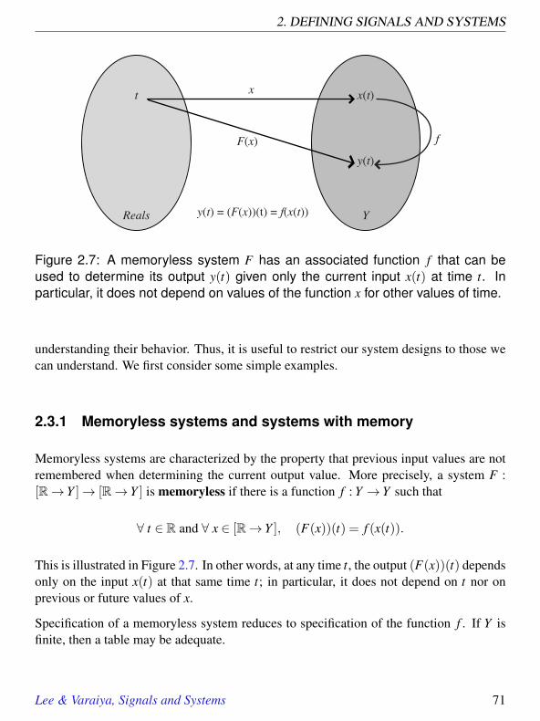
2. DEFINING SIGNALS AND SYSTEMS
Reals
t
Y
x(t)
y(t)
f
x
F(x)
y(t) = (F(x))(t) = f(x(t))
Figure 2.7: A memoryless system F has an associated function f that can beused to determine its output y(t) given only the current input x(t) at time t. Inparticular, it does not depend on values of the function x for other values of time.
understanding their behavior. Thus, it is useful to restrict our system designs to those wecan understand. We first consider some simple examples.
2.3.1 Memoryless systems and systems with memory
Memoryless systems are characterized by the property that previous input values are notremembered when determining the current output value. More precisely, a system F :[R→ Y ]→ [R→ Y ] is memoryless if there is a function f : Y → Y such that
∀ t ∈ R and ∀ x ∈ [R→ Y ], (F(x))(t) = f (x(t)).
This is illustrated in Figure 2.7. In other words, at any time t, the output (F(x))(t) dependsonly on the input x(t) at that same time t; in particular, it does not depend on t nor onprevious or future values of x.
Specification of a memoryless system reduces to specification of the function f . If Y isfinite, then a table may be adequate.
Lee & Varaiya, Signals and Systems 71

2.3. DEFINING SYSTEMS
Example 2.17: Consider a continuous-time system with input x and output y,where for all t ∈ R,
y(t) = x2(t).
This example defines a simple system, where the value of the output signal at eachtime depends only on the value of the input signal at that time. Such systems aresaid to be memoryless because you do not have to remember previous values of theinput in order to determine the current value of the output.
By contrast, here is an example of a system with memory.
Example 2.18: Consider a continuous-time system with input x and output y =F(x) such that ∀ t ∈ R,
y(t) =1M
∫ t
t−Mx(τ)dτ.
By a change of variables this can also be written
y(t) =1M
∫ M
0x(t− τ)dτ.
This system is clearly not memoryless. It has the effect of smoothing the inputsignal. We will study it and many related systems in detail in later chapters.
2.3.2 Differential equations
Consider a class of systems given by functions S : ContSignals → ContSignals whereContSignals is a set of continuous-time signals. Depending on the scenario, we couldhave ContSignals= [Time→R] or ContSignals= [Time→C], where Time=R or Time=R+. These are often called continuous-time systems because they operate on continuous-time signals. Frequently, such systems can be defined by differential equations that relatethe input signal to the output signal.
72 Lee & Varaiya, Signals and Systems

2. DEFINING SIGNALS AND SYSTEMS
Example 2.19: Consider a particle constrained to move forward or backwardsalong a straight line with an externally imposed force. We will consider this particleto be a system where the output is its position and the externally imposed force isthe input.
Denote the position of the particle by x : Time→ R, where Time = R+. By con-sidering only the non-negative reals, we are assuming that the model has a startingtime. We denote the acceleration by a : Time→R. By Newton’s law, which relatesforce, mass, and acceleration,
f (t) = ma(t),
where f (t) is the force at time t, and m is the mass. By the definition of acceleration,
∀ t ∈ R+, x(t) = a(t) = f (t)/m,
where x(t) denotes the second derivative with respect to time of x. If we know theinitial position x(0) and initial speed x(0) of the particle at time 0, and if we aregiven the input force f , we can evaluate the position at any t by integrating thisdifferential equation
x(t) = x(0)+ x(0)t +∫ t
0[∫ s
0( f (τ)/m)dτ]ds. (2.15)
We can regard the initial position and velocity as inputs, together with force, inwhich case the system is a function
Particle : R×R× [R+→ R]→ [R+→ R],
where for any inputs (x(0), x(0), f ), x = Particle(x(0), x(0), f ) must satisfy (2.15).
Suppose for example that the input is (1,−1, f ) where m= 1 and ∀ t ∈R+, f (t)= 1.We can calculate the position by carrying out the integration in (2.15) to find that
∀ t ∈ R+, x(t) = 1− t +0.5t2.
Suppose instead that x(0) = x(0) = 0 and ∀ t ∈ R+, f (t) = cos(ω0t), where ω0 issome fixed number. Again, we can carry out the integration to get∫ t
0
∫ s
0cos(ω0u)du ds =−cos(ω0t)−1
ω20
.
Lee & Varaiya, Signals and Systems 73

2.3. DEFINING SYSTEMS
Notice that the position of the particle is sinusoidal. Notice further that the ampli-tude of this sinusoid decreases as ω0 increases. Intuitively, this has to be the case.If the externally imposed force is varying more rapidly back and forth, the particlehas less time to respond to each direction of force, and hence its excursion is less.In subsequent chapters, we will study how the response of certain kinds of systemsvaries with the frequency of the input.
2.3.3 Difference equations
Consider a class of systems given by functions S : DiscSignals → DiscSignals whereDiscSignals is a set of discrete-time signals. Depending on the scenario, we could haveDiscSignals = [Z→ R] or DiscSignals = [Z→ C], or even DiscSignals = [N0→ R], orDiscSignals = [N0→ C]. These are often called discrete-time systems because they op-erate on discrete-time signals. Frequently, such systems can be defined by differenceequations that relate the input signal to the output signal.
Example 2.20: Consider a system
S : [N0→ R]→ [N0→ R]
where for all x ∈ [N0→ R], S(x) = y is given by
∀ n ∈ Z, y(n) = (x(n)+ x(n−1))/2.
The output at each index is the average of two of the inputs. This is a simpleexample of a moving average system, where typically more than two input valuesget averaged to produce an output value.
Suppose that x = u, the unit step function, defined by
∀ n ∈ Z, u(n) =
1 if n≥ 00 otherwise
(2.16)
We can easily calculate the output y,
∀ n ∈ Z, y(n) =
1 if n≥ 11/2 if n = 00 otherwise
74 Lee & Varaiya, Signals and Systems
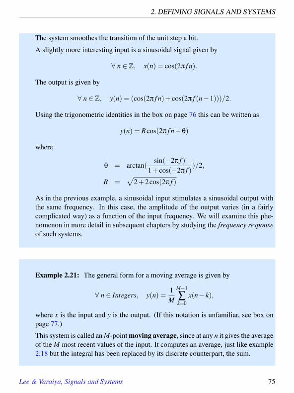
2. DEFINING SIGNALS AND SYSTEMS
The system smoothes the transition of the unit step a bit.
A slightly more interesting input is a sinusoidal signal given by
∀ n ∈ Z, x(n) = cos(2π f n).
The output is given by
∀ n ∈ Z, y(n) = (cos(2π f n)+ cos(2π f (n−1)))/2.
Using the trigonometric identities in the box on page 76 this can be written as
y(n) = Rcos(2π f n+θ)
where
θ = arctan(sin(−2π f )
1+ cos(−2π f ))/2,
R =√
2+2cos(2π f )
As in the previous example, a sinusoidal input stimulates a sinusoidal output withthe same frequency. In this case, the amplitude of the output varies (in a fairlycomplicated way) as a function of the input frequency. We will examine this phe-nomenon in more detail in subsequent chapters by studying the frequency responseof such systems.
Example 2.21: The general form for a moving average is given by
∀ n ∈ Integers, y(n) =1M
M−1
∑k=0
x(n− k),
where x is the input and y is the output. (If this notation is unfamiliar, see box onpage 77.)
This system is called an M-point moving average, since at any n it gives the averageof the M most recent values of the input. It computes an average, just like example2.18 but the integral has been replaced by its discrete counterpart, the sum.
Lee & Varaiya, Signals and Systems 75

2.3. DEFINING SYSTEMS
Moving averages are widely used on Wall Street to smooth out momentary fluctuations instock prices to try to determine general trends. We will study the smoothing properties ofthis system. We will also study more general forms of difference equations of which themoving average is a special case.
The examples above give declarative definitions of systems. Imperative definitions re-quire giving a procedure for computing the output signal given the input signal. It is clearhow to do that with the memoryless system, assuming that an imperative definition of thefunction f is available, and with the moving average. The integral equation, however, isharder to define imperatively. An imperative description of such systems that is suitablefor computation on a computer requires approximation via solvers for differential equa-tions. Simulink, for example, which is part of the Matlab package, provides such solvers.Alternatively, an imperative description can be given in terms of analog circuits or otherphysical systems that operate directly on the pertinent continuous domain. Discrete-timesystems often have reasonable imperative definitions as state machines, considered indetail in the next chapter.
Basics: Trigonometric Identities
The following trigonometric identities will prove useful repeatedly:
Acos(θ+α)+Bcos(θ+β) =C cosθ−S sinθ = Rcos(θ+φ)
whereC = Acosα+Bcosβ
S = Asinα+Bsinβ
R =√
C2 +S2
φ = arctan(S/C)
76 Lee & Varaiya, Signals and Systems

2. DEFINING SIGNALS AND SYSTEMS
Basics: Summations
In example 2.21, a discrete-time moving average system is defined by
∀ n ∈ Integers, y(n) =1M
M−1
∑k=0
x(n− k),
where x is the input and y is the output. The notationM−1∑
k=0indicates a sum of M terms.
The terms are x(n− k), where k takes on values from 0 to M−1. Thus,
M−1
∑k=0
x(n− k) = x(n)+ x(n−1)+ · · ·+ x(n−M+1).
Such summations are related to integrals. Example 2.18 describes a continuous-timesystem with input x and output y where
∀ t ∈ R, y(t) =1M
∫ t
t−Mx(τ)dτ.
This is similar to the discrete-time moving average in that it sums values of x, but itsums over a continuum of values of the dummy variable τ. In the discrete-time version,the sum is over discrete values of the dummy variable k, which takes only integer val-ues. The summation notation has an ambiguity that it does not share with the integralnotation. In particular, it is not clear how to interpret an expression like
M−1
∑k=0
1+2.
There are two possibilities, depending on whether the 2 is included in the summationor is interpreted as being outside the summation. One possibility gives a sum of 3M,while the other gives M+2. In integration, this ambiguity does not occur because of theexplicit reference to the dummy variable as dτ. In particular, it is clear that∫ T
01+2dτ 6=
∫ T
01dτ+2.
The left integral is equal to 3T , while the right integral is T +2.
Lee & Varaiya, Signals and Systems 77

2.3. DEFINING SYSTEMS
2.3.4 Composing systems using block diagrams
We have been using block diagrams informally to describe systems. But it turns out thatblock diagrams can have as rigorous and formal a meaning as mathematical notations.We begin the exploration of this concept here, and pursue it much further in Chapter 4.
A block diagram is a visual syntax for describing a system as an interconnection of other(component) systems, each of which emphasizes one particular input-to-output transfor-mation of a signal. A block diagram is a collection of blocks interconnected by arrows.Arrows are labeled by signals. Each block represents an individual system that transformsan incoming or input signal into an outgoing or output signal.
A block diagram, which is a composition of systems, is itself a system. We can usefunction composition, as discussed in Section 2.1.5, to give a precise meaning to thislarger system. A block represents a function, and the connection of an output from oneblock to the input of another represents the composition of their two functions. The onlyrequirement for interconnecting two blocks is that the output of the first block must be anacceptable input for the second.
Block diagrams can be much more readable than symbolic function composition, particu-larly for complicated interconnections. They also offer a natural hierarchy, where we cancombine blocks to hide certain signals and component systems and to emphasize others.
For certain sorts of blocks, composing them in a block diagram results in a new systemwhose properties are easy to determine. In chapter 4 we will show how to combine statemachine blocks to define a new state machine. In Chapter 8 we will show how to combinefilter blocks to define new filter blocks. Here, we consider the composition of blockswhen all we know about the blocks is that they represent functions with a given domainand range. No further structure is available.
The simplest block diagram has a single block, as in Figure 2.8. The block represents asystem with input signal x and output signal y. Here, x denotes a variable over the set X ,and y denotes a variable over the set Y . The system is described by the function S : X→Y .Both X and Y are sets of functions or signals. Therefore the variables x and y themselvesdenote functions.
In general, a system obtained by a cascade composition of two blocks is given by thecomposition of the functions describing those blocks. In figure 2.9 the function S de-scribes the system obtained by connecting the systems S1 and S2, with S = S2 S1, i.e.
∀ x ∈ X , S(x) = S2(S1(x)).
78 Lee & Varaiya, Signals and Systems

2. DEFINING SIGNALS AND SYSTEMS
S : X → Yx ∈ X y ∈Y
Y = [DY → RY]X = [DX → RX]
Figure 2.8: The simplest block diagram represents a function S that maps an inputsignal x ∈ X to an output signal y ∈ Y . The domain and range of the input are DX
and RX , repectively, and of the output, DY and RY .
S1 : X → x ∈ y X ∈Y
X = [D → R] Y = [D' → R']S2 : Y → Z
z ∈Z
Z = [D'' → R'']
S : X → Z
Y
Figure 2.9: The cascade composition of the two systems is described by S =S2 S1.
The combined system has input signal x, output signal z, and internal signal y. (Theinternal signal is not visible in the input or output of the combined system.) Of course,the range of the first system must be contained by the domain of the second for thiscomposition to make sense. In the figure, the typical case is shown where this range anddomain are the same. The voice path in (2.7) is an example of cascade composition.
Consider two more block diagrams with slightly more complicated structure. Figure 2.10is similar to Figure 2.9. The system described by S1 is the same as before, but the systemdescribed by S2 has a pair of input signals (w,y) ∈W ×Y . The combined system hasthe pair (x,w) ∈ X ×W as input signal, z as output signal, y as internal signal, and it isdescribed by the function S : X×W → Z, where
∀(x,w) ∈ X×W, S(x,w) = S2(w,S1(x)). (2.17)
Lee & Varaiya, Signals and Systems 79
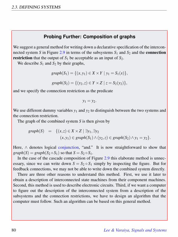
2.3. DEFINING SYSTEMS
Probing Further: Composition of graphs
We suggest a general method for writing down a declarative specification of the intercon-nected system S in Figure 2.9 in terms of the subsystems S1 and S2 and the connectionrestriction that the output of S1 be acceptable as an input of S2.
We describe S1 and S2 by their graphs,
graph(S1) = (x,y1) ∈ X×Y | y1 = S1(x),
graph(S2) = (y2,z) ∈ Y ×Z | z = S2(y2),and we specify the connection restriction as the predicate
y1 = y2.
We use different dummy variables y1 and y2 to distinguish between the two systems andthe connection restriction.
The graph of the combined system S is then given by
graph(S) = (x,z) ∈ X×Z | ∃y1,∃y2
(x,y1) ∈ graph(S1)∧ (y2,z) ∈ graph(S2)∧ y1 = y2.
Here, ∧ denotes logical conjunction, “and.” It is now straightforward to show thatgraph(S) = graph(S2 S1) so that S = S2 S1.
In the case of the cascade composition of Figure 2.9 this elaborate method is unnec-essary, since we can write down S = S2 S1 simply by inspecting the figure. But forfeedback connections, we may not be able to write down the combined system directly.
There are three other reasons to understand this method. First, we use it later toobtain a description of interconnected state machines from their component machines.Second, this method is used to describe electronic circuits. Third, if we want a computerto figure out the description of the interconnected system from a description of thesubsystems and the connection restrictions, we have to design an algorithm that thecomputer must follow. Such an algorithm can be based on this general method.
80 Lee & Varaiya, Signals and Systems

2. DEFINING SIGNALS AND SYSTEMS
S1 : X → x ∈ X y ∈Y
S2 : W × Y → z ∈Z
Y = [DY → RY]X = [DX → RX]
Z = [DZ → RZ]
w ∈
W = [DW → RW]
S : W × X →
Y
Z
Z
W
Figure 2.10: The combined system with input signals x,w and output signal z isdescribed by the function S, where ∀ (x,w), S(x,w) = S2(w,S1(x)).
Notice that it is now much harder to define this system using the function compositionnotation, , yet the block diagram makes its definition evident. In fact, the block diagramnotation is much more flexible.
The system of Figure 2.11 is obtained from that of figure 2.10 by connecting the outputsignal z to the input signal w. As a result the new system has input signal x, output signalz, internal signals y and w, and it is described by the function S′ : X → Z, where
∀ x ∈ X , S′(x) = S2(S′(x),S1(x)). (2.18)
The connection of z to w is called a feedback connection because the output z is fed backas input w. Of course, such a connection has meaning only if Z, the range of S2, is a subsetof W . The system in Figure 2.11 is again difficult to define using function compositionnotation, , yet again the block diagram definition is clear.
There is one enormous difference between (2.17) and (2.18). Expression (2.17) serves asa definition of the function S: to every (x,w) in its domain S assigns the value given bythe right-hand side which is uniquely determined by the given functions S1 and S2. But inexpression (2.18) the value S′(x) assigned to x may not be determined by the right-handside of (2.18), since the right-hand side itself depends on S′(x). In other words, (2.18) isan equation that must be solved to determine the value of S′(x) for a given x; i.e. S′(x) = ywhere y is a solution of
y = S2(y,S1(x)). (2.19)
Lee & Varaiya, Signals and Systems 81

2.4. SUMMARY
S1 : X → x ∈ X y ∈Y
S2 : W × Y → z ∈Z
Y = [DY → RY]X = [DX → RX]
Z = [DZ → RZ]
z ∈
Z ⊂ W
S' : X → Z
Z
Y
W
Figure 2.11: The combined system is described by the function S′, where S′(x) =S2(S′(x),S1(x)).
Such a solution, if it exists, is called a fixed point. We now face the difficulty that thisequation may have no solution, exactly one solution, or several solutions. Another diffi-culty is that the value y that solves (2.19) is not a number but a function. So it will notbe easy to solve such an equation. Since feedback connections always arise in controlsystems, we will study how to solve them. We will first solve them in the context of statemachines, which are introduced in the next chapter.
All of these block diagrams follow the same principles. They use component systemsto define composite systems. To be useful, of course, it is necessary to be able to inferproperties of the composite systems. Fortunately, this is often the case, although feedbackconnections will prove subtle. This idea is explored further in chapters 4 and 8.
2.4 Summary
Signals and systems both are modeled as functions. It is often straightforward to figureout the domain and range of a particular signal and system. It is more difficult to specifythe function’s assignment rule. Since the domain and range of a system are themselvessignal spaces, the assignment rule for a system is more complex than for a signal. Thedomain and range signal spaces of a system can be quite different: a modem converts bitsequences into sounds, an encoder converts sounds into bit sequences.
82 Lee & Varaiya, Signals and Systems

2. DEFINING SIGNALS AND SYSTEMS
The assignment rule of a function takes a declarative or imperative form. The declarativeform is usually mathematical, as in: define Chirp : [−1,1]→ R by
∀t ∈ [−1,1], Chirp(t) = cos(20πt2).
The imperative form is a procedure to evaluate the function at an arbitrary point in itsdomain. The procedure may involve a table lookup (if the domain is finite) or a computerprogram. If the domain is infinite, the evaluation procedure may only yield an approxi-mation of the declarative form of the “same” function.
A physical system is often described using differential or difference equations that em-body its “law of motion.” A mechanical system’s law of motion is derived from Newton’slaws. An electrical circuit’s law of motion is derived from Kirchhoff’s laws and the lawsof the circuit’s constitutive elements: resistors, capacitors, inductors, transistors.
Most systems are built by composing smaller subsystems. The composition may be ex-pressed in the visual syntax of block diagrams or, mathematically, using function compo-sition. Feedback is the most complex form of system composition: a feedback specifica-tion requires the solution of a fixed point equation.
Lee & Varaiya, Signals and Systems 83

EXERCISES
Exercises
Each problem is annotated with the letter E, T, C which stands for exercise, requires somethought, and requires some conceptualization. Problems labeled E are usually mechani-cal, those labeled T require a plan of attack, those labeled C usually have more than onedefensible answer.
1. E The broadcast signal of an AM radio station located at 110 on your dial has acarrier frequency of 110 kHz. An AM signal that includes the carrier has the form
∀ t ∈ Time, AMSignal(t) = (1+m(t))sin(2π×110,000t),
where m is an audio signal like Voice in figure 1.1, except that ∀ t ∈ Time, |m(t)|< 1.Since you cannot easily plot such a high frequency signal, give an expression forand plot AMSignal (using Matlab) for the case where Time = [0,1], m(t) = cos(πt),and the carrier frequency is 20 Hz.
2. T This problem studies the relationship between the notion of delay and the graphof a function.
(a) Consider two functions f and g from R into R where ∀ t ∈ R, f (t) = t andg(t) = f (t− t0), where t0 is a fixed number. Sketch a plot of f and g for t0 = 1and t0 = −1. Observe that if t0 > 0 then graph(g) is obtained by movinggraph( f ) to the right, and if t0 < 0 by moving it to the left.
(b) Show that if f : R→ R is any function whatsoever, and ∀ t, g(t) = f (t− t0),then if (t,y) ∈ graph( f ), then (t + t0,y) ∈ graph(g). This is another way ofsaying that if t0 > 0 then the graph is moved to the right, and if t0 < 0 then thegraph is moved to the left.
(c) If t represents time, and if t0 > 0, we say that g is obtained by delaying f .Why is it reasonable to say this?
3. E Indicate whether the following statements are true or false.
(a) [1,2,3→ a,b]⊂ [N→a,b](b) g | g = graph( f )∧ f : X → Y ⊂ X×Y(c) F : [R→ R]→ [R→ R], such that ∀ t ∈ R, and ∀ x ∈ [R→ R],
(F(x))(t) = sin(2π ·440t)
is a memoryless system.
84 Lee & Varaiya, Signals and Systems
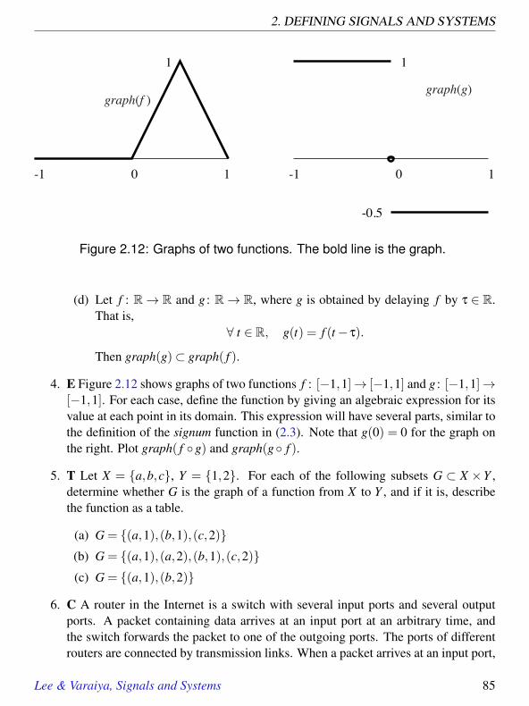
2. DEFINING SIGNALS AND SYSTEMS
-1 0 1
1
-1 0 1
1
-0.5
graph(f ) graph(g)
Figure 2.12: Graphs of two functions. The bold line is the graph.
(d) Let f : R→ R and g : R→ R, where g is obtained by delaying f by τ ∈ R.That is,
∀ t ∈ R, g(t) = f (t− τ).
Then graph(g)⊂ graph( f ).
4. E Figure 2.12 shows graphs of two functions f : [−1,1]→ [−1,1] and g : [−1,1]→[−1,1]. For each case, define the function by giving an algebraic expression for itsvalue at each point in its domain. This expression will have several parts, similar tothe definition of the signum function in (2.3). Note that g(0) = 0 for the graph onthe right. Plot graph( f g) and graph(g f ).
5. T Let X = a,b,c, Y = 1,2. For each of the following subsets G ⊂ X ×Y ,determine whether G is the graph of a function from X to Y , and if it is, describethe function as a table.
(a) G = (a,1),(b,1),(c,2)(b) G = (a,1),(a,2),(b,1),(c,2)(c) G = (a,1),(b,2)
6. C A router in the Internet is a switch with several input ports and several outputports. A packet containing data arrives at an input port at an arbitrary time, andthe switch forwards the packet to one of the outgoing ports. The ports of differentrouters are connected by transmission links. When a packet arrives at an input port,
Lee & Varaiya, Signals and Systems 85

EXERCISES
the switch examines the packet, extracting from it a destination address d. Theswitch then looks up the output port in its routing table, which contains entries ofthe form (d,outputPort). It then forwards the packet to the specified output port.The Internet works by setting up the routing tables in the routers.
Consider a simplified router with one input port and and two output ports, namedO1, O2. Let D be the set of destination addresses.
(a) Explain why the routing table can be described as a subset T ⊂D×O1,O2.(b) Is it reasonable to constrain T to be the graph of a function from D→O1,O2?
Why?
(c) Assume the signal at the input port is a sequence of packets. How would youdescribe the space of input signals to the router and output signals from therouter?
(d) How would you describe the switch as a function from the space of inputsignals to the space of output signals?
7. C For each of the following expressions, state whether it can be interpreted as anassignment, an assertion, or a predicate. More than one choice may be valid becausethe full context is not supplied.
(a) x = 5,
(b) A = 5,(c) x > 5,
(d) 3 > 5,
(e) x > 5∧ x < 3.
8. T A logic circuit with m binary inputs and n binary outputs is shown in Figure 2.13.It is described by a function F : X → Y where X = Binarym and Y = Binaryn. (Ina circuit, the signal values 1 and 0 in Binary correspond to voltage High and Low,respectively.) How many such distinct logic functions F are there?
9. E The function H : [R+→ R]→ [N0→ R] given by: ∀x ∈ [R+→ R],
∀n ∈ N0, H(x)(n) = x(10n),
is a mathematical example of a system with input signal space [R+→R] and outputsignal space [N0→ R]. Give a mathematical example of a system H whose
86 Lee & Varaiya, Signals and Systems

2. DEFINING SIGNALS AND SYSTEMS
F : Binm → Binn
x1 ∈ Binary
xm ∈ Binary
...
y1 ∈ Binary
yn ∈ Binary
...
Figure 2.13: The logic circuit has m binary inputs (x1, · · · ,xm) and n binary outputs(y1, · · · ,yn).
(a) input and output signal spaces both are [N0→ Binary].
(b) input signal space is [N0→ R] and output signal space is [N0→0,1].(c) input signal space is [Z→ R] and output signal space is [R→ R].
10. E Consider the functions
g : Y → R and f : N→ Y.
where Y is a set.
(a) Draw a block diagram for (g f ), with one block for each of g and f , andlabel the inputs and output of the blocks with the domain and range of g andf .
(b) Suppose Y is given by
Y = [1, · · · ,100→ R]
(Thus, the function f takes a natural number and returns a sequence of length100, while the function g takes a sequence of length 100 and returns a realnumber.)Suppose further that g is given by: for all y ∈ Y ,
g(y) =100
∑i=1
y(i) = y(1)+ y(2)+ · · ·+ y(100),
and f by: for all x ∈ N and z ∈ 1, · · · ,100,
( f (x))(z) = cos(2πz/x).
Lee & Varaiya, Signals and Systems 87

EXERCISES
(Thus, x gives the period of a cosine waveform, and f gives 100 samples ofthat waveform.) Give a one-line Matlab expression that evaluates (g f )(x)for any x ∈ N. Assume the value of x is already in a Matlab variable called x.
(c) Find (g f )(1).
11. T The following system S takes a discrete-time signal x ∈ X and transforms it intoa discrete-time signal y ∈ Y whose value at index n is the average of the previous 4values of x. Such a system is called a moving average. Suppose that X =Y = [N→R], where N is the set of natural numbers. More precisely, the system is describedby the function S such that for any x ∈ X , y = S(x) is given by
y(n) =
[x(1)+ · · ·+ x(n)]/4 for 1≤ n < 4[x(n−3)+ x(n−2)+ x(n−1)+ x(n)]/4 for n≥ 4
Notice that the first three samples are averages only if we assume that samples priorto those that are available have value zero. Thus, there is an initial transient whilethe system collects enough data to begin computing meaningful averages.
Write a Matlab program to calculate and plot the output signal y for time 1≤ n≤ 20for the following input signals:
(a) x is a unit step delayed by 10, i.e. x(n) = 0 for n≤ 9 and x(n) = 1 for n≥ 10.
(b) x is a unit step delayed by 15.
(c) x alternates between +1 and -1, i.e. x(n) = 1 for n odd, and x(n) = −1 for neven. Hint: Try computing cos(πn) for n ∈ N.
(d) Comment on what this system does. Qualitatively, how is the output signaldifferent from the input signal?
12. T The following system is similar to problem 11, but time is continuous. NowX = Y = [R→ R] and the system F : X → Y is defined as follows. For all x ∈ Xand t ∈ R
(F(x))(t) =110
∫ t
t−10x(s)ds.
Show that if x is the sinusoidal signal
∀ t ∈ R x(t) = sin(ωt),
then y is also sinusoidal
∀ t ∈ R, y(t) = Asin(ωt +φ).
88 Lee & Varaiya, Signals and Systems

2. DEFINING SIGNALS AND SYSTEMS
You do not need to give precise expressions for A and φ, but just show that theresult has this form. Also, show that as ω gets large, the amplitude of the outputgets small. Higher frequencies, which represent more abrupt changes in the input,are more attenuated by the system than lower frequencies.
Hint: The following fact from calculus may be useful:∫ b
asin(ωs)ds =
1ω(cos(ωa)− cos(ωb)).
Also, the identity in the footnote on page 76 might be useful to show that the outputis sinusoidal with the appropriate frequency.
13. E Suppose that f : R→ R and g : R→ Z such that for all x ∈ R,
g(x) =
1 if x > 00 if x = 0−1 if x < 0
andf (x) = 1+ x.
(a) Define h = g f .(b) Suppose that
F : [R→ R] → [R→ R]G : [R→ R] → [R→ Z]
such that for all s ∈ [R→ R] and x ∈ R,
(F(s))(x) = f (s(x))
(G(s))(x) = g(s(x))
where f and g are as given above. Sketch a block diagram for H = G F ,where you have one block for each of G and F . Label the inputs and outputsof your blocks with the domain and range of the functions in the blocks.
(c) Let s ∈ [R→ R] be such that for all x ∈ R,
s(x) = cos(πx).
Define u whereu = (GF)(s).
Give the domain, range, and assignment rule for u.
Lee & Varaiya, Signals and Systems 89

EXERCISES
14. T Let D = DiscSignals = [Z→ R] and let
G : D×D→ D
such that for all x,y ∈ D and for all n ∈ Z,
(G(x,y))(n) = x(n)− y(n−1).
Now suppose we construct a new system H as follows:
G
Hxy
Define H (as much as you can).
15. T Consider a similar system H to that in the previous problem,
G
Hxy
but where now x ∈ R+ and y ∈ R+. The inputs and outputs are no longer signals,but rather just non-negative real numbers. So G : R+×R+→R+. Block diagrams,of course, work just as well for such simpler functions.
In this problem, we explore fixed points by considering a classic algorithm forcalculating the square root of a non-negative real number. Let the function G abovebe given by
∀ x,y ∈ R+, G(x,y) = 0.5(y+ x/y). (2.20)
(a) Show that for a given x ∈ R+, if the fixed point exists, then H : R+→ R+ isgiven by
∀ x ∈ R+, H(x) =√
x.
90 Lee & Varaiya, Signals and Systems

2. DEFINING SIGNALS AND SYSTEMS
(b) To use the system above to calculate a square root, we simply start with aguess for y, say 1, and calculate G(x,y) repeatedly until it converges to astable value for y. That stable value is the fixed point. Do this calculation forx = 4 and for x = 12, repeating the evaluation of G until you obtain a closeapproximation to the true square root. You may want to use Matlab for this.
Lee & Varaiya, Signals and Systems 91

3State Machines
Contents3.1 Structure of state machines . . . . . . . . . . . . . . . . . . . . . . 94
3.1.1 Updates . . . . . . . . . . . . . . . . . . . . . . . . . . . . . 953.1.2 Stuttering . . . . . . . . . . . . . . . . . . . . . . . . . . . . 97
3.2 Finite state machines . . . . . . . . . . . . . . . . . . . . . . . . . 983.2.1 State transition diagrams . . . . . . . . . . . . . . . . . . . . 993.2.2 Update table . . . . . . . . . . . . . . . . . . . . . . . . . . 103
3.3 Nondeterministic state machines . . . . . . . . . . . . . . . . . . . 1073.3.1 State transition diagram . . . . . . . . . . . . . . . . . . . . 1073.3.2 Sets and functions model . . . . . . . . . . . . . . . . . . . . 110
3.4 Simulation relations . . . . . . . . . . . . . . . . . . . . . . . . . . 1123.4.1 Relating behaviors . . . . . . . . . . . . . . . . . . . . . . . 119
3.5 Summary . . . . . . . . . . . . . . . . . . . . . . . . . . . . . . . . 121Exercises . . . . . . . . . . . . . . . . . . . . . . . . . . . . . . . . . . . 129
Systems are functions that transform signals. The domain and the range of these functionsare both signal spaces, which significantly complicates specification of the functions. Abroad class of systems can be characterized using the concept of state and the idea thata system evolves through a sequence of changes in state, or state transitions. Suchcharacterizations are called state-space models.
A state-space model describes a system procedurally, giving a sequence of step-by-stepoperations for the evolution of a system. It shows how the input signal drives changes in
93

3.1. STRUCTURE OF STATE MACHINES
state, and how the output signal is produced. It is thus an imperative description. Imple-menting a system described by a state-space model in software or hardware is straight-forward. The hardware or software simply needs to sequentially carry out the steps givenby the model. Conversely, given a piece of software or hardware, it is often useful todescribe it using a state-space model, which yields better to analysis than more informaldescriptions.
In this chapter, we introduce state-space models by discussing systems with a finite (andrelatively small) number of states. Such systems typically operate on event streams, of-ten implementing control logic. For example, the decision logic of modem negotiationdescribed in Chapter 1 can be modeled using a finite state model. Such a model is muchmore precise than the English-language descriptions that are commonly used for suchsystems.
3.1 Structure of state machines
A description of a system as a function involves three entities: the set of input signals, theset of output signals, and the function itself,
F : InputSignals→ OutputSignals.
For a state machine, the input and output signals have the form
EventStream : N0→ Symbols,
where N0 = 0,1,2, · · ·, and Symbols is an arbitrary set. The domain of these signalsrepresents ordering but not necessarily time (neither discrete nor continuous time). Theordering of the domain means that we can say that one event occurs before or after anotherevent. But we cannot say how much time elapsed between these events. In Chapter 5 wewill study how state-space models can be used with functions of time.
A state machine constructs the output signal one symbol at a time by observing the inputsignal one symbol at a time. Specifically, a state machine StateMachine is a 5-tuple,
StateMachine = (States, Inputs,Outputs,update, initialState) (3.1)
where States, Inputs,Outputs are sets, update is a function, and initialState ∈ States. Themeaning of these names is:
94 Lee & Varaiya, Signals and Systems
3. STATE MACHINES
States is the state space,Inputs is the input alphabet,Outputs is the output alphabet,initialState ∈ States is the initial state, andupdate : States× Inputs→ States×Outputs is the update function.
This five-tuple is called the sets and functions model of a state machine.
Inputs and Outputs are the sets of possible input and output symbols. The set of inputsignals consists of all infinite sequences of input symbols,
InputSignals = [N0→ Inputs].
The set of output signals consists of all infinite sequences of output symbols,
OutputSignals = [N0→ Outputs].
Let x ∈ InputSignals be an input signal. A particular symbol in the signal can be writtenx(n) for any n ∈ N0. We write the entire input signal as a sequence
(x(0),x(1), · · · ,x(n), · · ·).
This sequence defines the function x in terms of symbols x(n) ∈ Inputs, which representparticular input symbols.
We reiterate that the index n in x(n) does not refer to time, but rather to the step number.This is an ordering constraint only: step n occurs after step n−1 and before step n+1.The state machine evolves (i.e. moves from one state to the next) in steps.1
3.1.1 Updates
The interpretation of update is this. If s(n) ∈ States is the current state at step n, andx(n) ∈ Inputs is the current input symbol, then the current output symbol and the nextstate are given by
(s(n+1),y(n)) = update(s(n),x(n)).
1Of course the steps could last a fixed duration of time, in which case there would be a simple relation-ship between step number and time. The relationship may be a mixed one, where some input symbols areseparated by a fixed amount of time and some are not.
Lee & Varaiya, Signals and Systems 95

3.1. STRUCTURE OF STATE MACHINES
Thus the update function makes it possible for the state machine to construct the outputsignal step by step by observing the input signal step by step.
The state machine StateMachine of (3.1) defines a function
F : InputSignals→ OutputSignals (3.2)
such that for any input signal x∈ InputSignals the corresponding output signal is y=F(x).However, it does much more than just define this function. It also gives us a procedure forevaluating this function on a particular input signal. The state response (s(0),s(1), · · ·)and output signal y are constructed as follows:
s(0) = initialState, (3.3)
∀n≥ 0, (s(n+1),y(n)) = update(s(n),x(n)), (3.4)
Observe that if the initial state is changed, the function F will change, so the initial stateis an essential part of the definition of a state machine.
Each evaluation of (3.4) is called a reaction because it defines how the state machinereacts to a particular input symbol. Note that exactly one output symbol is produced foreach input symbol. Thus, it is not necessary to have access to the entire input sequenceto start producing output symbols. This feature proves extremely useful in practice, sinceit is usually impractical to have access to the entire input sequence (it is infinite in size!).The procedure summarized by (3.3)–(3.4) is causal, in that the next state s(n+ 1) andcurrent output symbol y(n) depend only on the initial state s(0) and current and past inputsymbols x(0),x(1), · · · ,x(n).It is sometimes convenient to decompose update into two functions:
nextState : States× Inputs→ States is the next state function,output : States× Inputs→ Outputs is the output function.
The interpretation is this. If s(n) is the current state, and x(n) is the current input symbolat step n, the next state is
s(n+1) = nextState(s(n),x(n)),
and the current output symbol is
y(n) = output(s(n),x(n)).
Evidently, for all s(n) ∈ States and x(n) ∈ Inputs,
(s(n+1),y(n)) = update(s(n),x(n)) = (nextState(s(n),x(n)),output(s(n),x(n)).
96 Lee & Varaiya, Signals and Systems

3. STATE MACHINES
3.1.2 Stuttering
A state machine produces exactly one output symbol for each input symbol. For eachinput symbol, it may also change state (of course, it could also remain in the same stateby changing back to the same state). This means that with no input symbol, there isneither an output symbol nor a change of state.
Later, when we compose simpler state machines to construct more complicated ones, itwill prove convenient to be explicit in the model about the fact that no input triggers nooutput and no state change. We do that by insisting that the input and output symbol setsinclude a stuttering symbol, typically denoted absent. That is,
absent ∈ Inputs, and absent ∈ Outputs.
Moreover, we require that for any s ∈ States,
update(s,absent) = (s,absent). (3.5)
This is called a stuttering reaction because no progress is made. An absent input symboltriggers an absent output symbol and no state change. Now any number of absent sym-bols may be inserted into the input sequence, anywhere, without changing the non-absentoutput symbols. Stuttering reactions will prove essential for hybrid systems models, con-sidered in Chapter 6.
Example 3.1: Consider a 60-minute parking meter. There are three (non-stuttering) input symbols: in5 and in25 which represent feeding the meter 5 and25 cents respectively, and tick which represents the passage of one minute. Themeter displays the time in minutes remaining before the meter expires. When in5occurs, this time is incremented by 5, and when in25 occurs it is incremented by25, up to a maximum of 60 minutes. When tick occurs, the time is decrementedby 1, down to a minimum of 0. When the remaining time is 0, the display readsexpired.
We can construct a finite state machine model for this parking meter. The set ofstates is
States = 0,1,2, ...,60.The input and output alphabets are
Inputs = in5, in25, tick,absent,
Lee & Varaiya, Signals and Systems 97

3.2. FINITE STATE MACHINES
Outputs = expired,1,2, ...,60,absent.The initial state is
initialState = 0.
The update function
update : States× Inputs→ States×Outputs
is given by, ∀ s(n) ∈ States, x(n) ∈ Inputs,
update(s(n),x(n)) =
(0,expired)if x(n) = tick∧ (s(n) = 0∨ s(n) = 1)
(s(n)−1,s(n)−1)if x(n) = tick∧ s(n)> 1
(min(s(n)+5,60),min(s(n)+5,60))if x(n) = in5
(min(s(n)+25,60),min(s(n)+25,60))if x(n) = in25
(s(n),absent)if x(n) = absent
where min is a function that returns the minimum of its arguments.
If the input sequence is (in25, tick20, in5, tick10, · · ·), for example, then the outputsequence is
(expired,25,24, ...,6,5,10,9,8, · · · ,2,1,expired, · · ·).
Here, we are using the common notation tick10 to mean a sequence of 10 consecu-tive ticks.
3.2 Finite state machines
Often, States is a finite set. In this case, the state machine is called a finite state machine,abbreviated FSM. FSMs yield to powerful analytical techniques because, in principle, itis possible to explore all possible sequences of states. The parking meter above is a finite
98 Lee & Varaiya, Signals and Systems

3. STATE MACHINES
state machine. The remainder of this chapter and the next chapter will focus on finite statemachines. We will return to infinite state systems in Chapter 5.
When the number of states is small, and the input and output alphabets are finite (andsmall), we can describe the state machine using a very readable and intuitive diagramcalled a state transition diagram.
Example 3.2: A verbal description of an automatic telephone answering serviceor voice-mail service might go like this.
When a call arrives, the phone rings. If the phone is not picked up, thenon the third ring, the service answers. It plays a pre-recorded greetingrequesting that the caller leave a message (“Hello, sorry I can’t answeryour call right now ... Please leave a message after the beep”), thenrecords the caller’s message, and then automatically hangs up. If thephone is answered before the third ring, the service does nothing.
Figure 3.1 shows a state transition diagram for the state machine model of thisanswering service.
You can probably read the diagram in Figure 3.1 without any further explanation. It issufficiently intuitive. Nonetheless, we will explain it precisely.
3.2.1 State transition diagrams
Figure 3.1 consists of bubbles linked by arcs. (The arcs are also called arrows.) In thisbubbles-and-arcs syntax each bubble represents one state of the answering service, andeach arc represents a transition from one state to another. The bubbles and arcs areannotated, i.e. they are labeled with some text. The execution of the state machine consistsof a sequence reactions, where each reaction involves a transition from one state to another(or back to the same state) along one of the arcs. The tables at the bottom of the figure arenot part of the state transition diagram, but they improve our understanding of the diagramby giving the meanings of the names of the states, input symbols, and output symbols.
The notation for state transition diagrams is summarized in Figure 3.2. Each bubble islabeled with the name of the state it represents. The state names can be anything, but they
Lee & Varaiya, Signals and Systems 99

3.2. FINITE STATE MACHINES
must be distinct. The state machine of Figure 3.1 has five states. The state names definethe state space,
States = idle,count1,count2,play greeting,recording.
Each arc is labeled by a guard and (optionally) an output. If an output symbol is given,it is separated from the guard by a forward slash, as in the example ring/answer goingfrom state count2 to play greeting. A guard specifies which input symbols might triggerthe associated transition. It is a subset of the Inputs, the input alphabet, which for theanswering service is
Inputs = ring,offhook,end greeting,end message,absent.
In Figure 3.1, some guards are labeled “else.” This special notation designates an arc thatis taken when there is no match on any other guard emerging from a given state. The arcwith the guard else is called the else arc. Thus, else is the set of all input symbols notincluded in any other guard emerging from the state. More precisely, for a given state,else is the complement with respect to Inputs of the union of the guards on emerging arcs.For example in Figure 3.1, for state recording,
else = ring,end greeting.
For the example in Figure 3.2, else is defined by
else = i ∈ Inputs | i /∈ (guard1∪guard2).
If no else arc is specified, and the set else is not empty, then the else arc is implicitly a selfloop, as shown by the dashed arc in figure 3.2. A self loop is an arc that transitions backto the same state. When the else arc is a self loop, then the stuttering symbol may be amember of the set else.
Initially, the system of Figure 3.1 is in the idle state. The initial state is indicated bythe bold arc on the left that leads into the state idle. Each time an input symbol arrives,the state machine reacts. It checks the guards on arcs going out of the current state anddetermines which of them contains the input symbol. It then takes that transition.
Two problems might occur.
• The input symbol may not be contained in the guard of any outgoing arc. In ourstate machine models, for every state, there is at least one outgoing transition that
100 Lee & Varaiya, Signals and Systems

3. STATE MACHINES
matches the input symbol (because of the else arc). This property is called recep-tiveness; it means that the machine can always react to an input symbol. That is,there is always a transition out of the current state that is enabled by the currentinput symbol. (The transition may lead back to current state if it is a self loop.) Ourstate machines are said to be receptive.
• More than one guard going out from the current state may contain the input symbol.A state machine that has such a structure is said to be nondeterministic. Themachine is free to choose any arc whose guard contains the input symbol, so morethan one behavior is possible for the machine. Nondeterministic state machineswill be discussed further below. Until then, we assume that the guards are alwaysdefined to give deterministic state machines. Specifically, the guards on outgoingarcs from any state are mutually exclusive. In other words, the intersection of anytwo guards on outgoing arcs of a state is empty, as indicated in Figure 3.2. Ofcourse, by the definition of the else set, for any guard that is not else, it is true thatguard∩ else = /0.
A sequence of input symbols thus triggers a sequence of state transitions. The resultingsequence of states is called the state response.
Example 3.3: In Figure 3.1, if the input sequence is
(ring,ring,offhook, · · ·)
then the state response is
(idle,count1,count2, idle, · · ·).
The ellipsis (“· · ·”) are there because the answering service generally responds toan infinite input sequence, and we are showing only the beginning of that response.This behavior can be compactly represented by a trace,
idlering−→ count1
ring−→ count2offhook−→ idle · · ·
A trace represents the state response together with the input sequence that triggersit. This trace describes the behavior of the answering service when someone picksup a telephone extension after two rings.
Lee & Varaiya, Signals and Systems 101

3.2. FINITE STATE MACHINES
A more elaborate trace illustrates the behavior of the answering service when ittakes a message:
idlering−→ count1
ring−→ count2ring−→ play greeting (3.6)
end greeting−→ recordingend message−→ idle · · ·
A state machine also produces outputs. In Figure 3.1, the output alphabet is
Outputs = answer,record,recorded,absent.
An output symbol is produced as part of a reaction. The output symbol that is producedis indicated after a slash on an arc. If the arc annotation shows no output symbol, then theoutput symbol is absent.
Example 3.4: The output sequence for the trace (3.6) is
(absent,absent,answer,record,recorded, · · ·).
There is an output symbol for every input symbol, and some of the output symbolsare absent.
It should be clear how to obtain the state response and output sequence for any inputsequence. We begin in the initial state and then follow the state transition diagram todetermine the successive state transitions for successive input symbols. Knowing thesequence of transitions, we also know the sequence of output symbols.
Shorthand
State transition diagrams can get very verbose, with many arcs with complicated labels.A number of shorthand options can make a diagram clearer by reducing the clutter.
• If no guard is specified on an arc, then that transition is always taken when the statemachine reacts and is in the state from which arc emerges, as long as the input is
102 Lee & Varaiya, Signals and Systems

3. STATE MACHINES
not the stuttering symbol. That is, giving no guard is equivalent to giving the entireset Inputs as a guard, minus the stuttering symbol. The stuttering symbol, recall,always triggers a transition back to the same state, and always produces a stutteringsymbol on the output.
• Any clear notation for specifying subsets can be used to specify guards. For ex-ample, if Inputs = a,b,c, then the guard b,c can be given by ¬a (read “nota”).
• An else transition for a state need not be given explicitly. It is an implied self-loopif it is not given. This is why it is shown with a dashed line in Figure 3.2.
• The output symbol is the stuttering symbol of Outputs if it is not given.
These shorthand notations are not always a good idea. For example, the else transitionsoften correspond to exceptional (unexpected) input sequences, and staying in the samestate might not be the right behavior. For instance, in Figure 3.1, all else transitions areshown explicitly, and all exceptional input sequences result in the machine ending up instate idle. This is probably reasonable behavior, allowing the machine to recover. Hadwe left the else transitions implicit, we would likely have ended up with less reasonablebehavior. Use your judgment in deciding whether or not to explicitly include else transi-tions.
3.2.2 Update table
An alternative way to describe a finite state machine is by an update table. This is simplya tabular representation of the state transition diagram.
For the diagram of Figure 3.1, the table is shown in Figure 3.3. The first column lists thecurrent state. The remaining columns list the next state and the output symbol for each ofthe possible input symbols.
The first row, for example, corresponds to the current state idle. If the input symbol isring, the next state is count1 and the output symbol is absent. Under any of the otherinput symbols, the state remains idle and the output symbol remains absent.
Lee & Varaiya, Signals and Systems 103

3.2. FINITE STATE MACHINES
Types of State Machines
The type of state machines introduced in this section are known as Mealy machines,after G. H. Mealy, who studied them in 1955. Their distinguishing feature is that outputsymbols are associated with state transitions. That is, when a transition is taken, an outputsymbol is produced. Alternatively, we could have associated output symbols with states,resulting in a model known as Moore machines, after F. Moore, who studied them in1956. In a Moore machine, an output symbol is produced while the machine is in aparticular state. Mealy machines turn out to be more useful when they are composedsynchronously, as we will do in the next chapter. This is the reason that we choose thisvariant of the model.
It is important to realize that state machine models, like most models, are not unique. Agreat deal of engineering judgment goes into a picture like Figure 3.1, and two engineersmight come up with very different pictures for what they believe to be the same system.Often, the differences are in the amount of detail shown. One picture may show theoperation of a system in more detail than another. The less detailed picture is called anabstraction of the more detailed picture. Also likely are differences in the names chosenfor states, input symbols and output symbols, and even in the meaning of the input andoutput symbols. There may be differences in how the machine responds to exceptionalcircumstances (input sequences that are not expected). For example, what should theanswering service do if it gets the input sequence (ring,end greeting,end message)? Thisprobably reflects a malfunction in the system. In figure 3.1, the reaction to this sequenceis easy to see: the machine ends up in the idle state.
Given these likely differences, it becomes important to be able to talk about abstractionrelations and equivalence relations between state machine models. This turns out to bea fairly sophisticated topic, one that we touch upon below in Section 3.3.
The meaning of state
We have three equivalent ways of describing a state machine: sets and functions, the statetransition diagram, and the update table. These descriptions have complementary uses.The table makes obvious the sparsity of output symbols in the answering service example.The table and the diagrams are both useful for a human studying the system to follow itsbehavior in different circumstances. The sets and functions and the table are useful for
104 Lee & Varaiya, Signals and Systems

3. STATE MACHINES
building the state machine in hardware or software. The sets and functions description isalso useful for mathematical analysis.
Of course, the tables and the transition diagram can be used only if there are finitelymany states and finitely many input and output symbols, i.e. if the sets States, Inputs, andOutputs are finite. The sets and functions description is often equally comfortable withfinite and infinite state spaces. We will discuss infinite-state systems in Chapter 5.
Like any state machine, a telephone answering service is a state-determined system.Once we know its current state, we can tell what its future behavior is for any future inputsymbols. We do not need to know what input symbols in the past led to the current statein order to predict how the system will behave in the future. In this sense we can say thecurrent state of the system summarizes the past history of the system. This is, in fact, thekey intuitive notion of state.
The number of states equals the number of patterns we need to summarize the past his-tory. If this is intrinsically finite, then a finite-state model exists for the system. If it isintrinsically infinite, then no finite-state model exists. We can often determine which ofthese two situations applies using simple intuition. We can also show that a system hasa finite-state model by finding one. Showing that a system does not have a finite-statemodel is a bit more challenging.
Example 3.5: Consider the example of a system called CodeRecognizer whoseinput and output signals are sequences of 0 and 1 (with arbitrarily inserted stutteringsymbols, which have no effect). The system outputs recognize at the end of everysubsequence 1100 in the input, and otherwise it outputs absent. If the input x isgiven by a sequence
(x(0),x(1), · · ·),and the output y is given by the sequence
(y(0),y(1), · · ·),then, if none of the input symbols is absent,
y(n) =
recognize if (x(n−3),x(n−2),x(n−1),x(n)) = (1,1,0,0)absent otherwise
(3.7)
Intuitively, in order to determine y(n), it is enough to know whether the previouspattern of (non-absent) inputs is 0, 1, 11, or 110. If this intuition is correct, we
Lee & Varaiya, Signals and Systems 105
3.2. FINITE STATE MACHINES
can implement CodeRecognizer by a state machine with four states that rememberthe patterns 0, 1, 11, 110. The machine of Figure 3.4 does the job. The fact thatwe have a finite-state machine model of this system shows that this is a finite-statesystem.
The relationship in this example between the number of states and the number of inputpatterns that need to be stored suggests how to construct functions mapping input se-quences to output sequences that cannot be realized by finite state machines. Here is aparticularly simple example of such a function called Equal.
Example 3.6: An input signal of Equal is a sequence of 0 and 1 (again withstuttering symbols arbitrarily inserted). At each step, Equal outputs equal if theprevious inputs contain an equal number of 0’s and 1’s; otherwise Equal outputsnotEqual. In other words, if the input sequence x is the sequence (x(0),x(1), · · ·),with no stuttering symbols, then the output sequence y = F(x) is given by
∀ n ∈ N0, y(n) =
equal
if if number of 1’s is the same as 0’sin x(0), · · · ,x(n)
notEqualif otherwise
(3.8)
Intuitively, in order to realize Equal, the machine must remember the differencebetween the number of 1’s and 0’s that have occurred in the past. Since thesenumbers can be arbitrarily large, the machine must have infinite memory, and soEqual cannot be realized by a finite-state machine.
We give a mathematical argument to show that Equal cannot be realized by anyfinite-state machine. The argument uses contradiction.
Suppose that a machine with N states realizes Equal. Consider an input sequencethat begins with N 1’s, (1, · · · ,1,x(N), · · ·). Let the state response be
(s(0),s(1), · · · ,s(N), · · ·).
Since there are only N distinct states, and the state response is of length at least N+1, the state response must visit at least one state twice. Call that state α. Suppose
106 Lee & Varaiya, Signals and Systems

3. STATE MACHINES
s(m) = s(n) = α, with m < n ≤ N. Then the two sequences 1m0m and 1n0m mustlead to the same state, hence yield the same last output symbol on entering stateα. Recall that 1m means a sequence of m consecutive 1’s, similarly for 0m. But thelast output symbol for 1m0m should be equal, and the last output symbol for 1n0m
should be notEqual, which is a contradiction. So our hypothesis that a finite-statemachine realizes Equal must be wrong! Exercise 6 asks you to construct an infinitestate machine that realizes Equal.
3.3 Nondeterministic state machines
There are situations in which it is sufficient to give an incomplete model of a system. Suchmodels are more compact than complete models because they hide inessential details.This compactness will often make them easier to understand.
A useful form of incomplete model is a nondeterministic state machine. A nondetermin-istic state machine often has fewer states and transitions than would be required by acomplete model. The state machines we have studied so far are deterministic.
3.3.1 State transition diagram
The state transition diagram for a state machine has one bubble for each state and one arcfor each state transition. Nondeterministic machines are no different. Each arc is labeledwith by “guard/output,” where
guard ⊂ Inputs and output ∈ Outputs.
In a deterministic machine, the guards on arcs emerging from any given state are mutuallyexclusive. That is, they have no common symbols. This is precisely what makes themachine deterministic. For nondeterministic machines, we relax this constraint. Guardscan overlap. Thus, a given input symbol may appear in the guard of more than onetransition, which means that more than one transition can be taken when that input symbolarrives. This is precisely what makes the machine nondeterministic.
Lee & Varaiya, Signals and Systems 107

3.3. NONDETERMINISTIC STATE MACHINES
Example 3.7: Consider the state machine shown in Figure 3.5. It begins in statea and transitions to state b the first time it encounters a 1 on the input. It then staysin state b arbitrarily long. If it receives a 1 at the input, it must stay in state b. If itreceives a 0, then it can either stay in b or transition to a. Given the input sequence
(0,1,0,1,0,1, · · ·)
then the following are all possible state responses and output sequences:
(a,a,b,a,b,a,b, · · ·)(0,1,0,1,0,1, · · ·)
(a,a,b,b,b,a,b, · · ·)(0,1,1,1,0,1, · · ·)
(a,a,b,b,b,b,b, · · ·)(0,1,1,1,1,1, · · ·)
(a,a,b,a,b,b,b, · · ·)(0,1,0,1,1,1, · · ·)
Nondeterminism can be used to construct an abstraction of a complicated machine,which is a simpler machine that has all the behaviors of the more complicated machine.
Example 3.8: Consider again the 60-minute parking meter. Its input alphabet is
Inputs = coin5,coin25, tick,absent.
Upon arrival of coin5, the parking meter increments its count by five, up to a maxi-mum of 60 minutes. Upon arrival of coin25, it increments its count by 25, again up
108 Lee & Varaiya, Signals and Systems

3. STATE MACHINES
to a maximum of 60. Upon arrival of tick, it decrements its count by one, down toa minimum of zero.
A deterministic state machine model is illustrated schematically in Figure 3.6(a).The state space is
States = 0,1, · · · ,60,which is too many states to draw conveniently. Thus, patterns in the state space aresuggested with ellipsis “· · ·”.
Suppose that we are interested in modeling the interaction between this parkingmeter and a police officer. The police officer does not care what state the parkingmeter is in, except to determine whether the meter has expired or not. Thus, weneed only two nonstuttering output symbols, so
Outputs = safe,expired,absent.
The symbol expired is produced whenever the machine enters state 0.
The model has enough states that a full state transition diagram is tedious and com-plex enough that it might not be useful for generating insight about the design.Moreover, the detail that is modeled may not add insight about the interaction witha police officer.
Figure 3.6(b) is a nondeterministic model of the same parking meter. It has threestates,
States = 0,1,more.The input symbols coin5 and coin25 in state 0 or 1 cause a transition to state more.The input symbol tick in state more nondeterministically moves the state to 1 orleaves it in more.
The top state machine has more detail than the bottom machine. Shortly, we willgive a precise meaning to the phrase ‘has more detail’ using the concept of sim-ulation. For the moment, note that the bottom machine can generate any outputsequence that the top machine generates, for the same input sequence. But the bot-tom machine can also generate output sequences that the top machine cannot. Forexample, the sequence
(expired,safe,safe,expired, · · ·),
in which there are two safe output symbols between two expired output symbolsis not a possible output sequence of the top machine, but it is a possible output
Lee & Varaiya, Signals and Systems 109

3.3. NONDETERMINISTIC STATE MACHINES
sequence of the bottom machine. In the top machine, successive expired outputsymbols must be separated by 0 or at least five safe output symbols. This detail isnot captured by the bottom machine. But in modeling the interaction with a policeofficer, this detail may not be important, so omitting it may be entirely appropriate.
The machines that we design and build, including parking meters, are usually determin-istic. However, the state space of these machines is often very large, much larger than inthis example, and it can be difficult to understand their behavior. We use simpler nonde-terministic machine models that hide inessential details of the deterministic machine. Theanalysis of the simpler model reveals some properties, but not all properties, of the morecomplex machine. The art, of course, is in choosing the model that reveals the propertiesof interest.
3.3.2 Sets and functions model
The state machines we have been studying, with definitions of the form (3.1), are de-terministic. If we know the initial state and the input sequence, then the entire statetrajectory and output sequence can be determined. This is because any current states(n) and current input symbol x(n) uniquely determine the next state and output sym-bol (s(n+1),y(n)) = update(s(n),x(n)).
In a nondeterministic state machine, the next state is not completely determined by thecurrent state and input symbol. For a given current state s(n) and input symbol x(n), theremay be more than one next state. So we cannot characterize the machine by the functionupdate(s(n),x(n)) because there is no single next state. Instead, we define a functionpossibleUpdates so that possibleUpdates(s(n),x(n)) is the set of possible next states andoutput symbols. Whereas a deterministic machine has update function
update : States× Inputs→ States×Outputs,
a nondeterministic machine has a (nondeterministic) state transition function
possibleUpdates : States× Inputs→℘(States×Outputs), (3.9)
where ℘(State×Outputs) is the powerset of States×Outputs.
In order for a nondeterministic machine to be receptive, it is necessary that
∀ s(n) ∈ States,x(n) ∈ Inputs possibleUpdates(s(n),x(n)) 6= /0.
110 Lee & Varaiya, Signals and Systems

3. STATE MACHINES
Recall that a receptive machine accepts any input symbol in any state, makes a statetransition (possibly back to the same state), and produces an output symbol. That is, thereis no situation where the reaction to an input symbol is not defined.
Operationally, a nondeterministic machine arbitrarily selects the next state and currentoutput symbol from possibleUpdates given the current state and current input symbol.The model says nothing about how the selection is made.
Similar to deterministic machines, we can collect the specification of a nondeterministicstate machine into a 5-tuple
StateMachine = (States, Inputs,Outputs,possibleUpdates, initialState). (3.10)
The possibleUpdates function is different from the update function of a deterministicmachine.
Deterministic state machines of the form (3.1) are a special case of nondeterministic ma-chines in which possibleUpdates(s(n),x(n)) consists of a single element, namely update(s(n),x(n)).In other words,
possibleUpdates(s(n),x(n)) = update(s(n),x(n)).
Thus, any deterministic machine, as well as any nondeterministic machine, can be givenby (3.10).
In the nondeterministic machine of (3.10), an input sequence may give rise to manystate responses and output sequences. If (x(0),x(1),x(2), · · ·) is an input sequence, then(s(0),s(1),s(2), · · ·) is a (possible) state trajectory and (y(0),y(1),y(2), · · ·) is a (possible)output sequence provided that
s(0) = initialState
∀n≥ 0, (s(n+1),y(n)) ∈ possibleUpdates(s(n),x(n)).
A deterministic machine defines a function from an input sequence to an output sequence,
F : InputSignals→ OutputSignals,
whereInputSignals = [N0→ Inputs],
andOutputSignals = [N0→ Outputs].
Lee & Varaiya, Signals and Systems 111

3.4. SIMULATION RELATIONS
We define a behavior of the machine to be a pair (x,y) such that y = F(x), i.e., a be-havior is a possible input, output pair. A deterministic machine is such that for eachx ∈ InputSignals, there is exactly one y ∈ OutputSignals such that (x,y) is a behavior.
We define the setBehaviors⊂ InputSignals×OutputSignals, (3.11)
where
Behaviors = (x,y) ∈ InputSignals×OutputSignals| y is a possible output sequence for input sequence x.
For a deterministic state machine, the set Behaviors is the graph of the function F .
For a nondeterministic machine, for a given x∈ InputSignals, there may be more than oney ∈OutputSignals such that (x,y) is a behavior. The set Behaviors, therefore, is no longerthe graph of a function. Instead, it defines a relation—a generalization of a function wherethere can be two or more distinct elements in the range corresponding to the same elementin the domain. The interpretation is still straightforward, however: if (x,y) ∈ Behaviors,then input sequence x may produce output sequence y.
3.4 Simulation relations
Two different state machines with the same input and output alphabets may be equivalentin the sense that for the same input sequence, they produce the same output sequence. Weexplore this concept of equivalence in this section.
Example 3.9: The three state machines in Figure 3.7, have the same input andoutput alphabets:
Inputs = 1,absent and Outputs = 0,1,absent.
Machine (a) has the most states. However, its behavior is identical to that of (b).Both machines produce an alternating sequence of two 1’s and one 0 as they receivea sequence of 1’s at the input. The machine in (c) is non-deterministic. It has morebehaviors than (a) or (b): it can produce any sequence that has at least one 1 betweenany two zero’s. Thus (c) is more general, or more abstract than the machines (a) or(b).
112 Lee & Varaiya, Signals and Systems
3. STATE MACHINES
To study the relationships between the machines in Figure 3.7 we introduce the concept ofsimulation. The machine in (c) is said to simulate (b) and (a). Simulation can be viewedas a form of abstraction of state machines.
Example 3.10: In Figure 3.6, the bottom machine can generate any output se-quence that the top machine generates, for the same input sequence. The reverse isnot true; there are output sequences that the bottom machine can generate that thetop machine cannot. The bottom machine is an abstraction of the top one. We willsee that the bottom machine simulates the top machine (but not vice versa).
To understand simulation, it is easiest to consider a matching game between one machineX and another Y . We wish to determine whether Y simulates X . If it does, Y may beequivalent to X , or it may be an abstraction of X .
The game starts with both machines in their initial states. The first machine X is allowedto react to an input symbol. If this machine is nondeterministic, it may have more thanone possible reaction; it is permitted to choose any one of these reactions. The secondmachine Y must react to the same input symbol such that it produces the same outputsymbol. If it is non-deterministic, it is free to pick, from among the possible reactions,any one that matches the output symbol of machine X that will permit it to continueto match the output symbols of machine X in future reactions. Machine Y “wins” thismatching game (it simulates X) if it can always match the output symbol of machine X .We then say that machine Y simulates X . If X can produce an output symbol that Y cannotmatch, then Y does not simulate X .
Example 3.11: We wish to determine whether (c) simulates (b) in figure 3.7. Thegame starts with the two machines in their initial states, which we jointly denote bythe pair
s0 = (0and3,0) ∈ Statesb×Statesc.
Machine (b) (the one being simulated) moves first. Given an input symbol, it reacts.If it is nondeterministic, then it is free to react in any way possible, although in thiscase, (b) is deterministic, so it will have only one possible reaction. Machine (c)then has to match the move taken by (b); given the same input symbol, it mustreact such that it produces the same output symbol.
Lee & Varaiya, Signals and Systems 113

3.4. SIMULATION RELATIONS
There are two possible input symbols to machine (b), 1 and absent. If the inputsymbol is absent, the machine reacts by stuttering. Machine (c) can match this bystuttering as well. For this example, it will always do to match stuttering moves bystuttering, so we will not consider them further.
Excluding the stuttering input symbol, there is only one possible input symbol tomachine (b), 1. The machine reacts by producing the output symbol 1 and changingto state 1and4. Machine (c) can match this by taking the only possible transitionout of its current state, which also produces output symbol 1. The resulting statesof the two machines are denoted
s1 = (1and4,1to5) ∈ Statesb×Statesc.
From here, again there is only one non-stuttering input symbol possible, so (b) re-acts by moving to 2and5 and producing the output symbol 1. Now (c) has twochoices, but in order to match (b), it chooses the (self-loop) transition, which pro-duces 1. The resulting states are
s2 = (2and5,1to5) ∈ Statesb×Statesc.
From here, (b) reacts to the non-stuttering input symbol by moving to 0and3 andproducing output symbol 0. To match this move, (c) selects the transition thatmoves the state to 0, producing 0. The resulting states are s0, back to where westarted. So we know that (c) can always match (b).
The “winning” strategy of the second machine can be summarized by the set
Sb,c = s0,s1,s2 ⊂ Statesb×Statesc.
The set Sb,c in this example is called a simulation relation; it shows how (c) simulates (b).A simulation relation associates states of the two machines. Suppose we have two statemachines, X and Y , which may be deterministic or nondeterministic. Let
X = (StatesX , Inputs,Outputs,possibleUpdatesX , initialStateX),
and
Y = (StatesY , Inputs,Outputs,possibleUpdatesY , initialStateY ).
114 Lee & Varaiya, Signals and Systems

3. STATE MACHINES
The two machines have the same input and output alphabets. If either machine is deter-ministic, then its possibleUpdates function always returns a set with only one element init.
If Y simulates X , the simulation relation is given as a subset of StatesX × StatesY . Notethe ordering here; the machine that moves first in the game, X , the one being simulated,is first in StatesX ×StatesY .
To consider the reverse scenario, if X simulates Y , then the relation is given as a subset ofStatesY ×StatesX . In this version of the game Y must move first.
We can state the “winning” strategy mathematically. We say that Y simulates X if thereis a subset S⊂ StatesX ×StatesY such that
1. (initialStateX , initialStateY ) ∈ S, and
2. If (sX(n),sY (n)) ∈ S, then ∀ x(n) ∈ Inputs, and∀ (sX(n+1),yX(n)) ∈ possibleUpdatesX(sX(n),x(n)),there is a (sY (n+1),yY (n)) ∈ possibleUpdatesY (sY (n),x(n)) such that:
(a) (sX(n+1),sY (n+1)) ∈ S, and(b) yX(n) = yY (n).
This set S, if it exists, is called the simulation relation. It establishes a correspondencebetween states in the two machines.
Example 3.12: Consider again the state machines in Figure 3.7. The machine in(b) simulates the one in (a). The simulation relation is a subset
Sa,b ⊂ 0,1,2,3,4,5×0and3,1and4,2and5.
The names of the states in (b) (which are arbitrary) are suggestive of the appropriatesimulation relation. Specifically,
Sa,b = (0,0and3),(1,1and4),(2,2and5),
(3,0and3),(4,1and4),(5,2and5).
The first condition of a simulation relation, that the initial states match, is satisfiedbecause (0,0and3)∈ Sa,b. The second condition can be tested by playing the game,starting in each pair of states in Sa,b.
Lee & Varaiya, Signals and Systems 115

3.4. SIMULATION RELATIONS
Start with the two machines in one pair of states in Sa,b, such as the initial states(0,0and3). Then consider the moves that machine (a) can make in a reaction.Ignoring stuttering, if we start with (0,0and3), (a) must move to state 1 (giveninput 1). Given the same input symbol, can (b) match the move? To match themove, it must react to the same input symbol, produce the same output symbol, andmove to a state so that the new state of (a) paired with the new state of (b) is in Sa,b.Indeed, given input symbol 1, (b) produces output symbol 1, and moves to state1and4 which is matched to state 1 of (a).
It is easy (albeit somewhat tedious to do by hand) to check that this matching canbe done from any starting point in Sa,b.
This example shows how to use the game to check that a particular subset of StatesX ×StatesY is a simulation relation. Thus, the game can be used either to construct a simula-tion relation or to check whether a particular set is a simulation relation.
For the machines in Figure 3.7, we have shown that (c) simulates (b) and that (b) sim-ulates (a). Simulation is transitive, meaning that we can immediately conclude that (c)simulates (a). In particular, if we are given simulation relations Sa,b ⊂ Statesa× Statesb((b) simulates (a)) and Sb,c ⊂ Statesb×Statesc ((c) simulates (b)), then
Sa,c = (sa,sc) ∈ Statesa×Statesc | there exists sb ∈ Sb where(sa,sb) ∈ Sa,b and (sb,sc) ∈ Sb,c (3.12)
is a simulation relation showing that (c) simulates (a).
Example 3.13: For the examples in Figure 3.7, we have already determined that
Sa,b = (0,0and3),(1,1and4),(2,2and5),
(3,0and3),(4,1and4),(5,2and5).and
Sb,c = (0and3,0),(1and4,1to5),(2and5,1to5).From (3.12) we can conclude that
Sa,c = (0,0),(1,1to5),(2,1to5),(3,0),(4,1to5),(5,1to5),which further supports the suggestive choices of state names.
116 Lee & Varaiya, Signals and Systems

3. STATE MACHINES
Simulation relations are not (necessarily) symmetric.
Example 3.14: For the examples in Figure 3.7, (b) does not simulate (c). To seethis, we can attempt to construct a simulation relation by playing the game. Startingin the initial states,
s0 = (0and3,0),
we allow (c) to move first. Presented with a nonstuttering input symbol, 1, it pro-duces 1 and moves to 1to5. Machine (b) can match this by producing 1 and movingto 1and4. But from state 1to5, (c) can now produce 0 with input symbol 1, which(b) cannot match. Thus, the game gets stuck, and we fail to construct a simulationrelation.
Consider another example, one that illustrates that there may be more than one simulationrelation between two machines.
Example 3.15: In Figure 3.8, it is easy to check that (c) simulates (a) and (b). Wenow verify that (b) simulates (a) and also (a) simulates (b) by determining that notonly can (b) match any move (a) makes, but (a) can also match any move (b) makes.Note that (a) is nondeterministic, and in two of its states it has two distinct ways ofmatching the moves of (b). It can arbitrarily choose from among these possibilitiesto match the moves of (b).
If from state 1 it always chooses to return to state 0, then the simulation relation is
Sb,a = (0and2,0),(1and3,1).
Otherwise, if from state 2 it always chooses to return to state 1, then the simulationrelation is
Sb,a = (0and2,0),(1and3,1),(0and2,2).Otherwise, the simulation relation is
Sb,a = (0and2,0),(1and3,1),(0and2,2),(1and3,3).
All three are valid simulation relations. Thus, the simulation relation is not unique.
Lee & Varaiya, Signals and Systems 117

3.4. SIMULATION RELATIONS
A common use of simulation is to establish a relationship between a more abstract modeland a more detailed model. In the example above, (c) is a more abstract model of either(b) or (a). It is more abstract in the sense that it loses detail. For example, it has lost theproperty that 0’s and 1’s alternate in the output sequence. We now give a more compellingexample of such abstraction, where the abstraction dramatically reduces the number ofstates while still preserving some properties of interest.
Example 3.16: In the case of the parking meter, the bottom machine in Figure3.6 simulates the top machine. Let A denote the top machine, and let B denote thebottom machine. We will now identify the simulation relation.
The simulation relation is a subset S⊂ 0,1, · · · ,60×0,1,more. It is intuitivelyclear that 0 and 1 of the bottom machine correspond to 0 and 1, respectively, of thetop machine. Thus, (0,0) ∈ S and (1,1) ∈ S. It is also intuitive that more corre-sponds to all of the remaining states 2, · · ·60 of the top machine. So we propose todefine the simulation relation as
S = (0,0),(1,1)∪(sA,more) | 2≤ sA ≤ 60 (3.13)
We now check that S is indeed a simulation relation, as defined above.
The first condition of a simulation relation, that the initial states match, is satisfiedbecause (0,0) ∈ S. The second condition is more tedious to verify. It says that foreach pair of states in S, and for each input symbol, the two machines can transitionto a pair of new states that is also in S, and that these two transitions produce thesame output symbol. Since machine A is deterministic, there is no choice aboutwhich transition it takes and which output symbol it produces. In machine B, thereare choices, but all we require is that one of the choices match.
The only state of machine B that actually offers choices is more. Upon receivingtick, the machine can transition back to more or down to 1. In either case, the outputsymbol is safe. It is easy to see that these two choices are sufficient for state moreto match states 2,3, ...60 of machine A.
Thus the bottom machine indeed simulates the top machine with the simulationrelation (3.13).
118 Lee & Varaiya, Signals and Systems

3. STATE MACHINES
3.4.1 Relating behaviors
A simulation relation establishes a correspondence between two state machines, one ofwhich is typically much simpler than the other. The relation lends confidence that analyz-ing the simpler machine indeed reveals properties of the more complicated machine.
This confidence rests on a theorem and corollary that we will develop in this section.These results relate the input/output behaviors of state machines that are related by simu-lation.
Given an input sequence x = (x(0),x(1),x(2), · · ·), if a state machine can produce theoutput sequence y = (y(0),y(1),y(2), · · ·), then (x,y) is said to be a behavior of the statemachine. The set of all behaviors of a state machine obviously satisfies
Behaviors⊂ InputSignals×OutputSignals.
Theorem Let B simulate A. Then
BehaviorsA ⊂ BehaviorsB.
This theorem is easy to prove. Consider a behavior (x,y) ∈ BehaviorsA. We need to showthat (x,y) ∈ BehaviorsB.
Let the simulation relation be S. Find all possible state responses for A
sA = (sA(0),sA(1), · · ·)
that result in behavior (x,y). (If A is deterministic, then there will be only one.) Thesimulation relation assures us that we can find a state response for B
sB = (sB(0),sB(1), · · ·)
where (sA(i),sB(i)) ∈ S, such that given input symbol x, B produces y. Thus, (x,y) ∈BehaviorsB.
Intuitively, the theorem simply states that B can match every move of A and producethe same output sequence. It also implies that if B cannot produce a particular outputsequence, then neither can A. This is stated formally in the following corollary.
Corollary Let B simulate A. Then if
(x,y) /∈ BehaviorsB
Lee & Varaiya, Signals and Systems 119
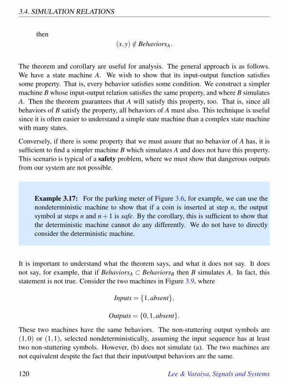
3.4. SIMULATION RELATIONS
then(x,y) /∈ BehaviorsA.
The theorem and corollary are useful for analysis. The general approach is as follows.We have a state machine A. We wish to show that its input-output function satisfiessome property. That is, every behavior satisfies some condition. We construct a simplermachine B whose input-output relation satisfies the same property, and where B simulatesA. Then the theorem guarantees that A will satisfy this property, too. That is, since allbehaviors of B satisfy the property, all behaviors of A must also. This technique is usefulsince it is often easier to understand a simple state machine than a complex state machinewith many states.
Conversely, if there is some property that we must assure that no behavior of A has, it issufficient to find a simpler machine B which simulates A and does not have this property.This scenario is typical of a safety problem, where we must show that dangerous outputsfrom our system are not possible.
Example 3.17: For the parking meter of Figure 3.6, for example, we can use thenondeterministic machine to show that if a coin is inserted at step n, the outputsymbol at steps n and n+1 is safe. By the corollary, this is sufficient to show thatthe deterministic machine cannot do any differently. We do not have to directlyconsider the deterministic machine.
It is important to understand what the theorem says, and what it does not say. It doesnot say, for example, that if BehaviorsA ⊂ BehaviorsB then B simulates A. In fact, thisstatement is not true. Consider the two machines in Figure 3.9, where
Inputs = 1,absent,
Outputs = 0,1,absent.
These two machines have the same behaviors. The non-stuttering output symbols are(1,0) or (1,1), selected nondeterministically, assuming the input sequence has at leasttwo non-stuttering symbols. However, (b) does not simulate (a). The two machines arenot equivalent despite the fact that their input/output behaviors are the same.
120 Lee & Varaiya, Signals and Systems

3. STATE MACHINES
To see this, we play the matching game. Machine (a) is allowed to move first. Ignoringstuttering, it has no choice but to move from a to b and produce output symbol 1. Machine(b) can match this two ways; it has no basis upon which to prefer one way to match it overanother, so it picks one, say moving to state f . Now it is the turn of machine (a), whichhas two choices. If it choses to move to d, then machine (b) cannot match its move. (Asimilar argument works if (b) picks state h.) Thus, machine (b) does not simulate machine(a), despite the fact that BehaviorsA ⊂ BehaviorsB.2
3.5 Summary
State machines are models of systems whose input and output signal spaces consist of se-quences of symbols. There are three ways of defining state machines: sets and functions,state transition diagram, and the update table. The state machine model gives a step-by-step procedure for evaluating the output signal. This is a state-determined system: oncewe know the current state, we can tell the future behavior for any future input symbols.
A state machine can be non-deterministic: given the current state and current input sym-bol, it may have more than one possible next state and current output symbol. Non-determistic machines typically arise through abstraction of deterministic machines. Twostate machines, with the same input and output alphabets, may be related through simula-tion. Simulation is used to understand properties of the behavior of one machine in termsof the behaviors of another (presumably simpler) machine.
2Recall that in our notation ⊂ allows the two sets to be equal.
Lee & Varaiya, Signals and Systems 121

3.5. SUMMARY
inputs
ring - incoming ringing signaloffhook - a telephone extension is picked upend greeting - greeting message is finished playingend message - end of message detected (e.g. dialtone)absent - no input of interest.
outputs
answer - answer the phone and start the greeting messagerecord - start recording the incoming messagerecorded- recorded an incoming messageabsent - default output when there is nothing interesting to say
idle
count1 count2ring
ring
ring /answer
else
else
playgreeting
end greeting /recordrecording
end message, offhook /recorded
else
else
else
states
idle: nothing is happeningcount1: one ring has arrivedcount2: two rings have arrivedplay greeting: playing the greeting messagerecording : recording the message
absent
absent
absent
absent
Figure 3.1: State transition diagram for a telephone answering service.
122 Lee & Varaiya, Signals and Systems

3. STATE MACHINES
state
guard1/output1
guard2/output2
else
initial state indicator
-0.2in
-0.2in
state machine:(States, Inputs,Outputs,update, initialState)update : States× Inputs→ States×OutputsinitialState ∈ States
elements:state ∈ Statesoutput1,output2 ∈ Outputsguard1,guard2⊂ Inputselse = i ∈ Inputs | i /∈ (guard1∪guard2)determinacy: (There is at most one possible reaction to an input symbol)guard1∩guard2 = /0
-0.2in
Figure 3.2: Summary of notation in state transition diagrams, shown for a singlestate with two outgoing arcs and one self loop.
Lee & Varaiya, Signals and Systems 123

3.5. SUMMARY
current (next state, output symbol) under specified input symbolstate ring offhook end greeting end message absentidle (count1, (idle, (idle, (idle, (idle,
absent) absent) absent) absent) absent)count1 (count2, (idle, (idle, (idle, (count1,
absent) absent) absent) absent) absent)count2 (play greeting, (idle, (idle, (idle, (count2,
answer) absent) absent) absent) absent)play greeting (idle, (idle, (recording, (idle, (play greeting,
absent) absent) record) absent) absent)recording (idle, (idle, (idle, (idle, (recording,
absent) recorded) absent) recorded) absent)
Figure 3.3: Update table for the telephone answering service specifies next stateand current output symbol as a function of current state and current input symbol.
start 1 11
1 1
00
1100/recognize
1
0
1
Figure 3.4: A machine that implements CodeRecognizer . It outputs recognize atthe end of every input subsequence 1100, otherwise it outputs absent .
124 Lee & Varaiya, Signals and Systems

3. STATE MACHINES
a b
1/1
0/0
0,1/1 0/0
Figure 3.5: A simple nondeterministic state machine.
0 1
coin5/safe
tick/expired
5
tick/expired
tick/safe
...
coin5/safe
... 25
tick/safe
coin25/safe coin25/safe
60
tick/safe
...
coin5,coin25/
safecoin5/
safe
coin25/safe
coin5/safe
0
tick/expired
1
tick/expired
more
tick/safe
coin5, coin25 / safe
coin5, coin25 /safe
coin5, coin25, tick /safe
(a)
(b)
Figure 3.6: Deterministic and nondeterministic models for a 60 minute parkingmeter.
Lee & Varaiya, Signals and Systems 125
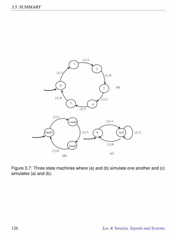
3.5. SUMMARY
1/1
1/1
1/0
1/1
1/1
1/0
0
1
2
3
45
0and3
1and4
2and51/0
1/1
1/1
1/1
1/0
1/10 1to5
(a)
(b)(c)
Figure 3.7: Three state machines where (a) and (b) simulate one another and (c)simulates (a) and (b).
126 Lee & Varaiya, Signals and Systems

3. STATE MACHINES
0 1
1/0
1/1
2
1/1
1/0
3
1/0
1/1
0and2 1and3
1/0
1/1
(a)
(b)
0to3
(c)
1/0
1/1
Figure 3.8: Three state machines where (a) and (b) simulate each other and (c)simulates (a) and (b)
Lee & Varaiya, Signals and Systems 127
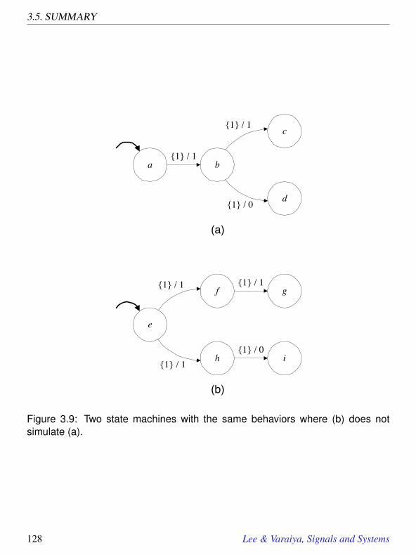
3.5. SUMMARY
a b
c
d
1 / 1
1 / 1
1 / 0
(a)
g
e
f
h
1 / 1
1 / 1
(b)
1 / 1
i1 / 0
Figure 3.9: Two state machines with the same behaviors where (b) does notsimulate (a).
128 Lee & Varaiya, Signals and Systems

3. STATE MACHINES
Exercises
In some of the following exercises you are asked to design state machines that carryout a given task. The design is simple and elegant if the state space is properly chosen.Although the state space is not unique, there often is a natural choice. As usual, eachproblem is annotated with the letter E, T, C which stands for exercise, requires somethought, requires some conceptualization. Problems labeled E are usually mechanical,those labeled T require a plan of attack, those labeled C usually have more than onedefensible answer.
1. E A state machine with
Inputs = a,b,c,d,absent,has a state s with two emerging arcs with guards
guard1 = aand
guard2 = a,b,d.
(a) Is this state machine deterministic?(b) Define the set else for state s and specify the source and destination state for
the else arc.
2. E For the answering service example of figure 3.1, assume the input sequence is
(offhook,offhook,ring,offhook,ring,ring,ring,offhook, · · ·).This corresponds to a user of the answering service making two phone calls, an-swering a third after the first ring, and answering a second after the third ring.
(a) Give the state response of the answering service.(b) Give the trace of the answering service.(c) Give the output sequence.
3. E Consider the alphabets
Inputs = Outputs = Binary = 0,1.Note that there is no stuttering input or output symbols here. This simplifies thenotation in the problem somewhat.
Lee & Varaiya, Signals and Systems 129

EXERCISES
(a) Construct a state machine that uses these alphabets such that given any inputsequence (x(0),x(1), · · ·) without stuttering symbols, the output sequence isgiven by, ∀ n ∈ N0,
y(n) =
1 if n≥ 2∧ (x(n−2),x(n−1),x(n)) = (1,1,1)0 otherwise
In words, the machine outputs 1 if the current input symbol and the two pre-vious input symbols are all 1’s, otherwise it outputs 0. (Had we included astuttering symbol, the above equation would be a bit more complicated.)
(b) For the same input and output alphabet, construct a state machine that out-puts 1 if the current input symbol and two previous input symbols are either(1,1,1) or (1,0,1), and otherwise it outputs 0.
4. E A modulo N counter is a device that can output any integer between 0 andN−1. The device has three input symbols, increment, decrement, and reset, plus,as always, a stuttering symbol absent; increment increases the output integer by 1;decrement decreases this integer by 1; and reset sets the output symbol to 0. Hereincrement and decrement are modulo N operations. Unless otherwise stated, youmay assume that the counter begins at 0.
Note: Modulo N numbers work as follows. For any integer m, m mod N = k where0≤ k≤N−1 is the unique integer such that N divides (m−k). Thus there are onlyN distinct modulo-N numbers, namely, 0, · · · ,N−1.
(a) Give the state transition diagram of this counter for N = 4.(b) Give the update table of this counter for N = 4.(c) Give a description of the state machine by specifying the five entities that
appear in (3.1); again assume N = 4.(d) Take N = 3. Calculate the state response for the input sequence
(increment4,decrement3, · · ·)starting with initial state 1, where sn means s repeated n times. You may givethe state response for the first seven reactions only.
5. T The state machine UnitDelay is defined to behave as follows. On the first non-stuttering reaction (when the first non-stuttering input symbol arrives), the outputsymbol a is produced. On subsequent reactions (when subsequent input symbolsarrive), the input symbol that arrived at the previous non-stuttering reaction is pro-duced as an output symbol.
130 Lee & Varaiya, Signals and Systems

3. STATE MACHINES
(a) Assume the input and output alphabets are
Inputs = Outputs = a,b,c,absent.Give a finite state machine that implements UnitDelay for this input set. Giveboth a state transition diagram and a definition of each of the components in(3.1).
(b) Assume the input and output sets are
Inputs = Outputs = N0∪absent,and that on the first non-stuttering reaction, the machine produces 0 insteadof a. Give an (informal) argument that no finite state machine can implementUnitDelay for this input set. Give an infinite state machine by defining eachof the components in (3.1).
6. T Construct an infinite state machine that realizes Equal.
7. C An elevator connects two floors, 1 and 2. It can go up (if it is on floor 1), down(if it is on floor 2) and stop on either floor. Passengers at any floor may press abutton requesting service. Design a controller for the elevator so that (1) everyrequest is served, and (2) if there is no pending request, the elevator is stopped.For simplicity, do not be concerned about responding to requests from passengersinside the elevator.
8. T The state machine in Figure 3.10 has the property that it outputs at least one1 between any two 0’s. Construct a two-state nondeterministic state machine thatsimulates this one and preserves that property.
0 1
1/ 0
0/ 1
2
1/ 1
0/ 1
3
1/ 1
0/ 1
1/ 1 0/ 1
Figure 3.10: Machine that outputs at least one 1 between any two 0’s.
Lee & Varaiya, Signals and Systems 131

EXERCISES
9. T For the nondeterministic state machine in Figure 3.11 the input and output al-phabets are
Inputs = Outputs = 0,1,absent.
(a) Define the possibleUpdates function (3.9) for this state machine.
(b) Define the relation Behaviors in (3.11) for this state machine. Part of the chal-lenge here is to find a way to describe this relation compactly. For simplicity,ignore stuttering; i.e. assume the input symbol is never absent.
10. E The state machine in Figure 3.12 implements CodeRecognizer, but has morestates than the one in Figure 3.4. Show that the two machines simulate each otherby giving simulation relations.
11. E The state machine in Figure 3.13 has input and output alphabets
Inputs = 1,a,
Outputs = 0,1,a,where a (short for absent) is the stuttering symbol. State whether each of the fol-lowing is in the set Behaviors for this machine. In each of the following, the ellipsis
A
B 1/1
1/0
0,1/1
C
0,1/0
0/0
Figure 3.11: Nondeterministic state machine for Exercise 9.
132 Lee & Varaiya, Signals and Systems

3. STATE MACHINES
“· · ·” means that the last symbol is repeated forever. Also, in each case, the inputand output signals are given as sequences.
(a) ((1,1,1,1,1, · · ·),(0,1,1,0,0, · · ·))
start 1 11
1 1
00
110
0/recognize
1100
0
1
1
0
1
Figure 3.12: A machine that implements CodeRecognizer , but has more statesthan the one in Figure 3.4.
a b1 / 0
c1 / 0
1 / 1
Figure 3.13: State machine for problem 11.
Lee & Varaiya, Signals and Systems 133

EXERCISES
(b) ((1,1,1,1,1, · · ·),(0,1,1,0,a, · · ·))(c) ((a,1,a,1,a, · · ·),(a,1,a,0,a, · · ·))(d) ((1,1,1,1,1, · · ·),(0,0,a,a,a, · · ·))(e) ((1,1,1,1,1, · · ·),(0,a,0,a,a, · · ·))
12. E The state machine in Figure 3.14 has
Inputs = 1,absent,
Outputs = 0,1,absent.
Find a state machine with only two states that simulates the one in Figure 3.14 andthat is simulated by the one in Figure 3.14, and give the simulation relations.
13. E You are told that state machine A has
Inputs = 1,2,absent,
Outputs = 1,2,absent,
States = a,b,c,d.
but you are told nothing further. Do you have enough information to construct astate machine B that simulates A? If so, give such a state machine, and the simula-tion relation.
a
b
d
1 / 1
c
1 / 0
1 / 11 / 0
Figure 3.14: A machine that has more states than it needs.
134 Lee & Varaiya, Signals and Systems

3. STATE MACHINES
14. E Construct a state machine with Inputs = 0,1,absent, Outputs = r,absent,that outputs r whenever the input signal (without stuttering symbols) contains thesequence (0,0,0), otherwise it outputs absent. More precisely, if x=(x(0),x(1), · · ·)is the input sequence then y = (y(0),y(1), · · ·) is the output sequence, where
y(n) =
r, if (x(n−2),x(n−1),x(n)) = (0,0,0)absent otherwise
15. T Consider a state machine where
Inputs = 1,absent,
Outputs = 0,1,absent,States = a,b,c,d,e, f,
initialState = a,
and the update function is given by the following table (ignoring stuttering):
(currentState, inputSymbol) (nextState,outputSymbol)(a,1) (b,1)(b,1) (c,0)(c,1) (d,0)(d,1) (e,1)(e,1) ( f ,0)( f ,1) (a,0)
(a) Draw the state transition diagram for this machine.
(b) Ignoring stuttering, give the Behaviors relation for this machine.
(c) Find a state machine with three states that simulates this one and that is simu-lated by this one. Draw that state machine, and give the simulation relations.
Lee & Varaiya, Signals and Systems 135

4Composing State Machines
Contents4.1 Synchrony . . . . . . . . . . . . . . . . . . . . . . . . . . . . . . . 1384.2 Side-by-side composition . . . . . . . . . . . . . . . . . . . . . . . 1394.3 Cascade composition . . . . . . . . . . . . . . . . . . . . . . . . . 1434.4 Product-form inputs and outputs . . . . . . . . . . . . . . . . . . . 1484.5 General feedforward composition . . . . . . . . . . . . . . . . . . 1514.6 Hierarchical composition . . . . . . . . . . . . . . . . . . . . . . . 1544.7 Feedback . . . . . . . . . . . . . . . . . . . . . . . . . . . . . . . . 155
4.7.1 Feedback composition with no inputs . . . . . . . . . . . . . 1574.7.2 State-determined output . . . . . . . . . . . . . . . . . . . . 1634.7.3 Feedback composition with inputs . . . . . . . . . . . . . . . 1674.7.4 Constructive procedure for feedback composition . . . . . . . 1714.7.5 Exhaustive search . . . . . . . . . . . . . . . . . . . . . . . . 1754.7.6 Nondeterministic machines . . . . . . . . . . . . . . . . . . . 175Probing Further: Constructive Semantics . . . . . . . . . . . . . . . 176
4.8 Summary . . . . . . . . . . . . . . . . . . . . . . . . . . . . . . . . 177Exercises . . . . . . . . . . . . . . . . . . . . . . . . . . . . . . . . . . . 179
We design interesting systems by composing simpler components. Since systems arefunctions, their composition is function composition, as discussed in Section 2.1.5. Statemachines, however, are not given directly as functions that map input sequences intooutput sequences. Instead, they are given procedurally, where the update function defines
137

4.1. SYNCHRONY
how to progress from one state to the next. This chapter explains how to define a newstate machine that describes a composition of multiple state machines.
In Section 2.3.4 we used a block diagram syntax to define compositions of systems. Wewill use the same syntax here, and we will similarly build up an understanding of compo-sition by first considering easy cases. The hardest cases are those where there is feedback,because the input of one state machine may depend on its own output. It is challengingin this case to come up with a procedure for updating the state of the composite machine.For some compositions, in fact, it isn’t even possible. Such compositions are said to beill-formed.
4.1 Synchrony
We consider a set of interconnected components, where each component is a state ma-chine. By “interconnected” we mean that the outputs of one component may be inputsof another. We wish to construct a state machine model for the composition of compo-nents. Composition has two aspects. The first aspect is straightforward: it specifies whichoutputs of one component are the inputs of another component. These input-output con-nections are specified using block diagrams.
The second aspect of composition concerns the timing relationships between inputs andoutputs. We choose a particular style of composition called synchrony. This style dictatesthat each state machine in the composition reacts simultaneously and instantaneously. Soa reaction of the composite machine consists of a set of simultaneous reactions of each ofthe component machines.
A reaction of the composite machine is triggered by inputs from the environment. Thus,when a reaction occurs is externally determined. This is the same as for a single machine.As with a single state machine, a composite machine may stutter. This simply means thateach component machine stutters.
A system that reacts only in response to external stimulus is said to be reactive. Becauseour compositions are synchronous, they are often called synchronous/reactive systems.
The reactions of the component machines and of the composite machine are viewed asbeing instantaneous. That is, a reaction does not take time. In particular, the output sym-bol from a state machine is viewed as being simultaneous with the input symbol, withoutdelay. This creates some interesting subtleties, especially for feedback composition when
138 Lee & Varaiya, Signals and Systems

4. COMPOSING STATE MACHINES
the input of a state machine is connected to its own output. We will discuss the ramifica-tions of the synchronous/reactive interpretation below.
Synchrony is a very useful model of the behavior of physical systems. Digital circuits,for example, are almost always designed using this model. Circuit elements are viewedas taking no time to calculate their outputs given their inputs, and time overall is viewedas progressing in a sequence of discrete time steps according to ticks of a clock. Ofcourse, the time that it takes for a circuit element to produce an output cannot ultimatelybe ignored, but the model is useful because for most circuit elements in a complex design,this time can be ignored. Only the time delay of the circuit elements along a critical pathaffects the overall performance of the circuit.
More recently than for circuits, synchrony has come to be used in software as well. Con-current software modules interact according to the synchronous model. Languages builton this principle are called synchronous languages. They are used primarily in real-timeembedded system1 design.
4.2 Side-by-side composition
A simple form of composition of two state machines is shown in figure 4.1. We call thisside-by-side composition. Side-by-side composition in itself is not useful, but it is usefulin combination with other types of composition. The two state machines in Figure 4.1do not interact with one another. Nonetheless we wish to define a single state machinerepresenting the synchronous operation of the two component state machines.
The state space of the composite state machine is simply
States = StatesA×StatesB.
We could take the cross product in the opposite order, resulting in a different but bisimilarcomposite state machine. The initial state is
initialState = (initialStateA, initialStateB).
1An embedded system is a computing system (a computer and its software) that is embedded in a largersystem that is not first and foremost a computer. A digital cellular telephone, for example, contains computersthat realize the radio modem and the speech codec. Recent cars contain computers for ignition control, anti-lock brakes, and traction control. Aircraft contain computers for navigation and flight control. In fact, mostmodern electronic controllers of physical systems are realized as embedded systems.
Lee & Varaiya, Signals and Systems 139

4.2. SIDE-BY-SIDE COMPOSITION
The input and output alphabets are
Inputs = InputsA× InputsB, (4.1)
Outputs = OutputsA×OutputsB. (4.2)
The update function of the composite machine, update, consists of the update functionsof the component machines, side-by-side:
((sA(n+1),sB(n+1)),(yA(n),yB(n))) = update((sA(n),sB(n)),(xA(n),xB(n))),
(StatesB, InputsB, OutputsB, updateB, initialStateB )
(StatesA, InputsA, OutputsA, updateA, initialStateA )
(States, Inputs, Outputs, update, initialState )
-0.2in
-0.2in
Definition of the side-by-side composite machine:States = StatesA×StatesB
Inputs = InputsA× InputsBOutputs = OutputsA×OutputsBinitialState = (initialStateA, initialStateB)((sA(n+1),sB(n+1)),(yA(n),yB(n)))= update((sA(n),sB(n)),(xA(n),xB(n))),
where
(sA(n+1),yA(n)) = updateA(sA(n),xA(n)) and(sB(n+1),yB(n)) = updateB(sB(n),xB(n))
-0.2in
Figure 4.1: Summary of side-by-side composition of state machines.
140 Lee & Varaiya, Signals and Systems

4. COMPOSING STATE MACHINES
where(sA(n+1),yA(n)) = updateA(sA(n),xA(n)),
and(sB(n+1),yB(n)) = updateB(sB(n),xB(n)).
Recall that InputsA and InputsB include a stuttering element. This is convenient because itallows a reaction of the composite when we really want only one of the machines to react.Suppose the stuttering elements are absentA and absentB. Then if the second componentof the input symbol is absentB, the reaction of the composite consists only of the reactionof the first machine. The stuttering element of the composite is the pair of stutteringelements of the component machines, (absentA,absentB).
Example 4.1: The side-by-side composition in the top of Figure 4.2 has the com-posite machine with state space
States = StatesA×StatesB = (1,1),(2,1),
and alphabets
Inputs = (0,0),(1,0),(absentA,0),(0,absentB),(1,absentB),(absentA,absentB),
Outputs = (a,c),(b,c),(absentA,c),(a,absentB),(b,absentB),(absentA,absentB).
The initial state isinitialState = (1,1).
The update function can be given as a table, only a part of which is displayed below.The state transition diagram in the lower part of Figure 4.2 gives the same part ofthe update function.
current (next state, output) for inputstate (0,0) (1,0) (absentA,0) · · ·(1,1) ((1,1),(a,c)) ((2,1),(b,c)) ((1,1)((absentA,c)) · · ·(2,1) ((2,1),(b,c)) ((1,1),(a,c)) ((2,1), ((absentA,c)) · · ·
Lee & Varaiya, Signals and Systems 141

4.2. SIDE-BY-SIDE COMPOSITION
Notice that if the second component of the input sequence is always absentB, thenthe side-by-side composition behaves essentially as machine A, and if the first com-
A
1 2
1/b 0/ b0/ a
1/a
B
1
0/ c
0, 1, absentA
0, absentB c, absentB
A
(1,1) (2,1)(1,0)/(b, c)
(0,0)/(b, c)
(0,0)/(a, c)
(1,0)/(a, c)
(absentA, 0)/(absentA, c)
(absentA, 0)/(absentA, c)
(1,absentB)/(b, absentB)
(1,absentB)/(a, absentB)
0, 1, absentA
0, absentB
a, b, absentA
c, absentB
a, b, absentA
Figure 4.2: Example of a side-by-side composition.
142 Lee & Varaiya, Signals and Systems

4. COMPOSING STATE MACHINES
ponent is always absentA, then it behaves as machine B. The stuttering element ofthe composite is of course the pair (absentA,absentB).
4.3 Cascade composition
We now interconnect two state machines as shown in Figure 4.3, where the output of oneis the input of the other. This is called a cascade composition or a series connection. Wedefine the composition so that the component machines react together, synchronously, asone state machine.
Suppose the two state machines are given by
StateMachineA = (StatesA, InputsA,OutputsA,updateA, initialStateA)
andStateMachineB = (StatesB, InputsB,OutputsB,updateB, initialStateB).
Let the composition be given by
StateMachine = (States, Inputs,Outputs,update, initialState).
Clearly, for a composition like that in Figure 4.3 to be possible we must have
OutputsA ⊂ InputsB.
Then any output sequence produced by machine A can be an input sequence for machineB. As a result,
OutputSignalsA ⊂ InputSignalsB.
This is analogous to a type constraint in programming languages, where in order for twopieces of code to interact, they must use compatible data types. We encountered a similarconstraint in discussing function composition, Section 2.1.5.
We are ready to construct a state machine model for this series connection. As noted inthe figure, the input alphabet of the composite is
Inputs = InputsA.
Lee & Varaiya, Signals and Systems 143

4.3. CASCADE COMPOSITION
The stuttering element of Inputs, of course, is just the stuttering element of InputsA. Theoutput alphabet of the composite is
Outputs = OutputsB.
(StatesB, InputsB, OutputsB, updateB, initialStateB )
(StatesA, InputsA, OutputsA, updateA, initialStateA )
(States, Inputs, Outputs, update, initialState )
-0.2in
-0.2in
Assumptions about the component machines:OutputsA ⊂ InputsB
Definition of the cascade composite machine:States = StatesA×StatesB
Inputs = InputsAOutputs = OutputsBinitialState = (initialStateA, initialStateB)((sA(n+1),sB(n+1)),yB(n)) = update((sA(n),sB(n)),x(n)),
where
(sA(n+1),yA(n)) = updateA(sA(n),x(n)) and(sB(n+1),yB(n)) = updateB(sB(n),yA(n)).
-0.2in
Figure 4.3: Summary of cascade composition of state machines.
144 Lee & Varaiya, Signals and Systems

4. COMPOSING STATE MACHINES
The state space of the composite state machine is the product set
States = StatesA×StatesB. (4.3)
This asserts that the composite state machine is in state (sA(n),sB(n)) when the StateMachineA
is in state sA(n) and StateMachineB is in state sB(n). The initial state is
initialState = (initialStateA, initialStateB).
We could equally well have defined the states of the composite state machine in the op-posite order,
States = StatesB×StatesA.
This would result in a different but bisimilar state machine description (either one simu-lates the other). Intuitively, it does not matter which of these two choices we make, andwe choose (4.3).
To complete the description of the composite machine, we need to define its update func-tion in terms of the component machines. Here, a slight subtlety arises. Since we areusing synchronous composition, the output symbol of machine A is simultaneous withits input symbol. Thus, in a reaction, the output symbol of machine A in that reactionmust be available to machine B in the same reaction. This seems intuitive, but it has somecounterintuitive consequences. Although the reactions of machine A and B are simulta-neous, we must determine the reaction of A before we can determine the reaction of B.This apparent paradox is an intrinsic feature of synchronous composition. We will have todeal with it carefully in feedback composition, where it is not immediately evident whichreactions need to be determined first.
In the cascade composition, it is intuitively clear what we need to do to define the updatefunction. We first determine the reaction of machine A. Suppose that at the n-th reactionthe input symbol is x(n) and the state is s(n) = (sA(n),sB(n)), where sA(n) is the state ofmachine A and sB(n) is the state of machine B. Machine A reacts by updating its state tosA(n+1) and producing output symbol yA(n),
(sA(n+1),yA(n)) = updateA(sA(n),x(n)). (4.4)
Its output symbol yA(n) becomes the input symbol to machine B. Machine B reacts byupdating its state to sB(n+1) and producing output symbol yB(n),
(sB(n+1),yB(n)) = updateB(sB(n),yA(n)). (4.5)
Lee & Varaiya, Signals and Systems 145

4.3. CASCADE COMPOSITION
The output of the composite machine, of course, is just the output of machine B, andthe next state of the composite machine is just (sA(n+ 1),sB(n+ 1)), so the compositemachine’s update is
((sA(n+1),sB(n+1)),yB(n)) = update((sA(n),sB(n)),x(n)),
where sA(n+ 1), sB(n+ 1), and yB(n) are given by (4.4) and (4.5). The definition of thecomposite machine is summarized in Figure 4.3.
Example 4.2: The cascade composition in Figure 4.4 has the composite machinewith state space
States = StatesA×StatesB = (0,0),(0,1),(1,0),(1,1))
A
0 1
1/1
1/0
0/0
0,1,absent
Inputs =0,1,absent
Outputs=0,1,absent
0/1
B
0 1
1/1
0/1
0/0 1/0
0,0
1,1
1/1
1/1
0/0
Inputs =0,1,absent
0/0
Outputs=0,1,absent
1,01/0
0/10/1
1/00,1
Figure 4.4: Example of a cascade composition. The composed state machine ison the right.
146 Lee & Varaiya, Signals and Systems

4. COMPOSING STATE MACHINES
and alphabetsInputs = Outputs = 0,1,absent.
The initial state isinitialState = (0,0).
The update function is given by the table:
current (next state, output) for inputstate 0 1 absent(0,0) ((0,0),0) ((1,1),1) ((0,0), absent)(0,1) ((0,0),1) ((1,1),0) ((0,1), absent)(1,0) ((1,1),1) ((0,0),0) ((1,0), absent)(1,1) ((1,1),0) ((0,0),1) ((1,1), absent)
The update function is also presented in the state transition diagram of Figure 4.4.The self-loops corresponding to the stuttering input symbol absent are not shownin the diagram.
Observe from the table or the diagram that states (0,1) and (1,0) are not reachablefrom the initial state. A state s is said to be reachable if some sequence of inputsymbols can take the state machine from the initial state to s. This suggests that asimpler machine with fewer states would exhibit the same input/output behaviors.In fact, notice from the table that the input is always equal to the output! A trivialone-state machine can exhibit the same input/output behaviors. (Exercise 8 gives aprocedure for calculating the reachable states of an arbitrary state machine.)
The simple behavior of the composite machine is not immediately apparent fromFigure 4.4. We have to systematically construct the composite machine to derivethis simple behavior. In fact, this composite machine can be viewed as an encoderand decoder, because the input bit sequence is encoded by a distinctly differentbit sequence (the intermediate signal in Figure 4.4), and then the second machine,given the intermediate signal, reconstructs the original.
This particular encoder is known as a differential precoder. It is “differential” inthat when the input symbol is 0, the intermediate signal sample is unchanged fromthe previous sample (whether it was 0 or 1), and when the input symbol is 1, thesample is changed. Thus, the input symbol indicates change in the input with a 1,and no change with a 0. Differential precoders are used when it is important that
Lee & Varaiya, Signals and Systems 147

4.4. PRODUCT-FORM INPUTS AND OUTPUTS
the average number of 1’s and 0’s is the same, regardless of the input sequence thatis encoded.
4.4 Product-form inputs and outputs
In the state machine model of (3.1), at each step the environment selects one input symbolto which the machine reacts and produces one output symbol. Sometimes we wish tomodel the fact that some input values are selected by one part of the environment, whileother input values are simultaneously selected by another part. Also, some output valuesare sent to one part of the environment, while other output values are simultaneously sentto another part. The product-form composition permits these models.
The machine in Figure 4.5 is shown as a block with two distinct input and output arrows.The figure suggests that the machine receives inputs from two sources and sends outputsto two destinations. In the answering machine example of Chapter 3, for instance, theend greeting input value might originate in a physically different piece of hardware in themachine than the offhook value.
The distinct arrows into and out of a block are called ports. Each port has a set of valuescalled the port alphabet associated with it, as shown in figure 4.5. Each port alphabetmust include a stuttering element. The set Inputs of input values to the state machineis the product of the input sets associated with the ports. Of course, the product can beconstructed in any order; each ordering results in a distinct (but bisimilar) state machinemodel.
InputsB
InputsA(States, Inputs, Outputs, update, initialState )
OutputsA
OutputsBInputs = InputsA × InputsB
Outputs = OutputsA × OutputsB
Figure 4.5: State machine with product-form inputs and outputs.
148 Lee & Varaiya, Signals and Systems

4. COMPOSING STATE MACHINES
In Figure 4.5 there are two input ports and two output ports. The upper input port canpresent to the state machine any value in the alphabet InputsA, which includes absent, itsstuttering element. The lower port can present any value in the set InputsB, which alsoincludes absent. The input value actually presented to the state machine in a reaction istaken from the set
Inputs = InputsA× InputsB.
The stuttering element for this alphabet is the pair (absent,absent). The output valueproduced by a reaction is taken from the set
Outputs = OutputsA×OutputsB.
If the output of the n-th reaction is (yA(n),yB(n)), then the upper port shows yA(n) and thelower port shows yB(n). These can now be separately presented as inputs to downstreamstate machines. Again, the stuttering element is (absent,absent).
Example 4.3: The answering machine of Figure 3.1 has input alphabet
Inputs = ring,offhook,end greeting,end message.
In a typical realization of an answering machine, ring and offhook come from a sub-system (often an ASIC, or application-specific integrated circuit) that interfacesto the telephone line. The value end greeting comes from another subsystem, suchas a magnetic tape machine or digital audio storage device, that plays the answermessage. The value end message comes from a similar, but distinct, subsystem thatrecords incoming messages. So a more convenient model will show three separatefactors for the inputs, as in figure 4.6. That figure also shows the outputs in prod-uct form, anticipating that the distinct output values will need to be sent to distinctsubsystems.
Several features distinguish the diagram in Figure 4.6 from that of Figure 3.1. Eachstate except the idle state has acquired a self-loop labeled stutter, which is a namefor the guard
stutter = (absent,absent,absent).This self loop prevents the state machine from returning to the idle state (via theelse transition) when nothing interesting is happening on the inputs. Usually, therewill not be a reaction if nothing interesting is happening on the inputs, but because
Lee & Varaiya, Signals and Systems 149

4.4. PRODUCT-FORM INPUTS AND OUTPUTS
of synchrony, this machine may be composed with others, and all machines haveto react at the same time. So if anything interesting is happening elsewhere in thesystem, then this machine has to react even though nothing interesting is happeninghere. Recall that such a reaction is called a stutter. The state does not change, andthe output symbol produced is the stuttering element of the output alphabet.
Each guard now consists of a set of triples, since the product-form input has threecomponents. The shorthand “(*, offhook, *)” on the arc from the record message
idle
count1
count2
( absent , ring , absent ) ( absent , ring , absent )
( absent , ring , absent )/ ( answer , absent , absent )
else
else play greeting
( end greeting , absent , absent )/ ( absent , absent , record )
record message
else /( absent , recorded , absent )
else
(*, offhook ,*)
rin
g , o
ff h o o
k , a
b s e n
t
e n d
m e s
s a g e
, a b s
e n t
r e c
o r d e
d ,
a b s e
n t
else
e n d
g r e
e t i n
g , a
b s e n
t
a n s
w e r
, a b s
e n t
r
e c o r
d , a
b s e n
t
stutter
stutter
stutter
stutter
NOTE : stutter = ( absent , absent , absent )
Figure 4.6: Answering machine with product-form inputs and outputs has threeinput ports and three output ports.
150 Lee & Varaiya, Signals and Systems

4. COMPOSING STATE MACHINES
state to the idle state represents a set,
(∗,offhook,∗) = (absent,offhook,absent),
(end greeting,offhook,absent),
(absent,offhook,end message),
(end greeting,offhook,end message).
The “*” is a don’t care or wildcard notation. Anything in its position will triggerthe guard.
Because there are three output ports, the output symbols are also triples, but mostof them are implicitly (absent,absent,absent).
4.5 General feedforward composition
Given that state machines can have product-form inputs and outputs, it is easy to constructa composition of state machines that combines features of both the cascade compositionof Figure 4.3 and the side-by-side composition of Figure 4.1. An example is shown in
(StatesB, InputsB, OutputsB, updateB, initialStateB )
(StatesA, InputsA, OutputsA, updateA, initialStateA )
(States, Inputs, Outputs, update, initialState )
InputsAOutputsA1
OutputsA2 ⊂ InputsB1
InputsB2OutputsB
OutputsA2
Figure 4.7: More complex composition.
Lee & Varaiya, Signals and Systems 151

4.5. GENERAL FEEDFORWARD COMPOSITION
Figure 4.7. In that figure,
OutputsA = OutputsA1×OutputsA2
InputsB = InputsB1× InputsB2.
Notice that the bottom port of machine A goes both to the output of the composite machineand to the top port of machine B. Sending a value to multiple destinations like this is calledforking. In Exercise 1 at the end of this chapter you are asked to define the compositemachine for this example.
Example 4.4: We compose the answering machine of figure 4.6 with a playbacksystem, shown in Figure 4.8, which plays messages that have been recorded bythe answering machine. The playback system receives the recorded input symbolfrom the answering machine whenever the answering machine is done recordinga message. Its task is to light an indicator that a message is pending, and to waitfor a user to press a play button on the answering machine to request that pendingmessages be played back. When that button is pressed, all pending messages areplayed back. When they are done being played back, then the indicator light isturned off.
nomessages
messagepending
playing
(recorded ,*,*)/(light on, absent)
(*,play,*)/(absent, play messages)
(*, *, done playing)/(light off, absent)
else
else
else
recorded ,absent
play, absent
done playing, absent
light on, light off, absent
play messages, absent
Figure 4.8: Playback system for composing with the answering machine.
152 Lee & Varaiya, Signals and Systems

4. COMPOSING STATE MACHINES
The composition is shown in Figure 4.9. The figure shows a number of other com-ponents, not modeled as state machines, to help understand how everything worksin practice. These other components are shown as three-dimensional objects, toemphasize their physicality. We have simplified the figure by omitting the absentelements of all the sets. They are implicit.
A telephone line interface provides ring and offhook when these are detected. De-tection of one of these can trigger a reaction of the composite machine. In fact, anyoutput symbol from any of the physical components can trigger a reaction of thecomposite machine. When AnsweringMachine generates the answer output sym-
telephoneline
interface
greetingplayback device
light
playbutton
message playbackdevice
end greeting
ring, offhook
end message
AnsweringMachine
answer
recorded message
Playback
play
light on, light off
done playing play messages
recording device
record
Figure 4.9: Composition of an answering machine with a message playback ma-chine. The three-dimensional boxes are physical components that are not mod-eled as state machines. They are the sources of some inputs and the destinationsof some outputs.
Lee & Varaiya, Signals and Systems 153

4.6. HIERARCHICAL COMPOSITION
bol, then the “greeting playback device” plays back the greeting. From the perspec-tive of the state machine model, all that happens is that time passes (during whichsome reactions may occur), and then an end greeting input symbol is received. Therecording device works similarly. When AnsweringMachine generates a recordedoutput symbol, then the Playback machine will respond by lighting the indicatorlight. When a user presses the play button the input symbol play is generated, thecomposite machine reacts, and the Playback machine issues a play messages out-put symbol to the “message playback device.” This device also allows time to pass,then generates a done playing input symbol to the composite state machine.
If we wish to model the playback or recording subsystem in more detail using finitestate machines, then we need to be able to handle feedback compositions. Theseare considered below.
4.6 Hierarchical composition
By using the compositions discussed above, we can now handle any interconnection ofstate machines that does not have feedback. Consider for example the cascade of threestate machines shown in Figure 4.10. The composition techniques we have discussed sofar involved only two state machines. It is easy to generalize the composition in Figure4.3 to handle three state machines (see Exercise 2), but a more systematic method mightbe to apply the composition of Figure 4.3 to compose two of the state machines, and thenapply it again to compose the third state machine with the result of the first composition.This is called hierarchical composition.
In general, given a collection of interconnected state machines, there are several waysto hierarchically compose them. For example, in Figure 4.10, we could first composemachines A and B to get, say, machine D, and then compose D with C. Alternatively, wecould first compose B and C to get, say, machine E, and then compose E and A. Thesetwo procedures result in different but bisimilar state machine models (each simulates theother).
154 Lee & Varaiya, Signals and Systems

4. COMPOSING STATE MACHINES
4.7 Feedback
In simple feedback systems, an output from a state machine is fed back as an input to thesame state machine. In more complicated feedback systems, several state machines mightbe connected in a loop; the output of one eventually affects its own input through someintervening state machines.
Feedback is a subtle form of composition in the synchronous model. In synchronouscomposition, in a reaction, the output symbol of a state machine is simultaneous with theinput symbol. So the output symbol of a machine in feedback composition depends on aninput symbol that depends on its own output symbol!
We frequently encounter such situations in mathematics. A common problem is to find xsuch that
x = f (x) (4.6)
(StatesB, InputsB, OutputsB, updateB, initialStateB )
(StatesA, InputsA, OutputsA, updateA, initialStateA )
(States, Inputs, Outputs, update, initialState )
(StatesC, InputsC, OutputsC, updateC, initialStateC )
Figure 4.10: Cascade composition of three state machines. They can be com-posed in different ways into different, but bisimilar, state machines.
Lee & Varaiya, Signals and Systems 155
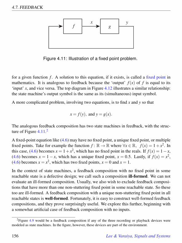
4.7. FEEDBACK
f gyx
Figure 4.11: Illustration of a fixed point problem.
for a given function f . A solution to this equation, if it exists, is called a fixed point inmathematics. It is analogous to feedback because the ‘output’ f (x) of f is equal to its‘input’ x, and vice versa. The top diagram in Figure 4.12 illustrates a similar relationship:the state machine’s output symbol is the same as its (simultaneous) input symbol.
A more complicated problem, involving two equations, is to find x and y so that
x = f (y), and y = g(x).
The analogous feedback composition has two state machines in feedback, with the struc-ture of Figure 4.11.2
A fixed-point equation like (4.6) may have no fixed point, a unique fixed point, or multiplefixed points. Take for example the function f : R→ R where ∀x ∈ R, f (x) = 1+ x2. Inthis case, (4.6) becomes x = 1+ x2, which has no fixed point in the reals. If f (x) = 1− x,(4.6) becomes x = 1− x, which has a unique fixed point, x = 0.5. Lastly, if f (x) = x2,(4.6) becomes x = x2, which has two fixed points, x = 0 and x = 1.
In the context of state machines, a feedback composition with no fixed point in somereachable state is a defective design; we call such a composition ill-formed. We can notevaluate an ill-formed composition. Usually, we also wish to exclude feedback composi-tions that have more than one non-stuttering fixed point in some reachable state. So thesetoo are ill-formed. A feedback composition with a unique non-stuttering fixed point in allreachable states is well-formed. Fortunately, it is easy to construct well-formed feedbackcompositions, and they prove surprisingly useful. We explore this further, beginning witha somewhat artificial case of feedback composition with no inputs.
2Figure 4.9 would be a feedback composition if any of the three recording or playback devices weremodeled as state machines. In the figure, however, these devices are part of the environment.
156 Lee & Varaiya, Signals and Systems

4. COMPOSING STATE MACHINES
4.7.1 Feedback composition with no inputs
The upper state machine in Figure 4.12 has an output port that feeds back to its input port.We wish to construct a state machine model that hides the feedback, as suggested by thefigure. The result will be a state machine with no input. This does not fit our model, whichrequires the environment to provide inputs to which the machine reacts. So we artificiallyprovide an input alphabet
Inputs = react,absent,as suggested in the lower machine in Figure 4.12. We interpret the input symbol react asa command for the internal machine to react, and the input symbol absent as a commandfor the internal machine to stutter. The output alphabet is
Outputs = OutputsA.
This is an odd example of a synchronous/reactive system because of the need for thisartificial input alphabet. Typically, however, such a system will be composed with others,as suggested in Figure 4.13. That composition does have an external input. So the overallcomposition, including the component with no external input, reacts whenever an external
(StatesA, InputsA, OutputsA, updateA, initialStateA )
(States, Inputs, Outputs, update, initialState )
OutputsA ⊂ InputsA
(StatesA, InputsA, OutputsA, updateA, initialStateA )
(States, Inputs, Outputs, update, initialState )
OutputsA ⊂ InputsA
react, absent
Figure 4.12: Feedback composition with no inputs.
Lee & Varaiya, Signals and Systems 157

4.7. FEEDBACK
input symbol is presented, and there is no need for the artificial inputs. Of course when astuttering element is provided to the composite, all components stutter.
Although it is not typical, we first consider the example in Figure 4.12 because the for-mulation of the composition is simplest. We will augment the model to allow inputs afterthis.
In Figure 4.12, for the feedback connection to be possible, of course, we must have
OutputsA ⊂ InputsA.
Suppose the current state at the n-th reaction is s(n) ∈ StatesA. The problem is to find theoutput symbol y(n) ∈ OutputsA. Since y(n) is also the input symbol, it must satisfy
(s(n+1),y(n)) = updateA(s(n),y(n)),
where s(n+ 1) is the next state. The difficulty here is that the “unknown” y(n) appearson both sides. Once we find y(n), s(n+ 1) is immediately determined by the updateAfunction. To simplify the discussion, we get rid of s(n+1) by working with the function
outputA : StatesA× InputsA→ OutputsA
This function gives the output symbol as a function of the current state and the currentinput symbol, as we saw in Section 3.1.1. So our problem is: given the current state s(n)
(StatesA, InputsA, OutputsA, updateA, initialStateA )
(States, Inputs, Outputs, update, initialState )
OutputsA ⊂ InputsA
(StatesB, InputsB, OutputsB, updateB, initialStateB )
Figure 4.13: Feedback composition composed with another state machine.
158 Lee & Varaiya, Signals and Systems

4. COMPOSING STATE MACHINES
and the known function outputA, find y(n) such that
y(n) = outputA(s(n),y(n)). (4.7)
Here s(n) is a known constant, so the equation is of the form (4.6), and its solution, if itexists, is a fixed point.
One solution that is always available is to stutter, i.e.,
y(n) = absent, (and then s(n+1) = s(n)),
since absent = outputA(s(n),absent), assuming that absent is the stuttering input symbolfor machine A. But this is not an interesting solution, since the state does not change. Wewant to find a non-stuttering solution for y(n).
We say that the composition of Figure 4.12 is well-formed if for every reachable s(n) ∈StatesA, there is a unique non-stuttering output symbol y(n) that solves (4.7); otherwise,the composition is ill-formed. If the composition is well-formed, the composite machinedefinition is:
States = StatesA
Inputs = react,absentOutputs = OutputsAinitialState = initialStateA
update(s(n),x(n)) =
updateA(s(n),y(n)),where y(n) 6= absent uniquely satisfies (4.7)if x(n) = react
(s(n),x(n))if x(n) = absent
Notice that the composite machine is defined only if the composition is well-formed, i.e.,there is a unique y(n) that satisfies (4.7). If there is no such y(n), the composition isill-formed and the composite machine is not defined.
The next example illustrates the difference between well-formed and ill-formed compo-sitions. It will suggest a procedure to solve (4.7) in the important special case of systemswith state-determined output.
Lee & Varaiya, Signals and Systems 159

4.7. FEEDBACK
1 2
false/false
true/true
true/false false/true
(a)
(b)
(c)
1 2
false/false
true/false
true/false false/true
1 2
false/false
true/true
true/true false/false
Figure 4.14: Three examples of feedback composition. Examples (b) and (c)are ill-formed. Composition (b) has no non-stuttering fixed point in state 2, whilecomposition (c) has two non-stuttering fixed points in either state.
160 Lee & Varaiya, Signals and Systems

4. COMPOSING STATE MACHINES
Example 4.5: Consider the three feedback compositions in Figure 4.14. In allcases, the input and output alphabets of the component machines are
InputsA = OutputsA = true, false,absent.
The input alphabet to the composite machine is react,absent, as in Figure 4.12,but we do not show this (to reduce clutter in the figure). We want to find a non-stuttering solution y(n) of (4.7). Since the output symbol is also the input symbol,we are looking for a non-stuttering input symbol.
Consider the top machine first. Suppose the current state is the initial state, s(n)= 1.There are two outgoing arcs, and for a non-stuttering input symbol, both producey(n) = false, so we can conclude that the output symbol of the machine is false.Since the output symbol is false, then the input symbol is also false, and the non-stuttering fixed point of (4.7) is unique,
outputA(1, false) = false.
The state transition taken by the reaction goes from state 1 to state 2.
Suppose next that the current state is s(n) = 2. Again, there are two outgoing arcs.Both arcs produce output symbol true for a non-stuttering input symbol, so we can
1 2
react/false
react/true
react,stutter
true,false
Figure 4.15: Composite machine for Figure 4.14(a).
Lee & Varaiya, Signals and Systems 161

4.7. FEEDBACK
conclude that the output symbol is true. Since the output symbol is true, then theinput symbol is also true, there is a unique non-stuttering fixed point,
outputA(2, true) = true,
and the state transition taken goes from 2 to 1. Since there is a unique non-stutteringfixed point in every reachable state, the feedback composition is well-formed.
The composite machine alternates states on each reaction, and produces the outputsequence
(false, true, false, true, false, true, · · ·)for the input sequence
(react,react,react, · · ·).The composite machine is shown in Figure 4.15.
Now consider the second machine in Figure 4.14. If the initial state is 1 the analysisis the same as above. There is a unique non-stuttering fixed point, the output andinput symbols are both false, and the state transition goes from 1 to 2. But if theinitial state is 2 and the unknown input symbol is true, the output symbol is false;and if the unknown input symbol is false, the output symbol is true. Thus there isno non-stuttering fixed point y(n) that solves,
outputA(2,y(n)) = y(n).
The feedback composition is not well-formed.
Consider the third machine in Figure 4.14. This feedback composition is also ill-formed but for a different reason. If the initial state is 1 and the unknown inputsymbol is true, the output symbol is also true, so true is a fixed point, and theoutput symbol can be true. However, the output symbol can also be false, sinceif it is, then a transition will be taken that produces the input symbol false. Sofalse is also a fixed point. Thus, the problem here is that there is more than onenon-stuttering solution, not that there are none!
Our conclusion is that with machines like the second and third, you cannot connectthem in a feedback composition as shown. The second is rejected because it hasno solution and the third because it has more than one. We only accept feedbackcompositions where there is exactly one non-stuttering solution in each reachablestate.
162 Lee & Varaiya, Signals and Systems

4. COMPOSING STATE MACHINES
4.7.2 State-determined output
In the first machine of Figure 4.14, in each state, all outgoing arcs produce the same outputsymbol, independent of the input symbol. In other words, the output symbol y(n) dependsonly on the state; in the example, y(n) = false if s(n) = 1, and y(n) = true if s(n) = 2.The unique fixed point of (4.7) is this output symbol, and we can immediately concludethat the feedback composition is well-formed.
We say that a machine A has state-determined output if in every reachable state s(n) ∈StatesA, there is a unique output symbol y(n) = b (which depends on s(n)) independentof the non-stuttering input symbol; i.e. for every x(n) 6= absent,
outputA(s(n),x(n)) = b.
In this special case of state-determined output, the composite machine is:
States = StatesA
Inputs = react,absentOutputs = OutputsAinitialState = initialStateA
update(s(n),x(n)) =
updateA(s(n),b),where b is the unique output symbol instate s(n) if x(n) = react
(s(n),x(n))if x(n) = absent
When a machine with state-determined output is combined with any other state machinesin a feedback composition, the resulting composition is also well-formed, as illustrated inthe next example.
Example 4.6:
In Figure 4.16 the machine A is combined with machine B in a feedback composi-tion. A is the same as the first machine, and B is the same as the second machinein Figure 4.14. (The output port of B is drawn on the left and the input port on theright so that the block diagram looks neater.) A has state-determined output, but Bdoes not. The composition is well-formed.
Lee & Varaiya, Signals and Systems 163

4.7. FEEDBACK
1 2
false/false
true/true
true/false false/true
1 2
false/false
true/false
true/false false/true
B
Areact,absent true,
false
(1,1) (2,2)
react/false
react/true
react,absent
true,false
(1,2) react/false
react/true
(2,1)
(a)
(b)
Figure 4.16: Machine A has state-determined output, but B does not. The feed-back composition is well-formed, and the composite machine is shown on thebottom. Note that state (1,2) is not reachable.
164 Lee & Varaiya, Signals and Systems

4. COMPOSING STATE MACHINES
To see this, suppose both machines are in their initial states 1. A produces outputsymbol false, independent of its input symbol. This output is the input of B whichthen produces output symbol false and makes the transition to state 2. The outputsymbol false of B is the input to A which makes the transition to its state 2. (Aand B make their state transitions together in our synchronous/reactive model.) Wecan determine the output symbol and transition in the same way for all other states.The state diagram of the composite machine is shown in the figure on the right.Note that state (1,2) is not reachable from the initial state (1,1), so we could haveignored it in determining whether the composition is well-formed.
The input alphabet of the composite machine is react,absent, taking absent asthe stuttering input symbol. The output alphabet is the same as the output alphabetof A, true, false,absent. The state space is StatesA×StatesB. The update functionis given by the table:
current (next state, output) for inputstate react absent(1,1) ((2,2),false) ((1,1),absent)(2,2) ((2,1),true) ((2,2), absent)(1,2) ((1,2),false) ((1,2), absent)(2,1) ((2,1),true) ((2,1), absent)
It is possible for a machine without state-determined outputs to be placed in a well-formedfeedback composition as illustrated in the next example.
Example 4.7: Consider the example in Figure 4.17. For the component ma-chine, the output alphabet is OutputsA = true, false,maybe,absent, and the inputalphabet is InputsA = true, false,absent. The stuttering element is absent. Themachine does not have state-determined output because, for instance, the outgoingarcs from state 1 can produce both maybe and false. Nevertheless, equation (4.7)has a unique non-stuttering fixed point in each state:
outputA(1, false) = false, and outputA(2, true) = true.
So the feedback composition is well-formed. The composite machine is shown onthe bottom.
Lee & Varaiya, Signals and Systems 165

4.7. FEEDBACK
react,absent
true,false
1 2
false/false
true/true
true/maybe
false/maybe
1 2
react/false
react/true
react,absent
true,false
A
(a)
(b)
Figure 4.17: Machine A does not have state-determined outputs, but the feed-back composition is well-formed. The machine on the bottom is the compositemachine.
166 Lee & Varaiya, Signals and Systems
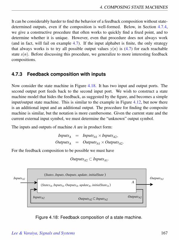
4. COMPOSING STATE MACHINES
It can be considerably harder to find the behavior of a feedback composition without state-determined outputs, even if the composition is well-formed. Below, in Section 4.7.4,we give a constructive procedure that often works to quickly find a fixed point, and todetermine whether it is unique. However, even that procedure does not always work(and in fact, will fail on example 4.7). If the input alphabet is finite, the only strategythat always works is to try all possible output values y(n) is (4.7) for each reachablestate s(n). Before discussing this procedure, we generalize to more interesting feedbackcompositions.
4.7.3 Feedback composition with inputs
Now consider the state machine in Figure 4.18. It has two input and output ports. Thesecond output port feeds back to the second input port. We wish to construct a statemachine model that hides the feedback, as suggested by the figure, and becomes a simpleinput/output state machine. This is similar to the example in Figure 4.12, but now thereis an additional input and an additional output. The procedure for finding the compositemachine is similar, but the notation is more cumbersome. Given the current state and thecurrent external input symbol, we must determine the “unknown” output symbol.
The inputs and outputs of machine A are in product form:
InputsA = InputsA1× InputsA2,
OutputsA = OutputsA1×OutputsA2.
For the feedback composition to be possible we must have
OutputsA2 ⊂ InputsA1.
(StatesA, InputsA, OutputsA, updateA, initialStateA )
(States, Inputs, Outputs, update, initialState )InputsA1 OutputsA1
OutputsA2 ⊂ InputsA2
A
InputsA2 OutputsA2
Figure 4.18: Feedback composition of a state machine.
Lee & Varaiya, Signals and Systems 167

4.7. FEEDBACK
The output function of A is
outputA : StatesA× InputsA→ OutputsA.
It is convenient to write it in product form as,
outputA = (outputA1,outputA2),
whereoutputA1 : StatesA× InputsA→ OutputsA1,
gives the output symbol at the first output port and
outputA2 : StatesA× InputsA→ OutputsA2,
gives the output symbol at the second output port.
Suppose we are given that at the n-th reaction, the current state of A is s(n) and the currentexternal input symbol is x1(n) ∈ InputsA1. Then the problem is to find the “unknown”output symbol (y1(n),y2(n)) ∈ OutputsA such that
outputA(s(n),(x1(n),y2(n))) = (y1(n),y2(n)). (4.8)
The symbol y2(n) appears on both sides because the second input x2(n) to machine A isequal to y2(n). In terms of the product form, (4.8) is equivalent to two equations:
outputA1(s(n),(x1(n),y2(n))) = y1(n), (4.9)
outputA2(s(n),(x1(n),y2(n))) = y2(n). (4.10)
In these equations, s(n) and x1(n) are known, while y1(n) and y2(n) are unknown. Ob-serve that if (4.10) has a unique solution y2(n), then the input symbol to A is (x1(n),y2(n))and the next state s(n+ 1) and output symbol y1(n) are determined. So the fixed pointequation (4.10) plays the same role as (4.7).
We say that the composition of Figure 4.18 is well-formed if for every reachable states(n) ∈ StatesA and for every external input symbol x1(n) ∈ InputsA1, there is a uniquenon-stuttering output symbol y2(n) ∈ OutputsA2 that solves (4.10). If the composition iswell-formed, the composite machine definition is:
States = StatesA
Inputs = InputsA1
168 Lee & Varaiya, Signals and Systems
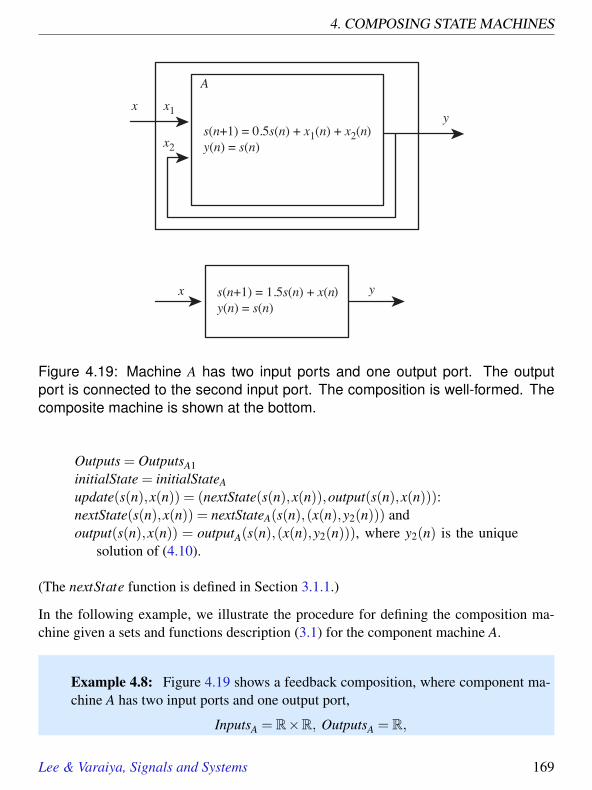
4. COMPOSING STATE MACHINES
xy
A
s(n+1) = 0.5s(n) + x1(n) + x2(ny(n) = s(n)
s(n+1) = 1.5s(n) + x(ny(n) = s(n)
x1
x2)
)x y
Figure 4.19: Machine A has two input ports and one output port. The outputport is connected to the second input port. The composition is well-formed. Thecomposite machine is shown at the bottom.
Outputs = OutputsA1initialState = initialStateA
update(s(n),x(n)) = (nextState(s(n),x(n)),output(s(n),x(n))):nextState(s(n),x(n)) = nextStateA(s(n),(x(n),y2(n))) andoutput(s(n),x(n)) = outputA(s(n),(x(n),y2(n))), where y2(n) is the unique
solution of (4.10).
(The nextState function is defined in Section 3.1.1.)
In the following example, we illustrate the procedure for defining the composition ma-chine given a sets and functions description (3.1) for the component machine A.
Example 4.8: Figure 4.19 shows a feedback composition, where component ma-chine A has two input ports and one output port,
InputsA = R×R, OutputsA = R,
Lee & Varaiya, Signals and Systems 169

4.7. FEEDBACK
and states StatesA = R. Thus A has infinite input and output alphabets and in-finitely many states. At the n-th reaction, the pair of input values is denoted by(x1(n),x2(n)), the current state by s(n), the next state by s(n+ 1), and the outputsymbol by y(n). In terms of these, the update function is given by
(s(n+1),y(n)) = updateA(s(n),(x1(n),x2(n)))
= (0.5s(n)+ x1(n)+ x2(n),s(n)).
Equivalently,
s(n+1) = nextStateA(s(n),(x1(n),x2(n)))
= 0.5s(n)+ x1(n)+ x2(n)
y(n) = outputA(s(n),(x1(n),x2(n))) = s(n).
Thus, the component machine A has state-determined output. The feedback con-nects the output port to the second input port, so x2(n) = y(n). Given the currentstate s(n) and the external input symbol x(n) at the first input port, (4.10) becomes,
outputA(s(n),(x1(n),x2(n))) = x2(n),
which givess(n) = x2(n).
So the composite machine is defined by
Inputs = R , Outputs = Reals, States = R
update(s(n),x(n)) = (0.5s(n)+ x(n)+ s(n),s(n))
= (1.5s(n)+ x(n),s(n)).
Note that the input to the composite machine is a scalar. The composite machine isshown in the lower part of the figure.
170 Lee & Varaiya, Signals and Systems

4. COMPOSING STATE MACHINES
4.7.4 Constructive procedure for feedback composition
Our examples so far involve one or two state machines and a feedback loop. If anymachine in the loop has state determined output, then finding the fixed point is easy. Mostinteresting designs are more complicated, involving several state machines and severalfeedback loops, and the loops do not necessarily include mahcines with state-determinedoutput.
In this section, we describe a constructive procedure for finding the fixed point that often(but not always) works. It is “constructive” in the sense that it can it be applied me-chanically, and will, in a finite number of steps, either identify a fixed point or give up.The approach is simple. At each reaction, begin with all unspecified signals having valueunknown. Then with what is known about the input symbols, try each state machine todetermine as much as possible about the output symbols. You can try the state machinesin any order. Given what you learn about the output symbols, then update what you knowabout the feedback input symbols, and repeat the process, trying each state machine again.Repeat this process until all signal values are specified, or until you learn nothing moreabout the output symbols. We illustrate the procedure in an example involving only onemachine, but keep in mind that the procedure works for any number of machines.
a b
1/(1,1)
1/(1,0)
0/(0,1) 0/(0,0)
0, 1, absent
0, 1, absentreact, absent
A
Figure 4.20: Feedback composition without state-determined output.
Lee & Varaiya, Signals and Systems 171

4.7. FEEDBACK
Example 4.9: Figure 4.20 shows a feedback composition without state-determinedoutput. Nonetheless, our constructive procedure can be used to find a unique fixedpoint for each reaction. Suppose that the current state is a, and that the input to thecomposition is react. Begin by assuming that the symbol on the feedback connec-tion is unknown. Try component machine A (this is the only component machine inthis example, but if there were more, we could try them in any order). Examiningmachine A, we see that in its current state, a, the output symbol cannot be fullydetermined. Thus, this machine does not have state-determined output. However,more careful examination reveals that in state a, the second element of the outputtuple is determined. That second element has value 1. Fortunately, this changes thevalue on the feedback connection from unknown to 1.
Now we repeat the procedure. We choose a state machine to try. Again, there isonly one state machine in this example, so we try A. This time, we know that theinput symbol is 1, so we know that the machine must take the transition from a tob and produce the output tuple (1,1). This results in all symbols being known forthe reaction, so we are done evaluating the reaction.
Now assume the current state is b. Again, the feedback symbol is initially unknown,but once again, trying A, we see that the second element of the output tuple must be0. Thus, we change the feedback symbol from unknown to 0 and try the machineagain. This time, its input is 0, so it must take the self loop back to b and producethe output tuple (0,0).
Recall that the set Behaviors is the set of all (x,y) such that x is an input sequenceand y is an output sequence. For this machine, ignoring stuttering, the only pos-sible input sequence is (react,react,react, · · ·). We have just determined that theresulting output sequence is (1,0,0,0, · · ·). Thus, ignoring stuttering,
Behaviors = ((react,react,react, · · ·),(1,0,0,0, · · ·)).
Of course, we should take into account stuttering, so this set needs to be augmentedwith all (x,y) pairs that look like the one above but have stuttering symbols inserted.
This procedure can be applied in general to any composition of state machines. If theprocedure can be applied successfully (nothing remains unknown) for all reachable states
172 Lee & Varaiya, Signals and Systems

4. COMPOSING STATE MACHINES
of the composition, then the composition is well-formed. The following example appliesthe procedure to a more complicated example.
Example 4.10: We add more detail to the message recorder in Figure 4.9. Inparticular, as shown in Figure 4.21, we wish to model the fact that the messagerecorder stops recording when either it detects a dialtone or when a timeout period is
telephoneline interface
greeting playbackdevice
light
playbutton
message playbackdevice
end greeting
ring, offhook
end message
AnsweringMachine
answer
recorded message
record
Playbackplay
light on, light off
done playing play messages
recording device
MessageRecorderdialtone
start recordingtimeout
Figure 4.21: Answering machine composition with feedback. The absent ele-ments are not shown (to reduce clutter).
Lee & Varaiya, Signals and Systems 173

4.7. FEEDBACK
reached. This is modeled by a two-state finite state machine, shown in Figure 4.22.Note that this machine does not have state-determined output. For example, in stateidle, the output could be (absent,start recording) or it could be (absent,absent)when the input is not the stuttering input.
The MessageRecorder and AnsweringMachine state machines form a feedbackloop. Let us verify that composition is well-formed. First, note that in the idlestate of the MessageRecorder, the upper output symbol is known to be absent (seeFigure 4.22). Thus, only in the recording state is there any possibility of a prob-lem that would lead to the composition being ill-formed. In that state, the outputsymbol is not known unless the input symbols are known. However, notice thatthe recording state is entered only when a record input symbol is received. In Fig-ure 4.6, you can see that the record value is generated only when entering staterecord message. But in all arcs emerging from that state, the lower output sym-bol of AnsweringMachine will always be absent; the input symbol does not needto be known to know that. Continuing this reasoning by considering all possiblestate transitions from this point, we can convince ourselves that the feedback loopis well-formed.
The sort of reasoning in this more complicated example is difficult and error-prone foreven moderate compositions of state machines. It is best automated. Compilers for syn-chronous languages do exactly this. Successfully compiling a program involves provingthat feedback loops are well-formed.
idle recording
(record, absent, absent)/(absent, start recording)
(absent, dialtone, absent), (absent, absent, timeout),(absent, dialtone, timeout)/
(end message , absent)
else
else
record, absent
dialtone, absent
timeout, absent
end message,absent
start recording ,absent
Figure 4.22: Message recorder subsystem of the answering system.
174 Lee & Varaiya, Signals and Systems

4. COMPOSING STATE MACHINES
4.7.5 Exhaustive search
If a feedback composition has one or more machines with state-determined output, thenfinding a unique fixed point is easy. Without such state-determined output, we can applythe procedure in the previous section. Unfortunately, if the procedure fails, we cannotconclude that the composition is ill-formed. The procedure fails for example 4.7, shownin Figure 4.17, despite the fact that this example is well-formed. For that example, we candetermine the unique fixed point by exhaustive search. That is, for each reachable stateof the composition, and for each possible input to the composition, we try all possibletransitions out of the current states of the component machines. We reject those that leadto a contradiction. For example, in Figure 4.17, assuming the current state is 1, the outputof the component machine cannot be maybe because then the input would have to bemaybe, which would result in the output being absent. If after rejecting all contradictionsthere remains exactly one possibility in each reachable state, then the composition is well-formed.
Exhaustive search works in Figure 4.17 only because the number of reachable states isfinite and the number of transitions out of each state is finite. If either of these conditionsis violated, then exhaustive search will not work. Thus, there are state machine that whenput in a feedback loop are well-formed, but where there is no constructive procedure forevaluating a reaction (see box on page 176). Even when exhaustive search is theoreticallypossible, in practice the number of possibilities that must be tried grows extremely fast.
4.7.6 Nondeterministic machines
Nondeterministic state machines can be composed just as deterministic state machinesare composed. In fact, since deterministic state machines are a special case, the two typesof state machines can be mixed in a composition. Compositions without feedback arestraightforward, and operate almost exactly as described above (see exercises 14 and 15).Compositions with feedback require a small modification to our evaluation process.
Recall that to evaluate the reaction of a feedback composition, we begin by setting tounknown any input symbols that are not initially known. We then proceed through a seriesof rounds where in each round, we attempt to determine the output symbols of the statemachines in the composition given what we know about the input symbols. After somenumber of rounds, no more information is gained. At this point, if all of the input and
Lee & Varaiya, Signals and Systems 175

4.7. FEEDBACK
Probing Further: Constructive Semantics
The term “semantics” means meaning. We have defined the meaning of compositionsof state machines using the notion of synchrony, which makes feedback compositionsparticularly interesting. When we define “well-formed,” we are, in effect, limiting thecompositions that are valid. Compositions that are not well-formed fall outside oursynchronous semantics. They have no meaning.
One way to define the semantics of a composition is to give a procedure for evaluatingthe composition (the resulting procedure is called an operational semantics). We havegiven three successively more difficult procedures for evaluating a reaction of a com-position of state machines with feedback. If at least one machine in each directed loophas state-determined output, then it is easy to evaluate a reaction. If not, we can applythe constructive procedure of section 4.7.4. However, that procedure may result in somefeedback connections remaining unknown even though the composition is well-formed.The ultimate procedure is exhaustive search, as described in section 4.7.5. However,exhaustive search is not always possible, and even when it is theoretically possible, thenumber of possibilities to explore may be so huge that it is not practical. There are statemachines that when put in a feedback loop are well-formed, but where there is no con-structive procedure for evaluating a reaction, and no constructive way to demonstratethat they are well-formed. Thus, there is no operational semantics for our feedbackcompositions.
This situation is not uncommon in computing and in mathematics. Kurt Godel’s fa-mous incompleteness theorem (1931), for example, states (loosely) that in any formallogical system, there are statements that are true but not provable. This is analogous inthat we can have feedback compositions that are well-formed, but we have no procedurethat will always work to demonstrate that they are well-formed. Around the same time,Alan Turing and Alonzo Church demonstrated that there are functions that cannot becomputed by any procedure.
To deal with this issue, Gerard Berry has proposed that synchronous composition havea constructive semantics, which means precisely that well-formed compositions aredefined to be those for which the constructive procedure of Section 4.7.4 works. Whenthat procedure fails, we simply declare the composition to be unacceptable. This is prag-matic solution, and in many situations, it is adequate. See G. Berry, The ConstructiveSemantics of Pure Esterel, Book Draft, http://www-sop.inria.fr/meije/esterel/doc/main-papers.html.
176 Lee & Varaiya, Signals and Systems

4. COMPOSING STATE MACHINES
output symbols are known, then the composition is well-formed. This procedure worksfor most (but not all) well-formed compositions.
This process needs to be modified slightly for nondeterministic machines because in eachreaction, a machine may have several possible output symbols and several possible nextstates. For each machine, at each reaction, we define the sets PossibleInputs ⊂ Inputs,PossibleNextStates⊂ States and PossibleNextOutputs⊂Outputs. If the inputs to a partic-ular machine in the composition are known completely, then PossibleInputs has exactlyone element. If they are completely unknown, then PossibleInputs is empty.
The rounds proceed in a similar fashion to before. For each state machine in the com-position, given what is known about the input symbols, i.e. given PossibleInputs, deter-mine what you can about the next state and output symbols. This may result in elementsbeing added to PossibleNextStates and PossibleNextOutputs. When a round results inno such added elements, the process has converged. If none of the PossibleInputs orPossibleOutputs sets is empty, then the composition is well-formed.
4.8 Summary
Many systems are designed as state machines. Usually the design is structured by com-posing component state machines. In this chapter, we considered synchronous composi-tion. Feedback composition proves particularly subtle because the input symbol of a statemachine in a reaction may depend on its own output symbol in the same reaction. We calla feedback composition well-formed if every signal has a unique non-stuttering symbolin each reaction.
Describing systems as compositions of state machines helps in many ways. It promotesunderstanding. The block diagram syntax that describes the structure often shows thatindividual components are responsible for distinct functions of the overall system. Somecomponents may already be available and so we can reuse their designs. The design of theanswering machine in Figure 4.9 takes into account the availability of the telephone lineinterface, recording device, etc. Composition also simplifies description; once we specifythe component state machines and the composition, the overall state machine is auto-matically defined by the rules of composition. Compilers for synchronous programminglanguages and tools for verification do this automatically.
We have three successively more difficult procedures for evaluating a reaction of a com-position of state machines with feedback. If at least one machine in each directed loop
Lee & Varaiya, Signals and Systems 177

4.8. SUMMARY
has state-determined output, then it is easy to evaluate a reaction. If not, we can apply theconstructive procedure of section 4.7.4. But that procedure may be inconclusive. The ul-timate procedure is exhaustive search, as described in section 4.7.5. However, exhaustivesearch is not always possible, and even when it is theoretically possible, the number ofpossibilities to explore may be so huge that it is not practical.
178 Lee & Varaiya, Signals and Systems

4. COMPOSING STATE MACHINES
Exercises
In some of the following exercises you are asked to design state machines that carry outa given task. The design is simplified and elegant if the state space is properly chosen.Although the state space is not unique, there often is a natural choice. Each problem isannotated with the letter E, T, C which stands for exercise, requires some thought, requiressome conceptualization. Problems labeled E are usually mechanical, those labeled Trequire a plan of attack, those labeled C usually have more than one defensible answer.
1. E Define the composite state machine in Figure 4.7 in terms of the componentmachines, as done for the simpler compositions in figures 4.3 and 4.1. Be sure tostate any required assumptions.
2. E Define the composite state machine in Figure 4.10 in terms of the componentmachines, as done for the simpler compositions in figures 4.3 and 4.1. Be sure tostate any required assumptions. Give the definition in two different ways:
(a) Directly form a product of the three state spaces.
(b) First compose the A and B state machines to get a new D state machine, andthen compose D with C.
(c) Comment on the relationship between the models in part (a) and (b).
3. T Consider the state machine UnitDelay studied in part (a) of exercise 5 at the endof the previous chapter.
(a) Construct a state machine model for a cascade composition of two such ma-chines. Give the sets and functions model (it is easier than the state transitiondiagram or table).
(b) Are all of the states in the state space of your model in part (a) reachable? Ifnot, give an example of an unreachable state.
(c) Give the state space (only) for cascade compositions of three and four unitdelays. How many elements are there in each of these state spaces?
(d) Give an expression for the size of the state space as function of the number Nof cascaded delays in the cascade composition.
4. C Consider the parking meter example of the previous chapter, example 3.1, andthe modulo N counter of Exercise 4 at the end of the previous chapter. Use these
Lee & Varaiya, Signals and Systems 179

EXERCISES
two machines to model a citizen that parks at the meter when the machines start,and inserts 25 cents every 30 minutes, and a police officer who checks the meterevery 45 minutes, and issues a ticket if the meter is expired. For simplicity, assumethat the police office issues a new ticket each time he finds the meter expired, andthat the citizen remains parked forever.
You may construct the model at the block diagram level, as in Figure 4.9, but de-scribe in words any changes you need to make to the designs of the previous chap-ter. Give state transition diagrams for any additional state machines you need. Howlong does it take for the citizen to get the first parking ticket?
Assume you have an eternal clock that emits an event tick every minute.
Note that the output alphabet of the modulo N counter does not match the inputalphabet of the parking meter. Neither does its input alphabet match the output al-phabet of the parking meter. Thus, one or more intermediate state machines will beneeded to translate these alphabets. You should fully specify these state machines(i.e., don’t just give them at the block diagram level). Hint: These state machines,which perform an operation called renaming, only need one state.
5. C Consider a machine with
States = 0,1,2,3,Inputs = increment,decrement,reset,absent,
Outputs = zero,absent,initialState = 0,
such that increment increases the state by 1 (modulo 4), decrement decreases thestate by 1 (modulo 4), reset resets the state to 0, and the output symbol is absentunless the next state is 0, in which case the output symbol is zero. So, for example,if the current state is 3 and the input is increment, then the new state will be 0 andthe output will be zero. If the current state is 0 and the input is decrement, then thenew state will be 3 and the output will be absent.
(a) Give the update function for this machine, and sketch the state transition dia-gram.
(b) Design a cascade composition of two state machines, each with two states,such that the composition has the same behaviors as the one above. Give adiagram of the state machines and their composition, and carefully define allthe input and output alphabets.
180 Lee & Varaiya, Signals and Systems

4. COMPOSING STATE MACHINES
(c) Give a simulation relation from the single machine and the cascade compo-sition, and a simulation relation from the cascade composition to the singlemachine.
6. C A road has a pedestrian crossing with a traffic light. The light is normally greenfor vehicles, and the pedestrian is told to wait. However, if a pedestrian presses abutton, the light turns yellow for 30 seconds and then red for 30 seconds. When itis red, the pedestrian is told “cross now.” After the 30 seconds of red, the light turnsback to green. If a pedestrian presses the button again while the light is red, thenthe red is extended to a full minute.
Construct a composite model for this system that has at least two state machines,TrafficLight for the traffic light seen by the cars, and WalkLight for the walk lightseen by the pedestrians. The state of machine should represent the state of thelights. For example, TrafficLight should have at least three states, one for green,one for yellow, and one for red. Each color may, however, have more than one stateassociated with it. For example, there may be more than one state in which thelight is red. It is typical in modeling systems for the states of the model to representstates of the physical system.
Assume you have a timer available such that if you emit an output start timer, then30 seconds later an input symbol timeout will appear. It is sufficient to give the statetransition graphs for the machines. State any assumptions you need to make.
7. E Suppose you are given two state machines A and B, Suppose the sizes of theinput alphabets are iA, iB, respectively, the sizes of the output alphabets are oA,oB
respectively, and the numbers of states are sA,sB, repectively. Give the sizes of theinput and output alphabets and the number of states for the following compositions:
(a) side-by-side,
(b) cascade,
(c) and feedback, where the structure of the feedback follows the pattern in Figure4.16(a).
8. T Example 4.2 shows a state machine in which a state is not reachable from theinitial state. Here is a recursive algorithm to calculate the reachable states for anynondeterministic machine,
StateMachine = (States, Inputs,Outputs,possibleUpdates, initialState).
Lee & Varaiya, Signals and Systems 181

EXERCISES
Recursively define subsets ReachableStates(n), n = 0,1, · · · of States by:
ReachableStates(0) = initialState, and for n≥ 0
ReachableStates(n+1) = s(n+1) | ∃s(n) ∈ ReachableStates(n),
∃ x(n) ∈ Inputs,
∃ y(n) ∈ Outputs,
(s(n+1),y(n))
∈ possibleUpdates(s(n),x(n))∪ ReachableStates(n).
In words: ReachableStates(n + 1) is the set of states that can be reached fromReachableStates(n) in one step using any input symbol, together with ReachableStates(n).
(a) Show that for all n, ReachableStates(n)⊂ ReachableStates(n+1).
(b) Show that ReachableStates(n) is the set of states that can be reached in n orfewer steps, starting in initialState. Now show that if for some n,
ReachableStates(n) = ReachableStates(n+1), (4.11)
then ReachableStates(n) = ReachableStates(n+ k) for all k ≥ 0.
(c) Suppose (4.11) holds for n = N. Show that ReachableStates(N) is the set ofall reachable states, i.e. this set comprises all the states that can be reachedusing any input sequence starting in initialState.
(d) Suppose there are N states. Show that (4.11) holds for n = N.
(e) Compute ReachableStates(n) for all n for the machine in Figure 4.4.
(f) Suppose States is infinite. Show that the set of reachable states is given by
∪∞n=0ReachableStates(n).
9. T The algorithm in Exercise 8 has a fixed point interpretation. For a nondetermin-istic state machine,
StateMachine = (States, Inputs,Outputs,possibleUpdates, initialState),
define the function nextStep : ℘(States)→℘(States) that maps subsets of Statesinto subsets of States (recall that ℘(A) is the powerset of A) as follows: for any
182 Lee & Varaiya, Signals and Systems

4. COMPOSING STATE MACHINES
S(n)⊂ States
nextStep(S(n)) = s(n+1) | ∃s(n) ∈ S(n),
∃x(n) ∈ Inputs,
∃y(n) ∈ Outputs,
(s(n+1),y(n))
∈ possibleUpdates(s(n),x(n))∪S(n).
By definition, a fixed point of nextStep is any subset S⊂ States such that nextStep(S)=S.
(a) Show that /0 and States are both fixed points of nextState.
(b) Let ReachableStates be the set of all states that can be reached starting ininitialState. Show that ReachableStates is also a fixed point.
(c) Show that ReachableStates is the least fixed point of nextStep containinginitialState.
10. C Recall the playback machine of Figure 4.8 and the CodeRecognizer machine ofFigure 3.4. Enclose CodeRecognizer in a block and compose it with the playbackmachine so that someone can play back the recorded messages only if she correctlyenters the code 1100. You will need to modify the playback machine appropriately.
11. E Consider the following state machine in a feedback composition, where the inputand output alphabets for the state machine is
1,2,3,absent :
Lee & Varaiya, Signals and Systems 183
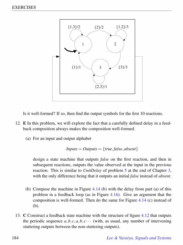
EXERCISES
1 2
2/2
3/3
1,3/2 1,2/3
31/1
2,3/1
Is it well-formed? If so, then find the output symbols for the first 10 reactions.
12. E In this problem, we will explore the fact that a carefully defined delay in a feed-back composition always makes the composition well-formed.
(a) For an input and output alphabet
Inputs = Outputs = true, false,absent
design a state machine that outputs false on the first reaction, and then insubsequent reactions, outputs the value observed at the input in the previousreaction. This is similar to UnitDelay of problem 5 at the end of Chapter 3,with the only difference being that it outputs an initial false instead of absent.
(b) Compose the machine in Figure 4.14 (b) with the delay from part (a) of thisproblem in a feedback loop (as in Figure 4.16). Give an argument that thecomposition is well-formed. Then do the same for Figure 4.14 (c) instead of(b).
13. C Construct a feedback state machine with the structure of figure 4.12 that outputsthe periodic sequence a,b,c,a,b,c · · · (with, as usual, any number of interveningstuttering outputs between the non-stuttering outputs).
184 Lee & Varaiya, Signals and Systems

4. COMPOSING STATE MACHINES
14. E Modify Figure 4.1 as necessary so that the machines in the side-by-side compo-sition are both nondeterministic.
15. E Modify Figure 4.3 as necessary so that the machines in the cascade compositionare both nondeterministic.
16. C,T Data packets are to be reliably exchanged between two computers over com-munication links that may lose packets. The following protocol has been suggested.Suppose computer A is sending and B is receiving. Then A sends a packet and startsa timer. If B receives the packet it sends back an acknowledgment. (The packet orthe acknowledgment or both may be lost.) If A does not receive the acknowledg-ment before the timer expires, it retransmits the packet. If the acknowledgmentarrives before the timer expires, A sends the next packet.
(a) Construct two state machines, one for A and one for B, that implement theprotocol.
(b) Construct a two-state nondeterministic machine to model the link from A toB, and another copy to model the link from B to A. Remember that the linkmay correctly deliver a packet, or it may lose it.
(c) Compose the four machines to model the entire system.
(d) Suppose the link correctly delivers a packet, but after a delay that exceeds thetimer setting. What will happen?
17. T Consider the following three state machines:
-0.5in-
0.5in
a b
1/0 1/00/ 0
0/1
machine A
c d
1, 0/1 0/0
1/0
e1/0
machine B
Lee & Varaiya, Signals and Systems 185

EXERCISES
machine A machine B
machine C
Machines A and B have input and output alphabets
Inputs = Outputs = 0,1,absent.
Machine C has the same output alphabet, but input alphabetInputsC = react,absent.
(a) Which of these machines is deterministic?
(b) Draw the state transition diagram for the composition (machine C), showingonly states that are reachable from the initial state.
(c) Give the BehaviorsC relation for the composition of machine C, ignoring stut-tering.
18. T The feedback composition in Figure 4.14(c) is ill-formed because it has twonon-stuttering fixed points in each of the two states of the component machine.Instead of declaring it to be ill-formed, we could have interpreted the compositionas representing a nondeterministic state machine. That is, in each state, we accepteither of the two possible fixed points as possible reactions of the machine. Usingthis interpretation, give the nondeterministic machine for the feedback compositionby giving its sets and functions model and a state transition diagram.
186 Lee & Varaiya, Signals and Systems

5Linear Systems
Contents5.1 Operation of an infinite state machine . . . . . . . . . . . . . . . . 189
5.1.1 Time . . . . . . . . . . . . . . . . . . . . . . . . . . . . . . 1915.2 Linear functions . . . . . . . . . . . . . . . . . . . . . . . . . . . . 1925.3 The [A,B,C,D] representation of a system . . . . . . . . . . . . . . 195
5.3.1 Impulse response . . . . . . . . . . . . . . . . . . . . . . . . 1985.3.2 One-dimensional SISO systems . . . . . . . . . . . . . . . . 1995.3.3 Zero-state and zero-input response . . . . . . . . . . . . . . . 2055.3.4 Multidimensional SISO systems . . . . . . . . . . . . . . . . 2085.3.5 Multidimensional MIMO systems . . . . . . . . . . . . . . . 2165.3.6 Linear input-output function . . . . . . . . . . . . . . . . . . 217
5.4 Continuous-time state-space models . . . . . . . . . . . . . . . . . 2185.5 Summary . . . . . . . . . . . . . . . . . . . . . . . . . . . . . . . . 219
Basics: Functions yielding tuples . . . . . . . . . . . . . . . . . . . . 220Basics: Matrices and vectors . . . . . . . . . . . . . . . . . . . . . . 221Basics: Vectors . . . . . . . . . . . . . . . . . . . . . . . . . . . . . 222Basics: Matrix arithmetic . . . . . . . . . . . . . . . . . . . . . . . . 223Basics: Matrix arithmetic (continued from page 223) . . . . . . . . . 224Probing Further: Impulse Responses of MIMO Systems . . . . . . . . 225Probing Further: Approximating continuous-time . . . . . . . . . . . 226
Exercises . . . . . . . . . . . . . . . . . . . . . . . . . . . . . . . . . . . 227
187

MIMO differenceequation system
States = Reals N
Reals
Reals
Reals
...
Reals
Reals
Reals
...
Out
puts
= R
eals
K
Inpu
ts =
Rea
ls M
Figure 5.1: Block representing a multiple-input, multiple output (MIMO) system.
Recall that the state of a system is a summary of its past. It is what the system needsto remember about the past in order to react at the present and move into the future. Inprevious chapters, systems typically had a finite number of possible states. Many usefuland interesting systems are not like that, however. They have an infinite number of states.The analytical approaches used to analyze finite-state systems, such as simulation, getmore difficult when the number of states is not finite.
In this chapter, we begin considering infinite-state systems. We impose two key con-straints. First, we require that the state space and input and output alphabets be numericsets. That is, we must be able to do arithmetic on members of these sets. (Contrast thiswith the answering machine example, where the states are symbolic names, and no arith-metic makes sense.) Second, we require that the update function be linear. We will definewhat this means precisely. In exchange for these two constraints, we gain a very richset of analytical methods for designing and understanding systems. In fact, most of theremaining chapters are devoted to developing these methods.
In particular, we study state machines with
States = RN
Inputs = RM (5.1)
Outputs = RK .
Such state machines are shown schematically in Figure 5.1. The inputs and outputs arein product form, as discussed for general state machines in Section 4.4. The system,therefore, can be viewed as having M distinct inputs and K distinct outputs. So the input
188 Lee & Varaiya, Signals and Systems

5. LINEAR SYSTEMS
is a tuple with M real numbers, and the ouptut is a tuple with K real numbers. Such asystem is called a multiple-input, multiple-output (MIMO) system. When M = K = 1,it is called a single-input, single-output (SISO) system. The state is a tuple with N realnumbers. N (rather than M or K) is called the dimension of the system.
Example 5.1: A stereo audio system processes two channels of audio, and there-fore has M = K = 2. ”Surround sound,” used in movie theaters and some homeaudio systems, has five channels, so M = K = 5.
Example 5.2: Some modern cars have traction control systems, where the torqueapplied to each wheel is controled individually to avoid skidding. The key inputcomes from the accelerator pedal, which specifies a desired acceleration. The out-put is the torque applied to each of four wheels. Hence, M = 1 and K = 4. A moresophisticated traction control system might also use as input the steering angle, inwhich case M = 2.
5.1 Operation of an infinite state machine
Recall that a deterministic state machine is a 5-tuple
M = (States, Inputs,Outputs,update, initialState) (5.2)
where States is the state space, Inputs is the input space, Outputs is the output space,update : States× Inputs→ States×Outputs is the update function, and initialState is theinitial state.
In this chapter, the update function has the form
update : RN×RM → RN×RK .
The result of evaluating this function is an N-tuple (the next state) and a K-tuple (thecurrent output). It will be useful in this chapter to break this function into two parts, as
Lee & Varaiya, Signals and Systems 189

5.1. OPERATION OF AN INFINITE STATE MACHINE
done in Section 3.1.1, one giving the new state and one giving the output,
update = (nextState,output),
wherenextState : RN×RM → RN ,
output : RN×RM → RK ,
such that
∀ s ∈ RN ,∀x ∈ RM, update(s,x) = (nextState(s,x),output(s,x)).
These two functions separately give the next state and the current output as a function ofthe current state and input. Given an input sequence x(0),x(1), · · · of M-tuples in RM, thesystem recursively generates a state response
s(0),s(1), · · ·
of N-tuples in RN and an output response y(0),y(1), · · · of K-tuples in RK as follows:
s(0) = initialState,
(s(n+1),y(n)) = update(s(n),x(n)), n≥ 0. (5.3)
The second equation can be rewritten as a separate state update equation,
∀ n ∈ Z, n≥ 0, s(n+1) = nextState(s(n),x(n)) (5.4)
and an output equation,
∀ n ∈ Z, n≥ 0, y(n) = output(s(n),x(n)). (5.5)
Equations (5.4) and (5.5) together are called a state-space model of the system, becauseinstead of giving the output directly as a function of the input, the state is explicitly de-scribed. The equations suggest a detailed procedure for calculating the response of asystem. We start with a given initial state s(0) = initialState, and an input sequencex(0),x(1), · · · . At step n = 0, we evaluate the right-hand side of (5.4) at the known valuesof s(0),x(0) and we assign the result to s(1). At step n = 1, we evaluate the right-handside at the known values of s(1),x(1) and we assign the result to s(2). To proceed fromstep n to step n+1, we only need to remember s(n) and know the new input x(n). At each
190 Lee & Varaiya, Signals and Systems

5. LINEAR SYSTEMS
step n, we evaluate the output y(n) using (5.5). This procedure is no different from thatused for state machines in previous chapters. However, starting with Section 5.2, we willspecialize the nextState and output functions so that they are linear, which will then leadto a powerful set of analytical tools.
5.1.1 Time
The index n in the equations above denotes the step number, the count of reactions, aswith any state machine. For general state machines, it is rare to associate a fixed timeinterval with a step. So there is normally no simple relation between the step number andthe real time at which the corresponding reaction occurs. For example, in the answeringmachine, if the initial state is idle, there may be an arbitrary amount of time before ringoccurs and the state moves to count1.
The systems we study in this and the next several chapters, however, usually evolve witha fixed time interval between updates. Suppose this interval is δ seconds. Then step noccurs at time nδ seconds, relative to time 0. Such systems are discrete-time systems, andthe index n is called the time index.
We will require that for each time index n, the input x(n) be in RM and the output y(n)be in RK . We disallow stuttering input or output values such as absent. This is consistentwith the interpretation of n as a real (physical) time index: the system’s input and outputmust take some physical value at each n, and absent is not such a value.
Example 5.3: Compact discs store digital audio signals as discrete-time signals.For each channel of audio, there are 44,100 numbers (samples) representing eachsecond of sound. The n-th number, therefore, represents the sound value at timenδ from the beginning of the CD, where δ = 1/44,100, about 23 microseconds.By contrast, the telephone network transmits speech signals by sending only 8,000samples per second, so the sampling interval is δ = 1/8,000, or 125 microseconds.We will see in Chapter 11 that this difference (partly) accounts for the lower audioquality over the telephone network, compared to CDs.
The systems in this chapter will be time-invariant systems, meaning that the nextStateand output functions do not change with the time index n. It is, therefore, a matter ofconvention to have time start at 0 rather than, say, at -10 or 50. We will stick to convention
Lee & Varaiya, Signals and Systems 191

5.2. LINEAR FUNCTIONS
and so the set of input signals in this chapter will be
InputSignals = [Z+→ RM],
where Z+ = N0 = 0,1,2, · · ·. Correspondingly,
OutputSignals = [Z+→ RK ].
The state response, then, is a function
s : Z+→ RN
where s(0) = initialState.
5.2 Linear functions
A function f : R→ R is a linear function if ∀u ∈ R and a ∈ R,
f (au) = a f (u),
and ∀u,v ∈ R,f (u+ v) = f (u)+ f (v).
The first property is called homogeneity and the second property is called additivity.When its domain and range both are R, a linear function can be represented as
∀x ∈ R, f (x) = ax, (5.8)
for some constant a. The term “linear” comes from the fact that the graph of this functionis a straight line through the origin, with slope a. (If the line did not pass through the ori-gin, the function is said to be affine. It would satisfy neither homogeniety nor additivity.)We need a more general notion of linear function, one that operates on tuples.
A function f : RN → RM is a linear function if ∀u,v ∈ RN and ∀a ∈ R,
f (au) = a f (u), (5.10)
f (u+ v) = f (u)+ f (v). (5.11)
192 Lee & Varaiya, Signals and Systems

5. LINEAR SYSTEMS
As before, (5.10) is the homogeneity property and (5.11) is the additivity property. Thetwo properties can be combined into the superposition property:
f is linear if ∀u,v ∈ RN and ∀a,b ∈ R,f (au+bv) = a f (u)+b f (v)
(5.12)
Above, superposition is defined by considering a linear combination au+ bv of two el-ements u and v in the domain of f . In fact, for linear functions, superposition holdsfor a linear combination of any number of elements. That is, ∀u1, · · · ,un ∈ RN and∀a1, · · · ,an ∈ R,
f (a1u1 + · · ·+anun) = a1 f (u1)+ · · ·+an f (un). (5.13)
In (5.13) u1, · · · ,un are vectors in RN , f (u1), · · · , f (un) are vectors in RM, and a1, · · · ,an
are scalars (numbers).
Every matrix defines a linear function in the following way. Let A be an M×N matrix.Then the function f : RN → RM defined by
∀x ∈ RN , f (x) = Ax. (5.14)
is a linear function, as can be checked using the basics of matrix arithmetic.
More interestingly, every linear function can be represented by such a matrix multiplica-tion, similarly to the scalar case (5.8). To show this, we show how to find the appropriatematrix given any linear function. Define the vectors
e1 =
10· · ·0
,e2 =
01· · ·0
, · · ·eN =
00· · ·1
.Then note that we can express any vector x ∈ RN as a sum
x = x1e1 + · · ·xNeN ,
where xi is the i-th element of the vector x (a scalar). Now consider a linear functionf : RN → RM. Then, by (5.13),
y = f (x) = x1 f (e1)+ · · ·+ xN f (eN). (5.15)
Lee & Varaiya, Signals and Systems 193

5.2. LINEAR FUNCTIONS
Write the column vector f (e j) ∈ RM as
f (e j) =
a1, ja2, j· · ·
aM, j
.Then we can rewrite (5.15) as
y =
y1y2· · ·yM
= x1
a1,1a2,1· · ·
aM,1
+ x2
a1,2a2,2· · ·
aM,2
+ · · ·+ xN
a1,Na2,2· · ·
aM.N
=
a1,1 a1,2 · · · a1,Na2,1 a2,2 · · · a2,N· · · · · · · · · · · ·aM,1 aM,2 · · · aM,N
x1x2· · ·xN
.More compactly,
y = Ax,
where A is the M×N matrix
A = [ai, j,1≤ i≤M,1≤ j ≤ N].
Thus, there is a straightforward association between linear functions with domain RN andrange RM and M×N matrices. This association will be very important for us.
Example 5.4: The function g : R3→ R given by
∀x ∈ R3, g(x1,x2,x3) = 0.5x1−0.4x3
is linear, as can be checked by verifying (5.12). Here, xi refers the the i-th elementof the vector x. The matrix representation is
g(x) = [0.5, 0,−0.4]
x1x2x3
.194 Lee & Varaiya, Signals and Systems
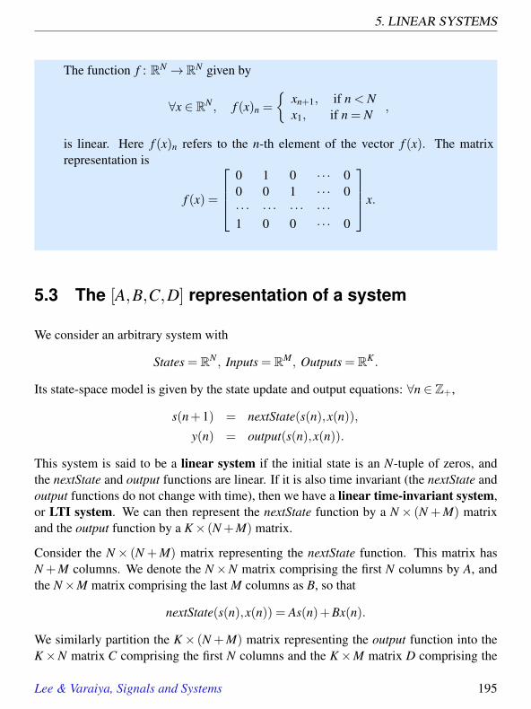
5. LINEAR SYSTEMS
The function f : RN → RN given by
∀x ∈ RN , f (x)n =
xn+1, if n < Nx1, if n = N
,
is linear. Here f (x)n refers to the n-th element of the vector f (x). The matrixrepresentation is
f (x) =
0 1 0 · · · 00 0 1 · · · 0· · · · · · · · · · · ·1 0 0 · · · 0
x.
5.3 The [A,B,C,D] representation of a system
We consider an arbitrary system with
States = RN , Inputs = RM, Outputs = RK .
Its state-space model is given by the state update and output equations: ∀n ∈ Z+,
s(n+1) = nextState(s(n),x(n)),
y(n) = output(s(n),x(n)).
This system is said to be a linear system if the initial state is an N-tuple of zeros, andthe nextState and output functions are linear. If it is also time invariant (the nextState andoutput functions do not change with time), then we have a linear time-invariant system,or LTI system. We can then represent the nextState function by a N× (N +M) matrixand the output function by a K× (N +M) matrix.
Consider the N× (N +M) matrix representing the nextState function. This matrix hasN +M columns. We denote the N×N matrix comprising the first N columns by A, andthe N×M matrix comprising the last M columns as B, so that
nextState(s(n),x(n)) = As(n)+Bx(n).
We similarly partition the K× (N +M) matrix representing the output function into theK×N matrix C comprising the first N columns and the K×M matrix D comprising the
Lee & Varaiya, Signals and Systems 195

5.3. THE [A,B,C,D] REPRESENTATION OF A SYSTEM
last M columns. Then
output(s(n),x(n)) =Cs(n)+Dx(n).
With this notation, the state-space model is represented as
s(n+1) = As(n)+Bx(n),
y(n) = Cs(n)+Dx(n).(5.16)
This is the [A,B,C,D] representation of the LTI system. This compact representationis very powerful. All the results in this chapter and the next are in terms of these fourmatrices. The A matrix is the most important, since it characterizes the system dynamicsas we will see in the sections below.
Example 5.5: Take [A,B,C,D] as
A =
1 1 00 1 10 0 1
, B =
001
,C =
[1 0 0
], D =
[1].
So N = 3,M = 1,K = 1. (This is a 3-dimensional, SISO system.) Using these in(5.16) gives the state-space model in tuple form,
s1(n+1) = s1(n)+ s2(n),
s2(n+1) = s2(n)+ s3(n),
s3(n+1) = s3(n)+ x(n),
y(n) = s1(n)+ x(n).
The first three equations together give the nextState function, the fourth equationgives the output function.
196 Lee & Varaiya, Signals and Systems

5. LINEAR SYSTEMS
Observe in (5.16) that if initialState is zero, s(0) = 0, and the input x(n) = 0, for all n≥ 0,then the state is unchanged, s(n) = 0. That is why we say that 0 is an equilibrium or reststate of the [A,B,C,D] system.
Example 5.6: An echo effect can be obtained for audio signals by realizing thefollowing difference equation,
y(n) = x(n)+αy(n−N),
where the (discrete-time) audio input is x, the output is y, 0 ≤ α < 1 is a real con-stant, and N ∈ N is an integer constant. Together, α and N determine how longthe echo lasts and what it sounds like. Once again, this is a SISO system, withM = 1,K = 1. This works simply because the output sample at n is a combinationof the current input x(n) and a scaled old output αy(n−N), called the echo term.Typically, N needs to be a large number to hear this as an echo. For example, if thesample rate is 8,000 samples per second, then if N = 8000, the echo term αy(n−N)is the previous output one second earlier. This will be heard as a distinct echo.
To construct a state-space model, we need to figure out what will work as the state.Since the output depends on y(n−N), which is past history, the state will have toyield y(n−N). The following state definition will work,
s(n) =
y(n−1)y(n−2)· · ·y(n−N)
.It is easy to check that with this state definition, [A,B,C,D] are given by
A =
0 0 · · · 0 0 α
1 0 · · · 0 0 00 1 · · · 0 0 0...
......
......
0 0 · · · 1 0 00 0 · · · 0 1 0
, B =
10...0
,
C =[
0 0 · · · 0 α], D =
[1],
Lee & Varaiya, Signals and Systems 197

5.3. THE [A,B,C,D] REPRESENTATION OF A SYSTEM
5.3.1 Impulse response
The [A,B,C,D] representation provides a complete description of an LTI system. It is acomplete in the sense that given any input sequence, we can calculate the output sequenceusing the state and output equations of (5.16) (or (5.19) and (5.20) for the scalar case).We will discover that there are several other descriptions of LTI systems that are alsocomplete. The first of these that we will consider is the impulse response. For systemsthat are initially at rest, the impulse response gives enough information to calculate theoutput sequence given any input sequence. The calculation is performed using what isknown as a convolution sum.
Suppose that M = 1, and the input sequence x is given by x = δ, where
∀ n ∈ Z, δ(n) =
1, if n = 00, if n 6= 0
. (5.17)
This function δ : Z→ R is called an impulse, or a Kronecker delta function (this func-tion figures prominently in chapters 8 and 9). Remarkably, the response of an LTI systemto this particular input is a complete description of the LTI system.
Assuming the system is initially at rest, we can use (5.16) to write the state response toinput δ as
s(0) = 0
s(1) = B
s(2) = AB
s(3) = A2B
· · ·s(n) = An−1B
· · ·
This is because if x = δ, then x(0) = 1 and x(n) = 0 for all n 6= 0.
To avoid confusion, we will use the name h instead of y for the output of a system whenthe input is the impulse δ. In other words, while y is the output for any input x, h is theoutput for the specific input δ. This output is called the impulse response. Using (5.16),
198 Lee & Varaiya, Signals and Systems

5. LINEAR SYSTEMS
it can be written as
h(0) = D
h(1) = CB
h(2) = CAB
h(3) = CA2B
· · ·h(n) = CAn−1B
· · ·Of course, since the system is initially at rest, h(n) = 0 for all n < 0. We can recognizethe pattern and write the impulse response as
∀ n ∈ Z, h(n) =
0, if n < 0D, if n = 0CAn−1B, if n≥ 1
. (5.18)
This formula is rarely the right way to compute an impulse response (usually it is easierto directly determine the output when the input is an impulse), but it does relate the im-pulse response to the [A,B,C,D] representation. The remarkable fact, developed below,is that knowing the impulse response is sufficient to calculate the output given any input(assuming the system is initially at rest).
The impulse response only makes sense if the dimension M of the input is one (otherwisethe input could not be an impulse as defined above). We can gain insight by consideringeven more special systems where N = K = 1, as done in the next section.
5.3.2 One-dimensional SISO systems
The simplest LTI system is the one-dimensional, SISO system. Since N = M = K = 1,the [A,B,C,D] representation is simply [a,b,c,d] where a,b,c,d are scalar constants. Thestate-space model (5.16) is ∀n ∈ Z+,
s(n+1) = as(n)+bx(n), (5.19)
y(n) = cs(n)+dx(n). (5.20)
The initial state s(0) = initialState. For this system, the state at a given time index is areal number, as are the input and the output.
Lee & Varaiya, Signals and Systems 199

5.3. THE [A,B,C,D] REPRESENTATION OF A SYSTEM
Let us consider an example where we construct a state-space model from an input-outputdescription of a system.
Example 5.7: In Section 2.3.3 we considered a simple moving average example,where the output y is given in terms of the input x by
∀ n ∈ Z+, y(n) = (x(n)+ x(n−1))/2. (5.21)
This is not a state-space model because it gives the output directly in terms of thecurrent and past input. To construct a state-space model for it, we first need todecide what the state is. Usually, there are multiple answers, so we face a choice.The state is a summary of the past. Examining (5.21), it is evident that we needto remember the previous input, x(n− 1), in order to produce an output y(n) (ofcourse, we also need the current input, x(n), but that is not part of the past; that isthe present). So we can define the state to be
∀ n ∈ Z+, s(n) = x(n−1).
We assume that the system is initially at rest, i.e., s(0) = 0. (If we knew x(−1), wewould take that to be the initial state.) With this choice of state, we need to choosea, b, c, and d so that (5.19) and (5.20) are equivalent to (5.21). Let us look first at(5.20), which reads
y(n) = cs(n)+dx(n).
Observing that s(n) = x(n− 1), can you determine c and d? From (5.21), it isobvious that c = d = 1/2.
Next, we determine a and b in
s(n+1) = as(n)+bx(n).
Since s(n) = x(n−1), it follows that s(n+1) = x(n), and this becomes
x(n) = ax(n−1)+bx(n),
from which we can see that a = 0 and b = 1.
Note that we could have chosen the state differently. For example,
∀ n ∈ Z+, s(n) = x(n−1)/2
would work fine. How would that change a, b, c, and d?
200 Lee & Varaiya, Signals and Systems

5. LINEAR SYSTEMS
In the preceding example, we started with an input-output description and obtained astate-space model. The next example shows we can also go the other way.
Example 5.8: Consider a one-dimensional SISO system
s(n+1) = as(n)+bx(n),
y(n) = cs(n)+dx(n).
From these equations we get
y(n) = c[as(n−1)+bx(n−1)]+dx(n),
y(n−1) = cs(n−1)+dx(n−1).
Multiplying the second equation by a and subtracting from the first eliminates thestate to yield a difference equation description of the system,
y(n)−ay(n−1) = dx(n)+(cb−ad)x(n−1).
There is a generalization of this example that works for state-space models of anydimension.
In the following example, we use a state-space model to calculate the output of a systemgiven an input sequence.
Example 5.9: Suppose the state s(n) is your bank balance at the beginning of dayn, and x(n) is the amount you deposit or withdraw during day n. If x(n) > 0, itmeans that you are making a deposit of x(n) dollars, and if x(n)< 0, it means thatyou are withdrawing x(n) dollars. The output of the system at time index n is thebank balance on day n. Thus,
States = Inputs = Outputs = R.
Note that these sets are probably not, strictly speaking, equal to R , since depositsand withdrawals can only be a whole number of cents. Using R is a considerablesimplification.
Lee & Varaiya, Signals and Systems 201

5.3. THE [A,B,C,D] REPRESENTATION OF A SYSTEM
Suppose that the daily interest rate is r. Then your balance at the beginning of dayn+1 is given by
∀ n ∈ Z, s(n+1) = (1+ r)s(n)+ x(n). (5.22)
The output of the system is your current balance,
∀ n ∈ Z, y(n) = s(n).
Comparing to (5.19)-(5.20), we have a = 1+ r, b = 1, c = 1, and d = 0. The initialcondition is initialState, your bank balance at the beginning of day 0. Supposethe daily interest rate is 0.01, or one percent (this would only be reasonable in aneconomy with hyperinflation). Suppose that initialState = 100, and you deposit1,000 dollars on day 0 and withdraw 30 every subsequent day for the next 30 days.What is your balance s(31) on day 31? You can compute s(31) recursively from
s(0) = 100,
s(1) = 1.01s(0)+1000,
· · ·s(n+1) = 1.01s(n)−30, n = 1, · · · ,30,
but this would be tedious. We can develop a formula that is easier to use. We willdo this for a general one-dimensional [a,b,c,d] system.
202 Lee & Varaiya, Signals and Systems

5. LINEAR SYSTEMS
Suppose we are given an input sequence x(0),x(1), · · · for an [a,b,c,d] system. As inexample 5.9, if we repeatedly use (5.19) we obtain the first few terms of a sequence,
s(0) = initialState, (5.23)
s(1) = as(0)+bx(0),
s(2) = as(1)+bx(1)
= aas(0)+bx(0)+bx(1)
= a2s(0)+abx(0)+bx(1),
s(3) = as(2)+bx(2)
= aa2s(0)+abx(0)+bx(10)+bx(2)
= a3s(0)+a2bx(0)+abx(1)+bx(2),
· · ·
From this it is not difficult to guess the general pattern for the state response and the outputresponse. The state response of (5.19) is given by
s(n) = aninitialState+n−1∑
m=0an−1−mbx(m) (5.24)
for all n≥ 0, and the output response of (5.20) is given by
y(n) = caninitialState+
n−1∑
m=0can−1−mbx(m)
+dx(n) (5.25)
for all n≥ 0.
We use induction to show that these are correct. Induction is where we show that these arecorrect for some fixed n, and then show that if it is correct for any n, then it is correct forn+1. For n = 0, (5.24) gives s(0) = a0initialState = initialState, which matches (5.23),and hence is correct.1 Now suppose that the right-hand side of (5.24) gives the correctvalue of the response for some n ≥ 0. We must show that it gives the correct value ofthe response for n+ 1. From (5.19) and using the hypothesis that (5.24) is the correct
1For any real number a, a0 = 1 by definition of exponentiation.
Lee & Varaiya, Signals and Systems 203

5.3. THE [A,B,C,D] REPRESENTATION OF A SYSTEM
expression for s(n), we get
s(n+1) = as(n)+bx(n)
= aaninitialState+n−1
∑m=0
an−1−mbx(m)+bx(n)
= an+1initialState+n−1
∑m=0
an−mbx(m)+bx(n)
= an+1initialState+n
∑m=0
an−mbx(m),
which is the expression on the right-hand side of (5.24) for n+1. It follows by inductionthat the response is indeed given by (5.24) for all n≥ 0. The fact that the output responseis given by (5.25) follows immediately from (5.20) and (5.24).
Example 5.10: We use formula (5.24) in example 5.9 to figure out the monthlypayment of $w on a $10,000, 32-month loan with a monthly interest of 0.01. Soin (5.24) we substitute n = 32,a = 1.01,b = 1, s(0) = −10,000,s(32) = 0, andx(0) = · · ·= x(31) = w, to get
0 =−1.0132×10000+31
∑m=0
1.0131−mw.
Using the identity (valid for ρ 6= 1)
M
∑m=0
ρm =
ρ1+M−1ρ−1
,
we get31
∑m=0
1.0131−mw =1.0132−1
0.01w.
So the monthly payment is
w = 0.01× 10000×1.0132
1.0132−1= 366.7.
204 Lee & Varaiya, Signals and Systems

5. LINEAR SYSTEMS
In the next example we identify the unknown parameter a of an [a,b,c,d] representationgiven input-output data.
Example 5.11: Financial analysts compare alternative investment opportunitiesusing a measure called the internal rate of return. Suppose an investment of$10,000 at the beginning of year 0 yields an income stream of $2,000 for each of10 successive years, and nothing thereafter. By definition, the investment’s internalrate of return is the annual interest rate r that a bank should give so that you can getthe same income stream. So we need to find r such that
s(n+1) = (1+ r)s(n)+ x(n),
with s(0) = 10,000, s(10) = 0, and x(0) = · · ·= x(9) =−2000. We recognize thisas a state update with a = 1+ r and b = 1. Substituting in (5.24) gives
0 = (1+ r)1010000−9
∑m=0
(1+ r)9−m×2000
= (1+ r)1010000− (1+ r)10−1r
×2000,
so1− (1+ r)−10 = 5r,
which we can solve by trial-and-error to obtain r ≈ 0.15 or 15 percent. Supposethere is another investment opportunity for the same $10,000 investment that yieldsan internal rate of return smaller than 15 percent. Then, all else being equal, onewould choose the first opportunity.
5.3.3 Zero-state and zero-input response
The expressions (5.24) for the state response and (5.25) for the output are each the sumof two terms. The role of these two terms will be better understood if we consider themin isolation.
If the system is initially at rest, initialState= 0, the first term vanishes, and only the secondterm is left. This second term is called the zero-state response. It gives the response of
Lee & Varaiya, Signals and Systems 205
5.3. THE [A,B,C,D] REPRESENTATION OF A SYSTEM
the system to an input sequence when the initial state is zero. For many applications,particularly when modeling a physical system, the zero-state response is what we areinterested in.
If the input sequence is zero, i.e. 0 = x(0) = x(1) = · · · , the second term vanishes, andonly the first term is left. The first term is called the zero-input response. It gives theresponse of the system to some initial condition, with zero input stimulus applied. Ofcourse, if the system is initially at rest and the input is zero, then the state remains at zero.So the zero-input response is only interesting if the system is not initially at rest.
So the right-hand side of both equations (5.24) and (5.25) are a sum of a zero-state re-sponse and a zero-input response. To make it clear which equation we are talking about,we use the following terminology:
zero-state state response The state sequence s(n) when theinitial state is zero.
zero-input state responseThe state sequence s(n) when theinput is zero.
zero-state output response The output sequence y(n) whenthe initial state is zero.
zero-input output responseThe output sequence y(n) whenthe input is zero.
Note that “zero-state” really means that the initial state is zero, while “zero input” meansthat the input is always zero.
Let us focus on the zero-state output response. First, note from (5.18) that in this scalarcase, the impulse response can be written
∀ n ∈ Z, h(n) =
0, if n < 0d, if n = 0can−1b, if n≥ 1
. (5.26)
We can use this sequence in (5.25) to simplify its form. This simplified form will show ushow to calculate the response to an arbitrary input given only the response to an impulse.
Combining (5.25) and (5.26), the zero-state output response can be written as
∀ n≥ 0, y(n) =n
∑m=0
h(n−m)x(m). (5.27)
206 Lee & Varaiya, Signals and Systems

5. LINEAR SYSTEMS
Thus, we see that h is a complete description of the system, in the sense that it is all weneed to know to find the output given any input x (assuming zero initial state).
Let x(n) = 0 for all n < 0, and, noting that h(n) = 0 for all n < 0, we can write this as
∀ n ∈ Z, y(n) =∞
∑m=−∞
h(n−m)x(m). (5.28)
The additional terms in the summation are harmless because they all have value zero. Asummation of this form is called a convolution sum. We say that y is the convolution ofh and x, and write it using the shorthand
y = h∗ x.
The ‘*’ symbol represents convolution. By changing variables, defining k = n−m, onecan see that the convolution sum can also be written in the equivalent form
∀ n ∈ Z, y(n) =∞
∑k=−∞
h(k)x(n− k). (5.29)
That is, h∗ x = x∗h. Convolution sums will be studied in much more detail in Chapter 9.
-0.5inThe impulse response of a system is simply the output when the input is an impulse. Ifthe system is initially at rest, then its output is given by the convolution of the input andthe impulse response.
Example 5.12: For our bank example, a = 1+ r, b = 1, c = 1, and d = 0 in (5.20).The impulse response of the bank system is given by (5.18),
h(n) =
0, if n≤ 0(1+ r)n−1, if n≥ 1
.
This represents the balance of a bank account with daily interest rate r if an initialdeposit of one dollar is put in on day 0, and no further deposits or withdrawals aremade. Notice that since 1+ r > 1, the balance continues to increase forever; see
Lee & Varaiya, Signals and Systems 207

5.3. THE [A,B,C,D] REPRESENTATION OF A SYSTEM
Figure 5.2. This system is said to be unstable because even though the input isalways bounded, the output grows without bound. The system is also an infiniteimpulse response (IIR) system.
Writing the output as a convolution, using (5.27), we see that
∀ n≥ 0, y(n) =n−1
∑m=0
(1+ r)n−m−1x(m).
This gives a simple formula that we can use to calculate the bank balance on anygiven day (although it will be tedious for large n, and you will want to use a com-puter).
The zero-input state response of the [a,b,c,d] system is
s(n) = ans(0),n≥ 0.
This is a geometric or exponential sequence. If s(0) 6= 0, the response will eventuallydie out, i.e. s(n)→ 0 as n→ ∞, if and only if |a|< 1, in which case we say the system isstable.
5.3.4 Multidimensional SISO systems
In the previous section we considered the simplest systems of the form of Figure 5.1with M = K = N = 1. Systems with larger dimension, N > 1, occur more frequently inpractice. In this section, we allow the dimension N to be arbitrarily large, but keep thesimplification that M = K = 1, so the system is still SISO (single-input, single-output). Inthe [A,B,C,D] representation, A is N×N, B is N×1, C is 1×N and D is 1×1. So for anSISO system we may write B = b, C = cT , D = d, where b,c are N-dimensional columnvectors and d is a scalar. Thus, SISO systems have an [A,b,c,d] representation, and theirstate-space model is
s(n+1) = As(n)+bx(n), (5.30)
y(n) = cT s(n)+dx(n). (5.31)
The result of evaluating the nextState function (5.30) is an N-dimensional vector, s(n+1).The N×N matrix A defines the linear combination of the N elements of s(n) that are used
208 Lee & Varaiya, Signals and Systems

5. LINEAR SYSTEMS
to calculate the N elements s(n+ 1). The N-dimensional column vector b defines theweights used to include x(n) in the linear combination for each element of s(n+1).
The result of evaluating the output function (5.31) is a scalar, y(n). The row vector cT
(which is N-dimensional) defines the linear combination of elements of s(n) and d definesthe weight used to include x(n) in the output y(n).
Example 5.13: Above we constructed a state-space model for a length-two mov-ing average. The general form of this is the M-point moving average, given by
∀ n ∈ Z, y(n) =1M
M−1
∑k=0
x(n− k). (5.32)
To be specific, let’s take M = 3. Equation (5.32) becomes
∀ n ∈ Z, y(n) =13(x(n)+ x(n−1)+ x(n−2)). (5.33)
We can construct a state-space model for this in a manner similar to what we did forthe length-two moving average. First, we need to decide what is the state. Recallthat the state is the summary of the past. Equation (5.33) tells us that we need toremember x(n− 1) and x(n− 2), the two past inputs. We could define these to bethe state, collected as a column vector,
s(n) =[
x(n−1)x(n−2)
].
(Of course, we could have equally well put the elements in the other order; seeExercise 9.)
Consider the output equation (5.31). We need to determine cT and d. The vectorcT is a row vector with dimension N = 2, so we must fill in the blanks in the outputequation below:
y(n) = [ , ]
[x(n−1)x(n−2)
]+[ ]x(n)
It is easy to see that each of the three blanks must be filled with 1/M = 1/3 in orderto get (5.33). Thus,
c =[
1/31/3
], d = 1/3.
Lee & Varaiya, Signals and Systems 209

5.3. THE [A,B,C,D] REPRESENTATION OF A SYSTEM
Consider next the state equation (5.30). We need to determine A and b. The matrixA is 2×2. The vector b is dimension 2 column vector. So we can fill in the blanksin the output equation below:
s(n+1) =[
x(n)x(n−1)
]=
[ ][x(n−1)x(n−2)
]+
[ ]x(n).
From this, we can fill in the blanks, getting
A =
[0 01 0
]and b =
[10
].
Note that once the state is specified, there is only one way to fill in the blanks andobtain the [A,b,c,d] representation.
The state response of the SISO system (5.30)-(5.31) is given by an expression similar to(5.24), but involving matrices and vectors rather than just scalars,
s(n) = AninitialState+n−1∑
m=0An−1−mbx(m) (5.34)
for all n≥ 0. The state response is also sometimes called the state trajectory. The outputresponse of (5.39) is given by
y(n) = cT AninitialState+
n−1∑
m=0cT An−1−mbx(m)
+dx(n) (5.35)
for all n≥ 0. (Exercise 13 asks you to derive these equations.)
Notice again that the state response (5.34) and the output response (5.35) are each thesum of two terms. The first term is the zero-input response and the second term is thezero-state response.
The impulse response, in terms of the state-space model, is the sequence of real numbers
h(n) =
0, if n < 0d, if n = 0cT An−1b, if n≥ 1
(5.36)
210 Lee & Varaiya, Signals and Systems

5. LINEAR SYSTEMS
This is just like (5.18) except that b and c are vectors, and d is a scalar. This formulacan be quite tedious to apply. It is usually easier to simply let x = δ, the Kronecker deltafunction, and observe or calculate the output. The zero-state output response is given byconvolution of this impulse response with the input, (5.29).
Example 5.14: We can find the impulse response h of the moving average systemof (5.32) by letting x = δ, where δ is given by (5.17). That is,
∀ n ∈ Z, h(n) =1M
M−1
∑k=0
δ(n− k).
Now, δ(n− k) = 0 except when n = k, at which point it equals one. Thus,
h(n) =
0 if n < 01/M if 0≤ n < M0 if n≥M
.
This function, therefore, is the impulse response of an M-point moving averagesystem. This result could also have been obtained by comparing (5.32) to (5.29),the output as a convolution. Or it could have been obtained by constructing a state-space model for the general length-M moving average, and applying (5.36). How-ever, this latter method would have proved the most tedious in this case.
Notice that in the previous example, the impulse response is finite in extent (it starts at 0and stops at M− 1). For this reason, such a system is called a finite impulse responsesystem or FIR system.
Example 5.15: The M-point moving average can be viewed as a special case ofthe more general FIR system given by
∀ n ∈ Z, y(n) =M−1
∑k=0
h(k)x(n− k).
Letting h(k) = 1/M for 0≤ k < M, we get the M-point moving average. Choosingother values for h(k), however, we can get other responses (this will be explored inchapter 8).
Lee & Varaiya, Signals and Systems 211

5.3. THE [A,B,C,D] REPRESENTATION OF A SYSTEM
A state-space model for the FIR system is constructed by again deciding on thestate. A reasonable choice is the M−1 past samples of the input,
s(n) = [x(n−1),x(n−2), · · · ,x(n−M+1)]T ,
a column vector. The state-space model is then given by (5.30) and (5.31) with
A =
0 0 0 0 · · · 0 01 0 0 0 · · · 0 00 1 0 0 · · · 0 0· · · · · · · · · · · · · · · · · · · · ·0 0 0 0 · · · 1 0
, b =
10· · ·00
,
c =
h(1)h(2)· · ·h(M−2)h(M−1)
, d = h(0).
Notice that the model that we found in example 5.13 has this form. The (M−1)×(M− 1) matrix A has coefficients ai+1,i = 1, while all other coefficients are zero.This is a rather special form of the A matrix, limited to FIR systems. The vector bhas the first coefficient equal to 1, while all others are zero. The vector c containsthe coefficients of the impulse response.
Many interesting systems, unlike this example, have an infinite impulse response, andare referred to as IIR systems.
Example 5.16: Recall from example 5.6 that an echo effect can be obtained foraudio signals by realizing the following difference equation,
∀ n ∈ Z, y(n) = x(n)+αy(n−N).
The impulse response h can be obtained by simply letting the input be an impulse,x = δ, and finding the output y = h. That is
∀ n ∈ Z, h(n) = δ(n)+αh(n−N). (5.37)
212 Lee & Varaiya, Signals and Systems

5. LINEAR SYSTEMS
But of course, this means that
h(n−N) = δ(n−N)+αh(n−2N).
Substituting this back into (5.37), we get
h(n) = δ(n)+αδ(n−N)+α2h(n−2N).
But of course,h(n−2N) = δ(n−2N)+αh(n−3N),
soh(n) = δ(n)+αδ(n−N)+α
2δ(n−2N)+α
3h(n−3N).
Continuing in this fashion, we see that the impulse response of the echo systemis the original impulse and an infinite set of echos (delayed and scaled impulses).This can be written compactly as follows,
∀ n ∈ Z, h(n) =∞
∑k=0
αkδ(n− kN).
This impulse response is plotted in Figure 5.3 for N = 4 and α = 0.7. In that figure,you can see that the original impulse gets through the system at n = 0, while thefirst echo is scaled by 0.7 and delayed to n = 4, and the second echo is scaled by0.72 and delayed to n = 8.
We can check this impulse response using the state-space representation of example5.6 in (5.36). From example 5.6, we have that d = 1, so (5.36) is obviously correctfor n < 0 and n = 0. Checking it for n > 0 is somewhat more involved. AssumingN = 4, we have from example 5.6
A =
0 0 0 α
1 0 0 00 1 0 00 0 1 0
, b =
1000
, c =
000α
, d =[
1].
To use (5.36) we need to know An−1. It is easy to check that
A2 =
0 0 α 00 0 0 α
1 0 0 00 1 0 0
, A3 =
0 α 0 00 0 α 00 0 0 α
1 0 0 0
,
Lee & Varaiya, Signals and Systems 213
5.3. THE [A,B,C,D] REPRESENTATION OF A SYSTEM
A4 =
α 0 0 00 α 0 00 0 α 00 0 0 α
= αI,
where I is the 4×4 identity matrix. Thus,
A5 = αA, A6 = αA2, A7 = αA3, A8 = αA4 = α2I.
The pattern continues. Note that because of the particular structure of b, An−1b issimply the first column of An−1. Thus,
h(1) = cT A0b = [0 0 0 α]
1000
= 0.
Similarly,
h(2) = cT Ab = [0 0 0 α]
0100
= 0,
and
h(3) = cT A2b = [0 0 0 α]
0010
= 0.
Only when we get to h(4) do we get a non-zero result,
h(4) = cT A3b = [0 0 0 α]
0001
= α.
Continuing in this fashion, we can determine that 3 of every four samples of theimpulse response are zero, and the non-zero ones have the form αn/4 where n is amultiple of four, in perfect agreement with figure 5.3.
214 Lee & Varaiya, Signals and Systems

5. LINEAR SYSTEMS
The echo system of the previous example is an example of an infinite impulse response(IIR) system because the response to an impulse never completely dies out. Here is an-other example of an IIR system.
Example 5.17: An audio oscillator is a system that produces a sinusoidal signalof a given frequency. We can construct one with the two-dimensional system givenby
A =
[cos(ω) −sin(ω)sin(ω) cos(ω)
], b =
[01
], c =
[10
],d = 0,
where ω is a constant that will turn out to be the oscillation frequency. It can beshown (see Exercise 14) that for all n = 0,1,2, · · ·
An =
[cos(nω) −sin(nω)sin(nω) cos(nω)
],
Suppose the initial state is
initialState = [0,1]T .
Then the zero-input state response is
szero−input(n) = An initialState
=
[cos(nω) −sin(nω)sin(nω) cos(nω)
][01
]
=
[−sin(nω)cos(nω)
],
and the zero-input response is
yzero−input(n) = cT An initialState
=[
1 0][ −sin(nω)
cos(nω)
]= −sin(nω).
Notice that without any input, as long as the initial state is non-zero, the systemwill produce a sinusoidal output in perpetuity.
Lee & Varaiya, Signals and Systems 215

5.3. THE [A,B,C,D] REPRESENTATION OF A SYSTEM
If we instead consider the situation where the system is initially at rest, then we findthat the impulse response is
h(n) =
d, if n = 0cT An−1b, if n≥ 1
.
For the values of A,b,c in this example we obtain
h(n) =
0, if n = 0−sin((n−1)ω), if n≥ 1
.
Thus, if the oscillator is initially at rest, it can be started with an impulse, and itsoutput will henceforth be sinusoidal, similar to the zero-input response. Thus, ifthe oscillator is initially at rest, it can be started with an impulse at the input.
5.3.5 Multidimensional MIMO systems
In the preceding sections, the input and output were both scalars. A MIMO system is onlyslightly more complicated. A state-space model for such a system is
∀ n ∈ Z+, s(n+1) = As(n)+Bx(n) (5.38)
y(n) = Cs(n)+Dx(n) (5.39)
where, s(n) ∈ RN , x(n) ∈ RM and y(n) ∈ RK , for any integer n. In the [A,B,C,D] repre-sentation, A is an N×N (square) matrix, B is an N×M matrix, C is a K×N matrix, andD is a K×M matrix. Now that these are all matrices, it is conventional to write them withcapital letters.
Let initialState ∈ RN be a given initial state. Let x(0),x(1),x(2), · · · , be a sequence ofinputs in RM (each input is a vector of dimension M). The state response of (5.38) isgiven by
s(n) = AninitialState+n−1
∑m=0
An−1−mBx(m) (5.40)
for all n≥ 0, and the output sequence of (5.39) is given by
y(n) =CAninitialState+
n−1
∑m=0
CAn−1−mBx(m)
+Dx(n) (5.41)
216 Lee & Varaiya, Signals and Systems
5. LINEAR SYSTEMS
for all n≥ 0 (each output is a vector of dimension K).
The right-hand sides of these equations are the sum of a zero-input response and a zero-state response. Consider the zero-state output response,
y(n) =n−1
∑m=0
CAn−1−mBx(m)+Dx(n) (5.42)
for all n≥ 0. Define the sequence h(0),h(1),h(2), · · · of K×M matrices by
h(n) =
D, if n = 0CAn−1B, if n≥ 1
(5.43)
This can no longer be called an impulse response, because the input cannot be an impulse;it has the wrong dimension (see box).
From (5.42) it follows that the zero-state output response is given by
y(n) =n
∑m=0
h(n−m)x(m), n≥ 0 (5.44)
This is once again a convolution sum.
The i, jth element of the matrix sequence h(0),h(1), · · · , namely
hi, j(0),hi, j(1), · · · ,
is indeed the impulse response of the SISO system whose input is x j and whose output isyi. In terms of Figure 5.1, this is the SISO system obtained by setting all inputs exceptthe jth input to zero, and considering only the ith output. If B j denotes the jth column ofB and CT
i denotes the ith row of C, then hi, j is the impulse response of the SISO system[A,B j,Ci,Di, j]. All these SISO systems have the same A matrix.
5.3.6 Linear input-output function
In the systems that this chapter considers, the nextState and output functions are linear.Recall that a function f : X → Y is linear if (and only if) it satisfies the superpositionproperty: for all x1,x2 ∈ X , and w,u ∈ R,
f (wx1 +ux2) = w f (x1)+u f (x2).
Lee & Varaiya, Signals and Systems 217

5.4. CONTINUOUS-TIME STATE-SPACE MODELS
What does it mean for a system to be linear? Recall that a system S is a function S : X→Y ,where X and Y are signal spaces. For a MIMO system, X = [Z→RM], and Y = [Z→RK ].The function S is defined by (5.41), which gives y = S(x), given x. So the answer isobvious. S is a linear system if S is a linear function. (It is an LTI system if it is also timeinvariant).
Examining (5.41), or its simpler SISO versions, (5.25) or (5.35), it is easy to see thatsuperposition is satisfied if initialState is zero. This is because with zero initial state, theoutput y(n) is a linear combination of the input samples x(n). Hence, a system given bya state-space model that is initially at rest is a linear system. The superposition propertyturns out to be an extremely useful property, as we will discover in the next chapters.
5.4 Continuous-time state-space models
A continuous-time state-space model for an LTI SISO system has the form
∀ t ∈ R+, z(t) = Az(t)+bv(t) (5.45)
w(t) = cT z(t)+dv(t) (5.46)
where
• z : R+→ RN gives the state response;• z(t) is the derivative with respect to time of z evaluated at t ∈ R+;• v : R+→ R is the input signal; and• w : R+→ R is the output signal.
As with the discrete-time SISO model, A is an N×N matrix, b and c are N× 1 columnvectors, and d is a scalar. As before, this is the [A,b,c,d] representation of the system, butthe equations are different.
Continuous-time systems are no longer state machines, since inputs, outputs, and statetransitions do not occur at discrete instances. Nevertheless, they share many properties ofdiscrete systems. The major difference between this model and that of (5.30) and (5.31)is that instead of giving new state as a function of the input and the old state, (5.45) givesthe derivative of the state. The derivative of a vector z is simply the vector consisting ofthe derivative of each element of the vector. A derivative, of course, gives the trend of thestate at any particular time. Giving a trend makes more sense than giving a new state fora continuous-time system, because the state evolves continuously.
218 Lee & Varaiya, Signals and Systems

5. LINEAR SYSTEMS
All of the methods that we have developed for discrete-time systems can also be developedfor continuous-time systems. However, they get somewhat more challenging mathemat-ically because the summations become integrals. We leave it to a more advanced text toexplore this.
A continuous-time state-space model may be approximated by a discrete-time state-spacemodel (see box). In fact, this approximation forms the basis for most computer simula-tions of continuous-time systems.
5.5 Summary
This chapter has begun the exploration of state machines whose state update and outputfunctions are linear. The number of possible states for such systems is typically infinite,so brute-force methods that enumerate the states will be ineffective. Instead, powerfulmathematical tools leverage the linearity of the key functions. This chapter barely beginsan exploration of the very rich set of tools that engineers have developed for such systems.Subsequent chapters will continue that exploration.
Lee & Varaiya, Signals and Systems 219

5.5. SUMMARY
Basics: Functions yielding tuples
The ranges of the nextState and output functions are tuples. It helps if we break themdown further into an N-tuple and K-tuple of functions, one for each element of the resulttuple. That is, we define the functions
nextStatei : RN×RM → R, i = 1, · · · ,N,
such that ∀ s ∈ RN ,∀x ∈ RM,
nextState(s,x) = (nextState1(s,x), · · · ,nextStateN(s,x)).
We write simplynextState = (nextState1, · · · ,nextStateN).
The output function can be given similarly as
output = (output1, · · · ,outputK),
whereoutputi : RN×RM → R, i = 1, · · · ,K.
Using these, the state update equation and output equation can be written as follows. Forall n ∈ Z, n≥ 0,
s1(n+1) = nextState1((s1(n), · · · ,sN(n)),(x1(n), · · · ,xM(n))),
s2(n+1) = nextState2((s1(n), · · · ,sN(n)),(x1(n), · · · ,xM(n))),
· · · (5.6)
sN(n+1) = nextStateN((s1(n), · · · ,sN(n)),(x1(n), · · · ,xM(n))),
and
y1(n) = output1((s1(n), · · · ,sN(n)),(x1(n), · · · ,xM(n))),
y2(n) = output2((s1(n), · · · ,sN(n)),(x1(n), · · · ,xM(n))),
· · · (5.7)
yK(n) = outputK((s1(n), · · · ,sN(n)),(x1(n), · · · ,xM(n))).
This system of equations shows the structure of the operation of such a machine.
220 Lee & Varaiya, Signals and Systems

5. LINEAR SYSTEMS
Basics: Matrices and vectors
An M×N matrix A is written as
A =
a1,1 a1,2 · · · a1,Na2,1 a2,2 · · · a2,N· · · · · · · · · · · ·aM,1 aM,2 · · · aM,N
.The dimension of the matrix is said to be M×N, where the number of rows is alwaysgiven first, and the number of columns is given second. In general, the coefficientsof the matrix are real or complex numbers, so they support all the standard arithmeticoperations. We write the matrix more compactly as
A = [ai, j,1≤ i≤M,1≤ j ≤ N],
or, even more simply as A = [ai, j] when the dimension of A is understood. The matrixentries ai, j are called the coefficients of the matrix.
Lee & Varaiya, Signals and Systems 221

5.5. SUMMARY
Basics: Vectors
A vector is a matrix with only one row or only one column. An N-dimensional columnvector s is written as an N×1 matrix
s =
s1s2· · ·sN
.An N-dimensional row vector zT is written as a 1×N matrix
zT = [z1,z2, · · · ,zN ].
The transpose of a M×N matrix A = [ai, j] is the N×M matrix AT = [a j,i]. Therefore,the transpose of an N-dimensional column vector s is the N-dimensional row vector sT ,and the transpose of an N-dimensional row vector z is the N-dimensional column vectorzT .
From now on, unless explicitly stated otherwise, all vectors denoted s,x,y,b,c etc.without the transpose notation are column vectors, and vectors denoted sT ,xT ,yT ,bT ,cT
with the transpose notation are row vectors. We follow convention and use lower caseletters to denote vectors and upper case letters to denote matrices.
A tuple of numeric values is often represented as a vector. A tuple, however, is neithera “row” nor a “column.” Thus, the representation as a vector carries the additionalinformation that it is either a row or a column vector.
222 Lee & Varaiya, Signals and Systems

5. LINEAR SYSTEMS
Basics: Matrix arithmetic
Two matrices (or vectors, since they are also matrices) can be added or subtracted pro-vided that they have the same dimension. Just as with adding or subtracting tuples,the elements are added or subtracted. Thus if A = [ai, j] and B = [bi, j] and both havedimension M×N, then
A+B = [ai, j +bi, j].
Under certain circumstances, matrices can also be multiplied. If A has dimension M×Nand B has dimension N×P, then the product AB is defined. The number of columns ofA must equal the number of rows of B. Suppose the matrices are given by
A =
a1,1 a1,2 · · · a1,Na2,1 a2,2 · · · a2,N· · · · · · · · · · · ·aM,1 aM,2 · · · aM,N
, B =
b1,1 b1,2 · · · b1,Pb2,1 b2,2 · · · b2,P· · · · · · · · · · · ·bN,1 bN,2 · · · bN,P
.Then the i, j element of the product C = AB isa
ci, j =N
∑m=1
ai,mbm, j. (5.9)
The product C has dimension M×P. (Continued on page 224.)aIf this notation is unfamiliar, see box on page 77.
Lee & Varaiya, Signals and Systems 223

5.5. SUMMARY
Basics: Matrix arithmetic (continued from page 223)
Matrix multiplication also works if one of the matrices is a vector. If b is a column vectorof dimension N, then c = Ab as defined by (5.9) is a column vector of dimension M. Ifon the other hand bT is a row vector of dimension M, then cT = bT A as defined by (5.9)is a row vector of dimension N.
Multiplying a matrix by a vector can be interpreted as applying a function to a tuple.The vector is the tuple and the matrix (together with the definition of matrix multiplica-tion) defines the function. Thus, in introducing matrix multiplication into our systems,we are doing nothing new except introducing a more compact notation for defining aparticular class of functions.
A matrix A is a square matrix if it has the same number of rows and columns. Asquare matrix may be multiplied by itself. Thus, An for some integer n > 0 is defined tobe A multiplied by itself n times. A0 is defined to be the identity matrix, also written I,which has ones along the diagonal and zeros everywhere else. If A has an inverse, thenthat inverse is denoted A−1, and AA−1 = A−1A = I.
-5 0 5 100
0.2
0.4
0.6
0.8
1
n
x
-5 0 5 100
0.5
1
1.5
2
2.5
n
s
Figure 5.2: Plots of the impulse (left) and the impulse response of example 5.12 (right)for r = 0.1.
224 Lee & Varaiya, Signals and Systems

5. LINEAR SYSTEMS
h(n)
n......
10.7
0.490.343
Figure 5.3: Impulse response of the echo example 5.16 for α = 0.7 and N = 4.
Probing Further: Impulse Responses of MIMO Systems
The h function in (5.43) is not the impulse response of a MIMO system with represen-tation [A,B,C,D]. However, with some care, it is possible to relate it to a set of impulseresponses that characterize the system.
The system has M inputs and K outputs, and for each integer n, h(n) in (5.43) is aK×M matrix. Each input symbol x(n) is an M-tuple of reals. Let xm(n) represent them-th element in this tuple, and let xm represent the sequence of such elements. Similarly,let yk(n) represent the k-th element of the output tuple, and yk the sequence of suchoutputs. Finally, let hk,m(n) represent the k,m-th element of the matrix h(n), and let hk,mrepresent the sequence of such elements.
The SISO system comprising the k-th output and m-th input has impulse responsehk,m. Specifically, if xm = δ and xp(n) = 0 for all p 6= m and for all n ∈ Z, then yk = hk,m.Thus, h can be viewed as a matrix of impulse responses, one for each possible pairingof input and output signals.
Lee & Varaiya, Signals and Systems 225

5.5. SUMMARY
Probing Further: Approximating continuous-time
Discrete LTI systems often arise as approximations of systems where differential equa-tions describe the physics. A differential equation has the form
∀ t ∈ R, z(t) = g(z(t),v(t)). (5.47)
Here t ∈R stands for continuous time, z :R→RN is the state response, and v :R→RM isthe input signal. That is, at any time t, z(t) is the state and v(t) is the input. The notationz stands for derivative of the state response z with respect to t, so g : RN ×RM → RN isa given function specifying the derivative of the state. Specifying the derivative of thestate is similar to specifying a state update. In a continuous-time system, state updatesoccur continuously rather than discretely.
In general, z is an N-tuple, z = (z1, · · · ,zN), where zi : R+→ R. The derivative of anN-tuple is the N-tuple of derivatives, z = (z1, · · · , zN). From calculus,
z(t) =dzdt
= limδ→0
z(t +δ)− z(t)δ
,
and so, if δ > 0 is a small number, we can approximate this derivative by
z(t)≈ z(t +δ)− z(t)δ
.
Using this for the derivative in the left-hand side of (5.47) we get
z(t +δ)− z(t) = δg(z(t),v(t)). (5.48)
Suppose we look at this equation at sample times t = 0,δ,2δ, · · · . Denote the value ofthe state response at the n-th sample time by s(n) = z(nδ), and the value of the input byx(n) = v(nδ). In terms of these variables, (5.48) becomes
s(n+1)− s(n) = δg(s(n),x(n))
which we can write as a state update equation,
s(n+1) = s(n)+δg(s(n),x(n)).
226 Lee & Varaiya, Signals and Systems

5. LINEAR SYSTEMS
Exercises
Each problem is annotated with the letter E, T, C which stands for exercise, requires somethought, requires conceptualization. Some of the problems require using Matlab.
1. E Use induction to obtain (5.13) as a consequence of (5.12).
2. E Use induction to show that if
A =
[a 10 a
],
then for all n≥ 0,
An =
[an nan−1
0 an
].
3. E Let f : RN → RN be a linear function given by ∀ x ∈ RN , f (x) = Ax for someN ×N matrix A. Give a similar definition for the composition f f . Is it alsolinear?
4. E What would be the monthly payment in example 5.10 if the monthly interest is0.015? Also, what would be the total payment over the 32 months?
5. E Construct a SISO state-space model for a system whose input and output arerelated by
∀ n ∈ Z, y(n) = x(n−1)+ x(n−2).
You may assume the system is initially at rest. It is sufficient to give the A matrix,vectors b and c, and scalar d of (5.30) and (5.31).
6. E The A matrix in (5.30) for a SISO system is
A =
[1 10 1
].
Calculate the zero-input state response if
(a) the initial state is [1,0]T ,
(b) the initial state is [0,1]T ,
(c) the initial state is [1,1]T .
Lee & Varaiya, Signals and Systems 227

EXERCISES
7. E Consider the one-dimensional state-space model, ∀ n ∈ Z+,
s(n+1) = s(n)+ x(n)y(n) = s(n)
Suppose the initial state is s(0)= a for some given constant a. Find another constantb such that if the first three inputs are x(0) = x(1) = x(2) = b, then y(3) = 0. Note:In general, problems of this type are concerned with controllability. The questionis whether you can find an input (in this case constrained to be constant) such thatsome particular condition on the output is met. The input becomes a control signal.
8. E A SISO LTI system has the A matrix given by
A =
[0 10 0
]and the b vector by [0,1]T . Suppose that s(0) = [0,0]T . Find the input sequencex(0),x(1) so that the state at step 2 is s(2) = [1,2]T .
9. E In example 5.13, the state was chosen to be s(n) = [x(n− 1),x(n− 2)]T . Howwould the [A,b,c,d] representation change if the state were chosen to be
(a) [x(n−2),x(n−1)]T ?
(b) [x(n−1)+ x(n−2),x(n−1)− x(n−2)]T ?
10. E Suppose the A matrix of a two-dimensional SISO system is
A = σ
[cos(π/6) sin(π/6)−sin(π/6) cos(π/6)
].
Suppose the initial state is s(0)= [1,0]T , and the input is zero. Sketch the zero-inputstate response for n = 0,1, · · · ,12 for the cases
(a) σ = 0
(b) σ = 0.9
(c) σ = 1.1
11. E In this problem we further consider example 5.9. As in the example, supposeinitialState = 100, and you deposit 1,000 dollars on day 0 and withdraw 30 dollarsevery subsequent day for the next 30 days.
228 Lee & Varaiya, Signals and Systems

5. LINEAR SYSTEMS
(a) Write a Matlab program to compute your bank balance s(n),0≤ n≤ 31, andplot the result.
(b) Use formula (5.24) to calculate your bank balance at the beginning of day 31.The following identity may prove useful:
N
∑m=0
am =1−aN+1
1−a,
where a 6= 1.
12. E Use Matlab to calculate and plot the impulse response of the system
s(n+1) = as(n)+bx(n)
y(n) = cs(n)
for the following cases:
(a) a = 1.1
(b) a = 1.0
(c) a = 0.9
(d) a =−0.5
where in all cases, b = c = 1 and d = 0.
13. E Use induction to derive the SISO response expressions (5.34) and (5.35).
14. E Consider the two-dimensional system given in example 5.17, which has
A =
[cos(ω) −sin(ω)sin(ω) cos(ω)
].
Show that for all n = 0,1,2, · · ·
An =
[cos(nω) −sin(nω)sin(nω) cos(nω)
],
Hint: use induction and the identities
cos(α+β) = cos(α)cos(β)− sin(α)sin(β)
sin(α+β) = sin(α)cos(β)+ cos(α)sin(β)
Lee & Varaiya, Signals and Systems 229

EXERCISES
15. E A damped oscillator is a variant of the oscillator in example 5.17, where thesinusoidal signal decays with time. The damped oscillator is identical, except thatthe A matrix is given by
A = α
[cos(ω) −sin(ω)sin(ω) cos(ω)
],
where 0 < α < 1 is a constant damping factor.
(a) Find the zero-input state response and the zero-input response for the initialstate
initialState = [0,1]T .
(b) Find the zero-state impulse response.
16. T Consider the audio echo system in example 5.6. A more interesting effect (some-times called reverberation) can be obtained by simultaneously combining multipleechos. In this problem, consider the following difference equation, which combinestwo echos,
y(n) = x(n)+αy(n−M)+βy(n−N),
where the (discrete-time) audio input is x, the output is y, and 0 ≤ α < 1 and 0 ≤β < 1 are constants that specify two distinct echo terms. Suppose for simplicity thatM = 4 and N = 5. These numbers are not large enough to yield an audible echo,but the mathematical model is similar for larger numbers, so these are adequatefor study. Note that the zero-state impulse response of this system is much morecomplicated than the simple echo system (try to find it!), which accounts for aconsiderably more realistic echo effect.
(a) Give a state-space representation [A,B,C,D] of this system.
(b) Modify the system so that the audio input has two channels (stereo), but theoutput is still one channel. Combine the two input channels by adding themwith equal weight. Give [A,B,C,D].
230 Lee & Varaiya, Signals and Systems

6Hybrid Systems
Contents6.1 Mixed models . . . . . . . . . . . . . . . . . . . . . . . . . . . . . 2336.2 Modal models . . . . . . . . . . . . . . . . . . . . . . . . . . . . . 2356.3 Timed automata . . . . . . . . . . . . . . . . . . . . . . . . . . . . 2406.4 More interesting dynamics . . . . . . . . . . . . . . . . . . . . . . 250
Probing Further: Internet protocols . . . . . . . . . . . . . . . . . . 2516.5 Supervisory control . . . . . . . . . . . . . . . . . . . . . . . . . . 2606.6 Formal model . . . . . . . . . . . . . . . . . . . . . . . . . . . . . 2666.7 Summary . . . . . . . . . . . . . . . . . . . . . . . . . . . . . . . . 268Exercises . . . . . . . . . . . . . . . . . . . . . . . . . . . . . . . . . . . 269
This text models signals and systems as functions. To develop understanding, we studythe structure of the domain and range of these functions, as well as the structure of themapping from the domain to the range. Despite the uniformity of this approach, we havebegun to evolve two distinct families of models. Chapters 3 and 4 structure this mappingusing state machines. Chapter 5 generalizes these state machines so that the number ofpossible states is infinite, and specializes them so that the systems are linear and time-invariant (LTI). LTI systems prove to yield to powerful analytical techniques, which areonly hinted at in Chapter 5. Chapters 7 through 14 will further develop these analyticaltechniques by structuring the system mapping using frequency-domain concepts.
231

The analytical methods available for LTI systems prove so compelling that we wish toapply them even to systems that are not LTI. In fact, no real-world system is truly LTI. Ata minimum, its properties were certainly different during the initial stages of the big bang,so it cannot be time invariant. More practically, systems change over time; they are turnedon and off, they deteriorate, etc. Moreover, systems that behave as linear systems typicallydo so only over some regime of operation. For example, if the magnitude the inputsexceed some threshold, a real-world system will overload, and will no longer behavelinearly. A similar effect might result when the state wanders beyond some modest range.This chapter shows how models that are only applicable some of the time can be usedeffectively.
In chapters 3 and 4, signals are sequences of events. Their domain is (typically) N0,and their range is (typically) a finite and arbitrary set of symbols. The domain is notinterpreted as time, but rather as indexes of a sequence. In chapters 5 and 7 through 14,the domain of signals is interpreted as time. For continuous-time signals, the domain iseither R or R+, whereas for discrete-time signals it is either Z or N0. This interpretationof the domain as time is essential to the notion of frequency that is used throughout theforthcoming chapters.
Chapter 5 and this one provide a bridge between state-machine models and such time-based models by developing state machine models for time-based systems. In this chap-ter, we build another bridge between these two families of models by showing that theycan often be usefully combined and used simultaneously in the same model, rather thanas alternative views of a system. The resulting models are called hybrid systems. Theyare a powerful tool for understanding real-world systems.
To understand the value of hybrid systems, it is useful to reflect on the relative strengthsand weaknesses of time-based models and state-machine models. Chapter 5 demonstratesthat state-machine models are more general by showing how they can be used to describetime-based models. Since they are more general, why not just always use state-machinemodels? The methods of state-machine models, such as composition by forming a productof the state spaces and simulation do not yield the depth of understanding that we will getin the subsequent chapters from looking at frequency response. Why not always usefrequency response? Frequency response is a rather specialized analytical tool. It appliesonly to LTI systems. Most real-world systems are not LTI, so such powerful analyticaltools must be applied with careful caveats about the regime of operation over which theydo apply.
232 Lee & Varaiya, Signals and Systems

6. HYBRID SYSTEMS
Consider for example a home audio system. It takes data from a compact disc and convertsit into auditory stimulus. Is it LTI? Well, obviously not, since its system function changesrather drastically when you turn it on and off. The acts of turning it on and off, however,seem to match well the state transitions of a state machine. Can we come up with a modelwhere there is a state machine with two states, “on” and “off,” and associated with eachstate there is an LTI system that describes the behavior of the system in the correspondingmode of operation? Indeed we can. Such a model is called a hybrid system.
In order to get state machine models to coexist with time-based models, we need to inter-pret state transitions on the time line used for the time-based portion of the system, be itcontinuous time or discrete time. In the audio system, for example, we need to associate atime with the acts of turning it on or off. The models used in chapters 3 and 4 do not nat-urally do this, since the signals there are sequences of events. That is, they are functionswhose domain is N0, where there is no temporal association with an n ∈ N0.
Recall from Chapter 3 that the input and output alphabets of a state machine are requiredto include a stuttering element, typically denoted absent. Whenever the state machinereacts, if its input is the stuttering element, then it does not change state and its outputwill be the stuttering element. This is key to hybrid system models because it allowsus to embed the state machine into a time-based model. At any time where there is nointeresting input event, the machine stutters.
A hybrid system combines time-based signals with sequences of events. The time-basedsignals are of the form x : T → R, where R is some range (such as R or C), and T iseither R, R+, Z, or N0, depending on whether the time domain is discrete or continuousand whether the model includes a time origin. In chapters 3 and 4, the event signals hadthe form u : N0→ Symbols, where the set Symbols has a stuttering element. For a hybridsystem, however, these have to share a common time base with the time-based signals,so they have the form u : T → Symbols. Thus, events occur in time. Typically, for mostt ∈ T , u(t) = absent, the stuttering element. The non-stuttering element is used only atthose discrete values of time where an event occurs.
6.1 Mixed models
A state machine model becomes a time-based model if it reacts at all times in the timebase T . This means that state machines and time-based models can interact as peers,sending time-based signals to one another.
Lee & Varaiya, Signals and Systems 233

6.1. MIXED MODELS
(x(n), y(n)) | x(n) > y(n) / buy
shortoverlong
longovershort
Trader
(x(n), y(n)) | x(n) < y(n) / sell
x
y
buy, sell, absent
shortTerm
longTerm
price
2x10
xy
price
0
5
10
15
20
25
30
35
0.0 0.1 0.2 0.3 0.4 0.5 0.6 0.7 0.8 0.9 1.0
day
clos
ing
pric
e
2x10
sell
absent
buy
0.0 0.1 0.2 0.3 0.4 0.5 0.6 0.7 0.8 0.9 1.0
day
Figure 6.1: An implementation of the classical moving average cross-over methodfor trading stocks.
234 Lee & Varaiya, Signals and Systems

6. HYBRID SYSTEMS
Example 6.1: Moving averages are popular on Wall Street for detecting trends instock prices. But in using them, a key question arises: how long should the movingaverage be? A short-term moving average might detect short-term trends, while along-term moving average might detect long term trends. A classical method com-bines the two and compares them to generate buy and sell signals. If the short-termtrend is more sharply upward than the long term trend, a buy signal is generated.If the short term trend is more sharply downward than the long term trend, a sellsignal is generated.
A system implementing this moving average cross-over method is shown inFigure 6.1. The input is the discrete-time signal price : Z→ R representing theclosing price of a stock each day. The LTI systems shortTerm and longTerm areboth moving average systems, but shortTerm averages fewer successive inputs thanlongTerm. The outputs of these systems are the discrete-time signals x and y. Thefinite state machine reacts on each sample from these signals. It begins in the stateshort over long. The transition out of this state has the guard
(x(n),y(n)) | x(n)> y(n).
When this transition is taken, a buy signal is generated. The sell signal is generatedsimilarly. The plots below show the buy and sell signals generated by a (synthetic)sequence of stock prices.
This example illustrates a simple form of technical stock trading. In this extremeform, it has the controversial feature that it ignores the fundamentals of the com-pany whose stock is being traded. It is using the stock price alone as the indicatorof worth. In fact, much more sophisticated signal processing methods are used bytechnical stock traders, and they often do take as inputs other quantifiers of com-pany worth, such as reported revenues and profits.
6.2 Modal models
In the previous section, time-based systems are combined with state machines as peers. Aricher interaction is possible with a hierarchical combination. The general structure of a
Lee & Varaiya, Signals and Systems 235

6.2. MODAL MODELS
guard/output action
guard/output action
state name
state name
...events
...time-based signals
... events
... time-based signals
time-based system time-based system
action
HybridSystem
Figure 6.2: Notation for hybrid systems.
hierarchical hybrid system model is shown in figure 6.2. In that figure, there is a two-statefinite state machine. There are some changes to the notation, however, from what wasused in chapters 3 and 4.
First, notice that the inputs and outputs include both event signals and time-based signals.Second, notice that each state of the state machine is associated with a time-based system,called the refinement of the state. The refinement of a state gives the time-based behaviorof HybridSystem while the machine is in that state. Thus, the states of the state machinedefine modes of operation of the system, where the behavior in a given mode is givenby the refinement. A hybrid system is sometimes called a modal model for this reason.The refinement has access to all the inputs of HybridSystem, and produces the time-basedoutput signals of HybridSystem while the machine is in its mode.
Note that the term “state” for such a hybrid system can become confusing. The statemachine has states, but so do the refinement systems (unless they are memoryless). Whenthere is any possibility of confusion we explicitly refer to the states of the machine asmodes, and we refer to the states of the refinement as refinement states. The (complete)state of the hybrid system is a pair (m,s) where m is the mode and s is the state of thetime-based refinement system associated with mode m.
236 Lee & Varaiya, Signals and Systems

6. HYBRID SYSTEMS
Another difference from the notation used in chapters 3 and 4 is that state transitions in themachine have, in addition to the usual guard and output notations, an action. The actionwill typically set the initial refinement state of the time-based system in the destinationmode.
The guards are, as usual, sets. However, we need for the guards to be rich enough thata transition can be triggered by a particular value of a refinement state or by a value of atime-based input. Thus, the elements of the guards are tuples containing values of inputevents, time-based signals, and the refinement states. In the state machines in chapters3 and 4, the elements of the guards only contained values of input events. For hybridsystems, we add time-based signals and refinement states.
Example 6.2: Overload of an electronic system might be modeled by a state tran-sition that is triggered by the magnitude of the current refinement state exceedingsome threshold.
On the other hand, when the system is in some mode, the refinement state is only affectedby the time-based inputs. It is not affected by the event inputs. This keeps the time-basedmodels simple, so that they don’t have to deal with stuttering inputs.
Correspondingly, the time-based outputs are generated by the refinement, and hence neednot be mentioned after the slash on the transitions.
The state machine may react at any time in the time base T . The mode in which it isbefore this reaction is called the current mode. It will take a discrete state transitionand switch to the destination mode if the input values and the refinement state at thattime match a guard. If it does not take a discrete state transition, then the state machinestutters. In either case, the refinement of the current mode also reacts to the time-basedinputs, changes its state and produces outputs.
Example 6.3: Many high-end audio systems offer “digital signal processing.”Such a system typically has an embedded computer (a digital signal processor orDSP, see box on page 402). This computer is used to process the audio signalin various ways, for example to add reverberation or to perform frequency selec-tive filtering. A particularly simple function that might be performed is loudnesscompensation, something offered by all but the cheapest audio systems.
Lee & Varaiya, Signals and Systems 237
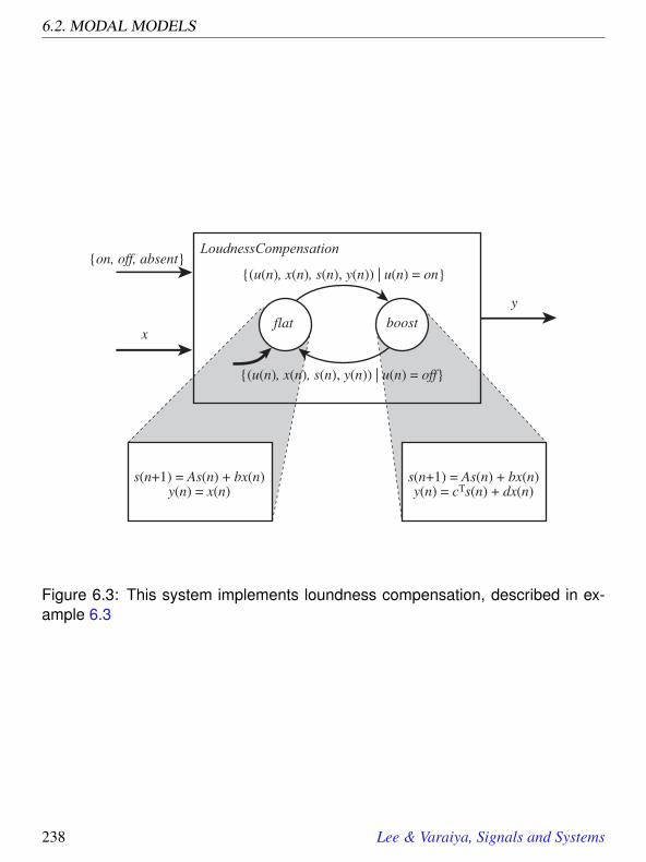
6.2. MODAL MODELS
(u(n), x(n), s(n), y(n)) | u(n) = on
flat boost
s(n+1) = As(n) + bx(n)y(n) = x(n)
LoudnessCompensation
x
y
on, off, absent
(u(n), x(n), s(n), y(n)) | u(n) = off
s(n+1) = As(n) + bx(n)y(n) = cTs(n) + dx(n)
Figure 6.3: This system implements loundness compensation, described in ex-ample 6.3
238 Lee & Varaiya, Signals and Systems

6. HYBRID SYSTEMS
At low volumes, the human ear is less sensitive to low frequencies (base notes)than to high frequencies. Loudness compensation boosts the low frequencies. Thisis done simply by implementing a filter, which is a linear time-invariant system thatcan be described by a state-space model, as in the previous chapter. Thus, there aretwo modes, one where the low frequencies are boosted (using the filter), and onewhere they are not.
A simple realization of loudness compensation offers a switch on a control panel toturn on and off the compensation. Figure 6.3 shows a hybrid system that reacts toinput events from this switch to select from among two modes. The upper input issimply an event indicating the position of the control switch when it is thrown. Thelower input x is a discrete-time signal, probably sampled at 44,100 samples/second,the CD rate. The LoudnessCompensation hybrid system has two modes. In the flatmode, the output y is simply set equal to the input x. That is, if Tf lat ⊂ Z is the timeindexes during which the machine is in the flat mode, then
∀ n ∈ Tf lat , y(n) = x(n).
This (obviously) does not boost low frequencies, since the output is equal to theinput.
When the on event occurs, the machine transitions to the boost mode, where thefilter is applied to the input x. This is done using the state update and output equa-tions
∀ n ∈ Tboost , s(n+1) = As(n)+bx(n)
y(n) = cT s(n)+dx(n),
where A,b,c,d are chosen to boost the low frequencies (how to do that is explainedin Chapter 9).
Note that in the flat mode, even though the output equation does not depend on thestate, the state update equation is still applied. This ensures that when switchingbetween states, no glitches are heard in the audio signal. The state of the boostrefinement is maintained even when the mode is flat.
This loudness compensator is not very sophisticated. A more sophisticated versionwould have a set of compensation filters and would select among them dependingon the volume level. This is explored in Exercise 1.
Lee & Varaiya, Signals and Systems 239

6.3. TIMED AUTOMATA
We consider a sequence of special cases of hybrid systems. Although the next few exam-ples are all continuous-time models, it is easy to construct similar discrete-time models.
6.3 Timed automata
Timed automata are the simplest continuous-time hybrid systems. They are modal modelswhere the time-based refinements have very simple dynamics; all they do is measure thepassage of time. Such refinements are called clocks. The resulting models are finite statemachines (automata) with time. Note that although all the examples in this section usecontinuous time, discrete-time versions are very similar.
A clock is modeled by a first-order differential equation,
∀ t ∈ Tm, s(t) = a,
where s : R→ R is a function, s(t) is the value of the clock at time t, and Tm ⊂ T is thesubset of time during which the hybrid system is in mode m. The rate of the clock, a, is aconstant while the system is in this mode.
Example 6.4: Suppose we want to produce a sequence of output events called tickwith the time between two consecutive ticks alternating between 1 and 2 seconds.That is, we want to produce a tick at times 1,3,4,6,7,9, · · · .A hybrid system tickGenerator that does this is illustrated in Figure 6.4. Thereare two modes labeled mode 1 and mode 2. The refinement state in each modeis the value of a clock at time t, denoted by s ∈ R. So at any time t the state oftickGenerator is the pair (mode(t),s(t)). The output is the event signal v and thetime-based signal s. There is no input.
In both modes, s evolves according to the differential equation s(t) = 1, where s(t)is the derivative of s with respect to time evaluated at some time t. Thus, s simplymeasures the passage of time, with its value rising 1 second for every second ofelapsed time.
The behavior of the system is shown in Figure 6.5. At time 0, as indicated by thebold arrow in Figure 6.4, the system initially enters mode 1. The bold arrow has anaction, “s(0) := 0,” which sets s(0) to 0. The notation “:=” is used instead of “=”to emphasize that this is an assignment, not an assertion (see Section A.1.1).
240 Lee & Varaiya, Signals and Systems
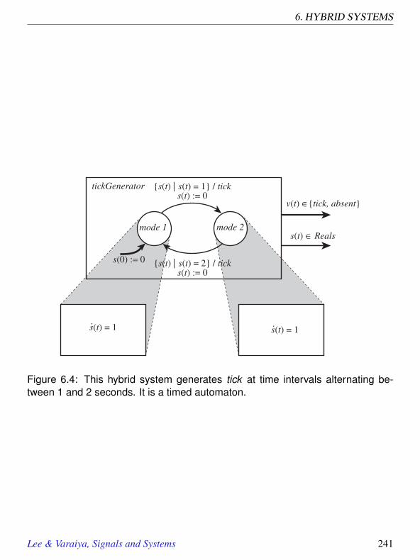
6. HYBRID SYSTEMS
s(t) | s(t) = 1 / ticks(t) := 0
mode 1 mode 2
s(t) = 1
tickGenerator
s(t) | s(t) = 2 / ticks(t) := 0
.s(t) = 1.
v(t) !tick, absent
s(t) ! Reals
s(0) := 0
Figure 6.4: This hybrid system generates tick at time intervals alternating be-tween 1 and 2 seconds. It is a timed automaton.
Lee & Varaiya, Signals and Systems 241

6.3. TIMED AUTOMATA
mode(t)
t...(a)
(b)
(c)
s(t)
t...
v(t)
t...absenttick
0 1 3 4
Figure 6.5: (a) The modes of the hybrid system of Figure 6.4, (b) the refinementstate s, and (c) the discrete event output v.
In this example, there is no input, so a guard is a subset of the possible values (R)of the refinement states. The guard on the transition from mode 1 to mode 2 is
s(t) | s(t) = 1,
which is satisfied one time unit after beginning. For all t ∈ [0,1], s(t) = t. At timet = 1, this guard is satisfied, the transition is taken, and the output event v(1) = tickis produced. For all t ∈ [0,1), v(t) has value absent.
This transition also has an action, “s(t) := 0,” which resets s to zero. This gives theinitial condition for the refinement system of the destination mode. In our defini-tion, at time t = 1, s(t) = 1, even though the action seems to contradict this. Thisis emphasized in Figure 6.5 by showing with a bold dot the value of s at each dis-continuity. The action s(t) := 0 is merely providing the initial conditions for therefinement of the destination mode. But the destination mode is not active untilt > 1, so the action is setting s(1+) to 0, where 1+ denotes a time infinitesimallylarger than 1.
242 Lee & Varaiya, Signals and Systems

6. HYBRID SYSTEMS
For t ∈ (1,3], the system remains in mode 2, evolving according to the differentialequation
s(t) = 1,
s(1) = 0.
So for 1 < t ≤ 3,
s(t) = s(1)+∫ t
11dt = t−1.
At time t = 3, the guard on the arc from mode 2 to mode 1 is satisfied, so thetransition is taken. The output event tick is again produced, and s is reset to 0 again.
Notice in Figure 6.5 that the output v is absent for all but a few discrete values of t ∈ R.This signal is called a discrete event signal for this reason. Of course, this signal can alsobe reinterpreted as a sequence of tick events with an arbitrary number of stuttering eventsin between. That signal could therefore be supplied as input to an ordinary state machine,enabling compositions of ordinary state machines with hybrid systems.
Also notice in Figure 6.5 that the hybrid system evolves in alternating phases: there is atime-passage phase in which the system stays in the same mode and its refinement statechanges with the passage of time; this is followed by an instantaneous discrete-eventphase in which a mode transition occurs, an output event is produced, and the refinementstate in the destination mode is initialized. In the figure, the time-passage phases are(0,1],(1,3],(3,4], · · · and the discrete-event phases occur at 1,3,4, · · · .Transitions between modes have actions associated with them. Sometimes, it is useful tohave transitions from one mode back to itself, just so that the action can be realized. Thisis illustrated in the next example.
Example 6.5: Figure 6.6 shows a hybrid system representation of the 60-minuteparking meter considered in Chapter 3. In the version in Figure 3.6, the states of astate machine are used to measure the passage of time by counting ticks providedby the environment. In the hybrid version of figure 6.6, the passage of time isexplicitly modeled by first-order differential equations.
There are two modes, expired and safe, and the refinement state at time t is s(t)∈R.At time t = 0, the initial mode is expired, and s(0) = 0. In the expired mode, s
Lee & Varaiya, Signals and Systems 243

6.3. TIMED AUTOMATA
nickel / absents(t) := 5
expired safe
s(t) = 0
parkingMeter
timeout / expired
.s(t) = !1.
v(t) "expired, absent
s(0) := 0
u(t) "coin5, coin25, absent
quarter / absents(t) := 25
nickel / absents(t) := min(s(t) + 5, 60)
quarter / absents(t) := min(s(t) + 25, 60)
timeout = (u(t), s(t)) | u(t) = absent and s(t) = 0nickel = (u(t), s(t)) | u(t) = coin5
quarter = (u(t), s(t)) | u(t) = coin25
Figure 6.6: A hybrid system representation of a 60-minute parking meter.
244 Lee & Varaiya, Signals and Systems

6. HYBRID SYSTEMS
remains at 0. The input events coin5 and coin25 cause one of two transitions fromexpired to safe to be taken. These transitions have guards that are named nickel andquarter and are defined by
nickel = (u(t),s(t)) | u(t) = coin5
quarter = (u(t),s(t)) | u(t) = coin25.Using names for these guards in the figure makes it more readable. It would becluttered if the guards were directly noted on the transitions.
The transitions from expired to safe produce absent. The actions on the transitionschange the value of s to 5 and 25, depending on whether coin5 or coin25 is received.
In the safe mode, the refinement state decreases according to the differential equa-tion of the clock,
∀ t ∈ Tsa f e, s(t) =−1.
There are three possible outgoing transitions from this mode. If the input eventcoin5 or coin25 occurs, then one of two self-loop transitions is taken, no output isproduced, and the associated action increments s by setting as s(t) := min(s(t)+5,60) or s(t) := min(s(t)+25,60). But if the guard timeout is satisfied, where
timeout = (u(t),s(t)) | u(t) = absent and s(t) = 0
then there is a transition to expired and the output event expired is produced. Notethat this guard requires that u(t) = absent, so that if the parking meter expires atthe very moment that a coin arrives, then the coin is properly registered.
In this system, the refinement state evolves differently in the two modes; in expired,s remains at 0 (since s(t) = 0), but in safe, s obeys the differential equation s(t) =−1.
In the previous example, the transitions from safe back to safe were used for their actions,which react to input events by setting the values of refinement states. This gives a cleanway to model discontinuities in continuous-time signals, because the state trajectory is acontinuous-time signal. A more extreme example is given next, where there is only onemode.
Lee & Varaiya, Signals and Systems 245

6.3. TIMED AUTOMATA
timer
s(t) = 1
TickGenerator
.
v(t) !safe,expired, absent
s(0) := 0
s(t) | s(t) = 1 / ticks(t) := 0 v(t) !tick,
absentparkingmeterstate
machine
u(t) !coin5, coin25, absent
Figure 6.7: The 60-minute parking meter as a cascade composition oftickGenerator and an ordinary finite state machine.
246 Lee & Varaiya, Signals and Systems

6. HYBRID SYSTEMS
Example 6.6: We could also implement the parking meter as a cascade compo-sition using a timed automaton, TickGenerator, with only one mode, timer, andwhich produces a tick event every minute. This event serves as an input to the park-ing meter finite state machine of Figure 3.6. The cascade composition is shown inFigure 6.7. The parking meter machine also accepts an additional (product-form)input event from coin5, coin25, and produces the output event safe or expired.The difference between Figure 3.6 and 6.7 is that in the former tick was an inputevent from the environment, whereas in the latter we explicitly construct a compo-nent, namely TickGenerator, which produces a tick every minute.
Timed automata are commonly used in modeling communication protocols, the logicused to achieve communication over a network. The following example models the trans-port layer of a sender of data on the internet.
Example 6.7: Consider how an application such as an e-mail program sends afile over a communication network like the internet. There are two host computerscalled the Sender and Receiver. The file that Sender wants to send to Receiver isfirst divided into a sequence of finite bit strings called packets. For the purposesof this example, we do not care what is contained by the packets, so we considerpacket to be an event. We are interested in the fact that it needs to be transmitted,not in its contents.
The problem we address in this example is that the network is unreliable. Packetsthat are launched into it may never emerge. If the network is congested, packets getdropped. We will design a protocol whereby the sender of a packet waits a certainamount of time for an acknowledgement. If it does not receive the acknowledge-ment in that time, then it retransmits the packet. This is an ideal application fortimed automata.
The upper diagram in Figure 6.8 shows the structure of the communication system.Everything begins when the sender produces a packet event. The SenderProtocolsystem reacts by producing a transmit event, which instructs its network interfacecard or NIC to launch the packet into the internet. The NIC is the physical de-vice (such as the ethernet card in your desktop computer) that converts the packet
Lee & Varaiya, Signals and Systems 247

6.3. TIMED AUTOMATA
Application
Sender
SenderProtocol
packet, absent ack, absent
NIC Internet NIC ReceiverProtocol
Application
Receiver
packet, absent
ack, absent
transmit, retransmit, absent packet, absent
ack, absent
packetArrives / (transmit, absent)s(t) := timeoutTime
idle timing
s(t) = 0
SenderProtocol
ackArrives / (absent, ack)s(t) := 0
.s(t) = !1.
v1(t) "transmit, retransmit, absent
s(0) := 0
v2(t) "ack, absent
timeout / (retransmit, absent)s(t) := timeoutTime
u1(t) "packet, absent
u2(t) "ack, absent
timeout = (u1(t), u2(t), s(t)) | s(t) = 0 and u2(t) # ackpacketArrives = (u1(t), u2(t), s(t)) | u1(t) = packet
ackArrives = (u1(t), u2(t), s(t)) | u2(t) = ack
Figure 6.8: The top diagram describes the structure of a communication system.The lower diagram is the timed automaton that implements the sender protocol.
248 Lee & Varaiya, Signals and Systems

6. HYBRID SYSTEMS
into the appropriate electrical signal that is transmitted through the network. Theinternet transfers this signal to the NIC of the receiver. That NIC converts thesignal back into the packet and forwards it to the ReceiverProtocol component.The ReceiverProtocol in turn forwards the packet to the e-mail application in theReceiver and simultaneously sends an acknowledgement packet, called ack, to itsNIC.
The receiver’s NIC sends the ack packet back through the network to the Sender.The sender’s NIC receives this packet and forwards an ack to the SenderProtocol.The SenderProtocol notifies the application that the packet was indeed delivered.The application can now send the next packet, and the cycle is repeated until theentire file is delivered.
In reality, the network may drop the packet so that it is not delivered to the receiver,who therefore will not send the corresponding ack. The SenderProtocol system isdesigned to take care of this contingency. It is a timed automaton with two modes,idle and timing, and one refinement state s corresponding to a clock. Initially it isin the idle mode and s(0) = 0. In the idle mode, s(t) = 0, so the refinement stateremains at zero. When SenderProtocol receives a packet it makes a transition to thetiming mode, sends the output event transmit to its NIC, and resets s to a timeoutvalue timeoutTime.
In the timing mode, there are two possibile transitions. In the normal case, the inputevent ack is received before the guard s(t) == 0 is satisfied. The transition tomode idle is taken, the output event ack is sent to the application, and the clockvalue s(t) is reset to 0. The system waits for another packet from the application.In the second case, the guard s(t) == 0 is satisfied (before event ack), and theself-loop transition is taken. In this case, the output event retransmit is sent to theNIC, and s(t) is reset to timeoutTime.
Notice a feature of this design that may not be expected. If a packet arrives whilethe machine is in mode timing, the packet is ignored. What happens if a packethappens to arrive simultaneously with an ack while the machine is mode timing?
Exercise 10 asks you to construct the corresponding receiver protocol, which issimpler.
In summary, the SenderProtocol machine repeatedly retransmits a packet everytimeoutTime seconds until it receives an ack. This reveals a flaw in the protocol.If the network is for some reason unable ever to successfully transmit a packet tothe receiver, the machine will continue retransmission for ever. A better protocol
Lee & Varaiya, Signals and Systems 249

6.4. MORE INTERESTING DYNAMICS
packetArrives / (transmit, absent)s(t) := timeoutTime
r(t) := 5 ! timeoutTime
idle timing
s(t) = 0r(t) = 0
BetterSenderProtocol
ackArrives / (absent, ack)s(t) := 0r(0) := 0.
s(t) = "1r(t) = "1
.
s(0) := 0r(0) := 0
timeout / (retransmit, absent)s(t) := timeoutTime
. .
failure / (absent, fail)s(t) := 0
timeout = (u1(t), u2(t), s(t), r(t)) | s(t) = 0 and r(t) # 0 and u1(t) # ackpacketArrives = (u1(t), u2(t), s(t), r(t)) | u1(t) = packet
ackArrives = (u1(t), u2(t), s(t), r(t)) | u2(t) = ack
v1(t) $transmit, retransmit, absent
v2(t) $ack,fail, absent
u1(t) $packet, absent
u2(t) $ack, absent
failure = (u1(t), u2(t), s(t), r(t)) | r(t) = 0 and u1(t) # ack
Figure 6.9: An improved sender protocol with two clocks, one of which detects afailed connection.
would retransmit a packet a certain number of times, say five times, and if it isunsuccessful, it would return to idle and send a message connectionFailed to theapplication. The hybrid system of Figure 6.9 incorporates this feature by addinganother clock whose value is r(t).
6.4 More interesting dynamics
In timed automata, all that happens in the time-based refinement systems is that timepasses. Hybrid systems, however, are much more interesting when the behavior of therefinements is more complex.
Example 6.8: Consider the physical system depicted in Figure 6.11. Two stickyround masses are attached to springs. The springs are compressed or extended and
250 Lee & Varaiya, Signals and Systems

6. HYBRID SYSTEMS
Probing Further: Internet protocols
Communication between two computers, Sender and Receiver, each connected to theinternet, is coordinated by a set of protocols. Each protocol can be modeled by a pairof hybrid systems, one in the Sender and the other in the Receiver. These protocols arearranged in a protocol stack, as shown in figure 6.10. Each layer in the stack performsa certain function, and interacts with the corresponding layer in the other computer. Thephysical layer converts a bit stream into an electrical signal and vice versa and transfersthe signal over one link of the network.
The network itself consists of many physical links connected by routers. The routersact as computers, but are missing the higher levels of the protocol stack. The physi-cal layer transports bits over wires, optical fibers, or radio links. The medium accesslayer manages contention for the physical communication resource, preventing colli-sions among multiple users of the link. The network layer routes packets appropriatelythrough the network. The transport layer ensures that the end-to-end transfer of pack-ets is reliable, even if the network layer is unreliable. The application layer convertswhatever information is to be sent (such as an image or e-mail) into packets and thenreassembles the packets into the appropriate information.
This layered approach provides an abstraction mechanism. Each layer conceptuallyinteracts with the corresponding layer at a remote machine, as suggested by the dottedlines in figure 6.10. Each layer provides a “service” to the layer above it. For example,the medium access layer offers as a service the transfer of a packet over a single link.The network layer uses this service to transfer a packet over a sequence of links betweenthe end hosts. This abstraction mechanism permits the design of a single layer, say thetransport layer, assuming the service of the network layer, without regard to the layersbelow the network layer. The hybrid system in example 6.7, for instance, models onlythe transport layer.
The transport layer in an end-to-end protocol, so it is implemented only at the endpoints in the connection, as shown in Figure 6.10. The routers in the network only needto implement the lower layers.
Each protocol layer is modeled as a pair of hybrid systems. Typically, these are timedautomata, since coordination between end hosts is achieved via several clocks as inexample 6.7. When a guard associated with a clock is satisfied, this signals some con-tingency in the communication, just as the timeout of the clock in Figure 6.8 signals thata packet may be lost.
Lee & Varaiya, Signals and Systems 251

6.4. MORE INTERESTING DYNAMICS
Application
Transport
Network
MediumAccess
Physical
Network
MediumAccess
Physical
Network
MediumAccess
Physical
Application
Transport
Network
MediumAccess
Physical...
Internet
link link
Sender Receiver
Figure 6.10: Network protocols are organized in a stack. Each protocol interactswith the corresponding layer in a remote computer. The dotted lines indicateconceptual interactions, whereas the solid lines indicate physical interactions.
252 Lee & Varaiya, Signals and Systems

6. HYBRID SYSTEMS
y1(t)
y2(t)
y1(t) y2(t)
0.0
0.5
1.0
1.5
2.0
2.5
3.0
0 5 10 15 20 25 30 35 40 45 50
Displacement of Masses
time
Figure 6.11: Sticky masses system considered in example 6.8.
Lee & Varaiya, Signals and Systems 253

6.4. MORE INTERESTING DYNAMICS
stick /
y(t) := y1(t)
y(t) := (y1(t)m1 + y2(t)m2)/(m1+ m2)
apart together
y1(t) = k1(p1 ! y1(t))/m1
stickyMasses
unstick /
y1(t) := y(t)
y2(t) := y(t)
y1(t) := y(t)
y2(t) := y(t)..
y1(t) " Reals
y2(t) " Reals
y1(0) := initialPosition1y2(0) := initialPosition2
y1(0) := 0y2(0) := 0
y2(t) = k2(p2 ! y2(t))/m2..
y(t) =.. k1 p1 + k2 p2 ! (k1+ k2)y(t)
m1+ m2
.
.
.
..
.
.
. .
y1(t) = y(t); y2(t) = y(t)
unstick = (y(t), y(t)) | (k1 ! k2)y(t) + k2 p2! k1p1 > stickiness.
stick = (y1(t), y1(t), y2(t), y2(t)) | y1(t) = = y2(t). .
Figure 6.12: Hybrid system model for the sticky masses system considered inexample 6.8.
254 Lee & Varaiya, Signals and Systems

6. HYBRID SYSTEMS
then released. The masses oscillate on a frictionless table. If they collide, they sticktogether and oscillate together. After some time, the stickiness decays, and massespull apart again.
A plot of the displacement of the two masses as a function of time is shown in thefigure. Both springs begin compressed, so the masses begin moving towards oneanother. They almost immediately collide, and then oscillate together for a briefperiod until they pull apart. In this plot, they collide two more times, and almostcollide a third time.
The physics of this problem is quite simple if we assume idealized springs. Lety1(t) denote the right edge of the left mass at time t, and y2(t) denote the left edgeof the right mass at time t, as shown in Figure 6.11. Let p1 and p2 denote theneutral positions of the two masses, i.e. when the springs are neither extended norcompressed, so the force is zero. For an ideal spring, the force at time t on the massis proportional to p1− y1(t) (for the left mass) and p2− y2(t) (for the right mass).The force is positive to the right and negative to the left.
Let the spring constants be k1 and k2, respectively. Then the force on the left springis k1(p1− y1(t)), and the force on the right spring is k2(p2− y2(t)). Let the massesbe m1 and m2 respectively. Now we can use Newton’s law, which relates force,mass, and acceleration,
f = ma.
The acceleration is the second derivative of the position with respect to time, whichwe write y1(t) and y2(t) respectively. Thus, as long as the masses are separate, theirdynamics are given by
y1(t) = k1(p1− y1(t))/m1 (6.1)
y2(t) = k2(p2− y2(t))/m2. (6.2)
When the masses collide, however, the situation changes. With the masses stucktogether, they behave as a single object with mass m1 +m2. This single object ispulled in opposite directions by two springs. While the masses are stuck together,y1(t) = y2(t). Let
y(t) = y1(t) = y2(t).
The dynamics are then given by
y(t) =k1 p1 + k2 p2− (k1 + k2)y(t)
m1 +m2. (6.3)
Lee & Varaiya, Signals and Systems 255

6.4. MORE INTERESTING DYNAMICS
It is easy to see now how to construct a hybrid systems model for this physicalsystem. The model is shown in Figure 6.12. It has two modes, apart and together.The refinement of the apart mode is given by (6.1) and (6.2), while the refinementof the together mode is given by (6.3).
We still have work to do, however, to label the transitions. The initial transition isshown in Figure 6.12 entering the apart mode. Thus, we are assuming the massesbegin apart. Moreover, this transition is labeled with an action that sets the initialrefinement state. Intuitively, the initial state of the masses is their positions andtheir initial velocities. In fact, we can define the refinement state to be
s(t) =
y1(t)y1(t)y2(t)y2(t)
.It is then a simple matter to rewrite (6.1) and (6.2) in the form
s(t) = g(s(t)) (6.4)
for a suitably chosen function g (see Exercise 12).
In Figure 6.12, the initial state has the masses at some specified displacement, andthe velocities at zero.
The transition from apart to together has the guard
stick = (y1(t), y1(t),y2(t), y2(t)) | y1(t) == y2(t).Thus, when the refinement state of apart satisfies this guard, the transition will betaken. No event output is produced, as indicated by the blank after the slash. How-ever, an action is taken to set the initial refinement state of together. The refinementstate of together could be the same s(t) as above, with the additional constraint thaty1(t) = y2(t) and y1(t) = y2(t), because the masses are stuck together. Or more sim-ply, we could define the state z(t) of together to be the position y(t) and velocityy(t), where y(t) = y1(t) = y2(t),
z(t) =[
y(t)y(t)
].
The transition from apart to together sets y(t) equal to y1(t) (it could equally wellhave chosen y2(t), since these are equal). It sets the velocity to conserve momen-tum. The momentum of the left mass is y1(t)m1, the momentum of the right mass
256 Lee & Varaiya, Signals and Systems

6. HYBRID SYSTEMS
is y2(t)m2, and the momentum of the combined masses is y(t)(m1 +m2). To makethese equal, it sets
y(t) =y1(t)m1 + y2(t)m2
m1 +m2.
The transition from together to apart has the more complicated guard
unstick = (y(t), y(t)) | (k1− k2)y(t)+ k2 p2− k1 p1 > stickiness.
This guard is satisfied when the right-pulling force on the right mass exceeds theright-pulling force on the left mass by more than the stickiness. The right-pullingforce on the right mass is simply
f2(t) = k2(p2− y(t))
and the right-pulling force on the left mass is
f1(t) = k1(p1− y(t)).
Thus,f2(t)− f1(t) = (k1− k2)y(t)+ k2 p2− k1 p1.
When this exceeds the stickiness, then the masses pull apart.
An interesting elaboration on this example, considered in problem 13, modifies thetogether mode so that the stickiness is initialized to a starting value, but then decaysaccording to the differential equation
s(t) =−as(t)
where s(t) is the stickiness at time t, and a is some positive constant. In fact, it isthe dynamics of such an elaboration that is plotted in Figure 6.11.
As in example 6.7, it is sometimes useful to have hybrid system models with only onestate. The actions on one or more state transitions define the discrete event behavior thatcombines with the time-based behavior.
Lee & Varaiya, Signals and Systems 257

6.4. MORE INTERESTING DYNAMICS
Example 6.9: Consider a bouncing ball. At time t = 0, the ball is dropped froma height y(0) = initialHeight meters. It falls freely. At some later time t1 it hitsthe ground with a velocity y(t1) < 0 m/sec. A bump event is produced when theball hits the ground. The collision is inelastic, and the ball bounces back up withvelocity −ay(t1), where a is constant in (0,1). The ball will then rise to a certainheight and fall back to the ground repeatedly.
The behavior of the bouncing ball can be described by the hybrid system of Figure6.13. There is only one mode, called free. When it is not in contact with the ground,we know that the ball follows the second-order differential equation,
y(t) =−g, (6.5)
where g = 10 m/sec2 is the acceleration imposed by gravity. We can define therefinement state of the free mode to be
s(t) =[
y(t)y(t)
]with the initial conditions y(0) = initialHeight and y(0) = 0. It is then a simplematter to rewrite (6.5) as a first-order differential equation,
s(t) = f (s(t)) (6.6)
for a suitably chosen function f (see Exercise 12).
At the time t1 when the ball first hits the ground, the guard
hit = (y(t), y(t)) | y(t) = 0
is satisfied, and the self-loop transition is taken. The output bump is produced, andthe action y(t) := −ay(t) assigns y(t1+) = −ay(t1). Here, y(t1+) is the velocityafter the bump, and y(t1) is the velocity before the bump. Then (6.5) is followedagain until the guard becomes true again.
By integrating (6.5) we get, for all t ∈ (0, t1),
y(t) = −gt,
y(t) = y(0)+∫ t
0y(τ)dτ = initialHeight− 1
2gt2.
258 Lee & Varaiya, Signals and Systems

6. HYBRID SYSTEMS
free
y(t) = ! g
BouncingBall
..
y(0) := initialHeighty(0) := 0
hit / bumpy(t) := ! a y(t)
y(t) " Reals
.bump, absent
. .
initialHeight
y(t)
t1 t2 time
y(t)
t1 t2 time
.
hit = (y(t), y(t)) | y(t) = 0.
Figure 6.13: The motion of a bouncing ball may be described as a hybrid systemwith only one mode. The system outputs a bump each time the ball hits theground, and also outputs the position of the ball. The position and velocity areplotted versus time at the right.
So t1 > 0 is determined by y(t1) = 0. It is the solution to the equation
initialHeight− 12
gt2 = 0.
Thus,t1 =
√2 initialHeight/g.
Figure 6.13 plots the refinement state versus time.
Lee & Varaiya, Signals and Systems 259

6.5. SUPERVISORY CONTROL
x(t)
y(t)AGV
globalcoordinate
frame
e(t)
track
(t)
Figure 6.14: Illustration of the automated guided vehicle of example 6.10. Thevehicle is shown as a large arrow on the left and as a small arrow on the right. Onthe right, the vehicle is following a curved painted track, and has deviated fromthe track by a distance e(t). The coordinates of the vehicle at time t with respectto the global coordinate frame are (x(t),y(t),φ(t)).
6.5 Supervisory control
We introduce supervisory control through a detailed example. A control system involvesfour components. There is a system called the plant—the physical process that is to becontrolled; the environment in which the plant operates; the sensors that measure somevariables of the plant and the environment; and the controller that determines the modetransition structure and selects the time-based inputs to the plant. The controller hastwo levels: the supervisory control that determines the mode transition structure, andthe ‘low-level’ control that selects the time-based inputs which control the behavior ofthe refinements. A complete design includes both levels of control as in the followingexample.
260 Lee & Varaiya, Signals and Systems

6. HYBRID SYSTEMS
stop left
Vehicle
right straight
x (t) = 10 cos φ(t)y (t) = 10 sin φ(t) φ (t) = - πe (t) = f(x(t), y(t))
u(t) e stop, start, absent
x (t) = 10 cos φ (t)y (t) = 10 sin φ (t)φ = πe (t) = f(x(t), y(t))
.
.
.
x (t) = 10 cos φ (t)y (t) = 10 sin φ (t)φ (t) = 0e (t) = f(x(t), y(t))
.
.
.
x = x0y = y0 φ = φ0
goRight/
goLeft/
x (t) = 0 y (t) = 0 φ (t) = 0e (t) = f(x(t), y(t))
.
.
.
...
goStraight= (u(t), x(t), y(t), φ (t)) | u(t) != stop, |e(t)| < ε1
goRight/
goStraight/
goLeft = (u(t), x(t), y(t), φ (t)) | u(t) != stop, - ε2 > − e(t)
goStraight/
goLeft/
goStop/ goStop/
goStop/
goStart/
goStop = (u(t), x(t), y(t), φ (t)) | u(t) = stopgoStart = (u(t), x(t), y(t), φ (t)) | u(t) = start
goRight =(u(t), x(t), y(t), φ (t)) | u(t) != stop, ε2 < e(t)
Figure 6.15: The automatic guided vehicle of example 6.10 has four modes: stop,straight , left , right .Lee & Varaiya, Signals and Systems 261

6.5. SUPERVISORY CONTROL
Example 6.10: The plant is an automated guided vehicle or AGV that movesalong a closed track painted on a warehouse or factory floor. We will design acontroller so that the vehicle closely follows the track.
The vehicle has two degrees of freedom. At any time t, it can move forward alongits body axis at speed u(t) with the restriction that 0 ≤ u(t) ≤ 10 mph. It can alsorotate about its center of gravity with an angular speed ω(t) restricted to −π ≤ω(t)≤ π radians/second. We ignore the inertia of the vehicle.
Let (x(t),y(t)) ∈ R2 be the position and φ(t) ∈ [−π,π] the angle (in radians) of thevehicle at time t relative to some fixed coordinate frame, as shown on the left inFigure 6.14. In terms of this coordinate frame, the motion of the vehicle is givenby a system of three differential equations,
x(t) = u(t)cosφ(t),
y(t) = u(t)sinφ(t), (6.7)
φ(t) = ω(t).
The track and the vehicle are shown on the right of Figure 6.14. Equations (6.7) de-scribe the plant. The environment is the closed painted track. It could be describedby an equation, but instead we will use a sensor to detect it.
The two-level controller design is based on a simple idea. The vehicle alwaysmoves at its maximum speed of 10 mph. If the vehicle strays too far to the leftof the track, the controller steers it towards the right; if it strays too far to theright of the track, the controller steers it towards the left. If the vehicle is closeto the track, the controller maintains the vehicle in a straight direction. Thus thecontroller guides the vehicle in four modes, left, right, straight, and stop. In stopmode an operator may bring the vehicle to a halt.
The following differential equations govern the AGV’s motion in the refinementof the four modes. They describe the low-level controller, i.e. the selection of thetime-based inputs in each mode.
straight
x(t) = 10cosφ(t)
y(t) = 10sinφ(t)
φ(t) = 0
262 Lee & Varaiya, Signals and Systems

6. HYBRID SYSTEMS
left
x(t) = 10cosφ(t)
y(t) = 10sinφ(t)
φ(t) = π
right
x(t) = 10cosφ(t)
y(t) = 10sinφ(t)
φ(t) = −π
stop
x(t) = 0
y(t) = 0
φ(t) = 0
In the stop mode, the vehicle is stopped, x(t),y(t),φ(t) are constant. In the leftmode, φ(t) increases at the rate of π radians/second, so from Figure 6.14 we seethat the vehicle moves to the left. In the right mode, it moves to the right. In thestraight mode, φ(t) is constant, and the vehicle moves straight ahead with a constantheading. The refinements of the four modes are shown in the boxes of Figure 6.15.
We design the supervisory control governing transitions between modes in sucha way that the vehicle closely follows the track, using a sensor that determineshow far the vehicle is to the left or right of the track. We can build such a sensorusing photodiodes. Let’s suppose the track is painted with a light-reflecting color,whereas the floor is relatively dark. Underneath the AGV we place an array ofphotodiodes as shown in figure 6.16. The array is perpendicular to the AGV bodyaxis. As the AGV passes over the track, the diode directly above the track generatesmore current than the other diodes. By comparing the magnitudes of the currentsthrough the different diodes, the sensor gives the displacement e(t) of the center ofthe array (hence, the center of the AGV) from the track. We adopt the conventionthat e(t) < 0 means that the AGV is to the right of the track and e(t) > 0 means itis to the left.
We model the sensor output as a function f of the AGV’s position,
∀t, e(t) = f (x(t),y(t)).
Lee & Varaiya, Signals and Systems 263

6.5. SUPERVISORY CONTROL
The function f of course depends on the environment—the track. We now specifythe supervisory controller precisely. We select two thresholds, 0 < ε1 < ε2, asshown in Figure 6.16. If the magnitude of the displacement is small, |e(t)| < ε1,we consider that the AGV is close enough to the track, and the AGV can movestraight ahead, in straight mode. If 0 < ε2 < e(t) (e(t) is large and positive), theAGV has strayed too far to the left and must be steered to the right, by switchingto right mode. If 0 >−ε2 > e(t) (e(t) is large and negative), the AGV has strayedtoo far to the right and must be steered to the left, by switching to left mode. Thiscontrol logic is captured in the mode transitions of Figure 6.15. The input eventsare stop,start,absent. By selecting events stop and start an operator can stop orstart the AGV. There is no time-based input. There is no external output. The initialmode is stop, and the initial values of its refinement are (x0,y0,φ0).
We analyze how the AGV will move. Figure 6.17 sketches one possible trajectory.Initially the vehicle is within distance ε1 of the track, so it moves straight. At somelater time, the vehicle goes too far to the left, the guard
goRight = (u(t),x(t),y(t),φ(t)) | u(t) 6= stop,ε2 < e(t)
is satisfied, and there is a mode switch to right. After some time, the vehicle isclose enough to the track, the guard
goStraight = (u(t),x(t),y(t),φ(t)) | u(t) 6= stop, |e(t)|< ε1
is satisfied, and there is a mode switch to straight. Some time later, the vehicle istoo far to the right, the guard
goLeft = (u(t),x(t),φ(t)) | u(t) 6= stop | − ε2 > e(t)
is satisfied, there is a mode switch to left, and so on.
The example illustrates the four components of a control system. The plant is describedby the differential equations (6.7) that govern the evolution of the refinement state at timet, (x(t),y(t),φ(t)), in terms of the time-based input, (u(t),ω(t)). The second componentis the environment—the closed track. The third component is the sensor, whose outputat time t, e(t) = f (x(t),y(t)), gives the position of the AGV relative to the track. Thefourth component is the two-level controller. The supervisory controller comprises thefour modes and the guards that determine when to switch between modes. The low-level
264 Lee & Varaiya, Signals and Systems

6. HYBRID SYSTEMS
photodiodetrack
e 1
2
Figure 6.16: An array of photodiodes under the AGV is used to estimate thedisplacement e of the AGV relative to the track. The photodiode directly abovethe track generates more current.
center of trackstraight
right
straight
left
1
2
Initial positionof vehicle
Figure 6.17: A trajectory of the AGV, annotated with modes.
Lee & Varaiya, Signals and Systems 265

6.6. FORMAL MODEL
controller specifies how the time-based inputs to the plant, u and ω, are selected in eachmode.
6.6 Formal model
We develop a formal model of a hybrid system similar to the ‘sets and functions’ modelof Section 3.1. A hybrid system HybridSystem is a 5-tuple,
HybridSystem = (States, Inputs,Outputs,TransitionStructure, initalState),
where, States, Inputs, Outputs are sets, and initalState∈ States is the initial state. TransitionStructureconsists of several items that determine how the hybrid system evolves in time t ∈ T . Tmay be R+ or N0. Here we assume T = R+.
States = Modes×RefinementStates is the state space. Modes is the finite set of modes.RefinementStates is the state space of the refinements. If the current state at time t is(m(t),s(t)) we say that the system is in mode m(t) and its refinement is in state s(t).
Inputs= InputEvents×TimeBasedInputs is the set of input symbols. The finite alphabet ofdiscrete input symbols is InputEvents, which includes a stuttering symbol. TimeBasedInputsis the set of input values to which the refinement reacts. An input signal consists of a pairof functions (u,x) where u : R+→ InputEvents and x : R+→ TimeBasedInputs. For allexcept a discrete set of times t, u(t) is the stuttering symbol, absent.
Outputs=OutputEvents×TimeBasedOutputs is the set of output symbols, where OutputEventsis the finite alphabet of discrete output symbols, including a stuttering output, absent, andTimeBasedOutputs is the set of continuous output values. An output signal consists of apair of functions (v,y) where v : R+ → OutputEvents and y : R+ → TimeBasedOutputs.For all except a discrete set of times, v(t) = absent.
The transition structure determines how a mode transition occurs and how the refinementstate changes over time. Suppose the inputs signal is (u,x). Suppose at time t the mode ism and the refinement state is s. For each destination mode d there is a guard
Gm,d = Um,d×Xm,d×Sm,d
⊂ InputEvents×TimeBasedInputs×RefinementStates.
There is also an output event, say vm,d , and an action Am,d : RefinmentStates→RefinmentStatesthat assigns a (possibly new) value to each refinement state, (possibly) depending on the
266 Lee & Varaiya, Signals and Systems

6. HYBRID SYSTEMS
current value of the refinement state. If there is a match (u(t),x(t),s(t))∈Gm,d , then thereis a discrete transition at t; the mode after the transition is d, the output event v(t) = vm,d isproduced, and the refinement state in mode d at time t+ immediately after the transitionis set to s(t+) = Am,d(s(t).
If no guard is satisfied at time t, then the refinement state s(t) and the time-based outputy(t) are determined by the time-based input signal x according to the equations governingthe refinement dynamics. Here we will need to be concrete. In all of the examples above,we have taken
RefinementStates = RN ,
TimeBasedInputs = RM, and
TimeBasedOutputs = RK .
In this concrete setting, the refinement dynamics are given as
∀t ∈ Tm, s(t) = fm(s(t),x(t)), (6.8)
y(t) = gm(s(t),x(t), (6.9)
where Tm ⊂ T is the set of times t when the system is in mode m, and the functions
fm : RN×RM : → RN ,
gm : RN×RM : → RK
characterize the behavior of the refinement system in mode m. The function
s : R+→ RefinementStates
is the trajectory of the refinment states.
We can now see how the hybrid system evolves over time. At time t = 0, the systemstarts in the initial state, say (m(0),s(0)). It evolves in alternating phases of time passage,(t0 = 0, t1],(t1, t2], · · · , and discrete transitions at t1, t2, · · · . During the first interval (t0, t1],no guard is satisfied and the system remains in mode m(0); the refinement state s(t)and time-based output y(t) are determined by (6.8), (6.9); and the discrete event outputv(t) = absent.
At time t1, the guard Gm(0),m(1) for some destination mode m(1) is matched by (u(t1),x(t1),s(t1)).There is a mode transition to m(1), the output event v(t1) is produced, and the continuousstate is set to s(t1+) = Am(0)m(1)(s(t1)). The discrete transition phase is now over, andthe system begins the time passage phase in the new mode m(1) and the continuous states(t1+).
Lee & Varaiya, Signals and Systems 267

6.7. SUMMARY
6.7 Summary
Hybrid systems bridge time-based models and state-machine models. The combination ofthe two families of models provides a rich framework for describing real-world systems.There are two key ideas. First, discrete events are embedded in a time base. Second, ahierarchical description is particularly useful, where the system undergoes discrete tran-sitions between different modes of operation. Associated with each mode of operationis a time-based system called the refinement of the mode. Mode transitions are takenwhen guards that specify the combination of inputs and refinement states are satisfied.The action associated with a transition, in turn, sets the refinement state in the destinationmode.
The behavior of a hybrid system is understood using the tools of state machine analysisfor mode transitions the tools of time-based analysis for the refinement systems. Thedesign of hybrid systems similarly proceeds on two levels: state machines are designedto achieve the appropriate logic of mode transitions, and refinement systems are designedto secure the desired time-based behavior in each mode.
268 Lee & Varaiya, Signals and Systems
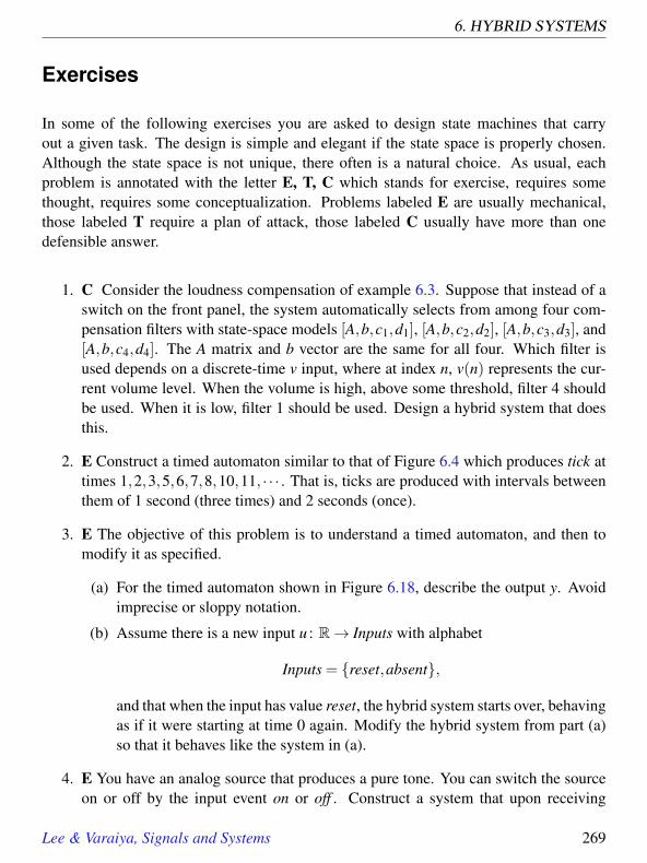
6. HYBRID SYSTEMS
Exercises
In some of the following exercises you are asked to design state machines that carryout a given task. The design is simple and elegant if the state space is properly chosen.Although the state space is not unique, there often is a natural choice. As usual, eachproblem is annotated with the letter E, T, C which stands for exercise, requires somethought, requires some conceptualization. Problems labeled E are usually mechanical,those labeled T require a plan of attack, those labeled C usually have more than onedefensible answer.
1. C Consider the loudness compensation of example 6.3. Suppose that instead of aswitch on the front panel, the system automatically selects from among four com-pensation filters with state-space models [A,b,c1,d1], [A,b,c2,d2], [A,b,c3,d3], and[A,b,c4,d4]. The A matrix and b vector are the same for all four. Which filter isused depends on a discrete-time v input, where at index n, v(n) represents the cur-rent volume level. When the volume is high, above some threshold, filter 4 shouldbe used. When it is low, filter 1 should be used. Design a hybrid system that doesthis.
2. E Construct a timed automaton similar to that of Figure 6.4 which produces tick attimes 1,2,3,5,6,7,8,10,11, · · · . That is, ticks are produced with intervals betweenthem of 1 second (three times) and 2 seconds (once).
3. E The objective of this problem is to understand a timed automaton, and then tomodify it as specified.
(a) For the timed automaton shown in Figure 6.18, describe the output y. Avoidimprecise or sloppy notation.
(b) Assume there is a new input u : R→ Inputs with alphabet
Inputs = reset,absent,
and that when the input has value reset, the hybrid system starts over, behavingas if it were starting at time 0 again. Modify the hybrid system from part (a)so that it behaves like the system in (a).
4. E You have an analog source that produces a pure tone. You can switch the sourceon or off by the input event on or off . Construct a system that upon receiving
Lee & Varaiya, Signals and Systems 269
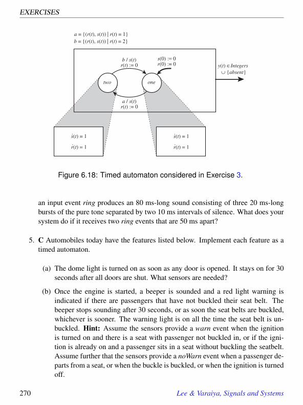
EXERCISES
b / s(t)r(t) := 0
two one
a / s(t)r(t) := 0
y(t) !Integers " absent
s(0) := 0r(0) := 0
b = (r(t), s(t)) | r(t) = 2a = (r(t), s(t)) | r(t) = 1
s(t) = 1
r(t) = 1
.
.s(t) = 1
r(t) = 1
.
.
Figure 6.18: Timed automaton considered in Exercise 3.
an input event ring produces an 80 ms-long sound consisting of three 20 ms-longbursts of the pure tone separated by two 10 ms intervals of silence. What does yoursystem do if it receives two ring events that are 50 ms apart?
5. C Automobiles today have the features listed below. Implement each feature as atimed automaton.
(a) The dome light is turned on as soon as any door is opened. It stays on for 30seconds after all doors are shut. What sensors are needed?
(b) Once the engine is started, a beeper is sounded and a red light warning isindicated if there are passengers that have not buckled their seat belt. Thebeeper stops sounding after 30 seconds, or as soon the seat belts are buckled,whichever is sooner. The warning light is on all the time the seat belt is un-buckled. Hint: Assume the sensors provide a warn event when the ignitionis turned on and there is a seat with passenger not buckled in, or if the igni-tion is already on and a passenger sits in a seat without buckling the seatbelt.Assume further that the sensors provide a noWarn event when a passenger de-parts from a seat, or when the buckle is buckled, or when the ignition is turnedoff.
270 Lee & Varaiya, Signals and Systems

6. HYBRID SYSTEMS
6. E A programmable thermostat allows you to select 4 times, 0≤ T1 ≤ ·· · ≤ T4 < 24(for a 24-hour cycle) and the corresponding temperatures a1, · · · ,a4. Construct atimed automaton that sends the event ai to the heating systems controller. Thecontroller maintains the temperature close to the value ai until it receives the nextevent. How many timers and modes do you need?
7. E Construct a parking meter similar to that in figure 6.6 that allows a maximum of30 minutes (rather than 60 minutes) and accepts coin5 and coin25 as inputs. Thendraw the state trajectories (both the mode and the clock state) and the output signalwhen coin5 occurs at time 0, coin25 occurs at time 3, and then there is no inputevent for the next 35 minutes.
8. T Consider the timed automaton of Figure 6.6. Suppose we view the box as adiscrete-event system with coin5,coin25,absent as the input alphabet and expired,absentas the output alphabet. Does the box behave as a finite state machine?
9. C Figure 6.19 depicts the intersection of two one-way streets, called Main andSecondary. A light on each street controls its traffic. Each light goes through a cycleconsisting of a red (R), green (G), and yellow (Y) phases. It is a safety requirementthat when one light is in its green or yellow phase, the other is in its red phase. Theyellow phase is always 20 seconds long.
The traffic lights operate as follows, in one of two modes. In the normal mode,there is a 5 minute-long cycle with the main light having 4 minutes of green and 20seconds of yellow–the secondary light is red for these 4 minutes and 20 seconds—and 40 seconds of red—during which the secondary light is green for 20 secondsfollowed by 20 seconds of yellow.
The second, or interrupt mode works as follows. Its purpose is to quickly give aright of way to the secondary road. A sensor in the secondary road detects if avehicle has crossed it. When this happens, the main light aborts its green phase andimmediately switches to its 20 second yellow phase. If the vehicle is detected whilethe main light is yellow or red, the system continues in its normal mode.
Design a hybrid system that controls the lights. Let this hybrid system have discreteoutputs that are pairs GG,GY,GR, etc. where the first letter denotes the color of themain light second letter denotes the color of the secondary light.
10. T Design a ReceiverProtocol hybrid system that works together with the SenderProtocolof example 6.7.
Lee & Varaiya, Signals and Systems 271

EXERCISES
Main
Secondary
light
detector
R
R G
G Y
Y
Figure 6.19: Traffic lights control the intersection of a main street and a secondarystreet. A detector senses when a vehicle crosses it. The red phase of one lightmust coincide with the green and yellow phases of the other light.
272 Lee & Varaiya, Signals and Systems

6. HYBRID SYSTEMS
11. E For the bouncing ball of example 6.9 let tn be the time when the ball hits theground for the n-th time, and let v(n) = y(tn) be the velocity at that time.
(a) Find a relation between v(n+1) and v(n) and then calculate v(n) in terms ofv(1).
(b) Obtain tn in terms of v(n).
(c) Calculate the maximum height reached by the ball after successive bumps.
12. E Translate refinement systems that are described as second-order differentialequations into first-order differential equations. Specifically:
(a) For the sticky masses system in example 6.8, find the function g such that(6.1) and (6.2) are represented as (6.4). Is this function linear?
(b) For the bouncing ball system in example 6.9, find the function f such that(6.5) is represented as (6.6). Is this function linear?
13. T Elaborate the hybrid system model of Figure 6.12 so that in the together mode,the stickiness decays according to the differential equation
s(t) =−as(t)
where s(t) is the stickiness at time t, and a is some positive constant. On the tran-sition into this mode, the stickiness should be initialized to some starting stickinessb.
14. T Show that the trajectory of the AGV of Figure 6.15 while it is in left or rightmode is a circle. What is the radius of this circle, and how long does it take tocomplete a circle?
15. E Express the hybrid system of Figure 6.15 in terms of the formal model of Section6.6. That is, identify the sets Inputs, Outputs, and the TransitionStructure.
Lee & Varaiya, Signals and Systems 273

7Frequency Domain
Contents7.1 Frequency decomposition . . . . . . . . . . . . . . . . . . . . . . . 277
Basics: Frequencies in Hertz and radians . . . . . . . . . . . . . . . 278Basics: Ranges of frequencies . . . . . . . . . . . . . . . . . . . . . 279Probing Further: Circle of fifths . . . . . . . . . . . . . . . . . . . . 281
7.2 Phase . . . . . . . . . . . . . . . . . . . . . . . . . . . . . . . . . . 2837.3 Spatial frequency . . . . . . . . . . . . . . . . . . . . . . . . . . . 2847.4 Periodic and finite signals . . . . . . . . . . . . . . . . . . . . . . . 2857.5 Fourier series . . . . . . . . . . . . . . . . . . . . . . . . . . . . . . 289
Probing Further: Uniform convergence . . . . . . . . . . . . . . . . 295Probing Further: Mean square convergence . . . . . . . . . . . . . . 2967.5.1 Uniqueness of the Fourier series . . . . . . . . . . . . . . . . 297Probing Further: Dirichlet conditions . . . . . . . . . . . . . . . . . 2977.5.2 Periodic, finite, and aperiodic signals . . . . . . . . . . . . . 2987.5.3 Fourier series approximations to images . . . . . . . . . . . . 300
7.6 Discrete-time signals . . . . . . . . . . . . . . . . . . . . . . . . . . 3007.6.1 Periodicity . . . . . . . . . . . . . . . . . . . . . . . . . . . 300Basics: Discrete-time frequencies . . . . . . . . . . . . . . . . . . . 3017.6.2 The discrete-time Fourier series . . . . . . . . . . . . . . . . 302
7.7 Summary . . . . . . . . . . . . . . . . . . . . . . . . . . . . . . . . 303Exercises . . . . . . . . . . . . . . . . . . . . . . . . . . . . . . . . . . . 304
275

We are interested in manipulating signals. We may wish to synthesize signals, as modemsneed to do in order to transmit a voice-like signal through the telephone channel. We mayinstead wish to analyze signals, as modems need to do in order to extract digital informa-tion from a received voice-like signal. In general, the field of communications is all aboutsynthesizing signals with characteristics that match a channel, and then analyzing signalsthat have often been corrupted by the channel in order to extract the original information.
We may also wish to synthesize natural signals such as images or speech. The field ofcomputer graphics puts much of its energy into synthesizing natural-looking images.Image processing includes image understanding, which involves analyzing images todetermine their content. The field of signal processing includes analysis and synthesis ofspeech and music signals.
We may wish to control a physical process. The physical process is sensed (using tem-perature, pressure, position and speed sensors). The sensed signals are processed in orderto estimate the internal state of the physical process. The physical process is controlledon the basis of the state estimate. Control system design includes the design of stateestimators and controllers.
In order to analyze or synthesize signals, we need models of those signals. Since a signalis a function, a model of the signal is a description or a definition of the function. Weuse two approaches. The first is a declarative (what is) approach. The second is animperative (how to) approach. These two approaches are complementary. Depending onthe situation, one approach is better than the other.
Signals are functions. This chapter in particular deals with signals where the domain istime (discrete or continuous). It introduces the concept of frequency-domain represen-tation of these signals. The idea is that arbitrary signals can be described as sums ofsinusoidal signals. This concept is first motivated by referring to psychoacoustics, howhumans hear sounds. Sinusoidal signals have particular psychoacoustic significance. Butthe real justification for the frequency domain approach is much broader. It turns out tobe particularly easy to understand the effect that LTI systems (linear time invariant sys-tems), discussed in Chapter 5, have on sinusoidal signals. A powerful set of analysis anddesign techniques then follow for arbitrary signals and the LTI systems that operate onthem.
Although we know that few (if any) real-world systems are truly LTI, we can easily con-strue models where the approximation is valid over some regime of operation. The previ-
276 Lee & Varaiya, Signals and Systems

7. FREQUENCY DOMAIN
ous chapter showed how modal models can be constructed to build realistic models over abroader range of operating conditions. Frequency domain methods are amenable to suchhybrid system treatment.
7.1 Frequency decomposition
For some signals, particularly natural signals like voice, music, and images, finding aconcise and precise definition of the signal can be difficult. In such cases, we try to modelsignals as compositions of simpler signals that we can more easily model.
Psychoacoustics is the study of how humans hear sounds. Pure tones and their frequencyturn out to be a very convenient way to describe sounds. Musical notes can be reasonablyaccurately modeled as combinations of relatively few pure tones (although subtle proper-ties of musical sounds, such as the timbre of a sound, are harder to model accurately).
When studying sounds, it is reasonable on psychoacoustic grounds to decompose thesounds into sums of sinusoids. It turns out that the motivation for doing this extends wellbeyond psychoacoustics. Pure tones have very convenient mathematical properties thatmake it useful to model other types of signals as sums of sinusoids, even when there isno psychoacoustic basis for doing so. For example, there is no psychoacoustic reason formodeling radio signals as sums of sinusoids.
1 Hz.2 Hz.3 Hz.4 Hz.
-1.0
-0.5
0.0
0.5
1.0
0.0 0.1 0.2 0.3 0.4 0.5 0.6 0.7 0.8 0.9 1.0
Time in seconds
Figure 7.1: Plot of four sinusoidal signals.
Lee & Varaiya, Signals and Systems 277

7.1. FREQUENCY DECOMPOSITION
Consider the range of frequencies covering one octave, ranging from 440Hz to 880 Hz.“Octave” is the musical term for a factor of two in frequency. The frequencies 440 Hzand 880 Hz both correspond to the musical note A, but one octave apart. The next higherA in the musical scale would have the frequency 1760 Hz, twice 880 Hz. In the westernmusical scale, there are 12 notes in every octave. These notes are evenly distributed
Basics: Frequencies in Hertz and radians
A standard measure of frequency is Hertz, meaning cycles per second. Figure 7.1 showsa plot of one second of four sine waves of different frequencies. For example, the fre-quencies in Hertz of the musical note A on the piano keyboard are
f1 = 55, f2 = 110, f3 = 220, f4 = 440,
f5 = 880, f6 = 1760, f7 = 3520, f8 = 7040.
A sinusoidal waveform x with frequency f4 = 440 can be defined by
∀ t ∈ R, x(t) = sin(440×2πt).
The factor 2π in this expressions is a nuisance. An argument to a sine function has unitsof radians, so 2π has units of radians/cycle. Explicitly showing all the units (in squarebrackets), we have
440[cycles/second]×2π[radians/cycle]t[seconds] = (440×2πt)[radians].
To avoid having to keep track of the factor 2π everywhere, it is common to use thealternative units for frequency, radians per second. The symbol ω is commonly used todenote frequencies in radians per second, while f is used for frequencies in Hertz. Therelationship between Hertz and radians per second is simple,
ω = 2π f ,
as is easily confirmed by checking the units. Thus, in radians per second, the frequenciesof the musical note A on the piano keyboard are
ω1 = 2π×55,ω2 = 2π×110,ω3 = 2π×220,ω4 = 2π×440,
ω5 = 2π×880,ω6 = 2π×1760,ω7 = 2π×3520,ω8 = 2π×7040.
278 Lee & Varaiya, Signals and Systems

7. FREQUENCY DOMAIN
(geometrically), so the next note above A, which is B flat, has frequency 440× 12√
2, where12√
2≈ 1.0595. The next note above B flat, which is B, has frequency 440× 12√
2× 12√
2.
In table 7.1, the frequencies of the complete musical scale between middle A and A-880are shown. Each frequency is β = 12
√2 times the frequency below it.
Frequencies that are harmonically related tend to sound good together. Figure 7.2 showsthe graph of a signal that is a major triad, a combination of the notes A, C] (C sharp), andE. By “combination” we mean “sum.” The A is a sinusoidal signal at 440 Hz. It is addedto a C], which is a sinusoidal signal at 554 Hz. This sum is then added to an E, which isa sinusoidal signal at 659 Hz. Each of the components is also shown, so you can verifygraphically that at each point in time, the value of the solid signal is equal to the sum ofvalues of the dashed signals at that time.
The stimulus presented to the ear is the solid waveform. What you hear, however, as-suming a small amount of musical training, is the three sinusoidal components, which thehuman ear interprets as musical notes. The human ear decomposes the stimulus into itssinusoidal components.
Basics: Ranges of frequencies
An extremely wide range of frequencies occur in natural and man-made signals. Thefollowing abbreviations are common:• Hz - hertz, cycles per second.
• kHz - kilohertz, thousands of cycles per second.
• MHz - megahertz, millions of cycles per second.
• GHz - gigahertz, billions of cycles per second.
• THz - terahertz, trillions of cycles per second.
Audible sounds signals are in the range of 20 Hz to 20 kHz. Sounds above this frequencyare called ultrasonic. Electromagnetic waves range from less than one hertz (used spec-ulatively in seismology for earthquake prediction) through visible light near 1015 Hz tocosmic ray radiation up to 1025 Hz.
Lee & Varaiya, Signals and Systems 279

7.1. FREQUENCY DECOMPOSITION
A 880A[ 831G 784F] 740F 698E 659D] 622D 587C] 554C 523B 494B[ 466A 440
Table 7.1: Frequencies of notes over one octave of the western musical scale, inHertz.
-3x10
SumA
C sharpE
-2
-1
0
1
2
3
0 1 2 3 4 5 6 7 8
Major Triad
Time in seconds
Figure 7.2: Graph of a major triad, showing its three sinusoidal components andtheir sum.
280 Lee & Varaiya, Signals and Systems

7. FREQUENCY DOMAIN
Probing Further: Circle of fifths
The western musical scale is based on our perception of frequency and the harmonicrelationships between frequencies. The following frequencies all correspond to the noteA:
110, 220, 440, 880, 1760, and 3520.
What about 440×3 = 1320? Notice that 1320/2 = 660, which is almost exactly the Ein table 7.1. Thus, 440×3 is (roughly) the note E, one octave above the E above A-440.E and A are closely harmonically related, and to most people, they sound good together.It is because
440×3≈ 659×2
The notes A, C], and E form a major triad. Where does the C] come from? Its frequencyis 554 (see table 7.1). Notice that
440×5≈ 554×4.
Among all the harmonic relationships in the scale, A, C], and E have one of the simplest.This is the reason for their pleasing sound together.
For more arcane reasons, the interval between A and E, which is a frequency rise ofapproximately 3/2, is called a fifth. The note 3/2 (a fifth) above E has frequency 988,which is one octave above B-494. Another 3/2 above that is approximately F sharp(740 Hz). Continuing in this fashion, multiplying frequencies by 3/2, and then possiblydividing by two, you can approximately trace the twelve notes of the scale. On the 13-th, you return to A, approximately. This progression is called the circle of fifths. Thenotion of key and scale in music are based on this circle of fifths, as is the fact that thereare 12 notes in the scale.
Table 7.1 is calculated by multiplying each frequency by 12√
2 to get the next higherfrequency, not by using the circle of fifths. Indeed, the 12
√2 method applied twelve times
yields a note that is exactly one octave higher than the starting point, while the circle offifths only yields an approximation. The 12
√2 method yields the well-tempered scale.
This scale was popularized by the composer J. S. Bach. It sounds much better than ascale based on the circle fifths when the range of notes spans more than one octave.
Lee & Varaiya, Signals and Systems 281
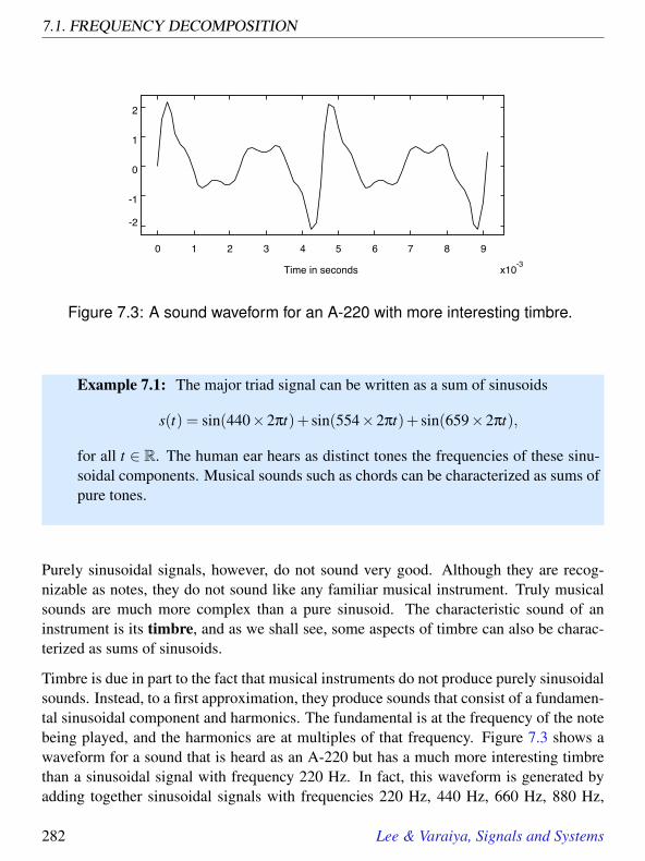
7.1. FREQUENCY DECOMPOSITION
-3x10
-2
-1
0
1
2
0 1 2 3 4 5 6 7 8 9
Time in seconds
Figure 7.3: A sound waveform for an A-220 with more interesting timbre.
Example 7.1: The major triad signal can be written as a sum of sinusoids
s(t) = sin(440×2πt)+ sin(554×2πt)+ sin(659×2πt),
for all t ∈ R. The human ear hears as distinct tones the frequencies of these sinu-soidal components. Musical sounds such as chords can be characterized as sums ofpure tones.
Purely sinusoidal signals, however, do not sound very good. Although they are recog-nizable as notes, they do not sound like any familiar musical instrument. Truly musicalsounds are much more complex than a pure sinusoid. The characteristic sound of aninstrument is its timbre, and as we shall see, some aspects of timbre can also be charac-terized as sums of sinusoids.
Timbre is due in part to the fact that musical instruments do not produce purely sinusoidalsounds. Instead, to a first approximation, they produce sounds that consist of a fundamen-tal sinusoidal component and harmonics. The fundamental is at the frequency of the notebeing played, and the harmonics are at multiples of that frequency. Figure 7.3 shows awaveform for a sound that is heard as an A-220 but has a much more interesting timbrethan a sinusoidal signal with frequency 220 Hz. In fact, this waveform is generated byadding together sinusoidal signals with frequencies 220 Hz, 440 Hz, 660 Hz, 880 Hz,
282 Lee & Varaiya, Signals and Systems

7. FREQUENCY DOMAIN
-3x10
Phase 1Phase 2Phase 3Phase 4Phase 5
-1.0
-0.5
0.0
0.5
1.0
0 1 2 3 4 5 6 7 8
Sinusoid with Five Phases
Time in seconds
Figure 7.4: Five sinusoidal signals with different phases.
1100 Hz, 1320 Hz, and higher multiples, with varying weights. The 220 Hz componentis called the fundamental, while the others are called harmonics. The first harmonic isthe component at 440 Hz. The second harmonic is the component at 660 Hz. Etc. Therelative weights of the harmonics is a major part of what makes one musical instrumentsound different from another.
7.2 Phase
A sinusoidal sound has not just a frequency, but also a phase. The phase may be thoughtof as the relative starting point of the waveform. Figure 7.4 shows five sinusoidal signalswith the same frequency but five different phases. These signals all represent the soundA-440, and all sound identical. For a simple sinusoidal signal, obviously, phase has nobearing on what the human ear hears.
Somewhat more surprising is that when two or more sinusoids are added together, therelative phase has a significant impact on the shape of the waveform, but no impact onthe perceived sound. The human ear is relatively insensitive to the phase of sinusoidalcomponents of a signal, even though the phase of those components can strongly affectthe shape. If these waveforms represent something other than sound, like stock prices forexample, the effect of phase could be quite significant. For a sinusoidal signal, the phase
Lee & Varaiya, Signals and Systems 283

7.3. SPATIAL FREQUENCY
Figure 7.5: Images that are sinusoidal horizontally, vertically, and both.
affects whether a particular point in time corresponds to a peak or a valley, for example.For stock prices, it makes a difference whether you sell at a high or a low.
There are certain circumstances in which the human ear is sensitive to phase. In particular,when two sinusoids of the same frequency combine, the relative phase has a big impact,since it affects the amplitude of the sum. For example, if the two sinusoids differ in phaseby 180 degrees (π radians), then when they add, they exactly cancel, yielding a zero signal.The human brain can use the relative phase of a sound in the two ears to help spatiallylocate the origin of a sound. Also, audio systems with two speakers, which simulatespatially distributed sounds (“stereo”), can be significantly affected by the relative phaseof the signal produced by the two speakers.
Phase is measured in either radians or degrees. An A-440 can be given by
g(t) = sin(440×2πt +φ),
for all t ∈ R, where φ ∈ R is the phase. Regardless of the value of φ, this signal is still anA-440. If φ = π/2 then
g(t) = cos(440×2πt).
7.3 Spatial frequency
Psychoacoustics provides a compelling motivation for decomposing audio signals as sumsof sinusoids. In principal, images can also be similarly decomposed. However, the moti-vations in this case are more mathematical than perceptual.
284 Lee & Varaiya, Signals and Systems

7. FREQUENCY DOMAIN
Figure 7.5 shows three images that are sinusoidal. Specifically, the intensity of the image(the amount of white light that is reflected by the page) varies spatially according to asinusoidal function. In the leftmost image, it varies horizontally only. There is no verticalvariation in intensity. In the middle image, it varies vertically only. In the rightmostimage, it varies in both dimensions.
The sinusoidal image has spatial frequency rather than temporal frequency. Its unitsare cycles per unit distance. The images in figure 7.5 have frequencies of roughly 2.5cycles/inch. Recall that a grayscale picture is represented by a function
Image : VerticalSpace×HorizontalSpace→ Intensity.
So an image that varies sinusoidally along the horizontal direction (with a spatial periodof H inches) and is constant along the vertical direction is represented by
∀x ∈ VerticalSpace ∀y ∈ HorizontalSpace Image(x,y) = sin(2πy/H).
Similarly, an image that varies sinusoidally along the vertical direction (with a spatialperiod of V inches) and is constant along the horizontal direction is represented by
∀x ∈ VerticalSpace ∀y ∈ HorizontalSpace Image(x,y) = sin(2πx/V ).
An image that varies sinusoidally along both directions is represented by
∀x ∈ VerticalSpace ∀y ∈ HorizontalSpace Image(x,y) = sin(2πx/V )× sin(2πy/H).
These sinusoidal images have much less meaning than audio sinusoids, which we perceiveas musical tones. Nonetheless, we will see that images can be described as sums ofsinusoids, and that such description is sometimes useful.
7.4 Periodic and finite signals
When the domain is continuous or discrete time, we can define a periodic signal. As-suming the domain is R, a periodic signal x with period p ∈ R is one where for all t ∈ R
x(t) = x(t + p). (7.1)
A signal with period p also has period 2p, since
x(t) = x(t + p) = x(t +2p).
Lee & Varaiya, Signals and Systems 285

7.4. PERIODIC AND FINITE SIGNALS
In fact, it has period K p, for any positive integer K. Usually, we define the period to bethe smallest p > 0 such that
∀ t ∈ R, x(t) = x(t + p).
Example 7.2: The sinusoidal signal x where for all t ∈ R
x(t) = sin(ω0t)
is a periodic signal with period 2π/ω0 since for all t ∈ R
sin(ω0(t +2π/ω0)) = sin(ω0t).
A periodic signal is defined over an infinite interval. If the domain is instead a subset[a,b]⊂ R, for some finite a and b, then we call this a finite signal.
Example 7.3: The signal y where for all t ∈ [0,2π/ω0],
y(t) = sin(ω0t)
is a finite signal with duration 2π/ω0. This interval spans exactly one cycle of thesine wave.
A finite signal with duration p can be used to define a periodic signal with period p. Allthat is needed is to periodically repeat the finite signal. Formally, given a finite signaly : [a,b]→ R, we can define a signal y′ : R→ R by
∀ t ∈ R, y′(t) =
y(t) if t ∈ [a,b]0 otherwise
(7.2)
286 Lee & Varaiya, Signals and Systems

7. FREQUENCY DOMAIN
In other words, y′(t) is simply y(t) inside its domain, and zero elsewhere. Then theperiodic signal can be given by1
x(t) =∞
∑m=−∞
y′(t−mp) (7.3)
where p= b−a. This is called a shift-and-add summation, illustrated in Figure 7.6. Theperiodic signal is a sum of versions of y′(t) that have been shifted in time by multiples ofp. Do not let the infinite sum intimidate: all but one of the terms of the summation are zerofor any fixed t! Thus, a periodic signal can be defined in terms of a finite signal, whichrepresents one period. Conversely, a finite signal can be defined in terms of a periodicsignal (by taking one period).
We can check that x given by (7.3) is indeed periodic with period p,
x(t + p) =∞
∑m=−∞
y′(t + p−mp) =∞
∑m=−∞
y′(t− (m−1)p)
=∞
∑k=−∞
y′(t− kp) = x(t),
by using a change of variables, k = m−1.
It is also important to note that the periodic signal x agrees with y in the finite domain[a,b] of y, since
∀t ∈ [a,b] x(t) =∞
∑m=−∞
y′(t−mp)
= y′(t)+ ∑m 6=0
y′(t−mp)
= y(t),
because, by (7.2), for t ∈ [a,b], y′(t) = y(t) and y′(t−mp) = 0 if m 6= 0.
We will see that any periodic signal, and hence any finite signal, can be described as a sumof sinusoidal signals. This result, known as the Fourier series, is one of the fundamentaltools in the study of signals and systems.
1If this notation is unfamiliar, see box on page 77.
Lee & Varaiya, Signals and Systems 287

7.4. PERIODIC AND FINITE SIGNALS
y'(t + p)
t
t
t
t
x(t)
t
y'(t)
p
y'(t ! p)
y'(t ! 2p)
a b
......
"
p
Figure 7.6: By repeating the finite signal y we can obtain a periodic signal x.
288 Lee & Varaiya, Signals and Systems
7. FREQUENCY DOMAIN
7.5 Fourier series
A remarkable result, due to Joseph Fourier, 1768-1830, is that a periodic signal x : R→Rwith period p ∈ R can (usually) be described as a constant term plus a sum of sinusoids,
x(t) = A0 +∞
∑k=1
Ak cos(kω0t +φk) (7.4)
This representation of x is called its Fourier series. The Fourier series is widely usedfor signal analysis. Each term in the summation is a cosine with amplitude Ak and phaseφk. The particular values of Ak and φk depend on x, of course. The frequency ω0, whichhas units of radians per second (assuming the domain of x is in seconds), is called thefundamental frequency, and is related to the period p by
ω0 = 2π/p.
In other words, a signal with fundamental frequency ω0 has period p = 2π/ω. The con-stant term A0 is sometimes called the DC term, where “DC” stands for direct current, areference back to the early applications of this theory in electrical circuit analysis. Theterms where k ≥ 2 are called harmonics.
Equation (7.4) is often called the Fourier series expansion for x because it expands x interms of its sinusoidal components.
If we had a facility for generating individual sinusoids, we could use the Fourier seriesrepresentation (7.4) to synthesize any periodic signal. However, using the Fourier seriesexpansion for synthesis of periodic signals is problematic because of the infinite summa-tion. But for most practical signals, the coefficients Ak become very small (or even zero)for large k, so a finite summation can be used as an approximation. A finite Fourierseries approximation with K +1 terms has the form
x(t) = A0 +K∑
k=1Ak cos(kω0t +φk). (7.5)
The infinite summation of (7.4) is, in fact, the limit of (7.5) as K goes to infinity. We needto be concerned, therefore, with whether this limit exists. The Fourier series expansionis valid only if it exists. There are some technical mathematical conditions on x that, ifsatisfied, ensure that the limit exists (see boxes on pages 295 and 296). Fortunately, theseconditions are met almost always by practical, real-world time-domain signals.
Lee & Varaiya, Signals and Systems 289

7.5. FOURIER SERIES
-3x10
idealK=1
K = 3K = 7
K = 32
-1.0-0.5
0.0
0.5
1.0
0 1 2 3 4 5 6 7 8
Time in seconds
(a)
3x10
0.00.2
0.4
0.6
0.8
1.0
1.2
0.0 0.5 1.0 1.5 2.0 2.5 3.0 3.5 4.0
Frequency in Hz
(b)
Figure 7.7: (a) One cycle of a square wave and some finite Fourier series ap-proximations. (b) The amplitudes of the Fourier series terms for the square wave.
290 Lee & Varaiya, Signals and Systems

7. FREQUENCY DOMAIN
Example 7.4: Figure 7.7 shows a square wave with period 8 msec and some finiteFourier series approximations to the square wave. Only one period of the squarewave is shown. The method for constructing these approximations will be coveredin detail in Chapter 10. Here, we will just observe the general structure of theapproximations.
Notice in Figure 7.7(a) that the K = 1 approximation consists only of the DC term(which is zero in this case) and a sinusoid with an amplitude slightly larger thanthat of the square wave. Its amplitude is depicted in Figure 7.7(b) as the heightof the largest bar. The horizontal position of the bar corresponds to the frequencyof the sinusoid, 125 Hz, which is 1/(8 msec), the fundamental frequency. TheK = 3 waveform is the sum of the K = 1 waveform and one additional sinusoidwith frequency 375 Hz and amplitude equal to the height of the second largest barin Figure 7.7(b).
A plot like that in Figure 7.7(b) is called a frequency domain representation of the squarewave, because it depicts the square wave by the amplitude and frequency of its sinusoidalcomponents. Actually, a complete frequency domain representation also needs to give thephase of each sinusoidal component.
Notice in Figure 7.7(b) that all even terms of the Fourier series approximation have zeroamplitude. Thus, for example, there is no component at 250 Hz. This is a consequence ofthe symmetry of the square wave, although it is beyond the scope of work now to explainexactly why.
Also notice that as the number of terms in the summation increases, the approximationmore closely resembles a square wave, but the amount of its overshoot does not appearto decrease. This is known as Gibb’s phenomenon. In fact, the maximum differencebetween the finite Fourier series approximation and the square wave does not convergeto zero as the number of terms in the summation increases. In this sense, the squarewave cannot be exactly described with a Fourier series (see box on page 295). Intuitively,the problem is due to the abrupt discontinuity in the square wave when it transitionsbetween its high value and its low value. In another sense, however, the square wave isaccurately described by a Fourier series. Although the maximum difference between theapproximation and the square wave does not go to zero, the mean square error does goto zero (see box on page 296). For practical purposes, mean square error is an adequate
Lee & Varaiya, Signals and Systems 291

7.5. FOURIER SERIES
criterion for convergence, so we can work with the Fourier series expansion of the squarewave.
Example 7.5: Figure 7.8 shows some finite Fourier series approximations for atriangle wave. This waveform has no discontinuities, and therefore the maximumerror in the finite Fourier series approxination converges to zero (see box on page295). Notice that its Fourier series components decrease in amplitude much morerapidly than those of the square wave. Moreover, the time-domain approximationsappear to be more accurate with fewer terms in the finite summation.
Many practical, real-world signals, such as audio signals, do not have discontinuities, andthus do not exhibit the sort of convergence problems exhibited by the square wave (Gibbsphenomenon). Other signals, however, such as images, are full of discontinuities. A (spa-tial) discontinuity in an image is simply an edge. Most images have edges. Nonetheless,a Fourier series representation for such a signal is almost always still valid, in a meansquare error sense (see box on page 296). This is sufficient for almost all engineeringpurposes.
Example 7.6: Consider an audio signal given by
s(t) = sin(440×2πt)+ sin(550×2πt)+ sin(660×2πt).
This is a major triad in a non-well-tempered scale. The first tone is A-440. Thethird is approximately E, with a frequency 3/2 that of A-440. The middle term isapproximately C], with a frequency 5/4 that of A-440. It is these simple frequencyrelationships that result in a pleasant sound. We choose the non-well-temperedscale because it makes it much easier to construct a Fourier series expansion forthis waveform. We leave the more difficult problem of finding the Fourier seriescoefficients for a well-tempered major triad to Exercise 5.
To construct the Fourier series expansion, we can follow these steps:
1. Find p, the period. The period is the smallest number p > 0 such that s(t) =s(t− p) for all t in the domain. To do this, note that
sin(2π f t) = sin(2π f (t− p))
292 Lee & Varaiya, Signals and Systems

7. FREQUENCY DOMAIN
-3x10
idealK = 1K = 3K = 7
K = 32
-1.0
-0.5
0.0
0.5
1.0
0 1 2 3 4 5 6 7 8
Time in seconds
(a)
3x10
0.0
0.2
0.4
0.6
0.8
0.0 0.5 1.0 1.5 2.0 2.5 3.0 3.5 4.0
Frequency in Hz
(b)
Figure 7.8: (a) One cycle of a triangle wave and some finite Fourier series approx-imations. (b) The amplitudes of the Fourier series terms for the triangle wave.
Lee & Varaiya, Signals and Systems 293

7.5. FOURIER SERIES
if f p is an integer. Thus, we want to find the smallest p such that 440p,550p, and 660p are all integers. Equivalently, we want to find the largestfundamental frequency f0 = 1/p such that 440/ f0, 550/ f0, and 660/ f0 areall integers. Such an f0 is called the greatest common divisor of 440, 550,and 660. This can be computed using the gcd function in Matlab. In thiscase, however, we can do it in our heads, observing that f0 = 110.
2. Find A0, the constant term. By inspection, there is no constant component ins(t), only sinusoidal components, so A0 = 0.
3. Find A1, the fundamental term. By inspection, there is no component at 110Hz, so A1 = 0. Since A1 = 0, φ1 is immaterial.
4. Find A2, the first harmonic. By inspection, there is no component at 220 Hz,so A2 = 0.
5. Find A3. By inspection, there is no component at 330 Hz, so A3 = 0.
6. Find A4. There is a component at 440 Hz, sin(440×2πt). We need to find A4and φ4 such that
A4 cos(440×2πt +φ4) = sin(440×2πt).
By inspection, φ4 =−π/2 and A4 = 1.
7. Similarly determine that A5 = A6 = 1, φ5 = φ6 = −π/2, and that all otherterms are zero.
Putting this all together, the Fourier series expansion can be written
s(t) =6
∑k=4
cos(kω0t−π/2)
where ω0 = 2π f0 = 220π.
The method used in the above example for determining the Fourier series coefficients istedious and error prone, and will only work for simple signals. We will see much bettertechniques in chapters 8 and 10.
294 Lee & Varaiya, Signals and Systems

7. FREQUENCY DOMAIN
Probing Further: Uniform convergence
The Fourier series representation of a periodic signal x is a limit of a sequence of func-tions xN for N = 1,2, · · · where
∀ t ∈ R, xN(t) = A0 +N
∑k=1
Ak cos(kω0t +φk).
Specifically, for the Fourier series representation to be valid, we would like that for allt ∈ R,
x(t) = limN→∞
xN(t).
A strong criterion for validity of the Fourier series is uniform convergence of this limit,in which for each real number ε > 0, there exists a positive integer M such that for allt ∈ R and for all N > M,
|x(t)− xN(t)|< ε
A sufficient condition for uniform convergence is that the signal x be continuous and thatits first derivative be piecewise continuous.
A square wave, for example, is not continuous, and hence does not satisfy this suffi-cient condition. Indeed, the Fourier series does not converge uniformly, as you can see infigure 7.7 by observing that the peak difference between x(t) and xK(t) does not decreaseto zero. A triangle wave, however, is continuous, and has a piecewise continuous firstderivative. Thus, it does satisfy the sufficient condition. Its Fourier series approximationwill therefore converge uniformly, as suggested in Figure 7.8. A weaker, but still useful,criterion for validity of the Fourier series is considered on page 296. That criterion ismet by the square wave.
See for example R. G. Bartle, The Elements of Real Analysis, Second Edition, JohnWiley & Sons, 1976, p. 117 (for uniform convergence) and p. 337 (for this sufficientcondition).
Lee & Varaiya, Signals and Systems 295
7.5. FOURIER SERIES
Probing Further: Mean square convergence
The Fourier series representation of a periodic signal x with period p is a limit of asequence of functions xN for N = 1,2, · · · where
∀ t ∈ R, xN(t) = A0 +N
∑k=1
Ak cos(kω0t +φk).
Specifically, for the Fourier series representation to be valid, we would like that for allt ∈ R,
x(t) = limN→∞
xN(t).
For some practical signals, such as the square wave of figure 7.7, this statement is notquite true for all t ∈ R. For practical purposes, however, we don’t really need for thisto be true. A weaker condition for validity of the Fourier series is that the total energyin the error over one period be zero. Specifically, we say that xN(t) converges in meansquare to x(t) if
limN→∞
p∫0
|x(t)− xN(t)|2dt = 0.
The integral here is the energy in the error x(t)− xN(t) over one period. It turns out thatif x itself has finite energy over one period, then xN(t) converges in mean square to x(t).That is, all we need is that
p∫0
|x(t)|2dt < ∞.
Virtually all signals with any engineering importance satisfy this criterion. Note thatconvergence in mean square does not guarantee that at any particular t ∈ R, x(t) =lim
N→∞xN(t). For a condition that (almost) ensures this for all practical signals, see box on
page 297.See for example R. V. Churchill, Fourier Series and Boundary Value Problems, Third
Edition, McGraw-Hill Book Company, New York, 1978.
296 Lee & Varaiya, Signals and Systems

7. FREQUENCY DOMAIN
7.5.1 Uniqueness of the Fourier series
Suppose x : R→R is a periodic function with period p. Then the Fourier series expansionis unique. In other words if it is both true that
x(t) = A0 +∞
∑k=1
Ak cos(kω0t +φk)
Probing Further: Dirichlet conditions
The Fourier series representation of a periodic signal x with period p is a limit of asequence of finite Fourier series approximations xN for N = 1,2, · · · . We have seen inthe box on page 295 a strong condition that ensures that ∀ t ∈ R,
x(t) = limN→∞
xN(t). (7.6)
We have seen in the box on page 296 a weaker condition that does not guarantee this,but instead guarantees that the energy in the error over one period is zero. It turns thatfor almost all signals of interest, we can assert that (7.6) holds for almost all t ∈ R. Inparticular, if the Dirichlet conditions are satisfied, then (7.6) holds for all t except wherex is discontinuous. The Dirichlet conditions are three:• Over one period, x is absolutely integrable, meaning that
p∫0
|x(t)|dt < ∞.
• Over one period, x is of bounded variation, meaning that there are no more thana finite number of maxima or minima. That is, if the signal is oscillating betweenhigh and low values, it can only oscillate a finite number of times in each period.
• Over one period, x is continuous at all but a finite number of points.
These conditions are satisfied by the square wave, and indeed by any signal of practicalengineering importance.
Lee & Varaiya, Signals and Systems 297

7.5. FOURIER SERIES
and
x(t) = B0 +∞
∑k=1
Bk cos(kω0t +θk),
where ω0 = 2π/p, then it must also be true that
∀ k ≥ 0, Ak = Bk and φk mod 2π = θk mod 2π.
(The modulo operation is necessary because of the non-uniqueness of phase.) Thus, whenwe talk about the frequency content of a signal, we are talking about something thatis unique and well defined. For a suggestion about how to prove this uniqueness, seeproblem 11.
7.5.2 Periodic, finite, and aperiodic signals
We have seen in Section 7.4 that periodic signals and finite signals have much in common.One can be defined in terms of the other. Thus, a Fourier series can be used to describea finite signal as well as a periodic one. The “period” is simply the extent of the finitesignal. Thus, if the domain of the signal is [a,b] ⊂ R, then p = b− a. The fundamentalfrequency, therefore, is just ω0 = 2π/(b−a).
An aperiodic signal, like an audio signal, can be partitioned into finite segments, and aFourier series can be constructed from each segment.
Example 7.7: Consider the train whistle shown in Figure 7.9(a). Figure 7.9(b)shows a segment of 16 msec. Notice that within this segment, the sound clearly hasa somewhat periodic structure. It is not hard to envision how it could be describedas sums of sinusoids. The magnitudes of the Ak Fourier series coefficients for this16 msec segment are shown in Figure 7.9(c). These are calculated on a computerusing techniques we will discuss later, rather than being calculated by hand as inthe previous example. Notice that there are three dominant frequency componentsthat give the train whistle its tonality and timbre.
298 Lee & Varaiya, Signals and Systems

7. FREQUENCY DOMAIN
-0.4
-0.2
0.0
0.2
0.4
0.0 0.2 0.4 0.6 0.8 1.0 1.2 1.4 1.6Time in seconds
(a)
-2x10
-0.2
-0.1
0.0
0.1
0.2
0.0 0.2 0.4 0.6 0.8 1.0 1.2 1.4 1.6
(b)
3x10
0.00
0.02
0.04
0.06
0.08
0.10
0.0 0.5 1.0 1.5 2.0 2.5 3.0 3.5 4.0
(c)Figure 7.9: (a) A 1.6 second train whistle. (b) A 16 msec segment of the trainwhistle. (c) The Fourier series coefficients for the 16 msec segment.
Lee & Varaiya, Signals and Systems 299

7.6. DISCRETE-TIME SIGNALS
7.5.3 Fourier series approximations to images
Images are invariably finite signals. Given any image, it is possible to construct a periodicimage by just tiling a plane with the image. Thus, there is again a close relationshipbetween a periodic image and a finite one.
We have seen sinusoidal images (Figure 7.5), so it follows that it ought to be possibleto construct a Fourier series representation of an image. The only hard part is that im-ages have a two-dimensional domain, and thus are finite in two distinct dimensions. Thesinusoidal images in Figure 7.5 have a vertical frequency, a horizontal frequency, or both.
Suppose that the domain of an image is [a,b]× [c,d] ⊂ R×R. Let pH = b− a, andpV = d − c represent the horizontal and vertical “periods” for the equivalent periodicimage. For constructing a Fourier series representation, we can define the horizontal andvertical fundamental frequencies as follows:
ωH = 2π/pH
ωV = 2π/pV
The Fourier series representation of Image : [a,b]× [c,d]→ Intensity is
Image(x,y) =∞
∑k=0
∞
∑m=0
Ak,m cos(kωHx+φk)cos(mωV y+ϕm)
For convenience, we have included the constant term A0,0 in the summation, so we assumethat φ0 = ϕ0 = 0. (Recall that cos(0) = 1).
7.6 Discrete-time signals
Consider signals of the form x : Z→ R, which if the domain is interpreted as time arediscrete-time signals. Discrete-time signals can be decomposed into sinusoidal compo-nents much like continuous-time signals. There are some minor subtleties, however.
7.6.1 Periodicity
A discrete-time signal is periodic if there is a non-zero integer p > 0 such that
∀ n ∈ Z, x(n+ p) = x(n).
300 Lee & Varaiya, Signals and Systems

7. FREQUENCY DOMAIN
Note that, somewhat counterintuitively, not all sinusoidal discrete-time signals are peri-odic. Consider
x(n) = cos(2π f n). (7.7)
For this to be periodic, we must be able to find a non-zero integer p such that for allintegers n,
x(n+ p) = cos(2π f n+2π f p) = cos(2π f n) = x(n).
This can be true only if (2π f p) is an integer multiple of 2π. That is, if there is someinteger m such that
2π f p = 2πm.
Dividing both sides by 2πp, we see that this signal is periodic only if we can find nonzerointegers p and m such that
f = m/p.
Basics: Discrete-time frequencies
When the domain of a signal is Z, then the units of frequency are cycles/sample.Consider for example the discrete-time signal given by
∀n ∈ Z, x(n) = cos(2π f n).
Suppose this represents an audio signal that is sampled at 8000 samples/second. Thento convert f to Hertz, just watch the units:
f [cycles/sample]×8000[samples/second] = 8000 f [cycles/second].
The frequency could have been equally well given in units of radians/sample, as in
x(n) = cos(ωn).
for all n ∈ Z. To convert ω to Hertz,
ω[radians/sample]×8000[samples/second]× (1/2π)[cycles/radian]
= (8000w/2π)[cycles/second].
Lee & Varaiya, Signals and Systems 301

7.6. DISCRETE-TIME SIGNALS
In other words, f must be rational. Only if f is rational is this signal periodic.
Example 7.8: Consider a discrete-time sinusoid x given by
∀ n ∈ Z, x(n) = cos(4πn/5).
Putting this into the form of (7.7),
x(n) = cos(2π(2/5)n),
we see that it has frequency f = 2/5 cycles/sample. If this were a continuous-timesinusoid, we could invert this to get the period. However, the inverse is not an inte-ger, so it cannot possibly be the period. Noting that the inverse is 5/2 samples/cycle,we need to find the smallest multiple of this that is an integer. Multiply by 2, weget 5 samples/(2 cycles). So the period is p = 5 samples.
In general, for a discrete sinusoid with frequency f cycles/sample, the period is p = K/ f ,where K > 0 is the smallest integer such that K/ f is an integer.
7.6.2 The discrete-time Fourier series
Assume we are given a periodic discrete-time signal x with period p. Just as with continuous-time signals, this signal can be described as a sum of sinusoids, called the discrete-timeFourier series (DFS) expansion,
x(n) = A0 +K∑
k=1Ak cos(kω0n+φk) (7.8)
where
K =
(p−1)/2 if p is oddp/2 if p is even
Unlike the continuous-time case, the sum is finite. Intuitively, this is because discrete-time signals cannot represent frequencies above a certain value. We will examine thisphenomenon in more detail in Chapter 11, but for now, it proves extremely convenient.
302 Lee & Varaiya, Signals and Systems

7. FREQUENCY DOMAIN
Mathematically, the above relation is much simpler than the continuous-time Fourier se-ries. All computations are finite. There is a finite number of signal values in one periodof the waveform. There is a finite number of terms in the Fourier series representationfor each signal value. Unlike the continuous-time case, it is easy for computers to man-age this representation. Given a finite set of values, A0, · · · ,AK , a computer can calculatex(n). Moreover, the representation is exact for any periodic signal. No approximation isneeded, and there is no question of convergence. In the continuous-time case, the Fourierseries representation is accurate only for certain signals. For the discrete-time case, it isalways accurate.
The DFS can be calculated efficiently on a computer using an algorithm called the fastFourier transform (FFT). All of the Fourier series examples that are plotted in this textwere calculated using the FFT algorithm.
7.7 Summary
A time-based signal can be described as a sum of sinusoids. This sum is called a Fourierseries. The magnitudes and phases of the sinusoids, taken together as a function of fre-quency, are called the frequency-domain representation of the signal. For audio signals,this frequency-domain representation has a direct psychoacoustic significance. But wewill see in the next chapter that this representation has a significance for all signals whenLTI systems are used to process the signals. We will see that the effect that an LTI systemhas on a signal is particularly easy to understand in the frequency domain.
Lee & Varaiya, Signals and Systems 303

EXERCISES
Exercises
Note: each problem is annotated with the letter E, T, C which stands for exercise, requiressome thought, requires some conceptualization. Problems labeled E are usually mechan-ical, those labeled T require a plan of attack, those labeled C usually have more than onedefensible answer.
1. E In (7.1) we defined periodic for continuous-time signals.
(a) Define finite and periodic for discrete-time signals, where the domain is Z.
(b) Define finite and periodic for images.
2. E Which of the following signals is periodic with a period greater than zero, andwhat is that period? All functions are of the form x : R→ C. The domain is time,measured in seconds, and so the period is in seconds.
(a) ∀ t ∈ R, x(t) = 10sin(2πt)+(10+2i)cos(2πt)
(b) ∀ t ∈ R, x(t) = sin(2πt)+ sin(√
2πt)
(c) ∀ t ∈ R, x(t) = sin(2√
2πt)+ sin(√
2πt)
3. E Consider the discrete-time signal x where
∀ n ∈ Z, x(n) = 1+ cos(4πn/9).
(a) Find the period p, where p > 0.
(b) Give the fundamental frequency corresponding to the period in (1). Give theunits.
(c) Give the coefficients A0,A1,A2, · · · and φ1,φ2, · · · of the Fourier series expan-sion for this signal.
4. E Consider a continuous-time signal x : R→ R defined by
∀ t ∈ R, x(t) = cos(ω1t)+ cos(ω2t),
where ω1 = 2π and ω2 = 3π radians/second.
(a) Find the smallest period p ∈ R+, where p > 0.
(b) Give the fundamental frequency corresponding to the period in (a). Give theunits.
304 Lee & Varaiya, Signals and Systems

7. FREQUENCY DOMAIN
(c) Give the coefficients A0,A1,A2, · · · and φ1,φ2, · · · of the Fourier series expan-sion for x.
5. T Determine the fundamental frequency and the Fourier series coefficients for thewell-tempered major triad,
s(t) = sin(440×2πt)+ sin(554×2πt)+ sin(659×2πt).
6. E Define x : R→ R
∀ t ∈ R, x(t) = 5cos(ω0t +π/2)
+5cos(ω0t−π/6)
+5cos(ω0t−2π/3).
Find A and φ so that
∀ t ∈ R, x(t) = Acos(ω0t +φ).
Hint: Appendix B might be useful.
7. T In this problem, we examine a practical application of the mathematical result inproblem 6. In particular, we consider multipath interference, a common problemwith wireless systems where multiple paths from a transmitter to a receiver canresult in destructive interference of a signal.
When a transmitter sends a radio signal to a receiver, the received signal consistsof the direct path plus several reflected paths. In Figure 7.10, the transmitter is ona tower at the left of the figure, the receiver is the telephone in the foreground, andthere are three paths: the direct path is l0 meters long, the path reflected from thehill is l1 meters long, and the path reflected from the building is l2 meters long.
Suppose the transmitted signal is a f Hz sinusoid x : R→ R,
∀ t ∈ R, x(t) = Acos(2π f t)
So the received signal is y such that ∀ t ∈ R,
y(t) = α0Acos(2π f (t− l0c))
+α1Acos(2π f (t− l1c))
+α2Acos(2π f (t− l2c)). (7.9)
Lee & Varaiya, Signals and Systems 305

EXERCISES
Here, 0≤ αi ≤ 1 are numbers that represent the attenuation (or reduction in signalamplitude) of the signal, and c = 3× 10⁸ m/s is the speed of light in a vacuum.2
Answer the following questions.
(a) Explain why the description of y given in (7.9) is a reasonable model of thereceived signal.
(b) What would be the description if instead of the 3 paths as shown in Figure7.10, there were 10 paths (one direct and 9 reflected).
(c) The signals received over the different paths cause different phase shifts, φi,so the signal y (with three paths) can also be written as
∀ t ∈ R, y(t) =2
∑k=0
αkAcos(2π f t−φk)
What are the φk? Give an expression in terms of f , lk, and c.
(d) Let Φ = maxφ1− φ0,φ2− φ0 be the largest difference in the phase of thereceived signals and let L = maxl1− l0, l2− l0 be the maximum path lengthdifference. What is the relationship between Φ,L, f ?
(e) Suppose for simplicity that there is only one reflected path of distance l1, i.e.take α2 = 0 in the expressions above. Then Φ = φ1− φ0. When Φ = π, thereflected signal is said to destroy the direct signal. Explain why the term “de-stroy” is appropriate. (This phenomenon is called destructive interference.)
(f) In the context of mobile radio shown in the figure, typically L ≤ 500m. Forwhat values of f is Φ ≤ π/10? (Note that if Φ ≤ π/10 the signals will notinteract destructively by much.)
(g) For the two-path case, derive an expression that relates the frequencies f thatinterfere destructively to the path length difference L = l1− l0.
8. T The function x : R→ R is given by its graph shown in Figure 7.11. Note that∀ t 6∈ [0,1], x(t) = 0, and x(0.4) = 1. Define y by
∀ t ∈ R, y(t) =∞
∑k=−∞
x(t− kp)
where p is the period.
2In reality, the reflections are more complicated than the model here.
306 Lee & Varaiya, Signals and Systems

7. FREQUENCY DOMAIN
reflected paths
direct path
Figure 7.10: A direct and two reflected paths from transmitter to receiver.
1
0 0.4 1x
Figure 7.11: The graph of x.
Lee & Varaiya, Signals and Systems 307

EXERCISES
(a) Prove that y is periodic with period p, i.e.
∀ t ∈ R,y(t) = y(t + p).
(b) Plot y for p = 1.(c) Plot y for p = 2.(d) Plot y for p = 0.8.(e) Plot y for p = 0.5.(f) Suppose the function z is obtained by advancing x by 0.4, i.e.
∀ t ∈ R, z(t) = x(t +0.4).
Define w by
∀ t ∈ R, w(t) =∞
∑k=−∞
z(t− kp)
What is the relation between w and y. Use this relation to plot w for p = 1.
9. T Suppose x : R→ R is a periodic signal with period p, i.e.
∀ t ∈ R, x(t) = x(t + p).
Let f : R→ R be any function, and define the signal y : R→ R by y = f x, i.e.
∀ t ∈ R, y(t) = f (x(t)).
(a) Prove that y is periodic with period p.(b) Suppose ∀ t ∈ R, x(t) = sin(2πt). Suppose f is the sign function, ∀ a ∈ R,
f (a) =
1 if a≥ 0−1 if a < 0
Plot x and y.(c) Suppose ∀ t ∈R, x(t) = sin(2πt). Suppose f is the square function, ∀ x∈R,
f (x) = x2. Plot y.
10. C Suppose the periodic square wave shown on the left in Figure 7.12 has the Fourierseries representation
A0 +∞
∑k=1
Ak cos(2πkt/p+φk)
Use this to obtain a Fourier series representation of the two-dimensional pattern ofrectangles on the right.
308 Lee & Varaiya, Signals and Systems

7. FREQUENCY DOMAIN
p
2p/3 2p/3 p
p
2p/3
Figure 7.12: A periodic square wave (left) and a periodic pattern (right).
11. T Suppose Ak ∈ C, ωk ∈ R, and k = 1,2, such that
∀ t ∈ R, A1eiω1t = A2eiω2t . (7.10)
Show that A1 = A2 and ω1 = ω2. Hint: Evaluate both sides of (7.10) at t = 0, andevaluate their derivatives at t = 0.
Discussion: This result shows that in order for two complex exponential signalsto be equal, their frequencies, phases, and amplitudes must be equal. More in-terestingly, this result can be used to show that if a signal can be described as asum of complex exponential signals, then that description is unique. There is noother sum of complex exponentials (one involving different frequencies, phases,or amplitudes) that will also describe the signal. In particular, the Fourier seriesrepresentation of a periodic signal is unique, as stated above in theorem 7.5.1.
Lee & Varaiya, Signals and Systems 309

8Frequency Response
Contents8.1 LTI systems . . . . . . . . . . . . . . . . . . . . . . . . . . . . . . . 313
8.1.1 Time invariance . . . . . . . . . . . . . . . . . . . . . . . . . 3138.1.2 Linearity . . . . . . . . . . . . . . . . . . . . . . . . . . . . 3188.1.3 Linearity and time-invariance . . . . . . . . . . . . . . . . . 321
8.2 Finding and using the frequency response . . . . . . . . . . . . . . 3258.2.1 Linear difference and differential equations . . . . . . . . . . 328Basics: Sinusoids in terms of complex exponentials . . . . . . . . . . 330Tips and Tricks: Phasors . . . . . . . . . . . . . . . . . . . . . . . . 3318.2.2 The Fourier series with complex exponentials . . . . . . . . . 3388.2.3 Examples . . . . . . . . . . . . . . . . . . . . . . . . . . . . 339
8.3 Determining the Fourier series coefficients . . . . . . . . . . . . . 3398.3.1 Negative frequencies . . . . . . . . . . . . . . . . . . . . . . 340
8.4 Frequency response and the Fourier series . . . . . . . . . . . . . 3408.5 Frequency response of composite systems . . . . . . . . . . . . . . 342
8.5.1 Cascade connection . . . . . . . . . . . . . . . . . . . . . . . 3428.5.2 Feedback connection . . . . . . . . . . . . . . . . . . . . . . 344
8.6 Summary . . . . . . . . . . . . . . . . . . . . . . . . . . . . . . . . 346Probing Further: Relating DFS coefficients . . . . . . . . . . . . . . 347Probing Further: Formula for Fourier series coefficients . . . . . . . 349Probing Further: Exchanging integrals and summations . . . . . . . 350Probing Further: Feedback systems are LTI . . . . . . . . . . . . . . 352
Exercises . . . . . . . . . . . . . . . . . . . . . . . . . . . . . . . . . . . 355
311

A class of systems that yield to sophisticated analysis techniques is the class of linear time-invariant systems (LTI system), discussed in Chapter 5. LTI systems have a key property:given a sinusoidal input, the output is a sinusoidal signal with the same frequency, butpossibly different amplitude and phase. Given an input that is a sum of sinusoids, theoutput will be a sum of the same sinusoids, each with its amplitude and phase (possibly)modified.
We can justify describing audio signals as sums of sinusoids on purely psychoacousticgrounds. However, because of this property of LTI systems, it is often convenient to de-scribe any signal as a sum of sinusoids, regardless of whether there is a psychoacousticjustification. The real value in this mathematical device is that by using the theory ofLTI systems, we can design systems that operate more-or-less independently on the sinu-soidal components of a signal. For example, abrupt changes in the signal value requirehigher frequency components. Thus, we can enhance or suppress these abrupt changes byenhancing or suppressing the higher frequency components. Such an operation is calledfiltering because it filters frequency components. We design systems by crafting theirfrequency response, their response to sinusoidal inputs. An audio equalizer, for exam-ple, is a filter that enhances or suppresses certain frequency components. Images can alsobe filtered. Enhancing the high frequency components will sharpen the image, whereassuppressing the high frequency components will blur the image.
State-space models described in previous chapters are precise and concise, but in a sense,not as powerful as a frequency response. For an LTI system, given a frequency response,you can assert a great deal about the relationship between an input signal and an outputsignal. Fewer assertions are practical in general with state-space models.
LTI systems, in fact, can also be described with state-space models, using differenceequations and differential equations, as explored in Chapter 5. But state-space modelscan also describe systems that are not LTI. Thus, state-space models are more general.It should come as no surprise that the price we pay for this increased generality is feweranalysis and design techniques. In this chapter, we explore the (very powerful) analysisand design techniques that apply to the special case of LTI systems.
312 Lee & Varaiya, Signals and Systems

8. FREQUENCY RESPONSE
8.1 LTI systems
LTI systems have received a great deal of intellectual attention for two reasons. First,they are relatively easy to understand. Their behavior is predictable, and can be fullycharacterized in fairly simple terms, based on the frequency domain representation ofsignals that we introduced in the previous chapter. Second, many physical systems canbe reasonably approximated by them. Few physical systems perfectly fit the model, butmany fit very well within a certain regime of operation. Hybrid system models can beused when we wish to model more than one such regime of operation.
8.1.1 Time invariance
Consider the set of signals whose domain is interpreted as time. Such signals are func-tions of time, sometimes called time-domain signals. The domain might be R , forcontinuous-time signals, or Z , for discrete-time signals. Physical audio signals, forexample, are continuous-time signals, while a digital audio file is a discrete-time sig-nal. Systems with continuous-time input and output signals are called continuous-timesystems. Systems with discrete-time input and output signals are called discrete-timesystems.
A simple continuous-time system is the delay system Dτ, where if the input is x, then theoutput y = Dτ(x) is given by
∀ t ∈ R, y(t) = x(t− τ). (8.1)
Positive values of τ result in positive delays (despite the subtraction in x(t − τ)). Anydelay results in a shifting left or right of the graph of a signal, as shown in Figure 8.1.
Example 8.1: Consider a continuous-time signal x given by
∀ t ∈ R, x(t) = cos(2πt).
Let y = D0.5(x). Then
∀ t ∈ R, y(t) = cos(2π(t−0.5)) = cos(2πt−π).
The delay by 0.5 seconds is equivalent to a phase shift of −π radians. For a sinu-soidal signal, and only for a sinusoidal signal, time delay and phase changes are
Lee & Varaiya, Signals and Systems 313
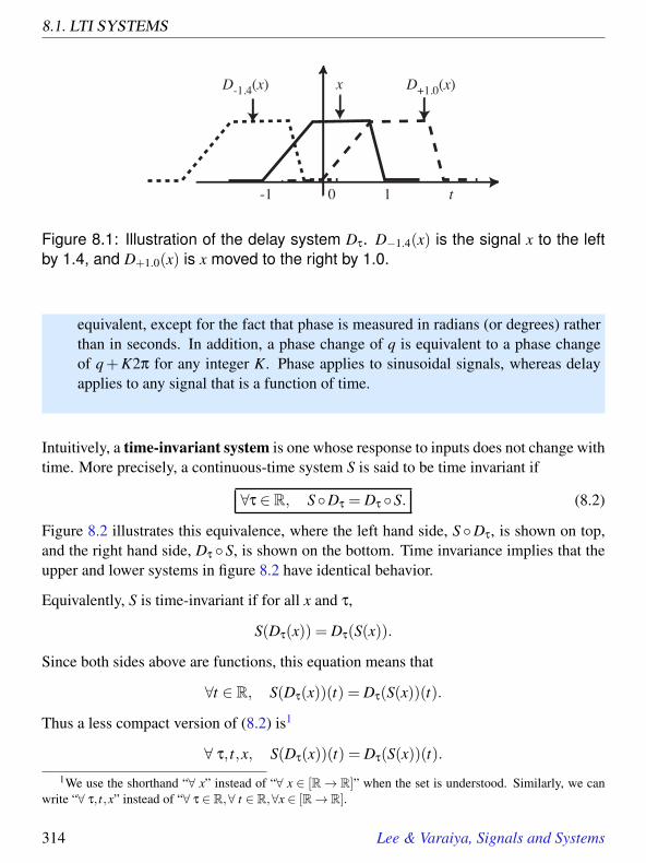
8.1. LTI SYSTEMS
t
x
0 1 -1
D+1.0(x)
D-1.4(x)
Figure 8.1: Illustration of the delay system Dτ. D−1.4(x) is the signal x to the leftby 1.4, and D+1.0(x) is x moved to the right by 1.0.
equivalent, except for the fact that phase is measured in radians (or degrees) ratherthan in seconds. In addition, a phase change of q is equivalent to a phase changeof q+K2π for any integer K. Phase applies to sinusoidal signals, whereas delayapplies to any signal that is a function of time.
Intuitively, a time-invariant system is one whose response to inputs does not change withtime. More precisely, a continuous-time system S is said to be time invariant if
∀τ ∈ R, SDτ = Dτ S. (8.2)
Figure 8.2 illustrates this equivalence, where the left hand side, S Dτ, is shown on top,and the right hand side, Dτ S, is shown on the bottom. Time invariance implies that theupper and lower systems in figure 8.2 have identical behavior.
Equivalently, S is time-invariant if for all x and τ,
S(Dτ(x)) = Dτ(S(x)).
Since both sides above are functions, this equation means that
∀t ∈ R, S(Dτ(x))(t) = Dτ(S(x))(t).
Thus a less compact version of (8.2) is1
∀ τ, t,x, S(Dτ(x))(t) = Dτ(S(x))(t).
1We use the shorthand “∀ x” instead of “∀ x ∈ [R→ R]” when the set is understood. Similarly, we canwrite “∀ τ, t,x” instead of “∀ τ ∈ R,∀ t ∈ R,∀x ∈ [R→ R].
314 Lee & Varaiya, Signals and Systems

8. FREQUENCY RESPONSE
xDτS
z
y
0 τ0
00
τ0
τ0
xDτ S
Figure 8.2: Time invariance implies that the top and bottom systems produce thesame output signal for the same input signal.
This is interpreted as follows:
A system S is time invariant if, for any input x that produces output y, a delayed inputDτ(x) produces output Dτ(y).
Similarly, the discrete-time M-sample delay is written DM. The signal y = DM(x) is givenby
∀ n ∈ Z, y(n) = x(n−M). (8.3)
A discrete-time system S is time invariant if
∀M,x, S(DM(x)) = DM(S(x)). (8.4)
Example 8.2: Consider a discrete-time system S,
S : [Z→ R]→ [Z→ R].
Suppose that any input x produces output y where
∀ n ∈ Z, y(n) = x(n)+0.9x(n−1). (8.5)
This system is time-invariant. To show this, consider a delayed input x = DM(x),for some integer M. That is,
∀ n, x(n) = x(n−M). (8.6)
Lee & Varaiya, Signals and Systems 315

8.1. LTI SYSTEMS
Suppose that this input produces output y = S(x). Then by the relation (8.5) be-tween an input and an output,
∀ n, y(n) = x(n)+0.9x(n−1).
Substituting (8.6), we see that
∀ n, y(n) = x(n−M)+0.9x(n−M−1) = y(n−M).
Since y = DM(y), the system is time-invariant.
Example 8.3: Consider the system DelayAndSquare, or DS for short,
DS : [R→ R]→ [R→ R].
Suppose that any input x produces output y where
∀ t ∈ R, y(t) = (x(t−1))2. (8.7)
This system is time-invariant. To show this, consider a delayed input x = Dτ(x), forsome real number τ. That is,
∀ t, x(t) = x(t− τ). (8.8)
Suppose that this input produces output y = S(x). Then by the relation (8.7) be-tween an input and an output,
∀ t, y(t) = (x(t−1))2.
Substituting (8.8), we see that
∀ t, y(t) = (x(t−1− τ))2 = y(t− τ).
Since y = Dτ(y), the system is time-invariant.
316 Lee & Varaiya, Signals and Systems

8. FREQUENCY RESPONSE
Example 8.4: Consider a system ReverseTime or RT ,
RT : [R→ R]→ [R→ R],
where any input x produces output y related by
∀ t ∈ R, y(t) = x(−t). (8.9)
This system is not time-invariant. To show this, consider a delayed input x = Dτ(x),for some real number τ. That is,
∀ t, x(t) = x(t− τ). (8.10)
Suppose that this input produces output y = S(x). Then by the relation (8.9) be-tween an input and an output,
∀ t, y(t) = x(−t).
Substituting (8.10), we see that
∀ t, y(t) = x(−t− τ) 6= y(t− τ) = x(−t + τ).
Since y 6= Dτ(y), the system is not time-invariant.
To be completely convinced that these two signals are different in general, considera particular signal x such that ∀t, x(t) = t, and take τ = 1. Then y(0) = −1, but(Dτ(y))(0) = 1.
Time invariance is a mathematical fiction. No electronic system is time invariant in thestrict sense. For one thing, such a system is turned on at some point in time. Clearly,its behavior before it is turned on is not the same as its behavior after it is turned on.Nevertheless, it proves to be a very convenient mathematical fiction, and it is a reasonableapproximation for many systems if their behavior is constant over a relatively long periodof time (relative to whatever phenomenon we are studying). For example, your audioamplifier is not a time-invariant system. Its behavior changes drastically when you turn iton or off, and changes less drastically when you raise or lower the volume. However, for
Lee & Varaiya, Signals and Systems 317

8.1. LTI SYSTEMS
the duration of a compact disc, if you leave the volume fixed, the system can be reasonablyapproximated as being time-invariant.
Some systems have a similar property even though they operate on signals whose domainis not time. For example, the domain of an image is a region of a plane. The outputof an image processing system may not depend significantly on where in the plane theinput image is placed. Shifting the input image will only shift the output image by thesame amount. This property which generalizes time invariance and holds for some imageprocessing systems, is called shift invariance (see problem 5).
8.1.2 Linearity
Consider the set of signals whose range is R or C . Such signals are real-valued functionsor complex-valued functions. Since real-valued functions are a subset of complex-valuedfunctions, we only need to talk about complex-valued functions. It does not matter (fornow) whether they are continuous-time signals or discrete-time signals. The domain couldbe R or Z.
Suppose x is a complex-valued function and a is a complex constant. Then we can definea new complex-valued function ax such that for all t in the domain of x,
(ax)(t) = a(x(t)).
In other words, the new function, which we call ax, is simply scaled by the constant a.
Similarly, given two complex-valued functions x1 and x2 with the same domain and range,we can define a new function (x1 + x2) such that for all t in the domain,
(x1 + x2)(t) = x1(t)+ x2(t).
Consider the set of all systems that map complex-valued functions to complex-valuedfunctions. Such systems are called complex systems. Again, it does not matter (for now)whether they are discrete-time systems or continuous-time systems. Suppose that S is acomplex system. S is said to be linear if for all a ∈ C and for all complex signals x,
S(ax) = aS(x) (8.11)
and for all complex signals x1 and x2 in the domain of S,
S(x1 + x2) = S(x1)+S(x2) (8.12)
318 Lee & Varaiya, Signals and Systems

8. FREQUENCY RESPONSE
Sax
S ax
Figure 8.3: If S is linear, then these two systems are equivalent. The trianglerepresents a system that scales a signal by some complex constant a.
The first of these—called the homogeneity property—says that if you scale the input, theoutput is scaled. The second one—called the additivity property—says that if the inputis described as the sum of two component signals, then the output can be described asthe sum of two signals that would result from the components alone. Recall that linearfunctions were introduced in Section 5.2. A linear system is one whose function relatingthe output to the input is linear.
In pictures, the first property says that the two systems in Figure 8.3 are equivalent if S islinear. Here, the triangle represents the scaling operation. The second property says thatthe two systems in Figure 8.4 are equivalent.
Example 8.5: Consider the same discrete-time system S of example 8.2, whereinput x produces output y such that
∀ n ∈ Z, y(n) = x(n)+0.9x(n−1).
This system is linear. To show this, we must show that (8.11) and (8.12) hold.Suppose input x = ax produces output y = S(x). Then
∀ n, y(n) = x(n)+0.9x(n−1)
= ax(n)+0.9ax(n−1)
= a(x(n)+0.9x(n−1))
= ay(n).
Lee & Varaiya, Signals and Systems 319

8.1. LTI SYSTEMS
S
x
y
S
S
x
y
Figure 8.4: If S is linear, then these two systems are equivalent.
Thus, S(ax) = aS(x), establishing (8.11).
To check (8.12), suppose input x1 produces output y1 and x2 produces y2. Letx = x1+x2 produce y. We must show that y = y1+y2. We leave this as an exercise.
Example 8.6: In the continuous-time system DelayAndSquare or DS of example8.3, an input x produces output y where
∀ t ∈ R, y(t) = (x(t−1))2.
This system is not linear. To show this we must show that either (8.11) or (8.12)does not hold for DS. We will show that (8.11) does not hold. To show this, considera scaled input x= ax, for some complex number a. Suppose that this input producesoutput y = S(x). Then,
∀ t, y(t) = (x(t−1))2.
Since x = ax,
∀ t, y(t) = (ax(t−1))2 = a2(x(t−1))2 6= ay(t) = a(x(t−1))2.
320 Lee & Varaiya, Signals and Systems
8. FREQUENCY RESPONSE
In particular, take for example a = 2, t = 0, and x such that ∀ t, x(t) = 1. Thesevalues result in
y(t) = 4 6= ay(t) = 2.
Example 8.7: In the time-reversal system RT of example 8.4,
RT : [R→ R]→ [R→ R],
any input x produces output y related by
∀ t ∈ R, y(t) = x(−t).
This system is linear. To show this we must show that (8.11) and (8.12) both hold.We first show that (8.11) holds; that is, for all a ∈ R,x ∈ [R→ R], and t ∈ R,
RT(ax)(t) = (aRT(x))(t).
But this is certainly true, since the left and right sides both evaluate to ax(−t). Asimilar argument is used to show (8.12).
Linearity is a mathematical fiction. No electronic system is linear in the strict sense. Asystem is designed to work with a range of input signals, and arbitrary scaling of the inputdoes not translate into arbitrary scaling of the output. If you provide an input to youraudio amplifier that is higher voltage than it is designed for, then it is not likely to justproduce louder sounds. Its input circuits will get overloaded and signal distortion willresult. Nonetheless, as a mathematical fiction, linearity is extremely convenient. It saysthat we can decompose the inputs to a system and study the effect of the system on theindividual components.
8.1.3 Linearity and time-invariance
For time-domain systems, time-invariance is a useful (if fictional) property. For com-plex (or real) systems, linearity is a useful (if fictional) property. For complex (or real)
Lee & Varaiya, Signals and Systems 321

8.1. LTI SYSTEMS
time-domain systems, the combination of these properties is extremely useful. Lineartime-invariant (LTI) systems turn out to have particularly simple behavior with sinusoidalinputs.
Given a sinusoid at the input, the output of an LTI system will be a sinusoid with thesame frequency, but possibly with different phase and amplitude.
It then follows that
Given an input that is described as a sum of sinusoids of certain frequencies, the outputcan be described as a sum of sinusoids with the same frequencies, but with (possible)phase and amplitude changes at each frequency.
A straightforward way to show that LTI systems have these properties starts by consid-ering complex exponentials (for a review of complex numbers, see Appendix B). Acontinuous-time complex exponential is a signal x ∈ [R→ C] where
∀ t ∈ R, x(t) = eiωt = cos(ωt)+ isin(ωt).
Complex exponential functions have an interesting property that will prove useful to us.Specifically,
∀ t ∈ R and τ ∈ R, x(t− τ) = eiω(t−τ) = e−iωτeiωt .
This follows from the multiplication property of exponentials,
eb+c = ebec.
Since Dτ(x)(t) = x(t− τ), we have that for the complex exponential x,
Dτ(x) = ax, where a = e−iωτ. (8.13)
In words, a delayed complex exponential is a scaled complex exponential, where thescaling constant is the complex number a = e−iωτ.
We will now show that if the input to a continuous-time LTI system is eiωt , then the outputwill be H(ω)eiωt , where H(ω) is a constant (not a function of time) that depends on thefrequency ω of the complex exponential. In other words, the output is only a scaledversion of the input.
When the output of a system is only a scaled version of the input, the input is called aneigenfunction, which comes from the German word for “same.” The output is (almost)the same as the input.
322 Lee & Varaiya, Signals and Systems

8. FREQUENCY RESPONSE
Complex exponentials are eigenfunctions of LTI systems, as we will now show. This isthe most important reason for the focus on complex exponentials in the study of signalsand systems. This single property underlies much of the discipline of signal processing,and is used heavily in circuit analysis, communication systems, and control systems.
Given an LTI system S : [R→ C]→ [R→ C], let x be an input signal where
∀ t ∈ R, x(t) = eiωt
Recall that S is time invariant if for all τ ∈ R,
SDτ = Dτ S.
ThusS(Dτ(x)) = Dτ(S(x)).
From (8.13),S(Dτ(x)) = S(ax)
where a = e−iωτ, and from linearity,
S(ax) = aS(x)
soaS(x) = Dτ(S(x)). (8.14)
Let y = S(x) be the corresponding output signal. Substituting into (8.14) we get
ay = Dτ(y).
In other words,∀ t,τ ∈ R, e−iωτy(t) = y(t− τ).
In particular, this is true for t = 0, so letting t = 0,
∀ τ ∈ R, y(−τ) = e−iωτy(0).
Changing variables, letting t =−τ , we note that this implies that
∀ t ∈ R, y(t) = eiωty(0).
Recall that y(0) is the output evaluated at 0 when the input is eiωt . It is a constant, in thatit does not depend on t, so this establishes that the output is a complex exponential, just
Lee & Varaiya, Signals and Systems 323
8.1. LTI SYSTEMS
like the input, except that it is scaled by y(0). However, y(0) does, in general, depend onω, so we define the function H : R→ C by
∀ ω ∈ R, H(ω) = y(0) = (S(x))(0), where ∀ t ∈ R, x(t) = eiωt . (8.15)
That is, H(ω) is the output at time zero when the input is a complex exponential withfrequency ω.
Using this notation, we write the output y as
∀ t ∈ R, y(t) = H(ω)eiωt
when the input is eiωt . Note that H(ω) is a function of ω ∈ R, the frequency of the inputcomplex exponential.
The function H : R→ C is called the frequency response. It defines the response of theLTI system to a complex exponential input at any given frequency. It gives the scalingfactor that the system imposes on that complex exponential.
For discrete-time systems, the situation is similar. By reasoning identical to that above,for an LTI system, if the input is a discrete complex exponential,
∀ n ∈ Z, x(n) = eiωn
then the output is the same complex exponential scaled by a constant (a complex numberthat does not depend on time),
∀ n ∈ Z, y(n) = H(ω)eiωn
H is once again called the frequency response, and since it is a function of ω, and ispossibly complex valued, it has the form H : R→ C.
There is one key difference, however, between discrete-time systems and continuous-timesystems. Since n is an integer, notice that
eiωn = ei(ω+2π)n = ei(ω+4π)n,
and so on. That is, a discrete complex exponential with frequency ω is identical to adiscrete complex exponential with frequency ω+2Kπ, for any integer K. The frequencyresponse, therefore, must be identical at these frequencies, since the inputs are identical.That is
∀ω ∈ R, H(ω) = H(ω+2Kπ)
for any integer K. That is, a discrete-time frequency response is periodic with period 2π.
324 Lee & Varaiya, Signals and Systems

8. FREQUENCY RESPONSE
8.2 Finding and using the frequency response
We have seen that if the input to an LTI system is a complex exponential signal x ∈ [R→C] where
∀ t ∈ R, x(t) = eiωt = cos(ωt)+ isin(ωt).
then the output is
∀t ∈ R, y(t) = H(ω)eiωt . (8.16)
where H(ω) is a (possibly complex-valued) number that is a property of the system. H(ω)is called the frequency response at frequency ω.
Example 8.8: Consider a delay system S = DT , for some T ∈ R. It is an LTIsystem, as is easy to verify by checking that (8.2), (8.11), and (8.12) are satisfied.Suppose the input to the delay system is the complex exponential x given by
∀ t ∈ R, x(t) = eiωt .
Then the output y satisfies
∀ t ∈ R, y(t) = eiω(t−T ) = e−iωT eiωt .
Comparing this to (8.16) we see that the frequency response of the delay is
H(ω) = e−iωT .
Example 8.9: Consider a discrete-time M-sample delay system S = DM. If y =S(x) then y is given by
∀ n ∈ Z, y(n) = x(n−M). (8.17)
This is an LTI system, as is easy to verify. We could find the frequency responseexactly the same way as in the previous example, but instead we use a slightlydifferent method. Since the system is LTI, we know that if the input is x such that
Lee & Varaiya, Signals and Systems 325

8.2. FINDING AND USING THE FREQUENCY RESPONSE
for all n ∈ Z, x(n) = eiωn, then the output is H(ω)eiωn, where H is the frequencyresponse. By plugging this input and output into (8.17), we get
H(ω)eiωn = eiω(n−M) = eiωne−iωM.
Divide both sides by eiωn to get
H(ω) = e−iωM.
The techniques in the previous examples can be used to find the frequency response ofmore complicated systems. Simply replace the input x in a difference equation like (8.17)with eiωn, and replace the output y with H(ω)eiωn, and then solve for H(ω).
Example 8.10: Consider a discrete-time, length two moving average, given by thedifference equation
∀ n ∈ Z, y(n) = (x(n)+ x(n−1))/2,
where x is the input and y is the output. When the input for all n is eiωn, this becomes
H(ω)eiωn = (eiωn + eiω(n−1))/2.
Solving for H(ω), we find that the frequency response is
H(ω) = (1+ e−iω)/2.
A similar approach can find the frequency response of a continuous-time system describedby a differential equation.
Example 8.11: Consider a continuous-time system with input x and output yrelated by the differential equation
∀t ∈ R, RCdydt
(t)+ y(t) = x(t), (8.18)
326 Lee & Varaiya, Signals and Systems

8. FREQUENCY RESPONSE
R
Cx(t) y(t)
+
-
+
-
Figure 8.5: The RC circuit of example 8.11.
where R and C are real-valued constants. This differential equation describes theRC circuit of Figure 8.5, which consists of an R-ohm resistance in series with a C-farad capacitor. The circuit has input voltage x, provided by a voltage source, shownas a circle on the left. The output is the voltage y across the capacitor. Kirchhoff’svoltage law gives the differential equation. It is easy to verify that this differntialequation describes an LTI system.
We can determine the frequency response of this system by assuming that the inputx is given by ∀ t ∈ R, x(t) = eiωt , and finding the output. Since the system is LTI,the output will be given by y(t) = H(ω)eiωt . Plugging these values for x and y into(8.18) gives
RC(iω)H(ω)eiωt +H(ω)eiωt = eiωt , (8.19)
becausedydt
(t) = iωH(ω)eiωt .
Dividing both sides of (8.19) by eiωt yields the frequency response of this circuit,
∀ω ∈ R, H(ω) =1
1+ iRCω.
Lee & Varaiya, Signals and Systems 327

8.2. FINDING AND USING THE FREQUENCY RESPONSE
8.2.1 Linear difference and differential equations
The procedure of example 8.10 can be used to write down by inspection the frequencyresponse of any high-order linear difference equation of the form, ∀ n ∈ Z,
a0y(n)+a1y(n−1)+ · · ·+aNy(n−N) = b0x(n)+b1x(n−1)+ · · ·+bMx(n−M). (8.20)
The coefficients of this difference equation, a0, · · · ,aN and b0, · · · ,bM, are real constants.(They could also be complex.) This describes an LTI system, and a good way to recognizethat a discrete-time system is LTI is to write it in this form. If the input for all n isx(n) = eiωn, then the output for all n is y(n) = H(ω)eiωn. Plugging these values of inputand output into (8.20) gives,
a0H(ω)eiωn +a1H(ω)eiω(n−1) + · · ·+aNH(ω)eiω(n−N)
= b0eiωn + b1eiω(n−1)+ · · ·+bMeiω(n−M).
Recognizing that eiω(n−m) = e−imωeiωn, we can divide both sides by eiωn and solve forH(ω) to get
∀ω ∈ R, H(ω) =b0 +b1e−iω + · · ·+bMe−iMω
a0 +a1e−iω + · · ·+aNe−iNω(8.21)
Observe that the frequency response (8.21) is a ratio of two polynomials in e−iω.
Example 8.12: Consider an LTI system given by the difference equation
∀n ∈ Z, y(n)− y(n−3) = x(n)+2x(n−1)+ x(n−2).
Its frequency response is
∀ω ∈ R, H(ω) =1+2e−iω + e−i2ω
1− e−i3ω.
In a similar way one can obtain the frequency response of any linear differential equationof the form,
∀t ∈ R, aNdNydtN (t)+ · · ·+a1
dydt (t)+a0y(t) =
bMdMxdtM (t)+ · · ·+b1
dxdt (t)+b0x(t), (8.22)
328 Lee & Varaiya, Signals and Systems

8. FREQUENCY RESPONSE
where the coefficients aN , · · · ,a0 and bM, · · · ,b0, are real (or complex) constants. Thisdescribes an LTI system, and a good way to recognize that a continuous-time system isLTI is to write it in this form. If the input for all t is x(t) = eiωt , the output for all t isy(t) = H(ω)eiωt . Plugging these values of input and output into (8.22), and recognizingthat
dk
dtk eiωt = (iω)keiωt ,
gives,
aN(iω)NH(ω)eiωt + · · · + a1(iω)H(ω)eiωt +a0H(ω)eiωt =
bM(iω)Meiωt + · · ·+b1(iω)eiωt +b0eiωt .
We can divide both sides by eiωt to get
∀ω ∈ R, H(ω) =bM(iω)M + · · ·+b1(iω)+b0
aN(iω)N + · · ·+a1(iω)+a0(8.23)
Observe that the frequency response (8.23) is a ratio of two polynomials in iω.
Example 8.13: Consider the continuous-time system given by the differentialequation
∀ t ∈ R,d2ydt2 (t)−3
dydt
(t)+2y(t) =dxdt
+ x(t),
where x is the input and y is the output. It has frequency response
∀ω ∈ R, H(ω) =iω+1
(iω)2−3iω+2.
Complex exponentials as inputs are rather abstract. We have seen that with audio signals,sinusoidal signals are intrinsically significant because the human ear interprets the fre-quency of the sinusoid as its tone. Note that a real-valued sinusoidal signal can be givenas a combination of exponential signals (see box on page 330),
cos(ωt) = (eiωt + e−iωt)/2.
Lee & Varaiya, Signals and Systems 329

8.2. FINDING AND USING THE FREQUENCY RESPONSE
Thus, if this is the input to an LTI system with frequency response H, then the output willbe
y(t) = (H(ω)eiωt +H(−ω)e−iωt)/2. (8.25)
Many (or most) LTI systems are not capable of producing complex-valued outputs whenthe input is real, so for such systems, this y(t) must be real. This implies that
H(ω) = H∗(−ω). (8.26)
To see why this is so, note that if y(t) is real then so is H(ω)eiωt +H(−ω)e−iωt . But forthis to be real, it must be that the imaginary parts of the two terms cancel,
ImH(ω)eiωt=−ImH(−ω)e−iωt. (8.27)
Note thatImH(ω)eiωt= ReH(ω)sin(ωt)+ ImH(ω)cos(ωt).
Basics: Sinusoids in terms of complex exponentials
Euler’s formula states thateiθ = cos(θ)+ isin(θ).
The complex conjugate ise−iθ = cos(θ)− isin(θ).
Summing these,eiθ + e−iθ = 2cos(θ)
orcos(θ) = (eiθ + e−iθ)/2.
Thus, for example,cos(ωt) = (eiωt + e−iωt)/2.
Similarly,
sin(θ) =−i(eiθ− e−iθ)/2.
In appendix A we show that many useful trigonometric identities are easily derived fromthese simple relations.
330 Lee & Varaiya, Signals and Systems
8. FREQUENCY RESPONSE
Using a similar fact for the right side of (8.27), we get
ReH(ω)sin(ωt)+ ImH(ω)cos(ωt)
=−ReH(−ω)sin(−ωt)− ImH(−ω)cos(−ωt).
Tips and Tricks: Phasors
Consider a general continuous-time sinusoidal signal, x(t)=Acos(ωt+φ), for all t ∈R.Here A is the amplitude, φ is the phase, and ω is the frequency of the sinewave. (Wecall this a sinewave, even though we are using cosine to describe it.) The units of φ areradians. The units of ω are radians per second, assuming t is in seconds. This can bewritten
x(t) = ReAei(ωt+φ)= ReAeiφeiωt= ReXeiωtwhere X = Aeiφ is called the complex amplitude or phasor. The representation
x(t) = ReXeiωt (8.24)
is called the phasor representation of x. It can be convenient. For example, considersumming two sinusoids with the same frequency,
x(t) = A1 cos(ωt +φ1)+A2 cos(ωt +φ2).
This is particularly easy using phasors, since
x(t) = Re(X1 +X2)eiωt= |X1 +X2|cos(ωt +∠(X1 +X2))
where X1 = A1eiφ1 and X2 = A2eiφ2 . Thus, addition of the sinusoids reduces to additionof two complex numbers.
The exponential Xeiωt in (8.24) is complex valued. If we represent it in a two-dimensional plane as in Figure 8.6, it will rotate in a counter-clockwise direction as tincreases. The frequency of rotation will be ω radians per second. At time 0 it will be X ,shown in gray. The real-valued sinewave x(t) is the projection of Xeiωt on the real axis,namely
ReXeiωt= |X |cos(ωt +∠X).
The sum of two sinusoids with the same frequency is similarly depicted in Figure 8.7.The two phasors, X1 and X2 are put head to tail and then rotated together. A similarmethod can be used to add sinusoids of different frequencies, but then the two vectorswill rotate at different rates.
Lee & Varaiya, Signals and Systems 331

8.2. FINDING AND USING THE FREQUENCY RESPONSE
Re
Im
X
Xeiωt
ωt
ReXeiωt = |X| cos(ωt + ∠X)
Figure 8.6: Phasor representation of a sinusoid.
If we evaluate this at t = 0 we get
ImH(ω)=−ImH(−ω),
and if we evaluate it at t = π/(2ω), we get
ReH(ω)= ReH(−ω),
which together imply (8.26).
Property (8.26) is called conjugate symmetry. The frequency response of a real system(one whose input and output signals are real-valued) is conjugate symmetric. Thus,combining (8.25) and (8.26), when the input is x(t) = cos(ωt), the output is
∀ t ∈ R, y(t) = ReH(ω)eiωt.
If we write H(ω) in polar form,
H(ω) = |H(ω)|ei∠H(ω),
332 Lee & Varaiya, Signals and Systems

8. FREQUENCY RESPONSE
Re
Im
X1
(X1+X2)eiωt
|X1+X2| cos(ωt + ∠(X1+X2))
X2
Figure 8.7: Phasor representation of the sum of two sinusoids with the samefrequency.
Lee & Varaiya, Signals and Systems 333

8.2. FINDING AND USING THE FREQUENCY RESPONSE
then when the input is cos(ωt), the output is
∀ t ∈ R, y(t) = |H(ω)|cos(ωt +∠H(ω)).
Thus, H(ω) gives the gain |H(ω)| and phase shift ∠H(ω) that a sinusoidal input withfrequency ω experiences. |H(ω)| is called the magnitude response of the system, and∠H(ω) is called the phase response.
Example 8.14: The delay system S = DT of example 8.8 has frequency response
H(ω) = e−iωT .
The magnitude response is|H(ω)|= 1.
Thus, any cosine input into a delay yields a cosine output with the same amplitude(obviously). A filter with a constant unity magnitude response is called an allpassfilter, because it passes all frequencies equally. A delay is a particularly simpleform of an allpass filter.
The phase response is∠H(ω) =−ωT.
Thus, any cosine input with frequency ω yields a cosine output with the same fre-quency, but phase shift −ωT .
Example 8.15: The M-sample discrete-time delay of example 8.9 is also an allpassfilter. Its phase response is
∠H(ω) =−ωM.
Example 8.16: The magnitude response of the length-two moving average con-sidered in example 8.10 is
|H(ω)|= |(1+ e−iω)/2|.
334 Lee & Varaiya, Signals and Systems
8. FREQUENCY RESPONSE
We can plot this using the following Matlab code, which (after adjusting the labels)results in Figure 8.8.
omega = [0:pi/250:pi];H = (1 + exp(-i*omega))/2;plot(omega, abs(H));
Notice that at frequency zero (a cosine with zero frequency has constant value), themagnitude response is 1. That is, a constant signal gets through the filter withoutany reduction in amplitude. This is expected, since the average of two neighbor-ing samples of a constant signal is simply the value of the constant signal. Noticethat the magnitude response decreases as the frequency increases. Thus, higherfrequency signals have their amplitudes reduced more by the filter than lower fre-quency signals. Such a filter is called a lowpass filter because it passes lower fre-quencies better than higher frequencies.
Example 8.17: The RC circuit of example 8.11 has frequency response given by
∀ω ∈ R, H(ω) =1
1+ iRCω.
We can express this in polar form, H(ω) = |H(ω)|ei∠H(ω) to get the magnitude andphase responses,
|H(ω)|= 1√1+(RCω)2
, ∠H(ω) =− tan−1 RCω.
If for all t, x(t) = cos(ωt), then y(t) = |H(ω)|cos(ωt−∠H(ω)). Since |H(ω)| → 0as ω→ ∞, this RC circuit is a (not very good) low-pass filter.
Lee & Varaiya, Signals and Systems 335
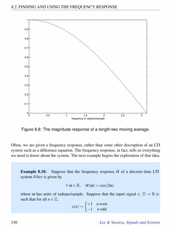
8.2. FINDING AND USING THE FREQUENCY RESPONSE
0 0.5 1 1.5 2 2.5 30
0.1
0.2
0.3
0.4
0.5
0.6
0.7
0.8
0.9
1
frequency in radians/sample
Figure 8.8: The magnitude response of a length-two moving average.
Often, we are given a frequency response, rather than some other description of an LTIsystem such as a difference equation. The frequency response, in fact, tells us everythingwe need to know about the system. The next example begins the exploration of that idea.
Example 8.18: Suppose that the frequency response H of a discrete-time LTIsystem Filter is given by
∀ ω ∈ R, H(ω) = cos(2ω)
where ω has units of radians/sample. Suppose that the input signal x : Z→ R issuch that for all n ∈ Z,
x(n) =+1 n even−1 n odd
336 Lee & Varaiya, Signals and Systems
8. FREQUENCY RESPONSE
We can determine the output. All we have to do is notice that the input can bewritten as
x(n) = cos(πn).
Thus, the input is a cosine with frequency π radians/sample. Hence, the output is
y(n) = |H(π)|cos(πn+∠H(π)) = cos(πn) = x(n).
This input is passed unchanged by the system.
Suppose instead that the input is given by
x(n) = 5.
Once again, the input is a cosine, but this time with zero frequency,
x(n) = 5cos(0n).
Hence the output is
y(n) = |H(0)| ·5cos(0n+∠H(0)) = 5 = x(n).
This input is also passed unchanged by the system.
Suppose instead that the input is
x(n) = cos(πn/2).
This input is given explicitly as a cosine, making our task easier. The output is
y(n) = |H(π/2)|cos(πn/2+∠H(π/2))
= cos(πn/2+π)
= −cos(πn/2)
= −x(n).
This input is inverted by the system.
Finally, suppose that the input is
x(n) = cos(πn/4).
The output isy(n) = |H(π/4)|cos(πn/4+∠H(π/4)) = 0.
This input is filtered out by the system.
Lee & Varaiya, Signals and Systems 337

8.2. FINDING AND USING THE FREQUENCY RESPONSE
8.2.2 The Fourier series with complex exponentials
The Fourier series for a continuous-time, periodic signal x : R → R with period p =2π/ω0, can be written as (see (7.4))
x(t) = A0 +∞
∑k=1
Ak cos(kω0t +φk).
For reasons that we can now understand, the Fourier series is usually written in terms ofcomplex exponentials rather than cosines. Since complex exponentials are eigenfunctionsof LTI systems, this form of the Fourier series decomposes a signal into components thatwhen processed by the system are only scaled.
Each term of the Fourier series expansion has the form
Ak cos(kω0t +φk)
which we can write (see box on page 330)
Ak cos(kω0t +φk) = Ak(ei(kω0t+φk)+ e−i(kω0t+φk))/2.
So the Fourier series can also be written
x(t) = A0 +∞
∑k=1
Ak
2(ei(kω0t+φk)+ e−i(kω0t+φk)).
Observe thatei(kω0t+φk) = eikω0teiφk ,
and let
Xk =
A0 if k = 00.5Akeiφk if k > 00.5A−ke−iφ−k if k < 0
(8.28)
Then the Fourier series becomes
x(t) =∞
∑k=−∞
Xkeikω0t . (8.29)
This is the form in which one usually sees the Fourier series. Notice from (8.28) that theFourier series coefficients are conjugate symmetric,
Xk = X∗−k.
338 Lee & Varaiya, Signals and Systems
8. FREQUENCY RESPONSE
Of course, since (8.29) is an infinite sum, we need to worry about convergence (see boxon page 295).
The discrete-time Fourier series (DFS) can be similarly written. If x : Z→ R is a peri-odic signal with period p = 2π/ω0, then we can write
x(n) =p−1∑
k=0Xkeikω0n (8.30)
for suitably defined coefficients Xk. Relating the coefficients Xk to the coefficients Ak andφk is a bit more difficult in the discrete-time case than in the continuous-time case (seebox on page 347).
There are two differences between (8.29) and (8.30). First, the sum in the discrete-timecase is finite, making it manageable by computer. Second, it is exact for any periodicwaveform. There are no mathematically tricky cases, and no approximation needed.
8.2.3 Examples
The Fourier series coefficients Ak of a square wave are shown in figure 7.7 in the previouschapter. The magnitudes of the corresponding coefficients Xk for the Fourier series ex-pansion of (8.29) are shown in figure 8.9. Since each cosine is composed of two complexexponentials, there are twice as many coefficients.
Notice the symmetry in the figure. There are frequency components shown at both pos-itive and negative frequencies. Notice also that the amplitude of the components is halfthat in Figure 7.7, |Xk| = |Ak|/2. This is because there are now two components, one atnegative frequencies and one at positive frequencies, that contribute.
8.3 Determining the Fourier series coefficients
We have seen in the previous chapter that determining the Fourier series coefficients bydirectly attempting to determine the amplitude of individual frequency components can bedifficult, even when the individual frequency components are known. Usually, however,they are not known. A general formula for computing the coefficients for a continuous-time periodic signal is
Lee & Varaiya, Signals and Systems 339

8.4. FREQUENCY RESPONSE AND THE FOURIER SERIES
Xm = 1p
p∫0
x(t)e−imω0tdt. (8.32)
The m-th Fourier series coefficient is obtained by multiplying x by a complex exponentialwith frequency −mω0 and averaging. The validity of this equation is demonstrated in thebox on page 349.
The discrete-time case is somewhat simpler. A discrete-time periodic signal x with periodp ∈ Z has Fourier series coefficients given by
Xk =1p
p−1∑
m=0x(m)e−imkω0 . (8.33)
This can be shown by manipulations similar to those in the box on page 349. The practicalimportance in computing is much greater than that of the Fourier series for continuous-time signals. Since this sum is finite, the DFS coefficients can be easily computed pre-cisely on a computer.
8.3.1 Negative frequencies
The Fourier series expansion for a periodic signal x(t) is
x(t) =∞
∑k=−∞
Xkeikω0t
This includes Fourier series coefficients for the constant term (when k = 0, eikω0t = 1),plus the fundamental and harmonics (k ≥ 1). But it also includes terms that seem tocorrespond to negative frequencies. When k ≤−1, the frequency kω0 is negative. Thesenegative frequencies balance the positive ones so that the resulting sum is real-valued.
8.4 Frequency response and the Fourier series
Recall that if the input to an LTI system S is a complex exponential signal x ∈ [R→ C]where
∀ t ∈ R, x(t) = eiω0t = cos(ω0t)+ isin(ω0t).
340 Lee & Varaiya, Signals and Systems
8. FREQUENCY RESPONSE
then the output for all t isy(t) = H(ω0)eiω0t ,
where the complex number H(ω0) is the frequency response of the system at the funda-mental frequency ω0 of the periodic input. It is equal to the output at time zero y(0) whenthe input is eiω0t . H itself is a function H : R→ C that in principle can be evaluated forany frequency ω ∈ R, including negative frequencies.
Recall further that if an input x to the system S is a periodic signal with period p, then itcan be represented as a Fourier series,
∀ t ∈ R, x(t) =∞
∑k=−∞
Xkeikω0t ,
where ω0 = 2π/p. By linearity and time invariance of S, the output y = S(x) for thisperiodic input x, is given by
∀ t ∈ R, y(t) =∞
∑k=−∞
H(kω0)Xkeikω0t .
Thus, linearity tells us that if the input is decomposed into a sum of components, then theoutput can be decomposed into a sum of components where each component is the re-sponse of the system to a single input component. Linearity together with time invariancetells us that each component, which is a complex exponential, is simply scaled. Thus, theoutput is given by a Fourier series with coefficients XkH(kω0).
This major result is summarized below:
For an LTI system, if the input is given by a sum of complex exponentials, then theoutput can be given by a sum of the same complex exponentials, each one scaled by thefrequency response evaluated at the corresponding frequency.
Among other things, this result tells us:
• There are no frequency components in the output that were not in the input. Theoutput consists of the same frequency components as the input, but with each com-ponent individually scaled.
• LTI systems can be used to enhance or suppress certain frequency components.Such operations are called filtering.
Lee & Varaiya, Signals and Systems 341

8.5. FREQUENCY RESPONSE OF COMPOSITE SYSTEMS
• The frequency response function characterizes which frequencies are enhanced orsuppressed, and also what phase shifts might be imposed on individual componentsby the system.
We will see many examples of filtering in the next chapter.
8.5 Frequency response of composite systems
In section 2.1.5 we studied several ways of composing systems (using block diagrams) toobtain more complex, composite systems. We will see in this section that when each blockis an LTI system, the resulting composite system is also LTI. Moreover, we can easily ob-tain the frequency response of the composite system from the frequency response of eachblock. This provides a useful way to construct interesting and complex systems by as-sembling simpler components. This tool works equally well with discrete and continuoussystems.
8.5.1 Cascade connection
Consider the composite system S obtained by the cascade connection of systems S1 andS2 in figure 8.10. Suppose S1 and S2 are LTI. We first show that S = S2 S1 is LTI. Toshow that S is time-invariant, we must show that for any τ, SDτ = Dτ S. But,
SDτ = S2 S1 Dτ
= S2 Dτ S1, since S1 is time-invariant
= Dτ S2 S1, since S2 is time-invariant
= Dτ S,
as required.
We now show that S is linear. Let x be any input signal and a any complex number. Then
S(ax) = (S2 S1)(ax)
= S2(S1(ax))
= S2(aS1(x)), since S1 is linear
= aS2(S1(x)), since S2 is linear
= aS(x).
342 Lee & Varaiya, Signals and Systems

8. FREQUENCY RESPONSE
Lastly, if x and y are two input signals, then
S(x+ y) = (S2 S1)(x+ y)
= S2(S1(x+ y))
= S2(S1(x)+S1(y)), since S1 is linear
= S2(S1(x))+S2(S1(y)), since S2 is linear
= S(x)+S(y).
This shows that S is linear.
We now compute the frequency response of S. Let H1(ω),H2(ω),H(ω) be the frequencyresponse of S1, S2, and S, respectively, at the frequency ω. Consider the complex expo-nential input x given by
∀t ∈ R, x(t) = eiωt .
Then the signal y = S1(x) is a multiple of x, namely, y = H1(ω)x. In particular, y is a(scaled) complex exponential, and so z = S2(y) is given by
z = H2(ω)y = H2(ω)H1(ω)x.
But since H(ω) is the frequency response of S at the frequency ω, we also have
z = S(x) = H(ω)x,
and so we obtain∀ω ∈ R, H(ω) = H2(ω)H1(ω). (8.34)
The frequency response of the cascade composition is the product of the frequency re-sponses of the components. Exactly the same formula applies in the discrete-time case.This is a remarkable result. First, suppose that the cascade connection of Figure 8.10 isreversed, i.e. consider the system S = S1 S2. Then the frequency response of S is
H(ω) = H1(ω)H2(ω) = H2(ω)H1(ω) = H(ω).
That is, S and S have the same frequency response! This implies, in fact, that S and S areequivalent; they give the same output for the same input. Hence,
In any cascade connection of LTI systems, the order in which the systems are composeddoes not matter.
Lee & Varaiya, Signals and Systems 343
8.5. FREQUENCY RESPONSE OF COMPOSITE SYSTEMS
8.5.2 Feedback connection
The feedback arrangement shown in figure 8.11 is fundamental to the design of controlsystems. Typically, S1 is some physical system, and S2 is a controller that we design toget the physical system to do our bidding. The overall system S is called a closed-loopsystem. We first show that S is LTI if S1 and S2 are LTI, and we then calculate its frequencyresponse.
Suppose x is the input signal, and define the signals u,z and y as shown. The circle withthe plus sign represents the relationship u = x+ z. The signals are then related by
y = S1(u)
= S1(x+ z)
= S1(x)+S1(z), since S1 is linear
= S1(x)+S1(S2(y)),
Note that this equation relates the input and output, but the output appears on both sides.We can rewrite this as
y−S1(S2(y)) = S1(x). (8.35)
Thus, given the input signal x, the output signal y is obtained by solving this equation. Wewill assume that for any signal x, (8.35) has a unique solution y. Then, of course, y= S(x).We can use (8.35) and methods similar to the ones we used for the cascade example toshow that S is LTI (see box on page 352).
We now compute the frequency response H(ω) of S at frequency ω. Let the frequencyresponse of S1 be H1, and of S2 be H2. Suppose the input signal is the complex exponential
∀t ∈ R, x(t) = eiωt .
For this input, we know that S1(x) = H1(ω)x and S2(x) = H2(ω)x. Since S is LTI, weknow that the output signal y is given by
y = H(ω)x.
Using this relation for y in (8.35) we get
H(ω)x−S1(S2(H(ω)x)) = H(ω)[x−S1(S2(x))], since S2,S1 are linear
= H(ω)[x−H1(ω)H2(ω)x]
= H(ω)[1−H1(ω)H2(ω)]x
= S1(x)
= H1(ω)x, by (8.35),
344 Lee & Varaiya, Signals and Systems

8. FREQUENCY RESPONSE
from which we get the frequency response of the feedback system,
H(ω) =H1(ω)
1−H1(ω)H2(ω)(8.38)
This relation is at the foundation of linear feedback control design.
Example 8.19: Consider a discrete-time feedback system as in Figure 8.11 whereS1 simply scales the input by 0.9. That is, for all discrete-time input signals u,S1(u) = 0.9u. Suppose further that S2 is a one-sample delay. That is, S2 = D1.From example 8.9, the frequency response of S2 is given by
∀ ω ∈ R, H2(ω) = e−iω.
The frequency response of S1 is (trivially) given by
∀ ω ∈ R, H1(ω) = 0.9.
Thus, the frequency response of the feedback composition is
∀ ω ∈ R, H(ω) =0.9
1−0.9e−iω .
We can plot the magnitude of this using the following Matlab code, which (afteradjusting the labels) results in Figure 8.12.
omega = [0:pi/250:pi];H = 0.9./(1 - 0.9.*exp(-i*omega));plot(omega, abs(H));
Notice that at zero frequency, the gain is 9, and that it rapidly drops off at higherfrequencies. Thus, this system behaves as a lowpass filter.
Example 8.20: We can use formula (8.38) to obtain the frequency response ofmore complex composition, such as the one shown in Figure 8.13. To find the
Lee & Varaiya, Signals and Systems 345

8.6. SUMMARY
frequency response of the composition S given on the left of the figure, we firstexpress as the composition on the right where the system S3 is given in the lowerpart of the figure. The frequency response H of S can now be obtained from formula(8.38) as
H(ω) =H1(ω)H3(ω)
1−H1(ω)H3(ω).
The same formula also gives the frequency response H3 of S3,
H3(ω) =H2(ω)
1−H2(ω),
which, upon substitution in the previous expression, yields,
H(ω) =H1(ω)H2(ω)
1−H2(ω)−H1(ω)H2(ω).
8.6 Summary
Linear time-invariant systems have a particularly nice property: if the input is a sinusoid,then the output is a sinusoid of the same frequency. Moreover, if the input is a sum of twosinusoids, then the output will be a sum of two sinusoids with the same frequencies as theinput sinusoids. Each sinusoid is scaled and shifted in phase by the system. The scalingand phase shift, as a function of frequency, is called the frequency response of the system.
It turns out that mathematically, this phenomenon is easiest to analyze using complexexponentials instead of real-valued sinusoids. The reason for this is that the phase shiftand scaling together amount to simple multiplication of the complex exponential by acomplex constant. If an input is represented as a sum of complex exponentials (a formof the Fourier series), then the output is simply the same Fourier series with each term ofthe series scaled by a complex constant. These scaling constants, viewed as a function offrequency, are the frequency response of the system.
Composing LTI system becomes particularly easy. The frequency response of the cascadeof two LTI systems is simply the product of the frequency responses of the individualsystems. This simple fact can be used to quickly ascertain the frequency response ofcomplicated compositions.
346 Lee & Varaiya, Signals and Systems

8. FREQUENCY RESPONSE
Probing Further: Relating DFS coefficients
We have two discrete-time Fourier series expansions (see (8.30) and (7.8)),
x(n) =p−1
∑k=0
Xkeikω0n (8.31)
x(n) = A0 +K
∑k=1
Ak cos(kω0n+φk), K =
(p−1)/2 if p is oddp/2 if p is even
There is a relationship between the coefficients Ak, φk and Xk, but the relationship ismore complicated than in the continuous-time case, given by (8.28). To develop thatrelationship, begin with the second of these expansions and write
x(n) = A0 +K
∑k=1
Ak
2(ei(kω0n+φk)+ e−i(kω0n+φk)).
Note that since ω0 = 2π/p, then for all integers n, eiω0 pn = 1, so
e−i(kω0n+φk) = e−i(kω0n+φk)eiω0 pn = ei(ω0(p−k)n−φk).
Thusx(n) = A0 +
K
∑k=1
Ak
2eiφk eikω0n++
K
∑k=1
Ak
2e−iφk eiω0(p−k)n
= A0 +K
∑k=1
Ak
2eiφk eikω0n++
p−1
∑m=K
Ap−m
2e−iφp−meiω0mn,
by change of variables. Comparing this against (8.31),
Xk =
A0 if k = 0Akeiφk/2 if k ∈ 1, · · · ,K−1Akeiφk/2+Ake−iφk/2 = Ak cos(φk) if k = KAp−ke−iφp−k/2 if k ∈ K +1, · · · , p−1
This relationship is more complicated than (8.28). Fortunately, it is rare that we need touse both forms of the DFS, so we can usually just pick one of the two forms and workonly with its set of coefficients.
Lee & Varaiya, Signals and Systems 347

8.6. SUMMARY
-3x10
K = 1K = 3K = 7
K = 32
-1.0
-0.5
0.0
0.5
1.0
-0 1 2 3 4 5 6 7 8
Time in seconds
(a)
3x10
-0.0
0.1
0.2
0.3
0.4
0.5
0.6
-4 -3 -2 -1 0 1 2 3 4
Frequency in Hz
(b)
Figure 8.9: (a) Some finite Fourier series approximations to one cycle of a squarewave. The number of Fourier series terms that are included in the approximationis 2K+1, so K is the magnitude of the largest index the terms. (b) The magnitudeof the complex Fourier series coefficients shown as a function of frequency.
348 Lee & Varaiya, Signals and Systems

8. FREQUENCY RESPONSE
Probing Further: Formula for Fourier series coefficients
To see that (8.32) is valid, try substituting for x(t) its Fourier series expansion,
x(t) =∞
∑k=−∞
Xkeikω0t
to get Xm =1p
∫ p
0
∞
∑k=−∞
Xkeikω0te−imω0tdt.
Exchange the integral and sum (assuming this is valid, see box on page 350) to get
Xm =1p
∞
∑k=−∞
Xk
∫ p
0eikω0te−imω0tdt.
The exponentials can be combined to get
Xm =1p
∞
∑k=−∞
Xk
∫ p
0ei(k−m)ω0tdt.
In the summation, where k varies over all integers, there will be exactly one term of thesummation where k = m. In that term, the integral evaluates to p. For the rest of theterms, k 6= m. Separating these two situations, we can write
Xm = Xm +1p
∞
∑k=−∞,k 6=m
Xk
p∫0
ei(k−m)ω0tdt,
where the first term Xm is the value of the term in the summation where k = m. For eachremaining term of the summation, the integral evaluates to zero, thus establishing ourresult. To show that the integral evaluates to zero, let n = k−m, and note that n 6= 0.Then ∫ p
0einω0tdt =
∫ p
0cos(nω0t)dt + i
∫ p
0sin(nω0t)dt
Since ω0 = 2π/p, these two integrals exactly span one or more complete cycles of thecosine or sine, and hence integrate to zero.
Lee & Varaiya, Signals and Systems 349

8.6. SUMMARY
Probing Further: Exchanging integrals and summations
The demonstration of the validity of the formula for the Fourier series coefficients in thebox on page 349 relies on being able to exchange an integral and an infinite summation.The infinite summation can be given as a limit of a sequence of functions
xN(t) =N
∑k=−N
Xkeikω0t .
Thus, we wish to exchange the integral and limit in
Xm =1p
∫ p
0( lim
N→∞xN(t))dt.
A sufficient condition for being able to perform the exchange is that the limit convergesuniformly in the interval [0, p]. A sufficient condition for uniform convergence is that xis continuous and that its first derivative is piecewise continuous.
See R. G. Bartle, The Elements of Real Analysis, Second Edition, John Wiley & Sons,1976, p. 241.
S1 S2S
x y z
Figure 8.10: The cascade connection of the two LTI systems is the system S =S2 S1. The frequency response is related by ∀ω,H(ω) = H1(ω)H2(ω).
350 Lee & Varaiya, Signals and Systems

8. FREQUENCY RESPONSE
S1
S2S
x y+
z
u
Figure 8.11: The feedback connection of the two LTI systems S1, S2 is the LTIsystem S. The frequency response is related by ∀ω ∈ R,H(ω) = H1(ω)/[1−H1(ω)H2(ω)].
Lee & Varaiya, Signals and Systems 351

8.6. SUMMARY
Probing Further: Feedback systems are LTI
To show that S in Figure 8.11 is time-invariant we must show that for any τ ∈ R,
S(Dτ(x)) = Dτ(S(x)) = Dτ(y), (8.36)
that is, we must show that Dτ(y) is the output of S when the input is Dτ(x). Now theleft-hand side of (8.35) with y replaced by Dτ(y) is
Dτ(y)−S1(S2(Dτ(y))) = Dτ(y)−Dτ(S1(S2(y)),
since S1 and S2 are time-invariant
= Dτ(y−S1(S2(y))), since Dτ is linear,
= Dτ(S1(x)), by (8.35)
= S1(Dτ(x)), since S1 is time-invariant
so that Dτ(y) is indeed the solution of (8.35) when the input is Dτ(x). This proves (8.36).Linearity is shown similarly. Let a be any complex number. To show that ay is the outputwhen the input is ax, we evaluate the left-hand side of (8.35) at ay,
ay−S1(S2(ay)) = ay−aS1(S2(y)), since S2 and S1 are linear
= a[y−S1(S2(y))]
= aS1(x), by (8.35)
= S1(ax), since S1 is linear
which shows that S(ax) = aS(x).Now suppose w is another input and z = S(w) is the corresponding output. I.e.,
z−S1(S2(z)) = S1(w). (8.37)
We evaluate the left-hand side of (8.35) at y+ z, using that S2 and S1 are linear,
(y+ z)−S1(S2(y+ z)) = [y−S1(S2(y))]+ [z−S1(S2(z)],
= S1(x)+S1(w), by (8.35) and (8.37)
= S1(x+w), since S1 is linear
and so S(x+w) = y+ z = S(x)+S(z).
352 Lee & Varaiya, Signals and Systems

8. FREQUENCY RESPONSE
0 0.5 1 1.5 2 2.5 3 3.50
1
2
3
4
5
6
7
8
9
frequency (radians/sample)
ampl
itude
resp
onse
Figure 8.12: The magnitude response of the feedback composition of example8.19.
Lee & Varaiya, Signals and Systems 353

8.6. SUMMARY
S1 S2
S
x y+
u+ S1 S3
x y+
S
S2+ S3
Figure 8.13: The composition on the left can be expressed as the one on theright, where S3 is the system at the bottom.
354 Lee & Varaiya, Signals and Systems

8. FREQUENCY RESPONSE
Exercises
Each problem is annotated with the letter E, T, C which stands for exercise, requires somethought, requires some conceptualization. Problems labeled E are usually mechanical,those labeled T require a plan of attack, those labeled C usually have more than onedefensible answer.
1. E Find A ∈ C so that
∀ t ∈ Reals, Aeiωt +A∗e−iωt = cos(ωt +π/4),
where A∗ is the complex conjugate of A.
2. E Plot the function s : R→ R given by
∀ x ∈ R, s(x) = Ime(−x+i2πx).
You are free to choose a reasonable interval for your plot, but be sure it includesx = 0.
3. E This exercise explores the fact that a delay in a sinewave causes a phase shift.That is, for any real numbers τ and ω, there is a phase shift φ ∈ R such that for allt ∈ R,
sin(ω(t− τ)) = sin(ωt−φ).
Give φ in terms of τ,ω. What are the units of τ,ω,φ? Hint: The argument to thesin function has units of radians.
4. E Let x : R→ R. Show that x is periodic with period p if and only if Dp(x) = x.Now show that if S is a time-invariant system and x is a periodic signal, then S(x)is also periodic with period p.
5. E Analogously to Dτ in (8.1) and DM in Section 8.1.3, define formally the followingvariants:
(a) A shift operator Sv,h that shifts an image v units vertically and h units horizon-tally, where v ∈ R and h ∈ R.
(b) A shift operator Sm,n that shifts a discrete image m units vertically and n unitshorizontally, where m ∈ Z and n ∈ Z.
Lee & Varaiya, Signals and Systems 355

EXERCISES
6. E Consider a discrete-time system D : [Z→R]→ [Z→R], where if y = D(x) then
∀ n ∈ Z, y(n) = x(n−1).
(a) Is D linear? Justify your answer.
(b) Is D time-invariant? Justify your answer.
7. E Consider a continuous-time system TimeScale : [R→ R]→ [R→ R], where ify = TimeScale(x) then
∀ t ∈ R, y(t) = x(2t).
(a) Is TimeScale linear? Justify your answer.
(b) Is TimeScale time-invariant? Justify your answer.
8. E Consider the continuous-time signal x where
∀ t ∈ R, x(t) = 1+ cos(πt)+ cos(2πt).
Suppose that x is the input to an LTI system with frequency response given by
∀ ω ∈ R, H(ω) =
eiω if |ω|< 4 radians/second0 otherwise
Find the output y of the system.
9. T Suppose that the continuous-time signal x : R→R is periodic with period p. Letthe fundamental frequency be ω0 = 2π/p. Suppose that the Fourier series coeffi-cients for this signal are known constants A0,A1,A2, · · · and φ1,φ2, · · · . Give theFourier series coefficients A′0,A
′1,A′2, · · · and φ′1,φ
′2, · · · for each of the following
signals:
(a) ax, where a ∈ R is a constant;
(b) Dτ(x), where τ ∈ R is a constant and Dτ is the delay system; and
(c) S(x), where S is an LTI system with frequency response H given by
∀ ω ∈ R, H(ω) =
1; if ω = 00; otherwise
(Note that this is a highly unrealistic frequency response.)
356 Lee & Varaiya, Signals and Systems
8. FREQUENCY RESPONSE
(d) Let y : R→R be another periodic signal with period p. Suppose y has Fourierseries coefficients A′′0,A
′′1,A′′2, · · · and φ′′1,φ
′′2, · · · . Give the Fourier series coef-
ficients of x+ y.
10. E Consider discrete-time systems with input x : Z→R and output y : Z→R. Eachof the following defines such a system. For each, indicate whether it is linear (L),time-invariant (TI), both (LTI), or neither (N).
(a) ∀ n ∈ Z, y(n) = x(n)+0.9y(n−1)
(b) ∀ n ∈ Z, y(n) = cos(2πn)x(n)
(c) ∀ n ∈ Z, y(n) = cos(2πn/9)x(n)
(d) ∀ n ∈ Z, y(n) = cos(2πn/9)(x(n)+ x(n−1))
(e) ∀ n ∈ Z, y(n) = x(n)+0.1(x(n))2
(f) ∀ n ∈ Z, y(n) = x(n)+0.1(x(n−1))2
11. E Suppose that the frequency response of a discrete-time LTI system S is given by
H(ω) = |sin(ω)|
where ω has units of radians/sample. Suppose the input is the discrete-time signalx given by ∀ n ∈ Z, x(n) = 1. Give a simple expression for y = S(x).
12. T Find the smallest positive integer n such that
n
∑k=0
ei5kπ/6 = 0.
Hint: Note that the term being summed is a periodic function of k. What is itsperiod? What is the sum of a complex exponential over one period?
13. T Consider a continuous-time periodic signal x with fundamental frequency ω0 = 1radian/second. Suppose that the Fourier series coefficients (see (7.4)) are
Ak =
1 k = 0, 1, or 20 otherwise
and for all k ∈ N0, φk = 0.
(a) Find the Fourier series coefficients Xk for all k ∈ Z (see (8.29)).
Lee & Varaiya, Signals and Systems 357

EXERCISES
(b) Consider a continuous-time LTI system Filter : [R→ R]→ [R→ R], withfrequency response
H(ω) = cos(πω/2).
Find y = Filter(x). I.e., give a simple expression for y(t) that is valid for allt ∈ R.
(c) For y calculated in (b), find the fundamental frequency in radians per second.I.e., find the largest ω′0 > 0 such that
∀ t ∈ R, y(t) = y(t +2π/ω′0)
14. T Consider a continuous-time LTI system S. Suppose that when the input x is givenby
∀t ∈ Reals, x(t) =
1, if 0≤ t < 10, otherwise
then the output y = S(x) is given by
∀t ∈ Reals, y(t) =
1, if 0≤ t < 20, otherwise
Give an expression and a sketch for the output of the same system if the input is
(a)
∀t ∈ Reals, x′(t) =
1, if 0≤ t < 1−1, if 1≤ t < 20, otherwise
(b)
∀t ∈ Reals, x′(t) =
1, if 0≤ t < 1/20, otherwise
15. T Suppose that the frequency response H of a discrete-time LTI system Filter isgiven by:
∀ ω ∈ [−π,π], H(ω) = |ω|.where ω has units of radians/sample. Note that since a discrete-time frequencyresponse is periodic with period 2π, this definition implicitly gives H(ω) for allω ∈R. Give simple expressions for the output y when the input signal x : Z→R issuch that ∀ n ∈ Z each of the following is true:
(a) x(n) = cos(πn/2).
358 Lee & Varaiya, Signals and Systems

8. FREQUENCY RESPONSE
(b) x(n) = 5.
(c) x(n) =
+1, n even−1, n odd
16. T Consider a continuous-time LTI system S. Suppose that when the input is givenby
x(t) =
sin(πt) 0≤ t < 10 otherwise
then the output y = S(x) is given by
y(t) =
sin(πt) 0≤ t < 1sin(π(t−1)) 1≤ t < 20 otherwise
for all t ∈ R.
(a) Carefully sketch these two signals.
(b) Give an expression and a sketch for the output of the same system if the inputis
x(t) =
sin(πt) 0≤ t < 1−sin(π(t−1)) 1≤ t < 20 otherwise
.
17. T Suppose you are given the building blocks shown below for building block dia-grams:
-0.5in-
0.5in
HW Gg
These blocks are defined as follows:
• An LTI system HW : [R→ R]→ [R→ R] that has a rectangular frequencyresponse given by
∀ ω ∈ R, H(ω) =
1 −W < ω <W0 otherwise
where W is a parameter you can set.
Lee & Varaiya, Signals and Systems 359

EXERCISES
• A gain block Gg : [R→ R]→ [R→ R] where if y = g(x), then
∀ t ∈ R, y(t) = gx(t)
where g ∈ R is a parameter you can set.
• An adder, which can add two continuous-time signals. Specifically, Add : [R→R]× [R→ R]→ [R→ R] such that if y = Add(x1,x2) then
∀ t ∈ R, y(t) = x1(t)+ x2(t).
Use these building blocks to construct a system with the frequency response shownbelow:
H(ω)
ω
1
2
1 2 0 −1−2
18. T Let u be a discrete-time signal given by
∀ n ∈ Z, u(n) =
1 0≤ n0 otherwise
This is the unit step signal, which we saw before in (2.16). Suppose that a discrete-time system H that is known to be LTI is such that if the input is u, the output isy = H(u) given by
∀ n ∈ Z, y(n) = nu(n).
This is called the step response of the system. Find a simple expression for theoutput w = H(p) when the input is p given by
∀ n ∈ Z, p(n) =
2 0≤ n < 80 otherwise
Sketch w.
19. T Suppose you are given the Fourier series coefficients · · ·X−1,X0,X1,X2, · · · for aperiodic signal x : R→ R with period p. Find the fundamental frequency and theFourier series coefficients of the following signals in terms of those of x.
360 Lee & Varaiya, Signals and Systems

8. FREQUENCY RESPONSE
(a) y such that ∀ t ∈ R, y(t) = x(at), for some positive real number a.
(b) w such that ∀ t ∈ R, w(t) = x(t)eiω0t , where ω0 = 2π/p.
(c) z such that ∀ t ∈ R, z(t) = x(t)cos(ω0t), where ω0 = 2π/p.
20. E Analogously to the box on page 349, show that the formula (8.33) for the discreteFourier series coefficients is valid.
21. C Consider a system Squarer : [R→ R]→ [R→ R], where if y = Squarer(x) then
∀ t ∈ R, y(t) = (x(t))2.
(a) Show that this system is memoryless.
(b) Show that this system is not linear.
(c) Show that this system is time invariant.
(d) Suppose that the input x is given by
∀ t ∈ R, x(t) = cos(ωt),
for some fixed ω. Show that the output y contains a component at frequency2ω.
Lee & Varaiya, Signals and Systems 361

9Filtering
Contents9.1 Convolution . . . . . . . . . . . . . . . . . . . . . . . . . . . . . . 365
9.1.1 Convolution sum and integral . . . . . . . . . . . . . . . . . 3679.1.2 Impulses . . . . . . . . . . . . . . . . . . . . . . . . . . . . 3719.1.3 Signals as sums of weighted delta functions . . . . . . . . . . 3729.1.4 Impulse response and convolution . . . . . . . . . . . . . . . 375
9.2 Frequency response and impulse response . . . . . . . . . . . . . . 3789.3 Causality . . . . . . . . . . . . . . . . . . . . . . . . . . . . . . . . 3829.4 Finite impulse response (FIR) filters . . . . . . . . . . . . . . . . . 382
Probing Further: Causality . . . . . . . . . . . . . . . . . . . . . . . 3839.4.1 Design of FIR filters . . . . . . . . . . . . . . . . . . . . . . 3859.4.2 Decibels . . . . . . . . . . . . . . . . . . . . . . . . . . . . . 391Probing Further: Decibels . . . . . . . . . . . . . . . . . . . . . . . 394
9.5 Infinite impulse response (IIR) filters . . . . . . . . . . . . . . . . 3959.5.1 Designing IIR filters . . . . . . . . . . . . . . . . . . . . . . 396
9.6 Implementation of filters . . . . . . . . . . . . . . . . . . . . . . . 3989.6.1 Matlab implementation . . . . . . . . . . . . . . . . . . . . . 3989.6.2 Signal flow graphs . . . . . . . . . . . . . . . . . . . . . . . 400Probing Further: Java implementation of an FIR filter . . . . . . . . 401Probing Further: FIR filter in a programmable DSP . . . . . . . . . . 402
9.7 Summary . . . . . . . . . . . . . . . . . . . . . . . . . . . . . . . . 403Exercises . . . . . . . . . . . . . . . . . . . . . . . . . . . . . . . . . . . 406
363

Linear time invariant systems have the property that if the input is described as a sum ofsinusoids, then the output is a sum of sinusoids of the same frequencies. Each sinusoidalcomponent will typically be scaled differently, and each will be subjected to a phasechange, but the output will not contain any sinusoidal components that are not also presentin the input. For this reason, an LTI system is often called a filter. It can filter outfrequency components of the input, and also enhance other components, but it cannotintroduce components that are not already present in the input. It merely changes therelative amplitudes and phases of the frequency components that are present in the inputs.
LTI systems arise in two circumstances in an engineering context. First, they may be usedas a model of a physical system. Many physical systems are accurately modeled as LTIsystems. Second, they may present an ideal for an engineered system. For example, theymay specify the behavior that an electronic system is expected to exhibit.
Consider for example an audio system. The human ear hears frequencies in the range ofabout 30 to 20,000 Hz, so a specification for a high fidelity audio system typically requiresthat the frequency response be constant (in magnitude) over this range. The human ear isrelatively insensitive to phase, so the same specification may say nothing about the phaseresponse (the argument, or angle of the frequency response). An audio system is free tofilter out frequencies outside this range.
Consider an acoustic environment, a physical context such as a lecture hall where soundsare heard. The hall itself alters the sound. The sound heard by your ear is not identical tothe sound created by the lecturer. The room introduces echoes, caused by reflections of thesound by the walls. These echoes tend to occur more for the lower frequency componentsin the sound than the higher frequency components because the walls and objects in theroom tend to absorb higher frequency sounds better. Thus, the lower frequency soundsbounce around in the room, reinforcing each other, while the higher frequency sounds,which are more quickly absorbed, become relatively less pronounced. In an extremecircumstance, in a room where the walls are lined with shag carpeting, for example, thehigher frequency sounds are absorbed so effectively that the sound gets muffled by theroom.
The room can be modeled by an LTI system where the frequency response H(ω) is smallerin magnitude for large ω than for small ω. This is a simple form of distortion introducedby a channel (the room), which in this case carries a sound from its transmitter (thelecturer) to its receiver (the listener). This form of distortion is called linear distortion, ashorthand for linear, time-invariant distortion (the time invariance is left implicit).
364 Lee & Varaiya, Signals and Systems

9. FILTERING
A public address system in a lecture hall may compensate for the acoustics of the room byboosting the high frequency content in the sound. Such a compensator is called an equal-izer because it corrects for distortion in the channel so that all frequencies are receivedequally well by the receiver.
In a communications system, a channel may be a physical medium, such as a pair ofwires, that carries an electrical signal. That physical medium distorts the signal, and thisdistortion is often reasonably well approximated as linear and time invariant. An equalizerin the receiver compensates for this distortion. Unlike the audio example, however, suchan equalizer often needs to compensate for the phase response, not just the magnituderesponse. Because the human ear is relatively insensitive to phase distortion, a publicaddress system equalizer need not compensate for phase distortion. But the wire pair maybe carrying a signal that is not an audio signal. It may be, for example, a modem signal.
Images may also be processed by LTI systems. Consider the three images shown in Figure9.1. The top image is the original, undistorted image. The lower left image is blurred,as might result for example from unfocused optics. The lower right image is, in a sense,the opposite of the blurred image. Whereas the blurred image deemphasizes the patternsin the outfit, for example, the right image deemphasizes the regions of constant value,changing them all to a neutral gray.
For images, time is not the critical variable. Its role is replaced by two spatial variables,one in the horizontal direction and one in the vertical direction. Thus, instead of LTI, wemight talk about an image processing system being a linear, space-invariant (LSI) sys-tem. The blurred image is constructed from the original by an LSI system that eliminateshigh (spatial) frequencies, passing unaltered the low frequencies. Such a system is calleda lowpass filter. The lower right image is constructed from the original by an LSI systemthat eliminates low frequencies, passing unaltered the high frequencies. Such a system iscalled a highpass system. Both images were created using Adobe Photoshop, althoughthe blurred image could have been just as easily created by a defocused lens.
9.1 Convolution
The frequency response of a system is a declarative description of the system. It tellsus what it is, not how it works. It tells us, for example, that it is a lowpass filter, but itdoes not tell us whether it is a defocused lens or a computer program, much less tellingus how the computer program works. In this chapter, we explore imperative descriptions
Lee & Varaiya, Signals and Systems 365

9.1. CONVOLUTION
Figure 9.1: An image and two versions that have been distorted by a linear,space-invariant system.
366 Lee & Varaiya, Signals and Systems

9. FILTERING
of systems, and build up to detailed descriptions of software that can implement certainkinds of LTI (or LSI) systems. These imperative descriptions are based on convolution.
9.1.1 Convolution sum and integral
For discrete-time signals the convolution operator is called the convolution sum, and forcontinuous-time signals it is called the convolution integral. We define these two operatorsnow and note some important properties.
Let x,y∈ [Z→R] be two discrete-time signals. The convolution of x and y is the discrete-time signal, denoted x∗ y, given by the convolution sum,
∀n ∈ Z, (x∗ y)(n) =∞
∑k=−∞
x(k)y(n− k). (9.1)
We note two properties. First, the order in the convolution does not matter, x ∗ y = y ∗ x.Indeed, if in (9.1) we change the variables in the summation, letting m = n− k, we get
∀n ∈ Z, (x∗ y)(n) =∞
∑k=−∞
x(k)y(n− k)
=∞
∑m=−∞
x(n−m)y(m).
Thus,(x∗ y)(n) = (y∗ x)(n). (9.2)
This property is called commutativity of the convolution operator.1
Another property of convolution is linearity. That is, if x,y1,y2 are three signals and a1and a2 are real numbers, then
x∗ (a1y1 +a2y2) = a1(x∗ y1)+a2(x∗ y2), (9.3)
which may be checked directly by applying definition (9.1) to both sides.
1Matrix multiplication is an example of an operator that is not commutative, while matrix addition is.Since the sum of two matrices M and N (of the same size) does not depend on the order, i.e., M+N = N+M,the matrix sum is a commutative operator. However, the product of two matrices depends on the order, i.e., itis not always true that M×N = N×M, so the matrix product is not commutative.
Lee & Varaiya, Signals and Systems 367
9.1. CONVOLUTION
We now use the convolution sum to define some LTI systems. Fix a discrete-time signalh, and define the system
S : [Z→ R]→ [Z→ R]
by∀ x ∈ [Z→ R], S(x) = h∗ x.
Thus the output signal y = S(x) corresponding to the input signal x is given by
∀ n ∈ Z, y(n) =∞
∑k=−∞
h(k)x(n− k).
We now show that S is LTI. The linearity of S follows immediately from the linearityproperty of the convolution. To show time-invariance, we must show that for any integerM, and any input signal x,
DM(h∗ x) = h∗ (DM(x)),
where DM is a delay by M. But this is easy to see, since for all n,
(DM(h∗ x))(n) = (h∗ x)(n−M)
=∞
∑k=−∞
h(k)x(n−M− k), by definition (9.1)
=∞
∑k=−∞
h(k)z(n− k), where z = DM(x)
= (h∗ z)(n).
Thus every discrete-time signal h defines an LTI system via convolution. In the nextsection we will see the converse result, that every LTI system is defined by convolutionwith some signal h.
Example 9.1: Consider a discrete-time signal h defined by
∀ n ∈ Z, h(n) =
1/3 if n ∈ 0,1,20 otherwise
This is shown in Figure 9.2. Let us define a system S as follows. If the input is x,then the output is
y = S(x) = h∗ x.
368 Lee & Varaiya, Signals and Systems

9. FILTERING
h(n)
n...... 1/3
Figure 9.2: Signal in example 9.1.
I.e.,
∀ n ∈ Z, y(n) =∞
∑k=−∞
h(k)x(n− k)
=2
∑k=0
(1/3)x(n− k)
= (x(n)+ x(n−1)+ x(n−2))/3. (9.4)
This system calculates the three-point moving average!
We now turn to the continuous time case. Let x,y ∈ [R→ R] be two continuous-timesignals. The convolution of x and y is the continuous-time signal, denoted x∗ y, given bythe convolution integral
∀ t ∈ R, (x∗ y)(t) =∞∫−∞
x(τ)y(t− τ)dτ. (9.5)
By a change of variable in the integral we can check that convolution again is commuta-tive, i.e.,
∀ t ∈ R, (x∗ y)(t) = (y∗ x)(t), (9.6)
and it is linear; i.e. if x,y1,y2 are three continuous-time signals and a1,a2 are real numbers,then
x∗ (a1y1 +a2y2) = a1(x∗ y1)+a2(x∗ y2). (9.7)
Again fix h ∈ [R→ R], and define the system
S : [R→ R]→ [R→ R]
Lee & Varaiya, Signals and Systems 369

9.1. CONVOLUTION
h(t)
t1/3
3
Figure 9.3: Signal in example 9.2.
by
∀ x ∈ [R→ R], S(x) = h∗ x.
Then in exactly the same way as for the discrete-time case, we can show that S is LTI.
Example 9.2: Consider a continuous-time signal h defined by
∀ t ∈ R, h(t) =
1/3 if t ∈ [0,3]0 otherwise
This is shown in Figure 9.3. Let us define a system S as follows. If the input is x,then the output is
y = S(x) = h∗ x.
I.e,
∀ t ∈ R, y(t) =
∞∫−∞
h(τ)x(t− τ)dτ
=13
3∫0
x(t− τ)dτ. (9.8)
This system is the length-three continuous-time moving average!
Note that we are using the same symbol ‘*’ for the convolution sum and the convolutionintegral. The context will determine which operator is intended.
370 Lee & Varaiya, Signals and Systems

9. FILTERING
δ(n)
n......1
Figure 9.4: The Kronecker delta function, a discrete-time impulse.
9.1.2 Impulses
Intuitively, an impulse is a signal that is zero everywhere except at time zero. In thediscrete-time case, the Kronecker delta function,
δ : Z→ R
is defined by
∀ n ∈ Z, δ(n) =
1 if n = 00 otherwise
(9.9)
Its graph is shown in Figure 9.4.
The continuous-time case, which is called the Dirac delta function, is mathematicallymuch more difficult to work with. Like the Kronecker delta function, it is zero everywhereexcept at zero. But unlike the Kronecker delta function, its value is infinite at zero. Wewill not concentrate on its subtleties, but rather just introduce it and assert some resultswithout fully demonstrating their validity. The Dirac delta function is defined to be
δ : R→ R++
where R++ = R∪∞,−∞, and
∀ t ∈ R where t 6= 0, δ(t) = 0
and where the following property is satisfied for any ε > 0 in R++,
ε∫−ε
δ(t)dt = 1
Lee & Varaiya, Signals and Systems 371

9.1. CONVOLUTION
δ(t)
t1
Figure 9.5: The Dirac delta function, a continuous-time impulse.
For the latter property to be satisfied, clearly no finite value at t = 0 would suffice. Thisis why the value must be infinite at t = 0. Notice that the Kronecker delta function has asimilar property,
a
∑n=−a
δ(n) = 1
for any integer a > 0, but that in this case, the property is trivial. There is no mathematicalsubtlety.
The Dirac delta function is usually depicted as in Figure 9.5. In any figure, of course,the infinite value at t = 0 cannot be shown directly. The figure suggests that infinite valuewith a vertical arrow. Next to the arrow is the weight of the delta function, ‘1’ in this case.In general, a Dirac delta function can be multiplied by any real constant a. Of course, thisdoes not change its value at t = 0, which is infinite, nor does it change its value at t 6= 0,which is zero. What it does change is its integral,
ε∫−ε
aδ(t)dt = a.
Thus, although the impulse is still infinitely narrow and infinitely high, the area under theimpulse has been scaled by a.
9.1.3 Signals as sums of weighted delta functions
Any discrete-time signal x : Z→ R can be expressed as a sum of weighted Kroneckerdelta functions,
∀ n ∈ Z, x(n) =∞
∑k=−∞
x(k)δ(n− k). (9.10)
372 Lee & Varaiya, Signals and Systems

9. FILTERING
n...... 1/3
(1/3)δ(n)
n...... 1/3
n...... 1/3
n...... 1/3
n......
0 δ(n+1)
n......
Σ
(1/3)δ(n − 1)
(1/3)δ(n − 2)
0 δ(n − 3)
...
...
(δ(n) + δ(n − 1) + δ(n − 2))/3
Figure 9.6: A discrete-time signal is a sum of weighted delta functions.
Lee & Varaiya, Signals and Systems 373

9.1. CONVOLUTION
The kth term in the sum is x(k)δ(n− k). This term, by itself, defines a signal that is zeroeverywhere except at n= k, where it has value x(k). This signal is called a weighted deltafunction because it is a (time shifted) delta function with a specified weight. Thus, anydiscrete-time signal is a sum of weighted delta functions, much the way that the Fourierseries describes a signal as a sum of weighted complex exponential functions.
Example 9.3: The signal h in example 9.1 can be written in terms of Kroneckerdelta functions,
∀ n ∈ Z, h(n) = (δ(n)+δ(n−1)+δ(n−2))/3.
This has the form of (9.10), and is illustrated in Figure 9.6. It is described as a sumof signals where each signal contains only a single weighted impulse.
Equation (9.10) is sometimes called the sifting property of the Kronecker delta functionbecause it “sifts out” the value of a function x at some integer n. That is, the infinitesum reduces to a single number. This property can often be used to eliminate infinitesummations in more complicated expressions.
The continuous-time version of this is similar, except that the sum becomes an integral(integration, after all, is just sum over a continuum). Given any signal x : R→ R,
∀ t ∈ R, x(t) =∞∫−∞
x(τ)δ(t− τ)dτ. (9.11)
Although this is mathematically much more subtle than the discrete-time case, it is verysimilar in structure. It describes a signal x as a sum (or more precisely, an integral) ofweighted Dirac delta functions.
Example 9.4: The signal h in Figure 9.3 and example 9.2 can be written as a sum(an integral, actually) of weighted Dirac delta functions,
∀ t ∈ R, h(t) =∫
∞
−∞
h(τ)δ(t− τ)dτ
=∫ 3
0(1/3)δ(t− τ)dτ.
374 Lee & Varaiya, Signals and Systems

9. FILTERING
This has the form of (9.11).
Equation (9.11) is sometimes called the sifting property of the Dirac delta function,because it sifts out from the function x the value at a given time t. The sifting propertycan often be used to eliminate integrals, since it replaces an integral with a single value.
9.1.4 Impulse response and convolution
Consider a discrete-time LTI system S : [Z→ R]→ [Z→ R]. Define its impulse re-sponse h to be the output signal when the input signal is the Kronecker delta function (animpulse), h = S(δ), that is,
∀ n ∈ Z, h(n) = (S(δ))(n).
Now let x be any input signal, and let y = S(x) be the corresponding output signal. In(9.10), x is given as sum of components, where each component is a weighted delta func-tion. Since S is LTI, the output can be given as a sum of the responses to these compo-nents. Each component is a signal x(k)δ(n−k) for fixed k, and the response to this signalis x(k)h(n−k). The response to a scaled and delayed impulse will be a scaled and delayedimpulse response. Thus, the overall output is
∀ n ∈ Z, y(n) =∞
∑k=−∞
x(k)h(n− k) = (x∗h)(n) = (h∗ x)(n).
Thus, the output of any discrete-time LTI system is given by the convolution of the inputsignal and the impulse response.
Example 9.5: The three-point moving average system S of example 9.1 has im-pulse response
∀ n ∈ Z, h(n) = (δ(n)+δ(n−1)+δ(n−2))/3.
This can be determined from (9.4) by just letting the input be x = δ. The impulseresponse, after all, is defined to be the output when the input is an impulse. Theimpulse response is shown in Figure 9.2.
Lee & Varaiya, Signals and Systems 375

9.1. CONVOLUTION
Consider now a continuous-time LTI system S : [R→ R]→ [R→ R]. Define its impulseresponse to be the output signal h when the input signal is the Dirac delta function, h =S(δ), i.e.,
∀t ∈ R, h(t) = S(δ)(t).
Now let x be any input signal and let y = S(x), be the corresponding output signal. By thesifting property we can express x as the sum (integral) of weighted delta functions,
x(t) =∫
∞
−∞
x(τ)δ(t− τ)dτ.
Since S is LTI, the output is a sum (integral) of the responses to each of the components(the integrand for fixed τ), or
∀ t ∈ R, y(t) =∞∫−∞
x(τ)h(t− τ)dτ = (x∗h)(t) = (h∗ x)(t). (9.12)
Thus,
The output of any continuous-time LTI system is given by the convolution of the inputsignal and the impulse response.
Example 9.6: The length-three continuous-time moving average system S of ex-ample 9.2 has impulse response
∀ t ∈ R, h(t) =
1/3 if t ∈ [0,3]0 otherwise
This can be determined from (9.8) by just letting the input be x = δ and then usingthe sifting property of the delta function. The impulse response, after all, is definedto be the output when the input is an impulse. The impulse response is shownin Figure 9.3. In general, a moving average has an impulse response with thisrectangular shape.
Example 9.7: Consider an M-step discrete-time delay system, as in example 8.9,where the output y is given in terms of the input x by the difference equation
∀ n ∈ Z, y(n) = x(n−M). (9.13)
376 Lee & Varaiya, Signals and Systems

9. FILTERING
The impulse response can be found by letting x = δ, to get
h(n) = δ(n−M).
The output can be given as a convolution of the input and the impulse response,
y(n) =∞
∑k=−∞
x(k)δ(n−M− k) = x(n−M),
using the sifting property. Of course, this agrees with (9.13).
Example 9.8: Consider a T second continuous-time delay system, where theoutput y is given in terms of the input x by the equation
∀ t ∈ R, y(t) = x(t−T ). (9.14)
The impulse response can be found by letting x = δ, to get
h(t) = δ(t−T ).
The output can be given as a convolution of the input and the impulse response,
y(t) =∞∫−∞
x(τ)δ(t−T − τ)dτ = x(t−T ),
using the sifting property. Of course, this agrees with (9.14).
Example 9.9: Suppose that we have two LTI systems (discrete or continuous time)with impulse responses h1 and h2, and we connect them in a cascade structure asshown in Figure 9.7. We can find the impulse response of the cascade compositionby letting the input be an impulse, x = δ. Then the output of the first system will beits impulse response, w = h1. This provides the input to the second system, so its
Lee & Varaiya, Signals and Systems 377

9.2. FREQUENCY RESPONSE AND IMPULSE RESPONSE
x
h
wh1 h2
y
Figure 9.7: A cascade combination of two discrete-time LTI systems.
output will be y = h1 ∗h2. Thus, the overall impulse response is the convolution ofthe two impulse responses,
h = h1 ∗h2.
We also know from the previous chapter that the frequency responses relate in avery simple way, namely
H(ω) = H1(ω)H2(ω).
We will find that, in general, convolution in the time domain is equivalent to multi-plication in the frequency domain.
9.2 Frequency response and impulse response
If a discrete-time LTI system has impulse response h, then the output signal y correspond-ing to the input signal x is given by the convolution sum,
∀ n ∈ Z, y(n) =∞
∑m=−∞
h(m)x(n−m).
In particular, suppose the input is the complex exponential function
∀n ∈ Z, x(n) = eiωn,
for some real ω. Then the output signal is
∀ n ∈ Z, y(n) =∞
∑m=−∞
h(m)eiω(n−m) = eiωn∞
∑m=−∞
h(m)e−iωm.
378 Lee & Varaiya, Signals and Systems

9. FILTERING
Recall further that when the input is a complex exponential with frequency ω, then theoutput is given by
∀ n ∈ Z, y(n) = H(ω)eiωn
where H(ω) is the frequency response. Comparing these two expressions for the outputwe see that the frequency response is related to the impulse response by
∀ω ∈ R, H(ω) =∞
∑m=−∞
h(m)e−iωm. (9.15)
This expression allows us, in principle, to calculate the frequency response from the im-pulse response. Equation (9.15) gives us a way to transform h, a time-domain function,into H, a frequency domain function. Equation (9.15) is called a discrete-time Fouriertransform (DTFT). Equivalently, we say that H is the DTFT of h. So the frequencyresponse of a discrete-time system is the DTFT of its impulse response.
Example 9.10: Consider the M-step delay from example 9.7. Its impulse responseis
∀ n ∈ Z, h(n) = δ(n−M).
We can find the frequency response by calculating the DTFT,
∀ ω ∈ R, H(ω) =∞
∑m=−∞
h(m)e−iωm
=∞
∑m=−∞
δ(m−M)e−iωm
= e−iωM
where the last step follows from the sifting property. This same result was obtainedmore directly in example 8.9. Note that the magnitude response is particularlysimple,
|H(ω)|= 1.
This is intuitive. An M-step delay does not change the magnitude of any complexexponential input. It only shifts its phase.
Lee & Varaiya, Signals and Systems 379
9.2. FREQUENCY RESPONSE AND IMPULSE RESPONSE
Notice from (9.15) that
If h is real-valued then H∗(−ω) = H(ω) (9.16)
(just conjugate both sides of (9.15) and evaluate at−ω). This property is called conjugatesymmetry. It implies
|H(−ω)|= |H(ω)|. (9.17)
This says that for any LTI system with a real-valued impulse response, a complex expo-nential with frequency ω experiences the same amplitude change as a complex exponen-tial with frequency −ω.
Notice further from (9.15) that
∀ ω ∈ R, H(ω+2π) = H(ω). (9.18)
I.e., the DTFT is periodic with period 2π. This says that a complex exponential withfrequency ω experiences the same amplitude and phase change as a complex exponentialwith frequency ω+2π. This should not be surprising since the two complex exponentialsare in fact identical,
∀ n ∈ Z, ei(ω+2π)n = eiωnei2πn = eiωn,
because ei2πn = 1 for any integer n.
The continuous-time version proceeds in the same way. Let S be a continuous-time systemwith impulse response h. Then the output signal y corresponding to an input signal x isgiven by
∀ t ∈ R, y(t) =∫
∞
−∞
x(t− τ)h(τ)dτ.
In particular, if the input signal is the complex exponential,
∀ t ∈ R, x(t) = eiωt ,
then the output signal is
y(t) =∫
∞
−∞
eiω(t−τ)h(τ)dτ = eiωt∫
∞
−∞
e−iωτh(τ)dτ.
The output is also given by y(t) = H(ω)eiωt where H(ω) is the frequency response, andso we have
H(ω) =∞∫−∞
h(t)e−iωtdt. (9.19)
380 Lee & Varaiya, Signals and Systems

9. FILTERING
So, given its impulse response, we can calculate the frequency response of a continuous-time LTI system by evaluating the integral (9.19). Like the DTFT, this integral transformsa time-domain signal h into a frequency-domain signal H. It is called the continuous-time Fourier transform (CTFT), or more commonly, simply the Fourier transform(FT). Thus the frequency response H of a continuous-time LTI system is just the CTFTof its impulse response h.
Example 9.11: Consider the T second delay from example 9.8. Its impulse re-sponse is
h(t) = δ(t−T ).
We can find the frequency response by calculating the CTFT,
H(ω) =
∞∫−∞
h(t)e−iωtdt
=
∞∫−∞
δ(t−T )e−iωtdt
= e−iωT
where the last step follows from the sifting property. Note that the magnitude re-sponse is particularly simple,
|H(ω)|= 1.
This is intuitive. A T second delay does not change the magnitude of any complexexponential input. It only shifts its phase.
Notice from (9.19) that the CTFT is also conjugate symmetric if h is real,
H∗(−ω) = H(ω) (9.20)
|H(−ω)|= |H(ω)|. (9.21)
Lee & Varaiya, Signals and Systems 381

9.3. CAUSALITY
9.3 Causality
A system is causal if the output value at a particular time depends only on the input valuesat that time or before. For LTI systems, if we examine the convolution sum,
y(n) =∞
∑m=−∞
h(m)x(n−m),
for a causal system it must be true that h(m) = 0 for all m < 0. Were this not true, therewould be non-zero terms in the sum with m < 0, and those terms would involve a futuresample of the input, x(n−m). Conversely, if h(m) = 0 for all m < 0, then the system iscausal since the sum for y(n) will involve only previous input values, x(n),x(n−1),x(n−2), · · · .Causality is an important practical property of a system that receives its data in real time(physical time). Such systems cannot possibly look ahead in time, at least not until some-one invents a time machine. However, there are many situations where causality is irrele-vant. A system that processes stored data, such as digital audio of a compact disk or audiofiles in a computer, has no difficulty looking ahead in “time.”
9.4 Finite impulse response (FIR) filters
Consider an LTI system S : [Z→R]→ [Z→R] with impulse response h : Z→R that hasthe properties
h(n) = 0 if n < 0, and h(n) = 0 if n≥ L,
where L is some positive integer. Such a system is called a finite impulse response (FIR)system because the interesting part (the non-zero part) of the impulse response is finite inextent. Because of that property, the convolution sum becomes a finite sum,
y(n) =∞
∑m=−∞
x(n−m)h(m) =L−1
∑m=0
x(n−m)h(m). (9.22)
L is the length of the impulse response.
This sum, since it is finite, is convenient to work with. It can be used to define a procedurefor computing the output of an FIR system given its input. This makes it easy to imple-ment on a computer. We will see that it is also reasonably straightforward to implementcertain infinite impulse response (IIR) filters on a computer.
382 Lee & Varaiya, Signals and Systems

9. FILTERING
Probing Further: Causality
We can give a much more general and formal definition of causality that does notrequire a system to be LTI. Consider a system S : [A→ B]→ [A→ B] that operates onsignals of type [A→ B]. Assume A is an ordered set and B is any ordinary set. Anordered set is one with relations “<” and “>” where for any two elements a and b, oneof the following assertions must be true:
a = b, a > b, or a < b.
Examples of ordered sets are Z and R .An example of a set that is not an ordered set is Z×Z where we define the ordering
relation “<” so that (a,b)< (c,d) if a< c and b< c, and we similarly define “>”. Underthese definitions, for the elements (1,2) and (2,1), none of the above assertions is true,so the set is not ordered.
However, we could define the ordering relation “<” so that (a,b) < (c,d) if one ofthe following is true:
a < c or
a = c, and b < c.
The relation “>” could be similarly defined. Under these definitions, the set is ordered.Define a function Prefixt : [A→ B]→ [At → B] that extracts a portion of a signal up to
t ∈ A. Formally, At ⊂ A such that a ∈ At if a ∈ A and a≤ t. Then for all x ∈ [A→ B] andfor all t ∈ At , (Prefixt(x))(t) = x(t).
A system S is causal if for all t ∈ A and for all x,y ∈ [A→ B]
Prefixt(x) = Prefixt(y)⇒ Prefixt(S(x)) = Prefixt(S(y)).
The symbol “⇒” reads “implies.” In words, the system is causal if when two inputsignals have the same prefix up to time t, it follows that the two corresponding outputsignals have the same prefix up to time t.
Lee & Varaiya, Signals and Systems 383

9.4. FINITE IMPULSE RESPONSE (FIR) FILTERS
A continuous-time finite impulse response could be defined, but in practice, continuous-time systems rarely have finite impulse responses, so there is not as much motivationfor doing so. Moreover, even though the convolution integral acquires finite limits, thisdoes not make it any more computable. Computing integrals on a computer is a difficultproposition whether the limits are finite or not.
Example 9.12: We have seen in example 9.1 a 3-point moving average. An L-point moving average system with input x has output y given by
y(n) =1L
L−1
∑m=0
x(n−m).
The output at index n is the average of the most recent L inputs. Such a filter iswidely used on Wall Street to try to detect trends in stock market prices. We canstudy its properties. First, it is easy to see that it is an LTI system. In fact, it is anFIR system with impulse response
h(n) =
1/L if 0≤ n < L0 otherwise
To see this, just let x = δ. The frequency response is the DTFT,
H(ω) =∞
∑m=−∞
h(m)e−iωm =1L
L−1
∑m=0
e−iωm.
We can write the frequency response as
H(ω) =1L
(1− e−iωL
1− e−iω
)where we have let a = e−iω, and we have used the useful identity
L−1
∑m=0
am =1−aL
1−a(9.23)
You can verify the identity by multiplying both sides by 1− a. We can plot themagnitude of the frequency response using Matlab as follows (for L = 4):
384 Lee & Varaiya, Signals and Systems

9. FILTERING
1 L = 4;2 w = [-pi:pi/250:pi];3 H = (1/L)*(1-exp(-i*w*L))./(1-exp(-i*w));4 plot(w, abs(H));5 xlabel(’frequency in radians/sample’);
This issues a “divide by zero” warning, but yields a correct plot nonetheless.The magnitude of the frequency response at ω = 0 is 1, as you can verify usingL’Hopital’s rule.
The plot is shown in Figure 9.8, together with plots for L = 8 and L = 16. Noticethat the plot shows only the frequency range −π < ω < π. Since the DTFT isperiodic with period 2π, this plot simply repeats outside this range.
Notice that in all three cases shown in Figure 9.8, the frequency response has alowpass characteristic. A constant component (zero frequency) in the input passesthrough the filter unattenuated. Certain higher frequencies, such as π/2, are com-pletely eliminated by the filter. However, if the intent was to design a lowpass filter,then we have not done very well. Some of the higher frequencies are attenuatedonly by a factor of about 1/10 (for the 16 point moving average) or 1/3 (for thefour point moving average). We can do better than that with more intelligent filterdesign.
9.4.1 Design of FIR filters
The moving average system in example 9.12 exhibits a lowpass frequency response, butnot a particularly good lowpass frequency response. A great deal of intellectual energyhas historically gone into finding ways to choose the impulse response of an FIR filter.The subject is quite deep. Fortunately, much of the work that has been done is readilyavailable in the form of easy-to-use software, so one does not need to be knowledgeableabout these techniques to be able to design good FIR filters.
Example 9.13: Matlab’s filter design facilities in its DSP toolbox provide somewell-studied algorithms for filter design. For example,
Lee & Varaiya, Signals and Systems 385

9.4. FINITE IMPULSE RESPONSE (FIR) FILTERS
−3 −2 −1 0 1 2 30
0.1
0.2
0.3
0.4
0.5
0.6
0.7
0.8
0.9
1
frequency in radians/sample
ampl
itude
Figure 9.8: The magnitude response of the moving average filter with lengthsL = 4 (solid line), 8 (dotted line), and 16 (dashed line).
386 Lee & Varaiya, Signals and Systems

9. FILTERING
>> h = remez(7,[0,0.125,0.25,1],[1,1,0,0])
h =Columns 1 through 6
0.0849 0.1712 0.1384 0.19120.1912 0.1384
Columns 7 through 80.1712 0.0849
This returns the impulse response of a length 8 FIR lowpass filter. The argumentsto the remez function specify the filter by outlining approximately the desiredfrequency response. You can use Matlab’s on-line help to get the details, but inbrief, the arguments above define a passband (a region of frequency where thegain is roughly 1) and a stopband (a region of frequency where the gain is roughly0). The first argument, 7 specifies that the length of the filter should be 8 (youwill have to ask The MathWorks why this is off by one). The second argument,[0,0.125,0.25,1], specifies that the first frequency band begins at 0 and ex-tends to 0.125π radians/sample, and that the second band begins at 0.25π and ex-tends to π radians/sample. (The π factor is left off.) The unspecified band, from0.125π to 0.25π, is a “don’t care” region, a transition band that allows for a grad-ual transition between the passband and the stopband.
The last argument, [1,1,0,0], specifies that the first band should have a magni-tude frequency response of approximately 1, and that the second band should havea magnitude frequency response of approximately 0.
The frequency response of this filter can be directly calculated and plotted usingthe following (rather brute force) Matlab code:
1 w = [-pi:pi/250:pi];2 H = h(1) + ...3 h(2)*exp(-i*w) + ...4 h(3)*exp(-i*2*w) + ...5 h(4)*exp(-i*3*w) + ...6 h(5)*exp(-i*4*w) + ...7 h(6)*exp(-i*5*w) + ...8 h(7)*exp(-i*6*w) + ...9 h(8)*exp(-i*7*w);
Lee & Varaiya, Signals and Systems 387

9.4. FINITE IMPULSE RESPONSE (FIR) FILTERS
10 plot(w, abs(H));
The result is shown in Figure 9.9, where it is plotted together with the magnituderesponse of a moving average filter with the same length. Notice that the attenuationin the stopband is better for the filter designed using the remez function than forthe moving average filter. Also notice that it is not zero, despite our request that itbe zero, and that the passband gain is not one, despite our request that it be one.
The remez function used in this example applies an optimization algorithm called theParks-McClellan algorithm, which is based on the Remez exchange algorithm (hencethe name of the function). This algorithm ensures that the sidelobes (the humps in thestopband) are of equal size. This turns out to minimize their maximum size. The Parks-McClellan algorithm is widely used for designing FIR filters.
In this example, the remez function is unable to deliver a filter that meets our request.The gain in the stopband is not zero, and the gain in the passband is not one. Generally,this is the problem with filter design (and much of the rest of life); we cannot have whatwe want. We can get closer by using more resources (also as in much of life). In this case,that means designing a filter with a longer impulse response. Since the impulse responseis longer, the filter will be more costly to implement. This is because the finite summationin (9.22) will have more terms.
Example 9.14: Consider for example the impulse response returned by
h = remez(63,[0,0.125,0.25,1],[1,1,0,0]);
This has length 64. The magnitude frequency response of this can be calculatedusing the following Matlab code (plotted in Figure 9.10):
1 H = fft(h, 1024);2 magnitude = abs([H(513:1024),H(1:512)]);3 plot([-pi:pi/512:pi-pi/1024], magnitude);
The frequency response achieved in this example appears in Figure 9.10 to exactly matchour requirements. However, this plot is somewhat deceptive. It suggests that the mag-
388 Lee & Varaiya, Signals and Systems

9. FILTERING
−3 −2 −1 0 1 2 30
0.1
0.2
0.3
0.4
0.5
0.6
0.7
0.8
0.9
1
frequency in radians/sample
ampl
itude
Figure 9.9: Magnitude response an FIR filter designed using the Parks-McClellanalgorithm (the Matlab remez function), compared to an ordinary moving average.
Lee & Varaiya, Signals and Systems 389

9.4. FINITE IMPULSE RESPONSE (FIR) FILTERS
−3 −2 −1 0 1 2 30
0.2
0.4
0.6
0.8
1
frequency (radians/sample)
ampl
itude
Figure 9.10: Magnitude frequency response of a 64-point lowpass FIR filter de-signed with the Parks-McClellan algorithm.
390 Lee & Varaiya, Signals and Systems

9. FILTERING
nitude frequency response in the stopband is in fact zero. However, it is not, except atcertain discrete frequencies. If you zoom in sufficiently on the plot, you will see that.Instead of zooming such plots, engineers usually construct such plots using a logarithmicvertical axis, as explained in the next subsection.
9.4.2 Decibels
The amplitude response of a filter is the magnitude of the frequency response. It specifiesthe gain experienced by a complex exponential at that frequency. This gain is simply theratio of the output amplitude to the input amplitude. Since it is the ratio of two amplitudeswith same units, the gain itself is unitless.
It is customary in engineering to give gains in a logarithmic scale. Specifically, if the gainof a filter at frequency ω is |H(ω)|, then we give instead
G(ω) = 20log10(|H(ω)|) . (9.24)
This has units of decibels, written dB. The multiplication by 20 and the use of base 10logarithms is by convention (see box on page 394).
Example 9.15: The plot in Figure 9.10 is redone using the following Matlabcommands,
1 H = fft(h, 1024);2 dB = 20*log10(abs([H(513:1024),H(1:512)]));3 plot([-pi:pi/512:pi-pi/1024], dB);
After some adjustment of the axes, the yields the plot in Figure 9.11. Notice thatin the passband, the gain is 0 dB. This is because log10(1) = 0. Zero decibelscorresponds to a gain of unity. In the stopband, the gain is almost -70 dB, a veryrespectable attenuation. If this were an audio signal, then frequency componentsin the stopband would probably not be audible as long as there is some signal inthe passband to mask them. They are 70 dB weaker than the components in thepassband, which translates into a factor of 3162 smaller in amplitude, since
20log10(1/3162)≈−70.
Lee & Varaiya, Signals and Systems 391
9.4. FINITE IMPULSE RESPONSE (FIR) FILTERS
We can find the gain given decibels by solving (9.24) for |H(ω)| in terms of G(ω)to get
|H(ω)|= 10G(ω)/20.
In this case, in the stopband
|H(ω)|= 10−70/20 ≈ 1/3162.
Notice that 20log(0) = −∞. Thus, whenever the gain is zero, the gain in decibelsis −∞. The downward spikes in figure 9.11 occur at frequencies where the gain iszero, or −∞ dB. The spikes do not necessarily precisely show this because the plotdoes not necessarily evaluate the gain at precisely the frequency that yields zero,hence the ragged bottoms.
392 Lee & Varaiya, Signals and Systems
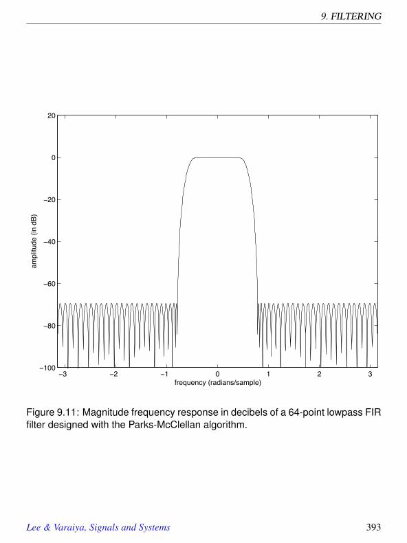
9. FILTERING
−3 −2 −1 0 1 2 3−100
−80
−60
−40
−20
0
20
frequency (radians/sample)
ampl
itude
(in
dB
)
Figure 9.11: Magnitude frequency response in decibels of a 64-point lowpass FIRfilter designed with the Parks-McClellan algorithm.
Lee & Varaiya, Signals and Systems 393

9.4. FINITE IMPULSE RESPONSE (FIR) FILTERS
Probing Further: Decibels
The term “decibel” is literally one tenth of a bel, which is named after Alexander GrahamBell. This unit of measure was originally developed by telephone engineers at BellTelephone Labs to designate the ratio of the power of two signals.
Power is a measure of energy dissipation (work done) per unit time. It is measured inwatts for electronic systems. One bel is defined to be a factor of 10 in power. Thus, a1000 watt hair dryer dissipates 1 bel, or 10 dB, more power than a 100 watt light bulb.Let p1 = 1000 watts be the power of the hair dryer and p2 = 100 be the power of thelight bulb. Then the ratio is
log10(p1/p2) = 1 bel, or
10log10(p1/p2) = 10 dB.
Comparing against (9.24) we notice a discrepancy. There, the multiplying factor is 20,not 10. That is because the ratio in (9.24) is a ratio of amplitudes, not powers. Inelectronic circuits, if an amplitude represents the voltage across a resistor, then the powerdissipated by the resistor is proportional to the square of the amplitude. Let a1 and a2be two such amplitudes. Then the ratio of their powers is
10log10(a21/a2
2) = 20log10(a1/a2).
Hence the multiplying factor of 20 instead of 10. A 3 dB power ratio amounts to afactor of 2 in power. In amplitudes, this is a ratio of
√2. The edge of the passband of
a bandpass filter is often defined to be the frequency at which the power drops to half,which is the frequency where the gain is 3 dB below the passband gain. The magnitudefrequency response here is 1/
√2 times the passband gain.
In audio, decibels are used to measure sound pressure. A statement like “a jet engineat 10 meters produces 120 dB of sound,” by convention, compares sound pressure toa defined reference of 20 micropascals, where a pascal is a pressure of 1 newton persquare meter. For most people, this is approximately the threshold of hearing at 1 kHz.Thus, a sound at 0 dB is barely audible. A sound at 10 dB has 10 times the power. Asound at 100 dB has 1010 times the power. The jet engine, therefore, would probablymake you deaf without ear protection.
394 Lee & Varaiya, Signals and Systems

9. FILTERING
9.5 Infinite impulse response (IIR) filters
The equation for an FIR filter (9.22) is a difference equation relating the output at indexn to the inputs at indices n− L+ 1 through n. A more general form of this differenceequation includes more indices of the output,
∀ n ∈ Z, y(n) =L−1
∑m=0
x(n−m)b(m)+M−1
∑m=1
y(n−m)a(m) (9.25)
where L and M are positive integers, and b(m) and a(m) are filter coefficients, which areusually real valued. If all the a coefficients are zero, then this reduces to an FIR filterwith impulse response b = h. However, if any a coefficient is non-zero, then the impulseresponse of this filter will never completely die out, since the output keeps getting recycledto affect future outputs. Such a filter is called an infinite impulse response or IIR filter, orsometimes a recursive filter.
Example 9.16: Consider a causal LTI system defined by the difference equation
∀ n ∈ Z, y(n) = x(n)+0.9y(n−1).
We can find the impulse response by letting x = δ, the Kronecker delta function.Since the system is causal, we know that h(n) = 0 for n < 0 (see page 382). Thus,
y(n) = 0 if n < 0
y(0) = 1
y(1) = 0.9
y(2) = 0.92
y(3) = 0.93
Noticing the pattern, we conclude that
y(n) = (0.9)nu(n),
where u is the unit step, seen before in (2.16),
u(n) =
1 if n≥ 00 otherwise
(9.26)
The output y and the magnitude of the frequency response (in dB) are plotted inFigure 9.12. Notice that this filter has about 20 dB of gain at DC, dropping to about-6 dB at π radians/sample.
Lee & Varaiya, Signals and Systems 395

9.5. INFINITE IMPULSE RESPONSE (IIR) FILTERS
9.5.1 Designing IIR filters
Designing IIR filters amounts to choosing the a and b coefficients for (9.25). As withFIR filters, how to choose these coefficients is a well-studied subject, and the results ofthis study are (for the most part) available in easy-to-use software. There are four widelyused methods for calculating these coefficients, resulting in four types of filters calledButterworth, Chebyshev 1, Chebyshev 2, and elliptic filters.
Example 9.17: We can design one of each of the four types of filters using theMatlab commands butter, cheby1, cheby2, ellip. The arguments for eachof these specify either a cutoff frequency, which is the frequency at which thefilter achieves -3 dB gain, or in the case of cheby2, the edge of the stopband. Forexample, to get lowpass filters with a gain of about 1 from 0 to π/8 radians/sample,and a stopband at higher frequencies, we can use the following commands:
N = 5;Wn = 0.125;[B1, A1] = butter(N, Wn);[B2, A2] = cheby1(N,1,Wn);[B3, A3] = cheby2(N,70,0.25);[B4, A4] = ellip(N,1,70,Wn);
The returned values are vectors containing the a and b coefficients of (9.25). Themagnitude frequency response of the resulting filters is shown in Figure 9.13. Inthat figure, we show only positive frequencies, since the magnitude frequency re-sponse is symmetric. We also only show the frequency range from 0 to π, since thefrequency response is periodic with period 2π. Notice that the Butterworth filter hasthe most gradual rolloff from the passband to the stopband. Thus, for a given filterorder, a Butterworth filter yields the weakest lowpass characteristic of the four. Theelliptic filter has the sharpest rolloff. The Butterworth filter, on the other hand, hasthe smoothest characteristic. The Chebyshev 1 filter has ripple in the passband,the Chebyshev 2 filter has ripple in the stopband, and the elliptic filter has ripple inboth.
In the above Matlab commands, N is the filter order, equal to L and M in (9.25).It is a constraint of these filter design techniques that L = M in (9.25). Wn is thecutoff frequency, as a fraction of π radians/sample. A cutoff frequency of 0.125
396 Lee & Varaiya, Signals and Systems

9. FILTERING
−5 0 5 10 15 20 25 300
0.2
0.4
0.6
0.8
1
discrete time index
−3 −2 −1 0 1 2 3−10
0
10
20
30
frequency (radians/sample)
ampl
itude
(in
dB
)
Figure 9.12: Impulse response (top) and magnitude frequency response in dB(bottom) of a simple causal IIR filter.
Lee & Varaiya, Signals and Systems 397

9.6. IMPLEMENTATION OF FILTERS
means 0.125π = π/8 radians/sample. The “1” argument in the cheby1 commandspecifies the amount of passband ripple that we are willing to tolerate (in dB).The 70 in the cheby2 and ellip commands specifies the amount of stopbandattenuation that we want (in dB). Finally, the 0.25 in the cheby2 line specifies theedge of the stopband.
9.6 Implementation of filters
We now have several ways to describe an LTI system (a filter). We can give a state-spacedescription, a frequency response, an impulse response, or a difference equation such as(9.25) or (9.22). All are useful. The state-space description and the difference equationsprove the most useful when constructing the filter.
A realization of a filter in hardware or software is called an implementation. Do notconfuse filter design with filter implementation. The term “filter design” is used in thecommunity to refer to the choice of frequency response, impulse response, or coefficientsfor a difference equation, not to how the frequency response is implemented in hardwareor software. In this section, we talk about implementation.
The output y of an FIR filter with impulse response h and input x is given by (9.22).The output of an IIR filter with coefficients a and b is given by (9.25). Each of thesedifference equations defines a procedure for calculating the output given the input. Wediscuss various ways of implementing these procedures.
9.6.1 Matlab implementation
If x is finite, and we can interpret it as an infinite signal that is zero outside the specifiedrange. Then we can compute the output of an FIR filter using Matlab’s conv function,and the output of an IIR filter using filter.
Example 9.18: Consider an FIR filter with an impulse response of length L. If xis a vector containing the P values of the input, and h is a vector containing the Lvalues of the impulse response, then
398 Lee & Varaiya, Signals and Systems
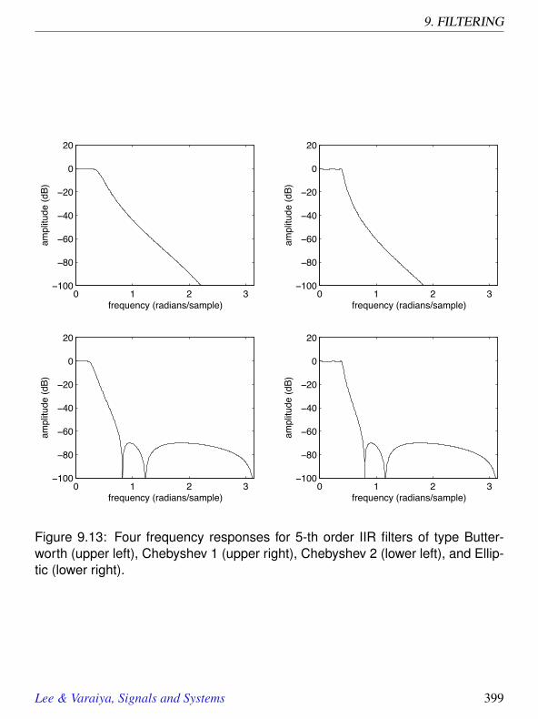
9. FILTERING
0 1 2 3−100
−80
−60
−40
−20
0
20
frequency (radians/sample)
ampl
itude
(dB
)
0 1 2 3−100
−80
−60
−40
−20
0
20
frequency (radians/sample)
ampl
itude
(dB
)0 1 2 3
−100
−80
−60
−40
−20
0
20
frequency (radians/sample)
ampl
itude
(dB
)
0 1 2 3−100
−80
−60
−40
−20
0
20
frequency (radians/sample)
ampl
itude
(dB
)
Figure 9.13: Four frequency responses for 5-th order IIR filters of type Butter-worth (upper left), Chebyshev 1 (upper right), Chebyshev 2 (lower left), and Ellip-tic (lower right).
Lee & Varaiya, Signals and Systems 399

9.6. IMPLEMENTATION OF FILTERS
y = conv(x, h);
yields a vector containing L+P−1 values of the output.
This strategy, of course, only works for finite input data, since Matlab requires that theinput be available in a finite vector.
Discrete-time filters can be implemented using standard programming languages and us-ing assembly languages on specialized processors (see boxes). These implementations donot have the limitation that the input be finite.
9.6.2 Signal flow graphs
We can describe the computations in a discrete-time filter using a block diagram withthree visual elements, a unit delay, a multiplier, and an adder. In the convolution sum foran FIR filter,
y(n) =L−1
∑m=0
h(m)x(n−m),
notice that at each n we need access to x(n), x(n−1), x(n−2), · · · , x(n−L+1). We canmaintain this set of values by cascading a set of unit delay elements to form a delay line,as shown in figure 9.14.
For each integer n, the output sample is the values in the delay line scaled by h(0), h(1),· · · , h(L−1). To obtain the values in the delay line, we simply tap the delay line, as shownin Figure 9.15. The triangular boxes denote multipliers that multiply by a constant (h(m),in this case). The circles with the plus signs denote adders. The structure in Figure 9.15is called a tapped delay line description of an FIR filter.
Diagrams of the type shown in Figure 9.15 are called signal flow graphs because theydescribe computations by focusing on the flow of signals between operators. Signal flowgraphs can be quite literal descriptions of digital hardware that implements a filter. Butwhat they really describe is the computation, irrespective of whether the implementationis in hardware or software.
An IIR filter can also be described using a signal flow graph. Consider the differenceequation in (9.25). A signal flow graph description of this equation is shown in Figure9.16. Notice that the left side is structurally equivalent to the tapped delay line, but stood
400 Lee & Varaiya, Signals and Systems

9. FILTERING
Probing Further: Java implementation of an FIR filter
The following Java class implements an FIR filter:
1 class FIR 2 private int length, count = 0;3 private double[] delayLine, impResp;4 FIR(double[] coefs) 5 length = coefs.length;6 impResp = coefs;7 delayLine = new double[length];8 9 double getOutputSample(double inputSample)
10 delayLine[count] = inputSample;11 double result = 0.0;12 int index = count;13 for (int i=0; i<length; i++) 14 result += impResp[i] * delayLine[index--];15 if (index < 0) index = length-1;16 17 if (++count >= length) count = 0;18 return result;19 20
A class in Java has both data members and methods. The methods are proceduresthat operate on the data, and may or may not take arguments or return values. In thiscase, there are two procedures, “FIR” and “getOutputSample.” The first, lines 4-8, isa constructor, which is a procedure that is called to create an FIR filter. It takes oneargument, an array of double-precision floating-point numbers that specify the impulseresponse of the filter. The second, lines 9-19, takes a new input sample as an argumentand returns a new output sample. It also updates the delay line using circular buffering,where the “count” member is used to keep track of where each new input sample shouldgo. It gets incremented (line 17) each time the getOutputSample() method iscalled. When it exceeds the length of the buffer, it gets reset to zero. At all times, itcontains the L most recently received input data samples. The most recent one is atindex count in the buffer. The second most recent is at count - 1, or if that isnegative, at length - 1. Line 15 makes sure that the variable index remains withinthe buffer as we iterate through the loop.
Lee & Varaiya, Signals and Systems 401

9.6. IMPLEMENTATION OF FILTERS
Probing Further: FIR filter in a programmable DSP
The following section of code is the assembly language for a programmable DSP, whichis a specialized microprocessor designed to implement signal processing functions ef-ficiently in embedded systems (such as cellular telephones, digital cordless telephones,digital audio systems, etc.). This particular code is for the Motorola DSP56000 familyof processors.
1 fir movep x:input,x:(r0)2 clr a x:(r0)-,x0 y:(r4)+,y03 rep m04 mac x0,y0,a x:(r0)-,x0 y:(r4)+,y05 macr x0,y0,a (r0)+6 movep a,x:output7 jmp fir
This processor has two memory banks called x and y. The code assumes that each inputsample can be successively read from a memory location called input, and that theimpulse response is stored in y memory beginning at an address stored in register r4.Moreover, it assumes that register r0 contains the address of a section of x memory touse for storing input samples (the delay line), and that this register has been set up toperform modulo addressing. Modulo addressing means that if it increments or decre-ments beyond the range of its buffer, then the address wraps around to the other endof the buffer. Finally, it assumes that the register m0 contains an integer specifying thenumber of samples in the impulse response minus one.
The key line (the one that does most of the work) is line 4. It follows a repinstruction, which causes that one line to be repeatedly executed the number of timesspecified by register m0. Line 4 multiplies the data in register x0 by that in y0 and addsthe result to a (the accumulator). Such an operation is called a multiply and accumulateor mac operation. At the same time, it loads x0 with an input sample from the delayline, in x memory at a location given by r0. It also loads register y0 with a sample fromthe impulse response, stored in y memory at a location given by r4. At the same time,it increments r0 and decrements r4. This one-line instruction, which carries out severaloperations in parallel, is obviously highly tuned to FIR filtering. Indeed, FIR filtering isa major function of processors of this type.
402 Lee & Varaiya, Signals and Systems

9. FILTERING
unitdelay
unitdelay
unitdelay
x(n) x(n!1) x(n!2) x(n!L+1)...
Figure 9.14: A delay line.
unitdelay
unitdelay
unitdelay
x(n) x(n!1) x(n!2) x(n!L+1)
h(L!1)h(2)h(1)h(0)
y(n)
...
...
Figure 9.15: A tapped delay line realization of an FIR filter, described as a signalflow graph.
on end. The right side represents the feedback in the filter, or the recursion that makes itan IIR filter rather than an FIR filter.
The filter structure in Figure 9.16 can be simplified somewhat by observing that sincethe left and right sides are LTI systems, their order can be reversed without changing theoutput. Once the order is reversed, the two delay lines can be combined into one, as shownin Figure 9.17. There are many other structures that can be used to realize IIR filters.
The relative advantages of one structure over another is a fairly deep topic, dependingprimarily on an understanding of the effects of finite precision arithmetic. It is beyond thescope of this text.
9.7 Summary
The output of an LTI system does not contain any frequencies that are not also presentin the input. Because of this property, LTI systems are often called filters. This chapterconsiders how filters might be implemented. The convolution sum (for discrete-time sys-tems) and convolution integral (for continuous-time systems) give descriptions of how to
Lee & Varaiya, Signals and Systems 403

9.7. SUMMARY
x(n)
x(n−1)
x(n−2)
b(L−1)
b(2)
b(1)
b(0) y(n)
unitdelay
unitdelay
...
unitdelay
y(n−1)
y(n−2)
a(M−1)
a(2)
a(1)unit
delay
unitdelay
...
unitdelay
y(n−M+1)x(n−L+1)
......
Figure 9.16: A signal flow graph describing an IIR filter. This is called a directform 1 filter structure.
calculate an output given an input signal. This description highlights the usefulness ofthe response that a system has to an idealized impulse, because the output is given by theconvolution of the input and the impulse response. The frequency response, moreover, isshown to be Fourier transform of the impulse response, where the Fourier transform is ageneralization of the Fourier series considered in previous chapters. Fourier transformsare considered in much more depth in the next chapter.
This chapter also considers the design of filters, by which we mean the selection of asuitable frequency response. Engineers are, as usual, forced to compromise to get anacceptable response at an acceptable computational cost. The response is assessed byconsidering how effectively it performs the desired filtering operation, and the cost isassessed by considering the arithmetic calculation that must be realized to implement thefilter. The chapter closes with a discussion of alternative ways of realizing the arithmeticcalculation.
404 Lee & Varaiya, Signals and Systems

9. FILTERING
x(n)
b(L!1)
b(2)
b(1)
b(0)y(n)
unit delay
unit delay
...
unit delaya(M!1)
a(2)
a(1)unit
delay
unit delay
...
unit delay
x(n)
b(L!1)
b(2)
b(1)
b(0)y(n)
a(M!1)
a(2)
a(1)unit
delay
unit delay
...
unit delay
(a)
(b)
... ...
......
Figure 9.17: (a) A signal flow graph equivalent to that in Figure 9.16, obtainedby reversing the left and right components. (b) A signal flow graph equivalent tothat in (a) obtained by merging the two delay lines into one. This is called a directform 2 filter structure.
Lee & Varaiya, Signals and Systems 405

EXERCISES
Exercises
Each problem is annotated with the letter E, T, C which stands for exercise, requires somethought, requires some conceptualization. Problems labeled E are usually mechanical,those labeled T require a plan of attack, those labeled C usually have more than onedefensible answer.
1. E Consider an LTI discrete-time system Filter with impulse response
h(n) =7
∑k=0
δ(n− k),
where δ is the Kronecker delta function.
(a) Sketch h(n).
(b) Suppose the input signal x : Z→ R is such that ∀ n ∈ Z, x(n) = cos(ωn),where ω = π/4 radians/sample. Give a simple expression for y = Filter(x).
(c) Give the value of H(ω) for ω = π/4, where H is the frequency response.
2. E Consider the continuous-time moving average system S, whose impulse responseis shown in Figure 9.3. Find its frequency response. The following fact from cal-culus may be useful:
b∫a
ecωcdω = ecb− eca
for real a and b and complex c. Use Matlab to plot the magnitude of this frequencyresponse over the range -5 Hz to 5 Hz. Note the symmetry of the magnitude re-sponse, as required by (9.21).
3. E Consider a continuous-time LTI system with impulse response given by
∀ t ∈ R, h(t) = δ(t−1)+δ(t−2),
where δ is the Dirac delta function.
(a) Find a simple equation relating the input x and output y of this system.
(b) Find the frequency response of this system.
406 Lee & Varaiya, Signals and Systems

9. FILTERING
(c) Use Matlab to plot the magnitude frequency response of this system in therange -5 to 5 Hz.
4. E Consider a discrete-time LTI system with impulse response h given by
∀ n ∈ Z, h(n) = δ(n)+2δ(n−1)
(a) Plot the impulse response.
(b) Find and sketch the output when the input is u, the unit step, given by (9.26).
(c) Find and sketch the output when the input is a ramp,
r(n) =
n if n≥ 00 otherwise
(d) Find the frequency response.
(e) Show that the frequency response is periodic with period 2π.
(f) Show that the frequency response is conjugate symmetric.
(g) Give a simplified expression for the magnitude response.
(h) Give a simplified expression for the phase response.
(i) Suppose that the input x is given by
∀ n ∈ Z, x(n) = cos(πn/2+π/6)+ sin(πn+π/3).
Find the output y.
5. E Consider the sawtooth signal shown in Figure 9.18. This is a periodic, continuous-time signal. Suppose it is filtered by an LTI system with frequency response
H(ω) =
1 if |ω| ≤ 2.5 radians/second0 otherwise
What is the output?
6. E Suppose that the following difference equation relates the input x and output y ofa discrete-time, causal LTI system S,
y(n)+αy(n−1) = x(n)+ x(n−1),
for some constant α.
Lee & Varaiya, Signals and Systems 407

EXERCISES
x(t)
t1
1 20
−1
Figure 9.18: A sawtooth signal.
(a) Find the impulse response h.
(b) Find the frequency response H.
(c) Find a sinusoidal input with non-zero amplitude such that the output is zero.
(d) Use Matlab to create a plot of the magnitude of the frequency response, as-suming α =−0.9.
(e) Find a state-space description for this system (define the state s and findA,b,cT ,d).
(f) Suppose α= 1. Find the impulse response and frequency response. Make sureyour answer makes sense (check it against the original difference equation).
7. T Each of the statements below refers to a discrete-time system S with input x andoutput y. Determine whether the statement is true or false. The signal u below isthe unit step, given by (9.26). The signal δ below is the Kronecker delta function.
(a) Suppose you know that if x is a sinusoid then y is a sinusoid. Then you canconclude that S is LTI.
(b) Suppose you know that S is LTI, and that if x(n) = cos(πn/2), then y(n) =2cos(πn/2). Then you have enough information to determine the frequencyresponse.
(c) Suppose you know that S is LTI, and that if x(n) = δ(n), then
y(n) = (0.9)nu(n).
Then you have enough information to determine the frequency response.
(d) Suppose you know that S is LTI, and that if x(n)= u(n), then y(n)= (0.9)nu(n).Then you have enough information to determine the frequency response.
408 Lee & Varaiya, Signals and Systems

9. FILTERING
(e) Suppose you know that S is causal, and that input x(n) = δ(n) produces outputy(n) = δ(n)+ δ(n− 1), and input x′(n) = δ(n− 2) produces output y′(n) =2δ(n−2)+δ(n−3). Then you can conclude that S is not LTI.
(f) Suppose you know that S is causal, and that if x(n) = δ(n)+ δ(n− 2) theny(n) = δ(n)+δ(n−1)+2δ(n−2)+δ(n−3). Then you can conclude that Sis not LTI.
8. T Consider the continuous-time systems Sk given by, ∀ t ∈ R,
(S1(x))(t) = x(t−2),
(S2(x))(t) = x(t +2),
(S3(x))(t) = x(t)−2,
(S4(x))(t) = x(2− t),
(S5(x))(t) = x(2t),
(S6(x))(t) = t2x(t),
(a) Which of these systems is linear?
(b) Which of these systems is time invariant?
(c) Which of these systems is causal?
9. T Consider an LTI discrete-time system Filter with impulse response
∀ n ∈ Z, h(n) = δ(n)+δ(n−2),
where δ is the Kronecker delta function.
(a) Sketch h.
(b) Find the output when the input is u, the unit step, given by (9.26).
(c) Find the output when the input is a ramp,
r(n) =
n if n≥ 00 otherwise
(d) Suppose the input signal x is such that
∀ n ∈ Z, x(n) = cos(ωn),
where ω = π/2 radians/sample. Give a simple expression for y = Filter(x).
Lee & Varaiya, Signals and Systems 409

EXERCISES
(e) Give an expression for H(ω) that is valid for all ω , where H is the frequencyresponse.
(f) Sketch the magnitude of the frequency response. Can you explain your answerin part (b)?
(g) Is there any other frequency at which a sinusoidal input with a non-zero am-plitude will yield an output that is zero?
10. T Consider an LTI discrete-time system Filter with impulse response
h(n) = δ(n)−δ(n−1)
where δ is the Kronecker delta function.
(a) Sketch h(n).
(b) Suppose the input signal x : Z→ R is such that ∀ n ∈ Z, x(n) = 1. Give asimple expression for y = Filter(x).
(c) Give an expression for H(ω) that is valid for all ω , where H is the frequencyresponse.
(d) Sketch the magnitude of the frequency response. Can you explain your answerin part (b)?
11. T Consider a discrete-time LTI system with impulse response h given by
∀ n ∈ Z, h(n) = δ(n−1)/2+δ(n+1)/2
And consider the periodic discrete-time signal given by
∀ n ∈ Z, x(n) = 2+ sin(πn/2)+ cos(πn).
(a) Is the system causal?
(b) Find the frequency response of the system. Check that your answer is periodicwith period 2π.
(c) For the given signal x, find the fundamental frequency ω0 and the Fourierseries coefficients Xk in the Fourier series expansion,
x(n) =∞
∑k=−∞
Xkeiω0kn.
Give the units of the fundamental frequency.
410 Lee & Varaiya, Signals and Systems

9. FILTERING
(d) Assuming the input to the system is x as given, find the output.
12. T Consider a continuous-time LTI system S. Suppose that when the input is thecontinuous-time unit step, given by
u(t) =
1, t ≥ 00, t < 0
(9.27)
then the output y = S(u) is given by
y(t) =
1, 0≤ t < 10, otherwise
This output y is called the step response because it is the response to a unit step.
(a) Express y in terms of sums and differences of u and D1(u), where D1 is thedelay operator.
(b) Give a signal flow graph that produces this result y = S(u) when the input is u.Note: We know that if two LTI systems have the same impulse response, thenthey are the same system. It is a fact, albeit a non-trivial one to demonstrate,that if two LTI systems have the same step response, then they are also thesame system. Thus, your signal flow graph implements S.
(c) Use your signal flow graph to determine what the output y′ of S is when theinput is
x(t) =
1, 0≤ t ≤ 10, otherwise
Plot your answer.
(d) What is the frequency response H(ω) of S?
13. T Suppose a discrete-time LTI system S has impulse response
h(n) = u(n)/2n =
1/2n if n≥ 00 otherwise
where u is the unit step function (9.26).
(a) What is the step response of this system? The step response is defined to bethe output when the input is the unit step. Hint: The identity (9.23) might behelpful.
Lee & Varaiya, Signals and Systems 411

EXERCISES
x(n) y(n)S+!
Figure 9.19: Feedback composition.
(b) What is the frequency response? Plot the magnitude and phase response (youmay use Matlab, or do it by hand). Hint: The following variant of the identity(9.23) might be useful. If |a|< 1,
∞
∑m=0
am =1
1−a.
This follows immediately from (9.23) by letting L go to infinity.
(c) Suppose S is put in cascade with another identical system. What is the fre-quency response of the cascade composition?
(d) Suppose S is arranged in a feedback composition as shown in figure 9.19.What is the frequency response of the feedback composition?
412 Lee & Varaiya, Signals and Systems

10The Four Fourier Transforms
Contents10.1 Notation . . . . . . . . . . . . . . . . . . . . . . . . . . . . . . . . 41410.2 The Fourier series (FS) . . . . . . . . . . . . . . . . . . . . . . . . 415
Probing Further: Showing inverse relations . . . . . . . . . . . . . . 41710.3 The discrete Fourier transform (DFT) . . . . . . . . . . . . . . . . 42110.4 The discrete-Time Fourier transform (DTFT) . . . . . . . . . . . . 42410.5 The continuous-time Fourier transform . . . . . . . . . . . . . . . 42810.6 Fourier transforms vs. Fourier series . . . . . . . . . . . . . . . . 434
10.6.1 Fourier transforms of finite signals . . . . . . . . . . . . . . . 43410.6.2 Fourier analysis of a speech signal . . . . . . . . . . . . . . . 43510.6.3 Fourier transforms of periodic signals . . . . . . . . . . . . . 438
10.7 Properties of Fourier transforms . . . . . . . . . . . . . . . . . . . 44410.7.1 Convolution . . . . . . . . . . . . . . . . . . . . . . . . . . . 44410.7.2 Conjugate symmetry . . . . . . . . . . . . . . . . . . . . . . 44910.7.3 Time shifting . . . . . . . . . . . . . . . . . . . . . . . . . . 45010.7.4 Linearity . . . . . . . . . . . . . . . . . . . . . . . . . . . . 45310.7.5 Constant signals . . . . . . . . . . . . . . . . . . . . . . . . 45510.7.6 Frequency shifting and modulation . . . . . . . . . . . . . . 456
10.8 Summary . . . . . . . . . . . . . . . . . . . . . . . . . . . . . . . . 458Probing Further: Multiplying signals . . . . . . . . . . . . . . . . . 459
Exercises . . . . . . . . . . . . . . . . . . . . . . . . . . . . . . . . . . . 460
413

10.1. NOTATION
In chapter 7 we saw that the Fourier series describes a periodic signal as a sum of complexexponentials. In chapter 8 we saw that if the input to an LTI system is a sum of complexexponentials, then the frequency response of the LTI system describes its response to eachof the component exponentials. Thus we can calculate the system response to any periodicinput signal by combining the responses to the individual components.
In chapter 9 we saw that the response of the LTI system to any input signal can also beobtained as the convolution of the input signal and the impulse response. The impulseresponse and the frequency response give us the same information about the system, butin different forms. The impulse response and the frequency response are related by theFourier transform, where in chapter 9 we saw both discrete time and continuous timeversions.
In this chapter, we will see that for discrete-time systems, the frequency response canbe described as a sum of weighted complex exponentials (the DTFT), where the weightsturn out to be the impulse response samples. We will see that the impulse response is, infact, a Fourier series representation of the frequency response, with the roles of time andfrequency reversed from the uses of the Fourier series that we have seen so far.
This reappearance of the Fourier series is not a coincidence. In this chapter, we explorethis pattern by showing that the Fourier series is a special case of a family of represen-tations of signals that are collectively called Fourier transforms. The Fourier seriesapplies specifically to continuous-time, periodic signals. The discrete Fourier series ap-plies to discrete-time, periodic signals. We complete the story with the continuous-timeFourier transform (CTFT), which applies to continuous-time signals that are not periodic,and the discrete-time Fourier transform (DTFT), which applies to discrete-time signalsthat are not periodic.
10.1 Notation
We define the following four sets of signals:
• ContSignals= [R→C]. Since R is included in C , ContSignals includes continuous-time signals whose range is R , and so we won’t need to consider these separately.
ContSignals includes continuous-time signals, but we are not insisting that the do-main be interpreted as time. Indeed, sometimes the domain could be interpreted as
414 Lee & Varaiya, Signals and Systems

10. THE FOUR FOURIER TRANSFORMS
space, if we are dealing with images. In this chapter we will see that it is usefulsometimes to interpret the domain as frequency.
• DiscSignals = [Z→ C].
This includes discrete-time signals whose domain is time or sample number, butagain we are not insisting that the domain be interpreted as time.
• ContPeriodicp ⊂ ContSignals.
This set is defined to contain all continuous signals that are periodic with period p,where p is a real number.
• DiscPeriodicp ⊂ DiscSignals.
This set is defined to contain all discrete signals that are periodic with period p,where p is an integer.
Note that whenever we talk about periodic signals we could equally well talk about finitesignals, where the domain of the finite signal is that of one cycle of the periodic signal.
10.2 The Fourier series (FS)
A periodic signal x ∈ ContPeriodicp may be described as a weighted sum of complexexponentials. This sum is the continuous-time Fourier series representation of x,
∀ t ∈ R, x(t) =∞
∑m=−∞
Xmeimω0t , (10.1)
where ω0 = 2π/p (radians/second). The Fourier series coefficients are given by
∀ m ∈ Z, Xm = 1p
p∫0
x(t)e−imω0tdt. (10.2)
Observe that the sequence of Fourier series coefficients given by (10.2) can be regardedas a signal X ∈ DiscSignals, where
∀m ∈ Z, X(m) = Xm.
Lee & Varaiya, Signals and Systems 415

10.2. THE FOURIER SERIES (FS)
InverseFourierSeriesp
X ∈ DiscSignals x ∈ ContPeriodicp
DFTp
X ∈ DiscPeriodicpx ∈ DiscPeriodicp
(b)
InverseDFTp
X ∈ DiscPeriodicp x ∈ DiscPeriodicp
(c)
DTFTX ∈ ContPeriodic2πx ∈ DiscSignals
(d)
InverseDTFTX ∈ ContPeriodic2π x ∈ DiscSignals
(e)
CTFTX ∈ ContSignalsx ∈ ContSignals
(f)
InverseCTFTX ∈ ContSignals x ∈ ContSignals
(g)
FourierSeriesp
X ∈ DiscSignalsx ∈ ContPeriodicp
(h)
(a)
Figure 10.1: Fourier transforms as systems.
So we can define a system FourierSeriesp with domain ContPeriodicp and range DiscSignalssuch that if the input is the periodic signal x, the output is its Fourier series coefficients,X . That is,
FourierSeriesp : ContPeriodicp→ DiscSignals.
This system is the first of four forms of the Fourier transform, and is depicted graphicallyin Figure 10.1(a). Its inverse is a system
InverseFourierSeriesp : DiscSignals→ ContPeriodicp,
depicted in Figure 10.1(b).
The two systems, FourierSeriesp and InverseFourierSeriesp, are inverses of each other,because (see box on page 417)
∀x ∈ ContPeriodicp, (InverseFourierSeriesp FourierSeriesp)(x) = x (10.3)
∀X ∈ DiscSignals, (FourierSeriesp InverseFourierSeriesp)(X) = X (10.4)
416 Lee & Varaiya, Signals and Systems

10. THE FOUR FOURIER TRANSFORMS
Probing Further: Showing inverse relations
In this chapter, and in previous chapters, we have given formulas that describe time-domain functions in terms of frequency-domain functions, and vice versa. By conven-tion, a formula that gives the frequency-domain function in terms of the time-domainfunction is called a Fourier transform, and the formula that gives the time-domainfunction in terms of the frequency-domain function is called an inverse Fourier trans-form. As shown in Figure 10.1, these transforms can be viewed as systems that takeas inputs signals in one domain and return signals in the other. We discuss four distinctFourier transforms and their corresponding inverses. In each case, it is possible to showthat the Fourier transform and its inverse are in fact inverses of one another, as stated in(10.3) and (10.4). We prove the second relation, (10.4), to illustrate how this is done.Similar proofs can be carried out for all four types of Fourier transforms, although some-times these proofs require you to be adept at manipulating Dirac delta functions, whichrequires significant mathematical skill.
Let X ∈ DiscSignals be the Fourier series for some x ∈ ContPeriodicp. That is, x =InverseFourierSeriesp(X). Let Y = FourierSeriesp(x). We now show that Y = X , i.e.Ym = Xm for all m.
Ym =1p
p∫0
x(t)e−imω0tdt, by (10.2)
=1p
p∫0
[∞
∑k=−∞
Xkeikω0t ]e−imω0tdt, by (10.1)
=∞
∑k=−∞
1p
Xk
p∫0
ei(k−m)ω0tdt
=1p
Xm
p∫0
dt + ∑k 6=m
1p
Xk
∫ p
0ei(k−m)ω0tdt
= Xm, since for k 6= m,∫ p
0ei(k−m)ω0tdt = 0.
Lee & Varaiya, Signals and Systems 417

10.2. THE FOURIER SERIES (FS)
x(t)
t1
1 2
Figure 10.2: A square wave.
|Xm|
m
1/21/π
1/3π1/5π 1/7π
Figure 10.3: Magnitude of the Fourier series coefficients of a square wave.
Example 10.1: Consider a square wave x ∈ ContPeriodic2, shown in Figure 10.2.It is periodic with period p = 2, so its fundamental frequency is ω0 = 2π/2 = π
radians/second. We can find its continuous-time Fourier series coefficients using(10.2) as follows,
Xm =12
2∫0
x(t)e−imπtdt
=12
1∫0
e−imπtdt.
Notice that when m = 0, this integral is easy to evaluate because e0 = 1, so
X0 = 1/2.
418 Lee & Varaiya, Signals and Systems

10. THE FOUR FOURIER TRANSFORMS
The following fact from calculus will help us solve the integral when m 6= 0,
b∫a
ecωc dω = ecb− eca (10.5)
for real a and b and complex c. Letting c =−imπ, the integral becomes
Xm =12c
1∫0
ectc dt
=−1
2imπ(e−imπ− e0)
=i
2mπ(e−imπ−1)
where the last step follows from multiplying top and bottom by i, observing thati2 =−1, and observing that e0 = 1. Notice that
e−imπ =
1 if m is even−1 if m is odd
Thus, when m 6= 0,
Xm =
0 if m is even−i/mπ if m is odd
The magnitude of these Fourier series coefficients is plotted in Figure 10.3. Noticethat the magnitudes of the coefficients decay rather slowly as m gets large (theydecay as 1/m). This accounts for the persistent overshoot (Gibbs phenomenon)seen in Figure 7.7. Finite Fourier series approximations of this periodic squarewave are not particularly good because the size of the Fourier series coefficientsdecays slowly.
Lee & Varaiya, Signals and Systems 419

10.2. THE FOURIER SERIES (FS)
Signal Fourier Series Reference∀ t ∈ R,
x(t) = eiω0t ,
where ω0 6= 0.
∀ m ∈ Z,
Xm =
1 if m = 10 otherwise
Exercise 2
∀ t ∈ R,
x(t) = cos(ω0t),
where ω0 6= 0.
∀ m ∈ Z,
Xm =
1/2 if |m|= 10 otherwise
Exercise 2
∀ t ∈ R,
x(t) = sin(ω0t),
where ω0 6= 0.
∀ m ∈ Z,
Xm =
1/2i if m = 1−1/2i if m =−10 otherwise
Exercise 2
∀ t ∈ R,
x(t) = 1
∀ m ∈ Z,
Xm =
1 if m = 00 otherwise
Exercise 2
Square wave:
∀ t ∈ [0, p],
x(t) =
1 if t < T or t > p−T0 otherwise
∀ m ∈ Z,
Xm =sin(mω0T )
(mπ)
Exercise 3
Impulse train:
∀ t ∈ R,
x(t) =∞
∑n=−∞
δ(t−np)
∀ m ∈ Z,
Xm = 1/p
Exercise 4
Table 10.1: Fourier series coefficients of periodic signals. In all cases, ω0 = 2π/p,where p is the period. We can obtain Fourier transforms for each of these signalsby using (10.16).
420 Lee & Varaiya, Signals and Systems

10. THE FOUR FOURIER TRANSFORMS
Other examples of Fourier series coefficients for various signals are given in table 10.1.
10.3 The discrete Fourier transform (DFT)
The discrete-time Fourier series (DFS) expansion for x ∈ DiscPeriodicp is (see (8.30))
∀ n ∈ Z, x(n) =p−1
∑k=0
Xkeikω0n, (10.6)
where ω0 = 2π/p (radians/sample). The Fourier series coefficients can be found usingthe formula
∀ k ∈ Z, Xk =1p
p−1
∑m=0
x(m)e−imkω0 . (10.7)
For historical reasons, the discrete Fourier transform (DFT) is the DFS with slightlydifferent scaling. It is defined by
∀ n ∈ Z, x(n) = 1p
p−1∑
k=0X ′keikω0n, (10.8)
∀ k ∈ Z, X ′k =p−1∑
m=0x(m)e−imkω0 . (10.9)
Obviously, the DFT coefficients are related to the DFS coefficients by
X ′k = pXk.
This scaling is somewhat unfortunate, since it means that the DFT coefficients do not havethe same units as the signal x, but the scaling is firmly established in the literature, so westick to it. We omit the prime when it is clear whether we are talking about the Fouriertransform instead of the Fourier series.
Lee & Varaiya, Signals and Systems 421

10.3. THE DISCRETE FOURIER TRANSFORM (DFT)
Observe that X ′ = DFT p(x) is a discrete signal that is itself periodic with period p. Toverify this, note that for any integer N and for all integers k,
X ′k+N p =p−1
∑m=0
x(m)e−im(k+N p)ω0
=p−1
∑m=0
x(m)e−imkω0e−imN pω0
=p−1
∑m=0
x(m)e−imkω0e−imN2π, since ω0 = 2π/p
=p−1
∑m=0
x(m)e−imkω0
= X ′k.
Note that (10.9) looks like a discrete Fourier series expansion of the periodic functionX ′. That is, the periodic function is described as a sum of complex exponentials. Theonly substantial difference, comparing with (10.6), is the sign of the exponent. Thissign difference can be easily removed with a change of variables. By doing so, you candiscover that x(−m) is the m-th Fourier series coefficient for the function X ′! The DFT israther special, therefore, in that both the time and frequency domain representations of afunction are Fourier series, and both are periodic.
The DFT therefore is the function
DFT p : DiscPeriodicp→ DiscPeriodicp,
given by (10.9). The inverse DFT is the function
InverseDFT p : DiscPeriodicp→ DiscPeriodicp,
given by (10.8). As in (10.3), (10.4), DFT p and InverseDFT p are inverses of each other.This can be verified using methods similar to those in the box on page 417. The DFT andits inverse are computed by systems that we can represent as shown in Figure 10.1(c) and(d).
The DFT is the most useful form of the Fourier transform for computation, because thesystem DFT p is easily implemented on a computer. Both summations (10.8) and (10.9)are finite. Moreover, there is an algorithm called the fast Fourier transform (FFT) that
422 Lee & Varaiya, Signals and Systems

10. THE FOUR FOURIER TRANSFORMS
x(n)
n1
Figure 10.4: A discrete square wave.
|X'k|
k
4
0
Figure 10.5: Magnitude of the DFT of a discrete square wave.
calculates these summations with far fewer arithmetic operations than the most directmethod. Moreover, because the sums are finite, the DFT always exists. There are nomathematical problems with convergence.
Example 10.2: Consider a discrete square wave x ∈ DiscPeriodic8, shown inFigure 10.4. It is periodic with period p = 8, so its fundamental frequency is ω0 =2π/8 = π/4 radians/sample. We can find its DFT using (10.9) as follows,
X ′k =7
∑m=0
x(m)e−imkω0
=3
∑m=0
e−imkπ/4.
Notice that when k = 0, this sum is easy to evaluate because e0 = 1, so
X ′0 = 4.
Lee & Varaiya, Signals and Systems 423

10.4. THE DISCRETE-TIME FOURIER TRANSFORM (DTFT)
Moreover, when k is any multiple of 8, we get X ′k = 4, as it should, since the DFT isperiodic with period 8. The following identity will help us simplify the summationwhen k 6= 0 nor any multiple of 8,
N∑
m=0am = 1−aN+1
1−a . (10.10)
(To demonstrate the validity of this identity, just multiply both sides by 1− a.)Letting N = 3 and a = e−ikπ/4, we get that for k 6= 0 nor any multiple of 8,
X ′k =1− e−ikπ
1− e−ikπ/4 .
Notice that the numerator is particularly simple, since
1− e−ikπ =
0 if k is even2 if k is odd
The magnitude of these DFT coefficients is plotted in figure 10.5.
Other examples of discrete Fourier transform coefficients for various signals are given intable 10.2.
10.4 The discrete-Time Fourier transform (DTFT)
We have shown in Section 9.2 that the frequency response H of an LTI system is relatedto the impulse response h by
∀ ω ∈ R, H(ω) =∞
∑m=−∞
h(m)e−iωm.
H is called the discrete-time Fourier transform (DTFT) of h. For any x ∈DiscSignals (notjust an impulse response), its DTFT is defined to be
∀ ω ∈ R, X(ω) =∞
∑m=−∞
x(m)e−iωm. (10.11)
424 Lee & Varaiya, Signals and Systems

10. THE FOUR FOURIER TRANSFORMS
Signal DFT Reference
∀ n ∈ Z,
x(n) = ei2π f n,
where f 6= 0.
∀ k ∈ Z,
X ′k =
p if k ∈ A0 otherwise
Exercise 5
∀ n ∈ Z,
x(n) = cos(2π f n),
where f 6= 0.
∀ k ∈ Z,
X ′k =
p/2 if k ∈ Ap/2 if k ∈ B0 otherwise
Exercise 5
∀ n ∈ Z,
x(n) = sin(i2π f n),
where f 6= 0.
∀ k ∈ Z,
X ′k =
p/2i if k ∈ A−p/2i if k ∈ B0 otherwise
Exercise 5
∀ n ∈ Z,
x(n) = 1
∀ k ∈ Z,
X ′k =
p if k ∈C0 otherwise
Exercise 5
Square wave:
∀ n ∈ 0,1, · · · , p−1,
x(n) =
1 if n≤M or n≥ p−M0 otherwise
∀ k ∈ Z,
X ′k =sin(k(M+0.5)ω0)
sin(kω0/2)
Exercise 6
Impulse train:
∀ n ∈ Z,
x(n) =∞
∑k=−∞
δ(n− kp)
∀ k ∈ Z,
X ′k = 1
Exercise 7
Table 10.2: Discrete Fourier transform of periodic signals. The fundamentalfrequency is ω0 = 2π/p, where p is the period. For the complex exponen-tial and sinusoidal signals, the frequency f must be rational, and is related tothe period p by f = m/p for some integer m (see Section 7.6.1). The follow-ing sets are used in this table: A = · · ·m− 2p,m− p,m,m+ p,m+ 2p, · · ·, B =· · ·−m−2p,−m− p,−m,−m+ p,−m+2p, · · ·, and C = · · ·−2p,−p,0, p,2p, · · ·.
Lee & Varaiya, Signals and Systems 425

10.4. THE DISCRETE-TIME FOURIER TRANSFORM (DTFT)
Of course, this definition is only valid for those x and those ω where the sum converges(it is not trivial mathematically to characterize this).
Notice that the function X is periodic with period 2π. That is, X(ω) = X(ω+ 2πN) forany integer N, because
e−iωt = e−i(ω+2πN)t
for any integer N. Thus, X ∈ ContPeriodic2π.
Note that (10.11) looks like a discrete Fourier series expansion of the periodic functionX . That is, the periodic function is described as a sum of complex exponentials. Theonly substantial difference, comparing with (10.1), is the sign of the exponent. Thissign difference can be easily removed with a change of variables. By doing so, you candiscover that x(−n) is the n-th Fourier series coefficient for the function X!
The DTFT (10.11) has similar structure to the DFT (10.9). In fact, the DTFT can beviewed as a generalization of the DFT to signals that are neither periodic nor finite. Inother words, as p approaches infinity, ω0 approaches zero, so instead of a discrete set offrequencies spaced by ω0 we have a continuum.
The DTFT is a system
DTFT : DiscSignals→ ContPeriodic2π
and its inverse is
InverseDTFT : ContPeriodic2π→ DiscSignals.
The inverse is given by
∀ n ∈ Z, x(n) = 12π
2π∫0
X(ω)eiωndω. (10.12)
Notice that because X is periodic, this can equivalently be written as
∀ n ∈ Z, x(n) =1
2π
π∫−π
X(ω)eiωndω.
We integrate over one cycle of the periodic function, so it does not matter where we start.These are depicted graphically in Figure 10.1(e) and (f).
426 Lee & Varaiya, Signals and Systems

10. THE FOUR FOURIER TRANSFORMS
x(n)
n1
Figure 10.6: A discrete rectangle signal.
|X(ω)|
ω
4
02πππ/2
Figure 10.7: Magnitude of the DTFT of a discrete rectangle.
Lee & Varaiya, Signals and Systems 427

10.5. THE CONTINUOUS-TIME FOURIER TRANSFORM
DTFT and InverseDTFT are inverses of each other. This follows from the fact thatFourierSeriesp and InverseFourierSeriesp are inverses of each other.
Example 10.3: Consider a discrete rectangle x ∈ DiscSignals, shown in Figure10.6. We can find its DTFT using (10.11) as follows,
X(ω) =∞
∑m=−∞
x(m)e−iωm
=3
∑m=0
e−iωm.
Notice that when ω = 0, this sum is easy to evaluate because e0 = 1, so
X(0) = 4.
Moreover, when ω is any multiple of 2π, we get X(ω) = 4, as it should, since theDTFT is periodic with period 2π. We can again use the identity (10.10), LettingN = 3 and a = e−iω, we get
X(ω) =1− e−i4ω
1− e−iω .
The magnitude of this function is plotted in figure 10.5.
Other examples of DTFTs for various signals are given in table 10.3.
10.5 The continuous-time Fourier transform
The frequency response and impulse response of a continuous-time LTI system are re-lated by the continuous-time Fourier transform (CTFT), more commonly called simplythe Fourier transform (FT),
∀ ω ∈ R, X(ω) =∞∫−∞
x(t)e−iωtdt. (10.13)
428 Lee & Varaiya, Signals and Systems

10. THE FOUR FOURIER TRANSFORMS
Signal DTFT Reference
∀ n ∈ Z, x(n) = δ(n) ∀ ω ∈ R, X(ω) = 1 Example10.8
∀ n ∈ Z,x(n) = δ(n−N)
∀ ω ∈ R, X(ω) = e−iωN Example10.8
∀ n ∈ Z, x(n) = K ∀ ω ∈ R,X(ω) = 2πK
∞
∑k=−∞
δ(ω− k2π)
Section10.7.5
∀ n ∈ Z,
x(n) = anu(n), |a|< 1
∀ ω ∈ R,
X(ω) =1
1−ae−iω
Exercise 18
∀ n ∈ Z,
x(n) =
1 if |n| ≤M0 otherwise
∀ ω ∈ R,
X(ω) =sin(ω(M+0.5))
sin(ω/2)
Exercise 8
∀ n ∈ Z,
x(n) =sin(Wn)
πn, 0 <W < π
∀ ω ∈ [−π,π],
X(ω) =
1 if |ω| ≤W0 otherwise
–
Table 10.3: Discrete time Fourier transforms of key signals. The function u is theunit step, given by (2.16).
Lee & Varaiya, Signals and Systems 429

10.5. THE CONTINUOUS-TIME FOURIER TRANSFORM
x(t)
t1
1
Figure 10.8: A rectangular pulse.
|X(ω)|
ω
1
0 2π 4π
Figure 10.9: Magnitude of the Fourier transform of the rectangular pulse in Figure10.8.
The CTFT can be defined for any function x ∈ ContSignals where the integral exists. Itneed not be the impulse response of any system, and it need not be periodic or finite. Theinverse relation is
∀ t ∈ R, x(t) = 12π
∞∫−∞
X(ω)eiωtdω. (10.14)
It is true but difficult to prove that the CTFT and the inverse CTFT are indeed inverses.
The CTFT can be viewed as a generalization of both the FS and DTFT where neither thefrequency domain nor the time domain signal needs to be periodic. Alternatively, it canbe viewed as the last remaining Fourier transform, where neither time nor frequency isdiscrete. Graphically, the CTFT is a system as shown in Figure 10.1(g) and (h).
430 Lee & Varaiya, Signals and Systems

10. THE FOUR FOURIER TRANSFORMS
Example 10.4: Consider a rectangular pulse x ∈ ContSignals, shown in Figure10.8. We can find its continuous-time Fourier transform using (10.13) as follows,
X(ω) =
∞∫−∞
x(t)e−iωtdt
=
1∫0
e−iωtdt.
Notice that when ω = 0, this integral is easy to evaluate because e0 = 1, so
X(0) = 1.
We can use (10.5) to solve the integral in general,
X(ω) =iω
[e−iω−1
].
We can get better intuition about this by manipulating it as follows,
X(ω) =iω
e−iω/2[e−iω/2− eiω/2
]= e−iω/2
[sin(ω/2)
ω/2
].
The leading factor has unit magnitude, so we see that the magnitude can be written
|X(ω)|=∣∣∣∣sin(ω/2)
ω/2
∣∣∣∣ .This magnitude is plotted in Figure 10.9. Notice that the magnitude decays ratherslowly as ω gets large (as 1/ω).
Other examples of Fourier transforms for various signals are given in table 10.4. The fourFourier transforms are summarized in table 10.5.
Lee & Varaiya, Signals and Systems 431

10.5. THE CONTINUOUS-TIME FOURIER TRANSFORM
Signal CTFT Reference
∀ t ∈ R, x(t) = δ(t) ∀ ω ∈ R, X(ω) = 1 Example10.7
∀ t ∈ R, x(t) = δ(t− τ), τ ∈ R ∀ ω ∈ R, X(ω) = e−iωτ Example10.7
∀ t ∈ R, x(t) = K ∀ ω ∈ R, X(ω) = 2πKδ(ω) Section10.7.5
∀ t ∈ R,
x(t) = atu(t), 0 < a < 1
∀ ω ∈ R,
X(ω) =1
jω− ln(a)
–
∀ t ∈ R,
x(t) =
π/a if |t| ≤ a0 otherwise
∀ ω ∈ R,
X(ω) =2πsin(aω)
aω
Exercise 23
∀ t ∈ R,
x(t) =sin(πt/T )
πt/T,
∀ ω ∈ R,
X(ω) =
T if |ω| ≤ π/T0 otherwise
Exercise 21
Table 10.4: Continuous time Fourier transforms of key signals. The function u isthe unit step, given by (9.27).
432 Lee & Varaiya, Signals and Systems

10. THE FOUR FOURIER TRANSFORMS
aperiodic timecontinuous frequency
periodic timediscrete frequency
aperiodicfrequency
continuoustime
CTFT :ContSignals→ ContSignals
X(ω) =
∞∫−∞
x(t)e−iωtdt
InverseCTFT :ContSignals→ ContSignals
x(t) =1
2π
∞∫−∞
X(ω)eiωtdω
FourierSeriesp :ContPeriodicp→ DiscSignals
Xm =1p
p∫0
x(t)e−imω0tdt
InverseFourierSeriesp :DiscSignals→ ContPeriodicp
x(t) =∞
∑k=−∞
Xkeikω0t
periodicfrequency
discretetime
DTFT :DiscSignals→ ContPeriodic2π
X(ω) =∞
∑n=−∞
x(n)e−inω
InverseDTFT :ContPeriodic2π→ DiscSignals
x(n) =1
2π
π∫−π
X(ω)eiωndω
DFT p :DiscPeriodicp→ DiscPeriodicp
Xk =p−1
∑n=0
x(n)e−inkω0
InverseDFT p :DiscPeriodicp→ DiscPeriodicp
x(n) =1p
p−1
∑k=0
Xkeikω0n
Table 10.5: The four Fourier transforms summarized. The column and row titlestell you when to use the specified Fourier transform and its inverse. The first rowapplies to continuous-time signals, and the second column applies to periodicsignals. Thus, if you have a continuous-time periodic signal, you should use theFourier series at the upper right.
Lee & Varaiya, Signals and Systems 433

10.6. FOURIER TRANSFORMS VS. FOURIER SERIES
10.6 Fourier transforms vs. Fourier series
For each of continuous and discrete-time signals, we have a Fourier transform and aFourier series (see table 10.5). The Fourier series applies only to periodic signals, whilethe Fourier transforms apply to any signal. The Fourier transforms, therefore, must alsobe applicable to periodic signals. Why do we need the Fourier series? Moreover, if wehave a finite signal, then we can find its Fourier series by considering it to be a periodicsignal, or we can find its Fourier transform by considering it to be zero outside its finitedomain. Which should we do?
10.6.1 Fourier transforms of finite signals
Consider a discrete-time signal y that is finite. Suppose it is defined for the domain [0, p−1]⊂ Z. As we did in Section 7.4, we can define a related periodic signal x as
∀ n ∈ Z, x(n) =∞
∑m=−∞
y′(n−mp)
where
∀ n ∈ Z, y′(n) =
y(n) if n ∈ [0, p−1]0 otherwise
The signal y′, of course, is an ordinary discrete-time signal, and hence posseses a DTFT.The signal x is a periodic signal, and therefore posseses a DFT. The DTFT and DFT areclosely related. The DTFT is given by
∀ ω ∈ R, Y ′(ω) =∞
∑n=−∞
y′(n)e−inω
=p−1
∑n=0
y(n)e−inω.
The DFT is
∀ k ∈ Z, Xk =p−1
∑n=0
x(n)e−inkω0
=p−1
∑n=0
y(n)e−inkω0 .
434 Lee & Varaiya, Signals and Systems

10. THE FOUR FOURIER TRANSFORMS
ampl
itude
-1
-0.5
0
0.5
time (in seconds)0 0.4 0.8 1.2 21.6
Figure 10.10: Two seconds of speech.
Comparing these, we see that
∀ k ∈ Z, Xk = Y ′(kω0).
In words, the DFT of the periodic signal is equal to samples of the DTFT of the finitesignal with sampling interval ω0 = 2π/p. This fact proves extremely useful when doingFourier analysis of real-world signals, as we see in the next subsection.
10.6.2 Fourier analysis of a speech signal
Consider the speech signal shown in Figure 10.10. It is two seconds of sound sampled at 8kHz, for a total of 16,000 samples. This is a finite signal, so we can find a DFT or DTFT, asexplained in the previous section. However, this would not be all that useful. As is evidentfrom the figure, the character of the signal changes several times in the two seconds. Thespeech sound is one of the authors saying “this is the sound of my voice.” Usually, it ismore interesting to perform Fourier analysis on a single phoneme, or elemental sound.Such analysis might be, for example, the first stage of a speech recognition system, whichattempts to automatically determine what was said.
Consider a much smaller segment of speech shown at the top in Figure 10.11. This isapproximately 64 msec of speech, or 512 samples at rate 8,000 samples/second. This
Lee & Varaiya, Signals and Systems 435

10.6. FOURIER TRANSFORMS VS. FOURIER SERIES
mag
nitu
de D
FT
0
10
20
30
frequency (in Hz)-4000 -2000 -1000 0 400020001000
ampl
itude
-0.8
-0.4
0
0.4
time (in seconds)0 0.01 0.02 0.03 0.060.050.04
Figure 10.11: A voiced segment of speech (top) and one cycle of the magnitudeof its DFT (bottom).
436 Lee & Varaiya, Signals and Systems

10. THE FOUR FOURIER TRANSFORMS
particular segment is the vowel sound in the word “sound.” Notice that the signal hasquite a bit of structure. Fourier analysis can reveal a great deal about that structure.
The first issue is to decide which of the four Fourier transforms to apply. This is easy,since there is only one of the four that is computable, the DFT. Since we do not have ananalytic expression for the speech signal, we cannot algebraically determine the DTFT.However, we know from the previous section that the DFT yields samples of the DTFTof a finite signal, so calculating the DFT reveals the structure of the DTFT.
The DFT of these 512 samples is shown at the bottom in Figure 10.11, which showsone cycle of the periodic DFT. The horizontal axis is labeled with the frequecies in Hzrather than the index k of the DFT coefficient. Recall that the k-th coefficient of theDFT represents a complex exponential with frequency kω0 = k2π/p radians/sample. Toconvert this to Hertz, we watch the units,
(k2π/p)[radians/sample]× (1/T )[samples/second]× (1/2π)[cycles/radian]
= k/(pT )[cycles/second],
where T = 1/8000 is the sampling interval.
Although this plot shows the DFT, the plot can equally well be interpreted as a plot ofthe DTFT. It shows 512 values of the DFT (one cycle of the periodic signal), and insteadof showing each individual value, it runs them together as a continuous curve. In fact,since the DFT is samples of the DTFT, that continuous curve is a pretty good estimateof the shape of the DTFT. Of course, the samples might not be close together enough toaccurately represent the DTFT, but probably they are. The next chapter will examine thisissue in considerable detail.
Notice that most of the signal is concentrated below 1 kHz. In Figure 10.12, we havezoomed in to this region of the spectrum. Notice that the DFT is strongly peaked, withthe lowest frequency peak occurring at about 120 Hz. Indeed, this is not surprising,because the time-domain signal at the top of Figure 10.11 looks somewhat periodic, witha period of about 80 msec, roughly the inverse of 120 Hz. That is, it looks like a periodicsignal with fundamental frequency 120 Hz, and various harmonics. The weights of theharmonics are proportional to the heights of the peaks in Figure 10.12.
The vowel in the word “sound” is created by vibrating the human vocal chords, and thenshaping the mouth into an acoustic cavity that alters the sound produced by the vocalchords. A sound that uses the vocal chords is called by linguists a voiced sound. Bycontrast, the “s” in “this” is an unvoiced sound. It is created without the help of the vocalchords by forcing air through a narrow passage in the mouth to create turbulence.
Lee & Varaiya, Signals and Systems 437

10.6. FOURIER TRANSFORMS VS. FOURIER SERIES
mag
nitu
de D
FT
0
10
20
30
frequency (in Hz)-1000 -600 -200 0 1000600200
Figure 10.12: DFT of the voiced segment of speech, shown over a narrowerfrequency range.
The “s” in “this” is shown in Figure 10.13. It is very different from the vowel sound in10.11. In particular, it looks much less regular. There is no evident periodicity in thesignal, so the DFT does not reveal a fundamental frequency and harmonics. It is a noise-like signal, where the DFT reveals that much of the noise is at low frequencies, below 500Hz, but there are also significant components all the way out to 4 kHz.
The analysis we have done on the segments of speech is a typical use of Fourier analysis.A long (even infinite) signal is divided into short segments, such as the two 512-samplesegments that we examined above. These segments are studied by calculating their DFT.Since the DFT is a finite summation, it is easy to realize on a computer. Also, as men-tioned before, there is a highly efficient algorithm called the fast Fourier transform orFFT to calculate the DFT. The fft function in Matlab was used to calculate the DFTsin figures 10.11 and 10.13. The DFT yields samples of the DTFT of the finite segment ofsignal. The spectrogram for the signal in Figure 10.10 is shown in Figure 10.14.
10.6.3 Fourier transforms of periodic signals
In the previous two sections, we have seen the relationship between the DTFT of a finitesignal and the DFT of the periodic signal that is constructed by repeating the finite signal.
438 Lee & Varaiya, Signals and Systems

10. THE FOUR FOURIER TRANSFORMS
mag
nitu
de D
FT
0
2
4
6
frequency (in Hz)-4000 -2000 -1000 0 400020001000
ampl
itude
-0.2
-0.1
0
0.1
time (in seconds)0 0.01 0.02 0.03 0.060.050.04
8
Figure 10.13: An unvoiced segment of speech (top) and one cycle of the magni-tude of its DFT (bottom).
Lee & Varaiya, Signals and Systems 439

10.6. FOURIER TRANSFORMS VS. FOURIER SERIES
4000
3000
2000
1000
0
Freq
uenc
y
Time (seconds)
Samples
0 0.5 1 1.5 2 2.5
0
0.5
1
- 0.5
- 10 5,000 10,000 15,000 20,000
Figure 10.14: Spectrogram of the voice segment in Figure 10.10.
440 Lee & Varaiya, Signals and Systems

10. THE FOUR FOURIER TRANSFORMS
The periodic signal, however, also has a DTFT itself. In the interest of variety, we willexplore this concept in continuous time.
A periodic continuous-time signal has a Fourier transform. But, as we will see, thatFourier transform has Dirac delta functions in it, which are mathematically tricky. Recallthat a Dirac delta function is an infinitely narrow and infinitely high pulse. The Fourierseries permits us to talk about the frequency domain representation of a periodic signalwithout dealing with Dirac delta functions.
It is useful, certainly, to simplify the mathematics. Using a Fourier series whenever pos-sible allows us to do that. Moreover, when working with signals computationally, ev-erything must be discrete and finite. Computers cannot deal with infinitely narrow andinfinitely high pulses numerically. Computation, therefore, must be done with the onlytransform that is completely discrete and finite, the DFS, or its scaled cousin, the DFT.
To be concrete, suppose a continuous-time signal x has Fourier transform
∀ ω ∈ R, X(ω) = 2πδ(ω−ω0) (10.15)
for some real value ω0. We can find x using the inverse CTFT (10.14),
∀ t ∈ R, x(t) =1
2π
∞∫−∞
2πδ(ω−ω0)eiωtdω.
Using the sifting rule, this evaluates to
x(t) = eiω0t .
This is a periodic function with period p = 2π/ω0. From table 10.1, we see that theFourier series for x is
∀ m ∈ Z, Xm =
1 if m = 10 otherwise
There is exactly one non-zero Fourier series coefficient, which corresponds to the exactlyone Dirac delta pulse in the Fourier transform (10.15).
More generally, suppose x has multiple Dirac delta pulses in its Fourier transform, eachwith different weights,
∀ ω ∈ R, X(ω) = 2π∞
∑m=−∞
Xmδ(ω−mω0). (10.16)
Lee & Varaiya, Signals and Systems 441

10.6. FOURIER TRANSFORMS VS. FOURIER SERIES
The inverse CTFT (10.14) tells us that
∀ t ∈ R, x(t) =∞
∑m=−∞
Xmeimω0t .
This is a periodic function with fundamental frequency ω0, and harmonics in variousweights. Its Fourier series coefficients, by inspection, are just Xm. Thus, for a periodicsignal, (10.16) relates the CTFT and the Fourier series. The Fourier series gives theweights of a set of Dirac delta pulses in the Fourier transform, within a scaling factor of2π.
Example 10.5: Consider x given by
∀ t ∈ R, x(t) = cos(ω0t).
From table 10.1, we see that the Fourier series for x is
∀ m ∈ Z, Xm =
1/2 if |m|= 10 otherwise
There are only two non-zero Fourier series coefficients. We can use (10.16) to writedown its Fourier transform,
∀ ω ∈ R, X(ω) = πδ(ω+ω0)+πδ(ω−ω0).
We sketch this as shown in Figure 10.15. See Exercise 9 at the end of the chapterfor a similar result for a sin function.
Example 10.6: Consider the square wave of example 10.1. The Fourier seriescoefficients are
Xm =
1/2 if m = 00 if m is even and m 6= 0−i/mπ if m is odd
The Fourier transform, therefore, has Dirac delta pulses with these weights at mul-tiples of ω0, scaled by 2π, as shown in Figure 10.16.
442 Lee & Varaiya, Signals and Systems

10. THE FOUR FOURIER TRANSFORMS
X(ω)
ω
π
ω0
π
−ω0
Figure 10.15: Fourier transform of a cosine.
|X(ω)|
ω
π2
2/32/5 2/7
ω0 3ω0
Figure 10.16: Fourier transform of a square wave.
Lee & Varaiya, Signals and Systems 443

10.7. PROPERTIES OF FOURIER TRANSFORMS
The same concept applies in the discrete-time case, although some care is needed becausethe DTFT and DFT are both periodic, and not every function of the form e jωn is periodic(see Section 7.6.1). In fact, in Figure 10.11, the peaks in the spectrum hint at the Diracdelta functions in the DTFT. The signal appears to be roughly periodic with period 120Hz, so the DFT shows strong peaks at multiples of 120 Hz. If the signal were perfectlyperiodic, and if we were plotting the DTFT instead of the DFT, then these peaks wouldbecome infinitely narrow and infinitely high.
10.7 Properties of Fourier transforms
In this section, we give a number of useful properties of the various Fourier transforms,together with a number of illustrative examples. These properties are summarized intables 10.6 through 10.9. The properties and examples can often be used to avoid solvingintegrals or summations to find the Fourier transform of some signal, or to find an inverseFourier transform.
10.7.1 Convolution
Suppose a discrete-time LTI system has impulse response h and frequency response H.We have seen that if the input to this system is a complex exponential, eiωn, then the outputis H(ω)eiωn. Suppose the input is instead an arbitrary signal x with DTFT X . Using theinverse DTFT relation, we know that
∀ n ∈ Z, x(n) =1
2π
2π∫0
X(ω)eiωndω.
View this as a summation of exponentials, each with weight X(ω). An integral, after all,is summation over a continuum. Each term in the summation is X(ω)eiωn. If this termwere an input by itself, then the output would be H(ω)X(ω)eiωn. Thus, by linearity, if theinput is x, the output should be
∀ n ∈ Z, y(n) =1
2π
2π∫0
H(ω)X(ω)eiωndω
444 Lee & Varaiya, Signals and Systems

10. THE FOUR FOURIER TRANSFORMS
Time domain Frequency domain Reference∀ t ∈ R, x(t) is real ∀ m ∈ Z, Xm = X∗−m Section
10.7.2∀ t ∈ R, x(t) = x∗(−t) ∀ m ∈ Z, Xm is real Section
10.7.2∀ t ∈ R, y(t) = x(t− τ) ∀ m ∈ Z, Ym = e−imω0τXm Section
13∀ t ∈ R, y(t) = eiω1tx(t)
where ω1 = Mω0, for some M ∈ Z∀ m ∈ Z, Ym = Xm−M Section
13∀ t ∈ R,
y(t) = cos(ω1t)x(t)where ω1 = Mω0, for some M ∈ Z
∀ m ∈ Z,Ym = (Xm−M +Xm+M)/2
Example13
∀ t ∈ R,y(t) = sin(ω1t)x(t)
where ω1 = Mω0, for some M ∈ Z
∀ m ∈ Z,Ym = (Xm−M−Xm+M)/2i
Exercise13
∀ t ∈ R,y(t) = ax(t)+bw(t)
∀ m ∈ Z,Ym = aXm +bWm
Section10.7.4
∀ t ∈ R, y(t) = x∗(t) ∀ m ∈ Z, Ym = X∗−m –
Table 10.6: Properties of the Fourier series. All time-domain signals are assumedto be periodic with period p, and fundamental frequency ω0 = 2π/p.
Lee & Varaiya, Signals and Systems 445
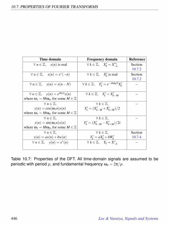
10.7. PROPERTIES OF FOURIER TRANSFORMS
Time domain Frequency domain Reference∀ n ∈ Z, x(n) is real ∀ k ∈ Z, X ′k = X ′∗−k Section
10.7.2∀ n ∈ Z, x(n) = x∗(−n) ∀ k ∈ Z, X ′k is real Section
10.7.2∀ n ∈ Z, y(n) = x(n−N) ∀ k ∈ Z, Y ′k = e−ikω0NX ′k –
∀ n ∈ Z, y(n) = eiω1nx(n)where ω1 = Mω0, for some M ∈ Z
∀ k ∈ Z, Y ′k = X ′k−M –
∀ n ∈ Z,y(n) = cos(ω1n)x(n)
where ω1 = Mω0, for some M ∈ Z
∀ k ∈ Z,Y ′k = (X ′k−M +X ′k+M)/2
–
∀ n ∈ Z,y(n) = sin(ω1n)x(n)
where ω1 = Mω0, for some M ∈ Z
∀ k ∈ Z,Y ′k = (X ′k−M−X ′k+M)/2i
–
∀ n ∈ Z,y(n) = ax(n)+bw(n)
∀ k ∈ Z,Y ′k = aX ′k +bW ′k
Section10.7.4
∀ n ∈ Z, y(n) = x∗(n) ∀ k ∈ Z, Yk = X∗−k –
Table 10.7: Properties of the DFT. All time-domain signals are assumed to beperiodic with period p, and fundamental frequency ω0 = 2π/p.
446 Lee & Varaiya, Signals and Systems

10. THE FOUR FOURIER TRANSFORMS
Time domain Frequency domain Reference∀ n ∈ Z, x(n) is real ∀ ω ∈ R, X(ω) = X∗(−ω) Section
10.7.2∀ n ∈ Z, x(n) = x∗(−n) ∀ ω ∈ R, X(ω) is real Section
10.7.2∀ n ∈ Z, y(n) = x(n−N) ∀ ω ∈ R, Y (ω) = e−iωNX(ω) Section
10.7.3∀ n ∈ Z, y(n) = eiω1nx(n) ∀ ω ∈ R, Y (ω) = X(ω−ω1) Section
10.7.6∀ n ∈ Z,
y(n) = cos(ω1n)x(n)∀ ω ∈ R,
Y (ω) = (X(ω−ω1)+X(ω+ω1))/2Example
10.11∀ n ∈ Z,
y(n) = sin(ω1n)x(n)∀ ω ∈ R,
Y (ω) = (X(ω−ω1)−X(ω+ω1))/2iExercise
12∀ n ∈ Z,
x(n) = ax1(n)+bx2(n)∀ ω ∈ R,
X(ω) = aX1(ω)+bX2(ω)Section10.7.4
∀ n ∈ Z, y(n) = (h∗ x)(n) ∀ ω ∈ R, Y (ω) = H(ω)X(ω) Section10.7.1
∀ n ∈ Z, y(n) = x(n)p(n) ∀ ω ∈ R,
Y (ω) = 12π
2π∫0
X(Ω)P(ω−Ω)dΩ
Box onpage 459
∀ n ∈ Z,
y(n) =
x(n/N) n multiple of N0 otherwise
∀ ω ∈ R,Y (ω) = X(NΩ)
Exercise14
Table 10.8: Properties of the DTFT.
Lee & Varaiya, Signals and Systems 447

10.7. PROPERTIES OF FOURIER TRANSFORMS
Time domain Frequency domain Reference∀ t ∈ R, x(t) is real ∀ ω ∈ R, X(ω) = X∗(−ω) Section
10.7.2∀ t ∈ R, x(t) = x∗(−t) ∀ ω ∈ R, X(ω) is real Section
10.7.2∀ t ∈ R, y(t) = x(t− τ) ∀ ω ∈ R, Y (ω) = e−iωτX(ω) Section
10.7.3∀ t ∈ R, y(t) = eiω1tx(t) ∀ ω ∈ R, Y (ω) = X(ω−ω1) Section
10.7.6∀ t ∈ R,
y(t) = cos(ω1t)x(t)∀ ω ∈ R,
Y (ω) = (X(ω−ω1)+X(ω+ω1))/2Example
10.11∀ t ∈ Z,
y(t) = sin(ω1t)x(t)∀ ω ∈ R,
Y (ω) = (X(ω−ω1)−X(ω+ω1))/2iExercise
12∀ t ∈ R,
x(t) = ax1(t)+bx2(t)∀ ω ∈ R,
X(ω) = aX1(ω)+bX2(ω)Section10.7.4
∀ t ∈ R, y(t) = (h∗ x)(t) ∀ ω ∈ R, Y (ω) = H(ω)X(ω) Section10.7.1
∀ t ∈ R, y(t) = x(t)p(t) ∀ ω ∈ R,Y (ω) = 1
2π
∞∫−∞
X(Ω)P(ω−Ω)dΩ
–
∀ t ∈ R,y(t) = x(at)
∀ ω ∈ R,Y (ω) = 1
|a| X(Ω/a)Exercise
11
Table 10.9: Properties of the CTFT.
448 Lee & Varaiya, Signals and Systems
10. THE FOUR FOURIER TRANSFORMS
Comparing to the inverse DTFT relation for y(n), we see that
∀ ω ∈ R, Y (ω) = H(ω)X(ω). (10.17)
This is the frequency-domain version of convolution
∀ n ∈ Z, y(n) = (h∗ x)(n).
Thus, the frequency response of an LTI system multiplies the DTFT of the input. This isintuitive, since the frequency response gives the weight imposed by the system on eachfrequency component of the input.
Equation (10.17) applies equally well to continuous-time systems, but in that case, H isthe CTFT of the impulse response, and X is the CTFT of the input.
10.7.2 Conjugate symmetry
We have already shown (see (8.29)) that for real-valued signals, the Fourier series coeffi-cients are conjugate symmetric,
Xk = X∗−k.
In fact, all the Fourier transforms are conjugate symmetric if the time-domain function isreal. We illustrate this with the CTFT. Suppose x : R→ R is a real-valued signal, andlet X = CTFT(x). In general, X(ω) will be complex-valued. However, from (10.13), wehave
[X(−ω)]∗ =∫
∞
−∞
[x(t)eiωt ]∗dt
=∫
∞
−∞
x(t)e−iωtdt
= X(ω),
Thus,X(ω) = X∗(−ω),
i.e. for real-valued signals, X(ω) and X(−ω) are complex conjugates of one another.
We can show that, conversely, if the Fourier transform is conjugate symmetric, then thetime-domain function is real. To do this, write the inverse CTFT
x(t) =1
2π
∞∫−∞
X(ω)eiωtdω
Lee & Varaiya, Signals and Systems 449
10.7. PROPERTIES OF FOURIER TRANSFORMS
and then conjugate both sides,
x∗(t) =1
2π
∞∫−∞
X∗(ω)e−iωtdω.
By changing variables (replacing ω with−ω) and using the conjugate symmetry of X , wecan show that
x∗(t) = x(t),
which implies that x(t) is real for all t.
The inverse Fourier transforms can be used to show that if a time-domain function isconjugate symmetric,
x(t) = x∗(−t),
then its Fourier transform is real. The same property applies to all four Fourier transforms.
In summary, if a function in one domain (time or frequency) is conjugate symmetric,then the function in the other domain (frequency or time) is real.
10.7.3 Time shifting
Given a continuous-time function x and its Fourier transform X = CTFT(x), let y bedefined by
∀ t ∈ R, y(t) = x(t− τ)
450 Lee & Varaiya, Signals and Systems

10. THE FOUR FOURIER TRANSFORMS
for some real constant τ. This is called time shifting or delay. We can find Y = CTFT(y)in terms of X as follows,
Y (ω) =
∞∫−∞
y(t)e−iωtdt
=
∞∫−∞
x(t− τ)e−iωtdt
=
∞∫−∞
x(t)e−iω(t+τ)dt
= e−iωτ
∞∫−∞
x(t)e−iωtdt
= e−iωτX(ω).
Thus, in summary,
y(t) = x(t− τ) ⇔ Y (ω) = e−iωτX(ω). (10.18)
The bidirectional arrow indicates that this relationship works both ways. If you know thatY (ω) = e−iωτX(ω), then you can conclude that y(t) = x(t− τ).
Example 10.7: One of the simplest Fourier transforms to compute is that of xwhen
x(t) = δ(t),
where δ is the Dirac delta function. Plugging into the formula,
X(ω) =
∞∫−∞
x(t)e−iωtdt
=
∞∫−∞
δ(t)e−iωtdt
= e−iω0
= 1,
Lee & Varaiya, Signals and Systems 451

10.7. PROPERTIES OF FOURIER TRANSFORMS
where we have used the sifting property of the delta function. To see how the siftingproperty works, note that the integrand is zero everywhere except where t = 0, atwhich point the complex exponential evaluates to 1. Then the integral of the deltafunction itself has value one.
The Fourier transform is a constant, 1. This indicates that the Dirac delta function,interestingly, contains all frequencies in equal amounts.
Moreover, this result is intuitive if one considers an LTI system with impulse re-sponse h(t) = δ(t). Such a system responds to an impulse by producing an impulse,which suggests that any input will be simply passed through unchanged. Indeed,its frequency response is H(ω) = 1 for all ω ∈ R, so given an input x with Fouriertransform X , the output y has Fourier transform
Y (ω) = H(ω)X(ω) = X(ω).
Since the output has the same Fourier transform as the input, the output is the sameas the input.
Using (10.18), we can now find the Fourier transform of another signal
x(t) = δ(t− τ),
for some constant τ ∈ R. It is
X(ω) = e−iωτ.
Note that, as required, this is conjugate symmetric. Moreover, it has magnitude 1.Its phase is −ωτ, a linear function of ω.
Again, we can gain some intuition by considering an LTI system with impulseresponse
h(t) = δ(t− τ). (10.19)
Such a system introduces a fixed time delay of τ. Its frequency response is
H(ω) = e−iωτ. (10.20)
Since this has magnitude 1 for all ω, it tells us that all frequencies get through thedelay system unattenuated, as expected. However, each frequency ω will experi-ence a phase shift of −ωτ, corresponding to a time delay of τ.
452 Lee & Varaiya, Signals and Systems

10. THE FOUR FOURIER TRANSFORMS
Discrete-time signals are similar. Consider a discrete-time signal x with X = DTFT(x),and let y be defined by
∀ t ∈ R, y(n) = x(n−N)
for some integer constant N. By similar methods, we can find that
y(n) = x(n−N) ⇔ Y (ω) = e−iωNX(ω). (10.21)
Example 10.8: Suppose we have a discrete-time signal x given by
x(n) = δ(n),
where δ is the Kronecker delta function. It is easy to show from the DTFT definitionthat
X(ω) = 1.
Using (10.21), we can now find the Fourier transform of another signal
x(n) = δ(n−N),
for some constant N ∈ Z. It is
X(ω) = e−iωN .
Notice that if N = 0, this reduces to X(ω) = 1, as expected.
10.7.4 Linearity
Consider three discrete-time signals x, x1, x2, related by
∀ n ∈ Z, x(n) = ax1(n)+bx2(n).
Then it is easy to see from the definition of the DTFT that
∀ ω ∈ R, X(ω) = aX1(ω)+bX2(ω)
where X = DTFT(x), X1 = DTFT(x1), and X2 = DTFT(x2).
Lee & Varaiya, Signals and Systems 453

10.7. PROPERTIES OF FOURIER TRANSFORMS
The same linearity property applies to the CTFT,
x(t) = ax1(t)+bx2(t) ⇔ X(ω) = aX1(ω)+bX2(ω)
Linearity of the Fourier transform is one of the most useful properties for avoiding evalu-ation of integrals and summations.
Example 10.9: Consider for example the discrete-time signal x given by
x(n) = δ(n+1)+δ(n−1),
where δ is the Kronecker delta function. Using linearity, we know that the DTFT ofx is the sum of the DTFT of δ(n+1) and the DTFT of δ(n−1). From the previousexample, we know those two DTFTs, so
X(ω) = eiω + e−iω
because N is −1 and 1, respectively. Using Euler’s relation, we can simplify this toget
X(ω) = 2cos(ω).
Interestingly, the DTFT of this example turns out to be real. This is because thetime-domain function is conjugate symmetric (the conjugate of something real isitself). Moreover, since it is real in the time domain, the DTFT turns out to beconjugate symmetric.
Linearity can also be used to find inverse Fourier transforms.
Example 10.10: Suppose you are told that a continuous-time signal has Fouriertransform
X(ω) = cos(ω).
How would you find the time-domain function? You could evaluate the inverseCTFT, but the integration that you would have to perform is quite difficult. Instead,use Euler’s relation to write
X(ω) = (eiω + e−iω)/2.
454 Lee & Varaiya, Signals and Systems

10. THE FOUR FOURIER TRANSFORMS
Then use linearity. The inverse Fourier transform of this sum will be the sum of theinverse Fourier transforms of the terms. These we can recognize from (10.19) and(10.20), so
x(t) = (δ(t +1)+δ(t−1))/2,
where δ is the Dirac delta function.
10.7.5 Constant signals
We have seen that the Fourier transform of a delta function is a constant. With the sym-metries that we have observed between time and frequency, it should come as no surprisethat the Fourier transform of a constant is a delta function.
Consider first a continuous-time signal x given by
∀ t ∈ R, x(t) = K
for some real constant K. Its CTFT is
X(ω) = K∞∫−∞
e−iωtdt,
which is not easy to evaluate. This integral is mathematically subtle. The answer is
∀ ω ∈ R, X(ω) = 2πKδ(ω),
where δ is the Dirac delta function. What this says is that a constant in the time domain isconcentrated at zero frequency in the frequency domain (which should not be surprising).Except for the multiplying constant of 2π, we probably could have guessed this answer.We can verify this answer by evaluating the inverse CTFT,
x(t) =1
2π
∞∫−∞
X(ω)eiωtdω
= K∞∫−∞
δ(ω)eiωtdω
= K,
Lee & Varaiya, Signals and Systems 455

10.7. PROPERTIES OF FOURIER TRANSFORMS
where the final step follows from the sifting property of the Dirac delta function. Thus, insummary,
x(t) = K ⇔ X(ω) = 2πKδ(ω) (10.22)
The discrete-time case is similar, but there is one subtlety because the DTFT is periodic.Let x be a discrete time signal where
∀ n ∈ Z, x(n) = K
for some real constant K. Its DTFT is
∀ ω ∈ [−π,π], X(ω) = 2πKδ(ω),
where δ is the Dirac delta function. This is easy to verify using the inverse DTFT. Again,what this says is that a constant in the time domain is concentrated at zero frequency inthe frequency domain (which should not be surprising). However, recall that a DTFT isperiodic with period 2π, meaning that for all integers N,
X(ω) = X(ω+N2π).
Thus, in addition to a delta function at ω = 0, there must be one at ω = 2π, ω = −2π,ω = 4π, etc. This can be written using a shift-and-add summation,
∀ ω ∈ R, X(ω) = 2πK∞
∑k=−∞
δ(ω− k2π).
Thus, in summary,
x(n) = K ⇔ X(ω) = 2πK∞
∑k=−∞
δ(ω− k2π). (10.23)
10.7.6 Frequency shifting and modulation
Suppose that x is a continuous-time signal with CTFT X . Let y be another continuous-timesignal defined by
y(t) = x(t)eiω0t
456 Lee & Varaiya, Signals and Systems

10. THE FOUR FOURIER TRANSFORMS
for some real constant ω0. The CTFT of y is easy to compute,
Y (ω) =
∞∫−∞
y(t)e−iωtdt
=
∞∫−∞
x(t)eiω0te−iωtdt
=
∞∫−∞
x(t)e−i(ω−ω0)tdt
= X(ω−ω0).
Thus, the Fourier transform of y is the same as that of x, but shifted to the right by ω0. Insummary,
y(t) = x(t)eiω0t ⇔ Y (ω) = X(ω−ω0). (10.24)
This result can be used to determine the effect of multiplying a signal by a sinusoid, aprocess called modulation (see Exercise 16).
Example 10.11: Suppose
y(t) = x(t)cos(ω0t).
Use Euler’s relation to rewrite this
y(t) = x(t)(eiω0t + e−iω0t)/2.
Then use (10.24) to get the CTFT,
Y (ω) = (X(ω−ω0)+X(ω+ω0))/2.
We can combine (10.24) with (10.22) to get the following facts:
x(t) = eiω0t ⇔ X(ω) = 2πδ(ω−ω0). (10.25)
Lee & Varaiya, Signals and Systems 457

10.8. SUMMARY
This says that a complex exponential signal with frequency ω0 is concentrated in thefrequency domain at frequency ω0, which should not be surprising. Similarly,
x(t) = cos(ω0t) ⇔ X(ω) = π(δ(ω−ω0)+δ(ω+ω0)). (10.26)
We can get a similar set of results for discrete-time signals. We summarize the resultshere, and leave their verification to the reader (see Exercise 14):
y(n) = x(n)eiω0n ⇔ Y (ω) = X(ω−ω0). (10.27)
y(n) = x(n)cos(ω0n) ⇔ Y (ω) = (X(ω−ω0)+X(ω+ω0))/2. (10.28)
x(n) = eiω0n ⇔ X(ω) = 2π∞
∑k=−∞
δ(ω−ω0− k2π). (10.29)
x(n) = cos(ω0n) ⇔ X(ω) = π∞
∑k=−∞
(δ(ω−ω0− k2π)+δ(ω+ω0− k2π)). (10.30)
Additional properties of Fourier transforms are explored in the exercises.
10.8 Summary
In previous chapters, we developed the result that signals can be represented as sums ofsinusoids. We used this representation to analyze the effect that a linear time invariantsystem has on signals. We variously considered periodic and non-periodic signals andimpulse and frequency responses of LTI systems.
In this chapter, we unified all frequency domain discussion by showing that there are fourclosely interrelated Fourier transforms. Two of these apply to discrete-time signals, andtwo apply to continuous-time signals. Two of them apply to periodic signals, and two ofthem apply to non-periodic signals.
The four Fourier transforms can be viewed as generalizations of the Fourier series. Conse-quently, they share many properties that are rooted in the Fourier series. These propertiescan be leveraged to analyze more complicated signals by using an analysis of simplersignals.
458 Lee & Varaiya, Signals and Systems

10. THE FOUR FOURIER TRANSFORMS
Probing Further: Multiplying signals
We have seen that convolution in the time domain corresponds to multiplication inthe frequency domain. It turns out that this relationship is symmetric, in that multiplica-tion in the time domain corresponds to a peculiar form of convolution in the frequencydomain. That is, given two discrete-time signals x and p with DTFTs X and P, if wemultiply them in the time domain,
∀ n ∈ Z, y(n) = x(n)p(n)
then in the frequency domain, Y (ω) = (X ∗P)(ω), where the symbol “∗” indicates cir-cular convolution, defined by
∀ ω ∈ R, (X ∗P)(ω) =1
2π
2π∫0
X(Ω)P(ω−Ω)dΩ.
To verify this, we can substitute into the above integral the definitions for the DTFTsX(ω) and P(ω) to get
(X ∗P)(ω) =1
2π
2π∫0
(∞
∑m=−∞
x(m)e−iΩm
)(∞
∑k=−∞
p(k)e−i(ω−Ω)k
)dΩ
=∞
∑k=−∞
p(k)e−iωk∞
∑m=−∞
x(m)1
2π
2π∫0
e−iΩ(m−k)dΩ
=∞
∑k=−∞
p(k)x(k)e−iωk,
where the last equality follows from the observation that the integral in the middle ex-pression is zero except when m= k, when it has value one. Thus, (X ∗P)(ω) is the DTFTof y = xp, as we claimed. The continuous-time case is somewhat simpler. If we have∀ t ∈ R, y(t) = x(t)p(t) then in the frequency domain,
∀ ω ∈ R, Y (ω) =1
2π(X ∗P)(ω) =
12π
∞∫−∞
X(Ω)P(ω−Ω)dΩ.
The ”∗” indicates ordinary convolution.
Lee & Varaiya, Signals and Systems 459

EXERCISES
Exercises
Each problem is annotated with the letter E, T, C which stands for exercise, requires somethought, requires some conceptualization. Problems labeled E are usually mechanical,those labeled T require a plan of attack, those labeled C usually have more than onedefensible answer.
1. E Show that if two discrete-time systems with frequency responses H1(ω) andH2(ω) are connected in cascade, that the DTFT of the output is given by Y (ω) =H1(ω)H2(ω)X(ω), where X(ω) is the DTFT of the input.
2. E This exercise verifies some of the relations in table 10.1.
(a) Let x be given by∀ t ∈ R, x(t) = eiω0t ,
where ω0 6= 0. Use (10.2) to verify that its Fourier series coefficients are
∀ m ∈ Z, Xm =
1 if m = 10 otherwise
(b) Let x be given by∀ t ∈ R, x(t) = cos(ω0t),
where ω0 6= 0. Use part (a) and properties of the Fourier series to verify thatits Fourier series coefficients are
∀ m ∈ Z, Xm =
1/2 if |m|= 10 otherwise
(c) Let x be given by∀ t ∈ R, x(t) = sin(ω0t),
where ω0 6= 0. Use part (a) and properties of the Fourier series to verify thatits Fourier series coefficients are
∀ m ∈ Z, Xm =
1/2i if m = 1−1/2i if m =−10 otherwise
460 Lee & Varaiya, Signals and Systems

10. THE FOUR FOURIER TRANSFORMS
x(t)
t1
T p−p −T
Figure 10.17: A symmetric square wave.
(d) Let x be given by∀ t ∈ R, x(t) = 1.
Use (10.2) to verify that its Fourier series coefficients are
∀ m ∈ Z, Xm =
1 if m = 00 otherwise
Notice that the answer does not depend on your choice for p.
3. T Consider a symmetric square wave x ∈ ContPeriodicp, shown in Figure 10.17. Itis periodic with period p, and its fundamental frequency is ω0 = 2π/p radians/sec-ond. Over one period, this is given by
∀ t ∈ [0, p], x(t) =
1 if t < T or t > p−T0 otherwise
(a) Show that its Fourier series coefficients are given by
∀ m ∈ Z, Xm =
2T/p if m = 0sin(mω0T )/(mπ) otherwise
You can use l’Hopital’s rule (see page 65) to verify that sin(x)/x = 1 whenx = 0, so this can be written more simply as
∀ m ∈ Z, Xm =sin(mω0T )
mπ(10.31)
Note that this is real, as expected, since x is symmetric. Hint: The integrationformula (10.5) may be helpful.
Lee & Varaiya, Signals and Systems 461

EXERCISES
x(n)
n1
pM
Figure 10.18: A symmetric discrete square wave.
(b) Let T = 0.5, and use Matlab to plot the Fourier series coefficients as a stemplot (using the stem commmand) for m ranging from -20 to 20. Note thatyou will have to be careful to avoid a divide by zero error at m = 0. Constructplots for p = 2, p = 4, and p = 8.
4. E Let x be a periodic impulse train, given by
∀ t ∈ R, x(t) =∞
∑n=−∞
δ(t−np)
where p > 0 is the period. This signal has a Dirac delta function at all multiples ofp. Use (10.2) to verify that its Fourier series coefficients are
∀ m ∈ Z, Xm = 1/p.
Note that there is a subtlety in using (10.2) here. There are impulses at each end ofthe integration interval. This subtlety can be avoided by observing that (10.2) can,in fact, integrate over any interval that covers one period. Thus, it can equally wellbe written
∀ m ∈ Z, Xm =1p
p/2∫−p/2
x(t)e−imω0tdt.
This simplifies the problem considerably.
5. E This exercise verifies some of the relations in table 10.2. In all cases, assumethat the frequency f is rational, and that it is related to the period p by f = m/p forsome integer m (see Section 7.6.1).
(a) Let x be given by∀ n ∈ Z, x(n) = ei2π f n,
462 Lee & Varaiya, Signals and Systems

10. THE FOUR FOURIER TRANSFORMS
where f 6= 0. Use (10.9) to verify that its Fourier series coefficients are
∀ k ∈ Z, X ′k =
p if k ∈ · · ·m−2p,m− p,m,m+ p,m+2p, · · ·0 otherwise
(b) Let x be given by∀ n ∈ Z, x(n) = cos(2π f n),
where f 6= 0. Use part (a) and properties of the DFT to verify that its Fourierseries coefficients are
X ′k =
p/2 if k ∈ · · ·m−2p,m− p,m,m+ p,m+2p, · · ·p/2 if k ∈ · · ·−m−2p,−m− p,−m,−m+ p,−m+2p, · · ·0 otherwise
(c) Let x be given by∀ n ∈ Z, x(n) = sin(i2π f n),
where f 6= 0. Use part (a) and properties of the DFT to verify that its Fourierseries coefficients are
X ′k =
p/2i if k ∈ · · ·m−2p,m− p,m,m+ p,m+2p, · · ·−p/2i if k ∈ · · ·−m−2p,−m− p,−m,−m+ p,−m+2p, · · ·0 otherwise
(d) Let x be given by∀ n ∈ Z, x(t) = 1.
Use (10.9) to verify that its Fourier series coefficients are
Xm =
p if k ∈ · · ·−2p,−p,0, p,2p, · · ·0 otherwise
Notice that this result depends on your choice for p. This is a consequence ofthe unfortunate scaling that is used for the DFT, vs. the discrete Fourier series(DFS).
6. T Consider a symmetric discrete square wave x ∈ DiscPeriodicp, shown in Figure10.18. It is periodic with period p, and its fundamental frequency is ω0 = 2π/pradians/sample. Over one period, this is given by
∀ n ∈ 0,1, · · · , p−1, x(n) =
1 if n≤M or n≥ p−M0 otherwise
where, in the figure, M = 2 and p = 8. For this problem, however, assume that Mand p can be any positive integers where p > 2M.
Lee & Varaiya, Signals and Systems 463

EXERCISES
(a) Show that the DFT is given by
∀ k ∈ Z, X ′k =
2M+1, if k is a multiple of psin(k(M+0.5)ω0)/sin(kω0/2), otherwise
You can use l’Hopital’s rule (see page 65) to verify that
sin(Kx)/sin(x) = K
when x = 0, so this can be written more simply as
∀ k ∈ Z, X ′k =sin(k(M+0.5)ω0)
sin(kω0/2)(10.32)
Note that this is real, as expected, since x is symmetric. Hint: The summationidentity formula (10.10) may be helpful.
(b) Let M = 2 and use Matlab to plot the Fourier series coefficients as a stem plot(using the stem commmand) for m ranging from −p+1 to p−1. Note thatyou will have to be careful to avoid a divide by zero error at k = 0. Constructplots for p = 8, p = 16, and p = 32.
7. E Let x be a discrete periodic impulse train, given by
∀ n ∈ Z, x(n) =∞
∑m=−∞
δ(n−mp)
where p > 0 is the integer period. This signal has a Kronecker delta function at allmultiples of p. Use (10.9) to verify that its DFT coefficients are
∀ k ∈ Z, X ′k = 1.
8. T Consider a symmetric discrete rectangle x∈DiscSignals, shown in Figure 10.19.This is given by
∀ n ∈ Z, x(n) =
1 if |n| ≤M0 otherwise
(a) Show that its DTFT is given by
∀ ω ∈ R, X(ω) =sin(ω(M+0.5))
sin(ω/2)
Hint: The summation identity formula (10.10) may be helpful.
464 Lee & Varaiya, Signals and Systems

10. THE FOUR FOURIER TRANSFORMS
x(n)
n
1
M−M
Figure 10.19: A symmetric discrete rectangle signal.
(b) Let M = 3 and use Matlab to plot the DTFT with ω ranging from −π to pi.
9. E Consider x given by∀ t ∈ R, x(t) = sin(ω0t).
Show that the CTFT is given by
∀ ω ∈ R, X(ω) = (π/i)δ(ω−ω0)− (π/i)δ(ω+ω0).
10. C In Section 10.6 we explored the relationship between the CTFT of a periodiccontinuous-time signal and its Fourier series. In this problem we do the same fordiscrete-time signals.
(a) Consider a discrete-time signal x with DTFT given by
∀ ω ∈ [−π,π], X(ω) = 2πδ(ω−ω0)
where ω0 = 2π/p for some integer p. The DTFT above is given over onecycle only, but note that since it is a DTFT, it is periodic. Use the inverseDTFT to determine x.
(b) Is x in part (a) periodic? If so, what is the period, and what is its DFT?
(c) More generally, consider a discrete-time signal x with DTFT given by
∀ ω ∈ [−π,π], X(ω) = 2π
bp/2c∑
k=−bp/2cXkδ(ω− kω0)
where ω0 = 2π/p for some integer p. For simplicity, assume that p is odd,and let bp/2c be the largest integer less than p. Use the inverse DTFT todetermine x.
Lee & Varaiya, Signals and Systems 465

EXERCISES
(d) Is x in part (c) periodic? If so, what is the period, and what is its DFT? Givethe DTFT in terms of the DFT coefficients.
11. T Consider a continuous-time signal x with Fourier transform X . Let y be such that
∀ t ∈ R, y(t) = x(at),
for some real number a. Show that its Fourier transform Y is such that
∀ ω ∈ R, Y (ω) =1|a|X(ω/a).
12. E Consider the discrete-time signal y given by
∀ n ∈ Z, y(n) = sin(ω1n)x(n).
Show that the DTFT is
∀ ω ∈ R, Y (ω) = (X(ω−ω1)−X(ω+ω1))/2i,
where X = DTFT(x).
13. E In this exercise, you verify various properties of the Fourier series in table 10.6.In all parts below, x is a periodic continuous-time signal with period p and funda-mental frequency ω0 = 2π/p.
(a) Let y be given by∀ t ∈ R, y(t) = x(t− τ)
for some real number τ. Show that the Fourier series coefficients of y aregiven by
∀ m ∈ R, Ym = e−imω0τXm,
where Xm are the Fourier series coefficients of x.
(b) Let y be given by∀ t ∈ R, y(t) = eiω1tx(t)
where ω1 = Mω0, for some M ∈ Z. Show that the Fourier series coefficientsof y are given by
∀ m ∈ Z, Ym = Xm−M,
where Xm are the Fourier series coefficients of x.
466 Lee & Varaiya, Signals and Systems

10. THE FOUR FOURIER TRANSFORMS
(c) Let y be given by∀ t ∈ R, y(t) = cos(ω1t)x(t)
where ω1 = Mω0, for some M ∈ Z. Show that the Fourier series coefficientsof y are given by
∀ m ∈ Z, Ym = (Xm−M +Xm+M)/2,
where Xm are the Fourier series coefficients of x.
(d) Let y be given by∀ t ∈ R, y(t) = sin(ω1t)x(t)
where ω1 = Mω0, for some M ∈ Z. Show that the Fourier series coefficientsof y are given by
∀ m ∈ Z, Ym = (Xm−M−Xm+M)/2i,
where Xm are the Fourier series coefficients of x.
14. T Consider a discrete-time signal x with Fourier transform X . For each of the newsignals defined below, show that its Fourier transform is as shown.
(a) If y is such that
∀ n ∈ Z, y(n) =
x(n/N) if n is an integer multiple of N0 otherwise
for some integer N, then its Fourier transform Y is such that
∀ ω ∈ R, Y (ω) = X(ωN).
(b) If w is such that∀ n ∈ Z, w(n) = x(n)eiαn,
for some real number α, then its Fourier transform W is such that
∀ ω ∈ R, W (ω) = X(ω−α).
(c) If z is such that∀ n ∈ Z, z(n) = x(n)cos(αn),
for some real number α, then its Fourier transform Z is such that
Z(ω) = (X(ω−α)+X(ω+α))/2.
Lee & Varaiya, Signals and Systems 467

EXERCISES
15. T Consider the FIR system described by the following block diagram:
unitdelay
unitdelay
unitdelay
x(n) x(n-1) x(n-2) x(n-3)
b0
y(n)
b1 b2 b3
The notation here is the same as in Figure 9.15. Suppose that this system hasfrequency response H. Define a new system with the identical structure as above,except that each unit delay is replaced by a double delay (two cascaded unit delays).Find the frequency response of that system in terms of H.
16. T This exercise discusses amplitude modulation or AM. AM is a technique thatis used to convert low frequency signals into high frequency signals for transmis-sion over a radio channel. Conversion of the high frequency signal back to a lowfrequency signal is called demodulation. The system structure is depicted below:
x(t)
cos (ωc t)
transmission medium (air)
H(ω)y(t)
cos (ωc t)
y(t) w(t) z(t)
The circular components multiply their input signals. The transmission medium(air, for radio signals) is approximated here as a medium that passes the signal yunaltered.
Suppose your AM radio station is allowed to transmit signals at a carrier frequencyof 740 kHz (this is the frequency of KCBS in San Francisco). Suppose you want tosend the audio signal x : R→ R. The AM signal that you would transmit is givenby, for all t ∈ R,
y(t) = x(t)cos(ωct),
468 Lee & Varaiya, Signals and Systems

10. THE FOUR FOURIER TRANSFORMS
where ωc = 2π× 740,000 is the carrier frequency (in radians per second). Sup-pose X(ω) is the Fourier transform of an audio signal with magnitude as shownbelow:
|X(ω)|
ω
2π10,000
α
−2π10,000 0
(a) Show that the Fourier transform Y of y in terms of X is
Y (ω) = (X(ω−ωc)+X(ω+ωc))/2.
(b) Carefully sketch |Y (ω)| and note the important magnitudes and frequencieson your sketch.Note that if X(ω) = 0 for |ω|> 2π×10,000, then Y (ω) = 0 for ||ω|− |ωc||>2π×10,000. In words, if the signal x being modulated is bandlimited to lessthan 10 kHz, then the modulated signal is bandlimited to frequencies that arewithing 10 kHz of the carrier frequency. Thus, an AM radio station only needsto occupy 20 kHz of the radio spectrum in order to transmit audio signals upto 10 kHz.
(c) At the receiver, the problem is to recover the audio signal x from y. One wayis to demodulate by multiplying y by a sinewave at the carrier frequency toobtain the signal w, where
w(t) = y(t)cos(ωct).
What is the Fourier transform W of w in terms of X? Sketch |W (ω)| and notethe important magnitudes and frequencies.
(d) After performing the demodulation of part (c), an AM receiver will filter thereceived signal through a low-pass filter with frequency response H(ω) suchthat H(ω) = 1 for |ω| ≤ 2π×10,000 and |H(ω)|= 0 for |ω|> 2π×20,000.Let z be the filtered signal, as shown in the figure above. What is the Fouriertransform Z of z? What is the relationship between z and x?
Lee & Varaiya, Signals and Systems 469

EXERCISES
17. T In the following parts, assume that x is a discrete-time signal given by
∀ n ∈ Z, x(n) = δ(n+1)+δ(n)+δ(n−1),
and that S is an LTI system with frequency response H given by
∀ ω ∈ R, H(ω) = e−iω.
(a) Find X = DTFT(x) and make a well-labeled sketch for ω ∈ [−π,π] in radian-s/sample. Check that X is periodic with period 2π.
(b) Let y = S(x). Find Y = DTFT(y).
(c) Find y = S(x).
(d) Sketch x and y and comment on what the system S does.
18. T Consider a causal discrete-time LTI system S with input x and output y such that
∀ n ∈ Z, y(n) = x(n)+ay(n−1)
where a ∈ R is a given constant such that |a|< 1.
(a) Find the impulse response h of S.
(b) Find the frequency response of S by letting the input be eiωn and the output beH(ω)eiωn, and solving for H(ω).
(c) Use your results in parts (a) and (b) and the fact that the DTFT of an impulseresponse is the frequency response to show that h given by
∀ n ∈ Z, h(n) = anu(n)
has the discrete-time Fourier transform H = DTFT(h) given by
H(ω) =1
1−ae−iω ,
where u(n) is the unit step, given by (2.16).
(d) Use Matlab to plot h(n) and |H(ω)| for a = −0.9 and a = 0.9. You maychoose the interval of n for your plot of h, but you should plot |H(ω)| in theinterval ω ∈ [−π,π]. Discuss the differences between these plots for the twodifferent values of a.
470 Lee & Varaiya, Signals and Systems

10. THE FOUR FOURIER TRANSFORMS
19. T Suppose a discrete-time signal x has DTFT given by
X(ω) = isin(Kω)
for some positive integer K. Note that X(ω) is periodic with period 2π, as it mustbe to be a DTFT.
(a) Determine from the symmetry properties of X whether the time-domain signalx is real.
(b) Find x. Hint: Use Euler’s relation and the linearity of the DTFT.
20. T Consider a periodic continuous-time signal x with period p and Fourier seriesX : Z→ C. Let y be another signal given by
y(t) = x(t− τ)
for some real constant τ. Find the Fourier series coefficients of y in terms of thoseof X .
21. T Consider the continuous-time signal given by
x(t) =sin(πt/T )(πt/T )
.
Show that its CTFT is given by
X(ω) =
T, if |ω| ≤ π/T0, if |ω|> π/T
The fact from calculus (10.5) may be useful.
22. T If x is a continuous-time signal with CTFT X , then we can define a new time-domain function y such that
∀ t ∈ R, y(t) = X(t).
That is, the new time domain function has the same shape as the frequency domainfunction X . Then the CTFT Y of y is given by
∀ ω ∈ R, Y (ω) = 2πx(−ω).
That is, the frequency domain of the new function has the shape of the time domainof the old, but reversed and scaled by 2π. This property is called duality because itshows that time and frequency are interchangeable. Show that the property is true.
Lee & Varaiya, Signals and Systems 471

EXERCISES
23. T Use the results of exercises 21 and 22 to show that a continuous time signal xgiven by
x(t) =
π/a, if |t| ≤ a0, if |t|> a
where a is a positive real number, has CTFT X given by
X(ω) = 2πsin(aω)
(aω).
472 Lee & Varaiya, Signals and Systems

11Sampling and Reconstruction
Contents11.1 Sampling . . . . . . . . . . . . . . . . . . . . . . . . . . . . . . . . 474
11.1.1 Sampling a sinusoid . . . . . . . . . . . . . . . . . . . . . . 474Basics: Units . . . . . . . . . . . . . . . . . . . . . . . . . . . . . . 47511.1.2 Aliasing . . . . . . . . . . . . . . . . . . . . . . . . . . . . . 47611.1.3 Perceived pitch experiment . . . . . . . . . . . . . . . . . . . 47711.1.4 Avoiding aliasing ambiguities . . . . . . . . . . . . . . . . . 481
11.2 Reconstruction . . . . . . . . . . . . . . . . . . . . . . . . . . . . . 482Probing Further: Anti-Aliasing for Fonts . . . . . . . . . . . . . . . . 48211.2.1 A model for reconstruction . . . . . . . . . . . . . . . . . . . 483
11.3 The Nyquist-Shannon sampling theorem . . . . . . . . . . . . . . 488Probing Further: Sampling . . . . . . . . . . . . . . . . . . . . . . . 492Probing Further: Impulse Trains . . . . . . . . . . . . . . . . . . . . 493
11.4 Summary . . . . . . . . . . . . . . . . . . . . . . . . . . . . . . . . 494Exercises . . . . . . . . . . . . . . . . . . . . . . . . . . . . . . . . . . . 495
Digital hardware, including computers, take actions in discrete steps. So they can dealwith discrete-time signals, but they cannot directly handle the continuous-time signalsthat are prevalent in the physical world. This chapter is about the interface between thesetwo worlds, one continuous, the other discrete. A discrete-time signal is constructedby sampling a continuous-time signal, and a continuous-time signal is reconstructed byinterpolating a discrete-time signal.
473

11.1. SAMPLING
SamplerT
Figure 11.1: Sampler.
11.1 Sampling
A sampler for complex-valued signals is a system
SamplerT : [R→ C]→ [Z→ C], (11.1)
where T is the sampling interval (it has units of seconds/sample). The system is de-picted in Figure 11.1. The sampling frequency or sample rate is fs = 1/T , in unitsof samples/second (or sometimes, Hertz), or ωs = 2π/T , in units radians/second. Ify = SamplerT (x) then y is defined by
∀ n ∈ Z, y(n) = x(nT ). (11.2)
11.1.1 Sampling a sinusoid
Let x : R→ R be the sinusoidal signal
∀ t ∈ R, x(t) = cos(2π f t), (11.3)
where f is the frequency of the sinewave in Hertz. Let y = SamplerT (x). Then
∀ n ∈ Z, y(n) = cos(2π f nT ). (11.4)
Although this looks similar to the continuous-time sinusoid, there is a fundamental differ-ence. Because the index n is discrete, it turns out that the frequency f is indistinguishablefrom frequency f + fs when looking at the discrete-time signal. This phenomenon iscalled aliasing.
474 Lee & Varaiya, Signals and Systems

11. SAMPLING AND RECONSTRUCTION
Basics: Units
Recall that frequency can be given with any of various units. The units of the f in (11.3)and (11.4) are Hertz, or cycles/second. In (11.3), it is sensible to give the frequency asω = 2π f , which has units of radians/second. The constant 2π has units of radians/cy-cle, so the units work out. Moreover, the time argument t has units of seconds, so theargument to the cosine function, 2π f t, has units of radians, as expected.
In the discrete time case (11.4), it is sensible to give the frequency as 2π f T , which hasunits of radians/sample. The sampling interval T has units of seconds/sample, so againthe units work out. Moreover, the integer n has units of samples, so again the argumentto the cosine function, 2π f nT , has units of radians, as expected.
In general, when discussing continuous-time signals and their sampled discrete-timesignals, it is important to be careful and consistent in the units used, or considerableconfusion can result. Many texts talk about normalized frequency when discussingdiscrete-time signals, by which they simply mean frequency in units of radians/sample.This is normalized in the sense that it does not depend on the sampling interval.
Lee & Varaiya, Signals and Systems 475

11.1. SAMPLING
11.1.2 Aliasing
Consider another sinusoidal signal u given by
∀ t ∈ R, u(t) = cos(2π( f +N fs)t),
where N is some integer and fs = 1/T . If N 6= 0, then this signal is clearly different fromx in (11.3). Let
w = SamplerT (u).
Then for all n ∈ Z,
w(n) = cos(2π( f +N fs)nT ) = cos(2π f nT +2πNn) = cos(2π f nT ) = y(n),
because Nn is an integer. Thus, even though u 6= x, SamplerT (u) = SamplerT (x). Thus,after being sampled, the signals x and u are indistinguishable. This phenomenon is calledaliasing, presumably because it implies that any discrete-time sinusoidal signal has manycontinuous-time identities (its “identity” is presumably its frequency).
Example 11.1: A typical sample rate for voice signals is fs = 8000 samples/sec-ond, so the sampling interval is T = 0.125 msec/sample. A continuous-time sinu-soid with frequency 440 Hz, when sampled at this rate, is indistinguishable froma continuous-time sinusoid with frequency 8,440 Hz, when sampled at this samerate.
Example 11.2: Compact discs are created by sampling audio signals at fs =44,100 Hz, so the sampling interval is about T = 22.7 µsec/sample. A continuous-time sinusoid with frequency 440 Hz, when sampled at this rate, is indistinguishablefrom a continuous-time sinusoid with frequency 44,540 Hz, when sampled at thissame rate.
The frequency domain analysis of the previous chapters relied heavily on complex expo-nential signals. Recall that a cosine can be given as a sum of two complex exponentials,using Euler’s relation,
cos(2π f t) = 0.5(ei2π f t + e−i2π f t).
476 Lee & Varaiya, Signals and Systems

11. SAMPLING AND RECONSTRUCTION
One of the complex exponentials is at frequency f , an the other is at frequency− f . Com-plex exponential exhibit the same aliasing behavior that we have illustrated for sinusoids.
Let x : R→ C be∀ t ∈ R, x(t) = ei2π f t
where f is the frequency in Hertz. Let y = SamplerT (x). Then for all n in Z ,
y(n) = ei2π f nT
Consider another complex exponential signal u,
u(t) = ei2π( f+N fs)t
where N is some integer. Letw = SamplerT (u).
Then for all n ∈ Z,
w(n) = ei2π( f+N fs)nT = ei2π f nT ei2πN fsnT = ei2π f nT = y(n),
because ei2πN fsnT = 1. Thus, as with sinusoids, when we sample a complex exponentialsignal with frequency f at sample rate fs, it is indistinguishable from one at frequencyf + fs (or f +N fs for any integer N).
There is considerably more to this story. Mathematically, aliasing relates to the periodicityof the frequency domain representation (the DTFT) of a discrete-time signal. We willalso see that the effects of aliasing on real-valued signals (like the cosine, but unlike thecomplex exponential) depend strongly on the conjugate symmetry of the DTFT as well.
11.1.3 Perceived pitch experiment
Consider the following experiment.1 Generate a discrete-time audio signal with an 8,000samples/second sample rate according to the formula (11.4). Let the frequency f beginat 0 Hz and sweep upwards through 4 kHz to (at least) 8 kHz. Use the audio output ofa computer to listen to the resulting sound. The result is illustrated in Figure 11.2. Asthe frequency of the continuous-time sinusoid rises, so does the perceived pitch, until thefrequency reaches 4 kHz. At that point, the perceived pitch begins to fall rather than rise,even as the frequency of the continuous-time sinusoid continues to rise. It will fall until
Lee & Varaiya, Signals and Systems 477

11.1. SAMPLING
8 kHz
8 kHz
Continuous-timesignal
4 kHz
4 kHz
Frequency of the continuous-time sinusoid
Perceivedpitch
frequ
ency
sweep
Figure 11.2: As the frequency of a continuous signal increases beyond theNyquist frequency, the perceived pitch starts to drop.
the frequency reaches 8 kHz, at which point no sound is heard at all (the perceived pitchis 0 Hz). Then the perceived pitch begins to rise again.
That the perceived pitch rises from 0 after the frequency f rises above 8000 Hz is notsurprising. We have already determined that in a discrete-time signal, a frequency of fis indistinguishable from a frequency f + 8000, assuming the sample rate is 8,000 sam-ples/second. But why does the perceived pitch drop when f rises above 4 kHz?
The frequency 4 kHz, fs/2, is called the Nyquist frequency, after Harry Nyquist, anengineer at Bell Labs who, in the 1920s and 1930s, laid much of the groundwork fordigital transmission of information. The Nyquist frequency turns out to be a key thresholdin the relationship between discrete-time and continuous-time signals, more importanteven than the sampling frequency. Intuitively, this is because if we sample a sinusoidwith a frequency below the Nyquist frequency (below half the sampling frequency), thenwe take at least two samples per cycle of the sinusoid. It should be intuitively appealingthat taking at least two samples per cycle of a sinusoid has some key significance. Thetwo sample minimum allows the samples to capture the oscillatory nature of the sinusoid.
1This experiment can be performed at http://www.eecs.berkeley.edu/eal/eecs20/week13/aliasing.html.
478 Lee & Varaiya, Signals and Systems

11. SAMPLING AND RECONSTRUCTION
0 0.5 1 1.5 2 2.5 3 3.5 4 4.5
x 10−3
−1
−0.8
−0.6
−0.4
−0.2
0
0.2
0.4
0.6
0.8
1
time (seconds)
Figure 11.3: A sinusoid at 7.56 kHz and samples taken at 8 kHz.
Fewer than two samples would not do this. However, what happens when fewer thantwo samples are taken per cycle is not necessarily intuitive. It turns out that the sinusoidmasquerades as one of another frequency.
Consider the situation when the frequency f of a continuous-time sinusoid is 7,560 Hz.Figure 11.3 shows 4.5 msec of the continuous-time waveform, together with samplestaken at 8 kHz. Notice that the samples trace out another sinusoid. We can determine thefrequency of that sinusoid with the help of Figure 11.2, which suggests that the perceivedpitch will be 8000− 7560 = 440 Hz (the slope of the perceived pitch line is −1 in thisregion). Indeed, if we listen to the sampled sinusoid, it will be an A-440.
Lee & Varaiya, Signals and Systems 479
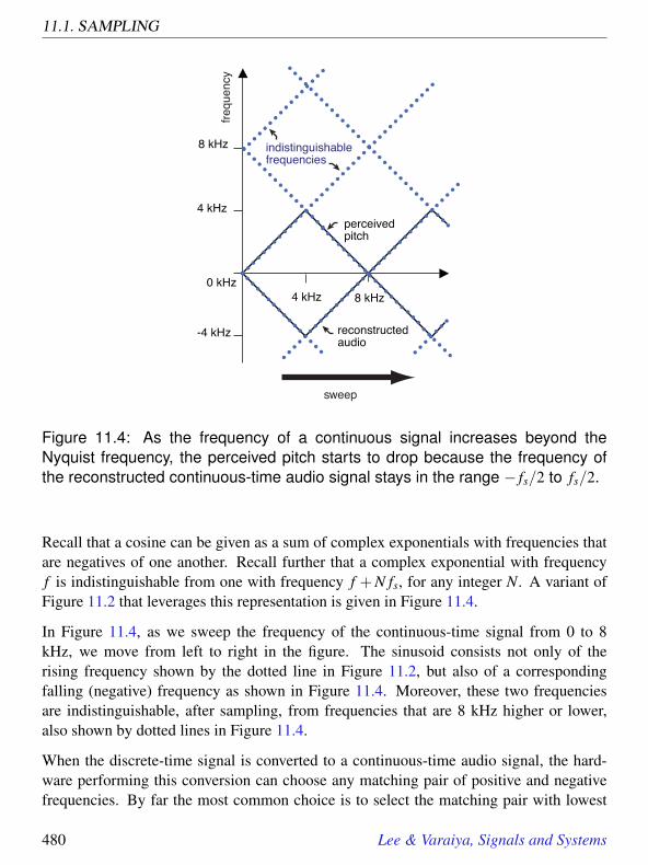
11.1. SAMPLING
8 kHz
8 kHz
indistinguishablefrequencies
4 kHz
4 kHzperceivedpitch
frequ
ency
sweep
reconstructedaudio
0 kHz
-4 kHz
Figure 11.4: As the frequency of a continuous signal increases beyond theNyquist frequency, the perceived pitch starts to drop because the frequency ofthe reconstructed continuous-time audio signal stays in the range − fs/2 to fs/2.
Recall that a cosine can be given as a sum of complex exponentials with frequencies thatare negatives of one another. Recall further that a complex exponential with frequencyf is indistinguishable from one with frequency f +N fs, for any integer N. A variant ofFigure 11.2 that leverages this representation is given in Figure 11.4.
In Figure 11.4, as we sweep the frequency of the continuous-time signal from 0 to 8kHz, we move from left to right in the figure. The sinusoid consists not only of therising frequency shown by the dotted line in Figure 11.2, but also of a correspondingfalling (negative) frequency as shown in Figure 11.4. Moreover, these two frequenciesare indistinguishable, after sampling, from frequencies that are 8 kHz higher or lower,also shown by dotted lines in Figure 11.4.
When the discrete-time signal is converted to a continuous-time audio signal, the hard-ware performing this conversion can choose any matching pair of positive and negativefrequencies. By far the most common choice is to select the matching pair with lowest
480 Lee & Varaiya, Signals and Systems

11. SAMPLING AND RECONSTRUCTION
frequency, shown in Figure 11.4 by the solid lines behind dotted lines. These result ina sinusoid with frequency between 0 and the Nyquist frequency, fs/2. This is why theperceived pitch falls after sweeping past fs/2 = 4 kHz.
Recall that the frequency-domain representation (i.e. the DTFT) of a discrete-time signalis periodic with period 2π radians/sample. That is, if X is a DTFT, then
∀ ω ∈ R, X(ω) = X(ω+2π).
In radians per second, it is periodic with period 2π fs. In Hertz, it is periodic with periodfs, the sampling frequency. Thus, in Figure 11.4, the dotted lines represent this peri-odicity. This periodicity is another way of stating that frequencies separated by fs areindistinguishable.
11.1.4 Avoiding aliasing ambiguities
Figure 11.4 suggests that even though a discrete-time signal has ambiguous frequencycontent, it is possible to construct a uniquely defined continuous-time signal from thediscrete-time waveform by choosing the one unique frequency for each component thatis closest to zero. This will always result in a reconstructed signal that contains onlyfrequencies between zero and the Nyquist frequency.
Correspondingly, this suggests that when sampling a continuous-time signal, if that signalcontains only frequencies below the Nyquist frequency, then this reconstruction strategywill perfectly recover the signal. This is an intuitive statement of the Nyquist-Shannonsampling theorem.
If a continuous-time signal contains only frequencies below the Nyquist frequency fs/2,then it can be perfectly reconstructed from samples taken at sampling frequency fs. Thissuggests that prior to sampling, it is reasonable to filter a signal to remove componentswith frequencies above fs/2. A filter that realizes this is called an anti-aliasing filter.
Example 11.3: In the telephone network, speech is sampled at 8000 samples persecond before being digitized. Prior to this sampling, the speech signal is lowpassfiltered to remove frequency components above 4000 Hz. This lowpass filteredspeech can then be perfectly reconstructed at the far end of the telephone connec-tion, which receives a stream of samples at 8000 sample per second.
Lee & Varaiya, Signals and Systems 481

11.2. RECONSTRUCTION
Before probing this further, let us examine in more detail what we mean by reconstruction.
11.2 Reconstruction
Consider a system that constructs a continuous-time signal x from a discrete-time signaly,
DiscToContT : DiscSignals→ ContSignals.
Probing Further: Anti-Aliasing for Fonts
When rendering characters on a computer screen, it is common to use anti-aliasing tomake the characters look better. Consider the two figures below:
At the left is an image of the Greek letter omega. At the right is the result of samplingthat rendition by taking only one pixel out of every 100 pixels in the original (every10-th pixel horizontally and vertically), and then rescaling the image so it has the samesize as the one on the left. The original image is discrete, and the resulting image isa smaller discrete image (this process is known as subsampling). To the discerningeye, the rendering can be improved considerably. The problem is that the character atthe upper left above has hard edges, and hence high (spatial) frequencies. Those highfrequencies result in aliasing distortion when subsampling. To improve the result, wefirst lowpass filter the character (blurring it), and then subsample, as shown below:
The result looks better.
482 Lee & Varaiya, Signals and Systems

11. SAMPLING AND RECONSTRUCTION
DiscToContT
Figure 11.5: Discrete to continuous converter.
This is illustrated in Figure 11.5. Systems that carry out such ‘discrete-to-continuous’conversion can be realized in any number of ways. Some common examples are illustratedin Figure 11.6, and defined below:
• zero-order hold: This means simply that the value of the each sample y(n) is heldconstant for duration T , so that x(t) = y(n) for the time interval from t = nT tot = (n+1)T , as illustrated in figure 11.6(b). Let this system be denoted
ZeroOrderHoldT : DiscSignals→ ContSignals.
• linear interpolation: Intuitively, this means simply that we connect the dots withstraight lines. Specifically, in the time interval from t = nT to t = (n+1)T , x(t) hasvalues that vary along a straight line from y(n) to y(n+ 1), as illustrated in figure11.6(c). Linear interpolation is sometimes called first-order hold. Let this systembe denoted
LinearInterpolatorT : DiscSignals→ ContSignals.
• ideal interpolation: It is not yet clear what this should mean, but intuitively, itshould result in a smooth curve that passes through the samples, as illustrated inFigure 11.6(d). We will give a precise meaning below. Let this system be denoted
IdealInterpolatorT : DiscSignals→ ContSignals.
11.2.1 A model for reconstruction
A convenient mathematical model for reconstruction divides the reconstruction processinto a cascade of two systems, as shown in Figure 11.7. Thus
x = S(ImpulseGenT (y)),
Lee & Varaiya, Signals and Systems 483

11.2. RECONSTRUCTION
y(n)
n......
x(t)
t......
x(t)
t......
x(t)
t......
(a)
(b)
(c)
(d)
w(t)
t......(e)
Figure 11.6: A discrete-time signal (a), a continuous-time reconstruction usingzero-order hold (b), a reconstruction using linear interpolation (c), a reconstruc-tion using ideal interpolation (d), and a reconstruction using weighted Dirac deltafunctions (e).
484 Lee & Varaiya, Signals and Systems

11. SAMPLING AND RECONSTRUCTION
DiscToContT
ImpulseGenT LTI System S
Figure 11.7: A model for reconstruction divides it into two stages.
where S is an LTI system to be determined. The first of these two subsystems,
ImpulseGenT : DiscSignals→ ContSignals,
constructs a continuous-time signal, where for all t ∈ R,
w(t) =∞
∑k=−∞
y(k)δ(t− kT ).
This is a continuous-time signal that at each sampling instant kT produces a Dirac deltafunction with weight equal to the sample value, y(k). This signal is illustrated in Figure11.6(e). It is a mathematical abstraction, since everyday engineering systems do not ex-hibit the singularity-like behavior of the Dirac delta function. Nonetheless, it is a usefulmathematical abstraction.
The second system in Figure 11.7, S, is a continuous-time LTI filter with an impulseresponse that determines the interpolation method. The impulse responses that yield theinterpolation methods in figure 11.6(b-e) are shown in figure 11.8(b-e). If
∀ t ∈ R, h(t) =
1 0≤ t < T0 otherwise
then the interpolation method is zero-order hold. If
∀ t ∈ R, h(t) =
1+ t/T −T < t < 01− t/T 0≤ t < T
0 otherwise
then the interpolation method is linear. If the impulse response is
∀ t ∈ R, h(t) =sin(πt/T )
πt/T
Lee & Varaiya, Signals and Systems 485

11.2. RECONSTRUCTION
h(t)
t(b)
(c)
(d)
h(t)
t(e)
1
T
h(t)
t1
T−T
h(t)
t1
T−T
1
Figure 11.8: The impulse responses for the LTI system S in figure 11.7 that yieldthe interpolation methods in figure 11.6(b-e).
486 Lee & Varaiya, Signals and Systems

11. SAMPLING AND RECONSTRUCTION
then the interpolation method is ideal. The above impulse response is called a sinc func-tion, and its Fourier transform, from table 10.4, is given by
∀ ω ∈ R, X(ω) =
T if |ω| ≤ π/T0 otherwise
Notice that the Fourier transform is zero at all frequencies above π/T radians/second,or fs/2 Hz, the Nyquist frequency. It is this characteristic that makes it ideal. It pre-cisely performs the strategy illustrated in Figure 11.4, where among all indistinguishablefrequencies we select the ones between − fs/2 and fs/2.
If we let SincT denote the LTI system S when the impulse response is a sinc function, then
IdealInterpolatorT = SincT ImpulseGenT .
In practice, ideal interpolation is difficult to accomplish. From the expression for the sincfunction we can understand why. First, this impulse response is not causal. Second, it isinfinite in extent. More importantly, its magnitude decreases rather slowly as t increases ordecreases (proportional to 1/t only). Thus, truncating it at finite length leads to substantialerrors.
If the impulse response of S ish(t) = δ(t),
where δ is the Dirac delta function, then the system S is a pass-through system, and thereconstruction consists of weighted delta functions.
Lee & Varaiya, Signals and Systems 487

11.3. THE NYQUIST-SHANNON SAMPLING THEOREM
11.3 The Nyquist-Shannon sampling theorem
We can now give a precise statement of the Nyquist-Shannon sampling theorem:
If x is a continuous-time signal with Fourier transform X and if X(ω) is zero outside therange −π/T < ω < π/T radians/second, then
x = IdealInterpolatorT (SamplerT (x)).
We can state this theorem slightly differently. Suppose x is a continuous-time signal withno frequency larger than some f0 Hertz. Then x can be recovered from its samples iff0 < fs/2, the Nyquist frequency.
A formal proof of this theorem involves some technical difficulties (it was first givenby Claude Shannon of Bell Labs in the late 1940s). But we can get the idea from thefollowing three-step argument (see figure 11.9).
Step 1. Let x be a continuous-time signal with Fourier transform X . At this point we donot require that X(ω) be zero outside the range −π/T < ω < π/T . We sample x withsampling interval T to get the discrete-time signal
y = SamplerT (x).
It can be shown (see box on page 492 ) that the DTFT of y is related to the CTFT of x by
Y (ω) =1T
∞
∑k=−∞
X(
ω
T− 2πk
T
).
This important relation says that the DTFT Y of y is the sum of the CTFT X with copiesof it shifted by multiples of 2π/T . Also, the frequency axis is normalized by dividing ω
by T . There are two cases to consider, depending on whether the shifted copies overlap.
First, if X(ω) = 0 outside the range −π/T < ω < π/T , then the copies will not overlap,and in the range −π < ω < π,
Y (ω) =1T
X(
ω
T
). (11.5)
In this range of frequencies, Y has the same shape as X , scaled by 1/T . This relationshipbetween X and Y is illustrated in figure 11.10, where X is drawn with a triangular shape.
In the second case, illustrated in figure 11.11, X does have non-zero frequency compo-nents higher than π/T . Notice that in the sampled signal, the frequencies in the vicinity
488 Lee & Varaiya, Signals and Systems

11. SAMPLING AND RECONSTRUCTION
ω
X(ω)
1
π/T−π/T
t
x(t)
SamplerT
ImpulseGenT
n
y(n)
ω
Y(ω)
π−π
ω
W(ω)
1/T
π/T−π/T
t
w(t)
−2π
−2π/T
2π
2π/T
SincT
t
z(t)
ω
Z(ω)
1
π/T−π/T
x
y
w
z
Time Frequency
X = CTFT (x )
Y = DTFT (y )
W = CTFT (w )
Z = CTFT (z )
1/T
IdealInterpolatorT
Figure 11.9: Steps in the justification of the Nyquist-Shannon sampling theorem.
Lee & Varaiya, Signals and Systems 489

11.3. THE NYQUIST-SHANNON SAMPLING THEOREM
ω
π−π
ω
X(ω)
Y(ω)
1
π/T−π/T
1/T......
3π−3π
Figure 11.10: Relationship between the CTFT of a continuous-time signal andthe DTFT of its discrete-time samples. The DTFT is the sum of the CTFT and itscopies shifted by multiples of 2π/T , the sampling frequency in radians per second.The frequency axis is also normalized.
ω
ω
−π π
X(ω)
Y(ω)
1
π/T−π/T
1/T
Figure 11.11: Relationship between the CTFT of a continuous-time signal and theDTFT of its discrete-time samples when the continuous-time signal has a broadenough bandwidth to introduce aliasing distortion.
490 Lee & Varaiya, Signals and Systems

11. SAMPLING AND RECONSTRUCTION
of π are distorted by the overlapping of frequency components above and below π/T inthe original signal. This distortion is called aliasing distortion.
We continue with the remaining steps, following the signals in figure 11.9.
Step 2. Let w be the signal produced by the impulse generator,
∀ t ∈ R, w(t) =∞
∑n=−∞
y(n)δ(t−nT ).
The Fourier Transform of w is W (ω) = Y (ωT ) (see box on page 492).
Step 3. Let z be the output of the IdealInterpolatorT . Its Fourier transform is simply
Z(ω) = W (ω)S(ω)
= Y (ωT )S(ω),
where S(ω) is the frequency response of the IdealInterpolatorT reconstruction filter. Asseen in exercise 21 of Chapter 10,
S(ω) =
T −π/T < ω < π/T0 otherwise
(11.6)
Substituting for S and Y , we get
Z(ω) =
TY (ωT ) −π/T < ω < π/T0 otherwise
=
∞
∑k=−∞
X(ω−2πk/T ) −π/T < ω < π/T
0 otherwise
If X(ω) is zero for |ω| larger than the Nyquist frequency π/T , then we conclude that
∀ ω ∈ R, Z(ω) = X(ω).
That is, w is identical to x. This proves the Nyquist-Shannon result.
However, if X(ω) does have non-zero values for some |ω| larger than the Nyquist fre-quency, then z will be different from x, as illustrated in figure 11.11.
Lee & Varaiya, Signals and Systems 491
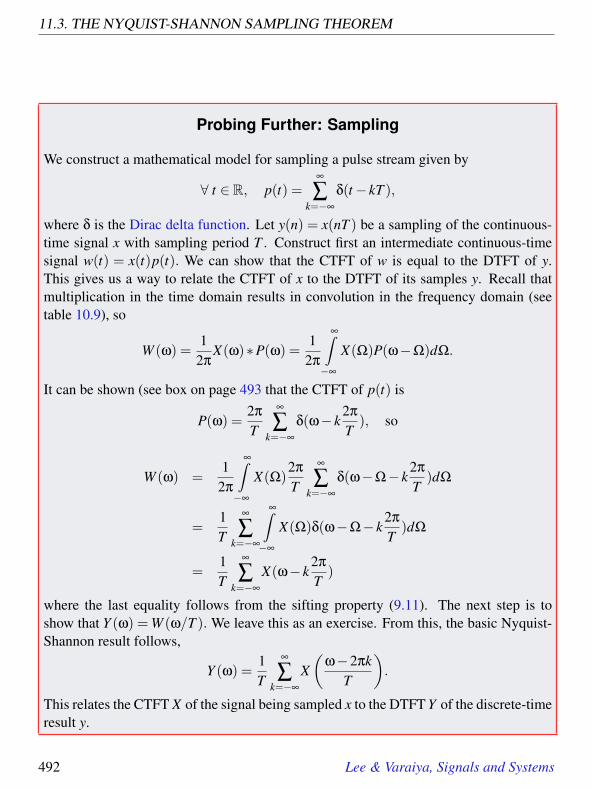
11.3. THE NYQUIST-SHANNON SAMPLING THEOREM
Probing Further: Sampling
We construct a mathematical model for sampling a pulse stream given by
∀ t ∈ R, p(t) =∞
∑k=−∞
δ(t− kT ),
where δ is the Dirac delta function. Let y(n) = x(nT ) be a sampling of the continuous-time signal x with sampling period T . Construct first an intermediate continuous-timesignal w(t) = x(t)p(t). We can show that the CTFT of w is equal to the DTFT of y.This gives us a way to relate the CTFT of x to the DTFT of its samples y. Recall thatmultiplication in the time domain results in convolution in the frequency domain (seetable 10.9), so
W (ω) =1
2πX(ω)∗P(ω) =
12π
∞∫−∞
X(Ω)P(ω−Ω)dΩ.
It can be shown (see box on page 493 that the CTFT of p(t) is
P(ω) =2π
T
∞
∑k=−∞
δ(ω− k2π
T), so
W (ω) =1
2π
∞∫−∞
X(Ω)2π
T
∞
∑k=−∞
δ(ω−Ω− k2π
T)dΩ
=1T
∞
∑k=−∞
∞∫−∞
X(Ω)δ(ω−Ω− k2π
T)dΩ
=1T
∞
∑k=−∞
X(ω− k2π
T)
where the last equality follows from the sifting property (9.11). The next step is toshow that Y (ω) =W (ω/T ). We leave this as an exercise. From this, the basic Nyquist-Shannon result follows,
Y (ω) =1T
∞
∑k=−∞
X(
ω−2πkT
).
This relates the CTFT X of the signal being sampled x to the DTFT Y of the discrete-timeresult y.
492 Lee & Varaiya, Signals and Systems

11. SAMPLING AND RECONSTRUCTION
Probing Further: Impulse Trains
Consider a signal p consisting of periodically repeated Dirac delta functions with periodT ,
∀ t ∈ R, p(t) =∞
∑k=−∞
δ(t− kT ).
This signal has the Fourier series expansion
∀ t ∈ R, p(t) =∞
∑m=−∞
1T
eiω0mt ,
where the fundamental frequency is ω0 = 2π/T . This can be verified by applying theformula from table 10.5. That formula, however, gives an integration range of 0 to theperiod, which in this case is T . This integral covers one period of the periodic signal, butstarts and ends on a delta function in p. To avoid the resultant mathematical subtleties,we can integrate from −T/2 to T/2, getting Fourier series coefficients
∀ m ∈ Z, Pm =1T
T/2∫−T/2
[∞
∑k=−∞
δ(t− kT )
]eiω0mtdt.
The integral is now over a range that includes only one of the delta functions. The kernelof the integral is zero except when t = 0, so by the sifting rule, the integral evaluates to1. Thus, all Fourier series coefficients are Pm = 1/T . Using the relationship between theFourier series and the Fourier Transform of a periodic signal (from Section 10.6.3), wecan write the continuous-time Fourier transform of p as
∀ ω ∈ R, P(ω) =2π
T
∞
∑k=−∞
δ
(ω− 2π
Tk).
Lee & Varaiya, Signals and Systems 493

11.4. SUMMARY
11.4 Summary
The acts of sampling and reconstructing signals bridge the world of continuous-time phys-ical signals with the discrete computational world. The periodicity of frequencies in thediscrete world implies that for each discrete-time sinusoidal signal, there are multiplecorresponding discrete-time frequencies. These frequencies are aliases of one another.When a signal is sampled, these frequencies become indistinguishable, and aliasing dis-tortion may result. The Nyquist-Shannon sampling theorem gives a simple conditionunder which aliasing distortion is avoided. Specifically, if the signal contains no sinu-soidal components with frequencies higher than half the sampling frequency, then therewill be no aliasing distortion. Half the sampling frequency is called the Nyquist frequencybecause of this key result.
494 Lee & Varaiya, Signals and Systems

11. SAMPLING AND RECONSTRUCTION
Exercises
Each problem is annotated with the letter E, T, C which stands for exercise, requires somethought, requires some conceptualization. Problems labeled E are usually mechanical,those labeled T require a plan of attack, those labeled C usually have more than onedefensible answer.
1. E Consider the continuous-time signal
x(t) = cos(10πt)+ cos(20πt)+ cos(30πt).
(a) Find the fundamental frequency. Give the units.
(b) Find the Fourier series coefficients A0,A1, · · · and φ1,φ2, · · · .(c) Let y be the result of sampling this signal with sampling frequency 10 Hz.
Find the fundamental frequency for y, and give the units.
(d) For the same y, find the discrete-time Fourier series coefficients, A0,A1, · · ·and φ1, · · · .
(e) Findw = IdealInterpolatorT (SamplerT (x))
for T = 0.1 seconds.
(f) Is there any aliasing distortion caused by sampling at 10 Hz? If there is,describe the aliasing distortion in words.
(g) Give the smallest sampling frequency that avoids aliasing distortion.
2. E Verify that SamplerT defined by (11.1) and (11.2) is linear but not time invariant.
3. E A real-valued sinusoidal signal with a negative frequency is always exactly equalto another sinusoid with positive frequency. Consider a real-valued sinusoid with anegative frequency −440 Hz,
y(n) = cos(−2π440nT +φ).
Find a positive frequency f and phase θ such that
y(n) = cos(2π f nT +θ).
Lee & Varaiya, Signals and Systems 495
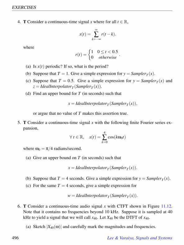
EXERCISES
4. T Consider a continuous-time signal x where for all t ∈ R,
x(t) =∞
∑k=−∞
r(t− k).
where
r(t) =
1 0≤ t < 0.50 otherwise
.
(a) Is x(t) periodic? If so, what is the period?
(b) Suppose that T = 1. Give a simple expression for y = SamplerT (x).
(c) Suppose that T = 0.5. Give a simple expression for y = SamplerT (x) andz = IdealInterpolatorT (SamplerT (x)).
(d) Find an upper bound for T (in seconds) such that
x = IdealInterpolatorT (SamplerT (x)),
or argue that no value of T makes this assertion true.
5. T Consider a continuous-time signal x with the following finite Fourier series ex-pansion,
∀ t ∈ R, x(t) =4
∑k=0
cos(kω0t)
where ω0 = π/4 radians/second.
(a) Give an upper bound on T (in seconds) such that
x = IdealInterpolatorT (SamplerT (x)).
(b) Suppose that T = 4 seconds. Give a simple expression for y = SamplerT (x).
(c) For the same T = 4 seconds, give a simple expression for
w = IdealInterpolatorT (SamplerT (x)).
6. T Consider a continuous-time audio signal x with CTFT shown in Figure 11.12.Note that it contains no frequencies beyond 10 kHz. Suppose it is sampled at 40kHz to yield a signal that we will call x40. Let X40 be the DTFT of x40.
(a) Sketch |X40(ω)| and carefully mark the magnitudes and frequencies.
496 Lee & Varaiya, Signals and Systems

11. SAMPLING AND RECONSTRUCTION
H(2π f)
f (kHz)1
10 -10
Figure 11.12: CTFT of an audio signal considered in exercise 6.
(b) Suppose x is sampled at 20,000 samples/second. Let x20 be the resulting sam-pled signal and X20 its DTFT. Sketch and compare x20 and x40.
(c) Now suppose x is sampled at 15,000 samples/second. Let x15 be the resultingsampled signal and X15 its DTFT. Sketch and compare X20 and X15. Makesure that your sketch shows aliasing distortion.
7. C Consider two continuous-time sinusoidal signals given by
x1(t) = cos(ω1t)
x2(t) = cos(ω2t),
with frequencies ω1 and ω2 radians/second such that
0≤ ω1 ≤ π/T and 0≤ ω2 ≤ π/T.
Show that if ω1 6= ω2 then
SamplerT (x1) 6= SamplerT (x2).
I.e., the two distinct sinusoids cannot be aliases of one another if they both havefrequencies below the Nyquist frequency. Hint: Try evaluating the sampled signalsat n = 1.
Lee & Varaiya, Signals and Systems 497

12Stability
Contents12.1 Boundedness and stability . . . . . . . . . . . . . . . . . . . . . . . 503
12.1.1 Absolutely summable and absolutely integrable . . . . . . . . 50312.1.2 Stability . . . . . . . . . . . . . . . . . . . . . . . . . . . . . 505Probing Further: Stable systems and their impulse response . . . . . 507
12.2 The Z transform . . . . . . . . . . . . . . . . . . . . . . . . . . . . 50912.2.1 Structure of the region of convergence . . . . . . . . . . . . . 51112.2.2 Stability and the Z transform . . . . . . . . . . . . . . . . . . 51612.2.3 Rational Z tranforms and poles and zeros . . . . . . . . . . . 517
12.3 The Laplace transform . . . . . . . . . . . . . . . . . . . . . . . . 52112.3.1 Structure of the region of convergence . . . . . . . . . . . . . 52312.3.2 Stability and the Laplace transform . . . . . . . . . . . . . . 52712.3.3 Rational Laplace tranforms and poles and zeros . . . . . . . . 528
12.4 Summary . . . . . . . . . . . . . . . . . . . . . . . . . . . . . . . . 530Exercises . . . . . . . . . . . . . . . . . . . . . . . . . . . . . . . . . . . 532
The four Fourier transforms prove to be useful tools for analyzing signals and systems.When a system is LTI, it is characterized by its frequency response H, and its input x andoutput y are related simply by
∀ω ∈ R, Y (ω) = H(ω)X(ω),
where Y is the Fourier transform of y, and X is the Fourier transform of x.
499
However, we ignored a lurking problem. Any of the three Fourier transforms, X , Y , orH, may not exist. Suppose for example that x is a discrete-time signal. Then its Fouriertransform (the DTFT) is given by
∀ ω ∈ R, X(ω) =∞
∑n=−∞
x(n)e−iωn. (12.1)
This is an infinite sum, properly viewed as the limit
∀ ω ∈ R, X(ω) = limN→∞
N
∑n=−N
x(n)e−iωn. (12.2)
As with all such limits, there is a risk that it does not exist. If the limit does not existfor any ω ∈ R, then the Fourier transform becomes mathematically treacherous at best(involving, for example, Dirac delta functions), and mathematical nonsense at worst.
Example 12.1: Consider the sequence
x(n) =
0, n≤ 0an−1, n > 0
,
where a > 1 is a constant. Plugging into (12.1), the Fourier transform should be
∀ ω ∈ R, X(ω) =∞
∑n=0
an−1e−iωn.
At ω = 0, it is easy to see that this sum is infinite (every term in the sum is greaterthan or equal to one). At other values of ω, there are also problems. For example,at ω = π, the terms of the sum alternate in sign and increase in magnitude as n getslarger. The limit (12.2) clearly will not exist.
A similar problem arises with continuous-time signals. If x is a continuous-time signal,then its Fourier transform (the CTFT) is given by
∀ ω ∈ R, X(ω) =
∞∫−∞
x(t)e−iωtdt. (12.3)
500 Lee & Varaiya, Signals and Systems

12. STABILITY
Mbody
tail
main rotor shaft
Figure 12.1: A highly simplified helicopter.
Again, there is a risk that this integral does not exist.
This chapter studies signals for which the Fourier transform does not exist. Such signalsprove to be both common and useful. The signal in example 12.1 gives the bank balanceof example 5.12 when an initial deposit of one dollar is made, and no further deposits orwithdrawals are made (thus, it is the impulse response of the bank account). This signalgrows without bound, and any signal that grows without bound will cause difficultieswhen using the Fourier transform.
The bank account is said to be an unstable system, because its output can grow withoutbound even when the input is always bounded. Such unstable systems are common, so itis unfortunate that the frequency domain methods we have studied so far do not appear toapply.
Example 12.2: A helicopter is intrinsically an unstable system, requiring an elec-tronic or mechanical feedback control system to stabilize it. It has two rotors, oneabove, which provides lift, and one on the tail. Without the rotor on the tail, thebody of the helicopter would start to spin. The rotor on the tail counteracts that spin.However, the force produced by the tail rotor must perfectly counter the torque ofthe main rotor, or the body will spin.
A highly simplified version of the helicopter is shown in figure 12.1. The body ofthe helicopter is modeled as a horizontal arm with moment of intertia M. The tailrotor goes on the end of this arm. The body of the helicopter rotates freely around
Lee & Varaiya, Signals and Systems 501

the main rotor shaft. Due to Newton’s third law, the main rotor will tend to causethe body to rotate by applying a torque as suggested by the curved arrow. Thetail rotor will have to counter that torque to keep the body of the helicopter fromspinning.
Let the input x to the system be the net torque on the tail of the helicopter, as afunction of time. That is, at time t, x(t) is the sum of the torque induced by themain rotor shaft and the counteracting torque exerted by the tail rotor. Let theoutput y be the velocity of rotation of the body. From basic physics, torque equalsmoment of inertia times rotational acceleration. The rotational acceleration is y, thederivative of y, so
y(t) = x(t)/M.
Integrating both sides, assuming that the initial velocity of rotation is zero, we getthe output as a function of the input,
∀ t ∈ R, y(t) =1M
t∫0
x(τ)dτ.
It is now easy to see that this system is unstable. Let the input be x = u, where u isthe unit step, given by
∀ t ∈ R, u(t) =
0, t < 01, t ≥ 0
. (12.4)
This input is clearly bounded. It never exceeds one in magnitude. However, theoutput grows without bound.
In practice, a helicopter uses a feedback system to determine how much torque toapply at the tail rotor to keep the body of the helicopter straight. We will see howto do this in Chapter 14.
In this chapter we develop the basics of modeling unstable systems in the frequency do-main. We define two new transforms, called the Z transform and Laplace transform.The Z transform is a generalization of the DTFT and applies to discrete-time signals. TheLaplace transform is a generalization of the CTFT and applies to continuous-time signals.These generalizations support frequency-domain analysis of signals that do not have aFourier transform, and thus allow analysis of unstable systems.
502 Lee & Varaiya, Signals and Systems

12. STABILITY
In particular, let X denote the Laplace or Z transform of x, depending on whether it is acontinuous or discrete-time signal. Then the Laplace or Z transform of the output of anLTI system is given by Y = HX , where H is the Laplace or Z transform of the impulseresponse. This relation applies even when the system is unstable. Thus, these transformstake the place of the Fourier transform when the Fourier transform cannot be used. H iscalled the transfer function of the LTI system, and it is a generalization of the frequencyresponse.
12.1 Boundedness and stability
In this section, we identify a simple condition for the existence of the DTFT, which is thatthe signal be absolutely summable. We then define a stable system and show that an LTIsystem is stable if and only if its impulse response is absolutely summable. Continuous-time signals are slightly more complicated, requiring slightly more than that they be abso-lutely integrable. The conditions for the existence of the CTFT are called the Dirichletconditions, and once again, if the impulse response of an LTI system satisfies these con-ditions, then it is stable.
12.1.1 Absolutely summable and absolutely integrable
A discrete-time signal x is said to be absolutely summable if
∞
∑n=−∞
|x(n)|
exists and is finite. The “absolutely” in “absolutely summable” refers to the absolute value(or magnitude) in the summation. The sum is said to converge absolutely. The followingsimple fact gives a condition for the existence of the DTFT:
If a discrete-time signal x is absolutely summable, then its DTFT exists and is finite forall ω.
To see that this is true, note that the DTFT exists and is finite if and only if
∀ ω ∈ R, |X(ω)|=∣∣∣∣∣ ∞
∑n=−∞
x(n)e−iωn
∣∣∣∣∣Lee & Varaiya, Signals and Systems 503

12.1. BOUNDEDNESS AND STABILITY
exists and is finite. But ∣∣∣∣∣ ∞
∑n=−∞
x(n)e−iωn
∣∣∣∣∣ ≤ ∞
∑n=−∞
|x(n)e−iωn| (12.5)
=∞
∑n=−∞
|x(n)| · |e−iωn| (12.6)
=∞
∑n=−∞
|x(n)|. (12.7)
This follows from the following facts about complex (or real) numbers:
|a+b| ≤ |a|+ |b|,
which is known as the triangle inequality (and generalizes to infinite sums),
|ab|= |a| · |b|,
and∀ θ ∈ R, |eiθ|= 1.
We can conclude from (12.5) that
∀ ω ∈ R, |X(ω)| ≤∞
∑n=−∞
|x(n)|.
This means that if x is absolutely summable, then the DTFT exists and is finite. It fol-lows from the fact that if a sum converges absolutely, then it also converges (without theabsolute value).
A continuous-time signal x is said to be absolutely integrable if∞∫−∞
|x(t)|dt
exists and is finite. A similar argument to that above (with summations replaced by inte-grals) suggests that if a continuous-time signal x is absolutely integrable, then its CTFTshould exist and be finite for all ω. However, caution is in order. Integrals are morecomplicated than summations, and we need some additional conditions to ensure that theintegral is well defined. We can use essentially the same conditions given on page 297for the convergence of the continuous-time Fourier series. These are called the Dirichletconditions, and require three things:
504 Lee & Varaiya, Signals and Systems

12. STABILITY
• x is absolutely integrable;
• in any finite interval, x is of bounded variation, meaning that there are no morethan a finite number of maxima or minima; and
• in any finite interval, x is continuous at all but a finite number of points.
Most any signal of practical engineering importance satisfies the last two conditions, sothe important condition is that it be absolutely integrable. We will henceforth assumewithout comment that all continuous-time signals satisfy the last two conditions, so theonly important condition becomes the first one. Under this assumption, the followingsimple fact gives a condition for the existence of the CTFT:
An absolutely integrable continuous-time signal x has a CTFT X , and its CTFT X(ω) isfinite for all ω ∈ R.
12.1.2 Stability
A system is said to be bounded-input bounded-output stable (BIBO stable or juststable) if the output signal is bounded for all input signals that are bounded.
Consider a discrete-time system with input x and output y. An input is bounded if thereis a real number M < ∞ such that |x(k)| ≤M for all k ∈ Z. An output is bounded if thereis a real number N < ∞ such that |y(n)| ≤ N for all n ∈ Z. The system is stable if for anyinput bounded by M, there is some bound N on the output.
Consider a discrete-time LTI system with impulse response h. The output y correspondingto the input x is given by the convolution sum,
∀n ∈ Z, y(n) = (h∗ x)(n) =∞
∑m=−∞
h(m)x(n−m). (12.8)
Suppose that the input x is bounded with bound M. Then, applying the triangle inequality,we see that
|y(n)| ≤∞
∑m=−∞
|h(m)||x(n−m)| ≤M∞
∑m=−∞
|h(m)|.
Thus, if the impulse response is absolutely summable, then the output is bounded withbound
N = M∞
∑m=−∞
|h(m)|.
Lee & Varaiya, Signals and Systems 505

12.1. BOUNDEDNESS AND STABILITY
Thus, if the impulse response of an LTI system is absolutely summable, then the systemis stable. The converse is also true, but more difficult to show. That is, if the system isstable, then the impulse response is absolutely summable (see box on page 507). Thesame argument applies for continuous-time signals, so in summary:
A discrete-time LTI system is stable if and only if its impulse response is absolutelysummable. A continuous-time LTI system is stable if and only if its impulse response isabsolutely integrable.
The following example makes use of the geometric series identity, valid for any real orcomplex a where |a|< 1,
∞
∑m=0
am =1
1−a. (12.9)
To verify this identity, just multiply both sides by 1−a to get
∞
∑m=0
am−a∞
∑m=0
am = 1.
This can be written
a0 +∞
∑m=1
am−∞
∑m=1
am = 1.
Now note that a0 = 1 and that the two sums are identical. Since |a|< 1, the sums converge,and hence they cancel, so the identity is true.
Example 12.3: As in example 12.1, the impulse response of the bank account ofexample 5.12 is
h(n) =
0, n≤ 0an−1, n > 0
,
where a > 1 is a constant that reflects the interest rate. This impulse response is notabsolutely summable, so this system is not stable. A system with the same impulseresponse, but where 0 < a < 1, however, would be stable, as is easily verified using
506 Lee & Varaiya, Signals and Systems

12. STABILITY
Probing Further: Stable systems and their impulse response
Consider a discrete-time LTI system with real-valued impulse response h. In this box,we show that if the system is stable, then its impulse response is absolutely summable.To show this, we show the contrapositive.a That is, we show that if the impulse responseis not absolutely summable, then the system is not stable. To do this, suppose that theimpulse response is not absolutely summable. That is, the sum
∞
∑n=−∞
|h(n)|
is not bounded. To show that the system is not stable, we need only to find one boundedinput for which the output either does not exist or is not bounded. Such an input is givenby
∀ n ∈ Z, x(n) =
h(−n)/|h(−n)|, h(n) 6= 00, h(n) = 0
This input is clearly bounded, with bound M = 1. Plugging this input into the convolu-tion sum (12.8) and evaluating at n = 0 we get
y(0) =∞
∑m=−∞
h(m)x(−m)
=∞
∑m=−∞
(h(m))2/|h(m)|
=∞
∑m=−∞
|h(m)|,
where the last step follows from the fact that for real-valued h(m), (h(m))2 = |h(m)|2.But since the impulse response is not absolutely summable, y(0) does not exist or is notfinite, so the system is not stable.
A nearly identical argument works for continuous-time systems.
aThe contrapositive of a statement “if p then q” is “if not q then not p.” The contrapositive is true if andonly if the original statement is true.
Lee & Varaiya, Signals and Systems 507

12.1. BOUNDEDNESS AND STABILITY
(12.9). To use this identity, note that
∞
∑n=−∞
|h(n)| =∞
∑n=1
an−1
=∞
∑m=0
am
=1
1−a,
where the second step results from a change of variables, letting m = n−1.
Example 12.4: Consider an LTI system with impulse response h(t) = atu(t), forall t ∈ R. where a > 0 is a real number and u is the unit step, given by (12.4).To determine whether this system is stable, we need to determine whether the im-pulse response is absolutely integrable. That is, we need to determine whether thefollowing integral exists and is finite,
∞∫−∞
|atu(t)|dt.
Since a > 0 and u is the unit step, this simplifies to
∞∫0
atdt.
From calculus, we know that this integral is infinite if a ≥ 1, so the system is un-stable if a≥ 1. The integral is finite if 0 < a < 1 and is equal to
∞∫0
atdt =−1/ ln(a).
Thus, the system is stable if 0 < a < 1.
508 Lee & Varaiya, Signals and Systems

12. STABILITY
As we see, when all pertinent signals are absolutely summable (or absolutely integrable),then we can use Fourier transform techniques with confidence. However, many usefulsignals do not fall in this category (the unit step and sinusoidal signals, for example).Moreover, many useful systems have impulse responses that are not absolutely summable(or absolutely integrable). Fortunately, we can generalize the DTFT and CTFT to get theZ transform and Laplace transform, which easily handle signals that are not absolutelysummable.
12.2 The Z transform
Consider a discrete-time signal x that is not absolutely summable. Consider the scaledsignal xr given by
∀ n ∈ Z, xr(n) = x(n)r−n, (12.10)
for some real number r ≥ 0. Often, this signal is absolutely summable when r is chosenappropriately. This new signal, therefore, will have a DTFT, even if x does not.
Example 12.5: Continuing with example 12.3, the impulse response of the bankaccount is
h(n) =
0, n≤ 0an−1, n > 0
,
where a > 1. This system is not stable. However, the scaled signal
hr(n) = h(n)r−n
Lee & Varaiya, Signals and Systems 509
12.2. THE Z TRANSFORM
is absolutely summable if r > a. Its DTFT is
∀r > a,∀ω ∈ R, Hr(ω) =∞
∑m=−∞
h(m)r−me−iωm
=∞
∑m=1
am−1(reiω)−m
=∞
∑n=0
an(reiω)−n−1
= (reiω)−1∞
∑n=0
(a(reiω)−1)n
=(reiω)−1
1−a(reiω)−1 .
The second step is by change of variables, n = m−1, and the final step applies thegeometric series identity (12.9).
In general, the DTFT of the scaled signal xr in (12.10) is
∀ ω ∈ R, Xr(ω) =∞
∑m=−∞
x(m)(reiω)−m.
Notice that this is a function not just of ω, but also of r, and in fact, we are only sure it isvalid for values of r that yield an absolutely summable signal hr. If we define the complexnumber
z = reiω
then we can write this DTFT as
∀ z ∈ RoC(x), X(z) =∞
∑m=−∞
x(m)z−m, (12.11)
where X is a function called the Z transform of x,
X : RoC(x)→ C
where RoC(x)⊂ C is given by
RoC(x) = z = reiω ∈ C | x(n)r−n is absolutely summable. (12.12)
510 Lee & Varaiya, Signals and Systems

12. STABILITY
The term RoC is shorthand for region of convergence.
Example 12.6: Continuing example 12.5, we can recognize from the form ofHr(ω) that the Z transform of the impulse response h is
∀ z ∈ RoC(h), H(z) =z−1
1−az−1 =1
z−a,
where the last step is the result of multiplying top and bottom by z. The RoC is
RoC(h) = z = reiω ∈ C | r > a
The Z tranform H of the impulse response h of an LTI system is called the transferfunction of the system.
12.2.1 Structure of the region of convergence
When a signal has a Fourier transform, then knowing the Fourier transform is equivalentto knowing the signal. The signal can be obtained from its Fourier transform, and theFourier transform can be obtained from the signal. The same is true of a Z transform, butthere is a complication. The Z transform is a function X : RoC→C, and it is necessary toknow the set RoC to know the function X . The region of convergence is a critical part ofthe Z transform. We will see that very different signals can have very similar Z transformsthat differ only in the region of convergence.
Given a discrete-time signal x, RoC(x) is defined to be the set of all complex numbersz = reiω for which the following series converges:
∞
∑m=−∞
|x(m)r−m|.
Notice that if this series converges, then so does
∞
∑m=−∞
|x(m)z−m|
Lee & Varaiya, Signals and Systems 511

12.2. THE Z TRANSFORM
Re z
Im zIm z
Re z
Im z
causal or right sided
Re z
anti-causaltwo-sided
RoC RoCRoC
(a) (b) (c)
Figure 12.2: Three possible structures for the region of convergence of a Z trans-form.
for any complex number z with magnitude r. This is because
|x(m)z−m|= |x(m)(reiω)−m|= |x(m)| · |r−m| · |e−iωm|= |x(m)| · |r−m|.
Thus, the set RoC could equally well be defined to be the set of all complex numbers zsuch that x(n)z−n is absolutely summable.
Notice that whether this series converges depends only on r, the magnitude of the complexnumber z = reiω, and not on ω, its angle. Thus, if any point z = reiω is in the set RoC,then all points z′ with the same magnitude are also in RoC. This implies that the set RoC,a subset of C, will have circular symmetry.
The set RoC turns out to have even more structure. There are only three possible patterns,illustrated by the shaded areas in Figure 12.2. Each figure illustrates the complex plane,and the shaded area is a region of convergence. Each possibility has circular symmetry,in that whether a point is in the RoC depends only on its magnitude.
Figure 12.2(a) shows the RoC of a causal signal. A discrete-time signal x is causal ifx(n) = 0 for all n < 0. The RoC is the set of complex numbers z = reiω where followingseries converges:
∞
∑m=−∞
|x(m)r−m|.
But if x is causal, then∞
∑m=−∞
|x(m)r−m|=∞
∑m=0|x(m)r−m|.
512 Lee & Varaiya, Signals and Systems

12. STABILITY
If this series converges for some given r, then it must also converge for any r > r (becausefor all m ≥ 0, r−m < r−m. Thus, if z ∈ RoC, then the RoC must include all points in thecomplex plane on the circle passing through z and every point outside that circle.
Note further that not only must the RoC include every point outside the circle, but theseries must also converge in the limit as z goes to infinity. Thus, for example, H(z) = zcannot be the Z transform of a causal signal because its RoC cannot possibly includeinfinity (H(z) is not finite there).
Figure 12.2(c) shows the RoC of an anti-causal signal. A discrete-time signal x is anti-causal if x(n) = 0 for all n > 0. By a similar argument, if z ∈ RoC, then the RoC mustinclude all points in the complex plane on the circle passing through z and every pointinside that circle.
Figure 12.2(b) shows the RoC of a signal that is neither causal nor anti-causal. Such asignal is called a two-sided signal. Such a signal can always be expressed as a sum ofa causal signal and an anti-causal signal. The RoC is the intersection of the regions ofconvergence for these two components. To see this, just note that the RoC is the set ofcomplex numbers z = reiω where following series converges:
∞
∑m=−∞
|x(m)r−m|=−1
∑m=−∞
|x(m)r−m|+∞
∑m=0|x(m)r−m|.
The first sum on the right corresponds to an anti-causal signal, and the second sum on theright to a causal signal. For this series to converge, both sums must converge. Thus, for atwo-sided signal, the RoC has a ring structure.
Example 12.7: Consider the discrete-time unit step signal u, given by
u(n) =
0, n < 01, n≥ 0
. (12.13)
The Z transform is, using geometric series identity (12.9),
U(z) =∞
∑m=−∞
u(m)z−m =∞
∑m=0
z−m =1
1− z−1 =z
z−1,
with domain
RoC(u) = z ∈ C |∞
∑m=1|z|−m < ∞= z | |z|> 1.
Lee & Varaiya, Signals and Systems 513

12.2. THE Z TRANSFORM
This region of convergence has the structure of Figure 12.2(a), where the dashedcircle has radius one (that circle is called the unit circle). Indeed, this signal iscausal, so this structure makes sense.
Example 12.8: The signal v given by
v(n) =−1, n < 00, n≥ 0
,
has Z transform
V (z) =∞
∑m=−∞
v(m)z−m =−1
∑m=−∞
z−m =−z∞
∑k=0
zk =z
z−1,
with domain
RoC(v) = z ∈ C |1
∑m=−∞
|z|−m < ∞= z | |z|< 1.
This region of convergence has the structure of Figure 12.2(c), where the dashedcircle is again the unit circle. Indeed, this signal is anti-causal, so this structuremakes sense.
Notice that although the Z transform U of u and V of v have the same algebraic form,namely, z/(z−1), they are different functions, because their domains are different. Thusthe Z transform of a signal comprises both the algebraic form of the Z transform as wellas its RoC.
A right-sided signal x is where for some integer N,
x(n) = 0, ∀ n < N.
Of course, if N ≥ 0, then this signal is also causal. However, if N < 0, then the signal istwo sided. Suppose N < 0. Then we can write the Z transform of x as
∞
∑m=−∞
|x(m)r−m|=−1
∑m=N|x(m)r−m|+
∞
∑m=0|x(m)r−m|.
514 Lee & Varaiya, Signals and Systems
12. STABILITY
The left summation on the right side is finite, and each term is finite for all z ∈ C, sotherefore it converges for all z∈C. Thus, the region of convergence is determined entirelyby the right summation, which is the Z transform of the causal part of x. Thus, the regionof convergence of a right-sided signal has the same form as that of a causal sequence, asshown in figure 12.2(a). (However, if the signal is not causal, the Z transform does notconverge at infinity.)
A left-sided signal x is where for some integer N,
x(n) = 0, ∀ n > N.
Of course, if N ≤ 0, then this signal is also anti-causal. However, if N > 0, then the signalis two sided. Suppose N > 0. Then we can write the Z transform of x as
∞
∑m=−∞
|x(m)r−m|=0
∑m=−∞
|x(m)r−m|+N
∑m=1|x(m)r−m|.
The right summation is finite, and therefore converges for all z ∈ C except z = 0, wherethe individual terms of the sum are not finite. Thus, the region of convergence is thatof the left summation, except for the point z = 0. Thus, the region of convergence of aleft-sided signal has the same form as that of an anti-causal sequence, as shown in figure12.2(c), except that the origin (z = 0) is excluded. This, of course, is simply the structureof 12.2(b) where the inner circle has zero radius.
Some signals have no meaningful Z transform.
Example 12.9: The signal x with x(n) = 1, for all n, does not have a Z trans-form. We can write x = u− v, where u and v are defined in the previous examples.Thus, the region of convergence of x must be the intersection of the regions of con-vergence of u and v. However, these two regions of convergence have an emptyintersection, so RoC(x) = /0.
Viewed another way, the set RoC(x) is the set of complex numbers z where
∞
∑m=−∞
|x(m)z−m|=∞
∑m=−∞
|z−m|< ∞.
But there is no such complex number z.
Lee & Varaiya, Signals and Systems 515

12.2. THE Z TRANSFORM
Note that the signal x in example 12.9 is periodic with any integer period p (becausex(n+ p) = x(n) for any p ∈ Z). Thus, it has a Fourier series representation. In fact, asshown in Section 10.6.3, a periodic signal also has a Fourier transform representation, aslong as we are willing to allow Dirac delta functions in the Fourier transform. (Recallthat this means that there are values of ω where X(ω) will not be finite.) With periodicsignals, the Fourier series is by far the simplest frequency-domain tool to use. The Fouriertransform can also be used if we allow Dirac delta functions. The Z transform, however,is more problematic, because the region of convergence is empty.
12.2.2 Stability and the Z transform
If a discrete-time signal x is absolutely summable, then it has a DTFT X that is finite forall ω ∈ R. Moreover, the DTFT is equal to the Z transform evaluated on the unit circle,
∀ ω ∈ R, X(ω) = X(z)|z=eiω = X(eiω).
The complex number z = eiω has magnitude one, and therefore lies on the unit circle. Re-call that an LTI system is stable if and only if its impulse response is absolutely summable.Thus,
A discrete-time LTI system with impulse response h is stable if and only if the transferfunction H, which is the Z transform of h, has a region of convergence that includes theunit circle.
Example 12.10: Continuing example 12.6, the transfer function of the bank ac-count system has region of convergence given by
RoC(h) = z = reiω ∈ C | r > a,
where a > 1. Thus, the region of convergence includes only complex numbers withmagnitude greater than one, and therefore does not include the unit circle. The bankaccount system is therefore not stable.
516 Lee & Varaiya, Signals and Systems

12. STABILITY
12.2.3 Rational Z tranforms and poles and zeros
All of the Z transforms we have seen so far are rational polynomials in z. A rationalpolynomial is simply the ratio of two finite-order polynomials. For example, the bankaccount system has transfer function
H(z) =1
z−a
(see example 12.6). The unit step of example 12.7 and its anti-causal cousin of example12.8 have Z transforms given by
U(z) =z
z−1, V (z) =
zz−1
,
albeit with different regions of convergence.
In practice, most Z transforms of practical interest can be written as the ratio of two finiteorder polynomials in z,
X(z) =A(z)B(z)
.
The order of the polynomial A or B is the power of the highest power of z. For the unitstep, the numerator polynomial is A(z) = z, a first-order polynomial, and the denominatoris B(z) = z−1, also a first-order polynomial.
Recall from algebra that a polynomial of order N has N (possibly complex-valued) roots,which are values of z where the polynomial evaluates to zero. The roots of the numeratorA are called the zeroes of the Z transform, and the roots of the denominator B are calledthe poles of the Z transform. The term “zero” refers to the fact that the Z transformevaluates to zero at a zero. The term “pole” suggests an infinitely high tent pole, wherethe Z transform evaluates to infinity. The locations in the complex plane of the poles andzeros turn out to yield considerable insight about a Z transform. A plot of these locationsis called a pole-zero plot. The poles are shown as crosses and the zeros as circles.
Example 12.11: The unit step of example 12.7 and its anti-causal cousin of exam-ple 12.8 have pole-zero plots shown in Figure 12.3. In each case, the Z transformhas the form
zz−1
=A(z)B(z)
,
Lee & Varaiya, Signals and Systems 517

12.2. THE Z TRANSFORM
|z|=1
Re z
Im z
RoC(u) |z|=1
Re z
Im z
RoC(v)
Figure 12.3: Pole-zero plots for the unit step u and its anti-causal cousin v. Theregions of convergence are the shaded area in the complex plane, not includingthe unit circle. Both Z tranforms, U and V , have one pole at z = 1 and one zero atz = 0.
where A(z) = z and B(z) = z− 1. A(z) has only one root, at z = 0, so the Z trans-forms each have one zero, at the origin in the complex plane. B(z) also has onlyone root, at z = 1, so the Z transform has one pole, at z = 1.
These plots also show the unit circle, with a dashed line, and the regions of conver-gence for the two examples, as shaded areas. Note that RoC(u) has the form of aregion of convergence of a causal signal, as it should, and RoC(v) has the form of aregion of convergence of an anti-causal signal, as it should (see Figure 12.2). Notethat neither RoC includes the unit circle, so if these signals were impulse responsesof LTI systems, then these systems would be unstable.
Consider a rational Z transform
X(z) =A(z)B(z)
.
The denominator polynomial B evaluates to zero at a pole. That is, if there is a pole atlocation z = p (a complex number), then B(p) = 0. Assuming that A(p) 6= 0, then X(p) isnot finite. Thus, the region of convergence cannot include any pole p that is not cancelledby a zero. This fact, combined with the fact that a causal signal always has a RoC of theform of the left one in Figure 12.2, leads to the following simple stability criterion forcausal systems:
518 Lee & Varaiya, Signals and Systems

12. STABILITY
|z|=1
Re z
Im z
RoC(x)
22
Figure 12.4: Poles and zeros with multiplicity greater than one are indicated by anumber next to the cross or circle.
A discrete-time causal system is stable if and only if all the poles of its transfer functionlie inside the unit circle.
A subtle fact about rational Z transforms is that the region of convergence is always bor-dered by the pole locations. This is evident in Figure 12.3, where the single pole at z = 1lies on the boundary of the two possible regions of convergence. In fact, the rationalpolynomial
zz−1
can be associated with only three possible Z transforms, two of which have the two regionsof convergence shown in Figure 12.3, plus the one not shown where RoC = /0.
Although a polynomial of order N has N roots, these roots are not necessarily distinct.Consider the (rather trivial) polynomial
A(z) = z2.
This has order 2, and hence two roots, but both roots are at z = 0. Consider a Z transformgiven by
∀ z ∈ RoC(x), X(z) =z2
(z−1)2 .
This has two zeros at z = 0, and two poles at z = 1. We say that the zero at z = 0 hasmultiplicity two. Similarly, the pole at z = 1 has multiplicity two. This multiplicity isindicated in a pole-zero plot by a number adjacent to the pole or zero, as shown in Figure12.4.
Lee & Varaiya, Signals and Systems 519

12.2. THE Z TRANSFORM
Example 12.12: Consider a signal x that is equal to the delayed Kronecker deltafunction,
∀ n ∈ Z, x(n) = δ(n−M),
where M ∈ Z is a constant. Its Z transform is easy to find using the sifting rule,
∀ z ∈ RoC(x), X(z) =∞
∑m=−∞
δ(m−M)z−m = z−M = 1/zM.
If M > 0, then this converges absolutely for any z 6= 0. Thus, if M > 0,
RoC(x) = z ∈ C | z 6= 0.
This Z transform has M poles at z = 0. Notice that this region of convergence,appropriately, has the form of that of a causal signal, Figure 12.2(a), but where thecircle has radius zero.
If M < 0, then the region of convergence is the entire set C, and the Z transformhas M zeros at z = 0. This signal is anti-causal, and its RoC matches the structureof 12.2(c), where the radius of the circle is infinite. Note that this Z transform doesnot converge at infinity, which it would have to do if the signal were causal.
If M = 0, then X(z) = 1 for all z ∈ C, so RoC = C, and there are no poles or zeros.This is a particularly simple Z transform.
Recall that for a causal signal, the Z transform must converge as z→ ∞. The regionof convergence must include everything outside some circle, including infinity.1 Thisimplies that for a causal signal with a rational Z transform, the Z transform must beproper. A rational polynomial is proper when the order of the numerator is smaller thanor equal to the order of the denominator. For example, if M =−1 in the previous example,then x(n) = δ(n+1) and H(z) = z, which has numerator order one and denominator orderzero. It is not proper, and indeed, it does not converge as z→∞. Any rational polynomialthat has a denominator of higher order than the numerator will not converge as z goes toinfinity, and hence cannot be the Z transform of a causal signal.
1Some texts consider poles and zeros at infinity, in which case a causal signal cannot have a pole atinfinity.
520 Lee & Varaiya, Signals and Systems

12. STABILITY
In the following chapter, table 13.1 gives many common Z tranforms, all of which arerational polynomials. Together with the properties discussed in the that chapter, we canfind the Z transforms of many signals.
12.3 The Laplace transform
Consider a continuous-time signal x that is not absolutely integrable. Consider the scaledsignal xσ given by2
∀ t ∈ R, xσ(t) = x(t)e−σt , (12.14)
for some real number σ. Often, this signal is absolutely integrable when σ is chosenappropriately. This new signal, therefore, will have a CTFT, even if x does not.
Example 12.13: Consider the impulse response of the simplified helicopter systemdescribed in example 12.2. The output as a function of the input is given by
∀ t ∈ R, y(t) =1M
t∫0
x(τ)dτ.
The impulse response is found by letting the input be a Dirac delta function andusing the sifting rule to get
∀ t ∈ R, h(t) = u(t)/M,
where u is the continuous-time unit step in (12.4). This is not absolutely integrable,so this system is not stable. However, the scaled signal
∀ t ∈ R, hσ(t) = h(t)e−σt
2The reason that this is different from the scaling by r−n used to get the Z transform is somewhat subtle.The two methods are essentially equivalent, if we let r = eσ. But scaling by e−σt turns out to be moreconvenient for continuous-time systems, as we will see.
Lee & Varaiya, Signals and Systems 521
12.3. THE LAPLACE TRANSFORM
is absolutely integrable if σ > 0. Its CTFT is
∀ σ > 0,∀ω ∈ R, Hσ(ω) =
∞∫−∞
h(t)e−σte−iωtdt
=1M
∞∫0
e−σte−iωtdt
=1M
∞∫0
e−(σ+iω)tdt
=1
M(σ+ iω).
The last step in example 12.13 uses the following useful fact from calculus,
b∫a
ectdt =1c(ecb− eca) , (12.15)
for any c ∈ C and a,b ∈ R∪−∞,∞ where ecb and eca are finite.
In general, the CTFT of the scaled signal xσ in (12.14) is
∀ ω ∈ R, Xσ(ω) =∫
∞
−∞
x(t)e−(σ+iω)tdt.
Notice that this is a function not just of ω, but also of σ. We are only sure it is valid forvalues of σ that yield an absolutely integrable signal hσ.
Define the complex numbers = σ+ iω.
Then we can write this CTFT as
∀ s ∈ RoC(x), X(s) =∞∫−∞
x(t)e−stdt, (12.16)
where X is a function called the Laplace transform of x,
X : RoC(x)→ C
522 Lee & Varaiya, Signals and Systems

12. STABILITY
where RoC(x)⊂ C is given by
RoC(x) = s = σ+ iω ∈ C | x(t)e−σt is absolutely integrable. (12.17)
The Laplace tranform H of the impulse response h of an LTI system is called the transferfunction of the system, just as with discrete-time systems.
Example 12.14: Continuing example 12.13, we can recognize from the form ofHσ(ω) that the transfer function of the helicopter system is
∀ s ∈ RoC(h), H(s) =1
Ms.
The RoC isRoC(h) = s = σ+ iω ∈ C | σ < 0
12.3.1 Structure of the region of convergence
As with the Z transform, the region of convergence is an essential part of a Laplace trans-form. It gives the domain of the function X . Whether a complex number s is in the RoCdepends only on σ, not on ω, as is evident in the definition (12.17). Since s = σ+ iω,whether a complex number is in the region of convergence depends only on its real part.Once again, there are only three possible patterns for the region of convergence, shownin Figure 12.5. Each figure illustrates the complex plane, and the shaded area is a regionof convergence. Each possibility has vertical symmetry, in that whether a point is in theRoC depends only on its real part.
Figure 12.5(a) shows the RoC of a causal or right-sided signal. A continuous-time signalx is right-sided if x(t) = 0 for all t < T for some T ∈ R. The RoC is the set of complexnumbers s = σ+ iω where following integral converges:
∞∫−∞
|x(t)e−σt |dt.
Lee & Varaiya, Signals and Systems 523

12.3. THE LAPLACE TRANSFORM
Re s
Im sIm s
Re s
Im s
causal or right-sided
Re s
anti-causal or left-sidedtwo-sided
RoC RoC RoC
(a) (b) (c)
Figure 12.5: Three possible structures for the region of convergence of a Laplacetransform.
But if x is right-sided, then
∞∫−∞
|x(t)e−σt |dt =∞∫
T
|x(t)e−σt |dt.
If T ≥ 0 and this integral converges for some given σ, then it must also converge for anyσ > σ because for all t ≥ 0, e−σt < e−σt . Thus, if s = σ+ iω ∈ RoC(x), then the RoC(x)must include all points in the complex plane on the vertical line passing through s andevery point to the right of that line.3
If T < 0, then∞∫
T
|x(t)e−σt |dt =0∫
T
|x(t)e−σt |dt +∞∫
0
|x(t)e−σt |dt,
then the finite integral exists and is finite for all σ, so the same argument applies.
Figure 12.5(c) shows the RoC of a left-sided signal. A continuous-time signal x is left-sided if x(t) = 0 for all t > T for some T ∈ R. By a similar argument, if s = σ+ iω ∈RoC(x), then the RoC(x) must include all points in the complex plane on the vertical linepassing through s and every point to the left of that line.
3It is convenient but coincidental that the region of convergence is the right half of a plane when thesequence is right sided.
524 Lee & Varaiya, Signals and Systems

12. STABILITY
Figure 12.5(b) shows the RoC of a signal that is a two-sided signal. Such a signal canalways be expressed as a sum of a right-sided signal and left-sided signal. The RoC is theintersection of the regions of convergence for these two components.
Example 12.15: Using the same methods as in examples 12.13 and 12.14 we canfind the Laplace transform of the continuous-time unit step signal u, given by
∀ t ∈ R, u(t) =
0, t < 01, t ≥ 0
. (12.18)
The Laplace transform is
∀ s ∈ RoC(u), U(s) =
∞∫−∞
u(t)e−stdt
=
∞∫0
e−stdt
=1s,
where again we have used (12.15). The domain of U is
RoC(u) = s ∈ C | Res> 0.
This region of convergence has the structure of Figure 12.5(a), where the dashedline sits exactly on the imaginary axis. The region of convergence, therefore, issimply the right half of the complex plane.
Example 12.16: The signal v given by
∀ t ∈ R, v(t) =−u(−t) =−1, t < 00, t ≥ 0
,
Lee & Varaiya, Signals and Systems 525

12.3. THE LAPLACE TRANSFORM
has Laplace transform
∀ s ∈ RoC(v), V (s) =
∞∫−∞
v(t)e−stdt
= −0∫
−∞
e−stdt
=1s
with domain RoC(v) = s ∈C | Res< 0. This region of convergence looks likeFigure 12.5(c), where the dashed line coincides with the imaginary axis.
Notice that although the Laplace transforms U and V have the same algebraic form,namely, 1/s, they are in fact different functions, because their domains are different.
Some signals have no meaningful Laplace transform.
Example 12.17: The signal x with x(t) = 1, for all t ∈ R, does not have a Laplacetransform. We can write x = u− v, where u and v are defined in the previousexamples. Thus, the region of convergence of x must be the intersection of theregions of convergence of u and v. However, these two regions have an emptyintersection, so RoC(x) = /0.
Viewed another way, the set RoC(x) is the set of complex numbers s where
∞∫−∞
|x(t)e−st |dt =∞∫−∞
|e−st |dt < ∞.
But there is no such complex number s.
Note that the signal x in example 12.17 is periodic with any period p ∈ R (because x(t +p) = x(t) for any p ∈ R). Thus, it has a Fourier series representation. In fact, as shown inSection 10.6.3, a periodic signal also has a Fourier transform representation, as long as we
526 Lee & Varaiya, Signals and Systems

12. STABILITY
are willing to allow Dirac delta functions in the Fourier transform. (Recall that this meansthat there are values of ω where X(ω) will not be finite.) In the continuous-time case asin the discrete-time case, with periodic signals, the Fourier series is by far the simplestfrequency-domain tool to use. The Fourier transform can also be used if we allow Diracdelta functions. The Laplace transform, however, is more problematic, because the regionof convergence is empty.
12.3.2 Stability and the Laplace transform
If a continuous-time signal x is absolutely integrable, then it has a CTFT X that is finitefor all ω ∈ R. Moreover, the CTFT is equal to the Laplace transform evaluated on theimaginary axis,
∀ ω ∈ R, X(ω) = X(s)|s=iω = X(iω).
The complex number s = iω is pure imaginary, and therefore lies on the imaginary axis.Recall that an LTI system is stable if and only if its impulse response is absolutely inte-grable. Thus
A continuous-time LTI system with impulse response h is stable if an only if the trans-fer function H, which is the Laplace transform of h, has a region of convergence thatincludes the imaginary axis.
Example 12.18: Consider the exponential signal h given by
∀ t ∈ R, h(t) = e−atu(t),
Lee & Varaiya, Signals and Systems 527

12.3. THE LAPLACE TRANSFORM
for some real or complex number a, where, as usual, u is the unit step. The Laplacetransform is
∀ s ∈ RoC(h), H(s) =
∞∫−∞
h(t)e−stdt
=
∞∫0
e−ate−stdt
=
∞∫0
e−(s+a)tdt
=1
s+a,
where again we have used (12.15). It is evident from (12.15) that for this integralto be valid, the domain of H must be
RoC(h) = s ∈ C | Res>−Rea.
This region of convergence has the structure of Figure 12.5(a), where the verticaldashed line passes through a.
Now suppose that h is the impulse response of an LTI system. That LTI system isstable if an only if Rea > 0. Indeed, if Rea < 0, then the impulse responsegrows without bound, because e−at grows without bound as t gets large.
12.3.3 Rational Laplace tranforms and poles and zeros
All of the Laplace transforms we have seen so far are rational polynomials in s. Inpractice, most Laplace transforms of interest can be written as the ratio of two finite orderpolynomials in s,
X(s) =A(s)B(s)
.
An exception is illustrated in the following example.
528 Lee & Varaiya, Signals and Systems

12. STABILITY
Example 12.19: Consider a signal x that is equal to the delayed Dirac delta func-tion,
∀ t ∈ R, x(t) = δ(t− τ),
where τ ∈ R is a constant. Its Laplace transform is easy to find using the siftingrule,
∀ s ∈ RoC(x), X(s) =∞∫−∞
δ(t− τ)e−stdt = e−sτ.
This has no finite-order rational polynomial representation.
Unlike the discrete-time case, pure time delays turn out to be rather difficult to realizein many physical systems that are studied using Laplace transforms, so we need not beoverly concerned with them. We focus henceforth on rational Laplace transforms.
For a rational Laplace transform, the order of the polynomial A or B is the power ofthe highest power of s. For the exponential of example 12.18, the numerator polynomialis A(s) = 1, a zero-order polynomial, and the denominator is B(s) = s+ a, a first-orderpolynomial. As with the Z transform, the roots of the numerator polynomial are called thezeros of the Laplace transform, and the roots of the denominator polynomial are calledthe poles.
Example 12.20: The exponential of example 12.18 has a single pole at s = −a,and no zeros. Note that as s approaches infinity, this Laplace transform approacheszero, and hence we could say that there is a zero at infinity. Equivalently, we mightsay that this Laplace transform has no finite zeros.
A pole-zero plot is shown in Figure 12.6, where we assume that a is a complexnumber with a positive real part. The region of convergence includes the imaginaryaxis, so this signal is absolutely integrable.
As with Z transforms, the region of convergence of a rational Laplace transform borderedby the pole locations. Hence,
Lee & Varaiya, Signals and Systems 529

12.4. SUMMARY
Im s
Re s
RoC
s = ! a
Figure 12.6: Pole-zero plot for the exponential signal of example 12.18, assuminga has a positive real part.
A continuous-time causal system is stable if and only if all the poles of its transferfunction lie in the left half of the complex plane. That is, all the poles must have negativereal parts.
Table 13.3 in the following chapter gives many common Laplace tranforms.
12.4 Summary
Many useful signals have no Fourier transform. A sufficient condition for a signal tohave a Fourier transform that is finite at all frequencies is that the signal be absolutelysummable (if it is a discrete-time signal) or absolutely integrable (if it is a continuous-time system).
Many useful systems are not stable, which means that even with a bounded input, theoutput may be unbounded. An LTI system is stable if and only if its impulse response isabsolutely summable (discrete-time) or absolutely integrable (continuous-time).
Many signals that are not absolutely summable (integrable) can be scaled by an exponen-tial to get a new signal that is absolutely summable (integrable). The DTFT (CTFT) ofthe scaled signal is called the Z transform (Laplace transform) of the signal.
The Z transform (Laplace transform) is defined over a region of convergence, where thestructure of the region of convergence depends on whether the signal is causal, anti-causal,or two-sided. The Z transform (Laplace transform) of the impulse response is called thetransfer function of an LTI system. The region of convergence includes the unit circle(imaginary axis), if and only if the system is stable.
530 Lee & Varaiya, Signals and Systems

12. STABILITY
A rational Z transform (Laplace transform) has poles and zeros, and the poles bound theregion of convergence. The locations of the poles and zeros yield considerable informa-tion about the system, including whether it is stable.
Lee & Varaiya, Signals and Systems 531

EXERCISES
Exercises
Each problem is annotated with the letter E, T, C which stands for exercise, requires somethought, requires some conceptualization. Problems labeled E are usually mechanical,those labeled T require a plan of attack, those labeled C usually have more than onedefensible answer.
1. E Consider the signal x given by
∀ n ∈ Z, x(n) = anu(−n),
where a is a complex constant.
(a) Find the Z transform of x. Be sure to give the region of convergence.
(b) Where are the poles and zeros?
(c) Under what conditions on a is x absolutely summable?
(d) Assuming that x is absolutely summable, find its DTFT.
2. T Consider the signal x given by
∀ n ∈ Z, x(n) =
1, |n| ≤M0, otherwise
,
for some integer M > 0.
(a) Find the Z transform of x. Simplify so that there remain no summations. Besure to give the region of convergence.
(b) Where are the poles and zeros? Do not give poles and zeros that cancel eachother out.
(c) Under what conditions is x absolutely summable?
(d) Assuming that x is absolutely summable, find its DTFT.
3. T Consider the unit ramp signal w given by
∀ n ∈ Z, w(n) = nu(n),
where u is the unit step. The following identity will be useful,∞
∑m=0
(m+1)am = (∞
∑m=0
am)2 =1
(1−a)2 . (12.19)
532 Lee & Varaiya, Signals and Systems

12. STABILITY
This is a generalization of the geometric series identity, given by (12.9). This seriesconverges for any complex number a with |a|< 1, because
∞
∑m=0
(m+1)|a|m = 1+2|a|+3|a|2 + · · ·
= (1+ |a|+ |a|2 + · · ·)(1+ |a|+ |a|2 + · · ·)
= (∞
∑m=0|a|m)2
< ∞.
(a) Use the given identity to find the Z transform of the unit ramp. Be sure to givethe region of convergence. Check your answer against that given on page 597.
(b) Sketch the pole-zero plot of the Z transform.
(c) Is the unit ramp absolutely summable?
4. E Sketch the pole-zero plots and regions of convergence for the Z transforms of thefollowing impulse responses, and indicate whether a discrete-time LTI system withthese impulse responses is stable:
(a) h1(n) = δ(n)+0.5δ(n−1).
(b) h2(n) = (0.5)nu(n).
(c) h3(n) = 2nu(n).
5. E Consider the anti-causal continuous-time exponential signal x given by
∀ t ∈ R, x(t) =−e−atu(−t),
for some real or complex number a, where, as usual, u is the unit step.
(a) Show that the Laplace transform of x is
X(s) =1
s+a
with region of convergence
RoC(x) = s ∈ C | Res<−Rea.
(b) Where are the poles and zeros?
Lee & Varaiya, Signals and Systems 533

EXERCISES
(c) Under what conditions on a is x absolutely integrable?
(d) Assuming that x is absolutely integrable, find its CTFT.
6. E This exercise demonstrates that the Laplace transform is linear. Show that if xand y are continuous-time signals, a and b are complex (or real) constants, and w isgiven by
∀ t ∈ R, w(t) = ax(t)+by(t),
then the Laplace transform is
∀ s ∈ RoC(w), W (s) = aX(s)+bY (s),
whereRoC(w)⊃ RoC(x)∩RoC(y).
7. T Let the causal sinusoidal signal y be given by
∀ t ∈ R, y(t) = cos(ω0t)u(t),
where ω0 is a real number and u is the unit step.
(a) Show that the Laplace transform is
∀ s ∈ s | Res> 0, Y (s) =s
s2 +ω20.
Hint: Use linearity, demonstrated in exercise 6, and Euler’s relation.
(b) Sketch the pole-zero plot and show the region of convergence.
8. E Consider a discrete-time LTI system with impulse response
∀n, h(n) = an cos(ω0n)u(n),
for some ω0 ∈ R. Determine for what values of a this system is stable.
9. T The continuous-time unit ramp signal w is given by
∀t ∈ R, x(t) = tu(t),
where u is the unit step.
534 Lee & Varaiya, Signals and Systems

12. STABILITY
(a) Find the Laplace transform of the unit ramp, and give the region of conver-gence.Hint: Use integration by parts in (12.16) and the fact that
∫∞
0 te−σtdt < ∞ forσ > 0.
(b) Sketch the pole-zero plot of the Laplace transform.
10. E Let h and g be the impulse response of two stable systems. They may be discrete-time or continuous-time. Let a and b be two complex numbers. Show that thesystem with impulse response ah+bg is stable.
11. T Consider a series composition of two (continuous- or discrete-time) systems withimpulse response h and g. The output v of the first system is related to its inputx by v = h ∗ x. The output y of the second system (and of the series composition)is y = g ∗ v. Suppose both systems are stable. Show that the series composition isstable.Hint: Use the definition of stability.
12. T Let h be the impulse response of a stable discrete-time system, so it is absolutelysummable, and denote
‖h‖=∞
∑n=−∞
|h(n)|.
(‖h‖ is called the norm of the impulse response.)
(a) Suppose the input signal x is bounded by M, i.e. ∀n, |x(n)| ≤ M. Show thatthe output y = h∗ x is bounded by ‖h‖M.
(b) Consider the input signal x where
∀n ∈ Z, x(n) =
h(−n)/|h(−n)|, h(n) 6= 00, h(n) = 0.
Show that ‖h‖ is the smallest bound of the output y = h∗ x.
(c) Let g be the impulse response of another stable system with norm ‖g‖. Showthat the norm satisfies the triangle inequality,
‖h+g‖ ≤ ‖h‖+‖g‖.
(d) Suppose the two systems are placed in series. The composition has the im-pulse response h∗g. Show that
‖h∗g‖ ≤ ‖h‖×‖g‖.
Lee & Varaiya, Signals and Systems 535

EXERCISES
x yh1
h2 g2
g1
+
Figure 12.7: System composition for Exercise 13.
13. E Show that the series-parallel composition of Figure 12.7 is stable if the fourcomponent systems are stable. Let h be the impulse response of the composition.Express h in terms of the component impulse responses and then estimate ‖h‖ interms of the norms of the components.
14. E Let x be a discrete-time signal of finite duration, i.e. x(n) = 0 for n<M and n>Nwhere M and N are finite integers (positive or negative). Let X be its Z transform.
(a) Show that all its poles (if any) are at z = 0.
(b) Show that if x is causal it has N poles at z = 0.
15. T This problem relates the Z and Laplace transforms. Let x be a discrete-time signalwith Z transform X : RoC(x)→C. Consider the continuous-time signal y related tox by
∀t ∈ R, y(t) =∞
∑n=−∞
x(n)δ(t−nT ).
Here T > 0 is a fixed period. So y comprises delta functions located at t = nT ofmagnitude x(n).
(a) Use the sifting property and the definition (12.16) to find the Laplace trans-form Y of y. What is RoC(y)?
(b) Show that Y (s) = X(esT ), where X(esT ) is X(z) evaluated at s = esT .
(c) Suppose X(z) = 1z−1 with RoC(x) = z | |z|> 1. What are Y and RoC(y)?
536 Lee & Varaiya, Signals and Systems

13Laplace and Z Transforms
Contents13.1 Properties of the Z tranform . . . . . . . . . . . . . . . . . . . . . 538
13.1.1 Linearity . . . . . . . . . . . . . . . . . . . . . . . . . . . . 54113.1.2 Delay . . . . . . . . . . . . . . . . . . . . . . . . . . . . . . 54413.1.3 Convolution . . . . . . . . . . . . . . . . . . . . . . . . . . . 54513.1.4 Conjugation . . . . . . . . . . . . . . . . . . . . . . . . . . . 54613.1.5 Time reversal . . . . . . . . . . . . . . . . . . . . . . . . . . 54713.1.6 Multiplication by an exponential . . . . . . . . . . . . . . . . 54813.1.7 Causal signals and the initial value theorem . . . . . . . . . . 548
13.2 Frequency response and pole-zero plots . . . . . . . . . . . . . . . 55013.3 Properties of the Laplace transform . . . . . . . . . . . . . . . . . 552
13.3.1 Integration . . . . . . . . . . . . . . . . . . . . . . . . . . . 55513.3.2 Sinusoidal signals . . . . . . . . . . . . . . . . . . . . . . . 55513.3.3 Differential equations . . . . . . . . . . . . . . . . . . . . . . 556
13.4 Frequency response and pole-zero plots . . . . . . . . . . . . . . . 55713.5 The inverse transforms . . . . . . . . . . . . . . . . . . . . . . . . 559
13.5.1 Inverse Z transform . . . . . . . . . . . . . . . . . . . . . . . 55913.5.2 Inverse Laplace transform . . . . . . . . . . . . . . . . . . . 568
13.6 Steady state response . . . . . . . . . . . . . . . . . . . . . . . . . 57013.7 Linear difference and differential equations . . . . . . . . . . . . . 573
13.7.1 LTI differential equations . . . . . . . . . . . . . . . . . . . . 57913.8 State-space models . . . . . . . . . . . . . . . . . . . . . . . . . . . 584
13.8.1 Continuous-time state-space models . . . . . . . . . . . . . . 59013.9 Summary . . . . . . . . . . . . . . . . . . . . . . . . . . . . . . . . 596
Probing Further: Derivatives of Z transforms . . . . . . . . . . . . . 597Probing Further: Inverse transform as an integral . . . . . . . . . . . 600Probing Further: (Continued) Inverse transform . . . . . . . . . . . . 601
537

13.1. PROPERTIES OF THE Z TRANFORM
Probing Further: Differentiation and Laplace transforms . . . . . . . 602Exercises . . . . . . . . . . . . . . . . . . . . . . . . . . . . . . . . . . . 603
In the previous chapter, we defined Laplace and Z transforms to deal with signals thatare not absolutely summable and systems that are not stable. The Z transform of thediscrete-time signal x is given by
∀ z ∈ RoC(x), X(z) =∞
∑m=−∞
x(m)z−m,
where RoC(x) is the region of convergence, the region in which the sum above convergesabsolutely.
The Laplace transform of the continuous-time signal x is given by
∀ s ∈ RoC(x), X(s) =∞∫−∞
x(t)e−stdt,
where RoC(x) is again the region of convergence, the region in which the integral aboveconverges absolutely.
In this chapter, we explore key properties of the Z and Laplace transforms and give ex-amples of transforms. We will also explain how, given a rational polynomial in z or s,plus a region of convergence, one can find the corresponding time-domain function. Thisinverse transform proves particularly useful, because compositions of LTI systems, stud-ied in the next chapter, often lead to rather complicated rational polynomial descriptionsof a transfer function.
Z transforms of common signals are given in table 13.1. Properties of the Z transform aresummarized in table 13.2 and elaborated in the first section below.
13.1 Properties of the Z tranform
The Z transform has useful properties that are similar to those of the four Fourier trans-forms. They are summarized in table 13.2 and elaborated in this section.
538 Lee & Varaiya, Signals and Systems

13. LAPLACE AND Z TRANSFORMS
Discrete-time signal∀ n ∈ Z
Z transform∀ z ∈ RoC(x)
Roc(x)⊂ C Reference
x(n) = δ(n−M) X(z) = z−M C Example12.12
x(n) = u(n) X(z) =z
z−1z | |z|> 1 Example
12.7
x(n) = anu(n) X(z) =z
z−az | |z|> |a| Example
13.3
x(n) = anu(−n) X(z) =1
1−a−1zz | |z|< |a| Exercise 1
in Chapter12
x(n) = cos(ω0n)u(n) X(z) =z2− zcos(ω0)
z2−2zcos(ω0)+1
z | |z|> 1 Example13.3
x(n) = sin(ω0n)u(n) X(z) =zsin(ω0)
z2−2zcos(ω0)+1,
z | |z|> 1 Exercise 1
x(n) =1
(N−1)!(n−1) · · ·(n−N +1)
an−Nu(n−N)
X(z) =1
(z−a)N z | |z|> |a| ( 13.13)
x(n) =(−1)N
(N−1)!(N−1−n) · · ·(1−n)
an−Nu(−n)
X(z) =1
(z−a)N z | |z|< |a| (13.14)
Table 13.1: Z transforms of key signals. The signal u is the unit step (12.13), δ isthe Kronecker delta, a is any complex constant, ω0 is any real constant, M is anyinteger constant, and N > 0 is any integer constant.
Lee & Varaiya, Signals and Systems 539

13.1. PROPERTIES OF THE Z TRANFORM
Time domain∀ n ∈ Z
Frequencydomain∀ z ∈ RoC
RoC Name(reference)
w(n) = ax(n)+by(n) W (z) =aX(z)+bY (z)
RoC(w)⊃RoC(x)∩RoC(y)
Linearity(Section 13.1.1)
y(n) = x(n−N) Y (z) = z−N X(z) RoC(y) = RoC(x) Delay(Section 13.1.2)
y(n) = (x∗h)(n) Y (z) = X(z)H(z) RoC(y)⊃RoC(x)∩RoC(h)
Convolution(Section 13.1.3)
y(n) = x∗(n) Y (z) = [X(z∗)]∗ RoC(y) = RoC(x) Conjugation(Section 13.1.4)
y(n) = x(−n) Y (z) = X(z−1) RoC(y) =z | z−1 ∈ RoC(x)
Time reversal(Section 13.1.5)
y(n) = nx(n) Y (z) =−zddz
X(z) RoC(y) = RoC(x) Scaling by n(page 597)
y(n) = a−nx(n) Y (z) = X(az) RoC(y) =z | az ∈ RoC(x)
Exponentialscaling
(Section 13.1.6)
Table 13.2: Properties of the Z transform. In this table, a,b are complex constants,and N is an integer constant.
540 Lee & Varaiya, Signals and Systems

13. LAPLACE AND Z TRANSFORMS
13.1.1 Linearity
Suppose x and y have Z transforms X and Y , that a,b are two complex constants, and that
w = ax+by.
Then the Z transform of w is
∀ z ∈ RoC(w), W (z) = aX(z)+bY (z).
This follows immediately from the definition of the Z transform,
W (z) =∞
∑m=−∞
w(m)z−m
=∞
∑m=−∞
(ax(m)+by(m))z−m
= aX(z)+bY (z).
The region of convergence of w must include at least the regions of convergence of x and y,since if x(n)r−n and y(n)r−n are absolutely summable, then certainly (ax(n)+by(n))r−n
is absolutely summable. Conceivably, however, the region of convergence may be larger.Thus, all we can assert in general is
RoC(w)⊃ RoC(x)∩RoC(y). (13.1)
Linearity is extremely useful because it makes it easy to find the Z transform of compli-cated signals that can be expressed a linear combination of signals with known Z trans-forms.
Example 13.1: We can use the results of example 12.12 plus linearity to find, forexample, the Z transform of the signal x given by
∀ n ∈ Z, x(n) = δ(n)+0.9δ(n−4)+0.8δ(n−5).
This is simplyX(z) = 1+0.9z−4 +0.8z−5.
Lee & Varaiya, Signals and Systems 541

13.1. PROPERTIES OF THE Z TRANFORM
We can identify the poles by writing this as a rational polynomial in z (multiply topand bottom by z5),
X(z) =z5 +0.9z+0.8
z5 ,
from which we see that there are 5 poles at z = 0. The signal is causal, so the regionof convergence is the region outside the circle passing through the pole with thelargest magnitude, or in this case,
RoC(x) = z ∈ C | z 6= 0.
Example 13.1 illustrates how to find the transfer function of any finite impulse response(FIR) filter. It also suggests that the transfer function of an FIR filter always has a regionof convergence that includes the entire complex plane, except possibly z = 0. The regionof convergence will also not include z = ∞ if the FIR filter is not causal.
Linearity can also be used to invert a Z transform. That is, given a rational polynomial anda region of convergence, we can find the time-domain function that has this Z transform.The general method for doing this will be considered in the next chapter, but for certainsimple cases, we just have to recognize familiar Z transforms.
Example 13.2: Suppose we are given the Z transform
∀ z ∈ z ∈ C | z 6= 0, X(z) =z5 +0.9z+0.8
z5 .
We can immediately recognize this as the Z transform of a causal signal, becauseit is a proper rational polynomial and the region of convergence includes the entirecomplex plane except z = 0 (thus, it has the form of Figure 12.2(a)).
If we divide through by z5, this becomes
∀ z ∈ z ∈ C | z 6= 0, X(z) = 1+0.9z−4 +0.8z−5.
By linearity, we can see that
∀ n ∈ Z, x(n) = x1(n)+0.9x2(n)+0.8x3(n),
542 Lee & Varaiya, Signals and Systems

13. LAPLACE AND Z TRANSFORMS
where x1 has Z transform 1, x2 has Z transform z−4, and x3 has Z transform z−5.The regions of convergence for each Z transform must be at least that of x, or atleast z ∈ C | z 6= 0. From example 12.12, we recognize these Z transforms, andhence obtain
∀ n ∈ Z, x(n) = δ(n)+0.9δ(n−4)+0.8δ(n−5).
Another application of linearity uses Euler’s relation to deal with sinusiodal signals.
Example 13.3: Consider the exponential signal x given by
∀ n ∈ Z, x(n) = anu(n),
where a is a complex constant. Its Z transform is
X(z) =∞
∑m=−∞
x(m)z−m =∞
∑m=0
amz−m =1
1−az−1 =z
z−a, (13.2)
where we have used the geometric series identity (12.9). This has a zero at z = 0and a pole at z = a. The region of convergence is
RoC(x) = z ∈ C |∞
∑m=0|a|m|z|−m < ∞= z | |z|> |a|, (13.3)
the region of the complex plane outside the circle that passes through the pole. Apole-zero plot is shown in Figure 13.1(a).
We can use this result plus linearity of the Z transform to determine the Z transformof the causal sinusoidal signal y given by
∀ n ∈ Z, y(n) = cos(ω0n)u(n).
Euler’s relation implies that
y(n) =12eiω0nu(n)+ e−iω0nu(n).
Lee & Varaiya, Signals and Systems 543

13.1. PROPERTIES OF THE Z TRANFORM
Re z
Im z
RoC(x) |z|=1
Re z
Im z
RoC(y)
a
|z|=|a|
eiω0
e-iω0
(a) (b)
Figure 13.1: Pole-zero plots for the exponential signal x and the sinusoidal signaly of example 13.3.
Using (13.2) and linearity,
Y (z) =12
z
z− eiω0+
zz− e−iω0
=
12
2z2− z(eiω0 + e−iω0)
(z− eiω0)(z− e−iω0)
=z(z− cos(ω0))
z2−2zcos(ω0)+1.
This has a zero at z = 0, another zero at z = cos(ω0), and two poles, one at z = eiω0
and the other at z = e−iω0 . Both of these poles lie on the unit circle. A pole-zeroplot is shown in Figure 13.1(b), where we assume that ω0 = π/4. We know from(13.1) and (13.3) that the region of convergence is at least the area outside the unitcircle. In this case, we can conclude that it is exactly the area outside the unit circle,because it must be bordered by the poles, and it must have the form of a region ofconvergence of a causal signal.
13.1.2 Delay
For any integer N (positive or negative) and signal x, let y = DN(x) be the signal given by
∀n ∈ Z, y(n) = x(n−N).
544 Lee & Varaiya, Signals and Systems

13. LAPLACE AND Z TRANSFORMS
Suppose x has Z transform X with domain RoC(x). Then RoC(y) = RoC(x) and
∀z ∈ RoC(y), Y (z) =∞
∑m=−∞
y(m)z−m =∞
∑m=−∞
x(m−N)z−m = z−NX(z). (13.4)
Thus
If a signal is delayed by N samples, its Z transform is multiplied by z−N .
13.1.3 Convolution
Suppose x and h have Z transforms X and H. Let
y = x∗h.
Then∀z ∈ RoC(y), Y (z) = X(z)H(z). (13.5)
This follows from using the definition of convolution,
∀n ∈ Z, y(n) =∞
∑m=−∞
x(m)h(n−m),
in the definition of the Z transform,
Y (z) =∞
∑n=−∞
y(n)z−n =∞
∑n=−∞
∞
∑m=−∞
x(m)z−mh(n−m)z−(n−m)
=∞
∑l=−∞
∞
∑m=−∞
x(m)z−mh(l)z−l = X(z)H(z).
The Z transform of y converges absolutely at least at values of z where both X and Hconverge absolutely. Thus,
RoC(y)⊃ RoC(x)∩RoC(h).
This is true because the double sum above can be written as
∞
∑n=−∞
y(n)z−n =
(∞
∑m=−∞
x(m)z−m
)(∞
∑l=−∞
h(l)z−l
).
Lee & Varaiya, Signals and Systems 545
13.1. PROPERTIES OF THE Z TRANFORM
This obviously converges absolutely if each of the two factors converges absolutely. Notethat the region of convergence may actually be larger than RoC(x)∩RoC(h). This canoccur, for example, if the product (13.5) results in zeros of X(z) cancelling poles of H(z)(see Exercise 3).
If h is the impulse response of an LTI system, then its Z transform is called the transferfunction of the system. The result (13.5) tells us that the Z transform of the output is theproduct of the Z transform of the input and the transfer function. The transfer function,therefore, serves the same role as the frequency response. It converts convolution intosimple multiplication.
13.1.4 Conjugation
Suppose x is a complex-valued signal. Let y be defined by
∀ n ∈ Z, y(n) = [x(n)]∗.
Then∀ z ∈ RoC(y), Y (z) = [X(z∗)]∗,
whereRoC(y) = RoC(x).
This follows because
∀ z ∈ RoC(x), Y (z) =∞
∑n=−∞
y(n)z−n
=∞
∑n=−∞
x∗(n)z−n
=
[∞
∑n=−∞
x(n)(z∗)−n
]∗= [X(z∗)]∗.
If x happens to be a real signal, then y = x, so Y = X , so
X(z) = [X(z∗)]∗.
The key consequence is:
546 Lee & Varaiya, Signals and Systems

13. LAPLACE AND Z TRANSFORMS
For the Z transform of a real-valued signal, poles and zeros occur in complex-conjugatepairs. That is, if there is a zero at z = q, then there must be a zero at z = q∗, and if thereis a pole at z = p, then there must be a pole at z = p∗.
This is because
0 = X(q) = (X(q∗))∗
Similarly, if there is a pole at z = p, then there must also be a pole at z = p∗.
Example 13.4: Example 13.3 gave the Z transform of a signal of the form x(n) =anu(n), where a is allowed to be complex, and the Z tranform of a signal of theform y(n) = cos(ω0n)u(n), which is real-valued. The pole-zero plots are shownin Figure 13.1. In that figure, the complex signal has a pole at z = a, and none atz = a∗. But the real signal has a pole at z = eiω0 and a matching pole at the complexconjugate, z = e−iω0 .
13.1.5 Time reversal
Suppose x has Z transform X and y is obtained from x by reversing time, so that
∀ n ∈ Z, y(n) = x(−n).
Then
∀z ∈ z ∈ C | z−1 ∈ Roc(x), Y (z) = X(z−1).
This is evident from the definition of the Z transform, which implies that
Y (z) =∞
∑m=−∞
x(−m)z−m =∞
∑n=−∞
x(n)(z−1)−n = X(z−1),
where X(z−1) is X evaluated at z−1.
//
Lee & Varaiya, Signals and Systems 547
13.1. PROPERTIES OF THE Z TRANFORM
13.1.6 Multiplication by an exponential
Suppose x has Z transform X , a is a complex constant, and y(n) = a−nx(n) for all n. Then
∀z ∈ z ∈ C | az ∈ RoC(x), Y (z) = X(az),
where X(az) is X evaluated at az. This is because
Y (z) =∞
∑m=−∞
y(m)z−m =∞
∑m=−∞
x(m)(az)−m = X(az).
Note that if X has a pole at p (or a zero at q), then Y has a pole at p/a (or a zero at q/a).
Example 13.5: Suppose x is given by
∀ n ∈ Z, x(n) = anu(n).
Then we know from example 13.3 that
∀ z ∈ z | |z|> |a|, X(z) =z
z−a.
This has a pole at z = a. Now let y(n) = a−nx(n) = u(n). The Z transform is
Y (z) = X(az) =az
az−a=
zz−1
,
as expected. Moreover, this has a pole at z = a/a = 1, as expected, and the regionof convergence is indeed given by
z ∈ C | az ∈ RoC(x)= z ∈ C | |z|> 1.
13.1.7 Causal signals and the initial value theorem
Consider a causal discrete-time signal x. Its Z transform is
∀ z ∈ z ∈ C | |z|> r, X(z) =∞
∑m=0
x(m)z−m,
548 Lee & Varaiya, Signals and Systems

13. LAPLACE AND Z TRANSFORMS
for some r (the largest magnitude of a pole). Then
limz→∞
∞
∑m=0
x(m)z−m = x(0)+ limz→∞
∞
∑m=1
x(m)z−m = x(0).
This is because as z goes to ∞, each term x(m)z−m goes to zero. Thus
If x is causal, x(0) = limz→∞
X(z) .
This is called the initial value theorem.
Example 13.6: The Z transform of the unit step x(n) = u(n) is X(z) = z/(z− 1),so, as expected,
x(0) = limz→∞
X(z) = limz→∞
zz−1
= limz→∞
11− z−1 = 1,
becauselimz→∞
z−1 = 0.
Suppose a Z transform X is the rational polynomial
X(z) =aMzM +aM−1zM−1 · · ·+a0
zN +bN−1zN−1 + · · ·+b0.
If x is causal, then this rational polynomial must be proper. Were this not the case, ifM > N, then by the initial value theorem, we would have
x(0) = limz→∞
X(z) = ∞,
which is certainly not right.
Example 13.7: Consider the Z transform
∀ z ∈ C, X(z) = z.
Lee & Varaiya, Signals and Systems 549

13.2. FREQUENCY RESPONSE AND POLE-ZERO PLOTS
This is not a proper rational polynomial (the numerator has order 1 and the denomi-nator, which is 1, has order 0). From example 12.12, we know that this correspondsto
∀ n ∈ Z, x(n) = δ(n+1).
This is not a causal signal.
13.2 Frequency response and pole-zero plots
A pole-zero plot can be used to get a quick estimate of key properties of an LTI system.We have already seen that it reveals whether the system is stable. It also reveals keyfeatures of the frequency response, such as whether the system is highpass or lowpass.
Consider a stable discrete-time LTI system with impulse response h, frequency responseH, and rational transfer function H. We know that the frequency response and transferfunction are related by
∀ω ∈ R, H(ω) = H(eiω).
That is, the frequency response is equal to the Z transform evaluated on the unit circle.The unit circle is in the region of convergence because the system is stable.
Assume that H is a rational polynomial, in which case we can express it in terms of thefirst-order factors of the numerator and denominator polynomials,
H(z) =(z−q1) · · ·(z−qM)
(z− p1) · · ·(z− pN),
with zeros at q1, · · · ,qM and poles at p1, · · · , pN . The zeros and poles may be repeated(i.e., they may have multiplicity greater than one). The frequency response is therefore
∀ ω ∈ R, H(ω) =(eiω−q1) · · ·(eiω−qM)
(eiω− p1) · · ·(eiω− pN).
The magnitude response is
∀ ω ∈ R, |H(ω)|= |eiω−q1| · · · |eiω−qM||eiω− p1| · · · |eiω− pN |
.
550 Lee & Varaiya, Signals and Systems

13. LAPLACE AND Z TRANSFORMS
Each of these factors has the form
|eiω−b|
where b is the location of either a pole or a zero. The factor |eiω−b| is just the distancefrom eiω to b in the complex plane.
Of course, eiω is a point on the unit circle. If that point is close to a zero at location q, thenthe factor |eiω−q| is small, so the magnitude response will be small. If that point is closeto a pole at p, then the factor |eiω− p| is small, but since this factor is in the denominator,the magnitude response will be large. Thus,
The magnitude response of a stable LTI system may be estimated from the pole-zeroplot of its transfer function. Starting at ω = 0, trace counterclockwise around the unitcircle as ω increases. If you pass near a zero, then the magnitude response should dip.If you pass near a pole, then the magnitude response should rise.
Example 13.8: Consider the causal LTI system of example 9.16, which is definedby the difference equation
∀ n ∈ Z, y(n) = x(n)+0.9y(n−1).
We can find the transfer function by taking Z transforms on both sides, using lin-earity, to get
Y (z) = X(z)+0.9z−1Y (z).
The transfer function is
H(z) =Y (z)X(z)
=1
1−0.9z−1 =z
z−0.9.
This has a pole at z = 0.9, which is closest to z = 1 on the unit circle, and a zero atz= 0, which is equidistant from all points on the unit circle. The zero, therefore, hasno effect on the magnitude response. The pole is closest to z= 1, which correspondsto ω = 0, so the magnitude response peaks at ω = 0, as shown in Figure 9.12.
Lee & Varaiya, Signals and Systems 551

13.3. PROPERTIES OF THE LAPLACE TRANSFORM
Example 13.9: Consider a legnth-4 moving average. Using methods like those inexample 9.12, we can show that the transfer function is
∀ z ∈ z ∈ C | z 6= 0, H(z) =14· 1− z−4
1− z−1 =14
z4−1z3(z−1)
.
The numerator polynomial has roots at the four roots of unity, which are z = 1,z = eiπ/2, z =−1, and z = ei3π/2. Thus, we can write this transfer function as
∀ z ∈ z ∈ C | z 6= 0,
H(z) =14(z−1)(z− eiπ/2)(z+1)(z− ei3π/2)
z3(z−1)
=14(z− eiπ/2)(z+1)(z− ei3π/2)
z3 .
The (z− 1) factors in the numerator and denominator cancel (fortunately, or wewould have a pole at z = 1, on the unit circle, and we would have to conclude thatthe system was unstable). A pole-zero plot is shown in Figure 13.2.
The magnitude response is shown in Figure 9.8. Relating that figure to the pole-zero plot, we see that the frequency response peaks at z= 1, and as we move aroundthe unit circle, we pass through zero at ω = π/2, or z = eiπ/2, and again throughzero at ω = π. The magnitude response is periodic with period 2π, so the zero atz = e3iπ/2 is also a zero at z = e−iπ/2, corresponding to a frequency of ω =−π/2.
13.3 Properties of the Laplace transform
The Laplace transform has useful properties that are similar to those of the Z transform.They are summarized in table 13.4 and elaborated mostly in the exercises at the end ofthis chapter. In this section, we elaborate on one of the properties that is not shared by theZ transform, namely integration, and then use the properties to develop some examples.Key Laplace transforms are given in table 13.3.
552 Lee & Varaiya, Signals and Systems

13. LAPLACE AND Z TRANSFORMS
Continuous-timesignal∀ t ∈ R
Laplacetransform∀ s ∈ RoC(x)
Roc(x) Reference
x(t) = δ(t− τ) X(s) = e−sτ C Exercise12.19
x(t) = u(t) X(s) = 1/s s ∈ C | Res> 0 Example12.15
x(t) = e−atu(t) X(s) =1
s+as ∈ C | Res>−Rea
Example12.18
x(t) =−e−atu(−t) X(s) =1
s+as ∈ C | Res<−Rea
Exercise 5
x(t) = cos(ω0t)u(t) X(s) =s
s2 +ω20
s | Res> 0 Exercise 7
x(t) = sin(ω0t)u(t) X(s) =ω0
s2 +ω20
s | Res> 0 Example13.10
x(t) =tN−1
(N−1)!e−atu(t)
X(z) =1
(s+a)N s ∈ C | Res>−Rea
—
x(t) =
− tN−1
(N−1)!e−atu(−t)
X(z) =1
(s+a)N s ∈ C | Res<−Rea
—
Table 13.3: Laplace transforms of key signals. The signal u is the unit step(12.18), δ is the Dirac delta, a is any complex constant, ω0 is any real constant, τ
is any real constant, and N is a positive integer.
Lee & Varaiya, Signals and Systems 553

13.3. PROPERTIES OF THE LAPLACE TRANSFORM
Time domain∀ t ∈ R
s domain∀ s ∈ RoC
RoC Name(reference)
w(t) = ax(t)+by(t) W (s) =aX(s)+bY (s)
RoC(w)⊃RoC(x)∩RoC(y)
Linearity(Exercise 6)
y(t) = x(t− τ) Y (s) = e−sτX(s) RoC(y) = RoC(x) Delay(Exercise 7)
y(t) = (x∗h)(r) Y (s) = X(s)H(s) RoC(y)⊃RoC(x)∩RoC(h)
Convolution(Exercise 8)
y(t) = x∗(t) Y (s) = [X(s∗)]∗ RoC(y) = RoC(x) Conjugation(Exercise 9)
y(t) = x(ct) Y (s) = X(s/c)/|c| RoC(y) =s | s/c ∈ RoC(x)
Time scaling(Exercise 10)
y(t) = tx(t)
Y (s) =− dds
X(s)
RoC(y) = RoC(x) Scaling by t—
y(t) = eatx(t) Y (s) = X(s−a) RoC(y) =s | s−a ∈ RoC(x)
Exponentialscaling
(Exercise 11)
y(t) =t∫−∞
x(τ)dτ Y (s) = X(s)/s RoC(y)⊃RoC(x)∩s | Res> 0
Integration(Section 13.3.1)
y(t) =ddt
x(t)
Y (s) = sX(s) RoC(y)⊃ RoC(x) Differentiation(page 13.5.2)
Table 13.4: Properties of the Laplace transform. In this table, a,b are complexconstants, c and τ are real constants.
554 Lee & Varaiya, Signals and Systems

13. LAPLACE AND Z TRANSFORMS
13.3.1 Integration
Let y be defined by
∀ t ∈ R, y(t) =t∫
−∞
x(τ)dτ.
The Laplace tranform is
∀ s ∈ RoC(y), Y (s) = X(s)/s,
whereRoC(y)⊃ RoC(x)∩s | Res> 0.
This follows from the convolution property in table 13.4. We recognize that
y(t) = (x∗u)(t),
where u is the unit step. Hence, from the convolution property,
Y (s) = X(s)U(s)
andRoC(y)⊃ RoC(x)∩RoC(u).
U and RoC(u) are given in example 12.15, from which the property follows.
13.3.2 Sinusoidal signals
Sinusoidal signals have Laplace transforms with poles on the imaginary axis, as illustratedin the following example.
Example 13.10: Let the causal sinusoidal signal y be given by
∀ t ∈ R, y(t) = sin(ω0t)u(t),
where ω0 is a real number and u is the unit step. Euler’s relation implies that
y(t) =12i[eiω0tu(t)− e−iω0tu(t)].
Lee & Varaiya, Signals and Systems 555
13.3. PROPERTIES OF THE LAPLACE TRANSFORM
Using (12.18) and linearity,
Y (s) =12i
1
s+ iω0− 1
s− iω0
=
ω0
s2 +ω20.
This has no finite zeros and two poles, one at s = iω0 and the other at s = −iω0.Both of these poles lie on the imaginary axis, as shown in Figure 13.3. The regionof convergence is the right half of the complex plane. Note that if this were theimpulse response of an LTI system, that system would not be stable. The region ofconvergence does not include the imaginary axis.
13.3.3 Differential equations
We can use the differentiation property in table 13.4 to solve differential equations withconstant coefficients.
Example 13.11: In the tuning fork example of example 2.16, the displacement yof a tine is related to the acceleration of the tine by
y(t) =−ω20y(t),
where ω0 is a real constant. Let us assume that the tuning fork is initially at rest,and an external input x (representing say, a hammer strike) adds to the accelerationas follows,
y(t) =−ω20y(t)+ x(t).
We can use Laplace transforms to find the impulse response of this LTI system.Taking Laplace transforms on both sides, using linearity and the differentiationproperty,
∀ s ∈ RoC(y)∩RoC(x), s2Y (s) =−ω20Y (s)+ X(s).
From this, we can find the transfer function of the system,
H(s) =Y (s)X(s)
=1
s2 +ω20.
556 Lee & Varaiya, Signals and Systems

13. LAPLACE AND Z TRANSFORMS
Comparing this with example 13.10, we see that this differs only by a scaling by ω0from the Laplace transform in that example. Thus, the pole-zero plot of the tuningfork is shown in Figure 13.3, and the impulse response is given by
∀ t ∈ R, h(t) = sin(ω0t)u(t)/ω0.
Interestingly, this implies that the tuning fork is not stable. This impulse responseis not absolutely integrable. However, this model of the tuning fork is idealized. Itfails to account for loss of energy due to friction. A more accurate model would bestable.
The above example can be easily generalized to find the transfer function of any LTIsystem described by a differential equation. In fact, Laplace transforms offer a powerfuland effective way to solve differential equations.
In the previous example, we inverted the Laplace transform by recognizing that it matchedthe example before that. In the next chapter, we will give a more general method forinverting a Laplace transform.
13.4 Frequency response and pole-zero plots
Just as with Z transforms, the pole-zero plot of a Laplace transform can be used to get aquick estimate of key properties of an LTI system. Consider a stable continuous-time LTIsystem with impulse response h, frequency response H, and rational transfer function H.We know that the frequency response and transfer function are related by
∀ω ∈ R, H(ω) = H(iω).
That is, the frequency response is equal to the Laplace transform evaluated on the imag-inary axis. The imaginary axis is in the region of convergence because the system isstable.
Assume that H is a rational polynomial, in which case we can express it in terms of thefirst-order factors of the numerator and denominator polynomials,
H(s) =(s−q1) · · ·(s−qM)
(s− p1) · · ·(s− pN),
Lee & Varaiya, Signals and Systems 557

13.4. FREQUENCY RESPONSE AND POLE-ZERO PLOTS
with zeros at q1, · · · ,qM and poles at p1, · · · , pN . The zeros and poles may be repeated(i.e., they may have multiplicity greater than one). The frequency response is therefore
∀ ω ∈ R, H(ω) =(iω−q1) · · ·(iω−qM)
(iω− p1) · · ·(iω− pN).
The magnitude response is
∀ ω ∈ R, |H(ω)|= |iω−q1| · · · |iω−qM||iω− p1| · · · |iω− pN |
.
Each of these factors has the form|iω−b|
where b is the location of either a pole or a zero. The factor |iω− b| is just the distancefrom iω to b in the complex plane.
Of course, iω is a point on the imaginary axis. If that point is close to a zero at locationq, then the factor |iω−q| is small, so the magnitude response will be small. If that pointis close to a pole at p, then the factor |iω− p| is small, but since this factor is in thedenominator, the magnitude response will be large. Thus,
The magnitude response of a stable LTI system may be estimated from the pole-zeroplot of its transfer function. Starting at iω = 0, trace upwards and downwards along theimaginary axis to increase or decrease ω. If you pass near a zero, then the magnituderesponse should dip. If you pass near a pole, then the magnitude response should rise.
Example 13.12: Consider an LTI system with transfer function given by
∀ s ∈ s | Res> Rea, H(s) =s
(s−a)(s−a∗).
Suppose that a = c + iω0. Figure 13.4 shows three pole-zero plots for ω0 = 1and three values of c, namely c = −1, c = −0.5, and c = −0.1. The magnitudefrequency responses can be calculated and plotted using the following Matlab code:
1 w = [-10:0.05:10];2 a1 = -1.0 + i;3 H1 = i*w./((i*w - a1).*(i*w-conj(a1)));4 a2 = -0.5 + i;
558 Lee & Varaiya, Signals and Systems

13. LAPLACE AND Z TRANSFORMS
5 H2 = i*w./((i*w - a2).*(i*w-conj(a2)));6 a3 = -0.1 + i;7 H3 = i*w./((i*w - a3).*(i*w-conj(a3)));8 plot(w, abs(H1), w, abs(H2), w, abs(H3));
The plots are shown together at the bottom of Figure 13.4. The plot with the higherpeaks corresponds to the pole-zero plot with the poles closer to the imaginary axis.
13.5 The inverse transforms
There are two inverse transforms. The inverse Z transform recovers the discrete-time sig-nal x from its Z transform X . The inverse Laplace transform recovers the continuous-timesignal x from its Laplace transform X . We study the inverse Z transform in detail. Theinverse Laplace transform is almost identical. The general approach is to break downa complicated rational polynomial into a sum of simple rational polynomials whose in-verse transforms we recognize. We consider only the case where X can be expressed as arational polynomial.
13.5.1 Inverse Z transform
The procedure is to construct the partial fraction expansion of X , which breaks it downinto a sum of simpler rational polynomials.
Example 13.13: Consider a Z transform given by
∀ z ∈ RoC(x), X(z) =1
(z−1)(z−2)=−1
z−1+
1z−2
. (13.6)
This sum is called the partial fraction expansion of X , and we will see below howto find it systematically. We can write this as
∀ z ∈ RoC(x), X(z) = X1(z)+ X2(z),
Lee & Varaiya, Signals and Systems 559

13.5. THE INVERSE TRANSFORMS
where X1(z) =−1/(z−1) and X2(z) = 1/(z−2) are the two terms.
To determine the inverse Z transforms of the two terms, we need to know theirregions of convergence. Recall from the linearity property that RoC(x) includes theintersection of the regions of convergence of the two terms,
RoC(x)⊃ RoC(x1)∩RoC(x2). (13.7)
Once we know these two regions of convergence, we can use table 13.1 to obtainthe inverse Z transform of each term. By the linearity property the sum of theseinverses is the inverse Z transform of X .
X given by (13.6) has one pole at z = 1 and one pole at z = 2. From section 12.2.3we know that RoC(x) is bordered by these poles, so it has one of three forms:
1. RoC(x) = z ∈ C | |z|< 1,2. RoC(x) = z ∈ C | 1 < |z|< 2, or
3. RoC(x) = z ∈ C | |z|> 2.
Suppose we have case (1), which implies that x is anti-causal. From (13.7), theregion of convergence of the term −1/(z− 1) must be z ∈ C | |z| < 1. Theonly other possibility is z ∈ C | |z| > 1, which would violate (13.7) unless theintersection is empty (which would not be an interesting case). Thus, from table13.1, the inverse Z transform of the first term must be the anti-causal signal x1(n) =u(−n), for all n ∈ Z.
For the second term, 1/(z− 2), its region of convergence could be either z ∈C | |z| < 2 or z ∈ C | |z| > 2. Again, the second possibility would violate(13.7), so we must have the first possibility. This results in x2(n) = −2n−1u(−n),from the last entry in table 13.1. Hence, the inverse Z transform is
∀ n ∈ Z, x(n) = u(−n)−2n−1u(−n).
If RoC(x) is given by case (2), we rewrite (13.6) slightly as
X(z) =−z−1 zz−1
+1
z−2.
The inverse Z transform of the first term is obtained from table 13.1, together withthe delay property in table 13.2. The inverse Z transform of the second term is the
560 Lee & Varaiya, Signals and Systems

13. LAPLACE AND Z TRANSFORMS
same as in case (1). We conclude that in case (2) the inverse Z transform is thetwo-sided signal
∀n, x(n) =−u(n−1)−2n−1u(−n).
In case (3), we write (13.6) as
X(z) =−z−1 zz−1
+ z−1 zz−2
,
and conclude that the inverse Z transform is the causal signal
∀n, x(n) =−u(n−1)+2n−1u(n−1).
We can generalize this example. Consider any strictly proper rational polynomial
X(z) =A(z)B(z)
=aMzM + · · ·+a1z+a0
zN +bN−1zN−1 + · · ·+b1z+b0.
The numerator is of order M, the denominator is of order N. ‘Strictly proper’ means thatM < N. We can factor the denominator,
X(z) =aMzM + · · ·+a1z+a0
(z− p1)m1(z− p2)m2 · · ·(z− pk)mk. (13.8)
Thus X has k distinct poles at pi, each with multiplicy mi. Since the order of the denomi-nator is N, it must be true that
N =k
∑i=1
mi . (13.9)
The partial fraction expansion of (13.8) is
X(z) =k
∑i=1
[Ri1
(z− pi)+
Ri2
(z− pi)2 + · · ·+Rimi
(z− pi)mi
]. (13.10)
A pole with multiplicity mi contributes mi terms to the partial fraction expansion, so thetotal number of terms is N, the order of the denominator, from (13.9). The coefficients Ri j
are complex numbers called the residues of the pole pi.
We assume that the poles p1, · · · , pN are indexed so that |p1| ≤ · · · |pN |. The RoC(x) musthave one of the following three forms:
Lee & Varaiya, Signals and Systems 561

13.5. THE INVERSE TRANSFORMS
1. RoC = z ∈ C | |z|< |p1|,2. RoC = z ∈ C | |p j−1|< |z|< |p j|, for j ∈ 2, · · · ,k, or
3. RoC = z ∈ C | |z|> |pk| .
As in example 13.13, each term in the partial fraction expansion has two possible regionsof convergence, only one of which overlaps with RoC(x). Thus, if we know RoC(x), wecan determine the region of convergence of each term of the partial fraction expansion,and then use table 13.1 to find its inverse.
The following example illustrates how to find the residues.
Example 13.14: We will find the inverse Z transform of
X(z) =2z+3
(z−1)(z+2)=
R1
z−1+
R2
z+2.
The residues R1,R2 can be found by matching coefficients on both sides. Rewritethe right-hand side as
(R1 +R2)z+(2R1−R2)
(z−1)(z+2).
Matching the coefficients of the numerator polynomials on both sides we concludethat R1 +R2 = 2 and 2R1−R2 = 3. We can solve these simultaneous equations todetermine that R1 = 5/3 and R2 = 1/3.
Alternatively, we can find residue R1 by multiplying both sides by (z−1) and eval-uating at z = 1. That is,
R1 =2z+3z+2
∣∣∣∣z=1
=53.
Similarly, we can find R2 by we multiplying both sides by z+ 2 and evaluating atz =−2, to get
2z+3z−1
|z=−2 = R2,
so R2 = 1/3. Thus the partial fraction expansion is
X(z) =5/3z−1
+1/3z+2
.
RoC(x) is either
562 Lee & Varaiya, Signals and Systems
13. LAPLACE AND Z TRANSFORMS
1. z ∈ C | |z|< 1,2. z ∈ C | 1 < |z|< 2, or
3. z ∈ C | |z|> 2.
Knowing which case holds, we can find the inverse Z transform of each term fromtable 13.1. In the first case, x is the anti-causal signal
∀n, x(n) =−53
u(−n)− 13(−2)n−1u(−n).
In the second case it is the two-sided signal
∀n, x(n) =53
u(n−1)− 13(−2)n−1u(−n).
In the third case it is the causal signal
∀n, x(n) =53
u(n−1)+13(−2)n−1u(n−1).
If some pole of X has multiplicity greater than one, it is slightly more difficult to carry outthe partial fraction expansion. The following example illustrates the method.
Example 13.15: Consider the expansion
X(z) =2z+3
(z−1)(z+2)2 =R1
z−1+
R21
z+2+
R22
(z+2)2 .
Again we can match coefficients and determine the residues. Alternatively, to ob-tain R1 we multiply both sides by (z− 1) and evaluate the result at z = 1, to getR1 = 5/9. To obtain R22 we multiply both sides by (z+2)2 and evaluate the resultat z =−2, to get R22 = 1/3.
To obtain R21 we multiply both sides by (z+2)2,
2z+3z−1
=(z+2)2R1
z−1+R21(z+2)+R22,
Lee & Varaiya, Signals and Systems 563
13.5. THE INVERSE TRANSFORMS
and then differentiate both sides with respect to z. We evaluate the result at z =−2,to get
ddz
2z+3z−1
∣∣∣∣z=−2
= R21.
Hence R21 =−5/9. So the partial fraction expansion is
2z+3(z−1)(z+2)2 =
5/9z−1
− 5/9z+2
+1/3
(z+2)2 .
Knowing the RoC, we can now obtain the inverse Z transform of X . For instance,in the case where RoC = z ∈ C | |z| > 2, the inverse Z transform is the causalsignal
∀n, x(n) =59
u(n−1)− 59(−2)n−1u(n−1)+
13(n−1)(−2)n−2u(n−2).
In example 13.15, we used the next to the last entry in table 13.1 to find the inversetransform of the term (1/3)/(z+2)2. That entry in the table is based on a generalizationof the geometric series identity, given by (12.9). The first generalization is
∞
∑n=0
(n+1)an = (∞
∑n=0
an)2 =1
(1−a)2 . (13.11)
The series above converges for any complex number a with |a| < 1 (see Exercise 3 ofChapter 12). The broader generalization, for any integer k ≥ 1, is
1k!
∞
∑n=0
(n+ k)(n+ k−1) · · ·(n+1)an =1
(1−a)k+1 , (13.12)
for any complex number a with |a|< 1.
Consider then a Z transform X that has a pole at p of multiplicity m and no zeros. Sincethe pole p cannot belong to RoC, the RoC is either
z ∈ C | |z|> |p| or z ∈ C | |z|< |p|.
564 Lee & Varaiya, Signals and Systems
13. LAPLACE AND Z TRANSFORMS
In the first case we expand X in a series involving only the terms z−n,n≥ 0,
X(z) =1
(z− p)m
=z−m
(1− pz−1)m
= z−m 1(m−1)!
∞
∑n=0
(m+n−1) · · ·(n+1)(pz−1)n, using (13.12)
=1
(m−1)!
∞
∑k=m
(k−1) · · ·(k−m+1)pk−mz−k, defining k = n+m,
and the series converges for any z with |z| > |p|. We can match the coefficients of thepowers of z in the Z transform definition,
X(z) =∞
∑k=−∞
x(k)z−k,
from which we can recognize that
∀k ∈ Z, x(k) =
0, k < m
1(m−1)!(k−1) · · ·(k−m+1)pk−m, k ≥ m
=1
(m−1)!(k−1) · · ·(k−m+1)pk−mu(k−m).
(13.13)
In the second case, RoC = z ∈ C | |z|< |p|, we expand X in a series involving only theterms z−n,n≤ 0,
X(z) =1
(z− p)m
=1
(−p)m1
(1− p−1z)m
=1
(−p)m1
(m−1)!
∞
∑n=0
(m+n−1) · · ·(n+1)(p−1z)n, using (13.12)
=(−1)m
(m−1)!
0
∑k=−∞
(m− k−1) · · ·(1− k)pk−mz−k, defining k =−n,
Lee & Varaiya, Signals and Systems 565

13.5. THE INVERSE TRANSFORMS
and the series converges for any z with |z| < |p|. Again, we match powers of z in the Ztransform definition to get
∀k ∈ Z, x(k) =
(−1)m
(m−1)!(m−1− k) · · ·(1− k)pk−m, k ≤ 00, k > 0
=(−1)m
(m−1)!(m−1− k) · · ·(1− k)pk−mu(−k).
(13.14)
Example 13.16: Suppose
X(z) =1
(z−2)2
with RoC = z ∈ C | |z|> 2. Then, by (13.13), X is the Z transform of the signal
∀k ∈ Z, x(k) =
0, k < 2(k−1)2k−2, k ≥ 2
.
Suppose
Y (z) =1
(z−2)2
with RoC = z ∈ C | |z|< 2. Then, by (13.14), Y is the Z transform of the signal
∀k ∈ Z, y(k) =
(1− k)2k−2, k ≤ 00, k > 0
.
Since the unit circle z ∈ C | |z| = 1 ⊂ RoC, the DTFT of y is defined and givenby
∀ω ∈ R, Y (ω) = Y (eiω) =1
(eiω−2)2 .
Now that we know how to inverse transform all the terms of the partial fraction expansion,we can generalize the method used in example 13.15 to calculate the inverse Z transform
566 Lee & Varaiya, Signals and Systems
13. LAPLACE AND Z TRANSFORMS
of any X of the form
X(z) =aMzM + · · ·+a0
zN +bN−1zN−1 + · · ·+b0.
Step 1 If M ≥ N, divide through to obtain
X(z) = cM−NzM−N + · · ·+ c0 +W (z),
where W is strictly proper.
Step 2 Carry out the partial fraction expansion of W and, knowing the RoC, obtain theinverse Z transform w. Then from table 13.1,
∀n, x(n) = cm+l−Nδ(n+m+ l−N)+ · · ·+ c0δ(n)+w(n).
Example 13.17: We follow the procedure for
X(z) =z2 + z+1+ z−1
(z+2)2 .
First, to get this into the proper form, as a rational polynomial in z, notice that
X(z) = z−1Y (z),
where
Y (z) =z3 + z2 + z+1
(z+2)2 .
Since z−1 corresponds to a one-step delay,
x(n) = y(n−1),
so if we find the inverse Z transform of Y , then we have found the inverse Z trasformof X .
Working now with Y , step 1 yields
Y (z) = z−3+9z+13
z2 +4z+4.
Lee & Varaiya, Signals and Systems 567
13.5. THE INVERSE TRANSFORMS
Step 2 gives
W (z) =9z+13(z+2)2 =
−5(z+2)2 +
9z+2
.
Suppose RoC = z ∈ C | |z|> 2. Then from table 13.1,
∀n, w(n) = −5(n−1)(−2)n−2u(n−2)+9(−2)n−1u(n−1),
∀n, y(n) = δ(n+1)−3δ(n)+w(n),
∀n, x(n) = y(n−1).
Hence, for all n ∈ Z,
x(n) = δ(n)−3δ(n−1)−5(n−2)(−2)n−3u(n−3)+9(−2)n−2u(n−2).
13.5.2 Inverse Laplace transform
The procedure to calculate the inverse Laplace transform is virtually identical. Supposethe Laplace transform X is a rational polynomial
X(s) =aMsM + · · ·+a0
sN +bN−1sN−1 + · · ·+b0.
We follow Steps 1 and 2 above. We divide through in case M ≥ N to obtain
X(s) = cM−NsM−N + · · ·+ c0 +W (s),
where W is strictly proper. We carry out the partial fraction expansion of W . KnowingRoC(x), we can again infer the region of convergence of each term. We then obtain theinverse Laplace transform term by term using table 13.3,
∀t ∈ R, x(t) = cm−nδ(M−N)(t)+ · · ·+ c0δ(t)+w(t).
Here w is the inverse Laplace transform of W , δ is the Dirac delta function, and δ(i) is theith derivative of the Dirac delta function.1
1The derivative of δ is a function only in a formal sense, and we obtain its Laplace transform using thedifferentiation property in table 13.4.
568 Lee & Varaiya, Signals and Systems

13. LAPLACE AND Z TRANSFORMS
Example 13.18: We follow the procedure and obtain the partial fraction expansionof
X(s) =s3 + s2 + s+1
s(s+2)2
= 1+−3s2−3s+1
s(s+2)2
= 1+1/4
s+−13/4s+2
+5/2
(s+2)2 .
X has one pole at s = 0 and a pole at s = −2 of multiplicity two. So its RoC hasone of three forms:
1. RoC = s ∈ C | Res<−2,2. RoC = s ∈ C | −2 < Res< 0, or
3. RoC = s ∈ C | Res> 0.
We now use table 13.3 to obtain the inverse Laplace transform of each term. In case(1), the continuous-time signal is the anti-causal signal
∀ t, x(t) = δ(t)− 14
u(−t)+134
e−2tu(−t)− 52
te−2tu(−t).
In case (2), it is the two-sided signal,
∀t, x(t) = δ(t)− 14
u(−t)− 134
e−2tu(t)+52
te−2tu(t).
In case (3), it is the causal signal,
∀t, x(t) = δ(t)+14
u(t)− 134
e−2tu(t)+52
te−2tu(t).
Lee & Varaiya, Signals and Systems 569

13.6. STEADY STATE RESPONSE
13.6 Steady state response
Although it has been a fair amount of work, being able to compute an inverse transformfor an arbitrary rational polynomial proves useful. Our first use will be to study the stead-state response of a causal and stable LTI system that has a sinusoidal input that starts attime zero.
If the input to an LTI system is a complex exponential,
∀t ∈ R, x(t) = eiωt ,
then the output y is an exponential of the same frequency but with amplitude and phasegiven by H(ω),
∀t ∈ R, y(t) = H(ω)eiωt ,
where H is the frequency response. However, this result requires the exponential input tostart at t =−∞. In practice, of course, an input may start at some finite time, say at t = 0,but this result does not describe the output if the input is
∀t ∈ R, x(t) = eiωtu(t). (13.17)
We will see that if the system is stable and causal,2 then the output y decomposes into twoparts, a transient output and a steady state output,
y = ytr + yss,
where the transient becomes vanishingly small for large t. That is,
limt→∞
ytr(t) = 0.
Moreover, the steady state signal is the exponential,
∀t, yss(t) = H(ω)eiωtu(t). (13.18)
Thus for stable systems, we can use the frequency response to describe the eventual outputto sinusoidal signals that start at some finite time.
For the special case ω = 0, the input (13.17) is the unit step, x = u, and yss = H(0)u. Sofor stable systems, the steady state response to a unit step input is a step of size H(0).
2This result can be generalized to non-causal systems, but causal systems will be sufficient for our pur-poses.
570 Lee & Varaiya, Signals and Systems

13. LAPLACE AND Z TRANSFORMS
(H(0) is called the dc gain.) This case is important in the design of feedback control,considered in the next chapter.
Let h be the impulse response and H be the Laplace transform of a stable and causal LTIsystem. We assume for simplicity that H is a strictly proper rational polynomial all ofwhose poles have multiplicity one,
H(s) =A(s)
(s− p1) · · ·(s− pN).
Because the system is causal, RoC(h) has the form
RoC(h) = s | Res> q,
where q is the largest real part of any pole. Since the system is stable, q < 0, so that theregion of convergence includes the imaginary axis.
From table 13.3 the Laplace transform X of the signal (13.17) is
X(s) =1
s− iω,
with RoC(x) = s ∈ C | Res> 0.The Laplace transform of the output y = h∗ x is
Y = HX ,
withRoC(y)⊃ RoC(h)∩RoC(x) = s ∈ C | Res> 0.
The partial fraction expansion of Y is
Y (s) = H(s)X(s) =A(s)
(s− p1) · · ·(s− pN)· 1
s− iω(13.19)
=R1
s− p1+ · · ·+ RN
s− pN+
Rω
s− iω. (13.20)
Because everything is causal, each term must be causal, so from table 13.3 we obtain
∀t, y(t) =N
∑k=1
Rkepktu(t)+Rωeiωtu(t).
Lee & Varaiya, Signals and Systems 571

13.6. STEADY STATE RESPONSE
We decompose y = ytr + yss, with
∀t, ytr(t) =N
∑k=1
Rkepktu(t),
∀t, yss(t) = Rωeiωtu(t).
Since Repk< 0 for k = 1, · · · ,N,
limt→∞
ytr(t) = 0.
Thus, the steady-state response yss is eventually all that is left.
Finally, the residue Rω is obtained by multiplying both sides of (13.19) by s− iω andevaluating at s = iω to get Rω = H(iω) = H(ω), so that
∀t, yss(t) = H(ω)eiωtu(t).
This analysis reveals several interesting features of the total response y. First, from (13.20)we see the poles p1, · · · , pN of the transfer function contribute to the transient responseytr, and the pole of the input X at iω contributes to the steady state response. Second wecan determine how quickly the transient response dies down. The transient response is
∀t, ytr(t) = R1ep1tu(t)+ · · ·+RNepNtu(t).
The magnitude of the terms is
|R1|eRep1t , · · · , |RN |eRepNt .
Each term decreases exponentially with t, since the real parts of the poles are negative.The slowest decrease is due to the pole with the least negative part. Thus the pole ofthe stable, causal transfer function with the least negative part determines how fast thetransient response goes to zero. Indeed for large t, we can approximate the response y as
y(t)≈ Riepit +H(ω)eiωt ,
where pi is the pole with the largest (least negative) real part.
There is a similar result for discrete-time systems, and it is obtained in the same way.Suppose an exponential input
∀n ∈ Z, x(n) = eiωnu(n),
572 Lee & Varaiya, Signals and Systems

13. LAPLACE AND Z TRANSFORMS
is applied to a stable and causal system with impulse response h, transfer function H, andfrequency response H. Then the output y = h∗ x can again be decomposed as
∀n, y(n) = ytr(n)+ yss(n),
where the transient ytr(n)→ 0 as n→ ∞, and the steady state response is
∀n, yss(n) = H(eiω)eiωnu(n) = H(ω)eiωnu(n).
For large n, the transient response decays exponentially as pni , i.e.
y(n)≈ Ri pni + yss(n),
where pi is the pole with the largest magnitude (which must be less than one, since thesystem is stable).
13.7 Linear difference and differential equations
Many natural and man-made systems can be modeled as linear differential equations ordifference equations. We have seen that when such systems are initially at rest, theyare LTI systems. Hence, we can use their transfer functions (which are Z transforms orLaplace transforms) to analyze the response of these systems to external inputs.
However, physical systems are often not initially at rest. Dealing with non-zero initialconditions introduces some complexity in the analysis. Mathematicians call such systemswith non-zero initial conditions initial value problems. We can adapt our methods todeal with initial conditions. The rest of this chapter is devoted to these methods.
Example 13.19: In example 13.8 we considered the LTI system described by thedifference equation
y(n)−0.9y(n−1) = x(n).
The transfer function of this system is H(z) = z/(z−0.9). If the system is initiallyat rest, we can calculate its response y from its Z transform Y = HX . For instance,if the input is the unit step, X(z) = z/(z−1),
Y (z) =z2
(z−0.9)(z−1)=−9z
z−0.9+
10zz−1
,
Lee & Varaiya, Signals and Systems 573

13.7. LINEAR DIFFERENCE AND DIFFERENTIAL EQUATIONS
and so y(n) =−9(0.9)n +10,n≥ 0.
We cannot use the transfer function, however, to determine the response if the initialcondition at time n = 0 is y(−1) = y(−1), and the input is x(n) = 0,n ≥ 0. Theresponse to this initial condition is
y(n) = y(−1)(0.9)n+1, n≥−1.
We can check that this expression is correct by verifying that it satisfies both theinitial condition and the difference equation.
If the initial condition is y(−1) = y(−1) and the input is a unit step, the responseturns out to be the sum of the response due to the input (with zero initial condition)and the response due to the initial condition (with zero input),
y(n) = [−9(0.9)n +10]+ [y(−1)(0.9)n+1], n≥ 0.
For small values of n the response depends heavily on the initial condition, espe-cially if y(0) is large. Because this system is stable, the effect of the initial conditionbecomes vanishingly small for large n.
An LTI difference equation has the form
y(n)+a1y(n−1)+ · · ·+amy(n−m) = b0x(n)+ · · ·+bkx(n− k), n≥ 0. (13.21)
We interpret this equation as describing a causal discrete-time LTI system in which x(n)is the input and y(n) is the output at time n. The ai and b j are constant coefficients thatspecify the system.
We have used difference equations before. In section 8.2.1 we used this form and thediscrete time Fourier transform to find the frequency response of this system. In section9.5 we showed how to realize such systems as IIR filters. In example 13.19 we used thetransfer function to find the response. But in all these cases, we had to assume that thesystem was initially at rest. We now develop a method to find the response for arbitraryinital conditions.
We assume the input signal x starts at some finite time, which we take to be zero, x(n) =0,n < 0. We wish to calculate y(n),n ≥ 0. From (13.21) we can see that we need to begiven m initial conditions,
y(−1) = y(−1), · · · ,y(−m) = y(−m).
574 Lee & Varaiya, Signals and Systems

13. LAPLACE AND Z TRANSFORMS
Given the input signal and these initial conditions, there is a straightforward procedure tocalculate the output response y(n),n≥ 0: Rewrite (13.21) as
y(n) =−a1y(n−1)−·· ·−amy(n−m)+b0x(n)+ · · ·+bkx(n− k), (13.22)
and recursively use (13.22) to obtain y(0),y(1),y(2), · · · . For n = 0, (13.22) yields
y(0) = −a1y(−1)−·· ·−amy(−m)+b0x(0)+ · · ·+bkx(−k)
= −a1y(−1)−·· ·−amy(−m)+b0x(0).
All the terms on the right are known from the initial conditions and the input x(0), so wecan calculate y(0). Next, taking n = 1 in (13.22),
y(1) =−a1y(0)+ · · ·+amy(1−m)+b0x(1)+ · · ·+bkx(1− k).
All the terms on the right are known either from the given data or from precalculatedvalues—y(0) in this case. Proceeding in this way we can calculate the remaining valuesof the output sequence y(2),y(3), · · · , one at a time.
We now use the Z transform to calculate the entire output sequence. Multiplying bothsides of (13.21) by u(n), the unit step, gives us a relation that holds among signals whosedomain is Z:
y(n)u(n)+a1y(n−1)u(n)+ · · ·+amy(n−m)u(n)
= b0x(n)u(n)+ · · ·+bkx(n− k)u(n), n ∈ Z.
We can now take the Z transforms of both sides. We multiply both sides by z−n and sum,
∞
∑n=0
y(n)z−n +a1
∞
∑n=0
y(n−1)z−n + · · ·+am
∞
∑n=0
y(n−m)z−n
= b0
∞
∑n=0
x(n)z−n + · · ·+bk
∞
∑n=0
x(n− k)z−n. (13.23)
Define
X(z) =∞
∑n=0
x(n)z−n, Y (z) =∞
∑n=0
y(n)z−n.
Lee & Varaiya, Signals and Systems 575

13.7. LINEAR DIFFERENCE AND DIFFERENTIAL EQUATIONS
Each sum in (13.23) can be expressed in terms of Y or X . In evaluting the Z transformsof the signals y(n−1)u(n),y(n−2)u(n), · · · we need to include the initial conditions:
∞
∑n=0
y(n−1)z−n = y(−1)z0 + z−1∞
∑n=1
y(n−1)z−(n−1) = y(−1)z0 + z−1Y (z),
∞
∑n=0
y(n−2)z−n = y(−2)z0 + y(−1)z−1 + z−2∞
∑n=2
y(n−2)z−(n−2)
= y(−2)z0 + y(−1)z−1 + z−2Y (z),
· · ·∞
∑n=0
y(n−m)z−n = y(−m)z0 + · · ·+ y(−1)z−(m−1)+ z−m∞
∑n=m
y(n−m)z−(n−m)
= y(−m)z0 + · · ·+ y(−1)z−(m−1)+ z−mY (z).
Because x(n) = 0,n < 0, by assumption, the sums on the right in (13.23) are simpler:∞
∑n=0
x(n−1)z−n = x(−1)z0 + z−1X(z) = z−1X(z)
∞
∑n=0
x(n−2)z−n = x(−2)z0 + x(−1)z−1 + z−2X(z) = z−2X(z)
· · ·∞
∑n=0
x(n− k)z−n = x(−k)z0 + · · ·+ x(−1)z−(k−1)+ z−kX(z) = z−kX(z).
(If there were non-zero initial conditions for x(−1), · · · ,x(−k), we could include them inthe Z transforms of x(n−1)u(n), · · · ,x(n−k)u(n).) Substituting these relations in (13.23)yields
Y (z) + a1[z−1Y (z)+ y(−1)z0]
+ · · ·+ am[z−mY (z)+ y(−m)z0 + · · · y(−1)z−(m−1)]
= b0X(z)+b1z−1X(z)+ · · ·bkXz−k, (13.24)
from which, by rearranging terms, we obtain
[1+a1z−1 + · · ·+amz−m]Y (z) = [b0 +b1z−1 + · · ·+bkz−k]X(z)+C(z),
where C(z) is an expression involving only the initial conditions
y(−1), · · · , y(−m).
576 Lee & Varaiya, Signals and Systems

13. LAPLACE AND Z TRANSFORMS
Therefore,
Y (z) =b0 +b1z−1 + · · ·bkz−k
1+a1z−1 + · · ·+amz−m X(z)+C(z)
1+a1z−1 + · · ·+amz−m .
We rewrite this relation as
Y (z) = H(z)X(z)+C(z)
1+a1z−1 + · · ·+amz−m . (13.25)
where
H(z) =b0 +b1z−1 + · · ·+bkz−k
1+a1z−1 + · · ·+amz−m . (13.26)
Observe that if the initial conditions are all zero, C(z) = 0, and we only have the first termon the right in (13.25); and if the input is zero—i.e., x(n) = 0 for all n, then X(z) = 0, andwe only have the second term.
By definition, Y (z) is the Z transform of the causal signal y(n)u(n),n ∈ Z. So its RoC =z ∈ C | |z| > |p| in which p is the pole of the right side of (13.25) with the largestmagnitude. The inverse Z transform of Y can be expressed as
∀n≥ 0, y(n) = yzs(n)+ yzi(n),
where yzs(n), the inverse Z transform of HX , is the zero-state response, and yzi(n), theinverse Z transform of C(z)/[1+ a1z−1 + · · ·+ amz−m], is the zero-input response. Thezero-state response, also called the forced response, is the output when all initial condi-tions are zero. The zero-input response, also called the natural response, is the outputwhen the input is zero.
Thus the (total) response is the sum of the zero-state and zero-input response. We firstencountered this property of linearity in Chapter 5.
By definition, the transfer function is the Z transform of the zero-state impulse response.Taking C = 0 and X = 1 in (13.25) shows that the transfer function is H(z). From (13.26)we see that H can be written down by inspection of the difference equation (13.21). If thesystem is stable—all poles of H are inside the unit circle—the frequency response is
∀ω, H(ω) = H(eiω) =b0 +b1e−iω + · · ·+bke−ikω
1+a1e−iω + · · ·+ame−imω.
We saw this relation in (8.21).
Lee & Varaiya, Signals and Systems 577
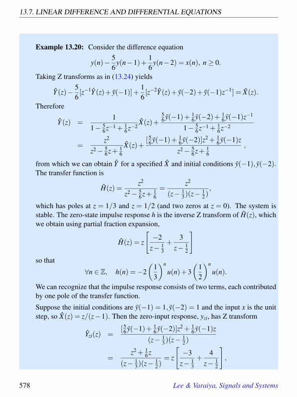
13.7. LINEAR DIFFERENCE AND DIFFERENTIAL EQUATIONS
Example 13.20: Consider the difference equation
y(n)− 56
y(n−1)+16
y(n−2) = x(n), n≥ 0.
Taking Z transforms as in (13.24) yields
Y (z)− 56[z−1Y (z)+ y(−1)]+
16[z−2Y (z)+ y(−2)+ y(−1)z−1] = X(z).
Therefore
Y (z) =1
1− 56 z−1 + 1
6 z−2X(z)+
56 y(−1)+ 1
6 y(−2)+ 16 y(−1)z−1
1− 56 z−1 + 1
6 z−2
=z2
z2− 56 z+ 1
6
X(z)+[5
6 y(−1)+ 16 y(−2)]z2 + 1
6 y(−1)z
z2− 56 z+ 1
6
,
from which we can obtain Y for a specified X and initial conditions y(−1), y(−2).The transfer function is
H(z) =z2
z2− 56 z+ 1
6
=z2
(z− 13)(z− 1
2),
which has poles at z = 1/3 and z = 1/2 (and two zeros at z = 0). The system isstable. The zero-state impulse response h is the inverse Z transform of H(z), whichwe obtain using partial fraction expansion,
H(z) = z
[−2
z− 13
+3
z− 12
]so that
∀n ∈ Z, h(n) =−2(
13
)n
u(n)+3(
12
)n
u(n).
We can recognize that the impulse response consists of two terms, each contributedby one pole of the transfer function.
Suppose the initial conditions are y(−1) = 1, y(−2) = 1 and the input x is the unitstep, so X(z) = z/(z−1). Then the zero-input response, yzi, has Z transform
Yzi(z) =[5
6 y(−1)+ 16 y(−2)]z2 + 1
6 y(−1)z
(z− 13)(z− 1
2)
=z2 + 1
6 z
(z− 13)(z− 1
2)= z
[−3
z− 13
+4
z− 12
],
578 Lee & Varaiya, Signals and Systems

13. LAPLACE AND Z TRANSFORMS
so
∀n, yzi(n) =−3(
13
)n
u(n)+4(
12
)n
u(n).
The zero-state response, yzs, has Z transform
Yzs(z) = H(z)X(z) =z3
(z− 13)(z− 1
2)(z−1)
= z
[1
z− 13
+−3
z− 12
+3
z−1
],
so
∀n, yzs(n) =(
13
)n
u(n)−3(
12
)n
u(n)+3u(n).
The (total) response
∀n ∈ Z, y(n) = yzs(n)+ yzi(n) = 3u(n)+ [−2(1/3)n +(1/2)n]u(n),
can also be expressed as the sum of the steady-state and the transient response withyss(n) = 3u(n) and ytr(n) = −2(1/3)nu(n)+ (1/2)nu(n). Note that the decompo-sition of the response into the sum of the zero-state and zero-input responses isdifferent from its decomposition into the steady-state and transient responses.
13.7.1 LTI differential equations
The analogous development for continuous time concerns systems described by a LTIdifferential equation of the form
dmydtm (t)+am−1
dm−1ydtm−1 (t)+ · · ·+a1
dydt
(t)+a0y(t)
= bkdkxdtk (t)+ · · ·+b1
dxdt
(t)+b0x(t), t ≥ 0. (13.27)
We interpret this equation as describing a causal continuous-time LTI system in whichx(t) is the input and y(t) is the output at time t. The constant coefficients ai and b j specifythe system.
Lee & Varaiya, Signals and Systems 579

13.7. LINEAR DIFFERENCE AND DIFFERENTIAL EQUATIONS
In section 8.2.1 we used this form to find the frequency response. In example 13.11, weused the Laplace transform to find the transfer function of a tuning force. But in bothcases, we assumed that the system was initially at rest. We now develop a method to findthe response to arbitrary initial conditions. We begin with a simple circuit example.
Example 13.21: A series connection of a resistor R, a capacitor C, and a voltagesource x, is described by the differential equation
dydt
(t)+1
RCy(t) = x(t),
in which y is the voltage across the capacitor. The differential equation is obtainedfrom Kirchhoff’s voltage law. The transfer function of this system is H(s) = 1/(s+1/RC). So if the system is initially at rest, we can calculate the response y from itsLaplace transform Y = HX . For instance, if the input is a unit step, X(s) = 1/s,
Y (s) =1
(s+1/RC)s=−RC
s+1/RC+
RCs,
therefore, y(t) =−RCe−t/RC +RC, t ≥ 0.
We cannot use this transfer function, however, to determine the response if theinitial capacitor voltage is y(0) = y(0) and x(t) = 0, t ≥ 0. The response in this caseis
y(t) = y(0)e−t/RC, t ≥ 0.
We can check that expression is correct by verifying that it satisfies the given initialcondition and the differential equation.
If the initial condition is y(0) = y(0) and the input is a unit step, the response turnsout to be the sum of the response due to the input (with zero initial condition) andthe response due to the initial condition (with zero input),
y(t) = [−RCe−t/RC +RC]+ [y(0)e−t/RC], t ≥ 0.
For the general case (13.27) we assume that the input x starts at some finite time whichwe take to be zero, so x(t) = 0, t < 0. We wish to calculate y(t), t ≥ 0. From the theory of
580 Lee & Varaiya, Signals and Systems

13. LAPLACE AND Z TRANSFORMS
differential equations we know that we need to be given m initial conditions,
y(0) = y(0),dydt
(0) = y(1)(0), · · · , dm−1ydtm−1 (0) = y(m−1)(0),
in order to calculate y(t), t ≥ 0.
Because time is continuous, there is no recursive procedure for calculating the outputfrom the given data as we did in (13.22). Instead we calculate the output signal using theLaplace transform. We define the Laplace transforms of the signals y(t)u(t),y(1)(t)u(t), · · · ,y(m)(t)u(t),x(t)u(t):
Y (s) =∫
∞
−∞
y(t)u(t)e−stdt =∫
∞
0y(t)e−stdt
Y (i)(s) =∫
∞
−∞
y(i)(t)u(t) =∫
∞
0y(i)(t)e−stdt, i = 1, · · · ,m
X(s) =∫
∞
−∞
x(t)u(t)e−stdt =∫
∞
0x(t)e−stdt.
Here we use the notation y(i)(t) = ditdt i y(t), t ≥ 0. We now derive the relations between
these Laplace transforms.
The derivative y(1)(t) = dydt (t) and y are related by
y(t)u(t) = y(0)u(t)+∫ t
0y(1)(τ)u(τ)dτ = y(0)u(t)+
∫ t
0y(1)(τ)u(τ)dτ, t ∈ R.
Using integration by parts,
Y (s) =∫
∞
0y(t)e−stdt =
∫∞
0y(0)e−stdt +
∫∞
0
(∫ t
0y(1)(τ)dτ
)e−stdt
=1s
y(0)− 1s
∫ t
0y(1)(τ)dτe−st |∞t=0 +
1s
∫∞
0y(1)(t)e−stdt
=1s[Y (1)(s)+ y(0)].
Therefore,
Y (1)(s) = sY (s)− y(0). (13.28)
Repeating this procedure, we get the Laplace transforms of the higher-order derivatives,
Y (2)(s) = sY (1)(s)− y(1)(0)
= s2Y (s)− sy(0)− y(1)(0)
· · ·Y (m)(s) = smY (s)− sm−1y(0)− sm−2y(1)(0)−·· ·− y(m−1)(0).
Lee & Varaiya, Signals and Systems 581

13.7. LINEAR DIFFERENCE AND DIFFERENTIAL EQUATIONS
On the other hand, because x(i)(t) = dixdt i (t) for all t ∈R, using the differentiation property
in table 13.4, we obtain
X (1)(s) = sX(s)
· · ·X (k)(s) = skX(s).
By substituting from the relations just derived, we obtain the Laplace transforms of all theterms in (13.27),
[smY (s)− sm−1y(0)−·· ·− ym−1(0)]
+ am−1[sm−1Y (s)− sm−2y(0)−·· ·− ym−2(0)]
· · ·+ a1[sY (s)− y(0)]
+ a0Y (s)
= bkskX(s)+ · · ·+b1sX(s)+b0X(s). (13.29)
Rearranging terms yields
[sm +am−1sm−1 + · · ·+a1s+a0]Y (s) = [bksk + · · ·+b1s+b0]X(s)+C(s),
in which C is an expression involving only the intial conditions
y(0), · · · , y(m−1)(0).
Therefore,
Y (s) =bksk +bk−1sk−1 + · · ·b1s+b0
sm +am−1sm−1 + · · ·a1s+a0X(s)+
C(s)sm +am−1sm−1 + · · ·a1s+a0
, (13.30)
which we also write as
Y (s) = H(s)X(s)+C(s)
sm +am−1sm−1 + · · ·a1s+a0, (13.31)
in which
H(s) =bksk + · · ·+b1s+b0
sm + · · ·+a1s+a0. (13.32)
582 Lee & Varaiya, Signals and Systems

13. LAPLACE AND Z TRANSFORMS
If the initial conditions are all zero, C(s) = 0, and we only have the first term on the rightin (13.31); if the input is zero—i.e., x(t) = 0 for all t, then X(s) = 0, and we only get thesecond term in (13.31).
By definition, Y (s) is the Laplace transform of the causal signal y(t)u(t), t ∈ R. So itsRoC = s ∈ C | Res > Rep, where p is a pole of the right side of (13.31) with thelargest real part.
Taking the inverse Laplace transform of Y , we can decompose the output signal y as
∀t, y(t) = yzs(t)+ yzi(t),
where yzs, the inverse Laplace transform of HX , is the zero-state or forced response andyzi, the inverse Laplace transform of C(s)/[sm + · · ·+ a0], is the zero-input or naturalresponse. The (total) response is the sum of the zero-state and zero-input response, whichis a general property of linear systems.
By definition, the transfer function is the Laplace transform of the zero-state impulseresponse. Taking C = 0 and X = 1 (the Laplace transform of the unit impulse) in (13.31)shows that the transfer function is H(s) which, as we see from (13.32), can be writtendown by inspection of the differential equation (13.27). If the system is stable—all polesof H(s) have real parts strictly less than zero—the frequency response is, as in (8.23)
∀ω, H(ω) = H(iω) =bk(iω)k + · · ·+b1iω+b0
(iω)m + · · ·+a1iω+a0.
Example 13.22: We find the response y(t), t ≥ 0, for the differential equation
d2ydt2 +3
dydt
+2y = 3x(t)+dxdt
,
when the input is a unit step x(t) = u(t) and the initial conditions are y(0) =1,y(1)(0) = 2. Taking Laplace transforms of both sides as in (13.29),
[s2Y (s)− sy(0)− y(1)(0)]+3[sY (s)− y(0)]+2Y (s) = 3X(s)+ sX(s).
Therefore,
Y (s) =s+3
s2 +3s+2X(s)+
sy(0)+ y(1)(0)+3y(0)s2 +3s+2
.
Lee & Varaiya, Signals and Systems 583

13.8. STATE-SPACE MODELS
Substituting X(s) = 1/s, y(0) = 1, y(1) = 2, yields
Y (s) =s+3
s(s2 +3s+2)+
s+5s2 +3s+2
= [3/2
s− 2
s+1+
1/2s+2
]+ [4
s+1− 3
s+2].
Taking inverse Laplace transforms gives
∀t, y(t) = yzs(t)+ yzi(t)
= [32
u(t)−2e−tu(t)+12
e−2tu(t)]+ [4e−tu(t)−3e−2tu(t)]
=32
u(t)+ [2e−t − 52
e−2t ]u(t)
= yss(t)+ ytr(t).
As in the case of difference equations, the decomposition of the response into zero-state and zero-input responses is different from the decomposition into transientand steady-state responses. (Indeed, the steady-state response does not exist if thesystem is unstable, whereas the former decomposition always exists.)
13.8 State-space models
This section is mathematically more advanced in that it uses the operation of matrix in-verse.
In section 5.3 we introduced single-input, single-output (SISO) multidimensional state-space models of discrete-time and continuous-time LTI systems. For LTI systems, state-space models provide an alternative description to difference or differential equation rep-resentations. The advantage of state-space models is that by using matrix notation wehave a very compact representation of the response, independent of the order of the sys-tem. We develop a method that combines this matrix notation with transform techniquesto calculate the response.
584 Lee & Varaiya, Signals and Systems

13. LAPLACE AND Z TRANSFORMS
The discrete-time SISO state-space model is
∀ n≥ 0, s(n+1) = As(n)+bx(n), (13.33)
y(n) = cT s(n)+dx(n), (13.34)
in which s(n) ∈ RN is the state, x(n) ∈ R is the input, and y(n) ∈ R is the output at timen. In this [A,b,c,d] representation, A is an N×N (square) matrix, b,c are N-dimensionalcolumn vectors, and d is a scalar. If the initial state is s(0), and the input sequence isx(0),x(1), · · · , by recursively using (13.33) and (13.34) we obtain the state and outputresponses:
s(n) = Ans(0)+n−1
∑m=0
An−1−mbx(m), (13.35)
y(n) = cT Ans(0)+n−1
∑m=0
cT An−1−mbx(m)+dx(n), (13.36)
for all n≥ 0. Notice that these “closed-form” formulas for the response are independent ofthe order N. Difference equation representations do not have such a closed-form formula.
Example 13.23: Consider the system described by the difference equation
y(n)−2y(n−1)−3y(n−2) = x(n).
As in section 5.3, we can construct a state-space model for this system by notingthat the state at time n should remember the previous two inputs y(n−1),y(n−2).Define the two-dimensional state vector s(n) = [s1(n) s2(n)]T by s1(n) = y(n−1),s2(n) = ay(n− 2), in which a 6= 0 is a constant. Problem 23 at the end of thischapter asks you to show that the [A,b,c,d] representation for this choice of state isgiven by
A =
[2 3/aa 0
], b =
[10
], cT = [2 3/a], and d = 1.
Different choices of a give a different state-space model. However, they all havethe same input-output relation because they all have the same transfer function.
Lee & Varaiya, Signals and Systems 585

13.8. STATE-SPACE MODELS
We will obtain the Z transforms of the response sequences (13.35), (13.36). The key isto compute the Z transform of the entire N×N matrix sequence Anu(n),n ∈ Z. This Ztransform is
∞
∑n=0
z−nAn = [I− z−1A]−1 = z[zI−A]−1. (13.37)
Here z is a complex number and I is the N×N identity matrix. The series on the left isan infinite sum of N×N matrices which converges to the N×N matrix on the right, forz ∈ RoC. RoC is determined later.
Assuming the series converges, it is easy to check the equality (13.37): Just multiply bothsides by [I− z−1A] and verify that
[I− z−1A]∞
∑n=0
z−nAn =∞
∑n=0
z−nA−n−∞
∑n=0
z−(n+1)An+1 = z0A0 = I.
Next, denote by F the matrix inverse,
F(z) = [I− z−1A]−1 = z[zI−A]−1, (13.38)
and the coefficients of An and F(z) by
An = [ai j(n) | 1≤ i, j ≤ N], F(z) = [ fi j(z) | 1≤ i, j ≤ N].
Then fi j(z) =∑∞n=0 z−nai j(n) is the Z transform of the sequence ai j(n),n≥ 0, 1≤ i, j≤N.
So we can obtain An,n≥ 0, by taking the inverse Z transform of each of the N2 coefficientsof F(z).
Example 13.24: Let
A =
[2 13 4
],
then
[zI−A]−1 =
[z−2 −1−3 z−4
]−1
=1
det[zI−A]
[z−4 1
3 z−2
],
in which det[zI−A] denotes the determinant of [zI−A],
det[zI−A] = (z−2)(z−4)−3 = z2−6z+5 = (z−1)(z−5).
586 Lee & Varaiya, Signals and Systems

13. LAPLACE AND Z TRANSFORMS
Hence,
F(z) = z[zI−A]−1 =z
(z−1)(z−5)
[z−4 1
3 z−2
]
=
z(z−4)
(z−1)(z−5)z
(z−1)(z−5)
3z(z−1)(z−5)
z(z−2)(z−1)(z−5)
.The partial fraction expansion of the coefficients of F is
F(z) =
(3/4)zz−1 + (1/4)z
z−5(−1/4)z
z−1 + (1/4)zz−5
(−3/4)zz−1 + (3/4)z
z−5(1/4)zz−1 + (3/4)z
z−5
.Using table 13.1 we find the inverse Z transform of every coefficient of F(z): forall n ∈ Z,
Anu(n) =
34 u(n)+ 1
4 5nu(n) −14 u(n)+ 1
4 5nu(n)
−34 u(n)+ 3
4 5nu(n) 14 u(n)+ 3
4 5nu(n)
.This is more revealingly expressed as
An =
[3/4 −1/4−3/4 1/4
]+5n
[1/4 1/43/4 3/4
], n≥ 0,
because it shows that the variation in n of An is determined by the two poles, atz = 1 and z = 5, in the coefficients of F(z). Moreover, these two poles are the zerosof
det[zI−A] = (z−1)(z−5).
This determinant is called the characterstic polynomial of the matrix A and itszeros are called the eigenvalues of A. The domain of convergence is RoC = z ∈C | |z|> 5.
Lee & Varaiya, Signals and Systems 587

13.8. STATE-SPACE MODELS
We return to the general case in (13.38). Denote the matrix inverse of [zI−A] as
[zI−A]−1 =1
det[zI−A]G(z),
in which G(z) is the N×N matrix of co-factors of [zI−A]. It follows that each coefficientfi j(z) of F(z) = z[zI−A]−1 is a rational polynomial whose denominator is the character-istic polynomial of A, det[zI−A]. Therefore, if there are no pole-zero cancellations, allcoefficients of F(z) have the same poles, which are the zeros of det[zI−A]. These zerosare called the eigenvalues of A. The polynomial det[zI−A] is of order N, and so A has Neigenvalues.
Because Anu(n),n ∈ Z, is a causal sequence, the region of convergence is RoC = z ∈C | |z|> |p|, in which p is the pole of F (or eigenvalue of A) with the largest magnitude.For the system (13.33), (13.34) to be stable, the poles of F must have magnitudes strictlysmaller than 1.
Suppose A has N distinct eigenvalues p1, · · · , pN ,
det[zI−A] = (z− p1) · · ·(z− pN).
Then the partial fraction expansion of F(z) has the form
F(z) =z
z− p1R1 + · · ·+
zz− pN
RN ,
in which Ri is the matrix of residues of the coefficients of F at the pole pi. Ri is a constantmatrix, possibly with complex coefficients if pi is complex. Recalling that z
z−piis the
inverse Z transform of pni u(n), we can take the inverse Z transform of F(z) to conclude
thatAn = pn
1R1 + · · · pnNRN , n≥ 0. (13.39)
Thus An is a linear combination of pn1, · · · , pn
N .
We can decompose the response (13.36) into the zero-input and zero-state responses,expressing the latter as a convolution sum,
y(n) = cT Ans(0)+n
∑m=0
h(n−m)x(m), n≥ 0,
where the (zero-state) impulse response is
h(n) =
0, n < 0d, n = 0cT An−1b, n≥ 1
.
588 Lee & Varaiya, Signals and Systems

13. LAPLACE AND Z TRANSFORMS
Let X ,Y , H,Yzi be the Z transforms:
X(z) =∞
∑n=0
x(n)z−n, Y (z) =∞
∑n=0
y(n)z−n,
H(z) =∞
∑n=0
h(n)z−n, Yzi(z) =∞
∑n=0
cT z−nAns(0).
ThenY = HX + Yzi.
Because ∑∞n=0 z−nAn = z[zI−A]−1, we obtain
H(z) = cT [zI−A]−1b+d,
andYzi(z) = zcT [zI−A]−1s(0).
Example 13.25: Suppose A is as in example 13.24, bT = [1 1],cT = [2 0],d = 3,and (s(0))T = [0 4]. Then the transfer function is
H(z) = [2 0]
(z−4)
(z−1)(z−5)1
(z−1)(z−5)
3(z−1)(z−5)
(z−2)(z−1)(z−5)
[ 11
]+3 =
2(z−4)+2(z−1)(z−5)
+3,
and the Z transform of the zero-input response is
Yzi(z) = [2 0]
z(z−4)
(z−1)(z−5)z
(z−1)(z−5)
3z(z−1)(z−5)
z(z−2)(z−1)(z−5)
[ 04
]=
8z(z−1)(z−5)
.
The transfer function
H(z) =2(z−4)+2(z−1)(z−5)
+3 =3z2−16z+9z2−6z+5
=3−16z−1 +9z−2
1−6z−1 +5z−2 .
Lee & Varaiya, Signals and Systems 589

13.8. STATE-SPACE MODELS
From (13.26) we recognize that H is also the transfer function of the differenceequation
y(n)−6y(n−1)+5y(n−2) = 3x(n)−16x(n−1)+9x(n−2).
This difference equation describes the same input-output relation as the state-spacemodel of this example.
13.8.1 Continuous-time state-space models
The continuous-time SISO state-space model introduced in section 5.4 has the represen-tation in terms of [A,b,c,d]
v(t) = Av(t)+bx(t), (13.40)
y(t) = cT v(t)+dx(t), (13.41)
in which v(t) ∈ RN is the state, x(t) ∈ R is the input, and y(t) ∈ R is the output at timet ∈R. A is an N×N matrix, and b,c are N-dimensional column vectors, and d is a scalar.(We use v instead of s to denote the state, because s is reserved for the Laplace transformvariable.)
Given the initial state v(0) and the input signal x(t), t ≥ 0, we will show that the stateresponse and the output response obey the formulas
v(t) = etAv(0)+∫ t
0e(t−τ)Abx(τ)dτ, (13.42)
y(t) = cT etAv(0)+ [∫ t
0cT e(t−τ)Abx(τ)dτ]+dx(t). (13.43)
In these formulas, etA or exp(tA) is the name of the N×N matrix
etA =∞
∑k=0
(tA)k
k!= I + tA+
(tA)2
2!+
(tA)3
3!+ · · · , (13.44)
where (tA)k is the matrix tA multiplied by itself k times, and (tA)0 = I, the N×N identitymatrix. Definition (13.44) of the matrix exponential is the natural generalization of theexponential of a real or complex number. (The series in (13.44) is absolutely summablebecause of the factor k! in the denominator.)
590 Lee & Varaiya, Signals and Systems

13. LAPLACE AND Z TRANSFORMS
Unlike in the discrete-time case, there is no recursive procedure to compute the responses(13.42), (13.43). This is because time is continuous, and the difficulty has to do withthe integrals in these formulas. For numerical calculation, one resorts to a finite sumapproximation of the integrals, as we indicated in Section 5.4. The Laplace transformprovides an alternative approach that is exact.
The key to showing (13.42) is the fact that etA, t ≥ 0, is the solution to the differentialequation
ddt
etA = AetA, t ≥ 0, (13.45)
with initial condition e0A = I. Note that (13.43) follows immediately from (13.42) and(13.41).
To verify (13.45) we substitute for etA from (13.44) and differentiate the sum term byterm,
ddt
etA =∞
∑k=0
ddt
(tA)k
k!=
∞
∑k=1
kAk!
(tA)k−1 = A∞
∑k=1
(tA)k−1
(k−1)!= AetA.
We can now check that (13.42) is indeed the solution of (13.40) by taking derivatives ofboth sides and using (13.45):
v(t) = AetAv(0)+ e0Abx(t)+∫ t
0Ae(t−τ)Abx(τ)dτ
= A[etAv(0)+∫ t
0Ae(t−τ)Abx(τ)dτ]+bx(t)
= Av(t)+bx(t).
We turn to the main difficulty in calculating the terms on the right in the responses (13.42),(13.43), namely the calculation of the N×N matrix etA, t ≥ 0. We determine the Laplacetransform of etAu(t), t ∈ R, denoting it by
G(s) =∫
∞
0etAe−stdt.
This means that gi j(s) is the Laplace transform of ai j(t), t ≥ 0, denoting by ai j(t) andgi j(s) the coefficients of the N ×N matrices etA and G(s), respectively. The region ofconvergence of G, RoC, is determined later.
Using the derivative formula (13.28) in (13.45) we see that
sG(s)− I = AG(s),
Lee & Varaiya, Signals and Systems 591
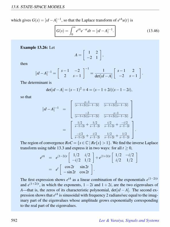
13.8. STATE-SPACE MODELS
which gives G(s) = [sI−A]−1, so that the Laplace transform of etAu(t) is
G(s) =∫
∞
0etAe−stdt = [sI−A]−1. (13.46)
Example 13.26: Let
A =
[1 2−2 1
],
then
[sI−A]−1 =
[s−1 −2
2 s−1
]−1
=1
det[sI−A]
[s−1 2−2 s−1
].
The determinant is
det[sI−A] = (s−1)2 +4 = (s−1+2i)(s−1−2i),
so that
[sI−A]−1 =
s−1
(s−1+2i)(s−1−2i)2
(s−1+2i)(s−1−2i)
−2(s−1+2i)(s−1−2i)
s−1(s−1+2i)(s−1−2i)
=
1/2s−1+2i +
1/2s−1−2i
i/2s−1+2i +
−i/2s−1−2i
−i/2s−1+2i +
i/2s−1−2i
1/2s−1+2i +
1/2s−1−2i
.The region of convergence RoC = s∈C | Res> 1. We find the inverse Laplacetransform using table 13.3 and express it in two ways: for all t ≥ 0,
etA = e(1−2i)t[
1/2 i/2−i/2 1/2
]+ e(1+2i)t
[1/2 −i/2i/2 1/2
]= et
[cos2t sin2t−sin2t cos2t
].
The first expression shows etA as a linear combination of the exponentials e(1−2i)t
and e(1+2i)t , in which the exponents, 1− 2i and 1+ 2i, are the two eigenvalues ofA—that is, the zeros of its characteristic polynomial, det[sI−A]. The second ex-pression shows that etA is sinusoidal with frequency 2 radians/sec equal to the imag-inary part of the eigenvalues whose amplitude grows exponentially correspondingto the real part of the eigenvalues.
592 Lee & Varaiya, Signals and Systems

13. LAPLACE AND Z TRANSFORMS
Returning to the general case (13.46), denote the matrix inverse of [sI−A] as
G(s) = [sI−A]−1 =1
det[sI−A]K(s),
in which K(s) is the N ×N matrix of co-factors of [sI−A]. Each coefficient gi j(s) ofG(s) is a rational polynomial of A whose denominator is the characterstic polynomial ofA, det[sI−A]. Therefore, if there are no pole-zero cancellations, all coefficients of G(s)have the same poles—the eigenvalues of A. Because etAu(t), t ∈ R, is a causal signal,the region of convergence of its Laplace transform G(s) is s ∈ C | Res > Rep, inwhich p is the pole of G with the largest real part.
Because det[sI−A] is a polynomial of order N, G has N poles. For the system (13.40),(13.41) to be stable, the poles of G(s) must have strictly negative real parts. The systemof example (13.26) is unstable, because the real part of the eigenvalues is +1.
Suppose the characteristic polynomial has N distinct zeros p1, · · · , pN ,
det[sI−A] = (s− p1) · · ·(s− pN).
Then the partial fraction expansion of G(s) has the form
G(s) = [sI−A]−1 =1
s− p1R1 + · · ·+
1s− pN
RN ,
in which Ri is the matrix of residues at the pole pi of the coefficients of G(s). Ri is aconstant matrix, possibly with complex coefficients, if pi is complex. Because the inverseLaplace transform of 1
s−piis epitu(t), the inverse Laplace transform of [sI−A]−1 is
etAu(t) = [ep1tR1 + · · ·+ epNtRN ]u(t). (13.47)
Thus the matrix etA as a function of t is a linear combination of ep1t , · · · ,epNt , where thepi are the eigenvalues of A—that is the zeros of det[sI−A].
We decompose the response (13.43) into the sum of the zero-input and zero-state re-sponses, expressing the latter as a convolution integral,
y(t) = cT etAv(0)+∫ t
0h(t− τ)x(τ)dτ, t ≥ 0,
in which the (zero-state) impulse response is: for all t ∈ R,
h(t) = cT etAbu(t)+dδ(t).
Lee & Varaiya, Signals and Systems 593

13.8. STATE-SPACE MODELS
(Here δ is the Dirac delta function.) Let X ,Y , H,Yzi be the Laplace transforms
X(s) =∫
∞
0 x(t)e−stdt, Y (s) =∫
∞
0y(t)e−stdt,
H(s) =∫
∞
−∞h(t)e−stdt, Yzi(s) =
∫∞
0cT etAv(0)e−stdt.
ThenY = HX + Yzi,
in whichH(s) = cT [sI−A]−1b+d,
andYzi(s) = cT [sI−A]−1v(0).
We continue with example 13.26.
Example 13.27: Suppose A is as in example 13.26, bT = [1 1]T ,cT = [2 0]T ,d = 3,and v(0)T = [0 4]T . Then the transfer function is
H(s) = [2 0]
s−1
(s−1)2−4−2
(s−1)2−4
2(s−1)2−4
s−1(s−1)2−4
[ 11
]+3 =
2s−6(s−1)2−4
+3,
and the Laplace transform of the zero-input response is
Yzi(s) = [2 0]
s−1
(s−1)2−4−2
(s−1)2−4
2(s−1)2−4
s−1(s−1)2−4
[ 04
]=
−16(s−1)2−4
.
The transfer function
H(s) =2s−6
(s−1)−4+3 =
3s2−4s−15s2−2s−3
.
From (13.32) we know that H is also the transfer function of the differential equa-tion
d2ydt2 (t)−2
dydt
(t)−3y(t) = 3d2xdt2 (t)−4
dxdt
(t)−15x(t).
Thus this differential equation describes the same system as the state-space modelof example 13.24.
594 Lee & Varaiya, Signals and Systems

13. LAPLACE AND Z TRANSFORMS
This example illustrates a general way of obtaining a differential equation description ofa continuous-time state-space model by means of its transfer function.
It is easier to obtain a state-space model with a specified proper transfer function,
H(s) =bN−1sN−1 + · · ·+b1s+b0
sN + · · ·+a1s+a0+bN .
(The first term in H is strictly proper. Some of the coefficients bi,a j may be zero.) Thenthe N-dimensional [A,b,c,d] representation
A =
0 1 0 · · · 00 0 1 · · · 0· · · · · · · · · · · ·0 0 0 · · · 1−a0 −a1 −a2 · · · −aN−1
, b =
00· · ·01
,
cT = [b0b1 · · ·bN−1], d = bN . (13.48)
has the same transfer function as H, that is
cT [sI−A]−1b+d = H(s). (13.49)
Exercise 30 at the end of this chapter asks you to verify (13.49).
Simply by interchanging the variables s and z we see that the proper rational polynomial
H(z) =bN−1zN−1 + · · ·+b1z+b0
zN + · · ·+a1z+a0+bN = d + cT [zI−A]−1b
is the transfer function of the discrete-time [A,b,c,d] representation.
Thus we can use any of three equivalent representations of LTI systems:
• difference or differential equations, used to describe many physical systems,
• transfer functions used for frequency-domain analysis, and in feedback design con-sidered in the next chapter,
• state-space models, used in modern control theory.
Lee & Varaiya, Signals and Systems 595

13.9. SUMMARY
13.9 Summary
The Z transform and Laplace transform have many of the same properties as the Fouriertransforms. They are linear, which greatly facilitates computation of the transforms andtheir inverses. Moreover, the Z transform (Laplace transform) of the output of an LTIsystem is the product of the Z transforms (Laplace transforms) of the input and the transferfunction. Thus, the Z transform (Laplace transform) plays the same role as the frequencyresponse, describing the relationship between the input and the output as a product ratherthan a convolution.
Linear difference and differential equations, and state-space models of LTI systems wereintroduced in Chapter 5 and Chapter 8. However, we lacked a method to calculate theresponse of these models for non-zero initial conditions. The Z transform and the Laplacetransform provide such a method.
596 Lee & Varaiya, Signals and Systems

13. LAPLACE AND Z TRANSFORMS
Probing Further: Derivatives of Z transforms
Calculus on complex-valued functions of complex variables can be intricate. Suppose Xis a function of a complex variable. The derivative can be defined as a limit,
ddz
X(z) = limε→0
X(z+ ε)− X(z)ε
,
where ε is a complex variable that can approach zero from any direction in the complexplane. The derivative exists if the limit does not depend on the direction. If the derivativeexists at all points within a distance ε > 0 of a point z in the complex plane, then X issaid to be analytic at z. A Z transform is a series of the form
∀ z ∈ RoC(x), X(z) =∞
∑n=−∞
x(n)z−n.
This is called a Laurent series in the theory of complex variables. It can be shown thata Laurent series is analytic at all points z ∈ RoC(x), and that the derivative is
∀ z ∈ RoC(x),ddz
X(z) =∞
∑m=−∞
−mx(m)z−m−1.
We can use this fact to show that the Z transform of y given by y(n) = nx(n) is
∀z ∈ Roc(x), Y (z) =−zddz
X(z).
This is because
Y (z) =∞
∑n=−∞
nx(n)z−n =∞
∑n=−∞
(−z)ddz
x(n)z−n =−zddz
X(z).
It is not difficult to show that Roc(y) = Roc(x) (see Exercise 5).This property can be used to find other Z transforms. For example, the Z transform
of the unit step, x = u, is X(z) = z/(z− 1), with RoC(x) = z ∈ C | |z| > 1. So the Ztransform of the unit ramp y, given by y(n) = nu(n), is
Y (z) =−zddz
zz−1
=z
(z−1)2 ,
with RoC(y) = z ∈C | |z|> 1. Another method for finding the Z transform of the unitramp is given in Exercise 3 of Chapter 12.
Lee & Varaiya, Signals and Systems 597

13.9. SUMMARY
|z|=1
Re z
Im z
3
Figure 13.2: Pole-zero plot for a length-4 moving average system.
Im s
Re s
RoC
s = iω
s = − iω
Figure 13.3: Pole-zero plot for the sinusoidal signal y of example 13.10.
598 Lee & Varaiya, Signals and Systems

13. LAPLACE AND Z TRANSFORMS
Im s
Re s
RoC
s = − 1 + i
2 4 6− 2− 4− 6
ω
|H(ω)|
s = − 1 − i
Im s
Re s
RoC
s = − 0.5 + i
s = − 0.5 − i
Im s
Re s
RoC
s = − 0.1 + i
s = − 0.1 − i
Figure 13.4: Pole-zero plots for the three transfer functions in example 13.12, andthe three corresponding magnitude frequency responses.
Lee & Varaiya, Signals and Systems 599

13.9. SUMMARY
Probing Further: Inverse transform as an integral
Even if the Z transform is not a rational polynomial, we can recover the signal x from itsZ transform, X : RoC(x)→C, using the DTFT. A non-empty RoC(x) contains the circleof radius r for some r > 0. So the series in the equation
X(reiω) =∞
∑m=−∞
x(m)(reiω)−m =∞
∑m=−∞
(x(m)r−m)e−iωm
is absolutely summable. Hence the signal xr: ∀n,xr(n) = x(n)r−n, has DTFT Xr:∀ω,Xr(ω) = X(reiω). We can, therefore, obtain xr as the inverse DTFT of Xr
∀n, xr(n) = r−nx(n) =1
2π
∫ 2π
0X(reiω)eiωndω.
Multiplying both sides by rn, we can recover x as
∀n ∈ Z, x(n) =1
2π
∫ 2π
0X(reiω)(reiω)ndω. (13.15)
This formula defines the inverse Z transform as an integral of the real variable ω. (Con-tinued on page 601.)
600 Lee & Varaiya, Signals and Systems

13. LAPLACE AND Z TRANSFORMS
Probing Further: (Continued) Inverse transform
It is conventional to write the inverse Z transform differently. Express z as z= reiω. Thenas ω varies from 0 to 2π, z varies as
dz = reiωidω = zidω, or dω =dziz.
Substituting this in (13.15) gives,
∀n, x(n) =1
2π
∮X(z)zn dz
iz=
12πi
∮X(z)zn−1dz.
Here the ‘circle’ in the integral sign,∮
, means that the integral in the complex z-planeis along any closed counterclockwise circle contained in RoC(x). (An integral along aclosed contour is called a contour integral.) In summary,
∀n ∈ Z, x(n) =1
2πi
∮X(z)zn−1dz, (13.16)
where the integral is along any closed counterclockwise circle inside RoC(x).We can similarly use the CTFT to recover any continuous-time signal x from its
Laplace transform by
∀t ∈ R, x(t) =1
2πi
σ+i∞∫σ−i∞
X(s)estds
where the integral is along any vertical line (σ− i∞,σ+ i∞) contained in RoC(x).
Lee & Varaiya, Signals and Systems 601

13.9. SUMMARY
Probing Further: Differentiation and Laplace transforms
We can use the inverse Laplace transform as given in the box on page 600 to demon-strate the differentiation property in table 13.4. Let y be defined by
∀ t ∈ R, y(t) =ddt
x(t).
We can write x in terms of its Laplace transform as
∀t ∈ R, x(t) =1
2πi
∫σ+i∞
σ−i∞X(s)estds.
Differentiating this with respect to t is easy,
∀t ∈ R,ddt
x(t) =1
2πi
∫σ+i∞
σ−i∞sX(s)estds.
Consequently, y(t) = dx(t)/dt is the inverse transform of sX(s), so
∀ s ∈ RoC(y), Y (s) = sX(s),
where RoC(y)⊃ RoC(x).
602 Lee & Varaiya, Signals and Systems

13. LAPLACE AND Z TRANSFORMS
Exercises
Each problem is annotated with the letter E, T, C which stands for exercise, requires somethought, requires some conceptualization. Problems labeled E are usually mechanical,those labeled T require a plan of attack, those labeled C usually have more than onedefensible answer.
1. E Consider the signal x given by
∀n, x(n) = sin(ω0n)u(n).
(a) Show that the Z transform is
∀ z ∈ RoC(x), X(z) =zsin(ω0)
z2−2zcos(ω0)+1,
whereRoC(x) = z ∈ C | |z|> 1.
(b) Where are the poles and zeros?
(c) Is x absolutely summable?
2. T Consider the signal x given by
∀ n ∈ Z, x(n) = a|n|,
where a ∈ C.
(a) Find the Z transform of x. Be sure to give the region of convergence.
(b) Where are the poles?
(c) Under what conditions is x absolutely summable?
3. E Consider a discrete-time LTI system with transfer function given by
∀ z ∈ z | |z|> 0.9, H(z) =z
z−0.9.
Suppose that the input x is given by
∀ n ∈ Z, x(n) = δ(n)−0.9δ(n−1).
Find the Z transform of the output y, including its region of convergence.
Lee & Varaiya, Signals and Systems 603

EXERCISES
4. E Consider the exponentially modulated sinusoid y given by
∀ n ∈ Z, y(n) = a−n cos(ω0n)u(n),
where a is a real number, ω0 is a real number, and u is the unit step signal.
(a) Find the Z transform. Be sure to give the region of convergence. Hint: Useexample 13.3 and Section 13.1.6.
(b) Where are the poles?
(c) For what values of a is this signal absolutely summable?
5. T Suppose x ∈ DiscSignals satisfies
∞
∑n=−∞
|x(n)r−n|< ∞, 0 < r1 < r < r2,
for some real numbers r1 and r2 such that r1 < r2. Show that
∞
∑n=−∞
|nx(n)r−n|< ∞, 0 < r1 < r < r2.
Hint: Use the fact that for any ε > 0 there exists N < ∞ such that n(1+ ε)−n < 1for all n > N.
6. T Consider a causal discrete-time LTI system where the input x and output y arerelated by the difference equation
∀ n ∈ Z, y(n)+b1y(n−1)+b2y(n−2) = a0x(n)+a1x(n−1)+a2x(n−2),
where b1, b2, a0, a1, and a2 are real-valued constants.
(a) Find the transfer function.
(b) Say as much as you can about the region of convergence.
(c) Under what conditions is the system stable?
7. E This exercise verifies the time delay property of the Laplace transform. Showthat if x is a continuous-time signal, τ is a real constant, and y is given by
∀ t ∈ R, y(t) = x(t− τ),
604 Lee & Varaiya, Signals and Systems

13. LAPLACE AND Z TRANSFORMS
then its Laplace transform is
∀ s ∈ RoC(y), Y (s) = e−sτX(s),
with region of convergence
RoC(y) = RoC(x).
8. E This exercise verifies the convolution property of the Laplace transform. Sup-pose x and h have Laplace transforms X and H. Let y be given by
∀ t ∈ R, y(t) = (x∗h)(t) =∞∫−∞
x(τ)h(t− τ)dτ.
Then show that the Laplace transform is
∀s ∈ RoC(y), Y (s) = X(s)H(s),
withRoC(y)⊃ RoC(x)∩RoC(h).
9. T This exercise verifies the conjugation property of the Laplace transform, andthen uses this property to demonstrate that for real-valued signals, poles and zeroscome in complex-conjugate pairs.
(a) Let x be a complex-valued continuous-time signal and y be given by
∀ t ∈ R, y(t) = [x(t)]∗.
Show that∀ s ∈ RoC(y), Y (s) = [X(s∗)]∗,
whereRoC(y) = RoC(x).
(b) Use this property to show that if x is real, then complex poles and zeros occurin complex conjugate pairs. That is, if there is a zero at s = q, then there mustbe a zero at s = q∗, and if there is a pole at s = p, then there must also be apole at s = p∗.
Lee & Varaiya, Signals and Systems 605

EXERCISES
10. T This exercise verifies the time scaling property of the Laplace transform. Let ybe defined by
∀ t ∈ R, y(t) = x(ct),
for some real number c. Show that
∀ s ∈ RoC(y), Y (s) = X(s/c)/|c|,
whereRoC(y) = s | s/c ∈ RoC(x).
11. E This exercise verifies the exponential scaling property of the Laplace transform.Let y be defined by
∀ t ∈ R, y(t) = eatx(t),
for some complex number a. Show that
∀ s ∈ RoC(y), Y (s) = X(s−a),
whereRoC(y) = s | s−a ∈ RoC(x).
12. T Consider a discrete-time LTI system with impulse response
∀n, h(n) = an cos(ω0n)u(n),
for some ω0 ∈ R. Show that if the input is
∀ n ∈ Z, x(n) = eiω0nu(n),
then the output y is unbounded.
13. E Find and plot the inverse Z transform of
X(z) =1
(z−3)3
with
(a) Roc(x) = z ∈ C | |z|> 3(b) Roc(x) = z ∈ C | |z|< 3.
606 Lee & Varaiya, Signals and Systems

13. LAPLACE AND Z TRANSFORMS
14. E Obtain the partial fraction expansions of the following rational polynomials. Firstdivide through if necessary to get a strictly proper rational polynomial.
(a)z+2
(z+1)(z+3)
(b)(z+2)2
(z+1)(z+3)
(c)z+2z2 +4
.
15. E Find the inverse Z transform x for each of the three possible regions of conver-gence associated with
X(z) =(z+2)2
(z+1)(z+3).
For which region of convergence is x causal? For which is x strictly anti-causal?For which is x two-sided?
16. E Find the inverse Z transform x for each of the two possible regions of convergenceassociated with
X(z) =z+2z2 +4
.
17. E Consider a stable system with impulse response
h(n) = (0.5)nx(n).
Find the steady-state response to a unit step input.
18. E Let h(n) = 2nu(−n), all n, and g(n) = 0.5nu(n), for all n. Find h ∗ u and g ∗ u,where u is the unit step.
19. E This exercise shows how we can determine the transfer function and frequencyresponse of an LTI system from its step response. Suppose a causal system withstep input x = u, produces the output
∀ n ∈ Z, y(n) = (1−0.5n)u(n).
(a) Find the transfer function (including its region of convergence).
Lee & Varaiya, Signals and Systems 607

EXERCISES
(b) If the system is stable, find its frequency response.
(c) Find the impulse response of the system.
20. E Consider an LTI system with impulse response h given by
∀ n ∈ Z, h(n) = 2nu(n).
(a) Find the transfer function, including its region of convergence.
(b) Use the transfer function to find the Z transform of the step response.
(c) Find the inverse transform of the result of part (b) to obtain the step responsein the time domain.
21. E Determine the zero-input and zero-state responses, and the transfer function forthe following. In both cases take y(−1) = y(−2) = 0 and x(n) = u(n).
(a) y(n)+ y(n−2) = x(n),n≥ 0.
(b) y(n)+2y(n−1)+ y(n−2) = x(n),n≥ 0.
22. E Determine the zero-input and the zero-state responses for the following.
(a) 5y+10y = 2x,y(0) = 2,x(t) = u(t).
(b) y+5y+6y =−4x−3x,y(0) =−1, y(0) = 5,x(t) = e−tu(t).
(c) y+4y = 8x,y(0) = 1, y(0) = 2,x(t) = u(t).
(d) y+2y+5y = x,y(0) = 2, y(0) = 0,x(t) = e−tu(t).
23. E Show that the [A,b,c,d] representation in example 13.23 is correct. Then showthat the transfer function of the state-space model is the same as that of the differ-ence equation.
24. T Consider the circuit of figure 13.5. The input is the voltage x, the output is thecapacitor voltage v. The inductor current is called i.
(a) Derive the [A,b,c,d] representation for this system using s(t) = [i(t),v(t)]T asthe state.
(b) Obtain an [F,g,h,k] representation for a discrete-time model of the samecircuit by sampling at times kT,k = 0,1, · · · and using the approximations(kT ) = 1/T (s((k+ 1)T )− s(kT )). (This is called a forward-Euler approx-imation.)
608 Lee & Varaiya, Signals and Systems

13. LAPLACE AND Z TRANSFORMS
+
-x(t)
R
L
v(t)i(t)
r
C+
-
Figure 13.5: Circuit of problem 24
25. E For the matrix A in example 13.24, determine etA, t ≥ 0.
26. E For the matrix A in example 13.26, determine An,n≥ 0.
27. T A continuous-time SISO system has [A,b,c,d] representation with
A =
[a b−b a
],
in which a,b are real constants.
(a) Find the eigenvalues of A.
(b) For what values of a,b is the SISO system stable?
(c) Calculate etA, t ≥ 0.
(d) Suppose b = c = [1 0]T , and d = 0. Find the transfer function.
28. T Let A be an N ×N matrix. Let p be an eigenvalue of A. An N-dimensional(column) vector e, possibly complex-valued, is said to be an eigenvector of A cor-responding to p if e 6= 0 and Ae = pe. Note that an eigenvector always exists sincedet[pI−A] = 0. Find eigenvectors for each of the two eigenvalues of the matricesin examples 13.24 and 13.26.
29. E Let A be a square matrix with eigenvalue p and corresponding eigenvector e.Determine the response of the following.
(a) s(k+1) = As(k),k ≥ 0; s(0) = e.
(b) s(t) = As(t), t ≥ 0; s(0) = e.
Hint. Show that Ane = pne and etAe = epte.
Lee & Varaiya, Signals and Systems 609
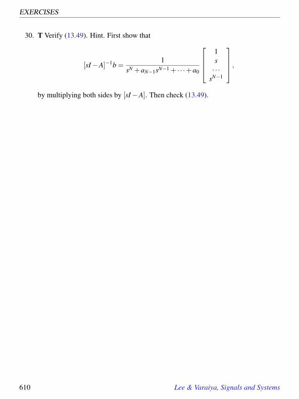
EXERCISES
30. T Verify (13.49). Hint. First show that
[sI−A]−1b =1
sN +aN−1sN−1 + · · ·+a0
1s· · ·
sN−1
,by multiplying both sides by [sI−A]. Then check (13.49).
610 Lee & Varaiya, Signals and Systems

14Composition and Feedback
Control
Contents14.1 Cascade composition . . . . . . . . . . . . . . . . . . . . . . . . . 613
14.1.1 Stabilization . . . . . . . . . . . . . . . . . . . . . . . . . . 61314.1.2 Equalization . . . . . . . . . . . . . . . . . . . . . . . . . . 614
14.2 Parallel composition . . . . . . . . . . . . . . . . . . . . . . . . . . 62014.2.1 Stabilization . . . . . . . . . . . . . . . . . . . . . . . . . . 62114.2.2 Noise cancellation . . . . . . . . . . . . . . . . . . . . . . . 622
14.3 Feedback composition . . . . . . . . . . . . . . . . . . . . . . . . . 62614.3.1 Proportional controllers . . . . . . . . . . . . . . . . . . . . 628
14.4 PID controllers . . . . . . . . . . . . . . . . . . . . . . . . . . . . . 63914.5 Summary . . . . . . . . . . . . . . . . . . . . . . . . . . . . . . . . 647Exercises . . . . . . . . . . . . . . . . . . . . . . . . . . . . . . . . . . . 648
A major theme of this book is that interesting systems are often compositions of simplersystems. Systems are functions, so their composition is function composition, as dis-cussed in section 2.1.5. However, systems are often not directly described as functions,so function composition is not the easiest tool to use to understand the composition. Wehave seen systems described as state machines, frequency responses, and transfer func-tions. In chapter 4 we obtained the state machine of the composite system from its compo-nent state machines. In section 8.5 we obtained the frequency response of the composite
611

14.1. CASCADE COMPOSITION
H1
x wH2
y
H = H1 H2
Figure 14.1: Cascade composition of two LTI systems with transfer functions H1and H2.
system from the frequency response of its component linear time-invariant (LTI) systems.We extend the latter study in this chapter to the composition of LTI systems described bytheir transfer functions. This important extension allows us to consider unstable systemswhose impulse response has a Z or Laplace transform, but not a Fourier transform.
As before, feedback systems prove challenging. A particularly interesting issue is how tomaintain stability, and how to construct stable systems out of unstable ones. We will findthat some feedback compositions of stable systems result in unstable systems, and con-versely, some compositions of unstable systems result in stable systems. For example, wecan stabilize the helicopter in example 12.2 using feedback, in fact we can precisely con-trol its orientation, despite the intrinsic instability. The family of techniques for doing thisis known as feedback control. This chapter serves as an introduction to that topic. Feed-back control can also be used to drive stable systems, in which case it serves to improvetheir response. For example, feedback can result in faster or more precise responses, andcan also prevent overshoot, where a system overreacts to a command.
We will consider three styles of composition, cascade composition, parallel composi-tion, and feedback composition. In each case, two LTI systems with transfer functionsH1 and H2 are combined to get a new system. The transfer functions H1 and H2 arethe (Z or Laplace) transforms of the respective impulse responses, h1 and h2. Much ofour discussion applies equally well whether the system is a continuous-time system or adiscrete-time system, so in many cases we leave this unspecified.
612 Lee & Varaiya, Signals and Systems
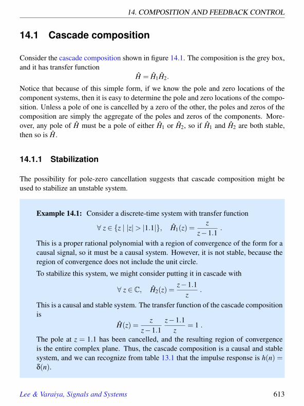
14. COMPOSITION AND FEEDBACK CONTROL
14.1 Cascade composition
Consider the cascade composition shown in figure 14.1. The composition is the grey box,and it has transfer function
H = H1H2.
Notice that because of this simple form, if we know the pole and zero locations of thecomponent systems, then it is easy to determine the pole and zero locations of the compo-sition. Unless a pole of one is cancelled by a zero of the other, the poles and zeros of thecomposition are simply the aggregate of the poles and zeros of the components. More-over, any pole of H must be a pole of either H1 or H2, so if H1 and H2 are both stable,then so is H.
14.1.1 Stabilization
The possibility for pole-zero cancellation suggests that cascade composition might beused to stabilize an unstable system.
Example 14.1: Consider a discrete-time system with transfer function
∀ z ∈ z | |z|> |1.1|, H1(z) =z
z−1.1.
This is a proper rational polynomial with a region of convergence of the form for acausal signal, so it must be a causal system. However, it is not stable, because theregion of convergence does not include the unit circle.
To stabilize this system, we might consider putting it in cascade with
∀ z ∈ C, H2(z) =z−1.1
z.
This is a causal and stable system. The transfer function of the cascade compositionis
H(z) =z
z−1.1z−1.1
z= 1 .
The pole at z = 1.1 has been cancelled, and the resulting region of convergenceis the entire complex plane. Thus, the cascade composition is a causal and stablesystem, and we can recognize from table 13.1 that the impulse response is h(n) =δ(n).
Lee & Varaiya, Signals and Systems 613

14.1. CASCADE COMPOSITION
Stabilizing systems by cancelling their poles in a cascade composition, however, is almostnever a good idea. If the pole is not precisely cancelled, then no matter how small theerror, the resulting system is still unstable.
Example 14.2: Suppose that in the previous example the pole location is notknown precisely, and turns out to be at z = 1.1001 instead of z = 1.1. Then thecascade composition has transfer function
H(z) =z
z−1.1001z−1.1
z=
z−1.1z−1.1001
,
which is unstable.
14.1.2 Equalization
While cascade compositions do not usually work well for stabilization, they do oftenwork well for equalization. An equalizer is a compensator that reverses distortion. Thesource of the distortion, which is often called a channel, must be an LTI system, and theequalizer is composed in cascade with it. At first sight this is easy to do. If the channelhas transfer function H1, then the equalizer could have transfer function
H2 = H−11 ,
in which case the cascade composition will have transfer function
H = H1H2 = 1,
which is certainly distortion-free.
Example 14.3: Some acoustic environments for audio have resonances, wherecertain frequencies are enhanced as the sound propagates through the environment.This will typically occur if the physics of the acoustic environment results in atransfer function with poles near the unit circle (for a discrete-time model) or nearthe imaginary axis (for a continuous-time model). Suppose for example that the
614 Lee & Varaiya, Signals and Systems

14. COMPOSITION AND FEEDBACK CONTROL
acoustic environment is well modeled by a discrete-time LTI system with transferfunction
∀ z ∈ z | |z|> 0.95, H1(z) =z2
(z−a)(z−a∗),
where a = 0.95eiω1 for some frequency ω1. Using the methods of Section 13.2, wecan infer that the magnitude response will have a strong peak at frequencies ω1 and−ω1, because the positions on the unit circle eiω1 and e−iω1 are very close to thepoles. This will result in distortion of the audio signal, where frequencies near ω1will be amplified.
An equalizer that will compensate for this distortion has transfer function
H2(z) = [H1(z)]−1 =(z−a)(z−a∗)
z2 =z2−2Reaz+ |a|2
z2 .
As in example 13.2, we can recognize this as the Z transform of an FIR filter withimpulse response
∀ n ∈ Z, h2(n) = δ(n)−2Reaδ(n−1)+ |a|2δ(n−2).
This filter is causal and stable, and hence can serve as an effective equalizer.
There are a number of potential problems with this approach, however. First, the transferfunction of the channel is probably not known, or at least not known precisely. Second,the channel may not have a stable and causal inverse.
Let us first examine the first difficulty, that the channel may not be known (precisely). Ifthe channel model H1 and its inverse H2 are both stable, then the cascade compositionis at least assured of being stable, even if the channel has been misconstrued. Moreover,if the equalizer is close to the inverse of the true channel, then often the distortion issignificantly reduced despite the errors (see exercise 1).
This difficulty can sometimes be dealt with by adaptively varying the equalizer based onmeasurements of the distortion. One way to measure the distortion is to send throughthe channel a known sequence called a training sequence and observe the output of thechannel. Suppose that the training sequence is a signal x with Z transform X , and that thechannel H1 is unknown. If we can observe the output y of the channel, and calculate its Z
Lee & Varaiya, Signals and Systems 615
14.1. CASCADE COMPOSITION
transform Y , then the channel transfer function is simply
∀ z ∈ RoC(h1), H1(z) =Y (z)X(z)
,
where RoC(h1) is determined by identifying the poles and zeros of the rational polyno-mial Y (z)/X(z) and finding the one ring-shaped region that includes the unit circle and isbordered by poles. This results in a stable channel model.
Training sequences are commonly used in digital communication systems, where, for ex-ample, a radio channel introduces distortion. However, it is also common for such chan-nels to change over time. Radio channels, for example, change if either the transmitter orreceiver moves, or if the weather changes, or if obstacles appear or disappear. Repeatedlytransmitting training sequences is an expensive waste of radio bandwidth, and fortunately,is not usually necessary, as illustrated in the following example.
Example 14.4: Consider a digital communication system where the channel ismodeled as a discrete-time LTI system with transfer function H1, representing forexample a radio transmission subsystem. Suppose that this digital communicationsystem transmits a bit sequence represented as a discrete-time signal x of form
x : Z→0,1.
Suppose further that we use a training sequence to obtain an initial estimate H2 ofthe inverse of the channel. But over time, the channel drifts, so that H2 is no longerthe inverse of H1. Assuming the drift is relatively slow, then after a short time, H2 isstill close to the inverse of H1, in that the cascade H1H2 yields only mild distortion.That is, if x(n) = 0 for some n, then y(n) ≈ 0. Similarly, if x(n) = 1 for some n,then y(n) ≈ 1. Thus, we can quantize y, getting an accurate estimate x withoutit having to be a known training sequence. That is, when y(n) ≈ 0, we assumethat x(n) = 0, and when y(n) ≈ 1, we assume that x(n) = 1. These assumptionsare called decisions, and in fact, such decisions must be made anyway for digitalcommunication to occur. We have to decide whether a 1 or a 0 was transmitted,and closeness to 1 or 0 seems like an eminently reasonable basis on which to makesuch a decision.
Assuming there are no errors in these decisions, we can infer that
H1H2Xd = Y ,
616 Lee & Varaiya, Signals and Systems

14. COMPOSITION AND FEEDBACK CONTROL
where Xd is the Z transform of the decision sequence. So, without using anothertraining sequence, we can revise our estimate of the channel transfer function asfollows,
H1 =Y
H2Xd.
We replace our equalizer H2 with
H ′2 = [H1]−1 =
H2Xd
Y.
Of course, we now start using H ′2, which will come closer to correcting the channeldistortion, which will make our decisions more reliable for the next update.
Example 14.4 outlines a widely used technique called decision-directed adaptive equal-ization. It is so widely used, in fact, that it may be found in every digital cellular tele-phone and almost every modem, including voiceband data modems, radio modems, cablemodems, DSL modems, etc. The algorithms used in practice to update the transfer func-tion of the equalizer are not exactly as shown in the example, and their details are beyondthe scope of this text, but they follow the general principle in the example.
Let us now turn our attention to the second difficulty with equalization, that the channelmay not have a stable and causal inverse. We begin with an example.
Example 14.5: Suppose that, similar to example 14.3, a channel has transferfunction
∀ z inz | |z|> 0.95, H1(z) =z
(z−a)(z−a∗),
where a = 0.95eiω1 for some frequency ω1. The inverse is
[H1(z)]−1 =(z−a)(z−a∗)
z=
z2−2Reaz+ |a|2)z
,
which is not a proper rational polynomial. Thus, this cannot be the Z transform ofa causal signal. Implementing a non-causal equalizer will usually be impossible,since it will require knowing future inputs. However, suppose we simply force the
Lee & Varaiya, Signals and Systems 617

14.1. CASCADE COMPOSITION
equalizer have a proper rational polynomial transfer function by dividing by a highenough power M of z to make [H1(z)]−1/zM proper. In this example, M = 1 issufficient, so we define the equalizer to be
H2(z) =[H1(z)]−1
z=
z2−2Reaz+ |a|2)z2 ,
which we again recognize as the Z transform of an FIR filter with impulse response
∀ n ∈ Z, h2(n) = δ(n)−2Reaδ(n−1)+ |a|2δ(n−2).
This filter is causal and stable, but does it serve as an effective equalizer? Considernow the cascade,
H(z) = H1(z)H2(z) =1z.
From Section 13.1.2 we recognize this as the transfer function of the unit delaysystem. That is, the equalizer completely compensates for the distortion, but at theexpense of introducing a one sample delay. This is usually a perfectly acceptablecost.
Example 14.5 demonstrates that when the channel inverse is not a proper rational polyno-mial, then introducing a delay may enable construction of a stable and causal equalizer.Not all equalization stories have such a happy ending, however. Consider the followingexample.
Example 14.6: Consider a channel with the following transfer function,
∀ z ∈ z ∈ C | z 6= 0, H1(z) =z−2
z.
This is a stable and causal channel. Its inverse is
[H1(z)]−1 =z
z−2.
This has a pole at z = 2, so in order to be stable, it would have to be anti-causal(so that the region of convergence can include the unit circle). Implementing ananti-causal equalizer is usually not possible.
618 Lee & Varaiya, Signals and Systems

14. COMPOSITION AND FEEDBACK CONTROL
Example 14.6 shows that not all channels can be inverted by an equalizer. All is notlost, however. Given a channel H1(z) that has a rational Z transform, we can usuallyfind a transfer function H2(z) that compensates for the magnitude response part of thedistortion. That is, we can find a transfer function H2(z) that is stable and causal such thatthe magnitude response of the composite satisfies
|H1(ω)H2(ω)|= |H1(eiω)H2(eiω)|= 1.
For some applications, this is sufficient. In audio equalization, for example, this is almostalways sufficient, because the human ear is not very sensitive to the phase of audio signals.It hears only the magnitude of the frequency components.
Example 14.7: Continuing example 14.6, let H2 be given by
H2 =z
1−2z=−0.5zz−0.5
.
This has a pole at z = 0.5, and is a proper rational polynomial, so it can be thetransfer function of a causal and stable filter. Consider the cascade composition,
H(z) = H1(z)H2(z) =z−2
z· −0.5z
z−0.5=
1−0.5zz−0.5
.
This hardly looks like what we want, but if we rewrite it slightly, it is easy to showthat the magnitude frequency response has value one for all ω,
H(z) =1−0.5zz−0.5
= zz−1−0.5z−0.5
.
The magnitude frequency response is
|H(ω)|= |H(eiω)|= |eiω| · |e−iω−0.5||eiω−0.5| = 1 .
This magnitude is equal to 1 because the numerator, e−iω− 0.5, is the complexconjugate of the denominator, eiω−0.5, so they have the same magnitude.
The method in example 14.7 can be generalized so that for most channels it is possibleto cancel any magnitude distortion. The key is that if the channel transfer function has a
Lee & Varaiya, Signals and Systems 619

14.2. PARALLEL COMPOSITION
zero outside the unit circle, say at z = a, then its inverse has a pole at the same location,z = a. A pole outside the unit circle makes it impossible to have a stable and causal filter.So the trick is to place a pole instead at z = 1/a∗. This pole will cancel the effect on themagnitude (but not the phase) of the zero at z = a.
There are still channels for which this method will not work.
Example 14.8: Consider a channel given by
∀ z ∈ z ∈ C | z 6= 0, H1(z) =z−1
z.
This has a pole at z = 0 and a zero at z = 1. Its inverse cannot be stable becauseit will have a pole at z = 1. In fact, no equalization is possible. This is intuitivebecause the frequency response is zero at ω = 0, and no stable equalizer in cascadewith this channel can reconstruct the original component at ω = 0. It would haveto have infinite gain at ω = 0, which would make it unstable.
14.2 Parallel composition
Consider the parallel composition shown in figure 14.2. The transfer function of thecomposition system is
H = H1 + H2.
This is valid whether these are Laplace transforms or Z transforms. Once again, noticethat a pole of H must be a pole of either H1 or H2, so if H1 and H2 are stable, then so isH. At the poles of H1, H1(z) is infinite, so very likely a pole of H1 will also be a pole ofH. However, just as in the cascade composition, this pole may be cancelled by a zero.
Determining the location of the zeros of the composition, however, is slightly more com-plicated than for cascade composition. The sum has to be put into rational polynomialform, and the polynomials then need to be factored.
620 Lee & Varaiya, Signals and Systems

14. COMPOSITION AND FEEDBACK CONTROL
H1x
w1
H2
y
H = H1+ H2
w2
Figure 14.2: Parallel composition of two LTI systems with transfer functions H1and H2.
14.2.1 Stabilization
Just as with cascade composition, stabilizing systems by cancelling their poles in a parallelcomposition is possible, but is almost never a good idea.
Example 14.9: Consider a discrete-time system with transfer function
∀ z ∈ z | |z|> |1.1|, H1(z) =z
z−1.1.
This describes a causal but unstable system. Suppose we combine this in parallelwith a system with transfer function
∀ z ∈ z | |z|> |1.1|, H2(z) =−1.1
z−1.1.
This is again causal and unstable. The transfer function of the parallel compositionis
H(z) =z
z−1.1+−1.1
z−1.1=
z−1.1z−1.1
= 1 .
The pole at z = 1.1 has been cancelled, and the resulting region of convergenceis the entire complex plane. Thus, the parallel composition is a causal and stablesystem with impulse response h(n) = δ(n).
Lee & Varaiya, Signals and Systems 621

14.2. PARALLEL COMPOSITION
H1x
w
H2
y
w1
w2
Figure 14.3: Structure of a noise canceller.
However, if the pole is not precisely cancelled, then no matter how small the error, theresulting system is still unstable.
Example 14.10: Suppose that in the previous example the pole location is notknown precisely, and turns out to be at z = 1.1001 instead of z = 1.1. Then theparallel composition has transfer function
H(z) =z
z−1.1001+−1.1
z−1.1=
z2−2.2z+1.21001(z−1.1001)(z−1.1)
,
which is unstable.
14.2.2 Noise cancellation
While parallel compositions do not usually work well for stabilization, with a small mod-ification they do often work well for noise cancellation. A noise canceller is a compen-sator that removes an unwanted component from a signal. The unwanted component iscalled noise.
The pattern of a noise cancellation problem is shown in figure 14.3. The signal x is a noisesource. This signal is filtered by H1 and added to the desired signal w. The result is a
622 Lee & Varaiya, Signals and Systems

14. COMPOSITION AND FEEDBACK CONTROL
noisy signal. To cancel the noise, the signal from the noise source is filtered by a noisecancelling filter H2 and the result is added to the noisy signal. If x has (Laplace or Z)transform X , w has transform W , and y has transform Y , then
Y = W +(H1 + H2)X .
From this it is evident that if we choose
H2 =−H1,
then y will be a clean (noise-free) signal, equal to w. The following examples describereal-world applications of this pattern.
Example 14.11: A connection to the telephone network uses two wires (calleda twisted pair, consisting of tip and ring) to connect a telephone to a centraloffice. The central office may be, perhaps, 4 kilometers away. The two wires carryvoice signals to and from the customer premises, representing the voice signals as avoltage difference across the two wires. Since two wires can only have one voltagedifference across them, the incoming voice signal and the outgoing voice signalshare the same twisted pair.
The central office needs to separate the voice signal from the local customerpremises (called the near-end signal) from the voice signal that comes from theother end of the connection (called the far-end signal). The near end signal istypically digitized (sampled and quantized), and a discrete-time representation ofthe voice signal is transmitted over the network to the far end. The network itselfconsists of circuits that can carry voice signals in one direction at a time. Thus, inthe network, four wires (or equivalent) are required for a telephone connection, onewire pair for each direction.
As indicated in figure 14.4, the conversion from a two-wire to a four-wire connec-tion is done by a device called a hybrid. A hybrid is a Wheatstone bridge, a circuitthat can separate two signals based on the electrical impedance looking into the lo-cal twisted pair and the electrical impedance looking into the network. The designof this circuit is a suitable topic for a text on electrical circuits.
A connection between subscribers A and B involves two hybrids, one in each sub-scriber’s central office. The hybrid in B’s central office ideally will pass all of the
Lee & Varaiya, Signals and Systems 623

14.2. PARALLEL COMPOSITION
A B
Hybridat A'sCO
Hybridat B'sCO
x = signal from A
y = leakage of A's signal plus signal from Becho
twisted pair
H1
x
w
H2
y
echo pathecho canceller
w1w2
Figure 14.4: A telephone central office converts the two-wire connection with acustomer telephone into a four-wire connection with the telephone network usinga device called a hybrid. An imperfect hybrid leaks, causing echo. An echocanceller removes the leaked signal.
624 Lee & Varaiya, Signals and Systems

14. COMPOSITION AND FEEDBACK CONTROL
incoming signal x to B’s two-wire circuit, and none back into the network. How-ever, the hybrid is not perfect, and some of the incoming signal x leaks through thehybrid into the return path back to A. The signal y in the figure is the sum of thesignal from B and the leaked signal from A. A hears the leaked signal as an echo,since it is A’s own signal, delayed by propagation through the telephone network.
If the telephone connection includes a satellite link, then the delay from one endof the connection to the other is about 300ms. This is the time it takes for a radiosignal to propagate to a geosynchronous satellite and back. The echo traversesthis link twice: once going from A to B, and the second time coming back. Thus,the echo is A’s own signal delayed by about 600ms. For voice signals, 600ms ofdelay is enough to create a very annoying echo that can make it difficult to speak.Humans have difficulty speaking when they hear their own voices 600ms later.Consequently, the designers of the telephone network have put echo cancellers into prevent the echo from occuring.
Let H1 be the transfer function of the hybrid leakage path. The echo canceller isthe filter H2 placed in parallel composition with the hybrid, as shown in the figure.The output w2 of this filter is added to the output w1+w of the hybrid, so the signalthat actually goes back is y = w2 +w1 +w. If
H2 =−H1,
then y = w and the echo is cancelled perfectly. Moreover, note that as long as H1 isstable and causal, so will be the echo canceller H2.
However, H1 is not usually known in advance, and also it changes over time. Soeither a fixed H2 is designed to match a ‘typical’ H1, or an adaptive echo cancelleris designed that estimates the characteristics of the echo path (H1) and changes H2accordingly. Adaptive echo cancellers are common in the telephone network today.
The following example combines cascade and parallel composition to achieve noise can-cellation.
Example 14.12: Consider a microphone in a noisy environment. For example,a traffic helicopter might be used to deliver live traffic reports over the radio, butthe (considerable) background noise of the helicopter would be highly undesirable
Lee & Varaiya, Signals and Systems 625

14.3. FEEDBACK COMPOSITION
H1x
w
H2
y
w1
w2H3 w3
w4
Figure 14.5: Traffic helicopter noise cancellation/equalization problem.
on the radio. Fortunately, the background noise can be cancelled. Referring toFigure 14.5, suppose that w is the announcer’s voice, x is the engine noise, andH1 represents the acoustic path from the engine noise to the microphone. Themicrophone picks up both the engine noise and the announcer’s voice, producingthe noisy signal w4. We can place a second microphone somewhere far enough fromthe announcer so as to not pick up much of his or her voice. Since this microphoneis in a different place, say on the back of the announcer’s helmet, the acoustic pathis different, so we model that path with another transfer function H2. To cancel thenoise, we design a filter H3. This filter needs to equalize (invert) H2 and cancel H1.That is, its ideal value is
H3 =−H1/H2.
Of course, as with the equalization scenario, we have to ensure that this filter re-mains stable. Once again, in practice, it is necessary to make the filter adaptive.
14.3 Feedback composition
Consider the feedback composition in figure 14.6. It is a composition of two systemswith transfer functions H1 and H2. We assume that these systems are causal and that H1and H2 are proper rational polynomials in z or s. The regions of convergence of thesetwo transfer functions are those suitable for causal systems (the region outside the largest
626 Lee & Varaiya, Signals and Systems

14. COMPOSITION AND FEEDBACK CONTROL
H1x e
H2
y
H =
w
H1H21 + H1 H2
!
Figure 14.6: Negative feedback composition of two LTI systems with transfer func-tions H1 and H2.
circle passing through a pole, for discrete time, and the region to the right of the pole withthe largest real part, for continuous-time).
In terms of Laplace or Z transforms, the signals in the figure are related by
Y = H2H1E,
andE = X− Y .
Notice that, by convention, the feedback term is subtracted, as indicated by the minussign adjacent to the adder (for this reason, this composition is called negative feedback).Combining these two equations to elimintate E, we get
Y = H1H2(X− Y ),
which we can solve for the transfer function of the composition,
H =YX
=H1H2
1+ H1H2. (14.1)
This is often called the closed-loop transfer function, to contrast it with the open-looptransfer function, which is simply H1H2. We will assume that this resulting system iscausal, and that the region of convergence of this transfer function is therefore determinedby the roots of the denominator polynomial, 1+ H1H2.
Lee & Varaiya, Signals and Systems 627

14.3. FEEDBACK COMPOSITION
The closed-loop transfer function is valid as long as the denominator 1+ H1H2 is notidentically zero (that is, it is not zero for all s or z in C – it may be zero some s or z in C).This is sufficient for the feedback loop to be well-formed, although in general, this factis not trivial to demonstrate (Exercise 8 considers the easier case where H1H2 is causaland strictly proper, in which case the system H1H2 has state-determined output). We willassume henceforth, without comment, that the denominator is not identically zero.
Feedback composition is useful for stabilizing unstable systems. In the case of cascadeand parallel composition, a pole of the composite must be a pole of one of the components.The only way to remove or alter a pole of the components is to cancel it with a zero. Forthis reason, cascade and parallel composition are not effective for stabilizing unstablesystems. Any error in the specification of the unstable pole location results in a failedcancellation, which results in an unstable composition.
In contrast, the poles of the feedback composition are the roots of the denominator 1+H1H2, which are generally quite different from the poles of H1 and H2. This leads to thefollowing important conclusion:
The poles of a feedback composition can be different from the poles of its componentsubsystems. Consequently, unstable system can be effectively and robustly stabilized byfeedback.
The stabilization is robust in that small changes in the pole or zero locations do not resultin the composition going unstable. We will be able to quantify this robustness.
14.3.1 Proportional controllers
In control applications, one of the two systems being composed, say H2, is called the plant.This is a physical system that is given to us to control. Its transfer function is determinedby its physics. The second system being composed, say H1, is the controller. We designthis system to get the plant to do what we want. The following example illustrates asimple strategy called a proportional controller or P controller.
Example 14.13: For this example we take as the plant the simplified continuous-time helicopter model of example 12.2,
y(t) =1M
w(t).
628 Lee & Varaiya, Signals and Systems

14. COMPOSITION AND FEEDBACK CONTROL
Here y(t) is the angular velocity at time t and w(t) is the torque. M is the momentof inertia.
We have renamed the input w (instead of x) because we wish to control the heli-copter, and the control input signal will not be the torque. Instead, let’s define theinput x to be the desired angular velocity. So, to get the helicopter to not rotate, weprovide input x(t) = 0.
Let us call the impulse response of the plant h2, to conform with the notation inFigure 14.6; it is given by
∀ t ∈ R, h2(t) = u(t)/M,
where u is the unit step. The transfer function is
H2(s) = 1/(Ms),
withRoC(h) = s ∈ C | Re(s)> 0.
H2 has a pole at s = 0, so this is an unstable system.
As a compensator we can simply place a gain K in a negative feedback composition,as shown in Figure 14.7. The intuition is as follows. Suppose we wish to keep thehelicopter from rotating. That is, we would like the output angular velocity to bezero, y(t) = 0. Then we should apply an input of zero, x(t) = 0. However, theplant is unstable, so even with a zero input, the output diverges (even the smallestnon-zero initial condition or the smallest input disturbance will cause it to diverge).With the feedback arrangement in Figure 14.7, if the output angular velocity risesabove zero, then the input is modified downwards (the feedback is negative), whichwill result in a negative torque being applied to the plant, which will counter therising velocity. If the output angular velocity drops below zero, then the torque willbe modified upwards, which again will tend to counter the dropping velocity. Theoutput velocity will stabilize at zero.
To get the helicopter to rotate, for example to execute a turn, we simply apply anon-zero input. The feedback system will again compensate so that the helicopterwill rotate at the angular velocity specified by the input.
The signal e is the difference between the input x, which is the desired angularvelocity, and the output y, which is the actual angular velocity. It is called the errorsignal. Intuitively, this signal is zero when everything is as desired, when the outputangular velocity matches the input.
Lee & Varaiya, Signals and Systems 629

14.3. FEEDBACK COMPOSITION
H1=Kx e
H2
y
H =
w
K / Ms + K / M
!Ms1=
desired angular velocity
angular velocity
torqueerror
Figure 14.7: A negative feedback proportional controller with gain K.
2− −2
K = −2K = +2 K = −K =
root locus
K = 0
Figure 14.8: Root locus of the helicopter P controller.
A compensator like that in example 14.13 and Figure 14.7 is called a proportional con-troller or P controller. The input w to the plant is proportional to the error e. Theobjective of the control system is to have the output y of the plant track the input x asclosely as possible. I.e., the error e needs to be small. We can use (14.1) to find thetransfer function of the closed-loop system.
Example 14.14: Continuing with the helicopter of example 14.13, the closed loopsystem transfer function is
G(s) =KH(s)
1+KH(s)=
K/Ms+K/M
. (14.2)
630 Lee & Varaiya, Signals and Systems

14. COMPOSITION AND FEEDBACK CONTROL
which has a pole at s = −K/M. If K > 0, the closed loop system is stable, andif K < 0, it is unstable. Thus, we have considerable freedom to choose K. Howshould we choose its value?
As K increases from 0 to ∞, the pole at at s =−K/M moves left from 0 to −∞. AsK decreases from 0 to−∞, the pole moves to the right from 0 to ∞. The locus of thepole as K varies is called the root locus, since the pole is a root of the denominatorpolynomial.
Figure 14.8 shows the root locus as a thick gray line, on which are marked thelocations of the pole for K = 0,±2,±∞. Since there is only one pole, the root locuscomprises only one ‘branch’. In general the root locus has as many branches asthe number of poles, with each branch showing by the movement of one pole as Kvaries.
Note that in principle, the same transfer function as the closed-loop transfer function canbe achieved by a cascade composition. But as in example 14.1, the resulting system isnot robust, in that even the smallest change in the pole location of the plant can causethe system to go unstable (see problem 6). The feedback system, however, is robust, asshown in the following example
Example 14.15: Continuing with the P controller for the helicopter, suppose thatour model of the plant is not perfect, and its actual transfer function is
H2(s) =1
M(s− ε),
for some small value of ε > 0. In that case, the closed loop transfer function is
H(s) =K/M
s− ε+K/M,
which has a pole at s = ε−K/M. So the feedback system remains stable so long as
ε < K/M.
Lee & Varaiya, Signals and Systems 631

14.3. FEEDBACK COMPOSITION
In practice, when designing feedback controllers, we first quantify our uncertainty aboutthe plant, and then determine the controller parameters so that under all possible planttransfer functions, the closed-loop system is stable.
Example 14.16: Continuing the helicopter example, we might say that ε < 0.5. Inthat case, if we choose K so that K/M > 0.5, we would guarantee stability for allvalues of ε < 0.5. We then say that the proportional feedback controller is robustfor all plants with ε < 0.5.
We still have a large number of choices for K. How do we select one? To understandthe implications of different choices of K we need to study the behavior of the output y(or the error signal e) for different choices of K. In the following examples we use theclosed-loop transfer function to analyze the response of a proportional controller systemto various inputs. The first example studies the response to a step function input.
Example 14.17: Continuing the helicopter example, suppose that the input is astep function, ∀t,x(t) = au(t) where a is a constant and u is the unit step. Thisinput declares that at time t = 0, we wish for the helicopter to begin rotating withangular velocity a. The closed-loop transfer function is given by (14.2), and theLaplace transform of x is X(s) = a/s, from table 13.3, so the Laplace transform ofthe output is
Y (s) = G(s)X(s) =K/M
s+K/M· a
s
Carrying out the partial fraction expansion, this becomes
Y (s) =−a
s+K/M+
as.
We can use this to find the inverse Laplace transform,
∀t, y(t) =−ae−Kt/Mu(t)+au(t).
The second term is the steady-state response yss, which in this case equals theinput. So the first term is the tracking error ytr, which goes to zero faster forlarger K. Hence for step inputs, the larger the gain K, the smaller the tracking error.
632 Lee & Varaiya, Signals and Systems

14. COMPOSITION AND FEEDBACK CONTROL
In the previous example, we find that the error goes to zero when the input is a stepfunction. Moreover, the error goes to zero faster if the gain K is larger than if it is smaller.In the following example, we find that if the input is sinusoidal, then larger gain K resultsin an ability to track higher frequency inputs.
Example 14.18: Suppose the input to the P controller helicopter system is a sinu-soid of amplitude A and frequency ω0,
∀ t ∈ R, x(t) = A(cosω0t)u(t).
We know that the response can be decomposed as y = ytr + yss. The transient re-sponse ytr is due to the pole at s =−K/M, and so it is of the form
∀ t ∈ R, ytr(t) = Re−Kt/M,
for some constant R. The steady-state response is determined by the frequencyresponse at ω0. The frequency response is
∀ ω ∈ R, H(ω) = H(iω) =K/M
iω+K/M,
with magnitude and phase given by
|H(ω)|= K/M[ω2 +(K/M)2]1/2 , ∠H(ω) =− tan−1 ωM
K.
So the steady-state response is
∀t, yss(t) = |H(ω0)|Acos(ω0t +∠H(ω0)).
Thus the steady-state output is a sinusoid of the same frequency as the input butwith a smaller amplitude (unless ω0 = 0). The larger ω0 is, the smaller the outputamplitude. Hence, the ability of the closed-loop system to track a sinusoidal inputdecreases as the frequency of the sinusoidal input increases. However, increasingK reduces this effect. Thus, larger gain in the feedback loop improves its ability totrack higher frequency sinusoidal inputs.
In addition to the reduction in amplitude, the output has a phase difference. Again,if ω0 = 0, there is no phase error, because tan−1(0) = 0. As ω0 increases, the phaselag increases (the phase angle decreases). Once again, however, increasing the gainK reduces the effect.
Lee & Varaiya, Signals and Systems 633

14.3. FEEDBACK COMPOSITION
The previous two examples suggest that large gain in the feedback loop is always better.For a step function input, it causes the transient error to die out faster. For a sinusoidalinput, it improves the ability to track higher frequency inputs, and it reduces the phaseerror in the tracking. A large gain is not always a good idea, however, as seen in the nextexample, a DC motor.
Example 14.19: The angular position y of a DC motor is determined by the inputvoltage w according to the differential equation
My(t)+Dy(t) = Lw(t),
where M is the moment of inertia of the rotor and attached load, Dy is the dampingforce, and the torqe Lw is proportional to the voltage. The transfer function is
H2(s) =L
Ms2 +Ds=
L/Ms(s+D/M)
.
which has one pole at s = 0 and one pole at s = −D/M. By itself the DC motoris unstable because of the pole at s = 0. The transfer function of the feedbackcomposition with proportional gain K is
H(s) =KH2(s)
1+KH2(s)=
KLMs2 +Ds+KL
.
There are two closed loop poles—the roots of Ms2 +Ds+KL—located at
s =− D2M±√
D2
4M2 −KLM
.
The closed loop system is stable if both poles have negative real parts, which is thecase if K > 0. If K < D2/(4ML) both poles are real. But if K > D2/(4ML), thetwo poles form a complex conjugate pair located at
s =− D2M± i
√KLM− D2
4M2 .
The real part is fixed at D/2M, but the imaginary part increases with K. We inves-tigate performance for the parameter values L/M = 10,D/M = 0.1. The transferfunction is
H(s) =10K
s2 +0.1s+10K.
634 Lee & Varaiya, Signals and Systems

14. COMPOSITION AND FEEDBACK CONTROL
Because there are two poles, the root locus has two branches, as shown in Figure14.9. For K = 0, the two poles are located at 0 and -0.1, as illustrated by crossesin the figure. As K increases the two poles move towards each other, coinciding at-0.05 when K = 0.00025. For larger values of K, the two branches split into a pairof complex conjugate poles.
To appreciate what values of K > 0 to select for good tracking, we consider theresponse to a step input x = u(t) for two different values of K. For K = 0.00025,the Laplace transform of the output y is
Y (s) =10K
s2 +0.1s+10K1s
=0.0025
(s+0.05)21s
= − 1s+0.05
− 0.05(s+0.05)2 +
1s.
So the time domain response is
∀t, y(t) = −e−0.05t −0.05te−0.05tu(t)+u(t). (14.3)
For K = 0.0025, the Laplace transform of the output y is
Y (s) =0.025
s2 +0.1s+0.0251s
≈ −0.5+ i0.17s+0.05− i0.15
+−0.5−0.17i
s+0.05+ i0.15+
1s.
So
∀t, y(t) = e−0.5t [0.527ei(0.15t+2.82)+0.527e−i(0.15t+2.82)]u(t)
+u(t)
= 0.527e−0.5t ×2cos(0.15t +2.82)u(t)+u(t). (14.4)
The right-hand panel in Figure 14.9 shows plots of the responses (14.3) and (14.4)that illustrate the design tradeoffs. In both cases, the output approaches the inputas t→∞, so the asymptotic tracking error is zero. The response for the higher gainis faster but it overshoots the asymptotic value. The response for the lower gain isslower but there is no overshoot. In this example, K must be selected to balancespeed of response versus the magnitude of the overshoot. In some applications,overshoot may be completely unacceptable.
Lee & Varaiya, Signals and Systems 635

14.3. FEEDBACK COMPOSITION
-0.05
-0.1 0K=0
K= 0.00025
K < 0Re s
Im s
K=0K < 0
- 50 0 50 100 1500
0 .2
0 .4
0 .6
0 .8
1
1 .2
1 .4
K = 0.0025
K = 0.00025
t
y
x
overshoot
Figure 14.9: The root locus and step response for two values of K of a DC motorwith proportional feedback.
We can now investigate the proportional feedback control in a general setting. Supposethe plant transfer function is a proper rational polynomial
H2(s) =A(s)B(s)
,
where A has degree M, B has degree N, and M ≤ N (H2 is proper). The closed looptransfer function is
H(s) =KH2(s)
1+KH2(s)=
KA(s)B(s)+KA(s)
. (14.5)
The closed loop poles are the N roots of the equation B(s)+KA(s) = 0. These roots willdepend on K, so we denote them p1(K), · · · , pn(K). As K varies, these roots will trace outthe N branches of the root locus. At K = 0, the poles are the roots of B(s) = 0, which arethe poles of the plant transfer function A(s)/B(s). The stability of the closed loop plantrequires that K must be such that
Rep1(K)< 0, · · · ,Repn(K)< 0. (14.6)
Within those values of K that satisfy (14.6) we must select K to get a good response.
636 Lee & Varaiya, Signals and Systems

14. COMPOSITION AND FEEDBACK CONTROL
The following example shows that a proportional compensator may be unable to guaranteeclosed loop stability.
Example 14.20: Consider a plant transfer function given by
H2(s) =A(s)B(s)
=s+1
(s−1)(s2 +0.5s+1.25).
There is one zero at s =−1, one pole at s = 1 and a pair of complex conjugate polesat s =−0.5± i1.09. The plant is unstable because of the pole at s = 1. The closedloop poles are the roots of the polynomial
P(K,s) = KA(s)+ B(s) = K(s+1)+(s−1)((s+0.25)2 +1.188).
Figure 14.10 shows the three branches of the root locus plot for K > 0. As Kincreases, the unstable pole moves towards the zero, while the complex conjugatepoles move into the right-half plane. We need to find the values of K that satisfythe stability condition (14.6). The value of K for which the pole at s = 1 moves tos = 0 is obtained from the condition P(K,0) = 0, which gives K− (0.52 + 1) = 0or K = 1.25. So one condition for stability is K > 1.25. The complex conjugatepoles cross the imaginary axis at s =±i1.15 for K = 0.6. So the second conditionfor stability is K < 0.6. The two conditions K > 1.25 and K < 0.6 are inconsistent,so no proportional compensator can stabilize this system.
We return to the general discussion. Suppose the stability condition (14.6) can be met.Among the values of K that achieve stability, we select that value for which the output yclosely tracks a step input, x = u. In this case, the Laplace transform of the input is 1/s,so the Laplace transform of y is, from (14.5),
Y (s) = H(s)1s=
KA(s)B(s)+KA(s)
1s. (14.7)
Assuming for simplicity that all the poles p1(K), · · · , pn(K) have multiplicity 1, Y has thepartial fraction expansion
Y (s) =n
∑i=1
Ri
s− pi(K)+
R0
s,
Lee & Varaiya, Signals and Systems 637

14.3. FEEDBACK COMPOSITION
-1 -0.8 -0.6 -0.4 -0.2 0 0.2 0.4 0.6 0.8 1
-4
-2
-6
2
4
6
0Re s
Im s
K = 1.25K > 1.25
K = 0.8K > 0.8
Figure 14.10: Root locus for example 14.20. Stability requires K > 1.25 and K <0.6. Therefore, there is no stabilizing proportional compensator.
638 Lee & Varaiya, Signals and Systems

14. COMPOSITION AND FEEDBACK CONTROL
and hence the time-domain behavior of
∀t, y(t) =
[n
∑i=1
Riepi(K)t
]u(t)+R0u(t).
The first term is the transient response, ytr, and the second term is the steady-state responseyss = R0u. The transient response goes to zero, since from (14.6), Repi(K) < 0 for alli. The input is the unit step, x = u. So the steady-state tracking error is |R0− 1|, whichdepends on R0. It is easy to find the residue R0. We simply multiply both sides of (14.7)by s and evaluate both sides at s = 0, to get
R0 = G(0) =KH2(0)
1+KH2(0).
To have zero steady-state error, we want R0 = 1, which can only happen if H2(0) = ∞.But this means s = 0 must be a pole of the plant transfer function H2. (This is the casein the examples of the helicopter and the DC motor.) If the plant does not have a pole ats = 0, the steady-state error will be∣∣∣∣1− KH2(0)
1+KH2(0)
∣∣∣∣ .This error is smaller the larger the gain K. So to minimize the steady-state error we shouldchoose as large a gain as possible, subject to the stability requirement (14.6).
However, a large value of K may lead to poor transient behavior by causing overshoots,as happened in the DC motor example in Figure 14.9 for the larger gain K = 0.0025. Todecide the appropriate K is a matter of trial and error. One studies the transient responsefor different (stabilizing) values of K (as we did for the DC motor) and selects K that givesa satisfactory transient behavior.
14.4 PID controllers
The P controller discussed in the previous section achieves zero steady-state error if theplant has a pole at s= 0. This means that the plant includes an integrator, since the transferfunction of an integrator is 1/s, which has a pole at s = 0. If the plant does not have a poleat s = 0, however, a non-zero error results. While this error can be reduced by choosing alarge gain K in the controller, this results in poor transient behavior.
Lee & Varaiya, Signals and Systems 639

14.4. PID CONTROLLERS
w(t)
D
y(t)
M
C
spring
damper
mass
H2(s) =yw
1 Ms2 + Ds + C
Figure 14.11: A mass-spring-damper system.
In this section, we develop the well-known PID controller, which includes an integratorin the controller. It can achieve zero steady-state error even if the plant does not havea pole at s = 0, and still achieve reasonable transient behavior. The PID controller is ageneralization of the P controller, in that with certain choices of parameters, it becomes aP controller.
We begin with an example that has rich enough dynamics to demonstrate the strengthsof the PID controller. This example describes a mechanical system, but just about anyphysical system that is modeled by a linear second-order differential equation is subject tosimilar analysis. This includes, for example, electrical circuits having resistors, capcitors,and inductors.
Example 14.21: A basic mass-spring-damper system is illustrated in Figure14.11. This system has a mass M that slides on a frictionless surface, a spring thatattaches the mass to a fixed physical object, and a damper, which absorbes mechan-ical energy. A damper might be, for example, a dashpot, which is a cylinder filledwith oil plus a piston. A familiar example of such a damper is a shock absorber inthe suspension system of a car.
640 Lee & Varaiya, Signals and Systems
14. COMPOSITION AND FEEDBACK CONTROL
Suppose that an external force w is applied to the mass, where w is a continuous-time signal. The differential equation governing the system is obtained by settingthe sum of all forces to zero,
My(t)+Dy(t)+Cy(t) = w(t).
The output y(t) is the position of the mass at time t, My(t) is the inertial force,Dy(t) is the damping force due to the damper, Cy(t) is the restoring force of thespring, and w(t) is the externally applied force. We assume that y(t) = 0 when thespring is in its equilibrium position (neither extended nor compressed). M, D, andC are constants. Taking the Laplace transform, using the differentiation propertyfrom table 13.4, gives
s2Y (s)+DsY (s)+CY (s) =W (s),
so the plant or open loop transfer function is
H2(s) =Y (s)W (s)
=1
Ms2 +Ds+C.
Suppose for example that the constants have values M = 1, D = 1,and C = 1.25.Then
H2(s) =1
s2 + s+1.25. (14.8)
In this case, the transfer function has a pair of complex poles at s =−0.5± i. Sincetheir real part is strictly negative, the system is stable.
Suppose we wish to drive the system to move the mass to the right one unit ofdistance at time t = 0. We can apply an input force that is a unit step, scaled so thatthe steady-state response places the mass at position y(t) = 1. The final steady-stateoutput is determined by the DC gain, which is H2(0) = 1/1.25 = 0.8, so we canapply an input given by
∀ t, ,w(t) =1
0.8u(t) = 1.25u(t),
where u is the unit step signal. The resulting response yo has Laplace transform
Yo(s) =1
s2 + s+1.25· 1.25
s=−0.5+0.25i
s+0.5− i+−0.5−0.25i
s+0.5+ i+
1s.
Lee & Varaiya, Signals and Systems 641

14.4. PID CONTROLLERS
yo(t)
t
overshoot
0 5 10 15 20 0
0 .2
0 .4
0 .6
0 .8
1
1 .2
1 .4
Figure 14.12: The open loop step response yo of the mass-spring-damper sys-tem.
We call this the open-loop step response, because there is no control loop (yet).
Taking the inverse transform gives the open-loop step response
∀ t, yo(t) = e−0.5t [(−0.5+0.25i)eit +(−0.5−0.25i)e−it ]u(t)+u(t).
By combining the complex conjugate terms, this can be expressed as
∀t, yo(t) = Re−0.5t cos(t +θ)u(t)+u(t),
where R = 1.12 and θ = 2.68. Figure 14.12 displays a plot of this open-loop stepresponse yo. Notice that the mass settles to position y(t) = 1 for large t.
This system in the previous example is stable, and therefore does not need a feedback con-trol loop to stabilize it. However, there are two difficulties with its open-loop response,shown in Figure 14.12, that can be corrected using a controller. First, it takes approxi-mately 10 units of time for the transient to disappear, which may be too slow for someapplications. Moreover, there is an overshoot of 20 percent beyond the final steady-statevalue, which may be too much.
642 Lee & Varaiya, Signals and Systems

14. COMPOSITION AND FEEDBACK CONTROL
x e y
H =H1H2
1 + H1 H2
−H2(s) =
w
Ms2 + Ds + CH1(s) = K1 + K2/s + K3s
PID controller Plant
1
Figure 14.13: The mass-spring-damper system composed with a PID controllerin a feedback composition.
We can correct for the slow response and the large overshoot, using a PID controller.The term ‘PID’ stands for proportional plus integral plus derivative. A PID controllergeneralizes the P controller of the previous section by adding an integral and derivativeterm.
The general form of the transfer function of a PID controller is
H1(s) = K1 +K2
s+K3s =
K3s2 +K1s+K2
s. (14.9)
We will compose this with the plant in a feedback loop, as shown in Figure 14.13. HereK1,K2,K3 are constants to be selected by the designer. If K2 = K3 = 0, then we have aP controller. If K1 = K3 = 0, H1(s) = K2/s, we have an integral contoller, so calledbecause 1/s is the transfer function of an integrator. That is, if the input to the integralcontroller is e, and the output is w, then
∀ t, w(t) = K2
∫ t
−∞
e(τ)dτ.
If K1 = K2 = 0, H2(s) = K3s, then we have a derivative controller, so called because s isthe transfer function of a differentiator. That is, if the input to the derivative controller ise, and the output is w, then
∀ t, w(t) = K3e(t).
Lee & Varaiya, Signals and Systems 643

14.4. PID CONTROLLERS
The following table offers guidelines for selecting the parameters of a PID controller.Of course, these are guidelines only—the actual performance of the closed loop systemdepends on the plant transfer function and must be checked in detail.
Parameter Response speed Overshoot Steady-state errorK1 Faster Larger DecreasesK2 Faster Larger ZeroK3 Minor change Smaller Minor change
Example 14.22: We now evaluate a PID controller for the mass-spring-dampersystem of Figure 14.11, using the feedback composition of Figure 14.6. We assumethe parameters values M = 1, D = 1, and C = 1.25, as in example 14.21. Theclosed-loop transfer function with the PID controller is
H(s) =H1(s)H2(s)
1+ H1(s)H2(s)=
K3s2 +K1s+K2
s3 +(1+K3)s2 +(1.25+K1)s+K2.
Suppose we provide as input a unit step. This means that we wish to move the massto the right one unit of distance, starting at time t = 0. The controller will attemptto track this input. The response to a unit step input has Laplace transform
Ypid(s) = H(s) · 1s=
K3s2 +K1s+K2
s3 +(1+K3)s2 +(1.25+K1)s+K2· 1
s. (14.10)
We now need to select the values for the parameters of the PID controller, K1, K2,and K3. We first try proportional control with K1 = 10, and K2 = K3 = 0. In thiscase, the step response has the Laplace transform
Yp(s) =10
s2 + s+11.25· 1
s.
The inverse Laplace transform gives the time response yp, which is plotted in Figure14.14. The steady-state value is determined by the DC gain of the closed looptransfer function,
10s2 + s+11.25
∣∣∣∣s=0
=10
11.25≈ 0.89.
644 Lee & Varaiya, Signals and Systems

14. COMPOSITION AND FEEDBACK CONTROL
0 2 4 6 8 10 12 14 16 18 200
0.5
1
1.5
yo
yp
ypd
ypid
Figure 14.14: The step response for open loop, yo, with P-control, yp, PD-control,ypd , and PID-control, ypid .
Lee & Varaiya, Signals and Systems 645

14.4. PID CONTROLLERS
This yields an error of 11 percent, and the overshoot of 50 percent is much worsethan that of the open-loop response yo, also shown in the figure. Thus, a P controllerwith gain K = 10 is useless for this application.
Following the guidelines in the table above, we add derivative control to reduce theovershoot. The result is a so-called PD controller, because it adds a proportionaland a derivative term. For the PD controller we choose K1 = 10 and K3 = 10.Substitution in (14.10) gives the Laplace transform of the step response,
Ypd(s) =10s+10
s2 +11s+11.25· 1
s.
The steady-state value is given by the DC gain of the closed loop transfer function,
10s+10s2 +11s+11.25
∣∣∣∣s=0≈ 0.89,
which is the same as the steady-state value for the P controller. The inverse Laplacetransform gives the time response ypd, which is plotted in Figure 14.14. Theovershoot is reduced to 10 percent—a large improvement. Also, the response isquicker—the transient disappears in about 4 time units.
Finally, to eliminate the steady-state error we add integral control. For the PIDcontroller we choose K1 = 10,K2 = 5,K3 = 10. Substitution in (14.10) gives theLaplace transform of the step response
Ypid(s) =10s2 +10s+5
s3 +11s2 +11.25s+5· 1
s.
The steady-state value is again given by the DC gain of the closed loop transferfunction,
10s2 +10s+5s3 +11s2 +11.25s+5
∣∣∣∣s=0
= 1.
So the steady-state error is eliminated, as expected. The time response ypid isplotted in Figure 14.14. It shows significant improvement over the other responses.There is no overshoot, and the transient disappears in about 4 time units. Furthertuning of the parameters K1,K2,K3 could yield small improvements.
646 Lee & Varaiya, Signals and Systems

14. COMPOSITION AND FEEDBACK CONTROL
14.5 Summary
This chapter considers cascade, parallel, and feedback compositions of LTI systems de-scribed by Z or Laplace transforms. Cascade composition is applied to equalization,parallel composition is applied to noise cancellation, and feedback composition is appliedto control.
Because we are using Z and Laplace transforms rather than Fourier transforms, we areable to consider unstable systems. In particular, we find that while, in principle, cas-cade and parallel compositions can be used to stabilize unstable systems, the result isnot robust. Small changes in parameter values can result in the system being once againunstable. Feedback composition, on the other hand, can be used to robustly stabilizeunstable systems. We illustrate this first with a simple helicopter example. The secondexample, a DC motor, benefits from more sophisticated controllers. The third example, amass-spring-damper system, motivates the development of the well-known PID controllerstructure. PID controllers can be used to stabilize unstable systems and to improve theresponse time, precision, and overshoot of stable systems.
Lee & Varaiya, Signals and Systems 647

EXERCISES
Exercises
Each problem is annotated with the letter E, T, C which stands for exercise, requires somethought, requires some conceptualization. Problems labeled E are usually mechanical,those labeled T require a plan of attack, those labeled C usually have more than onedefensible answer.
1. E This exercise studies equalization when the channel is only known approximately.Consider the cascade composition of figure 14.1, where H1 is the channel to beequalized, and H2 is the equalizer. If the equalizer is working perfectly, then x = y.For example, if
H1(z) =z
z−0.5and H2(z) =
z−0.5z
,
then x = y because H1(z)H2(z) = 1.
(a) Suppose that H2(z) is as given above, but the plant is a bit different,
H1(z) =z
z−0.5− ε.
Suppose that x = δ, the Kronecker delta function. Plot y− x for ε = 0.1 andε =−0.1.
(b) Now suppose that the equalizer is
H2(z) =z−2
z,
and the channel isH1(z) =
zz−2− ε
.
Again suppose that x = δ, the Kronecker delta function. Plot y− x for ε =0.1,−0.1.
(c) For part (b), show that equalization error y−x grows without bound wheneverε 6= 0, |ε|< 1.
2. E This exercise studies equalization for continuous-time channels. Consider thecascade composition of figure 14.1, where H1 is the channel to be equalized, andH2 is the equalizer. Both are causal. If
H1(s) =s+1s+2
and H2(s) =s+2s+1
,
648 Lee & Varaiya, Signals and Systems
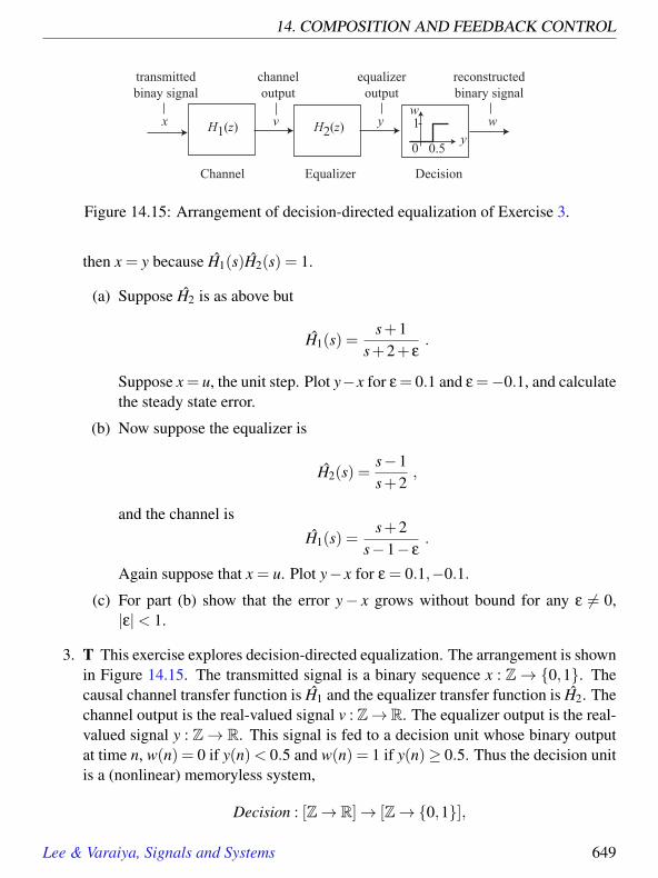
14. COMPOSITION AND FEEDBACK CONTROL
x v y wy
w
0.50
1H1(z) H2(z)
Channel Equalizer Decision
transmittedbinay signal
equalizeroutput
reconstructedbinary signal
channeloutput
Figure 14.15: Arrangement of decision-directed equalization of Exercise 3.
then x = y because H1(s)H2(s) = 1.
(a) Suppose H2 is as above but
H1(s) =s+1
s+2+ ε.
Suppose x = u, the unit step. Plot y−x for ε= 0.1 and ε=−0.1, and calculatethe steady state error.
(b) Now suppose the equalizer is
H2(s) =s−1s+2
,
and the channel isH1(s) =
s+2s−1− ε
.
Again suppose that x = u. Plot y− x for ε = 0.1,−0.1.
(c) For part (b) show that the error y− x grows without bound for any ε 6= 0,|ε|< 1.
3. T This exercise explores decision-directed equalization. The arrangement is shownin Figure 14.15. The transmitted signal is a binary sequence x : Z→ 0,1. Thecausal channel transfer function is H1 and the equalizer transfer function is H2. Thechannel output is the real-valued signal v : Z→R. The equalizer output is the real-valued signal y : Z→ R. This signal is fed to a decision unit whose binary outputat time n, w(n) = 0 if y(n)< 0.5 and w(n) = 1 if y(n)≥ 0.5. Thus the decision unitis a (nonlinear) memoryless system,
Decision : [Z→ R]→ [Z→0,1],
Lee & Varaiya, Signals and Systems 649

EXERCISES
defined by a threshold rule
∀n, (Decision(y))(n) =
0, y(n)< 0.5,1, y(n)≥ 0.5
At each point in time, the receiver has an estimate He1 of the true channel transfer
function, H1. The equalizer is set at
H2(z) = [He1(z)]
−1. (14.11)
(a) Suppose that initially H1(z) = zz−0.2 , and the estimate is perfect, He
1 = H1.(This perfect estimate is achieved using a known training sequence for x.)Determine the respective impulse responses h1 and h2.Now suppose the signal x is
∀n, x(n) =
0, n < 01, n≥ 0,n even0, n≥ 0,n odd
(14.12)
Calculate the channel output v(n) = (h1 ∗ x)(n),n ≤ 3. Then calculate theequalizer output y(n) = (h2 ∗ v)(n),n ≤ 3, and check that y(n) = x(n),n ≤ 3.Also check that w(n) = x(n),n≤ 3.
(b) Now suppose the channel transfer function has changed to
H1(z) =z
z−0.3,
but the receiver’s estimate hasn’t changed, i.e.
He1(z) =
zz−0.2
,
so the equalizer (14.11) hasn’t changed either. For the same input signal againcalculate the channel and equalizer outputs v(n) and y(n) for n ≤ 3. Checkthat y(n) 6= x(n) for n > 0. But show that the decision w(n) = x(n) for n≤ 3.So the equalizer correctly determines x.
(c) Since the receiver’s decision w = x, it can make a new estimate of the channelusing the fact that Y = H1H2X = H1H2W . The new estimate is
He1 =
YH2W
. (14.13)
650 Lee & Varaiya, Signals and Systems

14. COMPOSITION AND FEEDBACK CONTROL
Suppose time is 3, and the receiver has observed y(n),w(n),n ≤ 3. Since theZ transforms Y and W also depend on values of y(n),w(n) for n > 3, these Ztransforms can not be calculated at time n = 3, and so the estimator (14.13)cannot be used. The following approach will work, however.Suppose the receiver knows that the unknown channel transfer function is ofthe form
H1(z) =z
z−a,
so that only the parameter a has to be estimated. Using this information, wehave
Y (z) =z
z−az−0.2
zW (z) =
z−0.2z−a
W (z).
Now take the inverse Z transform and express the time-domain relation be-tween y and w. Show that you can estimate a knowing y(0),y(1),w(0),w(1).
4. E This continues Exercise 3. It shows that if the channel estimate He1 is not suf-
ficiently close to the true channel H1, the decision may become incorrect. Sup-pose the true channel is H1(z) = z
z−a , the estimate is He1(z) =
zz−0.2 , the equal-
izer is H2(z) = [He1(z)]
−1 = z−0.2z , and the decision is as in Figure 14.15. As-
sume the input signal x to be the same as in (14.12) Show that if a = 0.6 thenw(0) = x(0),w(1) = x(1),w(2) = x(2), but w(3) 6= x(3).
5. E This exercise continues the discussion in examples 14.5, 14.6 for the continuous-time, causal and stable channel with impulse response h1 and transfer function
∀s ∈ RoC(h1) = s | Res>−1, H1(s) =s−2s+1
.
(a) Calculate h1 and sketch it. (Observe how the zero in the right-half plane ats = 2 accounts for the negative values.)
(b) The inverse of H1,
H2(s) =s+1s−2
,
has a pole at s = 2. So as a causal system, the inverse is unstable. But as anon-causal system, it is stable with RoC = s | Res < 2 which includesthe imaginary axis. Evaluate the impulse response h2 of H2 as an anti-causalsystem, and give a sketch.
Lee & Varaiya, Signals and Systems 651
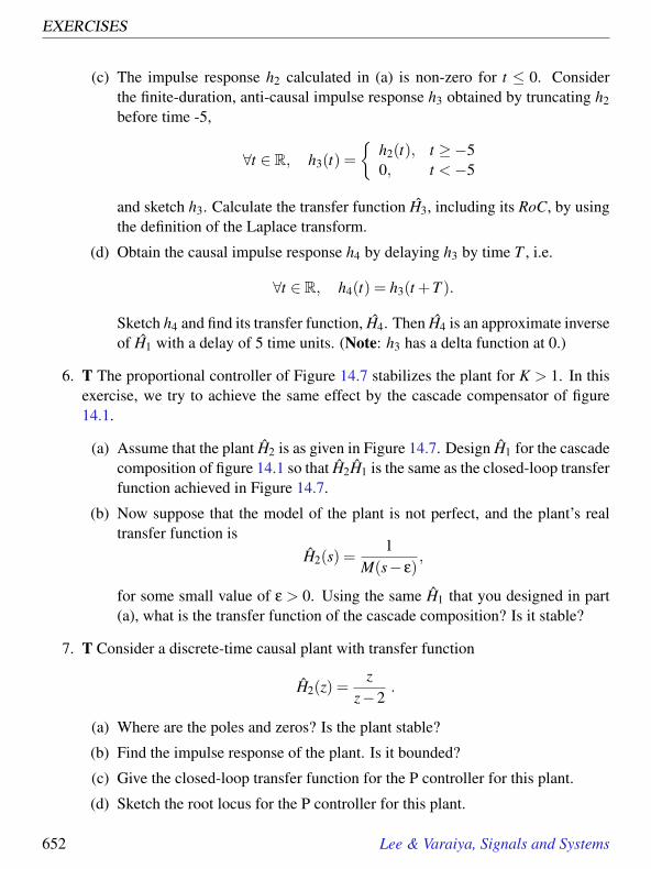
EXERCISES
(c) The impulse response h2 calculated in (a) is non-zero for t ≤ 0. Considerthe finite-duration, anti-causal impulse response h3 obtained by truncating h2before time -5,
∀t ∈ R, h3(t) =
h2(t), t ≥−50, t <−5
and sketch h3. Calculate the transfer function H3, including its RoC, by usingthe definition of the Laplace transform.
(d) Obtain the causal impulse response h4 by delaying h3 by time T , i.e.
∀t ∈ R, h4(t) = h3(t +T ).
Sketch h4 and find its transfer function, H4. Then H4 is an approximate inverseof H1 with a delay of 5 time units. (Note: h3 has a delta function at 0.)
6. T The proportional controller of Figure 14.7 stabilizes the plant for K > 1. In thisexercise, we try to achieve the same effect by the cascade compensator of figure14.1.
(a) Assume that the plant H2 is as given in Figure 14.7. Design H1 for the cascadecomposition of figure 14.1 so that H2H1 is the same as the closed-loop transferfunction achieved in Figure 14.7.
(b) Now suppose that the model of the plant is not perfect, and the plant’s realtransfer function is
H2(s) =1
M(s− ε),
for some small value of ε > 0. Using the same H1 that you designed in part(a), what is the transfer function of the cascade composition? Is it stable?
7. T Consider a discrete-time causal plant with transfer function
H2(z) =z
z−2.
(a) Where are the poles and zeros? Is the plant stable?
(b) Find the impulse response of the plant. Is it bounded?
(c) Give the closed-loop transfer function for the P controller for this plant.
(d) Sketch the root locus for the P controller for this plant.
652 Lee & Varaiya, Signals and Systems

14. COMPOSITION AND FEEDBACK CONTROL
(e) For what values of K is the closed-loop system stable?
(f) Find the step response of the closed-loop system. Identify the transient andsteady-state responses. For K = 10, what is the steady-state tracking error?
(g) Suppose that the plant is instead given by
H2 =z
z−2− ε,
for some real ε≥ 0. For what values of K is the P controller robust for plantswith |ε|< 0.5?
8. T Consider the feedback composition in Figure 14.6. Suppose that H1H2 is causaland strictly proper, meaning that the order of the numerator is greater than theorder of the denominator.
(a) Show that if H1H2 is causal and strictly proper, then so is H, the transferfunction of the feedback composition given by (14.1).
(b) For the discrete-time case, show that we can write
H1(z)H2(z) = z−1G(z), (14.14)
where G(z) is proper, and is the transfer function of a causal system. Intu-itively, this means that there must be a net unit delay in the feedback loop,because z−1 is the transfer function of a unit delay.
(c) Use the result of part (a) to demonstrate that the system H1H2 has state-determined output.
(d) For the continuous-time case, show that we can write
H1(s)H2(s) = s−1G(s), (14.15)
where G(s) is proper, and is the transfer function of a causal system. In-tuitively, this means that there must be an integration in the feedback loop,because s−1 is the transfer function of an integrator.
(e) Use the result of part (c) to demonstrate that the system H1H2 has state-determined output, assuming that the input is bounded and piecewise con-tinuous.
9. E Consider the mth order polynomial sN + am−1sm−1 + · · ·+ a1s + a0. Supposeall its roots have negative real parts. Show that all coefficients of the polynomial
Lee & Varaiya, Signals and Systems 653

EXERCISES
must be positive, i.e., am−1 > 0, · · · ,a0 > 0. Hint. Express the polynomial as (s−p1) · · ·(s− pm) with Repi > 0. Note that complex roots must occur in complexconjugate pairs. (The positiveness of all coefficients is a necessary condition. Asufficient condition is given by the Routh-Hurwitz criterion, described in controltheory texts.)
10. T Consider the feedback composition in figure 14.6. The plant’s transfer functionis H2(s) = 1/s2.
(a) Show that no PI controller in the form H1(s) = K1 +K2/s can stabilize theclosed loop system for any values of K1,K2. Hint. Use the result of problem9.
(b) Show that by the proper choice of the coefficients K1,K2 of a PD controllerin the form H1(s) = K1 +K2s, you can place the closed-loop poles at anylocations p1, p2 (these must be complex conjugate if they are complex).
11. T Consider the feedback composition in figure 14.6. The plant’s transfer functionis H2(s) = 1/(s2 +2s+1). The PI controller is H1(s) = K1 +K2/s.
(a) Take K2 = 0, and plot the root locus as K1 varies. For what values of K1 is theclosed loop system stable? What is the steady state error to a step input as afunction of K1?
(b) Select K1,K2 such that the closed loop system is stable and has zero-steadystate error.
654 Lee & Varaiya, Signals and Systems

ASets and Functions
ContentsA.1 Sets . . . . . . . . . . . . . . . . . . . . . . . . . . . . . . . . . . . 656
A.1.1 Assignment and assertion . . . . . . . . . . . . . . . . . . . 657A.1.2 Sets of sets . . . . . . . . . . . . . . . . . . . . . . . . . . . 658A.1.3 Variables and predicates . . . . . . . . . . . . . . . . . . . . 659A.1.4 Quantification over sets . . . . . . . . . . . . . . . . . . . . . 660Probing Further: Predicates in Matlab . . . . . . . . . . . . . . . . . 661A.1.5 Some useful sets . . . . . . . . . . . . . . . . . . . . . . . . 662A.1.6 Set operations: union, intersection, complement . . . . . . . . 663A.1.7 Predicate operations . . . . . . . . . . . . . . . . . . . . . . 664A.1.8 Permutations and combinations . . . . . . . . . . . . . . . . 665A.1.9 Product sets . . . . . . . . . . . . . . . . . . . . . . . . . . . 666Basics: Tuples, strings, and sequences . . . . . . . . . . . . . . . . . 667A.1.10 Evaluating an expression . . . . . . . . . . . . . . . . . . . . 672
A.2 Functions . . . . . . . . . . . . . . . . . . . . . . . . . . . . . . . . 677A.2.1 Defining functions . . . . . . . . . . . . . . . . . . . . . . . 679A.2.2 Tuples and sequences as functions . . . . . . . . . . . . . . . 679A.2.3 Function properties . . . . . . . . . . . . . . . . . . . . . . . 680
A.3 Summary . . . . . . . . . . . . . . . . . . . . . . . . . . . . . . . . 680Probing Further: Infinite sets . . . . . . . . . . . . . . . . . . . . . . 681Probing Further: Even bigger sets . . . . . . . . . . . . . . . . . . . 683
Exercises . . . . . . . . . . . . . . . . . . . . . . . . . . . . . . . . . . . 684
655

A.1. SETS
This appendix establishes the notation of sets and functions as used in the book. Wereview the use of this mathematical language to describe sets in a variety of ways, tocombine sets using the operations of union, intersection, and product, and to derive logicalconsequences. We also review how to formulate and understand predicates, and we definecertain sets that occur frequently in the study of signals and systems. Finally, we reviewfunctions.
A.1 Sets
A set is a collection of elements. The set of natural numbers, for example, is the collec-tion of all positive integers. This set is so commonly used that it is denoted by the specialsymbol N ,
N= 1,2,3, · · ·. (A.1)
In (A.1) the left hand side is the name of the set and the right hand side is an enumerationor list of all the elements of the set, enclosed by curly braces. We read (A.1) as ‘N isthe set consisting of the numbers 1,2,3, and so on.’ The ellipsis ‘· · · ’ means ‘and so on’.Because N is an infinite set we cannot list all its elements, and so we have to use ellipsis.For a finite set, we may use ellipsis as a convenient shorthand, as in
A = 1,2,3, · · · ,100, (A.2)
which defines A to be the set consisting of the first 100 natural numbers. N and A are setsof numbers.
Many authors include the number zero in the set of natural numbers. For no particularlygood reason, in this text, we denote the set of non-negative integers by a slightly differentsymbol,
N0 = 0,1,2,3, · · ·.
An element of a set is also said to be a member of the set. The number 10 is a memberof the set A defined in (A.2), but the number 110 is not a member of A. We express thesetwo facts by the two expressions:
10 ∈ A, 110 /∈ A.
656 Lee & Varaiya, Signals and Systems

A. SETS AND FUNCTIONS
The symbol ‘∈’ is read ‘is a member of’ or ‘belongs to’ and the symbol ‘/∈’ is read ‘is nota member of’ or ‘does not belong to.’
When we define a set by enumerating or listing all its elements, we enclose the list incurly braces · · ·. It is not always necessary to give the set a name. We can instead referto it directly by enumerating its elements. Thus
1,2,3,4,5
is the set consisting of the numbers 1,2, · · · ,5.
The order in which the elements of the set appear in the list is not (usually) significant.When the order is significant, the set is called an ordered set.
An element is either a member of a set or it is not. It cannot be a member more than once.So, for example, 1,2,1 is not a set.
Two sets are equal if and only if every element of the first set is also an element of thesecond set, and every element of the second set is a member of the first set. So if B =1,2,3,4,5 and C = 5,3,4,1,2, then it is correct to state
B =C. (A.3)
Let A = 1,2, · · · ,10, and B = 1, · · · ,5. B is a subset of A, and A is a subset of N . Weexpress these assertions as:
B⊂ A, A⊂ N.
Some texts use the symbol ⊂ to denote a proper subset, where A ⊂ B means “A is asubset of B and is not equal to B.” Those texts will write A⊆ B to mean “A is a subset ofB and may be equal to B.” In this text, we will not make the distinction. We will use thesymbol ⊂ to mean subset, and if we need to refer to a proper subset, we make it clear thatwe are talking about a proper subset.
The empty set (a set with no elements) is written /0. For any set A, /0⊂ A.
A.1.1 Assignment and assertion
Although the expressions (A.1) and (A.3) are both in the form of equations, the “=” inthese two expressions have very different meanings. Expression (A.1) (as well as (A.2))is an assignment: the set on the right-hand side is assigned to the name N on the left-hand
Lee & Varaiya, Signals and Systems 657

A.1. SETS
side. Expression (A.3) is an assertion, which is an expression that can be true or false. Inother words, an assertion is an expression that has a truth value. Thus (A.3) asserts thatthe two sides are equal. Since this is true, (A.3) is a true assertion. But the assertion
N= A
is a false assertion. An assertion is true or false, while an assignment is a tautology(something that is trivially true because the definition makes it so). Some notation systemsmake a distinction between an assignment and an assertion by writing an assignment usingthe symbol “:=” instead of “=” as in
N := 1,2,3, · · ·.
Other notation systems use “=” for assignments and ‘==’ for assertions. We will not makethese notational distinctions (except in Chapter 6), since it will be clear from the contextwhether an expression is an assignment or an assertion.1
Context is essential in order to disambiguate whether an expression like
MyNumbers = 1,3,5
is an assertion or an assignment. Thus, for example, in the context,
Define the set MyNumbers by MyNumbers = 1,3,5,
the expression is clearly an assignment, as indicated by “Define the set · · ·”. However, inthe following context,
If we define MyNumbers by MyNumbers = 1,3,5, thenMyNumbers = 3,5,1,
the first “=” is an assignment, but the second is an assertion.
A.1.2 Sets of sets
Nearly anything can be an element of a set, so sets can be elements that are themselvessets. Suppose, for example, that X is a set. Then we can construct the set of all subsets of
1A symbol such as “=” which has more than one meaning depending on the context is said to be over-loaded. C++ uses overloaded symbols, while Java does not (Java does support overloaded methods, how-ever). People often have difficulty reading other people’s code written in a language that permits overloading.
658 Lee & Varaiya, Signals and Systems

A. SETS AND FUNCTIONS
X , which is written ℘(X) and is called the powerset of X .2 Notice that since /0⊂ X , then/0 ∈℘(X). ( /0 denotes the empty set.)
The fact that elements of sets can themselves be sets leads to an interesting limitation inthe notion of sets. Consider a set R defined to consist of all sets that are not members ofthemselves. Then is the assertion R ∈ R true or false? If it is true, then R must not be amember of R, and if it is false, then R must be a member of R. This paradox is knownas Russell’s paradox. It demonstrates that the notion of sets is not in fact as universal asonce thought. This subtlety, however, will not in any way infringe on our ability to usesets in this book, so we can safely ignore it.
A.1.3 Variables and predicates
We can refer to a particular element of a set by using its name, for example the element 55in N . We often need to refer to a general element in a set. We do this by using a variable.We usually use lower case letters for variable names, such as x,y,n, t. Thus n ∈ N refersto any natural number. N is the set of values that the variable n can take on. We may alsouse a character string for a variable name such as city ∈ USCities. We say that “n is avariable over N ” and “city is a variable over USCities,” where USCities is the set of citiesin the United States.
A variable can be assigned (or substituted by) any value in its range. Thus the assignmentn = 5 assigns the value 5 to n, and city = Berkeley assigns the value Berkeley to city.
Once again the use of “=” in an expression like n= 5 is ambiguous, because the expressioncould be an assignment or an assertion, depending on the context. Thus, for example, inthe context,
Let n = 5,m = 6, and k = 2, then m = k+n
the first three “=” are assignments, but the last is an assertion, which happens to be false.
We can use variables to form expressions such as n≤ 5. Now, when we assign a particularvalue to n in this expression, the expression become an assertion that evaluates to true orfalse. (For instance, n≤ 5 evaluates to true for n= 3 and to false for n= 6.) An expressionsuch as x≤ 5 which evaluates to true or false when we assign the variable a specific value
2The powerset of X is sometimes written 2X .
Lee & Varaiya, Signals and Systems 659

A.1. SETS
is called a predicate (in x).3 Predicates are used to define new sets from old ones, as inthis example:
B = x ∈ N | x≤ 5which reads “B is the set of all elements x in N such that (the symbol ‘|’ means ‘such that’)the predicate x≤ 5 is true.” More generally, we use the following prototype expression todefine a new set NewSet from an old set Set
NewSet = x ∈ Set | Pred(x). (A.4)
In this prototype expression for defining sets, x ∈ Set means that x is a variable over theset Set, Pred(x) is a predicate in x, and so NewSet is the set consisting of all elements x inSet for which Pred(x) evaluates to true.
The concept of predicate is very general. In essence, a predicate is a condition involvingany attributes or properties of the elements of Set. Consider
TallStudents = name ∈ Students | name is more than 6 feet tall.
Here the predicate is “name is more than 6 feet tall.”
The variable name “x” used in (A.4) is not significant. The sets x ∈ N | x ≥ 5 andn ∈ N | n≥ 5 are the same sets even though the variable names used in the prototypesare different. This is because the predicates ‘n ≥ 5’ and ‘x ≥ 5’ both evaluate to trueor both evaluate to false when the same value is assigned to n and x. We say that thevariable name x used in (A.4) is a dummy variable since the meaning of the expressionis unchanged if we substitute x with another variable name, say y. You are already familiarwith the use of dummy variables in integrals. The two integrals below evaluate to the samenumber: ∫ 1
0x2dx =
∫ 1
0y2dy.
A.1.4 Quantification over sets
Consider the set A = 1,3,4. Suppose we want to make the assertion that every elementof A is smaller than 7. We could do this by the three expressions
1 < 7, 3 < 7, 4 < 7,3A specific value is said to satisfy a predicate if it evaluates to true, and not to satisfy the predicate if the
predicate evaluates to false.
660 Lee & Varaiya, Signals and Systems

A. SETS AND FUNCTIONS
which gets to be very clumsy if A has many more elements. So mathematicians haveinvented a shorthand. The idea is to be able to say that x < 7 for every value that thevariable x takes in the set A. The precise expression is
∀x ∈ A, x < 7. (A.5)
The symbol ‘∀’ reads ‘for all’, so the expression reads, “for all values of x in A, x < 7.”The phrase ∀x ∈ A is called universal quantification. Note that in the expression (A.5), xis again a dummy variable; the meaning of the expression is unchanged if we use anothervariable name. Note, also, that (A.5) is an assertion which, in this case, evaluates to true.However, the assertion
∀x ∈ A, x > 3
is false, since for at least one value of x ∈ A, namely x = 1, x > 3 is false.
Suppose we want to say that there is at least one element in A that is larger than 3. Wecan say this using existential quantification as in
∃x ∈ A, x > 3. (A.6)
Probing Further: Predicates in Matlab
In Matlab, “=” is always used as an assignment, while “==” is used to express an asser-tion. Thus the Matlab program,
n = 5, m = 6, k = 2, m = k+n
returns
n = 5, m = 6, k = 2, m =7
because the expression m=k+n assigns the value 7 to m. However, the Matlab program
n = 5, m = 6, k = 2, m == k+n
returns
n = 5, m = 6, k = 2, ans = 0
where ans = 0 means that the assertion m == k+n evaluates to false.
Lee & Varaiya, Signals and Systems 661
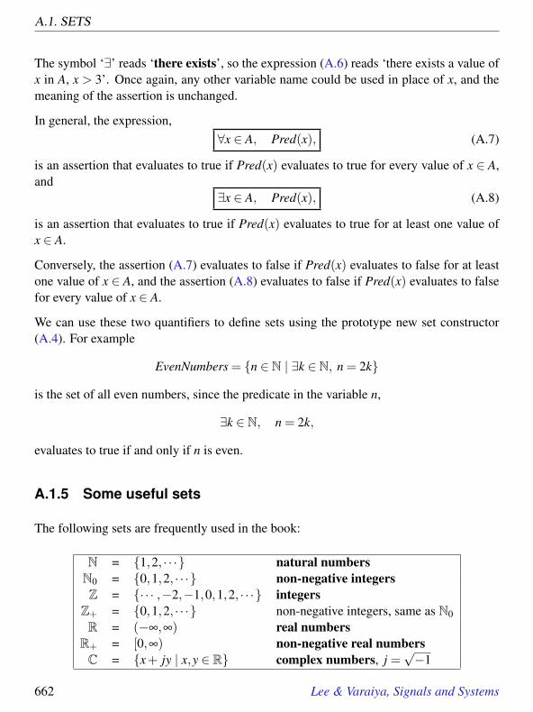
A.1. SETS
The symbol ‘∃’ reads ‘there exists’, so the expression (A.6) reads ‘there exists a value ofx in A, x > 3’. Once again, any other variable name could be used in place of x, and themeaning of the assertion is unchanged.
In general, the expression,∀x ∈ A, Pred(x), (A.7)
is an assertion that evaluates to true if Pred(x) evaluates to true for every value of x ∈ A,and
∃x ∈ A, Pred(x), (A.8)
is an assertion that evaluates to true if Pred(x) evaluates to true for at least one value ofx ∈ A.
Conversely, the assertion (A.7) evaluates to false if Pred(x) evaluates to false for at leastone value of x ∈ A, and the assertion (A.8) evaluates to false if Pred(x) evaluates to falsefor every value of x ∈ A.
We can use these two quantifiers to define sets using the prototype new set constructor(A.4). For example
EvenNumbers = n ∈ N | ∃k ∈ N, n = 2k
is the set of all even numbers, since the predicate in the variable n,
∃k ∈ N, n = 2k,
evaluates to true if and only if n is even.
A.1.5 Some useful sets
The following sets are frequently used in the book:
N = 1,2, · · · natural numbersN0 = 0,1,2, · · · non-negative integersZ = · · · ,−2,−1,0,1,2, · · · integers
Z+ = 0,1,2, · · · non-negative integers, same as N0R = (−∞,∞) real numbers
R+ = [0,∞) non-negative real numbersC = x+ jy | x,y ∈ R complex numbers, j =
√−1
662 Lee & Varaiya, Signals and Systems

A. SETS AND FUNCTIONS
If α,β are real numbers, then intervals of real numbers are written
[α,β] = x ∈ R | α≤ x≤ β(α,β) = x ∈ R | α < x < β(α,β] = x ∈ R | α < x≤ β
(−∞,∞) = R
Note the meaning of the difference in notation: both end-points α and β are included in[α,β], and we say that [α,β] is a closed interval; neither end-point is included in (α,β),and we call this an open interval; the interval (α,β] is said to be half-open, half-closed.Whether an end-point is included in an interval or not is indicated by the use of squarebrackets [, ] or parentheses (,).
Other useful sets are:
Binary = 0,1 the binary valuesBinary∗ = 0,1∗ set of all finite binary strings
Bools = true, false truth valuesBools∗ = true, false∗ set of finite sequences of truth values
Char = a,b, · · · set of all alphanumeric charactersChar∗ = a,b, · · ·∗ set of all finite character strings
A.1.6 Set operations: union, intersection, complement
If A and B are sets, then the intersection A∩B is the set consisting of all elements thatare in both A and B. The union A∪B is the set consisting of all elements that are eitherin A or in B or in both A and B. We can express these definitions using variables as:
A∩B = x | x ∈ A∧ x ∈ B, A∪B = x | x ∈ A∨ x ∈ B
where ∧ is the notation for the logical and and ∨ is the symbol for the logical or. Thepredicate “x ∈ A∧x ∈ B” reads “x is a member of A and x is a member of B”; “x ∈ A∨x ∈B” reads “x is a member of A or x is a member of B.” The logical and of two predicatesis also called their conjunction and their logical or is also called their disjunction. Thesymbols ∧ and ∨ are called logical connectives.
If A,X are sets, then X \A is the set consisting of all elements in X that are not in A (thinkof it as set subtraction, X −A). When A⊂ X , X \A is called the complement of A in X .When X is understood, we can write Ac instead of X \A.
Lee & Varaiya, Signals and Systems 663

A.1. SETS
B
A∩B
A
A∪B
X
Ac
A
(a) (b)
Figure A.1: (a) Union and intersection. (b) Set complement.
We gain some intuitive understanding by depicting sets and set operations using pictures.Figure A.1 illustrates union, intersection, and complement.
A.1.7 Predicate operations
Given two predicates P(x) and Q(x) we can form their conjunction P(x)∧Q(x), and theirdisjunction P(x)∨Q(x). These predicate operations correspond to the set operations ofintersection and union:
x ∈ X | P(x)∧Q(x) = x ∈ X | P(x)∩x ∈ X | Q(x)x ∈ X | P(x)∨Q(x) = x ∈ X | P(x)∪x ∈ X | Q(x). (A.9)
There is a helpful visual similarity between ∧ and ∩, and between ∨ and ∪.
The counterpart of the complement of a set is the negation of a predicate. We denoteby ¬Pred(x) the predicate that evaluates to false for any value of x for which Pred(x)evaluates to true, and that evaluates to true for any value of x for which Pred(x) evaluatesto false. We read “¬Pred(x)” as “not Pred(x)” or the “negation of Pred(x).” For example,
n ∈ N | ¬(n < 5)= 5,6,7, · · ·,
since ¬(n < 5) evaluates to true if and only if n < 5 evaluates to false, which happens ifand only if n is larger than or equal to 5.
664 Lee & Varaiya, Signals and Systems

A. SETS AND FUNCTIONS
In general we have the following correspondence between predicate negation and set com-plement:
x ∈ X | ¬Pred(x)= X \x ∈ X | Pred(x). (A.10)
We can combine (A.9), (A.9), and (A.10) to obtain more complex identities. If P(x) andQ(x) are predicates, then
x ∈ X | ¬(P(x)∧Q(x)) = x ∈ X | ¬P(x)∨¬Q(x),x ∈ X | ¬(P(x)∨Q(x)) = x ∈ X | ¬P(x)∧¬Q(x). (A.11)
These identities have counterparts for set operations. For some set X , if and Y ⊂ X andZ ⊂ X , then
X \ (Y ∩Z) = (X \Y )∪ (X \Z),X \ (Y ∪Z) = (X \Y )∩ (X \Z).
When the set X is understood, we can write these as
(Y ∩Z)c = Y c∪Zc,(Y ∪Z)c = Y c∩Zc.
These identities are called de Morgan’s rules.
A.1.8 Permutations and combinations
Given a set X with a finite number n of elements, we sometimes wish to construct a subsetwith a fixed number m≤ n of elements. The number of such subsets is given by(
nm
)=
n!m!(n−m)!
, (A.12)
where the exclamation point denotes the factorial function. The notation(n
m
)is read “n
choose m”. It gives the number of combinations of m elements from the set n.
A combination is a set, so order does not matter. Sometimes, however, order matters.Suppose for example that X = a,b,c. The number of subsets with two elements is(
32
)=
3!2!1!
=62= 3.
Lee & Varaiya, Signals and Systems 665

A.1. SETS
These subsets are a,b, a,c, and b,c. Suppose instead that we wish to constructordered subsets of X with two elements. In other words, we wish to consider [a,b] to bedistinct from [b,a] (note the temporary use of square brackets to avoid confusion with un-ordered sets). Such ordered subsets are called permutations. The number of m-elementpermutations of a set of size n is given by
n!(n−m)!
. (A.13)
The number of permutations is a factor of m! larger than the number of combinations inA.12. For example, the number of 2-element permutations of X = a,b,c is six. Theyare (a,b), (a,c), (b,c), (b,a), (c,a), and (c,b).
A.1.9 Product sets
The Cartesian product X ×Y of two sets X and Y consists of all pairs of elements (x,y)with x ∈ X and y ∈ Y , i.e.
X×Y = (x,y) | x ∈ X ,y ∈ Y.
The product of two sets may be visualized as in Figure A.2. These pictures are informal,to be used only to reinforce intuition. In Figure A.2(a), the set X = [0,6] is representedby a horizontal line segment, and the set Y = [1,8] is represented by the vertical linesegment. The product set X ×Y = [0,6]× [1,8] is represented by the rectangle whoselower left corner is the pair (0,1) and upper right corner is (6,8).
In Figure A.2(b), the discrete set X = 1,2,3,4,5,6 is represented by six points, whileand Y = [1,8] is represented the same as before. The product set is depicted by six verticalline segments, one for each element of X . For example, the fifth segment from the left isthe set (5,y) | 1≤ y≤ 8. One point in that set is shown.
In Figure A.2(c), the product of two discrete sets is shown as an array of points. Unlessthese are ordered sets, there is no significance to the the left-to-right or top-to-bottom or-der in which the points are shown. In all three cases in the figure, there is no significanceto the choice to depict the first set in the product X×Y on the horizontal axis, and the sec-ond set on the vertical axis. We could have done it the other way around. Although thereis no significance to which is depicted on the vertical axis and which on the horizontal,there is significance to the order of X and Y in X ×Y . The set X ×Y is not the same asY ×X unless X = Y .
666 Lee & Varaiya, Signals and Systems

A. SETS AND FUNCTIONS
Basics: Tuples, strings, and sequences
Given N sets, X1,X2, · · · ,XN , (which may be identical), an N-tuple is an ordered collec-tion of one element from each set. It is written in parentheses, as in
(x1,x2, · · · ,xN), where
xi ∈ Xi for each i ∈ 1,2, · · · ,N.The elements of an N-tuple are called its components or coordinates. Thus xi is the i-thcomponent or coordinate of (x1, · · · ,xN). The order in which the components are givenis important; it is part of the definition of the N-tuple. We can use a variable to refer tothe entire N-tuple, as in x = (x1, · · · ,xN).
Frequently the sets from which the tuple components are drawn are all identical, as in
(x1,x2, · · · ,xN) ∈ XN .
This notation means simply that each component in the tuple is a member of the same setX . Of course, this means that a tuple may contain identical components. For example, ifX = a,b,c then (a,a) is a 2-tuple over X .
Recall that a permutation is ordered, like a tuple, but like a set and unlike a tuple,it does not allow duplicate elements. In other words, (a,a) is not a permutation ofa,b,c. So a permutation is not the same as a tuple. Similarly, an ordered set does notallow duplicate elements, and thus is not the same as a tuple.
We define the set of finite sequences over X to be
(x1, · · ·xN) | xi ∈ X ,1≤ i≤ N,N ∈ N0.
where if N = 0 we call the sequence the empty sequence. This allows us to talk abouttuples without specifying N. Finite sequences are also called strings, although by con-vention, strings are written differently, omitting the parentheses and commas, as in
x1x2 · · ·xN .
We may even wish to allow N to be infinite. We define the set of infinite sequence overa set X to be
(x1,x2, · · ·) | xi ∈ X , i ∈ N0.
Lee & Varaiya, Signals and Systems 667

A.1. SETS
(0,1)
(6,8)
(5,6)
X = [0,6]
(a) (b)
X = 1, 2, 3, 4, 5, 6
Y = [1,8] [0, 6] × [1,8]
(c)
a b c d e f
g
h
i
j
X = a, b, c, d, e, f
Y = g, h, i, j
a, b, c, d, e, f × g, h, i, j
Y = [1,8]
1 2 3 4 5 6
1, 2, 3, 4, 5, 6 × [1, 8]
Figure A.2: Visualization of product sets. (a) The rectangle depicts the product set[0,6]× [1,8]. (b) Together, the six vertical lines depict the product set 1, · · · ,6×[1,8]. (c) The array of dots depicts the set a,b,c,d,e, f×g,h, i, j.
668 Lee & Varaiya, Signals and Systems
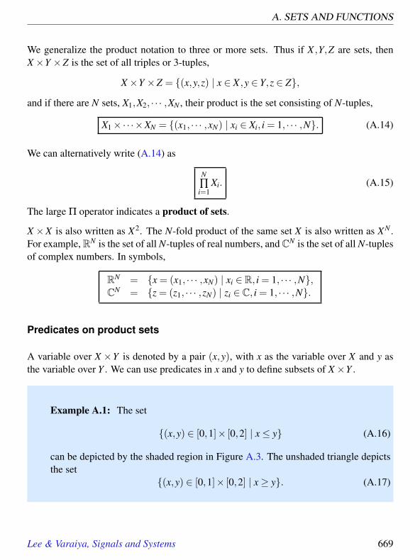
A. SETS AND FUNCTIONS
We generalize the product notation to three or more sets. Thus if X ,Y,Z are sets, thenX×Y ×Z is the set of all triples or 3-tuples,
X×Y ×Z = (x,y,z) | x ∈ X ,y ∈ Y,z ∈ Z,
and if there are N sets, X1,X2, · · · ,XN , their product is the set consisting of N-tuples,
X1×·· ·×XN = (x1, · · · ,xN) | xi ∈ Xi, i = 1, · · · ,N. (A.14)
We can alternatively write (A.14) as
N∏i=1
Xi. (A.15)
The large Π operator indicates a product of sets.
X ×X is also written as X2. The N-fold product of the same set X is also written as XN .For example, RN is the set of all N-tuples of real numbers, and CN is the set of all N-tuplesof complex numbers. In symbols,
RN = x = (x1, · · · ,xN) | xi ∈ R, i = 1, · · · ,N,CN = z = (z1, · · · ,zN) | zi ∈ C, i = 1, · · · ,N.
Predicates on product sets
A variable over X ×Y is denoted by a pair (x,y), with x as the variable over X and y asthe variable over Y . We can use predicates in x and y to define subsets of X×Y .
Example A.1: The set
(x,y) ∈ [0,1]× [0,2] | x≤ y (A.16)
can be depicted by the shaded region in Figure A.3. The unshaded triangle depictsthe set
(x,y) ∈ [0,1]× [0,2] | x≥ y. (A.17)
Lee & Varaiya, Signals and Systems 669

A.1. SETS
x = y
Y = [0, 2]
X = [0, 1]
Figure A.3: The rectangle depicts the set [0,1]× [0,2], the shaded region depictsthe set given by (A.16), and the unshaded triangle depicts the set given by (A.17).
Example A.2: The solid line in Figure A.4(a) represents the set
(x,y) ∈ R2 | x+ y = 1,
the shaded region (including the solid line) depicts
(x,y) ∈ R2 | x+ y≥ 1,
and the unshaded region (excluding the solid line) depicts
(x,y) ∈ R2 | x+ y < 1.
Similarly the shaded region in Figure A.4(b) depicts the set
(x,y) ∈ R2 | − x+ y≥ 1.
The overlap region in Figure A.4 (c) depicts the intersection of the two shadedregions, and corresponds to the conjunction of two predicates:
(x,y) ∈ R2 | [x+ y≥ 1]∧ [−x+ y≥ 1].
670 Lee & Varaiya, Signals and Systems

A. SETS AND FUNCTIONS
(a)
-x + y = 1
(b)
x + y = 1
(c)
x + y = 1-x + y = 1
Figure A.4: (a) The solid line depicts the subset of R2 satisfying the predicatex+y= 1. The shaded region satisfies x+y≥ 1. (b) The solid line satisfies −x+y=1, and the shaded region satisfies −x+ y ≥ 1. (c) The overlap region satisfies[x+ y≥ 1]∧ [−x+ y≥ 1].
Lee & Varaiya, Signals and Systems 671

A.1. SETS
A.1.10 Evaluating an expression
We have evaluated expressions several times in this appendix, each time relying on ourmathematical ability with simple expressions. We can develop systematic methods forevaluating expressions that rely less on intuition, and can therefore handle more compli-cated and intricate expressions.
Some examples of patterns of expressions are:
• A,B,N, · · · , names of sets
• A = list of elements
• x ∈ A, x /∈ A, set membership
• A = B, B⊂ A, and A⊃ B, set inclusion
• A∩B, A∪B, X×Y , X \A, Ac, set operations
• x,y, · · · , names of variables
• P(x),Q(x), · · · , predicates in x
• ∀x ∈ Set, P(x) and ∃x ∈ Set, Q(x), assertions obtained by quantification
• NewSet = x ∈ Set | Pred(x), set definition
• P(x)∧Q(x), P(x)∨Q(x), ¬(P(x)), predicate operations
The patterns define the rules of grammar of the notation. The notation itself consists ofexpressions, which are composed of
• constants, such as numbers and pre-defined sets,
• variables, which are names that are not pre-defined,
• operators, such as ∈, ∩, or = (as an assertion),
• quantifiers, such as ∀ and ∃, or
• definitions, namely = (as an assignment).
672 Lee & Varaiya, Signals and Systems

A. SETS AND FUNCTIONS
An expression is well-formed if it conforms to the established patterns.4 For example, ifP,Q and R are predicates, then the syntax implies that
¬[[¬(P(x))∨Q(x)]∧ [P(x)∨ [R(x)∧¬(P(x))]]] (A.18)
is also a predicate. Just as in the case of a computer language, you learn the syntax ofmathematical expressions through practice.5
In an expression, constants have a single meaning. For example, “20” is a number,“Berkeley” is a city, and the constant “true” has a truth value. By contrast, a variable,such as x, has no single meaning, unless it has been defined (which turns it into a con-stant). An expression on constants has a single meaning. For example, “10+ 3” means“13.” However, “x+3” has no single meaning, unless x has been defined. We say that inthe expression “x+3,” x is a free variable. An expression with a free variable acquires asingle meaning when that free variable is given a single meaning, if it is well formed withthat meaning. For example, “x+3,” has meaning 13 if x has meaning 10, but it is not wellformed if x has meaning Berkeley.
Quantifiers remove free variables from expressions.
Example A.3: In the expression “x = 0,” x is free. In the expression “∃ x ∈R, x = 0,” x is no longer free. In fact, this expression has value true. In theexpression “∀ x ∈ R, x = 0,”, again x is not free, but this expression has valuefalse. The expression “∃ y ∈ R, x + 1 = y” still has free x. However, “∀ x ∈R,∃ y ∈ R, x+ 1 = y” has no free variables, and has value true. The expression“∀ x ∈ R, x+ 7,” however, is not well formed. It has neither free variables nor avalue.
A predicate expression is one that either has a meaning that is a truth value (true or false),or can have such a meaning if its free variables are appropriately defined. Expression(A.18) is an example a predicate expression.
4In this text, we do not attempt to define precisely what these established patterns are. To do so, we wouldhave to define a grammar, something that can be done formally, but is beyond our scope.
5The syntax of a language is the set of rules (or patterns) whereby words can be combined to formgrammatical or well-formed sentences. Thus the syntax of the ‘C’ language is the set of rules that a sequenceof characters (the code) must obey to be a C program. A C compiler checks whether the code conforms to thesyntax. Of course, even if the code obeys the syntax, it may not be what you intend; i.e. it may not executethe intended computation.
Lee & Varaiya, Signals and Systems 673

A.1. SETS
Q(x)
∧
¬
P(x)
∨
R(x)∧ (¬P(x))
R(x)
∨
P(x) ∧
¬
¬
P(x) ¬P(x)
Figure A.5: Parse tree for the expression (A.18).
Expressions also contain punctuation, such as parentheses. These help define the rela-tionships among the components of the expression. It is beyond the scope of this bookto define completely the rules for constructing expressions6, but we can hint at the issueswith a brief discussion of parsing.
Parsing
To show that (A.18) is indeed a well-formed predicate expression, we must show that itcan be constructed using the syntax. We do this by parsing the expression (A.18) withthe help of matching brackets and parentheses. Parsing the expression will also enable usto evaluate it in a systematic way.
The result is the parse tree shown in Figure A.5. The leaves of this tree (the bottom-most nodes) are labeled by the elementary predicates P,Q,R, and the other nodes of thetree are labeled by one of the predicate operations ∧,∨,¬. Each of the intermediatenodes corresponds to a sub-predicate of (A.18). Two such sub-predicates are shown inthe figure. The last leaf on the right is labeled P(x). Its parent node is labeled ¬, and sothat parent node corresponds to the sub-predicate ¬(P(x)). Its parent node is labeled ∧,
6A text on compilers for computer programming languages will typically do this.
674 Lee & Varaiya, Signals and Systems

A. SETS AND FUNCTIONS
and it has another child node labeled R(x), so this node corresponds to the sub-predicateR(x)∧¬(P(x)).If we go up the tree in this way, we can see that the top of the tree (the root node) indeedcorresponds to the predicate (A.18). Since at each intermediate node, the sub-predicate isconstructed using the syntax, the root node is a well-formed predicate.
Evaluating
Suppose we know whether the predicates P(x),Q(x),R(x) evaluate to true or false forsome value of x. Then we can use the parse tree to figure out whether the predicate (A.18)evaluates to true or false. To do this, we begin with the known truth values at the leavesof the parse tree, use the meaning of the predicate operations to figure out the truth valuesof the sub-predicates corresponding to the parents of the leaf nodes, and then the parentsof those nodes, and work our way up the tree to figure out the truth value of the predicate(A.18) at the root node. In Figure A.6 the parse tree is annotated with the truth valuesof each of the nodes. Since the root node is annotated ‘false,’ we conclude that (A.18)evaluates to false.
Truth tables
The way in which the predicate operations transform the truth values is given in the fol-lowing truth table:
P(x) Q(x) ¬P(x) P(x)∧Q(x) P(x)∨Q(x)true true false true truetrue false false false true
false true true false truefalse false true false false
Consider a particular row of this table, say the first row. The first two entries specify thatP(x) is true and Q(x) is true. The remaining three entries give the corresponding truthvalues for ¬P(x), P(x)∧Q(x) and P(x)∨Q(x), namely, ¬P(x) is false, P(x)∧Q(x) istrue, and P(x)∨Q(x) is true. The four rows correspond to the four possible truth valueassignments of P(x) and Q(x). This truth table can be used repeatedly to evaluate anywell-formed expression given the truth value of P(x) and Q(x).
Lee & Varaiya, Signals and Systems 675

A.1. SETS
True
∧← True
¬← False
True
∨← True
True
∨← True
True ∧← False
¬← False
¬← True
True
Figure A.6: Parse tree for the expression (A.18) annotated with the truth valuesof each of the nodes.
676 Lee & Varaiya, Signals and Systems

A. SETS AND FUNCTIONS
Thus, given the truth values of predicates P1(x), . . . ,Pn(x), the truth value of any well-formed expression involving these predicates can be obtained by a computer algorithmthat constructs the parse tree and uses the truth table above. Such algorithms are used toevaluate logic circuits.
A.2 Functions
In the notationf : X → Y, (A.19)
X and Y are sets, and f is the name of a function. The function is an assignment rule thatassigns a value in Y to each element in X . If the element in X is x, then the value is writtenf (x).
We read (A.19) as “ f is (the name of) a function from X into (or to) Y .” We also saythat f maps X into Y . The set X is called the domain of f , written X = domain( f ), theset Y is called the range of f , written Y = range( f ).7 When the domain and range areunderstood from the context, we write “ f ” by itself to represent the function or the map.If x is a variable over X , we also say “ f is a function of x.”
Example A.4: Let the set Students contain all the students in this class. Eachelement of Students is represented by a student’s name,
Students = John Brown,Jane Doe, · · ·.
We assign to each name in Students the student’s marks in the final examination,a number between 0 and 100. This name-to-marks assignment is an example of afunction. Just as we give names to sets (e.g. Students), we give names to functions.In this example the function might be named Score. When we evaluate the functionScore at any name, we get the marks assigned to that name. We write this as
Score(John Brown) = 90, Score(Jane Doe) = 91.2, · · ·
7In some mathematics texts, the set Y which we call the range is called the codomain, and range( f ) isdefined to be the set of all values that f takes, i.e., range( f ) = f (x) | x ∈ X. However, we will not use thisterminology.
Lee & Varaiya, Signals and Systems 677

A.2. FUNCTIONS
JohnBrown
JaneDoe
[0, 100]
Students
Figure A.7: Illustration of Score.
Figure A.7 illustrates the function Score. Three things are involved in definingScore: the set Students, the set [0,100] of possible marks, and the assignment ofmarks to each name. In the figure this assignment is depicted by the arrows: thetail of the arrow points to a name and the head of the arrow points to the marksassigned to that name. We denote these three things by
Score : Students→ [0,100]
which we read as “Score is a function from Students into [0,100].” The domain ofthe function Score is Students, and the range of Score is [0,100].
It is easy to imagine other functions with the same domain Students. For example, Heightassigns to each student his or her height measured in cm, SSN assigns students their socialsecurity number, and Address assigns students their address. The range of these functionsis different. The range of Height might be defined to be [0,200] (200 cm is about 6.5feet). Since a social security number is a 9-digit number, we can take 0,1, · · · ,99 to bethe range of SSN. And we can take the range of Address to be Char100, assuming that anaddress can be expressed as a string of 100 characters, including blank spaces.
We usually use lower case letters for function names, such as f ,g,h, or more descriptivenames such as Score, Voice, Video, SquareWave, AMSignal.
678 Lee & Varaiya, Signals and Systems

A. SETS AND FUNCTIONS
Avoid a bad habit: It is important to distinguish between a function f and its valuef (x) at a particular point x ∈ domain( f ). The function f is a rule that assigns a valuein range( f ) to each x ∈ domain( f ), whereas f (x) is a point or element in range( f ).Unfortunately, too many books encourage the bad habit by using ‘ f (x)’ as a shorthandfor ‘ f is a function of x.’ If you keep the distinction between f and f (x), it will be easierto avoid confusion when we study systems.
A.2.1 Defining functions
To define a function, you must give the domain, the range, and the rule that producesan element in the range given an element in the domain. There are many ways to dothis, as explored in much more depth in Chapter 2. Here we mention only two. The firstis enumeration. That is, in tabular form or some other form, each possible value in thedomain is associated with a value in the range. This method would be appropriate for theScore function, for example. Alternatively, functions can be mathematically defined bythe prototype: define f : X → Y ,
∀ x ∈ X , f (x) = expression in x.
The ‘expression in x’ may be specified by an algebraic expression, by giving the graph off , by a table, or by a procedure.
A.2.2 Tuples and sequences as functions
An N-tuple x = (x1, · · · ,xN) ∈ XN can be viewed as a function
x : 1, · · · ,N→ X .
For each integer in 1, · · · ,N, it assigns a value in X . An infinite sequence y over the setY can also be viewed as a function
y : N→ Y,
ory : N0→ Y,
depending on whether you wish to begin indexing the sequence at zero or one (both con-ventions are widely used). This view of sequences as functions is in fact our model fordiscrete-time signals and event traces, as developed in Chapter 1.
Lee & Varaiya, Signals and Systems 679

A.3. SUMMARY
A.2.3 Function properties
A function f : X → Y is one-to-one if
∀ x1 ∈ X and ∀ x2 ∈ X , x1 6= x2⇒ f (x1) 6= f (x2).
Here the logical symbol ‘⇒’ means ‘implies’ so the expression is read: if x1,x2 are twodifferent elements in X , then f (x1), f (x2) are different.
Example A.5: The function Cube : R→ R given by
∀ x Cube(x) = x3,
is one-to-one, because if x1 6= x2, then x31 6= x3
2. But Square is not one-to-one be-cause, for example, Square(1) = Square(−1).
A function f : X → Y is onto if
∀ y ∈ Y, ∃ x ∈ X , such that f (x) = y.
The expression above reads: ‘For each y in Y , there exists x in X such that f (x) = y.’
Accordingly, f is onto if for every y in its range there is some x in its domain such thaty = f (x).
Example A.6: The function Cube : R → R is one-to-one and onto, whileSquare : R→ R is not onto. However, Square : R→ R+ is onto.
A.3 Summary
Sets are mathematical objects representing collections of elements. A variable is a rep-resentative for an element of a set. A predicate over a set is an expression involving avariable that evaluates to true or false when the variable is assigned a particular element
680 Lee & Varaiya, Signals and Systems

A. SETS AND FUNCTIONS
Probing Further: Infinite sets
The size of a set A, denoted |A|, is the number of elements it contains. By counting, weimmediately know that 1,2,3,4 and a,b,c,d have the same number of elements,whereas 1,2,3 has fewer elements. It is more difficult to compare the number ofelements in the following infinite sets:
A = N= 1,2,3,4, · · ·, B = 2,3,4,5 · · ·, C = [0,1].
At first, we might say that A has one more element than B, since A includes B and hasone additional element, 1 ∈ A. However, these two sets have the same size.
The cardinality of a set is the number of elements in the set, but generalized to handleinfinite sets. Comparing the cardinality of two sets is done by matching elements usingone-to-one functions. Consider two sets A and B. We say that A has a smaller cardinalitythan B, written |A| ≤ |B|, if there exists a one-to-one function mapping A into B. We saythat A and B have the same cardinality, written |A|= |B|, if |A| ≤ |B| and |B| ≤ |A|.
The cardinality of the infinite set A = N is denoted ℵ0, read “aleph zero” (aleph isthe first letter of the Hebrew alphabet). It is quite easy to prove using the definition ofcardinality that n < ℵ0 for any finite number n. We can now show that the cardinality ofB is also ℵ0. There is a one-to-one function f : A→ B, namely
∀ n ∈ A, f (n) = n+1,
so that |A| ≤ |B|, and there is a one-to-one function g : B→ A, namely
∀ n ∈ B, g(n) = n−1,
so that |B| ≤ |A|. A similar argument can be used to show that the set of even numbersand the set of odd numbers also have cardinality ℵ0.
It is more difficult to show that the cardinality of N×N is also ℵ0. To see this,consider a one-to-one function h : N2→ N (see Figure A.8),
h((1,1)) = 1, h((2,1)) = 2, h((2,2)) = 3, h((1,2)) = 4, h((1,3)) = 5, · · ·
Since a rational number m/n can be identified with the pair (m,n) ∈N2, we have shownthat the cardinality of the set of rational numbers is ℵ0.
Lee & Varaiya, Signals and Systems 681

A.3. SUMMARY
(1,1)
(2,2) (1,2)
(2,1)
(1,3) (2,3) (3,3)
(3,2)
(3,1) (4,1)
(4,2)
(4,3)
(4,4) (4,3) (4,2) (4,1)
(5,1)
Figure A.8: A correspondence between N2 and N.
of the set. Predicates are used to construct new sets from existing sets. If the variable in apredicate is quantified, the expression becomes an assertion.
Sets can be combined using the operations of union, intersection and complement. Thecorresponding operations on predicates are disjunction, conjunction and negation. Newsets can also be obtained by the product of sets.
Functions are mathematical objects representing a relationship between two sets, the do-main and the range. We have introduced the following patterns of expressions for func-tions
• f ,g,h,Score, · · · , names of functions,
• f : X → Y , X = domain( f ),Y = range( f ), a function from X to Y ,
A function f : X → Y assigns to each value x ∈ X a value f (x) ∈ Y .
682 Lee & Varaiya, Signals and Systems

A. SETS AND FUNCTIONS
Probing Further: Even bigger sets
We can show that the cardinality of [0,1] is strictly larger than that of N; i.e. |[0,1]|> |N|Since the function f : N→ [0,1] defined by
∀ n ∈ N, f (n) = 1/n
is one-to-one, we have |N| ≤ |[0,1]|. However, we can show that there is no one-to-onefunction in the other direction. If there were such a function g : [0,1]→N, then it wouldbe possible to enumerate all the elements of [0,1] in an ordered list,
[0,1] = x1,x2,x3, · · ·. (A.20)
(The superscript here is not raising to a power, but just indexing.) We can show that thisis not possible. If we express each element of [0,1] by its decimal expansion (ignoringthe element 1.0), this list looks like
x1 = 0.x11x1
2x13 · · ·
x2 = 0.x21x2
2x23 · · ·
x3 = 0.x31x3
2x33 · · ·
· · ·Construct any number y ∈ [0,1] with the decimal expansion
y = 0.y1y2y3 · · ·
such that for each i, yi 6= xii where xi
i is the i-th term in the decimal expansion of xi.Clearly such a number exists and is in [0,1]. But then for every i, y 6= xi, so that y cannotbe in the list x1,x2,x3, · · ·. Thus, the list (A.20) is not complete.
The cardinality of [0,1] is denoted ℵ1, pronounced “aleph one,” and is strictly greaterthan ℵ0. In this sense we can say that the continuum [0,1] has more elements than thedenumerable set N, even though both sets have infinite size. The obvious question iswhether there are cardinalities larger than ℵ1. In fact, there are sets of ever highercardinality,
ℵ0 < ℵ1 < ℵ2, · · ·and sets with cardinality larger than all of these!
Lee & Varaiya, Signals and Systems 683

EXERCISES
Exercises
Each problem is annotated with the letter E, T, C which stands for exercise, requires somethought, requires some conceptualization. Problems labeled E are usually mechanical,those labeled T require a plan of attack, those labeled C usually have more than onedefensible answer.
1. E In the spirit of Figure A.2, give a picture of the following sets:
(a) 1,2,3,(b) [0,1]×0,1,(c) [0,1]× [a,b].
(d) 1,2,3×a,b,(e) a,b× [0,1].
2. E How many elements are there in the sets
(a) 1, · · · ,6,(b) −2,−1, · · · ,10, and
(c) 0,1,2×2,3?
3. T Determine which of the following expressions is true and which is false:
(a) ∀n ∈ N, n > 1 ,
(b) ∃n ∈ N, n < 10 ,
(c) If A = 1,2,3 and B = 2,3,4 , then ∀x ∈ A,∀y ∈ B, x≤ y,
(d) If A = 1,2,3 and B = 2,3,4 , then ∀x ∈ A,∃y ∈ B, x≤ y,
(e) If A = 1,2,3 and B = 2,3,4 , then ∃x ∈ A,∀y ∈ B, x≤ y.
4. T In the following figure, X = (x,y) | x2 + y2 = 1 is depicted as a 2-dimensionalcircle and Z = [0,2] is shown as a 1-dimensional line segment. Explain why it isreasonable to show the product set as a 3-dimensional cylinder.
684 Lee & Varaiya, Signals and Systems

A. SETS AND FUNCTIONS
Z X
X × Z
5. E In the spirit of Figure A.2, give a picture for the product set
M,Tu,W,T h,F× [8.00,17.00]
and indicate on your drawing the lecture hours for this class.
6. E In the spirit of Figure A.2, give a picture for the set A = (x,y) | x ∈ [1,2],y ∈[1,2] and the set B = (x,x) | x ∈ [1,2]. Explain why the two sets are different.
7. C Give a precise expression for the predicate below so that Triangle is indeed atriangle:
Triangle = (x,y) ∈ R2 | Pred(x,y).There are many ways of writing this predicate. One way is to express Pred(x,y) asthe conjunction of three linear inequality predicates. Hint: We used the conjunctionof two linear inequality predicates in Figure A.4.
8. T If X has m elements and Y has n elements, how many elements are there in X×Y ?If Xi has mi elements, for i = 1, · · · , I, for some constant I, then how many elementsare there in
i=I
∏i=1
Xi = X1×·· ·×XI?
9. T How many different 10-letter strings are there if each letter is drawn from the setAl phabet consisting of the 26 lower case letters of the alphabet? How many suchstrings are there with exactly one occurrence of the letter a?
10. T Recall that a set cannot contain duplicate elements. Now suppose X contains 10elements.
(a) How many two-element combinations of elements from X are there?
(b) How many two-element permutations are there?
Lee & Varaiya, Signals and Systems 685

EXERCISES
11. C Construct predicates for use in the prototype (A.4) to define the following sets.Define them in terms of examples of sets introduced in this chapter.
(a) The set of U.S. cities with a population exceeding one million.
(b) The male students in the class.
(c) The old books in the library.
12. T Which of the following expressions is well formed? For those that are wellformed, state whether they are assertions. For those that are assertions, evaluatethe assertion to true or false. For those that are not assertions, find an equivalentsimpler expression.
(a) 2 ∈ 1,3,4,(b) 3⊂ 1,3,4,(c) 3 ⊂ 1,2,3,(d) 2∪1,3,4,(e) 2∪1,3,4,(f) [2.3,3.4] = x ∈ R | 2.3≤ x≤ 3.4,(g) x ∈ R | x > 3∧ x < 4,(h) [1,2]∩ [3,4] = /0.
13. E Define the following sets in terms of the sets named in section A.1.5
(a) The set of all 10-letter passwords.
(b) The set of all 5×6 matrices of real numbers.
(c) The set of all complex numbers with magnitude at most 1.
(d) The set of all 2-dimensional vectors with magnitude exactly 1.
14. E Give the set of all subsets ℘(X) of the set X = a,b,c.
15. T Suppose a set X has n elements. Let ℘(X) be the powerset of X . How manyelements are there in ℘(X)?
16. T Use Matlab to depict the following sets using the plot command:
(a) (t,x) ∈ R2 | x = sin(t), and t ∈ 0, 120 2π, 2
20 2π, · · · , 2020 2π,
(b) (y,x) ∈ R2 | y = ex, and x ∈ −1,−1+ 120 ,−1+ 2
20 , · · · ,1,
686 Lee & Varaiya, Signals and Systems

A. SETS AND FUNCTIONS
(c) (y,x) ∈ R2 | y = e−x, and x ∈ −1,−1+ 120 ,−1+ 2
20 , · · · ,1.
17. T Determine which of the following functions is onto, which is one-to-one, andwhich is neither, and give a short explanation for your answer.
(a) License : CalVehicles→Char∗ given by ∀ vehicle ∈ CalVehicles,License(vehicle) is the California license number of the vehicle
(b) f : R→ [−2,2], given by ∀ x ∈ R, f (x) = 2sin(x)
(c) f : R→ R, given by ∀ x ∈ R, f (x) = 2sin(x)
(d) conj : C→ C, the complex conjugate function
(e) f : C→ R2, given by ∀ z ∈ C, f (z) = (Re(z), Im(z)), where Re(z) is the realpart of z and Im(z) is the imaginary part of z.
(f) M : R2→ R2, ∀ (x1,x2) ∈ R2,
M(x1,x2) = (y1,y2)
where [1 22 1
][x1x2
]=
[y1y2
].
(g) Zero : R4→ R4,∀ x ∈ R4, Zero(x) = (0,0,0,0)
18. T Let A, B, and C be arbitrary sets. Let f : A→ A and g : A→ A be two functionswith domain and range A. Which of the following assertions is true for all choicesof A, B, C, f , and g?
(a) (A∪B)\C = (A\C)∪ (B\C).
(b) ℘(A∪B) =℘(A)∪℘(B).
(c) f g = g f .
(d) If both f and g are one-to-one, then f g is one-to-one.
Note that f g is function composition, defined in Section 2.1.5. X \Y is the com-plement of Y in X , as explained in Section A.1.6. ℘(X) is the powerset of X .
19. E Each of the following expressions is intended to be a predicate expression. De-termine whether it is true or false, or whether it is not well formed, or has a freevariable. If it has a free variable, identify the free variable.
(a) ∀ sets x, x⊂℘(x), where ℘(x) is the powerset of x.
Lee & Varaiya, Signals and Systems 687

EXERCISES
(b) ∃ x ∈ R, x ∈ Z|x+3 = 10.(c) ∀ n ∈ N, n = 2⇒ (n,n+1) ∈ 1,2,32.
(d) ∃x ∈ N, x+ y = 10.
688 Lee & Varaiya, Signals and Systems
BComplex Numbers
ContentsB.1 Imaginary numbers . . . . . . . . . . . . . . . . . . . . . . . . . . 690B.2 Arithmetic of imaginary numbers . . . . . . . . . . . . . . . . . . 691B.3 Complex numbers . . . . . . . . . . . . . . . . . . . . . . . . . . . 692B.4 Arithmetic of complex numbers . . . . . . . . . . . . . . . . . . . 693B.5 Exponentials . . . . . . . . . . . . . . . . . . . . . . . . . . . . . . 694B.6 Polar coordinates . . . . . . . . . . . . . . . . . . . . . . . . . . . 696
Basics: From Cartesian to polar coordinates . . . . . . . . . . . . . 697Exercises . . . . . . . . . . . . . . . . . . . . . . . . . . . . . . . . . . . 701
Complex numbers are used extensively in the modeling of signals and systems for tworeasons. The first reason is that complex numbers provide a compact and elegant wayto talk simultaneously about the phase and amplitude of sinusoidal signals. Complexnumbers are therefore heavily used in Fourier analysis, which represents arbitrary signalsin terms of sinusoidal signals. The second reason is that linear time-invariant systems treatsignals that can be described as complex exponential functions in an especially simpleway. They simply scale the signals.
These uses of complex numbers are developed in detail in the main body of this text. Thisappendix summarizes essential properties of complex numbers themselves. We reviewcomplex number arithmetic, how to manipulate complex exponentials, Euler’s formula,
689

B.1. IMAGINARY NUMBERS
the polar coordinate representation of complex numbers, and the phasor representation ofsinewaves.
B.1 Imaginary numbers
The quadratic equation,x2−1 = 0,
has two solutions, x = +1 and x = −1. These solutions are said to be roots of the poly-nomial x2−1. Thus, this polynomial has two roots, +1 and −1.
More generally, the roots of the n-th degree polynomial,
xn +a1xn−1 + · · ·+an−1x+an, (B.1)
are defined to be the solutions to the polynomial equation
xn +a1xn−1 + · · ·+an−1x+an = 0. (B.2)
The roots of a polynomial provide a particularly useful factorization into first-degree poly-nomials. For example, we can factor the polynomial x2−1 as
x2−1 = (x−1)(x+1).
Notice the role of the roots, +1 and −1. In general, if (B.1) has roots r1, · · · ,rn, then wecan factor the polynomial as follows
xn +a1xn−1 + · · ·+an−1x+an = (x− r1)(x− r2) · · ·(x− rn). (B.3)
It is easy to see that if x = ri for any i ∈ 1, · · ·n, then the polynomial evaluates to zero,so (B.2) is satisfied.
This raises the question whether (B.2) always has a solution for x. In other words, can wealways find roots for a polynomial?
The equationx2 +1 = 0 (B.4)
has no solution for x in the set of real numbers. Thus, it would appear that not all polyno-mials have roots. However, a surprisingly simple and clever mathematical device changes
690 Lee & Varaiya, Signals and Systems

B. COMPLEX NUMBERS
the picture dramatically. With the introduction of imaginary numbers, mathematiciansensure that all polynomials have roots. Moreover, they ensure that any polynomial ofdegree n has exactly n factors as in (B.3). The n values r1, · · · ,rn (some of which may berepeated) are the roots of the polynomial.
If we try by simple algebra to solve (B.4) we discover that we need to find x such that
x2 =−1.
This suggests thatx =√−1.
But −1 does not normally have a square root.
The clever device is to define an imaginary number, usually written i or j, that is equal to√−1. By definition,1
i× i =√−1×
√−1 =−1.
This (imaginary) number, thus, is a solution of the equation x2 +1 = 0.
For any real number y, iy is an imaginary number. Thus, we can define the set of imaginarynumbers as
ImaginaryNumbers = iy | y ∈ R, and i =√−1 (B.5)
It is a profound result that this simple device is all we need to guarantee that every poly-nomial equation has a solution, and that every polynomial of degree n can be factored inton polynomials of degree one, as in (B.3).
B.2 Arithmetic of imaginary numbers
The sum of i (or i1) and i is written i2. Sums and differences of imaginary numberssimplify like real numbers:
i3+ i2 = i5, i3− i4 =−i.
If iy1 and iy2 are two imaginary numbers, then
iy1 + iy2 = i(y1 + y2), iy1− iy2 = i(y1− y2). (B.6)
1Here, the operator is ordinary multiplication, not products of sets.
Lee & Varaiya, Signals and Systems 691

B.3. COMPLEX NUMBERS
The product of a real number x and an imaginary number iy is
x× iy = iy× x = ixy.
To take the product of two imaginary numbers, we must remember that i2 = −1, and sofor any two imaginary numbers, iy1 and iy2, we have
iy1× iy2 =−y1× y2. (B.7)
The result is a real number. We can use rule (B.7) repeatedly to multiply as many imagi-nary numbers as we wish. For example,
i× i =−1, i3 = i× i2 =−i, i4 = 1.
The ratio of two imaginary numbers iy1 and iy2 is a real number
iy1
iy2=
y1
y2.
B.3 Complex numbers
The sum of a real number x and an imaginary number iy is called a complex number. Thissum does not simplify as do the sums of two reals numbers or two imaginary numbers,and it is written as x+ iy or x+ jy.
Examples of complex numbers are
2+ i, −3− i2, −π+ i√
2.
In general a complex number z is of the form
z = x+ iy = x+√−1y,
where x,y are real numbers. The real part of z, written Rez, is x. The imaginary partof z, written Imz, is y. Notice that, confusingly, the imaginary part is a real number.The imaginary part times i is an imaginary number. So
z = Rez+ iImz.
692 Lee & Varaiya, Signals and Systems

B. COMPLEX NUMBERS
The set of complex numbers, therefore, is defined by
C= x+ iy | x ∈ R,y ∈ R, and i =√−1. (B.8)
Every real number x is in C , because x = x+ i0; and every imaginary number iy is in C ,because iy = 0+ iy.
Two complex numbers z1 = x1 + iy1 and z2 = x2 + iy2 are equal if and only if their realparts are equal and their imaginary parts are equal, i.e. z1 = z2 if and only if
Rez1= Rez2, and Imz1= Imz2.
B.4 Arithmetic of complex numbers
In order to add two complex numbers, we separately add their real and imaginary parts,
(x1 + iy1)+(x2 + iy2) = (x1 + x2)+ i(y1 + y2).
The complex conjugate of x+ iy is defined to be x− iy. The complex conjugate of acomplex number z is written z∗. Notice that
z+ z∗ = 2Rez, z− z∗ = 2iImz.
Hence, the real and imaginary parts can be obtained using the complex conjugate,
Rez= z+ z∗
2, and Imz= z− z∗
2i.
The product of two complex numbers works as expected if you remember that i2 = −1.So, for example,
(1+2i)(2+3i) = 2+3i+4i+6i2 = 2+7i−6 =−4+7i,
which seems strange, but follows mechanically from i2 =−1. In general,
(x1 + iy1)(x2 + iy2) = (x1x2− y1y2)+ i(x1y2 + x2y1). (B.9)
If we multiply z = x+ iy by its complex conjugate z∗ we get
zz∗ = (x+ iy)(x− iy) = x2 + y2,
Lee & Varaiya, Signals and Systems 693

B.5. EXPONENTIALS
which is a positive real number. Its positive square root is called the modulus or magni-tude of z, and is written |z|,
|z|=√
zz∗ =√
x2 + y2 .
How to calculate the ratio of two complex numbers is less obvious, but it is equally me-chanical. We convert the denominator into a real number by multiplying both numeratorand denominator by the complex conjugate of the denominator,
2+3i1+2i
=2+3i1+2i
× 1−2i1−2i
=(2+6)+(−4+3)i
1+4
=85− 1
5i.
The general formula is
x1 + iy1
x2 + iy2=
x1x2 + y1y2
x22 + y2
2+ i−x1y2 + x2y1
x22 + y2
2. (B.10)
In practice it is easier to calculate the ratio as in the example, rather than memorizingformula (B.10).
B.5 Exponentials
Certain functions of real numbers, like the exponential function, are defined by an infiniteseries. The exponential of a real number x, written ex or exp(x), is
ex =∞
∑k=0
xk
k!= 1+ x+
x2
2!+
x3
3!+ · · · .
We also recall the infinite series expansion for cos and sin:
cos(θ) = 1− θ2
2+
θ4
4!−·· ·
sin(θ) = θ− θ3
3!+
θ5
5!−·· ·
694 Lee & Varaiya, Signals and Systems

B. COMPLEX NUMBERS
The exponential of a complex number z is written ez or exp(z), and is defined in the sameway as the exponential of a real number,
ez =∞
∑k=0
zk
k!= 1+ z+
z2
2!+
z3
3!+ · · · . (B.11)
Note that e0 = 1, as expected.
The exponential of an imaginary number iθ is very interesting,
eiθ = 1+(iθ)+(iθ)2
2!+
(iθ)3
3!+ · · ·
= [1− θ2
2+
θ4
4!−·· · ]+ i[θ− θ3
3!+
θ5
5!−·· · ]
= cos(θ)+ isin(θ).
This identity is known as Euler’s formula:
eiθ = cos(θ)+ isin(θ). (B.12)
Euler’s formula is used heavily in this text in the analysis of linear time invariant systems.It allows sinusoidal functions to be given as sums or differences of exponential functions,
cos(θ) = (eiθ + e−iθ)/2 (B.13)
andsin(θ) = (eiθ− e−iθ)/(2i). (B.14)
This proves useful because exponential functions turn out to be simpler mathematically(despite being complex valued) than sinusoidal functions.
An important property of the exponential function is the product formula:
ez1+z2 = ez1ez2 . (B.15)
We can obtain many trigonometric identities by combining (B.12) and (B.15). For exam-ple, since
eiθe−iθ = eiθ−iθ = e0 = 1,
andeiθe−iθ = [cos(θ)+ isin(θ)][cos(θ)− isin(θ)] = cos2(θ)+ sin2(θ),
Lee & Varaiya, Signals and Systems 695

B.6. POLAR COORDINATES
so we have the identity
cos2(θ)+ sin2(θ) = 1.
Here is another example. Using
ei(α+β) = eiαeiβ, (B.16)
we get
cos(α+β)+ isin(α+β) = [cos(α)+ isin(α)][cos(β)+ isin(β)]
= [cos(α)cos(β)− sin(α)sin(β)]
+i[sin(α)cos(β)+ cos(α)sin(β)].
Since the real part of the left side must equal the real part of the right side, we get theidentity,
cos(α+β) = cos(α)cos(β)− sin(α)sin(β),
Since the imaginary part of the left side must equal the imaginary part of the right side,we get the identity,
sin(α+β) = sin(α)cos(β)+ cos(α)sin(β).
It is much easier to remember (B.16) than to remember these identities.
B.6 Polar coordinates
The representation of a complex number as a sum of a real and an imaginary number,z = x+ iy, is called its Cartesian representation.
Recall from trigonometry that if x,y,r are real numbers and r2 = x2 + y2, then there is aunique number θ with 0≤ θ < 2π such that
cos(θ) =xr, sin(θ) =
yr.
That number isθ = cos−1(x/r) = sin−1(y/r) = tan−1(y/x).
696 Lee & Varaiya, Signals and Systems

B. COMPLEX NUMBERS
We can therefore express any complex number z = x+ iy as
z = |z|( x|z| + i
y|z|) = |z|(cosθ+ isinθ) = |z|eiθ,
where θ = tan−1(y/x). The angle or argument θ is measured in radians, and it is writtenas arg(z) or ∠z. So we have the polar representation of any complex number z as
z = x+ iy = reiθ. (B.17)
The two representations are related by
r = |z|=√
x2 + y2
andθ = arg(z) = tan−1(y/x).
The values x and y are called the Cartesian coordinates of z, while r and θ are its polarcoordinates. Note that r is real and r ≥ 0.
Figure B.1 depicts the Cartesian and polar representations. Note that for any integer K,
rei(2Kπ+θ) = reiθ.
Basics: From Cartesian to polar coordinates
The polar representation of a complex number z is
z = x+ iy = reiθ,
wherer = |z|=
√x2 + y2 and θ = arg(z) = tan−1(y/x).
However, you must be careful in calculating tan−1(y/x). For any angle θ,
tan(θ) = tan(θ+π).
Thus, for any real number y/x, there are two possible values for θ = tan−1(y/x) that liewithin the range [0,2π). You should select the one of these that yields a non-negativevalue for r in
z = x+ iy = reiθ = r(cos(θ)+ isin(θ)).
This choice makes it reasonable to interpret r as the magnitude of the complex number.
Lee & Varaiya, Signals and Systems 697

B.6. POLAR COORDINATES
Im
Re
y
x
θr
z = x+ iy
Figure B.1: A complex number z is represented in Cartesian coordinates as z =x+ iy and in polar coordinates as z = reiθ. The x-axis is called the real axis, they axis is called the imaginary axis. The angle θ in radians is measured counter-clockwise from the real axis.
This is because
rei(2Kπ+θ) = rei2Kπeiθ
and
ei2Kπ = cos(2Kπ)+ isin(2Kπ) = 1.
Thus, the polar coordinates (r,θ) and (r,θ+ 2Kπ) for any integer K represent the samecomplex number. Thus, the polar representation is not unique; by convention, a uniquepolar representation can be obtained by requiring that the angle given by a value of θ
satisfying 0≤ θ < 2π or −π < θ≤ π. We normally require 0≤ θ < 2π.
Example B.1: The polar representation of the number 1 is 1 = 1ei0. Notice thatit is also true that 1 = 1ei2π, because the sine and cosine are periodic with period2π. The polar representation of the number −1 is −1 = 1eiπ. Again, it is true that−1 = 1ei3π, or, in fact, −1 = 1eiπ+K2π, for any integer K.
698 Lee & Varaiya, Signals and Systems

B. COMPLEX NUMBERS
Products of complex numbers represented in polar coordinates are easy to compute. Ifzi = |ri|eiθi , then
z1z2 = |r1||r2|ei(θ1+θ2).
Thus the magnitude of a product is a product of the magnitudes, and the angle of a productis the sum of the angles,
|z1z2|= |z1||z2|, ∠(z1z2) = ∠(z1)+∠(z2).
Example B.2: We can use the polar representation to find the n distinct roots ofthe equation zn = 1. Write z = reiθ, and 1 = 1e2kπ, so
zn = rneinθ = 1ei2kπ,
which gives r = 1 and θ = 2kπ/n, k = 0,1, · · · ,n−1. These are called the n rootsof unity. Figure B.2 shows the 5 roots of unity.
Whereas it is easy to solve the polynomial equation zn = 1, solving a general polynomialequation is difficult.
Theorem The polynomial equation
zn +a1zn−1 + · · ·+an−1z+an = 0,
where a1, · · · ,an are complex constants, has exactly n factors of the form(z−αi), where α1, · · ·αn are called the n roots. In other words, we can alwaysfind the factorization,
zn +a1zn−1 + · · ·+an−1z+an =n
∏k=1
(z−αk) .
Some of the roots may be identical.
Note that although this theorem ensures the existence of this factorization, it does notsuggest a way to find the roots. Indeed, finding the roots can be difficult. Fortunately,software for finding roots is readily available, for example using the Matlab roots func-tion.
Lee & Varaiya, Signals and Systems 699

B.6. POLAR COORDINATES
Im
Re1
Figure B.2: The 5th roots of unity.
700 Lee & Varaiya, Signals and Systems

B. COMPLEX NUMBERS
Exercises
Each problem is annotated with the letter E, T, C which stands for exercise, requires somethought, requires some conceptualization. Problems labeled E are usually mechanical,those labeled T require a plan of attack, those labeled C usually have more than onedefensible answer.
1. E Simplify the following expressions:
(a)3+4i5−6i
× 3+6i4−5i
,
(b)e2+πi.
2. E Express the following in polar coordinates:
2−2i, 2+2i,1
2−2i,
12+2i
, 2i, −2i.
3. E Depict the following numbers graphically as in Figure B.1:
i, −2, −3− i, −1− i.
4. E Find θ so thatRe(1+ i)eiθ=−1.
5. E Express the six distinct roots of unity, i.e. the six solutions to
z6 = 1
in Cartesian and polar coordinates.
6. T Express the six roots of −1, i.e. the six solutions to
z6 =−1
in Cartesian and polar coordinates. Depict these roots as in Figure B.2.
7. T Figure out in for all positive and negative integers n. (For a negative integer n,z−n = 1/zn.)
Lee & Varaiya, Signals and Systems 701

EXERCISES
8. T Factor the polynomial z5 +2 as
z5 +2 =5
∏k=1
(z−αk),
expressing the αk in polar coordinates.
9. C How would you define√
1+ i ? More generally, how would you define√
z forany complex number z?
10. T The logarithm of a complex number z is written logz or log(z) . It can be definedas an infinite series, or as the inverse of the exponential, i.e. define logz = w, ifew = z. Using the latter definition, find the logarithm of the following complexnumbers:
1, −1, i, −i, 1+ i
More generally, if z 6= 0 is expressed in polar coordinates, what is logz? For whichcomplex numbers z is logz not defined?
11. E Use Matlab to answer the following questions. Let z1 = 2+3i and z2 = 4−2i.Hint: Consult Matlab help on i, j, exp, real, imag, abs, angle, conj, andcomplex. Looking up “complex” in the help desk may also be helpful.
(a) What is z1 + z2? What are the real and imaginary parts of the sum?
(b) Express the sum in polar coordinates.
(c) Draw by hand two rays in the complex plane, one from the origin to z1 and theother from the origin to z2. Now draw z1 + z2 and z1− z2 on the same plane.Explain how you might systematically construct the sum and difference rays.
(d) Draw two rays in the complex plane to z3 = −2− 3i and z4 = 3− 3i. Nowdraw z3× z4 and z3/z4.
(e) Consider z5 = 2eiπ/6 and z6 = z∗5. Express z6 in polar coordinates. What isz5z6?
(f) Draw the ray to z0 = 1+1i. Now draw rays to zn = z0einπ/4 for n = 1,2,3, . . ..How many distinct zn are there?
(g) Find all the solutions of the equation z7 = 1. Hint: Express z in polar coordi-nates, z = reiθ and solve for r,θ.
12. E This problem explores how complex signals may be visualized and analyzed.
702 Lee & Varaiya, Signals and Systems

B. COMPLEX NUMBERS
(a) Use Matlab to plot the complex exponential function as follows:
plot(exp((-2+10i)*[0:0.01:1]))
The result is a spiraling curve corresponding to the signal f : [0,1]→C where
∀t ∈ [0,1] f (t) = e(−2+10i)t .
In the plot window, under the Tools menu item, use ‘Axes properties’ to turnon the grid. Print the plot and on it mark the points for which the function ispurely imaginary. Is it evident what values of t yield purely imaginary f (t)?
(b) Find analytically the values of t that result in purely imaginary and purely realf (t).
(c) Construct four plots, where the horizontal axis represents t and the verticalaxis represents the real and imaginary parts of f (t), and the magnitude andangle of f (t). Give these as four subplots.
(d) Give the mathematical expressions for the four functions plotted above in part(c).
13. T Euler’s formula is: for any real number θ,
eiθ = cosθ+ isinθ,
and the product formula is: for any complex numbers z1,z2,
ez1+z2 = ez1ez2 .
The following problems show that these two formulas can be combined to obtainmany useful identities.
(a) Express sin(2θ) and cos(2θ) as sums and products of sinθ and cosθ. Hint:Write ei2θ = eiθeiθ (by the product formula) and then use Euler’s formula.
(b) Express sin(3θ) and cos(3θ) also as sums and products of sinθ and cosθ.
(c) The sum of several sinewaves of the same frequency ω but different phases isa sinewave of the same frequency, i.e. given Ak,φk, k = 1, . . . ,n, we can findA,φ so that
Acos(ωt +φ) =n
∑k=1
Ak cos(ωt +φk)
Express A,φ in terms of Ak,φk.
Lee & Varaiya, Signals and Systems 703

Notation Index
[D→ R] signal space 28 function composition 58∑ summation 77DM delay (discrete time) 368Dτ delay (continuous time) 313[A,b,c,d] state-space model 585∗ convolution 207N= 1,2, · · · natural numbers 656· · · ellipsis 656N0 = 0,1,2, · · · non-negative integers 656∈ member 656/∈ not a member 656A⊂ B subset 657A⊆ B subset 657/0 empty set 657= assignment or assertion 657:= assignment 657== assertion 658℘(X) powerset 6592X powerset 659
705

NOTATION INDEX
| such that 660NewSet = x ∈ Set | Pred(x) prototype for sets 660∀ for all 661∃ there exists 662Z integers 662Z+ non-negative integers 662R real numbers 662R+ non-negative real numbers 662C complex numbers 662[α,β] closed interval 663(α,β) open interval 663(α,β] semi-open interval 663[α,β) semi-open interval 663Binary binary values 663Binary∗ binary strings 663Bools truth values 663Bools∗ sequences of truth values 663Char alphanumeric characters 663Char∗ strings of alphanumeric characters 663∩ intersection 663∪ union 663∧ logical and 663∨ logical or 663A\B set subtraction 663Ac complement 663¬ negation 664(n
m
)choose 665
A×B Cartesian product 666(x1,x2, · · ·) tuple 667N∏i=1
Xi product of sets 669
XN product of sets 669f : A→ B function 677⇒ implies 680|A| cardinality 681ℵ0 aleph zero 681ℵ1 aleph one 683
706 Lee & Varaiya, Signals and Systems

NOTATION INDEX
i imaginary number 691Rez real part 692Imz imaginary part 692z∗ complex conjugate 693|z| magnitude of a complex number 694argz argument of a complex number 697∠z argument of a complex number 697reiθ polar representation 697
Lee & Varaiya, Signals and Systems 707

Index
abs, 52abs command in Matlab, 702absent, 102absolute value, 52absolutely integrable, 297, 503, 504absolutely summable, 503, 503abstraction, 104, 108, 251abstraction relations, 104acoustic environment, 364acoustic environments, 614action, 237adaptive equalizer, 39adders, 400additivity, 192, 193, 319Adobe Photoshop, 365affine, 192automated guided vehicle, 262air pressure, 6air traffic control systems, 4aleph one, 683, 706aleph zero, 681, 706Alexander Graham Bell, 394
algorithm, 63aliasing, 474, 476aliasing distortion, 491allpass filter, 334alphanumeric characters, 663, 706AM, 468amplitude, 9, 331, 689amplitude modulation, 468analog signal, 26analytic, 597angle, 697angle command in Matlab, 702answering service, 99antenna arrays, 33anti-aliasing, 482anti-aliasing filter, 481anti-causal, 513, 515anti-lock brakes, 139aperiodic signals, 298application layer, 251application-specific integrated circuit, 149arcs, 99
708

INDEX
arg, 697argument, 697, 707arrows, 78, 99ASIC, 149assembly language, 402assertion, 658, 705assignment, 240, 657, 705assignment rule, 50audio, 5, 37, 614audio equalization, 619audio equalizer, 27audio signals, 66audio system, 364automata, 240automated guided vehicle, 262
Bach, 281bandlimiting filter, 35bank balance, 201base station, 32batteries, 32beams, 33behavior, 69, 112, 119Behaviors, 112bel, 394Bell Telephone Labs, 394Bell, Alexander Graham, 394Berry, Gerard, 176BIBO stable, 505Binary, 20Binary, 663binary, 663, 706binary strings, 663bits per second, 27BitStream, 62BitStreams, 62block diagrams, 78blurred images, 365
Bools, 663bounded, 505bounded variation, 297, 505bounded-input bounded-output stable, 505branches, 635broadband, 36bubble, 99butter command in Matlab, 396Butterworth filter, 396
cable, 31cable modems, 617calculus, 522calculus of complex variables, 597call center, 2capcitors, 640cardinality, 681, 706carrier frequency, 469Cartesian coordinates, 697Cartesian product, 5, 666, 706Cartesian representation, 696cascade composition, 78, 143, 144, 155, 612,
613causal, 96, 382, 512, 514causal sinusoidal signal, 534, 543, 555CD, 7, 37CD ROM, 38cells, 32cellular telephone, 139, 617cellular telephones, 32channel, 364, 614Char, 663Char∗, 663characteristic polynomial, 588characterstic polynomial, 587cheby1 command in Matlab, 396, 398cheby2 command in Matlab, 396, 398Chebyshev 1 filter, 396
Lee & Varaiya, Signals and Systems 709

INDEX
Chebyshev 2 filter, 396choose, 665, 706Church, Alonzo, 176circle of fifths, 281circuit, 327, 335, 580, 608circuit analysis, 323circular buffering, 401circular convolution, 450class, 401clocks, 240closed, 663closed-loop, 344closed-loop transfer function, 627coaxial cable, 31codec, 27coder, 27CodeRecognizer, 105codomain, 6, 56, 677collision avoidance, 4color, 13, 14ColorComputerImage, 15ColorImage, 13colormap, 14, 15, 59ColormapImage, 59ColormapImages, 48ColorMapIndexes, 15column vector, 222combinations, 665communication protocols, 247communication systems, 323communications, 36, 276commutativity, 367compact disc, 7, 37, 476compact discs, 191compensator, 614, 622complement, 663, 687, 706complex amplitude, 331
complex command in Matlab, 702complex conjugate, 52, 693, 707complex exponentials, 322complex number, 689, 692complex numbers, 662, 706complex systems, 318complex-valued functions, 318components, 667composition, 78computer graphics, 276ComputerImage, 15ComputerVoice, 8computing system, 139conj command in Matlab, 702conjugate, 52conjugate, 52conjugate symmetric, 332, 338conjugate symmetry, 332, 380, 449conjugation property:Laplace transform, 605conjugation property:Z transform, 546conjunction, 80, 663connection restriction, 59, 80constants, 672, 673constructive semantics, 176constructor, 401continuous time, 5continuous-time Fourier series, 415continuous-time Fourier transform, 381, 428continuous-time signal, 8continuous-time signals, 22, 72, 313, 414continuous-time state-space model, 218continuous-time systems, 72, 226, 313continuum, 5, 683contour integral, 601ContPeriodicp, 415contrapositive, 507control, 28
710 Lee & Varaiya, Signals and Systems

INDEX
control logic, 94control signal, 228control systems, 323controllability, 228controller, 28, 260, 276, 628ContSignals, 72, 414conv command in Matlab, 398converge absolutely, 503convergence in mean square, 296convergence of the Fourier series:in mean
square, 296convergence of the Fourier series:uniform,
295convolution, 207, 367, 369, 545, 605, 705convolution integral, 369convolution sum, 198, 217, 545, 605coordinates, 667copper, 30correctness, 65critical path, 139crosstalk, 35CTFT, 381, 428current mode, 237cutoff frequency, 396cycles per second, 9
DM, 315DM, 368Dτ, 313damped oscillator, 230damper, 640dashpot, 640DAT, 38Data, 21data sequences, 21dB, 391, 394DC, 289dc gain, 571
DC motor, 634de Morgan’s rules, 665decibels, 391, 394decision logic, 94decision-directed adaptive equalization, 617,
649decisions, 616declarative, 52, 63, 276, 365decoder, 27, 147decryption, 27definite integral formula, 419definite integrals, 522definitions, 672degree
of a polynomial, 690degrees, 284delay, 84, 315, 325, 368, 452, 705
continuous time, 313delay line, 400, 403delay:property of Laplace transform, 604delay:property of Z transform, 544delta function, 520, 529delta functions, 371, 493demodulation, 468denumerable, 683derivative controller, 643desired signal, 622destination mode, 237destructive interference, 305, 306detection, 27determinant, 586deterministic, 101DFS, 302, 339, 421DFS coefficients, 340DFT, 421difference equation, 574difference equations, 74, 312, 395
Lee & Varaiya, Signals and Systems 711

INDEX
differential equation, 326, 579, 640differential equations, 68, 72, 226, 312, 557differential precoder, 147differentiator, 643digital audio, 37, 191digital audio tape, 38digital cellular telephone, 617digital circuits, 139digital signal, 26digital signal processing, 237digital signal processor, 237digital telephony, 26digital video discs, 38dimension of a matrix, 221dimension of a system, 189Dirac delta function, 371, 462, 487, 492,
521, 529Dirac delta functions, 441, 484, 493, 500direct current, 289direct form 1, 404direct form 2, 405Dirichlet conditions, 297, 503, 504DiscPeriodicp, 415discrete complex exponential, 324discrete event, 243discrete Fourier transform, 421discrete rectangle, 428, 464discrete square wave, 423, 463discrete to continuous conversion, 483discrete-event phase, 243discrete-time Fourier series, 302, 339, 421discrete-time Fourier transform, 379, 424discrete-time signal, 8, 74discrete-time signals, 22, 300, 313discrete-time system, 74, 191discrete-time systems, 313DiscreteHorizontalSpace, 15
DiscreteTime, 8DiscreteVerticalSpace, 15DiscSignals, 74, 415DiscToCont, 482disjunction, 663Display, 15distortion, 27, 364, 614, 615DNA, 3domain, 6, 56, 677domain name server, 57don’t care, 151double, 63Doubles, 63DSL modems, 617DSP, 237DSP toolbox, 385DTFT, 379, 424DTMF, 35duality, 471dummy variable, 77, 660DVD, 38
e-mail application, 247echo cancellation, 623echo effect, 197, 212eigenfunction, 322eigenvalue, 593eigenvalues, 587, 588eigenvector, 609electrical circuits, 640electrical power, 11electromagnetic radiation, 3electromagnetic waves, 279elements, 656ellip command in Matlab, 396, 398ellipsis, 656, 705elliptic filter, 396else, 100
712 Lee & Varaiya, Signals and Systems

INDEX
else arc, 100embedded computer, 237embedded system, 139embedded systems, 402empty sequence, 667empty set, 657, 705Encoder, 62encoder, 27, 147encryption, 27, 36end-to-end, 251energy, 296EnglishText, 20EnglishWords, 20enhance, 27environment, 260Equal, 106equalization, 614equalizer, 365, 614equilibrium, 197equivalence relations, 104error signal, 629estimation, 276ethernet, 247Euler’s formula, 330, 695, 703Euler’s relation, 543event stream, 21event streams, 94event trace, 21EventSet, 21EventStream, 21exchanging integral and summation, 350existential quantification, 661Exp, 23exp, 53exp, 694exp command in Matlab, 702exponential, 53
complex numbers, 53exponential scaling property:Laplace trans-
form, 606exponential sequence, 208exponential signal, 527, 533exponential signal:Z transform, 543expressions, 672
f=ma, 73, 255factoring polynomials, 690factory automation, 3false assertion, 658far-end signal, 623fast Fourier transform, 303, 422, 438feedback, 81, 155, 403feedback composition, 612, 626feedback control, 612feedback control system, 39FFT, 303, 422, 438fft command in Matlab, 438fifth, 281File, 20filter, 364filter coefficients, 395filter command in Matlab, 398filter design, 398filter implementation, 398filtering, 312, 341finite, 304finite Fourier series approximation, 289finite impulse response, 382, 542finite impulse response system, 211finite signal, 286finite state machine, 98, 236finite summation identity, 424FIR, 211, 382, 542first harmonic, 283first-order hold, 483
Lee & Varaiya, Signals and Systems 713

INDEX
fixed point, 82, 156, 159fixed points, 90flash memory, 2focus, 365for all, 52, 661, 706forced response, 577, 583forking, 152forward-Euler approximation, 608Fourier analysis, 435Fourier series, 289, 289, 338Fourier series coefficients, 339, 415Fourier series expansion, 289Fourier transform, 381, 417, 428Fourier transforms, 414Fourier, Joseph, 289fourth-power law, 32frames, 16FrameTimes, 16free variable, 673frequency, 9, 331frequency domain, 276, 291frequency response, 75, 312, 324, 324, 379,
503, 550, 558difference equation, 577differential equation, 583
FSM, 98FT, 381, 428full duplex, 36function, 56, 677, 706function composition, 58, 705function space, 28functions, 54, 677
in Matlab, 64functions of time, 313fundamental, 283fundamental frequency, 289
Godel, 176
gain, 334, 391gcd, 294geometric series identity, 506geosynchronous, 35geosynchronous satellite, 625GHz, 279Gibb’s phenomenon, 291gigahertz, 279glitches, 239grammar, 672, 673graph, 54graphics, 276grayscale, 12greatest common divisor, 294ground wire, 11guard, 100guards, 237
hand off, 32hardware, 400harmonic motion, 70harmonics, 283, 289helicopter, 501Hertz, 9, 278hertz, 279hierarchical composition, 154high fidelity, 364highpass, 7, 365homogeneity, 192, 193, 319HorizontalSpace, 13hostnames, 57hot wires, 11household electrical power, 11human ear, 364, 619hybrid, 623hybrid systems, 232Hz, 9, 279
714 Lee & Varaiya, Signals and Systems

INDEX
i, 691i command in Matlab, 702ideal interpolation, 483IdealInterpolator, 483
textbf, 487identically zero, 628identities, 76identity, 204, 229, 384, 412, 506, 533, 564,
696identity matrix, 224identity:finite summation, 424ignition control, 139IIR, 208, 215, 382, 395IIR systems, 212ill-formed, 138, 156, 159Imz, 692imag command in Matlab, 702Image, 13image enhancement, 3Image processing, 276image understanding, 276images, 12ImageSet, 16, 29imaginary axis, 527imaginary number, 691, 707imaginary part, 692, 707impedance, 623imperative, 58, 63, 94, 276, 365implementation of filters, 398implies, 383, 680, 706impulse, 198impulse response, 198, 198, 210, 375, 376
SISO systems, 588impulse train, 462, 464ImpulseGen, 485impulses, 371incompleteness theorem, 176
Indices, 21induction, 203inductors, 640infinite impulse response, 208, 212, 215,
382, 395infinite sequence, 667, 679initial conditions, 574, 581initial state, 95initial value problems, 573Initial value theorem, 548initial value theorem, 549input alphabet, 95input signal, 78input signals, 95Inputs, 94instantaneous reactions, 138integers, 662, 706Integers16, 7integral contoller, 643integral formula, 419integrals, 522integration property:Laplace transform, 555Intensity, 13intensity, 285interactive voice response, 2internal rate of return, 205Internet, 29
sound, 27telephony, 35
internet, 247Internet image search, 3Internet protocol, 7internet protocols, 251interpolating, 473intersection, 663, 706interval, 663, 706inverse, 224
Lee & Varaiya, Signals and Systems 715

INDEX
inverse Fourier transform, 417inverse transform, 538inverse Z transform, 542inverses, 416IP, 7IP address, 57Iridium, 33ITU, 38iTunes visualizer, 2IVR, 2
j, 691j command in Matlab, 702Java, 63, 64, 401jet engines, 2
key, 281kHz, 279kilohertz, 279Kirchhoff’s voltage law, 327, 580Kronecker delta function, 198, 371, 464, 520
Laplace transform, 502, 522, 538Laurent series, 597left-sided, 524left-sided signal, 515LEO, 33lHopitalsRule, 65, 385light, 14line card, 30linear, 318linear distortion, 364linear function, 192, 192, 217linear inequality predicates, 685linear interpolation, 483linear system, 195, 218, 319linear time invariant systems, 276linear time-invariant system, 195
linear, space-invariant, 365LinearInterpolator, 483linearity, 367, 577
of Fourier transforms, 454linearity:of the Laplace transform, 534linearity:of the Z transform, 541LineSignals, 61local loop, 30LocalLoop, 61logical and, 663, 706logical connectives, 663logical or, 663, 706loudness, 237low-earth-orbit, 33lowpass, 335, 365LSI, 365LTI, 218LTI differential equation, 579LTI system, 14, 195, 231, 239, 312, 689LTI systems, 276, 689
mac, 402magnitude, 694, 707magnitude distortion, 619magnitude response, 334, 550, 558major triad, 279, 292malware, 3manufacturing defect, 3Maple, 65mass-spring-damper system, 640, 644matching game, 113Mathematica, 65Matlab, 64, 76
abs, 702angle, 702butter, 396cheby1, 396, 398cheby2, 396, 398
716 Lee & Varaiya, Signals and Systems

INDEX
complex, 702conj, 702conv, 398ellip, 396, 398exp, 702fft, 438filter, 398filter design, 385i, 702imag, 702j, 702real, 702remez, 387, 388roots, 699stem, 462, 464
matrices, 53matrix, 221, 221matrix exponential, 590matrix inverse, 224matrix multiplication, 223McClellan, 388Mealy machines, 104medium access layer, 251megahertz, 279member, 656, 705members, 401memoryless, 71meta data, 38method, 67, 401MHz, 279micropascals, 394microwave radio, 31millibars, 66MIMO, 188, 189, 216min, 98modal model, 236mode, 236, 266
model, 68modem, 36, 617modem negotiation, 38modes, 236modulation, 458modulo N counter, 130modulus, 694moment of inertia, 629moment of intertia, 501momentum, 256Moore machines, 104motor, 634Motorola, 33Motorola DSP56000, 402Mouthpiece, 61moving average, 74, 75, 88, 200, 209, 235,
369, 384, 552moving average cross-over method, 235MP3, 7MP3 player, 2muffled sound, 364multipath, 305multiple-input, multiple-output, 189multiple-input, multiple-output system, 188multiplicity, 519multipliers, 400multiply and accumulate, 402musical instrument, 283musical scale, 281
NaN, 63, 65natural numbers, 4, 656, 662, 705natural response, 577, 583N , 4, 656near-end signal, 623negation, 664, 706negative feedback, 627Network, 62
Lee & Varaiya, Signals and Systems 717

INDEX
network interface card, 247network layer, 251neutral wire, 11newton, 7, 394Newton’s law, 73, 255Newton’s second law of motion, 70Newton’s third law, 502next state function, 96nextState, 96, 190NIC, 247noise, 27, 35, 622noise cancellation, 622noise canceller, 622noisy environment, 625non-negative integers, 656, 662, 705non-negative real numbers, 662, 706nondeterministic, 101, 107nondeterministic state machine, 175norm, 535normalized frequency, 475not, 664not a number, 63, 65nslookup, 57nucleotide, 3Nyquist frequency, 478Nyquist-Shannon sampling theorem, 481, 488
obfuscated programs, 3object-oriented languages, 67octave, 278one-to-one, 680, 681OnOff , 40onto, 680open, 663open-loop response, 642open-loop step response, 642open-loop transfer function, 627operational semantics, 176
operators, 672optical fiber, 31optics, 365order, 396, 517, 529, 653ordered set, 657, 666, 667ordering, 94ordering constraint, 95oscillator, 215out of phase, 11output, 96, 190output alphabet, 95output equation, 190, 220output function, 96, 96output of a state machine, 100output response, 190, 210, 575, 585, 590output signal, 78output signals, 95Outputs, 94overloaded, 658overshoot, 635, 642
P controller, 628, 630, 643, 652Pa, 7packets, 85, 247parallel composition, 151, 612, 620parking meter, 108Parks-McClellan algorithm, 388parsing, 674partial fraction expansion, 559, 559pascal, 7, 394passband, 387PD controller, 646perceived pitch, 477period, 9periodic, 300, 304periodic signal, 285periodic signals, 415
718 Lee & Varaiya, Signals and Systems

INDEX
periodicity of discrete-time frequency response,324
periodicity of the DTFT, 380permutations, 666, 667phase, 283, 331, 689phase response, 334phase shift, 11, 334phasor, 331phoneme, 435PID controller, 640, 643pitch, 477pixel, 15, 24plant, 39, 260, 628polar coordinates, 697polar representation, 697, 707pole-zero plot, 517poles, 517, 529polynomial, 690port alphabet, 148Position, 17POSIX time, 4possibleUpdates, 110POTS, 29power, 32, 394power train, 39powerset, 110, 182, 659, 687, 705precision, 25predicate, 54, 56, 660predicate expression, 673Pressure, 6procedure, 63, 64procedures, 401product form inputs and outputs, 148product formula, 695, 703product of sets, 669, 706programmable DSP, 402propagation loss, 32
proper, 520, 549, 613, 617proper subset, 657proportional controller, 628, 630protocol stack, 251protocols, 247, 251prototype, 660, 706Psychoacoustics, 277psychoacoustics, 276public address system, 365punctuation, 674PureTone, 9
quantifiers, 672quantization, 24, 25
radar, 4radians, 278, 284radians per second, 278radio, 3radio modem, 139radio modems, 617radio telephones, 32ramp, 409, 597range, 677rational polynomials, 517, 528RC circuit, 326, 335Rez, 692reachable, 147, 179, 181reaction, 96, 191
composite state machines, 138reactive, 138, 157real command in Matlab, 702real numbers, 662, 706real part, 692, 707real time, 382real-valued functions, 318R+, 5R , 5
Lee & Varaiya, Signals and Systems 719

INDEX
receiver, 364receptive, 101, 110receptiveness, 101reconstruction, 473RecordingStudio, 37rectangle, 428, 464rectangular pulse, 431recursion, 403recursive filter, 395red eye, 3redundancy, 37RedundantBitStreams, 37Reed-Solomon code, 37refinement, 236refinement states, 236region of convergence, 511, 538relation, 56, 112remez command in Matlab, 387, 388Remez exchange algorithm, 388renaming, 180residue
matrix, 588, 593residues, 561resistors, 640resolution, 24resonances, 614rest, 197retina, 14reverberation, 230RGB, 13right-sided, 523right-sided signal, 514ripple, 396RMS, 11, 11roaming, 33robust, 628, 631, 632RoC, 511
rolloff, 396root locus, 631, 635root mean square, 11, 11roots, 517, 690, 691, 699roots command in Matlab, 699roots of unity, 552, 699router, 85Routh-Hurwitz, 654row vector, 222Russell’s paradox, 659
safety, 120safety-critical system, 2sample, 7sample rate, 474SampledExp, 23SampledImage, 24SampledVoice, 22Sampler, 474samples, 191sampling, 22, 473sampling frequency, 23, 474sampling interval, 23, 474sampling period, 23sampling rate, 23sampling theorem, 481, 488satellites, 31, 33satisfy, 660sawtooth, 407scale, 281, 281second harmonic, 283self loop, 100semantics, 176sensor, 260sequences, 20, 21, 667, 679series, 506, 597series connection, 143set, 656
720 Lee & Varaiya, Signals and Systems

INDEX
set subtraction, 663, 706sets and functions model, 95
nondeterministic state machines, 110Shannon, Claude, 488shift invariance, 318, 355shift-and-add summation, 287shock absorber, 640side-by-side composition, 139, 140sifting property, 374, 375, 492sifting rule, 520, 529signal, 2, 4
mathematical model, 4signal flow graph, 403–405signal flow graphs, 400signal processing, 276, 323signal space, 28, 705signum function, 53simple harmonic motion, 70simulates, 115simulation, 113, 188, 232simulation relation, 114, 115Simulink, 76Sinc, 64
textbf, 487sinc function, 487single-input, single-output, 189, 584sinusoidal discrete-time signals, 301sinusoidal images, 285sinusoidal signal, 331sinusoidal signal:Laplace transform, 534, 555sinusoidal signal:Z transform, 543SISO, 189, 199, 584, 590size of a matrix, 53Sound, 5sound, 5
on the Internet, 27sound pressure, 394
spatial frequency, 285spatial resolution, 24speech codec, 139speech recognition, 435spring, 640square matrix, 224square wave, 418, 423, 442, 461SquareRoot, 63stability criterion for causal systems, 518stable, 208stable system, 501, 503, 505state, 93, 99, 104, 188state estimators, 276state machine, 94state machines, 76state response, 96, 101, 190, 203, 210, 226,
585, 590state space, 95, 266state trajectory, 210state transition, 99state transition diagram, 99state transitions, 93state update equation, 190, 220state-determined, 105state-determined output, 163, 628, 653state-machine models, 232state-space model, 93, 190, 196, 208
continuous-time, 218, 590discrete-time, 585, 705
StateMachine, 94States, 94stead-state response, 570steady state output, 570steady-state response, 579, 584, 632stem command in Matlab, 462, 464stem plot, 8step, 191
Lee & Varaiya, Signals and Systems 721

INDEX
step number, 95step response, 360, 411steps, 95stock market prices, 384stock prices, 75, 235stopband, 387storage, 27strictly proper, 561, 653strings, 667stuttering element, 233stuttering reaction, 97stuttering symbol, 97subsampling, 482subscriber line, 30subset, 657, 705such that, 660, 706summation, 77, 77, 705summation identity, 424summing signals, 9SumOfTones, 9superposition, 193supervisory control, 260suspension system, 640switch, 31, 85symbolic algebra programs, 65symbolic mathematical software, 65Symbols, 21symmetry of Fourier series, 338symmetry of Fourier transforms, 449synchronous languages, 139synchronous/reactive, 138synchronous/reactive systems, 157synchrony, 138, 155system, 2, 4
tables, 57tapped delay line, 400, 403technical stock trading, 235
telephone, 29telephone answering service, 99telephone network, 481, 623television, 3terahertz, 279there exists, 662, 706three-prong plug, 11THz, 279timbre, 282Time, 6time index, 191time invariant, 315time reversal, 547time scaling property:Laplace transform, 606time shifting, 452time-based models, 232time-domain signals, 276, 313time-invariant, 191time-invariant system, 314time-passage phase, 243timed automata, 240tine, 68, 70tip and ring, 623torque, 502, 629trace, 101tracking error, 632traction control, 139, 189traffic helicopter, 625train whistle, 298training sequence, 615training signals, 39transfer function, 503, 511, 523, 546, 577
difference equation, 577differential equation, 582
transient, 88transient output, 570transient response, 579, 584
722 Lee & Varaiya, Signals and Systems

INDEX
transition, 99transition band, 387transition structure, 266transitivity of simulation, 116translation, 28transmission, 27transmitter, 364transport layer, 251transpose, 222triad, 279triangle inequality, 504trigonometric identities, 76, 229, 696true assertion, 658truncation, 25truth table, 675truth values, 663, 706tuning fork, 68, 70tuple, 667, 679, 706tuples, 669turbines, 2Turing, Alan, 176twisted pair, 30, 623two-sided signal, 513, 525type constraint, 143
ultrasonic, 279ultrasound imaging, 2uniform convergence, 295union, 663, 706uniqueness of the Fourier series, 309unit circle, 514, 516unit delay, 400, 618unit ramp, 532, 534, 597unit step, 74, 360, 395, 411, 470, 502, 508,
513, 521, 525UnitDelay, 130, 184universal quantification, 52, 661Unix time, 4
unstable, 208unstable system, 501unvoiced sound, 437update, 94update function, 95, 95, 96update table, 103
variable, 4, 659variables, 672vector, 222VerticalSpace, 13video, 16Video’, 16visual syntax, 78vocal chords, 437Voice, 6voice mail, 99voice over IP, 7voice-quality audio, 7voiceband data modem, 36voiceband data modems, 617voiced sound, 437Voices, 61VoIP, 7
Wall Street, 76, 235, 384watts, 394waveform, 6wavlength, 14weighted delta function, 374weighted delta functions, 372well-formed, 156, 159, 168, 628well-formed expressions, 673well-tempered scale, 281western musical scale, 281Wheatstone bridge, 623wildcard, 151wireless, 32
Lee & Varaiya, Signals and Systems 723
INDEX
Z transform, 502, 510, 538zero-input output response, 206zero-input response, 206, 210, 215, 217, 583
difference equation, 577zero-input state response, 206, 215zero-order hold, 483zero-state impulse response, 210zero-state output response, 206zero-state response, 205, 210, 217, 583
difference equation, 577zero-state state response, 206zeroes, 517ZeroOrderHold, 483zeros, 529
724 Lee & Varaiya, Signals and Systems