All-Optical Signal Processing and Analysis of Radio

All-Optical Signal

Processing and Analysis of

Radio Frequency

Waveforms

Yonatan Stern

Submitted in partial fulfillment of the requirements for the Master's

Degree in the Faculty of Engineering, Bar-Ilan University

Ramat-Gan, Israel 2013

This work was carried out under the supervision

of Dr. Avi Zadok from the Faculty of Engineering

at Bar-Ilan University

Acknowledgements

Fulfillment of this work would not have been possible without the aid of several

individuals, who kindly contributed to its completion.

First and foremost, I offer my utmost gratitude to my advisor, Dr. Avi Zadok. Besides

giving me the opportunity to work with him as both research and teaching assistant,

and sharing his vast knowledge and experience with me, he guided me with great

patience and has been an example from both the professional and the personal aspects.

His unique dedication and devotion to research and to his group members have

inspired me throughout these past couple of years. For these and more, I am truly

grateful.

Special thanks are given to Ofir Klinger, who accompanied me throughout both my

Master’s and Bachelor’s degrees. Except for being my partner for the first phases of

my research and study for over five years, he is also one of my closest friends and I

am sincerely thankful for that. I would like to thank him for all the help he has given

me and for all the times he was there for me.

I am also very grateful to Prof. Thomas Schneider, a good friend and colleague, for

his major help and support. In addition, I want to thank his current and former group

members in the Deutsche Telekom Hochschule für Telekommunikation, Leipzig:

Kambiz Jamshidi, Stefan Preussler and Fabian Pederiva, for their contribution to this

research.

I would also like to mention and thank Kun Zhong of Beijing University of posts and

telecommunications (BUPT) for his help in conducting these experiments, and Prof.

Moshe Tur of Tel-Aviv University and Dr. Yossef Ben-Ezra of Optiway Integrated

Solutions Ltd., for their assistance and collaboration.

I wish to thank all of Avi’s current and former group members for sharing their

experience and for creating a very friendly work environment: Alon Lehrer, Dr.

Arkady Rudnitsky, Daniel Grodensky, Daniel Kravitz, David Elooz, Eyal Preter, Idan

Bakish, Kun Zhong, Ofir Klinger, Rachel Katims, Raphi Cohen, Ran Califa, Shahar

Levi, Tali Ilovitsh, Vlada Artel and Yair Antman.

I would like to express my appreciation to the Faculty of Engineering at Bar-Ilan

University and to Mrs. Dina Yeminy for all their help, and to the Ministry of Industry,

Trade and Labor (Kamin fund), the German-Israeli Foundation (GIF) under Grant No.

I-2219-1978.10/2009 and The Bar-Ilan Institute of Nanotechnology and Advanced

Materials (BINA) for financially supporting me and this research.

Last but not least, I would like to express my gratitude to my parents and family, for

always believing in me, and for their endless love and encouragement.

TableofContents

ABSTRACT .................................................................................................................................................. I

1. INTRODUCTION .................................................................................................................................... 1

1.1 Microwave Photonics ..................................................................................................................... 1 1.2 Radio-over-Fiber and Microwave Photonic Filters ....................................................................... 2 1.3 Optical Delay Lines........................................................................................................................ 4 1.4 Chirped Waveforms ........................................................................................................................ 7 1.5 Stimulated Brillouin Scattering ...................................................................................................... 9 1.6 Optical Spectrum Analyzer Technology ....................................................................................... 13

2. VARIABLE MICROWAVE PHOTONIC DELAY OF CHIRPED WAVEFORMS ........................................... 16

2.1 Motivation and Background ......................................................................................................... 16 2.2 Principle of operation .................................................................................................................. 17 2.3 Simulations ................................................................................................................................... 23 2.4 Experimental Setup ...................................................................................................................... 26 2.5 Experimental Results for LFM waveforms ................................................................................... 31 2.6 Experimental Results for NLFM waveforms ................................................................................ 34 2.7 Experimental Results for LFM waveforms using an acousto-optic modulator ............................ 36 2.8 Discussion and summary .............................................................................................................. 37

3. STIMULATED BRILLOUIN SCATTERING-BASED POLARIZATION-ENHANCED OPTICAL SPECTRUM

ANALYZER ............................................................................................................................................... 40

3.1 Motivation and Background ......................................................................................................... 40 3.2 Principle of Operation ................................................................................................................. 42 3.3 Simulations ................................................................................................................................... 55 3.4 Experimental Setup ...................................................................................................................... 65 3.5 Experimental Results .................................................................................................................... 67 3.6 Discussion and Summary ............................................................................................................. 73

4. SHARP, TUNABLE MICROWAVE PHOTONIC BANDPASS FILTERS BASED ON POLARIZATION-

ENHANCED STIMULATED BRILLOUIN SCATTERING............................................................................... 76

4.1 Motivation and Background ......................................................................................................... 76 4.2 Principle of Operation ................................................................................................................. 77 4.3 Simulations ................................................................................................................................... 81 4.4 Experimental Setup ...................................................................................................................... 82 4.5 Experimental Results .................................................................................................................... 88 4.6 Discussion and Summary ............................................................................................................. 94

5. SUMMARY .......................................................................................................................................... 99

BIBLIOGRAPHY ..................................................................................................................................... 103

ListofFigures

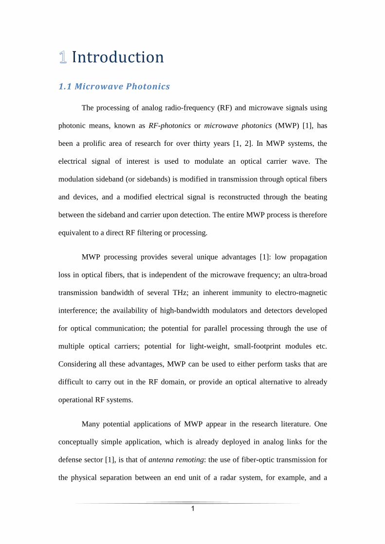
Figure 1: Typical layout of a single-source microwave photonic filter with a finite

impulse response [3] ...................................................................................................... 3

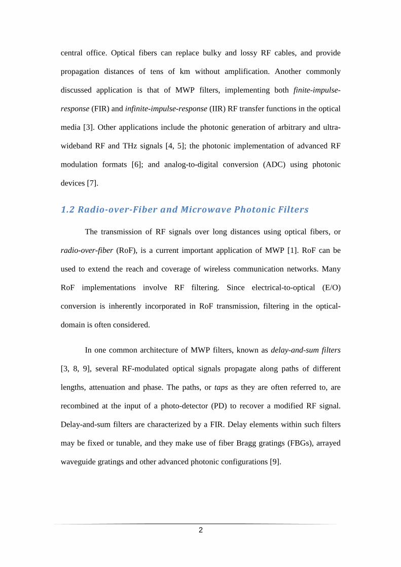
Figure 2: Schematic layout of a phased-array antenna. The steering of the beam is

achieved by differential phase shifts between the array elements ................................. 5

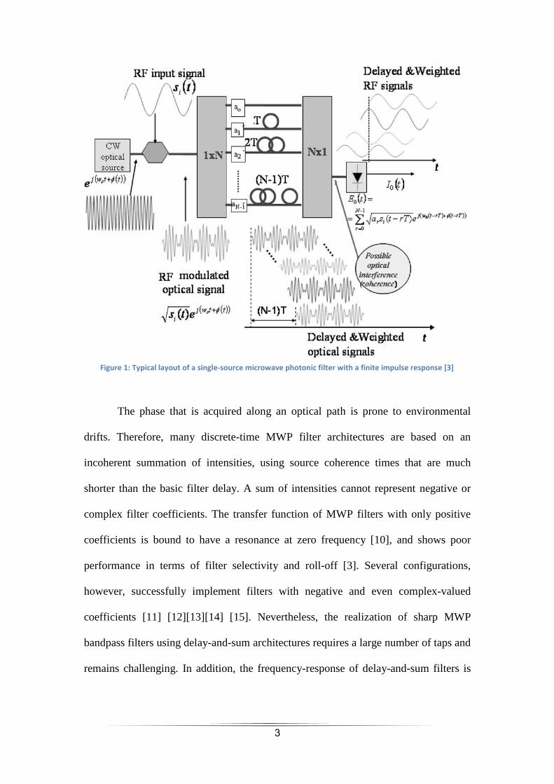
Figure 3: Illustration of PSLR, ISLR and Resolution .................................................... 8

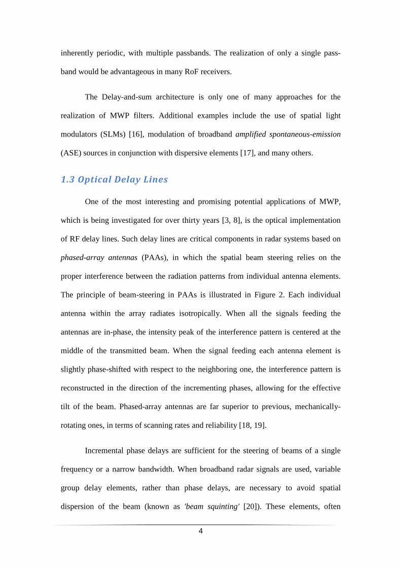
Figure 4: Schematic illustration of the mechanisms that provide a positive feedback in

stimulated Brillouin scattering. Image cutrsy of L. Thevenaz, EPFL Switzerland ..... 10

Figure 5: Simplified schematic of a SBS fiber ring laser [58] ..................................... 13

Figure 6: A modulated signal is offset without filtering and with filtering. Without

filtering, two replicas of the RF waveform appear with frequency offsets in different

directions [44] .............................................................................................................. 18

Figure 7: LFM signal’s frequency vs. time .................................................................. 23

Figure 8: Frequency vs. time for LFM signal (green) and for a delayed one (blue) ... 23

Figure 9: Frequency vs. time for LFM signal (green) and for a frequency shifted one

(yellow) ........................................................................................................................ 23

Figure 10: Frequency vs. time for LFM signal (green), showing the TTD (central bold

green) for time/frequency shifts overlap ...................................................................... 23

Figure 11: Simulated impulse responses of delayed and non-delayed LFM waveforms

with T=5 µs, B=500 MHz, and τ=100 ns ..................................................................... 25

Figure 12: Simulated correlations of LFM waveforms showing that the wider the

bandwidth is, the higher the resolution is .................................................................... 25

Figure 13: Simulated impulse responses of delayed and non-delayed 4th-order NLFM

waveforms with T=5 µs, B=500 MHz, and τ=100 ns .................................................. 26

Figure 14: Setup for the variable delay of the impulse responses of chirped waveforms

[43] ............................................................................................................................... 27

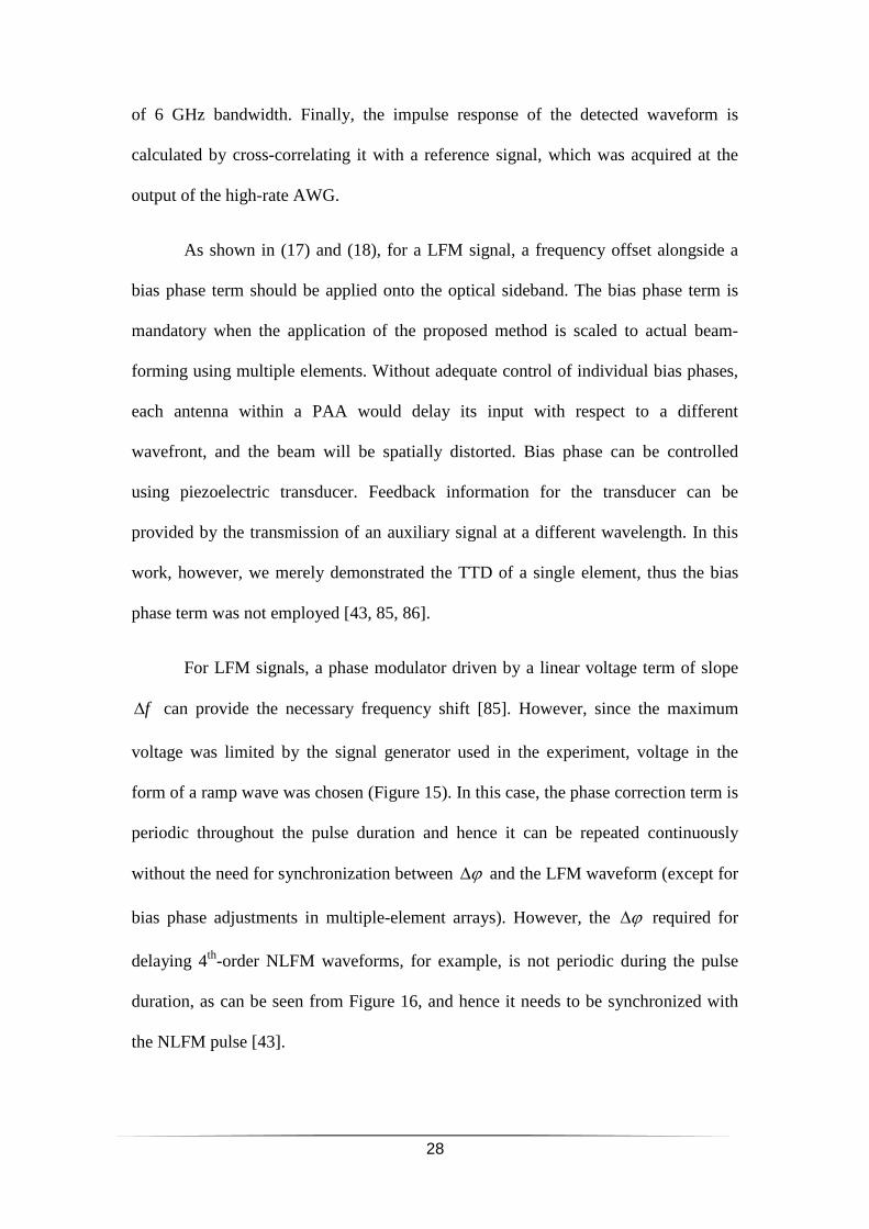
Figure 15: Phase correction term for LFM waveform of period 5 µs .......................... 29

Figure 16: Phase correction term for 4th-order NLFM waveform of period 5 µs ....... 29

Figure 17: Setup for the variable delay of the impulse responses of linear frequency

modulated waveforms using an acousto-optic modulator [85] .................................... 30

Figure 18: Experimintal correlation for TTDs of 0 ns – 50 ns, 100 ns, 150 ns, 200 ns,

250 ns from right to left ............................................................................................... 31

Figure 19: Simulated correlation for TTDs of 0 ns – 50 ns, 100 ns, 150 ns, 200 ns, 250

ns from right to left ...................................................................................................... 31

Figure 20: Expermintal correlation of TTD = 20 ns .................................................... 32

Figure 21: Simulated correlation of TTD = 20 ns........................................................ 32

Figure 22: Experimental correlation of TTD = 50 ns .................................................. 32

Figure 23: Simulated correlation of TTD = 50 ns........................................................ 32

Figure 24: Expermintal correlation of TTD = 100 ns .................................................. 32

Figure 25: Simulated correlation of TTD = 100 ns...................................................... 32

Figure 26: Comparison between simulated correlations, using ideal (left) and non-

ideal (right) ramp waveforms....................................................................................... 33

Figure 27: Experimental correlation of 4th-order NLFM waveforms for TTDs of 0 ns,

10 ns, 20 ns, 50 ns from right to left (k=0.015) ........................................................... 34

Figure 28: Simulated correlation of 4th-order NLFM waveforms for TTDs of 0 ns, 10

ns, 20 ns, 50 ns from right to left (k=0.015) ................................................................ 34

Figure 29: Experimental correlation of 8th-order NLFM waveforms for TTDs of 0 ns

and 20 ns ...................................................................................................................... 35

Figure 30: Simulated correlation of 8th-order NLFM waveforms for TTDs of 0 ns and

20 ns ............................................................................................................................. 35

Figure 31: Experimental correlation of 16th-order NLFM waveforms for TTDs of 0 ns

and 20 ns ...................................................................................................................... 35

Figure 32: Simulated correlation of 16th-order NLFM waveforms for TTDs of 0 ns

and 20 ns ...................................................................................................................... 35

Figure 33: Measured, normalized impulse responses of 500 MHz-wide, 5µs-long

LFM waveforms. The frequency offsets fAOM (in MHz) are: 35 (blue), 38 (red), 40

(green), 42 (black), and 45 (magenta). A magnified view of the primary correlation

peaks is shown in the inset ........................................................................................... 36

Figure 34: : Simulated SBS maximum power gain for pump power of 2 mW (blue), 6

mW (red), 10 mW (green), 14 mW (black), and 18 mW (magenta) ........................... 56

Figure 35: Simulated gain linewidths for scalar (red, dashed) and polarization-

enhanced (black, solid) SBS processes, for pump power of 2 mW ............................. 57

Figure 36: Simulated SBS gain linewidth for scalar (red, dashed) and polarization-

enhanced (black, solid) SBS processes, for pump power of 14 mW ........................... 58

Figure 37: Simulated reconstruction of the signal under test comprising a strong

central tone and two side-tones that are 25 dB weaker and detuned by ±20 MHz. The

reconstruction is shown for both scalar (red, dashed) and polarization-enhanced

(black, solid) SBS processes ........................................................................................ 59





























Figure 45: Input power spectral density of a signal under test, comprising 10 tones

which are separated by 10 MHz................................................................................... 64

Figure 46: Simulated reconstruction of the power spectral density of the signal under

test shown in Figure 45 ................................................................................................ 64

Figure 47: Input power spectral density of a signal under test, comprising tones which

are separated by 10 MHz, with tone no. 7 intentionally removed ............................... 64



Figure 49: Input power spectral density of a signal under test, comprising 10

subcarrier tones, separated by 10 MHz. Each subcarrier was modulated by an on-off

keying, pseudo-sequence bit sequence at 2.5 Mbit/s ................................................... 64



Figure 51: : Input power spectral density of a signal under test, comprising subcarrier

tones which are separated by 10 MHz. Each subcarrier was independently modulated

by an on-off keying, pseudo-sequence bit sequence at 2.5 Mbit/s. Subcarrier-tone no.

7 was intentionally removed ........................................................................................ 64



Figure 53: Experimental setup for stimulated Brillouin scattering-based optical

spectrum analyzer ........................................................................................................ 66

Figure 54: Experimental reconstruction of the power spectral density of a continuous

wave ............................................................................................................................. 69

Figure 55: Experimental reconstruction of the power spectral density of a signal under

test comprising two tones with spectral separation of 16 MHz ................................... 69






test comprising two tones with spectral separation of 8 MHz ..................................... 70

Figure 59: Simulated reconstruction of the power spectral density of a signal under

test, comprising a strong, central tone and two side-tones that are detuned by ±40

MHz and 27.4 dB weaker ............................................................................................ 71



MHz and 27.4 dB weaker ............................................................................................ 71



MHz and 30.45 dB weaker .......................................................................................... 71



MHz and 30.45 dB weaker .......................................................................................... 71



MHz and 33.5 dB weaker ............................................................................................ 71



MHz and 33.5 dB weaker ............................................................................................ 71

Figure 65: Experimental (magenta, solid) and simulated (blue, dashed) reconstruction

of the power spectral density of a signal under test comprising ten tones, separated by

10 MHz ........................................................................................................................ 73


of the power spectral density of the signal under test in figure 65, with tone no. 7

removed........................................................................................................................ 73


of the power spectral density of a signal under test comprising ten sub-carriers,

separated by 10 MHz, independently modulated by an on-off keying, pseudo-

sequence bit sequence at 2.5 Mbit/s ............................................................................. 73


of the power spectral density of the signal under test in figure 67, with sub-carrier no.

7 removed..................................................................................................................... 73

Figure 69: Simulated frequency response of a MWP, SBS-based bandpass filter. The

simulations are based on 500 MHz-wide simulated, ideal (red, dashed) and sampled

experimental (black, solid) pump waves ..................................................................... 82

Figure 70: The PSD of a 500 MHz-wide RF LFM waveform at the output of the

AWG ............................................................................................................................ 83

Figure 71: The PSD of the RF LFM waveform of figure 70, after adding a RF

amplifier ....................................................................................................................... 83

Figure 72: The PSD of the RF LFM waveform of figure 71, after adding a LPF ....... 83

Figure 73: The PSD of the RF LFM waveform of figure 72, following up-conversion

mixing with a local oscillator ....................................................................................... 84

Figure 74: The PSD of the RF LFM waveform of figure 73, after adding a HPF ....... 84

Figure 75: The PSD of the RF LFM waveform of figure 74, after adding a RF

amplifier ....................................................................................................................... 84

Figure 76: The PSD of the RF LFM waveform of figure 75, after adding a second

HPF .............................................................................................................................. 85

Figure 77: A full scheme of the RF LFM waveform generation ................................. 85

Figure 78: Experimental setup for the demonstration of polarization-enhanced

stimulated Brillouin scattering-based microwave-photonic bandpass filter ................ 87

Figure 79: Experimentally-obtained normalized frequency response of a MWP

bandpass filter with B=500 MHz and f0=1.9 GHz (black, solid) alongside the

expected one, based on samples from the pump wave (red, dashed) .......................... 89

Figure 80: Normalized frequency responses of a MWP bandpass filters with B=500

MHz and f0=1.65 GHz (green), f0=1.9 GHz (red) and f0=2.15 GHz (blue) .............. 89

Figure 81: Normalized frequency responses of MWP bandpass filters with B=250

MHz (red), B=500 MHz (green) and B=1 GHz (blue) ................................................ 90

Figure 82: Examples of normalized frequency responses of MWP filters with different

magnitude transfer functions........................................................................................ 91

Figure 83: Filter selectivity as a function of pump power ........................................... 91

Figure 84: Example for SNR measurement ................................................................. 92

Figure 85: Filter SNR as a function of pump power .................................................... 93

Figure 86: DNR measurement: Probe out RF power as a function of probe in optical

power............................................................................................................................ 94

Glossary

AFG Arbitrary Function Generator

ADC Analog-to-Digital Conversion

ASE Amplified Spontaneous Emission

AOM Acousto-Optic Modulator

AWG Arbitrary Waveform Generator

BFL Brillouin Fiber Laser

CW Continuous Wave

DFB Distributed-Feedback

DNR Dynamic Range

DSP Digital Signal Processing

E/O Electrical-to-Optical

EDFA Erbium-Doped Fiber Amplifier

FBG Fiber Bragg Grating

FIR Finite Impulse Response

FUT Fiber Under Test

FWHM Full-Width Half-Maximum

HNLF Highly-Nonlinear Fiber

HPF High-Pass Filter

IF Intermediate Frequency

IIR Infinite Impulse Response

ISLR Integrated Side-Lobe Ratio

LCFBG Linearly-Chirped Fiber Bragg Grating

LFM Linear Frequency Modulation

LO Local Oscillator

LPF Low-Pass Filter

MWP Microwave Photonics

MZM Mach-Zehnder Modulator

NLFM Non-Linear Frequency Modulation

O/E Optical-to-Electrical

O-OFDM Optical Orthogonal Frequency Division Multiplexing

ODL Optical Delay Line

OFDR Optical Frequency Domain Reflectometry

OSA Optical Spectrum Analyzer

PAA Phased-Array Antennas

PBS Polarization Beam-Splitter

PC Polarization Controller

PD Photo-Detector

PM Polarization- Maintaining

PRBS Pseudo-Random Bit Sequence

PSD Power Spectral Density

PSLR Peak-to-Side-Lobe Ratio (also referenced as PSL)

RF Radio Frequency

RoF Radio-over-Fiber

SBS Stimulated Brillouin Scattering

SC Suppressed-Carrier

SLM Spatial Light Modulator

SNR Signal-to-Noise Ratio

SOA Semiconductor Optical Amplifier

SOP State-of-Polarization

SUT Signal Under Test

SSB Single Sideband

TLS Tunable Laser Source

TTD True Time Delay

VFODL Variable Fiber-Optic Delay Line

VNA Vector Network Analyzer

VOA Variable Optical Attenuator

ListofPublications

Journal papers:

1. O. Klinger, Y. Stern, T. Schneider, K. Jamshidi and A. Zadok, "Long

microwave-photonic variable delay of linear frequency modulated

waveforms," IEEE Photonics Technology Letters, vol. 24, pp. 200-202, 2012.

2. Y. Stern, O. Klinger, T. Schneider, K. Jamshidi, A. Peer and A. Zadok, "Low-

distortion long variable delay of linear frequency modulated waveforms,"

IEEE Photonics Journal, vol. 4, pp. 499-503, 2012.

3. O. Klinger, Y. Stern, F. Pederiva, K. Jamshidi, T. Schneider and A. Zadok,

"Continuously variable long microwave-photonic delay of arbitrary frequency-

chirped signals," Optics Letters, vol. 37, pp. 3939-3941, 2012.

4. Y. Stern, K. Zhong, T. Schneider, Y. Ben-Ezra, R. Zhang, M. Tur and A.

Zadok, "Brillouin optical spectrum analyzer monitoring of subcarrier-

multiplexed fiber-optic signals," Applied Optics, vol. 52, pp. 6179-6184, 2013.

Conference papers:

1. Y. Stern, K. Zhong, T. Schneider, Y. Ben-Ezra, R. Zhang, M. Tur, and A.

Zadok, "Frequency-celective filtering and analysis of radio-over-fiber using

stimulated Brillouin scattering," IEEE International topical meeting on

microwave photonics, 2013.

I

Abstract

Microwave photonics (MWP) processing provides numerous potential

advantages over electrical domain techniques, such as broad bandwidth and long

reach. One potential application of MWP is the optical implementation of radio-

frequency (RF) delay lines, which are critical components in beam steering within

phased-array radar systems. Such true time delay (TTD) elements must accommodate

broadband RF waveforms and comply with stringent distortion requirements. Large

antenna arrays require delay variations of tens of ns. Despite considerable progress,

realization of continuously-variable long MWP TTDs remains challenging.

Rather than provide a universal group delay, we focus on the processing of

chirped waveforms, where the frequency is swept across a broad spectral bandwidth.

Chirped waveforms, which are prevalent in many radar systems, can be compressed

into an impulse response with narrow correlation peak with low sidelobes. The

simplest chirped signal is the linear frequency modulated (LFM) waveform, where the

frequency is swept at a constant rate. Further sidelobe suppression may be achieved

using nonlinear frequency modulated (NLFM) waveforms.

For chirped signals, the proposed processing is nearly equivalent to a variable

delay. In compromising the universality of the method, delays that are 100 times

longer than previously reported are obtained, while retaining sufficient waveform

quality. Based on their time-frequency relation, the compressed form of LFM

waveforms is delayed by up to ±50 ns with adequate sidelobe suppression. The delays

of the impulse responses of 4th-order NLFM waveforms by up to 50 ns, and 8th and

16th-order NLFM waveforms by up to 20 ns are also demonstrated.

II

Another important application of MWP is the transmission of RF signals over

long distances using optical fibers, or radio-over-fiber (RoF). Many RoF systems are

based on the multiplexing of densely packed subcarrier tones. The spectral separation

between neighboring data-carrying tones can be as narrow as a few MHz. The

monitoring of transmission in such systems at the optical layer improves the quality of

service, reduces downtimes and assists in the identification of faults. Optical spectrum

analyzers (OSAs) are among the most fundamental and widely employed tools of

signal monitoring. Traditional, grating-based OSAs provide a spectral resolution on

the order of 1GHz, which is often insufficient for the analysis of spectrally-efficient

optical communication systems.

Several groups demonstrated a high-resolution OSA that is based on

stimulated Brillouin scattering (SBS) processes in standard fibers. The power spectral

density (PSD) of a signal under test (SUT) is reconstructed through the scanning of a

Brillouin gain line through its spectral extent, and measurement of the amplified

signal power as a function of frequency. The spectral resolution of an SBS-OSA is

determined by the Brillouin linewidth, which is on the order of 30 MHz. SBS-OSAs

are prone, however, to cross-talk from out-of-band spectral contents. Out-of-band

spectral components of the SUT, although unamplified, propagate to the output

unattenuated. Therefore the ability to recover a relatively weak tone at the presence of

a strong one using an SBS-OSA could be rather limited.

A vector analysis of SBS had revealed that the state of polarization (SOP) of

the amplified signal is drawn towards a particular state, which is governed by the SOP

of the pump. That particular state can be made different from the output polarization

of unamplified, out-of-band signal components, unaffected by SBS. Based on this

III

principle, a judiciously-aligned output polarizer is used to reject the unamplified

spectral components, while those within the SBS bandwidth are partially transmitted.

The Brillouin gain window of a single, continuous-wave pump is scanned

across the spectral extent of the SUT. The polarization pulling effect associated with

SBS is employed to improve the rejection ratio of the analysis by an order of

magnitude. Ten tones, spaced by only 10 MHz and each carrying random-sequence

on-off keying data at 2.5 Mbit/s, are clearly resolved. The measurement identifies the

absence of a single subcarrier, directly in the optical domain. The results are

applicable to the monitoring of subcarrier multiplexed RoF transmission.

Last, many RoF implementations also involve RF filtering. Since electrical-to-

optical conversion is inherently incorporated in RoF transmission, filtering in the

optical-domain is often considered. Many implementations of MWP filters were

proposed in the literature, however the realization of sharp, tunable MWP filters

remains challenging. In addition, many of the proposed filters are inherently periodic,

with multiple passbands. The realization of only a single pass-band would be

advantageous in many RoF receivers.

Herein I present a significant enhancement of MWP filters that are based on

the polarization attributes of SBS and the associated polarization pulling. The PSD of

the Brillouin pump wave is broadened through external modulation to replicate the

shape of the desired RF filter. The method is employed in the implementation of

sharp, uniform and highly-flexible MWP bandpass filters with a single passband, a

variable bandwidth between 250 MHz – 1 GHz, tunable central transmission

frequency, and selectivity as high as 44 dB. The proposed selective filtering can be

very instrumental in all-optical signal processing in MWP systems.

1

Introduction

1.1 Microwave Photonics

The processing of analog radio-frequency (RF) and microwave signals using

photonic means, known as RF-photonics or microwave photonics (MWP) [1], has

been a prolific area of research for over thirty years [1, 2]. In MWP systems, the

electrical signal of interest is used to modulate an optical carrier wave. The

modulation sideband (or sidebands) is modified in transmission through optical fibers

and devices, and a modified electrical signal is reconstructed through the beating

between the sideband and carrier upon detection. The entire MWP process is therefore

equivalent to a direct RF filtering or processing.

MWP processing provides several unique advantages [1]: low propagation

loss in optical fibers, that is independent of the microwave frequency; an ultra-broad

transmission bandwidth of several THz; an inherent immunity to electro-magnetic

interference; the availability of high-bandwidth modulators and detectors developed

for optical communication; the potential for parallel processing through the use of

multiple optical carriers; potential for light-weight, small-footprint modules etc.

Considering all these advantages, MWP can be used to either perform tasks that are

difficult to carry out in the RF domain, or provide an optical alternative to already

operational RF systems.

Many potential applications of MWP appear in the research literature. One

conceptually simple application, which is already deployed in analog links for the

defense sector [1], is that of antenna remoting: the use of fiber-optic transmission for

the physical separation between an end unit of a radar system, for example, and a

2

central office. Optical fibers can replace bulky and lossy RF cables, and provide

propagation distances of tens of km without amplification. Another commonly

discussed application is that of MWP filters, implementing both finite-impulse-

response (FIR) and infinite-impulse-response (IIR) RF transfer functions in the optical

media [3]. Other applications include the photonic generation of arbitrary and ultra-

wideband RF and THz signals [4, 5]; the photonic implementation of advanced RF

modulation formats [6]; and analog-to-digital conversion (ADC) using photonic

devices [7].

1.2 Radio-over-Fiber and Microwave Photonic Filters

The transmission of RF signals over long distances using optical fibers, or

radio-over-fiber (RoF), is a current important application of MWP [1]. RoF can be

used to extend the reach and coverage of wireless communication networks. Many

RoF implementations involve RF filtering. Since electrical-to-optical (E/O)

conversion is inherently incorporated in RoF transmission, filtering in the optical-

domain is often considered.

In one common architecture of MWP filters, known as delay-and-sum filters

[3, 8, 9], several RF-modulated optical signals propagate along paths of different

lengths, attenuation and phase. The paths, or taps as they are often referred to, are

recombined at the input of a photo-detector (PD) to recover a modified RF signal.

Delay-and-sum filters are characterized by a FIR. Delay elements within such filters

may be fixed or tunable, and they make use of fiber Bragg gratings (FBGs), arrayed

waveguide gratings and other advanced photonic configurations [9].

3

The phase that is acquired along an optical path is prone to environmental

drifts. Therefore, many discrete-time MWP filter architectures are based on an

incoherent summation of intensities, using source coherence times that are much

shorter than the basic filter delay. A sum of intensities cannot represent negative or

complex filter coefficients. The transfer function of MWP filters with only positive

coefficients is bound to have a resonance at zero frequency [10], and shows poor

performance in terms of filter selectivity and roll-off [3]. Several configurations,

however, successfully implement filters with negative and even complex-valued

coefficients [11] [12][13][14] [15]. Nevertheless, the realization of sharp MWP

bandpass filters using delay-and-sum architectures requires a large number of taps and

remains challenging. In addition, the frequency-response of delay-and-sum filters is

Figure 1: Typical layout of a single-source microwave photonic filter with a finite impulse response [3]

4

inherently periodic, with multiple passbands. The realization of only a single pass-

band would be advantageous in many RoF receivers.

The Delay-and-sum architecture is only one of many approaches for the

realization of MWP filters. Additional examples include the use of spatial light

modulators (SLMs) [16], modulation of broadband amplified spontaneous-emission

(ASE) sources in conjunction with dispersive elements [17], and many others.

1.3 Optical Delay Lines

One of the most interesting and promising potential applications of MWP,

which is being investigated for over thirty years [3, 8], is the optical implementation

of RF delay lines. Such delay lines are critical components in radar systems based on

phased-array antennas (PAAs), in which the spatial beam steering relies on the

proper interference between the radiation patterns from individual antenna elements.

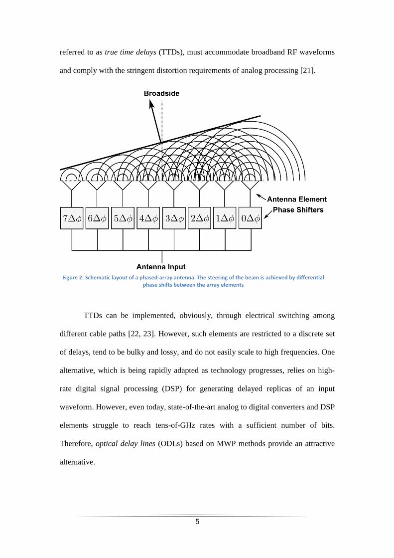
The principle of beam-steering in PAAs is illustrated in Figure 2. Each individual

antenna within the array radiates isotropically. When all the signals feeding the

antennas are in-phase, the intensity peak of the interference pattern is centered at the

middle of the transmitted beam. When the signal feeding each antenna element is

slightly phase-shifted with respect to the neighboring one, the interference pattern is

reconstructed in the direction of the incrementing phases, allowing for the effective

tilt of the beam. Phased-array antennas are far superior to previous, mechanically-

rotating ones, in terms of scanning rates and reliability [18, 19].

Incremental phase delays are sufficient for the steering of beams of a single

frequency or a narrow bandwidth. When broadband radar signals are used, variable

group delay elements, rather than phase delays, are necessary to avoid spatial

dispersion of the beam (known as 'beam squinting' [20]). These elements, often

5

referred to as true time delays (TTDs), must accommodate broadband RF waveforms

and comply with the stringent distortion requirements of analog processing [21].

TTDs can be implemented, obviously, through electrical switching among

different cable paths [22, 23]. However, such elements are restricted to a discrete set

of delays, tend to be bulky and lossy, and do not easily scale to high frequencies. One

alternative, which is being rapidly adapted as technology progresses, relies on high-

rate digital signal processing (DSP) for generating delayed replicas of an input

waveform. However, even today, state-of-the-art analog to digital converters and DSP

elements struggle to reach tens-of-GHz rates with a sufficient number of bits.

Therefore, optical delay lines (ODLs) based on MWP methods provide an attractive

alternative.

Figure 2: Schematic layout of a phased-array antenna. The steering of the beam is achieved by differential

phase shifts between the array elements

6

The simplest form of an ODL can be constructed by a switching matrix

between fiber sections of different lengths. In a series of works by Tur and coauthors

[24] -[25] [26], discrete ODLs were realized through wavelength-selective switching

among different paths. The quality of the delayed waveforms, in terms of distortion,

was excellent. However, the precise path lengths are difficult to control and delay

values cannot be varied continuously. Therefore, several, more elaborate methods

were proposed in order to provide a continuously variable TTD. Examples include the

application of regular, periodic FBGs [27, 28], use of linearly-chirped FBGs

(LCFBGs) in conjunction with tunable laser sources (TLSs) [29], fiber Prisms [30,

31], slow light-based techniques in fibers [32] -[33][34][35][36] [37] and in

semiconductor optical amplifiers (SOAs) [38, 39], and many more.

Another approach towards the realization of a variable fiber-optic delay line

(VFODL) was proposed by Nabeel A. Riza et al. in [40]. This approach is unique for

its use of both analog and digital delay lines. This hybrid combination solves earlier

resolution-range dilemmas as discrete fiber paths are used for long time delays, while

LCFBGs provide near-continuous high-resolution delays, down to 0.5 picoseconds,

between the discrete delays of the switched paths. Using hybrid VFODL, TTDs of up

to 25.6 ns were achieved. Among all universal MWP TTD implementations designed

for arbitrary waveforms, this method provides the longest delay, to the best of my

knowledge.

The key metric of MWP TTD elements is the product of the processed

waveform bandwidth times the range of delay variations (known as the 'delay-

bandwidth product'), subject to the constraint of acceptable waveform distortion

levels. For many of the aforementioned ODL implementations, the delay-bandwidth

7

product was inherently restricted to the order of unity. Thus far, in spite of much

effort and progress, MWP TTD setups struggle to reach delay-bandwidth products

above the order of unity.

1.4 Chirped Waveforms

A particular group of signals, that is prevalent in many radar systems, is the

family of frequency-modulated waveforms. This group can be divided into two types

of signals: the linear frequency modulated (LFM) and non-linear frequency

modulated (NLFM) waveforms. As their names suggest, the instantaneous frequency

of these signals is time dependent (a linear or non-linear dependence for the LFM and

NLFM signals, respectively), spanning a broad bandwidth over relatively long

durations. These categories of signals are often referred to collectively as chirped

waveforms. Chirped waveforms are of constant magnitude, and they circumvent the

transmission of short, high-peak power pulses, whose generation is more difficult, for

practical considerations [41]. LFM signals are simple to generate and process, and

with proper post-detection processing they can be compressed into a so-called

impulse response function, which is characterized by a strong and narrow peak with

low side-lobes.

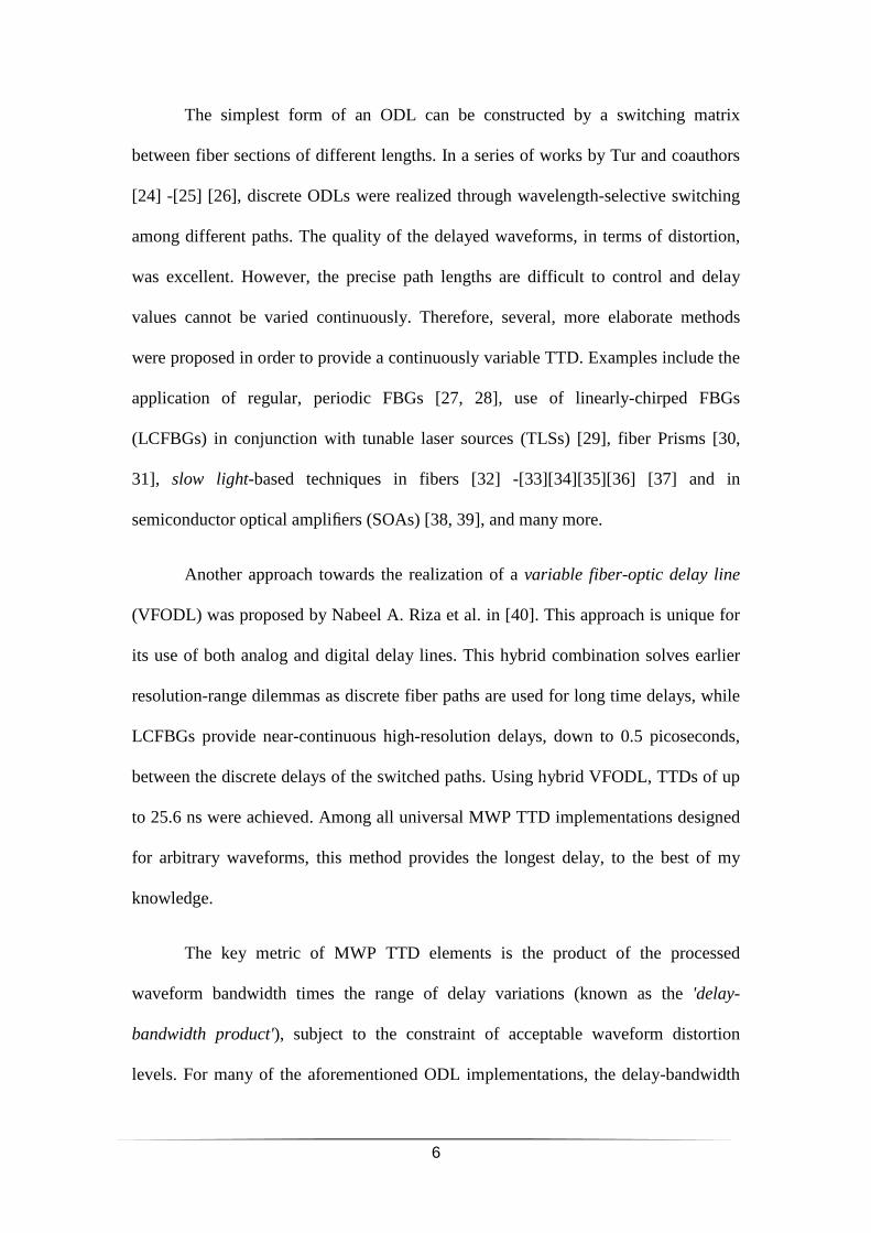
Three figures of merit are used to describe the quality of an impulse response

function. All three are illustrated in Figure 3: the peak-to-side-lobe ratio (PSLR) is the

ratio of main lobe peak power to the power highest side-lobe peak, which quantifies

the degradation due to localized disturbance; the integrated side-lobe ratio (ISLR) is

the ratio of the integrated energy within the main lobe to the integrated energy outside

the main lobe (illustrated in Figure 3 as the ratio between the red painted area and the

yellow painted area), which quantifies the degradation due to distributed interference;

8

resolution is defined as the full-width at half-maximum (FWHM) of the main impulse

lobe. The intersection of the impulse response with the -3 dB line (Figure 3, dashed),

defines the boundaries of the main lobe for all the above. The first two are measured

in dB, and the latter is measured in seconds.

To further reduce the impulse response side-lobes, NLFM signals were

introduced. These signals are characterized by a changing rate of frequency sweep,

rather than a constant one, as in LFM signals. The freedom to determine the frequency

sweep provides a way to shape the impulse response and get lower side-lobes than

those achieved with LFM signals. Both types of waveforms will be addressed in the

following chapter.

Few previous works addressed the MWP TTD of LFM waveforms. For

example, LFM waveforms were used in the aforementioned examples of discrete

optical delay lines [24] -[25] [26]. The continuously-variable TTD of LFM

waveforms was reported based on stimulated Brillouin scattering (SBS) slow light

[42], however the obtained delay was restricted to 230 ps. To the best of my

knowledge, the MWP processing of NLFM waveforms was not reported before this

work [43, 44].

Figure 3: Illustration of PSLR, ISLR and Resolution

9

In this work, an alternative MWP processing scheme for chirped waveforms is

proposed and demonstrated. While not strictly representing a TTD, the effect of the

processing scheme is shown to be nearly equivalent to that of a time delay, for the

family of chirped waveforms only. In sacrificing the universality of the delay

approach, and aiming specifically towards the variable delay of chirped waveforms,

the achievable delay can be extended by more than a hundred-fold.

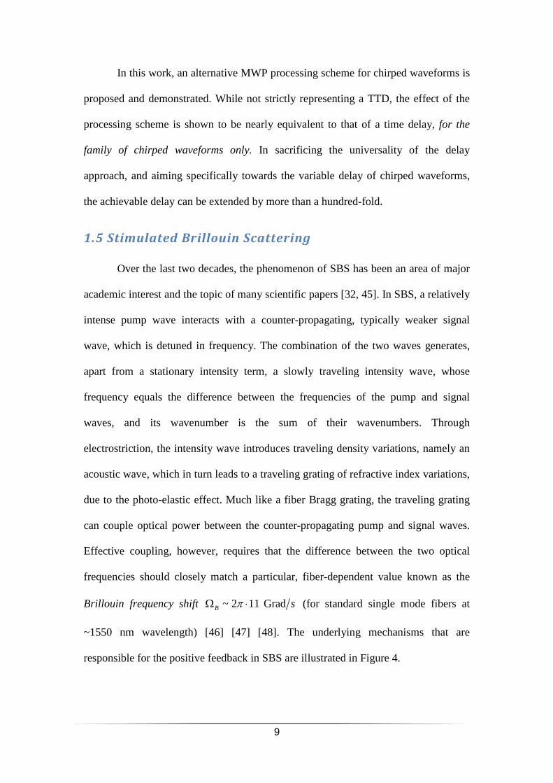
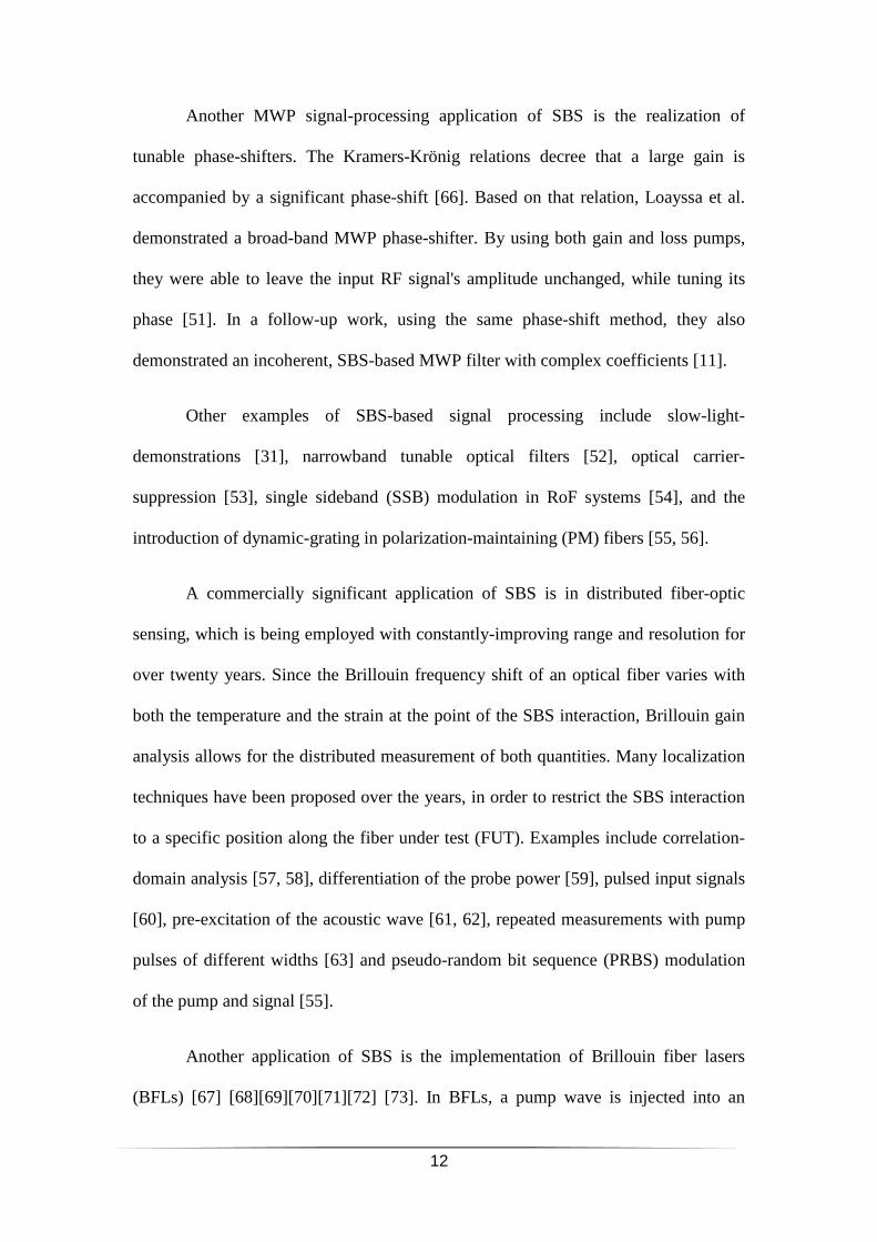
1.5 Stimulated Brillouin Scattering

Over the last two decades, the phenomenon of SBS has been an area of major

academic interest and the topic of many scientific papers [32, 45]. In SBS, a relatively

intense pump wave interacts with a counter-propagating, typically weaker signal

wave, which is detuned in frequency. The combination of the two waves generates,

apart from a stationary intensity term, a slowly traveling intensity wave, whose

frequency equals the difference between the frequencies of the pump and signal

waves, and its wavenumber is the sum of their wavenumbers. Through

electrostriction, the intensity wave introduces traveling density variations, namely an

acoustic wave, which in turn leads to a traveling grating of refractive index variations,

due to the photo-elastic effect. Much like a fiber Bragg grating, the traveling grating

can couple optical power between the counter-propagating pump and signal waves.

Effective coupling, however, requires that the difference between the two optical

frequencies should closely match a particular, fiber-dependent value known as the

Brillouin frequency shift ~ 2 11 GradB sπΩ ⋅ (for standard single mode fibers at

~1550 nm wavelength) [46] [47] [48]. The underlying mechanisms that are

responsible for the positive feedback in SBS are illustrated in Figure 4.

10

SBS amplification can be simply implemented in standard fibers at room

temperature. It has the lowest power threshold of all nonlinear optical mechanisms in

standard silica fibers [49], and is therefore very attractive for all-optical signal

processing [11, 32], [50] [51][52][53][54][55] [56] and sensing [57]

[58][59][60][61][62] [63] applications. In many cases of practical interest, as well as

throughout this work, the pump power is strong enough so that it is hardly affected by

the amplification of the probe. For this regime, known as that of undepleted pump

[46], the complex envelope of the pump wave pumpA remains constant and serves as a

parameter. In this case, the complex envelope of the probe wave sigA is exponentially

intensifying along the fiber:

(1) ( ) ( ) ( )0 exp 2sig sig sigA z A g zω = .

Figure 4: Schematic illustration of the mechanisms that provide a positive feedback in stimulated Brillouin

scattering. Image cutrsy of L. Thevenaz, EPFL Switzerland

11

Equation (1) defines a complex gain function ( ) 1msigg ω − , where sigω is the

frequency of the probe wave and z is the distance the probe traveled within the fiber.

For a continuous-wave (CW) pump laser of optical frequency pumpω and power pumpP ,

( )sigg ω is of Lorentzian shape [64]:

(2) ( ) ( )0

1 2pump

sig

pump sig B B

g Pg

jω

ω ω

⋅=

− − −Ω Γ.

Here, ~ 2 30 Mrad sB πΓ ⋅ denotes the narrow inherent linewidth of the SBS process,

and [ ] 1

0 W mg−

⋅ is the gain coefficient at the peak of the Brillouin gain line. When

the pump wave is modulated to obtain a broadened power spectral density (PSD)

( )pump pumpP ω , ( )sigg ω is given by a convolution of the pump PSD with the SBS line

shape [65]:

(3) ( ) ( )( )

0

1 2

pump pump

sig pump

pump sig B B

g Pg d

j

ωω ω

ω ω

⋅=

− − −Ω Γ∫ .

If the spectral width of the pump PSD is much wider than BΓ , the real part of

( )sigg ω may be approximated by [50]:

(4) ( ) ( )Re sig pump sig Bg Pω ω∝ +Ω .

Carefully synthesized pump modulation could provide a uniform PSD within a

broadened bandwidth of interest, up to several GHz [46]. Based on this principle, a

broadened SBS gain line was used to demonstrate GHz-wide flexible MWP bandpass

filters [50].

12

Another MWP signal-processing application of SBS is the realization of

tunable phase-shifters. The Kramers-Krönig relations decree that a large gain is

accompanied by a significant phase-shift [66]. Based on that relation, Loayssa et al.

demonstrated a broad-band MWP phase-shifter. By using both gain and loss pumps,

they were able to leave the input RF signal's amplitude unchanged, while tuning its

phase [51]. In a follow-up work, using the same phase-shift method, they also

demonstrated an incoherent, SBS-based MWP filter with complex coefficients [11].

Other examples of SBS-based signal processing include slow-light-

demonstrations [31], narrowband tunable optical filters [52], optical carrier-

suppression [53], single sideband (SSB) modulation in RoF systems [54], and the

introduction of dynamic-grating in polarization-maintaining (PM) fibers [55, 56].

A commercially significant application of SBS is in distributed fiber-optic

sensing, which is being employed with constantly-improving range and resolution for

over twenty years. Since the Brillouin frequency shift of an optical fiber varies with

both the temperature and the strain at the point of the SBS interaction, Brillouin gain

analysis allows for the distributed measurement of both quantities. Many localization

techniques have been proposed over the years, in order to restrict the SBS interaction

to a specific position along the fiber under test (FUT). Examples include correlation-

domain analysis [57, 58], differentiation of the probe power [59], pulsed input signals

[60], pre-excitation of the acoustic wave [61, 62], repeated measurements with pump

pulses of different widths [63] and pseudo-random bit sequence (PRBS) modulation

of the pump and signal [55].

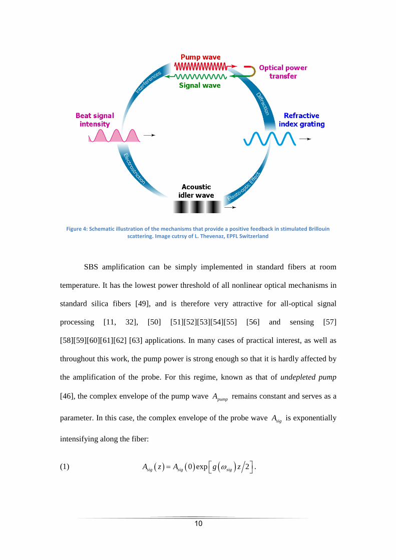
Another application of SBS is the implementation of Brillouin fiber lasers

(BFLs) [67] [68][69][70][71][72] [73]. In BFLs, a pump wave is injected into an

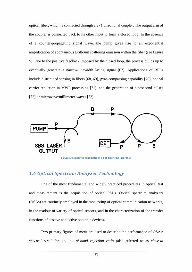
13

optical fiber, which is connected through a 2×1 directional coupler. The output arm of

the coupler is connected back to its other input to form a closed loop. In the absence

of a counter-propagating signal wave, the pump gives rise to an exponential

amplification of spontaneous Brillouin scattering emission within the fiber (see Figure

5). Due to the positive feedback imposed by the closed loop, the process builds up to

eventually generate a narrow-linewidth lasing signal [67]. Applications of BFLs

include distributed sensing in fibers [68, 69], gyro-compassing capability [70], optical

carrier reduction in MWP processing [71], and the generation of picosecond pulses

[72] or microwave/millimeter-waves [73].

1.6 Optical Spectrum Analyzer Technology

One of the most fundamental and widely practiced procedures in optical test

and measurement is the acquisition of optical PSDs. Optical spectrum analyzers

(OSAs) are routinely employed in the monitoring of optical communication networks,

in the readout of variety of optical sensors, and in the characterization of the transfer

functions of passive and active photonic devices.

Two primary figures of merit are used to describe the performance of OSAs:

spectral resolution and out-of-band rejection ratio (also referred to as close-in

Figure 5: Simplified schematic of a SBS fiber ring laser [58]

14

dynamic range). The spectral resolution quantifies the ability of the OSA to

distinguish between two, closely-spaced spectral components; the out-of-band

rejection ratio quantifies the ability to recognize a weak spectral component in the

presence of a second, stronger one at a closely spaced frequency.

Traditional, diffraction grating-based OSAs provide a spectral resolution on

the order of 1 GHz. In recent years, such resolution is increasingly becoming

insufficient. For example, spectrally-efficient, modern optical communication

formats, such as optical orthogonal frequency division multiplexing (O-OFDM),

make use of a large number of subcarrier tones that are densely packed [74]. The

frequency separation between adjacent subcarriers may be as small as a few MHz

[75], hence the monitoring of such signals would benefit from an OSA of comparable

resolution. Similarly, a high resolution, wideband OSA would be instrumental in the

characterization of dense radio-over-fiber transmission links [76, 77] and for

millimeter-wave communication systems [78].

An arbitrarily high spectral resolution may be obtained, at least in principle,

through heterodyne interference of a signal under test (SUT) with a local oscillator

and subsequent RF spectral analysis [79, 80]. The practical realization of such

coherent OSAs is often challenging, as they may require highly stable and low-noise

local oscillators, optical phase-locked loops or frequency comb sources [79, 80].

Measurement techniques which employ direct detection are in general simpler to

implement. Additionally, the usable spectral measurement range of coherent OSAs is

sometimes restricted by the bandwidth of the subsequent RF spectrum analyzer and

that of the photo diode, which are on the order of several tens of GHz. For ultra-

wideband optical systems this measurement range might not be enough.

15

In 2005, SBS amplification was used to implement high-resolution OSAs [81,

82]. In these demonstrations, the signal PSD was reconstructed through scanning the

frequency of the pump wave, and the associated SBS gain spectrum, across the

spectral extent of a SUT. The fundamental resolution of this technique is high: on the

order of BΓ (approximately 30 MHz [46]). SBS-OSAs are prone, however, to cross-

talk from out-of-band spectral contents. Signal components outside the SBS gain

window, although unamplified, propagate to the output with little loss, and thereby

deteriorate the optical rejection ratio [83].

In this work [84], we employ the polarization attributes of SBS in standard,

weakly birefringent fibers, which will be discussed in detail in subsequent chapters, to

block out the spectral components of a SUT that are not amplified by SBS. In doing

so, the optical rejection ratios of SBS-based OSAs are much improved. Using the

same principle, the selectivity of sharp and tunable MWP filters is enhanced as well.

16

VariableMicrowavePhotonic

delayofchirpedwaveforms

Note: The research detailed in this part deals with the implementation of

variable delay lines, designed specifically for chirped waveforms. This research was

carried out jointly by my group-mate Ofir Klinger and myself, and resulted in three

journal papers (with me as first author of one of them). This research described in this

chapter alone already served as the entire M.Sc. thesis of Ofir Klinger [44]. It is

therefore brought here only briefly. My further contributions, which followed after

Ofir's graduation, are detailed in chapters 3 and 4.

2.1 Motivation and Background

As mentioned in the introduction chapter, the realization of MWP variable

delay lines that provide the extent of delay necessary for large PAAs remains

challenging. Many of the methods proposed are inherently restricted to delay-

bandwidth products on the order of unity; this means that subject to the constraint of

acceptable distortion levels, the larger the bandwidth of the input RF signal is, the

shorter the attainable delay. Furthermore, some of the suggested implementations do

not support continuously-variable delays.

In this work we explored the potential benefits of a significant relaxation in

the objective of MWP delay elements. Rather than target the universal TTD of any

waveform, we focused instead on the processing of chirped waveforms, which are

prevalent in many radar systems. The proposed method of MWP TTD takes

advantage of the ambiguity between temporal delays and frequency and phase offsets

that is inherent to LFM and NLFM signals. The MWP processing scheme provides

17

the TTD of chirped pulses having arbitrary pre-designed sweep rate profiles. The

method relies on the application of a carefully synchronized phase-correction term to

a frequency-modulated optical sideband, and allows for the variable delay of general

NLFM waveforms with the necessary fidelity. It is applicable to the processing of

chirped pulses having arbitrarily high central RFs. By sacrificing the universality of

the method, and aiming specifically towards chirped waveforms, we obtained large,

continuously-tunable MWP TTDs with delay-bandwidth products of up to 50 [43, 44,

85, 86].

2.2 Principle of operation

The MWP TTD method proposed here takes advantage of the one-to-one

mapping between time t and instantaneous frequency ( )f t that is underlying both

LFM and NLFM waveforms. Consider for example LFM signals, for which ( )f t is a

linear function of time. Due to this dependence, the application of a constant

frequency shift, or in other words a correction to the instantaneous phase that is

linearly varying with time, to an infinitely-long LFM waveform is equivalent to its

delaying. Even though in practice the waveform duration is limited, and the

aforementioned equivalency is not absolute, I will later show that for sufficiently long

durations of LFM pulses, a time delay and a frequency shift have nearly identical

effects on the impulse response. Therefore, this property of LFM might be used to

obtain TTD. The concept for LFM signals can be generalized to NLFM signals, using

a phase correction term that is not a linear function of time.

A first step towards the implementation of this method would be to modulate a

chirped waveform of bandwidth B and center frequency 0f onto an optical carrier of

frequency optf . After modulation, the optical signal comprises of two sidebands

18

around the carrier. Trying to apply a phase shift to the optical waveform as a whole at

this point would not result in a delayed signal. The reason lies within the nature of the

detection. The detector uses the optical carrier as its quiescent point. If we shift the

carrier’s frequency along with those of sidebands, the frequency of the photo-

detected, RF domain waveform would remain unchanged. Thus, before applying the

frequency offset, it is imperative that we filter out the original optical carrier.

Subsequently, after optical processing and prior to detection, an unprocessed carrier is

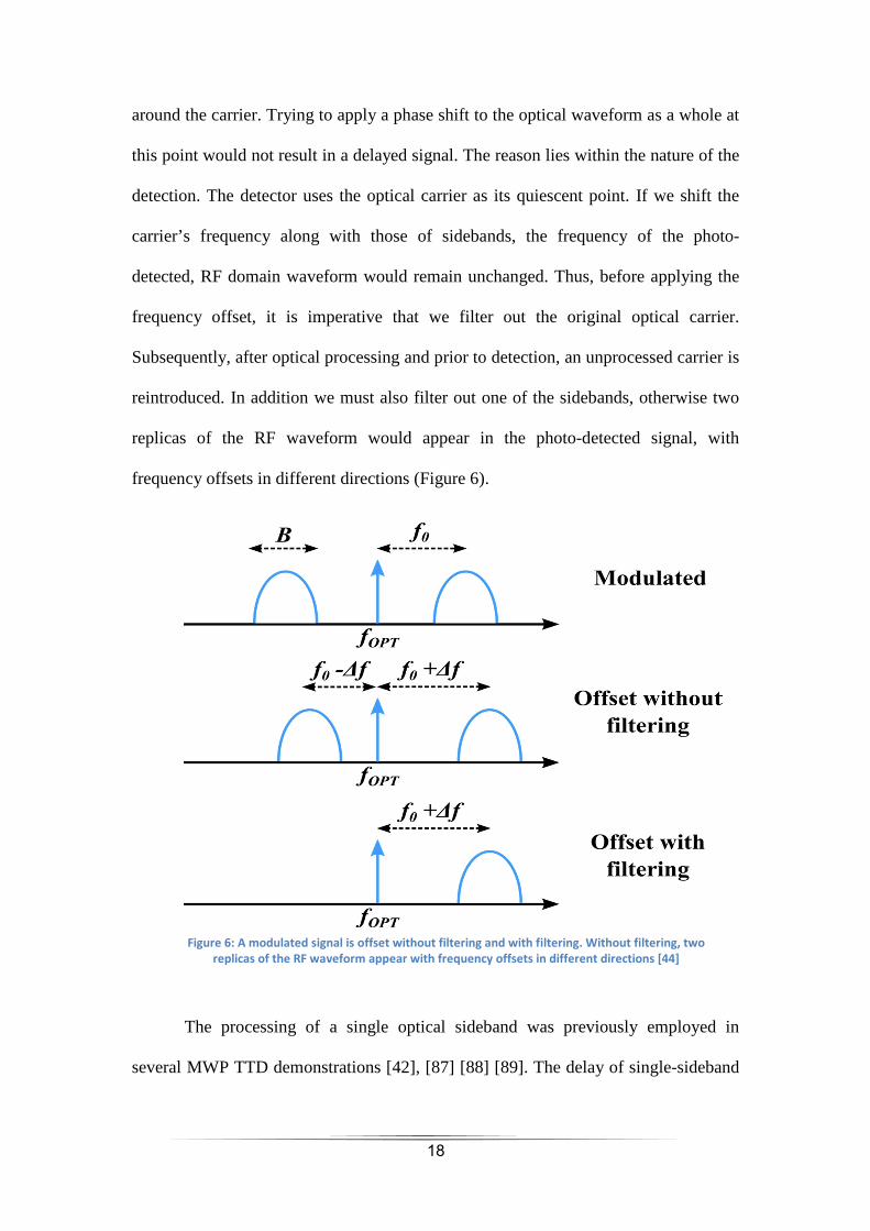
reintroduced. In addition we must also filter out one of the sidebands, otherwise two

replicas of the RF waveform would appear in the photo-detected signal, with

frequency offsets in different directions (Figure 6).

The processing of a single optical sideband was previously employed in

several MWP TTD demonstrations [42], [87] [88] [89]. The delay of single-sideband

Figure 6: A modulated signal is offset without filtering and with filtering. Without filtering, two

replicas of the RF waveform appear with frequency offsets in different directions [44]

19

analog waveforms benefits from piece-wise treatment [42]: since 0f B≫ , it is

sufficient for a MWP setup to provide an appropriate spectral phase across the

window 0 0,2 2opt opt

B Bf f f f

+ − + + , and at the carrier frequency optf itself, and the

spectral phases at all other optical frequencies need not be specified. The above

technique for the TTD of LFM waveforms may be regarded as a specific case of this

principle, which takes advantage of the particular attributes of the waveform.

After the optical signal is filtered, leaving only one sideband to work with, a

phase offset is applied to the remaining sideband, using an electro-optic phase

modulator or an acousto-optic modulator (AOM). Following detection, the recovered

RF signal is practically indistinguishable from a delayed replica of the original

chirped waveform, except for small fractions of its duration near both temporal edges.

The principle is elaborated in the following section.

An infinitely-long, arbitrary chirped waveform of constant amplitude 0A can

be expressed as:

(5) [ ]0( ) cos ( )chirpA t A tϕ= .

A replica of this waveform, true-time-delayed by τ is therefore:

(6) [ ]0( ) cos ( )chirpA t A t τϕτ− = − .

Consider now the introduction of an instantaneous phase correction term ( )tϕ∆ :

(7) [ ]0( ) cos ( ) ( )shiftedchirpA t A t tϕ ϕ= + ∆ .

Equivalence between the two is achieved provided that the phase correction term is:

20

(8) ( ) ( ) ( )t t tϕ τϕ ϕ∆ = − − .

Based on this concept, the adding of a phase-correction term can replicate a TTD of

an infinitely-long chirped signal. However in real systems, pulses are used rather than

infinitely-long waveforms. Therefore, we must also represent the time-frame T of the

chirped pulse:

(9) [ ]0( ) cos ( ) rectchirp

tA t A t

Tϕ =

,

where:

(10) 1 2

rect0 2

t Tt

T t T

≤ > ≜ .

Comparing the truly-delayed chirped pulse and the phase-shifted one, we now find:

(11) [ ]0( ) cos ( ) rectchirp

tA t A t

Tτ τϕ

τ− − = −

(12) [ ]0( ) cos ( ) ( ) rectshiftedchirp

tA t A t t

Tϕ ϕ = + ∆

.

The phase-corrected waveform could well approximate the delayed one,

provided that the phase-correction term in (8) is used and that Tτ ≪ . Differences

between the delayed signal and the phase-shifted one are confined to the edges of the

rectangular temporal window function, which is of course not delayed by the phase-

correction process. Since T is typically many µs long, substantial delays of tens of ns

to the impulse response should be possible, with tolerable performance degradation,

and differences between (11) and (12) are expected to be negligible. The validity of

21

the approximation is determined by the acceptable distortion levels, and must meet

the requirements of given PSLR and ISLR values.

In the specific case of LFM waveforms, the instantaneous phase can be

expressed as:

(13) 202( )LFM

Bt f t t

Tϕ π π= + .

Thus, a LFM waveform of duration T , bandwidth B and central radio-frequency 0f

can be expressed as:

(14) 02

0( ) cos 2 rectLFM

Bf t

T

tA t A t

Tπ π = +

.

The instantaneous frequency ( )f t of the waveform is:

(15) [ ] 20 0

1 1( ) 2

2( )

2

B Bt f t t t

T T

d df t f

dt dtϕ π π

π π = ⋅ ⋅ = +

+

= .

Since the signal is nonzero only for 2t T≤ , ( )f t is linearly sweeping between

0 2f B± along the waveform duration T .

Applying the phase-correction term in (8), we find:

(16) 2 20 0( ) ( ) ( ) (2 ) 2

B Bt t f t f t t

T Tϕ ϕ τ ϕ π τ π τ τ π π ∆ = + − = + + + − + =

2 2 2 20 0 0( ) 22 ) 2( 2 2

B B B Bf t t t f t t f t

T T T Tπ τ π τ τ π π π τ π τ π τ + + + + − + = + + ⋅

.

The necessary phase correction therefore consists of a bias term:

22

(17) 200 2

Bf

Tπ τϕ π τ+∆ = ,

and a linearly varying term that represents a frequency offset f∆ :

(18) 2 2B B

t f t fT T

π τ π τ⋅ ∆ ⋅ ⇒ ∆ =≜ .

As long as Tτ ≪ (and f B∆ ≪ ), the differences between the impulse responses of the

offset waveform and the truly-delayed one are expected to be negligible. Careful

adjustment of the bias phase term according to (17) is necessary to avoid spatial

distortion of the broadband transmitted beam in multiple-elements PAAs [87].

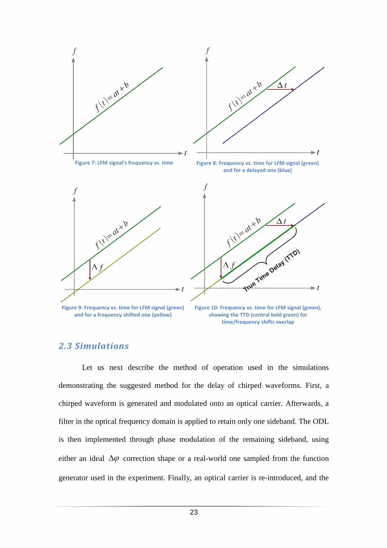
Although the time delay we can obtain using this principle is much longer

compared to what prior methods had achieved, it is not without limits. The

equivalency between time delay and phase shift is based on the chirped signal’s

nature, and is absolute only for theoretical, infinitely long signals. However, for real

world, finite-duration pulses this equivalency strictly depends on both the duration of

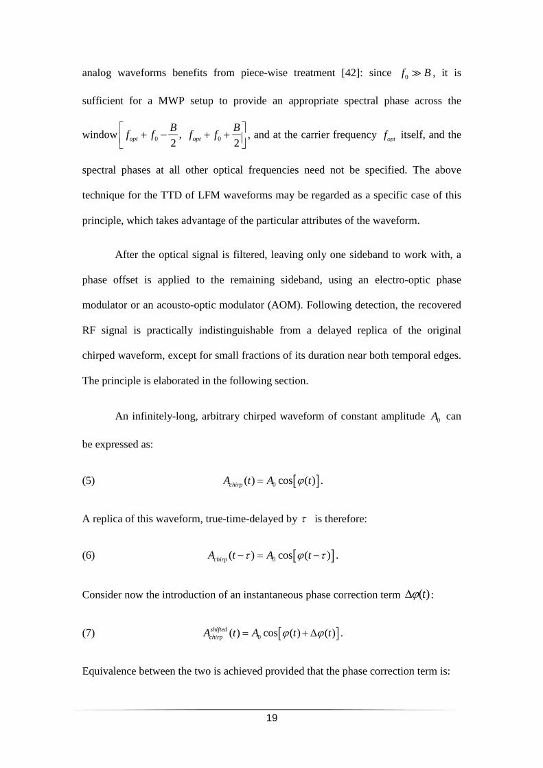
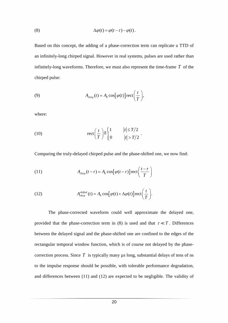
the pulse and its bandwidth. To demonstrate, let us examine the instantaneous

frequency of a LFM waveform (Figure 7). Both the delayed and the frequency-shifted

replicas are shown in Figure 8 and Figure 9, respectively. Comparing the two (Figure

10), it is obvious that even though the central portions of the waveform (noted in

green) of the delayed and the frequency-shifted waveforms are in overlap, their edges

differ, leading to the eventual degradation of the impulse response function of the

frequency-offset waveform.

23

2.3 Simulations

Let us next describe the method of operation used in the simulations

demonstrating the suggested method for the delay of chirped waveforms. First, a

chirped waveform is generated and modulated onto an optical carrier. Afterwards, a

filter in the optical frequency domain is applied to retain only one sideband. The ODL

is then implemented through phase modulation of the remaining sideband, using

either an ideal ϕ∆ correction shape or a real-world one sampled from the function

generator used in the experiment. Finally, an optical carrier is re-introduced, and the

Figure 7: LFM signal’s frequency vs. time Figure 8: Frequency vs. time for LFM signal (green)

and for a delayed one (blue)

Figure 9: Frequency vs. time for LFM signal (green)

and for a frequency shifted one (yellow) Figure 10: Frequency vs. time for LFM signal (green),

showing the TTD (central bold green) for

time/frequency shifts overlap

24

signal is detected and down-converted to the base-band. The impulse response of the

modified waveform is calculated through its cross-correlation with a replica of the

original waveform. The calculated, equivalent TTD is seen as a temporal offset of the

cross-correlation main lobe.

The correlation sidebands can be suppressed using a spectral windowing. The

simulation uses Hann’s window [90], however, the choice of a window is arbitrary, as

every window which reduces the correlation side-lobes is suitable, for example:

Hamming’s window [90]. It is important to mention that windowing should only be

applied to LFM waveforms and not to NLFM waveforms, since the spectrum of

NLFM signals is already shaped to meet the low side-lobes requirement, at least in

principle.

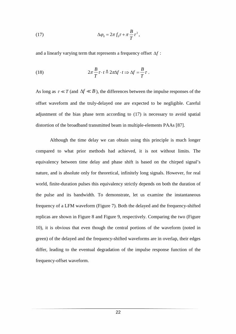
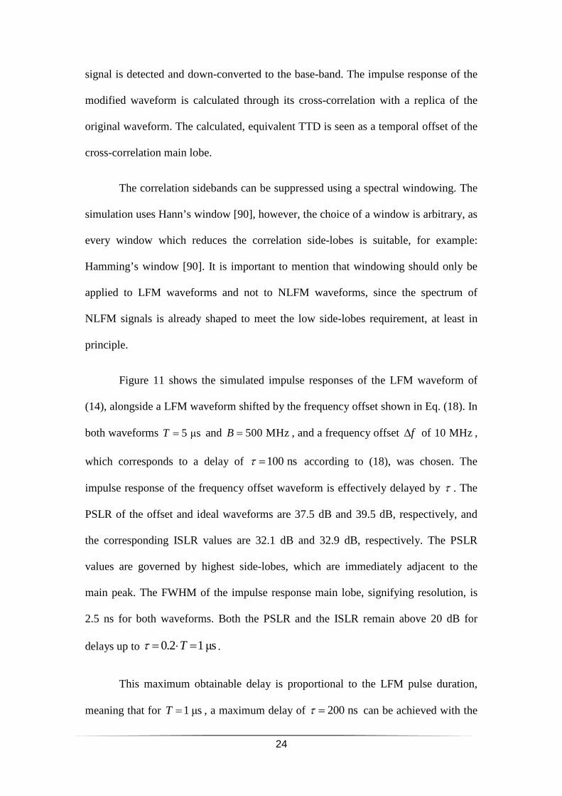
Figure 11 shows the simulated impulse responses of the LFM waveform of

(14), alongside a LFM waveform shifted by the frequency offset shown in Eq. (18). In

both waveforms µs5 T = and 500 MHzB = , and a frequency offset f∆ of 10 MHz,

which corresponds to a delay of 100 nsτ = according to (18), was chosen. The

impulse response of the frequency offset waveform is effectively delayed by τ . The

PSLR of the offset and ideal waveforms are 37.5 dB and 39.5 dB, respectively, and

the corresponding ISLR values are 32.1 dB and 32.9 dB, respectively. The PSLR

values are governed by highest side-lobes, which are immediately adjacent to the

main peak. The FWHM of the impulse response main lobe, signifying resolution, is

2.5 ns for both waveforms. Both the PSLR and the ISLR remain above 20 dB for

delays up to 0.2 1 µsTτ = ⋅ = .

This maximum obtainable delay is proportional to the LFM pulse duration,

meaning that for µs1 T = , a maximum delay of 200 nsτ = can be achieved with the

25

above PSLR values. Furthermore, the correlation resolution is the inverse of the LFM

bandwidth [44]. Therefore, wider bandwidth will result in higher resolution. This can

be seen in Figure 12, where the FWHM of an LFM pulse with 500 MHzB = is twice

the FWHM of an LFM pulse with 1 GHzB = .

These numerical simulations show that the impulse responses of manipulated

waveforms are effectively delayed with only marginal degradations in their figures of

merit: resolution, PSLR and ISLR. By compromising the universality of the TTD

element, we are able to scale the effective delay of LFM waveforms towards the

requirements of large phased-array antennas. Furthermore, the proposed method is

very simple and requires only few elements.

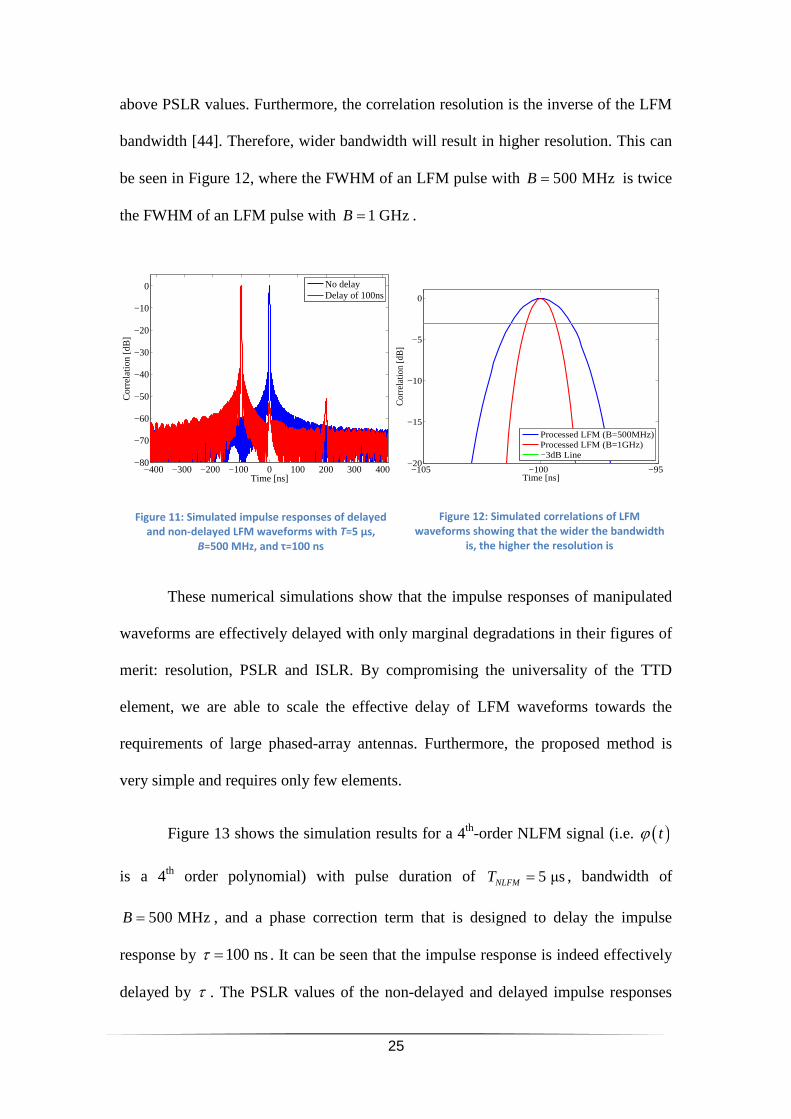
Figure 13 shows the simulation results for a 4th-order NLFM signal (i.e. ( )tϕ

is a 4th order polynomial) with pulse duration of 5 µsNLFMT = , bandwidth of

500 MHzB = , and a phase correction term that is designed to delay the impulse

response by 100 nsτ = . It can be seen that the impulse response is indeed effectively

delayed by τ . The PSLR values of the non-delayed and delayed impulse responses

−400 −300 −200 −100 0 100 200 300 400−80

−70

−60

−50

−40

−30

−20

−10

0

Time [ns]

Cor

rela

tion

[dB

]

No delayDelay of 100ns

Figure 11: Simulated impulse responses of delayed

and non-delayed LFM waveforms with T=5 µs,

B=500 MHz, and τ=100 ns

−105 −100 −95−20

−15

−10

−5

0

Time [ns]

Cor

rela

tion

[dB

]

Processed LFM (B=500MHz)Processed LFM (B=1GHz)−3dB Line

Figure 12: Simulated correlations of LFM

waveforms showing that the wider the bandwidth

is, the higher the resolution is

26

are 42.7 dB and 35 dB, respectively, and the ISLR values are 37.9 dB and 31.2 dB,

respectively. The resolution of the 4th-order NLFM waveform is 3 ns, for 8th-order it

is 5 ns, and for 16th-order it is 6.8 ns. As the NLFM order increases, the side-lobes

suppression improves at the expanse of resolution.

However, as both waveforms are effectively delayed based on phase

corrections, the ISLR and PSLR values of the NLFM waveform degrade more

severely than those of the LFM waveform, until they eventually go below them [44].

One explanation for the quicker degradation in the figures of merit of NLFM

waveforms lays in their design. NLFM waveforms are designed from a specific

spectrum, which provides them with better PSLR and ISLR values. The delay

imposed over NLFM waveforms using phase shifts cause their spectrum to distort

[44]. Hence, NLFM waveforms lose their advantage over LFM waveforms for long

delays.

2.4 Experimental Setup

The experimental setup for the TTD of the impulse response of arbitrarily

chirped waveforms is shown in Figure 14 [43, 85, 86]. The output of a CW laser

−400 −200 0 200 400−40

−30

−20

−10

0

Time [ns]

Cor

rela

tion

[dB

]


Figure 13: Simulated impulse responses of delayed and

non-delayed 4th

-order NLFM waveforms with T=5 µs,

B=500 MHz, and τ=100 ns

27

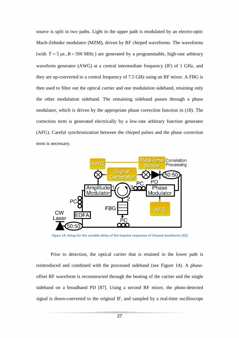
source is split in two paths. Light in the upper path is modulated by an electro-optic

Mach-Zehnder modulator (MZM), driven by RF chirped waveforms. The waveforms

(with 5 µsT = , 500 MHzB = ) are generated by a programmable, high-rate arbitrary

waveform generator (AWG) at a central intermediate frequency (IF) of 1 GHz, and

they are up-converted to a central frequency of 7.5 GHz using an RF mixer. A FBG is

then used to filter out the optical carrier and one modulation sideband, retaining only

the other modulation sideband. The remaining sideband passes through a phase

modulator, which is driven by the appropriate phase correction function in (18). The

correction term is generated electrically by a low-rate arbitrary function generator

(AFG). Careful synchronization between the chirped pulses and the phase correction

term is necessary.

Prior to detection, the optical carrier that is retained in the lower path is

reintroduced and combined with the processed sideband (see Figure 14). A phase-

offset RF waveform is reconstructed through the beating of the carrier and the single

sideband on a broadband PD [87]. Using a second RF mixer, the photo-detected

signal is down-converted to the original IF, and sampled by a real-time oscilloscope

Figure 14: Setup for the variable delay of the impulse responses of chirped waveforms [43]

28

of 6 GHz bandwidth. Finally, the impulse response of the detected waveform is

calculated by cross-correlating it with a reference signal, which was acquired at the

output of the high-rate AWG.

As shown in (17) and (18), for a LFM signal, a frequency offset alongside a

bias phase term should be applied onto the optical sideband. The bias phase term is

mandatory when the application of the proposed method is scaled to actual beam-

forming using multiple elements. Without adequate control of individual bias phases,

each antenna within a PAA would delay its input with respect to a different

wavefront, and the beam will be spatially distorted. Bias phase can be controlled

using piezoelectric transducer. Feedback information for the transducer can be

provided by the transmission of an auxiliary signal at a different wavelength. In this

work, however, we merely demonstrated the TTD of a single element, thus the bias

phase term was not employed [43, 85, 86].

For LFM signals, a phase modulator driven by a linear voltage term of slope

f∆ can provide the necessary frequency shift [85]. However, since the maximum

voltage was limited by the signal generator used in the experiment, voltage in the

form of a ramp wave was chosen (Figure 15). In this case, the phase correction term is

periodic throughout the pulse duration and hence it can be repeated continuously

without the need for synchronization between ϕ∆ and the LFM waveform (except for

bias phase adjustments in multiple-element arrays). However, the ϕ∆ required for

delaying 4th-order NLFM waveforms, for example, is not periodic during the pulse

duration, as can be seen from Figure 16, and hence it needs to be synchronized with

the NLFM pulse [43].

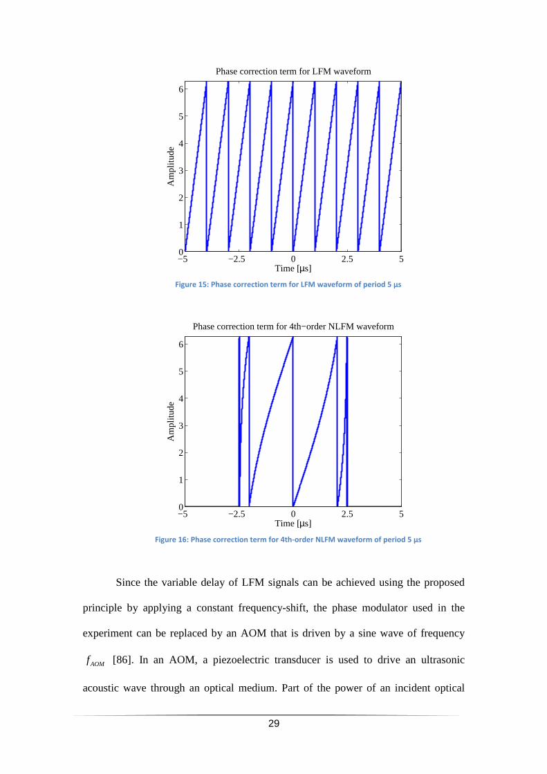
29

Since the variable delay of LFM signals can be achieved using the proposed

principle by applying a constant frequency-shift, the phase modulator used in the

experiment can be replaced by an AOM that is driven by a sine wave of frequency

AOMf [86]. In an AOM, a piezoelectric transducer is used to drive an ultrasonic

acoustic wave through an optical medium. Part of the power of an incident optical

−5 −2.5 0 2.5 50

1

2

3

4

5

6

Time [µs]

Am

plitu

de

Phase correction term for LFM waveform

Figure 15: Phase correction term for LFM waveform of period 5 µs

−5 −2.5 0 2.5 50

1

2

3

4

5

6

Time [µs]

Am

plitu

de

Phase correction term for 4th−order NLFM waveform

Figure 16: Phase correction term for 4th-order NLFM waveform of period 5 µs

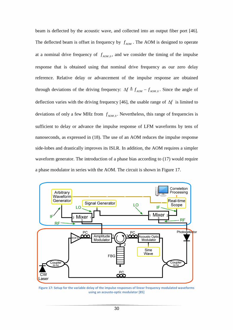
30

beam is deflected by the acoustic wave, and collected into an output fiber port [46].

The deflected beam is offset in frequency by AOMf . The AOM is designed to operate

at a nominal drive frequency of ,0AOMf , and we consider the timing of the impulse

response that is obtained using that nominal drive frequency as our zero delay

reference. Relative delay or advancement of the impulse response are obtained

through deviations of the driving frequency: ,0AOM AOMf f f∆ −≜ . Since the angle of

deflection varies with the driving frequency [46], the usable range of f∆ is limited to

deviations of only a few MHz from ,0AOMf . Nevertheless, this range of frequencies is

sufficient to delay or advance the impulse response of LFM waveforms by tens of

nanoseconds, as expressed in (18). The use of an AOM reduces the impulse response

side-lobes and drastically improves its ISLR. In addition, the AOM requires a simpler

waveform generator. The introduction of a phase bias according to (17) would require

a phase modulator in series with the AOM. The circuit is shown in Figure 17.

Figure 17: Setup for the variable delay of the impulse responses of linear frequency modulated waveforms

using an acousto-optic modulator [85]

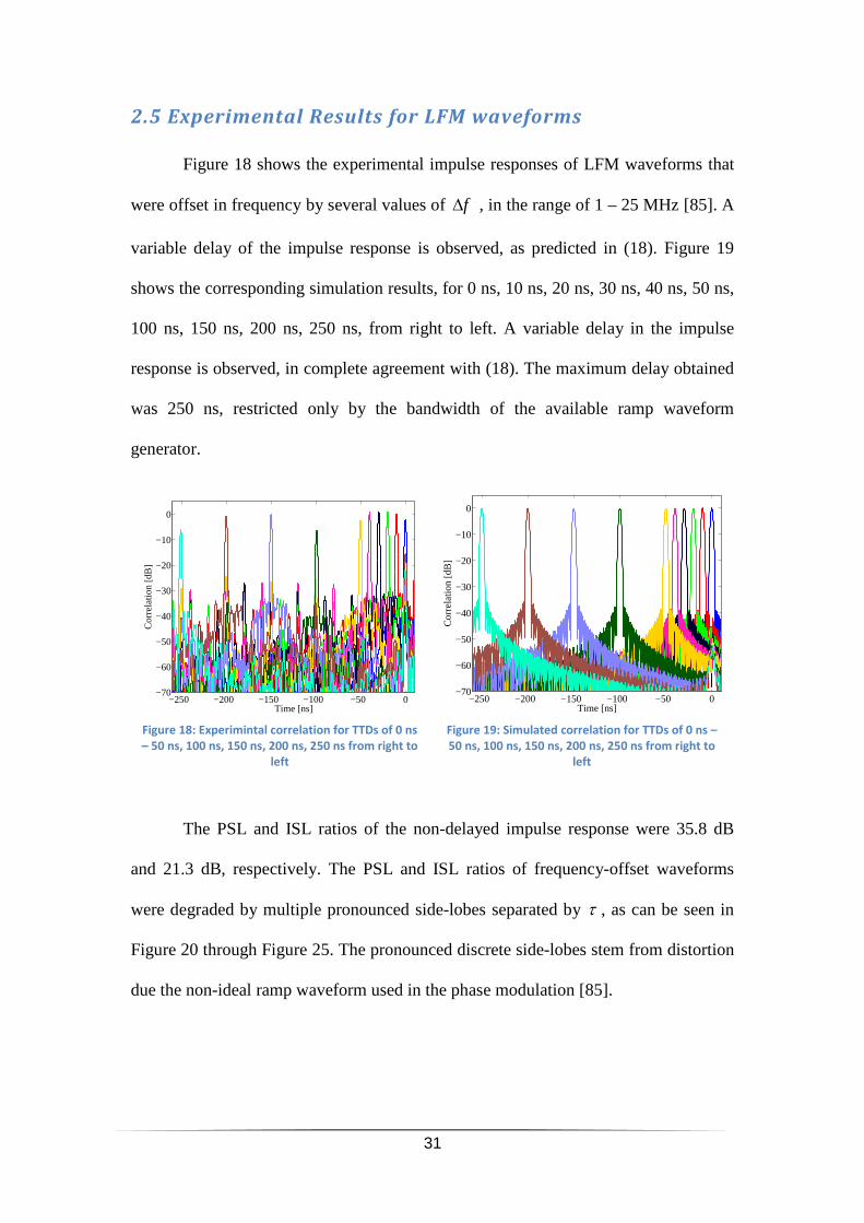
31

2.5 Experimental Results for LFM waveforms

Figure 18 shows the experimental impulse responses of LFM waveforms that

were offset in frequency by several values of f∆ , in the range of 1 – 25 MHz [85]. A

variable delay of the impulse response is observed, as predicted in (18). Figure 19

shows the corresponding simulation results, for 0 ns, 10 ns, 20 ns, 30 ns, 40 ns, 50 ns,

100 ns, 150 ns, 200 ns, 250 ns, from right to left. A variable delay in the impulse

response is observed, in complete agreement with (18). The maximum delay obtained

was 250 ns, restricted only by the bandwidth of the available ramp waveform

generator.

The PSL and ISL ratios of the non-delayed impulse response were 35.8 dB

and 21.3 dB, respectively. The PSL and ISL ratios of frequency-offset waveforms

were degraded by multiple pronounced side-lobes separated by τ , as can be seen in

Figure 20 through Figure 25. The pronounced discrete side-lobes stem from distortion

due the non-ideal ramp waveform used in the phase modulation [85].

−250 −200 −150 −100 −50 0−70

−60

−50

−40

−30

−20

−10

0

Time [ns]

Cor

rela

tion

[dB

]

Figure 18: Experimintal correlation for TTDs of 0 ns

– 50 ns, 100 ns, 150 ns, 200 ns, 250 ns from right to

left

−250 −200 −150 −100 −50 0−70

−60

−50

−40

−30

−20

−10

0

Time [ns]

Cor

rela

tion

[dB

]

Figure 19: Simulated correlation for TTDs of 0 ns –

50 ns, 100 ns, 150 ns, 200 ns, 250 ns from right to

left

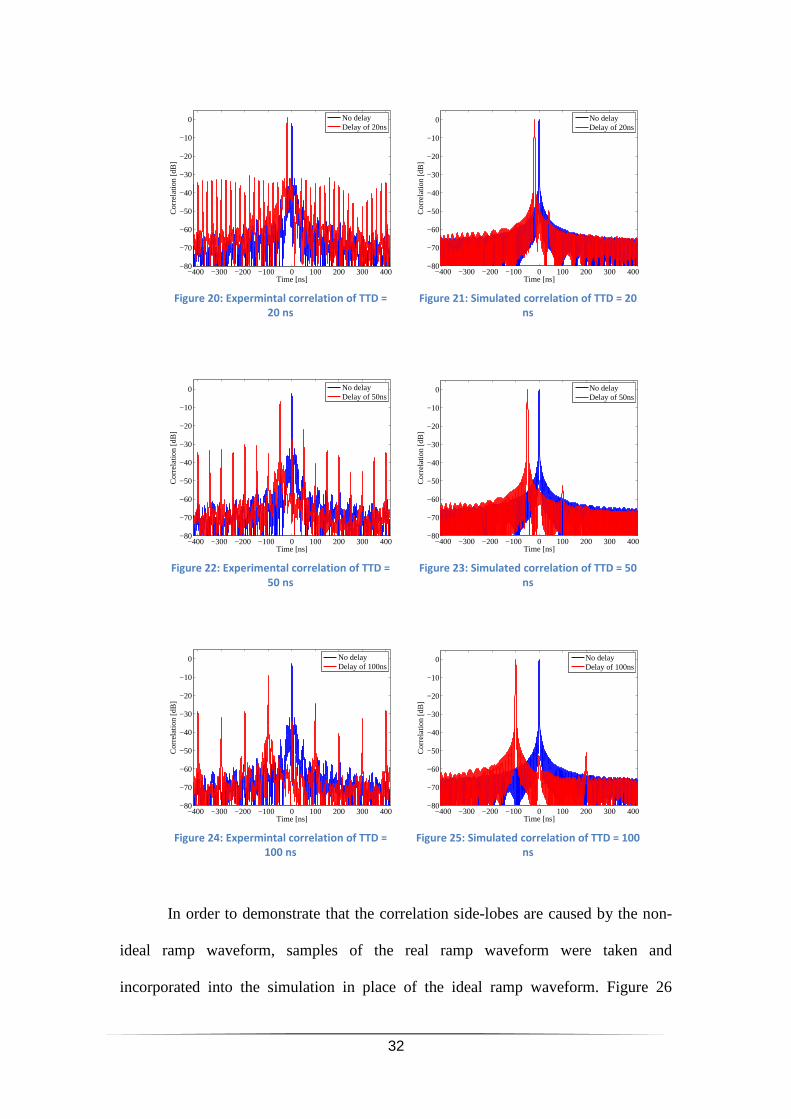
32

In order to demonstrate that the correlation side-lobes are caused by the non-

ideal ramp waveform, samples of the real ramp waveform were taken and

incorporated into the simulation in place of the ideal ramp waveform. Figure 26

−400 −300 −200 −100 0 100 200 300 400−80

−70

−60

−50

−40

−30

−20

−10

0

Time [ns]

Cor

rela

tion

[dB

]


Figure 20: Expermintal correlation of TTD =

20 ns

−400 −300 −200 −100 0 100 200 300 400−80

−70

−60

−50

−40

−30

−20

−10

0

Time [ns]

Cor

rela

tion

[dB

]


Figure 21: Simulated correlation of TTD = 20

ns

−400 −300 −200 −100 0 100 200 300 400−80

−70

−60

−50

−40

−30

−20

−10

0

Time [ns]

Cor

rela

tion

[dB

]


Figure 22: Experimental correlation of TTD =

50 ns

−400 −300 −200 −100 0 100 200 300 400−80

−70

−60

−50

−40

−30

−20

−10

0

Time [ns]

Cor

rela

tion

[dB

]



ns

−400 −300 −200 −100 0 100 200 300 400−80

−70

−60

−50

−40

−30

−20

−10

0

Time [ns]

Cor

rela

tion

[dB

]


Figure 24: Expermintal correlation of TTD =

100 ns

−400 −300 −200 −100 0 100 200 300 400−80

−70

−60

−50

−40

−30

−20

−10

0

Time [ns]

Cor

rela

tion

[dB

]



ns

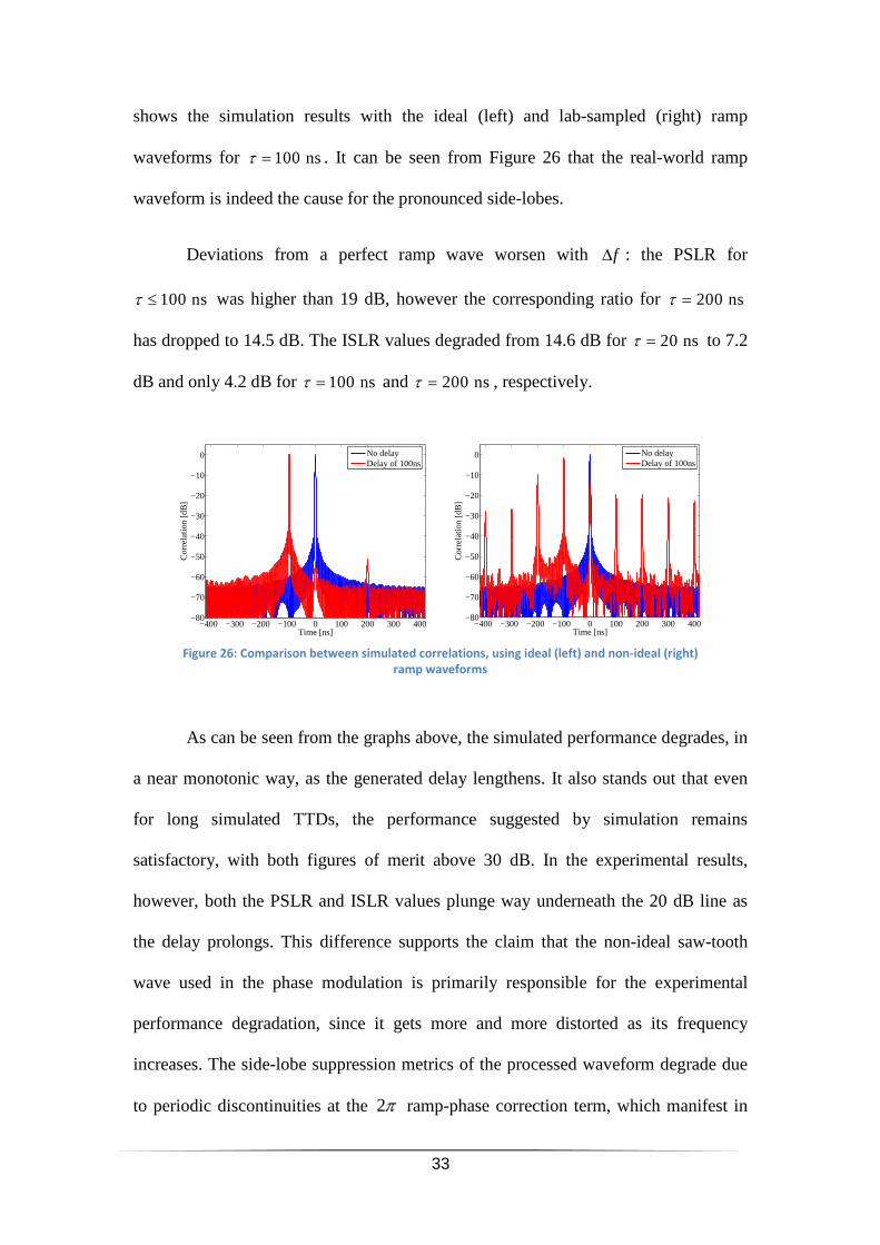
33

shows the simulation results with the ideal (left) and lab-sampled (right) ramp

waveforms for 100 ns τ = . It can be seen from Figure 26 that the real-world ramp

waveform is indeed the cause for the pronounced side-lobes.

Deviations from a perfect ramp wave worsen with f∆ : the PSLR for

100 ns τ ≤ was higher than 19 dB, however the corresponding ratio for 200 ns τ =

has dropped to 14.5 dB. The ISLR values degraded from 14.6 dB for 20 nsτ = to 7.2

dB and only 4.2 dB for 100 nsτ = and 200 nsτ = , respectively.

As can be seen from the graphs above, the simulated performance degrades, in

a near monotonic way, as the generated delay lengthens. It also stands out that even

for long simulated TTDs, the performance suggested by simulation remains

satisfactory, with both figures of merit above 30 dB. In the experimental results,

however, both the PSLR and ISLR values plunge way underneath the 20 dB line as

the delay prolongs. This difference supports the claim that the non-ideal saw-tooth

wave used in the phase modulation is primarily responsible for the experimental

performance degradation, since it gets more and more distorted as its frequency

increases. The side-lobe suppression metrics of the processed waveform degrade due

to periodic discontinuities at the 2π ramp-phase correction term, which manifest in

−400 −300 −200 −100 0 100 200 300 400−80

−70

−60

−50

−40

−30

−20

−10

0

Time [ns]

Cor

rela

tion

[dB

]


−400 −300 −200 −100 0 100 200 300 400−80

−70

−60

−50

−40

−30

−20

−10

0

Time [ns]

Cor

rela

tion

[dB

]


Figure 26: Comparison between simulated correlations, using ideal (left) and non-ideal (right)

ramp waveforms

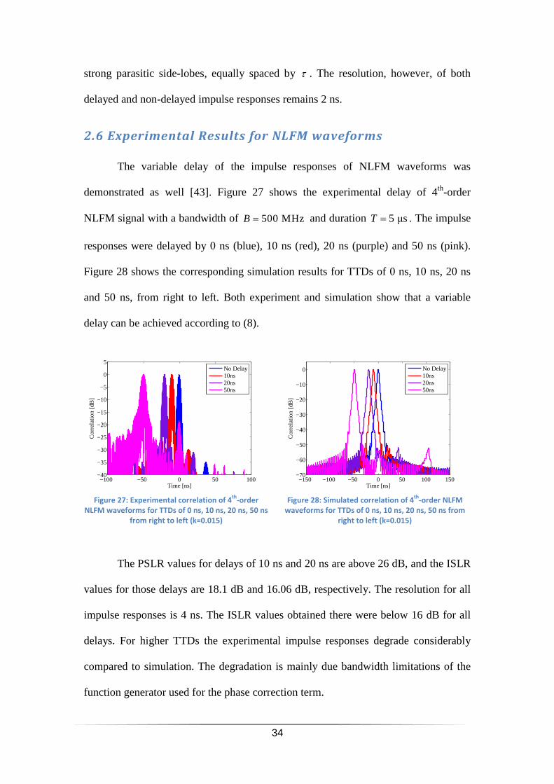
34

strong parasitic side-lobes, equally spaced by τ . The resolution, however, of both

delayed and non-delayed impulse responses remains 2 ns.

2.6 Experimental Results for NLFM waveforms

The variable delay of the impulse responses of NLFM waveforms was

demonstrated as well [43]. Figure 27 shows the experimental delay of 4th-order

NLFM signal with a bandwidth of 500 MHzB = and duration 5 µsT = . The impulse

responses were delayed by 0 ns (blue), 10 ns (red), 20 ns (purple) and 50 ns (pink).

Figure 28 shows the corresponding simulation results for TTDs of 0 ns, 10 ns, 20 ns

and 50 ns, from right to left. Both experiment and simulation show that a variable

delay can be achieved according to (8).

The PSLR values for delays of 10 ns and 20 ns are above 26 dB, and the ISLR

values for those delays are 18.1 dB and 16.06 dB, respectively. The resolution for all

impulse responses is 4 ns. The ISLR values obtained there were below 16 dB for all

delays. For higher TTDs the experimental impulse responses degrade considerably

compared to simulation. The degradation is mainly due bandwidth limitations of the

function generator used for the phase correction term.

−100 −50 0 50 100−40

−35

−30

−25

−20

−15

−10

−5

0

5

Time [ns]

Cor

rela

tion

[dB

]

No Delay10ns20ns50ns

Figure 27: Experimental correlation of 4th

-order

NLFM waveforms for TTDs of 0 ns, 10 ns, 20 ns, 50 ns

from right to left (k=0.015)

−150 −100 −50 0 50 100 150−70

−60

−50

−40

−30

−20

−10

0

Time [ns]

Cor

rela

tion

[dB

]

No Delay10ns20ns50ns

Figure 28: Simulated correlation of 4th

-order NLFM

waveforms for TTDs of 0 ns, 10 ns, 20 ns, 50 ns from

right to left (k=0.015)

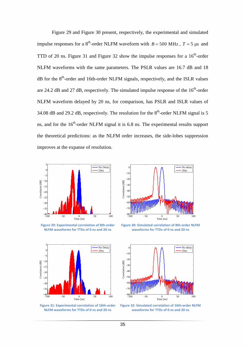
35

Figure 29 and Figure 30 present, respectively, the experimental and simulated

impulse responses for a 8th-order NLFM waveform with 500 MHzB = , 5 µsT = and

TTD of 20 ns. Figure 31 and Figure 32 show the impulse responses for a 16th-order

NLFM waveforms with the same parameters. The PSLR values are 16.7 dB and 18

dB for the 8th-order and 16th-order NLFM signals, respectively, and the ISLR values

are 24.2 dB and 27 dB, respectively. The simulated impulse response of the 16th-order

NLFM waveform delayed by 20 ns, for comparison, has PSLR and ISLR values of

34.08 dB and 29.2 dB, respectively. The resolution for the 8th-order NLFM signal is 5

ns, and for the 16th-order NLFM signal it is 6.8 ns. The experimental results support

the theoretical predictions: as the NLFM order increases, the side-lobes suppression

improves at the expanse of resolution.

−100 −50 0 50 100−40

−35

−30

−25

−20

−15

−10

−5

0

5

Time [ns]

Cor

rela

tion

[dB

]

No Delay20ns

Figure 29: Experimental correlation of 8th-order

NLFM waveforms for TTDs of 0 ns and 20 ns

−100 −50 0 50 100−80

−70

−60

−50

−40

−30

−20

−10

0

Time [ns]

Cor

rela

tion

[dB

]

No delay20ns

Figure 30: Simulated correlation of 8th-order NLFM

waveforms for TTDs of 0 ns and 20 ns

−100 −50 0 50 100−40

−35

−30

−25

−20

−15

−10

−5

0

5

Time [ns]

Cor

rela

tion

[dB

]

No Delay20ns

Figure 31: Experimental correlation of 16th-order

NLFM waveforms for TTDs of 0 ns and 20 ns

−100 −50 0 50 100−80

−70

−60

−50

−40

−30

−20

−10

0

Time [ns]

Cor

rela

tion

[dB

]

No delay20ns

Figure 32: Simulated correlation of 16th-order NLFM

waveforms for TTDs of 0 ns and 20 ns

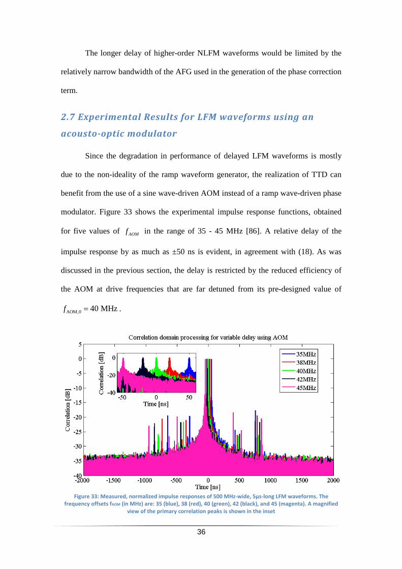
36

The longer delay of higher-order NLFM waveforms would be limited by the

relatively narrow bandwidth of the AFG used in the generation of the phase correction

term.

2.7 Experimental Results for LFM waveforms using an

acousto-optic modulator

Since the degradation in performance of delayed LFM waveforms is mostly

due to the non-ideality of the ramp waveform generator, the realization of TTD can

benefit from the use of a sine wave-driven AOM instead of a ramp wave-driven phase

modulator. Figure 33 shows the experimental impulse response functions, obtained

for five values of AOMf in the range of 35 - 45 MHz [86]. A relative delay of the

impulse response by as much as ±50 ns is evident, in agreement with (18). As was

discussed in the previous section, the delay is restricted by the reduced efficiency of

the AOM at drive frequencies that are far detuned from its pre-designed value of

AOM,0 40 MHzf = .

Figure 33: Measured, normalized impulse responses of 500 MHz-wide, 5µs-long LFM waveforms. The

frequency offsets fAOM (in MHz) are: 35 (blue), 38 (red), 40 (green), 42 (black), and 45 (magenta). A magnified

view of the primary correlation peaks is shown in the inset

37

For all values of f∆ , the FWHM of the impulse response main lobe was 2 ns.

The highest PSLR value is at the AOM,0f frequency, as anticipated, and it decreases as

f∆ increases. The lowest PSLR value is 17.5 dB. The ISLR for all impulse responses

is better than 20 dB [86].

Although ramp-wave phase modulation could provide longer delay variations

of LFM waveforms, by as much as ±125 ns, the ISLR values for delay variations

larger than 20 ns were unacceptably low, between 7-9 dB. The application of an AOM

eliminated the multiple periodic correlation side-lobes separated by τ that hindered

the performance of the earlier setup. The remaining side-lobes stem from a residual

incident beam that is not shifted, and from anti-Stokes and higher-order scattering in

the AOM. The range of frequency offset values f∆ may be increased, in principle,

with the construction of double-pass AOM in which the angle of beam deflection

remains fixed.

2.8 Discussion and summary

The long, continuously-variable MWP delay of chirped waveforms, based on

their time-frequency relations, was proposed and demonstrated. These waveforms are

prevalent in many radar systems as they provide narrow impulse response functions

with low side-lobes despite their long duration. It is shown, through analysis,

simulations and experiments, that the method has an effect which is nearly equivalent

to the delay of the impulse response functions of the chirped waveforms. It is

applicable to chirped waveforms of an arbitrary frequency sweep profile, duration,

bandwidth, or central radio frequency. The method provides an improvement of up to

two orders of magnitude in the delay-bandwidth product compared to previously

38

reported approaches, and can therefore provide the long delays that are necessary for

beam forming in large PAAs.

The method relies on the application of a low-bandwidth correction term to the

instantaneous phase of a single modulation sideband. Thus, delaying high-frequency

chirped waveforms can be accomplished using simpler and cheaper equipment. In

addition, it allows a greater flexibility in the design of chirped waveform, since

waveforms with complex sweep rates can be delayed by the same equipment used to

delay simpler waveforms, such as the LFM waveform.

The results obtained in this work were limited by several factors. First of all,

more than 5 dB in the ISLR were lost in the RF up and down conversions. In addition,

the limited bandwidth of the AFG used for providing the phase-correction term

restricted the longer delay of higher-order waveforms. Nevertheless, LFM waveforms

were successfully delayed by as much as ±50 ns, and 16th-order NLFM waveforms

were delayed by as much as 20 ns, with adequate PSLR and ISLR values.

Further work is dedicated to several efforts: first, the method can be extended

further to the TTD of chirped pulses whose amplitudes are temporally-varying as

well, with the application of an electro-optic intensity modulator in series. In addition,

several replicas of this setup can be incorporated within multiple elements of a PAA,

and demonstrate the actual steering of a radar beam. Each element would be fed with

a laser carrier and the input chirped waveform. In order to achieve beam steering,

however, one must address the absolute phases of the signals passing through each

element. Lastly, the output of this setup can be connected to an RF-transmitting

antenna, which would launch the group-delayed chirped waveform to free space,

while another antenna, positioned nearby, would receive the echoes of the signal as

39

they bounce back. Such an experiment would validate the proposed TTD principle, as

the application of the phase-correction term to the chirped waveform would appear to

'push a target object away'.

40

StimulatedBrillouinScattering-

BasedPolarization-Enhanced

OpticalSpectrumAnalyzer


Optical fiber communication networks are required to increase their

transmission efficiency, to keep pace with growing demands for capacity. One

strategy, which is rapidly being adapted from the realm of wireless communication, is

the multiplexing of densely-packed, orthogonal subcarrier tones, referred to as O-

OFDM [91]. As mentioned earlier, the separation between neighboring data-carrying

tones can be as narrow as several tens of MHz [75] or even several MHz [92].

Subcarrier multiplexed transmission is also prevalent on RoF applications [1], in

which fibers are used to extend the reach of wireless communication.

The monitoring of transmission at the optical level improves the quality of

service, reduces down-times and assists in the identification of faults. OSAs are

therefore widely employed in test and measurement of optical communications and

signal processing systems, and in the characterization of photonic devices. Most

conventional OSAs rely on diffraction-grating filters, and provide a spectral

resolution on the order of 1 GHz. Such resolution is often insufficient for the

monitoring of high-end analog and digital fiber-optic transmission.

As discussed above, several groups demonstrated a high-resolution OSA that

is based on SBS processes in standard fibers [82]. The power spectral density of a

SUT is reconstructed through the scanning of a Brillouin gain line through its spectral

extent, and measurement of the amplified signal power as a function of frequency.

41

The spectral resolution of a SBS-OSA is dictated by the Brillouin linewidth,

~ 2 30 Mrad sB πΓ ⋅ . The resolution can be improved by an order of magnitude using

a three-tone pump configuration, which includes a single, central gain line and two

symmetrically detuned SBS loss lines [93]. Out-of-band spectral components of the

SUT, although unamplified, are not affected by SBS and propagate to the output un-

attenuated. Therefore, the ability to recover a relatively weak tone at the presence of a

strong one using an SBS-OSA could be rather limited.

SBS is known to be highly polarization-dependent. A quantitative account of

the polarization dependence of SBS in standard, weakly birefringent fibers was given

experimentally by van Deventer and Boot [94], and later analytically by Zadok et al.

[95]. A vector analysis had revealed that the state of polarization (SOP) of the

amplified signal is drawn towards a particular state, which is governed by the SOP of

the pump (as explained in detail in the next section) [95]. That particular state can be

made different from the output polarization of unamplified, out-of-band signal

components, unaffected by SBS. Based on this principle, an output polarizer is used to

reject the unamplified spectral components, while those within the SBS bandwidth are

partially transmitted.

In combining both polarization-enhancement and three-line pump

composition, Preussler et al. demonstrated a SBS-OSA with a rejection ratio of 30 dB,

alongside a resolution of 3 MHz [83]. However, the three-tone pump configuration

was proven difficult to implement. Due to the complexity of the realization, the

spectrum of the SUT in [83] had to be scanned across a fixed, composite SBS gain

line, instead of the other way around. More realistic optical SUTs cannot be analyzed

42

in this manner. To the best of my knowledge, the characterization of closely-spaced,

subcarrier multiplexed signals using an SBS-OSA is not yet reported.

In this work [84], a polarization-enhanced SBS-OSA is employed in the

monitoring of fiber-optic transmission of ten subcarriers, with tone separation of 10

MHz. Each subcarrier was independently modulated by a pseudo-random, on-off

keying bit sequence at 2.5 Mbit/s rate. A rejection ratio of 35 dB is obtained using a

pump power of only 20 mW, limited by the finite extinction ratio of the polarizer used

in the experiment. The rejection ratio and resolution of the setup are sufficient to

recognize, for example, the absence of a single subcarrier, directly at the optical level.

A simple SBS-OSA configuration is used, based on a single gain line and polarization

control. The results illustrate the potential of SBS analysis in the monitoring of

advanced fiber-optic transmission.

3.2 Principle of Operation

The analytic derivation below for the polarization-dependence of SBS in

standard, weakly birefringent fibers was first given, for the most part, by Zadok et al.

[95]. I have reworked and repeated the analysis myself, and I detail it below. The

following description refers primarily to [95], with my own adaptations, re-

formulations and perspectives of later works on the subject.

Let us denote the column Jones vector of a monochromatic signal wave of

frequency sigω as ( )sigE z

, z indicating position along the fiber, with the launch and

exit points at 0z = and z L= , respectively (L is the fiber length). With no pump, the

propagation of ( )sigE z

can be described by:

(18) ( ) ( ) ( ), , 0,sig sig sig sig sigE z z Eω ω ω= T

,

43

with ( ),z ωT a frequency-dependent unitary Jones matrix representing the effect of

fiber birefringence. For convenience, the frequency-dependence will not be noted;

( ),sig sigE zω

, for instance, would simply be denoted as ( )sigE z

. We neglect linear

losses in the fiber for simplicity, although such losses can be included in the analysis.

Further, since the Brillouin shift BΩ is merely ~2 11 Grad sπ ⋅ , and only a few

kilometers of modern fibers are concerned, polarization mode dispersion can be

ignored and, therefore, shifting the optical frequency by BΩ has a negligible effect on

the Jones matrix of the fiber.

A monochromatic pump wave of frequency pumpω , whose Jones vector is

denoted by ( ),pump pumpE zω

, is launched into the fiber from the opposite end at z L= .

Throughout this analysis, we work in the same right-handed coordinate system

, ,x y z , where the signal propagates in the positive z direction, while the pump

propagates in the negative z direction. Thus, for example, if both ( )sigE z

and ( )pumpE z

equal the 2×1 vector [ ]1T

j (T stands for transpose), they represent a right-handed

circularly polarized signal and a left-handed circularly polarized pump wave,

respectively [96]. As deduced in [96], the evolution of a counter-propagating jones

vector can be expressed by:

(18) ( ) ( ) ( ) ( ) ( ) ( ) ( ) ( ) ( ) ( )1 † *0 0 0 0T T T

p p p p p pE z E z E z z E z E z E−

= ⇒ = = = T T T T

.

When both the probe and pump waves are present, the local evolution of

( )sigE z

and ( )pumpE z

is driven by both the fiber birefringence and the SBS effect. The

effect of local birefringence can be expressed as [97]:

44

(18) ( ) ( ) ( ) ( ) ( ) ( ) ( ) ( )†

00

sigsigsig sig

z EE z z zE z E z

z z z z

∂ ⋅∂ ∂ ∂ = = ⋅ = ⋅∂ ∂ ∂ ∂

T T TT

(18) ( ) ( ) ( ) ( ) ( ) ( ) ( ) ( )

* * *00

pumppump Tpump pump

z EE z z zE z E z

z z z z

∂ ⋅∂ ∂ ∂ = = ⋅ = ⋅∂ ∂ ∂ ∂

T T TT

.

Using [98], the local evolution of the signal subject to SBS amplification can

be expressed as:

(18) ( )

( ) ( ) ( )†0

2sig

pump pump sig

E z gE z E z E z

z

∂ = ∂

.

[ ] 1

0g W m−

⋅ is the SBS gain per unit length and unit of pump power for a scalar

interaction (i.e., for co-polarized pump and probe waves), and depends on the fiber

material properties, the mode field diameter, the pump optical spectrum and the

frequency offset between the pump and signal waves. We dedicate most of the

analysis to the Stokes wave scenario, so that 0g is positive, but the analysis and

results, properly interpreted, are equally valid for the anti-Stokes case, where the

optical frequency of the signal is BΩ above that of the pump. The anti-Stokes signal

transfers a fraction of its power to the pump, thereby becoming attenuated with a

coefficient of 0g− per unit length and unit pump power. Note that

( ) ( )†0

2 pump pump

gE z E z

is a 2×2 matrix, representing the outer product of a column

vector ( )pumpE z

with a row one (the transpose conjugate of ( )pumpE z

).

Since the pump wave experiences loss rather than gain, its evolution can be

similarly expressed by replacing 0g with 0g− . However, the two waves are counter-

propagating: while the signal intensifies with increasing z , the pump weakens with

decreasing z . Therefore:

45

(18) ( )

( ) ( ) ( )†0

2pump

sig sig pump

E z gE z E z E z

z

∂ = ∂

.

Combining (18)-(18), we can express the evolution of the counter-propagating

signal and pump waves, subject to both SBS and birefringence:

(18) ( ) ( ) ( ) ( ) ( ) ( )† †0

2sig

pump pump sig

E z z gz E z E z E z

z z

∂ ∂ = + ∂ ∂

TT

(18) ( ) ( ) ( ) ( ) ( ) ( )

*†0

2pump T

sig sig pump

E z z gz E z E z E z

z z

∂ ∂ = + ∂ ∂

TT

.

From now on it will be assumed that SBS-induced signal amplification or

attenuation negligibly affects the pump (i.e., the so-called undepleted pump

approximation [46]). Thus, the SBS term in Eq. (18) can be ignored and Eq. (18)

becomes linear in ( )sigE z

. Therefore, we may formally relate the output signal to that

of the input through an unknown transfer matrix:

(18) ( ) ( )0sig sigE L E= ⋅H

.

Here H is a 2×2 matrix, which depends on the fiber birefringence, the optical fiber

length L , the pump power, and its SOP at z L= . The matrix H is generally non-

unitary. Nevertheless, it can be processed using the singular value decomposition

(SVD) technique:

(18) 1† †

2

0,

0

G

G

= ⋅ ⋅ = ⋅ ⋅

H U S V U V

where U and V are unitary matrices, and 1G , 2G are real and positive values which

satisfy 1 2 1G G> > in the case of SBS amplification and 1 21 G G> > in the case of SBS

attenuation. Using this decomposition two orthogonal input signal Jones vectors can

46

be identified, which provide the maximum and minimum signal output powers,

namely:

(18) 1_ max † 1 1

0 0insigE

− = =

V V

(18) 1_ min † 0 0

1 1insigE

− = =

V V

.

The corresponding output Jones vectors would be:

(18) _ max †1

1 1 1

0 0 0outsigE G

= ⋅ ⋅ ⋅ = ⋅ =

U S V V U S U

(18) _ min †2

0 0 0

1 1 1outsigE G

= ⋅ ⋅ ⋅ = ⋅ =

U S V V U S U

,

and are, therefore, also orthogonal. It is thus convenient to represent an arbitrarily

polarized input signal using the orthogonal base of _ maxinsigE

, _ mininsigE

:

(18) _ max _ min0 0

in in insig sig sigE E Eα β= +

.

Using Eqs. (18)-(18), the output signal Jones vector and the signal power are:

(18) 0 1 0 2

1 0

0 1outsigE G Gα β

= +

U U

2 22 20 1 0 2

outsigP G Gα β= + .

When 1 2G G>> , Eq. (18) suggests that unless 0α is negligible, an arbitrarily polarized

input signal will be drawn towards the SOP of _ maxoutsigE

. This phenomenon is referred

to as SBS polarization pulling, and is supported by experiments [95].

47

Next, we try to relate _ maxinsigE

, _ mininsigE

to the SOP of the pump wave by

transforming Eq. (18) into Stokes space [95]. To that end, let us first express the outer

product †E E⋅

in Jones space:

(18) ( )* *

† * ** *

x x x x yx y

y y x y y

s s s s sE E s s

s s s s s

⋅ = =

,

where ( )Tx ys s is a complex jones vector, representing the SOP of E

. Next, let us

define the four Pauli matrices:

(18) 0 1 2 3

1 0 1 0 0 1 0= ; ; ;

0 1 0 1 1 0 0

j

jσ σ σ σ

− = = = −

.

This set of matrices form an orthogonal basis for 2×2 complex Hermitian

matrices, and every 2×2 matrix M can be decomposed along this basis [97]:

(18) 0 1 2 30 0 1 1 2 2 3 3

2 3 0 1

a a a jaa a a a

a ja a aσ σ σ σ

+ − = = + + + + −

M ,

where [ ]1

2i ia Tr Mσ≜ . If ( )1 2 3a a a a=

is a vector of real valued components and

( )1 2 3σ σ σ σ=

, M can also be expressed by:

(18) 0a a σ= + ⋅M I

.

In the specific case of interest to our discussion, let us examine the matrix

†E E⋅M

≜ . It can be shown that the decomposition coefficients of this matrix along

the basis of Pauli matrices are also the Stokes-space representation of the SOP of E

,

defined as follows:

48

(18) ( ) ( )† * * * * * *0 0

1 0

0 1x x

x y x y x x y yy y

s sE E s s s s s s s s s

s sσ

⋅ ⋅ = = = +

≜

( ) ( )† * * * * * *1 1

1 0

0 1x x

x y x y x x y yy y


s sσ

⋅ ⋅ = = = − −−

≜

( ) ( )† * * * * * *2 2

0 1

1 0x y

x y x y x y x yy x


s sσ

⋅ ⋅ = = = +

≜

( ) ( )† * * * * * *3 3

0

0x y

x y x y x y x yy x

s jsjE E s s s s j s s s s s

sj jsσ

− − ⋅ ⋅ = = = −

≜ .

We may therefore identify:

(18) ( )† 0 ˆ2

sE E s σ⋅ = + ⋅I

,

where ( )1 2 3 0s s s s s= is a normalized Stokes vector.

To convert the birefringence term in (18) into Stokes space, we use the three-

dimensional vector ( )zβ

, which describes the fiber birefringence in Stokes space

[96]:

(18) ( )

( )1

2sig

sig

E zj E z

zβ σ

∂= − ⋅ ⋅

∂

.

Substituting Eq. (18) into (18), we find that:

(18) ( ) ( ) ( ) ( ) ( ) ( )† †1

2 2sig sig

T z T z jT z E z j E z T z

z zβ σ β σ

∂ ∂= − ⋅ ⋅ ⇒ = − ⋅

∂ ∂

.

Finally, using Eqs. (18) and (18) we can transform (18) into Stokes space:

(18) ( ) ( )0 ˆ

2 4sig pump

pump sig

E z g Pjs E

zβ σ σ

∂ = − ⋅ + + ⋅ ∂

I

.

49

In Eq. (18), pumpP denotes the pump power, which for the undepleted, lossless case is

independent in z . Eq. (18) can be used to obtain an equation for the evolution of the

signal power [95]:

(18) ( ) ( ) ( ) ( )

†

0† ˆ2 4

sig sigsig pumpsig pump sig

E EP z g P zjE s E

z zβ σ σ

∂ ⋅∂ = = − ⋅ + + ⋅ +

∂ ∂ I

( ) ( ) ( ) ( )0 0† ˆ ˆ ˆ12 4 2

pump pumpsig pump sig pump sig sig

g P z g PjE s E s s P zβ σ σ

⋅ + + ⋅ = + ⋅

I

.

Note again that all four Pauli matrices are Hermitian. Here sigP is the signal power,

and ˆsigs and ˆpumps are 3×1 normalized and real-valued Stokes vectors, describing the

evolution of the polarizations of the counter-propagating signal and pump waves,

respectively. Eq. (18) is easily cast into a form:

(18) ( ) ( )0

lnˆ ˆ1

2sig pump

pump sig

P z g Ps s

z

∂ = + ⋅∂

,

which is readily solved by:

(18) ( ) ( )0 0

0

ˆ ˆ ˆ êxp 1 exp 12 2

Lpump pumpout in in

sig sig pump sig sig pump sigL

g P g PP P s s dz P L s s

= + ⋅ = + ⋅

∫ .

ˆ ˆpump sig Ls s⋅ is the scalar product of the pump and signal Stokes vectors, averaged

over the fiber length. Thus, for any input SOP one can define an effective SBS gain

coefficient, given by:

(18) ( )0 ˆ ˆ12eff pump sig L

gg s s+ ⋅≜ .

Obviously, effg depends on the signal input SOP, as well as on the pump SOP.

50

Let us assume first a very weak pump so that 0

1 2 1pumpPG G

→→ . In this limit,

the forward evolution of sigs and the backward evolution of ˆpumps are solely governed

by the birefringence term. We denote the maximum value of ˆ ˆpump sig Ls s⋅ over all

possible SOPs of the input signal ( )ˆ 0sigs z= , but for a given pump SOP ( )( )ˆpumps z L= ,

as( )

ˆ 0

ˆ ˆmaxsig

pump sig Ls zs s

=⋅ . We can assume that for a sufficiently long fiber, the average

over all position z is equivalent to the ensemble average over all realizations of the

matrix M up to a given point z [99]:

(18) ( ) ( )ˆ ˆ ˆ ˆ Ensamblepump sig pump sigL Avegare

s s s z s z⋅ ≈ ⋅ =

( ) ( ) ( ) ( ) ( ) ( ) ( ) ( )* *ˆ ˆ ˆ ˆ0 0 0 0T T T TEnsamble Ensamblepump sig pump sigAvegare Avegare

s z z s s z z s⋅ = ⋅ ⋅ ⋅T TT TM M M M .

Here ( )zTM and ( )* zT

M are the Mueller matrices representing ( )zT and ( )* zT ,

respectively, and the fiber is assumed to be long enough so that most z values are

much larger than many correlation lengths of the random birefringence. The ensemble

averaged value of the expression ( ) ( )*

T z z⋅ TTM M was calculated in [99] to give:

(18) ( ) ( )*

1 0 01

0 1 0 3

0 0 1

TEnsambleAvegare

z z

⋅ = −

TTM M .

And therefore:

(18) ( ) ( )1 0 0

1ˆ ˆ ˆ ˆ0 0 1 0 0

30 0 1

Tpump sig pump sigL

s s s s

⋅ ≈ ⋅ ⋅ −

.

51

Equation (18) signifies that through knowledge of the SOPs of both pump and

signal at a given z, for example at the input end of the signal wave, the expected

effective SBS gain coefficient can be estimated based on statistical considerations.

The maximum and minimum values of ˆ ˆpump sig Ls s⋅ can be found using the Cauchy-

Schwarz inequality:

(18) 2 2

1, 1, 2, 2, 3, 3,

1ˆ ˆ ˆ ˆ ˆ ˆ ˆ ˆ

9pump sig pump sig pump sig pump sigLs s s s s s s s⋅ = ⋅ + ⋅ − ⋅ ≤

( )( )2 2 2 2 2 2

1, 2, 3, 1, 2, 3,

1 1ˆ ˆ ˆ ˆ ˆ ˆ

9 9pump pump pump sig sig sigs s s s s s+ + − + + = .

By taking a square root, we conclude that:

(18) 1 1

ˆ ˆ3 3pump sig L

s s− ≤ ⋅ ≤ .

Since ( )

ˆ 0

1ˆ ˆmax

3sigpump sig Ls z

s s=

⋅ = , we get a maximum achievable gain coefficient

of ( ) 02 3 g (Eq. (18), see also a discussion in [94]). Thus:

(18) ( ) ( )max

1exp

3sig sigG g Lω ω =

.

This maximum is attained when ( )ˆ 0sigs z= is the image of ( )ˆ 0pumps z= on the

Poincare sphere, with the equatorial plane acting as a mirror, namely:

(18) ( ) ( )max max1, 1,ˆ ˆ0 0sig pumps z s z= = =

( ) ( )max max2, 2,ˆ ˆ0 0sig pumps z s z= = =

( ) ( )max max3, 3,ˆ ˆ0 0sig pumps z s z= = − = .

52

This ( )maxˆ 0sigs z= is the normalized Stokes representation of the complex conjugate of

the pump Jones vector at 0z = , namely, ( )* 0pumpE z=

. Conversely,

( ) ˆ 0

1ˆ ˆmin

3sigpump sig Ls z

s s=

⋅ = − , corresponding to a minimum gain coefficient of ( ) 01 3 g :

(18) ( ) ( )min

1exp

6sig sigG g Lω ω =

.

This minimum value is attained for ( ) ( )min maxˆ ˆ0 0sig sigs z s z= = − = , which is the Stokes

representation of a polarization orthogonal to that of ( )* 0pumpE z=

, to be denoted by

( )* 0pumpE z⊥ =

. It can be seen based on Eqs. (18) and (18) that for a unitary ( )zT (and

ignoring the Brillouin term), if sigE

and *pumpE

are a parallel pair at 0z = , they will

continue to be parallel for all 0 z L≤ ≤ , so that ( )_ maxoutsigE z L=

has the same

polarization as that of ( )*pumpE z L=

.

Let us next denote the unit Jones vectors which are aligned with _ maxoutsigE

and

_ minoutsigE

as maxôute and minôute , respectively. Similarly, the unit Jones vectors which are

aligned with _ maxinsigE

and _ mininsigE

will be denoted as maxîne and minîne . An arbitrarily

polarized input signal may therefore be decomposed in the basis of maxîne and minîne :

(18) ( ) ( )( )0 max minˆ ˆ, 0 in insig sigE z E ae beω ω= = +

.

Here, ( )0 sigE ω is a scalar, frequency-dependent complex magnitude and 2 21a b+ = .

The corresponding output signal vector takes the following form [83, 100]:

(18) ( ) ( )( )0 max max min minˆ ˆ, out outsig sigE z L E aG e bG eω ω= = +

.

53

Note again that maxG is typically much larger than minG . Consequently, the

polarization is pulled towards that of maxôute and the output Jones vector is almost

aligned with maxôute . Consider next a polarizer at the signal output end of the fiber. The

transmission axis of the polarizer is aligned with an SOP whose unit Jones vector is

max max min minˆ ˆ ôut outp p e p e= + , with 2 2

max min 1p p+ = . The field vector at the output end of the

polarizer would be:

(18) ( ) ( )max max† * *max min 0

min min

ˆ ôut p aGE pp E z L p p E

p bG

= ⋅ = = ⋅ =

22 **max max min max minmax max min max

2 2* *minmin max min max max min min min

aG p bG p pp p p aG

bGp p p aG p p bG p

+ = + .

The power of this vector can be expressed as:

(18) ( ) ( )2 † †† †ˆ ˆ ˆ ôut out outE E E pp E z L pp E z L = = = = =

( )† †ˆ ˆ Ê z L p p p = ⋅

( ) ( )

1 ††ˆ = outp E z L E z L E=

= =

.

Substituting (18) and (18) into (18), we get:

(18) ( )2 *

2 max max min max min* * * *max min 2*

max max min min min

outaG p bG p p

E a G b GaG p p bG p

+ = = +

2 2* * * * * *max max max min max min min max max min min mina G aG p bG p p b G aG p p bG p + + + =

2 2 2 2* * * * * *max max max min max min min max max min min minaG p a G bG p p b G aG p p bG p+ + + =

2* *max max min minap G bp G+ .

Therefore, The PSD of the output signal following the polarizer becomes [100]:

(18) ( ) ( ) ( ) ( )2 2 2

* *0 max max max min min minˆ ôut out out

sig sig sig sigE E ap e G bp e Gω ω ω ω= +

.

54

For any given choices of launch SOPs of both pump and test signal, we have

the freedom to adjust the output polarizer so that out-of-band spectral components, for

which maxG ~ minG ~ 1, are entirely rejected:

(18) * *max min 0ap bp+ = .

Subject to this adjustment, the output signal PSD becomes:

(18) ( ) ( ) ( ) ( ) ( ) ( )2 2 2 2 22*

max max min 0 0out

sig sig sig sig sig sigE ap G G E H Eω ω ω ω ω ω= −

≜ .

In (18), we have defined a transfer function for the amplified signal at the output of

the polarizer:

(18) ( ) ( ) ( )*max max minsig sig sigH ap G Gω ω ω − ≜

Although SBS amplification is a nonlinear optical phenomenon, it is nevertheless

linear in the signal wave within the undepleted pump regime [46], hence its

description in terms of an equivalent frequency domain transfer function is legitimate.

Let us now calculate the maximum value of the coefficient 2*

maxap . Since

2 22 2 * *min max 1a b p p+ = + = , we can express * *

max min, , ,a b p p using trigonometric

functions, such that:

(18) ( ) ( ) ( ) ( )* *max minsin ; b cos ; sin ; cosa p pθ θ ϕ ϕ≜ ≜ ≜ ≜ .

Subject to the constraint of complete out-of-band rejection in (18), we get:

(18) ( ) ( ) ( ) ( ) ( )sin sin cos cos cos 0 2θ ϕ θ ϕ θ ϕ ϕ θ π+ = − = ⇒ = − .

Substituting back into (18), we get:

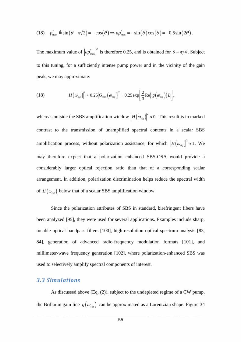
55

(18) ( ) ( ) ( ) ( ) ( )* *max maxsin 2 cos sin cos 0.5sin 2p apθ π θ θ θ θ− = − ⇒ = − = −≜ .

The maximum value of 2*

maxap is therefore 0.25, and is obtained for 4θ π= . Subject

to this tuning, for a sufficiently intense pump power and in the vicinity of the gain

peak, we may approximate:

(18) ( ) ( ) ( ) 2 2

max

20.25 0.25exp Re

3sig sig sigH G g Lω ω ω ≈ = ,

whereas outside the SBS amplification window ( )2

0sigH ω ≈ . This result is in marked

contrast to the transmission of unamplified spectral contents in a scalar SBS

amplification process, without polarization assistance, for which ( )2

1sigH ω ≈ . We

may therefore expect that a polarization enhanced SBS-OSA would provide a

considerably larger optical rejection ratio than that of a corresponding scalar

arrangement. In addition, polarization discrimination helps reduce the spectral width

of ( )sigH ω below that of a scalar SBS amplification window.

Since the polarization attributes of SBS in standard, birefringent fibers have

been analyzed [95], they were used for several applications. Examples include sharp,

tunable optical bandpass filters [100], high-resolution optical spectrum analysis [83,

84], generation of advanced radio-frequency modulation formats [101], and

millimeter-wave frequency generation [102], where polarization-enhanced SBS was

used to selectively amplify spectral components of interest.

3.3 Simulations

As discussed above (Eq. (2)), subject to the undepleted regime of a CW pump,

the Brillouin gain line ( )sigg ω can be approximated as a Lorentzian shape. Figure 34

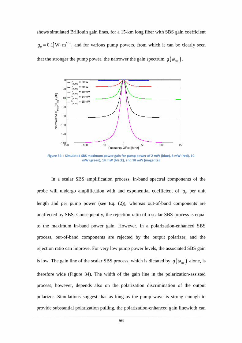
56

shows simulated Brillouin gain lines, for a 15-km long fiber with SBS gain coefficient

[ ] 1

0 0.1 W mg−

= ⋅ , and for various pump powers, from which it can be clearly seen

that the stronger the pump power, the narrower the gain spectrum ( )sigg ω .

In a scalar SBS amplification process, in-band spectral components of the

probe will undergo amplification with and exponential coefficient of 0g per unit

length and per pump power (see Eq. (2)), whereas out-of-band components are

unaffected by SBS. Consequently, the rejection ratio of a scalar SBS process is equal

to the maximum in-band power gain. However, in a polarization-enhanced SBS

process, out-of-band components are rejected by the output polarizer, and the

rejection ratio can improve. For very low pump power levels, the associated SBS gain

is low. The gain line of the scalar SBS process, which is dictated by ( )sigg ω alone, is

therefore wide (Figure 34). The width of the gain line in the polarization-assisted

process, however, depends also on the polarization discrimination of the output

polarizer. Simulations suggest that as long as the pump wave is strong enough to

provide substantial polarization pulling, the polarization-enhanced gain linewidth can

−150 −100 −50 0 50 100 150−140

−120

−100

−80

−60

−40

−20

0

Frequency Offset [MHz]

No

rma

lize

d G

ma

x(ωsi

g)

[dB

]

Ppump

= 2mW

Ppump

= 6mW

Ppump

= 10mW

Ppump

= 14mW

Ppump

= 18mW

Figure 34: : Simulated SBS maximum power gain for pump power of 2 mW (blue), 6 mW (red), 10

mW (green), 14 mW (black), and 18 mW (magenta)

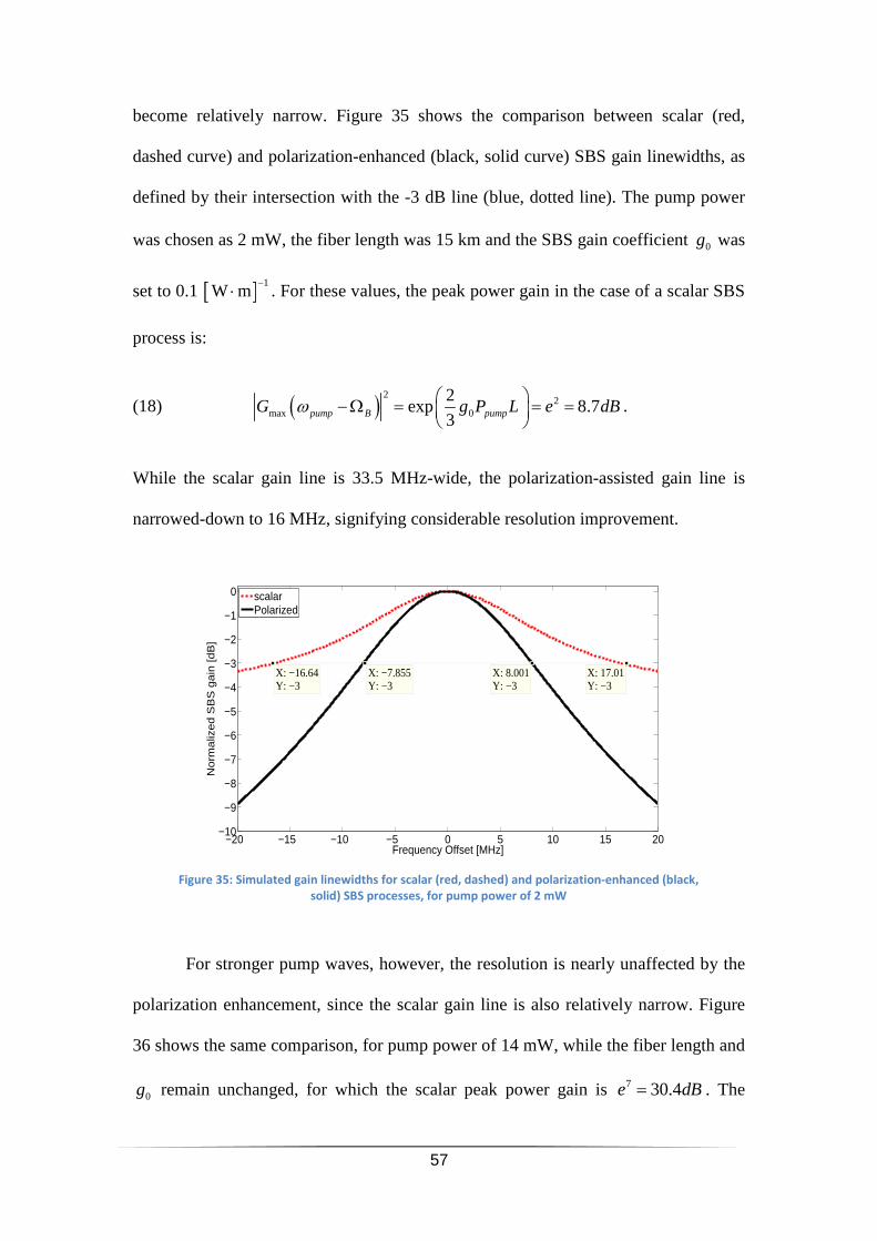
57

become relatively narrow. Figure 35 shows the comparison between scalar (red,

dashed curve) and polarization-enhanced (black, solid curve) SBS gain linewidths, as

defined by their intersection with the -3 dB line (blue, dotted line). The pump power

was chosen as 2 mW, the fiber length was 15 km and the SBS gain coefficient 0g was

set to 0.1 [ ] 1W m

−⋅ . For these values, the peak power gain in the case of a scalar SBS

process is:

(18) ( )2

2max 0

2exp 8.7

3pump B pumpG g P L e dBω −Ω = = =

.

While the scalar gain line is 33.5 MHz-wide, the polarization-assisted gain line is

narrowed-down to 16 MHz, signifying considerable resolution improvement.

For stronger pump waves, however, the resolution is nearly unaffected by the

polarization enhancement, since the scalar gain line is also relatively narrow. Figure

36 shows the same comparison, for pump power of 14 mW, while the fiber length and

0g remain unchanged, for which the scalar peak power gain is 7 30.4e dB= . The

−20 −15 −10 −5 0 5 10 15 20−10

−9

−8

−7

−6

−5

−4

−3

−2

−1

0

X: −16.64Y: −3


No

rma

lize

d S

BS

ga

in [

dB

]

X: −7.855Y: −3

X: 8.001Y: −3

X: 17.01Y: −3

scalarPolarized

Figure 35: Simulated gain linewidths for scalar (red, dashed) and polarization-enhanced (black,

solid) SBS processes, for pump power of 2 mW

58

resolution of both processes is nearly identical (a 7.3 MHz-wide gain line), and the

two become distinguishable only as the frequency offset increases.

Next, let us compare between the optical rejection ratio of the scalar process

and that of the polarization-assisted one, for the same values ( 14 mWpumpP = ,

15 kmL = and [ ] 1

0 0.1 W mg−

= ⋅ ). Figure 37 and Figure 38 demonstrate the

reconstruction of the PSD of SUTs which consist of a strong central tone and two,

relatively weak side-tones that are detuned by ±20 MHz. The relative power of the

side-tones is -25 dB (Figure 37) and -35 dB (Figure 38). The method of operation for

these reconstructions included the simulation of a single SBS gain line (for both the

scalar and the polarization-assisted SBS-OSA) and the convolution of this gain line

with the PSD of the SUT. The reconstruction is shown below for both scalar (red,

dashed) and polarization-enhanced (black, solid) SBS processes.

−50 −40 −30 −20 −10 0 10 20 30 40 50−35

−30

−25

−20

−15

−10

−5

0

X: 3.644Y: −3


No

rma

lize

d S

BS

ga

in [d

B]

scalarPolarized

Figure 36: Simulated SBS gain linewidth for scalar (red, dashed) and polarization-enhanced (black,

solid) SBS processes, for pump power of 14 mW

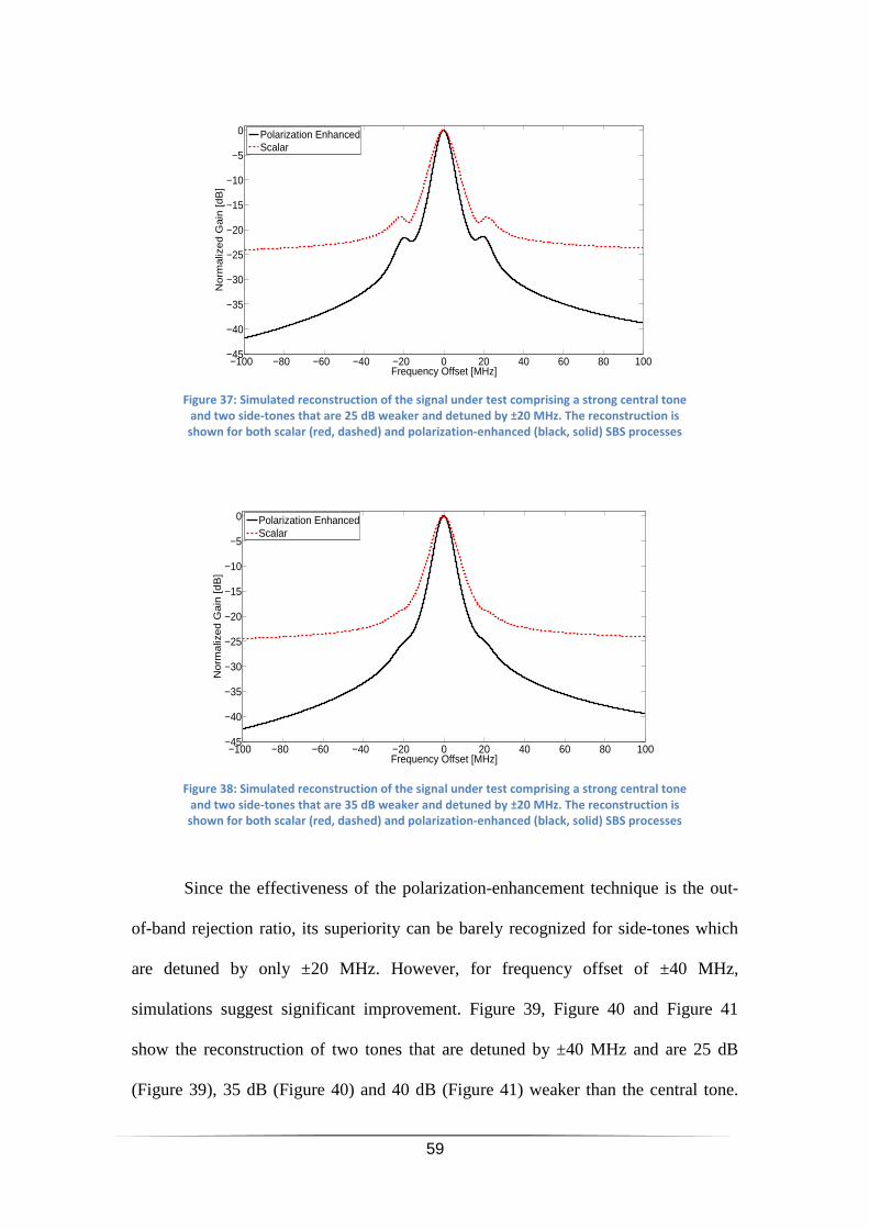
59

Since the effectiveness of the polarization-enhancement technique is the out-

of-band rejection ratio, its superiority can be barely recognized for side-tones which

are detuned by only ±20 MHz. However, for frequency offset of ±40 MHz,

simulations suggest significant improvement. Figure 39, Figure 40 and Figure 41

show the reconstruction of two tones that are detuned by ±40 MHz and are 25 dB

(Figure 39), 35 dB (Figure 40) and 40 dB (Figure 41) weaker than the central tone.

−100 −80 −60 −40 −20 0 20 40 60 80 100−45

−40

−35

−30

−25

−20

−15

−10

−5

0


No

rma

lize

d G

ain

[d

B]

Polarization EnhancedScalar

Figure 37: Simulated reconstruction of the signal under test comprising a strong central tone

and two side-tones that are 25 dB weaker and detuned by ±20 MHz. The reconstruction is

shown for both scalar (red, dashed) and polarization-enhanced (black, solid) SBS processes

−100 −80 −60 −40 −20 0 20 40 60 80 100−45

−40

−35

−30

−25

−20

−15

−10

−5

0


No

rma

lize

d G

ain

[d

B]





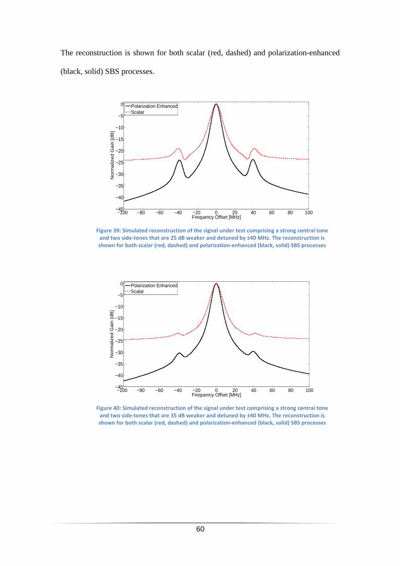
60

The reconstruction is shown for both scalar (red, dashed) and polarization-enhanced

(black, solid) SBS processes.

−100 −80 −60 −40 −20 0 20 40 60 80 100−45

−40

−35

−30

−25

−20

−15

−10

−5

0


No

rma

lize

d G

ain

[d

B]





−100 −80 −60 −40 −20 0 20 40 60 80 100−45

−40

−35

−30

−25

−20

−15

−10

−5

0


No

rma

lize

d G

ain

[d

B]





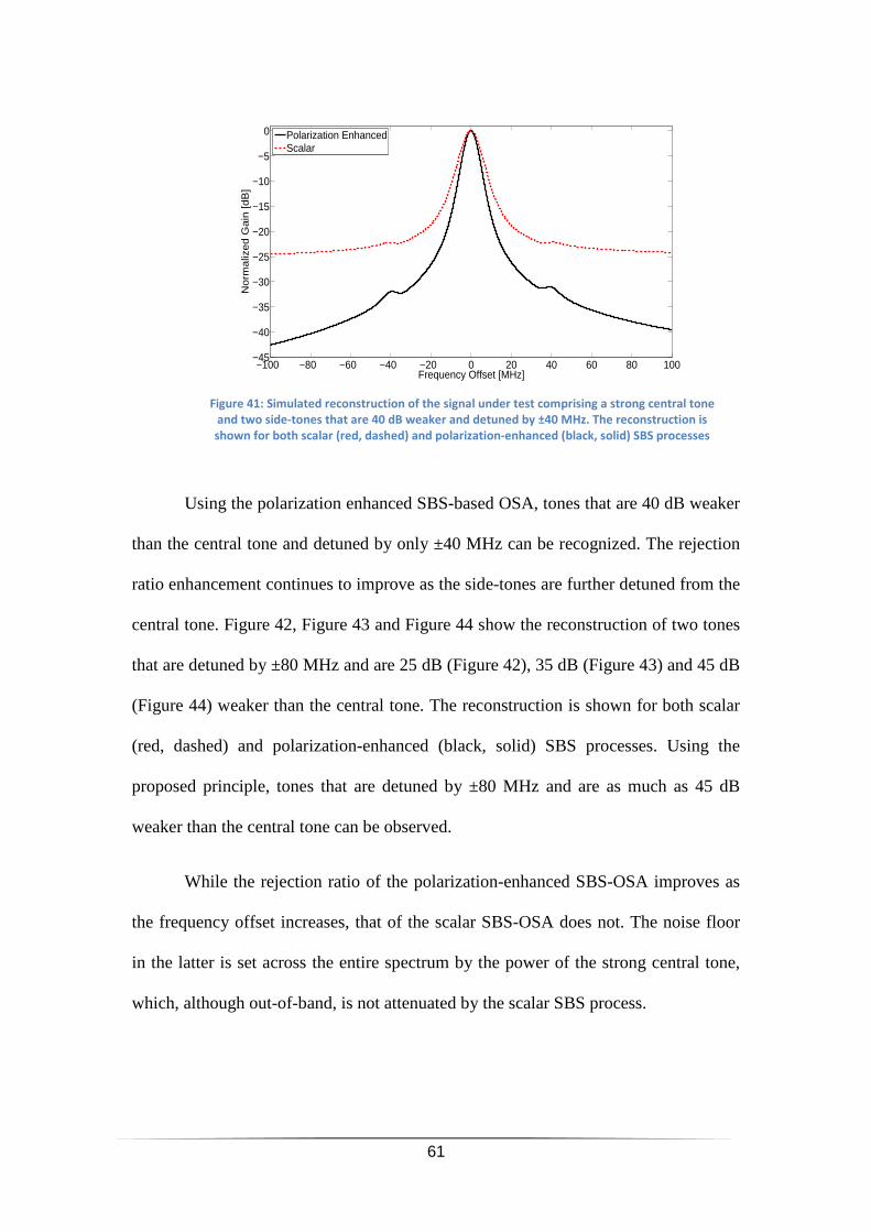
61

Using the polarization enhanced SBS-based OSA, tones that are 40 dB weaker

than the central tone and detuned by only ±40 MHz can be recognized. The rejection

ratio enhancement continues to improve as the side-tones are further detuned from the

central tone. Figure 42, Figure 43 and Figure 44 show the reconstruction of two tones

that are detuned by ±80 MHz and are 25 dB (Figure 42), 35 dB (Figure 43) and 45 dB

(Figure 44) weaker than the central tone. The reconstruction is shown for both scalar

(red, dashed) and polarization-enhanced (black, solid) SBS processes. Using the

proposed principle, tones that are detuned by ±80 MHz and are as much as 45 dB

weaker than the central tone can be observed.

While the rejection ratio of the polarization-enhanced SBS-OSA improves as

the frequency offset increases, that of the scalar SBS-OSA does not. The noise floor

in the latter is set across the entire spectrum by the power of the strong central tone,

which, although out-of-band, is not attenuated by the scalar SBS process.

−100 −80 −60 −40 −20 0 20 40 60 80 100−45

−40

−35

−30

−25

−20

−15

−10

−5

0


No

rma

lize

d G

ain

[d

B]





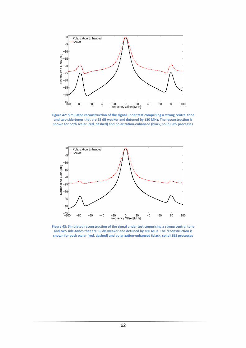
62

−100 −80 −60 −40 −20 0 20 40 60 80 100−45

−40

−35

−30

−25

−20

−15

−10

−5

0


No

rma

lize

d G

ain

[d

B]





−100 −80 −60 −40 −20 0 20 40 60 80 100−45

−40

−35

−30

−25

−20

−15

−10

−5

0


No

rma

lize

d G

ain

[d

B]





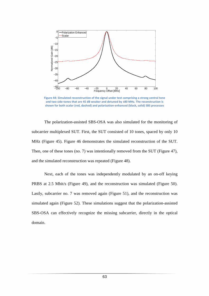
63

The polarization-assisted SBS-OSA was also simulated for the monitoring of

subcarrier multiplexed SUT. First, the SUT consisted of 10 tones, spaced by only 10

MHz (Figure 45). Figure 46 demonstrates the simulated reconstruction of the SUT.

Then, one of these tones (no. 7) was intentionally removed from the SUT (Figure 47),

and the simulated reconstruction was repeated (Figure 48).

Next, each of the tones was independently modulated by an on-off keying

PRBS at 2.5 Mbit/s (Figure 49), and the reconstruction was simulated (Figure 50).

Lastly, subcarrier no. 7 was removed again (Figure 51), and the reconstruction was

simulated again (Figure 52). These simulations suggest that the polarization-assisted

SBS-OSA can effectively recognize the missing subcarrier, directly in the optical

domain.

−100 −80 −60 −40 −20 0 20 40 60 80 100−45

−40

−35

−30

−25

−20

−15

−10

−5

0


No

rma

lize

d G

ain

[d

B]





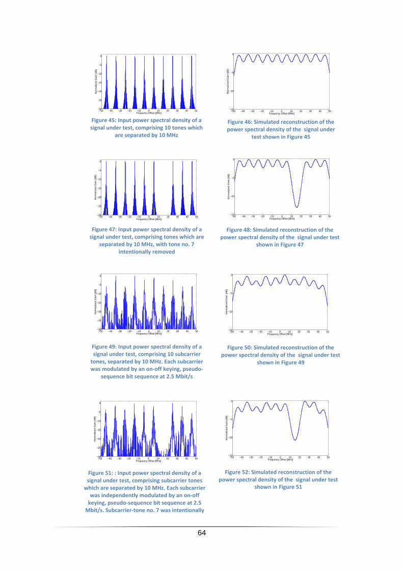
64

−50 −40 −30 −20 −10 0 10 20 30 40 50−30

−25

−20

−15

−10

−5

0


No

rma

lize

d G

ain

[d

B]

Figure 45: Input power spectral density of a

signal under test, comprising 10 tones which

are separated by 10 MHz

−50 −40 −30 −20 −10 0 10 20 30 40 50−15

−10

−5

0


No

rma

lize

d G

ain

[d

B]

Figure 46: Simulated reconstruction of the

power spectral density of the signal under

test shown in Figure 45

−50 −40 −30 −20 −10 0 10 20 30 40 50−30

−25

−20

−15

−10

−5

0


No

rma

lize

d G

ain

[d

B]


signal under test, comprising tones which are

separated by 10 MHz, with tone no. 7

intentionally removed

−50 −40 −30 −20 −10 0 10 20 30 40 50−15

−10

−5

0


No

rma

lize

d G

ain

[d

B]


power spectral density of the signal under test

shown in Figure 47

−50 −40 −30 −20 −10 0 10 20 30 40 50−30

−25

−20

−15

−10

−5

0


No

rma

lize

d G

ain

[d

B]


signal under test, comprising 10 subcarrier

tones, separated by 10 MHz. Each subcarrier

was modulated by an on-off keying, pseudo-

sequence bit sequence at 2.5 Mbit/s

−50 −40 −30 −20 −10 0 10 20 30 40 50−15

−10

−5

0


No

rma

lize

d G

ain

[d

B]



shown in Figure 49

−50 −40 −30 −20 −10 0 10 20 30 40 50−30

−25

−20

−15

−10

−5

0


No

rma

lize

d G

ain

[d

B]

Figure 51: : Input power spectral density of a

signal under test, comprising subcarrier tones

which are separated by 10 MHz. Each subcarrier

was independently modulated by an on-off

keying, pseudo-sequence bit sequence at 2.5

Mbit/s. Subcarrier-tone no. 7 was intentionally

removed

−50 −40 −30 −20 −10 0 10 20 30 40 50−15

−10

−5

0


No

rma

lize

d G

ain

[d

B]



shown in Figure 51

65


The experimental setup is shown below in Figure 53 [84]. The output of a TLS

is split in two branches. Light in the upper branch (the signal branch, colored in

green) is modulated by a radio-frequency waveform, generated by an AWG, and

serves as an optical SUT. The SUT is then modulated again by a sine wave of a low

frequency 200 kHzLΩ = , to allow for lock-in power measurement at the output.

Light in the lower branch (the pump branch, colored in blue) is modulated by a sine

wave of frequency Ω , in suppressed-carrier (SC), double-sideband format. A

narrowband FBG is then used to select the upper modulation sideband, which is

amplified to serve as CW pump. The pump and SUT counter-propagate in a 25 km-

long section of standard single-mode fiber, which constitutes the SBS gain medium.

In polarization-enhanced SBS-OSA measurements [84], the SUT at the output

of the gain medium is split using a polarization beam-splitter (PBS), and the output of

the fast axis is detected. The PBS is bypassed in scalar SBS measurements. The

frequency offset Ω is swept in 1 MHz increments, (the analysis block, colored in

purple), and the power of the output probe at the polarizer output is measured. This

measurement is performed by a broadband RF-spectrum, which is set to measure the

power of the lock-in tone at the frequency LΩ . These lock-in measurements of the

photo-current block the amplified spontaneous emission associated with SBS

amplification (SBS-ASE) almost entirely, and allow for a more accurate

reconstruction of the SUT PSD. Note that the RF spectrum measures electrical power,

which is proportional to the square of the detector output current. Since the latter is

linear in the optical power at the output of the PBS, the obtained RF power is

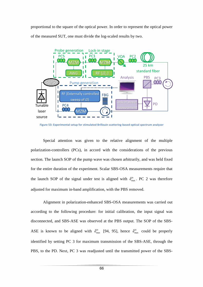
66

proportional to the square of the optical power. In order to represent the optical power

of the measured SUT, one must divide the log-scaled results by two.

Special attention was given to the relative alignment of the multiple

polarization-controllers (PCs), in accord with the considerations of the previous

section. The launch SOP of the pump wave was chosen arbitrarily, and was held fixed

for the entire duration of the experiment. Scalar SBS-OSA measurements require that

the launch SOP of the signal under test is aligned with maxîne . PC 2 was therefore

adjusted for maximum in-band amplification, with the PBS removed.

Alignment in polarization-enhanced SBS-OSA measurements was carried out

according to the following procedure: for initial calibration, the input signal was

disconnected, and SBS-ASE was observed at the PBS output. The SOP of the SBS-

ASE is known to be aligned with maxîne [94, 95], hence maxîne could be properly

identified by setting PC 3 for maximum transmission of the SBS-ASE, through the

PBS, to the PD. Next, PC 3 was readjusted until the transmitted power of the SBS-

Lock-in stage Probe generation

Tunable

laser

source

Analysis

PC5

AWG

VOA PC2

25 km

standard fiber

PBS PC3

Pump generation

MZM

PC1

MZM

RF ()

50/50

RF (Externally controlled

sweep of )

PC4

FBG

MZM

Lock-in power

measurement PD

Figure 53: Experimental setup for stimulated Brillouin scattering-based optical spectrum analyzer

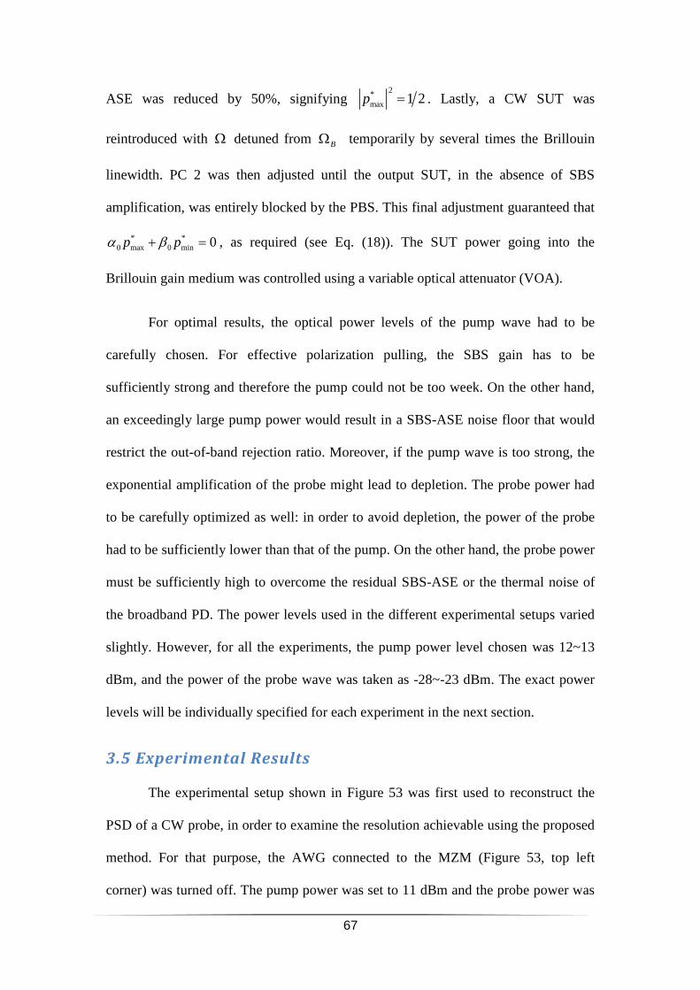
67

ASE was reduced by 50%, signifying 2*

max 1 2p = . Lastly, a CW SUT was

reintroduced with Ω detuned from BΩ temporarily by several times the Brillouin

linewidth. PC 2 was then adjusted until the output SUT, in the absence of SBS

amplification, was entirely blocked by the PBS. This final adjustment guaranteed that

* *0 max 0 min 0p pα β+ = , as required (see Eq. (18)). The SUT power going into the

Brillouin gain medium was controlled using a variable optical attenuator (VOA).

For optimal results, the optical power levels of the pump wave had to be

carefully chosen. For effective polarization pulling, the SBS gain has to be

sufficiently strong and therefore the pump could not be too week. On the other hand,

an exceedingly large pump power would result in a SBS-ASE noise floor that would

restrict the out-of-band rejection ratio. Moreover, if the pump wave is too strong, the

exponential amplification of the probe might lead to depletion. The probe power had

to be carefully optimized as well: in order to avoid depletion, the power of the probe

had to be sufficiently lower than that of the pump. On the other hand, the probe power

must be sufficiently high to overcome the residual SBS-ASE or the thermal noise of

the broadband PD. The power levels used in the different experimental setups varied

slightly. However, for all the experiments, the pump power level chosen was 12~13

dBm, and the power of the probe wave was taken as -28~-23 dBm. The exact power

levels will be individually specified for each experiment in the next section.

3.5 Experimental Results

The experimental setup shown in Figure 53 was first used to reconstruct the

PSD of a CW probe, in order to examine the resolution achievable using the proposed

method. For that purpose, the AWG connected to the MZM (Figure 53, top left

corner) was turned off. The pump power was set to 11 dBm and the probe power was

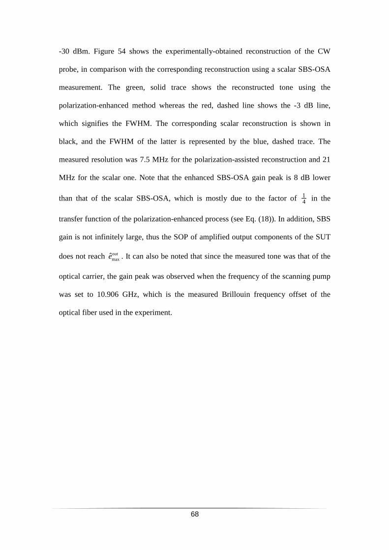
68

-30 dBm. Figure 54 shows the experimentally-obtained reconstruction of the CW

probe, in comparison with the corresponding reconstruction using a scalar SBS-OSA

measurement. The green, solid trace shows the reconstructed tone using the

polarization-enhanced method whereas the red, dashed line shows the -3 dB line,

which signifies the FWHM. The corresponding scalar reconstruction is shown in

black, and the FWHM of the latter is represented by the blue, dashed trace. The

measured resolution was 7.5 MHz for the polarization-assisted reconstruction and 21

MHz for the scalar one. Note that the enhanced SBS-OSA gain peak is 8 dB lower

than that of the scalar SBS-OSA, which is mostly due to the factor of 14 in the

transfer function of the polarization-enhanced process (see Eq. (18)). In addition, SBS

gain is not infinitely large, thus the SOP of amplified output components of the SUT

does not reach maxôute . It can also be noted that since the measured tone was that of the

optical carrier, the gain peak was observed when the frequency of the scanning pump

was set to 10.906 GHz, which is the measured Brillouin frequency offset of the

optical fiber used in the experiment.

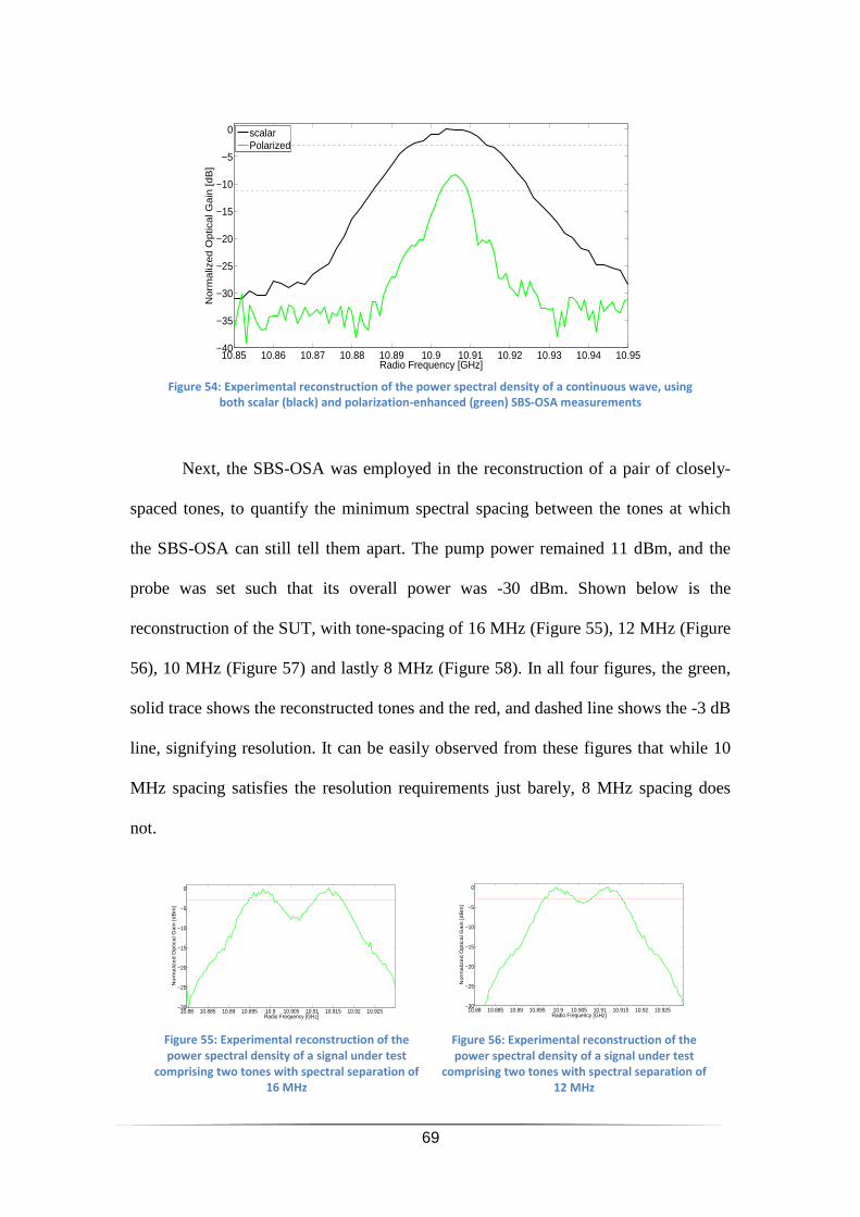
69

Next, the SBS-OSA was employed in the reconstruction of a pair of closely-

spaced tones, to quantify the minimum spectral spacing between the tones at which

the SBS-OSA can still tell them apart. The pump power remained 11 dBm, and the

probe was set such that its overall power was -30 dBm. Shown below is the

reconstruction of the SUT, with tone-spacing of 16 MHz (Figure 55), 12 MHz (Figure

56), 10 MHz (Figure 57) and lastly 8 MHz (Figure 58). In all four figures, the green,

solid trace shows the reconstructed tones and the red, and dashed line shows the -3 dB

line, signifying resolution. It can be easily observed from these figures that while 10

MHz spacing satisfies the resolution requirements just barely, 8 MHz spacing does

not.

10.85 10.86 10.87 10.88 10.89 10.9 10.91 10.92 10.93 10.94 10.95−40

−35

−30

−25

−20

−15

−10

−5

0

Radio Frequency [GHz]

No

rma

lize

d O

ptic

al G

ain

[d

B]

scalarPolarized

Figure 54: Experimental reconstruction of the power spectral density of a continuous wave, using

both scalar (black) and polarization-enhanced (green) SBS-OSA measurements

10.88 10.885 10.89 10.895 10.9 10.905 10.91 10.915 10.92 10.925−30

−25

−20

−15

−10

−5

0


No

rma

lize

d O

ptic

al G

ain

[d

Bm

]

Figure 55: Experimental reconstruction of the

power spectral density of a signal under test

comprising two tones with spectral separation of

16 MHz

10.88 10.885 10.89 10.895 10.9 10.905 10.91 10.915 10.92 10.925−30

−25

−20

−15

−10

−5

0


No

rma

lize

d O

ptic

al G

ain

[d

Bm

]




12 MHz

70

As discussed in previous sections, the main potential advantage of a

polarization-enhanced SBS-OSA is its extended rejection ratio. The next step would

therefore be to use the polarization-assisted scheme to recognize a weak tone at the

presence of an adjacent strong tone. The side-tones were taken to be detuned by ±40

MHz from the central tone. The pump power level was set to 12 dBm and the power

of the probe central tone was -28 dBm. The following figures compare the

performance of the polarization enhanced SBS-OSA with that of the scalar SBS-OSA,

for various relative side-tones power: simulated (Figure 59) and experimental (Figure

60) reconstruction where the side-tones were 27.4 dBm weaker than the central tone;

simulated (Figure 61) and experimental (Figure 62) reconstruction where the side-

tones were 30.45 dBm weaker than the central tone; and lastly, simulated (Figure 63)

and experimental (Figure 64) reconstruction where the side-tones were 33.5 dBm

weaker than the central tone.

10.88 10.885 10.89 10.895 10.9 10.905 10.91 10.915 10.92 10.925−30

−25

−20

−15

−10

−5

0


No

rma

lize

d O

ptic

al G

ain

[d

Bm

]




10 MHz

10.88 10.885 10.89 10.895 10.9 10.905 10.91 10.915 10.92 10.925−30

−25

−20

−15

−10

−5

0


No

rma

lize

d O

ptic

al G

ain

[d

Bm

]




8 MHz

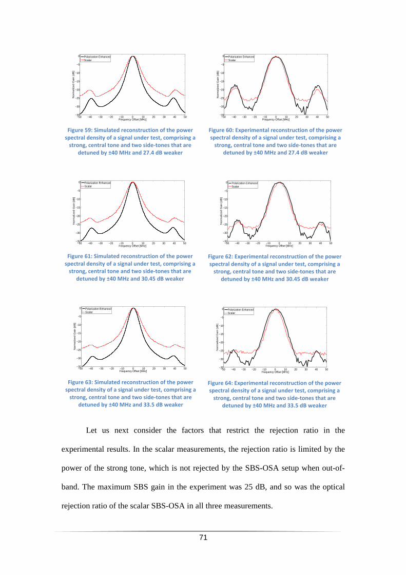
71

Let us next consider the factors that restrict the rejection ratio in the

experimental results. In the scalar measurements, the rejection ratio is limited by the

power of the strong tone, which is not rejected by the SBS-OSA setup when out-of-

band. The maximum SBS gain in the experiment was 25 dB, and so was the optical

rejection ratio of the scalar SBS-OSA in all three measurements.

−50 −40 −30 −20 −10 0 10 20 30 40 50−35

−30

−25

−20

−15

−10

−5

0


No

rma

lize

d G

ain

[d

B]


Figure 59: Simulated reconstruction of the power

spectral density of a signal under test, comprising a

strong, central tone and two side-tones that are

detuned by ±40 MHz and 27.4 dB weaker

−50 −40 −30 −20 −10 0 10 20 30 40 50−35

−30

−25

−20

−15

−10

−5

0


No

rma

lize

d G

ain

[d

B]


Figure 60: Experimental reconstruction of the power




−50 −40 −30 −20 −10 0 10 20 30 40 50−35

−30

−25

−20

−15

−10

−5

0


No

rma

lize

d G

ain

[d

B]






−50 −40 −30 −20 −10 0 10 20 30 40 50−35

−30

−25

−20

−15

−10

−5

0


No

rma

lize

d G

ain

[d

B]






−50 −40 −30 −20 −10 0 10 20 30 40 50−35

−30

−25

−20

−15

−10

−5

0


No

rma

lize

d G

ain

[d

B]






−50 −40 −30 −20 −10 0 10 20 30 40 50−35

−30

−25

−20

−15

−10

−5

0


No

rma

lize

d G

ain

[d

B]






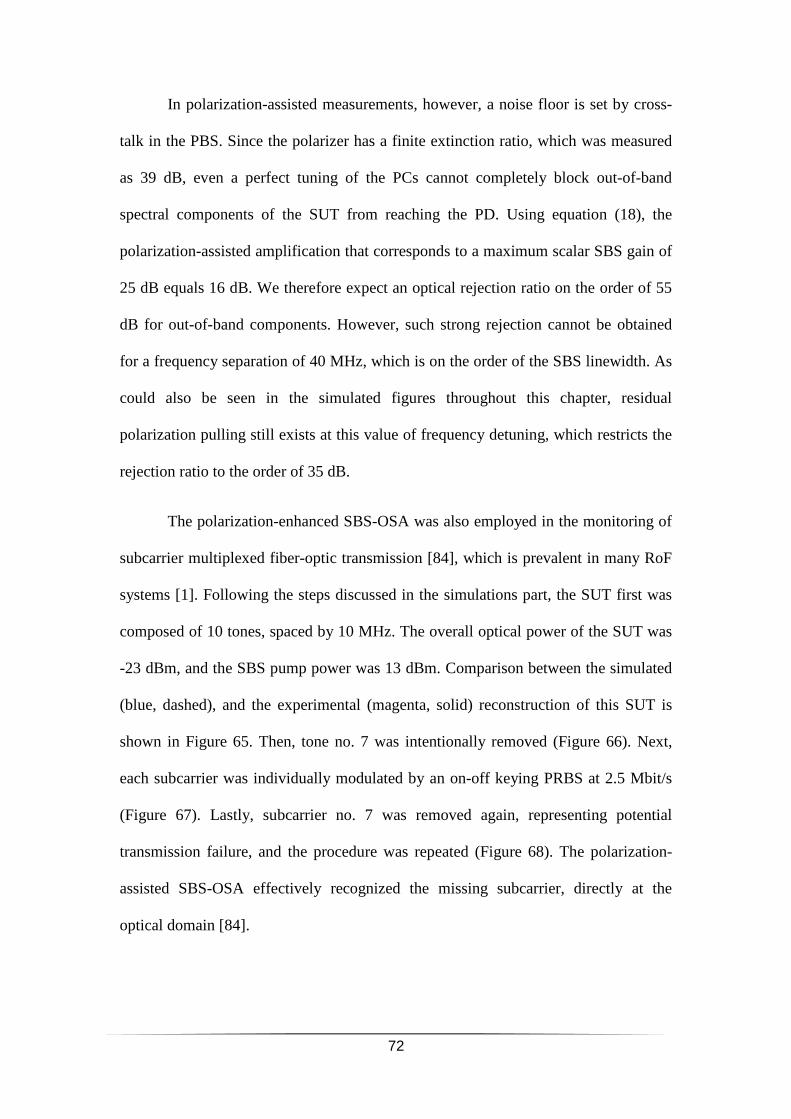
72

In polarization-assisted measurements, however, a noise floor is set by cross-

talk in the PBS. Since the polarizer has a finite extinction ratio, which was measured

as 39 dB, even a perfect tuning of the PCs cannot completely block out-of-band

spectral components of the SUT from reaching the PD. Using equation (18), the

polarization-assisted amplification that corresponds to a maximum scalar SBS gain of

25 dB equals 16 dB. We therefore expect an optical rejection ratio on the order of 55

dB for out-of-band components. However, such strong rejection cannot be obtained

for a frequency separation of 40 MHz, which is on the order of the SBS linewidth. As

could also be seen in the simulated figures throughout this chapter, residual

polarization pulling still exists at this value of frequency detuning, which restricts the

rejection ratio to the order of 35 dB.

The polarization-enhanced SBS-OSA was also employed in the monitoring of

subcarrier multiplexed fiber-optic transmission [84], which is prevalent in many RoF

systems [1]. Following the steps discussed in the simulations part, the SUT first was

composed of 10 tones, spaced by 10 MHz. The overall optical power of the SUT was

-23 dBm, and the SBS pump power was 13 dBm. Comparison between the simulated

(blue, dashed), and the experimental (magenta, solid) reconstruction of this SUT is

shown in Figure 65. Then, tone no. 7 was intentionally removed (Figure 66). Next,

each subcarrier was individually modulated by an on-off keying PRBS at 2.5 Mbit/s

(Figure 67). Lastly, subcarrier no. 7 was removed again, representing potential

transmission failure, and the procedure was repeated (Figure 68). The polarization-

assisted SBS-OSA effectively recognized the missing subcarrier, directly at the

optical domain [84].

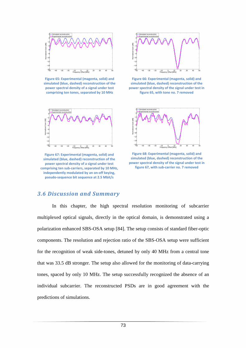
73

3.6 Discussion and Summary

In this chapter, the high spectral resolution monitoring of subcarrier

multiplexed optical signals, directly in the optical domain, is demonstrated using a

polarization enhanced SBS-OSA setup [84]. The setup consists of standard fiber-optic

components. The resolution and rejection ratio of the SBS-OSA setup were sufficient

for the recognition of weak side-tones, detuned by only 40 MHz from a central tone

that was 33.5 dB stronger. The setup also allowed for the monitoring of data-carrying

tones, spaced by only 10 MHz. The setup successfully recognized the absence of an

individual subcarrier. The reconstructed PSDs are in good agreement with the

predictions of simulations.

−50 −40 −30 −20 −10 0 10 20 30 40 50−16

−14

−12

−10

−8

−6

−4

−2

0

2


No

rma

lize

d G

ain

[d

B]

Simulated reconstructionExperimental reconstruction

Figure 65: Experimental (magenta, solid) and

simulated (blue, dashed) reconstruction of the


comprising ten tones, separated by 10 MHz

−50 −40 −30 −20 −10 0 10 20 30 40 50−16

−14

−12

−10

−8

−6

−4

−2

0

2


No

rma

lize

d G

ain

[d

B]




power spectral density of the signal under test in

figure 65, with tone no. 7 removed

−50 −40 −30 −20 −10 0 10 20 30 40 50−16

−14

−12

−10

−8

−6

−4

−2

0

2


No

rma

lize

d G

ain

[d

B]





comprising ten sub-carriers, separated by 10 MHz,

independently modulated by an on-off keying,

pseudo-sequence bit sequence at 2.5 Mbit/s

−50 −40 −30 −20 −10 0 10 20 30 40 50−16

−14

−12

−10

−8

−6

−4

−2

0

2


No

rma

lize

d G

ain

[d

B]




power spectral density of the signal under test in

figure 67, with sub-carrier no. 7 removed

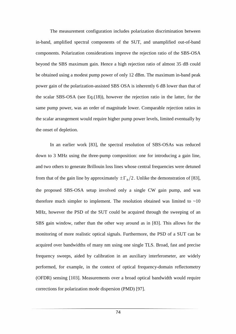
74

The measurement configuration includes polarization discrimination between

in-band, amplified spectral components of the SUT, and unamplified out-of-band

components. Polarization considerations improve the rejection ratio of the SBS-OSA

beyond the SBS maximum gain. Hence a high rejection ratio of almost 35 dB could

be obtained using a modest pump power of only 12 dBm. The maximum in-band peak

power gain of the polarization-assisted SBS OSA is inherently 6 dB lower than that of

the scalar SBS-OSA (see Eq.(18)), however the rejection ratio in the latter, for the

same pump power, was an order of magnitude lower. Comparable rejection ratios in

the scalar arrangement would require higher pump power levels, limited eventually by

the onset of depletion.

In an earlier work [83], the spectral resolution of SBS-OSAs was reduced

down to 3 MHz using the three-pump composition: one for introducing a gain line,

and two others to generate Brillouin loss lines whose central frequencies were detuned

from that of the gain line by approximately 2B±Γ . Unlike the demonstration of [83],

the proposed SBS-OSA setup involved only a single CW gain pump, and was

therefore much simpler to implement. The resolution obtained was limited to ~10

MHz, however the PSD of the SUT could be acquired through the sweeping of an

SBS gain window, rather than the other way around as in [83]. This allows for the

monitoring of more realistic optical signals. Furthermore, the PSD of a SUT can be

acquired over bandwidths of many nm using one single TLS. Broad, fast and precise

frequency sweeps, aided by calibration in an auxiliary interferometer, are widely

performed, for example, in the context of optical frequency-domain reflectometry

(OFDR) sensing [103]. Measurements over a broad optical bandwidth would require

corrections for polarization mode dispersion (PMD) [97].

75

In conclusion, SBS-OSA measurements could be highly instrumental in the

analysis and monitoring of advanced analog and digital optical transmission formats

[84]. Ongoing research is dedicated to a modification of the three-pump setup of [83],

so that the three lines could be scanned together across the spectral extent of an SUT

and provide an SBS-OSA resolution of 3 MHz.

76

Sharp,TunableMicrowave

PhotonicBandpassFiltersBasedon

Polarization-EnhancedStimulated

BrillouinScattering


As mentioned earlier, most delay-and-sum MWP filters are restricted to an

incoherent summation of intensities, and their finite impulse response is therefore

limited to real-valued, positive coefficients [3, 10]. Although several configurations

successfully implement filters with negative and complex coefficients [11, 14, 15,

104, 105], the realization of sharp MWP band-pass filters using delay-and-sum

architectures requires a large number of paths and remains challenging. In addition,

the frequency response of delay-and-sum filters is inherently periodic, with multiple

passbands. The realization of filters with only a single pass-band would be

advantageous in RoF receivers as well as in many other applications.

Alternatively, several MWP systems rely on nonlinear optical propagation

effects such as SBS. SBS amplification is simply implemented in standard fibers, has

the lowest power threshold of all optical nonlinear mechanisms in standard silica

fibers [49] and is highly frequency selective: its gain bandwidth is on the order of 30

MHz only [46]. Due to these attributes, SBS is an attractive platform for all-optical

signal processing applications, including optical [50] and microwave-photonic [11]

filtering.

In MWP filters based on SBS, the input RF signal modulates an optical

carrier, which propagates along an optical fiber and serves as a SBS probe wave. A

77

second, counter-propagating optical carrier is modulated by another RF waveform

which replicates the desired filter shape, and serves as a SBS pump wave with a

broadened spectrum. The latter generates a SBS gain window, which overlaps part of

one RF modulated sideband of the probe. A modified RF waveform is recovered by

interference of the filtered probe sideband with its optical carrier on a broadband PD.

The obtained RF bandpass filters are characterized by uniform transmission windows,

strong out-of-band rejection and reconfigurable bandwidths and central transmission

frequencies. Their frequency response is inherently aperiodic.

Herein, I present a significant enhancement to the performance of such filters.

In a similar manner to the operation of the SBS-OSA described in the previous

chapter, the out-of-band rejection of the MWP filters is enhanced based on the

polarization attributes of SBS in standard, weakly birefringent fibers [94, 95]. The

method was previously implemented in the realization of sharp and tunable optical

band-pass filters [100], and is employed here in MWP filters for the first time. In that

previous research [100], the pump wave was broadened using a directly-modulated

distributed-feedback (DFB) laser source [50], whereas the present experiment uses an

external modulation. Using this approach, the reconfigurability and tunability of the

obtained bandpass filters is extended even further.

4.2 Principle of Operation

As mentioned in the introduction chapter, when a pump wave is modulated to

obtain a broadened PSD, the Brillouin gain line ( )sigg ω is given by a convolution of

the pump PSD with the Lorenzian SBS line shape (see Eqs. (3)-(4))

Careful synthesis of the pump modulation could provide a uniform PSD

within a broadened bandwidth of interest, up to several GHz [46]. Based on this

78

principle, a broadened SBS gain line was used to demonstrate GHz-wide flexible

MWP [50] and optical bandpass filters [100]. In both [50] and [100], the broadening

of the pump spectrum was based on a carefully synthesized direct modulation of the

pump-laser injection current. Control over the injection current allows for the tuning

of the bandwidth and central frequency of the obtained pump spectrum. However,

spectral synthesis through direct modulation is an intricate process, which combines

carrier-dependent and thermal changes to the refractive index together with amplitude

modulation.

A more straight-forward approach towards the synthesis of broadened pump

spectra involves the generation of the desired broadband shape in the RF domain first,

followed by the external modulation of this shape onto an optical carrier. In using a

SC-SSB modulation format, only one sideband is retained, which replicates the

original RF spectrum and serves as the SBS broadened pump. Unlike the direct

modulation used in [50] and [100], external modulation-based synthesis provides

simple control over the pump spectral shape, central frequency and bandwidth in a

very intuitive manner, using programmable RF signal generators, filters and

amplifiers. In this work, a LFM waveform was chosen to serve as the RF-shape that is

driving the external pump modulation. LFM waveforms are easy to generate [41] and

their PSDs are uniform. Consequently, broadened SBS pumps with uniform PSDs can

be obtained.

The rejection ratios of the MWP bandpass filters proposed and demonstrated

in this chapter are enhanced using the polarization-assisted SBS process, which was

discussed in length in the previous chapter. Since a MWP scheme requires an optical-

to-electrical (O/E) conversion, a beating of the amplified output probe and an optical

79

carrier upon detection is necessary for the reconstruction of the filtered RF waveforms

(see following section for a detailed description of the filter configuration). This

beating is fundamentally polarization dependent. It can therefore replace the polarizer

at the probe output end, which provided the polarization-enhancement in the SBS-

OSA setup (see Figure 53). Through careful polarization alignment, the polarization

of unamplified, out-of-band spectral components can be made orthogonal to that of

the optical carrier, and the lack of interference between the two blocks out out-of-

band spectral components and improves the rejection ratio of the filter. Moreover,

interference can provide, at least in principle, an infinite rejection ratio, whereas PBS-

based blocking suffers from residual polarization cross-talk.

Since SBS is an active amplification process, it is accompanied by generation

of noise due to amplified spontaneous emission (SBS-ASE). When no probe wave is

provided, a SBS process could still be initiated from background hyper-sonic

vibrations that naturally exist in the fiber. The overall noise power associated with

SBS-ASE is calculated by integrating the noise PSD over the entire SBS gain

linewidth, and can be approximated by [46]:

(19) ( )2

maxASE n sigP h F G Bν ω= ⋅ ⋅ ⋅ ,

where [ ]Jhν is the energy of a photon at an optical frequency [ ]Hzν (equals

191.28 10 J−⋅ for a wavelength of 1550 nm), nF is the noise figure of SBS

amplification (typically on the order of 150 [106]), and B is the bandwidth of the

broadened pump.

SBS-ASE noise degrades the signal-to-noise ratio (SNR) of filtered signals:

the ratio between the output RF power of amplified, in-band signals to the output RF

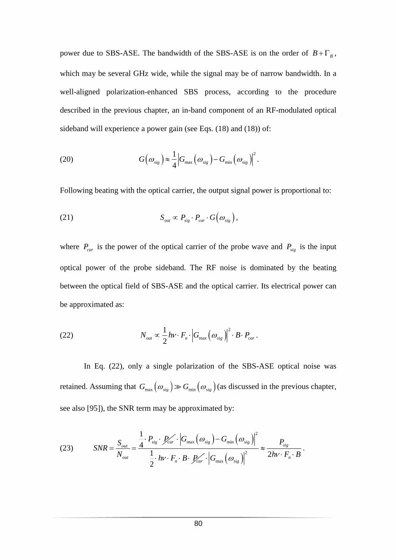
80

power due to SBS-ASE. The bandwidth of the SBS-ASE is on the order of BB+Γ ,

which may be several GHz wide, while the signal may be of narrow bandwidth. In a

well-aligned polarization-enhanced SBS process, according to the procedure

described in the previous chapter, an in-band component of an RF-modulated optical

sideband will experience a power gain (see Eqs. (18) and (18)) of:

(20) ( ) ( ) ( )2

max min

1

4sig sig sigG G Gω ω ω≈ − .

Following beating with the optical carrier, the output signal power is proportional to:

(21) ( )out sig car sigS P P Gω∝ ⋅ ⋅ ,

where carP is the power of the optical carrier of the probe wave and sigP is the input

optical power of the probe sideband. The RF noise is dominated by the beating

between the optical field of SBS-ASE and the optical carrier. Its electrical power can

be approximated as:

(22) ( )2

max

1

2out n sig carN h F G B Pν ω∝ ⋅ ⋅ ⋅ ⋅ .

In Eq. (22), only a single polarization of the SBS-ASE optical noise was

retained. Assuming that ( ) ( )max minsig sigG Gω ω≫ (as discussed in the previous chapter,

see also [95]), the SNR term may be approximated by:

(23)

14 sig car

out

out

P PSSNR

N

⋅ ⋅= =

( ) ( )2

max min

12

sig sig

n car

G G

h F B P

ω ω

ν

⋅ −

⋅ ⋅ ⋅ ⋅ ( )2

max2

sig

nsig

P

h F BG νω≈

⋅ ⋅⋅.

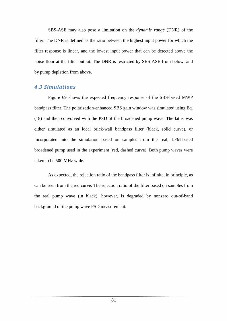
81

SBS-ASE may also pose a limitation on the dynamic range (DNR) of the

filter. The DNR is defined as the ratio between the highest input power for which the

filter response is linear, and the lowest input power that can be detected above the

noise floor at the filter output. The DNR is restricted by SBS-ASE from below, and

by pump depletion from above.

4.3 Simulations

Figure 69 shows the expected frequency response of the SBS-based MWP

bandpass filter. The polarization-enhanced SBS gain window was simulated using Eq.

(18) and then convolved with the PSD of the broadened pump wave. The latter was

either simulated as an ideal brick-wall bandpass filter (black, solid curve), or

incorporated into the simulation based on samples from the real, LFM-based

broadened pump used in the experiment (red, dashed curve). Both pump waves were

taken to be 500 MHz wide.

As expected, the rejection ratio of the bandpass filter is infinite, in principle, as

can be seen from the red curve. The rejection ratio of the filter based on samples from

the real pump wave (in black), however, is degraded by nonzero out-of-band

background of the pump wave PSD measurement.

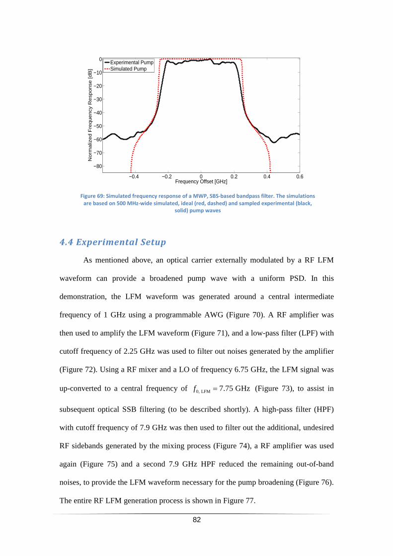
82


As mentioned above, an optical carrier externally modulated by a RF LFM

waveform can provide a broadened pump wave with a uniform PSD. In this

demonstration, the LFM waveform was generated around a central intermediate

frequency of 1 GHz using a programmable AWG (Figure 70). A RF amplifier was

then used to amplify the LFM waveform (Figure 71), and a low-pass filter (LPF) with

cutoff frequency of 2.25 GHz was used to filter out noises generated by the amplifier

(Figure 72). Using a RF mixer and a LO of frequency 6.75 GHz, the LFM signal was

up-converted to a central frequency of 0, LFM 7.75 GHzf = (Figure 73), to assist in

subsequent optical SSB filtering (to be described shortly). A high-pass filter (HPF)

with cutoff frequency of 7.9 GHz was then used to filter out the additional, undesired

RF sidebands generated by the mixing process (Figure 74), a RF amplifier was used

again (Figure 75) and a second 7.9 GHz HPF reduced the remaining out-of-band

noises, to provide the LFM waveform necessary for the pump broadening (Figure 76).

The entire RF LFM generation process is shown in Figure 77.

−0.4 −0.2 0 0.2 0.4 0.6

−80

−70

−60

−50

−40

−30

−20

−10

0

Frequency Offset [GHz]

No

rma

lize

d F

req

ue

ncy

Re

spo

nse

[d

B]

Experimental PumpSimulated Pump

Figure 69: Simulated frequency response of a MWP, SBS-based bandpass filter. The simulations

are based on 500 MHz-wide simulated, ideal (red, dashed) and sampled experimental (black,

solid) pump waves

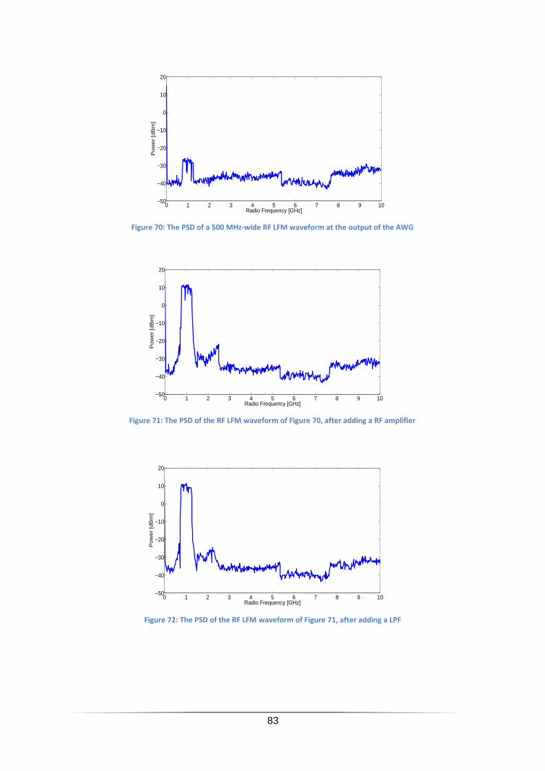
83

0 1 2 3 4 5 6 7 8 9 10−50

−40

−30

−20

−10

0

10

20


Po

we

r [d

Bm

]

Figure 70: The PSD of a 500 MHz-wide RF LFM waveform at the output of the AWG

0 1 2 3 4 5 6 7 8 9 10−50

−40

−30

−20

−10

0

10

20


Po

we

r [d

Bm

]

Figure 71: The PSD of the RF LFM waveform of Figure 70, after adding a RF amplifier

0 1 2 3 4 5 6 7 8 9 10−50

−40

−30

−20

−10

0

10

20


Po

we

r [d

Bm

]

Figure 72: The PSD of the RF LFM waveform of Figure 71, after adding a LPF

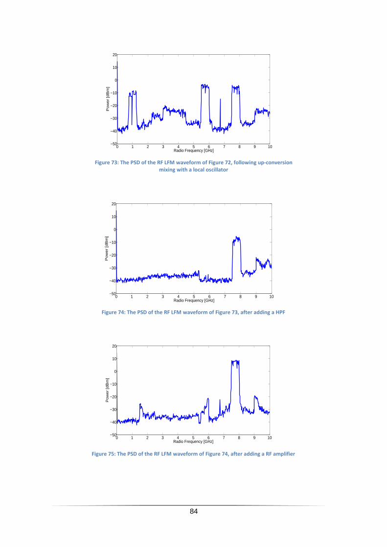
84

0 1 2 3 4 5 6 7 8 9 10−50

−40

−30

−20

−10

0

10

20


Po

we

r [d

Bm

]

Figure 73: The PSD of the RF LFM waveform of Figure 72, following up-conversion

mixing with a local oscillator

0 1 2 3 4 5 6 7 8 9 10−50

−40

−30

−20

−10

0

10

20


Po

we

r [d

Bm

]

Figure 74: The PSD of the RF LFM waveform of Figure 73, after adding a HPF

0 1 2 3 4 5 6 7 8 9 10−50

−40

−30

−20

−10

0

10

20


Po

we

r [d

Bm

]

Figure 75: The PSD of the RF LFM waveform of Figure 74, after adding a RF amplifier

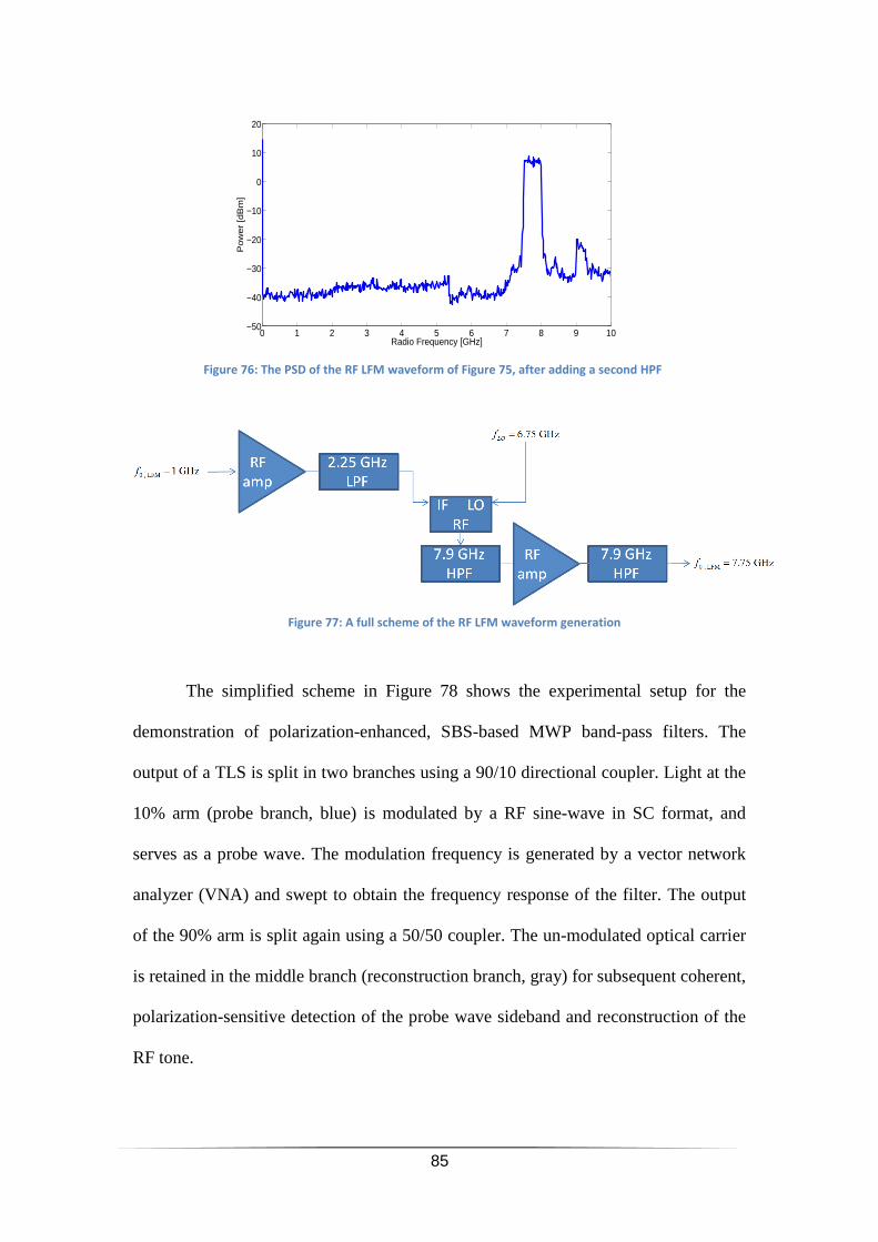
85

The simplified scheme in Figure 78 shows the experimental setup for the

demonstration of polarization-enhanced, SBS-based MWP band-pass filters. The

output of a TLS is split in two branches using a 90/10 directional coupler. Light at the

10% arm (probe branch, blue) is modulated by a RF sine-wave in SC format, and

serves as a probe wave. The modulation frequency is generated by a vector network

analyzer (VNA) and swept to obtain the frequency response of the filter. The output

of the 90% arm is split again using a 50/50 coupler. The un-modulated optical carrier

is retained in the middle branch (reconstruction branch, gray) for subsequent coherent,

polarization-sensitive detection of the probe wave sideband and reconstruction of the

RF tone.

0 1 2 3 4 5 6 7 8 9 10−50

−40

−30

−20

−10

0

10

20


Po

we

r [d

Bm

]

Figure 76: The PSD of the RF LFM waveform of Figure 75, after adding a second HPF

Figure 77: A full scheme of the RF LFM waveform generation

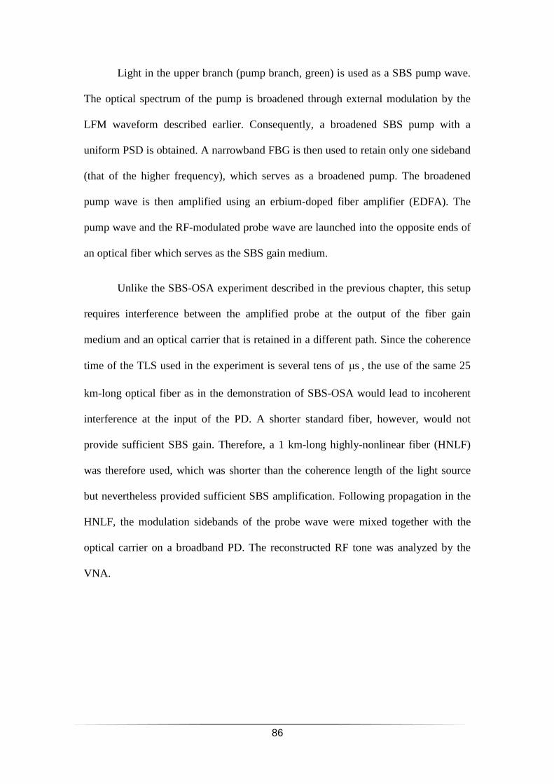
86

Light in the upper branch (pump branch, green) is used as a SBS pump wave.

The optical spectrum of the pump is broadened through external modulation by the

LFM waveform described earlier. Consequently, a broadened SBS pump with a

uniform PSD is obtained. A narrowband FBG is then used to retain only one sideband

(that of the higher frequency), which serves as a broadened pump. The broadened

pump wave is then amplified using an erbium-doped fiber amplifier (EDFA). The

pump wave and the RF-modulated probe wave are launched into the opposite ends of

an optical fiber which serves as the SBS gain medium.

Unlike the SBS-OSA experiment described in the previous chapter, this setup

requires interference between the amplified probe at the output of the fiber gain

medium and an optical carrier that is retained in a different path. Since the coherence

time of the TLS used in the experiment is several tens of µs , the use of the same 25

km-long optical fiber as in the demonstration of SBS-OSA would lead to incoherent

interference at the input of the PD. A shorter standard fiber, however, would not

provide sufficient SBS gain. Therefore, a 1 km-long highly-nonlinear fiber (HNLF)

was therefore used, which was shorter than the coherence length of the light source

but nevertheless provided sufficient SBS amplification. Following propagation in the

HNLF, the modulation sidebands of the probe wave were mixed together with the

optical carrier on a broadband PD. The reconstructed RF tone was analyzed by the

VNA.

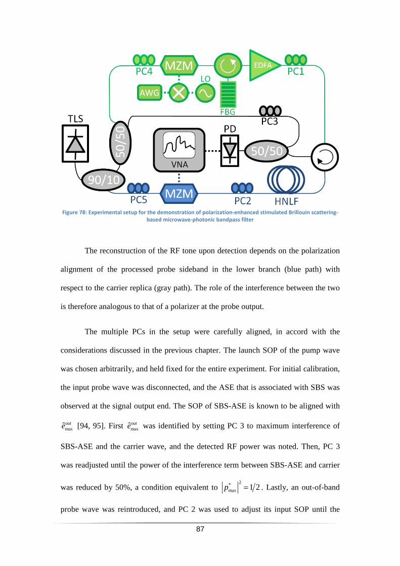
87

The reconstruction of the RF tone upon detection depends on the polarization

alignment of the processed probe sideband in the lower branch (blue path) with

respect to the carrier replica (gray path). The role of the interference between the two

is therefore analogous to that of a polarizer at the probe output.

The multiple PCs in the setup were carefully aligned, in accord with the

considerations discussed in the previous chapter. The launch SOP of the pump wave

was chosen arbitrarily, and held fixed for the entire experiment. For initial calibration,

the input probe wave was disconnected, and the ASE that is associated with SBS was

observed at the signal output end. The SOP of SBS-ASE is known to be aligned with

maxôute [94, 95]. First maxôute was identified by setting PC 3 to maximum interference of

SBS-ASE and the carrier wave, and the detected RF power was noted. Then, PC 3

was readjusted until the power of the interference term between SBS-ASE and carrier

was reduced by 50%, a condition equivalent to 2*

max 1 2p = . Lastly, an out-of-band

probe wave was reintroduced, and PC 2 was used to adjust its input SOP until the

Figure 78: Experimental setup for the demonstration of polarization-enhanced stimulated Brillouin scattering-

based microwave-photonic bandpass filter

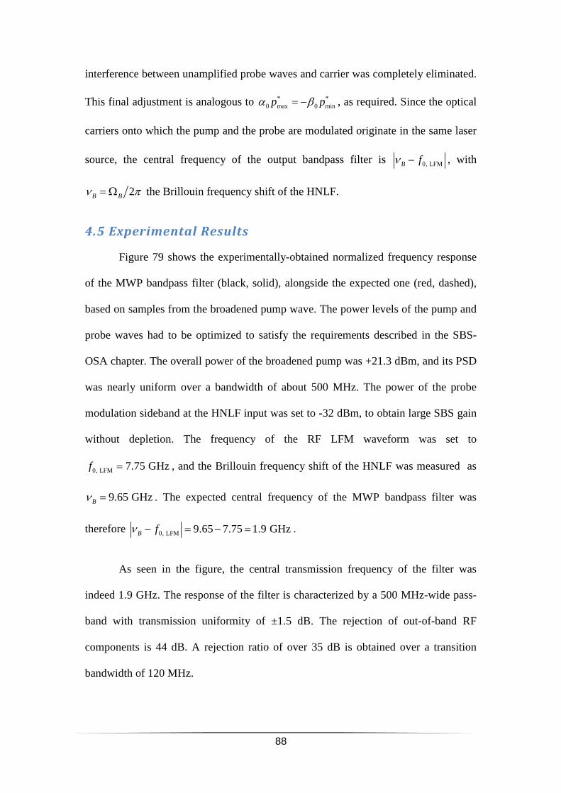
88

interference between unamplified probe waves and carrier was completely eliminated.

This final adjustment is analogous to * *0 max 0 minp pα β= − , as required. Since the optical

carriers onto which the pump and the probe are modulated originate in the same laser

source, the central frequency of the output bandpass filter is 0, LFMB fν − , with

2B Bν π= Ω the Brillouin frequency shift of the HNLF.

4.5 Experimental Results

Figure 79 shows the experimentally-obtained normalized frequency response

of the MWP bandpass filter (black, solid), alongside the expected one (red, dashed),

based on samples from the broadened pump wave. The power levels of the pump and

probe waves had to be optimized to satisfy the requirements described in the SBS-

OSA chapter. The overall power of the broadened pump was +21.3 dBm, and its PSD

was nearly uniform over a bandwidth of about 500 MHz. The power of the probe

modulation sideband at the HNLF input was set to -32 dBm, to obtain large SBS gain

without depletion. The frequency of the RF LFM waveform was set to

0, LFM 7.75 GHzf = , and the Brillouin frequency shift of the HNLF was measured as

9.65 GHzBν = . The expected central frequency of the MWP bandpass filter was

therefore 0, LFM 9.65 7.75 1.9 GHzB fν − = − = .

As seen in the figure, the central transmission frequency of the filter was

indeed 1.9 GHz. The response of the filter is characterized by a 500 MHz-wide pass-

band with transmission uniformity of ±1.5 dB. The rejection of out-of-band RF

components is 44 dB. A rejection ratio of over 35 dB is obtained over a transition

bandwidth of 120 MHz.

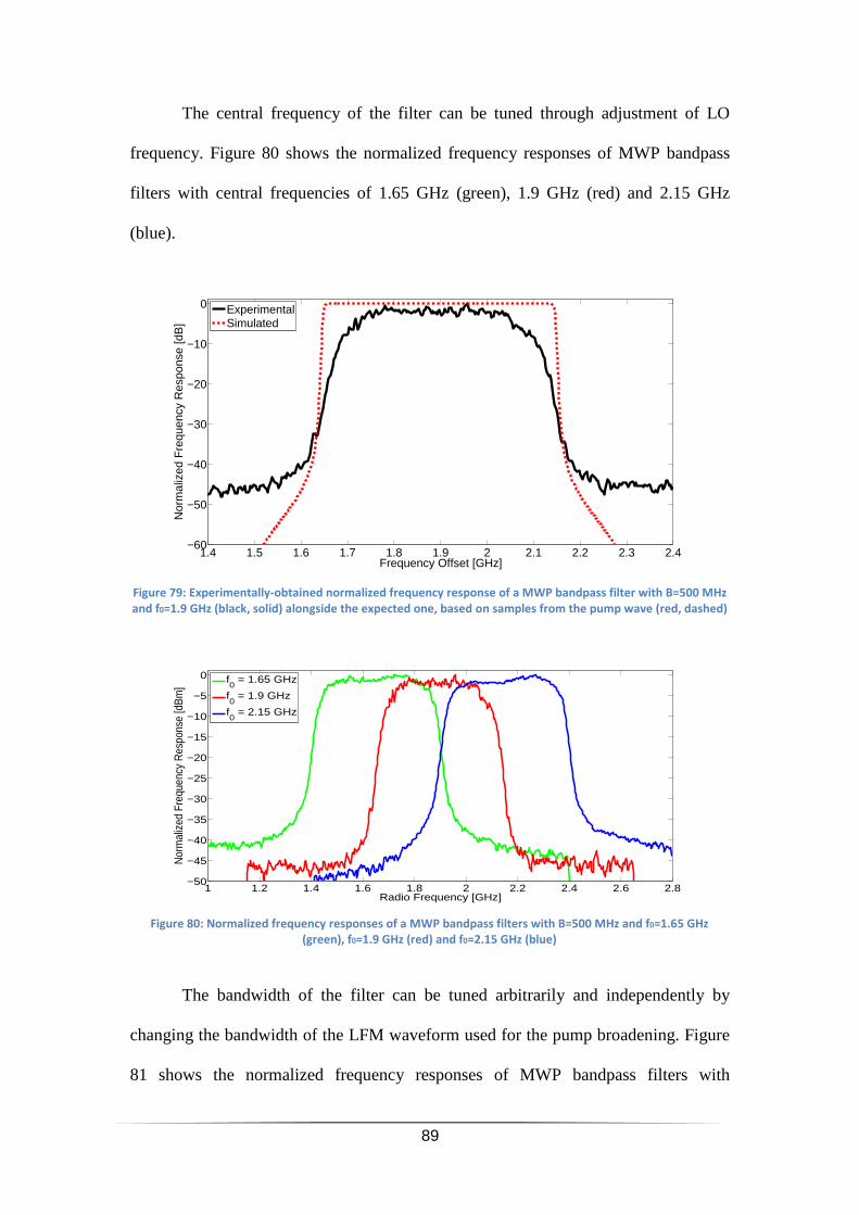
89

The central frequency of the filter can be tuned through adjustment of LO

frequency. Figure 80 shows the normalized frequency responses of MWP bandpass

filters with central frequencies of 1.65 GHz (green), 1.9 GHz (red) and 2.15 GHz

(blue).

The bandwidth of the filter can be tuned arbitrarily and independently by

changing the bandwidth of the LFM waveform used for the pump broadening. Figure

81 shows the normalized frequency responses of MWP bandpass filters with

1.4 1.5 1.6 1.7 1.8 1.9 2 2.1 2.2 2.3 2.4−60

−50

−40

−30

−20

−10

0

Frequency Offset [GHz]

Nor

mal

ized

Fre

quen

cy R

espo

nse

[dB

]

ExperimentalSimulated

Figure 79: Experimentally-obtained normalized frequency response of a MWP bandpass filter with B=500 MHz

and f0=1.9 GHz (black, solid) alongside the expected one, based on samples from the pump wave (red, dashed)

1 1.2 1.4 1.6 1.8 2 2.2 2.4 2.6 2.8−50

−45

−40

−35

−30

−25

−20

−15

−10

−5

0


Nor

mal

ized

Fre

quen

cy R

espo

nse

[dBm

]

f0 = 1.65 GHz

f0 = 1.9 GHz

f0 = 2.15 GHz

Figure 80: Normalized frequency responses of a MWP bandpass filters with B=500 MHz and f0=1.65 GHz

(green), f0=1.9 GHz (red) and f0=2.15 GHz (blue)

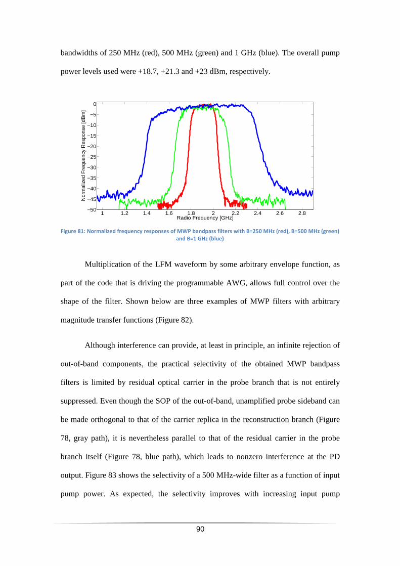
90

bandwidths of 250 MHz (red), 500 MHz (green) and 1 GHz (blue). The overall pump

power levels used were +18.7, +21.3 and +23 dBm, respectively.

Multiplication of the LFM waveform by some arbitrary envelope function, as

part of the code that is driving the programmable AWG, allows full control over the

shape of the filter. Shown below are three examples of MWP filters with arbitrary

magnitude transfer functions (Figure 82).

Although interference can provide, at least in principle, an infinite rejection of

out-of-band components, the practical selectivity of the obtained MWP bandpass

filters is limited by residual optical carrier in the probe branch that is not entirely

suppressed. Even though the SOP of the out-of-band, unamplified probe sideband can

be made orthogonal to that of the carrier replica in the reconstruction branch (Figure

78, gray path), it is nevertheless parallel to that of the residual carrier in the probe

branch itself (Figure 78, blue path), which leads to nonzero interference at the PD

output. Figure 83 shows the selectivity of a 500 MHz-wide filter as a function of input

pump power. As expected, the selectivity improves with increasing input pump

1 1.2 1.4 1.6 1.8 2 2.2 2.4 2.6 2.8−50

−45

−40

−35

−30

−25

−20

−15

−10

−5

0


Nor

mal

ized

Fre

quen

cy R

espo

nse

[dB

m]

Figure 81: Normalized frequency responses of MWP bandpass filters with B=250 MHz (red), B=500 MHz (green)

and B=1 GHz (blue)

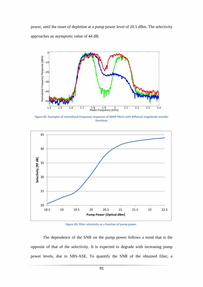
91

power, until the onset of depletion at a pump power level of 20.5 dBm. The selectivity

approaches an asymptotic value of 44 dB.

The dependence of the SNR on the pump power follows a trend that is the

opposite of that of the selectivity. It is expected to degrade with increasing pump

power levels, due to SBS-ASE. To quantify the SNR of the obtained filter, a

1.4 1.5 1.6 1.7 1.8 1.9 2 2.1 2.2 2.3 2.4

−50

−40

−30

−20

−10

0


Nor

mal

ized

Fre

quen

cy R

espo

nse

[dB

m]

Figure 82: Examples of normalized frequency responses of MWP filters with different magnitude transfer

functions

20

25

30

35

40

45

18.5 19 19.5 20 20.5 21 21.5 22 22.5

Se

lect

ivit

y [

RF

dB

]

Pump Power [Optical dBm]

Figure 83: Filter selectivity as a function of pump power

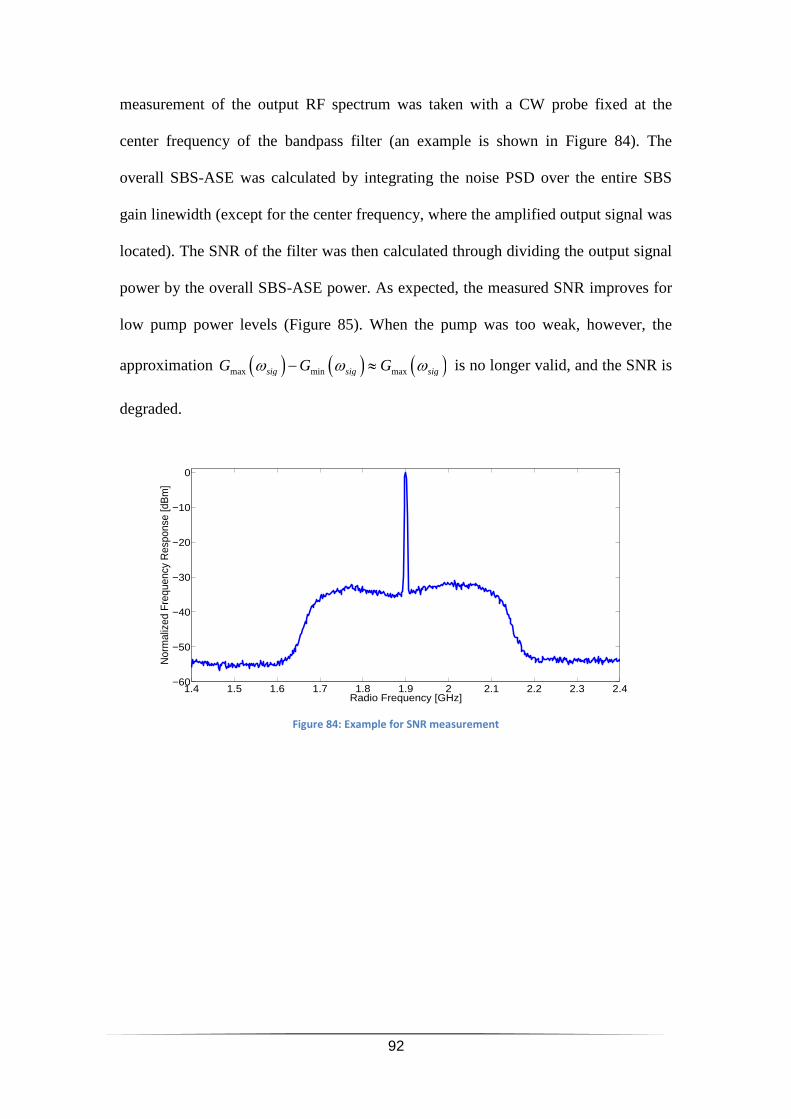
92

measurement of the output RF spectrum was taken with a CW probe fixed at the

center frequency of the bandpass filter (an example is shown in Figure 84). The

overall SBS-ASE was calculated by integrating the noise PSD over the entire SBS

gain linewidth (except for the center frequency, where the amplified output signal was

located). The SNR of the filter was then calculated through dividing the output signal

power by the overall SBS-ASE power. As expected, the measured SNR improves for

low pump power levels (Figure 85). When the pump was too weak, however, the

approximation ( ) ( ) ( )max min maxsig sig sigG G Gω ω ω− ≈ is no longer valid, and the SNR is

degraded.

1.4 1.5 1.6 1.7 1.8 1.9 2 2.1 2.2 2.3 2.4−60

−50

−40

−30

−20

−10

0


Nor

mal

ized

Fre

quen

cy R

espo

nse

[dB

m]

Figure 84: Example for SNR measurement

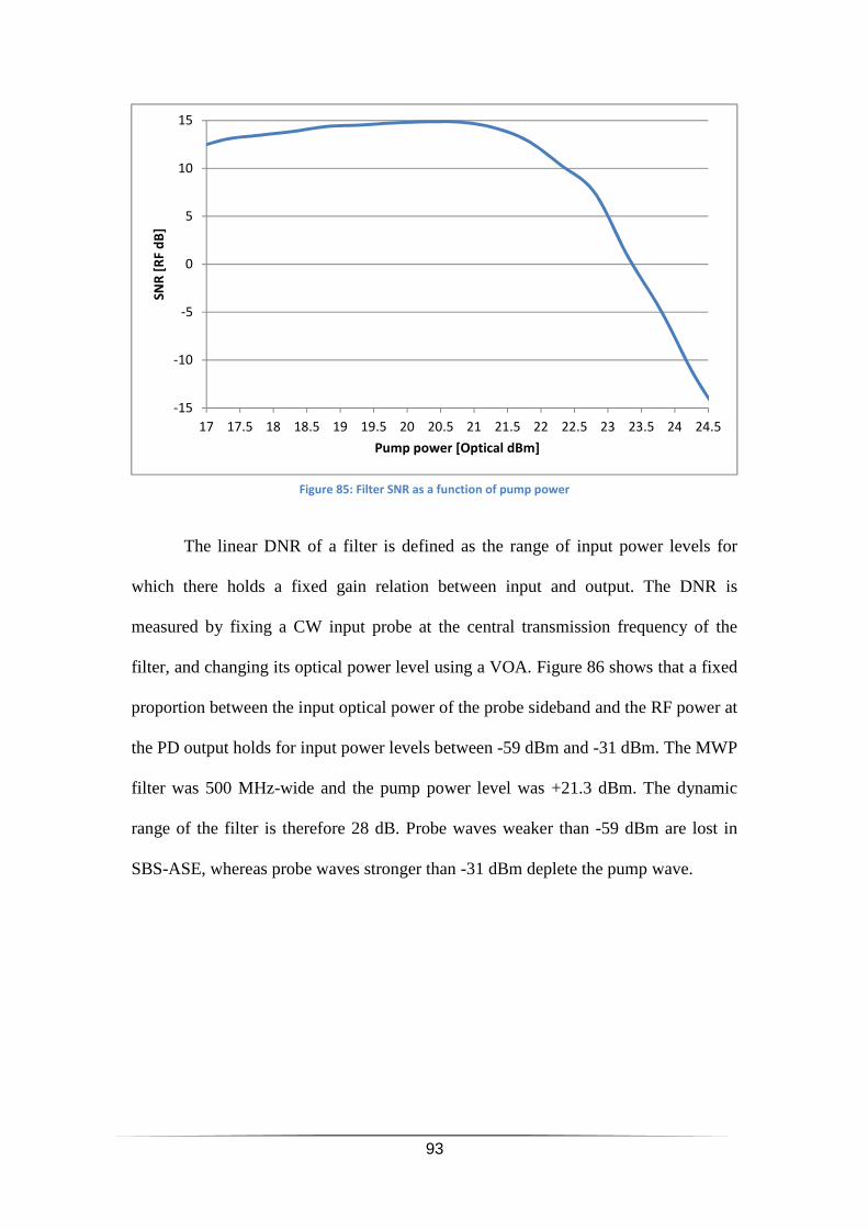
93

The linear DNR of a filter is defined as the range of input power levels for

which there holds a fixed gain relation between input and output. The DNR is

measured by fixing a CW input probe at the central transmission frequency of the

filter, and changing its optical power level using a VOA. Figure 86 shows that a fixed

proportion between the input optical power of the probe sideband and the RF power at

the PD output holds for input power levels between -59 dBm and -31 dBm. The MWP

filter was 500 MHz-wide and the pump power level was +21.3 dBm. The dynamic

range of the filter is therefore 28 dB. Probe waves weaker than -59 dBm are lost in

SBS-ASE, whereas probe waves stronger than -31 dBm deplete the pump wave.

-15

-10

-5

0

5

10

15

17 17.5 18 18.5 19 19.5 20 20.5 21 21.5 22 22.5 23 23.5 24 24.5

SN

R [

RF

dB

]

Pump power [Optical dBm]

Figure 85: Filter SNR as a function of pump power

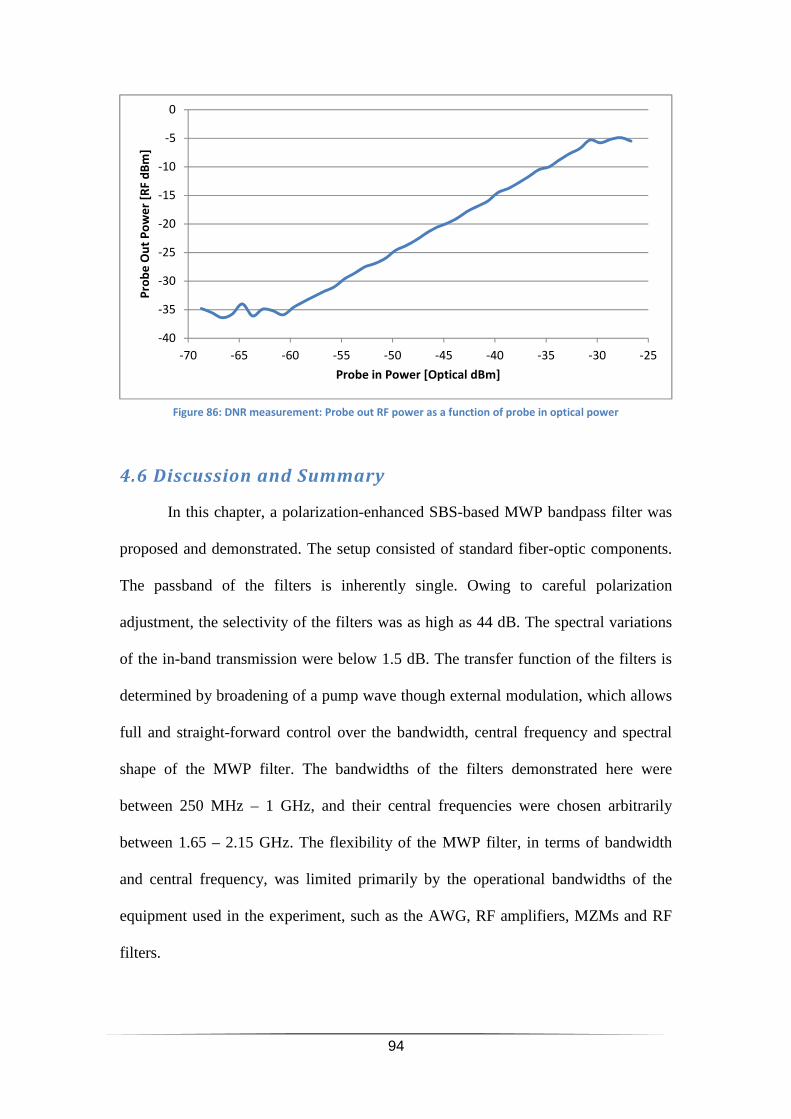
94

4.6 Discussion and Summary

In this chapter, a polarization-enhanced SBS-based MWP bandpass filter was

proposed and demonstrated. The setup consisted of standard fiber-optic components.

The passband of the filters is inherently single. Owing to careful polarization

adjustment, the selectivity of the filters was as high as 44 dB. The spectral variations

of the in-band transmission were below 1.5 dB. The transfer function of the filters is

determined by broadening of a pump wave though external modulation, which allows

full and straight-forward control over the bandwidth, central frequency and spectral

shape of the MWP filter. The bandwidths of the filters demonstrated here were

between 250 MHz – 1 GHz, and their central frequencies were chosen arbitrarily

between 1.65 – 2.15 GHz. The flexibility of the MWP filter, in terms of bandwidth

and central frequency, was limited primarily by the operational bandwidths of the

equipment used in the experiment, such as the AWG, RF amplifiers, MZMs and RF

filters.

-40

-35

-30

-25

-20

-15

-10

-5

0

-70 -65 -60 -55 -50 -45 -40 -35 -30 -25

Pro

be

Ou

t P

ow

er

[RF

dB

m]

Probe in Power [Optical dBm]

Figure 86: DNR measurement: Probe out RF power as a function of probe in optical power

95

Since the method relies on SBS, which is an active amplification process, the

performance of the obtained bandpass filters is degraded by SBS-ASE. The expected

SNR of filtered RF waveforms can be estimated based on Eq. (23). For a bandwidth

of 500 MHz, and input probe optical power of -32 dB, the expected SNR is 15 dB.

For the same values of bandwidth and input probe power, the SNR measured in the

experiment was 14.2 dB, which is in good agreement with the theoretical predictions.

As seen in the experimental data, higher input power of the probe wave would exceed

the linear dynamic range of the filter, and use of a stronger pump would degrade the

SNR. Therefore, the value of 15 dB represents an upper limit to the attainable SNR

for the particular bandwidth.

The selectivity of the filter can be expressed as the sum of the SBS in-band

gain and the out-of-band rejection. As discussed earlier, the rejection of out-of-band

spectral components is limited by the presence of a residual carrier tone in the probe

sideband branch. The rejection ratio is equivalent to the power ratio between the

intended carrier in the reconstruction branch and the residual carrier in the probe

branch, divided by four. The factor of four stems from the fact that the out-of-band

signal is reconstructed from the equal contributions of two probe modulation

sidebands, whereas the in-band signal is dominated by a single amplified sideband.

The ratio between the two optical carriers was measured as 29 dB. The maximum

SBS power gain ( )2

max sigG ω was on the order of 30 dB. This value corresponds to

in-band amplification ( ) ( )2

1max min4 sig sigG Gω ω− of approximately 23 dB. Therefore,

the expected selectivity of the filter is on the order of 29 + 23 – 6 = 46 dB. The

measured selectivity of 44 dB is again in good agreement with predictions.

96

The linear DNR of the filter is restricted by SBS-ASE noise from below and

by pump depletion from above. Both limitations are inherent to SBS-based filters.

Note that the measured linear DNR only relates to one half of the MWP filter

operation: the conversion of an optical RF-modulated sideband back to a RF tone

following amplification and detection. In practice, distortions and deviations from

linearity may also take place in the initial modulation process. In particular, the

conversion of RF power to optical sideband power through the transfer function of an

electro-optic modulator is an inherently nonlinear process as well [107]. The

measured linear dynamic range of 28 dB is therefore an upper bound only. However,

modulator nonlinearities are common to all MWP filter architectures, whereas the

limitations due to SBS-ASE and depletion are specific to the proposed concept. In

addition, modulator nonlinearity can be avoided, at least in principle, by using

arbitrarily weak RF power levels at the input of the MWP setup and using optical

amplifiers at the probe branch instead [107].

A prediction for the DNR can be taken by estimating both the maximum

signal power that does not deplete the pump, and the SBS-ASE-related noise power

within the spectral linewidth of that signal. For a 500 MHz-wide filter, the pump

power that fell within the Brillouin linewidth in our experiments was on the order of

+8 dBm. Depletion begins when the power of the amplified output probe is roughly

10 dB below that of the pump. Assuming SBS gain of 30 dB, the maximum probe

power that is on the verge of depletion is -32 dBm. This value is in good agreement

with the observed upper end of the linear DNR, which was -31 dBm. Based on Eq.

(22), the SBS-ASE noise within the measurement bandwidth of 3 MHz corresponds to

an input power level of approximately -70 dBm. We could therefore expect a

97

somewhat larger DNR than the experimentally obtained range of 28 dB. The reasons

for this discrepancy will be investigated in future research.

A high power of the input probe would improve the SNR at the output of the

filter. On the other hand, a strong probe would lead to pump depletion, and hence

limited gain and limited selectivity. A tradeoff exists, therefore, between selectivity

and noise considerations. This tradeoff can be expressed, at least roughly, in terms of

a figure-of-merit which quantifies the quality of the filter, subject to available pump

power resources and required bandwidth. The product of SNR multiplied by

sensitivity is given by (SL denoting selectivity):

(24) ( )

2

max

2 16

sigsig

n

GPSNR SL

h F B x

ω

ν× ≈ ×

⋅ ⋅ ⋅,

where 1x≪ denotes the ratio between the optical power of the residual carrier

in the probe branch and that of the intended carrier in the reconstruction branch, and

large gain ( ) ( )max minsig sigG Gω ω≫ is assumed. Eq. (24) seems to suggest that the

performance of the filter can be improved with the use of a stronger input probe.

However, as mentioned above, the amplified probe power ( )2

maxsig sigP G ω is

restricted to a certain fraction 1D < of the pump power that falls within the Brillouin

linewidth. We may therefore substitute:

(25) 1 1

2 16pump B

n

PSNR SL D

h F B x Bν

Γ× ≈ × × =

⋅ ⋅ ⋅

2 232pump pumpB

n

P PDC

h F x B BνΓ⋅ ⋅

≜ ,

98

where pumpP is the overall pump power. This result suggests that the

performance of the filter degrades quadratically with its bandwidth, and that it is

restricted by the available pump power. Given the experimentally observed ratios of

~ 0.001x and ~ 0.1D , the constant C in Eq. (25) can be estimated as 5⋅1024, in

units of 2Hz W . The SNR times sensitivity figure of merit of a 500 MHz-wide

filter is expected to be 63 dB. The experimental value was 58 dB.

In summary, the sharp and highly-flexible MWP bandpass filters demonstrated

in this chapter could be very instrumental in all-optical signal processing in RoF

systems. Compared with previously reported filters, the performance of the filters was

enhanced considerably using the polarimetric attributes of SBS. Fundamental bounds

on SNR and selectivity were discussed as well.

99

Summary

Several MWP signal processing modules were proposed and demonstrated in

this work. First, ODLs that are specifically designed for chirped waveforms were

demonstrated, with large delay-bandwidth products. The method relied on the

deterministic relation between time and instantaneous phase that is inherent to these

waveforms. In the specific case of LFM waveforms, a significant improvement in the

ISLR was obtained by using a sine wave-driven AOM instead of a ramp wave-driven

phase modulator. Second, the polarimetric properties of SBS in standard fibers were

employed to improve rejection ratios in SBS-based filtering. Polarization-enhanced

SBS processes were used in the demonstration of SBS-based OSA with extended

resolution and rejection ratio, as well as in the realization of sharp and highly-flexible

MWP bandpass filters. In particular, the PSD of closely-spaced, subcarrier-

multiplexed transmission could be properly recovered directly in the optical domain,

and sharp, uniform and flexible bandpass filters were demonstrated. In all three

experiments, the obtained performance exceeds that of previously reported,

corresponding configurations.

The results achieved in these experiments were limited in several aspects of

system performance. Some of these limitations are fundamental and inherent to the

principles used. In the case of the ODL demonstration, for example, the maximum

achievable delay is restricted by the duration of the chirped pulse, as differences

between a phase-offset signal and a truly-delayed one increase with the length of

delay variations (see Figure 10). However, the equipment used in the experiment

restricted the attainable delay before these fundamental limitations could be reached.

In the SBS-OSA setup too, the resolution is inherently limited by the SBS gain

100

linewidth. The resolution can only be improved by a three-line synthesis, or by using

a very strong pump, for which polarization treatment is no longer beneficial. The

rejection ratio of the SBS-OSA is limited by the onset of polarization pulling at the

spectral tails of the gain line. The SNR and DNR of the active MWP filters obtained

in this work are fundamentally limited by inevitable SBS-ASE and pump depletion

that are associated with the SBS process.

Some performance limitations, however, are not inherent to the methods used,

and are brought upon by the lack of better equipment. For example, the AFG used to

generate the phase-correction term in the ODL implementation had a limited

bandwidth of only 100 MHz. An AFG of broader bandwidth could have improved the

quality of the impulse responses attained, and mitigate the deterioration in

performance that accompanied any increase in the order of NLFM waveforms or

increase in delays. In the AOM-based, LFM-compatible delay line, the AOM output

collector lens restricted the maximum delay due to the beam deflection associated

with deviations from the nominal driving frequency. The use of an AOM in double-

pass configuration, which compensates for beam deflections, might allow for larger

delay-bandwidth products. As discussed in the previous chapter, the selectivity of the

obtained MWP filters was mostly limited by the presence of residual carrier tone in

the probe branch. The residual carrier could be further reduced in modulators with a

better extinction ratio. In addition, SC-SSB modulators would remove the mirror

modulation sideband that lowers the selectivity by 6 dB. The bandwidth of the filters

was restricted by the available pump power, and their flexibility was limited by the

operational bandwidths of the equipment used in the experiment, such as the RF

amplifiers and filters. All these limitations can be circumvented with high-end test

and measurement equipment.

101

The introduction of the proposed techniques into real-world systems could

provide certain opportunities, but would face several significant obstacles. As

mentioned earlier, the main motivation for the realization of a variable delay line for

chirped signals is to incorporate it into a real PAA, as a single TTD element.

However, in order to scale a single element towards an array, control over the

absolute phase of the signal is crucial. Active feedback compensation for optical path

length variations would become mandatory. Furthermore, the proposed setup could

become cumbersome and relatively expensive, and therefore less attractive for

industrial purposes. In contrast, commercial SBS-OSAs already exist. The

polarization enhancement proposed in this work can improve the resolution of such

instruments and extend their rejection ratio. A commercial polarization-enhanced

SBS-OSA can benefit from the option of a tunable pump power. The user might be

able to fit the spectrum analysis to the requirements of the specific measurement:

stronger pump power for higher resolution, or a weaker pump for optimal rejection

ratio. However, in polarization-enhanced SBS-based OSAs or MWP filters,

environmental polarization drifts (such as temperature and strain) would require

constant SOP monitoring.

Several topics may still be suitable for further academic inquiry. The principle

used for the delay of chirped waveforms, for example, may be extended for the delay

of waveforms that are both phase-modulated and amplitude-modulated, by adding an

intensity modulator in series. Control over the absolute phase of the ODL is a possible

subject for future work as well. Progress on this research front, however, is more

suitable for industrial efforts rather than for academia, since the principles of optical-

path control are well known. Further academic research may also be dedicated to the

derivation of three pump lines from a single carrier, which would allow for a high-

102

resolution optical spectrum analysis of real-world optical signals with extended

rejection ratio.

Despite being a prolific field of research for several decades, deployment of

MWP principles thus far has been mostly restricted to antenna remoting and to RoF

distribution, where optical fibers are merely used for the transport of signals. More

complex MWP signal processing is seldom used outside of research labs. Although

many researchers had long foreseen the replacement of electronics by MWP in the

processing of high-rate signals, electronic signal processing continues to improve and

dominate. Nevertheless, the challenges faced by electronic processing scale

considerably when waveforms push into millimeter-wave frequencies. Therefore, the

advanced performance reported in this work might raise the interest of industry, and

that of the defense sector in particular, in the proposed techniques.

103

Bibliography

[1] J. Capmany and D. Novak, "Microwave photonics combines two worlds," Nature Photonics, vol. 1, pp. 319-330, 2007.

[2] C. H. Cox and E. I. Ackerman, "Microwave photonics: past, present and future," in International topical meeting on Microwave photonics, 2008.

[3] J. Capmany, B. Ortega and D. Pastor, "A tutorial on microwave photonic filters," Journal of Lightwave Technology, vol. 24, p. 201, 2006.

[4] A. Zadok, D. Grodensky, D. Kravitz, Y. Peled, M. Tur, X. Wu and A. E. Willner, "Ultra-wideband waveform generation using nonlinear propagation in optical fibers," in In ultra wideband communications: novel trends – antennas and propagation (M. Matin Ed.), Intech, 2011.

[5] I. S. Lin, J. D. McKinney and A. M. Weiner, "Photonic synthesis of broadband microwave arbitrary waveforms applicable to ultra-wideband communication," IEEE Microwave and Wireless Components Letters, vol. 15, pp. 226-228, 2005.

[6] P. Candelas, J. Fuster, J. Marti and J. Roig, "Optically generated electrical-modulation formats in digital-microwave link applications," Journal of Lightwave Technology, vol. 21, pp. 496-499, 2003.

[7] R. A. Becker, C. E. Woodward, F. J. Leonberger and R. C. Williamson, "Wide-band electrooptic guided-wave analog-to-digital converters," Proceedings of the IEEE, vol. 72, pp. 802-819, 1984.

[8] D. E. Dudgeon, "Fundamentals of digital array processing," Proceedings of the IEEE, vol. 65, pp. 898-904, 1977.

[9] J. Capmany, B. Ortega, D. Pastor and S. Sales, "Discrete-time optical processing of microwave signals," Journal of Lightwave Technology, vol. 23, pp. 702-723, 2005.

[10] B. Moslehi, J. W. Goodman, M. Tur and H. J. Shaw, "Fiber-optic lattice signal processing," Proceedings of the IEEE, vol. 72, pp. 909-930, 1984.

[11] A. Loayssa, J. Capmany, M. Sagues and J. Mora, "Demonstration of incoherent microwave photonic filters with all-optical complex coefficients," IEEE Photonics Technology Letters, vol. 18, pp. 1744-1746, 2006.

[12] D. Pastor, J. Capmany, B. Ortega, A. Martinez, L. Pierno and M. Varasi, "Reconfigurable RF photonic filter with negative coefficients and flat-top resonances using phase inversion in a newly designed 2×1 integrated Mach-Zehnder modulator," IEEE Photonics Technology Letters, vol. 16, pp. 2126-

104

2128, 2004.

[13] J. Mora, M. Andres, J. Cruz, B. Ortega, J. Capmany, D. Pastor and S. Sales, "All -optical tunable microwave filters with negative multitaps based on uniform fiber Bragg gratings," in CLEO/Europe Conference on Lasers and Electro-Optics, 2003.

[14] J. Capmany, D. Pastor, A. Martinez, S. Sales and B. Ortega, "Using phase inversion in an electro-optic modulator to implement RF incoherent photonic filters with negative coefficients," in International Topical Meeting on Microwave Photonics, 2003.

[15] J. Mora, J. Capmany, A. Loayssa and D. Pastor, "Novel technique for implementing incoherent microwave photonic filters with negative coefficients using phase modulation and single sideband selection," IEEE Photonics Technology Letters, vol. 18, pp. 1943-1945, 2006.

[16] S. Xiao and A. M. Weiner, "Coherent photonic processing of microwave signals using spatial light modulators: Programmable amplitude filters," Journal of lightwave technology, vol. 24, p. 2523, 2006.

[17] T. X. Huang, X. Yi and R. A. Minasian, "Single passband microwave photonic filter using continuous-time impulse response," Optics Express, vol. 19, pp. 6231-6242, 2011.

[18] S. Yegnanarayanan and B. Jalali, "Wavelength-selective true time delay for optical control of phased-array antenna," IEEE Photonics Technology Letters, vol. 12, pp. 1049-1051, 2000.

[19] W. Von Aulock, "Properties of phased arrays," Proceedings of the IRE, vol. 48, pp. 1715-1727, 1960.

[20] I. Frigyes and A. Seeds, "Optically generated true-time delay in phased-array antennas," IEEE Transactions on Microwave Theory and Techniques, vol. 43, pp. 2378-2386, 1995.

[21] B. H. Kolner and D. W. Dolfi, "Intermodulation distortion and compression in an integrated electrooptic modulator," Applied optics, vol. 26, pp. 3676-3680, 1987.

[22] H. Fetterman, Y. Chang, D. Scott, S. Forrest, F. Espiau, M. Wu, D. Plant, J. Kelly, A. Mather, W. Steier and others, "Optically controlled phased array radar receiver using SLM switched real time delays," IEEE Microwave and Guided Wave Letters, vol. 5, pp. 414-416, 1995.

[23] N. A. Riza and N. Madamopoulos, "Phased-array antenna, maximum-compression, reversible photonic beam former with ternary designs and multiple wavelengths," Applied optics, vol. 36, pp. 983-996, 1997.

[24] O. Raz, S. Barzilay, R. Rotman and M. Tur, "Submicrosecond scan-angle

105

switching photonic beamformer with flat RF response in the C and X bands," Journal of Lightwave Technology, vol. 26, pp. 2774-2781, 2008.

[25] O. Raz, R. Rotman and M. Tur, "Wavelength-controlled photonic true time delay for wide-band applications," IEEE Photonics Technology Letters, vol. 17, pp. 1076-1078, 2005.

[26] R. Rotman, O. Raz and M. Tur, "Analysis of a true time delay photonic beamformer for transmission of a linear frequency-modulated waveform," Journal of lightwave technology, vol. 23, p. 4026, 2005.

[27] H. Zmuda, R. A. Soref, P. Payson, S. Johns and E. N. Toughlian, "Photonic beamformer for phased array antennas using a fiber grating prism," IEEE Photonics Technology Letters, vol. 9, pp. 241-243, 1997.

[28] A. Molony, C. Edge and I. Bennion, "Fibre grating time delay element for phased array antennas," Electronics letters, vol. 31, pp. 1485-1486, 1995.

[29] J. Cruz, B. Ortega, M. Andres, B. Gimeno, D. Pastor, J. Capmany and L. Dong, "Chirped fibre Bragg gratings for phased-array antennas," Electronics Letters, vol. 33, pp. 545-546, 1997.

[30] B. Vidal, T. Mengual, C. Ibanez-Lopez and J. Marti, "Optical beamforming network based on fiber-optical delay lines and spatial light modulators for large antenna arrays," IEEE Photonics Technology Letters, vol. 18, pp. 2590-2592, 2006.

[31] R. D. Esman, M. Frankel, J. Dexter, L. Goldberg, M. Parent, D. Stilwell and D. Cooper, "Fiber-optic prism true time-delay antenna feed," IEEE Photonics Technology Letters, vol. 5, pp. 1347-1349, 1993.

[32] A. Zadok, A. Eyal and M. Tur, "Stimulated Brillouin scattering slow light in optical fibers [Invited]," Applied Optics, vol. 50, pp. E38--E49, 2011.

[33] A. Zadok, A. Eyal and M. Tur, "Extended delay of broadband signals in stimulated Brillouin scattering slow light using synthesized pump chirp," Optics Express, vol. 14, pp. 8498-8505, 2006.

[34] M. D. Stenner, M. A. Neifeld, Z. Zhu, A. Dawes and D. J. Gauthier, "Distortion management in slow-light pulse delay," Faculty Scholarship (CAS), p. 4, 2005.

[35] K. Y. Song, M. G. Herráez and L. Thévenaz, "Gain-assisted pulse advancement using single and double Brillouin gain peaks in optical fibers," Optics Express, vol. 13, pp. 9758-9765, 2005.

[36] E. Shumakher, N. Orbach, A. Nevet, D. Dahan and G. Eisenstein, "On the balance between delay, bandwidth and signal distortion in slow light systems based on stimulated Brillouin scattering in optical fibers," Optics express, vol. 14, pp. 5877-5884, 2006.

106

[37] A. Zadok, S. Chin, L. Thévenaz, E. Zilka, A. Eyal and M. Tur, "Polarization-induced distortion in stimulated Brillouin scattering slow-light systems," Optics letters, vol. 34, pp. 2530-2532, 2009.

[38] S. Sales, W. Xue, J. Mork and I. Gasulla, "Slow and fast light effects and their applications to microwave photonics using semiconductor optical amplifiers," IEEE Transactions on Microwave Theory and Techniques, vol. 58, pp. 3022-3038, 2010.

[39] F. Ohman, K. Yvind and J. Mork, "Slow light in a semiconductor waveguide for true-time delay applications in microwave photonics," IEEE Photonics Technology Letters, vol. 19, pp. 1145-1147, 2007.

[40] N. A. Riza, M. A. Arain and S. A. Khan, "Hybrid analog-digital variable fiber-optic delay line," Journal of Lightwave technology, vol. 22, p. 619, 2004.

[41] R. J. Mailloux, Phased array antenna handbook, Artech House Boston, MA, 2005.

[42] A. Zadok, O. Raz, A. Eyal and M. Tur, "Optically controlled low-distortion delay of GHz-wide radio-frequency signals using slow light in fibers," IEEE Photonics Technology Letters, vol. 19, pp. 462-464, 2007.

[43] O. Klinger, Y. Stern, F. Pederiva, K. Jamshidi, T. Schneider and A. Zadok, "Continuously variable long microwave-photonic delay of arbitrary frequency-chirped signals," Optics Letters, vol. 37, pp. 3939-3941, 2012.

[44] O. Klinger, "Long microwave-photonic variable delay of chirped waveforms," M.Sc. dissertation, Bar-Ilan vniversity, 2012.

[45] X. Bao and L. Chen, "Recent progress in Brillouin scattering based fiber sensors," Sensors, vol. 11, pp. 4152-4187, 2011.

[46] R. W. Boyd, Nonlinear optics, Academic press, 2003.

[47] G. P. Agrawal, Nonlinear fiber optics, Springer, 2000.

[48] A. B. Ruffin, "Stimulated Brillouin scattering: An overview of measurements, system impairments, and applications," in Symposium on Optical Fiber Measurements, 2004.

[49] D. Cotter, "Observation of stimulated Brillouin scattering in low-loss silica fibre at 1.3 µm," Electronics Letters, vol. 18, pp. 495-496, 1982.

[50] A. Zadok, A. Eyal and M. Tur, "Gigahertz-wide optically reconfigurable filters using stimulated Brillouin scattering," Journal of lightwave technology, vol. 25, pp. 2168-2174, 2007.

[51] A. Loayssa and F. J. Lahoz, "Broad-band RF photonic phase shifter based on stimulated Brillouin scattering and single-sideband modulation," IEEE

107

Photonics Technology Letters, vol. 18, pp. 208-210, 2006.

[52] A. R. Chraplyvy and R. W. Tkach, "Narrowband tunable optical filter for channel selection in densely packed WDM systems," Electronics letters, vol. 22, pp. 1084-1085, 1986.

[53] A. Loayssa, D. Benito and M. J. Garde, "Optical carrier-suppression technique with a Brillouin—erbium fiber laser," Optics Letters, vol. 25, pp. 197-199, 2000.

[54] Y. Shen, X. Zhang and K. Chen, "Optical single sideband modulation of 11-GHz RoF system using stimulated Brillouin scattering," IEEE Photonics Technology Letters, vol. 17, pp. 1277-1279, 2005.

[55] Y. Antman, N. Primerov, J. Sancho, L. Thévenaz and A. Zadok, "Localized and stationary dynamic gratings via stimulated Brillouin scattering with phase modulated pumps," Optics Express, vol. 20, pp. 7807-7821, 2012.

[56] J. Sancho, N. Primerov, S. Chin, Y. Antman, A. Zadok, S. Sales and L. Thévenaz, "Tunable and reconfigurable multi-tap microwave photonic filter based on dynamic Brillouin gratings in fibers," Optics Express, no. 20, pp. 6157-6162, 2012.

[57] K. Hotate and M. Tanaka, "Distributed fiber Brillouin strain sensing with 1-cm spatial resolution by correlation-based continuous-wave technique," IEEE Photonics Technology Letters, vol. 14, pp. 179-181, 2002.

[58] M. Tanaka and K. Hotate, "Application of correlation-based continuous-wave technique for fiber Brillouin sensing to measurement of strain distribution on a small size material," IEEE Photonics Technology Letters, vol. 14, pp. 675-677, 2002.

[59] T. Sperber, A. Eyal, M. Tur and L. Thévenaz, "High spatial resolution distributed sensing in optical fibers by Brillouin gain-profile tracing," Doctoral dissertation, Tel Aviv University, 2010.

[60] T. Kurashima and M. Tateda, "Thermal effects on the Brillouin frequency shift in jacketed optical silica fibers," Applied optics, vol. 29, pp. 2219-2222, 1990.

[61] V. Lecoeuche, D. J. Webb, C. Pannell and D. A. Jackson, "Transient response in high-resolution Brillouin-based distributed sensing using probe pulses shorter than the acoustic relaxation time," Optics letters, vol. 25, pp. 156-158, 2000.

[62] J. C. Beugnot, M. Tur, S. F. Mafang and L. Thévenaz, "Distributed Brillouin sensing with sub-meter spatial resolution: modeling and processing," Optics express, vol. 19, pp. 7381-7397, 2011.

[63] W. Li, X. Bao, Y. Li and L. Chen, "Differential pulse-width pair BOTDA for high spatial resolution sensing," Optics Express, vol. 16, pp. 21616-21625, 2008.

108

[64] Z. Zhu, D. J. Gauthier, Y. Okawachi, J. E. Sharping, A. L. Gaeta, R. W. Boyd and A. E. Willner, "Numerical study of all-optical slow-light delays via stimulated Brillouin scattering in an optical fiber," Journal of the Optical Society of America, vol. 22, pp. 2378-2384, 2005.

[65] Z. Zhu, A. M. Dawes, D. J. Gauthier, L. Zhang and A. E. Willner, "12-GHz-bandwidth SBS slow light in optical fibers," in Optical Fiber Communication Conference, 2006.

[66] D. Hutchings, M. Sheik-Bahae, D. Hagan and E. Van Stryland, "Kramers-Krönig relations in nonlinear optics," Optical and Quantum Electronics, vol. 24, pp. 1-30, 1992.

[67] S. Smith, F. Zarinetchi and S. Ezekiel, "Narrow-linewidth stimulated Brillouin fiber laser and applications," Optics letters, vol. 16, pp. 393-395, 1991.

[68] A. Ullan, M. A. Quintela, L. Rodriguez-Cobo, A. Quintela and J. M. Lopez Higuera, "Sensor system based on a Brillouin fiber laser for remote in series fiber Bragg gratings interrogation," IEEE Sensors Journal, vol. 12, pp. 3480 - 3482, 2012.

[69] V. Lecoeuche, D. J. Webb, C. Pannell and D. A. Jackson, "Brillouin based distributed fibre sensor incorporating a mode-locked Brillouin fibre ring laser," Optics communications, vol. 152, pp. 263-268, 1998.

[70] M. Raab and T. Quast, "Two-color Brillouin ring laser gyro with gyro-compassing capability," Optics letters, vol. 19, pp. 1492-1494, 1994.

[71] S. Norcia, S. Tonda-Goldstein, D. Dolfi, J. P. Huignard and R. Frey, "Efficient single-mode Brillouin fiber laser for low-noise optical carrier reduction of microwave signals," Optics letters, vol. 28, pp. 1888-1890, 2003.

[72] S. Loranger, V. L. Iezzi and R. Kashyap, "Demonstration of an ultra-high frequency picosecond pulse generator using an SBS frequency comb and self phase-locking," Optics Express, vol. 20, pp. 19455-19462, 2012.

[73] L. Liu, Y. Shen, S. Zheng, X. Jin, H. Chi and X. Zhang, "Optical generation of microwave/millimeter-wave based on Brillouin-erbium fiber laser," Microwave and Optical Technology Letters, vol. 53, pp. 1761-1763, 2011.

[74] Y. Ma, Q. Yang, Y. Tang, S. Chen and W. Shieh, "1-Tb/s single-channel coherent optical OFDM transmission over 600-km SSMF fiber with subwavelength bandwidth access," Optics express, vol. 17, pp. 9421-9427, 2009.

[75] D. Hillerkuss, R. Schmogrow, T. Schellinger, M. Jordan, M. Winter, G. Huber, T. Vallaitis, R. Bonk, P. Kleinow, F. Frey and others, "26 Tbit s-1 line-rate super-channel transmission utilizing all-optical fast Fourier transform processing," Nature Photonics, vol. 5, pp. 364-371, 2011.

109

[76] T. Kuri, H. Toda, J. J. V. Olmos and K.-i. Kitayama, "Reconfigurable dense wavelength-division-multiplexing millimeter-waveband radio-over-fiber access system technologies," Journal of Lightwave Technology, vol. 28, pp. 2247-2257, 2010.

[77] C. S. Park, Y.-K. Yeo and L. C. Ong, "Demonstration of the GbE service in the converged radio-over-fiber/optical networks," Journal of Lightwave Technology, vol. 28, pp. 2307-2314, 2010.

[78] I. Kallfass, J. Antes, T. Schneider, F. Kurz, D. Lopez-Diaz, S. Diebold, H. Massler, A. Leuther and A. Tessmann, "All active MMIC-based wireless communication at 220 GHz," IEEE Transactions on Terahertz Science and Technology, vol. 1, pp. 477-487, 2011.

[79] D. M. Baney, B. Szafraniec and A. Motamedi, "Coherent optical spectrum analyzer," IEEE Photonics Technology Letters, vol. 14, pp. 355-357, 2002.

[80] F. Giorgetta, I. Coddington, E. Baumann, W. Swann and N. Newbury, "Fast high-resolution spectroscopy of dynamic continuous-wave laser sources," Nature Photonics, vol. 4, pp. 853-857, 2010.

[81] J. S. Domingo, J. Pelayo, F. Villuendas, C. Heras and E. Pellejer, "Very high resolution optical spectrometry by stimulated Brillouin scattering," IEEE Photonics Technology Letters, vol. 17, pp. 855-857, 2005.

[82] T. Schneider, "Wavelength and line width measurement of optical sources with femtometre resolution," Electronics Letters, vol. 41, pp. 1234-1235, 2005.

[83] S. Preussler, A. Zadok, A. Wiatrek, M. Tur and T. Schneider, "Enhancement of spectral resolution and optical rejection ratio of Brillouin optical spectral analysis using polarization pulling," Optics Express, vol. 20, pp. 14734-14745, 2012.

[84] Y. Stern, K. Zhong, T. Schneider, Y. Ben-Ezra, R. Zhang, M. Tur and A. Zadok, "Brillouin optical spectrum analyzer monitoring of subcarrier-multiplexed fiber-optic signals," Applied Optics, vol. 52, pp. 6179-6184, 2013.

[85] O. Klinger, Y. Stern, T. Schneider, K. Jamshidi and A. Zadok, "Long microwave-photonic variable delay of linear frequency modulated waveforms," IEEE Photonics Technology Letters, vol. 24, pp. 200-202, 2012.

[86] Y. Stern, O. Klinger, T. Schneider, K. Jamshidi, A. Peer and A. Zadok, "Low-distortion long variable delay of linear frequency modulated waveforms," IEEE Photonics Journal, vol. 4, pp. 499-503, 2012.

[87] P. A. Morton and J. B. Khurgin, "Microwave photonic delay line with separate tuning of the optical carrier," IEEE Photonics Technology Letters, vol. 21, pp. 1686-1688, 2009.

[88] S. Chin, L. Thévenaz, J. Sancho, S. Sales, J. Capmany, P. Berger, J.

110

Bourderionnet and D. Dolfi, "Broadband true time delay for microwave signal processing, using slow light based on stimulated Brillouin scattering in optical fibers," Optics Express, vol. 18, pp. 22599-22613, 2010.

[89] J. Sancho, S. Chin, M. Sagues, A. Loayssa, J. Lloret, I. Gasulla, S. Sales, L. Thévenaz and J. Capmany, "Dynamic microwave photonic filter using separate carrier tuning based on stimulated Brillouin scattering in fibers," IEEE Photonics Technology Letters, vol. 22, pp. 1753-1755, 2010.

[90] A. V. Oppenheim, R. W. Schafer, J. R. Buck and others, Discrete-time signal processing, vol. 5, Prentice Hall Upper Saddle River, 1999.

[91] J. Armstrong, "OFDM for optical communications," Journal of lightwave technology, vol. 27, pp. 189-204, 2009.

[92] A. J. Lowery, L. B. Du and J. Armstrong, "Performance of optical OFDM in ultralong-haul WDM lightwave systems," Journal of Lightwave Technology, vol. 25, pp. 131-138, 2007.

[93] S. Preussler, A. Wiatrek, K. Jamshidi and T. Schneider, "Ultrahigh-resolution spectroscopy based on the bandwidth reduction of stimulated Brillouin scattering," IEEE Photonics Technology Letters, vol. 23, pp. 1118-1120, 2011.

[94] M. O. Van Deventer and A. J. Boot, "Polarization properties of stimulated Brillouin scattering in single-mode fibers," Journal of Lightwave Technology, vol. 12, pp. 585-590, 1994.

[95] A. Zadok, E. Zilka, A. Eyal, L. Thévenaz and M. Tur, "Vector analysis of stimulated Brillouin scattering amplification in standard single-mode fibers," Optics Express, vol. 16, pp. 21692-21707, 2008.

[96] R. C. Jones, "A new calculus for the treatment of optical systems," Journal of the Optical Society of America , vol. 37, pp. 107-110, 1947.

[97] J. Gordon and H. Kogelnik, "PMD fundamentals: Polarization mode dispersion in optical fibers," Proceedings of the National Academy of Sciences, vol. 97, pp. 4541-4550, 2000.

[98] R. Stolen, "Polarization effects in fiber Raman and Brillouin lasers," IEEE Journal of Quantum Electronics, vol. 15, pp. 1157-1160, 1979.

[99] F. Corsi, A. Galtarossa and L. Palmieri, "Analytical treatment of polarization-mode dispersion in single-mode fibers by means of the backscattered signal," Journal of the Optical Society of America, vol. 16, pp. 574-583, 1999.

[100] A. Wise, M. Tur and A. Zadok, "Sharp tunable optical filters based on the polarization attributes of stimulated Brillouin scattering," Optics Express, vol. 19, pp. 21945-21955, 2011.

[101] M. Sagues and A. Loayssa, "Orthogonally polarized optical single sideband

111

modulation for microwave photonics processing using stimulated Brillouin scattering," Optics Express, vol. 18, pp. 22906-22914, 2010.

[102] B. Vidal, "Photonic millimeter-wave frequency multiplication based on cascaded four-wave mixing and polarization pulling," Optics letters, vol. 37, pp. 5055-5057, 2012.

[103] B. J. Soller, D. K. Gifford and M. S. &. F. M. E. Wolfe, "High resolution optical frequency domain reflectometry for characterization of components and assemblies," Optics Express, vol. 13, pp. 666-674, 2005.

[104] T. X. Huang, X. Yi and T. &. M. R. A. Chen, "Phase-modulation-based microwave photonic bandpass filter using a programmable-induced frequency response," IEEE Photonics Technology Letters, vol. 24, pp. 1197-1199, 15 July 2012.

[105] R. Tkach, A. Chraplyvy and R. Derosier, "Performance of a WDM network based on stimulated Brillouin scattering," IEEE Photonics Technology Letters, vol. 1, pp. 111-113, May 1989.

[106] Y. Zhang and S. Pan, "A Complex coefficient microwave photonic filter using a polarization-modulator-based phase shifter," IEEE Photonics Technology Letters, vol. 25, pp. 187-189, 2013.

[107] L. Yaron and M. Tur, "RF nonlinearities in an analog optical link and their effect on radars carrying linear and nonlinear frequency modulated pulses," Journal of Lightwave Technology, vol. 30, pp. 3475-3483, 2012.

א

תקציר

- רדיו או פוטוניים, באמצעים ומיקרוגל רדיו בתדרי מגנטיים- אלקטרו אותות עיבוד

פוטוניים- רדיו באמצעים לעיבוד שנה. 30- מ למעלה מזה פורה מחקר תחום הינו פוטוניקה,

- רוחב כדוגמת ,אלקטרוניים התקנים מבוססות בטכניקות ישיר עיבוד פני על רבים יתרונות

קווי של יישום הוא פוטוניקה- רדיו של אחד אפשרי שימוש .ארוך שידור וטווח גדול סרט

להטיית הכרחיים כרכיבים המשמשים אופטיים, באמצעים רדיו בתדרי לאותות השהייה

רחבי רדיו באותות לתמוך נדרשים אלה רכיבים אלמנטים. מרובות מכ"ם במערכות אלומות

השהיות דורשים גדולים האנטנ מערכי עיוותים. למניעת מחמירות בדרישות ולעמוד סרט

ארוכה השהייה בתחום, הרבה ההתקדמות למרות ויותר. שניות- ננו עשרות של גודל בסדר

משמעותי. אתגר מהווה עדיין פוטוניקה- רדיו באמצעות אותות של ומתכווננת

אותות של בעיבוד אתמקד שהוא, אות כל להשהות המסוגל אוניברסלי לרכיב כתחליף

.יחסית ארוך שידור משך פני- על רגעיים תדרים של רחב טווח סרקנ שבהם תדר,- סורקי

לדחיסה ניתנת מכ"ם, במערכות נרחב בשימוש המצויים אלה, אותות של השידור אנרגיית

האות נמוכות. צד- אונות על שמירה תוך בודדות, שניות- ננו של גודל מסדר צר זמני לתחום

מתבצעת הרגעי התדר סריקת ובו ,ניארילי תדר אפנון בעל הוא ביותר הפשוט התדר סורק

סריקת בעלי באותות שימוש לעיתים נעשה הצד, אונות של נוספת נחתהה לצורך קבוע. בקצב

קבוע. קצב בעלת בהכרח שאינה יותר, כללית תדר

תוצאה משיגה זו בעבודה המוצעת השיטה ,תדר סורקי אותות רעבו ספציפי באופן

להשיג מאפשר הרכיב, כלליות על ויתור ואולם, ננת.מתכוו להשהיה לחלוטין כמעט זהה

של מספקת איכות על שמירה כדי תוך בעבר, דווח שעליהן מאלו 100 פי עד הארוכות השהיות

הדחוסה הצורה האותות, של הרגעי לתדר הזמן בין המובנה הקשר ניצול תוך המעובד. האות

נמוכות צד אונות עם שניות- נונ 50± עד למשך תההושה קבוע בקצב סריקה בעלי אותות של

עד 20 - ב הם אף עוכבו קבוע שאינו בקצב תדר סריקת בעלי אותות בנוסף, רצון. משביע באופן

שניות.- ננו 50

בתקשורת שמקורם אותות של שידור הוא פוטוניקה- רדיו של נוסף חשוב יישום

מסוג רבות במערכות .סיב- גבי- על- רדיו או אופטיים, סיבים גבי- על ארוכים לטווחים אלחוטית

בין התדר שמרווח כך גבוהה, בצפיפות נושאים גלים של רב מספר בריבוב שימוש נעשה זה,

ב

כאלו במערכות התשדורת ניטור .בלבד בודדים הרץ- מגה להיות עשוי סמוכים נושאים גלים

מושבתת, המערכת בהם םזמניה את מצמצם השידור, איכות את שפרמ האופטית ברמה

ביותר והנפוצים הבסיסיים הכלים על נמנים אופטיים תדר- נתחי תקלות. באיתור סייעמו

יכולת מספקים והם סריגים, על מבוססים מסורתיים אופטיים תדר- נתחי אותות. ניטורב

ניטור לצרכי להספיק שלא עלול שכזה הפרדה כושר .הרץ- גיגה 1 של גודל מסדר הפרדה

מתקדמות. אופטית תקשורת מערכות

שימוש העושה גבוה, הבחנה כושר בעל אופטי תדר- נתח בעבר הדגימו קבוצות מספר

של הספקטרלית ההספק צפיפות סטנדרטיים. בסיבים מאולץ ברילואן פיזור של בתהליך

האות, של הספקטרלי רוחבו פני על ברילואן הגבר קו של סריקה ע"י משוחזרת הנבדק האות

רוחב פי על נקבע ברילואן מבוסס תדר- נתח של הבחנהה שרוכ בתדר. כתלות ההספק ומדידת

ברילואן מבוססי תדר- נתחי זאת, עם הרץ.- מגה 30 של גודל מסדר והוא שלו, ההגבר חלון

האות, של כאלה רכיבים ההגבר. לחלון מחוץ הנמצאים תדר רכיבי של זליגה ידי- על מוגבלים

ההבחנה יכולת כך, בשל מונחתים. אינם גם ברילואן, פיזור ע"י מוגברים שאינם פי על אף

.למדי מוגבלת ברילואן, מבוסס תדר- נתח ע"י יותר, חזק אות בנוכחות חלש באות

נמשך המוגבר האות של הקיטוב מצב כי חושפת ברילואן פיזור של וקטורית אנליזה

שונה להיות עשוי זה מסוים מצב השואב. האות של הקיטוב מצב "יפע הנקבע מסוים, לכיוון

ברילואן. פיזור ע"י מושפעים אינם ולכן ,ההגבר לחלון מחוץ מצויים אשר תדר רכיבי של מזה

תדר רכיבי מסנן המערכת, במוצא הממוקם היטב, מכוון קיטוב מפצל זה, בעקרון שימוש תוך

בחלקה. מועברת המוגברים התדר ברכיבי המצויה אנרגיה בעוד ,מוגברים שאינם

פני על בודד, תדר בעל שואב אות של יחיד הגבר חלון של סריקה מתבצעת זה, בניסוי

ברילואן לפיזור המתלווה הקיטוב בסיבוב שימוש הנמדד. האות של הספקטרלי הקיום תחום

מערך באמצעות גודל. בסדר סמוך חלק רכיב בנוכחות חלש תדר רכיב לזהות היכולת את משפר

אחד כל אשר הרץ,- מגה 10 של במרווח נושאים גלים עשרהב ברור באופן להבחין ניתן המדידה,

של בהיעדרו גם הבחינה המדידה הרץ.- מגה 2.5 של בקצב אקראי מידע ע"י בעוצמתו מאופנן

סיב- גבי- על- רדיו תעבורת של ניטורל ישימה התוצאה האופטי. בתחום במישרין בודד, טון

נושאים. גלים של רב מספר בריבוב שימוש ההעוש

ג

שהמרה מכיוון רדיו. אותות בסינון שימוש עושים רבים סיב- גבי- על- רדיו יישומי

עוד רדיו בתדרי תאותו לסנן ניתן אלה, במערכות יתמובנ האופטי לתחום הרדיו גלי מתחום

זאת, עם אך המקצועית, בספרות דווחו פוטוני- רדיו לסינון רבים מימושים .האופטי בתווך

רבים מסננים כך, על נוסף .מורכב גראת עודנו ןנומתכוו חד פוטוני- רדיו מסנן של מימוש

תחום בעל מסנן של מימוש מרובים. העברה תחומי ובעלי מחזוריים הינם זה לצורך שהוצעו

רבים. יתרונות בחובו טומן סיב- גבי- על- רדיו מקלטי עבור יחיד העברה

תכונות על המבוסס פוטוניים,- רדיו במסננים משמעותי שיפור אציג זו, בעבודה

של הספקטרלית ההספק צפיפות מהן. המשתמע הקיטוב וסיבוב ברילואן, פיזור של הקיטוב

מסנןה של זול תואמת תהיה השצורת כך חיצוני, אפנון באמצעות מורחבת השואב האות

יחיד העברה תחום בעלי חדים פוטוניים- רדיו מסננים ממומשים זו, בשיטה שימוש ע"י הרצוי.

,לכוונון הניתן מרכזי העברה תדר הרץ,- גיגה 1- ל הרץ- מגה 250 בין שנע סרט רוחב ,ואחיד

אופטי אותות עיבוד לצורך רב ערך בעל להיות עשוי המוצע הסינון דציבל. 44 של הבחנה ויכולת

פוטוניות.- רדיו במערכות

,צדוק אבי ר"ד של בהדרכתו נעשתה זו עבודה

אילן- בר אוניברסיטת של להנדסה מהפקולטה

של אופטיים ואנליזה אותות עיבוד

רדיו בתדרי אותות

שטרן יונתן מוסמך תואר קבלת לשם מהדרישות כחלק מוגשת זו עבודה

אילן- בר אוניברסיטת של להנדסה בפקולטה

תשע"ג גן רמת

Documents

All-Optical Signal Processing and Analysis of Radio