Alignment-free Sequence Searching over Whole Genomes Using

https://doi.org/10.31449/inf.v42i3.2276 Informatica 42 (2018) 357–368 357

Alignment-free Sequence Searching over Whole Genomes Using 3D RandomPlot of Query DNA Sequences

Da-Young Lee, Hae-Sung Tak, Han-Ho Kim and Hwan-Gue ChoDept. of Electrical and Computer Engineering, Pusan National University, South KoreaE-mail: {schematique, tok33, quant1216, hgcho}@pusan.ac.kr

Keywords: sequence search, sequence visualization, whole genome, 3D random plot

Received: March 29, 2018

Most genomic data studies are based on sequence comparisons and searches, and comparison models basedon alignment algorithms are most commonly used. This method is very accurate, but it is useful when thequery is short in kilobytes, because it requires the quadratic time and space complexity, O(n2) where nis the length of target and query sequences. With the development of Next Generation Sequencing tech-niques, researches on whole genome sequence data of megabyte size are being actively studied, and newcomparison and search methods for large-scale sequence data are needed. We propose a new alignment-free sequence comparison and search method to overcome the limitations of the alignment-based model. Inthis graphical model, the sequence searching problem in DNA strings can be reduced to find some parts ofgeometric object within a relatively small-scale geometric space. When comparing similarity by modifyingsequences of similar length, we can confirm that the comparison model is appropriate by accurately reflect-ing the degree of similarity. When searching the query sequence comparison model based on 200MB sizedwhole genome sequence, using the compressed coordinate information, it was able to search the 10MBsequences in 22s, which is a very reduced time compared to alignment. Although it is not possible tofind the exact position of the base pair unit as in the alignment result, it is a model that can be used as apreprocessing process to quickly search a whole genome sequence of several hundred megabytes-size.

Povzetek: Na podlagi 3D vizualizacije celotnega zaporedja genoma so avtorji pokazali, da je na dolžinipoizvedbe možno prilagodljivo hitro iskanje.

1 Introduction

Genomic data studies are done through sequence compar-isons, mostly using a model based on an alignment algo-rithm. For example, Basic Local Alignment Search Tool(BLAST)[1] is the most common method to search for se-quences in a database. It divides the query sequence intothree characters, finds the matching region, and graduallywidens the region to select candidates for alignment. Al-though it is very useful when searching for a short query inthe whole database, since it is based on alignment, it is dif-ficult to obtain an immediate processing result in the caseof a large sequence such as a megabyte-scale chromosomeowing to a large increase in computational cost. When uti-lizing the actual BLAST service, it is recommended to re-duce the database search scope when the query size is ofthe order of megabytes, and it is often time consuming tosearch and provide results by mail, rather than providing itimmediately.

In addition, since gene recombination is different fromsequence alignment based on conservation of contigu-ity between homologous segments, in order to overcomethis problem, alignment-free comparison method such likeword-frequency statistics, a method of calculating distancein space defined by frequency vectors, is also actively

underway[2]. Such research is also widely used as a pre-filter for processing queries of alignment-based models.

In this paper, we propose a geometric-based heuristictechnique that enables the rapid comparison and search ofsequences in personal computers. In this regard, AMSS[3]is a model that provides shape-based similarity compari-son, assuming that the time series data is a vector sequence.Instead of focusing on individual points of time series data,the model focuses on vectors and compares similarities be-tween data using cosine similarity. This method is advan-tageous in that it is effective for amplitude and time shift-ing. In this study, we also aimed to reduce the time andspace complexity by converting the genetic sequence intoa geometric object such as a random plot and performingcomparison and search, taking into account that the geneticsequence data is ordered sequence data. Instead of con-sidering a single separate base, as in the alignment algo-rithm, the method compares the vector generated based onthe sequence of the predetermined unit only once, and it ispossible to significantly reduce the time required for com-parison operation by visualizing a sequence search resultand presenting the information more intuitively. In addi-tion, the high-speed heuristic search technique can be ap-plied to large amounts of data, and it is possible to specifythe necessary precise alignment analysis.

358 Informatica 42 (2018) 357–368 D.-Y. Lee et al.

Compared to [14], we present an improved similaritycomputation algorithm that considers input sequences withdifferent lengths. We show the effectiveness of the pro-posed method with experiments on searching for shortquery sequences on a long sequence.

2 Related work

2.1 Genome Sequence VisualizationMost genetic data have a huge volume, and it is difficult tofind meaningful patterns in such data owing to the irregularconfiguration of the four bases. The visualization of se-quence information and sequence analysis information canhelp in forming an intuitive understanding of the genomicdata and enable the efficient representation of the results.Genome visualization research focuses on two aspects. Thefirst is the visualize of a large amount of genetic informa-tion in a short time and a limited space, and the second isthe representation of complex information as intuitively aspossible.

Figure 1: The compact graphical representation [4] of thefirst exon of human β-globin gene(a) and gorilla β-globingene. The visualization of search result for query sequenceof 10M size in human chromosome 1.

Figure 2: The vector design of ‘H-L curve’[5] (a)and graphical representation for the DNA sequences =‘ATGGCATGCA’ (b).

The ‘Worm Curve’[4, 6] represents genome informationin a limited space, and it assigns a binary code to each base.It is plotted on a Cartesian coordinate system, and its mostsignificant biggest advantage is that the curve can representall the information in a relatively small space, despite howlittle the point intersects with each other. Studies have been

actively conducted using a variety of curves to intuitivelyrepresent complex information. For example, the ‘Dual-Base Curve’ (DB-Curve)[7] has been designed to visual-ize the features of a genome sequence at a glance. In thiscurve, the two different bases are configured as a combina-tion, and a two-dimensional vector is assigned, where the ycomponent is assigned as a constant (+1) and the x compo-nents are assigned separately. In this visualized, since thecurve is continuous in the positive direction of the y axis,there is no point at which it crosses with itself. Obtaining aratio of the x-coordinates of the end points can confirm therelative existing ratio of the two bases to obtain the statisti-cal information of the sequence in an intuitive manner.

In contrast, the ‘H-L curve’[5] is a method of assign-ing a two-dimensional vector for the four bases with a con-stant x component, and this curve avoids intersection withitself because different y-components are assigned. Sincethe progress of a DNA sequence matches one-to-one withthe ‘H-L Curve,’ it has the advantage that the main differ-ence of each sequence with other sequences can be checkedquickly.

In addition to visualizing curves, there is a ‘Four-ColorMap’[8], which assigns colors to each base and fills ar-eas proportional to the frequency of occurrence with thecorresponding color, and ‘Circos’[9, 10], which visualizesthe whole genome in a circular track form. ‘Circos’ rep-resents a chromosome as a piece of a circular track, andconnects the interactive chromosome tracks with a curve,thereby effectively expressing the internal relation of thewhole genome. Although most relational connection vi-sualization methods express only one-to-one associations,‘Circos’ can express many-to-many associations as well byusing circular tracks.

2.2 Visualization Tool for Genome Sequence

Figure 3: 3D graphical representation of DNA sequenceusing Z-axis as time axis[11]. The graphical representationfor the sequence ‘ATGGTGCACC’.

To compensate for the drawbacks of the sequence align-ment method in terms of processing speed, a heuristicmethod based on visualization is utilized. By converting

Alignment-free Sequence Searching over Whole Genomes. . . Informatica 42 (2018) 357–368 359

a large amount of text information composed of only fourkinds of bases, the meaning of which is difficult to intu-itively grasp, to geometry information, heuristic methodsare able to identify the type of data through visual exam-ination to easily find patterns that cannot be revealed us-ing computational methods[12]. Furthermore, geometricrules found in the visible results often have a meaningfulrelationship with genomic analysis in the field. Heuristicmethods are especially useful when utilized for quickly cal-culating similarity or dissimilarity.

For example, large-scale genomic sequence informationis converted into information on a polygon domain, andthe problem of finding similarity is solved by replacing thecomparison of similarity of sequences with the compari-son of image similarity[13]. By setting a direction for eachbase, the sequence is converted to a random plot in whichthe polygon area is simplified with the k-convex hull, andthe homology of two random plots is compared. Studies[14, 15] have considered the extended space up to threedimensions in the vector assignment for each base. Conse-quently, a random plot can be visualized on three dimen-sions, and the similarity can be compared by simplifying itto be close to the actual random plot.

Since direct comparison is difficult for a walk-plot ob-ject in three dimensions, a random plot is populated in acertain space around the polygon area, and the orthogonalprojection of this space on each plane (X-Y, Y-Z, and X-Z)is used to compare the degree of similarity using the over-lap area ratio. However, the comparison method based onthe overlapping area has a drawback in that it does not takeinto account the random plot present in the local area. Toovercome this drawback without simplifying the randomplot, the shape of the line is maintained while the shortestdistance between any points of two random plots is calcu-lated for comparing the degree of similarity between twosequences[16].

Previously, an alignment method called ‘Four Line’involving graphical-domain sequence alignment, ratherthan string alignment, was proposed[17]. By assigning thefour bases to different points on the Y-axis and connectingthe matched points in the sequence to be subjected toalignment in the X-axis to make a visualization of thezigzag curve, the visualization result of the two sequencesare compared to conduct alignment.

In order to overcome the disadvantages such as lossof information and self-intersection of existing two-dimensional visualization methods, there is a study inwhich a DNA sequence is three-dimensionally utilized asa time axis[11]. Regardless of the information of the baseto the z-axis will always increases, and by assigning vec-tors x, y axis is increased or decreased for each base. Notonly it limited to visualization, to derive the geometricalcenter of the curve, this time the center of this curve is im-portant information indicating the distribution of each base.In this study, a similarity comparison model was devised byassigning vectors to each other in different ways and using

the Euclidean distance and angle correlation of the distanceto the start and end points of the vector through eight trans-form. As a result, they could construct the similarity ma-trix, it shown that the similar species such as human andgorilla have high similarity.

In this manner, visualization results can be used not onlyfor the intuitive delivery of sequence information but alsoas an analysis target to improve the processing speed andto obtain meaningful results. In this study, by focusing onthis point, we convert a whole genome sequence to a walk-plot object in three-dimensional space, extract a vector, andcompare and search for the sequence with improved speed.Furthermore, by visualizing a search query sequence to-gether with the random plot of the whole genome sequence,the position and distribution of the obtained similar se-quence can be transferred in an intuitive form.

Table 1: Functional Performance of Previous Research

Plotting Supports Global LocalResearch space large-scale similarity similarity

dimension sequence compute compute

BLAST [1] N/A 4 O OCompact 2D [4] 2D O O XH-L Curve [5] 2D 4 X XBo Liao [11] 3D 4 O X

3D Random [15] 3D O O XProposed 3D O O O

3 New method using 3D randomplot

3.1 Sequence Searching method with 3DRandom Plot Structure

An overview of our algorithm framework is shown in Fig-ure 4. Generally, all types of biological sequence compar-ison exploit the sequence alignment based on a dynamicprogramming approach. One popular alignment algorithmis the Needlemann–Wunsch algorithm, which is widelyused in molecular biology. There are many variations insequence alignment, such as global alignment, local align-ment, and semi-global alignment. Though the alignmentapproach has many advantages, it has a critical drawbackin that it involves high complexity in terms of execution-time complexity and space complexity. The complexity ofthe basic alignment algorithm is O(m · n) if the lengths oftwo input sequences are n and m. If Θ(n) = Θ(m), thecomplexity is quadratic: O(n2). When the size of the in-put sequence is greater than 100 megabytes, this alignmentis impractical, because it requires a main memory greaterthan the order of gigabytes. To overcome these problems,researchers developed heuristic alignment techniques suchas BLAST-like tools. Another problem in the alignmentalgorithm is that it is not easy to define the score/penaltymatrix to meet the many different constraints in biologicalsequence comparison.

The basic idea of our approach is that we compute thesimilarity of two sequences in ‘geometric random plot’


agtccgaatcg::::::::::::gtagaac

aggtcccgat::: ::::ttgaactagtaa

Reference Genome

Query Sequence

G

Q

Similarity(G;Q)

RG = ranwalk(G)

GeoSim(RG; RQ)

O(N 2) alignment

RQ = ranwalk(Q)

Sequence Space Random Geometric Space

Figure 4: Space transform from sequence to 3D geometricshape.

space, rather than ‘string sequence’ space. As shown inFigure 4, we first transform the input sequences into ran-dom plot in 3D space. Then, we compare or search for atarget sequence in 3D geometric object.

This transformed random plot can be visualized on anappropriately sized grid, and a sequence of megabytes insize can be represented by a list of pixels much smallerthan the actual number of bp.

Thus, we can say that our geometric transformation is atype of approximation with visualization. The advantage ofour transformation is that the global structure can be shownby hiding the biological noise embedded in the sequence.The main merit of our approach is that it is useful and ef-ficient in comparing very long sequences. Assume that weare asked to find the location of a sequence that is a fewmegabytes in length in a whole genome longer than 100megabytes.

3.2 Vector Allocation for random Plot

Sequence data are string information composed of{a,g,t,c}; therefore, they must be converted into graphicalinformation for visualization. Previous 2-D visualizationmethods have visualized genome sequences by assigninga separate base in the positive and negative directions ofeach axis (x and y). This method has a disadvantage in thata large amount of information is lost when a base having avector in opposite directions is continuously repeated. Fur-thermore, if the same pattern is continuously repeated, it isimpossible to visualize a large volume of data in a limitedspace. To overcome this disadvantage, [15] used a 3D vec-tor. A vector is assigned to each base, but a combination oftwo bases constitutes a random plot. When the two basesare coupled together with the vector in the opposite direc-tion, the representation is made three-dimensional with az-axis to minimize the lost information. In this study, byusing a 3D vector allocation model[15], we calculate thevector character of the sequence data and obtain sequencesearch positions to visualize the results.

Table 2: Vector allocation method for each 2-mer base in agenome sequence in three-dimensional geometric space

2-mer Vector 2-mer Vector

AA ( 2, 0, 0) AG(GA) ( 1, 1, 0)

AC(CA) ( 1, -1, 0) AT(TA) ( 0, 0, -2)

CC ( 0, -2, 0) CG(GC) ( 0, 0, +2)

CT(TC) ( -1, -1, 0) GG ( 0, 2, 0)

GT(TG) ( -1, 1, 0) TT ( -2, 0, 0)

Table 2 summarizes the vector allocation method foreach 2-mer. In Table 2, the base pairs AT and GC are rep-resented on the z axis. The other base pairs are representedas the sum of two unit vectors for each base, as given bythe WS-curve method.

After the vector transition for DNA genome data infor-mation, those vectors are visualized in three-dimensionalspace. The method of visualization is the same as thatof two-dimensional visualization, where the sum of vectorvalues is computed according to the order of sequences andthe results are connected with a line to provide the final vi-sualization result. For the random plot R, the starting pointis R(0) = (X0, Y0, Z0) (X0 = Y0 = Z0 = 0). Unit3d(i)is the converted value of the ith 2-mer of the unit vector.The ith point R(i) = (Xi, Yi, Zi) of the random plot iscomputed as follows:

R(i) = R(i− 1) + Unit3d

(i) =

i∑k=1

Unit3d

(k) (1)

Figure 5 shows the direction of the random plot for each

2-mer read. Since the first 2-mer read ‘AA’ is on the x-axis(+2), it can be confirmed from figure (a) that the positivex-axis moves from the origin O. Since the next 2-mer readis ‘AT’, a movement in the z-axis by (-2) can be confirmed.

This vector transformation rule are determined empir-ically in order to discriminate different sequences effec-tively. As Figure 6, similar sequences are likely to producesimilar walk plots.

In this way, the transformed random plot is visualizedin an appropriate sized three-dimensional grid. The defaultgrid size 500 × 500 × 500 is what we empirically figuredout at which this trade off between speed and correctnessof comparison is well balanced for the sequences used inthe experiments.

In case of the short genome sequence, it can be repre-sented in a 500×500×500 grid easily. But the large size se-quence needs space normalization to visualize the randomplot in limited space. When the vectors of the random plotare calculated, the points that are farthest from the originO(0, 0, 0) to the X, Y, and Z axes are maxx,maxy,maxz ,and the view size of visualization is V , the normalized ithpoint R(i) = (Xi, Yi, Zi) can be expressed as:


Sq : A A T G G T C C G T T A C ...0 5 10

Y

XO O X

Z

O Y

ZY

XO

Z

(a) (b)

(c) (d)

Figure 5: Movement of the random plot for each 2-merread. (a), (b), (c) and (d) show plots in the form of walks inthe X-Y, X-Z, and Y-Z planes in three-dimensional space.From O(0, 0, 0), the random plot proceeds in accordancewith the base assigned to 2-mer. The red random plot rep-resents movement on the X-Y plane, and the blue randomplot represents movement on the Z axis.

Regular(R(i)) = (Xi ·V

maxx, Yi ·

V

maxy, Zi ·

V

maxz)

(2)

This visualization model is so useful to compare thehuge whole genome. Figure 6 shows advantage of thisworks[15]. We have constructed the 3D random plots fromtwo whole genomes such as Human Chromosome 1 andChimpanzee Chromosome 1. In Figure 6, red random plotrepresents the Human and green one represents the Chim-panzee. Red random plots are up in the positive directionof the X and Y-axis than the green one. This visualizationmethod directly make us to confirm that two genomes arequite similar and the Human chromosome has more ‘G’and ‘A’ base compared to Chimpanzee.

3.3 Vector Extraction from Random PlotFor G, a genome sequence consisting of 4 DNA bases {a, g, t, c }, ranwalk(G) represents a three-dimensionalgeometric object constructed by our proposed algorithm.Therefore, ranwalk(Gi) consists of a list of linked pixelsas follows:

Definition 1.

ranwalk(G) =< P1, P2, . . . , Pl >

The position of a ranwalk pixel is denoted Pi =(xi, yi, zi) satisfying |xi − xi+1| ≤ 1, |yi − yi+1| ≤ 1and |zi − zi+1| ≤ 1, which means two pixels Pi and Pi+1

Figure 6: Visualization result of Human and Chimpanzeechromosome 1. Red plot is constructed from Human chro-mosome 1 and the green random plot is constructed fromthe whole genome of Chimpanzee (Pan troglodytes) chro-mosome 1.

are adjacent to each other, sharing a common face. We sayPi and Pi+1 are ‘adjacent’ if they are within a distance of1.

O

P1:0

P0:5

P0:25

P0:75

Figure 7: A geometric random plot (blue dotted line) andcorresponding vectors.

Now, we explain how to compute the distance betweentwo ranplot pixels obtained from two genomesGa andGbto be compared. Assume that we constructed two geomet-ric objects, Ra = ranplot(Ga) and Rb = ranplot(Gb).The proposed distance measure, random plot distance(Rdist), is a vector with two components ∆Span and∆Degree. The proposed Rdist() measure has another pa-rameter, depth k. The distance between two random plotRa and Rb at depth k is defined recursively as follows.In this definition, Ra1 is the first half of Ra, and Ra2 isthe last half of Ra. Rb1 and Rb2 are defined in a similarmanner. Thus, Ra = Ra1 � Ra2 , where � denotes thegeometric concatenation operation.Definition 2.Rdist(Ra, Rb, k) = Rdist(Ra1, Rb1, k+ 1) +Rdist(Ra2, Rb2, k+ 1)

Now, we explain how to compute Rdist(Ra, Rb, k = 1)at the basic depth = 1 level. In Figure 7, the thick blue


Po(0; 0; 0)

PA(Ax; Ay; Az)

PB(Bx; By; Bz)

6 θA;BjPBjjPAj jPA;Bj = max(jPAj; jPBj) �min(jP Aj; jPBj)Rdist(RA; RB) = < θA;B; LA;B >

LA;B =jPA;Bj

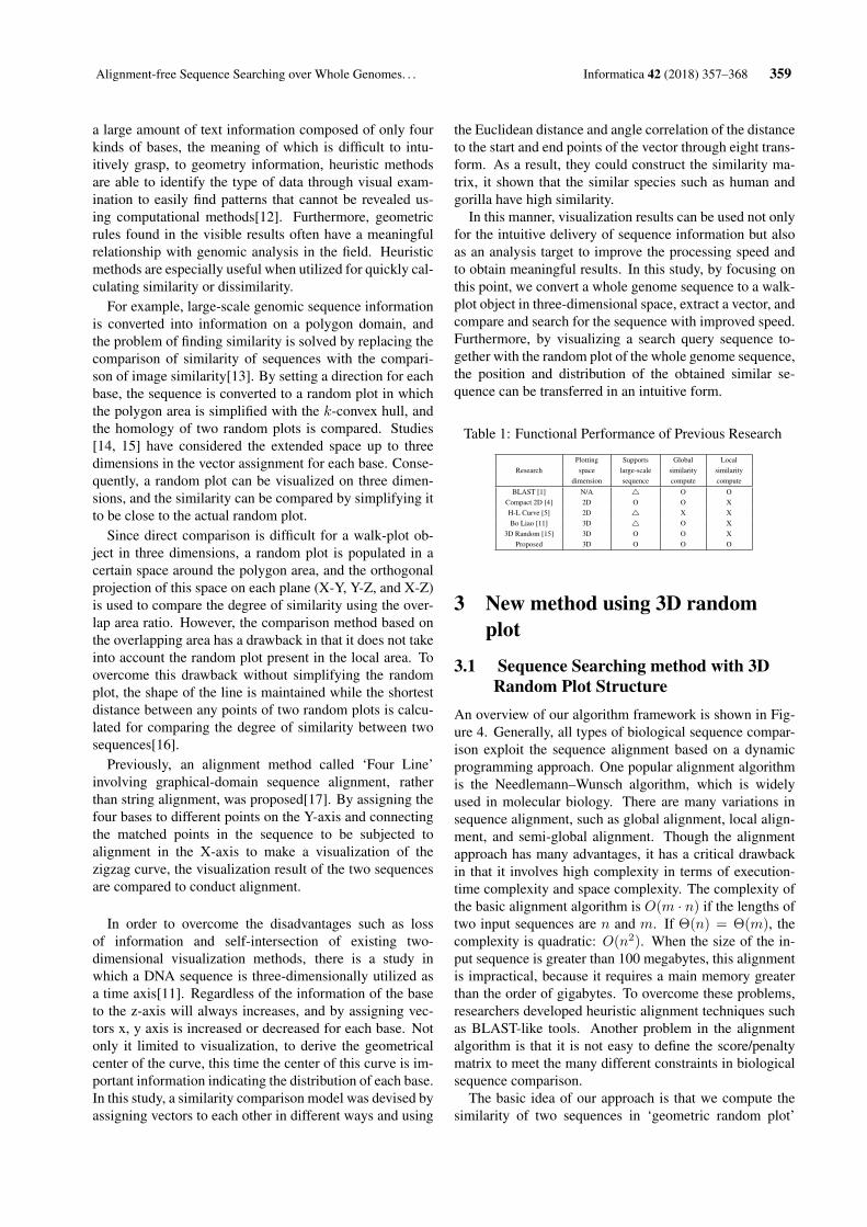
max(jPAj;jPBj)Figure 8: Two comparison parameters {θAB , LAB }.

dotted curve represents the random plot for a genome se-quence. Symbols P0(O) and P1 denote the first and lastpixel of a random plot, respectively. Pt denotes the first t-percentile pixel. Thus, P0.5 denotes the exact middle pixelin the list of pixels generated by our transformation algo-rithm.

For an interval in a random walk, we obtain a parameter,the length of the direction vector (P0, P1). If two randomwalks to be compared start with the origin (0, 0, 0), then wecan obtain the lengths of two direction vectors fromRa andRb and compute the angle difference between two vectorsPa1 and Pb1.

Assume the start and end points of Ra are Pa0, Pa1, andthose of Rb are Pb0, Pb1. If k = 1 is, the comparison tar-get is

−−−−→Pa0Pa1 and

−−−−→Pb0Pb1. If k = 2, further down one

step,divided into two vectors are compared both front andrear vector. Therefore, the comparison target are

−−−−−→Pa0Pa0.5

and−−−−−→Pb0Pb0.5,

−−−−−−→Pa0.5Pa1.0 and

−−−−−−→Pb0.5Pb1.0. If k = 3, by ap-

plying the same method, it performs a comparison of eighttimes (2k).

If the length of divided vector drops below the appro-priate length D, the recursion is aborted. In this paper, thethreshold D value is set to 100 times the unit size, whereunit size is the number of bp per pixel when visualized. TheD value was determined experimentally because at least thelength of the vector was more than 100px, meaningful com-parison was possible.

3.4 Computing Similarity and Search onRandom Plot

Rdist refers to the similarity distance between the two vec-tors. Figure 8 shows that two parameters of θA,B , LA,B forRdist. θA,B refers to the angle between the two vectors,and LA,B refers to the ratio between the length of two vec-tors differ and from those of the longer vector. If the twovectors have the same orientation, θA,B = 0, two vectors,if the length is equal to LA,B = is 0(0 ≤ θA,B ≤ 180, 0 ≤

Algorithm 2 Comparison Algorithminitialize beg ← 0initialize end← len(Ra)initialize O ← {0, 0, 0}initialize D ← threshold lenth of vectorprocedure SIM(beg, end : index of vector list, Ra, Rb :random plot of Ga, Gb, threshold θs, Ls)

mid← (end− beg)/2 + begcnt← 0if end− beg > D then

cnt+ = Sim(beg,mid,Ra, Rb)cnt+ = Sim(mid+ 1, end,Ra, Rb)

elseVa ← Ra[end]−Ra[beg]Vb ← Rb[end]−Rb[beg]Lena ← euclideanDist(O, Va)Lenb ← euclideanDist(O, Vb)

θa,b ← acos(dotProduct(Va,VbLena×Lenb )× 180

a,b ← abs(Lena−Lenb)max(Lena,Lenb)

if θa,b ≤ θs and a,b ≤ Ls thenreturn 1

elsereturn 0

end ifend ifreturn cnt

end procedure

LA,B ≤ 1).

To compare and visualize the random plot in a limitedspace, compression is necessary, as described earlier for-mula 2. However, in the case of the reference sequence, tocalculate the overall similarity of the two vectors, it main-tains the two normalized values set. One is a normalizedvalue that is used to process the query sequence, and theother is a normalized value of the calculated original ref-erence sequence. When comparing the sequence to searchwhen the use of normalized values of the query, and visual-ization uses the original normalized value. This is becauseit can not be an accurate comparison due to the size differ-ence between the reference and the query, the normalizedvalues differ.

After the normalization of the reference sequence andquery sequence the normalized according to the normal-ization value of the query sequence, extend the depth toa predetermined level k to proceed comparison by divid-ing a random plot as unit size. Compare all the pieces ofthe vector unit size extracted from the two random plotby Rdist(). When processing the results meet the pre-determined reference range, the higher the degree of simi-larity (θA,B ≤ θs and LA,B ≤ Ls). The ratio between thenumber of the unit vectors that meet the conditions and thetotal number of vector is similarity between two sequences.


3.5 Reference Sequence SlotIf the length of the query is long enough, the sequence in-formation is compressed at an appropriate rate during vi-sualization in a limited space. Therefore, it is possible toperform in the on-memory state by applying the same com-pression ratio when searching in the reference sequence.However, sequences with short lengths, such as the LTRsequence, are only kilo-bytes in size and remain uncom-pressed in the visualization process. In this case, vectorinformation becomes large, and query search becomes im-possible in on-memory state. In order to compensate forthis, when the length of the reference sequence differs bymore than 200 times, the reference sequence is divided intoan appropriate number of slots to perform the search. A slotis like a window. By reducing the search range by multipleof the query length at a certain point in time, the method de-scribed above can be applied even in a case where a searchis required at a low compression ratio in a large size se-quence.

|Slot(Q,R)| = |ranwalk(R)| − c0 · |ranwalk(Q)||ranwalk(Q)| · (c0 − 1)

(3)

Equation 3 is the number of slots created when a queryand reference sequence are given. Q and R are Query andReference sequence respectively, and len(ranwalk(X))represents the length of the whole vector information whenX sequence is expressed as a random plot. c0 is a controlconstant, which is the size of the space in which a vec-tor should be searched when a certain size query vector isgiven. In this paper, c0 is set to around 200.0. Since thequery may exist at the point where the slot is divided, theboundaries of each slot are overlapped by the length of thequery vector. Figure 9 shows that the vector of the refer-ence sequence is divided into slots.

Figure 9: Slot division in reference sequence vector basedon the vector length of the query sequence.

4 Experiments

4.1 Dataset PreparationActual biological sequence data were used for the search-ing experiment, and artificial data were used to validate thesimilarity comparison model. The biological sequences areHuman chromosome 1 (246MB size) and the sequence of

a 1M-10M size extracted from chromosome 1. Artificialsequence data are obtained by extracting a sequence of 1-10 MB length from the Human chromosome 1 sequence ata random location and inserting noise in a predeterminedratio. A number of bases with different sizes are deleted,inserted, and replaced by a ratio of 1% to 50%. The arti-ficial data information such as ratio and the b.p. size andnumber of pixels and compression ratio is shown in Tables3 and 4. ‘A1-0’ means that the artificial data of 1M sizeand 0% modified, namely it is just extracted from Humansequence, not modified. But ‘A10-25’ means that the arti-ficial data of 10M size and 25% modified.

This modification rate is expressed as ’M’ (M.Rate) inTable 3 and 4. ‘M’ (M.Rate) refers to the modified ratioof the number of B.P. on origin sequence. For verificationof the similarity comparison model, this rate was set highergradually as the experiment was repeated.

‘Ratio’ refers to the compression ratio of the number ofB.P. and pixels of the actual sequence to be converted to arandom plot. For example, in the Table 3, since A1-1 se-quence has 1000.02K bases, and random plot size consistsof 36K pixel, the compression ratio is 3.58%. ‘Sim’ meansthat the similarity result of origin sequence and modifiedsequence and ‘Comp.t’ represents the comparison time.

Table 3: Specification of artificial data of 1M, 2M size ex-tracted from Human chromosome 1 and comparison result

Sq M Length Plot Ratio Sim. Cmp.tN. (%) (K bp) (K px) (%) (%) (s)

A1-0 0 1000.02 36.00 3.58 100.00 0A1-1 1 999.93 35.79 3.58 99.59 0A1-2 2 1000.01 36.17 3.62 99.45 0A1-5 5 999.89 36.67 3.67 98.23 0A1-8 8 999.97 37.74 3.77 96.06 0

A1-10 10 1000.49 38.05 3.80 91.73 0A1-15 15 999.78 40.74 4.07 93.58 0.016A1-20 20 1000.29 42.49 4.25 91.76 0A1-25 25 999.92 44.2 4.42 86.14 0A1-30 30 999.79 47.18 4.72 84.23 0.015A1-40 40 1001.12 50.86 5.08 69.86 0.015A1-50 50 999.47 58.36 5.84 63.53 0.016A2-0 0 2000.04 67.09 3.35 100.00 0A2-1 1 1999.96 66.89 3.34 98.03 0A2-2 2 2000.15 67.27 3.36 95.85 0A2-5 5 2000.26 68.99 3.45 94.65 0A2-8 8 2000.2 70.4 3.52 90.5 0

A2-10 10 2000.14 69.64 3.48 91.2 0.016A2-15 15 1999.94 70.84 3.54 85.71 0A2-20 20 2000.18 77.56 3.88 83.62 0A2-25 25 2000.66 79.97 4.00 72 0A2-30 30 1999.85 89.15 4.46 73.37 0A2-40 40 2001.5 88.54 4.42 63.34 0.016A2-50 50 2000.62 104.11 5.20 54.91 0.016

Tables 5 and 6 are data for searching for LTR sequencesthat are frequently handled in real bioinformatics analysis.In the table 5, R-F-1 is the reference sequence and meanschromosome 1 sequence of the Flatfish. In the correspond-ing table 6, Q-F-1 is the query sequence of R-F-1 and isthe LTR sequence extracted from R-F-1. The biggest dif-ference from the artificially generated data is that the LTRsequence is too short and thus has a low compression rate


Table 4: Specification of artificial data of 4M, 10M sizeSq M Length Plot Ratio Sim. Cmp.tN. (%) (K bp) (K px) (%) (%) (s)

A4-0 0 4000.09 42.62 1.07 100.00 0A4-1 1 4000.18 42.69 1.07 99.3 0A4-2 2 3999.71 42.15 1.05 98.93 0A4-5 5 3999.51 44.13 1.10 98.18 0A4-8 8 3999.36 44.08 1.10 96.03 0A4-10 10 4000.1 45.95 1.15 96.27 0A4-15 15 3999.75 45.69 1.14 94.63 0A4-20 20 4000.23 49.33 1.23 91.33 0A4-25 25 3999.7 49.78 1.24 90.93 0A4-30 30 4001.21 53.79 1.34 84.36 0.016A4-40 40 3999.59 57.16 1.43 76.82 0.015A4-50 50 4000.14 64.1 1.60 66.87 0A10-0 0 10000.05 65.26 0.65 100.00 0A10-1 1 10000.03 65 0.65 98.08 0A10-2 2 10000.13 64.81 0.65 97.29 0A10-5 5 9999.47 66.32 0.66 96.76 0.015A10-8 8 9999.74 68.75 0.69 95.12 0

A10-10 10 10000.71 67.93 0.68 94.9 0.015A10-15 15 9999.97 75.13 0.75 91.18 0A10-20 20 9998.82 74.38 0.74 90.24 0A10-25 25 9999.4 78.34 0.78 87.68 0.016A10-30 30 9999.24 82.29 0.82 82.49 0A10-40 40 9999.82 87.51 0.88 78.48 0A10-50 50 10001.48 94.45 0.94 66.47 0

in the visualized space. This is because visualization ispossible in a limited space without compression. Since thereference sequences are based on the compression ratio ofthe query sequence, we can see that the random plot size ofthe reference sequence is very large relatively.

Table 5: Specification of biological data for referenceSq Chr. Species Length Plot RatioN. (M bp) (M px) (%)

R-F-1 1 Flatfish 19.80 19.02 95.06R-F-2 2 Flatfish 20.14 19.34 96.02R-F-3 3 Flatfish 22.24 21.36 96.04R-F-5 5 Flatfish 23.64 22.69 95.98R-H-1 1 Human 246.89 236.44 95.77

Table 6: Specification of biological data for querySq Chr. Species Length Plot RatioN. (K bp) (K px) (%)

Q-F-1 1 LTR 0.41 0.41 100.00Q-F-2 2 5’LTR 1.56 1.54 98.72Q-F-3 3 Gypsy 4.84 4.78 98.76Q-F-5 5 LTR 8.55 6.44 75.32Q-H-1 1 HERV-K 9.26 8.06 87.04

4.2 Experiment:Comparison BetweenModification ratio and Similarity basedproposed Model

Table 3 and Figure 12 show the result of similarity analysisof origin extracted sequence and modified sequences. InTable 3, ‘Sim’ means that the similarity result of origin se-quence and modified sequence and ‘Comp.t’ represents the

comparison time. As the modification ratio increases, thedegree of similarity decreases. Thus, it can be confirmedthat the similarity comparison model proposed in this studyaccurately reflects the similarity of the sequences. In addi-tion, except for sequence generation, the time required forcomparison is 0.02 seconds, which means that it can beprocessed at a very high speed.

Figure 10: Red random plot represents one part of Humanchromosome 1, the length of which is 4 MB, in terms ofnucleotide bases. Green random plot represents the 10%distorted sequence of the red one, Human chromosome 1.

Figure 11: Red random plot represents one part of Humanchromosome 1, the length of which is 4 MB, in terms ofnucleotide bases. Green random plot represents the 30%distorted sequence of the red one, Human chromosome 1.

4.3 Experiment:Artificial Sequence Searchover whole genome sequence

Table 7 is the result of sequence searching process for ex-tracted original sequence from Human chromosome 1 andthe modified sequences. ‘Unit B. P. ’ is the size of B.P. as


Figure 12: Similarity between origin sequence and modi-fied sequences in each size 1-10MB.

a unit of search,‘ Unit Vector’ refers to the size of the vec-tor to consider when comparing a time. ‘Error Dist.’ is thedistance between the actual sequence position and the re-sult of search position. ‘Find.t’ shows the amount of timespent on search. The original sequence (0% modified se-quence) search, as well as about the modified sequence ofup to 20% are also searched in a short time. The differ-ence between the actual position and the search result isrelatively accurate, as the query size is less than 200 B.P.when the query size is 1M, and only about 2000 B.P. whenthe query is 10M. Figure 13 and 14 are the visualization

Table 7: The result of sequence search for origin sequenceand modified sequence in Human chromosome 1

Q Unit sz. Vec.sz error Sim. Find.tsq. (bp) (px) Dist. (%) (s)

A1-0 28 11200 0 99.29 17.269A1-5 27 10800 150 97.27 21.341A1-10 26 10400 840 91.34 23.213A1-20 23 9200 120 88.75 22.514A4-0 92 36800 1160 92.81 6.537A4-5 90 36000 160 98.41 6.896A4-10 88 35200 1040 92.68 7.678A4-20 80 32000 1040 86.3 9.132A10-0 154 61600 1120 93.88 13.665A10-5 150 60000 560 97.21 16.065

A10-10 148 59200 280 95.09 14.245A10-20 134 53600 2020 81.95 22.241

result of search for the query sequence of 1MB, 10MB inthe chromosome 1 of the Human. Red random plot is a vi-sualization of Human chromosome 1, and blue point is thelocation where the query was searched. Through the visu-alization results, we can see that a query of 1MB size wasfound at a relatively early stage of the reference sequence,and a query of 10MB size was at the end of the sequence.This is consistent with the position in the actual sequence,and represents a search result in a more intuitive.

Figure 13: Searching result of query sequence (A1-0) inreference sequence (Human chromosome 1). Red plot rep-resents reference sequence and blue cross point representsthe position of searched query sequence.

4.4 Experiment:Biological Sequence Searchover whole genome sequence

Table 8 shows the results of searching a biological querysequence in a whole genome sequence. The search for theLTR sequence (Q-F-1) extracted from the flatfish chromo-some 1 resulted in a similarity of 85.7% within 90 B.P.of the actual query position within about 0.4 seconds ofsearch time. On the other hand, the HER-V sequence (Q-H-1) extracted from Human chromosome 1 took relativelylonger time, longer than 40 seconds because the length ofthe query sequence was short and the length of the refer-ence sequence was long. The difference between the actualposition and the search result is about 2000 B.P., which isrelatively accurate considering that the length of the refer-ence sequence is more than 200M.

Figures 15,16,17 and 18 visualize the flatfish chromo-some 1,2,3,5 sequences, respectively. The red one is a vi-sualization of the whole genome of a flatfish, and the areamarked in blue is where each query was searched. Fig-ures 17 and 18 show that the marked positions are almostidentical to the origin, reflecting that the Q-F-3 and Q-F-5 queries are actually located within 0.5 % of the flatfishwhole genome sequence. On the other hand, Figures 15and 16 reflect that the marked positions are relatively faraway from the origin, that the positions of the Q-F-1 andQ-F-2 queries are actually located within 7% and 10% ofthe flatfish whole genome sequence. Figure 19 visualizesthe Human chromosome 1 sequence and marks the resultof searching the Q-H-1 query. It is well reflected that theQ-H-1 query is actually located in the early 63 % (about155 MB.P.) of the Human sequence. Figure 20 is the re-sult of original query sequence (Q-H-1) and enlarged sub-sequence of the reference sequence (R-H-1) at searched po-sition. The similarity of the searched sequence in the ref-erence (green plot) was 78%, and it can be confirmed that


Figure 14: Searching result of query sequence (A10-0) inreference sequence (Human chromosome 1). Red plot rep-resents reference sequence and blue cross point representsthe position of searched query sequence.

the query is very similar to the query when matched withthe query sequence.

Table 8: The result of sequence search for biological querysequence in flatfish and Human chromosome 1.

Q Unit sz. Vec.sz error Sim. Find.tsq. (bp) (px) Dist. (%) (s)

Q-F-1 1 413 90 85.70 0.400Q-F-2 1 1540 180 72.40 1.030Q-F-3 1 4780 960 69.10 0.452Q-F-5 1 6443 1230 75.20 2.038Q-H-1 1 8063 2130 78.40 41.011

5 ConclusionMost genome sequence analyses proceed through compar-ative analysis by finding similar sequence data. Therefore,there is a need for a technique to quickly compare andsearch for large amounts of sequence data. The alignmenttechnique is a very accurate method to compare sequences,but its high time and space complexity is inadequate to han-dle large sequences. To overcome these disadvantage, wesuggest a new method for comparison and finding for Megasize sequence. Converts the genome sequence as a ran-dom plot on the three-dimensional, followed by replacingthe sequence comparison problem with geometric objectcomparison problem. As a result of experiments, similar-ity precessed by our comparison model accurately reflectsthe modified ratio between the modified sequence and theoriginal sequence. Most analytical studies based on visu-alization derive only a single result because they derive anumerical value based on the final result of the visualiza-tion. The search and comparison method based on the se-quence visualization proposed in this study has high valueof utilization of information because all compressed partial

Figure 15: Searching result of query sequence (Q-F-1) inreference sequence (R-F-1). Red plot represents referencesequence and blue cross point represents the position ofsearched query sequence.

visualization information is used for searching sequence. Itis useful in that the partial similarity of the sequence can bemeasured. In addition, a query sequence of size 1-10M wassearched in a whole genome sequence of 200M or more,and a relatively precise position was found for the originalsequence as well as the modified sequence up to 20%. Alsothe search time 25 seconds or less, was confirmed handledin a very improved speed compared to the alignment algo-rithm.

On the other hand, when a sequence with a shorter kilo-byte unit length is used as a query, such as an LTR se-quence, the compression rate is lowered at the time of vi-sualization, resulting in a lower compression rate of thereference sequence, which leads to a longer search time.However, considering the length of the reference, we canconfirm that the position searched is relatively accurate.

The proposed alignment-free searching method is veryfast and effective to find a long query sequence over thewhole genomes whose size is more than multi-hundredsmega-bytes. It was able to compare and search the se-quence at a much improved rate than the alignment-based model by modifying the sequence data into a three-dimensional random plot object and comparing the similar-ity with the compressed information. Searching algorithmbased on alignment method is popular and works good bi-ological sequence comparison but if the size of query andtarget reference is very large (more than 100 mega bases)the alignment base algorithm requires huge memory spaceand takes a long computation time. Though our algorithmcan’t locates the position of query sequence exactly by theDNA base unit, but we can use this procedure as one pre-processing step to find query sequence.



AcknowledgementThis research was supported by the Collaborative GenomeProgram of the Korea Institute of Marine Science and Tech-nology Promotion (KIMST) funded by the Ministry ofOceans and Fisheries (MOF) (No. 20140428).

References[1] Stephen F Altschul, Warren Gish, Webb Miller, Eu-

gene W Myers, and David J Lipman. Basic localalignment search tool. Journal of molecular biology,215(3):403–410, 1990. https://doi.org/10.1016/S0022-2836(05)80360-2.

[2] Susana Vinga and Jonas Almeida. Alignment-freesequence comparison—a review. Bioinformatics,19(4):513–523, 2003. https://doi.org/10.1093/bioinformatics/btg005.

[3] Tetsuya Nakamura, Keishi Taki, Hiroki Nomiya,Kazuhiro Seki, and Kuniaki Uehara. A shape-basedsimilarity measure for time series data with ensem-ble learning. Pattern Analysis and Applications,16(4):535–548, 2013. https://doi.org/10.1007/s10044-011-0262-6.

[4] Milan Randic, Marjan Vracko, Jure Zupan, and Mar-jana Novic. Compact 2-d graphical representa-tion of dna. Chemical physics letters, 373(5):558–562, 2003. https://doi.org/10.1016/S0009-2614(03)00639-0.

[5] Yongfan Li, Guohua Huang, Bo Liao, and ZanboLiu. H-l curve: a novel 2d graphical representationof protein sequences. MATCH-COMMUNICATIONS


IN MATHEMATICAL AND IN COMPUTER CHEM-ISTRY, 61(2):519–532, 2009. https://doi.org/10.1016/j.cplett.2008.07.046.

[6] Milan Randic. Graphical representations of dna as2-d map. Chemical Physics Letters, 386(4):468–471, 2004. https://doi.org/10.1016/j.cplett.2004.01.088.

[7] Yonghui Wu, Alan Wee-Chung Liew, Hong Yan,and Mengsu Yang. Db-curve: a novel 2dmethod of dna sequence visualization and repre-sentation. Chemical Physics Letters, 367(1):170–176, 2003. https://doi.org/10.1016/S0009-2614(02)01684-6.

[8] Milan Randic, Nella Lerš, Dejan Plavšic, Subhash CBasak, and Alexandru T Balaban. Four-color maprepresentation of dna or rna sequences and their nu-merical characterization. Chemical physics letters,407(1):205–208, 2005. https://doi.org/10.1016/j.cplett.2005.03.086.

[9] Martin Krzywinski, Jacqueline Schein, Inanc Birol,Joseph Connors, Randy Gascoyne, Doug Horsman,Steven J Jones, and Marco A Marra. Circos: an infor-mation aesthetic for comparative genomics. Genomeresearch, 19(9):1639–1645, 2009. https://doi.org/10.1101/gr.092759.109.

[10] Jiyuan An, John Lai, Atul Sajjanhar, Jyotsna Ba-tra, Chenwei Wang, and Colleen C Nelson. J-circos: an interactive circos plotter. Bioinformatics,31(9):1463–1465, 2015. https://doi.org/10.1161/CIRCULATIONAHA.115.015220.

[11] Bo Liao and Kequan Ding. A 3d graphical represen-tation of dna sequences and its application. Theoreti-



cal Computer Science, 358(1):56–64, 2006. https://doi.org/10.1016/j.tcs.2005.12.012.

[12] Alexey Pasechnik, Aleksandr Mylläri, TapioSalakoski, A Mylläri, T Salakoski, and T Salakoski.Dynamical visualization of the dna sequence and itsnucleotide content. Proceedings of KRBIO, 5:47–50,2005.

[13] Min-Ah Kim, Eun-Jeong Lee, Hwan-Gue Cho, andKie-Jung Park. A visualization technique for dnawalk plot using k-convex hull. Journal of WSCG, 5(1-3):212–221, 1997.

[14] Daegeon Kwon. Whole genome data visualizationand analysis using 3d random walk plot. Master’sthesis, Pusan National University, 2015.

[15] Lee Da-Young, Kim Kyung-Rim, Kim Taeyong, andCho Hwan-Gue. Comparison-specialized visualiza-tion model for whole genome sequences. Journal ofWSCG, 24(2):43–52, 2016.

[16] Hwan-gue Cho Dayoung Lee, Daegeon Kwon. Web-GL based Visualization System for Whole Genomes.In Proceedings of KIISE, pages 1414–1416. KOREAINFORMATION SCIENCE SOCIETY, 2016.

[17] Milan Randic, Jure Zupan, Dražen Vikic-Topic, andDejan Plavšic. A novel unexpected use of a graphi-cal representation of dna: Graphical alignment of dnasequences. Chemical Physics Letters, 431(4):375–379, 2006. https://doi.org/10.1016/j.cplett.2006.09.044.

Figure 19: Searching result of query sequence (Q-H-1) inreference sequence (R-H-1). Red plot represents referencesequence and blue cross point represents the position ofsearched query sequence.

Figure 20: Matching result between the query sequence (Q-H-1) and the extended subsequence of reference sequence(R-H-1), which was depicted as a blue cross in Figure 19.

Documents

Alignment-free Sequence Searching over Whole Genomes Using