Alignment by Maximization of Mutual Informationprince/smia/2009/papers2009/VioxIJCV97... · P1: LMW/STR/RKB/JHR P2: STR/SRK P3: STR/SRK QC: International Journal of Computer Vision

P1: LMW/STR/RKB/JHR P2: STR/SRK P3: STR/SRK QC:

International Journal of Computer Vision Kl470-04-Viola July 18, 1997 9:22

International Journal of Computer Vision 24(2), 137–154 (1997)c© 1997 Kluwer Academic Publishers. Manufactured in The Netherlands.

Alignment by Maximization of Mutual Information

PAUL VIOLAMassachusetts Institute of Technology, Artificial Intelligence Laboratory, 545 Technology Square,

Cambridge, MA [email protected]

WILLIAM M. WELLS IIIMassachusetts Institute of Technology, Artificial Intelligence Laboratory; and Harvard Medical School and

Brigham and Women’s Hospital, Department of [email protected]

Received August, 1995; Accepted September, 1995

Abstract. A new information-theoretic approach is presented for finding the pose of an object in an image. Thetechnique does not require information about the surface properties of the object, besides its shape, and is robustwith respect to variations of illumination. In our derivation few assumptions are made about the nature of theimaging process. As a result the algorithms are quite general and may foreseeably be used in a wide variety ofimaging situations.

Experiments are presented that demonstrate the approach registering magnetic resonance (MR) images, aligninga complex 3D object model to real scenes including clutter and occlusion, tracking a human head in a video sequenceand aligning a view-based 2D object model to real images.

The method is based on a formulation of the mutual information between the model and the image. As appliedhere the technique is intensity-based, rather than feature-based. It works well in domains where edge or gradient-magnitude based methods have difficulty, yet it is more robust than traditional correlation. Additionally, it has anefficient implementation that is based on stochastic approximation.

1. Introduction

In object recognition and image registration there isa need to find and evaluate the alignment of modeland image data. It has been difficult to find a suitablemetric for this comparison. In other applications, suchas medical imaging, data from one type of sensor mustbe aligned with that from another. We will present aninformation theoretic approach that can be used to solvesuch problems. Our approach makes few assumptionsabout the nature of the imaging process. As a result thealgorithms are quite general and may foreseeably beused with a wide variety of sensors. We will show thatthis technique makes many of the difficult problems ofmodel comparison easier, including accommodation ofthe vagaries of illumination and reflectance.

The general problem of alignment entails comparinga predicted image of an object with an actual image.Given an object model and a pose (coordinate transfor-mation), a model for the imaging process could be usedto predict the image that will result. The predicted im-age can then be compared to the actual image directly.If the object model and pose are correct the predictedand actual images should be identical, or close to it. Ofcourse finding the correct alignment is still a remainingchallenge.

The relationship between an object model (no matterhow accurate) and the object’s image is a complex one.The appearance of a small patch of a surface is a func-tion of the surface properties, the patch’s orientation,the position of the lights and the position of the ob-server. Given a modelu(x) and an imagev(y) we can



138 Viola and Wells

formulate an imaging equation,

v(T(x)) = F(u(x),q)+ η (1)

or equivalently,

v(y) = F(u(T−1(y)),q)+ η. (2)

The imaging equation has three distinct components.The first component is called a transformation, or pose,denotedT . It relates the coordinate frame of the modelto the coordinate frame of the image. The transforma-tion tells us which point in the model is responsible fora particular point in the image. The second compo-nent is the imaging function,F(u(x),q). The imagingfunction determines the value of image pointv(T(x)).In general a pixel’s value may be a function both of themodel and other exogenous factors. For example animage of a three dimensional object depends not onlyon the object but also on the lighting. The parameterq collects all of the exogenous influences into a sin-gle vector. Finally,η is a random variable that modelsnoise in the imaging process. In most cases the noiseis assumed Gaussian.

Alignment can be a difficult problem for a numberof reasons:

• F , the imaging function of the physical world, canbe difficult to model.• q, the exogenous parameters, are not necessarily

known and can be difficult to find. For examplecomputing the lighting in an image is a non-trivialproblem.• T , the space of transformations, which may have

many dimensions, is difficult to search. Rigid ob-jects often have a 6 dimensional transformationspace. Non-rigid objects can in principle have anunbounded number of pose parameters.

One reason that it is, in principle, possible to de-fine F is that the image does convey information aboutthe model. Clearly if there were no mutual informa-tion betweenu andv, there could be no meaningfulF .We propose to finesse the problem of finding and com-puting F andq by dealing with this mutual informa-tion directly. We will present an algorithm that alignsby maximizing the mutual information between modeland image. It requires no a priori model of the relation-ship between surface properties and scene intensities—it only assumes that the model tells more about thescene when it is correctly aligned.

Though the abstract suggestion that mutual informa-tion plays a role in object recognition may not be new,to date no concrete representations or efficient algo-rithms have been proposed. This paper will presenta new approach for evaluating entropy and mutual in-formation called EMMA1. It is distinguished in twoways: 1) EMMA does not require a prior model forthe functional form of the distribution of the data; 2)entropy can be maximized (or minimized) efficientlyusing stochastic approximation.

In its full generality, EMMA can be used wheneverthere is a need to align images from two different sen-sors, the so-called “sensor fusion” problem. For exam-ple, in medical imaging data from one type of sensor(such as magnetic resonance imaging—MRI) must bealigned to data from another sensor (such as computedtomography—CT).

2. An Alignment Example

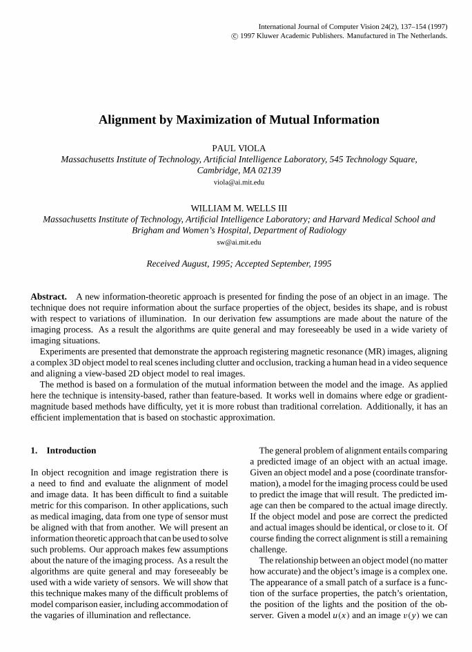
One of the alignment problems that we will addressinvolves finding the pose of a three-dimensional objectthat appears in a video image. This problem involvescomparing two very different kinds of representations:a three-dimensional model of the shape of the objectand a video image of that object. For example, Fig. 1contains a video image of an example object on the leftand a depth map of that same object on the right (theobject in question is a person’s head: RK). A depth mapis an image that displays the depth from the camera toevery visible point on the object model.

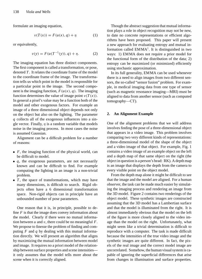
From the depth map alone it might be difficult to seethat the image and the model are aligned. For a humanobserver, the task can be made much easier by simulat-ing the imaging process and rendering an image fromthe 3D model. Figure 2 contains two renderings of theobject model. These synthetic images are constructedassuming that the 3D model has a Lambertian surfaceand that the model is illuminated from the right. It isalmost immediately obvious that the model on the leftof the figure is more closely aligned to the video im-age than the model on the right. Unfortunately, whatmight seem like a trivial determination is difficult toreproduce with a computer. The task is made difficultbecause the intensities of the true video image and thesynthetic images are quite different. In fact, the pix-els of the real image and the correct model image areuncorrelated. Somehow, the human visual system is ca-pable of ignoring the superficial differences that arisefrom changes in illumination and surface properties.



Alignment by Maximization of Mutual Information 139

Figure 1. Two different views of RK. On the left is a video image. On the right is a depth map of a model of RK that describes the distance toeach of the visible points of the model. Closer points are rendered brighter than more distant ones.

Figure 2. At left is a rendering of a 3D model of RK. The position of the model is the same as the position of the actual head. At right is arendering of the head model in an incorrect pose.

A successful computational theory of object recogni-tion must be similarly robust.

Lambert’s law is perhaps the simplest model of sur-face reflectivity. It is an accurate model of the re-flectance of a matte or non-shiny surface. Lambert’slaw states that the visible intensity of a surface patch isrelated to the dot product between the surface normaland the lighting. For a Lambertian object the imagingequation is:

v(T(x)) =∑

i

αi El i · u(x), (3)

where the model valueu(x) is the normal vector ofa surface patch on the object,l i is a vector pointingtoward light sourcei , andαi is proportional to the in-tensity of that light source ((Horn, 1986) contains anexcellent review of imaging and its relationship to vi-sion). As the illumination changes the functional rela-tionship between the model and image will change.

Since we can not know beforehand what the imag-ing function will be, aligning a model and image can be

quite difficult. These difficulties are only compoundedif the surface properties of the object are not well un-derstood. For example, many objects can not be mod-eled as having a Lambertian surface. Different surfacefinishes will have different reflectance functions. Ingeneral reflectance is a function of lighting direction,surface normal and viewing direction. The intensity ofan observed patch is then:

v(T(x)) =∑

i

R(αi , El i , Eo, u(x)), (4)

whereEo is a vector pointing toward the observer fromthe patch andR(·) is the reflectance function of thesurface. For an unknown material a great deal ofexperimentation is necessary to completely categorizethe reflectance function. Since a general vision sys-tem should work with a variety of objects and undergeneral illumination conditions, overly constrainingassumptions about reflectance or illumination shouldbe avoided.



140 Viola and Wells

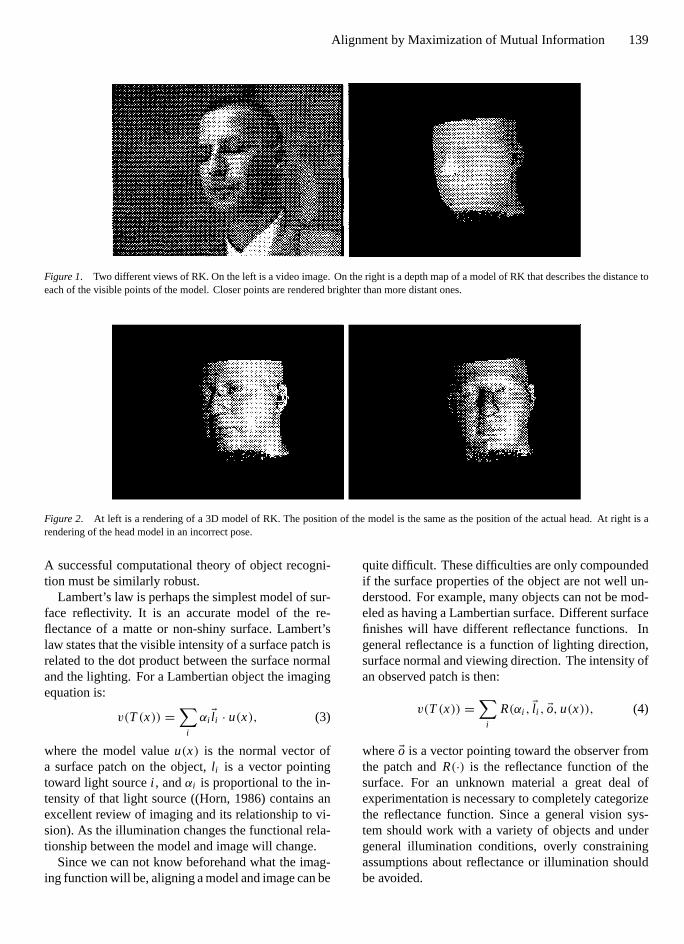
Figure 3. On the left is a video image of RK with the single scan-line highlighted. On the right is a graph of the intensities observed alongthis scan line.

Let us examine the relationship between a real im-age and model. This will allow us to build intuitionboth about alignment and image formation. Data fromthe real reflectance function can be obtained by align-ing a model to a real image. An alignment associatespoints from the image with points from the model. Ifthe alignment is correct, each pixel of the image can beinterpreted as a sample of the imaging functionR(·).The imaging function could be displayed by plottingintensity against lighting direction, viewing directionand surface normal. Unfortunately, because intensityis a function of so many different parameters the result-ing plot can be prohibitively complex and difficult tovisualize. Significant simplification will be necessaryif we are to visualize any structure in this data.

In a wide variety of real images we can assume thatthe light sources are far from the object (at least in termsof the dimensions of the object). When this is true andthere are no shadows, each patch of the object will beilluminated in the same way. Furthermore, we will as-sume that the observer is far from the object, and thatthe viewing direction is therefore constant throughoutthe image. The resulting relationship between normaland intensity is three dimensional. The normal vectorhas unit length and, for visible patches, is determinedby two parameters: thex andy components. The im-age intensity is a third parameter. A three dimensionalscatter plot of normal versus intensity is really a slicethrough the high dimensional space in whichR(·) isdefined. Though this graph is much simpler than theoriginal, three dimensional plots are still quite difficultto interpret. We will slice the data once again so that allof the points have a single value for they componentof the normal.

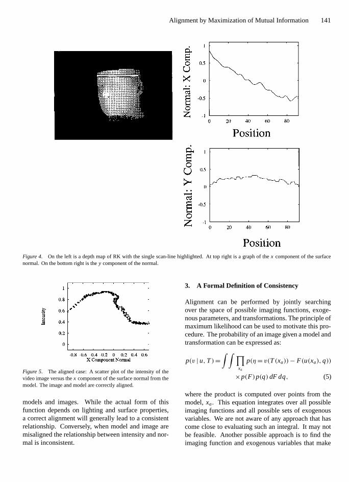
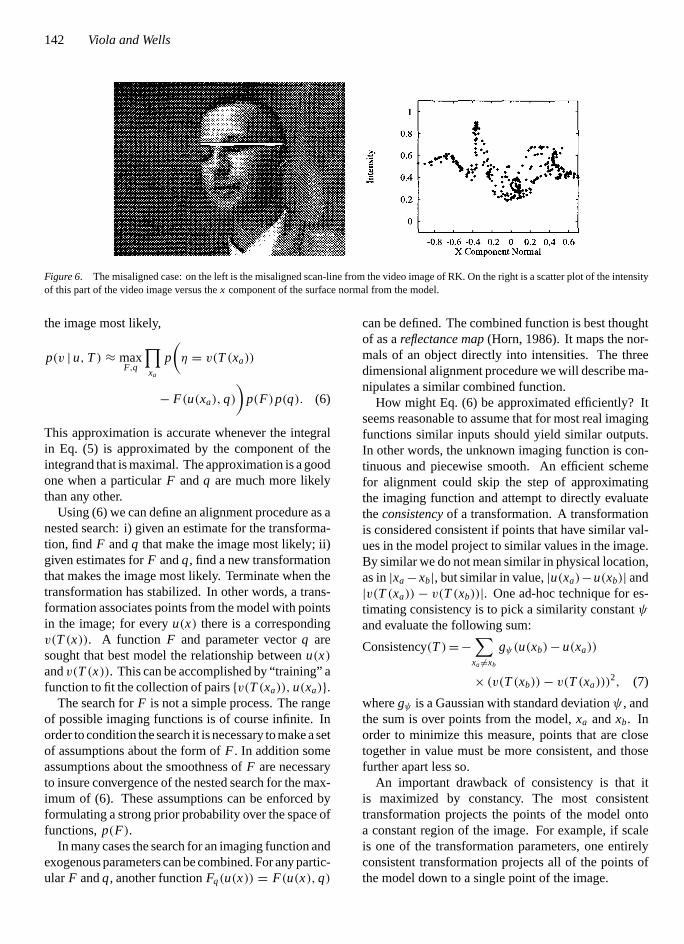
Figure 3 contains a graph of the intensities along asingle scan-line of the image of RK. Figure 4 showssimilar data for the correctly aligned model of RK.Model normals from this scan-line are displayed in twographs: the first shows thex component of the normalwhile the second shows they component. Notice thatwe have chosen this portion of the model so that theycomponent of the normal is almost constant. As a resultthe relationship between normal and intensity can bevisualized in only two dimensions. Figure 5 shows theintensities in the image plotted against thex compo-nent of the normal in the model. Notice that this rela-tionship appears both consistent and functional. Pointsfrom the model with similar surface normals have verysimilar intensities. The data in this graph could be wellapproximated by a smooth curve. We will call an imag-ing function like this oneconsistent. Interestingly, wedid not need any information about the illumination orsurface properties of the object to determine that thereis a consistent relationship between model normal andimage intensity.

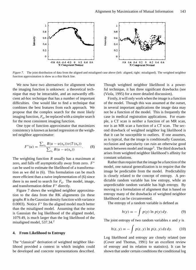
Figure 6 shows the relationship between normal andintensity when the model and image are no longeraligned. The only difference between this graph andthe first is that the intensities come from a scan-line 3centimeters below the correct alignment (i.e., the modelis no longer aligned with the image, it is 3 centimeterstoo low). The normals used are the same. The result-ing graph is no longerconsistent. It does not look asthough a simple smooth curve would fit this data well.

In summary, when model and image are aligned therewill be a consistent relationship between image inten-sity and model normal. This is predicted by our as-sumption that there is an imaging function that relates




Figure 4. On the left is a depth map of RK with the single scan-line highlighted. At top right is a graph of thex component of the surfacenormal. On the bottom right is they component of the normal.

Figure 5. The aligned case: A scatter plot of the intensity of thevideo image versus thex component of the surface normal from themodel. The image and model are correctly aligned.

models and images. While the actual form of thisfunction depends on lighting and surface properties,a correct alignment will generally lead to a consistentrelationship. Conversely, when model and image aremisaligned the relationship between intensity and nor-mal is inconsistent.

3. A Formal Definition of Consistency

Alignment can be performed by jointly searchingover the space of possible imaging functions, exoge-nous parameters, and transformations. The principle ofmaximum likelihood can be used to motivate this pro-cedure. The probability of an image given a model andtransformation can be expressed as:

p(v | u, T)=∫ ∫ ∏

xa

p(η= v(T(xa))− F(u(xa),q))

×p(F)p(q) dF dq, (5)

where the product is computed over points from themodel,xa. This equation integrates over all possibleimaging functions and all possible sets of exogenousvariables. We are not aware of any approach that hascome close to evaluating such an integral. It may notbe feasible. Another possible approach is to find theimaging function and exogenous variables that make



142 Viola and Wells

Figure 6. The misaligned case: on the left is the misaligned scan-line from the video image of RK. On the right is a scatter plot of the intensityof this part of the video image versus thex component of the surface normal from the model.

the image most likely,

p(v | u, T) ≈ maxF,q

∏xa

p

(η = v(T(xa))

− F(u(xa),q)

)p(F)p(q). (6)

This approximation is accurate whenever the integralin Eq. (5) is approximated by the component of theintegrand that is maximal. The approximation is a goodone when a particularF andq are much more likelythan any other.

Using (6) we can define an alignment procedure as anested search: i) given an estimate for the transforma-tion, find F andq that make the image most likely; ii)given estimates forF andq, find a new transformationthat makes the image most likely. Terminate when thetransformation has stabilized. In other words, a trans-formation associates points from the model with pointsin the image; for everyu(x) there is a correspondingv(T(x)). A function F and parameter vectorq aresought that best model the relationship betweenu(x)andv(T(x)). This can be accomplished by “training” afunction to fit the collection of pairs{v(T(xa)), u(xa)}.

The search forF is not a simple process. The rangeof possible imaging functions is of course infinite. Inorder to condition the search it is necessary to make a setof assumptions about the form ofF . In addition someassumptions about the smoothness ofF are necessaryto insure convergence of the nested search for the max-imum of (6). These assumptions can be enforced byformulating a strong prior probability over the space offunctions,p(F).

In many cases the search for an imaging function andexogenous parameters can be combined. For any partic-ular F andq, another functionFq(u(x)) = F(u(x),q)

can be defined. The combined function is best thoughtof as areflectance map(Horn, 1986). It maps the nor-mals of an object directly into intensities. The threedimensional alignment procedure we will describe ma-nipulates a similar combined function.

How might Eq. (6) be approximated efficiently? Itseems reasonable to assume that for most real imagingfunctions similar inputs should yield similar outputs.In other words, the unknown imaging function is con-tinuous and piecewise smooth. An efficient schemefor alignment could skip the step of approximatingthe imaging function and attempt to directly evaluatetheconsistencyof a transformation. A transformationis considered consistent if points that have similar val-ues in the model project to similar values in the image.By similar we do not mean similar in physical location,as in|xa−xb|, but similar in value,|u(xa)−u(xb)| and|v(T(xa)) − v(T(xb))|. One ad-hoc technique for es-timating consistency is to pick a similarity constantψ

and evaluate the following sum:

Consistency(T)=−∑

xa 6=xb

gψ(u(xb)− u(xa))

× (v(T(xb))− v(T(xa)))2, (7)

wheregψ is a Gaussian with standard deviationψ , andthe sum is over points from the model,xa andxb. Inorder to minimize this measure, points that are closetogether in value must be more consistent, and thosefurther apart less so.

An important drawback of consistency is that itis maximized by constancy. The most consistenttransformation projects the points of the model ontoa constant region of the image. For example, if scaleis one of the transformation parameters, one entirelyconsistent transformation projects all of the points ofthe model down to a single point of the image.




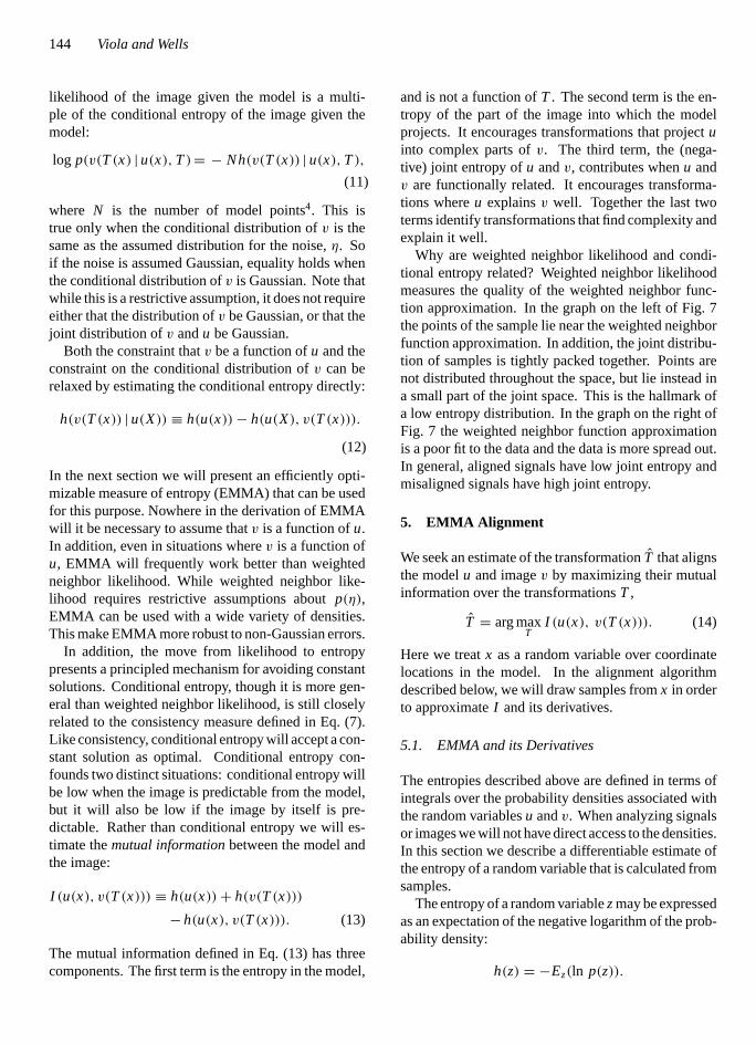
Figure 7. The joint distribution of data from the aligned and misaligned case above (left: aligned, right: misaligned). The weighted neighborfunction approximation is show as a thin black line.

We now have two alternatives for alignment whenthe imaging function is unknown: a theoretical tech-nique that may be intractable, and an outwardly effi-cient ad-hoc technique that has a number of importantdifficulties. One would like to find a technique thatcombines the best features from each approach. Wepropose that the complex search for the most likelyimaging function,Fq, be replaced with a simpler searchfor the most consistent imaging function.

One type of function approximator that maximizesconsistency is known as kernel regression or the weigh-ted neighbor approximator:

F∗(u) =∑

xaR(u− u(xa))v(T(xa))∑

xaR(u− u(xa))

. (8)

The weighting functionR usually has a maximum atzero, and falls off asymptotically away from zero.F∗

can be used to estimate the likelihood of a transforma-tion as we did in (6). This formulation can be muchmore efficient than a naive implementation of (6) sincethere is no need to search forFq. The model, image,and transformation defineF∗ directly.

Figure 7 shows the weighted neighbor approxima-tion to the data from the RK alignments (in thesegraphsR is the Gaussian density function with variance0.0003). NoticeF∗ fits the aligned model much betterthan the misaligned model. Assuming that the noiseis Gaussian the log likelihood of the aligned model,1079.49, is much larger than the log likelihood of themisaligned model, 537.34.2

4. From Likelihood to Entropy

The “classical” derivation of weighted neighbor like-lihood provided a context in which insights couldbe developed and concrete representations described.

Though weighted neighbor likelihood is a power-ful technique, it has three significant drawbacks (see(Viola, 1995) for a more detailed discussion).

Firstly, it will only work when the image is a functionof the model. Though this was assumed at the outset,in several important applications the image data maynot be a function of the model. This is frequently thecase in medical registration applications. For exam-ple, a CT scan is neither a function of an MR scan,nor is an MR scan a function of a CT scan. The sec-ond drawback of weighted neighbor log likelihood isthat it can be susceptible to outliers. If one assumes,as is typical, that the image is conditionally Gaussian,occlusion and specularity can ruin an otherwise goodmatch between model and image3. The third drawbackarises from weighted neighbor likelihood’s affinity forconstant solutions.

Rather than require that the image be a function of themodel, one natural generalization is to require that theimage be predictable from the model. Predictabilityis closely related to the concept of entropy. A pre-dictable random variable has low entropy, while anunpredictable random variable has high entropy. Bymoving to a formulation of alignment that is based onentropy many of the drawbacks of weighted neighborlikelihood can be circumvented.

The entropy of a random variable is defined as

h(y) ≡ −∫

p(y) ln p(y) dy. (9)

The joint entropy of two random variablesx andy is

h(z, y) ≡ −∫

p(z, y) ln p(z, y) dz dy. (10)

Log likelihood and entropy are closely related (see(Cover and Thomas, 1991) for an excellent reviewof entropy and its relation to statistics). It can beshown that under certain conditions the conditional log



144 Viola and Wells

likelihood of the image given the model is a multi-ple of the conditional entropy of the image given themodel:

log p(v(T(x) | u(x), T)= − Nh(v(T(x)) | u(x), T),(11)

where N is the number of model points4. This istrue only when the conditional distribution ofv is thesame as the assumed distribution for the noise,η. Soif the noise is assumed Gaussian, equality holds whenthe conditional distribution ofv is Gaussian. Note thatwhile this is a restrictive assumption, it does not requireeither that the distribution ofv be Gaussian, or that thejoint distribution ofv andu be Gaussian.

Both the constraint thatv be a function ofu and theconstraint on the conditional distribution ofv can berelaxed by estimating the conditional entropy directly:

h(v(T(x)) | u(X)) ≡ h(u(x))− h(u(X), v(T(x))).

(12)

In the next section we will present an efficiently opti-mizable measure of entropy (EMMA) that can be usedfor this purpose. Nowhere in the derivation of EMMAwill it be necessary to assume thatv is a function ofu.In addition, even in situations wherev is a function ofu, EMMA will frequently work better than weightedneighbor likelihood. While weighted neighbor like-lihood requires restrictive assumptions aboutp(η),EMMA can be used with a wide variety of densities.This make EMMA more robust to non-Gaussian errors.

In addition, the move from likelihood to entropypresents a principled mechanism for avoiding constantsolutions. Conditional entropy, though it is more gen-eral than weighted neighbor likelihood, is still closelyrelated to the consistency measure defined in Eq. (7).Like consistency, conditional entropy will accept a con-stant solution as optimal. Conditional entropy con-founds two distinct situations: conditional entropy willbe low when the image is predictable from the model,but it will also be low if the image by itself is pre-dictable. Rather than conditional entropy we will es-timate themutual informationbetween the model andthe image:

I (u(x), v(T(x))) ≡ h(u(x))+ h(v(T(x)))

− h(u(x), v(T(x))). (13)

The mutual information defined in Eq. (13) has threecomponents. The first term is the entropy in the model,

and is not a function ofT . The second term is the en-tropy of the part of the image into which the modelprojects. It encourages transformations that projectuinto complex parts ofv. The third term, the (nega-tive) joint entropy ofu andv, contributes whenu andv are functionally related. It encourages transforma-tions whereu explainsv well. Together the last twoterms identify transformations that find complexity andexplain it well.

Why are weighted neighbor likelihood and condi-tional entropy related? Weighted neighbor likelihoodmeasures the quality of the weighted neighbor func-tion approximation. In the graph on the left of Fig. 7the points of the sample lie near the weighted neighborfunction approximation. In addition, the joint distribu-tion of samples is tightly packed together. Points arenot distributed throughout the space, but lie instead ina small part of the joint space. This is the hallmark ofa low entropy distribution. In the graph on the right ofFig. 7 the weighted neighbor function approximationis a poor fit to the data and the data is more spread out.In general, aligned signals have low joint entropy andmisaligned signals have high joint entropy.

5. EMMA Alignment

We seek an estimate of the transformationT that alignsthe modelu and imagev by maximizing their mutualinformation over the transformationsT ,

T = arg maxT

I (u(x), v(T(x))). (14)

Here we treatx as a random variable over coordinatelocations in the model. In the alignment algorithmdescribed below, we will draw samples fromx in orderto approximateI and its derivatives.

5.1. EMMA and its Derivatives

The entropies described above are defined in terms ofintegrals over the probability densities associated withthe random variablesu andv. When analyzing signalsor images we will not have direct access to the densities.In this section we describe a differentiable estimate ofthe entropy of a random variable that is calculated fromsamples.

The entropy of a random variablezmay be expressedas an expectation of the negative logarithm of the prob-ability density:

h(z) = −Ez(ln p(z)).




Our first step in estimating the entropies fromsamples is to approximate the underlying probabil-ity density p(z) by a superposition of Gaussian den-sities centered on the elements of a sampleA drawnfrom z:

p(z) ≈ 1

NA

∑zj∈A

Gψ(z− zj ),

where

Gψ(z) ≡ (2π) −n2 |ψ | −1

2 exp

(− 1

2zTψ−1z

).

This method of density estimation is widely knownas theParzen Windowmethod. It is described in thetextbook by Duda and Hart (1973). Use of the Gaussiandensity in the Parzen density estimate will simplifysome of our subsequent analysis, but it isnotnecessary.Any differentiable function could be used. Anothergood choice is the Cauchy density.

Next we approximate statistical expectation withthe sample average over another sampleB drawnfrom z:

Ez( f (z)) ≈ 1

NB

∑zi∈B

f (zi ).

We may now write an approximation for the entropyof a random variablez as follows,

h(z) ≈ −1

NB

∑zi∈B

ln1

NA

∑zj∈A

Gψ(zi − zj ). (15)

The density ofzmay be a function of a set of parame-ters,T . In order to find maxima of mutual information,we calculate the derivative of entropy with respect toT . After some manipulation, this may be written com-pactly as follows,

d

dTh(z(T)) ≈ 1

NB

∑zi∈B

∑zj∈A

Wz(zi , zj )(zi − zj )T

×ψ−1 d

dT(zi − zj ), (16)

using the following definition:

Wz(zi , zj ) ≡ Gψ(zi − zj )∑zk∈A Gψ(zi − zk)

.

The weighting factorWz(zi , zj ) takes on values be-tween zero and one. It will approach one ifzi is sig-nificantly closer tozj than it is to any other element

of A. It will be near zero if some other element ofA is significantly closer tozi . Distance is interpretedwith respect to the squared Mahalanobis distance (see(Duda and Hart, 1973))

Dψ(z) ≡ zTψ−1z.

Thus,Wz(zi , zj ) is an indicator of the degree of matchbetween its arguments, in a “soft” sense. It is equiva-lent to using the “softmax” function of neural networks(Bridle, 1989) on the negative of the Mahalanobis dis-tance to indicate correspondence betweenzi and ele-ments ofA.

The summand in Eq. (16) may also be written as:

Wz(zi , zj )d

dT

1

2Dψ(zi − zj ).

In this form it is apparent that to reduce entropy, thetransformationT should be adjusted such that thereis a reduction in the average squared distance betweenthose values whichW indicates are nearby, i.e., clustersshould be tightened.

5.2. Stochastic Maximizationof Mutual Information

The entropy approximation described in Eq. (15) maynow be used to evaluate the mutual information of themodel and image (Eq. (13)). In order to seek a maxi-mum of the mutual information, we will calculate anapproximation to its derivative,

d

dTI (u(x), v(T(x))) = d

dTh(v(T(x)))

− d

dTh(u(x), v(T(x))).

Using Eq. (16), and assuming that the covariancematrices of the component densities used in the ap-proximation scheme for the joint density are block di-agonal:ψ−1

uv = DIAG (ψ−1uu , ψ

−1vv ), we can obtain an

estimate for the derivative of the mutual information asfollows:

d I

dT= 1

NB

∑xi∈B

∑xj∈A

(vi − v j )T

×[Wv(vi , v j )ψ

−1v −Wuv(wi , w j )ψ

−1vv

]× d

dT(vi − v j ). (17)



146 Viola and Wells

The weighting factors are defined as

Wv(vi , v j ) ≡ Gψv (vi − v j )∑xk∈A Gψv (vi − vk)

and

Wuv(wi , w j ) ≡ Gψuv (wi − w j )∑xk∈A Gψuv (wi − wk)

,

using the following notation (and similarly for indicesj andk),

ui ≡ u(xi ), vi ≡ v(T(xi )), and wi ≡ [ui , vi ]T .

If we are to increase the mutual information, then thefirst term in the brackets (of Eq. (17)) may be inter-preted as acting to increase the squared distance be-tween pairs of samples that are nearby in image inten-sity, while the second term acts to decrease the squareddistance between pairs of samples that are nearby inboth image intensityand the model properties. It isimportant to emphasize that distances are in the spaceof values (intensities, brightness, or surface properties),rather than coordinate locations.

The term ddT (vi − v j ) will generally involve gra-

dients of the image intensities and the derivative oftransformed coordinates with respect to the transfor-mation. In the simple case thatT is a linear operator,the following outer product expression holds:

d

dTv(T(xi )) = ∇v(T(xi ))x

Ti .

5.2.1. Stochastic Maximization Algorithm. We seeka local maximum of mutual information by using astochastic analog of gradient descent. Steps are repeat-edly taken that are proportional to the approximationof the derivative of the mutual information with respectto the transformation:

Repeat:

A← {sample of sizeNA drawn fromx}B← {sample of sizeNB drawn fromx}T ← T + λ d I

dT

The parameterλ is called thelearning rate. Theabove procedure is repeated a fixed number of times oruntil convergence is detected.

A good estimate of the derivative of the mutual in-formation could be obtained by exhaustively samplingthe data. This approach has serious drawbacks because

the algorithm’s cost is quadratic in the sample size. Forsmaller sample sizes, less effort is expended, but addi-tional noise is introduced into the derivative estimates.

Stochastic approximation is a scheme that uses noisyderivative estimate instead of the true derivative foroptimizing a function (see (Widrow and Hoff, 1960;Ljung and S¨oderstrom, 1983; Haykin, 1994)). Con-vergence can be proven for particular linear systems,provided that the derivative estimates are unbiased, andthe learning rate is annealed (decreased over time). Inpractice, we have found that successful alignment maybe obtained using relatively small sample sizes, forexampleNA = NB = 50. We have proven that thetechnique will always converge to a pose estimate thatis close to locally optimal (Viola, 1995).

It has been observed that the noise introduced by thesampling can effectively penetrate small local minima.Such local minima are often characteristic of continu-ous alignment schemes, and we have found that localminima can be overcome in this manner in these appli-cations as well. We believe that stochastic estimates forthe gradient usefully combine efficiency with effectiveescape from local minima.

5.2.2. Estimating the Covariance. In addition toλ,the covariance matrices of the component densities inthe approximation method of Section 5.1 are importantparameters of the method. These parameters may bechosen so that they are optimal in the maximum like-lihood sense with respect to samples drawn from therandom variables. This approach is equivalent to min-imizing the cross entropy of the estimated distributionwith the true distribution (Cover and Thomas, 1991).For simplicity, we assume that the covariance matricesare diagonal.

The most likely covariance parameters can be es-timated on-line using a scheme that is almost iden-tical in form to the scheme for maximizing mutualinformation.

6. Experiments

In this section we demonstrate alignment by maximiza-tion of mutual information in a variety of domains. Inall of the following experiments, bi-linear interpolationwas used when needed for non-integral indexing intoimages.

6.1. MRI Alignment

Our first and simplest experiment involves finding thecorrect alignment of two MR images (see Fig. 8).




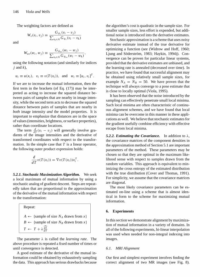
Figure 8. MRI alignment (from left to right): original proton-density image, original T2-weighted image, initial alignment, composite displayof final alignment, intensity-transformed image.

The two original images are components of a double-echo MR scan and were obtained simultaneously, asa result the correct alignment should be close to theidentity transformation. It is clear that the two im-ages have high mutual information, while they are notidentical.

A typical initial alignment appears in the center ofFig. 8. Notice that this image is a scaled, sheared,rotated and translated version of the original. A suc-cessful alignment is displayed as a checkerboard. Hereevery other 20×20 pixel block is taken either from themodel image or target image. Notice that the boundaryof the brain in the images is very closely aligned.

We represent the transformation by a 6 elementaffine matrix that takes two dimensional points fromthe image plane of the first image into the image planeof the second image. This scheme can represent anycombination of scaling, shearing, rotation and transla-tion. Before alignment the pixel values in the two MRimages are pre-scaled so that they vary from 0 to 1.The component densities areψuu = ψw = 0.1, and therandom samples are of size 20. We used a learning rateof 0.02 for 500 iterations and 0.005 for 500 iterations.Total run time on a Sparc 10 was 12 seconds.

Over a set of 50 randomly generated initial posesthat vary in position by 32 pixels, a little less than onethird of the width of the head, rotations of 28 degrees,and scalings of up to 20%, the “correct” alignmentis obtained reliably. Final alignments were well withinone pixel in position and within 0.5% of the identity ma-trix for rotation/scale. We report errors in percent herebecause of the use of affine transformation matrices.

The two MRI images are fairly similar. Good align-ment could probably be obtained with a normalizedcorrelation metric. Normalized correlation assumes, atleast locally, that one signal is a scaled and offset ver-sion of the other. Our technique makes no such as-sumption. In fact, it will work across a wide varietyof non-linear transformations. All that is required is

that the intensity transformation preserve a significantamount of information. On the right in Fig. 8. we showthe model image after a non-monotonic (quadratic) in-tensity transformation. Alignment performance is notsignificantly affected by this transformation.

This last experiment is an example that would defeattraditional correlation, since the signals (the secondand last in Fig. 8) are more similar in value when theyare badly mis-aligned (non-overlapping) than they arewhen properly aligned.

6.2. Alignment of 3D Objects

6.2.1. Skull Alignment Experiments. This sectiondescribes the alignment of a real three dimensional ob-ject of its video image. The signals that are comparedare quite different in nature: one is the video bright-ness, while the other consists of two components of thenormal vector at a point on the surface of the model.

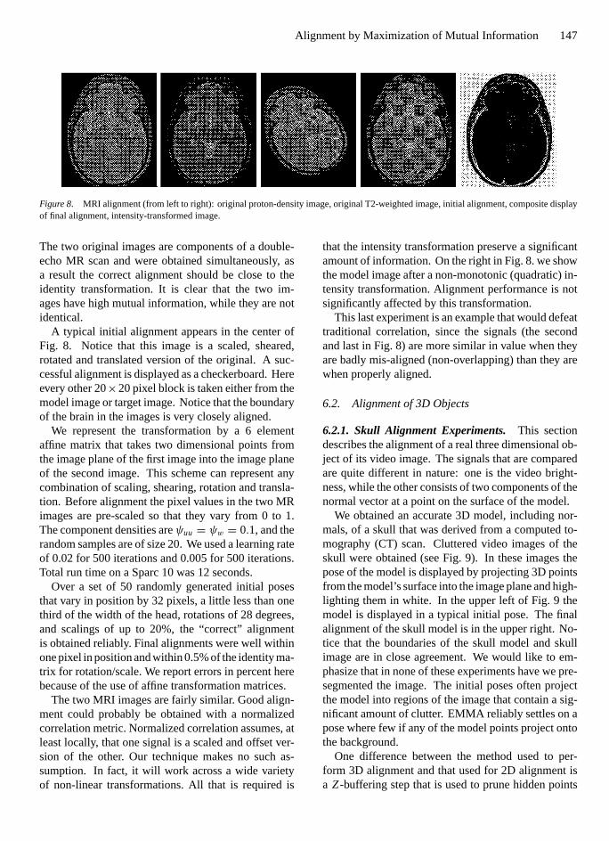
We obtained an accurate 3D model, including nor-mals, of a skull that was derived from a computed to-mography (CT) scan. Cluttered video images of theskull were obtained (see Fig. 9). In these images thepose of the model is displayed by projecting 3D pointsfrom the model’s surface into the image plane and high-lighting them in white. In the upper left of Fig. 9 themodel is displayed in a typical initial pose. The finalalignment of the skull model is in the upper right. No-tice that the boundaries of the skull model and skullimage are in close agreement. We would like to em-phasize that in none of these experiments have we pre-segmented the image. The initial poses often projectthe model into regions of the image that contain a sig-nificant amount of clutter. EMMA reliably settles on apose where few if any of the model points project ontothe background.

One difference between the method used to per-form 3D alignment and that used for 2D alignment isa Z-buffering step that is used to prune hidden points



148 Viola and Wells

Figure 9. Skull alignment experiments: Initial alignment, final alignment, initial alignment with occlusion, final alignment with occlusion.

from the calculations. SinceZ-buffer pruning is costly,and the pose does not change much between iterations,it proved sufficient to prune every 200 iterations. An-other difference is that the model surface sampling wasadjusted so that the sampling density in the image wascorrected for foreshortening.

In this experiment, the camera has a viewing an-gle of 18 degrees. We representT , the transforma-tion from model to image coordinates, as a doublequaternion followed by a perspective projection (Horn,1986). Assuming diagonal covariance matrices fourdifferent variances are necessary, three for the jointentropy estimate and one for the image entropy esti-mate. The variance for thex component of the normalwas 0.3, for they component of the normal was 0.3, forthe image intensity was 0.2 and for the image entropywas 0.15. The size of the random sample used is 50points.

Since the units of rotation and translation are verydifferent, two separate learning rates are necessary. Foran object with a 100 millimeter radius, a rotation of 0.01radians about its center can translate a model point upto 1 millimeter. On the other hand, a translation of 0.01can at most translate a model point 0.01 millimeters.As a result, a small step in the direction of the derivativewill move some model points up to 100 times furtherby rotation than translation. If there is only a single

learning rate a compromise must be made between therapid changes that arise from the rotation and the slowchanges that arise from translation. Since the modelsused have a radius that is on the order of 100 millime-ters, we have chosen rotation learning rates that are100 times smaller than translation rates. In our exper-iments alignment proceeds in two stages. For the first2000 iterations the rotation learning rate is 0.0005 andthe translation learning rate is 0.05. The learning ratesare then reduced to 0.0001 and 0.01 respectively for anadditional 2000 iterations. Running time is about 30seconds on a Sparc 10.

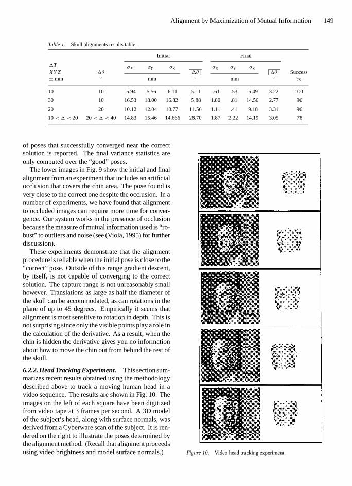
A number of randomized experiments were per-formed to determine the reliability, accuracy and re-peatability of alignment. This data is reported inTable 1. An initial alignment to an image was per-formed to establish a base pose. From this base pose,a random uniformly distributed offset is added to eachtranslational axis (labeled1T) and then the model isrotated about a randomly selected axis by a randomuniformly selected angle (1θ ). Table 1 describes fourexperiments each including 50 random initial poses.The distribution of the final and initial poses can becompared by examining the variance of the locationof the centroid, computed separately inX, Y and Z.In addition, the average angular rotation from the truepose is reported (labeled|1θ |). Finally, the number




Table 1. Skull alignments results table.

Initial Final

σX σY σZ σX σY σZ1TXY Z± mm

1θ◦ mm

|1θ |◦ mm

|1θ |◦

Success%

10 10 5.94 5.56 6.11 5.11 .61 .53 5.49 3.22 100

30 10 16.53 18.00 16.82 5.88 1.80 .81 14.56 2.77 96

20 20 10.12 12.04 10.77 11.56 1.11 .41 9.18 3.31 96

10< 1 < 20 20< 1 < 40 14.83 15.46 14.666 28.70 1.87 2.22 14.19 3.05 78

of poses that successfully converged near the correctsolution is reported. The final variance statistics areonly computed over the “good” poses.

The lower images in Fig. 9 show the initial and finalalignment from an experiment that includes an artificialocclusion that covers the chin area. The pose found isvery close to the correct one despite the occlusion. In anumber of experiments, we have found that alignmentto occluded images can require more time for conver-gence. Our system works in the presence of occlusionbecause the measure of mutual information used is “ro-bust” to outliers and noise (see (Viola, 1995) for furtherdiscussion).

These experiments demonstrate that the alignmentprocedure is reliable when the initial pose is close to the“correct” pose. Outside of this range gradient descent,by itself, is not capable of converging to the correctsolution. The capture range is not unreasonably smallhowever. Translations as large as half the diameter ofthe skull can be accommodated, as can rotations in theplane of up to 45 degrees. Empirically it seems thatalignment is most sensitive to rotation in depth. This isnot surprising since only the visible points play a role inthe calculation of the derivative. As a result, when thechin is hidden the derivative gives you no informationabout how to move the chin out from behind the rest ofthe skull.

6.2.2. Head Tracking Experiment. This section sum-marizes recent results obtained using the methodologydescribed above to track a moving human head in avideo sequence. The results are shown in Fig. 10. Theimages on the left of each square have been digitizedfrom video tape at 3 frames per second. A 3D modelof the subject’s head, along with surface normals, wasderived from a Cyberware scan of the subject. It is ren-dered on the right to illustrate the poses determined bythe alignment method. (Recall that alignment proceedsusing video brightness and model surface normals.) Figure 10. Video head tracking experiment.



150 Viola and Wells

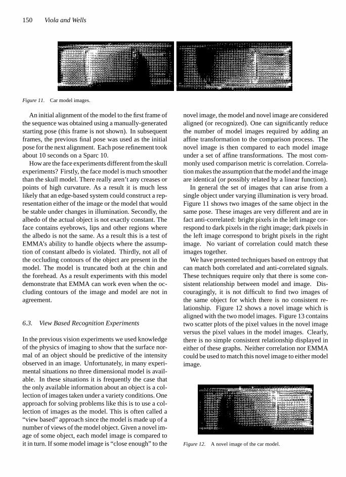
Figure 11. Car model images.

An initial alignment of the model to the first frame ofthe sequence was obtained using a manually-generatedstarting pose (this frame is not shown). In subsequentframes, the previous final pose was used as the initialpose for the next alignment. Each pose refinement tookabout 10 seconds on a Sparc 10.

How are the face experiments different from the skullexperiments? Firstly, the face model is much smootherthan the skull model. There really aren’t any creases orpoints of high curvature. As a result it is much lesslikely that an edge-based system could construct a rep-resentation either of the image or the model that wouldbe stable under changes in illumination. Secondly, thealbedo of the actual object is not exactly constant. Theface contains eyebrows, lips and other regions wherethe albedo is not the same. As a result this is a test ofEMMA’s ability to handle objects where the assump-tion of constant albedo is violated. Thirdly, not all ofthe occluding contours of the object are present in themodel. The model is truncated both at the chin andthe forehead. As a result experiments with this modeldemonstrate that EMMA can work even when the oc-cluding contours of the image and model are not inagreement.

6.3. View Based Recognition Experiments

In the previous vision experiments we used knowledgeof the physics of imaging to show that the surface nor-mal of an object should be predictive of the intensityobserved in an image. Unfortunately, in many experi-mental situations no three dimensional model is avail-able. In these situations it is frequently the case thatthe only available information about an object is a col-lection of images taken under a variety conditions. Oneapproach for solving problems like this is to use a col-lection of images as the model. This is often called a“view based” approach since the model is made up of anumber of views of the model object. Given a novel im-age of some object, each model image is compared toit in turn. If some model image is “close enough” to the

novel image, the model and novel image are consideredaligned (or recognized). One can significantly reducethe number of model images required by adding anaffine transformation to the comparison process. Thenovel image is then compared to each model imageunder a set of affine transformations. The most com-monly used comparison metric is correlation. Correla-tion makes the assumption that the model and the imageare identical (or possibly related by a linear function).

In general the set of images that can arise from asingle object under varying illumination is very broad.Figure 11 shows two images of the same object in thesame pose. These images are very different and are infact anti-correlated: bright pixels in the left image cor-respond to dark pixels in the right image; dark pixels inthe left image correspond to bright pixels in the rightimage. No variant of correlation could match theseimages together.

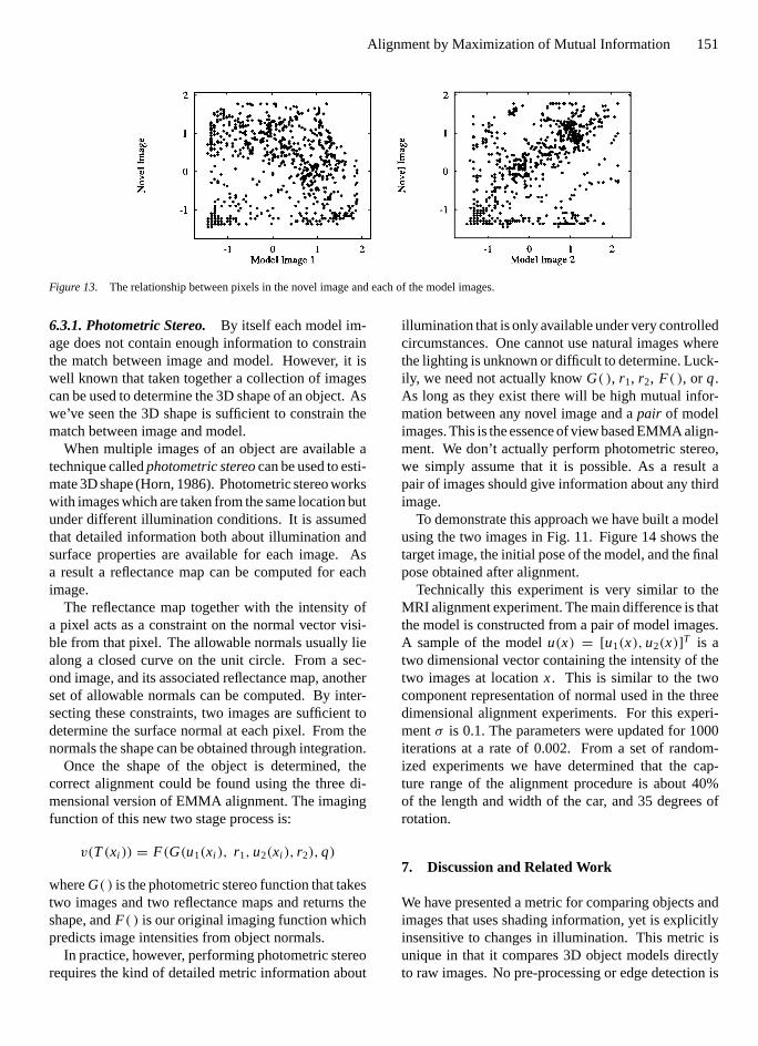
We have presented techniques based on entropy thatcan match both correlated and anti-correlated signals.These techniques require only that there is some con-sistent relationship between model and image. Dis-couragingly, it is not difficult to find two images ofthe same object for which there is no consistent re-lationship. Figure 12 shows a novel image which isaligned with the two model images. Figure 13 containstwo scatter plots of the pixel values in the novel imageversus the pixel values in the model images. Clearly,there is no simple consistent relationship displayed ineither of these graphs. Neither correlation nor EMMAcould be used to match this novel image to either modelimage.

Figure 12. A novel image of the car model.




Figure 13. The relationship between pixels in the novel image and each of the model images.

6.3.1. Photometric Stereo.By itself each model im-age does not contain enough information to constrainthe match between image and model. However, it iswell known that taken together a collection of imagescan be used to determine the 3D shape of an object. Aswe’ve seen the 3D shape is sufficient to constrain thematch between image and model.

When multiple images of an object are available atechnique calledphotometric stereocan be used to esti-mate 3D shape (Horn, 1986). Photometric stereo workswith images which are taken from the same location butunder different illumination conditions. It is assumedthat detailed information both about illumination andsurface properties are available for each image. Asa result a reflectance map can be computed for eachimage.

The reflectance map together with the intensity ofa pixel acts as a constraint on the normal vector visi-ble from that pixel. The allowable normals usually liealong a closed curve on the unit circle. From a sec-ond image, and its associated reflectance map, anotherset of allowable normals can be computed. By inter-secting these constraints, two images are sufficient todetermine the surface normal at each pixel. From thenormals the shape can be obtained through integration.

Once the shape of the object is determined, thecorrect alignment could be found using the three di-mensional version of EMMA alignment. The imagingfunction of this new two stage process is:

v(T(xi )) = F(G(u1(xi ), r1, u2(xi ), r2),q)

whereG( ) is the photometric stereo function that takestwo images and two reflectance maps and returns theshape, andF( ) is our original imaging function whichpredicts image intensities from object normals.

In practice, however, performing photometric stereorequires the kind of detailed metric information about

illumination that is only available under very controlledcircumstances. One cannot use natural images wherethe lighting is unknown or difficult to determine. Luck-ily, we need not actually knowG( ), r1, r2, F( ), or q.As long as they exist there will be high mutual infor-mation between any novel image and apair of modelimages. This is the essence of view based EMMA align-ment. We don’t actually perform photometric stereo,we simply assume that it is possible. As a result apair of images should give information about any thirdimage.

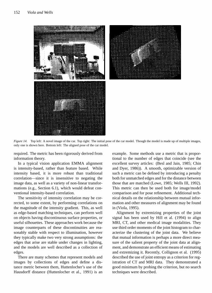
To demonstrate this approach we have built a modelusing the two images in Fig. 11. Figure 14 shows thetarget image, the initial pose of the model, and the finalpose obtained after alignment.

Technically this experiment is very similar to theMRI alignment experiment. The main difference is thatthe model is constructed from a pair of model images.A sample of the modelu(x) = [u1(x), u2(x)]T is atwo dimensional vector containing the intensity of thetwo images at locationx. This is similar to the twocomponent representation of normal used in the threedimensional alignment experiments. For this experi-mentσ is 0.1. The parameters were updated for 1000iterations at a rate of 0.002. From a set of random-ized experiments we have determined that the cap-ture range of the alignment procedure is about 40%of the length and width of the car, and 35 degrees ofrotation.

7. Discussion and Related Work

We have presented a metric for comparing objects andimages that uses shading information, yet is explicitlyinsensitive to changes in illumination. This metric isunique in that it compares 3D object models directlyto raw images. No pre-processing or edge detection is



152 Viola and Wells

Figure 14. Top left: A novel image of the car. Top right: The initial pose of the car model. Though the model is made up of multiple images,only one is shown here. Bottom left: The aligned pose of the car model.

required. The metric has been rigorously derived frominformation theory.

In a typical vision application EMMA alignmentis intensity-based, rather than feature based. Whileintensity based, it is more robust than traditionalcorrelation—since it is insensitive to negating theimage data, as well as a variety of non-linear transfor-mations (e.g., Section 6.1), which would defeat con-ventional intensity-based correlation.

The sensitivity of intensity correlation may be cor-rected, to some extent, by performing correlations onthe magnitude of the intensity gradient. This, as wellas edge-based matching techniques, can perform wellon objects having discontinuous surface properties, oruseful silhouettes. These approaches work because theimage counterparts of these discontinuities are rea-sonably stable with respect to illumination, howeverthey typically make two very strong assumptions: theedges that arise are stable under changes in lighting,and the models are well described as a collection ofedges.

There are many schemes that represent models andimages by collections of edges and define a dis-tance metric between them, Huttenlocher’s use of theHausdorff distance (Huttenlocher et al., 1991) is an

example. Some methods use a metric that is propor-tional to the number of edges that coincide (see theexcellent survey articles: (Besl and Jain, 1985; Chinand Dyer, 1986)). A smooth, optimizable version ofsuch a metric can be defined by introducing a penaltyboth for unmatched edges and for the distance betweenthose that are matched (Lowe, 1985; Wells III, 1992).This metric can then be used both for image/modelcomparison and for pose refinement. Additional tech-nical details on the relationship between mutual infor-mation and other measures of alignment may be foundin (Viola, 1995).

Alignment by extremizing properties of the jointsignal has been used by Hill et al. (1994) to alignMRI, CT, and other medical image modalities. Theyuse third order moments of the joint histogram to char-acterize the clustering of the joint data. We believethat mutual information is perhaps a more direct mea-sure of the salient property of the joint data at align-ment, and demonstrate an efficient means of estimatingand extremizing it. Recently, Collignon et al. (1995)described the use of joint entropy as a criterion for reg-istration of CT and MRI data. They demonstrated agood minimum by probing the criterion, but no searchtechniques were described.




Image-based approaches to modeling have been pre-viously explored by several authors. Objects need nothave edges to be well represented in this way, but caremust be taken to deal with changes in lighting and pose.Turk and Pentland have used a large collection of faceimages to train a system to construct representationsthat are invariant to some changes in lighting and pose(Turk and Pentland, 1991). These representations area projection onto the largest eigenvectors of the distri-bution of images within the collection. Their systemaddresses the problem of recognition rather than align-ment, and as a result much of the emphasis and manyof the results are different. For instance, it is not clearhow much variation in pose can be handled by theirsystem. We do not see a straightforward extensionof this or similar eigenspace work to the problem ofpose refinement. In other related work, Shashua hasshown that all of the images, under different lighting,of a Lambertian surface are a linear combination of anythree of the images (Shashua, 1992). A procedure forimage alignment could be derived from this theory. Incontrast, our image alignment method does not assumethat the object has a Lambertian surface.

Entropy is playing an ever increasing role within thefield of neural networks. We know of no work on thealignment of models and images, but there has beenwork using entropy and information in vision prob-lems. None of these techniques use a non-parametricscheme for density/entropy estimation as we do. Inmost cases the distributions are assumed to be eitherbinomial or Gaussian. Entropy and mutual informa-tion plays a role in the work of (Linsker, 1986; Beckerand Hinton, 1992; Bell and Sejnowski, 1995).

Acknowledgments

We were partially inspired by the work of Hill andHawkes on registration of medical images. SanjeevKulkarni introduced Wells to the concept of rela-tive entropy, and its use in image processing. NicolSchraudolph and Viola began discussions of this con-crete approach to evaluating entropy in an applicationof un-supervised learning.

We thank Ron Kikinis and Gil Ettinger for the 3Dskull model and MRI data. J.P. Mellor provided theskull images and camera model. Viola would like tothank Terrence. J. Sejnowski for providing some of thefacilities used during the preparation of this manuscript.

We thank for following sources for their support ofthis research: USAF ASSERT program, Parent Grant#:

F49620-93-1-0263 (Viola), Howard Hughes Medi-cal Institute (Viola), ARPA IU program via ONR#:N00014-94-01-0994 (Wells) and AFOSR # F49620-93-1-0604 (Wells).

Notes

1. EMMA is a random but pronounceable subset of the letters in thewords “Empirical entropy Manipulation and Analysis”.

2. Log likelihood is computed by first finding the Gaussian distribu-tion that fits the residual error, or noise, best. The log of (6) is thencomputed using the estimated distribution of the noise. For smallamounts of noise, these estimates can be much larger than 1.

3. Correlation matching is one of many techniques that assumes aGaussian conditional distribution of the image given the model.

4. Here we speak of the empirically estimated entropy of the condi-tional distribution.

References

Becker, S. and Hinton, G.E. 1992. Learning to make coherent predic-tions in domains with discontinuities. InAdvances in Neural Infor-mation Processing, J.E. Moody, S.J. Hanson, and R.P. Lippmann,(Eds.), Denver 1991. Morgan Kaufmann: San Mateo, vol. 4.

Bell, A.J. and Sejnowski, T.J. 1995. An information-maximisationapproach to blind separation. InAdvances in Neural Informa-tion Processing, Denver 1994. Morgan Kaufmann: San Francisco,vol. 4.

Besl, P. and Jain, R. 1985. Three-dimensional object recognition.Computing Surveys, 17:75–145.

Bridle, J.S. 1989. Training stochastic model recognition algorithmsas networks can lead to maximum mutual information estimationof parameters. InAdvances in Neural Information Processing 2,D.S. Touretzky (Ed.), Morgan Kaufman, pp. 211–217.

Chin, R. and Dyer, C. 1986. Model-based recognition in robot vision.Computing Surveys, 18:67–108.

Collignon, A., Vandermuelen, D., Suetens, P., and Marchal, G. 1995.3D multi-modality medical image registration using feature spaceclustering. InComputer Vision, Virtual Reality and Robotics inMedicine, N. Ayache (Ed.), Springer Verlag, pp. 195–204.

Cover, T.M. and Thomas, J.A. 1991.Elements of Information Theory.John Wiley and Sons.

Duda, R. and Hart, P. 1973.Pattern Classification and Scene Analy-sis. John Wiley and Sons.

Haykin, S. 1994.Neural Networks: A comprehensive foundation.Macmillan College Publishing.

Hill, D.L., Studholme, C., and Hawkes, D.J. 1994. Voxel similar-ity measures for automated image registration. InProceedings ofthe Third Conference on Visualization in Biomedical Computing,pp. 205–216, SPIE.

Horn, B. 1986.Robot Vision. McGraw-Hill: New York.Huttenlocher, D., Kedem, K., Sharir, K., and Sharir, M. 1991. The up-

per envelope of Voronoi surfaces and its applications. InProceed-ings of the Seventh ACM Symposium on Computational Geometry,pp. 194–293.

Linsker, R. 1986. From basic network principles to neural archi-tecture.Proceedings of the National Academy of Sciences, USA,vol. 83, pp. 7508–7512, 8390–8394, 8779–8783.



154 Viola and Wells

Ljung, L. and S¨oderstrom, T. 1983.Theory and Practice of RecursiveIdentification. MIT Press.

Lowe, D. 1985.Perceptual Organization and Visual Recognition.Kluwer Academic Publishers.

Shashua, A. 1992. Geometry and Photometry in 3D Visual Recog-nition. Ph.D. thesis, M.I.T Artificial Intelligence Laboratory, AI-TR-1401.

Turk, M. and Pentland, A. 1991. Face recognition using eigenfaces.In Proceedings of the Computer Society Conference on Computer

Vision and Pattern Recognition, Lahaina, Maui, Hawaii, pp. 586–591. IEEE.

Viola, P.A. 1995. Alignment by Maximization of Mutual Informa-tion. Ph.D. thesis, Massachusetts Institute of Technology.

Wells III, W. 1992. Statistical Object Recognition. Ph.D. thesis,MIT Department Electrical Engineering and Computer Science,Cambridge, Mass. MIT AI Laboratory TR 1398.

Widrow, B. and Hoff, M. 1960. Adaptive switching circuits. In1960IRE WESCON Convention Record, IRE, New York, 4:96–104.

Documents

Alignment by Maximization of Mutual Informationprince/smia/2009/papers2009/VioxIJCV97... · P1: LMW/STR/RKB/JHR P2: STR/SRK P3: STR/SRK QC: International Journal of Computer Vision