Embed Size (px)
Citation preview

Occasional Papers
Aligning School Finance With Academic Standards: A Weighted-Student Formula Based on a Survey of Practitioners
Jon Sonstelie
with research support from Irene Altman, Sarah Battersby, Cynthia Benelli, Elizabeth Dhuey, Paolo Gardinali, Brad Hill, and Stephen Lipscomb
March 2007 Supported by the Bill and Melinda Gates Foundation, The William and Flora Hewlett Foundation, The James Irvine Foundation, and the Stuart Foundation.
Public Policy Institute of California

The Public Policy Institute of California (PPIC) is a private operating foundation established in 1994 with an endowment from William R. Hewlett. The Institute is dedicated to improving public policy in California through independent, objective, nonpartisan research. PPIC’s research agenda focuses on three program areas: population, economy, and governance and public finance. Studies within these programs are examining the underlying forces shaping California’s future, cutting across a wide range of public policy concerns: California in the global economy; demography; education; employment and income; environment, growth, and infrastructure; government and public finance; health and social policy; immigrants and immigration; key sectors in the California economy; and political participation. PPIC was created because three concerned citizens—William R. Hewlett, Roger W. Heyns, and Arjay Miller—recognized the need for linking objective research to the realities of California public policy. Their goal was to help the state’s leaders better understand the intricacies and implications of contemporary issues and make informed public policy decisions when confronted with challenges in the future. PPIC does not take or support positions on any ballot measure or on any local, state, or federal legislation, nor does it endorse, support, or oppose any political parties or political candidates for public office. David W. Lyon is founding President and Chief Executive Officer of PPIC. Thomas C. Sutton is Chair of the Board of Directors.
Copyright © 2007 by Public Policy Institute of California All rights reserved San Francisco, CA Short sections of text, not to exceed three paragraphs, may be quoted without written permission provided that full attribution is given to the source and the above copyright notice is included. PPIC does not take or support positions on any ballot measure or on any local, state, or federal legislation, nor does it endorse, support, or oppose any political parties or candidates for public office. Research publications reflect the views of the authors and do not necessarily reflect the views of the staff, officers, or Board of Directors of the Public Policy Institute of California.

Contents
Summary iii
Acknowledgments xi
1. INTRODUCTION 1
2. AN OVERVIEW OF THE BUDGET SIMULATIONS 5 2.1. An Illustrative Example 6 2.2. Statistical Method 7 2.3. Resources and Unit Costs 13 2.4. Measures of Academic Achievement 15 2.5. School Characteristics 22 2.6. Special Education 24
3. SELECTION OF PARTICIPANTS AND ASSIGNMENT OF SCENARIOS 27 3.1. Selection of Participants 27 3.2. Assignment of Scenarios 28 3.3. Recruiting Participants 31 3.4. Comparing Simulation Schools with All Schools 32
4. RESULTS FROM ELEMENTARY SCHOOL SIMULATION 39
5. RESULTS FROM MIDDLE SCHOOL SIMULATIONS 57
6. RESULTS FROM HIGH SCHOOL SIMULATIONS 73
7. ALIGNING SCHOOL RESOURCES WITH STATE ACADEMIC STANDARDS 89 7.1. Origins of the Equalization Principle 89 7.2. School Budgets 90
8. OTHER SCHOOL DISTRICT COSTS 101
9. A WEIGHTED-STUDENT FORMULA 111 9.1. Adjusting for Regional Salary Differences 111 9.2. A Revenue Allocation Formula 114 9.3. Making the Transition to a Weighted-Student Formula 119
10. Conclusion 123
Appendix A. Estimating a Linear Expenditure System Using Simulation Data 127
Appendix B. The Definition of Unit Costs 137
- i -

Appendix C. Instructions for Elementary School Simulations 139 Background Material for Elementary Schools 139
School Description 139 Budget Spreadsheet 140 Assumptions 142 Resources and Programs 143
Appendix D. Instructions for Middle School Simulations 147 Background Material for Middle Schools 147
School Description 147 Budget Spreadsheet 148 Assumptions 150 Resources and Programs 151 Predictions of Academic Achievement 154
Appendix E. Instructions for High School Simulations 155 Background Material for High Schools 155
School Description 155 Budget Spreadsheet 156 Assumptions 158 Resources and Programs 159 Predictions of Academic Achievement 162
Appendix F. Recruitment Letter 163
Appendix G. Estimate of School District Expenditure 165
References 175
- ii -

Summary
This report contains estimates of the cost to California’s public schools of meeting the state’s achievement standards. In the aggregate, the cost is about 40 percent greater than the expenditures of California schools in 2003-04. The bulk of these additional costs are for resources needed to boost achievement in schools primarily serving students from low-income families.
The estimates derive from budget simulations conducted with 568 randomly selected public school teachers, principals, and school district superintendents. The simulations describe a hypothetical school—the characteristics of its students, the cost of its resources, and its total budget. Participants then select the quantities of each resource that would maximize the academic achievement of the school’s students. After making these choices, participants predict the academic achievement of the school’s students. In the elementary school simulations, the measure of academic achievement is the school’s Academic Performance Index (API), California’s official measure of school performance. Participants in the middle school simulation also predict the percentage of their school’s eighth graders who become proficient in mathematics. In the high school simulations, participants predict their school’s API and the graduation rate of its students.
Budget scenarios and student characteristics varied among participants, revealing how educational practitioners would spend additional funds and how they believe those funds would affect student achievement. Figure S.1 shows the average resource choices made by participants in the elementary school simulations. Choices are portrayed for two different budgets: $4,000 per pupil, approximately average for the state in 2003-04, and $6,000 per pupil, a 50 percent increase.
- iii -

Table S.1 Estimated Resource Choices for the Average Elementary School
Resource Unit of MeasureTeachers
Kindergarten FTE 4.5 5.2Grades 1-3 FTE 13.1 14.1Grades 4 and 5 FTE 6.6 7.8Specialty 1.3 2.2
AdministrationPrincipals FTE 1.2 1.2Assistant principals FTE 0.2 0.5Clerical office staff FTE 2.1 2.7
Support staffInstructional aides FTE 1.3 6.0Counselors FTE 0.4 0.7Nurses FTE 0.3 0.6Librarians FTE 0.4 0.9Security officers FTE 0.1 0.2Technology support staff FTE 0.4 1.0Community liaisons FTE 0.3 0.6
Professional developmentAcademic coaches FTE 0.2 1.4Collaborative time Hours/year/teacher 40.5 59.0
Student programsPre-school Students 0.4 1.6After-school tutoring Teacher hours/week 18.1 40.8Summer school Students 60.2 119.8Longer school year Days/year -0.3 4.3Longer school day Hours/day 0.0 0.3Full-day kindergarten 1=yes 0=no 0.5 0.6Computers for instruction Computers 65.5 151.5
Other $ thousands -14.5 52.5
Class sizeKindergarten 21.4 18.7Grades 1-3 22.2 20.7Grades 4 and 5 29.3 24.8
$4,000 $6,000Expenditures per Student
The choices portrayed in Table S.1 assume a school with 583 students, which was average for the simulations. As the school’s budget increases, resources increase in all areas. The teaching staff increases from 25.6 FTE to 29.3 FTE, an increase of 15 percent. Administrative staff increases from 3.4 FTE to 4.3 FTE, an increase of 27 percent. Both increases are much less than the percentage increase in total expenditures, which is 50 percent.
Necessarily, other areas increase much more in percentage terms. Support staff increase from 3.2 FTE to 9.9 FTE. Expenditures on professional development also rise
- iv -

substantially. With the larger budget, an academic coach is added, and the time teachers work together on curriculum, assessment, and pedagogy increases from 41 hours per year to 59 hours per year. With the larger budget, hours of instruction also increase. The school day is lengthened by 18 minutes, and the school year is lengthened by 4 days. The after-school tutoring program increases from 18 teacher hours per week to 41 hours. The number of students in summer school increases from 60 to 120.
- v -

Table S.2 Estimated Resource Choices for the Average Middle School
Resource Unit of MeasureTeachers
Core FTE 28.1 34.6Non-core FTE 5.9 8.0P.E. FTE 4.3 6.2
AdministrationPrincipals FTE 1.2 1.3Assistant principals FTE 1.5 1.9Clerical office staff FTE 4.1 5.0
Support staffInstructional aides FTE 5.8 7.7Counselors FTE 2.0 2.8Nurses FTE 0.6 0.9Librarians FTE 1.0 1.3Security officers FTE 1.3 1.7Technology support staff FTE 0.9 1.5Community liaisons FTE 0.8 1.2
Professional developmentAcademic coaches FTE 1.5 3.1Collaborative time Hours/year/teacher 44.7 122.1
Student programsAfter-school tutoring Teacher hours/week 55.6 133.1Summer school Students 204.5 271.2Longer school year Days/year 0.6 4.9Longer school day Hours/day 0.0 0.6Computers for instruction Computers 149.5 322.2
Other $ thousands 18.7 74.0
Class sizeCore 27.0 22.0Non-core 32.4 23.8P.E. 44.4 30.6
$4,000/student $6,000/student
Figure S.2 shows average choices for a middle school with 950 students. An expansion of the budget increases resources in all areas, though not proportionally. The teaching staff increases from 38.3 FTE to 48.8 FTE, an increase of 27 percent. Administrative FTE increase from 6.8 to 8.2, a 20 percent rise. The percentage increases are much larger for professional development and student programs. With the larger budget, 1.5 academic coaches are added, doubling the total, and the time each teacher spends collaborating with other teachers rises from 45 hours per year to 122 hours
- vi -

Table S.3 Estimated Resource Choices for Average High School
Resource Unit of MeasureTeachers
Core FTE 43.6 52.4Non-core FTE 26.3 34.3P.E. FTE 4.5 5.7
AdministrationPrincipals FTE 2.0 2.1Assistant principals FTE 2.2 3.2Clerical office staff FTE 7.3 11.4
Support staffInstructional aides FTE 5.2 13.8Counselors FTE 4.0 5.6Nurses FTE 0.7 1.1Librarians FTE 1.2 1.9Security officers FTE 2.2 3.9Technology support staff FTE 1.7 2.6Community liaisons FTE 0.6 1.7
Professional developmentAcademic coaches FTE 1.5 4.1Collaborative time Hours/year/teacher 42.5 100.1
Student programsAfter-school tutoring Teacher hours/week 63.2 153.9Summer school Students 346.1 598.9Longer school year Days/year 2.4 4.4Longer school day Hours/day 0.4 0.8Computers for instruction Computers 328.4 606.1
Other $ thousands 39.5 205.7
Class sizeCore 24.2 20.2Non-core 33.4 25.7P.E. 38.9 30.6
$4,000/student $6,000/student
per year. The after-school tutoring program nearly triples in size, the school year is lengthened by four days, and the school day is lengthened by 30 minutes.
Participants in the high school simulation followed the same pattern as their elementary and middle school counterparts (Figure S.3). With more money to spend, participants emphasized support staff, professional development, and student programs. While they also increased the teaching and administrative staffs, those areas were a lower priority.
The predictions participants made about student achievement lead to two important conclusions. First, participants believe that a larger budget can be used to increase student achievement. They believe, however, that the effect is modest. Second, participants believe that student poverty, as measured by the percentage of students participating in a school’s subsidized lunch program, has a strong, negative effect on student achievement. To illustrate, consider the average elementary school with 573
- vii -

students and a budget of $4,000 per student, about average for the state. If none of the students is classified as poor by this measure, the average prediction of simulation participants is that the school will achieve an API of 843, well above the state’s standard of 800. On the other hand, if all students are poor, the average prediction is 698. An increase in the school’s budget of $1,000 per pupil increases this prediction, but only by 13 API points. At the highest budget in the simulations, $7,600 per pupil, the average prediction rises to 745, well short of the 800 goal.
Participants in the middle and high school simulations made predictions along the same lines. Those simulations added another important element, however. Participants were told the average achievement of students in their school’s feeder schools. The achievement level varied among participants, revealing how academic preparation at a lower level affects achievement. As expected, participants believed that preparation had an important effect.
Even with that preparation, however, participants believed that very high budgets would be necessary for schools serving low-income neighborhoods to meet the state’s achievement standards. Based on the average API predictions of simulation participants, those budgets are given by the following formulas:
Elementary schools:
Budget = 2,103 – 0.75 * Enrollment + 111 * Lunch -0.76 * English (S.1)
Middle schools:
Budget = 1,936 + 0.83 * Enrollment + 91 * Lunch – 15 * English (S.2)
High schools:
Budget = 6,080 – 0.89 * Enrollment + 49 * Lunch + 43 * English (S.3)
In these equations, Budget is dollars per pupil required to meet the state’s API target, Enrollment is the enrollment of the school, Lunch is the percentage of the school’s students who participate in the subsidized lunch program, and English is the percentage of the school’s students who are classified as English learners.
To illustrate, consider the average elementary school with 583 students, 52 percent of whom participate in the subsidized lunch program and 26 percent of whom are English learners. Substituting those numbers into Equation (S.1) for Enrollment, Lunch, and English, we find that the school would need a budget of $7,439 per pupil to achieve the state’s API goal. If the percentage of students participating in the subsidized lunch program is reduced by 10 points, the required budget is reduced by $1,110 per pupil to $6,320 per pupil.
- viii -

Figure S.1 Estimate and Confidence Interval for School Budget Required to
Meet State Achievement Standard
$0
$2,000
$4,000
$6,000
$8,000
$10,000
$12,000
$14,000
0 25 50 75
Percent in Subsidized Lunch Program
Dol
lars
per
Pup
il
maximum budget
minimumbudget
100
These budget estimates are based on the average prediction of simulation
participants. Predictions of individual participants varied considerably around this average. As a consequence, if a different sample of educational practitioners were selected to complete the budget simulations, the same procedures would almost certainly produce a different average and thus a different equation for the budget necessary to meet the state’s achievement standards. To represent this uncertainty about the budget estimates, the report presents a confidence interval for the budget estimates. Figure S.1 portrays this confidence interval for the elementary school estimates. The dark lines represents the relationship between the Budget variable in equations (S.1) and the Lunch variable in that equations. The grey lines are the boundaries of a 90 percent confidence interval for the Budget variable. To be precise about this interval, consider a particular level of the Lunch variable and the predictions of all educational practitioners about the budget necessary for a school with these characteristics to achieve the target API. Now take the average of those budget predictions. With a probability of 90 percent, that average lies within the confidence interval portrayed in the figure.
The confidence interval is quite wide. For the average elementary school, the school in which 52 percent of students participate in the subsidized lunch program, the estimated budget is $7,430 per pupil and the 90 percent confidence interval runs from $6,403 per pupil to $8,368 per pupil.
In addition, the budget estimates exceed the maximum budget in the simulation in some cases and fall short of the minimum budget in other cases. The dashed lines in Figure S.1 represent the minimum and maximum budgets.
- ix -

The budget estimates from the middle and high school simulations have the same general characteristics as estimates from the elementary school simulation. The confidence intervals are wide, and the estimates exceed the simulation maximums for low-income schools and fall short of the simulation minimums for high-income schools.
The budget estimating equations are the first step in estimating the cost to each district of meeting the state’s achievement standards. The equations determine a cost for every school, which was then aggregated to the district level. In determining school costs, the budget estimates were truncated at the minimum and maximum in the simulations.
These budget estimates exclude a wide variety of school districts costs, such as district administration, transportation, maintenance and operations, and special education. The costs of these activities were added to the budget estimates and this total was adjusted for regional differences in employee compensation.
For the 950 districts with complete data, this adjusted total sums to $60 billion. By comparison, the total expenditures of the same districts in 2003-04 was $43 billion.
Cost per pupil varies widely across districts. If districts are ordered by cost per pupil, the bottom five percent had costs less than $7,379 per pupil. For the top five percent, cost per pupil was at least $11,490.
Though these cost estimates are a complex function of many variables, they can be reasonably well approximated by the following simple formula:
Dollars per Pupil = 9,533.31 + 58.62 * Salary + 11.99 * Poverty (S.4)
In this formula, Salary is the value of a regional salary index, and Poverty is the percentage of school-age children in a district living in poverty. Both variables are expressed in terms of percentage deviations from their averages for the state. Thus, in a region with average salaries, a district with average student poverty would need $9,533 per pupil to meet the state’s achievement standards. If salaries in the district’s region were 10 percent higher than the state average, it would need an additional $586 per pupil. If student poverty was 10 percent higher than average, it would need an additional $120 per pupil.
The paper concludes by discussing the possibility of using a formula like Equation S.4 to modify the school district revenue limits that determine how the bulk of revenue is allocated among California’s school districts. In a sense, this change amounts to amending the current formula by weighting each district’s enrollment by a regional salary index and a measure of student poverty.
- x -

Acknowledgments
This report represents the work of several people to whom I am deeply grateful. Heather Rose of the Public Policy Institute of California created the format for the budget simulations described in the report. Brad Hill and Paolo Gardinali of the UCSB Social Science Survey Center developed a web site that allowed teachers, principals, and superintendents to complete the simulations over the internet. Irene Altman of the UCSB Social Science Survey Center managed the selection and recruitment of participants for the simulations and organized the resulting data. Stephen Lipscomb of the UCSB Economics Department assembled the data on school district expenditures to estimate the linear expenditure system described in the report. He was aided in that effort by Elizabeth Dhuey and Cynthia Benelli, also of the UCSB Economics Department. Sarah Battersby of the UCSB Geography Department developed the density measures used in those estimates. I am grateful for financial support from the Bill and Melinda Gates Foundation, The William and Flora Hewlett Foundation, The James Irvine Foundation, and the Stuart Foundation. This study is part of a larger research project led by Susanna Loeb of Stanford University. I join my research partners in thanking Susanna for her wise leadership and valuable guidance throughout this process.
- xi -


1. Introduction
California public schools are in the early stages of an important transformation. The transformation began in 1995 when the state legislature established a commission to create academic content standards, detailing what public school students should learn in every grade. Following the adoption of these standards by the State Board of Education, the California Department of Education began administering a battery of standardized tests measuring whether students in every school are mastering those standards. While that accountability system is still a work in progress, the administrators of California public schools are now more focused than before on allocating school resources to maximize the academic achievement of students (Rose, Sonstelie, and Reinhard, 2006).
Reinforced by similar action at the federal level, the reach of public school accountability is likely to expand beyond its current focus on schools and classrooms. As teachers and principals are increasingly held accountable for the day-to-day decisions affecting the education of their students, it is only natural that public scrutiny will begin to extend up the chain of command. In a state where the funds provided to public schools are almost entirely a decision of the legislature, this extension will inevitably lead to the question of whether the legislature is allocating schools the revenue they need to be successful.
This important question does not have an easy answer. Many social scientists have studied the link between school resources and student achievement, studies that typically attempt to determine whether students achieve more in schools with more resources. Because many factors besides resources affect achievement and because these factors are often difficult to measure with precision, these studies have had limited success. For example, Hanushek (1997) reviewed 57 studies of the relationship between class size and student achievement, concluding that the studies reach no consensus about that relationship. In contrast, Krueger (2002) reviews the same studies, putting a heavier weight on studies with sounder methodology. With that weighting, he concluded that the evidence supports the common belief that lower class sizes lead to greater achievement. This disagreement between two respected scholars suggests that the state of the art in this research area has not yet developed to the point where it can provide reliable guidance for lawmakers.
This study turns to a different source for guidance: the teachers and administrators whom we are now holding accountable for student achievement. The study asks those practitioners what they believe their schools need to meet the state’s standards. This approach has the benefit of tapping the practical knowledge gained by those in the field—the people in public education who carry out its mission on a day-to-day, operational level. It may have the disadvantage, however, of courting a biased response. If any of us were asked what we need to do our jobs properly, it is only natural that we would tend to overstate our true needs. The goal of this study is to tap the wisdom of practitioners while minimizing this bias.
The centerpiece of the study is a series of budget simulations completed by over five hundred California teachers, principals, and superintendents. Each participant was presented with a description of a hypothetical school, a budget for that school, and the costs of various school resources. Given the description, budget, and costs, each participant chose how much of
- 1 -

each resource he or she would employ and then predicted the academic achievement of the school’s students given those resources. The descriptions, budgets, and costs varied among participants, revealing how school professionals view the relationship between school budgets and student achievement. Participants worked independently of each other, diminishing the opportunity for them to register a pattern of responses overstating the effectiveness of additional resources. In particular, any one participant did not know whether his or her budget was high or low relative to the budgets of other participants and thus how his or her response would affect the overall response pattern concerning the relationship between resources and achievement.
The simulations have one key shortcoming. In many cases, participants are asked to predict student achievement for hypothetical schools with more resources than any school they have experienced. Those predictions can not be based on hard evidence of what actual schools were able to achieve with equivalent resources. They are instead beliefs about what participants think schools could achieve with those resources. Throughout the report, these beliefs are referred to as API predictions.
This problem is not unique to this study, however. Particularly for schools with many low-income students, the state’s current standards ask schools to accomplish something that very few, if any, in similar circumstances have ever accomplished. In addressing the question of what resources schools need to meet state standards, any method is essentially an out-of-sample prediction.
The budget simulations reported below build on the work of Rose, Sonstelie, and Richardson (2004) and were inspired by the professional judgment panels convened in a number of states to “cost out an adequate education.” (See, for example, American Institutes for Research and Management Analysis and Planning (2004) and Myers and Silverstein (2002).) In the typical professional judgment panel, a group of educators is brought together to design an instructional program that would achieve a specified objective. Researchers then determine the cost of the resources involved in that program.
The budget simulations differ from the professional judgment panels in two notable ways. First, the budget simulations present participants with a fixed budget and the costs of resources, forcing participants to trade one resource off against another. In the professional judgment panels, participants are typically instructed to design a program that is the least costly method of meeting the objective, but they are not given the costs of resources. Without costs or a budget, participants are not explicitly forced to confront the reality that the value of employing more of one resource can only truly be measured in terms of the value of other resources that would have to be sacrificed. Second, the budget simulations produce responses from hundreds of individual participants revealing differences in opinion among educators in the value they place on various resources. While the process of reaching consensus in professional judgment panels is valuable because it forces participants to defend their views against those of others, it does blur differences of opinions among participants. The extent of these differences is important information for legislative decisions about revenue allocation.
The budget simulations reveal a central point. Professional educators believe that the resources a school needs to meet the state’s academic standards depend on the characteristics of the school’s students. These results are inconsistent with California’s current school finance
- 2 -

system, the dominant premise of which is that revenue per pupil should be equal across school districts. Given this observation, the study then turns to the question of what the simulations imply about how revenue should be allocated. To address that question, the study incorporates resource areas not addressed in the simulations, such as district administration, pupil transportation, and maintenance and operations. Resource needs in these areas are based on actual expenditures of California school districts.
The last section of the report combines results of the budget simulations with actual expenditures to produce an estimate of the revenue each district in California needs to meet the state’s academic content standards. It then reports estimates of the relationship between these revenue needs and a small number of factors external to each district. This relationship can be interpreted as a weighted-student formula for allocating revenue among districts. According to that interpretation, the revenue each district should receive can be represented as a per-student amount unique to each district, multiplied by the number of pupils in the district. The per-student amounts are a linear function of the external factors. In other words, the per-student amounts are weighted by various external factors, and thus is a weighted-student formula.
This report is written for state policymakers. The goal is to summarize for them the beliefs of teachers, principals, and superintendents about the resources schools need to be successful. Because the summary is based on responses from a random sample of educational practitioners, it involves fundamental statistical issues. Just as a pre-election survey of voter opinion is an estimate of election outcome, the summary provided here is an estimate of the opinions of all educational practitioners. Moreover, just as a pre-election survey has a margin of error in its estimate of the percentage favoring a candidate, the estimate reported here also has a margin of error. The primary difference between the two estimates is the object estimated. For the pre-election survey, it is the percentage of voters favoring a particular candidate or proposition. The object in this report is much more complicated. It consists of opinions about how a school’s budget should be allocated among various resources and beliefs about what a school’s students can achieve with various budgets. Consequently, the simple concepts of the percentage of survey respondents favoring a particular candidate and the margin of error around that percentage become the less familiar concepts of estimated coefficients and the standard errors of those estimates. While these concepts are common in social science research, they are often relegated to a technical appendix in reports to a policy audience. For the purposes of this report, however, these concepts are more than technical details: they are integral parts of the message. For example, while it is important to communicate what the simulation responses imply about the resources that practitioners on average believe is necessary to achieve the state’s goals for its schools, it is just as important to understand how confident one should be that the estimate of that average is close to the average belief of all practitioners. It is also important to understand how much individual opinions vary around this average. These important issues are captured by the standard errors of coefficient estimates and the confidence intervals that result from them. Consequently, when those concepts are relevant to interpreting the results of this research, this report attempts to describe them in simple, non-technical language. On the other hand, there are a number of other issues that will concern social scientists reading this report, but that are probably not of primary interest to other readers. For the most part, the report deals with those issues in technical appendices.
- 3 -


2. An Overview of the Budget Simulations
Table 2.1 Expenditures of California School Districts by Area, 2003-04
Expenditure AreaGeneral education - labor $4,442 $1,257 General education - non-labor 412 264 Instructional materials 84 61 Special education - labor 669 113 Special education - non-labor 126 131 District administration - labor 470 247 District administration - non-labor 232 234 Pupil transportation - labor 177 232 Pupil transportation - non-labor 108 177 Maintenance and operations - labor 398 204 Maintenance and operations - non-labor 428 420 Miscellaneous - labor 106 213 Miscellaneous - non-labor 174 319
Total expenditures per pupil 7,826 2,452
*Average across 973 school districts
Average* Standard Deviation
The budget simulations concern resources employed for general education at the school site. These resources include teachers, support staff, such as instructional aides and counselors, and school administrative staff. The simulations exclude resources involved in special education. While financial data for California school districts do not make a distinction between expenditures at the school site and expenditures at the district level, general education expenditures at the school site can be approximated by summing expenditures for resources that are typically employed in that capacity. In 2003-04, the average across districts of this sum is $4,442 per pupil (Table 2.1).1 These expenditures constitute approximately 60 percent of total expenditures. Special education expenditures are discussed in Section 2.6 and other expenditures in Section 8.
The simulations have three different versions: one for an elementary school (kindergarten through grade 5), one for a middle school (grades 6 through 8), and one for a high school (grades 9 through 12). Each version is unique, but all share a common design. In addition, the results from each version are analyzed by a common method. This section describes that method and design.
1 In calculating average expenditures, expenditures per pupil in each area are first calculated for each district. These per-pupil expenditures are then averaged across districts. Because expenditures per pupil tend to be larger in small districts, this average is larger than if expenditures in each area were summed across all districts and then divided by total enrollment in the state.
- 5 -

2.1. An Illustrative Example
In the simulations, teachers, principals, and superintendents are asked to consider the budget of a hypothetical school. The budget is presented as a spreadsheet on which each line specifies a resource and the cost of a unit of that resource. The spreadsheet also specifies a total budget, and participants are asked to choose the units of each resource that would maximize the academic achievement of the school’s students. As participants enter their choices, the spreadsheet automatically calculates the cost of those choices and the amount of the budget remaining. When the budget is spent, participants are asked to predict the academic achievement of the school’s students.
To illustrate, consider a simplified case with just two resources: teachers and clerical office staff. In that case, the budget spreadsheet is as follows:
Resource Unit of Measure Cost Per Unit Units Total Cost Teachers FTE $66,000 10 $660,000 Clerical office staff FTE $44,000 3 132,000 Total spending 792,000 Budget 800,000 Amount remaining 8,000
The unit of measure for both resources is full-time equivalent (FTE), which is a person employed full-time in the stipulated capacity for a standard day and year. The third column, cost per unit, is the cost of employing one FTE of each resource. Participants enter their choices in the fourth column, in this case ten teacher FTE and three staff FTE. The last column specifies the total cost of each resource (cost per unit multiplied by units), and the totals for each resource are summed in the third line as total spending. The fourth line specifies the budget, and the fifth line the amount of the budget remaining.
Participants are instructed to bring total spending within $1,000 of their budgets. When they have completed this, they are asked to predict the academic achievement of the school’s students. For all three versions of the simulation, participants are asked to predict the Academic Performance Index (API) of the school, the measure of academic achievement in California’s accountability system. For the middle school version, they are also asked to predict the percent of the school’s eighth graders who would achieve a score of proficient or better on the mathematics portion of the California Standards Test. Participants in the high school simulations are asked to predict the percent of the school’s entering ninth graders who will graduate in four years. These measures of achievement are discussed in more detail below.
The purpose of these simulations is to determine how practitioners would allocate resources under different budgets and how these different budgets would affect their predictions of academic achievement. For this purpose, each participant is presented with two different budget scenarios. The scenarios differ from each other in either the total amount of the budget or the unit costs of resources. Furthermore, different participants are presented with different budget scenarios. The result is a database with resource choices and achievement predictions made under a wide variety of budget scenarios.
- 6 -

2.2. Statistical Method
The statistical analysis aggregates this data into a relationship expressing the average response of practitioners as a function of budget scenarios. The relationship has the general form of the linear expenditure system, a tool used by economists to analyze the allocation of household budgets among categories of expenditures. This tool is simple in that it expresses expenditures in a particular area as a linear function of the total budget to be spent. The technical details are described in Appendix A.
- 7 -

Figure 2.1 Estimating the Relationship Between Predicted API and Total Expenditures
700
725
750
775
800
825
850
$3,500 $4,000 $4,500 $5,000 $5,500 $6,000 $6,500
Expenditures per Pupil
Pre
dict
ed A
PI
The data from the simulation also yield a relationship between the budget of a
hypothetical school and the academic achievement participants predicted for its students. This relationship answers the question of how much revenue practitioners think their schools need to meet the state standards. For example, if the relationship for a certain type of school were
Predicted API = 700 + 0.02* Expenditures per Pupil, (2.1)
then a budget of $5,000 per pupil would, in the view of practitioners, be sufficient for the school to achieve an API of 800. Because this relationship is so central to this report, additional detail about how it is constructed and how it should be interpreted is necessary.
The simulations produce observations on expenditures per pupil and the academic achievement that participants would predict for a school with that budget. As discussed below, other factors also enter, but the main concepts are easiest to explain by focusing on just expenditures per pupil and achievement. The points in Figure 2.1 represent hypothetical data from the simulations. Each point is the expenditures per pupil for one participant’s hypothetical school and the API he or she predicts for it. The goal is to represent those points with a straight line, which is determined by two coefficients, a base and a slope. Equation (2.1) is an example, with a base of 700 and a slope of 0.02. Of all possible values for those two coefficients, the statistical procedure picks the pair that minimizes the distance between the points and the line. The dark line in the figure represents that distance-minimizing line. The line provides the closest approximation to the results of the simulations.
More importantly, it is also an estimate of an underlying relationship holding among all K-12 educators in California, not just those who participated in the simulations. In particular,
- 8 -

the prediction that any individual practitioner would make in the simulations can be represented as the sum of two parts. The first is the average of the predictions that would result if all practitioners were to complete the simulations. The second is the difference between the individual’s prediction and the average prediction. In statistical terminology, this difference is the residual. The distance-minimizing coefficients derived from the sample of practitioners who actually completed the simulations are estimates of the actual coefficients for the underlying relationship between the average API prediction and the budget of a school.
Because the estimated coefficients are derived from a sample of practitioners, the estimates surely differ from the actual coefficients in the underlying relationship. If the sample had happened to include more optimistic practitioners (like those in the sample with predictions above the line) and less pessimistic practitioners (like those in the sample with predictions below the line), the line would have been higher. The dispersion of points around the line suggests how much the estimated coefficients are likely to change with a different sample. If the points are tightly clustered around the line, a different sample is not likely to yield very different estimates. If the points are very disperse, however, the reverse is true. A different sample may well yield very different estimates.
The extent of this dispersion reflects the extent of the consensus among practitioners about the relationship between budgets and achievement. If there is a great deal of consensus, the points will be tightly clustered around the line, and different samples will yield similar coefficient estimates. In that case, any one sample will produce an estimate of the underlying relationship that is very close to the actual relationship. On the other hand, if there is wide difference of opinion about the achievement that can be expected from any given budget, any one sample of practitioners will yield coefficient estimate that could be quite different from the actual coefficients.
The likely difference between the coefficient estimates and the actual coefficients is measured by the standard error of the estimates. The larger the standard error, the larger the difference is likely to be. To be precise, the standard error of a coefficient estimate defines an interval around the estimate. The lower end of this interval is the estimate minus the standard error. The upper end is the estimate plus the standard error. In other words, the interval is the coefficient estimate plus or minus its standard error.
The actual coefficient is likely to be within the interval. In particular, suppose the simulations were repeated 100 times, each time with a different sample of practitioners. Each time, the results from the simulations are used to estimate a coefficient, its standard error, and the interval around the coefficient. Then, the true coefficient would be expected to lie within the interval in 68 cases out of 100. For any one estimate and interval, the probability that the interval contains the actual coefficient is thus 68 percent. For example, suppose the estimated coefficient on expenditures per pupil is 0.02, its standard error is 0.01, and thus the interval runs from 0.01 to 0.03. The probability is 68 percent that this interval contains the actual coefficient of expenditures per pupil in the underlying relationship.
In statistical terminology, this interval is referred to as the confidence interval of the estimate, and the probability associated with it is referred to as the confidence level. For any given sample and the estimates from it, an increase in the interval increases the confidence level. For example, a wider interval is the coefficient estimate plus or minus 1.65 times its
- 9 -

standard error. The probability that the wider interval contains the actual coefficient is 90 percent. An even wider interval, plus or minus 1.96 times the standard error, has a confidence level of 95 percent.
These confidence intervals are very important in interpreting the results of the simulations. The coefficient estimates are the best estimates of the effect of particular variables on the average API prediction. However, if the standard error of an estimate is large relative to the estimate itself, the actual coefficient may be very different from the estimated coefficient. For example, suppose the data from the simulation yields a coefficient of 0.02 for expenditures per pupil. According to that estimate, an increase of $1,000 per pupil increases the average API prediction by 20 points. However, if the standard error of that estimate is also 0.02, one couldn’t rule out the possibilities that the average predicted increase is as large as 40 points or as small as zero.
This latter possibility points to the most basic question about the simulation results: On average, do practitioners believe that an increase in a school’s budget will increase student achievement? To answer that question affirmatively, the estimate coefficient on expenditures per pupil must be positive. In addition, all the numbers in the confidence interval surrounding that estimate should also be positive. In that case, because we are confident that the actual coefficient is within the interval, we can also be confident that the actual coefficient is positive. The wider that interval can be drawn without containing negative numbers, the more confident we can be that the answer is affirmative. If the coefficient estimate is twice its standard error, for example, the 95 percent confidence interval around that estimate contains only positive numbers. In that case, we can be very confident that the actual coefficient is positive.
This explanation of coefficient estimates and confidence intervals has focused on expenditures per pupil. Other factors affect academic achievement, however, such as the percentage of students from low-income families and the percentage of students who are English learners. These factors are incorporated by simply adding them to the relationship for the average API prediction. For example, incorporating English learners might change Equation 2.1 to something like the following:
Predicted API = 700 + 0.02 * Expenditures per Pupil (2.2)
– 0.1 * Percent English learners
The added variable, percent English learners, has its own coefficient (- 0.1), which is estimated by the same statistical procedure described above. The three coefficients in the equation are chosen to minimize the distance between the actual APIs predicted by participants and the estimate of the average API prediction from Equation 2.2. In addition to the coefficient estimate for each variable, the procedure also yields a standard error of the estimate, revealing whether the effect of that variable on student achievement is clearly positive or clearly negative. The first case has been covered above. For the second case, the coefficient estimate must be negative, and the confidence interval around that estimate must also include only negative numbers.
The coefficient estimates make it possible to estimate the average API prediction for any given value of budget and school description. The budget and other variables describing the
- 10 -

school are simply multiplied by their estimated coefficients, and these products are summed to yield the API estimate. Because the estimated coefficients have standard errors, the prediction also has a standard error and thus a confidence interval. The confidence interval is this estimate plus or minus the prediction standard error. The interval has the same interpretation as the confidence interval for an individual coefficient. The probability that the average prediction in the underlying population lies within the confidence interval is 68 percent. If 100 confidence intervals were constructed, each based on a different random sample of participants, 68 of those intervals would be expected to contain the average prediction in the underlying population. If the interval were expanded to 1.65 times the prediction standard error, this probability increases to 90 percent. For 1.94 times the prediction standard error, the probability is 95 percent.
- 11 -

Figure 2.2 The Average Relationship Between API and Total Expenditures and Its Confidence Interval
700
725
750
775
800
825
850
$3,500 $4,000 $4,500 $5,000 $5,500 $6,000 $6,500
Expenditures per Pupil
Pre
dict
ed A
PI
This confidence interval is represented in Figure 2.2. The dark line is the estimate of the
average API prediction as depicted in Figure 2.1. The gray lines are the estimated relationship plus or minus the prediction standard error. The confidence interval lies between the two lines. In general, the two lines forming the confidence interval will not be parallel. As depicted in Figure 2.2, the interval will be smaller for budgets near the average for the simulation than for budgets that are higher or lower than the average. This narrowing of the confidence interval has a natural explanation. Because we observe many API predictions for budget scenarios close to the average, we can be confident of estimates based on scenarios close to the average. However, while coefficient estimates can be used to estimate the average prediction for an extreme scenario, we are less confident of such a prediction because fewer participants were observed in similar situations. In what follows, the confidence intervals depicted in Figure 2.2 are reported for the elementary, middle, and high school simulations.
These confidence intervals concern the average prediction of the underlying population of practitioners. For public policy purposes, it is also important to know the extent of the consensus around that average. Consider a case in which 50 randomly selected participants predict that a particular school will have an API of 795 and 50 predict an API of 805, and another case, in which half predict 600 and half predict 800. The average prediction is 700 in both cases, but there is less difference of opinion in the first case than in the second. This difference is measured by another statistical concept, the residual standard error, which is the
- 12 -

average distance between the predictions of individual practitioners and the average prediction of all practitioners.2
The residual standard error yields a third type of confidence interval. To illustrate, suppose that the residual standard error is 10. Then, if 100 practitioners were asked to predict the API of the same school with the same budget, 68 of those predictions would be expected to lie within 10 API points of the average prediction in the underlying population. Ninety-five percent would be expected to be within 20 API points. The residual standard error indicates how wide the net must be cast to capture the bulk of individual predictions.
2.3. Resources and Unit Costs
The spreadsheets in each version contain many more categories of resources than teachers and clerical office staff. In concept, at least, the spreadsheets are intended to include every school district employee either directly involved in general instruction at the school level or in the support or administration of that instruction. Included are teachers, principals, assistant principals, clerical office staff, aides, counselors, nurses, librarians, security officers, technology support staff, tutors, and academic coaches. The simulations also include instructional computers. They exclude resources associated with the following areas: instructional materials, special education, maintenance and operations, pupil transportation, district administration, and extra-curricular activities. The resources included constitute more than 60 percent of school district expenditures. The remaining resources are considered in Section 9.
The decisions about what resources to include in the simulations were based on visits to 49 randomly selected school sites in California, summarized in Rose, Sonstelie, and Richardson (2004). That report also describes a series of budget simulations, which were a pilot for the simulations described in this report. In fact, the spreadsheets used in the simulations described here are virtually the same as those used in the pilot study. The only significant difference is that the present simulations separate kindergarten teachers from other elementary teachers, while the pilot study combined kindergarten teachers with teachers in first through third grades. For a detailed description of the design of those spreadsheets, please consult Rose, Sonstelie, and Richardson.
Naturally, teachers play a prominent role in all three versions of the spreadsheets. However, the elementary spreadsheet has a different classification of teachers than the middle and high school spreadsheets. The elementary spreadsheet has kindergarten teachers, teachers in grades one through three, teachers in grades four through five, and specialty teachers. Specialty teachers include reading specialists and art and music teachers, who do not have their own assigned classrooms. In contrast, the middle and high school spreadsheets have core teachers, non-core teachers, and physical education teachers. Core teachers teach required subjects such as English, math, science, and history. Non-core teachers teach elective subjects such as music and art.
2 In this context, average distance has a particular meaning. First, calculate the residual for all practitioners. Then, square each residual and calculate the average of these squared terms. The square root of this average is the average distance referred to in the text above.
- 13 -
Based on this classification of teachers, the spreadsheets calculate the average class size for various types of classes. For elementary schools, a participant’s choice of the four types of teachers determines the average size of classes at kindergarten, grades one through three, and grades four and five. For middle and high schools, the choice of teachers determines average class sizes in core, non-core and physical education classes. The spreadsheets display those average class sizes as the participants enter their choices. Underlying this calculation is an assumed distribution of students through grades and a distribution of students among core, non-core and physical education classes. The assumptions underlying each spreadsheet are detailed in Appendices C, D, and E, which are the instructions given to simulation participants.
Adding more teachers reduces class sizes, which may improve instruction and student achievement. As recent research has shown, however, a more important factor may be the effectiveness of teachers (Hanushek, Rivkin, and Kain (2005), Hanushek, Kain, O’Brien, and Rivkin (2005), and Koedel and Betts (2005)). Using data on individual students that includes achievement measures and the teacher to whom students are assigned, these studies attempt to estimate how much a student improves in teacher A’s classroom as opposed to his or her improvement in teacher B’s classroom. The studies find large differences in the effectiveness of different teachers. However, they also find that these differences are not systematically related to any measurable characteristic except one: teachers with less than three or four years of experience are less effective on average than those with more than three or four years of experience. In other words, these studies support the common view that the quality of instruction is very important, but they offer no suggestions about how that quality can be improved. In particular, they offer no method by which the quality of instruction could be improved by the application of resources, the subject of the budget simulations.
The simulations deal with teacher effectiveness in two ways: First, participants are instructed to assume that all teachers are fully credentialed with an average of eleven years of experience. In other words, they are asked to assume that their teachers are reasonably prepared and experienced. Second, participants are provided with two methods for improving the quality of instruction. They may hire academic coaches to work with teachers to improve instruction, help with curriculum design, and analyze results from student assessments. They may also purchase collaborative time for their teachers, time for teachers to work together on curriculum, pacing calendars, and student assessments. This collaborative time may also be used to work with instructional consultants on effective pedagogy. Collaborative time is assumed to be in addition to the standard work day and year, requiring that teachers be appropriately compensated for participating. The unit cost of collaborative time is detailed in Appendix B.
In addition to these staff positions, participants may allocate their budgets for certain other programs, which require additional staff. For example, in the elementary school spreadsheet, participants may decide to allocate some of their budget to send a specified number of their students to pre-school. The pre-school is assumed to have classes of twenty students staffed by one teacher and one aide. The compensation of that teacher and aide divided by 20 is the unit cost of pre-school, that is, the cost of sending one student to pre-school. Participants may also decide to make their kindergarten classes five hours per day instead of three, the cost of which is compensating kindergarten teachers for an additional two hours per day.
- 14 -
In all versions of the spreadsheet, participants may choose to allocate some of their budget to an after-school tutoring program to assist students who are struggling. The cost of this program is the salary of teachers who would be hired to conduct this program. Participants may also decide how many of their students to send to a summer school, which runs for four weeks and has class sizes of twenty students. The cost is the compensation of teachers who would be hired in this program.
Participants may also choose to lengthen the school day and school year, the cost of which is the additional compensation for teachers. These costs and those of collaborative time raise issues about how the unit cost of teachers is defined. For example, if the hourly salary of teachers is $50, a one-hour increase in collaborative time increases the unit cost of teachers by $50. Appendix B describes how these interactions are represented in the simulations.
All of these unit costs depend upon an hourly compensation for teachers, which is derived by dividing the annual cost of teachers by the number of hours a teacher is employed per year under the standard contract. According to the standard contract, teachers are employed seven hours per day for 184 days per year—180 days of instruction plus two days of professional development and two teacher-work days. Thus, under the standard contract, teachers are employed for 1,288 hours per year.
2.4. Measures of Academic Achievement
Apart from the definition of resources and the specification of unit costs, the most important issue in the design of the simulations is the measurement of academic achievement. Since the legislature passed the Public School Accountability Act in 1999, California has measured the academic achievement of a school’s students through the API, which is essentially a weighted average of students’ scores on a battery of statewide achievement tests. The tests are geared to California’s academic content standards and vary by grade level. In second through 11th grade, students take the California English-Language Arts Standards Tests. In second through 7th grades, they take the California Mathematics Standards Tests. In grades 8 through 11, students take mathematics tests geared to the courses in which they are enrolled—a student enrolled in algebra takes the algebra test, a student enrolled in geometry takes the geometry test, and so on. The California Science Standards Tests are taken in grade 5 and in grades 9 through 11. In grades 8 and 11, students take the California History-Social Science Standards Test. In addition, the scores of 10th graders on the California High School Exit Exam are incorporated into the API. Also incorporated are the scores of third and seventh graders on the California Achievement Test, a norm-referenced exam covering reading, language, spelling, and mathematics.
The scoring system for these tests translates individual outcomes on each test into one of five performance levels, each with its own numerical score. The levels and scores are advanced (1000), proficient (875), basic (700), below basic (500), and far below basic (200). The numerical scores are then averaged across students in the school, yielding a school-wide score for the test. A different scoring system applies for the High School Exit Exam and the norm-referenced tests, but individual scores on these exams are also translated into the same five numerical scores, which are then averaged across students. Different weights are assigned to different tests, and those weighted averages are added to yield one school-wide index, the API.
- 15 -

The state’s goal for each school is an API of 800. Schools with an index below that level are expected to show steady growth towards that target. The annual growth target for each school is 5 percent of the difference between 800 and its current API. For schools between 780 and 800, the growth target is one API point per year.
An alternative measure of academic achievement was introduced when Congress passed the No Child Left Behind Act (NCLB) in 2001. The act required states to develop their own accountability systems and gave them considerable leeway in designing their systems. However, NCLB did establish some general principles that all such systems must embody, one of which is that the performance of schools should be measured by the percent of students who are proficient in English and mathematics. While California’s system certainly includes that percent in its index, schools are also measured by the percent of students who are basic instead of below basic, advanced instead of proficient, and so on. In essence, California’s measure is based on an average of student outcomes, while the federal guidelines prescribe a measure based only on the percent of students who are proficient.
- 16 -

Figure 2.3 Percent Proficient in English versus Academic Performance Index,
California K-5 and K-6 Schools, 2004
0%
10%
20%
30%
40%
50%
60%
70%
80%
90%
100%
300 400 500 600 700 800 900 1000
Academic Performance Index
Per
cent
Pro
ficie
nt in
Eng
lish
Though the California measure and the federal guidelines are different in concept, in practice they give a very similar ranking of schools. Figure 2.3 shows the API scores for more than 4,000 K-5 and K-6 schools in 2004and the percentage of students scoring proficient or advanced in the California Standards Test in English-Language Arts. As the figure shows, a school’s API is a good predictor of the percent of its students who are proficient in English.
The prediction can be expressed mathematically as
Percent Proficient in English = -115 + 0.21*API (2.3)
For example, a school with an API of 800 is predicted to have 53 percent of its student proficient in English (-115+0.21*800=53). The prediction represents an average for schools with the same API. The actual distribution of schools is quite concentrated around that average, however. For 90 percent of schools depicted in Figure 2.3, the percent proficient in English is within seven points of the predicted percentage.
- 17 -
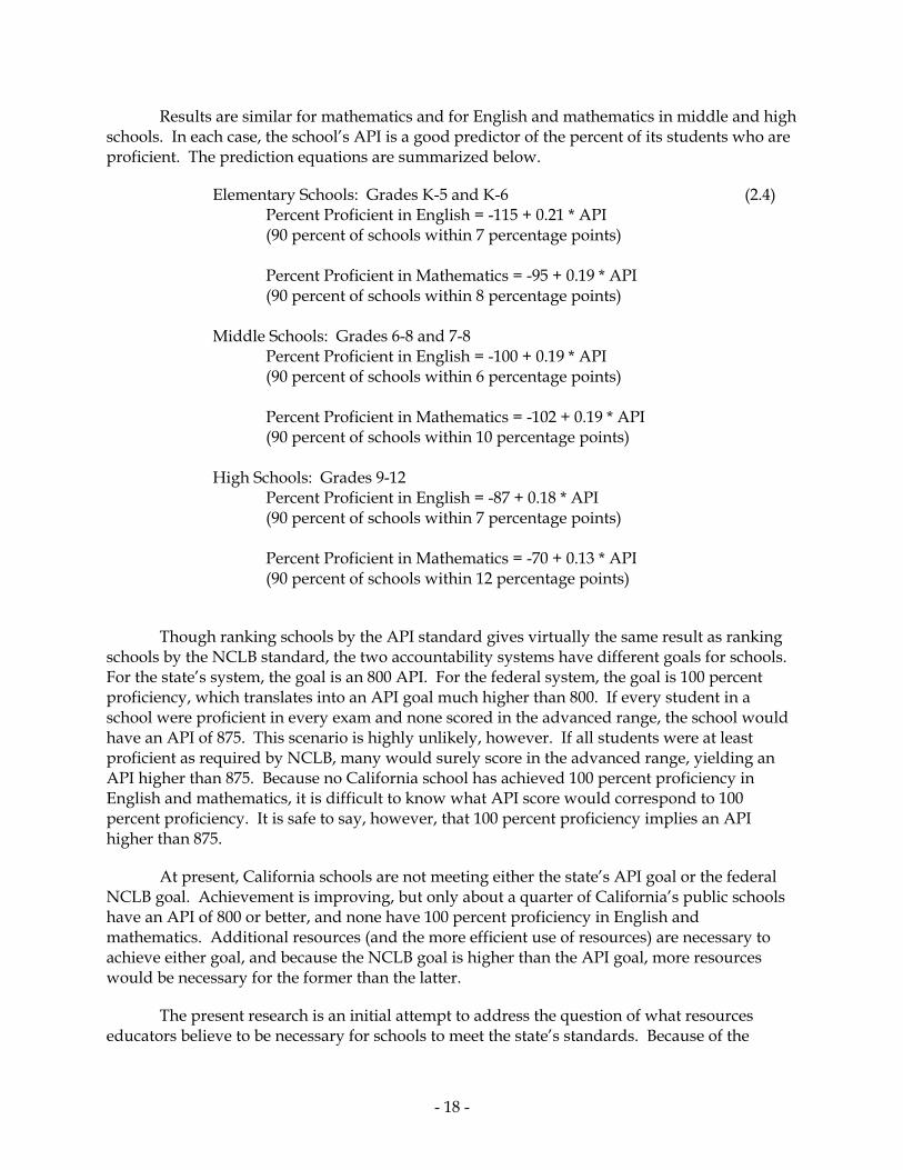
Results are similar for mathematics and for English and mathematics in middle and high schools. In each case, the school’s API is a good predictor of the percent of its students who are proficient. The prediction equations are summarized below.
Elementary Schools: Grades K-5 and K-6 (2.4) Percent Proficient in English = -115 + 0.21 * API (90 percent of schools within 7 percentage points) Percent Proficient in Mathematics = -95 + 0.19 * API (90 percent of schools within 8 percentage points) Middle Schools: Grades 6-8 and 7-8 Percent Proficient in English = -100 + 0.19 * API (90 percent of schools within 6 percentage points) Percent Proficient in Mathematics = -102 + 0.19 * API (90 percent of schools within 10 percentage points) High Schools: Grades 9-12 Percent Proficient in English = -87 + 0.18 * API (90 percent of schools within 7 percentage points) Percent Proficient in Mathematics = -70 + 0.13 * API (90 percent of schools within 12 percentage points)
Though ranking schools by the API standard gives virtually the same result as ranking schools by the NCLB standard, the two accountability systems have different goals for schools. For the state’s system, the goal is an 800 API. For the federal system, the goal is 100 percent proficiency, which translates into an API goal much higher than 800. If every student in a school were proficient in every exam and none scored in the advanced range, the school would have an API of 875. This scenario is highly unlikely, however. If all students were at least proficient as required by NCLB, many would surely score in the advanced range, yielding an API higher than 875. Because no California school has achieved 100 percent proficiency in English and mathematics, it is difficult to know what API score would correspond to 100 percent proficiency. It is safe to say, however, that 100 percent proficiency implies an API higher than 875.
At present, California schools are not meeting either the state’s API goal or the federal NCLB goal. Achievement is improving, but only about a quarter of California’s public schools have an API of 800 or better, and none have 100 percent proficiency in English and mathematics. Additional resources (and the more efficient use of resources) are necessary to achieve either goal, and because the NCLB goal is higher than the API goal, more resources would be necessary for the former than the latter.
The present research is an initial attempt to address the question of what resources educators believe to be necessary for schools to meet the state’s standards. Because of the
- 18 -

exploratory nature of the research, it seems prudent to begin with a conservative definition of that goal, which is the API goal of 800. While that definition is less demanding that the NCLB definition, it would still be a considerable achievement for California schools. As pointed out in Rose, Sonstelie, Reinhard, and Heng (2003), an 800 API is equivalent to 70 percent of a school’s students exceeding the median performance of students through the country. If the resources required to meet that goal seem feasible, it would then be appropriate to consider the question of what resources would be necessary to achieve the more ambitious goal of 100 percent proficiency in English and mathematics.
Because this research focuses on the API goal of 800, all simulation participants were asked to predict academic achievement in terms of the API. In addition, however, middle school participants were asked to predict the percentage of students scoring proficient or better on the mathematics portion of the California Standards Test, and high school participants were asked to predict their school’s graduation rate. Furthermore, Equation 2.4 provides simple formulas for translating API scores into measures of percent proficient. When results concerning API predictions are presented in what follows, those formulas are used to translate the results into predictions about percent proficient in English and mathematics.
This discussion of measures of academic achievement begs the more fundamental question of whether the state’s current battery of standardized tests adequately measures whether students are receiving the education outlined for them by the state’s academic content standards, which include standards in science, history, and social science as well as English and mathematics. The API does include scores from standardized tests in history and science, but the current index is weighted heavily towards English and mathematics. Even if those weights were changed, however, it is not clear that standardized tests could ever adequately measure a student’s comprehension of fundamental scientific and historical knowledge. Students may do well on a standardized test in science without ever conducting a laboratory experiment. They may do well on a multiple choice history exam without ever writing a paper attempting to connect seemingly disparate historical events. At best, therefore, our current battery of tests set certain necessary conditions for California students. Well-educated students should perform reasonably well on these tests. That does not mean, however, that students who perform well on standardized tests are well educated.
From that perspective, this research asks about the resources necessary for schools to reach some minimum achievement level, which is a necessary, but not sufficient, condition for an adequate education. Because three-fourths of schools have yet to achieve that minimum level, the question is worth asking, even though it is surely too narrow in scope. Furthermore, whatever one thinks about the API goal of 800, the legislature has asked California schools to achieve it. From a policy perspective, the cost of achieving that goal is therefore salient.
All measures of academic achievement are affected by the characteristics of students, a central feature of the simulations described below. In anticipation of those developments, the remainder of this section reviews two well-known relationships between student characteristics and the API. The first relationship concerns the income of a student’s family. Family income determines whether a student is eligible for the federal school lunch program and thus,
- 19 -

Figure 2.4 Percent of Students Participating in Subsidized School Lunch Program and API,
K-5 and K-6 Schools, 2004
300
400
500
600
700
800
900
1000
0% 20% 40% 60% 80% 100%
Percent of Students in School Lunch Program
Aca
dem
ic P
erfo
rman
ce In
dex
participation in the federal school lunch program can serve as a crude index of poverty. For K-5 and K-6 schools in 2004, Figure 2.4 plots the percent of a school’s students participating in the school lunch program and the school’s API.
As the figure makes clear, there is a clear negative relationship between API and the percent of students participating in the federal school lunch program. Of the schools depicted in Figure 2.4, 491 had 10 percent or fewer of their students participating in the school lunch program. Only 11 of those schools had an API less than 800. In contrast, 715 schools had 90 percent or more of their students participating in the school lunch program. Only one of those schools had an API exceeding 800. Similar results hold for middle and high schools.
- 20 -

Figure 2.5 Percent of Students Classified as English Learners and API,
K-5 and K-6 Schools, 2004
300
400
500
600
700
800
900
1000
0% 20% 40% 60% 80% 100%
Percent of Students Classified as English Learners
Aca
dem
ic P
erfo
rman
ce In
dex
The other important characteristic is the primary language spoken by the student’s family. As Figure 2.5 shows, a school’s API is negatively related to the percentage of its students classified as English learners. However, a comparison of Figures 2.4 and 2.5 suggests that API may not be as closely related to language status as it is to poverty.
- 21 -

This suggestion is confirmed by a simple statistical analysis. The statistical techniques described above were used to generate a prediction of a school’s API as a linear function of the percentage of its students in the federal school lunch program (LUNCH) and the percentage of its students classified as English learners (EL). The prediction equations are as follows:3
Elementary Schools: Grades K-5 and K-6 (2.5) Predicted API = 876 – 2.3 * LUNCH – 0.4 * EL (90 percent of schools within 75 API points) Middle Schools: Grades 6-8 and 7-8 Predicted API = 837 – 2.6 * LUNCH – 0.7 * EL (90 percent of schools within 80 API points) High Schools: Grades 9-12 Predicted API = 764 – 2.1 * LUNCH – 1.1 * EL (90 percent of schools within 88 API points)
In all three equations, the effect on the predicted API of an increase in student poverty is at least twice as great as the effect of an increase in the percentage of English learners. For the elementary schools, a 10-point increase in the percentage of students in the school lunch program decreases the predicted API by 23 points. In contrast, a 10-point increase in the percentage of English learners decreases the predicted API by 4 points. The effect on API of an increase in English learners is higher for middle schools than for elementary schools and higher for high schools than for middle schools. Even for high schools, however, an increase in the percentage of students in the school lunch program has a larger negative effect on the predicted API than an increase in the percentage of English learners.
2.5. School Characteristics
The clear relationship between academic achievement and family income demonstrates why student characteristics should play a role in the simulations. Accordingly, the simulations describe the students in each participant’s hypothetical school, and the descriptions varied among participants, revealing how student characteristics affect resource choices and API predictions. To ensure that participants had hypothetical schools like those they had experienced, the description of each hypothetical school was taken from the participant’s actual school. For superintendents, the hypothetical school was a school in the superintendent’s district. The variety of school descriptions in the simulations were thus determined by the selection of participants. Section 3 discusses the selection process. This section explains how the hypothetical schools were described to participants and how the characteristics of schools are incorporated in the statistical analysis.
The description of schools follows the format of the API reports produced by the California Department of Education for individual schools. In fact, the description of a
3 LUNCH and EL are significantly different from zero in all three regressions. The R-square is 0.74 for the elementary regression, 0.74 for the middle school regression, and 0.53 for the high school regression.
- 22 -

participant’s hypothetical school was taken from the 2004 API Base Report for the participant’s actual school. Here are the characteristics provided to participants:
Enrollment Participation in free or reduced price lunch program (percentage of students) English language learners (percentage of students) Race and ethnicity (percentage of students) African American (not of Hispanic origin) American Indian or Alaska Native
Asian Filipino Hispanic or Latino Pacific Islander
White (not of Hispanic origin) Parental education (percentage of students)
Not a high school graduate High school graduate Some college College graduate Graduate school
In addition, the middle and high school simulations provided a description of the average achievement of students in the hypothetical school’s feeder schools. Achievement levels were expressed in terms of both the average API of the feeder schools and the percent of students in those schools proficient in English and mathematics. However, unlike the student characteristics listed above for which variations were determined through the selection of participants, the average API of feeder schools was selected randomly just as were the budget levels. The feeder school API was then used to determine the percent proficient in English and mathematics, following Equation 2.4. The selection of the feeder school API is described in Section 3.
As described in Appendix A, the characteristics of hypothetical schools are incorporated into the linear expenditure system, which allows the predictions of the resource choices to depend on those characteristics. In particular, the analysis incorporates four characteristics: enrollment, percent of students participating in the free or reduced price lunch program, percent of students classified as English language learners, and the average API of feeder schools (for middle and high school simulations).
In addition, the analysis incorporates two variables describing the participants themselves. The first is their type: teacher, principal, or superintendent. The second is the similar school ranking of their school. This ranking is based on a school’s API relative to those of other schools with similar characteristics, particularly characteristics of the school’s students. A school with a ranking of 10 has an API in the top 10 percent of schools similar to it. A school with a ranking of 1 has an API in the bottom 10 percent of its similar schools. A school’s similar school ranking indicates how well it is doing given the conditions under which it operates. In
- 23 -

the case of superintendents, the similar school ranking is the average of the rankings of all schools in the superintendent’s district.
In the analysis that follows, resource choices are first presented for the average school, a hypothetical school that has average values for all of the characteristics incorporated in the analysis. Each characteristic is then analyzed separately showing how resource choices would change as the characteristic changes, holding all other characteristics at their average. The characteristics enumerated above—enrollment, percent participating in the subsidized lunch program, percent English learners, participant type, and similar school ranking—are also incorporated in the predictions of academic achievement.
2.6. Special Education
The simulations do not include resources for special education. In particular, participants were instructed to assume that none of the students in their hypothetical schools needed special education services. This section describes how the simulation estimates are adjusted to incorporate special education.
The adjustments are easiest to describe by example. Suppose the simulations yield the prediction that an elementary school with certain characteristics and a budget of $5,000 per pupil would achieve an API of 850. This prediction is made under the assumption that none of the school’s students have a disability requiring special education services. To incorporate special education, two adjustments are made. First, the budget is increased for the additional services special education students require. Second, the API prediction is lowered to reflect the reality that students with disabilities do less well, on average, on the standardized tests used to calculate the API of a school.
The first adjustment is based on the recent report by Parrish, Harr, Kidron, Brock and Anand (2004). Appendix H of that report lists the 13 student disabilities delineated in the California Special Education Management Information System (CASEMIS) and provides the average cost per student for each disability. The costs are additional: the total cost of educating a student with a particular disability minus the cost of educating a student with no disability. These additional costs for each disability were then multiplied by the number of students in California with each disability in 2003-04, and the products summed over disability categories to yield a total cost for special education. The total was $5.4 billion. Dividing by the total number of students in 2003-04 (6.2 million) yields a special education cost of $870 per student.
This cost is used in the following way. Returning to the example, suppose the cost of achieving an API of 850 in a hypothetical school is $5,000 per student. That number represents the cost of achieving that API assuming that none of the students in the school requires special education services. To this total, add $870 for a total of $5,870 per pupil, which is the cost per student of the hypothetical school assuming its students require special education services typical of schools throughout the state.
- 24 -

Table 2.2 Proficiency in Mathematics and English for Disabled and Non-disabled Students, 2004
Disabled 21.3 14.6 9.6Non-disabled 48.0 38.6 90.4All students 45.4 36.3
Disabled 7.9 7.3 13.6Non-disabled 35.1 37.6 86.4All students 32.5 33.5
Disabled 4.2 5.5 9.0Non-disabled 20.9 38.0 91.0All students 20.0 35.0
Percent ofStudents
Percent Proficient
Grades 2-5
Grades 6-8
Grades 9-11
Mathematics English
The second adjustment is made to the API prediction. As Table 2.2 demonstrates, students with disabilities have lower proficiency rates on state tests than do other students. These differences are used to adjust API predictions. The adjustments begin with the average relationship between the API of a school and the percent of its students proficient in mathematics (MATH) and English-language arts (ELA). A least-squares estimate of that relationships is as follows:
Elementary Schools: Grades K-5 and K-6 (2.6) API = 538 + 2.01 * MATH + 2.82 * ELA (R-square: 0.97) Middle Schools: Grades 6-8 and 7-8 API = 526 + 0.98 * MATH + 4.00 * ELA (R-square: 0.97) High Schools: Grades 9 – 12 API = 494 + 0.58 * MATH + 4.52 * ELA (R-square: 0.92)
These estimates are used to infer the effect of disabled students on a school’s API. Consider first a representative California elementary school. According to Table 2.2, if none of its students were disabled, 48 percent would be proficient in mathematics and 38.6 percent proficient in English, yielding an API of 743. If instead the school was representative of all students, disabled and non-disabled, the percent proficient in mathematics would fall to 45.4 percent, the percent proficient in English would fall to 36.3 percent, and the API would fall to 732, a decline of 1.6 percent. For middle schools, the equivalent decline in API would be 2.7 percent; for high schools, 2.0 percent.
When adjustments for special education are made in what follows, these percentages changes are applied to the predicted API from the simulations. Returning to the elementary
- 25 -

school example, based on the simulations, a school with a budget of $5,000 per student is predicted to have an API of 850. Adjusting this prediction to incorporate special education means increasing the school’s budget to $5,870 per pupil and reducing the API prediction by 1.6 percent, from 850 to 836.
- 26 -

3. Selection of Participants and Assignment of Scenarios
The simulations differ among elementary, middle, and high schools because of resource descriptions and achievement measures unique to each type of school. Within each type, the simulations also differ among participants. One difference is the description of the hypothetical school’s students, and another is the school’s budget. For middle and high school simulations, participants are also instructed to make different assumptions about the average API of their feeder schools. Because the description of each participant’s hypothetical school is taken from his or her actual school, the school descriptions in the simulations are determined by the selection of participants. The budgets and feeder APIs are part of the simulation design, however. This section describes the selection of participants and the assignment of budgets and feeder school APIs.
3.1. Selection of Participants
Participants were selected by first choosing schools and then selecting participants based on their association with those schools. In the case of a principal, a school was chosen, and then the principal of the school was invited to participate. In the case of teachers, a school was chosen, and its principal was asked to identify a volunteer among the school’s teachers. For superintendents, a school in each district was chosen to represent the district. From among those schools, a random sample was chosen, and their superintendents invited to participate.
Schools were chosen by stratified random sampling. Schools were stratified into 27 groups, and the same number of schools was randomly selected from each group. The stratifications were based on three factors: grade span, enrollment, and percent of students participating in a school’s free or reduced-price lunch program. In what follows, this last factor is referred to by the shorthand of socio-economic status (SES).
To stratify schools, all schools in California were first grouped according to grade span: elementary, middle, and high school. Within each grade span, schools were divided into three equally sized groups based on enrollment in 2003-04. Within each of these nine groups, schools were further separated into three equally sized groups based on SES. This stratification yields 27 groups. Within each of the 27 groups, schools were randomly selected to be either a source of principals or a source of teachers.
The same grouping of schools was used to select superintendents. First, each district was assigned to one of the 27 groups, based on the frequency of its schools in each group relative to the frequencies of schools in all districts. After a district was assigned to a group, one school was randomly selected from all the district’s schools in that group. This school represented the district. From that point, the selection of superintendents worked exactly as the selection of principals and teachers.
Certain types of schools were excluded from the sample. Excluded were day schools, alternative schools, juvenile court schools, special education schools, continuation schools, and regional occupation centers. Elementary schools were defined to be schools in which kindergarten is the lowest grade and grades 5 or 6 are the highest grade. More than 4,000
- 27 -

schools fell in this class. Middle schools were defined to be schools in which the lowest grade are either 6 or 7 and the highest grade is 8. This group has more than 1,000 schools. High schools were defined as schools with grades 9 through 12. Nearly 800 schools fall in this class. The largest group of schools excluded by these definitions are the K-8 schools, which number over 500.
The goal was a sample balanced by both group and participant type. In particular, the goal was to have 21 schools in each of the 27 groups. Furthermore, for each group, the goal was seven teachers, seven principals, and seven superintendents. This goal implies 189 elementary schools, 189 middle schools, and 189 high schools. It also implies 189 teachers, 189 principals, and 189 superintendents.
The selection procedure for teachers does not guarantee a random sample. Schools were selected randomly, but teachers within those schools were not. After a school was selected, its principal was contacted and asked to provide the name of a teacher who could be invited to participate. In some cases, principals asked for volunteers from all teachers and selected randomly among their volunteers. In other cases, principals selected individual teachers to ask about their willingness to participate. The invitation to participate was not extended to all teachers. Consequently, relative to a purely random selection of teachers, the teachers in our simulations are likely to be viewed more favorably by their principals, which suggests that their opinions about how resources ought to be allocated may be more in line with the opinions of principals than with those of a random sample of teachers.
3.2. Assignment of Scenarios
Each participant was asked to complete two simulations, each with a different budget. The budgets differed in one of two variables: total expenditures per pupil or the unit costs of certificated personnel. In addition, for participants in the middle and high schools simulations, the average API of feeder schools varied among participants. For an individual participant, however, this API was the same in both simulations. In what follows, the two budgets and the feeder school API are referred to as a scenario.
- 28 -

Table 3.1 Unit Costs of Personnel in Baseline
Certificated personnelTeacher 66,000Principal 112,000Assistant principal 100,000Counselor 87,000Librarian 75,000Academic coach 75,000
Other personnelClerical office staff 41,000Instructional aide 32,000Nurse 87,000Security officer 41,000Technology support staff 86,000Community liaison 40,000
Other resourcesComputer 400
ResourceCost per Year
(dollars)
The budgets are all simple modifications of a baseline. The baseline has total expenditures of $4,000 per pupil, which is approximately 9 percent less than California school districts spent in 2003-04 for the resources covered in the simulations. In the simulations, participants are presented with the total expenditures permitted by their budgets, not expenditures per pupil; but the underlying parameter varying between budgets is expenditures per pupil. The unit costs for the baseline are listed in Table 3.1. The costs are those used Rose, Sonstelie, and Richardson (2004), updated for the general increase in prices from 1999-2000 to 2003-04.
- 29 -

Table 3.2 Scenarios for Elementary Schools of Medium SES
Scenario1 0 0 20 0 Superintendent2 20 0 0 0 Principal3 10 0 30 0 Teacher4 30 0 10 0 Superintendent5 20 0 40 0 Principal6 40 0 20 0 Teacher7 30 0 50 0 Superintendent8 50 0 30 0 Principal9 40 0 60 0 Teacher
10 60 0 40 0 Superintendent11 50 0 70 0 Principal12 70 0 50 0 Teacher13 60 0 80 0 Superintendent14 80 0 60 0 Principal15 40 0 40 15 Teacher16 40 15 40 0 Superintendent17 40 15 40 30 Principal18 40 30 40 15 Teacher19 60 0 60 15 Superintendent20 60 15 60 0 Principal21 60 30 60 15 Teacher
Percent of BaselineFirst Budget Second Budget
ParticipantExpendituresper Student
CertificatedSalaries Type
Expendituresper Student
CertificatedSalaries
Budgets are referred to by the percentage by which they exceed either the baseline expenditures per pupil or unit costs. For elementary schools of medium SES, the budgets were 0, 10, 20, 30, 40, 50, 60, 70, or 80 percent of the baseline. Unit costs of certificated personnel were either 15 or 30 percent of the baseline. Table 3.2 list the 21 scenarios for elementary schools of medium SES.
The scenarios have two notable features. First, only one parameter changes between budgets: either total expenditures per pupil or the unit costs of certificated staff. Second, each scenario except the last has a mirror image. In scenario 1, for example, total expenditures are $4,000 per pupil in the first budget and $4,800 in the second budget. Its mirror image is scenario 2, in which total expenditures are $4,800 per pupil in the first budget and $4,000 per pupil in the second. As a consequence, half of the participants see an increase in resources between the first and second budgets and half see a decrease.
This set of scenarios is the same for large and small elementary schools, but it does vary with the SES of schools. For schools with low SES (the third in a given enrollment strata with the highest percentage of students participating in free or reduced-price lunch), the budget percentages in Table 3.2 were increased by 10 points. For schools with high SES, the percentages were decreased by 10 points.
- 30 -

Table 3.3 Scenarios for Middle and High Schools of Medium SES
Scenario1 650 20 0 40 0 Teacher2 650 40 0 20 0 Superintendent3 650 40 0 60 0 Principal4 650 60 0 40 0 Teacher5 650 60 0 60 15 Superintendent6 650 60 15 60 0 Principal7 650 60 15 60 30 Teacher8 750 10 0 30 0 Superintendent9 750 30 0 10 0 Principal
10 750 30 0 50 0 Teacher11 750 50 0 30 0 Superintendent12 750 50 0 50 15 Principal13 750 50 15 50 0 Teacher14 750 50 15 50 30 Superintendent15 850 0 0 20 0 Principal16 850 20 0 0 0 Teacher17 850 20 0 40 0 Superintendent18 850 40 0 20 0 Principal19 850 40 0 40 15 Teacher20 850 40 15 40 0 Superintendent21 850 40 15 40 30 Principal
per StudentCertificated
Salaries
FeederSchool
API TypeExpendituresper Student
CertificatedSalaries
Percent of BaselineFirst Budget Second Budget
ParticipantExpenditures
In addition to expenditures per pupil and unit costs, the middle and high school scenarios also include the average API of feeder schools. A third of the scenarios had an average API of 650, a third 750, and a third 850. As Table 3.3 shows, as the average API was increased from 650 to 750 or from 750 to 850, the budget percentages were decreased by10 points. As in the case of the elementary school simulations, the same set of scenarios was used for the groups of small and large schools. Also as in the case of elementary schools, the budget percentages varied with the SES of the group. For the low SES groups, budget percentages were reduced by five points. For the high SES groups, percentages were increased by five points.
3.3. Recruiting Participants
As a practical matter, the scenarios outlined above define 567 unique simulations. Invitations to complete the simulations were issues in six rounds. In the first, 567 individuals were identified by randomly selecting 21 schools from each group. A unique simulation was created for each individual using the scenarios and the description of their schools. Individuals were then sent a letter explaining the survey and inviting them to participate. The invitation specified a web site and log-in information that directed each to their unique simulation. Individuals were given three weeks to complete their simulations and were paid $250 for doing so. Appendix F is a copy of the invitation letter.
- 31 -

After the deadline, a second group of individuals was chosen in the same way to complete any scenarios not completed in the first round. School descriptions were changed to match the schools for this second group of individuals. Everything else proceeded as in the first round. Three more rounds were conducted in the same way, one invitation being issued for each scenario that hadn’t been completed. In the sixth and final round, multiple invitations were issued for the few remaining scenarios.
The response rate to these invitations varied by type of participant. It was highest among teachers; 86.7 percent of those invited completed the simulations. For principals and superintendents, the response rate was 43 percent and 41.5 percent. The high response rate from teachers is somewhat misleading, however. Principals of 1,214 schools were first asked to identify a teacher at their school who would be willing to participate in the simulations. This request yielded the names of 465 teachers. Invitations to participate were then sent to randomly selected teachers from this group. Because they had already expressed an interest in participating, it is only natural that they would be highly likely to do so if invited.
This recruitment process resulted in 568 complete simulations, one more than the goal. For teachers, all scenarios were completed, and none were duplicated, for a total of 189 responses. All scenarios were also completed for principals, and one was duplicated, for a total of 190 responses. For superintendents, 189 simulations were completed, and four were duplicated, leaving four scenarios uncompleted. The uncompleted scenarios were spread among grade spans, however. In total, there were 190 complete scenarios for elementary schools, 189 complete scenarios for middle schools, and 189 complete scenarios for high schools.
3.4. Comparing Simulation Schools with All Schools
Because the selection process described above is random, the resulting sample of schools should be representative of all California schools. This section compares the sample with all schools along four dimensions: region of the state, enrollment, percent of students in a school’s free or reduced-price lunch program, and percent of students classified as English learners. Comparisons are made between the sample school and all schools and between the sample school and the grade spans from which the sample was drawn: K-5, K-6, 6-8, 7-8, and 9-12. Several types of schools were excluded from the sample and are also excluded in calculating statistics for all schools: day schools, juvenile court schools, alternative schools, special education schools, continuation schools and regional occupation centers.
- 32 -

Table 3.4 Regional Distribution of California Public Schools, 2003-04
Northern California 7.0% 3.6% 7.0%Bay Area 17.8 19.7 18.4Central Coast 11.4 6.9 6.8Central Valley 23.1 19.0 21.2Los Angeles Area 32.8 42.4 38.4San Diego and Imperial Counties 7.9 8.4 8.2
Northern California: Butte, Colusa, Del Norte, Glenn, Humboldt, Lake, Lassen,Mendocino, Modoc, Nevada, Plumas, Shasta, Sierra, Siskiyou, Sutter, Tehama,Trinity, and Yuba Counties.Bay Area: Alameda, Contra Costa, Marin, Napa, San Francisco, San Mateo,Santa Clara, Solano, and Sonoma Counties.Central Coast: Monterey, San Benito, San Luis Obispo, Santa Barbara,Santa Cruz, and Ventura Counties.Central Valley: Alpine, Amador, Calaveras, El Dorado, Fresno, Inyo, Kern, KingsMadera, Mariposa, Merced, Mono, Placer, Sacramento, San Joaquin, Stanislaus,Tulare, Tuolumne, and Yolo Counties.Los Angeles Area: Los Angeles, Orange, Riverside, and San Bernardino Counties.
AllSchools
SampleSchools
K-5, K-6, 6-8, 7-8,and 9-12 Schools
The sample of schools is reasonably representative of California’s major regions. As Table 3.4 reveals, Northern California and the Central Coast are overrepresented in the sample, and the Los Angeles area is underrepresented. If the comparison is to all California schools, not just to the grade spans from which the sample schools were selected, the representation of the sample improves considerably.
- 33 -

Table 3.5 Enrollment in California Public Schools, 2003-04
Elementary SchoolsAverage 583 615 566Standard Deviation 226 241 275
Middle SchoolsAverage 959 981 942Standard Deviation 395 481 502
High SchoolsAverage 1,759 1,922 1,658Standard Deviation 993 1,016 1,129
All Schools
SampleSchools
K-5, K-6, 6-8, 7-8,and 9-12 Schools
Because the selection of schools was stratified in part on enrollment, the distribution of the sample schools by enrollment should closely follow the distribution of that of all schools. As Table 3.5 shows, that expectation is borne out. For each grade span, the average and standard deviation of enrollment for sample schools is very close to the same statistics for all schools.
- 34 -

Table 3.6 Percent of Students Participating in Subsidized Lunch Program, California Public Schools,
2003-04
Elementary SchoolsAverage 51.7% 54.0% 53.6%Standard Deviation 30.8 31.6 31.3
Middle SchoolsAverage 44.2 46.0 47.0Standard Deviation 27.8 27.3 27.8
High SchoolsAverage 31.9 34.6 35.4Standard Deviation 22.5 24.5 25.4
All Schools
SampleSchools
K-5, K-6, 6-8, 7-8,and 9-12 Schools
The selection of sample schools was also stratified by the percentage of students participating in the school’s free or reduced-price lunch program. As expected, the distribution of this variable in the sample closely matches the distribution among all schools (Table 3.6).
- 35 -

Table 3.7 Percent of Students Classified as English Learners, California Public Schools, 2003-04
Elementary SchoolsAverage 26.2% 29.1% 27.6%Standard Deviation 21.6 22.8 23.2
Middle SchoolsAverage 17.5 20.0 20.2Standard Deviation 15.9 16.6 17.4
High SchoolsAverage 13.4 16.0 15.1Standard Deviation 12.5 14.1 14.8
All Schools
SampleSchools
K-5, K-6, 6-8, 7-8,and 9-12 Schools
The selection process was not stratified according to the percentage of English learners in each school, but the distribution of this variable among sample schools is reasonably representative of all schools (Table 3.7). The mean of this variable is lower for each grade span of the sample schools than is the equivalent mean for all schools. However, the differences are small, and the sample schools display as much variation in this variable as do all schools.
- 36 -

Table 3.8 Distribution of Similar Schools Rank for Sample Schools
1 5.39 1.112 8.09 6.673 12.13 10.564 12.40 15.565 8.36 16.116 13.75 20.567 9.97 13.338 10.24 10.569 8.89 3.89
10 10.78 1.67
SimilarSchool Rank
Percentage ofTeachers and Principals
Percentage ofSuperintendents
The final variable to consider is the similar schools rank, which compares the API of a school to those of other schools with similar characteristics. It is a measure of academic achievement adjusting for the characteristics of schools, particularly the background of their students. Each rank is a decile, so roughly 10 percent of all schools should have each similar school rank. As Table 3.8 shows, the similar school ranks for principals and teachers in the sample are generally representative of all schools in the state. The lowest rank is underrepresented, but the remaining ranks are reasonably close to 10 percent.
The similar-schools rank for superintendents has higher frequencies than 10 percent near the middle of the distribution of ranks and lower frequencies near the extremes. This is to be expected, however, because the rank for each superintendent is the average of the ranks of all schools in his or her district.
- 37 -


4. Results from Elementary School Simulation
Because the elementary, middle, and high school simulations each have unique features, the results from those simulations are reported in three separate sections. However, a common method is used in analyzing those results, and the same format is used in presenting them. The sections begin by briefly describing the characteristics of the hypothetical schools. That description is followed by the resource choices predicted for the simulation’s average school, predictions based on the linear expenditure system described in Sections 2.2 and 2.5. The sections then show how those predictions change as the characteristics of schools and participants change. Finally, the sections report the relationship between predictions of student achievement and other factors, including total expenditures per pupil and student SES.
- 39 -

Table 4.1 Summary Statistics for Elementary School Simulations
Total expenditures (dollars/student) 5,709 844 3,600 7,600Unit cost for teachers (dollars/FTE) 69,048 5,908 66,000 85,800Enrollment 583 226 96 1263Percent in subsidized lunch program 52 31 0 100Percent English learners 26 22 0 82
MaximumStandard
Mean Deviation Minimum
School descriptions varied widely among participants in the elementary simulations. The smallest school had 96 students, and the largest had 1,263. Six of the 190 schools had no students participating in the free or reduced-price lunch program, and 12 had all students participating. One school had 82 percent of its students classified as English learners; another had 79 percent. Yet, seven schools had no English learners. Table 4.1 summarizes the distribution of key variables.
- 40 -

Table 4.2 Estimated Resource Choices for the Average Elementary School
Resource Unit of MeasureTeachers
Kindergarten FTE 4.5 5.2Grades 1-3 FTE 13.1 14.1Grades 4 and 5 FTE 6.6 7.8Specialty 1.3 2.2
AdministrationPrincipals FTE 1.2 1.2Assistant principals FTE 0.2 0.5Clerical office staff FTE 2.1 2.7
Support staffInstructional aides FTE 1.3 6.0Counselors FTE 0.4 0.7Nurses FTE 0.3 0.6Librarians FTE 0.4 0.9Security officers FTE 0.1 0.2Technology support staff FTE 0.4 1.0Community liaisons FTE 0.3 0.6
Professional developmentAcademic coaches FTE 0.2 1.4Collaborative time Hours/year/teacher 40.5 59.0
Student programsPre-school Students 0.4 1.6After-school tutoring Teacher hours/week 18.1 40.8Summer school Students 60.2 119.8Longer school year Days/year -0.3 4.3Longer school day Hours/day 0.0 0.3Full-day kindergarten 1=yes 0=no 0.5 0.6Computers for instruction Computers 65.5 151.5
Other $ thousands -14.5 52.5
Class sizeKindergarten 21.4 18.7Grades 1-3 22.2 20.7Grades 4 and 5 29.3 24.8
$4,000 $6,000Expenditures per Student
The resources chosen by participants under these varying conditions were used to estimate the linear expenditure system described in Sections 2.2 and 2.5. Table 4.2 reports the choices predicted by that system. The predictions are for the average school, which has 583 students, 52 percent of whom participate in the school’s subsidized lunch program and 26 percent of whom are English learners. Estimated resource choices are presented for two levels of total expenditures: $4,000 per pupil, which approximates the average budget of a California school in 2003-04, and $6,000 per pupil, a budget 50 percent larger.
The higher budget funds increases in all spending areas. Twenty-one percent of the increase is allocated to hiring more teachers, 5 percent to more administrators, 26 percent to
- 41 -

more staff positions, 11 percent to professional development, 31 percent to student programs, and 6 percent to other expenditures.
Because of differences in the allocation of revenue among areas in the baseline budget, the shares of additional spending translate into different percentage increases in each area. The teaching staff increases from 25.6 FTE to 29.3 FTE, an increase of 15 percent. The larger staff reduces average class sizes particularly in grades 4 and 5, where class sizes decline from 29 students per class to 25. Administrative staff increases from 3.4 FTE to 4.3 FTE, an increase of 27 percent. While the percentage increases in the teaching and administrative staff are substantial, both are much less than the 50 percent increase in total expenditures.
Necessarily, other areas increase much more in percentage terms. Support staff triples from 3.2 FTE to 9.9 FTE. More than half of that increase is due to an increase from 1.3 FTE to 6.0 FTE in instructional aides. Expenditures on professional development also rise substantially. With the larger budget, an academic coach is added, and the time teachers work together on curriculum, assessment, and pedagogy increases from 41 to 59 hours per year.
With the larger budget, hours of instruction also increase. The school day is lengthened by 18 minutes, and the school year by 4 days. Participants also add individualized instructional time for students who are falling behind. The after-school tutoring program increases from 18 teacher hours per week to 41. The number of students in summer school doubles to 120.
Given total expenditures of $6,000 per pupil, practitioners allocate over $90 per pupil to the category of “other expenditures.” Participants’ descriptions of these varied widely. In some cases, they described expenditures that fell under other categories in the spreadsheet—art and music teachers, for example, who are classified as specialty teachers in the spreadsheets. In other cases, participants mentioned resources that they were instructed to assume were adequately provided, such as instructional materials and school supplies. In several other cases, participants singled out specific expenditures that were related to other categories in the spreadsheet, but not explicitly included in those categories. Typical of those were a variety of professional development activities such as training workshops for teachers.
Those difficult cases notwithstanding, the descriptions convey a clear message. If provided more funds, participants would allocate some of those funds to enrichment activities such as field trips, science camps, assemblies, artistic performances, and guest speakers. Some would also allocate extra funds for parent education classes. One wrote that she would allocate more than $300,000 of her budget to hire “bilingual teachers to teach parent education classes on how to help their child succeed in school and guide an after-school tutoring program with parents being involved.”
- 42 -

Figure 4.1 Allocation of Expenditures as Total Expenditures Change, Elementary School Simulations
$0
$1,000
$2,000
$3,000
$4,000
Teach
ers
Admini
strati
on
Suppo
rt staff
Profes
sional
developm
ent
Student
program
sOthe
r
dolla
rs/s
tude
nt
$4,000/student$6,000/student
The general trends in Table 4.2 are summarized in Figure 4.1, which displays expenditures per student in the six resource areas. In percentage terms, the biggest area of increase is student programs, for which expenditures triple. Expenditures on support staff and professional development increase by more than 150 percent. In contrast, expenditures on administration increase by 24 percent, and expenditures on teachers increase by 15 percent.
- 43 -

Figure 4.2 Allocation of Expenditures as Enrollment Changes, Elementary School Simulations
$0
$1,000
$2,000
$3,000
$4,000
Teach
ers
Admini
strati
on
Suppo
rt staff
Profes
sional
developm
ent
Student
program
sOthe
r
dolla
rs/s
tude
nt
357 students809 students
The simulations suggest some modest economies of scale. Moving from a school with
357 students (one standard deviation below the average) to a school of 809 students (one standard deviation above the average), administrative expenditures per pupil decrease by 36 percent, permitting a 36 percent increase in expenditures per pupil on student programs. Expenditures per pupil on support staff also decrease by 18 percent, and other expenditures per pupil rise by 100 percent.
- 44 -

Figure 4.3 Allocation of Expenditures as Participation in Subsidized Lunch Program Changes,
Elementary School Simulations
$0
$1,000
$2,000
$3,000
$4,000
Teach
ers
Admini
strati
on
Suppo
rt staff
Profes
sional
developm
ent
Student
program
sOthe
r
dolla
rs/s
tude
nt
No students in lunch programAll students in lunch program
Expenditures by area also change as the socio-economic status of students change.
Moving from a school in which no students participate in the free or reduced-price lunch program to a school in which all students participate, expenditures on student programs increase by 20 percent and administrative expenditures increase by 27 percent. Expenditures on support staff also increase by 10 percent. These increases are financed by a decrease of 8 percent in teacher expenditures, 20 percent in professional development, and 30 percent in other expenditures.
- 45 -

Figure 4.4 Allocation of Expenditures as Percent of English Learners Changes,
Elementary School Simulations
$0
$1,000
$2,000
$3,000
$4,000
Teach
ers
Admini
strati
on
Suppo
rt staff
Profes
sional
developm
ent
Student
program
sOthe
r
dolla
rs/s
tude
nt
No English learners82% English learners
Though the percentage of English learners in a school is highly correlated with
participation in the subsidized lunch program, an increase in the percentage of English learners has a different effect on predicted expenditures. As students classified as English learners increase from zero percent to 82 percent (the highest percentage in the sample), expenditures on professional development increase by 83 percent. This increase is financed by decreases of 9 to 16 percent in every other area except teacher expenditures, which remain essentially unchanged.
- 46 -

Figure 4.5 Allocation of Expenditures by Participant Type, Elementary School Simulations
$0
$1,000
$2,000
$3,000
$4,000
Teach
ers
Admini
strati
on
Suppo
rt staff
Profes
sional
developm
ent
Student
program
sOthe
r
dolla
rs/s
tude
nt
TeachersPrincipalsSuperintendents
Resource choices also varied by the type of participant. In contrast to superintendents, teachers would allocate more of their budgets to support staff and less to student programs (Figure 4.5). Principals fall in between—more to support staff than superintendents but less than teachers, less to student programs than superintendents but more than teachers.
- 47 -
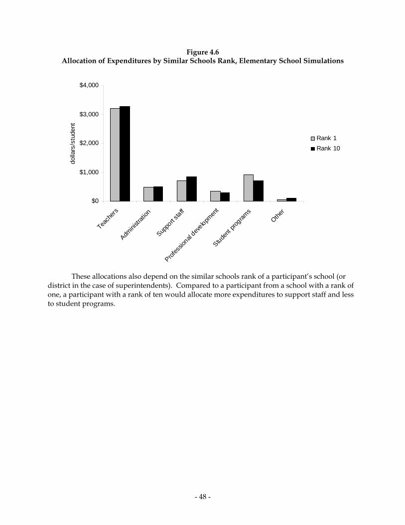
Figure 4.6 Allocation of Expenditures by Similar Schools Rank, Elementary School Simulations
$0
$1,000
$2,000
$3,000
$4,000
Teach
ers
Admini
strati
on
Suppo
rt staff
Profes
sional
developm
ent
Student
program
sOthe
r
dolla
rs/s
tude
nt
Rank 1Rank 10
These allocations also depend on the similar schools rank of a participant’s school (or
district in the case of superintendents). Compared to a participant from a school with a rank of one, a participant with a rank of ten would allocate more expenditures to support staff and less to student programs.
- 48 -

Table 4.3 Coefficient Estimates for Relationship Between Predicted Achievement
and Conditioning Variables, Elementary School Simulations
Conditioning VariablesExpenditures per pupil 0.0130 0.0039 0.0027 0.0025Unit cost of teachers -0.0004 0.0005 -0.0001 -0.0001Teacher index (1 if teacher, 0 otherwise) -2.4584 7.6614 -0.5163 -0.4671Principal index (1 if principal, 0 otherwise 10.9474 7.6443 2.2990 2.0800Enrollment 0.0099 0.0152 0.0021 0.0019Percent in subsidized lunch -1.4522 0.1523 -0.3050 -0.2759Percent English learners 0.0100 0.2332 0.0021 0.0019Similar schools rank 3.8082 1.2248 0.7997 0.7236Constant 787.3 40.6 50.3 54.6
R-squared 0.35
For Percent ProficientEnglish Math
Equivalent Coefficients
Coefficient St. Error
Academic Performance Index
Table 4.3 reports estimates of the relationship between the APIs predicted by participants and several important variables conditioning each simulation. These conditioning variables are either assumptions that participants were instructed to take as conditions defining the simulation (budget, unit costs, enrollment, student characteristics) or characteristics of the participants themselves (superintendent, principal, teacher, similar school rank). The API predictions are assumed to be a linear function of those conditioning variables. The first column lists the estimated coefficients for that function. For example, the coefficient for expenditures per pupil is 0.0130, implying that a $1,000 increase in expenditures per pupil increases the average API prediction by 13 points. The third and fourth columns present the same coefficient estimate transformed by Equation 2.8 so that they apply to the percentage of students proficient in English and mathematics. A $1,000 increase in expenditures per pupil, for example, increases the percentage proficient in English by 2.7 points.
As discussed in Section 2.2, the coefficients are estimates of actual coefficients for an underlying relationship expressing the average prediction of all practitioners (not just those sampled) as a function of the conditioning variables listed in Table 4.3. The second column of Table 4.3 gives the standard errors of those estimates. For any coefficient, the estimate plus or minus 1.65 times its standard error contains the actual coefficient with a probability of 90 percent. For example, the estimate coefficient on expenditures per pupil is 0.0130, its standard error is 0.0039, and so the interval runs from 0.0066 to 0.0194. The probability that this interval contains the coefficient in the underlying relationship is 90 percent. If the interval were expanded, constructed by multiplying the standard error by 1.96 instead of 1.65, the probability that the interval would contain the true coefficient would rise to 95 percent. Because both intervals contain only positive numbers, we can be confident that the actual coefficient is positive.
We can also be confident that the average API prediction falls with an increase in the percentage of students participating in the free or reduced-price lunch program. The estimated coefficient for that variable is -1.45 and its standard error is 0.15, implying a 95 percent
- 49 -

confidence interval of -1.74 to -1.16. A 10 percent increase in the number of students participating in the free or reduced-price lunch program will decrease the average API prediction by 11.6 to 17.4 points.
By the 95 percent standard, the only other variable that has a clearly positive or clearly negative effect is the similar schools rank. Participants from schools with a high similar school rank predict higher achievement, everything else equal, than participants from schools with a lower rank.
Even if the standard is lowered to 90 percent, no other variable has a clearly positive or clearly negative effect on predicted API. These variables are the unit cost of certificated staff, the type of participant (superintendent, principal, or teacher), the school’s enrollment, and the percentage of the school’s students who are English learners.
- 50 -
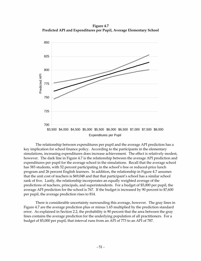
Figure 4.7 Predicted API and Expenditures per Pupil, Average Elementary School
700
725
750
775
800
825
850
$3,500 $4,000 $4,500 $5,000 $5,500 $6,000 $6,500 $7,000 $7,500 $8,000
Expenditures per Pupil
Pre
dict
ed A
PI
The relationship between expenditures per pupil and the average API prediction has a
key implication for school finance policy. According to the participants in the elementary simulations, increasing expenditures does increase achievement. The effect is relatively modest, however. The dark line in Figure 4.7 is the relationship between the average API prediction and expenditures per pupil for the average school in the simulations. Recall that the average school has 583 students, with 52 percent participating in the school’s free or reduced-price lunch program and 26 percent English learners. In addition, the relationship in Figure 4.7 assumes that the unit cost of teachers is $69,048 and that that participant’s school has a similar school rank of five. Lastly, the relationship incorporates an equally weighted average of the predictions of teachers, principals, and superintendents. For a budget of $5,000 per pupil, the average API prediction for the school is 767. If the budget is increased by 90 percent to $7,600 per pupil, the average prediction rises to 814.
There is considerable uncertainty surrounding this average, however. The gray lines in Figure 4.7 are the average prediction plus or minus 1.65 multiplied by the prediction standard error. As explained in Section 2.2, the probability is 90 percent that the area between the gray lines contains the average prediction for the underlying population of all practitioners. For a budget of $5,000 per pupil, that interval runs from an API of 773 to an API of 787.
- 51 -

The API predictions of individual participants vary considerably around the average prediction. The residual standard error is 60 API points, implying that an interval of 120 API points would be necessary to contain 68 percent of the API predictions for any given school.
The estimate of the coefficient on expenditures per pupil derives from two different elements of the budget simulations. First, because individual participants were asked to make API predictions with two different budgets, we observe how the API predictions of individuals change as their budgets change. Second, because different participants have similar schools but different budgets, we observe how the API predictions across participants are affected by the differences in their budgets. While both types of observations are incorporated in the estimates of the expenditure coefficient listed in Table 4.3, each taken individually yields a different estimate of that coefficient. The estimate based solely on how the predictions of individuals change when their budgets change is higher than the estimate based solely on the difference among individuals. However, the difference in coefficient estimates is not large enough to be statistically significant, and the estimates reported in Table 4.3 continue to be used in what follows.4 The same situation holds for estimates of the expenditure coefficient in the middle and high school simulations.
Like expenditures per pupil, the similar schools rank has a modest effect on the average API prediction. Increasing the similar schools rank from five to ten increases the average API prediction by 19 points. Its effect on the average prediction is approximately equal to the effect of an increase of $1,500 in expenditures per pupil. If the similar schools rank reflects the efficiency with which schools employ their resources, moving a school from average to peak efficiency is worth $1,500 per student.
In many cases, simulation participants were asked to predict the API of a school with substantially more resources than schools with which they had first-hand experience. As a consequence, those predictions must be carefully scrutinized. One test of those predictions is to compare them with the actual achievement of California schools. Suppose we assume that a school had a budget of $4,000 per pupil, which is roughly representative of California public schools in 2003-04. With that budget, is the API predicted by the simulation participants similar to the APIs achieved by California schools in 2003-04?
4 The F statistic for the equality of coefficient estimates is 1.98. For the middle school simulation, the statistic is 1.41. For the high school simulation, the statistic is 0.96.
- 52 -

Figure 4.8 Predicted and Actual Academic Performance Indexes: Elementary Schools
400
500
600
700
800
900
1000
0 25 50 75
Percent Subsidized Lunch
Aca
dem
ic P
erfo
rman
ce In
dex
100
The answer to that question lies in Figure 4.8. The figure plots the APIs of California elementary schools in 2003-04 against the percentage of each school’s students participating in the subsidized lunch program. The dark line in the figure is the average API prediction of the simulation participants. In forming that prediction, the school’s budget is assumed to be $4,000 per pupil, and the unit costs of certificated staff are set at their baseline values for the simulation ($66,000 for teachers). Other variables, except for the percentage in subsidized lunch, are set at their mean for the simulations. Under those assumptions, the line traces out the API prediction for different values of the subsidized lunch percentage.
The predicted APIs are reasonably consistent with actual APIs. For low-poverty schools, participants tended to predict lower APIs than schools actually achieved on average, and for high-poverty schools, the reverse is true. The differences between predicted and actual APIs are not large, however.
Another test of the API predictions is to compare them with recent research on the relationship between school resources and academic achievement. One standard for comparison is the analysis by Krueger (1999) of the Tennessee class size experiment. In the experiment, elementary school students and their teachers were randomly assigned to either small classes (13-17 students) or large classes (22-25 students). The assignments lasted from kindergarten through grade 3, and students were assessed at the end of each year using the Stanford Achievement Test (SAT). By the end of the third year, students in the smaller classes
- 53 -

were scoring five percentile points higher on average on the math and reading tests than did students in larger classes. These percentile gains can be directly transformed into equivalent API increases. When first initiated in 1999, California’s API was based solely on the SAT. According to Rogosa (2000), an increase by each student of five percentile points on the SAT translates into an API gain of 41 points.
The last element in this comparison is the cost of class size reductions of the magnitude implemented in Tennessee. The reduction was from about 23.5 students to 15 students in grades K through 3. Assuming the unit cost of teachers is $66,000 per year, the baseline assumption in the simulations, the cost per student of classroom teachers is $4,400 at a class size of 15 students ($66,000/15) and approximately $2,800 at class sizes of 23.5 students ($66,000/23.5). Thus, in the elementary simulation, the cost of reducing class sizes from 23.5 students to 15 students in grades K through 5 is about $1,600 per student. This cost estimate is conservative because it ignores any additional compensation of teachers for professional development time. Putting these elements together, Krueger finds that an expenditure of $1,600 on reducing class sizes would increase a school’s API by 41 points. The 41 point increase is conservative because it is based on achievement gains in grades K through 3 only and ignores possible gains in grades 4 and 5 because of small classes in those grades.
In comparison, the simulation participants predicted a much smaller effect of increased resources on academic achievement. According to the estimates, a $1 increase in expenditures per pupil increases the predicted API by 0.013 points. An increase of $1,600 would increase the predicted API by 21 points, half of the increase found by Krueger.
A second standard for comparison is the analysis of Texas achievement data by Rivkin, Hanushek, and Kain (2005). Though the class sizes in this study were not randomly assigned, the study does have two important advantages over other studies of class size. First, it uses test results for over one million students, making precise estimates more likely. Second, the records of students can be linked across time, revealing the gain in achievement in each grade. Achievement is measured by the Texas Assessment of Academic Skills, and Rivkin and his co-authors focus on math and reading gains in grades 4, 5, 6, and 7. Though that test is not the same as the SAT, Rivkin and his co-authors measure test results in standard deviations around the average test score, which allows estimated effects to be transformed into percentile gains in the distribution of all test scores.
Rivkin and his co-authors find that class size has a statistically significant effect on gains in reading and mathematics. A one-student reduction in class size increases the gain in 4th grade reading scores by 0.0107 standard deviations and the gain in 5th grade scores by 0.0081 standard deviations. Making the conservative assumption that a one-student reduction in grades K through 3 has no effect, the cumulative effect for grades K through 5 is 0.0124 standard deviations. The gain for an 8.5 student reduction is 0.1054 standard deviations. From the mean of the distribution of test scores, an increase of 0.1054 standard deviation is a gain of 4 percentile points. The hypothesized reduction in class size has a slightly larger effect on math score percentiles. From Rogosa, a 4 percentile increase in math and reading scores implies an API increase of 31 points, halfway between the 21 points predicted by simulation participants and the 41 points found by Krueger.
- 54 -

In interpreting these comparisons, it is important to bear in mind that participants would not allocate all of their increased budgets to reducing class sizes. On average, only about 20 percent of any budget increase is allocated to this purpose. Presumably, however, the portion allocated to other areas, such as professional development and after-school tutoring, would have an even larger effect on student achievement than if it were allocated to increasing class sizes. Under that presumption, if an increase of $1,600 per pupil were allocated solely to reducing class sizes, the average API gain predicted by simulation participants would be no greater than 21 points, which is considerably smaller than the achievement gains found by either of the two comparison studies.
- 55 -


5. Results from Middle School Simulations
The middle school simulations differ from the elementary school simulations in four ways. The first is the classification of teachers. In the elementary school simulations, teachers are classified by the grade they teach. In the middle school simulations, they are classified by the subject they teach: core, non-core, or P.E. Secondly, participants in the middle school simulations are not presented with two of the student programs available to participants in the elementary simulation: full-day kindergarten and pre-school. The third difference is that the middle school participants are given the average API of their feeder schools, an assumption that is not part of the elementary school simulations. Finally, in addition to the API prediction, participants in the middle school simulations are asked to predict the percentage of eighth graders proficient in mathematics.
- 57 -

Table 5.1 Summary Statistics for Middle School Simulations
Total expenditures per pupil (dollars) 5,333 695 3,600 6,400Unit cost for teachers (dollars) 69,510 6,044 66,000 85,800Average API of feeder schools 750 82 650 850Enrollment 950 395 159 2,377Percent in subsidized lunch program 44 28 0 100Percent English learners 18 16 0 68
MaximumStandard
Mean Deviation Minimum
The middle schools differed considerably in size and in student characteristics. The schools were almost twice as large, on average, as their elementary school counterparts. For middle schools, the average enrollment was 950 students, as compared to an average of 583 students for elementary schools. Nevertheless, several of the middle schools were quite small. The smallest had 159 students, and eight had fewer than 300 students. At the other extreme, five had more than 1,900 students; the largest had 2,377. Despite their larger average size, the middle schools were nearly as heterogeneous in student characteristics as the elementary schools. In two of the middle schools, no student participated in the subsidized lunch program. In seven schools, fewer than 3 percent of students participated. Yet, in seven other middle schools, all students participated in the subsidized lunch program. On average, fewer students in the middle schools were classified as English learners (18 percent) than was the case for elementary schools (26 percent). Nevertheless, in one middle school, 68 percent of students were English learners. Table 5.1 summarizes the key variables in the middle school simulations.
- 58 -

Table 5.2 Estimated Resource Choices for the Average Middle School
Resource Unit of MeasureTeachers
Core FTE 28.1 34.6Non-core FTE 5.9 8.0P.E. FTE 4.3 6.2
AdministrationPrincipals FTE 1.2 1.3Assistant principals FTE 1.5 1.9Clerical office staff FTE 4.1 5.0
Support staffInstructional aides FTE 5.8 7.7Counselors FTE 2.0 2.8Nurses FTE 0.6 0.9Librarians FTE 1.0 1.3Security officers FTE 1.3 1.7Technology support staff FTE 0.9 1.5Community liaisons FTE 0.8 1.2
Professional developmentAcademic coaches FTE 1.5 3.1Collaborative time Hours/year/teacher 44.7 122.1
Student programsAfter-school tutoring Teacher hours/week 55.6 133.1Summer school Students 204.5 271.2Longer school year Days/year 0.6 4.9Longer school day Hours/day 0.0 0.6Computers for instruction Computers 149.5 322.2
Other $ thousands 18.7 74.0
Class sizeCore 27.0 22.0Non-core 32.4 23.8P.E. 44.4 30.6
$4,000/student $6,000/student
Using the linear expenditure systems described in Sections 2.2 and 2.5, the resource choices made by simulation participants were used to estimate the average choice of participants conditional on their budgets, unit costs, and student characteristics. Those estimates are presented in Table 5.2 for the average middle school, which has 950 students. Forty-four percent of those students participate in the school’s subsidized lunch program, and 18 percent are English learners. The estimates are an average of those for teachers, principals, and superintendents, and they assume that the participants come from a school with a similar schools rank of five. In addition, the estimates assume that the average API of feeder schools is 750.
Resource choices are presented for two budget levels: $4,000 per pupil, representative of California school in 2003-04, and $6,000 per pupil, a 50 percent higher budget. As the table reveals, the additional funds are spread across the six resource areas. A third of the increase is allocated to increasing the teaching staff, 4 percent to increasing administrative staff, and 13
- 59 -

percent to increasing support staff. Professional development receives 16 percent of the increase, and 30 percent goes to student programs. Three percent of the increase is allocated to other expenditures.
These allocations of additional funds imply different percentage increases in each area. The teaching staff increases from 38.3 FTE to 48.8 FTE, an increase of 27 percent. As a result, the average size of core classes falls from 27 students to 22 students. For non-core classes, the decline is from an average of 32 students to an average of 24 students. The average size of P.E. classes also declines.
As in the case of elementary schools, administrative staff also increases less than proportionally to the expansion in the budget. Administrative FTE increase from 6.8 to 8.2, a 20 percent rise.
The percentage increases were much larger for professional development and student programs. With the larger budget, 1.5 academic coaches are added, doubling the total, and the time each teacher spends collaborating with other teachers rises from 45 hours per year to 122 hours per year. The after-school tutoring program nearly triples in size, the school year is lengthened by 4 days, and the school day is lengthen by 36 minutes. The number of computers also rises from 15 for every 100 students to 34 for every 100 students.
With the lower budget, participants allocated only $19 per student to expenditures not explicitly enumerated in the spreadsheet. With the higher budget, these expenditures rise to $74 per student. As in the case of elementary schools, some participants would spend these funds on field trips and professional development. Others would invest some of these funds in visiting colleges and universities or in various extra-curricular activities. In this regard, several specifically mentioned the AVID (Advancement Via Individual Determination) program, which is designed to encourage students to attend college and to prepare them to succeed in that environment.
- 60 -

Figure 5.1 Allocation of Expenditures as Total Expenditures Change, Middle School Simulations
$0
$1,000
$2,000
$3,000
$4,000
Teach
ers
Admini
strati
on
Suppo
rt staff
Profes
sional
developm
ent
Student
program
sOthe
r
dolla
rs/s
tude
nt
$4,000/student$6,000/student
In general terms, these patterns are similar to those for elementary school participants.
As the budget increases, professional development and student programs receive a more than proportional share of additional funds (Figure 5.1). With an increase of 50 percent in total expenditures, expenditures on administrators and teachers increase by 18 and 27 percent. At 40 percent, the increase for support staff is higher than for teachers and administrators, but still less than the increase in overall spending per pupil. In percentage terms, the biggest increases are for professional development (69 percent) and for student programs (198 percent).
- 61 -

Figure 5.2 Allocation of Expenditures as Enrollment Changes, Middle School Simulations
$0
$1,000
$2,000
$3,000
$4,000
Teach
ers
Admini
strati
on
Suppo
rt staff
Profes
sional
developm
ent
Student
program
sOthe
r
dolla
rs/s
tude
nt
555 students1345 students
As with the elementary simulations, there is some evidence of economies of scale in
school administration. As enrollment increases from 555 students to 1,345 students, per pupil expenditures for administration decrease by 29 percent. Expenditures per pupil for support staff also decrease by 13 percent, suggesting some economies of scale in that area also. These decreases permit increases in the remaining areas (Figure 5.2).
- 62 -

Figure 5.3 Allocation of Expenditures as Participation in Subsidized Lunch Program Changes,
Middle School Simulations
$0
$1,000
$2,000
$3,000
$4,000
Teach
ers
Admini
strati
on
Suppo
rt staff
Profes
sional
developm
ent
Student
program
sOthe
r
dolla
rs/s
tude
nt
No students in subsidized lunchAll students in subsidized lunch
The socio-economic status of students has a notable effect on the allocation of
expenditures (Figure 5.3). Compared to a school in which no students participate in the subsidized lunch program, expenditures on teachers are 14 percent less in a school in which every student participates. These lower expenditures finance increased expenditures on support staff (18 percent), student programs (27 percent), and professional development (61 percent).
- 63 -

Figure 5.4 Allocation of Expenditures as the Percentage of English Learners Changes,
Middle School Simulations
$0
$1,000
$2,000
$3,000
$4,000
Teach
ers
Admini
strati
on
Suppo
rt staff
Profes
sional
developm
ent
Student
program
sOthe
r
dolla
rs/s
tude
nt No English learners68% English learners
As in the elementary school simulations, the pattern is almost reversed for increases in
the percentage of English learners. As that percentage increases from zero to 68 percent, expenditures on teachers rise by 12 percent, expenditures on professional development decline by 16 percent, and expenditures on student programs fall by 37 percent.
- 64 -

Figure 5.5 Allocation of Expenditures by Participant Type, Middle School Simulations
$0
$1,000
$2,000
$3,000
$4,000
Teach
ers
Admini
strati
on
Suppo
rt staff
Profes
sional
developm
ent
Student
program
sOthe
r
dolla
rs/s
tude
nt
TeachersPrincipalsSuperintendents
On average, teachers would allocate resources somewhat differently from
administrators (Figure 5.5). Teachers would spend 23 percent more on support staff than would principals and superintendents. On the other hand, superintendents and principals would spent more than teachers on student programs (37 percent and 25 percent more). Teachers would also spend 18 percent more on professional development than superintendents.
- 65 -

Figure 5.6 Allocation of Expenditures by Similar Schools Rank, Middle School Simulations
$0
$1,000
$2,000
$3,000
$4,000
Teach
ers
Admini
strati
on
Suppo
rt staff
Profes
sional
developm
ent
Student
program
sOthe
r
dolla
rs/s
tude
nt
Rank 1Rank 10
The similar schools rank has a small effect on expenditure patterns. Compared to participants from schools with a rank of one, participants from schools with a rank of ten would allocate more funds to student programs (26 percent more) and less to administration (11 percent less) and support staff (9 percent less).
- 66 -

Table 5.3 Coefficient Estimates for Relationship Between Predicted Achievement
and Conditioning Variables, Middle School Simulations
Conditioning VariablesExpenditures per pupil 0.0115 0.0061 0.0022 0.0022Unit cost of teachers -0.0013 0.0006 -0.0002 -0.0002Teacher index (1 if teacher, 0 otherwise) -7.8768 8.1100 -1.4966 -1.4966Principal index (1 if principal, 0 otherwise -4.4131 7.9033 -0.8385 -0.8385Enrollment -0.0096 0.0084 -0.0018 -0.0018Percent in subsidized lunch -1.0440 0.1828 -0.1984 -0.1984Percent English learners 0.1688 0.3233 0.0321 0.0321Similar schools rank 1.1759 1.3867 0.2234 0.2234Average API of feeder schools 0.3916 0.0464 0.0744 0.0744Constant 563.4 58.2 7.0 5.0
R-squared 0.30
For Percent ProficientEnglish Math
Equivalent Coefficients
Coefficient St. Error
Academic Performance Index
Following the methods outlined in Section 2.2, the API predictions made by participants were used to estimate the average API prediction of all practitioners as a linear function of the key variables conditioning each simulation. The estimated coefficients for each of those variables are in the first column of Table 5.3. The second column lists their standard errors. For each coefficient, the estimate plus or minus 1.65 times its standard error defines a 90 percent confidence interval. The 95 percent confidence interval is the estimate plus or minus 1.94 times its standard error. The third and fourth columns present the same coefficient estimates transformed by Equation 2.8 so that they apply to the percentage of students proficient in English and mathematics.
Based on the coefficient estimates, participants with higher budgets predict higher APIs. The effect is modest, however. An increase of $1,000 per pupil increases the average API prediction by 11.5 API points. With 90 percent confidence, the achievement increase lies between 1.5 points and 21.5 API points. The 95 percent confidence interval is between -0.5 and 23.5 API points.
Holding the total budget constant, an increase in the unit cost of certificated staff decreases the real resources available to a school. This variable has a clear negative effect on the average API prediction. In the middle school simulations, the average unit cost for teachers was $69,510. If that cost and the unit costs of all other certificated staff are increased by 10 percent, the average API prediction falls by nine API points. The 90 percent confidence interval for that decline is between 2 and 15.7 API points; the 95 percent interval lies between 0.7 and 16.9 points.
In contrast to the relatively modest effect of resources on achievement, the academic preparation of students has a large effect on the average API prediction. If the average API of a school’s feeder schools increases by 100 API points, the average API prediction for the school increases by 39 points. The 95 percent confidence interval for that increase lies between 30 and 48 points.
- 67 -

The socio-economic status of students also has a large effect. If the percentage of students in a school’s subsidized lunch program increases by 10 percent, the average API prediction for the school decreases by 10.4 points. The 95 percent confidence interval for that decline is 6.9 to 14 points.
None of the other variables listed in Table 5.3 has a clear effect on the average API prediction. In particular, a 90 percent confidence interval for any of the remaining coefficient estimates includes both positive and negative numbers. As a result, based on the simulations, one could not conclude with a high degree of confidence that the effect of any the associated variables is either clearly positive or clearly negative. These variables are the type of participant (superintendent, principal, or teacher), the number of students, the percentage of students classified as English learners, and the similar schools rank of the participant’s school.
- 68 -

Figure 5.7 Predicted API and Expenditures per Pupil, Average Middle School
700
725
750
775
800
825
850
$3,500 $4,000 $4,500 $5,000 $5,500 $6,000 $6,500
Expenditures per Pupil
Pre
dict
ed A
PI
The effect of expenditures on predicted API is shown in Figure 5.7. The dark line
represents the estimated relationship between the average API prediction and expenditures per pupil for the average middle school. The grey lines are the estimated relationship plus or minus 1.65 times the prediction standard error. With 90 percent probability, the area between those lines contains the average prediction in the underlying population. For a budget of $5,000 per pupil, that interval runs from an API of 778 to an API of 797. The residual standard error is 63 API points, indicating a wide difference of opinion among participants.
- 69 -
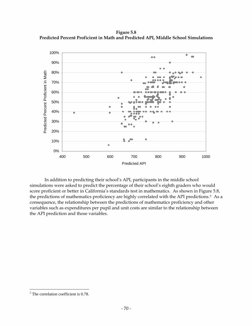
Figure 5.8 Predicted Percent Proficient in Math and Predicted API, Middle School Simulations
0%
10%
20%
30%
40%
50%
60%
70%
80%
90%
100%
400 500 600 700 800 900 100
Predicted API
Pre
dict
ed P
erce
nt P
rofic
ient
in M
ath
0
In addition to predicting their school’s API, participants in the middle school simulations were asked to predict the percentage of their school’s eighth graders who would score proficient or better in California’s standards test in mathematics. As shown in Figure 5.8, the predictions of mathematics proficiency are highly correlated with the API predictions.5 As a consequence, the relationship between the predictions of mathematics proficiency and other variables such as expenditures per pupil and unit costs are similar to the relationship between the API prediction and those variables.
5 The correlation coefficient is 0.78.
- 70 -

Figure 5.9 Predicted and Actual Academic Performance Indexes: Middle Schools
400
500
600
700
800
900
1000
0 25 50 75
Percent Subsidized Lunch
Aca
dem
ic P
erfo
rman
ce In
dex
100
To put these predictions in perspective, consider the relationship between the actual APIs of middle schools and the percentage of a school’s students participating in the subsidized lunch program (Figure 5.9). Each gray point in the figure represents the API and subsidized lunch percentage for a middle school in 2003-04. The dark line is the average API prediction of simulation participants as a function of the subsidized lunch percentage. In forming this prediction, the budget of the school is assumed to be $4,000 per student, the unit costs of certificated staff equal their baseline values ($66,000 for a teacher), and all other variables are set at their mean for the simulation. As with the elementary predictions, for high-poverty schools, the average prediction is higher than the average actual API.
Studies of the effect of resources on achievement are rare for middle schools. The best study is Rivkin, Hanushek, and Kain (2005), who examine reading and math scores of Texas students. As described in Section 4, the study finds that class size has significant effects for reading and math scores of elementary students. It also examines effects for 7th and 8th graders, but finds that the effects are much smaller. For math scores, a 10-student reduction in class sizes for grades 6 and 7 would increase 7th grade scores by only 0.001 standard deviations. For reading scores, the increase is larger—0.03 standard deviations. These increases translate into percentile changes of 0.3 and 1.2 points. From Rogosa (2000), if all students in a middle school were to increase their scores in all tests by one percentile point, the school’s API would increase by five points. Based on these reference points, it seems reasonable to conclude that
- 71 -

the Rivkin, Hanushek and Kain results suggest that a 10-student reduction in middle school class sizes would increase a school’s API by no more than four points.
The cost of a 10-student reduction in class size depends on the starting point. The cost is less for large classes than for small ones. For purposes of comparison, assume an initial class size of 30 students. Assuming the unit cost of teachers is $66,000, a reduction in class size from 30 to 20 would cost $1,100 per pupil.6 Thus, an expenditure of $1,000 on reducing middle school class sizes would increase a school’s API by no more than four points.
In contrast, participants in the simulation predicted a much larger effect. In the API prediction equation, the coefficient on expenditures per pupil is 0.0115, indicating that a $1,000 increase in expenditures per pupil is predicted to increase a school’s API by 11.5 points, more than twice as large as the API increase that could be reasonably inferred from the research of Rivkin, Hanushek and Kain. Part of this difference may be explained by the allocation of additional revenues. The seminar participants would allocate only about one-third of the addition to hiring more teachers. The additional two-thirds are allocated to professional development, after-school tutoring, and other areas, which participants believe to be more effective uses of resources than reducing class sizes.
6 The cost per pupil of teachers at a class size of 30 students is $2,200 ($66,000/30). At a size of 20 students, it is $3,300 ($66,000/20).
- 72 -

6. Results from High School Simulations
The high school simulations are virtually identical to the middle school simulations. The only significant difference is the predictions of academic achievement. In the middle school simulations, participants are asked to predict the API of their school and the percentage of its eighth graders who would score proficient or better on the California standards test in mathematics. Participants in the high school simulations are also asked to predict the API of their school; but, instead of predicting proficiency in mathematics, they are asked to predict the percentage of their entering ninth graders who will graduate in four years.
- 73 -

Table 6.1 Summary Statistics for High School Simulations
Budget (dollars/student) 5,342 689 3,600 6,400Unit cost for teachers (dollars/FTE) 69,510 6,044 66,000 85,800Average API of feeder schools 750 82 650 850Enrollment 1759 992 49 4541Percent subsidized lunch 32 22 0 100Percent English learners 13 12 0 52
MaximumStandard
Mean Deviation Minimum
California high schools are very large on average, a fact reflected in the average enrollment of schools in the high school simulations (Table 6.1). However, there are also many small high schools, creating a wide range of enrollments. Among the hypothetical schools in the high school simulations, the smallest had 49 students, and the largest had 4,541 students. Participation in the subsidized lunch program is lower for high schools than for elementary and middle schools. The average participation rate for the hypothetical high schools was 32 percent. For elementary schools, the average was 52 percent; for middle schools, 44 percent. Furthermore, relative to the elementary and middle schools in the simulations, the hypothetical high schools have fewer students classified as English learners. The average percentage for high schools is 13 percent as compared to 26 percent for elementary schools and 18 percent for middle schools. Yet, in one high school in the simulation, all students participated in the subsidized lunch program. In another high school, 52 percent of students were classified as English learners.
- 74 -

Table 6.2 Estimated Resource Choices for Average High School
Resource Unit of MeasureTeachers
Core FTE 43.6 52.4Non-core FTE 26.3 34.3P.E. FTE 4.5 5.7
AdministrationPrincipals FTE 2.0 2.1Assistant principals FTE 2.2 3.2Clerical office staff FTE 7.3 11.4
Support staffInstructional aides FTE 5.2 13.8Counselors FTE 4.0 5.6Nurses FTE 0.7 1.1Librarians FTE 1.2 1.9Security officers FTE 2.2 3.9Technology support staff FTE 1.7 2.6Community liaisons FTE 0.6 1.7
Professional developmentAcademic coaches FTE 1.5 4.1Collaborative time Hours/year/teacher 42.5 100.1
Student programsAfter-school tutoring Teacher hours/week 63.2 153.9Summer school Students 346.1 598.9Longer school year Days/year 2.4 4.4Longer school day Hours/day 0.4 0.8Computers for instruction Computers 328.4 606.1
Other $ thousands 39.5 205.7
Class sizeCore 24.2 20.2Non-core 33.4 25.7P.E. 38.9 30.6
$4,000/student $6,000/student
The average resource choice of participants in the high school simulations are presented in Table 6.2. The estimated averages are for a high school with 1,759 students, 32 percent of whom participate in the subsidized lunch program and 13 percent of whom are English learners. The estimates are an equally weighted average of the estimated choices of teachers, principals, and superintendents. They also assume a similar schools ranking of five for all participants and an average API of 750 for the school’s feeder middle schools.
As with elementary and middle schools, the estimates are presented for budget levels of $4,000 per pupil and $6,000 per pupil. The estimates reveal the same general pattern as those for elementary and middle school participants. With an increase in the budget, participants would spend more in all areas. The largest share of the increase (31 percent) is allocated to hiring more teachers. Another 9 percent of additional funds is allocated to increasing administrative staff. Twenty-three percent goes to increasing support staff. Professional development receives 16 percent of the additional budget, student programs 28 percent, and other expenditures 6 percent.
- 75 -

In terms of percentage increases, support staff, professional development, and student programs receive a heavier emphasis than teachers and administrators. With the 50 percent increase in the budget, the number of teachers increases by 24 percent and the number of administrators increases by 50 percent. In contrast, support staff doubles, the number of academic coaches increases from 1.5 to 4.1, and collaborative time more than doubles. Hours in the after-school tutoring program are nearly tripled, and nearly twice as many students attend summer school. Participants also extend the school year by two days and add 24 minutes to the school day. The number of computers increases from 19 per hundred students to 34 per hundred students.
With the budget of $6,000 per student, participants would spend an average of $206 per student on items not explicitly covered in the simulation spreadsheet. As did their elementary and middle school counterparts, many participants in the high school simulations wrote that they would spent some of this money on field trips, visits to colleges and universities, an AVID program, and motivational speakers. In addition, some participants identified activities unique to high schools. These included a mentoring program to help students with the transition from smaller middle schools to the complex environment of a large high school. In a similar spirit, another participant would devote some funds to establishing small learning communities within high schools. A few participants would spend money on conflict resolution among students. Several identified the need to enhance the vocational program in their school.
- 76 -

Figure 6.1 Allocation of Expenditures as Total Expenditures Change, High School Simulations
$0
$1,000
$2,000
$3,000
$4,000
Teach
ers
Admini
strati
on
Suppo
rt staf
f
Profes
siona
l dev
elopm
ent
Studen
t prog
rams
Other
dolla
rs/s
tude
nt $4,000/student$6,000/student
The broad priorities of participants are revealed by how they allocate expenditures
among resource areas as the budget for their school increases (Figure 6.1). As the budget increases by 50 percent, expenditures on teachers rise by 24 percent, and expenditures on administrative staff increase by 50 percent. By comparison, expenditures on support staff increase by 111 percent, expenditures on professional development rise by over 300 percent, and expenditures on student programs grow by 200 percent.
- 77 -

Figure 6.2 Allocation of Expenditures as Enrollment Changes, High School Simulations
$0
$1,000
$2,000
$3,000
$4,000
Teach
ers
Admini
strati
on
Suppo
rt staff
Profes
sional
developm
ent
Student
program
sOthe
r
dolla
rs/s
tude
nt
767 students2,751 students
As with the elementary and middle school simulations, participant choices are
consistent with economies of scale in administration and support staff. As enrollment increases from 767 students (one standard deviation below the average) to 2,751 students (one standard deviation above the average), administrative expenditures per pupil fall by 44 percent and support staff expenditures per pupil decline by 21 percent. The resources released by these decreases are allocated to professional development (up 36 percent) and student programs (up 44 percent). Other expenditures per pupil more than double. In contrast, teacher expenditures per pupil, and thus class sizes, remain unchanged.
- 78 -

Figure 6.3 Allocation of Expenditures as Participation in Subsidized Lunch Program Changes,
High School Simulations
$0
$1,000
$2,000
$3,000
$4,000
Teach
ers
Admini
strati
on
Suppo
rt staff
Profes
sional
developm
ent
Student
program
sOthe
r
dolla
rs/s
tude
nt
No students in subsidized lunch program
All students in subsidized lunch program
With an increase in student poverty, participants allocate more of their budget to
teachers and administration and less to professional development (Figure 6.3). The former increase by 4 and 28 percent, and the latter declines by more than 50 percent. Expenditures on student programs also decline by 5 percent.
- 79 -

Figure 6.4 Allocation of Expenditures as Percentage of English Learners Changes,
High School Simulations
$0
$1,000
$2,000
$3,000
$4,000
Teach
ers
Admini
strati
on
Suppo
rt staff
Profes
sional
developm
ent
Student
program
sOthe
r
dolla
rs/s
tude
nt No English learners52% English learners
As was the case in the elementary and middle school simulations, an increase in the
percentage of English learners has an opposite effect on the allocation of expenditures, as does an increase in student poverty (Figure 6.4). Expenditures on teachers decline by 7 percent, expenditures on administrators fall by 15 percent, and other expenditures decrease by 80 percent. These declines are offset by a 45 percent increase in professional development and a 20 percent increase in student programs.
- 80 -

Figure 6.5 Allocation of Expenditures by Participant Type, High School Simulations
$0
$1,000
$2,000
$3,000
$4,000
Teach
ers
Admini
strati
on
Suppo
rt staff
Profes
sional
developm
ent
Student
program
sOthe
r
dolla
rs/s
tude
nt
TeachersPrincipalsSuperintendents
The expenditure patterns of teachers differ noticeably from those of superintendents and
principals. In terms of expenditures on the number of teachers, participants who were teachers spend 10 percent more than superintendents and 7 percent more than principals. On the other hand, superintendents and principals spend about 20 percent more than teachers on professional development and about 40 percent more than teachers on student programs.
- 81 -

Figure 6.6 Allocation of Expenditures by Similar Schools Rank, High School Simulations
$0
$1,000
$2,000
$3,000
$4,000
Teach
ers
Admini
strati
on
Suppo
rt staff
Profes
sional
developm
ent
Student
program
sOthe
r
dolla
rs/s
tude
nt
Rank 1Rank 10
Spending patterns were somewhat affected by a participant’s similar schools rank
(Figure 6.6). Compared to participants with a rank of one, participants with a rank of ten spend about 20 percent more on administrative staff and about 15 percent less on professional development and student programs.
- 82 -

Table 6.3 Coefficient Estimates for Relationship Between Predicted Achievement
and Conditioning Variables, High School Simulations
Conditioning VariablesExpenditures per pupil 0.0102 0.0055 0.0018 0.0013Unit cost of teachers -0.0005 0.0005 -0.0001 -0.0001Teacher index (1 if teacher, 0 otherwise) -4.2569 7.0706 -0.7662 -0.5534Principal index (1 if principal, 0 otherwise -13.2359 7.0663 -2.3825 -1.7207Enrollment 0.0090 0.0030 0.0016 0.0012Percent in subsidized lunch -0.5055 0.1768 -0.0910 -0.0657Percent English learners -0.4400 0.3201 -0.0792 -0.0572Similar schools rank 1.5888 1.1650 0.2860 0.2065Average API of feeder schools 0.4545 0.0414 0.0818 0.0591Constant 413.6 51.1 -12.6 -16.2
R-squared 0.32
Coefficient St. Error
Academic Performance Index For Percent Proficient
English Math
Equivalent Coefficients
The API predictions of participants in the high school simulations follow the same general pattern as those for participants in the elementary and middle school simulations. The similarities are that resources have a positive, but modest, effect on achievement, student poverty has a strong negative effect, and the average API of feeder schools has a large, positive effect.
Table 6.3 presents coefficient estimates for the average API prediction as a linear function of important conditioning variables. The first column presents the coefficient estimates, the second is their standard errors, and the third and fourth present the estimates transformed by Equation 2.8 to apply to the percentage of students proficient in English and mathematics.
As the table shows, with 90 percent confidence, an increase of $1,000 per pupil increases the API prediction by one to 19 API points. A change in the average API of feeder schools has a more dramatic effect. With 90 percent confidence, a 100 point increase in that average increases the average API prediction by 39 to 52 points. Student poverty also has a strong effect. If the percentage of students participating in the subsidized lunch program increases by 10 points, with 90 percent confidence the average API prediction decreases by two to eight points.
Unlike the elementary and middle school simulations, the number of students has a clear positive effect on the average API prediction. The effect is relatively small, however. With 90 percent confidence, an increase in enrollment of 1,000 students increases the API prediction by three to 15 points. Another difference from the elementary and middle school simulations is that principals in the high school simulations are clearly more pessimistic about student achievement than are superintendents. With 90 percent confidence, the average prediction is two to 25 points lower than the average of superintendents.
- 83 -

None of the other variables have a clearly positive or negative effect on the average API prediction. In particular, though the estimated coefficient on the percentage of English learners is negative, the confidence interval around that estimate includes a range of positive numbers.
- 84 -

Figure 6.7 Predicted API and Expenditures per Pupil, Average High School
700
725
750
775
800
825
850
$3,500 $4,000 $4,500 $5,000 $5,500 $6,000 $6,500
Expenditures per Pupil
Pre
dict
ed A
PI
Figure 6.7 depicts the relationship between API predictions for the average high school
and expenditures per pupil for that school. The dark line is the estimate of the average prediction. The gray lines are that estimate plus or minus 1.65 times the prediction standard error. With a probability of 90 percent, the interval between those lines contains the average prediction in the underlying population. For a budget of $5,000 per pupil, that interval runs from an API of 760 to an API of 778. The residual standard error is 56 API points.
- 85 -

Table 6.4 Coefficient Estimates for Relationship Between Predicted Graduation Rate
and Conditioning Variables, High School Simulations
Conditioning VariablesExpenditures per pupil 0.0017 0.0007Unit cost of teachers -0.0001 0.0001Teacher index (1 if teacher, 0 otherwise) -4.1286 0.9163Principal index (1 if principal, 0 otherwise 0.4463 0.9158Enrollment -0.0016 0.0004Percent subsidized lunch -0.0918 0.0229Percent English learners -0.1186 0.0415Similar schools rank 0.2786 0.1510Average API of feeder schools 0.0172 0.0054Constant 79.6 6.6
R-squared 0.19
Coefficient ErrorStandard
Participants in the high school simulations were also asked to predict the graduation rate for their school. The average prediction was 91 percent, but there was considerable variation around that average. The same techniques used to estimate an average API prediction were used to estimate an average graduation rate prediction as a linear function of conditioning variables. Table 6.4 presents the coefficient estimates and standard errors for that relationship.
As with the API prediction, expenditures per pupil and the feeder API have a positive effect, and student poverty has a negative effect. An increase of $1,000 per pupil increases the average graduation rate by 1.7 percentage points. The 90 percent confidence interval for that increase lies between 0.6 and 2.9 percentage points. With 90 percent confidence, a 100 point increase in the feeder API increases the graduation rate by 0.8 to 2.6 percentage points. With the same confidence level, an increase of 10 percentage points in students participating in the subsidized lunch program decreases the graduation rate by 0.5 to 1.3 percentage points.
The effect of enrollment on the graduation rate is opposite to its effect on the API prediction. With 90 percent confidence, an increase of 1,000 students increases the API prediction by three to 15 points. At the same confidence level, a 1,000 student increase decreases the graduation rate by one to two percentage points.
- 86 -

Figure 6.8 Predicted Graduation Rate and Expenditures per Pupil, Average High School
80%
85%
90%
95%
100%
$3,500 $4,000 $4,500 $5,000 $5,500 $6,000 $6,500
Expenditures per Pupil
Gra
duat
ion
Rat
e
The relationship between expenditures per pupil and the predicted graduation rate is
depicted in Figure 6.8. The figure assumes an average high school with 1,759 students and average values for other conditioning variables. As in Figure 6.7, the dark line is an estimate of the average prediction and the gray lines form a 90 percent confidence interval for that estimate. For a budget of $5,000 per pupil, that interval runs from 90 to 92 percent.
- 87 -

Figure 6.9 Predicted and Actual Academic Performance Indexes: High Schools
400
500
600
700
800
900
1000
0 25 50 75
Percent Subsidized Lunch
Aca
dem
ic P
erfo
rman
ce In
dex
100
The API predictions of simulation participants tend to be higher than the APIs California high schools actually achieved in 2003-04. The gray points in Figure 6.9 represents the API and subsidized lunch percentage for high schools in 2003-04. The average API prediction of simulation participants is represented by the dark line in the figure. The prediction assumes a budget of $4,000 per student, the unit costs of certificated staff equal their baseline values ($66,000 for a teacher), and all other variables are at their mean for the simulation.
- 88 -

7. Aligning School Resources with State Academic Standards
The simulations point to two broad conclusions, with an obvious implication for the allocation of resources among public schools. The first is that student poverty has a strong, negative effect on academic achievement. The second is that school resources have a positive, but modest, effect. The implication is that if all schools are to achieve the same high standard, as California’s current policy dictates, schools serving low-income neighborhoods should have more resources than other schools. Furthermore, because poverty has a large effect on achievement and resources have a modest effect, California’s policy implies very large resource differences across schools.
The idea that some schools need more resources than others conflicts with the major objective of California’s school finance reform of the 1970s, which sought to equalize revenue per pupil across school districts. While revenue has not been completely equalized, by any reasonable standard the reform has achieved its objective. This section begins by briefly reviewing the history and rationale of the revenue equalization reform before detailing the implications of the current research for a very different reform.
7.1. Origins of the Equalization Principle
Though the roots of the equalization reform reach much further back, for this brief account it suffices to begin with Serrano v. Priest, a legal complaint filed in Los Angeles Superior Court in 1968.7 The complaint identified two injustices. The first was that educational opportunities differed widely across school districts in California. As evidence of this contention, the complaint cited differences in expenditures per pupil, but it also argued that equal expenditures per pupil were not sufficient “where pupils have different educational needs.” The second injustice was that, with the system of local property taxes used to support public schools at the time, the tax rate necessary to yield any particular level of expenditures per pupil differed across districts. The plaintiffs also alleged that poor and minority families were at a disadvantage in this regard, an allegation subsequently shown to be false.
The Superior Court dismissed the case without trial, and the plaintiffs appealed. At the same time, another case that was to have an important effect on the outcome of the Serrano complaint. was being heard in federal court. In McInnis vs. Shapiro, the plaintiffs argued that the school finance system in Illinois did not provide enough revenue for the Chicago public school district to address the exceptional educational needs of its many disadvantaged students. The court rejected that argument in part because educational need was too nebulous a concept to adjudicate.
As a result of this ruling, the Serrano lawyers narrowed their complaint. Their focus was largely inspired by a new legal theory developed by Coons, Clune, and Sugarman (1970). Coons and his co-authors advanced a more limited argument with a better chance of success. Instead of attempting to make the difficult argument that students with different backgrounds
7 This account in this section is based on Sonstelie, Brunner, and Ardon (2000).
- 89 -

require different resources, they embraced a more concrete alternative: expenditures per pupil measure educational opportunity. With that simplification, the focus of their argument shifted naturally and forcefully to the second injustice identified by the Serrano plaintiffs—equal property tax rates did not yield equal revenue per pupil. In essence, this new legal theory turned the Serrano complaint from a case about educational opportunity into a case about tax equity.
In its ruling on the case, the California Supreme Court accepted this new argument in its entirety, leaving the job of designing a new school finance system to the legislature. The legislature’s solution was to establish a revenue limit for each school district and to provide each district with state aid equal to the difference between its limit and its property tax revenue. The legislature then equalized per pupil limits across school districts. In essence, state aid now offset differences in property tax revenue across districts, satisfying the court’s requirement that differences in property tax wealth should not lead to differences in expenditures per pupil.
Unrestricted state aid and property tax revenue, funds subject to revenue limits, constitute nearly 70 percent of school district revenue. The remainder comes from a variety of state and federal categorical programs, many of which are also quite equally distributed across districts. A few state and federal programs target districts with large percentages of disadvantaged students, and thus these districts tend to receive higher total revenue per pupil (Rose, Sonstelie, Reinhard, and Heng (2003)). The differences in total revenue per pupil are relatively minor, however, a necessary consequence of the very equal distribution of the large fraction of total revenue subject to revenue limits.
The history of revenue equalization is much more complicated and interesting than was just portrayed. The objective here is only to tell enough of that story to support the following point: The Serrano plaintiffs won an outcome that was quite different from their original intent. The equalization of per pupil revenue was a concept devised to win a legal argument with its own history, ground rules, and logic. The legislature accepted the concept as a convenient solution to a difficult problem presented to it by the courts. However, revenue equalization had little connection with the realities of public schools, a fact the legislature began to realize as it grappled with implementing the concept. We should not be surprised, therefore, that the concept of revenue equalization, now long established, appears to conflict with the implications of California’s new academic standards, an effort that began with the fundamental issue of what students should learn in every grade, a reform rooted in the everyday realities of California public schools.
7.2. School Budgets
This brief history provides the background for working out the implications of the current research for school finance policy. This task begins with the API predictions, in particular the linear relationship between the average API that educational practitioners predict for a school and the values of variables including the school’s budget and the characteristics of its students. This relationship leads immediately to this important question: Given the characteristics of a school’s students, what budget would it need to achieve the state’s goal for it? The question becomes not what API would practitioners predict for a certain school with a
- 90 -

budget of $5,000 per pupil, but rather what budget do practitioners believe that school needs to achieve an 800 API, the API goal for all schools?
Because simulation participants were asked to assume that none of the students in their hypothetical schools require special education services, that goal must be adjusted slightly for the reality that schools do include special education students and that those students score lower, on average, on standardized tests than do other students. Section 2.6 explains the adjustment made to account for this reality. In essence, the adjustment is based on two simplifying assumptions. The first is that the percentage of special education students in each school equals the statewide average for schools with its grade span. The second assumption is that the average scores of special education students in each school are proportional to the average scores of other students in the school. Thus, for example, if the average scores of special education students statewide is, say, 70 percent of the statewide average scores for other students, the average scores of special education students in each school is assumed to be 70 percent of the average scores of other students in the school. Under those assumptions, students who do not require special education services would need to achieve an API higher than 800 for the school as a whole to achieve an 800 API. In particular, for elementary schools, students not requiring special education services would need to achieve an API of 813. For middle schools, the target is 822. For high schools, it is 816.
In determining the budget a school needs to achieve those target APIs, the same targets are assumed for the average feeder school APIs. Thus, for middle schools, the average API of feeder elementary schools is assumed to be 813. For high schools, the average is assumed to be 822. The budgets are determined using an equally weighted average of the API predictions of teachers, principals, and superintendents and assuming a score of five for the participant’s similar schools rank.
- 91 -

With those assumptions and conditions, the API prediction equations yield the following equations for the dollars per pupil needed to reach an 800 API:8
Elementary schools: Budget = 2,103 – 0.75 * Enrollment + 111 * Lunch -0.76 * English (7.1) Middle schools: Budget = 1,936 + 0.83 * Enrollment + 91 * Lunch – 15 * English (7.2) High schools: Budget = 6,080 – 0.89 * Enrollment + 49 * Lunch + 43 * English (7.3)
In these equations, Budget is dollars per pupil required for the target API, Enrollment is the enrollment of the school, Lunch is the percent of the school’s students who participate in the subsidized lunch program, and English is the percent of the school’s students who are classified as English learners. The budget total does not include the additional costs of special education services, which are added later in the analysis.
To illustrate, consider the average elementary school with 583 students, 52 percent of whom participate in the subsidized lunch program and 26 percent of whom are English learners. Substituting those numbers into Equation (7.1) for Enrollment, Lunch, and English, we find that the school would need a budget of $7,439 per pupil to achieve the state’s API goal. If the percentage of students participating in the subsidized lunch program is reduced by ten percentage points, the required budget is reduced by $1,110 per pupil to $6,320 per pupil. A reduction in enrollment of 100 students reduces the budget by $75 per pupil. A 10 percent reduction in English learners increases the budget by $7.60 per pupil.
8 The coefficients in these equations are the ratio of estimated coefficients from the API prediction regressions, specifically the estimated coefficient for each variable divided by the estimated coefficient for expenditures per pupil. Because the ratio of the expected values of two random variables does not equal the expected value of the ratio of those variables, the coefficients in the three equations are biased estimates.
- 92 -

Figure 7.1 Estimate and Confidence Interval for School Budget Required for 813 API,
Average Elementary School with No Special Education Students
$0
$2,000
$4,000
$6,000
$8,000
$10,000
$12,000
$14,000
0 25 50 75
Percent in Subsidized Lunch Program
Dol
lars
per
Pup
il
maximum budget
minimumbudget
100
These budget estimates are based on coefficient estimates from the API prediction
equations, a coefficient with standard errors that should be incorporated into the analysis. This uncertainty about coefficient estimates is reflected in the confidence intervals for the budget estimates. Figure 7.1 portrays the estimate and confidence interval for elementary schools.9 The dark line represents the relationship between the Budget variable in Equations 7.1 and the Lunch variable in that equation. The other variables in the equation, Enrollment and English, are fixed at their averages for the sample of hypothetical schools. The gray lines in the figure are the boundaries of a 90 percent confidence interval for the Budget variable. To be precise about this interval, consider a particular level of the Lunch variable and the predictions of all educational practitioners about the budget necessary for a school with these characteristics to achieve the target API. Now take the average of those budget predictions. With a probability of 90 percent, that average lies within the confidence interval portrayed in the figure.
As the figure reveals, the confidence interval is quite wide. For the average elementary school, the school in which 52 percent of students participate in the subsidized lunch program, the estimated budget required to reach an 813 API is $7,430 and the 90 percent confidence interval runs from $6,403 per pupil to $8,368 per pupil. The confidence interval widens as the rate of participation in the subsidized lunch program moves away from the average. For the school in which 75 percent of students participate in the subsidized lunch program, the 90 percent interval runs from $8,176 per pupil to $12,880 per pupil, a gap of $4,700. At 100 percent,
9 The confidence intervals were formed by the boot strap method. From the empirical distribution resulting from that method, the smallest 90 percent interval was chosen as the confidence interval for the estimate.
- 93 -

the gap is $7,600 per pupil. The confidence interval also widens as the percentage participating in subsidized lunch declines below 52 percent.
This widening of the confidence interval with increases or decreases in subsidized lunch participation is a natural consequence of the sample of schools in the simulations. For a subsidized lunch percentage in the middle of the sample of schools, there are many similar schools in the sample and thus many API predictions to compute an average prediction. As a consequence, we can be relatively confident about it. Schools at the extremes, however— schools with few poor students or schools with nearly all students poor— have relatively few similar schools in the sample. As a consequence, we are less confident about the average API prediction for those schools. Less confidence about the API prediction translates into less confidence about the budget necessary to reach a certain API, and thus to the wider confidence intervals.
For schools at the extremes of subsidized lunch participation, the budget estimates have another weakness. In those cases, the budget estimates are an out-of-sample prediction. For schools with few students in the subsidized lunch program, the estimated budget is less than $3,600 per pupil, the minimum budget used in the simulations. For schools in which almost all students participate in the subsidized lunch program, the estimated budget is greater than $7,600 per pupil, the maximum budget used in the simulations. These two outcomes follow naturally from the modest effect that resources have on achievement. With current budgets, California elementary schools with few poor students currently average an API well over 800. As a consequence, with budgets of $4,000 per pupil, which is about the average for California schools, participants in the simulations predicted APIs well in excess of 800. In fact, if no students participate in the subsidized lunch program, the average API prediction with a budget of $4,000 per pupil is 843, implying that a lower budget would be enough to achieve an 800 API. Because the effect of resources on achievement is modest, the implied budget reduction is considerable. Similarly, for California elementary schools in which most students are poor, the average API with current budgets is well below 800. This fact is reflected in the predictions made by simulation participants. For a hypothetical school in which all students participate in the subsidized lunch program and the budget is $4,000 per student, the average API prediction of participants was 700. With the estimated effect of resources on achievement, a much larger budget is necessary to reach 813, a budget larger than $7,600 per pupil, the maximum in the simulations. The dashed lines in Figure 7.1 represent the minimum and maximum budgets.
- 94 -

Figure 7.2 Estimate and Confidence Interval for School Budget Required for 822 API,
Average Middle School with No Special Education Students
$0
$2,000
$4,000
$6,000
$8,000
$10,000
$12,000
$14,000
0 25 50 75
Percent in Subsidized Lunch Program
Dol
lars
per
Pup
il
maximum budget
minimumbudget
100
Figure 7.2 portrays the equivalent estimates and confidence intervals for middle schools.
For the average middle school (42 percent of students participating in subsidized lunch), the estimated budget for an 822 API is $6,458 per pupil. The 90 percent confidence interval for that estimate lies between $4,874 per pupil and $9,649 per pupil. As with the elementary school simulations, the confidence interval widens as participation in the subsidized lunch program increases or decreases from the average for the sample. Also, the estimated budget is an out-of-sample prediction when participation in the subsidized lunch program is either very low or very high.
- 95 -
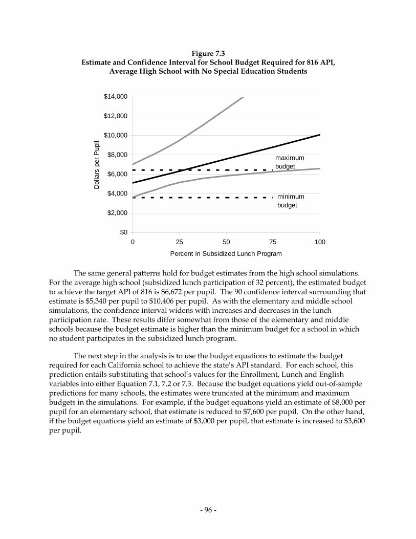
Figure 7.3 Estimate and Confidence Interval for School Budget Required for 816 API,
Average High School with No Special Education Students
$0
$2,000
$4,000
$6,000
$8,000
$10,000
$12,000
$14,000
0 25 50 75
Percent in Subsidized Lunch Program
Dol
lars
per
Pup
il
maximum budget
minimumbudget
100
The same general patterns hold for budget estimates from the high school simulations.
For the average high school (subsidized lunch participation of 32 percent), the estimated budget to achieve the target API of 816 is $6,672 per pupil. The 90 confidence interval surrounding that estimate is $5,340 per pupil to $10,406 per pupil. As with the elementary and middle school simulations, the confidence interval widens with increases and decreases in the lunch participation rate. These results differ somewhat from those of the elementary and middle schools because the budget estimate is higher than the minimum budget for a school in which no student participates in the subsidized lunch program.
The next step in the analysis is to use the budget equations to estimate the budget required for each California school to achieve the state’s API standard. For each school, this prediction entails substituting that school’s values for the Enrollment, Lunch and English variables into either Equation 7.1, 7.2 or 7.3. Because the budget equations yield out-of-sample predictions for many schools, the estimates were truncated at the minimum and maximum budgets in the simulations. For example, if the budget equations yield an estimate of $8,000 per pupil for an elementary school, that estimate is reduced to $7,600 per pupil. On the other hand, if the budget equations yield an estimate of $3,000 per pupil, that estimate is increased to $3,600 per pupil.
- 96 -

The significance of these truncations is demonstrated by the range of predicted APIs for schools given the budget assigned to them. For schools without truncated budgets, the predicted API is 800. For schools with budgets truncated at the maximum budget, the predicted API is calculated assuming that budget. For schools with budgets truncated at the minimum, the predicted API is calculated assuming the minimum budget. The range of predicted APIs is displayed in Table 7.1.
- 97 -
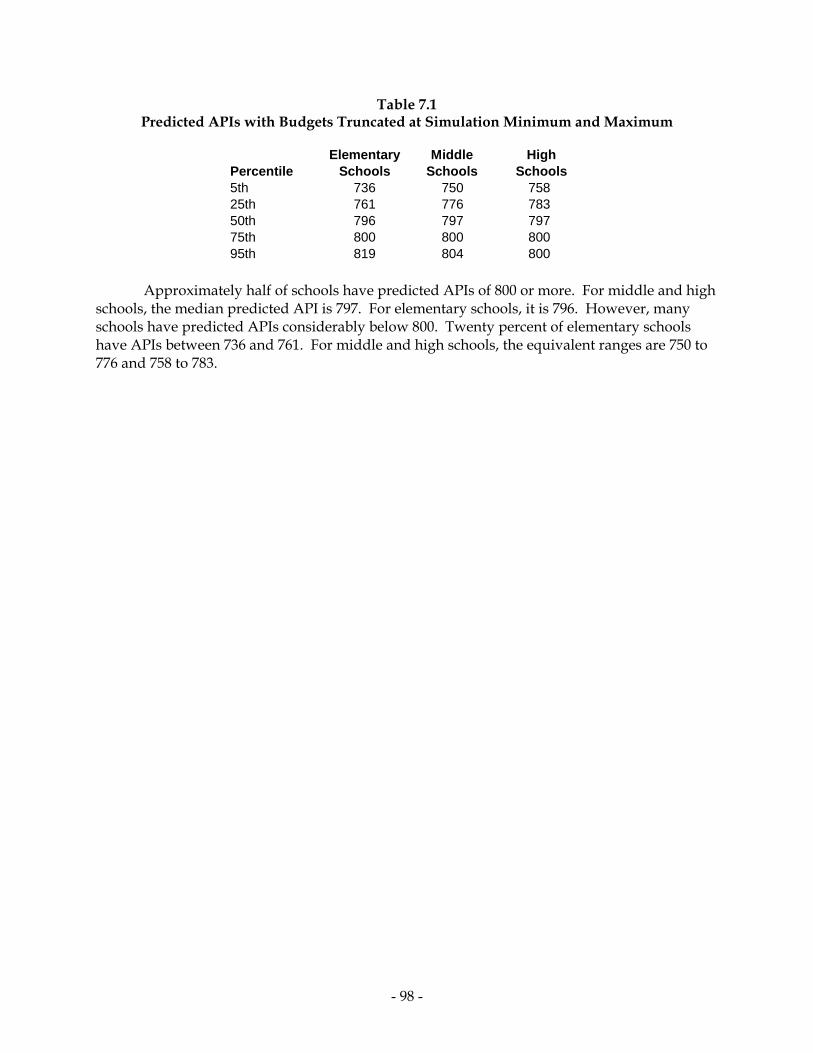
Table 7.1 Predicted APIs with Budgets Truncated at Simulation Minimum and Maximum
Percentile5th 736 750 75825th 761 776 78350th 796 797 79775th 800 800 80095th 819 804 800
Schools SchoolsSchoolsElementary Middle High
Approximately half of schools have predicted APIs of 800 or more. For middle and high schools, the median predicted API is 797. For elementary schools, it is 796. However, many schools have predicted APIs considerably below 800. Twenty percent of elementary schools have APIs between 736 and 761. For middle and high schools, the equivalent ranges are 750 to 776 and 758 to 783.
- 98 -

Table 7.2 Distribution of Estimated School Budgets Aggregated to the District Level, Dollars per Pupil
Percentile5th 3,600 2,57925th 4,916 4,87050th 6,334 6,76575th 7,093 8,90095th 7,600 11,963
With Truncation Without Truncation
The estimated budgets for each school are then aggregated to the school district level. This aggregate is a weighted average of the budget estimates for each school in a district where the weight for a school is its enrollment divided by the district’s enrollment. As the first column of Table 7.2 reveals, the district aggregates vary considerably. The district in the 5th percentile has an average of $3,600 per pupil, and the district in the 95th percentile has an average of $7,600 per pupil. Half of school districts lie between $4,916 per pupil and $7,093 per pupil. The median is $6,334 per pupil.
The budget truncations have a significant effect on the distribution of district aggregates. The last column of Table 7.2 shows the district aggregates without the truncations. Without the truncations, the median would increase from $6,334 to $6,766, and the span between the 25th and 75th percentile would expand from $2,474 to $4,030.
- 99 -

- 100 -

8. Other School District Costs
The budget simulations encompass resources constituting approximately 60 percent of school district expenditures. This section presents estimates of resource needs in remaining areas, areas such as district administration, pupil transportation, and maintenance and operations. The approach is to use actual expenditures of California school districts in 2003-04 to estimate expenditures in each area as a function of factors external to districts. The estimates are then used to predict what the average school district would spend in each area. In this prediction, the average school district is the school district with average revenue per pupil, average resource costs, and average values for all external factors. These expenditure predictions are then adjusted for the actual factors external to each district and for differences in resource costs. The adjusted expenditures provide each district with resources equivalent to those of the average district, accounting for factors unique to the district.
To understand these adjustments, consider the example of population density, which is one of the external factors used in the estimation procedure. A particular district has a lower population density than that of the average district. Its students have farther to travel to school each day, which means that the district must spend more on pupil transportation than the average district. If it had the same total expenditures per pupil as the average district, its higher expenditures on pupil transportation would imply lower expenditures in other areas. To offset the cost of its lower population density, the district would require more revenue than the average district. How much additional revenue would offset that cost? Enough so that the district could spend as much as the average district in areas other than pupil transportation, areas not directly affected by its lower population density. The estimated expenditure function is used to calculate this additional revenue. Appendix G describes this adjustment in detail.
In addition to external factors such as population density, expenditures in each expenditure area are also adjusted for local labor market conditions. To accommodate this adjustment, expenditures in each area are partitioned into expenditures on employee compensation and expenditures on other resources. The cost of personnel in each expenditure area is assumed to be affected by local labor market conditions, but the costs of non-compensation resources are assumed to be the same across districts. In estimating the linear expenditure system, expenditures on employee compensation in an expenditure area are treated as a different expenditure category from expenditures on other resources in that area. The estimated coefficients thus yield estimates of expenditures of both employee compensation and other resources in each expenditure area.
The expenditure areas are based on expenditure classifications in California’s Standardized Account Code Structure (SACS), which is used by California school districts to report revenue and expenditures. Table 8.1 describes each area. Table G.1 in Appendix G gives the SACS codes for each area.
- 101 -
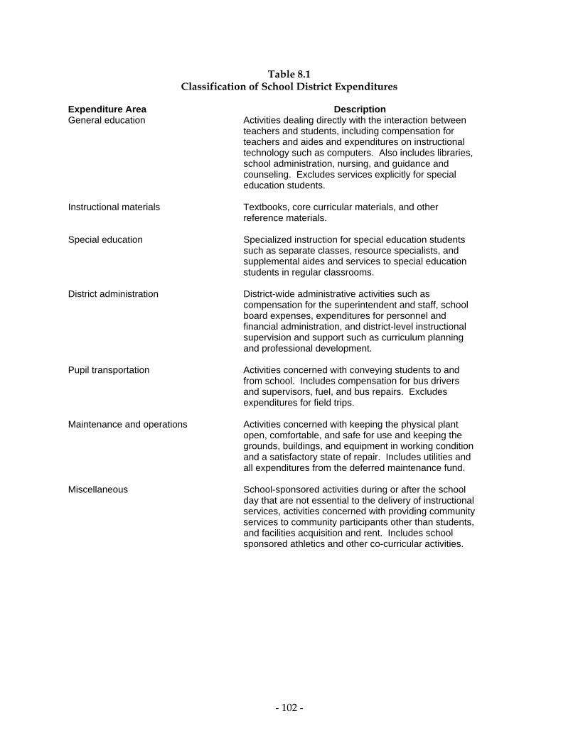
Table 8.1 Classification of School District Expenditures
Expenditure Area Description General education Activities dealing directly with the interaction between
teachers and students, including compensation for teachers and aides and expenditures on instructional technology such as computers. Also includes libraries, school administration, nursing, and guidance and counseling. Excludes services explicitly for special education students.
Instructional materials Textbooks, core curricular materials, and other reference materials.
Special education Specialized instruction for special education students such as separate classes, resource specialists, and supplemental aides and services to special education students in regular classrooms.
District administration District-wide administrative activities such as compensation for the superintendent and staff, school board expenses, expenditures for personnel and financial administration, and district-level instructional supervision and support such as curriculum planning and professional development.
Pupil transportation Activities concerned with conveying students to and from school. Includes compensation for bus drivers and supervisors, fuel, and bus repairs. Excludes expenditures for field trips.
Maintenance and operations Activities concerned with keeping the physical plant open, comfortable, and safe for use and keeping the grounds, buildings, and equipment in working condition and a satisfactory state of repair. Includes utilities and all expenditures from the deferred maintenance fund.
Miscellaneous School-sponsored activities during or after the school day that are not essential to the delivery of instructional services, activities concerned with providing community services to community participants other than students, and facilities acquisition and rent. Includes school sponsored athletics and other co-curricular activities.
- 102 -

Table 8.2 Expenditures per Pupil by Area, California School Districts, 2003-04*
Expenditure AreaGeneral education - compensation $4,442 $1,257 General education - non-compensation 412 264 Instructional materials 84 61 Special education - compensation 669 113 Special education - non-compensation 126 131 District administration - compensation 470 247 District administration - non-compensation 232 234 Pupil transportation - compensation 177 232 Pupil transportation - non-compensation 108 177 Maintenance and operations - compensation 398 204 Maintenance and operations - non-compensation 428 420 Miscellaneous - compensation 106 213 Miscellaneous - non-compensation 174 319
Total expenditures per pupil 7,826 2,452
*Statistics based on 973 school districts
Average Standard Deviation
General education is the largest expenditure area, constituting 62 percent of total expenditures. As shown in Table 8.2, the next largest area is maintenance and operations, which is 11 percent of the total. Expenditures on special education and district administration, areas which receive much public scrutiny, are 10 and 9 percent of total expenditures, respectively. Expenditures on instructional materials constitute only 1 percent of the total.
As the standard deviations for each area indicate, expenditures vary considerably across school districts. Part of that variation is due to differences across districts in total revenue and thus in total expenditures. However, some variation is also due to differences across districts in external factors, factors incorporated in estimating expenditures per pupil in each area.
- 103 -

Table 8.3 External Factors Used to Adjust School District Expenditures*
Population density -0.94 2.83 6.28Enrollment 3.83 7.27 10.11Special education cost 6.43 6.73 6.95
*All factors measured in natural logarithms
5th percentile average 95th percentile
The first factor is population density, which affects expenditures on pupil transportation. This factor is measured by first calculating the land area of each district using block-level Census data based on the 2002 TIGER line files. Blocks within school district boundaries were excluded if they were designated as water or had no population between the ages of five and seventeen. These exclusions reduce the land area of districts with large bodies of water, national or state parks, and uninhabited areas such as deserts or mountains. Density is measured by school district enrollment in 2003-4 divided by land area in square kilometers. Land area could not be determined for four small districts, so those districts were excluded from the statistical analysis.10 In the statistical analysis, density is measured in natural logarithms. Table 8.3 presents the average, 5th percentile, and 95th percentile for that measure.
The second external factor is district enrollment. Several studies have identified economies of scale for school districts, economies often associated with district administration (Andrews, Duncombe, and Yinger (2002) and Dumcombe, Miner, and Ruggiero (1995)). Accordingly, the natural logarithm of district enrollment is included as an external factor affecting district administration. Table 8.3 presents statistics for this variable.
The last factor is special education cost, which is the weighted average of the cost of various special education disabilities. The weights for each disability are the percentages of students in a district with that disability. Using the data from the California Special Education Management Information System (CASEMIS), the special education students in each Special Education Local Planning Area (SELPA) were assigned a disability type. Each disability type was then assigned a weight proportional to the estimated cost for that type.11 The sum of these student weights for each SELPA was then prorated to districts within each SELPA according to district enrollment. The external factor for special education costs is these prorated amounts divided by district enrollment. This factor was also measured in natural logarithms. Summary statistics are presented in Table 8.3.
In addition to the external factors, the statistical analysis incorporates a regional salary index. The index plays the role of the resource cost for expenditure areas involving employee compensation. The index, compiled by Rose (2006), is computed for each of 30 regions of California. Each region is either a county or a group of adjoining counties. For each region, the index is based on the average salary of workers with a college degree who are not employed by public school districts. As a consequence, the index represents local labor market conditions external to each district. The index for each county is presented in Table 8.4. 10 The districts are Pacifica Elementary (3,169 students), Casmalia Elementary (30 students), Pleasant Valley Elementary (7,455 students), and Big Oak Flat-Grove Unified (552 students). 11 The cost estimates were taken from Appendix H, column 3, of Parrish, Harr, Kidron, Brock, and Anand (2004).
- 104 -

Table 8.4 Regional Salary Index, 2003-04
Counties IndexAlameda, Contra Costa 116Alpine, Amador, Calaveras, Inyo, Mariposa, Mono, Tuolomne 90Butte 84Colusa, Glenn, Lassen, Modoc, Nevada, Plumas, Sierra, 88 Siskiyou, Tehama, TrinityDel Norte, Humboldt, Lake, Mendocino 82El Dorado, Placer, Sacramento 97Fresno, Madera 96Imperial 91Kern 95Kings, San Benito 93Los Angeles 109Marin, San Francisco, San Mateo 122Merced 94Monterey 107Napa, Solano 93Orange 108Riverside, San Bernardino 98San Diego 105San Joaquin 93San Luis Obispo 92Santa Barbara 104Santa Clara 122Santa Cruz 110Shasta 84Sonoma 107Stanislaus 94Sutter, Yuba 91Tulare 92Ventura 108Yolo 98
The data on expenditures, external factors, and regional compensation levels are used to
estimate expenditures as a function of external factors and compensation levels. Appendix G describes the function and presents the parameter estimates. These parameter estimates are then used to estimate expenditures in each area for the average district, the district with average values for total expenditures per pupil, the compensation index, and for the three external factors. The results are displayed in Table 8.5.
- 105 -

Table 8.5 Expenditures per Pupil by Area, California School Districts, 2003-04, Linear Expenditure
System Estimates for Average District Versus Statewide Averages
Expenditure AreaGeneral education - labor $4,438 $4,442General education - nonlabor 411 412Instructional materials 83 84Special education - labor 667 669Special education - nonlabor 125 126District administration - labor 475 470District administration - nonlabor 231 232Pupil transportation - labor 180 177Pupil transportation - nonlabor 108 108Maintenance and operations - labor 401 398Maintenance and operations - nonlabor 427 428Miscellaneous - labor 107 106Miscellaneous - nonlabor 173 174
Total expenditures per pupil 7,826 7,826
for Average District AverageSystem EstimatesLinear Expenditure
Statewide
As expected, the predicted expenditures for the average district are very close to average expenditures across all districts. The first column of Table 8.5 displays the predictions, and the second displays the averages from Table 8.2. To be precise, the first column gives the expenditures in each area from substituting average values for the three external factors into the estimated linear expenditure system. The second column is the per pupil expenditure in each area averaged across all school districts. The estimates for the average district are very close to the statewide averages. The largest difference is $7 per pupil.
- 106 -

Table 8.6 Expenditures per Pupil on Transportation, Adjusted for Population Density*
Population Density5th percentile $267 $176 $444Average* 180 108 28895th percentile 100 45 145
*Average of the natural logarithm of density
Compensation Expenditures ExpendituresEmployee Other Total
Using the method described by Equation 8.4, the predicted expenditures in each area are then adjusted for the external factors unique to each district. Table 8.6 illustrates the magnitude of those adjustments for the effect of population density on transportation expenditures. For the average district, transportation expenditures per pupil are $288—$180 for employee compensation and $108 for other expenses. Now consider a district with density in the 5th percentile, but the same values as the average district for other external factors. To offset the effect of its higher transportation costs, the district would need additional revenue of $155 per pupil ($443-$288).
- 107 -

Table 8.7 Expenditures per Pupil on District Administration, Adjusted for Enrollment
Enrollment5th percentile $464 $325 $789Average* 475 231 70695th percentile 484 154 638
*Average of the natural logarithm of enrollment
Compensation Expenditures ExpendituresEmployee Other Total
The second external factor, enrollment, affects expenditures on district administration, but the effects are smaller than those of density on transportation expenditures. As Table 8.7 shows, the estimates do not reveal economies of scale for administrative personnel. Personnel expenditures actually rise slightly with enrollment, although the effect is not statistically significant. Economies of scale occur for other administrative expenditures, however. For the average district, these other expenditures are $231 per pupil. Holding everything else constant, smaller districts would spend more in this area. To offset this effect, a district in the 5th percentile of enrollment would need additional revenues of $94 per pupil ($325-$231).
- 108 -

Table 8.8 Expenditures per Pupil on Special Education, Adjusted for Special Education Cost
Special Education Cost5th percentile $542 $17 $559Average* 667 125 79295th percentile 757 203 960
*Average of the natural logarithm of special education cost
Compensation Expenditures ExpendituresEmployee Other Total
Of the three external factors, special education cost has the largest effect on expenditures. A district in the 95th percentile of this measure would need $178 per pupil more than the average district to offset its higher costs. A district in the 5th percentile would need $246 per pupil less revenue. While these effects are noteworthy, adjusting for them runs counter to the spirit of California’s special education finance system which bases special education funding on total enrollment rather than special education enrollment. As a consequence, adjustments for special education enrollment are not made in determining revenue needed for individual school districts.
- 109 -

Table 8.9 Distribution of Total Adjusted Expenditures per Pupil
(All Areas Except Employee Compensation in General and Special Education)
Districts5th percentile $2,44125th percentile 2,474Average 2,72075th percentile 2,81795th percentile 2,944
Expenditures per Pupil
After adjustments to average expenditures for density and enrollment, all expenditures areas are then summed except two. The first is employee compensation for general education, which is the subject of the budget simulations. The second is employee compensation for special education, for which the estimates of Parrish and co-authors (2004) are used to adjust the results of the budget simulations. Table 8.9 shows the distribution of adjusted expenditures per pupil across the 973 districts with complete data. The 95th percentile of expenditure per pupil is $2,944 per pupil, and the 5th percentile is $2,441 per pupil, a difference of $503 per pupil.
- 110 -

9. A Weighted-Student Formula
This section combines the school budget estimates from the simulations, the estimates of special education costs from Parrish and co-authors (2004), and the district cost estimates from the SACS data to yield a per pupil total for each district. The total is then adjusted for regional salary differences to produce an estimate of the cost to each district of meeting the state’s academic achievement standards. In what follows, this per pupil amount is referred to as a district’s estimated total cost. The estimates are built from the ground up, school by school, and are thus the product of a number of complex factors. Though the estimates constitute a good starting place for a policy allocating revenue among districts, a revenue allocation formula should be simple and transparent. The section thus turns to the issue of approximating the estimated total cost of districts by a small number of factors. The section concludes by presenting an approximation involving just two factors: a regional salary index and a measure of family poverty. A revenue allocation formula based on this approximation can be interpreted as allocating revenue in proportion to the number of students, with the number of students weighted by the two factors. This weighted-student formula provides a good approximation to the estimated total cost of school districts.
9.1. Adjusting for Regional Salary Differences
A district’s estimated total cost is the sum of three elements. The first is the weighted average of the budget estimates for each school in the district (Section 7). A school’s weight in this average is its enrollment as a percentage of the district’s enrollment. The second element is the additional cost of special education, which is $870 per pupil (Section 2.6). The third is district-level cost adjusted for density and enrollment (Section 8).
Each of these three elements involves expenditures on employee compensation. In determining these expenditures, the report thus far has assumed that every district faces the same cost per FTE. In fact, however, the cost of personnel varies across the state. In 2003-04, college-educated employees in Santa Clara County earned 17 percent more, on average, than equivalent employees in Santa Barbara County. Because school districts must compete with other employers in their region, districts in Santa Clara County should expect to pay about 17 percent more than districts in Santa Barbara County to attract the same caliber of employees.
Accordingly, estimates of employee compensation are adjusted for local labor market conditions. To illustrate the adjustment, suppose that employee compensation in a particular expenditure area is estimated to be $100 per pupil for a district facing personnel costs that are average for the state. If employee compensation in the district’s local labor market is 5 percent higher than the state average, the district’s expenditures for employee compensation in that expenditure area are adjusted to be $105 per pupil. If compensation is 5 percent lower, expenditures are adjusted to be $95 per pupil.
These adjustments are implemented with the regional salary index compiled by Rose (2006). The index is based on the average salary of workers with a college degree who are not employed by public school districts. Values for the index are given in Table 8.4. The statewide average for the index is normalized to 100.
- 111 -

The index is applied differently to the three elements comprising a district’s estimated total cost. The first element is the budget estimate from the simulations, which, with the sole exception of computer expenditures, is composed of employee compensation. Accordingly, the entire budget estimate for each school is adjusted for regional salary differences. Similarly, because all of the additional costs of special education students are personnel expenditures, the $870 per pupil for special education costs is also adjusted for regional salary differences. In contrast, just 45 percent of the district-level costs are for employee compensation. Only the part of those costs due to employee compensation is adjusted for regional salary differences.
Because the initial cost estimates were made under the assumption that every district faced the statewide average cost per FTE, adjustments for regional salary differences increase the estimated total cost of some districts, decrease the cost of others, but keep the statewide sum roughly the same. This sum is considerably higher than actual expenditures by districts in 2003-04. In that year, the 950 school districts with complete data enrolled 6.1 million students and spent $43 billion for a per-pupil average of $7,055.12 Here, the sum of estimated total costs for these districts is $60.5 billion, $9,912 per pupil. This sum is 40 percent higher than actual expenditures in 2003-04.
As described in Section 7, the school budget estimates were truncated at the minimum and maximum budgets in the simulations. Without those truncations, total estimated cost would rise considerably. The total would be $68.6 billion ($11,244 per pupil), a total 59 percent higher than actual expenditures in 2003-04.
12 From the SACS data, there are district-level cost estimates for 973 districts. The school-level estimates require data on percentage of students participating in the subsidized lunch program and percentage of students classified as English learners. For these variables, there is complete data for only 950 districts. The districts with missing data are primarily small, one-school elementary districts. The 950 districts included comprise 98 percent of all students.
- 112 -

Table 9.1 Estimated Total Cost of Achieving State Standards, California School Districts, 2003-04
Districts5th percentile $ 7,37925th percentile 8,544Average 9,53575th percentile 10,53595th percentile 11,490
Cost per Pupil
Estimated total cost varies widely across districts (Table 9.1). For the district in the 5th percentile of the distribution of this variable, the estimated total cost is $7,379 per pupil. For the district in the 95th percentile, the estimate is $11,490 per pupil.
Estimated total costs differ substantially from the actual expenditures of districts in 2003-04. The estimate is lower than actual expenditures for 17 percent of districts. On the other hand, for 25 percent of districts, estimated total cost is more than 50 percent higher than actual expenditures.
Though nearly 20 percent of districts have higher actual expenditures than their estimated total costs, most of these districts are quite small. Their average enrollment is only 596 students as opposed to an average of over 7,600 students for other districts. As a consequence, relatively little revenue derives from reducing these districts’ expenditures to their estimated total costs. If all districts were held harmless, with none receiving less revenue than they currently do, the estimated total cost would rise by only $130 million, less than 1 percent of actual expenditures.
A 40 percent increase in educational expenditures implies a large additional burden for California’s public sector. Because public elementary and secondary education constitute almost 20 percent of state and local public expenditures in California, other public expenditures would have to decline by 10 percent to accommodate this increase without a change in total spending. On the other hand, an increase in K-12 spending of that approximately that magnitude would be necessary to raise resource levels in California schools to the levels of schools in other states. According to Gordon, Calleja Alderete, Murphy, Sonstelie, and Zhang (2007), holding the salaries of school personnel constant, a 32 percent increase in K-12 spending would be necessary for California to achieve the staff-student ratios of all other states. Larger increases would be necessary to achieve the even higher ratios of New York and Texas.
The 32 percent increase in K-12 spending assumes that the compensation of public school employees remains constant even as schools throughout the state substantially increase their hiring of new employees. Simple economics suggests that assumption is unlikely to hold. Likewise, the estimated total cost of achieving California’s standards for its schools makes the unrealistic assumption that a large number of teachers could be added to the state’s teaching staff without increasing the salary of teachers or lowering the standards for newly higher teachers. While this assumption may be valid for one school operating in isolation, as assumed in the simulations, it is surely not true when all schools attempt to increase their teaching staffs at the same time. On that account alone, the estimated total cost derived above is probably an underestimate of the cost of achieving California’s new standards.
- 113 -

9.2. A Revenue Allocation Formula
Assuming these estimated total costs represent district revenue needs, the next issue is to determine a formula that allocates revenue among districts according to those needs. The formula should balance accuracy against simplicity. The revenue provided to any district should match its needs, implying that the allocation formula should be a good approximation to the estimated total cost of districts. The more factors introduced in the formula, the more accurate the approximation. However, adding factors adds complexity, which conflicts with the important goal of simplicity in the allocation of funds and thus transparency in this process.
In addition, the factors included in this formula should not induce districts to behave in ways that are not in the public interest. For example, the average salary of a district’s employees is a good index of its personnel cost. However, if a district’s revenue were positively related to its average salary, the district would have less incentive to control the cost of employee compensation. Another example is the classification of students as English learners. If districts received more revenue for students classified as English learners, they would have less incentive to reclassify students as their English skills improve.
As these examples indicate, factors in a revenue allocation formula should be related to district needs but unaffected by district actions. In what follows, a short list of external factors is proposed and a linear function of those factors is presented that best approximates the estimated total costs of districts. In this context, a linear function means that each factor is multiplied by a coefficient and the products are then summed over the factors to yield total dollars per pupil. The coefficients are chosen to minimize the difference between this total amount and each district’s estimated total cost. To be precise, the objective to be minimized starts by calculating the difference between the dollars per pupil according to the approximation and the district’s estimated total cost. That difference is then squared, and these squares are summed across districts. The goal is to choose the coefficients to minimize this sum of squared differences.
The list of factors is motivated by the budget simulations and estimates of school district cost. One obvious factor is the regional salary index. It is external to any one district, but related to the cost of personnel in each district. Another obvious factor is student poverty. In the simulations, that factor was measured by the percentage of students participating in a school’s subsidized lunch program. A related measure is the percentage of school-age children in a district living in families with income below the poverty line. Because this measure is determined every 10 years by the Census, it is external to the actions and policies of districts and thus preferable to participation in the school lunch program. A third variable is population density, which is related to the density of school enrollment. The density of school enrollment was shown in Section 8 to have a positive effect on transportation cost. A fourth variable is district enrollment. This variable is included because the analysis in Section 8 revealed economies of scale in district administration.
- 114 -

These four factors are defined below:
• Salary. The regional average of the salaries of college-educated workers not employed by public school districts. Regions are defined by county boundaries. Values of the index are listed in Table 8.4
• Poverty. The percentage of children in a district between the age of five and seventeen who lived in families with income below the poverty line in the 2000 Census.
• Density. Population in the district in the 2000 Census divided by the square kilometers of inhabited land in the district.
• Enrollment. Number of students enrolled in the district in the fall of 2003.
In addition, because schools of different grade span have different costs in the budget simulation, the formula includes the type of district—elementary, high school, or unified. The linear function of these variables that best approximates estimated total cost is:
Dollars per Pupil = 9,608.46 + 51.43 * Salary + 11.87 * Poverty (9.1)
+ 0.87 * Density – 0.09 * Enrollment
This formula holds for unified districts. For elementary districts, the total is reduced by $92.24 per pupil; for high school districts, it is reduced by $258.48 per pupil. The four factors in Equation 9.1 are measured as percentage deviations from their average values across all districts. Thus, for example, for a unified district with average values for all factors, the approximation to total estimated cost is $9,608 per pupil. A 10 percent increase in the regional salary index increases that amount by $514 per pupil, and a 10 percent increase in the poverty variable increases the approximation by $119 per pupil. For density and enrollment, the respective changes are an increase of $9 per pupil and a decrease of $1.
- 115 -

Figure 9.1 Estimated Total Cost Versus Four-Factor Approximation
$7,000
$8,000
$9,000
$10,000
$11,000
$12,000
$13,000
$7,000 $8,000 $9,000 $10,000 $11,000 $12,000 $13,000
Estimated Total Cost
Four
Fac
tor A
ppro
xim
atio
n
This formula provides a reasonably close approximation to the estimated total cost for
each district. Figure 9.1 plots the approximation for each district against its estimated total cost. The dark line in the figure is the 45 degree line. If the approximation for each district were exactly equal to its estimated total cost, all points in the figure would lie on this line. While this is not the case, the points are evenly scattered around the line.13
13 The R-square of the regression in Equation 9.1 is 0.41.
- 116 -

Table 9.2 Distribution of the Difference Between the Four-Factor Approximation and Estimated Total
Cost
Approximation minus cost -1,667 -664 -16 683 1,53375th 95th
Percentiles5th 25th 50th
For more than half of the districts, the difference between the approximation and estimated total cost is less than $700 per pupil, which is about 7 percent of the average total cost. However, as Table 9.2 shows, the approximations for a few districts are quite far off the mark. In 5 percent of districts, the approximation is more than $1,667 short of estimated total cost. In another 5 percent, the approximation is more than $1,536 greater than estimated total cost.
- 117 -

Table 9.3 Distribution of Factors
FactorSalary 100 -20 -6 2 6 20Poverty 18 -83 -53 -12 39 124Density 1,908 -99 -97 -88 6 403Enrollment 6,427 -99 -94 -71 -2 282
75th 95thPercentiles for Deviation from Average
Average 5th 25th 50th
Based on the coefficients in Equation 9.1, salary and poverty seem like very important factors, but density and enrollment do not seem very important. However, density and enrollment vary much more across districts than salary and poverty. This variation is revealed in Table 9.3. The first column is each factor’s average across all districts. Following this column are various percentiles for the distribution of percentage differences from that average. To illustrate, consider the first row, which concerns the salary factor. The average for that factor is 100 (the index was normalized to average 100). If districts are ordered according to the percentage difference in the salary index from this average, 5 percent of districts (the 5th percentile) have a salary index 20 percent or less than the average. Twenty-five percent have an index 6 percent or less than the average and so on. For the salary index, the difference between the 95th and 5th percentile is 40 percentage points. For density, however, that difference is 500 percentage points. Though the coefficient on the density factor in Equation 9.1 is much smaller than the coefficient on the salary factor, the density factor has a wider variation and thus density could have a larger impact on dollars per pupil than salary.
Though possible in theory, this does not turn out to be the case. The salary and poverty factors have a much larger impact than do either density or enrollment. If salary is 20 percent below the average, the 5th percentile of the salary distribution, Equation 9.1 yields an approximation to estimated total cost of $8,579 per pupil. For the 95th percentile, the approximation is $10,636, yielding a difference between the 95th and 5th percentile of $2,057 per pupil. For poverty, the difference between the 95th and 5th percentile is $2,458 per pupil. In contrast, for density and enrollment, the differences are $436 and $34 per pupil.
The relatively small impacts of enrollment and density lead to the question of whether just two factors, salary and poverty, could provide an approximation almost as good as the four-factor approximation. The approximation based on these two factors is as follows:
Dollars per Pupil = 9,533.31 + 58.62 * Salary + 11.99 * Poverty (9.2)
Because district type did not have a large effect in the four-factor equation, it was not included in this new approximation. Equation 9.2 applies equally to unified, elementary, and high school districts. Compared to the four-factor equation, the coefficients for the salary and poverty factors are slightly higher. The differences are small, however.
- 118 -

Table 9.4 Comparing the Two-Factor and Four-Factor Approximations, Approximation Minus
Estimated Total Cost
Four factor approximation -1,667 -664 -16 683 1,533Two factor approximation -1,683 -688 -20 707 1,565
75th 95thPercentiles
5th 25th 50th
The two-factor equation provides nearly as good an approximation to total estimated cost as the four-factor equation (Table 9.4). With the four-factor approximation, the difference between the approximation and estimated total cost lies between -$664 per pupil and $683 per pupil for 50 percent of districts. With the two-factor approximation, the interval widens to -$688 per pupil and $707 per pupil, an increase of less than 4 percent. The increased simplicity from dropping the two factors (and district type) more than compensates for the loss in accuracy.14
9.3. Making the Transition to a Weighted-Student Formula
Equation 9.2 may be simple, but it represents a radical departure from the current system of allocating revenue among districts. Instead of equalizing revenue per pupil across districts, an objective in California school finance since the 1970s, the equation would result in some districts having much more revenue per pupil than other districts. Any large change such as this faces many political hurdles, which are likely to temper some of the more dramatic reallocations. Political considerations aside, however, the reallocations implied by Equation 9.2 are more likely to be effectively implemented if they are undertaken gradually. For a district targeted for a major increase in resources, a slow, steady increase towards that target is more likely to result in good resource decisions than an abrupt, immediate increase. Similarly, a district slated for a decrease can undoubtedly reduce resources more effectively if the reductions can be managed gradually over time, with substantial advance notice. Accordingly, this section concludes with some thoughts about the transition from the current system to a weighted-student formula for allocating revenue.
Ironically, perhaps, California’s experience with revenue equalization provides a good example of how a major reallocation of revenue can be implemented gradually over time. The groundwork for this change was laid with Senate Bill 90 in 1972. The bill established revenue limits for each district and also a formula for changing those limits over time (Sonstelie, Brunner, and Ardon (2000), pages 39-45). The limits for each district were set at the sum of its property tax revenue and state aid in 1972-73. The limits were then increased from that base, with the limits of low-spending districts increasing at a faster rate than the limits of high-spending districts. The limits were not binding in the first few years after SB 90 was passed; districts could override them with a majority vote of residents. However, in 1978 Proposition 13 took from districts the authority to set their own property tax rates, and the revenue limits became the basis for allocating property tax revenue and state aid among districts. From that point forward, the original formula for changing revenue limits led to a convergence in those limits over time.
14 The R-square declines by 1 percent.
- 119 -
This process ended in 1983, with revenue limits much closer to equality than in 1972. Various measures have been enacted since that time to cause further convergence in the limits. Among those measures are several instances in which the legislature appropriated funds to increase district revenue limits that were below the state average.
Just as revenue limits were changed at different rates for different districts to produce a convergence in limits, limits could once again be modified at different rates for different districts, to bring the allocation of revenue more closely in line with the needs of districts. One approach would be to specify targets for each district and modify the revenue limits of districts each year according to the difference between their targets and their current limits. The targets would be determined by a weighted-student formula such as Equation 9.2. The following equation captures that adjustment procedure.
Limit in Year T = Limit in Year T-1 (9.3)
+ Convergence Rate * (Target – Limit in Year T-1)
In this formula, the convergence rate is simply the percentage of the gap between the target and the existing limit to be closed in year T. To take the example above, in 2003-04 school districts spent $43 billion. According to the research described in this report, the costs to districts of meeting the state’s standards was $60 billion, a gap of $17 billion. If the legislature chose to allocate $3 billion to closing that gap in the following year, the convergence rate would be 17.6 percent.
- 120 -

Figure 9.2 Time Path in Revenue Limits for Hypothetical District
$6,000
$7,000
$8,000
$9,000
$10,000
$11,000
$12,000
2003 2005 2007 2009 2011 2013
Year
Rev
enue
Lim
it
10% rate20% ratetarget
Convergence rates need not be the same in each year. The rate could be altered to reflect
the state’s fiscal condition. To give some idea of the effect of different convergence rates, Figure 9.2 shows the time path of revenue limits for a hypothetical district. The district starts with a revenue limit of $7,000 per pupil in 2003-04. Its target is $11,000 per pupil. If the convergence rate is 10 percent, its limit reaches $9,745 per pupil in 2014. For the higher rate of 20 percent, its limit is $10,656 in that year.
The transition process outlined above pertains only to revenue limit funds. Certain categorical programs could also be folded into the formula. An obvious candidate is Economic Impact Aid, which is directed at districts serving disadvantaged students. Because a weighted-student formula would undoubtedly weight disadvantaged students more heavily than other students, there is less need for a separate categorical program for these students. Furthermore, convergence to the targets from the weighted-student formula would become a ready-made alternative to the creation of new categorical programs. Instead of allocating funds to a new program, the legislature would always have the option of investing those funds in increasing the convergence rate. The same process could be applied to cost-of-living increases.
- 121 -

10. Conclusion
In the last thirty years, California has fundamentally reformed its school finance system. Prior to the 1970s, school districts levied their own property tax rates. The state provided substantial aid to each district, but the marginal dollar came from the district’s own taxpayers. That changed in the 1970s with Serrano v. Priest and Proposition 13. Now the state determines a very large share of each district’s revenue, and following the court ruling in Serrano it has considerably equalized revenue per pupil across school districts. In addition, the passage of Proposition 98 in 1988 established a constitutional floor for the total revenue provided to school districts and community colleges, a floor that has been exceeded in very few years (Rose, Sonstelie, Reinhard, and Heng (2003)). As a result of these initiatives and the legislature’s reaction to them, the essence of California’s school finance system can summed up in this simple sentence: The legislature appropriates the funds dictated by Proposition 98 and allocates those funds among school districts in proportion to their enrollment. To a large extent, Serrano, Proposition 13, and Proposition 98 have put the important school finance decisions on autopilot.
California’s new academic standards require a different approach. To be consistent with those standards, the school finance system should start with the fundamental question of what resources schools need for their students to achieve those standards. The answer is very likely to be conditional: the resources schools need depend on the circumstances they face. With the great diversity of California schools, the answer is unlikely to be that every school district should have approximately the same revenue per pupil. Furthermore, when the needs of all schools are aggregated to the state level, it also seems unlikely that the sum equals the revenue schools received last year adjusted for inflation and enrollment growth, which is the Proposition 98 guarantee.
Because we currently lack solid evidence on the relationship between resources and student achievement, it will not be easy to design a school finance system aligned with the achievement objectives California has for its schools. In this regard, school finance is not unique. In many areas of public policy (and business), there is a similar lack of hard evidence linking resources with outcomes. Nevertheless, even in those situations, it is still possible to proceed systematically towards a rational policy. This report has attempted to demonstrate that possibility.
The introduction described a number of limitations and qualifications to the approach taken in this report. Here are a few more. First, because California is still in the early stages of its new system of academic standards and accountability, the simulation participants may have underestimated what students will be ultimately able to achieve. The students who were in kindergarten when the first state-wide tests were administered under the new system finished the seventh grade in the summer of 2006. During that time, many schools have made impressive gains, but there are surely more improvements on the horizon. As those gains are realized, it seems only natural that educational practitioners will increase their assessment of the academic achievement possible with any given level of resources.
Many of those gains will surely be due to improvements in the methods of instruction. As the simulations indicate, educational practitioners are willing to devote large sums to the
- 123 -

development of more effective teachers. However, another important element in the effectiveness of instruction is the talent and motivation of people drawn to the teaching profession. In this regard, school resources may also play an important role. If teachers have the resources they believe they need to be successful, the teaching profession is more likely to attract the type of individuals who would be successful teachers.
This secondary role of resources is particularly important for schools serving low-income neighborhoods. If those schools have more resources than their counterparts in more affluent neighborhoods, they will be better able to compete for the most talented teachers. Because the participants in our budget simulations were instructed to assume that the average effectiveness of their teachers does not change as their budgets change, their responses may have underestimated the achievement gains in low-income schools resulting from a re-allocation of revenue towards those schools.
The extent of any such gains is pure speculation, however. The reality is that at present there are few, if any, schools serving low-income neighborhoods that consistently meet the state’s achievement standards. How then can we know what resources those schools would need to meet the state standards? From the simulation, the answer appears to be “more resources than the state is willing to provide.” For elementary schools, for example, the largest budget in the simulations was roughly twice as high as the average budget elementary schools currently have, an increase that the state can’t afford and the simulation participants had difficulty visualizing. Yet, when presented with that budget, most simulation participants predicted that a low-income school would not be able to achieve the state’s API target.
In light of this outcome, the state should place a high priority on learning more about the effect of substantially more resources on low-income schools. From a social science viewpoint, a randomized experiment would be the best approach. Some schools would be randomly assigned to a control group with resources roughly the same as they currently have, and other schools would be randomly assigned to a treatment group with a budget, say, twice as high as the control group. After several years, the change in achievement for the treatment group could be compared to the change for the control group.
Though desirable in theory, a random experiment would face many practical difficulties. Motivated parents would seek to transfer their children to the schools in the treatment group, biasing the treatment effect. Teachers would leave some schools and join others, further complicating statistical inference. And these problems would surely pale compared to the political fallout from randomly selecting some schools to receive a huge infusion of state revenue.
An alternative approach would be to sacrifice the scientific model of a randomized experiment in favor of the more practical approach of a demonstration project. Under that approach, the state would issue a request for proposal to demonstrate successful approaches to increasing achievement in low-income schools. It would stipulate a budget for each school large enough to give schools a chance to demonstrate what a serious infusion of resources could accomplish. The state would also promise to provide those resources for a period long enough for a school to implement its proposed program and to have the students in the school experience all of their education under that program. Our simulations suggest that the school’s budget should be at least twice its current level. For an elementary school, the time period for
- 124 -

the demonstration should be a least six years, long enough for students in kindergarten at the start of the period to finish the fifth grade by the end of it. The state would select a number of schools based on the quality of their proposal and the likelihood of their success.
This approach has all the problems mentioned above with randomized experiments, except possibly the political issues. The goal, however, would be more modest. The goal would not be to estimate the effect of resources on the average school, but rather to determine if a school with a good plan and a proven track record could use a substantially larger budget to boost the achievement of low-income students to the levels that are the norm for students in more affluent schools. Such an approach would not be searching for the average effect but rather for the upper limit of possible effects. Could the school with the best chance of success achieve the state’s goal? If the answer is yes, we have at least a lower bound on the resources necessary for the average school to be successful. If the answer is no, we have learned that the state has chosen an achievement objective it cannot afford.
- 125 -


Appendix A. Estimating a Linear Expenditure System Using Simulation Data
The general form of the linear expenditure system used to analyze simulation data is
;T,...,1t;n,...,1i,zfab
)bcy(mbce
tiiit
jtn
1jjttiititit
==+=
∑−+== (A.1)
where n is the number of resource categories, T is the number of observations in the simulation, and zt is a k by 1 vector of variables describing the participant’s school and his or her characteristics. The variables in zt are school enrollment, percentage of students in the school’s free and reduced-price lunch program, percentage of students who are classified as English learners, average API of the feeder schools (for middle and high school simulations), an index indicating whether the participant is a teacher, an index indicating whether the participant is a principal, and the similar school ranking for the participant’s school (or district in the case of a superintendent). Expenditures in each resource area (eit) and total expenditures (yt) are expressed in dollars per student.
For all resource categories except computers and other expenditures, the unit costs for each resource (cit) are determined by the compensation of an FTE in that category. For certificated personnel (teachers, principals, assistant principals, counselors, librarians, coaches), this compensation varies across participants. For other personnel, it is the same for all participants. Furthermore, the compensation of certificated personnel is always the same multiple of the compensation for teachers. That is, for certificated personnel
tiit sc λ= (A.2)
where st is the unit cost of teachers. Combining Equations A.1 and A.2 yields the reduced form equation
;T,...,1t,n,...,1i;zszyme ttititiiit ==+++= πβα (A.3)
where αi is a constant term unique to each expenditure equation and βi and πi are 1 by k vectors of parameters also unique to each expenditure equation.
The structural parameters in Equation A.1 are over-identified by this reduced form equation. However, because the goal is to estimate expenditures in each area, not the underlying structural parameters, the reduced form is estimated by ordinary least squares without imposing cross-equation constraints. Even without imposing those constraints, the mi parameters sum to unity as required and the expenditure estimates in each category sum to total expenditures. Tables A.1, A.2, and A.3 report reduced form coefficients for the elementary, middle, and high school simulations.
- 127 -
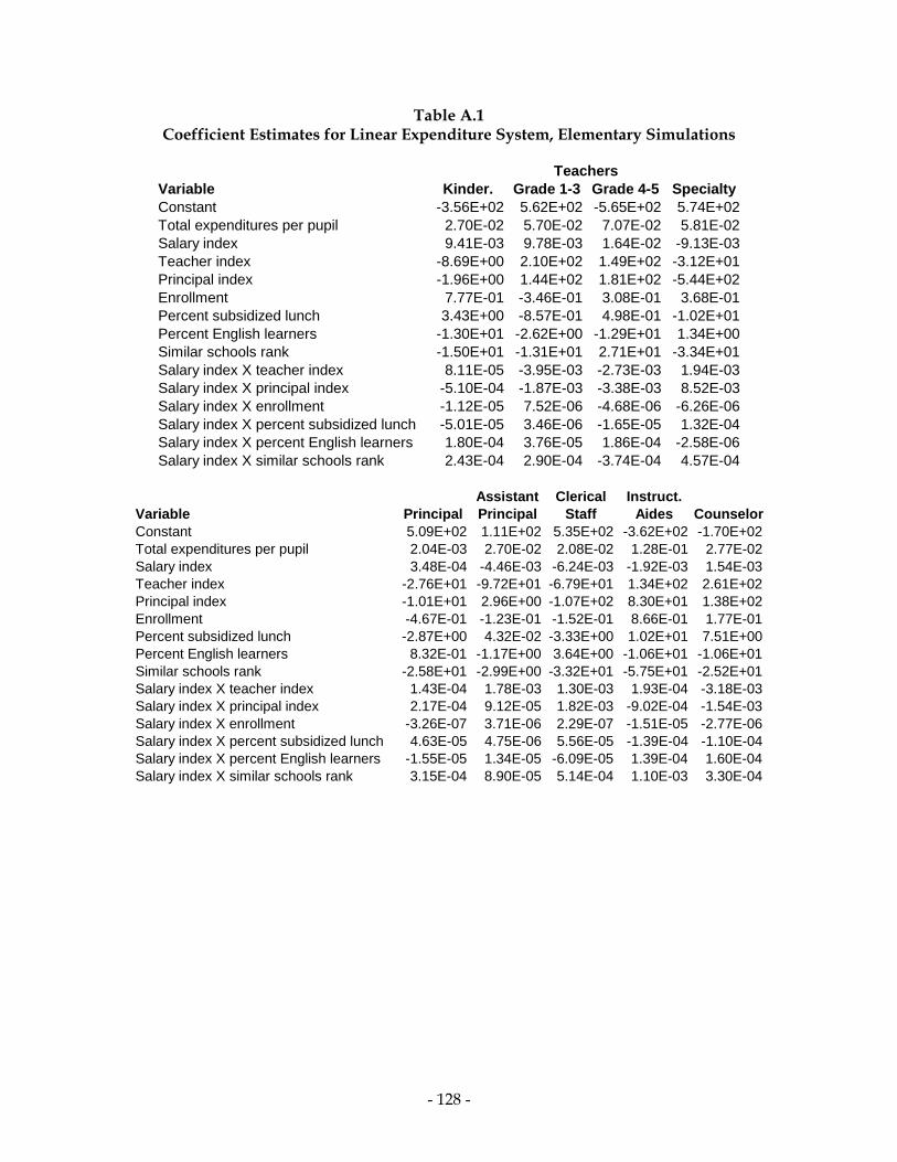
Table A.1 Coefficient Estimates for Linear Expenditure System, Elementary Simulations
Variable Kinder. Grade 1-3 Grade 4-5 SpecialtyConstant -3.56E+02 5.62E+02 -5.65E+02 5.74E+02Total expenditures per pupil 2.70E-02 5.70E-02 7.07E-02 5.81E-02Salary index 9.41E-03 9.78E-03 1.64E-02 -9.13E-03Teacher index -8.69E+00 2.10E+02 1.49E+02 -3.12E+01Principal index -1.96E+00 1.44E+02 1.81E+02 -5.44E+02Enrollment 7.77E-01 -3.46E-01 3.08E-01 3.68E-01Percent subsidized lunch 3.43E+00 -8.57E-01 4.98E-01 -1.02E+01Percent English learners -1.30E+01 -2.62E+00 -1.29E+01 1.34E+00Similar schools rank -1.50E+01 -1.31E+01 2.71E+01 -3.34E+01Salary index X teacher index 8.11E-05 -3.95E-03 -2.73E-03 1.94E-03Salary index X principal index -5.10E-04 -1.87E-03 -3.38E-03 8.52E-03Salary index X enrollment -1.12E-05 7.52E-06 -4.68E-06 -6.26E-06Salary index X percent subsidized lunch -5.01E-05 3.46E-06 -1.65E-05 1.32E-04Salary index X percent English learners 1.80E-04 3.76E-05 1.86E-04 -2.58E-06Salary index X similar schools rank 2.43E-04 2.90E-04 -3.74E-04 4.57E-04
Teachers
Assistant Clerical Instruct.Variable Principal Principal Staff Aides CounselorConstant 5.09E+02 1.11E+02 5.35E+02 -3.62E+02 -1.70E+02Total expenditures per pupil 2.04E-03 2.70E-02 2.08E-02 1.28E-01 2.77E-02Salary index 3.48E-04 -4.46E-03 -6.24E-03 -1.92E-03 1.54E-03Teacher index -2.76E+01 -9.72E+01 -6.79E+01 1.34E+02 2.61E+02Principal index -1.01E+01 2.96E+00 -1.07E+02 8.30E+01 1.38E+02Enrollment -4.67E-01 -1.23E-01 -1.52E-01 8.66E-01 1.77E-01Percent subsidized lunch -2.87E+00 4.32E-02 -3.33E+00 1.02E+01 7.51E+00Percent English learners 8.32E-01 -1.17E+00 3.64E+00 -1.06E+01 -1.06E+01Similar schools rank -2.58E+01 -2.99E+00 -3.32E+01 -5.75E+01 -2.52E+01Salary index X teacher index 1.43E-04 1.78E-03 1.30E-03 1.93E-04 -3.18E-03Salary index X principal index 2.17E-04 9.12E-05 1.82E-03 -9.02E-04 -1.54E-03Salary index X enrollment -3.26E-07 3.71E-06 2.29E-07 -1.51E-05 -2.77E-06Salary index X percent subsidized lunch 4.63E-05 4.75E-06 5.56E-05 -1.39E-04 -1.10E-04Salary index X percent English learners -1.55E-05 1.34E-05 -6.09E-05 1.39E-04 1.60E-04Salary index X similar schools rank 3.15E-04 8.90E-05 5.14E-04 1.10E-03 3.30E-04
- 128 -

Table A.1 (continued)
Security Tech. Com.Variable Nurse Librarian Officers Support LiaisonConstant -8.40E+01 -2.20E+02 -7.70E+01 -1.34E+02 1.32E+01Total expenditures per pupil 2.54E-02 2.82E-02 2.64E-03 4.28E-02 9.19E-03Salary index 2.55E-04 3.28E-03 5.39E-04 8.51E-04 -4.29E-04Teacher index 2.54E+01 7.98E+01 -5.56E+00 -2.14E+01 2.07E+01Principal index 9.11E-01 1.33E+02 5.92E+01 1.75E+02 4.38E+01Enrollment 6.36E-02 3.02E-02 9.36E-02 1.48E-01 1.16E-01Percent subsidized lunch 2.02E+00 3.57E+00 1.37E+00 4.58E+00 5.99E-01Percent English learners 9.60E-02 -4.16E+00 -1.11E+00 -5.45E+00 -6.63E-01Similar schools rank -1.35E+01 -1.40E+01 1.86E-01 -2.54E+01 -1.40E+01Salary index X teacher index -1.38E-04 -8.74E-04 1.72E-04 1.03E-03 -2.68E-04Salary index X principal index 4.96E-05 -1.87E-03 -7.27E-04 -2.36E-03 -6.02E-04Salary index X enrollment -1.23E-06 -1.55E-06 -8.20E-07 -3.07E-06 -1.87E-06Salary index X percent subsidized lunch -2.35E-05 -5.89E-05 -1.53E-05 -6.95E-05 -5.58E-06Salary index X percent English learners -8.46E-06 5.78E-05 1.26E-05 7.80E-05 1.27E-05Salary index X similar schools rank 2.03E-04 2.20E-04 7.59E-07 3.38E-04 1.80E-04
Academic Collab. Pre- Summer
Variable Coach Time school Tutoring SchoolConstant 2.43E+02 -2.62E+02 -8.05E+02 3.84E+02 -2.89E+02Total expenditures per pupil 7.51E-02 3.20E-02 1.05E-01 3.76E-02 1.92E-02Salary index -7.51E-03 2.86E-03 5.66E-03 -7.35E-03 3.24E-03Teacher index -5.55E+01 -1.54E+02 2.96E+02 1.04E+02 6.88E+01Principal index 3.32E+02 6.41E+02 -3.79E+02 2.83E+02 7.39E+01Enrollment -3.07E-01 1.33E-01 4.01E-01 -5.15E-01 7.11E-02Percent subsidized lunch -1.57E-01 -2.59E+00 -4.08E+00 -4.55E+00 1.94E+00Percent English learners -4.63E+00 1.21E+01 3.38E+00 9.58E+00 1.15E+00Similar schools rank -1.68E+01 1.18E+01 1.36E+02 -2.94E+01 4.22E+00Salary index X teacher index 8.05E-04 1.31E-03 -4.98E-03 -1.74E-03 -1.13E-03Salary index X principal index -4.37E-03 -8.58E-03 4.70E-03 -4.22E-03 -1.23E-03Salary index X enrollment 4.45E-06 -1.15E-06 -2.42E-06 8.36E-06 -5.54E-07Salary index X percent subsidized lunch 2.47E-06 2.67E-05 6.94E-05 6.48E-05 -2.25E-05Salary index X percent English learners 7.33E-05 -1.46E-04 -4.36E-05 -1.29E-04 -1.46E-05Salary index X similar schools rank 2.07E-04 -2.00E-04 -2.19E-03 4.02E-04 -8.83E-05
- 129 -

Table A.1 (continued)
Longer Longer Full-day
Variable Year Day Kinder. Computers OtherConstant 4.15E+02 6.92E+02 -1.59E+02 -1.56E+02 -4.00E+02Total expenditures per pupil 4.08E-02 5.71E-02 1.98E-02 2.95E-02 5.75E-02Salary index -7.49E-03 -1.40E-02 1.28E-03 1.57E-03 1.51E-03Teacher index -4.02E+02 -1.20E+02 7.30E+00 -1.49E+02 -2.17E+02Principal index -5.61E+02 -6.05E+02 1.73E+02 -3.07E+01 -2.24E+02Enrollment -4.85E-01 -1.33E+00 -3.51E-01 4.22E-02 4.79E-01Percent subsidized lunch -8.41E+00 -8.05E+00 -4.73E-01 4.50E+00 5.32E+00Percent English learners 1.66E+01 3.02E+01 6.02E+00 -6.18E+00 -1.19E+01Similar schools rank 3.49E+01 -2.63E+00 3.84E+01 1.62E+01 5.33E+01Salary index X teacher index 4.35E-03 1.62E-03 -4.61E-04 2.23E-03 2.50E-03Salary index X principal index 7.12E-03 9.08E-03 -2.49E-03 3.40E-04 2.71E-03Salary index X enrollment 7.33E-06 2.08E-05 6.35E-06 -3.83E-07 -5.36E-06Salary index X percent subsidized lunch 1.11E-04 1.28E-04 1.56E-05 -6.79E-05 -8.07E-05Salary index X percent English learners -2.25E-04 -4.63E-04 -9.90E-05 8.57E-05 1.71E-04Salary index X similar schools rank -5.32E-04 2.35E-05 -5.29E-04 -2.85E-04 -7.12E-04
- 130 -

Table A.2 Coefficient Estimates for Linear Expenditure System, Middle School Simulations
AssistantVariables Core Non-core PE Principal PrincipalConstant 2.34E+03 6.90E+02 9.81E+02 -1.15E+02 -5.22E+00Total expenditures per pupil 2.06E-01 6.70E-02 6.14E-02 2.36E-03 1.92E-02Salary index -9.95E-03 -9.14E-03 -1.29E-02 5.34E-03 1.30E-03Teacher index -2.41E+02 -1.14E+02 -1.48E+02 9.45E+01 -9.87E+01Principal index 3.46E+02 -3.54E+01 -4.32E+02 7.67E+01 5.71E+00Enrollment 1.09E+00 -4.04E-01 -2.75E-02 1.48E-01 -3.33E-01Percent subsidized lunch -1.27E+01 -5.05E+00 -4.13E+00 9.70E-01 -3.61E+00Percent English learners -2.86E+00 1.91E+01 1.59E+01 -4.66E+00 7.33E+00Similar schools rank 9.46E+01 6.07E+01 -4.58E+01 -3.51E+01 -9.85E+00Average feeder API -4.58E+00 -9.86E-01 -7.71E-01 1.54E-01 5.35E-01Salary index X teacher index 3.07E-03 2.20E-03 2.75E-03 -1.75E-03 1.75E-03Salary index X principal index -6.13E-03 8.08E-04 6.16E-03 -1.48E-03 6.42E-04Salary index X enrollment -1.52E-05 5.65E-06 5.10E-07 -4.93E-06 5.00E-06Salary index X percent subsidized lunch 1.85E-04 5.71E-05 4.99E-05 -8.48E-06 5.95E-05Salary index X percent English learners 3.74E-05 -2.68E-04 -2.21E-04 6.17E-05 -1.14E-04Salary index X similar schools rank -1.34E-03 -9.64E-04 5.67E-04 5.30E-04 9.09E-05Salary index X average feeder API 5.60E-05 1.69E-05 1.06E-05 -8.70E-07 -8.40E-06
Teachers
Clerical Instruct.Variables Staff Aides Counselor NurseConstant -4.18E+02 7.11E+02 -3.84E+02 -9.68E+01Total expenditures per pupil 2.02E-02 3.19E-02 3.08E-02 1.44E-02Salary index 6.29E-03 -6.23E-03 7.53E-03 3.91E-04Teacher index 3.35E+00 1.41E+02 -4.20E+00 1.15E+02Principal index -1.30E+02 -3.49E+01 2.45E+01 3.26E+00Enrollment -1.27E-01 5.78E-01 -5.07E-01 -7.09E-03Percent subsidized lunch -1.82E-01 8.54E-01 2.39E-01 1.43E+00Percent English learners 1.22E+00 -7.14E+00 -4.28E-02 -1.71E+00Similar schools rank 1.88E+01 -9.23E+01 4.02E+01 1.24E+01Average feeder API 8.73E-01 -6.02E-01 9.13E-01 -2.03E-02Salary index X teacher index 2.14E-04 -1.24E-03 3.05E-04 -1.48E-03Salary index X principal index 2.21E-03 1.67E-04 -2.99E-04 2.16E-05Salary index X enrollment 1.42E-06 -8.48E-06 7.40E-06 -3.16E-07Salary index X percent subsidized lunch -2.63E-06 2.17E-06 -4.50E-06 -2.37E-05Salary index X percent English learners -9.69E-06 9.57E-05 -8.96E-06 3.28E-05Salary index X similar schools rank -2.94E-04 1.41E-03 -6.69E-04 -1.55E-04Salary index X average feeder API -1.08E-05 2.77E-06 -1.43E-05 1.69E-06
- 131 -

Table A.2 (continued)
Security Tech. Com.Variables Librarian Officers Support LiaisonConstant -1.87E+02 -7.36E+02 1.71E+02 -1.79E+02Total expenditures per pupil 1.06E-02 7.86E-03 2.88E-02 9.21E-03Salary index 3.83E-03 1.02E-02 -3.10E-03 2.52E-03Teacher index -8.82E+01 2.52E+02 6.82E+01 1.04E+02Principal index -9.01E+01 1.68E+02 -9.05E+01 6.59E+01Enrollment -1.05E-01 -1.09E-01 5.30E-02 1.49E-02Percent subsidized lunch -1.44E+00 4.09E+00 -5.42E+00 3.01E+00Percent English learners 2.78E+00 -1.49E+00 9.22E+00 -3.34E+00Similar schools rank 1.87E+01 -1.91E+01 -2.17E+01 4.55E+00Average feeder API 3.12E-01 9.75E-01 5.34E-02 6.72E-02Salary index X teacher index 1.30E-03 -3.44E-03 -8.10E-04 -1.35E-03Salary index X principal index 1.15E-03 -2.12E-03 1.39E-03 -8.90E-04Salary index X enrollment 2.61E-07 1.90E-06 -1.42E-06 -4.57E-07Salary index X percent subsidized lunch 2.05E-05 -5.33E-05 7.70E-05 -4.03E-05Salary index X percent English learners -3.93E-05 1.66E-05 -1.29E-04 5.04E-05Salary index X similar schools rank -2.59E-04 2.01E-04 3.36E-04 -6.12E-05Salary index X average feeder API -3.68E-06 -1.35E-05 -3.15E-07 -1.11E-06
Academic Collab. Summer
Variables Coach Time Tutoring SchoolConstant -7.21E+02 5.63E+02 -2.12E+03 -3.98E+02Total expenditures per pupil 5.73E-02 1.05E-01 6.90E-02 1.15E-02Salary index 9.53E-03 -1.51E-02 2.39E-02 6.46E-03Teacher index 2.04E+02 6.00E+02 2.38E+02 -1.68E+02Principal index 7.83E+01 4.02E+02 3.96E+01 -1.81E+02Enrollment -3.19E-02 2.71E-01 4.04E-01 8.42E-02Percent subsidized lunch 1.10E+01 6.33E+00 6.04E+00 3.17E+00Percent English learners -7.67E+00 2.31E+00 -7.28E+00 -4.13E+00Similar schools rank 2.84E+00 -6.03E-01 -4.68E+01 7.70E+00Average feeder API 3.92E-01 -1.95E+00 2.38E+00 4.78E-01Salary index X teacher index -3.73E-03 -8.49E-03 -3.29E-03 2.00E-03Salary index X principal index -1.31E-03 -5.30E-03 -1.14E-05 2.57E-03Salary index X enrollment 2.74E-07 -2.31E-06 -4.83E-06 -8.30E-07Salary index X percent subsidized lunch -1.62E-04 -9.27E-05 -7.86E-05 -4.47E-05Salary index X percent English learners 1.11E-04 -3.96E-05 9.28E-05 6.62E-05Salary index X similar schools rank -5.38E-05 -8.85E-06 5.82E-04 -1.03E-04Salary index X average feeder API -6.27E-06 2.80E-05 -3.05E-05 -7.92E-06
- 132 -

Table A.2 (continued)
Longer LongerVariables Year Day Computers OtherConstant -3.33E+02 5.75E+02 -7.76E+02 4.43E+02Total expenditures per pupil 3.77E-02 1.44E-01 3.64E-02 2.91E-02Salary index 3.15E-03 -2.49E-02 9.37E-03 -8.38E-03Teacher index -2.53E+02 -4.54E+02 -3.55E+01 -2.14E+02Principal index -1.61E+02 -1.30E+02 -2.79E+01 1.03E+02Enrollment -2.68E-02 -9.92E-01 -1.86E-02 4.96E-02Percent subsidized lunch 1.45E+00 -1.20E+00 -1.75E+00 -3.16E+00Percent English learners -1.04E+01 -1.12E+01 3.08E+00 8.94E-01Similar schools rank -2.18E+00 5.19E+00 4.21E+01 -3.42E+01Average feeder API 7.26E-01 4.16E-01 8.47E-01 -2.16E-01Salary index X teacher index 2.78E-03 6.24E-03 1.91E-04 2.78E-03Salary index X principal index 1.60E-03 2.37E-03 7.98E-05 -1.63E-03Salary index X enrollment 9.36E-07 1.53E-05 3.47E-07 -2.23E-07Salary index X percent subsidized lunch -2.15E-05 1.78E-05 2.51E-05 3.84E-05Salary index X percent English learners 1.49E-04 1.66E-04 -4.41E-05 -5.09E-06Salary index X similar schools rank 9.93E-05 1.88E-04 -5.93E-04 4.98E-04Salary index X average feeder API -1.16E-05 1.46E-06 -1.15E-05 3.45E-06
- 133 -

Table A.3 Coefficient Estimates for Linear Expenditure System, High School Simulations
AssistantVariables Core Non-core PE Principal PrincipalConstant -3.75E+03 -1.14E+03 -2.37E+02 3.70E+02 -3.41E+02Total expenditures per pupil 1.51E-01 1.37E-01 2.09E-02 1.86E-03 2.74E-02Salary index 7.33E-02 2.07E-02 5.08E-03 3.82E-04 3.63E-03Teacher index 3.02E+02 8.36E+02 1.28E+02 -2.61E+02 -1.07E+02Principal index -4.50E+02 7.66E+02 9.91E+01 -7.75E+01 -5.63E+01Enrollment 7.35E-01 5.10E-03 -1.04E-02 -1.09E-01 -2.15E-02Percent subsidized lunch -3.25E+00 1.97E+01 -3.32E+00 6.44E+00 7.46E-02Percent English learners 3.19E+00 -3.69E+01 5.81E+00 -1.21E+01 1.17E+00Similar schools rank 4.44E+01 -5.63E+01 5.11E+00 1.81E+01 3.16E+01Average feeder API 2.96E+00 8.81E-01 1.21E-01 -1.91E-01 2.22E-01Salary index X teacher index -3.35E-03 -1.14E-02 -1.40E-03 3.54E-03 1.78E-03Salary index X principal index 7.09E-03 -1.09E-02 -1.53E-03 1.14E-03 1.16E-03Salary index X enrollment -1.19E-05 2.68E-07 -3.08E-08 -9.30E-08 4.88E-07Salary index X percent subsidized lunch 4.55E-05 -2.92E-04 5.05E-05 -8.53E-05 -7.13E-06Salary index X percent English learners -5.32E-05 5.25E-04 -8.02E-05 1.74E-04 -7.85E-06Salary index X similar schools rank -4.42E-04 7.03E-04 -9.31E-05 -1.75E-04 -5.51E-04Salary index X average feeder API -4.70E-05 -1.03E-05 -1.89E-06 5.49E-07 -1.12E-06
Teachers
Clerical Instruct.Variables Staff Aides Counselor NurseConstant 6.83E+01 -2.70E+02 4.47E+02 2.32E+02Total expenditures per pupil 4.87E-02 7.80E-02 3.69E-02 9.50E-03Salary index -1.84E-03 6.35E-05 -5.24E-03 -3.77E-03Teacher index -1.60E+02 -2.45E+02 1.50E+01 -9.83E+01Principal index -1.87E+02 -3.85E+02 -7.21E+01 -9.66E+01Enrollment -1.14E-01 -8.80E-02 -1.98E-01 -1.50E-02Percent subsidized lunch -1.87E+00 -5.53E+00 1.80E+00 -3.61E+00Percent English learners 1.04E+01 1.28E+01 8.96E-01 6.15E+00Similar schools rank -1.38E+01 -1.30E+01 1.85E+01 9.08E+00Average feeder API 4.65E-01 9.63E-01 -4.35E-01 -1.78E-01Salary index X teacher index 3.05E-03 3.95E-03 -1.17E-04 1.50E-03Salary index X principal index 3.55E-03 5.47E-03 1.40E-03 1.42E-03Salary index X enrollment 1.28E-06 1.37E-06 2.78E-06 1.06E-07Salary index X percent subsidized lunch 3.75E-05 8.04E-05 -2.19E-05 5.63E-05Salary index X percent English learners -1.84E-04 -2.00E-04 -1.30E-05 -9.13E-05Salary index X similar schools rank 3.13E-04 1.85E-04 -3.11E-04 -1.19E-04Salary index X average feeder API -6.89E-06 -1.38E-05 5.71E-06 2.98E-06
- 134 -
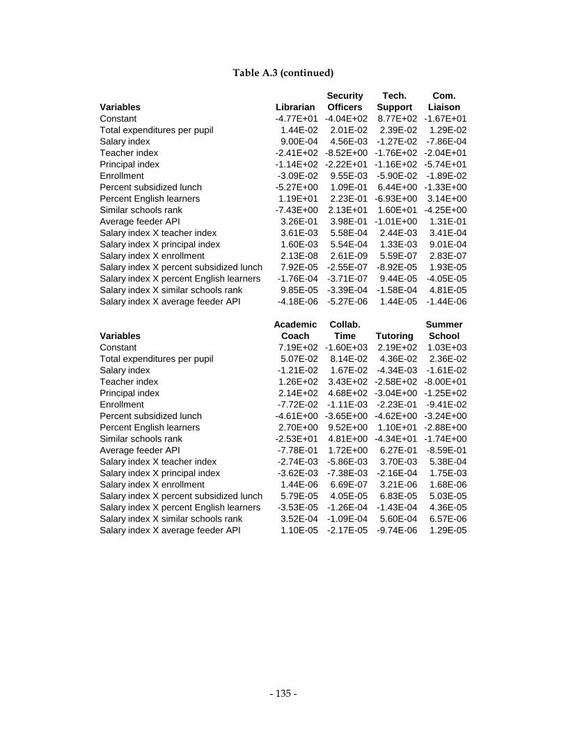
Table A.3 (continued)
Security Tech. Com.Variables Librarian Officers Support LiaisonConstant -4.77E+01 -4.04E+02 8.77E+02 -1.67E+01Total expenditures per pupil 1.44E-02 2.01E-02 2.39E-02 1.29E-02Salary index 9.00E-04 4.56E-03 -1.27E-02 -7.86E-04Teacher index -2.41E+02 -8.52E+00 -1.76E+02 -2.04E+01Principal index -1.14E+02 -2.22E+01 -1.16E+02 -5.74E+01Enrollment -3.09E-02 9.55E-03 -5.90E-02 -1.89E-02Percent subsidized lunch -5.27E+00 1.09E-01 6.44E+00 -1.33E+00Percent English learners 1.19E+01 2.23E-01 -6.93E+00 3.14E+00Similar schools rank -7.43E+00 2.13E+01 1.60E+01 -4.25E+00Average feeder API 3.26E-01 3.98E-01 -1.01E+00 1.31E-01Salary index X teacher index 3.61E-03 5.58E-04 2.44E-03 3.41E-04Salary index X principal index 1.60E-03 5.54E-04 1.33E-03 9.01E-04Salary index X enrollment 2.13E-08 2.61E-09 5.59E-07 2.83E-07Salary index X percent subsidized lunch 7.92E-05 -2.55E-07 -8.92E-05 1.93E-05Salary index X percent English learners -1.76E-04 -3.71E-07 9.44E-05 -4.05E-05Salary index X similar schools rank 9.85E-05 -3.39E-04 -1.58E-04 4.81E-05Salary index X average feeder API -4.18E-06 -5.27E-06 1.44E-05 -1.44E-06
Academic Collab. Summer
Variables Coach Time Tutoring SchoolConstant 7.19E+02 -1.60E+03 2.19E+02 1.03E+03Total expenditures per pupil 5.07E-02 8.14E-02 4.36E-02 2.36E-02Salary index -1.21E-02 1.67E-02 -4.34E-03 -1.61E-02Teacher index 1.26E+02 3.43E+02 -2.58E+02 -8.00E+01Principal index 2.14E+02 4.68E+02 -3.04E+00 -1.25E+02Enrollment -7.72E-02 -1.11E-03 -2.23E-01 -9.41E-02Percent subsidized lunch -4.61E+00 -3.65E+00 -4.62E+00 -3.24E+00Percent English learners 2.70E+00 9.52E+00 1.10E+01 -2.88E+00Similar schools rank -2.53E+01 4.81E+00 -4.34E+01 -1.74E+00Average feeder API -7.78E-01 1.72E+00 6.27E-01 -8.59E-01Salary index X teacher index -2.74E-03 -5.86E-03 3.70E-03 5.38E-04Salary index X principal index -3.62E-03 -7.38E-03 -2.16E-04 1.75E-03Salary index X enrollment 1.44E-06 6.69E-07 3.21E-06 1.68E-06Salary index X percent subsidized lunch 5.79E-05 4.05E-05 6.83E-05 5.03E-05Salary index X percent English learners -3.53E-05 -1.26E-04 -1.43E-04 4.36E-05Salary index X similar schools rank 3.52E-04 -1.09E-04 5.60E-04 6.57E-06Salary index X average feeder API 1.10E-05 -2.17E-05 -9.74E-06 1.29E-05
- 135 -

Table A.3 (continued)
Longer LongerVariables Year Day Computers OtherConstant 2.29E+02 2.28E+03 1.39E+03 -5.78E+01Total expenditures per pupil 2.12E-02 1.17E-01 3.16E-02 4.72E-02Salary index -4.85E-03 -3.84E-02 -2.13E-02 -3.97E-03Teacher index -1.49E+01 -3.09E+02 3.85E+01 1.90E+02Principal index 4.41E+01 3.88E+02 -5.34E+01 -1.62E+02Enrollment -1.05E-02 2.79E-01 -6.26E-02 1.05E-01Percent subsidized lunch -1.04E+00 9.63E+00 -4.81E+00 1.90E+00Percent English learners 2.43E+00 -1.41E+01 3.10E+00 -1.16E+01Similar schools rank -3.75E+00 4.64E+00 -1.24E+01 7.93E+00Average feeder API -2.07E-01 -3.61E+00 -1.44E+00 -9.06E-02Salary index X teacher index -2.81E-04 3.77E-03 -1.13E-03 -2.46E-03Salary index X principal index -8.22E-04 -5.13E-03 4.04E-04 1.82E-03Salary index X enrollment 3.75E-07 -2.51E-06 1.16E-06 -1.15E-06Salary index X percent subsidized lunch 1.48E-05 -1.39E-04 6.77E-05 -3.29E-05Salary index X percent English learners -1.59E-05 2.15E-04 -5.05E-05 1.64E-04Salary index X similar schools rank 1.40E-05 -1.80E-05 1.52E-04 -1.16E-04Salary index X average feeder API 3.49E-06 4.74E-05 2.14E-05 3.55E-06
- 136 -

Appendix B. The Definition of Unit Costs
For collaborative time, a longer school day, or a longer school year, teachers must be compensated for time in addition to that specified in a standard teacher’s contract. The cost of increasing collaborative time, the school day, or the school year depends on that compensation rate, but it also depends on the number of teachers to be compensated, which the participants in the simulation determine. For example, collaborative time is measured in hours per teacher per year. The cost of that program is thus affected by the number of teachers employed in the school. On the other hand, not only does the number of teachers affect the cost of collaborative time, the cost of hiring a teacher is also affected by the number of hours of collaborative time for which each teacher must be compensated.
These interactions are easiest to grasp by writing out a simple equation for the cost of teachers:
C=T(S+WN), (B.1)
In this equation, C is total cost, T is the number of teachers, S is the annual cost of teachers employed according to the standard contract, W is the cost of employing a teacher for an hour in addition to the hours in the standard contract, and N is the number of hours per year each teacher is paid for additional collaborative time. In this case, the cost of hiring a teacher depends on N as well as S. Furthermore, the cost of collaborate time depends on T as well as W.
This interaction creates an ambiguity in the definition of cost per unit. The cost per unit of teachers could be defined holding fixed the units of collaborative time, and the cost per unit of collaborative time could be defined holding constant the number of teachers. However, if unit costs were defined that way, multiplying costs by units and summing over resources and programs would yield a total greater than actual expenditures. The resolution is to adopt a different definition of cost, which, though somewhat arbitrary, has the virtue of yielding a total that equals actual expenditures. This definition starts by rewriting the equation above in the following way:
C=ST+TWN (B.2)
In this formulation, S, the annual cost of teachers under a standard contract, is the cost of hiring one more teacher, and TW, the hourly cost of teachers multiplied by the number of teachers, is the cost of increasing collaborative time by one hour per teacher.
The same issue arises with the cost of extending the school day and school year. Suppose D is the additional days beyond the standard school year of 180 days, and H is the additional hours per day of instruction. The standard contract calls for 7 hours per day, so the cost to a school of increasing the school year, assuming the standard school day, is 7TWD. If the school increases instruction time by H hours per day for 180+D instruction days, the cost is TW(180+D)H. The cost of collaborative time is TWN. Adding these costs together, the cost of employing teachers is as follows:
C=ST+TW(180+D)H+7TWD+TWN (B.3)
- 137 -

- 138 -
In this formulation, S is the unit cost of one more teacher, TW(180+D) is the unit cost of increasing the school day by one hour, 7TW is the unit cost of increasing the school year by one day, and TW is the cost of increasing collaborative time by one hour per teacher. The last three unit costs depend not only on the annual cost of teachers under a normal contract but also on the other choices a participant has made.
For the elementary school spreadsheet, there is one further complication. The norm for kindergarten classes is 3 hours of instruction per day. Respondents have the option of turning this half-day kindergarten into full-day, which is 5 hours per day. The cost of this option follows the general formula for increasing the school day explained above. In particular, it assumes that kindergarten classes have the same number of instruction days as other classes, and it incorporates any extra days for the school year the participant may have chosen. The cost of increasing the school day for grades 1 through 5 does not include the cost of extending kindergarten classes. On the other hand, the cost of extending the school year includes both kindergarten and grade 1 through 5 classes. The unit cost of this action follows the same convention explained above with kindergarten teachers employed for 5 hours per day and grade 1 through 7 teachers employed for 7 hours per day.

Appendix C. Instructions for Elementary School Simulations
Background Material for Elementary Schools
The survey begins by describing a hypothetical school.
You then see a spreadsheet for the school's budget. The spreadsheet lists important school resources and programs and provides you with a budget to spend on these resources and programs. You enter quantities of each resource and program, and the spreadsheet calculates how much of your budget you have spent. Your goal is to allocate your school's resources to maximize the academic achievement of its students. When you have accomplished that goal, you enter your prediction for student achievement.
After you have completed this first budget exercise, you complete a second exercise with a different budget scenario.
The components of the survey are described below.
School Description
The school enrolls students in kindergarten through fifth grade. The survey specifies the number of students enrolled. Students are equally distributed across the six grades in your school.
The survey describes the percentages of the school’s students and their parents with various characteristics. These are the same characteristics that appear on a school’s Academic Performance Index (API) report. The characteristics are as follows:
Student characteristics Parent education African American (Not of Hispanic origin) Participants in free or reduced price lunch Not a high school graduate American Indian or Alaska Native English learners High school graduate Asian Some college Filipino College graduate Hispanic or Latino Graduate school Pacific Islander White (not of Hispanic origin)
- 139 -

Budget Spreadsheet
On the right is a picture of the budget spreadsheet.
The first three columns set the parameters of the budget exercise. The first column lists the school’s resources and programs, the second column gives the unit of measure for each resource and program, and the third column specifies the cost of each unit. These elements are described on pages 5, 6, and 7.
Your goal is to allocate the school’s budget among its resources and programs to maximize the academic achievement of its students. You enter the units of each resource or program in the fourth column, labeled Units. The fifth column, labeled Total Cost, automatically calculates the total cost of the units you enter.
Your school’s budget and the total you have spent are displayed in a box in the middle of the page, just to the right of the Total Cost column.
You enter your prediction of the school’s API in the last cell of the Units column.
You must enter a number in every cell in the Units column. These cells are highlighted in yellow. If you choose not allocate any of your budget to a resource or program, enter zero in the corresponding cell.
- 140 -

When you are finished, click the button labeled “Click to continue,” which is at the bottom of the page. If you have overspent (or underspent) your budget, you will receive a warning message instructing you to bring your expenditures into line with your budget. Expenditures must be within $1,000 of your budget.
To the right of the Total Cost column are three tools to assist you. The first is the Class Size Calculator, just to the right of the cells in which you enter the number of teachers. The Class Size Calculator displays the average class size in various grade spans (K, 1-3, 4-5) resulting from your choice of the number of teachers in each grade span.
Directly below the Class Size Calculator is the Budget Calculator. The Budget Calculator displays the school’s total budget, the amount you have spent, and the balance that remains. Attached to the bottom of the Budget Calculator is a button labeled "Show School Statistics." If you click this button, you will see the characteristics of the school’s students and their parents.
Below the Budget Calculator is the After-School Calculator. You enter the number of students participating in the school’s after-school tutoring program, the number of students in each tutorial group, and the number of hours per week the groups meet. The calculator then returns the number of teacher-hours per week required by your program. Enter this number in the Units column for the after-school tutoring program.
- 141 -

Assumptions
In completing this survey, we ask you to make the following simplifying assumptions:
1. Special education. The school does not have any students requiring special education services. Item three in a numbered list.
2. Scope of expenditures. None of your budget needs to be spent on facilities, transportation services, maintenance and operations, instructional materials, or office supplies. Assume your school has adequate resources in these areas.
3. Additional revenues. The only funding source for the resources and programs listed in your spreadsheet is the budget provided. Your school does not have access to additional sources of funding such as state and federal categorical programs and contributions from parents, foundations, or other groups.
4. Expenditure restrictions. There are no restrictions on how you spend your school’s budget. In particular, your school does not have restrictions on maximum class size typical of collective bargaining agreements and some state categorical programs.
5. Salaries and benefits. The salaries and benefits for employees are sufficient to attract and retain qualified personnel. Salaries and benefits may change from one budget scenario to another, but continue to assume that they are sufficient.
6. School day and year. Students attend classes 180 days per year (these include state testing days). Instructional time depends on the grade level:
Grade level Instructional time per day Kindergarten 3.3 hours (200 minutes) Grades 1 - 5 5 hours (300 minutes)
Teachers are contracted to work 184 days per year. Two of these days are used for professional development, and two are teacher-work days used for parent conferences, preparation, and related activities. Teachers are contracted to work 7 hours per day. This includes 2.5 hours of preparation time per week. As you will learn below, you may elect to spend some of your school’s budget on lengthening the school day and year.
- 142 -

Resources and Programs
Staffing Categories
All staff positions are measured as full-time equivalents (FTE). One FTE works five full days per week. A staff member working one day per week is 0.2 FTE. When choosing staffing levels, assume that substitute teachers will staff absences. The cost of these substitutes is included in the cost of a teacher FTE.
Teachers Teachers refer to credentialed full-time teachers. Assume that teachers have an average of 11 years of experience. You may select the number of teachers for kindergarten, grades 1 through 3, and grades 4 through 5, thereby producing different average class sizes for these three grade spans. Within any grade span, treat these averages as guidelines. The school can have classes of different sizes within the same grade span. Ultimately, we are concerned only with the number of teachers and not how you deploy them.
The unit cost of kindergarten teachers is less than that of other teaches, because kindergarten teachers are assumed to be in class for 3.5 hours and on campus for an additional 1.5 hours per day, for a total of only 5 hours per day. We know that many schools employ kindergarten teachers for 7 hours per day, using the additional 2 hours in other special roles. The spreadsheet assumes that kindergarten teachers are only teaching in kindergarten, however. If you envision hiring kindergarten teachers for 7 hours and assigning those additional 2 hours in other programs, you must increase the number of teacher FTE to reflect that assignment. For example, 4 teachers who teach half-day kindergarten in the morning and assist first-grade teachers for 2 hours in the afternoon constitute 4 kindergarten teacher FTE and 1.14 (8/7) grade 1-3 teacher FTE.
In addition to kindergarten teachers and teachers in grades 1 through 5, the spreadsheet also allows you to select the number of specialty teachers. These are teachers in subjects such as music, art, and science who instruct students from several different classrooms in the school.
Administration All administrative positions are measured in FTE. Clerical office staff include attendance and other secretaries at the school site.
- 143 -

Support staff All support staff are measured in FTE. Instructional aides assist teachers in the classroom. Counselors help students with psychological, behavioral, and social issues. Technology support staff maintain the school’s computer systems, install software, and provide help to users. Community liaisons coordinate volunteers, promote community outreach, and work with parents, businesses, and public agencies.
Professional Development
Academic coaches Academic coaches include mentor teachers, curriculum development specialists, and testing and assessment specialists.
Collaborative time This program is the time teachers spend working together on curriculum development, pacing calendars, student assessments, and other related activities. It is also time teachers spend with instructional consultants on effective pedagogy. Collaborative time is measured by the hours each teacher would be engaged in these activities during the school year. If you want teachers to have an additional hour per week of common planning time for each of the 36 weeks in the school year, you would enter 36. The cost of these hours is determined by the salary of teachers, which is fixed for the budget scenario. These hours are in addition to the instructional and preparation time specified in teacher contracts. They are also in addition to the two days of professional development teachers already receive.
You do not need to assume that all teachers are engaged in these activities. If you only want half of your teachers to have 70 additional hours of collaborative time, enter 35 hours.
Assume that the appropriate materials, facilities, and transportation would be available for the activities you desire.
Student Programs
Pre-school You may use some of your school’s budget to provide pre-school for your school’s students. Enter the number of students for whom you would like to provide this program. Each pre-school class would have 20 students, 1 teacher, and 1 aide.
Full-day kindergarten You have the option of offering full-day (5 hours) kindergarten. This option provides full-day kindergarten to all kindergarten students. Enter “1” if you would like full-day kindergarten and “0” if you do not.
- 144 -

After-school tutoring program The after-school tutoring program provides extra help to students in a small group setting. In the Units column of the spreadsheet, enter the total number of hours teachers will be employed in this program each week, based on the Teacher hours/week from the After-School Calculator. The teachers for these groups are credentialed. The spreadsheet assumes that they are compensated at the same rate as full-time credentialed teachers.
Longer school day This option would increase the instructional school day for every student in the school. Please enter the number of hours by which you would like to increase the instructional day. If you would like to increase your day by half an hour, please enter 0.5. (The school currently has 3.3 hours of instructional time per day in kindergarten and five hours in grades 1-5.)
Summer school The summer school program consists of four weeks of full day attendance. Assume average class sizes of 20 students. Please enter the number of students you want to attend this summer school program.
Longer school year This option would increase the length of the school year for every student in the school. Please enter the number of days by which you would like to increase the school year. If you want a school year of 195 instructional days, you would enter 15. (The school currently has 180 instructional days.)
Computers for instruction This figure refers to the total number of computers you want for the school – computers for students, teachers, other staff, and labs. Assume the computers are equipped with the appropriate software.
Other Expenditures
You may want to allocate part of your budget to resources and programs not listed on our spreadsheet. For example, you might want to spend some of your budget on field trips for students. Please make sure, however, that your “other expenditures” are not in one of the areas in which resources are assumed to be adequate without additional expenditures. If you would like to spend some of your budget on resources or programs not listed on the spreadsheet, enter the cost of those resources and programs in thousands of dollars in the appropriate row of the Units column and then enter a brief description of these expenditures in the box at the bottom left of the spreadsheet.
- 145 -

Predictions of Academic Achievement At the end of each budget exercise, we ask you to predict the Academic Performance Index (API) of the school. We understand that you may view the API to be an imperfect measure of the academic achievement of a school’s students. Nevertheless, the State Board of Education has established the API as a measure of school performance, and we believe that focusing on that index is an effective way for you to communicate to state policymakers.
In making API predictions, assume that the resources you have chosen have been in place long enough for them to have their full effect on student achievement.
The API is an average of many tests, and you may find it easier to think in simpler terms such as proficiency in English-Language Arts and Mathematics. In fact, we have found that proficiency on the California Standards Tests in these two areas yields a very good predictor of a school’s API. The prediction follows this simple formula:
API = 540+200*MATH+277*ELA
In this equation, MATH stands for the percentage of students proficient or advanced on the California Standards Tests in Mathematics and ELA stands for the percentage of students proficient or advanced on the California Standards Tests in English-Language Arts. For example, if 40 percent are proficient or advanced in Mathematics and 60 percent are advanced or proficient in English-Language Arts, a good prediction of the school's API is
API = 540+200*0.40+277*0.60 = 540+80+166 = 786
- 146 -

Appendix D. Instructions for Middle School Simulations
Background Material for Middle Schools
The survey begins by describing a hypothetical school.
You then see a spreadsheet for the school's budget. The spreadsheet lists important school resources and programs and provides you with a budget to spend on these resources and programs. You enter quantities of each resource and program, and the spreadsheet calculates how much of your budget you have spent. Your goal is to allocate the school's budget to maximize the academic achievement of its students. When you have accomplished that goal, you enter your prediction for student achievement.
After you have completed this first budget exercise, you complete a second exercise with a different budget scenario.
The components of the survey are described below.
School Description
The school enrolls students in 6th 7th, and 8th grades. The survey specifies the number of students enrolled. Students are equally distributed across the three grades. The survey also specifies the academic achievement of students in your school's feeder elementary schools. You will see the Academic Performance Index (API) of those schools and the percentage of students in those schools who score proficient or advanced in the California Standards Tests in Mathematics and English-Language Arts.
The survey describes the percentages of the school’s students and their parents with various characteristics. These are the same characteristics that appear on a school’s API report. The characteristics are as follows:
Student characteristics Parent education African American (Not of Hispanic origin) Participants in free or reduced price lunch Not a high school graduate American Indian or Alaska Native English learners High school graduate Asian Some college Filipino College graduate Hispanic or Latino Graduate school Pacific Islander White (not of Hispanic origin)
- 147 -

Budget Spreadsheet On the right is a picture of the budget spreadsheet.
The first three columns set the parameters of the budget exercise. The first column lists the school’s resources and programs, the second column gives the unit of measure for each resource and program, and the third column specifies the cost of each unit. These elements are described on pages 5, 6, and 7.
Your goal is to allocate the school’s budget among its resources and programs to maximize the academic achievement of its students. You enter the units of each resource or program in the fourth column, labeled Units. The fifth column, labeled Total Cost, automatically calculates the total cost of the units you enter.
Your school’s budget and the total you have spent are displayed in a box in the middle of the page, just to the right of the Total Cost column.
In the last two cells of the Units column, you enter your prediction for two measures of the academic achievement of the school's students. The first is the school's API and the second is the percentage of the school's 8th graders who are proficient or advanced in the California Standards Tests in Mathematics.
You must enter a number in every cell in the Units column. These cells are highlighted in yellow. If you choose not to allocate any of your budget to a resource or program, enter zero in the corresponding cell.
- 148 -

When you are finished, click the button labeled “Click to continue,” which is at the bottom of the page. If you have overspent (or underspent) your budget, you will receive a warning message instructing you to bring your expenditures into line with your budget. Expenditures must be within $1,000 of your budget.
To the right of the Total Cost column are three tools to assist you. The first is the Class Size Calculator, just to the right of the cells in which you enter the number of teachers. The Class Size Calculator displays the average class size core, noncore, and P.E. classes resulting from your choice of the number of teachers in each type of class.
Directly below the Class Size Calculator is the Budget Calculator. The Budget Calculator displays the school’s total budget, the amount you have spent, and the balance that remains. Attached to the bottom of the Budget Calculator is a button labeled "Show School Statistics." If you click this button, you will see the characteristics of the school’s students and their parents.
Below the Budget Calculator is the After-School Calculator. You enter the number of students participating in the school’s after-school tutoring program, the number of students in each tutorial group, and the number of hours per week the groups meet. The calculator then returns the number of teacher-hours per week required by your program. Enter this number in the Units column for the after-school tutoring program.
- 149 -

Assumptions
In completing this survey, we ask you to make the following simplifying assumptions:
1. Special education. The school does not have any students requiring special education services. Item two in a numbered list.
2. Scope of expenditures. None of your budget needs to be spent on facilities, transportation services, maintenance and operations, instructional materials, or office supplies. Assume your school has adequate resources in these areas. Item four in a numbered list.
3. Additional revenues. The only funding source for the resources and programs listed in your spreadsheet is the budget provided. Your school does not have access to additional sources of funding such as state and federal categorical programs and contributions from parents, foundations, or other groups.
4. Expenditure restrictions. There are no restrictions on how you spend your school’s budget. In particular, your school does not have restrictions on maximum class size typical of collective bargaining agreements and some state categorical programs.
5. Salaries and benefits. The salaries and benefits for employees are sufficient to attract and retain qualified personnel. Salaries and benefits may change from one budget scenario to another, but continue to assume that they are sufficient.
6. School day and year. Students attend classes 180 days per year (these include state testing days). On average, there are 5.5 hours (330 minutes) of instructional time per day. Assume that students have a traditional schedule of six classes per day: English, mathematics, science, social science, physical education, and one elective.
Teachers are contracted to work 184 days per year. Two of these days are used for professional development, and two are teacher-work days used for parent conferences, preparation, and related activities. Teachers are contracted to work seven hours per day. This includes one hour of preparation time per day.
- 150 -
Resources and Programs
Staffing Categories
All staff positions are measured as full-time equivalents (FTE). One FTE works five full days per week. A staff member working one day per week is 0.2 FTE. When choosing staffing levels, assume that substitute teachers will staff absences. The cost of these substitutes is included in the cost of a teacher FTE.
Teachers Teachers refer to credentialed full-time teachers. Assume that teachers have an average of 11 years of experience.
The number of teachers you select will dictate the average class size. As you enter the number of teachers in the Units column of the spreadsheet, the Class Size Calculator will display an average class size for core, non-core and physical education classes.
By selecting different numbers of core, non-core, and physical education teachers, you can have different average class sizes for these different types of classes. Within any type of class, treat these averages as guidelines. Ultimately, we are concerned only with the number of teachers and not how you deploy them.
Core subjects include English, math, science, and history/social studies. Non-core subjects include visual and performing arts, foreign language, vocational education, and other electives.
Administration All administrative positions are measured in FTE. Clerical office staff include attendance and other secretaries at the school site. Support staff All support staff are measured in FTE. Instructional aides assist teachers in the classroom. Counselors help students with course schedules and with psychological, behavioral, and social issues. Technology support staff maintain the school’s computer systems, install software, and provide help to users. Community liaisons coordinate volunteers, promote community outreach, and work with parents, businesses, and public agencies.
- 151 -

Professional Development
Academic coaches Academic coaches include mentor teachers, curriculum development specialists, and testing and assessment specialists.
Collaborative time This program is the time teachers spend working together on curriculum development, pacing calendars, student assessments, and other related activities. It is also time teachers spend with instructional consultants on effective pedagogy. Collaborative time is measured by the hours each teacher would be engaged in these activities during the school year. If you want teachers to have an additional hour per week of common planning time for each of the 36 weeks in the school year, you would enter 36. The cost of these hours is determined by the salary of teachers, which is fixed for the budget scenario. These hours are in addition to the instructional and preparation time specified in teacher contracts. They are also in addition to the two days of professional development teachers already receive.
You do not need to assume that all teachers are engaged in these activities. If you only want half of your teachers to have 70 additional hours of collaborative time, enter 35 hours.
Assume that the appropriate materials, facilities, and transportation would be available for the activities you desire.
Student Programs
After-school tutoring program The after-school tutoring program provides extra help to students in a small group setting. In the Units column of the spreadsheet, enter the total number of hours teachers will be employed in this program each week, based on the Teacher hours/week from the After-School Calculator. The teachers for these groups are credentialed. The spreadsheet assumes that they are compensated at the same rate as full-time credentialed teachers.
Longer school day This option would increase the instructional school day for every student in the school. Please enter the number of hours by which you would like to increase the instructional day. If you would like to increase your day by half an hour, please enter 0.5. (The school currently has 5.5 hours of instructional time per day.)
- 152 -

Summer school The summer school program consists of four weeks of full day attendance. Assume average class sizes of 20 students. Please enter the number of students you want to attend this summer school program.
Longer school year This option would increase the length of the school year for every student in the school. Please enter the number of days by which you would like to increase the school year. If you want a school year of 195 instructional days, you would enter 15. (The school currently has 180 instructional days.)
Computers for instruction This figure refers to the total number of computers you want for the school – computers for students, teachers, other staff, and labs. Assume the computers are equipped with the appropriate software.
Other Expenditures
You may want to allocate part of your budget to resources and programs not listed on our spreadsheet. For example, you might want to spend some of your budget on field trips for students. Please make sure, however, that your “other expenditures” are not in one of the areas in which resources are assumed to be adequate without additional expenditures. If you would like to spend some of your budget on resources or programs not listed on the spreadsheet, enter the cost of those resources and programs in thousands of dollars in the appropriate row of the Units column and then enter a brief description of these expenditures in the box at the bottom left of the spreadsheet.
- 153 -

Predictions of Academic Achievement
At the end of each budget exercise, we ask you to predict the Academic Performance Index (API) of the school and the percentage of the school's 8th graders who would be proficient or advanced in the California Standards Tests (CST) in Mathematics. We understand that you may view the API and the CST to be imperfect measures of the academic achievement of a school’s students. Nevertheless, the State Board of Education has established these indexes as measures of school performance, and we believe that focusing on them is an effective way for you to communicate to state policymakers.
In making predictions for academic achievement, assume that the resources you have chosen have been in place long enough for them to have their full effect.
The API is an average of many tests, and you may find it easier to think in simpler terms such as proficiency in English-Language Arts and Mathematics. In fact, we have found that proficiency on the California Standards Tests in these two areas yields a very good predictor of a school’s API. The prediction follows this simple formula:
API = 527+105*MATH+389*ELA
In this equation, MATH stands for the percentage of students proficient or advanced on the California Standards Tests in Mathematics and ELA stands for the percentage of students proficient or advanced on the California Standards Tests in English-Language Arts. For example, if 40 percent are proficient or advanced in Mathematics and 60 percent are advanced or proficient in English-Language Arts, a good prediction of the school's API is
API = 527+105*0.40+389*0.60 = 527+42+233 = 802
- 154 -

Appendix E. Instructions for High School Simulations
Background Material for High Schools
The survey begins by describing a hypothetical school.
You then see a spreadsheet for the school's budget. The spreadsheet lists important school resources and programs and provides you with a budget to spend on these resources and programs. You enter quantities of each resource and program, and the spreadsheet calculates how much of your budget you have spent. Your goal is to allocate the school's budget to maximize the academic achievement of its students. When you have accomplished that goal, you enter your prediction for student achievement.
After you have completed this first budget exercise, you complete a second exercise with a different budget scenario.
The components of the survey are described below.
School Description
The school enrolls students in 9th, 10th, 11th, and 12th grades. The survey specifies the number of students enrolled. Students are equally distributed across the four grades. The survey also specifies the academic achievement of students in your school's feeder middle schools. You will see the Academic Performance Index (API) of those schools and the percentage of students in those schools who score proficient or advanced in the California Standards Tests in Mathematics and English-Language Arts.
The survey describes the percentages of the school’s students and their parents with various characteristics. These are the same characteristics that appear on a school’s API report. The characteristics are as follows:
Student characteristics Parent education African American (Not of Hispanic origin) Participants in free or reduced price lunch Not a high school graduate American Indian or Alaska Native English learners High school graduate Asian Some college Filipino College graduate Hispanic or Latino Graduate school Pacific Islander White (not of Hispanic origin)
- 155 -

Budget Spreadsheet
On the right is a picture of the budget spreadsheet.
The first three columns set the parameters of the budget exercise. The first column lists the school’s resources and programs, the second column gives the unit of measure for each resource and program, and the third column specifies the cost of each unit. These elements are described on pages 5, 6, and 7.
Your goal is to allocate the school’s budget among its resources and programs to maximize the academic achievement of its students. You enter the units of each resource or program in the fourth column, labeled Units. The fifth column, labeled Total Cost, automatically calculates the total cost of the units you enter.
Your school’s budget and the total you have spent are displayed in a box in the middle of the page, just to the right of the Total Cost column.
In the last two cells of the Units column, you enter your prediction for two measures of the academic achievement of the school's students. The first is the school's API and the second is the percentage of the school's ninth graders who will graduate in four years.
You must enter a number in every cell in the Units column. These cells are highlighted in yellow. If you do not choose to allocate any of your budget to a resource or program, enter zero in the corresponding cell.
- 156 -

When you are finished, click the button labeled “Click to continue,” which is at the bottom of the page. If you have overspent (or underspent) your budget, you will receive a warning message instructing you to bring your expenditures into line with your budget. Expenditures must be within $1,000 of your budget.
To the right of the Total Cost column are three tools to assist you. The first is the Class Size Calculator, just to the right of the cells in which you enter the number of teachers. The Class Size Calculator displays the average class size in core, noncore, and P.E. classes resulting from your choice of the number of teachers in each type of class.
Directly below the Class Size Calculator is the Budget Calculator. The Budget Calculator displays the school’s total budget, the amount you have spent, and the balance that remains. Attached to the bottom of the Budget Calculator is a button labeled "Show School Statistics." If you click this button, you will see the characteristics of the school’s students and their parents.
Below the Budget Calculator is the After-School Calculator. You enter the number of students participating in the school’s after-school tutoring program, the number of students in each tutorial group, and the number of hours per week the groups meet. The calculator then returns the number of teacher-hours per week required by your program. Enter this number in the Units column for the after-school tutoring program.
- 157 -

Assumptions
In completing this survey, we ask you to make the following simplifying assumptions:
1. Special education. The school does not have any students requiring special education services. Item two in a numbered list.
2. Scope of expenditures. None of your budget needs to be spent on facilities, transportation services, maintenance and operations, instructional materials, or office supplies. Assume your school has adequate resources in these areas.
3. Additional revenues. The only funding source for the resources and programs listed in your spreadsheet is the budget provided. Your school does not have access to additional sources of funding such as state and federal categorical programs and contributions from parents, foundations, or other groups.
4. Expenditure restrictions. There are no restrictions on how you spend your school’s budget. In particular, your school does not have restrictions on maximum class size typical of collective bargaining agreements and some state categorical programs.
5. Salaries and benefits. The salaries and benefits for employees are sufficient to attract and retain qualified personnel. Salaries and benefits may change from one budget scenario to another, but continue to assume that they are sufficient.
6. School day and year. Students attend classes 180 days per year (these include state testing days). On average, there are six hours (360 minutes) of instructional time per day. Assume that students have a traditional schedule of six periods per day. Further, students must complete 24 courses to graduate: four years of English courses, three years of mathematics, two years of science, three years of social science, two years of physical education, and ten year-long electives.
Teachers are contracted to work 184 days per year. Two of these days are used for professional development, and two are teacher-work days used for parent conferences, preparation, and related activities. Teachers are contracted to work seven hours per day. This includes one hour of preparation time per day
- 158 -

Resources and Programs
Staffing Categories
All staff positions are measured as full-time equivalents (FTE). One FTE works five full days per week. A staff member working one day per week is 0.2 FTE. When choosing staffing levels, assume that substitute teachers will staff absences. The cost of these substitutes is included in the cost of a teacher FTE.
Teachers Teachers refer to credentialed full-time teachers. Assume that teachers have an average of 11 years of experience.
The number of teachers you select will dictate the average class size. As you enter the number of teachers in the Units column of the spreadsheet, the Class Size Calculator will display an average class size for core, non-core and physical education classes.
By selecting different numbers of core, non-core, and physical education teachers, you can have different average class sizes for these different types of classes. Within any type of class, treat these averages as guidelines. Ultimately, we are concerned only with the number of teachers and not how you deploy them.
Core subjects include English, math, science, and history/social studies. Non-core subjects include visual and performing arts, foreign language, vocational education, driver education, and other electives.
Administration All administrative positions are measured in FTE. Clerical office staff include attendance and other secretaries at the school site.
Support staff All support staff are measured in FTE. Instructional aides assist teachers in the classroom. Counselors include those who help students with their course schedules, determine college plans, and coordinate school-to-work programs, as well as those who help students with psychological, behavioral, and social issues. Technology support staff maintain the school’s computer systems, install software, and provide help to users. Community liaisons coordinate volunteers, promote community outreach, and work with parents, businesses, and public agencies.
- 159 -

Professional Development
Academic coaches Academic coaches include mentor teachers, curriculum development specialists, and testing and assessment specialists.
Collaborative time This program is the time teachers spend working together on curriculum development, pacing calendars, student assessments, and other related activities. It is also time teachers spend with instructional consultants on effective pedagogy. Collaborative time is measured by the hours each teacher would be engaged in these activities during the school year. If you want teachers to have an additional hour per week of common planning time for each of the 36 weeks in the school year, you would enter 36. The cost of these hours is determined by the salary of teachers, which is fixed for the budget scenario. These hours are in addition to the instructional and preparation time specified in teacher contracts. They are also in addition to the two days of professional development teachers already receive.
You do not need to assume that all teachers are engaged in these activities. If you only want half of your teachers to have 70 additional hours of collaborative time, enter 35 hours.
Assume that the appropriate materials, facilities, and transportation would be available for the activities you desire.
Student Programs
After-school tutoring program The after-school tutoring program provides extra help to students in a small group setting. In the Units column of the spreadsheet, enter the total number of hours teachers will be employed in this program each week, based on the Teacher hours/week from the After-School Calculator. The teachers for these groups are credentialed. The spreadsheet assumes that they are compensated at the same rate as full-time credentialed teachers.
Longer school day This option would increase the instructional school day for every student in the school. Please enter the number of hours by which you would like to increase the instructional day. If you would like to increase your day by half an hour, please enter 0.5. (The school currently has 6 hours of instructional time per day .)
- 160 -

Summer school The summer school program consists of four weeks of full day attendance. Assume average class sizes of 20 students. Please enter the number of students you want to attend this summer school program.
Longer school year This option would increase the length of the school year for every student in the school. Please enter the number of days by which you would like to increase the school year. If you want a school year of 195 instructional days, you would enter 15. (The school currently has 180 instructional days.)
Computers for instruction This figure refers to the total number of computers you want for the school – computers for students, teachers, other staff, and labs. Assume the computers are equipped with the appropriate software.
Other Expenditures
You may want to allocate part of your budget to resources and programs not listed on our spreadsheet. For example, you might want to spend some of your budget on field trips for students. Please make sure, however, that your “other expenditures” are not in one of the areas in which resources are assumed to be adequate without additional expenditures. If you would like to spend some of your budget on resources or programs not listed on the spreadsheet, enter the cost of those resources and programs in thousands of dollars in the appropriate row of the Units column and then enter a brief description of these expenditures in the box at the bottom left of the spreadsheet.
- 161 -

At the end of each budget exercise, we ask you to predict the Academic Performance Index (API) of the school and its Graduation Percentage, the percentage of the school's 9th graders who will graduate in four years. We understand that you may view the API to be an imperfect measure of the academic achievement of a school’s students. Nevertheless, the State Board of Education has established the index as a measure of school performance, and we believe that focusing on that index is an effective way for you to communicate to state policymakers.
In this equation, MATH stands for the percentage of students proficient or advanced on the California Standards Tests in Mathematics and ELA stands for the percentage of students proficient or advanced on the California Standards Tests in English-Language Arts. For example, if 40 percent are proficient or advanced in Mathematics and 50 percent are advanced or proficient in English-Language Arts, a good prediction of the school's API is
The API is an average of many tests, and you may find it easier to think in simpler terms such as proficiency in English-Language Arts and Mathematics. In fact, we have found that proficiency on the California Standards Tests in these two areas yields a very good predictor of a school’s API. The prediction follows this simple formula:
In making predictions for academic achievement, assume that the resources you have chosen have been in place long enough for them to have their full effect.
- 162 -
API = 499+61*MATH+437*ELA
Predictions of Academic Achievement
API = 499+61*0.40+437*0.50 = 499+24+219 = 742

Appendix F. Recruitment Letter
Dear:
Please allow me to introduce myself. I am a Professor of Economics at the University of California, Santa Barbara, and a Senior Fellow at the Public Policy Institute of California (PPIC). I am writing to invite you to complete a web survey concerning public school resources. The goal of the survey is to give those with experience in how schools operate an opportunity to inform state policymakers about the resources schools need to be successful.
If you complete this one-hour survey by February 26, 2006, you will receive an honorarium of $250.
This research has been endorsed by State Superintendent Jack O’Connell, whose letter of support is enclosed. It is being funded by four foundations—the Bill and Melinda Gates Foundation, the William and Flora Hewlett Foundation, the James Irvine Foundation, and the Stuart Foundation.
The survey describes a hypothetical school, specifies key resources for that school, and asks survey respondents to allocate a budget among those resources to maximize the academic achievement of students. You were selected through a random sampling procedure, which identified 600 teachers, principals, and superintendents throughout the state. The survey results will be summarized in a report published by PPIC, but the report will not reveal the names, schools, or districts of survey respondents.
The enclosed packet provides background to read before you begin the survey. The yellow form gives the internet address of the survey and the number of a telephone helpline.
If you have any questions, please call me at (805) 893-2242 or email me at [email protected].
Sincerely yours,
Jon Sonstelie
Enclosures
- 163 -


Appendix G. Estimate of School District Expenditure
Data on district expenditures are from the 2003-04 financial reports districts provided to the California State Department of Education. The database follows the format of California’s Standardized Account Code Structure (SACS). Each transaction is identified by a fund, resource, project year, goal, function, and object code. The expenditures analyzed in this report are from two funds: the general fund and the deferred maintenance fund.
Functions and objects describe an expenditure’s purpose. The function code identifies main operational areas like instruction, pupil transportation, and general administration. Object codes specify the type of good or service purchased (i.e., teachers’ salaries or materials and supplies).
Revenue transactions do not include a function code. Instead, they are classified only by fund, resource, and object. An exclusive set of object codes identifies the type of revenue received. Types include revenue limit state aid, federal and state entitlements, and property taxes. Object and resource codes together describe the intended use of each dollar of revenue received. For example, Object Code 8980 designates contributions from unrestricted resources. Districts use this code when spending on a particular categorical program exceeds restricted revenue for that program, a situation referred to as encroachment. The protocol that districts follow is to cover the deficit by reducing their unrestricted revenue and augmenting revenue in the appropriate categorical program. They do this by making a transaction crediting Resource 0000 (Unrestricted) with Object 8980 and another transaction debiting a restricted resource code (>=2000) with Object 8980 for the same dollar amount. The resource codes that appear in combination with Object 8980 reveal the extent to which districts supplement categorical revenue with unrestricted funds.
Goal codes classify expenditures for educational program cost accounting purposes. Unlike functions, not all expenditures have a goal code. These expenditures cannot be linked to a specific educational program and are called “Undistributed.” The goal code plays only a minor role in the classification employed in this analysis.
The classification begins by dividing general fund expenditures among several operational areas using the function code. This initial division creates six categories: general education, special education, district administration, pupil transportation, maintenance and operations, and miscellaneous expenditures. Next, each main category is disaggregated by using the object code to separate expenditures on employee compensation from other expenditures. In addition, for general education, spending on instructional materials is separated from the rest of non-compensation expenditures. Expenditures in the deferred maintenance fund are divided into compensation and non-compensation categories. The basic classification creates the 15 expenditure categories that are listed in Table F.1 along with the SACS codes used to construct them.
- 165 -

Table G.1
Expenditure category Fund Function Object
General education - compensation 1 1000-1099, 2420-3160, 3900 1000-3999
General education - non-compensation 1 1000-1099, 2420-3160, 3900 4300-6900
Instructional materials 1 1000-1099, 2420-3160, 3900 4000-4299
Special education - compensation 1 1100-1190 1000-3999
Special education - non-compensation 1 1100-1190 4000-6900
District administration - compensation 1 2100-2200, 7000-7999 1000-3999
District administration - non-compensation 1 2100-2200, 7000-7999 4000-6900
Pupil transportation - compensation 1 3600 1000-3999
Pupil transportation - non-compensation 1 3600 4000-6900
Maintenance & operations - compensation 1 8000-8400 1000-3999
Maintenance & operations - non-compensation 1 8000-8400 4000-6900
Miscellaneous - compensation 1 3700, 4000-6999, 8500-9100 1000-3999
Miscellaneous - non-compensation 1 3700, 4000-6999, 8500-9100 4000-69007430-7439, 7699
Deferred maintenance - compensation 14 0-9100 1000-3999
Deferred maintenance - non-compensation 14 0-9100 4000-6900
Classification of District Expenditures Using SACS Codes
- 166 -

Compensation categories include certificated and classified personnel salaries (1000-2999) and benefits (3000-3999). Non-compensation categories include books and supplies (4000-4999) and services and other operating expenditures (5000-5999). They also include capital outlay (6000-6900) such as land improvements and equipment purchases. General education includes all regular instruction expenditures (1000-1099) as well as instructional media and technology (2420-2495), school administration (2700), and most pupil services (3000-3160, 3900). Special education includes instruction-related activities (1100-1190) such as separate classes, resource specialists, and supplemental services in the regular classroom. District administration includes both professional development (2100-2199) activities like supervision and curriculum development and general administrative expenses (2200, 7000-7999). Finally, miscellaneous categories include co-curricular activities and sports (4000-4999), community services (5000-5999), facilities acquisition and rents (8500-8999), and debt service (9100). Object codes 7430-7439 and 7699 are included in the miscellaneous non-labor category because they are used exclusively with the debt service function code. Miscellaneous expenditures also include function codes for food services (3700) and enterprise activities (6000-6999) although few of these expenditures occur in the General Fund.
Several modifications to the basic classification in Table G.1 are made to obtain the final categories. First, expenditures from the general fund are adjusted for direct and indirect support cost transfers to other funds. Second, the general fund is consolidated with the deferred maintenance fund. Third, special education expenditures undertaken by each Special Education Local Plan Area (SELPA) are prorated to districts in the SELPA. Fourth, spending by transportation Joint Powers Agencies (JPAs) is reallocated back to their member districts. Fifth, transfers to Regional Occupational Centers (ROC/Ps) are included in general education expenditures. Sixth, all remaining interagency transfers other than those for ROC/Ps and special education are prorated between the two miscellaneous categories. These modifications are detailed in the following six paragraphs.
1. Transfers of support costs. In the SACS code, object codes 7300-7399 designate transfers of support costs. These transactions typically occur when a district moves expenditures out of the undistributed goal (0000) and assigns them to a specific program. When these transfers take place within a fund, they do not affect expenditure totals since the pertinent object codes must net to zero by function. When transfers occur between funds, however, fund expenditures will not net to zero since the other half of the transaction is in a different fund. For example, if a district transfers $100,000 of administrative costs from the general fund to the cafeteria fund, it creates an entry with an object code 7350 or 7380 and function code of 7200 with a value of -$100,000. This reduces district administration in the general fund by $100,000. In the cafeteria fund, the district then creates the same entry with a value of $100,000. Inter-fund transfers of support costs should be treated as reductions in expenditures. SACS does not specify whether the costs that are being transferred are for compensation or non-compensation expenses. This creates an issue in this analysis because expenditures are separated into compensation and non-compensation. This issue was resolved by prorating the transfers between those two categories based on the percentage of function expenditures in each compensation/non-compensation category.
- 167 -

2. Consolidating the general and deferred maintenance funds. To consolidate the two funds, expenditures in the deferred maintenance fund were combined with maintenance and operations expenditures in the general fund.
3. Prorating special education expenditures. In California, special education revenue is distributed to each SELPA on a per student basis. Districts within each SELPA then cooperatively allocate these resources and the services each will provide. County Offices of Education are also members of SELPAs and provide a substantial portion of special education services, particularly on behalf of smaller districts. As a result, special education in California is characterized by considerable sharing across districts. To account for this and the expenditures undertaken by county offices, special education expenditures were aggregated to the SELPA level and each district was assigned a prorated portion of this total based on enrollment.15
4. Transportation JPAs. Several districts participate in Joint Powers Agencies (JPAs) to coordinate transportation activities. Typically, these JPAs receive transportation apportionments directly. As with special education, each transportation JPA’s expenditures were prorated back to the districts. That amount is then divided between compensation and non-compensation expenditures based on the fraction of each district’s transportation expenditures for employee compensation.
5. Regional occupation centers/programs (ROC/Ps). Districts also collectively operate ROC/Ps. These expenditures are classified as general education. In contrast to the special education and transportation examples, districts typically receive the ROC/P apportionments and transfer that money to the occupational center. In the SACS data, transfers between agencies use function code 9200. The data does not identify which district receives the transfer, however. To overcome this difficulty, transfers to ROC/Ps were identified through a combination of resource and goal codes. Since resource codes 6350-6370 pertain to categorical funding for ROC/Ps, these amounts were included when they are used in combination with function 9200. Transfers of unrestricted resources (Resource <2000) were also counted if they have an ROC/P goal (5000-5999). The ROC/P transfers are added to general education labor, non-labor, and instructional materials.
6. Other interagency transfers. Districts transfer resources between agencies for reasons other than ROC/Ps. These transfers are classified as miscellaneous expenditures so long as they are not for special education. All transferred dollars within a SELPA are already reflected as expenditures in the receiving district. Like ROC/P transfers, special education transfers are identified by resource (6500) and goal (6000-6999). All interagency transfers (Function 9200, Object 1000-7999) were totaled, and ROC/P and special education transfers were subtracted from that total. Finally, these totals were allocated to compensation and non-compensation expenditures according to the fraction of miscellaneous expenditures that is employee compensation.
After these modifications to the basic classification, there are 13 expenditure categories. All expenditure variables are in per pupil terms. The sample consists of 973 unified, common administration, elementary, and high school districts in California. 15 This is equivalent to providing each district in the SELPA the same per-pupil dollar amount.
- 168 -

The expenditures of district t in area i are modeled by the following system of linear equations:
⎟⎟⎠
⎞⎜⎜⎝
⎛∑−+==
n
1jiittiiitit bcymbce 1
1=∑
=
n
iim (G.1)
where equals district t’s expenditures per pupil in area i, is total expenditures per pupil in all areas for district t, and is the cost of a unit of resource i in district t. The base amounts in each area, , are linear functions of external factors affecting expenditures in that area:
ite ty
itc
ib
, (G.2) itiii zfab +=
where is the vector of external factors. itz
For expenditure categories involving employee compensation, the cost of a unit of resources, , is the regional salary index, described in Section 8. For other categories, the cost is assumed to be constant across districts and is normalized to unity. The estimation involves three external factors, also described in Section 8. Population density is assumed to affect pupil transportation expenditures, enrollment is assumed to affect expenditures on district administration, and special education enrollment is assumed to affect special education expenditures.
itc
Estimating the linear expenditure system is complicated by the fact that some regression coefficients are non-linear in the structural parameters and that the same ai and fi structural parameters appear in all equations. This means the structural parameters cannot be estimated through equation-by-equation ordinary least squares.16 That procedure estimates a different set of parameters in each equation, and those parameter estimates do not necessary imply the same structural parameters across equations. To overcome this, the model is estimated by non-linear least squares imposing the necessary restrictions on parameters across equations.
Estimates of the linear expenditure system are presented in Table G.2 based on the entire sample of 973 California school districts. Each column contains a different expenditure area. Section A pertains to compensation categories, and Section B to non-compensation categories. Rows list structural parameter estimates and their standard errors.
16 Since the right-hand side of each equation is the same, equation-by-equation ordinary least squares produces the same estimates as seemingly unrelated regression.
- 169 -

Table G.2 Linear Expenditure System Estimates: 973 California School Districts
General Instruct. Special District Pupil Maint. & Miscel-Education Materials Education Admin. Trans. Operations laneous
A. Compensationm i 0.481 --- 0.013 0.061 0.049 0.055 0.019
(0.018) (0.002) (0.004) (0.007) (0.005) (0.006)
a i 551 --- -2230 -42 -151 -36 -48
(451) (306) (99) (85) (67) (50)
f i --- --- 415 3 -23 --- ---
(46) (6) (5)
R-square 0.81 0.38 0.41 0.46 0.47 0.05
B. Non-compensationm i 0.083 0.009 0.001 0.055 0.022 0.109 0.044
(0.005) (0.003) (0.002) (0.008) (0.006) (0.011) (0.008)
a i -256 8 -2301 -19 -20 -450 -179(104) (26) (314) (104) (61) (152) (85)
f i --- --- 360 -27 -18 --- ---
(47) (5) (4)
Adj. R-squared 0.54 0.10 0.21 0.48 0.18 0.37 0.10
Note : Robust standard errors in parentheses.
The analysis makes no allowance for the fact that some revenue is restricted to specific purposes. This issue is examined by focusing on districts that spend more on categorical programs than they receive in aid. Specifically, the sample is restricted to include only districts contributing unrestricted resources to fund both special education and transportation. This restriction reduced the sample from 973 districts to 608 districts. Parameter estimates for this restricted sample are displayed in Table G.3. Parameter estimates and significance levels are very similar to those from the full sample of 973 districts.
- 170 -

Table G.3 Linear Expenditure System Estimates: 608 Districts with Transportation and Special
Education Encroachment
General Instruct. Special District Pupil Maint. & Miscel-Education Materials Education Admin. Trans. Operations laneous
A. Compensationm i 0.472 --- 0.015 0.059 0.051 0.049 0.027
(0.022) (0.002) (0.006) (0.011) (0.005) (0.010)
a i -532 --- -3018 -173 -276 -101 -176(448) (365) (122) (138) (74) (103)
f i --- --- 526 3 -25 --- ---(53) (7) (5)
R-squared 0.83 0.44 0.44 0.53 0.45 0.09
B. Non-Compensationm i 0.076 0.009 0.004 0.053 0.024 0.113 0.047
(0.007) (0.004) (0.004) (0.008) (0.008) (0.019) (0.011)
a i -432 -9 -2480 -202 -109 -794 -341(126) (42) (387) (119) (94) (247) (129)
f i --- --- 380 -19 -15 --- ---(56) (5) (3)
Adj. R-squared 0.51 0.03 0.19 0.49 0.22 0.41 0.12
Note : Robust standard errors in parentheses.
- 171 -

The linear expenditure system is the framework used to adjust expenditures for factors external to districts. To illustrate this adjustment, suppose there are two resource areas, areas 1 and 2. Expenditures in each area are represented as
)bcbcy(mbce 22111111 −−+= (G.3)
)bcbcy(mbce 22112222 −−+= ,
where e1 and e2 are expenditures per pupil in the two areas, c1 and c2 are the costs of a unit of resources in each area, y is total expenditures per pupil, and b1, b2, m1, and m2 are parameters to be estimated. The base amounts in each area, the parameters b1 and b2, are linear functions of external factors, z1 and z2, unique to each area. An example of such an external factor is population density in the district, which affects the cost of transporting students to school. The relationship between the base amounts and the external factors is
1111 zfab += (8.4)
2222 zfab += ,
where a1, a2, f1, and f2 are parameters to be estimated. Using data from a number of districts on expenditures per pupil (e1 and e2), resource costs (c1 and c2), external factors (z1 and z2), and total expenditures per pupil (y), the unknown parameters can be estimated by standard statistical techniques. The estimated parameters then yield estimates of expenditures in each area as functions of costs, total per pupil expenditures, and external factors. This functional relationship represents the average relationship for these districts. The estimated expenditures in each area are what we would expect to observe on average for a large number of districts, all with the same values for total expenditures, costs, and external factors. In particular, the functional relationship yields estimates of the average expenditures in each area for the average district, the district with average values for costs, total expenditure, and external factors.
The relationship can also be used to adjust average expenditures for factors unique to each district. Suppose, for example, that the population density of a district is less than that of the average district. Its students have farther to travel to school each day, which means that the district must spend more on pupil transportation than the average district. If it had the same total expenditures per pupil as the average district, its higher expenditures on pupil transportation would imply lower expenditures in other areas. To offset the cost of its lower population density, the district would require more revenue than the average district. How much additional revenue would offset that cost? Enough so that the district could spend as much as the average district in areas other than pupil transportation, areas not directly affected by its lower population density.
- 172 -

To see how that revenue compensation can be calculated, assume that area 1 is pupil transportation and area 2 is some other area not directly affected by population density. Let z1 represent population density, let Δz1 be the difference between the population density of this district and the average population density for all districts, and let Δy be the additional revenue provided to this district to compensate for its lower than average population density. Then, by the estimated relationship between external factors and expenditures, the difference in expenditures between this district and the average district, Δe1 and Δe2, is
)czfy(mczfe 11111111 Δ−Δ+Δ=Δ (8.3)
)czfy(me 11122 Δ−Δ=Δ
For the additional revenue to offset the effect of lower population density on area 2, the amount of that compensation must be
111 czfy Δ=Δ (8.4)
If the district is provided that additional revenue, the differences between its expenditures and that of the average district are
1111 czfe Δ=Δ (8.5)
0e2 =Δ
The district increases transportation expenditures by the amount of the increase in revenue, and other expenditures areas are unaffected. This simple example illustrates the method used below to adjust for external factors.
- 173 -


References
American Institutes for Research and Management Analysis and Planning, Inc., The New York Adequacy Study: Determining the Cost of Providing All Children in New York an Adequate Education, March 2004, available at http://www.air.org/news/documents/NYAdequacyReportVOLUMEI.pdf
Andrews, Matthew, William Duncombe, and John Yinger, “Revisiting Economies of Size in American Education: Are We Any Closer to a Consensus?,” Economics of Education Review, Vol. 21, 2002, pp. 245-262.
Coons, John E., William D. Clune, and Stephen D. Sugarman, Private Wealth and Public Education, Harvard University Press, Cambridge, Massachusetts, 1970.
Duncombe, William D., Jerry Miner, and John Ruggiero, “Potential Cost Savings from School District Consolidation: A Case Study of New York,” Economics of Education Review, Vo. 14, 1995, pp. 265-284.
Gordon, Tracy, Jaime Calleja Alderete, Patrick J. Murphy, Jon Sonstelie, and Ping Zhang, Fiscal Realities: Budget Tradeoffs for California Government, Public Policy Institute of California, San Francisco, California, 2007.
Hanushek, Eric A., “Assessing the Effects of School Resources on Student Performance: An Update,” Educational Evaluation and Policy Analysis, Vol. 19, No. 2, 1997, pp. 141-164.
Hanushek, Eric A., Steven G. Rivkin, and John F. Kain, “Teachers, Schools, and Academic Achievement,” Econometrica, Vol. 19, No. 2, 2005, pp. 417-458.
Hanushek, Eric A., John F. Kain, Daniel M. O’Brien, and Steven G. Rivkin, “The Market for Teacher Quality,” National Bureau of Economic Research Working Paper 11154, February 2005.
Koedel, Cory, and Julian R. Betts, “Re-Examining the Role of Teacher Quality in the Educational Production Function,” Department of Economics, University of California San Diego, October 2005.
Krueger, Alan B., “Experimental Estimates of Education Production Functions,” Quarterly Journal of Economics, Vol. 114, pp. 497-532.
Krueger, Alan B., “Understanding the Magnitude and Effect of Class Size on Student Achievement,” in Lawrence Mishel and Richard Rothstein (eds), The Class Size Debate, Economic Policy Institute, Washington, D.C., 2002.
Myers, John, and Justin Silverstein, Calculation of the Cost of a Suitable Education in Montana in 2001-2002 Using the Professional Judgment Approach, Augenblick & Myers, Inc., August 2002.
Parrish, Tom, Jenifer Harr, Yael Kidron, Leslie Brock, and Priyanka Anand, Study of the Incidence Adjustments in the Special Education Funding Model, American Institutes of Research, March 17, 2004.
- 175 -

- 176 -
Pollak, Robert A., and Terence J Wales, Demand System Specification and Estimation, Oxford University Press, New York, 1992.
Rogosa, David, “Interpretative Notes for the Academic Performance Index,” Stanford University, November 20, 2000.
Rose, Heather, and Ria Sengupta, “Teacher Compensation in California,” Public Policy Institute of California (in progress).
Rose, Heather, Jon Sonstelie, Ray Reinhard, and Sharmaine Heng, High Expectations, Modest Means: The Challenge Facing California’s Public Schools, Public Policy Institute of California, San Francisco, California, 2003.
Rose, Heather, Jon Sonstelie, and Peter Richardson, School Budgets and Student Achievement in California: The Principal’s Perspective, Public Policy Institute of California, San Francisco, California, 2004.
Rose, Heather, Jon Sonstelie, and Ray Reinhard, School Resources and Academic Standards in California: Lessons from the Schoolhouse, Public Policy Institute of California, San Francisco, California, 2006.
Sonstelie, Jon, Eric Brunner, and Kenneth Ardon, For Better or For Worse? School Finance Reform in California, Public Policy Institute of California, San Francisco, California, 2000.

PUBLIC POLICY INSTITUTE OF CALIFORNIA
Board of Directors
Thomas C. Sutton, Chair Chairman and Chief Executive Officer Pacific Life Insurance Company
Linda Griego President and Chief Executive Officer Griego Enterprises, Inc.
Edward K. Hamilton Chairman Hamilton, Rabinovitz & Alschuler, Inc.
Gary K. Hart Founder Institute for Education Reform California State University, Sacramento
Walter B. Hewlett Director Center for Computer Assisted Research in the Humanities
David W. Lyon President and Chief Executive Officer Public Policy Institute of California
Ki Suh Park Design and Managing Partner Gruen Associates
Constance L. Rice Co-Director The Advancement Project
Raymond L. Watson Vice Chairman of the Board Emeritus The Irvine Company
Carol Whiteside President Great Valley Center
Advisory Council
Stuart A. Gabriel Director and Lusk Chair Lusk Center for Real Estate University of Southern California
Clifford W. Graves
Elizabeth G. Hill Legislative Analyst State of California
Hilary W. Hoynes Associate Professor Department of Economics University of California, Davis
Andrés E. Jiménez Director California Policy Research Center University of California Office of the President
Norman R. King Director, University Transportation Center California State University, San Bernardino
Dean Misczynski Director California Research Bureau
Rudolf Nothenberg Chief Administrative Officer (Retired) City and County of San Francisco
Manuel Pastor Professor, Latin American & Latino Studies University of California, Santa Cruz
Peter Schrag Contributing Editor The Sacramento Bee
James P. Smith Senior Economist RAND Corporation

PUBLIC POLICY INSTITUTE OF CALIFORNIA 500 Washington Street, Suite 800 San Francisco, California 94111 Phone: (415) 291-4400 Fax: (415) 291-4401 www.ppic.org