Algorithms in a Robust Hybrid CFD-DEM Solver for Particle

Commun. Comput. Phys.doi: 10.4208/cicp.260509.230210a

Vol. 9, No. 2, pp. 297-323February 2011

Algorithms in a Robust Hybrid CFD-DEM Solver

for Particle-Laden Flows

Heng Xiao1,∗ and Jin Sun2

1 Institute of Fluid Dynamics, ETH Zurich, 8092 Zurich, Switzerland.2 Institute for Infrastructure and Environment, The University of Edinburgh,Edinburgh EH9 3JL, United Kingdom.

Received 26 May 2009; Accepted (in revised version) 23 February 2010

Communicated by Boo Cheong Khoo

Available online 27 August 2010

Abstract. A robust and efficient solver coupling computational fluid dynamics (CFD)with discrete element method (DEM) is developed to simulate particle-laden flows invarious physical settings. An interpolation algorithm suitable for unstructured meshesis proposed to translate between mesh-based Eulerian fields and particle-based La-grangian quantities. The interpolation scheme reduces the mesh-dependence of the av-eraging and interpolation procedures. In addition, the fluid-particle interaction termsare treated semi-implicitly in this algorithm to improve stability and to maintain accu-racy. Finally, it is demonstrated that sub-stepping is desirable for fluid-particle systemswith small Stokes numbers. A momentum-conserving sub-stepping technique is intro-duced into the fluid-particle coupling procedure, so that problems with a wide rangeof time scales can be solved without resorting to excessively small time steps in theCFD solver. Several numerical examples are presented to demonstrate the capabilitiesof the solver and the merits of the algorithm.

PACS: 47.55.Kf, 47.57.Gc

Key words: Fluid-particle interaction, particle-laden flow, discrete element method, computa-tional fluid dynamics, hybrid model.

1 Introduction

Particle-laden flows occur in many industrial and natural settings. For example, fluidizedbed reactors are widely used in chemical and petroleum industries to carry out multi-phase chemical reactions, where gas with high velocity is injected to beds of solid parti-cles to achieve effective heat transfer, mass mixing, and accelerated reactions. In coastalengineering, waves mobilize and suspend sediments from beaches and transport sand

∗Corresponding author. Email addresses: [email protected] (H. Xiao), [email protected] (J. Sun)

http://www.global-sci.com/ 297 c©2011 Global-Science Press

298 H. Xiao and J. Sun / Commun. Comput. Phys., 9 (2011), pp. 297-323

particles with the flow. In these examples, the fluid-particle and particle-particle interac-tions play important roles. Fluid-particle interactions are also found in blood flows [1],sand dune evolution [2], and other geological flows.

In the systems described above, the fluids are often modeled in the Eulerian framewith Navier Stokes equations or their variants. The particles can also be modeled in theEulerian frame, where particle volume fraction and particle flow field velocities are de-scribed and solved, and the individual particle motions are not tracked. This approach isreferred to as two-fluid model [3,4], since the particle phase is also treated as a fluid. An-other approach is to track the movement of each individual particle based on the forcesexerted on the particle by the fluid and by other particles, which is referred to as thehybrid computational fluid dynamics-discrete element method (CFD-DEM) model. Inboth approaches, depending on the treatment of the fluid-particle and particle-particleinteractions, the numerical methods can be categorized as one-way coupling (fluid-to-particle action only), two-way force coupling (fluid-particle mutual interactions), andfour-way coupling (fluid-particle interactions and particle-particle collisions) [5]. For di-lute flows with small solid volume fractions, one-way or two-way coupling are sufficient.For dense flows, which are common in fluidized-bed reactors and geological processessuch as sediment transport, the solid volume fraction could be very high (above 60% incertain regions), and fluid-particle interactions and particle-particle collisions are bothimportant. Another feature of geological flows and many other particle-laden flows isthe wide range of particle sizes. We aim to model the dense flows occurring in industrialand natural processes with wide ranges of particle-size distributions, and thus the CFD-DEM approach with four-way coupling is necessary. The mathematical models and thenumerical methods for these problems are the focuses of this paper.

Cundall and Strack [6] first used DEM to model granular flows without interstitialfluids in geotechnical engineering back in the 1970s. The hybrid CFD-DEM approach tomodel particle-laden flows was attempted later to solve industrial fluid-particle flows [7]and gained popularity in the past two decades. This approach has been used by manyresearchers to simulate multiphase flows in chemical engineering processes [8, 9] andother applications [10]. Wachem et al. [11] compared various formulations and closuremodels in the simulation of dense gas-solid systems. Kafui et al. [12] clarified the equa-tions used in the literature for CFD-DEM modeling. On the numerical aspect, Sundaramand Collins [13] presented an efficient algorithm for their numerical model simulatingdilute suspensions with fluid-particle and particle-particle interactions. However, thereare still several difficulties associated with fluid-particle interactions in the dense flowsthat have not been addressed in previous studies. Specifically, the following challengeswere encountered in our attempts to model dense particle-laden flows:

1. There is still a lack of proper schemes to translate between Eulerian fields based onunstructured meshes and Lagrangian particle quantities,

2. The fluid-particle interaction terms in the fluid momentum equation, if treated ex-plicitly, often cause convergence difficulty in flows with high volume faction of particles.

H. Xiao and J. Sun / Commun. Comput. Phys., 9 (2011), pp. 297-323 299

An alternative treatment of the interactions with better stability performance but withoutcompromising the accuracy is needed,

3. Particle beds with a wide range of diameter distributions can have multiple timescales and lead to stiff numerical problems, making conventional time stepping tech-niques inefficient.

In this paper, we present the numerical techniques to address these difficulties en-countered in the development of a robust and efficient CFD-DEM fluid-particle solver,which is capable of simulating particle-laden flows in complex geometries with a widerange of particle sizes and volume fractions.

The mathematical models describing the fluid-particle system are presented in Sec-tion 2. The numerical methods used to solve the equations are discussed in Section 3. InSection 4, numerical examples are presented to validate the solver and to illustrate themerits of the proposed algorithm. Section 5 concludes the paper.

2 Mathematical formulation

2.1 Mathematical model for particle motion

In fluid-particle systems, the translational and rotational motions of a spherical particlecan be described individually according to Newton’s second law [8, 14]

mi

dupi

dt= fti+f f pi+mig, (2.1)

IidΨi

dt=T i, (2.2)

where i is the particle index; t is the time; mi, Ii,upi,Ψi are the mass, momentum of iner-tia, velocity, and angular velocity, respectively, of the particle; fti,f f pi,T i are the particle-particle contact force, fluid-particle interaction force, and torque, respectively, on parti-cle i; g is the body force (gravity) per unit mass. The particles are modeled as visco-elastic spheres. The contact force between two particles is computed by assuming a linearspring-dashboard model [8]. The particle-particle and particle-wall collisions are charac-terized by the following physical parameters [14]: stiffness coefficient k (the elastic springconstant of the particles), restitution coefficient e (the percentage of elastic energy recov-ered during a particle-particle or particle-wall collision event, where e=1 corresponds toperfect collision with no elastic energy loss), and friction coefficient γ (the ratio betweenthe maximum frictional force and the normal force during particle-particle or particle-wall contacts). In this study, it is assumed that the torque on a particle is solely due tothe particle-particle contact, and the fluid-particle interactions do not contribute to therotational motions of particles.


2.2 Mathematical model for fluid phase dynamics

The locally averaged governing equations for incompressible flows are used to describethe fluid phase [12, 15]

∂

∂t(εfρf)+∇·(εfρfuf)=0, (2.3)

∂

∂t(εfρfuf)+∇·(εfρfufuf)=−∇p+∇·τ f +εfρfg−Ffp, (2.4)

where εf is the fluid volume fraction; ρf is the fluid density; uf is the fluid velocity; p isthe fluid pressure; τ f is the viscous stress of the fluid and ∇·τ f =µ∇2uf for a Newtonianfluid. The fluid-particle interaction force, Ffp, per unit volume is

Ffp =cn

∑i=1

f f pi

/Vc, (2.5)

with

f f pi =−Vpi∇p+Vpi∇·τ f +εffdi, (2.6)

where c is the cell index; cn is the number of particles in the cell with index c; Vpi is thevolume of the particle with index i; Vc is the volume of cell c; the subscript f denotesfluid phase; εffdi (instead of fdi) is the drag force applied on particle i. The particle dragforce notation is adopted to be consistent with the conventions in the previous literature(see, for example, [3, 12, 16]) since fdi is the quantity usually obtained from experimentalcorrelations.

Because both the fluid and the solid phases are assumed to be incompressible, thefollowing mass conservation equation, which is equivalent to Eq. (2.3), is solved in ourformulation

∇·(εfu f +εsus)=0, (2.7)

where us is the velocity of the solid/particle phase; εs is the solid volume fraction. Equa-tion (2.7) is analogous to the continuity equation for incompressible single phase flows(that is, ∇·u=0, with u being the fluid velocity). Physically Eq. (2.7) means that the vol-ume fraction-averaged velocity field of the mixture should be divergence-free, similar tothat in the single phase flow. For the momentum conservation, Eqs. (2.5), (2.6), and therelation between τf and uf are plugged into Eq. (2.4) to yield the following equation [12]

∂

∂t(εfρfuf)+∇·(εfρfufuf)=−εf∇p+εfµ∇

2uf−εf

cn

∑i=1

fdi

/Vc+εfρfg. (2.8)

In the equations above, the fluid volume fraction, εf, is not solved but obtained from therelation

εf =1−εs,


where εs is obtained by averaging the Lagrangian particle quantities from the DEM sim-ulations. The solid field velocity, us, is obtained by using a similar procedure. The termεf ∑

cni=1fdi is the sum of drag forces from all the cn particles in cell c. This is only the con-

ceptual representation. The actual implementation will be discussed in Section 3.1. Thedrag term fdi is correlated experimentally to the fluid and particle velocities [3, 17]

fdi =Vpi

εfεsβi(upi−u f i)=

πd3pi

6

1

εfεsβi(upi−u f i), (2.9)

where Vpi, dpi, upi are the volume, the diameter, and the velocity, respectively, of particlei; u f i is the fluid velocity interpolated at the location of particle i; and βi is the correla-tion coefficient. To facilitate the presentation of the fluid-particle interaction algorithm inSection 3.2, Eq. (2.9) is re-written as

fdi = Bi(upi−u f i), with Bi =Vpiβi

/εfεs (no summation over i). (2.10)

The specific form of βi depends on the drag correlations used. In this study, the dragcorrelation by Syamlal and O’Brien is adopted [3]

βi =3

4

Cd

V2r

ρf|upi−u f i|

dpiεsεf, with Cd =

(0.63+4.8

√Vr/Re

)2, (2.11)

where the particle Reynolds number Re is defined as

Re=ρfdpi|upi−u f i|/

µ, (2.12)

where Vr is the ratio of the terminal velocity of a group of particles to the terminal velocityof a single particle, obtained from the following correlation [18]

Vr =0.5(

A1−0.06Re+√

(0.06Re)2+0.12Re(2A2−A1)+A21

), (2.13)

with

A1 = ε4.14f , A2 =

0.8ε1.28

f , if εf≤0.85,

ε2.65f , if εf >0.85.

(2.14)

3 Numerical methods

The particle motion equations (2.1) and (2.2) are solved using a classical molecular dy-namics simulation solver, LAMMPS (Large-scale Atomic/Molecular Massively ParallelSimulator), developed at the Sandia National Laboratory [19]. It has been extensivelyused in previous studies of granular flows [8, 14].

The fluid flow solver is partly based on a two-fluid model simulator developedby Rusche [20] utilizing the library OpenFOAM (Open Field Operation and Manipu-lation) [21]. The finite volume method is used to discretize the equations on an unstruc-tured mesh. All variables are stored in the cell centers, that is, co-located grid is used. The


implicit Euler scheme is used for the time integration, which has only the first order ac-curacy but is unconditionally stable. The convection and diffusion terms are discretizedwith a blend of central difference (with second-order accuracy) and upwind difference(with first order accuracy). Further details of the numerical schemes are given in [20].

In the hybrid CFD-DEM solver, the fluid phase is solved in the Eulerian frame, andthe particle phase is tracked in the Lagrangian frame. The solvers for the two phasesare coupled using fluid-particle interaction models accounting for various forces suchas drag, buoyancy, and added mass. In this section, three specific issues in the fluid-particle interactions are discussed: (i) the translation between the Eulerian fields andLagrangian quantities; (ii) the treatment of fluid-particle interactions; and (iii) the effectsof sub-stepping. Finally, the overall algorithm of the CFD-DEM solver is summarized.

3.1 Forward and backward interpolations between Lagrangian and Eulerianfields

In Eqs. (2.7) and (2.9), solid volume fraction, εs, and Eulerian mesh-based particle phasevelocity, us, are needed. They are obtained from the particle data in the DEM simula-tion via averaging procedures. The problem of calculating εs can be stated as: given amesh and a set of particles with known locations and diameters, the mesh-based vol-ume fraction field is to be calculated. Lagrangian polynomial interpolation is the mostwidely used method for the Lagrangian-Eulerian averaging processes in previous works(e.g., [22]). However, it requires an orthogonal grid and is not applicable when a three-dimensional (3D) unstructured mesh is used. A heuristic approach is taken here to ex-plain the procedure used in this study.

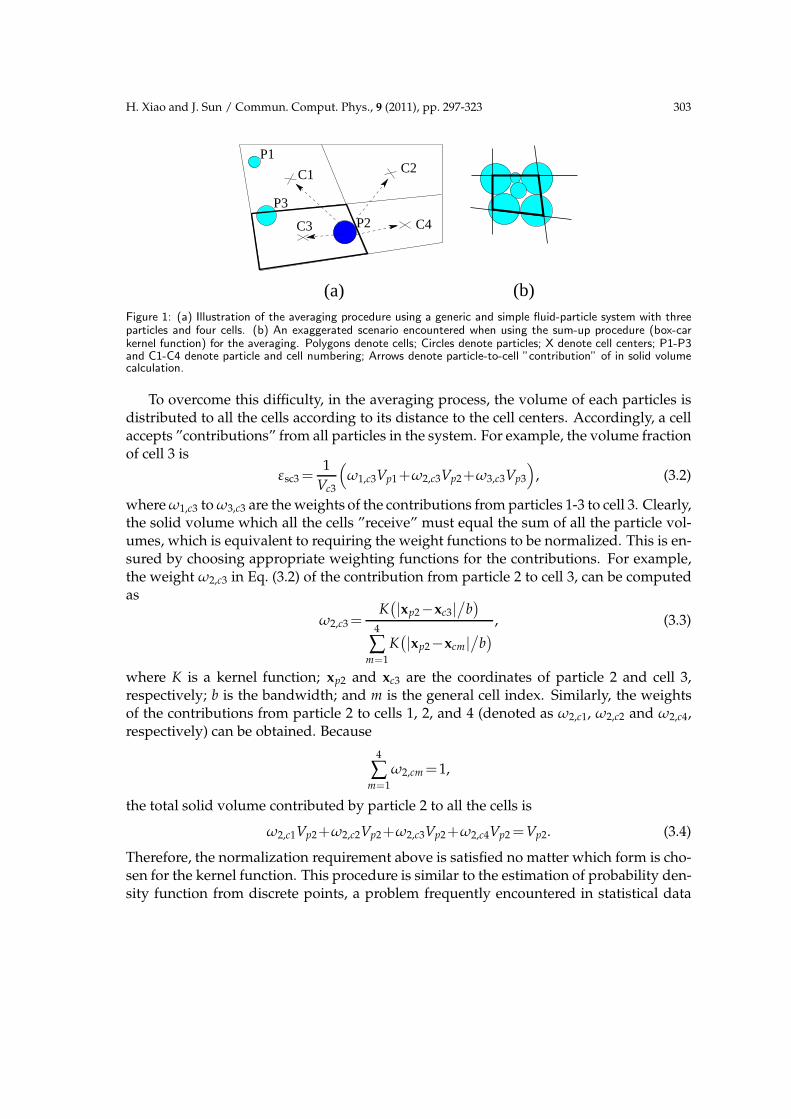
For the convenience of illustration, we consider a generic two-dimensional (2D) sys-tem with three particles (P1 to P3) and four cells (C1 to C4) as shown in Fig. 1(a). Apossible method of calculating the solid volume fraction is to sum up the volume of allthe particle centered in each cell and then divide by the corresponding cell volumes (seee.g., [10]). With this procedure, the solid volume fraction, εsc3, for cell 3 would be

εsc3 =1

Vc3(Vp2+Vp3), (3.1)

where Vc3 is the volume of cell 3; Vp2 and Vp3 are the volume of particles 2 and 3, respec-tively. This procedure, referred to as the sum-up procedure hereafter, may have difficultieswhen several large particles happen to have centers in one cell. Fig. 1(b) shows an exag-gerated scenario, where the volumes of the four large particles all contribute to cell at thecenter (denoted with thick edges), making it possible for εs of this cell to approach unity.The problem is even more pronounced when the particles have a wide range of size dis-tribution, because they could achieve more compact packing. When εs approaches unity,the drag force term obtained from Eq. (2.9) becomes unbounded, which in turn desta-bilizes the solution. In practice, instability often occurs whenever εs exceeds about 0.80during a simulation.


C3

(b)

C1

P1

P2

P3

C2

C4

(a)Figure 1: (a) Illustration of the averaging procedure using a generic and simple fluid-particle system with threeparticles and four cells. (b) An exaggerated scenario encountered when using the sum-up procedure (box-carkernel function) for the averaging. Polygons denote cells; Circles denote particles; X denote cell centers; P1-P3and C1-C4 denote particle and cell numbering; Arrows denote particle-to-cell ”contribution” of in solid volumecalculation.

To overcome this difficulty, in the averaging process, the volume of each particles isdistributed to all the cells according to its distance to the cell centers. Accordingly, a cellaccepts ”contributions” from all particles in the system. For example, the volume fractionof cell 3 is

εsc3 =1

Vc3

(ω1,c3Vp1+ω2,c3Vp2+ω3,c3Vp3

), (3.2)

where ω1,c3 to ω3,c3 are the weights of the contributions from particles 1-3 to cell 3. Clearly,the solid volume which all the cells ”receive” must equal the sum of all the particle vol-umes, which is equivalent to requiring the weight functions to be normalized. This is en-sured by choosing appropriate weighting functions for the contributions. For example,the weight ω2,c3 in Eq. (3.2) of the contribution from particle 2 to cell 3, can be computedas

ω2,c3 =K

(|xp2−xc3|

/b)

4

∑m=1

K(|xp2−xcm|

/b)

, (3.3)

where K is a kernel function; xp2 and xc3 are the coordinates of particle 2 and cell 3,respectively; b is the bandwidth; and m is the general cell index. Similarly, the weightsof the contributions from particle 2 to cells 1, 2, and 4 (denoted as ω2,c1, ω2,c2 and ω2,c4,respectively) can be obtained. Because

4

∑m=1

ω2,cm =1,

the total solid volume contributed by particle 2 to all the cells is

ω2,c1Vp2+ω2,c2Vp2+ω2,c3Vp2+ω2,c4Vp2 =Vp2. (3.4)

Therefore, the normalization requirement above is satisfied no matter which form is cho-sen for the kernel function. This procedure is similar to the estimation of probability den-sity function from discrete points, a problem frequently encountered in statistical data


analysis [23]. It is also applicable for the interpolation of other quantities such as velocityus. It can be easily generalized to 3D cases.

In summary of the illustration above, the volume fraction of each cell can be calcu-lated as

εsc ≡ εs(xc)=1

Vc

Np

∑i=1

ωi Vpi, (3.5a)

with

ωi =K

(|xi−xc|

/b)

Nc

∑m=1

K(|xi−xm|

/b)

, (3.5b)

where εsc is the solid volume fraction defined at the center of cell c; x is the coordinateof cells or particles; i is the general index for particles, which runs from 1 to Np (the totalnumber of particles in the system); The cell index m runs from 1 to Nc (the total number ofcells); ωi is the weight of the contribution from particle i, where the cell number is omittedfrom the subscript since it is clear that cell c is of concern in Eq. (3.5); The Gaussianfunction is a reasonable candidate for the kernel function K:

K(ζ)=exp[−ζ2],

where ζ = |xi−xc|/

b. However, due to efficiency considerations, the following kernelfunction is used in the implementation

K(ζ)=

[1−ζ2]4, if |ζ|<1,

0, if |ζ|≥1,(3.6)

which is very close to the Gaussian function for ζ between 0 and 1, as shown in [24]. Itcan be seen that the sum-up procedure mentioned above is equivalent to using a box-car kernel function in Eq. (3.5) with bandwidths equal to the local cell sizes, which maynot be globally uniform. Similarly, the solid phase velocity is obtained via the followingaveraging procedure

usc =1

εscVc

Np

∑i=1

[ωiuiVpi], (3.7)

with ωi given by (3.5b). In a similar approach, the drag force on the flow field per unitvolume of mixture (or on cell c when discretized) is computed from drag forces fromindividual particles as follows:

fdc ≡ fd(xc)=1

Vc

Np

∑i=1

[ωifdi], (3.8)


where ωi given by (3.5b), in lieu of the conceptual representation, fdc = ∑cni=1fdi

/Vc, in

Eq. (2.8).In Eqs. (3.5), (3.7), and (3.8), Eulerian fields are obtained from Lagrangian particle

quantities through averaging procedure. This operation is called averaging or backwardinterpolation. Another operation required in the drag calculation is to calculate the fluidvelocity, u f i, at the particle location, xi, given the fluid velocity field based on an unstruc-tured mesh. This operation, referred to as forward interpolation, can be conducted usingthe same kernel function

u f i≡uf(xi)=Nc

∑c=1

ωcuc, (3.9a)

with

ωc =K

(|xi−xc|

/b)

Nc

∑m=1

K(|xi−xm|

/b)

, (3.9b)

where ωc is the weight for cell c.The interpolation operations in Eqs. (3.5) and (3.7)-(3.9) share a similar form

q=N

∑j=1

ωjqj, (3.10)

where q is the quantity obtained via interpolation (scalar or vector); qj is the source datapoints, either particle quantities or fluid phase quantities; ωj is the weight for each source

data point. For the convenience of notation, we use ∑i to denote the weighted sum of thequantities from all the particles, that is,

∑iqi ≡

Np

∑i=1

ωiqi. (3.11)

For forward interpolations (from Eulerian fields to Lagrangian particle quantities), theindex i in Eq. (3.11) is replaced with c. With the new notation, Eqs. (3.5), (3.7) (3.8), and(3.9) are written in a unified framework as

εsc =1

Vc∑i

Vpi, usc =1

εscVc∑i

uiVpi, fdc =1

Vc∑i

fdi, and u f i =∑cuc, (3.12)

respectively. When the box-car kernel function is used, the weighted sum degenerates tothe regular sum.

Although theoretically the interpolation procedure in Eq. (3.12) has a computationalcomplexity of the order of O(NpNc), since all the particles and cells are examined at eachstep. In practice, however, the kernel functions have local supports, and thus only the


neighboring particles or cells need to be examined. Since the kernel function, K, dependson the particle-cell distance, |xi−xc|, which is a frame-independent norm, the results donot directly depend on the frame orientation and the mesh sizes.

In the simulations using the hybrid CFD-DEM solver, the Eulerian mesh has to befine enough for the fluid simulation to achieve grid convergence and reasonable accu-racy. On the other hand, in order to reduce the statistical error during the particle fieldaveraging procedure, each fluid cell has to contain enough particles. To satisfy both re-quirements, a large number of particles may be needed in the system, which could makethe computation very expensive, since the DEM simulations are computationally inten-sive. Introducing the kernel functions into the interpolation procedure can achieve smallstatistical errors with relatively small number of particles in each cell, and thus minimizemesh-dependence while keeping the computation cost low. In addition, in the scenarioswhere the cells are of nonuniform sizes, using the sum-up procedure would assume dif-ferent bandwidths (equal to local cell sizes) at different locations, while the kernel-basedaveraging procedure is free from this limitation. Therefore, overall speaking, the averag-ing procedure presented above is better than the sum-up procedure, although the laterhas slightly lower computation cost, and is more consistent on the boundaries.

Although the bandwidth b in the kernel function can take any value theoretically, ourexperience shows that taking b between 1.5∆ and 2.5∆ (where ∆ is the average cell di-mension) gives the best results. Computational expenses increase significantly when thebandwidth is too large, while using very small bandwidth makes the procedure degen-erate to the sum-up procedure and thus lose its advantages.

3.2 Robust treatment of fluid-particle interactions

In most of the previous studies of fluid-particle interactions using CFD-DEM approaches,the dynamic effects of the particles on the flow field are represented by a drag forceterm in the fluid momentum equation (see [9], [11], and the review in [25]). The dragterm is often treated explicitly in the numerical solution. This method of handling fluid-particle interactions was originally proposed by Crowe et al. [26], where the algorithmwas termed particle-source-in-cell model. Note that the inter-particle interactions werenot accounted for in [26]. As reported in the literature (e.g., [27]) and according to ourexperience, convergence difficulty often occurs in dense particle-laden flows, because ofthe large external momentum source term (∑

cni=1fdi/Vc in Eq. (2.8)). In this study, this

issue is addressed with a semi-implicit treatment of drag terms as described below.Using the drag relation in Eqs. (2.9) and (2.10), the momentum equation (2.8) can be

written as

∂

∂t(εfρfuf)+∇·(εfρfufuf)=−εf∇p+εfµ∇

2uf+εf

Vc∑i

Bi(upi−u f i)+εfρ f g, (3.13)

where Bi is defined in Eq. (2.10). The drag force which the particles exert on the flowfield (that is, the third term on the right-hand-side of Eq. (3.13)), is nonlinear in that the


coefficient Bi depends on the particle velocity upi and interpolated fluid velocity, u f i.This term is first linearized so that upi and u f i from previous step is used to calculateBi. The particle velocity upi is not a function of fluid velocity, and thus the contributionfrom the particle velocities toward the drag term can only be treated explicitly, alongwith other external source terms such as g. However, the interpolated fluid velocity,u f i, at the particle location is a function of the fluid velocity field, uf. Specifically, it is alinear combination of the fluid velocities at all the cell locations where uf is discretized.Therefore, it is possible to treat this term implicitly. To simplify the implementation,we use the cell closest to the particle to approximate the fluid velocity at the particlelocation instead of a weighted average of the fluid velocity from several (or all) cells. Thissimplification is for the convenience of implementation and is not theoretically essential.Separating the explicitly and implicitly treated terms, the fluid momentum equation canbe written as

∂

∂t(εfρfuf)+∇·(εfρfufuf)=−εf∇p+ εfρ f Ac+εfρ f g

︸︷︷︸Explicit treatment

+ εfµ∇2uf−εfρ f Ωcu f c︸︷︷︸

Implicit treatment

, (3.14)

with

Ac =1

ρfVc∑i

Biupi, Ωc =1

ρfVc

cn

∑i=1

Bi, (3.15)

where u f c is the fluid velocity of the cell of concern, that is, the discretized version of thefluid velocity field, u f . The term Ac is the acceleration on the fluid cell caused by theexplicitly treated drag force, that is, the discretized version of the explicit drag acceler-ation field. This field is referred to as explicit drag for simplicity, but note that it has thedimension of acceleration. The term Ωc is the coefficient for implicit drag and has thedimension of frequency (viz. [1/s]).

The semi-implicit treatment of the drag terms ensures good stability performance,easy implementation, and minimum mesh-dependence. Although this algorithm is notunconditionally stable, our experience suggests that in all the cases simulated in thisstudy, the stability performance of the algorithm has been excellent. This is a major im-provement over the fully explicit treatment in the current literature. Of course, a fullyimplicit treatment of the drag term would have even better stability performance (prob-ably unconditionally stable). However, this cannot be easily implemented because of thedifficulty in obtaining particle velocities for the current step.

Other components in the fluid-particle interactions include added masses, which aretreated implicitly, and lift forces, which are treated explicitly. Added mass is importantonly when the fluid density is comparable to the particles density (e.g., sand particles inwater).

The momentum equation (3.14) together with the mass conservation equation (2.7)are solved with a modified PISO algorithm. The original PISO algorithm with Rhie-Chow interpolation was developed to prevent pressure-velocity decoupling in fluid flow


simulations on co-located grids [28]. It was later modified for transient flow simula-tions [29,30] and two-fluid models [20]. The algorithm of Rusche [20] is used in this studywith some modifications to accommodate the CFD-DEM coupling (refer to Section 3.4).At individual time step for the fluid flow, the PISO algorithm can be summarized asfollows [20, 30]:

(i) Momentum prediction: solve the fluid momentum equation using the pressure field and theexternal forcing from the previous step,

(ii) Pressure solution: solve the pressure equation, which can be obtained from Eq. (2.7), for theupdated pressure field,

(iii) Velocity correction: correct the velocity field using the updated pressure field with the momentumequation,

(iv) Steps (ii) and (iii) are repeated until convergence.

The drag forces in Eq. (3.14) are computed based on each particles and then interpo-lated to the Eulerian field. An alternative approach is to average the particle quantities tomesh-based fields first, based on which the drag is then computed. However, to conservemomentum during the interaction, the computed drag needs to be distributed to the par-ticles in the cell, which makes it difficult to study some phenomena such as segregationof poly-dispersed particles, since the choice of drag distributions scheme inevitably in-fluences the results of the predictions [24]. The treatment presented here does not requiredrag distribution and addresses this difficulty well.

3.3 Particle relaxation time and sub-stepping

In the current algorithm, the drag force is constant for each fluid time step. Consider ascenario where a particle with zero velocity is released in a stream with constant velocity,Ue. Assuming the drag force computed according to initial relative velocity is appliedon the particle without decrease due to the decrease of the slip velocity (defined as uri =upi−u f i), the relaxation time, τp, of a particle can be easily computed as follows using thedrag correlation in Eq. (2.9)

τp =Ue

εf fdi

/mi

=ρsεs

βi, (3.16)

where ρs is the particle density; fdi is computed according to Eq. (2.9), with the slip ve-locity taken as Ue since the particle is stationary initially. The relaxation time above has asimilar interpretation as the particle characteristic time in the definition of Stokes number.Inserting the expression for βi in Eq. (2.11) into (3.16) yields

τp =ρsεs

34

Cd

V2r

ρfUe

dpiεfεs

=4ρsdpiV

2r

3CdUeρfεf. (3.17)


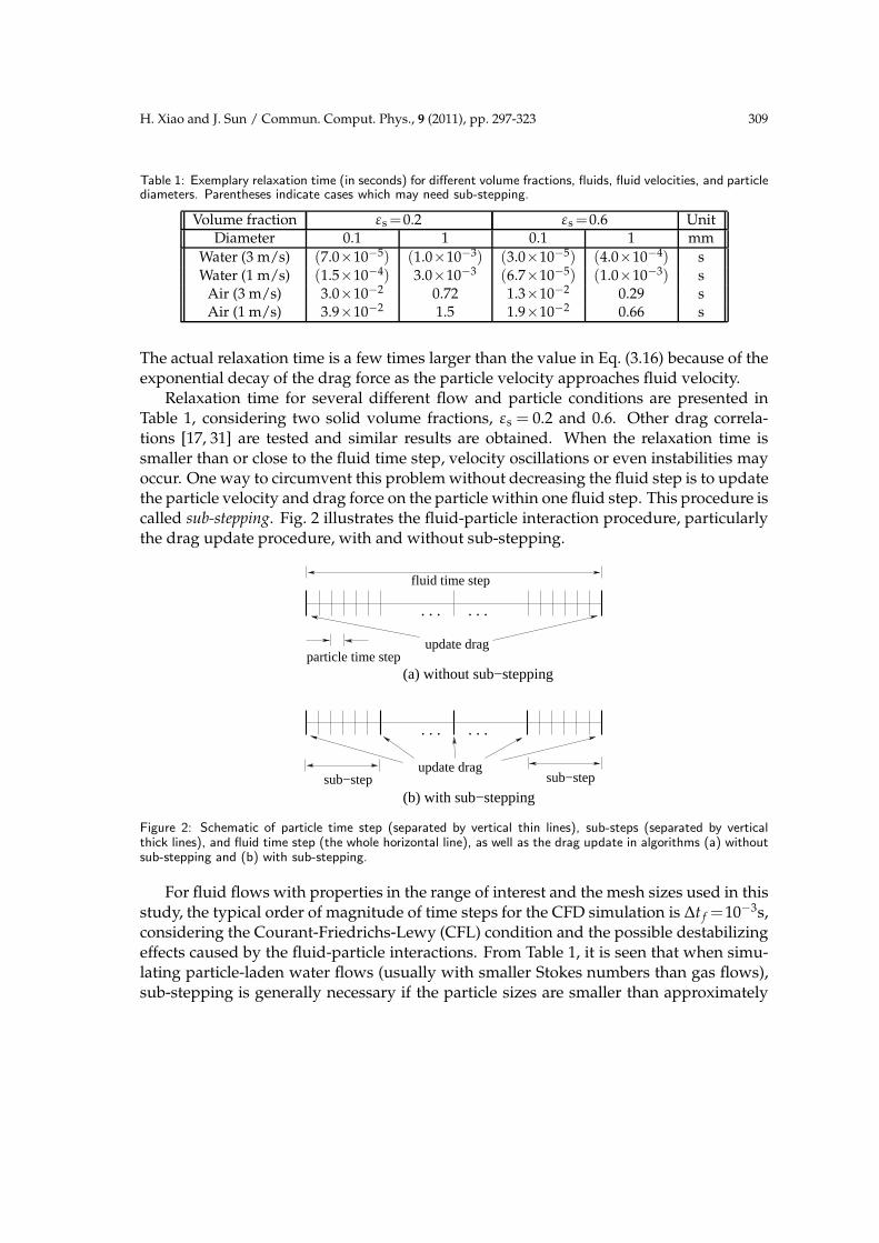
Table 1: Exemplary relaxation time (in seconds) for different volume fractions, fluids, fluid velocities, and particlediameters. Parentheses indicate cases which may need sub-stepping.

Volume fraction εs =0.2 εs =0.6 UnitDiameter 0.1 1 0.1 1 mm

Water (3 m/s) (7.0×10−5) (1.0×10−3) (3.0×10−5) (4.0×10−4) sWater (1 m/s) (1.5×10−4) 3.0×10−3 (6.7×10−5) (1.0×10−3) s

Air (3 m/s) 3.0×10−2 0.72 1.3×10−2 0.29 sAir (1 m/s) 3.9×10−2 1.5 1.9×10−2 0.66 s

The actual relaxation time is a few times larger than the value in Eq. (3.16) because of theexponential decay of the drag force as the particle velocity approaches fluid velocity.

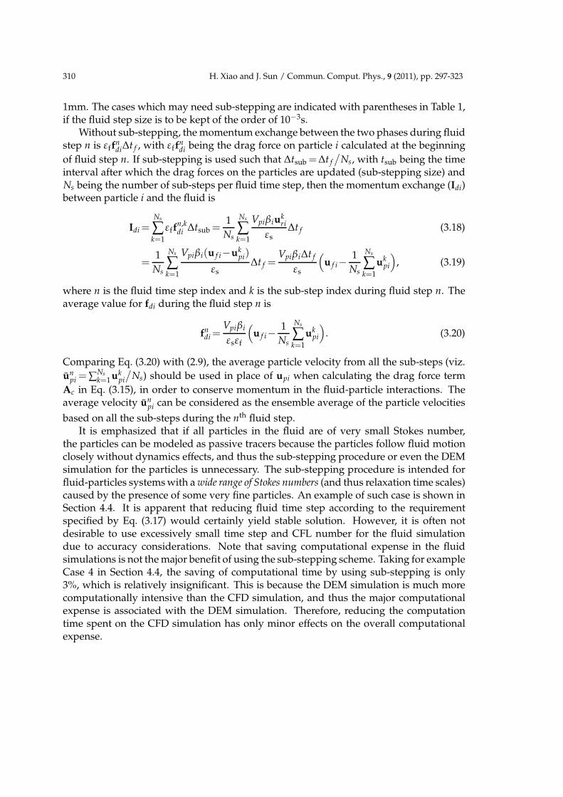
Relaxation time for several different flow and particle conditions are presented inTable 1, considering two solid volume fractions, εs = 0.2 and 0.6. Other drag correla-tions [17, 31] are tested and similar results are obtained. When the relaxation time issmaller than or close to the fluid time step, velocity oscillations or even instabilities mayoccur. One way to circumvent this problem without decreasing the fluid step is to updatethe particle velocity and drag force on the particle within one fluid step. This procedure iscalled sub-stepping. Fig. 2 illustrates the fluid-particle interaction procedure, particularlythe drag update procedure, with and without sub-stepping.

(b) with sub−stepping

particle time step

sub−step sub−step

. . . . . .

update drag

fluid time step

. . . . . .

update drag

(a) without sub−stepping

Figure 2: Schematic of particle time step (separated by vertical thin lines), sub-steps (separated by verticalthick lines), and fluid time step (the whole horizontal line), as well as the drag update in algorithms (a) withoutsub-stepping and (b) with sub-stepping.

For fluid flows with properties in the range of interest and the mesh sizes used in thisstudy, the typical order of magnitude of time steps for the CFD simulation is ∆t f =10−3s,considering the Courant-Friedrichs-Lewy (CFL) condition and the possible destabilizingeffects caused by the fluid-particle interactions. From Table 1, it is seen that when simu-lating particle-laden water flows (usually with smaller Stokes numbers than gas flows),sub-stepping is generally necessary if the particle sizes are smaller than approximately


1mm. The cases which may need sub-stepping are indicated with parentheses in Table 1,if the fluid step size is to be kept of the order of 10−3s.

Without sub-stepping, the momentum exchange between the two phases during fluidstep n is εff

ndi∆t f , with εff

ndi being the drag force on particle i calculated at the beginning

of fluid step n. If sub-stepping is used such that ∆tsub =∆t f

/Ns, with tsub being the time

interval after which the drag forces on the particles are updated (sub-stepping size) andNs being the number of sub-steps per fluid time step, then the momentum exchange (Idi)between particle i and the fluid is

Idi =Ns

∑k=1

εffn,kdi ∆tsub =

1

Ns

Ns

∑k=1

Vpiβiukri

εs∆t f (3.18)

=1

Ns

Ns

∑k=1

Vpiβi(u f i−ukpi)

εs∆t f =

Vpiβi∆t f

εs

(u f i−

1

Ns

Ns

∑k=1

ukpi

), (3.19)

where n is the fluid time step index and k is the sub-step index during fluid step n. Theaverage value for fdi during the fluid step n is

fndi =

Vpiβi

εsεf

(u f i−

1

Ns

Ns

∑k=1

ukpi

). (3.20)

Comparing Eq. (3.20) with (2.9), the average particle velocity from all the sub-steps (viz.

unpi = ∑

Ns

k=1ukpi

/Ns) should be used in place of upi when calculating the drag force term

Ac in Eq. (3.15), in order to conserve momentum in the fluid-particle interactions. Theaverage velocity un

pi can be considered as the ensemble average of the particle velocities

based on all the sub-steps during the nth fluid step.It is emphasized that if all particles in the fluid are of very small Stokes number,

the particles can be modeled as passive tracers because the particles follow fluid motionclosely without dynamics effects, and thus the sub-stepping procedure or even the DEMsimulation for the particles is unnecessary. The sub-stepping procedure is intended forfluid-particles systems with a wide range of Stokes numbers (and thus relaxation time scales)caused by the presence of some very fine particles. An example of such case is shown inSection 4.4. It is apparent that reducing fluid time step according to the requirementspecified by Eq. (3.17) would certainly yield stable solution. However, it is often notdesirable to use excessively small time step and CFL number for the fluid simulationdue to accuracy considerations. Note that saving computational expense in the fluidsimulations is not the major benefit of using the sub-stepping scheme. Taking for exampleCase 4 in Section 4.4, the saving of computational time by using sub-stepping is only3%, which is relatively insignificant. This is because the DEM simulation is much morecomputationally intensive than the CFD simulation, and thus the major computationalexpense is associated with the DEM simulation. Therefore, reducing the computationtime spent on the CFD simulation has only minor effects on the overall computationalexpense.


To ensure stability, the number of sub-steps Ns should be chosen as approximately∆t f

/τp,min, where τp,min is the smallest relaxation time associated with all the particles.

Usually the particles are of the same density and thus τp,min is the relaxation time of thesmallest particles.

3.4 Overall algorithm of fluid-particle interactions with CFD-DEM coupling

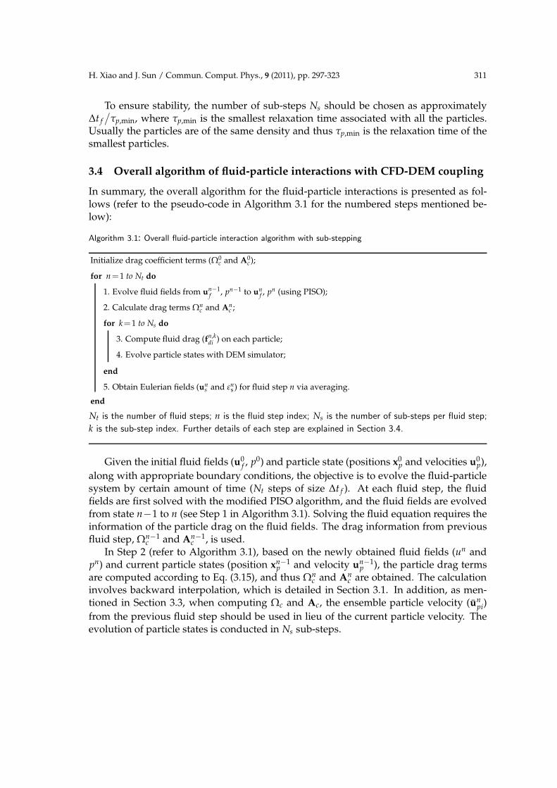
In summary, the overall algorithm for the fluid-particle interactions is presented as fol-lows (refer to the pseudo-code in Algorithm 3.1 for the numbered steps mentioned be-low):

Algorithm 3.1: Overall fluid-particle interaction algorithm with sub-stepping

Initialize drag coefficient terms (Ω0c and A0

c);

for n=1 to Nt do

1. Evolve fluid fields from un−1f , pn−1 to un

f , pn (using PISO);

2. Calculate drag terms Ωnc and An

c ;

for k=1 to Ns do

3. Compute fluid drag (fn,kdi ) on each particle;

4. Evolve particle states with DEM simulator;

end

5. Obtain Eulerian fields (uns and ε

ns ) for fluid step n via averaging.

end

Nt is the number of fluid steps; n is the fluid step index; Ns is the number of sub-steps per fluid step;

k is the sub-step index. Further details of each step are explained in Section 3.4.

Given the initial fluid fields (u0f , p0) and particle state (positions x0

p and velocities u0p),

along with appropriate boundary conditions, the objective is to evolve the fluid-particlesystem by certain amount of time (Nt steps of size ∆t f ). At each fluid step, the fluidfields are first solved with the modified PISO algorithm, and the fluid fields are evolvedfrom state n−1 to n (see Step 1 in Algorithm 3.1). Solving the fluid equation requires theinformation of the particle drag on the fluid fields. The drag information from previousfluid step, Ωn−1

c and An−1c , is used.

In Step 2 (refer to Algorithm 3.1), based on the newly obtained fluid fields (un andpn) and current particle states (position xn−1

p and velocity un−1p ), the particle drag terms

are computed according to Eq. (3.15), and thus Ωnc and An

c are obtained. The calculationinvolves backward interpolation, which is detailed in Section 3.1. In addition, as men-tioned in Section 3.3, when computing Ωc and Ac, the ensemble particle velocity (un

pi)

from the previous fluid step should be used in lieu of the current particle velocity. Theevolution of particle states is conducted in Ns sub-steps.


In each sub-step, the drag forces are computed according to fluid fields at current timestep n and particle state at current sub-step k (refer to Step 3 in Algorithm 3.1). With theinformation of fluid particle interaction forces, the particle states are evolved from (un−1

p ,

xn−1p ) to (un

p, xnp) with the DEM simulator in Ns sub-steps, where each sub-step consists of

a certain number of particle steps (refer to Step 4).

Finally in Step 5, (that is, after all the sub-steps and at the end of each fluid step),the Eulerian fields (εs and us) are obtained from the particle quantities (un

p and xnp) with

the averaging procedures detailed in Section 3.1. At the end of the fluid step, all thequantities and fields are all advanced to the new state, including the flow field (un

f and

pn), the particle state (unp and xn

p), and the Eulerian particle fields (uns and εn

s ).

4 Numerical examples

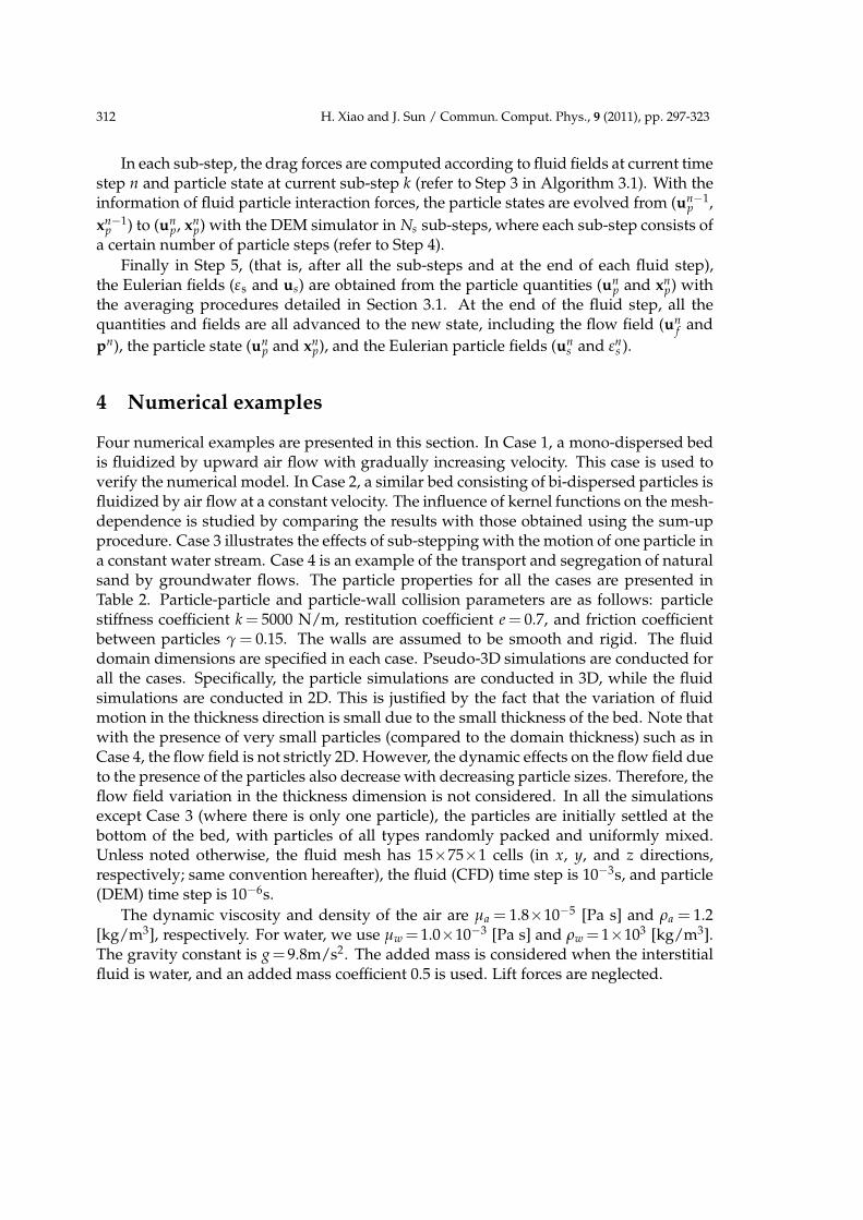
Four numerical examples are presented in this section. In Case 1, a mono-dispersed bedis fluidized by upward air flow with gradually increasing velocity. This case is used toverify the numerical model. In Case 2, a similar bed consisting of bi-dispersed particles isfluidized by air flow at a constant velocity. The influence of kernel functions on the mesh-dependence is studied by comparing the results with those obtained using the sum-upprocedure. Case 3 illustrates the effects of sub-stepping with the motion of one particle ina constant water stream. Case 4 is an example of the transport and segregation of naturalsand by groundwater flows. The particle properties for all the cases are presented inTable 2. Particle-particle and particle-wall collision parameters are as follows: particlestiffness coefficient k = 5000 N/m, restitution coefficient e = 0.7, and friction coefficientbetween particles γ = 0.15. The walls are assumed to be smooth and rigid. The fluiddomain dimensions are specified in each case. Pseudo-3D simulations are conducted forall the cases. Specifically, the particle simulations are conducted in 3D, while the fluidsimulations are conducted in 2D. This is justified by the fact that the variation of fluidmotion in the thickness direction is small due to the small thickness of the bed. Note thatwith the presence of very small particles (compared to the domain thickness) such as inCase 4, the flow field is not strictly 2D. However, the dynamic effects on the flow field dueto the presence of the particles also decrease with decreasing particle sizes. Therefore, theflow field variation in the thickness dimension is not considered. In all the simulationsexcept Case 3 (where there is only one particle), the particles are initially settled at thebottom of the bed, with particles of all types randomly packed and uniformly mixed.Unless noted otherwise, the fluid mesh has 15×75×1 cells (in x, y, and z directions,respectively; same convention hereafter), the fluid (CFD) time step is 10−3s, and particle(DEM) time step is 10−6s.

The dynamic viscosity and density of the air are µa = 1.8×10−5 [Pa s] and ρa = 1.2[kg/m3], respectively. For water, we use µw =1.0×10−3 [Pa s] and ρw =1×103 [kg/m3].The gravity constant is g=9.8m/s2. The added mass is considered when the interstitialfluid is water, and an added mass coefficient 0.5 is used. Lift forces are neglected.


Table 2: Particle properties for the computational Cases 1, 2, 3, and 4.

Model validation (Case 1)dp 1.5mmρs 2000kg/m3

Umf (theoretical* ) 84cm/sNumber of particles 2160

Mesh-dependence study (Case 2)Small particles Large particles

dp 1.52mm 2.49mmρs 2523kg/m3 2526kg/m3

Umf (theoretical**) ∼92cm/s ∼130cm/sNumber of particles 1783 377

Sub-stepping study (Case 3)dp 0.083mmρs 2000kg/m3

Number of particles 1Groundwater seepage problem (Case 4)

dp 0.083 — 2.5mmρs 2000kg/m3

Umf (theoretical**) 0.01 — 2.5cm/sNumber of particles 2160

* Obtained with drag correlation in Eq. (2.11) assuming εs = 0.554, the median valueof the initial solid volume fraction field.

** Assuming εs = 0.583. This is the measured value in the experiment [32] accordingto which this case is composed. Note that the bed with bi-dispersed particles in thiscase has higher volume fraction than the mono-dispersed bed in Case 1.

As an overview of the computational demand of the solver, the CPU time required tosimulate 2000 particles (Cases 1, 2, and 4) for a physical time of 20 s is about 6 hours onone processor (AMD Opteron R© 2.3GHz with 4 GB memory). Most of the CPU time isconsumed by the DEM simulations, particularly when the particles are densely packed,because more particle-particle collisions need to be handled.

4.1 Case 1: model validation

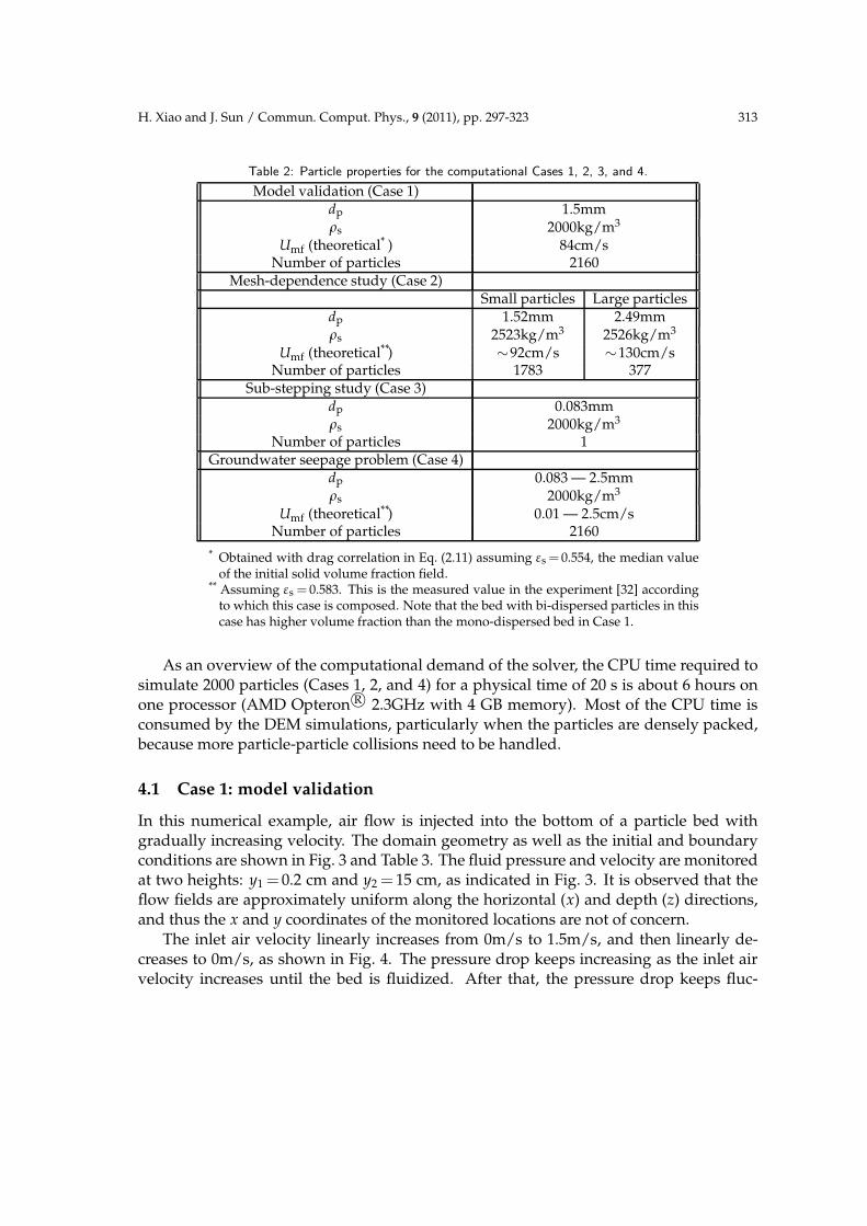
In this numerical example, air flow is injected into the bottom of a particle bed withgradually increasing velocity. The domain geometry as well as the initial and boundaryconditions are shown in Fig. 3 and Table 3. The fluid pressure and velocity are monitoredat two heights: y1 = 0.2 cm and y2 = 15 cm, as indicated in Fig. 3. It is observed that theflow fields are approximately uniform along the horizontal (x) and depth (z) directions,and thus the x and y coordinates of the monitored locations are not of concern.

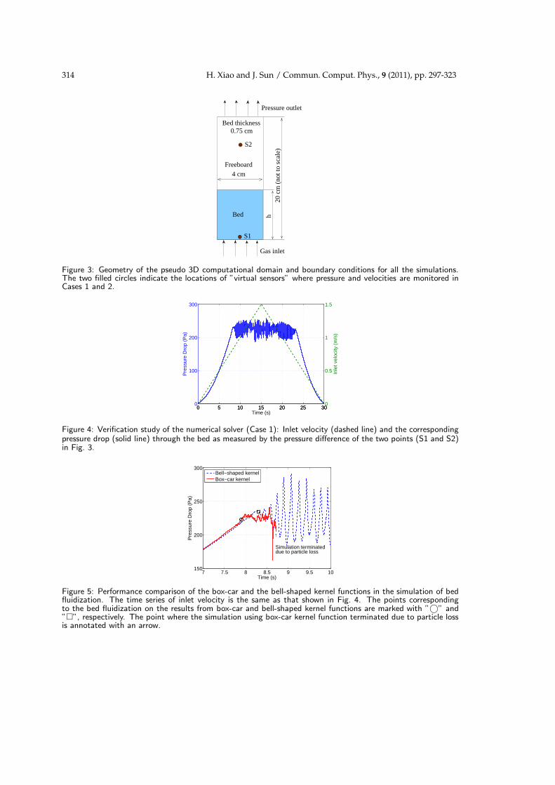
The inlet air velocity linearly increases from 0m/s to 1.5m/s, and then linearly de-creases to 0m/s, as shown in Fig. 4. The pressure drop keeps increasing as the inlet airvelocity increases until the bed is fluidized. After that, the pressure drop keeps fluc-


Pressure outlet

Gas inlet

4 cm

20 c

m (

not t

o sc

ale)

Freeboard

Bed thickness0.75 cm

h

S1

S2

Bed

Figure 3: Geometry of the pseudo 3D computational domain and boundary conditions for all the simulations.The two filled circles indicate the locations of ”virtual sensors” where pressure and velocities are monitored inCases 1 and 2.

0 5 10 15 20 25 300

100

200

300

Pre

ssur

e D

rop

(Pa)

Time (s)0 5 10 15 20 25 30

0

0.5

1

1.5

Inle

t vel

ocity

(m

/s)

Figure 4: Verification study of the numerical solver (Case 1): Inlet velocity (dashed line) and the correspondingpressure drop (solid line) through the bed as measured by the pressure difference of the two points (S1 and S2)in Fig. 3.

7 7.5 8 8.5 9 9.5 10150

200

250

300

↑

Simulation terminateddue to particle loss

Time (s)

Pre

ssur

e D

rop

(Pa)

Bell−shaped kernelBox−car kernel

Figure 5: Performance comparison of the box-car and the bell-shaped kernel functions in the simulation of bedfluidization. The time series of inlet velocity is the same as that shown in Fig. 4. The points correspondingto the bed fluidization on the results from box-car and bell-shaped kernel functions are marked with ”©” and””, respectively. The point where the simulation using box-car kernel function terminated due to particle lossis annotated with an arrow.


Table 3: Computational domain sizes and initial and boundary conditions for Cases 1, 2, and 4.

GeometryHeight of domain (Ly) 20cmWidth of domain (Lx) 4cmDepth of domain (Lz) 0.75cm

Initial bed height (h in Fig. 3)model validation (Case 1) ∼ 2.5cmmesh dependence (Case 2) ∼ 4cm

Groundwater seepage (Case 4) ∼ 2cmBoundary conditionsUniform fluid inflow Specified velocity

Pressure Zero gradient at outlet

tuating around a constant value but with increasing fluctuation amplitude as the inletflow velocity increases. The inlet velocity at which the pressure drop stops increasingis the minimum fluidization velocity of the bed. The pressure drop at this point shouldapproximately balance the gravity of the particle bed (air weight is ignored here due toits low density). When the inlet flow velocity decreases below the fluidization velocityagain, the pressure drop decreases. However, the decreasing and the increasing paths areof hysteresis, because the fluidization/de-fluidization process is history-dependent. Theminimum fluidization velocity and the corresponding pressure drop are Umf = 83cm/sand ∆p=235Pa, respectively. The theoretical prediction of Umf depends on the solid vol-ume fraction, εs. It is estimated to be Umf = 84cm/s assuming εs = 0.554, which is themedian value of the initial solid volume fraction field. The numerical prediction is veryclose to the theoretical value. The pressure drop across the fluidized bed can be theoreti-cally estimated according to

∆p= Npmig/(LxLz),

where Npmi is the total mass of all the particles. The estimation gives 254Pa according tothe particle and domain properties in Tables 2 and 3. This is close to the prediction fromthe simulation. The remaining discrepancy (less than 10%) is possibly explained by thejam effects from the wall.

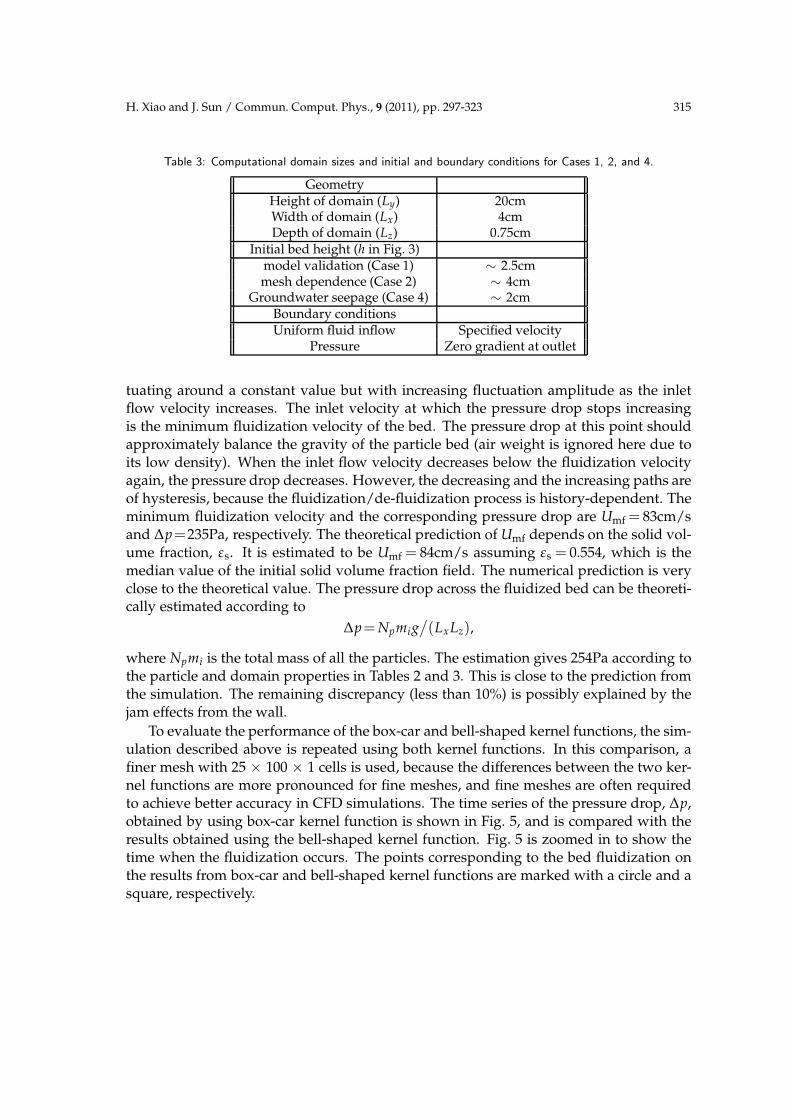
To evaluate the performance of the box-car and bell-shaped kernel functions, the sim-ulation described above is repeated using both kernel functions. In this comparison, afiner mesh with 25 × 100 × 1 cells is used, because the differences between the two ker-nel functions are more pronounced for fine meshes, and fine meshes are often requiredto achieve better accuracy in CFD simulations. The time series of the pressure drop, ∆p,obtained by using box-car kernel function is shown in Fig. 5, and is compared with theresults obtained using the bell-shaped kernel function. Fig. 5 is zoomed in to show thetime when the fluidization occurs. The points corresponding to the bed fluidization onthe results from box-car and bell-shaped kernel functions are marked with a circle and asquare, respectively.


Table 4: Comparison of predictions of minimum fluidized velocity (Umf) and pressure drop (∆p) in the simulationof Case 1, using the box-car and the bell-shaped kernel functions.

Box-car Bell-shaped Theoretical prediction ∗

Umf 79 cm/s 83 cm/s 84 cm/s∆p 223 Pa 235 Pa 254 Pa

∗ Note: Using the median value of the initial solid volume fraction (εs) field, 0.554.

The minimum fluidization velocity, Umf, and the corresponding pressure drop, ∆p,obtained using the two kernel functions are presented in Table 4, and are compared tothe theoretical predictions. It can be seen that the bell-shaped kernel function gives betteragreements with the theoretical values in terms of both Umf and ∆p. In particular, it isnoted that when the box-car kernel function is utilized in the averaging procedure, thepredicted minimum fluidization velocity, Umf, is lower than the numerical predictionsfrom the bell-shaped kernel function and the theoretical value. This is because the sum-up procedure inevitably gives unphysically high solid volume fractions in some cells (seeFig. 1(b) for a more detailed explanation) and thus leads to artificially early fluidization.During the simulation, when the computed solid volume fraction in any of the cells istoo high (e.g., larger than 0.80), particles in these cells may gain very large velocities,which leads to instability of the whole system and these particles may even leave thesimulation domain. In these scenarios, the simulation has to be terminated, which isindicated in Fig. 5 for the box-car kernel function case with arrow.

According to our experiences during this study, when box-car kernel functions areused, simulations often fail due to this reason. This drawback makes the box-car kernelfunction not a desirable choice for robust and stable solvers. Summarizing the compari-son presented in Fig. 5 and Table 4, the bell-shaped kernel functions have better robust-ness and accuracy than the box-car kernel functions in general, and are thus preferred.Another desirable feature for a robust solver is the mesh independence, which is investi-gated in Section 4.2 for both kernel functions.

4.2 Case 2: mesh-dependence study

In this example, a similar fluidized bed as in Case 1 is studied, except that the bed consistsof two types of bi-dispersed particles and the inlet air velocity is constant (1m/s). Thedomain geometry as well as the initial and boundary conditions are shown in Fig. 3 andTable 3. To study the mesh-dependence, simulations are conducted with two meshes.The fine mesh has 12×60×1 cells of size 3.33 mm ×3.33 mm ×7.5 mm, and the coarsemesh has 8×40×1 cells of size 5 mm×5 mm ×7.5 mm . The bandwidth for the kernelfunction is 10 mm for both the fine mesh and the coarse mesh.

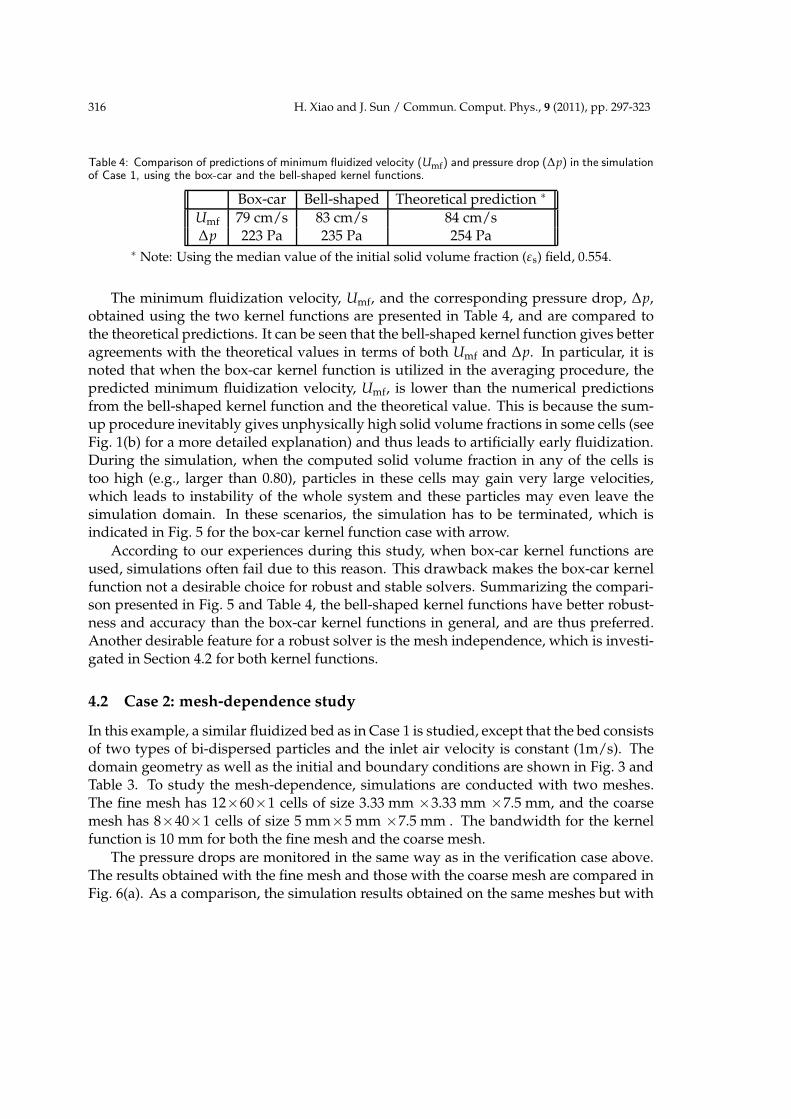
The pressure drops are monitored in the same way as in the verification case above.The results obtained with the fine mesh and those with the coarse mesh are compared inFig. 6(a). As a comparison, the simulation results obtained on the same meshes but with


0 0.5 1 1.5 20

100

200

300

400

500

600

700(a)

Time (s)

Pre

ssur

e dr

op (

Pa)

Fine meshCoarse mesh

0 0.5 1 1.5 20

100

200

300

400

500

600

700

Time (s)

Pre

ssur

e dr

op (

Pa)

(b)


Figure 6: Mesh-dependence study (Case 2): Simulated pressure drop through the bed with (a) bell-shapedkernel function and (b) box-car kernel function (sum-up procedure). Results obtained with a fine mesh andthose with a coarse mesh are compared.

0 0.5 1 1.5 20.8

0.9

1

1.1

1.2

1.3

1.4

1.5(a)

Time (s)

Sol

id p

hase

vel

ocity

(m

/s)


0 0.5 1 1.5 20.8

0.9

1

1.1

1.2

1.3

1.4

1.5(b)

Time (s)

Sol

id p

hase

vel

ocity

(m

/s)


Figure 7: Mesh-dependence study (Case 2): Vertical component of the Eulerian mesh-based particle phase ve-locity at S1 (see Fig. 3) with (a) bell-shaped kernel function and (b) box-car kernel function (sum-up procedure).Results obtained with a fine mesh and those with a coarse mesh are compared.

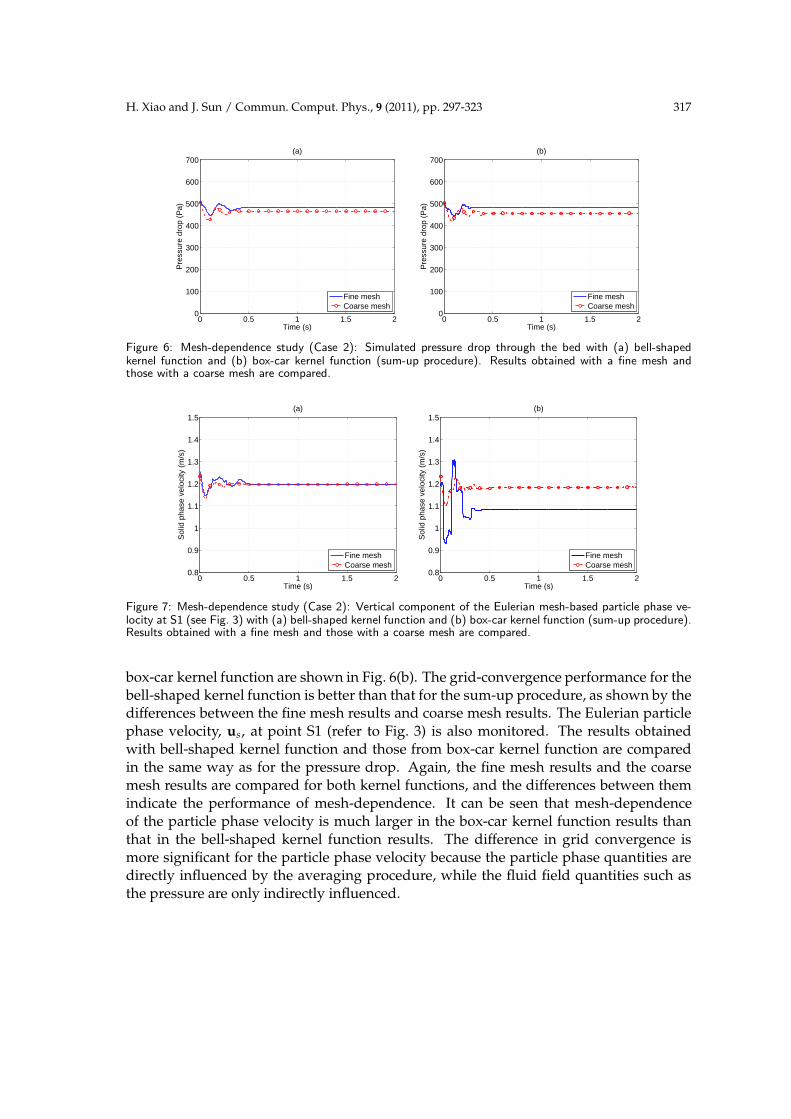
box-car kernel function are shown in Fig. 6(b). The grid-convergence performance for thebell-shaped kernel function is better than that for the sum-up procedure, as shown by thedifferences between the fine mesh results and coarse mesh results. The Eulerian particlephase velocity, us, at point S1 (refer to Fig. 3) is also monitored. The results obtainedwith bell-shaped kernel function and those from box-car kernel function are comparedin the same way as for the pressure drop. Again, the fine mesh results and the coarsemesh results are compared for both kernel functions, and the differences between themindicate the performance of mesh-dependence. It can be seen that mesh-dependenceof the particle phase velocity is much larger in the box-car kernel function results thanthat in the bell-shaped kernel function results. The difference in grid convergence ismore significant for the particle phase velocity because the particle phase quantities aredirectly influenced by the averaging procedure, while the fluid field quantities such asthe pressure are only indirectly influenced.


Another observation is that with bell-shaped kernel functions, finer mesh could beused to gain better accuracy for the flow field without causing the instability described inSection 3.1. In other words, we could have fewer particles in each cell. According to ourexperience, when using the sum-up procedure (box-car kernel function), instability oftenoccurs and it is more difficult to obtain reasonable results. Considering that the DEMis a computationally intensive method, this advantage of the proposed averaging proce-dure is of practical significance when the available computational resources are limitedcompared to the demands of the problems.

4.3 Case 3: sub-stepping study

In this example, we consider a single particle in a water flow of constant velocityUe = 0.05m/s. The domain geometry is shown in Fig. 3, with the same dimensions asin other cases but with different boundary and initial conditions so that uniform flow isachieved. The particle has an initial velocity of zero and is accelerated due to the fluiddrag. For simplicity, other external forces such as gravity, buoyancy, and added mass areneglected in this case, and the box-car kernel function is used. The particle has a diame-ter of 0.083mm and the cell size in the mesh is 2mm×2mm×2mm. The influence of theparticle to the overall flow field is negligible.

The particle velocity is described by

dupi

dt= Fdi, (4.1)

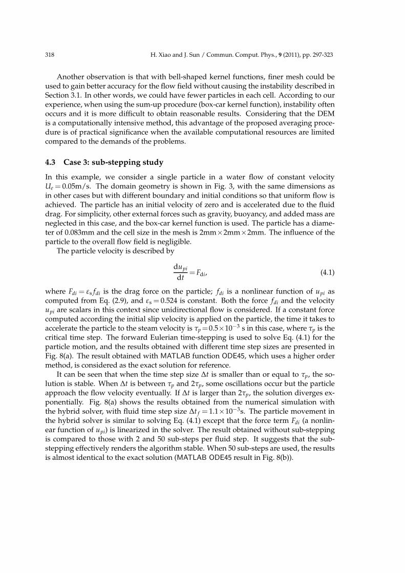
where Fdi = εs fdi is the drag force on the particle; fdi is a nonlinear function of upi ascomputed from Eq. (2.9), and εs = 0.524 is constant. Both the force fdi and the velocityupi are scalars in this context since unidirectional flow is considered. If a constant forcecomputed according the initial slip velocity is applied on the particle, the time it takes toaccelerate the particle to the steam velocity is τp =0.5×10−3 s in this case, where τp is thecritical time step. The forward Eulerian time-stepping is used to solve Eq. (4.1) for theparticle motion, and the results obtained with different time step sizes are presented inFig. 8(a). The result obtained with MATLAB function ODE45, which uses a higher ordermethod, is considered as the exact solution for reference.

It can be seen that when the time step size ∆t is smaller than or equal to τp, the so-lution is stable. When ∆t is between τp and 2τp, some oscillations occur but the particleapproach the flow velocity eventually. If ∆t is larger than 2τp, the solution diverges ex-ponentially. Fig. 8(a) shows the results obtained from the numerical simulation withthe hybrid solver, with fluid time step size ∆t f = 1.1×10−3s. The particle movement inthe hybrid solver is similar to solving Eq. (4.1) except that the force term Fdi (a nonlin-ear function of upi) is linearized in the solver. The result obtained without sub-steppingis compared to those with 2 and 50 sub-steps per fluid step. It suggests that the sub-stepping effectively renders the algorithm stable. When 50 sub-steps are used, the resultsis almost identical to the exact solution (MATLAB ODE45 result in Fig. 8(b)).


! " # $ % & '!!(!&

!

!(!&

!("

!("&

!(#

)*+,-."!!$-/0

1234*56,-7,685*49-.+:/0

.20

-

-;2462<-=>?%&!4-@-"

A

!4-@-"(B-"A

!4-@-#"A

!4-@-#(""A

0 1 2 3 4 5 6−0.05

0

0.05

0.1

0.15

0.2

Time (10−3 s)

Par

ticle

vel

ocity

(m

/s)

(b)

No sub−stepping2 sub−steps50 sub−steps

Figure 8: Sub-stepping study (Case 3): Particle velocity from (a) theoretical prediction with different time stepsizes and from (b) numerical simulations using the hybrid solver with and without sub-stepping.

4.4 Case 4: groundwater seepage-induced particle transport

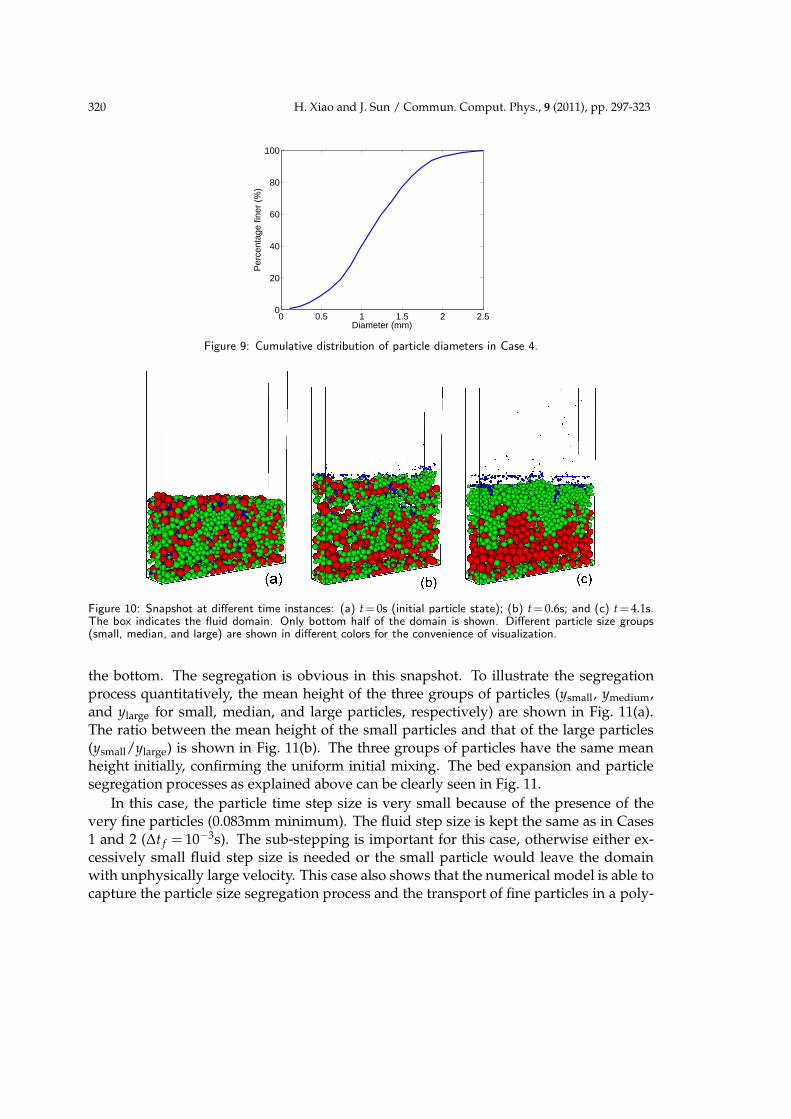
The transport of fine particles in porous media is of interest to researchers in various dis-ciplines. For example, in geotechnical engineering, rapid groundwater flow caused bydewatering can carry away the fine sand from the soil, leading to mass loss and even-tually the collapse of soil foundations. An example of seepage-induced transport is pre-sented here to show the capabilities of the solver. The domain geometry as well as theinitial and boundary conditions are shown in Fig. 3 and Table 3. The setup is similar toCases 1 and 2, except that the interstitial fluid is water, with an inlet velocity of 3.5cm/s.The particle diameter has a Gaussian distribution with a mean of 1.25mm and a stan-dard deviation of 0.5mm. The minimum and maximum particle diameters are 0.083mmand 2.5mm, respectively. The cumulative mass distribution curve shown in Fig. 9. Forthe convenience of visualization, the particles are categorized into three groups: small(0.083mm to 0.83mm), median (0.83mm to 1.67mm), and large (1.67mm to 2.5mm). Thesimulation is conducted for 4.1s, with particle time step size ∆tp =6×10−8s and 25 sub-steps per fluid step.

The snapshots at three time instances (t=0s, 0.6s, and 4.1s) are shown in Fig. 10. Par-ticles of different size groups are shown in different colors. The snapshot at t = 0 s inFig. 10(a) shows the initial configuration where particles of all sizes are stationary anduniformly mixed. During the initial period of approximately 1s, the bed expands grad-ually and meanwhile the very small particles start to rise to the top. The snapshot att = 0.6s is shown in Fig. 10(b) where many small particles are observed at the top sur-face of the bed. The segregation of median and large particles is not obvious from thesnapshot. Afterward, some small particles start to be transported upward and leave thebed. Meanwhile, the size segregation among all particle groups continues. The snap-shot at t = 4.1s in Fig. 10(c) shows the bed configuration after the segregation process,where smaller particles are concentrated at the top and the larger particles are settled at


0 0.5 1 1.5 2 2.50

20

40

60

80

100

Diameter (mm)

Per

cent

age

finer

(%

)

Figure 9: Cumulative distribution of particle diameters in Case 4.

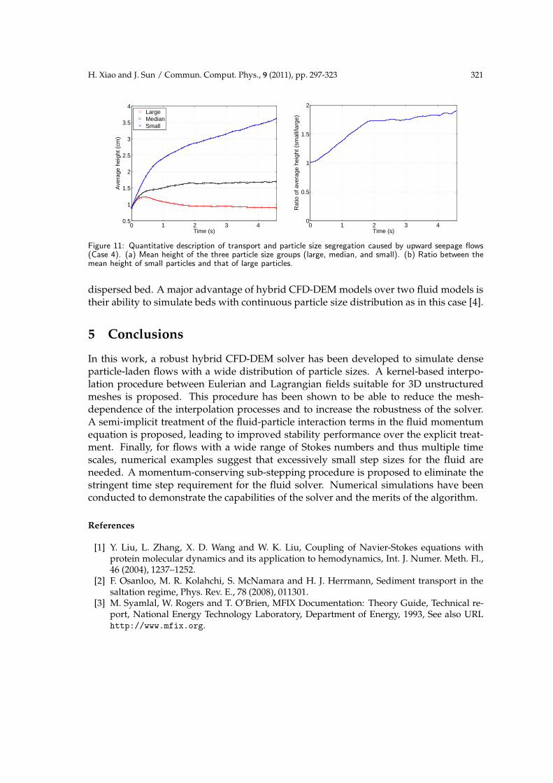
Figure 10: Snapshot at different time instances: (a) t=0s (initial particle state); (b) t=0.6s; and (c) t=4.1s.The box indicates the fluid domain. Only bottom half of the domain is shown. Different particle size groups(small, median, and large) are shown in different colors for the convenience of visualization.

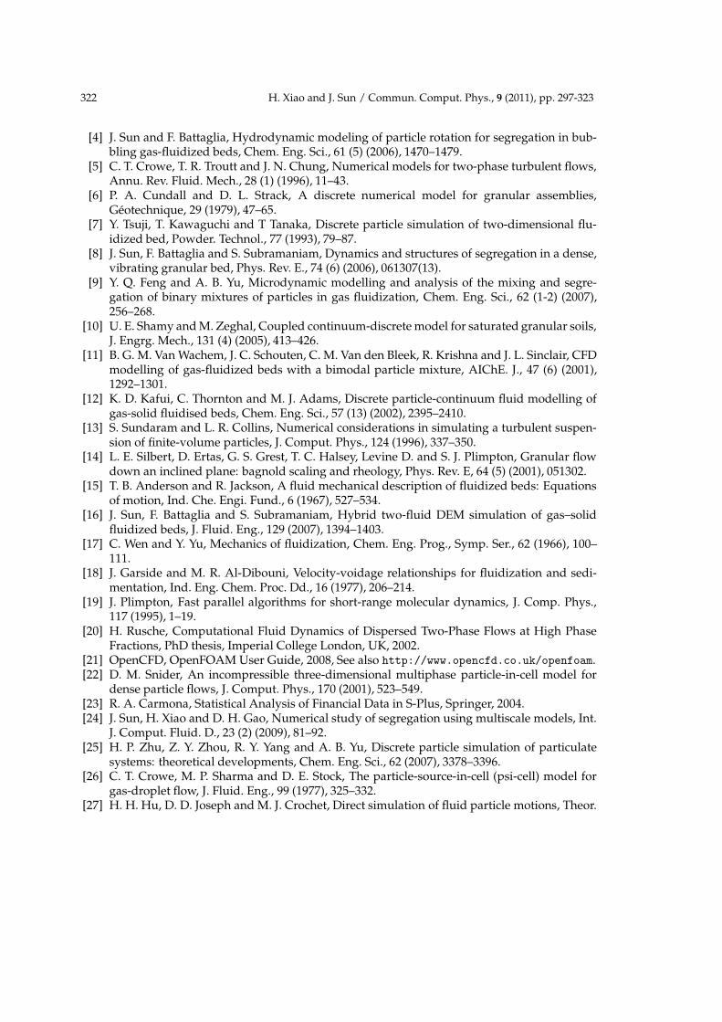
the bottom. The segregation is obvious in this snapshot. To illustrate the segregationprocess quantitatively, the mean height of the three groups of particles (ysmall, ymedium,and ylarge for small, median, and large particles, respectively) are shown in Fig. 11(a).The ratio between the mean height of the small particles and that of the large particles(ysmall/ylarge) is shown in Fig. 11(b). The three groups of particles have the same meanheight initially, confirming the uniform initial mixing. The bed expansion and particlesegregation processes as explained above can be clearly seen in Fig. 11.

In this case, the particle time step size is very small because of the presence of thevery fine particles (0.083mm minimum). The fluid step size is kept the same as in Cases1 and 2 (∆t f = 10−3s). The sub-stepping is important for this case, otherwise either ex-cessively small fluid step size is needed or the small particle would leave the domainwith unphysically large velocity. This case also shows that the numerical model is able tocapture the particle size segregation process and the transport of fine particles in a poly-


0 1 2 3 40.5

1

1.5

2

2.5

3

3.5

4

Time (s)

Ave

rage

hei

ght (

cm)

LargeMedianSmall

0 1 2 3 40

0.5

1

1.5

2

Time (s)

Rat

io o

f ave

rage

hei

ght (

smal

l/lar

ge)

Figure 11: Quantitative description of transport and particle size segregation caused by upward seepage flows(Case 4). (a) Mean height of the three particle size groups (large, median, and small). (b) Ratio between themean height of small particles and that of large particles.

dispersed bed. A major advantage of hybrid CFD-DEM models over two fluid models istheir ability to simulate beds with continuous particle size distribution as in this case [4].

5 Conclusions

In this work, a robust hybrid CFD-DEM solver has been developed to simulate denseparticle-laden flows with a wide distribution of particle sizes. A kernel-based interpo-lation procedure between Eulerian and Lagrangian fields suitable for 3D unstructuredmeshes is proposed. This procedure has been shown to be able to reduce the mesh-dependence of the interpolation processes and to increase the robustness of the solver.A semi-implicit treatment of the fluid-particle interaction terms in the fluid momentumequation is proposed, leading to improved stability performance over the explicit treat-ment. Finally, for flows with a wide range of Stokes numbers and thus multiple timescales, numerical examples suggest that excessively small step sizes for the fluid areneeded. A momentum-conserving sub-stepping procedure is proposed to eliminate thestringent time step requirement for the fluid solver. Numerical simulations have beenconducted to demonstrate the capabilities of the solver and the merits of the algorithm.

References

[1] Y. Liu, L. Zhang, X. D. Wang and W. K. Liu, Coupling of Navier-Stokes equations withprotein molecular dynamics and its application to hemodynamics, Int. J. Numer. Meth. Fl.,46 (2004), 1237–1252.

[2] F. Osanloo, M. R. Kolahchi, S. McNamara and H. J. Herrmann, Sediment transport in thesaltation regime, Phys. Rev. E., 78 (2008), 011301.

[3] M. Syamlal, W. Rogers and T. O’Brien, MFIX Documentation: Theory Guide, Technical re-port, National Energy Technology Laboratory, Department of Energy, 1993, See also URLhttp://www.mfix.org.


[4] J. Sun and F. Battaglia, Hydrodynamic modeling of particle rotation for segregation in bub-bling gas-fluidized beds, Chem. Eng. Sci., 61 (5) (2006), 1470–1479.

[5] C. T. Crowe, T. R. Troutt and J. N. Chung, Numerical models for two-phase turbulent flows,Annu. Rev. Fluid. Mech., 28 (1) (1996), 11–43.

[6] P. A. Cundall and D. L. Strack, A discrete numerical model for granular assemblies,Geotechnique, 29 (1979), 47–65.

[7] Y. Tsuji, T. Kawaguchi and T Tanaka, Discrete particle simulation of two-dimensional flu-idized bed, Powder. Technol., 77 (1993), 79–87.

[8] J. Sun, F. Battaglia and S. Subramaniam, Dynamics and structures of segregation in a dense,vibrating granular bed, Phys. Rev. E., 74 (6) (2006), 061307(13).

[9] Y. Q. Feng and A. B. Yu, Microdynamic modelling and analysis of the mixing and segre-gation of binary mixtures of particles in gas fluidization, Chem. Eng. Sci., 62 (1-2) (2007),256–268.

[10] U. E. Shamy and M. Zeghal, Coupled continuum-discrete model for saturated granular soils,J. Engrg. Mech., 131 (4) (2005), 413–426.

[11] B. G. M. Van Wachem, J. C. Schouten, C. M. Van den Bleek, R. Krishna and J. L. Sinclair, CFDmodelling of gas-fluidized beds with a bimodal particle mixture, AIChE. J., 47 (6) (2001),1292–1301.

[12] K. D. Kafui, C. Thornton and M. J. Adams, Discrete particle-continuum fluid modelling ofgas-solid fluidised beds, Chem. Eng. Sci., 57 (13) (2002), 2395–2410.

[13] S. Sundaram and L. R. Collins, Numerical considerations in simulating a turbulent suspen-sion of finite-volume particles, J. Comput. Phys., 124 (1996), 337–350.

[14] L. E. Silbert, D. Ertas, G. S. Grest, T. C. Halsey, Levine D. and S. J. Plimpton, Granular flowdown an inclined plane: bagnold scaling and rheology, Phys. Rev. E, 64 (5) (2001), 051302.

[15] T. B. Anderson and R. Jackson, A fluid mechanical description of fluidized beds: Equationsof motion, Ind. Che. Engi. Fund., 6 (1967), 527–534.

[16] J. Sun, F. Battaglia and S. Subramaniam, Hybrid two-fluid DEM simulation of gas–solidfluidized beds, J. Fluid. Eng., 129 (2007), 1394–1403.

[17] C. Wen and Y. Yu, Mechanics of fluidization, Chem. Eng. Prog., Symp. Ser., 62 (1966), 100–111.

[18] J. Garside and M. R. Al-Dibouni, Velocity-voidage relationships for fluidization and sedi-mentation, Ind. Eng. Chem. Proc. Dd., 16 (1977), 206–214.

[19] J. Plimpton, Fast parallel algorithms for short-range molecular dynamics, J. Comp. Phys.,117 (1995), 1–19.

[20] H. Rusche, Computational Fluid Dynamics of Dispersed Two-Phase Flows at High PhaseFractions, PhD thesis, Imperial College London, UK, 2002.

[21] OpenCFD, OpenFOAM User Guide, 2008, See also http://www.opencfd.co.uk/openfoam.[22] D. M. Snider, An incompressible three-dimensional multiphase particle-in-cell model for

dense particle flows, J. Comput. Phys., 170 (2001), 523–549.[23] R. A. Carmona, Statistical Analysis of Financial Data in S-Plus, Springer, 2004.[24] J. Sun, H. Xiao and D. H. Gao, Numerical study of segregation using multiscale models, Int.

J. Comput. Fluid. D., 23 (2) (2009), 81–92.[25] H. P. Zhu, Z. Y. Zhou, R. Y. Yang and A. B. Yu, Discrete particle simulation of particulate

systems: theoretical developments, Chem. Eng. Sci., 62 (2007), 3378–3396.[26] C. T. Crowe, M. P. Sharma and D. E. Stock, The particle-source-in-cell (psi-cell) model for

gas-droplet flow, J. Fluid. Eng., 99 (1977), 325–332.[27] H. H. Hu, D. D. Joseph and M. J. Crochet, Direct simulation of fluid particle motions, Theor.


Comp. Fluid. Dyn., 3 (1992), 285–306.[28] C. M. Rhie and W. L. Chow, A numerical study of the turbulent flow past an isolated airfoil

with trailing edge separation, AIAA., 21 (11) (1983), 1525–1532.[29] R. I. Issa, Solution of the implicitly discretised fluid flow equations by operator-splitting, J.

Comput. Phys., 62 (1986),40–65.[30] H. Jasak, Error Analysis and Estimation for the Finite Volume Method with Applications to

Fluid Flows, PhD thesis, Imperial College London, UK, 1996.[31] S. Ergun, Fluid flow through packed columns, Chem. Eng. Prog., 43 (2) (1952), 226–231.[32] M. Goldschmidt, Hydrodynamic Modelling of Fluidised Bed Spray Granulation, PhD thesis,

Twente University, The Netherlands, 2001.

Documents

Algorithms in a Robust Hybrid CFD-DEM Solver for Particle