Algorithms for the Multiplication TableProblem

Richard P. BrentAustralian National University andCARMA, University of Newcastle

19 May 2021

Collaborators

Carl Pomerance Jonathan Webster

Copyright c© 2021, R. P. Brent

Abstract

Let M(n) be the number of distinct entries in the multiplicationtable for integers < n. More precisely1,

M(n) := #{i × j |0 ≤ i , j < n}.

The order of magnitude of M(n) was established in a series ofpapers, starting with Erdos (1955) and ending with Ford (2008),but an asymptotic formula is still unknown. After describingsome of the history of M(n) we consider some algorithms forcalculating/approximating M(n) for large n. This naturally leadsto consideration of algorithms, due to Bach (1985–88) andKalai (2003), for generating random factored integers.The talk describes joint work with Carl Pomerance (Dartmouth,New Hampshire) and Jonathan Webster (Butler, Indiana). SeearXiv:1908.04251 for details.

1Often a slightly different definition is used.

Outline

I HistoryI Two algorithms for exact computation -

naive and incrementalI A (theoretically) faster algorithm for exact computationI Two approximate (Monte Carlo) algorithms -

Bernoulli and product trialsI Avoiding factoring - algorithms of Bach and KalaiI Counting divisorsI Numerical results

The multiplication table for n = 8

0 0 0 0 0 0 0 00 1 2 3 4 5 6 70 2 4 6 8 10 12 140 3 6 9 12 15 18 210 4 8 12 16 20 24 280 5 10 15 20 25 30 350 6 12 18 24 30 36 420 7 14 21 28 35 42 49

We’ve included in gray borders of zeroes but not the row andcolumn corresponding to multiplication by n = 8 (often theopposite convention is used). We could write rows in thereverse order. A set of distinct entries is shown in blue.The function M(n) is the number of distinct entries in the n × nmultiplication table: M(8) = 26 in the example shown. We saythat M(n) is the size of the table.

The cast

Paul Erdos Yuri Linnik I. M. Vinogradov Gérald Tenenbaum Kevin Ford

Quiz: which of these mathematicians fully understood M(n)?None could give an asymptotic formula, though Ford gave thecorrect order of magnitude.

Notation

f ∼ g if limx→∞ f (x)/g(x) = 1.

f = o(g) if limx→∞ f (x)/g(x) = 0.

f = O(g) if, for some constant K and all sufficiently large x ,|f (x)| ≤ K |g(x)|.

f � g means that f = O(g), and f � g means that g � f .

f � g means that f � g and f � g (equivalently, f = Θ(g)).ln(x) means the natural logarithm.lg(x) := ln(x)/ ln(2), the logarithm to base 2.

M(n) := #{i × j |0 ≤ i , j < n}.Note: often the slightly different definition

#{i × j |0 < i , j ≤ n} is used.This doesn’t affect the asymptotics.

A multilingual history

There is an easy lower bound

M(n) ≥∑

prime p < n

p � n2

ln n.

Erdos (1955, in Hebrew) gave an upper bound M(n) = o(n2)as n→∞. After some encouragement by Linnik andVinogradov, he proved (1960, in Russian) that

M(n) =n2

(ln n)c+o(1) as n→∞,

where c =

∫ 1/ ln 2

1ln t dt = 1− 1 + ln ln 2

ln 2≈ 0.0861.

In case you can’t read Russian, there is a review in German.Tenenbaum (1984, in French) clarified the “error term” (ln n)o(1)

but did not give its exact order of magnitude.

Erdos’s first paper on M(n)

Here is an excerpt from Erdos’s 1955 paper. The text runsright to left, but the mathematics runs left to right!

Recent history

Ford (2008, in English) got the exact order-of-magnitude

M(n) � n2

(ln n)c(ln ln n)3/2, (1)

where c ≈ 0.0861 is as in Erdos’s result.

In other words, there exist positive constants c1, c2 such that

c1g(n) ≤ M(n) ≤ c2g(n)

for all sufficiently large n, where g(n) is the RHS of (1).Ford did not give explicit values for c1, c2, but they couldprobably be worked out from his paper.

Asymptotic behaviour

We still do not know if there exists

K = limn→∞

M(n)(ln n)c(ln ln n)3/2

n2,

or have any good estimate of the value of K (if it exists).Ford’s result only shows that the lim inf and lim sup arepositive and finite.

Area-time complexity of multiplication

In 1981, RB and H. T. Kung considered how much area A andtime T are needed to perform n-bit binary multiplication in amodel of computation that was meant to be realistic for VLSIcircuits. We proved an “area-time” lower bound

AT � n3/2,

or more generally, for all α ∈ [0,1],

AT 2α � n1+α.

To prove this we needed a lower bound on M(n). The easybound M(n)� n2/ ln n was sufficient. On the basis ofnumerical evidence (next slide), we conjectured thatM(n)� n2/ ln ln n. Erdos wrote to me pointing out that he haddisproved our conjecture (in his 1960 paper written in Russian).It was later noticed that Erdos’s 1960 proof was incorrect, but itcan be fixed: see MR603312 (82c:10053).

RPB, HT Kung, and Geoffrey Brentnear Batemans Bay, 1975

Excerpt from Table II of Brent and Kung (1981)

n = 2w , M∗(n) =n2

0.71 + lg lg n, g(n) =

n2

(ln n)c(ln ln n)3/2.

w M(n) M(n)/M∗(n) M(n)/g(n)

12 3,902,357 0.999002 0.860613 15,202,050 0.999089 0.892214 59,410,557 0.999788 0.922015 232,483,840 0.999637 0.949016 911,689,012 0.999788 0.974517 3,581,049,040 1.000005 0.998628 13,023,772,682,665,849 0.997213 1.191530 204,505,763,483,830,093 0.996327 1.2176

On the basis of this table (excluding more recent gray entries),B&K conjectured that M(n) ∼ n2/ lg lg n. This contradicts theresult of Erdos.

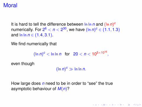
Moral

It is hard to tell the difference between ln ln n and (ln n)c

numerically. For 26 < n < 230, we have (ln n)c ∈ (1.1,1.3)and ln ln n ∈ (1.4,3.1).

We find numerically that

(ln n)c < ln ln n for 20 < n < 105×1018,

even though(ln n)c � ln ln n.

How large does n need to be in order to “see” the trueasymptotic behaviour of M(n)?

The asymptotic region

Ford’s result can be written as

M(n) � n2/Φ(n), where Φ(n) = (ln n)c(ln ln n)3/2.

The factor (ln n)c is asymptotically larger than the factor(ln ln n)3/2. However, for small n, the second factor varies morerapidly than the first.Write x := ln n, A = A(x) := xc , B = B(x) := (ln x)3/2, soΦ(n) = AB.Taking logarithmic derivatives, we have Φ′/Φ = A′/A + B′/B.Now |A′/A| < |B′/B| if c/x < 3/(2x ln x),i.e. if x < e3/2c ≈ 37,036,165, or

n < ee3/2c ≈ 253,431,908.

We need Monte Carlo methods to get numerical results for theregion where the true asymptotic behaviour of M(n) becomesevident (but first I’ll mention some exact methods).

Exact computation of M(n) – the naive algorithm

It is easy to write a program to compute M(n) for small valuesof n. We need an array A of size n2 bits, indexed 0 to n2 − 1,which is initially cleared. Then, using two nested loops, set

A[i × j]← 1 for 0 ≤ i ≤ j < n.

Finally, count the number of bits in the array that are 1 (or sumthe elements of the array). The time and space requirementsare both of order n2.The inner loop of the above program is essentially the same asthe inner loop of a program that is sieving for primes. Thus, thesame tricks can be used to speed it up. For example,multiplications can be avoided as the inner loop sets bitsindexed by an arithmetic progression.

Segmenting the sieve

If the memory requirement of n2 bits is too large, the problemcan be split into pieces. For given [ak ,ak+1) ⊆ [0,n2), we cancount the products ij ∈ [ak ,ak+1). Covering [0,n2) by a set ofdisjoint intervals [a0,a1), [a1,a2), . . ., we can split the probleminto as many pieces as desired.There is a certain startup cost associated with each interval, sothe method becomes inefficient if the interval lengths aresmaller than n.A parallel program can easily be implemented if each parallelprocess handles a separate interval [ak ,ak+1).

Exact computation - the incremental algorithm

The naive algorithm takes time � n2 to compute one valueM(n). If we want to tabulate M(k) for 1 ≤ k ≤ n, the timerequired is � n3. A more efficient approach might be tocompute the differences D(n) := M(n + 1)−M(n).Assuming we know M(n), we need to consider the productsm × n, for 1 ≤ m ≤ n. Let δ(n) denote the number of theseproducts that have already occurred in the table. The number ofelements that have not already appeared is D(n) = n − δ(n).Thus, it is sufficient to compute δ(n) in order to compute D(n)and then M(n + 1).

Computing δ(n)

Assume we know the divisors of n (these can be computed bytrial division). Suppose that g|n, and let h = n/g. By symmetrywe can assume that g ≤

√n ≤ h.

Can we express m× n as a product that already occurred in thetable? If m = i × j and n = g × h, then m× n = ij × gh = ih× jg.If ih < n and jg < n, then the product ih × jg has alreadyoccurred. Observe that ih < n iff i < g and jg < n iff j < h.Thus, to compute δ(n), we need to count the unique products ijwith 0 < i < g and 0 < j < n/g, for each divisor g ≤

√n of n.

This can be done by sieving in an array of size n (the naivealgorithm required size n2).If this is implemented so that work is not duplicated whererectangles of size g1 × n/g1 and g2 × n/g2 overlap, then thework is bounded by the number of lattice points under thehyperbola xy = n. Thus, we can compute δ(n) in (worst case)time O(n ln n) and space O(n).

Example: n = 24

If n = 24, the relevant divisors are g ∈ {2,3,4}.If g = 2, we sieve over (i , j) ∈ {1} × {1,2, . . . ,11}.If g = 3, we sieve over (i , j) ∈ {1∗,2} × {1∗,2,3,4,5,6,7}.If g = 4, we sieve over (i , j) ∈ {1∗,2∗,3} × {1∗,2∗,3,4,5}.Starred entries give duplicates so may be omitted.Conclude that m × n is already in the table iffm ∈ {1,2, . . . ,11,12,14,15}, so δ(n) = 14.e.g. 12× n = 16× 18, 14× n = 16× 21, 15× n = 20× 18.

Tabulating M(1), . . . ,M(n)

Using the algorithm that we just described to compute thedifferences D(n) = M(n + 1)−M(n) we can compute all ofM(1), . . . ,M(n) in time O(n2 ln n) and space O(n) (not countingspace for the output).This is much better than time O(n3) and space O(n2) using thenaive algorithm!Space requirementsIn practice, reducing space often reduces time, because of thememory hierarchy built into modern computers.The space requirement for the incremental algorithm can bereduced to O(

√n) without changing the time bound, by splitting

the sieve into O(√

n) segments. It could be reduced toO(n1/3(ln n)2/3), using ideas due to Harald Helfgott. What wehave implemented is O(

√n), which is fine for n ≤ 109.

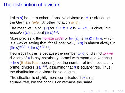
The distribution of divisors

Let τ(n) be the number of positive divisors of n. (τ stands forthe German Teiler. Another notation d(n).)The mean value of τ(k) for 1 ≤ k ≤ n is ∼ ln n [Dirichlet], butusually τ(n) is about (ln n)ln 2.More precisely, the normal order of ln τ(n) is ln(2) ln ln n, whichis a way of saying that, for all positive ε, τ(n) is almost always in[(ln n)ln(2)−ε, (ln n)ln(2)+ε].Heuristically, this is because the number ω(n) of distinct primedivisors of n is asymptotically normal with mean and varianceln ln n [Erdos-Kac theorem], but the number of (not necessarilyprime) divisors is 2ω(n), assuming that n is square-free. Thus,the distribution of divisors has a long tail.The situation is slightly more complicated if n is notsquare-free, but the conclusion remains the same.

OEIS A027417

The OEIS sequence A027417 is defined by an = M(2n).Until recently only a0, . . . ,a25 were listed.Using parallel implementations of the naive and incrementalalgorithms, we (RB and JW) have gone to a30.

n an 4n/an1 2 2.00002 7 2.28573 26 2.46154 90 2.8444· · · · · · · · ·26 830751566970327 5.421127 3288580294256953 5.477928 13023772682665849 5.532829 51598848881797344 5.586030 204505763483830093 5.6376

The scaled sequence

Since M(n) � n2

(ln n)c(ln ln n)3/2, replace n by N = 2n and

define

bn :=N2

M(N)� nc(ln n)3/2 and fn :=

bn

nc(ln n)3/2 � 1.

n bn fn10 4.0366 0.94815 4.6186 0.82120 5.0331 0.75025 5.3624 0.70430 5.6376 0.671

fn appears to be monotonic decreasing. It is not clear from thetable what limn→∞ fn is, or even if the limit exists. An estimate,using much larger values of n, is limn→∞ fn ≈ 0.116.

A subquadratic algorithm

Using the ideas of the incremental algorithm, and someoptimisations that depend on whether or not n is B-smooth withB = L(n)1/

√2, where L(n) := exp(

√ln n ln ln n), we can compute

M(n) in time O(n2/L(n)1/√

2+o(1)).For details, see our preprint arXiv:1908.04251.We have implemented the subquadratic algorithm for evaluationof M(n). In practice, it is not competitive with the best quadraticalgorithm for n ≤ 230.Although the time is theoretically subquadratic, the result is alittle disappointing — we were hoping for something likeKaratsuba’s O(n1.585), but we don’t see how to obtain this. It isnot clear whether we can evaluate M(n) in time O(nλ) for anyfixed λ < 2.

Monte Carlo computation

We can estimate M(n) using two different Monte Carlomethods. Recall that

M(n) = #Sn, Sn = {ij : 0 ≤ i < n, 0 ≤ j < n}.

Bernoulli trialsWe can generate a random integer x ∈ [0,n2), and count asuccess if x ∈ Sn. Repeat several times and estimate

M(n)

n2 ≈ #successes#trials

.

To check if x ∈ Sn we need to find some of the divisors of x ,which probably requires the prime factorisation of x . There isno obvious algorithm that is much more efficient than findingthe prime factors of x (but more on this later).

Monte Carlo computation - alternative method

There is another Monte Carlo algorithm, using what we callproduct trials.Generate random integers x , y ∈ [0,n). Count the numberν = ν(xy) of ways that we can write xy = ij with i < n, j < n.Repeat several times, and estimate

M(n)

n2 ≈∑

1/ν#trials

.

This works because z ∈ Sn is sampled at each trial withprobability ν(z)/n2, so the weight 1/ν(z) is necessary to givean unbiased estimate of M(n)/n2.To compute ν(xy) we need to find the divisors of xy .Note that x , y < n, whereas for Bernoulli trials x < n2, so theintegers considered in product trials are generally smaller thanthose considered in Bernoulli trials.

Comparison

For Bernoulli trials, p = M(n)/n2 is the probability of a success,and the distribution after T trials has mean pT , variancep(1− p)T ≈ pT .For product trials, we know E(1/ν) = M(n)/n2 = p, but we donot know E(1/ν2) theoretically. We can estimate it from thesample variance.It turns out that, for a given number T of trials, the productmethod has smaller expected error (by a factor of 2 to 3 intypical cases).This is not the whole story, because we also need to factor x(for Bernoulli trials) or xy (for product trials), and then find(some of) their divisors.For large n, the most expensive step is factoring, which iseasier for product trials because the numbers involved aresmaller.

Avoiding factoring large integers

We can avoid the factoring steps by generating randomintegers together with their factorisations, using algorithms dueto Bach (1988) or Kalai (2003).Bach’s algorithm is more efficient than Kalai’s, but also muchmore complicated, so I will describe Kalai’s algorithm and referyou to Bach’s paper, or the book Algorithmic Number Theory byBach and Shallit, for a description of Bach’s algorithm.

Kalai’s algorithm

Input: Positive integer n.

Output: A random integer r , uniformly distributed in [1,n],and its prime power factorisation.

1. Generate a sequence n = s0 ≥ s1 ≥ · · · ≥ s` = 1 bychoosing si+1 uniformly in [1, si ] until reaching 1.

2. Let r be the product of all the prime si , i > 0.

3. If r ≤ n, output r and its prime factorisation with probabilityr/n, otherwise restart at step 1.

Kalai’s algorithm clearly outputs an integer r ∈ [1,n] and itsprime factorisation, but why is r uniformly distributed in [1,n]?The answer is the acceptance-rejection step 3.

Correctness of Kalai’s algorithm

Kalai shows that, if 1 ≤ R ≤ n, then (after step 2)

Prob[r = R] =µn

R,

whereµn =

∏p prime, p≤n

(1− 1/p).

If 1 ≤ r ≤ n, then step 3 accepts r with probability r/n, so theprobability of outputting r at step 3 is proportional to

µn

rrn

=µn

n,

which is independent of r . Thus, the output is uniformlydistributed in [1,n].

The expected running time

The running time is dominated by the time for primality tests.The expected number of primality tests is Hn/µn, where

Hn =n∑

k=1

1k

= ln n + γ + O(

1n

).

By a theorem of Mertens (1874),

1µn∼ eγ ln n,

so the expected number of primality tests is

∼ eγ(ln n)2.

Bach’s algorithm

Bach’s algorithm requires prime power tests which are (slightly)more expensive than primality tests. However, it is possible tomodify the algorithm so that only primality tests are required.This is what we implemented. The idea of avoiding primepower tests was suggested independently by Herman Rubin.Bach’s algorithm is more efficient than Kalai’s – the expectednumber of primality tests is of order ln n. The reason is thatBach’s algorithm generates factored integers uniform in (n/2,n]rather than [1,n], which makes the acceptance/rejectionprocess more efficient as well as more complicated.We can generate integers in [1,n] by calling Bach’s algorithmappropriately, see arXiv:1908.04251.

Primality testing

For large n, the main cost of both Bach’s algorithm and Kalai’salgorithm is the primality tests.Since we are using Monte Carlo algorithms, it is reasonable touse the Miller-Rabin probabilistic primality test, which has anonzero (but tiny) probability of error, rather than a much slower“guaranteed” test such as the polynomial-time deterministic testof Agrawal, Kayal and Saxena (AKS), or the randomised buterror-free (“Las Vegas”) elliptic curve test (ECPP) of Atkin andMorain.The Miller-Rabin test makes it feasible to use Bach’s or Kalai’salgorithm for n up to say 21000.

Divisors (again)

An integerx =

∏pαi

i

hasτ(x) =

∏(αi + 1)

distinct divisors, each of the form∏

pβii for 0 ≤ βi ≤ αi .

We do not need all the divisors of the the random integers x , ythat occur in our Monte Carlo computation. We only need thedivisors in a certain interval.

Divisors in Bernoulli and product trials

Bernoulli trialsFor Bernoulli trials, we merely need to know if a given x < n2

has a divisor d < n such that x/d < n, i.e. x/n < d < n. Thus,given n and x ∈ [1,n), it is enough to compute the divisors of xin the interval (x/n,n) until we find one, or show that there arenone.Product trialsFor product trials we generate random (factored) x , y < n andneed (some of) the divisors of xy . We can easily compute theprime-power factorisation of z := xy from the factorisations ofx and y . We then need to count the divisors of z in the interval(z/n,n).

Cost of Bernoulli and product trials

An integer x ∈ [1,n2) has on average

∼ ln n2 = 2 ln n

divisors [Dirichlet]. This is relevant for Bernoulli trials.However, for product trials, our numbers z = xy have onaverage� (ln n)2 divisors, because x and y have on average∼ ln n divisors.Thus, the divisor computation for product trials is moreexpensive than that for Bernoulli trials.

Counting divisors in an interval

We can count the divisors of x in a given interval [a,b] fasterthan actually computing all the divisors in this interval, by usinga “divide and conquer” approach.Here is an outline. Write x = uv where (u, v) = 1 and u, v haveabout equal numbers of divisors. Find all the divisors of v andsort them. Then, for each divisor d of u, compute boundsa ≤ d ′ ≤ b for relevant divisors d ′ of v , and search fora and b in the sorted list, using a binary search.The expected running time is roughly (ignoring ln ln n factors)proportional to the mean value of τ(x)1/2 over x ≤ n. By aresult of Ramanujan [Montgomery and Vaughan, (2.27)],this is � (ln n)α, where α =

√2− 1 ≈ 0.4142.

Thus, for Bernoulli trials the cost is O(lnα n)and for product trials the cost is O(ln2α n).

Avoiding some primality testing

When n is very large, say greater than 21000, even Miller-Rabinprobabilistic primality testing becomes very expensive. We canavoid primality tests on large numbers by making a plausibleassumption about the density of primes in short intervals (butnot so short that Maier’s theorem applies). There is no time todiscuss this in detail today. If you are interested, see the slidesfrom my Hong Kong talk (6 February 2015), which are on mywebsite.Using the density assumption, we have estimated M(n) withan accuracy of three or more significant digits for n up to2500,000,000. This is in the region where the asymptoticbehaviour of M(n) might become evident (recall the argumentwe gave earlier).

Numerical results

N = 2n, bn :=N2

M(N), fn :=

bn

nc(ln n)3/2 � 1.

n bn fn10 4.0366 0.948102 7.6272 0.519103 12.526 0.381104 19.343 0.313105 28.74 0.273106 41.6 0.247107 59.0 0.228108 82.7 0.214

2×108 90.9 0.2105×108 103.4 0.206

The value of limn→∞ fn is not obvious from this table!

Least squares quadratic fit

From the numerical evidence, it is plausible that fn has anasymptotic expansion in negative powers of ln n.Fitting fn by a quadratic in x = (ln n)−1 to the data forn = 102,103, . . . ,5×108 (as in the previous table) givesfn ≈ 0.1157 + 1.7894x + 0.2993x2.

Conclusion

On the basis of the numerical results, a plausible conjecture is

bn = N2/M(N) ∼ c0nc(ln n)3/2, c0 ≈ 0.1157,

which suggestsM(N) ∼ K

N2

(ln N)c(ln ln N)3/2

withK =

(ln 2)c

c0≈ 8.4.

This estimate of K might be inaccurate, since we have onlytaken three terms in a plausible (but not proved) asymptoticseries

fn ∼ c0 + c1/ ln n + c2/(ln n)2 + · · · ,

and the first two terms are of the same order of magnitude inthe region where we can estimate M(N) = M(2n).

References

E. Bach, How to generate factored random numbers,SIAM J. on Computing 17 (1988), 179–193.E. Bach and J. Shallit, Algorithmic Number Theory, Vol. 1,MIT Press, 1996.R. P. Brent and H. T. Kung, The area-time complexity of binarymultiplication, J. ACM 28 (1981), 521–534 & 29 (1982), 904.R. P. Brent, C. Pomerance, D. Purdum, J. Webster, Algorithmsfor the multiplication table, arXiv:1908.04251, 5 May 2021.P. Erdos, Some remarks on number theory,Riveon Lematematika 9 (1955), 45–48 (Hebrew).P. Erdos, An asymptotic inequality in the theory of numbers,Vestnik Leningrad Univ. 15, 13 (1960), 41–49 (Russian).For a correction, see MR603312 (82c:10053).

K. Ford, The distribution of integers with a divisor in a giveninterval, Annals of Math. 168 (2008), 367–433.H. A. Helfgott, An improved sieve of Eratosthenes,Math. Comp. 89 (2020), 333–350.A. Kalai, Generating random factored numbers, easily,J. Cryptology 16 (2003), 287–289.H. Maier, Primes in short intervals, Michigan Math. J. 32(1985), 221–225.H. L. Montgomery and R. C. Vaughan, Multiplicative NumberTheory I. Classical Theory, Cambridge Univ. Press, 2007.S. Ramanujan, Some formulæ in the analytic theory ofnumbers, Messenger of Math. 45 (1916), 81–84.G. Tenenbaum, Sur la probabilité qu’un entier possède undiviseur dans un intervalle donné, Compositio Math. 51(1984),243–263 (French).