Algorithms for the Design of a Multi-stage Adaptive Kanban System

International Journal of Production Research

Vol. 47, No. 23, 1 December 2009, 6707–6738

Algorithms for the design of a multi-stage adaptive kanban system

G.D. Sivakumara* and P. Shahabudeenb

aDepartment of Mechanical Engineering, Sethu Institute of Technology, Pulloor, Kariapatti,Virudhu Nagar Dist, Tamil Nadu, India; bDepartment of Industrial Engineering,

Anna University, Chennai, Tamil Nadu, India

(Received 2 September 2007; final version received 7 April 2008)

The traditional kanban system with a fixed number of cards does not worksatisfactorily in an unstable environment. With the adaptive kanban-type pullcontrol mechanism, the number of kanbans is allowed to change with respect tothe inventory and backorder level. It is required to set the threshold values atwhich cards are added or deleted, which is part of the design. Previous studiesused local search and meta-heuristic methods to design an adaptive kanbansystem for a single stage. In a multi-stage system the cards are circulated withinthe stage and their presence at designated positions signals to the neighbouringstages details concerning the inventory. In this work, a model of a multi-stagesystem adapted from a traditional and adaptive kanban system is developed.A genetic and simulated annealing algorithm based search is employed to set theparameters of the system. The results are compared with a traditional kanbansystem and signs of improvement are found. The numerical results also indicatethat the use of a simulated annealing algorithm produces a better solution.

Keywords: advanced manufacturing processes; advanced manufacturing technol-ogy; adaptive control; JIT; kanban; lean manufacturing

Abbreviations

TKS traditional kanban systemAKS adaptive kanban system

MTKS multi-stage traditional kanban systemMAKS multi-stage adaptive kanban system

GA genetic algorithmSA simulated annealingJIT just in timeMP manufacturing processWIP work in process

CONWIP constant work in processCTMC continuous time Markov chain

tc total cardsc number of identical parallel servers� mean processing rate

*Corresponding author. Email: [email protected]

ISSN 0020–7543 print/ISSN 1366–588X online

� 2009 Taylor & Francis

DOI: 10.1080/00207540802302071

http://www.informaworld.com

M number of workstationsn number of parts in MP

N(t) quantity of finished parts in excess of back orders at time t�d demand rate

�P(n) expected throughput rateK number of production cards or kanban cardsE number of extra cardsC capture thresholdR release thresholdi number of finished parts in the system minus the total number of ordersx number of extra cards in circulationb cost ratio per unit timeU total number of states

P(i,x) probability of being in state (i,x)I(K,E,R,C) expected finished good inventory in adaptive kanban systemB(K,E,R,C) expected backlog in adaptive kanban-type pull control system

N final stagej stage ( j¼ 1, 2, . . . ,N)Z objective function for single stage

Zmult objective function for multi-stage

1. Introduction

In the traditional kanban system (TKS), the number of cards used in a manufacturingprocess (MP) is kept constant. However, in an unstable environment the TKS does notwork satisfactorily. Di Mascolo et al. (1996) developed an analytical method for theperformance evaluation of TKS. Wijngaard (2004) and Karaesmen et al. (2004) usedinventory control policies that resulted in significant cost savings in the TKS throughinventory reductions and improvement in customer service. Liberopoulos andKoukoumialos (2005) presented a simulation model of the TKS in which the effectof advanced demand information is analysed. However, in an unstable environment theTKS does not work satisfactorily. Philipoom et al. (1987) and Rees et al. (1987)investigated the key factors that affect the number of kanbans in the system. Savsarand Al-jawini (1995) presented a simulation study of the performance of JIT systems.In the latter paper the effects of processing time, demand variability, kanbanwithdrawal policies, number of kanbans between stations and the line length areexamined by computing the performance measures throughput rate, work-in-processand station utilisation. Savsar (1997) developed a simulation model to determine theminimum number of kanbans attached to batches of printed circuit boards to satisfy acertain percentage of demand. Savsar and Choueiki (2000) developed a generalisedsystematic procedure (GSP) to determine the optimum kanban allocation in JITcontrolled production lines. They also used the simulation model to simulate the JITproduction line and evaluated the line performance using a neural network. A fewpapers have discussed systems in which the number of kanban cards in use is adjustedaccording to the status of the MP. Such systems are called flexible or adaptivekanban systems (AKS). Previous studies used the local search method to design andfind the optimal solution in the adaptive kanban-type pull control mechanism.

6708 G.D. Sivakumar and P. Shahabudeen

Shahabudeen and Sivakumar (2003) developed a heuristic-based genetic algorithm to

solve the integrated optimisation model for a single-stage adaptive kanban-type pull

control mechanism. The numerical results for the problems indicate that the simulated

annealing algorithm (SA) is efficient for optimising the problems. In this paper a multi-

stage model for the traditional (MTKS) as well as the multi-stage adaptive kanban

(MAKS) system are developed. The systems are analysed using different heuristics and

the results are compared.

2. The traditional kanban system

In the traditional kanban system the number of cards in use is fixed at K. Customer

demand drives the MP. Each part is attached to a kanban. When a customer demand

arrives, the finished part is released to the customer and the kanban attached to that part is

transferred upstream to initiate production. The demand that cannot be met, due to the

non-availability of the finished part, stays as back ordered demand.

2.1 The TKS model

Tardif and Maaseidvaag (2001) developed a kanban system as a closed queuing model.

In this system, demand follows a Poisson process with demand rate �d, the finished parts

leave the manufacturing process according to a state-dependent Markovian process and

its processing rate �P(n) or the throughput depends on the number of parts ‘n’ in the MP.

The processing rate can be obtained by studying equivalent closed queuing networks. For

systems with a single workstation (WS) consisting of c identical parallel servers with mean

service rate �:

�PðnÞ ¼n�, n5c,c�, n � c:

�ð1Þ

According to Spearman (1991), for balanced systems with M workstations, each

consisting of a single server with mean rate �:

�PðnÞ ¼n�

ðnþM� 1Þ: ð2Þ

The behaviour can be modeled as a birth and death process with an infinite number of

states. Let PK(i) be the stationary probability of state i with K cards. These probabilities

exist only if

�d=�PðKÞ51, ð3Þ

and are defined by the rate balance equation where the net inflow of a particular state is

equal to the net outflow of that state. Therefore,

�dPKðiÞ ¼ �PðminðK� iþ 1,KÞÞPKði� 1Þ, ð4Þ

XKi¼�1

PKðiÞ ¼ 1: ð5Þ

International Journal of Production Research 6709

The entry of a raw part into the MP is completely synchronised with the release of a

finished part to the customer. Therefore, the number of parts in the system is constant and

equal to K.The single-stage kanban system is optimised by choosing the parameter K that

minimises the long-term average costs associated with backorders as well as holding

inventory. Let b be the ratio of backorder cost to holding cost in the system. Let B(K) bethe expected backlog for K number of kanban cards. Hence, it is required to determine the

value of K that minimises the total cost:

MinimiseZðKÞ ¼ Kþ b � BðKÞ, ð6Þ

where K40.

3. The adaptive kanban system

In a MP with fluctuation in demand, the TKS with a fixed number of cards leads to either

a huge WIP or heavy backorders. Hence the concept of dynamically varying the number of

kanban cards to suit the situation is given due consideration. Takahashi and Nakamura(1999) explored the benefits of the reactive just in time (JIT) control mechanism where

the kanban levels are reset by fuzzy logic. Hopp and Roof (1998) developed a statistical

throughput control to manipulate work in process (WIP) levels in constant work in

process (CONWIP) lines. Their goal was to achieve a target throughput rate when the

throughput rate fell outside the control limit. The number of kanbans is readjusted and

the throughput rate is maintained within the limits. Gupta and Al-Turki (1997) proposed

a procedure to adjust the number of kanbans in the system. The required number of

additional cards was determined based on the demand and the system capacity.

Shahabudeen and Sivakumar (2003) discussed the application of search heuristics in thedesign of an adaptive kanban system.

Tardif and Maaseidvaag (2001) devised an AKS to handle the variable supply and

demand condition. Here, the number of cards in use is allowed to vary based on the

current inventory and backorders. An extra card is added to the system if a demand arrives

while the inventory level is below a release threshold (R). When the inventory level exceeds

a capture threshold (C) a card is retrieved from the system. Queue P contains finished

parts, and queue D contains backordered demands. The single-stage adaptive mechanism

uses K kanban cards and E extra cards. Initially, before any customer demand arrives at

the system, queue P has a base stock of K finished parts, queue E contains all the extracards and queue D is empty and the MP is idle.

Let N(t) represent the quantity of finished parts in excess of back orders at time

t (P–D). When a customer demand arrives at time t, before the part is released to the

customer, if N(t) is less than or equal to the release threshold (R) and if some cards are in

queue E, an extra card is added to the MP and queue E is updated. Then the demand is

satisfied, which releases a card that is sent to the MP. However, if N(t) before part release

is greater than or equal to C, after satisfying the demand, the card is released but is not

sent to the MP, instead it is sent to E. Here, R5C, and C�Kþ 1 so as to ensure that the

system is able to return to the initial state (K, 0).The system is modeled in terms of the state (i, x) whose evaluation describes a

continuous time Markov chain (CTMC). State (i, x) denotes the total number of parts in

queue P minus the total number of back orders in queue D by i and the number of extra


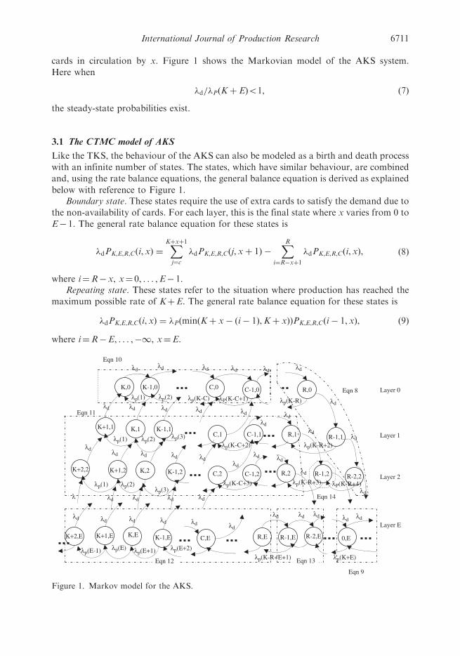
cards in circulation by x. Figure 1 shows the Markovian model of the AKS system.

Here when

�d=�PðKþ EÞ51, ð7Þ

the steady-state probabilities exist.

3.1 The CTMC model of AKS

Like the TKS, the behaviour of the AKS can also be modeled as a birth and death process

with an infinite number of states. The states, which have similar behaviour, are combined

and, using the rate balance equations, the general balance equation is derived as explained

below with reference to Figure 1.Boundary state. These states require the use of extra cards to satisfy the demand due to

the non-availability of cards. For each layer, this is the final state where x varies from 0 to

E� 1. The general rate balance equation for these states is

�dPK,E,R,Cði, xÞ ¼XKþxþ1j¼c

�dPK,E,R,Cðj, xþ 1Þ �XR

i¼R�xþ1

�dPK,E,R,Cði, xÞ, ð8Þ

where i¼R�x, x¼ 0, . . . ,E� 1.Repeating state. These states refer to the situation where production has reached the

maximum possible rate of KþE. The general rate balance equation for these states is

�dPK,E,R,Cði, xÞ ¼ �PðminðKþ x� ði� 1Þ,Kþ xÞÞPK,E,R,Cði� 1, xÞ, ð9Þ

where i¼R�E, . . . ,�1, x¼E.

Eqn 11

Eqn 14

K+2,E K+1,E K,E K-1,E C,E R,E R-1,E R-2,E 0,E

K+2,2 K+1,2 K,2 K-1,2 C,2

C,1 R-1,1

K+1,1

λp(E) λp(E+2)

λp(K-R+E+1)

λd

λdλdλd

λd

λd

λp(1) λp(2) λp(3)

λp(2) λp(3)

λp(K-C+3)

λp(K-C+2)

λp(K+E)

C-1,1

R,2 R-1,2 R-2,2λp(K-R+3) λP(K-R+4)

λdλdλdλd

λd λdλd

λd λd

λdC-1,2

λ λd λd λd

λd λd λd λd λd

λd λd λd λdλd

λd

λd

λd

λd

λp(E-1) λp(E+1)

λp(K-R+2)

R,1 K,1 K-1,1

K,0 C,0 R,0

λp(K-R)

λd

λp(1)

λp(2) λp(K-C) λP(K-C+1) C-1,0

λdλd λd λd λd

λd

K-1,0

λp(1)

λd

Eqn 8 Layer 0

Layer 1

Layer 2

Layer E

Eqn 10

Eqn 9

Eqn 12 Eqn 13

Figure 1. Markov model for the AKS.


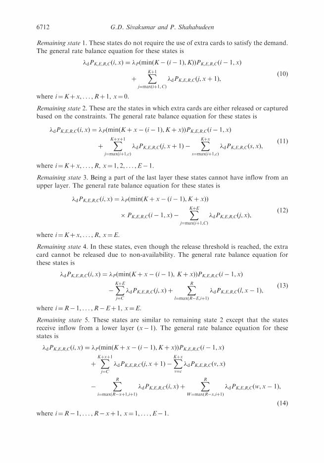
Remaining state 1. These states do not require the use of extra cards to satisfy the demand.

The general rate balance equation for these states is

�dPK,E,R,Cði, xÞ ¼ �P minðK� ði� 1Þ,KÞð ÞPK,E,R,Cði� 1, xÞ

þXKþ1

j¼maxðiþ1,CÞ

�dPK,E,R,Cðj, xþ 1Þ,ð10Þ

where i¼Kþx, . . . ,Rþ 1, x¼ 0.

Remaining state 2. These are the states in which extra cards are either released or captured

based on the constraints. The general rate balance equation for these states is

�dPK,E,R,Cði, xÞ ¼ �PðminðKþ x� ði� 1Þ,Kþ xÞÞPK,E,R,Cði� 1, xÞ

þXKþxþ1

j¼maxðiþ1,cÞ

�dPK,E,R,Cðj,xþ 1Þ �XKþx

s¼maxðiþ1,cÞ

�dPK,E,R,Cðs, xÞ,ð11Þ

where i¼Kþx, . . . ,R, x¼ 1, 2, . . . ,E� 1.

Remaining state 3. Being a part of the last layer these states cannot have inflow from an

upper layer. The general rate balance equation for these states is

�dPK,E,R,Cði, xÞ ¼ �PðminðKþ x� ði� 1Þ,Kþ xÞÞ

� PK,E,R,Cði� 1, xÞ �XKþE

j¼maxðiþ1,CÞ

�dPK,E,R,Cðj, xÞ,ð12Þ

where i¼Kþx, . . . ,R, x¼E.

Remaining state 4. In these states, even though the release threshold is reached, the extra

card cannot be released due to non-availability. The general rate balance equation for

these states is

�dPK,E,R,Cði, xÞ ¼ �PðminðKþ x� ði� 1Þ, Kþ xÞÞPK,E,R,Cði� 1,xÞ

�XKþEj¼C

�dPK,E,R,Cðj, xÞ þXR

l¼maxðR�E,iþ1Þ

�dPK,E,R,Cðl, x� 1Þ,ð13Þ

where i¼R� 1, . . . ,R�Eþ 1, x¼E.

Remaining state 5. These states are similar to remaining state 2 except that the states

receive inflow from a lower layer (x� 1). The general rate balance equation for these

states is

�dPK,E,R,Cði, xÞ ¼ �PðminðKþ x� ði� 1Þ,Kþ xÞÞPK,E,R,Cði� 1,xÞ

þXKþxþ1j¼C

�dPK,E,R,Cðj, xþ 1Þ �XKþxv¼c

�dPK,E,R,Cðv, xÞ

�XR

i¼maxðR�xþ1,iþ1Þ

�dPK,E,R,Cði, xÞ þXR

W¼maxðR�x,iþ1Þ

�dPK,E,R,Cðw, x� 1Þ,

ð14Þ

where i¼R� 1, . . . ,R� xþ 1, x¼ 1, . . . ,E� 1.


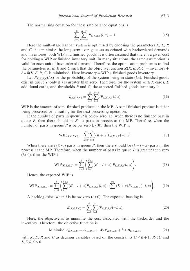
The normalising equation for these rate balance equations is

XEx¼0

XKþxi¼�1

PK,E,R,Cði, xÞ ¼ 1: ð15Þ

Here the multi-stage kanban system is optimised by choosing the parameters K, E, Rand C that minimise the long-term average costs associated with backordered demandsand inventories, both WIP and finished goods. It is often assumed that there is a given costfor holding a WIP or finished inventory unit. In many situations, the same assumption isvalid for each unit of backordered demand. Therefore, the optimisation problem is to findthe parameters K, E, R and C such that the objective function Z(K,E,R,C)¼ inventoryþb �B(K,E,R,C) is minimised. Here inventory¼WIPþ finished goods inventory.

Let PK,E,R,C(i,x) be the probability of the system being in state (i,x). Finished goodsexist in queue P only if i is greater than zero. Therefore, for the system with K cards, Eadditional cards, and thresholds R and C, the expected finished goods inventory is

IðK,E,R,CÞ ¼XEx¼0

XKþxi¼1

iPK,E,R,Cði, xÞ: ð16Þ

WIP is the amount of semi-finished products in the MP. A semi-finished product is eitherbeing processed or is waiting for the next processing operation.

If the number of parts in queue P is below zero, i.e. when there is no finished part inqueue P, then there should be Kþ x parts in process at the MP. Therefore, when thenumber of parts in queue P is below zero (i50), then the WIP is

WIPðK,E,R,CÞ ¼XEx¼0

X1i¼1

ðKþ xÞPK,E,R,Cð�i, xÞ: ð17Þ

When there are i (i40) parts in queue P, then there should be (k� iþ x) parts in theprocess at the MP. Therefore, when the number of parts in queue P is greater than zero(i40), then the WIP is


XKþxi¼0

ðK� iþ xÞ PK,E,R,Cði, xÞ

!: ð18Þ

Hence, the expected WIP is


XKþxi¼0

ðK� iþ xÞPK,E,R,Cði, xÞ

þX1i¼1

ðKþ xÞPK,E,R,Cð�i, xÞ

!: ð19Þ

A backlog exists when i is below zero (i50). The expected backlog is

BðK,E,R,CÞ ¼XEx¼0

X1i¼1

iPK,E,R,Cð�i, xÞ: ð20Þ

Here, the objective is to minimise the cost associated with the backorder and theinventory. Therefore, the objective function is

Minimise ZK,E,R,C ¼ IK,E,R,C þWIPK,E,R,C þ b � BK,E,R,C, ð21Þ

with K, E, R and C as decision variables based on the constraints C�Kþ 1, R5C andK,E,R,C40.


4. The multi-stage kanban system

The multi-stage manufacturing system is decomposed into stages and the stages are in atandem configuration. Each stage is controlled by a kanban mechanism. Thus theparameters of the control policy are the number of kanbans for each stage. Therefore, oncethe system has been decomposed into stages, the design of the kanban control system isreduced to setting the number of kanbans for each stage. These parameters play animportant role in the efficiency of the kanban control system. Bruno et al. (2001) presentedan analytical method for analysing a multi-class queuing network in which each kanbanloop is represented by a class of customers. Di mascalo et al. (1996) also presented ananalytical method to handle manufacturing stages consisting of any number of machines.Huang et al. (1983) carried out an extensive simulation study to determine the effects ofservice and production time at every stage. Mitra and Mitrani (1990, 1991) constructed astochastic model for a manufacturing facility and analysed the performance of thetraditional kanban system in all stages.

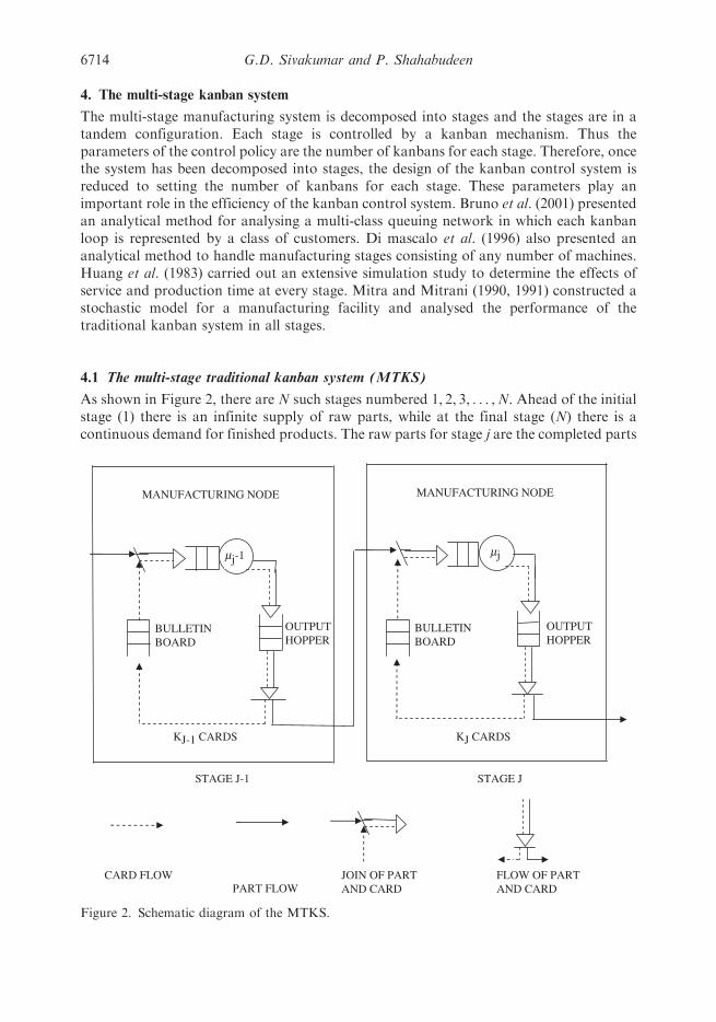
4.1 The multi-stage traditional kanban system (MTKS)

As shown in Figure 2, there are N such stages numbered 1, 2, 3, . . . ,N. Ahead of the initialstage (1) there is an infinite supply of raw parts, while at the final stage (N) there is acontinuous demand for finished products. The raw parts for stage j are the completed parts

JOIN OF PART AND CARD

FLOW OF PART AND CARD

KJ-1 CARDS

BULLETIN BOARD

MANUFACTURING NODE

mj-1

OUTPUT HOPPER

mj

BULLETIN BOARD

OUTPUT HOPPER

MANUFACTURING NODE

KJ CARDS

STAGE J-1 STAGE J

CARD FLOWPART FLOW

Figure 2. Schematic diagram of the MTKS.


of stage j� 1 ( j¼ 2, . . . ,N). In stage j, there is a fixed number, Kj, of cards, or kanbans(Kj� 1). A part must acquire one of these cards in order to enter the stage. Thus, theinventory in stage j (the total number of raw and completed parts) can never exceed Kj.Any unattached cards that are present in the stage are to be found on the bulletin boardand are considered as requests for raw parts.

Let Q be a part that has just completed service at the manufacturing node in stage j� 1,and O be the card attached to it. Q and O move to the output hopper of stage j� 1. Thereare two possible courses of action, depending on the state of the bulletin board in stage j.

(a) If that board is empty, then Q and O wait at the output hopper of stage j� 1.(b) If the board is not empty, then the following moves occur immediately. Q is

transferred from stage j� 1 to stage j, where it is attached to the leading card andmoves to the manufacturing node. O goes to the bulletin board of stage j� 1.

Some implications of the above rules are worth pointing out. One of these is that it isimpossible for the bulletin board in stage j and the output hopper in stage j� 1 to be non-empty simultaneously. In particular, since the pool of raw parts preceding stage 1 is neverempty, the bulletin board in stage 1 is always empty. As soon as a card appears thererequesting input, that request is satisfied and a new part enters the stage. Similarly, sincethe pool of demands following stage N is never empty, the output hopper in stage N isalways empty. As soon as a part is completed, it is removed from the stage. Hence, thebulletin board in stage 1 and output hopper of stage N are superfluous and theirelimination does not affect operation.

Another consequence of the scheduling rules is that a service completion event in onestage can trigger several simultaneous moves in the preceding stage. For instance, in thesituation illustrated in Figure 2, the arrival of a card into the bulletin board of stage jþ 1would cause a departure of a part from stage j, freeing a card in that stage, which in turnenables a part to move out of stage j� 1.

4.1.1 The multi-stage traditional kanban system model

Here we assume that the manufacturing system is decomposed into stages and in each stagethere are c parallel servers. The stages are in tandem configuration. Therefore, in the longrun, the throughputs of the stages are equal (Mitra and Mitrani 1991). We also assume thatthere is an infinite supply of raw parts at initial stage 1 and continuous demand at stage N.The service time is exponentially distributed and demand follows a Poisson distribution. Tomaintain a steady-state the average arrival rate of demand must be less than the throughputor production capacity of the system, i.e. (�d/�P(K))51. The mean service time per machinefor stage 1 and the mean demand rate of stage N are known.

4.1.1.1 Calculation of throughput and average production capacity per machine in eachstage. Since the stages of the system are in tandem the throughput of stages are equal,�PðK1Þ ¼ �PðK2Þ ¼ �PðK3Þ. The throughput of stage 1¼ throughput of stage 2¼ � � �¼ throughput of stage N.

(i) Using Equation (1) the throughput for stage 1 is

�PðK1Þ ¼K1�1, K15c1,c1�1, K1 � c1

�: ð22Þ


(ii) For the subsequent stages ( j¼ 2, 3, . . . ,N) we can compute the average

production capacity per machine or average service rate per machine mj basedon Kj and cj

�j ¼throughput=Kj, Kj5cj,throughput=cj, Kj � cj:

�ð23Þ

4.1.1.2 Calculation of the mean demand rate. In the long run the number of parts in the

output buffer of stage N is KN. When the mean demand arrives in stage j, this demand issatisfied and cards are sent to the bulletin board of stage j. The numbers of cards are the

mean demand rate for the j� 1 stage. For stage N, the demand rate is the actual arrivalrate of the customer

�dN ¼ �d: ð24Þ

If the number of demand arrivals is less than the number of kanban cards in

circulation, then the number of cards sent to the bulletin board depends on the demandarrival rate, otherwise it depends on the number of cards in circulation. Here, the number

of cards in the bulletin board is based on the demand arrival rate or number of cards incirculation of that stage. The number of cards in the bulletin board of stage j¼min{�dj,Kj}

�dj�1 ¼ minf�dj,Kjg, ð25Þ

where j¼ 1, 2, 3, . . . ,N� 1.

4.1.1.3 Objective function. After calculating the mean demand rate and production

capacity of each stage, the objective function value of each stage can be computed using

Equation (6). The overall objective function value of a multi-stage system is obtained bythe summation of the Z stages as given below, which should be minimised:

Zmult ¼ Z1 þ Z2 þ � � � þ ZN: ð26Þ

4.1.2 Algorithm for the design of MTKS

Algorithm for the design of MTKSStep 0: Input

N : number of stagescj : number of machines in stage jbj: cost ratio of stage j�1 : mean production rate/machine of stage 1�dN : mean demand arrival rate of stage N

Initialise

Zj : value of objective function at stage j¼ 0Zopt : optimum Z¼ 0K( j) : number of cards at stage j¼ 0

tc : total number of cards¼NZmin(tc� 1)¼ M (M is a largeþ ve value)

Step 1: Initialise Zmin(tc)¼Mfor ( j1¼ 1; j1� tc� (N� 1); j1þþ)


{for ( j2¼ 1; j2� tc� ( j1þ (N� 2)); j2þþ)

{:

for ( jN¼ 1; jN� tc� ( j1þ j2þ � � � þ jN�1); jNþþ){

K(1)¼ j1;K(2)¼ j2;

:K(N)¼ jN;Step 2: Compute �dj and mj for each stageStep 3: Compute Zj for each stageStep 4: Compute Zmult

Step 5: If Zmin(tc)4Zmult

Zmin(tc)¼Zmult

}:

}}

Step 6: IfZmin(tc)5Zmin(tc� 1), let tc¼ tcþ go to step 1

Else

Zopt ¼ Zminðtc� 1Þ

Step 7: The optimum card settings in stages 1, . . . ,N are K(1), . . . ,K(N).

4.2 The multi-stage adaptive kanban system (MAKS)

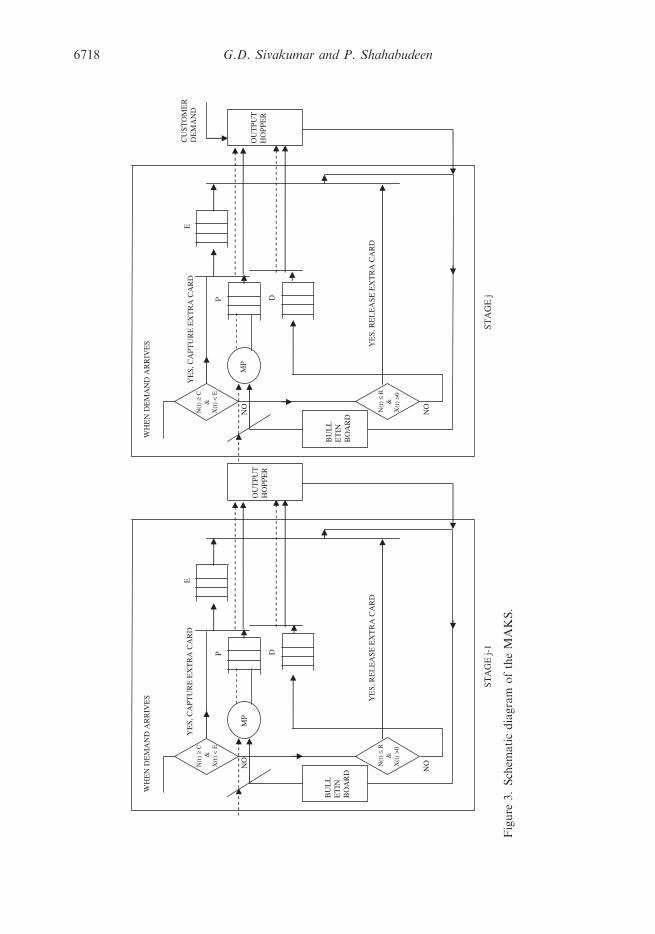
A systematic representation of a multi-stage adaptive kanban system is given in Figure 3.

The raw material enters stage 1, is processed through subsequent stages and the finished

product is delivered in stage N. The analysis and computation of the objective function

values are similar to MTKS as explained in Section 4.1.1. The difference lies in the

operations as given below.When a demand arrives it is satisfied at stage N from the output hopper. The

information to initiate production in the downstream stages is generated based on the

kanban cards at each stage. At any given stage there are Kj fixed cards and E extra cards

are provided. Rj and Cj are the release threshold and capture threshold, respectively,

for stage j. The operation of these threshold values is similar to the explanation given for

the single-stage adaptive kanban system (AKS).Since the value over all Z depends upon the values of K, E, R and C at the stages, it was

decided to employ a search heuristic.

4.2.1 Calculation of throughput and production capacity per machine in each stage

Since the stages are in tandem, the throughputs of all stages are equal. The throughput of

stage 1¼ throughput of stage 2¼ � � � ¼ throughput of stage N.


OU

TPU

T

HO

PPE

R

CU

STO

ME

R

DE

MA

ND

NO

NO

N

O

NO

N(t

) ≤

R

&

X

(t)

>0

N(t

) ≥

C

&

X(t

) <

E

WH

EN

DE

MA

ND

AR

RIV

ES

YE

S, C

APT

UR

E E

XT

RA

CA

RD

MP

E

P D

OU

TPU

T

HO

PPE

R

YE

S, R

EL

EA

SE E

XT

RA

CA

RD

BU

LL

E

TIN

B

OA

RD

N(t

) ≤

R

&

X

(t)

>0

N(t

) ≥

C

&

X(t

) <

E

WH

EN

DE

MA

ND

AR

RIV

ES

YE

S, C

APT

UR

E E

XT

RA

CA

RD

MP

E

P D

YE

S, R

EL

EA

SE E

XT

RA

CA

RD

BU

LL

E

TIN

B

OA

RD

STA

GE

j-1

STA

GE

j

Figure

3.Schem

aticdiagram

oftheMAKS.


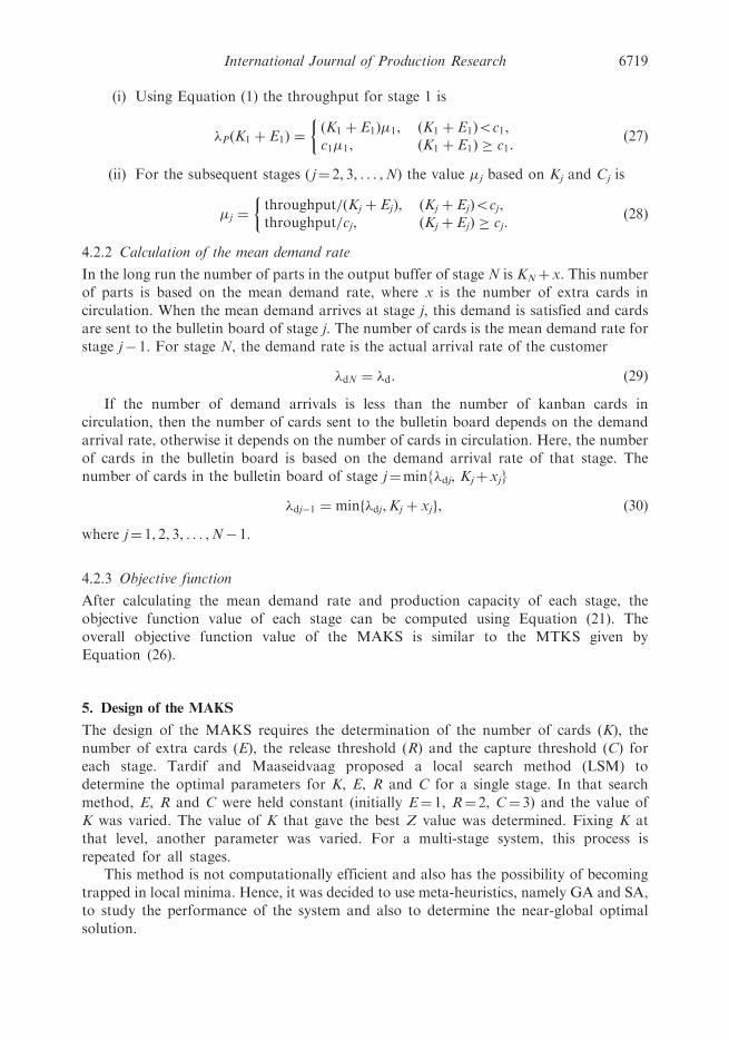
(i) Using Equation (1) the throughput for stage 1 is

�PðK1 þ E1Þ ¼ðK1 þ E1Þ�1, ðK1 þ E1Þ5c1,c1�1, ðK1 þ E1Þ � c1:

�ð27Þ

(ii) For the subsequent stages ( j¼ 2, 3, . . . ,N) the value �j based on Kj and Cj is

�j ¼throughput=ðKj þ EjÞ, ðKj þ EjÞ5cj,throughput=cj, ðKj þ EjÞ � cj:

�ð28Þ

4.2.2 Calculation of the mean demand rate

In the long run the number of parts in the output buffer of stage N is KNþx. This number

of parts is based on the mean demand rate, where x is the number of extra cards in

circulation. When the mean demand arrives at stage j, this demand is satisfied and cards

are sent to the bulletin board of stage j. The number of cards is the mean demand rate for

stage j� 1. For stage N, the demand rate is the actual arrival rate of the customer

�dN ¼ �d: ð29Þ

If the number of demand arrivals is less than the number of kanban cards in

circulation, then the number of cards sent to the bulletin board depends on the demand

arrival rate, otherwise it depends on the number of cards in circulation. Here, the number

of cards in the bulletin board is based on the demand arrival rate of that stage. The

number of cards in the bulletin board of stage j¼min{�dj, Kjþxj}

�dj�1 ¼ minf�dj,Kj þ xjg, ð30Þ

where j¼ 1, 2, 3, . . . ,N� 1.

4.2.3 Objective function

After calculating the mean demand rate and production capacity of each stage, the

objective function value of each stage can be computed using Equation (21). The

overall objective function value of the MAKS is similar to the MTKS given by

Equation (26).

5. Design of the MAKS

The design of the MAKS requires the determination of the number of cards (K), the

number of extra cards (E), the release threshold (R) and the capture threshold (C) for

each stage. Tardif and Maaseidvaag proposed a local search method (LSM) to

determine the optimal parameters for K, E, R and C for a single stage. In that search

method, E, R and C were held constant (initially E¼ 1, R¼ 2, C¼ 3) and the value of

K was varied. The value of K that gave the best Z value was determined. Fixing K at

that level, another parameter was varied. For a multi-stage system, this process is

repeated for all stages.This method is not computationally efficient and also has the possibility of becoming

trapped in local minima. Hence, it was decided to use meta-heuristics, namely GA and SA,

to study the performance of the system and also to determine the near-global optimal

solution.


5.1 Genetic algorithm

A genetic algorithm is an adaptive procedure that finds solutions to problems by an

evolutionary process based on natural selection and genetics (Pirlot 1996). It works with a

population of solutions and attempts to guide the search towards improvement, using a

survival-of-the-fittest principle (Dowsland 1996).The application of a GA to a kanban system is reported by Kochel and Nielander

(2002). They showed that their approach outperforms the heuristic methods of Mitra and

Mitrani (1991) and Wang and Wang (1990, 1991). Shahabudeen and Krishnaiah (1999)

used a GA to set the number of kanbans at each station and the lot size. A simulation

model with a single-card system was designed and used for analysis. Paris et al. (2001)

proposed a simulation model with a GA to optimise the design options of manufacturing

systems. These design options include type of material handling (automated guided

vehicles versus conveyor belts), the buffer stock (kanban versus CONWIP), etc. In

addition, the authors used a tree structure chromosome to represent this multilevel

structure. Reproduction, crossover and mutation are the operators employed in a GA.

5.1.1 GA for MAKS

The details of the GA parameters with respect to MAKS, such as chromosome design,

crossover operator and mutation operator, are given below.

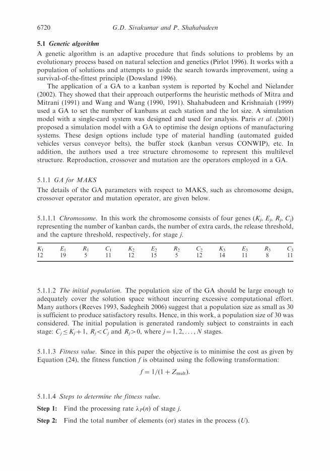
5.1.1.1 Chromosome. In this work the chromosome consists of four genes (Kj, Ej, Rj, Cj)

representing the number of kanban cards, the number of extra cards, the release threshold,

and the capture threshold, respectively, for stage j.

K1 E1 R1 C1 K2 E2 R2 C2 K3 E3 R3 C3

12 19 5 11 12 15 5 12 14 11 8 11

5.1.1.2 The initial population. The population size of the GA should be large enough to

adequately cover the solution space without incurring excessive computational effort.

Many authors (Reeves 1993, Sadegheih 2006) suggest that a population size as small as 30

is sufficient to produce satisfactory results. Hence, in this work, a population size of 30 was

considered. The initial population is generated randomly subject to constraints in each

stage: Cj�Kjþ 1, Rj5Cj and Rj40, where j¼ 1, 2, . . . ,N stages.

5.1.1.3 Fitness value. Since in this paper the objective is to minimise the cost as given by

Equation (24), the fitness function f is obtained using the following transformation:

f ¼ 1=ð1þ ZmultÞ:

5.1.1.4 Steps to determine the fitness value.

Step 1: Find the processing rate �PðnÞ of stage j.

Step 2: Find the total number of elements (or) states in the process (U).


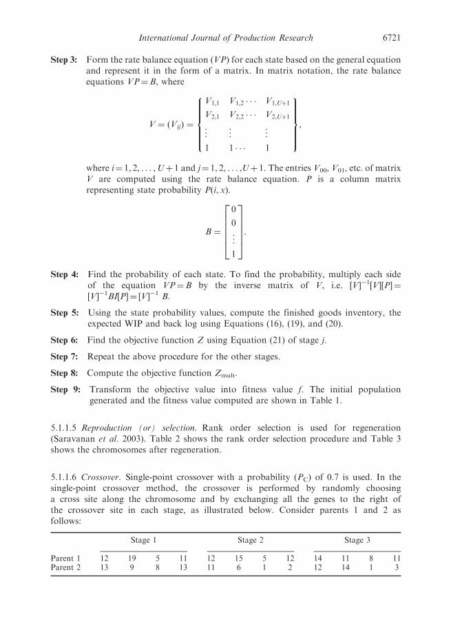
Step 3: Form the rate balance equation (VP) for each state based on the general equationand represent it in the form of a matrix. In matrix notation, the rate balanceequations VP¼B, where

V ¼ ðVijÞ ¼

V1,1 V1,2 � � � V1,Uþ1

V2,1 V2,2 � � � V2,Uþ1

..

. ... ..

.

1 1 � � � 1

8>>>><>>>>:

9>>>>=>>>>;,

where i¼ 1, 2, . . . ,Uþ 1 and j¼ 1, 2, . . . ,Uþ 1. The entries V00, V01, etc. of matrixV are computed using the rate balance equation. P is a column matrixrepresenting state probability P(i, x).

B ¼

0

0

..

.

1

266664

377775:

Step 4: Find the probability of each state. To find the probability, multiply each sideof the equation VP¼B by the inverse matrix of V, i.e. [V]�1[V][P]¼[V]�1BI[P]¼ [V]�1 B.

Step 5: Using the state probability values, compute the finished goods inventory, theexpected WIP and back log using Equations (16), (19), and (20).

Step 6: Find the objective function Z using Equation (21) of stage j.

Step 7: Repeat the above procedure for the other stages.

Step 8: Compute the objective function Zmult.

Step 9: Transform the objective value into fitness value f. The initial populationgenerated and the fitness value computed are shown in Table 1.

5.1.1.5 Reproduction (or) selection. Rank order selection is used for regeneration(Saravanan et al. 2003). Table 2 shows the rank order selection procedure and Table 3shows the chromosomes after regeneration.

5.1.1.6 Crossover. Single-point crossover with a probability (PC) of 0.7 is used. In thesingle-point crossover method, the crossover is performed by randomly choosinga cross site along the chromosome and by exchanging all the genes to the right ofthe crossover site in each stage, as illustrated below. Consider parents 1 and 2 asfollows:

Stage 1 Stage 2 Stage 3

Parent 1 12 19 5 11 12 15 5 12 14 11 8 11Parent 2 13 9 8 13 11 6 1 2 12 14 1 3


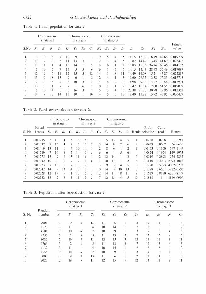
Table 1. Initial population for case 2.

S.No

Chromosome

in stage 1

Chromosome

in stage 2

Chromosome

in stage 3

Z1 Z2 Z3 Ztot

Fitness

valueK1 E1 R1 C1 K2 E2 R2 C2 K3 E3 R3 C3

1 7 10 6 7 10 9 1 3 9 5 4 5 14.15 18.72 16.79 49.66 0.019739

2 13 2 3 5 11 13 3 7 12 13 4 5 13.82 14.42 13.45 41.69 0.023425

3 13 11 1 4 10 14 1 2 8 6 1 2 13.85 18.85 36.76 69.46 0.014192

4 7 10 6 7 14 5 5 6 6 1 5 6 14.15 14.43 28.98 57.49 0.017097

5 12 19 5 11 12 15 5 12 14 11 8 11 14.49 14.08 15.2 43.87 0.022287

6 13 9 8 13 9 6 1 2 12 14 1 3 15.60 26.35 13.38 55.33 0.017753

7 7 13 4 7 5 10 3 5 14 8 2 6 16.98 39.30 14.27 70.56 0.013974

8 10 8 1 7 7 1 6 7 10 11 1 2 17.42 16.84 17.00 51.55 0.019029

9 5 10 4 5 6 16 3 7 5 13 4 5 23.38 25.80 30.78 79.96 0.012352

10 14 9 13 14 13 10 1 10 14 5 10 13 18.40 13.82 15.72 47.95 0.020429

Table 2. Rank order selection for case 2.

S. No

Sorted

fitness

Chromosome

in stage 1

Chromosome

in stage 2

Chromosome

in stage 3

Rank

Prob.

selection

Cum.

prob RangeK1 E1 R1 C1 K2 E2 R2 C2 K3 E3 R3 C3

1 0.01235 5 10 4 5 6 16 3 7 5 13 4 5 1 0.0268 0.0268 0–267

2 0.01397 7 13 4 7 5 10 3 5 14 8 2 6 2 0.0429 0.0697 268–696

3 0.01419 13 11 1 4 10 14 1 2 8 6 1 2 3 0.0453 0.1150 697–1149

4 0.01709 7 10 6 7 14 5 5 6 6 1 5 6 4 0.0824 0.1974 1149–1973

5 0.01775 13 9 8 13 11 6 1 2 12 14 1 3 5 0.0919 0.2893 1974–2892

6 0.01902 10 8 1 7 7 1 6 7 10 11 1 2 6 0.1110 0.4003 2893–4002

7 0.01973 7 10 6 7 10 9 1 3 9 5 4 5 7 0.1220 0.5223 4002–5222

8 0.02042 14 9 13 14 13 10 1 10 14 5 10 13 8 0.1328 0.6551 5222–6550

9 0.02228 12 19 5 11 12 15 5 12 14 11 8 11 9 0.1629 0.8180 6551–8179

10 0.02342 13 2 3 5 11 13 3 7 12 13 4 5 10 0.1818 1 8180–9999

Table 3. Population after reproduction for case 2.

S. No

Random

number

Chromosome

in stage 1

Chromosome

in stage 2

Chromosome

in stage 3

K1 E1 R1 C1 K2 E2 R2 C2 K3 E3 R3 C3

1 2001 13 9 8 13 11 6 1 2 12 14 1 3

2 1129 13 11 1 4 10 14 1 2 8 6 1 2

3 4501 7 10 6 7 10 9 1 3 9 5 4 5

4 9555 13 2 3 5 11 13 3 7 12 13 4 5

5 8025 12 19 5 11 12 15 5 12 14 11 8 11

6 9765 13 2 3 5 11 13 3 7 12 13 4 5

7 1132 13 11 1 4 10 14 1 2 8 6 1 2

8 4555 7 10 6 7 10 9 1 3 9 5 4 5

9 2007 13 9 8 13 11 6 1 2 12 14 1 3

10 8020 12 19 5 11 12 15 5 12 14 11 8 11


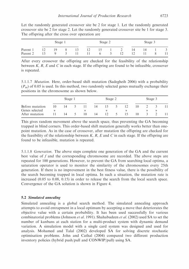
Let the randomly generated crossover site be 2 for stage 1. Let the randomly generatedcrossover site be 2 for stage 2. Let the randomly generated crossover site be 1 for stage 3.The offspring after the cross over operation are


Parent 1 12 19 8 13 12 15 1 2 14 14 1 3Parent 2 13 9 5 11 11 6 5 12 12 11 8 11

After every crossover the offspring are checked for the feasibility of the relationshipbetween K, R, E and C in each stage. If the offspring are found to be infeasible, crossoveris repeated.

5.1.1.7 Mutation. Here, order-based shift mutation (Sadegheih 2006) with a probability(Pm) of 0.05 is used. In this method, two randomly selected genes mutually exchange theirpositions in the chromosome as shown below.


Before mutation 10 14 5 11 14 15 5 12 10 2 3 11Genes selected � � � � � �

After mutation 11 14 5 10 14 12 5 15 10 3 2 11

This gives random movement above the search space, thus preventing the GA becomingtrapped in blind corners. This order-based shift mutation generally works better than one-point mutation. As in the case of crossover, after mutation the offspring are checked forthe feasibility of the relationship between K, R, E and C in each stage. If the offspring arefound to be infeasible, mutation is repeated.

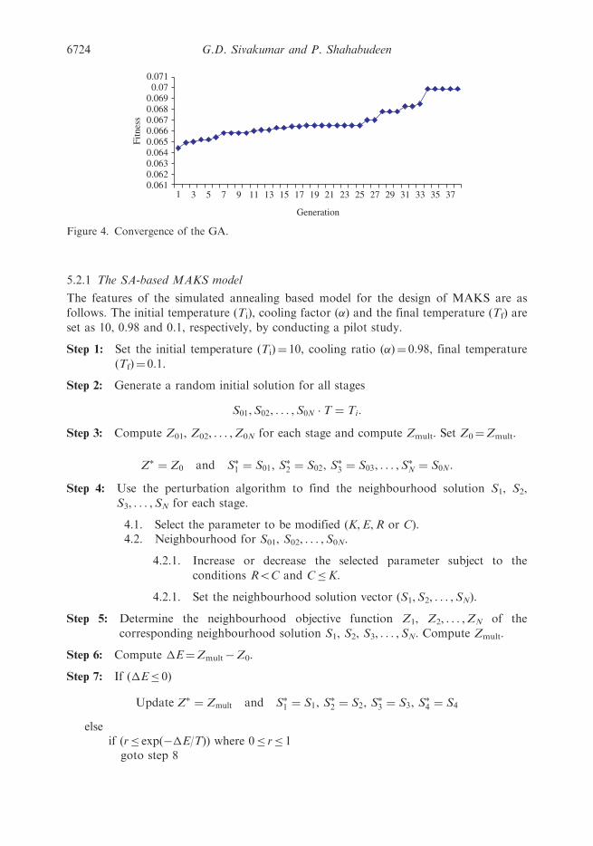
5.1.1.8 Generation. The above steps complete one generation of the GA and the currentbest value of f and the corresponding chromosome are recorded. The above steps arerepeated for 100 generations. However, to prevent the GA from searching local optima, asaturation operator is used to monitor the similarity of the chromosomes every 25thgeneration. If there is no improvement in the best fitness value, there is the possibility ofthe search becoming trapped in local optima. In such a situation, the mutation rate isincreased (0.05 to 0.08, 0.15) in order to release the search from the local search space.Convergence of the GA solution is shown in Figure 4.

5.2 Simulated annealing

Simulated annealing is a global search method. The simulated annealing approachattempts to avoid entrapment in a local optimum by accepting a move that deteriorates theobjective value with a certain probability. It has been used successfully for variouscombinatorial problems (Johnson et al. 1991). Shahabudeen et al. (2002) used SA to set thenumber of kanbans at each station for a multi-product system with dynamic demandvariation. A simulation model with a single card system was designed and used foranalysis. Mohamed and Talal (2002) developed SA for solving discrete stochasticoptimisation problems. John and Cathal (2004) compared two different productioninventory policies (hybrid push/pull and CONWIP/pull) using SA.


5.2.1 The SA-based MAKS model

The features of the simulated annealing based model for the design of MAKS are as

follows. The initial temperature (Ti), cooling factor (�) and the final temperature (Tf) are

set as 10, 0.98 and 0.1, respectively, by conducting a pilot study.

Step 1: Set the initial temperature (Ti)¼ 10, cooling ratio (�)¼ 0.98, final temperature

(Tf)¼ 0.1.

Step 2: Generate a random initial solution for all stages

S01,S02, . . . ,S0N � T ¼ Ti:

Step 3: Compute Z01, Z02, . . . ,Z0N for each stage and compute Zmult. Set Z0¼Zmult.

Z� ¼ Z0 and S�1 ¼ S01, S�2 ¼ S02, S

�3 ¼ S03, . . . ,S�N ¼ S0N:

Step 4: Use the perturbation algorithm to find the neighbourhood solution S1, S2,

S3, . . . ,SN for each stage.

4.1. Select the parameter to be modified (K,E,R or C).4.2. Neighbourhood for S01, S02, . . . ,S0N.

4.2.1. Increase or decrease the selected parameter subject to the

conditions R5C and C�K.

4.2.1. Set the neighbourhood solution vector (S1,S2, . . . ,SN).

Step 5: Determine the neighbourhood objective function Z1, Z2, . . . ,ZN of the

corresponding neighbourhood solution S1, S2, S3, . . . ,SN. Compute Zmult.

Step 6: Compute �E¼Zmult�Z0.

Step 7: If (�E� 0)

Update Z� ¼ Zmult and S�1 ¼ S1, S�2 ¼ S2, S

�3 ¼ S3, S

�4 ¼ S4

elseif (r� exp(��E/T)) where 0� r� 1

goto step 8

0.0610.0620.0630.0640.0650.0660.0670.0680.0690.07

0.071

1 3 5 7 9 11 13 15 17 19 21 23 25 27 29 31 33 35 37

Generation

Fitn

ess

Figure 4. Convergence of the GA.


elsegoto step 9.

Step 8: Set S01¼S1, S02¼S2, . . . ,S0N¼SN, Z0¼Zmult.

Step 9: The temperature is reduced to T¼T��.If Tf5T go to step 4.

Step 10: Final temperature reached. Report S�1, S�2, S

�3, . . . ,S�N and Z�. Stop.

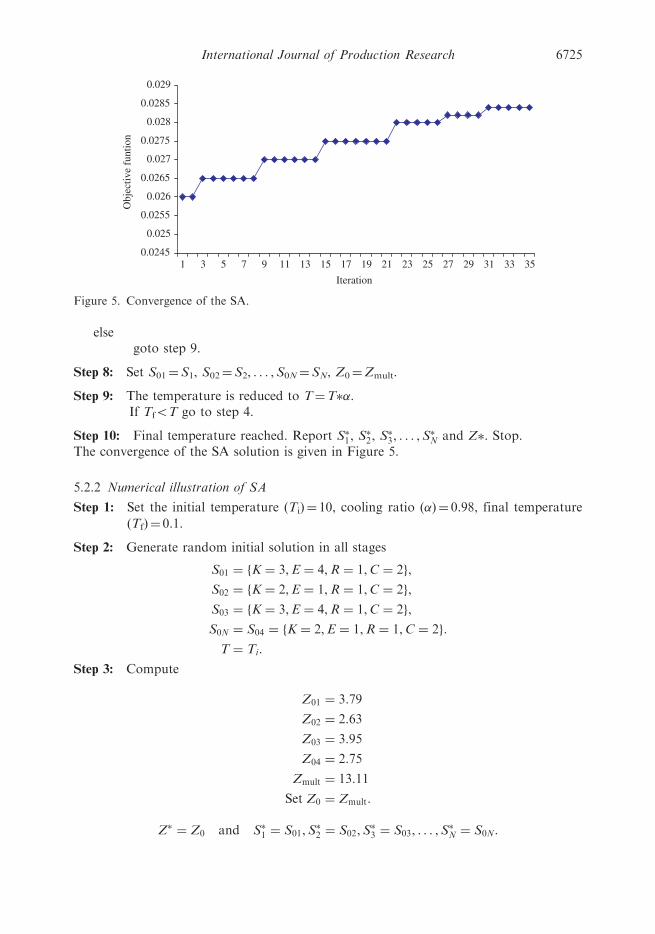
The convergence of the SA solution is given in Figure 5.

5.2.2 Numerical illustration of SA

Step 1: Set the initial temperature (Ti)¼ 10, cooling ratio (�)¼ 0.98, final temperature

(Tf)¼ 0.1.

Step 2: Generate random initial solution in all stages

S01 ¼ fK ¼ 3,E ¼ 4,R ¼ 1,C ¼ 2g,

S02 ¼ fK ¼ 2,E ¼ 1,R ¼ 1,C ¼ 2g,

S03 ¼ fK ¼ 3,E ¼ 4,R ¼ 1,C ¼ 2g,

S0N ¼ S04 ¼ fK ¼ 2,E ¼ 1,R ¼ 1,C ¼ 2g:

T ¼ Ti:

Step 3: Compute

Z01 ¼ 3:79

Z02 ¼ 2:63

Z03 ¼ 3:95

Z04 ¼ 2:75

Zmult ¼ 13:11

Set Z0 ¼ Zmult:

Z� ¼ Z0 and S�1 ¼ S01,S�2 ¼ S02,S

�3 ¼ S03, . . . ,S�N ¼ S0N:

0.02451 3 5 7 9 11 13 15 17 19 21 23 25 27 29 31 33 35

0.025

0.0255

0.026

0.0265

0.027

0.0275

0.028

0.0285

0.029

Iteration

Obj

ectiv

e fu

ntio

n

Figure 5. Convergence of the SA.


Step 4: Using the perturbation algorithm, find the neighbourhood solution S1, S2,

S3, . . . ,SN for each stage.

4.1 Select the parameter to be modified for solution S01, S02, S03, . . . ,S0Nin

each stage(i) For S01, Let r¼ 0.12.

Since r (0.23) lies in the range 0.00–0.25, parameter K isselected for

modification.(ii) For S02, Let r¼ 0.84.

Since r (0.84) lies in the range 0.75–1.00, parameter C isselected for

modification.(iii) For S03, Let r¼ 0.48.

Since r (0.48) lies in the range 0.25–0.50, parameter E isselected for

modification.(iv) For S04, Let r¼ 0.39.

Since r (0.39) lies in the range 0.25–0.50, parameter E isselected for

modification.

4.2 Neighbourhood for S01, S02, . . . ,S0N.

(i) For S01, Let r¼ 0.39. Since r50.5, increment the selected parameter

K subject to the condition R5C and C�K.Hence the neighbourhood solution vector (S1){4,4,1,2}

(ii) For S02, Let r¼ 0.39. Since r50.5, increment the selected parameter

C subject to the condition R5C and C�K.Hence the neighbourhood solution vector (S2){2,1,1,3}

(iii) For S03, Let r¼ 0.93. Since r40.5, decrement the selected

parameter E subject to the condition R5C and C�K.Hence the neighbourhood solution vector (S3){3,3,1,2}

(iv) For S04, Let r¼ 0.39. Since r50.5, increment the selected parameter

E subject to the condition R5C and C�K.Hence the neighbourhood solution vector (S4){2,2,1,2}

Step 5: The neighbourhood objective function

Z1 ¼ 4:23,

Z2 ¼ 2:52,

Z3 ¼ 3:47,

Z4 ¼ 2:86

of the corresponding neighbourhood solution S1, S2, S3, S4.Zmult¼ 13.08.

Step 6: Compute �E¼Zmult�Z0¼ 13.08–13.11¼�0.03.

Step 7: If (�E� 0)

Update Z� ¼ Zmult ¼ 13:08 and S�1 ¼ S1,S�2 ¼ S2,S

�3 ¼ S3,S

�4 ¼ S4:

Step 8: Set S01¼S1,S02¼S2, . . . ,S0N¼SN,Z0¼Zmult.


Step 9: The temperature is reduced to T¼T � �¼ 10 � 0.98¼ 9.8.Here Tf5T go to step 4.

Repeat steps 4 through 9 until the final temperature is reached.Report S�1, S

�2, S

�3, S

�4 and Z�. Stop.

6. Numerical experiments and results

The algorithm was implemented using MATLAB and tested with several examples, by

varying the number of stages, demand rate and the service rate of the manufacturing

process.

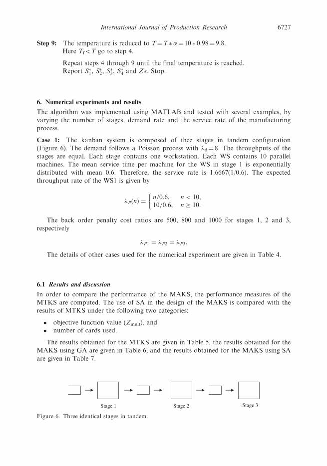
Case 1: The kanban system is composed of thee stages in tandem configuration

(Figure 6). The demand follows a Poisson process with �d¼ 8. The throughputs of the

stages are equal. Each stage contains one workstation. Each WS contains 10 parallel

machines. The mean service time per machine for the WS in stage 1 is exponentially

distributed with mean 0.6. Therefore, the service rate is 1.6667(1/0.6). The expected

throughput rate of the WS1 is given by

�PðnÞ ¼n=0:6, n < 10,10=0:6, n � 10:

�

The back order penalty cost ratios are 500, 800 and 1000 for stages 1, 2 and 3,

respectively

�P1 ¼ �P2 ¼ �P3:

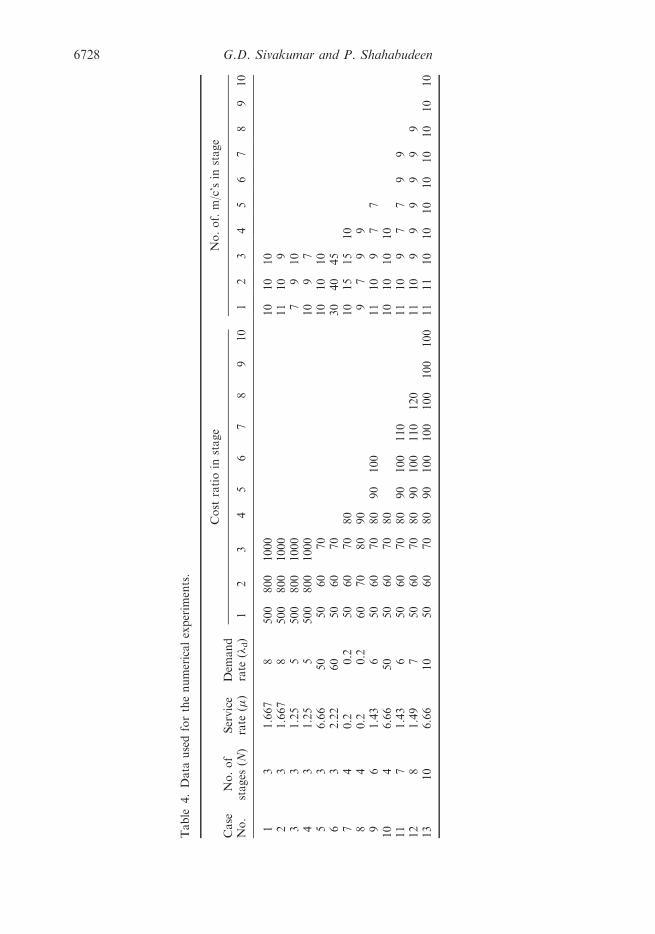
The details of other cases used for the numerical experiment are given in Table 4.

6.1 Results and discussion

In order to compare the performance of the MAKS, the performance measures of the

MTKS are computed. The use of SA in the design of the MAKS is compared with the

results of MTKS under the following two categories:

� objective function value (Zmult), and� number of cards used.

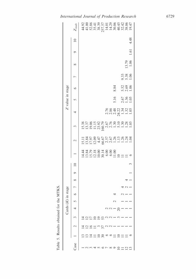
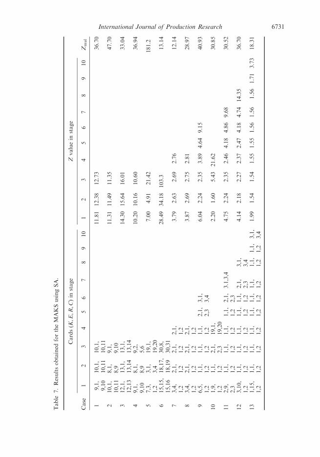
The results obtained for the MTKS are given in Table 5, the results obtained for the

MAKS using GA are given in Table 6, and the results obtained for the MAKS using SA

are given in Table 7.


Figure 6. Three identical stages in tandem.


Table

4.Data

usedforthenumericalexperim

ents.

Case

No.

No.of

stages

(N)

Service

rate

(�)

Dem

and

rate

(�d)

Cost

ratioin

stage

No.of.m/c’sin

stage

12

34

56

78

910

12

34

56

78

910

13

1.667

8500

800

1000

10

10

10

23

1.667

8500

800

1000

11

10

93

31.25

5500

800

1000

79

10

43

1.25

5500

800

1000

10

97

53

6.66

50

50

60

70

10

10

10

63

2.22

60

50

60

70

30

40

45

74

0.2

0.2

50

60

70

80

10

15

15

10

84

0.2

0.2

60

70

80

90

97

99

96

1.43

650

60

70

80

90

100

11

10

97

710

46.66

50

50

60

70

80

10

10

10

10

11

71.43

650

60

70

80

90

100

110

11

10

97

79

912

81.49

750

60

70

80

90

100

110

120

11

10

99

99

99

13

10

6.66

10

50

60

70

80

90

100

100

100

100

100

11

11

10

10

10

10

10

10

10

10


Table

5.Resultsobtained

fortheMTKS.

Case

Cards(K

)in

stage

Zvaluein

stage

Zmult

12

34

56

78

910

12

34

56

78

910

113

14

14

14.44

15.11

15.38

44.92

213

12

12

13.84

13.84

13.37

41.00

314

16

17

15.79

17.97

19.06

52.86

411

11

10

12.18

12.09

11.15

35.41

510

319

10.00

4.47

23.92

38.39

630

37

53

30.14

66.67

160.79

257.57

76

22

26.00

2.57

2.67

2.76

14.01

86

22

26.00

2.67

2.76

2.86

14.29

911

11

12

411.00

1.26

1.30

2.48

5.16

8.84

30.06

10

10

13

20

10

1.13

5.10

24.22

40.45

11

11

11

11

24

11

1.26

1.30

1.34

2.67

5.52

9.33

32.42

12

11

11

11

12

411

1.24

1.28

1.32

1.36

2.69

5.38

13.79

38.06

13

61

11

11

11

13

61.04

1.05

1.05

1.05

1.06

1.06

1.06

1.61

4.48

19.47


Table

6.Resultsobtained

fortheMAKSusingtheGA.

Case

Cards(K

,E,R

,C)in

stage

Zvaluein

stage

Zmul

12

34

56

78

910

12

34

56

78

910

19,1,

9,10

9,1,

9,10

8,1,

8,9

11.81

12.90

16.21

40.93

210,6,

6,8

9,1,

8,9

9,1,

9,10

13.33

12.03

11.35

36.70

314,8,

2,3

13,1,

13,14

14,1,

14,15

15.83

15.64

16.21

47.70

48,5,

6,7

8,1,

8,9

10,4,

4,10

11.62

10.16

11.27

33.04

58,2,2,3

3,1,2,3

19,1,

1,2

8.00

4.99

23.95

36.94

615,15,

15,16

18,17,

18,19

30,10,

30,31

28.49

34.66

118.0

181.2

73,4,

1,2

2,1,

1,2

3,4,

1,2

2,1,

1,2

3.79

2.63

3.95

2.75

13.14

83,4,

1,2

2,1,

1,2

2,1,

1,2

2,1,

1,2

3.87

2.69

2.75

2.81

12.14

96,5,

4,5

1,1,

1,2

1,1,

1,2

1,1,

1,2

2,1,

2,3

3,1,

3,4

6.67

2.24

2.35

3.89

4.64

9.15

28.97

10

6,4,

6,7

1,1,

1,2

4,1,

4,5

19,1,

19,20

6.88

1.75

5.39

21.63

35.65

11

2,9,

2,3

1,1,

1,2

1,1,

1,2

1,1,

1,2

1,1,

1,2

1,1,

1,2

2,1,

2,3

4.75

2.24

2.35

2.46

2.57

4.46

12.81

31.80

12

4,11,2,3

1,1,

1,2

1,1,

1,2

1,1,

1,2

1,1,

1,2

1,1,

1,2

2,1,

2,3

3,1,

3,4

4.77

2.18

2.27

2.37

2.47

4.18

4.74

14.35

37.36

13

1,7,

1,2

1,1,

1,2

1,1,

1,2

1,1,

1,2

1,1,

1,2

1,1,

1,2

1,1,

1,2

1,1,

1,2

1,1,

1,2

3,1,

3,4

2.20

1.57

1.58

1.58

1.59

1.60

1.61

1.60

1.89

3.96

19.18


Table

7.Resultsobtained

fortheMAKSusingSA.

Case

Cards(K

,E,R

,C)in

stage

Zvaluein

stage

Zmul

12

34

56

78

910

12

34

56

78

910

19,1,

9,10

10,1,

10,11

10,1,

10,11

11.81

12.38

12.73

36.70

210,1,

10,11

8,1,

8,9

9,1,

9,10

11.31

11.49

11.35

47.70

312,1,

12,13

13,1,

13,14

13,1,

13,14

14.30

15.64

16.01

33.04

49,1,

9,10

8,1,

8,9

9,2,

5,6

10.20

10.16

10.60

36.94

57,3,

1,2

3,1,

3,4

19,1,

19,20

7.00

4.91

21.42

181.2

615,15,

15,16

18,17,

18,19

30,8,

30,31

28.49

34.18

103.3

13.14

73,4,

1,2

2,1,

1,2

2,1,

1,2

2,1,

1,2

3.79

2.63

2.69

2.76

12.14

83,4,

1,2

2,1,

1,2

2,1,

1,2

2,1,

1,2

3.87

2.69

2.75

2.81

28.97

96,5,

1,2

1,1,

1,2

1,1,

1,2

1,1,

1,2

2,1,

2,3

3,1,

3,4

6.04

2.24

2.35

3.89

4.64

9.15

40.93

10

1,9,

1,2

1,1,

1,2

2,1,

2,3

19,1,

19,20

2.20

1.60

5.43

21.62

30.85

11

2,9,

2,3

1,1,

1,2

1,1,

1,2

1,1,

1,2

1,1,

1,2

2,1,

2,3

3.1,3,4

4.75

2.24

2.35

2.46

4.18

4.86

9.68

30.52

12

3,10,

1,2

1,1,

1,2

1,1,

1,2

1,1,

1,2

1,1,

1,2

1,1,

1,2

2,1,

2,3

3,1,

3,4

4.14

2.18

2.27

2.37

2.47

4.18

4.74

14.35

36.70

13

1,15,

1,2

1,1,

1,2

1,1,

1,2

1,1,

1,2

1,1,

1,2

1,1,

1,2

1,1,

1,2

1,1,

1,2

1,1,

1,2

3,1,

3,4

1.99

1.54

1.54

1.55

1.55

1.56

1.56

1.56

1.71

3.73

18.31


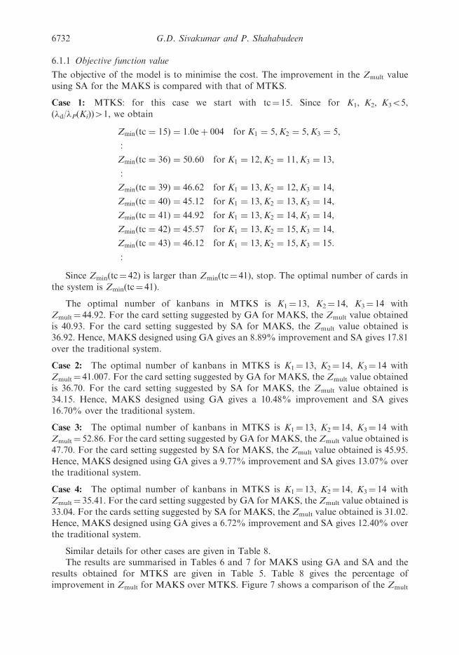
6.1.1 Objective function value

The objective of the model is to minimise the cost. The improvement in the Zmult valueusing SA for the MAKS is compared with that of MTKS.

Case 1: MTKS: for this case we start with tc¼ 15. Since for K1, K2, K355,(�d/�P(Ki))41, we obtain

Zminðtc ¼ 15Þ ¼ 1:0eþ 004 for K1 ¼ 5,K2 ¼ 5,K3 ¼ 5,

:

Zminðtc ¼ 36Þ ¼ 50:60 for K1 ¼ 12,K2 ¼ 11,K3 ¼ 13,

:

Zminðtc ¼ 39Þ ¼ 46:62 for K1 ¼ 13,K2 ¼ 12,K3 ¼ 14,

Zminðtc ¼ 40Þ ¼ 45:12 for K1 ¼ 13,K2 ¼ 13,K3 ¼ 14,

Zminðtc ¼ 41Þ ¼ 44:92 for K1 ¼ 13,K2 ¼ 14,K3 ¼ 14,

Zminðtc ¼ 42Þ ¼ 45:57 for K1 ¼ 13,K2 ¼ 15,K3 ¼ 14,

Zminðtc ¼ 43Þ ¼ 46:12 for K1 ¼ 13,K2 ¼ 15,K3 ¼ 15:

:

Since Zmin(tc¼ 42) is larger than Zmin(tc¼ 41), stop. The optimal number of cards inthe system is Zmin(tc¼ 41).

The optimal number of kanbans in MTKS is K1¼ 13, K2¼ 14, K3¼ 14 withZmult¼ 44.92. For the card setting suggested by GA for MAKS, the Zmult value obtainedis 40.93. For the card setting suggested by SA for MAKS, the Zmult value obtained is36.92. Hence, MAKS designed using GA gives an 8.89% improvement and SA gives 17.81over the traditional system.

Case 2: The optimal number of kanbans in MTKS is K1¼ 13, K2¼ 14, K3¼ 14 withZmult¼ 41.007. For the card setting suggested by GA for MAKS, the Zmult value obtainedis 36.70. For the card setting suggested by SA for MAKS, the Zmult value obtained is34.15. Hence, MAKS designed using GA gives a 10.48% improvement and SA gives16.70% over the traditional system.

Case 3: The optimal number of kanbans in MTKS is K1¼ 13, K2¼ 14, K3¼ 14 withZmult¼ 52.86. For the card setting suggested by GA for MAKS, the Zmult value obtained is47.70. For the card setting suggested by SA for MAKS, the Zmult value obtained is 45.95.Hence, MAKS designed using GA gives a 9.77% improvement and SA gives 13.07% overthe traditional system.

Case 4: The optimal number of kanbans in MTKS is K1¼ 13, K2¼ 14, K3¼ 14 withZmult¼ 35.41. For the card setting suggested by GA for MAKS, the Zmult value obtained is33.04. For the cards setting suggested by SA for MAKS, the Zmult value obtained is 31.02.Hence, MAKS designed using GA gives a 6.72% improvement and SA gives 12.40% overthe traditional system.

Similar details for other cases are given in Table 8.The results are summarised in Tables 6 and 7 for MAKS using GA and SA and the

results obtained for MTKS are given in Table 5. Table 8 gives the percentage ofimprovement in Zmult for MAKS over MTKS. Figure 7 shows a comparison of the Zmult


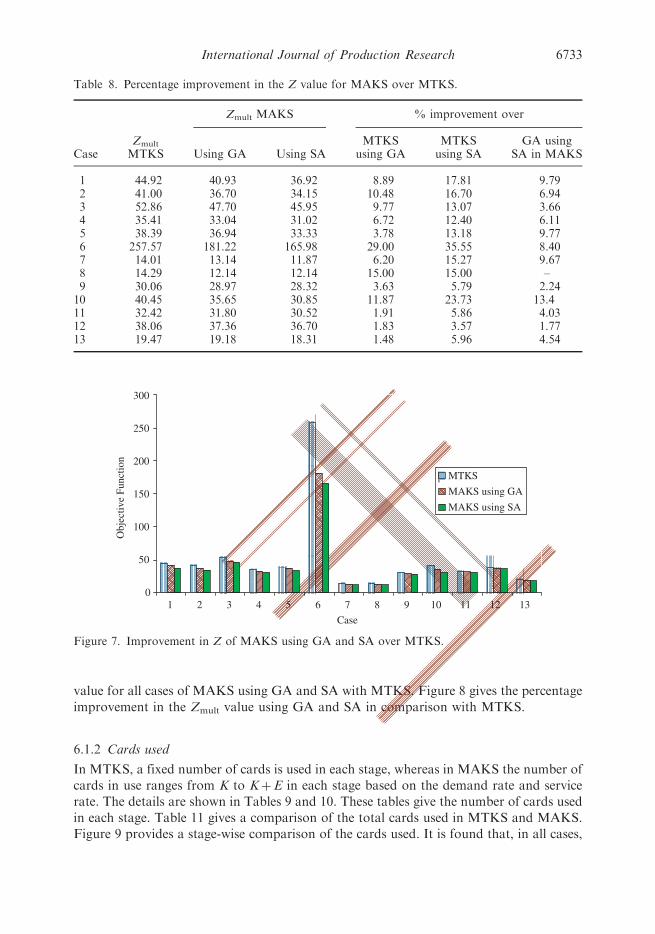
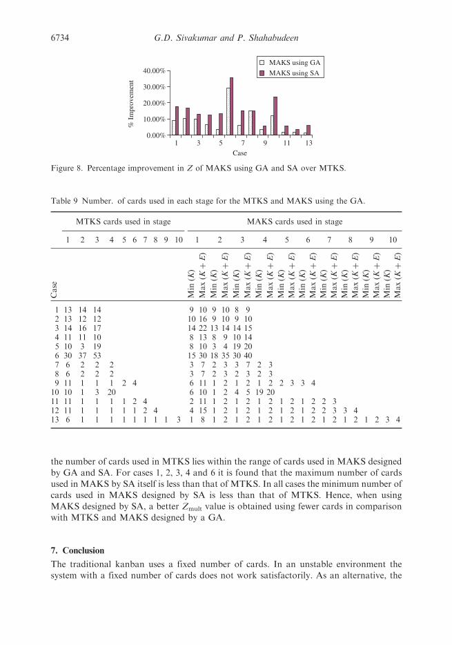
value for all cases of MAKS using GA and SA with MTKS. Figure 8 gives the percentage

improvement in the Zmult value using GA and SA in comparison with MTKS.

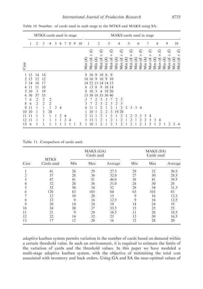
6.1.2 Cards used

In MTKS, a fixed number of cards is used in each stage, whereas in MAKS the number ofcards in use ranges from K to KþE in each stage based on the demand rate and servicerate. The details are shown in Tables 9 and 10. These tables give the number of cards used

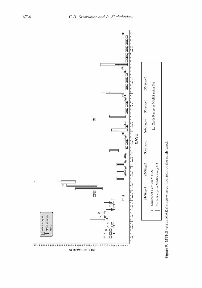
in each stage. Table 11 gives a comparison of the total cards used in MTKS and MAKS.Figure 9 provides a stage-wise comparison of the cards used. It is found that, in all cases,

Table 8. Percentage improvement in the Z value for MAKS over MTKS.

CaseZmult

MTKS

Zmult MAKS % improvement over

Using GA Using SAMTKS

using GAMTKSusing SA

GA usingSA in MAKS

1 44.92 40.93 36.92 8.89 17.81 9.792 41.00 36.70 34.15 10.48 16.70 6.943 52.86 47.70 45.95 9.77 13.07 3.664 35.41 33.04 31.02 6.72 12.40 6.115 38.39 36.94 33.33 3.78 13.18 9.776 257.57 181.22 165.98 29.00 35.55 8.407 14.01 13.14 11.87 6.20 15.27 9.678 14.29 12.14 12.14 15.00 15.00 –9 30.06 28.97 28.32 3.63 5.79 2.2410 40.45 35.65 30.85 11.87 23.73 13.411 32.42 31.80 30.52 1.91 5.86 4.0312 38.06 37.36 36.70 1.83 3.57 1.7713 19.47 19.18 18.31 1.48 5.96 4.54

01 2 3 4 5 6 7 8 9 10 11 12 13

50

100

150

200

250

300

Case

Obj

ectiv

e Fu

nctio

n

MTKS

MAKS using GA

MAKS using SA

Figure 7. Improvement in Z of MAKS using GA and SA over MTKS.


the number of cards used in MTKS lies within the range of cards used in MAKS designed

by GA and SA. For cases 1, 2, 3, 4 and 6 it is found that the maximum number of cards

used in MAKS by SA itself is less than that of MTKS. In all cases the minimum number of

cards used in MAKS designed by SA is less than that of MTKS. Hence, when using

MAKS designed by SA, a better Zmult value is obtained using fewer cards in comparison

with MTKS and MAKS designed by a GA.

7. Conclusion

The traditional kanban uses a fixed number of cards. In an unstable environment the

system with a fixed number of cards does not work satisfactorily. As an alternative, the

Table 9 Number. of cards used in each stage for the MTKS and MAKS using the GA.

MTKS cards used in stage MAKS cards used in stage

1 2 3 4 5 6 7 8 9 10 1 2 3 4 5 6 7 8 9 10

Case

MinðKÞ

MaxðKþEÞ

MinðKÞ

MaxðKþEÞ

MinðKÞ

MaxðKþEÞ

MinðKÞ

MaxðKþEÞ

MinðKÞ

MaxðKþEÞ

MinðKÞ

MaxðKþEÞ

MinðKÞ

MaxðKþEÞ

MinðKÞ

MaxðKþEÞ

MinðKÞ

MaxðKþEÞ

MinðKÞ

MaxðKþEÞ

1 13 14 14 9 10 9 10 8 92 13 12 12 10 16 9 10 9 103 14 16 17 14 22 13 14 14 154 11 11 10 8 13 8 9 10 145 10 3 19 8 10 3 4 19 206 30 37 53 15 30 18 35 30 407 6 2 2 2 3 7 2 3 3 7 2 38 6 2 2 2 3 7 2 3 2 3 2 39 11 1 1 1 2 4 6 11 1 2 1 2 1 2 2 3 3 410 10 1 3 20 6 10 1 2 4 5 19 2011 11 1 1 1 1 2 4 2 11 1 2 1 2 1 2 1 2 1 2 2 312 11 1 1 1 1 1 2 4 4 15 1 2 1 2 1 2 1 2 1 2 2 3 3 413 6 1 1 1 1 1 1 1 1 3 1 8 1 2 1 2 1 2 1 2 1 2 1 2 1 2 1 2 3 4

0.00%1 3 5 7 9 11 13

10.00%

20.00%

30.00%

40.00%

Case

% I

mpr

ovem

ent

MAKS using GA

MAKS using SA

Figure 8. Percentage improvement in Z of MAKS using GA and SA over MTKS.


adaptive kanban system permits variation in the number of cards based on demand withina certain threshold value. In such an environment, it is required to estimate the limits ofthe variation of cards and the threshold values. In this paper we have modeled amulti-stage adaptive kanban system, with the objective of minimising the total costassociated with inventory and back orders. Using GA and SA the near-optimal values of

Table 10 Number. of cards used in each stage in the MTKS and MAKS using SA.

MTKS cards used in stage MAKS cards used in stage

1 2 3 4 5 6 7 8 9 10 1 2 3 4 5 6 7 8 9 10

Case

MinðKÞ

MaxðKþEÞ

MinðKÞ

MaxðKþEÞ

MinðKÞ

MaxðKþEÞ

MinðKÞ

MaxðKþEÞ

MinðKÞ

MaxðKþEÞ

MinðKÞ

MaxðKþEÞ

MinðKÞ

MaxðKþEÞ

MinðKÞ

MaxðKþEÞ

MinðKÞ

MaxðKþEÞ

MinðKÞ

MaxðKþEÞ

1 13 14 14 9 10 9 10 8 92 13 12 12 10 16 9 10 9 103 14 16 17 14 22 13 14 14 154 11 11 10 8 13 8 9 10 145 10 3 19 8 10 3 4 19 206 30 37 53 15 30 18 35 30 407 6 2 2 2 3 7 2 3 3 7 2 38 6 2 2 2 3 7 2 3 2 3 2 39 11 1 1 1 2 4 6 11 1 2 1 2 1 2 2 3 3 410 10 1 3 20 1 10 1 2 2 3 19 2011 11 1 1 1 1 2 4 2 11 1 2 1 2 1 2 1 2 2 3 3 412 11 1 1 1 1 1 2 4 3 13 1 2 1 2 1 2 1 2 1 2 2 3 3 413 6 1 1 1 1 1 1 1 1 3 1 16 1 2 1 2 1 2 1 2 1 2 1 2 1 2 1 2 3 4

Table 11. Comparison of cards used.

MAKS (GA) MAKS (SA)

MTKSCards used Cards used

Case Cards used Min Max Average Min Max Average

1 41 26 29 27.5 29 32 30.52 37 28 36 32.0 27 30 28.53 47 41 51 46.0 38 41 39.54 32 26 36 31.0 26 30 285 32 30 34 32 29 34 31.56 120 63 105 84 63 103 837 12 10 20 15 9 16 12.58 12 9 16 12.5 9 16 12.59 20 14 24 19 14 24 1910 34 30 37 33.5 15 35 2511 21 9 24 16.5 11 26 18.512 22 14 32 23 13 30 16.513 17 12 20 16 12 28 20


S1-S

tage

1 S2

-Sta

ge2

S3-S

tage

3

S4-S

tage

4 S

5-St

age5

S6-S

tage

6

x

Num

ber

of C

ards

in M

TK

S

Car

ds R

ange

in M

AK

S us

ing

GA

Car

ds R

ange

in M

AK

S us

ing

SA

Figure

9.MTKSversusMAKSstage-wisecomparisonofthecardsused.


the MAKS parameters are estimated. For the sake of comparison, a multi-stage traditionalsystem has also been developed. The results are compared with the traditional kanbansystem and it is found that the Z value shows improvement by up to 35.55% when usingthe proposed model. Hence, it is concluded that MAKS gives a better performance thanMTKS. It is found that a SA-based search provides a better value for the objectivefunction when compared with the GA-based search. Hence, it is concluded that, in thedesign of MAKS, the use of SA is advantageous. The work could be extended further byincluding factors such as machine breakdowns, availability of operators, etc.

References

Bruno, B., et al., 2001. A multi class approximation technique for the analysis of kanban-like control

systems. International Journal of Production Research, 39 (2), 307–328.Di Mascolo, M., Frein, Y., and Dallery, Y., 1996. An analytical method for performance evaluation

of a kanban controlled production systems. Operational Research, 44 (1), 50–64.

Dowsland, K.A., 1996. Genetic algorithms – a tool for OR? Journal of Operation Research Society,

47 (3), 550–551.Gupta, S.M. and Al-Turki, Y.A.Y., 1997. An algorithm to dynamically adjust the number of

kanbans in stochastic processing times and variable demand environment. Production

Planning and Control, 8 (2), 133–141.

Hopp, W.J. and Roof, M.L., 1998. Setting WIP levels with statistical throughput control (STC) in

CONWIP production lines. International Journal of Production Research, 36 (4), 867–882.Hunag, P.Y., Rees, L.P., and Taylor, B.W., 1983. A simulation analysis of the Japanese

just-in-time technique (with kanbans) for a multiline, multistage production system.

Decision Science, 14 (3), 326–344.John, G. and Cathal, H., 2004. A comparison of hybrid PUSH/PULL and CONWIP/PULL

production inventory. International Journal of Production Economics, 91 (1), 75–90.

Johnson, D.S., et al., 1991. Optimisation by simulated annealing: an experimental evaluation,

Part II. Operation Research, 39 (3), 378–406.Karaesmen, G., Liberopoulos, G., and Dallery, Y., 2004. The value of advance demand information

in make-to-stock manufacturing systems. Annals of Operations Research, 126 (1), 135–157.Kochel, P. and Nielander, U., 2002. Kanban optimisation by simulation and evolution. Production

Planning and Control, 13 (8), 725–734.

Liberopoulos, G. and Koukoumialos, S., 2005. Tradeoffs between base stock levels, numbers of

kanbans, and planned supply lead times in production/inventory systems with advance

demand information. International Journal of Production Economics, 96 (2), 213–232.Mitra, D. and Mitrani, I., 1990. Analysis of a kanban discipline for cell coordination in production

lines I. Management Science, 36 (12), 1548–1566.

Mitra, D. and Mitrani, I., 1991. Analysis of a kanban discipline for cell coordination in production

lines II: Stochastic demands. Operations Research, 35 (5), 807–823.Mohamed, A.A. and Talal, M.A., 2002. Simulation based optimisation using simulated annealing

with ranking and selection. Computers and Operation Research, 29 (4), 387–402.Paris, J.L., Tautou-Guillaume, L., and Pierreval, H., 2001. Dealing with design options in the

optimisation of manufacturing systems: an evolutionary approach. International Journal of

Production Research, 39 (6), 1081–1094.

Philipoom, P.R., et al., 1987. An investigation of the factors influencing number of kanbans required

in the implementation of JIT technique with kanbans. International Journal of Production

Research, 25 (3), 457–472.Pirlot, M., 1996. General local search methods. European Journal of Operational Research, 92 (3),

493–511.


Rees, L.P., et al., 1987. Dynamically adjusting the number of kanbans in a just-in-time productionsystem using estimated values of lead time. IIE Transactions, l9 (2), 199–207.

Reeves, C.R., 1993. Genetic algorithms. In: Modern heuristic techniques for combinatorial problems.New York: Wiley.

Sadegheih, A., 2006. Scheduling problem using genetic algorithm, simulated annealing and effects ofparameter values on GA performance. Applied Mathematical Modeling, 30 (2), 147–154.

Saravanan, R., Asokan, P., and Vijayakumar, K., 2003. Machining parameters optimisation for

turning cylindrical stock into a continuous finished profile using genetic algorithm andsimulated annealing. International Journal of Advanced Manufacturing Technology, 21 (1), 1–9.

Savsar, M. and Al-Jawini, A., 1995. Simulation analysis of JIT systems. International Journal of

Production Economics, 42 (1), 67–78.Savsar, M., 1997. Simulation analysis of a pull–push system for an electronic assembly line.

International Journal of Production Economics, 51 (3), 205–214.

Savsar, M. and Choueiki, M.H., 2000. A Neural network procedure for kanban allocation in JITproduction control system. International Journal of Production Research, 38 (14), 3247–3265.

Shahabudeen, P. and Krishnaiah, K., 1999. Design of bi-criteria kanban system using geneticalgorithm. International Journal of Management and System, 15 (3), 257–274.

Shahabudeen, P., Krishnaiah, K., and Gopinath, R., 2002. Design of bi-criteria kanban system usingsimulated annealing technique. Computers and Industrial Engineering, 41 (4), 355–370.

Shahabudeen, P. and Sivakumar, G.D., (2003). An approach to adaptive kanban system. In:

International conference, SOM, IIM, Indore.Spearman, M.L., 1991. An analytic congestion model for closed production systems with IFR

processing times. Management Science, 37 (8), 1015–1029.

Takahashi, K. and Nakamura, N., 1999. Reacting JIT ordering systems to unstable changes indemand. International Journal of Production Research, 37 (10), 2293–2313.

Tardif, V. and Maaseidvaag, L., 2001. An adaptive approach to controlling kanban systems.European Journal of Operation Research, 132 (2), 411–424.

Wang, H. and Wang, H.P., 1990. Determining number of kanbans: step toward non stockproduction. International Journal of Production Research, 28 (11), 2101–2115.

Wang, H. and Wang, H.P., 1991. Optimum number of kanbans between two adjacent workstations

in a JIT system. International Journal of Production Economics, 22 (3), 179–188.Wijngaard, J., 2004. The effect of foreknowledge of demand in case of a restricted capacity: the

single-stage, single-product case. European Journal of Operation Research, 159 (1), 95–109.


Documents

Algorithms for the Design of a Multi-stage Adaptive Kanban System