Algorithms for Strategic Agentsby

S. Matthew Weinberg

B.A., Cornell Unversity (2010)

Submitted to the Department of Electrical Engineering and Computer Sciencein partial fulfillment of the requirements for the degree of

Doctor of Philosophy in Computer Science

at the

MASSACHUSETTS INSTITUTE OF TECHNOLOGY

June 2014

cMassachusetts Institute of Technology 2014. All rights reserved.

Author . . . . . . . . . . . . . . . . . . . . . . . . . . . . . . . . . . . . . . . . . . . . . . . . . . . . . . . . . . . . . . . . . . .Department of Electrical Engineering and Computer Science

May 21, 2014

Certified by . . . . . . . . . . . . . . . . . . . . . . . . . . . . . . . . . . . . . . . . . . . . . . . . . . . . . . . . . . . . . . .Constantinos Daskalakis

Associate Professor of EECSThesis Supervisor

Accepted by . . . . . . . . . . . . . . . . . . . . . . . . . . . . . . . . . . . . . . . . . . . . . . . . . . . . . . . . . . . . . .Leslie A. Kolodziejski

Chairman, Department Committee on Graduate Students

2

Algorithms for Strategic Agents

by

S. Matthew Weinberg

Submitted to the Department of Electrical Engineering and Computer Scienceon May 21, 2014, in partial fulfillment of the

requirements for the degree ofDoctor of Philosophy in Computer Science

AbstractIn traditional algorithm design, no incentives come into play: the input is given, and your algorithmmust produce a correct output. How much harder is it to solve the same problem when the inputis not given directly, but instead reported by strategic agents with interests of their own? Theunique challenge stems from the fact that the agents may choose to lie about the input in order tomanipulate the behavior of the algorithm for their own interests, and tools from Game Theory aretherefore required in order to predict how these agents will behave.

We develop a new algorithmic framework with which to study such problems. Specifically, weprovide a computationally efficient black-box reduction from solving any optimization problem on“strategic input,” often called algorithmic mechanism design to solving a perturbed version of thatsame optimization problem when the input is directly given, traditionally called algorithm design.

We further demonstrate the power of our framework by making significant progress on severallong-standing open problems. First, we extend Myerson’s celebrated characterization of singleitem auctions [Mye81] to multiple items, providing also a computationally efficient implementa-tion of optimal auctions. Next, we design a computationally efficient 2-approximate mechanismfor job scheduling on unrelated machines, the original problem studied in Nisan and Ronen’s paperintroducing the field of Algorithmic Mechanism Design [NR99]. This matches the guarantee ofthe best known computationally efficient algorithm when the input is directly given. Finally, weprovide the first hardness of approximation result for optimal mechanism design.

Thesis Supervisor: Constantinos DaskalakisTitle: Associate Professor of EECS

Acknowledgments

To start, I would like to thank my advisor, Costis Daskalakis, for his belief in me and all his

guidance in pushing me to be excellent. When I first arrived at MIT, Costis and I discussed research

directions. At the time, I was confident that I possessed the tools to make minor improvements on

prior work and excitedly told him this. Chuckling politely, he told me that this was great, but that

we should strive to solve more important problems. We worked long and hard that year, often

going long stretches without any progress, but by the end we had started down the path that would

eventually culminate in this thesis. Thank you, Costis, for teaching me to aim high in my pursuits,

to always push the boundaries of my comfort zone and for guiding me along this journey.

Special thanks are also due to Bobby Kleinberg, who introduced me to theoretical computer

science and taught me how to do research during my time at Cornell. His mix of patience and

enthusiasm turned me from an overexcited problem-solver into a competent researcher. Today,

Bobby is still one of my most trusted mentors and I am truly grateful for everything that he has done

for me. Thank you as well to everyone else who has mentored me through this journey: Moshe

Babaioff, Jason Hartline, Nicole Immorlica, Brendan Lucier, Silvio Micali, Christos Papadimitriou

and Éva Tardos; especially to Parag Pathak and Silvio for serving on my dissertation committee,

and Nicole and Brendan for an amazing summer internship at Microsoft Research.

I wish to thank the entire theory group at MIT. Thank you in particular to Costis, Silvio, Shafi

Goldwasser, Piotr Indyk, Ankur Moitra, and Madhu Sudan for always being available to provide

advice. Thanks as well to everyone who I’ve had the pleasure of collaborating with: Moshe,

Costis, Nicole, Brendan, Bobby, Silvio, Pablo Azar, Patrick Briest, Yang Cai, Shuchi Chawla,

Michal Feldman, and Christos Tzamos. A special thanks to Yang, without whom I’m certain the

work in this thesis would not have been possible. I also thank him for teaching me everything there

is to know about EECS at MIT - without him, I would be lost.

Thanks as well to the students of MIT, Cornell, and elsewhere who made work so enjoyable:

Pablo Azar, Alan Deckelbaum, Michael Forbes, Hu Fu, Nima Haghpanah, Darrell Hoy, G Kamath,

Yin-Tat Lee, Matthew Paff, Pedram Razavi, Ran Shorrer, Aaron Sidford, Greg Stoddard, Vasilis

Syrgkanis, Sam Taggart, and Di Wang.

Thank you to all my friends from Pikesville, Cornell, and MIT for supporting me through the

difficulties of research: Alex, Brandon, Josh, Megan, Shen, Andy, Ganesh, Farrah, Henry, Jason,

Job, Steve, Meelap, and Tahin. Thank you to MIT and Cornell Sport Taekwondo for teaching me

to pursue excellence in all aspects of life. Thanks especially to my coaches, Master Dan Chuang

and Master Han Cho.

I must thank Jennie especially for her unending love and support over the past five years. Her

presence in my life made it possible to weather the unavoidable hardships that accompany research

with determination and hope for the future.

Finally, words cannot express how grateful I am to my family for their incredible support over

this long journey. I am eternally grateful to Mom, Dad, Grandma, Alec, Syrus, Dagmara and Myles

for everything that they’ve done to support me; for their love, care, and encouragement. I wish to

dedicate this thesis to them.

Contents

1 Introduction 1

1.1 Mechanism Design . . . . . . . . . . . . . . . . . . . . . . . . . . . . . . . . . . 3

1.2 Multi-Dimensional Mechanism Design . . . . . . . . . . . . . . . . . . . . . . . . 4

1.2.1 Challenges in Multi-Dimensional Mechanism Design . . . . . . . . . . . . 5

1.3 Algorithmic Mechanism Design . . . . . . . . . . . . . . . . . . . . . . . . . . . 9

1.4 Overview of Results . . . . . . . . . . . . . . . . . . . . . . . . . . . . . . . . . . 11

1.5 Tools and Techniques . . . . . . . . . . . . . . . . . . . . . . . . . . . . . . . . . 14

1.6 Organization . . . . . . . . . . . . . . . . . . . . . . . . . . . . . . . . . . . . . . 18

2 Background 21

2.1 Concepts in Mechanism Design . . . . . . . . . . . . . . . . . . . . . . . . . . . 21

2.2 Multi-Dimensional Mechanism Design - Additive Agents . . . . . . . . . . . . . . 26

2.3 Linear Programming . . . . . . . . . . . . . . . . . . . . . . . . . . . . . . . . . 28

2.4 Related Work . . . . . . . . . . . . . . . . . . . . . . . . . . . . . . . . . . . . . 30

3 Additive Agents 37

3.1 A Linear Program . . . . . . . . . . . . . . . . . . . . . . . . . . . . . . . . . . . 39

3.2 The Space of Feasible Reduced Forms . . . . . . . . . . . . . . . . . . . . . . . . 40

3.2.1 Examples of Reduced Forms . . . . . . . . . . . . . . . . . . . . . . . . . 41

3.2.2 Understanding the Space of Feasible Reduced Forms . . . . . . . . . . . . 43

3.3 Implementation . . . . . . . . . . . . . . . . . . . . . . . . . . . . . . . . . . . . 46

3.4 Conclusions . . . . . . . . . . . . . . . . . . . . . . . . . . . . . . . . . . . . . . 47

7

4 Background: General Objectives and Non-Additive Agents 49

4.1 Preliminaries . . . . . . . . . . . . . . . . . . . . . . . . . . . . . . . . . . . . . 49

4.2 Additional Linear Programming Preliminaries . . . . . . . . . . . . . . . . . . . . 53

4.3 Related Work . . . . . . . . . . . . . . . . . . . . . . . . . . . . . . . . . . . . . 57

5 The Complete Reduction 63

5.1 A Linear Program . . . . . . . . . . . . . . . . . . . . . . . . . . . . . . . . . . . 64

5.2 The Space of Feasible Implicit Forms . . . . . . . . . . . . . . . . . . . . . . . . 66

5.3 Consequences of using𝒟′ . . . . . . . . . . . . . . . . . . . . . . . . . . . . . . 72

5.4 Instantiations of Theorem 7 . . . . . . . . . . . . . . . . . . . . . . . . . . . . . . 75

6 Equivalence of Separation and Optimization 79

6.1 Exact Optimization . . . . . . . . . . . . . . . . . . . . . . . . . . . . . . . . . . 80

6.2 Multiplicative Approximations . . . . . . . . . . . . . . . . . . . . . . . . . . . . 82

6.3 Sampling Approximation . . . . . . . . . . . . . . . . . . . . . . . . . . . . . . . 86

6.3.1 𝒜′ Defines a Closed Convex Region . . . . . . . . . . . . . . . . . . . . . 87

6.3.2 Every point in P is close to some point in P′ . . . . . . . . . . . . . . . . 89

6.3.3 Every point in P′ is close to some point in P . . . . . . . . . . . . . . . . . 91

7 (α, β)-Approximation Algorithms for Makespan and Fairness 95

7.1 Preliminaries . . . . . . . . . . . . . . . . . . . . . . . . . . . . . . . . . . . . . 95

7.2 Algorithmic Results . . . . . . . . . . . . . . . . . . . . . . . . . . . . . . . . . . 97

8 Revenue: Hardness of Approximation 105

8.1 Cyclic Monotonicity and Compatibility . . . . . . . . . . . . . . . . . . . . . . . 106

8.2 Relating SADP to BMeD . . . . . . . . . . . . . . . . . . . . . . . . . . . . . . . 110

8.3 Approximation Hardness for Submodular Bidders . . . . . . . . . . . . . . . . . . 113

9 Conclusions and Open Problems 119

8

A Extensions of Border’s Theorem 137

A.1 Algorithmic Extension . . . . . . . . . . . . . . . . . . . . . . . . . . . . . . . . 137

A.2 Structural Extension . . . . . . . . . . . . . . . . . . . . . . . . . . . . . . . . . . 142

B A Geometric Decomposition Algorithm 149

9

10

List of Figures

3-1 A linear programming formulation to find the revenue-optimal mechanism. . . . . 39

3-2 A reformulated linear program to find the revenue-optimal mechanism. . . . . . . . 41

5-1 A linear programming formulation for BMeD. . . . . . . . . . . . . . . . . . . . . 65

5-2 A linear program for BMeD, replacing F(ℱ ,𝒟,𝒪) with F(ℱ ,𝒟′,𝒪). . . . . . . . 66

6-1 A linear programming formulation to find a violated hyperplane. . . . . . . . . . . 81

6-2 A reformulation of Figure 6-1 using a separation oracle. . . . . . . . . . . . . . . . 82

6-3 A weird separation oracle. . . . . . . . . . . . . . . . . . . . . . . . . . . . . . . 83

7-1 LP(t). . . . . . . . . . . . . . . . . . . . . . . . . . . . . . . . . . . . . . . . . . 98

7-2 (a modification of) The configuration LP parameterized by T . . . . . . . . . . . . . 101

B-1 A linear program to output a corner in P that satisfies every constraint in E. . . . . 151

11

Chapter 1

Introduction

Traditionally, Algorithm Design is the task of producing a correct output from a given input in a

computationally efficient manner. For instance, maybe the input is a list of integers and the desired

output is the maximum element in that list. Then a good algorithm, findMax, simply scans the

entire list and outputs the maximum. A subtle, but important assumption made by the findMax

algorithm is that the input is accurate; that is, the input list is exactly the one for which the user

wants to find the maximum element.

While seemingly innocuous, this assumption implicitly requires the algorithm to be completely

oblivious both to where the input comes from and to what the output is used for. Consider for

example a local government with a stimulus package that they want to give to the company that

values it most. They could certainly try soliciting from each company their value for the package,

making a list, running the findMax algorithm, and selecting the corresponding company. After

all, findMax will correctly find the company with the largest reported value. But something is

obviously flawed with this approach: why would a company report accurately their value when a

larger report will make them more likely to win the package? Basic game theory tells us that each

company, if strategic, will report a bid of∞, and the winner will just be an arbitrary company.

The issue at hand here is not the validity of findMax: the maximum element of ∞, . . . ,∞

is indeed ∞. Instead, the problem is that separating the design and application of findMax is a

mistake. The companies control the input to findMax, the input to findMax affects the winner of

1

the stimulus package, and the companies care who wins the package. So it’s in each company’s

interest to manipulate the algorithm by misreporting their input.

A well-cited example of this phenomenon occured in 2008 when a strategic table update in

Border Gateway Protocol (BGP), the protocol used to propagate routing information throughout

the Internet, caused a global outage of YouTube [McC08, McM08]. What went wrong? At the

time, offensive material prompted Pakistani Internet Service Providers to censor YouTube within

Pakistan, updating their BGP tables to map from www.youtube.com to nowhere insted of correctly

to YouTube. The outage occurred when this update inadvertantly spread to the rest of the Internet

as well. What’s the point? BGP works great when everyone correctly updates their tables, so there

are no problems purely from the algorithmic perspective. But when users instead updated their

tables to serve their own interests, the protocol failed.

A more recent example occured in 2013, when an entire university class of students boycotted

an Intermediate Programming final in order to manipulate the professor’s grading policy [Bud13].

What went wrong? The professor’s policy curved the highest grade to 100 and bumped up all others

by the same amount. The students’ boycott guaranteed that their 0s would all be curved to 100s.

What’s the point? Algorithmically, grading on a curve is a great way to overcome inconsistencies

across different course offerings, so the system works well when all students perform honestly. But

when the students performed strategically, the resulting grades were meaningless.

Should every algorithm be implemented in a way that is robust to strategic manipulation? Of

course not. Sometimes data is just data and the input is directly given. But as the Internet continues

to grow, more and more of our data comes from users with a vested interest in the outcome of

our algorithms. Motivated by examples like those above, we are compelled to design algorithms

robust to potential manipulation by strategic agents in these settings. We refer to such algorithms

as mechanisms, and address in this thesis the following fundamental question:

Question 1. How much more difficult is mechanism design than algorithm design?

2

1.1 Mechanism Design

Before attempting to design mechanisms robust against strategic behavior, we must first understand

how strategic agents in fact behave. This daunting task is the focus of Game Theory, which aims

to develop tools for predicting how strategic agents will interact within a given environment or

system. Mechanism Design, sometimes referred to as “reverse game theory,” instead aims to design

systems where agents’ behavior is easily predictable, and this behavior results in a desireable

outcome. Returning to our stimulus package example, we see that findMax by itself is not a good

mechanism: even though each company will predictably report a value of∞, the outcome is highly

undesireable.

Still, a seminal paper of Vickrey [Vic61] provides a modification of the findMax algorithm

that awards the package to the company with the highest value even in the face of strategic play.

Vickrey showed that if in addition to awarding the package to the highest bidder, that same bidder

is also charged a price equal to the second-largest value reported, then the resulting mechanism,

called the second-price auction, is truthful. That is, it is in each company’s best interest to report

their true value. Therefore, even strategic agents will tell the truth, and the package will always go

to the company with the highest value.

Remarkably, Vickrey’s result was extended by Clarke [Cla71] and Groves [Gro73] far be-

yond single-item settings, generalizing the second-price auction to what is now called the Vickrey-

Clarke-Groves (VCG) mechanism. Imagine a designer choosing from any set ℱ of possible out-

comes, and that each agent i has a private value ti(x) should the outcome x be selected. Then if

the designer’s goal is to select the outcome maximizing the total welfare, which is the sum of all

agents’ values for the outcome selected and can be written as∑

i ti(x), the VCG mechanism is again

truthful and always selects the optimal outcome. The mechanism simply asks each agent to report

their value ti(x) for each outcome and selects the outcome argmaxx∈ℱ ∑

i ti(x). It turns out that

this selection procedure can be complemented by a pricing scheme to make a truthful mechanism;

one example of such a pricing scheme is called the Clarke pivot rule [Cla71]. Interestingly, one

can view the VCG mechanism as a reduction from mechanism to algorithm design: with black-

3

box access1 to an optimal algorithm for welfare, one can execute, computationally efficiently, an

optimal mechanism for welfare. That is, given black-box access to an algorithm that optimizes

welfare when each ti(x) is directly given, one can design a computationally efficient mechanism

that optimizes welfare when all ti(x) are instead reported by strategic agents.

1.2 Multi-Dimensional Mechanism Design

What if instead of optimizing the value of the agents, the designer aims to maximize his own

revenue? Finding the optimal mechanism in this case is of obvious importance, as millions of

users partake in such interactions every day. Before tackling this important problem, we must first

address what it means for a mechanism to be optimal in this setting. One natural definition might

be that the optimal mechanism obtains revenue equal to the best possible welfare, with each agent

paying their value for the outcome selected. However, even in the simplest case of a single agent

interested in a single item, this benchmark is unattainable: how can the designer possibly both

encourage the agent to report her true value for the item, yet also charge her a price equal to that

value?

The underlying issue in attaining this benchmark is that it is prior-free. Without any beliefs

whatsoever on the agent’s value, how can the designer know whether to interact on the scale of

pennies, dollars or billions of dollars? And is it even realistic to model the designer as lacking this

knowledge? Addressing both issues simultaneously, Economists typically model the designer as

having a Bayesian prior (i.e. a distribution) over possible values of the agents, and mechanisms

are judged based on their expected revenue. The goal then becomes to find the mechanism whose

expected revenue is maximized (over all mechanisms).

Within this model, a seminal paper of Myerson [Mye81] provides a strong structural charac-

terization of the revenue-optimal mechanism for selling a single item, showing that it takes the

following simple form: first, agents are asked to report their value for the item, then each agent’s

reported value is transformed via a closed formula to what is called an ironed virtual value,2 and1Black-box access to an algorithm means that one can probe the algorithm with input and see what output it selects,

but not see the inner workings of the algorithm.2The precise transformation mapping an agent’s reported value to its corresponding ironed virtual value depends

4

finally the item is awarded to the agent with the highest non-negative ironed virtual value (if any).

Furthermore, in the special case that the designer’s prior is independent and identically distributed

across agents and the marginals satisfy a technical condition called regularity,3 the optimal auction

is exactly a second price auction with a reserve price. That is, the item is awarded to the highest

bidder if he beats the reserve, and he pays the maximum of the second highest bid and the reserve.

If no agent beats the reserve, the item is unsold. Interestingly, one can also view Myerson’s optimal

auction as a reduction from mechanism to algorithm design: with black-box access to the findMax

algorithm, one can execute the optimal mechanism for revenue computationally efficiently.

While Myerson’s result extends to what are called single-dimensional settings (that include for

example the sale of k identical items instead of just one), it does not apply even to the sale of just

two heterogeneous items to a single agent. Thirty-three years later, we are still quite far from a

complete understanding of optimal multi-item mechanisms. Unsurprisingly this problem, dubbed

the optimal multi-dimensional mechanism design problem is considered one of the central open

problems in Mathematical Economics today.

Question 2. (Multi-Dimensional Mechanism Design) What is the revenue-optimal auction for sell-

ing multiple items?

This thesis makes a substantial contribution towards answering this question. We generalize

Myerson’s characterization to multi-item settings, albeit with some added complexity, and show

how to execute the optimal auction computationally efficiently. We provide in Section 1.4 further

details regarding our contributions, taking a brief detour in the following section to acclimate the

reader with some surprising challenges in multi-dimensional mechanism design.

1.2.1 Challenges in Multi-Dimensional Mechanism Design

Already in 1981, Myerson’s seminal work provided the revenue-optimal auction for many bidders

in single-dimensional settings. Yet thirty-three years later, a complete understanding of how to sell

just two items to a single buyer remains elusive. That is not to say that progress has not been made

on the Bayesian prior on the value of that agent. The precise formula for this transformation is not used in this thesis.3A one-dimensional distribution with CDF F and PDF f is regular if v − 1−F(v)

f (v) is monotonically non-decreasing.

5

(see Section 2.4 in Chapter 2 for a summary of this progress), but prior to this thesis we were still

quite far from any understanding in unrestricted settings. The goal of this section is to overview

some difficulties in transitioning from single- to multi-dimensional mechanism design.

We do so by presenting several examples involving additive agents. An agent if additive if they

have some (private) value vi for receiving each item i, and their value for receiving a set S of items

is∑

i∈S vi. Recall that in principle the agent’s private information could be some arbitrary function

mapping each set of items to the value that agent has for that set. So additive agents are a special

(but also very important) case. Drawing an analogy to welfare maximization, one might hope that

settings with additive agents are considerably better behaved than more general settings. Indeed,

if our goal was to maximize welfare, the VCG mechanism would simply award each item to the

agent with the highest value (for that item) and charge her the second highest bid (for that item).

In other words, the welfare optimal auction for many items and additive agents simply runs several

independent instances of the Vickrey auction. So does the revenue optimal auction for many items

and additive agents simply run several independent instances of Myerson’s auction? Unfortunately,

even in the case of a single additive agent and two items, the optimal auction can be significantly

more complex.

Lack of Indepencence. Consider a seller with two items for sale to a single additive buyer.

Assume further that the distribution of v1, the buyer’s value for item 1, is independent of v2, the

buyer’s value for item 2. Then as far as the buyer is concerned, there is absolutely no interaction

between the items: her value for receiving item 1 is completely independent of whether or not she

receives item 2. And furthermore her value for item 2 yields absolutely no information about her

value for item 1. It’s natural then to think that there should be no interaction between the items in

the optimal mechanism. However, this is false, as the following simple example shows.

Example: There is a single additive buyer whose value for each of two items is drawn inde-

pendently from the uniform distribution on 1, 2. Then the optimal mechanism that treats both

items separately achieves expected revenue exactly 2: the seller can sell each item at a price of 1,

and have it sell with probability 1, or at a price of 2, and have it sell with probability 1/2. In either

case, the expected per-item revenue is 1. Yet, the mechanism that offers a take-it-or-leave-it price

6

of 3 for both items together sells with probability 3/4, yielding expected revenue 9/4 > 2.

It’s hard to imagine a simpler multi-dimensional example than that above, and already we see

that the optimal mechanism may have counterintuitive properties. One could then ask if there is at

least a constant upper bound on the ratio between the optimal revenue and that of the mechanism

that optimally sells items separately.

Example: There is a single additive buyer whose value for each of m items is drawn indepen-

dently from the equal revenue distribution, which has CDF F(x) = 1 − 1/x for all x ≥ 1. Then

the optimal mechanism that treats each item separately achieves expected revenue exactly m: the

seller can set any price pi on item i, and have it sell with probability 1/pi, yielding an expected per-

item revenue of 1. Hart and Nisan [HN12] show that the mechanism offering a take-it-or-leave-it

price of Θ(m log m) for all m items together sells with probability 1/2, yielding expected revenue

Θ(m log m).4 As m→ ∞, the ratio between the two revenues is unbounded.

The takeaway message from these two examples is that just because the input distributions

have an extremely simple form does not mean that the optimal mechanism shares in any of this

simplicity. Specifically, even when there is absolutely no interaction between different items from

the perspective of the input, the optimal mechanism may require such interaction anyway.

Non-Monotonicity of Revenue. Compare two instances of the problem where a single agent is

interested in a single item: one where her value is drawn from a distribution with CDF F1, and

another where it is drawn from a distribution with CDF F2. Further assume that F1 stochastically

dominates F2 (that is, F1(x) ≤ F2(x) for all x). Which instance should yield higher expected

revenue? As F1 stochastically dominates F2, one way to sample a value from F1 is to first sample

a value from F2, and then increase it (by how much depends on the specifics of F1 and F2, but such

a procedure is always possible). Surely, increasing the agent’s value in this manner can’t possibly

decrease the optimal revenue, right? Right. The optimal revenue of selling a single item to an

agent whose value is drawn from F1 is at least as large as selling instead to an agent whose value

is drawn from F2. Indeed, a corollary of Myerson’s characterization is that the optimal mechanism

4Throughout this thesis we use the standard notation f (n) = O(g(n)) if there exists a universal constant c > 0 suchthat f (n) ≤ c · g(n) for all n, and f (n) = Ω(g(n)) if there exists a universal constant c > 0 such that f (n) ≥ c · g(n). Wealso write f (n) = Θ(g(n)) if f (n) = O(g(n)) and f (n) = Ω(g(n)).

7

for selling a single item to a single agent is to set a take-it-or-leave-it price. If p is the optimal price

for F2, then setting the same price for F1 yields at least as much revenue, as by definition we have

F1(p) ≤ F2(p).

What if there are two items, and the agent’s value for each item is sampled i.i.d. from F1 vs.

F2? It’s still the case that values from F1×F1 can be obtained by first sampling values from F2×F2

and increasing them (by possibly different amounts, again depending on the specifics of F1 and F2).

And again it seems clear that increasing the agent’s values in this way can’t possibly decrease the

optimal revenue. Mysteriously, this is no longer the case. Hart and Reny [HR12] provide a counter-

example: two one-dimensional distributions F1 and F2 such that F1 stochastically dominates F2,

but the optimal revenue is larger for values sampled from F2 × F2 than F1 × F1.

The takeaway from this discussion is that the optimal revenue may change erratically as a func-

tion of the input distribution. Specifically, changes to the input that should “obviously” increase

revenue, such as increasing values in a stochastically dominating way, can in fact cause the revenue

to decrease.

Role of Randomization. In principle, the designer could try making use of randomization to

increase revenue. For instance, maybe instead of simply offering an item at price 100, he could

also offer a lottery ticket that awards the item with probability 1/2 for 25, letting the agent choose

which option to purchase. Myerson’s characterization implies that for sellling a single item (even

to multiple agents), randomization doesn’t help: the designer can make just as much revenue by

setting a single fixed price. But in the case of multiple items, it does.

Example ([DDT13]). Consider a single additive agent interested in two items. Her value

for item 1 is drawn uniformly from 1, 2 and her value for item 2 is drawn independently and

uniformly from 1, 3. Then the unique optimal mechanism allows the agent to choose from the

following three options: receive both items and pay 4, or receive the first item with probability 1,

the second with probability 1/2 and pay 2.5, or receive nothing and pay nothing.

Daskalakis, Deckelbaum, and Tzamos further provide an example with a single additive agent

and two items where the unique optimal mechanism offers a menu of infinitely many lottery tickets

for the agent to choose from [DDT13]. And even worse, Hart and Nisan provide an instance with

8

a single additive agent, whose value for each of two items is correlated, where the revenue of the

optimal deterministic mechanism is finite, yet the revenue of the optimal randomized mechanism

is infinite [HN13].

The takeaway from this discussion is that randomization is not necessary in single-dimensional

settings, but quite necessary in multi-dimensional settings. Not only is the unique optimal mecha-

nism randomized in extremely simple examples, but there is a potentially infinite gap between the

revenue of the optimal randomized mechanism and that of the optimal deterministic one.

Difficulties like the above three certainly help explain why multi-dimensional mechanism de-

sign is so much more challenging than its single-dimensional counterpart, but they also provide

evidence that a characterization as strong as Myerson’s is unrealistic. In other words, any general

characterization of optimal multi-dimensional mechanisms must be rich enough to accommodate

all three complications discussed above, and therefore cannot be quite so simple.

1.3 Algorithmic Mechanism Design

The study of welfare and revenue is of clear importance, but the goal of this thesis is to provide a

generic connection between mechanism and algorithm design, not limited to any specific objective.

In traditional algorithm design (of the style considered in this thesis), one can model the input as

having k components, t1, . . . , tk, with the designer able to choose any outcome x ∈ ℱ . Based

on the input, ~t, each outcome x will have some quality 𝒪(~t, x), and the designer’s goal is to find

a computationally efficient algorithm mapping inputs ~t to outputs in argmaxx∈ℱ 𝒪(~t, x). As an

example objective, welfare can be written as 𝒪(~t, x) =∑

i ti(x).

In Algorithmic Mechanism Design, one instead models each component of the input as being

private information to a different self-interested agent, and allows the designer to charge prices as

well. The designer’s goal is still to find a computationally efficient mechanism that optimizes 𝒪.

Additionally, 𝒪may now also depend on the prices charged, so we write 𝒪(~t, x, ~p). As an example,

revenue can be written as∑

i pi. Two natural refinements of our motivating Question 1 arise and

lie at the heart of Algorithmic Mechanism Design:

9

Question 3. How much worse is the quality of solution output by the optimal mechanism versus

that of the optimal algorithm?

Question 4. How much more (computationally) difficult is executing the optimal mechanism versus

the optimal algorithm?

In this context, one can view the VCG mechanism as providing an answer to both Questions 3

and 4 of “not at all” when the objective is welfare, even in prior-free settings. Indeed, the VCG

mechanism guarantees that the welfare-optimal outcome is chosen. And furthermore, the only al-

gorithmic bottleneck in running the VCG mechanism is finding the welfare-optimal outcome for

the given input. For revenue, the answer to Question 3 is “infinitely worse,” even in Bayesian

settings: consider a single buyer whose value for a single item is sampled from the equal revenue

curve (F(x) = 1 − 1/x). Then the optimal mechanism obtains an expected revenue of 1 no matter

what price is set, whereas the optimal algorithm can simply charge the agent her value, obtaining

an expected revenue of ∞. Still, Myerson’s characterization still shows that the answer to Ques-

tion 4 is “not at all” in single-dimensional Bayesian settings. In this context, our results extending

Myerson’s characterization to multi-dimensional mechanism design further provide an answer of

“not at all” to Question 4 for revenue in all Bayesian settings as well.

Still, there are many important objectives beyond welfare and revenue that demand study. Nisan

and Ronen, in their seminal paper introducing Algorithmic Mechanism Design, study the objec-

tive of makespan minimization [NR99]. Here, the designer has a set of m jobs that he wishes to

process on k machines in a way that minimizes the makespan of the schedule, which is the time

until all jobs have finished processing (or the maximum load on any machine). Already this is

a challenging algorithmic problem that received much attention since at least the 1960s [Gra66,

Gra69, GJ75, HS76, Sah76, GIS77, GJ78, GLLK79, DJ81, Pot85, HS87, LST87, HS88, ST93a].

The challenge becomes even greater when the processing time of each job on each machine is

private information known only to that machine. In sharp contrast to welfare maximization, Nisan

and Ronen show that the optimal truthful mechanism can indeed perform worse than the optimal

algorithm, conjecturing that it is in fact much worse. A long body of work followed in attempt to

prove their conjecture [CKV07, KV07, MS07, CKK07, LY08a, LY08b, Lu09, ADL12], which still

10

remains open today, along with the equally pressing question of whether or not one can execute

the optimal mechanism computationally efficiently. Following their work, resolving Questions 3

and 4 has been a central open problem in Algorithmic Mechanism Design.

Our main result addressing these questions is a computationally efficient black-box reduction

from mechanism to algorithm design. That is, for any optimization problem, if one’s goal is to

design a truthful mechanism, one need only design an algorithm for (a perturbed version of) that

same optimization problem. While this reduction alone does not provide a complete answer to

Questions 3 or 4, it does provide an algorithmic framework with which to tackle them that has

already proved incedibly useful. Making use of this framework, we are able to resolve Question 4

for makespan minimization and other related problems with a resounding “not at all.”

1.4 Overview of Results

Our most general result is a computationally efficient black-box reduction from mechanism to

algorithm design for general optimization problems. But let us begin with an application of our

framework to the important problem of multi-dimensional mechanism design. Here, we show

the following result, generalizing Myerson’s celebrated result to multiple items. In this context,

one should interpret the term “virtual welfare” not as being welfare computed with respect to the

specific virtual values transformed according to Myerson’s formula, but instead as simply welfare

computed with respect to some virtual value functions, which may or may not be the same as the

agents’ original value functions.

Informal Theorem 1. The revenue optimal auction for selling multiple items is a distribution over

virtual welfare maximizers. Specifically, the optimal auction asks agents to report their valuation

functions, transforms these reports into virtual valuations (via agent-specific randomized trans-

formations), selects the outcome that maximizes virtual welfare, and charges prices to ensure that

the entire procedure is truthful. Furthermore, when agents are additive, the optimal auction (i.e.

the specific transformation to use and what prices to charge based on the designer’s prior) can be

found computationally efficiently.

11

In comparison to Myerson’s optimal single-dimensional auction, we show that the optimal

multi-dimensional auction has an identical structure, in that its allocation rule is still a virtual-

welfare maximizer. The important difference is that in single-dimensional settings the virtual trans-

formations are deterministic and computed according to a closed formula. In multi-dimensional

settings, the transformations are randomized, and we show that they can be computed computa-

tionally efficiently. Note that the use of randomization cannot be avoided even in extremely simple

multi-dimensional settings given the examples of Section 1.2.1. While certainly not as compelling

as Myerson’s original characterization, Informal Theorem 1 constitutes immense progress on both

the structural front (namely, understanding the structure of revenue-optimal auctions) and algo-

rithmic front (namely, the ability to find revenue-optimal auctions efficiently, regardless of their

structure). Section 2.4 in Chapter 2 overviews the vast prior work on this problem.

From here, we turn to more general objectives, aiming to describe our complete reduction

from mechanism to algorithm design. As we have already discussed, such a reduction is already

achieved for welfare by the VCG mechanism [Vic61, Cla71, Gro73]. However the resulting re-

duction is fragile with respect to approximation: if an approximately optimal welfare-maximizing

algorithm is used inside the VCG auction, the resulting mechanism is not a truthful mechanism at

all! As it is often NP-hard to maximize welfare in combinatorially rich settings, an approximation-

preserving5 reduction would be highly desireable.

Question 5. Is there an approximation-preserving black-box reduction from mechanism to algo-

rithm design, at least for the special case of welfare?

Interestingly, the answer to Question 5 depends on the existence of a prior. A recent series

of works [PSS08, BDF+10, Dob11, DV12] shows that in prior-free settings, the answer is no.

In contrast, a parallel series of works [HL10, HKM11, BH11] shows that in Bayesian settings,

the answer is yes. The takeaway message here is two-fold. First, accommodating approximation

algorithms in reductions from mechanism to algorithm design is quite challenging even when an

exact reduction is already known, as in the case of welfare optimization. And second, to have

5In this context, a reduction is approximation preserving if given black-box access to an α-approximation algo-rithm, the resulting mechanism is truthful, and also an α-approximation.

12

any hope of accommodating approximation, we must be in a Bayesian setting. Inspired by this, a

natural question to ask is the following:

Question 6. Is there an approximation-preserving black-box reduction from mechanism design for

any objective to algorithm design for that same objective in Bayesian settings?

Unfortunately, recent work shows that the answer to Question 6 is actually no [CIL12]. Specif-

ically, no such reduction can possibly exist for makespan minimization. Have we then reached the

limits of black-box reductions in mechanism design, unable to tackle objectives beyond welfare?

Informal Theorem 2 below states this is not the case, as we circumvent the impossibility result

of [CIL12] by perturbing the algorithmic objective.

Informal Theorem 2. In Bayesian settings, for every objective function 𝒪 there is a computation-

ally efficient, approximation-preserving black-box reduction from mechanism design optimizing 𝒪

to algorithm design optimizing 𝒪+virtual welfare.

Informal Theorem 2 provides an algorithmic framework with which to design truthful mecha-

nisms. This thesis continues by making use of this framework to design truthful mechanisms for

two paradigmatic algorithm design problems. The first problem we study is that of job scheduling

on unrelated machines, a specific instance of makespan minimization (from Section 1.3) and the

same problem studied in Nisan and Ronen’s seminal paper [NR99]. The term “unrelated” refers

to the fact that the processing time of job j on machine i is unrelated to the processing time of

job j on machine i′ or job j′ on machine i. Section 4.3 in Chapter 4 overviews the wealth of prior

work in designing mechanisms for makespan minimization. We only note here that the best known

computationally efficient algorithm obtains a 2-approximation.

Informal Theorem 3. There is a computationally efficient truthful mechanism for job scheduling

on unrelated machines that obtains a 2-approximation.

The second algorithmic problem we study is that of fair allocation of indivisible goods. Here,

a set of m indivisible gifts can be allocated to k children. Each child i has a value ti j for gift j, and

the total value of a child simply sums ti j over all gifts j awarded to child i. The goal is to find an

13

assignment of gifts that maximizes the value of the least happy child (called the fairness). There is

also a large body of work in designing both algorithms and mechanisms for fairness maximization,

which we overview in Section 4.3 of Chapter 4. We only note here that for certain ranges of k,m,

the best known computationally efficient algorithm is a minO(√

k),m − k + 1-approximation.6

Informal Theorem 4. There is a computationally efficient truthful mechanism for fair allocation

of indivisible goods that achieves a minO(√

k),m − k + 1-approximation.

Finally, we turn our attention back to revenue maximization, aiming to make use of our frame-

work to design computationally efficient auctions beyond additive agents. Unfortunately, it turns

out that maximizing virtual welfare becomes computationally hard quite quickly in such settings.

Does this mean that our approach falls short? Or perhaps instead that the original problem we were

trying to solve was computationally hard as well. We show that indeed the latter is true, providing

an approximation-sensitive7 reduction from designing algorithms for virtual welfare maximization

to designing mechanisms for revenue. Combined with Informal Theorem 1, this brings our reduc-

tion full circle, and in some sense shows that our approach is “tight” for revenue. Again making

use of our framework, we provide the first unrestricted hardness of approximation result for rev-

enue maximization. Specifically, we show that revenue maximization is computationally hard for

even one monotone submodular agent.8

Informal Theorem 5. It is NP-hard to approximately maximize revenue for one agent whose

valuation function for subsets of m items is monotone submodular within any poly(m) factor.

1.5 Tools and Techniques

Our technical contributions come on several fronts. Our first begins with an observation that all

mechanism design problems (of the form studied in this thesis) can be solved by a gigantic linear

6We use the standard notation g(n) = O( f (n)) to mean that g(n) = O( f (n) logc f (n)) for some constant c.7A reduction is approximation sensitive if whenever the reduction is given black-box access to an α-approximation,

the output is an f (α)-approximation, for some function f .8A set function f is monotone if f (S ) ≤ f (T ) for all S ⊆ T . f is submodular if it satisfies diminishing returns, or

formally f (S ∪ T ) + f (S ∩ T ) ≤ f (S ) + f (T ) for all S ,T .

14

program that simply stores a variable telling the mechanism exactly what to do on every possible

input. Such a solution is of no actual use, either computationally or to learn anything about the

structure of the mechanism, but it does provide a starting point for further improvement. From

here, we reformulate this program and drastically shrink the number of variables (essentially by

underspecifying mechanisms). After this reformulation, our task reduces to obtaining a separation

oracle9 for some convex region related to the original problem, and our focus shifts to purely

algorithmic techniques to resolve this.

From here, our next technical contribution is an extension of the celebrated “equivalence of

separation and optimization” framework developed by Grötschel, Lovász, and Schrijver and in-

dependently Karp and Papadimitriou [GLS81, KP80]. In 1979, Khachiyan showed that one can

optimize linear functions computationally efficiently over any convex region given black-box ac-

cess to a separation oracle for the same region using the ellipsoid algorithm [Kha79]. Remarkably,

Grötschel, Lovász, and Shrijver and Karp and Papadimitriou discovered that the converse is true

too: one can obtain a computationally efficient separation oracle for any convex region given black-

box access to an algorithm that optimizes linear functions over that same region.

Before continuing we should address a frequently raised question: If you can already opti-

mize linear functions, why would you want a separation oracle? Who uses separation oracles for

anything besides optimization? One compelling use is optimizing a linear function over the in-

tersection of two convex regions. Simply optimizing over each region separately does nothing

intelligent towards optimizing over their intersection. But separation oracles for each region sep-

arately can be easily composed into a separation oracle for their intersection, which can then be

plugged into Khachiyan’s ellipsoid algorithm. There are indeed several other uses [GLS81, KP80],

but this is the context in which we apply the framework.

Making use of the framework as-is, we are already able to find the revenue-optimal mechanism

in multi-dimensional settings with additive agents, but the existing framework is not robust enough

to accommodate combinatorially challenging problems that require approximation. To this end, we

extend the equivalence of separation and optimization framework to accommodate traditional ap-

9A separation oracle for a convex region P is an algorithm S O that takes as input a point ~x and outputs either “yes”if ~x ∈ P or a hyperplane (~w, t) such that ~x · ~w > t ≥ max~y∈P~y · ~w otherwise.

15

proximation algorithms, a new kind of bi-criterion approximation algorithm, and sampling error in

Chapter 6. That is, sometimes one can only approximately optimize linear functions over a convex

region and would like some meaningful notion of an approximate separation oracle. Unfortunately,

when starting from an approximation algorithm, the reduction of [GLS81, KP80] does not produce

a separation oracle, and the resulting algorithm may have quite erratic behavior. We call the re-

sulting algorithm a weird separation oracle (“weird” because of the erratic behavior, “separation

oracle” because at the very least this algorithm does sometimes say “yes” and sometimes output

a hyperplane) and show that weird separation oracles are indeed useful for optimization. Specif-

ically, we show first that running the ellipsoid algorithm with access to a weird separation oracle

instead of a true separation oracle results in an algorithm that approximately optimizes linear func-

tions, and second that any point on which the weird separation oracle says “yes” satisfies a strong

notion of feasibility (stronger than simply being inside the original convex region). Proving these

claims essentially boils down to analyzing the behavior of the ellipsoid algorithm when executed

over a non-convex region.

Sometimes, however, one can’t even approximately optimize linear functions over the desired

convex region computationally efficiently, and we must further search for ways to circumvent this

computational hardness. In many such cases, while obtaining a traditional approximation algo-

rithm is NP-hard, it may still be computationally feasible to obtain a bi-criterion approximation

algorithm. The specific kind of bi-criterion approximation we consider is where the algorithm is

first allowed to scale some coordinates of the solution by a multiplicative factor of β before com-

paring to α times the optimum (whereas a traditional α-approximation algorithm can be viewed as

always having β = 1). Done carelessly, such bi-criterion approximation algorithms can be com-

pletely useless for convex optimization. But done correctly, via what we call (α, β)-approximation

algorithms, such algorithms can replace traditional approximation algorithms within the equiva-

lence of separation and optimization framework while only sacrificing an additional factor of β in

performance. Section 4.2 in Chapter 4 contains a formal definition of such algorithms and more

details surrounding this claim.

Finally, it is sometimes the case that even bi-criterion approximation algorithms are computa-

16

tionally hard to design for a convex region, but that algorithms with small additive error can be

obtained via sampling. Such additive error isn’t small enough to be handled by the original frame-

work of [GLS81, KP80] directly, and the aforementioned techniques apply only to multiplicative

error. To this end, we further strengthen the framework to accommodate sampling error in a con-

sistent manner. Section 4.2 in Chapter 4 contains a formal definition of what we mean by sampling

error and more details surrounding these claims.

Thus far we have only described our technical contributions towards developing our general

framework for reducing mechanism to algorithm design. In order to apply our framework to the

problems of makespan and fairness, we develop new bi-criterion approximation algorithms for the

perturbed algorithmic problems output by our framework, namely makespan with costs and fair-

ness with costs. These algorithms are based on existing algorithms for the corresponding problems

without costs, and require varying degrees of additional insight.

Finally, we establish that our framework for revenue is “tight” in that the reduction from mech-

anism to algorithm design holds both ways. The difficulty in completing this framework is that

virtually nothing is known about the structure of approximately optimal mechanisms, yet estab-

lishing computational intractibility requires one to somehow use such mechanisms to solve NP-

hard problems. To this end, we define a restricted class of multi-dimensional mechanism design

instances that we call compatible and show that compatible instances are both restricted enough for

us to make strong claims about the structure of approximately optimal mechanisms, yet also rich

enough within which to embed NP-hard problems. Making use of this framework, we establish

the first unrestricted hardness of approximation result for revenue maximization. Note that prior

work has only been successful in establishing hardness of approximation for the optimal determin-

istic mechanism in settings where the optimal randomized mechanism can be found in polynomial

time [Bri08, PP11].

Moreso than any individual technique, we feel that our greatest contribution is this framework

itself. Designing complex truthful mechanisms is a really challenging task with little, if any, prece-

dent. Even in very simple settings the optimal mechanism is often quite complex, and the design of

such mechanisms requires tools that we simply don’t have. In contrast, the algorithms community

17

has developed very sophisticated tools for use in the design of complex algorithms, and our frame-

work allows for these tools to be used for the design of truthful mechanisms as well. Similarly,

there is little precedent for hardness of approximation results in revenue maximization, while again

the algorithms community has developed very sophisticated tools for hardness of approximation in

traditional algorithm design. Our framework allows for these tools as well to be used in mechanism

design.

1.6 Organization

Chapter 2 provides the necessary background to understand our results on multi-dimensional

mechanism design and formally defines the setting we study. Section 2.4 overviews related work

and provides context for our multi-dimensional mechanism design results. In Chapter 3, we pro-

vide a complete proof of our results on multi-item auctions (namely, a formal statement of Informal

Theorem 1). The purpose of separating this result from the rest is to demonstrate the key ideas be-

hind our approach without the technical tools required for full generality.

In Chapter 4, we extend the setting of Chapter 2 to accommodate the full generality of our

complete mechanism to algorithm design reduction. Section 4.3 overviews the large body of work

on Algorithmic Mechanism Design.

Chapter 5 provides a complete proof of Informal Theorem 2, a reduction from mechanism to

algorithm design. The skeleton of the approach is very similar to that of Chapter 3, but more

technical tools are required due to the increased generality.

Chapter 6 provides our algorithmic results related to linear programming, specifically extend-

ing the celebrated equivalence of separation and optimization to accommodate various types of

approximation error. Theorems from this chapter are used in the proofs of results from Chap-

ters 3 and 5. We separate them here because these results are of independent interest outside of

mechanism design.

Chapter 7 provides algorithmic results for makespan minimization and fairness maximization

that can be leveraged within our framework to yield formal statements of Informal Theorems 3

and 4.

18

Chapter 8 provides our hardness of approximation result for revenue maximization (namely, a

formal statement of Informal Theorem 5). We again derive this result as part of a larger framework

that will be useful in showing other new hardness of approximation results. In Chapter 9, we

provide conclusions and open problems.

Finally, in Appendix A we provide algorithmic and structural extensions of Border’s Theo-

rem. Both results provide an improved structural understanding of the mechanisms we design in

Chapter 3 for revenue maximization. While quite important for this setting, we separate them here

because there is no meaningful generalization of these results that applies in the setting of our

general reduction.

Results are based on joint work with Yang Cai and Constantinos Daskalakis. Chapters 3 and

Appendix A are based on [CDW12a]. Chapters 5 and 8 are based on [CDW13b]. Chapter 6 is

based on [CDW12b], [CDW13a], and [DW14]. Chapter 7 is based on [DW14].

19

20

Chapter 2

Background

Here we provide the necessary background for our results on multi-dimensional mechanism design.

We first introduce general concepts from mechanism design in Section 2.1. In Section 2.2, we

define formally the setting considered in the following chapter. Section 2.3 provides the necessary

preliminaries on linear programming. Finally, Section 2.4 provides an overview of related work on

multi-dimensional mechanism design.

2.1 Concepts in Mechanism Design

Mechanism Design Setting. In this thesis, a mechanism design setting consists of a single cen-

tral designer and k self-interested agents. The designer has to choose some possible outcome x

from a set ℱ of feasible outcomes, and may also charge prices to the agents.

Agent Preferences. Each agent has preferences over the various outcomes, and these preferences

are stored in their type. One can interpret the type of agent i as a function ti mapping outcomes in

ℱ to values in R. We use T to denote the set of possible types that agents may have, and assume

that |T | is finite. Throughout this thesis, we assume that agents are quasi-linear and risk-neutral.

That is, the utility of an agent of type ti for the randomized outcome X when paying (a possibly

random price with expectation) p is Ex←X[ti(x)] − p. From now on, for notational convenience, we

just write ti(X) to mean Ex←X[ti(X)]. We assume that agents are rational, in that they behave in a

21

way that maximizes utility.

Private Information. Each agent’s type is private information known only to that agent. How-

ever, the designer and remaining agents have beliefs about each agent’s possible type, modeled as

a Bayesian prior. That is, the designer and remaining agents believe that agent i’s type is sampled

from a distribution𝒟i. We denote by ~t a type profile (that is, a vector listing a type for each agent).

We also assume that the beliefs over agents’ types are independent, and denote by 𝒟 = ×i𝒟i the

designer’s prior over the joint distribution of type profiles.

Mechanisms. In principle, the designer could set up an arbitrary system for the agents to play,

involving randomization, multiple rounds of communication, etc. The agents would then use some

strategy to participate in the system, and in the end an outcome would be selected and prices would

be charged.

Nash Equilibria. How would utility-maximizing agents interact in such a system? Once the

strategies of the remaining agents are fixed, each single agent faces an optimization problem: find

the strategy maximizing utility. So if an agent knows exactly what strategies will be employed by

the remaining agents, she should find the utility-maximizing strategy (called the best response),

and use it. If each agent employs a strategy that is a best response to the strategies of other

agents, then this strategy profile is a Nash Equilibrium, and no agent has any incentive to change

their strategy. Nash showed that every finite complete information game (and therefore, any cor-

responding mechanism, assuming that all agents know the types of all other agents) has a Nash

Equilibrium [Nas51]. However, due to the uncertainty over preferences of other agents, the Nash

Equilibrium is not the right solution concept for this setting.

Bayes-Nash Equilibria. We would still like to model agent behavior via best responses, but we

must also take their uncertainty into account. In Bayesian settings (like ours), an agent’s behavior

isn’t just a single strategy, but is instead a mapping from possible types to strategies. Fixing an

agent’s type, if that agent knows exactly what mapping will be employed by the remaining agents

22

(but still has incomplete information about their types), she should still play a strategy that is a

best response. Overloading notation, one can then say a mapping is a best response if it maps

every possible type to a strategy that is a best response. If each agent employs a mapping that is

a best response to the mappings of other agents, then the collection of mappings is a Bayes-Nash

Equilirbium, and no agent has any incentive to change their mapping. Every finite incomplete

information game has a Bayes-Nash Equilibrium [OR94].

Revelation Principle. Even though we now have a meaningful solution concept with which to

predict agent behavior, it’s not clear how one should find a Bayes-Nash Equilibrium in an arbitrary

mechanism (in fact, it is often computationally hard [CS08, DGP09, CP14]), or further, how one

should optimize over the space of all Bayes-Nash Equilibria of all mechanisms. To cope with this,

Myerson introduced the revelation principle [Mye79, Mye81], which states that every incomplete

information game can be simulated by a direct mechanism. A direct mechanism simply asks each

agent to report a type, then directly selects an outcome (and charges prices) based on the reported

types. Given any system, one can imagine assigning a consultant to each agent whose job it is to

play that system in a way that maximizes the utility of his agent. The agent reports her type to her

consultant so that the consultant knows her preferences, and then the consultants play the resulting

system in a Bayes-Nash Equilibrium. Myerson’s revelation principle essentially suggests viewing

the consultants as part of the system. So the agents simply report a type to the new system, the

consultants play the original system in a Bayes-Nash Equilibrium, and some outcome is directly

chosen. Furthermore, Myerson showed that it is a Bayes-Nash Equilibrium in this new system for

each agent to report their true type. All of this is to say that even though in spirit the designer could

design an arbitrarily complicated system and expect agents to behave according to a Bayes-Nash

Equilibrium of that system, he may without loss of generality instead design a direct mechanism

where truthful reporting is a Bayes-Nash Equilibrium that selects the same outcome (and charges

the same prices).

Direct Mechanisms. In our setting, a direct mechanism consists of two functions, a (possibly

randomized) allocation rule and a (possibly randomized) price rule, which may be correlated. The

23

allocation rule takes as input a type profile ~t and (possibly randomly) outputs an allocation A(~t).

The price rule takes as input a profile ~t and (possibly randomly) outputs a price vector P(~t). When

the type profile ~t is reported to the mechanism M = (A, P), the (possibly random) allocation A(~t) is

selected and agent i is charged the (possibly random) price Pi(~t).

Truthful Mechanisms. A direct mechanism M = (A, P) is said to be Bayesian Incentive Com-

patible (BIC) if it is a Bayes-Nash Equilibrium for every agent to report truthfully their type.

Formally, for all i, ti, t′i ∈ T we must have:

Et−i←𝒟−i[ti(A(ti; t−i)) − P(ti, t−i)] ≥ Et−i←𝒟−i[ti(A(t′i ; t−i)) − P(t′i , t−i)].

That is, assuming that all other agents report truthfully their type, each agent’s utility is maximized

by telling the truth. A direct mechanism is said to be Individually Rational (IR) if it is in every

agent’s best interest to participate in the mechanism, no matter their type. Formally, for all i, ti ∈ T

we must have:

Et−i←𝒟−i[ti(A(ti; t−i)) − P(ti, t−i)] ≥ 0.

Dominant Strategy Incentive Compatibility (DSIC) is a more robust notion of truthfulness than

BIC. A direct mechanism is DSIC if it is in each agent’s best interest to report truthfully their type,

no matter what the other agents choose to report. Formally, for all i, ti, t′i ,~t−i we must have:

ti(A(ti; t−i)) − P(ti, t−i) ≥ ti(A(t′i ; t−i)) − P(t′i , t−i).

BIC and DSIC are both frequently studied notions of truthfulness. DSIC is obviously a more

robust solution concept, but BIC allows for a richer set of mechanisms. In other words, maybe

the performance of the optimal BIC mechanism is significantly better than that of the optimal

DSIC mechanism, and it’s unclear which is objectively “better:” If you believe that the agent’s

will play according to a Bayes-Nash Equilibrium, then the BIC mechanism is better. If you only

believe that agents are capable of playing dominant strategies, and that their behavior will be other-

24

wise unpredictable, then the DSIC mechanism is better. In single-dimensional settings, Myerson’s

characterization also shows that the optimal BIC mechanism is in fact DSIC [Mye81]. But in all

settings considered in this thesis, it’s unknown how much better the optimal BIC mechanism per-

forms. In such settings, one typically aims to design BIC mechanisms that are competitive with the

optimal BIC mechanism. If the designed mechanism happens to be DSIC as well, that is an addi-

tional bonus. We restrict attention in this thesis completely to BIC mechanisms, and only discuss

DSIC in reference to related work.

Ex-Post Individual Rationality. A mechanism is said to be ex-post individually rational if it

is in every agent’s best interest to participate in the mechanism, no matter their type, no matter

the types of the other agents, and no matter the outcome of any random coin tosses used by the

mechanism. In this thesis, we focus on designing mechanisms that are just individually rational,

but there is a simple reduction turning any individually rational mechanism into one that is ex-post

individually rational at no cost (in any setting considered in this thesis).

Observation 1. Let M = (A, P) be a BIC, IR mechanism. Then there is a BIC, ex-post IR mecha-

nism M′ = (A, P′) obtaining the same expected revenue as M.

Proof. For any agent i, and type ti, let Vi(ti) denote the expected value obtained by agent i when

truthfully reporting type ti to M (over the randomness in the other agents’ types and any random-

ness in M). Let also pi(ti) denote the expected price paid over the same randomness. Define M′

to first (possibly randomly) select an outcome x ∈ ℱ according to A, then charge agent i pricepi(ti)·ti(x)

Vi(ti).

As M was individually rational, we must have pi(ti)Vi(ti)≤ 1, so M′ is ex-post individually ratio-

nal. It’s also clear that the expected payment made by agent i when reporting type ti is exactly

E[ pi(ti)·ti(x)Vi(ti)

] =pi(ti)Vi(ti)E[ti(x)] = pi(ti). Therefore, if M was BIC, so is M′. Finally, notice that M and

M′ have the same allocation rule and the same expected revenue.

In light of Observation 1, we will just state and prove throughout this thesis that our mecha-

nisms are individually rational. However, Observation 1 guarantees that all of our mechanisms can

be made ex-post IR as well at no cost.

25

Goal of the Designer. The designer has some objective function in mind that he hopes to opti-

mize, and this objective may depend on the types of the agents, the prices charged, and the outcome

selected. For instance, welfare is the collective value of the agents for the outcome selected and

can be written as∑

i ti(x). Revenue is the collective payments made by the agents to the designer,

and can be written as∑

i pi. Makespan is the maximum value over all agents and can be written

as maxiti(x). Fairness is the minimum value over all agents and can be written as miniti(x).

Keeping in mind the revelation principle, the goal of the designer is to find the BIC, IR mechanism

M that optimizes in expectation the designers objective when agents with types sampled from 𝒟

play M truthfully.

Formal Problem Statements. We develop black-box reductions between two problems that we

call Bayesian Mechanism Design (BMeD) and the Generalized Objective Optimization Problem

(GOOP). BMeD is a well-studied mechanism design problem. GOOP is a new algorithmic prob-

lem that we show has strong connections to BMeD. We provide formal statements of BMeD and

GOOP in the following section (and again in Chapter 5 for the general problem).

2.2 Multi-Dimensional Mechanism Design - Additive Agents

Here, we further clarify some mechanism design terms as they apply to this setting and state

formally the problem we solve.

Mechanism Design Setting. In this chapter, the central designer has m heterogeneous items for

sale to k self-interested agents. The designer may allocate each item to at most one agent, and

charge them prices.

Agent Preferences. In this chapter, we further assume that agents are additive. That is, agent

i has some value ti j for each item j, and the agent’s value for any outcome that awards him the

set S of items is∑

j∈S ti j. We may therefore think of ti as a vector and will sometimes write ~ti to

emphasize this view.

26

Private Information. We still assume that each agent’s type is sampled independently from a

known distribution𝒟i. We make no assumptions about these distributions. For instance, the value

of an agent for items j and j′ may be correlated, but the value of agents i and i′ for item j are

independent. We also use𝒟i j to denote the marginal of𝒟i on item j.

Reduced Forms. It will be helpful to think of mechanisms in terms of their reduced form [MR84,

Mat84, Bor91, Bor07, MV10, CKM11, HR11]. The reduced form (of a mechanism M) is a func-

tion that takes as input an agent i, item j, and type ti ∈ T and outputs the probability that agent i

receives item j when reporting type ti to the mechanism M, over any randomness in M and in the

other agents’ types (assuming they are drawn from 𝒟−i. We write πMi j (ti) to denote the probability

that agent i receives item j when reporting type ti. We often want to think of the reduced form as

a vector that simply lists πMi j (ti) for all i, j, ti, and write ~πM to emphasize this view. We will also

want to treat separately the probabilities seen by agent i when reporting type ti across all items and

denote by ~πMi (ti) these probabilities. We will also use pM

i (ti) to denote the expected price paid by

agent i when reporting type ti to the mechanism (again over any randomness in M and the other

agents’ types).

With the reduced form in mind, we may rewrite the mathematical statement of Bayesian Incen-

tive Compatibility as simply ~ti · ~πMi (ti) − pM

i (ti) ≥ ~ti · ~πMi (t′i ) − pM

i (t′i ) for all i, ti ∈ T . We may also

rewrite Individual Rationality as simply ~ti · ~πMi (ti) − pM

i (ti) ≥ 0 for all i, ti ∈ T .

Feasible Reduced Forms. We can think of reduced forms separately from mechanisms, and say

that any vector ~π ∈ Rkm|T | is a reduced form. We say that a reduced form ~π is feasible if there exists

a feasible mechanism M (i.e. one that awards each item at most once on every profile) such that

~πM = ~π.

Goal of the Designer. In this chapter, the designer’s objective function is revenue.

Formal Problem Statements. Informally, BMeD asks for a BIC, IR mechanism that maximizes

expected revenue. GOOP asks for an allocation that awards each item to the highest non-negative

27

bidder. Note that GOOP is trivial to solve in this case, but we use this terminology anyway to make

the jump to general objectives easier.

BMeD. Input: A finite set of types T ⊆ Rm, and for each agent i ∈ [k], a distribution 𝒟i over T .

Goal: Find a feasible (on every profile awards each item at most once) BIC, IR mechanism M that

maximizes expected revenue when k agents with types sampled from𝒟 = ×i𝒟i play M truthfully

(with respect to all feasible, BIC, IR mechanisms).1

GOOP. Given as input ~f ∈ Rkm, assign item j to the agent i j satisfying i j = argmaxi fi j, 0.

2.3 Linear Programming

In this section, we provide the necessary preliminaries on linear programming for the subsequent

results in Chapter 3.

Computation and Bit Complexity. As our solutions make use of the ellipsoid algorithm, their

running time necessarily depends on the bit complexity of the input. We say that the bit complexity

of a rational number r is b if r can be written as r = x/y, where x and y are both b-bit integers. We

say that the bit complexity of a vector ~x ∈ Rd is b if each coordinate of ~x has bit complexity b.

Hyperplanes and Halfspaces. A hyperplane in Rd corresponds to a direction ~w ∈ Rd and value

c and is the set of points ~x |~x · ~w = c. A halfspace contains all points lying to one side of a

hyperplane, and can be written as ~x |~x · ~w ≤ c.

Closed Convex Regions. A set of points P is convex if for all ~x, ~y ∈ P, z~x + (1 − z)~y ∈ P, for all

z ∈ [0, 1]. P is closed if it contains all its limit points.2 A well-known fact about closed, convex

regions is stated below.

1By “find a mechanism” we formally mean “output a computational device that will take as input a profile of types~t and output (possibly randomly) a feasible outcome and a price to charge each agent.” The runtime of this device isof course relevant, and will be addressed in our formal theorem statements.

2~x is a limit point of P if for all ε > 0, the ball of radius ε centered at ~x contains a point in P.

28

Fact 1. A region P ∈ Rd is closed and convex if and only if P can be written as an intersection of

halfspaces. That is, there exists an index set ℐ such that P = ~x |~x · ~wi ≤ ci, ∀i ∈ ℐ.

Separation Oracles. A separation oracle for a closed convex region P is an algorithm that takes

as input a point ~y and outputs “yes” if ~y ∈ P, or a separating hyperplane otherwise. A separating

hyperplane is a direction ~w and value c such that ~x · ~w ≤ c for all ~x ∈ P but ~y · ~w > c. Fact 1 above

guarantees that every closed convex region admits a separation oracle.

Corners. Throughout this thesis, we use the term corner to refer to non-degenerate extreme

points of a closed convex region. In other words, ~y is a corner of the d-dimensional closed convex

region P if ~y ∈ P and there exist d linearly independent directions ~w1, . . . , ~wd such that ~x · ~wi ≤ ~y · ~wi

for all ~x ∈ P, 1 ≤ i ≤ d. Two well-known facts about corners of closed convex regions are stated

below.

Fact 2. If P is a closed convex region and ~y is a corner of P, then there is a corresponding direction

~w such that ~y · ~w > ~x · ~w for all ~x ∈ P − ~y.

Fact 3. Let P = ~x |~x · ~wi ≤ ci,∀i ∈ ℐ be a d-dimensional closed convex region such that ci and

~wi has bit complexity at most b for all i ∈ ℐ. Then every corner of P has bit complexity at most

poly(b, d).

Ellipsoid Algorithm. Khachiyan’s ellipsoid algorithm optimizes linear functions over any closed

convex region P in polynomial time with black-box access to a separation oracle for P. This

is stated formally below. In Theorem 1 below, and throughout this thesis, we use the notation

runtimeA(b) to denote an upper bound on the running time of algorithm A on inputs of bit com-

plexity b.

Theorem 1. [Ellipsoid Algorithm for Linear Programming] Let P be a closed convex region in Rd

specified via a separation oracle S O, and ~c · ~x be a linear function. Assume that all ~w and c, for

all separation hyperplanes ~w · ~x ≤ c possibly output by S O, and all ~c have bit complexity b. Then

we can run the ellipsoid algorithm to optimize ~c · ~x over P, maintaining the following properties:

29

1. The algorithm will only query S O on rational points with bit complexity poly(d, b).

2. The algorithm will solve the linear program in time poly(d, `, runtimeS O(poly(d, b))).

3. The output optimal solution is a corner of P.

Equivalence of Separation and Optimization. We make use of a linear programming frame-

work colloquially called the equivalence of separation and optimization. We state the theorem

below, and provide a proof in Section 6.1 of Chapter 6 in order to acclimate the reader with the

relevant techniques.

Theorem 2. ([GLS81, KP80]) Let P be any d-dimensional closed convex region and let 𝒜 be an

algorithm that optimizes linear functions over P. That is,𝒜 takes as input a d-dimensional vector

~w and outputs ~x ∈ argmax~x∈P~x · ~w. Then there exists a separation oracle S O for P such that

runtimeS O(b) = poly(d, b, runtime𝒜(poly(d, b)).

Decomposition Algorithm. In Chapter 3, we will also make use of the following theorem, stat-

ing that with black-box access to a separation oracle for a closed convex region P, one can decom-

pose any ~y ∈ P into a convex combination of corners of P in polynomial time. The algorithm is

folklore knowledge, but we prove Theorem 3 in Appendix B for completeness.

Theorem 3. Let P = ~x |~x · ~wi ≤ ci,∀i ∈ ℐ be a d-dimensional closed convex region specified via

a separation oracle S O. Let also ~y be any point in P, and further assume that ~y, ci and ~wi have bit

complexity at most b for all i ∈ ℐ. Then ~y can be written as a convex combination of at most d + 1

corners of P in time poly(b, d, runtimeS O(poly(b, d))).

2.4 Related Work

There is significant prior work in the field of multi-dimensional mechanism design, from both

Economists and Computer Scientists. We overview the most relevant related work addressing both

the structural and computational aspects of the problem below.

30

Structural. As stated before, our understanding of revenue maximization in single-dimensional

settings is quite good. Results of Myerson, and Riley and Zeckhauser show that the optimal mech-

anism is deterministic [Mye81, RZ83]. Myerson further characterizes the optimal mechanism as

the one maximizing virtual welfare. Bulow and Roberts later interpreted Myerson’s virtual values

as a marginal contribution to revenue [BR89]. In other words, one can view Myerson’s single-item

auction as awarding the item to the agent with the largest marginal contribution to revenue, fitting

a familiar theme from Microeconomics.

Moving beyond single-dimensional settings, very little is known about multi-dimensional auc-

tions in completely unrestricted environments. It is folklore knowledge that the optimal mechanism

can be found via a large linear program when the designer’s prior has finite support [BCKW10,

Voh11]. In the case of infinite support, Rochet and Choné show that the optimal mechanism

is the solution of a differential equation after a complex “sweeping” technique [RC98]. Rochet

also shows that every truthful mechanism satisfies a property called cyclic monotonicity [Roc87].

Cyclic monotonicity is a multi-dimensional analogue of monotonicity, and comes into play in

Chapter 8. Recently, Daskalakis, Deckelbaum, and Tzamos have developed a duality framework

for a single additive buyer, showing that a “dual” to the revenue-optimal mechanism can be found

by solving an optimal transport problem [DDT13, DDT14].

While the results of the previous paragraph are certainly of interest, they are also quite far

from a characterization as strong as Myerson’s. To this end, much work has also been devoted

to providing a stronger structural analysis in special cases. One such direction indentifies certain

“multi-dimensional hazard rate” conditions (similar to the one-dimensional condition of regular-

ity) under which the optimal mechanism has more structure [MM88]. Subject to the specifics of

the setting and these conditions, the optimal mechanism might be deterministic [MV06, Pav11],

involve limited randomness [TW14], or be the solution to a simple differential equation [Arm96].

As overviewed in Section 1.2.1 in Chapter 1, numerous examples bear witness to the need for such

restrictions in order to obtain these stronger structural results [Pav06, BCKW10, DDT13, DDT14,

HN12, HR12, Pav11, Tha04].

Another direction aims to classify further the space of truthful deterministic mechanisms. To

31

this end, Roberts shows that under certain assumptions on the space of possible types, every DSIC

deterministic mechanism is an affine maximizer [Rob79]. That is, every DSIC mechanism awards

to each agent a non-negative multiplier λi, and selects the outcome that maximizes the scaled

welfare, argmaxx∈ℱ ∑

i λiti(x). Prior to our work, no analogue of Roberts’ Theorem was known for

either randomized mechanisms or BIC mechanisms [Mis12]. Our structural results in Chapters 3

and 5 can therefore also be seen as an extension of Roberts’ Theorem both to randomized and

BIC mechanisms without requiring any assumption on the type space. We show that every BIC

mechanism is “equivalent” to a virtual welfare maximizer.

Computational. Numerous computationally efficient mechanisms have been developed in recent

years with various approximation and runtime guarantees in various settings. Before continuing,

we briefly discuss possible runtime guarantees, which have two flavors. The first guarantee is

simply that the mechanism can be found and implemented in time poly(|T |, k,m). For many settings

(in particular, the settings considered in this thesis), this is the natural description size of the input.

Some recent results require the additional assumption that each 𝒟i is a product distribution. In

this case, the natural description of the input is not to list explicitly the support of each 𝒟i and

the corresponding probabilities, but instead to list the support of each 𝒟i j and the corresponding

probabilities. In describing prior work, when we say “polynomial time,” we mean poly(|T |, k,m)

if no assumptions are made on the input distribution, or poly(maxi, j|𝒟i j|, k,m) if the input is

required to be a product distribution. All mechanisms described in this section run in polynomial

time.

We also note that all settings considered in prior work model additive agents with combinatorial

constraints on which agents can simultaneously receives which items. This includes, for instance,

settings with unit-demand or n-demand agents,3 where we can instead model agents as additive and

constrain the designer to never allocate a unit-demand agent more than one item (or an n-demand

agent more than n items). Another special case of this setting is what are called service constrained

environments [AFH+12, AFHH13], where agents have multi-dimensional preferences, but feasibil-

3An agent is unit demand if she has a value vi for item i and value maxi∈S vi for a set S of items. An agent isn-demand if she has a value vi for item and value maxS ′⊆S ,|S ′ |≤n

∑i∈S ′ vi for a set S of items.

32

ity only constrains which agents can simultaneously be served and importantly doesn’t constrain

which items they receive. With the exception of [KW12], all prior work is limited to studying

n-demand agents or service constrained environments, whereas our techniques apply to arbitrary

combinatorial constraints. Furthermore, our reduction provides the first algorithmic framework

with which to study multi-dimensional settings beyond additive agents (e.g. agents whose values

for sets of items are submodular, gross substitutes, subadditive, etc.).

Still, prior work has made great progress for the settings considered. One such setting is that

of many unit-demand agents whose values for each of the items is drawn independently. Al-

though this setting is multi-dimensional, Chawla, Hartline, and Kleinberg relate it to a single-

dimensional setting where virtual welfare analysis can be used to design a pricing scheme that

obtains a 3-approximation for a single agent [CHK07]. These techniques were further extended to

yield constant-factor approximations in settings with many agents and combinatorial constraints

on which agents may simultaneously receive which items [CHMS10, CMS10, KW12, AKW14].

Furthermore, all mechanisms designed via this approach are DSIC.

Another line of work studies settings with a constant number of n-demand agents whose val-

ues for each item are drawn independently from one-dimensional distributions that satisfy the

monotone hazard rate condition.4 Cai and Daskalakis develop extreme value theorems for such

distributions, and use them to find a near-optimal pricing scheme for a single unit-demand agent

(specifically, they develop a Polynomial Time Approximation Scheme (PTAS) [CD11].5 These

techniques were later extended to obtain near-optimal mechanisms in settings with a constant

number of additive agents, or many i.i.d. additive agents [CH13] as well as a constant number

of n-demand agents whose values for the items are all i.i.d. [DW12].

Still another line of work makes use of linear programming and linear programming relax-

ations. Constant-factor approximations are developed via linear programming relaxations for

additive agents in [Ala11, BGGM10]. Our work is most similar to that of Alaei et. al. and

Bhalgat et. al. who also solve linear programs using the reduced form to find optimal mecha-

4A one-dimensional distribution satisfies the monotone hazard rate condition if 1−F(x)f (x) is monotonically decreasing.

5A collection of algorithms parameterized by ε is a PTAS if for any desired constant ε, the algorithm correspondingto ε yields a (1 − ε)-approximate solution in polynomial time (but the runtime may depend exponentially or worse on1/ε).

33

nisms [AFH+12, AFHH13, BGM13]. The work of Alaei et. al. was done independently of ours,

and studies service constrained environments. The work of Bhalgat et. al. was subsequent to our

work on multi-dimensional mechanism design and extended our framework to accommodate a dif-

ferent linear programming algorithm (namely, Multiplicative Weights Updates) and various other

economic constraints, such as envy-freeness or ex-post budget constraints.

Finally, another line of work aims to design extremely simple approximately optimal auctions,

following the similar work of Hartline and Roughgarden in single-dimensional settings [HR09].

Hart and Nisan showed that when a single additive agent’s values for each item are indepen-

dent, that selling the items separately yields a poly-logarithmic approximation (in the number of

items) [HN12]. Li and Yao later improved this to a logarithmic approximation [LY13]. Babaioff

et. al. extend the logarithmic approximation to many bidders, and also show that either selling the

items separately or bundling them all together yields a constant-factor approximation for a single

agent [BILW14].

In comparison to this related work, our mechanisms developed in Chapter 5 apply to every

setting previously studied, providing a BIC mechanism that is a (1 − ε) approximation in time

poly(1/ε, |T |,m, k). In the case of additive buyers, we provide an exactly optimal solution in

polynomial time in Chapter 3. Still, our results do not subsume all prior work: some previously

designed mechanisms are DSIC, some obtain a better running time in the case of product dis-

tributions, and some have more structure than those we design. Our work constitutes a major

contribution in two ways. First, we extend greatly the capability of the state-of-the-art to in-

clude numerous important settings where previously no results were known. Second, we provide

a unifying framework and generally applicable techniques with which to tackle mechanism design

problems in unrestricted settings, whereas previous techniques were highly specialized, catering to

limited settings.

Reduced Forms. A key technical contribution enabling our results is an algorithm for determin-

ing when a given reduced form is feasible. This question was already studied in single-item settings

beginning with work of Maskin and Riley, and Matthews [MR84, Mat84]. The notable result in

this line of work is Border’s Theorem, which provides compelling necessary and sufficient con-

34

ditions for feasible reduced forms [Bor91, Bor07]. Subsequent work provided other formulations

and applications of Border’s Theorem [MV10, CKM11, HR11]. Importantly however, prior work

did not yield a computationally efficient algorithm to check whether or not Border’s conditions

hold for a given reduced form. We discuss further Border’s Theorem in Appendix A and provide

such an algorithm there. We also note that a similar algorithm was discovered independently by

Alaei et. al. [AFH+12]. Neither our algorithm in Appendix A nor that of [AFH+12] generalizes

beyond single-dimensional settings. For this reason, we present a different algorithm based on the

equivalence of separation and optimization in the following chapter that generalizes naturally to

multi-dimensional settings.

35

36

Chapter 3

Additive Agents

In this chapter, we characterize the optimal multi-dimensional mechanism with additive agents as

a distribution over virtual-welfare maximizers and show how to find it computationally efficiently.

More specifically, we show that the revenue-optimal auction takes the following form:

1. Each agent reports their value for each item.

2. These values are transformed into virtual values. This transformation is randomized and

pre-computed by a linear program.

3. Each item is awarded to the agent with the highest non-negative virtual value (or no one).

4. Payments are charged to ensure that the mechanism is truthful. These payments are also

pre-computed by a linear program.

This is stated formally in Theorem 4 below.

Theorem 4. Let b be an upper bound on the bit complexity of ti j and Pr[ti ← 𝒟i] for all ti. BMeD

can be solved in time poly(|T |,m, k, b), and the mechanism found can be implemented in time

poly(|T |,m, k, b) as well. Furthermore, the mechanism output will be a distribution over virtual-

welfare maximizers.

Here is a brief overview of our approach: We begin by writing a linear program using the

reduced form of an auction. It is easy to compute the expected revenue of a mechanism with

37

reduced form (~π, ~p), as the expected revenue is just a linear function of ~p. Furthermore, it is easy

to check whether or not a mechanism with reduced form (~π, ~p) is truthful: because agents are

additive, quasi-linear and risk-neutral, their expected value is also a linear function of (~π, ~p) (see

Section 2.2 in Chapter 2). The remaining challenge is determining if a reduced form is feasible or

not. In other words, we still need to ensure that any reduced form we accept not only represents a

truthful mechanism, but also one that doesn’t allocate any item more than once on any profile.

Explicitly writing linear constraints guaranteeing feasibility of a reduced form is actually quite

challenging, so we take a different approach. Instead of writing the constraints explicitly, we aim to

design a separation oracle for the space of feasible reduced forms. We then obtain such a separation

oracle using an approach colloquially called “the equivalence of separation and optimization.” The

combined results of Khachiyan, and Grötschel, Lovász and Schrijver, and Karp and Papadimitriou

claim the following: one can obtain a separation oracle for a closed convex region P in polynomial

time if and only if one can optimize linear functions over P in polynomial time. The only if direc-

tion is due to Khachiyan’s Ellipsoid algorithm [Kha79], and the if direction is due to independent

work of Grötschel, Lovász and Schrijver [GLS81], and Karp and Papadimitriou [KP80]. For our

purposes, this means that we can find the revenue-optimal reduced form so long as we can optimize

linear functions over the space of feasible (but not necessarily truthful) reduced forms.

Finally, we show that linear functions over the space of feasible reduced forms essentially cor-

respond to a virtual welfare computation, for appropriately defined virtual transformations. So

optimizing linear functions over the space of feasible reduced forms exactly corresponds to max-

imizing virtual welfare, without any truthfulness constraints. And maximizing virtual welfare in

this setting is trivial: just give every item to the agent with the highest non-negative virtual value,

if one exists.

Putting everything together, we start with a simple algorithm for maximizing virtual welfare.

This algorithm allows us then to optimize linear functions over the space of feasible reduced forms,

which then allows us to get a separation oracle for the space of feasible reduced forms using the

equivalence of separation and optimization. Finally, this separation oracle allows us to optimize

over the space of reduced forms that are both feasible and truthful to find the one that optimizes

38

expected revenue.

3.1 A Linear Program

In this section we write a linear program to find the reduced form of the revenue optimal mech-

anism. We begin with a linear program that is exponentially large, but easy to understand in

Figure 3-1.

Variables:

∙ πi j(ti), for 1 ≤ i ≤ k, 1 ≤ j ≤ m, ti ∈ T , denoting the probability that item j is awarded toagent i when reporting type ti.

∙ pi(ti), for 1 ≤ i ≤ k, ti ∈ T , denoting the expected price paid by agent i when reporting typeti.

∙ φi j(~t), for 1 ≤ i ≤ k, 1 ≤ j ≤ m, ~t ∈ ×i∈[k]T , denoting the probability that item j is awardedto agent i on profile ~t.

Constraints:

∙∑

j πi j(ti) · ti j − pi(ti) ≥∑

j πi j(t′i ) · ti j − pi(t′i ), for 1 ≤ i ≤ m, ti, t′i ∈ T , guaranteeing that thereduced form (~π, ~p) is truthful.

∙∑

j πi j(ti) · ti j − pi(ti) ≥ 0, for 1 ≤ i ≤ m, ti ∈ T , guaranteeing that the reduced form ~π isindividually rational.

∙∑

i φi j(~t) ≤ 1, for 1 ≤ j ≤ m, ~t ∈ ×i∈[k]T , guaranteeing that the mechanism is feasible (thateach item is awarded at most once on every profile).

∙ Pr[t′i ← 𝒟i] · πi j(t′i ) =∑~t|ti=t′i

Pr[~t ← 𝒟] · φi j(~t), for all i, j, t′i ∈ T guaranteeing that thereduced form is computed correctly.

Maximizing:

∙∑

i∑

t Pr[t ← 𝒟i] · pi(ti), the expected revenue of a mechanism with reduced form (~π, ~p).

Figure 3-1: A linear programming formulation to find the revenue-optimal mechanism.

Observation 2. Let b be an upper bound on the bit complexity of ti j and Pr[ti ← 𝒟i] for all ti. The

linear program of Figure 3-1 finds explicitly the revenue-optimal mechanism. Furthermore, this

39

LP can be solved in time poly(m, |T |k, b).

Proof. It is clear that there is a one to one correspondence between feasible, BIC mechanisms and

solutions to the LP in Figure 3-1. Given any solution to the LP, simply award item j to agent i

with probability φi j(~t) on profile ~t. The linear constraints guarantee that this is feasible, because

the probabilities sum to at most 1, and truthful, because the linear constraints for BIC and IR are

satisfied. Given any BIC, IR mechanism, one can similarly construct a feasible solution to the

LP. Therefore, the solution output by the LP corresponds to the revenue-optimal mechanism. That

the LP can be solved in the desired runtime is an immediate corollary of Khachiyan’s ellipsoid

algorithm (Theorem 1 in Chapter 2).

From here, we reformulate the linear program of Figure 3-1 to reduce the number of variables.

Essentially, we would like to remove the φi j(~t) variables completely, as there are exponentially

many of them, and keep only the variables corresponding to the reduced form. But in doing so, we

lose the ability to explicitly write linear constraints guaranteeing that the reduced form corresponds

to an actual mechanism at all, requiring us to replace these constraints with a separation oracle.

Observation 3. Let b be an upper bound on the bit complexity of ti j and Pr[ti ← 𝒟i] for all ti. The

LP of Figure 3-2 outputs the reduced form of the revenue-optimal mechanism. Furthermore, this

LP can be solved in time poly(|T |, k,m, b, runtimeS O(poly(|T |, k,m, b)), where S O is a separation

oracle determining feasibility of reduced forms.

The proof of Observation 3 immediately follows from Observation 2 and Khachiyan’s ellipsoid

algorithm (Theorem 1 in Chapter 2).

3.2 The Space of Feasible Reduced Forms

By Observation 3, we can solve BMeD as long as we can find a computationally efficient separation

oracle for the space of feasible reduced forms (which we denote by F(𝒟)). Our approach will be to

use the equivalence of separation and optimization (Theorem 2 in Section 2.3 of Chapter 2). Based

on this equivalence, the goal of this section is just to develop a computationally efficient algorithm

40

Variables:

∙ πi j(ti), for 1 ≤ i ≤ m, 1 ≤ j ≤ n, ti ∈ T , denoting the probability that item j is awarded toagent i when reporting type ti.

∙ pi(ti), for 1 ≤ i ≤ m, ti ∈ T , denoting the expected price paid by agent i when reportingtype ti.

Constraints:

∙∑

j πi j(ti) · ti j − pi(ti) ≥∑

j πi j(t′i ) · ti j − pi(t′i ), for 1 ≤ i ≤ m, ti, t′i ∈ T , guaranteeing that thereduced form (~π, ~p) is truthful.

∙∑

j πi j(ti) · ti j − pi(ti) ≥ 0, for 1 ≤ i ≤ m, ti ∈ T , guaranteeing that the reduced form ~π isindividually rational.

∙ (~π, ~p) is feasible. **A separation oracle is needed for this.**

Maximizing:

∙∑

i∑

t Pr[t ← 𝒟i] · pi(ti), the expected revenue of a mechanism with reduced form (~π, ~p).

Figure 3-2: A reformulated linear program to find the revenue-optimal mechanism.

that can optimize linear functions over F(𝒟). Before beginning, we provide some examples of

feasible and infeasible reduced forms below in Section 3.2.1. Our proof begins immediately after

in Section 3.2.2.

3.2.1 Examples of Reduced Forms

In this section we provide several examples of reduced forms with two agents and one item. The

purpose is to help familiarize the reader with the notion of a feasible reduced form. To make the

presentation more concise, we state here that in all examples each agent’s distribution is uniform

over her type space.

Example 1. Each agent has two possible types, A or B. π1(A) = 1, π1(B) = 0. π2(A) = 1/2,

π2(B) = 1/2. This reduced form is feasible. Consider the mechanism that awards the item to agent

1 whenever she reports type A, and agent 2 otherwise. If agent 1’s type is A, she receives the item

41

with probability 1. Agent 2 receives the item whenever agent 1’s type is B, no matter what she

reports. This occurs with probability 1/2.

Example 2. Each agent has two possible types, A or B. π1(A) = 1, π1(B) = ε. π2(A) = 1/2,

π2(B) = 1/2. This reduced form is infeasible. Let Xi(ti) be the indicator random variable for

the event that agent i’s type is ti and agent i wins the item. Then X1(A) = 1/2, X1(B) = ε/2,

X2(A) = 1/4, and X2(B) = 1/4. The expected number of items given away by any mechanism with

this reduced form is therefore 1 + ε/2. As there is only one item to give away, it’s clear that no

feasible mechanism can possibly match this reduced form.

A tempting conjecture following Example 2 is that perhaps any reduced form that awards at most

one item in expectation is feasible. Example 3 below shows that this is not the case.

Example 3. Each agent has two possible types, A or B. π1(A) = 1, π1(B) = 0. π2(A) = 1/2 + ε,

π2(B) = 0. In order to possibly be feasible, we’d need to give agent 1 the item whenever her type is

A. But now agent 2 can only get the item when agent 1’s type is B, which happens with probability

1/2. So no feasible mechanism can possibly match this reduced form, and it is infeasible. Note

also that the expected number of items given away is 3/4 + ε.

Example 4. Each agent has three possible types, A, B, or C. π1(A) = 5/6, π1(B) = 2/3, π1(C) =

0. π2(A) = 5/6, π2(B) = 1/3, π2(C) = 1/3. This reduced form is feasible. Consider the mechanism

with the following behavior: First, award the item to any agent whose type is A no matter what,

breaking ties uniformly at random. Next, award the item to any agent whose type is B, breaking

ties in favor of agent 1. If both types are C, award the item to agent 2. One can check that this

mechanism matches the given reduced form, and therefore the reduced form is feasible.

Example 5. Each agent has three possible types, A, B, or C. π1(A) = 5/6, π1(B) = 2/3, π1(C) =

0. π2(A) = 5/6, π2(B) = 1/3 + ε, π2(C) = 0. This reduced form is infeasible. Define again

indicator random variables Xi(ti) for the event that agent i’s type is ti and she receives the item.

Then the expected number of items awarded to an agent whose type is either A or B is equal to

42

X1(A) + X1(B) + X2(A) + X2(B) = 8/9 + ε/3. As any feasible mechanism can only award one

item to an agent with type A or B when some agent has type A or B, this value should be less than

the probability that some agent has type A or B, which is 8/9. Therefore, this reduced form is

infeasible.

We continue discussing single-item reduced forms in Appendix A. Border developed necessary

and sufficient conditions for a reduced form to be feasible [Bor91, Bor07]. We present two new

extensions of Border’s Theorem in Appendix A as well, one algorithmic and the other structural.

We conclude this section by noting that the examples above show that reasoning about the feasibil-

ity of reduced forms even in the case of a single item is non-trivial, motivating the series of works

resolving this question [MR84, Mat84, Bor91, Bor07, CKM11, HR11, AFH+12, CDW12a].

3.2.2 Understanding the Space of Feasible Reduced Forms

The examples of Section 3.2.1 above motivates the use of non-trivial algorithmic techniques to

determine the feasibility of reduced forms. Because there is no interaction between items in terms

of feasibility, we could try to make use of previous work (i.e. Border’s Theorem [Bor91, Bor07]).

Border’s theorem states that a reduced form is feasible if and only if it satisfies a list of linear con-

straints, but unfortunately this list is exponentially long. We present in Appendix A a shorter list of

only linearly many Border constraints that are equivalent to Border’s original list. In other words,

a reduced form satisfies every constraint in Border’s original list if and only if it satisfies every

constraint in our shorter list. Making use of this list would then provide us with a computationally

efficient separation oracle for this setting. However, we choose to present here a different proof

based on the equivalence of separation and optimization because these ideas generalize to far more

complex settings whereas the approach based on Border’s theorem does not. We begin now with

some helpful structural facts about F(𝒟).

Observation 4. An allocation rule is feasible if and only if it is a distribution over feasible deter-

ministic allocation rules.

Proof. For any feasible allocation rule M, and any type profile ~t, the (possibly randomized) alloca-

tion M(~t) is a distribution over feasible deterministic allocations. So let M(~t) sample the determin-

43

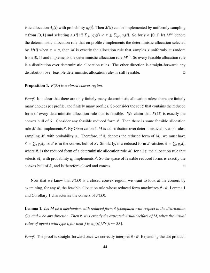
istic allocation Az(~t) with probability qz(~t). Then M(~t) can be implemented by uniformly sampling

x from [0, 1] and selecting Az(~t) iff∑

j<z q j(~t) < x ≤∑

j≤z q j(~t). So for y ∈ [0, 1] let M(y) denote

the deterministic allocation rule that on profile ~t implements the deterministic allocation selected

by M(~t) when x = y, then M is exactly the allocation rule that samples x uniformly at random

from [0, 1] and implements the deterministic allocation rule M(x). So every feasible allocation rule

is a distribution over deterministic allocation rules. The other direction is straight-forward: any

distribution over feasible deterministic allocation rules is still feasible.

Proposition 1. F(𝒟) is a closed convex region.

Proof. It is clear that there are only finitely many deterministic allocation rules: there are finitely

many choices per profile, and finitely many profiles. So consider the set S that contains the reduced

form of every deterministic allocation rule that is feasible. We claim that F(𝒟) is exactly the

convex hull of S . Consider any feasible reduced form ~π. Then there is some feasible allocation

rule M that implements ~π. By Observation 4, M is a distribution over deterministic allocation rules,

sampling Mz with probability qz. Therefore, if ~πz denotes the reduced form of Mz, we must have

~π =∑

z qz~πz, so ~π is in the convex hull of S . Similarly, if a reduced form ~π satisfies ~π =∑

z qz~πz,

where ~πz is the reduced form of a deterministic allocation rule Mz for all z, the allocation rule that

selects Mz with probability qz implements ~π. So the space of feasible reduced forms is exactly the

convex hull of S , and is therefore closed and convex.

Now that we know that F(𝒟) is a closed convex region, we want to look at the corners by

examining, for any ~w, the feasible allocation rule whose reduced form maximizes ~π · ~w. Lemma 1

and Corollary 1 characterize the corners of F(𝒟).

Lemma 1. Let M be a mechanism with reduced form ~π (computed with respect to the distribution

𝒟), and ~w be any direction. Then ~π · ~w is exactly the expected virtual welfare of M, when the virtual

value of agent i with type ti for item j is wi j(ti)/Pr[ti ← 𝒟i].

Proof. The proof is straight-forward once we correctly interpret ~π · ~w. Expanding the dot product,

44

we see that:

~π · ~w =∑

i

∑j

∑ti∈T

πi j(ti)wi j(ti)

=∑

i

∑j

∑ti∈T

Pr[ti ← 𝒟i]πi j(ti)wi j(ti)

Pr[ti ← 𝒟i].

If the “virtual value” of awarding item j to agent i when her reported type is A is wi j(ti)Pr[ti←𝒟i]

, then

the last line is exactly the expected virtual welfare of an allocation rule whose reduced form is

~π. This is because the term sums over all agents i, all types ti and all items j the probability that

agent i has type ti times the probability that agent i gets item j conditioned on this report, times the

virtual value of receiving item j with this type.

Corollary 1. Every corner ~π of F(𝒟) has a corresponding (deterministic) virtual transformation

such that the mechanism implementing ~π maximizes virtual welfare under this transformation.

Proof. As ℱ (𝒟) is a closed convex region, every corner ~π of F(𝒟) has a corresponding direction

~w (Fact 2 of Section 2.3 in Chapter 2) such that ~π = argmax~x∈F(𝒟)~x · ~w. By Lemma 1, this implies

that ~π is the reduced form with the maximum virtual welfare (under the specific transformation

corresponding to ~w)) over all feasible reduced forms. Therefore, the mechanism implementing ~π

necessarily maximizes virtual welfare under this transformation.

Now that we know the structure of the corners of F(𝒟), we turn back to computation and show

that we can optimize linear functions over F(𝒟) computationally efficiently. Until this point, we

have made use of the fact that agents are additive, but not of the specific nature of the feasibility

constraints. Proposition 1, Lemma 1, and Corollary 1 still hold true even if there are combinatorial

constraints on which agents can simultaneously receive which items. However, computing exactly

the reduced form of a virtual welfare maximizer is non-trivial in the face of combinatorial con-

straints and requires new tools in linear programming that we develop in Section 6.3 of Chapter 6.

It is for this reason that we choose to treat this case separately from the completely general settings

of Chapter 5. In Corollary 2 below, note that we are indeed making use of the simple nature of

feasibility constraints in this setting (that each item can be given to any agent, but at most one).

45

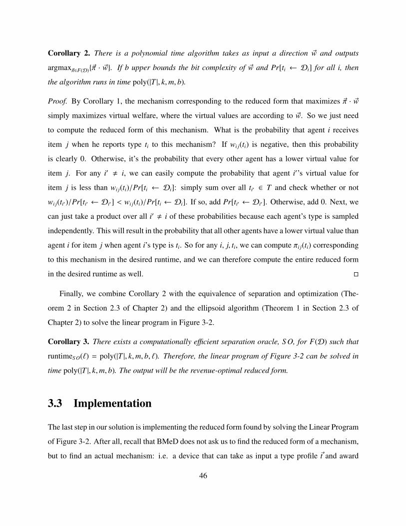
Corollary 2. There is a polynomial time algorithm takes as input a direction ~w and outputs

argmax~π∈F(𝒟)~π · ~w. If b upper bounds the bit complexity of ~w and Pr[ti ← 𝒟i] for all i, then

the algorithm runs in time poly(|T |, k,m, b).

Proof. By Corollary 1, the mechanism corresponding to the reduced form that maximizes ~π · ~w

simply maximizes virtual welfare, where the virtual values are according to ~w. So we just need

to compute the reduced form of this mechanism. What is the probability that agent i receives

item j when he reports type ti to this mechanism? If wi j(ti) is negative, then this probability

is clearly 0. Otherwise, it’s the probability that every other agent has a lower virtual value for

item j. For any i′ , i, we can easily compute the probability that agent i′’s virtual value for

item j is less than wi j(ti)/Pr[ti ← 𝒟i]: simply sum over all ti′ ∈ T and check whether or not

wi j(ti′)/Pr[ti′ ← 𝒟i′] < wi j(ti)/Pr[ti ← 𝒟i]. If so, add Pr[ti′ ← 𝒟i′]. Otherwise, add 0. Next, we

can just take a product over all i′ , i of these probabilities because each agent’s type is sampled

independently. This will result in the probability that all other agents have a lower virtual value than

agent i for item j when agent i’s type is ti. So for any i, j, ti, we can compute πi j(ti) corresponding

to this mechanism in the desired runtime, and we can therefore compute the entire reduced form

in the desired runtime as well.

Finally, we combine Corollary 2 with the equivalence of separation and optimization (The-

orem 2 in Section 2.3 of Chapter 2) and the ellipsoid algorithm (Theorem 1 in Section 2.3 of

Chapter 2) to solve the linear program in Figure 3-2.

Corollary 3. There exists a computationally efficient separation oracle, S O, for F(𝒟) such that

runtimeS O(`) = poly(|T |, k,m, b, `). Therefore, the linear program of Figure 3-2 can be solved in

time poly(|T |, k,m, b). The output will be the revenue-optimal reduced form.

3.3 Implementation

The last step in our solution is implementing the reduced form found by solving the Linear Program

of Figure 3-2. After all, recall that BMeD does not ask us to find the reduced form of a mechanism,

but to find an actual mechanism: i.e. a device that can take as input a type profile ~t and award

46

each item to an agent (or no one) and charge prices. To this end, we make use of Theorem 3 in

Section 2.3 of Chapter 2, which states that with access to a separation oracle for a closed convex

region P, any point ~π ∈ P can be decomposed in polynomial time into a convex combination of

corners of P. In this section, we observe that this suffices to implement any feasible reduced form.

Observation 5. Let ~π ∈ F(𝒟) have bit complexity `. Then we can decompose ~π =∑

z ~πzqz with

qz ≥ 0,∑

z qz = 1 in time poly(|T |, k,m, b, `), where each ~πz is a corner of F(𝒟).

Proof. This is a direct application of Theorem 3 from Section 2.3 in Chapter 2 and Corollary 3.

Corollary 4. Every feasible reduced form ~π ∈ F(𝒟) can be implemented as a distribution over

virtual-welfare maximizers. If the bit complexity of ~π is `, then this distribution can be found in

time poly(|T |, k,m, b, `).

Proof. Given any feasible reduced form ~π, first write ~π as a convex combination of corners of

F(𝒟) using the separation oracle of Corollary 3 in the decomposition algorithm of Theorem 3. By

Corollary 1, ~πz is the reduced form of the virtual welfare maximizer with virtual values according

to ~wz. So to implement ~π, simply run the mechanism corresponding to ~πz with probability qz. Each

~πz is a virtual welfare maximizer.

Proof of Theorem 4: Observation 3 reduces BMeD to developing a separation oracle for F(𝒟).

Theorem 2 in Chapter 2 reduces obtaining a separation oracle to obtaining an algorithm that opti-

mizes linear functions. Corollary 1 provides such an algorithm. Corollary 3 puts this all together

and states that we can find the revenue-optimal reduced form in the desired runtime. Corollary 4

states that we can implement the desired reduced form in the desired runtime as well, and also

provides the desired structure.

3.4 Conclusions

We have just shown that the revenue-optimal auction for additive agents is a distribution over

virtual-welfare maximizers, and that we can find and implement this auction in polynomial time.

This result also serves to prepare the reader for the complete reduction in Chapter 5. To that

47

end, there are four important steps to remember from this approach. First, we wrote a linear

program using a compact description of mechanisms (the reduced form), and showed that this

linear program can be solved with black-box access to a separation oracle for a closed convex

region (the space of feasible reduced forms). Second, we used the equivalence of separation and

optimization to show that this separation oracle can be obtained via an optimization algorithm for

the same closed convex region. Third, we showed that such an optimization algorithm simply

maximizes virtual welfare on every profile, completing the “reduction.” Finally, once we solve the

linear program, we have to implement whatever reduced form we find as an actual mechanism,

which is also done using tools from linear programming.

48

Chapter 4

Background: General Objectives and

Non-Additive Agents

Here we introduce the required background for general objectives and non-additive agents. Sec-

tion 4.1 updates notation related to mechanism design to the generalized setting, Section 4.2 pro-

vides additional preliminaries required for linear programming in our most general setting, and

Section 4.3 overviews related work in algorithmic mechanism design.

4.1 Preliminaries

Throughout the preliminaries and the remainder of the thesis, we state our definitions and results

when the goal is to minimize an objective (such as makespan). Everything extends to maximization

objectives (such as fairness) with the obvious changes (switching ≤ to ≥, min to max, etc.). We

often note the required changes. We choose to present in this way so that the reader sees an example

of the framework applied to both maximization (from Chapters 2 and 3) and minimization.

Mechanism Design Setting. For the remainder of this thesis, we will be in the general setting

put forth in Section 2.1. That is, the designer has to choose some possible outcome x from a set ℱ

of feasible outcomes, and we make no assumptions whatsoever on the structure of ℱ .

49

Agent Preferences. For the remainder of this thesis, we make no additional assumptions on the

agents’ preferences beyond those put forth in Section 2.1. That is, agents are still quasi-linear and

risk-neutral, but no longer additive. Agents have an arbitrary valuation function ti : ℱ → R. We

still assume that agents are rational and therefore behave in a way that maximizes their utility.

Private Information. We still assume that each agent’s type is sampled independently from a

known distribution. We make no assumptions about these distributions. For instance, the value of

agent i for outcomes x and x′ can be correlated, but the value of agents i and i′ for outcome x are

independent.

Interim Descriptions. In this chapter, it will be helpful to think of the interim description of

a mechanism. The interim allocation rule is a function that takes as input a agent i and a type

ti ∈ T and outputs the distribution of outcomes that agent i sees when reporting type ti, over

any randomness of the mechanism and the other agents’ types (assuming they report truthfully).

Specifically, if the interim allocation rule of M = (A, P) is X, then Xi(ti) is a distribution satisfying

Pr[x← Xi(ti)] = E~t−i←𝒟−i

[Pr[A(ti;~t−i) = x]

],

where ~t−i is the vector of types of all agents except i in ~t, and𝒟−i is the distribution of ~t−i. Similarly,

the interim price rule of the mechanism maps some agent i and type ti ∈ T of that agent to the

expected price agent i sees when reporting ti, i.e. pi(ti) = E~t−i←𝒟−i[Pi(ti;~t−i)].

With interim descriptions in mind, we may rewrite the mathematical statement of Bayesian

Incentive Compatible as simply ti(Xi(ti)) − pi(ti) ≥ ti(Xi(t′i )) − pi(t′i ) for all i and ti, t′i ∈ T . We may

also rewrite Individual Rationality as simply ti(Xi(ti)) − pi(ti) ≥ 0, for all i, ti ∈ i.

Implicit Forms. In addition to the interim description of a mechanism, it will be useful to in-

troduce a concept that we call the implicit form. The implicit form takes the role of the reduced

form from Chapter 2 and is used in optimization. For any feasible mechanism M = (A, P) for a

BMeD(ℱ ,𝒱,𝒪) instance, we define the three components of its implicit form ~πMI = (OM, ~πM, ~pM)

as follows.

50

∙ OM = E~t←𝒟[O(~t, A(~t))]. That is, OM is the expected value of 𝒪 when agents sampled from𝒟

play mechanism M.

∙ For all agents i and types ti, t′i ∈ T , πMi (ti, t′i ) = E~t−i←𝒟−i

[ti(A(t′i ;~t−i))]. That is, πMi (ti, t′i ) is the

expected value of agent i with real type ti for reporting type t′i to the mechanism M. The

expectation is taken over any randomness in M as well as the other agents’ types, assuming

they are sampled from𝒟−i.

∙ For all agents i and types ti ∈ T , pMi (ti) = E~t−i←𝒟−i

[Pi(ti;~t−i)]. That is, pMi (ti) is the expected

price paid by agent i when reporting type ti to the mechanism M. The expectation is taken

over any randomness in M as well as the other agents’ types, assuming they are sampled

from𝒟−i.

We can also talk about implicit forms separately from mechanisms, and call any (1 + k|T |2 +

k|T |)-dimensional vector an implicit form. We say that an implicit form ~πI = (O, ~π, ~p) is feasible

for a specific BMeD(ℱ ,𝒱,𝒪) instance if there exists a feasible mechanism M for that instance

such that O ≥ OM, ~π = ~πM, and ~p = ~pM. We say that the mechanism M implements the implicit

form ~πI when these inequalities hold. For maximization objectives, we instead constrain O ≤ OM.1

We denote by F(ℱ ,𝒟,𝒪) the set of all feasible implicit forms (with respect to a specific instance

of BMeD(ℱ ,𝒱,𝒪)).

Goal of the designer. We consider a designer with an arbitrary objective function 𝒪. For sim-

plicity of exposition, we will restrict attention in this chapter to objective functions 𝒪 that depend

only on the agents’ types and the outcome chosen and write the function 𝒪(~t, X) to emphasize

this. Examples of such objectives include welfare, makespan, and fairness but not revenue. The

modifications required to accommodate revenue or other objectives that depend on prices charged

are straight-forward, but notationally burdensome. We often note the required modifications infor-

mally. We also remark that our results further extend to objectives that are sensitive to randomness

in non-linear ways, so long as the dependence is concave in distributions over outcomes/prices for

1The relaxations O ≥ OM for minimization, and O ≤ OM for maximization objectives, instead of O = OM , arerequired for technical reasons.

51

maximization objectives and convex for minimization objectives. Note that “deterministic objec-

tives” such as makespan, fairness, welfare, and revenue that are extended to randomized outcomes

by taking expectations behave linearly with respect to randomness and are therefore both concave

and convex in this context. There are no modifications required to our techniques to accommodate

such objectives, but formally dealing with bit complexities for such functions becomes tedious, so

we omit any further discussion.

Normalization. In this chapter, we will also make use of an approximate notion of truthfulness

called ε-Bayesian Incentive Compatible. A mechanism is ε-BIC if each agent can gain at most an

additive ε by misreporting their type. That is, ti(Xi(ti)) − pi(ti) ≥ ti(Xi(t′i )) − pi(t′i ) − ε. In order

to make this additive guarantee meaningful, we assume that all types have been normalized so

that ti(X) ∈ [0, 1] for all X ∈ ℱ . Also, because our results accommodate an additive ε error, we

will restrict attention only to 𝒪 that are poly(k)-bounded. We say that 𝒪 is b-bounded if whenever

ti(X) ∈ [0, 1] for all i, 𝒪(~t, X) ∈ [0, b]. Note that makespan and fairness are both 1-bounded, and

welfare/revenue is k-bounded, so this is not a restrictive assumption.

Formal Problem Statements. We state both BMeD and GOOP for minimization objectives, but

both problems are also well-defined for maximization objectives with the obvious modifications,

discussed below. In the following definitions, we denote by𝒱 a set of potential types (i.e. functions

mapping ℱ to R), and by𝒱× the closure of𝒱 under addition and scalar multiplication.

BMeD(ℱ , 𝒱, 𝒪): Input: A finite set of types T ⊆ 𝒱, and for each agent i ∈ [k] a distribution

𝒟i over T . Goal: Find a feasible (outputs an outcome in ℱ with probability 1), BIC, and IR

mechanism M that minimizes 𝒪 in expectation, when k agents with types sampled from𝒟 = ×i𝒟i

play M truthfully, where the minimization is with respect to all feasible, BIC, and IR mechanisms.

M is said to be an α-approximation to BMeD if the expected value of 𝒪 is at most α times that of

the optimal mechanism.

GOOP(ℱ , 𝒱, 𝒪): Input: f ∈ 𝒱×, gi ∈ 𝒱 (1 ≤ i ≤ k), and a multiplier w ≥ 0. Goal: find a

52

feasible (possibly randomized) outcome X ∈ ∆(ℱ ) such that:

(w · 𝒪((g1, . . . , gk), X)) + f (X) = minX′∈ℱ

(w · 𝒪((g1, . . . , gk), X′)

)+ f (X′)

.

We define a bi-criterion approximation for GOOP. We say that X is an (α, β)-approximation to

GOOP for some β ≤ 1 ≤ α iff:

β (w · 𝒪((g1, . . . , gk), X)) + f (X) ≤ α(minX′∈ℱ

(w · 𝒪((g1, . . . , gk), X′)

)+ f (X′)

). (4.1)

An X satisfying (4.1) with β = 1 is an α-approximation to GOOP, which is the familiar notion of

approximation for minimization problems. If β < 1, our task becomes easier as the contribution of

the 𝒪 part to the objective we are looking to minimize is discounted.

Within the context of our reduction from BMeD to GOOP, one should interpret the function f

in the GOOP instance as representing virtual welfare, and each gi as representing the type reported

by agent i.

Remark 1. For maximization objectives 𝒪, we replace min by max in the definition of GOOP, and

we invert the direction of the inequality in (4.1). Moreover, the feasible range of parameters for an

(α, β)-approximation are now α ≤ 1 ≤ β.

4.2 Additional Linear Programming Preliminaries

In this section, we provide additional necessary preliminaries on linear programming required for

the results of the following chapter. We defer to Chapter 6 a proof of all claims, but we include

definitions and statements here so that the results of the following chapter are readable.

(α, β)-approximations. Let us first define what (α, β)-approximations are for linear optimization

problems. In the definition below, α and β are constants and S is a subset of the coordinates.

When we write the vector (c~xS , ~x−S ), we mean the vector ~x where all coordinates in S have been

multiplied by c.

53

Definition 1. An algorithm𝒜 is an (α, β, S )-minimization algorithm for a closed convex region P

iff for any input vector ~w the vector𝒜(~w) output by the algorithm satisfies:

(β𝒜(~w)S ,𝒜(~w)−S ) · ~w ≤ αmin~x∈P~x · ~w. (4.2)

Given such algorithm, we also define the algorithm𝒜βS that outputs (β𝒜(~w)S ,𝒜(~w)−S ).2

Taking β = 1 recovers the familiar notion of α-approximation, except that we do not require the

output of the algorithm to lie in P in our definition. (Most meaningful applications of our frame-

work will enforce this extra property though.) With β < 1 (respectively β > 1), the minimization

(resp. maximization) becomes easier as the coordinates indexed by S are discounted (boosted) by

a factor of β before comparing to α · OPT .

Weird Separation Oracles. In order to accommodate approximation algorithms in the equiv-

alence of separation and optimization, we introduce the notion of a weird separation oracle. A

weird separation oracle (WS O) looks kind of like a separation oracle, in that it is an algorithm

that sometimes says “yes” and sometimes outputs a hyperplane. But it’s behavior may be erratic,

and the set of points for which the algorithm says “yes” may not be convex, closed, or even con-

nected. We prove in Chapter 6 Theorem 5 below, which generalizes the equivalence of separation

and optimization (Theorem 2 in Chapter 2) to accommodate (α, β)-approximations. Specifically,

Theorem 5 states that an (α, β, S )-approximation algorithm for closed convex region P can be used

to obtain a weird separation oracle for αP (by αP we mean the closed convex region P blown

up by a factor of α or shrunk by a factor of α, depending on whether α ≥ 1 or α ≤ 1). Before

stating the theorem formally, let’s overview quickly what each property below is guaranteeing.

Property 1 guarantees that WS O is consistent at least with respect to points inside αP (but may

behave erratically outside of αP). Property 2 guarantees that even though the points accepted by

WS O may not be in αP (or even in P), they will at least satisfy some relaxed notion of feasibility.

Property 3 guarantees that WS O terminates in polynomial time. Property 4 guarantees that if we

2We can similarly define the concept of a (α, β, S )-maximization algorithm for closed convex region P by flippingthe inequality in (4.2) and also switching min to max.

54

run Ellipsoid with WS O instead of a real separation oracle for αP, that we don’t sacrifice anything

in terms of optimality (although the output is only guaranteed to satisfy the notion of feasibility

given in Property 2. It may be infeasible in the traditional sense, i.e. not contained in αP).

Theorem 5. Let P be a closed convex region in Rd and 𝒜 an (α, β, S )-minimization algorithm

for P, for some α, β > 0. Then we can design a weird separation oracle WS O for αP with the

following properties:

1. Every halfspace output by WS O will contain αP.

2. Whenever WS O(~x) = “yes” for some input ~x, the execution of WS O explicitly finds direc-

tions ~w1, . . . , ~wd+1 such that ~x ∈ Conv𝒜βS (~w1), . . . ,𝒜β

S (~wd+1), and therefore ( 1β~xS , ~x−S ) ∈

Conv𝒜(~w1), . . . ,𝒜(~wd+1) as well.

3. Let b be the bit complexity of ~x, ` an upper bound on the bit complexity of 𝒜(~w) for all

~w ∈ [−1, 1]d. Then on input ~x, WS O terminates in time poly(d, b, `, runtime𝒜(poly(d, b, `)))

and makes at most poly(d, b, `) queries to𝒜.

4. Let Q be an arbitrary closed convex region in Rd described via some separation oracle, ~c

a linear objective with ~c−S = ~0, and OPT = min~y∈αP∩Q~c · ~y. Let also ~z be the output

of the Ellipsoid algorithm for minimizing ~c · ~y over ~y ∈ αP ∩ Q, but using WS O as a

separation oracle for αP instead of a standard separation oracle for αP (i.e. use the exact

same parameters for Ellipsoid as if WS O was a valid separation oracle for αP, and still use

a standard separation oracle for Q). Then ~c ·~z ≤ OPT, and therefore ~c · ( 1β~zS ,~z−S ) ≤ 1

βOPT.

A complete proof of Theorem 5 appears in Section 6.2 of Chapter 6.

Sampling Error. Another necessary tool in the subsequent chapter will be an extension of the

equivalence of separation and optimization to accommodate sampling error in the optimization

algorithm. Specifically, what we will show is that if we start with a closed convex region P ⊆ Rd

that admits a certain kind of sampling-based optimization algorithm, then there is another closed

convex region P′ that is nearly identical to P and is more convenient for optimization. We be-

gin by defining these sampling-based optimization algorithms, that we call sample-optimization

55

algorithms. In the definition below, we use the notation ~wS to mean the vector ~w restricted to co-

ordinates S . So by (~wS , 0−S ) we mean the vector ~w where all coordinates except for S have been

zeroed out.

Definition 2. (sample-optimization algorithm) For all subsets S ⊆ [d], let AS be an exact op-

timization algorithm for some closed convex region Q(S ) ⊆ [0, poly(d)]d. We say that 𝒜 is a

sample-optimization algorithm if 𝒜(~w) first samples a subset of coordinates S ⊆ [d] according to

some distribution D, then outputs AS ((wS , 0−S )), where w is a vector with wi = wi/Pr[i ∈ S ], and

the probability in the denominator is with respect to D. We also define the sample complexity of

𝒜, to be maxi1/Pr[i ∈ S ], and the corner complexity to be log N, where N is the smallest integer

such that all corners of all Q(S ) are integer multiples of N. We denote by b(𝒜) the complexity of

𝒜, which upper bounds the sample and corner complexity.

Note that every exact optimization algorithm is also a sample-optimization algorithm (by sam-

pling S = [d] with probability 1).

Definition 3. (sample-optimization region) We say that a closed convex region P is a sample-

optimization region if there exists a sample-optimization algorithm 𝒜, sampling S from distribu-

tion D, with the additional property that for all ~w, there exists some ~z* ∈ argmax~x∈P~x · ~w such that

E[𝒜(~w)i|i ∈ S ] = z*i for all i, where again the conditioning in the expectation is taken with respect

to D. We also define the complexity of P, b(P) to be the minimum over all sample-optimization

algorithms𝒜 for P of b(𝒜).

For a sample-optimization region P, and corresponding sample-optimization algorithm 𝒜 and

distribution D, we also take poly(d, b(P), 1/ε) samples from D and denote by D′ the uniform

distribution over these samples. We further define the sample-optimization algorithm 𝒜′ that first

samples a subset S ′ of coordinates from D′ and then runs AS ′ . We claim that AS ′ defines a sample-

optimization region P′, and that with high probability over the samples taken for D′, P and P′ are

close.

Theorem 6. Let P be a sample-optimization region with corresponding sample-optimization al-

gorithm 𝒜, closed convex regions Q(S ), optimization algorithms AS , and distribution D over S .

56

For any ε, let D′ be the uniform distribution over poly(d, b(P), 1/ε) samples from D, and define

the sample-optimization algorithm 𝒜′ to sample S ′ from D′ (and then run AS ′). Then 𝒜′ defines

a sample-optimization region P′. Furthermore, with probability 1 − exp(poly(d, b(P), 1/ε)), the

following two guarantees hold:

1. For every ~x ∈ P, there exists an ~x′ ∈ P′ with |~x − ~x′|∞ ≤ ε.

2. For every ~w and all i ∈ [d], |E[𝒜(~w)i|i ∈ S ] − E[𝒜′(~w)i|i ∈ S ]| ≤ ε.

A complete proof of Theorem 6 appears in Section 6.3 of Chapter 6.

4.3 Related Work

In this section we overview related work in algorithmic mechanism design: specifically prior work

on black-box reductions, mechanisms for makespan, and mechanisms for fairness.

Black-Box Reductions in Mechanism Design. We have already established that the classical

VCG mechanism can be viewed as a mechanism to algorithm reduction for the important objective

of welfare [Vic61, Cla71, Gro73], and Myerson’s celebrated mechanism [Mye81] as a mechanism

to algorithm design reduction for revenue. Sometimes, however, these reductions ask for the de-

sign of algorithms that are computationally intractable. Work of [PSS08, BDF+10, Dob11, DV12]

establishes that in prior-free settings, no approximation-preserving reduction can possibly exist

even for welfare. Yet, work of [HL10, HKM11, BH11] establishes an approximation-preserving

reduction in Bayesian settings for welfare. Interestingly, for the special case of revenue in single-

dimensional settings, there is also a precedence of using the specific average-case structure of

the problem in order to develop approximation algorithms in settings where any finite approx-

imation seems computationally intractable at first glance [HIMM11, BHSZ13]. In the settings

studied by these papers, the algorithmic problem resulting from the reduction (namely virtual wel-

fare maximization) is highly inapproximable in the worst case. Nevertheless, they side-step this

intractability by exploiting the fact that the algorithmic problem need only be solved well in an

average-case sense (in particular, in expectation over the bidder’s virtual values) rather than on an

57

instance-to-instance basis, as well as the fact that, in single-dimensional settings, the virtual values

have very well-understood structure. This allows for the design of polynomial-time algorithms

that obtain a reasonable approximation guarantee on average, while possibly performing poorly on

some instances.

Outside of welfare and revenue in single-dimensional settings, there is no further precedent

of black-box reductions in mechanism design. Specifically, outside of our work there are no

known black-box reductions for multi-dimensional mechanism design, and the only prior result

for objectives beyond welfare or revenue is an impossibility result due to Chawla, Immorlica, and

Lucier [CIL12]. Specifically, they show that there is no black-box reduction from truthfully min-

imizing makespan to algorithmically minimizing makespan even in single-dimensional settings.

On this front, our work provides the first positive result for black-box reductions beyond welfare

or revenue in single-dimensional settings, and greatly improves the state of the art.

Makespan. A long line of work following the seminal paper of Nisan and Ronen [NR99] ad-

dresses the question of “how much better can the optimal makespan be when compared to the

optimal makespan obtained by a truthful mechanism?” The same paper showed that the an-

swer is at most a factor of k, and also that the answer is at least 2 for deterministic, DSIC,

prior-free mechanisms. It was later shown that the answer is at least 1 + φ (the golden ratio)

as k → ∞ [CKV07, KV07], and that the answer is in fact k for the restricted class of anonymous

mechanisms [ADL12]. It is conjectured that the answer is indeed k for all deterministic, DSIC,

prior-free mechanisms. Similar (but slightly different) bounds are known for the same question

with respect to randomized prior-free mechanisms [NR99, MS07, CKK07, LY08a, LY08b, Lu09].

More recently, the same question has been studied for prior-independent (rather than prior-free)

mechanisms [CHMS13]. Prior-independent mechanisms make distributional assumptions about

the processing times, but do not use the specifics of the distributions, just their properties. In

particular, when the processing times are drawn from a machine-symmetric product distribution

with Monotone Hazard Rate (MHR) marginals, Chawla, Hartline, Malec and Sivan show that the

answer is at most a factor of O(m/k), and at most a factor of O(√

log k), when all processing

58

times are i.i.d. [CHMS13]. Without the MHR assumption, they obtain bicriterion results.3 The

question has also been studied in related machines settings, where each job has a size (public)

and each machine has a speed (private). Due to the single-dimensional nature of the problem, the

answer is now exactly a factor of 1 [AT01]. Thus, focus has shifted towards the same question

for computationally efficient truthful mechanisms, and constant-factor approximations [AT01] and

PTAS’s [DDDR08, CK10] are known.

The focus of our work is different than most previous works, in that we do not study the gap

between the algorithmic and the mechanismic optimum. Instead, our focus is computational, aim-

ing for (approximately) optimal and computationally efficient mechanisms, regardless of how their

performance compares to the performance of optimal algorithms. Still, prior work has already

made some progress on this problem: we know that the VCG mechanism is a computationally effi-

cient k-approximation [NR99], and that the mechanisms of [CHMS13] provide an approximation

ratio of O(m/k) when the prior is a machine-symmetric product distribution with MHR marginals,

and a ratio of O(√

log k) if additionally the marginals are i.i.d. In addition, the NP-hardness result

of [LST87] implies that our problem is also NP-hard to approximate better than 3/2 − ε, for any

ε > 0. On this front, our work greatly improves the state-of-the-art as we give the first constant-

factor approximations for unrestricted settings. (The guarantees of [CHMS13] are constant in

settings where m = O(k) or k = O(1) and the prior is a machine-symmetric product distribution

with MHR marginals.) Indeed, our approximation guarantee (factor of 2) matches that of the best

polynomial-time algorithm for makespan minimization [LST87].

Max-Min Fairness. Fair division has been studied extensively in Mathematics and Economics

for over 60 years; see e.g. [Ste48, Kna46, BT96]. Several different flavors of the problem have

been studied: divisible or indivisible goods (in our terminology: jobs), with or without monetary

transfers to the players (in our terminology: machines), and several different notions of fairness.

For the allocation of indivisible goods, virtually all mechanisms proposed in the literature do not

optimize max-min fairness, aiming instead at other fairness guarantees (such as envy-freeness or

3Specifically, they obtain the same bounds with respect to a different benchmark, namely the optimal expectedmakespan using only a fraction of the k machines.

59

proportionality), very commonly trade off value from received items by the players with monetary

transfers to or from the players in the fairness guarantee, and are often susceptible to strategic ma-

nipulations. For max-min fairness, Bezakova and Dani [BD05] propose a prior-free mechanism for

2 players, which guarantees half of the optimal fairness, albeit under restrictions on the strategies

that the players can use. They also show that max-min fairness cannot be optimally implemented

truthfully in prior-free settings. In fact, Mu’alem and Schapira show that no DSIC, deterministic,

prior-free mechanism can obtain any approximation to the optimal max-min fairness [MS07].

Perhaps the poor state-of-the-art on mechanisms for max-min fairness owes to the fact that,

already as an algorithmic problem (i.e. even when the players’ true values for the items are as-

sumed exactly known), max-min fairness has proven quite challenging, indeed significantly more

so than makespan minimization. In particular, all state-of-the-art algorithms only provide poly-

nomial approximation guarantees [BD05, AS07, KP07, BCG09, CCK09], while the best known

computational hardness result is just a factor of 2 [BD05]. Specifically, the guarantees lying on

the Pareto boundary of what is achievable in polynomial time for the unrestricted problem are

approximation factors of m − k + 1 ([BD05]), O(√

k) ([AS07]), and O(m1/ε) ([BCG09, CCK09]).

Due to this, a restricted version of the problem is often studied, where every job has a fixed pro-

cessing time p j, and every machine is either capable or incapable of processing each job (that

is, pi j ∈ p j, 0). For the restricted version, the state of the art is an O(log log k/ log log log k)-

approximation due to Bansal and Sviridenko [BS06]. Asadpour, Feige, and Saberi [AFS08] also

proved that the integrality gap of the configuration LP used in [BS06] has an integrality gap of

5, and provided a heuristic (but not polynomial-time) rounding algorithm. O(1)-approximations

were obtained by Bateni, Charikar and Guruswami and independently by Chakrabarty, Chuzhoy

and Khanna by further restricting the graph structure of which machines can process which jobs

(i.e. by limiting the number of machines that can process each specific job or requiring that this

graph be acyclic) [BCG09, CCK09].

In view of this literature, our results provide the first approximately optimal mechanisms for

max-min fairness. Indeed, our approximation factors match those of approximation algorithms on

the Pareto boundary of what is achievable in polynomial time [BD05, AS07]. So, in particular,

60

our mechanisms cannot be strictly improved without progress on the algorithmic front. Obtain-

ing these mechanisms is already quite involved (see Chapter 7), and we leave open for future

investigation the problem of matching the bounds obtained in [BCG09, CCK09] for the general

problem, [AFS08, BS06] for the restricted problem, and [BCG09, CCK09] for the futher restricted

version.

In summary, our work greatly improves the state of the art for black-box reductions in mech-

anism design, and furthermore our new framework yields the first poly-time mechanisms for two

paradigmatic algorithmic problems (namely, makespan and fairness).

61

62

Chapter 5

The Complete Reduction

In this section we provide our black-box reduction from mechanism to algorithm design (formally,

BMeD to GOOP) in its complete generality. The proof of correctness follows a similar skeleton

to that of Theorem 4 from Chapter 3, but several extra algorithmic steps are required due to the

increased generality. Most of these algorithmic steps are taken separately in Chapter 6, as they are

of independent interest.

Our work in this chapter provides meaningful structure on the optimal mechanism for any

objective in addition to the computational implications. Specifically, we show that the optimal

mechanism takes the following form:

1. Each agent reports their type.

2. These types are transformed into virtual types. This transformation is randomized and pre-

computed by a linear program.

3. The outcome maximizing 𝒪+virtual welfare is selected.

4. Payments are charged to ensure that the mechanism is truthful. These payments are also

pre-computed by a linear program.

In the following theorem statement (and throughout the remainder of this chapter), we let b

denote an upper bound on the bit complexity of 𝒪(~t, x), Pr[ti ← 𝒟i], and ti(x) over all x ∈ ℱ ,

~ti ∈ T , ~t ∈ ×i∈[k]T .

63

Theorem 7. Let G be an (α, β)-approximation algorithm for GOOP(ℱ ,𝒱,𝒪), for some α ≥ 1 ≥

β > 0, and some minimization objective 𝒪. Also, fix any ε > 0. Then there is an approxi-

mation algorithm for BMeD(ℱ ,𝒱,𝒪) that makes poly(|T |, b, k, 1/ε) calls to G, and runs in time

poly(|T |, b, k, 1/ε, runtimeG(poly(|T |, b, k, 1/ε))). If OPT is the optimal obtainable expected value

of 𝒪 for some BMeD instance, then the mechanism M output by the algorithm on that instance

yields E[𝒪(M)] ≤ αβOPT + ε, and is ε-BIC. These guarantees hold with probability at least

1−exp(poly(|T |, b, k, 1/ε)). Furthermore, the output mechanism is feasible and can be implemented

in time poly(|T |, b, k, 1/ε, runtimeG(poly(|T |, b, k, 1/ε))). These guarantees hold with probability 1.

Sections 5.1, 5.2, and 5.3 below provide a complete proof of Theorem 7. As Theorem 7 is

quite general and a bit abstract, we provide in Section 5.4 several instantiations of Theorem 7 to

important or previously studied settings.

5.1 A Linear Program

We begin by stating the linear program used in our algorithm in Figure 5-1. Note the similarity

to the linear program of Figure 3-2 used in Chapter 3, the only difference is that we’ve replaced

the reduced form with the implicit form. Before continuing with our analysis, we should address

why this replacement is necessary. The issue with using the reduced form in settings with non-

additive agents is that there is simply not enough information in the reduced form to determine if

a mechanism is truthful or not. The following example illustrates why.

Example. Let there be a single agent and two items. Her value for receiving both items together

is 2, and her value for receiving a single item (or nothing) is 0. Consider the mechanism M that

awards both items with probability 1/2 and charges a price of 1, and the mechanism M′ that awards

a single item chosen uniformly at random and charges a price of 1. Then the reduced forms of M

and M′ are identical: each awards item 1 with probability 1/2, item 2 with probability 1/2, and

charges a price of 1. But the agent’s expected value for participating in M is 1, whereas her

expected value for participating in M′ is 0. Therefore, M is individually rational but M′ is not.

64

Variables:

∙ πi(ti, t′i ), for all agents i and types ti, t′i ∈ T , denoting the expected value obtained by agenti when their true type is ti but they report t′i instead.

∙ pi(ti), for all agents i and types ti ∈ T , denoting the expected price paid by agent i whenthey report type ti.

∙ O, denoting the expected value of 𝒪.

Constraints:

∙ πi(ti, ti) − pi(ti) ≥ πi(ti, t′i ) − pi(t′i ), for all agents i, and types ti, t′i ∈ T , guaranteeing that theimplicit form (O, ~π, ~p) is BIC.

∙ πi(ti, ti) − pi(ti) ≥ 0, for all agents i, and types ti ∈ T , guaranteeing that the implicit form(O, ~π, ~p) is individually rational.

∙ (O, ~π) is feasible. **A separation oracle is needed for this.**

Minimizing:

∙ O, the expected value of 𝒪 when played truthfully by agents sampled from𝒟.

Figure 5-1: A linear programming formulation for BMeD.

Observation 6. The linear program of Figure 5-1 finds the implicit form of a solution to a given

BMeD instance. Furthermore, is S O is a separation oracle for the space of feasible implicit forms,

this LP can be solved in time poly(k, |T |, b, runtimeS O(k, |T |, b)).

Remark 2. To optimize revenue instead of 𝒪, one can modify the linear program of Figure 5-1

by removing entirely the variable O. Feasibility now only constrains ~π instead of (O, ~π), and the

objective function should be the expected revenue,∑

i Pr[ti ← 𝒟i] · pi(ti) instead of O (and should

be maximized instead of minimized).

Remark 3. To optimize an objective𝒪 that depends on ~t, X, and ~p, modify the feasibility constraint

so that feasibility constraints all of (O, ~π, ~p) (instead of just (O, ~π)).

Unfortunately, even with our approximation-preserving equivalence of separation and opti-

mization, we can’t always get a meaningful separation oracle for the space of feasible implicit

forms, which we denote by F(ℱ ,𝒟,𝒪). To cope with this, we further develop the equivalence

65

of separation and optimization framework to accommodate an additive sampling error. Essen-

tially, we replace the closed convex region F(ℱ ,𝒟,𝒪) with the closed convex region F(ℱ ,𝒟′,𝒪),

where 𝒟′ is a uniform distribution over polynomially many samples from 𝒟. We postpone until

Section 6.3 a proof that this procedure is valid, but rewrite here the linear program we actually

solve in Figure 5-2. We also note that this replacement is the reason that ε appears in Theorem 7.

Variables:

∙ πi(ti, t′i ), for all agents i and types ti, t′i ∈ T , denoting the expected value obtained by agenti when their true type is ti but they report t′i instead.

∙ pi(t), for all agents i and types ti ∈ T , denoting the expected price paid by agent i whenthey report type ti.

∙ O, denoting the expected value of 𝒪.

Constraints:

∙ πi(ti, ti) − pi(ti) ≥ πi(ti, t′i ) − pi(t′i ), for all agents i, and types ti, t′i ∈ T , guaranteeing that theimplicit form (O, ~π, ~p) is BIC.

∙ πi(ti, ti) − pi(ti) ≥ 0, for all agents i, and types ti ∈ T , guaranteeing that the implicit form(O, ~π, ~p) is individually rational.

∙ (O, ~π) ∈ F(ℱ ,𝒟′,𝒪). **A separation oracle is needed for this.**

Minimizing:

∙ O, the expected value of 𝒪 when played truthfully by agents sampled from𝒟.

Figure 5-2: A linear program for BMeD, replacing F(ℱ ,𝒟,𝒪) with F(ℱ ,𝒟′,𝒪).

5.2 The Space of Feasible Implicit Forms

Like Chapter 3, our approach to solve the LP in Figure 5-2 by obtaining a separation oracle for

the space F(ℱ ,𝒟′,𝒪), making use of the equivalence of separation and optimization. However, in

order to accommodate approximation, we need to develop some new machinery. As this machinery

is of independent interest, we treat it separately in Chapter 6.

66

We now begin by proving that the linear program of Figure 5-2 can be solved computationally

efficiently by making use of machinery from Chapter 6 (specifically, Theorem 5).

Proposition 2. With black-box access to an (α, β, O)-optimization algorithm,𝒜, for F(ℱ ,𝒟′,𝒪),

one can use the weird separation oracle guaranteed by Theorem 5 inside the ellipsoid algo-

rithm to solve the linear program of Figure 5-2. The Ellipsoid algorithm will terminate in time

poly(|T |, b, k, 1/ε, runtime𝒜(poly(|T |, b, k, 1/ε))), and will output a truthful implicit form ~πI . The

objective component O of ~πI will satisfy O ≤ αOPT ′, where OPT ′ is the value of O in the opti-

mal solution to the LP of Figure 5-2. Furthermore, the algorithm will explicitly output a list of

d + 1 = poly(|T |, k) directions ~w1, . . . , ~wd+1 such that ~πI ∈ Conv𝒜β

O(~w1), . . . ,𝒜β

O(~wd+1).

Proof. Theorem 5 guarantees that the linear program can be solved in the desired runtime, and that

the desired directions ~w1, . . . , ~wd+1 will be output. It is clear that any implicit form satisfying the

constraints is truthful.

Let now OPT ′α denote the value of the LP in Figure 5-2 using a real separation oracle for

αF(ℱ ,𝒟′,𝒪). Theorem 5 also guarantees that O ≤ OPT ′α. So we just need to show that OPT ′α ≤

αOPT ′.

To see this, first observe that the origin satisfies every constraint in the linear program not due

to F(ℱ ,𝒟′,𝒪) (i.e. the truthfulness constraints) with equality. Therefore, if any implicit form ~πI

is truthful, so is the implicit form α~πI . This immediately implies that OPT ′α = αOPT ′.

Next, we show that one can obtain an (α, β, O)-optimization algorithm for F(ℱ ,𝒟′,𝒪) given

black-box access to an (α, β)-approximation algorithm for GOOP(ℱ ,𝒱,𝒪). We first need a tech-

nical lemma giving context to dot products in the space of feasible implicit forms.

Proposition 3. Let ~w be a direction in [−1, 1]1+k|T |2+k|T |. Define the virtual type of agent i with type

t′ as t′~w =

∑t∈T

wi(t,t′)Pr[t′←𝒟i]

t(·). That is, t′~w(X) =

∑t∈T

wi(t,t′)Pr[t′←𝒟i]

t(X). Define also the virtual objective 𝒪′~w

as:

𝒪′~w(~t ′, X) = wO · 𝒪(~t ′, X) +∑

i

ti′

~w(X)

67

Then for any mechanism M = (A, P), if ~πMI denotes the implicit form of M with respect to 𝒟,

~πMI · ~w is exactly the expected virtual objective of M on type profiles sampled from𝒟. Formally:

~πMI · ~w = E~t ′←𝒟[𝒪′~w(~t ′, A(~t ′))]

Proof. We begin by expanding the dot product:

~πMI · ~w = O · wO +

∑i

∑t,t′∈T

πi(t, t′)wi(t, t′)

Recalling that πi(t, t′) is the value of t for the interim allocation seen by t′, we rewrite πi(t, t′) =

t(Xi(t′)), yielding:

~πMI · ~w = O · wO +

∑i

∑t,t′∈T

wi(t, t′) · t(Xi(t′))

Now we multiply and divide each term by Pr[t′ ← 𝒟i], and rearrange the sum to sum first over

i, then t′, then t:

~πMI · ~w = O · wO +

∑i

∑t′∈T

Pr[t′ ← 𝒟i]∑t∈T

wi(t, t′)Pr[t′ ← 𝒟i]

· t(Xi(t′))

Now let’s interpret the sum above: O is exactly the expected value of 𝒪, taken across all

profiles, so O · wO is just the expected value multiplied by wO. Xi(t′) is the interim allocation

seen by agent i with type t′, and this allocation is being evaluated by the function∑

t∈Twi(t,t′)

Pr[t′←𝒟i]t(·),

which is exactly t′~w(·). As this is the virtual type of agent i with type t′ evaluating the interim

allocation seen, this is exactly the virtual value of type t′. So summing over all agents and all

types, Pr[t′ ← 𝒟i] times the virtual value of t′ yields exactly the expected virtual welfare. So ~πMI

is exactly the expected value of the objective plus the expected virtual welfare, which is exactly

the expected virtual objective.

With Proposition 3, we can now show how to get an (α, β, O)-optimization algorithm for

F(ℱ ,𝒟′,𝒪) using an (α, β)-approximation algorithm for GOOP.

68

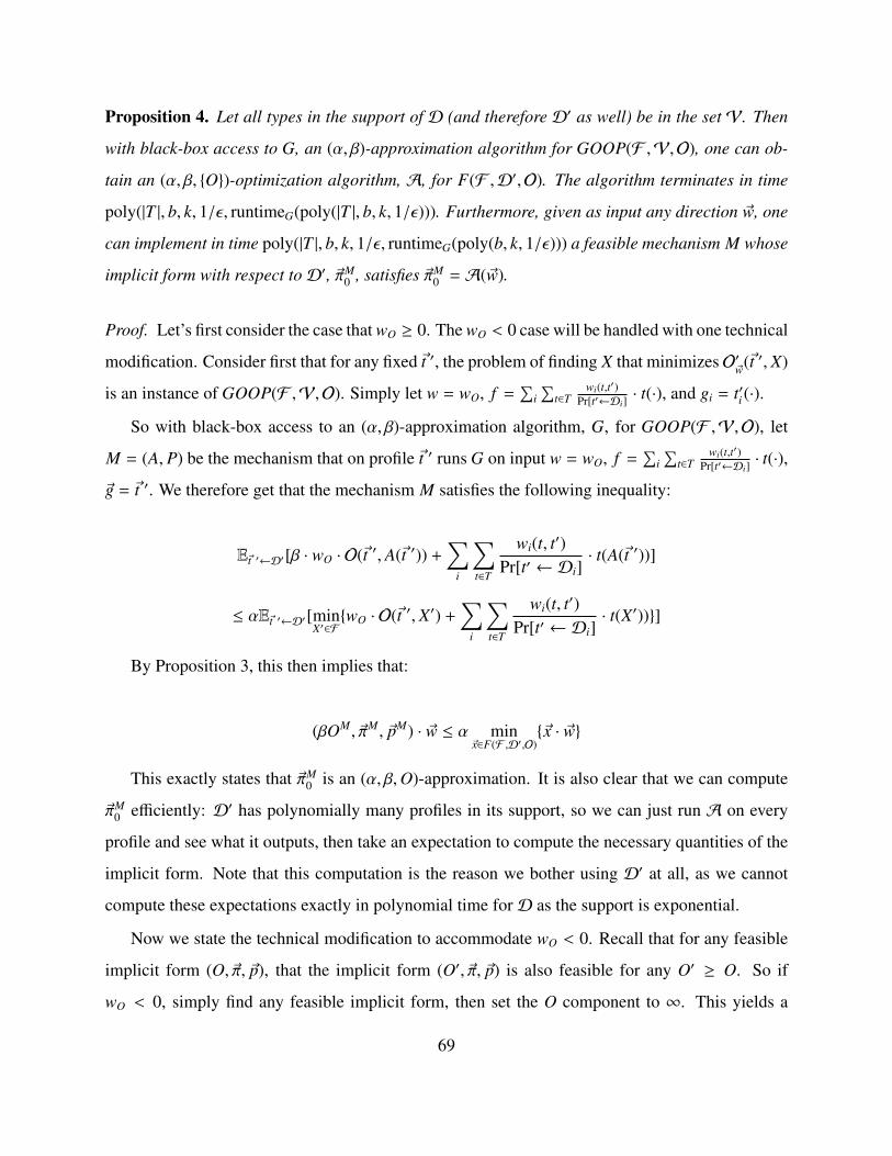
Proposition 4. Let all types in the support of 𝒟 (and therefore 𝒟′ as well) be in the set 𝒱. Then

with black-box access to G, an (α, β)-approximation algorithm for GOOP(ℱ ,𝒱,𝒪), one can ob-

tain an (α, β, O)-optimization algorithm, 𝒜, for F(ℱ ,𝒟′,𝒪). The algorithm terminates in time

poly(|T |, b, k, 1/ε, runtimeG(poly(|T |, b, k, 1/ε))). Furthermore, given as input any direction ~w, one

can implement in time poly(|T |, b, k, 1/ε, runtimeG(poly(b, k, 1/ε))) a feasible mechanism M whose

implicit form with respect to𝒟′, ~πM0 , satisfies ~πM

0 = 𝒜(~w).

Proof. Let’s first consider the case that wO ≥ 0. The wO < 0 case will be handled with one technical

modification. Consider first that for any fixed ~t ′, the problem of finding X that minimizes 𝒪′~w(~t ′, X)

is an instance of GOOP(ℱ ,𝒱,𝒪). Simply let w = wO, f =∑

i∑

t∈Twi(t,t′)

Pr[t′←𝒟i]· t(·), and gi = t′i (·).

So with black-box access to an (α, β)-approximation algorithm, G, for GOOP(ℱ ,𝒱,𝒪), let

M = (A, P) be the mechanism that on profile ~t ′ runs G on input w = wO, f =∑

i∑

t∈Twi(t,t′)

Pr[t′←𝒟i]· t(·),

~g = ~t ′. We therefore get that the mechanism M satisfies the following inequality:

E~t ′←𝒟′[β · wO · 𝒪(~t ′, A(~t ′)) +∑

i

∑t∈T

wi(t, t′)Pr[t′ ← 𝒟i]

· t(A(~t ′))]

≤ αE~t ′←𝒟′[minX′∈ℱwO · 𝒪(~t ′, X′) +

∑i

∑t∈T

wi(t, t′)Pr[t′ ← 𝒟i]

· t(X′))]

By Proposition 3, this then implies that:

(βOM, ~πM, ~pM) · ~w ≤ α min~x∈F(ℱ ,𝒟′,𝒪)

~x · ~w

This exactly states that ~πM0 is an (α, β,O)-approximation. It is also clear that we can compute

~πM0 efficiently: 𝒟′ has polynomially many profiles in its support, so we can just run 𝒜 on every

profile and see what it outputs, then take an expectation to compute the necessary quantities of the

implicit form. Note that this computation is the reason we bother using 𝒟′ at all, as we cannot

compute these expectations exactly in polynomial time for𝒟 as the support is exponential.

Now we state the technical modification to accommodate wO < 0. Recall that for any feasible

implicit form (O, ~π, ~p), that the implicit form (O′, ~π, ~p) is also feasible for any O′ ≥ O. So if

wO < 0, simply find any feasible implicit form, then set the O component to ∞. This yields a

69

feasible implicit form with ~πI · ~w = −∞, which is clearly an (α, β,O)-approximation (in fact, it is

a (1, 1,O)-approximation). If instead the problem has a maximization objective, we may w.l.o.g.

set O = 0 in the implicit form we output, which means that the contribution of 𝒪 is completely

ignored. So we can use the exact same approach as the wO ≥ 0 case and just set wO = 0.

So let𝒜 be the algorithm that runs G on every profile as described, and computes the implicit

form of this mechanism with respect to 𝒟′. 𝒜 clearly terminates in the desired runtime. Finally,

to implement a mechanism whose implicit form ~πM0 matches𝒜(~w), simply run G with the required

parameters on every profile.

Taken together, the above propositions provide an algorithm to find an implicit form ~πI whose

objective component is within an α-factor of optimal (for the linear program of Figure 5-2, at

least). The only remaining step is to implement it. As mentioned earlier, there’s a bit of a catch

here because ~πI may not even be feasible. We instead approximately implement ~πI , losing a factor

of β in the objective component but leaving the others untouched.

Proposition 5. Let ~πI = (O, ~π, ~p) be the implicit form and ~w1, . . . , ~wd+1 the auxiliary information

output by the algorithm of Proposition 2, when using some (α, β)-approximation algorithm G for

GOOP(ℱ ,𝒱,𝒪) in order to get the required (α, β, O)-optimization algorithm for F(ℱ ,𝒟′,𝒪),

via Proposition 4. Then one can implement in time poly(d, runtimeG(poly(b, k, 1/ε))) a mechanism

M whose implicit form ~π′MI with respect to𝒟′ satisfies:

∙ O′M = O/β.

∙ ~π′M

= ~π.

∙ ~p′M

= ~p.

Proof. By Proposition 2, the implicit form ~π′I output by the linear program of Figure 5-2 is in

the convex hull of 𝒜βS (~w1), . . . ,𝒜β

S (~wd+1). Therefore, the implicit form ~π′I = (O/β, ~π, ~p) is in

the convex hull of 𝒜(~w1), . . . ,𝒜(~wd+1). Therefore, we can implement ~π′I with respect to 𝒟′ by

randomly sampling a direction ~w j according to the convex combination, and then implementing the

70

corresponding𝒜(~w j). Call this mechanism M. By Proposition 4, this can be done time polynomial

in the desired quantities.

Now, we can combine Propositions 2 through 5 to prove the following corollary, which is

essentially Theorem 7 minus the issue of𝒟 vs. 𝒟′.

Corollary 5. Let G be an (α, β)-approximation algorithm for GOOP(ℱ ,𝒱,𝒪), for some α ≥

1 ≥ β > 0, and some minimization objective 𝒪. Then one can find a mechanism M in time

poly(|T |, b, k, 1/ε, runtimeG(poly(|T |, b, k, 1/ε))) with the following guarantees. The expected value

of the objective with respect to 𝒟′, O′M will satisfy O′M ≤ αOPT ′/β, where OPT ′ is the value

of O in the optimal solution to the LP of Figure 5-2. Furthermore, M is feasible, and can be

implemented in time poly(|T |, b, k, 1/ε, runtimeG(poly(|T |, b, k, 1/ε))). The implicit form of M with

respect to𝒟′ is truthful.

To get from Corollary 5 to Theorem 7, the last step is to quantify how much is lost by using𝒟′

instead of 𝒟 in our linear program. We conclude this section with two remarks on how to modify

this approach to optimize revenue or other objectives that depend on the prices charged. Again, the

modifications required are straight-forward, but notationally burdensome.

Remark 4. When optimizing revenue instead of𝒪, the O term may be dropped everywhere starting

from Proposition 3, and also in the definition of GOOP. In other words, determining whether or

not an imlicit form ~π is feasible again requires black-box access to an algorithm optimizing virtual

welfare.

Remark 5. When optimizing an objective 𝒪 that depends on ~t, X, and ~p, we must add a ~p term

everywhere starting from Proposition 3, and also to the definition of GOOP. In other words, in

addition to the virtual objective, there will be some linear function of ~p appearing in the statement

of GOOP that can be interpreted as a “virtual revenue” term. In this setting, the goal of GOOP is

to find an allocation and charge prices optimizing the virtual objective plus virtual revenue.

71

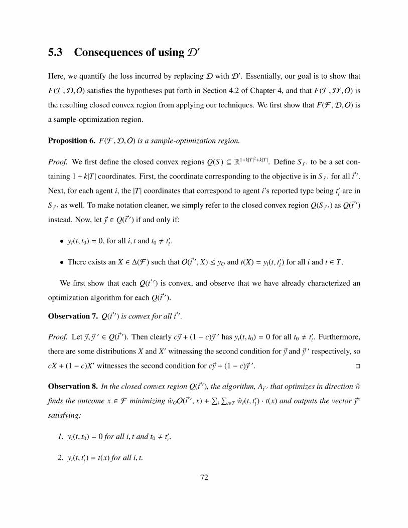
5.3 Consequences of using𝒟′

Here, we quantify the loss incurred by replacing 𝒟 with 𝒟′. Essentially, our goal is to show that

F(ℱ ,𝒟,𝒪) satisfies the hypotheses put forth in Section 4.2 of Chapter 4, and that F(ℱ ,𝒟′,𝒪) is

the resulting closed convex region from applying our techniques. We first show that F(ℱ ,𝒟,𝒪) is

a sample-optimization region.

Proposition 6. F(ℱ ,𝒟,𝒪) is a sample-optimization region.

Proof. We first define the closed convex regions Q(S ) ⊆ R1+k|T |2+k|T |. Define S ~t ′ to be a set con-

taining 1 + k|T | coordinates. First, the coordinate corresponding to the objective is in S ~t ′ for all ~t ′.

Next, for each agent i, the |T | coordinates that correspond to agent i’s reported type being t′i are in

S ~t ′ as well. To make notation cleaner, we simply refer to the closed convex region Q(S ~t ′) as Q(~t ′)

instead. Now, let ~y ∈ Q(~t ′) if and only if:

∙ yi(t, t0) = 0, for all i, t and t0 , t′i .

∙ There exists an X ∈ ∆(ℱ ) such that 𝒪(~t ′, X) ≤ yO and t(X) = yi(t, t′i ) for all i and t ∈ T .

We first show that each Q(~t ′) is convex, and observe that we have already characterized an

optimization algorithm for each Q(~t ′).

Observation 7. Q(~t ′) is convex for all ~t ′.

Proof. Let ~y, ~y ′ ∈ Q(~t ′). Then clearly c~y + (1 − c)~y ′ has yi(t, t0) = 0 for all t0 , t′i . Furthermore,

there are some distributions X and X′ witnessing the second condition for ~y and ~y ′ respectively, so

cX + (1 − c)X′ witnesses the second condition for c~y + (1 − c)~y ′.

Observation 8. In the closed convex region Q(~t ′), the algorithm, A~t ′ that optimizes in direction w

finds the outcome x ∈ ℱ minimizing wO𝒪(~t ′, x) +∑

i∑

t∈T wi(t, t′i ) · t(x) and outputs the vector ~yx

satisfying:

1. yi(t, t0) = 0 for all i, t and t0 , t′i .

2. yi(t, t′i ) = t(x) for all i, t.

72

3. yO = O(~t ′, x), if wO ≥ 0, or yO = ∞ if wO < 0.

Proof. The proof is immediate by the definition of Q(~t ′). We must have yi(t, t0) = 0 for all t0 , t′i .

Also, for whatever point ~y is chosen, there is some X ∈ ∆(ℱ ) witnessing ~y ∈ Q(~t ′). As ~y is a corner

w.l.o.g., X is in fact a point mass selecting some x ∈ ℱ with probability 1. Therefore, we must

have yi(t, t′i ) = t(x). Lastly, note we may set any value of yO ≥ O(~t ′, x) we choose. We want yO to

be as small as possible if wO ≥ 0, or as large as possible otherwise.

Notice now that the algorithm in Observation 8 looks familiar: it is exactly finding the outcome

x ∈ ℱ that optimizes a virtual objective. With this, we’re ready to complete our proof and show

that F(ℱ ,𝒟,𝒪) is a sample-optimization region.

Define a sample-optimization algorithm 𝒜 to sample ~t ′ ← 𝒟, and select the subset of coor-

dinates S ~t ′ . Observe now that for all coordinates (i, t, t′), Pr[(i, t, t′) ∈ S ~t ′] = Pr[t′ ← 𝒟i]. We

also know from Proposition 3 that the mechanism optimizing in direction ~w within F(ℱ ,𝒟,𝒪)

optimizes the virtual objective on every profile. By Observation 8, the optimization algorithm

for Q(~t ′) is exactly optimizing the virtual objective on profile ~t ′. If M is the mechanism op-

timizing the virtual objective corresponding to ~w on every profile, it is also easy to see that

πMi (t, t′) = E[(A~t ′((w~t ′ , 0−~t ′)))i(t, t′)] for all i, t, t′ and that πM

O = E[(A~t ′((w~t ′ , 0−~t ′)))O].

Now that we know that F(ℱ ,𝒟,𝒪) is a sample-optimization region, we’d like to make use of

Theorem 6. If 𝒟′ is a uniform distribution over samples from 𝒟, then it’s easy to see that taking

P = F(ℱ ,𝒟,𝒪) as in the statement of Theorem 6 results in P′ = F(ℱ ,𝒟′,𝒪). So we just need

to figure out how many samples we need to take for 𝒟′ in order for Theorem 6 to take effect. We

first remark that we can do some inconsequential rounding on the input probabilities and values to

BMeD which will aid in this.

Remark 6. We may without loss of generality assume the following about the input to a BMeD

instance without affecting the objective or truthfulness by more than an additive ε (and hence these

losses can be absorbed into the ε in the statement of Theorem 7):

1. All probabilities Pr[t ← 𝒟i] are at least ε/poly(k, |T |). To see this, observe that we can

modify any mechanism to first with probability ε/poly(k, |T |) ignore the type reported by

73

agent i and select for her a uniform random type instead. This modification does not affect

the truthfulness for agent i at all, but may affect truthfulness for other agents up to an additive

ε/poly(k, |T |), and may affect the objective by up to an additive ε/poly(k, |T |). We can then

view this new mechanism as just the original mechanism where the input comes from different

distributions with Pr[t ← 𝒟i] ≥ ε/poly(k, |T |). So consider any optimal mechanism M′ for

the rounded probability distributions. The reasoning above shows that the quality of M′ is at

most OPT + εk/poly(k, |T |). Furthermore, we have also argued that we can implement any

mechanism for the rounded distributions when agents are instead drawn from the original

distributions by resampling their type uniformly at random with probabilty ε/poly(k, |T |)

losing only an additional ε/poly(k, |T |) in truthfulness.

2. All values ti(x) are integer multiples of ε/poly(k). To see this, simply round every ti(x) down

to the nearest multiple of ε/poly(k) and treat this as the input instead. This can only affect the

truthfulness for agent i by up to an additive ε/poly(k), and the objective by up to an additive

ε/poly(k) and has no affect on the truthfulness of other agents. By the same reasoning as

the previous bullet, this means that the optimal mechanism M′ for the rounded values has

quality at most OPT + εk/poly(k). Furthermore, if M′′ is the mechanism that first rounds

the reported types, and then runs M′, then it’s clear that the truthfulness of M′′ is only

εk/poly(k) worse than the truthfulness of M′. And it’s also clear that the quality of M′′ is at

most εk/poly(k) worse than M′. This last statement holds whether or not M′ is optimal.

3. Both bullet points above suggest that we may first round the input distributions and values

as described, find a mechanism M′, and then apply some “unrounding” procedure to obtain

a mechanism M′′ for the original input. Both bullet points have argued that if M′ was

approximately optimal for the rounded input, then it is also approximately optimal for the

original input, up to an additional additive ε/poly(k, |T |). Furthermore, the total loss in both

truthfulness and quality from the procedure is bounded by ε/poly(k, |T |), and therefore can

be absorbed into the ε in the statement of Theorem 7.

With Remark 6 in mind, we can state formally the conclusion of this section below. Combined

with Corollary 5, this completes the proof of Theorem 7.

74

Proposition 7. Taking poly(1/ε, k, |T |) samples for 𝒟′ yields the following with probability 1 −

exp(poly(|T |, b, k, 1/ε)):

1. For all ~πMI ∈ F(ℱ ,𝒟,𝒪), there exists a ~π′

MI ∈ F(ℱ ,𝒟,𝒪) such that |~πM

I −~π′

MI |∞ ≤ ε.

2. Every mechanism M that optimizes a virtual objective on every profile has an implicit form

with respect to𝒟, ~πMI , and with respect to𝒟′, ~π′

MI satisfying |~π′

MI − ~π

′MI |∞ ≤ ε.

Proof. Both claims are immediate corollaries of Theorem 6 in Chapter 4 as long as we check

that we’ve taken enough samples. With Remark 6, all values of all agents for all outcomes are

integer multiples of ε/poly(k, |T |). As all the coordinates of all corners of each Q(~t ′) represent

the value of an agent for some outcome, this means that the corner complexity of each Q(~t ′)

is log(poly(k, |T |)/ε). Also by Remark 6, we may take the minimum probability Pr[t′ ← 𝒟i]

to be ε/poly(k, |T |). This means that the sample complexity of F(ℱ ,𝒟,𝒪) is bounded above by

poly(k, |T |)/ε. Therefore, b(F(ℱ ,𝒟,𝒪)) = poly(k, |T |, 1/ε). Plugging back into Theorem 6, this

means that forming𝒟′ with poly(k, |T |, 1/ε) samples from𝒟 suffices.

Proof of Theorem 7: With Proposition 7, it’s clear that OPT ′ ≤ OPT + ε. Combining this with

Corollary 5 proves the approximate optimality of the mechanism output. Also, as the implicit

form ~π′MI is BIC, Proposition 7 immediately guarantees that the implicit form ~πM

I is ε-BIC. The

remaining guarantees (that hold with probability 1) have already been shown in Corollary 5.

5.4 Instantiations of Theorem 7

In this section, we provide several instantiations of Theorem 7.

Revenue - Matching Markets. The designer has a single copy of each of m heterogeneous items

for sale to k unit-demand agents, and the goal is to maximize expected revenue. In this setting,

GOOP is simply asking for a max-weight matching in a bipartite graph with k agents on the left

and m items on the right. As GOOP can be solved exactly in poly-time, we obtain the following:

75

Theorem 8. There is a PTAS for revenue maximization in matching markets. For any desired

ε > 0, the output mechanism is ε-BIC, and has expected revenue at least OPT − ε with probability

at least 1 − exp(poly(b, |T |, k,m, 1/ε)). Furthermore, the output mechanism is feasible, and can

be implemented in time poly(b, |T |, k,m, 1/ε) with probability 1. The runtime of the algorithm is

poly(b, |T |, k,m, 1/ε). Furthermore, the allocation rule of the mechanism (randomly) assigns a

virtual value to each type of each agent for each item, and on every profile selects the matching

that maximizes virtual welfare.

Revenue - Arbitrary Feasibility Constraints. The designer has multiple copies of each of m

heterogenous goods for sale to k additive agents, and the goal is to maximize expected revenue.

Furthermore, there are feasibility constraints ℱ on which agents may simultaneously receive which

items. Formally, one may interpret ℱ ⊆ 2[k]×[m], and the set (i1, j1), . . . , (in, jn) ∈ ℐ as referencing

the fact that it is feasible to simultaneously award item j` to agent i` for all `. Note that this

generalizes matching markets where ℱ is the set of all matchings. In this setting, GOOP asks for

the maximum weight set S ∈ ℱ , where the weight of element (i, j) is the virtual value of agent i

for item j. Referring to this problem as MaxWeight(ℱ ), Theorem 7 implies the following:

Theorem 9. Let G be a poly-time α-approximation algorithm for MaxWeight(ℱ ). Then there is

an α-approximation algorithm for revenue maximization subject to feasibility constraints ℱ (for-

mally, BMeD(ℱ , additive functions with coefficients ti j ∈ [0, 1], revenue)). For any desired

ε > 0, the output mechanism is ε-BIC, and has expected revenue at least αOPT − ε with proba-

bility at least 1 − exp(poly(b, |T |, k,m, 1/ε)). Furthermore, the output mechanism is feasible, and

can be implemented in time poly(b, |T |, k,m, 1/ε) with probability 1. The runtime of the algorithm

is poly(b, |T |, k,m, 1/ε). Furthermore, the allocation rule of the mechanism (randomly) assigns a

virtual value to each type of each agent for each item, and on every profile runs G on the corre-

sponding virtual values.

A specific instantiation of Theorem 9 might have ℱ be the intersection of p matroids, in which

case we would take α = 1/p, or α = 1 for the case of p = 2.

76

Job Scheduling on Unrelated Machines. The designer has m jobs that he wishes to schedule

on k machines. The processing time of job j on machine i is ti j, and the goal is to minimize the

expected makespan. In this setting, GOOP is asking for a solution to the problem of makespan

minimization with costs. This problem is NP-hard to approximate within any finite factor, but a

poly-time (1, 1/2)-approximation exists and is developed in Chapter 7. Making use of this, we

obtain the following theorem.

Theorem 10. There is a polynomial-time 2-approximation algorithm for truthful job scheduling

on unrelated machines (formally the problem BMeD(0, 1km, additive functions with coefficients

ti j ∈ [0, 1], Makespan)). For any desired ε > 0, the output mechanism is ε-BIC, and has expected

makespan at most 2OPT + ε with probability at least 1− exp(poly(b, k,m, 1/ε)). Furthermore, the

output mechanism is feasible, and can be implemented in time poly(b, k,m, 1/ε) with probability 1.

The runtime of the algorithm is poly(b, k,m, 1/ε).

Fair Allocation of Indivisible Goods. The designer has m gifts that he wishes to award to k

children. Each child i has a value of ti j for item j, and the goal is to maximizes the expected

fairness. In this setting, GOOP is asking for a solution to the problem of fairness maximiza-

tion with costs. This problem is NP-hard to approximate within any finite factor, but a poly-time

(1,minO(√

k),m−k +1)-approximation exists and is developed in Chapter 7. Making use of this,

we obtain the following theorem.

Theorem 11. There is a polynomial-time minO(√

k),m − k + 1-approximation algorithm for

truthful fair allocation of indivisible goods (formally the problem BMeD(0, 1km, additive func-

tions with coefficients ti j ∈ [0, 1], Fairness)). For any desired ε > 0, the output mechanism is

ε-BIC, and has expected fairness at least minO(√

k),m − k + 1OPT − ε with probability at least

1−exp(poly(b, k,m, 1/ε)). Furthermore, the output mechanism is feasible, and can be implemented

in time poly(b, k,m, 1/ε) with probability 1. The runtime of the algorithm is poly(b, k,m, 1/ε).

77

78

Chapter 6

Equivalence of Separation and

Optimization

In this section we detail a general tool in linear programming, colloquially called “The Equivalence

of Separation and Optimization.” A well-known result of Khachiyan (Theorem 1 in Section 2.3

of Chapter 2) states that, given black-box access to a separation oracle for any d-dimensional

closed convex region P, linear functions can be optimized over P in time polynomial in d and

the runtime of the separation oracle. A lesser-known result of Grötschel, Lovász, and Schrijver

and independently Karp and Papadimitriou [GLS81, KP80] states that the converse holds as well:

given black-box access to an optimizer of linear functions over any d-dimensional closed convex

region P, one can obtain a separation oracle for P that runs in time polynomial in d and the runtime

of the optimizer. In other words, the problems of separation and optimization are computationally

equivalent.

While Khachiyan’s result has obvious implications for solving linear programs, it’s less clear

that the converse has a practical use. After all, the most common usage of separation oracles is as

a means to optimize linear functions, so why would we ever want to obtain a separation oracle if

we already had an algorithm for optimization? One compelling use of the converse is to optimize

linear functions over the intersection of two convex regions, P and Q. The ability to optimize

linear functions over P and Q separately tells us absolutely nothing about how to optimize over

79

P∩Q, but it does allow us to get a separation oracle for both P and Q (via the converse). This then

immediately gives us a separation oracle for P∩Q (simply run the separation oracle for P followed

by the separation oracle for Q if P accepts), and Khachiyan’s ellipsoid algorithm then allows us

to optimize over P ∩ Q. There are indeed other uses of separation oracles beyond optimization,

including the decomposition algorithm outlined in Theorem 3 of Section 2.3 in Chapter 2, the first

poly-time algorithm for submodular minimization [GLS81], and numerous others [GLS81, KP80].

In Section 6.1 we provide a very similar proof of the exact equivalence to the one given

in [GLS81] in order to acclimate the reader with these techniques. In Sections 6.2 we extend

the equivalence to be robust to traditional and bicriterion approximations and in 6.3 we extend the

equivalence to be robust to sampling error.

6.1 Exact Optimization

Here we provide a proof of the original equivalence of separation and optimization (stated as

Theorem 2 in Section 2.3 of Chapter 2) so that the reader is familiar with these techniques. Our

extensions will follow a similar approach but require more technical tools.

Proof of Theorem 2: Because P is a closed convex region, we know that ~x ∈ P if and only if

~x · ~w ≤ max~y∈P~y · ~w for all directions ~w ∈ Rd. In fact, the same is true even if we consider only

normalized ~w ∈ [−1, 1]d. So we can try to write a program to search over all ~w ∈ Rd for one that is

violated by ~x as in Figure 6-1:

Lemma 2. The linear program of Figure 6-1 has value > 0 if and only if ~x < P.

Proof. First, assume that ~x < P. Then there is some direction ~w ∈ [−1, 1]d such that ~x · ~w >

max~y∈P~y · ~w. Then consider setting t = max~y∈P~y · ~w, and the point (~w, t). It is clear that this point

is feasible, and also that ~x · ~w > t. So (~w, t) bears witness that the value of the linear program is

> 0.

Now, assume that the value of the linear program is > 0, and consider the point ~w, t witnessing

this. Then we clearly have ~x · ~w > t, as the value of the LP is > 0. And because (~w, t) is feasible,

80

Variables:

∙ ~w, a d-dimensional direction.

∙ t, a helper variable used to bound max~y∈P~y · ~w.

Constraints:

∙ ~w ∈ [−1, 1]d, guaranteeing that the entries of ~w have been normalized.

∙ t ≥ ~y · ~w ∀~y ∈ P, guaranteeing that t correctly bounds max~y∈P~y · ~w.

Maximizing:

∙ ~x · ~w − t, the gap between ~x · ~w and max~y∈P~y · ~w.

Figure 6-1: A linear programming formulation to find a violated hyperplane.

we must also have t ≥ max~y∈P~y · ~w. Putting these together, we have found a direction ~w such that

~x · ~w > max~y∈P~y · ~w, and therefore ~x < P.

In light of Lemma 2, we just need to solve the linear program of Figure 6-1 efficiently. Un-

fortunately, there are infinitely many constraints of the form t ≥ ~y · ~w, so we can’t hope to list

them all explicitly. Instead, we will define an efficient separation oracle for these constraints, S O.

Observe that if any constraint of the form t ≥ ~y · ~w is violated for some ~y ∈ P, then certainly

t ≥ argmax~y∈P~y · ~w is also violated. So rather than check each constraint, S O simply checks

this single constraint. And finally, we can actually find argmax~y∈P~y · ~w by simply running the

optimization algorithm𝒜 in direction ~w. Figure 6-2 details explicitly this approach.

Putting everything back together, the complete approach is the following. First, solve the LP

in Figure 6-2. By the reasoning above, this is also a solution to the LP in Figure 6-1. Finally, by

Lemma 2, if (~w*, t*) denotes the solution output, we either have ~x · ~w* ≤ t*, and ~x ∈ P, or ~x · ~w* > t*,

but ~y · ~w* ≤ t for all ~y ∈ P, and therefore (~w*, t) is a violated hyperplane.

81

Variables:

∙ ~w, a d-dimensional direction.

∙ t, a helper variable used to bound max~y∈P~y · ~w.

Constraints:

∙ ~w ∈ [−1, 1]d, guaranteeing that the entries of ~w have been normalized.

∙ S O(~w, t) =

– “yes” if t ≥ 𝒜(~w) · ~w;

– the violated hyperplane t′ ≥ 𝒜(~w) · ~w′ otherwise.

Maximizing:

∙ ~x · ~w − t, the gap between ~x · ~w and max~y∈P~y · ~w.

Figure 6-2: A reformulation of Figure 6-1 using a separation oracle.

6.2 Multiplicative Approximations

In this section we detail how to extend the equivalence of separation and optimization to accommo-

date a multiplicative bi-criterion approximation error that we call (α, β)-approximations (defined

in Section 4.2 of Chapter 4). We remind the reader that this section’s main theorem (Theorem 5 in

Section 4.2 of Chapter 4) states that an (α, β, S )-approximation algorithm for closed convex region

P can be used to obtain a weird separation oracle (WSO) for αP. We call the separation oracle

weird because it behaves kind of like a separation oracle in that in sometimes says “yes” and some-

times outputs hyperplanes, but the set of points accepted by the separation oracle isn’t necessarily

closed, convex or even connected.

We prove Theorem 5 for minimization algorithms, noting that the proof for maximization al-

gorithms is nearly identical after switching ≤ for ≥ and min for max where appropriate. The proof

is a series of five lemmas, one for each property, plus a technical lemma (Lemma 6). We begin by

defining our weird separation oracle in Figure 6-3. Throughout this section, b denotes an upper

bound on the bit complexity of ~y, and ` an upper bound on the bit complexity of𝒜βS (~w) for all ~w.

Lemma 3. If𝒜βS is an (α, β, S )-minimization algorithm for the closed convex region P, then every

82

WS O(~y) =

∙ “Yes” if the ellipsoid algorithm with N iterations (N = poly(d, b, `)) outputs “infeasible”on the following problem:

variables: ~w, t;constraints:

– ~w ∈ [−1, 1]d;

– t ≥ ~y · ~w + δ (δ = 2−poly(d,b,`));

– WS O(~w, t) =

* “yes” if t ≤ 𝒜βS (~w) · ~w;a

* the violated hyperplane t′ ≤ 𝒜βS (~w) · ~w′ otherwise.

∙ If a feasible point (t*, ~w*) is found, output the violated hyperplane ~w* · ~x ≤ t*.

aNotice that the set (~w, t)|WS O(~w, t) = “Yes” is not necessarily closed, convex or even connected.

Figure 6-3: A weird separation oracle.

halfspace output by WS O contains αP.

Proof. If WS O outputs a halfspace (~w*, t*), then we must have WS O(~w*, t*) = “yes”, implying

that t* ≤ 𝒜βS (~w*) · ~w*. Because 𝒜 is an (α, β, S )-approximation, we know that 𝒜β

S (~w*) · ~w* ≤

αmin~x∈P~x · ~w* = min~x∈αP~x · ~w*. Therefore, every ~x ∈ αP satisfies t* ≤ ~w* · ~x, and the halfspace

contains αP.

Lemma 4. On input ~y, WS O terminates in time poly(d, b, `, runtime𝒜(poly(d, b, `))) and makes at

most poly(d, b, `) queries to𝒜.

Proof. By Theorem 1, it is clear that WS O is queried at most poly(N, d, b, `, BC(δ)) times, where

BC(δ) is the bit complexity of δ. Each execution of WS O makes one call to𝒜. So the total runtime

is clearly as desired.

Lemma 5. Let Q be an arbitrary convex region in Rd described via some separation oracle, and

OPT = min~y∈αP∩Q~c · ~y for some vector ~c. Let also ~z be the output of the Ellipsoid algorithm

for minimizing ~c · ~y over ~y ∈ αP ∩ Q, but using WS O as a separation oracle for αP instead of a

standard separation oracle (i.e. use the exact parameters for the Ellipsoid algorithm as if WS O

83

was a valid separation oracle for αP, and still use a standard separation oracle for Q). Then

~z · ~c ≤ OPT.

Proof. When the Ellipsoid algorithm tries to minimize ~c · ~x, it does a binary search over possible

values C, and checks whether or not there is a point ~x satisfying ~x · ~c ≤ C, ~x ∈ Q, and WS O(~x) =

“yes”. If there is a point ~x satisfying ~x · ~c ≤ C, ~x ∈ Q, and ~x ∈ αP, then clearly every halfspace

output by the separation oracle for Q contains ~x, and so does the halfspace ~y · ~c ≤ C. Furthermore,

by Lemma 3, every halfspace output by WS O contains ~x as well. Therefore, if OPT ≤ C, the

Ellipsoid algorithm using WS O will find a feasible point and continue its binary search. Therefore,

the algorithm must conclude with a point ~z satisfying ~z · ~c ≤ OPT .

Lemma 6. Let W be any set of directions ~w′. Then the following closed convex region (P(W)) is

either empty, or has volume at least 2−poly(d,b,`):

t − ~x · ~w ≥ δ

t ≤ 𝒜βS (~w′) · ~w, ∀~w′ ∈ W

~w ∈ [−1, 1]d

Proof. First, it will be convenient to add the vacuous constraint t ≤ d to the definition of the

closed convex region. It is vacuous because it is implied by the existing constraints, but useful for

analysis. Define P′(W) by removing the first constraint. That is, P′(W) is the intersection of the

following halfspaces:

t ≤ d

t ≤ 𝒜βS (~w′) · ~w, ∀~w′ ∈ W

~w ∈ [−1, 1]d

If there is a point in P(W), then there is clearly a corner (t*, ~w*) of P′(W) in P(W) as well. As

all constraints in P′(W) have bit complexity b, we must have t* − ~x · ~w* ≥ γ, with γ = 2−poly(d,b,`).

Let δ = γ/4. Therefore, the point (t*/2, ~w*/2) is also clearly in P(W), and satisfies t* − ~x · ~w* ≥ 2δ.

84

Now, consider the box B = (×di=1[w*i

2 ,w*i2 + δ

2d ])× [ t*2 −δ,

t*2 −

δ2 ]. We claim that we have B ⊆ P(W)

as well. Let (t, ~w) denote an arbitrary point in B. It is clear that we have ~w ∈ [−1, 1]d still, as we

had ~w*/2 ∈ [−1/2, 1/2]d to start with. As each coordinate of ~x and 𝒜βS (~w′) for all ~w′ is in [−1, 1],

it is easy to see that:

(~w*/2) · ~x −δ

2≤ ~w · ~x ≤ (~w*/2) · ~x +

δ

2

(~w*/2) · 𝒜βS (~w′) −

δ

2≤ ~w · 𝒜β

S (~w′) ≤ (~w*/2) · 𝒜βS (~w′) +

δ

2∀~w′ ∈ W

As we must have t ≤ t*2 −

δ2 , and we started with t* ≤ ~w* · 𝒜β

S (~w′) for all ~w′ ∈ W, it is clear that

we still have t ≤ ~w · 𝒜βS (~w′) for all ~w′ ∈ W. Finally, since we started with t*/2 − ~x · ~w*/2 ≥ 2δ, and

t ≥ t*/2 − δ, we still have t − ~x · ~w ≥ δ.

Now, we simply observe that the volume of B is δd+1

dd2d+1 , which is 2−poly(d,b,`). Therefore, if P(W)

is non-empty, it contains this box B, and therefore has volume at least 2−poly(d,b,`).

Lemma 7. Whenever WS O(~y) = “yes” for some input ~y, the execution of WS O explicitly finds

directions ~w1, . . . , ~wd+1 such that ~y ∈ Conv𝒜βS (~w1), . . . ,𝒜β

S (~wd+1).

Proof. Consider the intersection of halfspaces P(W) as in the statement of Lemma 6.

If ~y < Conv(𝒜βS (~w)|~w ∈ W), there exists some weight vector ~w* ∈ [−1, 1]d such that ~y ·

~w* < min~w∈W𝒜βS (~w) · ~w*. And for appropriately chosen δ = 2−poly(d,b,`), we also have ~y · ~w* ≤

min~w∈W𝒜βS (~w) · ~w* − δ.

So if ~y < Conv(𝒜βS (~w)|~w ∈ W), consider the point ~w*, t*, with t* = min~w∈W𝒜

βS (~w) · ~w*. By

the reasoning in the previous paragraph, it’s clear that (~w*, t*) is in P(W).

So consider an execution of WS O that accepts the point ~y. Then taking W to be the set of

directions ~w queried by the Ellipsoid algorithm during the execution of WS O, P(W) is exactly the

closed convex region of halfspaces that the Ellipsoid algorithm maintained. Because we did N

iterations of the algorithm, and the volume of the maintained closed convex region decreases by a

multiplicative factor of 1 − 1/poly(d) at each iteration, taking N to be a large enough poly(d, b, `)

implies that the volume of P(W) is at most 2−poly(d,b,`) for any desired polynomial. So taking N

sufficiently large would mean that the volume of P(W) is in fact smaller than the 2−poly(d,b,`) in

85

the statement of Lemma 6, and therefore P(W) must be empty. This necessarily means that ~y ∈

Conv(𝒜βS (~w)|~w ∈ W), as otherwise the previous paragraphs prove that the above intersection of

halfspaces wouldn’t be empty.

So we may take ~w1, . . . , ~wd+1 to be (an appropriately chosen subset of) the directions queried

by the Ellipsoid algorithm during the execution of WS O and complete the proof of the lemma.

Proof of Theorem 5: Combine Lemmas 3, 4, 5, and 7.

6.3 Sampling Approximation

In this section we show how to extend the equivalence of separation and optimization to accom-

modate sampling error in an optimization algorithm over certain kinds of closed convex regions.

Our approach is quite different from the previous section in that we directly show that these cer-

tain kinds of closed convex regions can be approximated well by simpler closed convex regions

that are easier to optimize over. Recall that definitions of sample-optimization algorithms and

sample-optimization regions were given in Section 4.2 of Chapter 4.

For a given sample-optimization region P and sample-optimization algorithm 𝒜, denote as in

Section 4.2 of Chapter 4 by D the distribution from which S is sampled. If we could just enumerate

the support of D, then we could compute exactly E[𝒜(~w)i|i ∈ S ] for all i, and this would give us

z*i . So we can use𝒜 to obtain an exact optimization algorithm for P, but in potentially exponential

time. A natural approach is to just take polynomially many samples from D to get an additive

approximation, but unfortunately the equivalence of separation and optimization framework cannot

accommodate additive approximation error unless it is exponentially small (smaller than what can

be guaranteed by sampling). Instead, we take polynomially many samples from D once and for

all, let D′ be the uniform distribution over these samples, and define a new closed convex region

using D′ and𝒜.

We can now consider instead the sample-optimization algorithm𝒜′ that first samples a subset

S ′ from D′ instead of D. Because we can explicitly enumerate the support of D′, we can compute

exactly the expected value E[𝒜′(~w)i|i ∈ S ′]. But we need to guarantee that this is close to the orig-

86

inal expectation, for all ~w. Henceforth, we overload notation and refer to the algorithm that runs

𝒜′(~w), then enumerates the support of D′ and computes exactly the expected value E[𝒜′(~w)i|i ∈ S ′]

for all coordinates as𝒜′ instead.

We show that 𝒜′ is a useful algorithm by claiming that in fact, 𝒜′ is an exact optimization

algorithm for a different closed convex region P′. Therefore, we can use the equivalence of sepa-

ration and optimization with respect to the closed convex region P′ with no issues. After this, the

remaining task is showing that P and P′ are similar closed convex regions with high probability.

Without this, being able to optimize and separate over P′ is useless. Section 6.3.1 shows that 𝒜′

does indeed define a closed convex region P′. Sections 6.3.2 and 6.3.3 show that P and P′ are

similar regions.

6.3.1 𝒜′ Defines a Closed Convex Region

In this section, we show that𝒜′ is an exact optimization algorithm for some closed convex region

P′, which we describe now. Let ~y(X)X⊆[d] be an collection of vectors with each ~y(X) ∈ Q(X).

Q(X) are the closed convex regions used in the definition of a sample-optimization algorithm. Let

then ~y be the vector with yi =∑

X Pr[S ′ = X|i ∈ S ′]y(X)i. Define P′ to be the set of all ~y that can be

obtained this way. We begin with a quick observation that gives context to why we define P′ this

way:

Observation 9. 𝒜′(~w)i =∑

X Pr[S ′ = X|i ∈ S ′]AX((wX, 0−X)).

Proof. The right hand side exactly computes the expected value of 𝒜′(~w)i conditioned on i ∈

S ′.

To give context to P′, we are essentially defining the space of points resulting from replacing

AX((wX, 0−X)) with any point in Q(X). We now prove that P′ is a closed convex region.

Observation 10. P′ is closed and convex.

Proof. Take any two points ~y,~z ∈ P′. Then there exist some ~y(X),~z(X) ∈ Q(X) such that yi =∑X Pr[S ′ = X|i ∈ S ′]y(X)i and zi =

∑X Pr[S ′ = X|i ∈ S ′]z(X)i. As Q(X) is convex, we also have

cy(X) + (1 − x)z(X) ∈ Q(X), and such a point clearly satisfies

87

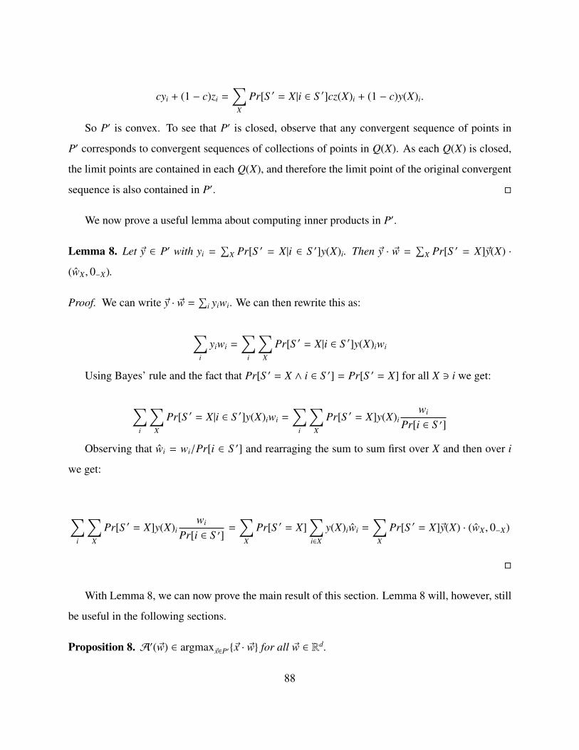
cyi + (1 − c)zi =∑

X

Pr[S ′ = X|i ∈ S ′]cz(X)i + (1 − c)y(X)i.

So P′ is convex. To see that P′ is closed, observe that any convergent sequence of points in

P′ corresponds to convergent sequences of collections of points in Q(X). As each Q(X) is closed,

the limit points are contained in each Q(X), and therefore the limit point of the original convergent

sequence is also contained in P′.

We now prove a useful lemma about computing inner products in P′.

Lemma 8. Let ~y ∈ P′ with yi =∑

X Pr[S ′ = X|i ∈ S ′]y(X)i. Then ~y · ~w =∑

X Pr[S ′ = X]~y(X) ·

(wX, 0−X).

Proof. We can write ~y · ~w =∑

i yiwi. We can then rewrite this as:

∑i

yiwi =∑

i

∑X

Pr[S ′ = X|i ∈ S ′]y(X)iwi

Using Bayes’ rule and the fact that Pr[S ′ = X ∧ i ∈ S ′] = Pr[S ′ = X] for all X ∋ i we get:

∑i

∑X

Pr[S ′ = X|i ∈ S ′]y(X)iwi =∑

i

∑X

Pr[S ′ = X]y(X)iwi

Pr[i ∈ S ′]

Observing that wi = wi/Pr[i ∈ S ′] and rearraging the sum to sum first over X and then over i

we get:

∑i

∑X

Pr[S ′ = X]y(X)iwi

Pr[i ∈ S ′]=

∑X

Pr[S ′ = X]∑i∈X

y(X)iwi =∑

X

Pr[S ′ = X]~y(X) · (wX, 0−X)

With Lemma 8, we can now prove the main result of this section. Lemma 8 will, however, still

be useful in the following sections.

Proposition 8. 𝒜′(~w) ∈ argmax~x∈P′~x · ~w for all ~w ∈ Rd.

88

Proof. By definition, every ~y ∈ P′ has some corresponding ~y(X) ∈ Q(X) with yi =∑

X Pr[S ′ =

X|i ∈ S ′]y(X)i. By Lemma 8, we know that ~y · ~w =∑

X Pr[S ′ = X]~y(X) · (wX, 0−X).

By Observation 9, we know that 𝒜′(~w)i =∑

X Pr[S ′ = X|i ∈ S ′]AX((wX, 0−X)), and therefore

𝒜′(~w) · ~w =∑

X Pr[S ′ = X]AX((wX, 0−X)) · (wX, 0−X) as well by Lemma 8. By definition, AX is

an exact optimization algorithm for Q(X), and ~y(X) ∈ Q(X), so we clearly have AX((wX, 0−X)) ·

(wX, 0−X) ≥ ~y(X) · (wX, 0−X) for all X. Therefore,𝒜′(~w) · ~w ≥ ~y · ~w.

As this holds for any ~y ∈ P′, the proposition is proved.

6.3.2 Every point in P is close to some point in P′

In this section, we use the following Theorem due to Hoeffding [Hoe63]. We also w.l.o.g. assume

that each Q(S ) ⊆ [0, 1]d (recall that we originally assumed that Q(S ) ⊆ [0, poly(d)]d. This further

assumption simply costs us an extra poly(d) factor, but makes analysis simpler).

Theorem 12. ([Hoe63]) Let X1, . . . , Xn be independent random variables in [0, 1] and let X =∑i Xi/n. Then Pr[|X − E[X]| > t ≤ 2e−2t2n.

We first show that a fixed ~y ∈ P is likely to be close to some ~y ∈ P′, so long as enough

samples are taken for D′. This will be a consequence of two simple lemmas: the first shows

that, conditioned on enough S ′ in the support of D′ containing i, yi is likely to be close to y′i .

The second shows that we are likely to sample enough S ′ containing i. Following the work in

Section 6.3.1, it’s easy to see now that any ~y ∈ P can also be written using ~y(X) ∈ Q(X) and

yi =∑

X Pr[S = X|i ∈ S ]y(X)i. We call such ~y(X) an implementation (with respect to D, if ~y ∈ P,

or with respect to D′ if ~y ∈ P′). What we will show is that the implementation of ~y with respect to

D bears witness that some ~y ′ ∈ P is very close to ~y. For the remainder of this section, for a given

~y, define ~y ′ to have the same implementation as ~y, but with respect to D′ instead of D.

Lemma 9. Fix i ∈ [d] and any ~y ∈ P. Condition on D′ so that |S ′ ∈ support(D′)|i ∈ S ′| = x.

Then over the randomness in generating D′ (conditioned on this), we have Pr[|y′i−yi| > t] ≤ 2e−2t2 x.

Proof. Let S j be the jth subset in the support of D′ with i ∈ S j. And let X j = y(X j)i. Then

y′i =∑

j X j/x, the X j are independent and in [0, 1], and each E[X j] = yi. Therefore, Hoeffding’s

89

inequality immediately yields the lemma.

In the lemma below, recall that b(P) is the sample complexity of P, which is maxi1/Pr[i ∈ S ]

for some corresponding sample-optimization algorithm𝒜.

Lemma 10. Fix i ∈ [d], and let xb(P) samples be taken for D′. Let Ni denote the number of sets in

the support of D′ containing i. Then:

Pr[Ni ≤ x/2] ≤ 2e−x

2b(P)

Proof. Let X j be the indicator random variable of whether or not the jth sample for D′ contains

i. Then Ni =∑

j X j, and E[Ni] ≥ x. So in order to have Ni ≤ x/2, we would also need Nixb(P) ≤

E[ Nixb(P) ] −

12b(P) . Plugging this into the Hoeffding inequality yields the desired bound.

Corollary 6. Fix any ~y ∈ P, and let 2xb(P)2 samples be taken for D′. Then:

Pr[|~y − ~y ′|∞ > t] ≤ 4de−t2 x

Proof. Lemma 10 and a union bound guarantees that we will have all Ni > x with probability at

least 1 − 2de−x. A union bound combined with Lemma 9, conditioned on this, guarantees that for

all i, |y′i − yi| ≤ t with probability at least 1 − 2de−2t2 x. Taking a union bound over both of these

events proves the corollary.

Corollary 7. Let 2xb(P)2d ln(1/t) samples be taken for D′. Then with probability at least 1 −

4de−t2 x, all ~y ∈ P have some ~y ′ ∈ P′ satisfying |~y − ~y ′|∞ ≤ 2t.

Proof. Consider an t-`∞ cover of P such that every point in P is within `∞ distance t of a point in

the cover. There is certainly a cover that uses at most(

1t

)dpoints, as there is a cover of the entire

hypercube using this many points. If for every point ~x in the cover, there is a point~z ∈ P′, such that

|~x − ~z|∞ ≤ 2t, then clearly for every point ~y in P, there is a point ~y ′ ∈ P′ such that |~y − ~y ′|∞ ≤ 2t

by the triangle inequality. So we simply take a union bound over all e−d ln t points in the cover and

apply Corollary 6 to conclude the proof.

90

6.3.3 Every point in P′ is close to some point in P

In the previous section, we showed that for all ~y ∈ P there is a nearby ~y ′ ∈ P′ over the randomness

in the choice of D′. In this section, we want to show the other direction, namely that for any ~y ′ ∈ P′

there is a nearby ~y ∈ P. However, it is not clear how to use the randomness over the choice of D′

to prove this, as for any ~y ′ ∈ P′, the implementation of ~y ′ is heavily dependent on D′ itself, which

is the object whose randomness we hope to use. To go around this circularity we show that after

fixing the number of samples for D′, but before actually selecting them, there are not too many

implementations that could possibly yield a corner of P′. So we aim to take a union bound over

all such implementations, showing that they yield vectors that are close with respect to D and D′.

As every point in P′ is a convex combination of the corners of P′, this suffices to prove the desired

claim. Our starting point is the following observation.

Lemma 11. Let N be such that all corners of all Q(S ) have coordinates that are integer multiples

of 1/N, and x be the number of samples taken for D′. Then every corrner of P′ has bit complexity

O(log x + log N).

Proof. Recall that every corner ~y ′ of P′ has a corresponding implementation such that y′i =∑X Pr[S ′ = X|i ∈ S ′]y(X)i, where each ~y(X) is a corner of Q(X). So each y(X)i is an integer

multiple of 1/N, and each probability is an integer multiple of 1/x because D′ is a uniform dis-

tribution over x sets. So each y′i will have a denominator of xN and a numerator at most xN, and

therefore has bit complexity O(log x + log N).

Given Lemma 11 the corners of P′ belong to a set of at most 2O(d(log x+log N)) vectors, independent

of D′. Still, the implementation of those vectors may vary depending on D′. We show that this can

be mitigated by appealing to the direction in which each corner is an extreme point.

Lemma 12. Suppose that ~y is the corner of a closed convex region P′ and that the corners of

P′ have bit complexity at most b. Then there exists a ~w of bit complexity poly(b, d) such that

~y = argmax~x∈P′~x · ~w.

Proof. Let P′0 denote the convex hull of all corners of P′ excluding ~y, and consider solving (for-

getting about computational efficiency, this is just an existence argument) the linear program of

91

Figure 6-2 from Section 6.1 using P′0 as the closed convex region and ~y as point to test. Clearly,

~y < P′0, so we will necessarily find a violating hyperplane. That is, we will find a direction ~w

such that ~w · ~y > max~x∈P′0~x · ~w. As exact optimization algorithms always output corners, every

hyperplane ever considered by the linear program has coefficients of bit complexity b. Therefore,

by Theorem 1, the output vector ~w has bit complexity poly(b, d).

With Lemma 12, we know now that every corner ~y ′ of P′ has an associated direction ~w of

poly(b, d) bit complexity and~y ′ can be implemented by having~y ′(X) = argmax~x∈Q~x·(wX, 0−X) for

all X. As Pr[i ∈ S ′] is an integer multiple of 1/x for all i, w also has bit complexity poly(b, d, log x).

Therefore, before we have sampled D′, but after we have chosen |D′|, there is a fixed set of at most

2poly(d,b,log x) implementations that can possibly result in a corner of D′. From here, we are ready to

take a union bound over all such implementations and complete the proof.

Corollary 8. Let 2xb(P)2 samples be taken for D′ and x = poly(d, t, b(P)2, b) be sufficiently large.

Then with probability at least 1 − 4de−t2 x/2, for all ~y ′ ∈ P′, there exists a ~y ∈ P with |~y − ~y ′|∞ ≤ t.

Furthermore, the same implementation that yields ~y ′ with respect to D′ yields ~y with respect to D.

Proof. We know from Corollary 6 that for any fixed implementation of ~y ∈ P with respect to D,

that same implementation yields a ~y ′ ∈ P′ with |~y − ~y ′|∞ ≤ t with probability at least 1 − 4de−t2 x.

We now want to take a union bound over all 2poly(d,b,log(2xb(P)2) implementations that can possibly

result in corners of P′ and claim that they all satisfy this property. Notice that both terms get larger

with x: as we decrease the probability of error, we need to take a union bound over more and more

implementations. However, notice that the exponent of the error probability increases linearly

with x, while the exponent of the number of terms we need to take a union bound over grows

polylogarithmically in x. Therefore, if we let x grow sufficiently large (polynomial in t, d, b, b(P)

suffices), we will have poly(d, b, log(2xb(P)2) < t2x/2. When this happens, we get the desired

guarantee.

Proof of Theorem 6: That P′ is a sample-optimization region is an immediate consequence of

Proposition 8 from Section 6.3.1. Taking t = ε, the first listed property of P′ is an immediate

92

consequence of Corollary 7 from Section 6.3.2. The second property is an immediate consequence

of Corollary 8 above (again taking t = ε).

93

94

Chapter 7

(α, β)-Approximation Algorithms for

Makespan and Fairness

Here, we design algorithms for scheduling unrelated machines with costs and fair allocation of

indivisible goods with costs and show that they imply mechanisms for scheduling unrelated ma-

chines and fair allocation of indivisible goods using the reduction of Chapter 5.

Theorems 10 and 11 in Chapter 5 are immediate corollaries of Theorem 7 combined with

Theorem 13 or Theorem 15.

7.1 Preliminaries

Here we define the problems of scheduling unrelated machines with costs and fair allocation of

indivisible goods with costs (noting that their versions without costs may simply set all costs to 0

in the definition).

Scheduling Unrelated Machines with Costs. There are k machines and m indivisible jobs. Each

machine i can process job j in time ti j ≥ 0. Additionally, processing job j on machine i costs ci j

units of currency, where ci j is unrestricted and in particular could be negative. An assignment of

jobs to machines is a km-dimensional vector ~x such that xi j ∈ 0, 1, for all i and j, where job j

is assigned to machine i iff xi j = 1. We denote by M(~x) = maxi∑

j xi jti j the makespan of an

95

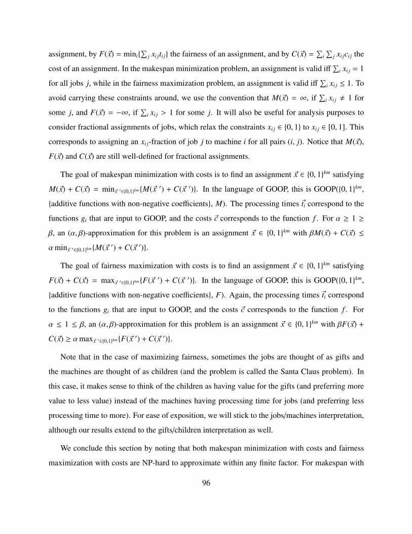
assignment, by F(~x) = mini∑

j xi jti j the fairness of an assignment, and by C(~x) =∑

i∑

j xi jci j the

cost of an assignment. In the makespan minimization problem, an assignment is valid iff∑

i xi j = 1

for all jobs j, while in the fairness maximization problem, an assignment is valid iff∑

i xi j ≤ 1. To

avoid carrying these constraints around, we use the convention that M(~x) = ∞, if∑

i xi j , 1 for

some j, and F(~x) = −∞, if∑

i xi j > 1 for some j. It will also be useful for analysis purposes to

consider fractional assignments of jobs, which relax the constraints xi j ∈ 0, 1 to xi j ∈ [0, 1]. This

corresponds to assigning an xi j-fraction of job j to machine i for all pairs (i, j). Notice that M(~x),

F(~x) and C(~x) are still well-defined for fractional assignments.

The goal of makespan minimization with costs is to find an assignment ~x ∈ 0, 1km satisfying

M(~x) + C(~x) = min~x ′∈0,1kmM(~x ′) + C(~x ′). In the language of GOOP, this is GOOP(0, 1km,

additive functions with non-negative coefficients, M). The processing times ~ti correspond to the

functions gi that are input to GOOP, and the costs ~c corresponds to the function f . For α ≥ 1 ≥

β, an (α, β)-approximation for this problem is an assignment ~x ∈ 0, 1km with βM(~x) + C(~x) ≤

αmin~x ′∈0,1kmM(~x ′) + C(~x ′).

The goal of fairness maximization with costs is to find an assignment ~x ∈ 0, 1km satisfying

F(~x) + C(~x) = max~x ′∈0,1kmF(~x ′) + C(~x ′). In the language of GOOP, this is GOOP(0, 1km,

additive functions with non-negative coefficients, F). Again, the processing times ~ti correspond

to the functions gi that are input to GOOP, and the costs ~c corresponds to the function f . For

α ≤ 1 ≤ β, an (α, β)-approximation for this problem is an assignment ~x ∈ 0, 1km with βF(~x) +

C(~x) ≥ αmax~x ′∈0,1kmF(~x ′) + C(~x ′).

Note that in the case of maximizing fairness, sometimes the jobs are thought of as gifts and

the machines are thought of as children (and the problem is called the Santa Claus problem). In

this case, it makes sense to think of the children as having value for the gifts (and preferring more

value to less value) instead of the machines having processing time for jobs (and preferring less

processing time to more). For ease of exposition, we will stick to the jobs/machines interpretation,

although our results extend to the gifts/children interpretation as well.

We conclude this section by noting that both makespan minimization with costs and fairness

maximization with costs are NP-hard to approximate within any finite factor. For makespan with

96

costs, this can be seen via a simple modification of an inapproximability result given in [LST87].

For the problem of scheduling unrelated machines, they construct instances with integer-valued

makespan that is always ≥ 3 and such that it is NP-hard to decide whether the makespan is 3

or ≥ 4. We can modify their instances to scheduling unrelated machines with costs instances by

giving each job a cost of z−32n+m on every machine for an arbitrary z > 0. Then the total cost of any

feasible solution is exactly z − 3. So their proof immediately shows that it is NP-hard to determine

if these instances have optimal makespan + cost that is z or ≥ 1 + z. Since z was arbitrary, this

shows that no finite approximation factor is possible.

For fairness with costs, Bezakova and Dani [BD05] present a family of max-min fairness in-

stances such that it is NP-hard to distinguish between OPT ≥ 2 and OPT ≤ 1. To each of these

instances add a special machine and a special job such that the processing time and cost of the

special machine for the special job are 2 and −1 respectively, while the processing time and cost of

the special machine for any non-special job or of any non-special machine for the special job are

0 and 0 respectively. Also, assign 0 cost to any non-special machine non-special job pair. In the

resulting max-min fairness with costs instances it is NP-hard to distinguish between OPT ≥ 1 and

OPT = 0, hence no finite approximation is possible.

7.2 Algorithmic Results

In this section we develop bicriterion algorithmic results for minimizing makespan and maxi-

mizing fairness. Additionally, we state a general theorem that is useful in developing (α, β)-

approximation algorithms via algorithms that round fractional solutions. In particular, this theorem

allows us to get a (12 , O(

√k))-approximation for fairness based on the algorithm of Asadpour and

Saberi [AS07]. We begin by stating our (α, β)-guarantees.

Theorem 13. There is a polynomial-time (1, 12 )-approximation for minimizing makespan with

costs on unrelated machines. The algorithm is based on a rounding theorem of Shmoys and Tar-

dos [ST93b].

Proof. Shmoys and Tardos show that if the linear program of Figure 7-1 outputs a feasible frac-

97

tional solution, then it can be rounded to a feasible integral solution without much loss. We will

refer to this linear program as LP(t) for various values of t.

Variables:

∙ xi j, for all machines i and jobs j denoting the fractional assignment of job j to machine i.

∙ T , denoting the maximum of the makespan and the processing time of the largest singlejob used.

Constraints:

∙∑k

i=1 xi j = 1, for all j, guaranteeing that every job is assigned.

∙∑m

j=1 ti jxi j ≤ T , for all i, guaranteeing that the makespan is at most T .

∙ xi j ≥ 0, for all i, j.

∙ xi j = 0 for all i, j such that ti j > t, guaranteeing that no single job has processing timelarger than t.

∙ T ≥ t.

Minimizing:

∙∑

i, j ci jxi j + T , (almost) the makespan plus cost of the fractional solution.

Figure 7-1: LP(t).

Theorem 14. ([ST93b]) Any feasible solution to LP(t) can be rounded to a feasible integral solu-

tion in polynomial time with makespan at most T + t and cost at most C =∑

i, j ci jxi j.

With Theorem 14 in hand, we can now design a (1, 1/2)-approximation algorithm. Define

M(·) as the modified makespan of an assignment to be M(~x) = maxi, j|xi j>0M(x), ti j. In other

words, M(~x) is the larger of the makespan and the processing time of the largest single job that

is fractionally assigned. Note that for any ~x ∈ 0, 1km that M(~x) = M(~x). Now consider solving

LP(t) for all km possible values of t, and let ~x * denote the best solution among all feasible solutions

output. The following lemma states that ~x * performs better than the integral optimum.

Lemma 13. Let ~x * denote the best feasible solution output among all km instances of LP(t), and let

~y denote the integral solution minimizing makespan plus cost. Then M(~x *)+C(~x *) ≤ M(~y)+C(~y).

98

Proof. Some job assigned in ~y has the largest processing time, say it is t. Then ~y is a feasible

solution to LP(t), and will have value M(~y) + C(~y). ~x * therefore satisfies M(~x *) + C(~x *) ≤ M(~y) +

C(~y). As ~y is an integral solution, we have M(~y) = M(~y), proving the lemma.

Comining Lemma 13 with Theorem 14 proves Theorem 13. Consider the algorithm that solves

LP(t) for all km values of t and outputs the fractional solution ~x * that is optimal among all feasible

solutions found. By Lemma 13, ~x * is at least as good as the optimal integral solution. By The-

orem 14, we can continue by rounding ~x * in polynomial time to an integral solution ~x satisfying12 M(~x) + C(~x) ≤ M(~x *) + C(~x *) ≤ M(~y) + C(~y).

We now move on to fairness. We postpone the proof of Theorem 15 to the end of the section.

Theorem 15. There is a polynomial-time algorithm for maximizing fairness with costs on unre-

lated machines with the following guarantees:

∙ A ( 12 , O(

√k))-approximation based on an algorithm of Asadpour and Saberi [AS07].

∙ A (1,m − k + 1)-approximation based on an algorithm of Bezakova and Dani [BD05].

Next, we state a theorem useful in the analysis of algorithms that round fractional solutions.

In the theorem statement below, ~x ∈ [0, 1]km denotes a fractional assignment of jobs to machines,

and ~y denotes a randomly sampled assignment in 0, 1km according to some rounding procedure.

Note that when we write F(~y), we mean the expected value of the random variable F(~y), and not

the fairness computed with respect to the fractional assignment E[yi j]. Finally, ~v ∈ 0, 1km denotes

the integral allocation that maximizes C(~w) over all ~w ∈ 0, 1km. In other words, ~v assigns each job

to the machine with the highest non-negative cost, if one exists (and nowhere if none exists). We

emphasize again that Theorem 16 is what enables the first bullet in Theorem 15 above, and will

likely have applications to the analysis of other potential (α, β)-approximation algorithms. We also

note that Theorem 16 applies to any maximization objective, not just fairness.

Theorem 16. Let ~x ∈ [0, 1]km be a fractional assignment of jobs to machines that is an (α, β)-

approximation with respect to the optimal integral assignment (that is, βF(~x) + C(~x) ≥ αOPT),

and ~y a random variable of assignments supported on 0, 1km satisfying z · F(~y) ≥ F(~x), for some

z ≥ 1, and E[yi j] ≤ xi j for all i, j. Then for any γ ∈ [0, 1], at least one of the following is true:

99

∙ z · βF(~y) + C(~y) ≥ γ(βF(~x) + C(~x)) ≥ γ · αOPT. That is, ~y is a (γα, zβ)-approximation.

∙ Or F(~v) + C(~v) ≥ (1 − γ)(βF(~x) + C(~x)) ≥ (1 − γ) · αOPT. That is, ~v is a ((1 − γ)α, 1)-

approximation. ~v is the assignment maximizing C(~w) over all feasible ~w ∈ 0, 1km.

Proof. We can break the cost of ~x into C(~x) = C+(~x) + C−(~x), where C+(~x) denotes the portion

of the cost due to jobs assigned to machines with positive cost, and C−(~x) denotes the portion of

the cost due to jobs assigned to machines with negative cost. As ~v assigns all jobs to the machine

with largest positive cost, we clearly have C+(~v) ≥ C+(~x) and C−(~v) = 0 (but may have F(~v) = 0).

Furthermore, as E[yi j] ≤ xi j for all i, j, we clearly have C−(~y) ≥ C−(~x) (but may have C+(~y) = 0).

So there are two cases to consider. Maybe βF(~x) + C−(~x) ≥ γ(βF(~x) + C(~x)). In this case,

we clearly have z · βF(~y) + C(~y) ≥ βF(~x) + C−(~x) ≥ γ(βF(~x) + C(~x)), and the first possibility

holds. The other case is that maybe C+(~x) ≥ (1 − γ)(βF(~x) + C(~x)), in which case we clearly have

F(~v) + C(~v) ≥ C+(~x) ≥ (1 − γ)(βF(~x) + C(~x)), and the second possibility holds.

With Theorem 16, we may now prove Theorem 15. We begin by describing our algorithm

modifying that of Asadpour and Siberi, which starts by solving a linear program known as the

configuration LP. We modify the LP slightly to minimize fairness plus cost, but this does not

affect the ability to solve this LP in polynomial time via the same approach used by Bansal and

Sviridenko [BS06].1 The modified configuration LP is in Figure 7-2. Note that T is a parameter,

and for any T we call the instantiation of the configuration LP CLP(T ). A configuration is a set

S of jobs. A configuration S is said to be “valid” for machine i if∑

j∈S ti j ≥ T , or if S contains a

single job with ti j ≥ T/√

k log3(k). Call the former types of configurations “small” and the latter

“big.” S (i,T ) denotes the set of all configurations that are valid for machine i.

Step one of the algorithm solves CLP(T ) for all T = 2x for which the fairness of the optimal

solution could possibly be between 2x and 2x+1. It’s clear that there are only polynomially many

(in the bit complexity of the processing times and k and m) such x. Let ~x(T ) denote the solution

found by solving CLP(T ) (if one was found at all). Then define ~x * = argmaxT 2T + C(~x(T )). We

first claim that ~x * is a good fractional solution.

1Note that this is non-trivial, as the LP has exponentially-many variables. The approach of Bansal and Sviridenkois to solve the dual LP via a separation oracle which requires solving a knapsack problem.

100

Variables:

∙ xi,S , for all machines i and configurations S denoting the fractional assignment of config-uration S to machine i.

Constraints:

∙∑

S∈S (i,T ) xi,S = 1, for all i, guaranteeing that every machine is fractionally assigned a validconfiguration with weight 1.

∙∑

i∑

S | j∈S xi,S ≤ 1, for all j, guaranteeing that no job is fractionally assigned with weightmore than 1.

∙ xi,S ≥ 0, for all i, S .

Maximizing:

∙∑

i∑

S∈S (i,T ) xi,S∑

j∈S ci j, the cost of the fractional solution ~x.

Figure 7-2: (a modification of) The configuration LP parameterized by T .

Lemma 14. Let OPT be the fairness plus cost of the optimal integral allocation. Then 2F(~x *) +

C(~x *) ≥ OPT.

Proof. Whatever the optimal integral allocation, ~z is, it has some fairness F(~z). For T = 2x sat-

isfying F(~z) ∈ [T, 2T ), ~z is clearly a feasible solution to CLP(T ), and therefore we must have

C(~x(T )) ≥ C(~z). As we also clearly have 2T ≥ F(~z) by choice of T , we necessariliy have

2F(~x(T )) + C(~x(T )) ≥ OPT . As ~x * maximizes 2F(~x(T )) + C(~x(T )) over all T , it satisfies the

same inequality as well.

From here, we will make use of Theorem 16: either we will choose the allocation ~v that as-

signs every job to the machine with the highest non-negative cost, or we’ll round ~x * to ~y via the

procedure used in [AS07]. We first state the rounding algorithm of [AS07].

1. Make a bipartite graph with k nodes (one for each machine) on the left and m nodes (one for

each job) on the right.

2. For each machine i and job j, compute xi j =∑

S∋ j xi,S . If ti j ≥ T/√

k log3 k, put an edge of

weight xi j between machine i and job j. Call the resulting graphℳ.

101

3. For each node v, denote by mv the sum of weights of edges incident to v.

4. Update the weights inℳ to remove all cycles. This can be done without decreasing C(~x) or

changing mv for any v, and is proved in Lemma 15.

5. Pick a random matching M in ℳ according to Algorithm 2 of [AS07]. Each edge (i, j)

will be included in M with probability exactly xi j, and each machine i will be matched with

probability exactly mi.

6. For all machines that were unmatched in M, select small configuration S with probability

xi,S /mi.

7. For all jobs that were selected both in the matching stage and the latter stage, award them just

to whatever machine received them in the matching. For all jobs that were selected only in

the latter stage, choose a machine uniformly at random among those who selected it. Throw

away all unselected jobs.

Before continuing, let’s prove that we can efficiently remove cycles without decreasing the cost

or changing any mv.

Lemma 15. Letℳ be a bipartite graph with an edge of weight xi j between node i and node j, and

denote by mv the sum of weights of edges incident to v. Let also each edge have a cost, ci j. Then

we can modify the weights ofℳ in poly-time so thatℳ is acyclic, without decreasing∑

i, j xi jci j or

changing any mv.

Proof. Consider any cycle e1, . . . , e2x. For e = (i, j), denote by c(e) = ci j and x(e) = xi j. Call

the odd edges those with odd subscripts and the even edges those with even subscripts. W.l.o.g.

assume that the odd edges have higher total cost. That is,∑x

z=1 c(e2z−1) ≥∑x

z=1 c(e2z). Let also

ε = minz x(e2z). Now consider decreasing the weight of all even edges by ε and increasing the

weight of all odd edges by ε. Clearly, we have not decreased the cost. It is also clear that we have

not changed mv for any v. And finally, it is also clear that we’ve removed a cycle (by removing

an edge). So we can repeat this procedure a polynomial number of times and result in an acyclic

graph.

102

Now, let ~x denote the fractional assignment obtained after removing cycles in ℳ. Then it’s

clear that 2F(~x) + C(~x) ≥ OPT . If we let ~y denote the randomized allocation output at the end of

the procedure, it’s also clear that E[yi j] ≤ xi j for all i, j. This is because if there were never any

conflicts (jobs being awarded multiple times), we would have exactly E[yi j] = xi j. But because

of potential conflicts, E[yi j] can only decrease. Asadpour and Siberi show the following theorem

about the quality of ~y:

Theorem 17. ([AS07]) With probability 1 − o(1), the fairness of the allocation output by the pro-

cedure is at least F(~x)/320√

k log3 k. This implies that F(~y) ∈ Ω(F(~x)/√

k).

And now we are ready to make use of Theorem 16.

Proposition 9. It is either the case that assigning every job to the machine with highest cost is

a ( 12 , 1)-approximation (which is a traditional 1

2 -approximation), or the ~y output by the algorithm

above is a ( 12 , O(

√k))-approximation.

Proof. After removing cycles, we have a fractional solution ~x that is a (1, 2)-approximation. By

using the randomized procedure of Asadpour and Siberi, we get a randomized ~y satisfying E[yi j] ≤

xi j for all i, j and O(√

k)F(~y) ≥ F(~x). Therefore, taking γ = 1/2, Theorem 16 tells us that either

assigning every job to the machine with highest non-negative cost yields a 12 -approximation, or ~y

is a (12 , O(

√k))-approximation.

We conclude this section by proving that the (m− k + 1)-approximation algorithm of Bezakova

and Dani for fairness can be modified to be a (1,m−k+1)-approximation for fairness plus costs. The

algorithm is fairly simple: for a fixed T , make the following bipartite graph. Put k nodes on the left,

one for each machine, and m nodes on the right, one for each job. Put an additional m− k nodes on

the left for dummy machines. Put an edge from every job node j to every dummy machine node of

weight maxi0, ci j, and an edge from every job node to every real machine node i of weight ci j only

if ti j ≥ T . Then find the maximum weight matching in this graph. For every job that is matched

to a real machine, assign it there. For every job that is assigned to a dummy machine, assign it to

the machine with the maximum non-negative cost (or nowhere if they’re all negative). Call this

assignment AT . Denote A* = argmaxT (m − k + 1)T + C(AT ). Finally, let V denote the allocation

103

that just assigns every job to the machine of highest cost. If F(V)+C(V) ≥ (m−k+1)F(A*)+C(A*),

output V . Otherwise, output A*.

Proposition 10. The algorithm above finds an allocation A satisfying (m − k + 1)F(A) + C(A) ≥

OPT. That is, A is a (1,m − k + 1)-approximation.

Proof. Consider the optimal assignment X. We either have F(X) = 0, or F(X) > 0. If F(X) = 0,

then clearly X = V . If F(X) > 0, then every machine is awarded at least one job, but at most

m − k + 1. For each machine i, define j(i) to be the job assigned to i with the highest processing

time. Except for j(i), reassign all other jobs to the machine with the highest non-negative cost.

This can only increase the cost, and will not hurt the fairness by more than a factor of m − k + 1.

So this solution, X′, clearly has (m − k + 1)F(X′) + C(X′) ≥ OPT . Futhermore, X′ corresponds to

a feasible matching when T = F(X′). Whatever solution AT is found instead clearly has fairness at

least T and cost at least C(X′). So AT , and therefore also A*, is a (1,m − k + 1)-approximation.

So in conclusion, either F(X) > 0, in which case A* is a (1,m − k + 1)-approximation, or

F(X) = 0, in which case F(V) + C(V) = OPT . So if we ever output V , we actually have V = OPT .

If we output A*, then either F(X) > 0, or (m− k + 1)F(A*) + C(A*) ≥ F(V) + C(V) = OPT . In both

cases, A* is a (1,m − k + 1)-approximation.

Proof of Theorem 15: Part 1) is proved in Proposition 9, and part 2) is proved in Proposition 10.

104

Chapter 8

Revenue: Hardness of Approximation

In this chapter we provide our framework for proving hardness of approximation and use it to

show that revenue maximization is NP-hard to approximate within any polynomial factor for a

single monotone submodular agent. We describe briefly first the prior work on the computational

hardness of revenue maximization.

Briest shows that for a single unit-demand agent, under well-believed complexity theory as-

sumptions, it is computationally hard to find any deterministic auction whose revenue is within a

poly(nε) factor of optimal for some ε > 0 [Bri08]. Papadimitriou and Pierrakos show that for three

agents whose values for a single item are correlated that finding the optimal deterministic auction

is APX-hard. Daskalakis, Deckelbaum and Tzamos show that, unless P#P ⊆ ZPP, one cannot find

the optimal auction for a single additive agent whose value for each of m items is sampled indepen-

dently from a distribution of support 2 in time poly(m) [DDT14]. Similarly, Chen et. al. show that

it is NP-hard to find the optimal deterministic mechanism for a single unit-demand agent whose

value for each of m items is sampled independently from a distribution of support 3 [CDP+14].

Lastly, Dobzinski, Fu, and Kleinberg show that it is NP-hard to find the optimal mechanism for a

single agent whose value for subsets of m items is OXS [DFK11].1

In summary, prior work establishing hardness of approximation only does so for finding deter-

ministic mechanisms [Bri08, PP11]. In both settings, the optimal randomized mechanism can be

1OXS valuations are a subclass of submodular functions.

105

found in polynomial time. The work of [DDT14, CDP+14] establishes computational hardness for

finding an exact solution, and also aims for a stronger runtime that is polynomial in the number of

items rather than polynomial in the number of potential types. Our results are therefore somewhat

incomparable to these. Our techniques are most similar to those used in [DFK11], however their

techniques are limited to showing only exact hardness, whereas we are able to show hardness of

approximation.

In developing our framework, we make use of the following generalization of GOOP that we

call the Solve Any Differences Problem (SADP). Essentially, SADP gives the solver the freedom

to solve any one of several instances of GOOP. We repeat the definition of BMeD for revenue

below, followed by the definition of SADP.

BMeD(ℱ ,𝒱): Input: A finite set of types T , and for each agent i ∈ [m], a distribution𝒟i over

T . Goal: Find a feasible (outputs an outcome in ℱ with probability 1) BIC, IR mechanism M, that

maximizes expected revenue, when k agents with types sampled from𝒟 = ×i𝒟i play M truthfully

(with respect to all feasible, BIC, IR mechanisms). M is said to be an α-approximation to BMeD

if its expected revenue is at least a α-fraction of the optimal obtainable expected revenue.

For our reduction, we will only require BMeD instances with k = 1.

SADP(ℱ , 𝒱): Given as input functions f j ∈ 𝒱× (1 ≤ j ≤ n), find a feasible outcome X ∈ ℱ

such that there exists an index j* ∈ [n − 1] such that:

f j*(X) − f j*+1(X) = maxX′∈ℱ f j*(X′) − f j*+1(X′).

X is said to be an α-approximation to SADP if there exists an index j* ∈ [n − 1] such that:

f j*(X) − f j*+1(X) ≥ αmaxX′∈ℱ f j*(X′) − f j*+1(X′).

8.1 Cyclic Monotonicity and Compatibility

We start with two definitions that discuss matching types to allocations. By this, we mean to form

a bipartite graph with types on the left and (possibly randomized) allocations on the right. The

106

weight of an edge between a type t and (possibly randomized) allocation X is exactly t(X). So the

weight of a matching in this graph is just the total welfare obtained by awarding each allocation to

its matched type. So when we discuss the welfare-maximizing matching of types to allocations, we

mean the max-weight matching in this bipartite graph. Below, cyclic monotonicity is a well-known

definition in mechanism design with properties connected to truthfulness. Compatibility is a new

property that is slightly stronger than cyclic monotonicity.

Definition 4. (Cyclic Monotonicity) A list of (possibly randomized) allocations (X1, . . . , Xn) is said

to be cyclic monotone with respect to (t1, . . . , tn) if the welfare-maximizing matching of types to

allocations is to match allocation Xi to type ti for all i.

Definition 5. (Compatibility) We say that a list of types (t1, . . . , tn) and a list of (possibly ran-

domized) allocations (X1, . . . , Xn) are compatible if (X1, . . . , Xn) is cyclic monotone with respect

to (t1, . . . , tn), and for any i < j, the welfare-maximizing matching of types ti+1, . . . , t j to (possibly

randomized) allocations Xi, . . . , X j−1 is to match allocation X` to type t`+1 for all `.

Compatibility is a slightly stronger condition than cyclic monotonicity. In addition to the stated

definition, it is easy to see that cyclic monotonicity also guarantees that for all i < j, the welfare-

maximizing matching of types ti+1, . . . , t j to allocations Xi+1, . . . , X j is to match allocation X` to type

t` for all `. Compatibility requires that the “same” property still holds if we shift the allocations

down by one.

Now, we want to understand how the type space and allocations relate to expected revenue.

Below, ~t denotes an ordered list of n types, ~q denotes an ordered list of n probabilities and ~X denotes

an ordered list of n (possibly randomized) allocations. We denote by Rev(~t, ~q, ~X) the maximum

obtainable expected revenue in a BIC, IR mechanism that awards allocation X j to type t j, and the

agent’s type is t j with probability q j. Proposition 11 provides an upper bound on Rev that holds in

every instance. Proposition 12 provides sufficient conditions for this bound to be tight.

Proposition 11. For all ~t, ~q, ~X, we have:

Rev(~t, ~q, ~X) ≤n∑`=1

∑j≥`

q jt`(X`) −n−1∑`=1

∑j≥`+1

q jt`+1(X`) (8.1)

107

Proof. Let p j denote the price charged in some BIC, IR mechanism that awards allocation X j to

type t j. Then IR guarantees that:

p1 ≤ t1(X1)

Furthermore, BIC guarantees that, for all j ≤ n:

t j(X j) − p j ≥ t j(X j−1) − p j−1

⇒ p j ≤ t j(X j) − t j(X j−1) + p j−1

Chaining these inequalities together, we see that, for all j ≤ n:

p j ≤ t1(X1) +

j∑`=2

(t`(X`) − t`(X`−1))

As the expected revenue is exactly∑

j p jq j, we can rearrange the above inequalities to yield:

∑j

p jq j ≤ t1(X1)∑

j

q j +

n∑`=2

∑j≥`

q j (t`(X`) − t`(X`−1))

≤ t1(X1) +

n∑`=2

∑j≥`

q jt`(X`) −n∑`=2

∑j≥`

q jt`(X`−1)

≤

n∑`=1

∑j≥`

q jt`(X`) −n−1∑`=1

∑j≥`+1

q jt`+1(X`)

Proposition 12. If ~t and ~X are compatible, then for all ~q, Equation (8.1) is tight. That is,

Rev(~t, ~w, ~X) =

n∑`=1

∑j≥`

q jt`(X`) −n−1∑`=1

∑j≥`+1

q jt`+1(X`)

Proof. Proposition 11 guarantees that the maximum obtainable expected payment does not exceed

108

the right-hand bound, so we just need to give payments that yield a BIC, IR mechanism whose

expected payment is as desired. So consider the same payments used in the proof of Proposition 11:

p1 = t1(X1)

p j = t j(X j) − t j(X j−1) + p j−1, j ≥ 2

= t1(X1) +

j∑`=2

(t`(X`) − t`(X`−1))

The exact same calculations as in the proof of Proposition 11 shows that the expected revenue

of a mechanism with these prices is exactly the right-hand bound. So we just need to show that

these prices yield a BIC, IR mechanism. For simplicity in notation, let p0 = 0, t0 = 0 (the 0

function), and X0 be the null allocation (for which we have t j(X0) = 0 ∀ j). To show that these

prices yield a BIC, IR mechanism, we need to show that for all j , `:

t j(X j) − p j ≥ t j(X`) − p`

⇔ t j(X j) − t j(X`) + p` − p j ≥ 0

First, consider the case that j > `. Then:

t j(X j) − t j(X`) + p` − p j = t j(X j) − t j(X`) −j∑

z=`+1

(tz(Xz) − tz(Xz−1))

= t j(X j) +

j∑z=`+1

tz(Xz−1) − t j(X`) −j∑

z=`+1

tz(Xz)

=

j∑z=`+1

tz(Xz−1) − t j(X`) −j−1∑

z=`+1

tz(Xz)

Notice now that∑ j

z=`+1 tz(Xz−1) is exactly the welfare of the matching that gives Xz−1 to tz for

all z ∈ ` + 1, . . . , j. Similarly, t j(X`) +∑ j−1

z=`+1 tz(Xz−1) is exactly the welfare of the matching that

109

gives Xz to tz for all z ∈ `+ 1, . . . , j− 1 and gives X` to t j. In other words, both sums represent the

welfare of a matching between allocations in X`, . . . , X j−1 and types in t`+1, . . . , t j. Furthermore,

compatibility guarantees that the first sum is larger. Therefore, this term is positive, and t j cannot

gain by misreporting any t` for ` < j (including ` = 0).

The case of j < ` is nearly identical, but included below for completeness:

t j(X j) − t j(X`) + p` − p j = t j(X j) − t j(X`) +∑

z= j+1

(tz(Xz) − tz(Xz−1))

= t j(X j) +∑

z= j+1

tz(Xz) − t j(X`) −∑

z= j+1

tz(Xz−1)

=∑z= j

tz(Xz) − t j(X`) −∑

z= j+1

tz(Xz−1)

Again, notice that∑`

z= j tz(Xz) is exactly the welfare of the matching that gives Xz to tz for all

z ∈ j, . . . , `. Similarly, t j(X`) +∑`

z= j+1 tz(Xz−1) is exactly the welfare of the matching that gives

Xz−1 to tz for all z ∈ j + 1, . . . , `, and gives X` to t j. In other words, both sums represent the

welfare of a matching between allocations in X j, . . . , X` and types in t j, . . . , t`. Furthermore,

cyclic monotonicity guarantees that the first sum is larger. Therefore, this term is positive, and t j

cannot gain by misreporting any t` for ` > j. Putting both cases together proves that these prices

yield a BIC, IR mechanism, and therefore the bound in Equation (8.1) is attained.

8.2 Relating SADP to BMeD

Proposition 12 tells us how, when given an allocation rule that is compatible with the type space, to

find prices that achieve the maximum revenue. However, if our goal is to maximize revenue over

all feasible allocation rules, it does not tell us what the optimal allocation rule is. Now, let us take a

110

closer look at the bound in Equation (8.1). Each allocation X` is only ever evaluated by two types:

t` and t`+1. So to maximize revenue, a tempting approach is to choose X*` to be the allocation that

maximizes (∑

j≥` q j)t`(X`)−(∑

j≥`+1 q j)t`+1(X`), and hope that that ~X* and~t are compatible. Because

we chose the X*` to maximize the upper bound of Equation (8.1), the optimal obtainable revenue

for any allocation rule can not possibly exceed the upper bound of Equation (8.1) when evaluated

at the X*` (by Proposition 11), and if ~X* is compatible with ~t, then Proposition 12 tells us that this

revenue is in fact attainable. Keeping these results in mind, we now begin drawing connections to

SADP. For simplicity of notation in the definitions below, we let fn+1(·) be the 0 function.

Definition 6. (C-compatible) We say that ( f1, . . . , fn) are C-compatible iff there exist multipliers

1 = Q1 < Q2 < . . . < Qn, of bit complexity at most C, and allocations (X*1, . . . , X*n) such that X*`

maximizes f`(·) − f`+1(·) for all ` and (X*1, . . . , X*n) is compatible with with (Q1 f1, . . . ,Qn fn).

Observation 11. Let 1 = Q1 < Q2 < . . . < Qn. Then

Rev((Q1 f1, . . . ,Qn fn), (1/Q1 − 1/Q2, 1/Q2 − 1/Q3, . . . , 1/Qn), ~X) ≤n∑`=1

f`(X`) − f`+1(X`)

This bound is tight when ~X is compatible with (Q1 f1, . . . ,Qn fn).

Proof. Plug in to Propositions 11 and 12.

Definition 7. (D-balanced) For a list of functions ( f1, . . . , fn), let X*` denote the allocation that

maximizes f`(·) − f`+1(·) for all ` ∈ [n]. We say that ( f1, . . . , fn) are D-balanced if fn(X*n) ≤

D( f`(X*` ) − f`+1(X*` )) for all ` ∈ [n − 1].

Proposition 13. For a C-compatible and D-balanced list of functions ( f1, . . . , fn), let X*` denote

the allocation that maximizes f`(·) − f`+1(·) for all ` ∈ [n] and let 1 = Q1 < Q2 < . . . < Qn be

multipliers such that (X*1, . . . , X*n) is compatible with (Q1 f1, . . . ,Qn fn). If (X1, . . . , Xn) are such that

Rev((Q1 f1, . . . ,Qn fn), (1/Q1 − 1/Q2, 1/Q2 − 1/Q3, . . . , 1/Qn), ~X)

≥ αRev((Q1 f1, . . . ,Qn fn), (1/Q1 − 1/Q2, 1/Q2 − 1/Q3, . . . , 1/Qn), ~X*),

111

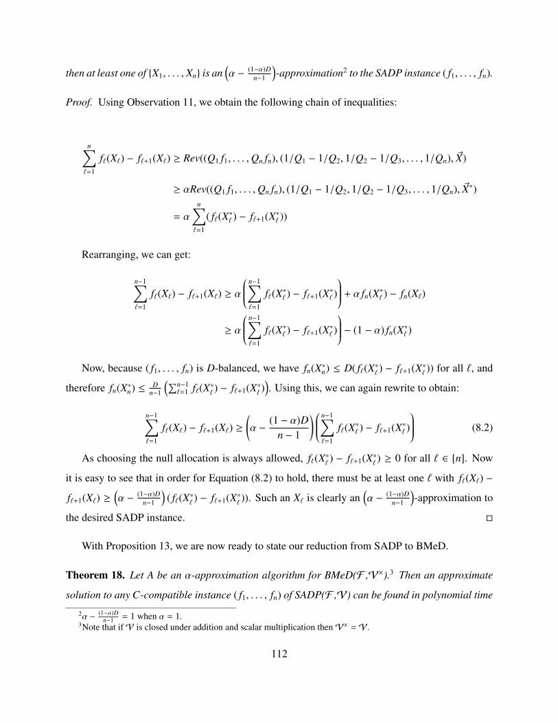
then at least one of X1, . . . , Xn is an(α − (1−α)D

n−1

)-approximation2 to the SADP instance ( f1, . . . , fn).

Proof. Using Observation 11, we obtain the following chain of inequalities:

n∑`=1

f`(X`) − f`+1(X`) ≥ Rev((Q1 f1, . . . ,Qn fn), (1/Q1 − 1/Q2, 1/Q2 − 1/Q3, . . . , 1/Qn), ~X)

≥ αRev((Q1 f1, . . . ,Qn fn), (1/Q1 − 1/Q2, 1/Q2 − 1/Q3, . . . , 1/Qn), ~X*)

= α

n∑`=1

( f`(X*` ) − f`+1(X*` ))

Rearranging, we can get:

n−1∑`=1

f`(X`) − f`+1(X`) ≥ α

⎛⎜⎜⎜⎜⎜⎝ n−1∑`=1

f`(X*` ) − f`+1(X*` )

⎞⎟⎟⎟⎟⎟⎠ + α fn(X*` ) − fn(X`)

≥ α

⎛⎜⎜⎜⎜⎜⎝ n−1∑`=1

f`(X*` ) − f`+1(X*` )

⎞⎟⎟⎟⎟⎟⎠ − (1 − α) fn(X*` )

Now, because ( f1, . . . , fn) is D-balanced, we have fn(X*n) ≤ D( f`(X*` ) − f`+1(X*` )) for all `, and

therefore fn(X*n) ≤ Dn−1

(∑n−1`=1 f`(X*` ) − f`+1(X*` )

). Using this, we can again rewrite to obtain:

n−1∑`=1

f`(X`) − f`+1(X`) ≥(α −

(1 − α)Dn − 1

) ⎛⎜⎜⎜⎜⎜⎝ n−1∑`=1

f`(X*` ) − f`+1(X*` )

⎞⎟⎟⎟⎟⎟⎠ (8.2)

As choosing the null allocation is always allowed, f`(X*` ) − f`+1(X*` ) ≥ 0 for all ` ∈ [n]. Now

it is easy to see that in order for Equation (8.2) to hold, there must be at least one ` with f`(X`) −

f`+1(X`) ≥(α − (1−α)D

n−1

)( f`(X*` ) − f`+1(X*` )). Such an X` is clearly an

(α − (1−α)D

n−1

)-approximation to

the desired SADP instance.

With Proposition 13, we are now ready to state our reduction from SADP to BMeD.

Theorem 18. Let A be an α-approximation algorithm for BMeD(ℱ ,𝒱×).3 Then an approximate

solution to any C-compatible instance ( f1, . . . , fn) of SADP(ℱ ,𝒱) can be found in polynomial time

2α − (1−α)Dn−1 = 1 when α = 1.

3Note that if𝒱 is closed under addition and scalar multiplication then𝒱× = 𝒱.

112

plus one black-box call to A. The solution has the following properties:

1. (Quality) If ( f1, . . . , fn) is D-balanced, the solution obtains an(α − (1−α)D

n−1

)-approximation.

2. (Bit Complexity) If b is an upper bound on the bit complexity of f j(X), then b + C is an

upper bound on the bit complexity of t j(X) for any t j input to A and any X ∈ ℱ , and every

probability input to A has bit complexity C.

Theorem 18 shows that there is a complete circle of reductions from BMeD to SADP and back.

In fact, the circle of exact reductions is complete even if we restrict SADP to instances with n = 2.

The reduction from SADP to BMeD is not quite approximation preserving, but it is strong enough

for us to show hardness of approximation for submodular agents in the following section.

8.3 Approximation Hardness for Submodular Bidders

We begin this section by defining submodularity. There are several known equivalent definitions

for submodularity. The one that will be most convenient for us is known as the property of dimin-

ishing returns.

Definition 8. (Submodular Function) A function f : 2S → R is said to be submodular if for all

X ⊂ Y ⊂ S , and all x < Y, we have:

f (X ∪ x) − f (X) ≥ f (Y ∪ x) − f (Y)

Definition 9. (Value Oracle) A value oracle is a black box that takes as input a set S and outputs

f (S ).

Definition 10. (Demand Oracle) A demand oracle is a black box that takes as input a vector of

prices p1, . . . , pm and outputs argmaxS⊆[m] f (S ) −∑

i∈S pi.

Definition 11. (Explicit Representation) An explicit representation of f is an explicit description

of a turing machine that computes f .

113

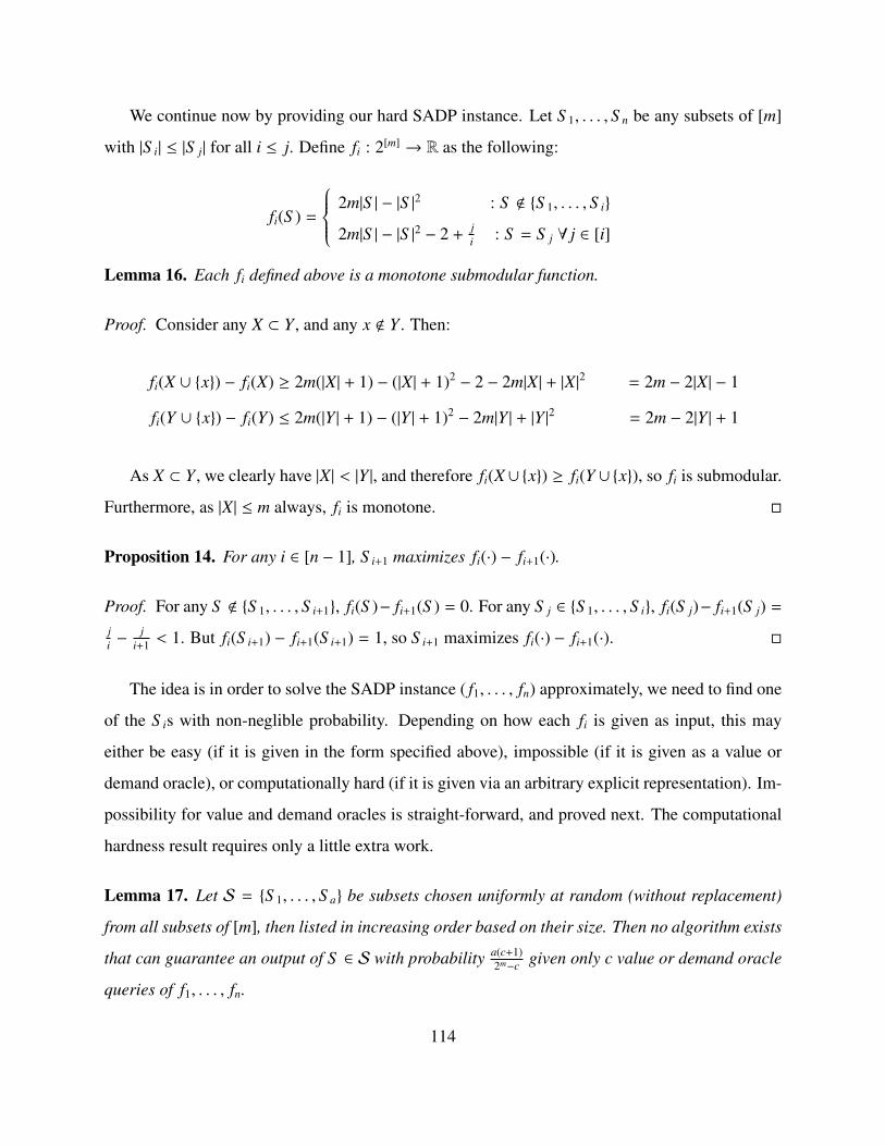
We continue now by providing our hard SADP instance. Let S 1, . . . , S n be any subsets of [m]

with |S i| ≤ |S j| for all i ≤ j. Define fi : 2[m] → R as the following:

fi(S ) =

⎧⎪⎪⎪⎨⎪⎪⎪⎩ 2m|S | − |S |2 : S < S 1, . . . , S i

2m|S | − |S |2 − 2 +ji : S = S j ∀ j ∈ [i]

Lemma 16. Each fi defined above is a monotone submodular function.

Proof. Consider any X ⊂ Y , and any x < Y . Then:

fi(X ∪ x) − fi(X) ≥ 2m(|X| + 1) − (|X| + 1)2 − 2 − 2m|X| + |X|2 = 2m − 2|X| − 1

fi(Y ∪ x) − fi(Y) ≤ 2m(|Y | + 1) − (|Y | + 1)2 − 2m|Y | + |Y |2 = 2m − 2|Y | + 1

As X ⊂ Y , we clearly have |X| < |Y |, and therefore fi(X∪x) ≥ fi(Y ∪x), so fi is submodular.

Furthermore, as |X| ≤ m always, fi is monotone.

Proposition 14. For any i ∈ [n − 1], S i+1 maximizes fi(·) − fi+1(·).

Proof. For any S < S 1, . . . , S i+1, fi(S )− fi+1(S ) = 0. For any S j ∈ S 1, . . . , S i, fi(S j)− fi+1(S j) =

ji −

ji+1 < 1. But fi(S i+1) − fi+1(S i+1) = 1, so S i+1 maximizes fi(·) − fi+1(·).

The idea is in order to solve the SADP instance ( f1, . . . , fn) approximately, we need to find one

of the S is with non-neglible probability. Depending on how each fi is given as input, this may

either be easy (if it is given in the form specified above), impossible (if it is given as a value or

demand oracle), or computationally hard (if it is given via an arbitrary explicit representation). Im-

possibility for value and demand oracles is straight-forward, and proved next. The computational

hardness result requires only a little extra work.

Lemma 17. Let 𝒮 = S 1, . . . , S a be subsets chosen uniformly at random (without replacement)

from all subsets of [m], then listed in increasing order based on their size. Then no algorithm exists

that can guarantee an output of S ∈ 𝒮 with probability a(c+1)2m−c given only c value or demand oracle

queries of f1, . . . , fn.

114

Proof. For any sequence of c value queries, the probability that none of them guessed a set S ∈ 𝒮

is at least 1 − ac/(2m − c). For a deterministic algorithm using c value queries, if it has never suc-

cessfully queried an element in 𝒮 during the execution, then the probability of success is no more

than a/(2m − c). Using union bound, we know that the probability of success for any deterministic

algorithm is at most a(c+1)/(2m−c). By Yao’s Lemma, this also holds for randomized algorithms.

A similar argument shows that the same holds for demand queries as well. First, let’s under-

stand how demand queries for f0 ( f0(S ) = 2m|S |−|S |2) and fi differ. Consider any prices p1, . . . , pm,

and let S = argmax f0(S ) −∑

i∈S pi. If S < 𝒮, then because fa(S ) = f0(S ) and fa(S ′) ≤ f0(S ′)

for all S ′, we also have S = argmax fa(S ) −∑

i∈S pi. If other words, if the prices we query are

such that a demand oracle for f0 would return some S < 𝒮, we have learned nothing about 𝒮 other

than that it does not contain S . From here we can make the exact same argument in the previous

paragraph replacing the phrase “query some S ∈ 𝒮” with “query some prices p1, . . . , pm such that

a demand oracle for f0 would return some S ∈ 𝒮.”

Corollary 9. For any constants c, d, no (possibly randomized) algorithm can guarantee a 1mc -

approximation to SADP(2[m],monotone submodular functions) in time (nm)d, as long as n ≤ mc′

for some constant c′, if the functions are given via a value or demand oracle.

Proof. Consider the input f1, . . . , fn chosen according to Lemma 17. Therefore by Proposition 14,

in any 1mc -approximation to this SADP instance necessarily finds some S i with probability at least

1mc . Lemma 17 exactly says that this cannot be done without at least 2m/n >> (nm)d queries.

Corollary 9 shows that SADP is impossible to approximate within any polynomial factor for

submodular functions given via a value or demand oracle. We continue now by showing compu-

tational hardness when the functions are given via an explicit representation. First, let g be any

correspondence between subsets of [m] and integers in [2m] so that |S | > |S ′| ⇒ g(S ) > g(S ′).4

Next, let 𝒫 denote any NP-hard problem with verifier V , and let p be a constant so that any “yes”

instance of 𝒫 of size z has a bitstring witness of length zp. For a given m, n, and specific instance

P ∈ 𝒫 of size (m − log n)1/p, we define:4Such a g can be implemented efficiently by ordering subsets of [m] first by their size, and then lexicographically,

and letting g(S ) be the rank of S in this ordering. The rank of S in this ordering can be computed by easy combinatoricsplus a simple dynamic program.

115

f Pi (S ) =

⎧⎪⎪⎪⎨⎪⎪⎪⎩ 2m|S | − |S |2 − 2 +ji : ( j−1)2m

n < g(S ) ≤ j2m

n ≤i2m

n and V(P, (g(S ) mod 2m

n ))

= “yes′′

2m|S | − |S |2 : otherwise

Lemma 18. If P is a “yes” instance of 𝒫, then any α-approximation to the SADP instance

f1, . . . , fn necessarily finds a witness for P with probability at least α.

Proof. It is clear that if P is a “yes” instance of 𝒫, then P has a witness of length (m − log n), and

therefore there is some x ≤ 2m/n such that V(P, x) = “yes.′′ Therefore, we would have f Pi (g−1(x +

i2m/n)) = 2m|S | − |S |2, but f Pi+1(g−1(x + i2m/n)) = 2m|S | − |S |2 − 1. It is also clear that in order to

have f Pi (S ) − f P

i+1(S ) > 0, we must have V(P, (g(S ) mod 2m/n)) = “yes′′. In other words, if P is a

“yes” instance of 𝒫, any α-approximation to the SADP instance f1, . . . , fn must find a witness for

P with probability at least α.

Corollary 10. Unless NP = RP, for any constants c, d no (possibly randomized) algorithm can

guarantee a 1mc -approximation to SADP(2[m],monotone submodular functions) in time (nm)d, as

long as n ≤ mc′ for some constant c′, even if the functions are given explicitly.

Proof. If we could obtain a 1mc -approximation to SADP(2[m],monotone submodular functions) in

time (nm)d ≤ mc′d+d, then for any “yes” instance P ∈ 𝒫, we could find a witness with probability

at least 1mc in time mc′d+d by Lemma 18. By running mc independent trials, we could amplify this

probability to 1/e in time mc′d+d+c. So we would have an RP algorithm for 𝒫.

We combine Corollaries 9 and 10 below into one theorem.

Theorem 19. As long as n ≤ mc′ for some constant c′, the problem SADP(2[m],monotone submod-

ular functions) is:

1. Impossible to approximate within any 1/poly(m)-factor with only poly(n,m) value oracle

queries.

2. Impossible to approximate within any 1/poly(m)-factor with only poly(n,m) demand oracle

queries.

116

3. Impossible to approximate within any 1/poly(m)-factor given explicit access to the input

functions in time poly(n,m), unless NP = RP.

Finally, we conclude this section by showing that the classes which we have just shown to be

hard for SADP can be used via the reduction of Theorem 18.

Lemma 19. All SADP instances defined in this section are 2n(log n + log m)-compatible and m2-

balanced.

Proof. That each instance is m2-balanced is easy to see: fn([m]) = m2, and for all i we have

maxS fi(S ) − fi+1(S ) = 1. To see that each instance is C-compatible, set Qi = (nm)2i−2. Then

it is easy to see that the maximum welfare obtainable by any matching that only uses types Q1 f1

through Qi fi obtains welfare at most m2iQi. In addition, the difference in value of Qi+1 fi+1 be-

tween two outcomes is at least Qi+1/(i + 1) > Qi+1/n if it is non-zero. Therefore, the minimum

non-zero difference between the value of Qi+1 fi+1 for two allocations is larger than the maximum

possible difference in welfare of all types Q1 f1 through Qi fi for two matchings of allocations. As

this holds for all i, this means that the max-weight matching of any set of allocations S to types

Qi fi, . . . ,Q j f j will necessarily match Q j f j to its favorite allocation in S , then Q j−1 f j−1 to its fa-

vorite of what remains, etc.

So let (S 1, . . . , S n) be any sets such that fi(S i+1) − fi(S i) = 1. It is not hard to verify that

|S 1| ≤ |S 2| ≤ . . . ≤ |S n|, and fi(S j) is monotonically increasing in j for any i. The reason-

ing above immediately yields that the max-weight matching of allocations (S i, . . . , S j) to types

(Qi fi, . . . ,Q j f j) necessarily awards S ` to Q` f` for all `, as fi, so (S 1, . . . , S n) is cyclic monotone

with respect to (Q1S 1, . . . ,QnS n). Furthermore, the same reasoning immediately yields that the

max-weight matching of allocations (S i, . . . , S j−1) to types (Qi+1 fi+1, . . . ,Q j f j) awards S ` to type

Q`+1 f`+1 for all `, so (S 1, . . . , S n) is also compatible with (Q1 f1, . . . ,Qn fn). It is clear that all Qi are

integers less than (n2m2)n−1 ≤ 22n(log n+log m), so ( f1, . . . , fn) are 2n(log n + log m)-compatible.

Corollary 11. The problem BMeD(2[m],monotone submodular functions) (for n = |T | = poly(m))

is:

1. Impossible to approximate within any 1/poly(m)-factor with only poly(n,m) value oracle

queries.

117

2. Impossible to approximate within any 1/poly(m)-factor with only poly(n,m) demand oracle

queries.

3. Impossible to approximate within any 1/poly(m)-factor given explicit access to the input

functions in time poly(n,m), unless NP = RP.

Proof. For any constant c, let n = mc+2 + 1, if we can find an 2/mc-approximate solution to BMeD

in polynomial time, we can find an 1/mc-approximate solution to SADP by Theorem 18, which

would contradict Theorem 19.

118

Chapter 9

Conclusions and Open Problems

As mediums like the Internet continue to grow, we see more and more that our algorithms are

interacting with strategic agents. These agents often have incentives to manipulate the algorithms

for their own gains, resulting in potentially global failures of otherwise sound algorithms [McC08,

McM08]. Such instances demonstrate the necessity of algorithms that are robust to potential ma-

nipulation by strategic agents, called mechanisms. In this thesis, we addressed a fundamental

question: How much more difficult is mechanism design than algorithm design?

In this study, we addressed two important areas of research. The first follows Myerson’s sem-

inal paper on optimal auction design, where he showed that the optimal single item auction is a

virtual welfare maximizer [Mye81]. Much effort had been devoted over the past three decades

to extend his characterization to multi-dimensional settings, but no compelling characterization in

unrestricted settings had been found. Our work directly extends Myerson’s characterization to un-

restricted multi-dimensional settings, showing that the optimal auction is a distribution over virtual

welfare maximizers.

This thesis also follows Nisan and Ronen’s seminal paper introducing the field of Algorithmic

Mechanism Design [NR99]. On this front, our work provides a black-box reduction from mecha-

nism to algorithm design. The existence of this reduction does not imply that we are now capable

of solving any mechanism design question asked, but it does provide an algorithmic framework

with which to tackle such problems, which was previously non-existent. We further make use

119

of our new framework to design the first computationally efficient, approximately-optimal mech-

anisms for the paradigmatic problems of makespan minimization and fairness maximization in

unrestricted settings. Furthermore, our framework allows for the first unrestricted hardness of

approximation result in revenue maximization.

On both fronts, our work constitutes some immense progress, but there is still much work

to be done. Myerson’s single-dimensional characterization combined with results of Bulow and

Roberts provides a meaningful economic interpretation of the transformation from types to virtual

types [Mye81, BR89], whereas our virtual transformation is randomized and computed by a lin-

ear program. While the use of randomization is necessary in even very simple multi-dimensional

settings [BCKW10, DDT13, HN13, HR12, Pav06, Tha04], it is still conceivable that these ran-

domized virtual transformations have economic significance, at least in some special cases.

Question 7. Is there any economic significance to the virtual transformations used by our mecha-

nisms?

We have also established a “tight” algorithmic framework to design multi-dimensional mech-

anisms, namely by designing algorithms for virtual welfare maximization. Applied to the case

of additive agents with feasibility constraints on which agents can simultaneously receive which

items (e.g. matching markets), we obtain numerous positive results (e.g. Theorems 4, 8, 9). Ap-

plied to the case of a single agent whose value for sets of items is submodular, we obtain hardness

of approximation within any polynomial factor (Theorem 19 and Corollary 11). Still, there are

numerous interesting classes of valuation functions between additive and submodular worthy of

study in multi-dimensional mechanism design, and this space of questions is largely unexplored.

Our framework proposes concrete algorithmic questions for use in this study.

Question 8. What is the computational complexity of virtual welfare maximization (and therefore

truthful revenue maximization as well via our reduction) for other classes of valuation functions?

One important instance is the class of gross substitute valuations.

A final question motivated in our work in multi-dimensional mechanism is whether or not our

mechanisms are prescriptive for the sale of multiple items in the real world. Most multi-item

120

sellers still opt to auction items in their inventory separately, even though numerous examples

show that this could potentially hurt revenue by a significant factor. One possibility indeed is

that sellers should consider using more complex mechanisms, and another is that “real-world”

instances don’t behave as poorly as the worst case. Understanding which world we live in is of

obvious importance, and our mechanisms provide a computational tool with which to address this

question (i.e. by executing our mechanisms on real-world instances).

Question 9. What is the gap between simple and optimal mechanisms in “real-world” instances?

If the gap is large, should sellers change the way they sell items? If the gap is small, what properties

of real-world instances enable this?

Within algorithmic mechanism design, our framework poses new concrete algorithmic ques-

tions. If one wants to design mechanisms optimizing any objective, one can instead use our

framework and design algorithms for that same objective plus virtual welfare. Algorithm design

questions like these are largely unstudied, as they were previously unmotivated. In light of our

framework, it is now quite important to solve such problems.

Question 10. For what other optimization problems 𝒪 can we design computationally efficient

algorithms for 𝒪+ virtual welfare?

Beyond the design of computationally efficient mechanisms, an equally pressing direction is

understanding the computational complexity of such mechanism design, e.g. by proving hardness

of approximation. Given the success of our framework in this direction for multi-dimensional

mechanism design, we are optimistic that our framework can help provide such results in algorith-

mic mechanism design as well. Of course, extending our framework to accommodate reductions

from algorithm to mechanism design was already challenging in the case of multi-dimensional

mechanism design, and will be even more challenging here. Consider for example job scheduling

on unrelated machines: we have shown that there is a computationally efficient 2-approximate

mechanism via a (1, 1/2)-approximation algorithm for makespan minimization with costs, yet

makespan minimization with costs is NP-hard to approximate (in a traditional sense) within any fi-

nite factor. In other words, any such reduction from algorithm to mechanism design must somehow

accommodate this fact and make use of (α, β)-approximations as well.

121

Question 11. Can one extend our framework for algorithmic mechanism design to allow for the

development of hardness of approximation results as well?

Finally, recall that there are two central questions in the field of algorithmic mechanism design,

refining our motivating question of “how much harder is mechanism than algorithm design?” This

thesis makes substantial progress in addressing the computational question: How much compu-

tationally harder is mechanism than algorithm design? We show that the answer for makespan

and fairness is “not at all,” and provide a framework with which to answer this question for other

objectives. But another important question simply addresses the quality of solution output by the

optimal mechanism versus the optimal algorithm, without regard for computation. Our work does

not directly address this question, but by designing computationally efficient mechanisms, we pro-

vide a new algorithmic tool with which to make progress.

Question 12. How much worse is the quality of solution output by the optimal mechanism versus

that of the optimal algorithm?

122

Bibliography

[ADL12] Itai Ashlagi, Shahar Dobzinski, and Ron Lavi. Optimal lower bounds for anonymous

scheduling mechanisms. Mathematics of Operations Research, 37(2):244–258, 2012.

[AFH+12] Saeed Alaei, Hu Fu, Nima Haghpanah, Jason Hartline, and Azarakhsh Malekian.

Bayesian Optimal Auctions via Multi- to Single-agent Reduction. In the 13th ACM

Conference on Electronic Commerce (EC), 2012.

[AFHH13] Saeed Alaei, Hu Fu, Nima Haghpanah, and Jason Hartline. The Simple Economics

of Approximately Optimal Auctions. In Proceedings of the 54th IEEE Symposium on

Foundations of Computer Science (FOCS), 2013.

[AFS08] Arash Asadpour, Uriel Feige, and Amin Saberi. Santa claus meets hypergraph match-

ings. In the 12th International Workshop on Approximation, Randomization, and

Combinatorial Optimization (APPROX-RANDOM), 2008.

[AKW14] Pablo D. Azar, Robert Kleinberg, and S. Matthew Weinberg. Prophet inequalities with

limited information. In the Twenty-Fifth Annual ACM-SIAM Symposium on Discrete

Algorithms (SODA), 2014.

[Ala11] Saeed Alaei. Bayesian Combinatorial Auctions: Expanding Single Buyer Mecha-

nisms to Many Buyers. In the 52nd Annual IEEE Symposium on Foundations of

Computer Science (FOCS), 2011.

[Arm96] Mark Armstrong. Multiproduct nonlinear pricing. Econometrica, 64(1):51–75, 1996.

123

[AS07] Arash Asadpour and Amin Saberi. An approximation algorithm for max-min fair

allocation of indivisible goods. In the 39th Annual ACM Symposium on Theory of

Computing (STOC), 2007.

[AT01] Aaron Archer and Éva Tardos. Truthful Mechanisms for One-Parameter Agents. In

the 42nd Annual Symposium on Foundations of Computer Science (FOCS), 2001.

[BCG09] MohammadHossein Bateni, Moses Charikar, and Venkatesan Guruswami. Maxmin

allocation via degree lower-bounded arborescences. In the 41st annual ACM sympo-

sium on Theory of Computing (STOC), pages 543–552, 2009.

[BCKW10] Patrick Briest, Shuchi Chawla, Robert Kleinberg, and S. Matthew Weinberg. Pric-

ing Randomized Allocations. In the Twenty-First Annual ACM-SIAM Symposium on

Discrete Algorithms (SODA), 2010.

[BD05] Ivona Bezáková and Varsha Dani. Allocating indivisible goods. SIGecom Exchanges,

5(3):11–18, 2005.

[BDF+10] David Buchfuhrer, Shaddin Dughmi, Hu Fu, Robert Kleinberg, Elchanan Mossel,

Christos H. Papadimitriou, Michael Schapira, Yaron Singer, and Christopher Umans.

Inapproximability for VCG-Based Combinatorial Auctions. In Proceedings of the

Twenty-First Annual ACM-SIAM Symposium on Discrete Algorithms (SODA), 2010.

[BGGM10] Sayan Bhattacharya, Gagan Goel, Sreenivas Gollapudi, and Kamesh Munagala. Bud-

get Constrained Auctions with Heterogeneous Items. In the 42nd ACM Symposium

on Theory of Computing (STOC), 2010.

[BGM13] Anand Bhalgat, Sreenivas Gollapudi, and Kamesh Munagala. Optimal Auctions via

the Multiplicative Weight Method. In the 14th ACM Conference on Electronic Com-

merce (EC), 2013.

[BH11] Xiaohui Bei and Zhiyi Huang. Bayesian Incentive Compatibility via Fractional As-

signments. In the Twenty-Second Annual ACM-SIAM Symposium on Discrete Algo-

rithms (SODA), 2011.

124

[BHSZ13] MohammadHossein Bateni, Nima Haghpanah, Balasubramanian Sivan, and Morteza

Zadimoghaddam. Revenue maximization with nonexcludable goods. In the 9th In-

ternational Conference on Web and Internet Economics (WINE), 2013.

[BILW14] Moshe Babaioff, Nicole Immorlica, Brendan Lucier, and S. Matthew Weinberg. A

simple and approximately optimal mechanism for an additive buyer. Working Paper,

2014. http://people.csail.mit.edu/smweinberg/additive.pdf.

[Bor91] Kim C. Border. Implementation of reduced form auctions: A geometric approach.

Econometrica, 59(4):1175–1187, 1991.

[Bor07] Kim C. Border. Reduced Form Auctions Revisited. Economic Theory, 31:167–181,

2007.

[BR89] J. Bulow and J. Roberts. The Simple Economics of Optimal Auctions. Journal of

Political Economy, 97:1060–1090, 1989.

[Bri08] Patrick Briest. Uniform Budgets and the Envy-Free Pricing Problem. In Proc. of the

35th International Colloquium on Automata, Languages, and Programming (ICALP),

pages 808–819, 2008.

[BS06] Nikhil Bansal and Maxim Sviridenko. The santa claus problem. In the 38th annual

ACM symposium on Theory of computing (STOC), pages 31–40, 2006.

[BT96] Steven J Brams and Alan D Taylor. Fair Division: From cake-cutting to dispute

resolution. Cambridge University Press, 1996.

[Bud13] Zack Budryk. Dangerous curves. Inside Higher Ed, 2013.

http://www.insidehighered.com/news/2013/02/12/students-boycott-final-challenge-

professors-grading-policy-and-get.

[CCK09] Deeparnab Chakrabarty, Julia Chuzhoy, and Sanjeev Khanna. On allocating goods

to maximize fairness. In 50th Annual IEEE Symposium on Foundations of Computer

Science (FOCS), 2009.

125

[CD11] Yang Cai and Constantinos Daskalakis. Extreme-Value Theorems for Optimal Multi-

dimensional Pricing. In the 52nd Annual IEEE Symposium on Foundations of Com-

puter Science (FOCS), 2011.

[CDP+14] Xi Chen, Ilias Diakonikolas, Dimitris Paparas, Xiaorui Sun, and Mihalis Yannakakis.

The complexity of optimal multidimensional pricing. In the Twenty-Fifth Annual

ACM-SIAM Symposium on Discrete Algorithms (SODA), 2014.

[CDW12a] Yang Cai, Constantinos Daskalakis, and S. Matthew Weinberg. An Algorithmic Char-

acterization of Multi-Dimensional Mechanisms. In the 44th Annual ACM Symposium

on Theory of Computing (STOC), 2012.

[CDW12b] Yang Cai, Constantinos Daskalakis, and S. Matthew Weinberg. Optimal Multi-

Dimensional Mechanism Design: Reducing Revenue to Welfare Maximization. In the

53rd Annual IEEE Symposium on Foundations of Computer Science (FOCS), 2012.

[CDW13a] Yang Cai, Constantinos Daskalakis, and S. Matthew Weinberg. Reducing Revenue

to Welfare Maximization: Approximation Algorithms and other Generalizations.

In the 24th Annual ACM-SIAM Symposium on Discrete Algorithms (SODA), 2013.

http://arxiv.org/pdf/1305.4000v1.pdf.

[CDW13b] Yang Cai, Constantinos Daskalakis, and S. Matthew Weinberg. Understand-

ing Incentives: Mechanism Design becomes Algorithm Design. In the 54th

Annual IEEE Symposium on Foundations of Computer Science (FOCS), 2013.

http://arxiv.org/pdf/1305.4002v1.pdf.

[CH13] Yang Cai and Zhiyi Huang. Simple and Nearly Optimal Multi-Item Auctions. In the

24th Annual ACM-SIAM Symposium on Discrete Algorithms (SODA), 2013.

[CHK07] Shuchi Chawla, Jason D. Hartline, and Robert D. Kleinberg. Algorithmic Pricing via

Virtual Valuations. In the 8th ACM Conference on Electronic Commerce (EC), 2007.

126

[CHMS10] Shuchi Chawla, Jason D. Hartline, David L. Malec, and Balasubramanian Sivan.

Multi-Parameter Mechanism Design and Sequential Posted Pricing. In the 42nd ACM

Symposium on Theory of Computing (STOC), 2010.

[CHMS13] Shuchi Chawla, Jason Hartline, David Malec, and Balasubramanian Sivan. Prior-

Independent Mechanisms for Scheduling. In Proceedings of 45th ACM Symposium

on Theory of Computing (STOC), 2013.

[CIL12] Shuchi Chawla, Nicole Immorlica, and Brendan Lucier. On the limits of black-box

reductions in mechanism design. In Proceedings of the 44th Symposium on Theory of

Computing (STOC), 2012.

[CK10] George Christodoulou and Annamária Kovács. A Deterministic Truthful PTAS for

Scheduling Related Machines. In the 21st Annual ACM-SIAM Symposium on Discrete

Algorithms (SODA), 2010.

[CKK07] George Christodoulou, Elias Koutsoupias, and Annamária Kovács. Mechanism De-

sign for Fractional Scheduling on Unrelated Machines. In the 34th International

Colloquium on Automata, Languages and Programming (ICALP), 2007.

[CKM11] Yeon-Koo Che, Jinwoo Kim, and Konrad Mierendorff. Generalized Reduced-Form

Auctions: A Network-Flow Approach. University of Zürich, ECON-Working Papers,

2011.

[CKV07] George Christodoulou, Elias Koutsoupias, and Angelina Vidali. A Lower Bound for

Scheduling Mechanisms. In the 18th Annual ACM-SIAM Symposium on Discrete

Algorithms (SODA), 2007.

[Cla71] Edward H. Clarke. Multipart pricing of public goods. Public Choice, pages 17–33,

1971.

[CMS10] Shuchi Chawla, David L. Malec, and Balasubramanian Sivan. The Power of Ran-

domness in Bayesian Optimal Mechanism Design. In the 11th ACM Conference on

Electronic Commerce (EC), 2010.

127

[CP14] Yang Cai and Christos Papadimitriou. Simultaneous bayesian auctions and computa-

tional complexity. In Proceedings of the 15th ACM Conference on Electronic Com-

merce (EC), 2014.

[CS08] Vincent Conitzer and Tuomas Sandholm. New Complexity Results about Nash Equi-

libria. Games and Economic Behavior, 63(2):621–641, 2008.

[DDDR08] Peerapong Dhangwatnotai, Shahar Dobzinski, Shaddin Dughmi, and Tim Roughgar-

den. Truthful Approximation Schemes for Single-Parameter Agents. In the 49th

Annual IEEE Symposium on Foundations of Computer Science (FOCS), 2008.

[DDT13] Constantinos Daskalakis, Alan Deckelbaum, and Christos Tzamos. Mechanism de-

sign via optimal transport. In the 14th ACM Conference on Electronic Commerce

(EC), 2013.

[DDT14] Constantinos Daskalakis, Alan Deckelbaum, and Christos Tzamos. The complexity

of optimal mechanism design. In the Twenty-Fifth Annual ACM-SIAM Symposium on

Discrete Algorithms (SODA), 2014.

[DFK11] Shahar Dobzinski, Hu Fu, and Robert D. Kleinberg. Optimal Auctions with Corre-

lated Bidders are Easy. In the 43rd ACM Symposium on Theory of Computing (STOC),

2011.

[DGP09] Constantinos Daskalakis, Paul W. Goldberg, and Christos H. Papadimitriou. The

Complexity of Computing a Nash Equilibrium. SIAM Journal on Computing,

39(1):195–259, 2009.

[DJ81] E. Davis and J.M. Jaffe. Algorithms for scheduling tasks on unrelated processors.

Journal of the Association for Computing Machinery, 28:821–736, 1981.

[Dob11] Shahar Dobzinski. An Impossibility Result for Truthful Combinatorial Auctions with

Submodular Valuations. In Proceedings of the 43rd ACM Symposium on Theory of

Computing (STOC), 2011.

128

[DV12] Shahar Dobzinski and Jan Vondrak. The Computational Complexity of Truthfulness

in Combinatorial Auctions. In Proceedings of the ACM Conference on Electronic

Commerce (EC), 2012.

[DW12] Constantinos Daskalakis and S. Matthew Weinberg. Symmetries and Optimal Multi-

Dimensional Mechanism Design. In the 13th ACM Conference on Electronic Com-

merce (EC), 2012.

[DW14] Constantinos Daskalakis and S. Matthew Weinberg. Bayesian truthful mechanisms

for job scheduling from bi-criterion approximation algorithms. Working Paper, 2014.

http://people.csail.mit.edu/smweinberg/makespan.pdf.

[GIS77] T. Gonzalez, O.H. Ibarra, and S. Sahni. Bounds for lpt schedules on uniform proces-

sors. SIAM Journal on Computing, 6:155–166, 1977.

[GJ75] M.R. Garey and D.S. Johnson. Complexity results for multiprocessor scheduling

under resource constraints. SIAM Journal on Computing, 4:397–411, 1975.

[GJ78] M.R. Garey and D.S. Johnson. Strong np-completeness results: Motivation, exam-

ples, and implications. Journal of the Association for Computing Machinery, 25:499–

508, 1978.

[GLLK79] R.L. Graham, E.L. Lawler, J.K. Lenstra, and A.H.G. Rinooy Kan. Optimization and

approximation in deterministic sequencing and scheduling: a survey. Annals of Dis-

crete Mathematics, 5:287–326, 1979.

[GLS81] Martin Grötschel, László Lovász, and Alexander Schrijver. The Ellipsoid Method

and its Consequences in Combinatorial Optimization. Combinatorica, 1(2):169–197,

1981.

[Gra66] R.L. Graham. Bounds for certain multiprocessing anomalies. Bell System Technolog-

ical Journal, 45:1563–1581, 1966.

129

[Gra69] R.L. Graham. Bounds on multiprocessing timing anomalies. SIAM Journal on Ap-

plied Mathematics, 17:416–429, 1969.

[Gro73] Theodore Groves. Incentives in teams. Econometrica, pages 617–623, 1973.

[HIMM11] Nima Haghpanah, Nicole Immorlica, Vahab S. Mirrokni, and Kamesh Munagala. Op-

timal auctions with positive network externalities. In the 12th ACM Conference on

Electronic Commerce (EC), 2011.

[HKM11] Jason D. Hartline, Robert Kleinberg, and Azarakhsh Malekian. Bayesian Incentive

Compatibility via Matchings. In the Twenty-Second Annual ACM-SIAM Symposium

on Discrete Algorithms (SODA), 2011.

[HL10] Jason D. Hartline and Brendan Lucier. Bayesian Algorithmic Mechanism Design. In

the 42nd ACM Symposium on Theory of Computing (STOC), 2010.

[HN12] Sergiu Hart and Noam Nisan. Approximate Revenue Maximization with Multiple

Items. In the 13th ACM Conference on Electronic Commerce (EC), 2012.

[HN13] Sergiu Hart and Noam Nisan. The Menu-Size Complexity of Auctions. In the 14th

ACM Conference on Electronic Commerce (EC), 2013.

[Hoe63] Wassily Hoeffding. Probability inequalities for sums of bounded random variables.

Journal of the American Statistical Association, 58(301):13–30, 1963.

[HR09] J.D. Hartline and T. Roughgarden. Simple versus optimal mechanisms. In Proceed-

ings of the 10th ACM conference on Electronic commerce, pages 225–234. ACM,

2009.

[HR11] Sergiu Hart and Philip J. Reny. Implementation of reduced form mechanisms: A sim-

ple approach and a new characterization. Technical Report, The Hebrew University of

Jerusalem, Center for Rationality DP-594, 2011. http://www.ma.huji.ac.il/hart/abs/q-

mech.html.

130

[HR12] Sergiu Hart and Philip J. Reny. Maximal revenue with multiple goods:

Nonmonotonicity and other obsevations. Technical Report, The He-

brew University of Jerusalem, Center for Rationality DP-630, 2012.

http://www.ma.huji.ac.il/hart/abs/monot-m.html.

[HS76] E. Horowitz and S. Sahni. Exact and approximate algorithms for scheduling noniden-

tical processors. Journal of the Association for Computing Machinery, 23:317–327,

1976.

[HS87] D.S. Hochbaum and D.B. Shmoys. Using dual approximation algorithms for schedul-

ing problems: practical and theoretical results. Journal of the Association for Com-

puting Machinery, 34:144–162, 1987.

[HS88] D.S. Hochbaum and D.B. Shmoys. A polynomial approximation scheme for machine

scheduling on uniform processors: using the dual approximation approach. SIAM

Journal on Computing, 17:539–551, 1988.

[Kha79] Leonid G. Khachiyan. A Polynomial Algorithm in Linear Programming. Soviet Math-

ematics Doklady, 20(1):191–194, 1979.

[Kna46] Bronislaw Knaster. Sur le probleme du partage pragmatique de h. steinhaus. In

Annales de la Societé Polonaise de Mathematique, volume 19, pages 228–230, 1946.

[KP80] Richard M. Karp and Christos H. Papadimitriou. On Linear Characterizations of

Combinatorial Optimization Problems. In the 21st Annual Symposium on Foundations

of Computer Science (FOCS), 1980.

[KP07] Subhash Khot and Ashok Kumar Ponnuswami. Approximation algorithms for the

max-min allocation problem. In the 11th International Workshop on Approximation,

Randomization, and Combinatorial Optimization (APPROX-RANDOM), 2007.

[KV07] Elias Koutsoupias and Angelina Vidali. A Lower Bound of 1+φ for Truthful Schedul-

ing Mechanisms. In the 32nd International Symposium on the Mathematical Founda-

tions of Computer Science (MFCS), 2007.

131

[KW12] Robert Kleinberg and S. Matthew Weinberg. Matroid Prophet Inequalities. In the

44th Annual ACM Symposium on Theory of Computing (STOC), 2012.

[LST87] Jan Karel Lenstra, David B. Shmoys, and Éva Tardos. Approximation algorithms for

scheduling unrelated parallel machines. In FOCS, 1987.

[Lu09] Pinyan Lu. On 2-Player Randomized Mechanisms for Scheduling. In the 5th Inter-

national Workshop on Internet and Network Economics (WINE), 2009.

[LY08a] Pinyan Lu and Changyuan Yu. An Improved Randomized Truthful Mechanism for

Scheduling Unrelated Machines. In the 25th Annual Symposium on Theoretical As-

pects of Computer Science (STACS), 2008.

[LY08b] Pinyan Lu and Changyuan Yu. Randomized Truthful Mechanisms for Scheduling

Unrelated Machines. In the 4th International Workshop on Internet and Network

Economics (WINE), 2008.

[LY13] Xinye Li and Andrew Chi-Chih Yao. On revenue maximization for selling multiple

independently distributed items. Proceedings of the National Academy of Sciences,

110(28):11232–11237, 2013.

[Mat84] Steven Matthews. On the Implementability of Reduced Form Auctions. Economet-

rica, 52(6):1519–1522, 1984.

[McC08] Declan McCullagh. How Pakistan knocked YouTube offline (and how to make sure

it never happens again). CNET, 2008. http://news.cnet.com/8301-10784_3-9878655-

7.html.

[McM08] Robert McMillan. Weekend youtube outage underscores big internet problem. Mac-

world, 2008. http://www.macworld.com/article/1132256/networking.html.

[Mis12] Debasis Mishra. Multidimensional Mechanism Design: Key Results and Research

Issues. Current Science, 103(9), 2012.

132

[MM88] Preston McAfee and John McMillan. Multidimensional Incentive Compatibility and

Mechanism Design. Journal of Economic Theory, 46(2):335–354, 1988.

[MR84] Eric Maskin and John Riley. Optimal Auctions with Risk Averse Buyers. Economet-

rica, 52(6):1473–1518, 1984.

[MS07] Ahuva Mu’alem and Michael Schapira. Setting lower bounds on truthfulness: ex-

tended abstract. In the 18th Annual ACM-SIAM Symposium on Discrete Algorithms

(SODA), 2007.

[MV06] Alejandro Manelli and Daniel Vincent. Bundling as an Optimal Selling Mechanism

for a Multiple-Good Monopolist. Journal of Economic Theory, 127(1):1–35, 2006.

[MV10] A. M. Manelli and D. R. Vincent. Bayesian and Dominant-Strrategy Implementation

in the Independent Private-Values Model. Econometrica, 78(6):1905–1938, 2010.

[Mye79] Roger B. Myerson. Incentive Compatibility and the Bargaining Problem. Economet-

rica, 41:61–73, 1979.

[Mye81] Roger B. Myerson. Optimal Auction Design. Mathematics of Operations Research,

6(1):58–73, 1981.

[Nas51] John F. Nash. Non-Cooperative Games. Annals of Mathematics, 54(2):286–295,

1951.

[NR99] Noam Nisan and Amir Ronen. Algorithmic Mechanism Design (Extended Abstract).

In Proceedings of the Thirty-First Annual ACM Symposium on Theory of Computing

(STOC), 1999.

[OR94] Martin J. Osborne and Ariel Rubinstein. A Course in Game Theory. MIT Press, 1994.

[Pav06] Gregory Pavlov. Optimal mechanism for selling substitutes, 2006. Boston University

- Department of Economics - Working Papers Series WP2006-014.

133

[Pav11] Gregory Pavlov. A Property of Solutions to Linear Monopoly Problems. B. E. Journal

of Theoretical Economics, 11(1), 2011. Article 4.

[Pot85] C.N. Potts. Analysis of a linear programming heuristic for scheduling unrelated par-

allel machines. Discrete Applied Mathematics, 10:155–164, 1985.

[PP11] Christos H. Papadimitriou and George Pierrakos. On Optimal Single-Item Auctions.

In the 43rd ACM Symposium on Theory of Computing (STOC), 2011.

[PSS08] Christos H. Papadimitriou, Michael Schapira, and Yaron Singer. On the hardness of

being truthful. In Proceedings of the 49th Annual IEEE Symposium on Foundations

of Computer Science (FOCS), 2008.

[RC98] Jean-Charles Rochet and Philippe Choné. Ironing, Sweeping, and Multidimensional

Screening. Econometrica, 66(4):783–826, 1998.

[Rob79] Kevin Roberts. The Characterization of Implementable Choice Rules. Aggregation

and Revelation of Preferences, pages 321–329, 1979.

[Roc87] Jean-Charles Rochet. A Necessary and Sufficient Condition for Rationalizability in a

Quasi-Linear Context. Journal of Mathematical Economics, 16:191–200, 1987.

[RZ83] John Riley and Richard Zeckhauser. Optimal Selling Strategies: When to Haggle,

When to Hold Firm. Quarterly J. Economics, 98(2):267–289, 1983.

[Sah76] S. Sahni. Algorithms for scheduling independent tasks. Journal of the Association

for Computing Machinery, 23:116–127, 1976.

[ST93a] David B Shmoys and Éva Tardos. An approximation algorithm for the generalized

assignment problem. Mathematical Programming, 62(1-3):461–474, 1993.

[ST93b] David B. Shmoys and Éva Tardos. Scheduling Unrelated Machines with Costs. In the

4th Symposium on Discrete Algorithms (SODA), 1993.

[Ste48] Hugo Steinhaus. The problem of fair division. Econometrica, 16(1), 1948.

134

[Tha04] John Thanassoulis. Haggling Over Substitutes. J. Economic Theory, 117:217–245,

2004.

[TW14] Pingzhong Tang and Zihe Wang. Optimal mechanisms with simple menus. In Pro-

ceedings of the 15th ACM Conference on Electronic Commerce (EC), 2014.

[Vic61] William Vickrey. Counterspeculation, auctions and competitive sealed tenders. Jour-

nal of Finance, pages 8–37, 1961.

[Voh11] Rakesh Vohra. Mechanism Design: A Linear Programming Approach. Cambridge

University Press, 2011.

135

136

Appendix A

Extensions of Border’s Theorem

In this chapter, we provide two extensions of Border’s Theorem for the feasibility of single-item

reduced forms. These results further strengthen our characterization of feasible multi-item mech-

anisms. Despite their importance, we choose to state the results separately here because they do

not generalize beyond additive settings. Section A.1 provides an algorithmic extension, showing

that we can determine if a reduced form is feasible or not by checking only a linear number of

constraints, rather than every possible violating set. Section A.2 provides a stronger structural

guarantee on feasible mechanisms.

A.1 Algorithmic Extension

We begin by reviewing Border’s Theorem.

Theorem 20 ([Bor91]). Suppose that the bidder’s types are i.i.d. distributed according to some

measure µ over T . Then a bidder-symmetric reduced form π is feasible if an only if

∀S ⊆ T : k ·∫

Sπ(t)dµ(t) ≤ 1 − (1 − µ(S ))k. (A.1)

Simply put, a reduced form is feasible if and only if the probability that the item is awarded to

a type in some set S (as computed by the reduced form) is at most the probability that someone

with type from S shows up to the auction (as computed by the type distribution), for all subsets of

137

types S ⊆ T . We call a set that violates this condition a constricting set. Clearly, the existence of a

constricting set bears witness that the reduced form is infeasible, as the auctioneer cannot possibly

award the item to someone in S if no one in S shows up. Border’s theorem states that this is in fact

a sufficient condition.

Recently, an alternative proof of Border’s theorem for distributions with finite support was

discovered in [Bor07] and again in [CKM11]. These proofs extend Theorem 20 to independent,

but not necessarily identical, bidders and non-symmetric reduced forms. In this case, (A.1) is

replaced by the following necessary and sufficient condition:

∀S 1 ⊆ T, . . . , S k ⊆ T :∑

i

∑A∈S i

πi(A) Pr[ti = A] ≤ 1 −∏

i

(1 − Pr[ti ∈ S i]). (A.2)

The interpretation of the LHS and RHS of the above inequality is the same as the one given above

for (A.1) except generalized to the non-iid non-symmetric setting. In addition to the above con-

dition, [CKM11] proves a generalization of Border’s extended result: If there is a constricting

S = (S 1, . . . , S k), then there is also a constricting set of the form S ′ = (S (1)x1 , . . . , S

(k)xk ), where

S (i)xi = A ∈ T |πi(A) > xi. In other words, each bidder has a different threshold xi, and S (i)

xi con-

tains all types of bidder i with πi above xi. Unfortunately, despite this simplification, there are still

(|T | + 1)k possible constricting sets, and testing each of them would take time exponential in the

number of bidders.

One might hope to obtain a stronger theorem that would only require testing a number of sets

polynomial in |T | and k. We prove such a theorem by introducing a notion of a scaled reduced

form, defined next. The idea behind the scaled reduced form is that the most difficult types to

satisfy are not those with the large values in the reduced form, but those with large scaled values

in the reduced form. We denote the scaled reduced form by π.

Definition 12. If π is a reduced form, we define its corresponding scaled reduced form π as follows:

for all i and types A ∈ T, πi(A) := Pr[πi(ti) ≤ πi(A)]πi(A).

It turns out that this definition exactly captures which types of different bidders are harder to satisfy.

In the bidder-symmetric case Theorem 20, we were able to compare a pair of types A and B

138

submitted by bidders i , i′ based only on their corresponding πi(A) and πi′(B). This is no longer

the case in the non-iid case, resulting in the more complicated constricting sets defined above.

Nevertheless, we show that A and B can be compared at face value of πi(A) and πi′(B):

Theorem 21. Suppose that the bidders are independent and there is a single item for sale. A

reduced form π is feasible if and only if: for all x, the sets S (i)x = A ∈ T |πi(A) > x satisfy:

∑i

∑A∈S (i)

x

πi(A) Pr[ti = A] ≤ 1 −∏

i

(1 − Pr[ti ∈ S (i)x ]). (A.3)

In particular, we can test the feasibility of a reduced form, or obtain a hyperplane separating the

reduced form from the set of feasible reduced forms, in time linear in k|T | · log (k|T |).

Before proving Theorem 21, we prove that the concept of a scaled reduced form is necessary.

Proposition 15. There exist reduced forms that are infeasible, yet for all S ix of the form S i

x =

A | πi(A) > x, ∀i:

∑i

∑A∈S i

x

πi(A) Pr[ti = A] ≤ 1 −m∏

i=1

(1 −∑A∈S i

x

Pr[ti = A]).

Proof. Consider the case with two bidders. Bidder 1 has two types, with Pr[t1 = A] = 1/8,

Pr[t1 = B] = 7/8, π1(A) = 5/8, π1(B) = 0. Bidder 2 has two types, with Pr[t2 = C] = 1/2,

Pr[t2 = D] = 1/2, π2(C) = 1, π2(D) = 3/4.

Then this reduced form is infeasible. Indeed, observe that C must always receive the item

whenever t2 = C, which happens with probability 1/2. So if se have π2(C) = 1, we cannot also

have π1(A) > 1/2. So the set A,C forms a constricting set. However, the sets of the form S ix are

C, C,D, C,D, A, C,D, A, B, and they all satisfy the above inequality.

Proposition 15 shows us that ordering the types of all bidders by decreasing π doesn’t allow us

to correctly determine the feasibility of a reduced form. Similarly, a partial ordering of the types

that only orders a single bidder’s types by decreasing π doesn’t give enough structure to efficiently

determine the feasibility of the reduced form. What we need is a correct total ordering of the types

139

of all bidders, and we can obtain it using scaled reduced forms. Here is a quick observation about

the scaled reduced forms, followed by a proof of Theorem 21.

Observation 12. For two types A, B ∈ Ti, πi(A) ≥ πi(B)⇔ πi(A) ≥ πi(B).

Proof. If πi(A) ≥ πi(B), then Pr[πi(ti) ≤ πi(A)] ≥ Pr[πi(ti) ≤ πi(B)]. Therefore, πi(A) ≥ πi(B). The

other direction is identical.

Proof of Theorem 21: We know from [Bor07, CKM11], that if a reduced form mechanism is

infeasible, then there is some constricting set of the form S =⋃m

i=1 S xi , where S xi = A | πi(A) ≥

xi, A ∈ T . (Forgive the abuse of notation here. Formally, S is a collection of m sets of types,

one for each bidder. To avoid cumbersome notation and take union casually in this proof, let us

assume that a type A ∈ T carries also the name of the bidder for whom this is their type. In other

words, think of each type as an ordered pair (i, A).) Now consider any minimal constricting set of

this form, i.e. a choice of x1, . . . , xk such that replacing S xi with S xi − A (A ∈ S xi) results in S no

longer being a constricting set. 1 Now let (i, A) ∈ argmini, A∈S xiπi(A). Then by Observation 12 and

by our choice of S , S − A is not a constricting set. Therefore, adding A to S − A must increase

the left-hand bound by more than it increases the right-hand bound:

Pr[ti = A]πi(A) > Pr[ti = A]∏j,i

Pr[π j(t j) < x j]

=⇒πi(A)∏

j,i Pr[π j(t j) < x j]> 1.

Now consider any other A′ ∈ T , A′ < S and π`(A′) ≥ πi(A). Observe first that we must have A′

from some bidder ` , i, as every A′′ ∈ T with πi(A′′) ≥ πi(A) has πi(A′′) ≥ πi(A) ≥ xi, so we would

1For a minimal set S , there could be many possible choices of x1, . . . , xk. We simply use any of them.

140

have A′′ ∈ S . So for this A′, we have:

π`(A′) Pr[π`(t`) ≤ π`(A′)] ≥ πi(A) Pr[πi(ti) ≤ πi(A)]

=⇒π`(A′) Pr[π`(t`) < x`] ≥ πi(A) Pr[πi(ti) < πi(A)]

=⇒π`(A′) Pr[π`(t`) < x`] ≥ πi(A) Pr[πi(ti) < xi]

=⇒π`(A′)∏j,i

Pr[π j(t j) < x j] ≥ πi(A)∏j,`

Pr[π j(t j) < x j]

=⇒πk(A′)∏

j,` Pr[π j(t j) < x j]≥

πi(A)∏j,i Pr[π j(t j) < x j]

.

And by our choice of A and the work above, we obtain:

π`(A′)∏j,` Pr[π j(t j) < x j]

> 1

=⇒ Pr[t` = A′]π`(A′) > Pr[t` = A′]∏j,`

Pr[π j(t j) < x j].

This equation tells us directly that we could add A′ to S and still get a constricting set. In fact,

it tells us something stronger. If S ′ =⋃

j S ′j, where S ′j ⊆ T j, is any constricting set containing

S , then we could add A′ to S ′ and still have a constricting set. This is because the change to the

left-hand side of the inequality is the same, no matter what set we are adding A′ to. It is always

Pr[t` = A′]π`(A′). And the change to the right-hand side is exactly Pr[t` = A′] times the probability

that none of the types in ∪ j,`S ′j show up. As we add more types to S , the probability that none of

the types in ∪ j,`S ′j show up will never increase. So for any constricting set S ′ containing S , we

can add A′ to S ′` and still get a constricting set.

So starting from a constricting set S and a type A ∈ T as above we can add every B ∈ T with

π j(B) ≥ πi(A) to S in order to obtain a constricting set of the form S x = B|B ∈ T ∧ π j(B) ≥ x,

where x = πi(A). So every infeasible reduced form has a constricting set of this form. Taking the

contrapositive proves the theorem.

141

A.2 Structural Extension

Here, we provide a structural extension of Border’s Theorem. A corollary of Border’s Theorem

is that every feasible reduced form can be implemented as a distribution over hierarchical mech-

anisms, that is, mechanisms that maintain a total ordering of all types and award the item to the

highest type in that ordering who shows up. Essentially, one proves this by showing that the cor-

ners of the space of feasible reduced forms are hierarchical mechanisms. However, one cannot

immediately learn any structure about the different orderings in the hierarchical mechanisms used.

The goal of this section is to show that in fact one may take all orderings in the distribution to

respect the same global ordering. We begin with some definitions.

Definition 13. A hierarchical mechanism consists of a function H :⋃

i(T×i)→ [k|T |]∪LOSE;

one should interpret LOSE as a value larger than k|T |. On bid vector (A1, . . . , Ak), if H(Ai, i) =

LOSE for all i, the mechanism throws the item away. Otherwise, the item is awarded uniformly at

random to a bidder in argmini H(Ai, i).

We say that a hierarchical mechanism H for non-identical bidders is partially-ordered w.r.t. π

if for all i and A, A′ ∈ T , πi(A) ≥ πi(A′) ⇒ H(A, i) ≤ H(A′, i). A consequence of Border’s original

theorem is that the corners of the space of feasible reduced forms are hierarchical mechanisms,

and therefore every feasible reduced form can be implemented as a distribution over hierarchical

mechanisms. Furthermore, one can make use of results in Section A.1 to show that every feasible

reduced form π can be implemented as a distribution over partially-ordered (w.r.t. π) hierarachical

mechanisms. While somewhat more compelling, one might still hope that a stronger statement

might be true, where each hierarchical mechanism respects not just the same partial order but a

single global order. A natural hope for this global order might be to order all types by their scaled

π (as in Section A.1). Unfortunately, this doesn’t work, as is shown in Observation 13. Still, we

show that there always exists some global ordering for which this holds: Let σ be a total ordering

on the elements of⋃

i(T × i) (i.e. a mapping σ :⋃

i(T × i)→ [k|T |]). We say that σ respects π

if πi(A) > πi(B) ⇒ σ(A, i) < σ(B, i). We also say that a hierachical mechanism H is σ-ordered if

σ(A, i) < σ(B, j)⇒ H(A, i) ≤ H(B, j).

142

Observation 13. There exist feasible reduced forms that are not implementable as distributions

over hierarchical mechanisms that respect the global ordering of the scaled reduced form.

Proof. Consider the following example with two bidders. Bidder one has a single type, A. Bidder

two has two types, B and C and is each with probability 1/2. Then π1(A) = 1/3, π2(B) = 2/3 + ε,

π2(C) = 2/3 − ε is a feasible reduced form. However, π1(A) > π2(C), so no distribution over

virtually-ordered hierarchical mechanisms can possibly have π2(C) > 1/2.

Theorem 22. If a reduced form π is feasible, there exists a total ordering σ on the elements

of⋃

i(T × i) that respects π such that π can be implemented as a distribution over σ-ordered

hierarchical mechanisms.

Proof. Let σ be a total ordering over all possible types, σ : ∪i(T × i) → [k|T |]. Define the un-

happiness Fσ(M) of a distribution over σ-ordered hierarchical mechanisms, M, as follows (Mi(A)

denotes the probability that mechanism M awards the item to bidder i when she reports type A):

Fσ(M) = maxi,A∈T

(πi(A) − Mi(A)).

We can view Fσ as a continuous function over a compact set: Consider the simplex whose ver-

tices represent all σ-ordered hierarchical mechanisms Then every distribution over σ-ordered hi-

erarchical mechanisms corresponds to a point inside this simplex. It is clear that the simplex

is compact, and that Fσ is continuous in this space. Hence it achieves its minimum. Let then

Mσ ∈ argminM Fσ(M) (where the minimization is over all distributions over σ-ordered hierar-

chical mechanisms) and define the set S σ to be the set of maximally unhappy types under Mσ;

formally, S σ = argmaxi,Aπi(A) − Mσi (A). If for some σ there are several minimizers Mσ, choose

one that minimizes |S σ|. Now, let MO be the set of the orderings σ that minimize Fσ(Mσ). Further

refine MO to only contain σ’s minimizing |S σ|. Formally, we first set MO = argminσFσ(Mσ)

and then refine MO as MOnew = argminσ∈MO|S σ|. We drop the subscript “new” for the rest of the

proof.

From now on, we call a type (A, i) happy if Mi(A) ≥ πi(A), otherwise we call (A, i) unhappy.

Intuitively, here is what we have already done: For every ordering σ, we have found a distribution

143

over σ-ordered hierarchical mechanisms Mσ that minimizes the maximal unhappiness and subject

to this, the number of maximally unhappy types. We then choose from these (σ,Mσ) pairs those

that minimize the maximal unhappiness, and subject to this, the number of maximally unhappy

types. We have made these definitions because we want to eventually show that there is an ordering

σ, such that Fσ(Mσ) ≤ 0, and it is natural to start with the ordering that is “closest” to satisfying

this property. We are one step away from completing the proof. What we will show next is that,

if τ ∈ MO does not make every type happy, then we can find some other ordering τ′, such that

Fτ′(Mτ′) = Fτ(Mτ), |S τ′ | = |S τ|, and S τ′ = τ−1(1), . . . , τ−1(|S τ′ |). In other words, only the top |S τ′ |

types in τ are maximally unhappy. From here, we will show that because τ′ ∈ MO, that S τ′ is a

constricting set and get a contradiction.

First, if the maximally unhappy types in S τ are not the top |S τ| ones, let i be the smallest i such

that τ−1(i + 1) ∈ S τ but τ−1(i) < S τ. We proceed to show that by changing either the distribution

M or the ordering τ, we can always move τ−1(i) into S τ and τ−1(i + 1) out without changing |S τ| or

the value Fτ(M). Then by repeating this procedure iteratively, we will get the τ′ we want.

Before we describe the procedure, we introduce some terminology. We say there is a cut

between τ−1(i) and τ−1(i+1) in a fixed τ-ordered hierarchical mechanism H if H(τ−1(i)) < H(τ−1(i+

1)), i.e. if τ−1(i) and τ−1(i + 1) are on different levels of the hierarchy. For the remainder of the

proof, we will let l be the level of τ−1(i) (H(τ−1(i))). When we talk about adding or removing a cut

below i, we mean increasing or decreasing H(τ−1( j)) by 1 for all j > i. We now proceed with a

case analysis, for fixed τ−1(i) < S τ, τ−1(i + 1) ∈ S τ. We let (A, j) = τ−1(i) and (B, k) = τ−1(i + 1).

∙ Case 1: j = k.

Since τ is a linear extension of the bidder’s own ordering, then π j(A) ≥ π j(B), but we know

that

π j(A) − Mτj (A) < π j(B) − Mτ

j (B),

thus Mτj (A) > Mτ

j (B) ≥ 0. Because A and B are types for the same bidder j, when A and B are

in the same level, they get the item with equal probability. Therefore, there must exist some

H ∈ supp(Mτ) with a cut below A, and in which A gets the item with non-zero probability.

We modify Mτ by modifying the mechanisms H in its support as follows.

144

Let H be a hierarchical mechanism in the support of Mτ. If there is no cut below A, we do

nothing. If all of the types on level l and level l + 1 are from bidder j, we remove the cut

below A. This does not affect Hq(C) (the probability that (C, q) gets the item under H) for

any q,C ∈ Tq, because it was impossible for two types in the combined level to show up

together anyway. As we have not changed Hq(C) for any q,C in the mechanisms we have

touched so far, yet none of these mechanisms has a cut between levels l and l + 1, there must

still be some H ∈ supp(Mτ) with a cut below A and in which A gets the item with non-zero

probability (otherwise it couldn’t be that Mτj (A) > Mτ

j (B) ≥ 0). For such an H, there is at

least one type not from bidder j in level l or l + 1. We distinguish two sub-cases:

– Every bidder has at least one type in level l + 1 or larger (in other words, every type

in level l + 1 wins the item with non-zero probability). Consider now moving the cut

from below i to below i − 1. Clearly, A will be less happy if we do this. Every type

not from bidder j in l will be strictly happier, as now they do not have to share the item

with A. Every type not from bidder j in l + 1 will be strictly happier, as they now get to

share the item with A. It is also not hard to see that all types , A from bidder j in level

l and l + 1 are not affected by this change, as they never share the item with A in either

case. So in particular B is unaffected. Consider instead moving the cut from below i

to below i + 1. Then B is happier, every type not from bidder j in l + 1 is less happy

than before (as they now don’t get to share with B), every type not from bidder j in l is

also less happy than before (because now they have to share with B), and all types , B

from bidder j in level l and l + 1 are not affected by the change (as they never share the

item with B in either case). To summarize, we have argued that, when we move the cut

to below i + 1, B becomes strictly happier, and every type that becomes less happy by

this change becomes strictly happier if we move the cut to below i − 1 instead. Also,

B is unaffected by moving the cut to i − 1. So with a tiny probability ε, move the cut

from below i to below i − 1, whenever H is sampled from Mτ. This makes all of the

types not from bidder j in level l or l + 1 strictly happier. With a tinier probability δ,

move the cut from below i to below i + 1, whenever H is sampled from Mτ. Choose

145

ε to be small enough that we don’t make A maximally unhappy, and choose δ to be

small enough so that we don’t make any types besides A less happy than they were in

H. Then we have strictly increased the happiness of B without making A maximally

unhappy, or decreasing the happiness of any other types. Therefore, we have reduced

|S τ|, a contradiction.

– If there is a bidder j′ whose types are all in levels 1, . . . , l (call such bidders high), then

no type in level l + 1 can possibly win the item. We also know that: every high bidder

has at least one type in level l by our choice of H (otherwise A would get the item with

probability 0); and all high bidders are different than j, since B is in level l + 1. Now

we can basically use the same argument as above. The only difference is that when

we move the cut to below i − 1 or the cut to below i + 1, types in level l + 1 that are

different than B will remain unaffected (i.e. the affected types different from B are only

those in level l). But since every high bidder has a type in level l, B will be unaffected

in the first case but strictly happier in the second, and it is still the case that every type

who is made unhappier by moving the cut to below i + 1 is made strictly happier by

moving the cut to below i− 1. So we can carry over the same proof as above, and get a

contradiction.

Therefore, it can not be the case that j = k.

∙ Case 2: j , k and there is never a cut below A.

This case is easy. If we switch (A, j) and (B, k) in τ, then the set S τ is exactly the same, and

the distribution Mτ is exactly the same. However, we have now relabeled the types in S τ so

that τ−1(i) ∈ S τ and τ−1(i + 1) < S τ.

∙ Case 3: j , k and there is sometimes a cut below A.

Pick a mechanism H in the support of Mτ that has a cut between A and B and in which A

gets the item with positive probability. (If such a mechanism doesn’t exist we can remove

the cut between i and i + 1 in all mechanisms in the support without changing the allocation

probabilities and return to Case 2). Let now i* = maxi′<ii′|τ−1(i′) ∈ S τ. By our choice of

146

i (specifically, that it is the smallest i such that τ−1(i + 1) ∈ S τ but τ−1(i) < S τ), we see that

τ−1(i′) ∈ S τ for all i′ ≤ i*, and τ−1(i′) < S τ for all i* < i′ ≤ i. There are again two sub-cases:

– H(τ−1(i*)) < l. By our choice of i*, this means that everyone in level l is not maximally

unhappy. By our choice of H, everyone in level l receives the item with non-zero

probability, so there is at least one type from each bidder in level l or larger. If we pick

a tiny ε, and with probability ε remove the cut from below i (whenever H is sampled

from Mτ), then everyone in level l + 1 is happier, everyone in level l is unhappier, and

everyone else is unaffected. In particular, B will be strictly happier with this change, as

he now gets to share with A (and possibly others). If we choose a sufficiently small ε,

no one in level l will be made maximally unhappy, and (B, k) will be removed from S τ,

a contradiction.

– H(τ−1(i*)) = l. In this case, introduce a cut below i* with some probability ε whenever

H is sampled from Mτ. The only types who may become happier by this change are

those in level l with τ(C, q) ≤ i*. The only types who may become unhappier by this

change are those in level l with τ(C, q) > i*. Everyone else is unaffected by this change.

But, if we can make any type happier, then we can choose ε small enough, so that we

remove this type from S τ (this type must be in S τ as all types in level l with τ(C, q) ≤ i*

are) without making any new type maximally unhappy (as all types that can possibly

become unhappier with this change are not in S τ). Again, we obtain a contradiction

because this would decrease |S τ| without increasing Fτ(Mτ). Thus, this change cannot

make anyone happier, and therefore cannot make anyone unhappier. So we may modify

Mσ by introducing a cut below i* with probability 1 whenever Mτ samples H, thereby

removing H from the support of Mτ (without making anyone happier or unhappier) and

replacing it with H′ satisfying: H′(τ−1(i*)) < H′(τ−1(i)) < H′(τ−1(i + 1)) and H′ awards

the item to τ−1(i) with non-zero probability. After this modification, we may return to

the previous sub-case to obtain a contradiction.

Hence, it can not be the case that j , k with sometimes a cut below A.

147

At the end of all three cases, we see that if we ever have τ−1(i) < S τ and τ−1(i + 1) ∈ S τ,

then these types must belong to different bidders, and no mechanism in the support of Mτ ever

places a cut between these types. Hence, we can simply swap these types in τ (as we described in

Case 2 above), and we do that repeatedly until we have S τ = τ−1(1), . . . , τ−1(|S τ|). Once such a

τ has been found, let k = |S τ|. Now consider a mechanism in the support of Mτ that has no cut

below k, and consider putting a cut there with some tiny probability ε whenever this mechanism is

sampled. The only effect this might have is that when the item went to a type outside S τ, it now

goes with some probability to a type inside S τ. Therefore, if anyone gets happier, it is someone in

S τ. However, if we make anyone in S τ happier and choose ε small enough so that we don’t make

anyone outside of S τ maximally unhappy, we decrease |S τ|, getting a contradiction. Therefore,

putting a cut below k cannot possibly make anyone happier, and therefore cannot make anyone

unhappier. So we may w.l.o.g. assume that there is a cut below k in all mechanisms in the support

of Mτ. But now we get that the item always goes to someone in S τ whenever someone in S τ shows

up, yet everyone in this set is unhappy. Therefore, S τ is a constricting set, certifying that the given

π is infeasible.

Putting everything together, we have shown that if there is no σ with Fσ(Mσ) ≤ 0 then the

reduced form is infeasible. So there must be someσwith Fσ(Mσ) ≤ 0, and such an Mσ implements

the reduced form by sampling only σ-ordered hierarchical mechanisms, completing the proof.

148

Appendix B

A Geometric Decomposition Algorithm

In this chapter we provide a poly-time algorithm for decomposing any point ~x in a closed convex

region P into a convex combination of corners. The algorithm is folklore knowledge, but we

provide it here and prove correctness for completeness. Carathéodory’s Theorem states that every

point ~x inside an d-dimensional closed convex region P can be written as a convex combination of

at most d + 1 corners of P.

At a high level, we begin with the input ~x and maintain at all times two points ~y ∈ P, ~z ∈ P,

such that ~x = c~y + (1 − c)~z, for some c ∈ [0, 1]. After step t of the algorithm is completed, ~y is the

convex combination of at most t corners of P, and ~z satisfies with equality t non-degenerate linear

equations bounding P. Hence, after at most d steps, ~z will satisfy with equality d non-degenerate

linear equations bounding P, and therefore must be a corner, so the algorithm will terminate after

at most d + 1 steps.

To go from step t to step t + 1, we pick an arbitrary corner, ~at, that satisfies the same t non-

degenerate linear constraints as ~z. Then, we let ct be as large as possible without pushing the point(1−

∑j<t c j)~z−ct ·~at

1−ct−∑

j<t c joutside of P. We update ~z to ~znew =

(1−∑

j<t c j)~zold−ct ·~at

1−ct−∑

j<t c jand update ~y appropriately to

include ~at in its convex combination of corners. The new ~z must satisfy with equality the original

t linear equations as the old ~z, as well as one new one that stopped us from further increasing ct.

Algorithm 1 provides the formal details. In its description E denotes the set of linear equations

satisfied by ~z. The formal guarantees of the algorithm are given by Theorem 23.

149

Algorithm 1: Algorithm for writing ~x as a convex combination of at most d + 1 corners1: Input: Point ~x; separation oracle SO; bound b on the number of bits required to describe

each coefficient in the hyperplanes output by SO, as well as the coordinates of ~x.2: Initialize: i := 1, ~y := ~0, ~z := ~x, E := ∅, ci := 0, ~ai := ~0 ∀i ∈ [d + 1].3: Invariants: c :=

∑i ci, ~y := 1

c

∑i ci~ai, or ~0 if c = 0, c~y + (1 − c)~z = ~x.

4: if S O(~x) , yes then5: Output no.6: end if7: while c < 1 do8: Let ~ai be a corner of P satisfying every linear constraint in E. Such a corner can be found

by solving the linear program of Figure B-19: if ~ai = ~z then

10: Set ci := 1 − c.11: Output c1, . . . , cd+1, ~a1, . . . , ~ad+1.12: else13: Set D := maxd (1 + q)~z − q~ai ∈ P.14: Set Ei = S O((1 + D + ε)~z − (D + ε)~ai) for sufficiently small ε > 0. /* the appropriate

choice of ε = ε(n, b) is explained in the proof of Theorem 23*/

15: Update: ci := (1 − 11+D )(1 − c), ~z := 1−c

1−c−ci~z − ci

1−c−ci~ai, ~y := c

c+ci~y + ci

c+ci~ai, c := c + ci,

E := E ∪ Ei, i := i + 1.16: end if17: end while

Theorem 23. Algorithm 1 correctly decomposes ~x into a convex combination of corners of P. The

algorithm terminates in time poly(d, b, runtimeS O(d, b)).

Proof. First, we describe how to execute Steps 13 and 14 of the algorithm, as it is clear how to

execute every other step. Step 13 can be done by solving a linear program using S O. Specifically,

maximize q subject to (1 + q)~z − q~ai ∈ P. For Step 14, we will explain later in the proof how to

choose an ε small enough so that the following property is satisfied:

(P): for all hyperplanes h touching the boundary of P, and for D computed in Step 13 of the

algorithm, if (1 + D)~z − D~ai is not contained in h, then (1 + D + ε)~z − (D + ε)~ai is on the same

side of h as (1 + D)~z − D~ai.

We will explain later why (P) suffices for the correctness of the algorithm, how to choose an ε so

that (P) holds, and why its description complexity is polynomial in d and b.

150

Variables:

∙ ~ai, the corner we’re looking for.

Constraints:

∙ S O(~ai) = “yes,′′ guaranteeing that ~ai ∈ P.

∙ ~ai · ~w = c, for all (~w, c) ∈ E, guaranteeing that ~ai satisfies every linear constraint in E.

Maximizing:

∙ ~c · ~ai, an arbitrary linear function to guarantee that the LP outputs a corner.

Figure B-1: A linear program to output a corner in P that satisfies every constraint in E.

We start with justifying the algorithm’s correctness, assuming that ε is chosen so that (P) holds.

We observe first that∑

i ci ≤ 1 always. If the algorithm ever increases c, it is because ~z , ~ai. If this

is the case, then D from Step 13 will have some finite positive value. So (1 − 11+D )(1 − c) < 1 − c,

and adding ci to c will not increase c past 1. We also observe that all the invariants declared in

Step 3 hold throughout the course of the algorithm. This can be verified by simply checking each

update rule in Step 15. Finally, we argue that every time the algorithm updates E, the dimension

of⋂

h∈E h decreases by 1, and (⋂

h∈E h)⋂

P , ∅ is maintained. Because ~ai and ~z both lie in⋂

h∈E

when Step 14 is executed, none of the hyperplanes in this intersection can possibly be violated at

(1+D+ε)~z−(D+ε)~ai. Therefore, the hyperplane output by S O((1+D+ε)~z−(D+ε)~ai) must reduce

the dimension of⋂

h∈E h by 1 when added to E at Step 15. Furthermore, because Ei is violated at

(1 + D + ε)~z− (D + ε)~ai, but not at (1 + D)~z−D~ai, it must be the case that (1 + D)~z−D~ai lies in the

hyperplane Ei. (This holds because we will guarantee that our ε satisfies Property (P), described

above.) Because this point is clearly in P, in the hyperplane Ei, and in all of the hyperplanes in E,

it bears witness that we maintain (⋂

h∈E h)⋂

P , ∅ always. Hence after at most d iterations of the

while loop, the dimension of the remaining space is 0, and we must enter the case where ~ai = ~z.

The algorithm then exits outputting a convex combination of corners equaling ~x.

It remains to argue that a choice of ε satisfying Property (P) is possible. Assuming the correct-

ness of our algorithm, we show first that all the coefficients ci computed by the algorithm have low

151

bit complexity. Indeed, let ~bi = (~ai, 1) for all i. Once we know the algorithm is correct, the ci’s

satisfy

∑i

ci~bi = (~x, 1),

where ci and ~ai are outputs of our algorithm. We will argue that, for these ~ais, the above system of

linear equations has a unique solution. If not, let ~c and ~c ′ be two different solutions, and di = ci−c′i .

We will show by induction on i that di = 0 for all i. In the base case, consider the hyperplane in E1.

We can write a corresponding (n + 1) dimensional vector ~t1, such that for all ~x′ ∈ P, (~x′, 1) ·~t1 ≤ 0,

and for all i > 1, ~bi · ~t1 = 0. But ~b1 · ~t1 , 0, otherwise, for any D, (1 + D)~z − D~a1 does not violate

the constraint in E1. On the other hand,∑

i di~bi · ~t1 = 0, therefore d1 = 0. Now assume when i < k,

di = 0, we will argue that dk = 0. Let ~tk be the corresponding vector for the hyperplane in Ek. For

any j > k, ~bk ·~tk = 0, and by the Inductive Hypothesis, for any i < k, di = 0, therefore dk~bk ·~tk = 0.

But we know ~bk ·~tk , 0, otherwise, for any D, (1 + D)~z−D~ak does not violate the constraint in Ek.

So dk = 0. Thus, di = 0 for all i.

So we have argued that the cis are in fact the unique solution to the above linear system. We

also know that the corners ~ai (in fact all corners of the closed convex region) have poly(d, b) bit

complexity. Applying the theory of Gaussian elimination, we deduce that each ci can be described

using no more than poly(d, b) bits, so the coefficients output by our algorithm have low bit com-

plexity. Hence the~z maintained by the algorithm has poly(d, b) bit complexity. So the intersections

dh of the ray R(q) = (1 + q)~z − q~ai with the hyperplanes h touching the boundary of P that do not

contain both~z and ~ai (and hence the whole ray) also have poly(d, b) bit complexity. This guarantees

that we can chose ε to be 2−poly(d,b) to satisfy Property (P).

The above reasoning justifies the correctness of the algorithm. It is also now clear that every

step runs in time polynomial in b, d, and the runtime of S O, and each step is executed at most d + 1

times. So the entire algorithm runs in polynomial time.

152