Embed Size (px)
Citation preview
This article was downloaded by: [Linnaeus University]On: 11 October 2014, At: 05:20Publisher: Taylor & FrancisInforma Ltd Registered in England and Wales Registered Number: 1072954 Registered office: MortimerHouse, 37-41 Mortimer Street, London W1T 3JH, UK
Journal of Statistical Theory and PracticePublication details, including instructions for authors and subscription information:http://www.tandfonline.com/loi/ujsp20
Algorithms for Generating Maximin Latin Hypercubeand Orthogonal DesignsHyejung Moon a , Angela Dean a & Thomas Santner aa Department of Statistics , The Ohio State University , 1958 Neil Avenue, Columbus, OH,43210, USAPublished online: 01 Dec 2011.
To cite this article: Hyejung Moon , Angela Dean & Thomas Santner (2011) Algorithms for GeneratingMaximin Latin Hypercube and Orthogonal Designs, Journal of Statistical Theory and Practice, 5:1, 81-98, DOI:10.1080/15598608.2011.10412052
To link to this article: http://dx.doi.org/10.1080/15598608.2011.10412052
PLEASE SCROLL DOWN FOR ARTICLE
Taylor & Francis makes every effort to ensure the accuracy of all the information (the “Content”) containedin the publications on our platform. However, Taylor & Francis, our agents, and our licensors make norepresentations or warranties whatsoever as to the accuracy, completeness, or suitability for any purpose ofthe Content. Any opinions and views expressed in this publication are the opinions and views of the authors,and are not the views of or endorsed by Taylor & Francis. The accuracy of the Content should not be reliedupon and should be independently verified with primary sources of information. Taylor and Francis shallnot be liable for any losses, actions, claims, proceedings, demands, costs, expenses, damages, and otherliabilities whatsoever or howsoever caused arising directly or indirectly in connection with, in relation to orarising out of the use of the Content.
This article may be used for research, teaching, and private study purposes. Any substantial or systematicreproduction, redistribution, reselling, loan, sub-licensing, systematic supply, or distribution in anyform to anyone is expressly forbidden. Terms & Conditions of access and use can be found at http://www.tandfonline.com/page/terms-and-conditions
© Grace Scientific PublishingJournal of
Statistical Theory and PracticeVolume 5, No. 1, March 2011
Algorithms for Generating Maximin Latin Hypercubeand Orthogonal Designs
Hyejung Moon, Department of Statistics, The Ohio State University,1958 Neil Avenue, Columbus, OH 43210, USA.
Email: [email protected]
Angela Dean, Department of Statistics, The Ohio State University,1958 Neil Avenue, Columbus, OH 43210, USA.
Email: [email protected]
Thomas Santner, Department of Statistics, The Ohio State University,1958 Neil Avenue, Columbus, OH 43210, USA.
Email: [email protected]
Received: April 19, 2010 Revised: September 12, 2010
Abstract
Various proposals for implementing the maximin criterion for space-filling designs for use in com-puter experiments are reviewed. A new, well-performing algorithm is presented for the constructionof maximin Latin hypercube designs using a 2-dimensional distance metric. An additional criterion,design orthogonality, is important when screening the effects of the input variables and a new searchalgorithm for orthogonal maximin designs is described for both 2-dimensional and multi-dimensionaldistance metrics. The new algorithms are shown to outperform existing algorithms under a variety ofcriteria.
AMS Subject Classification: 62K05; 05B15.
Key-words: Computer experiments; Evolutionary operation algorithm; Gram-Schmidt orthogonaliza-tion.
1. Introduction
A computer model is a computer code that implements a mathematical model of a phys-ical process. A computer experiment uses the computer code as an experimental tool todetermine the computational “response” of the code at a variety of input sites (the design).Because a computer code may take hours or even days to produce a single output, a fle-xible nonparametric predictor is often fitted to the set of inputs/outputs (“training data”), to
* 1559-8608/11-1/$5 + $1pp - see inside front cover© Grace Scientific Publishing, LLC
Dow
nloa
ded
by [
Lin
naeu
s U
nive
rsity
] at
05:
20 1
1 O
ctob
er 2
014
82 Hyejung Moon, Angela Dean & Thomas Santner
provide a rapidly-computable surrogate predictor (a metamodel for the code) which canbe used to explore the experimental region in detail. The performance of the predictordepends upon the choice of the training data input design points that are used to developit; in particular, the predictive performance depends on how well these training inputs arespread throughout the experimental region.
The output from most computer codes is deterministic and, hence, no replications arerequired at, or near, any previously run value. In particular, statements of predictive uncer-tainty cannot be obtained using replication. Designs for which the points are unreplicatedand “well spread” are called “space-filling.”
To be specific, let X be a k-dimensional input region of interest, where k is the numberof input variables, and let xxx ∈ X be a design point at which the computer code will be run.Let D(n,k) denote the set of possible designs, each design consisting of n distinct pointsselected from X . A design in D(n,k) will be represented by an n× k matrix XXX with rowsxxx⊤1 ,xxx
⊤2 , . . . ,xxx
⊤n specifying the n design points, and columns ξξξ 1, . . . ,ξξξ k specifying the input
values for each of the k input variables in the n runs. Throughout this paper it is assumedthat X is a hyper-rectangle and that each input has been scaled to [0, 1] so that X = [0,1]k.
McKay, Beckman and Conover (1979) introduced Latin hypercube designs (LHDs)for use in computer experiments. In its simplest form, the n× k design matrix XXX of anLHD has hth column ξξξ h = [ξ1h,ξ2h, . . . ,ξnh]
⊤ obtained from a random permutation πh =[π1h,π2h, . . . ,πnh]
⊤ of 1, . . . ,n, where ξih is the midpoint of the interval [(πih −1)/n,πih/n].In a slightly more sophisticated approach, a random point in this interval may be taken forξih; the latter approach is used by the algorithms proposed in this paper.
By virtue of their construction, all LHDs have the one-dimensional space-filling propertythat an observation is taken in every one of the n evenly spaced intervals over the [0,1]range of each input. However, such designs need not have space-filling properties in higherdimensions. Consequently, there has been much work in the literature on proposing criteriafor selecting LHDs having good higher-dimensional projection properties. Several distancemetrics and associated “maximin” criteria for achieving such space-fillingness are discussedin Section 2. Some existing algorithms and a new efficient algorithm for the generationof maximin LHDs are described in Section 3. The various algorithms are compared inSection 5.1 and it can be seen that our proposed maximin LHD algorithm performs betterthan the evolutionary operation algorithm described by Forrester, Sóbester and Keane (2008)under a 2-dimensional Euclidean distance metric.
A number of authors have restricted the search for good LHDs within the subclass oforthogonal LHDs, those XXX that have uncorrelated columns, as a means of helping to ensurespace-fillingness (see Tang (1993) and Owen (1994) for a discussion of rationale). Ye (1998)proposed a construction method for orthogonal LHDs with 2m +1 runs and k = 2m−2 in-put variables, and used an improvement algorithm for selecting designs within this classunder space-filling and other criteria. Ye (1998)’s method was extended by Cioppa and Lu-cas (2007) to achieve nearly-orthogonal and space-filling LHDs for n = 2m or n = 2m + 1runs and (m2 −m+2)/2 inputs. Other combinatorial construction methods and algorithmicsearch methods for orthogonal and nearly-orthogonal LHDs have been proposed by, for ex-ample, Owen (1994), Tang (1998), Butler (2001), Steinberg and Lin (2006), Sun, Liu andLin (2009), Lin, Mukerjee and Tang (2009), and Bingham, Sitter and Tang (2009). Josephand Hung (2008) proposed an exchange algorithm for efficient generation of LHDs under aweighted combination of orthogonality and space-filling criteria. Their method is described
Dow
nloa
ded
by [
Lin
naeu
s U
nive
rsity
] at
05:
20 1
1 O
ctob
er 2
014
Algorithms for Generating Maximin Latin Hypercube and Orthogonal Designs 83
in Section 4, together with a new algorithm for achieving orthogonal maximin designs usingGram-Schmidt orthogonalization. We show, in Section 5.2, that our new algorithm outper-forms that of Joseph and Hung (2008) under a variety of criteria. Conclusions and discussionare given in Section 6.
2. Maximin criteria for space-filling designs
The “maximin distance” design criterion was first introduced by Johnson, Moore andYlvisaker (1990) and shown to be a desirable property for prediction under a stationaryGaussian Process model with weak correlations (see also Morris and Mitchell, 1995). Fora given n × k design XXX = [xxx1, . . . ,xxxn]
⊤ ∈ D(n,k), let d(k)(xxxi,xxx j) denote a k-dimensionaldistance between xxxi and xxx j for a given metric such as the k-dimensional rectangular orEuclidean distance metrics, which are defined as:
d(k)R (xxxi,xxx j) =
k
∑h=1
|xih − x jh| and d(k)E (xxxi,xxx j) =
√√√√ k
∑h=1
(xih − x jh)2 , (2.1)
respectively.For the selected metric, let d1 be the minimum inter-point distance over all pairs of points
in design XXX , and let J1 denote the number of pairs of points that are distance d1 apart (the“index” of d1). Johnson, Moore and Ylvisaker (1990) defined a design to be maximin if thedesign maximizes d1 over all designs in D(n,k) and, among such designs, has minimum in-dex J1. Morris and Mitchell (1995) refined the definition of a maximin design by consideringdistances other than d1. Let d(k)
1 < d(k)2 < · · ·< d(k)
m denote the distinct distances d(k)(xxxi,xxx j)between all n(n−1)/2 pairs of design points in XXX , and let Jh be the number of pairs of pointsin XXX separated by distance d(k)
h , 1 ≤ h ≤ m. Morris and Mitchell (1995) defined XXX to be a
maximin design in D(n,k) if XXX maximizes sequentially {d(k)1 ,J−1
1 ,d(k)2 ,J−1
2 , . . . ,d(k)m ,J−1
m }.Note that if the design point locations are selected at random within the one-dimensionalequi-spaced intervals, it is generally the case that ties in the minimum distance value willnot occur, so that d(k)
min = d(k)1 is sufficient to define the maximin design without considering
d(k)2 < d(k)
3 < · · ·< d(k)m .
Morris and Mitchell (1995) proposed finding an (approximate) maximin design, XXX (k)Mm,
for k-dimensional rectangular and Euclidian distances by selecting XXX to minimize
ϕp(XXX) =
m
∑h=1
Jh[d(k)
h
]p
1/p
=
[∑∑
i< j
1[d(k)(xxxi,xxx j)
]p
]1/p
, (2.2)
where p is a positive integer that is “sufficiently large” to rank the designs uniquely. Thus,
XXX (k)Mm = argmin
XXX ∈D(n,k)ϕp(XXX) . (2.3)
These authors investigated values of p to achieve an approximately correct maximin ranking
Dow
nloa
ded
by [
Lin
naeu
s U
nive
rsity
] at
05:
20 1
1 O
ctob
er 2
014
84 Hyejung Moon, Angela Dean & Thomas Santner
of designs for various n and k. The use of (2.3) has been adopted for ranking designs byseveral authors including Forrester, Sóbester and Keane (2008) (see Section 3) and Josephand Hung (2008) (see Section 4).
There are situations in which the space-filling properties of the projections of an n× kdesign onto lower dimension subspaces is of primary importance. For example, this is thecase in Moon, Santner and Dean (2010) who discussed the screening setting in which onlya small (unknown) subset of inputs has a substantial effect on the output (i.e., only a fewinputs are “active”). In order to determine designs with good projected space-filling proper-ties, Welch (1985) proposed a criterion which minimizes the “average-reciprocal distance”between design points in any user-selected collection of subspaces of the k-dimensionalinput space.
In this paper, we use a maximin criterion over all 2-dimensional projections and show byexample, in Section 5.1, that LHDs that are optimal under this criterion are not only suitablefor the screening situation but also perform well under the k-dimensional maximin crite-rion (2.3). Our 2-dimensional criterion is as follows. For an n×k design XXX = (ξξξ 1, . . . ,ξξξ k)∈D(n,k) with ξξξ h = (ξ1h, . . . ,ξnh)
⊤, h = 1, . . . ,k, define d(2)h,ℓ (xxxi,xxx j) to be an inter-point dis-
tance between two design points xxxi and xxx j of XXX projected onto dimensions h and ℓ; forexample,
d(2)E,h,ℓ(xxxi,xxx j) =
√(ξih −ξ jh)2 +(ξiℓ−ξ jℓ)2 and d(2)
R,h,ℓ(xxxi,xxx j) = |ξih −ξ jh|+ |ξiℓ−ξ jℓ|(2.4)
denote the distance between (ξih,ξiℓ) and (ξ jh,ξ jℓ) for the Euclidean and rectangular dis-tance metrics, respectively. Then the minimum inter-point distance d(2)
min(XXX) over all projec-tions of the design XXX onto every 2-dimensional subspace is
d(2)min(XXX)≡ min
i< j; h<ℓd(2)
h,ℓ (xi,x j) , (2.5)
for i ̸= j ∈ {1,2, . . . ,n} and h ̸= ℓ ∈ {1,2, . . . ,k} for any specified 2-dimensional distancemetric. A design XXX (2)
Mm is defined to be a maximin design if XXX (2)Mm maximizes d(2)
min(XXX) overall designs in D(n,k); that is,
XXX (2)Mm = argmax
XXX∈D(n,k)d(2)
min(XXX) . (2.6)
In the examples, where we have used Euclidean (rectangular) distance (2.4), we denote theminimum distance by d(2)
E,min(XXX)(
d(2)R,min(XXX)
).
3. Algorithms for space-filling Latin hypercube designs
Let DL(n,k) ⊂ D(n,k) denote the class of LHDs. With large numbers of inputs, the setof Latin hypercube designs DL(n,k) is too large to allow a complete search for a maximindesign under either criterion (2.3) or (2.6) in reasonable time. For example, even reducingthe search to designs in which the design points are centered in the equally spaced intervalsin each one-dimensional projection, there are (15!)9 ≈ 1.12×10109 distinct Latin hypercube
Dow
nloa
ded
by [
Lin
naeu
s U
nive
rsity
] at
05:
20 1
1 O
ctob
er 2
014
Algorithms for Generating Maximin Latin Hypercube and Orthogonal Designs 85
designs for k = 10 and n = 15 runs (and an infinite number of LHDs if randomly selectedpoints in the intervals are used). Sections 3.1–3.3 describe three algorithms for selectingapproximate maximin designs from DL(n,k).
3.1. Random generation for maximin LHDs
The simplest method of finding an approximate maximin design over DL(n,k) is to gen-erate a very large number of LHDs at random, evaluate each design under the maximincriterion of choice and to select the best of the generated designs. We call this the “Ran-dom Generation” (RGLHD) method. However, this is not an efficient method for findingapproximate maximin designs and, in Sections 3.2 and 3.3, we describe more sophisticatedmethods for this purpose.
3.2. Random swap based algorithms for maximin LHDs
Morris and Mitchell (1995) proposed a simulated annealing search algorithm to find anXXX that satisfies criterion (2.3) using a rectangular or Euclidean distance metric (2.1). Theirsearch algorithm begins with a randomly generated LHD, XXX , and generates a sequence of“nearby” designs by perturbing XXX . A perturbed design, XXX try, is formed from XXX by ex-changing two randomly chosen elements within a randomly selected column of XXX . Theperturbed design XXX try is compared to the initial design XXX in terms of the value of ϕp in (2.2).Then XXX is set equal to XXX try with probability 1.0 if ϕp(XXX try) < ϕp(XXX), and with probabilityπ = exp{−[ϕp(XXX try)−ϕp(XXX)]/t} if ϕp(XXX try)> ϕp(XXX). The parameter t, called the “temper-ature,” is decreased as the algorithm proceeds. A specified number of exchanges are tried ata given t value, and t is decreased if none of these improve the design; the search continuesat the lower temperature. When no improvement in the design occurs after a large givennumber of tries, the algorithm stops and the best design is reported. This algorithm formsthe basis of the algorithm of Joseph and Hung (2008) discussed in Section 4.1.
Forrester, Sóbester and Keane (2008) took a slightly different approach and applied anevolutionary operation (EVOP) algorithm to search for a maximin design according to cri-terion (2.3). Their search process starts with a single randomly generated LHD, XXX , which iscalled a “parent.” Two randomly chosen elements within a randomly chosen column of theparent design are exchanged (swapped) creating a “mutation”. The mutated design is sub-jected to further mutations successively for a total of m mutations, which then yields a singlem-mutation “offspring”, XXX try. This process is repeated, again starting with the original par-ent, until a population of offspring has been produced. Finally, the design with minimumvalue of (2.2) is selected among all offspring and the parent; this best design becomes thenew parent for the next generation of offspring. The procedure is iterated a given number oftimes, I. The number of mutations, m, used to construct each offspring from each parent isdecreased during the iteration process.
In our comparison of algorithms, we replace ϕp, defined in (2.2) by d(2)min defined in (2.5),
and use multiple (random) starting designs in Forrester, Sóbester and Keane (2008)’s searchalgorithm to provide a more global search. We call this procedure the “Random Swap Ge-netic Algorithm LHD” (RSGA-LHD) algorithm. To execute the RSGA-LHD algorithm, thenumber of offspring constructed from each parent in each iteration, the number of mutationsused to produce each offspring, and the number of iterations, I, must be specified in advance.
Dow
nloa
ded
by [
Lin
naeu
s U
nive
rsity
] at
05:
20 1
1 O
ctob
er 2
014
86 Hyejung Moon, Angela Dean & Thomas Santner
In Section 5.1, we replace ϕp, defined in (2.2) by d(2)min defined in (2.5) for the purposes of
comparison with our new algorithm described in Section 3.3.
3.3. A smart swap method for maximin LHDs
In algorithms, such as RSGA-LHD, that search for a maximin LHD by making randomswaps, much computational effort can be wasted in making swaps that cannot possibly in-crease the minimum inter-point distance. In particular, under a criterion based on d(2)
min,the RSGA-LHD algorithm has a choice of kn(n− 1)/2 pairs of rows and single column inwhich a swap can be made at any stage, but when the minumum distance is unique, only4(n− 2) of these choices can possibly alter the minumum distance. The probability thatRSGA-LHD will make a swap that has any chance of increasing d(2)
min is, therefore, only8(n−2)/kn(n−1) which is small even for moderate sized k and n.
Consequently, for a 2-dimensional distance metric such as those in (2.4), this sectionproposes an algorithm that records the pair of rows (i∗, j∗) and the pair of columns (h∗, ℓ∗)that give rise to d(2)
min(XXX); it evaluates all possible swaps which involve one of these columnsand one of these rows. This ensures that, at every stage, we find a swap quickly that in-creases d(2)
min(XXX) if one exists. After making this swap, we find the new d(2)min(XXX) and associ-
ated i∗, j∗,h∗, ℓ∗, and evaluate a new set of swaps. When it is not possible to make furtherincreases, a new starting design is generated. We call this algorithm the “smart swap” algo-rithm (SSLHD).
We note that any 2-dimensional distance metric can be used in defining d(2)min(XXX) in
SSLHD. In Section 5.1, illustrations are given showing that, for the same computationaleffort, SSLHD finds better designs than RGLHD and RSGA-LHD under d(2)
E,min(XXX), definedin (2.4), while still performing well for minimizing ϕ15 and the average squared columncorrelation. The details of the SSLHD algorithm are given below.
Step 0: Choose the total number of starting designs T . Set s = 0 and d(2)min = 0.0.
Step 1: Set s = s+1. Generate an n× k random LHD, XXX , as an initial design.
Step 2: Calculate the minimum inter-point distance d(2)min(XXX). If s = 1, set XXXbest = XXX and
d(2)min,best = d(2)
min(XXX). Record the pair of rows (i∗, j∗) and the pair of columns (h∗, ℓ∗)
giving rise to d(2)min(XXX).
Step 3: For each possible selection of one of the columns, h∗ or ℓ∗, and one of the rows,i∗ or j∗, there are (n− 2) remaining rows from which another row may be selected.Thus, there is a total of cmax = 2× 2× (n− 2) = 4(n− 2) possible triples of such acolumn and pair of rows. Label these “choices” as 1,2, . . . ,cmax and set the choicenumber c = 0.
Step 4: Set c = c+ 1. Create XXX try by swapping the two selected row elements in the se-lected column for the cth choice of column and row pair listed in Step 3.
Dow
nloa
ded
by [
Lin
naeu
s U
nive
rsity
] at
05:
20 1
1 O
ctob
er 2
014
Algorithms for Generating Maximin Latin Hypercube and Orthogonal Designs 87
Step 5: Calculate the new inter-point distances of XXX try. Only (k−1)×(n−2)×2 distancesneed to be recalculated since there are (k−1) columns to be paired with the selectedcolumn and (n−2) rows to be paired with each of the two selected rows. Let ∆(2)
min,trydenote the minimum of the 2(k − 1)(n − 2) new inter-point distances and let a =
∆(2)min,try −d(2)
min(XXX).
Step 6:
6.1) If a > 0, set XXX = XXX try and compute d(2)min(XXX). Record the row and column indices
i∗, j∗,h∗, ℓ∗ associated with d(2)min(XXX). If, in addition, a > ε , for a pre-specified
ε > 0, then go to Step 3. Otherwise, if the improvement is smaller than or equalto ε , go to Step 7.
6.2) If a ≤ 0 and c < cmax, then go to Step 4 (to consider the next swap in the currentdesign XXX).
6.3) If a ≤ 0 and c = cmax, so that there are no more possible swaps, go to Step 7.
Step 7: If d(2)min(XXX) > d(2)
min,best , then set XXXbest = XXX and d(2)min,best = d(2)
min(XXX). If s ≤ T , go toStep 1 for a new parent design. If s > T , select XXXbest as the final design and stop.
We note that Step 2 of SSLHD could be modified in a similar way to Step 2 of OSGSD−ϕpin Section 4.2.2 to handle k-dimensional distances. Step 2 could also be modified to use acriterion of minimizing a function of column correlations. The algorithm SSLHD will becompared with the RGLHD and RSGA-LHD methods in Section 5, using the 2-dimensionalEuclidean distance d(2)
E (·, ·) in (2.4).
4. Algorithms for orthogonal maximin designs
As described in Section 1, several authors (e.g. Owen, 1994; Ye, 1998; Tang, 1998) havebeen concerned with minimizing the correlation of the columns of the input design matrixXXX . In Section 4.1, we review a proposal of Joseph and Hung (2008) which searches for LHDdesigns that minimize a weighted average of ϕp in (2.2) and the average column correlation.Then, in Section 4.2, we describe the use of maximin criteria within a class of orthognaldesigns originally developed by Moon, Santner and Dean (2010) for the screening situation.
4.1. Orthogonal maximin LHD
Joseph and Hung (2008) proposed a modification of the simulated annealing search al-gorithm of Morris and Mitchell (1995) described in Section 3.2. Rather than a random se-lection of a column and two rows for a mutation, they used a “smart swap” method in theirOMLHD algorithm to generate an orthogonal maximin LHD in an efficient way. Specifi-cally, they desired their selected design to have (approximately) minimum average pairwisecolumn correlation as well as minimum ϕp using the the k-dimensional rectangular distance
Dow
nloa
ded
by [
Lin
naeu
s U
nive
rsity
] at
05:
20 1
1 O
ctob
er 2
014
88 Hyejung Moon, Angela Dean & Thomas Santner
metric d(k)R (·, ·) defined in (2.1). They proposed minimizing the weighted objective function
ψp,w = wρ2ave +(1−w)
ϕp −ϕp,L
ϕp,U −ϕp,L, (4.1)
where w ∈ (0,1) is a pre-specified positive weight, ϕp is defined by (2.2), ϕp,U and ϕp,L arescaling factors for ϕp, and
ρ2ave =
∑ki=2 ∑i−1
j=1 ρ2i j
k(k−1)/2(4.2)
is the average of k(k− 1)/2 squared correlations ρ2i j, where ρi j is a correlation coefficient
computed between columns i and j.To select the column and one of the rows with which to make a swap, Joseph and
Hung (2008) suggested choosing the column ℓ∗ stochastically to favor columns having largeaverage correlation (4.2); that is, draw ℓ∗ from the multinomial distribution with probabili-ties
P(ℓ) =ραℓ
∑kℓ=1 ρα
ℓ
, where ρℓ =
√1
k−1 ∑j ̸=ℓ
ρ2ℓ j, 1 ≤ ℓ≤ k, (4.3)
with α ∈ [1,∞) a given constant. Similarly, they suggested selecting the row i∗ stochasticallyso as to favor rows with small average distance from other rows; that is, draw i∗ from themultinomial distribution with probabilities
P(i) =ϕ α
pi
∑ni=1 ϕ α
pi, where ϕpi =
[∑j ̸=i
1[d(k)(xxxi,xxx j)
]p
]1/p
, 1 ≤ i ≤ n, (4.4)
where d(k)(xxxi,xxx j) is the k-dimensional rectangular distance between the rows i and j definedin (2.1). When α = ∞ in (4.3) and (4.4), the column with maximum average correlation andthe row with maximum average reciprocal distance ϕpi are (deterministically) selected forthe swap.
Having selected i∗ and ℓ∗, the element in row i∗ and column ℓ∗ is exchanged with theelement in a randomly chosen row and the same column ℓ∗ to give XXX try. The perturbedLHD, XXX try, is evaluated under the criterion ψp,w in (4.1). The design XXX is replaced by XXX trywith probability 1.0 if ψp,w(XXX try)< ψp,w(XXX), and with probability π = exp{−[ψp,w(XXX try)−ψp,w(XXX)]/t} otherwise, using the simulated annealing algorithm as in Morris and Mitchell(1995). In their study, Joseph and Hung (2008) took α = ∞, w = 0.5, and chose p = 15for a reasonably accurate ordering of designs. To maintain comparability, in our examplesin Section 5 we have used rectangular distance and taken the same value of p. Joseph andHung (2008) pointed out that the speed of search algorithms based on ϕp can be increasedby using an updating formula given in Section 4 of their paper.
4.2. Orthogonal maximin Gram-Schmidt designs
A new class of designs, which in this paper we call Gram-Schmidt designs (GSDs), wasconstructed by Moon, Santner and Dean (2010) for the GSinCE screening procedure. For kinputs and n observations, a randomly generated GSD is created from a randomly generatedLHD, ΛΛΛ = (λλλ 1, . . . ,λλλ k), via centering, orthogonalization, and scaling as follows:
Dow
nloa
ded
by [
Lin
naeu
s U
nive
rsity
] at
05:
20 1
1 O
ctob
er 2
014
Algorithms for Generating Maximin Latin Hypercube and Orthogonal Designs 89
Center: Center the hth column of ΛΛΛ to have mean zero:
vvvh = λλλ h − (λλλ⊤h 111/n)111, for h = 1, . . . ,k,
where 111 is a vector of n unit elements.
Orthogonalize: Apply the Gram-Schmidt algorithm to vvv1,. . . ,vvvk to form orthogonal columns
uuuh =
{vvv1, h = 1;
vvvh −∑h−1i=1
uuu⊤i vvvh||uuui||2
uuui, h = 2, . . . ,k.(4.5)
Scale: Scale uuuh = (u1h, . . . ,unh)⊤ to have minimum element 0 and maximum element 1
yielding ξξξ h = (ξ1h, . . . ,ξnh)⊤, for h = 1, . . . ,k. Set XXX = (ξξξ 1, . . . ,ξξξ k).
Every pair of columns of XXX has zero correlation, but XXX may not be an LHD, nor needit have any 2-dimensional (or higher-dimensional) space-filling properties. In Subsections4.2.1 and 4.2.2, we modify XXX using smart swap methods to increase the minimum inter-pointdistance. After each swap, we move the perturbed column to the last (right-most) positionand re-orthogonalize it with respect to the remaining columns 1, . . . ,k− 1. In this way, weaim to achieve both space-fillingness and orthogonality. We propose two versions of an al-gorithm OSGSD (Orthogonal Swap Gram-Schmidt Design) using different distance metricsand different criteria. The first version, OSGSD-d(2)
min uses a 2-dimensional distance (2.4),criterion (2.6), and a smart swap procedure similar to that in Section 3. The second version,OSGSD-ϕp uses criterion (2.3) based on ϕp and a k-dimensional distance such as thosein (2.1). In both cases, all pairwise column correlations of the final designs will be zero byconstruction.
In Section 5.2, it is shown by example that the design produced by the OSGSD-ϕp al-gorithm, with p = 15, based on the rectangular k-dimensional distance metric and crite-rion (2.3) outperforms the OMLHD algorithm of Joseph and Hung (2008).
4.2.1. OSGSD using the d(2)min criterion
When maximization of d(2)min, defined in (2.5), is used as the design criterion, the orthogo-
nal swap method is similar to that of the SSLHD algorithm of Section 3.3 with the additionalstep of transforming the LHD into a GSD as above. So Steps 1, 4, and 5 of the algorithm inSection 3.3 are modified for the OSGSD-d(2)
min algorithm as follows.
Step 1: Set s = s+1. Generate an n× k random LHD and then convert it into a GSD viacentering, orthogonalization, and scaling. Call the result the initial design XXX .
Step 4: Set c= c+1 and create XXX try by swapping two selected row elements in the selectedcolumn for the cth choice of column and row-pair listed in Step 3. Exchange theperturbed column with the last column, so that the perturbed column becomes columnk. Apply the center, orthogonalize and scale steps of the GSD to new column k (only).
Dow
nloa
ded
by [
Lin
naeu
s U
nive
rsity
] at
05:
20 1
1 O
ctob
er 2
014
90 Hyejung Moon, Angela Dean & Thomas Santner
Step 5: Calculate the new inter-point distances of XXX try. Only (k− 1)n(n− 1)/2 distancesneed to be recalculated since there are (k− 1) columns to be paired with column k,and all n elements within column k are changed via the orthogonalization step. Let∆(2)
min,try denote the minimum of the (k− 1)n(n− 1)/2 new inter-point distances and
set a = ∆(2)min,try −d(2)
min(XXX).
4.2.2. OSGSD using the ϕp criterion
The OSGSD algorithm is described below for an arbitrary k-dimensional distance metricd(k)(·, ·) and objective function ϕp, although ϕp can be replaced by any other real-valuedobjective function. In Section 5, the designs produced by the OSGSD-ϕp algorithm will becompared to the designs produced by the OMLHD algorithm of Joseph and Hung (2008)using the rectangular distance metric d(k)
R (·, ·) in (2.1); OMLHD uses a criterion based onminimizing a weighted combination of ϕp and ρ2
ave as in (4.1). The steps of the OSGSD-ϕpalgorithm are as follows.
Step 0: Choose the total number of starting designs T . Set s = 0 and ϕp = ∞.
Step 1: Set s = s+1. Generate an n× k random LHD and then convert it into a GSD viacentering, orthogonalization, and scaling. Call the result the initial design XXX .
Step 2: Calculate ϕp(XXX) as in (2.2). If s = 1, set XXXbest = XXX and ϕp,best = ϕp(XXX). Recordthe pair of rows (i∗, j∗) giving rise to d(k)
min(XXX).
Step 3: For each selection of a single column from the k columns of XXX and one of the rowsi∗ or j∗, there are (n− 2) remaining rows from which another row may be selected.Thus, there is a total of cmax = k×2× (n−2) = 2k(n−2) possible triples of such acolumn and pair of rows. Label these “choices” as 1,2, . . . ,cmax, and set the choicenumber c = 0.
Step 4: Set c= c+1 and create XXX try by swapping the elements in the two selected rows andselected column specified in the cth choice listed in Step 3. Exchange the perturbedcolumn with the last column, so that the perturbed column becomes column k. Applythe center, orthogonalize and scale steps of the GSD to new column k (only).
Step 5: Calculate ϕp,try = ϕp(XXX try) for XXX try and let a = ϕp(XXX)−ϕp,try.
Step 6:
6.1) If a > 0, set XXX = XXX try and set ϕp(XXX) = ϕp,try. Compute the new d(k)min(XXX) and
record the associated the pair of rows (i∗, j∗). If, in addition, a > ε , for a pre-specified ε > 0, then go to Step 3. Otherwise, if the improvement is smaller thanor equal to ε , go to Step 7.
6.2) If a ≤ 0 and c < cmax, then go to Step 4 to consider the next possible swap in theinital design XXX .
6.3) If a ≤ 0 and c = cmax so that there are no more possible swaps, go to Step 7.
Dow
nloa
ded
by [
Lin
naeu
s U
nive
rsity
] at
05:
20 1
1 O
ctob
er 2
014
Algorithms for Generating Maximin Latin Hypercube and Orthogonal Designs 91
Step 7: If ϕp(XXX) < ϕp,best , then set XXXbest = XXX and ϕp,best = ϕp(XXX). If s ≤ T , go to Step 1for a new initial design. If s > T , select XXXbest as the final design and stop.
The OSGSD-ϕp algorithm in this section is similar to the algorithms in Sections 3.3 and4.2.1 in its swap rule for mutations; in Step 3, this algorithm selects an element in one ofthe two rows which give rise to the minimum distance d(k)
min(XXX) as an element to swap. Onthe other hand, the OMLHD algorithm of Joseph and Hung (2008) uses ϕpi defined in (4.4)for this determination. Also, the OSGSD-ϕp algorithm creates orthogonal columns whereasthe OMLHD algorithm uses swaps in an attempt to decrease the column correlations. Thesedifferences in determining the elements to swap lead to different performances of the algo-rithms and it is shown in Section 5.2 that OSGSD-ϕp tends to produce better designs thanthose obtained from OMLHD in a shorter time frame.
5. Comparisons
This section compares the various algorithms described in this paper. A zip file contain-ing MATLAB implementations of the SSLHD and OSGSD algorithms is available athttp://www.stat.osu.edu/˜comp_exp/moon_dean_santner_2010. Below, the algo-rithms described in Section 3 for constructing maximin LHDs are compared with respect totheir ability to generate a design satisfying the 2-dimensional maximin criterion (2.6) withEuclidean distance d(2)
E (·, ·), while the algorithms for orthogonal maximin designs are com-pared under criterion (2.3) using ϕp in (2.2) and rectangular k-dimensional distance, as wellas under the minimum correlation and maximin d(k)
R (·, ·) criteria.
5.1. Comparison of maximin LHD algorithms
First, the algorithms described in Sections 3.1, 3.2, and 3.3 are compared with respectto their ability to generate a maximin LHD for an example with n = 9 rows and k = 4columns when each input is scaled to [0,1] and maximin 2-dimensional Euclidean distanceis the criterion. As a baseline, the design that maximized d(2)
E,min using the random genera-tion RGLHD method with 10,000 randomly generated LHDs was determined (with randompoints selected in each of the nk equally spaced k-dimensional subintervals). This searchrequired 12.5 seconds using MATLAB code on a 64 bit Linux machine with 8 cores, 32 GBof RAM, and 2.66 GHz. For the same criterion (2.6) and the same 12.5 second time limit,the best design produced by the random swap algorithm RSGA-LHD of Forrester, Sóbesterand Keane (2008) was determined with 100 mutations and 100 offspring in each iteration.Similarly, the best design produced by the smart swap algorithm SSLHD was determinedwithin the 12.5 second time limit.
The results are compared according to various characteristics in Table 5.1. The SSLHDalgorithm produced the design with the largest value of d(2)
E,min. In this example, the SSLHDdesign was also best in terms of minimizing the average squared column correlation ρ2
aveand maximum absolute column correlation |ρ|max, but a little less good under minimizingϕ15 and maximizing d(4)
E,min.To examine the stability of the performance of the three algorithms in a short time frame,
we repeated this study 1000 times, with a 3 second time limit for each run, which is roughly
Dow
nloa
ded
by [
Lin
naeu
s U
nive
rsity
] at
05:
20 1
1 O
ctob
er 2
014
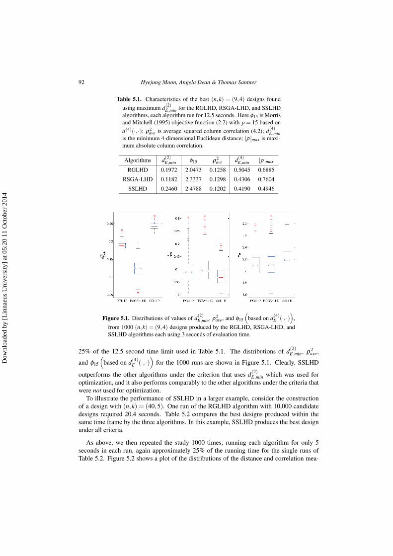
92 Hyejung Moon, Angela Dean & Thomas Santner
Table 5.1. Characteristics of the best (n,k) = (9,4) designs foundusing maximum d(2)
E,min for the RGLHD, RSGA-LHD, and SSLHDalgorithms, each algorithm run for 12.5 seconds. Here ϕ15 is Morrisand Mitchell (1995) objective function (2.2) with p = 15 based ond(4)(·, ·); ρ2
ave is average squared column correlation (4.2); d(4)E,min
is the minimum 4-dimensional Euclidean distance; |ρ|max is maxi-mum absolute column correlation.
Algorithms d(2)E,min ϕ15 ρ2
ave d(4)E,min |ρ|max
RGLHD 0.1972 2.0473 0.1258 0.5045 0.6885
RSGA-LHD 0.1182 2.3337 0.1298 0.4306 0.7604
SSLHD 0.2460 2.4788 0.1202 0.4190 0.4946
Figure 5.1. Distributions of values of d(2)E,min, ρ2
ave, and ϕ15
(based on d(4)
E (·, ·))
,
from 1000 (n,k) = (9,4) designs produced by the RGLHD, RSGA-LHD, andSSLHD algorithms each using 3 seconds of evaluation time.
25% of the 12.5 second time limit used in Table 5.1. The distributions of d(2)E,min, ρ2
ave,
and ϕ15
(based on d(4)
E (·, ·))
for the 1000 runs are shown in Figure 5.1. Clearly, SSLHD
outperforms the other algorithms under the criterion that uses d(2)E,min which was used for
optimization, and it also performs comparably to the other algorithms under the criteria thatwere not used for optimization.
To illustrate the performance of SSLHD in a larger example, consider the constructionof a design with (n,k) = (40,5). One run of the RGLHD algorithm with 10,000 candidatedesigns required 20.4 seconds. Table 5.2 compares the best designs produced within thesame time frame by the three algorithms. In this example, SSLHD produces the best designunder all criteria.
As above, we then repeated the study 1000 times, running each algorithm for only 5seconds in each run, again approximately 25% of the running time for the single runs ofTable 5.2. Figure 5.2 shows a plot of the distributions of the distance and correlation mea-
Dow
nloa
ded
by [
Lin
naeu
s U
nive
rsity
] at
05:
20 1
1 O
ctob
er 2
014
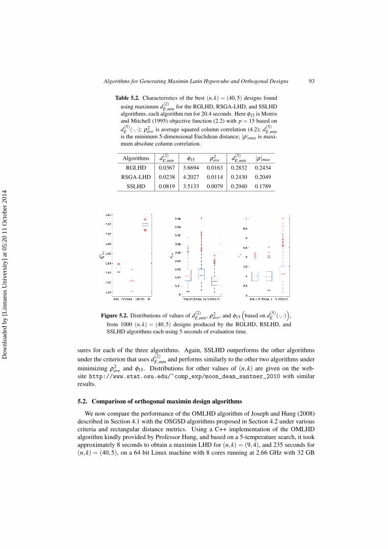
Algorithms for Generating Maximin Latin Hypercube and Orthogonal Designs 93
Table 5.2. Characteristics of the best (n,k) = (40,5) designs foundusing maximum d(2)
E,min for the RGLHD, RSGA-LHD, and SSLHDalgorithms, each algorithm run for 20.4 seconds. Here ϕ15 is Morrisand Mitchell (1995) objective function (2.2) with p = 15 based ond(5)
E (·, ·); ρ2ave is average squared column correlation (4.2); d(5)
E,minis the minimum 5-dimensional Euclidean distance; |ρ|max is maxi-mum absolute column correlation.
Algorithms d(2)E,min ϕ15 ρ2
ave d(5)E,min |ρ|max
RGLHD 0.0367 3.6694 0.0163 0.2832 0.2434
RSGA-LHD 0.0238 4.2027 0.0114 0.2430 0.2049
SSLHD 0.0819 3.5133 0.0079 0.2940 0.1789
Figure 5.2. Distributions of values of d(2)E,min, ρ2
ave, and ϕ15
(based on d(5)
E (·, ·))
,
from 1000 (n,k) = (40,5) designs produced by the RGLHD, RSLHD, andSSLHD algorithms each using 5 seconds of evaluation time.
sures for each of the three algorithms. Again, SSLHD outperforms the other algorithmsunder the criterion that uses d(2)
E,min and performs similarly to the other two algorithms underminimizing ρ2
ave and ϕ15. Distributions for other values of (n,k) are given on the web-site http://www.stat.osu.edu/˜comp_exp/moon_dean_santner_2010 with similarresults.
5.2. Comparison of orthogonal maximin design algorithms
We now compare the performance of the OMLHD algorithm of Joseph and Hung (2008)described in Section 4.1 with the OSGSD algorithms proposed in Section 4.2 under variouscriteria and rectangular distance metrics. Using a C++ implementation of the OMLHDalgorithm kindly provided by Professor Hung, and based on a 5-temperature search, it tookapproximately 8 seconds to obtain a maximin LHD for (n,k) = (9,4), and 235 seconds for(n,k) = (40,5), on a 64 bit Linux machine with 8 cores running at 2.66 GHz with 32 GB
Dow
nloa
ded
by [
Lin
naeu
s U
nive
rsity
] at
05:
20 1
1 O
ctob
er 2
014
94 Hyejung Moon, Angela Dean & Thomas Santner
of RAM. The criterion was the minimization of ψp,w in (4.1) with (p,w) = (15,0.5). TheOSGSD algorithms of Section 4.2 were coded in MATLAB. Despite the possible differencesin the numbers of actual computations performed by the compiled Joseph and Hung (2008)C++ and interpreted MATLAB programs, we used the same time limit for all algorithmswhen constructing designs.
For comparability with OSGSD designs which are on [0,1]k, all results reported belowscale the integer valued design points produced by the OMLHD program by (i−1)/(n−1),for i = 1, . . . ,n, and all programs use rectangular distance. Tables 5.3 and 5.4 summarize theperformance of the designs obtained from single runs of the three algorithms under severalcriteria for the (n,k) = (9,4) and (40,5) cases. The OMLHD design minimizes ψ15,0.5
in (4.1), the OSGSD-ϕ15 design minimizes ϕ15 in (2.2) using d(k)R (·, ·), and the OSGSD-
d(2)R,min design maximizes d(2)
R,min. in (2.5).
Table 5.3 shows that the OSGSD-d(2)R,min design for (n,k) = (9,4) has the largest value of
d(2)R,min, which is not surprising since this is the only one of the three algorithms that uses a
d(2)R,min-based criterion. Both OSGSD designs have zero column correlations by construction,
and so outperform the OMLHD design with respect to the average and maximum correlationmeasures. The OSGSD-ϕ15 design outperforms the OMLHD design under the criteria basedon maximizing d(4)
R,min and minimizing ϕ15 (and hence minimizing ψ15,0.5).
To investigate the stability and performance of OSGSD-ϕ15 when run for a limited time,we ran the algorithm 1000 times for 2 seconds per run, being 25% of the 8 seconds requiredto run the OMLHD algorithm. The distributions of ϕ15 and d(4)
R,min for the 1000 designsproduced by the OSGSD-ϕ15 algorithm are shown in Figure 5.3. Of the designs obtained in2 seconds, 98.1% have smaller ϕ15 values than the ϕ15 = 0.8624 of the OMLHD, and 47.5%of designs have larger minimum 4-dimensional rectangular distance than d(4)
R,min = 1.375of the OMLHD. We conclude that the OSGSD-ϕ15 algorithm outperforms the OMLHDalgorithm in terms of ϕ15 and correlation measures as well as computational efficiency forthe (n,k) = (9,4) design. It performs similarly in terms of d(4)
R,min.Now consider the larger problem of (n,k) = (40,5). The Joseph and Hung (2008) C++
code required 235 seconds to execute the OMLHD algorithm. Table 5.4 shows the results ofa single run of the OSGSD-d(2)
R,min and OSGSD-ϕ15 algorithms based on the same time limit.
The OSGSD-d(2)R,min design is again best in terms of maximizing d(2)
R,min. The OSGSD-ϕ15
design using d(5)R again outperforms the OMLHD in terms of minimizing ϕ15, ρ2
ave, |ρ|max,and maximizing d(5)
R,min.
To investigate the stability and performance of OSGSD-ϕ15 when run for a limited timefor this larger problem, we again conducted 1000 runs of the algorithm, each for 60 secondswhich is approximately 25% of 235 seconds. The distributions of ϕ15 and d(5)
R,min of the 1000runs are shown in Figure 5.4. All but two of the 1000 designs obtained with 60 seconds ofcomputational effort have smaller ϕ15 and all have larger d(5)
R,min values than the ϕ15 = 1.3176
and d(5)R,min = 0.9231 of the OMLHD design. Thus the OSGSD-ϕ15 algorithm outperforms
the OMLHD algorithm in terms of ϕ15, d(5)R,min, and correlation measures, as well as be-
ing considerably more computationally efficient. Distributions for other (n,k) are given on
Dow
nloa
ded
by [
Lin
naeu
s U
nive
rsity
] at
05:
20 1
1 O
ctob
er 2
014
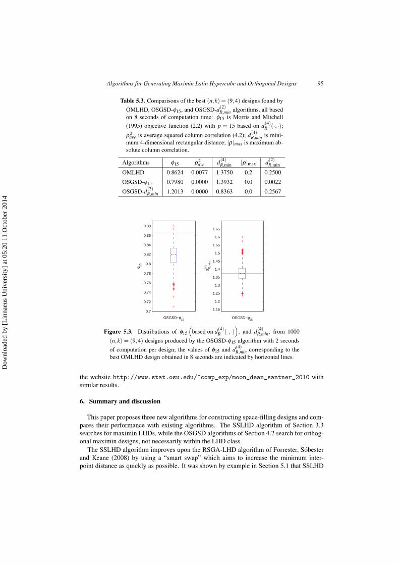
Algorithms for Generating Maximin Latin Hypercube and Orthogonal Designs 95
Table 5.3. Comparisons of the best (n,k) = (9,4) designs found byOMLHD, OSGSD-ϕ15, and OSGSD-d(2)
R,min algorithms, all basedon 8 seconds of computation time: ϕ15 is Morris and Mitchell(1995) objective function (2.2) with p = 15 based on d(4)
R (·, ·);ρ2
ave is average squared column correlation (4.2); d(4)R,min is mini-
mum 4-dimensional rectangular distance; |ρ|max is maximum ab-solute column correlation.
Algorithms ϕ15 ρ2ave d(4)
R,min |ρ|max d(2)R,min
OMLHD 0.8624 0.0077 1.3750 0.2 0.2500
OSGSD-ϕ15 0.7980 0.0000 1.3932 0.0 0.0022
OSGSD-d(2)R,min 1.2013 0.0000 0.8363 0.0 0.2567
0.7
0.72
0.74
0.76
0.78
0.8
0.82
0.84
0.86
0.88
OSGSD−φ15
φ 15
1.15
1.2
1.25
1.3
1.35
1.4
1.45
1.5
1.55
1.6
1.65
OSGSD−φ15
d(4)
R,m
in
Figure 5.3. Distributions of ϕ15
(based on d(4)
R (·, ·))
, and d(4)R,min, from 1000
(n,k) = (9,4) designs produced by the OSGSD-ϕ15 algorithm with 2 secondsof computation per design; the values of ϕ15 and d(4)
R,min corresponding to thebest OMLHD design obtained in 8 seconds are indicated by horizontal lines.
the website http://www.stat.osu.edu/˜comp_exp/moon_dean_santner_2010 withsimilar results.
6. Summary and discussion
This paper proposes three new algorithms for constructing space-filling designs and com-pares their performance with existing algorithms. The SSLHD algorithm of Section 3.3searches for maximin LHDs, while the OSGSD algorithms of Section 4.2 search for orthog-onal maximin designs, not necessarily within the LHD class.
The SSLHD algorithm improves upon the RSGA-LHD algorithm of Forrester, Sóbesterand Keane (2008) by using a “smart swap” which aims to increase the minimum inter-point distance as quickly as possible. It was shown by example in Section 5.1 that SSLHD
Dow
nloa
ded
by [
Lin
naeu
s U
nive
rsity
] at
05:
20 1
1 O
ctob
er 2
014
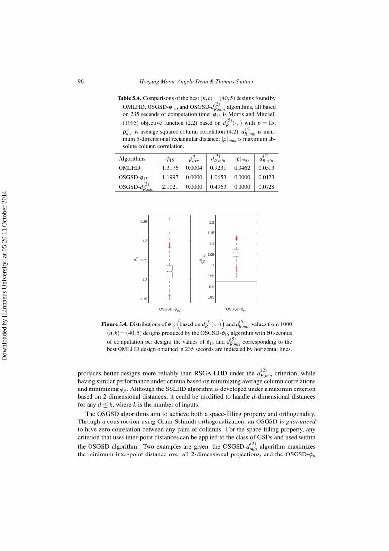
96 Hyejung Moon, Angela Dean & Thomas Santner
Table 5.4. Comparisons of the best (n,k) = (40,5) designs found byOMLHD, OSGSD-ϕ15, and OSGSD-d(2)
R,min algorithms, all basedon 235 seconds of computation time: ϕ15 is Morris and Mitchell(1995) objective function (2.2) based on d(5)
R (·, ·) with p = 15;
ρ2ave is average squared column correlation (4.2); d(5)
R,min is mini-mum 5-dimensional rectangular distance; |ρ|max is maximum ab-solute column correlation.
Algorithms ϕ15 ρ2ave d(5)
R,min |ρ|max d(2)R,min
OMLHD 1.3176 0.0004 0.9231 0.0462 0.0513
OSGSD-ϕ15 1.1997 0.0000 1.0653 0.0000 0.0123
OSGSD-d(2)R,min 2.1021 0.0000 0.4963 0.0000 0.0728
1.15
1.2
1.25
1.3
1.35
OSGSD−φ15
φ 15
0.85
0.9
0.95
1
1.05
1.1
1.15
1.2
OSGSD−φ15
d(5)
R,m
in
Figure 5.4. Distributions of ϕ15
(based on d(5)
R (·, ·))
and d(5)R,min values from 1000
(n,k) = (40,5) designs produced by the OSGSD-ϕ15 algorithm with 60 secondsof computation per design; the values of ϕ15 and d(5)
R,min corresponding to thebest OMLHD design obtained in 235 seconds are indicated by horizontal lines.
produces better designs more reliably than RSGA-LHD under the d(2)E,min criterion, while
having similar performance under criteria based on minimizing average column correlationsand minimizing ϕp. Although the SSLHD algorithm is developed under a maximin criterionbased on 2-dimensional distances, it could be modified to handle d-dimensional distancesfor any d ≤ k, where k is the number of inputs.
The OSGSD algorithms aim to achieve both a space-filling property and orthogonality.Through a construction using Gram-Schmidt orthogonalization, an OSGSD is guaranteedto have zero correlation between any pairs of columns. For the space-filling property, anycriterion that uses inter-point distances can be applied to the class of GSDs and used withinthe OSGSD algorithm. Two examples are given; the OSGSD-d(2)
min algorithm maximizesthe minimum inter-point distance over all 2-dimensional projections, and the OSGSD-ϕp
Dow
nloa
ded
by [
Lin
naeu
s U
nive
rsity
] at
05:
20 1
1 O
ctob
er 2
014
Algorithms for Generating Maximin Latin Hypercube and Orthogonal Designs 97
algorithm minimizes ϕp. In the examples in Section 5.2, we used d(2)R (·, ·) as the distance
for OSGSD-d(2)min, but this could have been replaced by the Euclidean distance d(2)
E,min or anyother 2-dimensional distance metric with the same gains in efficiency.
For k inputs, the examples in Section 5.2 used k-dimensional rectangular distance d(k)R (·, ·)
and p = 15 in the OSGSD-ϕp algorithm, and this could have been replaced by any other k-dimensional distance measure and any other value of p. The examples showed that OSGSD-ϕ15 outperforms the OMLHD algorithm by producing an orthogonal design with smaller ϕ15almost always and within a shorter time frame. Other examples are given on the websitehttp://www.stat.osu.edu/˜comp_exp/moon_dean_santner_2010 and show similarresults.
In summary, for cases where orthogonality of design inputs is not required but where theone-dimensional projection properties of a LHD are desired, we recommend our smart swapalgorithm, SSLHD, which is rapidly computable, has excellent space-filling properties in all2-dimensional subspaces, and achieves good k-dimensional space-filling properties. Whenorthogonal columns are required, the OSGSD algorithms are guaranteed to produce zerocolumn correlations. OSGSD-ϕp produces designs with smaller ϕp and larger d(k)
R,min thanthe OMLHD algorithm almost all of the time, even when run at 25% of the time requiredfor a single 5-temperature run of the latter.
Acknowledgments
The authors would like to thank Erin Leatherman for preparing the distribution tables andfigures for the paper and the website. The authors are grateful to Ying Hung for supplyingthe C++ code for the OMLHD algorithm. This research was sponsored, in part, by theNational Science Foundation under Agreement DMS-0806134 (The Ohio State University).Any opinions, findings, and conclusions or recommendations expressed in this material arethose of the author(s) and do not necessarily reflect the views of the National Science Foun-dation.
References
Bingham, D., Sitter, R.R., Tang, B., 2009. Orthogonal and nearly orthogonal designs for computer experi-ments. Biometrika, 96, 51–65.
Butler, N.A., 2001. Optimal and orthogonal Latin hypercube designs for computer experiments. Biometrika,88, 847–857.
Cioppa, T.M., Lucas, T.W., 2007. Efficient nearly orthogonal and space-filling Latin hypercubes. Techno-metrics, 49, 45–55.
Forrester, A., Sóbester, A., Keane, A., 2008. Engineering Design via Surrogate Modelling. Wiley, Chich-ester.
Johnson, M.E., Moore, L.M., Ylvisaker, D., 1990. Minimax and maximin distance designs. Journal ofStatistical Planning and Inference, 26, 131–148.
Joseph, V.R., Hung, Y., 2008. Orthogonal-maximin Latin hypercube designs. Statistica Sinica, 18, 171–186.Lin, C.D., Mukerjee, R., Tang, B., 2009. Construction of orthogonal and nearly orthogonal Latin hypercubes.
Biometrika, 96, 243–247.McKay, M.D., Beckman, R.J., Conover, W.J., 1979. A comparison of three methods for selecting values of
input variables in the analysis of output from a computer code. Technometrics, 21, 239–245.Moon, H., Santner, T.J., Dean, A.M., 2010. Two-stage sensitivity-based group screening in computer exper-
iments. Submitted for Publication.
Dow
nloa
ded
by [
Lin
naeu
s U
nive
rsity
] at
05:
20 1
1 O
ctob
er 2
014

98 Hyejung Moon, Angela Dean & Thomas Santner
Morris, M.D., Mitchell, T.J., 1995. Exploratory designs for computational experiments. Journal of Statisti-cal Planning and Inference, 43, 381–402.
Owen, A.B., 1994. Controlling correlations in Latin hypercube samples. Journal of the American StatisticalAssociation, 89, 1517–1522.
Steinberg, D.M., Lin, D.K.J., 2006. A construction method for orthogonal Latin hypercube designs.Biometrika, 93, 279–288, Correction, p. 1025.
Sun, F., Liu, M.-Q., Lin, D.K.J., 2009. Construction of orthogonal Latin hypercube designs. Biometrika, 96,971–974.
Tang, B., 1993. Orthogonal array-based latin hypercubes. Journal of the American Statistical Association,88, 1392–1397.
Tang, B., 1998. Selecting Latin hypercubes using correlation criteria. Statistica Sinica, 8, 965–978.Welch, W.J., 1985. ACED: Algorithms for the construction of experimental designs. The American Statisti-
cian, 39, 146.Ye, K.Q., 1998. Orthogonal column Latin hypercubes and their application in computer experiments. Jour-
nal of the American Statistical Association, 93, 1430–1439.
Dow
nloa
ded
by [
Lin
naeu
s U
nive
rsity
] at
05:
20 1
1 O
ctob
er 2
014


![Quantum maximin surfaces...2In the original maximin proposal [2] all Cauchy slices that contained @Rwere allowed in the maximin-imization. In the restricted maximin proposal [19] only](https://img.pdfslide.us/doc/110x75/60d45f33a34f5e6b1b3e45fa/quantum-maximin-surfaces-2in-the-original-maximin-proposal-2-all-cauchy-slices.jpg)