ALGORITHMS AND SOFTWARE FOR LINEAR AND NONLINEAR PROGRAMMING

Stephen J. WrightMathematics and Computer Science Division

Argonne National LaboratoryArgonne IL 60439

Abstract

The past ten years have been a time of remarkable developments in software tools for solving optimization problems. There have been algorithmic advances in such areas as linear programming and integer programming which have now borne fruit in the form of more powerful codes. The advent of modeling languages has made the process of formulating the problem and invoking the software much easier, and the explosion in computational power of hardware has made it possible to solve large, difficult problems in a short amount of time on desktop machines. A user community that is growing rapidly in size and sophistication is driving these developments. In this article, we discuss the algorithmic state of the art and its relevance to production codes. We describe some representative software packages and modeling languages and give pointers to web sites that contain more complete information. We also mention computational servers for online solution of optimization problems.

Keywords

Optimization, Linear programming, Nonlinear programming, Integer programming, Software.

Introduction

1

4 CONTROLLERS

Optimization problems arise naturally in many engineering applications. Control problems can be formulated as optimization problems in which the variables are inputs and states, and the constraints include the model equations for the plant. At successively higher levels, optimization can be used to determine setpoints for optimal operations, to design processes and plants, and to plan for future capacity.

Optimization problems contain the following key ingredients:

Variables that can take on a range of values. Variables that are real numbers, integers, or binary (that is, allowable values 0 and 1) are the most common types, but matrix variables are also possible.

Constraints that define allowable values or scopes for the variables, or that specify relationships between the variables;

An objective function that measures the desirability of a given set of variables.

The optimization problem is to choose from among all variables that satisfy the constraints the set of values that minimizes the objective function.

The term “mathematical programming”, which was coined around 1945, is synonymous with optimization. Correspondingly, linear optimization (in which the constraints and objective are linear functions of the variables) is usually known as “linear programming,” while optimization problems that involve constraints and have nonlinearity present in the objective or in at least some constraints, are known as “nonlinear programming” problems. In convex programming, the objective is a convex function and the feasible set (the set of points that satisfy the constraints) is a convex set. In quadratic programming, the objective is a quadratic function while the constraints are linear. Integer programming problems are those in which some or all of the variables are required to take on integer values.

Optimization technology is traditionally made available to users by means of codes or packages for specific classes of problems. Data is communicated to the software via simple data structures and subroutine argument lists, user-written subroutines (for evaluating nonlinear objective or constraint functions), text files in the standard MPS format, or text files that describe the problem in certain vendor-specific formats. More recently, modeling languages have become an appealing way to interface to packages, as they allow the user to define the model and data in a way that makes intuitive sense in terms of the application problem. Optimization tools also form part of integrated modeling systems such as GAMS and LINDO, and even underlie spreadsheets such as Microsoft’s Excel. Other “under the hood” optimization tools are present in certain logistics

packages, for example, packages for supply chain management or facility location.

The majority of this paper is devoted to a discussion of software packages and libraries for linear and nonlinear programming, both freely available and proprietary. We emphasize in particular packages that have become available during the past 10 years, that address new problem areas or that make use of new algorithms. We also discuss developments in related areas such as modeling languages and automatic differentiation. Background information on algorithms and theory for linear and nonlinear programming can be found in a number of texts, including those of Luenberger (1984), Chvatal (1983), Bertsekas (1995), Nash and Sofer (1996), and the forthcoming book of Nocedal and Wright (1999).

Online Resources and Computational Servers

As with so many other topics, a great deal of information about optimization software is available on the world-wide web. Here we point to a few noncommercial sites that give information about optimization algorithms and software, modeling issues, and operations research. Many other interesting sites can be found by following links from the sites mentioned below.

The NEOS Guide at www.mcs.anl.gov/otc/Guide contains

A guide to optimization software containing around 130 entries. The guide is organized by the name of the code, and classified according to the type of problem solved by the code.

An “optimization tree” containing a taxonomy of optimization problem types and outlines of the basic algorithms.

Case studies that demonstrate the use of algorithms in solving real-world optimization problems. These include optimization of an investment portfolio, choice of a lowest-cost diet that meets a set of nutritional requirements, and optimization of a strategy for stockpiling and retailing natural gas, under conditions of uncertainty about future demand and price.

The NEOS Guide also houses the FAQs for Linear and Nonlinear Programming, which can be found at www.mcs.anl.gov/otc/Guide/faq/. These pages, updated monthly, contain basic information on modeling and algorithmic issues, information for most of the available codes in the two areas, and pointers to texts for readers who need background information.

Michael Trick maintains a comprehensive web site on operations research topics at http://mat.gsia.cmu.edu. It contains pointers to most online resources in operations research, together with an extensive directory of researchers and research groups and of companies that are

2

3

involved in optimization and logistics software and consulting.

Hans Mittelmann and Peter Spellucci maintain a decision tree to help in the selection of appropriate optimization software tools at http://plato.la.asu.edu/guide.html. Benchmarks for a variety of codes, with an emphasis on linear programming solvers that are freely available to researchers, can be found at http://plato.la.asu.edu/bench.html. The page http://solon.cma.univie.ac.at/~neum/glopt.html, maintained by Arnold Neumaier, emphasizes global optimization algorithms and software.

The NEOS Server at www.mcs.anl.gov/neos/Server is a computational server for the remote solution of optimization problems over the Internet. By using an email interface, a Web page, or an xwindows “submission tool” that connects directly to the Server via Unix sockets, users select a code and submit the model information and data that define their problem. The job of solving the problem is allocated to one of the available workstations in the Server’s pool on which that particular package is installed, then the problem is solved and the results returned to the user.

The Server now has a wide variety of solvers in its roster, including a number of proprietary codes. For linear programming, the BPMPD, HOPDM, PCx, and XPRESS-MP/BARRIER interior-point codes as well as the XPRESS-MP/SIMPLEX code are available. For nonlinear programming, the roster includes LANCELOT, LOQO, MINOS, NITRO, SNOPT, and DONLP2. Input in the AMPL modeling language is accepted for many of the codes.

The obvious target audience for the NEOS Server includes users who want to try out a new code, to benchmark or compare different codes on data of relevance to their own applications, or to solve small problems on an occasional basis. At a higher level, however, the Server is an experiment in using the Internet as a computational, problem-solving tool rather than simply an informational device. Instead of purchasing and installing a piece of software for installation on their local hardware, users gain access to the latest algorithmic technology (centrally maintained and updated), the hardware resources needed to execute it and, where necessary, the consulting services of the authors and maintainers of each software package. Such a means of delivering problem-solving technology to its customers is an appealing option in areas that demand access to huge amounts of computing cycles (including, perhaps, integer programming), areas in which extensive hands-on consulting services are needed, areas in which access to large, centralized, constantly changing data bases, and areas in which the solver technology is evolving rapidly.

Linear Programming

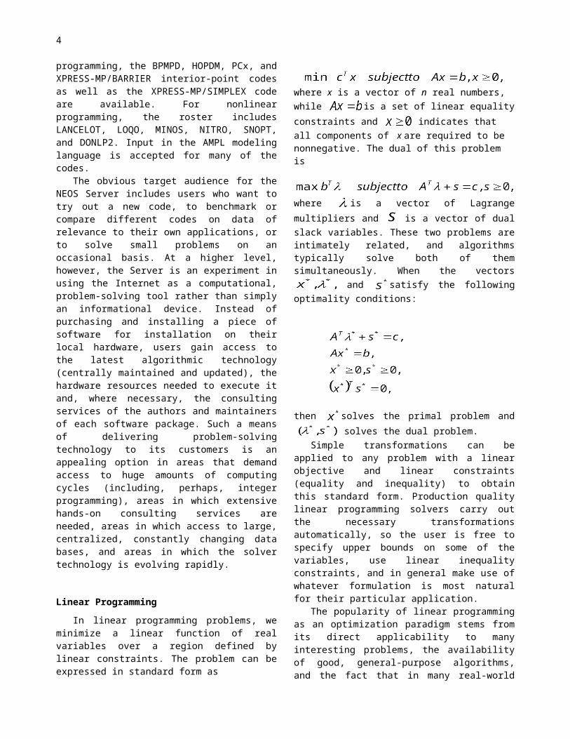
In linear programming problems, we minimize a linear function of real variables over a region defined by linear constraints. The problem can be expressed in standard form as

where x is a vector of n real numbers, while is a set of linear equality constraints and indicates that all components of x are required to be nonnegative. The dual of this problem is

where is a vector of Lagrange multipliers and is a vector of dual slack variables. These two problems are intimately related, and algorithms typically solve both of them simultaneously. When the vectors and satisfy the following optimality conditions:

then solves the primal problem and solves the dual problem.

Simple transformations can be applied to any problem with a linear objective and linear constraints (equality and inequality) to obtain this standard form. Production quality linear programming solvers carry out the necessary transformations automatically, so the user is free to specify upper bounds on some of the variables, use linear inequality constraints, and in general make use of whatever formulation is most natural for their particular application.

The popularity of linear programming as an optimization paradigm stems from its direct applicability to many interesting problems, the availability of good, general-purpose algorithms, and the fact that in many real-world situations, the inexactness in the model or data means that the use of a more sophisticated nonlinear model is not warranted. In addition, linear programs do not have multiple local minima, as may be the case with nonconvex optimization problems. That is, any local solution of a linear programone whose function value is no larger than any feasible point in its immediate vicinityalso achieves the global minimum of the objective over the whole feasible region. It remains true that more (human and computational) effort is invested in

4

solving linear programs than in any other class of optimization problems.

Prior to 1987, all of the commercial codes for solving general linear programs made use of the simplex algorithm. This algorithm, invented in the late 1940s, had fascinated optimization researchers for many years because its performance on practical problems is usually far better than the theoretical worst case. A new class of algorithms known as interior-point methods was the subject of intense theoretical and practical investigation during the period 1984—1995, with practical codes first appearing around 1989. These methods appeared to be faster than simplex on large problems, but the advent of a serious rival spurred significant improvements in simplex codes. Today, the relative merits of the two approaches on any given problem depend strongly on the particular geometric and algebraic properties of the problem. In general, however, good interior-point codes continue to perform as well or better than good simplex codes on larger problems when no prior information about the solution is available. When such “warm start” information is available, however, as is often the case in solving continuous relaxations of integer linear programs in branch-and-bound algorithms, simplex methods are able to make much better use of it than interior-point methods. Further, a number of good interior-point codes are freely available for research purposes, while the few freely available simplex codes are not quite competitive with the best commercial codes.

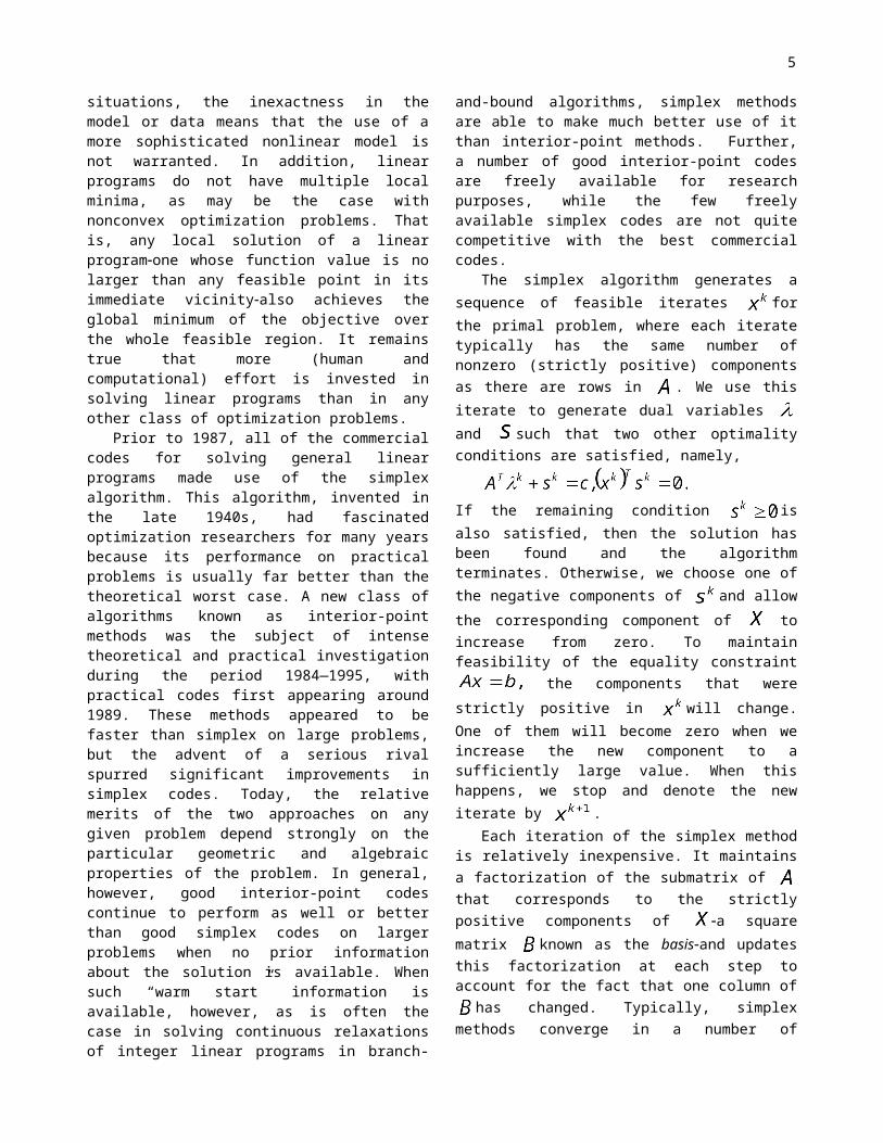
The simplex algorithm generates a sequence of feasible iterates for the primal problem, where each iterate typically has the same number of nonzero (strictly positive) components as there are rows in . We use this iterate to generate dual variables and such that two other optimality conditions are satisfied, namely,

If the remaining condition is also satisfied, then the solution has been found and the algorithm terminates. Otherwise, we choose one of the negative components of

and allow the corresponding component of to increase from zero. To maintain feasibility of the equality constraint the components that were strictly positive in will change. One of them will become zero when we increase the new component to a sufficiently large value. When this happens, we stop and denote the new iterate by .

Each iteration of the simplex method is relatively inexpensive. It maintains a factorization of the submatrix of that corresponds to the strictly positive components of a square matrix known as the basisand updates this factorization at each step to account for the fact that one column of has changed. Typically, simplex methods converge in a number of iterates that is about two to three times the number of columns in .

Interior-point methods proceed quite differently, applying a Newton-like algorithm to the three equalities in the optimality conditions and taking steps that maintain strict positivity of all the and components. It is the latter feature that gives rise to the term “interior-point” the iterates are strictly interior with respect to the inequality constraints. Each interior-point iteration is typically much more expensive than a simplex iteration, since it requires refactorization of a large matrix of the form , where and are diagonal matrices whose diagonal elements are the components of the current iterates and , respectively. The solutions to the primal and dual problems are generated simultaneously. Typically, interior-point iterates converge in between 10 and 100 iterations.

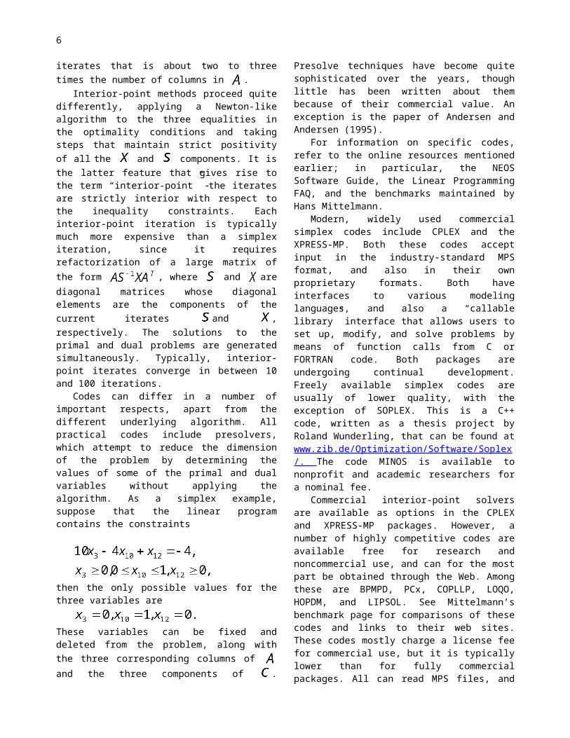
Codes can differ in a number of important respects, apart from the different underlying algorithm. All practical codes include presolvers, which attempt to reduce the dimension of the problem by determining the values of some of the primal and dual variables without applying the algorithm. As a simplex example, suppose that the linear program contains the constraints

then the only possible values for the three variables are

These variables can be fixed and deleted from the problem, along with the three corresponding columns of

and the three components of . Presolve techniques have become quite sophisticated over the years, though little has been written about them because of their commercial value. An exception is the paper of Andersen and Andersen (1995).

For information on specific codes, refer to the online resources mentioned earlier; in particular, the NEOS Software Guide, the Linear Programming FAQ, and the benchmarks maintained by Hans Mittelmann.

Modern, widely used commercial simplex codes include CPLEX and the XPRESS-MP. Both these codes accept input in the industry-standard MPS format, and also in their own proprietary formats. Both have interfaces to various modeling languages, and also a “callable library” interface that allows users to set up, modify, and solve problems by means of function calls from C or FORTRAN code. Both packages are undergoing continual development. Freely available simplex codes are usually of lower quality, with the exception of SOPLEX. This is a C++ code, written as a thesis project by Roland Wunderling, that can be found at www.zib.de/Optimization/Software/Soplex/. The code MINOS is available to nonprofit and academic researchers for a nominal fee.

Commercial interior-point solvers are available as options in the CPLEX and XPRESS-MP packages.

5

However, a number of highly competitive codes are available free for research and noncommercial use, and can for the most part be obtained through the Web. Among these are BPMPD, PCx, COPLLP, LOQO, HOPDM, and LIPSOL. See Mittelmann’s benchmark page for comparisons of these codes and links to their web sites. These codes mostly charge a license fee for commercial use, but it is typically lower than for fully commercial packages. All can read MPS files, and most are interfaced to modeling languages. LIPSOL is programmed in Matlab (with the exception of the linear equations solver), while the other codes are written in C and/or FORTRAN.

A fine reference on linear programming, with an emphasis on the simplex method, is the book of Chvatal (1983). An online Java applet that demonstrates the operation of the simplex method on small user-defined problems can be found at www.mcs.anl.gov/otc/Guide/CaseStudies/simplex/. Wright (1997) gives a description of practical interior-point methods.

Modeling Languages

From the user’s point of view, the efficiency of the algorithm or the quality of the programming may not be the critical factors in determining the usefulness of the code. Rather, the ease with which it can be interfaced to his particular applications may be more important; weeks of person-hours may be more costly to the enterprise than a few hours of time on a computer. The most suitable interface depends strongly on the particular application and on the context in which it is solved. For users that are well acquainted with a spreadsheet interface, for instance, or with MATLAB, a code that can accept input from these sources may be invaluable. For users with large legacy modeling codes that set up and solve optimization problems by means of subroutine calls, substitution of a more efficient package that uses more or less the same subroutine interface may be the best option. In some disciplines, (JP’s biology/chemistry pointer) application-specific modeling languages allow problems to be posed in a thoroughly intuitive way. In other cases, application-specific graphical user interfaces may be more appropriate.

For general optimization problems, a number of high-level modeling languages have become available that allow problems to be specified in intuitive terms, using data structures, naming schemes, and algebraic relational expressions that are dictated by the application and model rather than by the input requirements of the optimization code. Typically, a user starting from scratch will find the process of model building more straightforward and bug free with such a modeling language than, say, a process of writing FORTRAN code to pack the data into one-dimensional arrays, turning the

algebraic relations between the variables into FORTRAN expressions involving elements of these arrays, and writing more code to interpret the output from the optimization routine in terms of the original application.

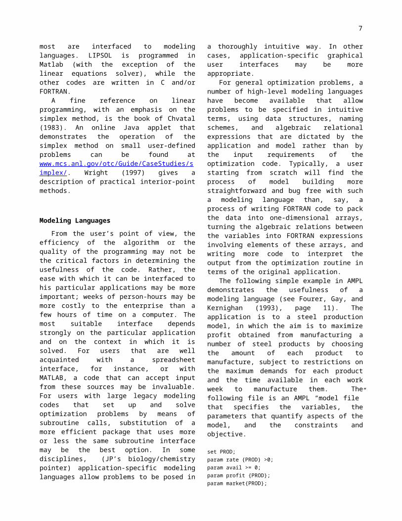
The following simple example in AMPL demonstrates the usefulness of a modeling language (see Fourer, Gay, and Kernighan (1993), page 11). The application is to a steel production model, in which the aim is to maximize profit obtained from manufacturing a number of steel products by choosing the amount of each product to manufacture, subject to restrictions on the maximum demands for each product and the time available in each work week to manufacture them. The following file is an AMPL “model file” that specifies the variables, the parameters that quantify aspects of the model, and the constraints and objective.

set PROD;param rate {PROD} >0;param avail >= 0;param profit {PROD};param market{PROD};

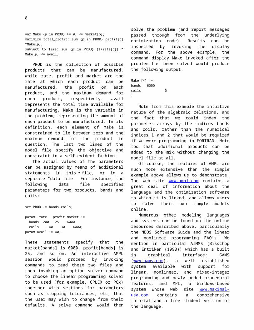
var Make {p in PROD} >= 0, <= market[p];maximize total_profit: sum {p in PROD} profit[p] *Make[p];subject to Time: sum {p in PROD} (1/rate[p]) * Make[p] <= avail;

PROD is the collection of possible products that can be manufactured, while rate, profit and market are the rate at which each product can be manufactured, the profit on each product, and the maximum demand for each product, respectively. avail represents the total time available for manufacturing. Make is the variable in the problem, representing the amount of each product to be manufactured. In its definition, each element of Make is constrained to lie between zero and the maximum demand for the product in question. The last two lines of the model file specify the objective and constraint in a self-evident fashion.

The actual values of the parameters can be assigned by means of additional statements in this file, or in a separate “data file.” For instance, the following data file specifies parameters for two products, bands and coils:

set PROD := bands coils;

param: rate profit market := bands 200 25 6000 coils 140 30 4000;param avail := 40;

These statements specify that the market[bands] is 6000, profit[bands] is 25, and so on. An interactive AMPL session would proceed by invoking commands to read these two files and then invoking an option solver command to choose the linear programming solver to be

6

used (for example, CPLEX or PCx) together with settings for parameters such as stopping tolerances, etc, that the user may wish to change from their defaults. A solve command would then solve the problem (and report messages passed through from the underlying optimization code). Results can be inspected by invoking the display command. For the above example, the command display Make invoked after the problem has been solved would produce the following output:

Make [*] :=bands 6000coils 0;

Note from this example the intuitive nature of the algebraic relations, and the fact that we could index the parameter arrays by the indices bands and coils, rather than the numerical indices 1 and 2 that would be required if we were programming in FORTRAN. Note too that additional products can be added to the mix without changing the model file at all.

Of course, the features of AMPL are much more extensive than the simple example above allows us to demonstrate. The web site www.ampl.com contains a great deal of information about the language and the optimization software to which it is linked, and allows users to solve their own simple models online.

Numerous other modeling languages and systems can be found on the online resources described above, particularly the NEOS Software Guide and the linear and nonlinear programming FAQ’s. We mention in particular AIMMS (Bisschop and Entriken (1993)) which has a built in graphical interface; GAMS (www.gams.com), a well established system available with support for linear, nonlinear, and mixed-integer programming and newly added procedural features; and MPL, a Windows-based system whose web site www.maximal-usa.com contains a comprehensive tutorial and a free student version of the language.

Other Input Formats

The established input format for linear programming problems has from the earliest days been MPS, a column oriented format (well suited to 1950s card readers) in which names are assigned to each primal and dual variable, and the data elements that define the problem are assigned in turn. Test problems for linear programming are still distributed in this format. It has significant disadvantages, however. The format is non-intuitive and the files are difficult to modify. Moreover, it restricts the precision to which numerical values can be specified. The format survives only because no universally accepted standard has yet been developed to take its place.

As mentioned previously, vendors such as CPLEX and XPRESS have their own input formats, which avoid the pitfalls of MPS. These formats lack the portability of the modeling languages described above, but they come bundled with the code, and may be attractive for users willing to make a commitment to a single vendor.

For nonlinear programming, SIF (the standard input format) was proposed by the authors of the LANCELOT code in the early 1990s. SIF is somewhat hamstrung by the fact that it is compatible with MPS. SIF files have a similar look to MPS files, except that there are a variety of new keywords for defining variables, groups of variables, and the algebraic relationships between them. For developers of nonlinear programming software, SIF has the advantage that a large collection of test problemsthe CUTE test setis available in this format. For users, however, formulating a model in SIF is typically much more difficult than using one of the modeling languages of the previous section.

For complete information about SIF, see www.numerical.rl.ac.uk/lancelot/sif/sifhtml.html

Nonlinear Programming

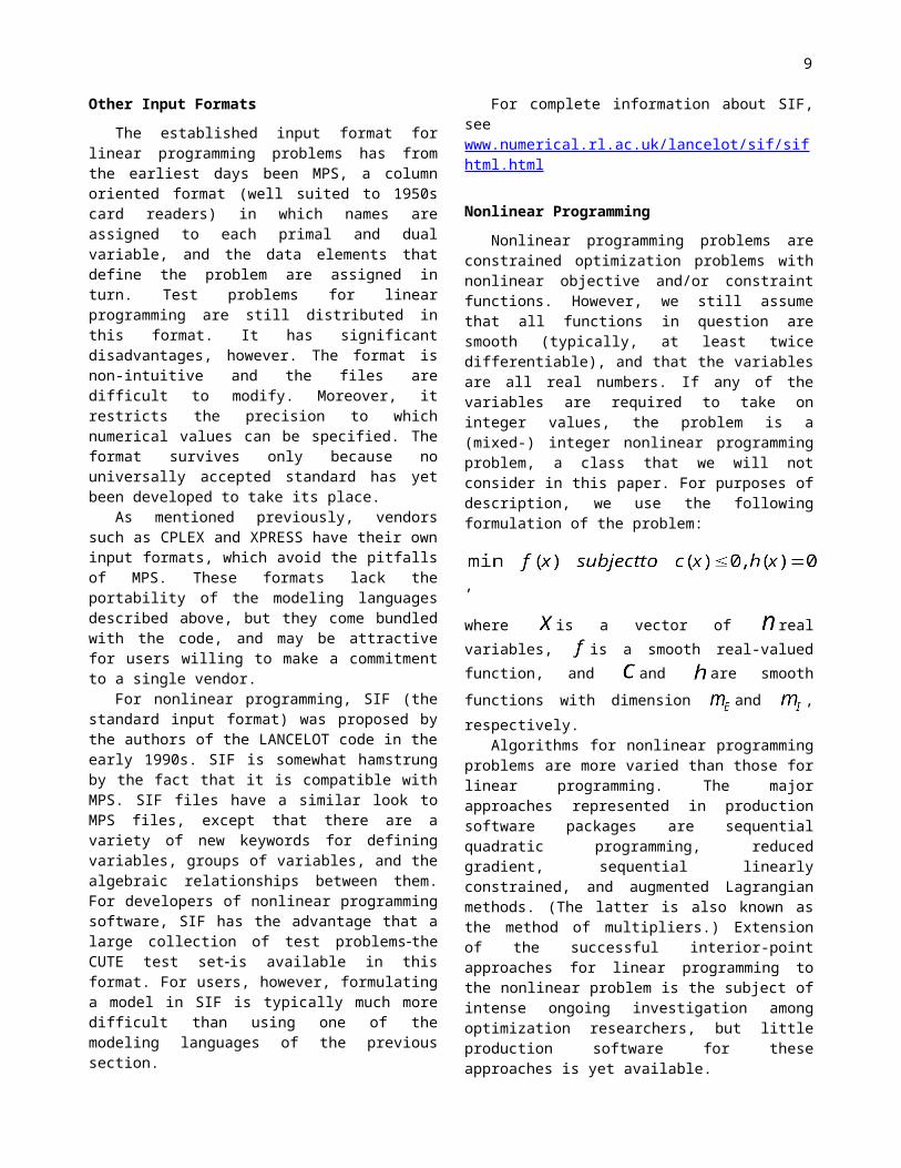
Nonlinear programming problems are constrained optimization problems with nonlinear objective and/or constraint functions. However, we still assume that all functions in question are smooth (typically, at least twice differentiable), and that the variables are all real numbers. If any of the variables are required to take on integer values, the problem is a (mixed-) integer nonlinear programming problem, a class that we will not consider in this paper. For purposes of description, we use the following formulation of the problem:

,

where is a vector of real variables, is a smooth real-valued function, and and are smooth functions with dimension and , respectively.

Algorithms for nonlinear programming problems are more varied than those for linear programming. The major approaches represented in production software packages are sequential quadratic programming, reduced gradient, sequential linearly constrained, and augmented Lagrangian methods. (The latter is also known as the method of multipliers.) Extension of the successful interior-point approaches for linear programming to the nonlinear problem is the subject of intense ongoing investigation among optimization researchers, but little production software for these approaches is yet available.

The use of nonlinear models may be essential in some applications, since a linear or quadratic model may be too simplistic and therefore produce useless results. However, there is a price to pay for using the more general nonlinear paradigm. For one thing, most

7

algorithms cannot guarantee convergence to the global minimum, i.e., the value that minimizes over the entire feasible region. At best, they will find a point that yields the smallest value of over all points in some feasible neighborhood of itself. (An exception occurs in convex programming, in which the functions and

are convex, while are linear. In this case, any local

minimizer is also a global minimizer. Note that linear programming is a special case of convex programming.) The problem of finding the global minimizer, though an extremely important one in some applications such as molecular structure determination, is very difficult to solve. While several general algorithmic approaches for global optimization are available, they are invariably implemented in a way that exploits heavily the special properties of the underlying application, so that there is a fair chance that they will produce useful results in a reasonable amount of computing time. We refer to Floudas and Pardalos (1992) and the journal Global Optimization for information on recent advances in this area.

A second disadvantage of nonlinear programming over linear programming is that general-purpose software is somewhat less effective because the nonlinear paradigm encompasses such a wide range of problems with a great number of potential pathologies and eccentricities. Even when we are close to a minimizer , algorithms may encounter difficulties because the solution may be degenerate, in the sense that certain of the active constraints become dependent, or are only weakly active. Curvature in the objective or constraint functions (a second-order effect not present in linear programming), and differences in this curvature between different directions, can cause difficulties for the algorithms, especially when second derivative information is not supplied by the user or not exploited by the algorithm. Finally, some of the codes treat the derivative matrices as dense, which means that they the maximum dimension of the problems they can handle is somewhat limited. However, most of the leading codes, including LANCELOT, MINOS, SNOPT, and SPRNLP are able to exploit sparsity, and are therefore equipped to handle large-scale problems.

Algorithms for special cases of the nonlinear programming problem, such as problems in which all constraints are linear or the only constraints are bounds on the components of , tend to be more effective than algorithms for the general problem because they are more able to exploit the special properties. (We discuss a few such special cases below.) Even for problems in which the constraints are nonlinear, the problem may contain special structures that can be exploited by the algorithm or by the routines that perform linear algebra operations at each iteration. An example is the optimal control

problem (arising, for example, in model predictive control), in which the equality constraint represents a nonlinear model of the “plant”, and the inequalities represent bounds and other restrictions on the states and inputs. The Jacobian (matrix of first partial derivatives of the constraints) typically has a banded structure, while the Hessian of the objective is symmetric and banded. Linear algebra routines that exploit this bandedness, or dig even deeper and exploit the control origins of the problem, are much more effective than general routines on such problems.

Local solutions of the nonlinear program can be characterized by a set of optimality conditions analogous to those described above for the linear programming problem. We introduce Lagrange multipliers and for the constraints and , respectively, and write the Lagrangian function for this problem as

The first-order optimality conditions (commonly known as the KKT conditions) are satisfied at a point if there exist multiplier vectors and such that

The active constraints are those for which equality holds at . All the components of are active by definition, while the active components of are those for which

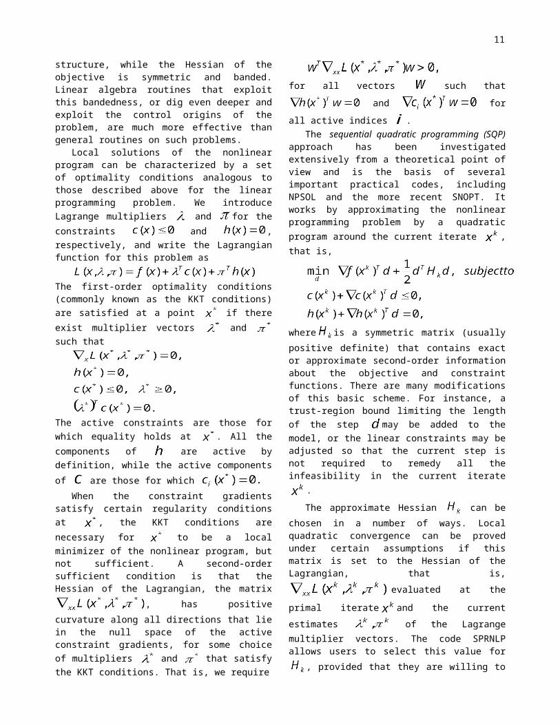
When the constraint gradients satisfy certain regularity conditions at , the KKT conditions are necessary for to be a local minimizer of the nonlinear program, but not sufficient. A second-order sufficient condition is that the Hessian of the Lagrangian, the matrix , has positive curvature along all directions that lie in the null space of the active constraint gradients, for some choice of multipliers and that satisfy the KKT conditions. That is, we require

for all vectors such that and

for all active indices . The sequential quadratic programming (SQP)

approach has been investigated extensively from a theoretical point of view and is the basis of several important practical codes, including NPSOL and the more recent SNOPT. It works by approximating the nonlinear programming problem by a quadratic program around the current iterate , that is,

8

where is a symmetric matrix (usually positive definite) that contains exact or approximate second-order information about the objective and constraint functions. There are many modifications of this basic scheme. For instance, a trust-region bound limiting the length of the step may be added to the model, or the linear constraints may be adjusted so that the current step is not required to remedy all the infeasibility in the current iterate .

The approximate Hessian can be chosen in a number of ways. Local quadratic convergence can be proved under certain assumptions if this matrix is set to the Hessian of the Lagrangian, that is,

evaluated at the primal iterate

and the current estimates of the Lagrange multiplier vectors. The code SPRNLP allows users to select this value for , provided that they are willing to supply the second derivative information. Alternatively,

can be a quasi-Newton approximation to the Lagrangian Hessian. Update strategies that yield local superlinear convergence are well known, and are implemented in dense codes such as NPSOL, DONLP2, NLPQL, and are available as an option in a version of SPRNLP that does not exploit sparsity. SNOPT also uses quasi-Newton Hessian approximations, but unlike the codes just mentioned it is able to exploit sparsity and is therefore better suited to large-scale problems. Another quasi-Newton variant is to maintain an approximation to the reduced Hessian, the two-sided projection of this matrix onto the null space of the active constraints. The latter approach is particularly efficient when the dimension of this null space is small in relation to the number of components of , as is the case in many process control problems, for instance. The approach does not appear to be implemented in general-purpose SQP software, however.

To ensure that the algorithm converges to a point satisfying the KKT conditions from any starting point, the basic SQP algorithm must be enhanced by the addition of a “global convergence” strategy. Usually, this strategy involves a merit function, whose purposes is to evaluate the desirability of a given iterate by accounting for its objective value and the amount by which it violates the constraints. The commonly used penalty function simply forms a weighted average of the objective and the constraint violations, as follows:

where is the vector of length whose elements

are and is a positive parameter. The simplest algorithm based on this function fixes and insists that all steps produce a “sufficient decrease” in the value of . Line search or trust region strategies are applied to ensure that steps with the required property can be found whenever the current point does not satisfy the KKT conditions. More sophisticated strategies contain mechanisms for adjusting the parameter and for ensuring that the fast local convergence properties are not compromised by the global convergence strategy.

We note that the terminology can be confusing”global convergence” in this context refers to convergence to a KKT point from any starting point, and not to convergence to a global minimizer.

For more information on SQP, we refer to the review paper of Boggs and Tolle (1996), and Chapter 18 of Nocedal and Wright (1999).

A second algorithmic approach is known variously as the augmented Lagrangian method or the method of multipliers. Noting that the first KKT condition, namely,

, requires to be a stationary point of the Lagrangian function , we modify this function to obtain an augmented function for which is not just a stationary point but also a minimizer. When only equality constraints are present (that is, is vacuous), the augmented Lagrangian function has the form

where is a positive parameter. It is not difficult to show that if is set to its optimal value (the value that satisfies the KKT conditions) and is sufficiently large, that is a minimizer of . Intuitively, the purpose of the squared-norm term is to add positive curvature to the function in just those directions in which it is neededthe directions in the range space of the active constraint gradients. (We know already from the second-order sufficient conditions that the curvature of in the null space of the active constraint gradients is positive.)

In the augmented Lagrangian method, we exploit this property by alternating between steps of two types:

Fixing and , and finding the value of that approximately minimizes

;

Updating to make it a better approximation to .

The update formula for has the form

where is the approximate minimizing value just calculated. Simple constraints such as bounds or linear equalities can be treated explicitly in the subproblem, rather than included in the second and third terms of .

9

(In LANCELOT, bounds on components of are treated in this manner.) Practical augmented Lagrangian algorithms also contain mechanisms for adjusting the parameter and for replacing the squared norm term

by a weighted norm that more properly reflects the scaling of the constraints and their violations at the current point.

When inequality constraints are present in the problem, the augmented Lagrangian takes on a slightly more complicated form that is nonetheless not difficult to motivate. We define the function as follows:

The definition of is then modified to incorporate the inequality constraints as follows:

The update formula for the approximate multipliers is

See the references below for details on derivation of this form of the augmented Lagrangian.

The definitive implementation of the augmented Lagrangian approach for general-purpose nonlinear programming problems is LANCELOT. It incorporates sparse linear algebra techniques, including preconditioned iterative linear solvers, making it suitable for large-scale problems. The subproblem of minimizing the augmented Lagrangian with respect to is a bound-constrained minimization problem, which is solved by an enhanced gradient projection technique. Problems can be passed to Lancelot via subroutine calls, SIF input files, and AMPL.

For theoretical background on the augmented Lagrangian approach, consult the books of Bertsekas (1982, 1995), and Conn, Gould, and Toint (1992), the authors of LANCELOT. The latter book is notable mainly for its pointers to the papers of the same three authors in which the theory of Lancelot is developed. A brief derivation of the theory appears in Chapter 17 of Nocedal and Wright (1999). (Note that the inequality constraints in this reference are assumed to have the form

rather than , necessitating a number of sign changes in the analysis.)

Interior-point solvers for nonlinear programming are the subjects of intense current investigation. An algorithm of this class, known as the sequential unconstrained minimization technique (SUMT) was actually proposed in the 1960s, in the book of Fiacco and McCormick (1968). The idea at that time was to define a barrier-penalty function for the NLP as follows:

where is a small positive parameter. Given some value of , the algorithm finds an approximation to the minimizer of . It then decreases and repeats the minimization process. Under certain assumptions, one can show that as so the sequence of iterates generated by SUMT should approach the solution of the nonlinear program provided that is decreased to zero. The difficulties with this approach are that all iterates must remain strictly feasible with respect to the inequality constraints (otherwise the log functions are not defined), and the subproblem of minimizing becomes increasingly difficult to solve as becomes small, as the Hessian of this function becomes highly ill conditioned and the radius of convergence becomes tiny. Many implementations of this approach were attempted, including some with enhancements such as extrapolation to obtain good starting points for each value of . However, the approach does not survive in the present generation of software, except through its profound influence on the interior-point research of the past 15 years.

Some algorithms for nonlinear programming that have been proposed in recent years contain echoes of the barrier function , however. For instance, the NITRO algorithm (Byrd, Gilbert, and Nocedal (1996)) reformulates the subproblem for a given positive value of

as follows:

NITRO then applies a trust-region SQP algorithm for equality constrained optimization to this problem, choosing the trust region to have the form

where the diagonal matrix and the trust-region radius are chosen so that the step does not violate strict positivity of the components, that is, NITRO is available through the NEOS Server at www.mcs.anl.gov/neos/Server/ . The user is required to specify the problem by means of FORTRAN subroutines to evaluate the objective and constraints. Derivatives are obtained automatically by means of ADIFOR.

An alternative interior-point approach is closer in spirit to the successful primal-dual class of linear programming algorithms. These methods generate iterates by applying Newton-like methods to the equalities in the KKT conditions. After introducing the slack variables for the inequality constraints, we can restate the KKT conditions as follows:

10

where and are diagonal matrices formed from the vectors and , respectively, while is the vector

. We generate a sequence of iterates satisfying the strict inequality

by applying a Newton-like method to the system of nonlinear equations formed by the first four conditions above. Modification of this basic approach to ensure global convergence is the major challenge associated with this class of solvers; the local convergence theory is relatively well understood. Merit functions can be used, along with line searches and modifications to the matrix in the equations that are solved for each step, to ensure that each step at least produces a decrease in the merit function. However, no fully satisfying complete theory has yet been proposed.

The code LOQO implements a primal-dual approach for nonlinear programming problems. It requires the problem to be specified in AMPL, whose built-in automatic differentiation features are used to obtain the derivatives of the objective and constraints. LOQO is also available through the NEOS Server at www.mcs.anl.gov/neos/Server/ , and or can be obtained for a variety of platforms.

The reduced gradient approach has been implemented in several codes that have been available for some years, notably, CONOPT and LSGRG2. This approach uses the formulation in which only bounds and equality constraints are present. (Any nonlinear program can be transformed to this form by introducing slacks for the inequality constraints and constraining the slacks to be nonnegative.) Reduced gradient algorithms partition the components of into three classes: basic, fixed, and superbasic. The equality constraint is used to eliminate the basic components from the problem by expressing them implicitly in terms of the fixed and superbasic components. The fixed components are those that are fixed at one of their bounds for the current iteration. The superbasics are the components that are allowed to move in a direction that reduces the value of the objective . Strategies for choosing this direction are derived from unconstrained optimization; they include steepest descent, nonlinear conjugate gradient, and quasi-Newton strategies. Both CONOPT and LSGRG2 use sparse linear algebra techniques during the elimination of the basic components, making them suitable for large-scale problems. While these codes have found use in many engineering applications, their

performance is often slower than competing codes based on SQP and augmented Lagrangian algorithms.

Finally, we mention MINOS, a code that has been available for many years in a succession of releases, and that has proved its worth in a great many engineering applications. When the constraints are linear, MINOS uses a reduced gradient algorithm, maintaining feasibility at all iterations and choosing the superbasic search direction with a quasi-Newton technique. When nonlinear constraints are present, MINOS forms linear approximations to them and replaces the objective with a projected augmented Lagrangian function in which the deviation from linearity is penalized. Convergence theory for this approach is not well establishedthe author admits that a reliable merit function is not knownbut it appears to converge on most problems.

The NEOS Guide page for SNOPT contains some guidance for users who are unsure whether to use MINOS or SNOPT. It describes problem features that are particularly suited to each of the two codes.

Obtaining Derivatives

One onerous requirement of some nonlinear programming codes has been their requirement that the user supply code for calculating derivatives of the objective and constraint functions. An important development of the past 10 years is that this requirement has largely disappeared. Modeling languages such as AMPL contain their own built-in systems for calculating first derivatives at specified values of the variable vector

, and supplying them to the underlying optimization code on request. Automatic differentiation software tools such as ADIFOR (Bischof et al. (1996)), which works with FORTRAN code, have been used to obtain derivatives from extremely complex “dusty deck” function evaluation routines. In the NEOS Server, all of the nonlinear optimization routines (including LANCELOT, SNOPT, and NITRO) are linked to ADIFOR, so that the user needs only to supply FORTRAN code to evaluate the objective and constraint functions, not their derivatives. Other high quality software tools for automatic differentiation include ADOL-C (Griewank, Juedes, and Utke (1996)), ODYSSEE (Rostaing, Dalmas, and Galligo (1993)), and ADIC (Bischof, Roh, and Mauer (1997)).

References

Andersen, E. D. and Andersen, K. D. (1995). Presolving in linear programming. Math. Prog., 71, 221-245.

Bertsekas, D. P. (1982). Constrained Optimization and Lagrange Multiplier Methods. Academic Press, New York.

Bertsekas, D. P. (1995). Nonlinear Programming. Athena Scientific.

11

Bischof, C., Carle, A., Khademi, P., and Mauer, A. (1996). ADIFOR 2.0: Automatic differentiation of FORTRAN programs. IEEE Computational Science and Engineering, 3, 18-32.

Bischof, C., Roh, L., and Mauer, A. (1997). ADIC: An extensible automatic differentiation tool for ANSI-C. Software-Practice and Experience, 27, 1427-1456.

Bisschop, J. and Entriken, R. (1993). AIMMS: The Modeling System. Available from AIMMS web site at http://www.paragon.nl

Boggs, P. T. and Tolle, J. W. (1996). Sequential quadratic programming, Acta Numerica, 4, 1-51.

Byrd, R. H., Gilbert, J.-C., and Nocedal, J. (1996). A trust-region algorithm based on interior-point techniques for nonlinear programming. OTC Technical Report 98/06, Optimization Technology Center. (Revised, 1998.)

Chvatal, V. (1983). Linear Programming. Freeman, New York.Conn, A. R., Gould, N. I. M., and Toint, Ph. L. (1992).

LANCELOT: A FORTRAN Package for Large-Scale Nonlinear Optimization (Release A). Volume 17, Springer Series in Computational Mathematics, Springer-Verlag, New York.

Czyzyk, J., Mesnier. M. P., and More’, J. J. (1998). The NEOS Server. IEEE Journal on Computational Science and Engineering, 5, 68-75.

Fiacco, A. V. and McCormick, G. P. (1968). Nonlinear Programming: Sequential Unconstrained Minimization Tecnhiques. John Wiley and Sons, New York. (Reprinted by SIAM Publications, 1990.)

Floudas, C. and Pardalos, P., eds (1992). Recent Advances in Global Optimization. Princeton University Press, Princeton.

Fourer, R., Gay, D. M., and Kernighan, B. W. (1993). AMPL: A Modeling Language for Mathematical Programming.The Scientific Press, San Francisco.

Griewank, A., Juedes, D., and Utke, J. (1996). ADOL-C, A package for the automatic differentiation of algorithms written in C/C++. ACM Transactions on Mathematical Software, 22, 131-167.

Luenberger, D. (1984). Introduction to Linear and Nonlinear Programming. Addison Wesley.

Nash, S. and Sofer, A. (1996). Linear and Nonlinear Programming. McGraw-Hill.

Nocedal, J. and Wright, S. J. (forthcoming,1999). Numerical Optimization. Springer, New York.

Rostaing, N., Dalmas, S., and Galligo, A. (1993). Automatic differentiation in Odyssee. Tellus, 45a, 558-568.

Wright, S. J. (1997). Primal-Dual Interior-Point Methods. SIAM Publications, Philadelphia, Penn.