Embed Size (px)
Citation preview

Algorithms and Data Structures:Average-Case Analysis of Quicksort
4th February, 2016
ADS: lect 8 – slide 1 – 4th February, 2016
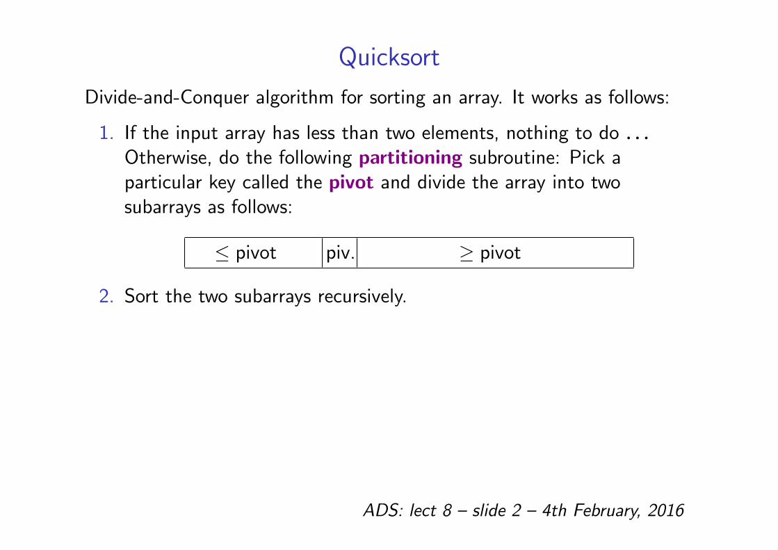
Quicksort
Divide-and-Conquer algorithm for sorting an array. It works as follows:
1. If the input array has less than two elements, nothing to do . . .Otherwise, do the following partitioning subroutine: Pick aparticular key called the pivot and divide the array into twosubarrays as follows:
≤ pivot piv. ≥ pivot
2. Sort the two subarrays recursively.
ADS: lect 8 – slide 2 – 4th February, 2016
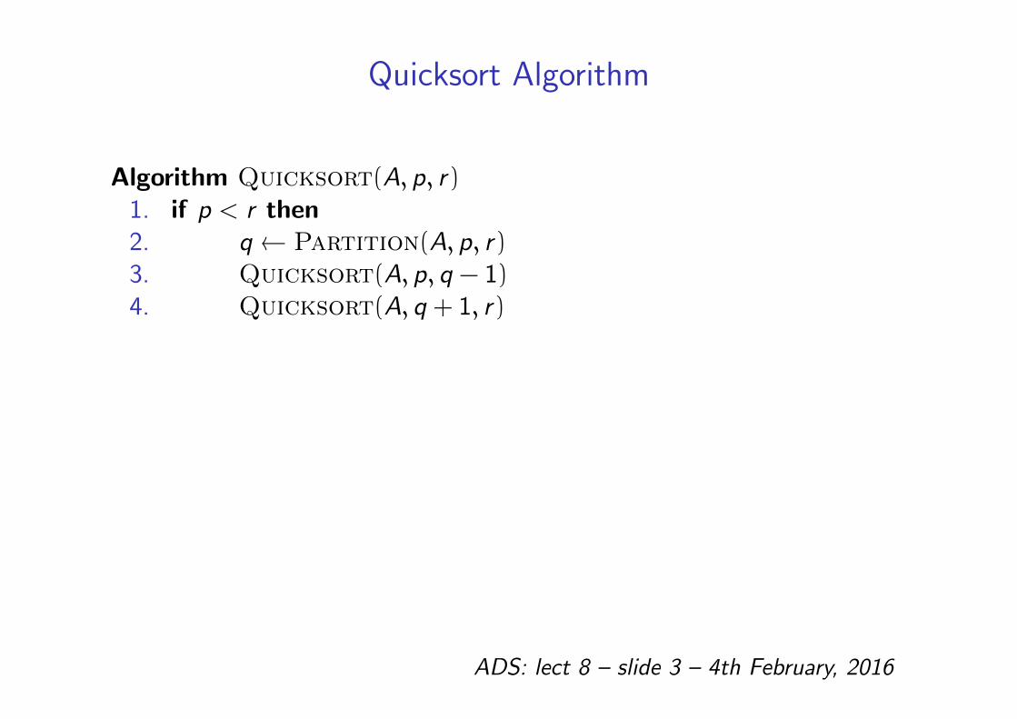
Quicksort Algorithm
Algorithm Quicksort(A, p, r)1. if p < r then2. q ← Partition(A, p, r)3. Quicksort(A, p, q − 1)4. Quicksort(A, q + 1, r)
ADS: lect 8 – slide 3 – 4th February, 2016
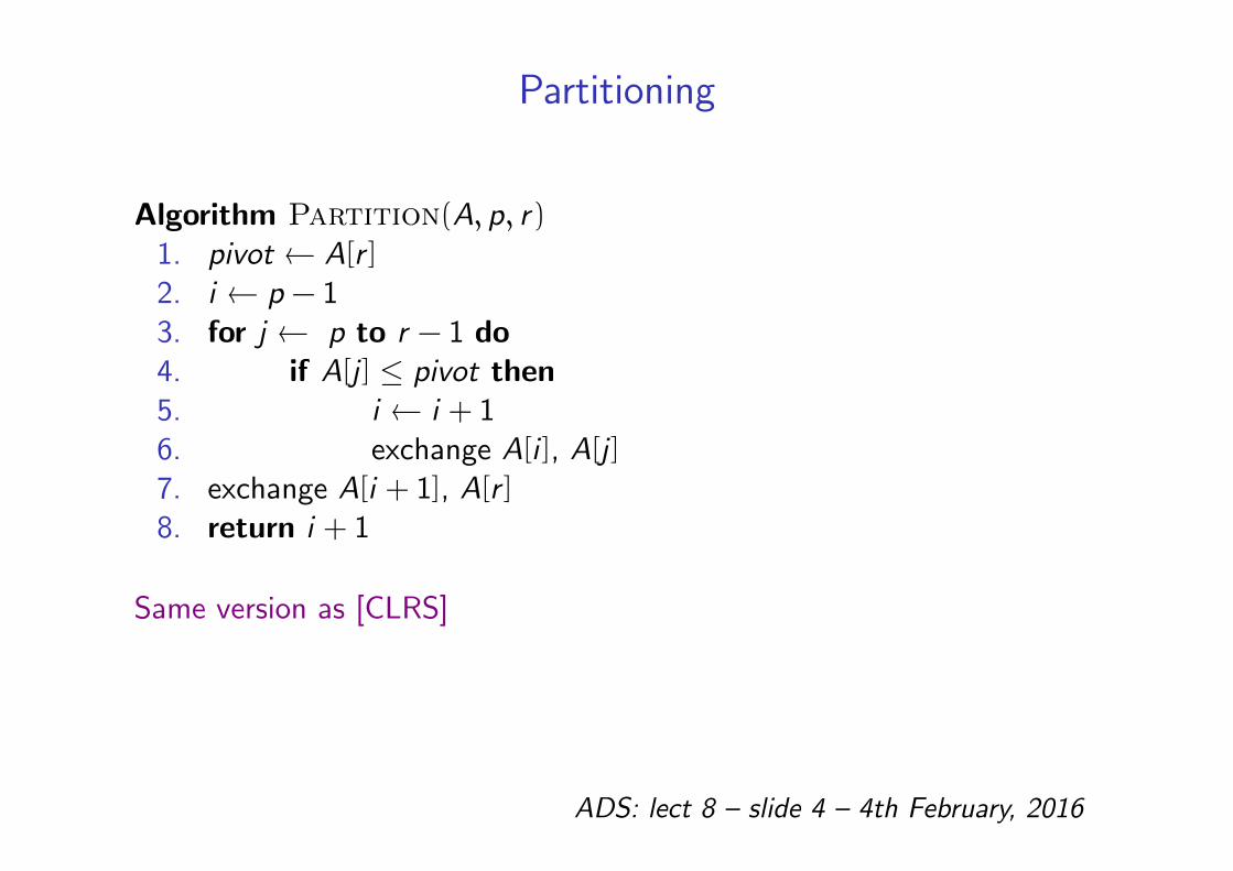
Partitioning
Algorithm Partition(A, p, r)1. pivot ← A[r ]2. i ← p − 13. for j ← p to r − 1 do4. if A[j ] ≤ pivot then5. i ← i + 16. exchange A[i ], A[j ]7. exchange A[i + 1], A[r ]8. return i + 1
Same version as [CLRS]
ADS: lect 8 – slide 4 – 4th February, 2016
Analysis of Quicksort
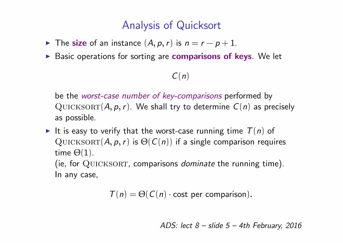
I The size of an instance (A, p, r) is n = r − p + 1.
I Basic operations for sorting are comparisons of keys. We let
C (n)
be the worst-case number of key-comparisons performed byQuicksort(A, p, r). We shall try to determine C (n) as preciselyas possible.
I It is easy to verify that the worst-case running time T (n) ofQuicksort(A, p, r) is Θ(C (n)) if a single comparison requirestime Θ(1).(ie, for Quicksort, comparisons dominate the running time).In any case,
T (n) = Θ(C (n) · cost per comparison).
ADS: lect 8 – slide 5 – 4th February, 2016
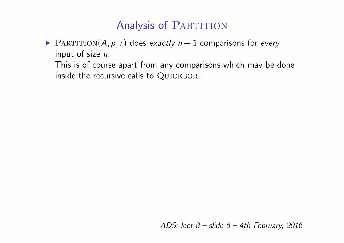
Analysis of Partition
I Partition(A, p, r) does exactly n − 1 comparisons for everyinput of size n.This is of course apart from any comparisons which may be doneinside the recursive calls to Quicksort.
ADS: lect 8 – slide 6 – 4th February, 2016
Worst-case Analysis of Quicksort
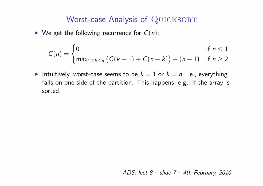
I We get the following recurrence for C (n):
C (n) =
0 if n ≤ 1
max1≤k≤n
(C (k − 1) + C (n − k)
)+ (n − 1) if n ≥ 2
I Intuitively, worst-case seems to be k = 1 or k = n, i.e., everythingfalls on one side of the partition. This happens, e.g., if the array issorted.
ADS: lect 8 – slide 7 – 4th February, 2016
Worst-Case Analysis (cont’d)
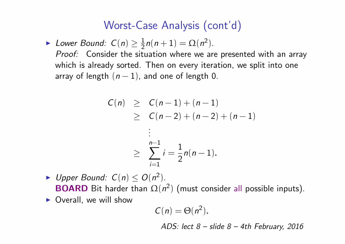
I Lower Bound: C (n) ≥ 12n(n + 1) = Ω(n2).
Proof: Consider the situation where we are presented with an arraywhich is already sorted. Then on every iteration, we split into onearray of length (n − 1), and one of length 0.
C (n) ≥ C (n − 1) + (n − 1)
≥ C (n − 2) + (n − 2) + (n − 1)...
≥n−1∑
i=1
i =1
2n(n − 1).
I Upper Bound: C (n) ≤ O(n2).BOARD Bit harder than Ω(n2) (must consider all possible inputs).
I Overall, we will showC (n) = Θ(n2).
ADS: lect 8 – slide 8 – 4th February, 2016
Best-Case Analysis
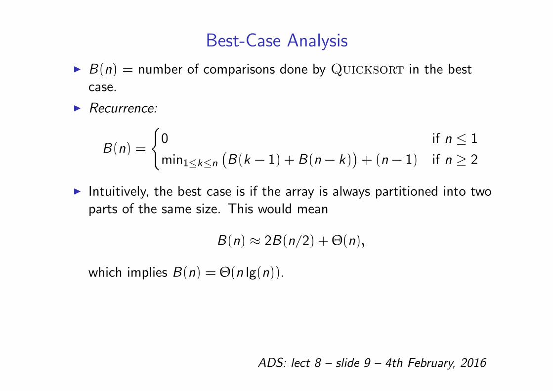
I B(n) = number of comparisons done by Quicksort in the bestcase.
I Recurrence:
B(n) =
0 if n ≤ 1
min1≤k≤n
(B(k − 1) + B(n − k)
)+ (n − 1) if n ≥ 2
I Intuitively, the best case is if the array is always partitioned into twoparts of the same size. This would mean
B(n) ≈ 2B(n/2) +Θ(n),
which implies B(n) = Θ(n lg(n)).
ADS: lect 8 – slide 9 – 4th February, 2016
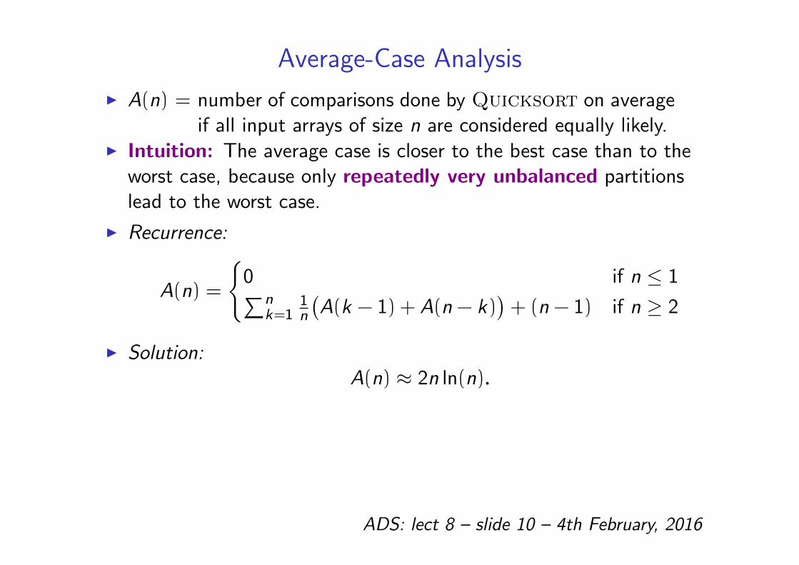
Average-Case Analysis
I A(n) = number of comparisons done by Quicksort on averageif all input arrays of size n are considered equally likely.
I Intuition: The average case is closer to the best case than to theworst case, because only repeatedly very unbalanced partitionslead to the worst case.
I Recurrence:
A(n) =
0 if n ≤ 1∑n
k=11n
(A(k − 1) + A(n − k)
)+ (n − 1) if n ≥ 2
I Solution:A(n) ≈ 2n ln(n).
ADS: lect 8 – slide 10 – 4th February, 2016
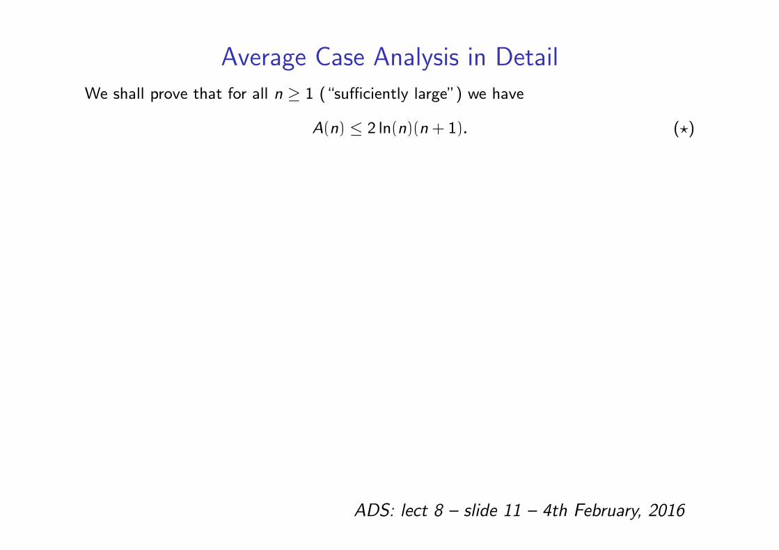
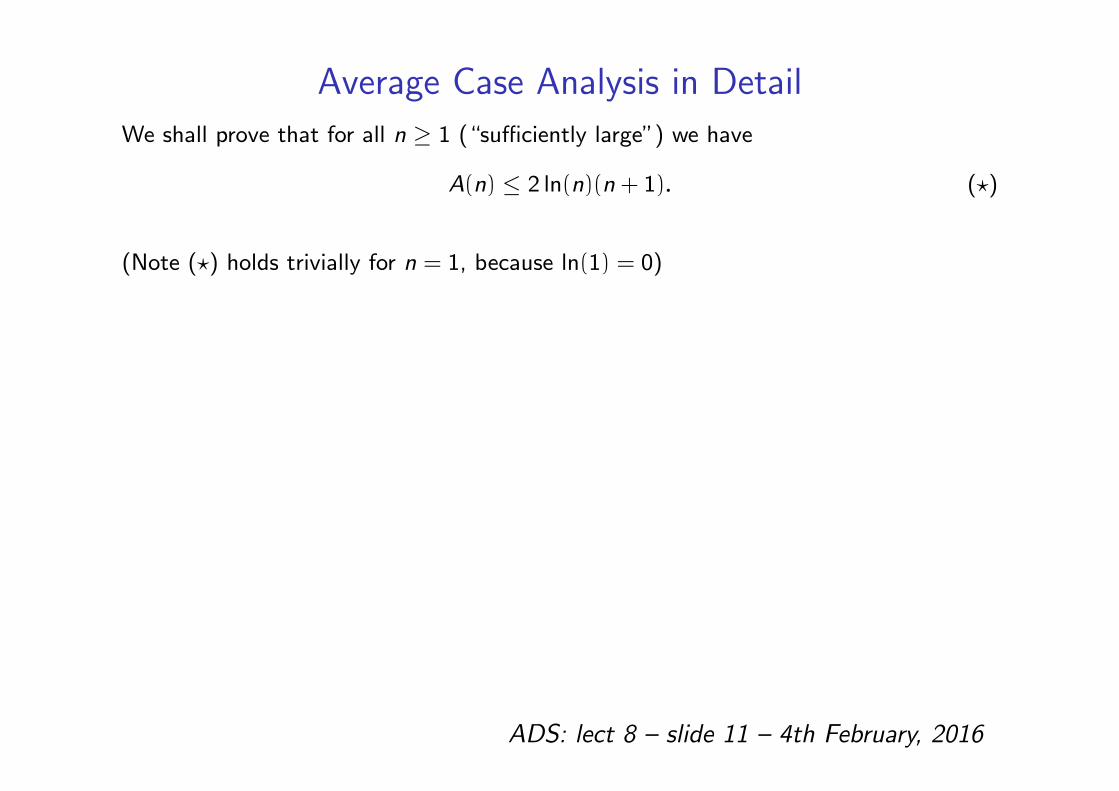
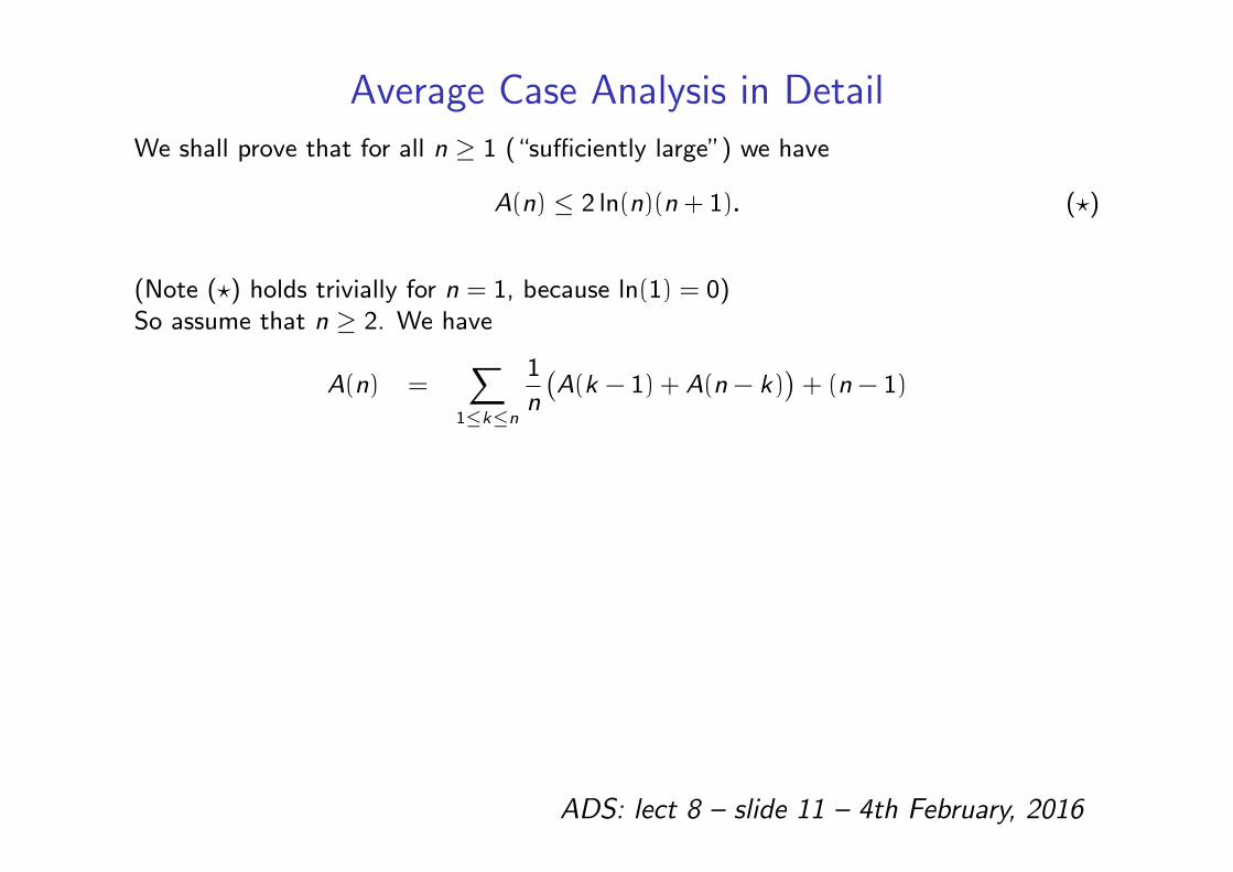
Average Case Analysis in Detail
We shall prove that for all n ≥ 1 (“sufficiently large”) we have
A(n) ≤ 2 ln(n)(n + 1). (?)
(Note (?) holds trivially for n = 1, because ln(1) = 0)So assume that n ≥ 2. We have
A(n) =∑
1≤k≤n
1
n
(A(k − 1) + A(n − k)
)+ (n − 1)
=2
n
n−1∑
k=0
A(k) + (n − 1).
Thus
nA(n) = 2n−1∑
k=0
A(k) + n(n − 1). (??)
ADS: lect 8 – slide 11 – 4th February, 2016
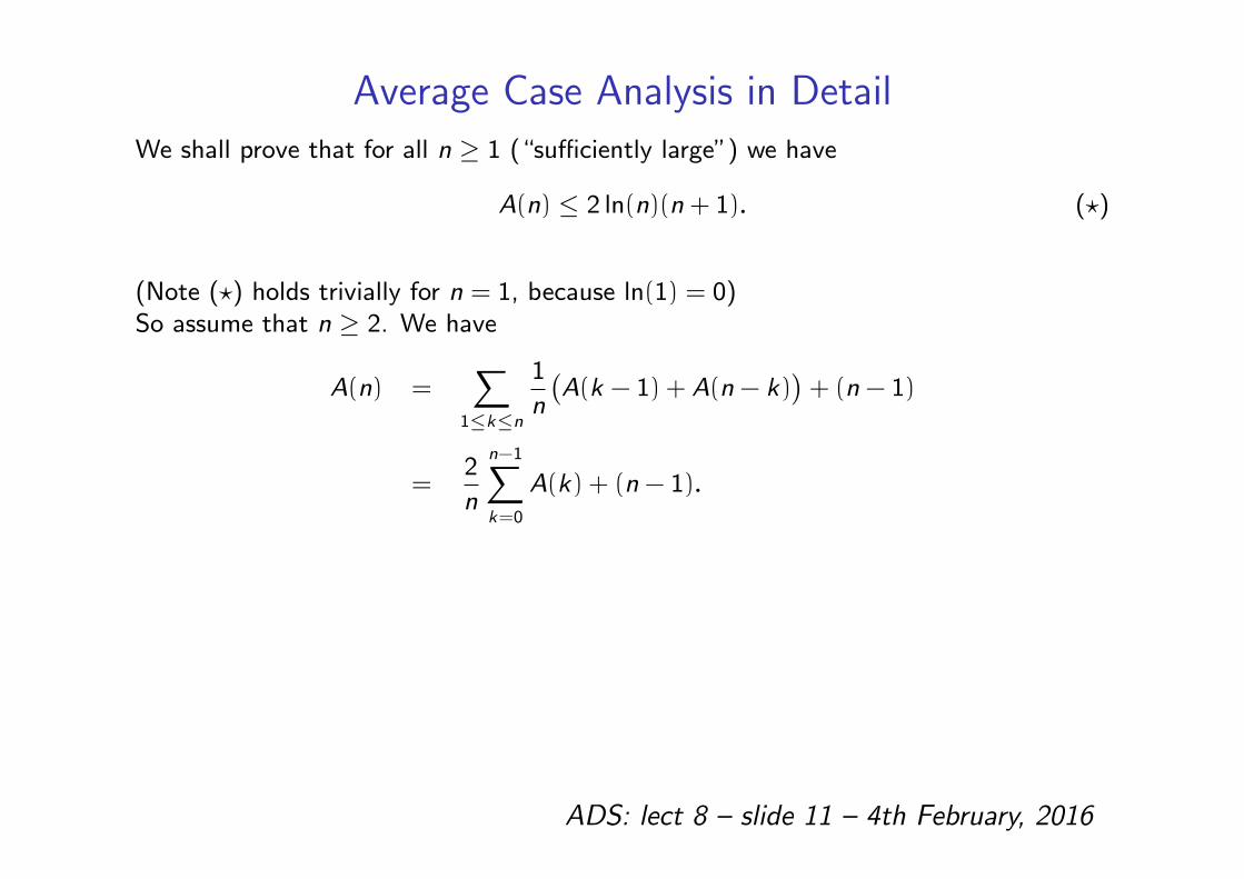
Average Case Analysis in Detail
We shall prove that for all n ≥ 1 (“sufficiently large”) we have
A(n) ≤ 2 ln(n)(n + 1). (?)
(Note (?) holds trivially for n = 1, because ln(1) = 0)
So assume that n ≥ 2. We have
A(n) =∑
1≤k≤n
1
n
(A(k − 1) + A(n − k)
)+ (n − 1)
=2
n
n−1∑
k=0
A(k) + (n − 1).
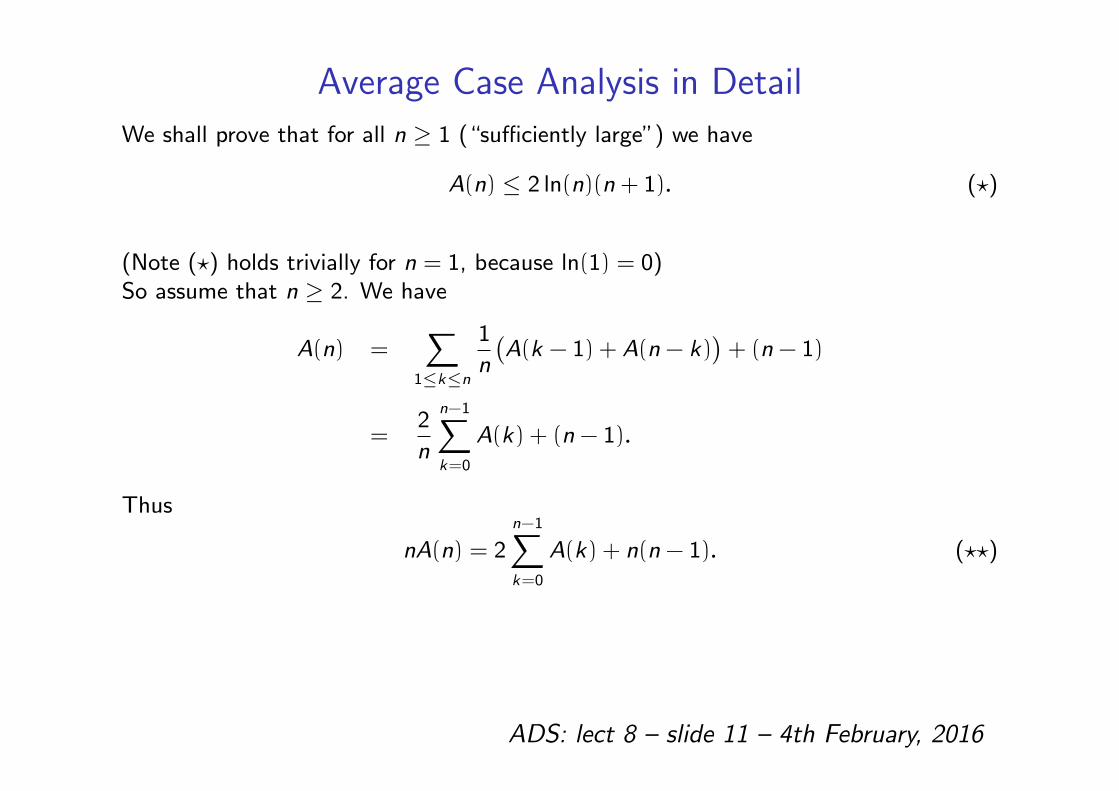
Thus
nA(n) = 2n−1∑
k=0
A(k) + n(n − 1). (??)
ADS: lect 8 – slide 11 – 4th February, 2016
Average Case Analysis in Detail
We shall prove that for all n ≥ 1 (“sufficiently large”) we have
A(n) ≤ 2 ln(n)(n + 1). (?)
(Note (?) holds trivially for n = 1, because ln(1) = 0)So assume that n ≥ 2. We have
A(n) =∑
1≤k≤n
1
n
(A(k − 1) + A(n − k)
)+ (n − 1)
=2
n
n−1∑
k=0
A(k) + (n − 1).
Thus
nA(n) = 2n−1∑
k=0
A(k) + n(n − 1). (??)
ADS: lect 8 – slide 11 – 4th February, 2016
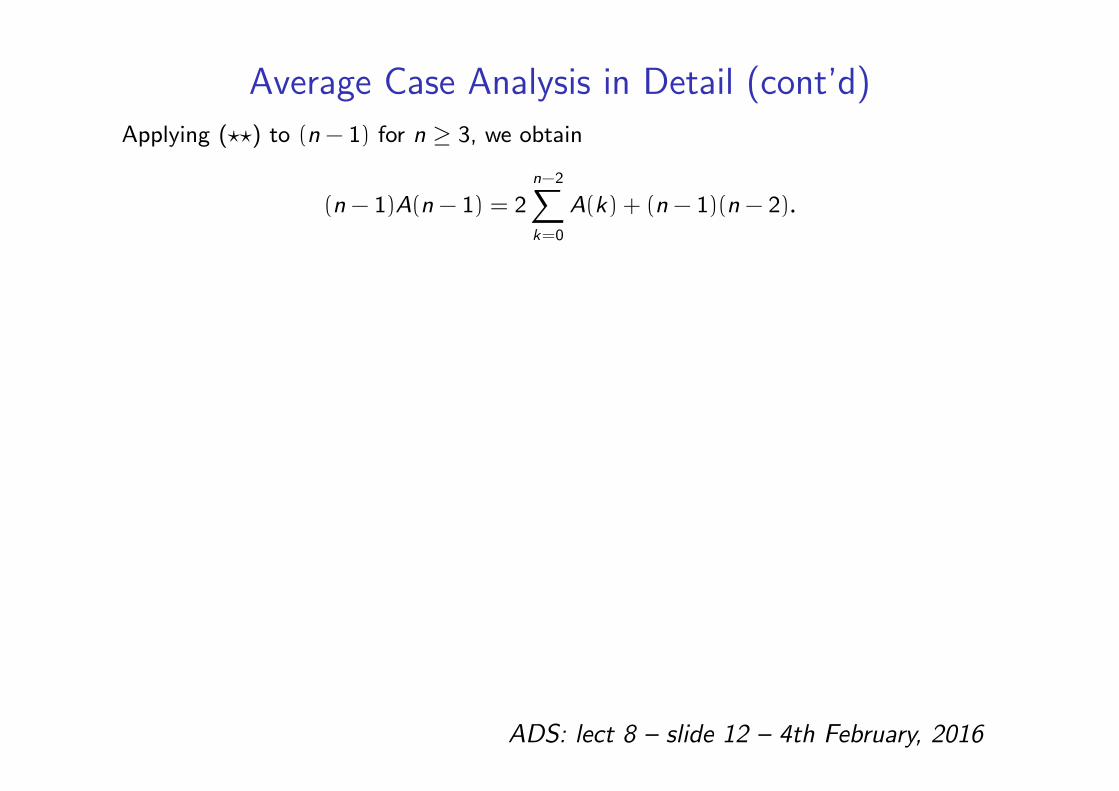
Average Case Analysis in Detail (cont’d)
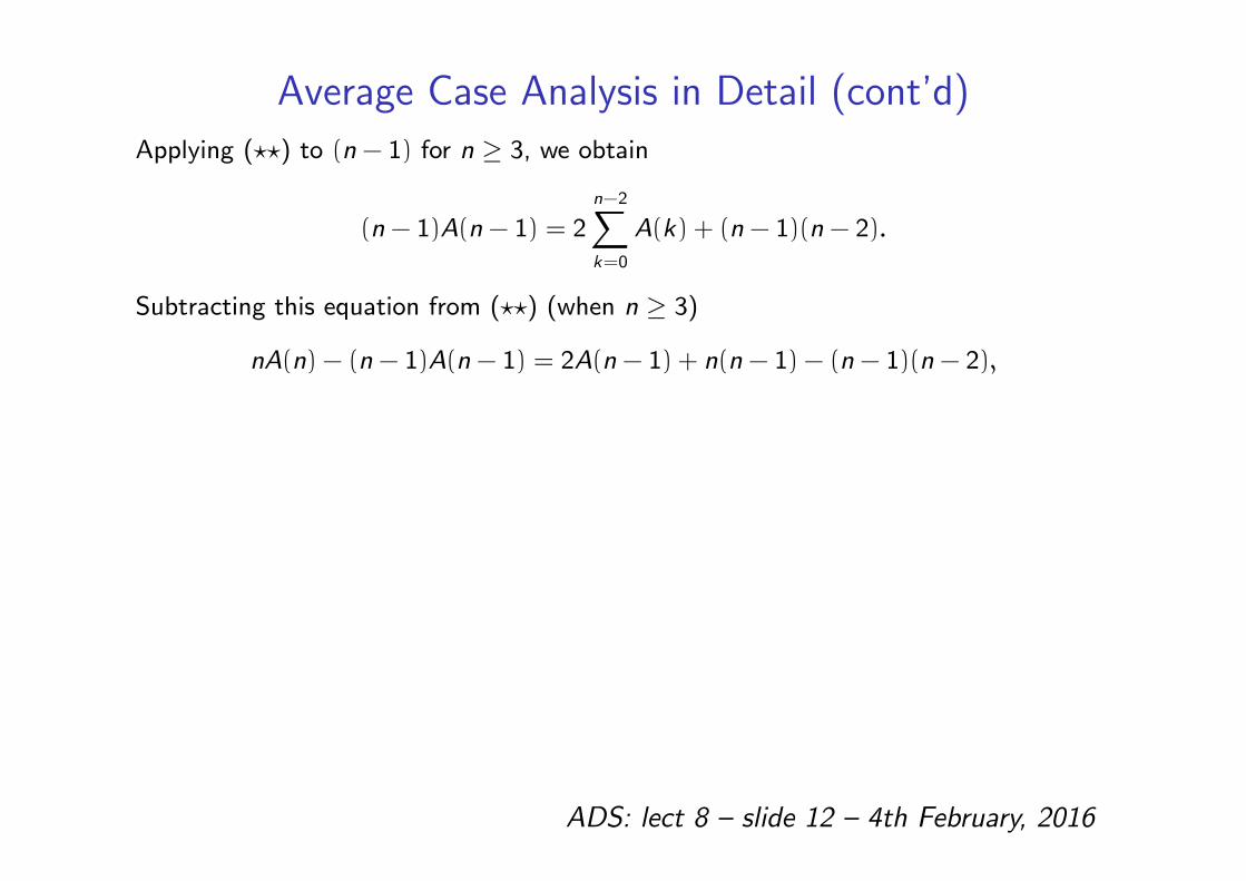
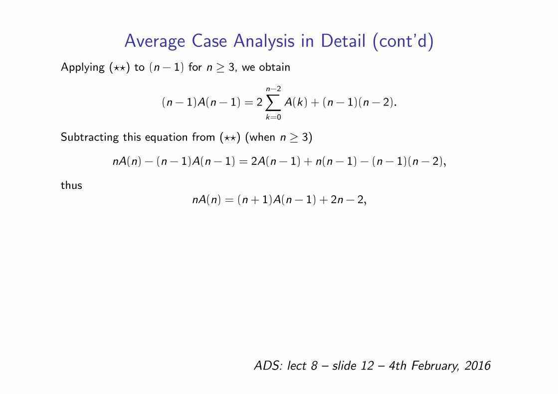
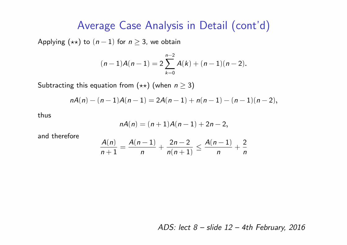
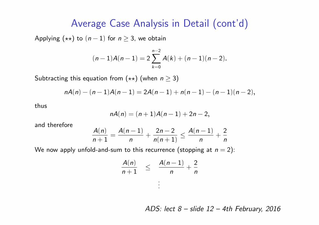
Applying (??) to (n − 1) for n ≥ 3, we obtain
(n − 1)A(n − 1) = 2n−2∑
k=0
A(k) + (n − 1)(n − 2).
Subtracting this equation from (??) (when n ≥ 3)
nA(n) − (n − 1)A(n − 1) = 2A(n − 1) + n(n − 1) − (n − 1)(n − 2),
thusnA(n) = (n + 1)A(n − 1) + 2n − 2,
and thereforeA(n)
n + 1=
A(n − 1)
n+
2n − 2
n(n + 1)≤ A(n − 1)
n+
2
n
We now apply unfold-and-sum to this recurrence (stopping at n = 2):
A(n)
n + 1≤ A(n − 1)
n+
2
n
...
ADS: lect 8 – slide 12 – 4th February, 2016
Average Case Analysis in Detail (cont’d)
Applying (??) to (n − 1) for n ≥ 3, we obtain
(n − 1)A(n − 1) = 2n−2∑
k=0
A(k) + (n − 1)(n − 2).
Subtracting this equation from (??) (when n ≥ 3)
nA(n) − (n − 1)A(n − 1) = 2A(n − 1) + n(n − 1) − (n − 1)(n − 2),
thusnA(n) = (n + 1)A(n − 1) + 2n − 2,
and thereforeA(n)
n + 1=
A(n − 1)
n+
2n − 2
n(n + 1)≤ A(n − 1)
n+
2
n
We now apply unfold-and-sum to this recurrence (stopping at n = 2):
A(n)
n + 1≤ A(n − 1)
n+
2
n
...
ADS: lect 8 – slide 12 – 4th February, 2016
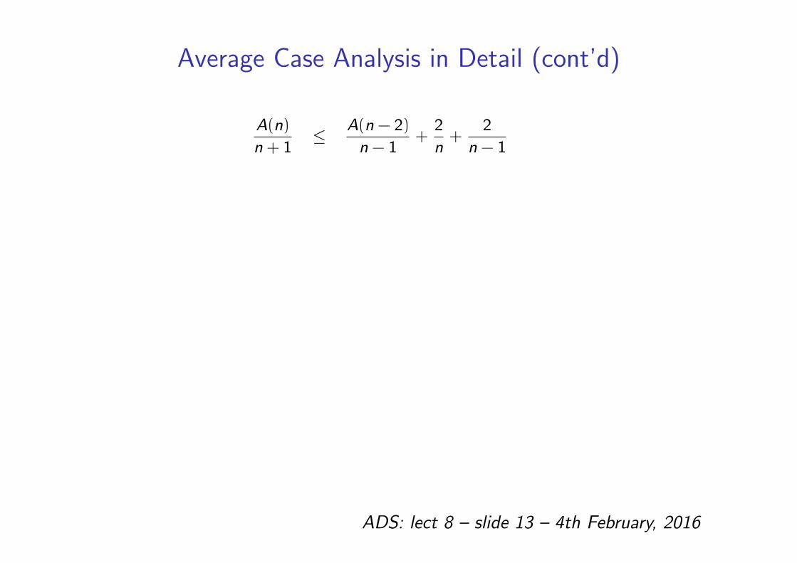
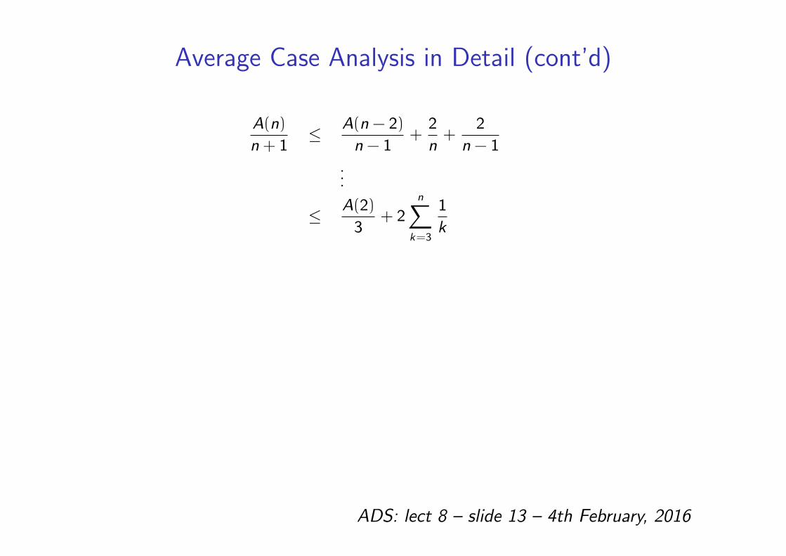
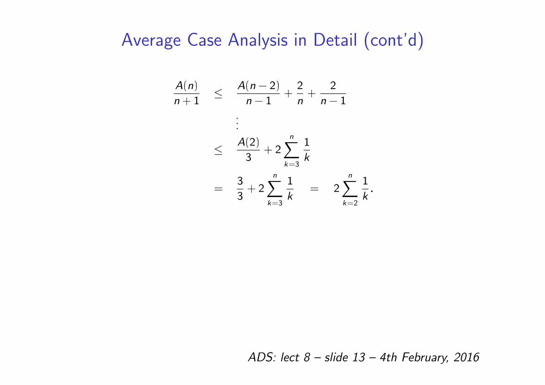
Average Case Analysis in Detail (cont’d)
A(n)
n + 1≤ A(n − 2)
n − 1+
2
n+
2
n − 1
...
≤ A(2)
3+ 2
n∑
k=3
1
k
=3
3+ 2
n∑
k=3
1
k= 2
n∑
k=2
1
k.
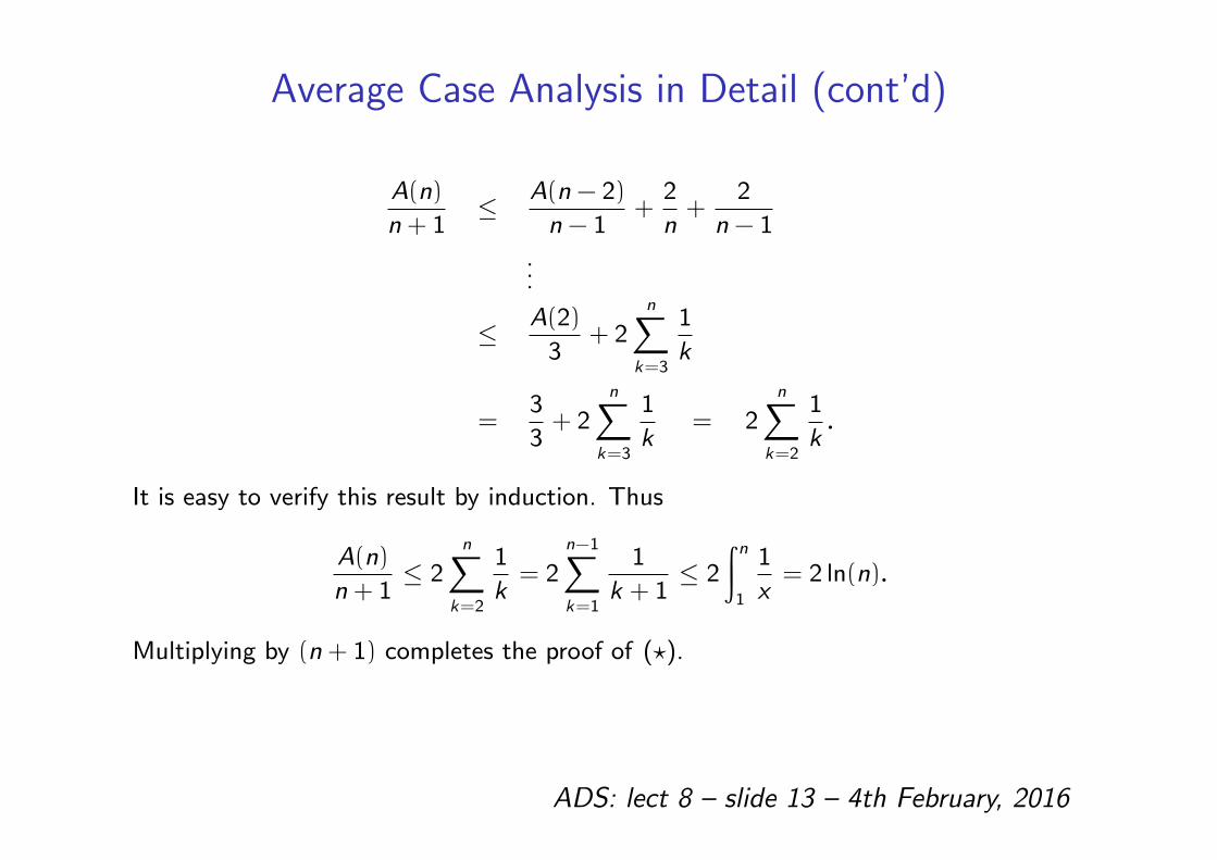
It is easy to verify this result by induction. Thus
A(n)
n + 1≤ 2
n∑
k=2
1
k= 2
n−1∑
k=1
1
k + 1≤ 2
∫ n
1
1
x= 2 ln(n).
Multiplying by (n + 1) completes the proof of (?).
ADS: lect 8 – slide 13 – 4th February, 2016
Average Case Analysis in Detail (cont’d)
A(n)
n + 1≤ A(n − 2)
n − 1+
2
n+
2
n − 1
...
≤ A(2)
3+ 2
n∑
k=3
1
k
=3
3+ 2
n∑
k=3
1
k= 2
n∑
k=2
1
k.
It is easy to verify this result by induction. Thus
A(n)
n + 1≤ 2
n∑
k=2
1
k= 2
n−1∑
k=1
1
k + 1≤ 2
∫ n
1
1
x= 2 ln(n).
Multiplying by (n + 1) completes the proof of (?).
ADS: lect 8 – slide 13 – 4th February, 2016
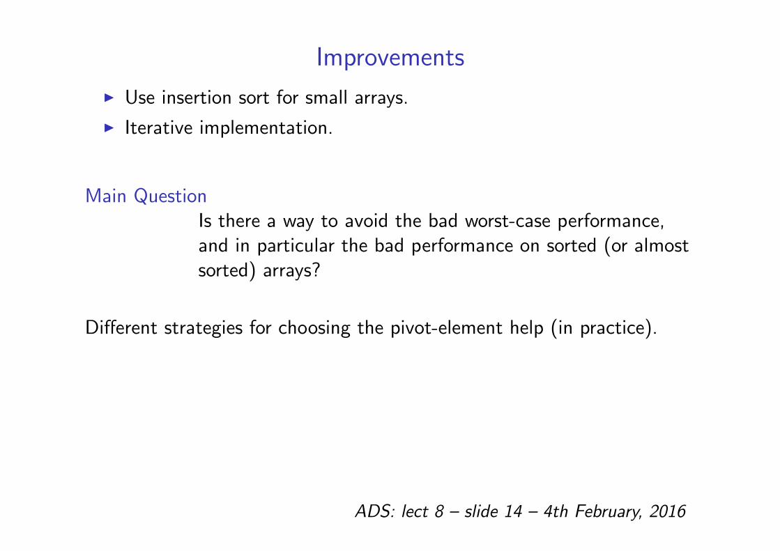
Improvements
I Use insertion sort for small arrays.
I Iterative implementation.
Main QuestionIs there a way to avoid the bad worst-case performance,and in particular the bad performance on sorted (or almostsorted) arrays?
Different strategies for choosing the pivot-element help (in practice).
ADS: lect 8 – slide 14 – 4th February, 2016
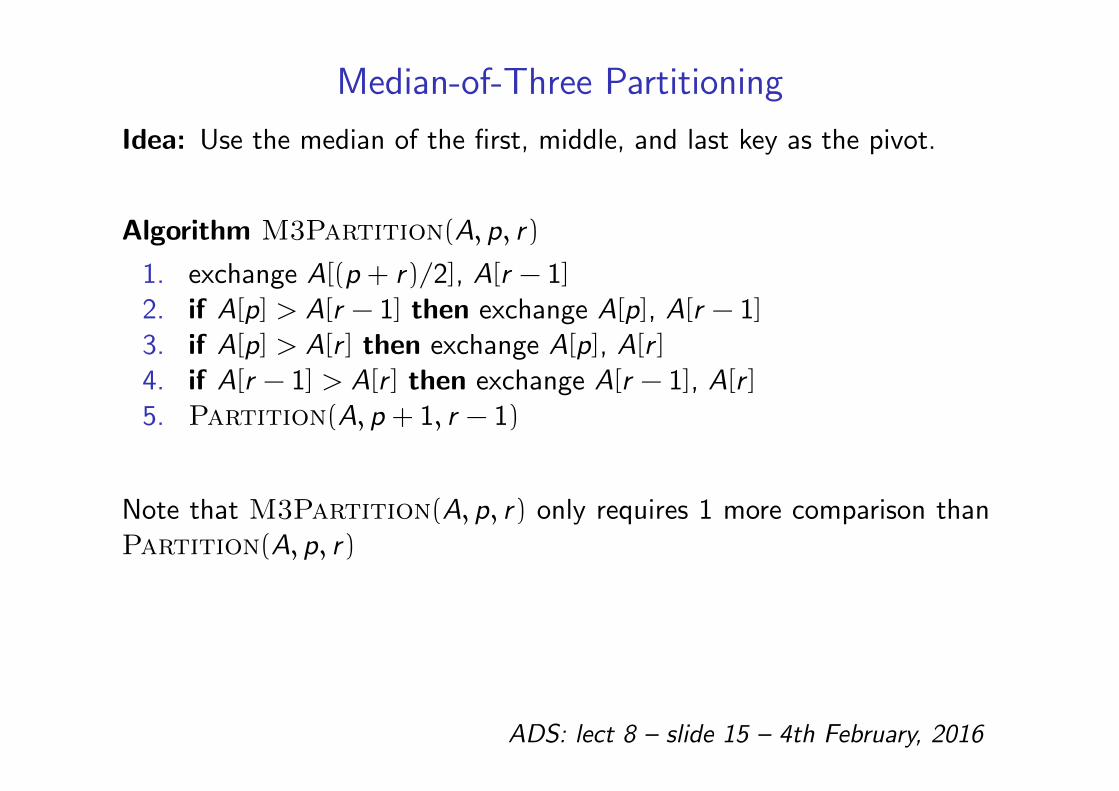
Median-of-Three Partitioning
Idea: Use the median of the first, middle, and last key as the pivot.
Algorithm M3Partition(A, p, r)
1. exchange A[(p + r)/2], A[r − 1]2. if A[p] > A[r − 1] then exchange A[p], A[r − 1]3. if A[p] > A[r ] then exchange A[p], A[r ]4. if A[r − 1] > A[r ] then exchange A[r − 1], A[r ]5. Partition(A, p + 1, r − 1)
Note that M3Partition(A, p, r) only requires 1 more comparison thanPartition(A, p, r)
ADS: lect 8 – slide 15 – 4th February, 2016
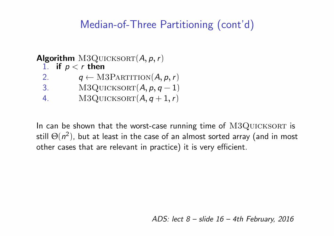
Median-of-Three Partitioning (cont’d)
Algorithm M3Quicksort(A, p, r)1. if p < r then2. q ←M3Partition(A, p, r)3. M3Quicksort(A, p, q − 1)4. M3Quicksort(A, q + 1, r)
In can be shown that the worst-case running time of M3Quicksort isstill Θ(n2), but at least in the case of an almost sorted array (and in mostother cases that are relevant in practice) it is very efficient.
ADS: lect 8 – slide 16 – 4th February, 2016
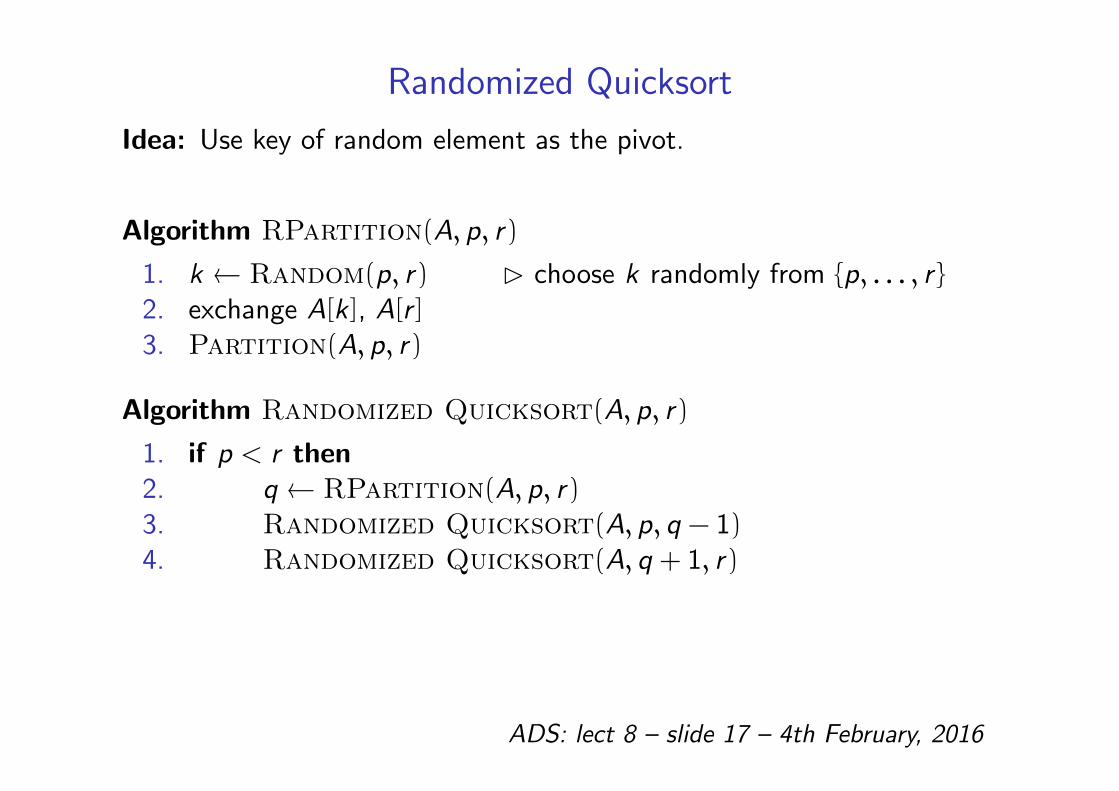
Randomized Quicksort
Idea: Use key of random element as the pivot.
Algorithm RPartition(A, p, r)
1. k ← Random(p, r) B choose k randomly from p, . . . , r 2. exchange A[k ], A[r ]3. Partition(A, p, r)
Algorithm Randomized Quicksort(A, p, r)
1. if p < r then2. q ← RPartition(A, p, r)3. Randomized Quicksort(A, p, q − 1)4. Randomized Quicksort(A, q + 1, r)
ADS: lect 8 – slide 17 – 4th February, 2016
Analysis of Randomized Quicksort
The running time of Randomized Quicksort on an input of size n isa random variable.
An analysis similar to the average case analysis of Quicksort shows:
TheoremFor all inputs (A, p, r), the expected number of comparisonsperformed during a run of Randomized Quicksort on input (A, p, r),is at most 2 ln(n)(n + 1), where n = r − p + 1.
Corollary
Thus the expected running time of Randomized Quicksort on anyinput of size n is Θ(n lg(n)).
ADS: lect 8 – slide 18 – 4th February, 2016
Reading Assignment
Sections 7.2, 7.3, 7.4 of [CLRS] (edition 2 or 3)
Problems
1. Convince yourself that Partition works correctly by working a fewexamples, or (better) try to prove that it works correctly.
2. In our proof of the Average-running time A(n), we can think of theinput as being some permutation of (1, . . . , n), and assume allpermutations are equally likely. Why does this explain the 1/n factorin the recurrence on slide 10?
3. Show that if the array is initially in decreasing order, then therunning time is Θ(n2).(the O(n2) is already taken care of on slide 8 (well, the board note),the Ω(n2) involves considering Partition on a decreasing array).
ADS: lect 8 – slide 19 – 4th February, 2016


![[Design and Analysis of Algorithms] · 2017. 2. 16. · Chapter: Introduction Design and Analysis of Algorithms Samujjwal Bhandari 6 Best, Worst and Average case Best case complexity](https://img.pdfslide.us/doc/110x75/60b0ba4825043614392e09fc/design-and-analysis-of-algorithms-2017-2-16-chapter-introduction-design.jpg)