Embed Size (px)
Citation preview

Algorithmic Aspects ofTriangle-Based Network
Analysis
zur Erlangung des akademischen Grades eines
Doktors der Naturwissenschaften
der Fakultat fur Informatikder Universitat Fridericiana zu Karlsruhe (TH)
genehmigte
Dissertationvon
Thomas Schankaus Offenburg
Tag der mundlichen Prufung: 14. Februar 2007
Erste Gutachterin: Frau Prof. Dr. Dorothea Wagner
Zweiter Gutachter: Herr Prof. Dr. Ulrik Brandes

2
Ausgabe August 20, 2007

Contents
1 Introduction 5
2 Preliminaries 11
2.1 Notation and Mathematical Foundation . . . . . . . . . . . . . 11
2.2 Graphs . . . . . . . . . . . . . . . . . . . . . . . . . . . . . . 12
2.3 Algorithms . . . . . . . . . . . . . . . . . . . . . . . . . . . . 17
2.4 Core Structure . . . . . . . . . . . . . . . . . . . . . . . . . . 18
3 Algorithms for Listing and Counting all Triangles in a Graph 21
3.1 Algorithms . . . . . . . . . . . . . . . . . . . . . . . . . . . . 23
3.1.1 Basic Algorithms . . . . . . . . . . . . . . . . . . . . . 23
3.1.2 Algorithm node-iterator and Related Algorithms . . . . 26
3.1.3 Algorithm edge-iterator and Derived Algorithms . . . 29
3.1.4 Overview of the Algorithms . . . . . . . . . . . . . . . 36
3.2 Experimental Results . . . . . . . . . . . . . . . . . . . . . . 36
4 Algorithms for Counting and Listing Triangles in SpecialGraph Classes 49
4.1 Graphs with Bounded Core Numbers . . . . . . . . . . . . . . 50
4.2 Comparability Graphs . . . . . . . . . . . . . . . . . . . . . . 51
4.3 Chordal Graphs . . . . . . . . . . . . . . . . . . . . . . . . . 53
4.4 Distance Hereditary Graphs . . . . . . . . . . . . . . . . . . . 56
3

4 CONTENTS
5 Applications of Triangle Listing in Network Analysis 73
5.1 Short Cycle Connectivity . . . . . . . . . . . . . . . . . . . . 74
5.2 Small Clique Connectivity . . . . . . . . . . . . . . . . . . . . 77
5.3 Neighborhood Density . . . . . . . . . . . . . . . . . . . . . . 79
5.3.1 Edge Weighted Neighborhood Density . . . . . . . . . 80
5.4 Clustering Coefficient and Transitivity . . . . . . . . . . . . . 85
6 A Graph Generator with Adjustable Clustering Coefficientand Increasing Cores 93
6.1 A Linear Preferential Attachment Generator . . . . . . . . . . 95
6.2 The Holme-Kim Generator . . . . . . . . . . . . . . . . . . . 96
6.3 The New-Generator . . . . . . . . . . . . . . . . . . . . . . . 100
6.3.1 Clustering Coefficient . . . . . . . . . . . . . . . . . . . 101
6.3.2 Core Structure . . . . . . . . . . . . . . . . . . . . . . 103
7 Approximating Clustering Coefficient, Transitivity and Neigh-borhood Densities 109
7.1 Approximating the Clustering Coefficient by Sampling Nodes 113
7.2 Approximating the Clustering Coefficient by Sampling Wedges 115
7.2.1 Approximating the Weighted Clustering Coefficient . . 116
7.2.2 Approximating the Clustering Coefficient . . . . . . . 118
7.3 Approximating the Neighborhood Densities . . . . . . . . . . 119
8 Conclusion 123
Acknowledgments 125
Summary in German Language 126
Bibliography 129
Index 136

Chapter 1
Introduction
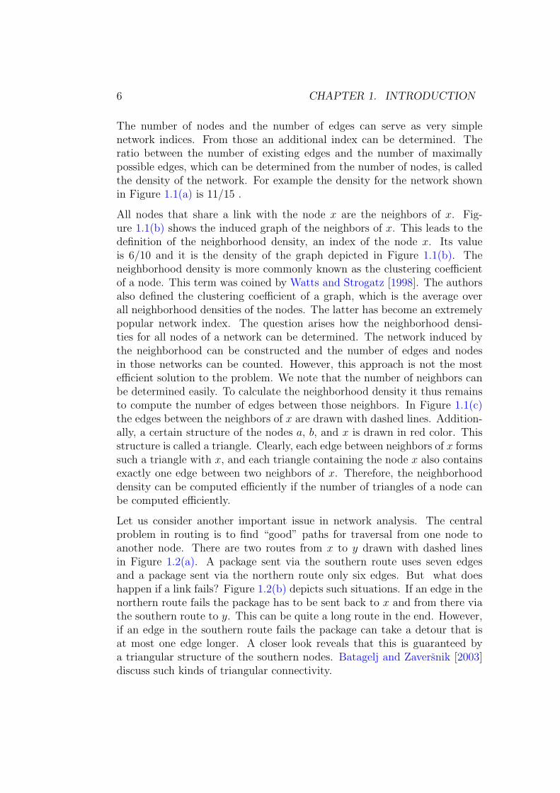
A network consists of nodes and edges between those nodes. Figure 1.1(a)depicts a network with 6 nodes and 11 edges. Many relations in our daily lifecan be modeled as networks. For example, a social network of people can becreated by linking any two of them if they share a friendship relation. Thereare networks based on communication, e.g. one can construct a network ofradio controlled sensors and put a link between two of them if they are closeenough to receive and send information via radio waves. A network can beconstructed merely from information. Let us consider the set of all existingweb pages as nodes. Two of them are related if either of the two referencesthe other. This example shows that networks can be quite huge.
Describing properties of a network is one aspect of network analysis. Anetwork index for example maps the network to a number. The structure ofthe network or at least a particular aspect of it should be reflected by theassociated number.
(a) network (b) neighborhood of x (c) triangle
Figure 1.1: Examples of networks.
5
6 CHAPTER 1. INTRODUCTION
The number of nodes and the number of edges can serve as very simplenetwork indices. From those an additional index can be determined. Theratio between the number of existing edges and the number of maximallypossible edges, which can be determined from the number of nodes, is calledthe density of the network. For example the density for the network shownin Figure 1.1(a) is 11/15 .
All nodes that share a link with the node x are the neighbors of x. Fig-ure 1.1(b) shows the induced graph of the neighbors of x. This leads to thedefinition of the neighborhood density, an index of the node x. Its valueis 6/10 and it is the density of the graph depicted in Figure 1.1(b). Theneighborhood density is more commonly known as the clustering coefficientof a node. This term was coined by Watts and Strogatz [1998]. The authorsalso defined the clustering coefficient of a graph, which is the average overall neighborhood densities of the nodes. The latter has become an extremelypopular network index. The question arises how the neighborhood densi-ties for all nodes of a network can be determined. The network induced bythe neighborhood can be constructed and the number of edges and nodesin those networks can be counted. However, this approach is not the mostefficient solution to the problem. We note that the number of neighbors canbe determined easily. To calculate the neighborhood density it thus remainsto compute the number of edges between those neighbors. In Figure 1.1(c)the edges between the neighbors of x are drawn with dashed lines. Addition-ally, a certain structure of the nodes a, b, and x is drawn in red color. Thisstructure is called a triangle. Clearly, each edge between neighbors of x formssuch a triangle with x, and each triangle containing the node x also containsexactly one edge between two neighbors of x. Therefore, the neighborhooddensity can be computed efficiently if the number of triangles of a node canbe computed efficiently.
Let us consider another important issue in network analysis. The centralproblem in routing is to find “good” paths for traversal from one node toanother node. There are two routes from x to y drawn with dashed linesin Figure 1.2(a). A package sent via the southern route uses seven edgesand a package sent via the northern route only six edges. But what doeshappen if a link fails? Figure 1.2(b) depicts such situations. If an edge in thenorthern route fails the package has to be sent back to x and from there viathe southern route to y. This can be quite a long route in the end. However,if an edge in the southern route fails the package can take a detour that isat most one edge longer. A closer look reveals that this is guaranteed bya triangular structure of the southern nodes. Batagelj and Zaversnik [2003]discuss such kinds of triangular connectivity.

7
(a) northern and southern route.
(b) the routes under failure of edges.
Figure 1.2: Routes in a network.
Both of the two described problems in network analysis are related to thetriangular structure of the network. We discuss these and similar applicationsin Chapter 5.
The key to handle such problems efficiently can be traced back to the algo-rithmic problem of finding and listing all triangles in the network. A trianglelisting algorithm outputs all triangles of a graph. Consequently it cannotperform less operations than the number of triangles in the graph. A count-ing algorithm attributes each node of a graph with the associated numberof triangles. There are two basic algorithms for triangle listing. Both areasymptotically equivalent in running time which can be coarsely boundedby the number of nodes times the number of edges. Itai and Rodeh [1978]introduced the first listing algorithm with improved running time boundedby the product of the number of edges and the square root of the latter.The achieved bound is sharp with respect to the number of edges. Chibaand Nishizeki [1985] give an improved bound that replaces the square root ofthe edges by the arboricity of the graph in the running time. With respectto triangle counting Alon et al. [1997] introduced the first algorithm thatbeats the bound given by Itai and Rodeh. All these publications discuss thecounting or listing of triangles as a special case of small cliques and morecommonly of short cycles. Chiba and Nishizeki extended their work also to

8 CHAPTER 1. INTRODUCTION
the listing of small subgraphs of other structure than cycles or cliques. Thisdirection has been continued until very recently [Sundaram and Skiena, 1995;Kloks et al., 2000; Vassilevska et al., 2006]. However, triangle listing has notbeen considered with respect to practical applications. The work of Batageljand Mrvar [2001] is the only one falling roughly into this category. Basedon one of the two folklore algorithms all subgraphs up to tree nodes arecounted. The feasibility of their approach is shown in one practical example.However, there still remains a gap in the running time of their approach andthose algorithms that have an optimal running time with respect to the sizeof the graph. We discuss this topic in in Chapter 3, in which we considerprimarily triangle listing algorithms with optimal running time with respectto the size of the graph. In Chapter 4 we investigate triangle listing andtriangle counting algorithms for certain graph classes, i.e. for graphs thathave certain properties.
The consideration of huge networks [Kumar et al., 2000; Abello et al., 2002;Eubank et al., 2004] requires algorithms that have at most linear or preferablysub-linear running time. In many cases it suffices to compute an approximateanswer to the problem. This is likely to be accepted if the approximation canbe computed much faster than the exact solution. As mentioned above theclustering coefficient is an average value, namely that of the neighborhooddensities of the nodes. In such a setup sampling techniques are a commonapproach. Eubank et al. [2004] use such a method of sampling nodes to ap-proximate the clustering coefficient of a graph. However, the neighborhooddensity of a node itself can be expressed as an average value. The questionarises if this property can be exploited to approximate the clustering coef-ficient more directly and consequently more efficiently. We discuss this inChapter 7.
The creation of random networks is important to understand existing net-works and to test algorithms. The model of Erdos and Renyi [1959] is prob-ably one of the best known. At that time other models were studied aswell [Gilbert, 1959; Austin et al., 1959]. These models are not equivalentbut very similar and for most applications the difference does not matter. Aresulting graph of any of these models shares the property that its degree dis-tribution does not show a high variation. This differs from findings in manyreal world networks [Faloutsos et al., 1999; Chen et al., 2001]. The linearpreferential attachment graph generator considered in [Barabasi and Albert,1999; Albert et al., 1999] does generate random graphs with that property.Subsequently, it was adapted in various ways to fulfill other properties, too.Holme and Kim [2002] for example propose a method that is very close topreferential attachment, but it also considers the triangular structure. It is
9
supposed to achieve a high clustering coefficient of the generated network.The approach in [Li et al., 2004] changes an existing graph such that theresulting clustering coefficient is higher whilst preserving the degree distri-bution. We discuss an alternative method that is also based on preferentialattachment in Chapter 6.
10 CHAPTER 1. INTRODUCTION

Chapter 2
Preliminaries
2.1 Notation and Mathematical Foundation
Symbols and Notation
We use lower case characters to denote numbers and functions to numbers.These might be Roman or Greek letters or other variations we think aresuitable, e.g. n, ρ, π, $ etc. We might use f(x), fx or even simply f inter-changeably, whenever the argument is clear from the context. We will usecapital characters to denote sets and objects that are not simple numbers orfunctions to numbers, e.g. G, Π, Υ, ∆, etc.
We try to keep this rules throughout this work. However, if it does notseem convenient or some other notation is wildly used in literature we willfollow the common usage. An example for this is the O-notation in the nextsection. In general we allow ourselves to abuse notation to a more mnemonicappearance if the meaning is clear from context and it is very unlikely thatmisunderstandings will happen. In rare cases we may not even give a formaldefinition of those notations, again only if their meaning is clear from context.
Numbers and Asymptotic Growth
We denote positive integer numbers including zero with N and the real num-bers with R.
To capture the asymptotic behavior of polynomials, Landau’s so called O-notation has become common practice. Let f and g be functions f, g : N→N. Then f is in O(g), or equivalently g is in Ω(f), if there exist two numbers
11

12 CHAPTER 2. PRELIMINARIES
n0 ∈ N and c ∈ R such that f(n) ≤ c · g(n) for all n ≥ n0. Informally we saythat f grows at most as fast as g. To describe equivalent asymptotic growthwe define Θ(g) as O(g) ∩ Ω(g). Finally, if there exists a number n0 ∈ N forany c ∈ R>0 such that f(n) ≤ c · g(n), we say that f is in o(g) for all n > n0
or equivalently g is in ω(f).
Probability
A pair (Ω, P) with Ω a finite set and P a mapping from P(Ω) all subsetsof Ω to R is a finite probability space if P [Ω] = 1, P [A] ≥ 0 for A ⊂ Ω,and P [A ∪B] = P [A] + P [B] for A ∩ B = ∅. The mapping P is called theprobability measure on Ω. The set Ω is called the sample space and a subsetA of Ω is called an event .
An arbitrary mapping X : Ω → R is called a random variable and we candefine shorthand
P [X ≤ x] = P [ω ∈ Ω : X(ω) ≤ x]
for example. The distribution or density p of a random variable X is theprobability measure p : X(Ω) ⊂ R→ [0, 1] for which
p(x) = P [X = x] = P [ω ∈ Ω : X(ω) = x] .
The expectation of a random variable X with its distribution p is defined as
E [X] =∑
x∈X(Ω)
x · p(x).
The variance of a random variable is
var [X] = E[X2]− (E [X])2,
and the standard deviation is the square root of the variance
σ(X) =√
var [X].
2.2 Graphs
A graph (network) consists of a set of vertices (nodes) V and a set of edges E.An edge connects two nodes. We denote the size of V with n, and the size ofE with m. In an undirected graph G = (V, E) the set of edges is conveniently
2.2. GRAPHS 13
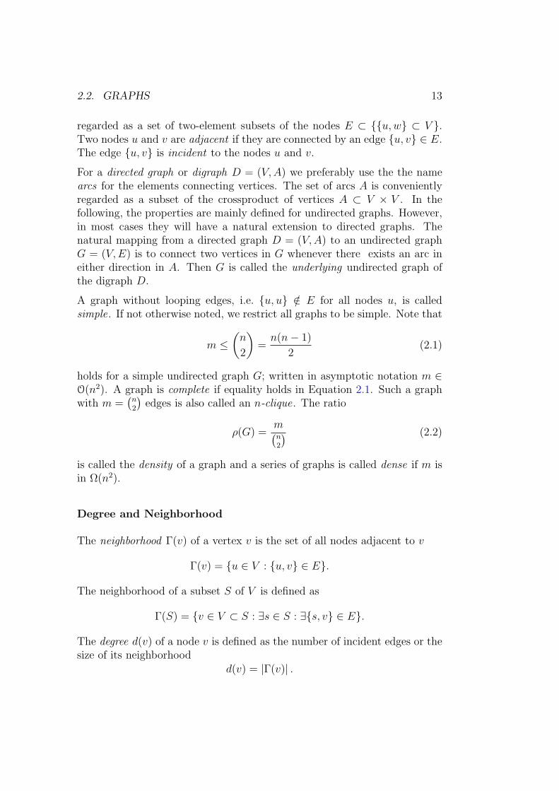
regarded as a set of two-element subsets of the nodes E ⊂ u, w ⊂ V .Two nodes u and v are adjacent if they are connected by an edge u, v ∈ E.The edge u, v is incident to the nodes u and v.
For a directed graph or digraph D = (V, A) we preferably use the the namearcs for the elements connecting vertices. The set of arcs A is convenientlyregarded as a subset of the crossproduct of vertices A ⊂ V × V . In thefollowing, the properties are mainly defined for undirected graphs. However,in most cases they will have a natural extension to directed graphs. Thenatural mapping from a directed graph D = (V, A) to an undirected graphG = (V, E) is to connect two vertices in G whenever there exists an arc ineither direction in A. Then G is called the underlying undirected graph ofthe digraph D.
A graph without looping edges, i.e. u, u /∈ E for all nodes u, is calledsimple. If not otherwise noted, we restrict all graphs to be simple. Note that
m ≤(
n
2
)=
n(n− 1)
2(2.1)
holds for a simple undirected graph G; written in asymptotic notation m ∈O(n2). A graph is complete if equality holds in Equation 2.1. Such a graphwith m =
(n2
)edges is also called an n-clique. The ratio
ρ(G) =m(n2
) (2.2)
is called the density of a graph and a series of graphs is called dense if m isin Ω(n2).
Degree and Neighborhood
The neighborhood Γ(v) of a vertex v is the set of all nodes adjacent to v
Γ(v) = u ∈ V : u, v ∈ E.
The neighborhood of a subset S of V is defined as
Γ(S) = v ∈ V ⊂ S : ∃s ∈ S : ∃s, v ∈ E.
The degree d(v) of a node v is defined as the number of incident edges or thesize of its neighborhood
d(v) = |Γ(v)| .
14 CHAPTER 2. PRELIMINARIES
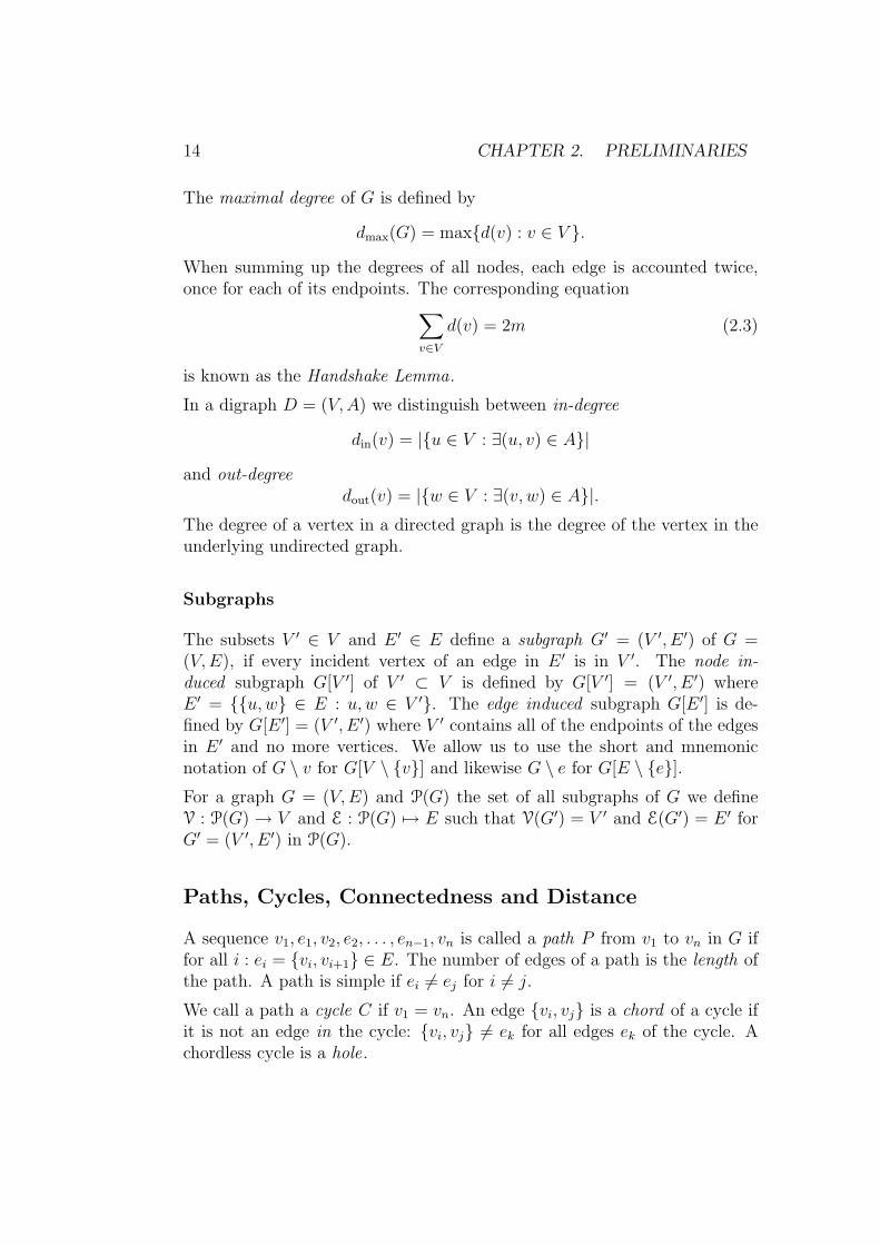
The maximal degree of G is defined by
dmax(G) = maxd(v) : v ∈ V .
When summing up the degrees of all nodes, each edge is accounted twice,once for each of its endpoints. The corresponding equation∑
v∈V
d(v) = 2m (2.3)
is known as the Handshake Lemma.
In a digraph D = (V, A) we distinguish between in-degree
din(v) = |u ∈ V : ∃(u, v) ∈ A|
and out-degreedout(v) = |w ∈ V : ∃(v, w) ∈ A|.
The degree of a vertex in a directed graph is the degree of the vertex in theunderlying undirected graph.
Subgraphs
The subsets V ′ ∈ V and E ′ ∈ E define a subgraph G′ = (V ′, E ′) of G =(V, E), if every incident vertex of an edge in E ′ is in V ′. The node in-duced subgraph G[V ′] of V ′ ⊂ V is defined by G[V ′] = (V ′, E ′) whereE ′ = u, w ∈ E : u, w ∈ V ′. The edge induced subgraph G[E ′] is de-fined by G[E ′] = (V ′, E ′) where V ′ contains all of the endpoints of the edgesin E ′ and no more vertices. We allow us to use the short and mnemonicnotation of G \ v for G[V \ v] and likewise G \ e for G[E \ e].For a graph G = (V, E) and P(G) the set of all subgraphs of G we defineV : P(G) → V and E : P(G) 7→ E such that V(G′) = V ′ and E(G′) = E ′ forG′ = (V ′, E ′) in P(G).
Paths, Cycles, Connectedness and Distance
A sequence v1, e1, v2, e2, . . . , en−1, vn is called a path P from v1 to vn in G iffor all i : ei = vi, vi+1 ∈ E. The number of edges of a path is the length ofthe path. A path is simple if ei 6= ej for i 6= j.
We call a path a cycle C if v1 = vn. An edge vi, vj is a chord of a cycle ifit is not an edge in the cycle: vi, vj 6= ek for all edges ek of the cycle. Achordless cycle is a hole.

2.2. GRAPHS 15
A graph is connected if there exists a path between any two pair of nodes inG. If not otherwise noted, we require a graph to be connected from now on.This implies m ∈ Ω(n) which allows us to write shorthand O(m) instead ofO(n + m).
The distance dist(u, w) of two nodes u and w is the length of a shortest pathbetween the nodes.
Trees
A graph is called a tree T if it is cycle free and connected. A tree has exactlym = n−1 edges. A node of degree one is called a leaf . A tree T is a spanningtree of a graph G if T is a subgraph of G and V(T ) = V(G).
Rooted Trees. Let us declare some node r ∈ V(T ) the root of T . For someedge u, w let us assume that u is closer to the root than w, i.e. dist(u, r) =dist(w, r) − 1. Then u is the predecessor of w (with respect to the root r).Likewise, w is a successor of w. Note, that every node except the root r hasexactly one predecessor.
Tree Orders. The subtree for a node v with respect to a root r is theinduced subgraph of all nodes w, for which v lies on the path from w to r.A numbering of the nodes (v1, . . . , v2) is in preorder if any node v appearsdirectly before all other nodes of v’s subtree. Likewise a numbering is inpostorder if for all nodes v all nodes of its subtree appear directly before v.
Neighborhood Density, Clustering Coefficient and Tran-sitivity
We briefly introduce the clustering coefficient and the transitivity here. Sec-tion 5.4 on page 85 has a more in-depth exploration along with extendedbibliographical remarks.
Triangles and Wedges. A triangle ∆uvw (or less specific simply ∆) of G isa complete subgraph of three distinct nodes u, v, and w: V(∆uvw) = u, v, wand E(∆uvw) = u, v, v, w, w, u. Motivated by this, the number oftriangles of node v is defined as the number of edges between neighbors
δ(v) = |E(G[Γ(v)])| . (2.4)

16 CHAPTER 2. PRELIMINARIES
Since each triangle contains three nodes (hence if we sum over all nodes eachtriangle is counted three times) the following definition is intuitive
δ(G) =1
3
∑v∈V
δ(v). (2.5)
For an n-clique δ =(
n3
)holds, and we get we get δ(G) ∈ O(n3) for a graph
in general. In terms of m this yields
δ(G) ∈ O(m3/2
). (2.6)
Note that a simple cycle of length three would have been a structurallyequivalent definition of a triangle. As a consequence, triangles occasionallyappear in literature as small complete subgraphs or short cycles.
A wedge Υuvw of G is a subgraph of three distinctive nodes u, v, and w:V(Υuvw) = u, v, w and two edges E(Υuvw) = u, v, v, w. Unlike atriangle, a wedge has a structurally distinguished center node v. The numberof wedges of a node v with d(v) ≥ 2 is then defined as
τ(v) =
(d(v)
2
), (2.7)
and summing the wedges of all nodes defines the number of wedges of thegraph
τ(G) =∑v∈V
τ(v). (2.8)
A wedge can also be seen as a path of length two. This alternative definition israther common in literature. If we consider an n-clique Kn we get 3 δ(Kn) =τ(Kn), and in general the following inequality
3 δ(G) ≤ τ(G) (2.9)
holds for a graph G.
Neighborhood Density. The neighborhood density of a vertex v is thedensity of the subgraph induced by the neighbors of v. It can be equivalentlyexpressed by the quotient of triangles and wedges of v
%(v) = ρ(G[Γ(v)]) =δ(v)
τ(v). (2.10)
Note that we require d(v) ≥ 2 as in Equation 2.7. The neighborhood densityis also known as the clustering coefficient of the node [Watts and Strogatz,1998].

2.3. ALGORITHMS 17
Clustering Coefficient. The clustering coefficient [Watts and Strogatz,1998] c (G) of a graph G with d(v) ≥ 2 for all vertices is the average neigh-borhood density of all nodes in G
c (G) =1
|V |∑v∈V
%(v). (2.11)
Transitivity. The transitivity [Newman et al., 2002] of a graph G isdefined as
t(G) =3 δ(G)
τ(G). (2.12)
As well as the clustering coefficient, it involves wedges and triangles and itsvalue ranges between zero and one by Equation 2.9.
2.3 Algorithms
An algorithm is a procedure that computes the desired output from anyallowed input instance in a finite number of steps . The running time of analgorithm assigns the number of computational steps to any input. Formallythe running time TA of algorithm A is a mapping from the set of all allowedinput instances Π to the natural numbers, TA : Π→ N.
In the context of this work the input is a graph G = (V, E) in most cases.To compare the running times we combine equivalent input elements into acollection, e.g. the set Gn,m of all graphs with n nodes and m edges. Theworst case running time of an algorithm A is then the maximum runningtime over all elements in such a collection. For the case of Gn,m graphs thedefinition reads
T ′A(Gn,m) = maxTA(G) : G ∈ Gn,m.
In many cases the only sensible general approach to compare running timesis the worst case running time. Therefore, we will use the term running time,respectively the symbol T , in the meaning of worst case running time fromnow on.
We say that an algorithm has linear running time, if its running time is inO(i + o) where i is the size of the input and o is the size of the output. Wefollow common usage in giving a statement like “algorithm A can be imple-mented with a running time in O(n)” in the shorthand form of “algorithm Ahas O(n) running time”.
18 CHAPTER 2. PRELIMINARIES
2.4 Core Structure
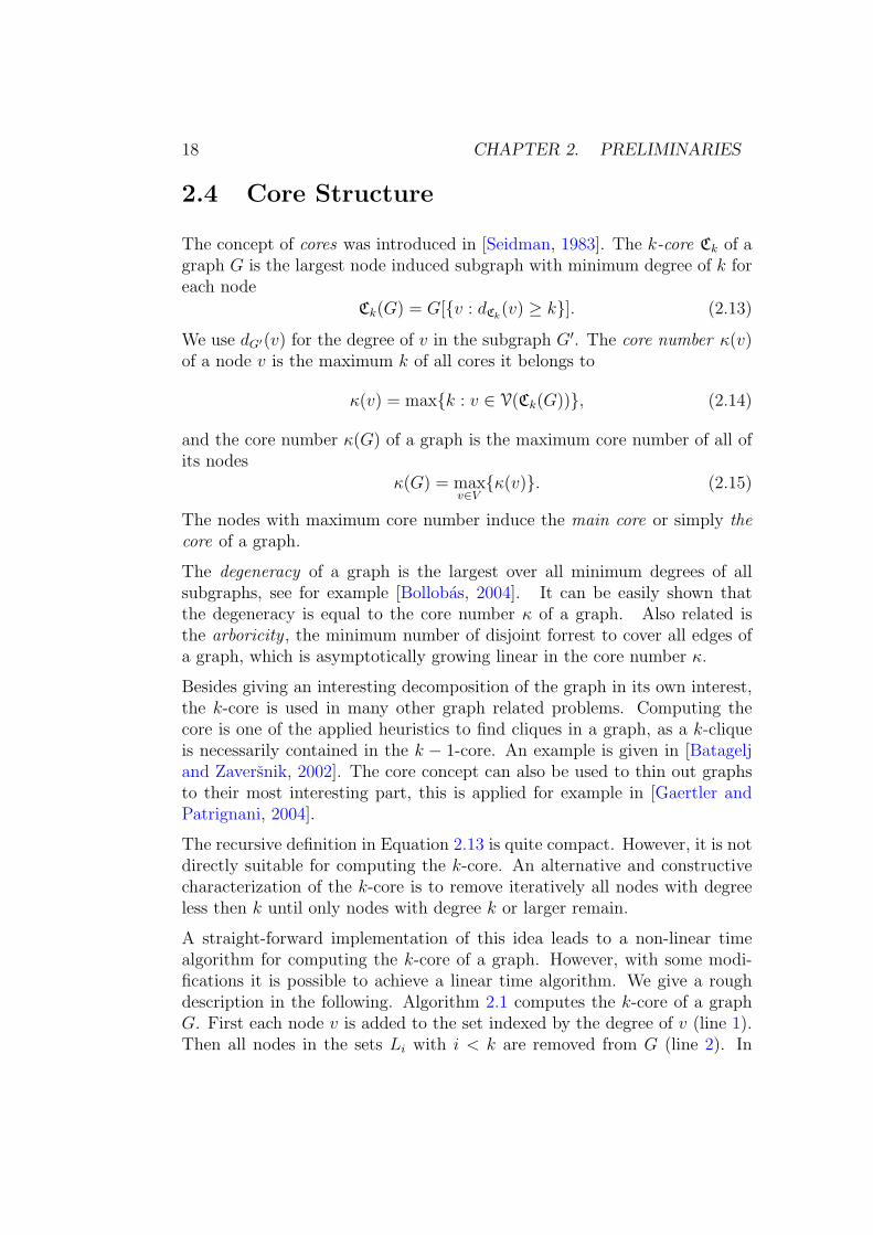
The concept of cores was introduced in [Seidman, 1983]. The k-core Ck of agraph G is the largest node induced subgraph with minimum degree of k foreach node
Ck(G) = G[v : dCk(v) ≥ k]. (2.13)
We use dG′(v) for the degree of v in the subgraph G′. The core number κ(v)of a node v is the maximum k of all cores it belongs to
κ(v) = maxk : v ∈ V(Ck(G)), (2.14)
and the core number κ(G) of a graph is the maximum core number of all ofits nodes
κ(G) = maxv∈Vκ(v). (2.15)
The nodes with maximum core number induce the main core or simply thecore of a graph.
The degeneracy of a graph is the largest over all minimum degrees of allsubgraphs, see for example [Bollobas, 2004]. It can be easily shown thatthe degeneracy is equal to the core number κ of a graph. Also related isthe arboricity , the minimum number of disjoint forrest to cover all edges ofa graph, which is asymptotically growing linear in the core number κ.
Besides giving an interesting decomposition of the graph in its own interest,the k-core is used in many other graph related problems. Computing thecore is one of the applied heuristics to find cliques in a graph, as a k-cliqueis necessarily contained in the k − 1-core. An example is given in [Batageljand Zaversnik, 2002]. The core concept can also be used to thin out graphsto their most interesting part, this is applied for example in [Gaertler andPatrignani, 2004].
The recursive definition in Equation 2.13 is quite compact. However, it is notdirectly suitable for computing the k-core. An alternative and constructivecharacterization of the k-core is to remove iteratively all nodes with degreeless then k until only nodes with degree k or larger remain.
A straight-forward implementation of this idea leads to a non-linear timealgorithm for computing the k-core of a graph. However, with some modi-fications it is possible to achieve a linear time algorithm. We give a roughdescription in the following. Algorithm 2.1 computes the k-core of a graphG. First each node v is added to the set indexed by the degree of v (line 1).Then all nodes in the sets Li with i < k are removed from G (line 2). In

2.4. CORE STRUCTURE 19
course of removing a node v, the sets Li of all its neighbors are updated(line 3). To achieve running time in O(m) the data structures have to becarefully chosen and some details must be considered. Since this is not ourfocus the interested reader might want to consult [Batagelj and Zaversnik,2002].
Algorithm 2.1: k-core
Input: Graph G = (V, E), k ∈ NOutput: k-core of Graph GData: L0, . . . , Ldmax initially empty sets of nodesforall v ∈ V do1
append v → Ld(v);
while ∃i < k : Li 6= ∅ do2
v ← pop Lmini:Li 6=∅;forall u ∈ Γ(v) do3
remove u← Ld(u);append u→ Ld(u)−1;
remove v from G;
Corollary 1 (folklore, [Batagelj and Zaversnik, 2002]) The k-core of a graphcan be computed in linear time.
We note that Algorithm 2.1 can be easily modified such that all the coresfrom 0 to κ(G) are computed in one single run whilst maintaining runningtime in O(m); e.g. by enclosing line 2 in a loop from 0 to κ(G).
Chapter Notes
In this chapter we introduced the most important concepts and required def-initions in a very compact manner. For a more in-depth exploration manytextbooks are available. Diestel [2000] and Bollobas [1998] give an introduc-tion to graph theory. Algorithms are treated by Cormen, Leiserson, Rivest,and Stein [2001]. Ross [2003] gives an introduction to probability which isdiscussed in context of algorithms by Motwani and Raghavan [1995].

20 CHAPTER 2. PRELIMINARIES

Chapter 3
Algorithms for Listing andCounting all Triangles in aGraph
Chapter Introduction
This chapter is devoted to algorithms for listing all triangles of a graph effi-ciently. The problem of triangle finding, counting and listing has been studiedbefore mainly from a theoretical point of view. The two basic algorithms areattributed to the folklore. They both achieve running time in O(dmax ·m).Itai and Rodeh [1978] introduced the first algorithm with running time inO(m3/2
). With respect of the number of edges the bound achieved by Itai’s
and Rodeh’s algorithm cannot be further improved for triangle listing algo-rithms. However, Chiba and Nishizeki [1985] can bound the running time oftheir algorithm in O(a ·m), in which a is the arboricity of the graph. Theyalso show that a ≤
√m.
The Ω(m3/2
)running time bound for listing algorithms does not hold for
counting algorithms. In this context Alon, Yuster, and Zwick [1997] givea counting algorithm with running time only dependent on m that indeedbeats this bound. This is achieved with fast matrix multiplication. Trianglecounting or listing can be seen as a special case of counting or listing eithershort cycles or small cliques. All the mentioned publications extend in oneor both of this fields.
All of the above publications do not consider any practical evaluation of thepresented algorithms. Batagelj and Mrvar [2001] give an extension of one
21

22 CHAPTER 3. TRIANGLE LISTING ALGORITHMS
of the folklore algorithms to count triads (all directed subgraphs with upto three nodes). This is also the only work we are aware of that containspractical results. They show, that an implementation of their algorithmsachieves very fast execution times. However, the algorithm they used has arunning time in ω
(m3/2
).
Contribution and Related Work. Our goal is to close the gap betweenalgorithms that are known to perform very good in practice, but do notachieve the theoretic best running times, and those algorithms that do so.We focus on the optimal bound given by the number of edges in O
(m3/2
).
Based on the known folklore algorithms we develop new triangle listing al-gorithms that achieve optimal running time with respect to the input sizem. Our experimental work shows that one of the new algorithms which wecall “forward” performs best with respect to execution time. This algorithmessentially uses the same basic operation as the algorithm of Batagelj andMrvar [2001]. But it also uses some further techniques that guarantee a run-ning time in O
(m3/2
). Our experiments show that it performs much better
for graphs with unbounded maximal degree.
The essence of our contribution was published in [Schank and Wagner, 2005b]and there exists also an extended technical report [Schank and Wagner,2005c].
All the introduced listing algorithms can be implemented with linear spaceconsumption. However, they can differ with respect to a constant factor.In a follow up work to [Schank and Wagner, 2005b], Latapy [2006] focusesmainly on memory consumption. Most notably he gives an improvement ofour algorithm forward that he calls compact-forward .
Organization. This chapter is organized as follows. We introduce somebasic concepts and notations directly following this section. In Section 3.1we will first introduce some well known algorithms for listing and countingtriangles followed by new variations of those. We will also prove that most ofthese new variations have good asymptotic running time bounds. The mostpromising candidates are evaluated in Section 3.2. We do this by experimentsof the execution time on generated and real world graphs. We close thischapter with a conclusion.

3.1. ALGORITHMS 23
Preliminaries
Recall that a triangle ∆uvw of a graph G = (V, E) is a three node subgraphwith V(∆) = u, v, w ⊂ V and E(∆) = u, v, v, w, w, u ⊂ E. Weuse the symbol δ(G) to denote the number of triangles in graph G. Note thatan n-clique has exactly
(n3
)triangles and asymptotically δclique ∈ Θ(n3). In
dependency to m we have accordingly δclique ∈ Θ(m3/2
)and by concentrating
as many edges as possible into a clique we get the following lemma.
Lemma 1 There exists a series of graphs Gm such that
δ(Gm) ∈ Θ(m3/2
).
We call an algorithm a triangle counting algorithm if it outputs the numberof triangles δ(v) for each node v and a triangle listing algorithm if it outputsthe three participating nodes of each triangle. As a listing algorithm requiresat least one operation per triangle we get the following by Lemma 1.
Corollary 2 A triangle listing algorithm has an asymptotic lower bound run-ning time in Ω(n3) in terms of n and in Ω
(m3/2
)in terms of m.
Note that one could further distinguish between counting the triangles for thewhole graph and counting the triangles for all of the nodes. However, thereis no complexity difference in running time known up to date and actuallyall known algorithms for counting the triangles of the whole graph do thisby counting them for all nodes first. For this reason we do not distinguishbetween these two cases.
3.1 Algorithms
We will list some algorithms for listing and counting triangles in the following.
3.1.1 Basic Algorithms
Algorithm “try-all”
A very simple algorithm with a running time in Θ(n3) is to check for edgesbetween nodes of every three element subset of V .

24 CHAPTER 3. TRIANGLE LISTING ALGORITHMS
Algorithm “matrix-multiplication”
If A is the adjacency matrix of graph G, then the diagonal elements of A3
contain two times the number of triangles of the corresponding node. Thisimmediately leads to a counting algorithm with running time Θ(n3). How-ever, it can also be implemented with fast matrix multiplication to run inΘ(nγ) time, where γ is the matrix multiplication exponent . It is known thatγ ≤ 2.376 [Coppersmith and Winograd, 1990].
Corollary 3 (folklore) All triangles of an undirected graph can be countedin O(nγ) time.
Algorithm “tree-lister”
Itai and Rodeh [1978] presented the fist algorithm that finds a triangle if itexists in time in O
(m3/2
). Their original algorithm stops after finding the first
triangle. However, it can be easily extended to list all triangles of a graphwithout additional cost in asymptotic running time. We call the trianglelisting variant “tree-lister”. The pseudo code is shown in Algorithm 3.1.
Algorithm 3.1: Triangle Lister “tree-lister”
Input: graph G = (V, E)Output: all triangles of Gwhile E 6= ∅ do
T ← Spanning Tree of G;for v, w ∈ E \ E(T ) do
if pred(v), w ∈ E then1
output Triangle pred(v), v, w;else if v, pred(w) ∈ E then2
output Triangle pred(w), v, w;
E ← E \ E(T )3
Theorem 1 All triangles of an undirected graph can be listed in O(m3/2
)time.
We will reproduce a proof for the above theorem with the following twoLemmas.
Lemma 2 Algorithm tree-lister outputs all triangles of a graph and no more.Each triangle is listed once and only once.

3.1. ALGORITHMS 25
Proof: Clearly Algorithm 3.1 outputs only triangles. It remains to beshown that each triangle is listed exactly once.
As a tree T is cycle free, each triangle has at least one edge in E \ E(T ).Assume first, that all the edges of an arbitrary triangle are contained inE \ E(T ), then the triangle is preserved after line 3. Since E is empty in theend, for any triangle there exists an iteration step where an edge is in E\E(T )and at least one edge is in E(T ). Clearly after this iteration the triangle isdestroyed. It remains to be shown that the triangle is listed exactly onceduring this iteration.
Now, let ∆ with V(∆) = u, v, w be the triangle destroyed in the cur-rent iteration. Without loss of generality, let v, w be in E \ E(T ). Then,pred(v) = u (the triangle is listed in line 1) or pred(w) = u (the triangleis listed in line 2, if not already listed in line 1) must be true, otherwise Twould not be a valid spanning tree or none of the edges would be in T , acontradiction to the assumption.
Lemma 3 Algorithm tree-lister can be implemented to run in O(m3/2
)time.
Proof: First note that with appropriate data structures the steps insidethe outer loop can be performed in O(m) time. We have to show that theouter loop is executed at most c ·
√m times, for some constant c.
In each loop at least the root node of each computed tree is split from thegraph and so the number of connected components γ increases in each itera-tion at least by one. We consider the costs while there are less (respectivelymore) than n−
√m components.
We first consider the costs until there are at most n −√
m components.Note, that in each iteration n−γ edges are removed. Hence, at least n−γ ≥n− (n−
√m) =
√m edges are removed in each step. After
√m such steps
m edges would be removed and consequently there cannot be more than√
msteps.
Now, we consider the case for γ ≥ n−√
m. The largest component has nodesize less than n− γ ≤
√m. As already mentioned, in each iteration at least
one node is split from each component, and hence, after at most√
m steps,we are left with only disconnected nodes.
We have seen the first existing m-optimal algorithm for triangle listing. How-ever, it is not a good candidate for an implementation. Let us mention the

26 CHAPTER 3. TRIANGLE LISTING ALGORITHMS
iterative construction of spanning trees and the tests for existence of edgeswith respect to the execution time. Moreover the dynamic modification of thegraph imposes comparatively high costs either in respect of execution timeor memory usage. This will become clear when we will have a closer look onthe experiments carried out on the algorithms which will be introduced inthe following sections.
3.1.2 Algorithm node-iterator and Related Algorithms
Algorithm “node-iterator”
Algorithm node-iterator iterates over all nodes and tests for each pair ofneighbors if they are connected by an edge. Line 1 ensures that each triangleis listed only once. In practice the required order “<” can be easily gainede.g. from array position or pointer addresses.
Algorithm 3.2: Triangle Lister “node-iterator”
Input: graph G = (V, E), arbitrary order < of the nodesOutput: all triangles of Gfor v ∈ V do
for all pairs of Neighbors u, w of v doif u, w ∈ G then
if u < v < w then1
output triangle u, v, w ;
The asymptotic running time is given by the expression∑v∈V
(d(v)
2
)(3.1)
and therefore bounded by O(d2max · n).
Corollary 4 (folklore) The algorithm node-iterator can be implemented torun in O(d2
max · n) time.
Algorithm “ayz” and “listing-ayz”
The counting algorithm due to Alon, Yuster, and Zwick [1997] combines thetechniques of the algorithms node-iterator and matrix-multiplication.

3.1. ALGORITHMS 27
Theorem 2 ([Alon et al., 1997]) All triangles of an undirected graph can becounted in time in O
(m2γ/(γ+1)
)⊂ O(m1.41).
Informally the algorithm splits the node set into low degree vertices Vlow =v ∈ V : d(v) ≤ β and high degree vertices Vhigh = V \ Vlow whereβ = mγ−1/γ+1 and γ is the matrix multiplication exponent. The standardmethod node-iterator is performed on the low degree nodes and (fast) matrixmultiplication on the induced subgraph of Vhigh, see Algorithm 3.3 for details.The running time is in O
(m2γ/(γ+1)
).
Algorithm 3.3: Triangle Counter “ayz”
Input: Graph G = (V, E); matrix multiplication parameter γOutput: number of triangles δ(v) for each nodeβ ←− m(γ−1)/(γ+1);1
for v ∈ V do2
δ(v)← 0;if d(v) ≤ β then
Vlow ← Vlow ∪ v;else
Vhigh ← Vhigh ∪ v;
for v ∈ Vlow do3
for all pairs of Neibours u, w of v doif edge between u and w exists then4
if u, w ∈ Vlow then5
for v ∈ v, u, w doδ(v)← δ(v) + 1/3;
else if u, w ∈ Vhigh then6
for v ∈ v, u, w doδ(v)← δ(v) + 1;
else7
for v ∈ v, u, w doδ(v)← δ(v) + 1/2;
A ← adjacency matrix of node induced subgraph of Vhigh;8
M ← A3;9
for v ∈ Vhigh do10
δ(v)← δ(v) + M(i, i)/2 where i is index of v;11

28 CHAPTER 3. TRIANGLE LISTING ALGORITHMS
We will give an extended version of the proof from [Alon et al., 1997] forTheorem 2.
Proof: The correctness of the algorithm can be easily seen by checkingthe case distinction for different types of triangles consisting of exactly three(line 5), two (line 7), one (line 6) or zero (line 11) low degree nodes.
To prove the time complexity we first note that the lines 1, 2, 8, and 10 canbe clearly implemented to run in linear time. We proof that loop beginning
at line 3 is in time in O(m2γ/(γ+1)
), that is O
(∑v∈Vlow
(d(v)2
))⊂ O
(m2γ/(γ+1)
).
Note that with a hashed edge set the test of line 4 can be implemented torun in constant time. The following tests in line 5, 6 and 7 can be clearlyperformed in constant time. The claim follows from
∑v∈Vlow
(d(v)2
)∈ O(mβ).
Now, we proof that line 9 is in time in O(m2γ/(γ+1)
). We have to show that
O(nγ
high
)⊂ O
(m2γ/(γ+1)
), which follows from nhigh ≤ 2m/β.
We can derive a listing algorithm listing-ayz with a running time in O(m3/2
)by using node-iterator also for the induced subgraph of Vhigh, in this caseβ =√
m.
Corollary 5 Algorithm listing-ayz has a running time in O(m3/2
).
Note that β is only bounded asymptotically to achieve the running times inthe lemmas above. Latapy [2006] shows that it behaves well for a range ofvalues. However, an optimal value still depends on the graph structure. Weuse β =
√m when we compare the algorithms experimentally in Section 3.2.
Algorithm node-iterator-core
The algorithm node-iterator-core listed in Algorithm 3.4 takes iteratively anode v with currently lowest degree, proceeds with it as in algorithm node-iterator , and then removes node v.
Note that an order of nodes that would give a node with currently minimaldegree, as required by the algorithm, can be computed in the same fashion asthe core numbers, see Section 2.4. Consequently, line 1 does not impose morethan an additional linear time cost during the execution of the algorithm.
We recall further from Section 2.4 that the k-core of a graph is the largestnode induced subgraph with minimum degree at least k. The core numberκ(v) of a node v is the maximum k of all cores it belongs to. The core number

3.1. ALGORITHMS 29
Algorithm 3.4: Triangle Lister “node-iterator-core”
Input: Graph G = (V, E)Output: all triangles of Gwhile V 6= ∅ do
v ← node with currently minimal degree;1
for all pairs of Neighbors u, w of v doif u, w ∈ G then
output triangle u, v, w ;
remove v from G;
of a graph κG is the maximal core number of all of its nodes. Hence, thecurrent degree of the node v from line 1 is less or equal than κ(v), and therunning time is bounded by
∑v∈V
(κ(v)
2
). (3.2)
Analogously to algorithm node-iterator, we can bound the running time byO(κ2
G · n). Note that after removing all nodes v with κ(v) ≤√
m the remain-ing graph is a subgraph of the node induced subgraph Vhigh of listing-ayz.Hence, this algorithm is an improvement to listing-ayz and the running timeis in O
(m3/2
), too.
3.1.3 Algorithm edge-iterator and Derived Algorithms
Algorithm “edge-iterator”
The algorithm edge-iterator iterates over all edges and compares the neigh-borhood of the two incident nodes. For an edge u, w the nodes u, v, winduce a triangle if and only if node v is present in both neighborhoods Γ(u)and Γ(w). It is possible to compare two neighborhoods Γ(u) and Γ(w) inO(d(u) + d(w)) time if those neighborhoods are stored as sorted adjacency ar-rays. The sorting can be achieved in linear time∗ or in O
(∑v∈V d(v) log d(v)
)⊂ O(m log n) time with standard sorting methods which has been used inour implementation. We will see in the experimental section how this pre-processing influences the overall execution time.
∗e.g. by proceeding in a similar manner as in Algorithm 3.6

30 CHAPTER 3. TRIANGLE LISTING ALGORITHMS
We display algorithm edge-iterator in Algorithm 3.5. Note that the listingis not presented in the shortest and most compact way. We list it as givento keep the differences minimal to an algorithm that will be introduced later(Algorithm 3.7 on page 35). The sorted array representation guarantees thatthe function “nextNeighborIndex” can be performed in constant time. Line 2ensures that each triangle is listed only once.
Algorithm 3.5: Triangle Lister “edge-iterator”
Input: graph G, array of vertices (v1, . . . , vn) in arbitrary order,adjacencies arrays sorted in the same order as the array ofvertices
Output: all trianglesFunctions:
firstNeighborIndex(vi) =
minν : vν ∈ Γ(vi) if exists
n else
nextNeighborIndex(vi, j) =
minν : vν ∈ Γ(vi), ν > j if exists
n else
for vi = (v1, . . . , vn) doforall vl ∈ Γ(vi) do
j ← firstNeighborIndex(vi);k ← firstNeighborIndex(vl);while j < n and k < n do1
if j < k thenj ← nextneighborindex(vi, j);
else if k < j thenk ← nextNeighborIndex(vl, k)
elseif i < k < l then2
output trianglevk, vi, vl;j ← nextNeighborIndex(vi, j);k ← nextNeighborIndex(vl, k);
For now we will disregard the preprocessing in the running time, which canthen be expressed with ∑
u,w∈E
d(u) + d(w). (3.3)
As with the previous algorithms we can give some less accurate bounds forthe running time which are: O(dmax ·m) ⊂ O(n ·m).

3.1. ALGORITHMS 31
Corollary 6 (folklore, [Batagelj and Mrvar, 2001]) Algorithm 3.5 lists ex-actly the triangles of a graph. It can be implemented to run in O(dmax ·m)time.
Comparing O(dmax ·m) with O(d2max · n) of node-iterator suggests that edge-
iterator is an improvement to node-iterator . However, this is not true. Con-sider the following amortized analysis: We split the costs d(u) + d(w) foran edge u, w in d(u) and d(w) units and assign d(u) to node u and d(w)to node w. In the outer loop each node v is passed d(v) times. Hence, therunning time captured by Equation 3.3 can be equivalently expressed with∑
v∈V
d(v)2. (3.4)
Corollary 7 Disregarding preprocessing, algorithm edge-iterator has the sameasymptotic time complexity as algorithm node-iterator.
The algorithm edge-iterator is equivalent to an algorithm introduced byBatagelj and Mrvar [2001]. It has been implemented within the softwarepackage Pajek [Batagelj and Mrvar, 1998].
Algorithm “edge-iterator-hashed”
This algorithm is based on edge-iterator. If we use a hashed container for theneighborhoods, we can ask for every node of the smaller container whether itis present in the larger container in O(1) time. This leads to a running timeasymptotically growing with∑
u,w∈E
mind(u), d(w). (3.5)
It has been shown in [Chiba and Nishizeki, 1985] that the expression ofEquation 3.5 is in O
(m3/2
).
Algorithm “forward”
This is a refinement of algorithm edge-iterator. Instead of comparing the fullneighborhood of two adjacent nodes, a subset A of those is compared. SeeAlgorithm 3.6 for the pseudo code and Figure 3.1 for an example.
As suggested by Figure 3.1 the algorithm is conveniently regarded on thedirected graph induced by the order of the nodes. The size of the data

32 CHAPTER 3. TRIANGLE LISTING ALGORITHMS
Algorithm 3.6: Triangle Lister “forward”
Input: graph G, array of vertices (v1, . . . , vn) in order of in increasingdegrees
Output: all trianglesData: initially empty array of nodes for each node v: A(v);for vi = (v1, . . . , vn) do
for vl ∈ Γ(vi) doif i < l then
foreach v ∈ A(vi) ∩ A(vl) do1
output triangle v, vi, vl ;
append vi → A(vl)
structure A(v) is then bounded by the in-degree of node v. Node also thatall arrays A are sorted with respect of the input order of the nodes during thewhole execution. Hence, the computation of the set of the common nodes ofA(vi) and A(vl) in line 1 can be performed in |A(vi)| + |A(vl)| steps. Therunning time for an arbitrary order is then bounded by the expression∑
u,w∈E
din(u) + din(w). (3.6)
As a “heuristic” to minimize Equation 3.6, the nodes are considered in nonincreasing order of their degrees, which implies a preprocessing in O(n log n).This order suffices to achieve the desired O
(m3/2
)bound.
Lemma 4 Algorithm forward lists all triangles of a graph and no more.Each triangle is listed once and only once.
Proof: Let ∆uvw be a triangle and without loss of generality u < v < wwith respect to the used order of the nodes. Then, there exists a time stept1 when vi = u and vl = v during the execution of Algorithm 3.6 when uis appended to A(v), because of u < v. Likewise, there exist time steps t2(respectively t3) when vi = u and vl = w (resp. vi = v and vl = w). Thetime steps t1 and t2 happen before time step t3, again because u < v < w.Consequently the node u is in both arrays A(v) and A(w) at time step t3and the triangle is listed. Thus, we have shown, that all triangles are listed.
Clearly nothing else but triangles are listed. Since the ordering u < v < winduces exactly one time step when the listing happens, each triangle is listed

3.1. ALGORITHMS 33
edge A(b) A(c) A(d) A(e) triangles1 (a, b) a2 (a, c) a a3 (a, d) a a a4 (a, e) a a a a
5 (b, c) a, b a a a a, b, c6 (b, d) a, b a a, b a
7 (d, e) a, b a a, b a, d a, d, e
1
2
3
4
5
6
7a b c d e
Figure 3.1: An example for algorithm forward .
once and only once.
Lemma 5 Algorithm forward can be implemented to have a running timein O
(m3/2
).
Proof: We actually show that Equation 3.6 is in O(m3/2
)for the chosen
order based on non increasing degrees. We can bound the expression ofEquation 3.6 by O(maxdin ·m), similar as in the case of algorithm edge-iterator . Now, we show that din(v) ∈ O(
√m) for all nodes v ∈ V .
Assume that there exists a node v with d(v) >√
m, otherwise din(v) ≤√
mfor all nodes is trivially true. Now, consider the vertices v1, . . . , vn wherewithout loss of generality d(v1) ≥ . . . ≥ d(vn) holds, i.e. in the nodes are inorder of non increasing degrees. Let k be the index where d(vk) >
√m but
d(vk+1) ≤√
m. Clearly, din(vi) ≤√
m holds for i > k.
It remains to be shown that din(vi) ∈ O(√
m) for i ≤ k. First note thatk√
m ≤∑
i≤k d(vi). Moreover the Handshake Lemma gives∑
i≤k d(vi) ≤∑i≤n d(vi) = 2m. It follows that k ≤ 2
√m and we can conclude that
din(vi) ≤ 2√
m for i ≤ k, too.
Let us remark that Chiba and Nishizeki [1985] did also use the order of nodessorted by non increasing degree to list a all triangles in a graph. However,

34 CHAPTER 3. TRIANGLE LISTING ALGORITHMS
their approach does work differently. It specifically requires dynamic graphmodifications. The authors mention the usage of doubly linked lists, whichwe already mentioned to be too memory consuming.
Algorithm “forward-hashed”
We can combine the methods of forward with edge-iterator-hashed . Theupcoming experiments will show if this manifests in an improved executiontime.
∑u,w∈E
mindin(u), din(w). (3.7)
Algorithm “compact-forward”
Very recently Latapy [2006] proposed an improvement to forward. The basicidea is to use iterators to compare the subsets of adjacencies, as it is done inedge-iterator . To this end, the adjacencies must be sorted and the comparisonmust be stopped once a certain index is reached. We give Latapy’s algorithm,adopted to our notation, in Algorithm 3.7.
Note that there are only three small differences of Algorithm 3.7 compared toAlgorithm 3.5. First algorithm compact-forward uses an ordering with nonincreasing degree as algorithm forward . Second the while-loop of line 1 nowstops at index i instead of n. Third the test in line 2 of Algorithm 3.5 canbe omitted.
Further note that stopping at index l in line 1 corresponds to comparing onlythe neighborhood with nodes which are before node vi in the given order.This is exactly what algorithm forward does.
Corollary 8 ([Latapy, 2006]) Algorithm 3.7 (compact-forward) lists all tri-angles of a graph. It can be implemented to run in time in O
(m3/2
).
Algorithm forward and compact-forward are very similar and have the sameasymptotic worst case bounds in running time and space consumption. How-ever, algorithm compact-forward does not require the additional arrays A.According to [Latapy, 2006] it is therefore more time and space efficient inpractice.

3.1. ALGORITHMS 35
Algorithm 3.7: Triangle Lister “compact-forward”
Input: graph G, array of vertices (v1, . . . , vn) in order of nonincreasing degrees, adjacencies arrays sorted in the same orderas the array of vertices
Output: all trianglesFunctions:
firstNeighborIndex(vi) =
minν : vν ∈ Γ(vi) if exists
n else
nextNeighborIndex(vi, j) =
minν : vν ∈ Γ(vi), ν > j if exists
n else
for vi = (v1, . . . , vn) doforall v` ∈ Γ(vi), ` < i do
j ← firstNeighborIndex(vi);k ← firstNeighborIndex(v`);while j < ` and k < ` do1
if j < k thenj ← nextNeighborIndex(vi, j);
else if k < j thenk ← nextNeighborIndex(v`, k);
elseoutput trianglevk, vi, v`;j ← nextNeighborIndex(vi, j);k ← nextNeighborIndex(v`, k);

36 CHAPTER 3. TRIANGLE LISTING ALGORITHMS
3.1.4 Overview of the Algorithms
Figure 3.2 shows an overview of the presented algorithms with their guaran-teed running time. The interesting listing algorithms will be experimentallycompared in the next section.
listing-ayz
node-iterator
matrix-multiplication
edge-iterator
forward
core
ayz using fast
matrix-
multiplication
listing algorithms
fast matrix-
multiplication
try-all
counting algorithms
forward-hashed
hashed
O(n3
)
O(dmax ·m)
O(m3/2
)
O(n3
)
O (nγ)
O(m
2γγ+1
)(compact)
Figure 3.2: Overview of the algorithms.
3.2 Experimental Results
Notes to the Implementation and Experiments
The algorithms were implemented in C++ using the Standard Template Li-brary and compiled with the gnu g++ compiler version 3.4 with Options “-g-O2”. The experiments were carried out on a 64-bit machine with two AMDOpteron processors clocked at 2.20GHz. The implemented algorithms onlyused one of the processors and were terminated if they used more than 6GB ofmemory. The execution times of the implemented algorithms were measuredin seconds using the getrusage function.
The graphs are represented using node pointers of std::vector type forthe nodes and their adjacency data structure. The algorithms node-iterator ,

3.2. EXPERIMENTAL RESULTS 37
listing-ayz and node-iterator-core use hashing for testing edge existence inconstant time. The hash function combines two random numbers of sizesize t with XOR, one for each node. The gnu cxx::hash map was used asa hash container. Creating the random bits is not contained in the executiontime of the experiments, whereas filling the container is included. We alsocompare the performance between a hashed container and a balanced binarytree in Section 19.
Let us note that a straight forward implementation of algorithm node-iterator-core requires doubly linked adjacency lists, due to the dynamic modificationof the graph. Such data structures turned out to be too space consuming tobe competitive. However, in the case of this algorithm we were able to usean equivalent static implementation instead.
The algorithm edge-iterator requires to find common nodes in two adja-cency data structures. For that purpose the used std::vector containersare sorted in a preprocessing step using the std::sort function. The sortingis included in the execution time of the algorithms. The generation of thenode order for forward is also included in the execution time.
The implemented algorithms are evaluated on several networks originatingfrom real world as well as on generated graphs. The algorithms are tested intwo ways. On the one hand we list the execution time of the algorithms. Onthe other hand we give the number of triangle operations, which in essencecaptures the asymptotic running time of the algorithm without preprocessing.The kind of operation considered as a triangle operation differs for the variousalgorithms but in all cases it represents the number of triangle tests, e.g. forthe algorithm node-iterator the number of triangle operations is equal to∑
v∈V
(d(v)2
)and for the edge-iterator equal to
∑v∈V d(v)2.
Experiments on Real World Networks
We will evaluate the introduced algorithms of Section 3.1 on three net-works: a road network (Section 3.2), a movie actor collaboration network(Section 3.2) and one generated from hyper links of an Internet sub domain(Section 3.2).
Road Network Germany
This network is based on the roads in Germany. Hence, it is very sparse, al-most planar, has very low average and maximum degree, and in consequence,

38 CHAPTER 3. TRIANGLE LISTING ALGORITHMS
a very low deviation from the average degree, see Figure 3.3(a). The standarddeviation from the average degree is an interesting measure. The square ofit bounds how much improvement is possible for the more refined algorithmscompared to the two standard algorithms node-iterator and edge-iterator .
The performance of the algorithms is listed in Figure 3.3(b) and Figure 3.3(c).As expected algorithm edge-iterator has the highest asymptotic effort in thenumber of triangle operations. However, in terms of execution time it outper-forms all the other algorithms. The two algorithms edge-iterator-hashed andforward-hashed , which use hashed data structures for every node, performbadly.
Movie Actor Network 2004
This graph is constructed from The Internet Movie Database of the year2004. Each node represents an actor. Two actors share a link if and only ifthey ever played together in a movie. The properties and results are shownin Figure 3.4.
This network has a more interesting structure compared to the network ofSection 3.2. The degree distribution is somewhat skewed with a std. de-viation of 183 from the average degree, see Figure 3.4(a). The algorithmsnode-iterator-core and forward-hashed are very efficient with respect to thenumber of triangle operations, Figure 3.4(c). As in Section 3.2 the algorithmlisting-ayz is no improvement to algorithm node-iterator , since
√m = 5252
is higher than the maximum degree. Again edge-iterator performs relativelywell in execution time, see Figure 3.4(b), considering highest number of trian-gle operations, see Figure 3.4(c). The implementation of algorithm forwardperforms best in execution time.
Notre Dame WWW
In this Network each node represents a web page within the nd.edu domain.An edge between two web pages exists if one of them was linking the other.Properties and results are shown in Figure 3.5.
Compared to the road network of Section 3.2 and even to the collaborationnetwork of Section 3.2 the difference between maximal degree to the averagedegree is more pronounced and there is a very sharp bend in the degrees ofthe nodes visible, see Figure 3.5(a). From this property one expects, that themore refined algorithms can reduce the number of operations comparatively

3.2. EXPERIMENTAL RESULTS 39
nodes 4799875edges 5947001dmax 7dmin 1davr 2.5
d stddeviation 0.90core number 3
wedges 10752498triangles 172699
transitivity 0.048clustering coefficient 0.050 1
2
3
4
5
6
7
0 500000 1e+06 1.5e+06 2e+06 2.5e+06 3e+06 3.5e+06 4e+06 4.5e+06 5e+06
node
deg
ree
node index
degree
(a) properties and degrees
algorithm seconds1 node-iterator 13.732 listing-ayz 13.953 node-iterator-core 11.994 edge-iterator 4.275 edge-iterator-hashed 55.476 forward 9.037 forward-hashed 43.97
0
10
20
30
40
50
60
0 1 2 3 4 5 6 7 8
(b) execution times
algorithm operations1 node-iterator 107524982 listing-ayz 107524983 node-iterator-core 12441944 edge-iterator 333989985 edge-iterator-hashed 144768556 forward 17865317 forward-hashed 1426197
0
5e+06
1e+07
1.5e+07
2e+07
2.5e+07
3e+07
3.5e+07
0 1 2 3 4 5 6 7 8
(c) triangle operations
Figure 3.3: Road Network Germany

40 CHAPTER 3. TRIANGLE LISTING ALGORITHMS
nodes 667609edges 27581275dmax 4605dmin 1davr 82.6
d stddeviation 183.18core number 1005
wedges 13452269555triangles 1176613576
transitivity 0.262clustering coefficient 0.796 0
500
1000
1500
2000
2500
3000
3500
4000
4500
5000
0 100000 200000 300000 400000 500000 600000 700000
node
deg
ree
node index
degree
(a) properties and degrees
algorithm seconds1 node-iterator 4649.052 listing-ayz 5285.503 node-iterator-core 610.614 edge-iterator 174.045 edge-iterator-hashed 1377.736 forward 64.487 forward-hashed 504.26
0
1000
2000
3000
4000
5000
6000
0 1 2 3 4 5 6 7 8
(b) execution times
algorithm operations1 node-iterator 134522695552 listing-ayz 134522695553 node-iterator-core 17256855264 edge-iterator 269597016605 edge-iterator-hashed 74608746646 forward 54236235607 forward-hashed 1745104092
0
5e+09
1e+10
1.5e+10
2e+10
2.5e+10
3e+10
0 1 2 3 4 5 6 7 8
(c) triangle operations
Figure 3.4: Movie Actor Network 2004

3.2. EXPERIMENTAL RESULTS 41
nodes 325729edges 1090108dmax 10721dmin 1davr 6.7
d stddeviation 42.82core number 155
wedges 304881174triangles 8910005
transitivity 0.088clustering coefficient 0.466 0
2000
4000
6000
8000
10000
12000
0 50000 100000 150000 200000 250000 300000 350000
node
deg
ree
node index
degree
(a) properties and degrees
algorithm seconds1 node-iterator 69.002 listing-ayz 18.583 node-iterator-core 2.474 edge-iterator 3.125 edge-iterator-hashed 6.116 forward 0.537 forward-hashed 3.49
0
10
20
30
40
50
60
70
0 1 2 3 4 5 6 7 8
(b) execution times
algorithm operations1 node-iterator 3048811742 listing-ayz 833747353 node-iterator-core 96646344 edge-iterator 6119425645 edge-iterator-hashed 313733266 forward 187421087 forward-hashed 9473218
0
1e+08
2e+08
3e+08
4e+08
5e+08
6e+08
7e+08
0 1 2 3 4 5 6 7 8
(c) triangle operations
Figure 3.5: Notre Dame WWW

42 CHAPTER 3. TRIANGLE LISTING ALGORITHMS
well, this is confirmed in Figure 3.5(c). However, algorithm forward againperforms best in execution time, see Figure 3.5(b).
Experiments on Generated Graphs
The networks used in Section 3.2 give an indication on the performancedifference of the various algorithms. To get a clearer picture, we investigatehow the algorithms perform on a series of random graphs with increasing size.In Section 3.2 we evaluate on standard random graphs. This is then amendedin Section 19 with a modified graph model that has a more interesting degreedistribution.
Generated Gn,m Graphs Figure 3.6 shows the results on generatedgraphs where m edges are inserted randomly between n nodes. We do notallow loops or multiple links in our Gn,m graphs. Note that the term Gn,m
graph is usually associated with the model of Erdos and Renyi [Erdos andRenyi, 1959], in which the set of non isomorphic graphs with n nodes andm edges is considered. Our generator is also related to the Gn,p model ofGilbert [Gilbert, 1959]. We differ from the latter in generating exactly medges, which are inserted uniformly at random between the
(n2
)possible
endpoints, whereas Gilberts model generates graphs with an expected num-ber of
(n2
)p edges. Nevertheless we stick to the symbol Gn,m since n and m
are our input parameters.
We consider graphs in which the relation of the parameters n and m is chosensuch that the average degree equals 50. Figure 3.6(a) shows the number oftriangle operations versus the number of edges. Since Gn,m graphs are veryunlikely to have high degree nodes, algorithm listing-ayz and node-iteratorperform equally well with respect to the number of triangle operations. Thealgorithms node-iterator-core and forward-hashed most efficiently limit thenumber of triangle operations. They are very close to the optimum, i.e. thenumber of triangles.
Figure 3.6(b) shows the execution time in seconds versus the number of edges.Again the algorithm edge-iterator performs best together with forward . Bothalgorithms are very simple and do not use complicated data structures. Incontrast, the use of hashing slows down the execution time of the correspond-ing algorithms. The plots of the algorithms using hashing show some notablepikes which are caused by automatic rehashing of the container.

3.2. EXPERIMENTAL RESULTS 43
0
1e+09
2e+09
3e+09
4e+09
5e+09
6e+09
7e+09
0 1e+07 2e+07 3e+07 4e+07 5e+07 6e+07 7e+07 8e+07 9e+07 1e+08
edge-iteratorlisting-ayz
node-iteratoredge-iterator-hashed
forwardnode-iterator-core
forward-hashed# triangles
(a) triangle operations vs number of edges
0
200
400
600
800
1000
1200
1400
0 1e+07 2e+07 3e+07 4e+07 5e+07 6e+07 7e+07 8e+07 9e+07 1e+08
listing-ayznode-iterator
edge-iterator-hashednode-iterator-core
forward-hashedforward
edge-iterator
(b) execution times in seconds vs number of edges
Figure 3.6: Generated Gn,m graphs.

44 CHAPTER 3. TRIANGLE LISTING ALGORITHMS
Generated Graphs with High Degree Nodes The Gn,m graphs like inSection 3.2 tend to have no high degree nodes and to have a very low deviationfrom the average degree in general. However, many real world networksshow a different behavior, see Section 3.2 and Section 3.2 for an example.The famous power law distributions in the degree found in many networks[Faloutsos et al., 1999] actually hint that skewed degree distributions are verycommon.
We use a very simple modification of the Gn,m model to achieve high degreenodes. As in Section 3.2 we first generate a prime graph Gn,m which weextend to a graph Gn,m,h. For each node 1 ≤ i ≤ h we add links to randomlyselected nodes until the degree of the i-th node is n
2h−ih
. The parameter h isset to h =
√n for the results shown in Figure 3.7.
Now, the number of triangle operations is obviously not linear in the graphsize, see Figure 3.7(a). Again the algorithms node-iterator-core and forward-hashed perform best in limiting the asymptotic effort. However, they areonly in second and third place in the execution time. Algorithm forwardperforms clearly best.
Remarks on the Experiments
Before discussing the results we complement the experiments by comparingHashing versus Balanced Tree data structures for storing edges, see Sec-tion 19. We also consider the statistical variation of the execution times inSection 19.
Hashing versus Balanced Trees
We investigate the performance between hashed containers and balanced treecontainers for storing the edges. The template from gnu cxx::hash map
was used for the hashed container. We store two pointers from the incidentnodes of an edge. The hashing function combines two random bit fields ofsize size t (one for each node) with the XOR operation. The tree container isbased on the template std::set, which is an implementation of a red-blacktree. An edge is coded with the lexicographic order of the two addresses ofthe incident node pointers.
The results are shown in the Figure 3.8. We can observe that the hasheddata structure outperforms the balanced tree structure. This justifies thechosen hashing function and the use of a hashed container in general for thepurpose of testing edge existence.

3.2. EXPERIMENTAL RESULTS 45
0
5e+09
1e+10
1.5e+10
2e+10
2.5e+10
3e+10
0 1e+07 2e+07 3e+07 4e+07 5e+07 6e+07 7e+07 8e+07 9e+07
edge-iteratornode-iterator
edge-iterator-hashedforward
listing-ayznode-iterator-core
forward-hashed# triangles
(a) triangle operations vs number of edges
0
500
1000
1500
2000
2500
3000
3500
4000
0 1e+07 2e+07 3e+07 4e+07 5e+07 6e+07 7e+07 8e+07 9e+07
node-iteratoredge-iterator
edge-iterator-hashedlisting-ayz
node-iterator-coreforward-hashed
forward
(b) execution times in seconds vs number of edges
Figure 3.7: Generated graphs with high degree nodes.

46 CHAPTER 3. TRIANGLE LISTING ALGORITHMS
0
1000
2000
3000
4000
5000
0 1e+07 2e+07 3e+07 4e+07 5e+07 6e+07 7e+07
node-iterator TREE node-iterator HASH
listing-ayz TREEnode-iterator-core TREE
listing-ayz HASHnode-iterator-core HASH
Figure 3.8: Hashing versus balanced trees: Execution time in seconds (y-axis)depending on the number of edges (x-axis).
Statistical Experiments of the Execution Times
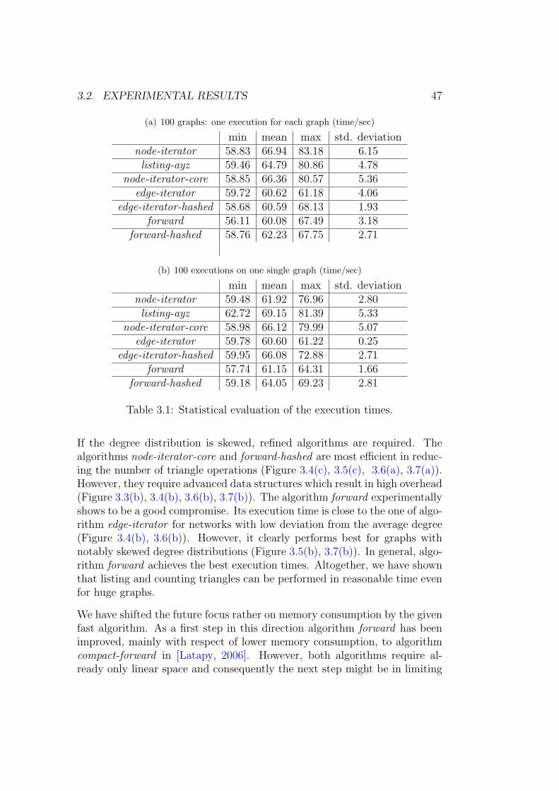
The algorithms show some unsteady behavior in the experiments for the ex-ecution times. The obvious pikes for the algorithms using a hashed containerfor the edges are caused by rehashing of the container. But there are otherinfluences like the variations in the structure of the generated graph or otherprocesses running on the same machine. To investigate these influences wegenerated for each algorithm 100 graphs. The sizes of the graphs are chosensuch that the average execution time is not far from 60 seconds.
The results are shown in the Table 3.1. The variation of the executiontimes behaves well. As expected it is lower when the algorithm runs onthe same graph (Table 3.0(a)) compared to test it on 100 different graphs(Table 3.0(b)).
Chapter Conclusion
The two known standard algorithms node-iterator and edge-iterator are asymp-totically equivalent (Lemma 7). However, the algorithm edge-iterator can beimplemented with much lower overhead (Figure 3.6(b)). It works very wellfor graphs with degrees that do not differ much from the average degree(Figure 3.3, Figure 3.6).
3.2. EXPERIMENTAL RESULTS 47
(a) 100 graphs: one execution for each graph (time/sec)
min mean max std. deviationnode-iterator 58.83 66.94 83.18 6.15listing-ayz 59.46 64.79 80.86 4.78
node-iterator-core 58.85 66.36 80.57 5.36edge-iterator 59.72 60.62 61.18 4.06
edge-iterator-hashed 58.68 60.59 68.13 1.93forward 56.11 60.08 67.49 3.18
forward-hashed 58.76 62.23 67.75 2.71
(b) 100 executions on one single graph (time/sec)
min mean max std. deviationnode-iterator 59.48 61.92 76.96 2.80listing-ayz 62.72 69.15 81.39 5.33
node-iterator-core 58.98 66.12 79.99 5.07edge-iterator 59.78 60.60 61.22 0.25
edge-iterator-hashed 59.95 66.08 72.88 2.71forward 57.74 61.15 64.31 1.66
forward-hashed 59.18 64.05 69.23 2.81
Table 3.1: Statistical evaluation of the execution times.
If the degree distribution is skewed, refined algorithms are required. Thealgorithms node-iterator-core and forward-hashed are most efficient in reduc-ing the number of triangle operations (Figure 3.4(c), 3.5(c), 3.6(a), 3.7(a)).However, they require advanced data structures which result in high overhead(Figure 3.3(b), 3.4(b), 3.6(b), 3.7(b)). The algorithm forward experimentallyshows to be a good compromise. Its execution time is close to the one of algo-rithm edge-iterator for networks with low deviation from the average degree(Figure 3.4(b), 3.6(b)). However, it clearly performs best for graphs withnotably skewed degree distributions (Figure 3.5(b), 3.7(b)). In general, algo-rithm forward achieves the best execution times. Altogether, we have shownthat listing and counting triangles can be performed in reasonable time evenfor huge graphs.
We have shifted the future focus rather on memory consumption by the givenfast algorithm. As a first step in this direction algorithm forward has beenimproved, mainly with respect of lower memory consumption, to algorithmcompact-forward in [Latapy, 2006]. However, both algorithms require al-ready only linear space and consequently the next step might be in limiting

48 CHAPTER 3. TRIANGLE LISTING ALGORITHMS
the usage of central memory. Since triangles can not be listed by stream-ing algorithms with reasonable models [Bar-Yosseff et al., 2002] further ap-proaches could be based on memory hierarchy methods. A survey on thismatter is [Meyer et al., 2003]. Indeed, in the meanwhile an apdoption of thealgorithm forward has been implemented into the secondary memory librarySTXXL [Dementiev et al., 2005].

Chapter 4
Algorithms for Counting andListing Triangles in SpecialGraph Classes
Chapter Introduction
In this chapter we will give efficient algorithms for listing and counting trian-gles for certain graph classes. We strive to achieve running time in O(m + δ),where δ is the number of triangles in the graph for listing triangles. In thecase of counting triangles for each node we aim to achieve running time inO(m). One could regard such running times as optimal with respect to theparameters m respectively δ.
However, it is possible to beat such optimal running times, for example ifwe know that we have a complete graph. While this case certainly is patho-logical and uninteresting, we will give an example in which we achieve O(n)running time for counting by using a certain encoding of the graph. Note thatwe purposely do not handle properties relying on solution methods that in-volve high constants in any implementation of the algorithms. We have seenthat there are very efficient general algorithms in Chapter 3. This rendersalgorithms with high constants disadvantageous to use.
Contribution and Related Work. As far as we know efficient trianglelisting algorithms have not been considered for special graph classes. Thereexist work for triangle counting that considers other parameters such as de-generacy or arboricity, see [Chiba and Nishizeki, 1985; Alon et al., 1997] for
49

50 CHAPTER 4. GRAPH CLASSES
example. For some parts triangle counting has been considered previously,albeit by other methods. In these cases we will give a reference to the relevantwork.
Organization. We consider graphs with bounded core number in Sec-tion 4.1. Planar graphs and graphs constructed by preferential attachmentbelong to this class. Section 4.2 treats comparability graphs and Section 4.3chordal graphs. In Section 4.4 distance hereditary graphs are discussed.
Before we start let us agree on the following. We will use a sentence like“Algorithm xyz lists all triangles.” in the meaning that algorithm xyz listsall triangles, each triangle is listed exactly once, and nothing else but tri-angles are listed by the algorithm. This convention makes many upcomingstatements compact and easy to read.
4.1 Graphs with Bounded Core Numbers
We introduced the core concept in Section 2.4 on page 18. And in Sec-tion 3.1.2 we have seen that there exists a listing algorithm with runningtime O(κ2 · n) where κ is the core number of the graph. See node-iterator-core listed in Algorithm 3.4 on page 29. If κ is bounded by a constant we geta running time in O(m) and we list a few graph classes which benefit from abounded core number in the following.
Planar Graphs
A planar graph is characterized by the property that it can be embedded inthe plane such that no two edges intersect except in the incident node. Alinear time algorithm for finding a triangle in a planar graph was given byItai and Rodeh [1978], see also page 24 in Section 3.1.1. It can be extendedto counting and listing all triangles without additional costs with respect toasymptotic running time.
Theorem 3 All triangles of a planar graph can be listed in linear time.
Our approach is slightly simpler than the algorithm in [Itai and Rodeh, 1978].We use the fact that each planar graph has at least one node with degreefive or less. Clearly, a planar graph remains planar when parts of it areremoved. Hence, the core number of any planar graph is also 5 or less.

4.2. COMPARABILITY GRAPHS 51
(a) transitive triangle (b) cyclic triangle
Figure 4.1: Directed triangle orientations.
Preferential Attachment Graphs
The so called preferential attachment graphs are generated graphs where inevery iteration a node v and µ new edges, each connecting v to some existingnode, are added. See Section 6.1 on page 95 for more details. We point outthat the last added node v has degree µ and consequently the core numberis bounded by the parameter µ.
Theorem 4 All triangles of generated preferential attachment graphs can belisted in linear time for fixed parameters µ.
4.2 Comparability Graphs
An undirected graph that has an acyclic transitive orientation is called acomparability graph. A digraph D = (V, A) is transitive oriented if (u, v),(v, w) ∈ A implies the existence of (u, w) ∈ A, see Figure 4.1(a). We willshow Theorem 5 in this section.
Theorem 5 All triangles of a comparability graph can be listed in O(m + δ)time and counted in O(m) time.
Golumbic [1977] gave an algorithm to compute a transitive orientation of acomparability graph in time in O(dmax ·m). The first linear time algorithmwas given much later by McConnell and Spinrad [1997].
A Triangle Listing Algorithm for Comparability Graphs
The required existence of the arc (u, w) in Figure 4.1(a) leads to a simplealgorithm for listing triangles. For every node v one simply outputs all pairsconsisting of one adjacent incoming with one adjacent outgoing node. Here,

52 CHAPTER 4. GRAPH CLASSES
incoming respectively outgoing refers to the edge by which the node is con-nected to v. This is idea is realized in Algorithm 4.1.
Algorithm 4.1: Triangle Lister for Comparability Graphs
Input: comparability graph D = (V, A) in transitive orientationOutput: all trianglesforall v ∈ V do1
forall u ∈ u ∈ V : ∃(u, v) ∈ A do2
forall w ∈ w ∈ V : ∃(v, w) ∈ A do3
output triangle u, v, w;
Lemma 6 Algorithm 4.1 lists all triangles of comparability graph given intransitive orientation. It can be implemented to run in O(n + δ) time.
Proof: We start with the correctness. Every triangle has to be in transi-tive orientation. Clearly each transitive triangle has a center node v, as inFigure 4.1(a). Hence, each triangle is listed exactly once by the algorithm.Clearly, each output u, v, w is guaranteed to be a triangle.
Let us consider the time complexity. If we consider the loop starting at line 1to be empty we iterate in n steps over all nodes. We start the loop of line 2conditional only if the outgoing links from v are not empty. Thus, we guar-antee that every iteration produces an output and both loops are in O(δ).Note that we still get running time in O(m + δ) if we do not perform thistest.
A Triangle Counting Algorithm for Transitively Ori-ented Graphs
Algorithm 4.1 lists the counting algorithm for comparability graphs in tran-sitive orientation.
Lemma 7 Algorithm 4.1 counts all triangles of a transitive orientation foreach node. It can be implemented to run in O(m) time.
Proof: Note that the number of outgoing and incoming edges (line 5 andline 3) of a node sum up to the degree. Then the running time is due to theHandshake Lemma.

4.3. CHORDAL GRAPHS 53
Algorithm 4.2: Triangle Counter for ComparabilityGraphsInput: comparability graph D = (V, A) in transitive orientationOutput: number of triangles δ(v) for each node vforall x ∈ V do1
δ(x)← din(x) · dout(x);2
forall v ∈ v ∈ V : ∃(x, v) ∈ A do3
δ(x)← δ(x) + dout(v);4
forall v ∈ v ∈ V : ∃(v, x) ∈ A do5
δ(x)← δ(x) + din(v) ;6
We distinguish between three types of triangles for each node x. There areexactly din(x) · dout(x) triangles for which x is the center node (x = v inFigure 4.1(a)). They are counted in line 2. The node x is the “first” node(x = u in Figure 4.1(a)) of the triangles with the pair (v, w) ∈ V × V forwhich (x, v), (v, w) ∈ A. There are exactly
∑v:(x,v)∈A dout(v) of those and
they are counted in the loop starting at line 3. The node x is the “last” node(x = w in Figure 4.1(a)) of the triangles with the pair (u, v) ∈ V × V forwhich (u, v), (v, x) ∈ A. There are exactly
∑v:(v,x)∈A din(v) of those and they
are counted in the loop starting at line 5.
4.3 Chordal Graphs
A graph is chordal if every simple cycle of length at least four has a chord,i.e. an edge between two nodes that do not induce an edge in the cycle.Equivalently, a chordal graph does not have an induced k-cycle for k largerthan three. A perfect elimination order (PEO) is an order of the nodesv1, . . . , vn such that all neighbors of vi in G[vj : j ≤ i] induce a clique.A graph is chordal if and only if it has a perfect elimination order [Fulker-son and Gross, 1965]. Testing chordality and moreover computing a perfectelimination order can be done in linear time [Rose et al., 1976].
This is done with so called lexicographic breadth first search (lexBFS) a vari-ant of BFS which ensures that unvisited neighbors of a currently visitednode are discovered before non-neighbors. A survey of lexBFS and relatedelimination orders can be found in [Corneil, 2004].

54 CHAPTER 4. GRAPH CLASSES
Now, we have collected all ingredients to efficiently perform triangle compu-tation in chordal graphs and in the end show the following Theorem:
Theorem 6 All triangles of a chordal graph can be listed in O(m + δ) timeand counted in O(m) time.
To do so, we first compute a PEO and then iterate over the nodes in theinverse order. In each iteration we determine all triangles of the currentnode with those nodes of lower PEO number. How this is precisely donedepends on whether we want to count, see Algorithm 4.4, or list all triangles,see Algorithm 4.3.
Algorithm 4.3: Triangle Lister for Chordal Graphs
Input: chordal graph G; PEO (v1, . . . , vn);Output: all trianglesfor vk = (vn, . . . , v1) do1
forall vi ∈ Γ(vk) do2
forall vj ∈ Γ(vk), i < j do3
output triangle vi, vj, vk;4
remove vk from G;5
Lemma 8 Algorithm 4.3 lists all triangles of a chordal graph. It can beimplemented, such that it runs in O(m + δ) time.
Proof: We start with the correctness of the algorithm. In line 4 onlytriangles are listed, since all neighbors of vk with lower PEO number thank induce a clique together with vk. Note that i < k (i.e. all neighbors of vk
have lower PEO number than vk) is always true because of line 5.
A triangle is listed at most once since any combination of i, j, k can appearat most once. This is due to the removal of node vk after processing it inline 5 and the requirement i < j in line 3.
It remains to be shown that all triangles are listed. Let G[u, v, w] be atriangle and without loss of generality assume u < v < w with respect of thegiven PEO. Since k iterates over all vertices there is a value of k such thatvk = w. Note that at this time u and v are still present in the graph becausewe iterate in invers PEO in line 1. Then there must exist some value of isuch that vi = u and some value of j such that vj = v. Therefore the triangleu, v, w is listed.

4.3. CHORDAL GRAPHS 55
We turn to the time complexity. A crucial point is to execute line 2 andline 3 efficiently, i.e. incrementing i and j in constant time. This can beachieved if the neighborhoods are also sorted according to the PEO. Sortingall neighborhoods according to a given order of nodes can be done in lineartime, e.g. by proceeding in a similar manner as in Algorithm 3.6 on page 32.
By the proof of correctness above line 4 is executed exactly δ times. However,the Loop in line 3 might be empty. Therefore, it remains to be shown thatall loops including those of line 3 are in linear time. This is nothing else butan iteration over all edges.
Algorithm 4.4: Triangle Counter for Chordal Graphs
Input: chordal graph G; PEO (v1, . . . , vn);Output: all trianglesfor i = (1, . . . , n) do
δ(vi)← 0;
for vk = (vn, . . . , v1) do1
δ(vk)← δ(vk) +(
d(vk)2
);2
forall vi ∈ Γ(vk) do3
δ(vi)← δ(vi) + d(vk)− 1;4
remove vk from G;5
Algorithm 4.4 is merely an adoption of Algorithm 4.3 for counting.
Lemma 9 Algorithm 4.4 counts all triangles of a chordal graph. It can beimplemented, such that it runs in O(m) time.
Proof: We start with the time complexity. Analogous as in the previousproof all loops together can be implemented to run in the order of the numberof edges. Nothing else remains to be shown here.
We show in the following that in every iteration of the loop beginning atline 1 all currently existing triangles containing the node vk (and no more)are counted.
Only neighbors of vk with lower PEO are present in the current loop k. Thereare |Γ(vk)| = d(vk) such neighbors with which vk induces a clique and hencethere are
(d(vk)
2
)triangles in this clique containing node vk. Consequently in
line 2 all triangles of node vk with nodes of lower PEO number than k arecounted for node vk.

56 CHAPTER 4. GRAPH CLASSES
(a) house (b) hole (c) domino (d) gem
Figure 4.2: Forbidden induced subgraphs.
It remains to be shown that the triangles are counted for the nodes withPEO number less than k. In the loop starting at line 3 the triangle numberfor these nodes is updated. There are again d(vk) of them. Each formstriangles with vk and the rest of the d(vk) − 1 nodes in the induced clique.Consequently the number d(vk)− 1 has to be added, which is done in line 4.
Arriving at line 5 all triangles containig node vk have been counted and vk
can be savely removed.
4.4 Distance Hereditary Graphs
The distance hereditary graphs will be the last graph class we consider inthis chapter.
Introduction and Preliminaries
A connected graph G is distance hereditary if for any path P of G the inducedsubgraph G[V(P )] is distance preserving (isometric). That means that anytwo nodes of P have the same distance in G as in G[V(P )]. We will use theabbreviation DH for distance hereditary in the following.
There exists an equivalent definition by forbidden subgraphs [Hammer andMaffray, 1990]: a graph is DH if and only if it does not have an inducedsubgraph of the type: house, hole (induced cycle of length at least five),domino or gem. See Figure 4.2. The abbreviation HHDG-free is frequentlyused in the literature.
Distance hereditary graphs have an equivalent description, like chordal graphs,based on an elimination order. A graph is distance hereditary if and only ifit has a 2-simplicial elimination order [Nicolai, 1996]. See for example the

4.4. DISTANCE HEREDITARY GRAPHS 57
(a) split (b) split decomposition
Figure 4.3: A split and its decomposition.
survey [Corneil, 2004] for the definition and computation of such an order.We used the perfect elimination order to efficiently list and count trianglesfor the case of chordal graphs in Section 4.3. However, here we will use afurther equivalent formulation for DH graphs based on splits.
We have listed the important and more common ways to describe DH graphs,but there are more. The book “Graph classes, a survey” [Brandstadt et al.,1999] is a good starting point for the interested reader.
Splits
A split [Cunningham, 1982] in a graph G = (V, E) is a partition of the set Vinto two sets U and W , such that |U | > 1 as well as |W | > 1, and such thatfor all u′, w′ : u′ ∈ U ′ = U ∩ Γ(W ), w′ ∈ W ′ = W ∩ Γ(U) ⇒ u′, w′ ∈ E.See Figure 4.3(a) for an example.
Given a split S = (U,W ) the graph can be split decomposed by
1. adding the split nodes u and w,
2. adding the split edge u, w,
3. adding the edges u′, u : u′ ∈ U ′ and w,w′ : w′ ∈ W ′ respec-tively, and
4. removing all edges u′, w′ : u′ ∈ U ′, w′ ∈ W ′.
See Figure 4.3 for an example. We will call the edges which are not createdin Step 2 the regular edges.
Without the split edge u, w the remaining graph falls into two connectedcomponents which are called the split components. This procedure can be ap-plied recursively until no further suitable split is found. If the result consistsof components of the size three the graph is called totally split decomposable,

58 CHAPTER 4. GRAPH CLASSES
(a) original graph (b) totally decomposed graph
Figure 4.4: A graph and its total decomposition.
see Figure 4.4. As the split edges always form bridges between the compo-nents the resulting graph is a tree of components which is called the splitdecomposition tree.
A graph is totally decomposable if and only if it is distance hereditary [Ham-mer and Maffray, 1990]. The total decomposition can then be computed inlinear time [Hammer and Maffray, 1990]. A later result also gives a lineartime decomposition algorithm for the general case [Dahlhaus, 1994].
Let us have a closer look to adjacent nodes in Figure 4.4(a) and their connec-tion in the decomposition in Figure 4.4(b). We can see that all of them areconnected by an alternating path of regular and split edges. This observationholds generally and we emphasize it in Lemma 10 since it will become veryuseful in later sections of this chapter.
Lemma 10 Two nodes are adjacent in G if and only if they are connectedby a path of alternating regular and split edges in the decomposition tree T .
Both directions can be easily seen by induction over the splits. Note, thatsuch a path always starts and ends with a regular edge.
There are only 9 variants of components in a total decomposition possible, seeFigure 4.5 on page 71. As the total decomposition is a tree of components wedivide the components into leaf components (Figure 4.5(a) to Figure 4.5(c)),and internal components(Figure 4.5(d) to Figure 4.5(h)). Component comp-0 (Figure 4.5(i)) is listed for completion. From now on, we will exclude graphsof size less than 4 from the discussion.

4.4. DISTANCE HEREDITARY GRAPHS 59
The Size of the Total Decomposition Tree
The algorithms for counting or listing triangles, which we will give laterin this section, take the decomposition tree of a DH graph as an input.We already mentioned that it can be efficiently computed in linear time.However, it is even more interesting if DH graphs are stored implicitly as atotal decomposition.
Lemma 11 Let T be an arbitrary total decomposition tree of a DH graph G.The size of T is linear in the number of the nodes of G.
Proof: Let T denote the total decomposition tree of a DH graph G. Letl1 be the number of leaf components, l2 the number of internal componentswith exactly 2 split nodes, and l3 the number of internal components with
3 split nodes. Then |T | ∈ Θ(l1 + l2 + l3) clearly holds since T is a tree.We show that l1 + l2 + l3 ∈ O(|V |) in the following. Since any of the leafcomponents includes two nodes of G we have
l1 ∈ O(|V |) . (4.1)
Likewise l2 ∈ O(|V |) is true, because each such component includes one nodeof G. It remains to be shown that l3 ∈ O(|V |).
Let T ′ be the tree in which all of the internal components with exactly 2split nodes have been replaced by a split edge. All the leaf components andinternal components with 3 split nodes remain. Since T ′ is a connected treeit follows by induction that l1 = 2 + l3. Now, by Equation 4.1 l3 ∈ O(|V |)holds, too.
The Listing Algorithm
We have collected all ingredients to formulate an algorithm and prove thefollowing theorem by the end of this chapter.
Theorem 7 All triangles of a distance hereditary graph can be listed in lineartime.
The algorithm we will develop in this section takes a total decompositiontree T as an input. The more or less straight forward solution would beto reconstruct the original graph G by iteratively rebuilding the splits. Let

60 CHAPTER 4. GRAPH CLASSES
us again consider Figure 4.3 on page 57. If we store the “inter split” edgesbetween W ′-nodes (as well those between U ′-nodes) we can easily output allthe triangles that occur across this split: each node in U ′ forms a trianglewith each inter W ′ edge (and also the other way round). No other trianglesare involved in this split.
We use the basic idea just mentioned. However, we proceed in a slightly morecomplicated fashion. The reason is that we can then reuse some concepts inthe next section, where we will discuss efficient triangle counting.
Instead of simply merging some random split we proceed from outside toinside, towards a randomly chosen split edge which we call the root. Wethereby use an order that ensures that the components lying to the outsideof the currently processed split have already been processed. Such an orderis the well known postorder tree traversal for example. Note that during thetraversal we do not rebuild G from its decomposition representation. We onlycarry along and modify interesting sets of nodes and edges that are potentialcandidates for triangles.
Let us go into details, Algorithm 4.5 on page 61 contains the core steps. Han-dling of the internal components is separated into Function 4.6 on page 62.In the first part of Algorithm 4.5 starting at line 1 the leaf components areinitialized. For each leaf component we create two sets: one containing
edges and the other containing nodes. These sets are associated with thesplit node of the component. The part starting at line 3 handles the pro-cessing of the internal components. Here, the associated data of alreadyprocessed neighboring components are evaluated (e.g. triangles lying acrossthe affected split are listed), updated and passed on. The chosen postorder inline 3 guarantees that components lying outside of a current component havealready been processed. In Figure 4.4 on page 58 the direction of the splitedges implies which components are outside with respect to the undirectedroot edge. The tuple of integers listed with each component is one valid pre-and postorder with respect to the root.
The actual handling of each internal component is listed in Function 4.6 onpage 62. Note that distinguishing between components does not suffice. Letus consider for example the component comp-iic:
• If the component is traversed as in Figure 4.6(c), by Lemma 10 the nodex does not share an edge with any of the nodes of the set associatedwith u′. This case is handled in line 1 and following.
• On the other hand, if the component is traversed as in Figure 4.6(d),again by Lemma 10 the node x forms triangles with all the edges in
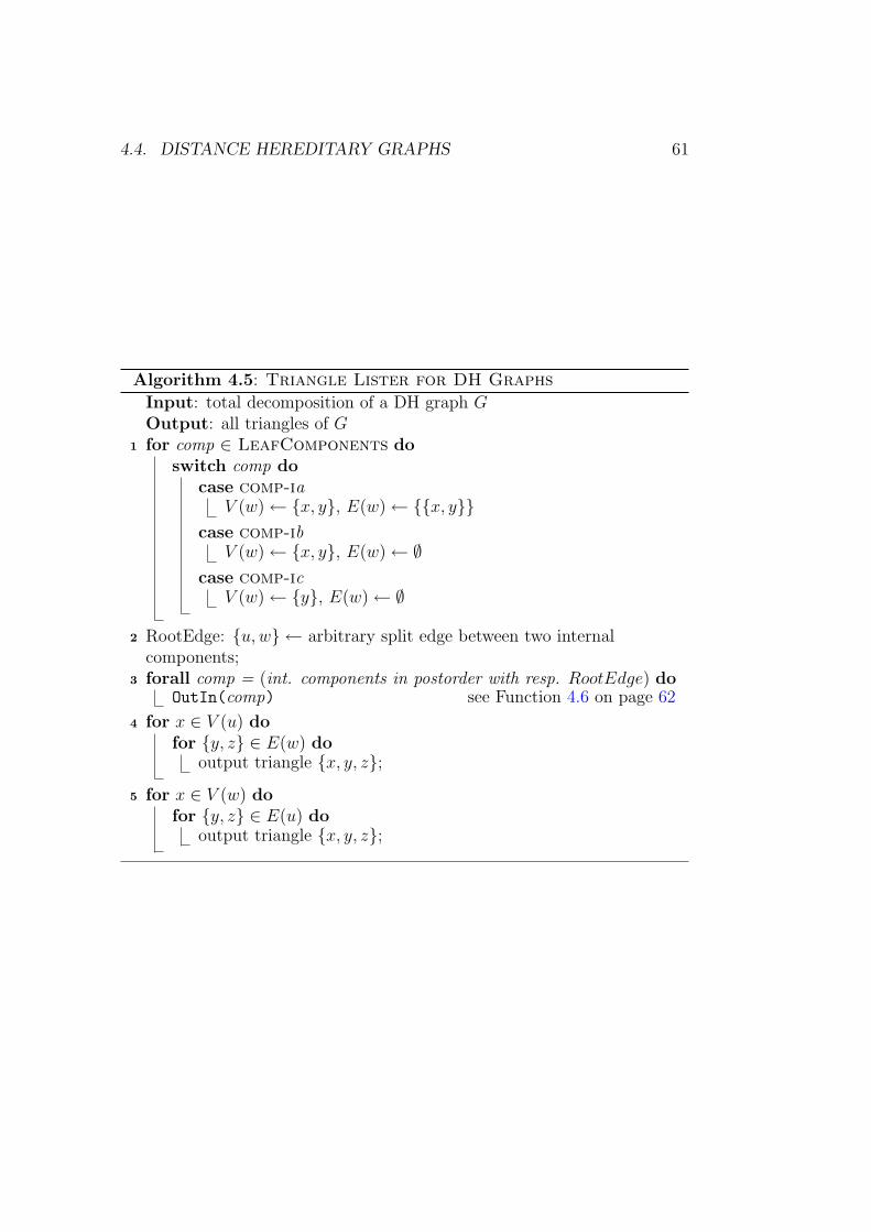
4.4. DISTANCE HEREDITARY GRAPHS 61
Algorithm 4.5: Triangle Lister for DH Graphs
Input: total decomposition of a DH graph GOutput: all triangles of Gfor comp ∈ LeafComponents do1
switch comp docase comp-ia
V (w)← x, y, E(w)← x, ycase comp-ib
V (w)← x, y, E(w)← ∅case comp-ic
V (w)← y, E(w)← ∅
RootEdge: u, w ← arbitrary split edge between two internal2
components;forall comp = (int. components in postorder with resp. RootEdge) do3
OutIn(comp) see Function 4.6 on page 62
for x ∈ V (u) do4
for y, z ∈ E(w) dooutput triangle x, y, z;
for x ∈ V (w) do5
for y, z ∈ E(u) dooutput triangle x, y, z;

62 CHAPTER 4. GRAPH CLASSES
Function 4.6: Triangle Lister for DH Graphs: OutIncase comp-iia Figure 4.6(a)
for y, z ∈ E(u′) dooutput triangle x, y, z;
V (w)← x, E(w)← ∅;case comp-iib Figure 4.6(b)
for y, z ∈ E(u′) dooutput triangle x, y, z;
E(w)← E(u′);for y ∈ V (u′) do
E(w)← E(w) ∪ x, y ;V (w)← V (u′) ∪ x;
case comp-iic case 1 Figure 4.6(c)1
E(w)← E(u′), V (w)← V (u′) ∪ x;case comp-iic case 2 Figure 4.6(d)2
for y, z ∈ E(u′) do3
output triangle x, y, z;E(w)← E(u′), V (w)← V (u′);4
case comp-iiia Figure 4.6(e)5
E(w)← E(u′) ∪ E(v′);for x ∈ V (u′) do
for y, z ∈ E(v′) dooutput triangle x, y, z;
for x ∈ V (v′) dofor y, z ∈ E(u′) do
output triangle x, y, z;
for x ∈ V (v′) dofor y ∈ V (u′) do
E(w)← E(w) ∪ x, y;
V (w)← V (u′) ∪ V (v′);
case comp-iiib case 1 Figure 4.6(f)for x ∈ V (u′) do
for y, z ∈ E(v′) dooutput triangle x, y, z;
for x ∈ V (v′) dofor y, z ∈ E(u′) do
output triangle x, y, z;
E(w)← E(v′), V (w)← V (v′);
case comp-iiib case 2 Figure 4.6(g)V (w)← V (u′) ∪ V (v′), E(w)← E(u′) ∪ E(v′)
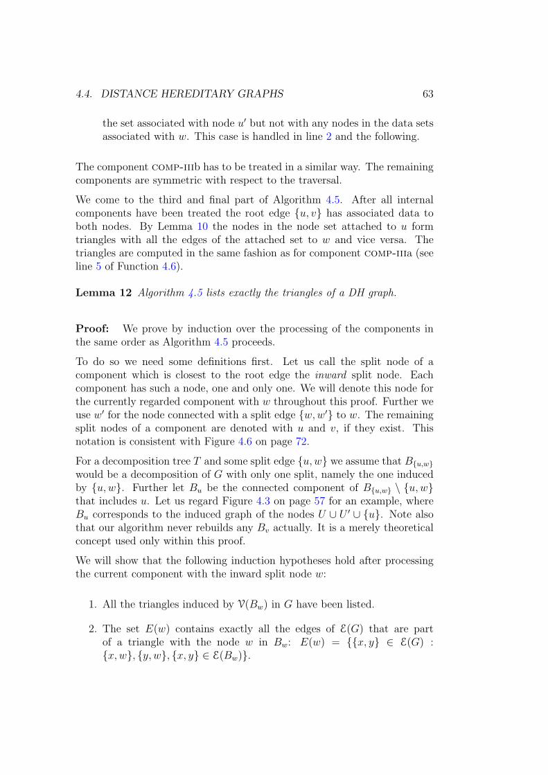
4.4. DISTANCE HEREDITARY GRAPHS 63
the set associated with node u′ but not with any nodes in the data setsassociated with w. This case is handled in line 2 and the following.
The component comp-iiib has to be treated in a similar way. The remainingcomponents are symmetric with respect to the traversal.
We come to the third and final part of Algorithm 4.5. After all internalcomponents have been treated the root edge u, v has associated data toboth nodes. By Lemma 10 the nodes in the node set attached to u formtriangles with all the edges of the attached set to w and vice versa. Thetriangles are computed in the same fashion as for component comp-iiia (seeline 5 of Function 4.6).
Lemma 12 Algorithm 4.5 lists exactly the triangles of a DH graph.
Proof: We prove by induction over the processing of the components inthe same order as Algorithm 4.5 proceeds.
To do so we need some definitions first. Let us call the split node of acomponent which is closest to the root edge the inward split node. Eachcomponent has such a node, one and only one. We will denote this node forthe currently regarded component with w throughout this proof. Further weuse w′ for the node connected with a split edge w,w′ to w. The remainingsplit nodes of a component are denoted with u and v, if they exist. Thisnotation is consistent with Figure 4.6 on page 72.
For a decomposition tree T and some split edge u, w we assume that Bu,wwould be a decomposition of G with only one split, namely the one inducedby u, w. Further let Bu be the connected component of Bu,w \ u, wthat includes u. Let us regard Figure 4.3 on page 57 for an example, whereBu corresponds to the induced graph of the nodes U ∪ U ′ ∪ u. Note alsothat our algorithm never rebuilds any Bv actually. It is a merely theoreticalconcept used only within this proof.
We will show that the following induction hypotheses hold after processingthe current component with the inward split node w:
1. All the triangles induced by V(Bw) in G have been listed.
2. The set E(w) contains exactly all the edges of E(G) that are partof a triangle with the node w in Bw: E(w) = x, y ∈ E(G) :x, w, y, w, x, y ∈ E(Bw).

64 CHAPTER 4. GRAPH CLASSES
3. The set V (w) contains exactly all the nodes of V(G) that are adjacentto w in Bw: V (w) = x ∈ V(G) : x, w ∈ E(Bw).
Note that only invariant 1 is relevant to finally show the Lemma, the re-maining ones are only helper statements. The inductive base cases consiston verifying the properties listed above for the components handled beforeline 2 is reached. These are all the leaf components and the correctness forthose is easy to see.
In the following we show that the statements hold when processing compo-nent “comp-iic case 2” as in Figure 4.6(d). This case is handled by line 2and following in Function 4.6. By Lemma 10 the node x is connected to allnodes in V (u′) and hence forms triangles with all the edges in E(u′). Allthese triangles (and no others) are listed in the Loop beginning at line 3.According to Lemma 10 the node x is not connected to any of the nodes ofV(Bw) ∩ V(G) in G. Hence, it must not be included in V (w), and conse-quently does not have an endpoint in E(w). The node u is incident to allnodes listed in V (u′), hence again by Lemma 10 we can simply assign theset V (u′) and E(u′) to the node w, which is done in line 4. This shows thatinvariant 2 and 3 hold from which the correctness of invariant 1 follows.
Showing the invariants for the remaining 6 cases of Function 4.6 is quitesimilar to what we have just seen. We omit the details here. We continuewith the final part, processing the root edge w, u. By the inductive hy-pothesis all triangles induced by V(Bw) and V(Bu) in G have been listed.By the invariants each edge in the set E(u) forms triangles with each nodein V (w) and the other way round. Also by the invariants and Lemma 10no further triangle exists that contains both nodes from V(Bw) and V(Bu).All these triangles and no further are listed in line 4 respectively line 5 ofAlgorithm 4.5.
Lemma 13 Algorithm 4.5 can be implemented to run in O(m + δ) time andO(m) space.
Proof: We consider linked lists as data structures to store the edges andnodes sets. They can be merged in constant time when the formation ofunions is required. The linear space requirement now follows from the factthat each edge respectively node is contained in at most one of the sets.
For the time complexity we note that finding and initializing all the leafcomponents can be done in linear time. Computing a postorder of the

4.4. DISTANCE HEREDITARY GRAPHS 65
internal components can also be done in linear time. We turn to the internalcomponents handled in Function 4.6. We first disregard all the for-loops, inthis case only set merging operations remain. Due to the linked lists such anoperation can be done in constant time and all merging operations togetherare in the size of the number of components. Now, we disregard all the loopscontaining triangle output. The remaining loops create edges and add themto the sets or they add nodes to the sets. As already mentioned with thespace complexity each edge and each node is listed only once. Hence, allthese operations are in O(m).
Finally we include the for-loops with triangle output in our consideration.With exception of component comp-iiib every iteration of the loops alsooutputs a triangle. For component comp-iiib some empty iterations of theouter loops iterating over the nodes could occur if the corresponding edgesets are empty. However, this can be avoided if the edge sets are previouslytested whether they are empty. In that case only one operation is required inthe other case every operation also outputs a triangle. Therefore, the numberof all operations is in O(m + δ) time.
The Counting Algorithm
We will show Theorem 8 by the end of this section. Note, that the O(n)bound requires the graph to be encoded in total decomposition. Otherwisea decomposition preprocessing step in O(m) time and space is required.
Theorem 8 All triangles of a distance hereditary graph can be counted inO(n) time and space.
The main code is listed in Algorithm 4.7. As promised we reuse some conceptsthat we developed with the listing algorithm of Section 26. Due to this wecan keep this introduction brief and focus on the main differences betweenthe two algorithms. Instead of storing sets of nodes and edges we only storethe size of those. We call the associated variables n(v) for the size of thenode set, respectively m(v) for the size of the edge set. In the listing case weproceeded from outside to inside and listed the triangles along this traversal.Here we traverse from outside to inside, too. See line 2 of Algorithm 4.7.However, we then also traverse from inside to outside (line 2) where we takealong the data to the nodes. The actual output is then computed in a finalstep in line 4.

66 CHAPTER 4. GRAPH CLASSES
Now, we proceed with actually showing Theorem 8 in several parts. Theseparts are self contained but generally rather compact compared to those ofthe previous chapter.
Algorithm 4.7: Triangle Counter for DH Graphs
Input: total decomposition of a DH GraphOutput: number of triangles δ(v) for each node vRootEdge ← arbitrary split edge between two internal components;1
forall comp = (components in postorder with resp. RootEdge) do2
OutIn(comp) see Function 4.8 on page 69
forall comp = (components in preorder with resp. RootEdge) do3
InOut(comp) see Function 4.9 on page 70
forall comp ∈ components do4
Calc-δ (comp) see Function 4.10 on page 71
Lemma 14 Algorithm 4.7 can be implemented to run in O(n) time andspace.
Proof: We consider the time complexity first. Note that the postorder andthe preorder can be computed in time linear in the size of a tree. Processingeach component in the Functions 4.8, 4.9 and 4.10 can be done in constanttime. By Lemma 11 there are only O(n) components. Each component isprocessed at most once in each of the three loops starting at line 2, 3, and 4.Hence, the total running time is in O(n).
Now, let us consider the space complexity. We associate at most 2 integerswith each node. There are no more than 3 nodes in any component and byLemma 11 the number of components is in O(n).
Lemma 15 Let T be the total decomposition tree of G. After the executionof line 3 for each split node u the following holds:
• n(u) is equal to the number of regular nodes that are connected to u inT by an alternating path,
• m(u) is equal to the number of pairs that consist of regular nodes, whichare themselves connected by an alternating path, and also connected byan alternating path to u.

4.4. DISTANCE HEREDITARY GRAPHS 67
Proof: Let T be the total split decomposition tree of a DH graph G witha designated root edge u, w. Let us call the split node of a componentwhich is closest to the root edge the inward split node. Each component hasexactly one such node. In Figure 4.4(b) on page 58 the inward split nodesare those split nodes which are not pointed by an arrowhead. The remainingsplit nodes are called the outward split nodes. Note that the in- and outwardsplit nodes define a partition on the set of the split nodes. Further, for somesplit edge w,w′ let Tw be the connected subtree of T \w,w′ that includesw.
We first prove the statement for all inward split nodes. We do so by inductionover processing the components in the same (post)order as used in line 2 ofAlgorithm 4.7. The induction basis is covered by the processing of the leafcomponents∗ handled in the Lines 1, 2, and 3 in Function 4.8. It is straightforward to see that the statement holds after processing the leaf componentsby Function 4.8.
We proceed to the inductive step where we consider exemplarily the process-ing of component “comp-iic case 1” starting at line 4 in Function 4.8. Byinduction hypothesis and by using postorder processing the associated n(u′)and m(u′) data for node u′ has been computed such that the statements hold.The node w is connected by an alternating path ending with a split edge tou′. All the alternating paths from u′ to regular nodes in Tu′ start with nonsplit edges. Hence, w is connected by an alternating path to all those nodes,too. Further w is connected by an alternating path to x. The number ofregular nodes connected to w by an alternating path in Tw is consequentlygiven by n(u′)+1. In Tw the node x is not connected by an alternating pathto any regular node that is connected to u′ by such a path. Hence, m(w) isequal to m(u′) in Tw.
The correctness for the remaining components can be shown analogously.This is rather straight forward and we do not go into further details. Nowthe statements have to be shown for all of the outward nodes. This can bedone by induction over the components in preorder. It is again very similarto the inward case and we omit the details here.
For a split node u let u, w be its incident split edge. Assume that Bu,wwould be the split decomposition of G with only one split, namely the oneinduced by split edge u, w. Further let Bu be the connected component of
∗following strictly Algorithm 4.7 the set of bases cases would be empty and the leafnodes are handled in the inductive step, either way yields the same result
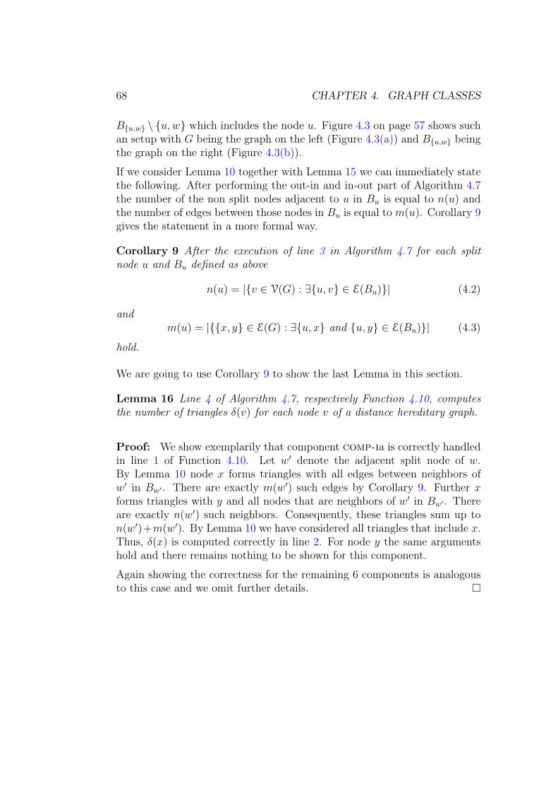
68 CHAPTER 4. GRAPH CLASSES
Bu,w \ u, w which includes the node u. Figure 4.3 on page 57 shows suchan setup with G being the graph on the left (Figure 4.3(a)) and Bu,w beingthe graph on the right (Figure 4.3(b)).
If we consider Lemma 10 together with Lemma 15 we can immediately statethe following. After performing the out-in and in-out part of Algorithm 4.7the number of the non split nodes adjacent to u in Bu is equal to n(u) andthe number of edges between those nodes in Bu is equal to m(u). Corollary 9gives the statement in a more formal way.
Corollary 9 After the execution of line 3 in Algorithm 4.7 for each splitnode u and Bu defined as above
n(u) = |v ∈ V(G) : ∃u, v ∈ E(Bu)| (4.2)
andm(u) = |x, y ∈ E(G) : ∃u, x and u, y ∈ E(Bu)| (4.3)
hold.
We are going to use Corollary 9 to show the last Lemma in this section.
Lemma 16 Line 4 of Algorithm 4.7, respectively Function 4.10, computesthe number of triangles δ(v) for each node v of a distance hereditary graph.
Proof: We show exemplarily that component comp-ia is correctly handledin line 1 of Function 4.10. Let w′ denote the adjacent split node of w.By Lemma 10 node x forms triangles with all edges between neighbors ofw′ in Bw′ . There are exactly m(w′) such edges by Corollary 9. Further xforms triangles with y and all nodes that are neighbors of w′ in Bw′ . Thereare exactly n(w′) such neighbors. Consequently, these triangles sum up ton(w′)+m(w′). By Lemma 10 we have considered all triangles that include x.Thus, δ(x) is computed correctly in line 2. For node y the same argumentshold and there remains nothing to be shown for this component.
Again showing the correctness for the remaining 6 components is analogousto this case and we omit further details.

4.4. DISTANCE HEREDITARY GRAPHS 69
Function 4.8: Triangle Counter for DH Graphs: OutInswitch comp do
case comp-ia Figure 4.5(a)1
n(w)← 2, m(w)← 1;
case comp-ib Figure 4.5(b)2
n(w)← 2, m(w)← 0;
case comp-ic Figure 4.5(c)3
n(w)← 1, m(w)← 0;
case comp-iia Figure 4.6(a)n(w) = 1;m(w) = 0;
case comp-iib Figure 4.6(b)n(w) = n(u′) + 1;m(w) = m(u′) + n(u′);
case comp-iic case 1 Figure 4.6(c)4
n(w) = n(u′) + 1;m(w) = m(u′);
case comp-iic case 2 Figure 4.6(d)n(w) = n(u′);m(w) = m(u′);
case comp-iiia Figure 4.6(e)n(w) = n(u′) + n(v′);m(w) = m(u′) + m(v′) + n(u′) · n(v′);
case comp-iiib case 1 Figure 4.6(f)n(w) = n(v′);m(w) = m(v′);
case comp-iiib case 2 Figure 4.6(g)n(w) = n(u′) + n(v′);m(w) = m(u′) + m(v′);

70 CHAPTER 4. GRAPH CLASSES
Function 4.9: Triangle Counter for DH Graphs: InOutswitch comp do
case comp-iia Figure 4.6(a)n(u) = 1;m(u) = 0;
case comp-iib Figure 4.6(b)n(u) = n(w′) + 1;m(u) = m(w′) + n(w′);
case comp-iic case 1 Figure 4.6(c)n(u) = n(w′);m(u) = m(w′);
case comp-iic case 2 Figure 4.6(d)n(u) = n(w′) + 1;m(u) = m(w′);
case comp-iiia Figure 4.6(e)n(u) = n(v′) + n(w′);m(u) = m(v′) + m(w′) + n(v′) · n(w′);n(v) = n(u′) + n(w′);m(v) = m(u′) + m(w′) + n(u′) · n(w′);
case comp-iiib case 1 Figure 4.6(f)n(u) = n(v′);m(u) = m(v′);n(v) = n(u′) + n(w′);m(v) = m(u′) + m(w′);
case comp-iiib case 2 Figure 4.6(g)n(u) = n(w′);m(u) = m(w′);n(v) = n(w′);m(v) = m(w′);

4.4. DISTANCE HEREDITARY GRAPHS 71
Function 4.10: Triangle Counter for DH Graphs: Calc-δswitch comp do
case comp-ia Figure 4.5(a)1
δ(x) ← m(w′) + n(w′);2
δ(y) ← m(w′) + n(w′);
case comp-ib Figure 4.5(b)δ(x) ← m(w′);δ(y) ← m(w′);
case comp-ic Figure 4.5(c)δ(y) ← m(w′);δ(x) ← 0;
case comp-iia Figure 4.5(d)δ(x) ← m(u′) + m(w′);
case comp-iib Figure 4.5(e)δ(y) ← m(u′) + m(w′) + n(u′)n(w′);
case comp-iic Figure 4.5(f)δ(x) ← m(w′);
(a) comp-ia (b) comp-ib (c) comp-ic
(d) comp-iia (e) comp-iib (f) comp-iic
(g) comp-iiia (h) comp-iiib (i) comp-0
Figure 4.5: Components of a total decomposition.

72 CHAPTER 4. GRAPH CLASSES
(a) comp-iia (b) comp-iib
(c) comp-iic case 1 (d) comp-iic case 2
(e) comp-iiia (f) comp-iiib case 1
(g) comp-iiib case 2
Figure 4.6: Directions for the processing the internal components.

Chapter 5
Applications of Triangle Listingin Network Analysis
Chapter Introduction
In this chapter we will discuss applications in network analysis for which thecomputation of the related indices is based either on triangle counting ortriangle listing.
The clustering coefficient introduced by Watts and Strogatz [1998] is prob-ably the most established network index that is computationally based ontriangle counting. Given three actors u, v and w with mutual relations be-tween v and u as well as between v and w, the clustering coefficient of thenode v represents the likelihood that u and w are also related. In other wordsit is the average value of edges between pairs of neighbors. When we con-sider the graph induced by the neighbors of v it is the density of this graph.Therefore we prefer to use the term neighborhood density. The average valueover all nodes is the clustering coefficient coefficient of the graph. It is one ofthe most popular network indices. At the time of this writing a search withscholar.google.com for the term yields about 112000 results.
Harary and Paper [1957] introduced the index of transitivity in the contextof linguistics. It has become popular again for some time. However, mainlybecause it has been used intendedly or unintendedly in the place of theclustering coefficient, in [Newman et al., 2002] for example.
Various versions of the edge weighted neighborhood density have becomepopular recently [Grindrod, 2002; Lopez-Fernandez et al., 2004; Barrat et al.,
73
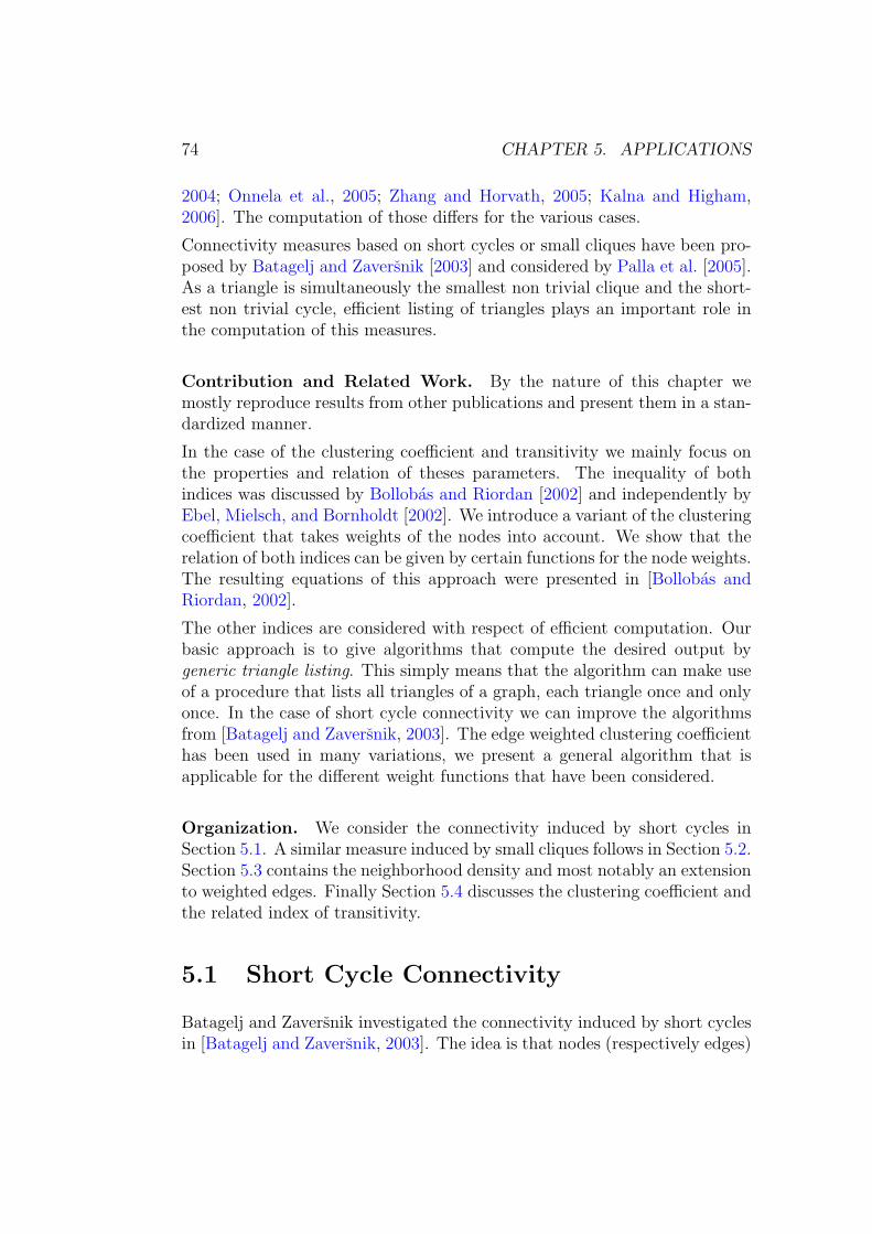
74 CHAPTER 5. APPLICATIONS
2004; Onnela et al., 2005; Zhang and Horvath, 2005; Kalna and Higham,2006]. The computation of those differs for the various cases.
Connectivity measures based on short cycles or small cliques have been pro-posed by Batagelj and Zaversnik [2003] and considered by Palla et al. [2005].As a triangle is simultaneously the smallest non trivial clique and the short-est non trivial cycle, efficient listing of triangles plays an important role inthe computation of this measures.
Contribution and Related Work. By the nature of this chapter wemostly reproduce results from other publications and present them in a stan-dardized manner.
In the case of the clustering coefficient and transitivity we mainly focus onthe properties and relation of theses parameters. The inequality of bothindices was discussed by Bollobas and Riordan [2002] and independently byEbel, Mielsch, and Bornholdt [2002]. We introduce a variant of the clusteringcoefficient that takes weights of the nodes into account. We show that therelation of both indices can be given by certain functions for the node weights.The resulting equations of this approach were presented in [Bollobas andRiordan, 2002].
The other indices are considered with respect of efficient computation. Ourbasic approach is to give algorithms that compute the desired output bygeneric triangle listing. This simply means that the algorithm can make useof a procedure that lists all triangles of a graph, each triangle once and onlyonce. In the case of short cycle connectivity we can improve the algorithmsfrom [Batagelj and Zaversnik, 2003]. The edge weighted clustering coefficienthas been used in many variations, we present a general algorithm that isapplicable for the different weight functions that have been considered.
Organization. We consider the connectivity induced by short cycles inSection 5.1. A similar measure induced by small cliques follows in Section 5.2.Section 5.3 contains the neighborhood density and most notably an extensionto weighted edges. Finally Section 5.4 discusses the clustering coefficient andthe related index of transitivity.
5.1 Short Cycle Connectivity
Batagelj and Zaversnik investigated the connectivity induced by short cyclesin [Batagelj and Zaversnik, 2003]. The idea is that nodes (respectively edges)

5.1. SHORT CYCLE CONNECTIVITY 75
have to be connected by a sequence of cycles which are overlapping in someterms. The authors introduce the concepts for cycles of length 3 and givealso algorithms for the computation in this case. Some properties are provenfor general k-cycles but without algorithmic context.
Triangular Node Connectivity
Two nodes u and w are triangularly node connected if there exists a sequenceof triangles (∆1, . . . , ∆s) with u ∈ V(∆1), V(∆i)∩V(∆i+1) 6= ∅ for 1 ≤ i < s,and w ∈ V(∆s). The triangular node connectivity defines an equivalencerelation V3 on the set of nodes.
Batagelj and Zaversnik give an algorithm to compute the equivalence classesof V3. It is based on algorithm edge-iterator (see page 29 in Section 3.1.3)and it inherits the running time in O(dmax ·m) of that algorithm.
Lemma 17 ([Batagelj and Zaversnik, 2003]) The equivalence classes of therelation V3 can be computed in O(dmax ·m) time.
By the above definition two nodes u and w are related by V3 if and only ifthere exists a path P that connects u and v and every edge in P is containedin a triangle. Algorithm 5.1 uses this observation to compute the equivalenceclasses of V3. It is based on generic triangle listing, which also bounds itsrunning time.
Corollary 10 The equivalence classes of V3 can be computed in O(m3/2
)time.
Algorithm 5.1: Equivalence classes of V3
Input: graph G = (V, E);Output: connected components C1,...,i of G, each containing
equivalent nodes;forall ∆uvw ∈ G do
markEdge(u, v); markEdge(v, w); markEdge(w, u);forall e ∈ E do
if e is not marked thenG← G[E \ e];
C1,...,i ← connected components of G;return C1,...,i;

76 CHAPTER 5. APPLICATIONS
Figure 5.1: An example of triangular connectivity. There is only one equiv-alence class of the nodes induced by V3 but three equivalence classes of theedges induced by E3.
Triangular Edge Connectivity
The triangular edge connectivity induces equivalence classes of edges simi-lar to the node connectivity. Two edges u, w and x, y are triangularlyconnected if there exists a sequence of triangles (∆1, . . . , ∆s) with u, w ∈E(∆1), E(∆i) ∩ E(∆i+1) 6= ∅ for 1 ≤ i < s, and x, y ∈ E(∆s). The trian-gular edge connectivity defines an equivalence relation E3 on the set of theedges. See Figure 5.1 for an example of induced equivalence classes given bythe two relations.
Lemma 18 ([Batagelj and Zaversnik, 2003]) The equivalence classes of therelation E3 can be computed in O(dmax ·m) time.
Algorithm 5.2: Equivalence classes of E3
Input: graph G = (V, E);Output: sets S1,...,i, each holding equivalent edgesforall u, w ∈ E do
makeSet (Su,w);
forall ∆uvw ∈ G dounion(Su,v, Su,w);union(Su,v, Sv,w);
return S1,...,i;
The algorithm in [Batagelj and Zaversnik, 2003] depends on processing thetriangles in a specific order. Unfortunately, this cannot be guaranteed bygeneric triangle listing. Our Algorithm 5.2 based on generic triangle listinguses basic set creation, finding, and merging operations. This multipliesthe complexity of such operations to the running time complexity of trianglelisting. However, they can be performed asymptotically in α(m), see [Cormenet al., 2001] for example. The function α is the inverse of the Ackermann

5.2. SMALL CLIQUE CONNECTIVITY 77
function. Note that α grows very slowly. It is a constant not bigger thanfour for any practical considerations.
Corollary 11 The equivalence classes of the relation E3 can be computed inO(α(m) ·m3/2
)time.
We note that this result is more of theoretic value. The required data struc-tures are generally not available in standard programming libraries, and theBOOST-graph-library is the only exception we are aware of. However, a run-ning time in O
(log m ·m3/2
)can be achieved by the more commonly used
dynamic tree data structures.
5.2 Small Clique Connectivity
In the two publications [Derenyi et al., 2005; Palla et al., 2005] connectivityby overlapping of small cliques is considered. The basic idea is similar to theshort cycle connectivity in [Batagelj and Zaversnik, 2003] which we discussedin in the previeous section. Indeed, Batagelj and Zaversnik [2003] generalizethe concept briefly and the connectivity considered by Palla et al. [2005]can be seen as a special case of this. Note that the contributions differ inprinciple. Batagelj and Zaversnik consider methods whereas [Derenyi et al.,2005; Palla et al., 2005] primarily contain analytical results on networks.
In the small clique connectivity the authors define two nodes u and w equiv-alent if they are connected by a path of k cliques, where the overlap of thecliques is k − 1 nodes at least. Let us give a more formal definition. LetGk = (V k, Ek) consist of the node set V k containing all k-cliques of G asnodes. Two nodes vk
i and vkj in V k are adjacent in Gk if and only if there
exist nodes v1, . . . , vk−1 ∈ V , all of them contained in V(vk
i
)and in V
(vk
j
),
i.e.∣∣V(vk
i
)∩ V(vk
j
)∣∣ ≥ k−1. The connected components in Gk are the basisof the analytical consideration in [Palla et al., 2005]. Clearly this approachdoes not define an equivalence relation on V as the cycle connectivity does.A node v ∈ V might be contained in several nodes vk
i ∈ V k which can belongto different connected components. The number of the different componentsfor a node v ∈ V is actually one of the considered properties.
Depending on what kind of analysis is done, one can either construct Gk
explicitly or construct sets, where each of those contains the nodes of V thatcan be found in one connected component of Gk. However, these methodsare not subject of this work and in the following we will focus on listingall of the k-cliques and in particular on the 4-cliques. The authors set k =

78 CHAPTER 5. APPLICATIONS
4 for the larger networks they consider. Let us note that they performedtheir computation in a different way, which is only vaguely described inthe publication (quote [Palla et al., 2005]: “we use an algorithm which isexponential”).
Algorithm 5.3 is essentially a compact presentation of Algorithm 3.7 onpage 35. We reproduce it here to conveniently compare the difference toAlgorithm 5.4 which is an extension to K4 listing. Now, let us consider the
Algorithm 5.3: 3-Clique Lister
Input: undirected graph G = (V, E);nodes (1, . . . , n) in order of non increasing degrees;adjacencies (γ1(v), . . . , γ|Γ|(v)) for each v = (1, . . . , n) ordered in sameorder as the nodes;Output: all 3-cliques as node-sets;for ` = (1, . . . , n) do1
for k ∈ Γ(`), k < ` do2
for j ∈ Γ(k) ∩ Γ(`), j < k do3
output j, k, l;
Algorithm 5.4: 4-Clique Lister
Input: undirected graph G = (V, E);nodes (1, . . . , n) in order of non increasing degrees;adjacencies (γ1(v), . . . , γ|Γ|(v)) for each v = (1, . . . , n) ordered in sameorder as the nodes;Output: all 4-cliques as node-sets;for ` = (1, . . . , n) do1
for k ∈ Γ(`), k < ` do2
for j ∈ Γ(k) ∩ Γ(`), j < k do3
for i ∈ Γ(j) ∩ Γ(k) ∩ Γ(`), i < j do4
output i, j, k, l;
time complexity. Recall from Section 3.1.3 that line 1 together with line 2require m-steps. Line 2 can be performed in 2
√m steps, because of k < l
(see also the proof of Lemma 5 on page 33). Now, by similar arguments line 4multiplies 3
√m more steps to the total running time and we can conclude
the following corollary.

5.3. NEIGHBORHOOD DENSITY 79
Corollary 12 Algorithm 5.4 lists all 4-cliques of an undirected graph. It canbe implemented to run in O(m2) time.
As in the case of the triangles we cannot expect any better result since ann-clique contains Θ(n4) 4-cliques in terms of n, or Θ(m2) 4-cliques in termsof m respectively. We can easily extend the algorithms to list all k-cliques.The total number of steps of such an algorithm is given asymptotically by1/k
∏ki=1 (i
√m) for k ≥ 2 and we can bound the running time of the derived
k-clique listing algorithm by O(k! mk/2
)for k ≥ 2.
We tested an implementation of Algorithm 5.4 on the “Movie Actor Network2004” (see page 38 in Section 3.2). The execution time to list all 4-cliquesturns out to be about 70 minutes. Let us recall that the execution timefor listing all triangles by an implementation of Algorithm 5.3 was about 1minute. We did not try to list all 5-cliques. We can estimate very roughlythat the computation of those for the same graph should take somewherebetween 4 and 2000 days. The first number is a linear extrapolation fromtriangle and 4-clique listing. The upper bound is due to the running timeanalysis from above.
5.3 Neighborhood Density
Neighborhood Density or Clustering Coefficient of aNode
Let us recall from Section 4 that the neighborhood density (also called theclustering coefficient) of a node v with degree at least 2 is given by the quo-tient of triangles and wedges %(v) = δ(v)/τ(v). A wedge of v is a simple pathof length 2 for which v is the center node. Therefore, the number of wedgescan be easily computed as
(d(v)2
). This leaves the determination of the num-
ber of triangles as the main problem in computing the neighborhood density.We briefly discussed triangle counting algorithms and their complexity inSection 3.1 on page 23. Up to date the most efficient counting algorithmsachieve running time in O(nγ) respectively in O
(m2γ/(γ+1)
), where γ is the
matrix multiplication coefficient.
An algorithm based on generic triangle listing is given in Algorithm 5.5.
Corollary 13 Algorithm 5.5 computes the neighborhood density (i.e. clus-tering coefficient of a node) for all nodes of a graph. It can be implementedto run in O
(m3/2
)time.

80 CHAPTER 5. APPLICATIONS
Algorithm 5.5: Neighborhood Densities
Input: graph G with ∀v : d(v) ≥ 2Output: neighborhood density %(v) for all nodes of Vfor v ∈ V do
δ(v)← 0;
forall triangles ∆u,v,w in G doδ(u)← δ(u) + 1;δ(v)← δ(v) + 1;δ(w)← δ(w) + 1;
for v ∈ V do
%(v)← δ(v)/(
d(v)2
);
The neighborhood densities are rarely considered for themselves. However,the clustering coefficient which is the average value over all neighborhooddensities of a graph is very popular. We will discuss it in Section 5.4. Avariation of the node density that takes edge weights into consideration willbe discussed in the following.
5.3.1 Edge Weighted Neighborhood Density
We extend the neighborhood density in a natural way to take weights on edgesinto account. A very general definition is given that includes the commonlyused varieties by which the weighted neighborhood desity can be defined.We will give an efficient algorithm to compute these. We will discuss somerestricted cases and develop a faster algorithm for those.
Generalized Presentation
Let µ denote a function that maps each edge of the graph to a strictly positivereal, i.e. µ : E → R+. We write shorthand µuv for µ(u, v) in the following.Recall that the neighborhood density %(v) of a node v is defined as thequotient of triangles divided by wedges %(v) = δ(v)/τ(v). We rewrite thisexpression first in Equation 5.1, in which we replace δ(v) with the sum overall triangles that contain node v. Likewise, we replace τ(v) with the sum ofall wedges for which v is the center node.

5.3. NEIGHBORHOOD DENSITY 81
%(v) =
∑∆uvw∈∆v⊂G
1∑Υuvw∈Υv⊂G
1(5.1)
We place functions of the participating edge weights into the sums insteadof simply adding up the number 1. This extended formulation is given inEquation 5.2. Note that we rather use a shorthand notation here, e.g. thearguments of f and g are the edge weights of the triangles and not thesubgraphs themselves.
%µ(v) = ϕ(v)
∑∆uvw∈∆v⊂G
f(µvu, µuw, µvw)∑Υuvw∈Υv⊂G
g(µvu, µvw)(5.2)
In this general setup we require the functions ϕ : V → R, g : R × R → R,and f : R3 → R to be computable in O(1) time. Further, µ and g must bechosen such that the denominator does not take the value zero. We alreadymentioned, that the unweighted version of the neighborhood density is notdefined for nodes with degree less than two. This caries over to the weightedcase. Table 5.1 lists a few functions for f and g that are self-evident. Somecombinations of those are shown in Table 5.2. Note that we omitted anyconstant factors in Table 5.2, for this reason the values may actually differin the referenced publications.
Matrix Formulation and Computation
Before we list algorithms for computing the weighted coefficient we will reviewan alternative formulation based on matrices that has been used for examplein [Barrat et al., 2004], [Onnela et al., 2005], and [Zhang and Horvath, 2005].
Let the nodes of G be indexed (v0, . . . , vn). Let A be the adjacency matrix:A ∈ 0, 1n×n with aij = 1 if vi, vj ∈ E, and aij = 0 otherwise. Quitesimilar, let M be a real quadratic n × n matrix M ∈ Rn×n with entriesmij = µ(vi, vj) if vi, vj ∈ E and mij = 0 else. With this notationEquation 5.2 can be equivalently expressed by Equation 5.3.
%µ(vk) = ϕ(vk)
∑1≤i≤n
∑i<j≤n
aikaijajk · f(mik, mij, mjk)∑1≤i≤n
∑i<j≤n
aikajk · g(mik, mjk)(5.3)
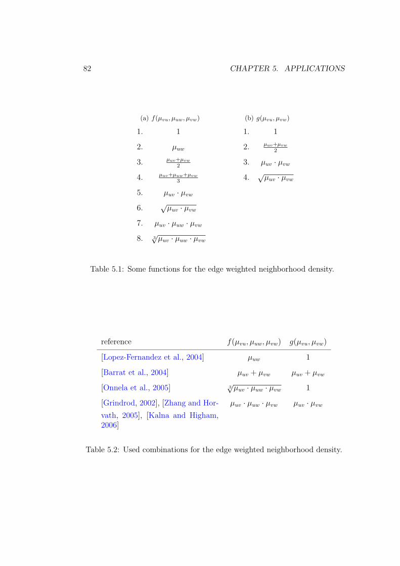
82 CHAPTER 5. APPLICATIONS
(a) f(µvu, µuw, µvw)
1. 1
2. µuw
3. µuv+µvw
2
4. µuv+µuw+µvw
3
5. µuv · µvw
6.√
µuv · µvw
7. µuv · µuw · µvw
8. 3√
µuv · µuw · µvw
(b) g(µvu, µvw)
1. 1
2. µuv+µvw
2
3. µuv · µvw
4.√
µuv · µvw
Table 5.1: Some functions for the edge weighted neighborhood density.
reference f(µvu, µuw, µvw) g(µvu, µvw)
[Lopez-Fernandez et al., 2004] µuw 1
[Barrat et al., 2004] µuv + µvw µuv + µvw
[Onnela et al., 2005] 3√
µuv · µuw · µvw 1
[Grindrod, 2002], [Zhang and Hor-
vath, 2005], [Kalna and Higham,2006]
µuv · µuw · µvw µuv · µvw
Table 5.2: Used combinations for the edge weighted neighborhood density.

5.3. NEIGHBORHOOD DENSITY 83
In the case of multiplicative functions like f = µuv ·µuw ·µvw and g = µuv ·µvw
this reduces to a simplified version as in Equation 5.4.
%∗µ(vk) = ϕ(vk)
∑1≤i≤n
∑i<j≤n
muv ·muw ·mvw∑1≤i≤n
∑i<j≤n
muv ·mvw
(5.4)
Kalna and Higham [2006] give their version in the form of Equation 5.4. Theyalso give an equivalent of Equation 5.4 in algebraic formulation using matrixpower operations and basic vector operations. They conclude that %∗µ(v) forall nodes can be computed in O(n3) time. The theoretic bound based on fastmatrix multiplication is in O(n2.37) [Coppersmith and Winograd, 1990]. Thealgebraic representation used by Kalna and Higham does not impose anydisadvantages in their case since the input is a dense matrix with mij > 0for i 6= j.
Grindrod [2002] uses the weighted neighborhood density in conjunction witha network model, no real networks are considered. Other publications [Lopez-Fernandez et al., 2004; Barrat et al., 2004; Onnela et al., 2005; Zhang andHorvath, 2005] do not go into details of computation. We note that thealgorithm directly gained from Equation 5.3 has a running time in Θ(n3)and due to the matrix representation a space consumption in Θ(n2). For theusual case of sparse networks the running time is not optimal and the spacerequirement makes such an approach intractable for larger networks.
Algorithms
We will give an algorithm to compute the weighted neighborhood density bygeneric triangle listing that is based on Equation 5.2. We will further givean improved version for restricted functions g.
A realization directly derived from Equation 5.2 is listed in Algorithm 5.6. Itcomputes the edge weighted neighborhood density for all nodes v of the inputgraph. We handle the general case of arbitrary functions f(µvu, µuw, µvw),g(µvu, µvw), and ϕ(v). We require that these functions are computable inO(1) time. We further note that depending on the function G and on thegraph structure, the result of Algorithm 5.6 might not be defined in the caseof a division by zero in Equation 5.2.
The correctness of Algorithm 5.6 is obvious due to the direct translation fromEquation 5.2. The loops of line 1 and 4 can be implemented to run in lineartime with reasonable data structures. The loops of line 2 and 3 are critical

84 CHAPTER 5. APPLICATIONS
Algorithm 5.6: Edge Weighted Neighborhood Densities
Input: graph G with ∀v : d(v) ≥ 2, edge weights µ : E → R+
Output: weighted neighborhood density %µ(v) for all nodes of Vfor v ∈ V do1
δ(v)← 0, τ(v)← 0;
forall triangles ∆u,v,w in G do2
δ(u)← δ(u) + f(µuv, µvw, µuw);δ(v)← δ(v) + f(µvu, µuw, µvw);δ(w)← δ(w) + f(µwu, µvu, µwv);
forall wedges Υu,v,w in G do3
τ(v)← τ(v) + g(µvu, µvw);
for v ∈ V do4
%µ(v)← ϕ(v) · δ(v)/τ(v);
for the running time. Recall from Chapter 3 that listing all triangles of agraph can be done asymptotically in the number of wedges. The wedges areconveniently listed by a loop over all pairs of neighbors of a node and weconclude with the following Lemma.
Lemma 19 Algorithm 5.6 can be implemented to run in O(m) space andO(τ)=O(
∑V d2(v)) time.
Let us remark that listing the wedges and for many cases computing g are“cheap” operations, i.e. they involve only small constants. However, listingthe triangles may be not so “cheap” and despite the above observation theline 2 can practically determine the execution time.
We now consider the case g(µvu, µvw) = c · (µuv + µvw), with c being aconstant. We can then reformulate the denominator of Equation 5.2 sincean edge incident with v is part of d(v)− 1 wedges:∑Υuvw∈Υv⊂G
g(µvu, µvw) =∑
Υuvw∈Υv⊂G
c · (µuv +µvw) = c∑
u∈Γ(v)
(d(v)− 1)µvu
An adapted version is listed in Algorithm 5.7, in which we replaced line 3of Algorithm 5.6. The computation of g for all nodes can now be performedin O(m) steps. Consequently the part requiring the most steps is now thelisting of the triangles and computing function f . This implies an effort inO(m3/2
), see Section 3.1 for details.

5.4. CLUSTERING COEFFICIENT AND TRANSITIVITY 85
Algorithm 5.7: Edge Weighted Neighborhood Densities withAdditive g
. . . (as in Algorithm 5.6) . . .
forall v ∈ V do3
forall u ∈ Γ(v) doτ(v)← τ(v) + (d(v)− 1)µvu;
. . . (as in Algorithm 5.6) . . .
Corollary 14 The edge weighted neighborhood density can be computed inO(m3/2
)time if g is restricted to g(µvu, µvw) = c · (µuv + µvw) or g = 1.
Usage of the Weighted Neighborhood Density
As in the case of the standard neighborhood density it is very popular tocompute the average over all nodes and argue for or against the small worldproperty of the considered network. But there are also cases, in which thedistribution of the weighted neighborhood densities are considered like in thefollowing example.
Kalna and Higham [2006] analyze gene expression correlation data from nor-mal and tumor tissues. They consider the distribution of weighted degreesand edge weighted neighborhood density. The latter is given in the form of
%µ(v) =
∑∆uvw∈∆v⊂G
µvu · µuw · µvw∑Υuvw∈Υv⊂G
µvu · µvw
.
They found that the cancer tissue has more pronounced features such assharper pikes in both the degree and neighborhood density distribution. Theauthors point out that in the weighted neighborhood density distributionthese differences are more clearly visible than in the degree distribution.
5.4 Clustering Coefficient and Transitivity
We have already introduced the clustering coefficient and the transitivity inthe Preliminaries, see Section 4. We first recall some definitions briefly. Thenwe further investigate the properties of the indexes and the relation of theboth.

86 CHAPTER 5. APPLICATIONS
The Clustering Coefficient
The clustering coefficient was introduced by Watts and Strogatz [1998] in thecontext of social network analysis. Given three actors u, v and w with mutualrelations between v and u as well as between v and w, it represents the like-liness that u and w are also related. We introduced this concept formally asthe neighborhood density %(v) = δ(v)/τ(v) (Equation 2.10 on page 16). Theclustering coefficient of a graph is the average over the neighborhood densi-ties of its nodes. To compute the clustering coefficient of existing networkswith nodes of degree one we define
c (G) =1
|V ′|∑v∈V ′
%(v), (5.5)
where V ′ is the set of nodes v with d(v) ≥ 2. Alternatively to Equation 5.5the term %(v) is in some cases defined to be either zero or one for nodes vwith degree at most one and included in the sum. The computation of theindex is straight forward. It essentially relies on computing the neighborhooddensities which we discussed in Section 5.3.
Transitivity
We defined the transitivity of a graph G as used in [Newman et al., 2002] as
t(G) =3 δ(G)
τ(G),
see Equation 2.12 on page 17. It is essentially the index of transitivity[Harary and Paper, 1957] or the transitivity ratio [Harary and Kommel, 1979]restricted to undirected graphs. Like the clustering coefficient it involveswedges and triangles and it is also between zero and one by Equation 2.9.The computation of this index is straight forward and its efficiency is boundedby the efficiency of counting all triangles in a graph. Note that there is noknown algorithm that is more efficient in counting the triangles for the wholegraph compared to counting the number of triangles for all nodes.
Let us consider a series of sparse graphs Gn with m ∈ o(n4/3
)and at least
one high degree node v with d(v) ∈ Θ(n). Because of the latter τ(G) ∈ Ω(n2)holds. By δ ∈ O
(m3/2
)(Equation 2.6) we get δ ∈ o(n2) and we can conclude
with the following.
Corollary 15 The transitivity t approaches zero for a series of growingsparse graphs with high degree nodes.

5.4. CLUSTERING COEFFICIENT AND TRANSITIVITY 87
This leads to some important consequences. Skewed or even power law degreedistributions have been found in many real work networks and these havecommonly nodes with relatively high degree. By Corollary 15 the transitivitydoes not seem to be a meaningful network index for those kinds of networks.Bollobas and Riordan [2002] proved that the value of t drops with (log2 n)/nfor constructed graphs by the LCD model . In practice this model is equivalentto the so called preferential attachment generators, which will be brieflydiscussed in this work in Section 6.1 on page 95.
Notes on Naming Conventions
We follow historical conventions in the way we use the names “clusteringcoefficient” and “transitivity” for a graph. The latter derives from transi-tive relations and the equivalent property in directed graphs, see page 51in Section 4.2 where the transitive orientation is introduced. A priori theterm doesn’t make much sense in undirected graphs. The word “clustering”itself is awfully overloaded in network analysis. For the case of the clusteringcoefficient of a node we rather prefer to use the term neighborhood density.In the case of the index for the whole graph we keep the name “clusteringcoefficient”. We can thus also easily distinguish between the correspondingvalue for nodes or the whole graph. What we call a wedge is called a triplein some publications that deal with both the clustering coefficient and thetransitivity. The term “triple” is also used with other meanings in literature,e.g. in [Buriol et al., 2006]. Therefore, we decided not to adopt this term.
Extending the Clustering Coefficient with Node Weightsand Formal Relation to the Transitivity
The basic results of the following were given by Bollobas and Riordan [2002].We give the contents in a unified presentation and extend them.
The transitivity as in Equation 2.12 was claimed to be equal to the clusteringcoefficient as in Equation 2.11 in [Newman et al., 2002]. However, this isclearly not true and the complete graph of four nodes with one edge removedis the smallest counterexample, see Figure 5.2(a). It is even possible toconstruct a series of graphs, such that c→ 1 and t→ 0 for n→∞, see thedouble star [Bollobas and Riordan, 2002] in Figure 5.2(b). The reverse casecan be constructed by a graph Gc+r consisting of a c-clique and an r-ring,see Figure 5.2(c). We get t(G) ≈
(c3
)/((
c3
)+ r/3
)and hence t(G) → 1 for

88 CHAPTER 5. APPLICATIONS
1
2 3
4
(a) c 6= t
1 2 3 4 n...
a
b
(b) c→ 1 and t→ 0
cc
c
c
rr
r
r
cr
(c) c→ 0 and t→ 1
Figure 5.2: Examples for the inequality of clustering coefficient and transi-tivity.
r ∈ o(c3). On the other hand we get c(G) ≈ c/(r + c) and hence c(G) → 0for r ∈ ω(c).
A formal relation between the two indices will follow after introducing thefollowing convenient extension. The definition of the clustering coefficientdoes not consider the fact that, depending on the network, some nodes mightbe more important than others. This can be specified by a weight functionthat is either induced by the graph structure or given explicitly. For a weightfunction w : V → R+ we define the node weighted clustering coefficient to be
cw(G) =1∑
v∈V ′w(v)
∑v∈V ′
w(v)%(v). (5.6)
Two implicit weight functions are immediate, the degree-based weight w(v) =d(v), and the weight given by the number of wedges w(v) = τ(v). In thesecond case, τ(v) simply cancels out in each additive term of the numerator,and we get cτ (G) =
∑δ(v)/
∑τ(v) which can be rewritten by equation
Equation 2.5 and Equation 2.12 to
t(G) = cτ (G). (5.7)
We recognize the transitivity herewith as the wedge weighted clustering coef-ficient. The following properties can be drawn directly from this observation.
Corollary 16 The indices c and t are equal for graphs where
• all nodes have the same degree, or

5.4. CLUSTERING COEFFICIENT AND TRANSITIVITY 89
• all nodes have the same clustering coefficient.
An equivalent of Equation 5.7 was given in [Bollobas and Riordan, 2002].
Historical Notes on Confusing the Clustering Coefficient with theTransitivity
As shortly mentioned previously the indices c and t are not uncommonlyconfused with each other. We list some literature on the history of this inchronological order.
Harary and Paper [1957] introduced the term index of transitivity in ananalytical sense. As the name suggests it is defined for directed graphs.However, simplified to undirected graphs it is essentially what we defined asthe transitivity.
Watts and Strogatz [1998] coined the term clustering coefficient. The indexwas introduced in context of studying what the authors refer as high local“clustering” and “cliquishness” of networks. On the one hand it is introducedas a measure on the nodes which is equivalent with what we defined as theneighborhood density. Watts and Strogatz define the clustering coefficientof a graph as the average of the neighborhood densities over all nodes. Theyshow that the value of the clustering coefficient is relatively high for many realworld networks compared to the random graph models of Erdos and Renyi[1959] and Gilbert [1959]. They also give a random graph “model” basedon random modification of a torus that achieves high clustering coefficientson the one hand but also a short average path length for a random pair ofnodes. The latter behavior is known as the “small world” or “six degrees ofseparation” result of Milgram [1967]. With the work [Watts and Strogatz,1998] a “small world” network becomes known as a network that has highclustering coefficient and short average path length.
Barrat and Weigt [2000] give a “simplified” version of the clustering coef-ficient. They write:“a simple redefinition” . . . “without altering its physicalsignification”. This redefinition is actually equivalent to the transitivity.However, Barrat and Weight use their version of the index only with re-spect to certain graphs that have little variation in their degree distributionfrom the average degree. We have seen that both definitions are practicallyequivalent for these networks, see Corollary 16. Barrat and Weight actuallysupport the equivalence with some mathematical arguments and “numericalchecks”, i.e. computational experiments on small world networks.

90 CHAPTER 5. APPLICATIONS
In 2001 and 2002 confusion manifest in a series of papers by Newman [2001];Newman, Strogatz, and Watts [2001]; Newman, Watts, and Strogatz [2002].The last of the three publications contains the quote “Consider the followingexpression for the clustering coefficient (which is one of a number of ways itcan be written):”
3× number of triangles on the graph
number of connected triples∗ of vertices(5.8)
Clearly, Equation 5.8 is equivalent to the definition of the transitivity inEquation 2.12. The publications [Newman et al., 2001] and [Newman et al.,2002] contain also computational results on real world networks where theclustering coefficient is considered. They compute a value of 0.199 for themovie actor collaboration network. We compute t = 0.166 and c = 0.785 forthe data set we have available for the movie actor collaboration of the year2002. While some variation might be explained by slightly different data sets(the movie actor network is updated frequently) it seem clear that Newman,Watts and Strogatz actually computed the transitivity. In the original work[Watts and Strogatz, 1998] the clustering coefficient is computed to 0,79 forthe movie actor collaboration network. Our result 0.785 agrees with this.
Bollobas and Riordan [2002] and independently Ebel, Mielsch, and Bornholdt[2002] state that the both terms c and t are not equivalent.
Values for Real World Networks
We consider values for c and t of real world networks to test of agreementwith Corollary 16 and Corollary 15. These are presented in Table 5.3 alongwith some other properties. Some of these networks have a longer descriptionalong with extended properties in Section 3.2.
The first network is based on the German roads, see also page 37. It is almostplanar, has little maximum degree and little variation in the degree, seeFigure 3.3(a) on page 39. The values of c and t are quite close. The followingthree networks are based on projections of bipartite networks. The “DBLPTrier” is based on collaborative publications within the computer sciencecommunity. The “actor” networks are based on actors playing together in amovie, see also page 38. All of these networks have considerable high valuesof c and comparatively lower values of t. The actor network has an increasein t from the year 2002 to the year 2004. Note that this is not a contradiction
∗wedges, in our definition

5.4. CLUSTERING COEFFICIENT AND TRANSITIVITY 91
roadsDBLPTrier
actor2002
actor2004
google2002
WWWNotreDame
n 4.8 · 106 3.1 · 105 3.8 · 105 6.7 · 105 3.9 · 105 3.3 · 105
m 5.9 · 106 8.3 · 105 1.5 · 107 2.7 · 107 4.8 · 105 1.1 · 107
dmax 7 248 3956 4605 1160 10721davr 2.5 5.4 78.7 82.6 2.4 6.7t 0.048 0.341 0.166 0.262 0.007 0.088c 0.050 0.760 0.785 0.796 0.228 0.466
Table 5.3: Clustering coefficient and transitivity in real networks.
to Corollary 15. The maximal degree did only increase by a factor of 1.16while the size of the network almost doubled.
The last two networks share some characteristics. The “WWW Notre Dame”is based on hyper links within a domain. See page 38 for a description andFigure 3.5(a) on page 41 for further properties. The “google 2002” network isbased on the google contest from the year 2002. We do not exactly now howit is constructed. By its properties and origin we might speculate on a webgraph background, too. Nevertheless, both have high degree nodes and quitesmall values for the transitivity. The values for “WWW Notre Dame” arehigher for those of “google 2002”, this can be explained by large number ofedges in the first one. In general we see good agreement with our conclusionsfrom Corollary 15 and Corollary 16 for the considered real networks.

92 CHAPTER 5. APPLICATIONS

Chapter 6
A Graph Generator withAdjustable ClusteringCoefficient and IncreasingCores
Chapter Introduction
The creation of random networks is important to understand existing net-works and to test algorithms. Seminal work exploring properties of ran-dom networks dates back to 1959, see e.g. [Erdos and Renyi, 1959], [Gilbert,1959], [Austin et al., 1959].
After the discovery of so called power-laws [Faloutsos et al., 1999] or at leastheavy tailed degree distributions [Chen et al., 2001] in Internet related graphsand other networks; generators were proposed that mimic this behavior. Avery popular approach functions by the so called linear preferential attach-ment [Barabasi and Albert, 1999; Albert et al., 1999]. Starting with a primegraph a newly inserted vertex connects to existing nodes with probabilitylinear to their current degree. The concept was introduced in [Barabasi andAlbert, 1999] and refined to a strict mathematical model in [Bollobas et al.,2001]. Efficient algorithms for various generators are discussed in [Batageljand Brandes, 2005].
However, generators only based on preferential attachment were found notto achieve various properties of existing graphs, see e.g. [Bu and Towsley,2002]. In this section, we consider generators that on the one hand work
93

94 CHAPTER 6. GRAPH GENERATORS
according to the preferential attachment rule but also achieve high values ofthe clustering coefficient. Our proposed generator achieves also an increasingcore number κ and increasing size of the cores. See page 18 in Section 2.4for an introduction to the core structure of a graph.
Contribution and Related Work. Holme and Kim proposed a gener-ator with “tunable clustering coefficient” based on preferential attachmentin [Holme and Kim, 2002]. However, we show that their approach gives thedesired high clustering coefficients only for a limited set of parameters. Onthe other hand the method in [Li, Leonard, and Loguinov, 2004] achieveshigh clustering coefficients in a more general sense. However, it does soby post-processing an existing graph and hence does not model a growingprocess.
We give a very simple and well defined extension of preferential attachmentand we show experimentally, that our approach can achieve any value of theclustering coefficient up to 0.68 for a wide range of input parameters. Wealso consider the core structure of the generated graphs. We reason thattraditional preferential attachment as well as the approach in [Holme andKim, 2002] does not achieve any non trivial core structure. However, wevalidate that our approach does so. More precisely we experimentally show,that our generator produces increasing core numbers κ and increasing size ofthe cores Ck≤κ for a series of growing graphs.
A simplified version of our generator was used in [Schank and Wagner, 2004,2005a] to test the efficiency of an algorithm for approximation of the clus-tering coefficient. These publications contain the results with respect to theachieved clusterings coefficient. However, these are presented in a very com-pact manner. The results with respect to the evolution of the core structureare new in this work. We are not aware of any other generators that aredesigned to produce increasing core structures for evolving graphs. Actually,results on the evolution of the core structure in real world networks appearedonly very recently, for example in [Aggarwal et al., 2006].
Organization. The remaining of this chapter is organized as follows. Westart with the general linear preferential attachment generator in Section 6.1where we give a well defined generator in pseudo code. We review the gen-erator by Holme and Kim [2002] in Section 6.2. We show experimentallythat it fails to generate high clustering coefficients for general parametersand give an explanation for this behavior. We give the new generator in Sec-tion 6.3 and experimentally verify some properties of the generated graphs.

6.1. A LINEAR PREFERENTIAL ATTACHMENT GENERATOR 95
We first give a well defined pseudo code of our generator in Section 6.3. Inthe following we consider the achieved clustering coefficients and the basiccore structure of the generated graphs. In the last part we give two vari-ants that address undiscretized clustering coefficient values and a simplifiedimplementation.
6.1 A Linear Preferential Attachment Gen-
erator
The basic idea behind linear preferential attachment is to connect in each stepone new vertex v with µ new edges to existing vertices. Algorithm 6.1 depictsa linear preferential attachment generator, where a part of it is outsourced inFunction 6.2. Linear preferential attachment is characterized by choosing anexisting vertex u to be connected to v with probability d(u)/
∑v∈V d(v) as
in line 1 of Function 6.2. The return statement in line 2 of function PA-Step
is not used in Algorithm 6.1, but it is required for the algorithm in the nextsection when we use Function 6.2 again.
Algorithm 6.1: A Preferential Attachment Generator
Input: integer n, µ ≥ 1 ;Output: graph GPA
n,µ
Data: initially empty node array A, node vG(V, E)← maxµ, 2-clique ;1
forall v ∈ V dofor (1, . . . , d(v)) do
append v → A;
for (µ + 1, . . . , n) dov ← NewNode() ;2
V ← V ∪ v;for (1, . . . , µ) do
PA-Step(v);

96 CHAPTER 6. GRAPH GENERATORS
Function 6.2: PA-Step
Input: node vData: Node: u;repeat
r ← uniformRandomInteger(0, . . . , |A|);1
u← A[r];until u 6= v and u, v /∈ E ;E ← E ∪ u, v;append u→ A, v → A;return u;2
Note that we differ in constructing a clique as a prime graph (line 1) frommany “traditional” descriptions of preferential attachment generators, in-cluding [Barabasi and Albert, 1999]. Often a single node or a graph with anempty edge set in the beginning is used. However, if there are no edges theoperation in line 1 of Function 6.2 is not defined. Further Function PA-Step
is easier to describe this way since it is always possible to find µ nodes thathave no link to v.
At first glance the running time appears to be a critical point. The µ + 1-thnode connects to all currently existing nodes. Choosing neighbors randomlyin the loop of Function 6.2 seems to be quite inefficient. However, it is actu-ally equivalent to the so called coupon collector problem and for connectingthe µ + 1-th to all other nodes the expected running is in O(µ log µ).
Corollary 17 Algorithm 6.1 is well defined. For a fixed value of µ it can beimplemented to use linear space and to run in expected linear time.
6.2 The Holme-Kim Generator
Holme and Kim give a variation of a preferential attachment generatorthat is also supposed to achieve a high clustering coefficient in [Holme andKim, 2002]. They try to achieve this by adding a so called “triad formationstep”. Algorithm 6.3 lists an equivalent of Holme’s and Kim’s algorithm and

6.2. THE HOLME-KIM GENERATOR 97
Function 6.4 lists the triad formation step.
Algorithm 6.3: Holme-Kim Generator
Input: integer: n, µ ≥ 1; real: 0 ≤ p ≤ 1 ;Output: graph GHK
n,µ,p
Data: initially empty node array A; nodes: v, wG(V, E)← maxµ, 2-clique ;1
forall v ∈ V dofor (1, . . . , d(v)) do
append v → A;
for (µ + 1, . . . , n) do2
v ← newNode() ;w ← PA-Step(v) ;3
for (2, . . . , µ) dowith probability p: TF-Step(v,w) ;4
else: w ← PA-Step(v) ;5
In each loop (line 2) of Algorithm 6.3 the PA-Step is called at least once(line 3). Then for the remaining 2 to µ new edges of v either TF-Step iscalled with probability p (line 4) or PA-Step is called again with probability1−p (line 5). In function TF-Step a triangle ∆v,w,u between the new node v,the node from the last PA-Step w and a random neighbor u of w is formed.
Function 6.4: TF-Step
Input: node v,wrepeat
u← uniformRandonAdjacentNode(w);until v 6= u and v, u /∈ E ;E ← E ∪ u, v;append u→ A, v → A;
We applied a subtle change to the original description of Holme and Kim,which is not given in pseudo code and leaves some room for interpretation.The difference is that we start with a µ- or at least 2-clique as in Algorithm 6.1of the previous section. As already noted this makes function PA-Step easierto describe but also simplifies Function 6.4. Any node in V \ v has atleast degree µ and in course of executing TF-Step node v has less than µneighbors. Hence it is always possible to find a neighbor of u of w that hasno link to v. In the original description this is not necessarily the case andPA-Step is performed instead. We remark that for large n and for highernumbers in the loop of line 2 this case rarely happens and both specifications

98 CHAPTER 6. GRAPH GENERATORS
0
0.1
0.2
0.3
0.4
0.5
0.6
0 50000 100000 150000 200000
clus
terin
g co
effic
ient
number of nodes
ξ=1.8ξ=1.5ξ=1.2ξ=0.9ξ=0.6ξ=0.3ξ=0.0
Figure 6.1: Clustering coefficients for the Holme-Kim generator with µ = 3.
are practically equivalent.
Now, let us analyze Algorithm 6.3 with respect of the achieved clusteringcoefficient. On average the TF-Step is called (µ − 1)p-times for each newnode v and Holme and Kim define∗
ξ = (µ− 1)p. (6.1)
Figure 6.1 shows the results for µ = 3 and various values of ξ. This agreeswith the result of Holme and Kim shown in Figure 3(a) in [Holme and Kim,2002]. As to be expected the clustering coefficient is highest for p = 1. Theauthors have carried out only experiments with µ = 3, and they write: “Weonly focus on the case of µ = 3 with expectation that other values of µ shouldgive qualitatively the same behavior.”†
We will check this claim experimentally in the following. Figure 6.2 showsthe results for p = 1, which will give the highest clustering coefficients, andvarious values of µ. We find that the clustering coefficient falls significantlywith higher values for µ. We will try to give an explanation for this in thefollowing.
Our hypothesis is, that the clustering coefficient of the Graph is “not far”from the neighborhood density of the most recently added node. Now, the
∗The original notation in is different: µ is denoted with m and ξ with mt.†We allowed us to change the symbols in the quotation to the ones we use.

6.2. THE HOLME-KIM GENERATOR 99
0
0.1
0.2
0.3
0.4
0.5
0.6
0.7
0.8
0 50000 100000 150000 200000 250000 300000
clus
terin
g co
effic
ient
number of nodes
µ=2 µ=3µ=5
µ=8µ=12µ=25
µ=50
Figure 6.2: Highest clustering coefficients achieved with the Holme-Kimgenerator for various µ.
µ 2 3 5 8 12 25 50(µ−1)p
(µ2)
= 2µ
1 0.67 0.4 0.25 0.17 0.08 0.04
cexp
(GHK
n,µ,p
)for n > 3 · 105 0.74 0.62 0.47 0.35 0.27 0.15 0.08
Table 6.1: Experimental results for the clustering coefficient cexp
(GHK
n,µ,p
)from Figure 6.2 compared with c
(GHK
n,µ,p
)as in Equation 6.2.
most recently added node v has ξ expected triangles created by the functionTF-Step. We ignore other triangles that may be induced by existing edgesbetween the neighbors of v for now. Since v has degree µ our claim is
limn→∞
c(GHK
n,µ,p
)≈ (µ− 1)p(
µ2
) =2p
µ. (6.2)
This is generally in agreement with Table 6.1 where we compare the achievedclustering coefficient with our prediction. We see two discrepancies:
• The observed coefficients are lower than our prediction for high values.We explain this by the fact that new arriving nodes introduce higherdegrees of existing nodes and therefore effectively reduce the coefficientof existing nodes.

100 CHAPTER 6. GRAPH GENERATORS
• For low values we get slightly higher coefficients. This can be explainedby “existing”, i.e. not by function TF-Step purposely created triangles.For low values they superimpose the effect mentioned above.
However, our general conclusion is that the clustering coefficient of the Holme-Kim generators falls with the inverse of µ.
6.3 The New-Generator
In the last section we observed, that the clustering coefficients of graphs gen-erated by the Holme-Kim generator fall significantly with increasing values ofµ, i.e. the number of added edges in each step. In the following we propose anew generator that is based on linear preferential attachment, but does alsoachieve high clustering coefficients as well as increasing core size for a familyof growing graphs.
The New-Generator listed in Algorithm 6.5 is similar to standard pref-erential attachment. However, in each round of the main loop we call anadditional CC-Step (Function 6.6) after each PA-Step. In the CC-Step edgesbetween the neighbors of the most recently added node v are inserted untilthe desired neighborhood density %(v) is reached.
Algorithm 6.5: New-Generator
Input: integer n, µ ≥ 1, ε ≤(
µ2
);
Output: graph GNEWn,µ,ε
Data: initially empty node array A, node vG(V, E)← maxµ, 2-clique ;forall v ∈ V do
for (1, . . . , d(v)) doappend v → A;
for (µ + 1, . . . , n) dov ← newNode() ;V ← V ∪ v;for (1, . . . , µ) do
PA-Step(v);
CC-Step(v, ε);

6.3. THE NEW-GENERATOR 101
Function 6.6: CC-Step
Input: node v, int ε;Data: node u;while δ(v) < ε do
repeatu←randomAdjacentNode(v);w ←randomAdjacentNode(v);
until u 6= w and u, w /∈ E ;E ← E ∪ u, w;append: u→ A, w → A;
0
1
2
3
4
5
6
7
8
9
10
0 200000 400000 600000 800000 1e+06 1.2e+06
number of nodes
ε=10ε=9ε=8ε=7
ε=6ε=5ε=4ε=3
ε=2ε=1
Figure 6.3: Number of added edges on average in CC-Step for µ = 5 andvarious ε.
6.3.1 Clustering Coefficient
We assume again that the clustering coefficient of a graph is mainly influencedby the last nodes that were added. Hence, we adjust the neighborhooddensity of the last added node v, by increasing the number of edges betweenneighbors of v until the number ε is reached, see Function 6.6. Note that theneighborhood density of the last added node is then bounded by
%(v) ≥ ε(µ2
) . (6.3)
Compared to standard preferential attachment and also to the Holme-Kimgenerator, it is not exactly known how many edges µ are inserted in each

102 CHAPTER 6. GRAPH GENERATORS
0
0.1
0.2
0.3
0.4
0.5
0.6
0.7
0 50000 100000 150000 200000 250000 300000 350000 400000 450000 500000
clus
terin
g co
effic
ient
number of nodes
ε=10ε=9ε=8ε=7
ε=6ε=5ε=4ε=3
ε=2ε=1ε=0
(a) µ = 5, various ε
0.675
0.68
0.685
0.69
0.695
0.7
0.705
0 100000 200000 300000 400000 500000 600000
clus
terin
g co
effic
ient
number of nodes
µ=10 ε=45µ=9 ε=36µ=8 ε=28µ=7 ε=21µ=6 ε=15
µ=5 ε=10µ=4 ε=6µ=3 ε=3µ=2 ε=1
(b) hightest clustering coefficients: ε =(µ2
)Figure 6.4: Clustering coefficients for Algorithm 6.5.

6.3. THE NEW-GENERATOR 103
ε
(µ2)
= ε10 0.1 0.2 0.3 0.4 0.5 0.6 0.7 0.8 0.9 1.0
cexp
(GNEW
n,5,ε
)0.07 0.12 0.19 0.25 0.32 0.39 0.46 0.52 0.60 0.68
Table 6.2: Experimental results from Figure 6.4 compared with Equation 6.3.
round by our method µ ≤ µ ≤ µ + ε. Figure 6.3 shows how many edges arecreated on average in Function CC-Step for µ = 5 and various values of ε.We can see that µ ≥ 9/10 · ε + µ and also that there is little fluctuation.
Figure 6.4(a) and Table 6.2 show the resulting clustering coefficients of Algo-rithm 6.5 for µ = 5 and various values of ε. Figure 6.4(b) shows the result forµ and the corresponding highest values of ε = µ(µ−1)/2. We first notice thatwe can achieve high clustering coefficients. If we compare with Equation 6.3,the neighborhood density of the last added node, we get approximately
limn→∞
c(GNEW
n,µ,ε
)≈ 0.7
ε(µ2
) . (6.4)
6.3.2 Core Structure
We introduced the core concept in Section 2.4. Table 6.3 lists some real worldnetworks with their corresponding core number and network size. Some ofthese networks have been introduced in Section 3.2, the others are describedin [Schank and Wagner, 2005c]. While the core number differs for the net-works, it is considerably high in many cases. The movie actor network showsa notable increase in the core number between the two given instances from2002 and 2004. As the movie actor network origins from a projection of abipartite network (see page 38 in Section 3.2), one might expect a relativehigh core number. The projection results in a number of larger cliques. Eachof them induces a core of its size minus one and the total core number canbe even larger due to overlaying of cliques.
The evolution of the core structure in the Autonomous System Graph ofthe Internet was studied in [Aggarwal et al., 2006]. This network is basedon routing paths between admistrative collections of Internet router subnet-works. This recent study shows that the core number actually increasedduring the years from 2001 to 2004. For the same network a layout methodwhich highlights the pronounced core structure was proposed in [Baur et al.,2005].

104 CHAPTER 6. GRAPH GENERATORS
0
5
10
15
20
25
30
35
40
45
0 20000 40000 60000 80000 100000 120000
core
-num
ber
number of nodes
(a) core number for µ = 3 and ε = 2
0
1000
2000
3000
4000
5000
0 20000 40000 60000 80000 100000
num
ber
of n
odes
in k
-cor
e
number of nodes
k=3k=4k=5k=7
k=10k=20
(b) core sizes for µ = 3 and ε = 2
Figure 6.5: Resulting cores for Algorithm 6.5.

6.3. THE NEW-GENERATOR 105
n m κ
Road Network of Germany 4799875 5947001 3Movie Actor Network 2002 382219 15038083 365Movie Actor Network 2004 667609 27581275 1005Movie Actor Network 2004 (no porn) 366131 7711904 173DBLP Authors 307971 831557 114Google Contest 2002 394510 480259 13High Energy Physics Publications 27240 341923 37Internet Router Network 192244 609066 32Notre Dame WWW 325729 1090108 155US Patents 3774768 16518947 64
Table 6.3: Core numbers for some real world networks.
In standard preferential attachment as well as in the Holme-Kim generatornew edges are always inserted with the node added at last, which has then adegree of µ. Therefore the empty graph remains when all nodes with degreeµ or less are removed iteratively. We can draw the following corollary fromthis observation.
Corollary 18 The core number of a graph generated by standard preferentialattachment or generated by the Holme-Kim generator is not higher than thenumber of added edges in each round: κ
(GPA
n,µ
)≤ µ and κ
(GHK
n,µ,p
)≤ µ.
We want to emphasize that both the core number and the core size onlydepend on the input parameter µ but not on the size of the graph.
Let us now consider the proposed generator Algorithm 6.5. Additionally toadding µ edges to a new node v we also add ε edges between the neighborsof v. Theses neighbors have been selected by preferential attachment and wecan therefore hope that we also place a considerable fraction of these edgesbetween high degree nodes. This should increase the density within thesubgraph of the high degree nodes and we expect that the core size κ(G) andalso the number of nodes in the k-cores are increasing for growing graphs.This can only be true if ε > 0 holds, otherwise the New-Generator isidentical to the preferential attachment generator.
Figure 6.5 shows the core number, and some k-core sizes for graphs generatedwith our algorithm. As we predicted both are increasing over time, i.e. forgrowing sizes of the graph. We therefore argue that our generator modelsreal world networks also with respect of the core structure much better thanprevious algorithms.
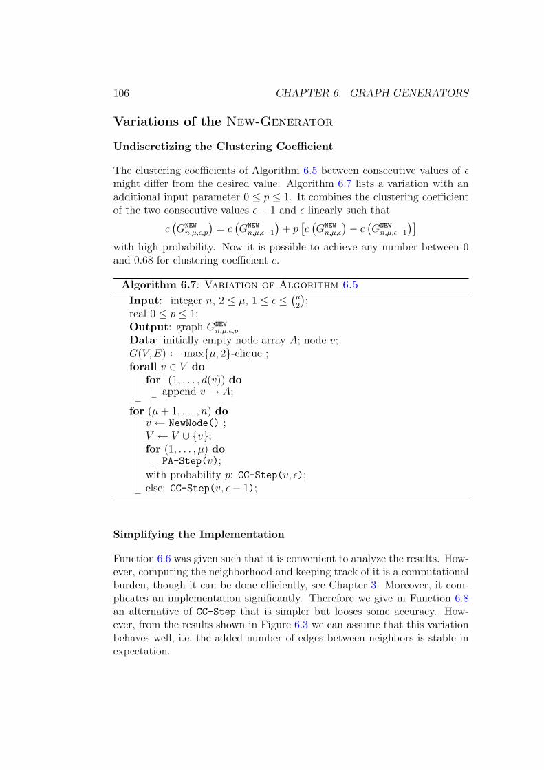
106 CHAPTER 6. GRAPH GENERATORS
Variations of the New-Generator
Undiscretizing the Clustering Coefficient
The clustering coefficients of Algorithm 6.5 between consecutive values of εmight differ from the desired value. Algorithm 6.7 lists a variation with anadditional input parameter 0 ≤ p ≤ 1. It combines the clustering coefficientof the two consecutive values ε− 1 and ε linearly such that
c(GNEW
n,µ,ε,p
)= c
(GNEW
n,µ,ε−1
)+ p
[c(GNEW
n,µ,ε
)− c
(GNEW
n,µ,ε−1
)]with high probability. Now it is possible to achieve any number between 0and 0.68 for clustering coefficient c.
Algorithm 6.7: Variation of Algorithm 6.5
Input: integer n, 2 ≤ µ, 1 ≤ ε ≤(
µ2
);
real 0 ≤ p ≤ 1;Output: graph GNEW
n,µ,ε,p
Data: initially empty node array A; node v;G(V, E)← maxµ, 2-clique ;forall v ∈ V do
for (1, . . . , d(v)) doappend v → A;
for (µ + 1, . . . , n) dov ← NewNode() ;V ← V ∪ v;for (1, . . . , µ) do
PA-Step(v);
with probability p: CC-Step(v, ε);else: CC-Step(v, ε− 1);
Simplifying the Implementation
Function 6.6 was given such that it is convenient to analyze the results. How-ever, computing the neighborhood and keeping track of it is a computationalburden, though it can be done efficiently, see Chapter 3. Moreover, it com-plicates an implementation significantly. Therefore we give in Function 6.8an alternative of CC-Step that is simpler but looses some accuracy. How-ever, from the results shown in Figure 6.3 we can assume that this variationbehaves well, i.e. the added number of edges between neighbors is stable inexpectation.

6.3. THE NEW-GENERATOR 107
Function 6.8: Variation of CC-Step
Input: node v, int εData: node: u;for (1, . . . , ε) do
u←RandomAdjacentNode(v);do
w ←RandomAdjacentNode(v);while u = w ;if u, w /∈ E then
E ← E ∪ u, v;append: u→ A, v → A;
Chapter Conclusion
We gave a new graph generator that is based on preferential attachment andcreates graphs with adjustable clustering coefficient, in which any value upto 0.68 can be achieved. The value of the clustering coefficient does notdepend on the total number of edges added in each round. The total numberof edges added in each round is not deterministic but it can be estimatedwell. Our experiments show that core number and the size of the cores of thegenerated graphs grow with the size of the graph. This behavior is reasonablefor existing evolving networks as it has been shown recently. The dynamicanalysis of the core structure seems to be at its very beginning. Our generatoris a first step in this area with qualitative reasonable behavior.

108 CHAPTER 6. GRAPH GENERATORS

Chapter 7
Approximating ClusteringCoefficient, Transitivity andNeighborhood Densities
Chapter Introduction
The consideration of very large graphs in network analysis [Kumar et al.,2000; Abello et al., 2002; Eubank et al., 2004] requires or makes it at leastvery desirable that the analysis can be performed in linear or preferablyeven in sub-linear time. We have seen in Chapter 3 that triangle listing andtriangle counting can be performed very efficiently. However, the algorithmsdo still have super-linear running times with respect to the input size. Itis even impossible to achieve running time in the size of the input for thecase of triangle listing. Consequently applying these algorithms to computenetwork indices like the clustering coefficient results in super-linear runningtimes, too.
This chapter is devoted to algorithms for the efficient approximation of thefollowing indices in sub-linear time with respect to the size of graph. Weconsider the case of approximating the clustering coefficient c and its nodeweighted version cw for which the transitivity is a special case. We alsoconsider the neighborhood densities of the nodes.
Contribution and Related Work. Approximation algorithms based onsampling are well known and have been used extensively for various applica-tions. Eubank et al. [2004] use such a method to approximate the clustering
109

110 CHAPTER 7. APPROXIMATION
coefficient c by sampling nodes and compute the average neighborhood den-sity of the samples. They mention that by applying general probabilisticbounds it suffices to take O(log n) samples.
Our main contribution is a O(1) time algorithm for approximating the clus-tering coefficient c. We further give a O(n) time algorithm for the case ofthe node weighted clustering coefficient cw of a graph. These results and thealgorithms on which they are based on were published in [Schank and Wag-ner, 2005a]. These work here extends our publication by the following. Wereview the method based on sampling nodes and also show why our methodto approximate c is favorable. We will further give an algorithm to approx-imate all neighborhood densities of a graph in O(n log n) time, along withsome consideration of practical applications.
Peripherally related to our work is the approximation of the number of trian-gles by streaming algorithms [Bar-Yosseff et al., 2002; Jowhari and Ghodsi,2005; Buriol et al., 2006].
Organization. The rest of this chapter is organized as follows. We givesome definitions and other prerequisites first. We review the method ofapproximating c by sampling the neighborhood density of several nodes inSection 7.1. We will then introduce a method based on sampling wedges inSection 7.2. In Section 7.3 we consider the approximation of the neighbor-hood density of nodes of a graph. A conclusion closes this chapter.
Preliminaries
Approximation and Randomized Algorithms
We introduced the concept and especially the running time of an algorithmon page 17 in Section 2.3. An approximation algorithm is an algorithm thattransforms the input to an output that is by some measure close to thedesired output. The full meaning for our purpose will become clear withinthis chapter. Randomized algorithms appear frequently in the context ofapproximation algorithms. A randomized algorithm uses a number of randombits besides its usual input. In general either the output or the running timeor both will depend also on the random input bits. The main interest will bein the expected output or the expected running time and the behavior of thedistribution “around” the expected value. Actually, we have already seenrandomized algorithms in Chapter 6. The probabilistic context there was

111
quite clear without giving any additional explanation. However, this chapterrequires some further knowledge in this area which we will introduce now.
Probability
We will extend the basic concepts of probability which we presented onpage 12 in Section 2.1. Two random variables X and Y are independentif for all x, y ∈ R
P [X = x ∩ Y = y] = p(x) · p(y).
For a real number r and independent random variables X, Y the linearity ofexpectation
E [r ·X · Y ] = r · E [X] · E [Y ] (7.1)
is a useful property. There exist several results that bound the likeliness todeviate from the expectation of a random variable. The very general Markovinequality
P [X ≥ rE [X]] =1
r. (7.2)
is valid for non-negative random variables X and r a positive real. For sumsof non-negative independent random variables the much stronger Chernoffbound can be derived from Equation 7.2. The most general version of thisbound can not be applied with ease in many cases and therefore many vari-ants exist.
A very convenient bound for our purpose is due to Hoeffding [Hoeffding,1963]. Since it is similar to the Chernoff bound it is also referred to as theChernoff-Hoeffding bound. Let Xi be independent real random variablesbounded by 0 ≤ Xi ≤ β for all i. Then, Hoeffding’s bound [Hoeffding, 1963]states for k ∈ N>0
P
(∣∣∣∣∣1k(
k∑i=1
Xi
)− E
[1
k
(k∑
i=1
Xi
)]∣∣∣∣∣ ≥ ε
)≤ 2e
−2kε2
β2 . (7.3)
Hoeffding’s Bound in Example
We give an example on approximating an average value by Hoeffding’s boundfirst. Assume that we have m boxes. Each box is either empty or containsone item. We can compute the average number of items in a box in O(m)
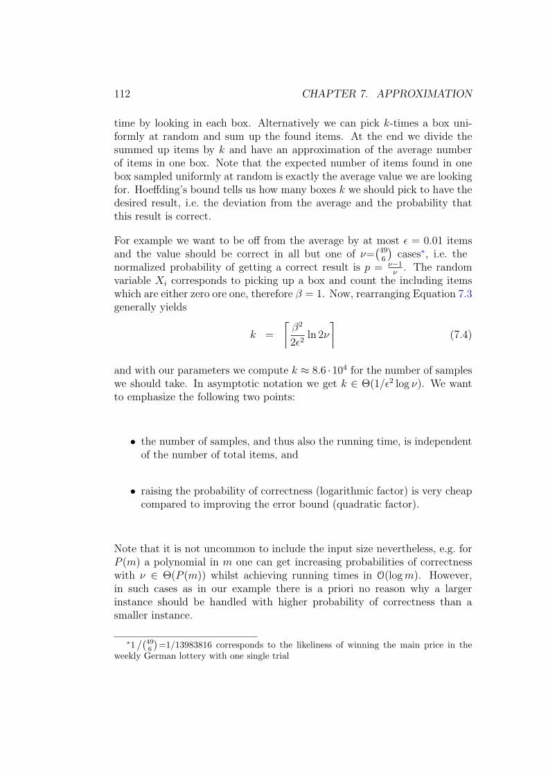
112 CHAPTER 7. APPROXIMATION
time by looking in each box. Alternatively we can pick k-times a box uni-formly at random and sum up the found items. At the end we divide thesummed up items by k and have an approximation of the average numberof items in one box. Note that the expected number of items found in onebox sampled uniformly at random is exactly the average value we are lookingfor. Hoeffding’s bound tells us how many boxes k we should pick to have thedesired result, i.e. the deviation from the average and the probability thatthis result is correct.
For example we want to be off from the average by at most ε = 0.01 itemsand the value should be correct in all but one of ν=
(496
)cases∗, i.e. the
normalized probability of getting a correct result is p = ν−1ν
. The randomvariable Xi corresponds to picking up a box and count the including itemswhich are either zero ore one, therefore β = 1. Now, rearranging Equation 7.3generally yields
k =
⌈β2
2ε2ln 2ν
⌉(7.4)
and with our parameters we compute k ≈ 8.6 ·104 for the number of sampleswe should take. In asymptotic notation we get k ∈ Θ(1/ε2 log ν). We wantto emphasize the following two points:
• the number of samples, and thus also the running time, is independentof the number of total items, and
• raising the probability of correctness (logarithmic factor) is very cheapcompared to improving the error bound (quadratic factor).
Note that it is not uncommon to include the input size nevertheless, e.g. forP (m) a polynomial in m one can get increasing probabilities of correctnesswith ν ∈ Θ(P (m)) whilst achieving running times in O(log m). However,in such cases as in our example there is a priori no reason why a largerinstance should be handled with higher probability of correctness than asmaller instance.
∗1/(
496
)=1/13983816 corresponds to the likeliness of winning the main price in the
weekly German lottery with one single trial

7.1. APPROXIMATING THE CLUSTERING COEFFICIENT BY SAMPLING NODES 113
7.1 Approximating the Clustering Coefficient
by Sampling Nodes
Let us recall that the clustering coefficient of a graph G is the average neigh-borhood density
c (G) =1
|V |∑v∈V
%(v),
in which %(v) = δ(v)/(
d(v)2
). We assume, that %(v) is well defined for all
nodes, i.e. d(v) ≥ 2 for all v ∈ V .
A straightforward method to approximate the clustering coefficient of a graphc (G) would be to take samples from the neighborhood densities of the setof nodes. Let S be a multiset of nodes chosen uniformly at random from V .Then
apx (c (G)) =1
|S|∑v∈S
%(v)
is an approximation of c (G) and Algorithm 7.1 lists a direct realization withk = |S|.
Algorithm 7.1: c-Approximation by Node Sampling
Input: graph G = (V, E) with ∀v ∈ V : (v) ≥ 2;number of samples k;Output: approximation of c (G);Data: real r;r ← 0;for (1, . . . , k) do
v ← uniformRandomNode of all nodes V ;r ← r + %(v);1
return apx (c (G)) = r/k;
This method has been used by Eubank et al. [2004]. They mention thatchoosing k in Θ(log n) “is easily shown via a Chernoff bound to give anaccurate estimate”.
Actually, if we directly apply Hoeffding’s bound (Equation 7.3) it sufficesto choose k ∈ O(1) for a fixed error bound ε and fixed probability p ofapproximating within the range induced by this bound. See the example onpage 111 for details. In the following we will assume k ≥ 1 to be boundedby a constant.
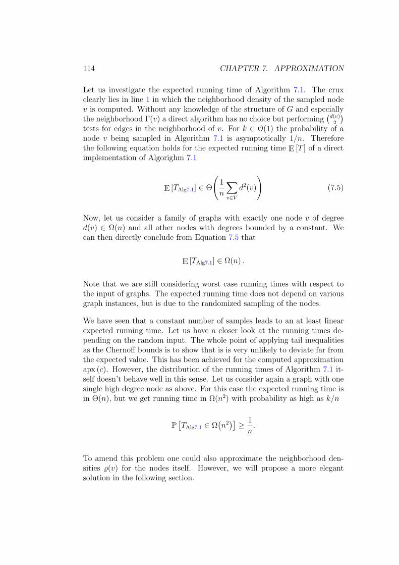
114 CHAPTER 7. APPROXIMATION
Let us investigate the expected running time of Algorithm 7.1. The cruxclearly lies in line 1 in which the neighborhood density of the sampled nodev is computed. Without any knowledge of the structure of G and especiallythe neighborhood Γ(v) a direct algorithm has no choice but performing
(d(v)2
)tests for edges in the neighborhood of v. For k ∈ O(1) the probability of anode v being sampled in Algorithm 7.1 is asymptotically 1/n. Thereforethe following equation holds for the expected running time E [T ] of a directimplementation of Algorighm 7.1
E [TAlg7.1] ∈ Θ
(1
n
∑v∈V
d2(v)
)(7.5)
Now, let us consider a family of graphs with exactly one node v of degreed(v) ∈ Ω(n) and all other nodes with degrees bounded by a constant. Wecan then directly conclude from Equation 7.5 that
E [TAlg7.1] ∈ Ω(n) .
Note that we are still considering worst case running times with respect tothe input of graphs. The expected running time does not depend on variousgraph instances, but is due to the randomized sampling of the nodes.
We have seen that a constant number of samples leads to an at least linearexpected running time. Let us have a closer look at the running times de-pending on the random input. The whole point of applying tail inequalitiesas the Chernoff bounds is to show that is is very unlikely to deviate far fromthe expected value. This has been achieved for the computed approximationapx (c). However, the distribution of the running times of Algorithm 7.1 it-self doesn’t behave well in this sense. Let us consider again a graph with onesingle high degree node as above. For this case the expected running time isin Θ(n), but we get running time in Ω(n2) with probability as high as k/n
P[TAlg7.1 ∈ Ω
(n2)]≥ 1
n.
To amend this problem one could also approximate the neighborhood den-sities %(v) for the nodes itself. However, we will propose a more elegantsolution in the following section.

7.2. APPROXIMATING THE CLUSTERING COEFFICIENT BY SAMPLING WEDGES 115
7.2 Approximating the Clustering Coefficient
by Sampling Wedges
We will give approximation algorithms for the node weighted clustering coef-ficient cw (including the transitivity) and for the unweighted clustering coef-ficient c. Before getting to the algorithms we will first extend the transitivityt(G) in a similar manner as the clustering coefficient c (G) in Equation 5.6on page 88.
Extending the Transitivity
Let Π be the set of all wedges in a graph G, then τ(G) = |Π|. Furtherconsider the mapping X : Π→ 0, 1, where X(Υ) equals one if there is anedge between the outer nodes of the wedge Υ, and zero otherwise. Then wecan rewrite the transitivity as
t(G) =1
|Π|∑Υ∈Π
X(Υ).
This equation is similar to the definition of the clustering coefficient in Equa-tion 2.11 on page 17. We define
t$(G) =1∑
Υ∈Π
$(Υ)
∑Υ∈Π
$(Υ)X(Υ). (7.6)
with a weight function $ : Π→ R+.
Lemma 20 The weighted clustering coefficient is a special case of the weightedtransitivity.
Proof: For a node weight function w, let $(Υ) = w(v)τ(v)
where v is the centerof wedge Υ. Further, let Πv be the set of wedges with center v. Then ac-cordingly τ(v) = |Πv| and
∑Πv
X(Υ) = δ(v). The following transformationcompletes the proof:
cw = 1PV ′
w(v)
∑V ′
w(v)%(v) = 1PV ′
w(v)t(v)
t(v)
∑V ′
w(v)m(v)t(v)
= 1PV ′
w(v)t(v)
PΠv
1
∑V ′
w(v)t(v)
∑Πv
X(Υ) = 1PV ′
PΠv
w(v)t(v)
∑V ′
∑Πv
w(v)t(v)
X(Υ)
= 1PΠ
$v
∑Π
$vX(Υ) = T$
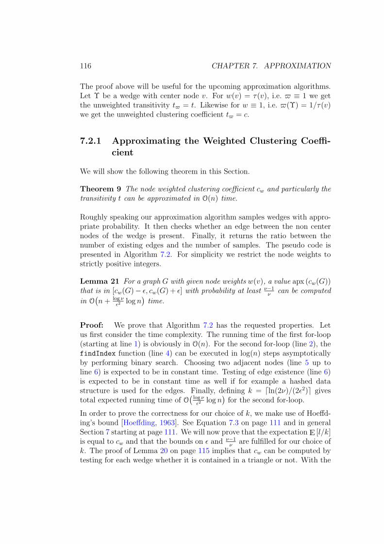
116 CHAPTER 7. APPROXIMATION
The proof above will be useful for the upcoming approximation algorithms.Let Υ be a wedge with center node v. For w(v) = τ(v), i.e. $ ≡ 1 we getthe unweighted transitivity t$ = t. Likewise for w ≡ 1, i.e. $(Υ) = 1/τ(v)we get the unweighted clustering coefficient t$ = c.
7.2.1 Approximating the Weighted Clustering Coeffi-cient
We will show the following theorem in this Section.
Theorem 9 The node weighted clustering coefficient cw and particularly thetransitivity t can be approximated in O(n) time.
Roughly speaking our approximation algorithm samples wedges with appro-priate probability. It then checks whether an edge between the non centernodes of the wedge is present. Finally, it returns the ratio between thenumber of existing edges and the number of samples. The pseudo code ispresented in Algorithm 7.2. For simplicity we restrict the node weights tostrictly positive integers.
Lemma 21 For a graph G with given node weights w(v), a value apx (cw(G))that is in [cw(G)− ε, cw(G) + ε] with probability at least ν−1
νcan be computed
in O(n + log ν
ε2log n
)time.
Proof: We prove that Algorithm 7.2 has the requested properties. Letus first consider the time complexity. The running time of the first for-loop(starting at line 1) is obviously in O(n). For the second for-loop (line 2), thefindIndex function (line 4) can be executed in log(n) steps asymptoticallyby performing binary search. Choosing two adjacent nodes (line 5 up toline 6) is expected to be in constant time. Testing of edge existence (line 6)is expected to be in constant time as well if for example a hashed datastructure is used for the edges. Finally, defining k = dln(2ν)/(2ε2)e givestotal expected running time of O
(log νε2
log n)
for the second for-loop.
In order to prove the correctness for our choice of k, we make use of Hoeffd-ing’s bound [Hoeffding, 1963]. See Equation 7.3 on page 111 and in generalSection 7 starting at page 111. We will now prove that the expectation E [l/k]is equal to cw and that the bounds on ε and ν−1
νare fulfilled for our choice of
k. The proof of Lemma 20 on page 115 implies that cw can be computed bytesting for each wedge whether it is contained in a triangle or not. With the

7.2. APPROXIMATION BY SAMPLING WEDGES 117
Algorithm 7.2: Node Weighted Clustering Coefficient Ap-proximationInput: graph G = (V, E) with ∀v ∈ V : d(v) ≥ 2;arbitrary indexed order of nodes (v1, . . . , vn);node weights w : V → N>0;number of samples: k;Output: approximation of cw
Data: node variables: u, w;integer variables: r, l, j, φ0,...,n;φ0 ← 0;for i = (1, . . . , n) do1
φi ← φi−1 + w(vi);
l← 0 ;for (1, . . . , k) do2
r ← uniformRandomNumber(1, . . . , φn);3
j ← findIndex( i : φi−1 < r ≤ φi);4
u← uniformRandomAdjacentNode(vj) ;5
repeatw ← uniformRandomAdjacentNode(vj) ;
until u 6= w ;if u, w ∈ E then6
l← l + 1;
return apx (cw(G)) = l/k ;

118 CHAPTER 7. APPROXIMATION
same notation as in Section 7.2 and particularly as in the proof of Lemma20, we get
cw(G) =1∑
u∈V ′w(u)
∑v∈V ′
∑Υ∈Πv
w(v)
τ(v)X(Υ)
where w(v)/τ(v) is the weight of the corresponding wedge. This correspondsto the probability of w(v)/ (τ(v)
∑w(u)) that a wedge is chosen in one single
loop starting at line 2. Hence, by linearity of the expectation E [l/k] = cw
holds. The random variable X(Υ) is a mapping from Π to 0, 1, and conse-quently β = 1 in Equation 7.3. We can now immediately see that the boundson ε and the probability ν−1
νare fulfilled for our choice of k.
One may regard the error bound ε and the probability ν as fixed parameters.The number of wedges τ(v) for a node v can be computed in O(1) time ife.g. adjacency arrays are used. Theorem 9 follows from these observations.
7.2.2 Approximating the Clustering Coefficient
The central statement of this section is the following Theorem.
Theorem 10 The clustering coefficient c of a graph G can be approximatedin constant time.
To show it we will use a simplified version of Algorithm 7.2 which is listedin Algorithm 7.3. The main difference is that the node v, which correspondsto node vj in Algorithm 7.2, is now sampled uniformly at random from allnodes in V . Thus, all lines dealing with the node weights are not requiredand removed.
To see the correctness one verifies that a wedge at center node v is sampledwith probability 1/ (τ(v)|V |) which corresponds to the correct weight w ≡ 1or $ = 1/τ for obtaining c, compare to the proof of Lemma 20 on page 115and the paragraph following that proof. The rest follows analogously as inthe proof of Lemma 21 on page 116.
Corollary 19 For a graph G a value apx (c (G)) that is in [c(G)−ε, c(G)+ε]with probability at least ν−1
νcan be computed in O
(log νε2
)time.

7.2. APPROXIMATING THE NEIGHBORHOOD DENSITIES 119
Algorithm 7.3: Clustering Coefficient Approximation
Input: graph G = (V, E) with ∀v ∈ V : d(v) ≥ 2;number of samples: k;Output: approximation of cw
Data: node variables: u, w;integer variables: l;l← 0 ;for (1, . . . , k) do
v ← uniformRandomNode(V );u← uniformRandomAdjacentNode(v) ;repeat
w ← uniformRandomAdjacentNode(v) ;until u 6= w ;if u, w ∈ E then
l← l + 1;
return apx (c (G)) = l/k ;
Performance in Practice. We implemented Algorithm 7.3 to approxi-mate the clustering coefficient. We set the parameters to ε = 0.01 andν =
(496
). It takes between 0.8 seconds for a very small graph of 4 nodes up
to 1.4 seconds for the larger “Movie Actor Network 2004” (see page 38 inSection 3.2). This difference could be explained by the cache of the CPU.Note, that the execution times do not contain the creation of the used hashdata structures for the edges.
7.3 Approximating the Neighborhood Densi-
ties
In this section we give algorithms to approximate the neighborhood density%(v), i.e. the clustering coefficient of the nodes of a graph. The main resultis compactly given by the following theorem.
Theorem 11 All the neighborhood densities %(v) of a graph G can be ap-proximated in O(n log n) time.
The main algorithm is listed in Algorithm 7.4. We will discuss it in thefollowing.
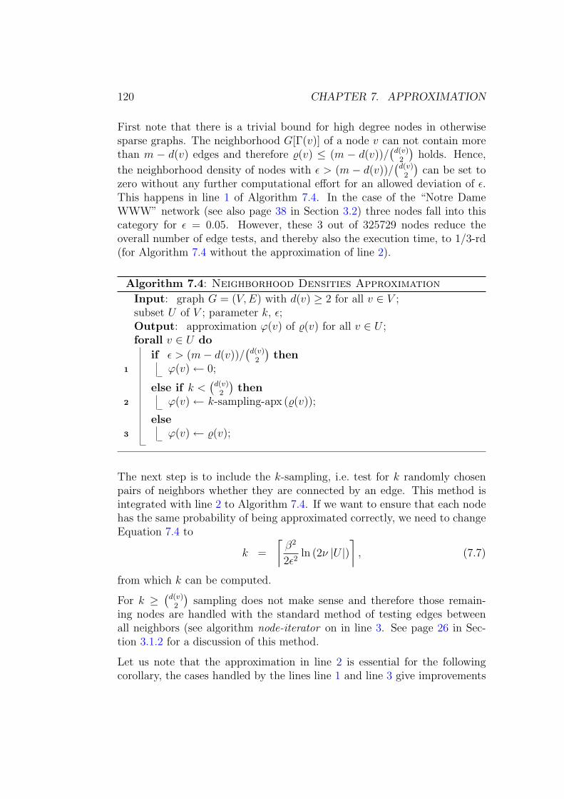
120 CHAPTER 7. APPROXIMATION
First note that there is a trivial bound for high degree nodes in otherwisesparse graphs. The neighborhood G[Γ(v)] of a node v can not contain morethan m − d(v) edges and therefore %(v) ≤ (m − d(v))/
(d(v)2
)holds. Hence,
the neighborhood density of nodes with ε > (m − d(v))/(
d(v)2
)can be set to
zero without any further computational effort for an allowed deviation of ε.This happens in line 1 of Algorithm 7.4. In the case of the “Notre DameWWW” network (see also page 38 in Section 3.2) three nodes fall into thiscategory for ε = 0.05. However, these 3 out of 325729 nodes reduce theoverall number of edge tests, and thereby also the execution time, to 1/3-rd(for Algorithm 7.4 without the approximation of line 2).
Algorithm 7.4: Neighborhood Densities Approximation
Input: graph G = (V, E) with d(v) ≥ 2 for all v ∈ V ;subset U of V ; parameter k, ε;Output: approximation ϕ(v) of %(v) for all v ∈ U ;forall v ∈ U do
if ε > (m− d(v))/(
d(v)2
)then
ϕ(v)← 0;1
else if k <(
d(v)2
)then
ϕ(v)← k-sampling-apx (%(v));2
elseϕ(v)← %(v);3
The next step is to include the k-sampling, i.e. test for k randomly chosenpairs of neighbors whether they are connected by an edge. This method isintegrated with line 2 to Algorithm 7.4. If we want to ensure that each nodehas the same probability of being approximated correctly, we need to changeEquation 7.4 to
k =
⌈β2
2ε2ln (2ν |U |)
⌉, (7.7)
from which k can be computed.
For k ≥(
d(v)2
)sampling does not make sense and therefore those remain-
ing nodes are handled with the standard method of testing edges betweenall neighbors (see algorithm node-iterator on in line 3. See page 26 in Sec-tion 3.1.2 for a discussion of this method.
Let us note that the approximation in line 2 is essential for the followingcorollary, the cases handled by the lines line 1 and line 3 give improvements
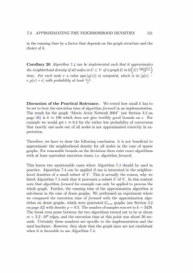
7.3. APPROXIMATING THE NEIGHBORHOOD DENSITIES 121
in the running time by a factor that depends on the graph structure and thechoice of k.
Corollary 20 Algorithm 7.4 can be implemented such that it approximates
the neighborhood density of all nodes in U ⊂ V of a graph G in O(|U | log(ν|U |)
ε2
)time. For each node v a value apx (%(v)) is computed, which is in [%(v) −ε, %(v) + ε] with probability at least ν−1
ν.
Discussion of the Practical Relevance. We tested how small k has tobe set to beat the execution time of algorithm forward in an implementation.The result for the graph “Movie Actor Network 2004” (see Section 3.2 onpage 38) is k ≈ 190 which does not give terribly good bounds on ε. Forexample we would get ε ≈ 0.2 for the rather low probability of correctnessthat exactly one node out of all nodes is not approximated correctly in ex-pectation.
Therefore, we have to draw the following conclusion: it is not beneficial toapproximate the neighborhood density for all nodes in the case of sparsegraphs. For reasonable bounds on the deviation there exist exact algorithmswith at least equivalent execution times, i.e. algorithm forward .
This leaves two mentionable cases where Algorithm 7.4 should be used inpractice. Algorithm 7.4 can be applied if one is interested in the neighbor-hood densities of a small subset of V . This is actually the reason, why welisted Algorithm 7.4 such that it processes a subset U of V . In this contextnote that algorithm forward for example can only be applied to process thewhole graph. Further, the running time of the approximation algorithm issub-linear in the case of dense graphs. We performed an experiment wherewe compared the execution time of forward with the approximation algo-rithm on dense graphs, which were generated Gn,m graphs (see Section 3.2on page 42) with density ρ = 0.5. The number of samples was set to k = 3429.The break even point between the two algorithms turned out to be at aboutm = 2.2 · 106 edges, and the execution time at this point was about 20 sec-onds. Certainly these numbers are specific to the implementation and theused hardware. However, they show that the graph sizes are not exorbitantwhen it is favorable to use Algorithm 7.4.

122 CHAPTER 7. APPROXIMATION
Chapter Conclusion
We have seen various results on the approximation of the clustering coeffi-cient. We highlight the possibility of approximating the clustering coefficientc of a graph in constant time. We have shown that it is feasible to apply thismethods in practice. However, especially in the case of approximating theclustering coefficient of all nodes it has to be carefully considered whether itis worth applying an approximative method instead of a fast exact algorithm.
The algorithms might have a further impact on the approximation of thecoefficients for very large networks that do not fit into main memory. Forexample, it is known that the exact number of triangles can not be countedby streaming algorithms with reasonable models [Bar-Yosseff et al., 2002].However, it can be approximated within some bounds [Bar-Yosseff et al.,2002; Jowhari and Ghodsi, 2005; Buriol et al., 2006]. This is a field forfuture research.

Chapter 8
Conclusion
We introduced a triangle listing algorithm which is very efficient in practice.Its execution time is competitive to the previously considered practical al-gorithms. However, our algorithm also achieves optimal running time withrespect to the input size of the network. Due to the improved running time,our algorithm performs much better on large graphs with high degree nodes.These types of networks are quite commonly considered in network analysis.Our algorithm achieves execution times in minutes on recent hardware forgraphs that fill up all the main memory of an adequately equipped com-puter. The bottleneck is now rather memory consumption, and techniquesthat avoid storing the graphs in central memory will be the focus in thefuture.
We considered a variety of graph classes with respect to triangle listing andtriangle counting. We presented triangle listing algorithms that achieve alinear running time in the input (the size of the graph) and the output (thenumber of triangles). For the case of triangle counting we developed algo-rithms that have a running time linear in the number of edges or even inthe number of nodes. These algorithms do not use techniques that involvehigh constants in the running times. Therefore, they can be used in practicalapplications. They also exploit the triangular structure of the graph method-ologically, which gives insights into the respective triangular structures.
We reviewed a variety of network analysis related problems that benefit fromefficient triangle listing algorithms. We discussed the neighborhood densitiesand different weighted variants thereof. We gave a unified notation of thoseweighted versions and a general algorithm to compute them by generic tri-angle listing. We discussed the clustering coefficient and the related indexof transitivity. We gave improved algorithms to compute equivalence classes
123
124 CHAPTER 8. CONCLUSION
of triangular connected nodes and edges. In the context of connectivity bycliques we showed that our triangle listing algorithm can be extended to a4-clique listing algorithm that achieves acceptable execution times even forlarger graphs.
We reviewed the approach to approximate the clustering coefficient of a graphby computing the average of the neighborhood densities of randomly samplednodes. We have observed that this approach leads to an expected runningtime at least linear in the number of nodes. We gave an approximation algo-rithm that achieves a constant running time. It is based on sampling wedgesand can be extended to approximate weighted versions of the clustering co-efficient. Similar techniques can be used to approximate the neighborhooddensity of a node. In the case of considering all nodes of a graph, thesealgorithms have a strong competitor based on the very efficient triangle list-ing algorithm as discussed above. However, we have shown cases where theapproximation nevertheless shows considerable advantages.
We gave a graph generator that is based on preferential attachment. Unlikepreviously presented approaches, our generator achieves high clustering co-efficient values for a wide range of parameters. Additionally, we achieve anontrivial core structure of the generated networks that increases with thegraph size.

Acknowledgments
First of all I would like to thank my supervisor Dorothea Wagner for givingme the opportunity to work with her, for the advice and help all over theyears, and for providing the very nice environment in her algorithmics group.I’m very thankful to Ulrik Brandes, who provided many times the help of asecond supervisor and particularly let me work with him and his group inKonstanz.
I enjoyed the time with my former office colleague Sabine Cornelsen and mycurrent Christian Pich. Sabine gave me excellent guidance at the beginningof this work. Christian was always very helpful and had a lot of patience withme. Special thanks to Christian and Sabine as well as Michael Baur, MartinHoefer, Martin Holzer and Svetlana Mansmann for their critical proofreadingof parts of this manuscript. I warmly thank Sabine Cornelsen for hintingto and discussing split decomposable graphs, as well as Ulrik Brandes forhinting to and discussing chordal graphs. Many administrative duties wouldhave cost me much more time without the help of Marco Gaertler.
Some work done during recent years did not find its way into this thesis,simply because it did not fit so well to the main topic. Nevertheless I wouldlike to thank the people that were involved with it. Thomas Erlebach andAlexander Hall let me join their interesting work during my time at the ETHZurich. Michael Baur’s help was and is very valuable for the recent work inthe CREEN project.
I also enjoyed incredible support and patience from Monika Kulartz duringthe compilation of this work. I’m very thankful to my parents for theirsupport and trust during my whole education.
Last but not least let me thank again Dorothea Wagner and Ulrik Brandesfor taking their time as referees for this thesis.
125

126 CHAPTER 8. ZUSAMMENFASSUNG
Zusammenfassung
Verschiedene Methoden in der Netzwerkanalyse basieren auf dem effizientenAbzahlen oder Auflisten aller Dreiecke eines Graphen. Die Nachbarschafts-dichte (engl. clustering coefficient) ist eine der zur Zeit popularsten Kenn-großen der Netzwerkanalyse. Ihre schnelle Berechnung hangt von dem effizi-enten Abzahlen aller Dreiecke eines Graphen ab. Diese Arbeit beschaftigt sichmit algorithmischen Problemen in der Netzwerkanalyse, die in engem Bezugzu der Anzahl und der Struktur der Dreiecke in einem gegebenen Netzwerkstehen.
Wir betrachten zunachst Algorithmen fur das effiziente Auflisten aller Drei-ecke eines Graphen. Im Gegensatz zum Abzahlen der Dreiecke ist das Aufli-sten ein universelleres Werkzeug, da sich beispielsweise aus einem Algorith-mus zum Auflisten aller Dreiecke sehr einfach ein Algorithmus zum Abzahlenaller Dreiecke ableiten lasst. Beide Probleme wurden in der Vergangenheitweitgehend nur theoretisch betrachtet. Es sei hierzu insbesondere auf [Alonet al., 1997] verwiesen, die den bis dato effizientesten Algorithmus zum Ab-zahlen aller Dreiecke vorstellt. Dieser Algorithmus basiert auf schneller Ma-trizen-Multiplikation, eine Technik, die zwar weitreichende theoretische Kon-sequenzen hat, in der Praxis aber nicht verwendet wird. Wir konzentrierenuns jedoch insbesondere auf die praktische Anwendbarkeit von Algorithmenfur das Auflisten aller Dreiecke. Die bisher einzige Arbeit, die dieses Pro-blem auch im Hinblick auf praktische Anwendungen beleuchtet ist [Batageljand Mrvar, 2001]. Der dort betrachtete Algorithmus dient uns als Grundla-ge fur die Entwicklung eines neuen Algorithmus mit besserer Laufzeit. Wirerweitern ihn um einige sehr einfache zusatzliche Operationen und Daten-strukturen und beweisen, dass seine asymptotische Laufzeit bezuglich derAnzahl der Kanten optimal ist. Zudem zeigen wir experimentell, dass dieserAlgorithmus im allgemeinen sehr schnelle Ausfuhrungszeiten erreicht undinsbesondere auch bei Eingaben mit hohen Knotengraden sehr effektiv ist.
Weiterhin befassen wir uns mit dem Auflisten und Aufzahlen aller Dreiecke inspeziellen Graphklassen. Hierbei steht nicht die praktische Anwendung, son-dern die angewandte Methodik im Vordergrund. Wir beginnen mit Graphen,deren Kernzahl durch eine Konstante beschrankt ist. Dazu gehoren plana-re Graphen und auch Graphen die durch die Methode lineare Bevorzugung,besser bekannt unter dem englischen Begriff “linear preferential attachment”,erzeugt werden. Im weiteren behandeln wir transitiv orientierbare und chor-dale Graphen. Als letzte Klasse betrachten wir sogenannte distanzvererbendeGraphen, bei denen in jedem durch einen Pfad induzierten Untergraph diegleichen Knotenabstande wie im Originalgraph gelten. Die vorgestellte Me-

8.0. ZUSAMMENFASSUNG 127
thode zum Auflisten und Zahlen der Dreiecke basiert bei distanzvererbendenGraphen allerdings auf einer weiteren, durch Zerlegung charakterisierten Ei-genschaft. Falls der Graph in einer impliziten Zerlegung kodiert ist, erreichenwir fur das Zahlen der Dreiecke eine Laufzeit, die linear in der Anzahl derKnoten ist. Insgesamt erreichen wir fur alle erwahnten Graphklassen Lauf-zeiten, die linear in der Große von Eingabe und Ausgabe sind. Im Falle desAufzahlens bedeutet dies, dass die Laufzeit linear in der Große des Graphenist, und im Falle des Auflistens, dass sie linear in der Große des Graphen plusder Anzahl der im Graphen vorhanden der Dreiecke ist.
Im Bezug auf Anwendungen in der Netzwerkanalyse beschranken wir uns aufAlgorithmen, die als Eingabe eine Liste der Dreiecke des Graphen verwenden.Dies ist zum einen aus den schon besprochenen Inhalten und zum anderenaus der praktischen Wiederverwendbarkeit des immer gleichen Algorithmuszur Auflistung aller Dreiecke motiviert. Als erste Anwendung behandeln wirdie Berechnung der Aquivalenzklassen, die durch Wege sich uberlappenderkurzer Zyklen induziert sind. Dieser Verallgemeinerung von Zusammenhangs-komponenten in Graphen wurde in [Batagelj and Zaversnik, 2003] vorgestellt.Als Spezialfall werden auch Zusammenhangskomponenten, die auf kurzen Zy-klen der Lange drei - also Dreiecken beruhen, betrachtet und Algorithmenzur Berechnung der entsprechenden Aquivalenzklassen angegeben. Basierendauf dem generischen Auflisten von Dreiecke konnen wir Algorithmen mitverbesserter Laufzeit aufzeigen. Ahnlich zu dem Zusammenhangsbegriff, derauf Wegen sich uberlappender kurzer Zyklen beruht, lasst sich Zusammen-hang auf Basis der Uberlappung von kleinen Cliquen definieren. In diesemKontext zeigen wir die Erweiterbarkeit unseres Algorithmus zum Auflistenaller Dreiecke auf das Auflisten aller k-Cliquen und belegen experimentelldessen Anwendbarkeit, indem wir alle 4-Cliquen eines großeren Netzwerkesauflisten.
Die Dichte des durch die Nachbarn induzierten Graphen eines Knotens be-zeichnen wir als Nachbarschaftsdichte. Sie ist in der englischsprachigen Lite-ratur als “clustering coefficient” eines Knotens bekannt. Algorithmisch lasstsich diese fur alle Knoten sehr einfach durch das Abzahlen und damit auchAuflisten aller Dreiecke berechnen. Wir konzentrieren uns bei der algorith-mischen Besprechung auf den interessanteren Fall des mit Kantengewich-ten versehenen Graphen. Der Mittelwert der Nachbarschaftsdichten uber alleKnoten wird als Nachbarschaftsdichte oder Cluster-Koeffizient des Graphenselbst bezeichnet. Seine Berechnung selbst ist algorithmisch weniger inter-essant, aber da in der Literatur wir der Cluster-Koeffizient und der ahnlichdefinierte Transitivitats-Index manchmal falschlicherweise synonym verwen-det werden, diskutieren wir einige Eigenschaften dieser Indizes, insbesondere

128 CHAPTER 8. ZUSAMMENFASSUNG
die Unterschiede zwischen den entsprechenden Werte fur bestimmte Graph-klassen.
Eine wichtige Rolle fur das Verstandnis real existierender Netzwerke spielenAlgorithmen zur Generierung von Graphen mit bestimmten Eigenschaften.Zudem werden Graphgeneratoren zum Testen von Algorithmen benotigt. Einsehr populares Modell fur die Erzeugung von Graphen ist die sogenanntelineare Bevorzugung. Mit ihr lassen sich Graphen erzeugen, bei denen dieVerteilung der Knotengrade gute Ubereinstimmung mit der entsprechendenVerteilung bei vielen realen Netzwerken hat. Es hat sich allerdings gezeigt,dass der Cluster-Koeffizient eines auf diese Weise erzeugten Graphen deut-lich niedriger ist als bei den in realen Netzwerken typischerweise gefundenenWerten. Eine entsprechend angepasster Generator, der angeblich einen hohenCluster-Koeffizient erzielt, wurde in [Holme and Kim, 2002] vorgestellt. Wirzeigen experimentell, dass dieser Ansatz tatsachlich nur sehr eingeschranktfunktioniert. Wir fuhren einen neuen Algorithmus zur Generierung von Gra-phen ein, der diese Einschrankungen nicht zeigt. Weiterhin zeigen wir, dassdie von unserem Algorithmus generierten Graphen, im Gegensatz zu dendurch die erwahnten Methoden erstellen Graphen, eine nicht triviale Kern-struktur aufweisen.
Im letzten Kapitel befassen wir uns mit der naherungsweisen Berechnungdes Cluster-Koeffizienten eines Graphen durch Stichprobenerhebung. Einesolche Methode mit einer erwarteten Laufzeit, die mindestens proportionalzu der Anzahl der Knoten ist, wird in [Eubank et al., 2004] angewendet. Wirzeigen, dass sich der Cluster-Koeffizient durch Stichprobenerhebung sogar inkonstanter Laufzeit approximieren lasst.

Bibliography
James Abello, Panos M. Pardalos, and Mauricio G. C. Resende, editors.Handbook of massive data sets. Kluwer Academic Publishers, Norwell,MA, USA, 2002. ISBN 1-4020-0489-3.
Vinay Aggarwal, Anja Feldmann, Marco Gaertler, Robert Gorke, andDorothea Wagner. Analysis of Overlay-Underlay Topology Correla-tion using Visualization. In Proc. 5th IADIS International ConferenceWWW/Internet Geometry, Murcia, Spain, 5–8 October 2006.
Reka Albert, Albert-Laszlo Barabasi, and Hawoong Jeong. Mean-field theoryfor scale-free random networks. Physica A, 272:173–187, 1999.
Noga Alon, Raphael Yuster, and Uri Zwick. Finding and counting givenlength cycles. Algorithmica, 17(3):209–223, 1997.
T.L. Austin, R.E. Fagen, W.F. Penney, and J. Riordan. The number of com-ponents of random linear graphs. The Annals of Mathematical Statistics,30:747–754, 1959.
Ziv Bar-Yosseff, Ravi Kumar, and D. Sivakumar. Reductions in streamingalgorithms, with an application to counting triangles in graphs. In SODA’02: Proceedings of the thirteenth annual ACM-SIAM symposium on Dis-crete algorithms, pages 623–632, Philadelphia, PA, USA, 2002. Society forIndustrial and Applied Mathematics. ISBN 0-89871-513-X.
Albert-Laszlo Barabasi and Reka Albert. Emergence of scaling in randomnetworks. Science, 286:509–512, 1999.
Alain Barrat and Martin Weigt. On the properties of small-world networkmodels. The European Physical Journal B, 13:547–560, 2000.
Alain Barrat, Marc Barthelemy, Romualdo Pastor-Satorras, and Alessan-dro Vespignani. The architecture of complex weighted networks.PROC.NATL.ACAD.SCI.USA, 101:3747–3752, 2004.
129

130 BIBLIOGRAPHY
Vladimir Batagelj and Ulrik Brandes. Efficient generation of large randomnetworks. Physical Review E, 71(036113), 2005.
Vladimir Batagelj and Andrej Mrvar. Pajek – A program for large networkanalysis. Connections, 21(2):47–57, 1998.
Vladimir Batagelj and Andrej Mrvar. A subquadratic triad census algorithmfor large sparse networks with small maximum degree. Social Networks,23:237–243, 2001.
Vladimir Batagelj and Matjaz Zaversnik. An O(m) algorithm for cores de-composition of networks. Technical Report Preprint Series, volume 40,number 798, Insitute of Mathematics, Physics and Mechanics, Depart-ment of Theoretical Computer Science, University of Ljublana, Ljubljana,Slovania, 2002.
Vladimir Batagelj and Matjaz Zaversnik. Short cycles connectivity, 2003.
Michael Baur, Ulrik Brandes, Marco Gaertler, and Dorothea Wagner. Draw-ing the as graph in 2.5 dimensions. In Proceedings of the 12th InternationalSymposium on Graph Drawing (GD’04), Lecture Notes in Computer Sci-ence, pages 43–48, 2005.
Bela Bollobas. Extremal Graph Theory. Dover Publications, Incorporated,2004. ISBN 0486435962.
Bela Bollobas. Modern Graph Theory, volume 184 of Graduate Texts inMathematics. Springer-Verlag, 1998.
Bela Bollobas and Oliver M. Riordan. Mathematical results on scale-freerandom graphs. In Stefan Bornholdt and Heinz Georg Schuster, editors,Handbook of Graphs and Networks: From the Genome to the Internet,pages 1–34. Wiley-VCH, 2002.
Bela Bollobas, Oliver M. Riordan, Joel Spencer, and Gabor Tusnady. Thedegree sequence of a scale-free random graph process. Randoms Structuresand Algorithms, 18:279–290, 2001.
Andreas Brandstadt, Van Bang Le, and Jeremy P. Spinrad. Graph classes:a survey. Society for Industrial and Applied Mathematics, Philadelphia ,PA , USA, 1999. ISBN 0-89871-432-X.
Tian Bu and Don Towsley. On distinguishing between Internet power lawtopology generators. In infocom02 infocom02.

BIBLIOGRAPHY 131
Luciana S. Buriol, Gereon Frahling, Stefano Leonardi, Alberto Marchetti-Spaccamela, and Christian Sohler. Counting triangles in data streams.In PODS ’06: Proceedings of the twenty-fifth ACM SIGMOD-SIGACT-SIGART symposium on Principles of database systems, pages 253–262,New York, NY, USA, 2006. ACM Press. ISBN 1-59593-318-2.
Qian Chen, Hyunseok Chang, Ramesh Govindan, Sugih Jamin, ScottShenker, and Walter Willinger. The origin of power laws in Internet topolo-gies revisited. In infocom02 infocom02.
Norishige Chiba and Takao Nishizeki. Arboricity and subgraph listing algo-rithms. SIAM J. Comput., 14(1):210–223, 1985. ISSN 0097-5397.
Don Coppersmith and Shmuel Winograd. Matrix multiplication via arith-metic progressions. Journal of Symbolic Computation, 9(3):251–280, 1990.
Thomas H. Cormen, Charles E. Leiserson, Ronald L. Rivest, and CliffordStein. Introduction to Algorithms. MIT Press, 2nd edition, 2001.
Derek G. Corneil. Lexicographic breadth first search - a survey. In JurajHromkovic, Manfred Nagl, and Bernhard Westfechtel, editors, WG, volume3353 of Lecture Notes in Computer Science, pages 1–19. Springer, 2004.ISBN 3-540-24132-9.
W.H. Cunningham. Decomposition of directed graphs. SIAM J. Alg. Disc.Meth., 3:214–228, 1982.
Elias Dahlhaus. Efficient parallel and linear time sequential split decompo-sition (extended abstract). In P. S. Thiagarajan, editor, FSTTCS, volume880 of Lecture Notes in Computer Science, pages 171–180. Springer, 1994.ISBN 3-540-58715-2.
Roman Dementiev, Lutz Kettner, and Peter Sanders. Stxxl: Standard tem-plate library for xxl data sets. In Gerth Stølting Brodal and StefanoLeonardi, editors, ESA, volume 3669 of Lecture Notes in Computer Sci-ence, pages 640–651. Springer, 2005. ISBN 3-540-29118-0.
Imre Derenyi, Gergely Palla, and Tamas Vicsek. Clique percolation in ran-dom networks. Physical Review Letters, 94:160202, 2005.
Reinhard Diestel. Graph Theory. Graduate Texts in Mathematics. Springer-Verlag, 2nd edition, 2000.
Holger Ebel, Lutz-Ingo Mielsch, and Stefan Bornholdt. Scale-free topologyof e-mail networks. Phys. Rev. E, 66(3):035103, Sep 2002.

132 BIBLIOGRAPHY
Paul Erdos and Alfred Renyi. On random graphs I. Publicationes Mathe-maticae Debrecen, 6:290–297, 1959.
Stephen Eubank, V.S. Anil Kumar, Madhav V. Marathe, Aravind Srinivasan,and Nan Wang. Structural and algorithmic aspects of massive social net-works. In Proceedings of the 14th Annual ACM–SIAM Symposium onDiscrete Algorithms (SODA’04), pages 718–727, 2004.
Michalis Faloutsos, Petros Faloutsos, and Christos Faloutsos. On power-lawrelationships of the Internet topology. In Proceedings of SIGCOMM’99,1999.
Delbert R. Fulkerson and O. A. Gross. Incidence matrices and intervalgraphs. Pacific J. Math., 15(3):835–855, 1965.
Marco Gaertler and Maurizio Patrignani. Dynamic analysis of the au-tonomous system graph. In IPS 2004 – Inter-Domain Performance andSimulation, pages 13–24, March 2004.
Horst Gilbert. Random graphs. The Annals of Mathematical Statistics, 30(4):1141–1144, 1959.
Martin C. Golumbic. The complexity of comparability graph recognition andcoloring. 18(3):199–208, 1977.
Peter Grindrod. Range-dependent random graphs and their application tomodeling large small-world proteome datasets. Physical Review E, 66(6):066702, 2002.
Peter L. Hammer and Frederic Maffray. Completely separable graphs. Dis-crete Appl. Math., 27(1-2):85–99, 1990. ISSN 0166-218X.
Frank Harary and Helene J. Kommel. Matrix measures for transitivity andbalance. Journal of Mathematical Sociology, 6:199–210, 1979.
Frank Harary and Herbert H. Paper. Toward a general calculus of phonemicdistribution. Language : Journal of the Linguistic Society of America, 33:143–169, 1957.
Wassily Hoeffding. Probability inequalities for sums of bounded randomvariables. Journal of the American Statistical Association, 58(301):713–721, 1963.
Petter Holme and Beom Jun Kim. Growing scale-free networks with tunableclustering. Physical Review E, 65(026107), 2002.

BIBLIOGRAPHY 133
infocom02. Proceedings of Infocom’02, 2002.
Alon Itai and Michael Rodeh. Finding a minimum circuit in a graph. SIAMJournal on Computing, 7(4):413–423, 1978.
Hossein Jowhari and Mohammad Ghodsi. New streaming algorithms forcounting triangles in graphs. In Lusheng Wang, editor, COCOON, volume3595 of Lecture Notes in Computer Science, pages 710–716. Springer, 2005.ISBN 3-540-28061-8.
Gabriela Kalna and Des Higham. Clustering coefficients for weighted net-works. volume 3, pages 132–138, 2006.
Ton Kloks, Dieter Kratsch, and Haiko Muller. Finding and counting smallinduced subgraphs efficiently. Information Processing Letters, 74(3–4):115–121, 2000.
Ravi Kumar, Prabhakar Raghavan, Sridhar Rajagopalan, D. Sivakumar,Andrew Tomkins, and Eli Upfal. The Web as a graph. In Proc. 19thACM SIGACT-SIGMOD-AIGART Symp. Principles of Database Systems,PODS, pages 1–10. ACM Press, 15–17 2000.
Matthieu Latapy. Theory and practice of triangle problems in very large(sparse (power-law)) graphs, 2006.
Xiafeng Li, Derek Leonard, and Dmitri Loguinov. On reshaping of cluster-ing coefficients in degree-based topology generators. In Stefano Leonardi,editor, Algorithms and Models for the Web-Graph: Third InternationalWorkshop, WAW 2004, Rome, Italy, October 16, 2004, Proceeedings, vol-ume 3243 of Lecture Notes in Computer Science, pages 68–79. Springer-Verlag, 2004.
Luis Lopez-Fernandez, Gregorio Robles, and Jesus M. Gonzalez-Barahona.Applying social network analysis to the information in cvs repositories. InProceedings of the International Workshop on Mining Software Reposito-ries, pages 101–105, 2004.
Ross M. McConnell and Jeremy P. Spinrad. Linear-time transitive orienta-tion. In SODA ’97: Proceedings of the eighth annual ACM-SIAM sympo-sium on Discrete algorithms, pages 19–25, Philadelphia , PA , USA, 1997.Society for Industrial and Applied Mathematics. ISBN 0-89871-390-0.
Ulrich Meyer, Peter Sanders, and Jop F. Sibeyn, editors. Algorithmsfor Memory Hierarchies, Advanced Lectures [Dagstuhl Research Seminar,

134 BIBLIOGRAPHY
March 10-14, 2002], volume 2625 of Lecture Notes in Computer Science,2003. Springer. ISBN 3-540-00883-7.
Stanley Milgram. The small world problem. Psychology Today, 1:61, 1967.
Rajeev Motwani and Prabhakar Raghavan. Randomized Algorithms. Cam-bridge Univ. Press, 1995. ISBN 0-521-47465-5.
Mark E. J. Newman. Scientific collaboration networks. i. network construc-tion and fundamental results. Phys. Rev. E, 64(1):016131, Jun 2001.
Mark E. J. Newman, Steven H. Strogatz, and Duncan J. Watts. Randomgraphs with arbitrary degree distributions and their applications. Phys.Rev. E, 64(2):026118, Jul 2001.
Mark E. J. Newman, Duncan J. Watts, and Steven H. Strogatz. Randomgraph models of social networks. Proceedings of the National Academy ofScience of the United States of America, 99:2566–2572, 2002.
Falk Nicolai. A hypertree characterization of distance-hereditary graphs,1996.
J. P. Onnela, J. Saramaki, J. Kertesz, and K. Kaski. Intensity and coherenceof motifs in weighted complex networks. Physical Review E, 71:065103,2005.
Gergely Palla, Imre Derenyi, Illes Farkas, and Tamas Vicsek. Uncoveringthe overlapping community structure of complex networks in nature andsociety. Nature, 435:814, 2005.
Donald J. Rose, Robert E. Tarjan, and George S. Lueker. Algorithmic aspectsof vertex elimination on graphs. SIAM Journal on Computing, 5(2):266–283, 1976.
Sheldon M. Ross. Introduction to Probability Models. Academic Press, 8thedition, 2003.
Thomas Schank and Dorothea Wagner. Approximating clustering-coefficientand transitivity. Technical Report 2004-9, Universitat Karlsruhe, Fakultatfur Informatik, 2004.
Thomas Schank and Dorothea Wagner. Approximating clustering coefficientand transitivity. Journal of Graph Algorithms and Applications, 9(2):265–275, 2005a.

BIBLIOGRAPHY 135
Thomas Schank and Dorothea Wagner. Finding, counting and listing alltriangles in large graphs, an experimental study. In Proceedings on the4th International Workshop on Experimental and Efficient Algorithms(WEA’05), volume 3503 of Lecture Notes in Computer Science. Springer-Verlag, 2005b.
Thomas Schank and Dorothea Wagner. Finding, counting and listing alltriangles in large graphs, an experimental study. Technical report, Univer-sitat Karlsruhe, Fakultat fur Informatik, 2005c.
Stephen B. Seidman. Network structure and minimum degree. Social Net-works, 5:269–287, 1983.
Gopalakrishnan Sundaram and Steven S. Skiena. Recognizing small sub-graphs. NETWORKS: Networks: An International Journal, 25, 1995.
Virginia Vassilevska, Ryan Williams, and Raphael Yuster. Finding the small-est -subgraph in real weighted graphs and related problems. In MicheleBugliesi, Bart Preneel, Vladimiro Sassone, and Ingo Wegener, editors,ICALP (1), volume 4051 of Lecture Notes in Computer Science, pages262–273. Springer, 2006. ISBN 3-540-35904-4.
Duncan J. Watts and Steven H. Strogatz. Collective dynamics of “small-world” networks. Nature, 393:440–442, 1998.
Bin Zhang and Steve Horvath. A general framework for weighted geneco-expression network analysis. Statistical Applications in Genetics andMolecular Biology, 4, 2005.
Index
adjacent, 13algorithm, 17
approximation, 110randomized, 110step, 17triangle counting, 23triangle listing, 23
arboricity, 18, 21arc, 13
BFSlexBFS, 53
chord, 14, 53clique
n-, 13clustering coefficient, 16, 17, 86, 89
of a node, 87weighted
node, 88connected, 15
triangularly edge, 76triangularly node, 75
core, 18k-, 18main, 18number, 18the, 18
cycle, 14
degeneracy, 18degree, 13
in-, 14maximal, 14
out-, 14density, 12, 13digraph, 13distance, 15distribution, 12
edge, 12elimination order
2-simplicial, 56perfect, 53
event, 12expectation, 12
linearity of, 111
graph, 12chordal, 53comparability, 51complete, 13dense, 13directed, 13distance hereditary, 56simple, 13undirected, 12
underlying, 13graph model
LCD, 87preferential attachment, 87
Handshake Lemma, 14hole, 14
incident, 13independent, 111isometric, 56
136
INDEX 137
leaf, 15linear preferential attachment, 93
matrix multiplication exponent, 24
neighborhood, 13neighborhood density, 16, 79, 87, 89network, 12node, 12
O-notation, 11
path, 14length, 14
planar graph, 50postorder, 15predecessor, 15preferential attachment, 51preorder, 15probability measure, 12probability space, 12
random variable, 12running time
linear, 17worst case, 17
sample space, 12small world property, 85split, 57split decomposition, 58standard deviation, 12subgraph, 14
edge induced, 14node induced, 14
subtree, 15successor, 15
transitive orientation, 51, 87transitivity, 17, 86
index of, 86, 89ratio, 86
tree, 15
root, 15spanning, 15
triangle, 15triple, 87
variance, 12vertex, 12
wedge, 16, 87

138 CHAPTER 8. CURRICULUM VITAE
Curriculum Vitae
Thomas Schank studied mathematics and physics at the University of Kon-stanz. He spent the third year of his studies at the Northern ArizonaUniversity in Flagstaff/USA. He graduated in 2002 with the degree “Wis-senschaftliches Staatsexamen”. From October 2002 to March 2003 he partic-ipated in the “Predoc Course: Combinatorics, Geometry and Computation”at the ETH-Zurich/Switzerland. In 2000, he started as a Ph.D. student inthe Algorithms & Data Structures group in Konstanz. Since 2004, he worksas a scientific assistant in the algorithmics group of Prof. Dr. Wagner at theUniversity of Karlsruhe (TH).