Algebras and Coalgebras

Yde Venema

Institute for Logic, Language and Computation, University of Amsterdam, Plantage Muidergracht 24, NL–1018 TVAmsterdam. E-mail:yde@science.uva.nl

Abstract

This chapter1 sketches some of the mathematical surroundings of modal logic. First, we discuss the algebraic perspectiveon the field, showing how the theory of universal algebra, and more specifically, that of Boolean algebras with operators,can be used to prove significant results in modal logic. In the second and last part of the chapter we describe how modallogic, and its model theory, provides many natural manifestations of the more general theory of universal coalgebra.

Contents

1 Introduction 22 Basics of modal logic 43 Modal logic in algebraic form 74 Varieties of expanded Boolean algebras 125 Frames and algebras 166 Logics and varieties 287 Case study: canonical equations 378 Special algebraic topics 479 Coalgebras: an introduction 5110 Final coalgebras 5611 Bisimulation & behavioral equivalence 5912 Covarieties 6413 Modal logic and coalgebras 6714 Co-Birkhoff theorems and cofree coalgebras 7215 Duality of algebra and coalgebra 76A Basics of universal algebra and category theory 77Index 81References 83

1 This text has been written as a chapter for theHandbook of Modal Logic(to appear), edited by Johan van Benthem, PatrickBlackburn and Frank Wolter. Accordingly, the introductory section on the basics of modal logis is written rather scantily; it doesprovide definitions but depends for explanation and context on other chapters. Also, at some specific points, the final version of thistext will contain references to (specific parts of) other chapters of the book; for the time being, these references are represented by theletters ‘HBML ’.

Preprint submitted to 19 October 2005

1 Introduction

Modal logic is not an isolated field. When studied from a mathematical perspective, it has evident connectionswith many other areas in logic, mathematics and theoretical computer science. Other chapters of this handbookpoint out some of the links between modal logic and areas like (finite) model theory or automata theory. Herewe will outline thealgebraicandcoalgebraicenvironments of the theory of modal logic.

First we approach modal logic with the methodology ofalgebraic logic, a discipline which aims at study-ing all kinds of logics using tools and techniques from universal algebra — in fact, much of the theory ofuniversal algebra was developed in tandem with that of algebraic logic. The idea is to associate, with anylogicL, a classAlg(L) of algebras, in such a way that (natural) logical properties ofL correspond to (natural)algebraic properties ofAlg(L). Carrying out this program for modal logic, we find that normal modal logicshave algebraic counterparts in varieties ofBoolean algebras with operators(BAOs). In the simplest case ofmonomodal logics, the algebras that we are dealing with are simplymodal algebras, that is, expansions ofBoolean algebras with a single, unary operation that preserves finite joins (disjunctions). One advantage ofthe algebraic semantics over the relational one is that it allows a generalcompletenessresult, but the algebraicapproach may also serve to prove many significant results concerning properties of modal logics such as com-pleteness, canonicity, and interpolation. As we will see, a crucial observation in the algebraic theory of modallogic is that standard algebraic constructions correspond to well-known operations on Kripke frames. Thesecorrespondences can be made precise in the form of categoricaldualities, which may serve to explain much ofthe interaction between modal logic and universal algebra. Our discussion of the algebraic approach towardsmodal logics takes up the sections 3 to 8.

Thecoalgebraicperspective on modal logic is much more recent (see section 9 for references). Coalgebrasare simple but fundamental mathematical structures that capture the essence of dynamic or evolving systems.The theory of universal coalgebra seeks to provide a general framework for the study of notions related to(possibly infinite) behavior such as invariance, and observational indistinguishability. When it comes to modallogic, an important difference with the algebraic perspective is that coalgebrasgeneralizerather thandualizethe model theory of modal logic. Many familiar notions and constructions, such as bisimulations and boundedmorphisms, have analogues in other fields, and find their natural place at the level of coalgebra. Perhaps evenmore important is the realization that one may generalize the concept of modal logic from Kripke frames toarbitrary coalgebras. In fact, the link between (these generalizations of) modal logic and coalgebra is so tight,that one may even claim that modal logic is the natural logic for coalgebras — just like equational logic is thatfor algebra. The second and last part of this chapter, starting from section 9, is devoted to coalgebra.

What is the point of taking such an abstract perspective on modal logic, be it algebraic or coalgebraic?Obviously, making the above kind of mathematical generalizations, one should not aim at solving all concreteproblems for specific modal logics. Rather, the approach may serve to isolate those aspects of a problemthat are easy in the sense of being solvable by general means; it thus enables us to focus on the remainingaspects that are specific to the problem at hand. To give an example, it is certainly not the case that all modalformulas are canonical, but Sahlqvist’s theorem considerably simplifies completeness proofs by taking careof the canonical part of the axiomatization. A second benefit of embedding modal logic in its mathematicalcontext is that it may lead to a better understanding of notions from modal logic. Taking an example fromcoalgebra, the notion of a bounded morphism between Kripke models (or frames), becomes much more naturalonce we understand that it coincides with the natural coalgebraic notion of a homomorphism.

Our main aim with this chapter is to give the reader an impression of both the algebraic and the coalgebraicperspective on modal logic. Our focus will be on concepts and ideas, but we will also mention importanttechniques and landmark results; proofs, or rather proof sketches, are given as much as possible. Despite itsover-average length, a text of this size cannot come close to being comprehensive; our main selection criterionhas been to focus ongeneralityof methods and results. Unfortunately, even some important topics have fallenprey to this, most particularly, thealgebras of relations, even though they played and continue to play a crucialrole in the history of algebraic logic. Fortunately, these kinds ofBAOs are well documented elsewhere, see forinstance HENKIN , MONK & TARSKI [57] for cylindric algebras, or HIRSCH & H ODKINSON [58] for relation

2

algebras. A second topic receiving only fragmented attention ishistorical context. While we do attributeresults as much as possible, readers with an interest in the (fascinating!) history of modal logic, will not findmuch to suit their taste here. Rather, they should consult GOLDBLATT [44], or perhaps the historical notesof BLACKBURN , DE RIJKE & V ENEMA [13]. Finally, a warning: in this chapter we assume familiarity withbasic notions from category theory (such as functors, duality), universal algebra (such as congruences, freealgebras), and more specifically, Boolean algebras. Readers encountering unfamiliar concepts in this chapterare advised to consult some text book in universal algebra or category theory. For convenience, in an appendixwe have summed up all the material that we consider to be background knowledge.

AcknowledgmentsMany people have contributed to this chapter by commenting on earlier versions of it.I am grateful to Nick Bezhanishvili, Mai Gehrke, Cigdem Gencer, Rob Goldblatt, H. Peter Gumm, GaelleFontaine, Helle Hansen, Ian Hodkinson, Ramon Jansana, Clemens Kupke, Alessandra Palmigiano, Jan Rutten,and Mark Theunissen for their help. Great is my gratitude to Alexander Kurz, who provided a large numberof suggestions to improve the paper.

3

2 Basics of modal logic

In this section we briefly review the basic definitions of modal logic. Starting with syntax, we take a fairlygeneral approach towards modal languages and allow modal connectives of arbitrary finite rank. Amodalsimilarity type is a setτ of modal connectives, together with an arity functionar : τ → ω assigning to eachsymbol∇ ∈ τ a rank or arity ar(∇). Given a modal similarity typeτ and a setX of variables we inductivelydefine the setFmaτ (X) of modal τ -formulas in X by the following rule:

ϕ ::= x ∈ X | > | ⊥ | ¬ϕ | ϕ ∧ ψ | ϕ ∨ ψ | ∇(ϕ1, . . . , ϕn)

with ∇ ∈ τ andn = ar(∇). We will use standard abbreviations such as→ and↔; we also define thedual operator∆ of ∇ ∈ τ as∆(ϕ1, . . . , ϕn) := ¬∇(¬ϕ1, . . . ,¬ϕn). Unary modalities are usually calleddiamonds, and their duals,boxes; to denote these modalities we reserve (possibly indexed) symbols of theshape3 and2, respectively.

Throughout this chapter we will work with an arbitrary but fixed modal similarity typeτ . Often, we willprovide proofs only for thebasic modal similarity type which consists of a single diamond that will alwayssimply be denoted as3 (its dual as2). Unless explicitly stated otherwise, we are always dealing with a fixed,countably infinite setX of variables; in order not to clutter up notation we will suppress explicit references toX as much as possible.

It will be convenient to have names and notation for some special formulas that behave just like ordinarydiamond formulas of the form3x. Fix a special dummy variablev. In the basic modal language, we maydefine acompound diamond as any disjunction of formulas of the form3nv (here30ϕ := ϕ and3n+1ϕ :=33nϕ). The general case is a bit more involved; for any modality∇ of arity n > 0, and any1 ≤ i ≤ n, theformula3(∇,i)v := ∇(>, . . . ,>, v,>, . . . ,>) (i.e., all arguments are> except for thei-th one which isv) iscalled thei-th induced diamond of∇. The collectionCD(τ) of compound diamonds of τ is defined via:

v ::= v | 3(∇,i)v | 1v ∨ 2v.

We will write ϕ rather than(ϕ) for the formula in which every occurrence ofv is substituted byϕ (notethatv is theuniquevariable occurring in a compound diamond). Induced and compoundboxesare defined inthe obvious way.

Modal logic can be approached from a semantic or from a purely syntactic/axiomatic angle. In this chapterwe follow both approaches, starting with the semantic one.

Definition 2.1 A τ -frame is a structureS = 〈S,R〉 whereS is a non-empty set of objects calledstates, points,or worlds, andR is an interpretation assigning ann+ 1-ary relationR∇ onS to everyn-ary modal connective∇. A valuation on S is a mapV : X → P(S) assigning a subset ofS to each variablex. A τ -model is astructureM = 〈S,R, V 〉 such that〈S,R〉 is aτ -frame, on whichV is a valuation; the frame〈S,R〉 is calledtheunderlying frame ofM.

The notion oftruth is defined by formula induction. The set of points whereϕ is true will always be denotedas[[ϕ]].

Definition 2.2 Given aτ -modelM, we define by induction when a formulaϕ is true at a states ofM, notation:M, s ϕ:

M, s x if s ∈ V (x),M, s > always,

M, s ⊥ never,

M, s ¬ϕ if M, s 6 ϕ,M, s ϕ ∧ ψ if M, s ϕ andM, s ψ,

M, s ϕ ∨ ψ if M, s ϕ orM, s ψ,

M, s ∇(ϕ1, . . . , ϕn) if R∇ss1 . . . sn for somes1, . . . , sn such thatM, si ϕi for eachi.

4

We writeM ϕ if ϕ is truethroughout M, that is, true at every state ofM.

Definition 2.3 Given aτ -frameS, we say that a modal formulaϕ is valid in S, notation:S ϕ if ϕ is truethroughout any model based onS. Similarly standard definitions apply to sets of formulas and classes offrames.

We extend the interpretationR of a τ -frameS = 〈S,R〉 to the compound diamonds by putting

Rv := Id ,R3(∇,i) := (s, si) | R∇ss1 · · · sn for somes1, . . . , si−1, si+1, . . . , sn ∈ S R,R1∨2 :=R1 ∪R2 .

We further defineRS :=⋃∇∈τ

⋃1≤i≤ar(∇)R∇i , andRω :=

⋃∈CD(τ)R. Given a binary relationQ, we let

Q[s] := t | Qst denote the collection ofQ-successors ofs. It is then straightforward to verify that in anyframeS, RS[s] consists of all those points that can be reached froms in one step, thatRω is the reflexive andtransitive closure ofRS, and that for any valuationV it holds that

S, V, s ϕ iff S, V, t ϕ for somet with Rst.

That is, compound diamonds indeed behave like diamonds.Frames and models do not exist in isolation. Given twoτ -framesS andS′, a mapθ : S → S′ is called a

bounded morphism from S to S′, notation:θ : S→ S′, if θ satisfies the following conditions for all∇ ∈ τ :

(forth) R∇ss1 . . . sn only if R′∇θ(s)θ(s1) . . . θ(sn), and

(back) R′∇θ(s)s′1 . . . s

′n only if there ares1, . . . , sn such thatR∇ss1 . . . sn andθ(si) = s′i for eachi.

We letFrτ denote the category withτ -frames as objects and bounded morphisms as arrows.If such a bounded morphismθ is surjective, we callS′ abounded morphic image of S, notation:S S

′; ifθ is injective we writeS S

′ and call the subframe ofS′ based on the imageθ[S] agenerated subframe of S′.We leave it for the reader to verify that the structure〈T,RT 〉 (whereRT maps each∇ ∈ τ to therestrictionof R∇ to T ) is a generated subframe ofS if and only if T is a hereditary subset ofS, that is, if t ∈ T thenR∇tt1 . . . tn implies that all theti belong toT . Given a pointr in S, we denote withSr the least generatedsubframe containingr; the domain of this subframe is thus the setRω[r]. If S = Sr we callr a root of S, andsay thatS is rooted. Finally, given afamily Si | i ∈ I of τ -frames, we define itsdisjoint union

∑i∈I Si as

the structure〈∑

i∈I Si, R∇ | ∇ ∈ τ〉, where the domain∑

i∈I Si =⋃i∈Ii × Si is the disjoint union of

the domainsSi, and the relationR∇ is given byR∇(i, s)(i1, s1) . . . (in, sn) :⇐⇒ i = i1 = . . . = in and(Ri)∇ss1 . . . sn.

Remark 2.4 More general than Kripke frames are the neighborhood frames, which we now review verybriefly, and for the basic modal similarity type only. The reader can find more details on these structuresin HBML . A neighborhood frame is a structureS = 〈S, σ〉 with σ : S → PP(S); such a structure is called Jmonotone if σ(s) is upwards closed for alls ∈ S, that is,X ∈ σ(s) andX ⊆ Y imply Y ∈ σ(s). Elementsof σ(s) are calledneighborhoods of s, and the semantics of the modality∇ (we will not use3 and2 in thiscontext) in aneighborhood model M = 〈S, σ, V 〉 with V : X → P(S) a valuation is given by

M, s ∇ϕ if [[ϕ]] ∈ σ(s), (1)

that is,∇ϕ holds ats iff s has a neighborhood ofϕ-points. Both the box and the diamond interpretation inKripke models follow the pattern of (1): takeσ3(s) = A ⊆ S | A ∩ R[s] 6= ∅, andσ2(s) = A ⊆ S |R[s] ⊆ A, respectively.

A mapf : S → S′ is aneighborhood morphism between two neighborhood frames〈S, σ〉 and〈S′, σ′〉 iffor all s ∈ S and allX ′ ⊆ S′ it holds thatX ′ ∈ σ′(fs) iff f−1[X ′] ∈ σ(s).

Now we turn to the more syntactic approach towards modal logic. We identify logics with sets of theorems— the more general approach based onconsequence relationswill be discussed in Chapter?? of this book.

5

A modal τ -logic is then a setL ⊆ Fmaτ which (i) contains all classical propositional tautologies, and (ii) isclosed under the derivation rules (MP) ofModus Ponens (if both ϕ andϕ → ψ belong toL then so doesψ),and (US) ofuniform substitution (if ϕ belongs toL then so do all of its substitution instances). If a formulaϕbelongs to a modal logicL then we say thatϕ is atheorem of L, notation:`L ϕ.

A modal logic is calledclassical if it is closed under the following rule:L ϕi ↔ ψi⇒`L ∇(ϕ1, . . . , ϕn)↔∇(ψ1, . . . , ψn); monotone if it is closed under L ϕi → ψi⇒`L ∇(ϕ1, . . . , ϕn)→ ∇(ψ1, . . . , ψn); andnor-mal if it contains in addition, for each∇ ∈ τ , the axioms¬∇i⊥ and∇(p, q∨ q′, r)→ ∇(p, q, r)∨∇(p, q′, r)wherep andr denote arbitrary sequences of propositional variables of combined lengthar(∇)− 1. We leaveit as an exercise for the reader to verify that this definition coincides with the standard one in the case of basicmodal logic.

The minimal classical, monotone and normal modal logics for a similarity typeτ are denoted asCτ ,Mτ andKτ , respectively. Here we use the convention thatC, M andK denote the minimal logics for thebasic modal similarity type. It is easy to see that the collection of normal modal logics is closed under takingarbitrary intersections and therefore forms a complete lattice under the inclusion ordering. Hence, with anysetΓ of τ -formulas we may associate theleast normal modalτ -logic extendingK and containing all formulasin Γ; this logic is denoted asKτ .Γ. We say that this logic isaxiomatized by Γ, since any theorem inKτ .Γcan be obtained as the result of aderivation from the axioms of the logic (including formulas inΓ) using itsderivation rules. Similar definitions and notation apply to extensions ofCτ andMτ .

The validity relation between frames and formulas induces a Galois connection consisting of two maps,Log andFr, defined as follows. Given a classC of frames,Log(C), thelogic of C, is the set of modal formulasthat are valid inC. Conversely, given a setΓ of formulas, letFr(Γ) denote the class of frames on whichΓ isvalid. (We call this a Galois connection because we always haveC ⊆ Fr(Γ) iff Γ ⊆ Log(C).) Thestable sets offormulas of this connection, that is, the setsΓ such thatΓ = Log(Fr(Γ)) are called(Kripke) complete logics —we leave it for the reader to verify that such sets are indeed normal modal logics. On the other side, thestableframe classes, that is, the ones that are closed under the compositionFr Log , are called(modally) definable.Not all modal logics are Kripke complete (seeHBML ) and not all frame classes are modally definable (seeJHBML ). J

6

3 Modal logic in algebraic form

As indicated in the introduction, it is the aim of algebraic logic to study logic by algebraic means. Nowadays,most people will associate modal logic primarily with relational structures, but, as with other branches of logic,the 19th century infancy of modern symbolic modal logic was completely algebraic, see MACCOLL [82]).Somehow during the 20th century however, the traditions of algebraic logic and of modal logic got separated,and for decades proceeded without any interaction whatsoever. In particular, while JONSSON& TARSKI [70]introduced not only Boolean algebras with operators and their representation over relational structures, but alsothe rudiments of canonicity and correspondence theory, this seminal work did not mention modal logic, and itwas completely overlooked by modal logicians for many years. This is not to say that algebras were to remainabsent from the modal logic tradition — they were introduced by LEMMON [80]. But only in the 1970s, prob-ably with the discovery of the fundamental incompleteness of the relational semantics by THOMASON [102],did universal algebraic (and topological) methods regain importance — as examples we mention BLOK [14],ESAKIA [23], GOLDBLATT [37,38], and RAUTENBERG [91]. And it would even have to wait until the 1990sbefore the algebraic and modal traditions would be completely rejoined, with collaborations between modaland algebraic logicians (leading to, for instance, the introduction of the guarded fragment in ANDREKA , VAN

BENTHEM & N EMETI [7]), with modal logicians investigating algebras of relations from a modal perspective(MARX & V ENEMA [84]), or with algebraic logicians responding to the modal tradition (JONSSON[69]). Itis from this perspective that the algebraic part of this chapter has been written.

Before we explain how toalgebraizemodal logic using the key structures of Boolean algebras with op-erators (BAOs), let us first briefly introduce the algebraic perspective on (propositional) logic itself. Thinkof proposition letters as atomic objects referring to entities called propositions, and of connectives as func-tion symbols to be interpreted as operations on propositions. Then notice the complete analogy between thedefinitions of formulas and terms, respectively, and already we have worked our way towards one of the keyideas underlying the algebraic approach towards (propositional) logic:propositional formulas can be seen asalgebraic terms denoting propositions.

Definition 3.1 Given a modal similarity typeτ , we define its corresponding algebraic similarity typeBoolτsimply as the union ofτ with the Boolean similarity typeBool = >,⊥,¬,∧,∨.

We will use≈ as the equality symbol of this algebraic language; as abbreviations we use6≈ and in theirstandard meaning. Since the standard Boolean symbols are function symbols in this algebraic language, wewill not use them to denote Boolean combination of equations. For that purpose we let the symbols& and⇒denote conjunction and implication, respectively.

The setFmaτ (X) of formulas over a set of variablesX can then be identified with the setTerBoolτ (X)of algebraicBoolτ -terms overX. More importantly, we may imposealgebraic structureon formulas.

Definition 3.2 The τ -formula algebra is the structureFmaτ := 〈Fmaτ , ♥Fmaτ | ♥ ∈ Boolτ〉, where foreach (Boolean or modal) connective♥, its interpretation

♥Fmaτ : (ϕ1, . . . , ϕn) 7→ ♥(ϕ1, . . . , ϕn)

defines a map of arityn = ar(♥) on Fmaτ .

As a first advantage of this algebraic point of view, recall that substitutions are completely determined bytheir values on the variables. Putting this algebraically, for any functionσ assigning formulas to variables, thesubstitution induced byσ is the unique extensionσ of σ to anendomorphismon the formula algebra. Moregenerally, it is easy to see that given an arbitrary algebraA of typeBoolτ , any assignment mapping variablesto elements of the carrier ofA has a unique extensionα which is ahomomorphismfrom Fmaτ toA. That is,we have the following result.

Proposition 3.3 Fmaτ is theω-generated absolutely free algebra of the similarity typeBoolτ .

7

Logical languages may now be interpreted in many different kinds of algebras; but of course, we are onlyinterested in structures that can plausibly be viewed as algebras of propositions.

Example 3.4 Consider thetruth value algebra22 of the Boolean similarity type. Its carrier is given as the set2 = 0, 1 where0 (‘false’) and1 (‘true’) are the classical truth values, while its interpretation of the Booleanconnectives/function symbols is given by the standardtruth tables. Given avaluationV : X → 2 of truthvalues to propositional variables, we can simplycomputethe truth valueV (ϕ) of any propositional formulaϕ, using the unique homomorphismV : Fmaτ → 22 extending the assignmentV . That is, we see anothermanifestation of the absolute freeness of the formula algebra.

The algebras arising from the relational semantics of modal languages are the so-called complex algebras.(This terminology dates back to the times when subsets of groups were referred to ascomplexesof the group.)

Definition 3.5 Given ann+ 1-ary relationR on a setS, define then-ary map〈R〉 on the power set ofS by

〈R〉(a1, . . . , an) := s ∈ S | Rss1 . . . sn for somes1, . . . , sn with si ∈ ai for all i.

Thecomplex algebra S+ of a τ -frameS is obtained by expanding the power set algebraP(S) with operations〈R∇〉 for each modal connective∇; that is,

S+ := 〈P(S), S,∅,∼S ,∩,∪, 〈R∇〉 | ∇ ∈ τ〉. (2)

Given a frame classC, we letCm(C) denote the class of complex algebras of frames inC; conversely, for aclassK of algebras,Str(K) denotes the class of frames whose complex algebras belong toK.

Remark 3.6 More generally, given a neighborhood frameS = 〈S, σ〉, define the mapσ+ : P(S)→ P(S) byσ+(A) := s ∈ S | A ∈ σ(s), and defineS+ as the expansion ofP(S) with the operationσ+.

From the perspective of complex algebras, avaluation is nothing but anassignment of variables to elementsof the complex algebra ofS+. Furthermore, and much more importantly, given a valuationV on a frameS, astraightforward induction proves that

S, V, s ϕ iff s ∈ V (ϕ), (3)

whereV : Fmaτ → S+ is the unique homomorphism extendingV . With themeaning function [[·]]S,V defined

as the function that maps a formulaϕ to its extension [[ϕ]] := s ∈ S | S, V, s ϕ, what (3) reveals is that,in a slogan,meaning is a homomorphism:

Proposition 3.7 Let V be some valuation on aτ -frameS. Then the meaning function[[·]]S,V is the uniquehomomorphismV : Fmaτ → S

+ that extendsV .

As a corollary of this, letϕ≈ denote the equationϕ ≈ >, then we find that for anyτ -frameS, and anyτ -formulasϕ, ψ:

S ϕ iff S+ |= ϕ≈ and S ϕ↔ ψ iff S+ |= ϕ ≈ ψ, (4)

that is, the validity of aformula in the frameS corresponds to that of anequation2 in the complex algebra ofS, and vice versa. We have arrived at one of the most fundamental notion of algebraic logic, namely, that of aclass of algebrasalgebraizinga logic.

Definition 3.8 LetL be a modalτ -logic, andK a class ofBoolτ -algebras. We say thatK algebraizes L, if wehave

`L ϕ iff K |= ϕ≈, (5)

K |= ϕ ≈ ψ iff `L ϕ↔ ψ, (6)

for all formulas/termsϕ andψ.

2 In the sequel, we will be sloppy about the distinction between a formula and its equational translation, writing for instanceA |= ϕif we meanA |= ϕ≈.

8

The point of this definition is to alert the reader that algebraizations constitute stronger links between logicsand classes of algebras than the mere existence of a completeness result, as would be expressed by (5) on itsown. If the classK algebraizes the modal logicL, then it is not just the case thatK contains all the informationof L through the translation(·)≈, but also,L encodes the full equational theory ofK through the translationmapping an equationϕ ≈ ψ to the formulaϕ ↔ ψ. Furthermore, the second translation is aninverseto thefirst one in the sense that if we translate the formulaϕ back and forth, the resultϕ↔ > is L-equivalent toϕ.Given the Boolean backbone of modal logics, this property holds vacuously, so there is no need to formulatethis as an additional clause of the definition.

Also, observe that it immediately follows from the definition that ifK algebraizesL, then so does thevariety generated byK.

Remark 3.9 The above definition is a specific instantiation of a much wider notion, which is due to BLOK &PIGOZZI [16]. The basic idea of a class of algebrasalgebraizing a logic always involves uniform translationsfrom formulas to equations, and from equations to formulas, that are, modulo equivalence, inverse to eachother. But the general case is of course not limited to modal logics, or to logics extending classical proposi-tional logic; also, the translations may be from formulas to sets of equations, and from equations to sets offormulas.

The most important point is however that the natural habitat of the concept is that ofconsequence relationsrather than of logics (in our sense of the word, that is, of logics as sets of sentences). In this more general set-ting, the requirement that the translations are each other’s inverse, is expressed on the logical side by means ofthe consequence relation, and can equivalently be described on the algebraic side using (infinitary versions of)quasi-equations. For more details on modal consequence relations and the way to algebraize them, the readeris referred to Chapter?? of HBML . For the general theory of algebraizing logics, see CZELAKOWSKI [21] or JFONT & JANSANA [26].

In any case, it will be clear that we can already state our first algebraization result, the proof of which isimmediate from (4):

Theorem 3.10 Let C be a class ofτ -frames. ThenCm(C) algebraizesLog(C).

Turning to the algebraization of arbitrary modal logics, we now introduce the key players:Boolean alge-bras with operators, together with some related concepts.

Definition 3.11 Given two Boolean algebrasB andB′, it is often convenient to call a functionf : B → B′

a map from B to B′. Such a map is calledmonotone if a ≤ b in B implies f(a) ≤′ f(b) in B′, normal iff(⊥) = ⊥′, andadditive if 3 f(a∨ b) = f(a)∨′ f(b), andmultiplicative if f(a∧ b) = f(a)∧′ f(b). We willcall an operationf : Bn → B anoperator if it is normal and additive in each of its coordinates.

BAEτ denotes the class ofτ -expanded Boolean algebra, (shortly,τ -BAEs), that is, of algebras

A = 〈A,>,⊥,−,∧,∨, ∇A | ∇ ∈ τ〉

with a Booleanreduct 〈A,>,⊥,−,∧,∨〉 that is indeed a Boolean algebra.A is called amonotone τ -expandedBoolean algebra, or aτ -BAM , if each∇A is a monotone operation, and aBoolean algebra with τ -operators, orτ -BAO, if each∇A is an operator. The classes of these algebras are denoted as, respectively,BAMτ andBAOτ .In the case of the basic modal similarity type, we speak ofmodal algebras rather than ofτ -BAOs; MA denotesthe class of these algebras. Given a setΓ of modalτ -formulas, and a classK of τ -expanded Boolean algebras,we defineK(Γ) as the class of algebras inK that validate the set of equationsΓ≈ := γ ≈ > | γ ∈ Γ.

Given twoτ -BAEsA andA′, we call a mapη : A→ A′ aBoolean homomorphism if it is a homomorphismfrom the Boolean reduct ofA to that ofA′, and amodal homomorphism it if is a homomorphism with respectto the modal operations. Thus a homomorphism between twoτ -BAEs is a map that is both a Boolean and a

3 Observe that we write∨ and∨′ rather than∨A and∨A′, respectively; this convention will always apply to the interpretations of the

Boolean symbols, and sometimes to the modal connectives as well.

9

modal homomorphism. We letBAEτ , BAMτ , etc. also denote the category with theτ -BAEs, . . . , as objectsand the homomorphisms as arrows.

Example 3.12 Algebras of the formS+, with S someτ -frame, are the prime specimens of Boolean algebraswith operators. These algebras are sometimes referred to asconcrete BAOs.

More generally, the complex algebra of a neighborhood frame (see Remark 3.6) is an example of aBAE

for the basic modal similarity type; it is easy to see that such anS+ belongs toBAM iff S is a monotone

neighborhood frame.

Our terminological convention will be that properties of and notions pertaining to Boolean algebras (suchas atomicity, completeness, filters, . . . ) apply to an expanded Boolean algebra as they apply to its underlyingBoolean algebras.

All of the properties defined in Definition 3.11 can be given in equational form, so all of the classes definedthere are in factvarieties. In the next section we discuss the algebraic properties of these varieties; let us firstsee why they are so important from a logical perspective. This can be formulated very concisely.

Theorem 3.13 Let Γ be a set of modalτ -formulas. ThenBAEτ (Γ) algebraizesCτ .Γ, BAMτ (Γ) algebraizesMτ .Γ, andBAOτ (Γ) algebraizesKτ .Γ. In particular, MA(Γ) algebraizesK.Γ.

Note that this theorem implies a general, algebraic,completenessresult: for instance, concerning modallogics in the basic modal similarity type, it states that

`K.Γ ϕ iff MA(Γ) |= ϕ≈. (7)

That is to say,ϕ is a theorem of the logicaxiomatizedby Γ if and only if ϕ is valid in the class of algebrasdefinedby Γ.

The key tool in theproof of Theorem 3.13 is played by the so-calledLindenbaum-Tarski algebraof a logic.The introduction of this fundamental tool is based on the observation that for all classical modal logics, thenotion of logical equivalence is a congruence on the formula algebra.

Definition 3.14 LetL be a modalτ -logic. The relation≡L between formulas is defined by puttingϕ ≡L ψ ifϕ↔ ψ is anL-theorem.

Proposition 3.15 For any classical modalτ -logicL, the relation≡L is a congruence on the formula algebraFmaτ .

Definition 3.16 Given a modalτ -logicL, we denote the congruence class of the formulaχ under the relation≡L by [χ]L; for a set of formulasΦ, we let[Φ]L denote the set[ϕ]L | ϕ ∈ Φ. The quotient algebraFmaτ/≡Lis called theLindenbaum-Tarski algebra ofL, notation:FL.

Note that the elements of the Lindenbaum-Tarski algebraFL are the equivalence classes of the relation≡Lof the setFmaτ . The algebraic operations are defined as follows:>FL = [>]L,⊥FL = [⊥]L, [ϕ]L∧FL [ψ]L =[ϕ ∧ ψ]L, etc. We briefly remind the reader that all of these definitions could be parameterized by making thesetX of variables explicit.

It is hard to overestimate the importance of Lindenbaum-Tarski algebras. For a start, the algebraFL

contains all the information of its logicL, in the following sense.

Theorem 3.17 LetL be a modal logic for some similarity typeτ . Then for any twoτ -formulasϕ andψ, wehave

FL |= ϕ ≈ ψ iff ϕ ≡L ψ.

Proof. For the direction from left to right, consider the natural assignmentν : x 7→ [x]L. It follows from thevalidity of ϕ ≈ ψ in FL that ν(ϕ) = ν(ψ). But an easy formula induction shows thatν(χ) = [χ]L, for allformulasχ. Hence we obtain that[ϕ]L = [ψ]L, that is,ϕ ≡L ψ.

For the reverse direction, letα be some assignment on the Lindenbaum-Tarski algebra. Choose for eachvariablex a representativeσ(x) of the equivalence classα(x); that is, for each variablex we have thatα(x) =

10

[σ(x)]L. Note that this mapσ is nothing but a substitution; recall thatσ is the extension ofσ to all formulas.It is not hard to prove that all formulasχ satisfyα(χ) = [σ(χ)]L. But it follows fromϕ ≡L ψ that σ(ϕ) ≡Lσ(ψ), sinceL is closed under uniform substitution. Hence we find thatα(ϕ) = α(ψ). And sinceα wasarbitrary, this shows thatFL |= ϕ ≈ ψ, as required. 2

On the other hand, Lindenbaum-Tarski algebras play an important algebraic role as well, as is conciselyformulated in the following Theorem.

Theorem 3.18 For any classical modalτ -logicL,FL is theω-generated free algebra for the varietyBAEτ (L).

Proof. Let A be an algebra inBAEτ (L), and consider an arbitrary mapα : [X]L → A (recall thatX de-notes the set of variables, and that[X]L = [x]L | x ∈ X). We will prove thatα can be extended to ahomomorphism fromFL toA.

To this aim, consider the compositionα ν : X → A of α with the natural mapν : x 7→ [x]L. It followsfrom the universal mapping property ofFmaτ overX that this map can be extended to a homomorphismα ν : Fmaτ → A.

We claim thatker(ν) ⊆ ker(α ν). To see this, consider formulasϕ andψ such that(ϕ,ψ) ∈ ker(ν);then[ϕ]L = [ψ]L, and soϕ ≡L ψ. It follows fromA being inBAEτ (L) thatA |= ϕ ≈ ψ, soϕ ≈ ψ certainlyholds inA under the assignmentα ν. But that is just another way of saying that(ϕ,ψ) ∈ ker(α ν).

But then from this claim it follows that the mapα : Fmaτ/≡L→ A, given by

α([ϕ]L) := α ν(ϕ)

is well-defined. It is not hard to show thatα is in fact a homomorphism fromFL to A, and since it clearlyextendsα, we have established the universal mapping property ofFL for BAEτ (L) over[X]L. 2

Finally, in order to prove the Algebraization Theorem 3.13 from these two theorems, we need one addi-tional result concerning varieties of the formBAEτ (L) if L is a modal logic axiomatized by a setΓ of formulas.We leave the rather tedious but straightforward proof of this proposition as an exercise for the reader.

Proposition 3.19 Let Γ be a set ofτ -formulas. ThenBAEτ (Cτ .Γ) = BAEτ (Γ), BAEτ (Mτ .Γ) = BAMτ (Γ),andBAEτ (Kτ .Γ) = BAOτ (Γ).

This finishes our introduction to the algebraization of modal logics. In section 6 we will have a lot more tosay about the link between normal modal logics and varieties ofBAOs.

11

4 Varieties of expanded Boolean algebras

In this section we discuss what the theory of universal algebra has to say about Boolean algebras with operatorsand their siblings.

Lattices of congruencesA very important theme in universal algebra has been to relate the properties of a variety to the shape of thecongruence lattices of its algebras. In the case of Boolean algebras and their expansions, this has turned out tobe particularly fruitful.

Definition 4.1 An algebraA haspermuting congruences if Θ1 Θ2 = Θ2 Θ1 for all congruencesΘ1,Θ2

overA ; A is congruence distributive if Cg(A), its lattice of congruences, is distributive.These properties hold of a variety if they hold of each of its members; and a variety is calledarithmetical

if it is both congruence permutable and congruence distributive.

It is a rather strong property for an algebra to have permuting congruences, or to be congruence distributive,and both notions have important applications. Concerning the second notion, we will see an important propertyof congruence distributive varieties in Theorem 4.12. In order to motivate the first concept here we just mentionthat it allows a considerable simplification in the computation of joins in congruence lattices: whereas ingeneral the joinΘ1 ∨ Θ2 of two congruencesΘ1 andΘ2 is given asΘ1 ∨ Θ2 = Θ1 ∪ (Θ1 Θ2) ∪ (Θ1 Θ2 Θ1) ∪ · · · , in the case of permuting congruence this rearranges itself asΘ1 ∨Θ2 = Θ1 Θ2.

Theorem 4.2 Varieties of expanded Boolean algebras are arithmetical.

Proof. This proof can be seen as a consequence of a result by A. Pixley, who proved that a variety is arith-metical if and only if it admits the definition of so-calledMal’cevand 2

3 -majority terms. For some detail, letVbe a variety of expanded Boolean algebras. First consider the ternary (Boolean) termp(x, y, z) given by

p(x, y, z) := (x ∧ z) ∨ (x ∧ ¬y ∧ ¬z) ∨ (¬x ∧ ¬y ∧ z).

We leave it for the reader to verify that this is aMal’cev term, that is,

V |= p(x, x, z) ≈ z andV |= p(x, z, z) ≈ x. (8)

From this it follows thatV is congruence permutable: letA be some algebra in the variety and leta, b ∈ Abe elements such that(a, b) ∈ Θ1 Θ2 for some congruencesΘ1 andΘ2. Then there is somec ∈ A with(a, c) ∈ Θ1 and(c, b) ∈ Θ2. From this it follows that(a, b) ∈ Θ2 Θ1, because

a = pA(a, b, b)Θ2pA(a, c, b)Θ1p

A(c, c, b) = b.

This proves thatΘ1Θ2 ⊆ Θ2Θ1 which means thatA has permuting congruences. Congruence distributivitycan be proven in a similar way: consider the termM given by

M(x, y, z) := (x ∨ y) ∧ (y ∨ z) ∧ (z ∨ x).

The reader will have little trouble in showing that

V |= M(x, x, y) ≈M(x, y, x) ≈M(y, x, x) ≈ x, (9)

i.e.,M is a 23 -majority term. In a similar way as above we can then use (9) to showV is congruence distribu-

tive. 2

12

Congruences and filtersOne of the nicest features ofBAOs is that their congruences can be characterized by certainsubsetsof thealgebra.

Definition 4.3 Let B be a Boolean algebra. A subsetF ⊆ B is called a(Boolean) filter of B if it (i) containsthe top element ofB, (ii) is closed under taking meets (that is, ifa, b ∈ F thena∧ b ∈ F ), and (iii) is anup-set(that is,a ∈ F anda ≤ b imply b ∈ F ). A filter F is proper if it does not contain the bottom element ofB, orequivalently, ifF 6= B. We letFi(B) denote the collection of filters ofB.

Example 4.4 It is not difficult to see that the setFi(B) is closed under taking intersections; hence, we mayspeak of thesmallestfilter FD containing a given setD ⊂ B; this filter can also be defined as the followingset

FD = > ∪ b ∈ B | there ared1, . . . , dn ∈ D such thatd1 ∧ · · · ∧ dn ≤ b,

which explains why we also refer to this set as the filtergenerated by D. In case thatD is a singletona, wewrite a↑ for Fa; this set is called theprincipal filter generated by a. Clearly we havea↑ := b ∈ B | a ≤ b.

The filterFD is proper iffD has the so-calledfinite meet property (that is,∧D0 > ⊥ for all finite subsets

D0 ⊆ D).

Definition 4.5 LetA be aBAO; a subsetF ⊆ A is amodal or open filter of A if F is a filter of (the underlyingBA of)Awhich is closed under the application of induced boxes; that is,a ∈ F impliesa ∈ F for all inducedboxes. The collection of modal filters ofA is denoted asMFi(A).

In anyBAO A, the sets>A andA are modal filters; the singleton>A is called thetrivial (modal) filterof A, and any filter different fromA is calledproper.

Note that for the basic modal similarity type this definition boils down to requiring that a modal filter is a(Boolean) filterF such that2a ∈ F whenevera ∈ F .

The following theorem will prove to be extremely useful.

Theorem 4.6 LetA be a Boolean algebra with operators. Then

(i) the collectionMFi(A) is closed under taking arbitrary intersections and hence forms a complete latticewith respect to the subset ordering;

(ii) this lattice is isomorphic to the congruence lattice ofA through the isomorphismΠ : MFi(A)→ Cg(A)given by

ΠM := (a, b) ∈ A×A | a↔ b ∈M,

and its inverseN : Cg(A)→ MFi(A) by

NΘ := a ∈ A | (a,>) ∈ Θ.

It follows from the completeness of the lattice of modal filters of aBAO A, that with each setD ⊆ A wemay associate thesmallest modal filterMD includingD. The following proposition explains why we alsorefer toMD as the modal filtergenerated by D:

Proposition 4.7 LetA be a Boolean algebra withτ -operators, andD a subset ofA. Then

MD = a ∈ A | 1d1 ∧ . . . ∧ndn ≤ a for some1, . . . ,n ∈ CD(τ), d1, . . . , dn ∈ D.

In particular, whenD is a singleton, say,D = d, we find

Md = a ∈ A | d ≤ a for some ∈ CD(τ), d ∈ D.

13

Subdirect irreducibilityWe now turn to the algebraic notion of subdirect irreducibility, which plays an important role in the analysisof varieties. The motivation for introducing this concept is the search for the universal algebraic analogon ofthe prime numbers, as it were. That is, we want to isolate a class of algebraic building blocks that are basic inthe sense that (i) every algebra may be decomposed into basic ones, while (ii) the basic ones themselves onlyallow trivial decompositions. Now there are various interpretations of the words ‘basic’ and ‘decomposition’.

Definition 4.8 An algebraA is simple if its only homomorphic images areA itself and the trivial algebra ofits similarity type, anddirectly indecomposable if in any decompositionA ∼=

∏Ai, A is isomorphic to one of

theAi.

Both of these notions are important and interesting, but neither one is exactly what we want. The notionof simplicity is too restrictive since not every variety is generated by its simple members. And, whereasevery finite algebra is isomorphic to a direct product of directly indecomposable algebras, this does not holdfor all infinite algebras. For instance, it is not hard to see that the algebra22 of Example 3.4 is the onlynontrivial directly indecomposable Boolean algebra, while a straightforward cardinality argument shows thatno countably infinite algebra can be isomorphic to a direct power of22.

Hence, in order to meet our criteria, we arrive at a notion which at first sight may seem somewhat involved.In words, an algebra is subdirectly irreducible iff it does not allow a propersubdirect decomposition.

Definition 4.9 LetA be an algebra, andAi | i ∈ I a family of algebras of the same type. An embeddingηof A into

∏i∈I Ai is calledsubdirect if πi η is surjective for each projection functionπi. If A is a subalgebra

of∏i∈I Ai, then we say thatA is a subdirect product of the familyAi | i ∈ I, or that the family forms a

subdirect decomposition of A, if the inclusion map is a subdirect embedding.A is calledsubdirectly irreducible, or, briefly,s.i., if for every subdirect embeddingη : A→

∏i∈I Ai there

is ani ∈ I such thatπi η : A→ Ai is an isomorphism.

In practice, one always uses a nice characterization of subdirect irreducibility in terms of the congru-ence lattice of the algebra, and similarly for simple and directly indecomposable algebras. For the proofof this proposition we refer to any standard textbook on universal algebra. For a proper understandingof its formulation, recall that any algebraA always has at least two congruences: thediagonal relation∆A = (a, a) | a ∈ A, and theglobal relationΥA = A×A.

Proposition 4.10 LetA be an algebra. Then

(i) A is simple iffCg(A) = ∆,Υ;(ii) A is directly indecomposable iff there are no two congruencesΘ1 andΘ2 such thatΘ1 ∧ Θ2 = ∆ and

Θ1 Θ2 = Υ;

(iii) A is subdirectly irreducible iff it has has amonolith, that is, a smallest non-diagonal congruence.

The following theorem can be read as stating that, indeed, subdirect irreducibility is the proper conceptwhen it comes to finding the basic building blocks of varieties.

Theorem 4.11 (Birkhoff) Every algebra can be subdirectly decomposed into subdirectly irreducible alge-bras. As a corollary, every variety is generated by its subdirectly irreducible members.

As a corollary of this theorem, we see that the study of the lattice of subvarieties of a given variety canbe conducted by way of inspecting the s.i. members of the variety. In the case of expanded Boolean algebras,the logical meaning of this is that it gives us a tool for the study of extensions of a given modal logic. For,as we will see in section 6 that the subvarieties of the variety determined by a modal logic, correspond to theextensions of that logic. Also, because expanded Boolean algebras are congruence distributive, we may applyJonsson’s Lemma. This result involves the class operationsH, S andPu, which are defined in the appendix.

Theorem 4.12 (Jonsson) Let K be a class of algebras such thatVar(K) is congruence distributive. Then allsubdirectly irreducible members ofVar(K) belong toHSPu(K).

14

The use of this theorem lies in the fact that ifK generates a congruence distributive varietyV, then thes.i. members ofV still resemble the algebras inK in many ways. For instance, ifK is a finite set offinitemembers, thenPu(K) = K; hence we obtain the following result for finitely generated varieties of expandedBoolean algebras.

Corollary 4.13 Let K be a finite set of finiteτ -expanded Boolean algebras. ThenVar(K) only has finitelymany subvarieties, each of which is determined by a subset ofHS(K).

Finally, restricting our attention to Boolean algebras with operators, we encounter yet another nice prop-erty, namely that we can characterize subdirect irreducibility of an algebra by the existence of onesingleelement — one with rather special properties, that is.

Definition 4.14 An elemente of a BAO A is calledessential or anopremum if e < >, while for all b < >there is a compound modality such thatb ≤ e. Dually, we say that an elementρ is radical in A, or aradixof A, if ρ > ⊥, while for all a > ⊥ there is a compound modality such thatρ < a.

Clearly, an elemente of a BAO is essential iff its complement−e is radical. In the sequel this fact will beused implicitly, context deciding which formulation is the most convenient.

Example 4.15 Let S be arooted frame with rootr. It is easy to see that the singletonr is radical inS+: leta ⊆ S be a nonempty element ofS+. Take an elements from a; sincer is a root ofS, there must be somecompound modality such thatRrs; from this it is immediate thatr ⊆ 〈R〉a.

The following theorem (or at least, the more important statement concerning subdirect irreducibility) isdue to RAUTENBERG, see for instance [91].

Theorem 4.16 LetA be a nontrivial Boolean algebra withτ -operators. ThenA is simple iff every non-topelement ofA is essential, and subdirectly irreducible iff it has an essential element.

Proof. It follows immediately from Theorem 4.6 thatA is s.i. iff it has a smallest non-trivial modal filter, andit is not hard to see that any such filter is of the formMe for some elemente of A. The proof of the statementon subdirect irreducibility is thus complete if we can show that for an arbitrary elemente ∈ A:

Me is a smallest nontrivial modal filter iffe is essential. (10)

First suppose thatMe is a smallest nontrivial modal filter. SinceMe is nontrivial, it follows immediately thate 6= >. In order to show thate is essential, consider an arbitrary elementa < > ∈ A, and consider the filterMa generated bya. It follows from our assumption onMe thatMe ⊆ Ma, so thate ∈ Ma. Hence we maydeduce from Proposition 4.7 that there is some compound modality such thata ≤ e. This suffices to provethate is essential.

For the converse direction, suppose thate is essential, and letM be an arbitrary nontrivial modal filter onA. That is,M 6= >, soM contains an elementa 6= >. but then it follows from the essentiality ofe thatthere is some compound modality such thata ≤ e; this shows thate ∈ M , whenceMe ⊆ M . In otherwords,Me is the smallest modal filter onA.

The proof concerning simplicity is completely similar and therefore left as an exercise. 2

15

5 Frames and algebras

5.1 Introduction

The algebraic study of modal logic was started in section 3. Its main result, Theorem 3.13, links normal modallogics to varieties of Boolean algebras with operators by stating a general algebraization result. But no matterhow well-behaved these algebras are, most modal logicians will still prefer the relational semantics, eitherbecause they find it more intuitive, or because frames simply happen to be the structures in which they takean (application driven) interest. Hence there is an obvious need to understand the precise relation between theworlds of frames and algebras, respectively. As we will discuss in this section, much of this relation can beunderstood within the framework of two dualities, both of which relate algebras to (topological) frames, andone forgetful functor. In order to explain whytwo dualities are needed, it is best to considerfinite structuresfirst. For the sake of a smooth presentation we confine ourselves to the basic modal language.

Let FinFram andFinMA denote the respective categories of finite frames with bounded morphisms, and offinite modal algebras with homomorphisms. Recall that in Definition 3.5 we coded up a frameS = (S,R) bymeans of itscomplex algebraS+. Conversely, ifA = 〈A,⊥,>,−,∧,∨,3〉 is a finite modal algebra, then wecan base a frame on the setAt(A) of atoms(see Definition 5.1) ofA by putting

R3pq :⇐⇒ p ≤ 3q.

It is then easy to see thatS∼= (S+)+ andA ∼= (A+)+

for an arbitrary finite frameS and an arbitrary finite modal algebraA. And, with the appropriate extension ofthe constructions(·)+ and(·)+ to morphisms, we can in fact establish that

the functors(·)+ and(·)+ form a dual equivalence betweenFinFram andFinMA. (11)

Unfortunately, there is no way to remove the restriction to finite structures in (11) and obtain a dual equiv-alence between the categoriesFr andMA. In fact, since the categoryMA has an initial object (the free modalalgebra over zero generators), whileFr does not have a final object (cf. section 10 for details),no dualitywhatsoever can be established between these two categories. However, thereis a natural way to associate aframe with an arbitrary modal algebraA, if we let ultrafilters generalize the notion of an atom. That is, wecan simply base theultrafilter frameA• of A on the collection of ultrafilters of (the Boolean reduct of)A byputting

R3uv :⇐⇒ 3a ∈ u for all a ∈ v.

Again, this construction can be extended to a functor(·)• from MA to Fr.We will see that there is interesting interaction between the functors(·)+ and(·)•. The most important

result is the Jonsson-Tarski representation theorem stating that every modal algebraA can be embedded in its‘double dual’Aσ := (A•)+. As we will see in the next section, this result lies at the root of the application ofalgebra in modal completeness results.

While there is no duality between the categoriesFr andMA, with some modifications, both functors(·)+

and(·)• do provide interesting dualities. Here there are two basic observations. First, the complex dualityfunctor (·)+ is injective on objects; that is, any frame may be recovered (modulo isomorphism) from itscomplex algebra. Second, although the functor(·)• does not have this property (sse Example 5.14), thereis a simple remedy for this problem, namely, toadd the missing information, topologically encoded, to theframeA• of an algebraA. Thus we see that two fairly nice dualities can be found if we remove the finitenessconstraint oneitherside of the duality (11):

• a ‘complex’ or ‘discrete’ duality obtains (see Theorem 5.8) if we consider the entire category on the frameside, and asubcategoryof perfectalgebras withcompletehomomorphisms on the other side;

• a ‘topological’ duality obtains (see Theorem 5.28) if, conversely, we keep the category on the algebra sideintact, butadd topological structureon the frame side.

16

Both dualities restrict to (11) in the finite case, and the topological and the complex duality are linked bythe functor thatforgetsthe topological structure on the frame side. Furthermore, similar results can be provedconnecting (monotone) neighborhood frames and (monotone) expanded Boolean algebras. In fact, the picturesketched above applies to far wider contexts [68].

For a brief overview of this section, below we first introduce the above mentioned functors and dualities,in some detail. We then see how the algebraic notions of subdirect irreducibility and simplicity turn up on theother side of this duality. We finish the section with a brief discussion of the interaction of the functors(·)+

and(·)• with more ‘intrinsic’ constructions on algebras and frames such as products and disjoint unions.

5.2 Complex duality

We have already seen how to transform frames into algebras; we now consider these complex algebras from amore abstract perspective. In order to characterize them among the class of all Boolean algebras with operators,we need some terminology.

Definition 5.1 A Boolean algebraB is calledcomplete if it is complete as a lattice, that is, if every subsetXof B has both a meet (or greatest lower bound)

∧X and a join (or least upper bound)

∨X. B is calledatomic

if below every non-bottom element ofB there is anatom, (i.e., an elementp satisfying⊥ < p while there isnoa such that⊥ < a < p).

Now letB andB′ be two Boolean algebras; a mapf : B → B′ is calledcompletely additive if it preservesall non-empty joins, that is, if for all non-empty subsetsX of B for which

∨X exists, it holds that

f(∨X) =

∨′f [X].

An n-ary operationf on a Boolean algebraB is called acomplete operator if it preserves all joins in eachcoordinate (or, equivalently, if it is normal and completely additive in each of its coordinates). Finally, aBoolean algebra with operators is calledperfect if it is complete and atomic, and all its operators are complete.

The reader can easily verify that all complex algebras are perfect. It is equally easy to see that every finiteBAO is perfect, since such an algebra has no infinite joins, and a straightforward induction proves that operatorspreserve finite joins in each of their arguments. For an example of an operator that is not complete, letS be aninfinite set, and definef : P(S)→ P(S) by puttingf(X) = X if X is finite whilef(X) = S otherwise.

In the very same way as we defined above for finite structures, given a perfectBAO we can define a framebased on the set of atoms ofA. In fact, for the definition to make sense, we only need theBAO to be atomic.

Definition 5.2 Let B be an atomic Boolean algebra, andf an n-ary operator onB. Define then + 1-aryrelationQf on At(B) by

Qfp0p1 . . . pn :⇐⇒ p0 ≤ f(p1, . . . , pn).

Given an atomicτ -BAO A, define itsatom structure A+ as theτ -frameA+ = 〈AtA, Q∇A | ∇ ∈ τ〉.

Now that we have ways to turn frames into atomic algebras and vice versa, the natural question is howthese constructions interact. The following proposition seems to be folklore.

Proposition 5.3 Let, for a modal similarity typeτ , S be aτ -frame, andA an atomicτ -BAO. Then

(i) S ∼= (S+)+;

(ii) A ∼= (A+)+ iff A is perfect.

Proof. Concerning the first part, it is straightforward to verify that the mapι : x 7→ x is the requiredisomorphism. For the second item, let the mapε : A → P(At(A)) be given byε(a) := p ∈ AtA | p ≤ a.The crucial observation in the proof is that

ε embedsA into (A+)+ iff all operations ofA are complete. (12)

17

This map is then an isomorphism iffA is perfect. 2

As we will see now, the link between frames and algebras is not restricted to objects. With the naturaldefinition for morphisms between perfectBAOs, we will see how to turn bounded morphisms between framesinto thesecompleteBAO homomorphisms, and vice versa.

Definition 5.4 Let A andA′ be two perfectτ -BAOs. A complete homomorphism from A to A′ is a homo-morphismη : A → A

′ which preservesall meets and joins. That is, for every subsetX ⊆ A we have thatη(∨X) =

∨′ η[X] andη(∧X) =

∧′ η[X]. We letBAO+τ denote the category of perfect Boolean algebras

with τ -operators as objects, and complete homomorphisms as arrows.

Definition 5.5 Let S andS′ two τ -frames. Given a bounded morphismθ : S → S′, define the mapθ+ :

P(S′)→ P(S) byθ+(X ′) := s ∈ S | θ(s) ∈ X ′.

Conversely, given perfectτ -BAOs A andA′ and a complete homomorphismη : A → A′, define the map

η+ : At(A′)→ A, which can be shown to map atoms to atoms, by

η+(p′) :=∧a ∈ A | p′ ≤ η(a).

It is our aim to prove that(·)+ and(·)+ form a duality between the categoriesFrτ andBAO+τ . We first

show functoriality:

Proposition 5.6 (·)+ is a contravariant functor fromFrτ to BAO+τ .

Proof. The important issue here is that for any bounded morphismθ : S → S′, the mapθ+ is a complete

homomorphism fromS′+ to S+. It is easy to see thatθ+ is a complete Boolean homomorphism between therespective power set algebras; in order to prove that it is also a modal homomorphism, it suffices to show thatfor ann+ 1-ary relationR we have

〈R〉(θ+(X1), . . . , θ+(Xn)) = θ+(〈R′〉(X1, . . . , Xn)

)(13)

in caseθ is a bounded morphism with respect toR andR′. Here it is interesting to note that in fact the inclusion⊆ is equivalent to theforth property, and the converse inclusion⊇, to theback propertyof θ. In a way, (13)can be seen as a piece of evidence that bounded morphisms provide in fact the right kind of morphism betweenframes. 2

Proposition 5.7 (·)+ is a contravariant functor fromBAO+τ to Frτ .

Proof. Here the first point is to prove that ifη : A → A′ is a complete Boolean homomorphism between the

perfectτ -BAOsA andA′, thenη+ maps atoms ofA′ to atoms ofA. To see this, letp′ be an atom ofA′; itsuffices to show thatη+(p′) is join prime in A. That is, we assume thatη+(p′) ≤

∨X for someX ⊆ A, and

have to show thatη+(p′) ≤ x for somex ∈ X. From the assumption we may derive that

p′ ≤′ ηη+(p′) ≤′ η(∨X) =

∨′η[X].

Here the first inequality directly follows from the definition ofη+(p′). But sincep′ is an atom ofA′, the factthatp′ ≤′

∨′ η[X] implies thatp′ ≤′ η(x) for somex ∈ X. The definition ofη+(p′) then immediately givesthatη+(p′) ≤′ x.

Unfortunately, we do not have the space here to prove that ifη is in addition a modal homomorphism,thenη+ is a bounded morphism, or that the operation(·)+ commutes with function composition, i.e., that(θ η)+ = η+ θ+ if η : A→ A

′ andθ : A′ → A′′ are complete homomorphisms. 2

The following result, that we will refer to as thecomplex dualityfor BAOs, is due to THOMASON [103](for the basic modal logic case).

18

Theorem 5.8 The functors(·)+ and(·)+ constitute a dual equivalence between the categoriesFrτ andBAO+τ .

Proof. Given the results already established, it suffices to prove that the isomorphismsιS : S → (S+)+ andεA : A → (A+)+, defined in the proof of Proposition 5.3, arenatural. For instance, concerningε, we have toprove thatεA′ η = (η+)+ εA for an arbitrary complete homomorphismη : A→ A

′. The reader can easilyverify this by a direct calculation. 2

5.3 Ultrafilter frames

Now let us see how to remove the restriction to finite structures on the algebra side of (11); our first goal isto represent arbitrary (that is, not necessarily finite or even atomic) algebras by frames. But, given aBAO A,what to take as the points of a frame representingA? This problem of course already appears on the Booleanlevel, and its solution is provided by Stone’s representation theorem. This celebrated piece of mathematicsstates that every Boolean algebra can be embedded in the set algebra over itsultrafilters; let us briefly reviewthe basic facts concerning ultrafilters.

Definition 5.9 Let B be a Boolean algebra. Anultrafilter of B is a proper filteru such that eithera or −abelongs tou, for all a ∈ B. The collection of ultrafilters ofB is denoted asUf (B). Given a setS, wesometimes refer to ultrafilters of the power set algebra ofS asultrafilters over S.

Example 5.10 Given a setS, and an elements ∈ S, define theprincipal ultrafilter πs as the setX ⊆ S |s ∈ X. It is straightforward to verify that this set is indeed an ultrafilter overS. More generally, ifp is anatom of theBA B, then the principal filterp↑ = a ∈ B | p ≤ a is in fact an ultrafilter; it is in this sense thatultrafilters form a generalization of atoms.

For an example of a non-principal ultrafilter, consider the Boolean algebra of finite and cofinite sets ofsome infinite setT ; the collection of cofinite subsets ofT forms an ultrafilter of this algebra.

As a last example, ultrafilters can be seen to generalize the notion of amaximal consistent set. Considerthe Lindenbaum-Tarski algebraFL of a modal logicL; it is easy to verify thatΦ is a maximalL-consistent setof formulas if and only if the set[ϕ]L | ϕ ∈ Φ is an ultrafilter ofFL.

Ultrafilters can be characterized as the proper filters that are maximal with respect to the inclusion ordering;this identification provides the key tool for establishing the existence of ultrafilters, as the proof sketch of thefollowing Theorem reveals.

Theorem 5.11 (Ultrafilter Theorem) Any proper filter of a Boolean algebraB can be extended to an ultra-filter ofB.

Proof. Given a proper filterF , apply Zorn’s Lemma to the collectionC of proper filters that extendF , andobtain a proper filteru that is maximal inC. It is not hard to prove thatu is in fact a maximal proper filter, andfrom this it is easily follows thatu is an ultrafilter. 2

Stone’s representation theorem suggests to take the collectionUf (A) of a BAO A as thedomainof a framethat will representA; for the accessibility relation on this ultrafilter frame we will (in the case of the basicmodal similarity type) make the ultrafilterv visible fromu if there is no explicit information preventing this;that is, if there is noa ∈ v with 3a 6∈ u. For an arbitrary similarity type we have the following definition.

Definition 5.12 Given ann-ary operatorf on the Boolean algebraB, define itsdual relation Rf as then+ 1-ary relation onUf (B) given by:

Rfuu1 · · ·un :⇐⇒ f(a1, . . . , an) ∈ u for all a1 ∈ u1, . . . , an ∈ un.

Now letA be a Boolean algebra withτ -operators; then we define theultrafilter frame or canonical structureof A as the structure

A• := 〈Uf (A), R∇A | ∇ ∈ τ〉.

Given a classK of algebras, we letCst(K) denote the class of ultrafilter frames of algebras inK.

19

Example 5.13 Recall from Chapter?? of HBML that thecanonical frame of a normal modal logicL is the JstructureCL = 〈C,R〉whereC is the set of maximallyL-consistent set of formulas, and (we confine ourselvesto the basic modal similarity type)R is the canonical accessibility relation given byRuv :⇐⇒ 3ϕ ∈ u forall ϕ in v. Using the identification that we made in Example 5.10 of maximalL-consistent sets with ultrafiltersof the Lindenbaum-Tarski algebraFL, it is fairly obvious that the canonical frame forL is isomorphic to theultrafilter frame ofFL.

As a second example of the ultrafilter frame construction we mention that theultrafilter extensionueS ofa frameS (as defined in Chapter?? of HBML ) is nothing but the ‘double dual’(S+)• of S. Verifying this is Jsimply a matter of unraveling the definitions.

Unlike the complex algebra functor, the ultrafilter frame construction is not injective.

Example 5.14 LetA be the collection of finite and cofinite subsets ofN, and letB contain in addition thosesets of natural numbers that differ in at most finitely many elements from either the setE of evens or the setO of odds. BothA andB are closed under the Boolean operations, and it is easy to see thatA has exactly onenon-principal ultrafilter, andB, exactly two: one containing the setE, and one the setO. Now suppose thatwe create algebrasA andB by endowingA andB with some dummy operator, say, the identity map. Thenwe find that the respective ultrafilter framesA• andB• are isomorphic: both have countably many points,and in both cases, the accessibility relation is simply the diagonal. But the algebrasA andB are clearly notisomorphic.

As we will see further on, the following theorem from JONSSON& TARSKI [70] is not only vital whenit comes to applications of the algebraic approach in modal completeness theory. It is also a manifestationof a fundamental mathematical concept, namely that of arepresentationtheorem stating that every abstractstructure in an axiomatically defined class is in fact isomorphic to a concrete, ‘intended’ structure of the kindthat the axioms try to capture.

Theorem 5.15 (Jonsson-Tarski Representation Theorem)Let A be a Boolean algebra withτ -operators.Then the Stone representation map· : A→ PUf (A) given by

a := u ∈ Uf (A) | a ∈ u (14)

is an embedding ofA into (A•)+.

Proof. We omit details concerning the Boolean part of this theorem, which is of course nothing but Stone’srepresentation theorem for Boolean algebras.

Concerning the additional operations, we restrict ourselves to the basic modal similarity type. So weconsider a modal algebraA = 〈A,>,⊥,−,∧,∨,3〉 and show that

3a = 〈R3〉a. (15)

First we consider an ultrafilteru ∈ 〈R3〉a. It follows by the definition of〈R3〉 (see 3.5) that there is anultrafilter v such thatR3uv andv ∈ a, that is,a ∈ v. Then by definition ofR3 it follows that3a ∈ u, and,hence, thatu ∈ 3a. This proves that3a ⊆ 〈R3〉a.

For the converse direction, take an arbitrary ultrafilteru ∈ 3a; that is,3a ∈ u. We have to come upwith an ultrafilterv such that (i)R3uv and (ii) v ∈ a, or, equivalently,a ∈ v. We first reformulate the firstcondition:

R3uv iff a ∈ v for all a with −3−a ∈ u. (16)

Hence, by the Ultrafilter Theorem 5.11 it suffices to show that the setx ∈ A | −3−x ∈ u ∪ a has thefinite meet property, see Example 4.4. In order to prove this, first observe that the setx ∈ A | −3−x ∈ uis closed under taking meets — this easily follows from the additivity of3 and the fact thatu is a filter.

But then it is left to show thatx ∧ a > ⊥ for anyx ∈ A with −3−x ∈ u. Suppose for contradictionthatx ∧ a = ⊥. We obtaina ≤ −x so3a ≤ 3−x by monotonicity of3, and so we find3−x in u because3a ∈ u. This gives the desired contradiction since we already had−3−x in u. 2

20

Definition 5.16 Given a Boolean algebra withτ -operatorsA, the ‘double dual’ algebra(A•)+ is known asthecanonical embedding algebra of A, thecanonical extension of A and theperfect extension of A; we willmainly use the second term, and usually denote the structure asA

σ.

The Jonsson-Tarski theorem thus states that the constructions(·)+ and(·)• interact well if we start withalgebras:A (A•)+ for everyBAO A. Unfortunately, if we start with frames, then the return is less safe: fora τ -frameS, the maps 7→ πs (assigning to points ofS their associated principal ultrafilters) is an embeddingof S into (S+)• only if S is image finite. (In fact, the condition of image-finiteness is also sufficient.) Andif S contains a point from which paths of arbitrary finite length emanate, but no infinite path, then there isno bounded morphism fromS to (S+)• whatsoever. From this it follows that there is no way to extend theultrafilter frame construction to a functor that isadjoint to that of taking complex algebras. This is a notabledivergence of the case of Boolean algebras per se (that is, without operators) — the formation of the canonicalextensionBσ of a Boolean algebraB is afreeconstruction, see [68] for more information on these matters.

Nevertheless, the operation of taking ultrafilter frames can be extended to a functor, as follows.

Definition 5.17 LetA andA′ be two Boolean algebras withτ -operators. Given a homomorphismη : A→ A′,

we define the mapη• : UfA′ → P(A), which can be shown to map ultrafilters to ultrafilters, by putting

η•(u′) := a ∈ A | η(a) ∈ u. (17)

Proposition 5.18 (·)• is a contravariant functor fromBAOτ to Frτ .

Proof. If η : A→ A′ is a Boolean homomorphism, then it follows almost immediately thatη•maps ultrafilters

to ultrafilters, while it is not too hard either to prove that, for any modality∇ of rank, say,n:

η• has the forth property forR∇ if ∇′(ηa1, . . . , ηan) ≤ η(∇(a1, . . . , an)),η• has the back property forR∇ if ∇′(ηa1, . . . , ηan) ≥ η(∇(a1, . . . , an)).

This shows thatη• is a bounded morphism fromA′• to A• if η : A → A′ is a homomorphism. It is then left

to show that(·)• is functorial, and in particular, that(η θ)• = θ• η• for homomorphismsθ : A → A′ and

η : A′ → A′′. This can be checked by a straightforward calculation which we leave for the reader. 2

5.4 Topological duality

In the previous subsection we encountered a problem of the functor(·)•: in general, algebras cannot be re-trieved from their ultrafilter frames. A very simple remedy is then toadd this information to the frame bymelting algebra and frame into one structure. Since this issue already pertains at the level of Boolean algebras(without additional operations), that is where we start the discussion.

Definition 5.19 A field of sets is a pair〈S,A〉 with A ⊆ P(S) being closed under all Boolean set-theoreticoperations, or equivalently, withA such that〈A,S,∅,∼S ,∩,∪〉 is a subalgebra ofPS. The elements ofA arecalled theadmissible subsets ofS.

Given a Boolean algebraA = 〈A,>,⊥,−,∧,∨〉, put A := a ⊆ Uf (A) | a ∈ A, with · as in (15), anddefineA∗ := 〈UfA, A〉 as theassociated field of sets of A. Conversely, theassociated Boolean algebra of afield of setsS = 〈S,A〉 is the structureS∗ := 〈A,S,∅,∼S ,∩,∪〉.

It will be clear that the Boolean algebrasA and(A∗)∗ will always be isomorphic; however, we will onlyhave thatS ∼= (S∗)∗ if S has some special properties.

Definition 5.20 A field of setsS = 〈S,A〉 is discrete if A contains all singletons ofS, differentiated if forany two distinct pointss 6= t of S there is a seta ∈ A such thats ∈ a andt 6∈ a, andfull if A = P(S). S iscompact if every subset ofA with the finite intersection property has a non-empty intersection, anddescriptiveif it is both differentiated and compact.

In a descriptive field of sets, the points and the admissible sets are inbalance: there are sufficiently manyadmissible sets to separate distinct points, while there are enough points to witness all the ultrafilters of the

21

algebra. More precisely, one can prove that for any field of setsS = 〈S,A〉, the map

s 7→ a ∈ A | s ∈ a (18)

provides an bijection betweenS and the collection of ultrafilters ofS∗ iff S is descriptive.

Remark 5.21 Our terminology strongly suggests a topological connection. In order to make this explicit, notethat the collection of admissible sets of a field of setsS = 〈S,A〉 forms a basis for a topologyσA; and that,conversely, we may take the setClp(X) of clopen(that is, closed and open) elements of a topologyX = (X, τ)as a collection of admissible sets. In accordance with this, we define a subsetX ⊆ S to beopen if it is a unionof admissible sets, andclosed if it is an intersection of admissible sets. Thus the study of fields of sets takesus into a rather specific branch of set-theoretic topology in which all spaces arezero-dimensional, that is, havea basis of clopens.

One may prove for any field of setsS = 〈S,A〉 thatS is descriptive iff〈S, σA〉 is aStone space, that is,σAis a compact, Hausdorff and zero-dimensional topology. Basically then, descriptive fields of sets and Stonespaces are two ways of formulating the same mathematical objects; the difference is no more than a matter offocus, be it on the topology itself, or rather on its sets of clopens.

The topological nature also comes out clearly when we discussmorphisms.

Definition 5.22 Given two fields of setsS = 〈S,A〉 andS′ = 〈S′, A′〉, we call a mapθ : S → S′ continuousif the set

θ∗(a′) := s ∈ S | θ(s) ∈ a′ (19)

belongs toA for all a′ ∈ A′.We define the dualη∗ : UfA′ → UfA of a morphismη : A → A

′ between two Boolean algebras as themapη∗(u′) := a ∈ A | η(a) ∈ u′.

Without further proof we mention (our reformulation of) the following seminal result from STONE [101](see JOHNSTONE[68] for an extensive discussion of its impact).

Theorem 5.23 (Stone duality)The functors(·)∗ and (·)∗ form a dual equivalence between the category ofBoolean algebras with homomorphism, and that of descriptive fields of sets with continuous maps.

The duality forBAOs can now be developed by incorporating the ultrafilter functor(·)• into the Stoneduality: the dual object representing a Boolean algebra with operators will combine theBAO and its dualKripke frame in one structure.

Definition 5.24 A general τ -frame is a structureG = 〈G,R,A〉, whereR = R∇ | ∇ ∈ τ is a family ofrelations onG, such that (i)〈G,R〉 is aτ -frame and (ii)〈G,A〉 is a field of sets such that (iii)A is closed underthe operation〈R∇〉 for each operation symbol∇ ∈ τ . The structure〈G,R〉 is called theunderlying Kripkeframe ofG.

Given a general frameG = 〈G,R,A〉, defineG∗ as the subalgebra of〈G,R〉+ with carrierA. Conversely,given aτ -BAO A, define its dual general frameA∗ as the structure〈Uf (A), R∇A | ∇ ∈ τ, A〉.

As in the case of the duals of Boolean algebras, general frames of the formA∗ are rather special, also withrespect to the interaction between their relational and the topological side. We let notions like differentiated-ness apply to a general frame〈G,R,A〉 as it applies to the underlying field of sets〈G,A〉.

Definition 5.25 A general frameG = 〈G,R,A〉 is tight if every tuple(s, s1, . . . , sn) which is not in therelationR∇ (with ∇ an arbitrary relation symbol of arityn) is witnessed by admissible setsa1, . . . , an suchthat si ∈ ai for eachi, while s 6∈ 〈R∇〉(a1, . . . , an). G is refined if it is both differentiated and tight, anddescriptive if it is both refined and compact.

Remark 5.26 An easy proof shows that we may reformulate the property of tightness equivalently by requir-ing that (restricting to the basic modal language here)R[s] =

⋂a ∈ A | s ∈ [R]a for each points in

22

G = 〈G,R,A〉. In other words, the relationR is point-closed, since each point ofG has aclosedsuccessor set— closed in the induced topologyσA, that is. Thus from a topological perspective, descriptive general framescan be identified with point-closed relational Stone spaces.

In order to turn the constructions(·)∗ and (·)∗ into functors we have to introduce morphisms between(descriptive) general frames as well. Again, we combine modal and topological aspects in the natural way.

Definition 5.27 Given two general framesG = 〈G,R,A〉 andG′ = 〈G′, R′, A′〉, a mapθ : G→ G′ is called acontinuous bounded morphism if it is both a bounded morphism from〈G,R〉 to 〈G′, R′〉 and a continuous mapfrom 〈G,A〉 to 〈G′, A′〉. The category of descriptive generalτ -frames with continuous bounded morphisms isdenoted asDGFτ .

Now let us see how(·)∗ and(·)∗ operate on morphisms. For the definition ofθ∗ for θ a continuous boundedmorphism we refer to (19); conversely, given a homomorphismη : A → A

′ between twoτ -BAOs, defineη∗as in Definition 5.22, that is:η∗(u′) := a ∈ A | η(a) ∈ u. We have now arrived at the main result of thissubsection, Theorem 5.28 below, which is due to GOLDBLATT [37,39]. Independently, ESAKIA [23] came upwith such a duality for a more specific variety of algebras.

Theorem 5.28 The functors(·)∗ and (·)∗ constitute a dual equivalence between the categoriesBAOτ andDGFτ .

Proof. It is rather straightforward to verify that(·)∗ and(·)∗ are functors which form a dual adjunction betweenthe categoriesDGFτ andBAOτ . It is then left to show thatG ∼= (G∗)∗ for any descriptive general frameG, andthatA ∼= (A∗)∗ for any Boolean algebra withτ -operatorsA. But both of these claims are easy to establish: forthe first isomorphism, take the map of (18); and for the second isomorphism, simply take the Stone embedding· of (14). The proof details are left to the reader. 2

It is straightforward to derive from this duality that for any classC of general frames, the class of dualalgebras algebraizesC (once we have properly defined all notions involved), but we leave the details for thereader.

5.5 Simplicity and Subdirect irreducibility

As an application of these dualities, let us look at the frame counterparts of the notions of simplicity andsubdirect irreducibility. In the complex duality of section 5.2, this question has a satisfactory answer, at leastfor subdirect irreducibility:

Theorem 5.29 LetS be aτ -frame. Then

(i) S+ is simple only if each point is a root ofS;

(ii) S+ is subdirectly irreducible iffS is rooted.

Proof. Concerning subdirect irreducibility, the direction from right to left, first mentioned in GOLDBLATT [39],was already treated in Example 4.15. The proof of the converse implication appeared first in SAMBIN [99].For its details, suppose thatρ is a radix of the algebraS+, and consider an arbitrary points ∈ S. Then bydefinition of radicality we find thatρ ⊆ 〈R〉s for some compound modality. It is easy to see that thisimpliesRrs for eachr ∈ ρ, so that each element ofρ is in fact a root ofS. Hence, ifS+ is simple, then everypoint is a root ofS, since every non-empty subset ofS is a radix ofS+ by Theorem 4.16. IfS+ is s.i., then bythe same theorem it has at least one radix; rootedness ofS thus follows from the fact that radical elements arenon-empty by definition. 2

Perhaps contrary to the reader’s expectation, the converse of Theorem 5.29(i) is not true.

Example 5.30 Consider the frameZ = (Z,R) for the basic modal similarity type, withZ as the set of integersandRxy iff |x− y| = 1. Then clearly every integer is a root ofZ, while on the other hand,Z+ is not simple.An easy way to see this is by proving that the only radical elements ofZ

+ are the finite subsets ofZ.

23

In the topological duality of section 5.4, the correspondence between subdirect irreducibility and rooted-ness is not so nice either. In general, subdirect irreducibility ofA neither implies rootedness ofA∗, nor is itimplied by it, as the following examples from SAMBIN [99] witness.

Example 5.31 For an example of the first kind, take the subalgebraA 〈N,>〉+ based on the collectionof finite and cofinite subsets of the setN of natural numbers. As we will see later on,A is not subdirectlyirreducible. However, the frameA• is rooted, since it adds one reflexive pointω (corresponding to the ultrafilterof the cofinite sets) to〈N,>〉, in such a way thatω sees all other points.

Conversely, consider the frameZ of the previous example, and take its subalgebraB based on the finiteand cofinite sets. It is easy to see thatB is s.i.: simply note that every singleton is radical. However, the onereflexive point∞ thatB∗ adds toZ is not related to any other point inB∗. Hence,B∗ provides an example ofan s.i. algebra of which the dual general frame has no roots at all.

These examples indicate that if we are looking for a characterization of the notion of subdirect irreducibil-ity, it does not suffice to look at the dual Kripke frame alone: we have to take the topology into account. Ourcharacterization will be in terms of so-called topological roots or, briefly, topo-roots. Recall that aroot of aτ -frameS = 〈S,R〉 is a pointr of S such thatRω[r] = S, where the relationRω is given as the union of theaccessibility relations of the compound diamonds. It is straightforward to verify that in a frame of the formA∗this boils down to

Rωuv iff there is a compound diamond with a ∈ u for all a ∈ v. (20)

Our definition of thetopo-reachability relation is obtained by swapping the universal and the existential quan-tifier in (20).

Definition 5.32 Given a Boolean algebra with operatorsA, define thetopo-reachabilityrelationR? ⊆ UfA×UfA as follows:

R?uv iff for all a ∈ v there is a compound diamond with a ∈ u. (21)

We letTA denote the set oftopo-rootsof A∗; that is, the collection of those ultrafiltersu such thatR?[u] =UfA.

The topological terminology will be clarified by the following alternative characterization ofR?.

Proposition 5.33 LetA be some Boolean algebra withτ -operators, andu some ultrafilter ofA. ThenR?[u] =Rω[u]; that is,R?[u] is the topological closure ofRω[u] in the Stone topology ofA∗.

As the following theorem from VENEMA [108] witnesses, topo-roots provide the right tool for the charac-terization of the notions of simplicity and subdirect irreducibility.

Theorem 5.34 LetA be a Boolean algebra withτ -operators. Then

(i) A is simple iffTA = UfA;

(ii) A is subdirectly irreducible iffTA is open and non-empty.

Unfortunately, we do not have the space for a proof or even a proof sketch. We confine ourselves to notingthat the proof makes use of the correspondence between modal filters ofA and closed, hereditary subsets ofA∗.

Example 5.35 It is now obvious why the algebraA of Example 5.31 is not s.i.: its dual frame does have a(single) rootω but the setω of roots is not open in the topology ofA∗. The algebraB of the same exampleon the other handis s.i. Whereas its dual frameB• has norootsat all, almost every point ofB∗ is a topo-root.

As corollaries of the last theorem we obtain some (well-)known results showing that in many cases, nicercharacterizations are indeed possible. We call a Boolean algebra with operatorsω-transitive if it has amaster

24

modality, that is, a compound diamond♦ such thata ≤ ♦a for all compound diamonds and alla inA. (With some authors, this property goes under the name ofweak transitivity). The following result isdue to SAMBIN [99] (whereas in the closely related field of intuitionistic logic, similar characterizations ofs.i. Heyting algebras in terms of their dual structures had been known for some time, cf. ESAKIA [24]).

Corollary 5.36 LetA be anω-transitive Boolean algebra with operators. ThenA is subdirectly irreducibleiff the collection of roots ofA∗ is non-empty and open.

Proof. This follows from Theorem 5.34 by the observation that ifA is ω-transitive, thenR? = Rω = R♦(where♦ is the master modality ofA), whence the notions of root and topo-root coincide. 2

Results concerning the duals offinite BAOs are already covered by Theorem 5.29, since for finiteBAOs thecomplex and the topological dualities coincide.

5.6 Class operations

While the functors(·)+ and(·)• do not form a duality, they do provide an interesting link between the cate-goriesFrτ andBAOτ . We already discussed the role of the ‘double duals’, that is, thecanonical embeddingalgebraAσ = (A•)+ of a BAO A, and theultrafilter extension (S+)• of a frameS. But there is also a wealthof results concerning the direct interaction of the mentioned functors with the more ‘intrinsic’ constructionson algebras and frames. We confine ourselves here to the algebraic operations of taking homomorphic im-ages, subalgebras and products, and their frame counterparts of taking generated subframes, bounded morphicimages, and disjoint unions. The results listed in Theorem 5.37 are more or less direct consequences of thedualities established earlier on; therefore, we leave the proofs to the reader.

Theorem 5.37 Let S, S′ and all Si with i ∈ I beτ -frames, and letA, A′ and allAj with j ∈ J be Booleanalgebras withτ -operators. Then

(i) θ : S S′ only if θ+ : S′+ S

+;

(ii) θ : S S′ only if θ+ : S′+ S

+;

(iii) η : A A′ only if η• : A′• A•;

(iv) η : A A′ only if η• : A′• A•;

(v)(∑

i∈I Si)+ ∼= ∏i∈I S

+i ;

(vi)(∏

i∈I Ai)•∼=∑

j∈J(Aj)• if J is finite.

In general it is not true that the ultrafilter frame(∏j∈J Ai)• is isomorphic to the disjoint union

∑j∈J(Aj)•:

the problem is that for infiniteI, not every ultrafilter of the product can be linked to an ultrafilter of one ofthe factors. Fortunately, we do have the following ‘second best’ connection, essentially due to GEHRKE [27],which states that the ultrafilter frame of the product is isomorphic to the disjoint union of the ultrafilter framesof all ultraproductsof the original algebras over the index set.

Theorem 5.38 LetAi | i ∈ I be a family of Boolean algebras withτ -operators. Then(∏i∈IAi

)•

∼=∑

D∈Uf (I)

(∏DAi

)•.

Proof. Given an elementa of A :=∏I Ai, let d(a) := i ∈ I | a(i) 6= ⊥ be thesupport set of a. Then it is

not hard to prove thatd[u] := d(a) | a ∈ u is an ultrafilter overI for everyu ∈ Uf (A).Now given an ultrafilterD over I, the natural homomorphismνD : a 7→ a/D is a surjective homomor-

phism fromA ontoAD :=∏D Ai. So by Theorem 5.37(iv), its dualνD• : (AD)• → A• is a frame embedding.

We now claim thatRange

(νD•)

= u ∈ UfA | d[u] = D. (22)

25

For the inclusion⊆, take an arbitrary ultrafilterz of AD. For anya ∈ νD• (z), it holds by definition thatνD(a) = a/D belongs toz; but thena/D must be distinct from the bottom element ofAD. Henced(a) ∈ Dby definition ofd. Since this applies to arbitrarya ∈ νD• (z) it follows thatd[νD• (z)] ⊆ D. But then we musthave equality because bothd[νD• (z)] andD are ultrafilters overI. For the converse inclusion, ifu ∈ UfAsatisfiesd[u] = D, then the setuD := a/D | a ∈ u is easily seen to be an ultrafilter ofAD which satisfiesνD• (uD) = u. This proves (22).

Clearly for each ultrafilterD overI, Range(νD•)

is (the domain of) a generated subframe ofA•; it nowfollows from the fact thatd[u] ∈ Uf (I) and (22) that these subframes are mutually disjoint, but jointly coverthe full domainUfA of A•. From this the theorem is immediate. 2

On the basis of the Theorems 5.37 and 5.38 we may develop a ‘calculus of class operations’. For instance,lettingSf denote the operation of taking generated subframes, Theorem 5.37(i) can be read as stating ‘CmSf ≤HCm’, meaning thatCmSf(C) ⊆ HCm(C) for every frame classC. There are many constructions of eitherframes or algebras that have been investigated, and many results, similar to the Theorems 5.37 and 5.38, havebeen obtained. The interested reader is referred to work by GOLDBLATT , for instance [40,41].

Unfortunately, we have only space here for one further example (which will be used in the next section).

Proposition 5.39 For any classC of frames,PuCm(C) ⊆ SCmPu(C).

Proof. Let Si | i ∈ I be a family ofτ -frames, and letD be an ultrafilter overI. Define the mapη :∏I P(Si)/D → P(

∏I Si/D) by putting, fors/D in

∏I Si/D:

s/D ∈ η(a/D) :⇐⇒ i ∈ I | s(i) ∈ a(i) ∈ D.

We leave it for the reader to verify that this is a well-defined embedding of∏I S

+i /D into (

∏I Si/D)+. 2

We will give one application of the Theorems 5.37 and 5.38 here, more use of these results will be madein the next sections. Theorem 5.40 below, due to GOLDBLATT & T HOMASON [47], can be read as a modaldual of Birkhoff’s theorem identifying varieties with equational classes. For a definition of Birkhoff’s theoremfrom acoalgebraicperspective, the reader is referred to section 14.

Theorem 5.40 (Goldblatt-Thomason Theorem)Let C be a class ofτ -frames. Then

(i) if C is modally definable then it reflects ultrafilter extensions, and is closed under taking bounded morphicimages, generated subframes and disjoint unions;

(ii) the converse of (i) holds ifC is closed under taking ultrapowers, (for instance, ifC is elementary).

Proof. First assume thatC is modally definable; that is,C = Fr(Γ) for some setΓ of modalτ -formulas (infact, we may takeΓ to the logic ofC, but this is not relevant now). Now suppose that the frameS

′ is thebounded morphic image of someS in C. FromS in C it follows thatS Γ whenceS+ |= Γ≈; but at the sametime we see that by Theorem 5.37(ii),S′+ is a subalgebra ofS+. Hence alsoS′+ |= Γ≈, soS′ |= Γ whichimmediately implies thatS′ belongs toC. This shows thatC is closed under taking bounded morphic images;the case of generated subframes and disjoint unions is proved similarly.

Now suppose that the ultrafilter extensionueS = (S+)• belongs toC. Then((S+)•)+ |= Γ≈, and so

S+ Γ≈ sinceS+ is a subalgebra of((S+)•)

+ by the Jonsson-Tarski Theorem 5.15. But fromS+ |= Γ≈ itfollows thatS Γ whenceS belongs toC. This shows thatC reflects ultrafilter extensions, and thus provespart (i).

For the second part, assume thatC enjoys all of the listed closure properties. In order to prove thatC =Fr(Log(C)), take an arbitrary frameS such thatS Log(C). It suffices to show thatS actually belongs toC.

It follows from S Log(C) that S+ validates the equational theory of the classCm(C), and so byBirkhoff’s variety theoremS+ belongs to the varietyVarCm(C) generated by the class of complex algebrasoverC. Then by Tarski’sHSP-theorem,S+ belongs toHSPCm(C). That is, for some familyFi | i ∈ I offrames inC, and some algebraA we have that

S+ A

∏IF

+i .

26

Note that∏I F

+i∼= (∑

I Fi)+ by Theorem 5.37(v), and thatF :=

∑I Fi belongs toC. Then using Theo-

rem 5.37(iii) and (iv) we find that (S

+)• A•

(F

+)• .

Now it follows by Theorem?? in Chapter?? of HBML that (F+)• is a bounded morphic image of some JultrapowerFJ/D of F. Then by the various listed closure properties ofC, we show that subsequently, eachof the framesFJ/D, (F+)•, A• and(S+)• belong toC. Finally then, alsoS belongs toC since its ultrafilterextension(S+)• does so. 2

27

6 Logics and varieties

This section, which forms the heart of the algebra part of this chapter, discusses the connection between normalmodal logics (NMLs) and varieties ofBAOs. The main part of the section consists in showing how standardproperties of a logic turn up on the algebraic side of the picture, but we start with showing how thelattice ofnormal modal logics is dually isomorphic to that of the varieties ofBAOs.

Definition 6.1 Given a normal modal logicL, we say that a normal modal logicL′ is anormal extension ofL simply if L ⊆ L′. The lattice of normal extensions ofL is denoted asNExt(L).

We have already seen that with every normal modalτ -logic we may associate a varietyBAOτ (L) of τ -BAOs. Conversely, every class of these algebras gives rise to a normal modal logic.

Definition 6.2 Given a classK of Boolean algebras withτ -operators, we defineLog(K) := ϕ ∈ Fmaτ |K |= ϕ≈.

The following theorem then describes the intimate connection between normal modal logics and varietiesof BAOs. Similar results can be proved about arbitrary modal logics and varieties ofBAEs, and about monotonemodal logics and varieties ofBAMs.

Theorem 6.3 (i) The mapsBAOτ (·) andLog(·) form a Galois connection, in the sense that for every setΓof τ -formulas, and every classK of Boolean algebras withτ -operators,Γ ⊆ Log(K) iff K ⊆ BAOτ (Γ).

(ii) The stable formula sets of this connection are precisely the normal modalτ -logics, while the stableclasses of algebras are precisely the varieties of Boolean algebras withτ -operators.

(iii) Hence,Log is a dual isomorphism between the lattice of subvarieties ofBAOτ and the latticeNExt(Kτ )of normal modalτ -logics

Proof. It is not hard to see the Galois connection, since we haveΓ ⊆ Log(K) iff A |= γ≈ for all A in K andall γ ∈ Γ iff K ⊆ BAOτ (Γ).

Now let Γ be a stable set of formulas of this connection, that is, suppose thatΓ = Log(BAOτ (Γ)); oneeasily infers that such aΓ must be a normal modal logic. Conversely, ifL is a normal modal logic, thenL = Log(BAOτ (L)) by the Algebraization Theorem 3.13.

At the other side of the connection, it is immediate from the definition that every classBAOτ (Γ) is a variety.Conversely, assume thatV is a variety ofτ -BAOs. Then clearlyV ⊆ BAOτ (Log(V)) since this holds for anyclass; for the opposite inclusion, by Birkhoff’s variety theorem it suffices to show thatBAOτ (Log(V)) validatesevery equation ofV. So suppose thatV |= ϕ ≈ ψ; thenV |= (ϕ ↔ ψ) ≈ > sinceV has a Boolean basis;from this it follows thatϕ ↔ ψ ∈ Log(V), whenceBAOτ (Log(V)) validates the equation(ϕ ↔ ψ) ≈ >,by definition. ButBAOτ (Log(V)) also has a Boolean basis, so we find thatBAOτ (Log(V)) |= ϕ ≈ ψ, asrequired.

The last part of the theorem is then immediate by the general theory of Galois connections. 2

The dual isomorphism given by Theorem 6.3, linking the lattice of normal modal logics to that of varietiesof BAOs, has yielded a wealth of information on modal logics. For instance, universal algebraic theory onsplitting algebras led algebraically minded modal logicians to strong results on thedegree of Kripke incom-pleteness of a modal logic, see for instance BLOK [15]. We will not discuss the lattice of modal logics anyfurther in this chapter, referring the reader to the Chapters??and??of HBML . J

Instead we turn to the question, how standard logical phenomena fit in the algebraic framework presentedso far. The answer to this question depends on the issue at stake, so let us consider a number of examples:

completenessis a property not so much of a single logic but rather of a pair of logics. For instance, Kripkecompleteness of a logicL means thatL coincides with the logic of its frame classC. Algebraically, thiscorresponds to the fact that the varietyBAOτ (L) is generated by the class of complex algebrasCm(C).More details will be provided in subsection 6.1.

28

canonicity of a modal logicL has, as we will see in subsection 6.2, an algebraic counterpart in the propertyof a class of algebras being closed under taking canonical extensions.

correspondenceis more about formulas, or equations, than about logics, or varieties of algebras. Nevertheless,it has a clear algebraic meaning: We can say that an equations ≈ t corresponds, over a frame class C to afirst-order formulaα in the language of frames, if, for all framesS in C, we have thatS+ |= s ≈ t iff S |= α.

interpolation is a property of a normal modal logic. In subsection 6.3 we will see that it corresponds to anamalgamation property on the algebraic side.

Let us now move to a more detailed discussion of some of these issues.

6.1 Completeness

As we mentioned already, Theorem 3.13 can be read as ageneralalgebraiccompleteness result. So in thisrespect the algebraic semantics behaves much better than the relational one: Classes of Kripke frames aregenerally not adequate for revealing all distinctions between normal modal logics, seeHBML for the details. JIt clearly meanssomething for a modal logic to be Kripke complete, so what about the associated algebraicvariety? For an answer, recall the notion of aperfectBAO from Definition 5.1.

Theorem 6.4 A normal modalτ -logic L is (Kripke) complete iffBAOτ (L) is generated by its perfect mem-bers.

Proof. Straightforward by the observation that any varietyV of BAOs is generated by its perfect members iffits equational theory coincides with that of the classCmStr(V). 2

This inspires the following definition.

Definition 6.5 A varietyV of Boolean algebras withτ -operators is called(Kripke) complete if V is generatedby its perfect members.

The phenomenon of Kripke incompleteness of normal modal logics is thus algebraically reflected by thefact that many different varieties ofBAOs may share the same class of perfect members.

The formulation of Theorem 6.4 strongly suggests that Kripke completeness is only one of afamily ofproperties pertaining to normal modal logics. In fact, one may wonder whether varieties of Boolean algebraswith operators are generated by those of their members that meet any given constraint. For instance, we mightconsider varieties that are generated by theirfinite members. Since every finiteBAO is perfect this gives astrong version of Kripke completeness that is known on the logical side as thefinite model propertyof thelogic.

In this respect it is also interesting to see what happens if we considerweakeningsor variationsof the no-tion of perfection. For instance, recall that perfection of aBAO is the conjunction of three properties: atomicityand completeness of the underlying Boolean algebra, and complete additivity of the operators. Hence, we maynaturally ask which varieties ofBAOs are generated by their atomic members, their complete and completelyadditive members, etc. Recent investigations have provided answers to some of these questions. First how-ever, we mention a result of BUSZKOWSKI [18] which has been around for almost twenty years already, butwhich seems to have received little attention. Call a first-order formula or equation in the language of Booleanalgebras with operatorsmodally guarded if every variable occurs within the scope of a modality.

Theorem 6.6 Let V be a variety of expanded Boolean algebras which is axiomatized by modally guardedequations. ThenV is generated by its atomic members.

Proof. Given two BAEs A andA′, call an embeddingη : A A′ guarded if for all guarded formulas

ϕ(x1, . . . , xk), and alla1, . . . , ak ∈ A, it holds thatA |= ϕ[a1, . . . , ak] iff A′ |= ϕ[ηa1, . . . , ηak]. Then

everyBAE A has a guarded embedding into an atomicBAE. (23)

29

It is straightforward to prove the theorem from (23): Any algebraA in V can be embedded into an atomicBAE

B that satisfies the same guarded sentences asA, and thus in particular, also belongs toV.For a proof of (23), letA be someτ -expanded Boolean algebra. By the Stone representation theorem,

we may assume that for some setX, A is of the form〈A,X,∅,∼X ,∪,∩, ∇A | ∇ ∈ τ〉. In fact, we mayassume that every non-emptya ∈ A is aninfinitesubset ofX. (Otherwise, replaceX with the setX × ω and,using the natural embeddingP 7→ P × ω of the power set algebra ofX into that ofX × ω, continue with theimage ofA under this map.) Now letB be the collection of those subsetsb of X that differ in at most finitelymany elements from some element ofA; that is,

B := b ⊆ X | (a ∩ ∼Xb) ∪ (b ∩ ∼Xa) is finite, for somea ∈ A.

It is not hard to see that for everyb ∈ B there is in fact auniqueelementa ∈ A such that the symmetricdifference(a ∩ ∼Xb) ∪ (b ∩ ∼Xa) is finite; this element will be denoted asb∗.

One then easily proves that the structure〈B,X,∅,∼X ,∪,∩〉 is an atomic Boolean algebra, so if we define,for∇ ∈ τ :

∇B(b1, . . . , bn) := ∇A(b∗1, . . . , b∗n),

we obtain aτ -expanded Boolean algebraB. Finally, a straightforward induction on the complexity of guardedformulas shows that the identity map is the required guarded embedding ofA intoB. This proves (23). 2

However, the restriction toguardedaxioms in Theorem 6.6 is essential, as the following result of VEN-EMA [106] implies that there are varieties ofBAOs that havenoatomic members.

Theorem 6.7 There are nontrivial varieties of Boolean algebras with operators of which all members areatomless.

Proof. The basic idea underlying this proof is straightforward: construct a particular, nontrivial,BAO A, anda unary termπ(x) such that the formulaα ≡ ∀x(⊥ ≺ x ⇒ ⊥ ≺ π(x) ≺ x) holds inA. This shows not onlythatA is atomless, but that this atomlessness is witnessed by aterm function.

Lacking the space for further details concerning the construction ofA, we briefly sketch how to prove thetheorem from here. LetK be the class ofBAOs satisfyingα. Without loss of generality, assume thatK has aglobal modality (see section 8.2). It then follows that the classSP(K) is a variety, and thus, that the formulaα, being a universal Horn sentence, holds in every member of this variety. But then every such algebra isatomless, so the theorem follows if we can prove thatK is nontrivial. But this is an immediate consequence ofthe existence of the algebraA. 2

Regarding the order/lattice theoretic property of completeness, a similar result obtains, due to LITAK [81].

Theorem 6.8 There are nontrivial varieties of Boolean algebras with operators without complete members.

Proof. Consider the similarity type oftense logic, as in section 8.1. LetS = 〈N,<〉 be the bidirectionalframe of the natural numbers with the standard ordering. That is, we interpret the diamonds3F and3P viathe relations< and>, respectively. Furthermore, letA be the subalgebra ofS+ based on the collection offinite and cofinite subsets ofN. We claim thatVar(A), the variety generated byA, has no complete members.Suppose for contradiction thatC is a complete member ofVar(A).

Each natural numbern is, insideS, the unique point satisfying the variable free formulaϕn := 3nP> ∧

2n+1P ⊥. Observe that the inequalitiesϕn ∧ ϕm ⊥ (for m 6= n), andϕn 3Fϕn+1 hold inA, hence in

Var(A), and therefore, inC. Definean := ϕC2n andbn := ϕC2n+1. It is then immediate thatan ≤ 3F bn,bn ≤ 3Fan+1, andan ∧ bm = ⊥, for all m,n (we write 3F rather than3CF ). But C is complete, so itcontains elementsa =

∨n an andb =

∨n bn, for which we easily derive thata ≤ 3F b, b ≤ 3Fa, and

a ∧ b = ⊥. Hence, from the fact thatC |= 3F3Fx 3Fx it follows that a ≤ 3Fa ∧ 3F−a, whencea∧(2Fa∨2F−a) = ⊥. ThusC refutes the inequality3Fx 3F (x∧2Fx∨2F¬x), while a straightforwardproof shows this inequality to hold inA, and hence, inVar(A). This provides the required contradiction.2

30

For more information on such notions of incompleteness that are weaker than Kripke incompleteness, thereader is referred to LITAK [81]. To mention one open problem: it is not known whether an analogue of theprevious two results can be proved for the notion of completely additivity.

6.2 Canonicity

In Chapter?? of HBML , a normal modal logicL is defined to becanonical if CL L, whereCL is the Jcanonical frame for the logicL. In order to put this in an algebraic perspective, first note thatCL L isequivalent to the requirement thatC+

L |= L≈. Also, recall from Example 5.13 that the canonical frame forL is isomorphic to the ultrafilter frame of the Lindenbaum-Tarski algebraFL. Hence, we see that the issue iswhether(FL)σ = ((FL)•)+ |= L≈, whereas we know thatFL |= L≈, cf. Theorem 3.17. This inspires thefollowing definition.

Definition 6.9 A class of Boolean algebras withτ -operators iscanonical if it is closed under taking canonicalembedding algebras. Accordingly, an equationη is calledcanonical if the varietyBAOτ (η) is canonical, thatis, if A |= η only if Aσ |= η, for all BAOsA.

From the definition it is obvious that any normal modal logic is canonical if the varietyBAOτ (L) iscanonical, but what about the converse implication? Here we need to be a bit more precise about the definitionof the canonical frame; in particular, about the size of the set of variables. For, observe that the notion ofmaximalityof anL-consistent set of formulas depends on the surrounding set of formulas, and hence, on the setX of variables. Thus the shape of the canonical frameCL depends on thesizeof the setX of variables; in orderto make this dependence explicit, we will writeCL(X) for the canonical frame in which the points are maximalL-consistent subsets ofFma(X). A similarly convention applies to Lindenbaum-Tarski algebras. Taking thiscardinal subtlety into account, we arrive at a sharpened definition of the logical concept of canonicity.

Definition 6.10 A normal modal logicL is canonical if CL(X) L for all setsX. A formulaϕ is calledcanonical ifCL(X) ϕ for all normal modal logicsL containingϕ.

Fortunately, we can prove that the logical and the algebraic notion of canonicity coincide.

Theorem 6.11 For any normal modalτ -logicL, L is canonical iffBAOτ (L) is a canonical variety.

Proof. LetA be an arbitrary algebra inBAOτ (L), and letX be a set containing a separate variablexa for eacha ∈ A. ThenA is a homomorphic image ofFL(X) by the fact thatFL(X) is the free algebra forBAOτ (L)over the set[X]L, see Theorem 3.18 for the case of countableX. Now two applications of Theorem 5.37 showthat (FL(X))σ A

σ. But (FL(X))σ belongs toBAOτ (L) by canonicity ofL, and soAσ is in BAOτ (L)because varieties are closed under taking homomorphic images. 2

It is not known whether, for the varietyBAOτ (L) to be canonical, it suffices that the canonical frames forcountable variable sets validateL. Leaving this question as an open problem, we turn to the logicalmotivationof the concept of canonicity. This lies in its applications in modal completeness theory, see Chapter?? ofHBML for details. Algebraically, these applications are connected to the following result. J

Theorem 6.12 LetV be a variety of Boolean algebras withτ -operators. IfV is canonical, thenV is complete.

Proof. If V is canonical thenV ⊆ SCmCst(V) so clearlyV is generated by its perfect members. 2

So where do we find canonical varieties? In general there seem to be two roads here, a syntactic and amodel-theoretic one. The syntactic approach is the most important one for applications. Basically, the idea isto find out whether a logic is canonical on the basis of the syntactic shape of the axioms. Now in general itis undecidablewhether a given formulaϕ is canonical (see KRACHT [72] for a proof). Fortunately, however,there are fairly large classes of canonical formulas that occur frequently in practice, and are easily recognized.We confine our attention here toSahlqvist formulas — these are also discussed in the Chapters?? and?? ofHBML . J

31

In the sequel it will be convenient to assume that the primitive symbols of our language are, besides theBoolean connectives>,⊥, ¬, ∧ and∨, and the modalities∇ | ∇ ∈ τ, also the implication symbol→, andthe dual modalities∆ | ∇ ∈ τ. Also, recall that boxes are the duals of diamonds, that is, ofunarymodaloperators.

Definition 6.13 Given a modal similarity typeτ , we define the following classes of terms/formulas. Aboxedatom is a variable, possibly preceded by a string of boxes. A formulaπ is positive (negative) if all of itsvariables are in the scope of an even (odd, respectively) number of negation symbols. ASahlqvist formula isa formula of the formϕ → ψ, whereϕ is built up from negative formulas, boxed atoms, and constants, usingonly modalities,∧ and∨, whileψ is a positive formula.

The following results are some of the most celebrated general results in modal logic. Theorem 6.14 below,from SAHLQVIST [98], put the crown on the work of many contemporary modal logicians.

Theorem 6.14 (Sahlqvist Canonicity)Every Sahlqvist formula is canonical.

For theproof, the reader is referred to section 7. As a corollary of this theorem and thecorrespondenceresult for Sahlqvist formulas (see Chapter??of HBML ), we obtain the following. J

Corollary 6.15 LetL = Kτ .Σ be a normal modal logic axiomatized by a collectionΣ of Sahlqvist axioms.ThenL is sound and complete with respect to the class of frames defined by the first-order correspondents ofthe formulas ofΣ.

Remark 6.16 Although the Sahlqvist canonicity theorem takes care of most of the canonical formulas thatone encounters in practice, it certainly does not cover the concept completely. For instance, GORANKO &VAKARELOV [49] widen the class to that of so-calledinductiveformulas, see Chapter?? of HBML for some Jdiscussion. JONSSON[69] generalizes an example of FINE [25] to the result that for every positive formulaϕ(x), the equationϕ(x ∨ y) ≈ ϕ(x) ∨ ϕ(y) is canonical. And of course, there are individual examples ofcanonical formulas, such as the conjunction of the transitivity axiom4 and the McKinsey axiom23x ≤ 32x,cf. [69] for an algebraic proof.

As we mentioned, a second way to arrive at canonical varieties ofBAOs proceeds via a model-theoreticroad. The basic idea here is that varieties are canonical if they can begenerated in a certain way. A first andseminal result in this direction was the following.

Theorem 6.17 (Fine) If K is an elementary class of frames, thenLog(K) is a canonical normal modal logic.

Algebraically, Theorem 6.17 reads that elementary frame classes generate canonical varieties. This resultpoints at an intriguing connection between elementary frame classes and canonical varieties. In particular, ithas been an open problem for a long time whether the converse of Fine’s theorem would hold as well, that is,whether every canonical variety would be generated by some elementary frame class. Recently however, thisissue has been settled negatively in GOLDBLATT, HODKINSON & V ENEMA [46].

Theorem 6.18 There is a canonical variety that is not generated by any elementary frame class.

Proof. The example that we give here is based on a famous graph-theoretic result due to Erdos. Here agraphis a pairG = (G,E) with E an irreflexive, symmetric relation onG. A k-coloring ofG is a partition ofG intok independent sets, i.e., sets containing no pair of neighboring vertices. Thechromatic number χ(G) of G isthe smallest numberk for which it has ak-coloring, and∞ if it has no finite coloring. Acycle in G is a pathx1Ex2E . . . ExnEx1 such thatn ≥ 3 andx1, . . . ,xn are all distinct vertices; the length of this cycle isn.

Now intuitively, a lack of short cycles, indicating a certain ‘looseness’ of the graph, should make it easyto color a graph with few colors, but ERDOS [22] reveals the existence of a sequence of finite graphs whosen-th memberGn has chromaticity bigger thann whileGn hasno cycles of length≤ n. Fix such a sequenceGn | n ≥ 2, under the additional assumption that|Gn| > |Gm| if n > m. (Here|G| denotes the number ofvertices inG.)

32

The modal similarity typeε of our varietyEG will have two diamonds,3 and E. On a graphG, thefirst of these will be interpreted through the edge relation, and the second, through theglobal relationΥG =G × G. That is,E is aglobal modality, cf. section 8.2. In the sequel we will blur the distinction between thestructures〈G,E,ΥG〉 and〈G,E〉, for instance calling〈G,E,ΥG〉+ the complex algebra ofG, and denotingit, accordingly, asG+.

For the definition ofEG we extend the notion of chromaticity to arbitrary algebras. An elementa of anε-BAO A is calledindependent if a ∧ 3a = ⊥; write χ(A) for the chromatic number ofA, that is, for theleastk such that there are independenta1, . . . , ak with a1 ∨ · · · ∨ ak = > andai ∧ aj = ⊥ for i 6= j, puttingχ(A) = ∞ if there is no finite suchk. Note that this definition generalizes the one given earlier, in the sensethat for any graphG, χ(G) = χ(G+).

Now letψn,m be the first order formula in this algebraic language stating that ifA has at least2n elements,thenχ(A) > m, and define

Ψ := ψ1,2 ∪ ψ|Gn|,n | n ≥ 2,Γ := x Ex,EEx Ex,E¬E¬x x,3x Ex.

Note thatΓ is the set of equations definingE to be a global modality, cf. Definition 8.11 for the logicalincarnation ofΓ. Let C denote the class of algebras satisfying the formulasΨ ∪ Γ, and letEG denote thevariety generated byC. It follows from Theorem 8.15 thatEG = SP(C).

We first show thatEG is canonical. Note that sinceC is an elementary class, it suffices by Theorem 6.19below to prove thatC itself is canonical. Take an arbitrary algebraA in C. If A is finite, thenAσ ∼= A is in Cby assumption. IfA is infinite, then|A| > 2|Gn| for all n ≥ 2, so byA |= ψ|Gn|,n we obtain thatχ(A) > n forall n ≥ 2. Clearly thenχ(A) =∞; from this we may derive that the ultrafilter frameA• has areflexivepoint,which implies that(A•)+, being the complex algebra ofA•, has infinite chromaticity as well. But then we seethatAσ |= ψm,n for all m,n, so we certainly haveAσ |= Ψ. It is easily seen that the formulasΓ are canonical,so that we have proved thatAσ belongs toC.

It is left to prove thatEG is not elementarily generated. Theorem 4.12 of GOLDBLATT [40] states thatany varietyV of BAOs which is elementarily generated, is generated by an elementary frame classK such thatCst(V) ⊆ K ⊆ Str(V). Hence, for our purpose it suffices to come up with a family of frames inCst(EG) thatprovide an ultraproduct outsideStr(EG), and the obvious candidates for this are the Erdos framesGn | n ≥2. It is easy to check thatG+

n |= Ψ for eachn ≥ 2, so eachG+n belongs toC. But then all Erdos frames

belong toCst(C), because eachGn, being finite, is isomorphic to(G+n )•. Now take a non-principal ultrafilter

D over the setω \ 0, 1. Observe that for eachk, only finitely many of theGn have any cycles of lengthk;hence, by Łos’ theorem, the ultraproduct

∏D Gn has no cycles at all, and hence, it is2-colorable.

This shows that∏D Gn does not belong toC, since it follows fromC |= ψ1,2 that every nontrivial algebra

in C has chromaticity at least three. But fairly direct proofs show thatχ(∏I Ai) ≥ χ(Ai) for all i, and that

χ(A) ≥ χ(A′) if A A′. This implies thatχ(A) > 2 for all A in SP(C), so by the fact thatSP(C) = EG it

follows that(∏D Gn)+ does not belong toEG. 2

Nevertheless, the converse of Fine’s theorem may fail be true in general, in many interesting cases it doeshold — we refer to GOLDBLATT, HODKINSON & V ENEMA [46] for a state of the art survey. Note that it isstill an open problem whether everyfinitely axiomatizablecanonical variety is elementarily generated.

Finally, recent work has put Fine’s result in a wider algebraic context. We formulate the following theoremfor Boolean algebras with operators, but in fact, it holds in a much wider setting, see for instance GEHRKE &HARDING [28].

Theorem 6.19 LetK be a class of Boolean algebras withτ -operators which is closed under taking ultraprod-ucts and canonical extensions. Then the variety generated byK is canonical.

Proof. Let A be in the variety generated byK; we will showAσ to belong toVar(K) as well. By Tarski’s‘HSP’-theorem, there is a familyBi | i ∈ I ⊆ K, and an algebraB such thatA B

∏IBi. Then it

follows from two times two applications of Theorem 5.37 thatAσ B

σ (∏IBi)

σ, so it suffices to show

33

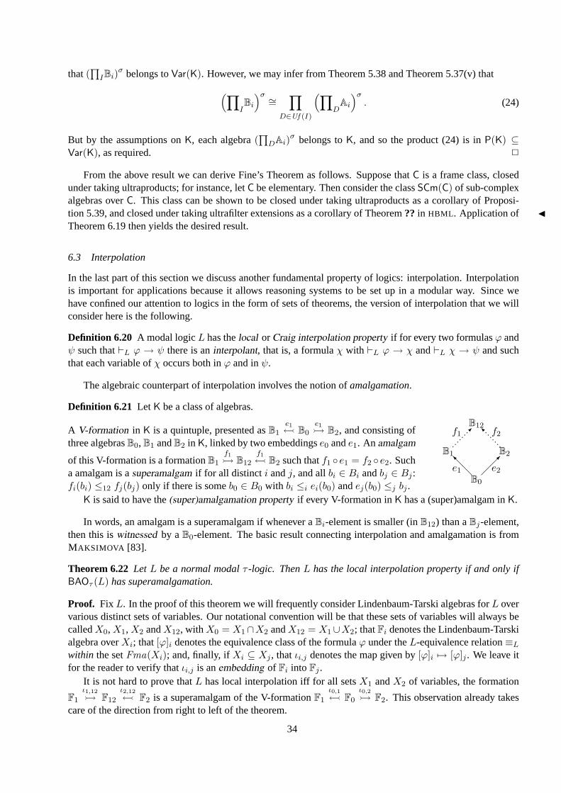
that(∏IBi)

σ belongs toVar(K). However, we may infer from Theorem 5.38 and Theorem 5.37(v) that(∏IBi

)σ ∼= ∏D∈Uf (I)

(∏DAi

)σ. (24)

But by the assumptions onK, each algebra(∏DAi)

σ belongs toK, and so the product (24) is inP(K) ⊆Var(K), as required. 2

From the above result we can derive Fine’s Theorem as follows. Suppose thatC is a frame class, closedunder taking ultraproducts; for instance, letC be elementary. Then consider the classSCm(C) of sub-complexalgebras overC. This class can be shown to be closed under taking ultraproducts as a corollary of Proposi-tion 5.39, and closed under taking ultrafilter extensions as a corollary of Theorem?? in HBML . Application of JTheorem 6.19 then yields the desired result.

6.3 Interpolation

In the last part of this section we discuss another fundamental property of logics: interpolation. Interpolationis important for applications because it allows reasoning systems to be set up in a modular way. Since wehave confined our attention to logics in the form of sets of theorems, the version of interpolation that we willconsider here is the following.

Definition 6.20 A modal logicL has thelocal or Craig interpolation property if for every two formulasϕ andψ such that L ϕ → ψ there is aninterpolant, that is, a formulaχ with `L ϕ → χ and`L χ → ψ and suchthat each variable ofχ occurs both inϕ and inψ.

The algebraic counterpart of interpolation involves the notion ofamalgamation.

Definition 6.21 Let K be a class of algebras.

A V-formation in K is a quintuple, presented asB1e1 B0

e1 B2, and consisting of

three algebrasB0,B1 andB2 in K, linked by two embeddingse0 ande1. An amalgam

of this V-formation is a formationB1

f1 B12

f1 B2 such thatf1 e1 = f2 e2. Such

a amalgam is asuperamalgam if for all distinct i andj, and allbi ∈ Bi andbj ∈ Bj :fi(bi) ≤12 fj(bj) only if there is someb0 ∈ B0 with bi ≤i ei(b0) andej(b0) ≤j bj .

B0

B1 B2

B12

@@I

p p p p p p p p I ppppppppe2e1

f2f1

K is said to have the(super)amalgamation property if every V-formation inK has a (super)amalgam inK.

In words, an amalgam is a superamalgam if whenever aBi-element is smaller (inB12) than aBj-element,then this iswitnessed by aB0-element. The basic result connecting interpolation and amalgamation is fromMAKSIMOVA [83].

Theorem 6.22 LetL be a normal modalτ -logic. ThenL has the local interpolation property if and only ifBAOτ (L) has superamalgamation.

Proof. Fix L. In the proof of this theorem we will frequently consider Lindenbaum-Tarski algebras forL overvarious distinct sets of variables. Our notational convention will be that these sets of variables will always becalledX0,X1,X2 andX12, withX0 = X1∩X2 andX12 = X1∪X2; thatFi denotes the Lindenbaum-Tarskialgebra overXi; that[ϕ]i denotes the equivalence class of the formulaϕ under theL-equivalence relation≡Lwithin the setFma(Xi); and, finally, ifXi ⊆ Xj , thatιi,j denotes the map given by[ϕ]i 7→ [ϕ]j . We leave itfor the reader to verify thatιi,j is anembedding of Fi into Fj .

It is not hard to prove thatL has local interpolation iff for all setsX1 andX2 of variables, the formation

F1

ι1,12

F12

ι2,12

F2 is a superamalgam of the V-formationF1

ι0,1 F0

ι0,2 F2. This observation already takes

care of the direction from right to left of the theorem.

34

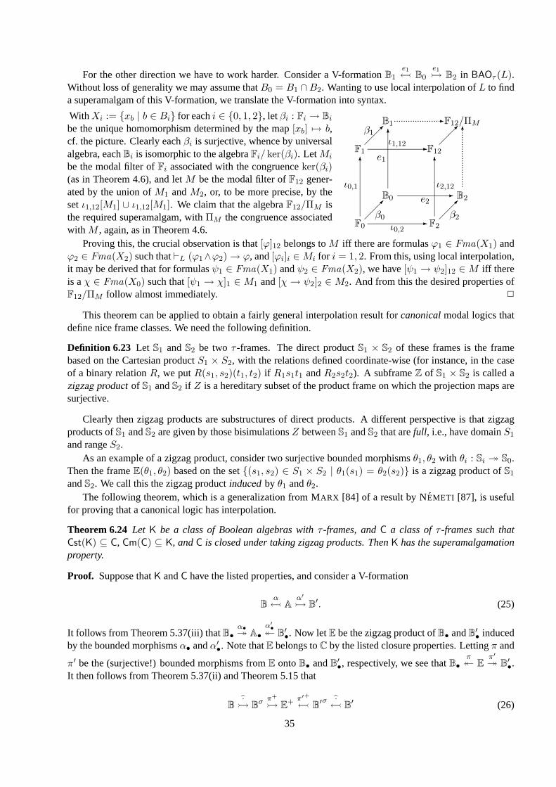
For the other direction we have to work harder. Consider a V-formationB1e1 B0

e1 B2 in BAOτ (L).

Without loss of generality we may assume thatB0 = B1 ∩B2. Wanting to use local interpolation ofL to finda superamalgam of this V-formation, we translate the V-formation into syntax.

WithXi := xb | b ∈ Bi for eachi ∈ 0, 1, 2, letβi : Fi → Bi

be the unique homomorphism determined by the map[xb] 7→ b,cf. the picture. Clearly eachβi is surjective, whence by universalalgebra, eachBi is isomorphic to the algebraFi/ ker(βi). LetMi

be the modal filter ofFi associated with the congruenceker(βi)(as in Theorem 4.6), and letM be the modal filter ofF12 gener-ated by the union ofM1 andM2, or, to be more precise, by thesetι1,12[M1] ∪ ι1,12[M1]. We claim that the algebraF12/ΠM isthe required superamalgam, withΠM the congruence associatedwith M , again, as in Theorem 4.6.

F0

F1

F2

F12

B0

B1

B2

F12/ΠM

6 6

-

-6

-

p p p p p p p p p p p p p p p p p p p p-

ppppppppppppppppppppppppp6

ι0,1

ι0,2

ι2,12

ι1,12

e1

e2

β0

β1

β2

Proving this, the crucial observation is that[ϕ]12 belongs toM iff there are formulasϕ1 ∈ Fma(X1) andϕ2 ∈ Fma(X2) such that L (ϕ1∧ϕ2)→ ϕ, and[ϕi]i ∈Mi for i = 1, 2. From this, using local interpolation,it may be derived that for formulasψ1 ∈ Fma(X1) andψ2 ∈ Fma(X2), we have[ψ1 → ψ2]12 ∈M iff thereis aχ ∈ Fma(X0) such that[ψ1 → χ]1 ∈ M1 and[χ→ ψ2]2 ∈ M2. And from this the desired properties ofF12/ΠM follow almost immediately. 2

This theorem can be applied to obtain a fairly general interpolation result forcanonicalmodal logics thatdefine nice frame classes. We need the following definition.

Definition 6.23 Let S1 andS2 be two τ -frames. The direct productS1 × S2 of these frames is the framebased on the Cartesian productS1 × S2, with the relations defined coordinate-wise (for instance, in the caseof a binary relationR, we putR(s1, s2)(t1, t2) if R1s1t1 andR2s2t2). A subframeZ of S1 × S2 is called azigzag product of S1 andS2 if Z is a hereditary subset of the product frame on which the projection maps aresurjective.

Clearly then zigzag products are substructures of direct products. A different perspective is that zigzagproducts ofS1 andS2 are given by those bisimulationsZ betweenS1 andS2 that arefull, i.e., have domainS1

and rangeS2.As an example of a zigzag product, consider two surjective bounded morphismsθ1, θ2 with θi : Si S0.

Then the frameE(θ1, θ2) based on the set(s1, s2) ∈ S1 × S2 | θ1(s1) = θ2(s2) is a zigzag product ofS1

andS2. We call this the zigzag productinduced by θ1 andθ2.The following theorem, which is a generalization from MARX [84] of a result by NEMETI [87], is useful

for proving that a canonical logic has interpolation.

Theorem 6.24 Let K be a class of Boolean algebras withτ -frames, andC a class ofτ -frames such thatCst(K) ⊆ C, Cm(C) ⊆ K, andC is closed under taking zigzag products. ThenK has the superamalgamationproperty.

Proof. Suppose thatK andC have the listed properties, and consider a V-formation

B

α A

α′

B′. (25)

It follows from Theorem 5.37(iii) thatB•α• A•

α′• B

′•. Now letE be the zigzag product ofB• andB′• induced

by the bounded morphismsα• andα′•. Note thatE belongs toC by the listed closure properties. Lettingπ and

π′ be the (surjective!) bounded morphisms fromE ontoB• andB′•, respectively, we see thatB•π E

π′

B′•.

It then follows from Theorem 5.37(ii) and Theorem 5.15 that

B

· B

σ π+

E+ π′+

B′σ · B

′ (26)

35

We claim that in fact, (26) is a superamalgam of (25), but leave further proof details for the reader. 2

As a corollary of this theorem, suppose thatΓ is a set of canonical formulas defining an elementary frameclass that is closed under taking direct products and substructures — for instance,Γ corresponds to a set ofuniversal Horn sentences. ThenKτ .Γ has Craig interpolation.

Chapter?? of HBML contains more information on interpolation. Related properties, such as Beth defin-Jability, also have algebraic characterizations; for details we refer to HOOGLAND [59].

36

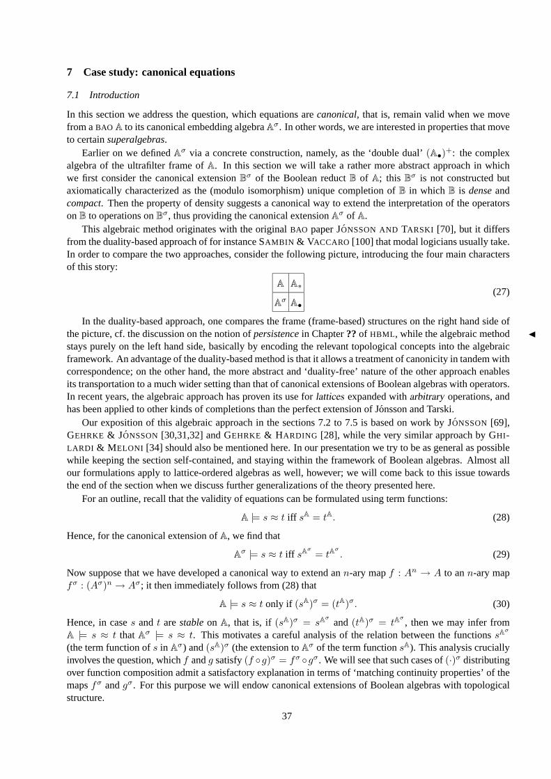
7 Case study: canonical equations

7.1 Introduction

In this section we address the question, which equations arecanonical, that is, remain valid when we movefrom aBAO A to its canonical embedding algebraAσ. In other words, we are interested in properties that moveto certainsuperalgebras.

Earlier on we definedAσ via a concrete construction, namely, as the ‘double dual’(A•)+: the complexalgebra of the ultrafilter frame ofA. In this section we will take a rather more abstract approach in whichwe first consider the canonical extensionBσ of the Boolean reductB of A; this Bσ is not constructed butaxiomatically characterized as the (modulo isomorphism) unique completion ofB in which B is denseandcompact. Then the property of density suggests a canonical way to extend the interpretation of the operatorsonB to operations onBσ, thus providing the canonical extensionAσ of A.

This algebraic method originates with the originalBAO paper JONSSON ANDTARSKI [70], but it differsfrom the duality-based approach of for instance SAMBIN & VACCARO [100] that modal logicians usually take.In order to compare the two approaches, consider the following picture, introducing the four main charactersof this story:

A A∗

AσA•

(27)

In the duality-based approach, one compares the frame (frame-based) structures on the right hand side ofthe picture, cf. the discussion on the notion ofpersistencein Chapter??of HBML , while the algebraic method Jstays purely on the left hand side, basically by encoding the relevant topological concepts into the algebraicframework. An advantage of the duality-based method is that it allows a treatment of canonicity in tandem withcorrespondence; on the other hand, the more abstract and ‘duality-free’ nature of the other approach enablesits transportation to a much wider setting than that of canonical extensions of Boolean algebras with operators.In recent years, the algebraic approach has proven its use forlattices expanded witharbitrary operations, andhas been applied to other kinds of completions than the perfect extension of Jonsson and Tarski.

Our exposition of this algebraic approach in the sections 7.2 to 7.5 is based on work by JONSSON[69],GEHRKE & JONSSON[30,31,32] and GEHRKE & H ARDING [28], while the very similar approach by GHI-LARDI & M ELONI [34] should also be mentioned here. In our presentation we try to be as general as possiblewhile keeping the section self-contained, and staying within the framework of Boolean algebras. Almost allour formulations apply to lattice-ordered algebras as well, however; we will come back to this issue towardsthe end of the section when we discuss further generalizations of the theory presented here.

For an outline, recall that the validity of equations can be formulated using term functions:

A |= s ≈ t iff sA = tA. (28)

Hence, for the canonical extension ofA, we find that

Aσ |= s ≈ t iff sA

σ= tA

σ. (29)

Now suppose that we have developed a canonical way to extend ann-ary mapf : An → A to ann-ary mapfσ : (Aσ)n → Aσ; it then immediately follows from (28) that

A |= s ≈ t only if (sA)σ = (tA)σ. (30)

Hence, in cases and t arestableon A, that is, if (sA)σ = sAσ

and(tA)σ = tAσ, then we may infer from

A |= s ≈ t thatAσ |= s ≈ t. This motivates a careful analysis of the relation between the functionssAσ

(the term function ofs in Aσ) and(sA)σ (the extension toAσ of the term functionsA). This analysis cruciallyinvolves the question, whichf andg satisfy(f g)σ = fσ gσ. We will see that such cases of(·)σ distributingover function composition admit a satisfactory explanation in terms of ‘matching continuity properties’ of themapsfσ andgσ. For this purpose we will endow canonical extensions of Boolean algebras with topologicalstructure.

37

7.2 Canonical extensions of Boolean algebras

In this section we define the canonical extension of a Boolean algebraB as the uniquecompletionof B inwhichB is denseandcompact. We introduce these notions one by one.

A Boolean algebraC is acompletionof a Boolean algebraB if C is complete andB is a subalgebra ofC.If C agrees withB on all meets and joins, then we callC a regular completion ofB, but in general we do notrequire completions to be regular. Thus the notation∨ for finite joins is unambiguous, but not so for infinitejoins. Our convention will be that

∨X always denotes

∨CX, that is, the join taken in the completion.

For an example of a completion, consider a field of setsS = 〈S,A〉 and note that the power set algebraPSis a completion ofS∗.

Before we define the concept of density, we introduce some preliminary notions. Given a completionC

of the Boolean algebraB, we call an elementc ∈ C closed (open) if c is the meet (join, respectively) inC ofelements inB. We letKC(B) andOC(B) denote the collections of closed and open elements, respectively.Objects (such as the elements ofB) that are both closed and open are calledclopen. This terminology is inaccordance with the topological perspective on fields of sets as in Remark 5.21. In the sequel, we may writeKC, K(B), or evenK, instead ofKC(B), if the suppressed details are clear from context; and similarly forthe setOC(B).

We say thatB is meet-dense in C if KC(B) = C, join-dense if OC(B) = C, anddense if KC(OC(B)) =OC(KC(B)) = C. In words,A is dense inC if every element ofC is both a meet of open elements, anda join of closed elements. As a simple example of join-density, note that a Boolean algebra is atomic iff thecollection of atoms forms a join-dense set. Building on this, we leave it as an exercise for the reader to verifythat a field of setsS = 〈S,A〉 is differentiated iffS∗ is dense inPS.

Now we turn to the notion of compactness. Given a completionC of the Boolean algebraB, we say thatB is compact inC if for all setsX andY of closed and open elements, respectively,

∧X ≤

∨Y implies

the existence of finite subsetsX0 ⊆ X, Y0 ⊆ Y such that∧X0 ≤

∨Y0. An alternative (but equivalent)

characterization of compactness is that, for any closedp and openu,

p ≤ u only if p ≤ b ≤ u for someb ∈ B,

as can easily be verified. Also note that, again, our definition of compactness coincides with standard topolog-ical terminology; this easily follows from the observation that for any pairC,U of collections of subsets of asetS, we have

⋂C ⊆

⋃U iff S ⊆

⋃U ∪

⋃∼Sc | c ∈ C.

We are now ready to define canonical extensions.

Definition 7.1 A completionC of the Boolean algebraB is called acanonical extension of B if B is bothcompact and dense inC.

It is in fact a rather strong property for one Boolean algebra to be the canonical extension of another. Tostart with, every Boolean algebra has aunique canonical extension.

Theorem 7.2 LetB be some Boolean algebra. Then

(i) (existence)B has a canonical extension;

(ii) (unicity) Any two canonical extensions ofB are isomorphic via a unique isomorphism that restricts to theidentity onB.

Proof. Recall from the topological duality thatB∗ = 〈Uf B, B〉 is a differentiated and compact field of sets.By the comments made above it should be clear thatP(Uf B) is a canonical extension ofB.

For unicity, suppose thatC is a canonical extension ofB. We leave it as an exercise for the reader to verifythat, by compactness, the mapF 7→

∧F forms a dual (that is, order-reversing) isomorphism between the

lattice 〈Fi(B),⊆〉 and the induced ordering on the setK(B) of closed elements. Its inverse is given by themapp 7→ a ∈ B | a ≥ p. Similarly, there is a dual isomorphism between the lattice of ideals ofB, andthe induced ordering of the open elements. Also, we have forp closed andu open, thatp ≤ u iff there is an

38

a ∈ B with p ≤ a ≤ u, and thatu ≤ p iff a ≤ b for all a andb in A with a ≤ u andp ≤ b. In other words, bycompactnessthe induced poset on the setK ∪ O of closed or open elements is completely determined by theordering ofB. This suffices to prove the theorem, since bydensity, the elements ofC can be identified with thepairs(L,U) of subsets ofC such thatL is the collection of closed lower bounds ofU , andU is the collectionof open upper bounds ofL. Summarizing, we see that together, compactness and density completely fix theorder relation of the canonical extension. 2

The above theorem justifies our speaking of ‘the’ canonical extension of a Boolean algebraB; this algebrawill be denoted asBσ. Furthermore, we need the following facts.

Proposition 7.3 LetC be a canonical extension of the Boolean algebraB. Then

(i) B = K(B) ∩O(B); that is,B coincides with the set of clopen elements ofC;

(ii) the setK(B) forms a sublattice ofC which is closed under taking infinitary meets;

(iii) C is atomic andAtC ⊆ K(B); that is, all atoms are closed.

We leave the proof of this proposition to the reader; note that by Theorem 7.2, it suffices to restrict attentionto the double dualP(Uf B) of B. For instance, part (iii) follows almost immediately from the identification ofatoms ofP(Uf B) with ultrafilters ofB.

As a last introductory remark, we note that canonical extensions interact well with finite products and orderduals. Concerning the latter notion, recall that theorder dual of a Boolean algebraB = 〈B,>,⊥,−,∧,∨〉 isthe structureB∂ = 〈B,⊥,>,−,∨,∧〉. The fact, thatB∂ is a Boolean algebra as well, enables us to shortenquite a lot of definitions and proofs by referring to theprinciple of order duality: Every fact concerningBoolean algebras remains valid after swapping> with ⊥, ∧ with ∨, etc.

Proposition 7.4 LetB1, . . . ,Bn be Boolean algebras. Then

(i) (B1 × · · · × Bn)σ ∼= Bσ1 × · · · × Bσn;

(ii) (B∂)σ ∼= (Bσ)∂ ;

Proof. Both statements can be proved on the basis of Theorem 5.37. As intermediate steps, one can provefacts likeK(B1)× · · · × Bn) = K(B1)× · · · ×K(Bn) andK(B∂) = O(B). 2

7.3 Extending maps to the canonical extension

In the introduction to this section we saw that in order to investigate the canonicity of an equations ≈ t, it isuseful to define extensions of the term functions on aBAO to maps on the canonical extension of theBAO. Butin fact, there are canonical ways to extend anarbitrary map between two Boolean algebrasA andB, to a mapbetweenAσ andBσ. This general definition will be discussed at the end of this section — for the time beingwe will confine ourselves to extensions ofmonotone maps.

The easiest way to understand these definitions is to break them down in two steps. For a start, the definitionof closed and open elements suggests the following extension off : A → B to a mapf defined onK(A) ∪O(A):

f(p) :=∧f(a) | p ≤ a ∈ A for p ∈ K(A),

f(u) :=∨f(a) | u ≥ a ∈ A for u ∈ O(A).

(31)

Note that this is a correct definition becauseK ∩O = A by Proposition 7.3(i), thatf(a) = f(a) for a ∈ A bymonotonicity off , and thatf itself is also order preserving.

Now for the second step of the construction. The fact that every element is both the join of the closedelements below it, and the meet of the opens above it, suggeststwoways to proceed:

fσ(x) :=∨f(p) | x ≥ p ∈ K(A),

fπ(x) :=∧f(u) | x ≤ u ∈ O(A).

(32)

39

The mapsfσ andfπ are called thelower andupper extension of f , respectively.Let us first gather some basic facts concerning these definitions. The following proposition says that the

names ‘lower’, ‘upper’, and ‘extension’ are well chosen.

Proposition 7.5 Letf : A→ B be a monotone map between Boolean algebras. Then

(i) bothfσ andfπ extendf ;

(ii) fσ ≤ fπ, with equality holding on the closed and on the open elements.

Proof. The first statement is immediate by the definitions and the monotonicity off . For the second statement,take, forx ∈ Aσ, a closedp ≤ x and an openu ≥ x. By compactness there is ana ∈ [p, u]∩A. This elementsatisfiesf(p) ≤ f(a) ≤ f(u) by definition off ; hencefσ(x) ≤ fπ(x) by definition offσ andfπ. Finally,for closedp we may derive from the first part of the proposition thatfπ(p) ≤ f(p), and from the monotonicityof f thatf(p) = fσ(p). Thus we obtain the desired equalityfσ = fπ onK. The result for opens follows byorder duality. 2

Maps for which the lower and upper extension coincide are obviously of interest.

Definition 7.6 A monotone mapf between Boolean algebras is calledsmoothif fσ = fπ.

Example 7.7 As a first example of a smooth operation, consider theglobal modalityg on a Boolean algebraB, given byg(⊥) = ⊥ while g(b) = > for b > ⊥, see Definition 8.7. It is easy to see thatg satisfies theseconditions as well, whence it is equally easy to infer that bothgσ andgπ coincide with the global modality ofBσ; smoothness is then immediate. Similarly, one can prove that themeetandjoin operations ofB are smooth,

and that their extensions coincide with the meet and the join ofBσ, respectively.

For an operation that is not smooth, consider the composition of the global modality with the meet opera-tion, i.e., the mapf : B2 → B given byf(a, b) = ⊥ if a ∧ b = ⊥, while f(a, b) = > otherwise. Now ifBis infinite, thenBσ must contain some elementc which is closed but not open; a straightforward verificationshows that for such ac, we have thatfσ(c,−c) = ⊥, whilefπ(c,−c) = >. This shows that not even operatorsare smooth.

While it may not be the case that the lower and the upper extension agree in all cases, both kinds ofextensions generally display good behavior; often they even improve on the original map. For the definitionsof the notions mentioned in the theorem below, see Definition 3.11 and 5.1.

Proposition 7.8 Letf : A→ B be a map between Boolean algebras. Then

(i) if f is monotone then so isfσ;

(ii) if f is an operator thenfσ is a complete operator;

(iii) if f is additive or multiplicative thenf is smooth.

Proof. The proof of the first statement is easy and hence omitted, while we postpone the proof of the last state-ment (it is in fact a rather straightforward consequence of the Propositions 7.13 and 7.14). For the remainingpart, we need to show that iff is normal and additive in each coordinate, thenfσ is normal and completelyadditive in each coordinate. Leaving the easy proof for normality as an exercise for the reader, concerningadditivity, we will prove that iff : A0 ×A1 → B is additive in its first coordinate and monotone in its second,thenfσ preserves all non-empty joins in its first coordinate.

Fix elementsx0 ∈ Aσ0 andx1 ∈ Aσ1 . By atomicity ofBσ, and monotonicity offσ, it suffices to prove, foran arbitrary atomp of Bσ:

p ≤ fσ(x0, x1) only if there is aq ∈ At0 with p ≤ fσ(q, x1), (33)

whereAt0 denotes the set of atoms inAσ0 belowx0. Note that sincefσ(x0, x1) =∨fσ(c0, c1) | xi ≥ ci ∈

K(Ai) we may safely assume that bothx0 andx1 are closed.

40

Now suppose for contradiction that (33) fails. Then for some atomp of Bσ we havep ≤ fσ(x0, x1)while for eachq ∈ At0 there are, by definition offσ, elementsaq,0 ∈ A0 aboveq andaq,1 ∈ A1 abovex1,such thatp 6≤ fσ(aq,0, aq,1). It follows thatx0 =

∨At0 ≤

∨aq,0 | q ∈ At0, whence by compactness

x0 ≤∨aq,0 | q ∈ F for somefinitesetF ⊆ At0.

Now observe that the joina0 =∨aq,0 | q ∈ F is inA0, and the meeta1 =

∧aq,1 | q ∈ F is inA1.

Clearly p 6≤ fσ(aq,0, a1) for eachq ∈ F ; sincep is an atom this meansp 6≤∨fσ(aq,0, a1) | q ∈ F =

f(a0, a1), where in the last identity we use the additivity off in its first coordinate.On the other hand, fromx0 ≤ a0 andx1 ≤ a1 it follows that fσ(x0, x1) ≤ f(a0, a1) which gives the

desired contradiction. 2

In the proof above we already used the fact that complete additivity offσ means that it is completelydetermined by its values on theatomsof Bσ. Now recall that (in the concrete representation of)B

σ, the atomsare nothing but theultrafiltersof B. From this the following proposition is immediate.

Proposition 7.9 LetA be some Boolean algebra withτ -operators with underlying Boolean algebraB. ThenAσ := (A•)+ is isomorphic to the algebraBσ expanded with the family(∇A)σ | ∇ ∈ τ of complete

operators.

This proposition, which can be summarized as ‘∇Aσ = (∇A)σ ’, will be used throughout the sequel, butalways implicitly.

7.4 Composite maps

We now investigate the interaction between composing maps between Boolean algebras and taking their canon-ical extensions. That is, we will take a look at the relation between the maps(gf)σ and gσfσ for mapsf : A→ A

′, andg : A′ → A′′. We are obviously eager to find cases in which we have(gf)σ = gσfσ, but also

conditions under which one of the inequalities (≤ or ≥) apply will turn out to be of interest. As we will seeshortly, many of these conditions can naturally be described intopologicalterms.

For this purpose, we will introduce no less than six topologies on each setAσ. Fortunately, these topologiescan be neatly organized in two families, each consisting of an upper, a lower and a join topology. As aterminological convention, let us call a map between the algebrasA

σ andBσ (ρ, ρ′)-continuous, if it is acontinuous function between the topological spaces〈Aσ, ρ〉 and〈Bσ, ρ′〉.

The first family is that of the Scott topologies. Although these can already be defined on arbitrary partialorders, here we will only consider topologies on canonical extensions ofBAOs. Recall that a subsetD of apartial order is calledup-directed, if every pair of elements ofD has an upper bound inD.

Definition 7.10 Given a Boolean algebraB, call a subsetU of Bσ Scott open if U is an up-set such thatU ∩D 6= ∅ for every up-directed setD with

∨D ∈ U . TheScott topology is defined as the collectionγ↑ of

Scott open sets; the topologyγ↓ is given by the principle of order duality, and we defineγ := U ∩ V | U ∈γ↑, V ∈ γ↓ as the join ofγ↑ andγ↓ in the lattice of topologies overB.

In practice it is sometimes easier to work with theclosedsets in the Scott topology; these are preciselythe down-sets ofC that are closed under taking up-directed unions. From this observation one easily derivesthe (well-known) fact that a map between partial orders is Scott continuous (that is,(γ↑, γ↑)-continuous) iff itpreserves up-directed joins. But this implies that a map is completely additive iff it is both additive and Scottcontinuous, which may help to explain the relevance of the Scott topologies for our purposes.

We now turn to the second family of topologies. Recall from Example 4.4 that for an arbitrary elementbof a Boolean algebraB, the setsb↑ andb↓ are defined asb↑ = a ∈ B | b ≤ a andb↓ = a ∈ B | a ≤ b.

Proposition 7.11 For any Boolean algebraB, the setsσ↑ := p↑ | p ∈ K andσ↓ := u↓ | u ∈ O bothform a topology onAσ; and so does the setσ := p↑∩ u↓ | K 3 p ≤ u ∈ O, which is in fact identical to thejoin σ↑ ∨ σ↓ in the lattice of topologies onAσ.

In the sequel, we will write[p, u] for theinterval betweenp andu, that is,[p, u] = p↑ ∩ u↓.

41

Proof. The fact thatσ↑ is a topology follows from the fact that the setK(A) is closed under finitary joins andarbitrary meets ofAσ, see Proposition 7.3(ii). 2

Remark 7.12 As suggested by notation, the topologyσ is closely connected to the kind of inclusion ofB inBσ. Let us just mention a couple of salient facts here. First, it is easy to see that the set[a, b] | a, b ∈ B is a

basisfor σ. This reveals that the setB is topologicallydensein σ, in the sense that everyσ-open set containsan element ofB. But also,B constitutes the collection ofisolated pointsof σ — recall that a pointx is isolatedin a topology if the singletonx is open. It is the latter two properties that make it possible to extend arbitrarymaps between Boolean algebras to their extensions; we will come back to this at the end of this section.

The following proposition, which links the two topological families, will be crucial when it comes tofinding the ‘matching continuities’ mentioned in the introduction.

Proposition 7.13 LetA be a Boolean algebra. Thenγ↑ ⊆ σ↑, γ↓ ⊆ σ↓ andγ ⊆ σ.

Proof. Confining ourselves to the first claim, it suffices to prove thatU =⋃p↑ | p ∈ U ∩K for an arbitrary

Scott open setU ⊆ Aσ. The crucial observation here is that everyu ∈ U is theup-directedjoin of the closedelements below it. Further proof details are left to the reader. 2

The following proposition is a first sign that these topologies can be useful.

Proposition 7.14 Letf : A→ B be a monotone map between the Boolean algebrasA andB. Then

(i) fσ is the largest monotone(σ, γ↑)-continuous extension off ;

(ii) f is smooth ifffσ is (σ, γ)-continuous;

(iii) if f is an operator thenfσ is (γ↑, γ↑)-continuous;

(iv) if f is additive thenfσ is (σ↓, σ↓)-continuous.

(v) if f is multiplicative thenfσ is (σ↑, σ↑)-continuous.

Proof. Concerning the first part of the proposition, we already know from Proposition 7.5 thatfσ is anextension off . Now for x ∈ Aσ take an arbitrary Scott open setV ⊆ Bσ with fσ(x) ∈ V . That is,∨fσ(p) | x ≥ p ∈ K(A) ∈ V . Now it is easy to see that the collectionQ := fσ(p) | x ≥ p ∈ K(A) is

up-directed, soQ∩V 6= ∅. In other words, there is a closedp ≤ x with fσ(p) ∈ V . But then by monotonicityof fσ we have thatfσ[p↑] ⊆ V . Sincex ∈ p↑ ∈ σ this suffices to prove thatfσ is (σ, γ↑)-continuous, whileby Proposition 7.8 it is monotone.

In order to show thatf is the largest such map, take a monotone(σ, γ↑)-continuous extensiong : Aσ → Bσ

of f , and suppose for contradiction thatg(x) 6≤ fσ(x) for somex ∈ Aσ. By atomicity ofBσ there must beanatomp of Bσ which lies belowg(x), but not belowfσ(x). Becauseg(x) ∈ p↑ ∈ γ↑, the continuity ofgprovides us with ac ∈ K such thatc ≤ x andg[c↑] ⊆ p↑. In other words, we find thatp ≤ g(c) whenceby monotonicity it follows thatp ≤ g(a) for all a ∈ A abovec. But then by the fact thatg extendsf , andthe definition offσ, we may infer thatp ≤ fσ(c). From this we obtain, as the required contradiction, thatp ≤ fσ(x).

For part (ii), it follows from part (i) by order duality thatfπ is the smallest monotone(σ, γ↓)-continuousextension off . Hence iff is smooth, thenfσ = fπ is both(σ, γ↑)- and(σ, γ↓)-continuous, and hence,(σ, γ)-continuous. Conversely, iffσ is (σ, γ)-continuous, then it is, a fortiori,(σ, γ↓)-continuous. This implies, againby the order dual of part (i), thatfπ ≤ fσ; but then we have equality because of Proposition 7.5(ii).

Concerning part (iii), iff : An → A is an operator then by Proposition 7.8(ii),fσ : (Aσ)n → Aσ is

additive in each coordinate. From this it is straightforward to derive thatfσ preserves up-directed joins.For part (iv), suppose thatf : A → B is additive, and take an arbitraryσ↓-open subsetu↓ of Bσ, that is,

u ∈ O(B). It follows by Proposition 7.8(ii) thatfσ preserves all non-empty joins. From this one may derivethat the set(fσ)−1[u↓] is either empty, in which case it certainly belongs toσ, or else it is of the formv↓,wherev =

∨(fσ)−1[u↓] satisfiesfσ(v) = u. In order to show thatv↓ is open inσ, it suffices to prove thatv

is an open element ofAσ.

42

Consider an arbitrary closed elementp ≤ v; then∧f [p↑ ∩ A] = fσ(p) ≤ fσ(v) = u. Hence by

compactness there is a finite setF ⊆ p↑ ∩ A such that∧f [F ] ≤ u. Puttingap :=

∧F we find thatap ∈ A,

p ≤ ap andap ≤ v sincef(ap) ≤∧f [F ]. Clearly thenv =

∨p | v ≥ p ∈ K ≤

∨ap | v ≥ p ∈ K ≤ v

which shows thatv is identicalto the second join, and hence, open.Finally, part (v) follows from part (iv) by order duality. 2

As we announced already in the introduction to this section, the following properties will be crucial inproving canonicity results further on. The reason for this lies in the observation that for some termst, we mayapply Proposition 7.15(ii) by the fact that the term functiontA

σin the canonical extensionAσ can be decom-

posed astAσ

= gσ fσ wheregσ is (τ, γ↑)-continuous andfσ is (σ, τ)-continuous, for some ‘intermediate’topologyτ . This is the principle ofmatching continuitiesthat we mentioned in the introduction.

Proposition 7.15 Let f : A→ B andg : B→ C be monotone maps between the Boolean algebrasA, B andC. Then

(i) (gf)σ ≤ gσfσ;

(ii) (gf)σ ≥ gσfσ whenevergσfσ is (σ, γ↑)-continuous.

Proof. Part (ii) of the proposition is an immediate consequence of Proposition 7.14(i) sincegσfσ is an exten-sion ofgf (andgf is monotone). Concerning part (i), we first show that(gf)σ(p) ≤ gσfσ(p) for closedp.Note that

(gf)σ(p) =∧gf(a) | p ≤ a ∈ A,

gσfσ(p) =∧g(b) | fσ(p) ≤ b ∈ B.

where the latter identity holds becausefσ(p) is closed inAσ. Now take ab ∈ B with fσ(p) ≤ b. Asfσ(p) =

∧f(a) | p ≤ a ∈ A is a down-directed meet, compactness provides somea ∈ A with p ≤ a and

f(a) ≤ b. Then(gf)σ(p) ≤ gf(a) ≤ gb; and hence,(gf)σ(p) ≤ gσfσ(p).Now we turn to arbitraryx ∈ Aσ. Note that

(gf)σ(x) =∨(gf)σ(p) | x ≥ p ∈ K(A),

gσfσ(x) =∨gσ(q) | fσ(x) ≥ q ∈ K(B).

Take an arbitraryp ∈ K(A) with p ≤ x; then(gf)σ(p) ≤ gσfσ(p), as we just saw. Sincefσ(x) ≥ fσ(p) ∈K(B), this shows that every joinand(gf)σ(p) of (gf)σ(x) is below some joinandgσ(q) of gσfσ(x). Thissuffices to prove the desired inequality. 2

7.5 Canonical equations

Time to harvest. The key idea for proving canonicity results for an equations ≈ t will be to use propertiesof the term functionssA and tA. Recall that for a termt(x1, . . . , xn), the term functiontA : An → A isinductively defined as follows:

xAi := πni ,

(♥(t1, . . . , tn))A :=♥A 〈tA1 , . . . , tAn〉.whereπni : (a1, . . . , an) 7→ ai is thei-th projection function, and, for mapsf1, . . . , fn : X → Y , the map〈f1, . . . , fn〉 : X → Y n is given by〈f1, . . . , fn〉(x) = (f1(x), . . . , fn(x)).

In the context of canonical extensions the following definitions are crucial.

Definition 7.16 A term t is expandingon an expanded Boolean algebraA if (tA)σ ≤ tAσ, contracting if

(tA)σ ≥ tAσ , andstableif (tA)σ = tAσ. We let these properties apply to classes of algebras in case they apply

to all members of the class.

Proposition 7.17 Lets andt be twoτ -terms, andK a class ofτ -expanded Boolean algebras. Ifs is contract-ing andt is expanding onK, then the inequalitys t is canonical onK.

43

Proof. Consider an algebraA in K such thatA |= s t. In other words, we havesA ≤ tA, so that(sA)σ ≤(tA)σ. But then by the assumptions ons andt it follows thatsA

σ ≤ (sA)σ ≤ (tA)σ ≤ tAσ, which shows that

Aσ |= s t. 2

So which terms are contracting, and which ones are expanding? Here the topologies prove their value.Before moving on to these results, we need to get one technicality out of the way. Basically, the followingproposition states that the product map〈f1, . . . , fn〉 behaves as well as one could hope for.

Proposition 7.18 Letf1,. . . ,fn be monotone maps between the Boolean algebrasA andB. Then

〈f1, . . . , fn〉σ = 〈fσ1 , . . . , fσn 〉,

and for allρ, ρ′ ∈ γ↓, γ↑, γ, σ↓, σ↑, σ it holds that

〈f1, . . . , fn〉σ is (ρ, ρ′)-continuous iff eachfσi is (ρ, ρ′)-continuous.

We leave the rather tedious but not very difficult proof of this proposition to the reader, and move on tomore interesting facts. First we associate topological properties with term functions.

Proposition 7.19 LetA be aτ -expanded Boolean algebra, andt a τ -term. Then

(i) If A interprets all connectives int as operators, thentAσ

is (γ↑, γ↑)-continuous.

(ii) If A interprets all connectives int as additive maps, thentAσ

is (σ↓, σ↓)-continuous.

(iii) If A interprets all connectives int as multiplicative maps, thentAσ

is (σ↑, σ↑)-continuous.

Proof. All three statements can be proved by a straightforward term induction, using the Propositions 7.14and 7.18 for the induction step. For the induction base, note that the projection maps are both join- and meetpreserving, and hence, their canonical extensions have all the continuity properties mentioned in the statementsof this proposition. 2

Here we arrive at the core of the algebraic approach towards the canonicity of equations. On the basis ofthe syntactic shape of some terms we can see whether it is expanding or stable. In Theorem 7.20 we give somesample results; observe that the key idea in the proof of part (iii) is the principle of ‘matching continuities’ asdescribed before Proposition 7.15.

Theorem 7.20 LetA be aτ -expanded Boolean algebra, andt a τ -term. Then

(i) If A interprets all connectives int as monotone maps, thent is expanding.

(ii) If A interprets all connectives int as operators or dual operators, thent is stable.

(iii) If t is of the forms(u1, . . . , un) such thatA interprets all connectives ins as operators, and all connec-tives in each of theui as meet-preserving operations, thent is stable.

Proof. Part (i) is proved by term induction. The base case is immediate from the definitions. For the inductivestep, suppose thatt ≡ ∇(t1, . . . , tn), then

(tA)σ = (∇A 〈tA1 , . . . , tAn〉)σ

≤ (∇A)σ 〈tA1 , . . . , tAn〉σ

= ∇Aσ 〈(tA1 )σ, . . . , (tAn)σ〉

≤ ∇Aσ 〈tAσ1 , . . . , tAσ

n 〉

= tAσ.

Here the first and last step are by definition, the second step is by Proposition 7.15(i) and monotonicity,the third step is by definition of∇Aσ = (∇A)σ and by Proposition 7.18, and the fourth step is by the inductivehypothesis and the monotonicity of∇Aσ .

44

For part (ii) and (iii) it suffices to prove thattAσ ≤ (tA)σ, since the opposite inequality holds by part (i). In

the case of part (ii) this follows from a straightforward induction, whereas for part (iii) we need the principleof matching topologies.

Let t be as described in part (iii), thentAσ

= sAσ 〈uAσ1 , . . . , uA

σ

n 〉 = (sA)σ 〈(uA1 )σ, . . . , (uAn)σ〉with the second identity holding by part (ii). Also, note that by Proposition 7.14, the term functionsA

σis

(γ↑, γ↑)-continuous, and eachuAσ

i is (σ↑, σ↑)-continuous. From this we infer by Proposition 7.18 that themap〈(uA1 )σ, . . . , (uAn)σ〉 = 〈uA1 , . . . , uAn〉σ is (σ↑, σ↑)-continuous as well, whence byγ↑ ⊆ σ↑ it is (σ↑, γ↑)-continuous. Thus the(γ↑, γ↑)-continuity of sA

σmatcheswith the (σ↑, γ↑)-continuity of 〈uA1 , . . . , uAn〉σ.

Hence, we may apply Proposition 7.15(ii), and find thattAσ

= (sA)σ〈uA1 , . . . , uAn〉σ ≤ (sA〈uA1 , . . . , uAn〉)σ =(tA)σ, as desired. 2

As a sample application, we show how Sahlqvist canonicity is an easy consequence of the previous theo-rem.

Corollary 7.21 Sahlqvist equations are canonical over the class of all Boolean algebras withτ -operators.

Proof. First we treat inequalities of the formϕ(β1, . . . , βn) ≤ ψ, whereϕ only uses∧, ∨ and modalities, allβi are boxed atoms, andψ is positive. But then it is immediate by the previous proposition thatϕ(β1, . . . , βn)is stable, whileψ is expanding. Hence the result follows from Proposition 7.17.

Now consider an arbitrary Sahlqvist inequality. Without loss of generality we may assume that it is in factan equation of the form

ϕ(β1, . . . , βn,¬ψ1, . . . ,¬ψk) ≈ ⊥, (34)

whereϕ and theβ’s are as before, while allψj are positive formulas. It is easy to see that this equation isequivalent to the quasi-equation(

&1≤i≤n

xi ≤ ¬ψi)⇒ ϕ(β1, . . . , βn, x1, . . . , xk) ≈ ⊥,

which in its turn is equivalent to(&

1≤i≤nxi ∧ ψi ≈ ⊥

)⇒ ϕ(β1, . . . , βn, x1, . . . , xk) ≈ ⊥. (35)

Now suppose that weadda diamondE to the language, and interpret this diamond as the global modality onevery algebra (see section 8.2). Then clearly the quasi-equation (35) is equivalent to the formula

ϕ(β1, . . . , βn, x1, . . . , xk) ∨

1≤i≤nE(xi ∧ ψi). (36)

(Note that this reduction of a quasi-equation to an equivalent equation is a specific example of Proposi-tion 8.14.)

The result then follows by the observation that (36) is a Sahlqvist inequality of the kind already treated,together with the fact that the canonical extension of the global modality is again the global modality (seeRemark 7.7). 2

7.6 Further remarks

The ideas described in this section allow for variations and generalizations in at least two directions.To start with, the algebraic approach has already been put to work for a far wider class of structures than

just Boolean algebras with operators. In particular, nothing in the theory crucially depends on theBooleannature of the underlying order of the algebras. The notion of a canonical extension, with all the results insection 7.2 pertaining to them, has been extended to (first distributive and then) arbitrary lattices, with workon partial orders under way.

45

Furthermore, the restriction to monotone operations is not necessary either;arbitrary maps between latticescan be extended to maps between their canonical extensions. First suppose that we are dealing with a densesetX ′ in a topology〈X, ρ〉, and letf : X ′ → C be a map fromX ′ to the carrierC of a complete latticeC.Then define

fσ(x) :=∨∧f [U ∩X ′] | x ∈ U ∈ ρ,

fπ(x) :=∧∨f [U ∩X ′] | x ∈ U ∈ ρ.

(37)

In order to apply this definition for the canonical extension of a mapf between two latticesL andM, notethat (just like in the case for Boolean algebras, see Remark 7.12) the carrierL of L forms a dense subset of theσ-topology over the carrierLσ. Also observe thatfσ andfπ areextensionsof f because all elements ofL areisolatedpoints off , and that formonotonef , (37) agrees with (32).

Finally, it is not just the definitions that translate to the more general setting of lattice expansions (thatis, lattices with additional operations), the same holds for the theory. To mention just one example: onemay prove that any equations ≈ t is canonical provided that all the primitive symbols (including the joinoperation∧) occurring ins andt are interpreted as operators. Details can be found in for instance GEHRKE &HARDING [28].

The second generalization that we want to mention involves other ways of completing lattices and latticeexpansions, such as theMacNeille completion, which generalizes Dedekind’s construction of the reals from therationals to arbitrary partial orders. For a characterization in the style of this section, one may start by provingthat any latticeL has a (modulo isomorphism) unique completionLµ, its MacNeille completion, in whichL is both join- and meet dense. This way of extending lattices is obviously similar to that of the canonicalextension, but a substantial difference is that the MacNeille completion agrees with the original lattices onallmeets and joins, whereas the canonical extension only agrees on thefiniteones.

In any case, it follows from join- and meet density, that any map between two lattices can be extended to amap between their MacNeille completions, in two ways. In the case of amonotoneoperationf between twolatticesL andM, we define thelower extension f and theupper extension f by

f(x) :=∨f(a) | x ≥ a ∈ L

f(x) :=∧f(a) | x ≤ a ∈ L

Clearly then, almost all questions concerning canonical extensions have an obvious counterpart for MacNeillecompletions. Generally speaking, MacNeille completions are less well-behaved than canonical extensions; forinstances, unary operators (diamonds) are no longer smooth, and the variety of modal algebras is not closedunder taking lower MacNeille completions. Probably for this reason, MONK [85] introduced the notion of theMacNeille completion of aBAO only for Boolean algebras withcompleteoperators. On the other hand, in casethe primitive operations areresiduated (see Proposition 8.5), the situation improves; for instance, GIVANT &VENEMA [36] show that the validity of all Sahlqvist equations is preserved under taking MacNeille comple-tions oftensealgebras. As a final remark, there are interesting connections between the MacNeille completionand the canonical extension of a lattice expansion: for instance, GEHRKE, HARDING & V ENEMA [29] provethat the canonical extension of lattice expansionA can be embedded in the MacNeille completion of someultrapower ofA. As a consequence, every variety of lattice expansions that is closed under taking MacNeillecompletions, is also canonical in the sense of canonical extensions.

46

8 Special algebraic topics

In this final section on algebra we discuss the algebraic perspective on two further issues in modal logic.

8.1 Tense logic

Our first example concernstense logic; as its name already indicates, this branch of modal logic originates inthe formal semantics of natural language, cf. Chapter??of HBML . J

Definition 8.1 The modal similarity typeϑ of tense logic is fixed by its two diamonds,3F and3P .

The letters3F and3P are mnemonic offuture andpast, respectively. This already indicates that thestandard interpretation of this language is in frames representing a flow of time, such that3F obtains themeaning ‘sometime in the future’, and dually3P means ‘sometime in the past’. Tense logic thus forms a rathersimple example oftemporallogic, cf. Chapter??of HBML . Here we abstract from the temporal interpretationsJof tense logics; what is then left is that in the intended frames for this language, the two diamonds of thelanguage are interpreted along the two directions of asinglebinary relation.

Definition 8.2 A ϑ-frameS = 〈S,RF , RP 〉 is calledbidirectional if RF andRP are each other’s converse.

This definition explains why aϑ-frame is often represented simply as the pair〈S,RF 〉. Turning to logic,we define the following.

Definition 8.3 A modal ϑ-logic L is a tense logic if both formulasp → 2F3P p andp → 2P3F p aretheorems ofL; the minimal tense logic is denoted asKt. Algebraically, atense algebra is a Boolean algebraexpanded with monotoneϑ-operations satisfying the corresponding equationsx 2F3Px andx 2P3Fx.

It is easy to see thatS+ is a tense algebra if and only ifS is a bidirectional frame. In the other direction,it is not a priori clear whether we can extract a useful frame from an arbitrary tense algebra: First we mustshow that tense algebras are Boolean algebras with operators. In fact, already JONSSON& TARSKI [70] showsomething better.

Theorem 8.4 LetA = A = 〈A,>,⊥,−,∧,∨,3F ,3P 〉 be a tense algebra. Then

(i) the operations3F and3P are complete operators;

(ii) the structureA• is a bidirectional frame, and the algebraAσ is again a tense algebra.

Proof. For part i of the Theorem, leta ∈ A be the least upper bound of some subsetX of A. Then bymonotonicity,3Fa is an upper bound of the set3F [X]. Now suppose thatb is also an upper bound of this set,that is,3Fx ≤ b for all x ∈ X. From this it follows, for eachx ∈ X, thatx ≤ 2P3Fx ≤ 2P b (here we usemonotonicity of2P , which is easily proven). Thus we see thata ≤ 2P b by our assumption ona. But thenby monotonicity of3F we obtain that3Fa ≤ 3F2P b ≤ b. This proves that3Fa is in fact the least upperbound of the set3F [X].

Concerning the second part of the theorem, thatAσ is a tense algebra is a special of the Sahlqvist Canonicity

Theorem 6.14; the bidirectionality ofA• is then immediate sinceAσ = (A•)+. 2

There is a lot more to say about the complete additivity of the diamonds in tense algebras. To start with,the definition of tense algebras can be reformulated using either of the algebraically more familiar notions ofconjugationor residuation.

Proposition 8.5 LetA = 〈A,>,⊥,−,∧,∨,3F ,3P 〉 be a monotoneϑ-expanded Boolean algebra. Then thefollowing are equivalent:

(i) A is a tense algebra,

(ii) 3F and3P are conjugated operations, that is, they satisfy the following:

A |= ∀xy (x ∧3F y ≈ ⊥ ⇔ y ∧3Px ≈ ⊥), (38)

47

(iii) 3F and2P form a residual pair, that is,

A |= ∀xy (3Fx y ⇔ x 2P y). (39)

This connection with residuation shows that from a general mathematical perspective, tense logic is not justany bimodal logic: It provides the modal logic manifestation of the fundamental category theoretic conceptof adjoint functors. Theorem 8.4(i) is thus a rather special case of the category theoretic fact that left adjointfunctors preserve all (existing) colimits.

Another nice property of tense logic that should be mentioned here is that somehow, tense algebras arericher than ordinary Boolean algebras with operators. For instance, consider an atomic modal algebraA,and suppose thatA satisfies some Sahlqvist equationη. Then it isnot guaranteed that the atom structureA•(see Definition 5.2) satisfies the first-order correspondentcη of η, not even if the diamond ofA is completelyadditive. However, in caseA is atense algebra, it contains sufficient information to enforce this.

Theorem 8.6 LetA be anatomictense algebra. Then for every Sahlqvist equationη: A |= η iff A+ |= cη iff(A•)+ |= η.

Proof. Clearly, the equivalence of the last two statements follows from Sahlqvist correspondence theory. Forthe implication from right to left, it suffices to observe thatA is a subalgebra of(A•)+ because of the completeadditivity of the operators. This follows from (12) in the proof of Proposition 5.3.

The remaining implication is a special case of the preservation of Sahlqvist equations under taking (lower)MacNeille completions of tense algebras, see the end of section 7 for some discussion, and GIVANT & V EN-EMA [36] for proofs. 2

Finally, tense algebras play a role in other part of universal algebra as well. For instance, anylattice canbe represented as the sublattice of a tense algebra that has the solution set of the equationx ≈ 2P3Fxas its carrier. This idea basically goes back to BIRKHOFF [12]; for more details, the reader is referred toHARDING [56].

Nevertheless, despite their rather special characteristics, just like all bimodal logics, tense logics can besimulatedby monomodal ones; for details we refer to Chapter??of HBML . J

8.2 Global modality & discriminator varieties

Recent years have witnessed an increasing interest in formalisms that enhance the expressive power of standardmodal languages, see for instance Chapter??of HBML . In such a pursuit, one naturally arrives at theglobal or Juniversal modalityE which has the global relationS × S of a frameS as its (intended) accessibility relation,see GORANKO & PASSY [48]. But also, a large number of standard logics come with an intended semanticsin which the global relation interprets some more complex term of the language: as an example we mentionthe compound modality3F3P in the tense logic over any linear flow of time.

Definition 8.7 Algebraically, we define theglobal modality or unary discriminator over a Boolean algebra(with operators)B as the function given by

b 7→

⊥ if b = ⊥,

> if b > ⊥.

The termγ(x) is called aglobal modality or unary discriminator term over an expanded Boolean algebraA ifit is interpreted as the global modality onA.

This notion can be seen as theBAO manifestation of the well-known algebraic concept of adiscriminator,see JIPSEN [67] for a first explicit discussion of the connections.

Definition 8.8 We call a ternary termd a discriminator term over an algebraA if it is interpreted as thediscriminator function onA, that is, ifdA(a, b, c) = a if a 6= b, anddA(a, b, c) = c if a = b. Any varietyVgenerated by a class of algebras with a common discriminator term, is called adiscriminator variety.

48

Proposition 8.9 LetA be aτ -expanded Boolean algebra.

(i) If γ is a global modality forA, then the term(γ(¬(x↔ y))∧x)∨ (γ(¬(x↔ y))∧ z) is a discriminatorterm forA.

(ii) If d(x, y, z) is a discriminator term forA, then the term¬d(⊥, x,>) is a global modality forA.

Before going into further detail of the connection with the global modality, let us, for future reference, listsome of the many nice properties that discriminator varieties have.

Theorem 8.10 Let K be a class of algebras with a discriminator termd. Then

(i) all algebras inK are simple;

(ii) Var(K) is congruence-distributive and congruence-permutable;

(iii) all subdirectly irreducible algebras inVar(K) are simple, and vice versa;

(iv) Var(K) is semi-simple; that is, every algebra inVar(K) is a subdirect product of simple algebras.

(v) d is a discriminator term for every simple algebra inVar(K).

Proof. For the first statement of the theorem, define the terms(x, y, u, v) := d(d(x, y, u), d(x, y, v), v). It iseasy to see thats is a so-calledswitching term for K; that is, for everyA in K, and for alla, b, c andd in A:

sA(a, b, c, d) =

c if a = b,

d if a 6= b.

Now let Θ 6= ∆A be a congruence ofA; then there are two elementsa 6= b with (a, b) ∈ Θ. But then we find(c, d) = (sA(a, a, c, d), sA(a, b, c, d)) ∈ Θ for everyc andd in Θ. In other words, such aΘ must be the trivialcongruenceA×A. But this clearly means thatA is simple. Details of the proof of the second statement, whichis similar to that of Theorem 4.2, are left to the reader.

For the third part of the theorem, it is not hard to verify thatd is a discriminator term forSPu(K) aswell, whenceSPu(K) consists of simple algebras by part (i). So by definition of simplicity, we find thatHSPu(K) = SPu(K); hence, all algebras inHSPu(K) are simple. However, by part ii we may apply Jonsson’sLemma, which states that all s.i. members ofVar(K) belong toHSPu(K). Thus every s.i. algebra inVar(K) issimple.

Part (iv) is immediate from part (iii) by Birkhoff’s subdirect indecomposability theorem, while the finalstatement follows from the fact that every simple algebra belongs toSPu(K), and thus shares the discriminatorterm ofK. 2

In particular, since the notions of simplicity and subdirect irreducibility coincide in a discriminator vari-ety, its subvarieties are completely determined by its simple members. Let us now see how these issues areaxiomatized in normal modal logics.

Definition 8.11 A τ -formulaγ(x) is aglobal modality for a normal modalτ -logicL if the formulasΓ

• ∇(x1, . . . , xn)→ γ(xi) for every∇ ∈ τ , and everyi ∈ 1, . . . , n;• x→ γ(x), γ(γ(x))→ γ(x) andγ(¬γ(¬x))→ x;

are theorems ofL.

That is,L defines a global modality iff there is a termγ(x) that satisfies theS5 axioms, plus the inclusionaxiom∇ix→ γ(x) for every induced diamond∇i. It is not hard to derive that such an axiomatically definedglobal modalityγ(x) also hasγ(¬γ(x))→ ¬γ(x), and`L x→ γ(x) for all compound diamonds.

The terminology of Definition 8.11 is justified by the following Proposition, which is essentially takenfrom JIPSEN [67].

Proposition 8.12 LetL be a normal modalτ -logic, andγ(x) a τ -formula. Thenγ(x) is a global modality forL if and only ifBAOτ (L) = Var(K) for some classK of algebras sharingγ as a global modality.

49

Proof. The direction from right to left is immediate by the fact that any unary discriminator term satisfies allthe formulas listed in Definition 8.11.

For the other direction, by Theorem 4.11 it suffices to show thatγ is a unary discriminator term on subdi-rectly irreducible algebras inBAOτ (L). In order to prove this, suppose for contradiction thatA has a radicalelementρ, while γA is not the global modality onA. That is, somea ∈ A satisfiesa 6= ⊥ while γA(a) 6= >,whence−γA(a) 6= ⊥. Sinceρ is radical inA there are compound diamonds1 and2 such thatρ ≤ 1aandρ ≤ 2−γA(a). However, fromρ ≤ 1a we obtainρ ≤ γA(a), while fromρ ≤ 2−γA(a) we may inferthatρ ≤ γA(−γA(a)) ≤ −γA(a). This contradicts the fact thatρ > ⊥, and so we may conclude thatγ is theglobal modality onA. 2

A very useful property of discriminators is that they allow the effective replacement of universal sentenceswith equations. In the case ofBAOs, this works out as follows.

Definition 8.13 Suppose thatγ(x) is a global modality term forK. Inductively we define a functionλmappingquantifier-free formulas (in the first order language ofBAOs) toτ -terms:

s ≈ t 7→ (s ∧ ¬t) ∨ (¬s ∧ t),∼P 7→ ¬γ(λP ),

P & Q 7→ λP ∨ λQ.

Theorem 8.14 Let K be a class of Boolean algebras withτ -operators with a discriminator termγ. Then anyuniversal formulaP is equivalent overK to the equationλP ′ ≈ ⊥, whereP ′ is the quantifier-free part ofP .

Proof. A straightforward induction shows that for any algebraA in K, any assignmentα on A and anyquantifier-free formulaP it holds that

A |=α P iff A |=α λP ≈ ⊥.

From this, the statement of the theorem is immediate. 2

Working with discriminator classes has many advantages. For instances, ifK is a discriminator class, thenwe may generateVar(K) from K just by taking products and subalgebras (that is, homomorphic images arenot needed). The result in this generality is due to GIVANT [35].

Theorem 8.15 Let K be a class of Boolean algebras with a common global modality termγ(x).

(i) If Pu(K) ⊆ S(K), thenSP(K) is a variety andS(K) is the universal class of simple algebras inSP(K).

(ii) If K is axiomatized by a setΦ of universal formulas, thenSP(K) is axiomatized by the setλP ≈ ⊥ |P ∈ Φ, together with the setΓ of Definition 8.11.

Proof. Assume thatPu(K) ⊆ S(K), then it is easy to see that the classS(K) is closed under taking ultraprod-ucts and subalgebras. It then follows by standard universal algebra, see [17, Theorem 2.20], thatS(K) is auniversal class, that is, an elementary class axiomatized by universal formulas.

By assumption, the algebras inK have a common discriminator term, and, hence, we find, reasoningas in the proof of Theorem 8.10(iii), thatSirVar(K) = SPu(K), whereSirVar(K) denotes the class of s.i.members inVar(K). Thus by the assumption we find thatSirVar(K) = S(K) and therefore,S(K) is the classof simple algebras inVar(K), since the notions of simplicity and subdirect irreducibility coincide. Finallythen, by Birkhoff’s and Jonsson’s theorems, the varietyVar(K) is the class of subdirect products of algebrasin HSPu(K) = S(K); a straightforward calculation then will show thatVar(K) = SP(K).

Part two of the theorem is a straightforward consequence of Proposition 8.12 and Theorem 8.14.2

Finally, for more information on the global modality, the reader is referred to Chapter??of HBML . J

50

9 Coalgebras: an introduction

This section forms a brief introduction to the field ofCoalgebra. While certain kinds of coalgebras had alreadybeen studied in the sixties, the field really took off after it was realized that coalgebra can be conceived as ageneral and uniform theory of dynamic systems, taken in a broad sense.

Many structures in mathematics and theoretical computer science can naturally be represented as coalge-bras. Probably the first example was provided by ACZEL [2], who models transition systems and non-well-founded sets as coalgebras. On the basis of Aczel’s work, BARWISE & M OSS [11] discuss a wide rangeof phenomena involving the notions of circularity and self-reference, with applications ranging from theo-retical economics to the semantics of natural language. A second paradigmatic specimen of coalgebras incomputer science is given by (deterministic) automata, see RUTTEN [96]. Further important examples includethe representation of infinite data structures, and the formal modeling of objects and classes in object orientedprogramming, see REICHEL [92] or JACOBS [61]. But for modal logicians, it will be Kripke frames and mod-els that provide the prime examples of coalgebras; this link goes back to at least ABRAMSKY [1]. In fact, themodel theory of modal logic is coalgebraic in nature, so modal logicians entering the field will have much thesame experience as group theorists learning about universal algebra, in that they will recognize many familiarnotions and results, lifted to a higher level of generality and abstraction.

For readers that want to learn more about coalgebras, the literature harbors some well written introductionsand surveys (although at the time of writing there is no text book or monograph available). We refer thereader to JACOBS & RUTTEN [65] for a very accessible introduction, and to RUTTEN [97] or GUMM [50] forcomprehensive surveys. IHRINGER [60] has an appendix on coalgebras by Gumm. For more details on theconnection between coalgebra and modal logic, the reader may consult KURZ [75] or PATTINSON [90].

What then are coalgebras? The most concrete, state-based specimens, calledsystems, simply consist of asetS endowed with some kind of transition, formally modeled as some mapσ fromS to another setΩS. HereΩ is some functor constituting thetypeor signatureof the coalgebra at stake. The transition map providessome kind of structure onS, but whereasalgebraicoperations are ways toconstructcomplex objects out ofsimple ones, coalgebraic operations, goingout of the carrier set, should be seen as ways tounfoldor observeobjects. This explains the central role of the notion ofbehaviorin the theory of coalgebras.

More generally, given an endofunctorΩ on some base categoryC, anΩ-coalgebra is a pairC = 〈C, γ〉,with C an arbitrary object inC, andγ aC-arrow fromC to ΩC. The full functorial power ofΩ comes in whenwe turnΩ-coalgebras into a categoryCoalg(Ω) by introducing morphisms: A homomorphism from〈C, γ〉 to〈C ′, γ′〉 is an arrowf : C → C ′ such thatγ′ f = (Ωf) γ. This set-up enables the canonical definition oftwo notions of equivalence between coalgebras, namely, bisimulation and behavioral equivalence. As we willsee as well, the definitions make the concept of a coalgebra very similar to that of an algebra. However, if onemakes this connection mathematically precise, it turns out that coalgebras over the base categoryC aredual toalgebras over theoppositecategoryCop . This explains not only the name ‘coalgebra’, but, as we will see, alsomany of the peculiarities ofuniversal coalgebra, that is, the general coalgebraic theory of systems.

Given the nature of coalgebra as a very general model of state-based dynamics, there is a natural placefor modal logicas a formalism for reasoning about behavior. It was MOSS[11,86] who realized that one maygeneralize the concept of modal logic from Kripke frames and models to coalgebras over arbitrary set functors.Over subsequent years, the development and study of modal languages for the specification of properties ofcoalgebras has been actively pursued and studied by various authors, includingJacobs [62,64],Kurz [77,76],Pattinson [88,89], andRoßiger [95]. In fact, as we will see, the link between modal logics and coalgebrais so tight, that one may even claim that modal logic is the natural logic for coalgebras — just like equationallogic is that for algebra.

We now turn to the technical development of the topic, starting with the definition of acoalgebra.

Definition 9.1 Given an endofunctorΩ on a categoryC, anΩ-coalgebra is a pairA = (A,α), whereA is anobject ofC called thecarrier of A, andα : A→ ΩA is an arrow inC, called thetransition map of A. In caseΩis an endofunctor onSet, Ω-coalgebras may also be calledΩ-systems; apointed Ω-system is a triple〈A,α, a〉

51

such that〈A,α〉 is anΩ-system, anda is a state inA, that is, an element ofA.

As we mentioned already, the action of the functorΩ on thearrows of the categoryC will be neededwhen we introduce, in Definition 9.9 below, homomorphisms betweenΩ-coalgebras. First we consider someexamples of systems.

Example 9.2 Probably the simplest example of a system is that of anC-colored set, that is, a pair〈S, γ : S →C〉. No matter where we start, this system can only display the color of the current state, and halt after doingso.

A slightly more interesting example is provided by a black box machine which may be prompted to displaya value, or color, fromC, and to move on to a next state. These states are internal to the machine, that is,invisible to an outside observer. Such a machine can abstractly be modeled as a coalgebraµ : M → C ×M ,with π0(µ(s)) ∈ C denoting the current value of the machine, andπ1(µ(s)) ∈ M representing the machine’snext internal state. (Hereπ0 : C ×M → C andπ1 : C ×M →M are the projection functions.)

Example 9.3 For our second example, we turn to automata theory. Recall thatdeterministic automataareusually modeled as quintuplesA = 〈A, aI , C, δ, F 〉 such thatA is the state space of the automatonA, aI ∈ Ais its initial state,C its alphabet, δ : A × C → A its transition function and finally,F ⊆ A its collection ofaccepting states.

Now observe that we may representF by its characteristic mapχF : A → 2 (with 2 denoting the set0, 1) which mapsa ∈ A to 1 if a ∈ F , and to 0 ifa 6∈ F . Furthermore, we can and will viewδ as a mapfromA → AC , whereAC denotes the collection of maps fromC toA. Thus we see that we may represent adeterministic automaton over the alphabetC as a pointed system over the functorS 7→ 2× SC .

Example 9.4 Our third example provides the crown witness when it comes to the connection between coalge-bra and modal logics: We will now see thatframesandmodelsare in fact coalgebras in disguise. The crucialobservation is here that a binary relationR ⊆ S × S can be represented by the functionR[·] : S → P(S)mapping a points to the collectionR[s] of its successors. Thus frames for the basic modal similarity typecorrespond to coalgebras over the covariant power set functorP. (This functor maps a setS to its power setP(S) and a functionf : S → S′ to the image mapPf given by(Pf)(X) := f [X](= f(x) | x ∈ X).)

Similarly, a ternary relationT ⊆ S3 can be modeled as the functionT [·] : S → P(S2) given byT [s] =(t1, t2) ∈ S2 | Tst1t2. Thus for any modal similarity typeτ , we can representτ -frames as coalgebras forthe functorS 7→

∏∇∈τ P(Sar(∇)). Also note thatimage finite frames, that is, frames in whichR[s] is a finite

set for all pointss, correspond to coalgebras over thefinitary power set functorPω.Concerning models, in this section we letProp denote the set of propositional variables. It is easy to

see that a valuationV : Prop → P(S) on a frameS = 〈S,R〉 could equivalently have been defined as aP(Prop)-coloring ofS, that is, as the map sending a states to the collectionV −1[s] = p ∈ Prop | s ∈ V (p)of proposition letters holding ats. Thus models for the basic modal similarity type can be identified withcoalgebras of the functorΩ given byX 7→ P(Prop)× P(X).

Example 9.5 For our last example, letP denote thecontravariantpower set functor. This functor agrees withthe covariant power set functor on objects, while on arrowsP takesinverseimages. That is, forf : A → A′,the functionPf : PA′ → PA is given by(Pf)(X ′) := f−1[X ′](= x ∈ A | f(x) ∈ X ′). Note thatP isnot a functor fromSet to Set, and thus does not produce coalgebras. Its composition with itself, however,isan endofunctor onSet, so that we may considerP P-coalgebras. Because the transition functionσ of such acoalgebra〈S, σ〉 is a functionσ : S → PPS, the structure〈S, σ〉 may also be seen as aneighborhood frame.

Some variants of the functorP P are of interest as well — we discuss the examplesUP andFP . Recallthat P P(S) = PP(S) is the set ofall collections of subsets ofS. UP(S) denotes the set of allupwardclosedcollections of subsets ofS, whileFP(S) denotes the set of allfilters of S. On arrows, these functorscoincide withP P; more precisely, forf : S → S′, we setUPf andFPf as the restrictions of(P P)f toUPS andFPS, respectively.

It is not hard to show thatUP andFP are indeed functorsSet → Set. The reader may in fact be fa-

52

miliar with (some) coalgebras for these functors. TheUP -coalgebras correspond exactly to themonotonicneighborhood frames, as can easily be verified. Prime examples ofFP -coalgebras are the topological spaces.To see this, represent the topologyσ on the setS by the function mapping a points ∈ S to the collectionU ∈ σ | s ∈ U of its neighborhoods.

Example 9.6 For each set functorΩ, the empty set∅, with the unique map from∅ to Ω∅, provides anΩ-coalgebra.

The functors mentioned in the Examples 9.2, 9.3 and 9.4, are examples of so-calledKripke polynomialfunctorswhich share some pleasant properties as we will see further on.

Definition 9.7 The collection ofpolynomial functors is inductively defined as follows:

K ::= I | C | K0 +K1 | K0 ×K1 | KD. (40)

HereI denotes the identity functor on the categorySet; C the constant functorX 7→ C; K0 + K1 thecoproduct functorX 7→ K0(X) + K1(X); K0 × K1 the product functor; andKD denotes the exponentfunctorX 7→ K(X)D.

Similarly, the collection ofKripke polynomial functors is given by

K ::= I | C | K0 +K1 | K0 ×K1 | KD | PK, (41)

wherePK is the composition ofK with the power set functorP. ReplacingP with thefinite power set functorPω, and demanding the exponentD in KD to be finite, we obtain the collection offinitary Kripke polynomialfunctors.

In each of these cases, the setIngK of ingredient functors of a (Kripke) polynomial functorK is definedby an obvious induction, with clausesIng(I) := I, Ing(PK) := PK ∪ Ing(K), etc.

With the notation of this definition, Example 9.2 provides examples of coalgebras for the functorsC andI ×C. Deterministic automata over the alphabetC are2×IC-coalgebras. Kripke frames arePI-coalgebras,and Kripke models are coalgebras for the functorPProp × PI. (Note that in the format (41), the power setfunctor as such is not a Kripke polynomial functor: It has to be represented as the functorPI. In the sequel,we will keep working with Kripke frames asP-coalgebras, unless explicitly mentioned otherwise.)

After Set, the base category for coalgebras that carries most interest to modal logicians, is probably that ofStone spaces.

Example 9.8 Recall from Remark 5.21 that a Stone space is pairS = (S, σ) such thatσ is a compact Haus-dorff space with a basis of clopens. LetStone denote the category with Stone spaces as objects, and continuousmaps as arrows. We will show thatdescriptive general framescan be viewed asStone-coalgebras for the so-calledVietoris functor V — for details on this observation, which is due to ABRAMSKY [1], see KUPKE,KURZ & V ENEMA [74].

This functor, which forms the topological counterpart of the power set functor, is defined as follows. Givena topological spaceS = 〈S, σ〉, letK(S) denote the collection of closed subsets ofS, and let3 ⊆ K(S)× Sdenote the converse membership relation. Then (in accordance with our earlier notation), we define, for anysubsetU ⊆ S, the sets〈3〉U = F ∈ K(S) | F ∩ U 6= ∅ and [3]U = F ∈ K(S) | F ⊆ U. Thetopology onK(S), generated by taking the collection〈3〉U, [3]U | U ∈ σ as a subbasis, is called theVietoris topology of σ, and the resulting space, theVietoris space V(S) associated withS.

The Vietoris construction preserves several properties of topological spaces; in particular, ifS is a Stonespace, then so isV(S). Also, we may extend it to a functor, by defining, for a continuous mapf : S→ S

′, thefunctionVf as the image map given by(Vf)(X) := f [X]. Here we omit the proof thatVf is indeed an arrowin the categoryStone, i.e., that it is acontinuousmap fromV(S) to V(S′).

Now letG = 〈G,R,A〉 be a descriptive general frame (cf. Definition 5.25), with associated Stone spaceσA. Recall from Remark 5.26 that the mapR[·] mapping a point inG to the collection of its successors, is afunction fromG toK(〈G, σA〉). It is not too hard to prove that this is in fact acontinuousmap from〈G, σA〉to its Vietoris space. Thus we may representG as the Stone coalgebra〈〈G, σA〉, R[·]〉.

53

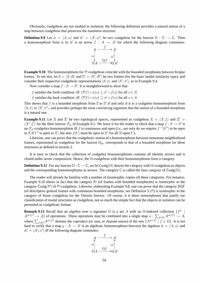
Obviously, coalgebras are not studied in isolation; the following definition provides a natural notion of amap between coalgebras that preserves the transition structure.

Definition 9.9 Let A = 〈A,α〉 andA′ = 〈A′, α′〉 be two coalgebras for the functorΩ : C → C. Thena homomorphism from A to A′ is an arrowf : A → A′ for which the following diagram commutes:

ΩA

A

ΩA′

A′

? ?-

-

α α′

f

Ωf

Example 9.10 The homomorphisms forP-coalgebras coincide with the bounded morphisms between Kripkeframes. To see this, letS = 〈S,R〉 andS′ = 〈S′, R′〉 be two frames (for the basic modal similarity type), andconsider their respective coalgebraic representations〈S, σ〉 and〈S′, σ′〉, as in Example 9.4.

Now consider a mapf : S → S′. It is straightforward to show that

f satisfies the forth condition iff(Pf) σ(s) ⊆ σ′ f(s) for all s ∈ S,f satisfies the back condition iff(Pf) σ(s) ⊇ σ′ f(s) for all s ∈ S.

This shows thatf is a bounded morphism fromS to S′ if and only if it is a coalgebra homomorphism from〈S, σ〉 to 〈S′, σ′〉, and provides perhaps the most convincing argument that the notion of a bounded morphismis a natural one.

Example 9.11 Let X andX′ be two topological spaces, represented as coalgebrasX = 〈X, ξ〉 andX′ =〈X ′, ξ′〉 for the filter functorFP of Example 9.5. We leave it for the reader to check that a mapf : S → S′ isanFP -coalgebra homomorphism ifff is continuous and open (i.e., not only do we requiref−1[U ′] to be openin X if U ′ is open inX′, but alsof [U ] must be open inX′ for all X-openU ).

Likewise, one can prove that the coalgebraic notion of a homomorphism between monotone neighborhoodframes, represented as coalgebras for the functorUP , corresponds to that of a bounded morphism for thesestructures as defined in section 2.

It is easy to check that the collection of coalgebra homomorphisms contains all identity arrows and isclosed under arrow composition. Hence, theΩ-coalgebras with their homomorphisms form a category.

Definition 9.12 For any functorΩ : C→ C, we letCoalg(Ω) denote the category withΩ-coalgebras as objectsand the corresponding homomorphisms as arrows. The categoryC is called thebase category of Coalg(Ω).

The reader will already be familiar with a number of (isomorphic copies of) these categories. For instance,Example 9.10 shows in fact that the categoryFr (of frames with bounded morphisms) isisomorphicto thecategoryCoalg(P) of P-coalgebras. Likewise, elaborating Example 9.8, one can prove that the categoryDGF(of descriptive general frames with continuous bounded morphisms, see Definition 5.27) is isomorphic to thecategory of Stone coalgebras for the Vietoris functor. Of course, it is these isomorphisms that justify ourclassification of modal structures as coalgebras, not so much the simple fact that the objects in isolation can bepresented in coalgebraic format.

Remark 9.13 Recall that analgebra over a signatureΩ is a setA with an Ω-indexed collectionfA |Aar(f) → A of operations. These operations may be combined into a single mapα :

∑f∈ΩA

ar(f) → A,

where∑

f∈ΩAar(f) denotes thecoproduct(or sum, or disjoint union) of the setsAar(f) | f ∈ Ω. It is not

hard to verify that a mapg : A → A′ is an algebraic homomorphism between the algebrasA = 〈A,α〉 andA′ = 〈A′, α′〉 iff the following diagram commutes:

ΩA

A

ΩA′

A′

6 6

-

-

α α′

f

Ωf

54

where we now view the signatureΩ as the polynomial setfunctor∑

f∈Ω Iar(f). That is,Ω operates as wellon functions between sets. This naturally suggests the following generalization.

Given an endofunctorΩ on a categoryC, anΩ-algebra is a pairA = 〈A,α〉 whereα : ΩA → A is anarrow in C. A homomorphism from anΩ-algebraA to anΩ-algebraA′ is an arrowf : A → A′ such thatf α = α′ (Ωf). The induced category is denoted asAlg(Ω).

Now the obvious similarities between the notions of algebra and coalgebra can be made very precise. Thebasic observation, which also explains the name ‘coalgebra’, is that a coalgebraC = 〈C, γ : C → ΩC〉 over abase categoryC can also be seen as an algebra in theoppositecategoryCop — we will come back to this issuein section 15. Note however, that universal coalgebra, dealing with arbitrary set functors, is more general than(what is usually called) universal algebra, which involves only polynomial functors.

55

10 Final coalgebras

Definition 10.1 A functor Ω : C → C is said toadmit a final or terminal coalgebra if the categoryCoalg(Ω)has a final object, that is, a coalgebraZ such that from every coalgebraA in Coalg(Ω) there is a uniquehomomorphism!A : A→ Z.

Functors admitting a final coalgebra are of special interest. In the case of state-based coalgebras, one reasonfor this is that final coalgebras often provide an intuitive encoding of the notion ofbehavior. And in fact, manyinteresting and well-known mathematical objects can be naturally associated with the final coalgebra of somefunctor.

Example 10.2 Consider a black box machineM = 〈M,µ〉 as in Example 9.2. Starting from, say, statex0,the machine makes a transitionµ(x0) = (c0, x1) and continues withµ(x1) = (c1, x2), µ(x2) = (c2, x3), etc.Since the statesx0, x1, . . . are internal to the machine, the only observable part of this dynamics is the infinitesequence orstream beh(x0) = (c0, c1, c2, . . .) ∈ Cω of values in the data setC.

The collectionCω of all infinite words overC forms itself a system for the functorC × I. Simply endowthe setCω with the transition structureγ splitting an infinite streamu = c0c1c2 . . . into itshead h(u) = c0 andits tail t(u) = c1c2c3 . . . Puttingγ(u) = (h(u), t(u)), one easily proves that the behavior mapx 7→ beh(x)is the unique homomorphism fromM to this coalgebra〈Cω, γ〉. This shows that〈Cω, γ〉 is the final object inthe categoryCoalg(C × I).

Example 10.3 For a second example, consider again the coalgebraic representation of a deterministic automa-ton over the alphabetC as a2 × IC-coalgebra. Now we will see that the collectionP(C∗) of all languagesoverC provides (the carrier of) the final coalgebra. We can turn this setP(C∗) into a coalgebra by imposingon it the following transition functionλ : P(C∗)→ 2×P(C∗)C . Writing λ(L) = (λ0(L), λ1(L)), we defineλ0(L) := 1 iff the empty string belongs toL, andλ1(L)(c) := w ∈ C∗ | cw ∈ L. (The latter set issometimes called thec-derivative of L.)

We leave it for the reader to verify that with this definition, the structure〈P(C∗), λ〉 forms the final objectin Coalg(2×IC). Given a2×IC-coalgebraA, the unique homomorphism!A : A→ 〈P(C∗), λ〉maps a statea ∈ A to the language that is accepted by the automaton that we obtain by takinga as initial state ofA.

Example 10.4 An interesting example in modal logic is provided by the final coalgebra for the Vietoris func-tor V of Example 9.8. The existence of a finalV-coalgebra is in fact an immediate consequence of the iso-morphismCoalg(V) ∼= DGF, and the duality betweenDGF andMA (the category of modal algebras withhomomorphisms).MA has an initial object (namely, the Lindenbaum-Tarski algebra generated by the emptyset of variables, or, equivalently, the free modal algebra over zero generators), and so by duality,Coalg(V) musthave a final object. In fact, thecanonicaldescriptive general frame, based on the set of maximal consistentclosed formulas, fulfills this role — a nice and perhaps quite unexpected application of this construction.

An important application of final coalgebras is provided by the principle ofcoinduction, which is one ofthe fundamental coalgebraic notions. There are two sides to this principle: it serves both as an important prooftool and as an elegant means of providing definitions. As a definition principle, coinduction is based on theexistence of unique homomorphisms into the finalΩ-systemZ = 〈Z, ζ〉. For, suppose that we can endow asetS with anΩ-coalgebra mapσ : S → ΩS, thus obtaining theΩ-systemS. Then there is a unique functionfσ = !S : S → Z which is consistent with the coalgebra specificationσ, in the sense that it is a coalgebraichomomorphism from〈S, σ〉 toZ. Thus the functionfσ is defined by coinduction from (the specification)σ.

Example 10.5 For instance, take the function that merges two streams by taking elements from either streamin turn. For a coinductive definition of this map, define the transition mapzip : Cω ×Cω → C × (Cω ×Cω)as follows:

zip(u, v) := (h(u), (v, t(u))),

whereh andt are the head and tail maps of Example 10.2. Then by finality there is a unique homomorphismfzip : Cω × Cω → Cω. One may verify that this indeed defines the map that zips two streams together.

56

The previous example is fairly typical in that it uses coinduction to define a function from a product ofthe final system to itself. It should also be noted that coinduction works particularly well for structures thatcombine algebraic and coalgebraic features, such as streams of data objects which are subject themselves toalgebraic operations.

Unfortunately, final coalgebras do not exist for every functorΩ. For instance,Set-endofunctors involvingthe power set functor in a nontrivial way, will generally not admit a final coalgebra; in particular, there is nofinal Kripke frame or model. By Cantor’s theorem, these results are immediate consequence of the followingproposition, which is due to Lambek [79].

Proposition 10.6 Let Ω : C → C be some functor admitting a final systemZ = 〈Z, ζ〉. Thenζ is anisomorphism (inC) betweenZ andΩZ.

Proof. Suppose thatZ = 〈Z, ζ〉 is the final object ofCoalg(Ω). It can easily be verified thatζ is in facta coalgebra homomorphism fromZ to Z2 := 〈ΩZ,Ωζ〉. But then the composition!Z2 ζ is a coalgebrahomomorphism fromZ to itself, just like the identity arrowidZ on Z. Thus by uniqueness it follows that!Z2 ζ = idZ . For the reverse compositionζ !Z2 we have, by the fact that!Z2 is a homomorphism, thatζ !Z2 = Ω!Z2 Ωζ = Ω(!Z2 ζ) = Ω(idZ) = idΩZ . From this the result is immediate. 2

So which functors admit final coalgebras? Some good sufficient conditions are known.

Definition 10.7 Let Ω be some set functor, andκ some cardinal. CallΩ κ-small if

Ω(S) =⋃(Ωι)[Ω(A)] | ι : A → S, |A| < κ,

for all setsS 6= ∅. Ω is small if it is small for some cardinalκ.

In words, the definition requires every element ofΩ(S) to be in the range ofΩι for an appropriate inclusionmapι : A → S. In caseΩ is astandardfunctor (meaning thatΩ maps inclusionsι : A → B to inclusions(Ωι) : ΩA → ΩB), the definition boils down to the requirement thatΩ(S) =

⋃Ω(A) | A ⊆ S, |A| < κ.

The notion of smallness is easily seen to be equivalent to the instantiation inSet of the more general notion ofaccessibility, and it is also equivalent to the concept ofboundedness, cf. ADAMEK & PORST [6] for details.

Examples of small functors abound; for instance, whenever we replace, in a Kripke polynomial functor,the power set functor by a bounded variant such as the finite power set functor, the result is a small functor.For instance, the finite power set functorPω is ω-small. The following result, due to ACZEL & M ENDLER [3]and BARR [9], witnesses the importance of the notion.

Fact 10.8 Every small set functor admits a final coalgebra.

As one of the immediate corollaries of this fact, the categories of image finite frames and image finitemodels, which can be represented as coalgebras for the functorPω, andPProp× Pω, respectively, have finalobjects.

Remark 10.9 ForSet-based functors that do not admit a final coalgebra, one maycreatea final coalgebra — atleast, if one is willing to allow coalgebras with a class rather than a set as their carrier. LetSET be the categorythat has classes as objects, and set-continuous functions as arrows. These are functionsf : C → C′ betweenclasses with the property thatf(C) =

⋃f(S) | S ⊆ C andS is a set. An endofunctor onSET is set-based

if for each classC and eachc ∈ Ω(C) there is a setS ⊆ C such thatc ∈ (Ωι)[Ω(S)], whereι : S → C isthe inclusion map. (If the set functor is standard, this boils down to requiring thatΩ is a set-continuous mapon objects.) Now ACZEL & M ENDLER [3] proved that every set-based endofunctorΞ : SET → SET admitsa final coalgebra. The similarity to Fact 10.8 is no coincidence: BARR [9] showed that the result of Aczel &Mendler can in fact be reformulated as Fact 10.8.

This fact can be used as follows. Given an endofunctorΩ onSet, there is auniqueway to extendΩ to a setbased endofunctorΩ+ on SET. (On objects, simply putΩ+(C) :=

⋃(Ωι)[Ω(S) | ι : S → C, S a set.) The

theorem of Aczel & Mendler then guarantees the existence of a final objectZ in Coalg(Ω+). This coalgebra

57

will be class-based ifΩ does not admit a final coalgebra, but it will be final, not only with respect to theset-based coalgebras inCoalg(Ω+), but also with respect to the class-based ones. As an important instanceof this idea, ACZEL [2] showed that the class of non-well-founded sets provides the final coalgebra for (theSET-based extension of) the power set functor.

Remark 10.10 Whether the functor admits a final coalgebra or not, one may always (try to) approximate it.Thefinal or terminal sequence associated with a given set functorΩ, is an ordinal indexed sequence of objects〈Zα〉 with mapspαβ : Zα → Zβ for β ≤ α, such that (i)Zα+1 = ΩZα andpα+1

β+1 = Ωpαβ , (ii) pαα = idZα and

pβγ pαβ = pαγ , (iii) if λ is a limit ordinal, thenZλ with pλα | α < λ is a limit of the diagram with objectsZα | α < λ and arrowspαβ | α, β < λ. (In particular, taking0 to be a limit ordinal, we find thatZ0 = 1 issome initial object1 of the categorySet.) It is not hard to prove that, modulo isomorphism, the final sequenceis uniquely determined by these conditions.

Intuitively, it can be seen as an approximation of the final coalgebra forΩ. That is, where elements of thefinal coalgebra represent ‘complete’ behavior, elements ofZα represent behavior that can be performed inαsteps. To make this precise and formal, observe that for anyΩ-coalgebraS there is auniqueordinal-indexedclass of functions!α : S → Zα such that!0 is fixed by the finality ofZ0 in Set, !α+1 = (Ω!α) σ, and for limitλ, !λ is given as the unique map!λ : S → Zλ such that!λ = pλα !α for all α < λ. It is not hard to prove that,for instance,S, s ≡Ω S

′, s′ implies that!α(s) = !α(s′) for all α.The relation with final coalgebras can be made precise, as follows. On the one hand, if the final sequence

converges, in the sense that some arrowpα+1α is a bijection, then the coalgebra〈Zα, (pα+1

α )−1〉 is a finalcoalgebra forΩ. And conversely, under some constraints onΩ, ADAMEK & K OUBEK [5] proved that ifΩadmits a final coalgebra, then the final sequence converges to it. More information on the final sequence of setfunctors can be found in WORRELL [109].

58

11 Bisimulation & behavioral equivalence

In this section we discuss the most important notions of equivalence between systems: behavioral equivalenceand bisimulation. Both of these generalize the concept of a bisimulation between two Kripke models.

Probably the most intuitive notion of equivalence between systems is that ofbehavioral, or observational,equivalence. The idea here is to consider two states to be similar if we cannot distinguish them by observations,because they display the same behavior. For instance, we call two deterministic automata (pointed2 × IC-coalgebras) equivalent if they recognize the same language. In case the functorΩ admits a final coalgebraZ, this idea is easily formalized by making states0 in coalgebraS0 equivalent to states1 in coalgebraS1 if!S0(s0) = !S1(s1). In case the functor does not admit a final coalgebra, we generalize this demand as follows.

Definition 11.1 LetS = 〈S, σ〉 andS′ = 〈S′, σ′〉 be two systems for the set functorΩ. Thens ∈ S ands′ ∈ S′arebehaviorally equivalent, notation:S, s ≡Ω S

′, s′ if there is anΩ-systemX = 〈X, ξ〉 and homomorphismsf : S→ X andf ′ : S′ → X such thatf(s) = f ′(s′).

Remark 11.2 It is easily checked that in caseΩ admits a final coalgebra, then indeedS, s ≡Ω S′, s′ iff

!S(s) = !S′(s′). In the case thatΩ does not admit a final coalgebra, then one may show that behavioralequivalence is captured in the same way by the final coalgebra of the extensionΩ+ of Ω to the categorySET,see Remark 10.9.

Remark 11.3 As a variation of behavioral equivalence, the final sequence can be used to study behavior, in away that is not unlike modal logic. For instance, call two pointedΩ-systems(S, s) and(S′, s′) α-equivalentif !α(s) = !α(s′). In the case of Kripke models, this notion coincides with that of bounded bisimilarity,see Chapter?? of HBML . One may prove that behavioral equivalence itself coincide with the intersection ofJα-equivalence for all ordinalsα.

In almost all cases of interest, behavioral equivalence can be characterized via the equally fundamentalconcept ofbisimilarity, which is due to ACZEL & M ENDLER [3]. The definition of bisimilarity and bisim-ulations may not be so intuitive at first sight, but, as we will see, these notions have some rather elegantmathematical properties.

Definition 11.4 Let S = 〈S, σ〉 andS′ = 〈S′, σ′〉 be two systems for the set functorΩ. A relationB ⊆ S×S′is called abisimulation between S andS′, if we can endow it with a coalgebra mapβ : B → ΩB, in sucha way that the two projectionsπ : B → S andπ′ : B → S′ are homomorphisms from〈B, β〉 to S andS′,respectively:

ΩS ΩB ΩS′

S B S′

?

pppppppp? ?

-

-

σ β σ′

π

Ωπ

π′

Ωπ′

If there exists a bisimulationB with (s, s′) ∈ B, we say thats ands′ arebisimilar, notation:S, s ↔ S′, s′ (or

B : S, s↔ S′, s′ in case we want to make the bisimulationB explicit).

Finally, if S = S′ we say thatB is a bisimulationon S; if this B happens to be an equivalence relation, we

call it a bisimulation equivalence onS.

Remark 11.5 Intuitively, bisimulation equivalences correspond tocongruencesin universal algebra. To makethis analogy somewhat more precise, call a relationR ⊆ A0 × A1, linking the carrier sets of twoΩ-algebrasA0 andA1, substitutive if there exists analgebraic structureρ : ΩR → R, such that the two projectionsπi : R → Ai are (algebraic) homomorphisms. This is clearly an algebraicanalogue (rather than a dualversion) of a bisimulation, so that the correspondence between congruences and bisimulation equivalencesobtains through the observation that a congruence is nothing but a substitutive equivalence relation.

Example 11.6 LetS0 = 〈S0, σ0〉 andS1 = 〈S1, σ1〉 be two coalgebras over the functorPProp×P. That is,S0

andS1 are Kripke models in coalgebraic shape; writeσi(s) = (λi(s), Ri[s]), whereλi(s) is the collection of

59

proposition letters true ats in Si, andRi[s] is the successor set ofs in Si, as in the examples 9.4 and 9.10. Nowconsider an arbitrary relationB ⊆ S0 × S1. It is a very instructive exercise to check thatB is a bisimulationin the coalgebraic sense if and only if it is a bisimulation in the sense of Kripke models. Recall that the latterproperty means that for any pair(s0, s1) ∈ B:

(atom) p ∈ λ0(s) iff p ∈ λ1(s), for all p ∈ Prop;

(forth) for all t0 ∈ R0[s0] there is somet1 ∈ R1[s1] with (t0, t1) ∈ B;

(back) for all t1 ∈ R1[s1] there is somet0 ∈ R0[s0] with (t1, t0) ∈ B.

One way to prove this equivalence uses the fact that bounded morphisms coincide with coalgebra morphisms,cf. Example 9.10. Details are left to the reader.

Example 11.7 Recall from Example 9.3 that deterministic automata over an alphabetC can be representedas2 × IC-coalgebras. Now letA = (A, o, ν) andA′ = (A′, o′, ν ′) be two such automata. We leave it forthe reader to verify thatB ⊆ A × A′ is a bisimulation betweenA andA′ iff every pair (s, s′) ∈ B satisfies(i) o(s) = o′(s′) and (ii) (ν(s)(c), ν ′(s′)(c)) ∈ B for everyc ∈ C. In this case it is easy to see that bisimilarstates are also behaviorally equivalent.

Example 11.8 For an arbitrary set functorΩ, it is easy to see that for any coalgebraS, the diagonal relation∆S is a bisimulation equivalence onS. Furthermore, the converse of a bisimulation is again a bisimulation.However, the collection of bisimulations is not in general closed under taking relational composition.

Finally, homomorphisms can be seen as functional bisimulations. To be more precise, letf : S0 → S1

be a function between the carriers of twoΩ-coalgebrasS0 andS1. Recall that thegraph of f is the relationGf := (s, f(s)) | s ∈ S. Then it holds that

f is a coalgebraic homomorphism iff its graph is a bisimulation. (42)

In order to see why this is so, first suppose thatGf : S0 ↔ S1. Since the projection mapπ0 : Gf → S0 is abijective homomorphism, its inverseπ−1

0 is also a homomorphism. But thenf = π1 π−10 , as the composition

of two homomorphisms, is also a homomorphism. For the other direction, suppose thatf is a homomorphism;then it is straightforward to verify that the map(Ωπ0)−1σπ0 equips the setGf with the required coalgebraicstructure.

Bisimulations admit an elegant alternative characterization which involves the notion ofrelation lifting.As an example, consider the power set functorP. Recall thatB ⊆ S0 × S1 is a bisimulation betweenS0 = 〈S0, R0[·]〉 andS1 = 〈S1, R1[·]〉 iff B satisfies the conditions(back)and(forth) of Example 11.6. Nowsuppose that we define, for an arbitrary relationR ⊆ S0×S1, the relationP(R) ⊆ P(S0)×P(S1) by putting

P(R) := (Q0, Q1) | ∀q0 ∈ Q0 ∃q1 ∈ Q1. (q0, q1) ∈ R and∀q1 ∈ Q1 ∃q0 ∈ Q0. (q0, q1) ∈ R. (43)

In other words, welift the relationR to the level of the power sets ofS0 andS1. The definition of a bisimulationbetweenP-coalgebras can now be nicely characterized as follows:

B : S0 ↔ S1 iff (R0[s0], R1[s1]) ∈ P(B) for all (s0, s1) ∈ B.

This nice way of characterizing bisimulation via relation lifting is not limited to the power set functor — itapplies in fact toeveryset functor.

Definition 11.9 Let S0 andS1 be two coalgebras for some set functorΩ. Given a relationR ⊆ S0 × S1,consider the following diagram, whereπi : R→ Si andpi : ΩS0 × ΩS1 → ΩSi denote the projection maps.

60

ΩS0 ΩR ΩS1

S0 R S1

? ?

-

-

σ0 σ1

π0

Ωπ0

π1

Ωπ1

ΩS0 × ΩS1

p13

p0QQQQQk

ρR

pppppppp?

It follows from the category theoretic properties of the productΩS0 × ΩS1 that there is a unique mapρR =〈Ωπ0,Ωπ1〉 from ΩR to ΩS0 × ΩS1 such thatpi ρR = Ωπi for i = 0, 1. We define therelation lifting of Ras the relation

ΩR := ((Ωπ0)(u), (Ωπ1)(u)) | u ∈ ΩR, (44)

that is,ΩR is the image ofΩR underρR.

The results listed in the following theorem, which summarize the most important properties of bisimula-tions, basically date back to ACZEL & M ENDLER [3].

Theorem 11.10LetS0 andS1 be two coalgebras for some set functorΩ.

(i) B : S0 ↔ S1 iff (σ0(s0), σ1(s1)) ∈ Ω(B) for all (s0, s1) ∈ B.

(ii) The collection of bisimulations betweenS0 andS1 forms a complete lattice under the inclusion order,with joins given by unions.

(iii) The bisimilarity relation↔ is the largest bisimulation betweenS0 andS1.

Proof. The first part of the theorem is an almost immediate consequence of the definitions, so we leave thedetails to the reader.

The crucial observation in the proof of the other two parts is that

Ω : P(S0 × S1)→ P(ΩS0 × ΩS1) is a monotone operation. (45)

For a proof, letR ⊆ R′ be two relations betweenS0 andS1, with ι : R → R′ denoting the inclusionmap. By definition ofΩ, we may without loss of generality represent an arbitrary element ofΩ(R) as a pairρR(u) = ((Ωπ0)(u), (Ωπ1)(u)) for someu ∈ ΩR. Defineu′ := (Ωι)(u), thenu′ belongs toΩR′, and foreachi we find that(Ωπ′i)(u

′) = (Ωπ′i Ωι)(u) = (Ω(π′i ι)(u) = (Ωπi)(u). That is,ρR(u) = ρR′(u′), whichshows thatρR(u) belongs toΩR′. This proves (45).

Now for the proof of part ii, recall that a partial order is a complete lattice if it closed under arbitraryjoins. Hence, it suffices to prove that the unionB of a collectionBj | j ∈ J of bisimulations is again abisimulation. Take an arbitrary pair(s0, s1) ∈ B. Then(s0, s1) belongs toBj for somej ∈ J . Hence, bypart i, we find(s0, s1) in Ω(Bj), so(s0, s1) ∈ Ω(B) by the monotonicity ofΩ. But thenB is a bisimulationby part i.

Finally, for part iii, note that it is an immediate consequence of part ii that↔, being the union of allbisimulations betweenS0 andS1, is a bisimulation itself. Hence, by definition, it is the greatest bisimulationbetweenS0 andS1. In fact, it follows by the Knaster-Tarski theorem (on fixed points of monotone operations oncomplete lattices), that↔ is in fact the greatest fixed point of the mapΛ : R 7→ (s0, s1) | (σ0(s0), σ1(s1)) ∈Ω(R). 2

In the case of Kripke polynomial functors, relation lifting can be characterized usinginduction on theconstruction of the functor, cf. JACOBS [63].

Proposition 11.11 LetS andS′ be two sets, andR ⊆ S × S′ a binary relation betweenS andS′. Then thefollowing induction defines the relation liftingK(R) ⊆ KS ×KS′, for each Kripke polynomial functorK:

61

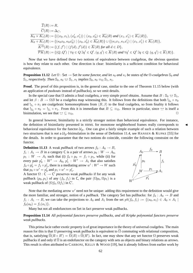
I(R) :=R,

C(R) := ∆C ,

K0 ×K1(R) := ((x0, x1), (x′0, x′1)) | (x0, x

′0) ∈ K0(R) and(x1, x

′1) ∈ K1(R),

K0 +K1(R) := (κ0x0, κ0x′0) | (x0, x

′0) ∈ K0(R) ∪ (κ1x1, κ1x

′1) | (x1, x

′1) ∈ K1(R),

KD(R) := (f, f ′) | (f(d), f ′(d)) ∈ K(R) for all d ∈ D,PK(R) := (Q,Q′) | ∀q ∈ Q∃q′ ∈ Q′. (q, q′) ∈ K(R) and∀q′ ∈ Q′ ∃q ∈ Q. (q, q′) ∈ K(R).

Now that we have defined these two notions of equivalence between coalgebras, the obvious questionis how they relate to each other. One direction is clear: bisimilarity is a sufficient condition for behavioralequivalence.

Proposition 11.12 LetΩ : Set→ Set be some functor, and lets0 ands1 be states of theΩ-coalgebrasS0 andS1, respectively. ThenS0, s0 ↔ S1, s1 impliesS0, s0 ≡Ω S1, s1.

Proof. The proof of this proposition is, in the general case, similar to the one of Theorem 11.15 below (withan application ofpushouts instead of pullbacks), so we omit details.

In the special case thatΩ admits a final coalgebra, a very simple proof obtains. Assume thatB : S0 ↔ S1,and letβ : B → ΩB be a coalgebra map witnessing this. It follows from the definitions that both!S0 π0

and !S1 π1 are coalgebraic homomorphisms from〈B, β〉 to the final coalgebra, so from finality it followsthat !S0 π0 = !S1 π1. From this it is immediate thatB ⊆ ≡Ω. Hence in particular, since↔ is itself abisimulation, we see that↔ ⊆ ≡Ω. 2

In general however, bisimilarity is a strictly stronger notion than behavioral equivalence. For instance,the definition of bisimilarity presented inHBML for monotone neighborhood frames really corresponds toJbehavioral equivalence for the functorUP . One can give a fairly simple example of such a relation betweentwo structures that isnot aUP -bisimulation in the sense of Definition 11.4, see HANSEN & K UPKE [55] forthe details. In order to guarantee that the two notions do coincide, consider the following constraint on thefunctor.

Definition 11.13 A weak pullback of two arrowsf0 : A0 → B,f1 : A1 → B in a categoryC is a pair of arrowsp0 : W → A0,p1 : W → A1 such that (i)f0 p0 = f1 p1, while (ii) forevery pairp′0 : W ′ → A0, p′1 : W ′ → A1 that also satisfiesf0 p′0 = f1 p′1, there is a mediating arroww′ : W ′ →W suchthatp0 w′ = p′0 andp1 w′ = p′1.A functor Ω : C → C′ preserves weak pullbacks if for any weakpullback (p0, p1) of any (f0, f1) in C, the pair(Ωp0,Ωp1) is aweak pullback of(Ωf0,Ωf1) in C′.

W

A0

A1

B

W ′

6 6

-

-

1

p′0

p0 f1

p′1

p1

f0

p p p p p p p p

Note that the mediating arroww′ need not be unique: adding this requirement to the definition would givethe more familiar, and stronger, notion of apullback. The categorySet has pullbacks: forf0 : A0 → B andf1 : A1 → B, we can take the projections toA0 andA1 from the setpb(f0, f1) := (a0, a1) ∈ A0 × A1 |f0(a0) = f1(a1).

Many but not all endofunctors onSet in fact preserve weak pullbacks.

Proposition 11.14 All polynomial functors preserve pullbacks, and all Kripke polynomial functors preserveweak pullbacks.

This prima facie rather exotic property is of great importance in the theory of universal coalgebra. The mainreason for this is thatΩ preserving weak pullbacks is equivalent toΩ commuting with relational composition,that is, satisfyingΩ(R R′) = Ω(R) Ω(R′). In fact, one may show that any set functorΩ preserves weakpullbacks if and only ifΩ is an endofunctor on the category with sets as objects and binary relations as arrows.This result is often attributed to CARBONI, KELLY & W OOD [19], but it already follows from earlier work by

62

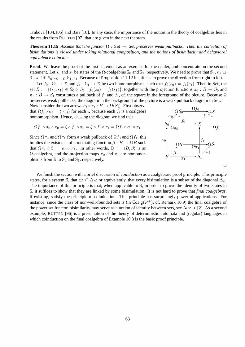
Trnkova [104,105] and Barr [10]. In any case, the importance of the notion in the theory of coalgebras lies inthe results from RUTTEN [97] that are given in the next theorem.

Theorem 11.15Assume that the functorΩ : Set → Set preserves weak pullbacks. Then the collection ofbisimulations is closed under taking relational composition, and the notions of bisimilarity and behavioralequivalence coincide.

Proof. We leave the proof of the first statement as an exercise for the reader, and concentrate on the secondstatement. Lets0 ands1 be states of theΩ-coalgebrasS0 andS1, respectively. We need to prove thatS0, s0 ↔S1, s1 iff S0, s0 ≡Ω S1, s1. Because of Proposition 11.12 it suffices to prove the direction from right to left.

Let f0 : S0 → X andf1 : S1 → X be two homomorphisms such thatf0(s0) = f1(s1). Then inSet, thesetB := (s0, s1) ∈ S0 × S1 | f0(s0) = f1(s1), together with the projection functionsπ0 : B → S0 andπ1 : B → S1 constitutes a pullback off0 andf1, cf. the square in the foreground of the picture. BecauseΩpreserves weak pullbacks, the diagram in the background of the picture is a weak pullback diagram inSet.Now consider the two arrowsσi πi : B → Ω(Si). First observethatΩfi σi = ξ fi for eachi, because eachfi is a coalgebrahomomorphism. Hence, chasing the diagram we find that

Ωf0 σ0 π0 = ξ f0 π0 = ξ f1 π1 = Ωf1 σ1 π1.

SinceΩπ0 andΩπ1 form a weak pullback ofΩf0 andΩf1, thisimplies the existence of a mediating functionβ : B → ΩB suchthat Ωπi β = σi π1. In other words,B := 〈B, β〉 is anΩ-coalgebra, and the projection mapsπ0 andπ1 are homomor-phisms fromB to S0 andS1, respectively.

B

S0

S1

X

ΩB

ΩS0

ΩS1

ΩX

6 6

-

-6 6

-

-

p p p p p p p pπ0 f1

Ωπ0 Ωf1

π1

f0

Ωπ1

Ωf0

σ0 ξ

σ1β

2

We finish the section with a brief discussion ofcoinductionas a coalgebraic proof principle. This principlestates, for a systemS, that↔ ⊆ ∆S ; or equivalently, that every bisimulation is a subset of the diagonal∆S .The importance of this principle is that, when applicable toS, in order to prove the identity of two states inS, it suffices to show that they are linked by some bisimulation. It is not hard to prove thatfinal coalgebras,if existing, satisfy the principle of coinduction. This principle has surprisingly powerful applications. Forinstance, since the class of non-well-founded sets is (inCoalg(P+), cf. Remark 10.9) the final coalgebra ofthe power set functor, bisimilarity may serve as a notion of identity between sets, see ACZEL [2]. As a secondexample, RUTTEN [96] is a presentation of the theory of deterministic automata and (regular) languages inwhich coinduction on the final coalgebra of Example 10.3 is the basic proof principle.

63

12 Covarieties

What is the coalgebraic analog of a variety? In other words, what are natural closure operations on classes ofcoalgebras? We start with homomorphic images.

Definition 12.1 Let Ω be some endofunctor onSet. If ϕ : A→ B is a surjective homomorphism between theΩ-coalgebrasA andB, then we say thatB is ahomomorphic image of A.

In universal algebra, one finds a one-one correspondence between homomorphic images and congruences.Something similar applies here, but the analogy is perfect only in the case of functors that preserve weakpullbacks.

Proposition 12.2 LetS = 〈S, σ〉 be anΩ-coalgebra for some set functorΩ. Then

(i) Given a bisimulation equivalenceE onS, there is a unique coalgebra structureσ′ onS/E such that thequotient mapν : S → S/E is a homomorphism.

(ii) If Ω preserves weak pullbacks, thenker(ϕ) is a bisimulation equivalence for any homomorphismϕ :S→ S

′ .

Proof. For part i, the coalgebra mapσ′ can be defined by puttingσ′([s]E) := (Ων) σ(s). Further proofdetails can be found in RUTTEN [97]. For the second part of the proposition, observe thatker(ϕ) is therelational composition of the graph ofϕ with its converse. The result then follows from Theorem 11.15.2

The next class operation that we consider is that of taking subcoalgebras.

Definition 12.3 Let A = 〈A,α〉 andS = 〈S, σ〉 be twoΩ-coalgebras, such thatS is a subset ofA. If theinclusion mapι : S → A is a homomorphism from〈S, σ〉 to 〈A,α〉, then we say thatS is open with respecttoA, and we call the structure〈S, αS〉 a subcoalgebra of A.

Interestingly enough, the transition map of a subcoalgebra is completely determined by the underlyingopen set:

Proposition 12.4 LetS0 = 〈S, σ0〉 andS1 = 〈S, σ1〉 be two subcoalgebras of the coalgebraA. Thenσ0 = σ1.

Proof. The case ofS being empty is trivial, so suppose otherwise. Then from the assumption thatS0 andS1

are subcoalgebras ofA, we may infer that(Ωι) σ0 = α ι = (Ωι) σ1, whereι is the inclusion map ofSintoA. It follows from the functoriality ofΩ thatΩι is an injection, so that we may conclude thatσ0 = σ1. 2

Some further observations concerning subcoalgebras are in order. First of all, the topological terminologyis justified by the following proposition.

Proposition 12.5 Given a coalgebraA for some set functorΩ, the collectionτA of A-open sets forms atopology.

Proof. Closure ofτA under taking (arbitrary) unions follows from Theorem 11.10, together with the observa-tion that

S ⊆ A is open with respect toA iff ∆S is a bisimulation onA, (46)

which in its turn is an immediate consequence of (42). We skip the proof of the fact that theintersection oftwo opens is open, since it requires a little more work. We refer the reader to GUMM & SCHRODER [54] forthe details. 2

It follows from the Proposition above that, given a subsetS of (the carrier of) a coalgebraA, there is alargest subcoalgebra ofA (of which the carrier is) contained inS: Its universe is given as the union of all opensubsets ofS. It also follows from Proposition 12.5 that the collectionτA of open subsets ofA forms acompletelattice under set inclusion. Hence, given a subsetS of A, there is an open setU ⊆ A which is themeetof thecollectionQ ∈ τA | S ⊆ Q. However, there is no guarantee thatU is also theintersectionof this collection,

64

or, indeed, thatS is actually a subset ofU . Thus we may not in general speak of the smallest subcoalgebracontaining a given subset, as the following example from GUMM [50] witnesses.

Example 12.6 Consider the standard Euclidean topology on the real numbers, seen as a coalgebra for thefilter functorFP , cf. Example 9.5. One can show, that a setS of reals is open in the topological sense iff it isopen in the sense of Definition 12.3 — in fact, this holds for any topology. Now take an arbitrary pointr in R.Obviously, we have that themeetof all open neighborhoods containingr is the empty set.

Before we turn to further coalgebraic constructions, consider the following natural link between homomor-phic images and subcoalgebras.

Proposition 12.7 Given a coalgebraic homomorphismϕ : A → B, there is a (unique) subcoalgebraϕ[A] ofB such thatϕ : A→ ϕ[A] is a surjective homomorphism.

Proof. For a proof of this proposition, letS := ϕ[A] be the (set-theoretic) image ofA underϕ, and letf : S → A be a right inverse ofϕ, that is,ϕ(f(s)) = s for all s ∈ S. Now defineσ : S → ΩS byσ := Ωϕ α f . It can be shown that the resulting structureS is always a subcoalgebra ofB, and thatϕ : A→ S is a surjective homomorphism; for details the reader is referred to RUTTEN [97]. 2

Our last example of a coalgebraic construction concerns the straightforward generalization of the disjointunion of Kripke models and frames. The idea is as follows. Recall that inSet, a concrete representationof the coproduct of a collectionAi | i ∈ I of sets is given by the disjoint union

⊎I Ai, together with

the inclusions/embeddingsei : Ai →⊎I Ai. Hence, the defining property of coproducts provides the key

ingredient of the coalgebraic notion of a coproduct, or sum of a family of coalgebras.

Definition 12.8 The sum∐I Ai of a family Ai | i ∈ I of coalgebras for some set functorΩ, is defined

by endowing the disjoint unionA :=⊎I Ai with the unique mapα : A → ΩA which turns all embeddings

ei : Ai → A into homomorphisms.

We have now gathered all the basic class operations needed to define the notion of a covariety, which wasintroduced in RUTTEN [97] as the natural dual of a variety in universal algebra.

Definition 12.9 Let Ω be some endofunctor onSet. A class ofΩ-coalgebras is acovariety if it closed undertaking homomorphic images, subcoalgebras and sums. The smallest covariety containing a classK of Ω-coalgebras is called the covarietygenerated by K, notation:Covar(K).

As in the case of universal algebra, in order to obtain a more succinct characterization of the covarietygenerated by a class of coalgebras, one may develop a calculus of class operations.

Definition 12.10 Let H, S andΣ denote the class operations of taking (isomorphic copies of) homomorphicimages, subcoalgebras, and sums, respectively.

On the basis of these (and other) operations one may investigate the validity of ‘inequalities’ likeHS ≤ SH(meaning thatHS(K) ⊆ SH(K) for all classesK of coalgebras). Results of these kind lead to the followingcoalgebraic analog of Tarski’s HSP-theorem in universal algebra, due to GUMM & SCHRODER [53].

Theorem 12.11Let K be a class ofΩ-coalgebras for some set functorΩ. ThenCovar(K) = SHΣ(K).

Proof. It is straightforward to prove the theorem on the basis of the idempotency of the class operationsH, SandΣ, together with the following three ‘inequalities’:HS ≤ SH, ΣS ≤ SΣ, andΣH ≤ HΣ. For proofs ofthese (and more) inequalities, the reader is referred to GUMM & SCHRODER [53]. 2

As in the case of varieties, one may wonder about the basic building blocks of varieties. Dualizing thenotion of subdirect irreducibility, we arrive at the following definition. It uses the notion of a conjunct sum,which is known, in the case of Kripke frames, under the name ofbounded union.

65

Definition 12.12 LetA be someΩ-coalgebra for some set functorΩ. A conjunct representation A by a familyAi | i ∈ I of coalgebras is a family of embeddingsei : Ai → A | i ∈ I such thatA =

⋃i∈I ei[Ai]. In this

case we callA aconjunct sum of theAi. A coalgebraA is calledconjunctly irreducible if each of its conjunctrepresentations is trivial in the sense that one of the embeddings is an isomorphism.

Covarieties are easily seen to be closed under taking conjunct sums — we will use this fact without furthernotice.

Given the results on dualizing the notion of subdirect irreducibility in section 5, in particular, Theorem 5.29,one would expect that conjunct irreducibility can be explained in terms of roots. Call a states of a systemS aroot of S if S itself is the only subcoalgebra ofS that containss. It is then fairly easy to prove that a coalgebrais conjunctly irreducible if and only if it has a root. However, GUMM [50] proves that there is no analog ofBirkhoff’s s.i. theorem here, at least not for an arbitrary functor. For instance, expanding Example 12.6, oneeasily shows that a topological coalgebra will generally not be a conjunct sum of rooted coalgebras.

66

13 Modal logic and coalgebras

If coalgebras are mathematical structures that represent the essence of dynamics, then there is an obvious needfor logics to represent and reason about properties of such structures. This is of particular importance forcomputer scientists who are interested in the formal specification and verification of the behavior of a system.Thekind of properties that one wants to describe formally may differ from one application to another, but itseems natural to restrict attention to properties that are invariant under behavioral equivalence. MOSS[11,86]was the first to realize that such properties can be conveniently formalized in a version ofmodal logic, properlygeneralized from Kripke structures to systems for an arbitrary set functor. This connection between modallogic and coalgebra has provided a quite active research area. At the time of writing, quite a few proposals forcoalgebraic modal logics are around; most of them are roughly based on one of the approaches to be discussedin this section.

We start with Moss’ original approach, which is also the most general. In order to introduce his formalism,we first put ordinary modal logic in a slightly different perspective by introducing a new connective∇. Themeaning of this modality, which takes aset of formulas as its argument, can be summarized by presenting theformula∇Φ, with Φ a set of formulas, as the following abbreviation:

∇Φ := 2∨

Φ ∧∧

3Φ, (47)

where3Φ denotes the set3ϕ | ϕ ∈ Φ, and∨

and∧

denote disjunction and conjunction. We do not wantto exclude the possibility thatΦ is an infinite set — coalgebraic logic is generally of an infinitary nature. Theoperator∇ pops up in a number of areas in modal logic, cf.HBML . We may also decide to treat this∇ as Ja primitive connective. As long as we keep∨ and> in our language, both the standard diamond and boxconnective are definable in terms of∇, since we have the following equivalences:

3ϕ≡∇ϕ,>,2ϕ≡∇∅ ∨∇ϕ,

so that we may in factreplacethe diamond and box with this new modality.Spelling out the truth definition of∇Φ, we see that it can in fact be expressed in terms of therelation

lifting that we defined in section 11. For, letS = 〈S, λ,R[·]〉 be a modal model in coalgebraic shape. Thenit is straightforward to verify thatS, s ∇Φ if and only if the pair(R[s],Φ) belongs to the relation liftingP( S) of the satisfaction relation S ⊆ S × Φ: Everyϕ ∈ Φ must hold at some successort ∈ R[s], and atevery successort of s someϕ ∈ Φ must hold, see (43). This fundamental insight paves the way for Moss’development ofcoalgebraic logic, in which the same principle is applied to an arbitrary (but fixed) set functorΩ. Basically, the idea is to have

S, s S ∇P iff (P, σ(s)) ∈ Ω( S).

Note that in this perspective, the satisfaction relation is much like a bisimulation between a language and acoalgebra; this observation was first made and exploited in BALTAG [8].

In order to provide a more precise definition, recall from Remark 10.9 that we may uniquely extendΩ toa set based endofunctorΩ+ on the categorySET that has classes as objects, and set-continuous functions asarrows. For convenience, we follow MOSS[86] in that we confine our attention tostandardset functors, thatis, functors that map inclusions to inclusions.

Definition 13.1 Let Ω : Set → Set be a standard set functor that preserves weak pullbacks. ThenLΩ, thelanguage ofcoalgebraic formulas for Ω, is defined as the least classC such that (i)

∧Φ ∈ LΩ if Φ ⊆ LΩ is a

setof formulas, and (ii)∇P ∈ LΩ for anyP ∈ Ω+(LΩ).

Categorically,〈LΩ,∧,∇〉 can be characterized as theinitial algebraof the functor(P+Ω)+. This explains

our move to the categorySET: if we want to guarantee theexistenceof such a structure, for reasons similar asgiven in the discussion following Proposition 10.6, we need to allow class-based algebras.

67

Definition 13.2 Let Ω : Set → Set preserve weak pullbacks. Given anΩ-coalgebraS = 〈S, σ〉, define S ⊆ S × LΩ as the least relation satisfying

s S∧

Φ if s S ϕ for all ϕ ∈ Φ,

s S ∇P if (P, σ(s)) ∈ Ω(W ) for some setW ⊆ S.

Example 13.3 Consider the functorPProp × P of Kripke models. Unraveling the definitions, we find thatan arbitrary element ofΩ+(LΩ) must be of the form(A,Φ) with A ⊆ Prop a set of proposition letters, andΦ ⊆ LΩ a set of formulas. It is not hard to verify that

S, s ∇(A,Φ) iff S, s ∧A ∧

∧¬(Prop \A) ∧2

∨Φ ∧

∧3Φ,

where∧¬(Prop \ A) denotes the formula

∧¬p | p ∈ P \ A. It is instructive to observe the difference

between this and (47) which displays an arbitrary∇-formula for the functorP of Kripke frames as opposed tomodels.

Example 13.4 For another example, an arbitrary element of the classΩ+(LΩ), whereΩ is now the functorI × I, must be apair of formulas, say,(ϕ0, ϕ1). Clearly then we have

S, s ∇(ϕ0, ϕ1) iff S, π0(σ(s)) ϕ0 andS, π1(σ(s)) ϕ1.

This in fact implies thatall formulas are true atall states ofall coalgebras; in other words, in the absence ofpropositions, the languageLΩ may be rather uninteresting.

Obviously, many variations of this language exist, or may be defined. For instance, it is easy to develop fini-tary versions of the language, while independently of this, one may add Boolean connectives like negation or(infinitary) disjunction. Interestingly,LΩ on its own is already powerful enough to characterize behavior. The-orem 13.5 below shows that it has theHennessy-Milner property(cf. Chapter?? of HBML ): non-bisimilarity Jof two points is witnessed by some formula in the language.

Theorem 13.5 Let Ω : Set→ Set preserves weak pullbacks, and letS andS′ be twoΩ-coalgebras. Then forany pair of statess ∈ S, s′ ∈ S′:

S, s↔ S′, s′ iff s ands′ satisfy the sameLF -formulas.

Proof. The direction from left to right is proved by induction on the complexity of formulas. That is, we defineΘ to be the class of formulas on which all bisimilar points inS andS′ agree. Then we prove thatΘ = LΩ byshowing thatΘ is closed under

∧and∇ (in the sense that

∧Φ ∈ Θ for all subsetsΦ ⊆ Θ, and that∇P ∈ Θ

for all P ∈ Ω(Θ)). We leave the fairly straightforward details as an exercise for the reader.The proof for the other direction is analogous to that of Karp’s Theorem for modal logic (see Chapter??),

so we confine ourselves to a brief sketch here. Given anΩ-systemS, by ordinal induction we define a familyϕSα : S → LΩ as follows (we omit the superscript):

ϕ0(s) :=>ϕα+1(s) :=∇(Ωϕα)(σ(s)),

ϕλ(s) :=∧ϕα(s) | α < λ.

One approach to the proof would then be to show that the relation≡ϕ, defined vias ≡ϕ t if ϕα(s) = ϕα(t)for all α, is itself a bisimulation. 2

Moss’ definition provides powerful languages, of which syntax and semantics uniformly depend on thecoalgebraic signature, but his systems are not very welcoming to our intuitions on modal languages as ex-tensions of propositional logic with diamonds and boxes that are interpreted via accessibility relations. BAL -TAG [8] introduces variants of Moss’ language in which the connectives2

∨Φ and

∧3Φ of (47) are (sep-

arately) generalized from Kripke frames to arbitrary functors, but also his formalism is far too abstract forpractical purposes. It therefore seems worthwhile to develop more ‘concrete’ and practical alternatives toLΩ.

68

In the case of Kripke polynomial functors, the concrete, inductive definition of the functor allows for moredown to earth modal languages, as was first observed by KURZ [77]. Here we present a formalism that wasintroduced in ROESSIGER[95], and studied by JACOBS [62]. From the perspective of modal logic, its onlynon-standard feature is that both its syntax and semantics aresortedby the setIngK of ingredient functors ofK.

Definition 13.6 Fix a Kripke polynomial functorK. We define the languageFmaK =⋃

Λ∈Ing(K) FmaK(Λ)of K-sorted modal formulas, by the following induction. (All functors appearing in the definition below aresupposed to be ingredient functors ofK.)

• ⊥ ∈ FmaK(Λ) for everyΛ ∈ Ing(K);• if ϕ,ψ ∈ FmaK(Λ) then¬ϕ,ϕ ∨ ψ ∈ FmaK(Λ);• if c ∈ C thenc ∈ FmaK(C);• if ϕ ∈ FmaK(Λi) then3κiϕ ∈ FmaK(Λ0 + Λ1);• if ϕ ∈ FmaK(Λi) then3πiϕ ∈ FmaK(Λ0 × Λ1);• if ϕ ∈ FmaK(Λ) then3dϕ ∈ FmaK(ΛD) for all d ∈ D;

• if ϕ ∈ FmaK(Λ) then33ϕ ∈ FmaK(PΛ);• if ϕ ∈ FmaK(K) thenϕ ∈ FmaK(I).

We say thatϕ is of sort Λ if ϕ ∈ FmaK(Λ) — note that this sort need not be unique.

How do we interpret these formulas in coalgebras? Intuitively, with eachK-coalgebraS, we associatea multi-sorted frame based on the set

⋃Λ∈Ing(K) Λ(S). The accessibility relations of this frame (which we

will not make explicit) are completely determined by the shape of the functor. For instance, to link the set(Λ0 + Λ1)(S) to Λ0(S), we lay down the relationRκ0 = (κ0s0, s0) | s0 ∈ Λ0(S). Likewise, the conversemembership relation3 provides the accessibility relation fromPΛ(S) to Λ(S).

Definition 13.7 Let S = 〈S, σ〉 be aK-coalgebra for some Kripke polynomial functorK. By formula induc-tion we define a sorted satisfaction relation =

⋃Λ∈Ing(K) Λ, with Λ ⊆ Λ(S)× FmaK(Λ):

s Λ ⊥ : never,

s Λ ¬ϕ if s 6 Λ ϕ (buts ∈ Λ(S)),s Λ ϕ ∨ ψ if s Λ ϕ or s Λ ψ,

s C c if s = c,

s Λ0+Λ1 3κiϕ if s = κi(t) for somet ∈ Λi(S) with t Λi ϕ,

s Λ0×Λ1 3πiϕ if s = (s0, s1) andsi Λi ϕ,

s ΛD 3dϕ if s(d) Λ ϕ,

s PΛ 33ϕ if there is somet ∈ s with t Λ ϕ,

s I ϕ if σ(s) K ϕ.

Furthermore we employ the usual terminology concerning validity, etc.

Example 13.8 Consider the functorΩ = PProp×P(I×I) corresponding to Kripke models based on frameswith a ternary accessibility relationT . In the standard modal language for such models, we would be workingwith a binary modality3, whereas here, we are dealing with four unary modalities:, 33, 3π1 and3π2 .We leave it for the reader to verify that the modal formulaϕ13ϕ2 in the first language can be rendered as33(3π0ϕ1 ∧3π1ϕ2) in the second. That is, we have

S, s |= 33(3π0ϕ1 ∧3π1ϕ2) iff there aret1, t2 with Tst1t2 andS, ti ϕi.

Bisimulation invariance of this language is easily proved:

69

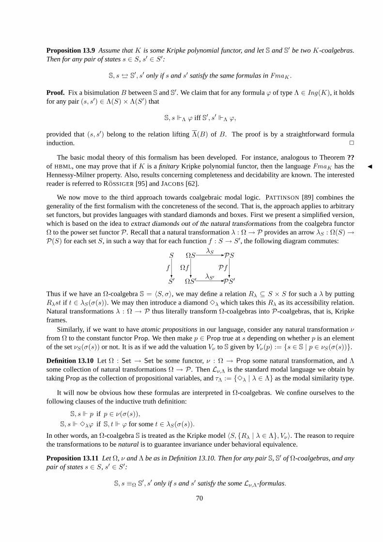
Proposition 13.9 Assume thatK is some Kripke polynomial functor, and letS andS′ be twoK-coalgebras.Then for any pair of statess ∈ S, s′ ∈ S′:

S, s↔ S′, s′ only if s ands′ satisfy the same formulas inFmaK .

Proof. Fix a bisimulationB betweenS andS′. We claim that for any formulaϕ of typeΛ ∈ Ing(K), it holdsfor any pair(s, s′) ∈ Λ(S)× Λ(S′) that

S, s Λ ϕ iff S′, s′ Λ ϕ,

provided that(s, s′) belong to the relation liftingΛ(B) of B. The proof is by a straightforward formulainduction. 2

The basic modal theory of this formalism has been developed. For instance, analogous to Theorem??of HBML , one may prove that ifK is afinitary Kripke polynomial functor, then the languageFmaK has the JHennessy-Milner property. Also, results concerning completeness and decidability are known. The interestedreader is referred to ROSSIGER[95] and JACOBS [62].

We now move to the third approach towards coalgebraic modal logic. PATTINSON [89] combines thegenerality of the first formalism with the concreteness of the second. That is, the approach applies to arbitraryset functors, but provides languages with standard diamonds and boxes. First we present a simplified version,which is based on the idea toextract diamonds out of the natural transformations from the coalgebra functorΩ to the power set functorP. Recall that a natural transformationλ : Ω→ P provides an arrowλS : Ω(S)→P(S) for each setS, in such a way that for each functionf : S → S′, the following diagram commutes:

S′ ΩS′ PS′

S ΩS PS

? ? ?-

-

f Ωf Pf

λS

λS′

Thus if we have anΩ-coalgebraS = 〈S, σ〉, we may define a relationRλ ⊆ S × S for such aλ by puttingRλst if t ∈ λS(σ(s)). We may then introduce a diamond3λ which takes thisRλ as its accessibility relation.Natural transformationsλ : Ω → P thus literally transformΩ-coalgebras intoP-coalgebras, that is, Kripkeframes.

Similarly, if we want to haveatomic propositionsin our language, consider any natural transformationνfrom Ω to the constant functorProp. We then makep ∈ Prop true ats depending on whetherp is an elementof the setνS(σ(s)) or not. It is as if we add the valuationVν to S given byVν(p) := s ∈ S | p ∈ νS(σ(s)).

Definition 13.10 Let Ω : Set → Set be some functor,ν : Ω → Prop some natural transformation, andΛsome collection of natural transformationsΩ → P. ThenLν,Λ is the standard modal language we obtain bytakingProp as the collection of propositional variables, andτΛ := 3λ | λ ∈ Λ as the modal similarity type.

It will now be obvious how these formulas are interpreted inΩ-coalgebras. We confine ourselves to thefollowing clauses of the inductive truth definition:

S, s p if p ∈ ν(σ(s)),S, s 3λϕ if S, t ϕ for somet ∈ λS(σ(s)).

In other words, anΩ-coalgebraS is treated as the Kripke model〈S, Rλ | λ ∈ Λ, Vν〉. The reason to requirethe transformations to benatural is to guarantee invariance under behavioral equivalence.

Proposition 13.11 LetΩ, ν andΛ be as in Definition 13.10. Then for any pairS, S′ of Ω-coalgebras, and anypair of statess ∈ S, s′ ∈ S′:

S, s ≡Ω S′, s′ only if s ands′ satisfy the someLν,Λ-formulas.

70

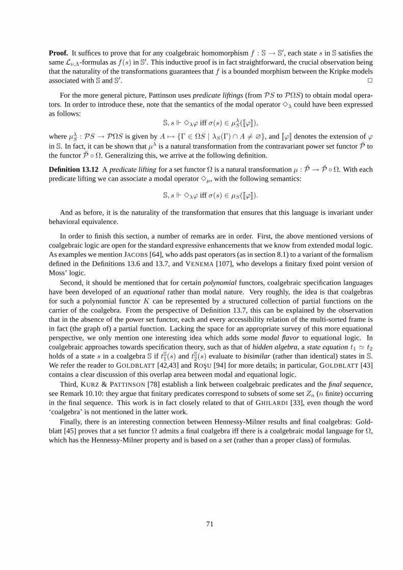
Proof. It suffices to prove that for any coalgebraic homomorphismf : S → S′, each states in S satisfies the

sameLν,Λ-formulas asf(s) in S′. This inductive proof is in fact straightforward, the crucial observation beingthat the naturality of the transformations guarantees thatf is a bounded morphism between the Kripke modelsassociated withS andS′. 2

For the more general picture, Pattinson usespredicate liftings(from PS to PΩS) to obtain modal opera-tors. In order to introduce these, note that the semantics of the modal operator3λ could have been expressedas follows:

S, s 3λϕ iff σ(s) ∈ µλS([[ϕ]]),

whereµλS : PS → PΩS is given byA 7→ Γ ∈ ΩS | λS(Γ) ∩ A 6= ∅, and[[ϕ]] denotes the extension ofϕin S. In fact, it can be shown thatµλ is a natural transformation from the contravariant power set functorP tothe functorP Ω. Generalizing this, we arrive at the following definition.

Definition 13.12 A predicate lifting for a set functorΩ is a natural transformationµ : P → P Ω. With eachpredicate lifting we can associate a modal operator3µ, with the following semantics:

S, s 3λϕ iff σ(s) ∈ µS([[ϕ]]).

And as before, it is the naturality of the transformation that ensures that this language is invariant underbehavioral equivalence.

In order to finish this section, a number of remarks are in order. First, the above mentioned versions ofcoalgebraic logic are open for the standard expressive enhancements that we know from extended modal logic.As examples we mention JACOBS [64], who adds past operators (as in section 8.1) to a variant of the formalismdefined in the Definitions 13.6 and 13.7, and VENEMA [107], who develops a finitary fixed point version ofMoss’ logic.

Second, it should be mentioned that for certainpolynomialfunctors, coalgebraic specification languageshave been developed of anequationalrather than modal nature. Very roughly, the idea is that coalgebrasfor such a polynomial functorK can be represented by a structured collection of partial functions on thecarrier of the coalgebra. From the perspective of Definition 13.7, this can be explained by the observationthat in the absence of the power set functor, each and every accessibility relation of the multi-sorted frame isin fact (the graph of) a partial function. Lacking the space for an appropriate survey of this more equationalperspective, we only mention one interesting idea which adds somemodal flavorto equational logic. Incoalgebraic approaches towards specification theory, such as that ofhidden algebra, a state equation t1 ' t2holds of a states in a coalgebraS if tS1(s) andtS2(s) evaluate tobisimilar (rather than identical) states inS.We refer the reader to GOLDBLATT [42,43] and ROSU [94] for more details; in particular, GOLDBLATT [43]contains a clear discussion of this overlap area between modal and equational logic.

Third, KURZ & PATTINSON [78] establish a link between coalgebraic predicates and thefinal sequence,see Remark 10.10: they argue that finitary predicates correspond to subsets of some setZn (n finite) occurringin the final sequence. This work is in fact closely related to that of GHILARDI [33], even though the word‘coalgebra’ is not mentioned in the latter work.

Finally, there is an interesting connection between Hennessy-Milner results and final coalgebras: Gold-blatt [45] proves that a set functorΩ admits a final coalgebra iff there is a coalgebraic modal language forΩ,which has the Hennessy-Milner property and is based on aset(rather than a proper class) of formulas.

71

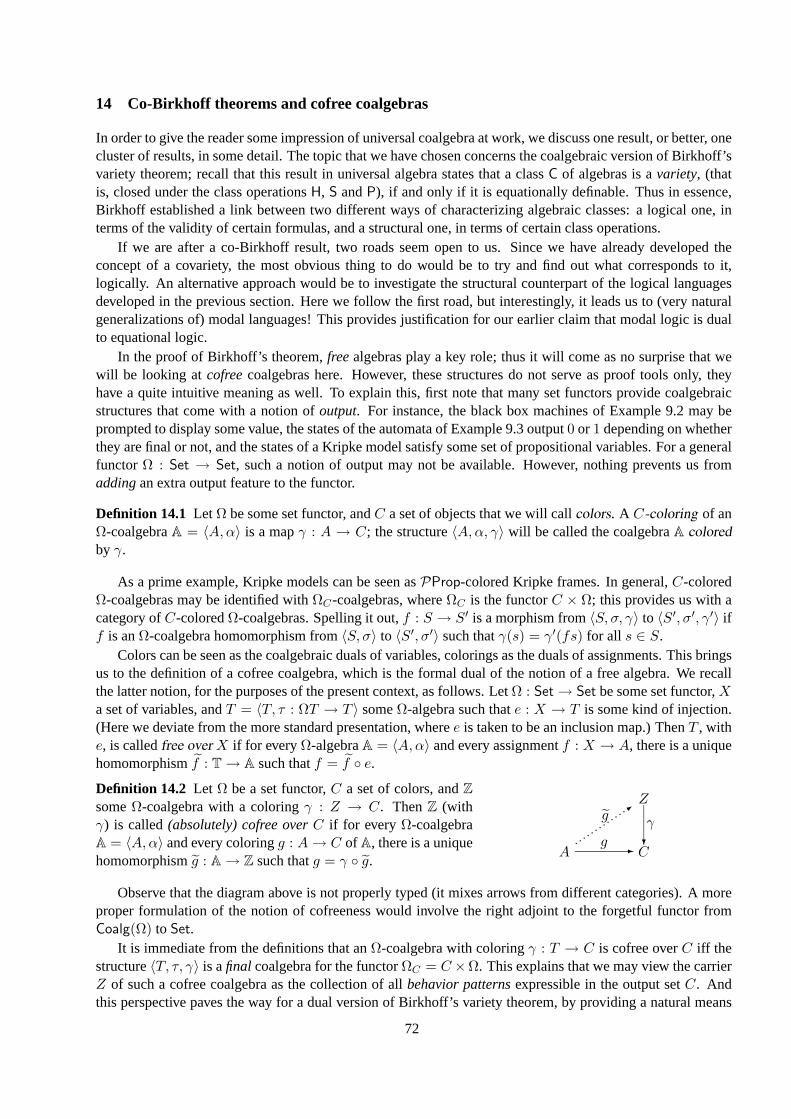
14 Co-Birkhoff theorems and cofree coalgebras

In order to give the reader some impression of universal coalgebra at work, we discuss one result, or better, onecluster of results, in some detail. The topic that we have chosen concerns the coalgebraic version of Birkhoff’svariety theorem; recall that this result in universal algebra states that a classC of algebras is avariety, (thatis, closed under the class operationsH, S andP), if and only if it is equationally definable. Thus in essence,Birkhoff established a link between two different ways of characterizing algebraic classes: a logical one, interms of the validity of certain formulas, and a structural one, in terms of certain class operations.

If we are after a co-Birkhoff result, two roads seem open to us. Since we have already developed theconcept of a covariety, the most obvious thing to do would be to try and find out what corresponds to it,logically. An alternative approach would be to investigate the structural counterpart of the logical languagesdeveloped in the previous section. Here we follow the first road, but interestingly, it leads us to (very naturalgeneralizations of) modal languages! This provides justification for our earlier claim that modal logic is dualto equational logic.

In the proof of Birkhoff’s theorem,freealgebras play a key role; thus it will come as no surprise that wewill be looking atcofreecoalgebras here. However, these structures do not serve as proof tools only, theyhave a quite intuitive meaning as well. To explain this, first note that many set functors provide coalgebraicstructures that come with a notion ofoutput. For instance, the black box machines of Example 9.2 may beprompted to display some value, the states of the automata of Example 9.3 output0 or 1 depending on whetherthey are final or not, and the states of a Kripke model satisfy some set of propositional variables. For a generalfunctor Ω : Set → Set, such a notion of output may not be available. However, nothing prevents us fromaddingan extra output feature to the functor.

Definition 14.1 Let Ω be some set functor, andC a set of objects that we will callcolors. A C-coloring of anΩ-coalgebraA = 〈A,α〉 is a mapγ : A → C; the structure〈A,α, γ〉 will be called the coalgebraA coloredby γ.

As a prime example, Kripke models can be seen asPProp-colored Kripke frames. In general,C-coloredΩ-coalgebras may be identified withΩC-coalgebras, whereΩC is the functorC × Ω; this provides us with acategory ofC-coloredΩ-coalgebras. Spelling it out,f : S → S′ is a morphism from〈S, σ, γ〉 to 〈S′, σ′, γ′〉 iff is anΩ-coalgebra homomorphism from〈S, σ〉 to 〈S′, σ′〉 such thatγ(s) = γ′(fs) for all s ∈ S.

Colors can be seen as the coalgebraic duals of variables, colorings as the duals of assignments. This bringsus to the definition of a cofree coalgebra, which is the formal dual of the notion of a free algebra. We recallthe latter notion, for the purposes of the present context, as follows. LetΩ : Set→ Set be some set functor,Xa set of variables, andT = 〈T, τ : ΩT → T 〉 someΩ-algebra such thate : X → T is some kind of injection.(Here we deviate from the more standard presentation, wheree is taken to be an inclusion map.) ThenT , withe, is calledfree over X if for everyΩ-algebraA = 〈A,α〉 and every assignmentf : X → A, there is a uniquehomomorphismf : T→ A such thatf = f e.

Definition 14.2 Let Ω be a set functor,C a set of colors, andZsomeΩ-coalgebra with a coloringγ : Z → C. ThenZ (withγ) is called(absolutely) cofree overC if for every Ω-coalgebraA = 〈A,α〉 and every coloringg : A→ C of A, there is a uniquehomomorphismg : A→ Z such thatg = γ g.

A C

Z

p p p p p p p p p p pp p p3?

-

γg

g

Observe that the diagram above is not properly typed (it mixes arrows from different categories). A moreproper formulation of the notion of cofreeness would involve the right adjoint to the forgetful functor fromCoalg(Ω) to Set.

It is immediate from the definitions that anΩ-coalgebra with coloringγ : T → C is cofree overC iff thestructure〈T, τ, γ〉 is afinal coalgebra for the functorΩC = C ×Ω. This explains that we may view the carrierZ of such a cofree coalgebra as the collection of allbehavior patternsexpressible in the output setC. Andthis perspective paves the way for a dual version of Birkhoff’s variety theorem, by providing a natural means

72

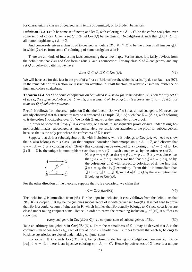
for characterizing classes of coalgebras in terms of permitted, or forbidden, behaviors.

Definition 14.3 Let Ω be some set functor, and letZ, with coloringγ : Z → C, be the cofree coalgebra oversome setC of colors. Given a setQ in Z, let Cov(Q) be the class ofΩ-coalgebrasA such thatη[A] ⊆ Q forall homomorphismsη : A→ Z.

And conversely, given a classK of Ω-coalgebras, defineBhv(K) ⊆ Z to be the union of all imagesg[A]in which g arises from someC-coloringg of some coalgebraA in K.

There are all kinds of interesting facts concerning these two maps. For instance, it is fairly obvious fromthe definitions thatBhv andCov form a (dual) Galois connection: For any classK of Ω-coalgebras, and anysetQ of behavior patterns, we have

Bhv(K) ⊆ Q iff K ⊆ Cov(Q). (48)

We will have use for this fact in the proof of a first co-Birkhoff result, which is basically due to RUTTEN [97].In the remainder of this section we restrict our attention tosmall functors, in order to ensure the existence offinal and cofree coalgebras.

Theorem 14.4 Let Ω be some endofunctor onSet which isκ-small for some cardinalκ. Then for any setCof sizeκ, the cofree coalgebra overC exists, and a classK of Ω-coalgebras is a covariety iffK = Cov(Q) forsome setQ of behavior patterns.

Proof. It follows from the assumption onΩ that the functorΩC = C ×Ω has a final coalgebra. However, wealready observed that this structure may be represented as a triple〈Z, ζ, γ〉 such thatZ = 〈Z, ζ〉, with coloringγ, is the cofreeΩ-coalgebra overC. We fix thisZ andγ for the remainder of the proof.

In order to show thatCov(Q) is a covariety, one needs to subsequently prove closure under taking ho-momorphic images, subcoalgebras, and sums. Here we restrict our attention to the proof for subcoalgebras,because that is the only part where the cofreeness ofZ is used.

Suppose thatA is a subcoalgebra ofB, with inclusionι, while B belongs toCov(Q); we need to showthatA also belongs to this class. For that purpose, consider a homomorphismη : A → Z, and observe thatγ η : A → C is a coloring ofA. Clearly this coloring can be extended to a coloringg : B → C of B. Letg : B→ Z be the unique homomorphism such thatg = γ g — such a map exists by the cofreeness ofZ.

B

A

C

Z

3

? ?-

-

ι γg

g

η

Now g = γ g, so thatγ g ι = g ι. But g was chosen sothatg ι = γ η. Hence we find thatγ g ι = γ η, so bythe cofreeness ofZ with respect to colorings ofA, we find thatg ι = η, that is, g extendsη. From this it is immediate thatη[A] = gA[A] ⊆ g[B], so thatη[A] ⊆ Q by the assumption thatB belongs toCov(Q).

For the other direction of the theorem, suppose thatK is a covariety; we claim that

K = Cov(Bhv(K)). (49)

The inclusion⊆ is immediate from (48). For the opposite inclusion, it easily follows from the definitions thatBhv(K) is Z-open. LetBK be the (unique) subcoalgebra ofZ with carrier setBhv(K). It is not hard to provethatBK is a conjunct sum of algebras inK, which implies thatBK actually belongs toK since covarieties areclosed under taking conjunct sums. Hence, in order to prove the remaining inclusion⊇ of (49), it suffices toshow that

every coalgebra inCov(Bhv(K)) is a conjunct sum of subcoalgebras ofBK. (50)

Take an arbitrary coalgebraA in Cov(Bhv(K)). From theκ-smallness ofΩ it may be derived thatA is theconjunct sum of coalgebrasAi, each of size at mostκ. Clearly then it suffices to prove that eachAi belongs toK, since covarieties are closed under taking conjunct sums.

Fix somei ∈ I; clearly Cov(Bhv(K)), being closed under taking subcoalgebras, containsAi. Since|Ai| ≤ κ = |C|, there is an injective coloringei : Ai → C. Hence by cofreeness ofZ there is a unique

73

homomorphismei : Ai → Z such thatei = γ ei. This ei must also be injective, which implies thatAi isisomorphic to its imageei[Ai]. But, sinceAi belongs toCov(Bhv(K)), the structureei[Ai] is a subcoalgebraof BK, and thus, belongs toK. From this it is immediate that eachAi belongs toK, and thus, so does theconjunct sumA. 2

Clearly, not only the statement, but also the proof of Theorem 14.4 is dual to that of Birkhoff’s varietytheorem. For instance, the coalgebraBK clearly fulfills the role of thecofree coalgebrafor the class K overthe color setC. What seems to be missing from Theorem 14.4, however, is some notion of logic, involvingsyntax. (It should be noted that also in the algebraic case, the straightforward characterization of varieties interms of equations only obtains in the case of relatively simple functors.) Since we are discussing a dual ofBirkhoff’s theorem, the question this raises is: what areco-equations?

Given the nature of systems as state-based models of dynamics, it seems natural to require that formulasdescribebehavior. This would provide natural constraints on possible coequational languages, namely, thatformulas are evaluated at states, in such a way that truth is invariant under behavioral equivalence. Further-more, we allow the use of colors in order to obtain sufficient expressive power. It was an insight of KURZ [76]that these requirements may also be read as a naturaldefinitionof coalgebraic modal logic.

Definition 14.5 Let Ω be some set functor. Acoalgebraic modal language for Ω consists of a setC of colors, aclassLC of formulas, and, for eachC-coloredΩ-coalgebra〈S, g〉, a truth or satisfaction relation S,g⊆ S×LCsuch that is invariant under behavioral equivalence. That is, if〈S, g〉, s ≡ΩC 〈T, h〉, t, thenS, s ≡LC T, t,where the latter notation indicates thats in 〈S, g〉 andt in 〈T, h〉 satisfy exactly the sameLC-formulasϕ.

In the sequel we will use notation and terminology from modal logic. For instance, we write〈S, g〉, s ϕinstead ofs S,g ϕ, and we defineS, g ϕ andS ϕ by quantifying over all elements and all valuations,respectively.

How can we link such modal languages to the cofree coalgebra? The idea here is that modal formulascorrespond to subcoalgebras: ifZ, with C-coloringγ is a cofree coalgebra overC, then define

[[ϕ]]Z,γ := z ∈ Z | Z, γ, z ϕ.

Using the behavioral invariance of the logic, it is not hard to see that[[ϕ]] (we usually omit superscripts)is alwaysZ-open. Now one way to obtain nice co-Birkhoff results is to require the modal language to beexpressive enough for the converse to hold as well.

Definition 14.6 Let Ω be someκ-small set functor, and let〈C,LC , 〉, with |C| = κ constitute a coalgebraicmodal logic forΩ. This modal logic is calledexpressive if every open set of theC-cofree coalgebraZ is ofthe form[[ϕ]] for some formulaϕ.

This may seem a strong requirement on a language, but expressive languages are not hard to come by.

Example 14.7 Under some mild additional assumptions onΩ, one may show that Moss’ logic of Defini-tion 13.1 and 13.2, extended with infinitedisjunctions, is expressive. For a proof sketch: strengthen Theo-rem 13.5 by proving that for any pointedΩC-system(S, s), there is a formulaϕS,s such that for all pointedΩC-system(S′, s′) one has thatS′, s′ ϕS,s iff S′, s′ ≡ΩC S, s. Then, given an open setU of the cofreeΩC-coalgebraZ, one may defineϕU :=

∨ϕZ,u | u ∈ U.

Now the next theorem bears witness to the tight link between modal logic and coalgebras. It is due toKURZ [76], while a very similar result was proved in GUMM & SCHRODER [53].

Theorem 14.8 Let Ω be someC-small set functor, and let〈C,LC , 〉 constitute an expressive coalgebraicmodal logic forΩ. Then a classK of Ω-coalgebras is a covariety iff for some formulaϕ, K is the class of allΩ-coalgebrasS such thatS ϕ.

Proof. Let Z, with coloringγ : Z → C, be the cofreeΩ-coalgebra overC. Given a formulaϕ, it is a directconsequence of cofreeness and truth invariance, that for anyΩ-coalgebraS with C-coloring g, and for any

74

states in S, we haveS, g, s ϕ iff g(s) ∈ [[ϕ]], (51)

from which one easily derives that for anyLC-formulaϕ:

Cov([[ϕ]]) is the class of allΩ-coalgebrasS such thatS ϕ. (52)

From (52) the direction ‘⇐’ of the Theorem is immediate. For the other direction, suppose thatK is a co-variety. Then by expressiveness,Bhv(K) = [[ϕ]] for some formulaϕ, so by (49) and (52) it follows thatK = Cov(Bhv(K)) = Cov([[ϕ]]), as required. 2

Although this theorem, being formulated in terms of a fairly general notion of modal logic, may stillseem to be rather abstract, it does provide a useful tool to provide more concrete results. For instance, givenExample 14.7, as a corollary to Theorem 14.8 one may obtain very general modal co-Birkhoff results forMoss’ coalgebraic logic. Or, to give an even more concrete corollary of Theorem 14.8, call an (ordinary)modal frameκ-boundedfor some cardinalκ if every point has less thanκ successors.

Corollary 14.9 A classK ofκ-bounded frame is (within the class of allκ-bounded frames) definable by meansof infinitary modal formulas, if and only ifK is closed under taking generated subframes, homomorphic imagesand disjoint unions.

The reader who compares the above two result to the Goldblatt-Thomasson Theorem 5.40, may be puzzledby the absence of ultrafilter extensions here. The explanation for this absence is of course that such Stone-type completions are not relevant in the presence of infinite disjunctions and conjunctions. If one takes thealternative road to co-Birkhoff theorems and starts, not from the notion of a covariety, but from afinitarycoalgebraic logical formalism, one will find that notions like ultrafilter extensions or ultraproducts are neededin the characterization of definable classes of coalgebras. Results in this direction can be found in for instanceGOLDBLATT [42,43] or ROSU [94].

Finally, the search for coalgebraic versions of Birkhoff’s variety theorem has received considerable atten-tion in the coalgebraic literature, as is witnessed by many contributions in [66,93,20,52,4]. Perhaps GUMM [51]should get some special mentioning for developing an alternative coequational syntax based on equivalenceclasses of infinite labeled trees.

75

15 Duality of algebra and coalgebra

Various other coalgebraic topics may be of interest to modal logicians, but here we confine ourselves to a briefdiscussion of the duality between algebra and coalgebra.

In remark 9.13 we already observed that some of the similarities between algebra and coalgebra are basedon the fact that a coalgebraC = 〈C, γ : C → ΩC〉 over an endofunctorΩ : C → C can also be seen as analgebra in theoppositecategoryCop . In fact, it is a trivial exercise to show that

Coalg(Ω) = (Alg(Ωop))op . (53)

That is, the category ofΩ-coalgebras is dually isomorphic to the category of algebras over the functorΩop

(which acts on objects and arrows just likeΩ does, the difference being thatΩop is an endofunctor onCop).This duality between algebras and coalgebras has been a major guideline in the development of universal

coalgebra, see RUTTEN [97]. To mention just one example (many more can be found in the text): whereasinitial algebras play an important role in universal algebra, it is thefinal objects that are relevant in coalgebra.For instance, whereas the principle of induction is based on the fact that initial algebras have no proper sub-algebras, the dualcoinduction principle boils down to the fact that final coalgebras have no proper quotients.However, it is important to realize that in (53) thebasecategory has been dualized. This means, for instance,that systems, orSet-coalgebras, correspond, not so much to algebras overSet, as to algebras over the oppositecategorySetop (which happens to be equivalent to the category of complete and atomic Boolean algebras withcomplete homomorphisms). As a consequence, a general theory of systems cannot be obtained by a straight-forward dualization of universal (Set-based) algebra. On the other hand, the fact that systems are, just likestandard algebras, ‘sets with structure’, indicates that many universal algebraic concepts may apply to coal-gebra byanalogyrather than by duality — see for instance Proposition 12.2. Thus, the universal coalgebraictheory of systems is an interesting mix of dualized and non-dualized universal algebra, with, of course, somecharacteristics of its own.

In case that there is an informativeduality for the base categoryC, more can be said of (53). This appliesfor instance to the just mentioned duality of the categorySet, but for the present purpose we prefer to focuson the categoryStone of Stone spaces. The point is, that sinceStone is dually equivalent to the well-knowncategoryBA of Boolean algebras, every endofunctorΩ on Stone induces an endofunctorΩ∗ := (·)∗ Ω (·)∗on BA. It is then an immediate consequence of (53) that the categoriesCoalg(Ω) and Alg(Ω∗) are duallyequivalent:

Coalg(Ω) Alg(Ω∗). (54)

For an example of this, consider the Vietoris functorV of Example 9.8. Concretely, the behavior of its dualfunctorV∗ : BA→ BA on objects is as follows. To a Boolean algebraB it assigns the Boolean algebraV∗(B)freely generated by the set3b | b ∈ B, subject to the axioms3⊥ = ⊥ and3a ∨ 3b = 3(a ∨ b). Sincethe categoryCoalg(V) is dually equivalent to that of modal algebras, we thus see that the latter category,MA,may be represented as an algebraic categoryAlg(V∗). This insight in fact provided the very first connectionbetween modal logic and coalgebra, see ABRAMSKY [1]. Recently, the duality that (54) provides betweenalgebra and coalgebra has been used to prove results on coalgebraic modallogics, where we now use the word‘logic’ in the technical sense. For instance, JACOBS [62] and KUPKE, KURZ & V ENEMA [74] use dualitiesin the style of (54) to prove completeness results for the multi-sorted modal logic of Definition 13.6 and 13.7.KUPKE, KURZ & PATTINSON [73] apply the above framework in order to characterize properties of arbitrarycoalgebraic modal logics.

Let us finish the chapter with the observation thatbothof the fundamental dualities underlying the math-ematical theory of modal logic are nontrivial instances of an algebra/coalgebra duality. This means that thealgebraic and the coalgebraic approach towards modal logic may be fruitfully operated in tandem. We believethat a thorough study of the interaction of algebra and coalgebra will provide a better understanding, not onlyof modal logic itself, but also of its mathematical surroundings.

76

A Basics of universal algebra and category theory

This section provides some technical preliminaries to this Chapter; we briefly review notation and terminologyon universal algebra and category theory.

If we equip a set with a collection of finitary operations, we call the resulting structure analgebra; twosuch structures are calledsimilar if their operations correspond in number and rank. In order to formalize thisnotion we introduce the notion of asimilarity type as a setΣ of function symbols each of which comes witha nonnegative integer to be called itsrank or arity. The arity of a function symbolf is denoted asar(f).Function symbols of rank zero are calledconstants.

The similarity type of (bounded) lattices is the setLatt = >,⊥,∧,∨ where> (‘top’) and⊥ (‘bottom’)are constants, and∧ (‘meet’) and∨ (‘join’) are binary symbols. As the similarity type for Boolean algebraswe take the setBool = >,⊥,¬,∧,∨ where>, ⊥, ∧ and∨ are as before, and¬ (‘complementation’) is aunary symbol.

A Σ-algebra is then a pairA = (A, I), in which theinterpretation I assigns to each function symbolf ∈ Σ an operation of arityar(f) on thecarrier A of the algebra. Usually we writefA rather thanI(f),and denote the algebraA = 〈A, I〉 by A = 〈A, fA | f ∈ Σ〉. As an example, let, for a setS, P(S) =〈P(S), S,∅,∼S ,∩,∪〉 be the power set algebra, where∼S denotes the unary operation of complementationwith respect toS. An algebra is calledtrivial if it has just one element; this completely determines the behaviorof the operations.

A homomorphism from a Σ-algebraA to a similar algebraB is a mapθ : A → B that preservesΣ-structure, in the sense that, for allf ∈ Σ, and alla1, . . . , an in A (wheren = ar(f)):

θ(fA(a1, . . . , an)) = fB(θa1, . . . , θan). (A.1)

An injective homomorphism is called anembedding and a surjective one, anepimorphism; an isomorphismis a bijective homomorphism. A homomorphism with the same source as target algebra is called anendomor-phism in general, and anautomorphisms if it is bijective.

Homomorphisms are closely related to special equivalence relations: acongruence onA is an equivalencerelation∼ satisfying, for allf ∈ Σ:

if a1 ∼ b1 & . . . & an ∼ bn, thenfA(a1, . . . , an) ∼ fA(b1, . . . , bn), (A.2)

wheren is the rank off . Given a congruence∼ onA, thequotient algebra ofA by∼ is the algebraA/∼whose carrier is the setA/∼ := [a] | a ∈ A of equivalence classes ofA under∼, and whose operations aredefined by

fA/∼([a1], . . . , [an]) = [fA(a1, . . . , an)].

(This is well-defined by (A.2).) The close connection between homomorphisms and congruences is formedby the fact that ifθ : A → B is a homomorphism, itskernel ker(θ) := (a, b) ∈ A × A | θ(a) = θ(b) is acongruence onA, while, on the other hand, for any congruence∼ onA, the associatednatural map ν∼ takingan elementa ∈ A to its equivalence class[a] is a surjective homomorphism fromA ontoA/∼.

The set of congruencesCgA of an algebraA forms in fact a complete lattice under the subset ordering;this lattice is denoted asCg(A); the meet operation of this lattice is simply their intersection, while the join oftwo congruences is given byΘ1 ∨Θ2 = Θ1 ∪ (Θ1 Θ2) ∪ (Θ1 Θ2 Θ1) ∪ · · · .

A Σ-algebraA is asubalgebra of a Σ-algebraB if A ⊆ B and for allf ∈ Σ, the operationfA coincideswith the restriction offB toA. Thedirect product A =

∏i∈I Ai of a family of Σ-algebras is an algebra with

carrier∏i∈I Ai and such that forf ∈ Σ anda1, . . . , an ∈

∏i∈I Ai:

fA(a1, . . . , an)(i) := fAi(a1(i), . . . , an(i))

We assume familiarity with the notions of ultraproduct and ultrapower.

77

Given a classK of algebras, we letH(K) denote the class of homomorphic images of algebras inK; S(K)is the class of isomorphic copies of subalgebras of algebras inK, and likewise definitions applies for the classoperationsP (products),Pu (ultraproducts) andPw (ultrapowers).

A class of algebras is called avariety if it is closed under taking subalgebras, homomorphisms, and prod-ucts; the smallest variety containing a classK is called the varietygenerated by K, notation:Var(K). Usinginequalities likeSH ≤ HS (meaning that, for any class of algebrasK, SH(K) is a subclass ofHS(K)), togetherwith the idempotence of the class operationsS, H andP, one can prove Tarski’s Theorem stating that

Var(K) = HSP(K) (A.3)

for any class of algebrasK.Given a similarity typeΣ and a set of variablesX, we define the setTerΣ(X) of Σ-terms over X by a

straightforward induction: it is the smallest includingX which containsf(t1, . . . , tn) whenever it containst1, . . . , tn andf ∈ Σ is a function symbol of rankn. (In particular,TerΣ(X) contains all constants inΣ.) Inthis chapter we adopt the convention that unless explicitly indicated otherwise,X denotes a countably infiniteset of variables; we often omit explicit reference toX, writing for instanceTerΣ rather thanTerΣ(X), etc.Also, writing s(x1, . . . , xn) for a terms, we indicate that the variables occurring ins are amongx1, . . . , xn.

Given an assignmentα of a setX of variables to (the carrierA of) an algebraA, we inductively define themeaning α(s) of a terms as follows:

α(x) = α(x)

α(f(t1, . . . , tn)) = fA(α(t1), . . . , α(tn)).(A.4)

Thus any terms(x1, . . . , xn) induces ann-ary term function sA onA, given bysA(a1, . . . , an) = α(s), whereα is any assignment mapping eachxi to ai. (Of course,sA can also be given an inductive definition.)

Using the close resemblance between the second clause of (A.4) and (A.1), we can turn the meaningfunction into a real homomorphism by imposingΣ-algebra structure on the setTerΣ(X), obtaining thetermalgebra TerΣ(X). The idea is to interpret the function symbolf ∈ Σ as follows:

fTerΣ(X) : (t1, . . . , tn) 7→ f(t1, . . . , tn).

Elaborating on this perspective, letK be a class ofΣ-algebras, andF aΣ-algebra generated by a setX ⊆ F .Suppose that for everyA in K and every mapα : X → A there is a homomorphismα : F → A extendingα. Then we say thatF has theuniversal mapping property for K over X, or thatF is free for K over X. Theidentities of (A.4) thus reveal thatTerΣ(X) is free overX for the class ofall Σ-algebras; for this reason it isoften referred to as theabsolutely free algebra over X.

Free algebras have a number of important properties of which we mention the following:

• every algebra inK is a homomorphic image of a free algebra over an appropriately large set of generators;

• all free algebras forK belongs to the classSP(K);• if F andF′ are free forK over the generator setsX andX ′, respectively, andX andX ′ have the same

cardinality, thenF andF′ are isomorphic.

Universal algebra may on the one hand be seen as generalizing the study of individual classes of algebrassuch as groups, fields, or lattices. On the other hand we may consider it as a rather special branch of modeltheory in which one is interested in structures for a language without relation symbols. The standard languagefor talking about such structures isequational.

An equation is nothing but a pair(s, t) of terms, always denoted ass ≈ t. The equations ≈ t (withs, t ∈ TerΣ(X)) is true or holds in the algebraA under the assignment α : X → A, notation:A |=α s ≈ t ifs andt obtain the same meaning inA underα, that is, ifα(s) = α(t). An equations ≈ t holds in the algebraA, or, equivalently, the algebraA satisfies the equations ≈ t, notation:A |= s ≈ t, if A |=α s ≈ t for everyassignmentα.

78

The relation|= induces a Galois connection between sets of formulas and classes of algebras; the polaritiesof this connection are given as the mapsEqu andMod, whereEqu(K) is the set of all equations that hold inK, andMod(E) denotes the class of algebras that satisfy every equation inE. The classes of algebras that arestable under this connection, that is, the classesK of the formMod(E) for some setE of equations, are calledequational classes. An important result by Birkhoff states that this notion coincides with that of a variety, andthat for any classK of algebras it holds that

Mod(Equ(K)) = Var(K). (A.5)

The relations ≡K t :⇐⇒ K |= s ≈ t

corresponding to the setEqu(K) is in fact acongruenceon the term algebraTerΣ. The algebraTerΣ(X)/ ≡K

has the universal mapping property forK over [X] (the set of equivalence classes ofX under≡K), which,together with the third fact on free algebras listed above, explains why we call it thefree algebra for K over[X].

A category C consists of a classOb(C) of objects, and for each pair of objectsA,B, a family C(A,B)of arrows. If f belongs to the latter set, we writef : A → B, and callA the domain andB the codomainof the arrow. The collection of arrows is endowed with some algebraic structure: for every objectA of Cthere is an arrowidA : A → A, and every pairf : A → B, g : B → C can be uniquelycomposed to anarrow g f : A → C. These operations are supposed to satisfy the associative law for composition, whilethe appropriate identity arrows are left- and right neutral elements. An arrowf : A → B is aniso if it hasan inverse, that is, an arrowg : B → A such thatf g = idB andg f = idA. Examples of categoriesareSet, the class of sets with functions, and, for every similarity typeΣ, the classAlg(Σ) of Σ-algebras, withhomomorphisms as arrows. Theopposite categoryCop of a given categoryC has the same objects asC, whileCop(A,B) = C(B,A) for all objectsA,B from C, and the operations on arrows are defined in the obviousway.

An objectX is initial in a categoryC if for every objectA in C there is a unique arrowα : X → A,andfinal if for all A there is a uniqueα : A → X. In Set, the empty set is initial, and the final objects areprecisely the singletons. Aproduct of two objectsA0 andA1 in a categoryC consists of a triple(A,α0 :A → A0, α1 : A → A1), such that for every triple(A′, α′0 : A′ → A0, α

′1 : A′ → A1) there is a unique

arrowf : A′ → A such thatαi f = α′i for both i. Coproductsof A0 andA1 are defined dually as triples(A,α0 : A0 → A,α1 : A1 → A), such that for every triple(A′, α′0 : A0 → A′, α′1 : A1 → A′) there is aunique arrowf : A→ A′ such thatf αi = α′i for eachi. The categorySet has both products and coproducts— that is, every pair(S0, S1) of sets has both a product (for which we may take the cartesian productS0 × S1

together with the two projection functionsπi : S0 × S1 → Si), and a coproduct (for which we may takethe disjoint unionS0 ] S1 = S0 × 0 ∪ S1 × 1 together with the coproduct mapsκ0 andκ1 given byκi(s) = (s, i)).

A functor Ω : C → D from a categoryC to a categoryD consists of an operation mapping objects andarrows ofC to objects and arrows ofD, respectively, in such a way thatΩf : ΩA → ΩB if f : A → B,Ω(idA) = idΩA andΩ(g f) = (Ωg) (Ωf) for all objects and arrows involved. A functorΩ : C → Dop issometimes called acontravariant functor fromC to D. An endofunctor on C is a functorΩ : C→ C.

As examples we consider the followingset functors (that is, endofunctors onSet): (i) for a fixed setC, theconstant functor mapping all sets toC and all arrows toidC ; this functor is denoted asC, (ii) the power setfunctor P, which maps any setS to its power setPS, and any mapf : S → S′ to the mapPf : PS → PS′given byPf : X 7→ fx | x ∈ X, and (iii) for every cardinalκ, the variantPκ of the power set functor,which maps any setS to the the collectionPκS := X ⊆ S | κ > |X|, and agrees withP on the arrowsfor which is defined. Furthermore, given two functorsΩ0 andΩ1, their product functor Ω0 × Ω1 is given(on objects) by(Ω0 × Ω1)S := Ω0S × Ω1S, while for f : S → S′, the map(Ω0 × Ω1)f is given as((Ω0 × Ω1)f)(σ0, σ1) := ((Ω0f)(σ0), (Ω1f)(σ1)). Thecoproduct functor is defined similarly. Finally, everycategoryC admits theidentity functor IC : C→ C which is the identity on both objects and arrows ofC.

79

Let C andD be two categories, and letΩ andΨ be two functors fromC to D. A natural transformation τfrom Ω to Ψ, notationτ : Ω ⇒ Ψ, consists ofD-arrowsτA : ΩA → ΨA such thatτB Ωf = Ψf τA foreachf : A→ B in C.

Finally, letΩ : C→ D andΨ : D→ C be two functors linking the categoriesC andD. Ω andΨ constituteanequivalence betweenC andD if their compositions are naturally isomorphic to the identity functors, that is,if there are natural transformationsσ : IC ⇒ ΨΩ andτ : ID ⇒ ΩΨ such that all arrowsσA : A→ ΨΩA andτB : B → ΩΨB are isos. If suchΩ andΨ exist, then the categoriesC andD are calledequivalent ; if Ω andΨare in fact each other’s inverse (both on maps and on arrows) thenC andD areisomorphic. If Ω andΨ forma dual equivalence between the categoriesC andD, that is, an equivalence between the categoriesC andDop ,then we say that the categories aredual or dually equivalent to each other.

80

Index

additive, 9completely, 17

algebraizes, 8atom, 17atom structure, 17atomic, 17

BAO, 9base category, 54behavioral equivalence, 59bisimilar, 59bisimulation

between coalgebras, 59equivalence, 59

Boolean algebraexpanded, 9with operators, 9

box, 4

canonicalclass, 31equation, 31extension, 21, 38formula, 31normal modal logic, 31

Cm, 8coalgebra, 51cofree, 72color, 72coloring, 72compact, 38complete

Boolean algebra, 17homomorphism, 18variety, 29

completion, 38MacNeille, 46

complex algebra, 8congruence distributive, 12covariety, 65Cst, 19

dense, 38diamond, 4

compound, 4induced, 4

discriminatorunary, 48

discriminator term, 48duality

complex, 18

essential, 15expanding, 43

field of sets, 21filter, 13

modal/open, 13principal, 13proper, 13

final coalgebra, 56final sequence, 58formula algebra, 7

general frame, 22descriptive, 22

global modality, 48, 49

homomorphic imagecoalgebraic, 64

homomorphismbetween coalgebras, 54

interpolation, local, 34

Lindenbaum-Tarski algebra, 10

modal logiccoalgebraic, 74

monotone, 9multiplicative, 9

neighborhood frame, 5normal, 9normal extension, 28

open setof coalgebra, 64

operator, 9

81

complete, 17

perfect, 17pointed, 51polynomial functor, 53

finitary Kripke, 53Kripke, 53

pullback, 62weak, 62

radical, 15relation lifting, 61root, 5

Sahlqvist formula, 32similarity type, basic modal, 4similarity type, modal, 4simple, 14small, 57smooth, 40stable, 43standard, 57Stone space, 22Str, 8subcoalgebra, 64subdirectly irreducible, 14sum, 65

conjunct, 66superamalgamation, 34system, 51

tense algebra, 47tense logic, 47

ultrafilter, 19ultrafilter frame, 19up-directed, 41up-set, 13

Vietoris construction, 53

82

References

[1] S. Abramsky. A Cook’s Tour of the FinitaryNon-Well-Founded Sets, 1988. Invited Lecture atBCTCS.

[2] P. Aczel. Non-well-founded sets, volume 14 ofCSLI Lecture Notes. CSLI, 1988.

[3] P. Aczel and N. Mendler. A final coalgebratheorem. In D.H. Pitt, A. Poigne, andD.E. Rydeheard, editors,Category Theory andComputer Science, volume 389 ofLecture Notesin Computer Science. Springer, 1989.

[4] J. Adamek, editor. Coalgebraic Methodsin Computer Science (CMCS’04), volume ??of Electronic Notes in Theoretical ComputerScience. Elsevier, 2004.

[5] J. Adamek and V. Koubek. On the greatest fixedpoint of a set functor. Theoretical ComputerScience, 150:57–75, 1995.

[6] J. Adamek and H.-E. Porst. From varieties ofalgebras to covarieties of coalgebras. In Corradiniet al. [20].

[7] H. Andreka, J. van Benthem, and I. Nemeti.Modal languages and bounded fragments ofpredicate logic.Journal of Philosophical Logic,27:217–274, 1998.

[8] A. Baltag. A logic for coalgebraic simulation. InReichel [93].

[9] M. Barr. Terminal coalgebras in well-founded set theory. Theoretical ComputerScience, 114(2):299–315, 1993. (Corrigendum inTheor.Comp.Sci.124:189–192,1994).

[10] M. Barr. Relational algebras. In S. Mac Lane,editor,Reports of the Midwest Category SeminarIV, volume 137 ofLecture Notes in Mathematics.Springer Verlag, 1997.

[11] J. Barwise and L. Moss. Vicious Circles,volume 60 of CSLI Lecture Notes. CSLIPublications, 1996.

[12] G. Birkhoff. Lattice Theory. Number 25 inColloquium Publications. AmericanMathematical Society, Providence, 1967. Thirdedition.

[13] P. Blackburn, M. de Rijke, and Y. Venema.Modal Logic. Number 53 in Cambridge Tractsin Theoretical Computer Science. CambridgeUniversity Press, 2001.

[14] W. Blok. Varieties of Interior Algebras. PhDthesis, Mathematisch Instituut, University ofAmsterdam, 1976.

[15] W. Blok. The lattice of modal algebras: Analgebraic investigation. Journal of SymbolicLogic, 45:221–236, 1980.

[16] W. Blok and D. Pigozzi. Algebraizable logics.Memoirs of the American Mathematical Society,77(396), 1989.

[17] S. Burris and H.P. Sankappanavar.A Coursein Universal Algebra. Graduate Texts inMathematics. Springer, 1981.

[18] W. Buszkowski. Embedding Boolean structuresinto atomic Boolean structures. Zeitschriftfur mathemathische Logik und Grundlagen derMathematik, 32:227–228, 1986.

[19] A. Carboni, G. Kelly, and R. Wood. A 2-categorical approach to change of base andgeometric morphisms I. Technical Report 90-1,Department of Pure Mathematics, University ofSydney, 1990.

[20] A. Corradini, M. Lenisa, and U. Montanari,editors. Coalgebraic Methods in ComputerScience (CMCS’01), volume 44 of ElectronicNotes in Theoretical Computer Science. Elsevier,2001.

[21] J. Czelakowski.Protoalgebraic Logic. Trends inLogic. Kluwer Academic Press, 2001.

[22] Paul Erdos. Graph theory and probability.Canadian Journal of Mathematics, 11:34–38,1959.

[23] L. Esakia. Topological Kripke models.SovietMathematics Doklady, 15:147–151, 1974.

[24] L. Esakia. To the theory of modal andsuperintuitionistic systems. In V. Smirnov, editor,Proceedings of the USSR Symposium on LogicalInference, pages 147–172. Nauka, Moscow, 1979.(In Russian).

[25] K. Fine. Some connections between elementaryand modal logic. In Kanger [71].

[26] J.M. Font and R. Jansana.A general algebraicsemantics for sentential logics. Lecture Notes inLogic. Springer, 1996.

[27] M. Gehrke. The order structure of Stonespaces and theTD-separation axiom.Zeitschriftfur mathemathische Logik und Grundlagen derMathematik, 37:5–15, 1991.

[28] M. Gehrke and J. Harding. Bounded latticeexpansions. Journal of Algebra, 238:345–371,2001.

[29] M. Gehrke, J. Harding,and Y. Venema. MacNeille completions andcanonical extensions. Transactions of theAmerican Mathematical Society, to appear.

83

[30] M. Gehrke and B. Jonsson. Bounded distributivelattices with operators.Mathematica Japonica,40:207–215, 1994.

[31] M. Gehrke and B. Jonsson. Monotone boundeddistributive lattices expansions. MathematicaJaponica, 52:197–213, 2000.

[32] M. Gehrke and B. Jonsson. Bounded distributivelattice expansions.Mathematica Scandinavica,94:3–45, 2004.

[33] S. Ghilardi. An algebraic theory of normal forms.Annals of Pure and Applied Logic, 71:189–245,1995.

[34] S. Ghilardi and G. Meloni. Constructivecanonicity in non-classical logics.Annals of Pureand Applied Logic, 86:1–32, 1997.

[35] S. Givant. Universal classes of simple relationalgebras.The Journal of Symbolic Logic, 64:575–589, 1999.

[36] S. Givant and Y. Venema. The preservations ofSahlqvist equations in completions of Booleanalgebras with operators.Algebra Universalis,41:47–84, 1999.

[37] R. Goldblatt. Metamathematics of modal logic I.Reports on Mathematical Logic, 6:41–78, 1976.

[38] R. Goldblatt. Metamathematics of modal logic II.Reports on Mathematical Logic, 7:21–52, 1976.

[39] R. Goldblatt. Varieties of complex algebras.Annals of Pure and Applied Logic, 38:173–241,1989.

[40] R. Goldblatt. Elementary generation andcanonicity for varieties of Boolean algebras withoperators. Algebra Universalis, 34:551–607,1995.

[41] R. Goldblatt. Algebraic polymodal logic: asurvey. Logic Journal of the IGPL, 8:393–450,2000.

[42] R. Goldblatt. A calculus of terms for coalgebrasof polynomial functors. In Corradini et al. [20].

[43] R. Goldblatt. What is the coalgebraic analogueof Birkhoff’s variety theorem. TheoreticalComputer Science, 266:853–886, 2001.

[44] R. Goldblatt. Mathematical modal logic: a viewof its evolution. Journal of Applied Logic,1:309—392, 2003. An updated version isavailable from the web site of the author.

[45] R. Goldblatt. Final coalgebras and the hennessy-milner property. Annals of Pure and AppliedLogic, to appear.

[46] R. Goldblatt, I. Hodkinson, and Y. Venema.Erdos graphs resolve Fine’s canonicity problem.Bulletin of Symbolic Logic, 10:186–208, 2004.

[47] R. Goldblatt and S. Thomason. Axiomatic classesin propositional modal logic. In J. Crossley,editor, Algebra and Logic, pages 163–173.Springer, 1974.

[48] V. Goranko and S. Passy. Using the universalmodality: Gains and questions.Journal of Logicand Computation, 2:5–30, 1992.

[49] V. Goranko and D. Vakarelov. Sahlqvistformulas unleashed in polyadic modal languages.In F. Wolter, H. Wansing, M. de Rijke,and M. Zakharyaschev, editors,Advances inModal Logic, Volume 3, pages 221–240. WorldScientific, 2002.

[50] H. Peter Gumm. Elements of the general theoryof coalgebras,1999. Lecture Notes for LUATCS’99, RandAfricaans University, Johannesburg; availablefrom http://www.mathematik.uni-marburg.de/˜gumm/ .

[51] H. Peter Gumm. Birkhoffs variety theorem forcoalgebras. Contributions to General Algebra,13:159–173, 2000.

[52] H. Peter Gumm, editor. Coalgebraic Methodsin Computer Science (CMCS’03), volume 82of Electronic Notes in Theoretical ComputerScience. Elsevier, 2003.

[53] H. Peter Gumm and T. Schroder. Covarietiesand complete covarieties.Theoretical ComputerScience, 260:71–86, 2001.

[54] H. Peter Gumm and T. Schroder. Coalgebrasof bounded type. Mathematical Structures inComputer Science, 12:565–578, 2002.

[55] H. Hansen and C. Kupke. A coalgebraicperspective on monotone modal logic. InAdamek [4].

[56] J. Harding. Canonical completions of latticesand ortholattices.Tatra Mountains MathematicalPublications, 15:85–96, 1998.

[57] L. Henkin, J.D. Monk, and A. Tarski.CylindricAlgebras. Part 1. Part 2. North-HollandPublishing Company, Amsterdam, 1971, 1985.

[58] R. Hirsch and I.M. Hodkinson.Relation Algebrasby Games. Number 147 in Studies in Logic.Elsevier, Amsterdam, 2002.

[59] E. Hoogland. Definability and Interpolation.Model-theoretic investigations. PhD thesis,Institute for Logic, Language and Computation,University of Amsterdam, 2001.

84

[60] T. Ihringer. Allgemeine Algebra. Mit einemAnhang uber Universelle Coalgebra von H. P.Gumm, volume 10 ofBerliner Studienreihe zurMathematik. Heldermann Verlag, 2003.

[61] B. Jacobs. Objects and classes, coalgebraically.In B. Freitag, C. Jones, C. Lengauer, andH.-J. Schek, editors,Object-Orientation withParallelism and Persistence, volume 44, pages83–103. Kluwer Academic Publishers, 1997.

[62] B. Jacobs. Many-sorted coalgebraic modal logic:a model-theoretic study.Theoretical Informaticsand Applications, 35(1):31–59, 2001.

[63] B. Jacobs. Exercises in coalgebraic specification.In R. Backhouse, R. Crole, and J. Gibbons,editors, Algebraic and Coalgebraic Methodsin the Mathematics of Program Construction,volume 44 ofLecture Notes in Computer Science,pages 237–280. Springer, 2002.

[64] B. Jacobs. The temporal logic of coalgebrasvia Galois algebras.Mathematical Structure inComputer Science, 12:875–903, 2002.

[65] B. Jacobs and J. Rutten. A tutorial on(co)algebras and (co)induction.Bulletin of theEuropean Association for Theoretical ComputerScience, 62:222–259, 1997.

[66] B. Jacobs and J. Rutten, editors.CoalgebraicMethods in Computer Science (CMCS’00),volume 19 of Electronic Notes in TheoreticalComputer Science. Elsevier, 1999.

[67] P. Jipsen. Discriminator varieties of Booleanalgebras with residuated operators. In C. Rauszer,editor,Algebraic Methods in Logic and ComputerScience, volume 28of Banach Center Publications, pages 239–252.Polish Academy of Sciences, 1993.

[68] P.J. Johnstone. Stone Spaces, volume 3 ofCambridge Studies in Advanced Mathematics.Cambridge University Press, Cambridge, 1982.

[69] B. Jonsson. On the canonicity of Sahlqvistidentities.Studia Logica, 4:473–491, 1994.

[70] B. Jonsson and A. Tarski. Boolean algebraswith operators, Part I. American Journal ofMathematics, 73:891–939, 1952.

[71] S. Kanger, editor. Proceedings of the ThirdScandinavian Logic Symposium. Uppsala 1973.North-Holland Publishing Company, 1975.

[72] M. Kracht. Tools and Techniques in ModalLogic. Number 142 in Studies in Logic. Elsevier,Amsterdam, 1999.

[73] C. Kupke, A. Kurz, and D. Pattinson. Algebraicsemantics for coalgebraic logics. In Adamek [4].

[74] C. Kupke, A. Kurz, and Y. Venema. Stonecoalgebras. Theoretical Computer Science,327:109–134, 2004.

[75] A. Kurz. Coalgebras and modal logic, 1999.Lecture Notes for ESSLLI’01; available fromhttp://www.folli.uva.nl/CD/2001/courses/readers/K40.pdf .

[76] A. Kurz. A co-variety-theorem for modal logic.In M. Zakharyaschev, K. Segerberg, M. de Rijke,and H. Wansing, editors,Advances in ModalLogic, Volume 2. CSLI Publications, 2000.

[77] A. Kurz. Specifying coalgebras with modallogic. Theoretical Computer Science, 260:119–138, 2001.

[78] A. Kurz and D. Pattinson. Coalgebraic modallogic of finite rank. Mathematical Structures inComputer Science, to appear. Also available asCWI Technical Report SEN-R0222, 2002.

[79] J. Lambek. A fixpoint theorem for completecategories.Mathematische Zeitschrift, 103:151–161, 1968.

[80] E. Lemmon. Algebraic semantics for modallogics, Parts I & II. Journal of Symbolic Logic,pages 46–65 & 191–218, 1966.

[81] T. Litak. On notions of completeness weakerthan Kripke incompleteness. In R. Schmidt,I. Pratt-Hartmann, M. Reynolds, and H. Wansing,editors, Advances in Modal Logic, Volume 5.King’s College London Publications, to appear.

[82] H. MacColl. Symbolic Logic and its Applications.Longmans, Green, and Co., London, 1906.

[83] L. Maksimova. Interpolation theorems in modallogic and amalgable varieties of topologicalBoolean algebras.Algebra and Logic, 18:348–370, 1979.

[84] M. Marx and Y. Venema. MultidimensionalModal Logic, volume 4 ofApplied Logic Series.Kluwer Academic Publishers, 1997.

[85] J. Monk. Completions of Boolean algebras withoperators. Mathematische Nachrichten, 46:47–55, 1970.

[86] L. Moss. Coalgebraic logic. Annals of Pureand Applied Logic, 96:277–317, 1999. (ErratumpublishedAnn.P.Appl.Log.99:241–259, 1999).

[87] I. Nemeti. Cylindric-relativized set algebras havestrong amalgamation.Journal of Symbolic Logic,50:689–700, 1985.

85

[88] D. Pattinson. Semantical principles in the modallogic of coalgebras. In H. Reichel and A. Ferreira,editors,Proc. 18th International Symposium onTheoretical Aspects of Computer Science (STACS2001), volume 2010 of LNCS, Berlin, 2001.Springer.

[89] D. Pattinson. Coalgebraic modallogic: Soundness, completeness and decidabilityof local consequence. Theoretical ComputerScience, 309:177–193, 2003.

[90] D. Pattinson. An introduction to the theoryof coalgebras, 2003. Notes accompanyinga course at NASSLLI 2003; available fromhttp://www.indiana.edu/˜nasslli/ .

[91] W. Rautenberg. Klassische und nichtklassischeAussagenlogik. Vieweg & Sohn, 1979.

[92] H. Reichel. An approach to object semanticsbased on terminal coalgebras.MathematicalStructures in Computer Science, 5:129–152,1995.

[93] H. Reichel, editor. Coalgebraic Methodsin Computer Science (CMCS’00), volume 33of Electronic Notes in Theoretical ComputerScience. Elsevier, 2000.

[94] G. Rosu. Equational axiomatizability forcoalgebra. Theoretical Computer Science,260:229–247, 2001.

[95] M. Roßiger. Coalgebras and modal logic. InReichel [93], pages 299–320.

[96] J. Rutten. Automata and coinduction (an exercisein coalgebra). In D. Sangiorigi and R. de Simone,editors, Proceedings of CONCUR ’98, volume1466 of Lecture Notes in Computer Science,pages 194–218. Springer, 1998.

[97] J. Rutten. Universal coalgebra: A theory ofsystems. Theoretical Computer Science, 249:3–80, 2000.

[98] H. Sahlqvist. Completeness and correspondencein the first and second order semantics for modallogic. In Kanger [71], pages 110–143.

[99] G. Sambin. Subdirectly irreducible modalalgebras and initial frames. Studia Logica,62:269–282, 1999.

[100] G. Sambin and V. Vaccaro. A topological proof ofSahlqvist’s theorem.Journal of Symbolic Logic,54:992–999, 1989.

[101] M. Stone. The theory of representations forBoolean algebras.Transactions of the AmericanMathematical Society, 40:37–111, 1936.

[102] S. Thomason. Semantic analysis of tense logics.Journal of Symbolic Logic, 37:150–158, 1972.

[103] S. Thomason. Categories of frames for modallogics. Journal of Symbolic Logic, 40:439–442,1975.

[104] V. Trnkova. Relational automata in a categoryand theory of languages. In M. Karpinski,editor, Fundamentals of computation theory:proceedings of the 1977 international FCT-conference, volume 56 of Lecture Notes inComputer Science, pages 340–355. Springer,1977.

[105] V. Trnkova. General theory of relationalautomata.Fundamenta Informaticae, 3:189–234,1979.

[106] Y. Venema. Atomless varieties. Journal ofSymbolic Logic, 68:607–614, 2003.

[107] Y. Venema. Automata and fixed point logics forcoalgebras. In Adamek [4].

[108] Y. Venema. A dual characterization of subdirectlyirreducible BAOs. Studia Logica, 77:105–115,2004.

[109] J. Worrell. Terminal sequences for accessibleendofunctors. In Jacobs and Rutten [66], pages39–53.

86