Embed Size (px)
Citation preview

Algebraic Structure in Network Information Theory
Michael Gastpar∗ and Bobak Nazer†
∗EPFL / Berkeley †Boston University
ISIT 2011
July 31, 2011

Motivation
pY |X

Motivation
pY |X

Motivation
pY |X
pY |X1X2

Motivation
pY |X
pY |X1X2 pY1Y2Y3|X1X2X3

Disclaimer
In the interest of telling a certain story,
• this tutorial does not attempt to provide an authoritativechronological account of the results;
• this tutorial does not claim to be complete (although a certain effortin this direction was made);

What This Tutorial Is Not About
We will not address the following very interesting questions (andapologize for a potentially misleading title):
• Complexity of coding schemes
• New families of algebraic codes
• Algebraic coding theory
•

What This Tutorial Is About
• Achievable rates that seem out of reach for “classical” arguments.
• Novel communication strategies where algebraic arguments appearto be of key importance.
• Recipes for how to apply these strategies to networks.
• Elements missing from Information Theory books.

Outline
I. Discrete Alphabets
II. AWGN Channels
III. Network Applications

Point-to-Point Channels
w Ex pY |X
yD w
The Usual Suspects:
• Message w ∈ {0, 1}k
• Encoder E : {0, 1}k → X n
• Input x ∈ X n
• Estimate w ∈ {0, 1}k
• Decoder D : Yn → {0, 1}k
• Output y ∈ Yn
• Memoryless Channel p(y|x) =n∏
i=1
p(yi|xi)
• Rate R =k
n.
• (Average) Probability of Error: P{w 6= w} → 0 as n→∞. Assumew is uniform over {0, 1}k .

i.i.d. Random Codes
• Generate 2nR codewordsx = [X1 X2 · · · Xn] independentlyand elementwise i.i.d. according tosome distribution pX
p(x) =
n∏
i=1
pX(xi)
• Bound the average error probabilityfor a random codebook.
• If the average performance overcodebooks is good, there must existat least one good fixed codebook.
0 1 2 3 4 · · · q − 1
0
1
2
3
4
...
q − 1

(Weak) Joint Typicality
• Two sequences x and y are (weakly) jointly typical if
∣
∣
∣
∣
−1
nlog p(x)−H(X)
∣
∣
∣
∣
<ǫ
∣
∣
∣
∣
−1
nlog p(y)−H(Y )
∣
∣
∣
∣
<ǫ
∣
∣
∣
∣
−1
nlog p(x,y) −H(X,Y )
∣
∣
∣
∣
<ǫ
• For our considerations, weak typicality is convenient as it can also bestated in terms of differential entropies.
• If x and y are i.i.d. sequences, the probability that they are jointlytypical goes to 1 as n goes to infinity.

Joint Typicality Decoding
Decoder looks for a codeword that is jointly typical with the receivedsequence y
Error Events
1. Transmitted codeword x is not jointly typicalwith y.=⇒ Low probability by the
Weak Law of Large Numbers.
2. Another codeword x is jointly typical with y.
Cuckoo’s Egg Lemma
Let x be an i.i.d. sequence that is independent from the receivedsequence y.
P
{
(x,y) is jointly typical}
≤ 2−n(I(X;Y )−3ǫ)
See Cover and Thomas.

Point-to-Point Capacity
• We can upper bound the probability of error via the union bound:
P{w 6= w} ≤∑
w 6=w
P
{
(x(w),y) is jointly typical.}
≤ 2−n(I(X;Y )−R−3ǫ) ← Cuckoo’s Egg Lemma
• If R < I(X;Y ), then the probability of error can be driven to zeroas the blocklength increases.
Theorem (Shannon ’48)
The capacity of a point-to-point channel is C = maxpX
I(X;Y ).
Linear Codes
• Linear Codebook: A linear map between messages and codewords(instead of a lookup table).
q-ary Linear Codes
• Represent message w as a length-k vector over Fq.
• Codewords x are length-n vectors over Fq.
• Encoding process is just a matrix multiplication, x = Gw.
x1x2...xn
=
g11 g12 · · · g1kg21 g22 · · · g2k...
.... . .
...gn1 gn2 · · · gnk
w1
w2...wk
• Recall that, for prime q, operations over Fq are just mod qoperations over the reals.
• Rate R =k
nlog q

Random Linear Codes
• Linear code looks like a regularsubsampling of the elements of Fn
q .
• Random linear code: Generateeach element gij of the generatormatrix G elementwise i.i.d.according to a uniform distributionover {0, 1, 2, . . . , q − 1}.
• How are the codewords distributed?0 1 2 3 4 · · · q − 1
0
1
2
3
4
...
q − 1
Fq
Fq

Codeword Distribution
It is convenient to instead analyze the shifted ensemble x = Gw ⊕ v
where v is an i.i.d. uniform sequence. (See Gallager.)
Shifted Codeword Properties
1. Marginally uniform over Fnq . For a given message w, the codeword x
looks like an i.i.d. uniform sequence.
P{x = x} =1
qnfor all x ∈ F
nq
2. Pairwise independent. For w1 6= w2, codewords x1, x2 areindependent.
P{x1 = x1, x2 = x2} =1
q2n= P{x1 = x1}P{x2 = x2}

Achievable Rates
• Cuckoo’s Egg Lemma only requires independence between the truecodeword x(w) and the other codeword x(w). From theunion bound:
P{w 6= w} ≤∑
w 6=w
P
{
(x(w),y) is jointly typical.}
≤ 2−n(I(X;Y )−R−3ǫ)
• This is exactly what we get from pairwise independence.
• Thus, there exists a good fixed generator matrix G and shift v forany rate R < I(X;Y ) where X is uniform.

Removing the Shift
w Ex
z
yD w
• For a binary symmetric channel (BSC), the output can be written asthe modulo sum of the input plus i.i.d. Bernoulli(p) noise,
y = x⊕ z
y = Gw ⊕ v ⊕ z
• Due to this symmetry, the probability of error depends only on therealization of the noise vector z.=⇒ For a BSC, x = Gw is a good code as well.
• We can now assume the existence of good generator matrices forchannel coding.

Random I.I.D. vs. Random Linear
• What have we gotten for linearity (so far)?Simplified encoding. (Decoder is still quite complex.)
• What have we lost?Can only achieve R = I(X;Y ) for uniform X instead ofmaxpX
I(X;Y ).
• In fact, this is a fundamental limitation of group codes,Ahlswede ’71.
• Workarounds: symbol remapping Gallager ’68, nested linear codes
• Are random linear codes strictly worse than random i.i.d. codes?
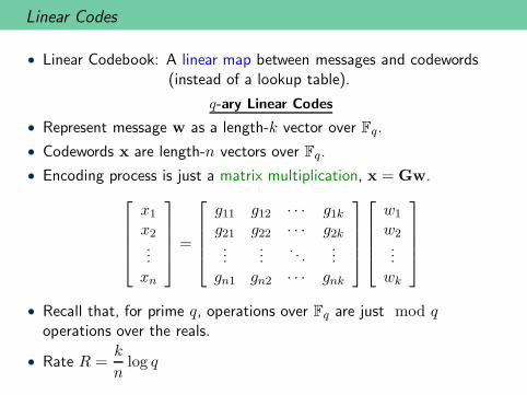
Slepian-Wolf Problem
s1 E1R1
s2 E2R2
Ds1s2
• Joint i.i.d. sources p(s1, s2) =
m∏
i=1
pS1S2(s1i, s2i)
• Rate Region: Set of rates (R1, R2) such that the encoders cansend s1 and s2 to the decoder with vanishing probability of error
P{(s1, s2) 6= (s1, s2)} → 0 as m→∞

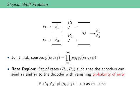
Random Binning
• Codebook 1: Independently and uniformly assign each sourcesequence s1 to a label {1, 2, . . . , 2mR1}
• Codebook 2: Independently and uniformly assign each sourcesequence s2 to a label {1, 2, . . . , 2mR2}
• Decoder: Look for jointly typical pair (s1, s2) within the receivedbin. Union bound:
P
{
jointly typical (s1, s2) 6= (s1, s2) in bin (ℓ1, ℓ2)}
≤∑
jointly typical (s1 ,s2)
2−m(R1+R2)
≤ 2m(H(S1,S2)+ǫ)2−m(R1+R2)
• Need R1 +R2 > H(S1, S2).
• Similarly, R1 > H(S1|S2) and R2 > H(S2|S1)

Slepian-Wolf Problem: Binning Illustration
1 2 3 2nR14 · · ·
1
2
3
4
...
2nR2
Slepian-Wolf Problem: Binning Illustration
1 2 3 2nR14 · · ·
1
2
3
4
...
2nR2

Random Linear Binning
• Assume source symbols take values in Fq.
• Codebook 1: Generate matrix G1 with i.i.d. uniform entries drawnfrom Fq. Each sequence s1 is binned via matrix multiplication,w1 = G1s1.
• Codebook 2: Generate matrix G2 with i.i.d. uniform entries drawnfrom Fq. Each sequence s2 is binned via matrix multiplication,w2 = G2s2.
• Bin assignments are uniform and pairwise independent (except forsℓ = 0)
• Can apply the same union bound analysis as random binning.

Slepian-Wolf Rate Region
Slepian-Wolf Theorem
Reliable compression possible if and
only if:
R1 ≥ H(S1|S2) = hB(p)
R2 ≥ H(S2|S1) = hB(p)
R1 +R2 ≥ H(S1, S2) = 1 + hB(p)
Random linear binning is as goodas random i.i.d. binning!
R2
R1
S-W
hB(p)
hB(p)
R1 +R2 = 1 + hB(p)
Example: Doubly Symmetric Binary SourceS1 ∼ Bern(1/2) U ∼ Bern(p) S2 = S1 ⊕ U

Korner-Marton Problem
• Binary sources
• s1 is i.i.d. Bernoulli(1/2)
• s2 is s1 corrupted by Bernoulli(p)noise
• Decoder wants the modulo-2 sum .
s1 E1R1
s2 E2R2
D u
u = s1 ⊕ s2
Rate Region: Set of rates (R1, R2) such that there exist encoders anddecoders with vanishing probability of error
P{u 6= u} → 0 as m→∞
Are any rate savings possible over sending s1 and s2 in their entirety?

Random Binning
• Sending s1 and s2 with random binning requiresR1 +R2 > 1 + hB(p)?
• What happens if we use rates such that R1 +R2 < 1 + hB(p)?
• There will be exponentially many pairs (s1, s2) in each bin!
• This would be fine if all pairs in a bin have the same sum, s1 + s2.But this probability goes to zero exponentially fast!

Korner-Marton Problem: Random Binning Illustration
1 2 3 2nR14 · · ·
1
2
3
4
...
2nR2

Korner-Marton Problem: Random Binning Illustration
1 2 3 2nR14 · · ·
1
2
3
4
...
2nR2

Linear Binning
• Use the same random matrix G for linear binning at each encoder:
w1 = Gs1 w2 = Gs2
• Idea from Korner-Marton ’79: Decoder adds up the bins.
w1 ⊕w2 = Gs1 ⊕Gs2
= G(s1 ⊕ s2)
= Gu
• G is good for compressing u if R > H(U) = hB(p).
Korner-Marton Theorem
Reliable compression of the sum is possible if and only if:
R1 ≥ hB(p) R2 ≥ hB(p) .

Korner-Marton Problem: Linear Binning Illustration
1 2 3 2nR14 · · ·
1
2
3
4
...
2nR2

Korner-Marton Problem: Linear Illustration
1 2 3 2nR14 · · ·
1
2
3
4
...
2nR2

Korner-Marton Rate Region
R2
R1
S-W
K-M
hB(p)
hB(p)
Linear codes can improve performance!
(for distributed computation of dependent sources)

Multiple-Access Channels
w1 E1x1
w2 E2x2
pY |X1X2
yD
w1
w2
• Rate Region: Set of rates (R1, R2) such that the encoders cansend w1 and w2 to the decoder with vanishing probability of error
P{(w1, w2) 6= (w1,w2)} → 0 as m→∞

Multiple-Access Channels
• Cuckoo’s egg lemma applies to all three error events.
• For example, event that only w1 is wrong:
P{w1 6= w1, w2 = w2} ≤∑
w1 6=w1
P
{
(x1(w1),x2(w2),y) jointly typical}
≤ 2−n(I(X1;Y |X2)−R1−3ǫ)
Rate Region (Ahlswede, Liao)
Convex closure of all (R1, R2) satisfying
R1 < I(X1;Y |X2)
R2 < I(X2;Y |X1)
R1 +R2 < I(X1,X2;Y )
for some p(x1)p(x2).

Finite-Field Multiple-Access Channels
• Linear codes can achieveany rate available foruniform p(x1), p(x2).
• For finite field MACs, canachieve the whole capacityregion.
w1 E1x1
w2 E2x2
z
yD
w1
w2
R2
R1log q − H(Z)
log q − H(Z)
• Receiver observes noisy modulo sum ofcodewords y = x1 ⊕ x2 ⊕ z
Finite Field MAC Rate Region
All rates (R1, R2) satisfying
R1 +R2 ≤ log q −H(Z)

Computation over Finite Field Multiple-Access Channels
• Independent msgsw1,w2 ∈ F
kq .
• Want the sum u = w1 ⊕w2
with vanishing prob. of errorP{u 6= u} → 0
w1 E1x1
w2 E2x2
z
yD u
u = w1 ⊕w2
I.I.D. Random Coding
• Generate 2nR1 i.i.d. uniform codewords for user 1.
• Generate 2nR2 i.i.d. uniform codewords for user 2.
• With high probability, (nearly) all sums of codewords are distinct.
• This is ideal for multiple-access but not for computation.
• Need R1 +R2 ≤ log q −H(Z)
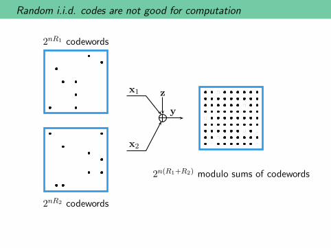
Random i.i.d. codes are not good for computation
2nR1 codewords
2nR2 codewords
2n(R1+R2) modulo sums of codewords
x1
x2
z
y

Computation over Finite Field Multiple-Access Channels
Independent msgs w1,w2.
Want the sum u = w1 ⊕w2
with vanishing prob. of errorP{u 6= u} → 0
w1 E1x1
w2 E2x2
z
yD u
u = w1 ⊕w2
Random Linear Coding
• Same linear code at both transmitters x1 = Gw1, x2 = Gw2.
• Sums of codewords are themselves codewords:
y = x1 ⊕ x2 ⊕ z
= Gw1 ⊕Gw2 ⊕ z
= G(w1 ⊕w2)⊕ z
= Gu⊕ z
• Need max(R1, R2) ≤ log q −H(Z)

Random linear codes are good for computation
2nR1 codewords
2nR2 codewords
2nmax(R1,R2) modulo sums of codewords
x1
x2
z
y
Computation over Finite Field Multiple-Access Channels
R2
R1
Linear
I.I.D.
log q −H(Z)
log q −H(Z)
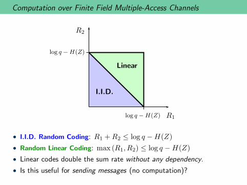
• I.I.D. Random Coding: R1 +R2 ≤ log q −H(Z)
• Random Linear Coding: max (R1, R2) ≤ log q −H(Z)
• Linear codes double the sum rate without any dependency.
• Is this useful for sending messages (no computation)?

Two-Way Relay Channel
w1Has
Wants w2 w1
Has
Wants
w2Relay
• Elegant example proposed by Wu-Chou-Kung ’04.
• Closely related to butterfly network from Ahlswede-Cai-Li-Yeung ’00.

Two-Way Relay Channel – Time-Division
w1 w2
w1 w2w1
w1 w2w1 w2
w1 w1 w2w1 w2
(a)
(b)
(c)
(d)

Two-Way Relay Channel – Network Coding
w1 w2
w1 w2w1
w1 w2w1 w2
(a)
(b)
(c)
w1 ⊕w2

Two-Way Relay Channel – Physical-Layer Network Coding
w1 w2
w1 w2
(a)
(b)
w1 ⊕w2

Two-Way Relay Channel – Physical-Layer Network Coding
w1 w2
w1 w2
(a)
(b)
w1 ⊕w2
• Physical-layer network coding: exploiting the wireless medium fornetwork coding. Independently and concurrently proposed byZhang-Liew-Lam ’06, Popovski-Yomo ’06, Nazer-Gastpar ’06.
• Sometimes referred to as Analog Network CodingKatti-Gollakota-Katabi ’08.
• Some recent surveys Liew-Zhang-Lu ’11, Nazer-Gastpar ’11.

q-ary Two-Way Relay Channel
w1Has
Wants w2 w1
Has
Wants
w2Relay
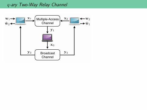
q-ary Two-Way Relay Channel
w1 w2Multiple-Access
Channel
Broadcast
Channel
x1 x2
y1
y3 y4
x3
w2 w1

q-ary Two-Way Relay Channel
zMAC
yMAC
Relay
xBC
z2z1
User 1
x1w1
w2
User 2
x2 w2
w1
• i.i.d. noise sequences with
entropy H(Z).
• Rates R1 and R2.
• Upper Bound:max (R1, R2) ≤ log q −H(Z)
• Random i.i.d.: Relay decodes w1,w2 and transmits w1 ⊕w2.R1 +R2 ≤ log q −H(Z)
• Random linear: Relay decodes and retransmits w1 ⊕w2
max (R1, R2) ≤ log q −H(Z)

q-ary Two-Way Relay Channel
R2
R1
Linear
I.I.D.
log q −H(Z)
log q −H(Z)
• I.I.D. Random Coding: R1 +R2 ≤ log q −H(Z)
• Random Linear Coding: max (R1, R2) ≤ log q −H(Z)
• Linear codes can double the sum rate for exchanging messages.

Generalizing Linear Codes...
• Observation: For linear codes, the codeword statistics are uniform.This follows straightforwardly from the fact that the sum of any twocodewords is again a codeword.
• Question: Can we retain some algebraic structure and havenon-uniform codeword statistics?
• Idea: Nested Linear Codes (see, for instance, Conway and Sloane
’92, Forney ’89, Zamir-Shamai-Erez ’02 ...):

Nested Linear Codes
• Consider a linear code Cc of rate 1− k/n :
x1x2...xn
=
g11 g12 · · · g1,n−k
g21 g22 · · · g2,n−k...
.... . .
...gn1 gn2 · · · gn,n−k
w1...
wn−k
with parity check matrix Hc.
• For every binary sequence u of length k, define its coset as
Cc(u) = {x : Hcx = u}
• The coset leader is the one sequence in Cc(u) that has the smallestHamming weight.

Nested Linear Codes
• For any sequence x we write x mod Cc to denote the coset leadercorresponding to Hcx.
• Observation: This satisfies all the usual properties of the modulooperation, such as
(x⊕ y) mod Cc = (x mod Cc ⊕ y mod Cc) mod Cc
Theorem
There exists a binary linear code of rate 1− k/n such that all 2k cosetleaders satisfy wHamming ≤ m, where
k/n ≥ Hb(m/n)− ǫ
Note: Such a code is thus a good covering code.

Nested Linear Codes
Next step: Decimate coset leaders: retain only those belonging to a(“fine”) code.
That way, we end up with a code of 2k−k′ codewords satisfying twoproperties:
1 Noise protection just like the fine code
2 The sum of any two codewords, modulo “the coarse code,” is againa codeword
On the BSC with crossover probability p, this code achieves a rate
R = Hb(m/n)−Hb(p).
Note that this is not the capacity of this channel.

Distributed Dirty Paper Coding (Binary case)
Philosof-Zamir ’09, Philosof-Zamir-Erez ’09:
w1 E1x1
s1
w2 E2x2
s2
z
yD w1, w2
Without input constraints, the problem is trivial.
But now, consider
wH(x1) ≤ m and wH(x2) ≤ m.

Distributed Dirty Paper Coding
• Choose codewords t1 and t2. Transmit
x1 = (t1 ⊕ s1) mod Cc and x2 = (t2 ⊕ s2) mod Cc
• Choose coarse code to satisfy Hamming input constraints. Receive:
y = [(x1 ⊕ s1) mod Cc]⊕ [(x2 ⊕ s2) mod Cc]⊕ s1 ⊕ s2 ⊕ z
• The key step is the following pre-processing step at the decoder:
y mod Cc = (x1 ⊕ s1 ⊕ x2 ⊕ s2 ⊕ s1 ⊕ s2 ⊕ z) mod Cc
= (x1 ⊕ x2 ⊕ z) mod Cc
• Last step: show that the noise is essentially unchanged by themodulo operation.
• Can show that this achieves the capacity (see Philosof-Zamir-Erez
’09.)
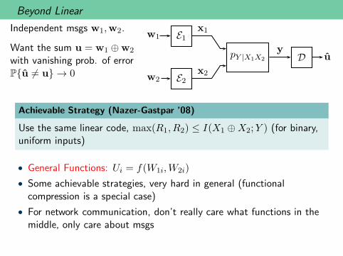
Beyond Linear
Independent msgs w1,w2.
Want the sum u = w1 ⊕w2
with vanishing prob. of errorP{u 6= u} → 0
w1 E1x1
w2 E2x2
pY |X1X2
yD u
Achievable Strategy (Nazer-Gastpar ’08)
Use the same linear code, max(R1, R2) ≤ I(X1 ⊕X2;Y ) (for binary,uniform inputs)
• General Functions: Ui = f(W1i,W2i)
• Some achievable strategies, very hard in general (functionalcompression is a special case)
• For network communication, don’t really care what functions in themiddle, only care about msgs

Outline
I. Discrete Alphabets
II. AWGN Channels
III. Network Applications

Main References
Nested lattice results in this section are almost entirely drawn from:
• U. Erez and R. Zamir, Achieving 12 log(1 + SNR) on the AWGN
channel with lattice encoding and decoding, IEEE Transactions onInformation Theory, vol. 50, pp. 2293-2314, October 2004.
• U. Erez, S. Litsyn, and R. Zamir, Lattices which are good for (al-most) everything, IEEE Transactions on Information Theory, vol. 51,pp. 3401-3416, October 2005.
• R. Zamir, Lattices are everywhere, in Proceedings of the 4th AnnualWorkshop on Information Theory and its Applications, La Jolla, CA,February 2009.

Gaussian MMSE Estimation
• Signal X is a scalar Gaussian r.v. with mean 0 and variance P .
• Noise Z is an independent scalar Gaussian r.v. with mean 0 andvariance N .
• Estimate X from noisy observation Y = X + Z.
• Mean-squared error: E[(Y −X)2] = E[Z2] = N .
• Minimum mean-squared error (MMSE):
E[(αY −X)2] = E[(αX + αZ −X)2]
= E[α2Z2 + (1− α)2X2] Part of error due to X
= α2N + (1− α)2P
• Optimal α =P
N + Pyields E[(αY −X)2] =
PN
N + P.

Point-to-Point AWGN Channels
• Codewords must satisfy powerconstraint:
‖x‖2 ≤ nP .
• i.i.d. Gaussian noise with varianceN :
z ∼ N (0, NI) .
• Shannon ’48: Channel capacity:
C =1
2log
(
1 +P
N
)
w Ex
zy
D w
(Cover and Thomas,Elements of Information Theory)
• In high dimensions, noise starts to look spherical.

Lattices
• A lattice Λ is a discrete subgroup ofRn.
• Can write a lattice as a lineartransformation of the integervectors,
Λ = BZn ,
for some B ∈ Rn×n.
Lattice Properties
• Closed under addition:λ1, λ2 ∈ Λ =⇒ λ1 + λ2 ∈ Λ.
• Symmetric: λ ∈ Λ =⇒ −λ ∈ ΛZn is a simple lattice.

Lattices
• A lattice Λ is a discrete subgroup ofRn.
• Can write a lattice as a lineartransformation of the integervectors,
Λ = BZn ,
for some B ∈ Rn×n.
Lattice Properties
• Closed under addition:λ1, λ2 ∈ Λ =⇒ λ1 + λ2 ∈ Λ.
• Symmetric: λ ∈ Λ =⇒ −λ ∈ ΛBZ
n

Voronoi Regions
• Nearest neighbor quantizer:
QΛ(x) = argminλ∈Λ
‖x− λ‖2
• The Voronoi region of a lattice pointis the set of all points that quantizeto that lattice point.
• Fundamental Voronoi region V:points that quantize to the origin,
V = {x : QΛ(x) = 0}
• Each Voronoi region is just a shift ofthe fundamental Voronoi region V
Nested Lattices
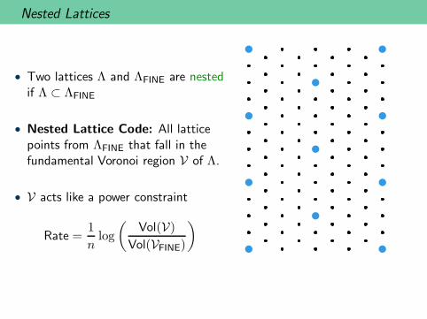
• Two lattices Λ and ΛFINE are nestedif Λ ⊂ ΛFINE
• Nested Lattice Code: All latticepoints from ΛFINE that fall in thefundamental Voronoi region V of Λ.
• V acts like a power constraint
Rate =1
nlog
(
Vol(V)
Vol(VFINE)
)

Nested Lattices
• Two lattices Λ and ΛFINE are nestedif Λ ⊂ ΛFINE
• Nested Lattice Code: All latticepoints from ΛFINE that fall in thefundamental Voronoi region V of Λ.
• V acts like a power constraint
Rate =1
nlog
(
Vol(V)
Vol(VFINE)
)

Nested Lattices
• Two lattices Λ and ΛFINE are nestedif Λ ⊂ ΛFINE
• Nested Lattice Code: All latticepoints from ΛFINE that fall in thefundamental Voronoi region V of Λ.
• V acts like a power constraint
Rate =1
nlog
(
Vol(V)
Vol(VFINE)
)

Nested Lattices
• Two lattices Λ and ΛFINE are nestedif Λ ⊂ ΛFINE
• Nested Lattice Code: All latticepoints from ΛFINE that fall in thefundamental Voronoi region V of Λ.
• V acts like a power constraint
Rate =1
nlog
(
Vol(V)
Vol(VFINE)
)

Nested Lattices
• Two lattices Λ and ΛFINE are nestedif Λ ⊂ ΛFINE
• Nested Lattice Code: All latticepoints from ΛFINE that fall in thefundamental Voronoi region V of Λ.
• V acts like a power constraint
Rate =1
nlog
(
Vol(V)
Vol(VFINE)
)
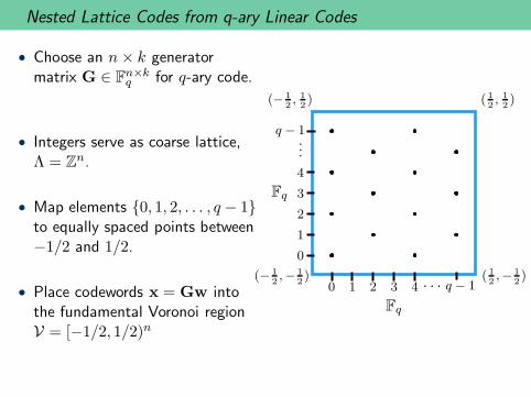
Nested Lattice Codes from q-ary Linear Codes
• Choose an n× k generatormatrix G ∈ F
n×kq for q-ary code.
• Integers serve as coarse lattice,Λ = Z
n.
• Map elements {0, 1, 2, . . . , q − 1}to equally spaced points between−1/2 and 1/2.
• Place codewords x = Gw intothe fundamental Voronoi regionV = [−1/2, 1/2)n
0 1 2 3 4 · · · q − 1
0
1
2
3
4
...
q − 1
Fq
Fq
(− 12,− 1
2) ( 1
2,− 1
2)
(− 12, 12) ( 1
2, 12)

Modulo Operation
• Modulo operation with respect tolattice Λ is just the residualquantization error,
[x] mod Λ = x−QΛ(x) .
• Mimics the role of mod q in q-aryalphabet.
• Distributive Law:[
x1 + [x2] mod Λ]
mod Λ
= [x1 + x2] mod Λ

Modulo Operation
• Modulo operation with respect tolattice Λ is just the residualquantization error,
[x] mod Λ = x−QΛ(x) .
• Mimics the role of mod q in q-aryalphabet.
• Distributive Law:[
x1 + [x2] mod Λ]
mod Λ
= [x1 + x2] mod Λ

Modulo Operation
• Modulo operation with respect tolattice Λ is just the residualquantization error,
[x] mod Λ = x−QΛ(x) .
• Mimics the role of mod q in q-aryalphabet.
• Distributive Law:[
x1 + [x2] mod Λ]
mod Λ
= [x1 + x2] mod Λ
mod Λ

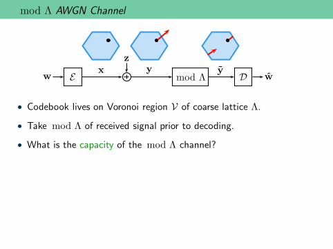
mod Λ AWGN Channel
w Ex
zy
mod Λy
D w
• Codebook lives on Voronoi region V of coarse lattice Λ.
• Take mod Λ of received signal prior to decoding.
• What is the capacity of the mod Λ channel?
mod Λ AWGN Channel
w Ex
zy
mod Λy
D w
• Codebook lives on Voronoi region V of coarse lattice Λ.
• Take mod Λ of received signal prior to decoding.
• What is the capacity of the mod Λ channel?

mod Λ AWGN Channel
w Ex
zy
mod Λy
D w
• Codebook lives on Voronoi region V of coarse lattice Λ.
• Take mod Λ of received signal prior to decoding.
• What is the capacity of the mod Λ channel?
Using random i.i.d. code drawn over V: C =1
nmaxp(x)
I(x; y)

mod Λ AWGN Channel Capacity
w Ex
zy
mod Λy
D w
nC = maxp(x)
I(x; y)
= maxp(x)
(
h(y)− h(y|x))

mod Λ AWGN Channel Capacity
w Ex
zy
mod Λy
D w
nC = maxp(x)
I(x; y)
= maxp(x)
(
h(y)− h(y|x))
= maxp(x)
(
h(y)− h(
[z] mod Λ))
Distributive Law

mod Λ AWGN Channel Capacity
w Ex
zy
mod Λy
D w
nC = maxp(x)
I(x; y)
= maxp(x)
(
h(y)− h(y|x))
= maxp(x)
(
h(y)− h(
[z] mod Λ))
Distributive Law
≥ maxp(x)
(
h(y)− h(z))
Point Symmetry of Voronoi Region

mod Λ AWGN Channel Capacity
w Ex
zy
mod Λy
D w
nC = maxp(x)
I(x; y)
= maxp(x)
(
h(y)− h(y|x))
= maxp(x)
(
h(y)− h(
[z] mod Λ))
Distributive Law
≥ maxp(x)
(
h(y)− h(z))
Point Symmetry of Voronoi Region
= maxp(x)
(
h(y)−n
2log(2πeN)
)
Entropy of Gaussian Noise

mod Λ AWGN Channel Capacity
w Ex
zy
mod Λy
D w
• Channel output entropy is equal to the logarithm of the Voronoiregion volume if it is uniform over V:
h(y) = log(Vol(V)) if y ∼ Unif(V)
• y = [x+ z] mod Λ is uniform over V if x is uniform over V.
• Random i.i.d. coding over the Voronoi region V can achieve:
R =1
nlog(Vol(V)) −
1
2log(2πeN)

Power Constraints and Second Moments
w Ex
zy
mod Λy
D w
• Must scale lattice Λ so that the uniform distribution over theVoronoi region V meets the power constraint P .
• Set second moment σ2Λ =
1
nVol(V)
∫
V‖x‖2dx equal to P .

Power Constraints and Second Moments
w Ex
zy
mod Λy
D w
• Must scale lattice Λ so that the uniform distribution over theVoronoi region V meets the power constraint P .
• Set second moment σ2Λ =
1
nVol(V)
∫
V‖x‖2dx equal to P .
Normalized Second Moment: G(Λ) =σ2Λ
(Vol(V))2/n
=⇒1
nlog(Vol(V)) =
1
2log
(
σ2Λ
G(Λ)
)
=1
2log
(
P
G(Λ)
)

mod Λ AWGN Channel Capacity
w Ex
zy
mod Λy
D w
• Random i.i.d. coding over the Voronoi region V can achieve:
C ≥1
nlog(Vol(V))−
1
2log(2πeN)
=1
2log
(
P
G(Λ)
)
−1
2log(2πeN)
=1
2log
(
P
N
)
−1
2log(2πeG(Λ))

What is G(Λ)?
w Ex
zy
mod Λy
D w
• The normalized second moment G(Λ) is a dimensionless quantitythat captures the shaping gain.
• Integer lattice is not so bad, G(Zn) = 1/12.
• Capacity under mod Zn is at least
C ≥1
2log
(
P
N
)
−1
2log
(
2πe
12
)
≈1
2log
(
P
N
)
− 0.255

Asymptotically Good G(Λ)
Theorem (Zamir-Feder-Poltyrev ’94)
There exists a sequence of lattices Λ(n) such that limn→∞
G(Λ(n)) =1
2πe.
n = 1 n = 2
· · ·
n→∞
• Best possible normalized second moment is that of a sphere.
• Using a sequence Λ(n) with an asymptotically good G(Λ(N)) allowsto approach
R =1
2log
(
P
N
)
−1
2log
(
2πe
2πe
)
=1
2log
(
P
N
)

Asymptotically Good G(Λ)
• Can actually get this with a linear code tiled over Zn (see, forinstance, Erez-Litsyn-Zamir ’05.)
• Many works looking at this from different perspectives.
• We will just assume existence.

Properties of Random Linear Codes
Recall the two key properties of random linear codes G from earlier:
Codeword Properties
1. Marginally uniform over Fnq . For a given message w 6= 0, the
codeword x = Gw looks like an i.i.d. uniform sequence.
P{x = x} =1
qnfor all x ∈ F
nq
2. Pairwise independent. For w1,w2 6= 0, w1 6= w2, codewords x1,x2
are independent.
P{x1 = x1,x2 = x2} =1
q2n= P{x1 = x1}P{x2 = x2}

Linear Codes for mod Λ Channels
• Instead of an “inner” randomcodes, we can use a q-ary linearcode.
• This is exactly a nested lattice.
• Each codeword has a uniformmarginal distribution over thegrid.
• Rate loss due to finiteconstellation which goes to 0 asq →∞.
• Codewords are pairwiseindependent so we can apply theunion bound.
0 1 2 3 4 · · · q − 1
0
1
2
3
4
...
q − 1
Fq
Fq
(− 12,− 1
2) ( 1
2,− 1
2)
(− 12, 12) ( 1
2, 12)
x = [γGw] mod Zn

Linear Codes for mod Λ Channels
• General coarse lattice Λ = BZn.
• First, apply generator matrix forlinear code Gw. Then scaledown by γ and tile over Zn.
• Multiply by B and apply mod Λto get codebook.
• As q gets large, each codeword’smarginal distribution looksuniform over V.
• Codewords are pairwiseindependent so we can apply theunion bound.
x = [BγGw] mod Λ

MMSE Scaling
• Erez-Zamir ’04: Prior to taking mod Λ, scale by α.
y = [αy] mod Λ
= [αx+ αz] mod Λ
= [x+ αz− (1− α)x] mod Λ
Effective Noise
• For now, ignore that the effective noise is not independent of thecodeword. Effective noise variance NEFFEC = α2N + (1− α)2P .
• Optimal choice of α is the MMSE coefficient αMMSE =P
N + P.
NEFFEC = α2MMSEN + (1− αMMSE)
2P =PN
N + P
C =1
2log
(
P
NEFFEC
)
=1
2log
(
1 +P
N
)

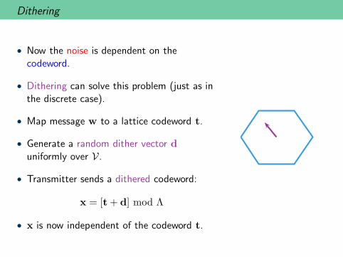
Dithering
• Now the noise is dependent on thecodeword.
• Dithering can solve this problem (just as inthe discrete case).
• Map message w to a lattice codeword t.
• Generate a random dither vector duniformly over V.
• Transmitter sends a dithered codeword:
x = [t+ d] mod Λ
• x is now independent of the codeword t.

Decoding – Remove Dither First
• Transmitter sends dithered codeword x = [t+ d] mod Λ.
• After scaling the channel output y by α, the decoder subtracts thedither d.
y = [αy − d] mod Λ
= [αx+ αz− d] mod Λ
= [x− d+ αz− (1− α)x] mod Λ
=[
[t+ d] mod Λ− d+ αz− (1− α)x]
mod Λ
= [t+ αz− (1− α)x] mod Λ Distributive Law
• Effective noise is now independent from the codeword t.
• By the probabilistic method, (at least) one good fixed dither exists.No common randomness necessary.

Summary
• Linear code embedded in the integer lattice:
R =1
2log
(
P
N
)
−1
2log
(
2πe
12
)
• Linear code embedded in the integer lattice, MMSE scaling:
R =1
2log
(
1+P
N
)
−1
2log
(
2πe
12
)
• Linear code embedded in a good shaping lattice, MMSE scaling:
R =1
2log
(
1+P
N
)
Theorem (Erez-Zamir ’04)
Nested lattice codes can achieve the AWGN capacity.

Gaussian Multiple-Access Channel
Rate Region
R1 <1
2log
(
1 +P1
N
)
R2 <1
2log
(
1 +P2
N
)
R1 +R2 <1
2log
(
1 +P1 + P2
N
)
w1 E1x1
w2 E2x2
z
yD
w1
w2
Power constraints P1, P2. Noise variance N .
Successive Cancellation
R2
R1
(
1
2log
(
1 +P1
N + P2
)
,1
2log
(
1 +P2
N
))
Corner Point
1. Decode x1, treating x2 as noise.
2. Subtract x1 from y.
3. Decode x2.
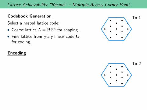
Lattice Achievability “Recipe” – Multiple-Access Corner Point
Codebook Generation
Select a nested lattice code:
• Coarse lattice Λ = BZn for shaping.
• Fine lattice from q-ary linear code G
for coding.
Encoding
Tx 1
Tx 2

Lattice Achievability “Recipe” – Multiple-Access Corner Point
Codebook Generation
Select a nested lattice code:
• Coarse lattice Λ = BZn for shaping.
• Fine lattice from q-ary linear code G
for coding.
Encoding
• Map messages w1,w2 to latticepoints t1, t2.
t1 = [BγGw1] mod Λ
Tx 1
t2 = [BγGw2] mod Λ
Tx 2

Lattice Achievability “Recipe” – Multiple-Access Corner Point
Codebook Generation
Select a nested lattice code:
• Coarse lattice Λ = BZn for shaping.
• Fine lattice from q-ary linear code G
for coding.
Encoding
• Map messages w1,w2 to latticepoints t1, t2.
• Choose independent dithers d1,d2
uniformly over Voronoi region V.
• Add dithers to lattice points andtake mod Λ to get transmittedsignals x1,x2.
t1 = [BγGw1] mod Λ
x1 = [t1 + d1] mod Λ
Tx 1
t2 = [BγGw2] mod Λ
x2 = [t1 + d2] mod Λ
Tx 2

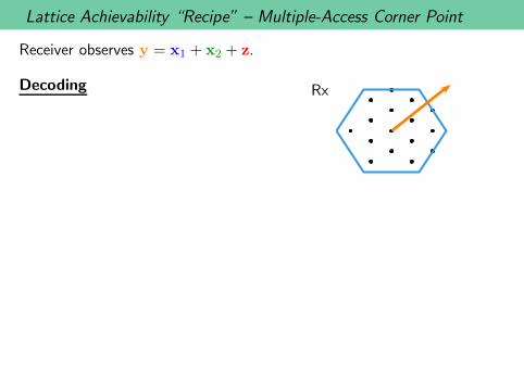
Lattice Achievability “Recipe” – Multiple-Access Corner Point
Receiver observes y = x1 + x2 + z.
Decoding Rx
Lattice Achievability “Recipe” – Multiple-Access Corner Point
Receiver observes y = x1 + x2 + z.
Decoding Rx

Lattice Achievability “Recipe” – Multiple-Access Corner Point
Receiver observes y = x1 + x2 + z.
Decoding
• Scale by α.
Rx

Lattice Achievability “Recipe” – Multiple-Access Corner Point
Receiver observes y = x1 + x2 + z.
Decoding
• Scale by α.
• Subtract dither d1.
Rx

Lattice Achievability “Recipe” – Multiple-Access Corner Point
Receiver observes y = x1 + x2 + z.
Decoding
• Scale by α.
• Subtract dither d1.
• Take mod Λ.
Rx

Lattice Achievability “Recipe” – Multiple-Access Corner Point
Receiver observes y = x1 + x2 + z.
Decoding
• Scale by α.
• Subtract dither d1.
• Take mod Λ.
• Decode to nearest codeword.
[αy − d1] mod Λ
= [α(x1 + x2 + z)− d1] mod Λ
= [x1 − d1 + αz+ αx2 − (1− α)x1] mod Λ
=[
[t1 + d1] mod Λ− d1 + αz+ αx2 − (1− α)x1
]
mod Λ
= [t1 + αz+ αx2 − (1− α)x1]
Effective Noise
Rx

Lattice Achievability “Recipe” – Multiple-Access Corner Point
• Effective noise after scaling is NEFFEC = α2(N + P2) + (1− α)2P1.
• Minimized by setting α to be the MMSE coefficient:
αMMSE =P1
N + P1 + P2
• Plugging in, we get
NEFFEC =(N + P2)P1
N + P1 + P2
• Resulting rate is
R =1
2log
(
P1
NEFFEC
)
=1
2log
(
1 +P1
N + P2
)
• To obtain different rates for x1 and x2, use nested linear codes G1
and G2 inside Voronoi region V.

AWGN Two-Way Relay Channel – Symmetric Rates
w1Has
Wants w2 w1
Has
Wants
w2Relay

AWGN Two-Way Relay Channel – Symmetric Rates
zMAC
yMAC
Relay
xBC
z2z1
User 1
x1w1
w2
User 2
x2 w2
w1
• Equal power constraints P .
• Equal noise variances N .
• Equal rates R.

AWGN Two-Way Relay Channel – Symmetric Rates
zMAC
yMAC
Relay
xBC
z2z1
User 1
x1w1
w2
User 2
x2 w2
w1
• Equal power constraints P .
• Equal noise variances N .
• Equal rates R.
• Upper Bound:
R ≤1
2log
(
1 +P
N
)
• Decode-and-Forward: Relay decodes w1,w2 and transmits w1 ⊕w2.
R =1
4log
(
1 +2P
N
)
• Compress-and-Forward: Relay transmits quantized y.
R =1
2log
(
1 +P
N
P
3P +N
)

AWGN Two-Way Relay Channel – Symmetric Rates
0 5 10 15 200
0.5
1
1.5
2
2.5
3
3.5
SNR in dB
Rat
e pe
r U
ser
Upper Bound
Compress
Decode

Decoding the Sum of Lattice Codewords
Encoders use the same nestedlattice codebook.
Transmit lattice codewords:
x1 = t1
x2 = t2
t1 E1x1
t2 E2x2
z
yD v
v = [t1 + t2] mod Λ
Decoder recovers modulo sum.
[y] mod Λ
= [x1 + x2 + z] mod Λ
= [t1 + t2 + z] mod Λ
=[
[t1 + t2] mod Λ + z]
mod Λ Distributive Law
= [v + z] mod Λ
R =1
2log
(
P
N
)

Decoding the Sum of Lattice Codewords – MMSE Scaling
Encoders use the same nestedlattice codebook.
Transmit dithered codewords:
x1 = [t1 + d1] mod Λ
x2 = [t2 + d2] mod Λ
t1 E1x1
t2 E2x2
z
yD v
v = [t1 + t2] mod Λ
Decoder scales by α, removes dithers, recovers modulo sum.
[αy − d1 − d2] mod Λ
= [α(x1 + x2 + z)− d1 − d2] mod Λ
= [x1 + x2 − (1− α)(x1 + x2) + αz− d1 − d2] mod Λ
=[
[t1 + t2] mod Λ− (1− α)(x1 + x2) + αz]
mod Λ
= [v − (1− α)(x1 + x2) + αz] mod Λ
Effective Noise NEFFEC = (1− α)22P + α2N

Decoding the Sum of Lattice Codewords – MMSE Scaling
• Effective noise after scaling is NEFFEC = (1− α)22P + α2N .
• Minimized by setting α to be the MMSE coefficient:
αMMSE =2P
N + 2P
• Plugging in, we get
NEFFEC =2NP
N + 2P
• Resulting rate is
R =1
2log
(
P
NEFFEC
)
=1
2log
(
1
2+
P
N
)
• Getting the full “one plus” term is an open challenge. Does notseem possible with nested lattices.

From Messages to Lattice Points and Back
• Map messages to lattice points
t1 = φ(w1) = [BγGw1] mod Λ
t2 = φ(w2) = [BγGw2] mod Λ
• Mapping between finite field messages and lattice codewordspreserves linearity:
φ−1(
[t1 + t2] mod Λ)
= w1 ⊕w2
• This means that after decoding a mod Λ equation of lattice pointswe can immediately recover the finite field equation of the messages.See Nazer-Gastpar ’11 for more details.

Finite Field Computation over a Gaussian MAC
Map messages to lattice points:
t1 = φ(w1)
t2 = φ(w2)
Transmit dithered codewords:
x1 = [t1 + d1] mod Λ
x2 = [t2 + d2] mod Λ
w1 E1x1
w2 E2x2
z
yD u
u = w1 ⊕w2
• If decoder can recover [t1 + t2] mod Λ, it also can get the sum ofthe messages
w1 ⊕w2 = φ−1(
[t1 + t2] mod Λ)
.
• Achievable rate R =1
2log
(
1
2+
P
N
)
.

AWGN Two-Way Relay Channel – Symmetric Rates
w1Has
Wants w2 w1
Has
Wants
w2Relay
• Equal power constraints P .
• Equal noise variances N .
• Equal rates R.
• Upper Bound:
R ≤1
2log
(
1 +P
N
)
• Compute-and-Forward: Relay decodes w1 ⊕w2 and retransmits.
R =1
2log
(
1
2+
P
N
)
• Wilson-Narayanan-Pfister-Sprintson ’10: Applies nested lattice codesto the two-way relay channel.

AWGN Two-Way Relay Channel – Symmetric RateszMAC
yMAC
Relay
xBC
z2z1
User 1
x1w1
w2
User 2
x2 w2
w1
• Equal power constraints P .
• Equal noise variances N .
• Equal rates R.
• Upper Bound:
R ≤1
2log
(
1 +P
N
)
• Compute-and-Forward: Relay decodes w1 ⊕w2 and retransmits.
R =1
2log
(
1
2+
P
N
)
• Wilson-Narayanan-Pfister-Sprintson ’10: Applies nested lattice codesto the two-way relay channel.

AWGN Two-Way Relay Channel – Symmetric Rates
0 5 10 15 200
0.5
1
1.5
2
2.5
3
3.5
SNR in dB
Rat
e pe
r U
ser
Upper Bound
Compute
Compress
Decode

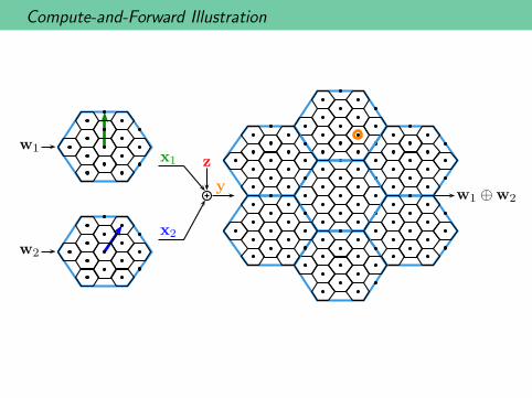
Compute-and-Forward Illustration
w2
w1x1
x2
z
yw1 ⊕w2
Compute-and-Forward Illustration
w2
w1x1
x2
z
yw1 ⊕w2

Random i.i.d. codes are not good for computation
2nR codewords each. 2n2R possible sums of codewords.

Random i.i.d. codes are not good for computation
2nR codewords each. 2n2R possible sums of codewords.
x1
x2
z
y

Random i.i.d. codes are not good for computation
2nR codewords each. 2n2R possible sums of codewords.
x1
x2
z
y

Random i.i.d. codes are not good for computation
2nR codewords each. 2n2R possible sums of codewords.
x1
x2
z
y

Unequal Power Constraints – Double Nesting
• What if the power constraintsare not equal?
• Idea fromNam-Chung-Lee ’10:
• Draw the codewords from thesame fine lattice ΛFINE.
• Use two nested coarse latticesΛ1 and Λ2 to enforce thepower constraints P1 and P2.

Unequal Power Constraints – Double Nesting
• What if the power constraintsare not equal?
• Idea fromNam-Chung-Lee ’10:
• Draw the codewords from thesame fine lattice ΛFINE.
• Use two nested coarse latticesΛ1 and Λ2 to enforce thepower constraints P1 and P2.

Unequal Power Constraints – Double Nesting
• What if the power constraintsare not equal?
• Idea fromNam-Chung-Lee ’10:
• Draw the codewords from thesame fine lattice ΛFINE.
• Use two nested coarse latticesΛ1 and Λ2 to enforce thepower constraints P1 and P2.

Unequal Power Constraints – Double Nesting
• What if the power constraintsare not equal?
• Idea fromNam-Chung-Lee ’10:
• Draw the codewords from thesame fine lattice ΛFINE.
• Use two nested coarse latticesΛ1 and Λ2 to enforce thepower constraints P1 and P2.

Unequal Power Constraints – Double Nesting
• What if the power constraintsare not equal?
• Idea fromNam-Chung-Lee ’10:
• Draw the codewords from thesame fine lattice ΛFINE.
• Use two nested coarse latticesΛ1 and Λ2 to enforce thepower constraints P1 and P2.

Unequal Power Constraints – Double Nesting
t1 E1x1
t2 E2x2
z
yD v
v = [t1 + t2] mod Λ2
• Encoder 1 sends x1 = [t1 + d1] mod Λ1. Coarse lattice Λ1 hassecond moment P1.
• Encoder 2 sends x2 = [t2 + d2] mod Λ2. Coarse lattice Λ2 hassecond moment P2 > P1.
• Decoder performs MMSE scaling, remove dithers, recovers mod Λ2
sum.
R1 =1
2log
(
P1
P1 + P2+
P1
N
)
R2 =1
2log
(
P2
P1 + P2+
P2
N
)

AWGN Two-Way Relay Channel
zMAC
yMAC
Relay
xBC
z2z1
User 1
x1w1
w2
User 2
x2 w2
w1
• User powers P1, P2.
• MAC noise variance NMAC.
• Relay power PBC .
• Broadcast noise variances
N1, N2.
Theorem (Nam-Chung-Lee ’10)
Capacity region is within 1/2 bit of:
R1 ≤ min
(
1
2log
(
P1
P1 + P2
+P1
NMAC
)
,1
2log
(
1 +PBC
N2
))
R2 ≤ min
(
1
2log
(
P2
P1 + P2
+P2
NMAC
)
,1
2log
(
1 +PBC
N1
))
Moreover, “constant gap” goes to zero as powers increase.

Multiple-Access Networks
w
Z2
Z1
Z3
w
w
w
• Multicast
demands
• Multi-access
interference
• No broadcast
constraints
• Compute-and-forward is well-suited for multicasting overmultiple-access networks.
• Equal transmitter powers: Nazer-Gastpar ’07.
Unequal transmitter powers: Nam-Chung-Lee ’09.

Outline
I. Discrete Alphabets
II. AWGN Channels
III. Network Applications

Many-to-One Interference Channel – Symmetric Very Strong Case
• Equal rates R.
• Only receiver 1 seesinterference:
y1 = x1 + βK∑
ℓ=2
xℓ + z1
• How big does β have to be toachieve R = 1
2 log(
1 + PN
)
?(i.e. “very strong” case)
w1 E1x1
w2 E2x2
β
wK EKxK
β.
.
.
.
.
.
z1y1
z2y2
zKyK
D1 w1
D2 w2
DK wK
• Scheme A: Decode w2, . . . ,wK at receiver 1 and remove prior todecoding w1.
R ≤1
2(K − 1)log
(
1 +β2(K − 1)P
N + P
)
• Scheme B: Decode w2 ⊕ · · · ⊕wK at receiver 1 and remove prior todecoding w1.

Many-to-One Interference Channel – Symmetric Very Strong Case
Encoders use the same nestedlattice codebook.
Transmit dithered codewords:
xℓ = [tℓ + dℓ] mod Λ
w1 E1x1
w2 E2x2
β
wK EKxK
β.
.
.
.
.
.
z1y1
z2y2
zKyK
D1 w1
D2 w2
DK wK
Decoder scales by β−1, removes dithers, recovers modulo sum.
[
β−1y1 −K∑
ℓ=2
dℓ
]
mod Λ =
[ K∑
ℓ=2
(xℓ − dℓ) + β−1(x1 + z1)
]
mod Λ
(Distributive Law) =
[
[
K∑
ℓ=2
tℓ
]
mod Λ + β−1(x1 + z1)
]
mod Λ

Many-to-One Interference Channel – Symmetric Very Strong Case
[
β−1y1 −K∑
ℓ=2
dℓ
]
mod Λ =
[
[
K∑
ℓ=2
tℓ
]
mod Λ + β−1(x1 + z1)
]
mod Λ
• Effective noise variance NEFFEC = β−2(P +N).
• Can decode mod Λ sum of lattice points at rate R = 12 log
( β2PP+N
)
.
• Setting equal to “very strong” condition R = 12 log
(
1 + PN
)
we get
β2 =(P +N)2
PN
• How can we recover w1?
• We need to first subtract the real sum of the codewords. So far, weonly have the modulo-sum.

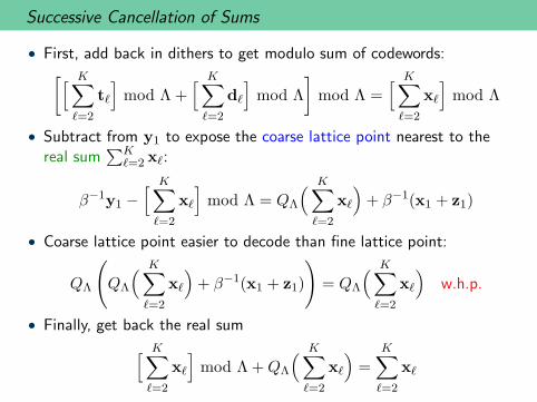
Successive Cancellation of Sums
• First, add back in dithers to get modulo sum of codewords:[
[
K∑
ℓ=2
tℓ
]
mod Λ +[
K∑
ℓ=2
dℓ
]
mod Λ
]
mod Λ =[
K∑
ℓ=2
xℓ
]
mod Λ

Successive Cancellation of Sums
• First, add back in dithers to get modulo sum of codewords:[
[
K∑
ℓ=2
tℓ
]
mod Λ +[
K∑
ℓ=2
dℓ
]
mod Λ
]
mod Λ =[
K∑
ℓ=2
xℓ
]
mod Λ
• Subtract from y1 to expose the coarse lattice point nearest to thereal sum
∑Kℓ=2 xℓ:
β−1y1 −[
K∑
ℓ=2
xℓ
]
mod Λ = QΛ
(
K∑
ℓ=2
xℓ
)
+ β−1(x1 + z1)
• Coarse lattice point easier to decode than fine lattice point:
QΛ
(
QΛ
(
K∑
ℓ=2
xℓ
)
+ β−1(x1 + z1)
)
= QΛ
(
K∑
ℓ=2
xℓ
)
w.h.p.
• Finally, get back the real sum
[
K∑
ℓ=2
xℓ
]
mod Λ +QΛ
(
K∑
ℓ=2
xℓ
)
=
K∑
ℓ=2
xℓ

Successive Cancellation of Sums
• We now have the sum of interfering codewords and can cancel themout:
y1 − β
K∑
ℓ=2
xℓ = x1 + z1
• Can apply standard MMSE lattice decoding to recover lattice pointt1 and then map back to w1.
• Overall, structured coding permits
β2 ≥(P +N)2
PN
• Compare to decoding interfering codewords in their entirety:
β2 ≥
(
(1 + PN )K−1 − 1
)
(N + P )
(K − 1)P
• Originally shown in Sridharan-Jafarian-Vishwanath-Jafar ’08 usingspherical shaping region. Nested lattice scheme from Nazer ’11.

Many-to-One Interference Channel – Approximate Capacity
w1 E1x1 h11
w2 E2x2
h12
......
wK EKxK hKK
h1K
h22
z1y1
z2y2
zKyK
D1 w1
D2 w2
DK wK
Lattice Codes
......
• Deterministic model by Avestimehr-Diggavi-Tse ’11 shows how todecompose by signal scale.
Theorem (Bresler-Parekh-Tse ’10)
Lattices codes combined with the deterministic model can approachthe capacity region to within (3K + 3)(1 + log(K + 1)) bits per user.

Interference Channel – Symmetric Very Strong Case
w1 E1x1
w2 E2x2
...
wK EKxK
H
z1y1
z2y2
zKyK
D1 w1
D2 w2
...
DK wK
• Equal rates R. How big does β have to be to achieveR = 1
2 log(
1 + PN
)
? (i.e. “very strong” case)
• Can use the many-to-one decoder at every receiver to get
β2 ≥(P +N)2
PN
• What about asymmetric interference channels?

Interference Channel – Symmetric Very Strong Case
w1 E1x1
w2 E2x2
...
wK EKxK
1 β · · · β
β 1 · · · β...
.... . .
...
β β · · · 1
z1y1
z2y2
zKyK
D1 w1
D2 w2
...
DK wK
• Equal rates R. How big does β have to be to achieveR = 1
2 log(
1 + PN
)
? (i.e. “very strong” case)
• Can use the many-to-one decoder at every receiver to get
β2 ≥(P +N)2
PN
• What about asymmetric interference channels?

Interference Channel
w1 E1x1
w2 E2x2
...
wK EKxK
H
z1y1
z2y2
zKyK
D1 w1
D2 w2
...
DK wK
• Not clear how to map to a deterministic model using lattices.
• “Real” interference alignment scheme of Motahari et al. ’08 uses alattice structure to get K/2 DoF (up to a set of measure one)
• Some special cases at finite SNR: Jafarian-Viswanath ’09,’10,
Ordentlich-Erez ’11
• Much more known for time-varying channels: Cadambe-Jafar ’08,
Nazer et al. ’11, much more

Summary
• So far we have seen that lattices are very effective for scenarioswhere there is a single interference bottleneck.
• Also effective for multiple bottlenecks but less is known.
• We have so far assumed that the fading coefficients are known atthe transmitters.
• In general, transmitters may not have access to channel stateinformation.
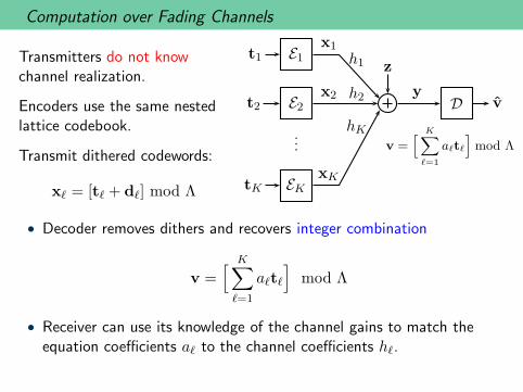
Computation over Fading Channels
Transmitters do not knowchannel realization.
Encoders use the same nestedlattice codebook.
Transmit dithered codewords:
xℓ = [tℓ + dℓ] mod Λ
t1 E1x1
h1
t2 E2x2 h2
tK EKxK
hK...
z
yD v
v =[
K∑
ℓ=1
aℓtℓ
]
mod Λ
• Decoder removes dithers and recovers integer combination
v =[
K∑
ℓ=1
aℓtℓ
]
mod Λ
• Receiver can use its knowledge of the channel gains to match theequation coefficients aℓ to the channel coefficients hℓ.

Distributive Law
• Distributive Law also holds for integer combinations. Let a, b ∈ Z.
[
a[x1] mod Λ + b[x2] mod Λ
]
mod Λ
=
[
a(
x1 −QΛ(x1))
+ b(
x2 −QΛ(x2))
]
mod Λ
=
[
ax1 + bx2 − aQΛ(x1)− bQΛ(x2)
]
mod Λ
= [ax1 + bx2] mod Λ
• Last step follows since since aQΛ(x1) and bQΛ(x2) are elements ofthe lattice Λ.

Computation over Fading Channels
• Transmit dithered codewords xℓ = [tℓ + dℓ] mod Λ
• Decoder removes dithers and recovers integer combination
[
y−K∑
ℓ=1
aℓdℓ
]
mod Λ
=[
K∑
ℓ=1
hℓxℓ + z−K∑
ℓ=1
aℓdℓ
]
mod Λ
=[
K∑
ℓ=1
aℓ(xℓ − dℓ) +
K∑
ℓ=1
(hℓ − aℓ)xℓ + z]
mod Λ
=
[
[
K∑
ℓ=1
aℓtℓ
]
mod Λ +
K∑
ℓ=1
(hℓ − aℓ)xℓ + z
]
mod Λ Distributive Law
Effective Noise

Computation over Fading Channels – Effective Noise
• Effective noise due to mismatch between channel coefficientsh = [h1 · · · hK ]T and equation coefficients a = [a1 · · · aK ]T .
NEFFEC = N + P‖h− a‖2
R =1
2log
(
P
N + P‖h− a‖2
)

Computation over Fading Channels – Effective Noise
• Effective noise due to mismatch between channel coefficientsh = [h1 · · · hK ]T and equation coefficients a = [a1 · · · aK ]T .
NEFFEC = N + P‖h− a‖2
R =1
2log
(
P
N + P‖h− a‖2
)
• Can do better with MMSE scaling.
NEFFEC = α2N + P‖αh − a‖2
R = maxα
1
2log
(
P
α2N + P‖αh− a‖2
)
=1
2log
(
N + P‖h‖2
N‖a‖2 + P (‖h‖2‖a‖2 − (hTa)2)
)
• See Nazer-Gastpar ’11 for more details.

Computation over Fading Channels – Special Cases
• The rate expression simplifies in some special cases.
R =1
2log
(
N + P‖h‖2
N‖a‖2 + P (‖h‖2‖a‖2 − (hTa)2)
)
• Integer channels: h = a.
R =1
2log
(
1
‖a‖2+
P
N
)
• Recovering a single message: Set a = δm, the mth unit vector.
R =1
2log
(
1 +h2mP
N + P∑
ℓ 6=m h2ℓ
)

Finite Field Computation over Fading Channels
Transmitters do not knowchannel realization.
Encoders use the same nestedlattice codebook.
Transmit dithered codewords:
xℓ = [tℓ + dℓ] mod Λ
w1 E1x1
h1
w2 E2x2 h2
wK EKxK
hK...
z
yD u
u =
K⊕
ℓ=1
aℓwℓ
• Recall that mapping tℓ = φ(wℓ) between messages and latticepoints preserves linearity.
φ−1
(
[
K∑
ℓ=1
aℓtℓ
]
mod Λ
)
=[
K∑
ℓ=1
aℓwℓ
]
mod q =
K⊕
ℓ=1
aℓwℓ
• Digital interface that fits well with network coding.

Computation Coding
All users pick the same nested lattice code:

Computation Coding
Choose messages over field wℓ ∈ Fkq :
w2
w1

Computation Coding
Map wℓ to lattice point tℓ = φ(wℓ):
w2
w1

Computation Coding
Transmit lattice points over the channel:
w2
w1x1
h1
x2h2
z
y
h = [ 1.4 2.1 ]
a = [ 2 3 ]

Computation Coding
Transmit lattice points over the channel:
w2
w1x1
h1
x2h2
z
y
h = [ 1.4 2.1 ]
a = [ 2 3 ]

Computation Coding
Lattice codewords are scaled by channel coefficients:
w2
w1x1
h1
x2h2
z
y
h = [ 1.4 2.1 ]
a = [ 2 3 ]

Computation Coding
Scaled codewords added together plus noise:
w2
w1x1
h1
x2h2
z
y
h = [ 1.4 2.1 ]
a = [ 2 3 ]

Computation Coding
Scaled codewords added together plus noise:
w2
w1x1
h1
x2h2
z
y
h = [ 1.4 2.1 ]
a = [ 2 3 ]

Computation Coding
Extra noise penalty for non-integer channel coefficients:
w2
w1x1
h1
x2h2
z
y
h = [ 1.4 2.1 ]
a = [ 2 3 ]
Effective noise: N + P‖h− a‖2

Computation Coding
Scale output by α to reduce non-integer noise penalty:
w2
w1x1
h1
x2h2
z
y
αh = [ α1.4 α2.1 ]
a = [ 2 3 ]
Effective noise: α2N + P‖αh− a‖2

Computation Coding
Scale output by α to reduce non-integer noise penalty:
w2
w1x1
h1
x2h2
z
y
αh = [ α1.4 α2.1 ]
a = [ 2 3 ]
Effective noise: α2N + P‖αh− a‖2

Computation Coding
Decode to closest lattice point:
w2
w1x1
h1
x2h2
z
y
αh = [ α1.4 α2.1 ]
a = [ 2 3 ]
Effective noise: α2N + P‖αh− a‖2

Computation Coding
Compute sum of lattice points modulo the coarse lattice:
w2
w1x1
h1
x2h2
z
y
αh = [ α1.4 α2.1 ]
a = [ 2 3 ]
Effective noise: α2N + P‖αh− a‖2

Computation Coding
Map back to equation of message symbols over the field:
w2
w1x1
h1
x2h2
z
y
αh = [ α1.4 α2.1 ]
a = [ 2 3 ]
Effective noise: α2N + P‖αh− a‖2
K⊕
ℓ=1
aℓwℓ

Computation over Fading Channels – Multiple Receivers
w1 E1x1
w2 E2x2
...
wK EKxK
H
z1y1
z2y2
zKyK
D1 u1
D2 u2
...
DK uK
• Equal rates R. No channel state information (CSI) at transmitters.• Receivers use their CSI to select coefficients, decode linear equation
uk =K⊕
ℓ=1
akℓwℓ
• Reliable decoding possible if
R < mink:akℓ 6=0
1
2log
(
N + P‖hk‖2
N‖ak‖2 + P (‖hk‖2‖ak‖2 − (hTk ak)
2)
)

Case Study – Hadamard Relay Network
w1 E1x1
w2 E2x2
...
wK EKxK
H
z1y1
z2y2
zKyK
R1
x1R
R2
x2R
...
RK
xKR
z1Ry1R
z2Ry2R
zKR
yKR
D
w1
w2
...wK
• Equal rates R. H is a Hadamard matrix, HHT = KI
Upper Bound Compute-and-Forward
1
2log
(
1 +P
N
)
1
2log
(
1
K+
P
N
)
Compress-and-Forward Decode-and-Forward
1
2log
(
1 +P
N
P
N +KP
)
1
2Klog
(
1 +KP
N
)

Case Study – Hadamard Relay Network
w1 E1x1
w2 E2x2
...
wK EKxK
1 1 · · · 11 1 · · · −1...
.... . .
...
1 −1 · · · −1
z1y1
z2y2
zKyK
R1
x1R
R2
x2R
...
RK
xKR
z1Ry1R
z2Ry2R
zKR
yKR
D
w1
w2
...wK
• Equal rates R. H is a Hadamard matrix, HHT = KI
Upper Bound Compute-and-Forward
1
2log
(
1 +P
N
)
1
2log
(
1
K+
P
N
)
Compress-and-Forward Decode-and-Forward
1
2log
(
1 +P
N
P
N +KP
)
1
2Klog
(
1 +KP
N
)

Computation over Fading Channels – No CSIT
w1 E1x1
h1
w2 E2x2 h2
w3 E3x3
h3
z
yD u
u =K⊕
ℓ=1
aℓwℓ
• Three transmitters thatdo not know the fadingcoefficients.
• Average rate plotted fori.i.d. Gaussian fading.
Relay either decodes somelinear function of messagesor an individual message.
0 5 10 15 20 250
0.5
1
1.5
2
2.5
Transmitter Power in dB
Ave
rate
Rat
e in
bits
per
cha
nnel
use
Decode an EquationDecode a MessageInterference as Noise

Computation over Fading Channels – No CSIT
• Receiver observes y = x1 + hx2 + z.• Recovers aw1 ⊕ bw2 for a, b 6= 0.
10dB
0 0.1 0.2 0.3 0.4 0.5 0.6 0.7 0.8 0.9 10
0.2
0.4
0.6
0.8
1
1.2
1.4
1.6
1.8
Channel coefficient h
Mes
sage
rat
e R
Upper Bound
Compute
Decode Both

Computation over Fading Channels – No CSIT
• Receiver observes y = x1 + hx2 + z.• Recovers aw1 ⊕ bw2 for a, b 6= 0.
20dB
0 0.1 0.2 0.3 0.4 0.5 0.6 0.7 0.8 0.9 10
0.5
1
1.5
2
2.5
3
3.5
Channel coefficient h
Mes
sage
rat
e R
Upper Bound
Compute
Decode Both

Computation over Fading Channels – No CSIT
• Receiver observes y = x1 + hx2 + z.• Recovers aw1 ⊕ bw2 for a, b 6= 0.
30dB
0 0.1 0.2 0.3 0.4 0.5 0.6 0.7 0.8 0.9 10
0.5
1
1.5
2
2.5
3
3.5
4
4.5
5
Channel coefficient h
Mes
sage
rat
e R
Upper Bound
Compute
Decode Both

Computation over Fading Channels – No CSIT
• Receiver observes y = x1 + hx2 + z.• Recovers aw1 ⊕ bw2 for a, b 6= 0.
40dB
0 0.1 0.2 0.3 0.4 0.5 0.6 0.7 0.8 0.9 10
1
2
3
4
5
6
7
Channel coefficient h
Mes
sage
rat
e R
Upper Bound
Compute
Decode Both

Computation over Fading Channels – No CSIT
• Receiver observes y = x1 + hx2 + z.• Recovers aw1 ⊕ bw2 for a, b 6= 0.
50dB
0 0.1 0.2 0.3 0.4 0.5 0.6 0.7 0.8 0.9 10
1
2
3
4
5
6
7
8
9
Channel coefficient h
Mes
sage
rat
e R
Upper Bound
Compute
Decode Both

Rate-Constrained Cellular Backhaul
RemoteCentralProcessor
RhaulRhaul Rhaul
• Well-studied cellular model: Wyner ’94, Shamai-Wyner ’97,
Sanderovich et al. ’09

Structured Superposition
Even Codeword
Private
Odd Codeword

Structured Superposition
Even Codeword
Private
Odd Codeword
1h h
z
y

Structured Superposition
Even Codeword
Private
Odd Codeword
1h h
z
y

Structured Superposition
Even Codeword
Private
Odd Codeword
1hODD hODD
z
y

Structured Superposition
Even Codeword
Private
Odd Codeword
1h h
z
y
1hODD hODD
z
y

Structured Superposition
Even Codeword
Private
Odd Codeword
1h h
z
y
1hODD hODD
z
y

Structured Superposition
Even Codeword
Private
Odd Codeword
1hEVEN hEVEN
z
y
1hODD hODD
z
y

Structured Superposition
Even Codeword
hODD > h > hEVEN
Private
Odd Codeword
1hEVEN hEVEN
z
y
1hODD hODD
z
y

Structured Superposition
x0
1hE hE
z0
y0
x1
1hO hO
z1
y1
xM
1 hOhO
zM
yM
· · ·
· · ·
· · ·
· · ·
Nazer et al. ’09: Each cell-site sees either hE or hO which is strictlybetter than h.

Structured Superposition
x0
1hE hE
z0
y0
aE xM + bE x0 + aE x1
x1
1hO hO
z1
y1
xM
1 hOhO
zM
yM
· · ·
· · ·
· · ·
· · ·
Nazer et al. ’09: Each cell-site sees either hE or hO which is strictlybetter than h.

Structured Superposition
x0
1hE hE
z0
y0
aE xM + bE x0 + aE x1
x1
1hO hO
z1
y1
aO x0 + bO x1 + aO x2
xM
1 hOhO
zM
yM
aO xM−1 + bO xM + aO x0
· · ·
· · ·
· · ·
· · ·
Nazer et al. ’09: Each cell-site sees either hE or hO which is strictlybetter than h.

Structured Superposition: Performance
SNR = 10dB, Backhaul Rate Rhaul = 2.5
0 0.2 0.4 0.6 0.8 10
0.5
1
1.5
2
2.5
3
(α)Interference Strength
Rat
e pe
r U
ser
Upper
Compress
Struc. Sup.
Compute
Decode
• Compress-and-forward rate taken from Sanderovich et al. ’09
• Layering can reduce “non-integer loss.”

Structured Superposition: Performance
SNR = 15dB, Backhaul Rate Rhaul = 3.5
0 0.2 0.4 0.6 0.8 10
0.5
1
1.5
2
2.5
3
3.5
4
(α)Interference Strength
Rat
e pe
r U
ser
Upper
Compress
Struc. Sup.
Compute
Decode
• Compress-and-forward rate taken from Sanderovich et al. ’09
• Layering can reduce “non-integer loss.”

Structured Superposition: Performance
SNR = 20dB, Backhaul Rate Rhaul = 4.5
0 0.2 0.4 0.6 0.8 10
1
2
3
4
5
(α)Interference Strength
Rat
e pe
r U
ser
Upper
Compress
Struc. Sup.
Compute
Decode
• Compress-and-forward rate taken from Sanderovich et al. ’09
• Layering can reduce “non-integer loss.”

Diophantine Approximation
• Choose equation coefficients to maximize rate:
RCOMP = maxa∈ZK
maxα
1
2log
(
P
α2N + P‖αh− a‖2
)
• Equivalently mina∈ZK
minα
α2N + P‖αh − a‖2.
• Closely connected to Diophantine approximation, i.e. approximatingirrationals with rationals.
• Niesen-Whiting ’11 shows that DoF = limP→∞
RCOMP12 log(1 + P )
≤ 2
• Also shows that by combining compute-and-forward withinterference alignment can get DoF to K.

Dirty Paper Coding
s is interference knownnoncausally to the encoder.
Assume s i.i.d. Gaussian,very large variance PS .
Erez-Shamai-Zamir ’05:
Encoder subtracts αs, dithers,and takes mod Λ.
x = [t− αs+ d] mod Λ
w Ex
s z
yD w
Decoder scales by α, removes dither, takes mod Λ, and recovers t.Interference is cancelled.
[αy − d] mod Λ = [x+ αs− d+ z− (1− α)x] mod Λ
=[
[t− αs+ d] mod Λ + αs− d+ z− (1− α)x]
mod Λ
=[
t+ z− (1− α)x]
mod Λ

Dirty Gaussian Multiple-Access Channel
w1 E1x1
s1
w2 E2x2
s2
z
yD w1, w2
Philosof-Zamir-Erez-Khisti ’11:
• Encoder 1 knows interference s1.
• Encoder 2 knows interference s2.
• Need to cancel out interference in a distributed fashion.
• Assume i.i.d. Gaussian interference with very large variance PS .Random i.i.d. methods yield rate that goes to 0 as PS goes toinfinity.

Dirty Gaussian Multiple-Access Channel
Subtract (part of) the interference signals ahead of time:
x1 = [t1 − αs1 + d1] mod Λ
x2 = [t2 − αs2 + d2] mod Λ
Decoder removes dithers:
[αy − d1 − d2] mod Λ
= [α(x1 + x2 + s1 + s2 + z)− d1 − d2] mod Λ
= [x1 + x2 + α(s1 + s2)− (1− α)(x1 + x2) + αz) − d1 − d2] mod Λ
=[
t1 + t2 + (1− α)(x1 + x2) + αz]
mod Λ
Select α = 2P/(2P +N) to obtain
R1 +R2 ≤
[
1
2log
(
1
2+
P
N
)
]+

Secrecy
• He-Yener ’09: Lattice codesare useful for physical-layersecrecy.
• Random i.i.d. codes achieve0 secure-degrees-of-freedom.
• Basic result: Random latticecodes achieve positivesecure-degrees-of-freedom.
Two-Way Relay Channel
w1Has
Wants w2 w1
Has
Wants
w2RelayUntrustedRelay
Interference Channel
1
2
K
Eavesdropper
1
2
K

Relaying
w Ex
zR
RxR z
yD w
What can we prove with lattice codes for the AWGN relay channel?
• The full decode-and-forward rate can be achieved.See Song-Devroye ’10, Nockleby-Aazhang ’11.
• The full compress-and-forward rate can be achieved.See Song-Devroye ’11.

Distributed Source Coding: “Gaussian Korner-Marton Problem”
• Correlated Gaussian sources.(
s1s2
)
∼ N
(
0,
[
1 ρρ 1
])
• Decoder wants the difference.
• Nested lattices are also goodfor Gaussian source coding.
s1 E1R1
s2 E2R2
D u
u = s1 − s2
D = 1nE‖u− u‖2

Distributed Source Coding: “Gaussian Korner-Marton Problem”
• Correlated Gaussian sources.(
s1s2
)
∼ N
(
0,
[
1 ρρ 1
])
• Decoder wants the difference.
• Nested lattices are also goodfor Gaussian source coding.
• Krithivasan-Pradhan ’09:
with high probability, s1 ands2 will land near the samecoarse lattice point.
• Only need to send:
t1 =[
QΛFINE(s1)
]
mod Λ
t2 =[
QΛFINE(s2)
]
mod Λ
s1 E1R1
s2 E2R2
D u
u = s1 − s2
D = 1nE‖u− u‖2
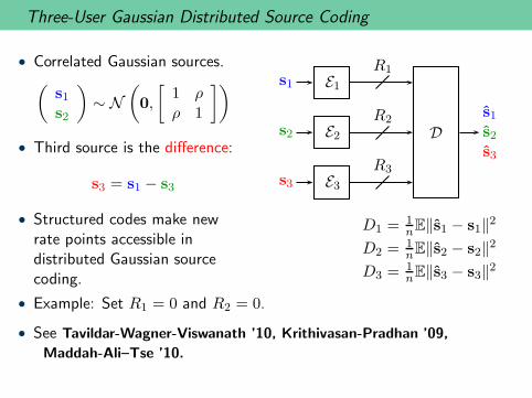
Three-User Gaussian Distributed Source Coding
• Correlated Gaussian sources.(
s1s2
)
∼ N
(
0,
[
1 ρρ 1
])
• Third source is the difference:
s3 = s1 − s3
• Structured codes make newrate points accessible indistributed Gaussian sourcecoding.
s1 E1R1
s2 E2R2
s3 E3R3
D
s1s2s3
D1 =1nE‖s1 − s1‖
2
D2 =1nE‖s2 − s2‖
2
D3 =1nE‖s3 − s3‖
2
• Example: Set R1 = 0 and R2 = 0.
• See Tavildar-Wagner-Viswanath ’10, Krithivasan-Pradhan ’09,
Maddah-Ali–Tse ’10.

Practical Implementations of Compute-and-Forward
• Feng-Silva-Kschischang ’10 develop practical nested lattice codesthat work quite well for blocklengths as small as 100.
• Hern and Narayanan ’10 develop multi-level codes to use fields ofsize 2k.
• Ordentlich and Erez ’10 propose mapping by set partitioning to gofrom binary codewords to higher order constellations.
• Further emerging work includes Osmane and Belfiore ’11

Concluding Remarks
• Codes with algebraic structure lead to the highest known achievablerates for some communication scenarios of great interest.
• This applies to source coding, channel coding, and also jointsource-channel coding.
• We have discussed a set of tools to apply and analyze random linearand random lattice codes to communication network scenarios.
• However, there is currently no general unified theory of how togenerally use algebraic structure in the context of networkinformation theory.

References – Random I.I.D. Codes
C. E. Shannon, “A mathematical theory of communication,” Bell Systems Technical Journal, vol. 27, pp. 379–423,
623–656, 1948.
R. Gallager, Information Theory and Reliable Communication. New York: John Wiley and Sons, Inc., 1968.
I. Csiszar and J. Korner, Information Theory: Coding Theorems for Discrete Memoryless Systems.
New York: Academic Press, 1982.
T. Cover and J. Thomas, Elements of Information Theory, 2nd ed. Hoboken, NJ: Wiley-Interscience, 2006.
A. El Gamal and Y.-H. Kim, Lecture Notes on Network Information Theory, 2010, http://arxiv.org/abs/1001.3404.
R. L. Dobrushin, “Asymptotic optimality of group and systematic codes for some channels,” Theory of Probability
and its Applications, vol. 8, no. 1, pp. 47–59, 1963.
R. Ahlswede, “Multi-way communication channels,” in Proc. IEEE Int. Symp. Inf. Theory, Prague. Publishing
House of the Hungarian Academy of Sciences, 1971, pp. 23–52.
H. Liao, “Multiple access channels,” PhD thesis, University of Hawaii, Honolulu, 1972.
D. Slepian and J. Wolf, “Noiseless Coding of Correlated Information Sources,” IEEE Transactions on Information
Theory, vol. 19, no. 4, pp. 471–480, 1973.
T .M. Cover, “A proof of the data compression theorem of Slepian and Wolf for ergodic sources,” IEEE
Transactions on Information Theory, vol. 21, no. 3, pp. 226–228, March 1975.
R. Ahlswede, N. Cai, S.-Y. R. Li, and R. W. Yeung, “Network information flow,” IEEE Transactions on Information
Theory, vol. 46, no. 4, pp. 1204–1216, Jul. 2000.

References – Random Linear Codes
P. Elias, “Coding for Noisy Channels,” in IRE Convention Record, pp. 37–46, 1955.
R. Gallager, Information Theory and Reliable Communication. New York: John Wiley and Sons, Inc., 1968.
I. Csiszar, “Linear Codes for Sources and Source Networks: Error Exponents, Universal Coding,” IEEE
Transactions on Information Theory, vol. 28, no. 4, pp. 585–592, 1982.
H.-A. Loeliger, “Averaging bounds for lattices and linear codes,” IEEE Trans. Inf. Theory, vol. 43, no. 6, pp.
1767–1773, Nov. 1997.
R. Zamir, S. Shamai (Shitz), and U. Erez, “Nested linear/lattice codes for structured multiterminal binning,” IEEE
Trans. Inf. Theory, vol. 48, no. 6, pp. 1250–1276, Jun. 2002.
S.-Y. R. Li, R. W. Yeung, and N. Cai, “Linear network coding,” IEEE Trans. Inf. Theory, vol. 49, no. 2, pp.
371–381, Feb. 2003.
R. Koetter and M. Medard, “An algebraic approach to network coding,” IEEE/ACM Trans. on Netw., vol. 11, pp.
782–795, Oct. 2003.
M. Effros, M. Medard, T. Ho, S. Ray, D. R. Karger, R. Koetter, and B. Hassibi, “Linear network codes: A unified
framework for source, channel, and network coding,” in DIMACS Workshop on Network Information Theory,Piscataway, NJ, 2003.
T. Ho, M. Medard, R. Koetter, D. R. Karger, M. Effros, J. Shi, and B. Leong, “A random linear network coding
approach to multicast,” IEEE Trans. Inf. Theory, vol. 52, no. 10, pp. 4413–4430, Oct. 2006.

References – Linear Codes Help
J. Korner and K. Marton, “How to encode the modulo-two sum of binary sources,” IEEE Transactions on
Information Theory, vol. 25, no. 2, pp. 219–221, Mar. 1979.
B. Nazer and M. Gastpar, “Computation over multiple-access channels,” IEEE Transactions on Information
Theory, vol. 53, no. 10, pp. 3498–3516, Oct. 2007.
T. Philosof and R. Zamir, “The rate loss of single-letter characterization: The “dirty” multiple access channel,”
IEEE Transactions on Information Theory, vol. 55, no. 6, pp. 2442–2454, June 2009.
T. Philosof, R. Zamir, and U. Erez “The capacity region of the binary dirty MAC,” Proc. of Inf. Theory Workshop,
Volos, Greece, June 2009.
B. Nazer and M. Gastpar, “The case for structured random codes in network capacity theorems,” European
Transactions on Telecommunications, vol. 19, pp. 455–474, June 2008.
D. Krithivasan and S. S. Pradhan, “Distributed source coding using Abelian group codes: A new achievable
rate-distortion region,” IEEE Transactions on Information Theory, vol. 57, no.3, pp. 1495–1519, March 2011.
D. Gunduz, O. Simeone, A. J. Goldsmith, H. V. Poor, and S. Shamai; , “Multiple Multicasts With the Help of a
Relay,” IEEE Transactions on Information Theory, vol. 56, no.12, pp. 6142–6158, Dec. 2010
J. Goseling, M. Gastpar, and J. Weber, “Line and lattice networks under deterministic interference models,” IEEE
Transactions on Information Theory, vol. 57, no. 5, pp. 3080–3099, May 2011.

References – Physical-Layer Network Coding
Y. Wu, P. A. Chou, and S.-Y. Kung, “Information exchange in wireless networks with network coding and
physical-layer broadcast,” Microsoft Research, Redmond, WA, Tech. Rep. MSR-TR-2004-78, Aug. 2004.
S. Zhang, S. Liew, and P. Lam, “Hot topic: Physical-layer network coding,” in Proc. ACM Int. Conf. Mobile
Comp. Netw., Los Angeles, CA, Sep. 2006.
B. Nazer and M. Gastpar, “Computing over multiple-access channels with connections to wireless network
coding,” in Proc. IEEE Int. Symp. Inf. Theory, Seattle, WA, Jul. 2006.
P. Popovski and H. Yomo, “Bi-directional amplification of throughput in a wireless multi-hop network,” in Proc.
IEEE Veh. Tech. Conf., Melbourne, Australia, May 2006.
S. Katti, S. Gollakota, and D. Katabi, “Embracing wireless interference: Analog network coding,” ACM
SIGCOMM, Kyoto, Japan, August 2007.
M. P. Wilson, K. Narayanan, H. Pfister, and A. Sprintson, “Joint physical layer coding and network coding for
bidirectional relaying,” IEEE Trans. Inf. Theory, vol. 11, no. 56, pp. 5641–5654, Nov. 2010.
W. Nam, S.-Y. Chung, and Y. H. Lee, “Capacity of the Gaussian two-way relay channel to within 1/2 bit,” IEEE
Transactions on Information Theory, vol. 56, no. 11, pp. 5488–5494, Nov. 2010.
W. Nam, S.-Y. Chung, and Y. H. Lee, “Nested Lattice Codes for Gaussian Relay Networks with Interference,” in
IEEE Transactions on Information Theory, Submitted February 2009. http://arxiv.org/abs/0902.2436
I. Maric, A. Goldsmith, and M. Medard, “Analog network coding in the high-SNR regime,” in Proceedings of the
IEEE Wireless Network Coding Conference (WiNC 2010), (Boston, MA), June 2010.
B. Nazer and M. Gastpar, “Reliable physical layer network coding,” Proceedings of the IEEE, vol. 99, no. 3,
pp. 438–460, March 2011.
S.-C. Liew, S. Zhang, and L. Lu, “Physical-layer network coding: Tutorial, survey, and beyond,” in Physical
Communication, to appear 2011. http://arxiv.org/abs/1105.4261.

References – Relaying
T. Cover and A. El Gamal, “Capacity Theorems for the Relay Channel,” IEEE Transactions on Information
Theory., vol. 25, no. 5, pp. 572–584, 1979.
G. Kramer, M. Gastpar, and P. Gupta, “Cooperative strategies and capacity theorems for relay networks,” IEEE
Transactions on Information Theory, vol. 51, pp. 3037–3063, September 2005.
S. Avestimehr, S. Diggavi, and D. Tse, “Wireless network information flow: A deterministic approach,” IEEE
Transactions on Information Theory, vol. 57, pp. 1872–1905, April 2011.
S. H. Lim, Y.-H. Kim, A. El Gamal, and S.-Y. Chung, “Noisy network coding,” IEEE Transactions on Information
Theory, vol. 57, pp. 3132–3152, May 2011.
Y. Song and N. Devroye, “List decoding for nested lattices and applications to relay channels,” in Proc. Allerton
Conf. Commun. Control Comput., Monticello, IL, Sep. 2010.
Y. Song and N. Devroye, “A lattice compress-and-forward strategy for canceling known interference in Gaussian
multi-hop channels,” Conf. on Inf. Sci. and Sys., Baltimore, March 2011.
M. Nokleby, B. Aazhang, ”Lattice coding over the relay channel,” IEEE Int. Conf. Comm., Kyoto, Japan, June
2011.

References – Lattices
J. H. Conway and N. J. A. Sloane, Sphere Packings, Lattices and Groups. New York: Springer, 1992.
R. de Buda, “Some optimal codes have structure,” IEEE Journal on Sel. Areas Comm., vol. 7, no. 6, pp. 893–899,
Aug. 1989.
T. Linder, C. Schlegel, and K. Zeger, “Corrected proof of de Buda’s theorem,” IEEE Transactions on Information
Theory, vol. 39, no. 5, pp. 1735–1737, Sep. 1993.
G. Poltyrev, “On coding without restrictions for the AWGN channel,” IEEE Transactions on Information Theory,
vol. 40, no. 2, pp. 409–417, Mar. 1994.
R. Zamir and M. Feder, “On lattice quantization noise,” IEEE Transactions on Information Theory, vol. 42, no. 4,
pp. 1152–1159, July 1996.
H.-A. Loeliger, “Averaging bounds for lattices and linear codes,” IEEE Transactions on Information Theory,
vol. 43, no. 6, pp. 1767–1773, Nov. 1997.
R. Urbanke and B. Rimoldi, “Lattice codes can achieve capacity on the AWGN channel,” IEEE Transactions on
Information Theory, vol. 44, no. 1, pp. 273–278, Jan. 1998.
G. Forney, M. Trott, and S.-Y. Chung, “Sphere-bound-achieving coset codes and multilevel coset codes,” IEEE
Transactions on Information Theory, vol. 46, no. 3, pp. 820–850, May 2000.
R. Zamir, S. Shamai (Shitz), and U. Erez, “Nested linear/lattice codes for structured multiterminal binning,” IEEE
Transactions on Information Theory, vol. 48, no. 6, pp. 1250–1276, Jun. 2002.
U. Erez and R. Zamir, “Achieving 1
2log (1 + SNR) on the AWGN channel with lattice encoding and decoding,”
IEEE Transactions on Information Theory, vol. 50, no. 10, pp. 2293–2314, Oct. 2004.
U. Erez, S. Litsyn, and R. Zamir, “Lattices which are good for (almost) everything,” IEEE Transactions on
Information Theory, vol. 51, no. 10, pp. 3401–3416, Oct. 2005.
R. Zamir, “Lattices are everywhere,” in Proc. Workshop Inf. Theory Applications, La Jolla, CA, Feb. 2009.

References – Lattices Help: Interference Channels
G. Bresler and A. Parekh and D. N. C. Tse, ”The approximate capacity of the many-to-one and one-to-many
Gaussian interference channels,” IEEE Transactions on Information Theory., vol. 56, no. 9, pp. 4566-4592, Sep.2010.
S. Sridharan, A. Jafarian, S. Vishwanath, and S. A. Jafar, “Capacity of symmetric K-user Gaussian very strong
interference channels,” in GLOBECOM, Monticello, IL, Sep. 2008.
S. Sridharan, A. Jafarian, S. Vishwanath, S. A. Jafar, and S. Shamai, “A layered lattice coding scheme for a class
of three user Gaussian interference channels,” in Proc. Allerton Conf. Commun. Control Comput., Monticello, IL,Sep. 2008.
R. Etkin and E. Ordentlich, “The degrees-of-freedom of the K-user Gaussian interference channel is discontinuous
at rational channel coefficients,” IEEE Transactions on Information Theory, vol. 55, pp. 4932–4946, November2009.
A. S. Motahari, S. O. Gharan, M.-A. Maddah-Ali, and A. K. Khandani, “Real interference alignment: Exploiting
the potential of single antenna systems,” IEEE Transactions on Information Theory, Submitted November 2009.See http://arxiv.org/abs/0908.2282.
S. Vishwanath and S. A. Jafar, “Generalized degrees of freedom of the symmetric Gaussian K-User interference
channel,” IEEE Transactions on Information Theory, vol.56, no.7, pp.3297-3303, July 2010.
B. Bandemer and A. El Gamal, Interference decoding for deterministic channels, IEEE Transactions on Information
Theory, vol. 57, no. 5, pp. 2966–2975, May 2011
A. Jafarian and S. Vishwanath, “Gaussian interference networks: Lattice alignment,” Proc. of Inf. Theory
Workshop, Cairo, Egypt, January 2010.
O. Ordentlich and U. Erez, “Interference Alignment at Finite SNR for Time-Invariant Channels,” Submitted to
IEEE Transactions on Information Theory April 2011. http://arxiv.org/abs/1104.5456
H. Huang and V. K. N. Lau, Y. Du and S. Liu, “Robust lattice alignment for K-user MIMO interference channels
with imperfect channel knowledge,” IEEE Transactions on Information Theory, vol. 59, no. 7, pp. 3315–3325, July2011.

References – Lattices Help: Compute-and-Forward
B. Nazer and M. Gastpar, “Compute-and-forward: Harnessing interference through structured codes,” IEEE
Transactions on Information Theory, to appear October 2011. http://arxiv.org/abs/0908.2119
M. P. Wilson, K. Narayanan, H. Pfister, and A. Sprintson, “Joint physical layer coding and network coding for
bidirectional relaying,” IEEE Transactions on Information Theory, vol. 11, no. 56, pp. 5641–5654, Nov. 2010.
W. Nam, S.-Y. Chung, and Y. H. Lee, “Capacity of the Gaussian two-way relay channel to within 1/2 bit,” IEEE
Transactions on Information Theory, vol. 56, no. 11, pp. 5488–5494, Nov. 2010.
U. Niesen and P. Whiting, “The Degrees of Freedom of Compute-and-Forward,” arXiv:1101.2182v1 [cs.IT], 2011.
L. Ong, C. M. Kellett, and S. J. Johnson, “Capacity theorems for the AWGN multi-way relay channel,” in Proc.
IEEE Int. Symp. Inf. Theory, Austin, TX, Jun. 2010.
C. Feng, D. Silva, and F. Kschischang, “An algebraic approach to physical-layer network coding,” in Proc. IEEE
Int. Symp. Inf. Theory, Austin, TX, June 2010.
B. Hern and K. Narayanan, “Multilevel coding schemes for compute-and-forward,” see Proc. IEEE Int. Symp. Inf.
Theory, St. Petersburg, Russia, June 2011.
O. Ordentlich, J. Zhan, U. Erez, B. Nazer, and M. Gastpar. “Practical Code Design for Compute-and-Forward”,
Proc. IEEE Int. Symp. Inf. Theory, St. Petersburg, Russia, June 2011.
A. Osmane and J.-C. Belfiore, “The Compute-and-Forward Protocol: Implementation and Practical Aspects,”
Submitted to IEEE Communications Letters 2011. http://arxiv.org/abs/1107.0300
M. Nokleby and B. Aazhang, ”Cooperative computation in wireless networks,” Proc. IEEE Int. Symp. Inf. Theory,
St. Petersburg, Russia, June 2011.
B. Nazer, “Compute-and-Forward: Improved Successive Cancellation,” To be submitted.

References – Lattices Help: Cellular Uplink, “Dirty” MAC, Secrecy
A. D. Wyner, Shannon-theoretic approach to a Gaussian cellular multiple-access channel, IEEE Transactions on
Information Theory., vol. 40, pp. 1713 1727, Nov. 1994.
A. Sanderovich, O. Somekh, H. V. Poor, S. and Shamai (Shitz), “Uplink macro diversity of limited backhaul
cellular network,” IEEE Transactions on Information Theory, vo. 55, no. 8, pp. 3457–3478. August 2009.
A. Sanderovich, M. Peleg, and S. Shamai (Shitz), “Scaling laws in decentralized processing of interfered Gaussian
channels,” in Proc. Int. Zurich Seminar Comm., Zurich, Switzerland, March 2008.
B. Nazer, A. Sanderovich, M. Gastpar, and S. Shamai, “Structured Superposition for Backhaul Constrained
Cellular Uplink,” in Proc. IEEE Int. Symp. Inf. Theory, Seoul, South Korea, Jun. 2009.
U. Erez, S. Shamai, and R. Zamir, “Capacity and lattice strategies for canceling known interference,” IEEE
Transactions on Information Theory, vol. 51, no. 11, pp. 3820–3833, November 2005.
T. Philosof and R. Zamir, “The rate loss of single-letter characterization: The “dirty” multiple access channel,”
IEEE Transactions on Information Theory, vol. 55, no. 6, pp. 2442–2454, June 2009.
T. Philosof, R. Zamir, and U. Erez “The capacity region of the binary dirty MAC,” Proc. of Inf. Theory Workshop,
Volos, Greece, June 2009.
T. Philosof, R. Zamir, U. Erez, and A. J. Khisti, “Lattice strategies for the dirty multiple access channel,” IEEE
Transactions on Information Theory, vol. 57, no. 8, pp. 5006–5035, August 2011.
X. He and A. Yener, “Providing secrecy with structured codes: Tools and applications to two-user Gaussian
channels,” Submitted to IEEE Transactions on Information Theory, Jul. 2009, see http://arxiv.org/abs/0907.5388
S. Agrawal and S. Vishwanath, “On the secrecy rate of interference networks using structured codes,” in Proc.
IEEE Int. Symp. Inf. Theory, Seoul, South Korea, Jun. 2009.
X. He and A. Yener, “The Gaussian many-to-one interference channel with confidential messagse,” Submitted to
IEEE Transactions on Information Theory, Apr. 2010, see http://arxiv.org/abs/1005.0624

References – Lattices Help: Distributed Source Coding
D. Krithivasan and S. S. Pradhan, “Lattices for distributed source coding: Jointly Gaussian sources and
reconstruction of a linear function,” IEEE Transactions on Information Theory, vol. 55, pp. 5268–5651, December2009.
S. Tavildar and P. Viswanath and A. B. Wagner, “The Gaussian Many-Help-One Distributed Source Coding
Problem,” IEEE Transactions on Information Theory., vol. 56, no. 1, pp. 564–571, 2010.
A. B. Wagner, On distributed compression of linear functions, IEEE Transactions on Information Theory., Vol. 57,
No. 1, pp. 79-94, 2011.
D. Krithivasan and S. S. Pradhan, “Distributed source coding using Abelian group codes: A new achievable
rate-distortion region,” IEEE Transactions on Information Theory, vol. 57, no.3, pp. 1495–1519, March 2011.
M. A. Maddah-Ali, and D. N. C. Tse, “Interference neutralization in distributed lossy source coding,” in Proc.
IEEE Int. Symp. Inf. Theory, Austin, TX, Jun. 2009.