Algebraic Path Finding - DIMACSdimacs.rutgers.edu/Workshops/NetworkServices/Slides/Tim_Griffin.pdf · Algebraic Path Finding ... 4 6 4 4 1 4 5 4 4 4 4 1 3 7 7 7 7 5 Matrix A solves

Algebraic Path Finding

Timothy G. Griffin

Computer LaboratoryUniversity of Cambridge, UK

[email protected]

DIMACS Working Group on Abstractions for Network Services,Architecture, and Implementation

23 May, 2012

tgg22 ( Computer Laboratory University of Cambridge, UK [email protected] )Algebraic Path Finding 23-05-2012 1 / 37

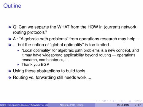
Outline

Q: Can we separte the WHAT from the HOW in (current) networkrouting protocols?A : “Algebraic path problems” from operations research may help...... but the notion of “global optimality” is too limited.

I “Local optimality” for algebraic path problems is a new concept, andit may have widespread applicability beyond routing — operationsresearch, combinatorics, ...

I Thank you BGP.

Using these abstractions to build tools.Routing vs. forwarding still needs work....


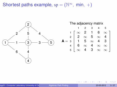
Shortest paths example, sp = (N∞, min, +)

1

2

3

4

5

6

5 42

1

4

3

The adjacency matrix

A =

1 2 3 4 5

1 ∞ 2 1 6 ∞2 2 ∞ 5 ∞ 43 1 5 ∞ 4 34 6 ∞ 4 ∞ ∞5 ∞ 4 3 ∞ ∞


Shortest paths example, continued

1

2

3

4

5

6

5 42

1

4

3

Bold arrows indicate theshortest-path tree rooted at 1.

The routing matrix

A∗ =

1 2 3 4 5

1 0 2 1 5 42 2 0 3 7 43 1 3 0 4 34 5 7 4 0 75 4 4 3 7 0

Matrix A∗ solves this globaloptimality problem:

A∗(i , j) = minp∈P(i, j)

w(p),

where P(i , j) is the set of all pathsfrom i to j .


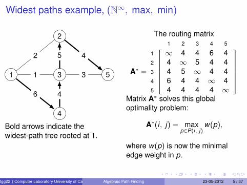
Widest paths example, (N∞, max, min)

1

2

3

4

5

2

1 3

6 4

5 4

Bold arrows indicate thewidest-path tree rooted at 1.

The routing matrix

A∗ =

1 2 3 4 5

1 ∞ 4 4 6 42 4 ∞ 5 4 43 4 5 ∞ 4 44 6 4 4 ∞ 45 4 4 4 4 ∞

Matrix A∗ solves this globaloptimality problem:

A∗(i , j) = maxp∈P(i, j)

w(p),

where w(p) is now the minimaledge weight in p.


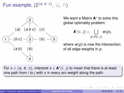
Fun example, (2{a, b, c}, ∪, ∩)

1

2

3

4

5

{a}

{b c} {b}

{a b} {b}

{a b c} {c}

We want a Matrix A∗ to solve thisglobal optimality problem:

A∗(i , j) =⋃

p∈P(i, j)

w(p),

where w(p) is now the intersectionof all edge weights in p.

For x ∈ {a, b, c}, interpret x ∈ A∗(i , j) to mean that there is at leastone path from i to j with x in every arc weight along the path.


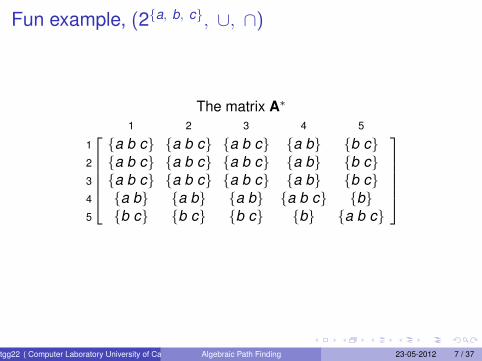
Fun example, (2{a, b, c}, ∪, ∩)

The matrix A∗

1 2 3 4 5

1 {a b c} {a b c} {a b c} {a b} {b c}2 {a b c} {a b c} {a b c} {a b} {b c}3 {a b c} {a b c} {a b c} {a b} {b c}4 {a b} {a b} {a b} {a b c} {b}5 {b c} {b c} {b c} {b} {a b c}


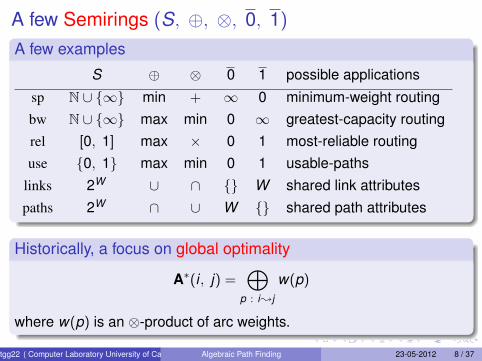
A few Semirings (S, ⊕, ⊗, 0, 1)A few examples

S ⊕ ⊗ 0 1 possible applications

sp N ∪ {∞} min + ∞ 0 minimum-weight routingbw N ∪ {∞} max min 0 ∞ greatest-capacity routingrel [0, 1] max × 0 1 most-reliable routinguse {0, 1} max min 0 1 usable-paths

links 2W ∪ ∩ {} W shared link attributespaths 2W ∩ ∪ W {} shared path attributes

Historically, a focus on global optimality

A∗(i , j) =⊕

p : i;j

w(p)

where w(p) is an ⊗-product of arc weights.


Recommended Reading


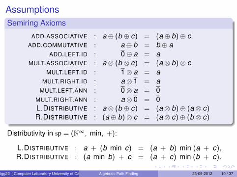
AssumptionsSemiring Axioms

ADD.ASSOCIATIVE : a⊕ (b ⊕ c) = (a⊕ b)⊕ cADD.COMMUTATIVE : a⊕ b = b ⊕ a

ADD.LEFT.ID : 0⊕ a = aMULT.ASSOCIATIVE : a⊗ (b ⊗ c) = (a⊗ b)⊗ c

MULT.LEFT.ID : 1⊗ a = aMULT.RIGHT.ID : a⊗ 1 = a

MULT.LEFT.ANN : 0⊗ a = 0MULT.RIGHT.ANN : a⊗ 0 = 0L.DISTRIBUTIVE : a⊗ (b ⊕ c) = (a⊗ b)⊕ (a⊗ c)R.DISTRIBUTIVE : (a⊕ b)⊗ c = (a⊗ c)⊕ (b ⊗ c)

Distributivity in sp = (N∞, min, +):

L.DISTRIBUTIVE : a + (b min c) = (a + b) min (a + c),R.DISTRIBUTIVE : (a min b) + c = (a + c) min (b + c).


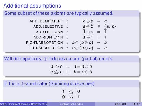
Additional assumptionsSome subset of these axioms are typically assumed.

ADD.IDEMPOTENT : a⊕ a = aADD.SELECTIVE : a⊕ b ∈ {a, b}

ADD.LEFT.ANN : 1⊕ a = 1ADD.RIGHT.ANN : a⊕ 1 = 1

RIGHT.ABSORBTION : a⊕ (a⊗ b) = aLEFT.ABSORBTION : a⊕ (b ⊗ a) = a

With idempotency, ⊕ induces natural (partial) orders

a ≤l b ≡ a = a⊕ ba ≤r b ≡ b = a⊕ b

If 1 is a ⊕-annihilator (Semiring is bounded)

1 ≤l 00 ≤r 1

In this case A∗ exists.tgg22 ( Computer Laboratory University of Cambridge, UK [email protected] )Algebraic Path Finding 23-05-2012 11 / 37

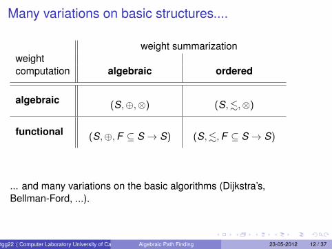
Many variations on basic structures....

weight summarizationweightcomputation algebraic ordered

algebraic (S,⊕,⊗) (S,.,⊗)

functional (S,⊕,F ⊆ S → S) (S,.,F ⊆ S → S)

... and many variations on the basic algorithms (Dijkstra’s,Bellman-Ford, ...).


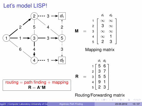
Let’s model LISP!

1

2

3

4

5

d1

d2

6

5 42

1

4

3

2

3

3

1

routing = path finding + mappingR = A∗M

M =

d1 d2

1 ∞ ∞2 3 ∞3 ∞ ∞4 ∞ 15 2 3

Mapping matrix

R =

d1 d2

1 5 62 3 73 5 54 9 15 2 3

Routing/Forwarding matrix


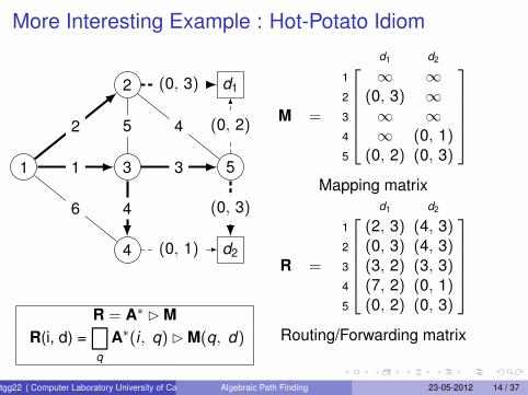
More Interesting Example : Hot-Potato Idiom

1

2

3

4

5

d1

d2

6

5 42

1

4

3

(0, 2)

(0, 1)

(0, 3)

(0, 3)

R = A∗ � MR(i, d) =

m

q

A∗(i , q)� M(q, d)

M =

d1 d2

1 ∞ ∞2 (0, 3) ∞3 ∞ ∞4 ∞ (0, 1)5 (0, 2) (0, 3)

Mapping matrix

R =

d1 d2

1 (2, 3) (4, 3)2 (0, 3) (4, 3)3 (3, 2) (3, 3)4 (7, 2) (0, 1)5 (0, 2) (0, 3)

Routing/Forwarding matrix


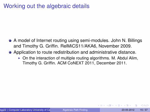
Working out the algebraic details

A model of Internet routing using semi-modules. John N. Billingsand Timothy G. Griffin. RelMiCS11/AKA6, November 2009.Application to route redistribution and administrative distance.

I On the interaction of multiple routing algorithms. M. Abdul Alim,Timothy G. Griffin. ACM CoNEXT 2011, December 2011.


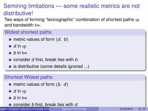
Semiring limitations — some realistic metrics are notdistributive!Two ways of forming “lexicographic” combination of shortest paths spand bandwidth bw.

Widest shortest pathsmetric values of form (d , b)d in sp

b in bw

consider d first, break ties with bis distributive (some details ignored ...)

Shortest Widest pathsmetric values of form (b, d)d in sp

b in bw

consider b first, break ties with dNOT distributive

What can we do?


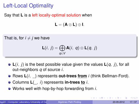
Left-Local Optimality

Say that L is a left locally-optimal solution when

L = (A⊗ L)⊕ I.

That is, for i 6= j we have

L(i , j) =⊕q∈V

A(i , q)⊗ L(q, j)

L(i , j) is the best possible value given the values L(q, j), for allout-neighbors q of source i .Rows L(i , _) represents out-trees from i (think Bellman-Ford).Columns L(_, i) represents in-trees to i .Works well with hop-by-hop forwarding from i .


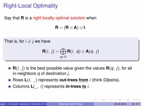
Right-Local Optimality

Say that R is a right locally-optimal solution when

R = (R⊗ A)⊕ I.

That is, for i 6= j we have

R(i , j) =⊕q∈V

R(i , q)⊗ A(q, j)

R(i , j) is the best possible value given the values R(q, j), for allin-neighbors q of destination j .Rows L(i , _) represents out-trees from i (think Dijkstra).Columns L(_, i) represents in-trees to i .


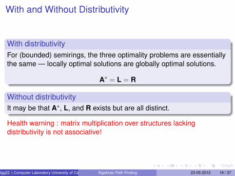
With and Without Distributivity

With distributivityFor (bounded) semirings, the three optimality problems are essentiallythe same — locally optimal solutions are globally optimal solutions.

A∗ = L = R

Without distributivityIt may be that A∗, L, and R exists but are all distinct.

Health warning : matrix multiplication over structures lackingdistributivity is not associative!


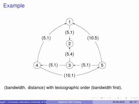
Example

1

2

34 5

(5,1)

(5,1)

(5,4)

(5,1)

(10,5)

(10,1)

(5,1)

(bandwidth, distance) with lexicographic order (bandwidth first).


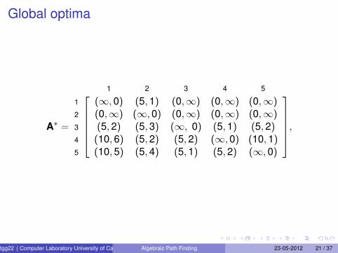
Global optima

A∗ =

1 2 3 4 5

1 (∞,0) (5,1) (0,∞) (0,∞) (0,∞)2 (0,∞) (∞,0) (0,∞) (0,∞) (0,∞)3 (5,2) (5,3) (∞, 0) (5,1) (5,2)4 (10,6) (5,2) (5,2) (∞,0) (10,1)5 (10,5) (5,4) (5,1) (5,2) (∞,0)

,


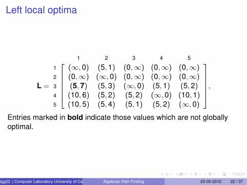
Left local optima

L =

1 2 3 4 5

1 (∞,0) (5,1) (0,∞) (0,∞) (0,∞)2 (0,∞) (∞,0) (0,∞) (0,∞) (0,∞)3 (5,7) (5,3) (∞,0) (5,1) (5,2)4 (10,6) (5,2) (5,2) (∞,0) (10,1)5 (10,5) (5,4) (5,1) (5,2) (∞,0)

,Entries marked in bold indicate those values which are not globallyoptimal.


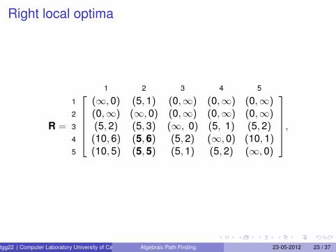
Right local optima

R =

1 2 3 4 5

1 (∞,0) (5,1) (0,∞) (0,∞) (0,∞)2 (0,∞) (∞,0) (0,∞) (0,∞) (0,∞)3 (5,2) (5,3) (∞, 0) (5, 1) (5,2)4 (10,6) (5,6) (5,2) (∞,0) (10,1)5 (10,5) (5,5) (5,1) (5,2) (∞,0)

,


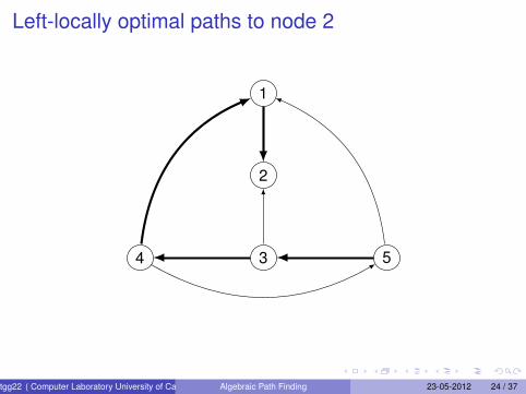
Left-locally optimal paths to node 2

1

2

34 5


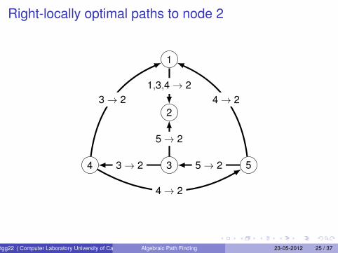
Right-locally optimal paths to node 2

1

2

34 5

5→ 2

1,3,4→ 2

5→ 23→ 2

4→ 2

4→ 23→ 2


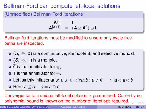
Bellman-Ford can compute left-local solutions(Unmodified) Bellman-Ford iterations

A[0] = IA[k+1] = (A⊗ Ak )⊕ I,

Bellman-ford iterations must be modified to ensure only cycle-freepaths are inspected.

(S, ⊕, 0) is a commutative, idempotent, and selective monoid,(S, ⊗, 1) is a monoid,0 is the annihilator for ⊗,1 is the annihilator for ⊕,Left strictly inflationarity, L.S.INF : ∀a,b : a 6= 0 =⇒ a < a⊗ bHere a ≤ b ≡ a = a⊕ b.

Convergence to a unique left-local solution is guaranteed. Currently nopolynomial bound is known on the number of iterations required.


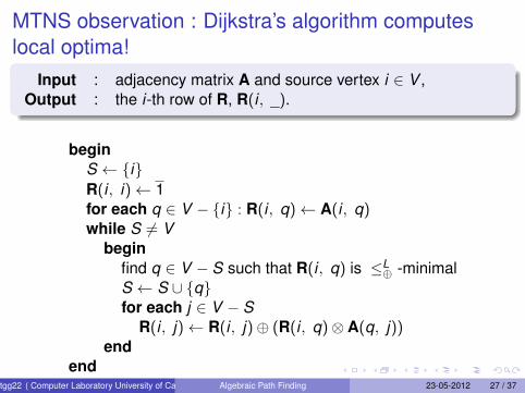
MTNS observation : Dijkstra’s algorithm computeslocal optima!

Input : adjacency matrix A and source vertex i ∈ V ,Output : the i-th row of R, R(i , _).

beginS ← {i}R(i , i)← 1for each q ∈ V − {i} : R(i , q)← A(i , q)while S 6= V

beginfind q ∈ V − S such that R(i , q) is ≤L

⊕ -minimalS ← S ∪ {q}for each j ∈ V − S

R(i , j)← R(i , j)⊕ (R(i , q)⊗ A(q, j))end

endtgg22 ( Computer Laboratory University of Cambridge, UK [email protected] )Algebraic Path Finding 23-05-2012 27 / 37

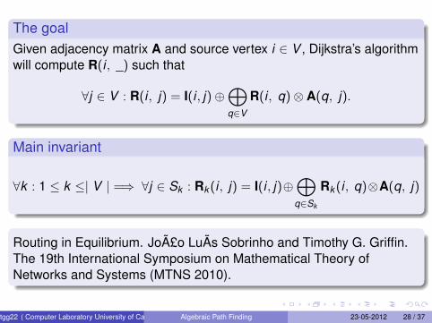
The goalGiven adjacency matrix A and source vertex i ∈ V , Dijkstra’s algorithmwill compute R(i , _) such that

∀j ∈ V : R(i , j) = I(i , j)⊕⊕q∈V

R(i , q)⊗ A(q, j).

Main invariant

∀k : 1 ≤ k ≤| V | =⇒ ∀j ∈ Sk : Rk (i , j) = I(i , j)⊕⊕q∈Sk

Rk (i , q)⊗A(q, j)

Routing in Equilibrium. JoÃ£o LuÃs Sobrinho and Timothy G. Griffin.The 19th International Symposium on Mathematical Theory ofNetworks and Systems (MTNS 2010).


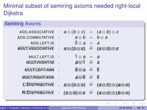
Minimal subset of semiring axioms needed right-localDijkstra

///////////Semiring Axioms

ADD.ASSOCIATIVE : a⊕ (b ⊕ c) = (a⊕ b)⊕ cADD.COMMUTATIVE : a⊕ b = b ⊕ a

ADD.LEFT.ID : 0⊕ a = aMULT.ASSOCIATIVE/////////////////////// : a⊗ (b ⊗ c)////////////// =// (a⊗ b)⊗ c//////////////

MULT.LEFT.ID : 1⊗ a = aMULT.RIGHT.ID////////////////// : a⊗ 1////// =// a/

MULT.LEFT.ANN/////////////////// : 0⊗ a////// =// 0/

MULT.RIGHT.ANN//////////////////// : a⊗ 0////// =// 0/

L.DISTRIBUTIVE//////////////////// : a⊗ (b ⊕ c)////////////// =// (a⊗ b)⊕ (a⊗ c)/////////////////////

R.DISTRIBUTIVE//////////////////// : (a⊕ b)⊗ c////////////// =// (a⊗ c)⊕ (b ⊗ c)/////////////////////


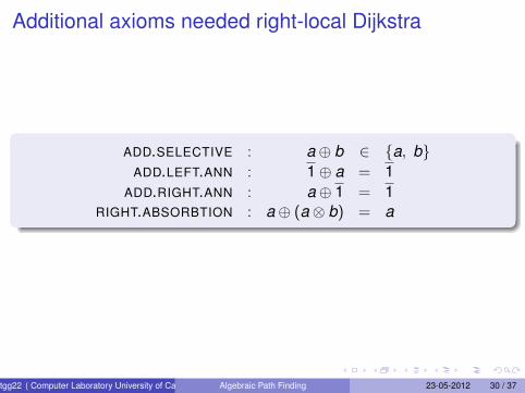
Additional axioms needed right-local Dijkstra

ADD.SELECTIVE : a⊕ b ∈ {a, b}ADD.LEFT.ANN : 1⊕ a = 1

ADD.RIGHT.ANN : a⊕ 1 = 1RIGHT.ABSORBTION : a⊕ (a⊗ b) = a


Need left-local optima?

L = (A⊗ L)⊕ I ⇐⇒ LT = (LT ⊗T AT )⊕ I

where ⊗T is matrix multiplication defined with as

a⊗T b = b ⊗ a

and we assume left-inflationarity holds, L.INF : ∀a,b : a ≤ b ⊗ a.


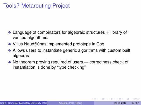
Tools? Metarouting Project

Language of combinators for algebraic structures + library ofverified algorithms.Vilius Naudžiunas implemented prototype in CoqAllows users to instantiate generic algorithms with custom builtalgebrasNo theorem proving required of users — correctness check ofinstantiation is done by “type checking”


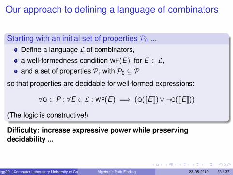
Our approach to defining a language of combinators

Starting with an initial set of properties P0 ...Define a language L of combinators,a well-formedness condition WF(E), for E ∈ L,and a set of properties P, with P0 ⊆ P

so that properties are decidable for well-formed expressions:

∀Q ∈ P : ∀E ∈ L : WF(E) =⇒ (Q(JEK) ∨ ¬Q(JEK))

(The logic is constructive!)

Difficulty: increase expressive power while preservingdecidability ...


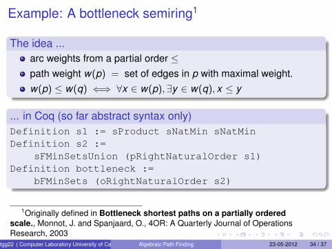
Example: A bottleneck semiring1

The idea ...arc weights from a partial order ≤path weight w(p) = set of edges in p with maximal weight.w(p) ≤ w(q) ⇐⇒ ∀x ∈ w(p),∃y ∈ w(q), x ≤ y

... in Coq (so far abstract syntax only)Definition s1 := sProduct sNatMin sNatMinDefinition s2 :=

sFMinSetsUnion (pRightNaturalOrder s1)Definition bottleneck :=

bFMinSets (oRightNaturalOrder s2)

1Originally defined in Bottleneck shortest paths on a partially orderedscale., Monnot, J. and Spanjaard, O., 4OR: A Quarterly Journal of OperationsResearch, 2003


The language design methodology

For every combinator C and every property Pfind wfP,C and βP,C such that

wfP,C(~a)⇒ (P(C(~a))⇔ βP,C(~a))

... which is then turned into two “bottom-up rules” ...

wfP,C(~a) ∧ βP,C(~a) ⇒ P(C(~a))wfP,C(~a) ∧ ¬βP,C(~a) ⇒ ¬P(C(~a)),


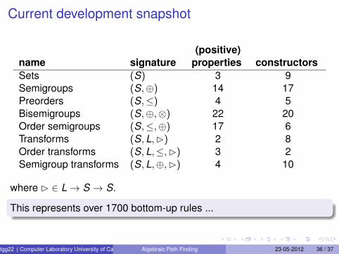
Current development snapshot

(positive)name signature properties constructorsSets (S) 3 9Semigroups (S,⊕) 14 17Preorders (S,≤) 4 5Bisemigroups (S,⊕,⊗) 22 20Order semigroups (S,≤,⊕) 17 6Transforms (S,L,�) 2 8Order transforms (S,L,≤,�) 3 2Semigroup transforms (S,L,⊕,�) 4 10

where � ∈ L→ S → S.

This represents over 1700 bottom-up rules ...


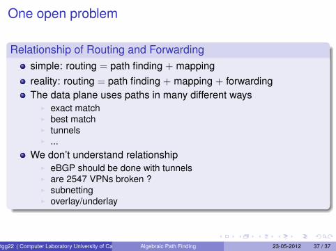
One open problem

Relationship of Routing and Forwardingsimple: routing = path finding + mappingreality: routing = path finding + mapping + forwardingThe data plane uses paths in many different ways

I exact matchI best matchI tunnelsI ...

We don’t understand relationshipI eBGP should be done with tunnelsI are 2547 VPNs broken ?I subnettingI overlay/underlay


Documents

Algebraic Path Finding - DIMACSdimacs.rutgers.edu/Workshops/NetworkServices/Slides/Tim_Griffin.pdf · Algebraic Path Finding ... 4 6 4 4 1 4 5 4 4 4 4 1 3 7 7 7 7 5 Matrix A solves