Algebraic methods for chromatic polynomials

Philipp Augustin Reinfeld

London School of Economies and Politicai Science

Ph.D.

2

Abstract: The chromatic polynomials of certain families of graphs can be calcu-

lai ed by a transfer matrix method. The transfer matrix commutes with an action

of the symmetric group on the colours. Using représentation theory, it is shown

that the matrix is équivalent to a block-diagonal matrix. The multiplicities and

the sizes of the blocks are obtained.

Using a repeated inclusion-exclusion argument the entries of the blocks can be

calculated. In particular, from one of the inclusion-exclusion arguments it follows

that the transfer matrix can be written as a linear combination of operators which,

in certain cases, form an algebra. The eigenvalues of the blocks can be inferred

from this structure.

The form of the chromatic polynomials permits the use of a theorem by Beraha, Kahane and Weiss to determine the limiting behaviour of the roots. The theorem says that, apart from some isolated points, the roots approach certain curves in the complex piane. Some improvements have been made in the methods of calculating these curves.

Many examples are discussed in détail. In particular the chromatic polynomials

of the family of the so-called generalized dodecahedra and four similar families of

cubic graphs are obtained, and the limiting behaviour of their roots is discussed.

Contents

1 Introduction 11

1.1 Overview 11

2 Modules and colourings 14

2.1 Some représentation theory 14

2.2 The symmetric group 17

2.3 The module of colourings Vk{B) 24

2.4 The irreducible submodules of Vk(B) 27

2.4.1 The complété graph case 29

2.4.2 A change of basis 32

2.4.3 The général case 34

2.5 Examples 34

2.6 A new module 40

3 The compatibility matrix method 44

3.1 Bracelets 44

3.2 The compatibility matrix method 47

3.3 Décomposition of the compatibility matrix 49

3

C O N T E N T S 4

3.4 Réduction to the complété base graph 52

3.5 The S m opérât ors 54

3.6 Change of basis 57

3.7 Action of S m (&) on the irreducible submodules of Vk{b) 59

3.8 Examples 64

3.9 Summary 75

4 Explicit calculations of chromatic poiynomials 79

4.1 A catalogue of U^ 80

4.1.1 The case b > 3 and d = 3 81

4.1.2 The case b = 3 and d > 3 83

4.2 Two Examples 85

4.3 Permutations of the vertex sets 89

4.4 Réduction of base graphs 90

4.5 Generalised dodecahedra 92

4.6 Four more families of cubic graphs 100

4.6.1 The family (468)n 102

4.6.2 The family (477)n 106

4.6.3 The family (567)n 110

4.6.4 The family (666)n 114

5 Equimodular curves 119

5.1 A theorem of Beraha, Kahane and Weiss 120

5.2 Equimodular points 122

C O N T E N T S 5

5.3 The résultant 123

5.4 Equimodular curves 125

5.4.1 Examples 127

5.5 Dominance 129

5.6 Numerical computations 131

5.6.1 The path of length three with the identity linking set . . . . 132

5.6.2 Generalised dodecahedra 136

5.6.3 The family (468)n 138

5.6.4 The family (477)n 140

5.6.5 The family (567)n 142

5.6.6 The family (666)n 144

6 The operator algebras and 146

6.1 A binary opération for matchings 147

6.2 The operator algebra Ab{k) 147

6.3 A minimal generating set 149

6.4 The operator algebra A^ik) 152

6.5 The level b — 1 for the identity linking set 155

A Newton's formula 164

B The H-sériés catalogue 165

C The reduced matrices for level 2 173

C O N T E N T S 6

D Maple programs 177

D.l The program EquiDominantPoints 177

D.2 The program DomTest 179

D.3 The program Slices 180

List of Tables

2.1 Summary of Example 2.10 39

4.1 The induced graphs \ni\(Lnijii)\'R.j\ in case of the family Dn 93

4.2 The graphs of the H-series 94

4.3 The graphs of the #*-series 95

4.4 The induced graphs (£7 ,7 )17 1 in case of the family (468)n . . . 103

4.5 The induced graphs (-^,7^)17^1 in case of the family (477)„ . . . 107

4.6 The induced graphs 171 (1 ,7 )17^1 in case of the family (567)n . . . I l i

4.7 The induced graphs ^(L-jz^n^i7^1 in case of the family (666)n . . . 115

6.1 The matrices Ufo , Ufo and Ufo in the case b — 3 154

7

For Amalia, who left too early.

8

Acknowledgements

First of all, I would like to thank Norman Biggs for being such a excellent Super-

visor. He has supported, guided and encouraged me, and he has also kept my feet

on the ground when it was necessary. I am very grateful for his time and patience

throughout my PhD.

Next I would like to thank the rest of the department. In particular Jan van den

Heuvel, Mark Baltovic, Jackie Everid and David Scott for always having an open

ear and good advice.

Thanks also to Robert Shrock, of Stony Brook University, New York, for finding

the time and the financial support for me to visit and work with him.

I am indebted to the UK Engineering and Physical Sciences Research Council (EP-

SRC) , the London School of Economies and Politicai Science and the Department

of Mat hématies for financial assistance throughout my PhD.

My parents have also been a source of moral and financial support throughout my

studies. They have always given my sisters and myself unconditional support and

the security and warmth of a true family. I must also thank Maria del Mar for her

most wonderful support, patience and understanding over the last three years.

Finally I would like to finish by praising the European Union for providing a frame-

work and some financial support for my studies abroad. In particular I have to

thank the English university system for its openness and flexibility: recognizing

my German high school degree and allowing me to study in England; covering my

tuition fees; fully validating my year of studies in Italy; and ali with a minimal

amount of bureaucracy. I hope that this openness and flexibility becomes common

practice throughout the European Union.

9

Statement of originality

Most of the work presented in this thesis is a continuation of work by N.L. Biggs [5],

[8], [7], [9], [4] and [6]. The work appearing in this thesis is entirely my own except

where stated otherwise. In particular:

• The observation that the compatibility matrix commutes with the action of

the symmetric group has also been exploited by M.H. Klin and C. Pech;

see [9].

• The Examples 3.7, 3.8 and 3.9 have been published in [9]. They are due to

me.

• The chromatic polynomial for the generalised dodecahedron was obtained by

S.C. Chang [11]. Here, the polynomial is calculaied in a différent way, to

illustrâte the compatibility matrix method.

• The Lemmas 6.12, 6.14 and Corollaries 6.13 and 6.15 are joint work with Jan van den Heuvel.

10

Chapter 1

Introduction

1.1 Overview

A graph B consista of two sets; a vert ex set and a edge set whose members are

unordered pairs of vertices. We say a pair of vertices are adjacent if they are an

edge. Given a set of k "colours", usually the first k positive integers, a proper

vertex ft-colouring of the graph B is a fonction from the vertex set into the set

of colours such that adjacent vertices take différent "colours" under the colouring.

We omit the words "proper" and "vertex", and just speak of a /c-colouring of B.

The chromatic polynomial P(B, k) corresponding to a graph B is the polynomial

function which evaluated at a positive integer k equals the number of /c-colourings

of B.

In theory, the standard method of deletion-and-contraction allows us to fìnd the

chromatic polynomial for any given finite graph. However this method is not very

élégant in the sense that it requires exponentially many steps (in the number of

edges). In general there is no efficient method.

In this thesis we are studying the chromatic polynomials for families of graphs with

a cyclic symmetry using a transfer matrix method. These families of graphs consist

of n copies of a "base graph" arranged in a "ring". Adjacent copies of the "base

graph" have extra edges between them according to a "linking set".

11

1 . 1 . OVERVIEW 12

Although the deletion-and-contraction method destroys the symmetry in the first

step, it has been used to obtain a transfer matrix via a recursion relation by D.A.

Sands (in an unpublished thesis, 1972), N.L. Biggs and G.H.J. Meredith in [1], J.

Salas and A.D. Sokal in [21], and by R. Shrock and co-workers in [25], [13] and a

sériés of other works.

Here, in this work we use and develop a slightly différent transfer matrix method

which enables us to utilize the symmetry to a maximum. This method was intro-

duced by N.L. Biggs in [2], and recently used and developed in [5], [8], [7], [19],

and [9].

This transfer matrix commutes with an action of the symmetric group permuting

the colours. Using représentation theory, it is shown that the matrix is équivalent

to a block-diagonal matrix. The multiplicities and the sizes of the blocks are

obtained. Using a repeated inclusion-exclusion argument the entries of the blocks

can be calculated (Chapters 2 and 3).

In particular, from one of the inclusion-exclusion arguments it follows that the

transfer matrix can be written as a linear combination of operators which, in certain

cases, form an algebra. In Chapter 6 parts of the structure of this algebra are

investigated.

In Chapter 4 many examples are discussed in détail. In particular the chromatic

polynomials of the family of the so-called generalized dodecahedra and four similar

families of cubic graphs are obtained.

The form of the chromatic polynomials permits the use of a theorem by Beraha,

Kahane and Weiss to determine the limiting behaviour of the roots as the number of

copies of the "base graph" goes to infinity. The theorem says that, apart from some

isolated points, the roots approach certain curves in the complex plane. Chapter 5

contains calculations based on [4] and [6] by N.L. Biggs. The results here are by no

means complete, and many phenomena observed in the limiting curves described

in the examples of Chapter 5 remain to be analyzed.

These limiting curves have also been studied by R. Shrock and co-workers in [24]

1 . 1 . OVERVIEW 13

and in a sériés of works, and by J. Salas and A.D. Sokal in, for example, [21] and

[15].

The chromatic polynomials for this type of graphs have also been the focus of

research in statistical mechanics. This is due to the fact that the zero-temperature

partition function of the k~state Potts antiferromagnet on the graph B is equal to

P(B,k); [13] and [22]. In particular the behaviour of the roots of P(B,k) as the

number of vertices goes to infinity is of paramount interest.

In future the theoretical framework introduced in Chapters 2 and 3 will hopefully be

used to obtain the chromatic polynomials for more families of graphs. In particular

the families of graphs with the cycle or the path on b vertices as "base graphs", and

the "identity linking set" are obvious candidates for further research. In [23] A. D.

Sokal finds a upper bound for the radius of a disc in the complex plane containing

ali the roots. This upper bound depends on the maximum degree of the graph.

The hope is to be able to find a connection between the limiting curves of the roots

and the type of "base graph" or the "linking set".

Chapter 2

Modules and colourings

The first part of this chapter gives a brief outline of some basic results of represen-

tation theory, in particular of the Symmetrie group. This is based on the books by

G.D. James [16], W. Ledermann [17] and B.E. Sagan [20]. In the second part this

theory is applied to the modules obtained when the Symmetrie group SymÄ acts

on the set of /c-colourings of a graph.

2.1 Some representation theory

Let G be a (finite) group written multiplicatively. We denote the identity element

of G by e. Let V be a vector space over C of dimensión n. A representation of G

on y is a group homomorphism p : G —• Aut(V) where Aut(K) is the group of

automorphisms of V. By choosing a particular basis for V it follows that p assigns

to every g E G a non-singular n x n matrix A(g) with coefficients in C. We say

that A(g), or A, is a matrix representation of G with degree n corresponding to p.

We denote by CG the group algebra consisting of all finite linear combinations

Y^zgg feec) geG

14

2 . 1 . SOME REPRESENTATION THEORY 15

with the componentwise addition, and multiplication given by

Y,**9) h = ( Z) zsz*) ,gEG ) \heG J / € G \gh=f }

Denote by End (y) the algebra of homomorphisms on V. Then a representation of G can be extended to a representation of CG. That is p : CG —y End(T ) is an algebra homomorphism defined as:

P =J2Z9P(9) \geG J g£G

with zg € €. This makes V into a CG-module. The two notions of a representation of CG - CG-module V and the algebra homomorphism p : CG —End("K) - are equivalent and we use them interchangeably. We denote by Matn the algebra of all nxn matrices with coefficients in C. Then, as before, by choosing a particular basis for V it follows that p : CG —» Matn is the corresponding matrix representation.

A subspace U of V is a submodule of V if U is invariant under the action of CG. A module V is irreducible if its only submodules are V itself and the zero module, otherwise we cali V reducible. We say that two matrix representations A(x) and B(x) are equivalent if there exists a non-singular matrix T such that T~1A(x) T = B{x). Let A{x) be the matrix representation corresponding to p.

Then, from the above definition of reducibility, it follows that A{x) is reducible if it is equivalent to a representation of the form

D{ x) O

E{x) F{x)

where O is an all-zero matrix. Otherwise A{x) is irreducible.

We say that a matrix is the direct sum of the matrices Ai, A2,..., Ai if A is the

diagonal block matrix diag(Ai, A2, ..., Ai). We write: i

A = A\ ® A2 © ... © Ai ~ ^J^ A{. i-1

Maschke's Theorem asserts that over the field C every matrix representation is completely reducible, that is for some choice of the basis of V it follows that

i A{x) = diag(A10z),A2(z)>--->A(z)) =

i=i

2 . 1 . SOME REPRESENTATION THEORY 16

where the Ai(x) are irreducible représentations. Equivalently, the corresponding

CG-module V is the direct sum of l irreducible submodules.

Let A = (a,ij) and B be matrices of degrees n and m respectively. Then the tensor

product, direct product or Kronecker product A® B is the nm x nm matrix obtained

by replacing the entry a - in A by the matrix a¿¿¿?. With this notation we can write

every matrix représentation A (x) as:

A(z) = 0(/m i<g>A ¿(x)) i

where the Ai{ x) are now inequi valent, irreducible représentations of degree and

multiplicity mi in A (a;), and Imi is the identity matrix of size mi.

Let A be a matrix représentation of CG. Then C(A) is the commutant algebra of A. This is the subalgebra of Matn consisting of ali T satisfying A(x)T = TA(x) for ali x G CG. If A is irreducible then Schur's Lemma asserts that C(A) only consists of scalar multiples of the identity matrix.

If A(x) = Im®B(x) where B is irreducible then T e C(A) is of the form X 0 In

where X e Matm and n is the degree of B(x). By a change of basis, that is

reordering the basis vectors, it can be shown that T is équivalent to In ® X. In

general the following lemma holds.

Lemma 2.1 Let A(x) be any matrix représentation ofCG of the form:

i A(x) = ($(Irni®Ai(x))

¿=i

where the Ai(x) are inequivalent, irreducible représentations of degree ni and mul-

tiplicity mi in A (x). Then every T € C(A) is équivalent to a matrix of the form:

i

i~l

with Xi e Matmi.

i Proof: Let A = @Bi(x) where Bf(x) = ( I m i ®Ai{x ) ) . If T e C{A) then

¿=1

2 . 2 . T H E SYMMETRIC GROUP 17

Bi Tn T12 T2I T22

•• r u

BiJ \Tn Tl2 ...

fTn T12

Î21 T22

Tl2

Tu

T21

Bi

Bi

aj v ä V

implies that = TijBj. The matrices Bi and Bj are inequivalent by assumption.

Thus from Schur's Lemma follows that Tij is the zéro matrix if i ^ j. Again Schur's

Lemma and the argument preceding this lemma imply that Tu = X i ® Ini where

XI E Matmi. Rearranging the order of the basis vectors it follows that Tu is

équivalent to In. <g) X . •

2.2 The symmetric group

Let us now focus on the symmetric group and its représentations. A permutation

of a set K is a bijection from K into itself. We can assume that K is the set of

numbers {1,2, . . . , k}. Then a permutation tu can be expressed as a product of

disjoint cycles. For example:

/ l 2 3 4 5 6 7 8 \ , W W W N = (1587) (2) (34) (6),

y 5 2 4 3 8 6 1 7 y

where 1-cycles are often omitted. For any two functions g and / their composition

is defined as (g o f)(x) = g}{x) = g(f(x)). In particular, the composition of two

permutations is a sequence of instructions read from right to left. For example

(12)(23) = (123). The set of ail permutations of the set { l ,2 , . . . , / c } together

with the composition of functions is the symmetric group Symk of degree k. The

identity element is denoted by e. In général, we dénoté by Sym^ the group of ail

permutations of a set X.

2 . 2 . T H E SYMMETRIC GROUP 18

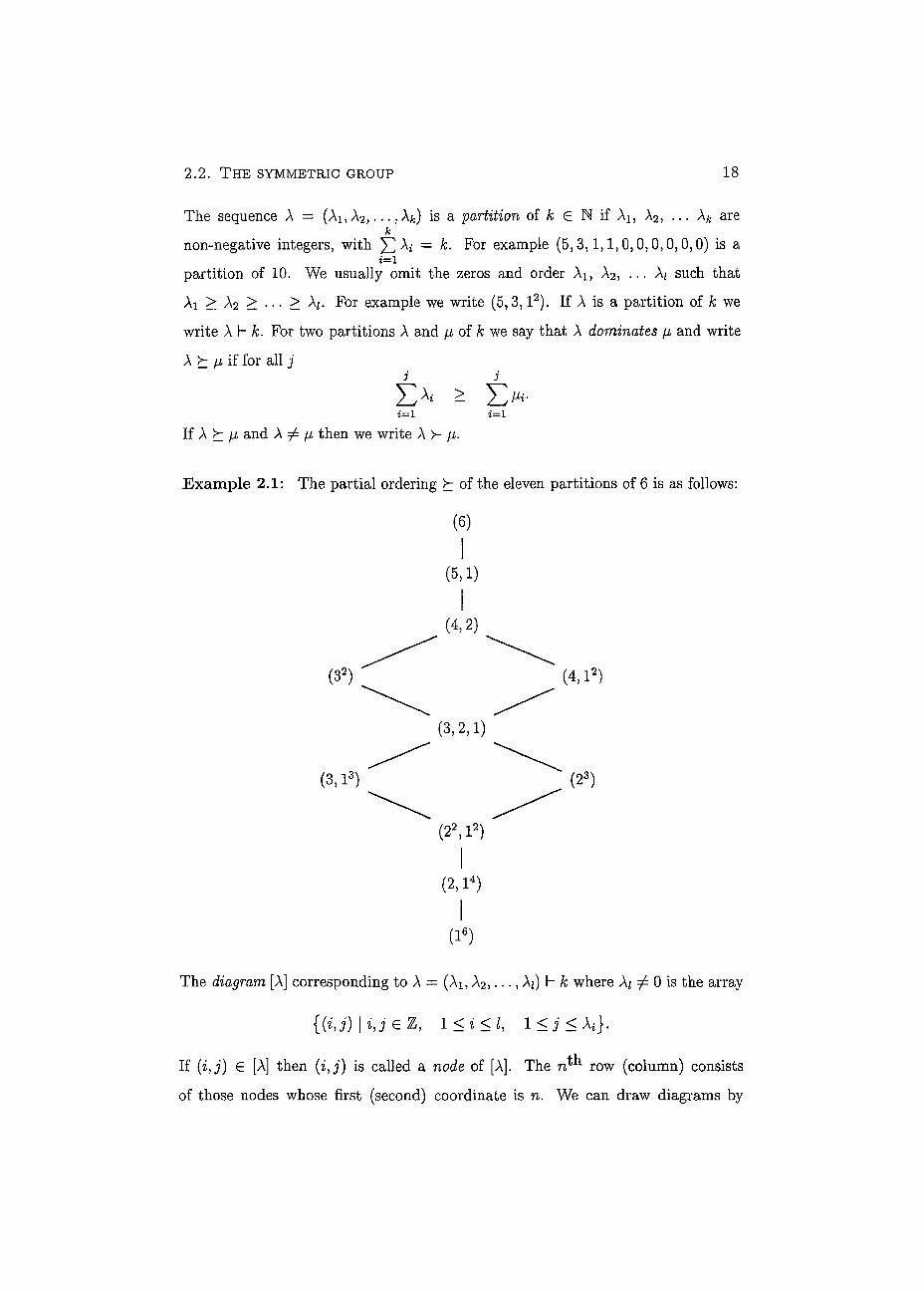
The sequence A = (Ai, À2 , . . . , A*) is a partition of A; e N if Ai, À2, . . . ÀA are k

non-negative integers, with A* = k. For example (5,3,1,1,0,0,0,0,0,0) is a i=1

partition of 10. We usually omit the zeros and order Ài, A2, . . . A/ such that

Ai > A2 > • • • > A;. For example we write (5,3, l2). If A is a partition of k we

write A h i For two partitions A and fi of k we say that A dominates fi and write

A y fi if for ali j 3 j I > > ¿=1 i=l

If A y ¡i and A fi then we write \ y ji.

Example 2.1: The partial ordering y of the eleven partitions of 6 is as follows:

(6)

(5,1)

(3,l3)

(4,2)

(3,2,1)

(22,l2)

(2, 1«)

(l6)

(4, l2)

The diagram [A] corresponding to A = (Ài, A2,..., Àj) h k where A; / 0 is the array

{(ij) \iJeZ, 1 <i<U 1 < i < Ai}.

If (i,j) G [A] then (i,j) is called a node of [A]. The rfi1 row (column) consists

of those nodes whose first (second) coordinate is n. We can draw diagrams by

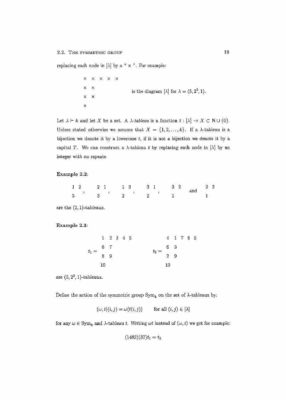
2 . 2 . T H E SYMMETRIC GROUP 19

replacing each node in [À] by a " x ". For example:

x x x x x

x x is the diagram [À] for A = (5,2 ,1).

x x

x

Let À h k and let X be a set. A X-tableau is a fonction t : [À] —> X c N U {0}.

Unless stated otherwise we assume that X = {1 ,2, . . . , If a À-tableau is a

bijection we dénoté it by a lowercase i, if it is not a bijection we dénoté it by a

capital T. We can construct a A-tableau t by replacing each node in [A] by an

integer with no repeats.

Example 2.2:

1 2 2 1 1 3 3 1 3 2 2 3 , , , , and

3 3 2 2 1 1

are the (2,1)-tableaux.

Example 2.3:

1 2 3 4 5 4 1 7 8 5

6 7 6 3 ii = ti =

8 9 2 9

10 10

are (5, 22, l)-tableaux.

Define the action of the symmetric group Symfc on the set of À-tableaux by:

(to,t)(iJ) = oj{t(iJ)) for ail (i,j) G [A]

for any Co 6 Symfc and A-tableau t. Writing u)t instead of (CJ, t) we get for example:

(1482)(37)ix = t2

2 . 2 . T H E SYMMETRIC GROUP 20

where ti and t2 are as in Example 2.3. For a given t we denote by Ct the subgroup of Symfc which fixes setwise the elements in each column of t. That is

Ct = {u £ Symk | V(«J) E [A] 3(pJ) E [A] such that ut(itj) = t{p,j)}.

We cali Ct the column-stabilizer of t. Similarly we define the row-stabilizer Rt of t

as:

Rt = {cj e Sym . | V(i,j) E [A] 3(i,p) E [A] such that ut(i,j) =

Defìne the équivalence relation ~ on the set of A-tableaux by t ~ t' if and only if

tot = t' for some LJ E Rt- Therefore t ~ t! if and only if the set of entries in row

i is the same for t and t' for ali i. We denote by {t} the équivalence class of t

under this relation and cali it a tabloid. Roughly speaking {t} is obtained from t

by ignoring the order of the elements in each of the respective rows, i.e. the rows

in { i } are unordered sets. This means the A-tabloid {t} is a partition of the set X

corresponding to A. The parts of {£} are its rows. We indicate a tabloid {t} by

drawing lines between the rows of t.

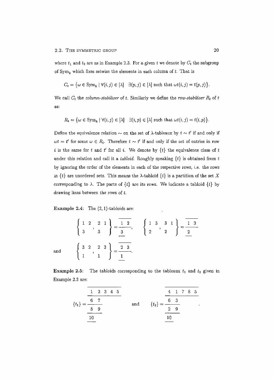
Example 2.4: The (2, l)-tabloids are:

1 2 2 1 1 2 1 3 3 1 1 3 J l ) ! 3

and

Example 2.5: The tabloids corresponding to the tableaux t\ and t2 given in

Example 2.3 are:

1 2 3 4 5 4 1 7 8 5

r -, 6 7 6 3 {ti} = and {t2} =

8 9 2 9

10 10

2 . 2 . T H E SYMMETRIC GROUP 21

Let Mx be the vector space over C spanned by the À-tabloids. The action of Sym^

on the À-tableaux induces an action on the À-tabloids. For every choice of two

À-tableaux t and t' there exists a u G Symfc such that t = ut'. It follows that Mx

is generated by one À-tabloid under this action of CSym . This makes Mx into a

cyclic CSym^-module. Its dimension is

k\ dim(M) = À1!À2!...Afcr

For a given t define the signed column sum Kt G CSym*. as Kt — X) sign(o;) w. u>€Ct

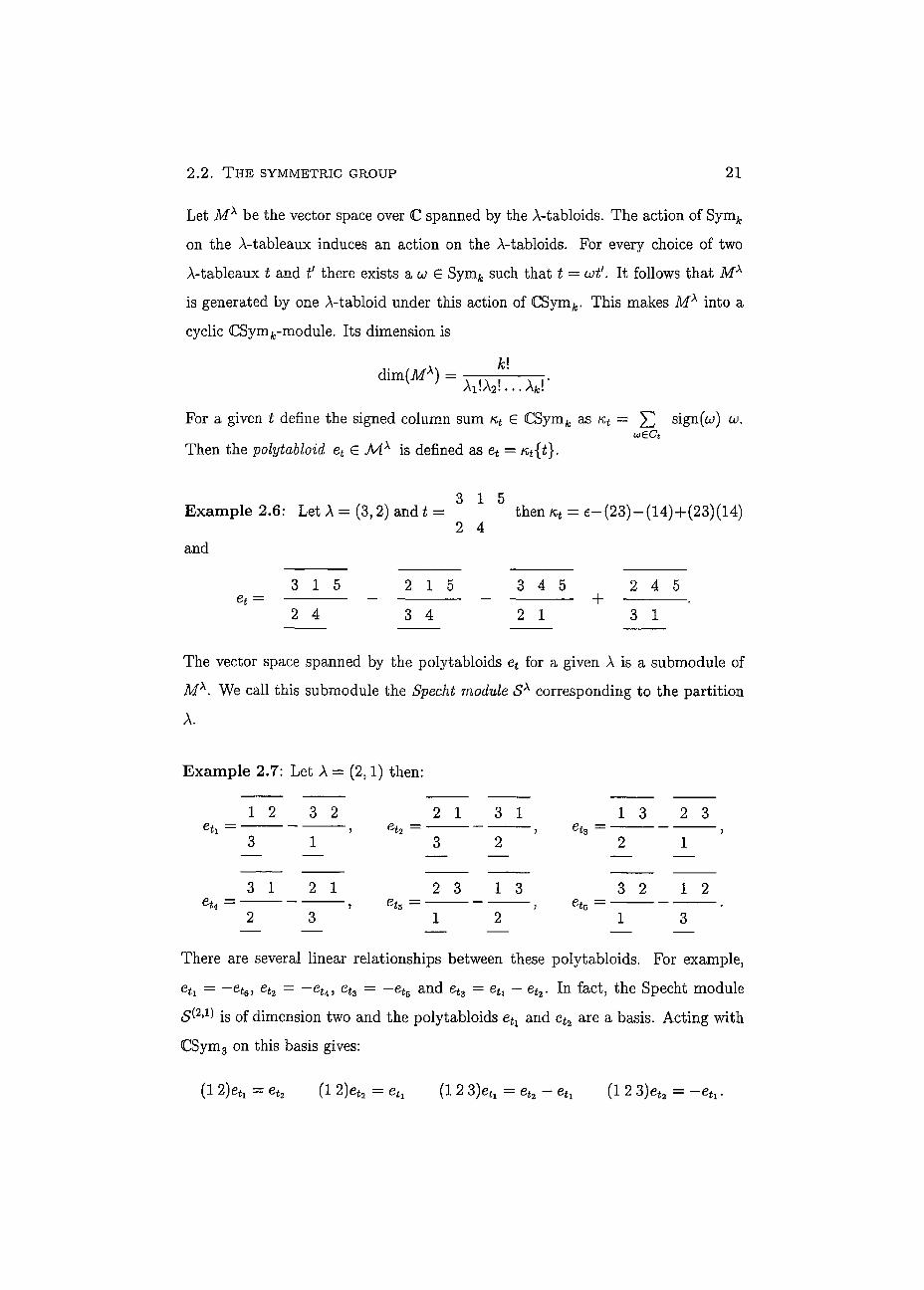
Then the polytabloid et G Mx is defined as et = Kt{t}-

3 1 5 Example 2.6: Let A = (3,2) and i = then Kt = e— (23)—(14)+(23)(14)

2 4 and

3 1 5 2 1 5 3 4 5 2 4 5 e* = ~ - +

2 4 3 4 2 1 3 1

The vector space spanned by the polytabloids et for a given À is a submodule of Mx. We call this submodule the Specht module Sx corresponding to the partition A.

Example 2.7: Let À = (2,1) then:

1 2 3 2 2 1 3 1 eh = , eÎ2 = 5 et3 =

1 00 2 3

2 1

3 2 1 2 3 1 2 1 2 3 1 3 eu = > ets = 7 ei6 =

There are several linear relationships between these polytabloids. For example,

etl = -et6, et2 = — etA, eÎ3 = — ets and eÎ3 = etl — ef2. In fact, the Specht module

is of dimension two and the polytabloids etl and et2 are a basis. Acting with

CSym3 on this basis gives:

(1 2)etl = et2 (1 2)et2 = etl (1 2 3)eh = et2 - etl (1 2 3)eÉa = - e t l .

2 . 2 . T H E SYMMETRIC GROUP 22

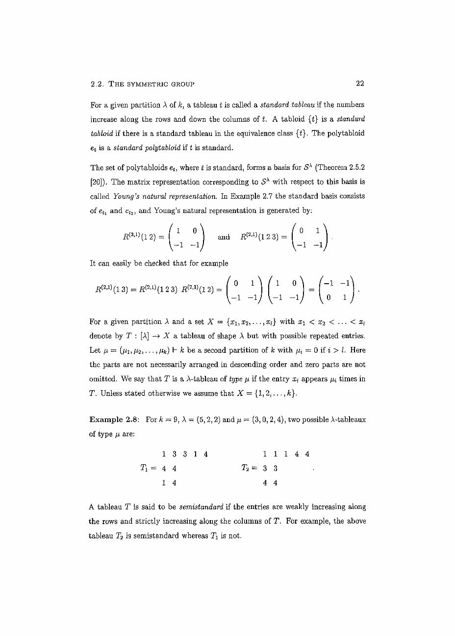
For a given partition À of k, a tableau t is called a standard tableau if the numbers

increase along the rows and down the columns of t. A tabloid {t} is a standard

tabloid if there is a standard tableau in the équivalence class The polytabloid

et is a standard polytabloid if t is standard.

The set of polytabloids et, where t is standard, forms a basis for <SA (Theorem 2.5.2

[20]). The matrix représentation corresponding to Sx with respect to this basis is

called Young's naturai représentation. In Example 2.7 the standard basis consists

of etx and eÎ3, and Young's naturai représentation is generated by:

For a given partition À and a set X = {xi, ar2,..., xi} with X\ < x2 < • • • <

dénoté by T : [A] —¥ X a tableau of shape A but with possible repeated entries.

Let jjl — (fii, /¿2, • • •, fJ>h) l~ k be a second partition of k with fa = 0 if i > L Here

the parts are not necessarily arranged in descending order and zéro parts are not

omitted. We say that T is a À-tableau of type ¡i if the entry xappears & times in

T. Unless stated otherwise we assume that X = {1,2 ,...,&}.

Example 2.8: For k = 9, À = (5,2,2) and ¡i = (3,0,2,4), two possible À-tableaux

of type ¡jl are:

It can easily be checked that for example

^ ( l 3) = ¿ ^ ( l 2 3) ¿ ^ ( l 2) =

1 3 3 1 4 1 1 1 4 4 T i = 4 4

1 4

T 2 = 3 3

4 4

A tableau T is said to be semistandard if the entries are weakly increasing along

the rows and strictly increasing along the columns of T, For example, the above

tableau X2 is semistandard whereas Ti is not.

2 . 2 . T H E S Y M M E T R I C G R O U P 2 3

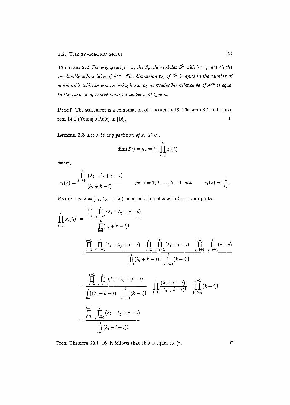
Theorem 2.2 For any given fi\~ k, the Specht modules Sx with X>z fi are ali the

irreducible submodules of M?. The dimension nx of Sx is equal to the number of

standard X-tableaux and its multiplicity m\ as irreducible submodule of Ai^ is equal

to the number of semistandard X-tableaux of type fi.

Proof: The statement is a combination of Theorem 4.13, Theorem 8.4 and Theo-

rem 14.1 (Young's Rule) in [16]. •

Lemma 2.3 Let X be any partition of k. Then, k

dim(<SA) = nx = k\ JJ^W ¿=i

where, k

j n ( A i - À j + j - o i

Xi(A) = , . ^ for i = 1,2, . . . , k - 1 and xk{X) = —. (A i + k-i)\ Afc!

Proof: Let A = (Ai, À2,..., X{) be a partition of k with l non zero parts. k—1 k

k n n ^ - A j + j - o A) = ^ ^

ncAi H- fc—*>i ¿=1

ff n ( A Ì - A J + J - O n ff n i i - o ¿=1 j-i+l t=1 j=l+1 j-i+i

ri(K+k-iy. n (*-«•)!

¿=1 i=l+1

ri ri ( x i - x j + j - i ) 1 fe-i 1 k 11 Ò)\ 11 1

Z—1 ì-l+l

n ri - X j + j ~ i ) 2=1 j-i+l

ri( k+i-iy. ¿=1

From Theorem 20.1 [16] it follows that this is equal to . •

2 . 3 . T H E MODULE OF COLOURINGS VK(B)

2.3 The module of colourings Vk{B)

2 4

A graph B consists of a vert ex setV = {v i,v2ì... ,Vb} and a subset of unordered

pairs of vertices called the edge set of B. In the following, we exclude the possibility

that {u, v} is in the edge set. That is, we deal only with loop-less graphs. We say

that two vertices v and w of B are adjacent if {v, w} is in the edge set of B. We

usually assume that V = {1,2, . . . ,6}.

The graph with edge set consisting of ali possible unordered pairs of vertices (but

excluding the case {T;, W}) is called a complete graph and we denote it by Kb. Its

vertex set is denoted by Vij,.

Let B be a graph with vertex set V. Throughout this section we regard the naturai

number k as fixed and we denote by K = {1, 2,... k} the set of colours. A k-

colouring of B is a function a : V —>• {1,2, . . . k} satisfying ^ a(ii;) whenever

{ti, w} is in the edge set of B. That is, adjacent vertices in B take différent colours.

We denote the set of ali colourings of B by Tk(B). In the case where B is the

complete graph on b vertices, I\(b) — Vk{K\,) is the set of injections from V& into

K.

Every function 6 : V —K induces a partition = {Ri, R2ì..., i£r} of V", written

as 9 |= 71, by letting two vertices v and w be in the same part Ri if and only if

9(v) = 9{w).

An independent set R is a subset of the vertex set V such that no pair of vertices of

R are an edge of B. Note that ali singletons are independent sets. A collection of

disjoint non-empty independent sets whose union is V is called a colour-partition

of V. We write colour-partitions as sets and separate the independent sets by " | ".

For example, in case of the path on four vertices there are fìve colour-partitions:

^ = {1121314}, K2 = {13|2|4}, = {1|24|3},

= {14|2|3} and K5 = {13|24}.

\1Z\ denotes the number of independent sets in and II(B) is the set of ali colour-

partitions of V for a given graph B. Note that a is a colouring of B if and only if

2 .3 . T H E MODULE OF COLOURINGS Vk(B) 25

a | = ^ f o r some K 6 U(B).

The symmetric group Symfc acts on Tk{B) in the obvious way. That is, for any

oj £ Synifc and a € Tk(B),

(w, a)(t>) = for all v G V.

Two colourings a and /? lie in the same orbit under Sym^ if and only if they induce

the same colour-partition.

Denote by VA(£) the vector space of complex-valued functions defined on rk(B).

If B = Kb we write Vk{b). The standard basis for 14(1?) consists of the functions

[a] for every a G Rk(B) defined as follows

! 1 if a = ft

0 otherwise.

The action of Symk on r^B) induces an action on (B). This makes Vk(B) into

a CSym¿.-module.

For any colour-partition 7Z the cyclic submodule of Vk(B) spanned by the set

{[a] | a |= 1Z} will be denoted by (1Z). Since for every [a] G Vk{B) we have that

[CM] G (71) for exactly one 71 G II(B), it follows that Vk(B) is the direct sum of the

(11).

For any 71 e 11(B), let be the partition (k - \7l\, I17*1) of k. Recall that MXk^

is the CSym¿.-module generated by the A*, -tabloids.

Theorem 2.4 The CSymk-modules (7Z) and MXk<n are isomorphic.

Proof: Let t be any A/^-tableau. Then t' is in the equivalence class {t} if and

only if

i'(z, 1) = t(x, 1) for alii = 2,3, . . . , \7l\ + 1.

Let G (71) be such that a t ( i - l ) =t(i, 1) for all z = 2,3, . . . , \7l\ + l. This defines

a bijection between the set of A^-tabloids and the set of colourings a satisfying

2 . 3 . T H E MODULE OF COLOURINGS Vk(B) 26

a |= 7Z. This bijection clearly respects the action of CSymfc. Hence follows the

result. •

Since Vk(B) is the direct sum of the (7Z) it follows from Theorem 2.4 that:

Corollary 2.5 The CSyrn¡.-modules Vk(B) and 0 MXk-n are isomorphic. neii(B) •

Prom Theorem 2.2 and Lemma 2.3 we know the decomposition of the MXk'n in

terms of irreducible submodules. This allows us to deduce the structure of Vk{B).

Denote by Ak,b the partition (k — b, l6) of ft, where b = \V\. Then Ak)<ji h for all

7Z e n(£) . Prom Theorem 2.2 and Corollary 2.5, it follows that every irreducible

composition factor of Vk(B) is isomorphic to some Sx with A >: Ak,b-

Let 0 < t < b and n h £. Denote by tt* the partition (A; — £, 7Ti, 7r2,..., ni) of k.

Then irk >: Ak,b and every A y Xktb is of the form nk for some 0 < £ < b and -k h £.

As a result of Lemma 2.3, the dimension n\ of <SA is given by k

dim(<SA) =nx = k\ JJ^iA) ¿=1

where

n ( A z - A j + i - o j=i+i JL ^i(A) = M , , zr. for i = 1,2, . . . , k - 1 and xk(X) = —. (Aj +/c — i)\ Ak\

Assume b + 2 < k and replace A by irk. If £ = 0 then nwk = 1. If £ > 1, it follows

that

n ( f c - ^ + j - i ) - ^ t^:

Xl{ir } ~~ (2k-£-l)\

Yl(k-£-7Tj^j) _ ~ & '

Xi(7Tk) =

and Xi(iTk) —

Xi-I(TT) for i = 2 , 3 , . . . , ^ + l

1 for i > £ + 2.

2 . 4 . THE IRREDUCIBLE SUBMODULES OF 14(2?) 27

k The dimension of <5* can then be written as

fc! J\

i

= '7T' Zi(A) = J7 _ M75")) where hi(ir) —iti+Î-i.

To find the multiplicity m k in VK(B) of the submodule isomorphic to <S7r'!, we have

to add up the numbers of semistandard 7rfc-tableaux of type Àk,Ti for all % £ n(£) .

If 71 is a given colour-partition, then any irk y Xk,n is of the form 7Tk = (k —

7Ti, 7T2, . . . , 7TI) for some 0 < £ < \7Z\ and ir\~L Every ^-tableaux T of type X^N

has k — \1Z\ times the entry 1 and each of the entries 2,3,...,|7£| + 1 exactly once.

A necessary condition for T to be semistandard is that all the entries 1 are in the

first row and the first k — \%\ columns. The entries not equal to 1 in the first row

have to be in increasing order along the row. If T satisfies this necessary condition

then T is semistandard if and only if the restriction of T to [IR] is a standard IT

tableau (assuming that k > |7£|). Hence the multiplicity of <S7r& in MXk>n is ( ' ^ » V

Now, summing over the set of colour-partitions gives the multiplicity in VK(B) of

the submodule isomorphic to «S71- .

Theorem 2.6 Every irreducible submodule of VK(B) is isomorphic to some S**

with 0 < £ < b and -N h L If £ = 0 the dimension of SN is one. If £ > 0 the

dimension of S^ is

and N^ is the dimension of S*. The number of submodules in VK(B) isomorphic to

i

~J\ II $ ^ M ) where HI(7r) = ^ + £ - %

S*K is

•

2.4 The irreducible submodules of Vk(B)

In this section we investigate the irreducible submodules of the CSymfc-module

VK(B). In particular we obtain a basis of the irreducible submodules.

2 . 4 . T H E IRREDUCIBLE SUBMODULES OF 14(2?) 28

Recali that for every 1Z € 11(5) the submodule (7Z) of Vk(B) is generated by the

set {[a] | a f= 1Z}> Since 14(B) is equal to the direct sum of the (7Z) we can

decompose each of the (7Z) separately.

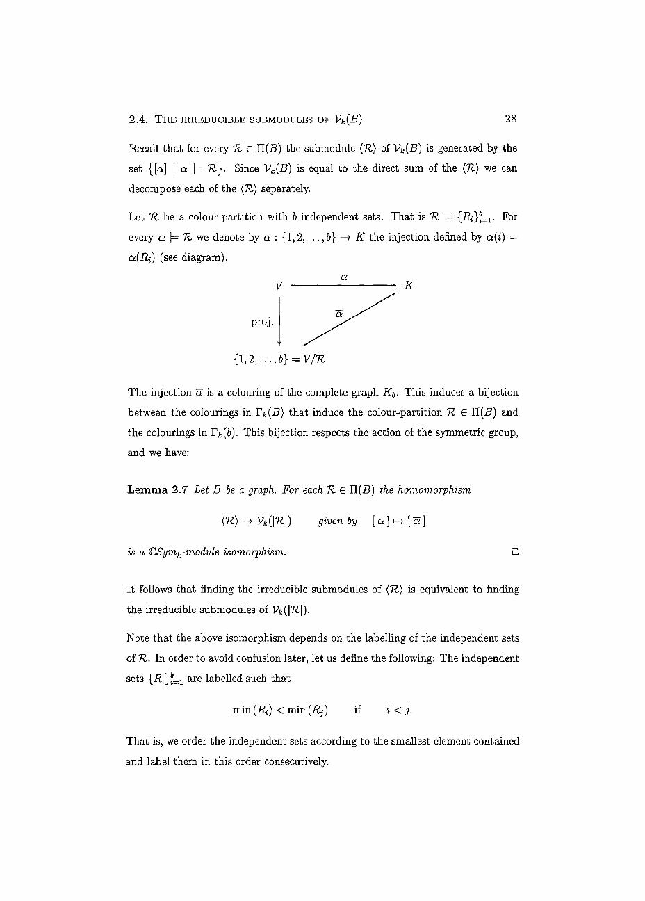
Let 7Z be a colour-partition with b independent sets. That is 1Z — { R i F o r

every a |= 1Z we denote by a : {1,2, . . . , b} —)• K the injection defined by a(i) =

a(Ri) (see diagram).

The injection a is a colouring of the complete graph K T h i s induces a bijection between the colourings in 1^(2?) that induce the colour-partition 1Z E IÌ(jB) and the colourings in Fk(b). This bijection respects the action of the symmetric group, and we have:

Lemma 2.7 Let B be a graph. For each 1Z £ 11(5) the homomorphìsm

{1Z)-ì Vk{\TZ\) givenby [cx]H>[a]

¿5 a CSymk~module isomorphism. •

It follows that finding the irreducible submodules of (1Z) is equivalent to finding

the irreducible submodules of 14(|7£|).

Note that the above isomorphism depends on the labelling of the independent sets

of 1Z. In order to avoid confusion later, let us define the following: The independent

sets {Ri}bi=zl are labelled such that

min (Ri) < min (Rj) if i < j.

That is, we order the independent sets according to the smallest element contained

and label them in this order consecutively.

2 . 4 . 1 . T H E COMPLETE GRAPH CASE

2.4.1 The complete graph case

2 9

We are now going to find the irreducible submodules of Let 0 < £ < b and

7r h £ be given. For the rest of this section let i be a fixed 7rfe-tableau.

Let T : [ir*] {0} UVb be a ^-tableau of type Ak,b- That is T is a surjection

with kernel of size k — b. Denote by %ktxkb the set of ^-tableaux of type Xk,b-

We define the action of Symfc on 7 b by

{u>,T)(i,j) = T( i ' , / ) where w *(»',/) = t{i, j) for all (i,j) e [TT^]

for every u G Symk. This agrees with the definition given in [20] Page 80, and

makes Tlxkixkb into a CSymfc-module.

We are going to show that 7^k,xkb a nd are isomorphic as CSymfc-modules.

Then we use results from [20] Section 2.9 to deduce the decomposition of Vfc(6) in

terms of irreducible submodules.

For every T E define olt : Vb —> K as qt(i>) = t(i,j) where T(i}j) = v

for all v E Vb- This is an injection and hence a colouring of Kb.

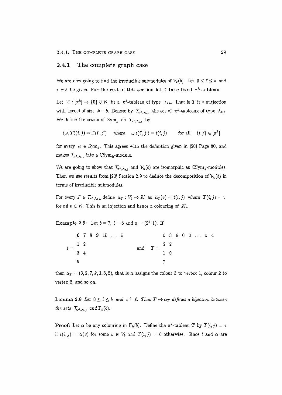
Example 2.9: Let b = 7, £ = 5 and ir = (22,1). If

6 7 8 9 10 . . . k 0 3 6 0 0 . . . 0 4 1 2 5 2

t = and T = 3 4 1 0

5 7

then &t = (3, 2,7, k, 1,8,5), that is a assigns the colour 3 to vertex 1, colour 2 to

vertex 2, and so on.

Lemma 2.8 Let 0 < £ < b and TT b- £. Then T Q>T defines a bijection between

the sets 7i*,Afcfc andTk(b).

Proof: Let a be any colouring in Tk{b). Define the ^-tableau T by T(i,j) = v

if t(i,j) — ce(v) for some v E Vb and T(i,j) = 0 otherwise. Since t and a are

2 . 4 . 1 . THE COMPLETE GRAPH CASE 30

injections it follows that T is well defined. Clearly, T is of type Xk>b. It follows that

aT = a, and hence Q>t defìnes a surjection between the sets 7^ iXkb and rk(b) .

Suppose that a, ¡3 e Tk{b) with a ^ fi. Then there exists v G Vb such that

a(v) ^ f}(v) From the definition of &t it follows that a(v) = t(i,j) with T(i}j) — v

and P(v) = t(i',f ) with T'tfJ') = v. Since t is an injection it follows that

{hj) {i'tf)i a nd since v ^ 0 it follows that T ^T'. It follows that ax defìnes

an injection between the sets rk(b) and %kt\khi and hence a bijection. •

Lemma 2.9 Let 0 < i < b and 7r h l. For any T G %ktXk>b

LO OÙT = TTUT f0T aM w € Symk.

Proof: For every v € Vb we have

&ut(v) = t(i,j) where (u,T){i,j) = v

= ut(i',j') where T{i'J') = (u,T)(i,j) = v

= U Oìt(V).

•

Corollary 2.10 Let 0 < t < b and ir i. ThenT >->• [QÌT] defìnes an isomorphism

between the CSymk-modules %ktXkb and Vk{b). •

Following [20] Section 2.9, we define for every given T E T^kìXk b the homomorphism

eT : M*k Vk(b) b y eT({t}) = ] T M

se{T]

and cyclic extension using cyclicity of M*k. That is, for every ^-tableau t' there

exists awG Symfc such that t' = ut. Then

M W ) = *r({«*}) = « M W ) = OJ Y , [osi-s e { T )

2 . 4 . 1 . T H E COMPLETE GRAPH CASE 3 1

The 7rfc-tabloid {T} is defined in the obvious way. Note that in [20] Section 2.9 the

homomorphism 9T is into %ktxkbt but with Corollary 2.10 we can extend it into

Vfc(6). From the cyclic extension it follows that 9T respects the action of Symk. In

particular QT(et) = = MtW = *t Y, I^l-

se{T}

Denote by 0T : S*k Vk{b) the restriction of 6T to S*k .

We say that a tableau T E T\,\k b is almost semistandard if none of its columns

has a repeated entry. In particular every semistandard tableau is also almost

semistandard. From [20] Proposition 2.9.4 it follows that 9t is non-zero, i.e. is not

the zero map, if and only if T is almost semistandard. Thus, the image Im(^)

is an irreducible submodule of Vk(b) isomorphic to . Denote this irreducible

submodule by z4(tt> T, b).

Let Xkb be the set of semistandard 7rfc-tableaux of type A I n [20] Theorem 2.10.1 it has been shown that

I r e

is a basis of Hom(<S7r\ Vk(b)). It follows that the Uk(n,T,b) are non-identical for different T E 73, > . " j Ak,b

Lemma 2.11 Let 0 < £ < b, n h £ and T E x . Then Uk(ir,T,b) is an

irreducible submodule of Vk{b) isomorphic to S*k with basis

| ^ ^ fe] I w £ Symk such thatujt is a standard irk-tableau j . se{T}

Moreover, the Uk(ir,T, b) are non-identical for different T E AFCB and

{i'M*,T,b) I 7 6 75^}

is the complete set of submodules of Vk(b) isomorphic to Snk.

Proof: Recall that the set {e t | tot is standard } is the standard basis for <S7ffc.

From eut = ujet ([20] Lemma 2.3.3) using 9T it follows that the

[a5l se{T}

2 . 4 . 2 . A CHANGE OF BASIS 3 2

with tot being standard form a basis of Uk(TT, T, b).

Further, since {ST | T G A } is a basis of Hom^* , Vk{b)) it follows that:

• £4(tt, T, b) ? Uk(7T, T', 6) for T, T G with T + T.

• {Uk(7r, T, b) | T G TjtAjfcfc} comPlete set of submodules of Vk(b) f.

isomorphic to SK .

•

For every T G 6 let ET,t = *t £ Then, by [20] Lemma 2.3.3: SG{T}

ujET,t = ^«t [<*s] = «wt ^ [was] = Etm S<={T} 5€{T}

for all w G Symfc, as required, and

Uk(7r,T,b) = jwi?^ | wt is a standard 7rfc-tableau for some u G Symfc j .

Lemma 2.12 Let be N. Then

•

2.4.2 A change of basis

Let X Ç Vb and let g : X —K be an injection. We define the function [X | g] G

Vk(b) by

(1 if OÎX = g

0 otherwise for every a G F^ (6) where ax is the restriction of a to X. Equivalently

[X19] = £ M-5x=g

2.4.2 . A CHANGE OF BASIS 33

Let us proceed by expressing the irreducible submodules Uk{ir,T,b) of VA(6) in

ternis of linear combinations of [X \ g]. Let 0 < t < b and 7r 1- t be given. For

the rest of this section let t be a fixed 7rfc-tableau. For every tableau

T G %kM<b dénoté by % : [tt] Vb U {0} the restriction of T to [ir]. That is,

Tv{i,j) = T(i + 1 J ) for ail (i,j) E [TT]. Dénoté by X T the image of Tn. If T is

semistandard of type \k,b then XT Ç Vb and Tn is a standard tableau. Dénoté by

gx : XT —>- K the restriction of ar to XT. That is, gr{x) = t(i,j) where T(i,j) = x

for ail x E XT. Similarly, deiine tv to be the restriction of t to [7r]. Observe that

the image of gT as a set is independent of T and depends only on the choice of t.

where Rt„ is the row-stabilizer corresponding to the tableau tn.

Proof: First observe that = XT for ail S E {T}. Partition {T} into r =

7TiÎ7r2!... irt]. parts B\, . . . , Br each of size (k — t)(k — t — 1 ) . . . (k - b + 1) by

letting

Let B be any of these parts. Then as = ots' on XT for ail S', S e B. Dénoté by

g¡3 : Xt — K the restriction of as to Xt-

For every a with a = as on XT for some S € B there exists a S' € B such that

a = as> on Vj,. Thus

Let S'y S E {T}. Let x be any element of XT- Then as(x) = t(i,j) and as>{x) =

t(i 'J') where S(i,j) — x and S'(i',j') = x. Since the rows of S and S' are equal as

sets it follows that i = i'. Hence as{x) and as'(x) are in the same row i of tv and

thus uas{x) — as'(x) for some u E Rtn. This holds for ail x E XT and the resuit

Lemma 2.13 Let T E 7?* x . Then

Se {T} u€Rt,

S, S' e B if and only if 5V = S

follows. •

2 . 4 . 3 . T H E GENERAL CASE 3 4

For every T £ XK ^ follows that EX,T — «t J2 P^r I U9T] and by [20] Lemma ueRtn

2.3.3 it follows that, as required,

7ET>t =/i7i \-Xt I = K-rt [Xt I U 9 t\ u€Rtn we-yRtn

=Kit ]C [Xt I ^ISt] ~ ETilt.

2.4.3 The general case

Let us now return to the general case, i.e. B is not necessarily a complete graph with b vertices.

Denote by Uk(n} T, 1Z) the irreducible submodule of (7Z) isomorphic to ¿4(7r, T, \7Z\)

obtained via the isomorphism in Lemma 2.7.

Since Vk{B) is the direct sum the (1Z) with 1Z e 11(B) it follows that:

Theorem 2.14 Let B be any graph. Then

MB)= ©VHkOr.B) 0<t<b 7rH£

where

Wfc(7T,B)= 0 0 Uk(n,T,K). •Ren(B) rer°fc ,

\K\>£ 77

Each submodule Z4(7r,T, is isomorphic to ¿>*h, and yVk(^,B) is the direct sum

of all irreducible submodules ofVk(B) isomorphic to S^. •

We say that Wk(^-> B) is the submodule of Vk(B) at level £ and partition 7r b L If

B is the complete graph Kb then we write Wk{7r, b).

2.5 Examples

Example 2.10: Let B be the complete graph with 3 vertices K3. Then 14(3)

splits up into three levels £ = 0,1,2,3.

2 . 5 . E X A M P L E S 3 5

At level i — 0 there is only the empty-partition 7r = (). We assume that

f = 1 2 .. . k •

There is only one semistandard tablean T = 0 0 . . . 0 1 2 3 in Afc 3.

The tabloid {X} contains all (fc)-tableaux of type X^. Then Kt = e and

Z4((),T,3) consists of one element

ET,% = X) = ]C M» se{T} aerfc(3)

that is the all-one function. The submodule Wfc((),3) is equal to í/fc((), T, 3).

At level i = 1, again there is only one partition ir = (1). We assume that

2 3 . . . k t =

1

There are three semistandard tableaux in TP. n , :

0 0 . . . 0 2 3 0 0 . . . 0 1 3 TI = } T 2 =

1 2

and 0 0 . . . 0 1 2

T3 = 3

Then Kt = e ~ (12), and

= E [«] - E M. ET2¡t = [a] - ¿ 2 [a] a(l)=l a(l)=2 a(2)=l a(2)=2

and

s«* = E M - E M a(3)=l a(3)=2

where a(i) = j means that a assigns the colour j to vertex i. The submodule

Uk{{ 1), Ti, 3) is generated by the polytabloids coErut = Er^ut with cot being

1 3 4 . . . A; 1 2 4 . . . k 1 2 3 . . . k - 1 5 , . . . ,

2 3 k

2 . 5 . EXAMPLES 36

Similarly Z4((1),T2,3) and Z4((1),T3,3). From Theorem 2.6 it follows that each

of them is of dimension n^-i,!) = k — 1 respectively. The submodule Wfc((l), 3) is

the direct sum of these three irreducible submodules.

At level t = 2 there are two partitions, ir = (2) and 7r = (l2). For 7r = (2) we 3 4 5 . . . *

assume that t = . There are (£) 1 = 3 semistandard tableaux in 1 2

0 0 0 . . . 0 3 0 0 0 . . . 0 2 Ti = , T2 =

1 2 1 3

and 0 0 0 . . . 0 1

T3 = 2 3

Then Kt = (e - (13))(e - (24)) = e - (13) - (24) + (13)(24), and

E> T,, = ( E M + E M) - ( E H + E H) a(l)=l a(2)=l Q(1)=3 a(2)=3 a(2)=2 q(1)=2 a(2)=2 a(l)=2

- ( E M + E H) + ( E m + E M). q(1)=1 a( 2)=1 a(l)=3 a(2)=3 a(2)=4 a(l)=4 a(2)=4 ct(l)=4

= ( E M + E w) - ( E M + E [« a(l)ssl q(3)=1 a(l)=3 a(3)=3 a(3)=2 q(1)=2 a(3)=2 Q(1)=2

- ( E H + E M) + ( E N + E [«: û(1)=1 o( 3)=1 a(l)=3 a(3)=3 a(3)=4 Q(1)=4 a(3)=4 a(l)=4

and similarly for Er3lt• The irreducible submodule £4((2), Ti, 3) is generated by

the polytabloids ujE^ t with ait being a standard tableau. Similarly Z4((2), T2,3)

and ¿4((2),T3,3). From Theorem 2.6 it follows that each of them is of dimension

n(k-2,2) = — 3)& respectively. The submodule >14((2),3) is the direct sum of

these three irreducible submodules.

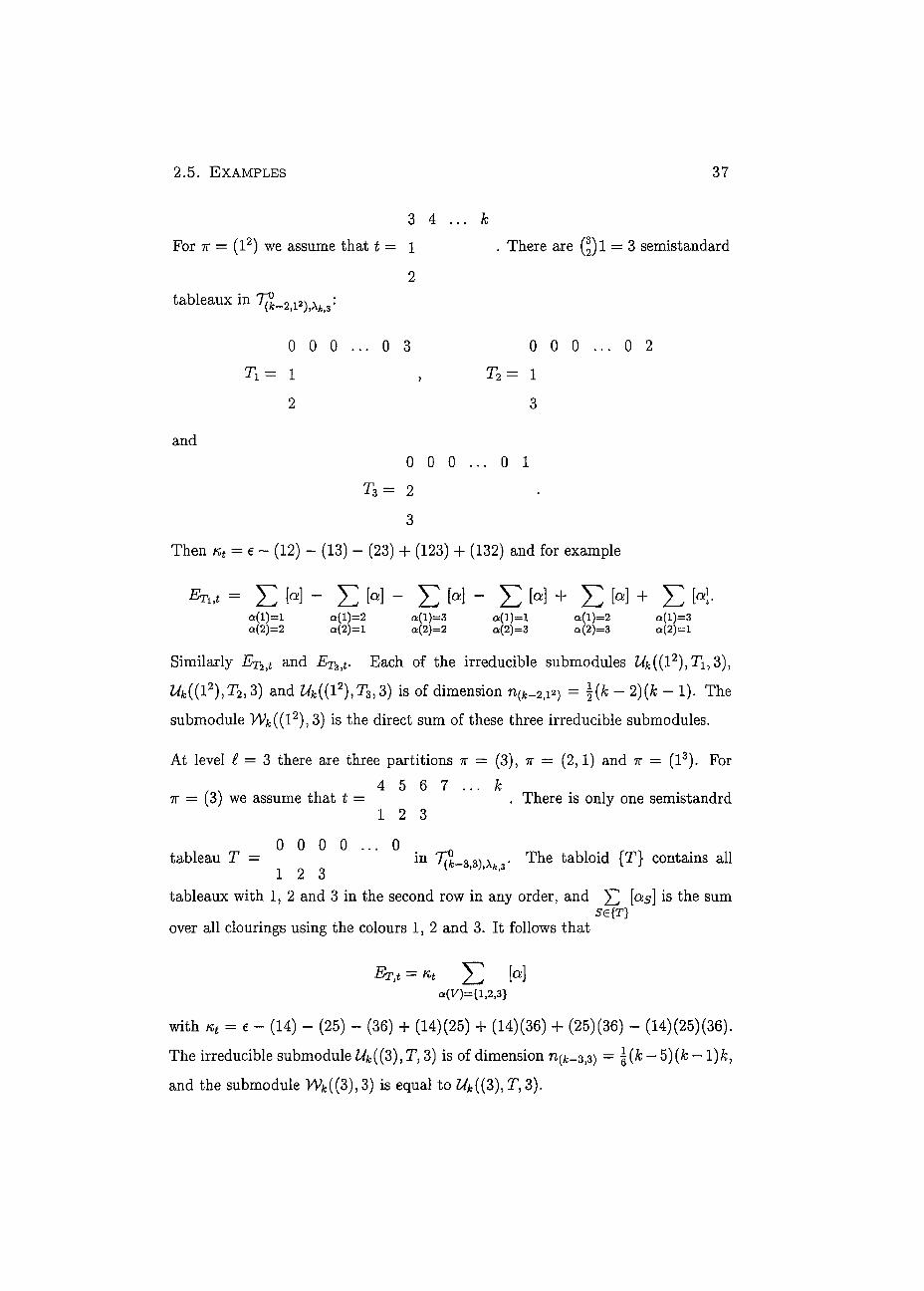
2 . 5 . EXAMPLES 37

3 4 . . . k For 7T = (l2) we assume that t = l . There are Q)l = 3 semistandard

2

tableaux in 771 \ {k-2,l£),Aki3

0 0 0 . . . 0 3 0 0 0 . . . 0 2

Ti= 1 , T2= 1

2 3

and 0 0 0 . . . 0 1

T 3 = 2

3

Then Kt = €~ (12) - (13) - (23) + (123) + (132) and for example

ETut = E M - £ M - £ H - E H + E H + E M-û(l)=l a(l)=2 ct(l)—3 a( l )=l <x(l)=2 a(l)=3 a(2)=2 a(2)=l a(2)=2 û(2)=3 q(2)=3 a(2)=l

Similarly £r2,t and Er3it- Each of the irreducible submodules Z4((12),T\,3)3

Z4((12),T2,3) and Z4((12),T3,3) is of dimension n ( f c _ 2 , = \(k - 2){k - 1). The

submodule V\4((l2),3) is the direct sum of these three irreducible submodules.

At level £ = 3 there are three partitions 7T = (3), 7r = (2,1) and ir = (l3). For 4 5 6 7 . . . À;

7r = (3) we assume that t = . There is only one semistandrd 1 2 3

0 0 0 0 . . . 0 . tableau T = in 3,3)^3- The tabloid (T) contains ail

1 2 3 tableaux with 1, 2 and 3 in the second row in any order, and ^ [as] is the sum

56{T} over ali clourings using the colours 1, 2 and 3. It follows that

Et ,t = « t £ M a{V)={ 1,2,3}

with Kt = e ~ (14) - (25) - (36) + (14)(25) + (14)(36) + (25)(36) - (14)(25)(36).

The irreducible submodule ¿4((3), T, 3) is of dimension n^k-3,3) = — 5)(A; — 1 )k,

and the submodule Wfc((3), 3) is equal to ¿4((3), T, 3).

2 . 5 . EXAMPLES 3 8

4 5 6 ... k

For 7r = (2,1) we assume that ¿ = 1 2 • There are two semistandrd

3 tableaux in 7g_3|2|1)|AM:

0 0 0 0 . . . 0 0 0 0 0 . . . 0 Ti = 1 2 and T2 = 1 3

3 2

Writing colourings of Ks as three-tuples, that is (h, i, j) is the colouring that assigns

colour h to vertex 1, colour i to vertex 2 and colour j to vertex 3 it follows that:

[as] - ( 1 ,2 ,3 ) + (2,1,3) and £ [as] = (1,3,2) + (2,3,1)

and Erut = «¿((1, 2,3) + (2,1,3)) and £T2,t = ( ( 1 , 3 , 2) + (2,3,1)) where

«, = (e - (13) - (14) - (34) + (134) + (143)) (e - (25)).

The irreducible submodules Z4((2,1), Ti, 3) and ¿4((2,1), T2,3) both are of dimen-sion (£-3,2,1) = \(k — 4){k — 2)k. The submodule Wk({2,1),3) is the direct sum of these two irreducible submodules.

4 5 . . . k

For 7r = (l3) we assume that t = . There is one semistandard tableau 2

0 0 0

'(/5-3,l3),Afc,3' T = 1 in 13) A t T h e n {T} = T and ETìt = « t( l , 2,3) where 2

3 «Ì is the alternating sum of the elements of the group of permutations of the set

{1,2,3,4}. The dimension of Z4((13),T,3) is n{k_3|1s) = |(/c - 3)(k - 2)(k - 1).

The submodule Wfc((l3), 3) is equal to ¿4((13),T, 3).

The Table 2.1 summarizes this example. The module 14(3) is the direct sum of

14 irreducible submodules 3). Adding their dimensions up gives k(k — 1)

[k- 2)=dim(V*(3)).

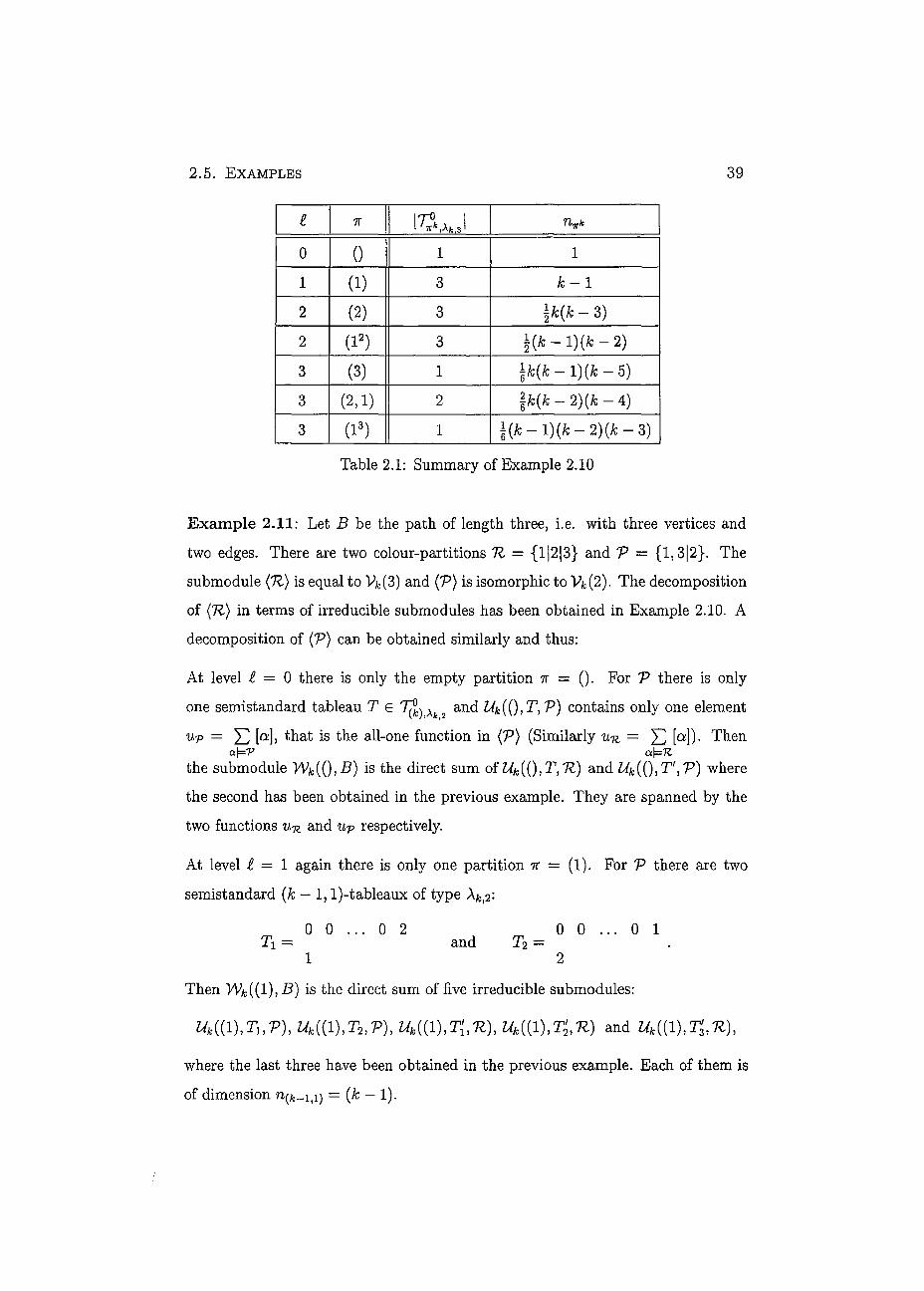
2 . 5 . EXAMPLES 39

1 7T nTk

0 0 1 1 1 (i) 3 k- 1 2 (2) 3 \k{k - 3) 2 (I2) 3 i(k-l){k-2)

3 (3) 1 Jfc(fc-l)(fc-5) 3 (2,1) 2 |fc(fc-2)(A!-4) 3 (I3) 1 \(k-l){k-2)(k-Z)

Table 2.1: Summary of Example 2.10

Example 2.11: Let B be the path of length three, i.e. with three vertices and two edges. There are two colour-partitions 71 = {1|2|3} and V = {1,3|2}. The submodule (71) is equal to 14(3) and (V) is isomorphic to Vjt(2). The decomposition of (7Z) in terms of irreducible submodules has been obtained in Example 2.10. A decomposition of (V) can be obtained similarly and thus:

At level i = 0 there is only the empty partition 7r = (). For V there is only one semistandard tableau T e T^Xk2 and Uk((), T, V) contains only one element u-p = ^ MJ that is the all-one function in (V) (Similarly u-R. = [aD- Then

a\=P a\=TZ

the submodule Wk{Q,B) is the direct sum of Uk{Q,T,7l) and Z4(()JT',7?) where the second has been obtained in the previous example. They are spanned by the two functions Un and up respectively.

At level £ = 1 again there is only one partition ir = (1). For V there are two

semistandard (k — 1, l)-tableaux of type Ajt)2:

0 0 ... 0 2 0 0 ... 0 1 Xi = and T2 =

1 2

Then Wfc((l), B) is the direct sum of five irreducible submodules:

Uk((l),TuV), Z4((1),T2,7>), Z 4 ( ( U k ( ( l ) , T ^ ) and Uk{{ 1 ) , ^ ) ,

where the last three have been obtained in the previous example. Each of them is of dimension = (& — !).

2 . 6 . A NEW MODULE 40

At level t = 2 there are two partitions ir = (2) and ir = (l2). For V there is only

one semistandard (k — 2,2)-tableau and one semistandard (k — 2, l2)-tableau both

of type \k,2' 0 0 . . . 0

0 0 0 . . . 0 and l

1 2 2

Then Wk((2),B) is the direct sum of four irreducible submodules:

Z4 ( (2 ) ,T ,n ¿4((2),TÎ,ft), Uk((2)X,K) and Uk(( 2 ) , ^ ) ,

where the last three have been obtained in the previous example. Each of them is

of dimension n(jt_2,2) = \k(k — 3). Similarly, Wk{{l2),B) is the direct sum of four

irreducible submodules:

Z4(( l 2 ) , T , n U k ( ( l 2 ) , T i ^ Uk(( l 2 )X,K) and ¿ 4 ( ( i 2 ) , T ^ ) ,

where the last three have been obtained in the previous example. Each of them is

of dimension n^-2,i2) = - !)(& — 2).

At level £ = 3 there are three partitions % — (3), ir = (2,1) and ir = (l3). For V

ail submodules Uk(,KìTìV) are zero-modules. Thus the Wk(ix,B) are the same as

in Example 2.10.

Adding up the dimensions of ali the W^ir, B) gives k(k — l)(k — 2) 4- k(k — 1) =

dim(V*(£))

2.6 A new module

In the previous sections we considered the CSym^-modules Uk(ir}T, \7l\) which are

generated by the set

{ET,t 11 is a standard ^-tableau}

and T is a fìxed almost semistandard 7rfc-tableau of type In this section we

shall consider the modules generated by the set of Er,t where we keep t fìxed and

vary T (with some restrictions).

2 . 6 . A NEW MODULE 41

Let X = {rci, x2) • • • be such that Xi < x2 < . . . < xt. We let Sym£ act on X

by

(7> = f°r all ^ £ X and every 7 G Sym .

We write yx{ instead of (7,2:1). This induces an action of Sym€ on the set

{Te%^\T[w]=X}.

That is, for every 7 G Sym£

(7, T)(p, q) = 7Xi where x{ = T(p, q) for all (p, q) G [ir].

Thus Sym£ acts on the indices of Tn. We write 7T instead of (7, T). Let T G %*t\k b

with T[7r] = X. Then T induces a ir tableaux t by replacing the entry xi in X\ by

i. For example

0 x7 ••• 0 x8 0 1 3 5

t = 2 6 corresponds to T = x2 x5

4 X4

For fixed X, this incuces a bijection between the set of tabloids {T} with T G %K}XK b

and T[n] = X, and the set of 7r tabloids {t}. This Bijection commutes with the

action of Syme. It follows that the CSym¿-module generated by the set

{ Y , s I T £ T„k,Xk<b with T{TT] = X} •?<={T}

together with the action

(%£*)= £ * is isomorphic to Mv.

Now, let t be any irk tableau. Recall the action of Sym . on defined on

Page 29, we get that the column stabilizer Ct permutes the positions rather than

the entries of the elements of %kiXk b. It follows that Ct is the column stabilizer for

every elements in 7vk,\kb- Thus

I T ( e 7 ^ , 6 with T[TT] = X) se{T}

2 . 6 . A NEW MODULE 4 2

generates a CSym¿-module isomorphic to S7r. With the €Symk isomorphism from Corollary 2.10 it follows that

E M I T E with T[TT] = X } 5e{T}

generates a CSymrmodule isomorphic to Sn.

Lemma 2.15 There exists some Qt € CSymk such that Kt = Qt^u- a

Proof: The column stabilizer Ct7r is a subgroup of Ct Let Dt be a (left) transversal

of Ct,, in Ct (i.e a complete set of (left) coset representatives). Then

Qt = Y^ sign (5) 5 5<=Dt

•

Corollary 2.16 For every T E with XT C Vj, the set

| ElT,t | 7 e Sym^

together with the action (7, Er,t) ^ E-?T,t generates a CSymg-module isomorphic to

•

Example 2.12: Let 6 = 3. As in Example 2.10, for 7r = (2,1) we assume that 4 5 6 . . . /c

t = 1 2 . There are two semistandrd tableaux in 7^_3j2ji)jAfc 3:

3

0 0 0 0 . . . 0 0 0 0 0 . . . 0

T i = I 2 and T 2 = 1 3

3 2

Writing colourings of as three-tuples, that is (h, i,.;') is the colouring that assigns

colour h to vertex 1, colour i to vertex 2 and colour j to vertex 3 it follows that:

[as] = (1,2,3) + (2,1,3) and £ [a5] = (1,3,2) + (2,3,1) se{Ti} se{r2}

2 . 6 . A NEW MODULE 4 3

and ETut = ««((1,2,3) +(2,1,3)) and ET2it = « t ( ( l , 3,2) + (2,3,1)) where

Let Qt = (e - (14) - (34)) (e - (25)) and = (e- (13)). Then:

((12), Erut) = QÎ((2, 1,3) - (2,3,1) + (1, 2,3) - (3,2,1)) = ETl)ti

((12), ET2it) = Qt((3,1,2) - (1,3,2) + (3,2,1) - (1,2,3)) = -ETut - ET2,t,

((123), ETut) = Qt((3,1,2) - (1,3,2) + (3, 2,1) - (1,2,3)) = -ETut - ET,it

and ((123),ET2it) = Qt{(2,1,3) - (2,3,1) + (1,2,3) - (3,2,1)) = ETut.

It can easily be checked that they indeed generate a matrix representation for Sym3 corresponding to IR = (2,1). Hence ETLLT and ETXìÌ together with the action (7, ET,Ì) E lTìt generate an irreducible submodule isomorphic to S^K

« , = ( £ - (13)) (e - (14) - (34)) (e - (25)).

The corresponding matrices are i?(12) = and #(123) =

Chapter 3

The compatibility matrix method

In this chapter we shall describe the compatibility matrix method, introduced by

N.L. Biggs in [2], and recently used and developed in [5], [8], [7], and [9]. We

show how it can be used to obtain the chromatic polynomials for certain families

of graphs.

The compatibility matrix commutes with the action of the Symmetrie group. Using

the results from Representation Theory, introduced in the previous chapter, we

show that the matrix is équivalent to a block-diagonal matrix, and the multiplicities

and the sizes of the blocks are obtained. Using a repeated inclusion-exclusion

argument the entries of the blocks can be calculated.

This method has previously been used by Biggs and co-workers in [7] and [9] in the

case where the "base graph" is the complété graph K . Here this approach will be

extended for général "base graphs".

3.1 Bracelets

Given a graph B, a set L Ç V x V and an integer n > 3 the bracelet Ln(B) is the

graph constructed as follows. Take n disjoint copies of B and link them by extra

edges according to the rule: For every i = 1,2, . . . , n and each pair (v, w) € L join

44

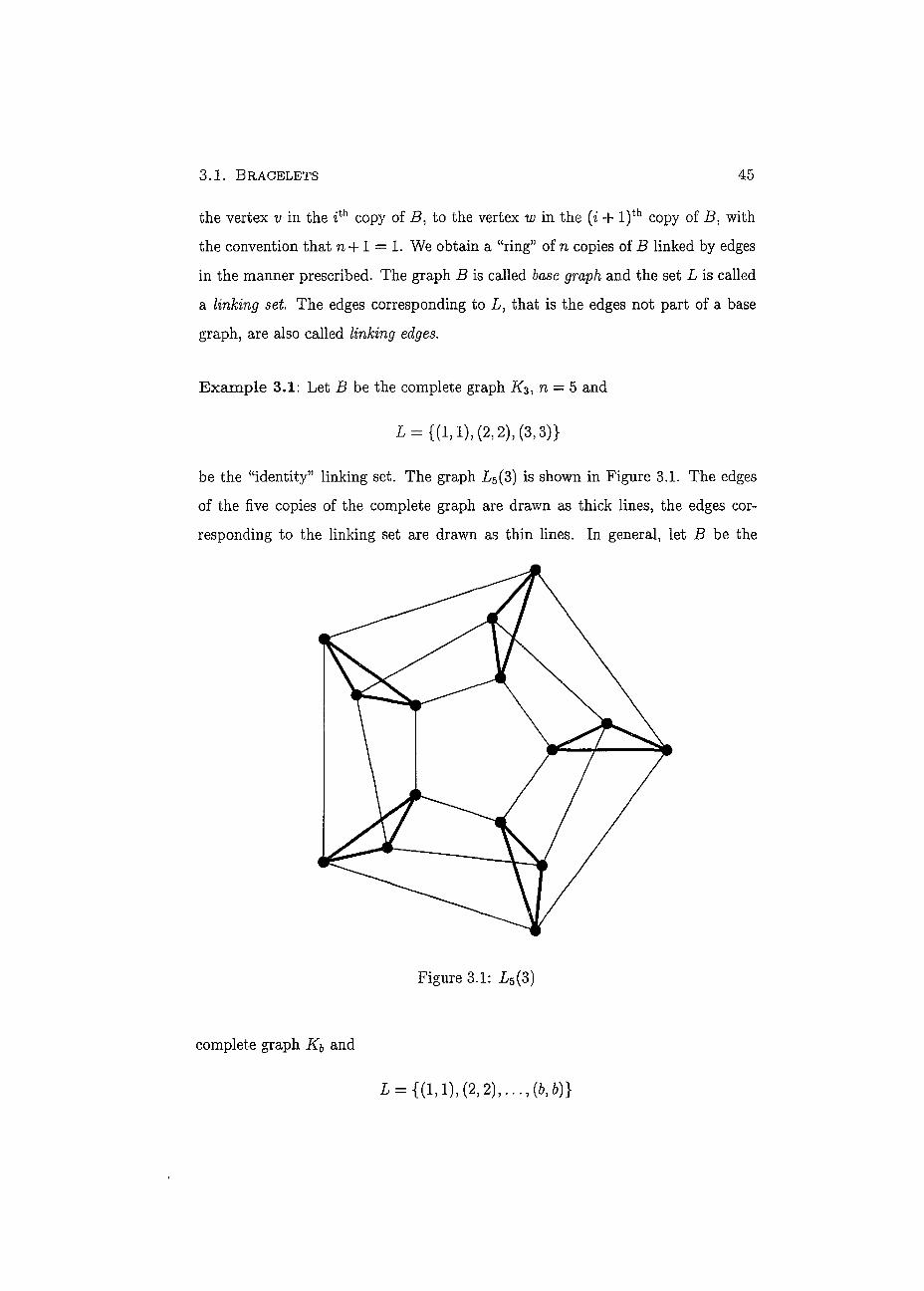
3 . 1 . BRACELETS 4 5

the vertex v in the ith copy of to the vertex w in the (i + l)th copy of B, with

the convention that n +1 = 1. We obtain a "ring" of n copies of B linked by edges

in the manner prescribed. The graph B is called base graph and the set L is called

a linking set The edges corresponding to L, that is the edges not part of a base

graph, are also called linking edges.

Example 3.1: Let B be the complete graph n = 5 and

¿ = { ( 1 , 1 ) , (2 ,2 ) , ( 3 , 3 ) }

be the "identity" linking set. The graph £5(3) is shown in Figure 3.1. The edges

of the fìve copies of the complete graph are drawn as thick lines, the edges cor-

responding to the linking set are drawn as thin lines. In general, let B be the

Figure 3.1: L5(3)

complete graph Ki, and

L = {(1,1), (2,2),. . . , (6,6)}

3 . 1 . BRACELETS 46

be the "identity" linking set. The resulting graph is denoted by Bn(b). For b = 2

the resulting bracelet is also called the ladder graph [5]. The case b — 3 has been

covered in [10]. The chromatic polynomial in the case 6 = 4 has been obtained in

[7] and [11], and the cases b = 5,6 have been treated by this method in [12].

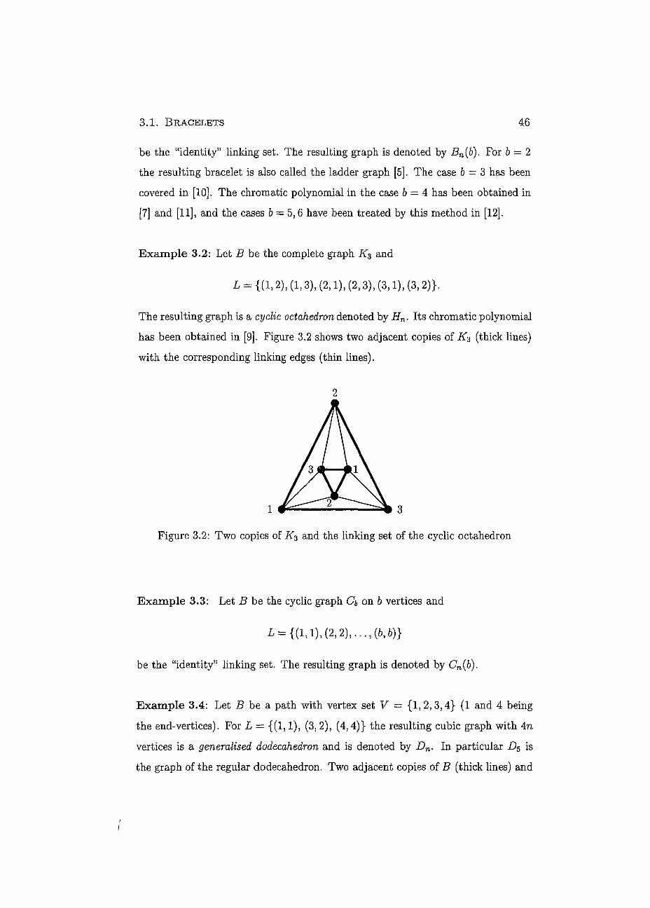
Example 3.2: Let B be the complete graph and

L = {(1,2), (1,3), (2,1), (2,3), (3,1), (3, 2)}.

The resulting graph is a cyclic octahedron denoted by Hn. Its chromatic polynomial

has been obtained in [9]. Figure 3.2 shows two adjacent copies of (thick lines)

with the corresponding linking edges (thin lines).

2

Figure 3.2: Two copies of and the linking set of the cyclic octahedron

Example 3.3: Let B be the cyclic graph Cb on b vertices and

L = {(1,1), (2,2),..., (6, b)}

be the "identity" linking set. The resulting graph is denoted by Cn(ò).

Example 3.4: Let B be a path with vertex set V = {1,2,3,4} (1 and 4 being

the end-vertices). For L = {(1,1), (3, 2), (4,4)} the resulting cubic graph with 4n

vertices is a generalised dodecahedron and is denoted by Dn. In particular D5 is

the graph of the regular dodecahedron. Two adjacent copies of B (thick lines) and

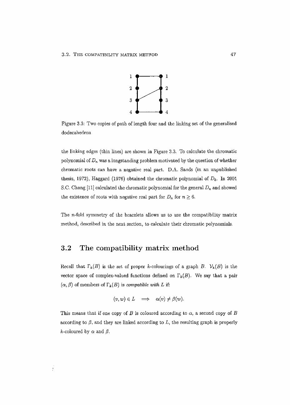
3 . 2 . T H E COMPATIBILITY MATRIX METHOD 4 7

3

4

2

1

2

4

3

1

Figure 3.3: Two copies of path of length four and the linking set of the generalised dodecahedron

the linking edges (thin lines) are shown in Figure 3.3. To calculai e the chromât ic

polynomial of Dn was a longstanding problem motivated by the question of whether

chromatic roots can have a negative real part. D.A. Sands (in an unpublished

thesis, 1972), Haggard (1976) obtained the chromatic polynomial of D5. In 2001

S.C. Chang [11] calculated the chromatic polynomial for the general Dn and showed

the existence of roots with negative real part for Dn for n > 6.

The n-fold symmetry of the bracelets allows us to use the compatibility matrix

method, described in the next section, to calculate their chromatic polynomials.

3.2 The compatibility matrix method

Recali that Tjfc(B) is the set of proper /c-colourings of a graph B. Vk(B) is the

vector space of complex-valued functions defined on Tk(B). We say that a pair

(QÌ, J3) of members of Tjt(B) is compatible with L if:

This means that if one copy of B is coloured according to a, a second copy of B

according to and they are linked according to L, the resulting graph is properly

fc-coloured by a and

3 .2 . T H E COMPATIBILITY MATRIX METHOD 48

The compatibility operator TL = Ti(k) is defìned by the matrix whose entries are

Il if (a,ß) is compatible with L;

0 otherwise.

It is convenient to use the same symbol TL for the linear operator represented

by the matrix TL, with respect to the standard basis of Vk{B). The connection

between TL and the chromatic polynomial P(Ln(B)\k) arises from the following

theorem [5].

Theorem 3.1 The number of k-colourings ofLn(B) is equal to the trace ofTL(k)n.

Proof: Let a, /?, 7 , . . . , r be n colourings in Tk(B). Colour the first copy of B with

a, the second copy with ß and so on up to the nth copy coloured with r. The

resulting colouring of Ln(B) is a proper /¡-colouring if and only if

(XLWPL)^ • • • pL)Ta = 1-

The number of proper ft-colourings of Ln(B) is equal to the sum of this product

over ali possible combinations of a, ß, 7 , . . . , r in Tk{B):

E P Ì M T L ) * . . . (TL)ra = = tr(2T). a,ß, 7,...,r a

•

Observe, that for the moment k is stili a fìxed integer. Only later we will be able

to show that the trace of Ti(k)n is indeed of the form of a polynomial in k and

hence we can replace k with the complex variable

Since the trace of a matrix is equal to the sum of the eigenvalues multiplied by the

corresponding algebraic multiplicities it follows [5]:

Corollary 3.2 Suppose that Ai(&), À . . . , As(k) are the eigenvalues ofTL(k)

and

mi(k)ìm2(k),... ,ms(k) are the corresponding algebraic multiplicities. Then the

number of proper k-colourings of Ln(B) is equal to

Ê mi(k) xm-i=l

•

3 . 3 . DÉCOMPOSITION OF THE COMPATIBILITY MATRIX 4 9

3.3 Décomposition of the compatibility matrix

Recali from the previous chapter that we defined the action of the symmetric group

Sym* on Tk(B) by

(a;, a)(v) = cu(a(v)) for every v € V

for ali cu G Symj. and A G IV Clearly, for every OJ G Symfc, if (ce,/?) is compatible with L then so is (eoa, ufi), Let be the matrix représentation corresponding to the CSymfc-module Vk(B) with respect to the canonical basis. That is

Il if ufi = a

0 otherwise.

It can easily be checked that T^k) A(to) — A{w) T^k) for ail lj G Symk . This

means that TL(k) belongs to the commutant algebra C(A) of A(u). Moreover, this

holds for any linking set L. Let b = \V\. From Lemma 2.1 and Theorem 2.6 it

follows that Ti(k) is équivalent to a matrix of the form

© ( i r ® NI), 0<t<b 7rK

where /n is the identity matrix of size nnk and N£ is a m^k x mnk matrix with entries depending on k.

Theorem 3.3 For any given base graph B and any linking set L the number of

k-colourings of Ln(B) is equal to b

E * ( * ) Mwz)". e=o TTI--£

where r}^(k) = 1 if 1 = 0 and

t vAk) = ir Il (k-hi(7r)) with /^(tt) = ^ + t - i if

i= 1

NI is a matrix of size nn with entries depending on k, and neu(B)

Un is the dimension of the Spechi module S17 given in Lemma 2.3.

3 . 3 . DÉCOMPOSITION OF THE COMPATIBILITY MATRIX 50

Proof: From the argument preceding this theorem and from Theorem 3.1 it follows

that for any given k E N the number of /c-colourings of Ln(B) is equal to

tr ® (ir ® (JVZ)B) = E E * ( * ) t r ( ^ ) n o<l<b £=0 ir\-£ TTl-i

where ty(k) = n k is the size of IVÌ independent of B, given in Theorem 2.6. Also from Theorem 2.6 follows the size of •

Recali from Theorem 2.14 that Vk{B) is the direct sum of the submodules Wfc(7r, B)

where

W*(*,B)= 0 0 Uk(n,T,K) •ReTHB)

for ail partitions 7r h t with 0 < t < b.

It follows that each iVJ corresponds to the submodule The rows and

columns of N£ correspond to the Uk(7r,T, \1Z\).

Observe that the r\ (k) are independent of L and they are given by an explicit formula. The matrix NI is dépendent on L and our main task is to explain how to calculai e it.

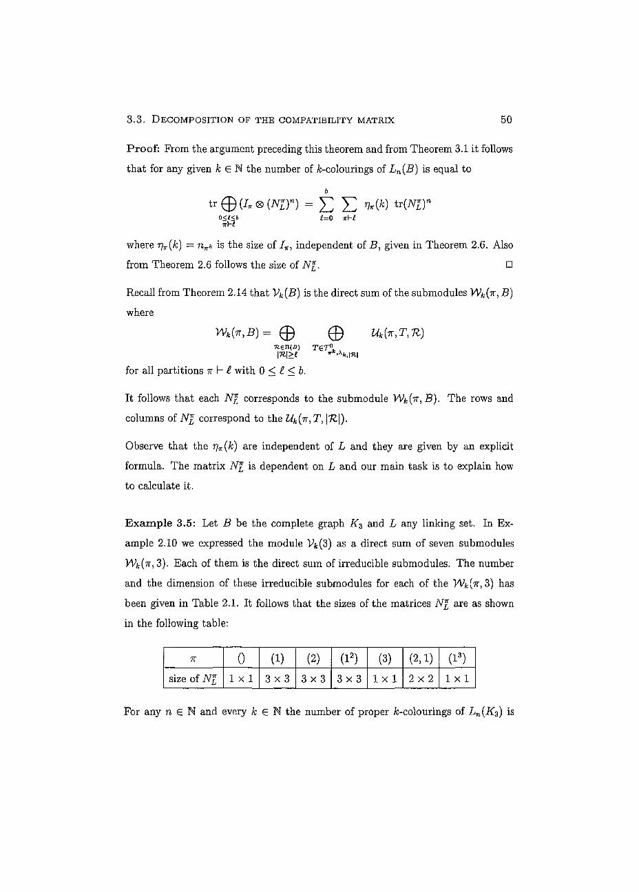
Example 3.5: Let B be the complete graph and L any linking set. In Ex-

ample 2.10 we expressed the module 14(3) as a direct sum of seven submodules

Wjb(7T, 3). Each of them is the direct sum of irreducible submodules. The number

and the dimension of these irreducible submodules for each of the Wki^, 3) has

been given in Table 2.1. It follows that the sizes of the matrices NI are as shown

in the following table:

7T 0 (1) (2) (l2) (3) (2,1) (l3) size of NI 1 x 1 3 x 3 3 x 3 3 x 3 l x l 2 x 2 1 x 1

For any n E N and every k E N the number of proper /c-colourings of Ln(Ks) is

3 .3 . DECOMPOSITION OF THE COMPATIBILITY MATRIX 51

equal to

tr{N^)71 + {k - 1) tr(Af))«

Hb \k{k - 3) tr(iVf)» + \(k ~ 1 )(k - 2) tr( ivf >)»

+ ^A;(Jfc-l)(fc-5) tr(7V[3))n

Later (Theorem 3.13), we will show that the entries of the matrices N£ are poly-

nomials in k over C. It follows that tr(A^J)n is a polynomial in k and hence

b P(Ln(B); k) = J2 E tr(^)n G

¿=0 7r(-£

Replacing fc with the complex variable z we can make P(Z/n(£?); 2;) € €[2;] into a

polynomial with complex variable 2 such that that P(Ln(B); z) is the number of

proper z-colourings for all 2 E N. Hence P(Ln(B)\ z) is the chromatic polynomial

of Ln(B). In order to find tr^N^)71 it is convenient if we can find the eigenvalues

A I ( £ , TT; k), \2(L, 7R; & ) , . . . , A S ( L : 7R; k)

and the corresponding algebraic multiplicities mi(L, 1r),m2(L, 7r),..., ms(L, 7r) of JVJ. Then

5 ¿=1

However, the eigenvalues of JVJ might not always be polynomials (but the sum of

the their nth powers is).

We refer to the (k) as the global multiplicities and to the rrii(L, 7r) as the local

multiplicities. As mentioned earlier, the global multiplicities do not depend on L

whereas the local multiplicities do.

3 . 4 . REDUCTION TO THE COMPLETE BASE GRAPH 52

3.4 Reduction to the complete base graph

Let b and d be two positive integers and let L be a subset of Vb x Vd, where V& is the

vertex set of Kb and V4 the vertex set of Kd. We consider the graph consisting of Kb

and Kd with extra edges according to L. As before, we say that a pair of colourings

(a, ¡3) G Vk(b) x Vk(d) is compatible with L if (v, w) e L implies a(v) ^ ¡3(w). We

define the compatibility operator (and use the same symbol) TL(/C), as before, as

the matrix whose entry in position (a, /3) is one if (a, ¡3) is compatible with L and

zero otherwise.

Let the graph B and the linking set L be given. Suppose that V and 71 are

two colour-partitions of the vertex set of B consisting of b and d independent

sets respectively. That is 7Z = {Ri}bi==1 and V ~ {Pi}f=1 where we assume that

min (FU) < min (Rj) if i < j, and min (Pi) < min (Pj) if i < j. We define L-KP C

Vb x by

(i,j) £ Lnv implies that there exists (v,w) G L such that v G Ri and w G Pj.

Recall that (71) is the submodule of Vk(B) generated by the set {[a] | a |= 71}.

By Lemma 2.7 each of the (71) is isomorphic to 14(6) if b = \7Z\.

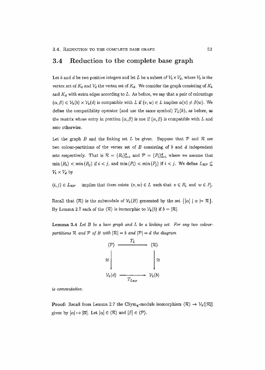
Lemma 3.4 Let B be a base graph and L be a linking set. For any two colour-

partitions 71 and V of B with \7Z\ = b and \V\ —d the diagram

TL (V) (71)

Vfc(d) Ti

Vk(b) LKV

is commutative.

Proof: Recall from Lemma 2.7 the CSymfc-module isomorphism (71) —> Vk(\7l\)

given by [a] ^ [a]. Let [a] G (71) and [0] G (V).

3 . 4 . REDUCTION TO THE COMPLETE BASE GRAPH 53

If Pl)QJ3 — 1 then a(v) ^ P(w) for ail (v,w) G L. From the définition of Lnv

follows that â(i) ± ¡3(j) for ali (ij) G L-ji-p. Hence = 1.

If (T^ap = 0 then a(v) = fi(w) for some (v,w) G L. Let (i,j) be such that

v G Ri and w G Pj. Then (i,j) G LUT and it follows that â(i) = fi(j). Hence

PWW = o- D

As in the previous section Tinv : Vk(d) Vfc(ò) commutes with the action of Symfc

and hence is équivalent to

0 ( i r ® ^ ) . 0<i<min(b,d) 7rK

where is the identity matrix of size nrk and N ^ is a (J)^ x (^n^ matrix.

Since Vk(B) is equal to the direct sum of the (11) it follows from Theorem 2.14

that:

Lemma 3.5 Let B be a base graph and L be a linking set. For any 0 < £ < |V|

and any it Y- £ the matrix NI consists of submatrices équivalent to N1nv with

Ti, V G II(B). Its rows correspond to the Z4(7r,T,7l) with T G A and the

columns correspond to the Z4(7r, T', V) with T' G T£k Afc • 1=1

From this lemma it follows that in order to obtain the entries of NI we may find

the entries of each of the matrices NI individually and then use them to obtain

the original matrix JVJ. Hence we are interest ed in finding iVJ for the case where

we have two complete base graphs of not necessarily the same size and a linking

set L. We write b(L)d for the graph consisting of one copy of Kb and one of Kd

with extra edges according to L. Then \n\ (L-jiv) \-p\ gives rise to and to N^v.

Each of the vertices in K\n\ corresponds to an independent set in 1Z. That is

i G Vyji\ corresponds to Ri with respect to the labelling of the independent sets

satisfying that min (Ri) < min (Rj) if i < j.

Before further investigating N[ for general &(L)d in the next section we give an

example.

3.5 . THE SM OPERATORS 54

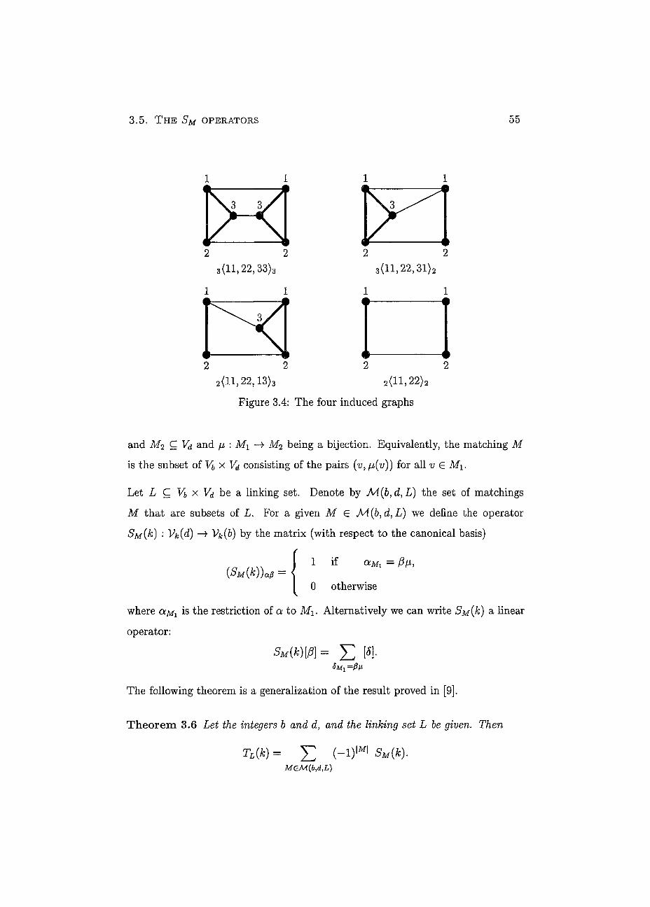
Example 3.6: Let B be the path on three vertices. Let

¿ = {(1,1), (2,2), (3,3)}

be the "identity" linking set. There are two colour-partitions 7Z = {1|2|3} and

V = {1,3|2} and thus there are four induced graphs

3(11,22,33)3, 3(11,22,31)2, 2(11,22,13)3 and 2(11,22)2

where we write for example 2(11,22)2 rather than 2({(1,1), (2, 2)})2- These four

graphs are shown in Figure 3.4 on Page 55. The edges of the base graphs are drawn

as thick lines, the linking edges are drawn as thin lines.

For any i = 0,1,2,3 and any 7r h t the matrix NI consists of four bloeks:

The sizes of these bloeks and of NI have been obtained in Example 2.11, and are

as shown in the following table:

7r 0 (1) (2) ( l 2) (3) (2,1) (l3)

size of 1 x 1 3 x 3 3 x 3 3 x 3 1 x 1 2 x 2 1 x 1

size of N l n v 1 X 1 3 x 2 3 x 2 3 x 2 1 x 0 2 x 0 1 x 0

size of Nr J-'VTZ 1 X 1 2 x 3 2 x 3 2 x 3 0 x 1 0 x 2 0 x 1

size of N l v v 1 X 1 2 x 2 2 x 2 2 x 2 0 x 0 0 x 0 0 x 0

size of iVJ 2 x 2 5 x 5 5 x 5 5 x 5 1 x 1 2 x 2 1 x 1

Observe that the "structure" of iVJ, that is the sizes of the , is independent

of the linking set L.

3.5 The S m operators

Let b and d be two positive integers, and as before let V& be the vertex set of Kb

and Vd the vertex set of Kd- A matching M is a triple (Mi, M2, /¿) with M\ C Vj,

3 . 5 . T H E SM OPERATORS 55

2 2

3(11,22,33)3

2 2 2 ( 1 1 , 2 2 , 1 3 ) 3

2 2 3(11,22,31)2

2 2 2(11322)2

Figure 3.4: The four induced graphs

and M2 Ç Vd and : M\ —> M2 being a bijection. Equivalently, the matching M

is the subset of V& x Vd consisting of the pairs (i>, ¿¿(v)) for ali v G M\.

Let L Ç Vb x Vd be a linking set. Denote by M(bì d, L) the set of matchings

M that are subsets of L. For a given M G M.(b}d,L) we defìne the operator

SMW : Vk(d) —Vfc(ò) by the matrix (with respect to the canonical basis)

, , .. 1 if aMl=Pfi, (SM(k)U = <

I 0 otherwise

where olmx is the restriction of aio M\. Alternatively we can write S m (k) a linear

operator:

s u ( k m = E M -SMl =PfJL

The following theorem is a generalization of the result proved in [9].

Theorem 3.6 Let the integers b and d} and the linking set L be given. Then

TL{k) = E (-1)|M| SM{k). MeM(b,d,L)

3 . 5 . T H E SM OPERATORS 56

Proof: For any a G (b) and ß G Fk(d) we shall show that

{TlU = E (-1)|M| MÇM(b,d,L)

Let Maß be the subset of L such that a(u) = ß(w) for every (v,w) G Maß. Since

a and ß are injections it follows that Maß G .M(6, d,L). Then, (Sm)aß = 1 if and

only if M Ç M^.

E (-i)|M| (SmU = E (-i)|M|-MGM(b,d,L) MCMaß

If [a,ß) is compatible with L then Maß is the empty matching and the sum is

equal to one. If (a, ß) is not compatible with L then Maß is not empty and

(-i)|M| = (i + (~i))iM i = o. MCMaß

•

It is easily verified that each of the commutes with the action of Symfc on

the colourings. By a similar argument as in Section 3.3 it follows that:

Corollary 3.7 Let the integers b and d, and the linking set L be given. Then there

exist matrices Ufa each of size nn x n^ such that

**i = E (-i)|J" uM-MçM(b,d,L)

•

The matrix (1v 0 Ufa) represents the induced linear operator

SM(k):Wk^ìd)-^Wk{'Kìb)

where is the identity matrix of size n^k. The columns of Ufa corresponding

to the irreducible submodules U^ir^T, d) with Te T k \kd and rows corresponding

to the irreducible submodules Uk(iri S, b) with S G Xkb- Later it will be shown

that Ufa is the all-zero matrix if £ > \M\. The next aim is to find the entries of TTir uM.

2.4.2. A C H A N G E O F BASIS

3.6 Change of basis

5 7

Recall from Section 2.4.2 the following: Let X Ç Vj, and let g : X —>• K be an injection. We define the function [X \ g] G VK{b) by

1 if ay ~ g \X I s)(a) = ;

0 otherwise.

for every a G Tk(b) where ax is the restriction of a to X. Equivalently

[x I g] = E [«]• àx=9

For every matching M — (Mi, M2, ¡jl) we can write

SM(k)[a] = ]T [5] = [Mx | a/i].

5Ml —otfJ.

Lemma 3.8 Let [X | g] G Vk{d) and M G M{b, d, L) be given. Then

SM(k)[X\g]= c Y (-1)1*1-1™,! £ [Y[g(j)] l*-1(XnM2)ÇYÇM1 (j>eGM(YtX)

where Gm(Y,X) is the set of injections <j> \ Y X such that 4>FI~L is the identity

map on X H M2; and c is a non-zéro constant

Proof: From définitions follows on the left hand side that

E l = s M \ x ig] = Su e m = E E m = E K E !)• otx=9 ax=9 PM, PeTk(b) <*x=9 an=pMl

Dénoté by the map

E C(-l)lyH™» £ [;Y\g4,] FI-HXNMI^YÇMI <P£GM{Y,X)

Let 7 G Tk(b). We are going to compare We may assume that

7/LÎ - 1 = g on X i l M2, because otherwise both sides are zéro. Indeed, for it

follows immediately from a — g and a = 7¡JT1 on X H M2. For by définition

2.4.2. A CHANGE OF BASIS 58

[Y | g</>](y) = 1 only if g<j) = 7 on Y. Since ^(X n l 2 ) ÇY C M1 it follows from

the définition of Gm{Y, X) that g^jjT1 = g = ypr1 on X D M2.

If 7 ^ ( y ) ^ g(X) for ail v G M2\{X Cl M2) then there exists a a such that

afi = 7M l and ax = It follows that J^L(t) 1S n o n - z e r o - O11 the right hand

side, since Y Ç Ml and g<p{Y) Ç g(X) it follows that [Y \ g<t>}{7) ± 0 only if

Y = fT^X D M2). And thus YLnil) = c-

If € for some v g M 2 \ ( J n M 2 ) . Then, since ax = g it follows that

there exists x G X such that a(x) = 7(11). On the other hand 7Mx — implies

that a(v) = a(x). Since v ^ x it follows that = For rïght hand side

let

Q={vGM2\(XnM2) | 7 fi-'iv) G g{X) }.

Then [Y | ^ 0 only if n~l{X H M2) Ç F Ç iTl{(X fi M2) U Q) and the

injection (/) is such that g(j) = 7y. Since we assumed that g = 7¡i~l on X D M2 it

follows that such a 4> exists in GM(Y,X). And thus

I » = E c (-irHxnmi[Y i7y](7) R ti-1(xnM2)çYÇfx-1(xnM2)uQ

= c (-l)|K|_|XnM21

r=0 ^ '

•

Lemma 3.9 Let Y Ç Vh and X ÇVd- Let g : X —»• K be an injection. Then the

coefficient of[Y | gtf>] in SM{k)[X | g] with (Mi,M2,/i) G M(b,d,L) and injection

<j) :Y —X is non-zero if and only if

(i)

(ii)

¡rx(X N M2) Ç Y Ç MI, and

ififi-1 is the identity map on X fl Mi.

3 . 7 . ACTION OF s M [ k ) ON THE IRREDUCIBLE SUBMODULES OF Vk{b) 5 9

Let f3(d, k) = (k — s)d_s = (k — s)(k — s — 1 ) . . . (k — d -+- 1) be the falling

factorial. If the conditions (i) and (ii) are satisfied the coefficient is

( - D M - ™ W I L ( D I * )

Proof: The first part of the lemma follows directly from Lemma 3.8. More-

over it follows that when the conditions (i) and (ii) are satisfied the coefficient is

c F r o m t h e p r o o f o f Lemma 3.8 it follows that c is equal to the

number of a € r^d) satisfying afi = g' and ax = g• That is, a is fixed on X

and on M2, and there are k — \X U M2\ colours left to be assigned to d — \X U M2\

vertices to complete a. •

3.7 Action of S m (fi) o n the irreducible submod-

ules of Vk(b)

Let 0 < i < b and ir h t. For the rest of this section let i be a fixed irk-

tableau. Recali from Section 2.4.2 the following. For every tableau T €

we denote by Tv : [ît] — Vj, U {0} the restriction of T to [tt] . The image of T^

is denoted by Xt• If T is semistandard of type Ak,b then XT Ç V& and X'K is a

standard tableau. Denote by gr ' Xt K the restriction of ar to Xt. That is,

gT(x) = t(i,j) where T(i,j) = x for ail x G Xt- Similarly, define tv to be the

restriction of i to [7r].

In Section 2.4.1 it has been shown that for every semistandard tableau T e Xkb

the set

|Et,7î | 7 £ Symfc such that jt is a standard ^-tableau j

where

Er,t = «t X) I^l = Kt S I U9Ti Se{T} uÇRtx

is the standard basis of the submodule Uk(ir» T, b).

Since the S M (k) commute with the action of Symk it follows that we only have to

consider the effect of SM(&) on Etj-

3 . 7 . ACTION OF sM[k) ON THE IRREDUCIBLE SUBMODULES OF Vk{b) 60

Lemma 3.10 Let M G M(b, d,L) andT G %kt\kd. Then Sm(k) Ex,t is a linear

combination of

Y I T$

where yrl{XT nM2) ÇY Ç M1 with \Y\ = £ and (¡3 G G]fT.

Proof: From Lemma 3.8 and since SM commutes with Symfc it follows that

SM(k)^t Y t X t I u9t\)

= E c (-D|y|-|xnMj| E * E [ y i ^T4>I

¡I~L{XTR\M2)ÇYÇ.MI <J>£GM{Y,XT) UERTLT

Choose any n~l{XT n Af2) Ç Y C M1 with \Y\ < i and any </> G G]fT. We can write

Kt I S t ^ ] = Y sign(5) [Y I 8u)gT<t>] ueRtn we^ seCt

Choose any co G Rtn. Let g : Y —> K be such that g = ujgT<f>- Partition Ct into parts

B2, . • •, Br according to the rule that ô and ô' are in the same part if and only

if [Y | ôg] — [Y | ô'g}. Since \Y\ < i it follows that each of the parts contains more

than one element. For every j = 1,2,... ,7Ti denote by Dj the set of colours that

are in the jth column of t but not in g (Y). Let H = SymDl x Sym^ x . . . x S y m ^ .

Then for every B it holds that B = 6H for some Ô G B. That is, B is a left coset

of H. Thus

Y sign(ô) [Y\ôg}= sign(<5) £ sign(r) [Y \ ôrg] Ô€B TEH

= sign(â) [Y\Sg] ^ s ign ( r ) T€H

7T1 = sign(<5) [Y | ôg] £(1 ' ^

3=1

This holds for ail B and hence follows the resuit. •

3 . 7 . ACTION OF sM[k) ON THE IRREDUCIBLE SUBMODULES OF Vk{b) 61

Let us recali Section 2.6 and study its implications. Let X = {^i, x2ì..., xfì be a

subset of Vd such that Xi < x2 < •.. < xi. We let Sym^ act on X by

(7, xi) = x7i for ali Xi E X and every 7 E Sym£.

We write 7Xi instead of (7,2^). This induces an action of Sym^ on the set

{T 6 | TW = X } .

That is, for every 7 6 Sym£

(7, T)(p, q) = 7Xi where x{ = T(p, q) for ali (p, q) € [ir].

We write 7T instead of (7,X). We can assume that the irk tableau t is such that

t[ir] = {1, 2 , . . . , £}. Let Y = {yu y2,..., be a subset of Vb with yx < y2 < ... <

yt. Choose Tx € and TY e %ktXh>b such that Tx[ir] = X and TY{vr] = Y,

and

9TX FA) = 9Ty fa) =I for ali i = 1, 2 , . . . , L

For any matching M = (M1,M2, FI) € M(b, d, £) with \M\ < t denote by F^x the

subset of Sym^ satisfying

FMx = {pz I te, Xj) e (Y X x) N M => i = p(j)}

There is a one to one relationship between the elements of F ^ x and G s u c h that

9TYP~1 = 0TX<T> o n 7 .

Lemma 3.11 Let T € %k)Xkb with T[ir] = X. Then

glT = gT7-1 for ali 7 € Symi

Proof: By definition of gT for every X{ E X :

9jrfa) = t(p, q) if 7T(p, q)-Xi.

It follows T(p, g) = and thus = t(p, q). •

3 . 7 . A C T I O N OF SM(k) ON THE IRREDUCIBLE SUBMODULES OF Vk(b) 6 2

It follows that

«t \-X I ^dTx^} = «t E ty I ^STyP'1] = EpTy,t

and for every 7 6 Sym£ it follows that

— Ep^TyJ,-

Assume that 7Ty is semistandard then the restriction of 77V to ¡7r] is a standard

7r tableau. From Corollary 2.16 it follows that

Ep1ty = E ( ^ ( P ) ) EaTY,t a- gSym^

crTy-is semistandard

where i?71" is Young's natural représentation corresponding to Sn. Observe that the

rows and columns of RK correspond to the standard 7r tableaux, but we label them

(for brevity) by the elements 7 G Sym£ such that the restriction of 7Ty to [71"] is a

standard 1r tableau.

From Lemma 3.10 it follows that

SMELTX,T = C M { X ) ^ «T S I U9ITX<I>],

r1(xnM2)çyçM1 é€GXlx * where

From the argument above it follows that

SMEJTXJ = C M { X ) E KT T . ^ I

/x-i(xnM2)çyçAf1 peFÏjx 0}<=Rt7( \Y\=£ M

- C M { X ) ^ ^ EpiTy,f

\Y\=e M

Corollary 3.12 Let M G M(b, d, L), T G %kM d and T G

If irl{XT H Af2) C XT> Ç Mx and 0T; = /or some 0 G then

SM(k) : Z4(7r,X, &) —> Ukin^T'.b) is the isomorphism given by

ET* h- CM(XT) where CM(X) = (-lY~lXnM*1 f\xuM2\(d, k).

3 . 7 . ACTION OF sM[K) ON THE IRREDUCIBLE SUBMODULES OF Vk{b)

Otherwise Su(k) : UkfajT^) -» ^(ÎT, T', b) is the zero-map.

6 3

•

This resuit is no surprise since Z4(7r}T', d) and £&(7r, T, b) are irreducible and from

Schur's Lemma follows that S M [k) : 24(7r,T, b) —> ^ ( ^ T " , 6) is either the zero-

map or a multiplication by a scalar.

Since 7Ty is semistandard if and only if 7Tx is semistandard, it follows if 7Tx is semistandard that:

SME-yTx,t = CM(X) X ¿ L ( EeTYyt crj

n-1(Xr\M2)ÇYÇM1 p£FÏ)x a^Symi |Y\=i crTy is semistandard

It follows that:

Theorem 3.13 Let 0 < £ < min (M) , tt £ and M e M(b,d,L). Then the

matrix Ufc consists of square submatrices (Uld)YX where X Ç Vj and Y ÇVj, with

\X\ = \Y\ = L Each of the {U^)YX is of the form

\cM{X) £ R*(p) ifïi-1(XDM2)ÇYÇM1 (U^)YX = ^ KFV

O otherwise. \

where

CM(X) = (-i)£-|xnAÎ!lw2|Kfe)

and B?(p) is Young's natural représentation, that is the n^ x n^. matrix représen-

tation corresponding to and O is the all-zero matrix of size n^ x •

Observe that depends on £ but not on ir h £.

Theorem 3.14 Let B be any base graph with vertex set V and L any linking set.

Then \v\

p(Ln(B):k) = j2 £ ttrW M f l z r . 0 ir\-e

is the chromatic polynomial of Ln(B) in k where ^(k) = 1 if £ = 0, £

fi r

7]n(k) = ~~ I l (k — hi(7r)) with hi(ir) = ^ -f £ — i if £ > 0, i=1

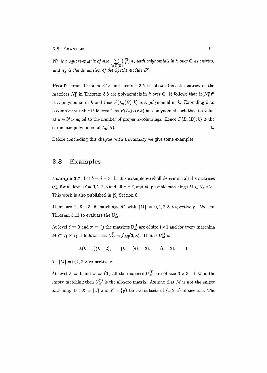
2.5. EXAMPLES 6 4

NI is a square-matrix of size n^ with polynomials in k over C as entries,

and is the dimension of the Specht module S7r.

Proof: From Theorem 3.13 and Lemma 3.5 it follows that the entries of the

matrices N£ in Theorem 3.3 are polynomials in k over C. It follows that tr(JVJ)n

is a polynomial in k and thus P(Ln(B); k) is a polynomial in k. Extending k to

a complex variable it follows that P(Ln(B)\ k) is a polynomial such that its value

at k E N is equal to the number of proper /c-colourings. Hence P(Ln(B); k) is the

chromatic polynomial of Ln (B). •

Before concluding this chapter with a summary we give some examples.

3.8 Examples

Example 3.7: Let b = d = 3. In this example we shall determine all the matrices

Ufa for all levels £ = 0,1,2, 3 and all 7r h £, and all possible matchings M C V3 x V3.

This work is also published in [9] Section 6.

There are 1, 9, 18, 6 matchings M with \M\ = 0,1,2,3 respectively. We use

Theorem 3.13 to evaluate the Ufa.

At level i = 0 and 7r = () the matrices C/£- are of size 1x1 and for every matching

M C V3 x V3 it follows that = /|M|(3, k). That is U% is

k{k-l)(k-2)} (k — l)(k — 2), [k - 2), 1

for \M\ = 0,1,2,3 respectively.

At level 1 = 1 and n = (1) all the matrices are of size 3 x 3 . If M is the

empty matching then is the ali-zero matrix. Assume that M is not the empty

matching. Let X = {rc} and Y = { y } be two subsets of {1,2,3} of size one. The

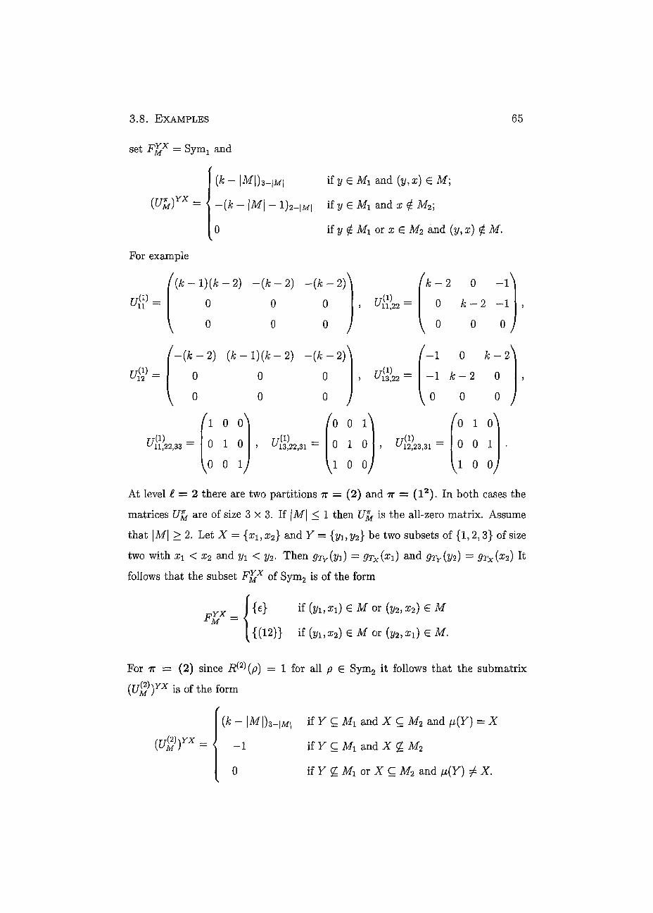
3 . 8 . EXAMPLES 65

set = Symj and

O f t ) ™ =

{k - |M|)3-|m| if y e Mi and (y, x) G M;

-{k - \M\ - 1 ) 2 — | A f | if y e Ml and x £ M2;

0 if 2/ £ Mi or x G M2 and (y, x) ^ M.

For example

f(k-l)(k-2) ~(k~2) -(k-2))

0 0 0

\ o o o y

f-(k- 2) (fc-l)(ifc-2) -(Ä-2))

u n — > 11,22 —

f h-2 0 - 1 ^

Tj( 1) _ U12 —

/

TjH) _ 5 ^13,22 —

Tj( 1) _ ^11,22,33 ~

^ 1 0 0^

0 1 0

Vo 0 V 7/(1) -

0 0 1

0 1 0

V1 0 0

77(1)

0 k — 2 —1

0 0 0

- 1 0 fc-2

- 1 jfe — 2 0

0 0 0

1 o \ 0 0 1

1 0 V At level £ = 2 there are two partitions 7r = (2) and 7r = ( l 2 ) . In both cases the

matrices Ufa are of size 3 x 3. If \M\ < 1 then U^ is the all-zero matrix. Assume

that \M\ > 2. Let X = {a;i, x2} and Y = {yi, y2} be two subsets of {1,2,3} of size

two with xi < x2 and yi < y2. Then gTy{yi) = 9TX(X 1) a n d 0ry(îfe) = 9TX{x2) It

follows that the subset of Sym2 is of the form

rpYX _ *M -

{e} if (yi, xi) G M or (y2ì x2) € M

{(12)} if fei, x2) e M or (y2,a*) G M.

For 7T = (2) since R^(p) = 1 for all p G Sym2 it follows that the submatrix

CuM)Y X is o f t h e f o r m

(k - |M|)3_|M1 if F Ç Mi and X Ç M2 and ß(Y) = X

- 1 if F Ç M i a n d X g M 2

0 if F 2 Mi or X Ç M2 and p{Y) ¿ X.

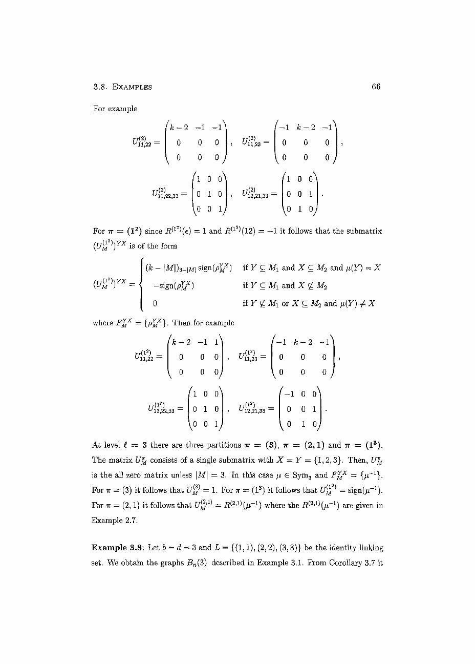
3 .8 . EXAMPLES 66

For example

U{2) -11,22 —

(k- 2 - 1 -l\

0 0 0

0 0 0

(\ 0 0^

7/(2) -J UU, 23 —

/c — 2

0 0 0

0 0 0

rr(2) _ ull,22,33 — 0 1 0

0 0 1

Tj( 2) _ J 12,21,33 —

( \ 0 0^

0 0 1

V o 1 V For 7r = ( l 2 ) since i^ l2)(e) = 1 and i?( l2)( 12) = - 1 it follows that the submatrix

0 u M ] ) Y X i s o f t h e f o r m

( ^ V * =

(k - |M|)3_¡m| sign(pJ7) if Y C Mi and X Ç M2 and fjt(Y) = X

- s i g n ( ^ ) if Y Ç Mi and X g M2

0 ifY g M1 ox XCM2 and p(Y) # X

where Fj¿x = {p j^ } . Then for example

( k - 2 - 1 l\

0 0 0 r/d2) _ 11,22 —

\ 0 0

/ - l A: — 2 - 1 ^ 77(l2) -i u 11,23 ~

°J \

Mi2) _ 11,22,33 ~

0 (A

0 1 0

0 0 1

TjH2) _ 5 u 12,21,33 —

0 0 0

0 0 0

' ' - i o o^

0 0 1

0 1 V At level £ = 3 there are three partitions ir = (3), 7r = (2,1) and 7r = ( l 3 ) .

The matrix Ufa consists of a single submatrix with X = Y = {1,2,3}. Then, Ufa

is the all zero matrix unless \M\ = 3. In this case fi G Sym3 and = {¿A-1}.

For Tí = (3) it follows that = 1. For tt = (l3) it follows that U^ = sign^LT1).

For 7T = (2,1) it follows that = R&Vfa-1) where the jRÍ2»1^/!"1) are given in

Example 2.7.

E x a m p l e 3.8 : Let ö = d = 3 and L = { (1 ,1 ) , (2,2), (3 ,3 ) } be the identity linking

set. We obtain the graphs Bn(3) described in Example 3.1. From Corollary 3.7 it

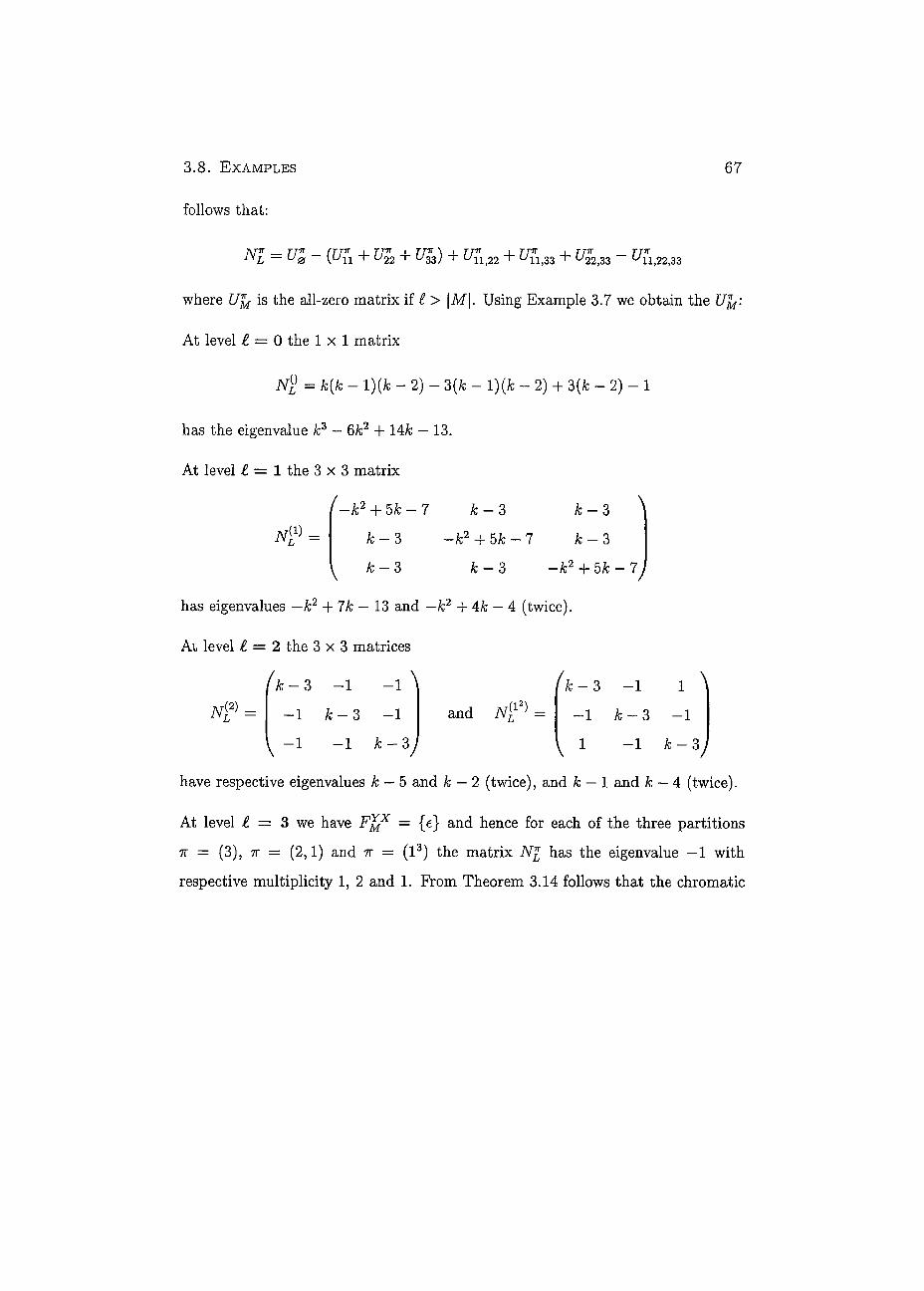
3 . 8 . E X A M P L E S

follows that:

67

N I , = U ¡ 3 ~ ( V i l + ^22 + ^33) + ^11,22 + ^11,33 + ^22,33 ~~ ^11,22,33

where Ufa is the all-zero matrix if I > \M\. Using Example 3.7 we obtain the Ufa:

At level i = 0 the l x l matrix

n2 = k{k - l){k - 2) - 3(fc - l)(fc - 2) + Z(k - 2) - 1

has the eigenvalue /c3 — 6k2 + 14k — 13.

At level t = 1 the 3 x 3 matrix

/—k2 + 5fc — 7 A; — 3 k-3 = /c — 3 —/c2 -h 5/c — T /c — 3

^ k - 3 /c — 3 -/c2 + 5 /c -7y

has eigenvalues — A;2 -I- 7k — 13 and — k2 + Ak — 4 (twice).

At level t = 2 the 3 x 3 matrices

¡ k ~ 3 - 1 - 1 ^

- 1 jfe - 3 - 1

y -1 -1 k-Zj

and M l 2 ) =

V

k- 3 - 1 1 ^

- 1 k- 3 - 1

1 - 1 k-Sj

have respective eigenvalues k — 5 and A; — 2 (twice), and k — 1 and k — 4 (twice).

At level i = 3 we have = {e} and hence for each of the three partitions

7T = (3), 7T = (2,1) and 7r = (l3) the matrix iVJ has the eigenvalue —1 with

respective multiplicity 1, 2 and 1. From Theorem 3.14 follows that the chromatic

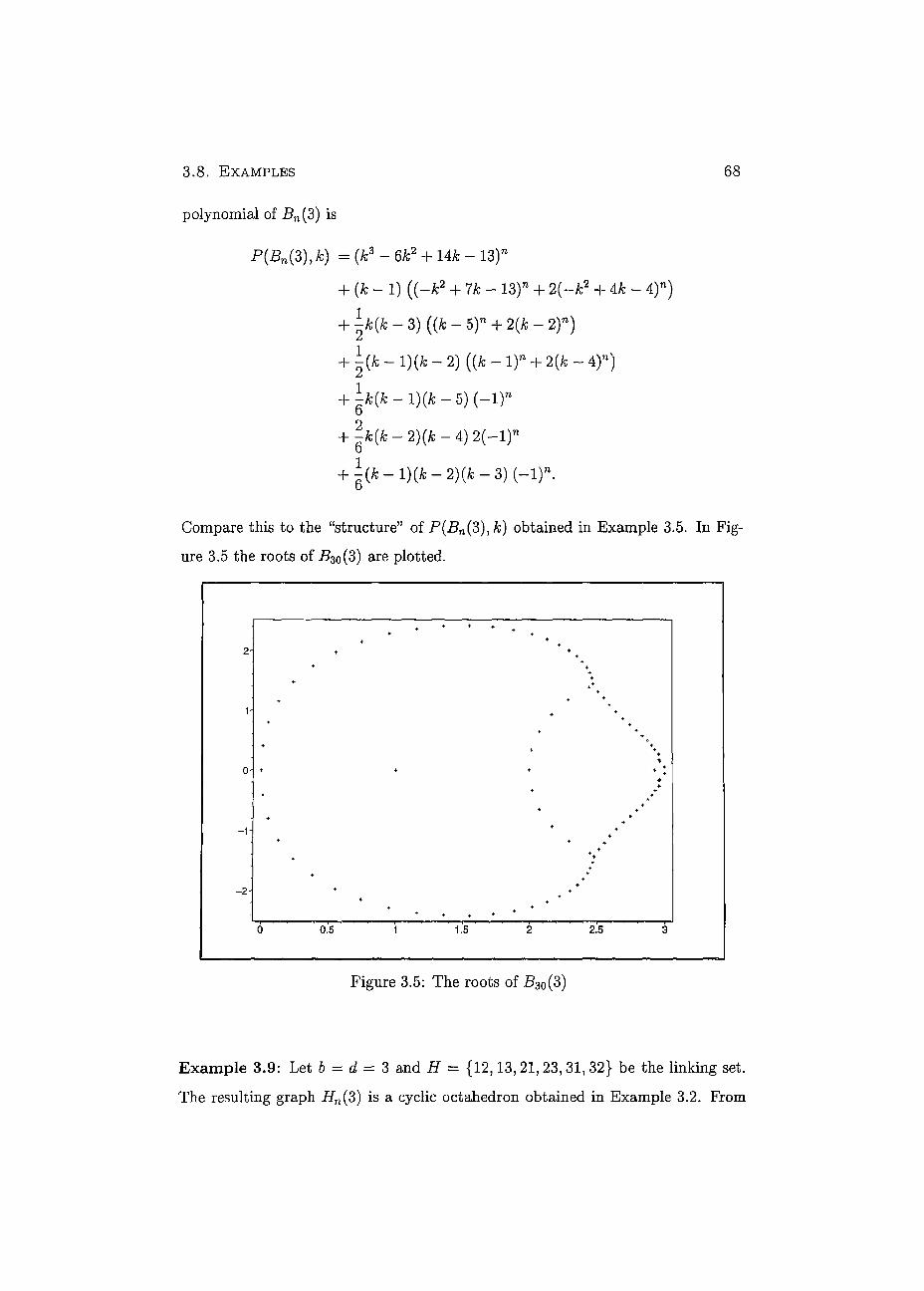
3.8 . EXAMPLES 68

polynomial of Bn(3) is

P(Bn(3),k) = (k3 - 6k2 + 14* - 13)n

+ (Jb - 1) ((-k2 + 7k- 13)" + 2(—k2 + 4k~ 4)n)

+ \k{k - 3) ((A; - 5)n + 2(k - 2)n) /

+ h k - - 2) ((A: - 1)" + 2(k - 4)n) / + h ( k - i ) ( k - 5) ( - î ) »

b + \k(k — 2)(k — 4) 2(—l)71

+ | ( * - l ) ( * - 2 ) ( f c - 3 ) ( - 1 )».

Compare this to the "structure" of P(.Bn(3),&) obtained in Example 3.5. In Fig-

ure 3.5 the roots of 530(3) are plotted.

Figure 3.5: The roots of B30(3)

E x a m p l e 3.9 : Let b = d = 3 and H = {12,13, 21, 23,31, 32} be the linking set.

The resulting graph Hn(3) is a cyclic octahedron obtained in Example 3.2. From

3 . 8 . EXAMPLES 69

Corollary 3.7 follows that:

Nl=Ul- (Ift + Eft + E£ + Eft + Eft + Eft)

+ (^12,21 + ^12,23 + ^13,21 + ^13,31 + ^12,31 + ^13,32 + ^23,32 + ^23,31 + ^23,3l)

(^12,23,31 + ^13,21,32)

At level ¿ = 0 the l x l matrix

= ¿(fc _ i ) ^ _ 2) - 6(jfe - l)(fc - 2) + 9(k - 2) - 2,

has the eigenvalue A;3 - 9&2 + 29A; — 32.

At level t — 1 the 3 x 3 matrix

( 2k - 6 -k2 + 7k- 13 nh} = - k 2 + 7k - 13 2k - 6

^-/c2 + 7/c-13 - / c 2 + 7 / e - 1 3

has eigenvalues — 2(k — 4)2 and k2 — 5k+ 7 (twice).

—k2 -\-7k —

-k2 + 7k - 13

2k- 6 f

At level i = 2 the 3 x 3 matrices

TV (2) _ H

/c - 4 k - 5 A; - 5

fc - 5 fc - 4 k - 5

yfc — 5 / c - 5 fc — 4

and 7V£2) = f Jfc-4 -(A; - 3) Jfe-3 ^

—(fc — 3) k- 4 -(A; - 3)

^ Ä - 3 - ( f c - 3) fc-4 j

have respective eigenvalues 3A; — 14 and 1 (twice), and k~2 and —2k — 7 (twice).

At level £ = 3, the matrices JVJ = -(¿T(123) + iT (132)) with ?r = (3), TT = (2,1)

and 7r = (l3) are of size 1 x 1 , 2 x 2 and l x l respectively. For 7r = (3) and = (l3)

the eigenvalue is —2. For n = (2,1) the eigenvalue is 1 (twice).

The global multiplicities do not depend on the linking set so they are the same as

in Example 3.8. From Theorem 3.14 it follows that the chromatic polynomial of

i

2.5. EXAMPLES 70

Hn(3) is

P(Hn(3);k) (k3 - 9k2 + 29k - 32)"

+ (fc - 1) ((-2(ife - 4)2)n + 2(k2 -hk + 7)n)

+ \k(k - 3) (3/s - 14)n + 2)

+ - l)(fc - 2) ((A - 2)n + 2(—2/c + 7)n)

+ - l)(fc - 5)(—2)" + - 1)(* - 2)(Ä - 3)(—2)n

+ i*( fc -2) (A; -4) (2) . o

Example 3.10: Let b = 3 and d = 2. In this example we shall determine all

the matrices Ufa for all levels £ = 0,1,2 and all 7r b and all possible matchings

M CV3 X V2.

There are 1, 6, 6 matchings M with |M| = 0,1, 2 respectively. We use Theorem 3.13

to evaluate the Ufa. At level t — 0 and 7T = () the matrices [/£- are

k{k- 1), (A; — 1), 1 for \M\ = 0,1,2 respectively.

At level t = 1 and 7r = (1) the matrices C/^ are of size 3 x 2 . Suppose that

M is not the empty matching. Let { z } C {1,2} and {?/} C {1,2,3}. The set FMX = SYMI AND

(k - |M|)2_|M| if y € Mi and (y,x) G M;

W ) ™ = I - 1 if y CE M1 and x Í M2;

0 if y £ Mi or x e M2 and (y, x) ^ M.

Then for example

4 - 1 U-(i) _ IX 0 0

0 0

TT(I) _ 5 ( - / 2 2

0 0 -1 k — 1 0 0

\ / Tj( 1) _ 3 31 —

rj{ 1) _ 11,22 —

fx ^

0 1

Vo ° /

77(1) _

0 0 \

0 0

k- 1 -1 y

o\ 0 1

V1 V

2.5. EXAMPLES 71

At level i = 2 there are two partitions 7r = (2) and 7r = ( l2 ) . in both cases

the matrices Ufa are of size 3 x 1 . Suppose that |M\ > 2. Let X — {1, 2} and

Y = {í/i, y2} C {1,2,3} with yi < y2. The subset F^x of Sym2 is of the form

-

{€} if (2/1,1) 6 M or (y2i 2) 6 M

{(12)} if (yu2) e M 01 (y2,l) e M.

Since R^(p) = 1 and R^{p) = sign(p) for all p G Sym2 it follows that the

submatrix (Uy¡)YX is of the form

(U'm)yx = R"(ßV) if YCM1

0 otherwise

where p f f is the element in F^ x . Then for example

fl\ fo\ fl\ TJ( 2) 11,22 — 0 TJ( 2) u22,31 — 0 U (I2)

11,22 0 u 22,31 ~ 0

w V1/ w i-v Example 3.11: Let b — 2 and d = 3. In this example we shall determine all

the matrices C/Jj- for all levels £ = 0,1, 2 and all TT I- and all possible matchings

M C V2 x V5. Although this case is very similar to the previous example we shall

repeat all the calculations to avoid difficulties when referring to the results in later

examples.

Again, there are 1, 6, 6 matchings M with \M\ = 0,1, 2 respectively. We use

Theorem 3.13 to evaluate the Ufa. At level T = 0 and TT = () the matrices Uare

k(k-l)(k-2), (k-l)(k-2), k-2 for |M| = 0,1,2 respectively.

At level £ = 1 and 7r = (1) the matrices U $ are of size 2 x 3 . Suppose that

M is not the empty matching. Let { z } C {1,2,3} and {y} C {1,2}. The set FMX = Symx and

(Ufa) 7T =

(k - |M|)3-|Mf if y e Ml and (y, x) € M ;

~(k - \M\ - 1)2-|m| if y E M i and x M 2 ;

0 if y £ M i or x G M 2 and (y, x) £ M.

3 .8 . EXAMPLES 72

Then for example

^i)=f(*-l)(A-2) -(k- 2) —(k — 2) 11 0 0 0

0 0 0 22 ~ I

- ( k - 2) ( ¿ - l ) ( / c - 2 ) —(A: — 2) rr(D _ L oo

r,iD_ - ( f e - 2 ) (fc - l)(fc - 2) 31 — I

0 0 0

m 1 - 1 0 k — 2\ m Ik-2 0 - 1 U& 3i = U n d CT 22 =

- 1 A ; -2 0 / \ 0 k — 2 —1

At level t = 2 there are two partitions 7r = (2) and 7r = ( l 2 ) . In both cases

the matrices U^ are of size 1 x 3 . Suppose that \M\ > 2. Let F = {1,2} and

X = {rei, x 2 } C {1, 2,3} with X\ < x2. The subset F]¿x of Sym2 is of the form

zpyx . W if ( W G M o r (2,z2) G Af FM =

{(12)} if (l,x2) e M or (2,xi) G M.

Since i?(2>(p) = 1 and R^(p) = sign(^) for all p G Sym2 it follows that the

submatrix ( U ^ ) Y X is of the form

\UM) — ^ \-Rw{PMX) otherwise

where pffî is the element in . Then for example

U [ % 2 = ( k ~ 2 - 1 - l ) , t 4 2 ? 3 i = ( - 1 - 1 A : - 2 ) ,

Îî,22 = (k - 2 - 1 l ) , = ( - 1 1 - ( f c - 2 ) ) IA

Example 3 .12: Let B be the path on three vertices and let

L = {(1,1), (2,2), (8,3)}

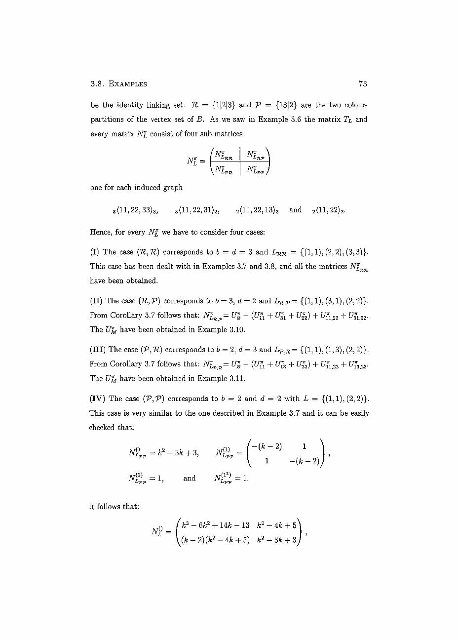
3 .8 . EXAMPLES 73

be the identity linking set. K = {1|2|3} and V = {13|2} are the two colour-

partitions of the vertex set of B. As we saw in Example 3.6 the matrix TL and

every matrix 7VJ consist of four sub matrices

one for each induced graph

3(11,22,33)3, 3(11,22,31)2, 2(11,22,13)3 and 2<H,22>2.

Hence, for every 7V¿ we have to consider four cases:

(I) The case (11,11) corresponds to b = d = 3 and Lnn = {(1,1), (2,2), (3,3)}.

This case has been dealt with in Examples 3.7 and 3.8, and all the matrices iV¿

have been obtained.

(II) The case (11, V) corresponds to b = 3, d = 2 and Lnj> = {(1,1), (3,1), (2,2)}.

From Corollary 3.7 follows that: Nlnv= VI - (£/£ + U^ + V%2) + U^22 + U^22.

The Í/J- have been obtained in Example 3.10.

(III) The case (V,1l) corresponds to b = 2, d= 3 and Lptn= {(1,1), (1,3), (2,2)}.

From Corollary 3.7 follows that: N[v n= VI - (C/ft + C/f3 + U%2) + U^22 + U^22.

The VM have been obtained in Example 3.11.

(IV) The case (V,V) corresponds to b = 2 and d = 2 with L = {(1,1), (2,2)}.

This case is very similar to the one described in Example 3.7 and it can be easily

checked that:

It follows that:

^L = k3 - 6k2 + Uk - 13 k2-4k + $\

(k - 2)(k2 - + 5) k2 - 3k + 3 / '

2.5. EXAMPLES 7 4

with characteristic equation

A2 + (-A;3 + 5k2 - Ilk + 10)A + k4 - 7k3 + 19A:2 - 24k + 11 = 0.

N; (1)

(—k2 + — 7 k- 3 A; - 3 -A; + 2

k ~ 3 -fc2 + 5A; - 7 /c — 3 1

A: - 3 A; — 3 -A;2 + 5/c - 7 -k + 2

—k2 + 5A; — 7 2A; — 4 -A;2 + 5A; - 7 -A; + 2

k - S —k2 + 5A; — 6 A; - 3 1

with characteristic equation V

1 \

-A;+ 3

1

1

•A; + 2y

(1 + A) (A + 4 - 4A; + k2) (A3 + a2{k) A2 + ax{k)\ + a0{k)) = 0

where a2 (A;) = 2A;2 - +12, ax {k) = A;4 - 10A;3 + 36A;2 - 56A; + 31 and

a0(k) = - k 5 + 10A;4 - 38A;3 + 69A:2 - 62k + 22.

4 - 3 - 1 - 1

- 1 - 1 4 - 3 - 1 1 l \

k — S - 1 0 and N p =

- 1 k-3 - 1 0 and N p =

- 1 A; — 3 1 1 - 1 k-3 - 1

- 2 fc-3 1 j y Ä - 3 0 -A;+ 3 1 y

both have the same characteristic equation

(1 + A)(A; - 1 - A){k - 2 - A)(Ar- 4 - A) = 0.

At level I - 3 the matrix N\ is equal to N ^ for 7r = (3), ir = (2,1) and tt = (l3)

respectively.

In principale, from here it easy to obtain the chromatic polynomial of Ln (£), but

only that some of the eigenvalues of N® are not polynomials in k. Although, in

this case an explicit expression for this eigenvalues exists it is more convenient to

use the so called "Newton's formula", described in Appendix A, to obtain the sum

of their nth powers recursively in n.

3 . 9 . SUMMARY 75

Then from Theorem 3.14 it follows that the chromatic polynomial of Ln(B) can be

written as

P{Ln(B)-z) = An(z)

+ (z-l)(Bn{z) + {-z2 + 4z-4)n+{-l)n)

-I- (z2 -3z + l) ( ( - l ) n + (z- l)n + (z - 2)n + (z- 4)n)

+ (z3 — 6z2 + 8z — 1)(—l)n

where An(z) is the sum of the nth power of the roots of

A2 + ( - z 3 + 5z2 - llz + 10)A + z4 - 7z3 + 19 2 - 24z + 11 = 0

and Bn(z) is the sum of the nth power of the roots of

A3 + a2(z)À2 + ax(z)\ - a0(z) = 0

where

a2{z) = (2z2 — 9z + 12),

ai(z) = (z4 - 10 3 + 36z2 - 56z + 31) and

oo(*) =z5 + 10z4 - 38z3 + 69^2 - 62z + 22

In Figure 3.6 the roots of L3o(B) are plotted (the complex variable has been shifted

to z = c + 2). Clearly visible are two roots (and their conjugates) on the left of the

line c = —2 (dotted). It follows that Ln(B) for certain n has roots with negative

real part.

3.9 Summary

Let b and d be integers, and let L C Vb x Vd be a linking set. The compatibility

matrix TL corresponding to the graph b{L)d is equivalent to

0 (1,9 NI), 0<i<min (b,d) Vhl

3 .9 . SUMMARY 76

Figure 3.6: The roots of Lw(B) where B is the path of length three and L is the

identity linking set

where Iv is the identity matrix of size 1 if £ = 0 and

t

£\ 1 ^ JJ (k -h i (* ) ) with /ii(7r) = 7ri + £ - i if ¿ > 0 .

i=1

From Corollary 3.7 it follows that 7VJ can be written as an alternating sum of

matrices

m= E (-1)1"1 uM-MEM{b,d,L)

If \M\ < £ then UJ^ is the ali zero matrix. For \M| > £ each matrix consists of

sub matrices (JJLI)YX one for each pair (Y",.X") where Y is a subset of V&,

X is a subset of Vd and both are of size £. Each of the (UJ/I)YX is of the form

(Theorem 3.13)

m y x =

CM(X) E RHP) TFNM2) CYCMI p^V

O otherwise.

3 . 9 . SUMMARY 7 7

where CM(X) = (-l)£~ixnM^fixuM2\(d, k),

FMX = { p e Sym¿ I fe, X j ) E (Y x X) n M i = p(j)}

assuming that xx < x2 < ... < x¿ and yi < y2 < ... < y¿, and R?{p) is Young's

natural representation corresponding to S1* and O is the all zero matrix of size

Tijj* X TTrj- •

Now, let B be any base graph with vertex set V and L any linking set. The

corresponding compatibility matrix is equivalent to

® (ir®JVZ), 0 < / < m i n ( M )

where, as before, is the identity matrix of size 1 if £ = 0 and

i

TT I I ( f c - ^ M ) w i t h h M = Ki + £ - i if ¿ > o . ¿=i

Prom Lemma 3.5 it follows that each of the matrices N£ consistslof 11(B)2 subma-

trices Nlnv one for each pair (7Z,V) E TL(B) x Ti{B). The matrix N£nv is of size

C?)n7r x ('I')n?r anc^ equivalent to the matrix NJ, described above, corresponding

to the graph \ti\( tiv}\t\ì where Ln<p C Vb x V¿ is defined by

(iyj) E Lfcp implies that there exists (v,w) € L such that v E Ri and w E Py

If \n\ < £ then (W) = 0, and similarly = 0 if \P\ < L

If

Ai(L, 1r; k), A2(L, 7r; k),..., AS(L,7r; /C)

are the eigenvalues of and

mi (L, 7t) , m2 (£, 7r),..., ms (L, n)

the corresponding local multiplicities in N¿ it follows that

tr(Nl)n = J 2 « , (£ , * ) A? (£,»;*) i= 1

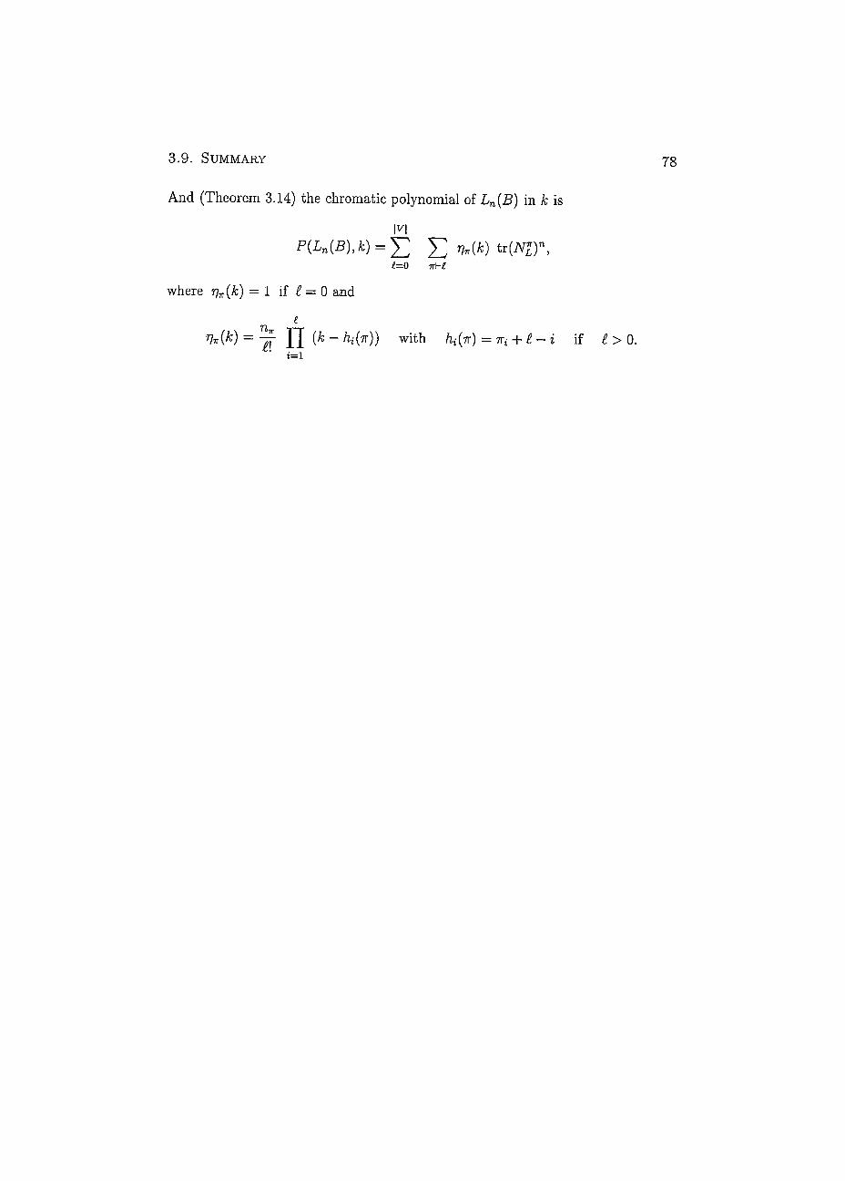
3 . 9 . SUMMARY 78

And (Theorem 3.14) the chromatic polynomial of Ln(B) in k is

M P{Ln(B\k) = Y J £ tr(iVZ)»,

¿=0 <rr\-£

where ^(k) = 1 if i = 0 and

i

= i f I l ( ^ - ^ W ) w i t h ht(ir) = in + e-i if £ > 0 . i=1

Chapter 4

Explicit calculations of chromatic

polynomials

In this chapter the theory developed in the previous chapters will be used to cai-

culate the chromatic polynomials for various families of graphs. In particular we

calculate the chromatic polynomials for the generalized dodecahedra described in

Example 3.4, and four other families of cubie graphs.

In the following we assume that:

• We order the subsets X and X' of a vertex set V C N according to the

dictionary ordering, that is according to their smallest non-common elements.

For example we order the four subsets of size three of V4 as follows:

{1,2,3} {1,2,4} {1,3,4} {2,3,4}.

This fixes the order of the rows and columns in the submatrices NI and Ufa.

• We also use the dictionary odering for the independent sets of a colour-

partition.

• In the following figures, the edges of the base graphs are represented by thick

lines and the linking edges are represented by thin lines.

79

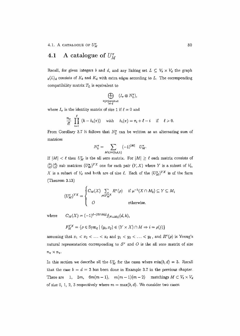
4 . 1 . A CATALOGUE OF UL 80

4.1 A catalogue of Ufo

Recali, for given integers b and cJ, and any linking set L C Vb x Vd the graph

b(L)d consists of Kb and Kd with extra edges according to L. The corresponding

compatibility matrix Tu is equivalent to

© (I«®Nl), 0</<min{M) irh£

where Iv is the identity matrix of size 1 if £ — 0 and i

From Corollary 3.T it follows that can be written as an alternating sum of

matrices

JVZ= E (-1)| M | V*. MeM{b,d,L)

If \M\ < £ then U^ is the ali zero matrix. For \M\ > £ each matrix consists of

sub matrices (U^)YX one for each pair where Y is a subset of Vb,

X is a subset of Vd and both are of size £. Each of the {UM ) y x the f ° r m

(Theorem 3.13)

\cM(X) £ RW(P) if fJ.~1(XDM2) CY CM1

(U*m)YX =

I 0 otherwise.

where CM(X) = (-l)£-|XnM2'/|xuM2|(^ k),

? M X = Sym, | [yh Xj) € {Y x X) fi M i = p{j)}

assuming that x\ < x2 < . . . < Xi and yi < y2 < . . . < yi, and R*(p) is Young's

naturai representation corresponding to S a n d 0 is the ali zero matrix of size

In this section we describe ali the Ufo for the cases where min(&, d) = 3. Recali

that the case b = d = 3 has been done in Example 3.7 in the previous chapter.

There are 1, 3m, 6m(m — 1), m(m — l)(m — 2) matchings M C 14 x Vd

of size 0, 1, 2, 3 respectively where m = max(ò, d). We consider two cases:

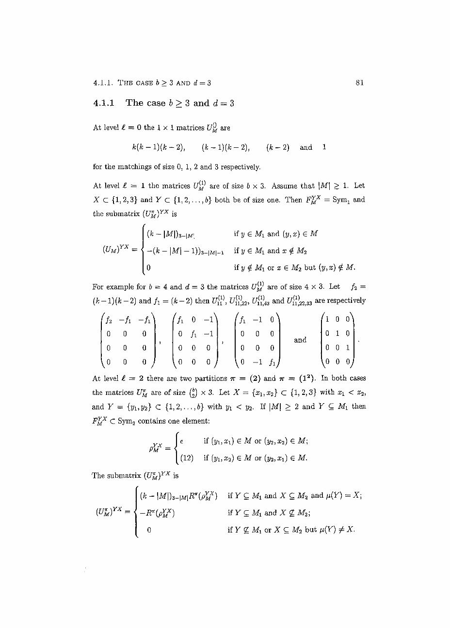
4 .1 .1 . THE CASE b > 3 AND d = 3

4.1.1 The case b > 3 and d = 3

81

At level = 0 the l x l matrices t/£- are

fc(/c — l)(k — 2), ( f e - l ) ( f e -2 ) , ( f c -2 ) and 1

for the matchings of size 0, 1, 2 and 3 respectively.

At level i = 1 the matrices are of size 6 x 3 . Assume that |M| > 1. Let X C {1,2,3} and Y C {1,2,. . . , 6} both be of size one. Then = Syn^ and the submatrix (Ufa)YX is

(UM)YX = <

(k - |M|)3HM, if y E Mi and (y, z) E M

-(/e - |M| - 1))3-|m|-i if y e Mi and z g M2

0 if y g Mi or x E M2 but (y, s) ^ M.

For example for b = 4 and d = S the matrices are of size 4 x 3 . Let /2 = 'M r{l) rrtt) rr(l) ( f c - l ) ( f c -2 ) and = (k- 2) then C/Ji;, l ^ , and t/ 22,33 are respectively

{h -h ~fi\ 1

0 0 0

0 0 0

0 0 0 /

h 0 - i \ 0 fi -1

0 0 0

0 0 0 y

(h - 1

0 0 0

0 0 0

V0 - 1 h)

and

1 0 0

0 1 0

0 0 1

0 0 0

At level i = 2 there are two partitions 7R = (2) and 7R = (L2). In both cases

the matrices Ufa are of size (J) x 3. Let X — {xx,x2} C {1, 2,3} with x\ < x2i

and Y = {2/1,2/2} C {1,2, . . . ,6} with 2/1 < y2. If |M| > 2 and Y C Mx then

Fh x C Sym2 contains one element:

PMX

e if ( 2 / 1 ? E M or (y2ìx2) E M ;

(12) if (î/i, £2) E M or (2/2? ari) G M. V

The submatrix (Ufa)YX is

tfe - IMDS-IMI^ÍPM^) if ^ Ç M I and X Ç M 2 and fi(Y) = X ;

if Y Ç M i and X % M 2 ;

if Y g M i or X C M 2 but p(Y) ¿ X .

W A = -R*(PyMX)

0

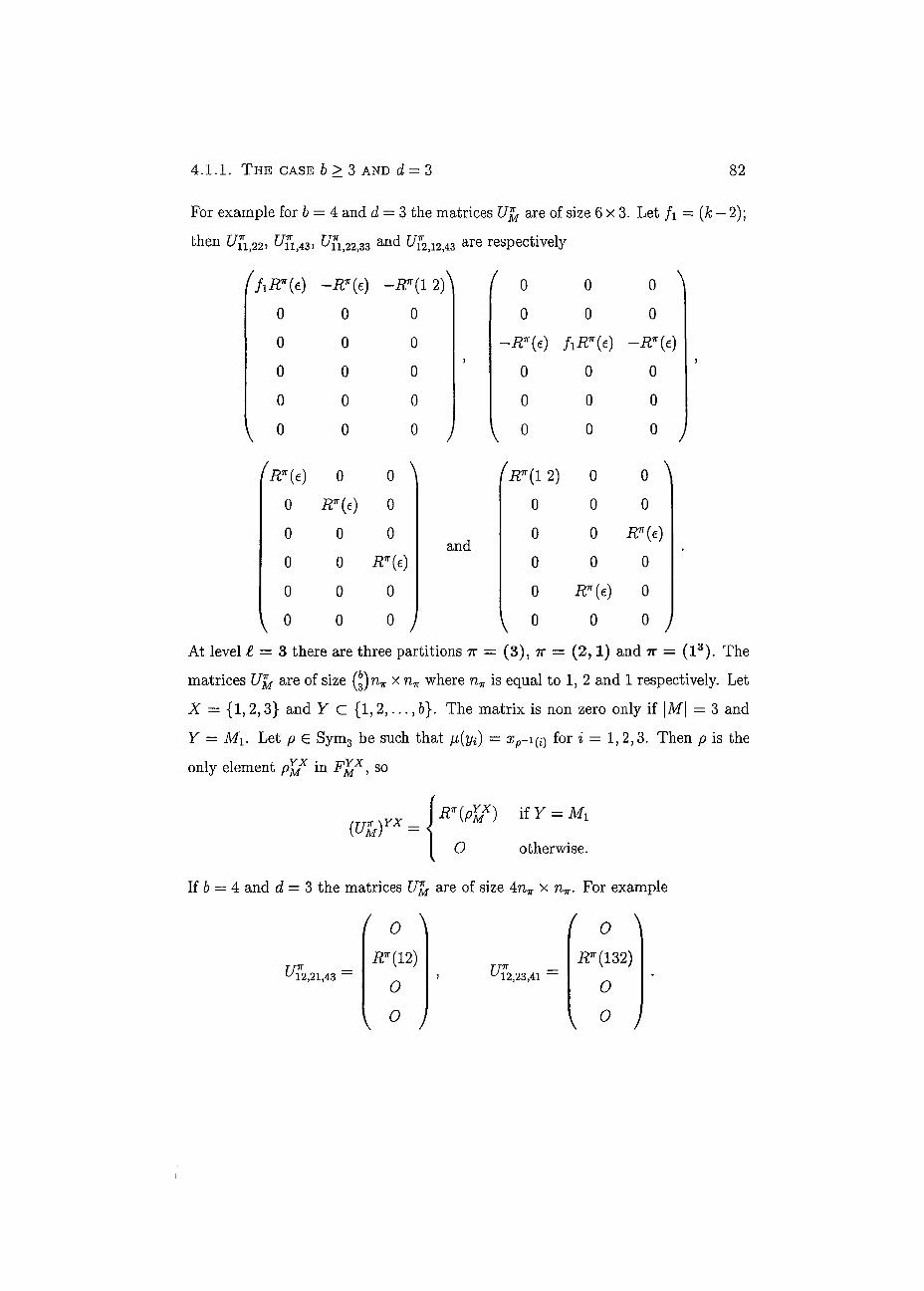
4 . 1 . 1 . T H E CASE 6 > 3 AND d = 3 82

For example for b = 4 and d = 3 the matrices Ufo are of size 6x3. Let f\ = (k — 2);

then J7* 22, Í7f1)43, f/f1)22j33 and C/f2|12|43 are respectively

0

0

0

0

0

i T ( e )

0

0

0

0

0

0

0

0

0

0

0

0

0

0

0

•]Rr( 12)^

0

0

0

0

0

0 0 0

0 0 0

0 0 0

0

0

\

and

0

0

0

R*( 1 2)

0

0

0

0

0

0

0

0

0 0 0 0

R"(e)

0

0

0

0

0 \ 0

R*(e)

0

0

0 /

At level I — 3 there are three partitions TT = (3), 7r = (2,1) and 7r = ( l3 ) . The

matrices Ufo are of size (*) 7T>tj- X Tiff where n„ is equal to 1, 2 and 1 respectively. Let

X — {1, 2,3} and 7 c {1,2,. . . , b}. The matrix is non zero only if \M\ = 3 and

Y = Mi. Let p G Sym3 be such that /j,(yi) = xp-1(¿) for i = 1, 2,3. Then p is the

only element p i n , so

(U¡i)¥X = R"(pfox) if y = Mi

o otherwise.

If b = 4 and d = 3 the matrices Ufo are of size 4tn„ x n^. For example

TTTT ^12,21,43

O

IF (12)

O

O

\

TTTT u12,23,41

( o

R*( 132)

o

0

\

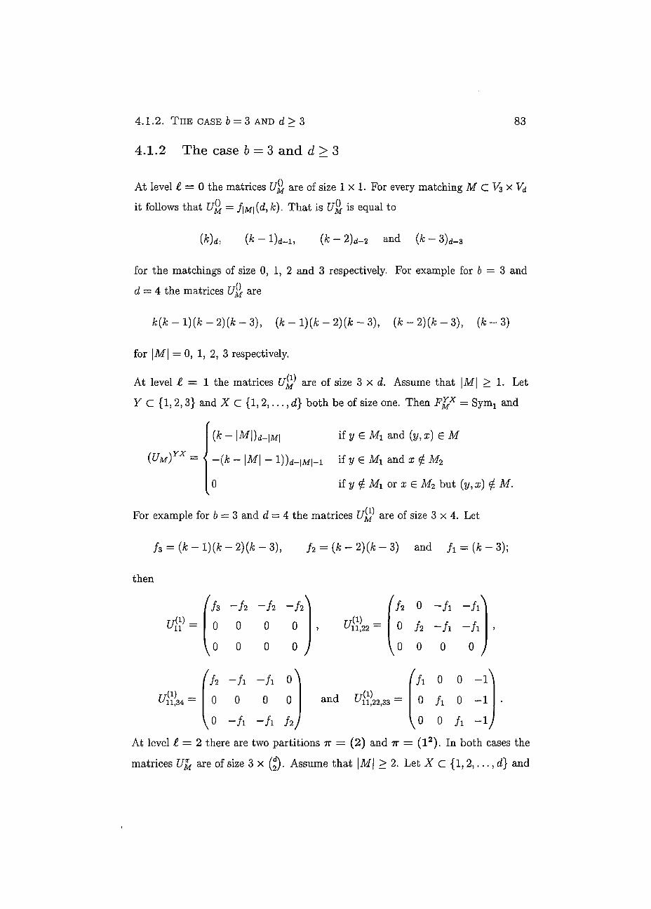
4 . 1 . 2 . T H E CASE b = 3 AND d > 3

4.1.2 The case b = 3 and d > 3

83

At level = 0 the matrices [/£. are of size l x l . For every matching M C x Vd

it follows that U2[ = /|Af|(d, k). That is i/jyr is equal to

{k - l)d_i, (As - 2)d-2 and (A; - 3)d_3

for the matchings of size 0, 1, 2 and 3 respectively. For example for b = 3 and

d = 4 the matrices £/[/ a r e

A:(/c - 1)(A; - 2)(A; - 3), (A; - 1)(A; - 2)(A; - 3), {k - 2)(k - 3), (Ac - 3)

for \M\ = 0, 1, 2, 3 respectively.

At level Í = 1 the matrices U^ are of size 3 x d. Assume that |M| > 1. Let

Y C {1, 2,3} and X c { l , 2 d} both be of size one. Then = Syn^ and

(UM) YX

(k - |M|)d_|M| if y e Ml and (y: x) e M

-(k - \M\ - l))d_|M|-i if y G Mi and x <£ M2

0 if y £ Mi or x 6 M2 but (y,x) i M.

For example for b = 3 and d = 4 the matrices uff are of size 3 x 4 . Let

f3 = (k-l)(k-2)(k-Z), f2 = (k-2)(k-3) and A = (A; - 3);

then

TT(l) _ ull —

(h I 2 -h -f^ o o o o

0 0 0 0 J

if, -

U-(1) 11,34

Î2 -fi -fl 0

0 0 0 0

yo -fl -fl hj

l h 0 - h - S ^ r/(1) - 0 h -A -fl

0 0 0 0

and ^í¿2,33 —

fi 0 0

0 / i 0 - 1

\0 0 / i - I )

At level i = 2 there are two partitions n — (2) and 7r = ( l 2 ) . In both cases the

matrices U^ are of size 3 x (g). Assume that \M\ > 2. Let X c {1 ,2 , . . . , d} and

i

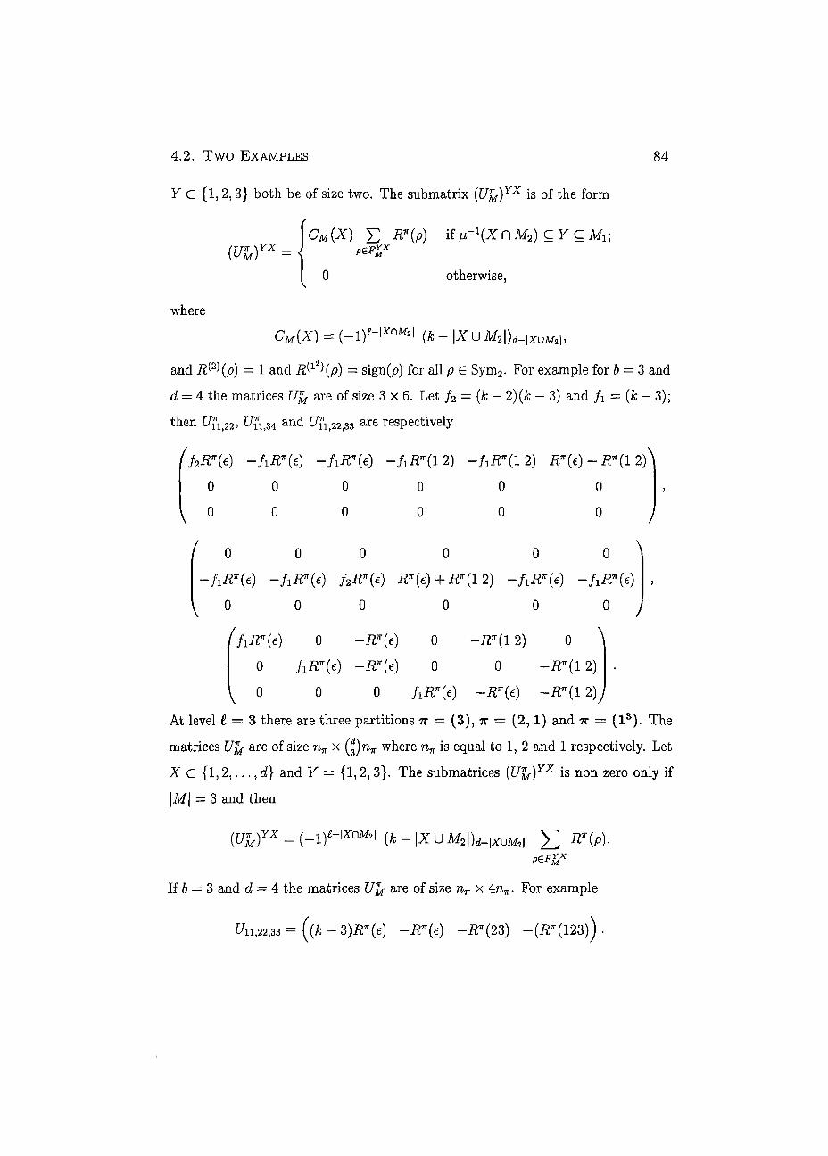
4 . 2 . T w o EXAMPLES 84

Y c {1, 2,3} both be of size two. The submatrix (Ufa)YX is of the form

\cM(X) £ R*(p) if^ixn M2)CYCM1; (Ufa)YX = I

I 0 otherwise,

where

CM(X) = (k- IXUM2|)d_|XUAf2i,

and R{2](p) = 1 and R^Kfl) = sign(p) for all p € Sym2. For example for b = 3 and

d = 4 the matrices £7] are of size 3 x 6 . Let f2 = (k — 2)(k — 3) and fi = (k — 3);

then U?lt22, LTf134 and C/î1(22)33 a r e respectively

ff2B?(e) -fiR^e) ~fiRn(e) ~fiRn(l 2) - / i ¿T( l 2) iF(e) + ^ ( 1 2)

0 0 0 0 0 0

^ 0 0 0 0 0 0 J

^ 0 0 0 0 0 0 ^

-hR?{e) -hR7{e) f2R*(e) iF(e)+^(12) -fiR"(e) - ^ ( e ) ,

^ 0 0 0 0 0 O y

(¡iR*{e) 0 -Rn(e) 0 - i T ( l 2) 0 ^

0 A/Ffc ) - ¿^ (e ) 0 0 - ¿ T ( 1 2 ) .

y 0 0 0 / i iT(e) -BT{e) 2)y

At level i = Z there are three partitions 7r = (3), 7r = (2,1) and 7r = ( l 3 ) . The

matrices Ufa are of size n^ x ( 3 )^ where n^ is equal to 1, 2 and 1 respectively. Let

X C {1, 2 , . . . , d] and Y = {1,2, 3}. The submatrices (Ufa)YX is non zero only if

\M\ = 3 and then

(Ufa)YX = (k-\XU M2|)d_|xuM2| E W-

If b = 3 and d = 4 the matrices f/J- are of size x Ann. For example

C/n.22,33 = ((A; - 3)R«{e) -R«(e) -IP(23) - ( £ * ( 123)).

4 . 2 . T w o EXAMPLES 85

3 4 Figure 4.1: The graph

3(11,22,34)4

1 1 Figure 4.2: The graph

4(11,32,42)3

4.2 Two Examples

Example 4.1: Let us find the matrices Ufo for all levels and all matchings for

the graph 3(11, 22, 34)4 shown in Figure 4.1. There are 1, 3, 3 and 1 matchings of

size 0, 1, 2 and 3 respectively: { } ,

{(1,1)}, {(2,2)}, {(3,4)},

{(1,1), (2,2)}, {(1,1), (3,4)}, {(2, 2), (3,4)},

{(1,1), (2,2), (3,4)}.

From Corollary 3.7 it follows that

Nl = Ul- (Ift + + Ifc) + (Eft* + Ufa + 34) - t/T1ÄM .

At level Í = 0 the matrices are

fc(fc - l)(fc - 2)(A - 3), (A; - l)(fc - 2){k - 3), (A; - 2){k - 3), (k - 3)

for the matchings of size 0, 1, 2 respectively. Thus

N¡¡¡ = k{k - 1 )(k - 2)(k - 3) - 3[k - l)(Jfe - 2)(A; - 3) + 3(fc - 2)(Ac - 3) - (k - 3).

Let /3 = ( f c - l ) ( f c - 2 ) ( f c - 3 ) , f2 = {k-2){k-3) and = [k - 3).

At level Í — 1 the matrices U $ are

un —

fh -Í2 -Í2

0 0 0 0 0 0 0 0

Tj{ 1) _ U22 —

/ o o o 0 \ — ¡2 h —¡2 —f2

0 0 0 0 J

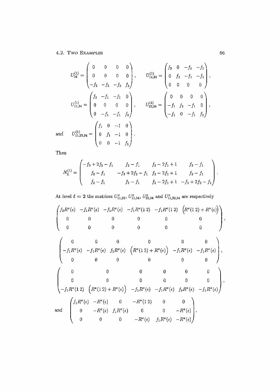
4 . 2 . T w o EXAMPLES 86

Tj( i) _ u3A — F 0 0 0 (A

0 0 0 0

\~Î2 ~A -f2 A (

7 / (1) ^11,22

7/(1) _ UUM ~

A -fi -fi 0

0 0 0 0 7 / (1 ) u 22,34

and U-(i) 11,22,34

\0 -fi -fi h)

(h 0 -1 o\ 0 / 1 - 1 0

0 - 1 fij

¡2 0 - h - h 0 Í2 -A -A

0 0 0 0

0 0 0 0

~/l Í2 -A 0

\-h 0 - A h)

Then

^ / 3 + 2 / 2 - A A - / ! / 2 - 2 / x + 1 A - A \

A - A -/3 + 2/2-/1 /2-2/1 + 1 A - A

\ ¡2 — fl / 2 - / 1 / 2 - 2 A + I - / 3 + 2 / 2 - A y

At level £ = 2 the matrices E/n 22> 11,34 > 22,34 a nd 11,22,34 a r e respectively

ff2R*(e) -fiR*(e) -fiR"(e) —fiR*(l 2 ) -^(12) (r*(1 2 ) +

0 0 0 0 0 0

0 0 0 0 0 0

/ 0 0 0 0 0 0 \

V 0 0 0 0 0 0 / 0 0 0 0 0 0

0 0 0 0 0 0

[-f1R«(12) (Ä*(12) + JF(e)) -fiR*(e) -hR«(e) A ^ )

( t TDD7T t H TDTT ( 1 0\ A H \

and 0 0

—Ä""(e) 0 0 -R*{e)

0 0 -Ä*(e)

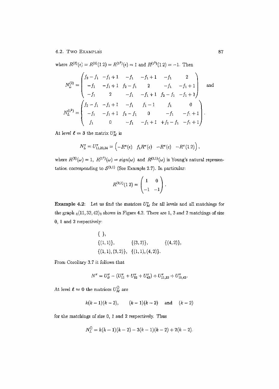
4 . 2 . T w o EXAMPLES 8 7

iVf = and

where = RP\ 1 2) = R ^ { e ) = 1 and #( l2)(l 2) = - 1 . Then

( h - h - A + 1 - A - A + 1 - A 2 ^

- A - A + 1 A - A 2 - A - A + 1

V - A 2 - A - A + i A - A - A + V

/ A - A - A + I - A A - I A 0 ^

- A - A + i A - A o - A - A + i

v A o - A - A + i + / 2 - A - A + iy

At level i = 3 the matrix t/Jj- is

Nl = 1,22,34 = ( - iF (e ) hR*{e) -Ä*(e) -R*( 1 2)) ,

where = 1, = sign(u) and R^(ÜJ) is Young's natural represen-

tation corresponding to «S 2'1) (See Example 2.7). In particular:

^ ( 1 2) = - 1 - 1

Example 4.2: Let us find the matrices Ufo for all levels and all matchings for

the graph 4(11,32,42)3 shown in Figure 4.2. There are 1, 3 and 2 matchings of size

0, 1 and 2 respectively:

{}• {(1,1)}, {(3,2)}, {(4,2)},

{(1,1), (3,2)}, {(1,1), (4,2)}.

From Corollary 3.7 it follows that

N* = Ul- (tft + + u:2) + Ufa + irn¡i2.

At level Í — 0 the matrices U£- are

k(k — l)(/c — 2), ( ¿ - l ) ( / c - 2 ) and (k — 2)

for the matchings of size 0, 1 and 2 respectively. Thus

nS = k{k - l ) ( k - 2 ) ~ 3(k - l)(k - 2) + 2{k - 2).

4 . 2 . T w o EXAMPLES 88

Let f2=(k- 1 )(k - 2) and A = (k - 2). At level £ = 1 the matrices are

U{1) -u n —

(H - A 0 0 0 0 0 0

Io 0 0 Ì

J u 3 2 —

( 0 0 0 ^ 0 0 0

— / l A —fl

\ 0 0 0

/

rrd) '42

rji 1) u 11,32 —

A o 0 0 0

0 fl -1

0 0 0

Then

U-(i) _ 11,42

J

-h + 2/i 0

fi

\ *

\~A A

1 fi 0 - 1 \

0 0 0

0 0 0

VO A - 1

0 ^ 0 0

-Ay

/

A o

A - 2 0

- A + A A - 1

- A + A A - y At level = 2 the matrices i/f1)32 and C/Ji 42 are respectively

0 0 0

fiR?{e) -iFfc) -¿^(12)

0 0 0

0 0 0

0 0 0

0 0 0

0 0 0

0 0 0

fiR'ir(e) —K" (e) - i T ( l 2)

0 0 0

0 0 0

0 0 0

•vhere = R&(1 2) = R^{e) = 1 and 1 2) = - 1 . Then

0 0 0

A - i - i

A - i - i

o o o

0 0 0

0 0 0

\

and N ( P =

^0 0

A - i 1

A - 1 1

0 0 0

0 0 0

0 0)

.t level Í = 3 the matrices are the 4 x 1 all-zero matrix for 7T = (3) and

= (l3) respectively, and the 8 x 2 all-zero matrix for n = (2,1).

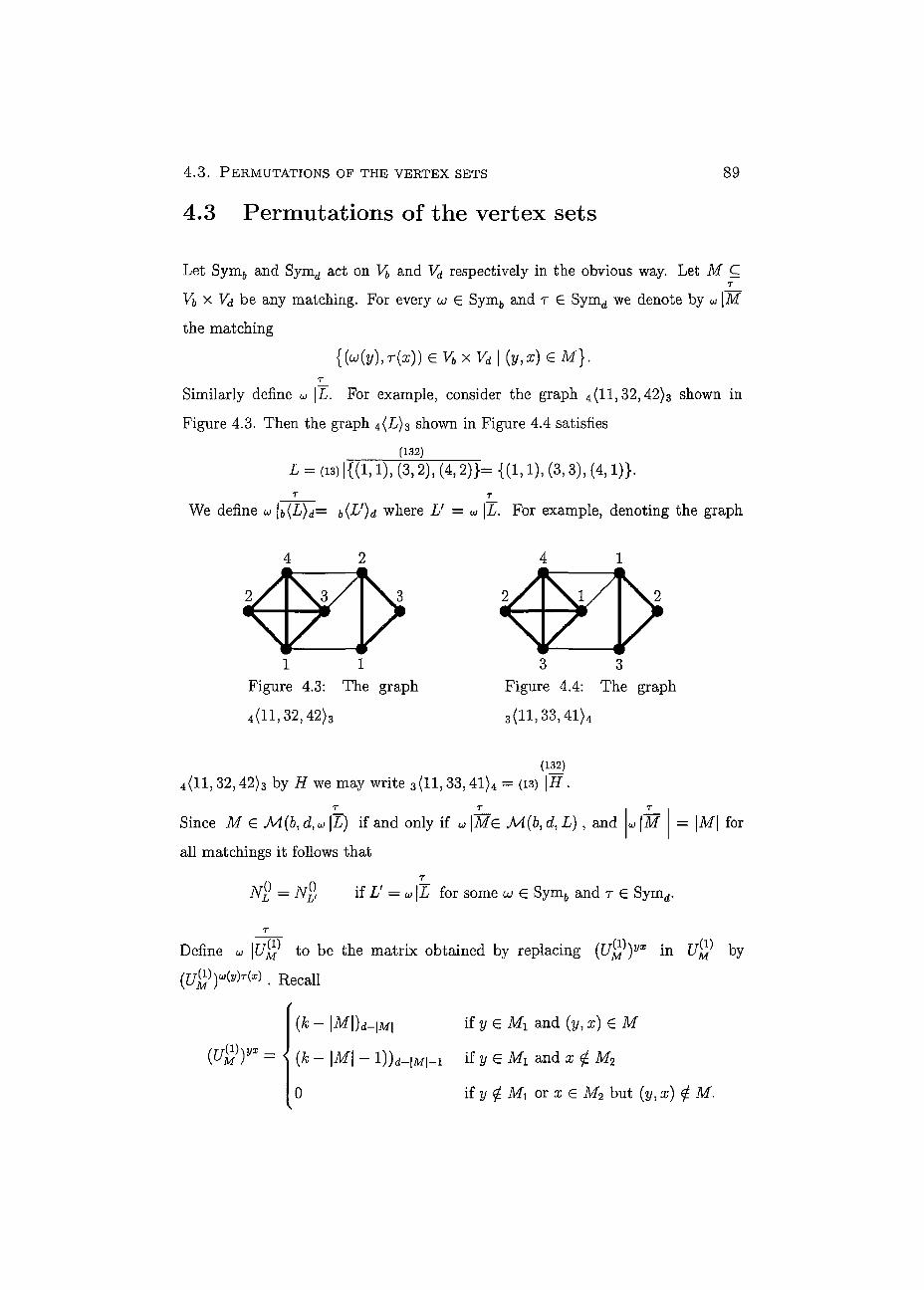
4 .3 . PERMUTATIONS OF THE VERTEX SETS

4.3 Permutations of the vertex sets

89

Let Sym^ and Symd act on VB and VD respectively in the obvious way. Let M Ç T

Vb X Vd be any matching. For every CJ E Symb and r € Symd we denote by w \M

the matching {{uj(y)iT(x))eVbxVd\(y,x)eM}.

T

Similarly define U \L. For example, consider the graph 4(11,32,42)3 shown in

Figure 4.3. Then the graph A(L)3 shown in Figure 4.4 satisfies (132)

L = (13) |{(1,1), (3,2), (4,2)}= {(1,1), (3,3), (4,1)}.

We define u \b(L)d= b(L')d where V = w |L. For example, denoting the graph

1 1 Figure 4.3: The graph

4(11,32,42)3

3 3 Figure 4.4: The graph

3(11,33,41)4

(132)

4(11,32,42)3 by H we may write 3(11,33,41)4 = (i3) |H . T T T

Since M G M(b, d,u\L) if and only if w |Mg M(b, d, L) , and u \M

all matchings it follows that

= |M| for

N2 = NL, 0 if L' = U \L for some LJ € Symb and r € Symd.

Define u |U^ to be the matrix obtained by replacing {U^)yx in by

. Recall

(uïïr =

[k - |M|)d_|M| if y G Mi and (y, x) € M

(k - \M\ - l))d-|M|-i if y e M i and x i M 2

0 if y £ Mi or x E M2 but (y, x) £ M.

4 . 4 . RÉDUCTION OF BASE GRAPHS 90

It can easily be checked that is the equal to U^} where M' = u\M. T T

The matrix u\N£ is deiined analogously to u\Ufa

Lemma 4.1 Let the graph b(L)d, w E Symb and r G Symd be given.

Then N^ = and w \n£}= N^, where V = » \L. •

The above results can be generalized for n h t with t > 2, but things are getting

quite a bit more complicated since the F™ are not trivial anymore. In the ex-

amples considered in the following sections it turns out to be more convenient to

calculate the JVJ "by hand" rather than using a generalization of the above.

4.4 Réduction of base graphs

We are now going to discuss another case where the matrices corresponding to

one graph can be obtained from the matrix N™ corresponding to another graph.

Let us begin with an example.

Example 4.3: Let us consider the graphs 3(11,22,34)4 and 4(11,32,44)4 shown

in Figures 4,5 and 4.6. Denote by iVJ 2234 and iV-ft 32 44 the respective matrices

corresponding to these graphs. Let M G M(b, d, L), 0 < t < 3 and 7r h 1.

1 1 1 1

3 4 4 4

Figure 4.5: The graph

3 (11,22,34)4

Figure 4.6: The graph 4(11, 32,44)4

From Theorem 3.13 it follows that (Ufa)YX corresponding to graph 4(11,32,44)4

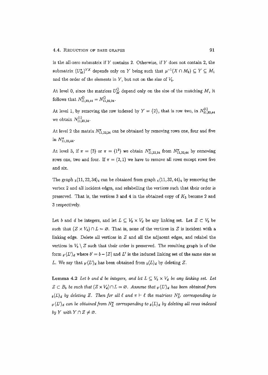
4 . 4 . RÉDUCTION OF BASE GRAPHS 9 1

is the ali-zero submatrix if Y contains 2. Otherwise, if Y does not contain 2, the

submatrix {JJfo)YX depends only on Y being such that jx~l(X Pi M2) Ç.Y Ç Mx

and the order of the elements in Y, but not on the size of V&.

At level 0, since the matrices U d e p e n d only on the size of the matching M, it

follows that N[{32>44 = JVg^.

At level 1, by removing the row indexed by Y = {2}, that is row two, in 44

we obtain N[{]22M.

At level 2 the matrix N{rlj22)34 can be obtained by removing rows one, four and five

in N11,32,U'

At level 3, if 7T = (3) or w = (l3) we obtain A Jr1 22)34 from iVju 32 44 by removing

rows one, two and four. If ir = (2,1) we have to remove ail rows except rows five

and six.

The graph 3(11, 22,34)4 can be obtained from graph 4(11,32,44)4 by removing the

vertex 2 and ail incident edges, and relabelling the vertices such that their order is

preserved. That is, the vertices 3 and 4 in the obtained copy of K3 become 2 and

3 respectively.

Let b and d be integers, and let L Ç Vb x Vd be any linking set. Let Z C V& be

such that (Z xVd) CiL = 0. That is, none of the vertices in Z is incident with a

linking edge. Delete ail vertices in Z and ali the adjacent edges, and relabel the

vertices in V& \ Z such that their order is preserved. The resulting graph is of the

form b'(L')d where b' = b — \Z\ and L'is the induced linking set of the same size as

L. We say that b'{L')d has been obtained from &(£)</ by deleting Z.

Lemma 4.2 Let b and d be integers; and let L Ç Vb x Vd be any linking set Let

Z C Bb be such that (Z xVd)C\L = 0. Assume that b'(L')d has been obtained from

b(L)d by deleting Z. Then for ail l and 7r h t the matrices corresponding to

b'(L')d can be obtained from NI corresponding to b(L)d by deleting ail rows indexed

by Y with YnZ ¿0.

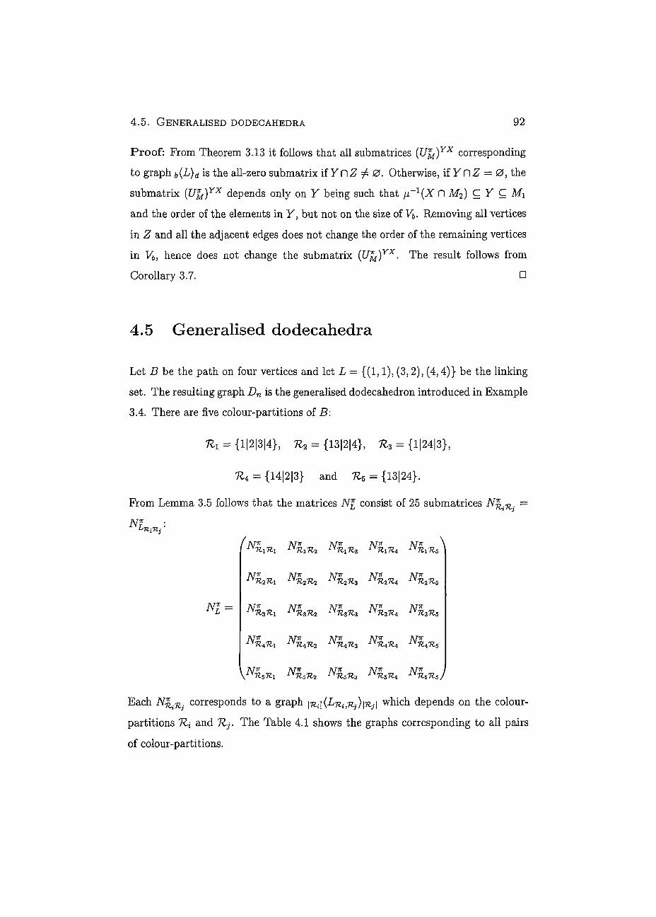
5.6.2. GENERALISED DODECAHEDRA 92

Proof: From Theorem 3.13 it follows that ail submatrices (JJM)YX corresponding

to graph b{L)d is the all-zero submatrix if Y HZ ^ 0. Otherwise, if Y HZ = 0, the

submatrix (Ul I)YX depends only on Y being such that X n M2) Ç Y Ç M\

and the order of the elements in V, but not on the size of Vj,. Removing ail vertices

in Z and ail the adjacent edges does not change the order of the remaining vertices

in VB, hence does not change the submatrix (UM)YX• The resuit follows from

Corollary 3.7. •

4.5 Generalised dodecahedra

Let B be the path on four vertices and let L = {(1,1), (3,2), (4,4)} be the linking

set. The resulting graph Dn is the generalised dodecahedron introduced in Example

3.4. There are five colour-partitions of B:

lli = {1|2|3|4}, K2 = { 13|2|4}, 11, = {1|24|3},

K4 = {14|2|3} and 7l5 = {13|24}.

From Lemma 3.5 follows that the matrices iVJ consist of 25 submatrices N^n =

N? , :

( Nv A/"71" A/"71" A/"71" A/"77 \

AT7T AT7T ]\TTT ATTT AJTÏ iyK2Tii iV7 27 2 •ÍV7 27 3 iyn2nb

rq = ATTT AT7T 7\T7r AT7T AT7T Iyin3ni iV7 37 2 iyn3Ti3 iyn3n4 iyn3n5

AT7T AT7T ATTT AT7T AJTT lsnAn! iV7 47 2 ^-R^fu ^HAR*

\ntz5ih Nnsn2 NK5K3 ^57^4 Nn5nJ

Each corresponds to a graph i^i (£7 ,7 )17 1 which depends on the colour-

partitions 1Zi and 11 j. The Table 4.1 shows the graphs corresponding to ail pairs

of colour-partitions.

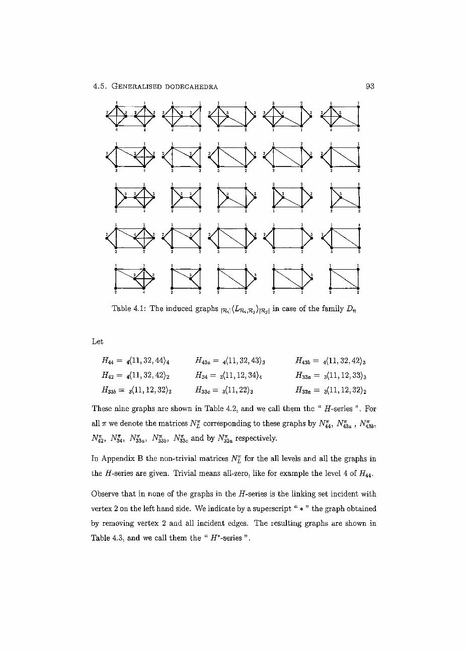
5.6.2. GENERALISED DODECAHEDRA 93

1 1 1 1 1

3 3

1 3

2 1 1 1

2 1 1 3 2

1 1 — w.3

Sp EI H> H> IS 2 3

1 1

3 2

Table 4.1: The induced graphs \Ki\(Lni,iij)\Tij\ in case of the family D7

Let

# 4 4 = 4(11,32,44)4 # 4 3 a - 4(11,32,43)3 #43b = 4(11, 32,42)3

#42 = 4(11, 32, 42)2 #34 = 3(11, 12, 34)4 #33a = 3<H, 12, 33>S

#336 = 3(11, 12, 32)3 #330 = 3(11, 22)3 #32q = 3(11, 12, 32)2

These nine graphs are shown in Table 4.2, and we cali them the " #-series ". For

ali 7T we denote the matrices corresponding to these graphs by 7VJ4, jVJ3o ,

JV42, jVJ3a, A 3Ò, iV37r3c and by N&a respectively.

In Appendix B the non-trivial matrices iV£ for the ali levels and ali the graphs in

the #-series are given. Trivial means ali-zero, like for example the level 4 of #44.

Observe that in none of the graphs in the #-series is the linking set incident with

vertex 2 on the left hand side. We indicate by a superscript " * " the graph obtained

by removing vertex 2 and ali incident edges. The resulting graphs are shown in

Table 4.3, and we cali them the " #*-series

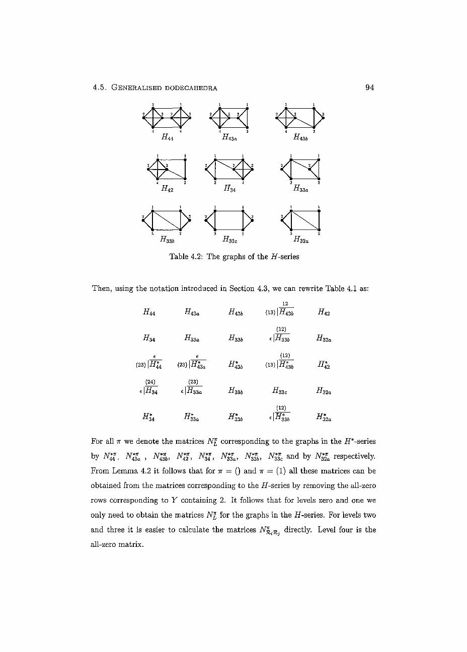
5.6.2. GENERALISED DODECAHEDRA 9 4

i i i i i i

K 44

2 > .3

ff 43a

4 2 3 4

ffd9 ffs :34

ff 436

1 1

2/

3 3

- 33a

-#336 #330 -#320

Table 4.2: The graphs of the #-series

Then, using the notation introduced in Section 4.3, we can rewrite Table 4.1 as:

12 ff 44 ff 43a

ff: 34 ff; 33a

(23) |ff4*4

(24)

e I-Ö34

TT* -"34

(23)| Í3a

(23)

e|ff33a

tt* n33a

# 4 3 6

-"336

TT* 436

#336

TT* 336

(13) I # 4 3 6

(12)

e I #336

(12)

as) Iff;

ff 42

ff: 32a

436 ff 42

# 3 3 c

(12)

ff 32a

336 ff 32a

For all 7T we denote the matrices JV£ corresponding to the graphs in the ff*-series

by N¡¡ , N£a , JVS, Äff , AÇi, i v a , ^S», 3*30 and by Nga respectively.

From Lemma 4.2 it follows that for it = () and ir = (1) all these matrices can be

obtained from the matrices corresponding to the ff-series by removing the all-zero

rows corresponding to Y containing 2. It follows that for levels zero and one we

only need to obtain the matrices iV£ for the graphs in the ff-series. For levels two

and three it is easier to calculate the matrices N^.^ directly. Level four is the

all-zero matrix.

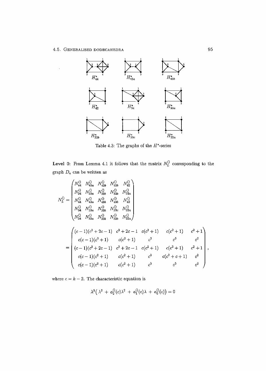
5.6.2. GENERALISED DODECAHEDRA 9 5

H. 44 H. 43a H: 436

H: 42

v3

H< 34 H. 33 a

> 336 33c

TT* 12 32a

Table 4.3: The graphs of the H*-series

Level 0: From Lemma 4.1 it follows that the matrix N® corresponding to the

graph Dn can be written as

ÍN0 N° N° N° N°\ IV44 IV43Û IV43& IV43FT IV42

J\JO ATO JVTO ATO ATO JV34 iV33a 33b iy33b iV32a

Nga N&b Ng

Nil Nga N&b Ngc NU

iN° N° 1V° N° N° ¡ \iV34 iV33a 33b iV336 JV32o/

f ( c - l ) ( c 3 + 2 c - l ) C3 + 2C - 1 C(C2 + 1) c(c2 + l) c2 +

c ( c - l ) ( c 2 + l) c(c2 + l) C3 C3 C2

( c - l ) ( c 3 + 2 c - l ) c3 + 2 c - l c(c2 + l) c(c2 + l) c2 + l

c ( c - l ) ( c 2 + l) c(c2 + l) c3 c(c2 + c + l ) c2

^ c ( c - l ) ( c 2 + l) c(c2 + l) C3 C3 C2 J

where c = k — 2. The characteristic equation is

A 2 ( A 3 + 4 }(c)A2 + a?(c) A + a§(c)) = 0

4 . 5 . GENERALISED DODECAHEDRA 96

with

«2° M

°í'(c)

a°(c)

(_c4 _ 2c3 - 4c2 - 1)

(c6 + 2c5 + 3c4 + 2c3 + 2c2 + 2c)

= - c 4 2c3 - c2.

Level 1: From Lemma 4.1 it follows that the 15 x 15 matrix corresponding to

the graph DN can be written as

'44 N: (i) 43a N: (i) 43b

N< (1) 34 N, (1)

33a N: (1)

(34) iJYTi1)

(24)

(34) I '43a

(23)

ANill

N:

33 6

*(1) 43 ft

(12)

(13)|iVS

(12)

<\N¡¡1

(12)

N: (i) \

42

N, (i)

(13) \N¡{1) '436

32a

AJ*(1) -ÍV42

(i)

JV« *(i) 34 N, =(1)

33a N,

336

*(1) 336

N.. (1) 33c N, (i)

32a

(12)

I 336 32a J

Then the characteristic equation of N ^ is

A8(A - 1) (A6 + a ^ ^ A 5 + a$\c)A4 + 4x)(c)A3 + a^í^A2 + a ^ ^ A + a ^ c ) ) = 0

with

,(1

Û41

.(1

0>2 .(1

.(1

= 2C3+4C~2

= c6 2c5 + 2c4 - 4c3 + 2c2 - 2c - 1

= - 2c8 - 2c7 - 6c6 - 4c5 - c4 + 6c3 - 4c + 1

= c10 + 2c9 + 3c8 + 4c7 + 7c6 + 6c5 + 3c4 - 2c3 - 5c2 + 1

= 2c - 6c7 - 8c4 - 2c8 - 8c5 - 4c3 + 2c2 - 8c6

= 6c4 + c6 + 4c5 + 4c3 + c2,

where, as before, c = k — 2.

5.6.2. GENERALISED DODECAHEDRA 97

Level 2: There are 7r = (2) and 7T = (l2). In both cases the matrix 7VJ correspond-

ing to Dn is of size 16 x 16. We calculate all the submatrices directly, as

shown in the beginning of the chapter and then use them to obtain iVJ. Omitting

all the rows and columns corresponding to a sets Y and X containing 2 respec-

tively we can reduce N£ to 9 x 9 matrices. This reduced matrices are shown in

Appendix C. It turns out that the characteristic equation corresponding to ir = (2)

and 7T = (l2) are both equal to

A u ( A - 1 ) ( A 4 + 4 ( c ) A3 + aj(c) A2 + <(c)A + aj(c)) = 0

with aj(c) = ~c2 + 2 c - 2 aj(c) = -2c 3 + c 2 - 2 c - l

aj(c) = —C4 4 -1 O>Q (C) = C2 + 2 C + 1 ,

where c — k — 2.

Level 3: Here there are three partitions ir = (3), 7r = (l3) and 7r = (2, l). The

matrix N£ corresponding to Dn is of size 7 x 7 for 7r = (3) and 7r = (l3), and 14 x 14

for 7T = (2,1). The set M(b, d,L) contains a matching of size three only in the

case of the graphs H44 and (and the corresponding reduced graphs #44 and

Ü43J. Since all the rows in N¿ corresponding to a y containing 2 are zero it follows

that N^a and N£3a are the zero matrices. In JV44 only the rows corresponding to

Y = {1,3,4} are non-zero. Since ^^2,44 = ( e ) where Y — X — {1,3,4}, it follows

that N1 can be reduced to Young's natural representation of e. It follows

that the characteristic equations for ir = (3), 7r = (l3) and 7r = (2,1) are

A6(A - 1) = 0, A6(A - 1) = 0 and A12(A - l)2 = 0 respectively.

Level 4: Here JVJ corresponding to Dn is equal to which is the all-zero matrix,

and hence does not contribute to the chromatic polynomial.

T h e Chromatic Polynomial of D 5 : The global multiplicities are given in fol-

lowing table

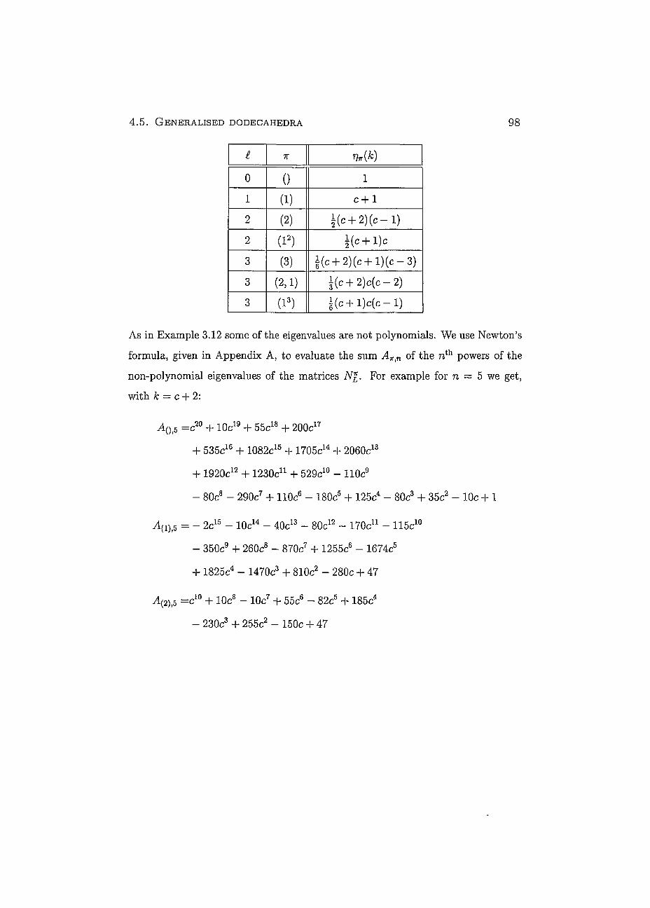
5.6.2. GENERALISED DODECAHEDRA 98

I 7r vAk)

0 0 i

1 (i) c + l 2 (2) i(c + 2 ) ( c - l )

2 (I2) ! ( c + l ) c

3 (3) i ( c + 2 ) ( c + l ) ( c - 3 )

3 (2,1) i ( c + 2 ) c ( c - 2 )

3 (I3) i ( c + l ) c ( c - l )

As in Example 3.12 some of the eigenvalues are not polynomials. We use Newton's

formula, given in Appendix A, to evaluate the sum AWtn of the nth powers of the

non-polynomial eigenvalues of the matrices For example for n = 5 we get,

with ft = c + 2:

A ( ) I 5 =C2 0 + 10c19 + 55c18 + 200c17

+ 535c16 -f 1082c15 + 1705c14 + 2060c13

+ 1920c12 + 1230c11 + 529c10 - 110c9

- 80c8 - 290c7 + 110c6 - 180c5 + 125c4 - 80c3 + 35c2 - 10c + 1

A{i),5 = - 2c15 - 10c14 - 40c13 - 80c12 - 170c11 - 115c10

- 350c9 + 260c8 - 870c7 + 1255c6 - 1674c5

-I- 1825c4 - 1470c3 + 810c2 - 280c + 47

A2),5 =c10 + 10c8 - 10c7 + 55c6 - 82c5 + 185c4

- 230c3 + 255c2 - 150c + 47

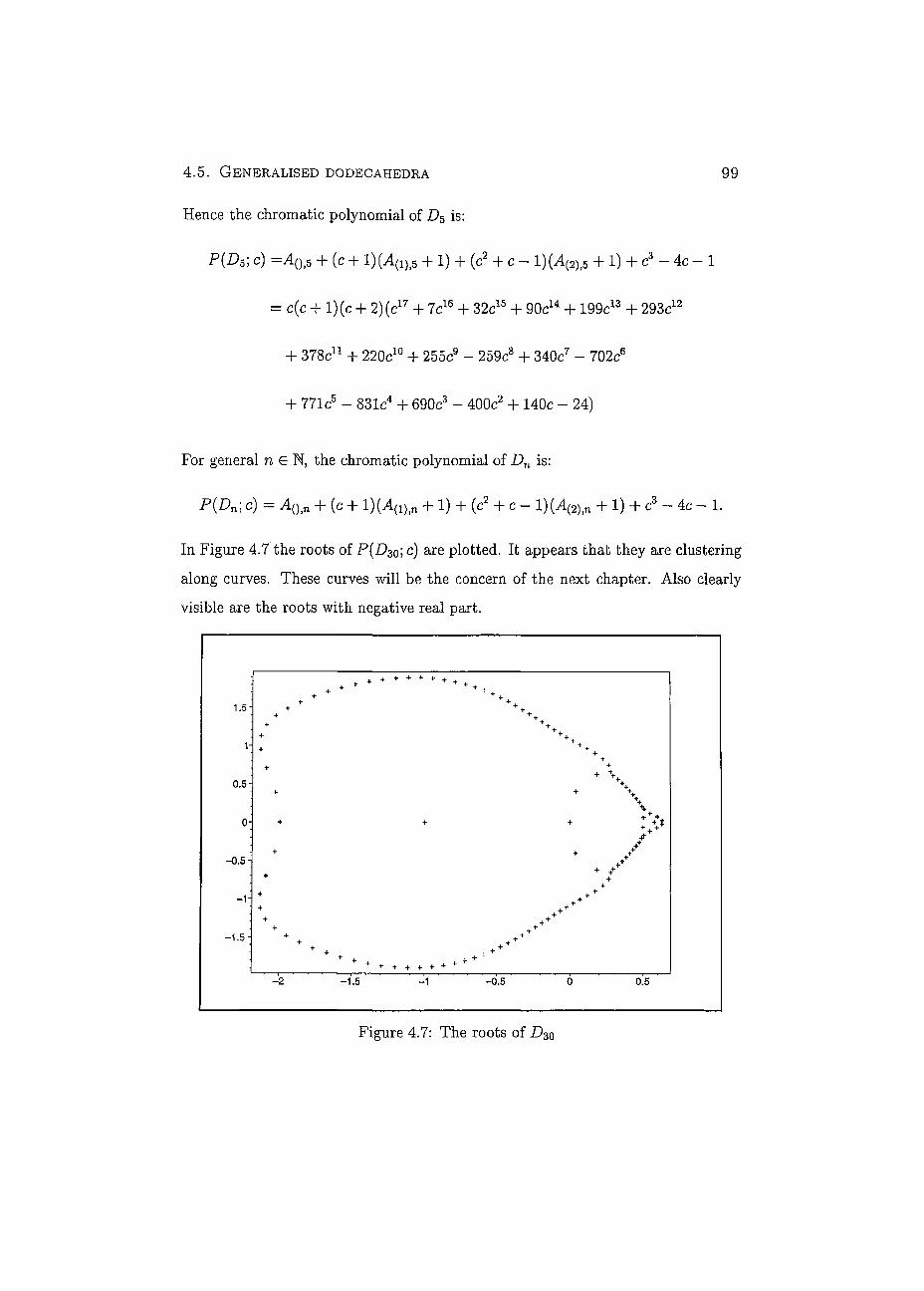
5.6.2. GENERALISED DODECAHEDRA 99

Hence the chromatic polynomial of D5 is:

P(D5; c) + (c + l)(A(i),5 + 1) + (c2 + c - 1)(A(2),5 + 1) + c3 - 4c - 1

= c(c + l ) ( c+ 2)(c17 + 7c16 + 32c15 + 90c14 + 199c13 + 293c12

+ 378C11 + 220c10 + 255c9 - 259c8 + 340c7 ~ 702c6

+ 771 c5 - 83le4 + 690c3 - 400c2 + 140c - 24)

For general ne N, the chromatic polynomial of Dn is:

P(Dn-c) = A0)n + (c + l)(A(1)in + 1) + (c2 + c - 1 )(A(2)>n + 1) + c3 - 4c - 1.

In Figure 4.7 the roots of P(D30-, c) are plotted. It appears that they are clustering

along curves. These curves will be the concern of the next chapter. Also clearly

visible are the roots with negative real part.

+ + + ^ + + +

+

+ + \

+ + + + + + + +

+ +

+ * \

+ + + ± + + +

+ + + ± + + +

+ . / +

+

+

+ + +

+ + + + +

+ +++ + + + +

+ +

+ +

+ + 4- * + ' + + + + + + + f

-2 -1.5 ' -0.5 ~~ 0 0.5

Figure 4.7: The roots of D 3 0

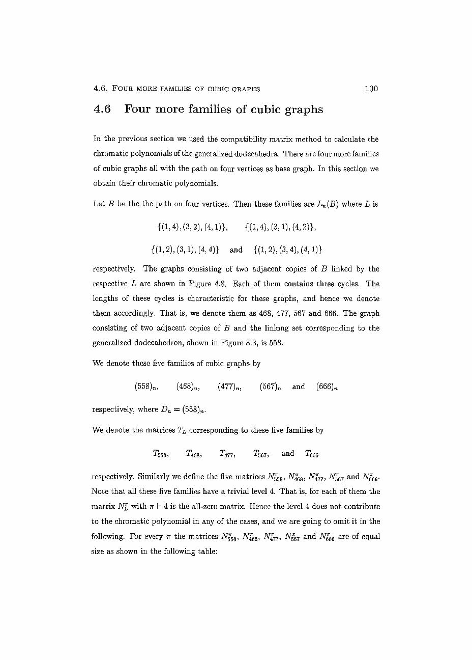
4 . 6 . FOUR MORE FAMILIES OF CUBIC GRAPHS

4.6 Four more families of cubic graphs

1 0 0

In the previous section we used the compatibility matrix method to calculate the chromatic polynomials of the generalized dodecahedra. There are four more families of cubic graphs ali with the path on four vertices as base graph. In this section we obtain their chromatic polynomials.

Let B be the the path on four vertices. Then these families are Ln(B) where L is

{(1,4), (3, 2), (4,1)}, {(1,4), (3,1), (4, 2)},

{(1,2), (3,1), (4, 4)} and {(1, 2), (3,4), (4,1)}

respectively. The graphs consisting of two adjacent copies of B linked by the

respective L are shown in Figure 4.8. Each of them contains three cycles. The

lengths of these cycles is characteristic for these graphs, and hence we denote

them accordingly. That is, we denote them as 468, 477, 567 and 666. The graph

consisting of two adjacent copies of B and the linking set corresponding to the

generalized dodecahedron, shown in Figure 3.3, is 558.

We denote these five families of cubic graphs by

(558)„, (468)n, (477) n, (567)n and (666)n

respectively, where Dn = (558)n.

We denote the matrices TL corresponding to these five families by

^558 j ^468 j ^477 J ^567> &nd TQQQ

respectively. Similarly we define the five matrices Nt%8, N%68, N%77, Ng67 and

Note that ail these five families have a trivial level 4. That is, for each of them the

matrix iVJ with ?r h 4 is the all-zero matrix. Hence the level 4 does not contribute

to the chromatic polynomial in any of the cases, and we are going to omit it in the

following. For every 7r the matrices Ng5Bi N%68, N%771 Ng67 and Ng66 are of equal

size as shown in the following table:

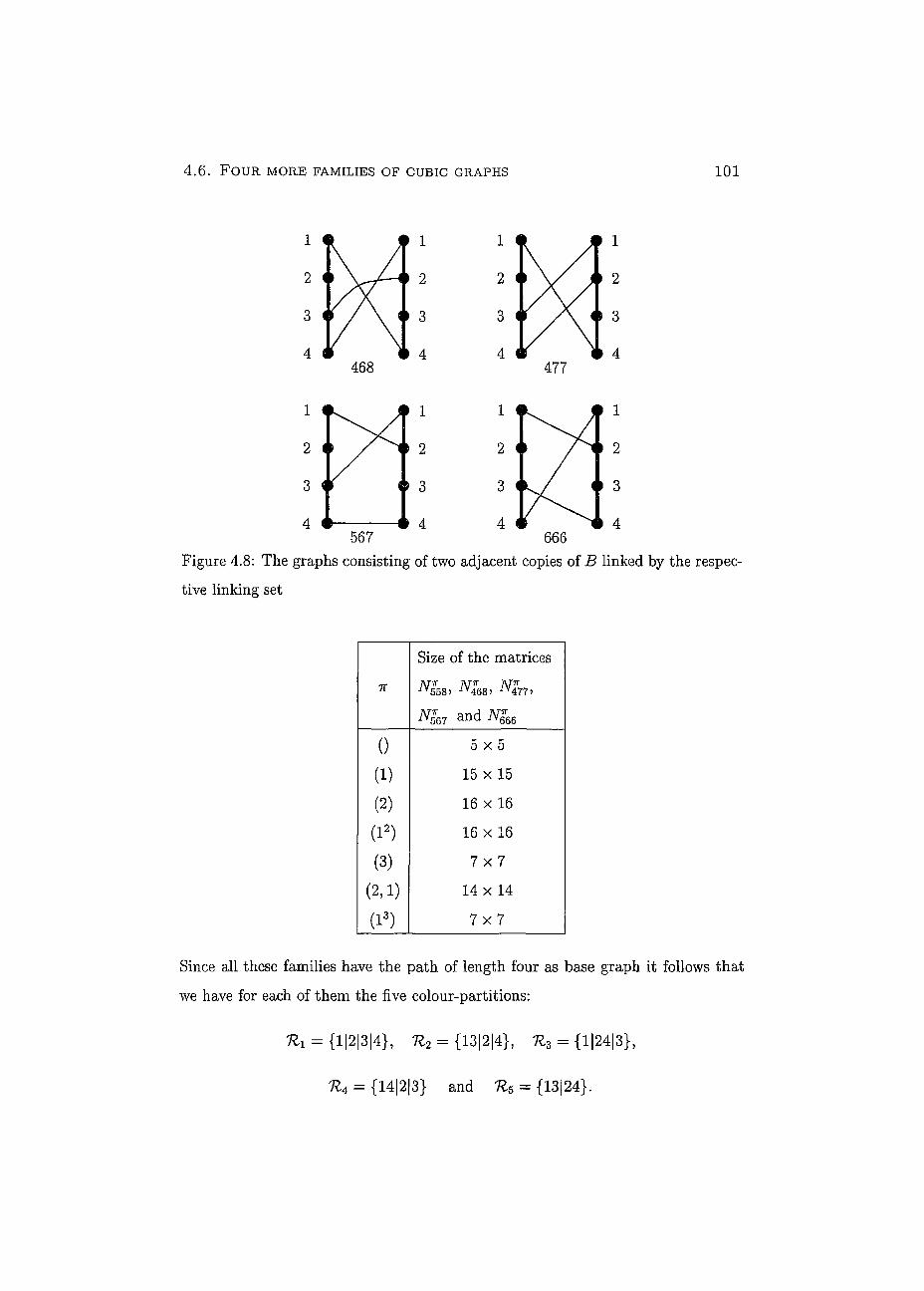
4 . 6 . FOUR MORE FAMILIES OF CUBIC GRAPHS 101

M: 477

H: 666

adj acent copies of B linked by the respec-

7T Size of the matrices Afir MTT Afn jv5583 ìv4685 ìv477J N£67 and

0 5 x 5

(i) 15 x 15

(2) 16 x 16

(l2) 16 x 16

(3) 7 x 7

(2,1) 14 x 14

(l3) 7 x 7

Since ali these families have the path of length four as base graph it follows that

we have for each of them the five colour-partitions:

= {1|2|3|4}, U2 = {13|2|4}, ^3 = {1|24|3},

n 4 = {14|2|3} and K 5 = {13|24}.

Figure 4.8: The graphs consisting of two tive linking set

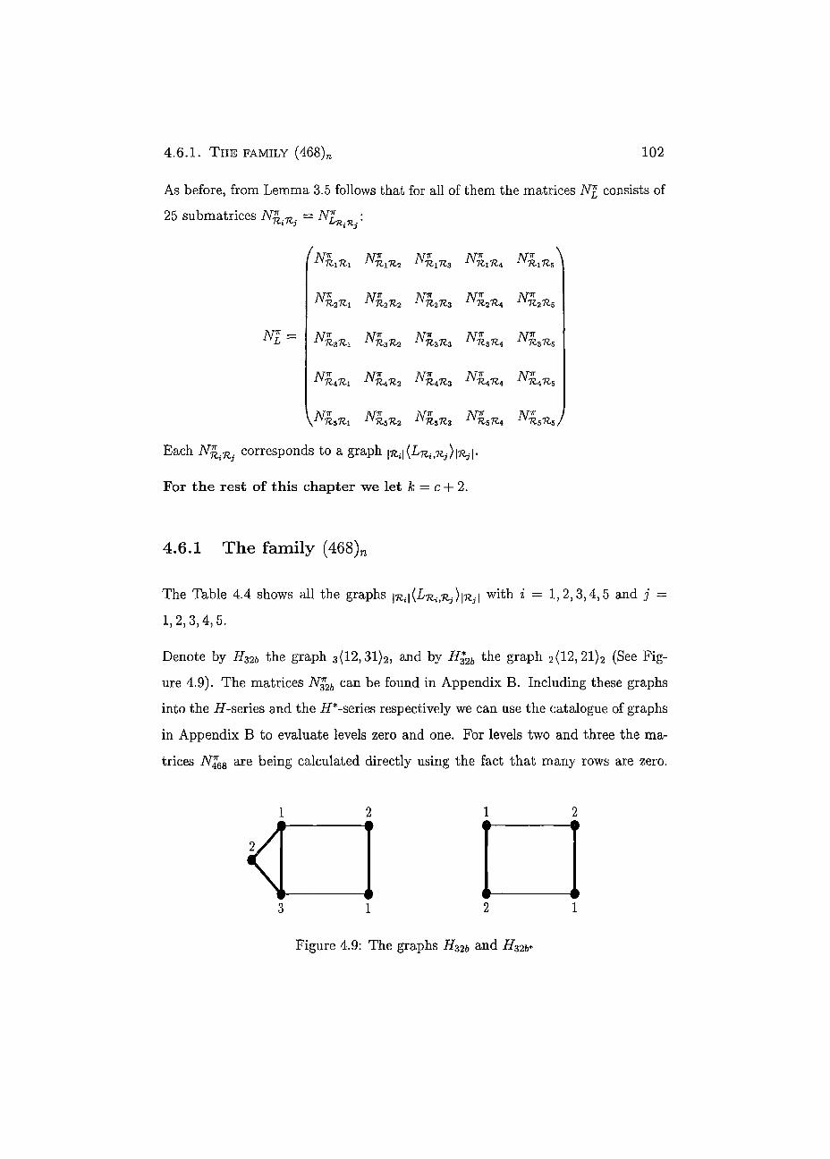
4 . 6 . 1 . T H E FAMILY (468) 102

As before, from Lemma 3.5 follows that for all of them the matrices iVJ consists of 25 submatrices = NfM_ : ^L-R.-Jlj

( N* Nv A/"71" N* iynxnz

NZ =

RN ATTT \ 'tIxIIA US

Nn2iii ^h2n2

AT7T AT7T jvr-rc ATTÏ AT TT 72.3iV7^37^2 iV7?.3 4 iyn*R*

A7-7T AT7T ATîT AT7T AT7T ^7^2

Nrisili

Each j M ^ corresponds to a graph ^(¿T^JI^-I .

For the rest of this chapter we let k = c + 2.

4.6.1 The family (468)n

The Table 4.4 shows all the graphs (£7 ,7 )17 1 with i = 1,2,3,4,5 and j =

1,2,3,4,5.

Denote by ii32& the graph 3(12,31)2, and by H¡2b the graph 2(12, 21)2 (See Fig-

ure 4.9). The matrices can be found in Appendix B. Including these graphs

into the H-series and the H*-series respectively we can use the catalogue of graphs

in Appendix B to evaluate levels zero and one. For levels two and three the ma-

trices iVJgg are being calculated directly using the fact that many rows are zero.

1 2 1 2

« a 3 1

Figure 4.9: The graphs #320 and H&b*

4 . 6 . 2 . THE FAMILY (477)N 103

i i 3 1

2 1 2 1

1 1 2 1

H E3> 13 2 3

s rz> s > Table 4.4: The induced graphs (£7 ,7 )17 1 in case of the family (468)n

Level 0: The matrix N^ corresponding to the graph (468)n can be written as

ÍN° n° n° n° n°\ IV 4 4 IV4Q IV 4 U -ÍV.OÍ, IV4O

N° -JV468 —

'44 43a 436 JV436 i V 4 2

AfO jvrO jvrö jvrO ivrO 34 i V33a 33c JV336 i V326

A/"0 AT() AT-0 TvrO jvtO 44 43a 436 JV436 i V 42

JVâa ^ 6 Nga

N&a Ngb Ngb)

f(c— l)(c3 + 2c — 1) c3 + 2 c - l c(c2 + l) c(c2 + l) c2 + l ^

c ( c - l ) ( c 2 + l) c(c2 + l) c(c2 + c + l ) c3 c2-f-c + 1

( c - l ) ( c 3 + 2 c - l ) C3 + 2 C - 1 C(C2 + 1) c(c2 + 1) c2 + 1

c ( c - l ) ( c 2 + l) c(c2 + l) c3 c(c2 + c + l ) c2

^ c(c - l) (c2 + 1) c(c2 + 1) c(c2 + c + 1) c3 c2 + c + ly

The characteristic equation is

A2 (A3 + aP(c)A2 + ap(c)A + af (c)) = 0

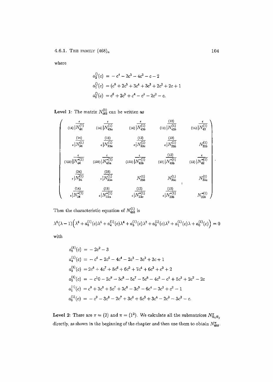
4 .6 .1 . THE FAMILY (468)N 104

where

a{](c) = — c4 — 2c3 — 4c2 — c — 2

a?(c) = (c6 + 2c5 + 3c4 + 3c3 + 2c2 + 2c + 1

a§(c) = c6 + 2c5 + c 4 - c 3 - 2 c 2 - c .

Level 1: The matrix N[H can be written as

(12)

( 1 4 ) 1 ^ <14)|iV£> ( 1 4 ) | i V S d3)| ( U ) | W i ?

(14) (13) (12) (12)

Ä ANÜl E\N$b

e e e (12) e

(IMJI^F (123)|iV^> ( 1 2 3 ) 1 ^ ( 1 3 ) 1 ^ (12) i j ^

(21) (23) « K «IJVSi i V « Nil

)

(14) (13) (12) (12)

rf rf rf N® }

Then the characteristic equation of N^H is

A8(A - 1) (A6 + 4 1 } (c)A5 + a?(c)A4 + a ^ (c)A3 + a ( c ) A 2 + a ^ (c)A + ag*(c)) = 0

with

flW(c) = - 2 c 2 - 3

aP( c ) = - c6 - 2c5 - 4c4 - 2c3 - 3c2 + 3c + 1

a ^ (c) = 2c8 + 4c7 4- 8c6 + 6c5 + 7c4 + 6c3 + c2 + 2

4 l 5(c) = - cx0 - 2c9 - 3c8 - 5c7 - 5c6 - 4c5 - c4 + 5c3 + 2c2 - 2c

41) (c) = c9 + 3c8 + 5c7 + 3c6 - 3c5 - 6c4 - 3c3 + c2 - 1

aW (c) = - c9 - 3c8 - 2c7 + 3c6 + 6c5 + 3c4 - 2c3 - 3c2 - c.

Level 2: There are ir = (2) and 7r = ( l2) . We calculate all the submatrices

directly, as shown in the beginning of the chapter and then use them to obtain N%68.

4 . 6 . 1 . THE FAMILY (468)N 105

Omitting all the rows and columns corresponding to a sets Y and X containing

2 respectively we can reduce iVJ68 to 9 x 9 matrices. These reduced matrices are

shown in Appendix C. The characteristic equations of iVJgg with ir = (2) and

7T = (l2) are respectively

A11 (A - 1) (A4 + a3(c)A3 + a2(c)A2 + ai(c)A + a0(c)) = 0

a n ( a - 1)(a4 - a3(c)a3 + a2(c)a2 - ai{c)X + a0(c)) = 0

with a3(c) = - c 2 — 2, a2(c) = —c2 + 2c - 1,

ai(c) = c4 — c2 + c + 1 and ßo(c) = —c3 — c2 + c + 1.

Level 3: Here there are three partitions % = (3), 7r — (l3) and 7r = (2,1). Omitting

all the zero rows and the corresponding columns, following a similar argument as in

the case of the generalized dodecahedra, we can reduce these matrices to ^(13) ,

Young's natural representation of (13). It follows that the characteristic equations

for 7T = (3), 7T = (l3) and tt = (2,1) are

A6(A - 1) = 0, A6(A + 1) = 0 and A12(A - 1)(A + 1) = 0

respectively.

As in the case of the generalized dodecahedron, Newton's formula, given in Ap-

pendix A, can be used to evaluate the sum A^^ of the nth powers of the non-

polynomial eigenvalues of the matrices JVJ. Then, for general n e N, the chromatic

polynomial of (468)n is:

P((468)N ; c) = + (c + l)(A(i),n + 1)

+ i (c 2 + c - 2)(A(2)jn + 1) + i ( c 2 + c)(A(ia)tn 4-1)

+ i ( c 3 - 3 c ) ( - i r + i ( c 3 - 5 c - 2 )

In Figure 4.10 the roots of (468)3o are plotted. Again, clearly visible are the roots

with negative real part.

4 . 6 . 1 . T H E FAMILY (468)N 106

1.5-

0.5-

-0.5

-1.5

- 2

+ + + + + +

+ + + + + + +

-1.5 - 1 -0.5

+ +

+ +

0.5

Figure 4.10: The roots of (468)30

4.6.2 The family (477)n

The Table 4.5 shows ali this graphs I^IC^,7^)17^1 with % = 1,2,3,4,5 and j =

1,2,3,4,5.

Ali induced subgraphs are part of the catalogue of graphs in Appendix B which we

will use to evaluate levels zero and one. For levels two and three we calculate the

matrices directly.

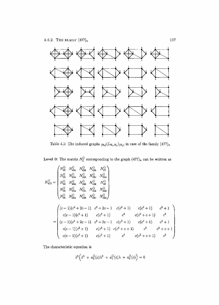
4 .6 .2 . THE FAMILY (477)N 107

1 3

4 1

s „ > 3

1

V s /

2 3

3 2

1 1 1 1

2 1 1 1 1 1 1 1

2 3

3 3

3 1 3 1 1 2 1 1 1 2 1 1 3 1

1 2 1 2 1

1 3

1 1

C3 H3> Table 4.5: The induced graphs ^(¿T^rc,-)^! in case of the family (477),

Level 0: The matrix corresponding to the graph (477)n can be written as

ÍN& N¡ I Ng

Nil N¡I N&b ,v33c

N0 _ ^ 477 — ato jvto j\to 44 43a 43b

ML

ML Nga

Ml N? 43b 42 jvro ätu af JV34 iV33o iV33c 0 ArO '0 Nu /VL JV33& 326 /V^ AT Af y 34 iV33a iV33b N, 33c AfO iV32o)

((c— l)(c3 + 2c — 1) c3 + 2 c - l c(c2 H-1) c(c2 + l) c2 + 1 ^

c(c - 1) (c2 + 1) c(c2 + 1) c3 c(c2 -f c + 1) c2

( c - l ) ( c 3 + 2 c - l ) c3 + 2 c - l c ( c 2 - f l ) c(c2 +1 ) c2 + l

c ( c - l ) ( c 2 + l) c(c2 + l) c(c2 + c + l) c3 c2 + c + l

^ c (e~l ) (c 2 + l) c(e2 + l) c3 c(c2 + c -M) c2 y

The characteristic equation is

A2 (A3 + aP(c)A2 + ap(c)A + a f ( c ) ) = 0

4 .6 .2 . THE FAMILY (477)N 108

where

a§(c) = - c4 - 2c3 - 3c2 + c - 1

o?(c) = - 2c5 - 5c4 - 5c3 - 2c2

a$(c) = - c6 - 2c5 - c4 + c3 + 2c2 + c.

Level 1: The matrix N¿ll can be written as / (142) 132

.iwffi e

(i3) i ¿vis (12)

( 1 4 ) | ^ • \

(13)

(24) *

(23)

•liVfii i V ( 1 ) 336 33c i V { 1 ) *32a

(14) (13) e (12) e

e 1 44 MliVá? (13)|iVl2(1)

(14) (13)

AN&Ì (12)

Nili (12)

i V ( 1 ) 326

(24) (23)

336 33c AT*(1) .

iV32a /

Then the characteristic equation of N±77 is

A8 A7+a^ (c) A6 H- a^ (c) A5 + a ^ (c) A 4 +a^ (c) À3 + a ^ (c) A2 + a ^ (c) A+a^ (c) = 0

with

4x )(c) = 4c — 1

4 ° (c) = 2c5 + 3c4 4- 7c3 + 4c2 + 2c - 2

<41}(c) = - c8 - 2c7 + c6 + 9c5 + 10c4 + 5c3 + c - 3

4x )(c) = - 2c9 - 5c8 - 3c7 + c6 + c5 - 2c4 - 8c3 - 2c2 - 2c - 2

41}(c) = c9 + 2c8 + 3c7 -I- 2c6 - 5c4 - 9c3 - 6c2 - 3c - 1

(c) = 4c6 + 7c5 + 2c4 - 4c3 - 6c2 - 3c

a^(c) = - c9 - 3c8 - 2c7 + 3c6 + 6c5 + 3c4 - 2c3 - 3c2 - c.

Level 2: There are 7r = (2) and 7r = ( l 2 ) . We calculate all the submatrices

directly, as shown in the beginning of the chapter, and then use them to

4 .6 .1 . THE FAMILY (468)N 109

obtain N%77. Omitting all the rows and columns corresponding to a sets Y and X containing 2 respectively we can reduce iVJ77 to 9 x 9 matrices. These reduced matrices are shown in Appendix G. The characteristic equations of jVJ77 for ir = (2) and 7T = (I2) are

A11 (A5 + aj(c) A4 + aj(c) A3 + aj(c) A2 + aj(c) A + aj(c)) = 0

with 4 2 ) (c) = 2c - 1, 4 2 ) (c) = c - 2, 42 ) (c) = - c 4 - 3,

42)(c) = c3 + c2 - 2c - 2, a®(c) = c3 + c2 - c - 1,

or a f ) ( c ) = - 2 c + l , af\c) = -3c, 4 l 2 )(c) = - c 4 - 3,

a p ( c ) - - c 3 - c2, a p ( c ) = - c 3 - c 2 + c + l.

Level 3: Here there are three partitions 7r = (3), 7r = (l3) and n = (2,1). Omitting all the zero rows and the corresponding columns, following a similar argument as in the case of the generalized dodecahedra, we can reduce these matrices to jR7r(123), Young's natural representation of (123) . It follows that the characteristic equations for 7T = (3), 7T = (l3) and 7r = (2,1) are

A6(A — 1) = 0, A 6 (A-1) = 0 and A12(A2 + A + 1) = 0

respectively.

As before, Newton's formula, given in Appendix A, can be used to evaluate the

sum Ax,n °f the nth powers of the non-polynomial eigenvalues of the matrices iVJ.

Then, for general n G N, the chromatic polynomial of (477)n is:

P((477)n; c) = + (c + 1 )AilU

+ Ì(C2 + C ~ 2)A(2),n + \(C2 + C)A{12),n

+ i(c3-4c)^(2,i) )n + ^ ( c 3 - 4 c - 3 )

In Figure 4.10 the roots of (468)3o are plotted. Again, clearly visible are the roots

with negative real part.

4 . 6 . 1 . T H E FAMILY (468)N 110

Figure 4.11: The roots of (477)30

4.6.3 The family (567)n

The Table 4.6 shows all this graphs ^ ¡ ( I / ^ , ^ ) ^ ! with i = 1,2,3,4,5 and j =

1,2,3,4,5.

All induced subgraphs are part of the catalogue of graphs in Appendix B which we

will use to evaluate levels zero and one. For levels two and three we calculate the

matrices directly.

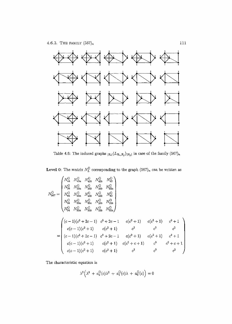
4 . 6 . 3 . T H E FAMILY (567)N 111

<3 :

k.3

& 0 I3> S 2 4 2 3 2 2 2 1 1 2

3 1 2 1 2 1

1 1 3

1 3 1 2 1 1

3

3 2

Table 4.6: The induced graphs \Hi\(Lni,iij)\Kj\ in c a s e of the family (567)n

Level 0: The matrix N® corresponding to the graph (567)n can be written as

ÍN° N° 44 *43a

/VU -567 —

i V34

44

r()

n: o 33a

N° N° N° \ 436 iV436 42

n (K n° 336 33

]\r0 ATO I\T() ju() MAA JV43a iV436 iV43i No N0 y33c ^330 --¡y¿

ML ML 41

42

¿ V 0 i V 32 a

'436 flS

^ ML ^ ML

326

rU A/" 336 32a J

( (c — l)(c3 + 2c — 1) C3 + 2 C - 1 c(c2 + 1) c(c2 + l) c2 + 1 ^

c ( c - l ) ( c 2 + l) c(c2 + l) c3 c3 c2

( c - l ) ( c 3 + 2 c - l ) C3 + 2 C - 1 C(C2 + 1) c(c2 +1) c2 + 1

c ( c - l ) ( c 2 + l) c(c2 + 1 ) c(c2 + c + l ) c3 c2 + c + l

^ c ( c - l ) ( c 2 + l) c(c2 + l) C3 C3 C2 J

The characteristic equation is

A2 (A 3 + 4 } ( c ) A2 + ¿¿(e) A + AFTE)) = 0

4 . 6 . 3 . T H E FAMILY (567)N

where

c§(c)

a»(C)

a?(c)

112

- c4 - 2c3 - 3c2 + c - 1

- c5 - 3c4 - 2c3 + c2 + c

c4 + 2c3 + c2.

: The matrix N$7 can be written as (12) (12) £ (12) « \

(13)1^

.-1

33a N(1) 33b

(12)

ANÍH iV(1) 32a

(124) (123) e (12) e

(13) 1 N'V

(14) (13)

AMU (12)

«1MZ

(12)

<\N¡¡1 N{1) 32b

(12)

«1 N*{1) 1 iV32a / V Then the characteristic equation of is

A8 A7 + afp (c) A6+a^ (c) À5 + a ^ (c) À4 + dp (c) A3 -f- a ^ (c)A2+a^ (c) A+ap (c)

with

:) =C 3 + 4 C - 2

;) = 2c4 + c3 + 2 c 2 - c - 2

;) = c8 + 2c7 + 4c6 + 2c5 + c4 - 2c3 - 2c2 - 6c + 2

;) = c9 + 3c8 + 3c7 - 2c4 ~ 3c3 - c2 + 3c

:) = - c 8 - 4c7 - 8c6 - 9c5 - 8c4 - 3c3 + 4c2 + 2c - 1

;) = - c7 - 3c6 - 3c5 + 2c4 + 5c3 -b c2 - c

:) = c6 -h 4c5 H- 6c4 + 4c3 + c2.

= 0

4%

4%

afte

4 %

4%

4%

4x ) (c

Level 2: There are ir = (2) and 7r = (l2) . We calculate all the submatrices

N^i1Zj directly, as shown in the beginning of the chapter, and then use them to

4 .6 .1 . THE FAMILY (468)N 113

obtain Ng67. Omitting ail the rows and columns corresponding to a sets Y and

X containing 2 respectively we can reduce Ng67 to 9 x 9 matrices. These reduced

matrices are shown in Appendix C. The characteristic équations of Ng67 for TT = (2)

and 7r = (l2) are

A11 (A5 + < ( c ) A4 + aj(c) A3 + aj(c) A2 + a\(c) A + aj(c)) = 0

with a f (c) = 2c - 2, <42) (c) — c3 + c2 — c — 2, a!>2) (c) = c4 - c + 2,

(c) = - c 3 _ 2c2 - c, 4 2 ) (c) = - c 2 - 2c - 1,

or a(p (c) = - 2 , af} (c) = c3 - c2 + 3c, af] (c) = - c 4 - 3c + 2,

a[l2>(c) = - c 3 - c - 2, 4 l 2 ) (c ) = c2 + 2c + 1.

Level 3: Here there are three partitions 7r = (3), TT = (l3) and % = (2,1). Omitting

ail the zéro rows and the corresponding columns, following a similar argument as in

the case of the generalized dodecahedra, we can reduce these matrices to ^ (12) ,

Young's natural représentation of (12). It follows that the characteristic équations

for 7r = (3), 7r = (l3) and ir = (2,1) are

A6(A - 1) = 0, A6(A + 1) = 0 and A12(A - 1)(A + 1) = 0

respectively.

As before, Newton's formula, given in Appendix A, can be used to evaluate the

sum Ar,n of the nth powers of the non-polynomial eigenvalues of the matrices N[.

Then, for général n e N, the chromatic polynomial of (567)n is:

P((567)n; c) = % n + (c + 1)A(I)>b

1 1 + 2 (c2 + ° ~ 2)A(2 ),n + ^(c2 + c)A(i a)>n

+ i ( c 3 - 3 c ) ( - i r + i ( c 3 - 5 c - 2 )

In Figure 4.10 the roots of (468)3o are plotted. Again, clearly visible are the roots

with negative real part.

4 . 6 . 1 . T H E FAMILY (468)N 1 1 4

1.5 + +

+ +

+

+ + +

+ + + +

1 +

' + + + +*+ 0.5 \

+ +

0 + Í / ++ 4 + ++ -0.5

++ + ++

+

-1- +

+ + + +

+ +

-1.5- + +

+ + + + + +

-2 -1.5 -1 -0.5 0 0.5

Figure 4.12: The roots of (567)30

4.6.4 The family (666)n

The Table 4.7 shows all this graphs with i = 1,2,3,4,5 and j =

1,2,3,4,5.

All induced subgraphs are part of the catalogue of graphs in Appendix B which we

will use to evaluate levels zero and one. For levels two and three we calculate the

matrices directly.

4 .6 .4 . THE FAMILY (666)N 115

2 4

1 4

2 1 1 1 2 1 2 1

3 2

1 2

1 3

» El I3> H> is; 1 1

Table 4.7: The induced graphs ^{Ln^n^iij ] in case of the family (666)n

Level 0: The matrix N¿¡ corresponding to the graph (666)n can be written as

r0 jvrO jvrO JvrO \

N° -666 —

JV43b 2y43b 42

0 Mi Ngb Ngb ATU AT i V 34 iV33fl

JV44 iV43a

^ 34 ^ 33a

atO wO /V 43b 43b 42

juO 7\r() ivr() J 33b 33b 32a

ATO atO /vr() ivqi„ IVirth iy32b/

0

V^li JVS 33a -^330 1 33b

( (c — l)(c3 + 2c — 1 ) c3 + 2 c - l C(C2 + 1 ) c(c2 + 1 ) c2 + 1 ^

c ( c - l ) ( c 2 + l) c(c2 + l) c(c2 + c + l) c3 c 2 - f c + l

( c - l ) ( c 3 + 2 c - 1 ) C3 + 2 C - 1 C(C2 + 1) c(c2 + l) c2 + 1

c ( c - l ) ( c 2 + l) c(c2 4-1) c3 c3 c2

^ c ( c - l ) ( c 2 + l) c(c2 + l) c(c2 + c-f-l) c3 c2 + c+lj

The characteristic equation is

A 2 (a 3 + a^c )A 2 + op(c)A H- 4 ( c ) ) = 0

4 . 6 . 4 . T H E FAMILY (666),

where

116

o? (c)

ai (c)

4 ( c )

= -c4 -2c3- 3c2 - 2

= - c 4 + l

= _ c 4 _ 2 C 3 - c 2 .

Level 1: The matrix N^g can be written as

/ (124) *

(123) €

(14) (13)

Ä (12)

(12)

e K l 1 ' (12) €

(12)

(i) 336

N(1)

34

(14)

iV, (1)

*(1) 34 |iv.

33a

(13) *(1) 33a

iV(1)

336

(12)

Then the characteristic equation of jVgJg is

A8 A7-f-afß^ (c) A 6 +a^ (c) A 5 +a^ (c) A 4 +a^ (c) A 3 +a^ (c) A2 4- a ^ (c) A+a^ (c)

with

(12)

_(12)

e\N:

(12)

(12)

(12)

(14) |

r(l) N. 326

d2)|iv;2(1)

N. ( i ) 32a

)

= 0

4 1 } (c

4 x ) ( c

a i^c

4 1 } (c

4X )(c

4 x ) (c

= - 2c2 - 4

= - c4 - 2c2 + 4c + 4

= - c8 - 2c7 - 5c6 - 4c5 - c4 + 6c3 + c2 - 2

= c8 + 6c7 + 10c6 + 8c5 + 3c4 + 2c3 - 2c2 - 4c-1- 4

= - 2c7 - 5c6 - 6c5 - 5c4 - 2c3 + 4c2 - 4

= 2c6 + 6c5 + 7c4 + 2c3 - 2c2 + 1 = - c6 _ 4c5 _ 6c4 _ 4c3 _ c2_

Level 2: There are ir = (2) and 7r = (l2) . We calculate all the submatrices

N^ i1Zj directly, as shown in the beginning of the chapter, and then use them to

4 .6 .1 . THE FAMILY (468)N 117

obtain Nq66. Omitting all the rows and columns corresponding to a sets Y and X containing 2 respectively we can reduce Nq6Q to 9 x 9 matrices. These reduced matrices are shown in Appendix C. The characteristic equations of Ng66 for TT = (2) and 7T = (l2) are

A11 (A5 + 4 (c ) A4 + a¡{c) A3 + aJ(c)A2 + a»(c) A + aS(c)) = 0

with 4 2 ) (c) = - 3 , 4 2 ) (c) = -2c2 + 2c +1, a^ (c) = - c 4 - 2c2 - 1,

a<2) (c) = 2c3 + 3c2 + 4c + 3, a(02) (c) = - c 2 - 2c - 1,

or af\c) = 1, 4 l 2 )(c) = 2c2 - 2c + 1, af\c) = - c 4 - 2c2 - 1,

a p t e ) = -2c3 - c2 - 1, 4 l 2 )(c) = - c 2 - 2c - 1.

Level 3: Here there are three partitions ir = (3), 7r = (l3) and ir = (2,1). Omitting

all the zero rows and the corresponding columns, following a similar argument as in

the case of the generalized dodecahedra, we can reduce these matrices to ^(132),

Young's natural representation of (132). It follows that the characteristic equations

for ?r = (3), 7T = (l3) and tr = (2,1) are

A6(A — 1) = 0, A6(A - 1) = 0 and A12(A2 + A + 1) = 0

respectively.

As before, Newton's formula, given in Appendix A, can be used to evaluate the

sum AVin of the nth powers of the non-polynomial eigenvalues of the matrices iV£.

Then, for general n G N, the chromatic polynomial of (666)n is:

P((666)„; c) = A0,„ + (c + 1) A(i)in

+ \{<? + c - 2)A(2)|B + i(c2 + c)A{12)>n

+ i(c3 -4c)A ( 2 ,1 ) ) n + i ( c 3 - 4 c - 3 )

In Figure 4.10 the roots of (468)3o are plotted. Again, clearly visible are the roots

with negative real part.

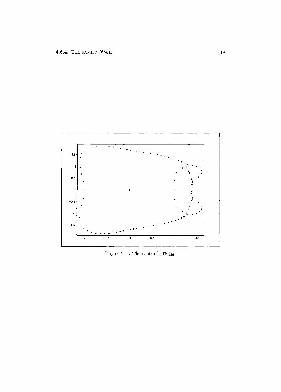
4 . 6 . 1 . T H E FAMILY (468)N 118

Figure 4.13: The roots of (666)30

Chapter 5

Equimodular curves

In this chapter we discuss the behaviour of the roots of the chromatic polynomial

as the number of copies of the base graph goes to infinity. We shall refer to them

as chromatic roots. The framework for the following is taken from [4] and [6].

Recall that for any given base graph B, any linking set L and k G N the compati-

bility matrix TL (k) corresponding to the family Ln (B) is equivalent to a matrix of

the form

© ( i r ® J V Z ) . 0<l<b

where is the identity matrix of size ^(k) given in Theorem 3.3, and iVJ is a

matrix of size nTr with entries depending on k (nv is the dimension of nm (B)

the Specht module S71").

By Theorems 3.3 and 3.13 it follows that for every n G N the chromatic polynomial

of Ln(B) is of the form b

p(Ln{B), k) = j2 E *(*) tr(Nz)n-£=0 7rh£

Further, recall that for every 7r, if Ai(£), AJ(ft),. • •, K W a r e the eigenvalues of

N1 with respective algebraic multiplicities mf , m j , . . . in iVJ then

1=1

119

5 . 1 . A THEOREM OF BERAHA, K AH ANE AND WEISS 1 2 0

This particular structure of the chromatic polynomials allows us to use a theorem by Beraha, Kahane and Weiss to investigate the limiting behaviour of the chromatic roots as n goes to infinity.

5.1 A theorem of Beraha, Kahane and Weiss

The Figures 3.5, 4.7, 4.10, 4.11, 4.12 and 4.13 suggest that the roots approach some set of curves as n grows (plus some isolated points). This behaviour of the roots can be understood using a theorem of Beraha, Kahane and Weiss [18]: Suppose that we have a family of polynomials {Pn(z)} of the form

s

pn(z) = ]r m i (z ) (\ i (z ) ) n . Z—l

A complex number ( is defined to be a limit point of roots of this family if there exists a sequence {Zj} tending to such that Zj is a root of Pj(z) for every j . We say that a root dominâtes the other roots if it has the largest modulus.

Theorem 5.1 [Beraha, Kahane, Weiss 1980] Under the non-degeneracy conditions

that {Pn(z)} does not satisfy a lower order recurrence, and Xi(z)/X3 (z) is not iden-

tically a constant of unit modulus for any i ^ j, the complex number £ is a limit

point of zéros of {Pn(z)} if and only if atz^C,, one of the following two conditions

holds:

• One of the roots Ai(z) dominâtes all the other roots , and the corresponding

rrii(z) =0. Or,

• Two or more of the roots Ai(z) are of equal modulus and dominate the others.

The chromatic polynomials obtained by the compatibility matrix method are ex-

actly of the form required for the above theorem. The limit points of the first type

are isolated points and easy to determine. We shall concentrate on fìnding limit

points of the second type.

5 .1 . A THEOREM OF BeRAHA, K AH ANE AND WEISS 121

We first consider ail points where two or more of the roots À¿(z) are of equal modulus, and then check their dominance. The Xi(z) in Theorem 5.1 are the eigenvalues of the matrices N

Example 5.1: Recall the family B(3)n with complété base graph K3 and identity

linking set. Its chromatic polynomial has been obtained in Example 3.8. This

example is particularly "nice" since ail the characteristic équations of ail the the

N£ factorize into linear factors in À. That is ail the eigenvalues are ail polynomials

in k. There are eight distinct eigenvalues:

Ai = A;3 — 6k2 + 14k - 13, A2 = -k2 + 7k - 13, A3 = -k2 + 4k - 4

A4 = k — 2, A5 = k - 5, X6 = k-1,

\7 = k — 4 and Ag = 1.

Then |Ai| = \Xj\ is équivalent to

where 3ft(A) dénotés the real and ^(A) the imaginary part of a complex function

A. Using the "implicitplot" function in Maple 7 we obtain a a collection of

"equimodular curves". There are 28 |Àj| = \Xj\ with % ^ j , but only a few of

them contain points where the eigenvalues of equal modulus also dominate the

other eigenvalues. We call them "dominant points". In Figure 5.1 the curves

corresponding to |Ai| = |A |, |Ai| — |As| and \X2\ = |As| are shown. It turns

out that these are the only curves containing dominant points. Ail three curves

intersect in what will be called "triple points". In the following sections we will

show that ail points of a segment of an "equimodular curve" containing at most

two "triple points" as endpoints are either ail dominant or ail are not. In Figure 5.1

the roots of Bs0 (circles) are also shown. Clearly, they cluster along segments of

these curves, and the "dominance" property changes at the triple points.

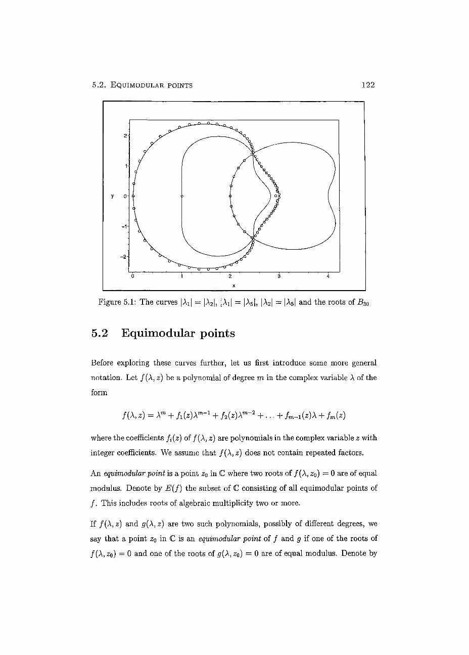
5.2. EQUIMODULAR POINTS 122

y o

-2"

-1

2

0 2 3 4

x

Figure 5.1: The curves |Ai| = |A2|, |Ai| = |As|, |A2| = |Aq| and the roots of B^

5.2 Equimodular points

Before exploring these curves further, let us first introduce some more general

notation. Let /(A, z) be a polynomial of degree m in the complex variable A of the

form

where the coefficients fi(z) of /(A, z) are polynomials in the complex variable z with

integer coefficients. We assume that f ( \ z ) does not contain repeated factors.

An equimodular point is a point zq in C where two roots of f(X,z0) = 0 are of equal

modulus. Dénoté by E(f ) the subset of C consisting of ail equimodular points of

/ . This includes roots of algebraic multiplicity two or more.

If f(X,z) and g{X,z) are two such polynomials, possibly of diiferent degrees, we

say that a point z0 in C is an equimodular point of / and g if one of the roots of

f(X,zo) — 0 and one of the roots of g(X,z0) = 0 are of equal modulus. Dénoté by

/(A, z) = \m + fl(z)Xm~1 + h(z)Xm~2 + . . . + fm-l(z)X + fm(z)

5 . 3 . T H E RÉSULTANT

E(f,g) the subset of C containing ali the equimodular points of / and g.

Suppose that / factors as /(A, z) — u(X,z)w(Xtz)t where u(X,z) and w(X:z) are

polynomials of the same form as /(A, z) with degrees l and d respectively. Then

E(f) = E{u) U E{w) U E(u, w).

Recali that for ali ir the matrices JVJ corresponding to a graph Ln(B) are such that

every component is a polynomial in k with integer coefficients. The coefficients of its

characteristic polynomial are sums of principal minors of iV£ and thus polynomials

in k with integer coefficients. Thus we can replace k by a complex variable z and

it follows that the characteristic polynomial of iVJ is of the form /(A, z).

5.3 The résultant

If /(A, z) factorizes into linear factors in A then ali the roots are polynomial func-

tions in and we can equate their moduli one by one, as done in Example 5.1.

From algebraic geometry it follows that the E(f) are collections of continuous and

almost every where diiferentiable curves on the Riemann Sphere. Unfortunately the

polynomials f(X,z) do not always factorize completely as we saw in the previous

chapter. That is the roots are not ali polynomial functions. More powerful tools

are needed. Assume that m = l + d and let

u(A) = X1 + uiX1-1 + u2Xl~2 + ... + ut-iA + ui

and

w(X) - Xd + w^-1 + w2Xd~2 + ... + wd^X + wd

be two polynomials in C[A]. The key idea is that if Xu is a root of it(A) and A^

is a root of w(A) with |AU| = \XW\ then there exists s G C with |s| = 1 such that

Xw = sXu. It follows that Xu is a common root of the polynomials u(X) and

ws(A) = w(sX) = sdXd + wis^X*'1 + w2sd~2Xd~2 + ... + ^d-isA + wd

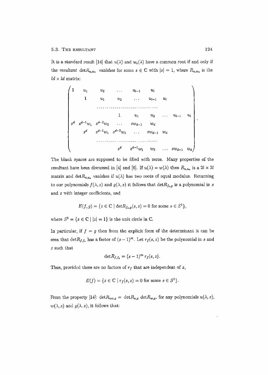
5.3 . THE RÉSULTANT 124

It is a standard result [14] that u(A) and ws(X) have a common root if and only if

the résultant detily^ vanishes for some s G C with |s| = 1, where Ru,ws ^ the.

Id x Id matrix:

^ 1 Ui ¿2 • • • ui-1 ui ^

1 Ui U2 . . . Ui-1 Ui

1 Ui U2 Ui-i Ui

Sd Sd~lWi Sd~~2W2 . . . SWd~ 1 Wd

Sd S^W I Sd~2w 2 • • . SWd-1 l^d

y sd s^Wi w2 ... syjd-i wdJ

The blank spaces are supposed to be fìlled with zéros. Many properties of the

résultant have been discussed in [4] and [6]. If u(A) = w(X) then Ru)Us is a 21 x 21

matrix and deti^)Ua vanishes if ti (A) has two roots of equal modulus. Returning

to our polynomials /(A, z) and ¿/(A, 2) it follows that detRfSt9 is a polynomial in s

and z with integer coefficients, and

E{f,g) = {z e C | detRfa}g(s1 z) = 0 for some 5 € S1} ,

where S1 = {z € C | \z\ = 1} is the unit circle in C.

In particular, if f = g then from the explicit form of the déterminant it can be

seen that detRfja has a factor of (5 — l)m . Let r/(s, z) be the polynomial in s and

2: such that

detRfjs = (s-l)mrf(Sìz).

Thus, provided there are no factors of Tf that are independent of z,

E(f) = {ze C | 7 7 (s, z) = 0 for some 5 e S1}.

From the property [14]: det i t^g = deti^ j 5 detiì !^, for any polynomials u(\ z),

w(A, z) and g(X, z), it follows that:

5 . 4 . EQUIMODULAR CURVES 125

Lemma 5.2 Ij f(\,z) = u(X,z)w(X,z), whereu(X,z) andw(X}z) are polynomials

of degrees l and d in X respectively, then

(s - l)l+drf{s, z) = detRfJs = (s - l)i+dru(s, z) rw(s, z) detRuSiW detRu,Ws.

•

Note that in [4] and [6] using the substitution t = s + s - 1 + 2 the polynomial

Vf : [0,4] x C — C is obtained where s e S1 implies that t 6 [0,4]. This has the

advantage that t is a real variable. In this case

E(f) = {z € C | vf{t,z) = 0 for some t e [0,4]}.

5.4 Equimodular curves

Let detRf3i9 : S1 x C — € and suppose that (SOJ O) € S1 x C is such that

det-R/S)fl(so3 ¿o) = 0- From the Implicit Function Theorem it follows that if the

Jacobian of the mapping z detifyS)5(s, z) is not zero at (s0, ^o) then there exists

a unique continuous and differentiable map (j> : fi —> C defined on some open

neighborhood Q, C S1 such that </)(s0) = zo and det i?/ai9(s, (f>(s)) = 0 for ail s G fi.

Since there is only a finite number of points (so, ¿o) € S1 x C with detRf3iS(so, zo) =

0 and a vanishing Jacobian, it follows that E(f: g) is the union of homeomorphic

images of the open intervais fi. We refer to E(f,g) (or E(f) if / = g) as the sets

of the equimodular curves corresponding to f(X,z) and g(X, z).

Denote by E(TL) the set of equimodular curves corresponding to the characteristic

polynomial of TL for some given Ln(B). Denote by f*(\jz) the characteristic

polynomial of iVJ. From Lemma 5.2 it follows that:

Corollary 5.3 The set of equimodular points E(TL) consists, except for some iso-

lated points ("degenerate curves"), of the union of piecewise differentiable curves.

Moreover, it is the union of ali the E(fv) and E^J*') for distinct 7r and ir'.

•

5 . 4 . EQUIMODULAR CURVES 126

Note that the "degenerate curves" in the previous corollary correspond to factors

of the résultant that are independent of s.

Lemma 5.4 Let the polynomial f(\z) be given. Then rf(s,z) = r/(s, z), where

s denotes the coniugate of s.

Proof: Recali that r/(s0,^o) = 0 for some (so,^o) € S1 x C if and only if

/(s0À, Z0) = 0 and /(A, Z§) = 0 for some A G C.

Let A' = so A then

/(sô1 A', zo) = /(A, zo) = 0 and /(A', z0) = f(s0A, z0) = 0.

Hence 77 (SQ\ ^o) = 0. This-holds for ali (so, z0) G S1 x C with r/(s0, z0) — 0. Since

s - 1 = s, the resuit follows. •

Let S+ = {z G S1 | $(*) > 0} and S~ = {z e S1 \ < 0}. From the

previous lemmas we have the following:

Corollary 5.5 Except for some isolated points ("degenerate curves"), E(f) is the

union of piecewise differentiable curves where the points corresponding to rj(l,z) =

0 and to r/(—1,2) = 0 are endpoints. Further:

E(f) = {z G C | rf(s, z) = 0 /or some s G

= {z G C | r/(s, z) = 0 for some s G S~}.

•

In [4] Section 5 it has been shown that every point corresponding to 77(—l,z) = 0

is a double root. Hence, the above curves occur in pairs that coincide in the points

corresponding to r/(—l,z) = 0.

5 . 4 . 1 . EXAMPLES

5.4.1 Examples

127

Let B be the path on three vertices and let L = {(1,1), (2,2), (3,3)} be the identity

linking set. The resulting graph Ln{B) has been considered in Example 3.12 and

the matrices N£ for ali ir have been obtained. The polynomials

/(A, z) = A2 + {-zz - z2 - Zz)\ + + z3 + 22 — 1

and g(X, z) = A — c + 2 are irreducible factors in the characteristic polynomials at levels zero and two respectively. In the following two examples we shall study the sets E(f) and E(f,g) in détail. In Section 5.6.1 ail levels corresponding to this example are analyzed mimerically.

Example 5.2: Let us analyze the set E(f). Here

rf(sjz) = (z + l)(z3 + z — l)ç(s,.z) where

ç(s, z) = - ssf - 2szb + (s2 - 55 + 1 )z4 + (s2 - 4s + l)*3

+ (s2 — 7s + l)z2 — s2 — 2s — 1.

In Figure 5.2 the equimodular curves E(f) are shown. The points 2; satisfying

77(5, z) = 0 for 5 = 1 and s = —1 are indicated by O and • respectively. One can

see very nicely that E(f) consists of a union of curves with endpoints O and •.

The points • (—0.5±1.6583z and 0) are double roots where pairs of curves coincide.

Further there are four points ("degenerate curves") at —1, — 0.3412 ± 1.1615Ï and

0.6823 corresponding to the équation (z + l)(z3 + 2 — 1) = 0. Here and in the

following, points are represented by approximations to four décimal places.

Example 5.3: Let us analyze the set E(f,g). Here

det%,s(s, z) = ( -5 + 1 )z4 + (5 + 1>3 + (s2 - s + 1 )z2 + ( -4s2 + 6s)z + 4s2 - 1.

The coefficient for z4 vanishes for s = 1. This implies that one of the points in

E(f, g) corresponding to s = 1 is at infinity. For ail other s € S1 there are four solu-

tions of detRf s ,g(s, z) = 0. Hence there are four segments in E(f1 g). In Figure 5.3

5 .4 .1 . EXAMPLES 128

Figure 5.2: E{f)

the equimodular curves E(f,g) are shown. The points z satisfying detRfs,g = 0

for s = 1 and s = — 1 are indicated by O and • respectively. The closed curve on

the left hand side contains three points 0.2500 ± 1.1990Ì and —1 corresponding to

5 = 1, and three points —0.7906 ± 10.7193î and 0.3365 corresponding to s — —1.

In this case, as s runs over the values in S1 in an anti-clockwise direction we move

along the curve in an anti-clockwise direction (as indicated).

The curve has two cusps at u and co5 where u is a primitive sixth root of unity.

They are represented by circles. These points can be obtained as follows:

D(z) = (z2-z + 1 )(z4 + 3z3 + 5z2 + 4z + 4){z - 2)2

is the discriminant of detRfSì9(sìz) with respect to s. For each 2 where D(z)

vanishes there exists a root s of detRfaìg(s, z) of multiplicity at least two. Only the

two roots (z2 — z + 1) correspond to s € S1. In fact z = co corresponds to s = a;5,

and z = oj5 corresponds to s = u.

The curve on the right hand side has one point corresponding to s = — 1 at 1.2446.

Its point corresponding to s = 1 is at infìnity. Its points in the half-plane with

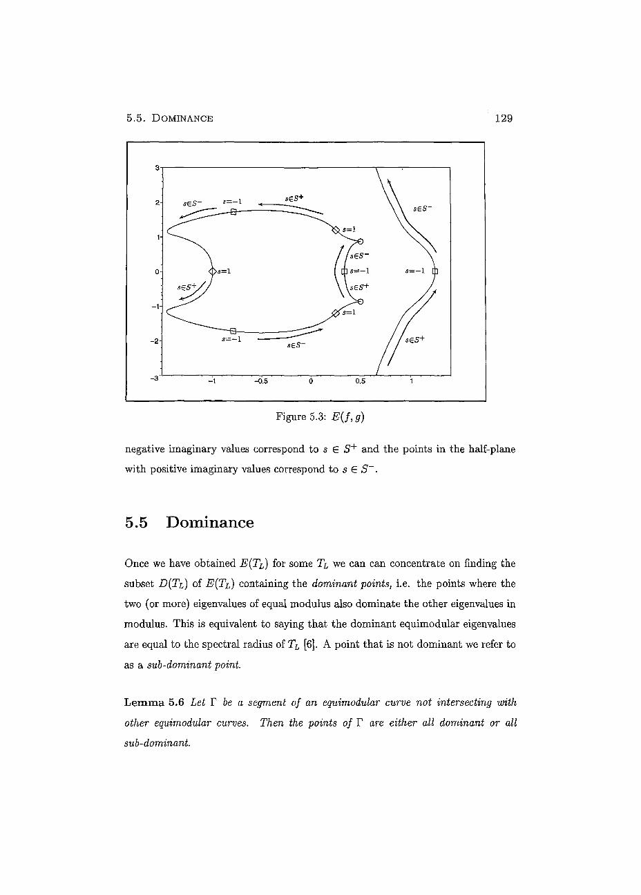
5 . 5 . DOMINANCE 129

Figure 5.3: E(f,g)

negative imaginary values correspond to s G S+ and the points in the half-plane

with positive imaginary values correspond to s € S~.

5.5 Dominance

Once we have obtained E(TL) for some TL we can can concentrate on finding the

subset D(TL) of E(TL) containing the dominant points, i.e. the points where the

two (or more) eigenvalues of equal modulus also dominate the other eigenvalues in

modulus. This is équivalent to saying that the dominant equimodular eigenvalues

are equal to the spectral radius of TL [6]. A point that is not dominant we refer to

as a sub-dominant point

Lemma 5.6 Let F be a segment of an equimodular curve not intersecting with

other equimodular curves. Then the points of V are either ail dominant or ail

sub-dominant.

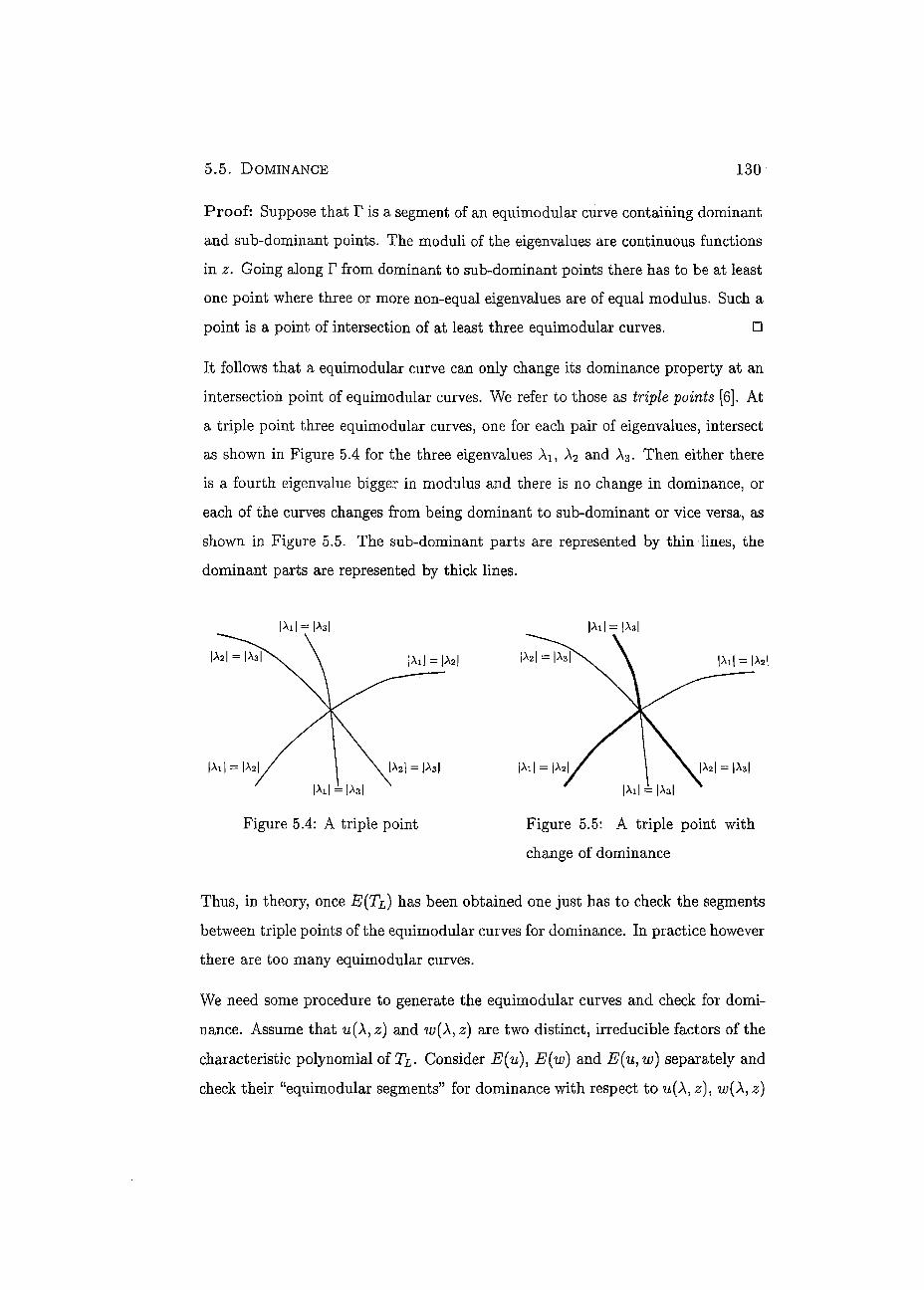
5 . 5 . DOMINANCE 1 3 0

Proof: Suppose that Y is a segment of an equimodular curve containing dominant

and sub-dominant points. The moduli of the eigenvalues are continuous functions

in z. Going along F from dominant to sub-dominant points there has to be at least

one point where three or more non-equal eigenvalues are of equal modulus. Such a

point is a point of intersection of at least three equimodular curves. •

It follows that a equimodular curve can only change its dominance property at an

intersection point of equimodular curves. We refer to those as triple points [6]. At

a triple point three equimodular curves, one for each pair of eigenvalues, intersect

as shown in Figure 5.4 for the three eigenvalues Ai, A2 and A3. Then either there

is a fourth eigenvalue bigger in modulus and there is no change in dominance, or

each of the curves changes from being dominant to sub-dominant or vice versa, as

shown in Figure 5.5. The sub-dominant parts are represented by thin lines, the

dominant parts are represented by thick lines.

IAI| = |A8| |AI| = |A3|

Figure 5.4: A triple point Figure 5.5: A triple point with

change of dominance

Thus, in theory, once E(TL) has been obtained one just has to check the segments

between triple points of the equimodular curves for dominance. In practice however

there are too many equimodular curves.

We need some procedure to generate the equimodular curves and check for domi-

nance. Assume that u(A, z) and il?(A, z) are two distinct, irreducible factors of the

characteristic polynomial of TL- Consider E(u), E(w) and E(u,w) separately and

check their "equimodular segments" for dominance with respect to u(A, z), w(A, z)

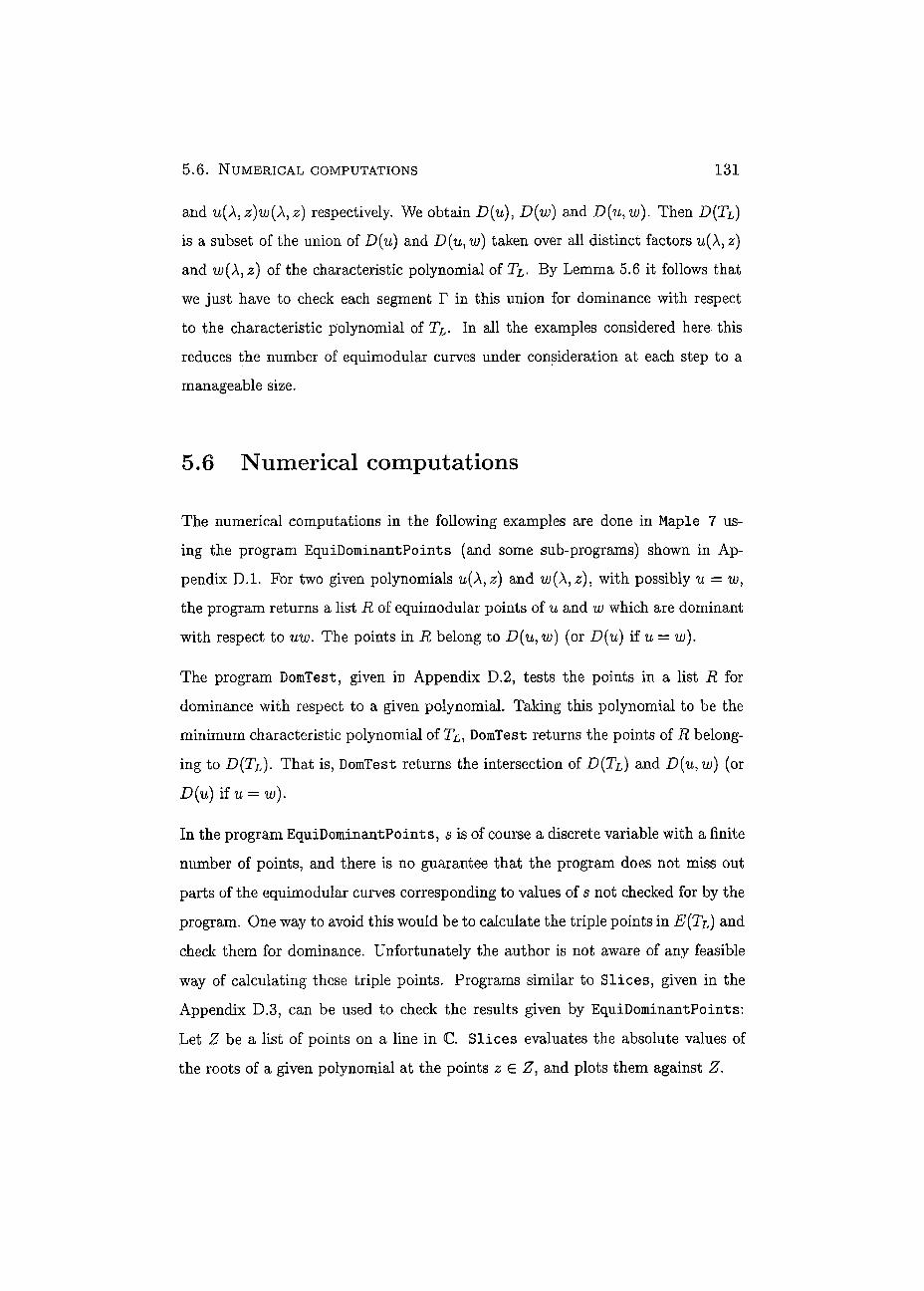
5 .6 . NUMERICAL COMPUTATIONS 131

and u(X, z)w(X, z) respectively. We obtain D(u), D(w) and D(u}w). Then D(TL)

is a subset of the union of D(u) and D(u, w) taken over ail distinct factors z)

and w(X,z) of the characteristic polynomial of TL. By Lemma 5.6 it follows that

we just have to check each segment T in this union for dominance with respect

to the characteristic polynomial of TL. In ali the examples considered here this

reduces the number of equimodular curves under considération at each step to a

manageable size.

5.6 Numerical computations

The numerical computations in the following examples are done in Maple 7 us-

ing the program EquiDominantPoints (and some sub-programs) shown in Ap-

pendix D.l. For two given polynomials u(X,z) and w(X,z), with possibly u — w,

the program returns a list R of equimodular points of u and w which are dominant

with respect to uw. The points in R belong to D(u, w) (or D(u) if u — w).

The program DomTest, given in Appendix D.2, tests the points in a list R for

dominance with respect to a given polynomial. Taking this polynomial to be the

minimum characteristic polynomial of T^, DomTest returns the points of R belong-

ing to D(TL). That is, DomTest returns the intersection of D{TI) and D(u,w) (or

D(u) if u = w).

In the program EquiDominantPoints, s is of course a discrete variable with a finite

number of points, and there is no guarantee that the program does not miss out

parts of the equimodular curves corresponding to values of s not checked for by the

program. One way to avoid this would be to calculate the triple points in E(TL) and

check them for dominance. Unfortunately the author is not aware of any feasible

way of calculating these triple points. Programs similar to Slices, given in the

Appendix D.3, can be used to check the results given by EquiDominantPoints:

Let Z be a list of points on a line in C. Slices evaluates the absolute values of

the roots of a given polynomial at the points z € Z: and plots them against Z.

5 . 6 . 1 . T H E PATH OF LENGTH THREE WITH THE IDENTITY LINKING SET 1 3 2

In the following we are using these programs to obtain approximations of dominant

points of the equimodular curves for various examples. This is not a full analysis of

these curves, and in fact there appear to be many unexplained phenomena leaving

space for future research. We assume that:

• The output of EquiDominantPoints with respect to u(A,z) and w(X: z) is

denoted by R(u,w) (or R(u) if u = w).

• We use 100 < n < 200 and e = 10~6 in EquiDominantPoints.

• In the following plots the intersection of the sets R(u) or R(uì w) with D(Tl) is represented by solid lines.

• Since the sets R(u), R(u, w) and D(Tl) are symmetric with respect to the

real axis we only show the positive half piane in the following plots.

• Points are represented by approximations to four decimai places.

• The complex variable z has been shifted by — 2.

5.6.1 The path of length three with the identity linking set

Let B be the path on three vertices and let L = {(1,1), (2,2), (3,3)} be the identity

linking set. The resulting graph Ln(B) has been considered in Example 3.12 and

the matrices NI for ali ir have been obtained. The characteristic polynomials are:

/0(A, z) = A2 + (-z3 - z 2 - 3z) A + z4 + z3 + z2- 1,

A, z) = { 1 + A) (A + z2) (A3 + 02(z) A2 + ax(z) A + a0(s)),

/(2)(A, z) = /<12>(A, Z) = (1 + A)(A - s - l)(z - X)(z - 2 - A),

/^ (A , z) = / ( l3 )(A, z)=\ + l and ^ ( A , z) = (A + l)2,

where a2(z) = 2z2 — z + 2, a\ (z) = z4 — 2z3 — 1 and

a0(z) = -z5 + 2z3 + z2 - 2z - 2.

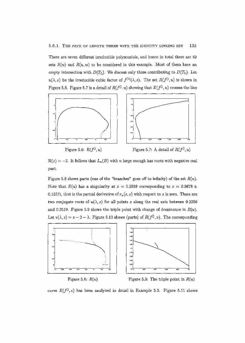
5 .6 .1 . THE PATH OF LENGTH THREE WITH THE IDENTITY LINKING SET 133

There are seven différent irreducible polynomials, and hence in total there are 49

sets and R(u, w) to be considered in this example. Most of them hâve an

empty intersection with D(TL)- We discuss only those contributing to D(TL). Let

u(\,z) be the irreducible cubic factor of f^(X,z). The set R(f(\u) is shown in

Figure 5.6: u) Figure 5.7: A detail of R(f\u)

SR(z) = - 2 . It follows that Ln (B) with n large enough has roots with negative real

part.

Figure 5.8 shows parts (one of the "branches" goes off to infinity) of the set R(u).

Note that E(u) has a singularity at z = 0.2889 corresponding to s = 0.9878 ±

0.1557z, that is the partial derivative of ru(s, z) with respect to 0 is zéro. There are

two conjugate roots of u(À, z) for ail points 2 along the real axis between 0.2256

and 0.3519. Figure 5.9 shows the triple point with change of dominance in R(u).

Let i>(À, z) = z — 2 — A. Figure 5.10 shows (parts) of R(f^K v). The corresponding

Figure 5.8: R(u) Figure 5.9: The triple point in R(u)

curve E(f(\v) has been analyzed in detail in Example 5.3. Figure 5.11 shows

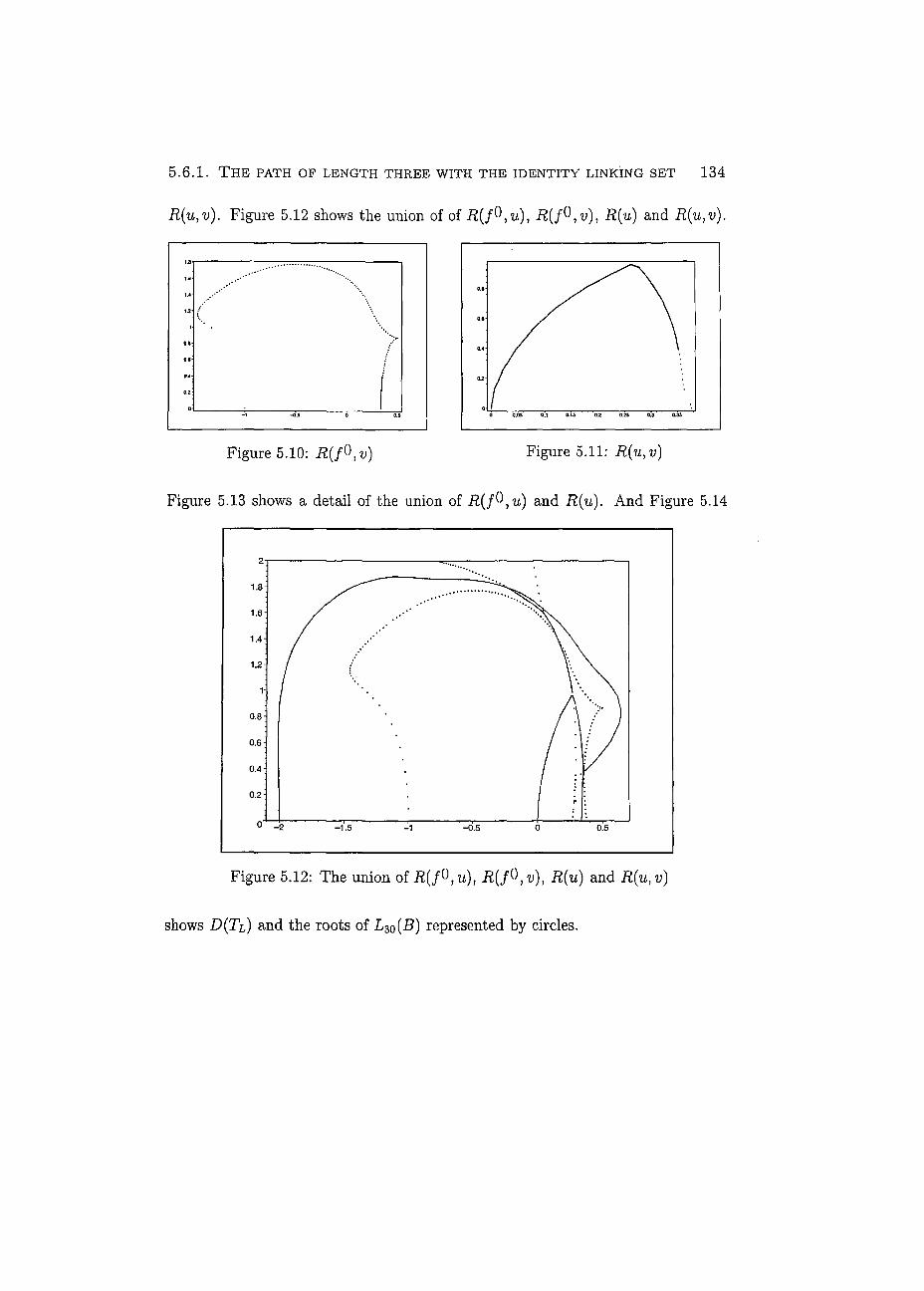
5 . 6 . 1 . T H E PATH OF LENGTH THREE WITH THE IDENTITY LINKING SET 1 3 4

R(u,v). Figure 5.12 shows the union of of R(f®,u), R{f(\v), R{u) and

Figure 5.10: R(f{\v) Figure 5.11: R(u,v)

Figure 5.13 shows a detail of the union of R(f^\u) and R(u). And Figure 5.14

Figure 5.12: The union of R{f°,u), R{f°,v), R{u) and R(u,v)

shows D(TL) and the roots of L,0(B) represented by circles.

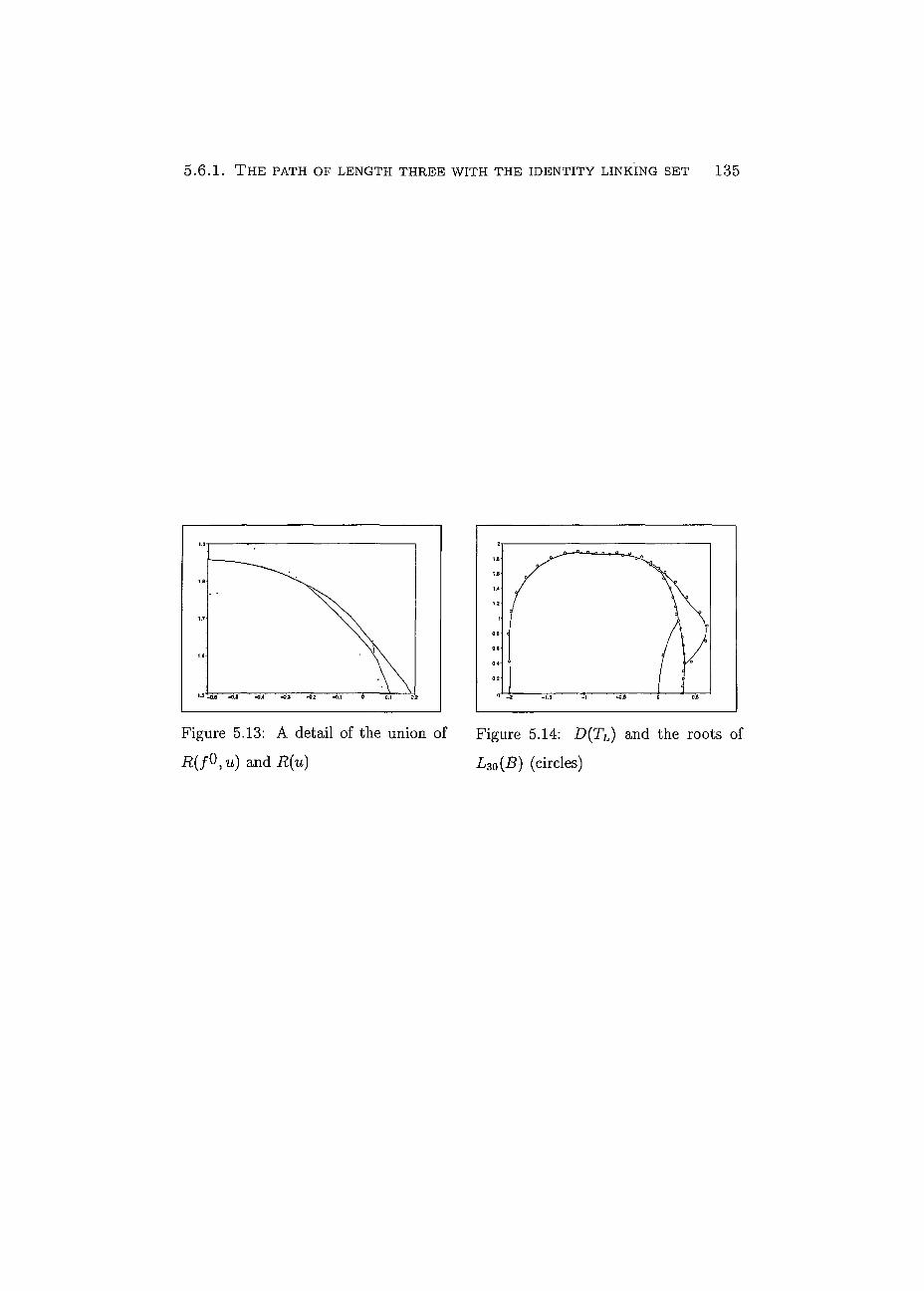
5 . 6 . 1 . T H E PATH OF LENGTH THREE WITH THE IDENTITY LINKING SET 135

Figure 5.13: A detail of the union of Figure 5.14: D{T£) and the roots of

R{f{\u) and R(u) Lzo(B) (circles)

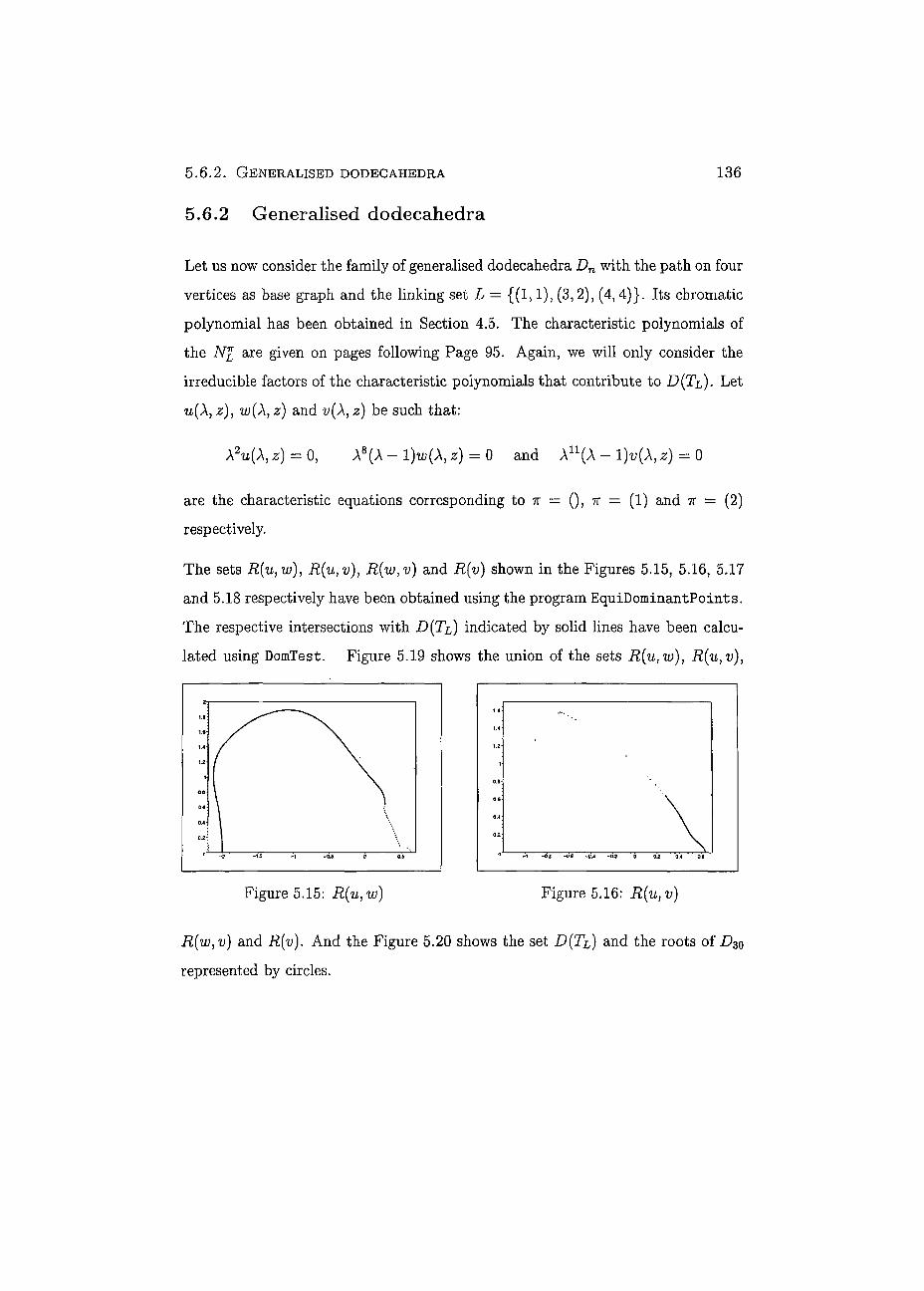
5.6 .2 . GENERALISED DODECAHEDRA 136

5.6.2 Generalised dodecahedra

Let us now consider the family of generalised dodecahedra DN with the path on four

vertices as base graph and the linking set L = {(1,1), (3,2), (4,4)}. Its chromatic

polynomial has been obtained in Section 4.5. The characteristic polynomials of

the NI are given on pages following Page 95. Again, we will only consider the

irreducible factors of the characteristic polynomials that contribute to D(TL). Let

u(X,z), w(X,z) and v(X,z) be such that:

A2u(A,2) = 0, A8(A — l)w(A, z) = 0 and AU(A - l)u(A, z) = 0

are the characteristic equations corresponding to 7r = (), 7r = (1) and 7r = (2)

respectively.

The sets R(u, w), R(u,v), R(w,v) and R(v) shown in the Figures 5.15, 5.16, 5.17

and 5.18 respectively have been obtained using the program EquiDominantPoints.

The respective intersections with D(TL) indicated by solid lines have been calcu-

lated using DomTest. Figure 5.19 shows the union of the sets R(u, w), R(u, v),

Figure 5.15: R(u,w) Figure 5.16: R(u, v)

R(wìv) and R(v). And the Figure 5.20 shows the set D(TL) and the roots of Z)30

represented by circles.

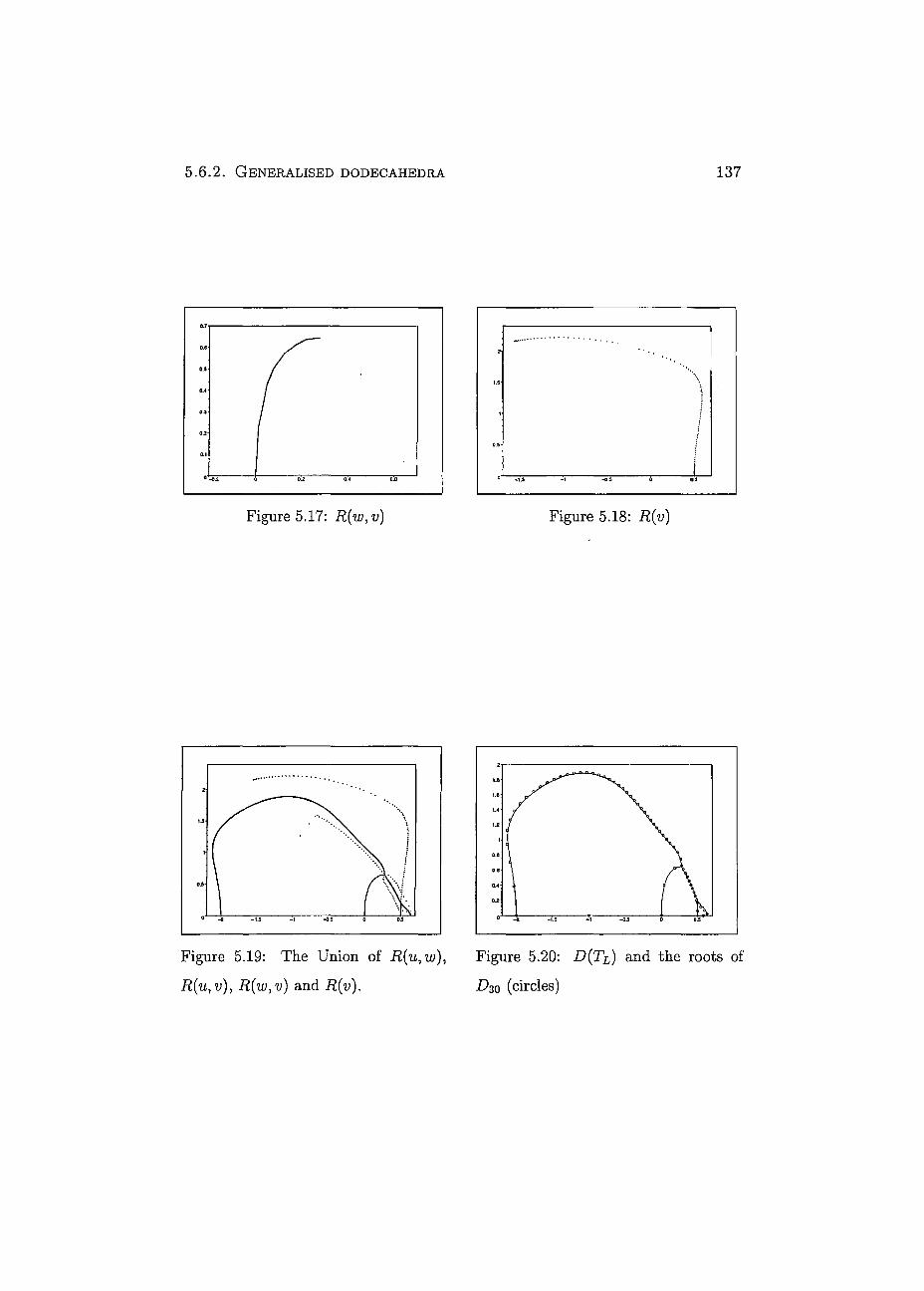
5 . 6 . 2 . GENERALISED DODECAHEDRA 137

0.5

Figure 5.17: R(w,v) Figure 5.18: R(v)

Figure 5.19: The Union of R(u,w), Figure 5.20: D(TL) and the roots of

R(u,v), R(w,v) and R(V). D^Q (circles)

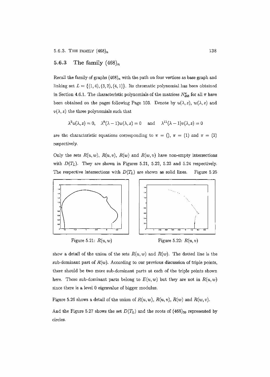
5.6.3. THE FAMILY (468)N

5.6.3 The family (468)n

138

Recali the family of graphs (468)n with the path on four vertices as base graph and

linking set L — {(1, 4), (3,2), (4,1)}. Its chromatic polynomial has been obtained

in Section 4.6.1. The characteristic polynomials of the matrices N%68 for all ir have

been obtained on the pages following Page 103. Denote by iü(A,2:) and

v(A, z) the three polynomials such that

À2IÌ(À, z) = 0, A8(A — l)W(A, z) — 0 and AN(A - 1)U(A,JS) = 0

are the characteristic équations corresponding to 7r = (), ir = (1) and 7r = (2)

respectively.

Only the sets R{u, w), R(u, Ü), R(W) and R(w,v) have non-empty intersections

with D(TL). They are shown in Figures 5.21, 5.22, 5.23 and 5.24 respectively.

The respective intersections with D(TL) are shown as solid lines. Figure 5.25

1.0-

1.4-

1.2

o.a

o.s

0.4

0 2

Figure 5.21: R(u,w) Figure 5.22: R(u,v)

show a detail of the union of the sets R(u,w) and R(w). The dotted line is the

sub-dominant part of R(w). According to our previous discussion of triple points,

there should be two more sub-dominant parts at each of the triple points shown

here. These sub-dominant parts belong to E(u, w) but they are not in R(u,w)

since there is a level 0 eigenvalue of bigger modulus.

Figure 5.26 shows a detail of the union of R(u, tu), R(uìv)ì R(w) and R(wyv).

And the Figure 5.27 shows the set D(TL) and the roots of (468)30 represented by

circles.

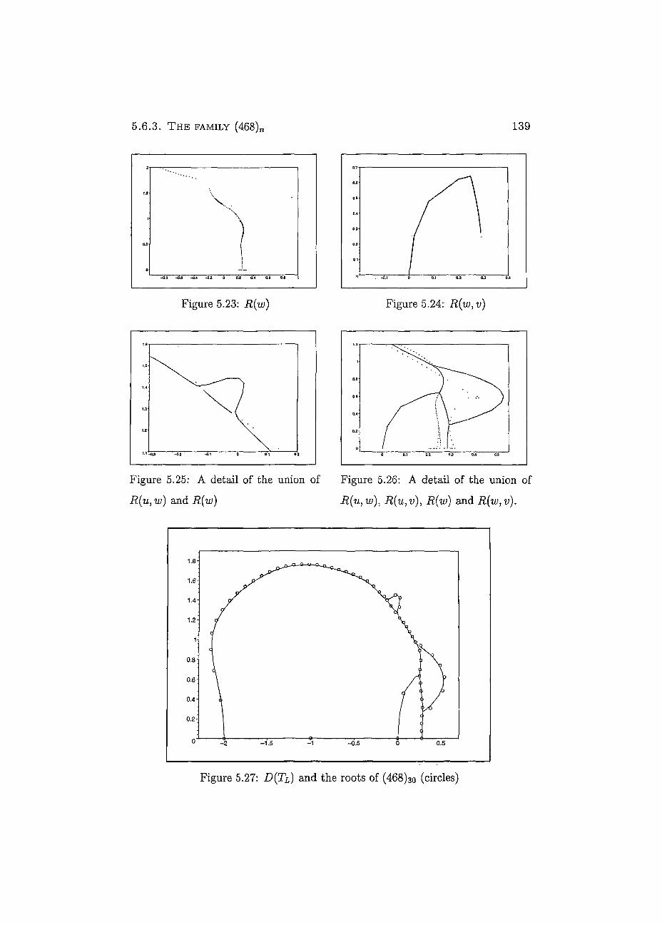
5.6.3. THE FAMILY (468)„ 139

Figure 5.23: R(w) Figure 5.24: R(w,v)

Figure 5.25: A detail of the union of Figure 5.26: A detail of the union of

R(u,w) and R(w) R(u, w): R(u,v), R(w) and R(w,v).

Figure 5.27: D(TL) and the roots of (468)30 (circles)

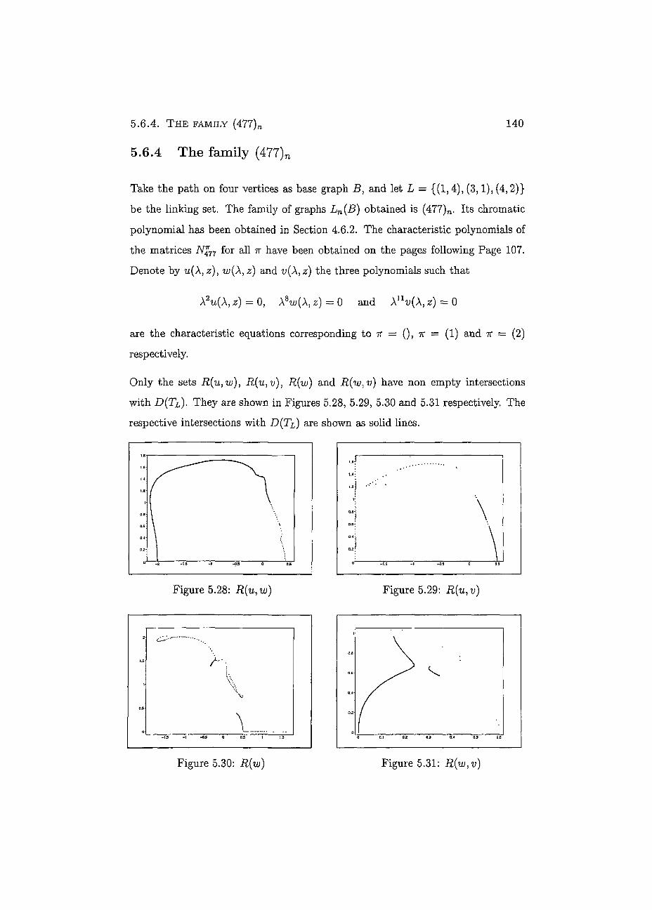
5 . 6 . 4 . T H E FAMILY ( 4 7 7 ) N

5.6.4 The family (477)n

140

Take the path on four vertices as base graph B, and let L = {(1,4), (3,1), (4,2)}

be the linking set. The family of graphs Ln(B) obtained is (477)n. Its chromatic

polynomial has been obtained in Section 4.6.2. The characteristic polynomials of

the matrices N%77 for all TV have been obtained on the pages following Page 107.

Denote by w(A,2), w(Xiz) and i>(A,2:) the three polynomials such that

A 2 U ( A , Z) = 0 , A 8 U;(A, Z) = 0 a n d A N W ( A , z) = 0

are the characteristic equations corresponding to it = (), 7T = (1) and 7r = (2)

respectively.

Only the sets R(u: w), R(u,v), R(w) and R(w,v) have non empty intersections

with D(TL). They are shown in Figures 5.28, 5.29, 5.30 and 5.31 respectively. The

respective intersections with D{T£) are shown as solid lines.

Figure 5.30: R(w) Figure 5.31: R(w, v)

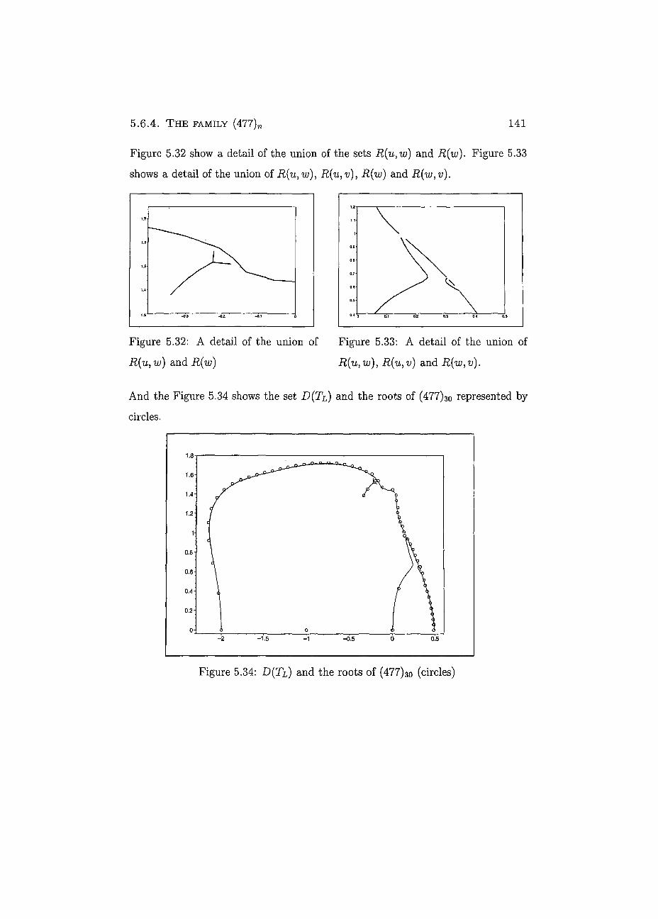
4 .6 .1 . T H E FAMILY (468)N 141

Figure 5.32 show a detail of the union of the sets R(u, w) and R(w). Figure 5.33

shows a detail of the union of R(u, w), R(u, v), R(w) and R(w,v).

Figure 5.32: A detail of the union of Figure 5.33: A detail of the union of

R(u,w) and R(w) R(u, w), R(u, v) and R(w,v).

And the Figure 5.34 shows the set D(TL) and the roots of (477)30 represented by circles.

Figure 5.34: D(TL) and the roots of (477)30 (circles)

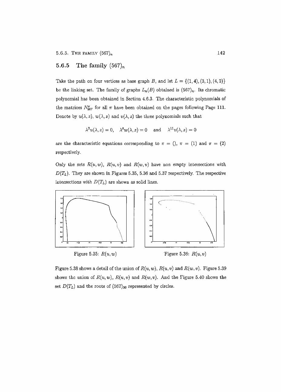
5 . 6 . 5 . T H E FAMILY ( 5 6 7 ) N

5.6.5 The family (567)

142

Take the path on four vertices as base graph B, and let L = {(1,4), (3,1), (4,2)}

be the linking set. The family of graphs Ln(B) obtained is (567)n. Its chromatic

polynomial has been obtained in Section 4.6.3. The characteristic polynomials of

the matrices Ng67 for ali ir have been obtained on the pages following Page 111.

Denote by U ( A , 2 ) , U>(A, z) and v(X,z) the three polynomials such that

A 2 U ( A , Z) = 0 , A 8 U ; ( A , Z) = 0 a n d A N T ; ( A , z) = 0

are the characteristic equations corresponding to TT = (), ir = (1) and ir = (2)

respectively.

Only the sets R(u, w), R(u,v) and R(wìv) have non empty intersections with

D(TL). They are shown in Figures 5.35, 5.36 and 5.37 respectively. The respective

intersections with D{TI) are shown as solid lines.

Figure 5.35: u>) Figure 5.36: R(ti,i>)

Figure 5.38 shows a detail of the union of R{uì w), R(u, v) and R(w, v). Figure 5.39

shows the union of R(u, w), R(u,v) and R(w,v). And the Figure 5.40 shows the

set D(TL) and the roots of (567)3q represented by circles.

5 . 6 . 6 . T H E FAMILY (666) N 143

Figure 5.37: R(w,v) Figure 5.38: A detail of the union of R(u¡ w), R(u, v) and R(w, v).

Figure 5.39: The union of R(uiw)1 Figure 5.40: D(TL) and the roots of

R(u,v) and R(w1v). (567)30 (circles)

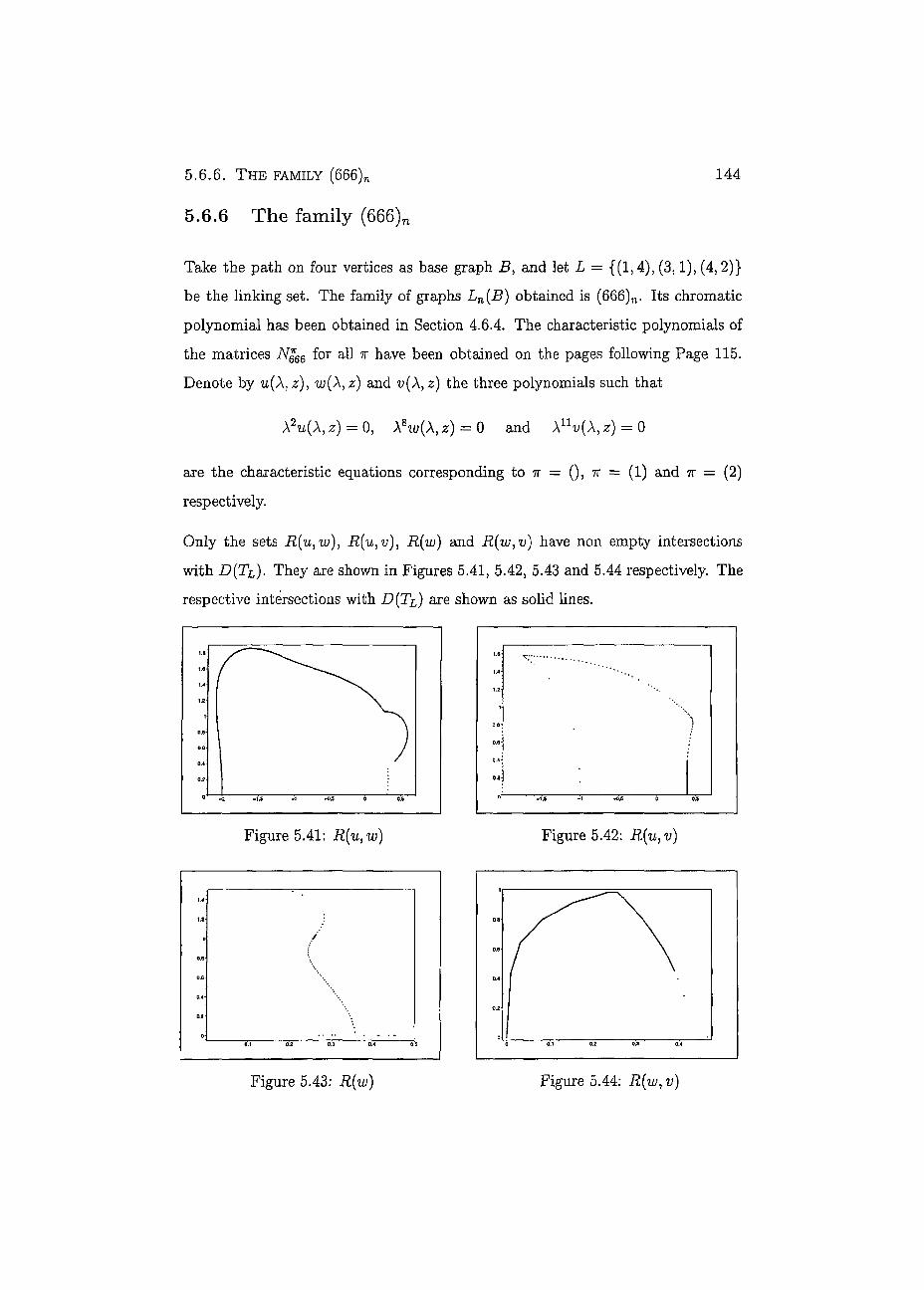
5 . 6 . 6 . T H E FAMILY ( 6 6 6 ) N

5.6.6 The family (666)

144

Take the path on four vertices as base graph B, and let L = {(1, 4), (3,1), (4,2)}

be the linking set. The family of graphs Ln(B) obtained is (666)n. Its chromatic

polynomial has been obtained in Section 4.6.4. The characteristic polynomials of

the matrices Ng66 for ali ir have been obtained on the pages following Page 115.

Denote by u(X, z), w(X,z) and v(X,z) the three polynomials such that

X2u(X, z) = 0, X8w(X, z) = 0 and Anv(À, z) = 0

are the characteristic equations corresponding to 7r = (), 7T = (1) and TV = (2)

respectively.

Only the sets Rlv^w), R(w) and -u) have non empty intersections

with D(TL). They are shown in Figures 5.41, 5.42, 5.43 and 5.44 respectively. The

respective intersections with D{TL) are shown as solid lines.

1.4

1.2'

1-

0.8

0.6

0.4

0.2-

0-

Figure 5.43: R{w)

1.8-

1.4-

1.2;

1-

0.0'

0.6

0.4

0.2

Figure 5.42: R(u, v)

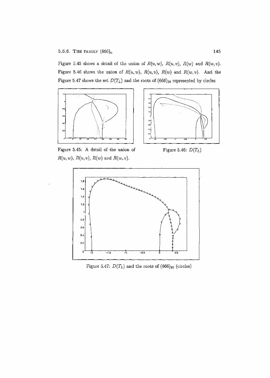
5 . 6 . 6 . T H E FAMILY (666)N 145

Figure 5.45 shows a détail of the union of R(u, n), R(w) and R(wìv).

Figure 5.46 shows the union of R(u} w), Rfav), R(w) and R(w,v). And the

Figure 5.47 shows the set D(TL) and the roots of ( 6 6 6 ) 3 0 represented by circles

Figure 5.45: A détail of the union of Figure 5.46: D(TL)

R(u, w), R(u,v), R(w) and R(w,v).

Figure 5.47: D{TL) and the roots of ( 6 6 6 ) 3 0 (circles)

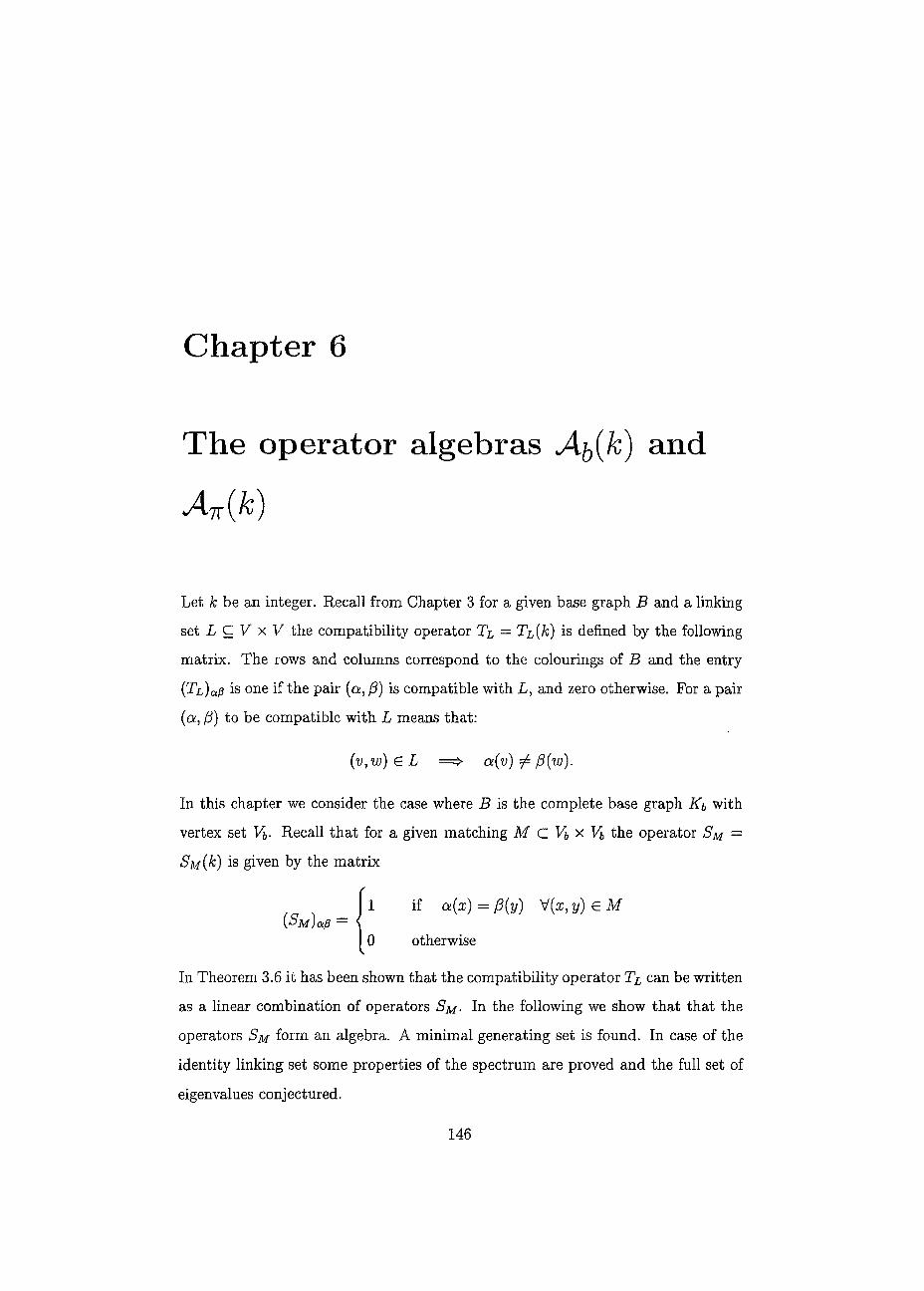
Chapter 6

The operator algebras A^k) and

Let k be an integer. Recali from Chapter 3 for a given base graph B and a linking

set L C V x V the compatibility operator T¿ = [k) is defined by the following

matrix. The rows and columns correspond to the colourings of B and the entry

(TL)Û^ is one if the pair (a, ¡3) is compatible with L, and zero otherwise. For a pair

(a, ¡3) to be compatible with L means that:

In this chapter we consider the case where B is the complete base graph Kb with

vertex set Vb. Recali that for a given matching M C Vb X Vb the operator S m =

SJII(fc) is given by the matrix

In Theorem 3.6 it has been shown that the compatibility operator can be written

as a linear combination of operators S m- In the following we show that that the

operators SM form an algebra. A minimal generating set is found. In case of the

identity linking set some properties of the spectrum are proved and the full set of

eigenvalues conjectured.

(v,w) G L => a(v) 7& p(w).

0 otherwise

146

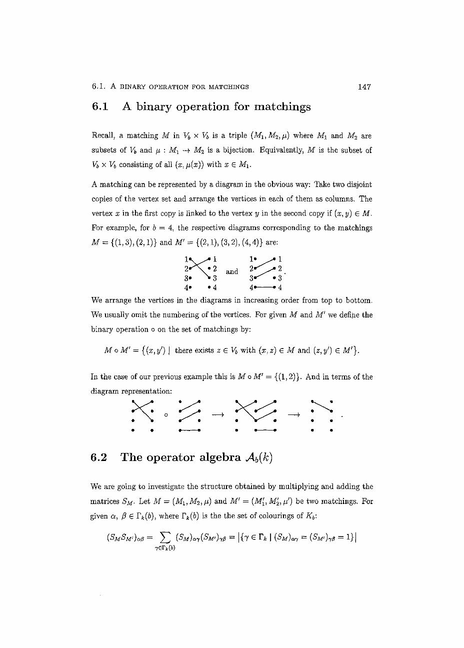
6.1 . A BINARY OPERATION FOR MATCHINGS 147

6.1 A binary opération for matchings

Recali, a matching M in Vb x V& is a triple (MiìM2ìfJ>) where M\ and M2 are

subsets of Vf, and ¡i : M\ —M2 is a bijection. Equivalently, M is the subset of

Vb x Vb consisting of ail (x:fj,{x)) with x G M\.

A matching can be represented by a diagram in the obvious way: Take two disjoint

copies of the vertex set and arrange the vertices in each of them as columns. The

vert ex x in the first copy is linked to the vertex y in the second copy if (x, y) G M.

For example, for b = 4, the respective diagrams corresponding to the matchings

M = {(1,3), (2,1)} and M' = {(2,1), (3,2), (4,4)} are:

1« ^ 1 V 1 2 » " x * 2 and 2 3* • 3 • 3 4* • 4 4* • 4

We arrange the vertices in the diagrams in increasing order from top to bottom.

We usually omit the numbering of the vertices. For given M and M' we defitte the

binary opération o on the set of matchings by:

M o M' = {(a;, y') | there exists z e Vb with (x, z) G M and (z, y') € M'}.

In the case of our previous example this is M o M' = {(1,2)}. And in terms of the

diagram représentation:

6.2 The operator algebra Ab{k)

We are going to investigate the structure obtained by multiplying and adding the

matrices SM- Let M = (Mlt M2i fj) and M' = (M[, M2, /1!) be two matchings. For

given a, ¡3 e Tk(b), where 1^(6) is the the set of colourings of K

[SMSM')aP — {£>M ) ay M' ) 7/? = |{7 ^ | ( S M) ori = (SM ' ) iP = 1}| ierk(b)

6 . 2 . T H E OPERATOR ALGEBRA Ab{k) 148

Observe that: (5,M)Û7 = 1 if 7 = ayT1 on M2

and {SM')^? — 1 if 7 = ¡3 y! on M{.

It follows that necessary conditions for (SMSM')ap ^ 0 a r e :

• a/z -1 = ftu' on M2 n M{

and since 7 is an injection:

• a i T l { M 2 \ (M2 n MO) H fin'(Mi \ (M2 H MO) = 0.

Suppose that a and ¡3 are such that above conditions are satisfied. Then 7 is

completely determined on M2 U M[ . For 7 on Vb \ (M2 U M[) there are

(A; - |M2 U M[\)(k - ]M2 U MIL - 1). . . (k - b + 1)

choices. Recall that we denoted the falling factorial by fs(d, k) = (k — s)d~s =

(k — s)(k — s — 1 ) . . . (k - d + 1). Hence the above conditions are also sufficient for

(•SMSM')UP 0, and in this case (SMSM>)ap = f\M2uM[\(b, k). Then: (SMSM')ap =

f\M2uM[\(b, k) if for ail (x,y) € M and (x',y') E M' it holds that

Q:(:E) = fi (y') if and only if y = x',

and (Sm S m') a fi = 0 otherwise.

Using the binary opération o on the matchings the first of the above necessary

conditions can be formulated as:

(•SM$M')ap 0 if {Sm°M')ocP = 1

Define the set of matchings AfMM» = {M \ M O M1 Ç M C MI X M2}. For

example for M = {(1,3), (2,1)} and M' = {(2,1), (3, 2), (4,4)}

Ar » • ^ ^ -N MM' —

Lemma 6.1 Let M = (Mu M2, ¡J,) and M' = (M[, M2, //) be two matchings. Then

SMSM' = (-L)LMOMYIM2UMil(B,K) ] T

6.3. A MINIMAL GENERATING SET 149

Proof: Let A, ß 6 1^(6) be given. We are comparing {SMSM')^ to

denoted by Let W{a,ß) = 6 Mi x MJ | a(a;) = ß(y')}. Then

{$M)(XP = 1 any M E jVMM' only if MC W(a, ß), and ( S = 0 otherwise.

We have to consider three cases:

(i) If M o M' % W{a, ß) clearly both (SmSm' W Haß a r e eQu alto zer0-

(ii) If M o M' = W{a, /3) from the argument preceding the lemma it follows that

{SMSM<)aß = /|M2UMÌ|(M)- In the sum we have {S^)aß = 1 only if M =

M o M'. Hence follows equality.

(iii) I f M o M ' c ß) then (SM^MO^ = A n d i n the s u m J2aß & h o l d s t h a t

(Sü)aß = 1 only if M Ç W(a, /?). It follows that:

E ( -1 ) , A | V*)aß = E ( - 1 ) 1 " 1 M£Mmm, MoM'CMCW(a,ß)

- (-l)iMoM 'l(l - ijdWia l-lMoAf'l)

This complétés the proof. •

Corollary 6.2 For every integer k the operators SM with M C Vj, x Vj, a matching

form an algebra Ab{k) over C. •

6.3 A minimal generating set

In this section we find a minimal generating set for Ab{k). Clearly there is a one-

to-one relationship between the matchings of size b and the elements of Sym&. For

any w € Symb the corresponding matching is defined as = {(CJ (y)^) \ y =

1, 2 , . . . , b}. Observe that if we write Mu as a triple (Mi, M2, then ß = u)~l.

Lemma 6.3 For any to and r in Symb the following holds: MW O MT = MWT.

6.3- A MINIMAL GENERATING SET 150

Proof: Recali

MU o MT = {(z,2/) | there exists z e VB with (x,z) G M,U and (z,y) G M r |

where (x, z) G MU if x = and (z, y) G MR if s = r(j/). Thus (x, y) G o MT

lî X = Lü(r(y)). •

Let er = (1 2 3 . . . ò) and <j) = (1 2) . The corresponding matchings are:

MA = {(2,1), (3, 2) , . . . , (0,0-1), (1,6)}

and Mj, = {(1,2), (2,1), (3,3), (4,4),..., (&, b)}.

Then, for example M+ o Ma = M ^ = {(3,1), (2,2), (4,3), (5,4),..., (1, b)}. From

Lemma 6.1 it follows that SmtSmw = Smuomt = Since a and <j> generate

Symb it follows that Ma and M^ generate all matchings of size 6. And thus, SMa

and S Mt generate every S^ with \M\ = b.

For any X Ç Vb denote by Mx the following matching

Mx = {(y,y)\yeVb\X}.

Then MYB is the empty matching and M0 = ME the "identity matching". If X = {2;} we write MX.

Choose any two x and y in Vbi and any UJ G Symb such that cj(y) = x. Then

MU-I OMXOMCJ = MY.

From Lemma 6.1 it follows that SMv = SMuj-1SMxSMw- Then, for some given a; G Vb

every matching M with \M\ — b — 1 can be written in the form M7 o My o MT for

some 7, T G Sym6. And SM = SMySMySMr-

Lemma 6.4 The set {SMS MSMx} for any given x G Vj, is a generating set for

the algebra Ab(k)

Proof: We will use a proof by induction on the size s of the matchings. The base

step is given by the argument preceding the lemma for s = b. Suppose now that

6.3 . A MINIMAL GENERATING SET 151

for some 0 < s < b all S m with \M\ > s are generated a by finite product of

the elements in {5m<,> S MSMx}- Let M' be any matching with \M'\ — s — 1.

Let M be a matching of size s containing M'. That is, M = M' U {(¿c,j/)} for

some (x,y) f M[ x M'2. Then M^ o M = M' and by Lemma 6.1 it follows that

= SM' H- where H is a linear combination of S M with \M\ > s. This

complétés the proof. •

This implies that for every integer k and every matching M there exists a poly-

nomial FM over C in three non commutative variables Ç</> and Çx such that

FMÌSMV, SM , SMx) = SM- For example FM^ = ÇaQ- Then Theorem 3.6 can be

written as

Tl = (-1)'M'-Pm('S,M<t3 Smj,, SMx)> MeM(L)

Example 6.1: Let b = 3. We write for example Fn^ rather than F{(iii)>(2,2)} or

Fmx• Then 11,22,33 = Cj a nd FIIj22 = (3- ^ convenient to use the diagrams in

order to obtain the FM- For example if M3 = « • and M2 =• • then

M a o M a o M z o M a = = • ••

From Lemma 6.1 it follows that -Fn>33 = CÎ-^ii^Co- = CC3 Cr and similarly 22,33

CxCaC

For M2 — • • and M 3 = • • the set NM2M3 = • • • •

With • ^ = 1 = Ma o Mç o Ma o Mo- o M3

6 . 4 . T H E OPERATOR ALGEBRA An{k) 1 5 2

and from Lemma 6.1 it follows that:

Fn — - 11,33- 11,22 + = aÌt + (<rC<p(a(3j

F22 = CaFuC, F33 = C^iiG and

F0 = FnF22/{k - 2) + F12 = FnF22/{k - 2) + Fn(<p

For L = { ( 1 , 1 ) , (2,2), ( 3 , 3 ) } , the identity linking set, we obtain the graphs Bn(3)

(see Example 3.1). The chromatic polynomial has been obtained in Example 3.8.

With the above, the matrix TL is equal to

F0 — (Fu + F2 2 + F33) + FLi ,22 + 1,33 + - 22,33 — 11,22,33

evaluated at SM^ SM^ and SMz-

Observe that if cSjf = SMSM' then |M| < min (|M|, |M'|), where c € €. It follows

that for every 0 < £ < b the set of SM with \M\ < i generates a subalgebra of

Ab{k).

6.4 The operator algebra A7V(k)

Recali that each SM is equivalent to a matrix of the form

© ( i r ® Ci ) . 0 <t<b 7fr-i

where In is the identity matrix of size equal to the dimension of the Specht module

S*k, and UM is a matrix of size (J)nn with entries depending on k. From Lemma 6.1

it follows that:

Lemma 6.5 Let 7r b t for some 0 < £ < b. For any integer k and any two

matchìngs M and M' inVbxVb we have

The set of the forms an algebra A^k) over C. •

6.4. THE OPERATOR ALGEBRA A-(FC) 153

Lemma 6.6 Let 7r h £ for some 0 < i <b. For any integer k the algebra k) is

isomorphic to the quotient algebra Ab{k) j I^SM \M\ < where ^SM | \M\ < i^J

is the subalgebra generated by all SM with \M\ < £.

Proof: The result follows from the observation that Ufa is the zero matrix if

\M\ <£. •

From Lemma 6.4 follows that:

Corollary 6.7 Let ir b £ for some 0 < £ < b. The set {Ufa^ Ufa^, Ufa J for some

x eVb is a generating set for the algebra A^k) •

Clearly the polynomials Fm over C in three non commutative variables (o-, and

Cx introduced in the previous section satisfy the condition that

FM{SMO-j Smj,, SMx) = SM

then FM(Ufaff, Ufa^ UfaJ = Ufa

with the extra property that FM(Ufat^ Ufa , Ufax) is the zero matrix if \M\ < £.

Further it is the case that

MeM(L)

The problem of calculating all the Ufa for a given b and 7r is thus equivalent to

finding the relevant FM and the three matrices Ufao, Ufa and Ufax.

Example 6.2: In Example 6.1 we obtained the polynomials for b = 3 and the

identity linking set. The matrices Ufa^, Ufa^ and Ufa3 for all ?r shown in Table 6.1

on Page 154 have been obtained in Example 3.7. Then iVJ is equal to

F& ~ (Fu + F22 + F33) + -Fll.22 + ^ 1 1 , 3 3 + ^22,33 — ^ 1 1 , 2 2 , . 3 3

evaluated at Ufa^, Ufa^ and Ufaz. It can easily be checked that the matrices obtained

here agree with the ones in Example 3.8.

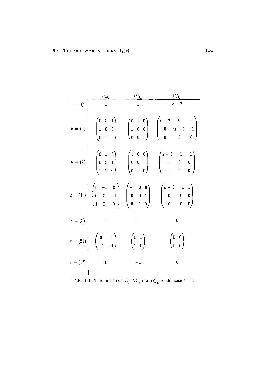
6 . 4 . T h e OPERATOR ALGEBRA A„(k) 1 5 4

* = 0

T = ( l )

t = (2)

» = (l2)

TT = (3 )

TT = (21)

TTTT Ma

A) 0 1

1 0 0

V° 1 V

0 1

- 1 - 1

TTTT uM4>

1 0

1 0 0

\0 0 1

TTTT u M 3

k~ 2

(k~ 2 0 -l\

0 k- 2 - 1

0 0 0

fo ì ° ì

il 0 ° ì

fk- 2 - 1 - A

0 0 1 0 0 1 0 0 0

V1 0 V 1° 1 l 0 0 0 j

- 1

fo -1 0 ^ f-1 0 ° ì

(k-2 - 1 A

0 0 - 1 0 0 1 0 0 0

[l o o j 1 ° 1 V l 0 0 0 J

0 TT = (l3)

Table 6.1: The matrices Ufaff, Ufa and Ufa3 in the case 6 = 3

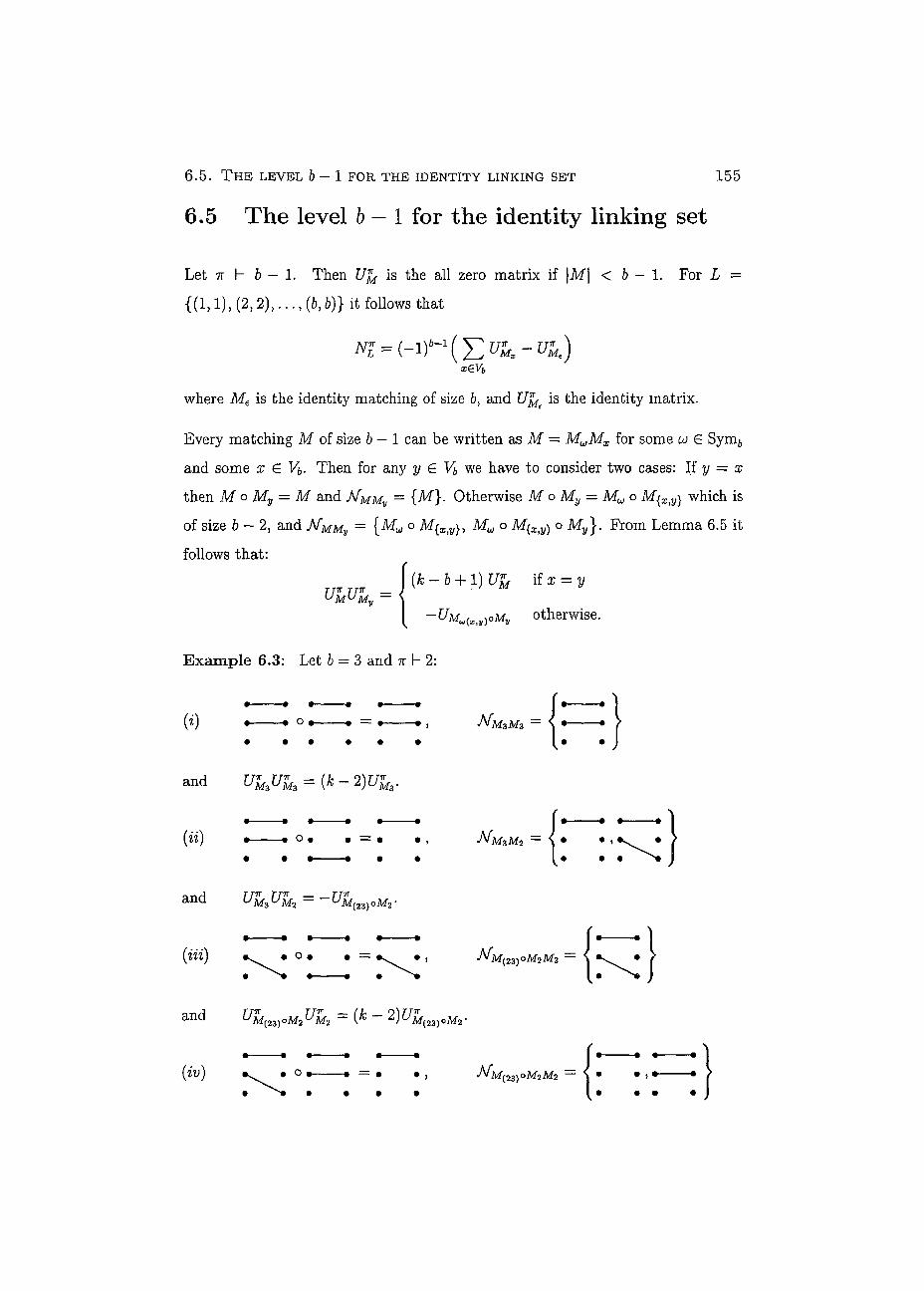
6 . 5 . T H E LEVEL b - 1 FOR THE IDENTITY LINKING SET 1 5 5

6.5 The level 6—1 for the identity linking set

Let 7T h b - 1. Then Ufo is the all zero matrix if \M\ < b - 1. For L =

{(1,1), (2,2), . . . , (6, &)} it follows that

sevi,

where Me is the identity matching of size ò, and Ufo is the identity matrix.

Every matching M of size ò — 1 can be written as M = MUMX for some CJ E Synif,

and some x E Vb. Then for any y E Vb we have to consider two cases: If y = x

then Mo My = M and MMMv = {M}. Otherwise M o My = Mw o M{X)y} which is

of size b — 2, and MMMv = o Mw o M(œjy) o M y } . From Lemma 6.5 it

follows that:

[k-b + l)Ufo if x = y

XiV)°My otherwise.

TT TT TT-* _ UMUMy —

Example 6.3: Let b = 3 and 7r h 2:

-• 9 • (O • • ° • • = • •, AÍM3Ms —

• • • • • •

and Ufo3Ufoz = (k - 2)Ufo3.

(<ii) • . o . . = • • , JVj M3M2 — \ • • 1

and UfoJJfo2 — —Ufo{23) oMa.

(¿Ü) • O • « = ». • , A/*M(23)OM2M2

and Ufo^)oM2Ufo2 — (k — 2 )Ufo[23)oM2.

(•IV) • O « » = « • , A/M(23)oM2M2 -• m-

• i • I • • •

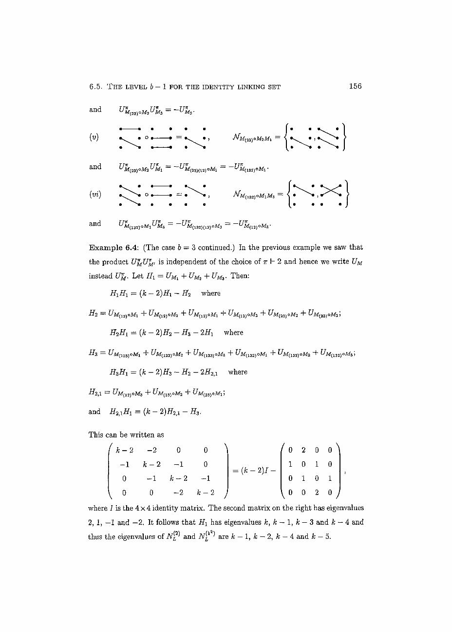
6.5. THE LEVEL b - 1 FOR THE IDENTITY LINKING SET 156

and Ut OM2 — ~ •

• O A/M, \23)OM2M\ —

and U«M{23)oM2U*Ml - Ufc[2sKi2)OMl — UM{132)0MX-

(vi) e • • •

A/m(132)oMiM3 = l * ^ ^ * i

NNH 77* TTTT — TTIR _ _R/7T ana V M^OM^ M3 — ^m(132){13)om3 - um (12)oM3 '

Example 6.4: (The case 6 = 3 continued.) In the previous example we saw that the product U^U^i is independent of the choice of 7r h 2 and hence we write UM

instead Ufa. Let HI = UMx + + UM3- Then:

H^Hi = (k- 2)Hi - H2 where

H2 — ^M(12)oMi + UM(12)0M2 + ^M(13)OMi + ^M(13)oM3 + UM( 23)OM2 + UM(2Z)OMZ\

H2Hx = {k- 2)H2 - HZ - 2HY where

Hz = UM(123)OMI + UM^iz)°M2 f Ai(123)oM3 H~ UM(i32)oM\ + UM^IZ2)OM2 ^M(132)oM3;

fTajffi = (/c - 2)Ä3 - Ä2 - 2F2}1 where

H2II = UM(12)omZ + Í/M(13) oM2 "F" ^M(23)0MI>

and F2)1F! = (* - 2 ) ^ 1 - #3-

This can be written as (

\

- 2 - 2 0 0 - 1 k — 2 -1 0 0 -1 k — 2 - 1

0 0 - 2 k-

\

= {k-2)I-

)

^ 0 2 0 0 1 0 1 0 0 1 0 1

y 0 0 2 0

\

J where I is the 4 x 4 identity matrix. The second matrix on the right has eigenvalues

2, 1, —1 and —2. It follows that Hi has eigenvalues k, k — 1, k — 3 and k — 4 and

thus the eigenvalues of N j p and iV^1 ^ are k — 1, k — 2, k — 4 and k — 5.

6.5. THE LEVEL b - 1 FOR THE IDENTITY LINKING SET 157

Let us now generalize these results for general b G N. Define the following two

opérations on the set of partitions A of b:

• For any two distinct nonzero parts A¿ and Aj denote by AAiVÀj" the partition

obtained by joining the part A ¿ and A j. For example (5,3,22,1)3V2 = (52,2,1).

• For any A¿ and 1 < q < A¿ denote by XqAXi~q the partition obtained by splitting

the part A¿ into a parts of size A¿ — q and q. For example (5, 3,22,1)2A1 = (5,23, l2).

For the rest of this section we assume that ali permutations are written as the

product of disjoint cycles. Let u G Sym6 and let x, y E V&. We consider the

product u(xy). There are two cases:

• If x and y are in the same orbit under u we can write

cj — ôJ(xa1a2 • • • aq-iyaq+i... aì) for some ôJ G Sym6. Then

u(xy) = üj(xaia2 ... aq-iyaq+1... a.i)(xy) = ÔJ(xaq+iaq+2 • • • di)(yaia2 ... aq-1).

• If x and y are in différent orbits under oj we can write u = c¡;(aia2 • • • Q>q-\%)

(bib2 . . . bp^iy) for some ZJ E Sym&. Then

cj(xy) = ZJ(aia2 ... aq^ix){bib2 ... bp-iy)(xy) - co(xbib2 ... òp_1ya1a2 ... i).

A conjugacy class of Sym6 is a subset of Sym6 containing ali permutations with a

certain cycle type. Henee there is a natural bijection between the conjugacy classes

of Sym¿, and the partitions A of b. Denote by C\ the conjugacy class corresponding

to A. For any u G C\ and any x,y G T4 it follows by the above arguments that:

• cj(xy) G CXqAXi-q if x and y are in the same orbit of size A¿ and ujq(x) = y or

= y.

• tü(xy) G C^vXj if x and y are in différent orbits of respective size A¿ and Xj.

Since UfaUfa, is independent of the choice of tt h b — 1 we write UM instead of Ufa.

For any UJ G Sym¿ and 1 < i < b let

X(cü, i) — {x G VB | x is in an orbit of length i under cu}.

6 .5. THE LEVEL b - 1 FOR THE IDENTITY LINKING SET 158

Defìne the operatore

= E E Um»° m*-

For example in Example 6.4 we can write: HX = Ì i ( ( l 3 ) , l ) , H2 = H((2,l),2),

H3 = H((3),Z) and = if((2,1), 1).

Lemma 6.8 Let U E C\ for some partition X of b. Let x E K be in an LO-orbit

under co of size Xand let y be any vertex in Vb. Then UMuoMxUMy is either:

• equal to (k - ò + 1)UMuOMx ifx = y, or

• a term in H(XXiS/Xi, Ài+Aj) ify is in an orbit under u) of size Xj not containing

x, or

• a term in H(X9AXi"q, q) voliere toQ(x) = y.

Proof: Recali from the beginning of this section:

{k-b + l)Ufa ìf x = y U"MU*My =

-UM^Xty)oMv otherwise.

The first two cases follow directly from the argument preceding the lemma. For

the case when x and y are in the same orbit of uì recali that

u){xy) = uj{xaia2 ... aq_iyaq+ì... ai)(xy) = U(xaq+iap+2 ... ai){yaia2 ... ag_i).

Hence, y is in a orbit of size q if uq(x) = y. •

Lemma 6.9 Let X be a partition of b. Let Xi and Xj be two non-zero parts with

i ^ j, but possibly Xi = Xj. Then every term in H(XXiVXi, Xi + Xj) can be written

UmwomxUmv where u E C\, x E Vb is in an orbit under u of size Xi and y E Vb

is in an orbit under oj of size Xj not containing x.

6.5. T H E LEVEL b - 1 FOR THE IDENTITY LINKING SET 159

Proof: By definition every term in H(XXIVXI, A¿ + AJ) is of the form UMT°MV for

some r E C^vx,- and y in an orbit of r of size A ¿ + A j. Let x be the element in the

orbit containing y such that TX*(X) = y. Then

r = r(aia2 . . . aXi-ixaXi+i... aXi+Xj-iy)

= r(aia2 ... axi-ix){axi+i... aXi+Xj~iy){xy)

for some r E Sym6. Let u = r(aia2... aA._1a;)(aAi+1... axi+Xj-iv)- Then u E Cx

and the result follows. •

Lemma 6.10 Let X be a partition of b, and A¿ be a non-zero part. For any 1 <

q < Xi — 1 every term in H(XqAXi~q, q) can be written as UmuomxUmv "where u E CX}

x,y E Vt are in an orbit under u of size X¿ and toq(x) = y.

Proof: By definition every term in H(XqAXi~q, q) is of the form UMtOMv for some

T E CXq^\i-q and y is in an orbit under r of size q. Choose any of the orbits under

T of size A q not containing y, and denote one of the vertices in this orbit by x.

Then

r — r(aia2... axi-q-ix)(axi-q+i... a^-iy)

= r(aia2 ... axi-g-ixaxi-q+i... aXi-iy){xy)

for some r E Symò. Let u = r(aio2 . . . ax.-q-ixax.-q+i... a^-iy). Then u E Cx

and the result follows. •

Theorem 6.11 Let X be any partition ofb, and X¿ be any non-zero part. Then

H(A, A¿) H((lb), 1) = (k - b + 1) iJ((lb), 1) - X ] Ai + Aj) Aj- distinct

in size Ai —1

r(A9AAi~9, Ai - q) (A¿ - q) H(XqAXi~qì q) 9=1

w/iere r(XqAXi~q, Ai — ç) ¿5 equal to the number of parts of size Xi — q in XqAXi~q if

Xi — q^q, and is equal to the number of parts of size Xi — q in XqAXi~q minus one if

Ai — q = q. The first sum in the above equation is over all parts Xj in X of distinct

size. This includes the possibility that Xj — Xi with j ^ i.

6 . 5 . T H E LEVEL b - 1 FOR THE IDENTITY LINKING SET 160

PROOF: This result follows from Lemma 6.8, Lemma 6.9 and Lemma 6.10. The factors in the second sum follow from counting in the proof of Lemma 6.10 the number of ways to choose an orbit under r of size Ai — qì and the number of ways to choose x in this orbit. •

For any given integer b denote by M(b) the operator on the space spanned by the

operators H(A, A*) such that (k — b + 1)7 — M(b) is the operator corresponding

to the multiplication on the right by H((lò), 1) as given in the previous theorem.

Here I is the identity operator.

EXAMPLE 6 . 5 : Let 6 = 4. There are five partitions of 4: (L4), (2, L2), (22) , (3,1)

and (4), and thus there are seven operators:

ir((l4),l), H{{ 22),2), #((3,1), 3), H(( 3,1),1),

H(( 2,12),2), H{{ 2,12),1) and ¿((4), 4).

Then

ff((l4),l)ii((l4),l

H((22),2) H({ 14),1

H{(3,l),3)H((li),l

i?((3,l),l)ir((l4),l

ÌT((2,12),2)H((14),1

H((2, l2), 1) H((l% 1

F ( ( 4 ) , 4 ) I F ( ( L 4 ) , L

= (k — 3)H((14), 1) — H((2, l2), 2);

= (k - 3)iT((22), 2) - H((4), 4) - ff((2, l2), 1);

= (k- 3)ff((3,1), 3) - H((4), 4) - 2H((2, l2), 2)

— 2H((2, l2), 1);

= (k — 3)i?((3,1), 1) — H({4), 4);

= (* - 3)H((2, l2), 2) - fT((3,1), 3) - 3ff((l4), 1);

= (k - 3)H((2, l2), 1) - H((3,1), 3) - Ji((22), 2);

= (fc - 3)H((4),4) - i?((3,1),3) - 3H((3,1), 1) — 2if((22), 2).

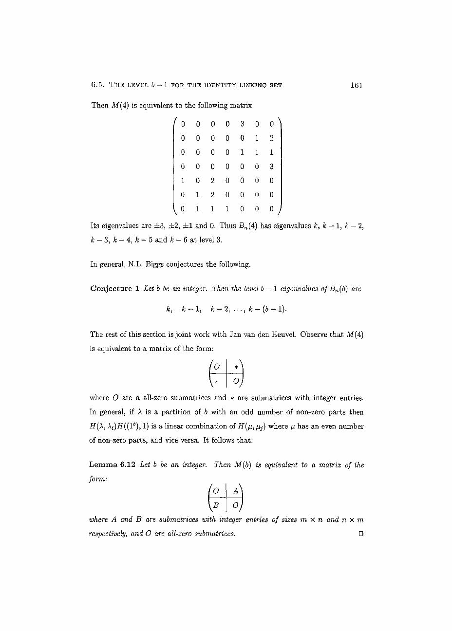
6.5. THE LEVEL B - 1 FOR THE IDENTITY LINKING SET 161

Then M(4) is équivalent to the following matrix:

f 0 0 0 0 3 0 0 \ 0 0 0 0 0 1 2

0 0 0 0 1 1 1

0 0 0 0 0 0 3 1 0 2 0 0 0 0

0 1 2 0 0 0 0

0 1 1 1 0 0 0 y

Its eigenvalues are ±3, ±2, ±1 and 0. Thus £n(4) has eigenvalues fc, k — 1, k — 2,

k — 3, k — 4, k — 5 and k — 6 at level 3.

In général, N.L. Biggs conjectures the following.

Conjecture 1 Let b be an integer. Then the level b — 1 eigenvalues of Bn(b) are

The rest of this section is joint work with Jan van den Heuvel. Observe that M(4)

is équivalent to a matrix of the form:

where O are a all-zero submatrices and * are submatrices with integer entries.

In général, if À is a partition of b with an odd number of non-zero parts then

iï(À, Xi)H((l6), 1) is a linear combination of H(pb, (j,j) where ¡JL has an even number

of non-zero parts, and vice versa. It follows that:

Lemma 6.12 Let b be an integer. Then M(b) is équivalent to a matrix of the

form:

where A and B are submatrices with integer entries of sizes m x n and n x m

k, k - 1, /c — 2, . . . , & — (& — !).

respectively, and O are all-zero submatrices. •

6 .5 . T H E LEVEL 6 - 1 FOR THE IDENTITY LINKING SET 162

Corollary 6.13 Let b be an integer. If X is an eigenvalue of M(b) then —X is also

an eigenvalue of M (b).

Proof: With Lemma 6.12 we can assume that M(6) is of the form:

where O are all-zero submatrices and A and B are submatrices with integer entries

of sizes m x n and n x m respectively. Suppose that A is a non-zero eigenvalue of

M M(b) and I is the corresponding eigenvector where v and u are the subblocks W

in sizes m and n respectively. From

(o À) B Oj U \JDV \U

it follows that Au = Xv and Bv = Xu. Since À is non-zero it follows that v and u

are non-zero. And thus

O A\( v\ = f-Au\ = /-A„\ = _A

B O \-u \Bv VA u \-u

That is | ] is an eigenvector of M (b) with eigenalue —A. • —u

Lemma 6.14 Let b be an integer. Then a matrix corresponding to M(6) has con-

stant row sums equal to b — 1.

Proof: Let A be any partition of b and Xp be any part in A. Let [i be an other

partition of b. Then

if and only if A is /¿wVAX-> for some parts /IJ and ¡ij with ¡±i + fij = Xp. The number

of pairs (fa, ¡ij) such that fii + fJ>j = Xp is equal to Xp — 1.

Further:

g) = H(A, Xp)

6 . 5 . T H E LEVEL b - 1 FOR THE IDENTITY LINKING SET 1 6 3

if and only if q = |AP| and ¡i is equal to AA'VAp for some part Xj. For each such fi

there is an operato H(X, Xp) with coefficient r(^ApAA->, Aj) (A ). The sum of ali this coefficients over ali such fi is equal to

E Xj = b - |AP|

It follows that the row sum of the row corresponding to H(Xy Xp) is equal to

6-|Ap| + |Ap|-l = 6 - l .

Since this holds for ali choices of A and Xp the result follows. •

Corollary 6.15 Let b he an integer. Then M(b) has eigenvalues ±(b — 1).

Proof: From Lemma 6.14 follows that the all-one vector v is an eigenvector with

eigenvalue 6 — 1. From Corollary 6.13 follows that 1 — 6 is also an eigenvalue. •

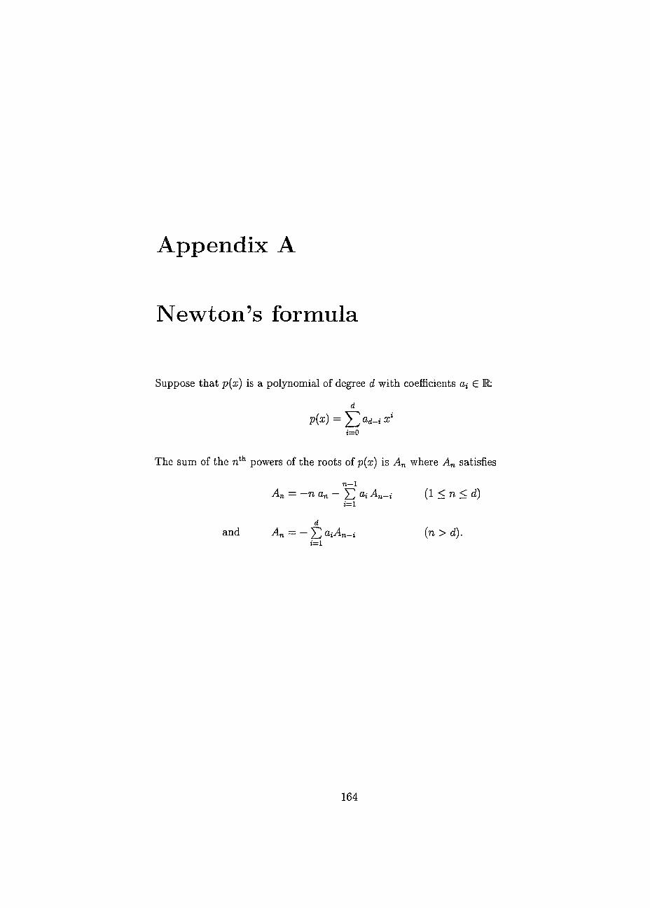
Appendix A

Newton's formula

Suppose that p(x) is a polynomial of degree d with coefficients ai G M:

d P(x) = ad~i x%

i=0

The sum of the nth powers of the roots of p(x) is An where An satisfies

n—1 An = -n an- J2 ai An-i (1 < n < d)

i=1

d and An = - aiAn_i (n > d).

i=1

164

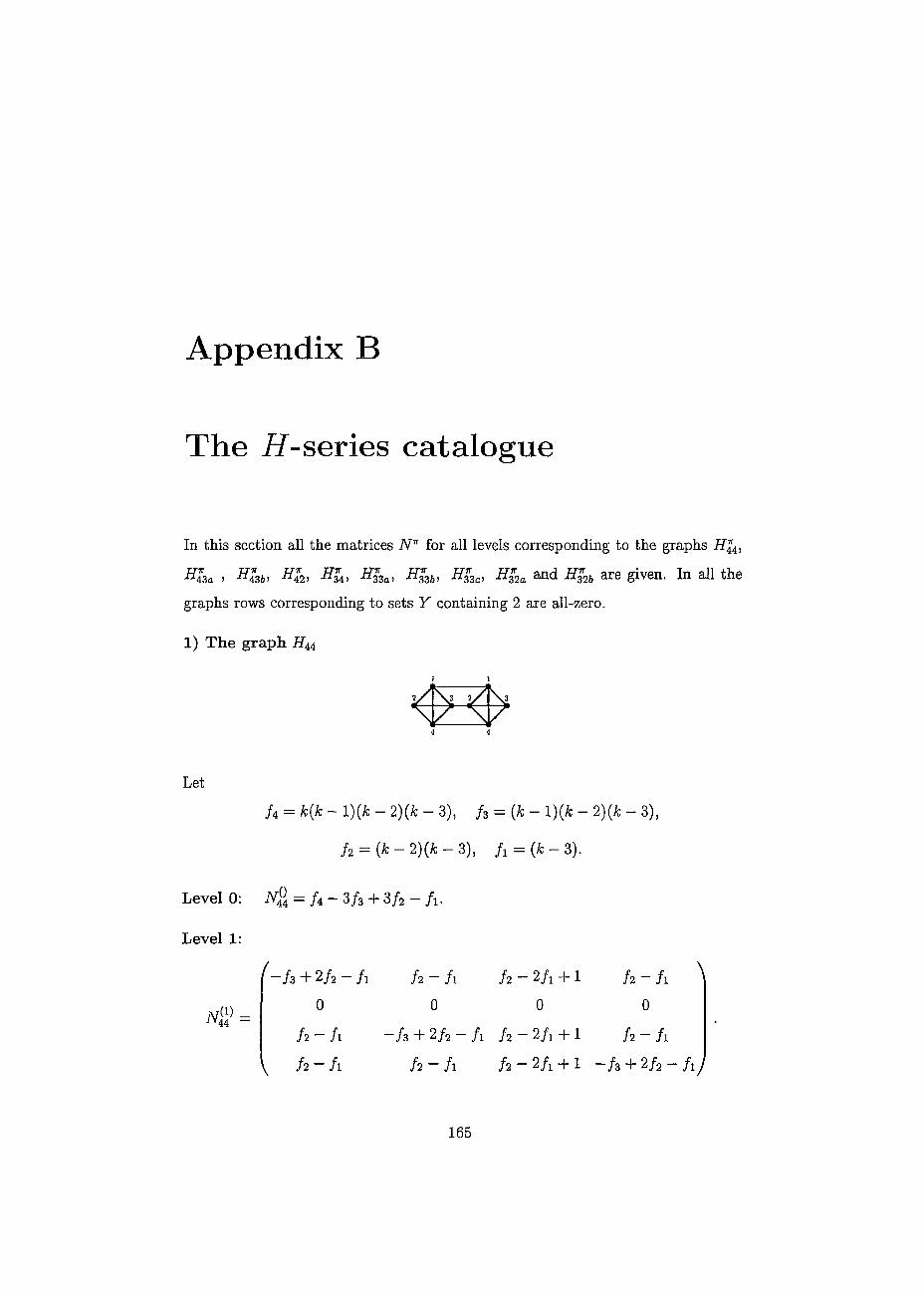
Appendix B

The H-series catalogue

In this section all the matrices Nn for all levels corresponding to the graphs ifj^,

H?3a , HZ36, Hl4, -H335) ¿ZJ3cJ ^32a and ^ are given. In all the

graphs rows corresponding to sets Y containing 2 are all-zero.

1) The graph Hu

Let

U = k{k - 1 ){k - 2)(Ä? - 3), h = {k- l)(k - 2){k - 3),

¡2 = {k — 2)(k — 3), / ! = (*;-3).

Level 0: JV£ = /4 - 3/3 4- 3/2 - A.

Level 1:

iv44 —

/ s + 2 / 2 - / l h - fl h - 2 / 1 + 1

0 0 0

h - h ~ h + 2/2 - A h - 2A + 1

/2 - /1 /2 - fi /a - 2 A + 1

h ~ fi ^ 0

/ 2 - / 1

- / a + 2 / 2 - / 1 /

165

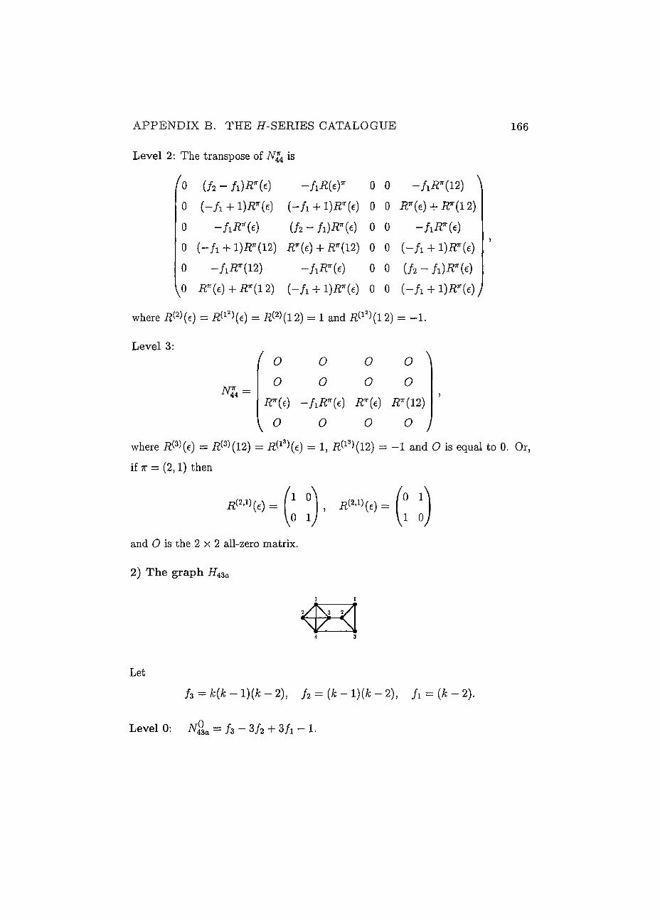
A P P E N D I X B. T H E F - S E R I E S C A T A L O G U E 166

Level 2: The transpose of Nfa is

fo ( / 2 - / i ) ^ ( e ) -fiR{e)* 0 0 - / iÄ*(12) ^

0 ( - A + l)iT(e) ( - A + l)R*{e) 0 0 iT(e) + JF(12)

0 -fil?(e) (h-fJR^e) 0 0 -fiB*{e)

0 ( - / i + 1)^(12) Rv{e)+ BT(12) 0 0 ( - A + l)R*(e)

0 -fiET(12) ~fiR*(e) 0 0 (/2 - / O ^ c )

v0 R"(e) + iF(12) ( - A + l)iT(e) 0 0 (~A + 1 W ) /

where = ^ ( e ) = i?(2)(l 2) = 1 and ^ ( l 2) = - 1 .

Level 3: ( O O O O ^

0 0 0 0 N* — i V44 — >

Ä*(e) —f\R*(e) R"{e) R*( 12)

K O O O O j

where R^{e) = 12) = i?(l3)(e) = 1, H(l3)(12) = - 1 and O is equal to 0. Or, if TT = (2,1) then

and O is the 2 x 2 all-zero matrix.

2) The graph H43a

4 3

Let

f3 = k(k-l)(k~2), }2 = {k~ l)(k-2), / i = ( Ä - 2 ) .

Level 0: N&a = f3 - 3f2 + 3A - 1.

A P P E N D I X B. T H E JT-SERIES C A T A L O G U E 167

Level 1:

JV(1) -43a —

/

V

Ä + 2 / i - l 0

/ i - l

/ i - l

/ i - 1 / i - 1 X

0 0

- / 2 + 2 / 1 - 1 /1 - 1

A - i - / 2 + 2 / 1 - i y

/V71" — JV43a —

0

Level 2:

( 0 0

(/1 ~ l)i^(e) -Ä*(c) -E*(12)

- i ^ e ) ( A - 1 )R*(e) —R*(e)

0 0 0

0 0 0

\ - iT(12) -R*(e) ( A - l )R*(e)J

where i^2)(e) = i?(l2)(e) = 1.

Level 3:

43a

( O ^ o

Ä(e)*

V 0 / where R{e)<3) = Ä(e)(l3) = 1 with O eqaal to 0, or if TT = (2,1) then

R^(e) =

and O is the 2 x 2 all-zero matrix.

3) The graph HA3b

Let

f3 = k(k-l)(k-2)t /2 = ( * - ! ) ( * - 2 ) , fx = (k-2).

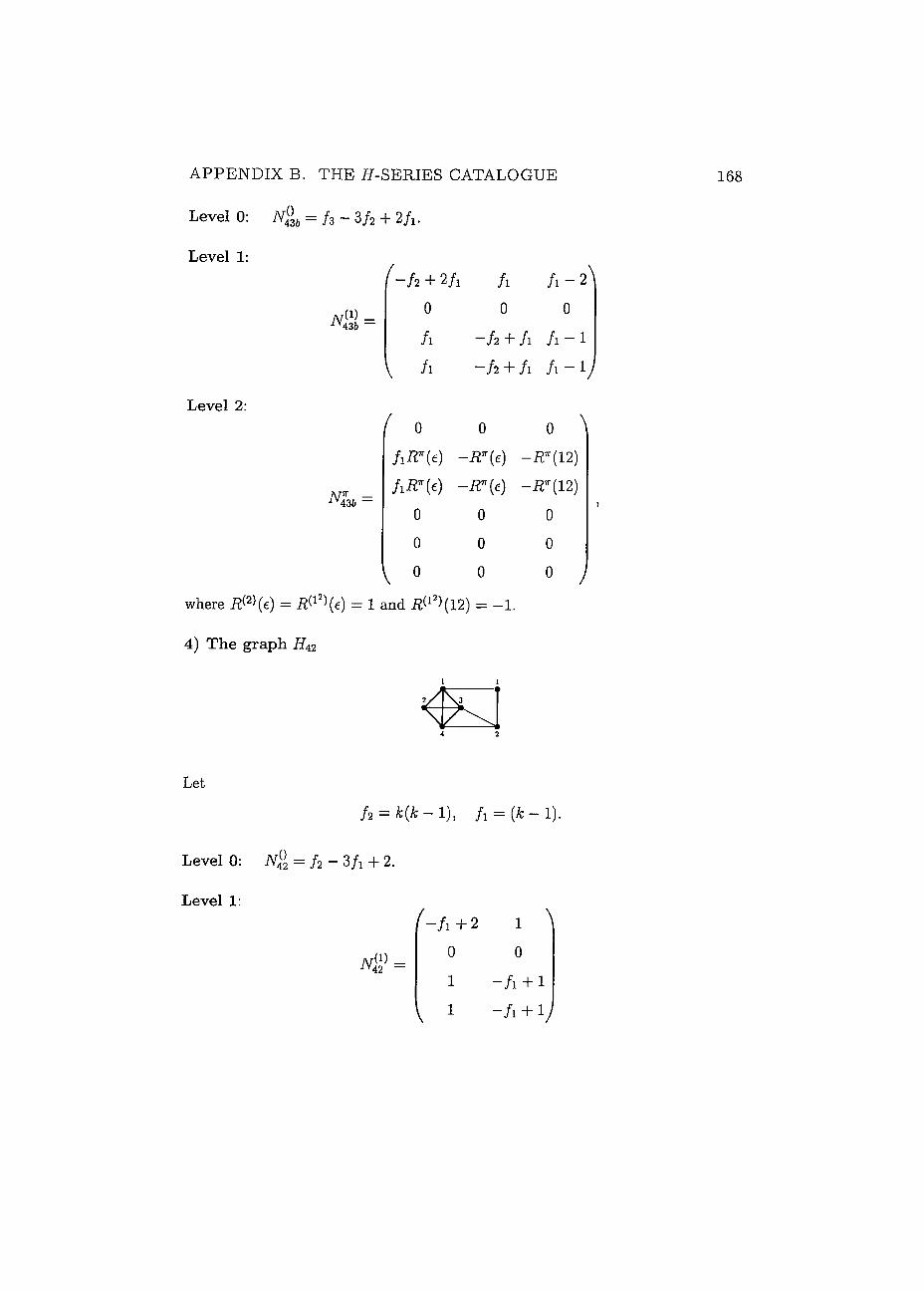
A P P E N D I X B. T H E F-SERIES C A T A L O G U E 168

Level 0: N&b = /3 - 3/2 + 2fv

Level 1:

Level 2:

N(1) -436 —

Ii

\ / l

_9\ /2 + 2/i /i /i - 2

0 0 0

- / 2 + / 1 / i - l

- / 2 + / 1 / i - y

/v71" — 436 —

/ 0 0 0 ^

/ ^ ( e ) -2F(e) -Ä»(12)

A-R^e) -iT(c) -¿^(12)

0 0 0

0 0 0

0 0 0

where Ä<2>(e) = i^2)(e) = 1 and #(l2)(12) = -1 .

4) The graph #42

\

Let

f2 = k(k- 1), /1 = (A: — 1).

Level 0: N& = f2 - 3fx + 2.

Level 1:

-

- / 1 + 2

0 1

1

1 \

0

- / 1 + 1

- / i + V

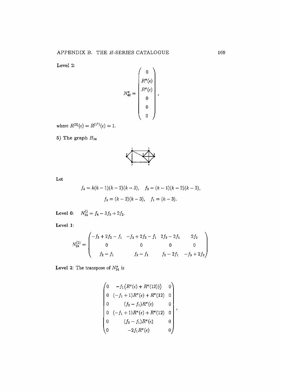
A P P E N D I X B. T H E ¿T-SERIES C A T A L O G U E 169

Level 2:

where R&(e) = Ä<l2>(c) == 1.

5) The graph Hu

Nn 42

( o \ R"(e)

R"(t)

0

0

V 0 /

l l

Let

U = k{k ~ 1 ){k - 2){k - 3), /3 = {k - 1)(Ä - 2)(k - 3),

¡2 = {k — 2){k — 3), fi — (k — 3).

Level 0: = /4 - 3/s + 2/2.

Level 1:

/ - / 3 + 2 / 2 - A - / 3 + 2 / 2 - Z x 2/2 — 2fi 2 h N

=

\ /2 - / l

0 0 0

/ 2 - / 1 h - 2/1 - / 3 + 2 / 2 ;

Level 2: The transpose of A^ is

0 - A (#*(<:)+ iT(12))) 0 0 ( - / i + 1 ) ^ ( 6 ) + ^ ( 1 2 ) 0

0 (f2 ~ fi)IT(e) 0

0 ( - A + l ) ir(e) + £7r(12) 0

0 ( / 2 - /OJFOO 0

V0 -2hR*{e) Oy

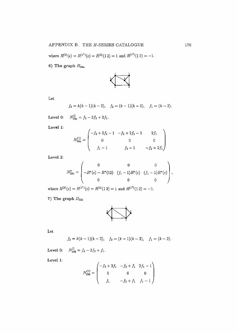
A P P E N D I X B. T H E # - S E R I E S C A T A L O G U E

where R&{e) = = R&{ 12) = 1 and Ä<l2>(l 2) = -1 .

6) The graph H33a

Let

/3 = * ( * - ! ) ( * - 2 ) , f2 = (k — l)(k — 2), / i = ( fc-2) .

Level 0: N&a = /3 - 3/2 + 2fx.

Level 1:

-33a —

( - h + V i - l - / 2 + 2 / 1 - I 2/j ^

0 0 0

V / 1 - 1 / 1 - 1 - / 2 + 2/1;

Level 2:

/V71" — 33a —

/ 0 0 0 ^ -Ä*(e) - Ä'(12) (/1 - 1)^(6) ( A - l ) Ä * ( € )

0 0 0

where Ä<2>(e) = R ^ { e ) = 12) = 1 and #(l2>(12) = - 1 .

7) The graph ii33ii

V

Let

/ 3 = FC(Ä-L)(FC-2), / 2 = ( Ä - 1 ) ( A : - 2 ) J fi = { k - 2).

Level 0: = /3 - 3/2 + /1 •

Level 1:

r(l) _ NK } -336 —

(~f2 + 2fl - / 2 + / 1 2/1 —

0 0 0

V A - / 2 + / 1 / 1 - 1 y

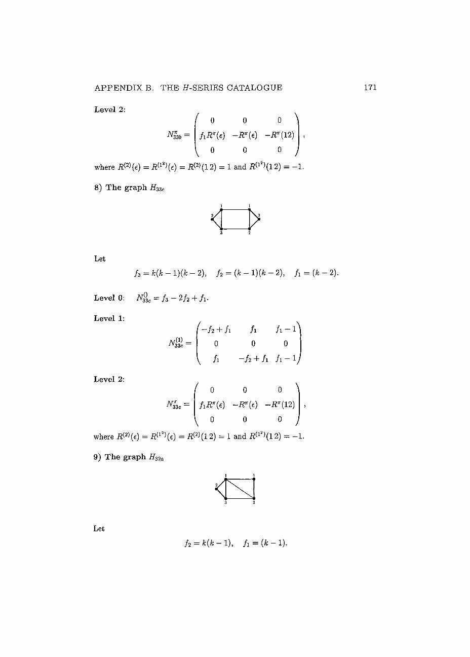
A P P E N D I X B. T H E JT-SERIES C A T A L O G U E 171

Level 2:

/V71" — 33f> ~

( 0 0 0

fiRn{e) -R*{e) -R*{ 12)

V / 0 0 0

where = R ^ { e ) = Ä<2>(12) = 1 and 1 2) = - 1 .

8) The graph if33c

<Z> Let

/3 = k(k - l)(k - 2), f2 = (k- l)(k - 2), A = (fc - 2).

Level 0: 7Vgc = /3 - 2/2 + / i .

Level 1:

TV. (i) _ 33c

/2 + / l / l / l - l

Level 2:

AP — 33c —

0 0 0

^ /i - / 2 + / i A - i y

( 0 0 0 \

/iÄ""(c) —Ä""(c) —Ä7r(12)

\ 0 0 0 y

where = R ^ { e ) = 12) = 1 and 2) = - 1

9) The graph H32a

Let

f2 — k{k l), f1 = (k- 1).

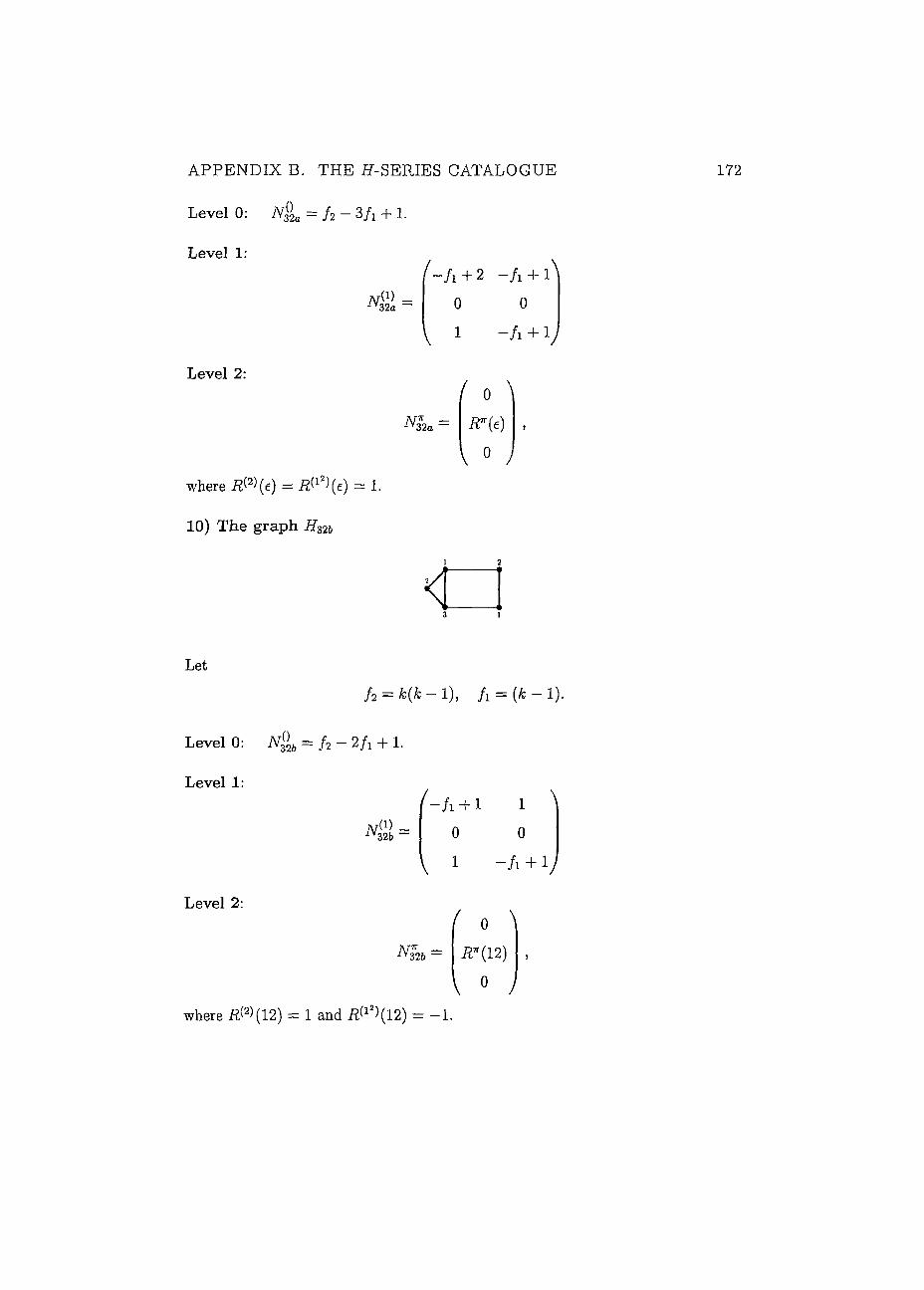
A P P E N D I X B. T H E F-SERIES C A T A L O G U E 172

Level 0: NL = f2 - Sfi + 1.

Level 1:

N^ -32a

/ - / i + 2 - / i + l^

0 0

1 - / i + v

Level 2:

where R^(e) = R ^ ( e ) = 1.

10) The graph H m

/V71" — iV32a —

f o N R"(t)

\ 0 I

< Let

/2 = * ( * - ! ) , /i = — 1).

Level 0: = f2 - 2A + 1.

Level 1:

iV(1) -32b ~

A + i l

0 o

1 -h + V

Level 2:

=

( o Ä»(12)

V 0 / where Ä<2>(12) = 1 and ä(i2>(12) = - 1 .

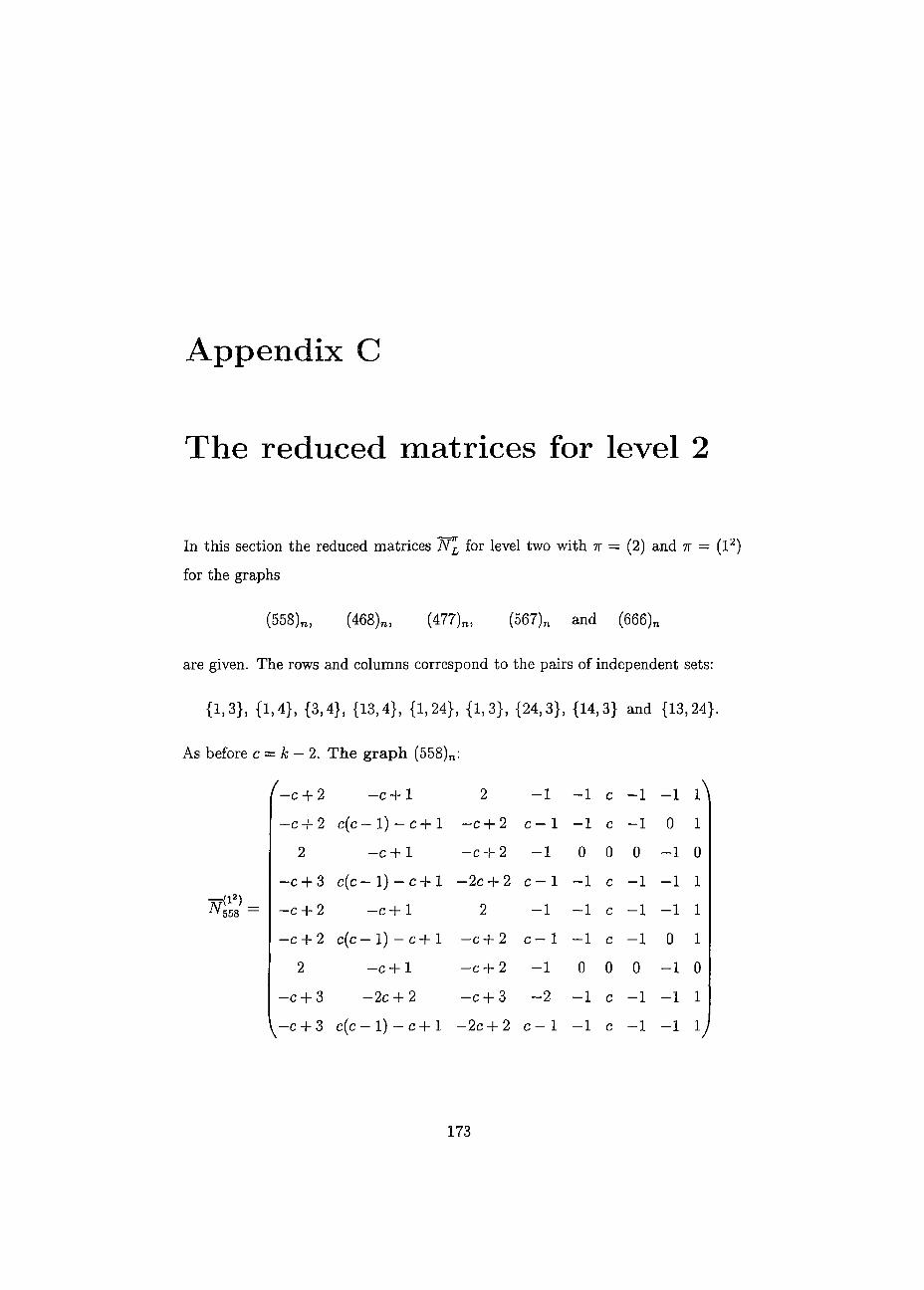
Appendix C

The reduced matrices for level 2

In this section the reduced matrices NL for level two with 7r = (2) and ir = (l2)

for the graphs

(558)„, (468)n, (477)n, (567)n and (666)n

are given. The rows and columns correspond to the pairs of independent sets:

{1,3}, {1,4}, {3,4}, {13,4}, {1,24}, {1,3}, {24,3}, {14,3} and {13,24}.

As before c = k — 2. The graph (558)n:

r - c + 2 - C + 1 2 - 1 —1 c — 1 - 1 M

- c + 2 c(c - 1) - c + 1 —c + 2 c - 1 —1 c — 1 0 1 2 - c + 1 —c + 2 - 1 0 0 0 - 1

—c + 3 c(c - l ) - c + l - 2 c + 2 c - 1 —1 c — 1 - 1 1 —c + 2 - c + 1 2 - 1 —1 c — 1 - 1 1

—c + 2 c(c - l ) - c + l —c + 2 c - 1 —1 c —1 0 1

2 - c + 1 —c + 2 - 1 0 0 0 - 1

- c + 3 - 2 c + 2 - c + 3 - 2 —1 c —1 - 1 1

\ - c + 3 c(c - l ) - c + l - 2 c + 2 c - 1 —1 c —1 - 1 V

173

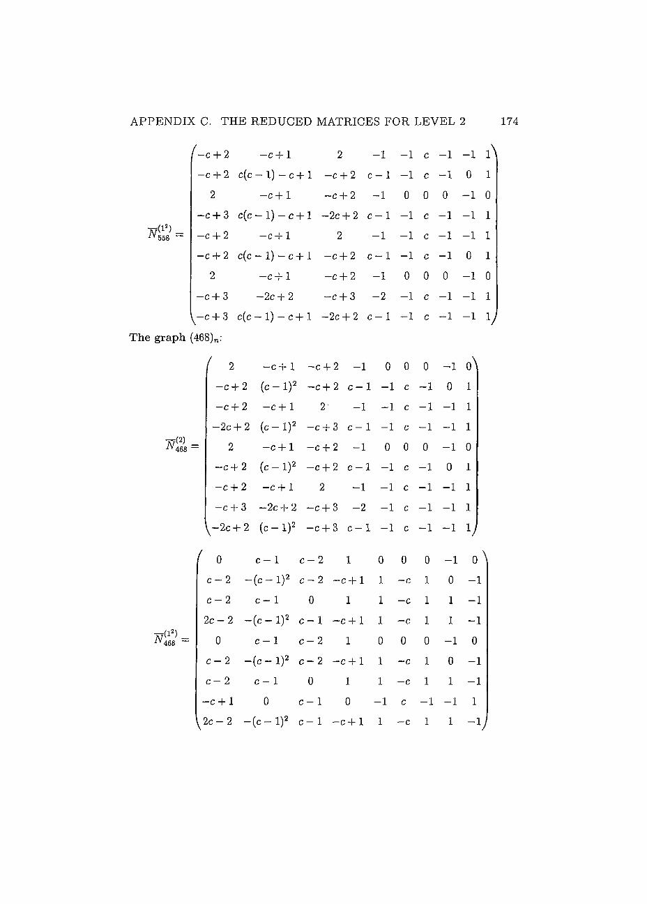
A P P E N D I X C. T H E R E D U C E D M A T R I C E S F O R L E V E L 2 174

F ( l 2 ) -iV 558 ~

(~c + 2 —c + 1 2 - 1 —1 c - 1 - 1 l\ - c + 2 c(c 1) c + 1 - c + 2 c - 1 —1 c - 1 0 1

2 —c + 1 - c + 2 - 1 0 0 0 - 1 0 - c + 3 c(c - l ) - c + l - 2 c + 2 c - 1 —1 c - 1 - 1 1 - c + 2 - c + 1 2 - 1 —1 c - 1 - 1 1 - c + 2 c(c l) C + 1 - c + 2 c - 1 —1 c - 1 0 1

2 c + 1 - c + 2 - 1 0 0 0 - 1 0 - c + 3 —2c + 2 - c + 3 - 2 —1 c - 1 - 1 1

c + 3 c(c - l ) - c + l - 2 c + 2 c - 1 —1 c - 1 - 1 V The graph (468)n:

N { 2 ) i V468

iV468 ~

f 2 - c + 1 - c + 2 - 1 0 0 0 - 1 Ol

- c + 2 ( c - 1 ) 2 - c + 2 c - 1 - 1 c —1 0 1

- c + 2 - c + 1 2 - 1 - 1 c — 1 - 1 1 - 2 c + 2 (c - l)2 - c + 3 c - 1 - 1 c —1 - 1 1

= 2 - c + 1 - c + 2 - 1 0 0 0 - 1 0 - c + 2 ( c - 1 ) 2 - c + 2 c - 1 - 1 c —1 0 1 - c + 2 - C + 1 2 - 1 - 1 c — 1 - 1 1 - c + 3 - 2 c + 2 - c + 3 - 2 - 1 c —1 - 1 1

2c + 2 ( c - 1 ) 2 - c + 3 c - 1 - 1 c —1 - 1 V 0 c — 1 c - 2 1 0 0 - 1 0 \

c - 2 - ( c - 1 ) 2 c - 2 -c + 1 1 —c 1 0 — 1 c — 2 c - 1 0 1 1 —c 1 1 — 1 2c-2 - ( c - 1 ) 2 c - 1 -c + 1 1 —c 1 1 — 1

0 c — 1 c - 2 1 0 0 - 1 0 c - 2 - ( c - 1 ) 2 c - 2 -c + 1 1 —c 1 0 1 c — 2 c - 1 0 1 1 —c 1 1 1 - c + 1 0 c - 1 0 - 1 c —1 - 1 1

i 2c — 2 -( c - 1 ) 2 c - 1 -c + 1 1 —c 1 1 1

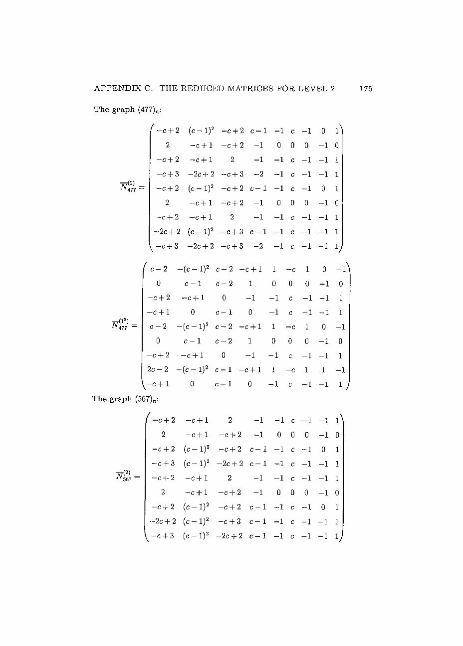
APPENDIX C. THE REDUCED MATRICES FOR LEVEL 2

The graph (477)n:

Äf(2) 477

F ( I 2 ) -477 —

F ( 2 ) -567 —

f -c + 2 ( c - 1 ) 2 - c + 2 c - 1 - 1 c - 1 0 A 2 - c + 1 - c + 2 - 1 0 0 0 - 1 0

- c + 2 - c + 1 2 - 1 - 1 c - 1 - 1 1 —c + 3 - 2 c + 2 —c + 3 - 2 - 1 c - 1 - 1 1 —c + 2 ( c - 1 ) 2 - c + 2 c - 1 - 1 c - 1 0 1

2 - C + 1 - c + 2 - 1 0 0 0 - 1 0 —c + 2 - c + 1 2 - 1 - 1 c - 1 - 1 1

- 2 c + 2 ( c - 1 ) 2 —c + 3 c - 1 - 1 c - 1 - 1 1 ^ - c + 3 - 2 c + 2 —c + 3 - 2 - 1 c - 1 - 1 V c — 2 -- ( c - 1 ) 2 c - 2 -c + 1 1 —c 1 0 - i

0 c — 1 c - 2 1 0 0 0 - 1 0 - c + 2 - c + 1 0 - 1 - 1 c - 1 - 1 1 - c + 1 0 c - 1 0 - 1 c - 1 - 1 1 c — 2 -( c - 1 ) 2 c - 2 -c + 1 1 —c 1 0 - 1

0 c — 1 c - 2 1 0 0 0 - 1 0 - c + 2 - c + 1 0 - 1 - 1 c - 1 - 1 1 2 c - 2 - ( c - 1 ) 2 c - 1 - c + 1 1 —c 1 1 - 1

- c + 1 0 c - 1 0 - 1 c - 1 - 1 1

7)n.

( -c + 2 - C + 1 2 - 1 - 1 c - 1 - 1 l\ 2 - c + 1 - c + 2 - 1 0 0 0 - 1 0

- c + 2 ( c - 1 ) 2 - c + 2 c - 1 - 1 c - 1 0 1 —c + 3 ( c - 1 ) 2 --2c+ 2 c - 1 - 1 c - 1 - 1 1

- c + 2 - c + 1 2 - 1 - 1 c - 1 - 1 1

2 - c + 1 -- c + 2 - 1 0 0 0 - 1 0 - c + 2 ( c - 1 ) 2 -- c + 2 c - 1 - 1 c - 1 0 1

- 2 c + 2 ( c - 1 ) 2 --c + 3 c - 1 - 1 c - 1 - 1 1

—c + 3 ( c - 1 ) 2 -•2c+ 2 c - 1 - 1 c - 1 - 1 V

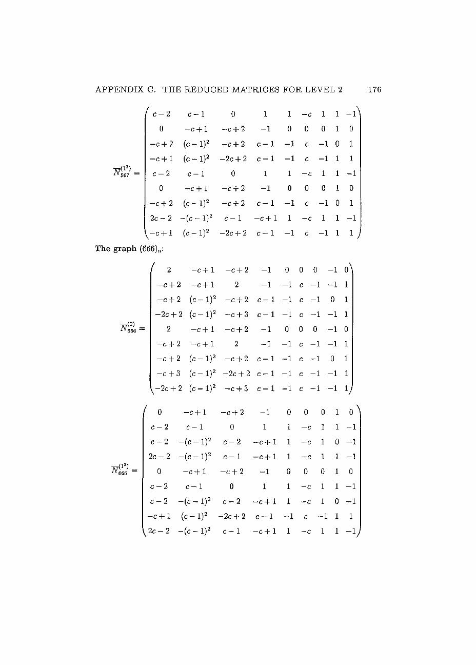
A P P E N D I X C. T H E R E D U C E D M A T R I C E S F O R L E V E L 2

1

n { i 2 ) -567 ~

( c — 2 c — 1

0 - c + 1

—c + 2 ( c - 1 ) 2

- c + 1 ( c - 1 ) 2

c — 2 c - 1

0 - c + 1

—c + 2 ( c - 1 ) 2

2 c - 2 - ( c - 1 ) 2

\-c+l ( c - 1 ) 2

The graph (666)n:

l 2 - c + 1 —c + 2 - c + 1 —c + 2 ( c - 1 ) 2

- 2 c + 2 ( c - 1 ) 2

2 - c + 1 —c + 2 - c + 1 —c + 2 ( c - 1 ) 2

—c + 3 ( c - 1 ) 2

\-2c + 2 ( c - 1 ) 2

( 0 - c + 1 c — 2 c - 1 c — 2 - ( c - 1 ) 2

2 c - 2 - ( c - 1 ) 2

0 - c + 1

c — 2 c - 1

c — 2 - ( c - 1 ) 2

- c + 1 ( c - 1 ) 2

\2c—2 - ( c - 1 ) 2

0 —c + 2 - 1

—c + 2 c - 1

- 2 c + 2 c - 1 0 1

—c + 2 - 1

—c + 2 c - 1

1 0

- 1 - 1

- c 1

0 0

c

c

1 - c

0 0

- 1 c

i - A 1 0

- 1 0 1 - 1 1 1 1 1 - 1 0 1 0

- 1 0 1

N (2) 666

2

—c + 2

2

—c + 2

N ( i 2 ) -J V 6 6 6 ~

0

C - 2

c - 1

—c + 2

0

c — 2

- c + 1 1 - c 1 1 - 1

c - 1 - 1 c - 1 1 1

- 1 0 0 0 - 1 o\ - 1 — 1 c - 1 - 1 1

c - 1 — 1 c - 1 0 1

c - 1 —1 c - 1 -1 1

- 1 0 0 0 -1 0 - 1 —1 c - 1 -1 1

c - 1 —1 c - 1 0 1

c - 1 —1 c - 1 -1 1

c - 1 —1 c - 1 -1 V

- 1 0 0 1 0 1 1 —c 1 1 — :

- c + 1 1 - c 1 0 — ;

- c + 1 1 - c 1 1 — ;

- 1 0 0 1 0

1 1 - c 1 1 —

- C + 1 1 - c 1 0 — :

c - 1 - 1 c - 1 1 L

- c + 1 1 - c 1 1 —i /

Appendix D

Maple programs

D . l The program EquiDominantPoints

The program EquiDominantPoints has as input a naturai number n, two polyno-mials /(A, z) and g(X, z) and a real number e > 0.

It first calculâtes the résultant detR(fSi g) with respect to A. This is a polynomial in

s and z with integer coefficients. For each point Si in a given sequence {sì}"=1 C S1

the program evaluates the roots of the résultant and saves them as a list R.

For each of these roots Ri the sub-program EquidomOne if / = g or EquidomTwo

if / g is called. In the case of EquidomOne the roots of f(X,Ri) are calculated,

the absolute values found and the biggest two compared. If their différence is less

than e the value Ri is saved as Pk and k increases by one.

In case of EquidomTwo the roots of/(À, Ri) and /(A, Ri) are calculated, the absolute values found and the respective biggest ones are compared. If their différence is less than e the value Ri is saved as Pk and k increases by one. In the end EquiDominantPoints returns the list Pk lying on the dominant equimodular curves D{f, g) (or D(f) if / = g).

177

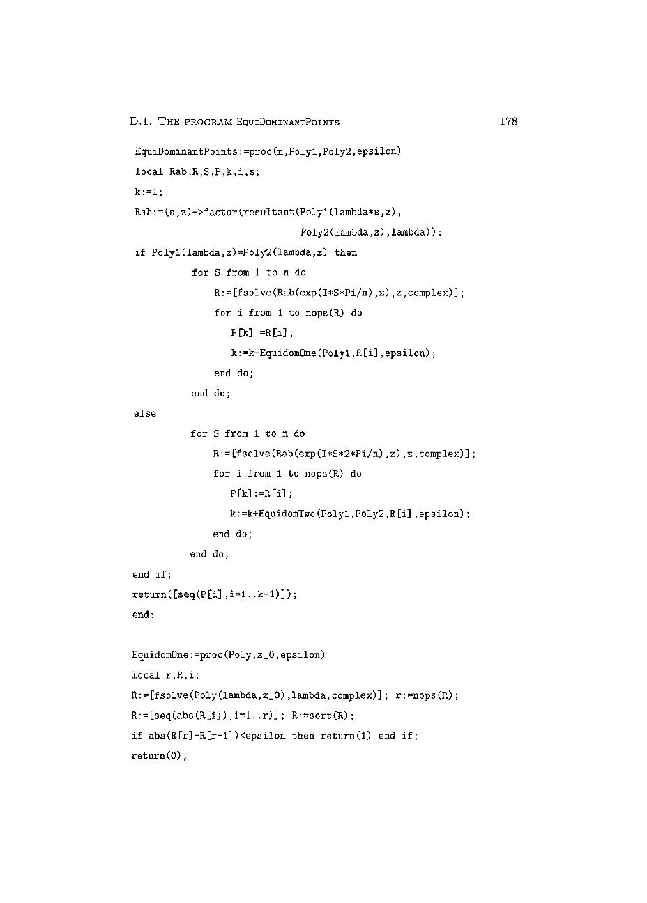
D . L . T H E PROGRAM EQUIDOMINANTPOINTS 178

E q u i D o m i n a n t P o i n t s : = p r o c ( n , P o l y 1 , P o l y 2 , e p s i l o n )

l o c a l R a b , R , S , P , k , i , s ;

k : = l ;

R a b : = ( s , z ) - > f a c t o r ( r é s u l t a n t ( P o l y l ( l a m b d a * s , z ) ,

P o l y 2 ( l a m b d a , z ) , l a m b d a ) ) :

i f P o l y l ( l a m b d a , z ) = P o l y 2 ( l a m b d a , z ) t h e n

f o r S f r o m 1 t o n d o

R : = [ f s o l v e ( R a b ( e x p ( I * S * P i / n ) , z ) , z , c o m p l e x ) ] ;

f o r i f r o m 1 t o n o p s ( R ) d o

P [ k ] : =R [ i ] ;

k : = k + E q u i d o m O n e ( P o l y l , R [ i ] , e p s i l o n ) ;

e n d d o ;

e n d d o ;

e l s e

f o r S f r o m 1 t o n d o

R : = [ f s o l v e ( R a b ( e x p ( I * S * 2 * P i / n ) , z ) , z , c o m p l e x ) ] ;

f o r i f r o m 1 t o n o p s ( R ) d o

P [ k ] : =R C i ] ;

k : = k + E q u i d o m T w o ( P o l y l , P o l y 2 , R [ i ] , e p s i l o n ) ;

e n d d o ;

e n d d o ;

e n d i f ;

r e t u r n ( [ s e q ( P [ i ] , i = l . . k - 1 ) ] ) ;

e n d :

E q u i d o m O n e : = p r o c ( P o l y , z _ 0 , e p s i l o n )

l o c a l r , R , i ;

R : = [ f s o l v e ( P o l y ( l a m b d a , z _ 0 ) , l a m b d a , c o m p l e x ) ] ; r : = n o p s ( R ) ;

R : = [ s e q ( a b s ( R [ i ] ) , i = l . . r ) ] ; R : = s o r t ( R ) ;

i f a b s ( R [ r ] - R [ r - 1 ] ) < e p s i l o n t h e n r e t u r n ( l ) e n d i f ;

r e t u r n ( 0 ) ;

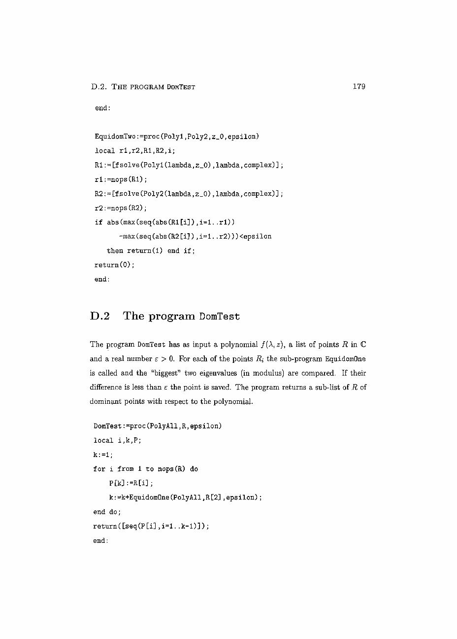
D . 2 . T H E PROGRAM DOMTEST 179

e n d :

E q u i d o m T w o : = p r o c ( P o l y l , P o l y 2 , z _ 0 , e p s i l o n )

l o c a i r l , r 2 , R l , R 2 , i ;

R I : = [ f s o l v e ( P o l y l ( l a m b d a , z _ 0 ) , l a m b d a , c o m p l e x ) ] ;

r i : = n o p s ( R l ) ;

R 2 : = [ f s o l v e ( P o l y 2 ( l a m b d a , z _ 0 ) , l a m b d a , c o m p l e x ) ] ;

r 2 : = n o p s ( R 2 ) ;

i f a b s ( m a x ( s e q ( a b s ( R l [ i ] ) , i = l . . r i ) )

- m a x ( s e q ( a b s ( R 2 [ i ] ) , i = l . . r 2 ) ) ) < e p s i l o n

t h e n r e t u r n ( 1 ) e n d i f ;

r e t u r n ( 0 ) ;

e n d :

D.2 The program DomTest

The program DomTest has as input a polynomial f(\,z), a list of points R in C and a real number e > 0. For each of the points Ri the sub-program EquidomOne is called and the "biggest" two eigenvalues (in modulus) are compared. If their difference is less than e the point is saved. The program returns a sub-list of R of dominant points with respect to the polynomial.

D o m T e s t : = p r o c ( P o l y A l l , R , e p s i l o n )

l o c a i i , k , P ;

k : = l ;

f o r i f r o m 1 t o n o p s ( R ) d o

P [ k ] : = R [ i ] ;

k : - k + E q u i d o m O n e ( P o l y A l l , R [ 2 ] , e p s i l o n ) ;

e n d d o ;

r e t u r n ( [ s e q ( P [ i ] , i = l . . k - 1 ) ] ) ;

e n d :

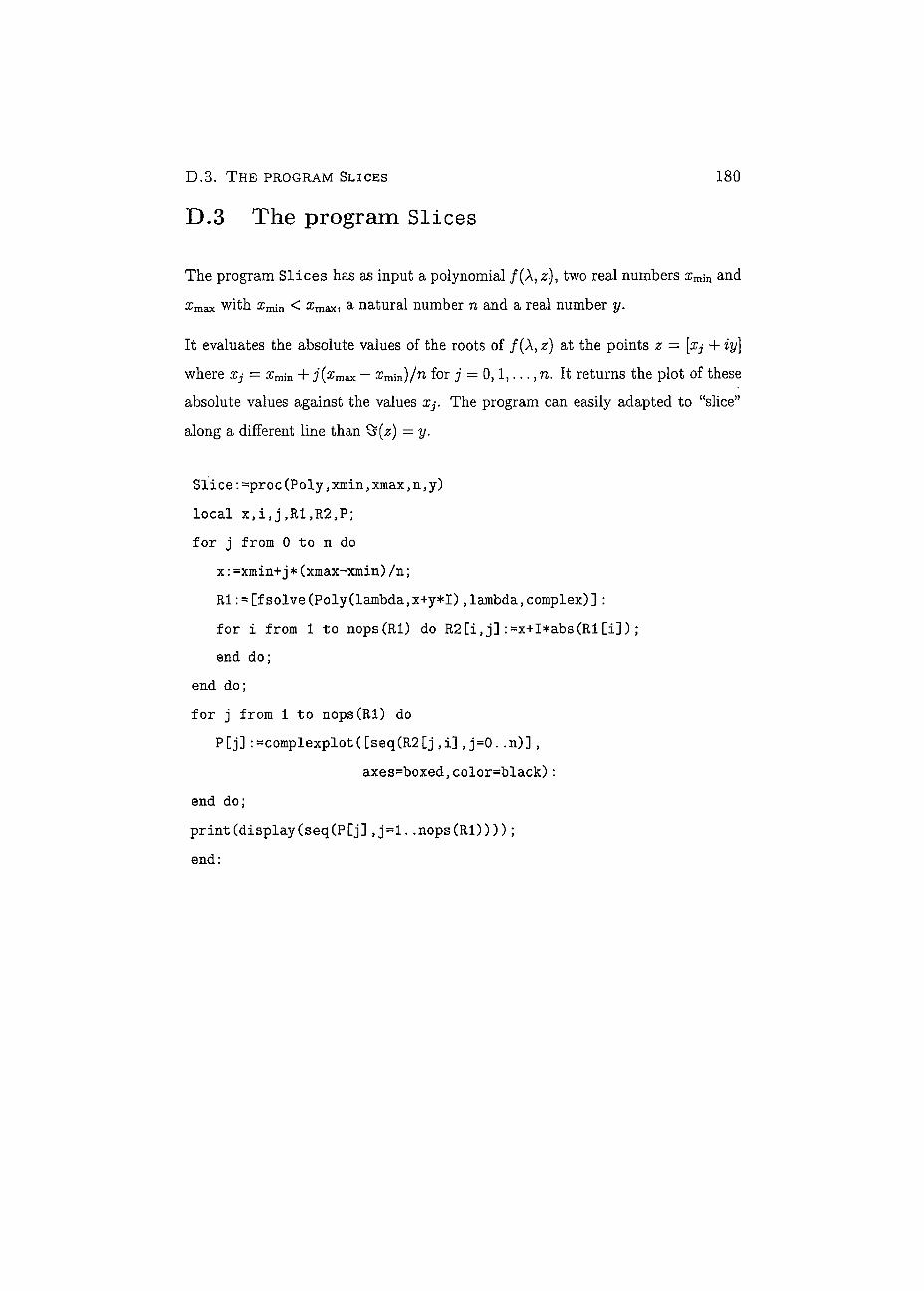
D . 2 . T H E PROGRAM DOMTEST

D.3 The program Slices

180

The program Slices has as input a polynomial /(A, z), two real numbers xmm and

xmax with xmjn < xmax, a naturai number n and a real number y.

It evaluates the absolute values of the roots of /(A, z) at the points z = [xj + iy]

where Xj = rcmjn + j(xmax — xm\n)/n for j = 0,1,. . . , n. It returns the plot of these absolute values against the values Xj. The program can easily adapted to "slice" along a différent line than = y.

S l i c e : = p r o c ( P o l y , x m i n , x m a x , IL , y )

l o c a l x ì i , j , R l , R 2 , P ;

f o r j f r o m 0 t o n d o

x : = x m i n + j * ( x m a x - x m i n ) / n ;

R I [ f s o l v e ( P o l y ( l a m b d a , x + y * I ) , l a m b d a , c o m p l e x ) ] :

f o r i f r o m 1 t o n o p s ( R l ) d o R 2 [ i , j ] : = x + I * a b s ( R l [ i ] ) ;

e n d d o ;

e n d d o ;

f o r j f r o m 1 t o n o p s ( R l ) d o

P [ j ] : = c o m p l e x p l o t ( [ s e q ( R 2 [ j , i ] , j = 0 . . n ) ] ,

a x e s = b o x e d , c o l o r = b l a c k ) :

e n d d o ;

p r i n t ( d i s p l a y ( s e q ( P [ j ] , j = l . . n o p s ( R l ) ) ) ) ;

e n d :

Bibliography

[1] Biggs N.L., Meredith G.H.J. Approximations for Chromatic Polynomials. J. Combinatorial Theory (B), 20 (1976) 5-19.

[2] Biggs N.L.

Colouring of square lattice graphs.

Bulletin of the London Mathematical Society, 9 (1977) 54-56.

[3] Biggs N.L. Algebraic Graph Theory. (1993)

Cambridge University Press, Cambridge.

[4] Biggs N.L.

Equimodular Curves.

to appear in Discrete Mathematics.

[5] Biggs N.L.

A matrix method for chromatic polynomials.

J. Combinatorial Theory (B): 82 (2001) 19-29.

[6] Biggs N.L.

Equimodular Curves for Reducible Matrices.

CDAM Research Report Series, LSE-CDAM-2001-01.

[7] Biggs N.L.

Chromatic polynomials and representations of the symmetric group.

to appear in Linear Algebra and its Applications.

181

BIBLIO G R A P H Y 182

[8] Biggs N.L.

Chromatic polynomials for twisted bracelets.

Bulletin of the London Mathematical Society, 34 (2002) 129-139.

[9] Biggs N.L., Klin M.H., Reinfeld R

Algebraic Methods for Chromatic Polynomials.

to appear in the European Journal of Combinatorics.

[10] Biggs N.L. Shrock R.

T = 0 partition functions for Potts antiferromagnets on Square lattice strips

with (twisted) periodic boundary conditions. J. Phys. A: Math. Gen. 32 (1999)

L1-L5.

[11] Chang S.C. Chromatic Polynomials for Lattice Strips with Cyclic Boundary Conditions. Physice A, 296 (2001) 495-522.

[12] Chang S.C. Exact Chromatic Polynomials of Toroidal Chains of Complete Graphs. arXiv: math-ph/0111028vl 16 Nov 2001.

[13] Chang S.C, Shrock R.

T = 0 partition functions for Potts antiferomagnets on lattice strips with fully

periodic boundary conditions.

Physice A, 292 (2001) 307-345.

[14] Cox D , Little J, O'Shea D. Using Algebraic Geometry. (1998) Springer-Verlag New York, Inc., New York.

[15] Jacobsen J.L, Salas J, Sokal A.D.

Transfer matrices and partition-function zeros for antiferromagnetic Potts

models III. Triangular-lattice chromatic polynomial.

e-Print Archive: cond-mat/0204587.

BIBLIO G R A P H Y 183

[16] James G.D. The Representation Theory of the Symmetrie Groups. (1978) Lecture Notes in Mathematics 682, Springer Verlag, Berlin.

[17] Ledermann W. Introduction to Group Gharacters. (1977) Cambridge University Press, Cambridge.

[18] Read R., Royle G.F. Chromatic roots of families of graphs. In: Y. Alavi, G. Chartrand, O.R. Ollermann, A.J. Schwenk, editors, Graph Theory, Combinatorics and Applications. (1991) John Wiley and Sons, Inc., New York.

[19] Reinfeld P. Chromatic Polynomials and the Spectrum of the Kneser Graph. CDAM Research Report Series, LSE-CDAM-2000-02.

[20] SaganB.E. The Symmetrie Group. (2001) Springer-Verlag New York, Inc., New York.

[21] Salas J., Sokal A.D. Transfer Matrices and Partition-Function Zeros for Antiferromagnetic Potts Models.

J. Statist. Phys. 104 (2001) 609-699.

[22] Sokal A.D.

Chromatic polynomials, Potts models and all that.

Physica A 279 (2000) 324-332.

[23] Sokal A.D. Bounds on the complex zeros of (di)chromatic polynomials and Potts model partition funetions. J. Comb. Probab. Comput 10 (2001) 41-77.

BIBLIO G R A P H Y 184

[24] Shrock R., Tsai S.H.

Asymptotic limits and zeros of chromatic polynomials and ground state en-

tropy of Potts antiferromagnets.

Phys. RevE55 (1997) 5165-5179.

[25] Shrock R., Tsai S.H.

Exact partition functions for Potts antiferromagnets on cyclic lattice strips.

Physice A, 275 (2000) 429-449.