Algebraic and combinatorial properties of binomial edge ideals · Resumo Com esta dissertac¸ao pretende-se fazer uma introduc¸˜ ao˜ a` Algebra Comutativa Combinat´ oria e mais´

Algebraic and combinatorial properties of binomial edge idealsJoao Pedro Martins dos Santos

Dissertacao para obtencao do grau de mestre em

Matematica e Aplicacoes

JuriPresidente: Professor Miguel Tribolet de Abreu

Orientadora: Professora Maria da Conceicao Pizarro de Melo Telo Rasquilha Vaz Pinto

Vogal: Professora Teresa Maria Jeronimo Sousa

Junho de 2015

Acknowledgements

I would like to thank my advisor, Maria Vaz Pinto, for introducing me to a very interesting topic in Commu-

tative Algebra, thus lengthening my knowledge in this area. I would also like to thank her for all her support

and advice when I had to apply for PhD programmes and in choosing which university and which advisor

would suit me better.

I would also like to thank the Geometry and Mathematical Physics project of Instituto Superior Tcnico

for the fellowship which was awarded to me a year ago and I would like to thank my professors for their

teachings and their advice during these five years.

By last but not least, I would like to thank my family and my friends for their support, both financial and

psychological.

2

Resumo

Com esta dissertacao pretende-se fazer uma introducao a Algebra Comutativa Combinatoria e mais

precisamente a um topico de grande interesse nessa area desde a sua introducao em 2009: os ideais

binomiais de arestas. Comecando com o estudo de ideais monomiais e bases de Grobner (pre-requisito

fundamental em Algebra Comutativa Combinatoria), a dissertacao consiste principalmente no estudo das

propriedades algebricas do ideal binomial de arestas JG em funcao das propriedades combinatorias do

grafo simples G. Mais precisamente, caracterizar-se-ao os ideais primos minimais de JG para qualquer

grafo simples G e, para determinadas classes de grafos, determinar-se-a se JG satisfaz ou nao a condicao

de Cohen-Macaulay e estudar-se-a a regularidade de Castelnuovo-Mumford de JG.

Palavras-chave: Algebra Comutativa Combinatoria, Grafos simples, Ideais binomiais de arestas,

Condicao de Cohen-Macaulay, Regularidade de Castelnuovo-Mumford.

3

Abstract

This dissertation is an introduction to Combinatorial Commutative Algebra and more precisely to a topic

of great interest since its introduction in 2009: binomial edge ideals. Starting with the study of monomial

ideals and Grobner bases (a fundamental pre-requisite for anyone who wants to study Combinatorial Com-

mutative Algebra), this dissertation consists mainly in the study of the algebraic properties of a binomial

edge ideal JG in terms of the combinatorial properties of the simple graph G. More precisely, for any sim-

ple graph G the minimal prime ideals of JG will be determined and, for some classes of graphs, we will

study whether JG satisfies the Cohen-Macaulay property. Finally, we will study the Castelnuovo-Mumford

regularity of JG.

Keywords: Combinatorial Commutative Algebra, Simple graphs, Binomial edge ideals, Cohen-Macaulay

property, Castelnuovo-Mumford regularity.

4

Contents

Introduction 7

0 Preliminaries 8

0.1 Basic notations . . . . . . . . . . . . . . . . . . . . . . . . . . . . . . . . . . . . . . . . . . . . 8

0.2 Basic commutative algebra . . . . . . . . . . . . . . . . . . . . . . . . . . . . . . . . . . . . . 8

0.3 Height, dimension and grade . . . . . . . . . . . . . . . . . . . . . . . . . . . . . . . . . . . . 11

0.4 Graded rings and modules . . . . . . . . . . . . . . . . . . . . . . . . . . . . . . . . . . . . . 14

0.5 Cohen-Macaulay graded rings . . . . . . . . . . . . . . . . . . . . . . . . . . . . . . . . . . . 17

0.6 Free resolutions and Castelnuovo-Mumford regularity . . . . . . . . . . . . . . . . . . . . . . 19

0.7 Graph theory . . . . . . . . . . . . . . . . . . . . . . . . . . . . . . . . . . . . . . . . . . . . . 22

1 Monomial ideals and Grobner bases 29

1.1 Monomial ideals . . . . . . . . . . . . . . . . . . . . . . . . . . . . . . . . . . . . . . . . . . . 29

1.2 Simplicial complexes and Stanley-Reisner ideals . . . . . . . . . . . . . . . . . . . . . . . . . 35

1.3 Grobner bases . . . . . . . . . . . . . . . . . . . . . . . . . . . . . . . . . . . . . . . . . . . . 39

2 Binomial edge ideals and closed graphs 50

2.1 Monomial edge ideals and bipartite graphs . . . . . . . . . . . . . . . . . . . . . . . . . . . . 50

2.2 Binomial edge ideals and their minimal primes . . . . . . . . . . . . . . . . . . . . . . . . . . 55

2.3 A special class of chordal graphs . . . . . . . . . . . . . . . . . . . . . . . . . . . . . . . . . . 66

2.4 Closed graphs . . . . . . . . . . . . . . . . . . . . . . . . . . . . . . . . . . . . . . . . . . . . 73

3 Regularity of binomial edge ideals 81

3.1 Regularity bounds . . . . . . . . . . . . . . . . . . . . . . . . . . . . . . . . . . . . . . . . . . 82

3.2 Regularity of binomial edge ideals of closed graphs . . . . . . . . . . . . . . . . . . . . . . . . 84

3.3 Partial results on two conjectures . . . . . . . . . . . . . . . . . . . . . . . . . . . . . . . . . . 89

Bibliography 93

5

Introduction

Commutative algebra was built in step with algebraic geometry and played an essential role in its devel-

opment. In the 1950’s, homological aspects of modern commutative algebra became a new and important

focus of research inspired by the work of Melvin Hochster. In 1975, Richard Stanley proved affirmatively

the upper bound conjecture for spheres by using the theory of Cohen-Macaulay rings. This created another

new trend of commutative algebra, as it turned out that commutative algebra supplies basic methods in

the algebraic study of combinatorics on convex polytopes and simplicial complexes. Stanley was the first

to use concepts and techniques from commutative algebra in a systematic way to study simplicial com-

plexes by considering the Hilbert function of Stanley-Reisner rings, whose defining ideals are generated by

square-free monomials. Since then, the study of square-free monomial ideals from both the algebraic and

combinatorial points of view has become a very active area of research in commutative algebra.

Finite simple graphs are just a special class of simplicial complexes and so the results on Stanley-

Reisner ideals can be used to study monomial edge ideals. The study of these ideals was started by Rafael

Villarreal in the 1990’s and, since then, a lot of mathematicians studied their algebraic properties in terms

of the combinatorial properties of the underlying graph. In 2003, in [10], Jrgen Herzog and Takayuki Hibi

classified Cohen-Macaulay bipartite graphs and in 2010, in [14], Russ Woodroofe showed that the regularity

of the monomial edge ideal of a weakly chordal graph is given by its induced matching number. These two

results are particularly important in stuyding binomial edge ideals of closed graphs.

On the other hand, in the late 1980’s, the theory of Grobner bases and initial ideals came into fashion

in many branches of mathematics, since it provided new methods. They have been used not only for com-

putational purposes but also to deduce theoretical results in commutative algebra and combinatorics. For

example, based on the fundamental work of Gelfand, Kapranov, Zelevinsky and Sturmfels, the study of reg-

ular triangulations of a convex polytope by using suitable initial ideals (far beyond the classical techniques in

combinatorics) turned out to be a very successful approach, and, after the pioneering work of Sturmfels, the

algebraic properties of determinantal ideals have been explored by considering their initial ideal, which for a

suitable monomial order is a square-free monomial ideal and hence is accessible to powerful techniques.

At about the same time, Galligo, Bayer and Stillman observed that generic initial ideals have particularly

nice combinatorial structures and provide a basic tool for the combinatorial and computational study of the

minimal free resolution of a graded ideal of the polynomial ring. Algebraic shifting, which was introduced by

6

Kalai and which contributed to the modern development of enumerative combinatorics on simplicial com-

plexes, can be discussed in the frame of generic initial ideals.

Chapter 0 is basically a list of definitions and results in Commutative Algebra and Graph Theory which

will be used throughout this dissertation. Consulting this chapter is recommendable for any reader who is

not familiarized with these definitions and results.

Chapter 1 is just a first course in monomial ideals, simplicial complexes and Grobner bases. Even if a

reader does not want to study monomial edge ideals or binomial edge ideals, this chapter is meant to be

a first introduction to combinatorial Commutative Algebra. To complete one’s learning, we recommend, for

example, the first two chapters of [5] or the first three chapters of [6].

In chapter 2, binomials edge ideals are studied. These ideals were introduced in [11], in 2009, where its

minimal primes ideals were studied only in terms of the combinatorial properties of their underlying graphs.

The results on minimal prime ideals of a binomial edge ideal apply for the class of conditional independence

ideals where a fixed binary variable is independent of a collection of other variables, given the remaining

ones. In this case the primary decomposition has a natural statistical interpretation.

Similar to what happens with monomial edge ideals, a general classification of Cohen-Macaulay binomial

edge ideals seems to be hopeless. However, in [12], in 2010, the Cohen-Macaulayness of binomial edge

ideals was studied for two special classes of graphs: closed graphs and chordal graphs such that any two

maximal cliques intersect in at most one vertex.

In chapter 3, the regularity of binomial edge ideals is studied. Woodroofe studied the regularity of mono-

mial edge ideals. Recently some mathematicians started studying the regularity of binomial edge ideals. In

[17], in 2013, Viviana Ene and Andrei Zarojanu showed that the regularity of the binomial edge ideal of a

closed graph is given by the lengths of its induced paths. With respect to the class of chordal graphs such

that any two maximal cliques intersect in at most one vertex, Ene and Zarojanu showed that this class of

graphs satisfy both the Madani-Kiani and the Matsuda-Murai conjectures.

While in this dissertation the Matsuda-Murai conjecture was meant to be presented as a conjecture, it

happened to be fully shown this year, on April 6th, in [18] by Madani and Kiani. Since the partial proof for

chordal graphs such that any two maximal cliques intersect in at most one vertex is an interesting proof which

uses some nice results on the combinatorial data of these graphs, I decided to keep it in the dissertation,

not forgetting to indicate a reference for the full proof of the Matsuda-Murai conjecture.

7

Chapter 0

Preliminaries

0.1 Basic notations

• If A and B are two sets, we write A ⊂ B when A is a subset of B and we write A ( B when A is a

proper subset of B.

• The set of integers is denoted by Z.

• The set of non-negative integers is denoted by N.

• Given a positive integer n, we denote [n] = {1, · · · , n}.

• Given a, b ∈ Z, we denote [a, b] = {x ∈ Z : a ≤ x ≤ b}.

• All rings will be commutative and will have a unit.

0.2 Basic commutative algebra

In this section R is a ring and M is an R-module.

Proposition 0.2.1. Let I, J ⊂ R be two ideals. Then there exists an exact sequence

0 −→ R

I ∩ J−→ R

I⊕ R

J−→ R

I + J−→ 0.

Proof. Consider the R-homomorphisms f : R/(I ∩ J)→ R/I ⊕R/J and g : R/I ⊕R/J → R/(I + J) given

by f(r+I∩J) = (r+I, r+J),∀r ∈ R and g(r+I, s+J) = r−s+I+J, ∀r, s ∈ R. These R-homomorphisms

are well defined, f is injective, g is surjective and g ◦ f = 0 holds. It remains to check that ker(g) ⊂ im(f).

Let (r + I, s + J) ∈ ker(g). Then r − s ∈ I + J . Pick r′ ∈ I and s′ ∈ J such that r − s = r′ + s′.

Then r − r′ = s + s′, and since r + I = r − r′ + I and s + J = s + s′ + J , it follows that (r + I, s + J) =

(r − r′ + I, s+ s′ + J) = (r − r′ + I, r − r′ + J) = f(r − r′ + I ∩ J).

8

Definition 0.2.2. Let I, J ⊂ R be two ideals. The ideal I : J = {f ∈ R : fg ∈ I, ∀g ∈ J} is called the colon

ideal of I with respect to J .

Definition 0.2.3. The ideal√I = {f ∈ R : ∃k > 0 : fk ∈ I} is called the radical ideal of I.

Definition 0.2.4. The ideal I is called a radical ideal if I =√I.

Proposition 0.2.5. The radical ideal of a given ideal is the intersection of the prime ideals containing it.

Proof. See [2, 1].

Corollary 0.2.6. An ideal is a radical ideal if and only if it is the intersection of prime ideals.

Definition 0.2.7. If I is an ideal of R, then I[x] is the ideal of the polynomials in R[x] whose coefficients lie

in I. Equivalently, considering the inclusion I ⊂ R ⊂ R[x], I[x] is the ideal of R[x] generated by the elements

of I.

Notation 0.2.8. Similarly I[x1, · · · , xn] is the ideal of the polynomials in R[x1, · · · , xn] whose coefficients lie

in I.

Proposition 0.2.9. Let P be an ideal of R. Then P is a prime ideal of R if and only if P [x] is a prime ideal

of R[x].

Proof. Since P = P [x] ∩R, P [x] being a prime ideal of R[x] implies P is a prime ideal of R.

Conversely, let f, g ∈ R[x] \ P [x]. Let f =∑fkx

k and g =∑gkx

k. Let m and n be the smallest integers

such that fm 6∈ P and gn 6∈ P , respectively. Then the coefficient of degree m+ n of fg is

(fm+ng0 + · · ·+ fm+1gn−1) + fmgn + (fm−1gn+1 + · · ·+ f0gm+n).

Since f0, · · · , fm−1 ∈ P , it follows that fm−1gn+1 + · · ·+ f0gm+n ∈ P . Similarly, g0, · · · , gn−1 ∈ P implies

fm+ng0 + · · ·+ fm+1gn−1 ∈ P . But fm, gn 6∈ P implies fmgn 6∈ P , hence fg 6∈ P [x].

Corollary 0.2.10. Let P be an ideal of R. Then P is a prime ideal of R[x] if and only if P [x1, · · · , xn] is a

prime ideal of R[x1, · · · , xn].

Sometimes, when there is no ambiguity, I may denote any of the ideals I, I[x] or I[x1, · · · , xn].

Definition 0.2.11. A presentation of an ideal I as an intersection I = Q1 ∩ · · · ∩ Qm of ideals is called

irredundant if none of the ideals Qi can be omitted in this presentation.

Notation 0.2.12. The set of minimal prime ideals of an ideal I is Min(I).

Lemma 0.2.13. Suppose I has irredundant presentation I = P1∩· · ·∩Pm as an intersection of prime ideals.

Then Min(I) = {P1, · · · , Pm}.

9

Proof. Suppose without loss of generality that P1 6∈ Min(I). Then there exists a prime ideal Q such that

I ⊂ Q ( P1. Since I = P1 ∩ · · · ∩ Pm ⊂ Q and Q is a prime ideal, then some Pi is contained in Q, thus

Pi ⊂ Q ( P1, therefore the presentation I = P1∩· · ·∩Pm is not irredundant. Hence {P1, · · · , Pm} ⊂ Min(I).

On the other hand, let Q ∈ Min(I). Again, since I = P1 ∩ · · · ∩ Pm ⊂ Q and Q is a prime ideal,

some Pi is contained in Q, and since both Pi and Q are minimal prime ideals of I, Q = Pi. Hence,

Min(I) = {P1, · · · , Pm}, as desired.

Lemma 0.2.14 (Prime avoidance). Let I be an ideal and let P1, · · · , Pn be prime ideals such that I ⊂

P1 ∪ · · · ∪ Pn. Then I ⊂ Pk for some 1 ≤ k ≤ n.

Proof. See [2, 1].

Definition 0.2.15. A prime ideal P is called an associated prime ideal of M if there exists an element

m ∈M \ {0} such that P = Ann(m).

Notation 0.2.16. The set of associated prime ideals of M is denoted Ass(M).

Proposition 0.2.17. Every maximal ideal of the set Σ = {Ann(m) : m ∈M \ {0}} is a prime ideal.

Proof. See [1, 2;6].

Corollary 0.2.18. If R is Noetherian, then Ass(M) 6= ∅.

Proposition 0.2.19. If R is Noetherian and M is finitely generated, then Ass(M) is a finite non-empty set.


As a corollary of the Hilbert’s basis theorem (see [2, 7]), the polynomial rings K[x1, · · · , xn], where

K is a field, are Noetherian. Since most rings on this dissertation will be quotients of these rings (and

hence Noetherian), from now on all rings are Noetherian and all modules are finitely generated (hence

Noetherian).

Proposition 0.2.20. For every prime ideal P one has P ∈ Ass(M) if and only if PP ∈ Ass(MP ).

Proof. See [1, 2;6]

Proposition 0.2.21. For every ideal I one has Min(I) ⊂ Ass(R/I).

Proof. Let P ∈ Min(I). Then PP ∈ Min(IP ), thus PP is the only prime ideal containing IP . Since all associ-

ated prime ideals of RP /IP must contain IP , it follows that Ass(RP /IP ) ⊂ {PP }, and since Ass(RP /IP ) 6= ∅,

then Ass(RP /IP ) = {PP }. On the other hand, RP /IP and (R/I)P are isomorphic RP -modules, and so

Ass((R/I)P ) = {PP }. Hence P ∈ Ass(R/I).

Definition 0.2.22. An ideal I is a primary ideal if for every x, y ∈ R such that xy ∈ I one has x ∈ I or

y ∈√I.

10

Proposition 0.2.23. If I is a primary ideal, then√I is a prime ideal.

Definition 0.2.24. An ideal I is a P -primary ideal if it is a primary ideal such that√I = P .

Proposition 0.2.25. An ideal I is a P -primary ideal if and only if Ass(R/I) = {P}.


Definition 0.2.26. A primary irredundant decomposition of an ideal I is an irredundant decomposition I =

Q1 ∩ · · · ∩Qm such that all ideals Qi are primary ideals.

Proposition 0.2.27. If I 6= R, then I admits a primary irredundant decomposition. Moreover, if I = Q1 ∩

· · · ∩Qm is such a decomposition with Pi =√Qi for i ∈ [m], then Ass(R/I) = {P1, · · · , Pm}.


Corollary 0.2.28. If I 6= R is a radical ideal, then Min(I) = Ass(R/I).

Proof. Just recall that I is the intersection of its minimal prime ideals and such intersection is a primary

irredundant decomposition.

0.3 Height, dimension and grade

Recall that all rings considered are Noetherian and that all modules considered are finitely generated.

Definition 0.3.1. The height of a prime ideal P is

ht(P ) = sup{n ∈ N : there exists an ascending chain of prime ideals P0 ( · · · ( Pn = P}.

Theorem 0.3.2. If P is a minimal prime of I = (r1, · · · , rn), then ht(P ) ≤ n.

Proof. See [2, 11].

Corollary 0.3.3. If P is a prime ideal, then ht(P ) <∞.

Definition 0.3.4. The height of an ideal I is

ht(I) = min{ht(P ) : P ∈ Min(I)}.

Definition 0.3.5. An ideal I is unmixed if ht(I) = ht(P ) for every P ∈ Ass(R/I).

In particular, if I is unmixed, then Min(I) = Ass(R/I).

Definition 0.3.6. The Krull dimension of a ring R is

dim(R) = sup{n ∈ N : there exists an ascending chain of prime ideals P0 ( · · · ( Pn ( R}.

11

Though prime ideals in a Noetherian ring always have finite height, there are Noetherian rings with

infinite Krull dimension. Nonetheless, since polynomial rings have finite Krull dimension and most rings

considered in this dissertation are quotients of polynomial rings, we will assume that all rings considered

are Noetherian rings with finite Krull dimension.

Proposition 0.3.7. For every prime ideal P one has dim(R) ≥ ht(P ) + dim(R/P ).

Corollary 0.3.8. For every ideal I (not necessarily prime) one has dim(R) ≥ ht(I) + dim(R/I).

Proof. Pick P ∈ Min(I) such that dim(R/P ) = dim(R/I). Then dim(R) ≥ ht(P ) + dim(R/P ) = ht(P ) +

dim(R/I) ≥ ht(I) + dim(R/I), as desired.

Definition 0.3.9. Let r ∈ R. We say that r is regular on M , or M -regular, if rm = 0 implies m = 0 for every

m ∈M .

Notation 0.3.10. The set of elements of R which are not M -regular is denoted by Z(M).

Proposition 0.3.11. Z(M) is the union of the associated primes of M .

Proof. Let P ∈ Ass(M). Let m ∈M such that P = Ann(m). Then Pm = 0, and since m 6= 0, P ⊂ Z(M).

Let r ∈ Z(M) and let Σ = {Ann(m) : m ∈ M \ {0}}. Pick x ∈ M \ {0} such that rx = 0. Since R is

Noetherian, then there exists a maximal ideal in Σ containing Ann(x), say Ann(y). By proposition 0.2.17,

Ann(y) is a prime ideal, and thus an associated prime, containing r.

Corollary 0.3.12. If I is an ideal without M -regular elements, then I is contained in some associated prime

of M .

Proof. Just use prime avoidance and the previous proposition.

Definition 0.3.13. A sequence r1, · · · , rn ∈ R is called a regular sequence on M , or an M -regular se-

quence, if the following conditions hold:

• (r1, · · · , rn)M 6= M .

• For every 1 ≤ i ≤ n, ri is M/(r1, · · · , ri−1)M -regular.

Theorem 0.3.14 (Rees). Let I be an ideal such that IM 6= M . Then all maximal M -regular sequences in I

have the same length.

Proof. See [4, 1.2].

Definition 0.3.15. The common length of all maximal M -regular sequences in I is called the grade of I on

M , denoted by grade(I,M).

Proposition 0.3.16. Let r ∈ I be M -regular. Then grade(I,M/rM) = grade(I,M)− 1.

12

Proof. Let r1, · · · , rn ∈ I be a maximal (M/rM)-regular sequence. Since r ∈ I is M -regular, it follows that

r, r1, · · · , rn ∈ I is a M -regular sequence, hence grade(I,M) ≥ n+ 1 = grade(I,M/rM) + 1.

Since r ∈ I is M -regular, by Rees theorem there exists a maximal M -regular sequence r, r1, · · · , rn ∈ I,

therefore r1, · · · , rn ∈ I is a (M/rM)-regular sequence, hence grade(I,M/rM) ≥ n = grade(I,M)− 1.

Combining these two inequalities one gets the desired result.

Proposition 0.3.17. Let P be a prime ideal and r ∈ P be regular. Then ht(P ) ≥ ht(P/(r)) + 1.

Proof. Let P0 ( · · · ( Pn be a maximal ascending chain of prime ideals such that (r) ⊂ P0 ( · · · ( Pn = P .

Suppose P0 ∈ Min(R). Then P0 ∈ Ass(R) and so r ∈ Z(R), a contradiction. Thus there exists a prime ideal

P−1 strictly contained in P0 and so P−1 ( P0 ( · · · ( Pn = P is an ascending chain of prime ideals, hence

ht(P ) ≥ n+ 1 = ht(P/(r)) + 1.

Corollary 0.3.18. If r ∈ R is regular, then dim(R) ≥ dim(R/(r)) + 1.

Proof. Let P be a prime ideal inR containing r. Since r ∈ P is regular, then dim(R) ≥ ht(P ) ≥ ht(P/(r))+1.

Since dim(R) ≥ ht(P/(r))+1 for any prime ideal P containing r, it follows that dim(R) ≥ dim(R/(r))+1.

Proposition 0.3.19. For every prime ideal P one has grade(P,R) ≤ ht(P ).

Proof. Induct on n = grade(P,R). The case n = 0 is trivial.

Suppose n > 0. Pick r ∈ P regular. Then P/(r) is a prime ideal of R/(r) such that grade(P/(r), R/(r)) =

grade(P,R/(r)) = n− 1, thus ht(P/(r)) ≥ n− 1 and hence ht(P ) ≥ n, as desired.

Corollary 0.3.20. For every ideal I (not necessarily prime) one has grade(I,R) ≤ ht(I).

Proof. Pick P ∈ Min(I) such that ht(P ) = ht(I). Then grade(I,R) ≤ grade(P,R) ≤ ht(P ) = ht(I).

Definition 0.3.21. If I ⊂ R is an ideal generated by a regular sequence, then I is called a complete

intersection.

Proposition 0.3.22. If I is a complete intersection, then grade(I,R) = ht(I).

Proof. Let r1, · · · , rn be the regular sequence that generates I. Then grade(I,R) = n. Since I = (r1, · · · , rn),

ht(P ) ≤ n for every P ∈ Min(I), thus by definition ht(I) ≤ n, hence n = grade(I,R) ≤ ht(I) ≤ n.

Proposition 0.3.23. If I is an ideal of R and 0 −→ A −→ B −→ C −→ 0 is a short exact sequence of finitely

generated R-modules, then:

1. grade(I, A) ≥ min{grade(I,B), grade(I, C) + 1};

2. grade(I,B) ≥ min{grade(I, A), grade(I, C)};

3. grade(I, C) ≥ min{grade(I, A)− 1, grade(I,B)}.


13

0.4 Graded rings and modules

Recall that all rings considered are Noetherian and that all modules considered are finitely generated.

Definition 0.4.1. A graded ring is a ring R together with a decomposition R =⊕∞

i=0Ri as an abelian group

such that RiRj ⊂ Ri+j ,∀i, j ∈ N.

Example 0.4.2. The polynomial ring R = K[x1, · · · , xn] is a graded ring, where, for each i ∈ N, Ri is the

K-vector subspace of homogeneous polynomials of degree i.

If f ∈ Ri \ {0}, we say that f is homogeneous of degree i. Any element f ∈ R can be written uniquely

as f =∑∞i=0 fi, with fi ∈ Ri and only finitely many fi are non-zero. Such fi are called the homogeneous

components of f .

Definition 0.4.3. Let R be a graded ring. We say that I is a graded ideal of R if one of the following

equivalent conditions hold:

• I =⊕∞

i=0(Ri ∩ I).

• I is generated by homogeneous elements of R.

• For every f ∈ I, all the homogeneous components of f also belong to I.

Proposition 0.4.4. If I is a graded ideal of R, then R/I is a graded ring with (R/I)i = (Ri + I)/I for every

i ∈ N.

Proof. Since R =⊕∞

i=0Ri, then R =∑∞i=0(Ri + I), hence R/I =

∑∞i=0(Ri + I)/I. Now we show that this

sum is in fact a direct sum.

Let ri ∈ Ri such that ri + I ∈∑j 6=i(Rj + I). Then ri + s =

∑j 6=i rj , with s ∈ I and rj ∈ Rj , thus

s =∑j 6=i rj − ri, and since s ∈ I and I is homogeneous, ri ∈ I, therefore ri + I = 0. Hence R/I =⊕∞

i=0(Ri + I)/I.

By last, if ri ∈ Ri and rj ∈ Rj , then rirj ∈ Ri+j , therefore (ri + I)(rj + I) = rirj + I ∈ (Ri+j + I)/I.

Hence (Ri + I)/I · (Rj + I)/I ⊂ (Ri+j + I)/I.

We know that the polynomial rings K[x1, · · · , xn], where K is a field, are Noetherian graded rings. Since

most rings on this dissertation will be quotients of these rings by graded ideals (and hence Noetherian

graded rings), from now on all rings are Noetherian graded rings.

Definition 0.4.5. A graded R-module is an R-module M with a decomposition M = ⊕∞i=0Mi such that

RiMj ⊂Mi+j for every i, j ∈ N.

In particular, if R is a graded R-module and I is a graded ideal of R, then R/I is also a graded R-module.

If f ∈ Mi \ {0}, we say that f is homogeneous of degree i. Any element f ∈ M can be written uniquely as

f =∑∞i=0 fi, with fi ∈ Mi and only finitely many fi 6= 0. Such fi are called the homogeneous components

of f .

14

Proposition 0.4.6. A finitely generated graded R-module M can be generated by a finite system of homo-

geneous elements.

Proof. Pick any finite set of generators of M . Then the homogeneous components of such generators are

a finite set of generators of M .

Definition 0.4.7. Let M be a graded R-module. An R-submodule U of M is called a graded R-submodule

of M if U is a graded R-module with Ui = U ∩Mi for every i ∈ N.

Proposition 0.4.8. If U is a graded submodule of M , then M/U is a graded R-module with (M/U)i =

(Mi + U)/U for every i ∈ N.

Proof. Since M =⊕∞

i=0Mi, then M =∑∞i=0(Mi+U), hence M/U =

∑∞i=0(Mi+U)/U . Now we show that

this sum is in fact a direct sum.

Let mi ∈ Mi such that mi + U ∈∑j 6=i(mj + U). Then mi + u =

∑j 6=imj , with u ∈ U and mj ∈ Mj ,

thus u =∑j 6=imj − mi, and since u ∈ U and U is graded, mi ∈ U , therefore mi + U = 0. Hence

M/U =⊕∞

i=0(Mi + U)/U .

By last, if ri ∈ Ri and mj ∈ Mj , then rimj ∈ Mi+j , therefore ri(mj + U) = rimj + U ∈ (Mi+j + U)/U .

Hence Ri · (Mj + U)/U ⊂ (Mi+j + U)/U .

Definition 0.4.9. Let M and N be graded R-modules. An R-homomorphism ϕ : M → N is called homoge-

neous if ϕ(Mi) ⊂ Ni for every i ∈ N.

Proposition 0.4.10. The kernel and the image of an homogeneous R-homomorphism ϕ : M → N are

graded submodules of M and N , respectively.

Proof. Let m =∑∞i=0mi ∈ kerϕ. Then 0 = ϕ(m) =

∑∞i=0 ϕ(mi), and since ϕ(mi) ∈ Ni for every i ∈ N, it

follows that ϕ(mi) = 0 for every i ∈ N, that is, mi ∈ kerϕ for every i ∈ N. Hence kerϕ =⊕∞

i=0(kerϕ ∩Mi),

that is, kerϕ is graded.

Let m =∑∞i=0mi ∈M . Since M =

⊕∞i=0Mi, then ϕ(M) =

∑∞i=0 ϕ(Mi). Since N =

∑∞i=0Ni is a direct

sum and ϕ(Mi) ⊂ Ni holds for every i ∈ N, it follows that ϕ(M) =∑∞i=0 ϕ(Mi) is also a direct sum, that is,

ϕ(M) is graded.

Definition 0.4.11. Let K be a field. A ring R is called a graded K-algebra if R is a graded ring such that

R0 = K.

As a consequence of this definition, if R is a K-algebra, then each Ri is a K-vector space.

Proposition 0.4.12. The only maximal graded ideal of a graded K-algebra R is m =⊕∞

i=1Ri.

Proof. Suppose I 6⊂ m is a graded ideal of R. Then there exists f =∑∞i=0 fi ∈ I with f0 6= 0. Since I is a

graded ideal, all homogeneous components of f belong to I and in particular f0 ∈ I. But f0 ∈ K \ {0}, thus

1 = f−10 f0 ∈ I and so I = R.

15

Corollary 0.4.13. If R is a graded K-algebra, then every proper graded ideal of R is contained in m.

Proposition 0.4.14. If R is graded K-algebra and I is a proper graded ideal of R, then R/I is also a graded

K-algebra.

Proof. Consider the K-linear map φ : K → (R/I)0 given by φ(k) = k + I for every k ∈ K. This map is

surjective since (R/I)0 = (K+ I)/I. Since any proper graded ideal of R is contained in m, then in particular

I ⊂ m and so K ∩ m = {0} implies that K ∩ I = {0}. Hence φ is also injective and so φ is a natural

K-isomorphism between K and (R/I)0. Hence R/I is a graded K-algebra.

We know that the polynomial rings K[x1, · · · , xn], where K is a field, are Noetherian graded K-algebras.

Since most rings on this dissertation will be quotients of these rings by graded ideals (and hence Noetherian

graded K-algebras), for the rest of the dissertation all rings are Noetherian graded K-algebras.

Let M be a graded R-module. In general, the multiplication ϕ : M → M by an homogeneous element

r ∈ R is not an homogeneous R-homomorphism, for ϕ(Mi) ⊂ Mi+deg r for every i ∈ N. This problem is

solved by shifting the homogeneous components of M .

Definition 0.4.15. Given a graded R-module M and j ∈ N, then M(−j) is defined to be the graded R-

module whose graded components are M(−j)i = Mi−j if i ≥ j and M(−j)i = 0 otherwise.

Now the multiplication ϕ : M(−deg r) → M by an homogeneous element r ∈ R is a graded R-

homomorphism.

Lemma 0.4.16 (Graded Nakayama). Let M be a graded R-module such that M = mM . Then M = 0.

Proof. Suppose M 6= 0. Let α be the smallest integer such that Mα 6= 0. Then Mα ⊂ M = mM ⊂⊕∞i=α+1Mi. Since Mα ⊂

⊕∞i=α+1Mi, it follows that Mα = 0, a contradiction.

Corollary 0.4.17. If U is a graded R-submodule of M such that M = U + mM , then M = U .

Proof. From M = U + mM it follows that M/U = m(M/U), hence M/U = 0, as desired.

Corollary 0.4.18. If m1, · · · ,mr are homogeneous elements whose residue classes modulo mM form a

K-basis for M/mM , then m1, · · · ,mr generate M .

Proof. Let U be the R-submodule of M generated by m1, · · · ,mr. Then U is a graded submodule such that

M = U + mM , hence M = U .

Corollary 0.4.19. All homogeneous minimal systems of generators of M have the same cardinality, namely

dimK(M/mM).

16

0.5 Cohen-Macaulay graded rings

In this section, R will denote a Noetherian graded algebra over a field K will maximal homogeneous

ideal m. Moreover, all modules considered are finitely generated graded R-modules.

Definition 0.5.1. LetM be a finitely generated gradedR-module. The depth ofM is depth(M) = grade(m,M).

Proposition 0.5.2. For every graded ideal I, there exists an M -regular sequence of length grade(I,M)

consisting of homogeneous elements of I.


Hence, to determine depth(M), it is enough to consider regular sequences of homogeneous elements

of M .

Proposition 0.5.3. If r ∈ m is M -regular, then depth(M/rM) = depth(M)− 1.

Proof. This is a direct corollary of proposition 0.3.16.

Proposition 0.5.4. Let I be a graded ideal of R. Then the depth of R/I is the same either as a graded ring

or as a graded R-module.

Proof. Just notice that r1, · · · , rn is R/I-regular if and only if r1 + I, · · · , rn + I is R/I-regular.

Proposition 0.5.5. Let M be a graded R-module. Then depth(M) ≤ dim(R/P ) for every P ∈ Ass(M).

Proof. Induct on n = depth(M). The case n = 0 is trivial.

Suppose n > 0. Let P ∈ Ass(M). Let r ∈ m be a M -regular homogeneous element. By proposition

0.3.16, one has depth(M/rM) = n − 1. Let Σ be the set of cyclic R-submodules of M annihilated by P .

Since P ∈ Ass(M), then Σ contains a non-zero cyclic R-submodule of M , and since R is Noetherian, then

Σ has a maximal element (y), with y ∈ M \ {0}. Suppose y ∈ rM . Then y = rm for some m ∈ M , and

since r ∈ m and M is a graded R-module, then (y) ( (m). On the other hand, r(Pm) = 0, and since

r is M -regular, Pm = 0, hence (m) ∈ Σ, contradicting the maximality of (y). Hence y 6∈ rM , and since

Py = 0, it follows that P ⊂ Z(M/rM), therefore P is contained in some Q ∈ Ass(M/rM). By induction,

dim(R/Q) ≥ depth(M/rM) = n − 1. Since r(M/rM) = 0 and r 6∈ P , then P 6∈ Ass(M/rM), thus P ( Q,

therefore dim(R/P ) > dim(R/Q) ≥ n− 1, hence dim(R/P ) ≥ n, as desired.

Corollary 0.5.6. Let R be a graded K-algebra. Then depth(R) ≤ dimR.

Definition 0.5.7. Let K be a field and let R be a graded K-algebra. Then R is a Cohen-Macaulay graded

ring if depth(R) = dim(R).

In an abuse of notation, one says that a graded ideal I is a Cohen-Macaulay ideal if R/I is a Cohen-

Macaulay ring.

17

Proposition 0.5.8. If I is a Cohen-Macaulay ideal, then depth(R/I) = dim(R/I) = dim(R/P ) for every

P ∈ Ass(R/I).

Proof. If P ∈ Ass(R/I), by proposition 0.5.5 one has depth(R/I) ≤ dim(R/P ) ≤ dim(R/I), and since

depth(R/I) = dim(R/I), the assertion follows.

In particular, if I is a Cohen-Macaulay ideal, then Min(I) = Ass(R/I).

Proposition 0.5.9. If R is a Cohen-Macaulay ring and r ∈ R is regular, then R/(r) is a Cohen-Macaulay

ring as well.

Proof. Since R is a Cohen-Macaulay ring, then depth(R) = dim(R). On the other hand, since r is regular,

by proposition 0.3.16 one has depth(R/(r)) = depth(R) − 1 and by corollary 0.3.18 one has dim(R) ≥

dim(R/(r)) + 1. Hence dim(R/(r)) ≤ dim(R)− 1 = depth(R)− 1 = depth(R/(r)), as desired.

Corollary 0.5.10. Any complete intersection in a Cohen-Macaulay ring is a Cohen-Macaulay ideal.

Proposition 0.5.11. The polynomial ring R = K[x1, · · · , xn] satisfies dim(R) = n.

Proof. See [3, 10].

Since x1, · · · , xn ∈ m is a regular sequence of length n, it follows that K[x1, · · · , xn] is a Cohen-Macaulay

ring.

Proposition 0.5.12. If I is an ideal of R = K[x1, · · · , xn], then ht(I) + dim(R/I) = n.


Corollary 0.5.13. If I ⊂ K[x1, · · · , xn] is a Cohen-Macaulay ideal, then I is unmixed.

Proof. Let P ∈ Ass(R/I). Since I is a Cohen-Macaulay ideal, by proposition 2.2.34 one has dim(R/I) =

dim(R/P ), and from the equalities ht(I) + dim(R/I) = n and ht(P ) + dim(R/P ) = n it follows that ht(I) =

ht(P ).

Notation 0.5.14. Let K[x] and K[y] be two polynomial rings over a field K. If I1 and I2 are graded ideals

of K[x] and K[y], respectively, then I1 + I2 denotes the graded ideal of K[x,y] generated by I1 and I2.

Proposition 0.5.15. If I1 and I2 are graded ideals of K[x] and K[y], respectively, then depth(K[x]/I1) +

depth(K[y]/I2) = depth(K[x,y]/(I1 + I2)) and dim(K[x]/I1) + dim(K[y]/I2) = dim(K[x,y]/(I1 + I2)).


Corollary 0.5.16. The ring K[x,y]/(I1 + I2) is Cohen-Macaulay if and only if the rings K[x]/I1 and K[y]/I2are Cohen-Macaulay.

Corollary 0.5.17. If I1 and I2 are graded ideals of K[x1, · · · , xn] and K[y1, · · · , ym], respectively, then

ht(I1 + I2) = ht(I1) + ht(I2).

18

Proof. By proposition 0.5.12, the following equalities hold:

ht(I1) + dim(K[x1, · · · , xn]/I1) = n, ht(I2) + dim(K[y1, · · · , ym]/I2) = m,

ht(I1 + I2) + dim(K[x1, · · · , xn, y1, · · · , ym]/(I1 + I2)) = n+m.

By proposition 0.5.15 the following equality holds:

dim(K[x1, · · · , xn, y1, · · · , ym]/(I1 + I2)) = dim(K[x1, · · · , xn]/I1) + dim(K[y1, · · · , ym]/I2).

Combining these four equalities yields ht(I1 + I2) = ht(I1) + ht(I2), as desired.

0.6 Free resolutions and Castelnuovo-Mumford regularity

Recall that R is a Noetherian graded algebra over a field K.

Let M be a finitely generated graded R-module with homogeneous generators m1, · · · ,mr ∈ M and

degmi = ai for i = 1, · · · , r. Let F0 be the free R-module with generators e1, · · · , er. Then there exists an

R-epimorphism ε : F0 =⊕r

i=1Rei → M with ei 7→ mi. Assigning to ei the degree ai for i = 1, · · · , r, the

map F0 → M becames graded and F0 becomes isomorphic to⊕r

i=1R(−ai). Let U = ker ε. Since U is a

submodule of F0 and R is a Noetherian ring, then U is a finitely generated graded R-module. Now we find

again a graded R-epimorphism F1 → U . Composing it with the inclusion map U → F0 we obtain the exact

sequence F1 −→ F0 −→ M −→ 0 of graded R-modules. Proceeding in this way we obtain a long exact

sequence

F : · · · −→ F2 −→ F1 −→ F0 −→M −→ 0

of graded R-modules and graded R-homomorphisms. Such an exact sequence is called a graded free

resolution of M .

Notation 0.6.1. The R-homomorphism from Fi to Fi−1 will be called ϕi.

Lemma 0.6.2. Let m1, · · · ,mr be a homogeneous set of generators of M . Let F0 =⊕r

i=1Rei →M be the

epimorphism with ei 7→ mi for i = 1, · · · , r. Then m1, · · · ,mr is a minimal system of generators of M if and

only if ker ε ⊂ mF0.

Proof. See [5, A.2].

Definition 0.6.3. A graded free resolution F is called minimal if the image of each Fi → Fi−1 is contained

in mFi−1.

The previous lemma implies that each finitely generated R-module admits a graded minimal free resolu-

tion.

19

Proposition 0.6.4. Let M be a finitely generated graded R-module and let F and G be two minimal graded

free resolutions ofM . Then F and G are isomorphic, that is, there exist gradedR-isomorphisms αi : Fi → Gi

such that the diagram

· · · // F1

α1

��

// F0

α0

��

// M

Id��

// 0

· · · // G1 // G0 // M // 0

is commutative.


Let F be a graded minimal free resolution of M with Fi =⊕

j R(−j)βij(M). Proposition 0.6.4 tells us that

the numbers βij(M) are uniquely determined by M . They are called the graded Betti numbers of M .

Definition 0.6.5. The projective dimension of a graded module M is

projdim(M) = sup{i : ∃j ≥ 0 : βij(M) 6= 0}.

For the remaining of this section we will only consider finitely generated graded modules over

the polynomial ring S = K[x1, · · · , xn].

Theorem 0.6.6 (Auslander-Buchsbaum). For any S-module M one has projdim(M) + depth(M) = n.


Corollary 0.6.7. For any S-module M one has projdim(M) ≤ n (and in particular the projective dimension

is always finite).

Definition 0.6.8. The Castelnuovo-Mumford regularity of M is reg(M) = max{j : ∃i ≥ 0 : βi,i+j(M) 6= 0}.

The corollary of Auslander-Buchsbaum theorem tells us that reg(M) <∞.

Proposition 0.6.9. If I is a graded ideal of S, then reg(I) = reg(S/I) + 1.

Proof. If

· · · −→ F2 −→ F1 −→ S −→ S/I −→ 0

is a minimal graded free resolution for S/I, then

· · · −→ F2 −→ F1 −→ I −→ 0

is a minimal graded free resolution for I. Hence βi,j(I) = βi+1,j(S/I), and since β0,j(S/I) = 0 for j > 0,

it follows that reg(I) = max{j : ∃i ≥ 0 : βi,i+j(I) 6= 0} = max{j : ∃i ≥ 1 : βi,i+(j−1)(S/I) 6= 0} =

= max{j : ∃i ≥ 0 : βi,i+(j−1)(S/I) 6= 0} = max{j − 1 : ∃i ≥ 0 : βi,i+(j−1)(S/I) 6= 0}+ 1 = reg(S/I) + 1.

Proposition 0.6.10. For every S-module M and k ∈ N one has reg(M(−k)) = reg(M) + k.

20

Proof. If

· · · −→ F2 −→ F1 −→ F0 −→M −→ 0

is a minimal graded free resolution for M , then

· · · −→ F2(−k) −→ F1(−k) −→ F0(−k) −→M(−k) −→ 0

is a minimal graded free resolution for M(−k). Hence βi,j(M(−k)) = βi,j−k(M), therefore reg(M(−k)) =

max{j : ∃i ≥ 0 : βi,i+j(M(−k)) 6= 0} = max{j : ∃i ≥ 0 : βi,i+j−k(M) 6= 0} =

= max{j − k : ∃i ≥ 0 : βi,i+j−k(M) 6= 0}+ k = reg(M) + k.

Proposition 0.6.11. If 0 −→ A −→ B −→ C −→ 0 is a short exact sequence of graded S-modules, then:

1. reg(A) ≤ max{reg(B), reg(C) + 1};

2. reg(B) ≤ max{reg(A), reg(C)};

3. reg(C) ≤ max{reg(A)− 1, reg(B)}.

Proof. See [3, 20.5].

Corollary 0.6.12. If A and B are graded S-modules, then reg(A⊕B) ≤ max{reg(A), reg(B)}.

Proof. Just consider the short exact sequence 0 −→ A −→ A⊕B −→ B −→ 0 and apply inequality (2).

Proposition 0.6.13. If f ∈ S is an M -regular homogeneous element of degree k > 0, then reg(M/fM) =

reg(M) + k − 1.

Proof. Consider the graded exact sequence 0 −→ M(−k) −→ M −→ M/fM −→ 0, where the S-

homomorphism M(−k) −→M is the multiplication by f . By inequality (1) of proposition 0.6.11,

reg(M(−k)) ≤ max{reg(M), reg(M/fM) + 1},

that is, reg(M) + k ≤ max{reg(M), reg(M/fM) + 1}, hence reg(M) + k ≤ reg(M/fM) + 1, that is,

reg(M/fM) ≥ reg(M) + k − 1. On the other hand, by inequality (3),

reg(M/fM) ≤ max{reg(M(−k))− 1, reg(M)} = max{reg(M) + k − 1, reg(M)} = reg(M) + k − 1,

thus the equality follows.

Corollary 0.6.14. Let f1, · · · , fr ∈ S be an M -regular sequence of homogeneous elements of degrees

k1, · · · , kr, respectively. Then reg(M/(f1, · · · , fr)M) = reg(M) + k1 + · · ·+ kr − r.

Proof. Use induction on r and the previous proposition.

Lemma 0.6.15. Let M and N be graded modules over K[x] and K[y], respectively. Then M ⊗K N is

a graded module over K[x,y] such that depth(M ⊗K N) = depth(M) + depth(N) and reg(M ⊗K N) =

reg(M) + reg(N).

21

Proof. See [9, 2] (the proof of this lemma uses local cohomology, a tool which is beyond this dissertation).

0.7 Graph theory

Definition 0.7.1. A graph G is an ordered pair of disjoint finite sets (V,E) such that E is a subset of the set

of unordered pairs of V .

The set V is the set of vertices and the set E is called the set of edges. An edge z = {u, v}, with u, v ∈ V ,

is said to join the vertices u and v. We also say that the edge z is incident with u and v or that vertices u and

v are adjacent or neighbouring vertices of G.

Definition 0.7.2. The order of a graph is its number of vertices.

Notation 0.7.3. The vertex set and the edge set of G are often denoted by V (G) and E(G), respectively.

Definition 0.7.4. The degree deg(v) of a vertex v is the number of edges incident with v.

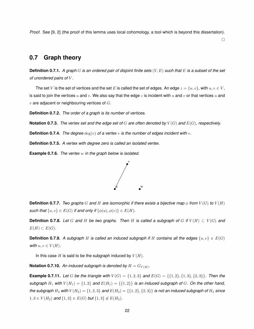
Definition 0.7.5. A vertex with degree zero is called an isolated vertex.

Example 0.7.6. The vertex w in the graph below is isolated.

Definition 0.7.7. Two graphs G and H are isomorphic if there exists a bijective map φ from V (G) to V (H)

such that {u, v} ∈ E(G) if and only if {φ(u), φ(v)} ∈ E(H).

Definition 0.7.8. Let G and H be two graphs. Then H is called a subgraph of G if V (H) ⊂ V (G) and

E(H) ⊂ E(G).

Definition 0.7.9. A subgraph H is called an induced subgraph if H contains all the edges {u, v} ∈ E(G)

with u, v ∈ V (H).

In this case H is said to be the subgraph induced by V (H).

Notation 0.7.10. An induced subgraph is denoted by H = GV (H).

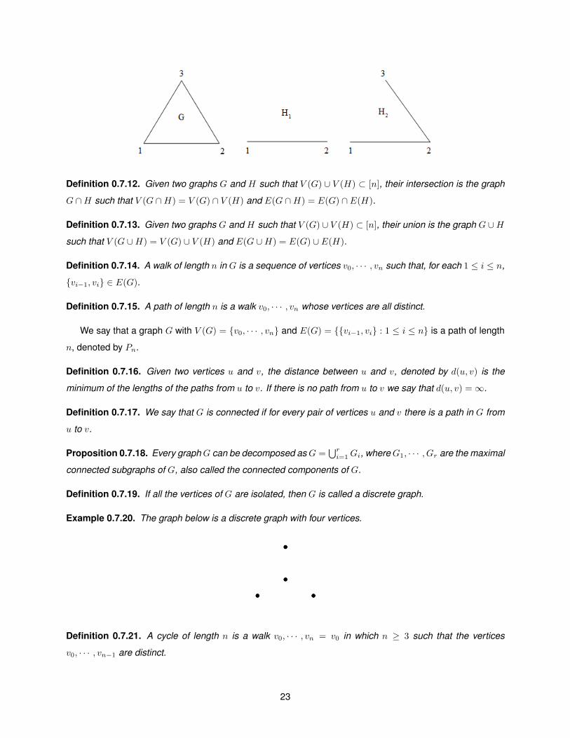
Example 0.7.11. Let G be the triangle with V (G) = {1, 2, 3} and E(G) = {{1, 2}, {1, 3}, {2, 3}}. Then the

subgraph H1 with V (H1) = {1, 2} and E(H1) = {{1, 2}} is an induced subgraph of G. On the other hand,

the subgraph H2 with V (H2) = {1, 2, 3} and E(H2) = {{1, 2}, {2, 3}} is not an induced subgraph of H2 since

1, 3 ∈ V (H2) and {1, 3} ∈ E(G) but {1, 3} 6∈ E(H2).

22

Definition 0.7.12. Given two graphs G and H such that V (G) ∪ V (H) ⊂ [n], their intersection is the graph

G ∩H such that V (G ∩H) = V (G) ∩ V (H) and E(G ∩H) = E(G) ∩ E(H).

Definition 0.7.13. Given two graphs G and H such that V (G) ∪ V (H) ⊂ [n], their union is the graph G ∪H

such that V (G ∪H) = V (G) ∪ V (H) and E(G ∪H) = E(G) ∪ E(H).

Definition 0.7.14. A walk of length n in G is a sequence of vertices v0, · · · , vn such that, for each 1 ≤ i ≤ n,

{vi−1, vi} ∈ E(G).

Definition 0.7.15. A path of length n is a walk v0, · · · , vn whose vertices are all distinct.

We say that a graph G with V (G) = {v0, · · · , vn} and E(G) = {{vi−1, vi} : 1 ≤ i ≤ n} is a path of length

n, denoted by Pn.

Definition 0.7.16. Given two vertices u and v, the distance between u and v, denoted by d(u, v) is the

minimum of the lengths of the paths from u to v. If there is no path from u to v we say that d(u, v) =∞.

Definition 0.7.17. We say that G is connected if for every pair of vertices u and v there is a path in G from

u to v.

Proposition 0.7.18. Every graphG can be decomposed asG =⋃ri=1Gi, whereG1, · · · , Gr are the maximal

connected subgraphs of G, also called the connected components of G.

Definition 0.7.19. If all the vertices of G are isolated, then G is called a discrete graph.

Example 0.7.20. The graph below is a discrete graph with four vertices.

Definition 0.7.21. A cycle of length n is a walk v0, · · · , vn = v0 in which n ≥ 3 such that the vertices

v0, · · · , vn−1 are distinct.

23

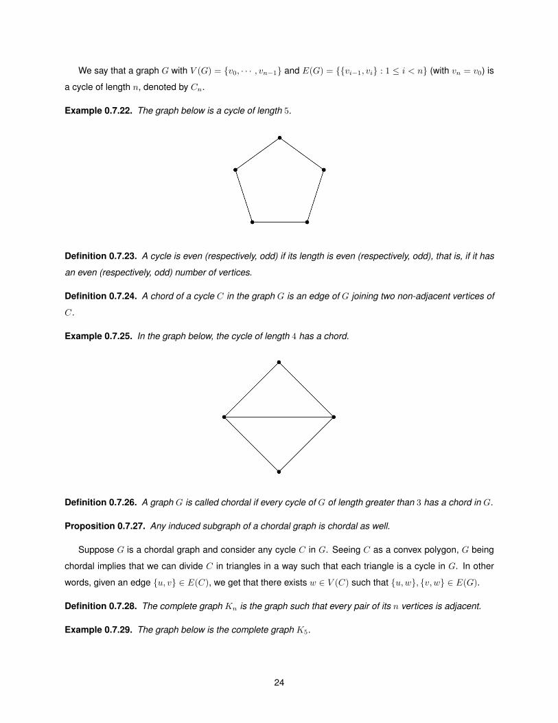
We say that a graph G with V (G) = {v0, · · · , vn−1} and E(G) = {{vi−1, vi} : 1 ≤ i < n} (with vn = v0) is

a cycle of length n, denoted by Cn.

Example 0.7.22. The graph below is a cycle of length 5.

Definition 0.7.23. A cycle is even (respectively, odd) if its length is even (respectively, odd), that is, if it has

an even (respectively, odd) number of vertices.

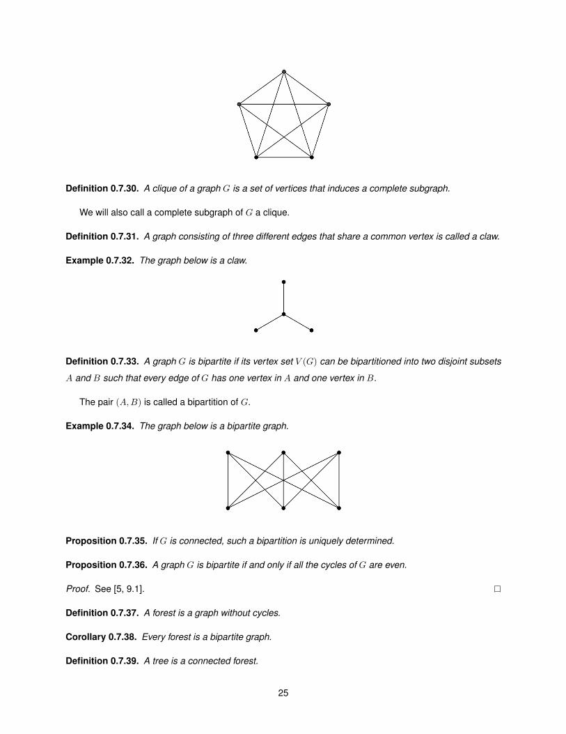
Definition 0.7.24. A chord of a cycle C in the graph G is an edge of G joining two non-adjacent vertices of

C.

Example 0.7.25. In the graph below, the cycle of length 4 has a chord.

Definition 0.7.26. A graph G is called chordal if every cycle of G of length greater than 3 has a chord in G.

Proposition 0.7.27. Any induced subgraph of a chordal graph is chordal as well.

Suppose G is a chordal graph and consider any cycle C in G. Seeing C as a convex polygon, G being

chordal implies that we can divide C in triangles in a way such that each triangle is a cycle in G. In other

words, given an edge {u, v} ∈ E(C), we get that there exists w ∈ V (C) such that {u,w}, {v, w} ∈ E(G).

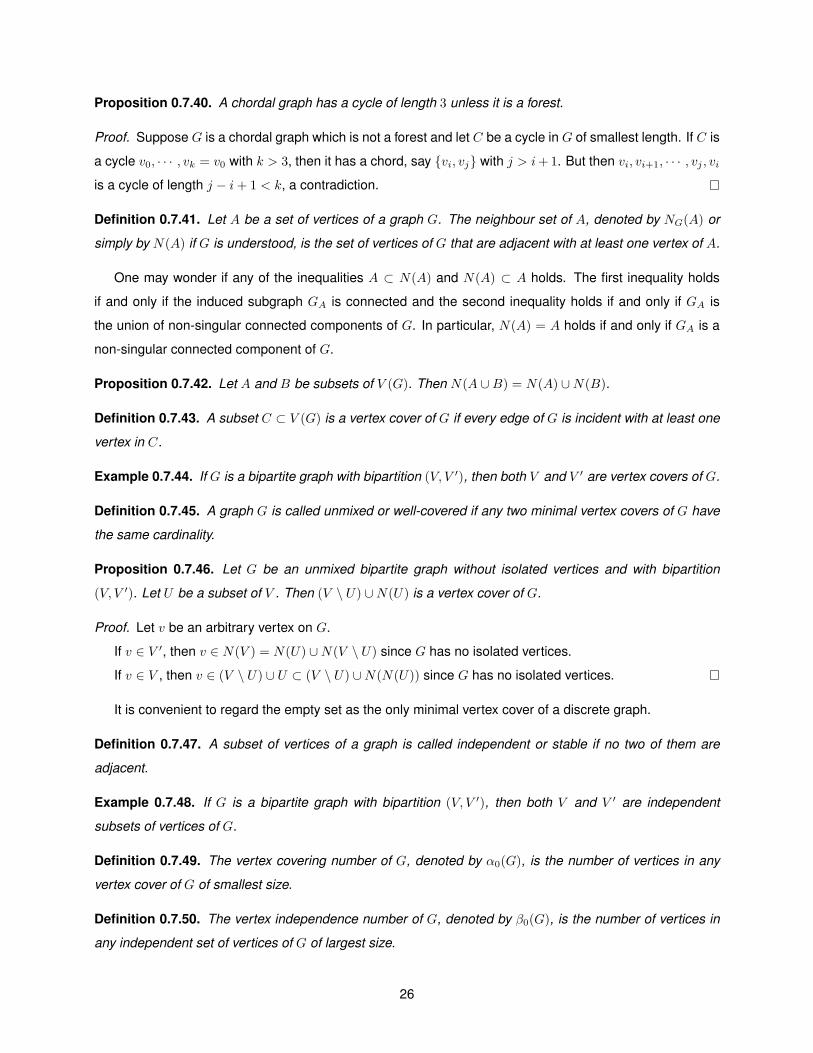
Definition 0.7.28. The complete graph Kn is the graph such that every pair of its n vertices is adjacent.

Example 0.7.29. The graph below is the complete graph K5.

24

Definition 0.7.30. A clique of a graph G is a set of vertices that induces a complete subgraph.

We will also call a complete subgraph of G a clique.

Definition 0.7.31. A graph consisting of three different edges that share a common vertex is called a claw.

Example 0.7.32. The graph below is a claw.

Definition 0.7.33. A graph G is bipartite if its vertex set V (G) can be bipartitioned into two disjoint subsets

A and B such that every edge of G has one vertex in A and one vertex in B.

The pair (A,B) is called a bipartition of G.

Example 0.7.34. The graph below is a bipartite graph.

Proposition 0.7.35. If G is connected, such a bipartition is uniquely determined.

Proposition 0.7.36. A graph G is bipartite if and only if all the cycles of G are even.


Definition 0.7.37. A forest is a graph without cycles.

Corollary 0.7.38. Every forest is a bipartite graph.

Definition 0.7.39. A tree is a connected forest.

25

Proposition 0.7.40. A chordal graph has a cycle of length 3 unless it is a forest.

Proof. Suppose G is a chordal graph which is not a forest and let C be a cycle in G of smallest length. If C is

a cycle v0, · · · , vk = v0 with k > 3, then it has a chord, say {vi, vj} with j > i+ 1. But then vi, vi+1, · · · , vj , viis a cycle of length j − i+ 1 < k, a contradiction.

Definition 0.7.41. Let A be a set of vertices of a graph G. The neighbour set of A, denoted by NG(A) or

simply by N(A) if G is understood, is the set of vertices of G that are adjacent with at least one vertex of A.

One may wonder if any of the inequalities A ⊂ N(A) and N(A) ⊂ A holds. The first inequality holds

if and only if the induced subgraph GA is connected and the second inequality holds if and only if GA is

the union of non-singular connected components of G. In particular, N(A) = A holds if and only if GA is a

non-singular connected component of G.

Proposition 0.7.42. Let A and B be subsets of V (G). Then N(A ∪B) = N(A) ∪N(B).

Definition 0.7.43. A subset C ⊂ V (G) is a vertex cover of G if every edge of G is incident with at least one

vertex in C.

Example 0.7.44. If G is a bipartite graph with bipartition (V, V ′), then both V and V ′ are vertex covers of G.

Definition 0.7.45. A graph G is called unmixed or well-covered if any two minimal vertex covers of G have

the same cardinality.

Proposition 0.7.46. Let G be an unmixed bipartite graph without isolated vertices and with bipartition

(V, V ′). Let U be a subset of V . Then (V \ U) ∪N(U) is a vertex cover of G.

Proof. Let v be an arbitrary vertex on G.

If v ∈ V ′, then v ∈ N(V ) = N(U) ∪N(V \ U) since G has no isolated vertices.

If v ∈ V , then v ∈ (V \ U) ∪ U ⊂ (V \ U) ∪N(N(U)) since G has no isolated vertices.

It is convenient to regard the empty set as the only minimal vertex cover of a discrete graph.

Definition 0.7.47. A subset of vertices of a graph is called independent or stable if no two of them are

adjacent.

Example 0.7.48. If G is a bipartite graph with bipartition (V, V ′), then both V and V ′ are independent

subsets of vertices of G.

Definition 0.7.49. The vertex covering number of G, denoted by α0(G), is the number of vertices in any

vertex cover of G of smallest size.

Definition 0.7.50. The vertex independence number of G, denoted by β0(G), is the number of vertices in

any independent set of vertices of G of largest size.

26

Definition 0.7.51. Given a graph G on [n], its complement G is the graph on [n] such that {i, j} ∈ E(G) if

and only if {i, j} 6∈ E(G).

Example 0.7.52. The two graphs below are complements of each other.

Proposition 0.7.53. A subset of vertices of a graph is independent if and only if its complement is a vertex

cover.

Proof. Let C ⊂ [n] be a subset of vertices of G. Then C is independent if and only if {i, j} 6∈ E(G) for every

i, j ∈ C. In other words, C is independent if and only if each edge in G contains a vertex in [n] \C, that is, if

and only if [n] \ C is a vertex cover of G.

Corollary 0.7.54. For any graph G on [n], one has α0(G) + β0(G) = n.

Proof. Since a subset of [n] is independent if and only if its complement is a vertex cover, it follows that a

subset of [n] is a maximal independent set if and only if its complement is a maximal vertex cover. Hence

the result follows.

Definition 0.7.55. A set of edges in a graph G is called independent if no two of them have a vertex in

common.

Example 0.7.56. In the graph below, the three vertical edges form an independent set of edges.

Definition 0.7.57. A set of independent edges that covers all vertices of a graph G is called a perfect

matching.

Thus G has a perfect matching if and only if G has an even number of vertices and there is an indepen-

dent set of edges containing all the vertices.

Example 0.7.58. The independent set of edges of the graph above is a perfect matching.

27

Theorem 0.7.59 (Marriage theorem). Let G be a bipartite graph on the vertex set V ∪ V ′ with |V | = |V ′|.

Suppose that |N(U)| ≥ |U | for every U ⊂ V . Then there exist labellings V = {x1, · · · , xn} and V ′ =

{y1, · · · , yn} such that {xi, yi} ∈ E(G) for every i ∈ [n].


Definition 0.7.60. An induced matching of a graph is an induced subgraph consisting of pairwise disjoint

edges.

Example 0.7.61. Any pair of opposite edges of the hexagon below is an induced matching.

Definition 0.7.62. Given a graph G, its induced matching number, denoted by indmatch(G), is the number

of edges in an induced matching of G of largest size.

28

Chapter 1

Monomial ideals and Grobner bases

Monomial ideals, simplicial complexes and Stanley-Reisner ideals are fundamental pre-requisites in or-

der to study combinatorical Commutative Algebra and so the inclusion of this chapter, instead of just stating

the most important results and giving references for their proofs (as we did in chapter 0), is very helpful for

a first reader.

In section 1.1, monomial ideals are introduced and their properties are studied in detail.

In section 1.2, simplicial complexes are defined and, to each simplicial complex, we associate its Stanley-

Reisner ideal. In fact, simplicial complexes are uniquely determined by their Stanley-Reisner ideals.

In section 1.3, it is shown that a Grobner basis of an ideal I is also a set of generators of I and the

Buchberger’s criterion gives necessary and sufficient conditions for a set of generators of an ideal to be a

Grobner basis. We end by stating some relations between the algebraic properties of an arbitrary ideal of

polynomials (such as its depth, dimension and regularity) and the same properties of its initial ideal. Such

relations will be used in chapters 2 and 3 when studying of binomial edge ideals of closed graphs.

1.1 Monomial ideals

Monomials form a natural K-basis for the polynomial ring S = K[x1, · · · , xn]. A monomial ideal I also

has a K-basis of monomials. As a consequence, a polynomial f ∈ S belongs to I if and only if all monomials

in f with a non-zero coefficient also belong to I. This is one of the reasons why algebraic operations with

monomial ideals are easy to perform and one may take advantage of this fact when studying general ideals

in S by considering its initial ideal with respect to some monomial order.

Definition 1.1.1. A monomial in S is a product xa = xa11 · · ·xan

n , with a = (a1, · · · , an) ∈ Nn.

The monomials in S correspond bijectively to the lattice points in Rn+ (where R+ is the set of non-negative

real numbers). Moreover, xaxb = xa+b holds for every a,b ∈ Nn.

Notation 1.1.2. If I is an ideal of S, then the set of monomials of I is Mon(I).

29

Definition 1.1.3. An ideal I ⊂ S is called a monomial ideal if it is generated by monomials.

It is well known that S is a Noetherian ring, that is, every ideal of S is finitely generated. As it would be

expected, every monomial ideal of S has a finite system of monomial generators.

Proposition 1.1.4. Any monomial ideal has a finite system of monomial generators.

Proof. Given a non-zero monomial ideal I, let Σ be the set of ideals with a finite system of monomial

generators in I. Since S is Noetherian and Σ 6= ∅, then Σ has a maximal ideal J . Suppose J 6= I. Since

I is a monomial ideal, then there exists u ∈ Mon(I) \ J and thus J + (u) is an ideal with a finite system

of monomial generators in I which strictly contains J , a contradiction. Hence I = J has a finite system of

monomial generators.

The set Mon(S) is a K-basis of S, that is, every polynomial f ∈ S is a unique finite K-linear combination

of monomials

f =∑

u∈Mon(S)

auu, with au ∈ K. (1.1)

Definition 1.1.5. The support of f is supp(f) = {u ∈ Mon(S) : au 6= 0}.

Theorem 1.1.6. If I is a monomial ideal, then the set N of monomials belonging to I is a K-basis of I.

Proof. It is clear that the elements of N are linearly independent, as N ⊂ Mon(S).

To show that N generates the K-vector space I, it is enough to show that supp(f) ⊂ N for any f ∈ I.

In fact, if f ∈ I, then there exist monomials u1, · · · , um ∈ I and polynomials f1, · · · , fm ∈ S such that

f =∑mi=1 fiui, hence supp(f) ⊂

⋃mi=1 supp(fiui). Since each monomial in supp(fiui) is of the form wui with

w ∈ supp(fi), it follows that supp(fiui) ⊂ N for every 1 ≤ i ≤ m, hence supp(f) ⊂ N , as desired.

Recall definition 0.4.3. Monomial ideals can be characterized similarly.

Corollary 1.1.7. The ideal I ⊂ S is a monomial ideal if and only if supp(f) ⊂ I for every f ∈ I.

Proof. Suppose I is a monomial ideal and let f ∈ I. According to theorem 1.1.6, there exist monomi-

als u1, · · · , um ∈ I and constants a1, · · · , am ∈ K such that f = a1u1 + · · · + amum, hence supp(f) ⊂

{u1, · · · , um} ⊂ I.

Suppose supp(f) ⊂ I for every f ∈ I and let f1, · · · , fm ∈ I be a set of generators of I. Since supp(fi) ⊂

I for every i, it follows that⋃mi=1 supp(fi) is a set of monomial generators of I and thus I is a monomial

ideal.

Definition 1.1.8. For monomials xa = xa11 · · ·xan

n and xb = xb11 · · ·xbn

n of S, we say that xb divides xa, and

we write xb | xa, if bi ≤ ai for each i.

Proposition 1.1.9. Let {u1, · · · , um} be a monomial system of generators of I. Then the monomial v

belongs to I if and only if ui | v for some i ∈ [m].

30

Proof. Suppose v ∈ I. Then there exist polynomials f1, · · · , fm ∈ S such that v = f1u1 + · · · + fmum,

therefore v ∈ supp(fiui) for some i ∈ [m], that is, v = wui for some w ∈ supp(fi), hence ui | v.

Proposition 1.1.10. A monomial set of generators G of an ideal I is minimal if and only if there is no pair of

distinct monomials u, v ∈ G such that u | v.

Proof. We will show that G is not minimal if and only if there exists two distinct monomials u, v ∈ G such

that u | v.

Suppose G is not minimal. Then there exists a monomial set of generators G′ of I such that G′ ( G. Let

v ∈ G′ \G. By proposition 1.1.9 there exists u ∈ G′ such that u | v.

Suppose there exists two distinct monomials u, v ∈ G such that u | v. Then G \ {v} is a monomial set of

generators of I strictly contained in G, hence G is not minimal.

Proposition 1.1.11. Each monomial ideal has a unique minimal monomial set of generators.

Proof. Let G1 = {u1, · · · , ur} and G2 = {v1, · · · , vs} be two minimal sets of generators of the monomial

ideal I. Let i ∈ [r]. Since ui ∈ Mon(I), then vj | ui for some j ∈ [s]. Similarly, uk | vj for some k ∈ [r],

therefore uk | ui, and since G1 is a minimal set of generators, ui = uk, therefore ui = vj ∈ G2. This shows

that G1 ⊂ G2. By symmetry we also have G2 ⊂ G1.

Notation 1.1.12. The unique minimal set of monomial generators of the monomial ideal I is denoted by

G(I).

Definition 1.1.13. LetM be a non-empty subset of Mon(S). A monomial xa ∈ M is said to be a minimal

element ofM with respect to divisibility if whenever xb | xa with xb ∈M, then xb = xa.

Notation 1.1.14. The set of minimal elements ofM is denoted byMmin.

Theorem 1.1.15 (Dickson’s lemma). Let M be a non-empty subset of Mon(S). Then Mmin is a finite

non-empty set.

Proof. Let I ⊂ S be the ideal with generator set M. Since G(I) is the only minimal set of monomial

generators of I, then G(I) ⊂M. We will show that G(I) =Mmin, from where the result follows.

Let u ∈ G(I). Suppose there exists v ∈ M such that v | u. Then v ∈ Mon(I) and by proposition 1.1.9

there exists w ∈ G(I) such that w | v. Since w | v and v | u, then w | u, and since u,w ∈ G(I), it follows that

w = u and so v = u. Hence u ∈Mmin.

Let u ∈ Mmin. Then u ∈ I, therefore there exists v ∈ G(I) such that v | u. But then v ∈ M, and since

v | u, it follows that u = v ∈ G(I).

It is obvious that sums and products of monomial ideals are again monomial ideals. More precisely, if I

and J are monomial ideals, then so are I + J and IJ , with G(I + J) ⊂ G(I)∪G(J) and G(IJ) ⊂ G(I)G(J).

31

Notation 1.1.16. Given two monomials u and v, we denote by gcd(u, v) their greatest common divisor and

by lcm(u, v) their least common multiple.

Proposition 1.1.17. Let I and J be monomial ideals. Then I ∩ J is a monomial ideal and

{lcm(u, v) : u ∈ G(I), v ∈ G(J)}

is a set of generators of I ∩ J .

Proof. Let f ∈ I ∩ J . By corollary 1.1.7, supp(f) ⊂ I ∩ J . Since f ∈ I ∩ J is arbitrary, applying corollary

1.1.7 again we see that I ∩ J is a monomial ideal.

Let w ∈ Mon(I ∩ J). Then there exist u ∈ G(I) and v ∈ G(J) such that u | w and v | w, therefore

lcm(u, v) | w. It is clear that {lcm(u, v) : u ∈ G(I), v ∈ G(J)} ⊂ I ∩J , hence {lcm(u, v) : u ∈ G(I), v ∈ G(J)}

is a set of generators of I ∩ J .

Proposition 1.1.18. Let I and J be monomial ideals. Then I : J is a monomial ideal such that

I : J =⋂

v∈G(J)

I : (v).

Moreover, {u/ gcd(u, v) : u ∈ G(I)} is a set of generators of I : (v).

Proof. Let f ∈ I : J . Then fv ∈ I for every v ∈ G(J). In view of corollary 1.1.7 we have supp(f)v =

supp(fv) ⊂ I. This implies that supp(f) ⊂ I : J . Since f ∈ I : J is arbitrary, corollary 1.1.7 yields that I : J

is a monomial ideal.

The given interpretation of I : J as an intersection is obvious, and it is clear that {u/ gcd(u, v) : u ∈

G(I)} ⊂ I : (v). So now let w ∈ Mon(I : (v)). Then vw ∈ I, therefore there exists u ∈ G(I) such that u | vw,

hence u/ gcd(u, v) | w, as desired.

Proposition 1.1.19. The radical of a monomial ideal I is again a monomial ideal.

Proof. Let f ∈√I. Then fk ∈ I for some k ≥ 1 and by corollary 1.1.7 one has supp(fk) ⊂ I since I is a

monomial ideal. Let supp(f) = {xa1 , · · · ,xar}. Then some ai, say a1, does not belong to the convex hull of

the set {a1, · · · ,ar} \ {ai}.

Assume (xa1)k = (xa1)k1(xa2)k2 · · · (xar )kr , with k = k1 + · · · + kr and k1 < k. Then a1 =∑ri=2

ki

k−k1ai

with∑ri=2

ki

k−k1= 1, so a1 belongs to the convex hull of {a2, · · · ,ar}, a contradiction. It follows that the

monomial (xa1)k cannot cancel against other terms in fk and hence (xa1)k belongs to supp(fk), which is a

subset of I. Therefore xa1 ∈√I and f − cxa1 ∈

√I, where c is the coefficient of f in the monomial xa1 . By

induction on the cardinality of supp(f) we conclude that supp(f) ⊂√I. Thus corollary 1.1.7 implies that

√I

is a monomial ideal.

Definition 1.1.20. A monomial xa11 · · ·xan

n ∈ S is called square-free if a1, · · · , an ∈ {0, 1}.

Notation 1.1.21. For u = xa11 · · ·xan

n we set√u =

∏i:ai 6=0 xi.

32

One has u =√u if and only if u is square-free.

Proposition 1.1.22. Let I be a monomial ideal. Then {√u, u ∈ G(I)} is a set of generators of

√I.

Proof. Obviously {√u, u ∈ G(I)} ⊂

√I. Since

√I is a monomial ideal, it is enough to show that each

monomial v ∈√I is a multiple of some

√u with u ∈ G(I). In fact, if v ∈

√I, then vk ∈ I for some integer

k ≥ 1 and therefore u | vk for some u ∈ G(I). This yields the desired conclusion.

Definition 1.1.23. A monomial ideal I is called a square-free monomial ideal if it is generated by square-free

monomials.

Corollary 1.1.24. A monomial ideal is a radical ideal if and only if it is a square-free monomial ideal.

Theorem 1.1.25. Let I ⊂ K[x1, · · · , xn] be a monomial ideal. Then I =⋂mi=1Qi, where each Qi is gener-

ated by pure powers of the variables. In other words, each Qi is of the form (xa1i1, · · · , xak

ik). Moreover, an

irredundant presentation of this form is unique.

Proof. Let G(I) = {u1, · · · , ur}, and suppose some ui, say u1, is not a pure power of a variable. Then

we can write u1 = vw where v, w ∈ Mon(S) are such that gcd(v, w) = 1 and v 6= 1 6= w. We claim that

I = I1 ∩ I2, where I1 = (v, u2, · · · , ur) and I2 = (w, u2, · · · , ur). Obviously, I is contained in the intersection.

Conversely, let u ∈ Mon(I1 ∩ I2). If u is the multiple of some ui, with 2 ≤ i ≤ r, then u ∈ I. If not, then u is a

multiple of both v and w, and since gcd(v, w) = 1, u is a multiple of u1. In any case, u ∈ I.

If either G(I1) or G(I2) contains an element which is not a pure power, we proceed as before and, after

a finite number of steps, we obtain a presentation of I as an intersection of monomial ideals generated

by pure powers. By ommiting those ideals which contain the intersection of the others we end up with an

irredundant presentation.

Let Q1 ∩ · · · ∩Qr = Q′1 ∩ · · · ∩Q′s be two such irrendundant presentations of I. We will show that for each

i ∈ [r] there exists j ∈ [s] such that Q′j ⊂ Qi. By symmetry we then also have that for each k ∈ [s] there

exists l ∈ [r] such that Ql ⊂ Q′k. This will then imply that r = s and {Q1, · · · , Qr} = {Q′1, · · · , Q′s}.

In fact, let i ∈ [r]. We may assume that Qi = (xa11 , · · · , xak

k ). Suppose that Q′j 6⊂ Qi for all j ∈ [s]. Then

for each j there exists xbj

lj∈ Q′j \ Qi. It follows that either lj 6∈ [k] or bj < alj . Let u = lcm(xb1

l1, · · · , xbs

ls).

We have u ∈⋂sj=1Q

′j = I ⊂ Qi. Thus there exists i ∈ [k] such that xai

i divides u. But this is obviously

impossible.

Example 1.1.26. Let I = (x21x2, x

21x

23, x

22, x2x

23) ⊂ K[x1, x2, x3]. Then:

I = (x21x2, x

21x

23, x

22, x2x

23) = (x2

1, x21x

23, x

22, x2x

23) ∩ (x2, x

21x

23, x

22, x2x

23) =

= (x21, x

22, x2x

23) ∩ (x2, x

21x

23) = (x2

1, x22, x2) ∩ (x2

1, x22, x

23) ∩ (x2, x

21) ∩ (x2, x

23) =

= (x21, x

22, x

23) ∩ (x2, x

21) ∩ (x2, x

23).

33

Definition 1.1.27. A monomial ideal is called irreducible if it cannot be written as proper intersection of two

other monomial ideals. It is called reducible if it is not irreducible.

Corollary 1.1.28. A monomial ideal is irreducible if and only if it is generated by pure powers of the variables.

Proof. Let Q = (xa1i1, · · · , xak

ik) and suppose Q = I ∩ J , where I and J are monomial ideals properly

containing Q. By theorem 1.1.25 we have I =⋂ri=1Qi and J =

⋂sj=1Q

′j , where the ideals Qi and Q′j

are generated by pure powers. Therefore we get the presentation

Q =r⋂i=1

Qi ∩s⋂j=1

Q′j .

By ommiting suitable ideals in the intersection on the right hand side, we obtain an irredundant presen-

tation of Q. The uniqueness of the irredundant presentation implies that Q = Qi for some i ∈ [r] or Q = Q′j

for some j ∈ [s], a contradiction.

Conversely, if G(Q) contains a monomial u = vw with gcd(v, w) = 1 and v 6= 1 6= w, then, as in the proof

of theorem 1.1.25, Q can be written as the intersection of monomial ideals properly containing Q.

If I is a square-free monomial ideal, the above procedure yields that the irreducible monomial ideals

appearing in the intersection of I are all of the form (xi1 , · · · , xik ). These monomial ideals are precisely the

monomial prime ideals.

Corollary 1.1.29. A square-free monomial ideal is the intersection of monomial prime ideals.

Combining this corollary with lemma 0.2.13 we obtain:

Corollary 1.1.30. Let I ⊂ S be a square-free monomial ideal. Then I =⋂P∈Min(I) P , and each P ∈ Min(I)

is a monomial prime ideal.

Proposition 1.1.31. The irreducible ideal (xa1i1, · · · , xak

ik) is (xi1 , · · · , xik )-primary.

Proof. Let Q = (xa1i1, · · · , xak

ik) and P = (xi1 , · · · , xik ). By proposition 0.2.25, Q is P -primary if and only

if Ass(S/Q) = {P}. Notice that Min(Q) = {P}. Since P ∈ Min(Q), by proposition 0.2.21 it follows that

P ∈ Ass(S/Q). Suppose there exists another P ′ ∈ Ass(S/Q).

Let g ∈ S \Q such that P ′ = Ann(g+Q) and consider its decomposition as a finite K-linear combination

of monomials. Removing from such K-linear combination the monomials which are multiples of some

monomial in the set {xa1i1, · · · , xak

ik}, we get a polynomial g′ ∈ S\Q whose support does not intersect Mon(Q)

and such that g+Q = g′+Q. Hence we can suppose without loss of generality that supp(g)∩Mon(Q) = ∅.

Since Q ⊂ P ′ and Min(Q) = {P}, then P ( P ′.

Pick f ∈ P ′ \ P and consider its decomposition as a finite K-linear combination of monomials. Re-

moving from such K-linear combination the monomials which are multiples of some monomial in the set

{xi1 , · · · , xik}, we get a polynomial in P ′ \ P whose support does not intersect Mon(P ). Hence we can

suppose without loss of generality that supp(f) ∩Mon(P ) = ∅.

34

Since f 6= 0 and g 6= 0, then fg 6= 0. Let w ∈ supp(fg). Then there exist u ∈ supp(f) and v ∈ supp(g)

such that w = uv. Since none of the monomials xi1 , · · · , xik divide u and none of the monomials xa1i1, · · · , xak

ik

divide v, it follows that none of the monomials xa1i1, · · · , xak

ikdivide w. Since w ∈ supp(fg) is arbitrary, then

supp(fg) ∩Mon(Q) = ∅, hence fg 6∈ Q. But since f ∈ P ′ and P ′ = Ann(g +Q), by definition it follows that

fg ∈ Q, a contradiction.

Corollary 1.1.32. The irredundant decomposition of a monomial ideal as the intersection of monomial ideals

generated by pure powers is in fact a primary irredundant decomposition.

Corollary 1.1.33. The associated prime ideals of a monomial ideal are monomial prime ideals.

Even though a primary irredundant decomposition of a monomial ideal I may not be unique, the primary

decomposition, obtained from an irredundant intersection of irreducible ideals as described above, is unique.

We call it the standard primary decomposition of I.

Example 1.1.34. As we saw in example 1.1.26, if I = (x21x2, x

21x

23, x

22, x2x

23), then

I = (x21, x

22, x

23) ∩ (x2, x

21) ∩ (x2, x

23)

is the standard primary decomposition of I and in particular Ass(R/I) = {(x1, x2), (x2, x3), (x1, x2, x3)}.

Notice that, in this particular case, Min(I) 6= Ass(R/I).

We end this section by stating a result which will be important in the study of monomial edge ideals:

Proposition 1.1.35. If P is a monomial prime ideal generated by k variables, then

ht(P ) = k and dim(S/P ) = n− k.

Proof. Let P = (xi1 , · · · , xik ). Since P is generated by k elements of S, theorem 0.3.2 implies that ht(P ) ≤

k. On the other hand, (0) ( (xi1) ( (xi1 , xi2) ( · · · ( (xi1 , · · · , xik−1) ( P is an ascending chain of prime

ideals of length k and so ht(P ) = k. By proposition 0.5.12, ht(P ) + dim(S/P ) = n and so dim(S/P ) =

n− k.

1.2 Simplicial complexes and Stanley-Reisner ideals

Sometimes, when studying graphs, is it is a good idea to think about them as simplicial complexes. In

fact, for each graph G, we can associate a simplicial complex ∆(G), called its clique complex, such that

there is an obvious correspondence between the faces of G and the cliques of ∆(G). Since each graph is

uniquely determined by its clique complex, then graphs are just a special class of simplicial complexes.

Definition 1.2.1. A simplicial complex ∆ on the vertex set [n] is a collection of subsets of [n] that contains

all one-element subsets and such that if F ∈ ∆ and F ′ ⊂ F , then F ′ ∈ ∆.

35

Definition 1.2.2. A face of ∆ is just an element of ∆.

Definition 1.2.3. The dimension of a face F is |F | − 1.

Definition 1.2.4. A vertex is a face of dimension 0.

Definition 1.2.5. An edge is a face of dimension 1.

Definition 1.2.6. A facet is a maximal face with respect to inclusion.

Notation 1.2.7. The set of facets of ∆ is denoted by F(∆).

It is clear that F(∆) determines ∆ and so we write ∆ = 〈F1, · · · , Fm〉 when F(∆) = {F1, · · · , Fm}. More

generally, given a set {G1, · · · , Gs} of faces of ∆, we denote by 〈G1, · · · , Gs〉 the subcomplex of ∆ consisting

of those faces of ∆ which are contained in some Gi.

Definition 1.2.8. A non-face of ∆ is a subset of [n] such that F 6∈ ∆.

Notation 1.2.9. The set of minimal non-faces of ∆ is denoted by N (∆).

Definition 1.2.10. A simplicial complex ∆ is pure if all its facets have the same dimension. More precisely,

if such dimension is d, we say ∆ is a pure d-dimensional simplicial complex.

Let S = K[x1, · · · , xn] be the polynomial ring in n variables over K and let ∆ be a simplicial complex on

[n].

Notation 1.2.11. For F ⊂ [n], we denote xF =∏i∈F xi.

Definition 1.2.12. The Stanley-Reisner ideal of ∆ is the ideal I∆ ⊂ S generated by the square-free mono-

mials xF with F 6∈ ∆.

Proposition 1.2.13. If ∆ is a simplicial complex, then I∆ is a monomial ideal with G(I∆) = {xF : F ∈

N (∆)}.

Notation 1.2.14. For each subset F ⊂ [n] we denote F = [n] \ F .

Notation 1.2.15. For each subset F ⊂ [n], PF is the prime ideal of S generated by the variables xi with

i ∈ F .

Lemma 1.2.16. The standard primary decomposition of I∆ is I∆ =⋂F∈F(∆) PF .

Proof. Let F ∈ F(∆). If G is a non-face of ∆, then G 6⊂ F . Pick i ∈ G \ F . Then xi ∈ PF and xi | xG, hence

xG ∈ PF . Since G is an arbitrary non-face of ∆, I∆ ⊂ PF .

Let u ∈ Mon(S) such that u ∈⋂F∈F(∆) PF . Then for each F ∈ F(∆) there exists iF ∈ F such that

xiF | u and so lcm(xiF : F ∈ F(∆)) | u. On the other hand, {iF : F ∈ F(∆)} cannot be contained in any

facet of ∆ and so it is a non-face of ∆, which implies u ∈ I∆. Since⋂F∈F(∆) PF is a monomial ideal (for it

is a finite intersection of monomial ideals), it follows that⋂F∈F(∆) PF ⊂ I∆.

Since the Stanley-Reisner ideal of a simplicial complex is uniquely determined by its facets, the primary

decomposition I∆ =⋂F∈F(∆) PF turns out to be irredundant.

36

Definition 1.2.17. A simplicial complex ∆ is Cohen-Macaulay over a field K if the ideal I∆ is Cohen-

Macaulay.

Proposition 1.2.18. If ∆ is a Cohen-Macaulay simplicial complex, then ∆ is a pure simplicial complex.

Proof. By lemma 1.2.16, Ass(S/I∆) = {PF : F ∈ F(∆)}. If ∆ is a Cohen-Macaulay simplicial complex on

[n], that is, I∆ is Cohen-Macaulay, then by proposition 2.2.34, dim(S/PF ) = dim(S/I∆) for every F ∈ F(∆).

But PF is a monomial prime ideal generated by n−|F | variables and so, by proposition 1.1.35, dim(S/PF ) =

|F |, hence |F | = dim(S/I∆). This means that all facets of ∆ have dimension dim(S/I∆) − 1 and so ∆ is a

pure simplicial complex.

Definition 1.2.19. Let F ∈ ∆. The link of F in ∆ is the subcomplex

link∆(F ) = {G ∈ ∆ : F ∪G ∈ ∆, F ∩G = ∅}.

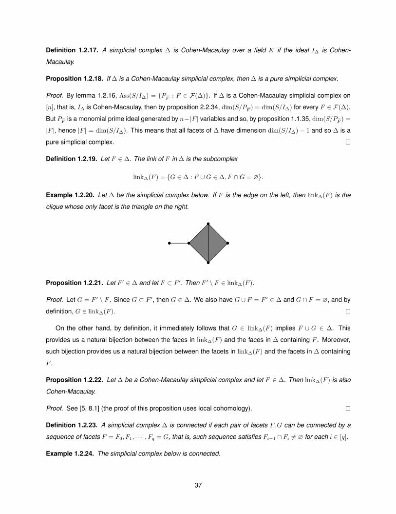
Example 1.2.20. Let ∆ be the simplicial complex below. If F is the edge on the left, then link∆(F ) is the

clique whose only facet is the triangle on the right.

Proposition 1.2.21. Let F ′ ∈ ∆ and let F ⊂ F ′. Then F ′ \ F ∈ link∆(F ).

Proof. Let G = F ′ \ F . Since G ⊂ F ′, then G ∈ ∆. We also have G ∪ F = F ′ ∈ ∆ and G ∩ F = ∅, and by

definition, G ∈ link∆(F ).

On the other hand, by definition, it immediately follows that G ∈ link∆(F ) implies F ∪ G ∈ ∆. This

provides us a natural bijection between the faces in link∆(F ) and the faces in ∆ containing F . Moreover,

such bijection provides us a natural bijection between the facets in link∆(F ) and the facets in ∆ containing

F .

Proposition 1.2.22. Let ∆ be a Cohen-Macaulay simplicial complex and let F ∈ ∆. Then link∆(F ) is also

Cohen-Macaulay.

Proof. See [5, 8.1] (the proof of this proposition uses local cohomology).

Definition 1.2.23. A simplicial complex ∆ is connected if each pair of facets F,G can be connected by a

sequence of facets F = F0, F1, · · · , Fq = G, that is, such sequence satisfies Fi−1 ∩ Fi 6= ∅ for each i ∈ [q].

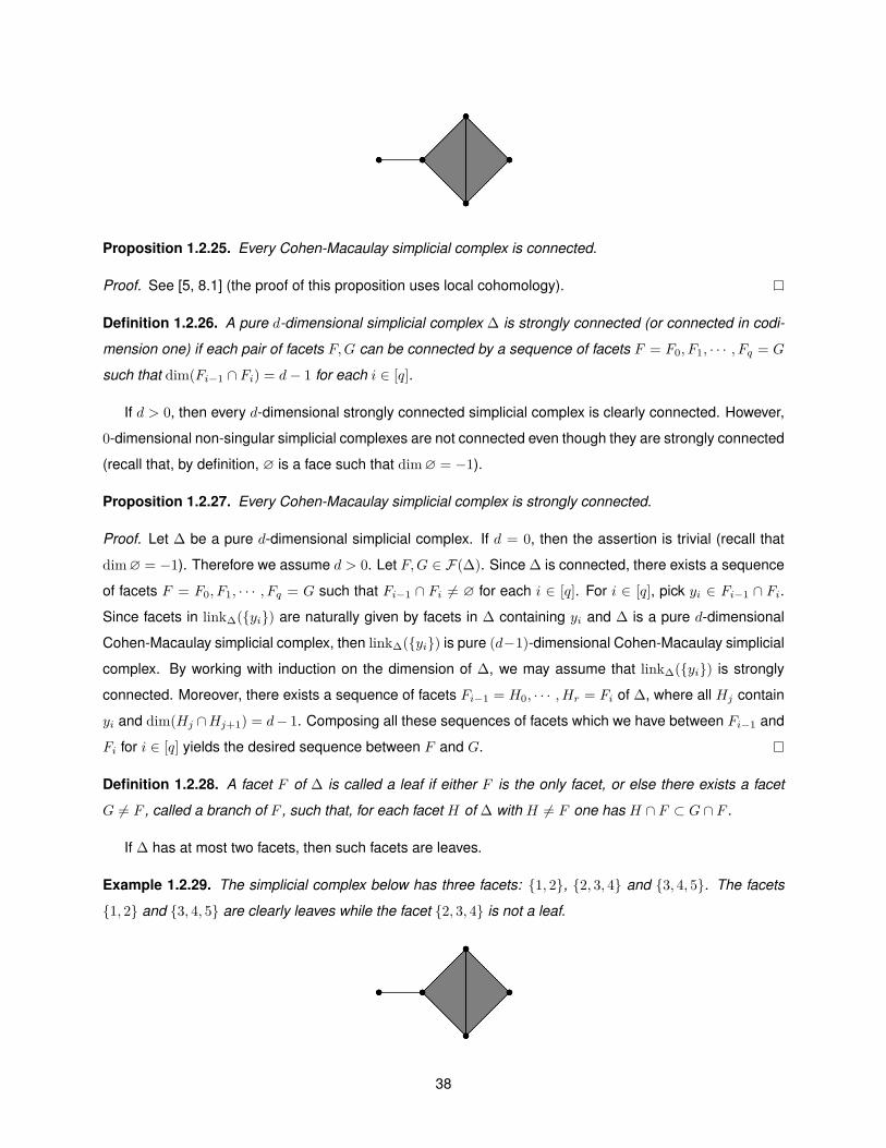
Example 1.2.24. The simplicial complex below is connected.

37

Proposition 1.2.25. Every Cohen-Macaulay simplicial complex is connected.


Definition 1.2.26. A pure d-dimensional simplicial complex ∆ is strongly connected (or connected in codi-

mension one) if each pair of facets F,G can be connected by a sequence of facets F = F0, F1, · · · , Fq = G

such that dim(Fi−1 ∩ Fi) = d− 1 for each i ∈ [q].

If d > 0, then every d-dimensional strongly connected simplicial complex is clearly connected. However,

0-dimensional non-singular simplicial complexes are not connected even though they are strongly connected

(recall that, by definition, ∅ is a face such that dim∅ = −1).

Proposition 1.2.27. Every Cohen-Macaulay simplicial complex is strongly connected.

Proof. Let ∆ be a pure d-dimensional simplicial complex. If d = 0, then the assertion is trivial (recall that

dim∅ = −1). Therefore we assume d > 0. Let F,G ∈ F(∆). Since ∆ is connected, there exists a sequence

of facets F = F0, F1, · · · , Fq = G such that Fi−1 ∩ Fi 6= ∅ for each i ∈ [q]. For i ∈ [q], pick yi ∈ Fi−1 ∩ Fi.

Since facets in link∆({yi}) are naturally given by facets in ∆ containing yi and ∆ is a pure d-dimensional

Cohen-Macaulay simplicial complex, then link∆({yi}) is pure (d−1)-dimensional Cohen-Macaulay simplicial

complex. By working with induction on the dimension of ∆, we may assume that link∆({yi}) is strongly

connected. Moreover, there exists a sequence of facets Fi−1 = H0, · · · , Hr = Fi of ∆, where all Hj contain

yi and dim(Hj ∩Hj+1) = d− 1. Composing all these sequences of facets which we have between Fi−1 and

Fi for i ∈ [q] yields the desired sequence between F and G.

Definition 1.2.28. A facet F of ∆ is called a leaf if either F is the only facet, or else there exists a facet

G 6= F , called a branch of F , such that, for each facet H of ∆ with H 6= F one has H ∩ F ⊂ G ∩ F .

If ∆ has at most two facets, then such facets are leaves.

Example 1.2.29. The simplicial complex below has three facets: {1, 2}, {2, 3, 4} and {3, 4, 5}. The facets

{1, 2} and {3, 4, 5} are clearly leaves while the facet {2, 3, 4} is not a leaf.

38

Proposition 1.2.30. Each leaf F has at least one free vertex, that is, a vertex which belongs to F but to no

other facet.

Proof. If F is the only facet of ∆, the result is obvious. Otherwise, let G be a branch of F and suppose F

has no free vertices. Let i ∈ F . Then there exists another facet H such that i ∈ H and so i ∈ H∩F ⊂ G∩F .

Since i ∈ F is arbitrary, it follows that F ⊂ G∩F , which is absurd. Hence F has at least one free vertex.

Definition 1.2.31. The simplicial complex ∆ is called a quasi-forest if its facets F1, · · · , Fr can be ordered

in a way such that for all i > 1 the facet Fi is a leaf of the simplicial complex with facets F1, · · · , Fi−1, Fi.

Such an order of the facets is called a leaf order. As one would expect, a connected quasi-forest is called

a quasi-tree.

Definition 1.2.32. The clique complex of a graph G on [n] is the simplicial complex ∆(G) on [n] whose faces

are the cliques of G.

Since any graph is uniquely determined by its clique complex, it follows that each graph can be viewed

as a simplicial complex ∆ on [n] with the property that if F ⊂ [n] is such that all two-element subsets of F

are faces of ∆, then F ∈ ∆.

Definition 1.2.33. A graph G has a perfect elimination order if its vertices can be labelled 1, · · · , n such that

for all j ∈ [n], the set Cj = {i : i ≤ j, {i, j} ∈ E(G)} ∪ {j} is a clique of G.

Example 1.2.34. If G is a path, then we get a perfect elimination order by labelling its vertices in a way such

that every two consecutive vertices are adjacent.

Theorem 1.2.35. The following conditions are equivalent:

1. G is chordal.

2. G has a perfect elimination order.

3. ∆(G) is a quasi-forest.

Proof. In 1961, in [13], Dirac showed that (1) and (2) are equivalent. In [5][9.2] it is shown that (2) and (3)

are equivalent. Hence the conclusion follows.

1.3 Grobner bases

Grobner basis theory has become a fundamental field in algebra which provides a wide range of theo-

retical and computational methods in many areas of mathematics and other sciences. Bruno Buchberger

defined the notion of Grobner basis in 1965. An intensive research in this theory, related algorithms and

applications developed, and many books on this topic have appeared since then.

Let S = K[x1, · · · , xn] be a polynomial ring in n variables over a field K.

39

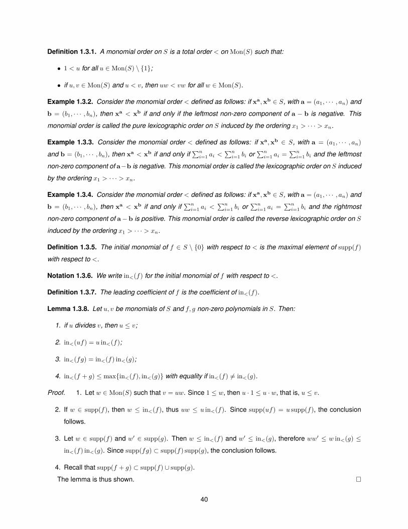
Definition 1.3.1. A monomial order on S is a total order < on Mon(S) such that:

• 1 < u for all u ∈ Mon(S) \ {1};

• if u, v ∈ Mon(S) and u < v, then uw < vw for all w ∈ Mon(S).

Example 1.3.2. Consider the monomial order < defined as follows: if xa,xb ∈ S, with a = (a1, · · · , an) and

b = (b1, · · · , bn), then xa < xb if and only if the leftmost non-zero component of a − b is negative. This

monomial order is called the pure lexicographic order on S induced by the ordering x1 > · · · > xn.

Example 1.3.3. Consider the monomial order < defined as follows: if xa,xb ∈ S, with a = (a1, · · · , an)

and b = (b1, · · · , bn), then xa < xb if and only if∑ni=1 ai <

∑ni=1 bi or

∑ni=1 ai =

∑ni=1 bi and the leftmost

non-zero component of a−b is negative. This monomial order is called the lexicographic order on S induced

by the ordering x1 > · · · > xn.

Example 1.3.4. Consider the monomial order < defined as follows: if xa,xb ∈ S, with a = (a1, · · · , an) and

b = (b1, · · · , bn), then xa < xb if and only if∑ni=1 ai <

∑ni=1 bi or

∑ni=1 ai =

∑ni=1 bi and the rightmost

non-zero component of a−b is positive. This monomial order is called the reverse lexicographic order on S

induced by the ordering x1 > · · · > xn.

Definition 1.3.5. The initial monomial of f ∈ S \ {0} with respect to < is the maximal element of supp(f)

with respect to <.

Notation 1.3.6. We write in<(f) for the initial monomial of f with respect to <.

Definition 1.3.7. The leading coefficient of f is the coefficient of in<(f).

Lemma 1.3.8. Let u, v be monomials of S and f, g non-zero polynomials in S. Then:

1. if u divides v, then u ≤ v;

2. in<(uf) = u in<(f);

3. in<(fg) = in<(f) in<(g);

4. in<(f + g) ≤ max{in<(f), in<(g)} with equality if in<(f) 6= in<(g).

Proof. 1. Let w ∈ Mon(S) such that v = uw. Since 1 ≤ w, then u · 1 ≤ u · w, that is, u ≤ v.

2. If w ∈ supp(f), then w ≤ in<(f), thus uw ≤ u in<(f). Since supp(uf) = u supp(f), the conclusion

follows.

3. Let w ∈ supp(f) and w′ ∈ supp(g). Then w ≤ in<(f) and w′ ≤ in<(g), therefore ww′ ≤ w in<(g) ≤

in<(f) in<(g). Since supp(fg) ⊂ supp(f) supp(g), the conclusion follows.

4. Recall that supp(f + g) ⊂ supp(f) ∪ supp(g).

The lemma is thus shown.

40

Proposition 1.3.9. LetM be a non-empty set of monomials in S and let < be a monomial order in S. Then

M has a unique minimal element with respect to <.

Proof. By Dickson’s lemma, Mmin is a finite non-empty set. Let u be the smallest monomial inMmin with

respect to <.

Let v ∈M. Then there exists w ∈Mmin such that w | v, hence w ≤ v. On the other hand, u ≤ w and so

u ≤ v. Since v ∈M is arbitrary, then u is the unique minimal element ofM

Definition 1.3.10. Let I be a non-zero ideal of S. The initial ideal of I with respect to < is the monomial

ideal of S which is generated by the set {in<(f) : f ∈ I \ {0}}.

Notation 1.3.11. We write in<(I) for the initial ideal of I.

Since in<(I) is a monomial ideal such that Mon(in<(I)) = {in<(f) : f ∈ I \ {0}}, then by proposition

1.1.4 there exists a finite number of non-zero polynomials g1, · · · , gs ∈ I such that in<(I) = (in<(g1), · · · , in<(gs)).

Definition 1.3.12. Let I be a non-zero ideal of S. A finite set of non-zero polynomials {g1, · · · , gs} ⊂ I is

said to be a Grobner basis of I with respect to < if the initial ideal in<(I) is generated by the monomials

in<(g1), · · · , in<(gs).

Theorem 1.3.13. Let I be a non-zero ideal of S and {g1, · · · , gs} a Grobner basis of I with respect to a

monomial order < on S. Then I = (g1, · · · , gs). In other words, every Grobner basis of I is a generator set

of I.

Proof. Suppose I 6= (g1, · · · , gs) and let M = {in<(g) : g ∈ I 6= (g1, · · · , gs)}. Pick f ∈ I \ (g1, · · · , gs)

such that in<(f) is the minimal element ofM with respect to <. Since {g1, · · · , gs} is a Grobner basis of I,

by proposition 1.1.9 some in<(gi) must divide in<(f). Let w ∈ Mon(S) such that in<(f) = w in<(gi). Let

c0, ci ∈ K \ {0} be the coefficients of in<(f) and in<(gi) in f and gi, respectively. Then f − c0c−1i wgi ∈

I \ (g1, · · · , gs) is such that in<(f − c0c−1i wgi) < in<(f), a contradiction.

It is natural to ask if the converse of theorem 1.3.13 is true or false. That is to say, if I = (f1, · · · , fs) is

an ideal of S, then does there exist a monomial order < on S such that {f1, · · · , fs} is a Grobner basis of I

with respect to <?

Example 1.3.14. Let S = K[x1, · · · , x10] and I the ideal generated by f1 = x1x8 − x2x6, f2 = x2x9 − x3x7,

f3 = x3x10 − x4x8, f4 = x4x6 − x5x9 and f5 = x5x7 − x1x10. There exists no monomial order < on S such

that {f1, · · · , f5} is a Grobner basis of I with respect to <.

Suppose, on the contrary, that there exists a monomial order < on S such that G = {f1, · · · , f5} is a

Grobner basis of I with respect to <. First, notice that each of the five polynomials

x1x8x9 − x3x6x7, x2x9x10 − x4x7x8, x2x6x10 − x5x7x8, x3x6x10 − x5x8x9, x1x9x10 − x4x6x7

41

belongs to I. Let, say, x1x8x9 > x3x6x7. Since x1x8x9 ∈ in<(I), there exists g ∈ G such that in<(g) | x1x8x9.

Such g must be f1, hence x1x8 > x2x6. Thus x2x6 6∈ in<(I). Hence there exists no g ∈ G such that

in<(g) | x2x6x10, hence x2x6x10 < x5x7x8. Thus x5x7 > x1x10. Continuing these arguments yields

x1x8x9 > x3x6x7, x2x9x10 > x4x7x8, x2x6x10 < x5x7x8, x3x6x10 > x5x8x9, x1x9x10 < x4x6x7

and

x1x8 > x2x6, x2x9 > x3x7, x3x10 > x4x8, x4x6 > x5x9, x5x7 > x1x10.

Hence (x1x8)(x2x9)(x3x10)(x4x6)(x5x7) > (x2x6)(x3x7)(x4x8)(x5x9)(x1x10). However, both sides of the

inequality coincide with x1 · · ·x10, a contradiction.

It is well known that, given polynomials f and g 6= 0 in one variable x, there exist unique polynomials

q and r such that f = gq + r, where either r = 0 or deg r < deg g. The division algorithm generalizes this

result.

Theorem 1.3.15 (The division algorithm). Fix a monomial order < on S. Let g1, · · · , gs be non-zero polyno-

mials. Then, given a polynomial f ∈ S \ {0}, there exist polynomials f1, · · · , fs and f ′ in S with

f = f1g1 + · · ·+ fsgs + f ′, (1.2)

such that the following conditions are satisfied:

• if f ′ 6= 0 and u ∈ supp(f ′), then none of the initial monomials in<(g1), · · · , in<(gs) divides u, that is, no

monomial u ∈ supp(f ′) belongs to (in<(g1), · · · , in<(gs));

• if fi 6= 0, then in<(f) ≥ in<(figi).

The right-hand side of (1.2) is said to be a standard expression for f with respect to g1, · · · , gs, and the

polynomial f ′ is said to be a remainder of f with respect to g1, · · · , gs. One also says that f reduces to f ′

with respect to g1, · · · , gs.

Proof. If supp(f)∩ (in<(g1), · · · , in<(gs)) = ∅, then f has a standard expression with f1 = · · · = fs = 0 and

f ′ = f . For f ∈ S \ {0} such that supp(f) ∩ (in<(g1), · · · , in<(gs)) 6= ∅, let uf be the maximal monomial in

supp(f) ∩ (in<(g1), · · · , in<(gs)) with respect to <.

Let Σ be the set of non-zero polynomials in S without a standard expression and suppose Σ 6= ∅. Let

M = {ug : g ∈ Σ}. Pick f ∈ Σ such that uf is the minimal element ofM with respect to <. Some in<(gi)

must divide uf . Let w ∈ Mon(S) such that uf = w in<(gi). Let c0, ci ∈ K \ {0} be the coefficients of

uf and in<(gi) in f and gi, respectively. Suppose f = c0c−1i wgi. Then in<(f) ≥ uf = in<(wgi), hence

f has a standard expression with fj = 0 for j 6= i, fi = c0c−1i w and f ′ = 0. Suppose f 6= c0c

−1i wgi.

Then f − c0c−1i wgi is such that uf 6∈ supp(f − c0c−1

i wgi). If f − c0c−1i wgi has a standard expression, say

f − c0c−1i wgi = f1g1 + · · ·+ fsgs + f ′, then f =

∑j 6=i fjgj + (fi + c0c

−1i w)gi + f ′ is a standard expression for

f , a contradiction. In fact, in<((fi + c0c−1i w)gi) ≤ max{in<(figi), in<(wgi)} = max{in<(figi), uf} ≤ in<(f).

42

Hence f − c0c−1i wgi does not have a standard expression, that is, f − c0c−1

i wgi ∈ Σ and in particular

supp(f − c0c−1i wgi) ∩ (in<(g1), · · · , in<(gs)) 6= ∅. Since uf 6∈ supp(f − c0c−1

i wgi) and in<(wgi) = uf , then

every element of supp(f − c0c−1i wgi) ∩ (in<(g1), · · · , in<(gs)) is smaller than uf with respect to <, hence

uf−c0c−1iwgi

< uf , which contradicts the minimality of uf .

Example 1.3.16. Consider the lexicographic order on S = K[x, y, z] induced by x > y > z. Let g1 =

x2 − z, g2 = xy − 1 and f = x3 − x2y − x2 − 1. Each of f = (x − y − 1)g1 + (xz − yz − z − 1) and

f = (x− 1)g1 − xg2 + (xz − x− z − 1) is a standard expression for f with respect to g1 and g2, and each of

xz − yz − z − 1 and xz − x− z − 1 is a remainder of f .

This example says that in the division algorithm a remainder of f is, in general, not unique. However, the

following lemma holds:

Lemma 1.3.17. If {g1, · · · , gs} is a Grobner basis of I = (g1, · · · , gs), then for any non-zero polynomial f in

S, there is a unique remainder of f with respect to g1, · · · , gs.

Proof. Suppose there exist two distinct remainders f ′ and f ′′ of f with respect to g1, · · · , gs. Then f ′−f ′′ ∈ I

and supp(f ′ − f ′′) ⊂ supp(f ′) ∪ supp(f ′′). On other hand, supp(f ′) ∩ (in<(g1), · · · , in<(gs)) = supp(f ′′) ∩

(in<(g1), · · · , in<(gs)) = ∅, hence supp(f ′−f ′′)∩ (in<(g1), · · · , in<(gs)) = ∅, which contradicts the fact that

{g1, · · · , gs} is a Grobner basis of I.

Lemma 1.3.18. If {g1, · · · , gs} is a Grobner basis of I = (g1, · · · , gs), then a non-zero polynomial f of S

belongs to I if and only if the unique remainder of f with respect to g1, · · · , gs is 0.

Proof. If there exists a standard expression for f with remainder 0, then it is clear that f ∈ I.

Suppose f ∈ I is a non-zero polynomial with standard expression f = f1g1 + · · · + fsgs + f ′ such that

f ′ 6= 0. Then supp(f ′) ∩ (in<(g1), · · · , in<(gs)) = ∅ and in particular in<(f ′) 6∈ (in<(g1), · · · , in<(gs)). On

other hand, f ′ ∈ I, which contradicts the fact that {g1, · · · , gs} is a Grobner basis of I.

Proposition 1.3.19. Let I be a non-zero ideal of S and< a monomial order on S. Then the set of monomials

which do not belong to in<(I) form a K-basis of S/I.

Proof. Let {g1, · · · , gs} be a Grobner basis for I. Let f ∈ S \ I and let f ′ be a remainder of f with respect to

g1, · · · , gs. Then f + I = f ′+ I and supp(f ′)∩ in<(I) = ∅, hence f + I is a linear combination of monomials

which do not belong to in<(I). Hence the set of monomials which do not belong to in<(I) generates S/I

as a K-vector space. Suppose there exists a non-zero linear combination f =∑u auu ∈ I of monomials

which do not belong to in<(I). Then in<(f) is a monomial in such linear combination belonging to in<(I),

a contradiction. Hence the set of monomials which do not belong to in<(I) is K-linearly independent as a

subset of S/I.

Proposition 1.3.20. Let I ( J be non-zero ideals of S and let < and <′ be monomial orders on S. Then:

43

• in<(I) ⊂ in<(J) and in<(I) 6= in<(J);

• in<(I) ⊂ in<′(I) implies in<(I) = in<′(I).

Proof. It is obvious that in<(I) ⊂ in<(J). Let f ∈ J \ I. Let f ′ be the remainder of f with respect to a

Grobner basis for I. Then f ′ 6= 0 and supp(f ′) ∩ in<(I) = ∅, therefore in<(f ′) ∈ in<(J) \ in<(I). Hence

in<(I) 6= in<(J).

For the second part, recall that both sets Mon(S)\Mon(in<(I)) and Mon(S)\Mon(in<′(I)) are K-bases

for S/I, and since Mon(S) \ Mon(in<′(I)) ⊂ Mon(S) \ Mon(in<(I)), such bases must coincide, that is,

in<(I) = in<′(I).

Definition 1.3.21. A Grobner basis G = {g1, · · · , gs} is called reduced if the following conditions are satis-

fied:

• The coefficient of in<(gi) in gi is 1 for all 1 ≤ i ≤ s;

• If i 6= j, then none of the monomials of supp(gj) is divisible by in<(gi).

From the second condition of definition 1.3.21, it follows that if G = {g1, · · · , gs} is a reduced Grobner

basis of an ideal I, then G(in<(I)) = {in<(g1), · · · , in<(gs)}.

Theorem 1.3.22. A reduced Grobner basis exists and is uniquely determined.

Proof. Let I be a non-zero ideal of S and let G(in<(I)) = {u1, · · · , us}. For each 1 ≤ i ≤ s we choose a

polynomial gi ∈ I with in<(gi) = ui.

Let g1 = f2g2 + · · ·+ fsgs + h1 be a standard expression of g1 with respect to g2, · · · , gs. Since in<(g1) ≥

in<(figi) for 2 ≤ i ≤ s, it follows that in<(g1) coincides with some of the monomials

in<(f2) in<(g2), · · · , in<(fs) in<(gs), in<(h1).

Since u1 = in<(g1) is not divisible by any of the monomials in<(g2), · · · , in<(gs), one has in<(h1) = in<(g1).

Hence {h1, g2, · · · , gs} is a Grobner basis of I. Since h1 is a remainder of g1 with respect to g2, · · · , gs, then

each monomial in supp(h1) is not divisible by any of the monomials in<(g2), · · · , in<(gs).

Similarly, if h2 is a remainder of g2 with respect to h1, g3, · · · , gs, then in<(h2) = in<(g2) and each

monomial in supp(h2) is not divisible by any of the monomials in<(h1), in<(g3), · · · , in<(gs). Moreover,

{h1, h2, g3, · · · , gs} is a Grobner basis of I. Since in<(h2) = in<(g2), each monomial in supp(h1) is not divis-

ible by any of the monomials in<(h2), in<(g3), · · · , in<(gs). Continuing these procedures yields polynomials

h3, · · · , hs such that {h1, · · · , hs} is a Grobner basis satisfying the second condition of definition 1.3.21.

Dividing each hi by the coefficient of in<(hi), we obtain a reduced Grobner basis of I.

Let {g1, · · · , gs} and {h1, · · · , ht} be two reduced Grobner bases of I. Then

G(in<(I)) = {in<(g1), · · · , in<(gs)} = {in<(h1), · · · , in<(ht)},

44

thus we may assume that s = t and in<(gi) = in<(hi) for i ∈ [s]. If gi 6= hi, then gi−hi ∈ I \{0} and in<(gi−

hi) < in<(gi) and in particular in<(gi) cannot divide in<(gi − hi). Since in<(gi − hi) ∈ supp(gi) ∪ supp(hi),

it follows that in<(gi − hi) is not divisible by any in<(gj) = in<(hj) with j 6= i. Hence in<(gi − hi) 6∈ in<(I),

which contradicts gi − hi ∈ I.

Notation 1.3.23. We write Gred(I;<) for the reduced Grobner basis of I with respect to <.

Corollary 1.3.24. Let I and J be non-zero ideals of S. Then I = J if and only if Gred(I;<) = Gred(J ;<).

Proof. Just recall that the Grobner basis of a given ideal is a set of generators for that ideal.

Let f and g be non-zero polynomials of S. Let cf denote the coefficient of in<(f) in f and let cg denote

the coefficient of in<(g) in g. The polynomial

S(f, g) = lcm(in<(f), in<(g))cf in<(f) f − lcm(in<(f), in<(g))

cg in<(g) g

is called the S-polynomial of f and g.

Lemma 1.3.25. Let f and g be non-zero polynomials and suppose that gcd(in<(f), in<(g)) = 1. Then

S(f, g) reduces to 0 with respect to f, g.

Proof. To simplify notation we will assume that each of the coefficients of in<(f) in f and of in<(g) in g

is equal to 1. Let f = in<(f) + f1 and g = in<(g) + g1. Then S(f, g) = in<(g)f − in<(f)g = (g −

g1)f − (f − f1)g = f1g − g1f . Suppose in<(f1g) = in<(g1f). Then in<(f1) in<(g) = in<(g1) in<(f).

Since gcd(in<(f), in<(g)) = 1, then in<(f) | in<(f1) and so in<(f) ≤ in<(f1), which is absurd. Hence

in<(f1g) 6= in<(g1f) and so in<(S(f, g)) = max{in<(f1g), in<(g1f)}. Hence S(f, g) = f1g − g1f is a

standard expression for S(f, g) with respect to f, g and so S(f, g) reduces to 0 with respect to f, g.

Lemma 1.3.26. Let w ∈ Mon(S) and f1, · · · , fs ∈ S be polynomials whose initial ideal is w. Let g =∑si=1 bifi be a non-zero K-linear combination of f1, · · · , fs (that is, b1, · · · , bs ∈ K) and suppose that

in<(g) < w. Then g is a linear combination of the S-polynomials S(fj , fk) with j, k ∈ [s].

Proof. Let ci denote the coefficient of w in fi. Let gi = fi/ci. Then S(fj , fk) = gj − gk for j, k ∈ [s], hence

in<(S(fj , fk)) < w. Now

g =s∑i=1

bifi =s∑i=1

bicigi =

= b1c1(g1 − g2) + (b1c1 + b2c2)(g2 − g3) + · · ·+ (b1c1 + · · ·+ bs−1cs−1)(gs−1 − gs) + (b1c1 + · · ·+ bscs)gs =

=s∑i=2

(b1c1 + · · ·+ bi−1ci−1)S(fi−1, fi) + (b1c1 + · · ·+ bscs)gs.

Since in<(g) < w, then b1c1 + · · ·+ bscs must be zero, hence

g =s∑i=2

(b1c1 + · · ·+ bi−1ci−1)S(fi−1, fi),

as desired.

45

Theorem 1.3.27 (Buchberger’s criterion). Let I be a non-zero ideal and let G = {g1, · · · , gs} be a system of

generators of I. Then G is a Grobner basis of I if and only if, for all i 6= j, S(gi, gj) reduces to 0 with respect

to g1, · · · , gs.

Proof. For all i 6= j, S(gi, gj) ∈ I. Thus, if G is a Grobner basis of I, by lemma 1.3.18 it follows that S(gi, gj)

reduces to 0 with respect to g1, · · · , gs.

Suppose that, for all i 6= j, S(gi, gj) reduces to 0 with respect to g1, · · · , gs. If f ∈ I \ {0}, then we write

Hf for the set of sequences h = (h1, · · · , hs) with each hi ∈ S such that f =∑si=1 higi. We associate

each sequence h ∈ Hf with the monomial δh = max{in<(higi) : higi 6= 0}. Among such monomials δh with

h ∈ Hf , we are interested in the monomial δf = min{δh : h ∈ Hf}.

Since in<(f) ≤ δh for every h ∈ Hf , then in<(f) ≤ δf . It is not hard to show that G is a Grobner basis of

I if in<(f) = δf for every f ∈ I \ {0}. In fact, if in<(f) = δf and δf = δh with h = (h1, · · · , hs) ∈ Hf , then

in<(f) = in<(higi) for some 1 ≤ i ≤ s, hence in<(f) ∈ (in<(g1), · · · , in<(gs)).

So our goal is to show that in<(f) = δf for every f ∈ I \ {0}. Suppose there exists f ∈ I \ {0} such that

in<(f) < δf and choose a sequence h = (h1, · · · , hs) ∈ Hf with δf = δh. Then

f =∑

in<(higi)=δf

higi +∑

in<(higi)<δf

higi =

=∑

in<(higi)=δf

ci in<(hi)gi +∑

in<(higi)=δf

(hi − ci in<(hi))gi +∑

in<(higi)<δf

higi,

where ci is the coefficient of in<(hi) in hi. Since in<(f) < δf and

in<

∑in<(higi)=δf

(hi − ci in<(hi))gi +∑

in<(higi)<δf

higi

< δf ,

it follows that

in<

∑in<(higi)=δf

ci in<(hi)gi

< δf .

By lemma 1.3.26, ∑in<(higi)=δf

ci in<(hi)gi

is a linear combination of those S-polynomials S(in<(hj)gj , in<(hk)gk) with in<(hjgj) = in<(hkgk) = δf .

One can easily check that

S(in<(hj)gj , in<(hk)gk) = (δf/ lcm(in<(gj), in<(gk))S(gj , gk).

Let ujk = δf/ lcm(in<(gj), in<(gk)). It then follows that there exists an expression of the form∑in<(higi)=δf

ci in<(hi)gi =∑j,k

cjkujkS(gj , gk),

with cjk ∈ K and in<(ujkS(gj , gk)) < δf since in<(S(gj , gk)) < lcm(in<(gj), in<(gk)).

46

Since each S(gj , gk) reduces to 0 with respect to g1, · · · , gs, then there exists an expression of the form

S(gj , gk) =s∑i=1

pjki gi,

with pjki ∈ S and in<(pjki gi) ≤ in<(S(gj , gk)).

Combining these two equalities yields

∑in<(higi)=δf

ci in<(hi)gi =s∑i=1

∑j,k

cjkujkpjki

gi.

If we define h′i =∑j,k cjkujkp

jki for 1 ≤ i ≤ s, then in<(h′igi) < δf since in<(pjki gi) ≤ in<(S(gj , gk)) <

lcm(in<(gj), in<(gk)) for every j, k. Consequently, the polynomial f finally can be expressed as f =∑si=1 h

′′i gi, with in<(h′′i gi) < δf . The existence of such an expression contradicts the definition of δf .

Combining lemma 1.3.25 with Buchberger’s criterion we get:

Corollary 1.3.28. If g1, · · · , gs are non-zero polynomials of S such that gcd(in<(gi), in<(gj)) = 1 for every

i 6= j, then {g1, · · · , gs} is a Grobner basis of I = (g1, · · · , gs).

Proposition 1.3.29. Let < be a monomial order on K[x1,x2] and let <1 and <2 be the monomial orders on

K[x1] and K[x2], respectively, induced by <. For i ∈ {1, 2}, let Ii be an ideal of K[xi] with Grobner basis Giwith respect to <i. Then G1 ∪ G2 is a Grobner basis of I1 + I2 ⊂ K[x1,x2].

Proof. Since G1 and G2 generate I1 and I2, respectively, then G1 ∪ G2 generates I1 + I2. Since G1 is a

Grobner basis of I1, Buchberger’s criterion implies that, for every f, g ∈ G1, S(f, g) reduces to 0 with respect

to G1. Similarly, for every f, g ∈ G2, S(f, g) reduces to 0 with respect to G2. To show that G1 ∪G2 is a Grobner

basis of I1 +I2, it remains to check that if f ∈ G1 and g ∈ G2, then S(f, g) reduces to 0 with respect to G1∪G2.

But in this case in<(f) and in<(g) have no common factors and by lemma 1.3.25 the result follows.

The Buchberger criterion supplies an algorithm to compute a Grobner basis of an ideal I starting from a

system of generators of I.

Let {g1, · · · , gs} be a system of generators of a non-zero ideal I of S. Compute the S-polynomials

S(gi, gj). If all S(gi, gj) reduce to 0 with respect to g1, · · · , gs, then, by the Buchberger criterion, {g1, · · · , gs}

is a Grobner basis. Otherwise one of the S(gi, gj) has a nonzero remainder gs+1. and so none of the

monomials in<(g1), · · · , in<(gs) divides in<(gs+1). In other words, the inclusion (in<(g1), · · · , in<(gs)) ⊂

(in<(g1), · · · , in<(gs), in<(gs+1)) is strict.

Notice that gs+1 ∈ I. Now we replace {g1, · · · , gs} by {g1, · · · , gs, gs+1} and compute all the S-polynomials

for this new system of generators. If all S-polynomials reduce to 0 with respect to g1, · · · , gs, gs+1, then

{g1, , · · · , gs, gs+1} is a Grobner basis. Otherwise there is a non-zero remainder gs+2 and we obtain the new

system of generators {g1, · · · , gs+1, gs+2}, and the inclusion

(in<(g1), · · · , in<(gs), in<(gs+1)) ⊂ (in<(g1), · · · , in<(gs+1), in<(gs+2))

47

is strict.

Since S is Noetherian, it follows that these procedures will terminate after a finite number of steps, and

a Grobner basis can be obtained.

The above algorithm to find a Grobner basis starting from a system of generators of I is said to be

Buchberger’s algorithm.

Example 1.3.30. Let S = K[x1, · · · , x7] and let < be the lexicographic order on S induced by x1 > · · · > x7.

Let f = x1x4 − x2x3 and g = x4x7 − x5x6 with their initial monomials in<(f) = x1x4 and in<(g) = x4x7.

Let I = (f, g). Then {f, g} is not a Grobner basis of I with respect to <. Now, as a remainder of S(f, g) =

x7f − x1g = x1x5x6 − x2x3x7 with respect to f and g, we choose S(f, g) itself. Let h = S(f, g) with

in<(h) = x1x5x6. Then gcd(in<(g), in<(h)) = 1. On the other hand, S(f, h) = x2x3g reduces to 0 with

respect to f, g, h. It follows from the Buchberger criterion that {f, g, h} is a Grobner basis of I with respect

to <.

Example 1.3.31. Let S = K[x1, · · · , x7] and let < be the reverse lexicographic order on S induced by

x1 > · · · > x7. Let f and g as in the previous example. In this case, in<(f) = x2x3 and in<(g) = x5x6,

therefore gcd(in<(f), in<(g)) = 1, hence {f, g} is a Grobner basis of I = (f, g). As a consequence of this,

we see that a Grobner basis with respect to a given monomial order is not necessarily a Grobner basis for

every other monomial order.

Definition 1.3.32. Let t ∈ [n]. An elimination order on S for x1, · · · , xt is a monomial order < on S which

satisfies the following condition: for any two monomials u, v ∈ S such that xj | u for some j ∈ [t] and xj - v

for all j ∈ [t] one has u > v.

In other words, < is an elimination order for the first t variables if any monomial which is divisible by

some variable xj with j ∈ [t] is strictly greater than any monomial in the last n− t variables. Obviously, this

is equivalent to saying that if a polynomial f ∈ S has the property that its initial monomial with respect to <

belongs to the subring K[xt+1, · · · , xn], then f ∈ K[xt+1, · · · , xn].

Example 1.3.33. For every t ∈ [n−1], the pure lexicographic order on S induced by the ordering x1 > · · · >

xn is an elimination order for x1, · · · , xt.

Example 1.3.34. The lexicographic order induced by the ordering x1 > · · · > xn is not an induced order for

x1, · · · , xt. In fact, f = xt + x2t+1 is such that in<(f) = x2

t+1 ∈ K[xt+1, · · · , xn] but f 6∈ K[xt+1, · · · , xn].

Example 1.3.35. Given two monomial orders <1 and <2 on K[x1, · · · , xt] and K[xt+1, · · · , xn], respectively,

we can construct a monomial order < induced by these two orders. In fact, define < as following: let

u, v ∈ Mon(S) and let u = u1u2 and v = v1v2, with u1, v1 ∈ K[x1, · · · , xt] and u2, v2 ∈ K[xt+1, · · · , xn]. Then

u < v if and only if u1 < u2 or u1 = u2 and v1 < v2.

48

Theorem 1.3.36 (Elimination theorem). Let I ⊂ S be an ideal and let t ∈ [n]. If G is a Grobner basis of

I with respect to some elimination order < for x1, · · · , xt, then G ∩ K[xt+1, · · · , xn] is a Grobner basis of

I ∩K[xt+1, · · · , xn] with respect to the induced order on the subring K[xt+1, · · · , xn].

Proof. Let G = {g1, · · · , gs} and assume that G ∩ K[xt+1, · · · , xn] = {g1, · · · , gr}. By the choice of the

monomial order, we have in<(gj) 6∈ K[xt+1, · · · , xn] for all j > r. We show that the set {in<(g1), · · · , in<(gr)}

generates in<(I ∩K[xt+1, · · · , xn]). Let f ∈ I ∩K[xt+1, · · · , xn] be a non-zero polynomial. Since in<(f) ∈

in<(I) and in<(f) is a monomial in the last n− t variables, we must have in<(gj) | in<(f) for some j ∈ [r],

hence in<(f) ∈ (in<(g1), · · · , in<(gr)). Therefore we have in<(I∩K[xt+1, · · · , xn]) ⊂ (in<(g1), · · · , in<(gr)).

The other inclusion is obvious.

Corollary 1.3.37. Let I ⊂ S be an ideal and let t ∈ [n]. Then in<(I ∩ K[xt+1, · · · , xn]) = in<(I) ∩

K[xt+1, · · · , xn] for any elimination order < on S for x1, · · · , xt.

The following results will be useful when studying binomial edge ideals:

Theorem 1.3.38. If I ⊂ S is a graded ideal and < is a monomial order on S, then:

• dim(S/I) = dim(S/ in<(I));

• projdim(S/I) ≤ projdim(S/ in<(I));

• reg(S/I) ≤ reg(S/ in<(I));

• depth(S/I) ≥ depth(S/ in<(I)).


Corollary 1.3.39. Let I be a graded ideal such that in<(I) is a Cohen-Macaulay ideal. Then I is also

Cohen-Macaulay.

Proof. By theorem 1.3.38, depth(S/ in<(I)) ≤ depth(S/I) and dim(S/I) = dim(S/ in<(I)). But since in<(I)

is Cohen-Macaulay, then depth(S/ in<(I)) = dim(S/ in<(I)). Hence dim(S/I) ≤ depth(S/I) and so I is

Cohen-Macaulay.

Proposition 1.3.40. If I ⊂ S is a graded ideal and in<(I) is a square-free monomial ideal, then I is a radical

ideal.


Proposition 1.3.41. Let I be an ideal with graded Grobner basis I = (g1, · · · , gs) such that in<(I) =

(in<(g1), · · · , in<(gs)) is a complete intersection. Then I = (g1, · · · , gs) is also a complete intersection.


49

Chapter 2

Binomial edge ideals and closed graphs

The algebraic properties of determinantal ideals have been explored by considering their initial ideal,

which for a suitable monomial order is a square-free monomial ideal and hence is accessible to powerful

techniques. In [8] such properties are studied and in particular it is shown that determinantal ideals are

Cohen-Macaulay prime ideals.

Determinantal ideals of 2-minors of a 2× n matrix of indeterminates have a natural generalization: bino-

mial edge ideals. As shown in [11], binomial edge ideals are radical ideals and so they are the intersection of

their minimal primes. In section 2.2, we determine such minimal primes in terms of the algebraic properties

of the associated graphs.

Similar to what happens with monomial edge ideals, a general classification of Cohen-Macaulay binomial

edge ideals seems to be hopeless. Thus we have to restrict our attention to special classes of graphs. In

section 2.3 we consider the class of chordal graphs such that any two distinct maximal cliques intersect in

at most one vertex (this class includes in particular all forests) and in section 2.4 we consider the class of

closed graphs. More precisely, a graph is closed if and only if the standard generators of its binomial edge

ideal form a Grobner basis. If G is a closed graph, then in<(JG), where < is the lexicographic order, is the

monomial edge ideal of a bipartite graph H. This motivates the study of monomial edge ideals in section

2.1 and, in particular, the study of Cohen-Macaulay bipartite graphs.

2.1 Monomial edge ideals and bipartite graphs

Monomial edge ideals are the simplest class of ideals that can be built of graphs. The same way a Cohen-

Macaulay simplicial complex is defined as a simplicial complex whose Stanley-Reisner ideal is Cohen-

Macaulay, a Cohen-Macaulay graph will be defined as a graph whose monomial edge ideal is Cohen-

Macaulay.

In this section we classify Cohen-Macaulay bipartite graphs, and such classification will provide us a

50

classification of Cohen-Macaulay binomial edge ideals of closed graphs in section 2.4.

Let G be a graph on [n] and let, as usual, S = K[x1, · · · , xn] be the polynomial ring in n variables over a

field K.

Definition 2.1.1. The monomial edge ideal of G is the ideal I(G) of S generated by all square-free mono-

mials xixj such that {i, j} ∈ E(G). If G is a discrete graph, we set I(G) = (0).

Hence monomial edge ideals are Stanley-Reisner ideals generated by degree two monomials.

Proposition 2.1.2. A subset C ⊂ [n] is a vertex cover of G if and only if the monomial prime ideal PC

contains I(G).

Proof. Suppose C is a vertex cover of G. Let {i, j} ∈ E(G). Since C is a vertex cover of G, then i ∈ C or

j ∈ C and so xi ∈ PC or xj ∈ PC , hence xixj ∈ PC . Since {i, j} ∈ E(G) is arbitrary, I(G) ⊂ PC .

Suppose I(G) ⊂ PC . Let {i, j} ∈ E(G). Then xixj ∈ I(G) and so xixj ∈ PC . Since PC is a prime ideal,

then xi ∈ PC or xj ∈ PC , and so i ∈ C or j ∈ C. Since {i, j} ∈ E(G) is arbitrary, C is vertex cover of G.

Since I(G) is a square-free monomial ideal, then by corollary 1.1.30 I(G) is the intersection of its minimal

prime ideals, which are monomial ideals. Moreover, thanks to the above proposition it is possible to state

combinatorial properties of a graph G as algebraic properties of I(G).

Corollary 2.1.3. A subset C ⊂ [n] is a minimal vertex cover of G if and only if PC is a minimal prime ideal of

I(G).

Thanks to this corollary, we can determine the minimal vertex covers of G using Macaulay2: we just have

to use Macaulay2 to determine the minimal prime ideals of I(G) (and it makes no difference which base field

we consider).

Corollary 2.1.4. For every graph G, one has α0(G) = ht(I(G)).

Proof. By proposition 1.1.35 one has ht(PC) = |C| for every subset C ⊂ [n].

Hence corollary 2.1.3 implies that ht(I(G)) = min{ht(PC) : C is a minimal vertex cover of G} =

= min{|C| : C is a minimal vertex cover of G} = α0(G).

Corollary 2.1.5. For every graph G, one has β0(G) = dim(S/I(G)).

Proof. By corollary 0.7.54 one has α0(G) + β0(G) = n and by proposition 0.5.12 one has ht(I(G)) +

dim(S/I(G)) = n. Combining these two equalities with corollary 2.1.4 it follows that β0(G) = dim(S/I(G)).

Corollary 2.1.6. A graph G is unmixed if and only if the ideal I(G) is unmixed.

Proof. Since I(G) is the intersection of its minimal primes, then Ass(S/I(G)) = Min(I(G)) = {PC :

C is a minimal vertex cover of G}. Combining corollary 2.1.4 and proposition 1.1.35, the result follows.

51

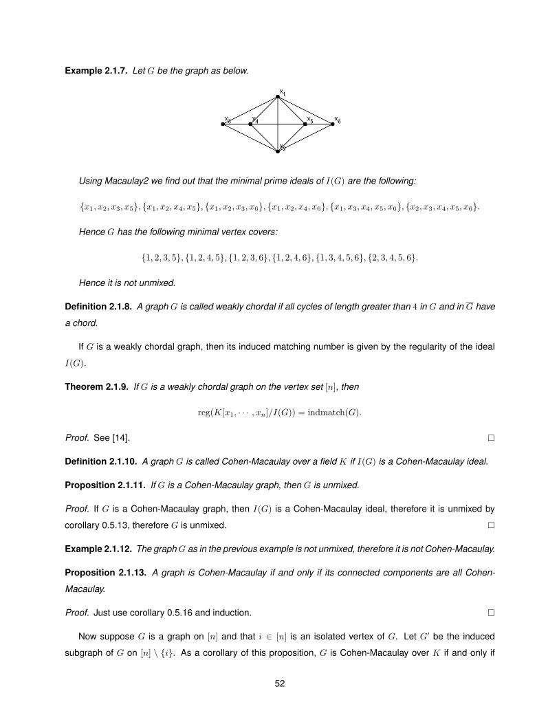
Example 2.1.7. Let G be the graph as below.

Using Macaulay2 we find out that the minimal prime ideals of I(G) are the following:

{x1, x2, x3, x5}, {x1, x2, x4, x5}, {x1, x2, x3, x6}, {x1, x2, x4, x6}, {x1, x3, x4, x5, x6}, {x2, x3, x4, x5, x6}.

Hence G has the following minimal vertex covers:

{1, 2, 3, 5}, {1, 2, 4, 5}, {1, 2, 3, 6}, {1, 2, 4, 6}, {1, 3, 4, 5, 6}, {2, 3, 4, 5, 6}.

Hence it is not unmixed.

Definition 2.1.8. A graph G is called weakly chordal if all cycles of length greater than 4 in G and in G have

a chord.

If G is a weakly chordal graph, then its induced matching number is given by the regularity of the ideal

I(G).

Theorem 2.1.9. If G is a weakly chordal graph on the vertex set [n], then

reg(K[x1, · · · , xn]/I(G)) = indmatch(G).

Proof. See [14].

Definition 2.1.10. A graph G is called Cohen-Macaulay over a field K if I(G) is a Cohen-Macaulay ideal.

Proposition 2.1.11. If G is a Cohen-Macaulay graph, then G is unmixed.

Proof. If G is a Cohen-Macaulay graph, then I(G) is a Cohen-Macaulay ideal, therefore it is unmixed by

corollary 0.5.13, therefore G is unmixed.

Example 2.1.12. The graphG as in the previous example is not unmixed, therefore it is not Cohen-Macaulay.

Proposition 2.1.13. A graph is Cohen-Macaulay if and only if its connected components are all Cohen-

Macaulay.

Proof. Just use corollary 0.5.16 and induction.

Now suppose G is a graph on [n] and that i ∈ [n] is an isolated vertex of G. Let G′ be the induced

subgraph of G on [n] \ {i}. As a corollary of this proposition, G is Cohen-Macaulay over K if and only if

52

G′ is Cohen-Macaulay over K. Hence, when studying which graphs are Cohen-Macaulay or not, we can

always assume that G has no isolated vertices. Our main goal in this section is to classify Cohen-Macaulay

bipartite graphs.

Let P = {p1 · · · , pn} be a finite partially ordered set (poset for short) with a partial order ≤ and let

Vn = {x1, · · · , xn, y1, · · · , yn}. The bipartite graph on Vn whose edges are the two-element subset {xi, yj}

such that pi ≤ pj is denoted G(P ).

Definition 2.1.14. We say that a bipartite graph G with bipartition (V, V ′) comes from a poset if |V | = |V ′|

and if there is a finite poset on [n], where n = |V |, such that after relabelling the vertices of G one has

G(P ) = G.

Proposition 2.1.15. A bipartite graph coming from a poset is Cohen-Macaulay.


Proposition 2.1.16. Let G be a bipartite graph with bipartition (V, V ′). Then G is a Cohen-Macaulay graph

if and only if |V | = |V ′| and the vertices V = {x1, · · · , xn} and V ′ = {y1, · · · , yn} can be labelled such that:

• For every i ∈ [n], {xi, yi} ∈ E(G).

• If i > j, then {xi, yj} 6∈ E(G).

• If {xi, yj}, {xj , yk} ∈ E(G), then {xi, yk} ∈ E(G).

Proof. Suppose |V | = |V ′| and V = {x1, · · · , xn} and V ′ = {y1, · · · , yn} can be labelled such that those

three conditions hold. Let P = {p1, · · · , pn} be the poset with pi ≤ pj if and only if {xi, yj} ∈ E(G). We need

to check that P is indeed a poset.

• If i ∈ [n], then {xi, yi} ∈ E(G) and so pi ≤ pi.

• If pi ≤ pj and pj ≤ pi, then {xi, yj}, {xj , yi} ∈ E(G). If i 6= j, then either i > j or j > i and so

{xi, yj} 6∈ E(G) or {xj , yi} 6∈ E(G), a contradiction. Hence i = j.

• If pi ≤ pj and pj ≤ pk, that is, {xi, yj} ∈ E(G) and {xj , yk} ∈ E(G), then {xi, yk} ∈ E(G), that is

pi ≤ pk.

Hence P is a poset such that G = G(P ), therefore G is a Cohen-Macaulay graph.

Suppose G is a Cohen-Macaulay graph. By corollary 2.1.11, G is unmixed. Since G has no isolated

vertices, both V and V ′ are minimal vertex covers of G, hence |V | = |V ′|. Let U be a subset of V . By

proposition 0.7.46, (V \ U) ∪ N(U) is a vertex cover of G, and since G is unmixed and V is a minimal

vertex cover of G, |V | ≤ |(V \ U) ∪N(U)| ≤ |V \ U | + |N(U)| = |V | − |U | + |N(U)|, hence |N(U)| ≥ |U |.

Now the marriage theorem (theorem 0.7.59) tells us that there exist labellings W = {x1, · · · , xn} and W ′ =

{y1, · · · , yn} such that {xi, yi} ∈ E(G) for every i ∈ [n].

53

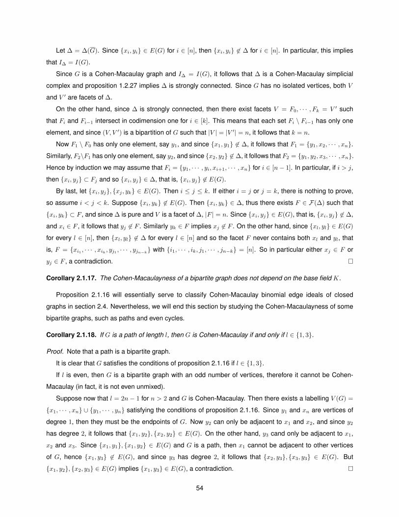
Let ∆ = ∆(G). Since {xi, yi} ∈ E(G) for i ∈ [n], then {xi, yi} 6∈ ∆ for i ∈ [n]. In particular, this implies

that I∆ = I(G).

Since G is a Cohen-Macaulay graph and I∆ = I(G), it follows that ∆ is a Cohen-Macaulay simplicial

complex and proposition 1.2.27 implies ∆ is strongly connected. Since G has no isolated vertices, both V

and V ′ are facets of ∆.

On the other hand, since ∆ is strongly connected, then there exist facets V = F0, · · · , Fk = V ′ such

that Fi and Fi−1 intersect in codimension one for i ∈ [k]. This means that each set Fi \ Fi−1 has only one

element, and since (V, V ′) is a bipartition of G such that |V | = |V ′| = n, it follows that k = n.

Now F1 \ F0 has only one element, say y1, and since {x1, y1} 6∈ ∆, it follows that F1 = {y1, x2, · · · , xn}.

Similarly, F2\F1 has only one element, say y2, and since {x2, y2} 6∈ ∆, it follows that F2 = {y1, y2, x3, · · · , xn}.

Hence by induction we may assume that Fi = {y1, · · · , yi, xi+1, · · · , xn} for i ∈ [n− 1]. In particular, if i > j,

then {xi, yj} ⊂ Fj and so {xi, yj} ∈ ∆, that is, {xi, yj} 6∈ E(G).

By last, let {xi, yj}, {xj , yk} ∈ E(G). Then i ≤ j ≤ k. If either i = j or j = k, there is nothing to prove,

so assume i < j < k. Suppose {xi, yk} 6∈ E(G). Then {xi, yk} ∈ ∆, thus there exists F ∈ F(∆) such that

{xi, yk} ⊂ F , and since ∆ is pure and V is a facet of ∆, |F | = n. Since {xi, yj} ∈ E(G), that is, {xi, yj} 6∈ ∆,

and xi ∈ F , it follows that yj 6∈ F . Similarly yk ∈ F implies xj 6∈ F . On the other hand, since {xl, yl} ∈ E(G)

for every l ∈ [n], then {xl, yl} 6∈ ∆ for every l ∈ [n] and so the facet F never contains both xl and yl, that

is, F = {xi1 , · · · , xik , yj1 , · · · , yjn−k} with {i1, · · · , ik, j1, · · · , jn−k} = [n]. So in particular either xj ∈ F or

yj ∈ F , a contradiction.

Corollary 2.1.17. The Cohen-Macaulayness of a bipartite graph does not depend on the base field K.

Proposition 2.1.16 will essentially serve to classify Cohen-Macaulay binomial edge ideals of closed

graphs in section 2.4. Nevertheless, we will end this section by studying the Cohen-Macaulayness of some

bipartite graphs, such as paths and even cycles.

Corollary 2.1.18. If G is a path of length l, then G is Cohen-Macaulay if and only if l ∈ {1, 3}.

Proof. Note that a path is a bipartite graph.

It is clear that G satisfies the conditions of proposition 2.1.16 if l ∈ {1, 3}.

If l is even, then G is a bipartite graph with an odd number of vertices, therefore it cannot be Cohen-

Macaulay (in fact, it is not even unmixed).

Suppose now that l = 2n− 1 for n > 2 and G is Cohen-Macaulay. Then there exists a labelling V (G) =

{x1, · · · , xn} ∪ {y1, · · · , yn} satisfying the conditions of proposition 2.1.16. Since y1 and xn are vertices of

degree 1, then they must be the endpoints of G. Now y2 can only be adjacent to x1 and x2, and since y2

has degree 2, it follows that {x1, y2}, {x2, y2} ∈ E(G). On the other hand, y3 cand only be adjacent to x1,

x2 and x3. Since {x1, y1}, {x1, y2} ∈ E(G) and G is a path, then x1 cannot be adjacent to other vertices

of G, hence {x1, y3} 6∈ E(G), and since y3 has degree 2, it follows that {x2, y3}, {x3, y3} ∈ E(G). But

{x1, y2}, {x2, y3} ∈ E(G) implies {x1, y3} ∈ E(G), a contradiction.

54

In particular, paths of odd length greater than 3 are examples of unmixed graphs which are not Cohen-

Macaulay.

Proposition 2.1.16 can be used in a simpler way for even cycles.

Corollary 2.1.19. If G is an even cycle, then G is not Cohen-Macaulay.

Proof. Suppose G is Cohen-Macaulay with |V (G)| = 2n. Since G is a bipartite graph, then there exists a

labelling V (G) = {x1, · · · , xn} ∪ {y1, · · · , yn} as in the proposition 2.1.16. But in particular y1 and xn are

vertices of degree 1, which is an absurd since G is a cycle.

In particular, if G is a cycle of length 4, then G is an unmixed graph which is not Cohen-Macaulay.

Proposition 2.1.16 cannot be used when G is an odd cycle for in this case G is not a bipartite graph.

2.2 Binomial edge ideals and their minimal primes

The class of binomial edge ideals is a natural generalization of the ideal of 2-minors of a 2 × n matrix

of indeterminates. Indeed, the ideal of 2-minors of a 2 × n matrix of indeterminates may be interpreted as

the binomial edge ideal of a complete graph on [n]. In the case of a path our binomial edge ideal may be

interpreted as an ideal of adjacent minors. In this section, we classify the Cohen-Macaulayness of some

binomial edge ideals and, for every graph G, we determine the minimal primes of JG.

Definition 2.2.1. A binomial is a polynomial of the form u− v, where u and v are monomials.

LetG be a graph on the vertex set [n], letK be a field and S = K[x1, · · · , xn, y1, · · · , yn] be the polynomial

ring in 2n variables.

Notation 2.2.2. If i, j ∈ [n] are such that i < j, we denote fij = xiyj − xjyi

Definition 2.2.3. The binomial edge ideal JG ⊂ S is the ideal generated by the binomials fij = xiyj − xjyisuch that i < j and {i, j} ∈ E(G). If G is a discrete graph, we set JG = (0).

Proposition 2.2.4. If G and G′ are graphs on [n] such that JG ⊂ JG′ , then G is a subgraph of G′.

Proof. Let {i, j} ∈ E(G) with i < j. Then fij ∈ JG, and so fij ∈ JG′ . Since deg(fij) = 2 and the

generators of JG′ have degree 2, it follows that fij is a K-linear combination of the binomials fkl with k < l

and {k, l} ∈ E(G′), say fij =∑{k,l}∈E(G′) aklfkl. Since the binomials fkl with k < l are a K-linearly

independent subset of S, it follows that {i, j} ∈ E(G′). Since {i, j} ∈ E(G) is arbitrary, E(G) ⊂ E(G′).

55

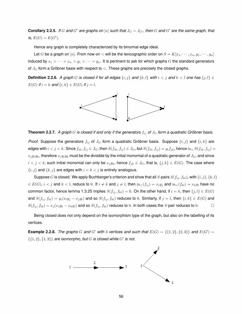
Corollary 2.2.5. If G and G′ are graphs on [n] such that JG = JG′ , then G and G′ are the same graph, that

is, E(G) = E(G′).

Hence any graph is completely characterized by its binomial edge ideal.

Let G be a graph on [n]. From now on < will be the lexicographic order on S = K[x1, · · · , xn, y1, · · · , yn]

induced by x1 > · · · > xn > y1 > · · · > yn. It is pertinent to ask for which graphs G the standard generators

of JG form a Grobner basis with respect to <. These graphs are precisely the closed graphs.

Definition 2.2.6. A graph G is closed if for all edges {i, j} and {k, l} with i < j and k < l one has {j, l} ∈

E(G) if i = k and {i, k} ∈ E(G) if j = l.

Theorem 2.2.7. A graph G is closed if and only if the generators fij of JG form a quadratic Grobner basis.

Proof. Suppose the generators fij of JG form a quadratic Grobner basis. Suppose {i, j} and {i, k} are

edges with i < j < k. Since fik, fij ∈ JG, then S(fik, fij) ∈ JG, but S(fik, fij) = yifjk, hence in< S(fik, fij) =

xjyiyk, therefore xjyiyk must be the divisible by the initial monomial of a quadratic generator of JG, and since

i < j < k, such initial monomial can only be xjyk, hence fjk ∈ JG, that is, {j, k} ∈ E(G). The case where

{i, j} and {k, j} are edges with i < k < j is entirely analogous.

SupposeG is closed. We apply Buchberger’s criterion and show that all S-pairs S(fij , fkl), with {i, j}, {k, l}

∈ E(G), i < j and k < l, reduce to 0. If i 6= k and j 6= l, then in<(fij) = xiyj and in<(fkl) = xkyl have no

common factor, hence lemma 1.3.25 implies S(fij , fkl) = 0. On the other hand, if i = k, then {j, l} ∈ E(G)

and S(fij , fkl) = yi(xlyj − xjyl) and so S(fij , fkl) reduces to 0. Similarly, if j = l, then {i, k} ∈ E(G) and

S(fij , fkl) = xj(xiyk − xkyi) and so S(fij , fkl) reduces to 0. In both cases the S-pair reduces to 0.

Being closed does not only depend on the isomorphism type of the graph, but also on the labelling of its

vertices.

Example 2.2.8. The graphs G and G′ with 3 vertices and such that E(G) = {{1, 2}, {2, 3}} and E(G′) =

{{1, 2}, {1, 3}} are isomorphic, but G is closed while G′ is not.

56

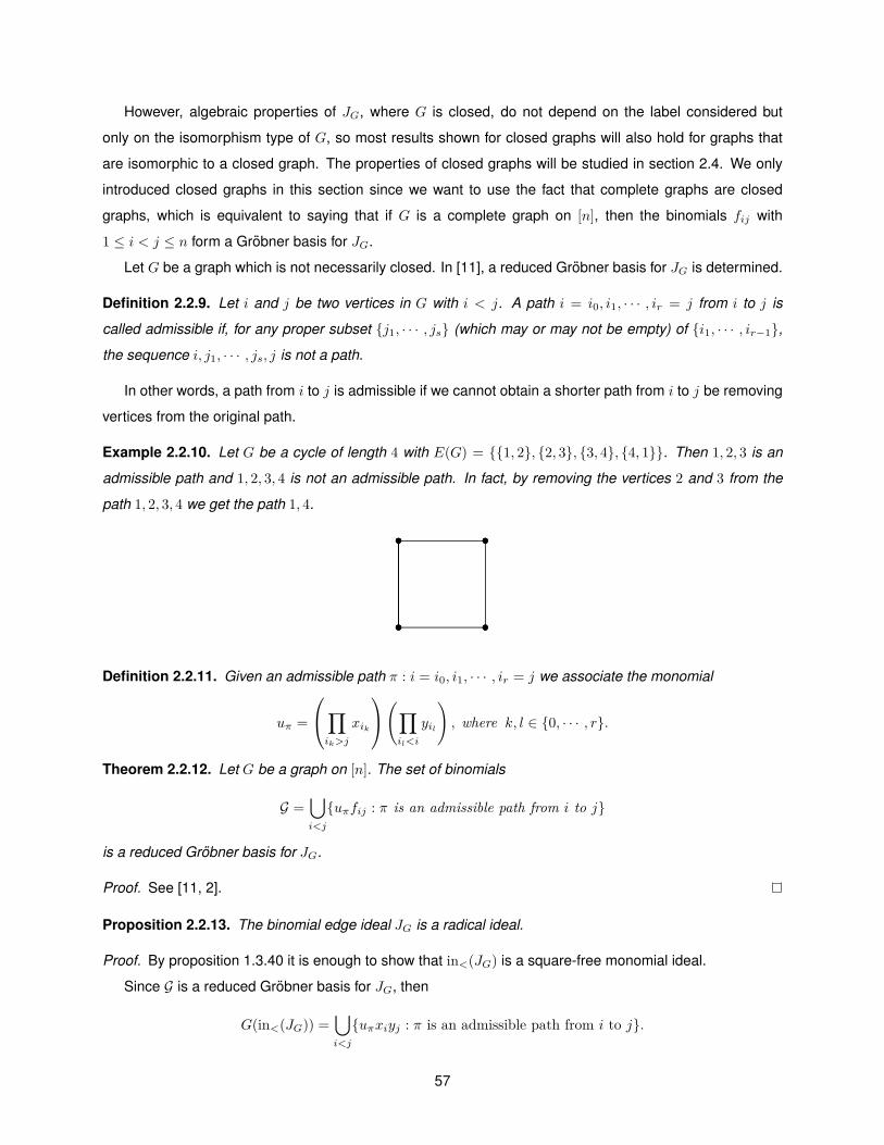
However, algebraic properties of JG, where G is closed, do not depend on the label considered but

only on the isomorphism type of G, so most results shown for closed graphs will also hold for graphs that

are isomorphic to a closed graph. The properties of closed graphs will be studied in section 2.4. We only

introduced closed graphs in this section since we want to use the fact that complete graphs are closed

graphs, which is equivalent to saying that if G is a complete graph on [n], then the binomials fij with

1 ≤ i < j ≤ n form a Grobner basis for JG.

Let G be a graph which is not necessarily closed. In [11], a reduced Grobner basis for JG is determined.

Definition 2.2.9. Let i and j be two vertices in G with i < j. A path i = i0, i1, · · · , ir = j from i to j is

called admissible if, for any proper subset {j1, · · · , js} (which may or may not be empty) of {i1, · · · , ir−1},

the sequence i, j1, · · · , js, j is not a path.

In other words, a path from i to j is admissible if we cannot obtain a shorter path from i to j be removing

vertices from the original path.

Example 2.2.10. Let G be a cycle of length 4 with E(G) = {{1, 2}, {2, 3}, {3, 4}, {4, 1}}. Then 1, 2, 3 is an

admissible path and 1, 2, 3, 4 is not an admissible path. In fact, by removing the vertices 2 and 3 from the

path 1, 2, 3, 4 we get the path 1, 4.

Definition 2.2.11. Given an admissible path π : i = i0, i1, · · · , ir = j we associate the monomial

uπ =

∏ik>j

xik

(∏il<i

yil

), where k, l ∈ {0, · · · , r}.

Theorem 2.2.12. Let G be a graph on [n]. The set of binomials

G =⋃i<j

{uπfij : π is an admissible path from i to j}

is a reduced Grobner basis for JG.

Proof. See [11, 2].

Proposition 2.2.13. The binomial edge ideal JG is a radical ideal.

Proof. By proposition 1.3.40 it is enough to show that in<(JG) is a square-free monomial ideal.

Since G is a reduced Grobner basis for JG, then

G(in<(JG)) =⋃i<j

{uπxiyj : π is an admissible path from i to j}.

57

The monomials uπxiyj are all square-free, hence in<(JG) is a square-free monomial ideal, as desired.

Since JG is a radical ideal, then JG is the intersection of its minimal prime ideals. We want to determine

such prime ideals. One starts by considering the case when G is a complete graph. In this case, S/JG

turns out to be a determinantal ring. The study of determinantal rings is beyond this dissertation, so only

the necessary results will be stated.

Definition 2.2.14. Let X be an m× n matrix of indeterminates over K and let K[X] be the polynomial ring

whose variables are the entries of X. Let t be an integer such that 1 ≤ t ≤ max{m,n}. Then It(X) is the

ideal generated by the t-minors of the matrix X and the determinantal ring Rt is the quotient K[X]/It(X).

Proposition 2.2.15. The determinantal ring Rt has dimension dim(Rt) = (t− 1)(m+ n− t+ 1).

Proof. See [8, 1.C].

Proposition 2.2.16. The determinantal ring Rt is a Cohen-Macaulay domain, that is, It(X) is a Cohen-

Macaulay prime ideal.

Proof. See [8, 2.B].

Corollary 2.2.17. IfG is a complete graph, then JG is a Cohen-Macaulay prime ideal such that dim(S/JG) =

n+ 1.

Proof. Just notice that JG = I2(X), where X =

x1 · · · xn

y1 · · · yn

.

Corollary 2.2.18. If G is a complete graph, then ht(JG) = n− 1.

Proof. Just recall that, by proposition 0.5.12, one has ht(JG) + dim(S/JG) = 2n.

Proposition 2.2.19. Let f1, · · · , fq ∈ K[x1, · · · , xn] and let ϕ : K[t1, · · · , tq] → K[x1, · · · , xn] be the ring

homomorphism induced by ϕ(ti) = fi for i ∈ [q]. Then kerϕ = (f1 − t1, · · · , fq − tq) ∩K[t1, · · · , tq].

Proof. See [7][8.2].

Let ϕ : S → K[t, z1, · · · , zn] be the ring homomorphism induced by ϕ(xi) = zi and ϕ(yi) = tzi. Then

kerϕ = I∩S where I = (z1−x1, · · · , zn−xn, tz1−y1, · · · , tzn−yn). Note that tzi−yi = t(zi−xi)+(txi−yi)

for i ∈ [q] and so I = (z1 − x1, · · · , zn − xn, tx1 − y1, · · · , txn − yn). Consider any elimination order < on

K[t, z1, · · · , zn, x1, · · · , xn, y1, · · · , yn] for t, z1, · · · , zn whose restriction to S is the lexicographic order on S

induced by x1 > · · · > xn > y1 > · · · > yn (in example 1.3.35 we saw how such an order can be obtained).

Proposition 2.2.20. The set G = {z1 − x1, · · · , zn − xn, tx1 − y1, · · · , txn − yn} ∪ {fij : 1 ≤ i < j ≤ n} is a

Grobner basis of I with respect to the elimination order considered above.

58

Proof. We will use Buchberger’s criterion. Recall corollary 1.3.28. If g, h are distinct elements in G, then the

only cases when in<(g) and in<(h) have common factors (and so S(g, h) may not reduce to 0 with respect

to g, h) are the following cases:

• If g = txi − yi and h = txj − yj for i 6= j. In this case, suppose without loss of generality that i < j.

Then in<(g) = txi and in<(h) = txj , hence S(g, h) = xjg − xih = fij and so S(g, h) reduces to 0 with

respect to G.

• If, without loss of generality, g = txi − yi and h = fij for i < j. In this case S(g, h) = yi(txj − yj) and

so S(g, h) reduces to 0 with respect to G.

• If g, h ∈ {fij : 1 ≤ i < j ≤ n}, then, according to the proof of theorem 2.2.7, S(g, h) reduces to 0 with

respect to {fij : 1 ≤ i < j ≤ n}.

Hence G is a Grobner basis of I.

From the elimination theorem (theorem 1.3.36) and these two propositions it follows that {fij : 1 ≤ i <

j ≤ n} is a Grobner basis of kerϕ and in particular kerϕ = JG, where G is the complete graph on [n].

Now suppose G1, · · · , Gc are complete graphs on disjoint sets of vertices. Let i ∈ [c].

Let ϕi : Si → K[ti, {zj}j∈V (Gi)], where Si = K[{xj , yj}j∈V (Gi)], be the ring homomorphism induced by

ϕi(xj) = zj and ϕ(yj) = tizj . Then kerϕi = Ii ∩ Si where Ii = (zj − xj , tzj − yj : j ∈ V (Gi)). Let <i be an

elimination order on K[ti, {zj}j∈V (Gi), {xj , yj}j∈V (Gi)] for {ti} ∪ {zj : j ∈ V (Gi)} whose restriction to Si is

the lexicographic order on Si such that, if j, k, l,m ∈ V (Gi) are such that j < k and l < m, then xj > xk >

yl > ym. By proposition 2.2.20, the set Gi = {zj − xj , tzj − yj : j ∈ V (Gi)} ∪ {fjk : j < k ∧ j, k ∈ V (Gi)} is a

Grobner basis of Ii.

Now let

ϕ : S → K[t1, · · · , tc,c⋃i=1{zj}j∈V (Gi)], where S = K[

c⋃i=1{xj , yj}j∈V (Gi)],

be the ring homomorphism induced by ϕ(xj) = zj and ϕ(yj) = tizj if j ∈ V (Gi). Then kerϕ = I ∩ S, where

I = I1 + · · ·+ Ic. Let < be an elimination order on

K[t1, · · · , tc,c⋃i=1{zj}j∈V (Gi),

c⋃i=1{xj , yj}j∈V (Gi)] for {t1, · · · , tc} ∪

c⋃i=1{zj : j ∈ V (Gi)}

such that, for every i ∈ [c], the restriction of < to K[ti, {zj}j∈V (Gi), {xj , yj}j∈V (Gi)] is <i. For i ∈ [c], Gi is a

Grobner basis of Ii, and using induction and proposition 1.3.29, it follows that⋃ci=1 Gi is a Grobner basis of

I. Since < is an elimination order on

K[t1, · · · , tc,c⋃i=1{zj}j∈V (Gi)] for {t1, · · · , tc} ∪

c⋃i=1{zj : j ∈ V (Gi)},

then, by theorem 1.3.36, S∩⋃ci=1 Gi is a Grobner basis for kerϕ. But Gi ⊂ K[ti, {zj}j∈V (Gi), {xj , yj}j∈V (Gi)]

for every i ∈ [c], therefore

S ∩c⋃i=1Gi =

c⋃i=1

(Gi ∩ Si) =c⋃i=1{fjk : j < k ∧ j, k ∈ V (Gi)}.

59

Since⋃ci=1{fjk : j < k ∧ j, k ∈ V (Gi)} is a Grobner basis of kerϕ, it follows in particular that kerϕ =

JG1 + · · ·+ JGc (recall that G1, · · · , Gc are complete graphs on disjoint sets of vertices).

Corollary 2.2.21. If G1, · · · , Gc are complete graphs on disjoint sets of vertices, then JG1 + · · · + JGcis a

prime ideal.

Proof. Recall that JG1 + · · ·+ JGc= kerϕ, where ϕ is a ring homomorphism between two polynomial rings,

which we denote by S and S′, respectively, and so S/ kerϕ and ϕ(S) are isomorphic rings. But ϕ(S) is a

subring of S′, which is a domain, and so ϕ(S) is also a domain. But S/ kerϕ is a domain if and only if kerϕ

is a prime ideal, hence the conclusion follows.

Notation 2.2.22. Given a graph G, the complete graph on the vertex set V (G) is denoted by G.

Notation 2.2.23. Given a subset A ⊂ [n], the complete graph on the vertex set A is denoted by A.

Let G be a graph on [n]. For each subset R ⊂ [n] we define a prime ideal PR(G). Let G1, · · · , Gc(R)

be the connected components of G[n]\R. We define PR(G) as being the ideal generated by the ideals

JG1, · · · , JGc(R)

and by the variables xi, yi with i ∈ R. This also works for R = ∅ and in this case PR(G) is

the binomial edge ideal of the graph G1 ∪ · · · ∪ Gc(R).

Proposition 2.2.24. The ideal PR(G) is a prime ideal.

Proof. Recall that PR(G) = JG1+ · · ·+JGc(R)

+(xi, yi : i ∈ R) and so, under the ring isomorphism S/(xi, yi :

i ∈ R) ∼= K[{xi, yi : i 6∈ R}], the ideal PR(G)/(xi, yi : i ∈ R) corresponds to the ideal JG1+ · · · + JGc(R)

⊂

K[{xi, yi : i 6∈ R}]. By corollary 2.2.21, JG1+ · · · + JGc(R)

is a prime ideal of K[{xi, yi : i 6∈ R}] and so

PR(G)/(xi, yi : i ∈ R) is a prime ideal of S/(xi, yi : i ∈ R). This implies that PR(G) is a prime ideal of S, as

desired.

Lemma 2.2.25. Let G be a graph on [n] and let R ⊂ [n]. Then ht(PR(G)) = |R|+ (n− c(R)).

Proof. Let G1, · · · , Gc(R) be the connected components of the induced subgraph G[n]\R. As a consequence

of 0.5.17 we have ht(PR(G)) = ht((xi : i ∈ R)) + ht((yi : i ∈ R)) +∑c(R)j=1 ht(JGj

) = 2 |R|+∑c(R)j=1 (|V (Gj)| −

1) = 2 |R|+∑c(R)j=1 |V (Gj)| − c(R) = 2 |R|+ (n− |R|)− c(R) = |R|+ (n− c(R)).

Corollary 2.2.26. Let G be a graph on [n] and let R ⊂ [n]. Then dim(S/PR(G)) = c(R) + (n− |R|).

Proof. Just recall that, by proposition 0.5.12, one has ht(PR(G)) + dim(S/PR(G)) = 2n.

Theorem 2.2.27. Let G be a graph on the vertex set [n]. Then JG =⋂

R⊂[n]

PR(G).

Proof. It is obvious that each of the prime ideals PR(G) contains JG. We will show by induction on [n] that

each minimal prime ideal containing JG is of the form PR(G) for some R ⊂ [n]. Since JG is a radical ideal,

the assertion of the theorem will follow.

60

Suppose this result is true for connected graphs. Let G1, · · · , Gr be the connected components of G.

Let P ∈ Min(JG). For i ∈ [r], let Si be the polynomial ring in the variables xj , yj with j ∈ V (Gi). Since

P is a prime ideal of S, then P ∩ Si is a prime ideal of Si, and since JGi⊂ JG ∩ Si, then JGi

⊂ P ∩ Si.

Let Pi ∈ Min(JGi) such that Pi ⊂ P ∩ Si. Since Pi ∈ Min(JGi

), then there exists Ri ⊂ V (Gi) such that

Pi = PRi(Gi). Let R =⋃ri=1Ri. Then PR(G) = PR1(G1) + · · · + PRr (Gr) and so PR(G) ⊂ P , and from

P ∈ Min(JG) it follows that P = PR(G), as desired.

So let G be connected and let P ∈ Min(JG). Let T = {xi ∈ P : yi 6∈ P} and T ′ = {yi ∈ P : xi 6∈ P}.

Suppose T = {x1, · · · , xn}. Then JG ⊂ P∅(G) ( (x1, · · · , xn) ⊂ P , contradicting the fact that P ∈

Min(JG). Hence T 6= {x1, · · · , xn}. Similarly, T ′ 6= {y1, · · · , yn}

Suppose that one of the sets T, T ′, say T , is non-empty. Since T 6= {x1, · · · , xn} and G is connected,

then there exists {i, j} ∈ E(G) such that xi ∈ T but xj 6∈ T . Since xiyj−xjyi ∈ JG ⊂ P and xi ∈ P , it follows

that xjyi ∈ P . Since xi ∈ T , then yi 6∈ P , therefore xjyi ∈ P implies xj ∈ P , and since xj 6∈ T , it follows that

yj ∈ P . Since xj , yj ∈ P , one can write P = P + (xj , yj), where P is an ideal of K[{xk, yk : k 6= j}].

Let G′ be the restriction of G to the vertex set [n] \ {j}. Then JG′ + (xj , yj) = JG + (xj , yj) ⊂ P

and in particular P ∈ Min(JG′ + (xj , yj)), therefore P/(xj , yj) ∈ Min((JG′ + (xj , yj))/(xj , yj)). But, under

the ring isomorphism S/(xj , yj) ∼= K[{xk, yk : k 6= j}], the ideals (JG′ + (xj , yj))/(xj , yj) and P/(xj , yj)

correspond to the ideals JG′ and P of K[{xk, yk : k 6= j}], respectively, hence P ∈ Min(JG′). By induction

hypothesis, P is of the form PR(G′) for some subset R ⊂ [n] \ {j}. Since P = PR(G′), it follows that

P = P + (xj , yj) = PR∪{j}(G).

It remains to consider the case where T = T ′ = ∅. Let R = {i ∈ [n] : xi ∈ P}. Then yi ∈ P if and only if

i ∈ R.

Suppose R = ∅, that is, P contains no variables. We claim that if i, j ∈ [n] with i < j, then fij ∈ P . From

this it will follow that JG ⊂ P , and since JG = P∅(G) (recall that G is connected) is a prime ideal containing

JG and P ∈ Min(JG), we conclude that P = P∅(G).

Let i = i0, i1, · · · , ir = j be a path from i to j. We proceed by induction on r to show that fij ∈ P . The

assertion is trivial for r = 1. Suppose now that r > 1. Our induction hypothesis says that fi1j ∈ P . On the

other hand, one has xi1fij = xjfii1 + xifi1j . Thus xi1fij ∈ P . Since P is a prime ideal and xi1 6∈ P , we see

that fij ∈ P .

Now suppose R 6= ∅. One can write P = P + (xi, yi : i ∈ R), where P is an ideal of K[{xi, yi :

i 6∈ R}] containing no variables. Let G′ be the restriction of G to the vertex set [n] \ R. Then JG′ +

(xi, yi : i ∈ R) = JG + (xi, yi : i ∈ R) ⊂ P and in particular P ∈ Min(JG′ + (xi, yi : i ∈ R)), therefore

P/(xi, yi : i ∈ R) ∈ Min((JG′ + (xi, yi : i ∈ R))/(xi, yi : i ∈ R)). But, under the ring isomorphism

S/(xi, yi : i ∈ R) ∼= K[{xi, yi : i 6∈ R}], the ideals (JG′ + (xi, yi : i ∈ R))/(xi, yi : i ∈ R) and P/(xi, yi : i ∈ R)

correspond to the ideals JG′ and P of K[{xi, yi : i 6∈ R}], respectively, hence P ∈ Min(JG′). By induction

hypothesis, P is of the form PR′(G′) for some subset R′ ⊂ [n] \ R. Since P = PR′(G′), it follows that

P = P + (xi, yi : i ∈ R) = PR∪R′(G).

61

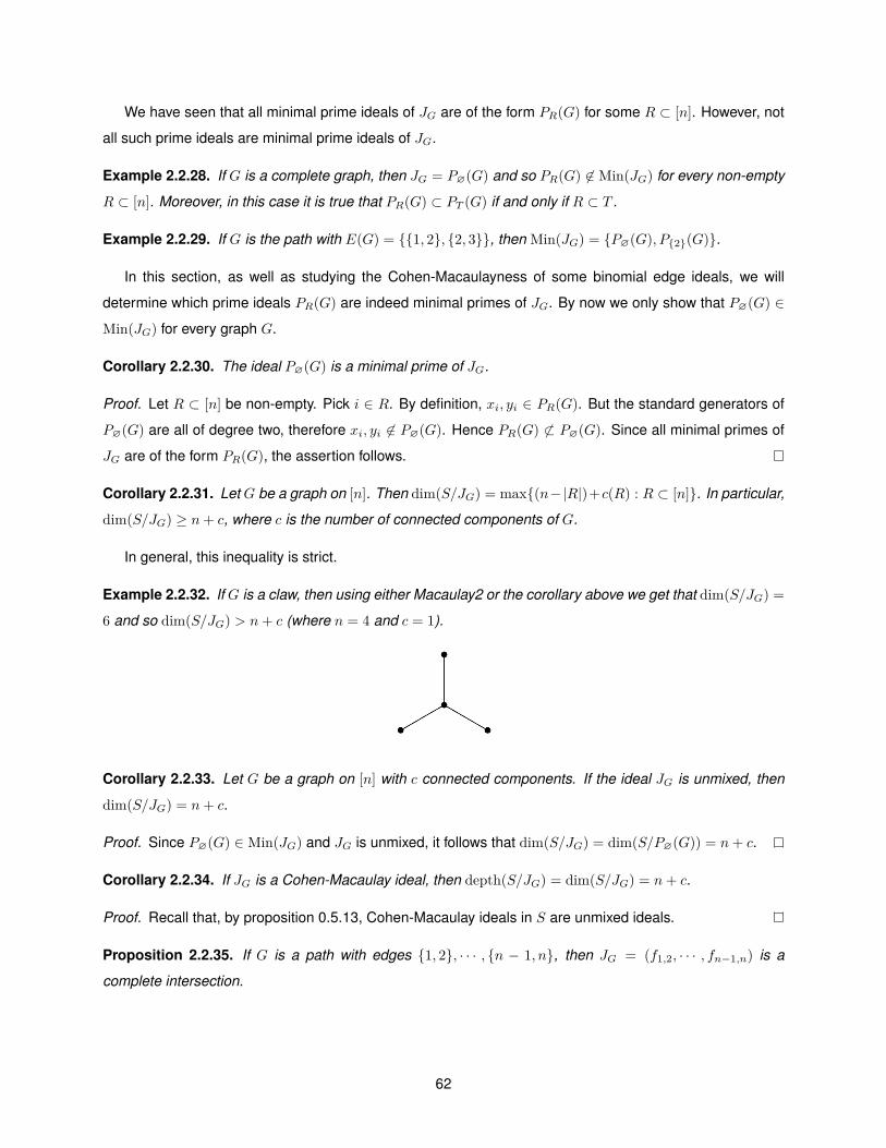
We have seen that all minimal prime ideals of JG are of the form PR(G) for some R ⊂ [n]. However, not

all such prime ideals are minimal prime ideals of JG.

Example 2.2.28. If G is a complete graph, then JG = P∅(G) and so PR(G) 6∈ Min(JG) for every non-empty

R ⊂ [n]. Moreover, in this case it is true that PR(G) ⊂ PT (G) if and only if R ⊂ T .

Example 2.2.29. If G is the path with E(G) = {{1, 2}, {2, 3}}, then Min(JG) = {P∅(G), P{2}(G)}.

In this section, as well as studying the Cohen-Macaulayness of some binomial edge ideals, we will

determine which prime ideals PR(G) are indeed minimal primes of JG. By now we only show that P∅(G) ∈

Min(JG) for every graph G.

Corollary 2.2.30. The ideal P∅(G) is a minimal prime of JG.

Proof. Let R ⊂ [n] be non-empty. Pick i ∈ R. By definition, xi, yi ∈ PR(G). But the standard generators of

P∅(G) are all of degree two, therefore xi, yi 6∈ P∅(G). Hence PR(G) 6⊂ P∅(G). Since all minimal primes of

JG are of the form PR(G), the assertion follows.

Corollary 2.2.31. Let G be a graph on [n]. Then dim(S/JG) = max{(n−|R|)+c(R) : R ⊂ [n]}. In particular,

dim(S/JG) ≥ n+ c, where c is the number of connected components of G.

In general, this inequality is strict.

Example 2.2.32. If G is a claw, then using either Macaulay2 or the corollary above we get that dim(S/JG) =

6 and so dim(S/JG) > n+ c (where n = 4 and c = 1).

Corollary 2.2.33. Let G be a graph on [n] with c connected components. If the ideal JG is unmixed, then

dim(S/JG) = n+ c.

Proof. Since P∅(G) ∈ Min(JG) and JG is unmixed, it follows that dim(S/JG) = dim(S/P∅(G)) = n+ c.

Corollary 2.2.34. If JG is a Cohen-Macaulay ideal, then depth(S/JG) = dim(S/JG) = n+ c.

Proof. Recall that, by proposition 0.5.13, Cohen-Macaulay ideals in S are unmixed ideals.

Proposition 2.2.35. If G is a path with edges {1, 2}, · · · , {n − 1, n}, then JG = (f1,2, · · · , fn−1,n) is a

complete intersection.

62

Proof. For i ∈ [n− 1] one has in<(fi,i+1) = xiyi+1, hence corollary 1.3.28 implies that {f1,2, · · · , fn−1,n} is

a Grobner basis for JG.

Since JG = (f1,2, · · · , fn−1,n) is a graded Grobner basis such that in<(JG) = (x1y2, x2y3, · · · , xn−1yn) is

a complete intersection, proposition 1.3.41 implies JG = (f1,2, · · · , fn−1,n) is also a complete intersection,

as desired.

Corollary 2.2.36. If G is a path, then JG is a Cohen-Macaulay ideal.

Proof. Just use corollary 0.5.10.

Note in particular that G being a Cohen-Macaulay graph and JG being a Cohen-Macaulay ideal are not

equivalent statements.

Example 2.2.37. If G is a path of length 2, then, by corollary 2.1.18, G is not a Cohen-Macaulay graph.

However, JG is a Cohen-Macaulay ideal.

We now know that JG is a Cohen-Macaulay when G is either a complete graph or a path.

Example 2.2.38. Let G be the path on [n] with E(G) = {{1, 2}, · · · , {n − 1, n}}. Then G is a connected

graph and JG is a Cohen-Macaulay ideal, therefore dim(S/JG) = n + 1. By corollary 2.2.26, the minimal

prime ideals of JG are the prime ideals PR(G) for which c(R) = |R| + 1. Let R ⊂ [n]. There exist integers

1 ≤ a1 ≤ b1 < a2 ≤ b2 < a3 ≤ b3 < · · · < ar ≤ br ≤ n such that R =⋃ri=1[ai, bi]. Suppose also that, for each

i ∈ [r−1], bi and ai+1 are not consecutive integers. We see that |R| =∑ri=1(br−ar+1) =

∑ri=1(br−ar)+r,

and that c(R) = r − 1 if a1 = 1 and br = n, c(R) = r + 1 if a1 6= 1 and br 6= n, and c(R) = r otherwise. Thus

c(R) = |R|+ 1 if and only if a1 6= 1, br 6= n and ai = bi for all i ∈ [r]. In other words, the minimal prime ideals

of G are those PR(G) for which R is a subset of [n] of the form {a1, · · · , ar}, with 1 < a1 < a2 < · · · < ar < n

and such that no two of these r integers are consecutive integers.

Proposition 2.2.39. The ideal JG is a prime ideal if and only if each connected component of G is a

complete graph.

Proof. If each of the connected components of G is a complete graph, then JG = P∅(G) and so JG is a

prime ideal.

Let G1, · · · , Gr be the connected components of G and suppose that JG is a prime ideal. Since P∅(G) =

JG1+ · · · + JGr

is a minimal prime ideal of JG, it follows that JG = JG1+ · · · + JGr

= JG1∪···∪Gr, therefore,

by corollary 2.2.5, G = G1 ∪ · · · ∪ Gr and so each connected component of G is a complete graph, as

desired.

As it happens with monomial edge ideals:

Proposition 2.2.40. The binomial edge ideal of a graph is Cohen-Macaulay if and only if each of the binomial

edge ideals of its connected components is Cohen-Macaulay.

63

Proof. As in the proof for monomial edge ideals, one just needs to use corollary 0.5.16 and induction.

Thus, to study the Cohen-Macaulayness of binomial edge ideals (which is the goal of this chapter), it is

enough to consider connected graphs.

We have seen that the binomial edge ideal of a complete graph is Cohen-Macaulay. The following result

tells us which cycles have a Cohen-Macaulay binomial edge ideal.

Corollary 2.2.41. Let G be a cycle of length n. Then the following conditions are equivalent:

1. n = 3.

2. JG is a prime ideal.

3. JG is unmixed.

4. JG is a Cohen-Macaulay ideal.

Proof. The implication (1) ⇒ (2) follows from proposition 2.2.39. Moreover, if JG is a prime ideal, then

each of the connected components of G is a complete graph and so, by corollary 2.2.17, the binomial

edge ideal of each connected component of G is Cohen-Macaulay, therefore proposition 2.2.40 implies JG

is also Cohen-Macaulay. Furthermore, by corollary 0.5.13, any Cohen-Macaulay ideal is unmixed, so all

equivalences follow once it is shown that (3)⇒ (2).

One of the minimal prime ideals of JG is P∅(G) and ht(P∅(G)) = n − 1. Now let R ⊂ [n] with R 6= ∅.

We may assume that we have labelled the vertices of the cycle counterclockwise and that R =⋃ri=1[ai, bi]

with 1 = a1 ≤ b1 < a2 ≤ b2 < · · · < ar ≤ br < n. Suppose also that, for each i ∈ [r − 1], bi and ai+1 are

not consecutive integers. Then c(R) = r and ht(PR(G)) = |R| + n − c(R) =∑ri=1(br − ar) + r + n − r =

n +∑ri=1(br − ar) ≥ n. Thus if JG is unmixed, then Min(JG) = {P∅(G)}, and by theorem 2.2.27 it follows

that JG = P∅(G) is a prime ideal, as desired.

We still have not answered which of the prime ideals PR(G), besides from P∅(G), are the minimal primes

of JG.

Proposition 2.2.42. Let G be a graph on [n] and let R and T be subsets of [n]. Let G1, · · · , Gr be the

connected components ofG[n]\R and letH1, · · · , Ht be the connected components ofG[n]\T . Then PT (G) ⊂

PR(G) if and only if T ⊂ R and for all i ∈ [t] one has V (Hi) \R ⊂ V (Gj) for some j ∈ [r].

Proof. Suppose that PT (G) ⊂ PR(G).

Let i ∈ T . Then xi, yi ∈ PT (G) and so xi, yi ∈ PR(G), and since the only variables in PR(G) are the

variables xj , yj such that j ∈ R, it follows that i ∈ R. Since i ∈ T is arbitrary, then T ⊂ R.

For i ∈ [t], let H ′i = (Hi)[n]\R. Then JH′1 + · · · + JH′t⊂ PT (G) ⊂ PR(G), and since PR(G) = (xi, yi : i ∈

R) + JG1+ · · ·+ JGr

and the standard generators of JH′1 + · · ·+ JH′tare polynomials in K[{xi, yi : i 6∈ R}], it

follows that JH′1 + · · ·+ JH′t⊂ JG1

+ · · ·+ JGr, that is, JH′1∪···∪H′t ⊂ JG1∪···∪Gr

and so, by proposition 2.2.4,

64

H ′1 ∪ · · · ∪ H ′t ⊂ G1 ∪ · · · ∪ Gr. Since each of the graphs H ′1, · · · , H ′t is connected, it follows that, for all i ∈ [t],

one has V (Hi) \R ⊂ V (Gj) for some j ∈ [r].

Suppose that T ⊂ R and that for all i ∈ [t] one has V (Hi) \R ⊂ V (Gj) for some j ∈ [r].

Let i ∈ T . Then i ∈ R and so xi, yi ∈ PR(G).

Let a ∈ [t] and let i, j ∈ V (Ha) with i < j. If {i, j} ∩ R 6= ∅, then fij ∈ (xk, yk : k ∈ R) ⊂ PR(G).

Otherwise, i, j ∈ V (Ha) \ R. Pick b ∈ [s] such that V (Ha) \ R ⊂ V (Gb). Then i, j ∈ V (Gb) and so

fij ∈ JGb⊂ PR(G).

Hence PT (G) ⊂ PR(G).

Corollary 2.2.43. Let G be a connected graph on [n] and let R ⊂ [n]. Then PR(G) ∈ Min(JG) if and only if

S = ∅ or S 6= ∅ and for each i ∈ R one has c(R \ {i}) < c(R).

Proof. Let G1, · · · , Gc(R) be the connected components of G[n]\R. For each i ∈ R set Ti = R \ {i}.

Suppose that i is only adjacent to vertices in Ti. Then the connected components of G[n]\Tiare

G1, · · · , Gc(R), {i}, thus c(Ti) = c(R) + 1.

Suppose that there are exactly ki connected components ofG[n]\R, sayG1, · · · , Gki , with ki ≥ 1, contain-

ing vertices which are adjacent to i. Then the connected components of G[n]\Tiare G′1, Gki+1, · · · , Gc(R),

where V (G′1) =⋃ki

l=1 V (Gl) ∪ {i}, thus c(Ti) = c(R)− ki + 1.

We get that, for every i ∈ R, c(Ti) = c(R)− ki + 1, where ki ≥ 0 is the number of connected components

of G[n]\R containing vertices which are adjacent to i.

Suppose that PR(G) ∈ Min(JG). Let i ∈ R. Then PTi(G) 6⊂ PR(G), and since Ti ⊂ R, then proposition

2.2.42 implies that G[n]\Tihas a connected component H such that V (H) \R is not contained in any of the

sets V (G1), · · · , V (Gc(R)). But since the connected components of G[n]\Tiare G′1, Gki+1, · · · , Gc(R), where

V (G′1) =⋃ki

l=1 V (Gl) ∪ {i}, then this is only possible if ki ≥ 2 and H = G′1, hence c(Ti) < c(R), as desired.

Conversely, suppose that c(Ti) < c(R) for every i ∈ R. We will show that PT (G) 6⊂ PR(G) for every

T ( R, from where it will follow that PR(G) ∈ Min(JG).

Let T ( R and pick i ∈ R \ T . Since c(Ti) < c(R) and c(Ti) = c(R)− ki + 1, it follows that ki ≥ 2. Recall

that the connected components of G[n]\Tiare G′1, Gki+1, · · · , Gc(R), where V (G′1) =

⋃ki

l=1 V (Gl)∪{i}. Since

T ⊂ Ti, that is, [n] \ Ti ⊂ [n] \ T , then G[n]\T has one connected component H containing G′1 and in

particular V (H) \R contains the subsets V (G1) and V (G2). Hence V (H) \R is not contained in any V (Gk),

with k ∈ [c(R)]. According to proposition 2.2.42, this means that PT (G) 6⊂ PR(G).

Example 2.2.44. Let G be a cycle of length n > 3. Then, besides of the prime ideal P∅(G), which is of

height n − 1, the only other minimal prime ideals are the ideals PR(G) where |R| > 1 and no two elements

i, j ∈ R belong to the same edge of G. By lemma 2.2.25, each of these prime ideals has height n. In

particular this implies that JG is not unmixed and therefore not Cohen-Macaulay, as we have shown before.

65

2.3 A special class of chordal graphs

A general classification of Cohen-Macaulay binomial edge ideals seems to be hopeless. We then restrict

our attention to a special class of chordal graphs: the chordal graphs such that any two distinct maximal

cliques intersect in at most one vertex. For this class of graphs, we can determine depth(S/JG) and use

that result to study the Cohen-Macaulayness of G.

Forests are a good example of such graphs.

Proposition 2.3.1. If G is a forest, then G is a chordal graph and any two distinct maximal cliques in G

intersect in at most one vertex.

Proof. Since a forest has no cycles, then G is clearly chordal and all its maximal cliques have exactly two

vertices. This means that any two distinct maximal cliques intersect in at most one vertex, as desired.

We know a formula for dim(S/JG) which depends only on the properties of the graph G and we would

like to find a similar formula for depth(S/JG). By corollary 2.2.34 one has depth(S/JG) = n+ c whenever G

is a graph on [n] with c connected components such that JG is a Cohen-Macaulay ideal. This is also true for

chordal graphs such that any two distinct maximal cliques intersect in at most one vertex.

So suppose now G is such a connected graph. By theorem 1.2.35, G is chordal if and only if ∆(G) is a

quasi-forest. So let us consider a leaf order F1, · · · , Fr on the facets of ∆(G). If r = 1, then G is a complete

graph, so we will consider only r > 1.

Proposition 2.3.2. There exists a unique vertex i ∈ Fr such that i also belongs to some other facet of ∆(G).

Proof. Such i exists since G is connected. We will show that i is unique.

Pick j ∈ [r − 1] such that Fj is a branch of Fr. Pick k ∈ [r − 1] such that i ∈ Fk. Then i ∈ Fk ∩ Fr, and

since Fk ∩ Fr ⊂ Fj ∩ Fr, then i ∈ Fj ∩ Fr. Since any two distinct facets of ∆(G) intersect in at most one

vertex, it follows that Fj ∩ Fr = {i}. In particular, such vertex i is unique.

Proposition 2.3.3. The ideal Q1 is the binomial edge ideal of the graph G′ which is obtained from G by

replacing the facets Ft1 , · · · , Ftq , Fr by the clique on the vertex set Fr ∪(⋃q

j=1 Ftj

).

Proof. Let R be a subset of [n] \ {i}. Let {j, k} ∈ E(G′) with j < k. If either {j, k} ∈ E(G) or {j, k} ∩R 6= ∅,

then clearly xjyk − xkyj ∈ PR(G). Suppose {j, k} 6∈ E(G) and j, k 6∈ R. Then j, k ∈ Fr ∪(⋃q

j=1 Ftj

)and in

particular j, i, k is a path in G, and since i, j, k 6∈ R, it follows that j, k lie in the same connected component

of the induced subgraph of G in [n] \ R, hence xjyk − xkyj ∈ PR(G). Since {j, k} ∈ E(G′) is arbitrary,

JG′ ⊂ PR(G). Since R ⊂ [n] \ {i} is arbitrary, JG′ ⊂ Q1.

It remains to show that Q1 ⊂ JG′ . Since G ⊂ G′, then PR(G) ⊂ PR(G′) for every R ⊂ [n]. Let R be a

subset of [n] with i 6∈ R. Now we will show that PR(G′) ⊂ PR∪{i}(G′) for every S ⊂ [n] \ {i}. To show this, it

is enough to show that if j, k ∈ [n] \ (R∪{i}) lie in the same connected component of the induced subgraph

of G′ in [n] \R, then fjk ∈ PR∪{i}(G′).

66

Let P be a path in G′[n]\R from j to k whose length is the smallest possible. Suppose that P passes

through i, that is, P is of the form j, · · · , j′, i, k′, · · · , k. Then the vertices j′ and k′ belong to the clique

Fr ∪(⋃q

j=1 Ftj

)and so {j′, k′} ∈ E(G′). But then j, · · · , j′, k′, · · · , k is a path in G′[n]\R from j to k whose

length is smaller than the length of P , a contradiction. Hence P does not pass through i and in particular j

and k lie in the same connected component of G′[n]\(R∪{i}), thus fjk ∈ PR∪{i}(G′).

Since PR(G′) ⊂ PR∪{i}(G′) for every R ⊂ [n] \ {i}, then JG′ =⋂R⊂[n]\{i} PR(G′) and so it follows that

Q1 =⋂R⊂[n]\{i} PR(G) ⊂

⋂R⊂[n]\{i} PR(G′) = JG′ .

Proposition 2.3.4. The graphG′ is also a connected chordal graph on [n] such that any two distinct maximal

cliques intersect in at most one vertex.

Proof. Since G and G′ are graphs on [n] such that G ⊂ G′ and G is connected, then G′ is also connected.

Let C be a cycle in G′ of length greater than 3. If C is already a cycle in G, there is nothing to prove.

Otherwise, there exists j, k ∈ V (C) such that {j, k} ∈ E(C) but {j, k} 6∈ E(G), hence j and k belong to

distinct facets in the collection of facets Ft1 , · · · , Ftq , Fr and in particular j and k are adjacent to i.

Suppose that j and k are the only vertices in C which are adjacent to i. Then the edges of C other than

{j, k} are edges in G and so, by replacing the edge {j, k} by the edges {j, i}, {i, k}, we get a cycle C ′ in

G that must have a chord {j′, k′} ∈ E(G) such that {j′, k′} 6= {j, k} and i 6∈ {j′, k′}. Then j′, k′ ∈ V (C),

{j′, k′} ∈ E(G′) and {j′, k′} 6∈ E(C), therefore {j, k} is a chord in C.

Suppose that there exists another vertex l in C which is adjacent to i. Then j, k, l belong to the same

maximal clique in G′. Now suppose without loss of generality that k and l are not adjacent vertices in the

cycle C. But {k, l} ∈ E(G′) and so {k, l} is a chord in C.

It remains to show that the clique Fr ∪(⋃q

j=1 Ftj

)of G′ intersects any other maximal clique in at most

one vertex. Let k ∈ [r − 1] \ {t1, · · · , tq}. Then Fr ∩ Fk = ∅ and so it is enough to show that Fk intersects⋃qj=1 Ftj in at most one vertex.

Suppose this is not the case. Since Fk intersects each other maximal clique of G in at most one vertex,

then there exist two cliques in the collection {Ft1 , · · · , Ftq}, say Ft1 and Ft2 , intersecting Fk in distinct

vertices. Let Ft1 ∩ Fk = {j1} and Ft2 ∩ Fk = {j2}. Then the vertices i, j1, j2 form a clique in G which

intersects Fk in two vertices but is not contained in it, a contradiction.

Notation 2.3.5. We denote Si = K[{xj , yj : j 6= i}] ⊂ S.

Proposition 2.3.6. The ideal Q2 is such that Q2 = (xi, yi) + JG′′ , where G′′ is the restriction of G to the

vertex set [n] \ {i}.

Proof. If R is a subset of [n] containing i, then (xi, yi) ∈ PR(G). Hence (xi, yi) ⊂ Q2. On other hand, since

G′′ ⊂ G, it follows that JG′′ ⊂ JG ⊂ Q2, and so (xi, yi) + JG′′ ⊂ Q2.

It remains to show that Q2 ⊂ (xi, yi) + JG′′ . Let f ∈ Q2. Then f ∈ P{i}(G), and since P{i}(G) =

(xi, yi) + P∅(G′′) and P∅(G′′) ⊂ Si, then f can be written in a unique way f = g + h such that g ∈ (xi, yi)

and h ∈ Si.

67

Let R be a subset of [n] \ {i}. Then f ∈ PR∪{i}(G), and since PR∪{i}(G) = (xi, yi) + PR(G′′) and

PR(G′′) ⊂ Si, it follows that h ∈ PR(G′′). Since R ⊂ [n] \ {i} is arbitrary, it follows that h ∈ JG′′ , hence

f ∈ (xi, yi) + JG′′ , as desired.

Corollary 2.3.7. The ideal Q2 is such that S/Q2 ∼= Si/JG′′ .

Proposition 2.3.8. The graph G′′ is a chordal graph on [n] \ {i} such that any two distinct maximal cliques

intersect in at most one vertex. But it is not connected for it has q + 1 connected components.

Proof. Since G is a chordal graph such that any two distinct maximal cliques intersect in at most one vertex

and G′′ is induced by G, then G′′ is also a chordal graph such that any two distinct maximal cliques intersect

in at most one vertex.

We will now show that the cliques Ft1 \ {i}, · · · , Ftq \ {i}, Fr \ {i} all lie in distinct connected components

of G′′.

Suppose this is not the case and consider points u, v in distinct cliques of the collection Ft1 \{i}, · · · , Ftq \

{i}, Fr \ {i} such that d(u, v) (as vertices of G′′) is the smallest possible. Consider a path u, · · · , v in G′′ of

length d(u, v). Then i, u, · · · , v, i is a cycle in G, and since G is chordal, that cycle has a vertex w such that

{i, w}, {v, w} ∈ E(G), and so the vertices i, v, w form a clique in G. This clique intersects the clique of the

collection Ft1 , · · · , Ftq , Fr which contains i and w in two vertices, a contradiction.

Hence G′′ has at least q + 1 connected components. Suppose G′′ has more than q + 1 connected

components.

Consider vertices j1, · · · , jq+2 that lie in distinct connected components of G′′. For k ∈ [q + 2] consider

paths jk, · · · , j′k, i inG. Then j′1, · · · , j′k ∈ Fr∪(⋃q

j=1 Ftj

)\{i} and so two of the j′1, · · · , j′k, say j′1 and j′2 must

lie on the same clique of the collection of cliques Ft1 \ {i}, · · · , Ftq \ {i}, Fr \ {i}. But then {j′1, j′2} ∈ E(G′′)

and so j1, · · · , j′1, j′2, · · · , j2 is a path from j1 to j2 in G′′, a contradiction.

Proposition 2.3.9. The ideal Q1 +Q2 is such that S/(Q1 +Q2) ∼= Si/JH , where H is the restriction of G′ to

the vertex set [n] \ {i}.

Proof. Since G′′ ⊂ G′, then JG′′ ⊂ JG′ , hence Q1 + Q2 = JG′ + ((xi, yi) + JG′′) = JG′ + (xi, yi). Since H

is the restriction of G′ to the vertex set [n] \ {i}, then JG′ + (xi, yi) = JH + (xi, yi) and so the conclusion

follows.

Proposition 2.3.10. The graph H is a connected chordal graph on [n] \ {i} such that any two distinct

maximal cliques intersect in at most one vertex.

Proof. Since G′ is a chordal graph such that any two distinct maximal cliques intersect in at most one vertex

and H is induced by G′, then H is also a chordal graph such that any two distinct maximal cliques intersect

in at most one vertex. It remains to show that H is connected. Let j, k ∈ [n] \ {i}. Since G′ is connected,

then there exists a path in G′ from j to k. Let P be a path in G′ from j to k whose length is the smallest

68

possible. Suppose that P passes through i, that is, P is of the form j, · · · , j′, i, k′, · · · , k. Then the vertices j′

and k′ belong to the clique Fr ∪(⋃q

j=1 Ftj

)and so {j′, k′} ∈ E(G′). But then j, · · · , j′, k′, · · · , k is a path in

G′ from j to k whose length is smaller than the length of P , a contradiction. Hence P does not pass through

i and so P is a path in H. Hence the assertion follows.

Theorem 2.3.11. Let G be a chordal graph on [n] such that any two distinct maximal cliques intersect in at

most one vertex. Then depth(S/JG) = n+ c, where c is the number of connected components of G.

Proof. As a consequence of lemma 0.5.15, we may assume that G is connected.

Let r be the number of maximal cliques of G. If r = 1, then G is a complete graph and by corollary 2.2.17

JG is a Cohen-Macaulay ideal, and by corollary 2.2.34 depth(S/JG) = dim(S/JG) = n + 1, as desired.

Suppose r > 1.

We will use induction on n+ r. The base case is n+ r = 2. But in this case r = 1. Suppose n+ r > 2.

Since G′ is a connected chordal graph on [n] such that any two distinct maximal cliques intersect in at

most one vertex and with less than r maximal cliques, by induction it follows that depth(S/JG′) = n+ 1, and

since Q1 = JG′ , then depth(S/Q1) = n+ 1.

Since G′′ is a chordal graph on [n] \ {i} such that any two distinct maximal cliques intersect in at most

one vertex, with q+ 1 connected components and with at most r maximal cliques, by induction it follows that

depth(Si/JG′′) = (n− 1) + (q + 1) = n+ q, and since S/Q2 ∼= Si/JG′′ , then depth(S/Q2) = n+ q.

Now consider the following exact sequence of S-modules:

0 −→ S

Q1−→ S

Q1⊕ S

Q2−→ S

Q2−→ 0.

By inequality (1) of proposition 0.3.23, depth(S/Q1) ≥ min{depth(S/Q1⊕S/Q2),depth(S/Q2) + 1}, that

is, n+ 1 ≥ min{depth(S/Q1⊕S/Q2), n+ q+ 1}, hence depth(S/Q1⊕S/Q2) ≤ n+ 1. On the other hand, by

inequality (2), depth(S/Q1 ⊕ S/Q2) ≥ min{depth(S/Q1),depth(S/Q2)} = min{n+ 1, n+ q} = n+ 1, hence

depth(S/Q1 ⊕ S/Q2) = n+ 1.

SinceH is a connected chordal graph on [n]\{i} such that any two distinct maximal cliques intersect in at

most one vertex and with at most r maximal cliques, by induction it follows that depth(Si/JH) = (n−1)+1 =

n, and since S/(Q1 +Q2) ∼= Si/JH , then depth(S/(Q1 +Q2)) = n.

The decomposition JG = Q1 ∩Q2 yields the following exact sequence of S-modules:

0 −→ S

JG−→ S

Q1⊕ S

Q2−→ S

Q1 +Q2−→ 0.

By inequality (3) of proposition 0.3.23, depth(S/(Q1+Q2)) ≥ min{depth(S/JG)−1,depth(S/Q1⊕S/Q2)},

that is, n ≥ min{depth(S/JG) − 1, n + 1}, hence depth(S/JG) − 1 ≤ n, that is, depth(S/JG) ≤ n + 1. On

the other hand, by inequality (1), depth(S/JG) ≥ min{depth(S/Q1 ⊕ S/Q2),depth(S/(Q1 + Q2)) + 1} =

min{n+ 1, n+ 1} = n+ 1, hence depth(S/JG) = n+ 1, as desired.

Corollary 2.3.12. If G is a forest on the vertex [n] with c connected components, then depth(S/JG) = n+ c.

69

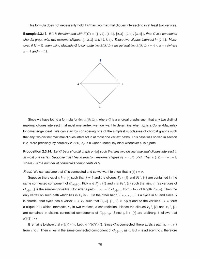
This formula does not necessarily hold if G has two maximal cliques intersecting in at least two vertices.

Example 2.3.13. If G is the diamond with E(G) = {{1, 2}, {1, 3}, {2, 3}, {2, 4}, {3, 4}}, then G is a connected

chordal graph with two maximal cliques: {1, 2, 3} and {2, 3, 4}. These two cliques intersect in {2, 3}. More-

over, if K = Q, then using Macaulay2 to compute depth(S/JG) we get that depth(S/JG) = 4 < n+ c (where

n = 4 and c = 1).

Since we have found a formula for depth(S/JG), where G is a chordal graphs such that any two distinct

maximal cliques intersect in at most one vertex, we now want to determine when JG is a Cohen-Macaulay

binomial edge ideal. We can start by considering one of the simplest subclasses of chordal graphs such

that any two distinct maximal cliques intersect in at most one vertex: paths. This case was solved in section

2.2. More precisely, by corollary 2.2.36, JG is a Cohen-Macaulay ideal whenever G is a path.

Proposition 2.3.14. Let G be a chordal graph on [n] such that any two distinct maximal cliques intersect in

at most one vertex. Suppose that i lies in exactly r maximal cliques F1, · · · , Fr of G. Then c({i}) = r+ c−1,

where c is the number of connected components of G.

Proof. We can assume that G is connected and so we want to show that c({i}) = r.

Suppose there exist j, k ∈ [r] such that j 6= k and the cliques Fj \ {i} and Fk \ {i} are contained in the

same connected component of G[n]\{i}. Pick u ∈ Fj \ {i} and v ∈ Fk \ {i} such that d(u, v) (as vertices of

G[n]\{i}) is the smallest possible. Consider a path u, · · · , v in G[n]\{i} from u to v of length d(u, v). Then the

only vertex on such path which lies in Fk is v. On the other hand, i, u, · · · , v, i is a cycle in G, and since G

is chordal, that cycle has a vertex w 6∈ Fk such that {i, w}, {v, w} ∈ E(G) and so the vertices i, v, w form

a clique in G which intersects Fk in two vertices, a contradiction. Hence the cliques Fj \ {i} and Fk \ {i}

are contained in distinct connected components of G[n]\{i}. Since j, k ∈ [r] are arbitrary, it follows that

c({i}) ≥ r.

It remains to show that c({i}) ≤ r. Let u ∈ V (G)\{i}. SinceG is connected, there exists a path u, · · · , v, i

from u to i. Then u lies in the same connected component of G[n]\{i} as v. But v is adjacent to i, therefore

70

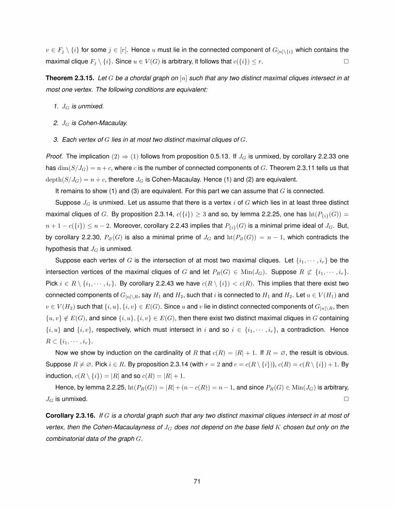
v ∈ Fj \ {i} for some j ∈ [r]. Hence u must lie in the connected component of G[n]\{i} which contains the

maximal clique Fj \ {i}. Since u ∈ V (G) is arbitrary, it follows that c({i}) ≤ r.


most one vertex. The following conditions are equivalent:

1. JG is unmixed.

2. JG is Cohen-Macaulay.

3. Each vertex of G lies in at most two distinct maximal cliques of G.

Proof. The implication (2) ⇒ (1) follows from proposition 0.5.13. If JG is unmixed, by corollary 2.2.33 one

has dim(S/JG) = n+ c, where c is the number of connected components of G. Theorem 2.3.11 tells us that

depth(S/JG) = n+ c, therefore JG is Cohen-Macaulay. Hence (1) and (2) are equivalent.

It remains to show (1) and (3) are equivalent. For this part we can assume that G is connected.

Suppose JG is unmixed. Let us assume that there is a vertex i of G which lies in at least three distinct

maximal cliques of G. By proposition 2.3.14, c({i}) ≥ 3 and so, by lemma 2.2.25, one has ht(P{i}(G)) =

n + 1 − c({i}) ≤ n − 2. Moreover, corollary 2.2.43 implies that P{i}(G) is a minimal prime ideal of JG. But,

by corollary 2.2.30, P∅(G) is also a minimal prime of JG and ht(P∅(G)) = n − 1, which contradicts the

hypothesis that JG is unmixed.

Suppose each vertex of G is the intersection of at most two maximal cliques. Let {i1, · · · , ir} be the

intersection vertices of the maximal cliques of G and let PR(G) ∈ Min(JG). Suppose R 6⊂ {i1, · · · , ir}.

Pick i ∈ R \ {i1, · · · , ir}. By corollary 2.2.43 we have c(R \ {i}) < c(R). This implies that there exist two

connected components of G[n]\R, say H1 and H2, such that i is connected to H1 and H2. Let u ∈ V (H1) and

v ∈ V (H2) such that {i, u}, {i, v} ∈ E(G). Since u and v lie in distinct connected components of G[n]\R, then

{u, v} 6∈ E(G), and since {i, u}, {i, v} ∈ E(G), then there exist two distinct maximal cliques in G containing

{i, u} and {i, v}, respectively, which must intersect in i and so i ∈ {i1, · · · , ir}, a contradiction. Hence

R ⊂ {i1, · · · , ir}.

Now we show by induction on the cardinality of R that c(R) = |R| + 1. If R = ∅, the result is obvious.

Suppose R 6= ∅. Pick i ∈ R. By proposition 2.3.14 (with r = 2 and c = c(R \ {i})), c(R) = c(R \ {i}) + 1. By

induction, c(R \ {i}) = |R| and so c(R) = |R|+ 1.

Hence, by lemma 2.2.25, ht(PR(G)) = |R|+ (n− c(R)) = n− 1, and since PR(G) ∈ Min(JG) is arbitrary,

JG is unmixed.

Corollary 2.3.16. If G is a chordal graph such that any two distinct maximal cliques intersect in at most of

vertex, then the Cohen-Macaulayness of JG does not depend on the base field K chosen but only on the

combinatorial data of the graph G.

71

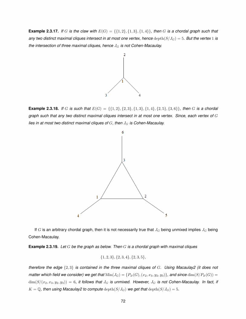
Example 2.3.17. If G is the claw with E(G) = {{1, 2}, {1, 3}, {1, 4}}, then G is a chordal graph such that

any two distinct maximal cliques intersect in at most one vertex, hence depth(S/JG) = 5. But the vertex 1 is

the intersection of three maximal cliques, hence JG is not Cohen-Macaulay.

Example 2.3.18. If G is such that E(G) = {{1, 2}, {2, 3}, {1, 3}, {1, 4}, {2, 5}, {3, 6}}, then G is a chordal

graph such that any two distinct maximal cliques intersect in at most one vertex. Since, each vertex of G

lies in at most two distinct maximal cliques of G, then JG is Cohen-Macaulay.

If G is an arbitrary chordal graph, then it is not necessarily true that JG being unmixed implies JG being

Cohen-Macaulay.

Example 2.3.19. Let G be the graph as below. Then G is a chordal graph with maximal cliques

{1, 2, 3}, {2, 3, 4}, {2, 3, 5},

therefore the edge {2, 3} is contained in the three maximal cliques of G. Using Macaulay2 (it does not

matter which field we consider) we get that Min(JG) = {P∅(G), (x2, x3, y2, y3)}, and since dim(S/P∅(G)) =

dim(S/(x2, x3, y2, y3)) = 6, it follows that JG is unmixed. However, JG is not Cohen-Macaulay. In fact, if

K = Q, then using Macaulay2 to compute depth(S/JG) we get that depth(S/JG) = 5.

72

Corollary 2.3.20. Let G be a forest on the vertex set [n]. The following conditions are equivalent:

1. JG is unmixed.

2. JG is a Cohen-Macaulay.

3. JG is a complete intersection.

4. Each connected component of G is a path.

Proof. The implications (3) ⇒ (2) ⇒ (1) follow from corollaries 0.5.10 and 0.5.13, while (1) ⇒ (4) follows

from implication (1)⇒ (3) of theorem 2.3.15. It remains to show the implication (4)⇒ (3).

By proposition 2.2.35, the binomial edge ideal of a path is a complete intersection, therefore the binomial

edge ideal of a disjoint union of paths is also a complete intersection, hence the implication (4) ⇒ (3)

follows.

Example 2.3.21. We can also show that JG is not Cohen-Macaulay when G is a claw using this corollary.

In fact, G is a tree which is not a path, hence the result follows.

2.4 Closed graphs

In the previous section we studied which chordal graphs such that any two distinct maximal cliques

intersect in at most one vertex have a Cohen-Macaulay binomial edge ideal. In this section we will answer

the same question, but for closed graphs. Recall that closed graphs were defined in section 2.2.

Let G be a closed graph. Then the binomials fij with i < j and {i, j} ∈ E(G) form a Grobner basis for

G and so the square-free monomials in<(fij) = xiyj are the generators of in<(JG), and so there exists a

unique bipartite graph H on the set of vertices {x1, · · · , xn} ∪ {y1, · · · , yn} whose monomial edge ideal is

in<(JG). The equality in<(JG) = I(H) suggests the notation H = in<(G). Equivalently, H = in<(G) is the

73

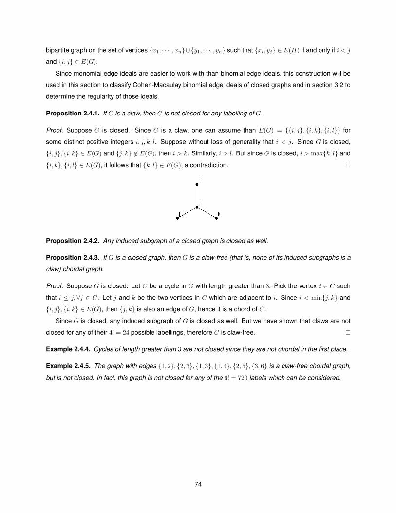
bipartite graph on the set of vertices {x1, · · · , xn}∪{y1, · · · , yn} such that {xi, yj} ∈ E(H) if and only if i < j

and {i, j} ∈ E(G).

Since monomial edge ideals are easier to work with than binomial edge ideals, this construction will be

used in this section to classify Cohen-Macaulay binomial edge ideals of closed graphs and in section 3.2 to

determine the regularity of those ideals.

Proposition 2.4.1. If G is a claw, then G is not closed for any labelling of G.

Proof. Suppose G is closed. Since G is a claw, one can assume than E(G) = {{i, j}, {i, k}, {i, l}} for

some distinct positive integers i, j, k, l. Suppose without loss of generality that i < j. Since G is closed,

{i, j}, {i, k} ∈ E(G) and {j, k} 6∈ E(G), then i > k. Similarly, i > l. But since G is closed, i > max{k, l} and

{i, k}, {i, l} ∈ E(G), it follows that {k, l} ∈ E(G), a contradiction.

Proposition 2.4.2. Any induced subgraph of a closed graph is closed as well.

Proposition 2.4.3. If G is a closed graph, then G is a claw-free (that is, none of its induced subgraphs is a

claw) chordal graph.

Proof. Suppose G is closed. Let C be a cycle in G with length greater than 3. Pick the vertex i ∈ C such

that i ≤ j,∀j ∈ C. Let j and k be the two vertices in C which are adjacent to i. Since i < min{j, k} and

{i, j}, {i, k} ∈ E(G), then {j, k} is also an edge of G, hence it is a chord of C.

Since G is closed, any induced subgraph of G is closed as well. But we have shown that claws are not

closed for any of their 4! = 24 possible labellings, therefore G is claw-free.

Example 2.4.4. Cycles of length greater than 3 are not closed since they are not chordal in the first place.

Example 2.4.5. The graph with edges {1, 2}, {2, 3}, {1, 3}, {1, 4}, {2, 5}, {3, 6} is a claw-free chordal graph,

but is not closed. In fact, this graph is not closed for any of the 6! = 720 labels which can be considered.

74

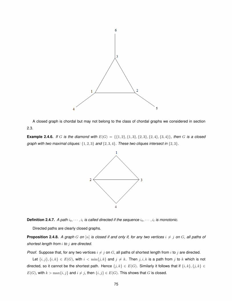
A closed graph is chordal but may not belong to the class of chordal graphs we considered in section

2.3.

Example 2.4.6. If G is the diamond with E(G) = {{1, 2}, {1, 3}, {2, 3}, {2, 4}, {3, 4}}, then G is a closed

graph with two maximal cliques: {1, 2, 3} and {2, 3, 4}. These two cliques intersect in {2, 3}.

Definition 2.4.7. A path i0, · · · , il is called directed if the sequence i0, · · · , il is monotonic.

Directed paths are clearly closed graphs.

Proposition 2.4.8. A graph G on [n] is closed if and only if, for any two vertices i 6= j on G, all paths of

shortest length from i to j are directed.

Proof. Suppose that, for any two vertices i 6= j on G, all paths of shortest length from i to j are directed.

Let {i, j}, {i, k} ∈ E(G), with i < min{j, k} and j 6= k. Then j, i, k is a path from j to k which is not

directed, so it cannot be the shortest path. Hence {j, k} ∈ E(G). Similarly it follows that if {i, k}, {j, k} ∈

E(G), with k > max{i, j} and i 6= j, then {i, j} ∈ E(G). This shows that G is closed.

75

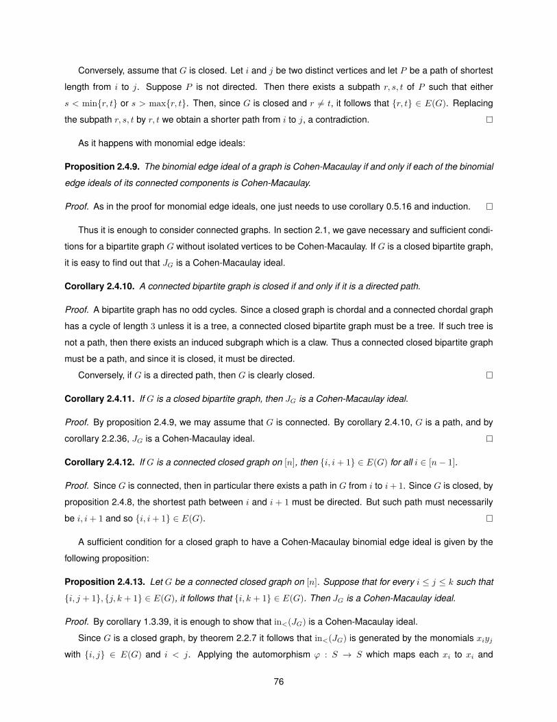
Conversely, assume that G is closed. Let i and j be two distinct vertices and let P be a path of shortest

length from i to j. Suppose P is not directed. Then there exists a subpath r, s, t of P such that either

s < min{r, t} or s > max{r, t}. Then, since G is closed and r 6= t, it follows that {r, t} ∈ E(G). Replacing

the subpath r, s, t by r, t we obtain a shorter path from i to j, a contradiction.

As it happens with monomial edge ideals:

Proposition 2.4.9. The binomial edge ideal of a graph is Cohen-Macaulay if and only if each of the binomial

edge ideals of its connected components is Cohen-Macaulay.

Proof. As in the proof for monomial edge ideals, one just needs to use corollary 0.5.16 and induction.

Thus it is enough to consider connected graphs. In section 2.1, we gave necessary and sufficient condi-

tions for a bipartite graph G without isolated vertices to be Cohen-Macaulay. If G is a closed bipartite graph,

it is easy to find out that JG is a Cohen-Macaulay ideal.

Corollary 2.4.10. A connected bipartite graph is closed if and only if it is a directed path.

Proof. A bipartite graph has no odd cycles. Since a closed graph is chordal and a connected chordal graph

has a cycle of length 3 unless it is a tree, a connected closed bipartite graph must be a tree. If such tree is

not a path, then there exists an induced subgraph which is a claw. Thus a connected closed bipartite graph

must be a path, and since it is closed, it must be directed.

Conversely, if G is a directed path, then G is clearly closed.

Corollary 2.4.11. If G is a closed bipartite graph, then JG is a Cohen-Macaulay ideal.

Proof. By proposition 2.4.9, we may assume that G is connected. By corollary 2.4.10, G is a path, and by

corollary 2.2.36, JG is a Cohen-Macaulay ideal.

Corollary 2.4.12. If G is a connected closed graph on [n], then {i, i+ 1} ∈ E(G) for all i ∈ [n− 1].

Proof. Since G is connected, then in particular there exists a path in G from i to i+ 1. Since G is closed, by

proposition 2.4.8, the shortest path between i and i + 1 must be directed. But such path must necessarily

be i, i+ 1 and so {i, i+ 1} ∈ E(G).

A sufficient condition for a closed graph to have a Cohen-Macaulay binomial edge ideal is given by the

following proposition:

Proposition 2.4.13. Let G be a connected closed graph on [n]. Suppose that for every i ≤ j ≤ k such that

{i, j + 1}, {j, k + 1} ∈ E(G), it follows that {i, k + 1} ∈ E(G). Then JG is a Cohen-Macaulay ideal.

Proof. By corollary 1.3.39, it is enough to show that in<(JG) is a Cohen-Macaulay ideal.

Since G is a closed graph, by theorem 2.2.7 it follows that in<(JG) is generated by the monomials xiyj

with {i, j} ∈ E(G) and i < j. Applying the automorphism ϕ : S → S which maps each xi to xi and

76

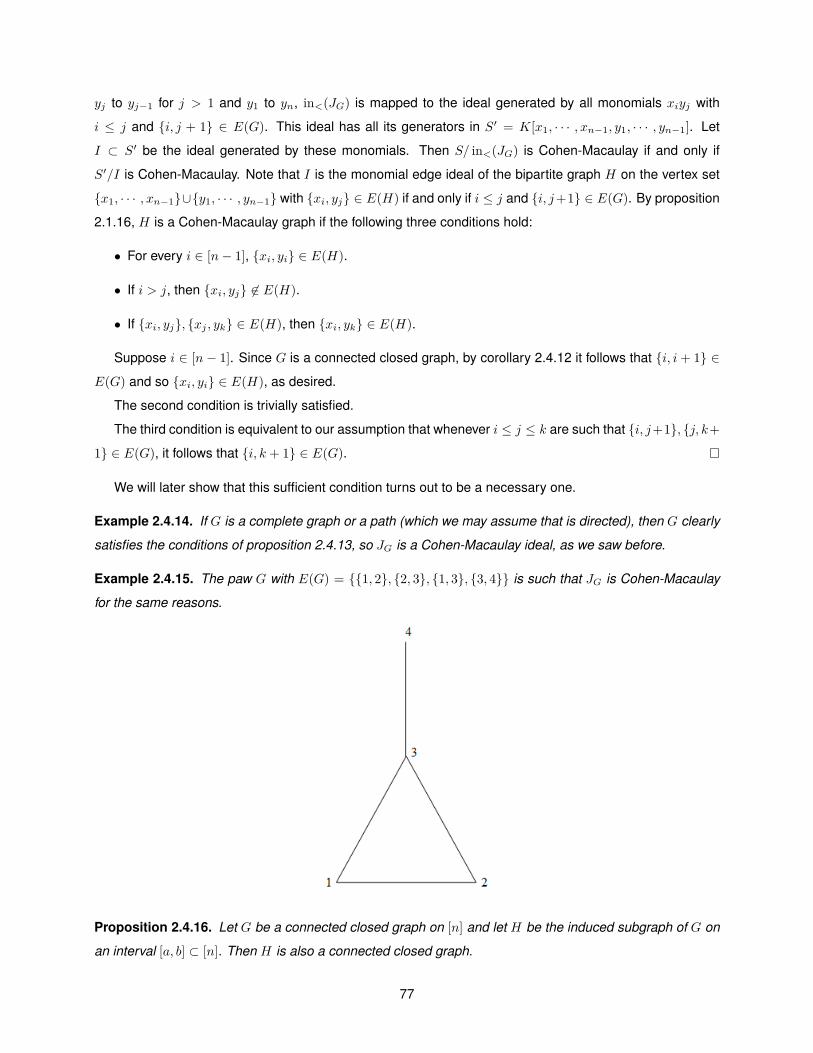
yj to yj−1 for j > 1 and y1 to yn, in<(JG) is mapped to the ideal generated by all monomials xiyj with

i ≤ j and {i, j + 1} ∈ E(G). This ideal has all its generators in S′ = K[x1, · · · , xn−1, y1, · · · , yn−1]. Let

I ⊂ S′ be the ideal generated by these monomials. Then S/ in<(JG) is Cohen-Macaulay if and only if

S′/I is Cohen-Macaulay. Note that I is the monomial edge ideal of the bipartite graph H on the vertex set

{x1, · · · , xn−1}∪{y1, · · · , yn−1} with {xi, yj} ∈ E(H) if and only if i ≤ j and {i, j+1} ∈ E(G). By proposition

2.1.16, H is a Cohen-Macaulay graph if the following three conditions hold:

• For every i ∈ [n− 1], {xi, yi} ∈ E(H).

• If i > j, then {xi, yj} 6∈ E(H).

• If {xi, yj}, {xj , yk} ∈ E(H), then {xi, yk} ∈ E(H).

Suppose i ∈ [n− 1]. Since G is a connected closed graph, by corollary 2.4.12 it follows that {i, i+ 1} ∈

E(G) and so {xi, yi} ∈ E(H), as desired.

The second condition is trivially satisfied.

The third condition is equivalent to our assumption that whenever i ≤ j ≤ k are such that {i, j+1}, {j, k+

1} ∈ E(G), it follows that {i, k + 1} ∈ E(G).

We will later show that this sufficient condition turns out to be a necessary one.

Example 2.4.14. If G is a complete graph or a path (which we may assume that is directed), then G clearly

satisfies the conditions of proposition 2.4.13, so JG is a Cohen-Macaulay ideal, as we saw before.

Example 2.4.15. The paw G with E(G) = {{1, 2}, {2, 3}, {1, 3}, {3, 4}} is such that JG is Cohen-Macaulay

for the same reasons.

Proposition 2.4.16. Let G be a connected closed graph on [n] and let H be the induced subgraph of G on

an interval [a, b] ⊂ [n]. Then H is also a connected closed graph.

77

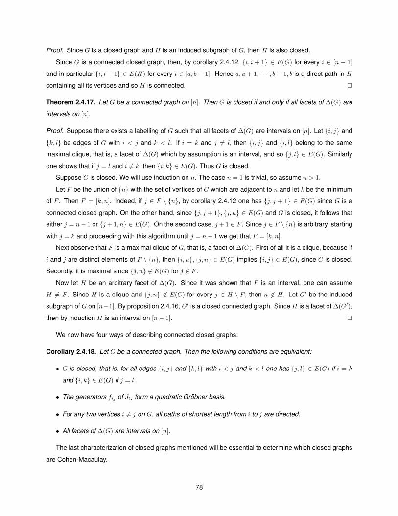
Proof. Since G is a closed graph and H is an induced subgraph of G, then H is also closed.

Since G is a connected closed graph, then, by corollary 2.4.12, {i, i + 1} ∈ E(G) for every i ∈ [n − 1]

and in particular {i, i + 1} ∈ E(H) for every i ∈ [a, b − 1]. Hence a, a + 1, · · · , b − 1, b is a direct path in H

containing all its vertices and so H is connected.

Theorem 2.4.17. Let G be a connected graph on [n]. Then G is closed if and only if all facets of ∆(G) are

intervals on [n].

Proof. Suppose there exists a labelling of G such that all facets of ∆(G) are intervals on [n]. Let {i, j} and

{k, l} be edges of G with i < j and k < l. If i = k and j 6= l, then {i, j} and {i, l} belong to the same

maximal clique, that is, a facet of ∆(G) which by assumption is an interval, and so {j, l} ∈ E(G). Similarly

one shows that if j = l and i 6= k, then {i, k} ∈ E(G). Thus G is closed.

Suppose G is closed. We will use induction on n. The case n = 1 is trivial, so assume n > 1.

Let F be the union of {n} with the set of vertices of G which are adjacent to n and let k be the minimum

of F . Then F = [k, n]. Indeed, if j ∈ F \ {n}, by corollary 2.4.12 one has {j, j + 1} ∈ E(G) since G is a

connected closed graph. On the other hand, since {j, j + 1}, {j, n} ∈ E(G) and G is closed, it follows that

either j = n− 1 or {j + 1, n} ∈ E(G). On the second case, j + 1 ∈ F . Since j ∈ F \ {n} is arbitrary, starting

with j = k and proceeding with this algorithm until j = n− 1 we get that F = [k, n].

Next observe that F is a maximal clique of G, that is, a facet of ∆(G). First of all it is a clique, because if

i and j are distinct elements of F \ {n}, then {i, n}, {j, n} ∈ E(G) implies {i, j} ∈ E(G), since G is closed.

Secondly, it is maximal since {j, n} 6∈ E(G) for j 6∈ F .

Now let H be an arbitrary facet of ∆(G). Since it was shown that F is an interval, one can assume

H 6= F . Since H is a clique and {j, n} 6∈ E(G) for every j ∈ H \ F , then n 6∈ H. Let G′ be the induced

subgraph of G on [n−1]. By proposition 2.4.16, G′ is a closed connected graph. Since H is a facet of ∆(G′),

then by induction H is an interval on [n− 1].

We now have four ways of describing connected closed graphs:

Corollary 2.4.18. Let G be a connected graph. Then the following conditions are equivalent:

• G is closed, that is, for all edges {i, j} and {k, l} with i < j and k < l one has {j, l} ∈ E(G) if i = k

and {i, k} ∈ E(G) if j = l.

• The generators fij of JG form a quadratic Grobner basis.

• For any two vertices i 6= j on G, all paths of shortest length from i to j are directed.

• All facets of ∆(G) are intervals on [n].

The last characterization of closed graphs mentioned will be essential to determine which closed graphs

are Cohen-Macaulay.

78

Theorem 2.4.19. Let G be a connected closed graph on [n]. Then the following conditions are equivalent:

1. JG is unmixed.

2. JG is Cohen-Macaulay.

3. in<(JG) is Cohen-Macaulay.

4. G satisfies the condition that whenever {i, j + 1} with i ≤ j and {j, k + 1} with j ≤ k are edges of G,

then {i, k + 1} is an edge of G.

5. There exist integers 1 = a1 < · · · < ar < ar+1 = n and a leaf order of the facets F1, · · · , Fr of ∆(G)

such that Fi = [ai, ai+1] for every i ∈ [r].

Proof. The implication (4) ⇒ (3) is shown in the proof of proposition 2.4.13. The implications (3) ⇒ (2) ⇒

(1) are due to corollaries 1.3.39 and 0.5.13, respectively.

We now prove the implication (5) ⇒ (4). Let i ≤ j ≤ k be three vertices of G such that {i, j + 1} and

{j, k + 1} are edges of G. If i = j or j = k, then the implication is obvious. Suppose i < j < k. Notice that

i and j + 1 belong to the same facet of ∆(G), let us say Fl. Since i < j < j + 1, then the only facet which

contains j is Fl. But then k + 1 must belong to Fl as well since it is adjacent to j. Therefore i and k + 1 are

adjacent for they both belong to Fl.

It remains to show the implication (1)⇒ (5). Since G is closed, then by theorem 2.4.17 ∆(G) has facets

F1, · · · , Fr where each facet is an interval. We may order the intervals Fi = [ai, bi] such that 1 = a1 < · · · <

ar < n. Then 1 < b1 < · · · < br = n and since G is connected, it follows that ai+1 ≤ bi for every i ∈ [r − 1].

Let i ∈ [r − 1] and R = [ai+1, bi]. Suppose c(R) = 1. Since G is closed, then G[n]\R is also closed,

and since c(R) = 1, by corollary 2.4.12 it follows that {ai+1 − 1, bi + 1} ∈ E(G). Let j ∈ [r] such that

[aj , bj ] is a facet of ∆(G) containing both ai+1 − 1 and bi + 1. Then aj < ai+1, therefore j ≤ i. On the

other hand, bj > bi, therefore j > i, a contradiction. Hence c(R) ≥ 2. Since G is a connected closed

graph, by proposition 2.4.16 G[1,ai+1−1] and G[bi+1,n] are connected graphs and so c(R) = 2, therefore

ht(PR(G)) = n + |R| − c(R) = n + (bi − ai+1 + 1) − 2 = n + (bi − ai+1) − 1. Since c(R) = 2, then to show

PR(G) ∈ Min(JG), by corollary 2.2.43 it is enough to show that G([n]\R)∪{j} is connected for every j ∈ R.

Let j ∈ R. Since we have seen that G[1,ai+1−1] and G[bi+1,n] are connected graphs, then to show that

G([n]\R)∪{j} is connected it is enough to show that j is adjacent to ai ∈ [1, ai+1−1] and bi+1 ∈ [bi+ 1, n]. But

j ∈ [ai+1, bi] ⊂ [ai, bi] ∩ [ai+1, bi+1] and the conclusion follows since both [ai, bi] and [ai+1, bi+1] are cliques

in G.

Since both P∅(G) and PR(G) are minimal primes of JG, our assumption implies that n+(bi−ai+1)−1 =

n− 1, that is, bi = ai+1. Putting ar+1 = br = n we get that Fi = [ai, ai+1] for every i ∈ [r]. It is clear from this

that F1, · · · , Fr is a leaf order.

Corollary 2.4.20. If G is a closed graph, then the Cohen-Macaulayness of JG does not depend on the base

field K chosen but only on the graph G.

79

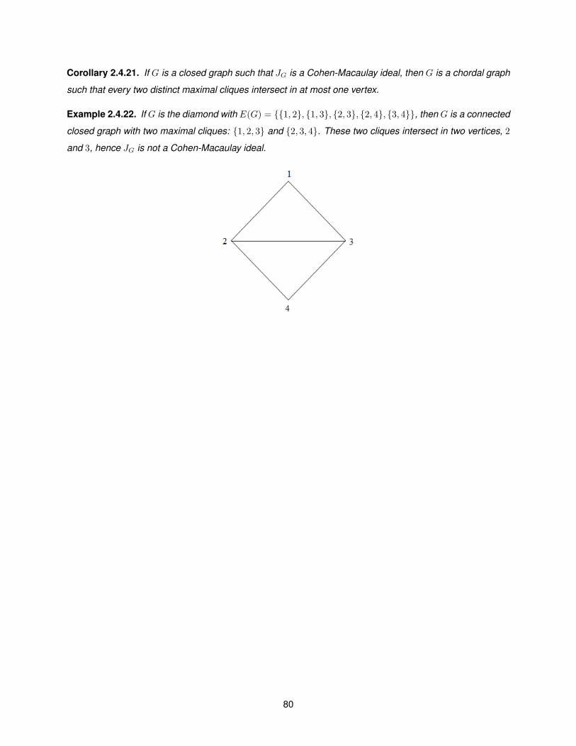
Corollary 2.4.21. If G is a closed graph such that JG is a Cohen-Macaulay ideal, then G is a chordal graph

such that every two distinct maximal cliques intersect in at most one vertex.

Example 2.4.22. If G is the diamond with E(G) = {{1, 2}, {1, 3}, {2, 3}, {2, 4}, {3, 4}}, then G is a connected

closed graph with two maximal cliques: {1, 2, 3} and {2, 3, 4}. These two cliques intersect in two vertices, 2

and 3, hence JG is not a Cohen-Macaulay ideal.

80

Chapter 3

Regularity of binomial edge ideals

Castelnuovo-Mumford regularity is one of the most fundamental invariants in Commutative Algebra and

Algebraic Geometry. In fact, already in the late 19th century this invariant was present, a long time before it

was properly defined. One of its first hidden appearances may be found in Castelnuovo’s work.

However, a proper definition of Castelnuovo-Mumford regularity was only given in 1966 by Mumford,

who called it Castelnuovo regularity. In fact, Mumford defined the notion of being m-regular in the sense of

Castelnuovo for a coherent sheaf of ideals over a projective space and a given integer m. More precisely,

a sheaf of ideals over a projective space is called m-regular if, for every i > 0, the i-th Serre cohomology

group of the (m−i)-fold twist of this sheaf vanishes. The smallest m such that the sheaf of ideals in question

is m-regular is what today is usually called the Castelnuovo-Mumford regularity of such sheaf.

Castelnuovo-Mumford regularity also found much interest in Commutative Algebra. In 1982, Ooishi de-

fined the Castelnuovo-Mumford regularity of a graded module in terms of certain local cohomology modules.

His definition essentially corresponds to Mumford’s definition via the Serre-Grothendieck correspondence

between local cohomology and sheaf cohomology. In 1984, Eisenbud and Goto made explicite the link

between this ”algebraic” Castelnuovo-Mumford regularity of a graded module over a polynomial ring and its

minimal free resolution. In fact, in section 0.6 we defined the Castelnuovo-Mumford regularity of a graded

module in terms of its minimal free resolution.

As Woodroofe wrote in [14], the Castelnuovo-Mumford regularity of an ideal I is one of the main mea-

sures of the complexity of I. In this chapter, the regularity of binomial edge ideals will be studied.

In section 3.1 we state some results and conjectures about regularity bounds of binomial edge ideals.

In section 3.2 we show that, when G is a closed graph, the regularity of JG is given by the lengths of its

induced paths.

In section 3.3 we show that the conjectures stated in section 3.1 hold not only for closed graphs but also

for the class of graphs considered in section 2.3.

81

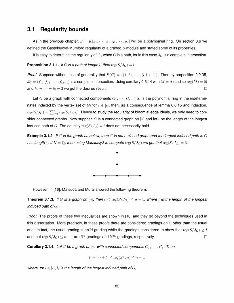
3.1 Regularity bounds

As in the previous chapter, S = K[x1, · · · , xn, y1, · · · , yn] will be a polynomial ring. On section 0.6 we

defined the Castelnuovo-Mumford regularity of a graded S-module and stated some of its properties.

It is easy to determine the regularity of JG when G is a path, for in this case JG is a complete intersection.

Proposition 3.1.1. If G is a path of length l, then reg(S/JG) = l.

Proof. Suppose without loss of generality that E(G) = {{1, 2}, · · · , {l, l + 1}}. Then by proposition 2.2.35,

JG = (f12, f23, · · · , fl,l+1) is a complete intersection. Using corollary 0.6.14 with M = S (and so reg(M) = 0)

and k1 = · · · = kl = 2 we get the desired result.

Let G be a graph with connected components G1, · · · , Gc. If Si is the polynomial ring in the indetermi-

nates indexed by the vertex set of Gi for i ∈ [c], then, as a consequence of lemma 0.6.15 and induction,

reg(S/JG) =∑ci=1 reg(Si/JGi). Hence to study the regularity of binomial edge ideals, we only need to con-

sider connected graphs. Now suppose G is a connected graph on [n] and let l be the length of the longest

induced path of G. The equality reg(S/JG) = l does not necessarily hold.

Example 3.1.2. If G is the graph as below, then G is not a closed graph and the largest induced path in G

has length 4. If K = Q, then using Macaulay2 to compute reg(S/JG) we get that reg(S/JG) = 6.

However, in [16], Matsuda and Murai showed the following theorem:

Theorem 3.1.3. If G is a graph on [n], then l ≤ reg(S/JG) ≤ n − 1, where l is the length of the longest

induced path of G.

Proof. The proofs of these two inequalities are shown in [16] and they go beyond the techniques used in

this dissertation. More precisely, in these proofs there are considered gradings on S other than the usual

one. In fact, the usual grading is an N-grading while the gradings considered to show that reg(S/JG) ≥ l

and that reg(S/JG) ≤ n− 1 are Nn-gradings and N2n-gradings, respectively.

Corollary 3.1.4. Let G be a graph on [n] with connected components G1, · · · , Gc. Then

l1 + · · ·+ lc ≤ reg(S/JG) ≤ n− c,

where, for i ∈ [c], li is the length of the largest induced path of Gi.

82

Proof. Just combine the equality reg(S/JG) =∑ci=1 reg(Si/JGi) with the inequalities li ≤ reg(S/JGi) ≤

|V (Gi)| − 1 where i ∈ [c].

In section 3.2 it will be shown that the equality reg(S/JG) = l1 + · · ·+ lc turns out to be true whenever G

is a closed graph.

Corollary 3.1.5. If G is a connected graph such that reg(S/JG) = 1, then G is a complete graph.

Proof. Suppose by contradiction that G is not complete. Then G has an induced path of length 2, hence

reg(S/JG) ≥ 2.

In section 3.2 we will see that the converse of this corollary holds.

In [15], Madani and Kiani conjectured that if G is a graph with r maximal cliques, then reg(S/JG) ≤ r.

Note that it is not always true that r ≤ n− c.

Example 3.1.6. If G is the cycle of length 4, then n = 4, c = 1 and r = 4, hence r > n− c.

Proposition 3.1.7. Let G a graph with connected components G1, · · · , Gc and with r maximal cliques. Then

l1 + · · ·+ lc ≤ r, where, for i ∈ [c], li is the length of the largest induced path in Gi.

Proof. Since r = r1 + · · ·+ rc, where, for i ∈ [c], ri is the number of maximal cliques in Gi, then it is enough

to show this when G is connected.

Let P be a path in G of length greater than r. Then two of the edges of P , say {u, v}, {u′, v′}, with

v′ 6∈ {u, v}, must be contained in the same maximal clique of G and in particular {v, v′} ∈ E(G) and so P is

not an induced path of G.

Hence, once proven that reg(S/JG) = l1 + · · ·+ lc when G is a closed graph, it will follow that the Madani-

Kiani conjecture holds for closed graphs. We will show in section 3.3 that it also turns out to be true for the

class of graphs considered in section 2.3.

In [16], Matsuda and Murai conjectured that if G is a graph on [n], then reg(S/JG) = n − 1 if and only

if G is a path. Once proven that reg(S/JG) = l1 + · · · + lc when G is a closed graph, it will follow that this

conjecture holds for closed graphs. As with the Madani-Kiani conjecture, in section 3.3 it will also be shown

that this conjecture turns out to be true for the class of graphs considered in section 2.3.

While in this dissertation the Matsuda-Murai conjecture was meant to be presented as a conjecture, it

happened to be fully shown this year, on April 6th, in [18] by Madani and Kiani. Since the partial proof for

chordal graphs such that any two maximal cliques intersect in at most one vertex is an interesting proof which

83

uses some nice results on the combinatorial data of these graphs, I decided to keep it in the dissertation,

not forgetting to indicate a reference for the full proof of the Matsuda-Murai conjecture.

3.2 Regularity of binomial edge ideals of closed graphs

If G is a closed graph, then by theorem 1.3.38, reg(S/JG) ≤ reg(S/ in<(JG)). But in<(JG) is the mono-

mial edge ideal of a bipartite graph and so results on the regularity of monomial edge ideals of bipartite

graphs can be used to study the regularity of binomial edge ideals of closed graphs.

Lemma 3.2.1. Let G be a connected closed graph on [n]. Then the bipartite graph H = in<(G) is weakly

chordal.

Proof. Let C be a cycle in H of length greater than 4. The induced subgraphs of H on the sets {x1, · · · , xn}

and {y1, · · · , yn} are complete graphs. Since C is a cycle of length greater than 4, then it contains at least

three vertices from one of those two complete graphs, therefore it has a chord.

Since H is a bipartite graph on {x1, · · · , xn} ∪ {y1, · · · , yn}, then a cycle C in H of length greater than

4 has set of vertices {xi1 , yj1 , · · · , xik , yjk}, where k ≥ 3. We make the convention that ik+1 = i1 and

jk+1 = j1. We divide the proof that C has a chord in the following steps:

1. Check that, for l ∈ [k], max{il, il+1} < jl and {il, jl}, {il+1, jl}, {il, il+1}, {jl, jl+1} ∈ E(G).

2. Consider the case when there exists l ∈ [k] such that il < jl+1 < jl. This case is easy to solve. The

other case is when, for every l ∈ [k], either jl+1 ≤ il or jl < jl+1 holds.

3. For the remaining case, pick t ∈ [k] such that it is the maximum of the sequence i1, · · · , ik, ik+1 = i1

and start by checking that one of two following inequalities hold: it+1 < jt+1 ≤ it < jt or it+1 < it <

jt < jt+1.

4. By last, check that any of those two inequalities will imply that C has a chord.

For the first step, let l ∈ [k]. Then {xil , yjl} ∈ E(H), that is, il < jl and {il, jl} ∈ E(G). On the other hand,

{xil+1 , yjl} ∈ E(H), that is, il+1 < jl and {il+1, jl} ∈ E(G). Let l ∈ [k]. Since G is closed, max{il, il+1} < jl

and {il, jl}, {il+1, jl} ∈ E(G), it follows that {il, il+1} ∈ E(G). Since G is closed, il+1 < min{jl, jl+1} and

{il+1, jl}, {il+1, jl+1} ∈ E(G), it follows that {jl, jl+1} ∈ E(G).

For the second step, let l ∈ [k] such that il < jl+1 < jl. Since G is closed, il < jl+1 < jl and

{il, jl}, {jl+1, jl} ∈ E(G), it follows that {il, jl+1} ∈ E(G) and so {xil , yjl+1} ∈ E(H), hence {xil , yjl+1} is a

chord in C.

For the third step we know that, for every l ∈ [k], either jl+1 ≤ il or jl < jl+1 holds. In the first case, the

inequalities il < jl and il+1 < jl+1 imply

il+1 < jl+1 ≤ il < jl. (3.1)

84

In the second case, the inequality max{il, il+1} < jl implies the inequality

max{il, il+1} < jl < jl+1. (3.2)

Pick t ∈ [k] such that it is the maximum of the sequence i1, · · · , ik, ik+1 = i1. Since this sequence

cannot have two consecutive equal terms, then max{it−1, it+1} < it. Since it−1 < it, the inequality (3.1)

with l = t− 1 cannot hold, and so the inequality (3.2) with l = t− 1, that is, max{it−1, it} < jt−1 < jt, holds.

Moreover, it−1 < it implies it−1 < it < jt−1 < jt. On the other hand, one of the two inequalities (3.1) and

(3.2), with l = t, must hold. The first inequality is it+1 < jt+1 ≤ it < jt. Since it+1 < it, the second inequality

implies that it+1 < it < jt < jt+1.

Now we end with the fourth and final step.

If it+1 < jt+1 ≤ it < jt holds, we get the chain it+1 < jt+1 ≤ it < jt−1 < jt. Since G is closed, it+1 <

jt−1 < jt and {it+1, jt}, {jt−1, jt} ∈ E(G), it follows that {it+1, jt−1} ∈ E(G) and so {xit+1 , yjt−1} ∈ E(H),

hence {xit+1 , yjt−1} is a chord in C.

If it+1 < it < jt < jt+1 holds, since G is closed, it+1 < it < jt+1 and {it+1, it}, {it+1, jt+1} ∈ E(G), it

follows that {it, jt+1} ∈ E(G) and so {xit , yjt+1} ∈ E(H), hence {xit , yjt+1} is a chord in C.

Corollary 3.2.2. Let G be a closed graph on [n] and let H = in<(G). Then

reg(K[x1, · · · , xn, y1, · · · , yn]/I(H)) = indmatch(H).

Proof. By lemma 3.2.1, H is a weakly chordal bipartite graph. By theorem 2.1.9 the result follows.

Proposition 3.2.3. Let G be a connected closed graph on [n] and H = in<(G). Then indmatch(H) = l,

where l is the length of the longest induced path of G.

Proof. First we show that indmatch(H) ≥ l. Let i0, · · · , il be an induced path in G of length l. If such

path is not directed, then one can suppose without loss of generality that there exists t ∈ [l − 1] such that

max{it−1, it+1} < it. But then, since {it−1, it}, {it, it+1} ∈ E(G) and it−1 6= it+1, it follows that {it−1, it+1} ∈

E(G), which contradicts the fact that i0, · · · , il is an induced path in G. Hence i0, · · · , il is a directed path

and in particular we can assume that i0 < · · · < il and so the edges {xi0 , yi1}, · · · , {xil−1 , yil} form an

induced subgraph of H, which is an induced matching.

We now show that indmatch(H) ≤ l. Let indmatch(H) = m. Then H has m pairwise disjoint edges

{xi1 , yj1}, · · · , {xim , yjm} that form an induced subgraph of H. We may assume that i1 < · · · < im. To

show the desired inequality we construct an induced path of length m in G. We now divide the proof in the

following steps:

1. Show that one can suppose without loss of generality that if t ∈ [n] and s ∈ [m] are such that t < is

and {xt, yjs} ∈ E(H), then {xi1 , yj1}, · · · , {xis−1 , yjs−1}, {xt, yjs

}, {xis+1 , yjs+1}, · · · , {xim , yjm} is not

an induced matching of H.

85

2. Show that the inequality i1 < j1 ≤ i2 < j2 ≤ · · · < jm−1 ≤ im < jm holds.

3. We will show that i1, · · · , im, jm is an induced path in G. First, we show that {is, jm} 6∈ E(G) for every

s ∈ [m− 1] and that {is, is′} 6∈ E(G) whenever s′ > s+ 1.

4. Finally, we show that {is, is+1} ∈ E(G) for every s ∈ [m − 1]. Suppose {is, is+1} 6∈ E(G) for some

s ∈ [m− 1]. First we show that {js, is+1} 6∈ E(G).

5. Secondly, consider j to be the smallest t such that {t, is+1} ∈ E(G). Show that j > js and, from there,

get a contradiction. We conclude that {is, is+1} ∈ E(G) for every s ∈ [m− 1].

For the first step, let s ∈ [m]. Since {xis , yjs} ∈ E(H), then is < js and {is, js} ∈ E(G).

Let i′1 be the smallest integer t such that {xt, yj1} ∈ E(H) and {xt, yj1}, {xi2 , yj2} · · · , {xim , yjm} is an

induced matching of H. Then i′1 is well defined and i′1 ≤ i1. Moreover, if t < i′1 is such that{xt, yj1} ∈ E(H),

then {xt, yj1}, {xi2 , yj2} · · · , {xim , yjm} is not an induced matching.

Let i′2 be the smallest integer t such that {xt, yj2} ∈ E(H) and {xi′1 , yj1}, {xt, yj2}, {xi3 , yj3} · · · , {xim , yjm}

is an induced matching of H. Then i′2 is well defined and i′2 ≤ i2. Moreover, if t < i′2 is such that

{xt, yj2} ∈ E(H), then {xi′1 , yj1}, {xt, yj2}, {xi3 , yj3} · · · , {xim , yjm} is not an induced matching.

Proceeding with this construction, we define i′3, · · · , i′m such that {xi′1 , yj1}, · · · , {xi′m , yjm} is an induced

matching of H and if t ∈ [n] and s ∈ [m] are such that t < i′s and {xt, yjs} ∈ E(H), then

{xi′1 , yj1}, · · · , {xi′s−1, yjs−1}, {xt, yjs

}, {xis+1 , yjs+1}, · · · , {xim , yjm}

is not an induced matching ofH. To simplify notations, we replace i′1, · · · , i′s by i1, · · · , is in the affirmation we

just made. That is, {xi1 , yj1}, · · · , {xim , yjm} is an induced matching of H and if t ∈ [n] and s ∈ [m] are such

that t < is and {xt, yjs} ∈ E(H), then {xi1 , yj1}, · · · , {xis−1 , yjs−1}, {xt, yjs}, {xis+1 , yjs+1}, · · · , {xim , yjm} is

not an induced matching of H.

For the second step, suppose there exists s ∈ [m − 1] such that js > is+1. Since G is closed, then by

theorem 2.4.17 all facets of ∆(G) are intervals, and since {is, js} ∈ E(G), it follows that [is, js] is a face in

∆(G), and since is < is+1 < js, it follows in particular that {is+1, js} ∈ E(G), hence {xis+1 , yjs} ∈ E(H).

But then the edges {xis , yjs}, {xis+1 , yjs+1} do not form an induced matching of H, a contradiction. Hence

js ≤ is+1 for every s ∈ [m− 1].

Then the following inequality holds: i1 < j1 ≤ i2 < j2 ≤ · · · < jm−1 ≤ im < jm.

Now consider the third step. Suppose that there exists s ∈ [m − 1] such that {is, jm} ∈ E(G). Since

is < jm, then {xis , yjm} ∈ E(H), hence the edges {xis , yjs

}, {xim , yjm} do not form an induced matching of

H, a contradiction.

Suppose there exists s, s′ ∈ [m] such that s′ > s + 1 and {is, is′} ∈ E(G). Since all facets of ∆(G)

are intervals, then [is, is′ ] is a face in ∆(G), and since is < js ≤ is+1 ≤ is′−1 < js′−1 ≤ is′ , it follows

in particular that {is, js′−1} ∈ E(G), and since is < js′−1, then {xis , yjs′−1} ∈ E(H). But then the edges

{xis , yjs}, {xis′−1 , yjs′−1} do not form an induced matching of H, a contradiction.

86

For the fourth step, let s ∈ [m− 1] such that {is, is+1} 6∈ E(G). Since js ≤ is+1 and {is, js} ∈ E(G), then

js 6= is+1, therefore js < is+1 and so is < js < is+1. Suppose {js, is+1} ∈ E(G). We will show that, in this

case,

{xi1 , yj1}, · · · , {xis , yjs}, {xjs

, yis+1}, {xis+1 , yjs+1}, · · · , {xim , yjm}

is an induced matching of H with m + 1 edges, contradicting indmatch(H) = m. We just have to show

that xjsis adjacent to none of the vertices yj1 , · · · , yjm

and that yis+1 is adjacent to none of the vertices

xi1 , · · · , xim .

Suppose there exists q ∈ [m] such that {xiq , yis+1} ∈ E(H). Then iq < is+1 and {iq, is+1} ∈ E(G), and

by the third step q = s. But our initial assumption was that {is, is+1} 6∈ E(G). Therefore yis+1 is adjacent to

none of the vertices xi1 , · · · , xim .

Suppose there exists q ∈ [m] such that {xjs , yjq} ∈ E(H). Then js < jq and {js, jq} ∈ E(G), therefore

q > s. Since G is closed, by theorem 2.4.17 all facets of ∆(G) are intervals, and since {js, jq} ∈ E(G), it

follows that [js, jq] is a face in ∆(G), and since js < is+1 ≤ iq < jq, it follows in particular that {is+1, jq} ∈

E(G), thus {xis+1 , yjq} ∈ E(H), and since {xi1 , yj1}, · · · , {xim , yjm

} is an induced matching of H, it follows

that q = s+ 1. But in this case

{xi1 , yj1}, · · · , {xis , yjs}, {xjs , yjs+1}, {xis+2 , yjs+2}, · · · , {xim , yjm}

is an induced matching of H, contradicting the fact that is+1 is the smallest t such that

{xi1 , yj1}, · · · , {xis , yjs}, {xis+1 , yjs+1}, {xis+2 , yjs+2}, · · · , {xim , yjm}

is an induced matching of H. We have shown that {js, is+1} 6∈ E(G).

We arrive at the fifth and final step. Let j be the smallest t such that {t, is+1} ∈ E(G). Since G is closed,

by corollary 2.4.12 one has {is+1 − 1, is+1} ∈ E(G), hence j < is+1. Since G is closed, by theorem 2.4.17

all facets of ∆(G) are intervals, and since {j, is+1} ∈ E(G), then [j, is+1] is a face in ∆(G). Suppose j ≤ js.

Then j ≤ js < is+1, and since [j, is+1] is a face in ∆(G), it follows in particular that {js, is+1} ∈ E(G), a

contradiction. Hence j > js.

We will now show that

{xi1 , yj1}, · · · , {xis , yjs}, {xj , yis+1}, {xis+1 , yjs+1}, · · · , {xim , yjm

}

is an induced matching of H with m + 1 edges, contradicting indmatch(H) = m (this contradiction implies

that {is, is+1} ∈ E(G) for every s ∈ [m− 1]). We just have to show that xj is adjacent to none of the vertices

yj1 , · · · , yjmand that yis+1 is adjacent to none of the vertices xi1 , · · · , xim .

Suppose there exists q ∈ [m] such that {xiq , yis+1} ∈ E(H). Then iq < is+1 and {iq, is+1} ∈ E(G), and

by the third step q = s. But our initial assumption was that {is, is+1} 6∈ E(G). Therefore yis+1 is adjacent to

none of the vertices xi1 , · · · , xim .

Suppose there exists q ∈ [m] such that {xj , yjq} ∈ E(H). Then j < jq and {j, jq} ∈ E(G), thus

js < j < jq, therefore q > s. SinceG is closed, then all facets of ∆(G) are intervals, and since {j, jq} ∈ E(G),

87

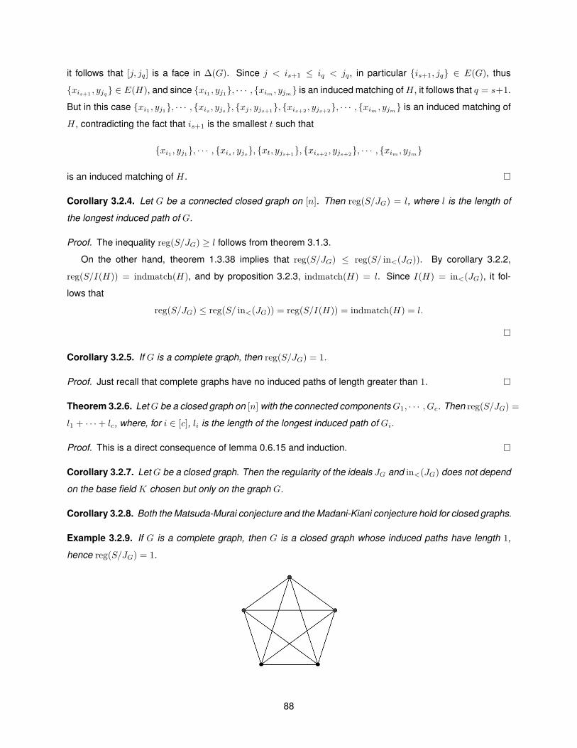
it follows that [j, jq] is a face in ∆(G). Since j < is+1 ≤ iq < jq, in particular {is+1, jq} ∈ E(G), thus

{xis+1 , yjq} ∈ E(H), and since {xi1 , yj1}, · · · , {xim , yjm} is an induced matching ofH, it follows that q = s+1.

But in this case {xi1 , yj1}, · · · , {xis , yjs}, {xj , yjs+1}, {xis+2 , yjs+2}, · · · , {xim , yjm

} is an induced matching of

H, contradicting the fact that is+1 is the smallest t such that

{xi1 , yj1}, · · · , {xis , yjs}, {xt, yjs+1}, {xis+2 , yjs+2}, · · · , {xim , yjm

}

is an induced matching of H.

Corollary 3.2.4. Let G be a connected closed graph on [n]. Then reg(S/JG) = l, where l is the length of

the longest induced path of G.

Proof. The inequality reg(S/JG) ≥ l follows from theorem 3.1.3.

On the other hand, theorem 1.3.38 implies that reg(S/JG) ≤ reg(S/ in<(JG)). By corollary 3.2.2,

reg(S/I(H)) = indmatch(H), and by proposition 3.2.3, indmatch(H) = l. Since I(H) = in<(JG), it fol-

lows that

reg(S/JG) ≤ reg(S/ in<(JG)) = reg(S/I(H)) = indmatch(H) = l.

Corollary 3.2.5. If G is a complete graph, then reg(S/JG) = 1.

Proof. Just recall that complete graphs have no induced paths of length greater than 1.

Theorem 3.2.6. LetG be a closed graph on [n] with the connected componentsG1, · · · , Gc. Then reg(S/JG) =

l1 + · · ·+ lc, where, for i ∈ [c], li is the length of the longest induced path of Gi.

Proof. This is a direct consequence of lemma 0.6.15 and induction.

Corollary 3.2.7. Let G be a closed graph. Then the regularity of the ideals JG and in<(JG) does not depend

on the base field K chosen but only on the graph G.

Corollary 3.2.8. Both the Matsuda-Murai conjecture and the Madani-Kiani conjecture hold for closed graphs.

Example 3.2.9. If G is a complete graph, then G is a closed graph whose induced paths have length 1,

hence reg(S/JG) = 1.

88

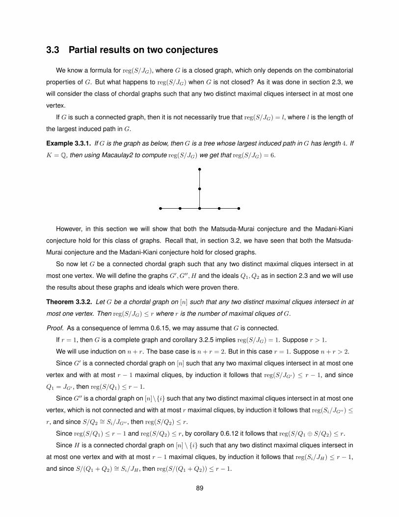
3.3 Partial results on two conjectures

We know a formula for reg(S/JG), where G is a closed graph, which only depends on the combinatorial

properties of G. But what happens to reg(S/JG) when G is not closed? As it was done in section 2.3, we

will consider the class of chordal graphs such that any two distinct maximal cliques intersect in at most one

vertex.

If G is such a connected graph, then it is not necessarily true that reg(S/JG) = l, where l is the length of

the largest induced path in G.

Example 3.3.1. If G is the graph as below, then G is a tree whose largest induced path in G has length 4. If

K = Q, then using Macaulay2 to compute reg(S/JG) we get that reg(S/JG) = 6.

However, in this section we will show that both the Matsuda-Murai conjecture and the Madani-Kiani

conjecture hold for this class of graphs. Recall that, in section 3.2, we have seen that both the Matsuda-

Murai conjecture and the Madani-Kiani conjecture hold for closed graphs.

So now let G be a connected chordal graph such that any two distinct maximal cliques intersect in at

most one vertex. We will define the graphs G′, G′′, H and the ideals Q1, Q2 as in section 2.3 and we will use

the results about these graphs and ideals which were proven there.


most one vertex. Then reg(S/JG) ≤ r where r is the number of maximal cliques of G.

Proof. As a consequence of lemma 0.6.15, we may assume that G is connected.

If r = 1, then G is a complete graph and corollary 3.2.5 implies reg(S/JG) = 1. Suppose r > 1.

We will use induction on n+ r. The base case is n+ r = 2. But in this case r = 1. Suppose n+ r > 2.

Since G′ is a connected chordal graph on [n] such that any two maximal cliques intersect in at most one

vertex and with at most r − 1 maximal cliques, by induction it follows that reg(S/JG′) ≤ r − 1, and since

Q1 = JG′ , then reg(S/Q1) ≤ r − 1.

Since G′′ is a chordal graph on [n]\{i} such that any two distinct maximal cliques intersect in at most one

vertex, which is not connected and with at most r maximal cliques, by induction it follows that reg(Si/JG′′) ≤

r, and since S/Q2 ∼= Si/JG′′ , then reg(S/Q2) ≤ r.

Since reg(S/Q1) ≤ r − 1 and reg(S/Q2) ≤ r, by corollary 0.6.12 it follows that reg(S/Q1 ⊕ S/Q2) ≤ r.

Since H is a connected chordal graph on [n] \ {i} such that any two distinct maximal cliques intersect in

at most one vertex and with at most r − 1 maximal cliques, by induction it follows that reg(Si/JH) ≤ r − 1,

and since S/(Q1 +Q2) ∼= Si/JH , then reg(S/(Q1 +Q2)) ≤ r − 1.

89

Recall the following exact sequence of S-modules:

0 −→ S

JG−→ S

Q1⊕ S

Q2−→ S

Q1 +Q2−→ 0.

By inequality (1) of proposition 0.6.11, reg(S/JG) ≤ max{reg(S/Q1 ⊕ S/Q2), reg(S/(Q1 +Q2)) + 1} ≤ r,

as desired.

Hence the Madani-Kiani conjecture holds for chordal graphs such that any two distinct maximal cliques


Proposition 3.3.3. Let G be a chordal graph on [n] without isolated vertices such that any two distinct

maximal cliques intersect in at most one vertex. Then G has at most n− 1 maximal cliques.

Proof. We may assume that G is connected and we will use induction on n. If n = 2, the result is obvious.

Suppose n > 2.

Let K be the largest clique on G. Given a vertex v in K, we define Gv as the induced subgraph of G

such that V (Gv) = {v} ∪ {u ∈ V (G) : there exists a path from u to v whose only vertex in K is v}. Since G

is connected, it follows that [n] =⋃v∈V (K) V (Gv).

The graphs Gv are pairwise disjoint. In fact, suppose that there exists a vertex u not in K and vertices

v, v′ in K such that u ∈ Gv ∩ Gv′ . Let u, · · · , v and u, · · · , v′ be paths in G whose only vertices in K are v

and v′, respectively. Then u, · · · , v, v′, · · · , u is a cycle in G whose only vertices in K are v and v′. Since G

is chordal, that cycle has a vertex w not in K such that {v, w}, {v′, w} ∈ E(G) and so the vertices v, v′, w

form a clique in G which is not contained in K but intersects it in two vertices, a contradiction.

Let v, v′ be distinct vertices inK. Let u ∈ V (Gv)\{v} and u′ ∈ V (Gv′)\{v′}. Let u, · · · , v and u′, · · · , v′ be

paths in G whose only vertices in K are v and v′, respectively. If {u, u′} ∈ E(G), then u, · · · , v, v′, · · · , u′, u

is a cycle in G whose only vertices in K are v and v′. Since G is chordal, that cycle has a vertex w not in K

such that {v, w}, {v′, w} ∈ E(G) and so the vertices v, v′, w form a clique in G which is not contained in K

but intersects it in two vertices, a contradiction. Hence {u, u′} 6∈ E(G).

In particular, every clique in G not contained in K must be a clique in some Gv, and since G is a

connected graph, such Gv must have vertices other than v. Let C = {v ∈ V (K) : V (Gv) 6= {v}}.

Let v ∈ C. Since Gv is an induced subgraph of G, it follows that Gv is also a chordal graph whose

maximal cliques intersect in at most one vertex and by induction Gv has at most |V (Gv)| − 1 maximal

cliques.

HenceG has at most∑v∈C(|V (Gv)|−1)+1 maximal cliques. Since |V (Gv)|−1 = 0 whenever v ∈ V (K)\

C, then∑v∈C(|V (Gv)|−1)+1 =

∑v∈V (K)(|V (Gv)|−1)+1 =

∑v∈V (K) |V (Gv)|−|V (K)|+1 = n−|V (K)|+1,

which is smaller than n− 1 since |V (K)| ≥ 2.

Corollary 3.3.4. Let G be a connected chordal graph on [n] such that any two distinct maximal cliques

intersect in at most one vertex. If G has n− 1 maximal cliques, then G is a tree.

90

Proof. As in the proof of proposition 3.3.3, G has at most n−|V (K)|+1 maximal cliques. But n−|V (K)|+1 ≤

n− 1, and so such inequality must be an equality, that is, |V (K)| = 2, and since K is the largest clique in G,

G has no cycles of length 3, and since G is chordal, G must be a tree.

Corollary 3.3.5. Let G be a connected chordal graph on [n] such that any two distinct maximal cliques

intersect in at most one vertex. If reg(S/JG) = n− 1, then G is a path.

Proof. We will use induction on n. If n = 2, the result is obvious. Suppose n > 2.

Since reg(S/JG) = n−1, by theorem 3.3.2 it follows that G has at least n−1 maximal cliques. Moreover,

by proposition 3.3.3 it follows that G has exactly n− 1 maximal cliques. Hence, by corollary 3.3.4, it follows

that G is a tree.

Since G′ is a graph with less maximal cliques that G, then G′ has at most n− 2 maximal cliques and so

theorem 3.3.2 implies reg(S/JG′) ≤ n− 2, and since Q1 = JG′ , then reg(S/Q1) ≤ n− 2.

Since G′′ is a chordal graph on [n] \ {i} such that any two distinct maximal cliques intersect in at most

one vertex, then by proposition 3.3.3 G′′ has at most n − 2 maximal cliques and so theorem 3.3.2 implies

reg(Si/JG′′) ≤ n− 2, and since S/Q2 ∼= Si/JG′′ , then reg(S/Q2) ≤ n− 2.

Since reg(S/Q1) ≤ n− 2 and reg(S/Q2) ≤ n− 2, by corollary 0.6.12 it follows that reg(S/Q1 ⊕ S/Q2) ≤

n− 2.

Consider again the following exact sequence of S-modules:

0 −→ S

JG−→ S

Q1⊕ S

Q2−→ S

Q1 +Q2−→ 0.

By inequality (1) of proposition 0.6.11, n− 1 = reg(S/JG) ≤ max{reg(S/Q1⊕S/Q2), reg(S/(Q1 +Q2)) +

1} ≤ max{n − 2, reg(S/(Q1 + Q2)) + 1}. From the inequality n − 1 ≤ max{n − 2, reg(S/(Q1 + Q2)) + 1} it

follows that reg(S/(Q1 +Q2)) + 1 ≥ n− 1, that is, reg(S/(Q1 +Q2)) ≥ n− 2.

Since S/(Q1 +Q2) ∼= Si/JH , where H is a connected chordal graph on [n]\{i} such that any two distinct

maximal cliques intersect in at most one vertex, then by theorem 3.1.3 it follows that reg(S/(Q1+Q2)) = n−2,

and by induction H must be a path. This implies that the clique on(Fr ∪

⋃qj=1 Ftj

)\ {i} has two vertices

and so it follows that q = 1. Let i, j, k be the three vertices in Fr ∪ Ft1 . Then the graph G can be obtained

from the path H by adding the vertex i and by replacing the edge {j, k} by the edges {i, j} and {i, k}. Hence

G is a path.

Hence the Matsuda-Murai conjecture holds for chordal graphs such that any two distinct maximal cliques


Example 3.3.6. LetG be a connected chordal graph on 4 vertices such that any two distinct maximal cliques

intersect in at most one vertex. If G is a complete graph, then reg(S/JG) = 1. If G is a path of length 3,

then reg(S/JG) = 3. In the remaining cases, the length of the largest induced path of G is 2, hence theorem

3.1.3 implies that reg(S/JG) ≥ 2. On the other hand, corollary 3.3.5 implies that reg(S/JG) < 3 and so

reg(S/JG) = 2.

91

This year, on April 6th, Madani and Kiani presented a full proof for the Matsuda-Murai conjecture in [18].

92

Bibliography

[1] Hideyuki Matsumura, Commutative ring theory, Cambridge University Press, 1987.

[2] M. F. Atiyah and I. G. MacDonald, Introduction to Commutative Algebra, Addison-Wesley Publishing

Company, 1969.

[3] David Eisenbud, Commutative Algebra with a view toward Algebraic Geometry, Springer-Verlag, 1995.

[4] Winfried Bruns and Jurgen Herzog, Cohen-Macaulay rings, Cambridge University Press, 1998.

[5] Jurgen Herzog and Takayuki Hibi, Monomial ideals, Springer-Verlag, 2011.

[6] Jurgen Herzog and Viviana Ene, Grobner bases in Commutative Algebra, Graduate Studies in Mathe-

matics, 2012.

[7] Rafael H. Villarreal, Monomial algebras, second edition, CRC Press, 2014.

[8] Winfried Bruns and Udo Vetter, Determinantal rings, Springer-Verlag, 1988.

[9] Huy Tai Ha, Ngo Viet Trung and Tran Nam Trung, Depth and regularity of powers of sums of ideals,

preprint (2015) (arXiv:1501.06038v1).

[10] Jurgen Herzog and Takayuki Hibi, Distributive lattices, bipartite graphs and Alexander duality, Journal

of Algebraic Combinatorics 22 (2005), 289-302 (arXiv:0307235v1).

[11] Jurgen Herzog, Takayuki Hibi, Freyja Hreinsdottir, Thomas Kahle and Johannes Rauh, Binomial edge

ideals and conditional independence statements, Advances in Applied Mathematics 45 (2010), 317-333

(arXiv:0909.4717v2).

[12] Viviana Ene, Jurgen Herzog and Takayuki Hibi, Cohen-Macaulay binomial edge ideals, Nagoya Math-

ematical Journal 204 (2011), 57-68 (arXiv:1004.0143v2).

[13] G. A. Dirac, On rigid circuit graphs, Abh. Math. Sem. Univ. Hamburg 38 (1961), 7176.

[14] Russ Woodroofe, Matchings, coverings and Castelnuovo-Munford regularity, Journal of Commutative

Algebra, volume 6, number 2 (2014), 287-304 (arXiv:1009.2756v4).

93

http://arxiv.org/abs/1501.06038v1

http://arxiv.org/abs/math/0307235v1




[15] Sara Saeedi Madani and Dariush Kiani, On the binomial edge ideal of a pair of graphs, The Electronic

Journal of Combinatorics, volume 20, issue 1 (2013), page 48.

[16] Kazunori Matsuda and Satoshi Murai, Regularity bounds for binomial edge ideals, Journal of Commu-

tative Algebra, volume 5, number 1 (2013), 141-149 (arXiv:1208.2415v1).

[17] Viviana Ene and Andrei Zarojanu, On the regularity of binomial edge ideals, Mathematische

Nachrichten, volume 288, issue 1 (2015), 1924 (arXiv:1307.2141v1).

[18] Sara Saeedi Madani and Dariush Kiani, The Castelnuovo-Munford regularity of binomial edge ideals,

preprint (2015) (ArXiv:1504.01403v1).

94




Documents

Algebraic and combinatorial properties of binomial edge ideals · Resumo Com esta dissertac¸ao pretende-se fazer uma introduc¸˜ ao˜ a` Algebra Comutativa Combinat´ oria e mais´