Algebra &NumberTheory

msp

Volume 10

2016No. 2

Squarefree polynomials and Möbius valuesin short intervals

and arithmetic progressionsJonathan P. Keating and Zeev Rudnick

mspALGEBRA AND NUMBER THEORY 10:2 (2016)

dx.doi.org/10.2140/ant.2016.10.375

Squarefree polynomials and Möbius valuesin short intervals

and arithmetic progressionsJonathan P. Keating and Zeev Rudnick

We calculate the mean and variance of sums of the Möbius function µ and theindicator function of the squarefrees µ2, in both short intervals and arithmeticprogressions, in the context of the ring Fq [t] of polynomials over a finite field Fq

of q elements, in the limit q→∞. We do this by relating the sums in questionto certain matrix integrals over the unitary group, using recent equidistributionresults due to N. Katz, and then by evaluating these integrals. In many cases ourresults mirror what is either known or conjectured for the corresponding problemsinvolving sums over the integers, which have a long history. In some cases thereare subtle and surprising differences. The ranges over which our results hold issignificantly greater than those established for the corresponding problems in thenumber field setting.

1. Introduction 3762. Asymptotics for squarefrees: Proof of Theorem 1.3 3833. Asymptotics for Möbius sums 3844. Variance in arithmetic progressions: General theory 3865. Variance in short intervals: General theory 3886. Characters, L-functions and equidistribution 3957. Variance of the Möbius function in short intervals 3978. Variance of the Möbius function in arithmetic progressions 3999. The variance of squarefrees in short intervals 40110. Squarefrees in arithmetic progressions 404Appendix: Hall’s theorem for Fq [t]: The large degree limit 407Acknowledgements 418References 418

MSC2010: primary 11T55; secondary 11M38, 11M50.Keywords: squarefrees, Möbius function, short intervals, Good–Churchhouse conjecture, Chowla’s

conjecture, function fields, equidistribution.

375

376 Jonathan P. Keating and Zeev Rudnick

1. Introduction

The goal of this paper is to investigate the fluctuation of sums of two importantarithmetic functions, the Möbius function µ and the indicator function of thesquarefrees µ2, in the context of the ring Fq [t] of polynomials over a finite field Fq

of q elements, in the limit q→∞. The problems we address, which concern sumsover short intervals and arithmetic progressions, mirror long-standing questionsover the integers, where they are largely unknown. In our setting we succeed ingiving definitive answers.

Our approach differs from those traditionally employed in the number field setting:we use recent equidistribution results due to N. Katz, valid in the large-q limit, toexpress the mean and variance of the fluctuations in terms of matrix integrals overthe unitary group. Evaluating these integrals leads to explicit formulae and preciseranges of validity. For many of the problems we study, the formulae we obtain matchthe corresponding number-field results and conjectures exactly, providing furthersupport in the latter case. However, the ranges of validity that we can establish aresignificantly greater than those known or previously conjectured for the integers,and we see our results as supporting extensions to much wider ranges of validity inthe integer setting. Interestingly, in some other problems we uncover subtle andsurprising differences between the function-field and number-field asymptotics,which we examine in detail.

We now set out our main results in a way that enables comparison with thecorresponding problems for the integers.

The Möbius function. It is a standard heuristic to assume that the Möbius func-tion behaves like a random ±1 supported on the squarefree integers, which havedensity 1/ζ(2) (see, e.g., [Chatterjee and Soundararajan 2012]). Proving any-thing in this direction is not easy. Even demonstrating cancellation in the sumM(x) :=

∑1≤n≤x µ(n), that is that M(x)= o(x), is equivalent to the prime num-

ber theorem. The Riemann hypothesis is equivalent to square root cancellation:M(x)= O(x1/2+o(1)).

For sums of µ(n) in blocks of length H ,

M(x; H) :=∑

|n−x |<H/2

µ(n) (1-1)

it has been shown that there is cancellation for H � x7/12+o(1) [Motohashi 1976;Ramachandra 1976], and assuming the Riemann hypothesis one can take H �x1/2+o(1). If one wants cancellation only for “almost all” values of x , then more isknown. In particular, very recently Matomäki and Radziwiłł [2015] have shown

Squarefree polynomials and Möbius values 377

(unconditionally) that

1X

∫ 2X

XM(x; H)2dx = o(H 2)

whenever H = H(X)→∞ as X →∞, and in particular M(x; H) = o(H) foralmost all x ∈ [X, 2X ].

We expect the normalized sums M(x; H)/√

H to have mean zero (this followsfrom the Riemann hypothesis) and variance 6/π2

= 1/ζ(2):

1X

∫ 2X

X|M(x; H)|2 ∼

Hζ(2)

. (1-2)

Moreover, M(x; H)/√

H/ζ(2) is believed to have a normal distribution asymptoti-cally. These conjectures were formulated and investigated numerically by Goodand Churchhouse [1968], and further studied by Ng [2008], who carried out ananalysis using the generalized Riemann hypothesis and a strong version of Chowla’sconjecture on correlations of Möbius, showing that (1-2) is valid for H� X1/4−o(1)

and that a Gaussian distribution holds (assuming these conjectures) for H � X ε .It is important that the length H of the interval be significantly smaller than itslocation, that is H < X1−ε , since otherwise one expects non-Gaussian statistics,see [Ng 2004].

Concerning arithmetic progressions, Hooley [1975] studied the following aver-aged form of the total variance (averaged over moduli)

V (X, Q) :=∑

Q′≤Q

∑A mod Q′

( ∑n≤X

n=A mod Q′

µ(n))2

(1-3)

and showed that for Q ≤ X ,

V (X, Q)=6Q Xπ2 + O(X2(log X)−C) (1-4)

for all C > 0, which yields an asymptotic result for X/(log X)C � Q < X .For polynomials over a finite field Fq , the Möbius function is defined as for the

integers, namely by µ( f )= (−1)k if f is a scalar multiple of a product of k distinctmonic irreducibles, and µ( f )= 0 if f is not squarefree. The analogue of the fullsum M(x) is the sum over all monic polynomials Mn of given degree n, for whichwe have ∑

f ∈Mn

µ( f )=

1, n = 0,−q, n = 1,

0, n ≥ 2,(1-5)

378 Jonathan P. Keating and Zeev Rudnick

so that in particular the issue of size is trivial1. However that is no longer the casewhen considering sums over “short intervals”, that is over sets of the form

I(A; h)= { f : ‖ f − A‖ ≤ qh} (1-6)

where A ∈Mn has degree n, 0≤ h ≤ n− 2 and2 the norm is

‖ f ‖ := #Fq [t]/( f )= qdeg f . (1-7)

To facilitate comparison between statements for number field results and for functionfields, we use a rough dictionary:

X ↔ qn, log X ↔ n,

H ↔ qh+1, log H ↔ h+ 1.(1-8)

Set

Nµ(A; h) :=∑

f ∈I(A;h)

µ( f ). (1-9)

The number of summands here is qh+1=: H and we want to display cancellation

in this sum and study its statistics as we vary the “center” A of the interval.We can demonstrate cancellation in the short interval sums Nµ(A; h) in the large

finite field limit q→∞, n fixed (we assume q is odd throughout the paper).

Theorem 1.1. If 2≤ h ≤ n− 2 then for all A of degree n,

|Nµ(A; h)| �nH√

q

the implied constant uniform in A, depending only on n = deg A.

For h = 0, 1 this is no longer valid; that is, there are A’s for which there is nocancellation. See Section 3.

We next investigate the statistics of Nµ(A; h) as A varies over all monic poly-nomials of given degree n, and q→∞. It is easy to see that for n ≥ 2, the meanvalue of Nµ(A; h) is 0. Our main result concerns the variance.

Theorem 1.2. If 0≤ h ≤ n− 5 then as q→∞, q odd,

VarNµ( • ; h)=1

qn

∑A∈Mn

|Nµ(A; h)|2 ∼ H∫

U (n−h−2)

|tr Symn U |2 dU = H

1This ceases to be the case when dealing with function fields of higher genus, see, e.g., [Cha 2011;Humphries 2014].

2For h = n− 1, I(A; n− 1)=Mn is the set of all monic polynomials of degree n.

Squarefree polynomials and Möbius values 379

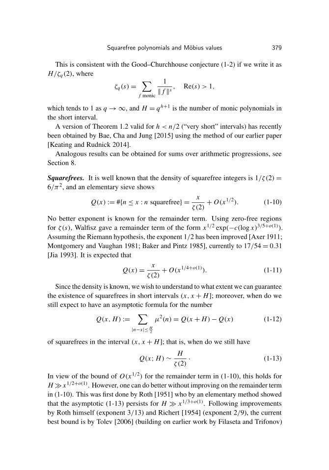
This is consistent with the Good–Churchhouse conjecture (1-2) if we write it asH/ζq(2), where

ζq(s)=∑

f monic

1‖ f ‖s

, Re(s) > 1,

which tends to 1 as q→∞, and H = qh+1 is the number of monic polynomials inthe short interval.

A version of Theorem 1.2 valid for h < n/2 (“very short” intervals) has recentlybeen obtained by Bae, Cha and Jung [2015] using the method of our earlier paper[Keating and Rudnick 2014].

Analogous results can be obtained for sums over arithmetic progressions, seeSection 8.

Squarefrees. It is well known that the density of squarefree integers is 1/ζ(2)=6/π2, and an elementary sieve shows

Q(x) := #{n ≤ x : n squarefree} =xζ(2)+ O(x1/2). (1-10)

No better exponent is known for the remainder term. Using zero-free regionsfor ζ(s), Walfisz gave a remainder term of the form x1/2 exp(−c(log x)3/5+o(1)).Assuming the Riemann hypothesis, the exponent 1/2 has been improved [Axer 1911;Montgomery and Vaughan 1981; Baker and Pintz 1985], currently to 17/54= 0.31[Jia 1993]. It is expected that

Q(x)=xζ(2)+ O(x1/4+o(1)). (1-11)

Since the density is known, we wish to understand to what extent we can guaranteethe existence of squarefrees in short intervals (x, x + H ]; moreover, when do westill expect to have an asymptotic formula for the number

Q(x, H) :=∑

|n−x |≤ H2

µ2(n)= Q(x + H)− Q(x) (1-12)

of squarefrees in the interval (x, x + H ]; that is, when do we still have

Q(x; H)∼Hζ(2)

. (1-13)

In view of the bound of O(x1/2) for the remainder term in (1-10), this holds forH� x1/2+o(1). However, one can do better without improving on the remainder termin (1-10). This was first done by Roth [1951] who by an elementary method showedthat the asymptotic (1-13) persists for H � x1/3+o(1). Following improvementsby Roth himself (exponent 3/13) and Richert [1954] (exponent 2/9), the currentbest bound is by Tolev [2006] (building on earlier work by Filaseta and Trifonov)

380 Jonathan P. Keating and Zeev Rudnick

who gave H � x1/5+o(1). It is believed that (1-13) should hold for H � xε for anyε > 0, though there are intervals of size H � log x/ log log x which contain nosquarefrees, see [Erdös 1951].

As for almost-everywhere results, one way to proceed goes through a studyof the variance of Q(x, H). In this direction, Hall [1982] showed that providedH = O(x2/9−o(1)), the variance of Q(x, H) admits an asymptotic formula:

1x

∑n≤x

∣∣∣∣Q(n, H)− Hζ(2)

∣∣∣∣2 ∼ A√

H , (1-14)

with

A =ζ(3/2)π

∏p

p3− 3p+ 2

p3. (1-15)

Based on our results below, we expect this asymptotic formula to hold for H aslarge as x1−ε .

Concerning arithmetic progressions, denote by

S(x; Q, A) =∑n≤x

n=A mod Q

µ(n)2

the number of squarefree integers in the arithmetic progression n = A mod Q.Prachar [1958] showed that for Q < x2/3−ε , and A coprime to Q,

S(x; Q, A)∼1ζ(2)

∏p|Q

(1−

1p2

)−1 xQ=

1ζ(2)

∏p|Q

(1+

1p

)−1 xφ(Q)

(1-16)

In order to understand the size of the remainder term, one studies the variance

Var(S)=1

φ(Q)

∑gcd(A,Q)=1

∣∣∣∣S(x; Q, A)−1ζ(2)

∏p|Q

(1−

1p2

)−1 xQ

∣∣∣∣2 (1-17)

as well as a version where the sum is over all residue classes A mod Q, not nec-essarily coprime to Q, and the further averaged form over all moduli Q′ ≤ Q à laBarban, Davenport and Halberstam, see [Warlimont 1980].

Without averaging over moduli, Blomer [2008, Theorem 1.3] gave an upperbound for the variance, which was very recently improved by Nunes [2015], whogave an asymptotic expression for the variance in the range X

3141+ε < Q < X1−ε :

Var(S)∼ A∏p|Q

(1−

1p

)−1(1+

2p

)−1 X1/2

Q1/2 , (1-18)

Squarefree polynomials and Möbius values 381

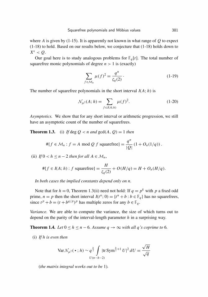
where A is given by (1-15). It is apparently not known in what range of Q to expect(1-18) to hold. Based on our results below, we conjecture that (1-18) holds down toX ε < Q.

Our goal here is to study analogous problems for Fq [t]. The total number ofsquarefree monic polynomials of degree n > 1 is (exactly)∑

f ∈Mn

µ( f )2 =qn

ζq(2). (1-19)

The number of squarefree polynomials in the short interval I(A; h) is

Nµ2(A; h)=∑

f ∈I(A;h)

µ( f )2. (1-20)

Asymptotics. We show that for any short interval or arithmetic progression, we stillhave an asymptotic count of the number of squarefrees.

Theorem 1.3. (i) If deg Q < n and gcd(A, Q)= 1 then

#{ f ∈Mn : f = A mod Q f squarefree} =qn

|Q|(1+ On(1/q)) .

(ii) If 0< h ≤ n− 2 then for all A ∈Mn ,

#{ f ∈ I(A; h) : f squarefree} =Hζq(2)

+ O(H/q)= H + On(H/q).

In both cases the implied constants depend only on n.

Note that for h = 0, Theorem 1.3(ii) need not hold: If q = pk with p a fixed oddprime, n = p then the short interval I(tn

; 0)= {tn+ b : b ∈ Fq} has no squarefrees,

since t p+ b = (t + bq/p)p has multiple zeros for any b ∈ Fq .

Variance. We are able to compute the variance, the size of which turns out todepend on the parity of the interval-length parameter h in a surprising way.

Theorem 1.4. Let 0≤ h ≤ n− 6. Assume q→∞ with all q’s coprime to 6.

(i) If h is even then

VarNµ2( • ; h)∼ qh2

∫U (n−h−2)

|tr Symh2+1 U |2 dU =

√H√

q

(the matrix integral works out to be 1).

382 Jonathan P. Keating and Zeev Rudnick

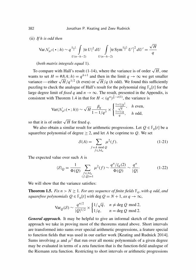
(ii) If h is odd then

VarNµ2( • ; h)∼ qh−1

2

∫U (n−h−2)

|tr U |2 dU∫

U (n−h−2)

∣∣tr Symh+3

2 U ′∣∣2 dU ′ =

√H

q

(both matrix integrals equal 1).

To compare with Hall’s result (1-14), where the variance is of order√

H , onewants to set H = #I(A; h) = qh+1 and then in the limit q →∞ we get smallervariance — either

√H/q1/2 (h even) or

√H/q (h odd). We found this sufficiently

puzzling to check the analogue of Hall’s result for the polynomial ring Fq [t] for thelarge degree limit of fixed q and n→∞. The result, presented in the Appendix, isconsistent with Theorem 1.4 in that for H < (qn)

29−o(1), the variance is

Var(Nµ2( • ; h))∼√

Hβq

1− 1/q3 ×

{ 1+1/q2√

q , h even,1+1/q

q , h odd,

so that it is of order√

H for fixed q .We also obtain a similar result for arithmetic progressions. Let Q ∈ Fq [t] be a

squarefree polynomial of degree ≥ 2, and let A be coprime to Q. We set

S(A)=∑

f=A mod Qf ∈Mn

µ2( f ). (1-21)

The expected value over such A is

〈S〉Q =1

8(Q)

∑f ∈Mn( f,Q)=1

µ2( f )∼qn/ζq(2)8(Q)

∼qn

|Q|. (1-22)

We will show that the variance satisfies:

Theorem 1.5. Fix n > N ≥ 1. For any sequence of finite fields Fq , with q odd, andsquarefree polynomials Q ∈ Fq [t] with deg Q = N + 1, as q→∞,

VarQ(S)∼qn/2

|Q|1/2×

{1/√

q, n 6= deg Q mod 2,1/q, n = deg Q mod 2.

General approach. It may be helpful to give an informal sketch of the generalapproach we take in proving most of the theorems stated above. Short intervalsare transformed into sums over special arithmetic progressions, a feature specialto function fields that was used in our earlier work [Keating and Rudnick 2014].Sums involving µ and µ2 that run over all monic polynomials of a given degreemay be evaluated in terms of a zeta function that is the function-field analogue ofthe Riemann zeta function. Restricting to short intervals or arithmetic progressions

Squarefree polynomials and Möbius values 383

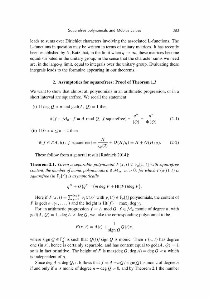
leads to sums over Dirichlet characters involving the associated L-functions. TheL-functions in question may be written in terms of unitary matrices. It has recentlybeen established by N. Katz that, in the limit when q→∞, these matrices becomeequidistributed in the unitary group, in the sense that the character sums we needare, in the large-q limit, equal to integrals over the unitary group. Evaluating theseintegrals leads to the formulae appearing in our theorems.

2. Asymptotics for squarefrees: Proof of Theorem 1.3

We want to show that almost all polynomials in an arithmetic progression, or in ashort interval are squarefree. We recall the statement:

(i) If deg Q < n and gcd(A, Q)= 1 then

#{ f ∈Mn : f = A mod Q, f squarefree} ∼qn

|Q|∼

qn

8(Q). (2-1)

(ii) If 0< h ≤ n− 2 then

#{ f ∈ I(A; h) : f squarefree} =Hζq(2)

+ O(H/q)= H + O(H/q). (2-2)

These follow from a general result [Rudnick 2014]:

Theorem 2.1. Given a separable polynomial F(x, t) ∈ Fq [x, t] with squarefreecontent, the number of monic polynomials a ∈Mm , m > 0, for which F(a(t), t) issquarefree (in Fq [t]) is asymptotically

qm+ O

(qm−1(m deg F +Ht(F)

)deg F

).

Here if F(x, t)=∑deg F

j=0 γ j (t)x j with γ j (t) ∈ Fq [t] polynomials, the content ofF is gcd(γ0, γ1, . . . , ) and the height is Ht( f )=max j deg γ j .

For an arithmetic progression f = A mod Q, f ∈Mn monic of degree n, withgcd(A, Q)= 1, deg A < deg Q, we take the corresponding polynomial to be

F(x, t)= A(t)+1

sign QQ(t)x,

where sign Q ∈ F×q is such that Q(t)/ sign Q is monic. Then F(x, t) has degreeone (in x), hence is certainly separable, and has content equal to gcd(A, Q)= 1,so is in fact primitive. The height of F is max(deg Q, deg A)= deg Q < n whichis independent of q.

Since deg A< deg Q, it follows that f = A+aQ/ sign(Q) is monic of degree nif and only if a is monic of degree n− deg Q > 0, and by Theorem 2.1 the number

384 Jonathan P. Keating and Zeev Rudnick

of such a for which F(a(t), t) is squarefree is

qn−deg Q+ O(qn−deg Q−1)=

qn

|Q|(1+ O(1/q)).

This proves (2-1).To deal with the short interval case, let 0< h ≤ n− 2, and A ∈Mn be monic of

degree n. We want to show that the number of polynomials f in the short intervalI(A; h) which are squarefree is H + O(H/q) (recall H = #I(A; h)= qh+1).

We writeI(A; h)= (A+P≤h−1)∪

∐c∈F×q

(A+ cMh).

The number of squarefrees in A+P≤h−1 is at most #P≤h−1 = qh . The squarefreesin A+ cMh are the squarefree values at monic polynomials of degree h of thepolynomial F(x, t)= A(t)+ cx , which has degree 1, content gcd(A(t), c)= 1 andheight Ht(F)= deg A = n. By Theorem 2.1 the number of substitutions a ∈Mh

for which F(a) is squarefree is

qh+ O(nqh−1).

Hence number of squarefrees in I(A; h) is∑c∈F×q

(qh+ O(nqh−1))+ O(qh)= H + O(H/q),

proving (2-2).

3. Asymptotics for Möbius sums

In this section we deal with cancellation in the individual sums

Nµ(A; h)=∑

f ∈I(A;h)

µ( f ).

Note that the interval I(A; h) consists of all polynomials of the form A+ g, whereg ∈ P≤h is the set of all polynomials of degree at most h.

Small h. We first point out that for h = 0, 1 there need not be any cancellation. Werecall Pellet’s formula for the discriminant (in odd characteristic)

µ( f )= (−1)deg f χ2(disc f ) (3-1)

where χ2 : F×q →{±1} is the quadratic character of Fq and disc f is the discriminant

of f . From Pellet’s formula we find (as in [Carmon and Rudnick 2014])

Nµ(A; h)= (−1)deg A∑

g∈P≤h

χ2(disc(A+ g)). (3-2)

Squarefree polynomials and Möbius values 385

Let A(t)= tn . The discriminant of the trinomial tn+ at + b is (see, e.g., [Swan

1962])

disc(tn+ at + b)= (−1)n(n−1)/2(nnbn−1

+ (1− n)n−1an). (3-3)

Hence for the interval I(tn; 1)= {tn

+ at + b : a, b ∈ Fq} we obtain

Nµ(tn; 1)= (−1)nχ2(−1)n(n−1)/2

∑a,b∈Fq

χ2(nnbn−1

+ (1− n)n−1an). (3-4)

Therefore if q = pk with p an odd prime and 2p | n then

Nµ(tn; 1)= χ2(−1)n/2q

∑a∈Fq

χ2(a)n =±q(q − 1), (3-5)

so that |Nµ(tn; 1)| � q2

= H . A similar construction also works for h = 0.

Large h. We also note that for h = n− 2, and p - n (p is the characteristic of Fq )the Möbius sums all coincide. This is because µ( f (t))= µ( f (t + c)) if deg f ≥ 1.Therefore

Nµ(A(t); h)=Nµ(A(t + c); h).

Now if A(t) = tn+ an−1tn−1

+ · · · is the center of the interval, then choosingc =−an−1/n gives

A(t + c)= tn+ an−2tn−2

+ · · ·

which contains no term of the form tn−1. Therefore if h = n− 2 then

Nµ(tn+ an−1tn−1

; n− 2)=Nµ(tn; n− 2)

has just one possible value.Thus we may assume that h ≤ n− 3.We note that the same is true for the squarefree case.

Proof of Theorem 1.1. We show that for h ≥ 2, for any (monic) A(t) of degree n,∑a∈P≤h

µ(A+ a)�H√

q. (3-6)

Writing a(t) = ah th+ · · · + a1t + b, it suffices to show that there is a constant

C = C(n, h) (independent of A and Ea = (a1, . . . , ah)) such that for “most” choicesof Ea, (i.e., for all but O(qh−1)) we have∣∣∣∣∑

b∈Fq

µ(A(t)+ ah th+ · · ·+ a1t + b)

∣∣∣∣≤ C√

q. (3-7)

386 Jonathan P. Keating and Zeev Rudnick

Using Pellet’s formula, we need to show that for most Ea,∣∣∣∣∑b∈Fq

χ2(disc(A(t)+ ah th

+ · · ·+ a1t + b))∣∣∣∣≤ C

√q (3-8)

Now Da(b) := disc(A(t)+ ah th+ · · · + a1t + b) is a polynomial in b, of degree

≤ n− 1, and if we show that for most Ea it is nonconstant and squarefree then byWeil’s theorem we will get that (3-8) holds for such Ea’s, with C = n − 2. Theargument in [Carmon and Rudnick 2014, Section 4] works verbatim here to provethat. �

An alternative argument is to use the work of Bank, Bary-Soroker and Rosenzweig[2015] who prove equidistribution of cycle types of polynomials in any shortinterval I(A; h) for 2≤ h ≤ n− 2 and q odd (this also uses [Carmon and Rudnick2014]). Now for f ∈Mn squarefree, µ( f ) = (−1)n sign(σ f ) where σ f ⊂ Sn

is the conjugacy class of permutations induced by the Frobenius acting on theroots of f , and sign is the sign character. For any f ∈ Mn , not necessarilysquarefree, we denote by λ( f ) = (λ1, . . . , λn) the cycle structure of f , whichfor squarefree f coincides with the cycle structure of the permutation σ f . Thensign(σ f )= sign(λ( f )) :=

∏nj=1(−1)( j−1)λ j . Thus∑

f ∈I(A;h)

µ( f )= (−1)n∑

f ∈I(A;h)squarefree

sign(σ f ). (3-9)

By Theorem 1.3, all but On(H/q) of the polynomials in the short interval I(A; h)are squarefree, hence∑

f ∈I(A;h)squarefree

sign(σ f )=∑

f ∈I(A;h)

sign(σ f )+ O(

Hq

)

= H(

1n!

∑σ∈Sn

sign(σ )+ O(

1√

q

))= O

(H√

q

), (3-10)

by equidistribution of cycle types in short intervals [Bank et al. 2015], and recallingthat

∑σ∈Sn

sign(σ )= 0 for n > 1.

4. Variance in arithmetic progressions: General theory

Let α : Fq [t] → C be a function on polynomials, which is “even” in the sense that

α(c f )= α( f )

for the units c ∈ F×q . We assume that

maxdeg f≤n

|α( f )| ≤ An (4-1)

Squarefree polynomials and Möbius values 387

with An independent of q . We will require some further constraints on α later on.We denote by 〈α〉n the mean value of α over all monic polynomials of degree n:

〈α〉n :=1

qn

∑f ∈Mn

α( f ). (4-2)

Let Q ∈ Fq [t] be squarefree, of positive degree. For an arithmetic functionα : Fq [t] → C, we define its mean value over coprime residue classes by

〈α〉Q :=1

8(Q)

∑A mod Q

gcd(A,Q)=1

α(A). (4-3)

The sum of α over all monic polynomials of degree n lying in the arithmeticprogressions f = A mod Q is

Sα,n,Q(A) :=∑

f ∈Mnf=A mod Q

α( f ). (4-4)

We wish to study the fluctuations in S(A) as we vary A over residue classes coprimeto Q. The mean value of S is

〈Sα〉Q =1

8(Q)

∑f ∈Mn( f,Q)=1

α( f ), (4-5)

where 8(Q) is the number of invertible residues modulo Q.Our goal is to compute the variance

VarQ(Sα)=1

8(Q)

∑A mod Q(A,Q)=1

|Sα(A)−〈Sα〉|2. (4-6)

A formula for the variance. Expanding in Dirichlet characters modulo Q gives

S(A)=1

8(Q)

∑χ mod Q

χ(A)M(n;αχ), (4-7)

whereM(n;αχ) :=

∑f ∈Mn

χ( f )α( f ). (4-8)

The mean value is the contribution of the trivial character χ0:

〈S〉Q =1

8(Q)

∑f ∈Mn

gcd( f,Q)=1

α( f ), (4-9)

388 Jonathan P. Keating and Zeev Rudnick

so thatS(A)−〈S〉Q =

18(Q)

∑χ 6=χ0 mod Q

χ(A)M(n;αχ). (4-10)

Inserting (4-7) and using the orthogonality relations for Dirichlet characters asin [Keating and Rudnick 2014], we see that the variance is

VarQ(S)= 〈|S −〈S〉Q |2〉Q =

18(Q)2

∑χ 6=χ0

|M(n;αχ)|2. (4-11)

Small n. If n<deg Q, then there is at most one f with deg f =n and f = A mod Q,and in this case

VarQ(S)∼qn

8(Q)〈α2〉n, n < deg Q. (4-12)

Indeed, if n < deg Q, then

|〈S〉Q | =∣∣∣∣ 18(Q)

∑f ∈Mn

gcd( f,Q)=1

α( f )∣∣∣∣≤ 1

8(Q)

∑f ∈Mn

|α( f )| ≤Anqn

8(Q)�n

1q

. (4-13)

HenceVarQ(S)=

18(Q)

∑A mod Q

gcd(A,Q)=1

|S(A)|2(1+ O(q−1))

=1

8(Q)

∑f ∈Mn

gcd( f,Q)=1

|α( f )|2(1+ O(q−1))

=qn

8(Q)〈|α|2〉n(1+ O(q−1))

as claimed.

5. Variance in short intervals: General theory

Given an arithmetic function α : Fq [t] → C, define its sum on short intervals as

Nα(A; h)=∑

f ∈I(A;h)

α( f ). (5-1)

The mean value of Nα is (see Lemma 5.2)

〈Nα( • , h)〉 = qh+1〈α〉n = H〈α〉n. (5-2)

Our goal will be to compute the variance of Nα,

VarNα =1

qn

∑A∈Mn

|Nα(A)−〈Nα〉|2, (5-3)

Squarefree polynomials and Möbius values 389

and more generally, given two such functions α, β, to compute the covariance

cov(Nα,Nβ)=⟨(Nα −〈Nα〉)(Nβ −〈Nβ〉)

⟩. (5-4)

Background on short intervals (see [Keating and Rudnick 2014]). Let

Pn = { f ∈ Fq [t] : deg f = n} (5-5)

be the set of polynomials of degree n,

P≤n = {0} ∪⋃

0≤m≤n

Pm (5-6)

the space of polynomials of degree at most n (including 0), and Mn ⊂Pn the subsetof monic polynomials.

By definition of short intervals,

I(A; h)= A+P≤h, (5-7)

and hence#I(A; h)= qh+1

=: H. (5-8)

For h = n−1, I(A; n−1)=Mn is the set of all monic polynomials of degree n.For h ≤ n−2, if ‖ f − A‖ ≤ qh then deg f = deg A and A is monic if and only if fis monic. Hence for A monic, I(A; h) consists of only monic polynomials and allmonic f ’s of degree n are contained in one of the intervals I(A; h) with A monicof degree n. Moreover,

I(A1; h)∩ I(A2; h) 6=∅↔ deg(A1− A2)≤ h↔ I(A1; h)= I(A2; h), (5-9)

and we get a partition of Pn into disjoint “intervals” parameterized by B ∈Pn−(h+1):

Pn =∐

B∈Pn−(h+1)

I(th+1 B; h), (5-10)

and likewise for monics (recall h ≤ n− 2):

Mn =∐

B∈Mn−(h+1)

I(th+1 B; h). (5-11)

An involution. Let n ≥ 0. We define a map θn : P≤n→ P≤n by

θn( f )(t)= tn f (t−1),

which takes f (t)= f0+ f1t +· · ·+ fntn , n = deg f to the “reversed” polynomial

θn( f )(t)= f0tn+ f1tn−1

+ · · ·+ fn. (5-12)

390 Jonathan P. Keating and Zeev Rudnick

For 0 6= f ∈ Fq [t] we define

f ∗(t) := tdeg f f (t−1) (5-13)

so that θn( f )= f ∗ if f (0) 6= 0. Note that if f (0)= 0 then this is false, for example(tk)∗ = 1 but θn(tk)= tn−k if k ≤ n.

We have deg θn( f ) ≤ n with equality if and only if f (0) 6= 0. Moreover forf 6= 0, f ∗(0) 6= 0 and f (0) 6= 0 if and only if deg f ∗ = deg f . When restricted topolynomials which do not vanish at 0 (equivalently, which are coprime to t), theoperator ∗ is an involution:

f ∗∗ = f, f (0) 6= 0. (5-14)

We also have multiplicativity:

( f g)∗ = f ∗g∗. (5-15)

The map θm gives a bijection

θm :Mm→ {C ∈ P≤m : C(0)= 1}

B 7→ θm(B)(5-16)

with polynomials of degree ≤ m with constant term 1. Thus as B ranges over Mm ,θm(B) ranges over all invertible residue classes C mod tm+1 such that C(0)= 1.

Short intervals as arithmetic progressions modulo tn−h. Suppose h ≤ n− 2. De-fine the arithmetic progression

P≤n(tn−h;C)= {g ∈ P≤n : g ≡ C mod tn−h

} = C + tn−hP≤h . (5-17)

Note that the progression contains qh+1 elements.

Lemma 5.1. Let h ≤ n−2 and B ∈Mn−h−1. Then the map θn takes the “interval”I(th+1 B; h) bijectively onto the arithmetic progression P≤n(tn−h

; θn−h−1(B)), withf ∈ I(th+1 B; h) such that f (0) 6= 0 mapping onto those g ∈ P≤n(tn−h

; θn−h−1(B))of degree exactly n.

Proof. We first check that θn maps the interval I(th+1 B; h) to the arithmeticprogression P≤n(tn−h

; θn−h−1(B)). Indeed if B = b0+ · · · + bn−h−1tn−h−1, withbn−h−1 = 1, and f = f0+ · · ·+ fntn

∈ I(th+1 B; h) then

f = f0+ · · ·+ fh th+ th+1(b0+ · · ·+ bn−h−1tn−h−1) (5-18)

so thatθn( f )= f0tn

+ · · ·+ fh tn−h+ b0tn−h−1

+ · · ·+ bn−h−1

= θn−h−1(B) mod tn−h . (5-19)

Hence θn( f ) ∈ P≤n(tn−h; θn−h−1(B)).

Squarefree polynomials and Möbius values 391

Now the map θn : P≤n → P≤n is a bijection, and both P≤n(tn−h; θn−h−1(B))

and I(th+1 B; h) have size qh+1. Therefore θn : I(th+1 B; h)→ P≤n(tn−h; B∗) is a

bijection. �

The mean value.

Lemma 5.2. The mean value of Nα( • ; h) over Mn is

〈Nα( • ; h)〉 = qh+1 1qn

∑f ∈Mn

α( f )= H〈α〉n. (5-20)

Proof. From the definition, we have

〈Nα( • ; h)〉 =1

#Mn−h−1

∑B∈Mn−h−1

Nα(th+1 B; h)

=1

qn−h−1

∑B∈Mn−h−1

∑f ∈I(th+1 B;h)

α( f )

= qh+1 1qn

∑f ∈Mn

α( f )= qh+1〈α〉n. (5-21)

�

A class of arithmetic functions. Let α : Fq [t] → C be a function on polynomials,which is:

• Even in the sense that

α(c f )= α( f ), c ∈ F×q .

• Multiplicative, that is, α( f g)= α( f )α(g) if f and g are coprime. In fact wewill only need a weaker condition , “weak multiplicativity”: If f (0) 6= 0, i.e.,gcd( f, t)= 1 then

α(tk f )= α(tk)α( f ), f (0) 6= 0.

• Bounded, that is, it satisfies the growth condition

maxf ∈Mn

|α( f )| ≤ An

independent of q .

• Symmetric under the map f ∗(t) := tdeg f f (t−1),

α( f ∗)= α( f ), f (0) 6= 0.

392 Jonathan P. Keating and Zeev Rudnick

Examples are the Möbius function µ, its square µ2 which is the indicator functionof squarefree-integers, and the divisor functions (see [Keating et al. 2015]).

Note that multiplicativity (and the “weak multiplicativity” condition) excludesthe case of the von Mangoldt function, treated in [Keating and Rudnick 2014] wherewe are counting prime polynomials in short intervals or arithmetic progressions. Arelated case of almost primes was treated by Rodgers [2015].

A formula for Nα(A; h). We present a useful formula for the short interval sumsNα( • , h) in terms of sums over even Dirichlet characters modulo tn−h . Recallthat a Dirichlet character χ is “even” if χ(c f )= χ( f ) for all scalars c ∈ F×q , andwe say that χ is “odd” otherwise. The number of even characters modulo tm is8ev(tm)= qm−1. We denote by χ0 the trivial character.

Lemma 5.3. If α : Fq [t] → C is even, symmetric and weakly multiplicative, and0≤ h ≤ n− 2, then for all B ∈Mn−h−1,

Nα(th+1 B; h)= 〈Nα( • ; h)〉

+1

8ev(tn−h)

n∑m=0

α(tn−m)∑

χ mod tn−h

χ 6=χ0 even

χ(θn−h−1(B))M(m;αχ), (5-22)

whereM(n;αχ)=

∑f ∈Mn

α( f )χ( f ). (5-23)

Proof. Writing each f ∈Mn uniquely as f = tn−m f1 with f1 ∈Mm and f1(0) 6= 0,for which θn( f )= θm( f1)= f ∗1 , we obtain, using (weak) multiplicativity,

Nα(th+1 B; h)=n∑

m=0

∑f1∈Mmf1(0) 6=0

tn−m f1∈I(th+1 B;h)

α(tn−m f1)

=

n∑m=0

α(tn−m)∑

f1∈Mmf1(0) 6=0

tn−m f1∈I(th+1 B;h)

α( f1). (5-24)

Since f1(0) 6= 0, we have that f ∗1 = θm( f1) runs over all polynomials g of degreem (not necessarily monic) so that g ≡ θn−h−1(B) mod tn−h by Lemma 5.1, andmoreover α( f1)= α( f ∗1 )= α(θm( f1)). Hence

Nα(th+1 B; h)=n∑

m=0

α(tn−m)∑

deg g=mg≡θn−h−1(B) mod tn−h

α(g). (5-25)

Squarefree polynomials and Möbius values 393

Using characters to pick out the conditions g ≡ θn−h−1(B) mod tn−h (note thatsince B is monic, θn−h−1(B) is coprime to tn−h) gives∑

deg g=mg≡θn−h−1(B) mod tn−h

α(g)=1

8(tn−h)

∑χ mod tn−h

χ(θn−h−1(B))M(m;αχ), (5-26)

where

M(m;αχ)=∑

deg g=m

χ(g)α(g), (5-27)

the sum running over all g of degree m.Since α is even, we find that

M(m;αχ)=∑

f ∈Mm

∑c∈F×q

χ(c f )α(c f )

=

∑f ∈Mm

α( f )χ( f )∑c∈F×q

χ(c)

=

{(q − 1)

∑f ∈Mm

α( f )χ( f ), χ even,0, χ odd,

where now the sum is over monic polynomials of degree m.Thus we get, on noting that 8(tn−h)/(q − 1)=8ev(tn−h), that∑

deg g=mg≡θn−h−1(B) mod tn−h

α(g)=1

8ev(tn−h)

∑χ mod tn−h

χ even

χ(θn−h−1(B))M(m;αχ). (5-28)

Therefore

Nα(th+1 B; h)=n∑

m=0

α(tn−m)1

8ev(tn−h)

∑χ mod tn−h

χ even

χ(θn−h−1(B))M(m;αχ).

(5-29)The trivial character χ0 contributes a term

18ev(tn−h)

n∑m=0

∑g∈Mmg(0) 6=0

α(tn−m)α(g)=qh+1

qn

∑f ∈Mn

α( f ) (5-30)

on using weak multiplicativity. Inserting this into (5-29) and using Lemma 5.2 weobtain the formula claimed. �

394 Jonathan P. Keating and Zeev Rudnick

Formulae for variance and covariance. Given an arithmetic function α, the vari-ance of Nα is

Var(Nα)=⟨|Nα −〈Nα〉|

2⟩=

1qn−h−1

∑B∈Mn−h−1

∣∣Nα(th+1 B; h)−〈Nα〉∣∣2 (5-31)

and likewise given two such functions α, β, the covariance of Nα and Nβ is

cov(Nα,Nβ)=⟨(Nα −〈Nα〉)(Nβ −〈Nβ〉)

⟩. (5-32)

We use the following lemma, an extension of the argument of [Keating andRudnick 2014].

Lemma 5.4. If α, β are even, symmetric and weakly multiplicative, and 0 ≤ h ≤n− 2, then

cov(Nα,Nβ)=

18ev(tn−h)2

∑χ mod tn−h

χ 6=χ0 even

n∑m1,m2=0

α(tn−m1)β(tn−m2)M(m1;αχ)M(m2;βχ). (5-33)

Proof. By Lemma 5.3, cov(Nα,Nβ) equals

18ev(tn−h)2

∑χ1,χ2 mod tn−h

χ1,χ2 6=χ0 even

n∑m1,m2=0

α(tn−m1)β(tn−m2)M(m1;αχ1)M(m2;βχ2)

×1

qn−h−1

∑B∈Mn−h−1

χ1(θn−h−1(B))χ2(θn−h−1(B)).

As B runs over the monic polynomials Mn−h−1, the image θn−h−1(B) runs overall polynomials C mod tn−h with C(0)= 1 (see (5-16)). Thus∑

B∈Mn−h−1

χ1(θn−h−1(B))χ2(θn−h−1(B))=∑

C mod tn−h

C(0)=1

χ1(C)χ2(C). (5-34)

Since χ1, χ2 are both even, we may ignore the condition C(0)= 1 and use theorthogonality relation (recall 8ev(tn−h)= qn−h−1) to get

1qn−h−1

∑C mod tn−h

C(0)=1

χ1(C)χ2(C)= δ(χ1, χ2) (5-35)

(see [Keating and Rudnick 2014, Lemma 3.2]), so that

Squarefree polynomials and Möbius values 395

cov(Nα,Nβ)=

18ev(tn−h)2

∑χ mod tn−h

χ 6=χ0 even

n∑m1,m2=0

α(tn−m1)β(tn−m2)M(m1;αχ)M(m2;βχ) (5-36)

as claimed. �

6. Characters, L-functions and equidistribution

Before applying the variance formulae presented above, we survey some backgroundon Dirichlet characters, their L-functions and recent equidistribution theorems dueto N. Katz.

Background on Dirichlet characters and L-functions. Recall that a Dirichlet char-acter χ is “even” if χ(c f ) = χ( f ) for all scalars c ∈ F×q , and we say that χ is“odd” otherwise. The number of even characters modulo tm is 8ev(tm)= qm−1. Wedenote by χ0 the trivial character.

A character χ is primitive if there is no proper divisor Q′ | Q such that χ(F)= 1whenever F is coprime to Q and F = 1 mod Q′. We denote by 8prim(Q) thenumber of primitive characters modulo Q. As q→∞, almost all characters areprimitive in the sense that

8prim(Q)8(Q)

= 1+ O(1/q), (6-1)

the implied constant depending only on deg Q.Moreover, as q→∞ with deg Q fixed, almost all characters are primitive and

odd:8odd

prim(Q)

8(Q)= 1+ O(1/q), (6-2)

the implied constant depending only on deg Q.One also has available similar information about the number 8ev

prim(Q) of evenprimitive characters. What we will need to note is that for Q(t)= tm , m ≥ 2,

8evprim(t

m)= qm−2(q − 1). (6-3)

The L-function L(u, χ) attached to χ is defined as

L(u, χ)=∏P-Q

(1−χ(P)udeg P)−1, (6-4)

where the product is over all monic irreducible polynomials in Fq [t]. The productis absolutely convergent for |u| < 1/q. If χ = χ0, i.e., χ is the trivial character

396 Jonathan P. Keating and Zeev Rudnick

modulo Q, then

L(u, χ0)= Z(u)∏P|Q

(1− udeg P), (6-5)

where

Z(u)=∏

P prime

(1− udeg P)−1=

11− qu

is the zeta function of Fq [t]. Also set ζq(s) := Z(q−s).If Q ∈ Fq [t] is a polynomial of degree deg Q ≥ 2, and χ 6= χ0 (χ is a nontrivial

character mod Q), then the L-function L(u, χ) is a polynomial in u of degreedeg Q− 1. Moreover, if χ is an “even” character, then there is a “trivial” zero atu = 1.

We may factor L(u, χ) in terms of the inverse roots

L(u, χ)=deg Q−1∏

j=1

(1−α j (χ)u). (6-6)

The Riemann hypothesis, proved by Andre Weil (1948), is that for each (nonzero)inverse root, either α j (χ)= 1 or

|α j (χ)| = q1/2. (6-7)

If χ is a primitive and odd character modulo Q, then all inverse roots α j haveabsolute value

√q, and for χ primitive and even the same holds except for the

trivial zero at 1. We then write the nontrivial inverse roots as α j = q1/2eiθ j anddefine a unitary matrix

2χ = diag(eiθ1, . . . , eiθN ). (6-8)

which determines a unique conjugacy class in the unitary group U (N ), whereN = deg Q− 1 for χ odd, and N = deg Q− 2 for χ even. The unitary matrix 2χ(or rather, the conjugacy class of unitary matrices) is called the unitarized Frobeniusmatrix of χ .

Katz’s equidistribution theorems. Crucial ingredients in our results on the varianceare equidistribution and independence results for the Frobenii 2χ due to N. Katz.

Theorem 6.1. (i) [Katz 2013b] Fix3 m ≥ 4. The unitarized Frobenii 2χ for thefamily of even primitive characters mod T m+1 become equidistributed in theprojective unitary group PU (m− 1) of size m− 1, as q→∞.

3If the characteristic of Fq is different than 2 or 5 then the result also holds for m = 3.

Squarefree polynomials and Möbius values 397

(ii) [Katz 2015b] If m ≥ 5 and in addition the q’s are coprime to 6, then the set ofpairs of conjugacy classes (2χ ,2χ2) become equidistributed in the space ofconjugacy classes of the product PU (m− 1)× PU (m− 1).

For odd characters, the corresponding equidistribution and independence resultsare

Theorem 6.2. (i) [Katz 2013a] Fix m ≥ 2. Suppose we are given a sequenceof finite fields Fq and squarefree polynomials Q(T ) ∈ Fq [T ] of degree m. Asq → ∞, the conjugacy classes 2χ with χ running over all primitive oddcharacters modulo Q, are uniformly distributed in the unitary group U (m−1).

(ii) [Katz 2015a] If in addition we restrict to q odd, then the set of pairs ofconjugacy classes (2χ ,2χ2) become equidistributed in the space of conjugacyclasses of the product U (m− 1)×U (m− 1).

7. Variance of the Möbius function in short intervals

For n ≥ 2, the mean value of Nµ(A; h) over all A ∈Mn is

〈Nµ( • ; h)〉 = 0. (7-1)

Indeed, by Lemma 5.2

〈Nµ( • ; h)〉 =Hqn

∑f ∈Mn

µ( f ). (7-2)

Now as is well known and easy to see, for n ≥ 2,∑f ∈Mn

µ( f )= 0, (7-3)

hence we obtain (7-1).We will demonstrate the following asymptotic property of the variance.

Theorem 7.1. If 0≤ h ≤ n− 5 then

VarNµ( • ; h)∼ H, q→∞. (7-4)

We use the general formula of Lemma 5.4 which gives

Var(Nµ( • ; h))=1

q2(n−h−1)

∑χ mod tn−h

χ 6=χ0 even

|M(n;µχ)−M(n− 1;µχ)|2, (7-5)

whereM(n;µχ)=

∑f ∈Mn

µ( f )χ( f ). (7-6)

398 Jonathan P. Keating and Zeev Rudnick

Lemma 7.2. Suppose that χ is a primitive even character modulo tn−h . Then

M(n;µχ)=n∑

k=0

qk/2 tr Symk 2χ , (7-7)

where Symn is the symmetric n-th power representation (n = 0 corresponds to thetrivial representation). In particular,

M(n;µχ)−M(n− 1;µχ)= qn/2 tr Symn 2χ . (7-8)

If χ 6= χ0 and χ is not primitive, then

|M(n;µχ)| �n qn/2. (7-9)

Proof. We compute the generating function∞∑

n=0

M(n;µχ)un=

∑f monic

χ( f )µ( f )udeg f=

1L(u, χ)

, (7-10)

where L(u, χ)=∑

f monic χ( f )udeg f is the associated Dirichlet L-function. Nowif χ is primitive and even, then

L(u, χ)= (1− u) det(I − uq1/22χ ), (7-11)

where 2χ ∈U (n− h− 2) is the unitarized Frobenius class. Therefore we find

(1− u)∞∑

n=0

M(n;µχ)un=

1det(I − uq1/22χ )

=

∞∑k=0

qk/2 tr Symk 2χuk, (7-12)

where we have used the identity

1det(I − u A)

=

∞∑k=0

uk tr Symk A. (7-13)

Comparing coefficients gives (7-7).For nonprimitive but nontrivial characters χ 6= χ0, the L-function still has the

form L(u, χ)=∏n−h−1

j=1 (1−α j u) with all inverse roots |α j | ≤√

q , and hence weobtain (7-9). �

We can now compute the variance using (7-5). We start by bounding the contri-bution of nonprimitive characters, whose number is O( 1

q8ev(tn−h))= O(qn−h−2),and by (7-9) each contributes O(qn) to the sum in (7-5), hence the total contributionof nonprimitive characters is bounded by On(qh). Consequently we find

VarNµ( • ; h)=qh+1

8ev(tn−h)

∑χ mod tn−h

χ even and primitive

|tr Symn 2χ |2+ O(qh). (7-14)

Squarefree polynomials and Möbius values 399

Using Theorem 6.1(i) we get, once we replace the projective group by the unitarygroup,

limq→∞

Var(Nµ( • ; h))qh+1 =

∫U (n−h−2)

|tr Symn U |2 dU. (7-15)

Note that by Schur–Weyl duality (and Weyl’s unitary trick), Symn is an irreduciblerepresentation. Hence ∫

U (n−h−2)

|tr Symn U |2 dU = 1, (7-16)

and we conclude that Var(Nµ( • ; h))∼ qh+1= H , as claimed.

8. Variance of the Möbius function in arithmetic progressions

We defineSµ,n,Q(A)= Sµ(A)=

∑f ∈Mn

f=A mod Q

µ( f ).

Theorem 8.1. If n≥ deg Q ≥ 2 then the mean value of Sµ(A) tends to 0 as q→∞,and

VarQ(Sµ)∼qn

8(Q)

∫U (Q−1)

∣∣tr Symn U∣∣2 dU =

qn

8(Q). (8-1)

The mean value over all residues coprime to Q is

〈Sµ〉 =1

8(Q)

∑f ∈Mn

gcd( f,Q)=1

µ( f )=1

8(Q)M(n, µχ0). (8-2)

To evaluate this quantity, we consider the generating function∞∑

n=0

M(n, µχ0)un=

∑gcd( f,Q)=1

µ( f )udeg f

=

∏P-Q

(1− udeg P)=1− qu∏

P|Q(1− udeg P)

=1− qu∏

k(1− uk)λk, (8-3)

where λk is the number of prime divisors of Q of degree k. Using the expansion

1(1− z)λ

=

∞∑n=0

(n+λ−1λ−1

)zn

400 Jonathan P. Keating and Zeev Rudnick

gives

1∏k(1− uk)λk

=

∞∑n=0

C(n)un

with

C(n)=∑

∑k knk=n

∏k

(nk+λk−1λk−1

),

and hence for n ≥ 1,

M(n, µχ0)= C(n)− qC(n− 1).

Thus we find that for n ≥ 1,

〈Sµ〉 =C(n)− qC(n− 1)

8(Q)(8-4)

and in particular for deg Q > 1,

|〈Sµ〉| �q|Q|→ 0, q→∞. (8-5)

For the variance we use (4-11) which gives

VarQ(Sµ)=1

8(Q)2∑χ 6=χ0

|M(n;µχ)|2. (8-6)

As in (7-10), the generating function of M(n;µχ) is 1/L(u, χ). Now for χ oddand primitive, L(u, χ)= det(I−uq1/22χ ) with2χ ∈U (deg Q−1) unitary. Hencefor χ odd and primitive,

M(n;µχ)= qn/2 tr Symn 2χ . (8-7)

For nontrivial χ that is not odd and primitive, we can still write

L(u, χ)=deg Q−1∏

j=1

(1−α j u)

with all inverse roots |α j | ≤√

q , and hence for χ 6= χ0 we have a bound

|M(n;µχ)| �n qn/2. (8-8)

The number of even characters is 8ev(Q) = 8(Q)/(q − 1) and the number ofnonprimitive characters is O(8(Q)/q), hence the number of characters which are

Squarefree polynomials and Möbius values 401

not odd and primitive is O(8(Q)/q). Inserting the bound (8-8) into (8-6) showsthat the contribution of such characters is O(qn−1/8(Q)). Hence

VarQ Sµ =qn

8(Q)1

8(Q)

∑χ odd primitive

|tr Symn 2χ |2+ O

(qn−1

8(Q)

). (8-9)

Using Theorem 6.2(i) gives that, as q→∞,

VarQ Sµ ∼qn

8(Q)

∫U (Q−1)

|tr Symn U |2 dU =qn

8(Q). (8-10)

9. The variance of squarefrees in short intervals

In this section we study the variance of the number of squarefree polynomials inshort intervals. The total number of squarefree monic polynomials of degree n > 1is (exactly) ∑

f ∈Mn

µ( f )2 =qn

ζq(2)= qn

(1−

1q

). (9-1)

The number of squarefree polynomials in the short interval I(A; h) is

Nµ2(A; h)=∑

f ∈I(A;h)

µ( f )2. (9-2)

Theorem 9.1. Let 0≤ h ≤ n− 6. Assume q→∞ with all q’s coprime to 6.

(i) If h is even then

VarNµ2( • ; h)∼ qh2

∫U (n−h−2)

∣∣tr Symh2+1 U

∣∣2 dU =

√H√

q. (9-3)

(ii) If h is odd then

VarNµ2( • ; h)∼ qh−1

2

∫U (n−h−2)

|tr U |2 dU∫

U (n−h−2)

∣∣tr Symh+3

2 U ′∣∣2 dU ′

=

√H

q. (9-4)

Proof. To compute the variance, we use Lemma 5.4. Since µ2(tm)= 1 for m = 0, 1and equals 0 for m > 1, we obtain

Var(Nµ2( • ; h))=1

8ev(tn−h)2

∑χ 6=χ0 mod tn−h

χ even

∣∣M(n;µ2χ)+M(n−1;µ2χ)∣∣2, (9-5)

402 Jonathan P. Keating and Zeev Rudnick

where

M(n;µ2χ)=∑

f ∈Mn

µ( f )2χ( f ). (9-6)

To obtain an expression for M(n;µ2χ), we consider the generating function

∞∑n=0

M(n;µ2χ)un=

∑f

µ( f )2χ( f )udeg f=

L(u, χ)L(u2, χ2)

. (9-7)

Assume that χ is primitive, and that χ2 is also4 primitive (modulo tn−h). Then

L(u, χ)= (1− u) det(I − uq1/22χ ),

L(u2, χ2)= (1− u2) det(I − u2q1/22χ2).

Writing for U ∈U (N )

det(I − xU )=N∑

j=0

λ j (U )x j ,

1det(I − xU )

=

∞∑k=0

tr Symk U xk,

(9-8)

gives, on abbreviating

λ j (χ) := λ j (2χ ), Symk(χ2)= tr Symk 2χ2,

that

L(u, χ)L(u2, χ2)

=det(I − uq1/22χ )

(1+ u) det(I − u2q1/22χ2)

=

∞∑m=0

∑0≤ j≤N

∞∑k=0

(−1)mλ j (χ)Symk(χ2)q( j+k)/2um+ j+2k,

and hence

M(n;µ2χ)= (−1)n∑

j+2k≤n0≤ j≤N

k≥0

(−1) jλ j (χ)Symk(χ2)q( j+k)/2. (9-9)

4If q is odd then primitivity of χ and of χ2 are equivalent.

Squarefree polynomials and Möbius values 403

Therefore

M(n;µ2χ)+M(n− 1;µ2χ)= (−1)n∑

j+2k≤n0≤ j≤N

k≥0

(−1) jλ j (χ)Symk(χ2)qj+k2

+ (−1)n−1∑

j+2k≤n−10≤ j≤N

k≥0

(−1) jλ j (χ)Symk(χ2)qj+k2

= (−1)n∑

j+2k=n0≤ j≤N

k≥0

(−1) jλ j (χ)Symk(χ2)qj+k2

= qn/4∑

0≤ j≤Nj=n mod 2

λ j (χ)Symn− j

2 (χ2)q j/4.

Therefore, recalling that N = n− h− 2,

M(n;µ2χ)+M(n− 1;µ2χ)

= (−1)n(1+ O(q−1/2))×

{q

n2−

h+14 −

14λN (χ)Sym

h+22 (χ2), n = N mod 2,

qn2−

h+14 −

12λN−1(χ)Sym

h+32 (χ2), n 6= N mod 2.

Noting that n = N mod 2 is equivalent to h even, we finally obtain

|M(n;µ2χ)+M(n− 1;µ2χ)|2

= (1+ O(q−1/2))×

{qn− h+1

2 −12 |λN (χ)Sym

h+22 (χ2)|2, h even,

qn− h+12 −1|λN−1(χ)Sym

h+32 (χ2)|2, h odd.

(9-10)

Inserting (9-10) into (9-5) gives an expression for the variance, up to terms whichare smaller by q−1/2. The contribution of nonprimitive characters is bounded as inprevious sections and we skip this verification. We separate cases according to heven or odd.

h even. We have |λN (χ)| = | det2χ | = 1, so that

VarNµ2( • ; h)∼ qh2

18ev(tn−h)

∑χ mod tn−h

χ primitive even

|Symh+2

2 (χ2)|2. (9-11)

Here the change of variable χ 7→ χ2 is an automorphism of the group of evencharacters if q is odd, since then the order of the group is 8ev(tn−h) = qn−h−1,which is odd. Using Theorem 6.1(i) for even primitive characters modulo tn−h

404 Jonathan P. Keating and Zeev Rudnick

allows us to replace the average over characters by a matrix integral, leading to

VarNµ2( • ; h)∼ qh2

∫U (n−h−2)

|tr Symh2+1 U |2 dU. (9-12)

Since the symmetric powers Symk are irreducible representations, the matrix integralworks out to be 1. Hence (with H = qh+1)

VarNµ2( • ; h)∼ qh/2=

√H√

q. (9-13)

h odd. In this case

VarNµ2( • ; h)∼ qh−1

21

8ev(tn−h)

∑χ mod tn−h

χ primitive even

|λN−1(χ)Symh+3

2 (χ2)|2. (9-14)

Note that |λN−1(U )| = |tr U |, because λN−1(U ) = (−1)N−1 det U tr U−1 and forunitary matrices, | det U | = 1 and tr U−1

= tr U .We now use Theorem 6.1(ii), which asserts that, for 0≤ h ≤ n− 6 and q→∞

with q coprime to 6, both 2χ and 2χ2 are uniformly distributed in PU (n− h− 2)and that 2χ , 2χ2 are independent. We obtain

VarNµ2( • ; h)∼ qh−1

2

∫U (n−h−2)

|tr U |2 dU∫

U (n−h−2)

|tr Symh+3

2 U ′|2 dU ′

=

√H

q, (9-15)

by irreducibility of the symmetric power representations. �

10. Squarefrees in arithmetic progressions

As in previous sections, we set

S(A)=∑

f=A mod Qf ∈Mn

µ2( f ). (10-1)

We have the expected value

〈S〉Q =1

8(Q)

∑f ∈Mn( f,Q)=1

µ2( f )∼qn/ζq(2)8(Q)

∼qn

|Q|(10-2)

Squarefree polynomials and Möbius values 405

and the variance

VarQ(S)=1

8(Q)2∑χ 6=χ0

|M(n;µ2χ)|2. (10-3)

Theorem 10.1. Fix n > N ≥ 1. For any sequence of finite fields Fq , with q odd,and squarefree polynomials Q ∈ Fq [t] with deg Q = N + 1, as q→∞,

VarQ(S)∼qn/2

|Q|1/2×

{1/√

q, n 6= deg Q mod 2,1/q, n = deg Q mod 2.

Proof. The generating function of M(n;µ2χ) is

∞∑n=0

M(n;µ2χ)un=

∑f

µ( f )2χ( f )udeg f=

L(u, χ)L(u2, χ2)

. (10-4)

If both χ , χ2 are primitive, odd, characters (which happens for almost all χ ), then

L(u, χ)= det(I − uq1/22χ ), L(u2, χ2)= det(I − u2q1/22χ2), (10-5)

and writing (with N = deg Q− 1)

det(I − uq1/22χ )=

N∑j=0

λ j (χ)q j/2u j , (10-6)

1det(I − q1/2u22χ2)

=

∞∑k=0

Symk(χ2)qk/2u2k, (10-7)

we get, since n ≥ N ,

M(n;µ2χ)=∑

j+2k=n0≤ j≤N

k≥0

λ j (χ)Symk(χ2)qj+k2

= qn4

N∑j=0

j=n mod 2

λ j (χ)Symn− j

2 (χ2)qj4 , (10-8)

and hence

M(n;µ2χ)=

(1+ O(q−12 ))q

n+N4 ×

{λN (χ)Sym

n−N2 (χ2), n = N mod 2,

q−14λN−1(χ)Sym

n−N+12 (χ2), n 6= N mod 2.

(10-9)

406 Jonathan P. Keating and Zeev Rudnick

Since λN (χ)= det2χ , which has absolute value one, we find

|M(n;µ2χ)|2 =

(1+ O(q−12 ))q

n+N2 ×

{|Sym

n−N2 (χ2)|2, n = N mod 2

q−12 |λN−1(χ)Sym

n−N+12 (χ2)|2, n 6= N mod 2.

(10-10)

If χ 6= χ0 and χ is not odd, or not primitive, we may use the same computationto show that

|M(n;µ2χ)| �n q(n+N )/4, χ 6= χ0 and is even or imprimitive. (10-11)

We thus have a formula for Var(S). We may neglect the contribution of charactersχ for which χ or χ2 are nonprimitive or even, as these form a proportion ≤ 1/q ofall characters, and thus their contribution is

�1

8(Q)1q

q(n+N )/2�

1q

qn/2

|Q|1/2√

q,

which is negligible relative to the claimed main term in the Theorem.To handle the contribution of primitive odd characters we invoke Theorem 6.2(ii)

which asserts that both 2χ and 2χ2 are uniformly distributed in U (deg Q− 1) andare independent (for q odd). To specify the implications, we separate into cases:

If n = N mod 2 (i.e., n 6= deg Q mod 2) then

VarQ(S)∼qn/2

|Q|1/2q1/2

18(Q)

∑χ,χ2 primitive

|Symn−N

2 (χ2)|2. (10-12)

By equidistribution

18(Q)

∑χ,χ2primitive

|Symn−N

2 (χ2)|2 ∼

∫U (N )

|tr Symn−N

2 U |2 dU. (10-13)

Note that∫

U (N ) |tr Symn−N

2 U |2 dU = 1 by irreducibility of Symk . Thus we obtain

VarQ(S)∼qn/2

|Q|1/2q1/2 , n 6= deg Q mod 2. (10-14)

If n 6= N mod 2 (i.e., n = deg Q mod 2), then we get

VarQ(S)∼qn/2

q|Q|1/21

8(Q)

∑χ,χ2 primitive

|λN−1(χ)Symn−N+1

2 (χ2)|2. (10-15)

Squarefree polynomials and Möbius values 407

Note that as in Section 9, |λN−1(χ)| = |tr2χ |. By Theorem 6.2(ii),

18(Q)

∑χ,χ2 primitive

∣∣λN−1(χ)Symn−N+1

2 (χ2)∣∣2 ∼

∫∫U (N )×U (N )

|tr U |2 ·∣∣tr Sym

n−N+12 U ′

∣∣2 dU dU ′ = 1, (10-16)

and hence

VarQ(S)∼qn/2

q|Q|1/2. (10-17)

Thus we find

VarQ(S)∼

qn/2

|Q|1/2q1/2 , n 6= deg Q mod 2,

qn/2

|Q|1/2q, n = deg Q mod 2,

(10-18)

as claimed. �

Appendix: Hall’s theorem for Fq[t]: The large degree limit

Let Q(n, H) be the number of squarefree integers in an interval of length H aboutn:

Q(n, H) :=H∑

j=1

µ2(n+ j). (A-1)

Hall [1982] studied the variance of Q(n, H) as n varies up to X . He showed thatprovided H = O(X2/9−o(1)), the variance grows like

√H and in fact admits an

asymptotic formula:

1X

∑n≤X

∣∣∣∣Q(n, H)−Hζ(2)

∣∣∣∣2 ∼ A√

H , (A-2)

with

A =ζ(3/2)π

∏p

(1−

3p2 +

2p3

). (A-3)

We give a version of Hall’s theorem for the polynomial ring Fq [t] with q fixed.Let

N (A)=∑

| f−A|≤qh

µ2( f )

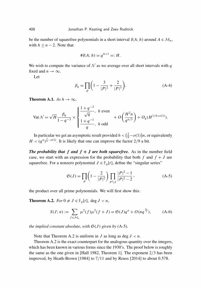
408 Jonathan P. Keating and Zeev Rudnick

be the number of squarefree polynomials in a short interval I(A; h) around A ∈Mn ,with h ≤ n− 2. Note that

#I(A; h)= qh+1=: H.

We wish to compute the variance of N as we average over all short intervals with qfixed and n→∞.

Let

βq =∏

P

(1−

3|P|2+

2|P|3

). (A-4)

Theorem A.1. As h→∞,

VarN =√

Hβq

1− q−3 ×

1+ q−2

√q

, h even

1+ q−1

q, h odd

+ O(

H 2nqn/3

)+ Oq(H 1/4+o(1)).

In particular we get an asymptotic result provided h<( 2

9−o(1))n, or equivalently

H < (qn)29−o(1). It is likely that one can improve the factor 2/9 a bit.

The probability that f and f + J are both squarefree. As in the number fieldcase, we start with an expression for the probability that both f and f + J aresquarefree. For a nonzero polynomial J ∈ Fq [t], define the “singular series”

S(J )=∏

P

(1−

2|P|2

) ∏P2|J

|P|2− 1|P|2− 2

, (A-5)

the product over all prime polynomials. We will first show this:

Theorem A.2. For 0 6= J ∈ Fq [t], deg J < n,

S(J ; n) :=∑

f ∈Mn

µ2( f )µ2( f + J )=S(J )qn+ O(nq

2n3 ), (A-6)

the implied constant absolute, with S(J ) given by (A-5).

Note that Theorem A.2 is uniform in J as long as deg J < n.Theorem A.2 is the exact counterpart for the analogous quantity over the integers,

which has been known in various forms since the 1930’s. The proof below is roughlythe same as the one given in [Hall 1982, Theorem 1]. The exponent 2/3 has beenimproved, by Heath-Brown [1984] to 7/11 and by Reuss [2014] to about 0.578.

Squarefree polynomials and Möbius values 409

A decomposition of µ2. We start with the identity

µ2( f )=∑d2| f

µ(d) (A-7)

(the sum over monic d). Pick an integer parameter 0< z ≤ n/2, write Z = q z , anddecompose the sum into two parts, one over “small” divisors, that is with deg d < z,and one over “large” divisors:

µ2= µ2

z + ez, (A-8)

µ2z ( f )=

∑d2| f

deg d<z

µ(d), ez( f )=∑d2| f

deg d≥z

µ(d). (A-9)

LetSz(J ; n) :=

∑f ∈Mn

µ2z ( f )µ2

z ( f + J ). (A-10)

We want to replace S by Sz .

Bounding S(J; n)− Sz(n; J).

Proposition A.3. If z ≤ n/2 then

|S(J ; n)− Sz(J ; n)| �qn

Z,

where Z = q z .

Proof. Note that

µ2( f )µ2( f+J )=

µ2z ( f )µ2

z ( f+J )+ ez( f )µ2( f+J )−µ2( f )ez( f+J )− ez( f )ez( f+J ) (A-11)

so that (recall µ2( f )≤ 1)∣∣µ2( f )µ2( f+J )−µ2z ( f )µ2

z ( f+J )∣∣≤|ez( f )|+|ez( f+J )|+|ez( f )ez( f+J )|

≤ |ez( f )| + |ez( f+J )| + 12 |ez( f )|2+ 1

2 |ez( f+J )|2 (A-12)

and therefore, summing (A-12) over f ∈Mn and noting that since deg J < n, sumsof f + J are the same as sums of f ,

|S(J ; n)− Sz(J ; n)| ≤ 2∑

f ∈Mn

|ez( f )| +∑

f ∈Mn

|ez( f )|2. (A-13)

We have

|ez( f )| =∣∣∣∣ ∑

d2| f

deg d≥z

µ(d)∣∣∣∣≤ ∑

d2| f

deg d≥z

1,

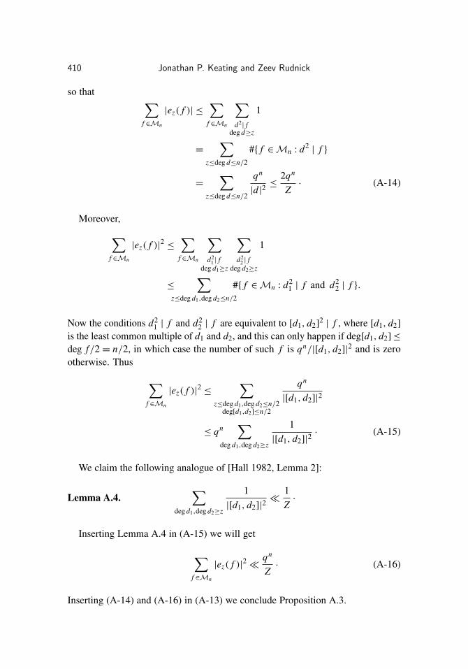
410 Jonathan P. Keating and Zeev Rudnick

so that ∑f ∈Mn

|ez( f )| ≤∑

f ∈Mn

∑d2| f

deg d≥z

1

=

∑z≤deg d≤n/2

#{ f ∈Mn : d2| f }

=

∑z≤deg d≤n/2

qn

|d|2≤

2qn

Z. (A-14)

Moreover,∑f ∈Mn

|ez( f )|2 ≤∑

f ∈Mn

∑d2

1 | fdeg d1≥z

∑d2

2 | fdeg d2≥z

1

≤

∑z≤deg d1,deg d2≤n/2

#{ f ∈Mn : d21 | f and d2

2 | f }.

Now the conditions d21 | f and d2

2 | f are equivalent to [d1, d2]2| f , where [d1, d2]

is the least common multiple of d1 and d2, and this can only happen if deg[d1, d2] ≤

deg f/2 = n/2, in which case the number of such f is qn/|[d1, d2]|2 and is zero

otherwise. Thus ∑f ∈Mn

|ez( f )|2 ≤∑

z≤deg d1,deg d2≤n/2deg[d1,d2]≤n/2

qn

|[d1, d2]|2

≤ qn∑

deg d1,deg d2≥z

1|[d1, d2]|2

. (A-15)

We claim the following analogue of [Hall 1982, Lemma 2]:

Lemma A.4.∑

deg d1,deg d2≥z

1|[d1, d2]|2

�1Z

.

Inserting Lemma A.4 in (A-15) we will get

∑f ∈Mn

|ez( f )|2�qn

Z. (A-16)

Inserting (A-14) and (A-16) in (A-13) we conclude Proposition A.3.

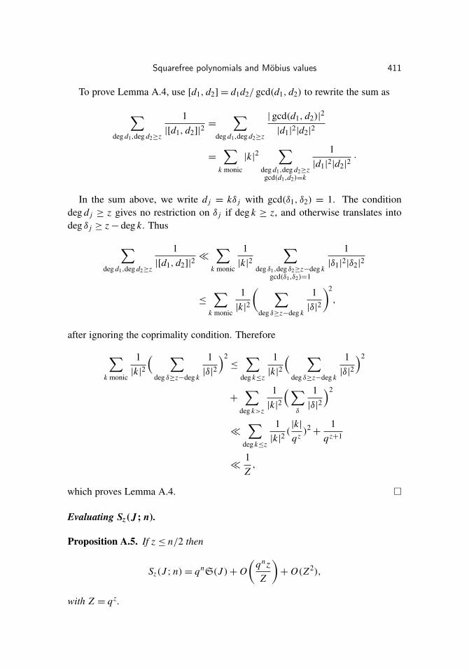
Squarefree polynomials and Möbius values 411

To prove Lemma A.4, use [d1, d2] = d1d2/ gcd(d1, d2) to rewrite the sum as

∑deg d1,deg d2≥z

1|[d1, d2]|2

=

∑deg d1,deg d2≥z

| gcd(d1, d2)|2

|d1|2|d2|2

=

∑k monic

|k|2∑

deg d1,deg d2≥zgcd(d1,d2)=k

1|d1|2|d2|2

.

In the sum above, we write d j = kδ j with gcd(δ1, δ2) = 1. The conditiondeg d j ≥ z gives no restriction on δ j if deg k ≥ z, and otherwise translates intodeg δ j ≥ z− deg k. Thus

∑deg d1,deg d2≥z

1|[d1, d2]|2

�

∑k monic

1|k|2

∑deg δ1,deg δ2≥z−deg k

gcd(δ1,δ2)=1

1|δ1|2|δ2|2

≤

∑k monic

1|k|2

( ∑deg δ≥z−deg k

1|δ|2

)2

,

after ignoring the coprimality condition. Therefore

∑k monic

1|k|2

( ∑deg δ≥z−deg k

1|δ|2

)2≤

∑deg k≤z

1|k|2

( ∑deg δ≥z−deg k

1|δ|2

)2

+

∑deg k>z

1|k|2

(∑δ

1|δ|2

)2

�

∑deg k≤z

1|k|2

(|k|q z )

2+

1q z+1

�1Z,

which proves Lemma A.4. �

Evaluating Sz(J; n).

Proposition A.5. If z ≤ n/2 then

Sz(J ; n)= qnS(J )+ O(

qnzZ

)+ O(Z2),

with Z = q z .

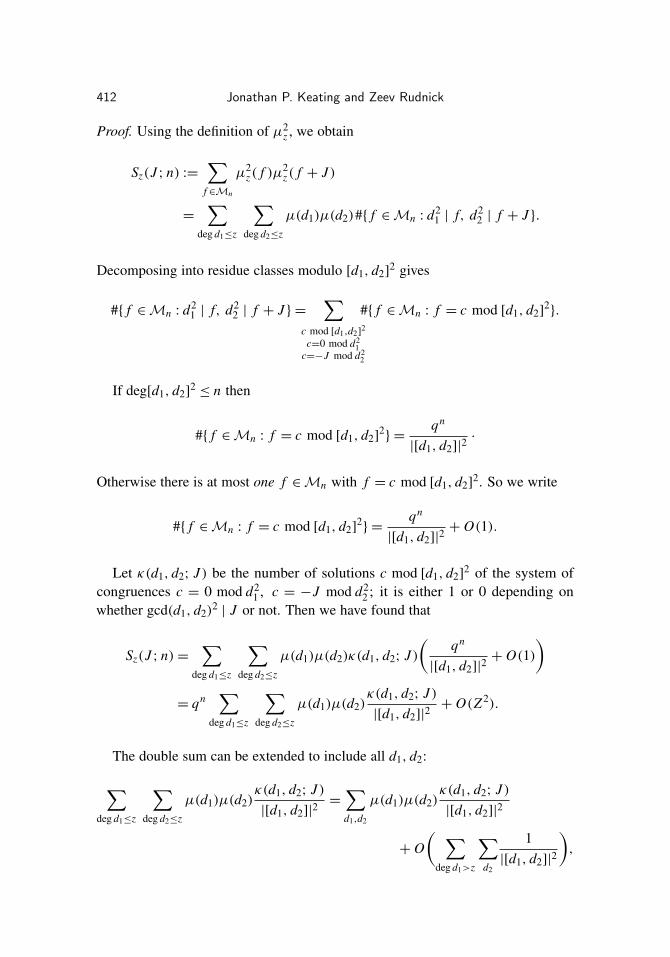
412 Jonathan P. Keating and Zeev Rudnick

Proof. Using the definition of µ2z , we obtain

Sz(J ; n) :=∑

f ∈Mn

µ2z ( f )µ2

z ( f + J )

=

∑deg d1≤z

∑deg d2≤z

µ(d1)µ(d2)#{ f ∈Mn : d21 | f, d2

2 | f + J }.

Decomposing into residue classes modulo [d1, d2]2 gives

#{ f ∈Mn : d21 | f, d2

2 | f + J } =∑

c mod [d1,d2]2

c=0 mod d21

c=−J mod d22

#{ f ∈Mn : f = c mod [d1, d2]2}.

If deg[d1, d2]2≤ n then

#{ f ∈Mn : f = c mod [d1, d2]2} =

qn

|[d1, d2]|2.

Otherwise there is at most one f ∈Mn with f = c mod [d1, d2]2. So we write

#{ f ∈Mn : f = c mod [d1, d2]2} =

qn

|[d1, d2]|2+ O(1).

Let κ(d1, d2; J ) be the number of solutions c mod [d1, d2]2 of the system of

congruences c = 0 mod d21 , c = −J mod d2

2 ; it is either 1 or 0 depending onwhether gcd(d1, d2)

2| J or not. Then we have found that

Sz(J ; n)=∑

deg d1≤z

∑deg d2≤z

µ(d1)µ(d2)κ(d1, d2; J )(

qn

|[d1, d2]|2+ O(1)

)

= qn∑

deg d1≤z

∑deg d2≤z

µ(d1)µ(d2)κ(d1, d2; J )|[d1, d2]|2

+ O(Z2).

The double sum can be extended to include all d1, d2:

∑deg d1≤z

∑deg d2≤z

µ(d1)µ(d2)κ(d1, d2; J )|[d1, d2]|2

=

∑d1,d2

µ(d1)µ(d2)κ(d1, d2; J )|[d1, d2]|2

+ O( ∑

deg d1>z

∑d2

1|[d1, d2]|2

),

Squarefree polynomials and Möbius values 413

so that

Sz(J ; n)= qn∑d1,d2

µ(d1)µ(d2)κ(d1, d2; J )|[d1, d2]|2

+ O( ∑

deg d1>z

∑d2

1|[d1, d2]|2

)+ O(Z2). (A-17)

The sum in the remainder term of (A-17) is bounded in the following analogueof [Hall 1982, Lemma 3].

Lemma A.6. ∑deg d1>z

∑d2

1|[d1, d2]|2

�z

q z =zZ

.

Proof. We argue as in the proof of Lemma A.4: We write the least common multipleas [d1, d2] = d1d2/ gcd(d1, d2) and sum over all pairs of d1, d2 with given gcd:∑

deg d1>z

∑d2

1|[d1, d2]|2

=

∑k

|k|2∑

deg d1>z

∑d2

gcd(d1,d2)=k

1|d1|2|d2|2

=

∑k

|k|2∑

deg δ1>z−deg k

1|k|2|δ1|2

∑δ2

gcd(δ1,δ2)=1

1|k|2|δ2|2

.

after writing d j = kδ j with δ1, δ2 coprime.Ignoring the coprimality condition gives∑deg d1>z

∑d2

1|[d1, d2]|2

�

∑k

1|k|2

∑deg δ1>z−deg k

1|δ1|2

∑δ2

1|δ2|2

�

∑deg k≤z

1|k|2

∑deg δ1>z−deg k

1|δ1|2+

∑deg k>z

1|k|2

∑δ1

1|δ1|2

�

∑deg k≤z

1|k|2|k|q z +

∑deg k>z

1|k|2

�z

q z =zZ,

which proves Lemma A.6. �

Putting together (A-17) and Lemma A.6, we have shown that

Sz(J ; n)= qn∑d1

∑d2

µ(d1)µ(d2)κ(d1, d2; J )|[d1, d2]|2

+ O(

qnzZ

)+ O(Z2). (A-18)

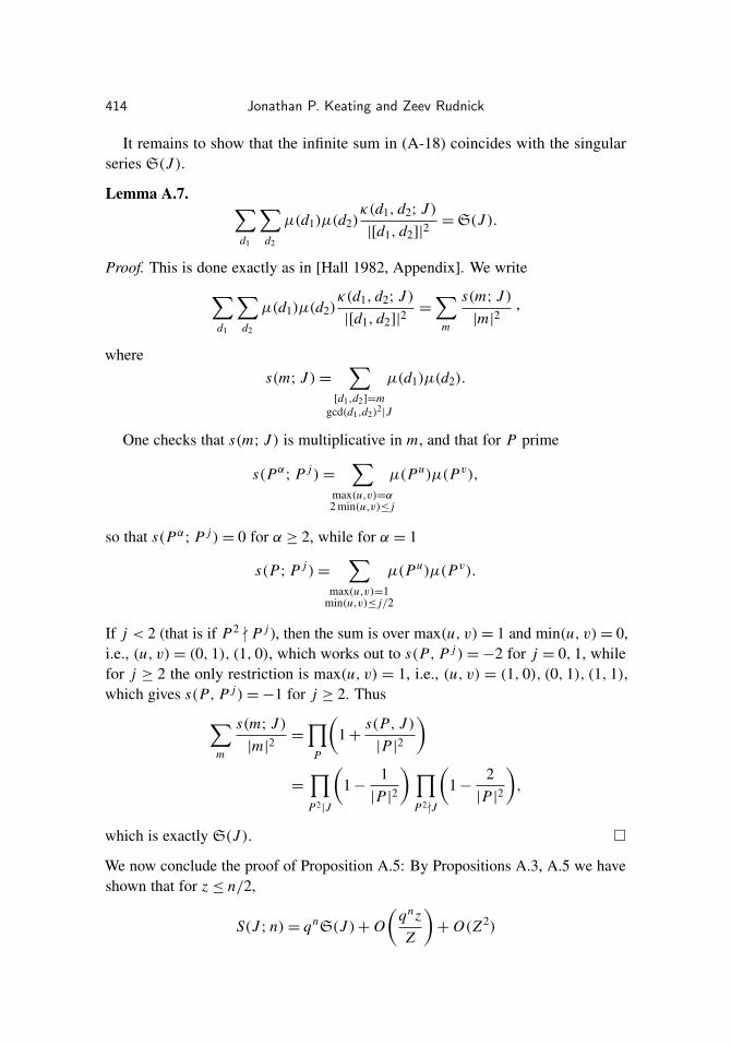
414 Jonathan P. Keating and Zeev Rudnick

It remains to show that the infinite sum in (A-18) coincides with the singularseries S(J ).

Lemma A.7. ∑d1

∑d2

µ(d1)µ(d2)κ(d1, d2; J )|[d1, d2]|2

=S(J ).

Proof. This is done exactly as in [Hall 1982, Appendix]. We write∑d1

∑d2

µ(d1)µ(d2)κ(d1, d2; J )|[d1, d2]|2

=

∑m

s(m; J )|m|2

,

wheres(m; J )=

∑[d1,d2]=m

gcd(d1,d2)2|J

µ(d1)µ(d2).

One checks that s(m; J ) is multiplicative in m, and that for P prime

s(Pα; P j )=∑

max(u,v)=α2 min(u,v)≤ j

µ(Pu)µ(Pv),

so that s(Pα; P j )= 0 for α ≥ 2, while for α = 1

s(P; P j )=∑

max(u,v)=1min(u,v)≤ j/2

µ(Pu)µ(Pv).

If j < 2 (that is if P2 - P j ), then the sum is over max(u, v)= 1 and min(u, v)= 0,i.e., (u, v)= (0, 1), (1, 0), which works out to s(P, P j )=−2 for j = 0, 1, whilefor j ≥ 2 the only restriction is max(u, v) = 1, i.e., (u, v) = (1, 0), (0, 1), (1, 1),which gives s(P, P j )=−1 for j ≥ 2. Thus∑

m

s(m; J )|m|2

=

∏P

(1+

s(P, J )|P|2

)=

∏P2|J

(1−

1|P|2

) ∏P2-J

(1−

2|P|2

),

which is exactly S(J ). �

We now conclude the proof of Proposition A.5: By Propositions A.3, A.5 we haveshown that for z ≤ n/2,

S(J ; n)= qnS(J )+ O(

qnzZ

)+ O(Z2)

Squarefree polynomials and Möbius values 415

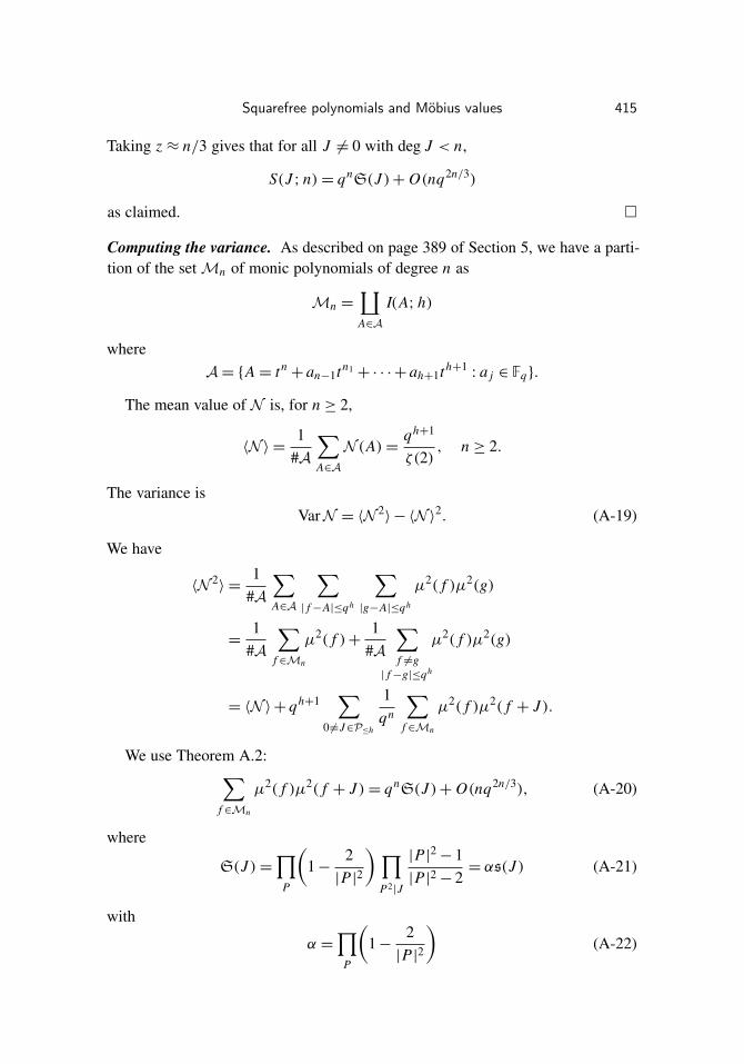
Taking z ≈ n/3 gives that for all J 6= 0 with deg J < n,

S(J ; n)= qnS(J )+ O(nq2n/3)

as claimed. �

Computing the variance. As described on page 389 of Section 5, we have a parti-tion of the set Mn of monic polynomials of degree n as

Mn =∐A∈A

I(A; h)

whereA= {A = tn

+ an−1tn1 + · · ·+ ah+1th+1: a j ∈ Fq}.

The mean value of N is, for n ≥ 2,

〈N 〉 =1

#A

∑A∈A

N (A)=qh+1

ζ(2), n ≥ 2.

The variance isVarN = 〈N 2

〉− 〈N 〉2. (A-19)

We have

〈N 2〉 =

1#A

∑A∈A

∑| f−A|≤qh

∑|g−A|≤qh

µ2( f )µ2(g)

=1

#A

∑f ∈Mn

µ2( f )+1

#A

∑f 6=g

| f−g|≤qh

µ2( f )µ2(g)

= 〈N 〉+ qh+1∑

06=J∈P≤h

1qn

∑f ∈Mn

µ2( f )µ2( f + J ).

We use Theorem A.2:∑f ∈Mn

µ2( f )µ2( f + J )= qnS(J )+ O(nq2n/3), (A-20)

where

S(J )=∏

P

(1−

2|P|2

) ∏P2|J

|P|2− 1|P|2− 2

= αs(J ) (A-21)

with

α =∏

P

(1−

2|P|2

)(A-22)

416 Jonathan P. Keating and Zeev Rudnick

and

s(J )=∏P2|J

|P|2− 1|P|2− 2

.

This gives that

Var= 〈N 〉− 〈N 〉2+αqh+1∑

06=J∈P≤h

s(J )+ O(H 2nq−n/3)

=qh+1

ζ(2)−

(qh+1

ζ(2)

)2

+αqh+1(q − 1)h∑

j=0

∑J∈M j

s(J )+ O(H 2nq−n/3),

(A-23)the last step using homogeneity: S(cJ )=S(J ), c ∈ F×q .

Computing∑

J s(J). To evaluate the sum of s(J ) in (A-23), we form the gener-ating series

F(u)=∑

J monic

s(J )udeg J .

Since s(J ) is multiplicative, and s(Pk)= 1 if k = 0, 1, and s(Pk)= s(P2)=|P|2−1|P|2−2

if k ≥ 2, we find

F(u)=∏

P

(1+ udeg P

+ s(P2)∑k≥2

uk deg P)

=

∏P

(1+ udeg P

+|P|2− 1|P|2− 2

u2 deg P

1− udeg P

)= Z(u)

∏P

(1+

1|P|2− 2

u2 deg P),

with

Z(u)=∏

P

(1− udeg P)−1=

11− qu

.

We further factor

∏P

(1+

1|P|2− 2

u2 deg P)= Z(u2/q2)

∏P

(1+

2u2 deg P− u4 deg P

|P|2(|P|2− 2)

),

with the product absolutely convergent for |u|< q3/4.

Squarefree polynomials and Möbius values 417

We haveh∑

j=0

∑J∈M j

s(J )=1

2π i

∮F(u)

1− u−(h+1)

u− 1du

=1

2π i

∮F(u)

1u− 1

du+1

2π i

∮F(u)

u−(h+1)

1− udu, (A-24)

where the contour of integration is a small circle around the origin not includingany pole of F(u), say |u| = 1/q2, traversed counterclockwise.

The first integral is zero, because the integrand is analytic near u = 0. As for thesecond integral, we shift the contour of integration to |u| = q3/4−δ, and obtain

12π i

∮F(u)

u−(h+1)

1− udu =− Res

u=1/q−Res

u=1− Res

u=±√

q+

12π i

∮|u|=q3/4−δ

F(u)u−(h+1)

1− udu.

As h→∞, we may bound the integral around |u| = q3/4−δ by

12π i

∮|u|=q3/4−δ

F(u)u−(h+1)

1− udu�q q−(3/4−δ)(h+1),

the implied constant depending on q.The residue at u = 1/q gives

− Resu=1/q

=1

αζ(2)2qh+1

(q − 1)

and hence its contribution to VarN is(qh+1

ζ(2)

)2

, (A-25)

which exactly cancels out the term −〈N 〉2 in (A-23).The residue at u = 1 gives

−Resu=1

F(u)u−(h+1)

1− u= F(1)=

11− q

∏P

(1+

1|P|2− 2

)=−

1(q − 1)αζq(2)

(A-26)

and its contribution to VarN is

−qh+1

ζq(2), (A-27)

which exactly cancels out the term 〈N 〉 in (A-23).

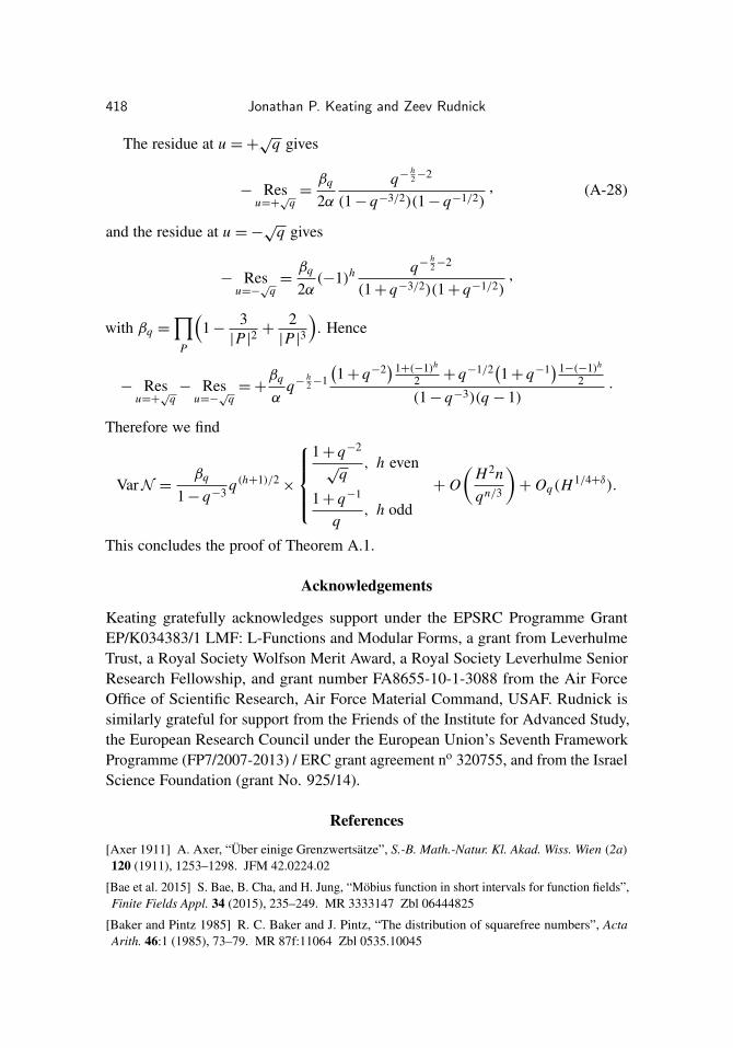
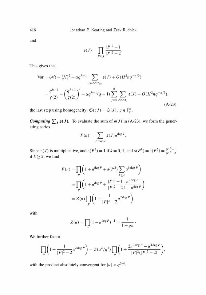
418 Jonathan P. Keating and Zeev Rudnick

The residue at u =+√

q gives

− Resu=+√

q=βq

2αq−

h2−2

(1− q−3/2)(1− q−1/2), (A-28)

and the residue at u =−√

q gives

− Resu=−√

q=βq

2α(−1)h

q−h2−2

(1+ q−3/2)(1+ q−1/2),

with βq =∏

P

(1− 3|P|2+

2|P|3

). Hence

− Resu=+√

q− Res

u=−√

q=+

βq

αq−

h2−1

(1+ q−2

) 1+(−1)h2 + q−1/2

(1+ q−1

) 1−(−1)h2

(1− q−3)(q − 1).

Therefore we find

VarN =βq

1− q−3 q(h+1)/2×

1+ q−2

√q

, h even

1+ q−1

q, h odd

+ O(

H 2nqn/3

)+ Oq(H 1/4+δ).

This concludes the proof of Theorem A.1.

Acknowledgements

Keating gratefully acknowledges support under the EPSRC Programme GrantEP/K034383/1 LMF: L-Functions and Modular Forms, a grant from LeverhulmeTrust, a Royal Society Wolfson Merit Award, a Royal Society Leverhulme SeniorResearch Fellowship, and grant number FA8655-10-1-3088 from the Air ForceOffice of Scientific Research, Air Force Material Command, USAF. Rudnick issimilarly grateful for support from the Friends of the Institute for Advanced Study,the European Research Council under the European Union’s Seventh FrameworkProgramme (FP7/2007-2013) / ERC grant agreement no 320755, and from the IsraelScience Foundation (grant No. 925/14).

References

[Axer 1911] A. Axer, “Über einige Grenzwertsätze”, S.-B. Math.-Natur. Kl. Akad. Wiss. Wien (2a)120 (1911), 1253–1298. JFM 42.0224.02

[Bae et al. 2015] S. Bae, B. Cha, and H. Jung, “Möbius function in short intervals for function fields”,Finite Fields Appl. 34 (2015), 235–249. MR 3333147 Zbl 06444825

[Baker and Pintz 1985] R. C. Baker and J. Pintz, “The distribution of squarefree numbers”, ActaArith. 46:1 (1985), 73–79. MR 87f:11064 Zbl 0535.10045

Squarefree polynomials and Möbius values 419

[Bank et al. 2015] E. Bank, L. Bary-Soroker, and L. Rosenzweig, “Prime polynomials in shortintervals and in arithmetic progressions”, Duke Math. J. 164:2 (2015), 277–295. MR 3306556Zbl 06416949

[Blomer 2008] V. Blomer, “The average value of divisor sums in arithmetic progressions”, Q. J. Math.59:3 (2008), 275–286. MR 2009j:11158 Zbl 1228.11153

[Carmon and Rudnick 2014] D. Carmon and Z. Rudnick, “The autocorrelation of the Möbius functionand Chowla’s conjecture for the rational function field”, Q. J. Math. 65:1 (2014), 53–61. MR 3179649Zbl 1302.11073

[Cha 2011] B. Cha, “The summatory function of the Möbius function in function fields”, preprint,2011. arXiv 1008.4711

[Chatterjee and Soundararajan 2012] S. Chatterjee and K. Soundararajan, “Random multiplica-tive functions in short intervals”, Int. Math. Res. Not. 2012:3 (2012), 479–492. MR 2885978Zbl 1248.11056

[Erdös 1951] P. Erdös, “Some problems and results in elementary number theory”, Publ. Math.Debrecen 2 (1951), 103–109. MR 13,627a Zbl 0044.03604

[Good and Churchhouse 1968] I. J. Good and R. F. Churchhouse, “The Riemann hypothesis andpseudorandom features of the Möbius sequence”, Math. Comp. 22 (1968), 857–861. MR 39 #1416Zbl 0182.37503

[Hall 1982] R. R. Hall, “Squarefree numbers on short intervals”, Mathematika 29:1 (1982), 7–17.MR 83m:10077 Zbl 0502.10027

[Heath-Brown 1984] D. R. Heath-Brown, “The square sieve and consecutive square-free numbers”,Math. Ann. 266:3 (1984), 251–259. MR 85h:11050 Zbl 0514.10038

[Hooley 1975] C. Hooley, “On the Barban–Davenport–Halberstam theorem, III”, J. London Math.Soc. (2) 10 (1975), 249–256. MR 52 #3090c Zbl 0304.10029

[Humphries 2014] P. Humphries, “On the Mertens conjecture for function fields”, Int. J. NumberTheory 10:2 (2014), 341–361. MR 3189983 Zbl 1303.11109

[Jia 1993] C. H. Jia, “The distribution of square-free numbers”, Sci. China Ser. A 36:2 (1993),154–169. MR 94f:11095 Zbl 0772.11033

[Katz 2013a] N. M. Katz, “On a question of Keating and Rudnick about primitive Dirichlet charac-ters with squarefree conductor”, Int. Math. Res. Not. 2013:14 (2013), 3221–3249. MR 3085758Zbl 06437663

[Katz 2013b] N. M. Katz, “Witt vectors and a question of Keating and Rudnick”, Int. Math. Res. Not.2013:16 (2013), 3613–3638. MR 3090703 Zbl 06437675

[Katz 2015a] N. M. Katz, “On two questions of Entin, Keating, and Rudnick on primitive Dirichletcharacters”, Int. Math. Res. Not. 2015:15 (2015), 6044–6069. MR 3384472 Zbl 06505082

[Katz 2015b] N. M. Katz, “Witt vectors and a question of Entin, Keating, and Rudnick”, Int. Math.Res. Not. 2015:14 (2015), 5959–5975. MR 3384464 Zbl 06513161

[Keating and Rudnick 2014] J. P. Keating and Z. Rudnick, “The variance of the number of primepolynomials in short intervals and in residue classes”, Int. Math. Res. Not. 2014:1 (2014), 259–288.MR 3158533 Zbl 1319.11084

[Keating et al. 2015] J. P. Keating, E. Roditty-Gershon, and Z. Rudnick, “Sums of divisor functionsin Fq [t] and matrix integrals”, preprint, 2015. arXiv 1504.07804

[Matomäki and Radziwiłł 2015] K. Matomäki and M. Radziwiłł, “Multiplicative functions in shortintervals”, Ann. of Math. (online publication October 2015).

420 Jonathan P. Keating and Zeev Rudnick

[Montgomery and Vaughan 1981] H. L. Montgomery and R. C. Vaughan, “The distribution ofsquarefree numbers”, pp. 247–256 in Recent progress in analytic number theory (Durham, 1979),vol. 1, edited by H. Halberstam and C. Hooley, Academic Press, London, 1981. MR 83d:10010Zbl 0462.10029

[Motohashi 1976] Y. Motohashi, “On the sum of the Möbius function in a short segment”, Proc.Japan Acad. 52:9 (1976), 477–479. MR 54 #12685 Zbl 0372.10033

[Ng 2004] N. Ng, “The distribution of the summatory function of the Möbius function”, Proc. LondonMath. Soc. (3) 89:2 (2004), 361–389. MR 2005f:11215 Zbl 1138.11341

[Ng 2008] N. Ng, “The Möbius function in short intervals”, pp. 247–257 in Anatomy of integers(Montréal, 2006), edited by J.-M. De Koninck et al., CRM Proceedings and Lecture Notes 46,American Mathematical Society, Providence, RI, 2008. MR 2009i:11118 Zbl 1187.11025

[Nunes 2015] R. M. Nunes, “Squarefree numbers in arithmetic progressions”, J. Number Theory 153(2015), 1–36. MR 3327562 Zbl 06435729

[Prachar 1958] K. Prachar, “Über die kleinste quadratfreie Zahl einer arithmetischen Reihe”, Monatsh.Math. 62 (1958), 173–176. MR 19,1160g Zbl 0083.03704

[Ramachandra 1976] K. Ramachandra, “Some problems of analytic number theory”, Acta Arith. 31:4(1976), 313–324. MR 54 #12682 Zbl 0291.10034

[Reuss 2014] T. Reuss, “Pairs of k-free numbers, consecutive square-full numbers”, preprint, 2014.arXiv 1212.3150

[Richert 1954] H.-E. Richert, “On the difference between consecutive squarefree numbers”, J. LondonMath. Soc. 29 (1954), 16–20. MR 15,289c Zbl 0055.04001

[Rodgers 2015] B. Rodgers, “The covariance of almost-primes in Fq [T ]”, Int. Math. Res. Not.2015:14 (2015), 5976–6004. MR 3384465 Zbl 06513162

[Roth 1951] K. F. Roth, “On the gaps between squarefree numbers”, J. London Math. Soc. 26 (1951),263–268. MR 13,208d Zbl 0043.04802

[Rudnick 2014] Z. Rudnick, “Square-free values of polynomials over the rational function field”, J.Number Theory 135 (2014), 60–66. MR 3128452

[Swan 1962] R. G. Swan, “Factorization of polynomials over finite fields”, Pacific J. Math. 12 (1962),1099–1106. MR 26 #2432 Zbl 0113.01701

[Tolev 2006] D. I. Tolev, “On the distribution of r-tuples of squarefree numbers in short intervals”,Int. J. Number Theory 2:2 (2006), 225–234. MR 2008a:11111 Zbl 1196.11130

[Warlimont 1980] R. Warlimont, “Squarefree numbers in arithmetic progressions”, J. London Math.Soc. (2) 22:1 (1980), 21–24. MR 82b:10055 Zbl 0444.10036

Communicated by Brian ConradReceived 2015-02-15 Revised 2015-10-09 Accepted 2015-11-30

j.p.keating@bristol.ac.uk School of Mathematics, University of Bristol,Bristol BS8 1TW, United Kingdom

rudnick@post.tau.ac.il Raymond and Beverly Sackler School of MathematicalSciences, Tel Aviv University, Tel Aviv 69978, Israel

mathematical sciences publishers msp

Algebra & Number Theorymsp.org/ant

EDITORS

MANAGING EDITOR

Bjorn PoonenMassachusetts Institute of Technology

Cambridge, USA

EDITORIAL BOARD CHAIR

David EisenbudUniversity of California

Berkeley, USA

BOARD OF EDITORS

Georgia Benkart University of Wisconsin, Madison, USA

Dave Benson University of Aberdeen, Scotland

Richard E. Borcherds University of California, Berkeley, USA

John H. Coates University of Cambridge, UK

J-L. Colliot-Thélène CNRS, Université Paris-Sud, France

Brian D. Conrad Stanford University, USA

Hélène Esnault Freie Universität Berlin, Germany

Hubert Flenner Ruhr-Universität, Germany

Sergey Fomin University of Michigan, USA

Edward Frenkel University of California, Berkeley, USA

Andrew Granville Université de Montréal, Canada

Joseph Gubeladze San Francisco State University, USA

Roger Heath-Brown Oxford University, UK

Craig Huneke University of Virginia, USA

Kiran S. Kedlaya Univ. of California, San Diego, USA

János Kollár Princeton University, USA

Yuri Manin Northwestern University, USA

Philippe Michel École Polytechnique Fédérale de Lausanne

Susan Montgomery University of Southern California, USA

Shigefumi Mori RIMS, Kyoto University, Japan

Raman Parimala Emory University, USA

Jonathan Pila University of Oxford, UK

Anand Pillay University of Notre Dame, USA

Victor Reiner University of Minnesota, USA

Peter Sarnak Princeton University, USA

Joseph H. Silverman Brown University, USA

Michael Singer North Carolina State University, USA

Vasudevan Srinivas Tata Inst. of Fund. Research, India

J. Toby Stafford University of Michigan, USA

Ravi Vakil Stanford University, USA

Michel van den Bergh Hasselt University, Belgium

Marie-France Vignéras Université Paris VII, France

Kei-Ichi Watanabe Nihon University, Japan

Efim Zelmanov University of California, San Diego, USA

Shou-Wu Zhang Princeton University, USA

PRODUCTIONproduction@msp.org

Silvio Levy, Scientific Editor

See inside back cover or msp.org/ant for submission instructions.

The subscription price for 2016 is US $290/year for the electronic version, and $485/year (+$55, if shipping outside the US)for print and electronic. Subscriptions, requests for back issues and changes of subscribers address should be sent to MSP.

Algebra & Number Theory (ISSN 1944-7833 electronic, 1937-0652 printed) at Mathematical Sciences Publishers, 798 EvansHall #3840, c/o University of California, Berkeley, CA 94720-3840 is published continuously online. Periodical rate postagepaid at Berkeley, CA 94704, and additional mailing offices.

ANT peer review and production are managed by EditFLOW® from MSP.

PUBLISHED BY

mathematical sciences publishersnonprofit scientific publishing

http://msp.org/© 2016 Mathematical Sciences Publishers

Algebra & Number TheoryVolume 10 No. 2 2016

215Kummer theory for Drinfeld modulesRICHARD PINK

235Parity and symmetry in intersection and ordinary cohomologySHENGHAO SUN and WEIZHE ZHENG

309Generalized Heegner cycles at Eisenstein primes and the Katz p-adic L-functionDANIEL KRIZ

375Squarefree polynomials and Möbius values in short intervals and arithmetic progressionsJONATHAN P. KEATING and ZEEV RUDNICK

421Equidistribution of values of linear forms on a cubic hypersurfaceSAM CHOW

1937-0652(2016)10:2;1-N

Algebra

&N

umber

Theory2016

Vol.10,N

o.2