Algebra II Chapter - California Department of Education · Algebra II Chapter of the. Mathematics Framework. for California Public Schools: Kindergarten Through Grade Twelve. Adopted

Algebra II Chapter

of the

Mathematics Framework for California Public Schools:

Kindergarten Through Grade Twelve

Adopted by the California State Board of Education, November 2013

Published by the California Department of EducationSacramento, 2015

Algebra II

Geometry

Algebra II

Algebra I

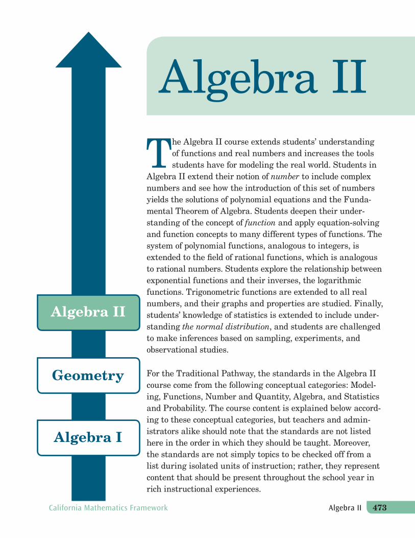
The Algebra II course extends students’ understanding of functions and real numbers and increases the tools students have for modeling the real world. Students in

Algebra II extend their notion of number to include complex numbers and see how the introduction of this set of numbers yields the solutions of polynomial equations and the Funda-mental Theorem of Algebra. Students deepen their under-standing of the concept of function and apply equation-solving and function concepts to many different types of functions. The system of polynomial functions, analogous to integers, is extended to the field of rational functions, which is analogous to rational numbers. Students explore the relationship between exponential functions and their inverses, the logarithmic functions. Trigonometric functions are extended to all real numbers, and their graphs and properties are studied. Finally, students’ knowledge of statistics is extended to include under-standing the normal distribution, and students are challenged to make inferences based on sampling, experiments, and observational studies.

For the Traditional Pathway, the standards in the Algebra II course come from the following conceptual categories: Model-ing, Functions, Number and Quantity, Algebra, and Statistics and Probability. The course content is explained below accord-ing to these conceptual categories, but teachers and admin-istrators alike should note that the standards are not listed here in the order in which they should be taught. Moreover, the standards are not simply topics to be checked off from a list during isolated units of instruction; rather, they represent content that should be present throughout the school year in rich instructional experiences.

California Mathematics Framework Algebra II 473

474 Algebra II California Mathematics Framework

What Students Learn in Algebra IIBuilding on their work with linear, quadratic, and exponential functions, students in Algebra II extend their repertoire of functions to include polynomial, rational, and radical functions.1 Students work closely with the expressions that define the functions and continue to expand and hone their abilities to model situations and to solve equations, including solving quadratic equations over the set of complex numbers and solving exponential equations using the properties of logarithms. Based on their previous work with functions, and on their work with trigonometric ratios and circles in Geometry, students now use the coordinate plane to extend trigonometry to model periodic phenomena. They explore the effects of transformations on graphs of diverse functions, including functions arising in applications, in order to abstract the general principle that transformations on a graph always have the same effect regardless of the type of underlying function. They identify appropriate types of functions to model a situation, adjust parameters to improve the model, and compare models by analyzing appropriateness of fit and making judgments about the domain over which a model is a good fit. Students see how the visual displays and summary statistics learned in earlier grade levels relate to different types of data and to probability distributions. They identify different ways of collecting data—including sample surveys, experiments, and simulations—and the role of randomness and careful design in the conclusions that can be drawn.

Examples of Key Advances from Previous Grade Levels or Courses• In Algebra I, students added, subtracted, and multiplied polynomials. Students in Algebra II divide

polynomials that result in remainders, leading to the factor and remainder theorems. This is theunderpinning for much of advanced algebra, including the algebra of rational expressions.

• Themes from middle-school algebra continue and deepen during high school. As early as grade six,students began thinking about solving equations as a process of reasoning (6.EE.5). This perspectivecontinues throughout Algebra I and Algebra II (A-REI). “Reasoned solving” plays a role in Algebra IIbecause the equations students encounter may have extraneous solutions (A-REI.2).

• In Algebra I, students worked with quadratic equations with no real roots. In Algebra II, they extendtheir knowledge of the number system to include complex numbers, and one effect is that theynow have a complete theory of quadratic equations: Every quadratic equation with complexcoefficients has (counting multiplicity) two roots in the complex numbers.

• In grade eight, students learned the Pythagorean Theorem and used it to determine distances in acoordinate system (8.G.6–8). In the Geometry course, students proved theorems using coordinates(G-GPE.4–7). In Algebra II, students build on their understanding of distance in coordinate systemsand draw on their growing command of algebra to connect equations and graphs of conic sections(for example, refer to standard G-GPE.1).

• In Geometry, students began trigonometry through a study of right triangles. In Algebra II, theyextend the three basic functions to the entire unit circle.

• As students acquire mathematical tools from their study of algebra and functions, they apply thesetools in statistical contexts (for example, refer to standard S-ID.6). In a modeling context, studentsmight informally fit an exponential function to a set of data, graphing the data and the model functionon the same coordinate axes (Partnership for Assessment of Readiness for College and Careers 2012).

1. In this course, rational functions are limited to those with numerators having a degree not more than 1 and denominatorshaving a degree not more than 2; radical functions are limited to square roots or cube roots of at most quadratic polynomi-als (National Governors Association Center for Best Practices, Council of Chief State School Officers [NGA/CCSSO] 2010a).

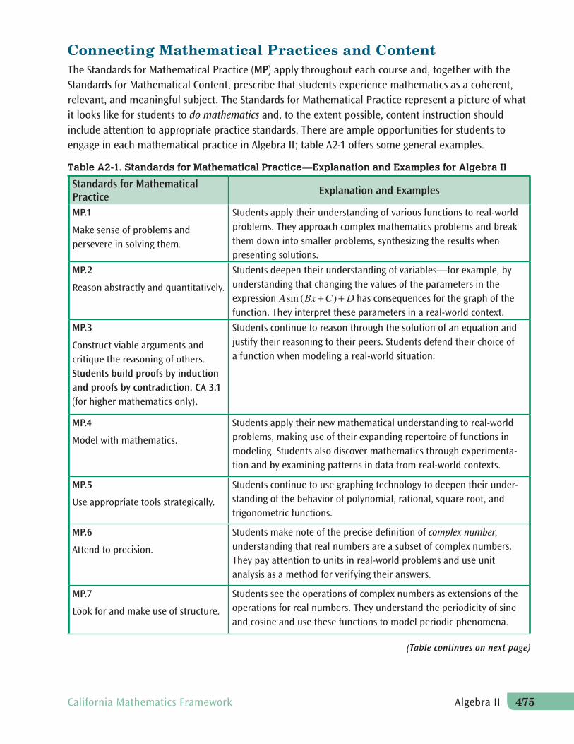
Connecting Mathematical Practices and ContentThe Standards for Mathematical Practice (MP) apply throughout each course and, together with the Standards for Mathematical Content, prescribe that students experience mathematics as a coherent, relevant, and meaningful subject. The Standards for Mathematical Practice represent a picture of whit looks like for students to do mathematics and, to the extent possible, content instruction should include attention to appropriate practice standards. There are ample opportunities for students to engage in each mathematical practice in Algebra II; table A2-1 offers some general examples.

at

Table A2-1. Standards for Mathematical Practice—Explanation and Examples for Algebra II

Standards for Mathematical Practice

Explanation and Examples

MP.1

Make sense of problems and persevere in solving them.

Students apply their understanding of various functions to real-world problems. They approach complex mathematics problems and break them down into smaller problems, synthesizing the results when presenting solutions.

MP.2

Reason abstractly and quantitatively.

Students deepen their understanding of variables—for example, by understanding that changing the values of the parameters in the expression has consequences for the graph of the function. They interpret these parameters in a real-world context.

MP.3

Construct viable arguments and critique the reasoning of others. Students build proofs by induction and proofs by contradiction. CA 3.1 (for higher mathematics only).

Students continue to reason through the solution of an equation and justify their reasoning to their peers. Students defend their choice of a function when modeling a real-world situation.

MP.4

Model with mathematics.

Students apply their new mathematical understanding to real-world problems, making use of their expanding repertoire of functions in modeling. Students also discover mathematics through experimenta-tion and by examining patterns in data from real-world contexts.

MP.5

Use appropriate tools strategically.

Students continue to use graphing technology to deepen their under-standing of the behavior of polynomial, rational, square root, and trigonometric functions.

MP.6

Attend to precision.

Students make note of the precise definition of complex number, understanding that real numbers are a subset of complex numbers. They pay attention to units in real-world problems and use unit analysis as a method for verifying their answers.

MP.7

Look for and make use of structure.

Students see the operations of complex numbers as extensions of the operations for real numbers. They understand the periodicity of sine and cosine and use these functions to model periodic phenomena.

(Table continues on next page)


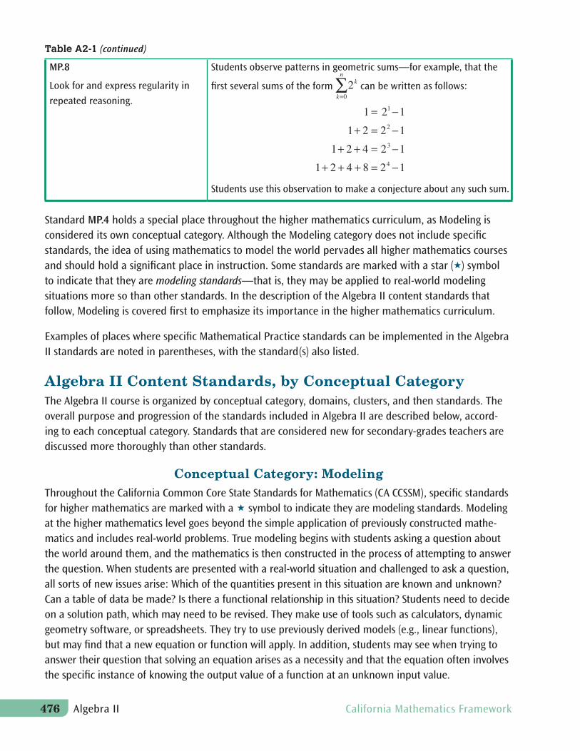
MP.8

Look for and express regularity in

repeated reasoning.

Table A2-1 (continued)

Students observe patterns in geometric sums—for example, that the

first several sums of the form can be written as follows:

Students use this observation to make a conjecture about any such sum.

Standard MP.4 holds a special place throughout the higher mathematics curriculum, as Modeling is considered its own conceptual category. Although the Modeling category does not include specific standards, the idea of using mathematics to model the world pervades all higher mathematics courses and should hold a significant place in instruction. Some standards are marked with a star () symbol to indicate that they are modeling standards—that is, they may be applied to real-world modeling situations more so than other standards. In the description of the Algebra II content standards that follow, Modeling is covered first to emphasize its importance in the higher mathematics curriculum.

Examples of places where specific Mathematical Practice standards can be implemented in the Algebra II standards are noted in parentheses, with the standard(s) also listed.

Algebra II Content Standards, by Conceptual CategoryThe Algebra II course is organized by conceptual category, domains, clusters, and then standards. The overall purpose and progression of the standards included in Algebra II are described below, accord-ing to each conceptual category. Standards that are considered new for secondary-grades teachers are discussed more thoroughly than other standards.

Conceptual Category: ModelingThroughout the California Common Core State Standards for Mathematics (CA CCSSM), specific standards for higher mathematics are marked with a symbol to indicate they are modeling standards. Modeling at the higher mathematics level goes beyond the simple application of previously constructed mathe-matics and includes real-world problems. True modeling begins with students asking a question about the world around them, and the mathematics is then constructed in the process of attempting to answer the question. When students are presented with a real-world situation and challenged to ask a question, all sorts of new issues arise: Which of the quantities present in this situation are known and unknown? Can a table of data be made? Is there a functional relationship in this situation? Students need to decide on a solution path, which may need to be revised. They make use of tools such as calculators, dynamic geometry software, or spreadsheets. They try to use previously derived models (e.g., linear functions), but may find that a new equation or function will apply. In addition, students may see when trying to answer their question that solving an equation arises as a necessity and that the equation often involves the specific instance of knowing the output value of a function at an unknown input value.


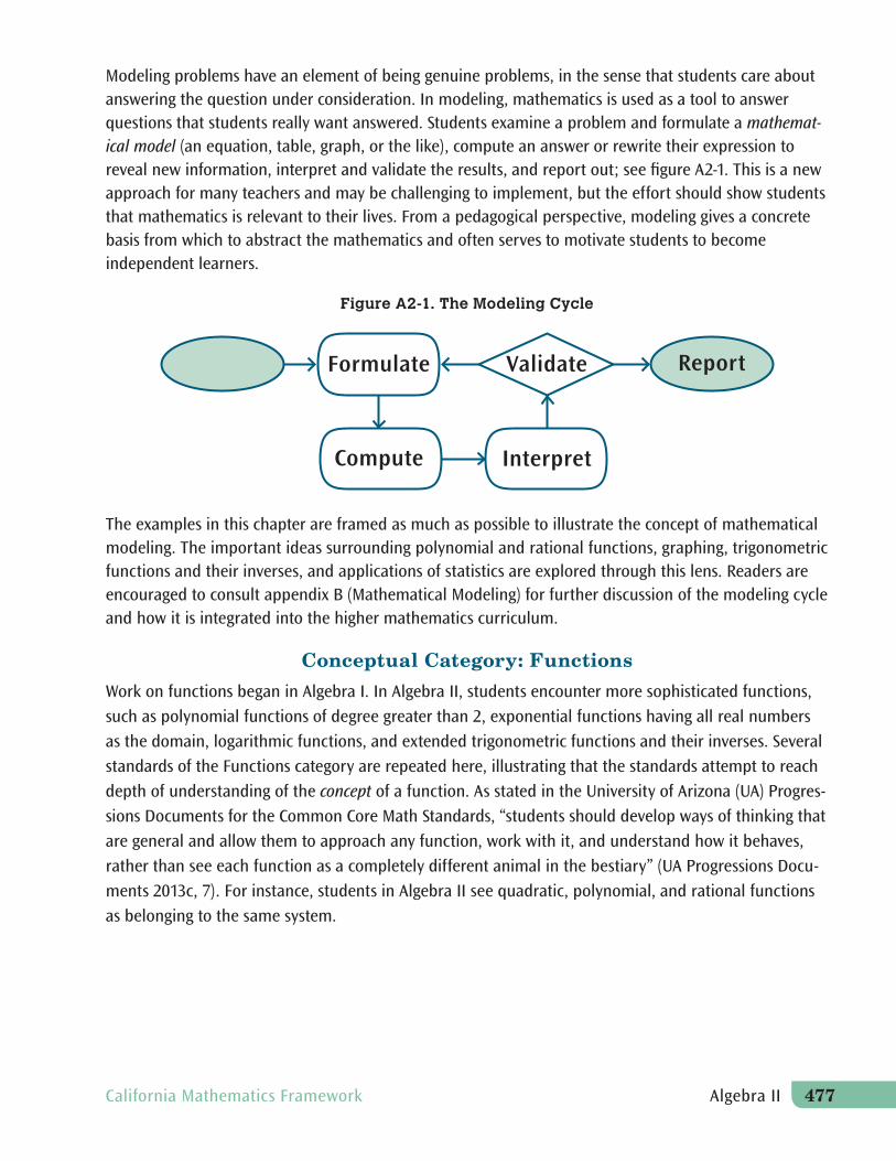
Modeling problems have an element of being genuine problems, in the sense that students care about answering the question under consideration. In modeling, mathematics is used as a tool to answer questions that students really want answered. Students examine a problem and formulate a mathemat-ical model (an equation, table, graph, or the like), compute an answer or rewrite their expression to reveal new information, interpret and validate the results, and report out; see figure A2-1. This is a new approach for many teachers and may be challenging to implement, but the effort should show students that mathematics is relevant to their lives. From a pedagogical perspective, modeling gives a concrete basis from which to abstract the mathematics and often serves to motivate students to become independent learners.

Figure A2-1. The Modeling Cycle

Problem ReportValidateFormulate

Compute Interpret

The examples in this chapter are framed as much as possible to illustrate the concept of mathematical modeling. The important ideas surrounding polynomial and rational functions, graphing, trigonometric functions and their inverses, and applications of statistics are explored through this lens. Readers are encouraged to consult appendix B (Mathematical Modeling) for further discussion of the modeling cycle and how it is integrated into the higher mathematics curriculum.

Conceptual Category: Functions

Work on functions began in Algebra I. In Algebra II, students encounter more sophisticated functions,

such as polynomial functions of degree greater than 2, exponential functions having all real numbers

as the domain, logarithmic functions, and extended trigonometric functions and their inverses. Several

standards of the Functions category are repeated here, illustrating that the standards attempt to reach

depth of understanding of the concept of a function. As stated in the University of Arizona (UA) Progres-

sions Documents for the Common Core Math Standards, “students should develop ways of thinking that

are general and allow them to approach any function, work with it, and understand how it behaves,

rather than see each function as a completely different animal in the bestiary” (UA Progressions Docu-

ments 2013c, 7). For instance, students in Algebra II see quadratic, polynomial, and rational functions

as belonging to the same system.


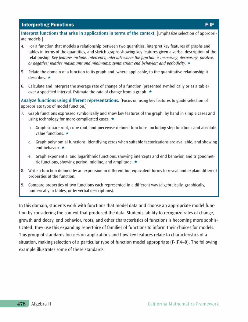
Interpreting Functions F-IF

Interpret functions that arise in applications in terms of the context. [Emphasize selection of appropri-ate models.]

4. For a function that models a relationship between two quantities, interpret key features of graphs andtables in terms of the quantities, and sketch graphs showing key features given a verbal description of therelationship. Key features include: intercepts; intervals where the function is increasing, decreasing, positive,or negative; relative maximums and minimums; symmetries; end behavior; and periodicity.

5. Relate the domain of a function to its graph and, where applicable, to the quantitative relationship itdescribes.

6. Calculate and interpret the average rate of change of a function (presented symbolically or as a table)over a specified interval. Estimate the rate of change from a graph.

Analyze functions using different representations. [Focus on using key features to guide selection of appropriate type of model function.]

7. Graph functions expressed symbolically and show key features of the graph, by hand in simple cases andusing technology for more complicated cases.

b. Graph square root, cube root, and piecewise-defined functions, including step functions and absolutevalue functions.

c. Graph polynomial functions, identifying zeros when suitable factorizations are available, and showingend behavior.

e. Graph exponential and logarithmic functions, showing intercepts and end behavior, and trigonomet-ric functions, showing period, midline, and amplitude.

8. Write a function defined by an expression in different but equivalent forms to reveal and explain differentproperties of the function.

9. Compare properties of two functions each represented in a different way (algebraically, graphically,numerically in tables, or by verbal descriptions).

In this domain, students work with functions that model data and choose an appropriate model func-

tion by considering the context that produced the data. Students’ ability to recognize rates of change,

growth and decay, end behavior, roots, and other characteristics of functions is becoming more sophis-

ticated; they use this expanding repertoire of families of functions to inform their choices for models.

This group of standards focuses on applications and how key features relate to characteristics of a

situation, making selection of a particular type of function model appropriate (F-IF.4–9). The following

example illustrates some of these standards.


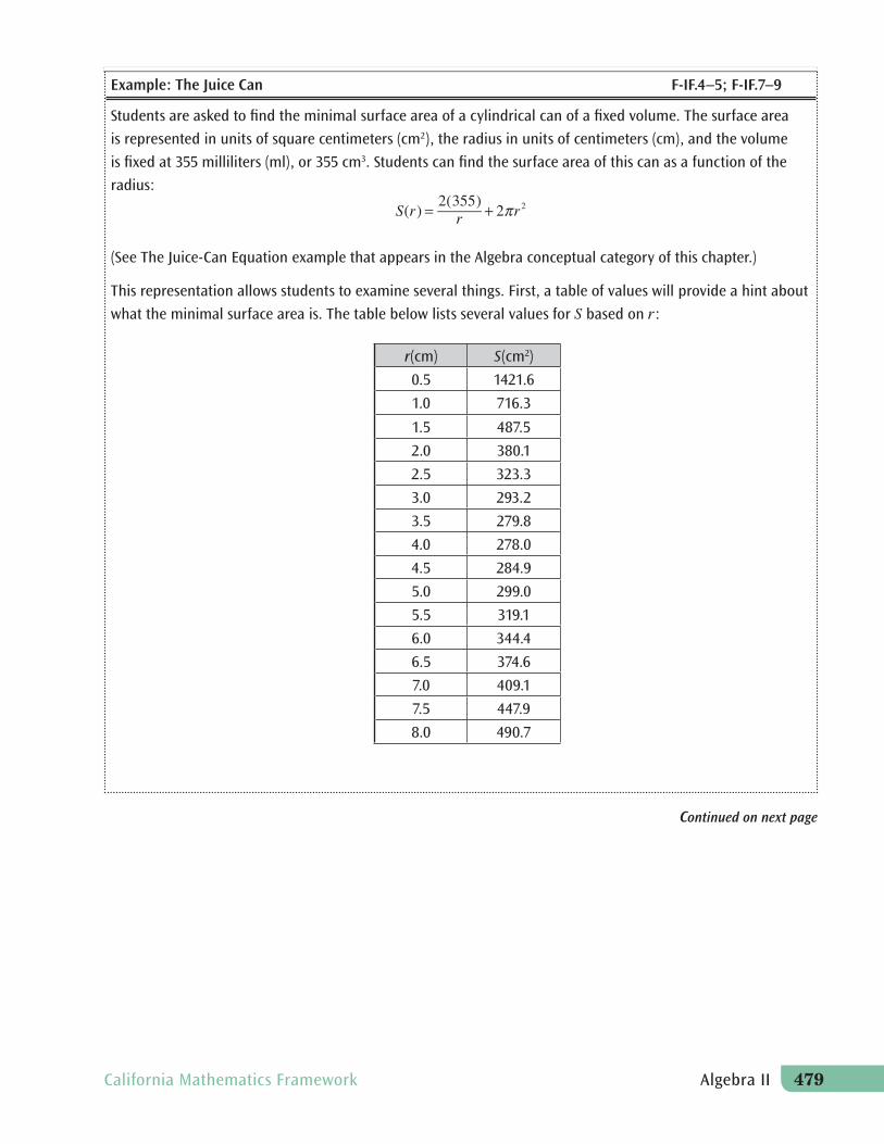
Example: The Juice Can F-IF.4–5; F-IF.7–9

Students are asked to find the minimal surface area of a cylindrical can of a fixed volume. The surface area

is represented in units of square centimeters (cm2), the radius in units of centimeters (cm), and the volume

is fixed at 355 milliliters (ml), or 355 cm3. Students can find the surface area of this can as a function of the

radius:

(See The Juice-Can Equation example that appears in the Algebra conceptual category of this chapter.)

This representation allows students to examine several things. First, a table of values will provide a hint about

what the minimal surface area is. The table below lists several values for based on :

r(cm) S(cm2)

0.5 1421.6

1.0 716.3

1.5 487.5

2.0 380.1

2.5 323.3

3.0 293.2

3.5 279.8

4.0 278.0

4.5 284.9

5.0 299.0

5.5 319.1

6.0 344.4

6.5 374.6

7.0 409.1

7.5 447.9

8.0 490.7

Continued on next page


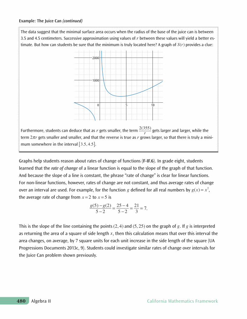
Furthermore, students can deduce that as gets smaller, the term gets larger and larger, while the

term gets smaller and smaller, and that the reverse is true as grows larger, so that there is truly a mini-

mum somewhere in the interval .

Graphs help students reason about rates of change of functions (F-IF.6). In grade eight, students

learned that the rate of change of a linear function is equal to the slope of the graph of that function.

And because the slope of a line is constant, the phrase “rate of change” is clear for linear functions.

For non-linear functions, however, rates of change are not constant, and thus average rates of change

over an interval are used. For example, for the function defined for all real numbers by ,

the average rate of change from to is

.

This is the slope of the line containing the points and on the graph of . If is interpreted

as returning the area of a square of side length , then this calculation means that over this interval the

area changes, on average, by 7 square units for each unit increase in the side length of the square (UA

Progressions Documents 2013c, 9). Students could investigate similar rates of change over intervals for

the Juice Can problem shown previously.

Example: The Juice Can (continued)

The data suggest that the minimal surface area occurs when the radius of the base of the juice can is between

3.5 and 4.5 centimeters. Successive approximation using values of between these values will yield a better es-

timate. But how can students be sure that the minimum is truly located here? A graph of provides a clue:

0 5 10

2000

1000


Building Functions F-BF

Build a function that models a relationship between two quantities. [Include all types of functions studied.]

1. Write a function that describes a relationship between two quantities.

b. Combine standard function types using arithmetic operations. For example, build a function thatmodels the temperature of a cooling body by adding a constant function to a decaying exponential, andrelate these functions to the model.

Build new functions from existing functions. [Include simple radical, rational, and exponential functions; emphasize common effect of each transformation across function types.]

3. Identify the effect on the graph of replacing by , , , and for specific values of (both positive and negative); find the value of given the graphs. Experiment with cases and illustrate an explanation of the effects on the graph using technology. Include recognizing even and odd functions from their graphs and algebraic expressions for them.

4. Find inverse functions.

a. Solve an equation of the form for a simple function that has an inverse and write an expression for the inverse. For example, or for .

Students in Algebra II develop models for more complex situations than in previous courses, due to the expansion of the types of functions available to them (F-BF.1). Modeling contexts provide a natural place for students to start building functions with simpler functions as components. Situations in which cooling or heating are considered involve functions that approach a limiting value according to a decay-ing exponential function. Thus, if the ambient room temperature is 70 degrees Fahrenheit and a cup of tea is made with boiling water at a temperature of 212 degrees Fahrenheit, a student can express the function describing the temperature as a function of time by using the constant function to represent the ambient room temperature and the exponentially decaying function to represent the decaying difference between the temperature of the tea and the temperature of the room, which leads to a function of this form:

Students might determine the constant experimentally (MP.4, MP.5).

Example: Population Growth F-BF.1

The approximate population of the United States, measured each decade starting in 1790 through 1940, can

be modeled with the following function:

In this function, represents the number of decades after 1790. Such models are important for planning

infrastructure and the expansion of urban areas, and historically accurate long-term models have been

difficult to derive.

Continued on next page


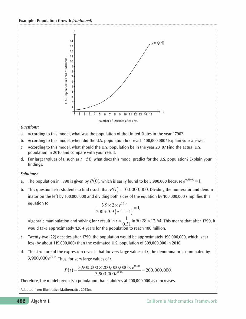
Example: Population Growth (continued)

y

14 y =Q( )t13

12

U.S

. Pop

ulat

ion

in T

ens o

f Mill

ions

11

10

9

8

7

6

5

4

3

2

1t

1 2 3 4 5 6 7 8 9 10 11 12 13 14 15

Number of Decades after 1790

Questions:

a. According to this model, what was the population of the United States in the year 1790?

b. According to this model, when did the U.S. population first reach 100,000,000? Explain your answer.

c. According to this model, what should the U.S. population be in the year 2010? Find the actual U.S.population in 2010 and compare with your result.

a. The population in 1790 is given by , which is easily found to be 3,900,000 because .

b. This question asks students to find such that . Dividing the numerator and denom-

inator on the left by 100,000,000 and dividing both sides of the equation by 100,000,000 simplifies this

equation to

Algebraic manipulation and solving for result in . This means that after 1790, it

would take approximately 126.4 years for the population to reach 100 million.

.

d. The structure of the expression reveals that for very large values of , the denominator is dominated by

. Thus, for very large values of ,

.

d. For larger values of , such as , what does this model predict for the U.S. population? Explain your findings.

Solutions:

c. Twenty-two (22) decades after 1790, the population would be approximately 190,000,000, which is farless (by about 119,000,000) than the estimated U.S. population of 309,000,000 in 2010.

Therefore, the model predicts a population that stabilizes at 200,000,000 as increases.

Adapted from Illustrative Mathematics 2013m.


Students can make good use of graphing software to investigate the effects of replacing a function

by , , , and for different types of functions (MP.5). For example,

starting with the simple quadratic function , students see the relationship between these

transformed functions and the vertex form of a general quadratic, . They under-

stand the notion of a family of functions and characterize such function families based on their

properties. These ideas are explored further with trigonometric functions (F-TF.5).

With standard F-BF.4a, students learn that some functions have the property that an input can be

recovered from a given output; for example, the equation can be solved for , given that

lies in the range of . Students understand that this is an attempt to “undo” the function, or to “go

backwards.” Tables and graphs should be used to support student understanding here. This standard

dovetails nicely with standard F-LE.4 described below and should be taught in progression with it.

Students will work more formally with inverse functions in advanced mathematics courses, and so

standard F-LE.4 should be treated carefully to prepare students for deeper understanding of functions

and their inverses.

Linear, Quadratic, and Exponential Models F-LE

Construct and compare linear, quadratic, and exponential models and solve problems.

4. For exponential models, express as a logarithm the solution to where , , and are numbers and the base is 2, 10, or ; evaluate the logarithm using technology. [Logarithms as solutions for exponentials]

4.1 Prove simple laws of logarithms. CA

4.2 Use the definition of logarithms to translate between logarithms in any base. CA

4.3 Understand and use the properties of logarithms to simplify logarithmic numeric expressions and to identify their approximate values. CA

Students worked with exponential models in Algebra I and continue this work in Algebra II. Since the

exponential function is always increasing or always decreasing for , 1, it can be deduced

that this function has an inverse, called the logarithm to the base , denoted by . The

logarithm has the property that if and only if , and this arises in contexts where one

wishes to solve an exponential equation. Students find logarithms with base equal to 2, 10, or by

hand and using technology (MP.5). Standards F-LE.4.1–4.3 call for students to explore the properties

of logarithms, such as , and students connect these properties to those of

exponents (e.g., the previous property comes from the fact that the logarithm represents an exponent

and that ). Students solve problems involving exponential functions and logarithms and

express their answers using logarithm notation (F-LE.4). In general, students understand logarithms

as functions that undo their corresponding exponential functions; instruction should emphasize this

relationship.


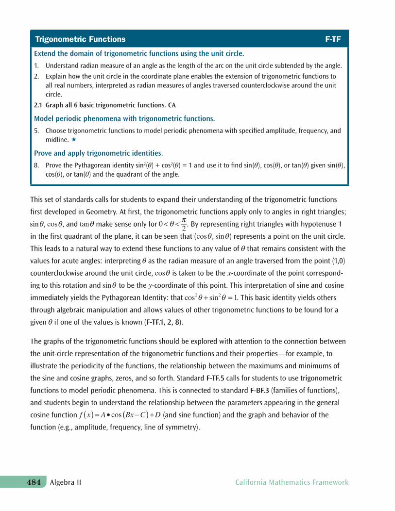
Trigonometric Functions F-TF

Extend the domain of trigonometric functions using the unit circle.

1. Understand radian measure of an angle as the length of the arc on the unit circle subtended by the angle.

2. Explain how the unit circle in the coordinate plane enables the extension of trigonometric functions toall real numbers, interpreted as radian measures of angles traversed counterclockwise around the unitcircle.

2.1 Graph all 6 basic trigonometric functions. CA

Model periodic phenomena with trigonometric functions.

5. Choose trigonometric functions to model periodic phenomena with specified amplitude, frequency, andmidline.

Prove and apply trigonometric identities.

8. Prove the Pythagorean identity sin2( ) + cos2( ) = 1 and use it to find sin( ), cos( ), or tan( ) given sin( ),cos( ), or tan( ) and the quadrant of the angle.

This set of standards calls for students to expand their understanding of the trigonometric functions

first developed in Geometry. At first, the trigonometric functions apply only to angles in right triangles;

, , and make sense only for . By representing right triangles with hypotenuse 1

in the first quadrant of the plane, it can be seen that ( , ) represents a point on the unit circle.

This leads to a natural way to extend these functions to any value of that remains consistent with the

values for acute angles: interpreting as the radian measure of an angle traversed from the point (1,0)

counterclockwise around the unit circle, is taken to be the -coordinate of the point correspond-

ing to this rotation and to be the -coordinate of this point. This interpretation of sine and cosine

immediately yields the Pythagorean Identity: that . This basic identity yields others

through algebraic manipulation and allows values of other trigonometric functions to be found for a

given if one of the values is known (F-TF.1, 2, 8).

The graphs of the trigonometric functions should be explored with attention to the connection between

the unit-circle representation of the trigonometric functions and their properties—for example, to

illustrate the periodicity of the functions, the relationship between the maximums and minimums of

the sine and cosine graphs, zeros, and so forth. Standard F-TF.5 calls for students to use trigonometric

functions to model periodic phenomena. This is connected to standard F-BF.3 (families of functions),

and students begin to understand the relationship between the parameters appearing in the general

cosine function (and sine function) and the graph and behavior of the

function (e.g., amplitude, frequency, line of symmetry).


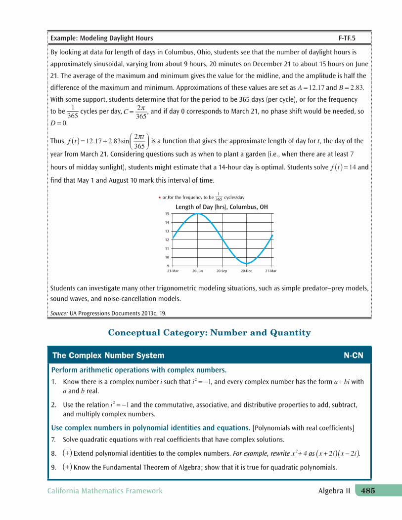
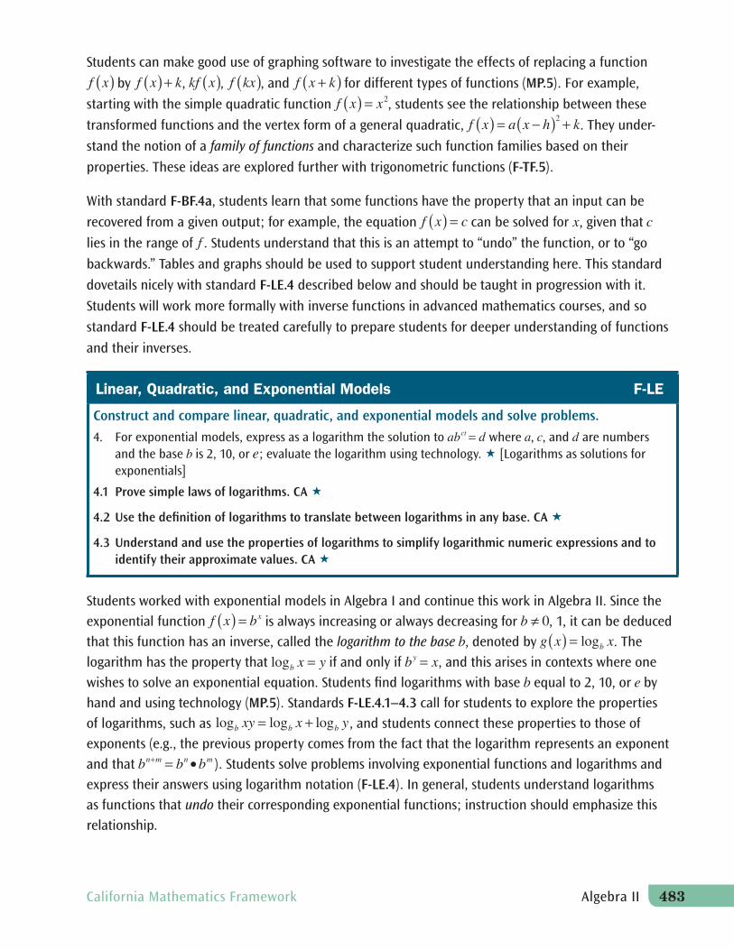
Example: Modeling Daylight Hours F-TF.5

By looking at data for length of days in Columbus, Ohio, students see that the number of daylight hours is

approximately sinusoidal, varying from about 9 hours, 20 minutes on December 21 to about 15 hours on June

21. The average of the maximum and minimum gives the value for the midline, and the amplitude is half the

difference of the maximum and minimum. Approximations of these values are set as and .

With some support, students determine that for the period to be 365 days (per cycle), or for the frequency

to be cycles per day, , and if day 0 corresponds to March 21, no phase shift would be needed, so

.

Thus, is a function that gives the approximate length of day for , the day of the

year from March 21. Considering questions such as when to plant a garden (i.e., when there are at least 7

hours of midday sunlight), students might estimate that a 14-hour day is optimal. Students solve and

find that May 1 and August 10 mark this interval of time.

Use complex numbers in polynomial identities and equations. [Polynomials with real coefficients]

7. Solve quadratic equations with real coefficients that have complex solutions.

9. Know the Fundamental Theorem of Algebra; show that it is true for quadratic polynomials.

8. Extend polynomial identities to the complex numbers. For example, rewrite as .

1. Know there is a complex number such that , and every complex number has the form with and real.

2. Use the relation and the commutative, associative, and distributive properties to add, subtract, and multiply complex numbers.

• or for the fry equency to be cycles/day

15

14

13

12

11

10

9

Length of Day (hrs), Columbus, OH

21-Mar 20-Jun 20-Sep 20-Dec 21-Mar

Students can investigate many other trigonometric modeling situations, such as simple predator–prey models,

sound waves, and noise-cancellation models.

Source: UA Progressions Documents 2013c, 19.

Conceptual Category: Number and Quantity

The Complex Number System N-CN

Perform arithmetic operations with complex numbers.


In Algebra I, students worked with examples of quadratic functions and solved quadratic equations,

encountering situations in which a resulting equation did not have a solution that is a real number—

for example, . In Algebra II, students complete their extension of the concept of number

to include complex numbers, numbers of the form , where is a number with the property that

. Students begin to work with complex numbers and apply their understanding of properties of

operations (the commutative, associative, and distributive properties) and exponents and radicals

to solve equations like those above, by finding square roots of negative numbers—for example, (MP.7). They also apply their understanding of properties of

operations and exponents and radicals to solve equations:

, which implies , or .

Now equations like these have solutions, and the extended number system forms yet another system

that behaves according to familiar rules and properties (N-CN.1–2; N-CN.7–9). By exploring examples

of polynomials that can be factored with real and complex roots, students develop an understanding

of the Fundamental Theorem of Algebra; they can show that the theorem is true for quadratic poly-

nomials by an application of the quadratic formula and an understanding of the relationship between

roots of a quadratic equation and the linear factors of the quadratic polynomial (MP.2).

Conceptual Category: Algebra

Along with the Number and Quantity standards in Algebra II, the Algebra conceptual category standards

develop the structural similarities between the system of polynomials and the system of integers.

Students draw on analogies between polynomial arithmetic and base-ten computation, focusing on

properties of operations, particularly the distributive property. Students connect multiplication of

polynomials with multiplication of multi-digit integers and division of polynomials with long division

of integers. Rational numbers extend the arithmetic of integers by allowing division by all numbers

except zero; similarly, rational expressions extend the arithmetic of polynomials by allowing division

by all polynomials except the zero polynomial. A central theme of this section is that the arithmetic of

rational expressions is governed by the same rules as the arithmetic of rational numbers.

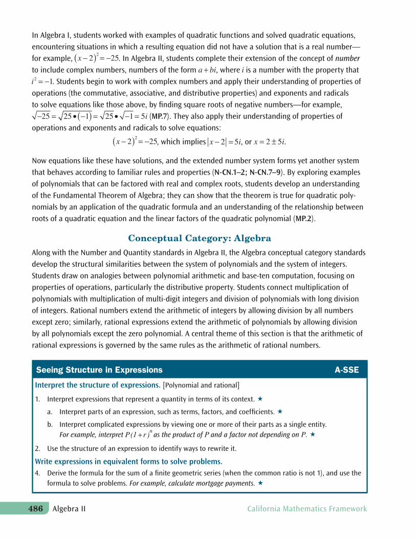
Seeing Structure in Expressions A-SSE

Interpret the structure of expressions. [Polynomial and rational]

1. Interpret expressions that represent a quantity in terms of its context.

a. Interpret parts of an expression, such as terms, factors, and coefficients.

b. Interpret complicated expressions by viewing one or more of their parts as a single entity.For example, interpret as the product of and a factor not depending on .

2. Use the structure of an expression to identify ways to rewrite it.

Write expressions in equivalent forms to solve problems.4. Derive the formula for the sum of a finite geometric series (when the common ratio is not 1), and use the

formula to solve problems. For example, calculate mortgage payments.


In Algebra II, students continue to pay attention to the meaning of expressions in context and interpret

the parts of an expression by “chunking”—that is, viewing parts of an expression as a single entity

(A-SSE.1–2). For example, their facility in using special cases of polynomial factoring allows them to

fully factor more complicated polynomials:

.

In a physics course, students may encounter an expression such as , which arises in the

theory of special relativity. Students can see this expression as the product of a constant and a term

that is equal to 1 when and equal to 0 when . Furthermore, they might be expected to see

this mentally, without having to go through a laborious process of evaluation. This involves combining

large-scale structure of the expression—a product of and another term—with the meaning of inter-

nal components such as (UA Progressions Documents 2013b, 4).

By examining the sums of examples of finite geometric series, students can look for patterns to justify

why the equation for the sum holds: . They may derive the formula with proof by

mathematical induction (MP.3) or by other means (A-SSE.4), as shown in the following example.

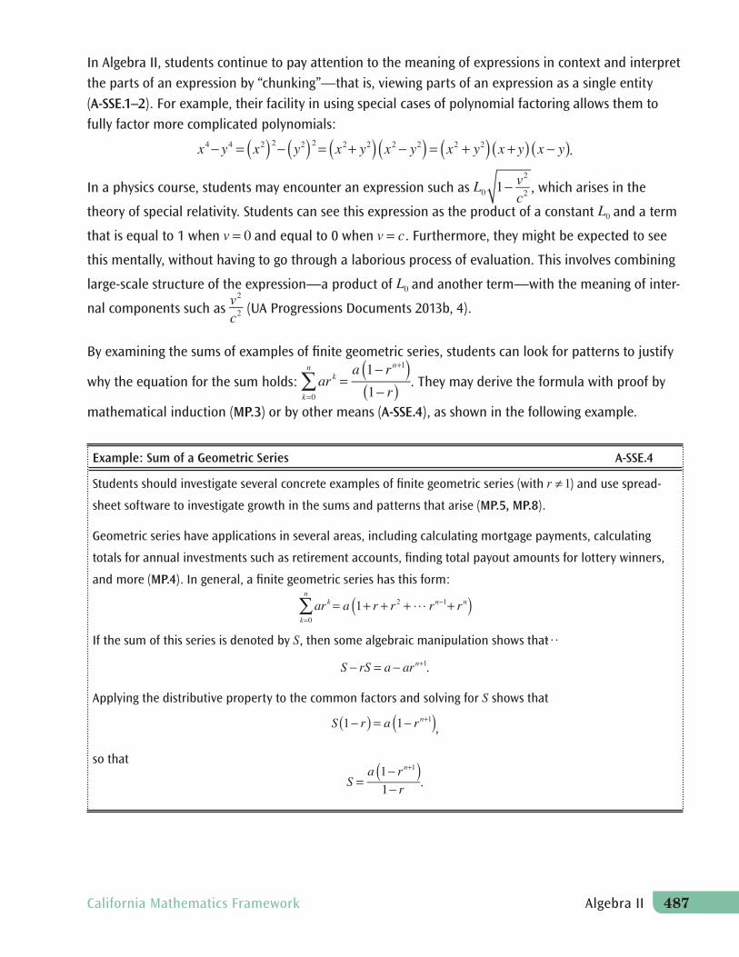
Example: Sum of a Geometric Series A-SSE.4

Students should investigate several concrete examples of finite geometric series (with ) and use spread-

sheet software to investigate growth in the sums and patterns that arise (MP.5, MP.8).

Geometric series have applications in several areas, including calculating mortgage payments, calculating

totals for annual investments such as retirement accounts, finding total payout amounts for lottery winners,

and more (MP.4). In general, a finite geometric series has this form:

If the sum of this series is denoted by , then some algebraic manipulation shows that

.

Applying the distributive property to the common factors and solving for shows that

,

so that

.


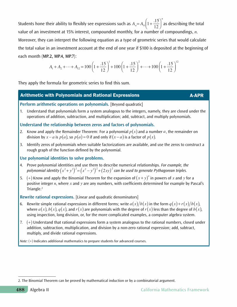
Students hone their ability to flexibly see expressions such as as describing the total

value of an investment at 15% interest, compounded monthly, for a number of compoundings, .

Moreover, they can interpret the following equation as a type of geometric series that would calculate

the total value in an investment account at the end of one year if $100 is deposited at the beginning of

each month (MP.2, MP.4, MP.7):

They apply the formula for geometric series to find this sum.

Arithmetic with Polynomials and Rational Expressions A-APR

Perform arithmetic operations on polynomials. [Beyond quadratic]

1. Understand that polynomials form a system analogous to the integers, namely, they are closed under theoperations of addition, subtraction, and multiplication; add, subtract, and multiply polynomials.

Understand the relationship between zeros and factors of polynomials.

2. Know and apply the Remainder Theorem: For a polynomial and a number , the remainder on division by is , so if and only if is a factor of .

3. Identify zeros of polynomials when suitable factorizations are available, and use the zeros to construct arough graph of the function defined by the polynomial.

Use polynomial identities to solve problems.

4. Prove polynomial identities and use them to describe numerical relationships. For example, thepolynomial identity can be used to generate Pythagorean triples.

5. Know and apply the Binomial Theorem for the expansion of in powers of and for a positive integer , where and are any numbers, with coefficients determined for example by Pascal’s Triangle.2

Rewrite rational expressions. [Linear and quadratic denominators]

6. Rewrite simple rational expressions in different forms; write in the form , where , , , and are polynomials with the degree of less than the degree of , using inspection, long division, or, for the more complicated examples, a computer algebra system.

7. Understand that rational expressions form a system analogous to the rational numbers, closed underaddition, subtraction, multiplication, and division by a non-zero rational expression; add, subtract,multiply, and divide rational expressions.

Note: Indicates additional mathematics to prepare students for advanced courses.

2. The Binomial Theorem can be proved by mathematical induction or by a combinatorial argument.



In Algebra II, students continue to develop their understanding of the set of polynomials as a system

analogous to the set of integers that exhibits particular properties, and they explore the relationship

between the factorization of polynomials and the roots of a polynomial (A-APR.1–3). It is shown that

when a polynomial is divided by , is written as , where is

a constant. This can be done by inspection or by polynomial long division (A-APR.6). It follows that

, so that is a factor of if and only if . This

result is generally known as the Remainder Theorem (A-APR.2), and provides an easy check to see

if a polynomial has a given linear polynomial as a factor. This topic should not be simply reduced to

“synthetic division,” which reduces the theorem to a method of carrying numbers between registers,

something easily done by a computer, while obscuring the reasoning that makes the result evident. It

is important to regard the Remainder Theorem as a theorem, not a technique (MP.3) [UA Progressions

Documents 2013b, 7].

Students use the zeros of a polynomial to create a rough sketch of its graph and connect the results to

their understanding of polynomials as functions (A-APR.3). The notion that polynomials can be used to

approximate other functions is important in higher mathematics courses such as Calculus, and standard

A-APR.3 is the first step in a progression that can lead students, as an extension topic, to constructing

polynomial functions whose graphs pass through any specified set of points in the plane.

In Algebra II, students explore rational functions as a system analogous to that of rational numbers.

They see rational functions as useful for describing many real-world situations—for instance, when

rearranging the equation to express the rate as a function of the time for a fixed distance and

obtaining . Now students see that any two polynomials can be divided in much the same way

as with numbers (provided the divisor is not zero). Students first understand rational expressions as

similar to other expressions in algebra, except that rational expressions have the form for both

and polynomials. They should have opportunities to evaluate various rational expressions for

many values of , both by hand and using software, perhaps discovering that when the degree of

is larger than the degree of , the value of the expression gets smaller in absolute value as gets

larger. When students understand the behavior of rational expressions in this way, it helps them see

rational expressions as functions and sets the stage for working with simple rational functions.


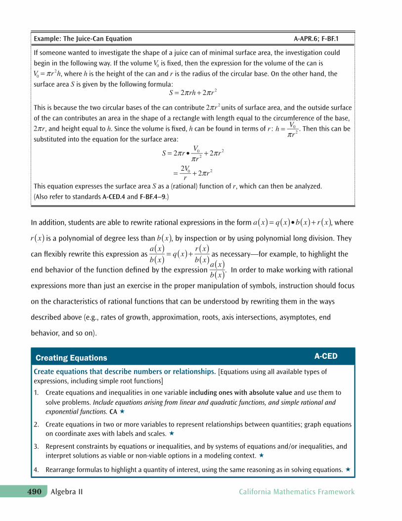
If someone wanted to investigate the shape of a juice can of minimal surface area, the investigation could

begin in the following way. If the volume is fixed, then the expression for the volume of the can is

, where is the height of the can and is the radius of the circular base. On the other hand, the

surface area is given by the following formula:

This is because the two circular bases of the can contribute units of surface area, and the outside sur

of the can contributes an area in the shape of a rectangle with length equal to the circumference of the b

, and height equal to . Since the volume is fixed, can be found in terms of : . Then this can

substituted into the equation for the surface area:

face

ase,

be

Example: The Juice-Can Equation A-APR.6; F-BF.1

This equation expresses the surface area as a (rational) function of , which can then be analyzed.

(Also refer to standards A-CED.4 and F-BF.4–9.)

In addition, students are able to rewrite rational expressions in the form , w

is a polynomial of degree less than , by inspection or by using polynomial long division. T

can flexibly rewrite this expression as as necessary—for example, to highlight t

end behavior of the function defined by the expression . In order to make working with rati

here

hey

he

onal

expressions more than just an exercise in the proper manipulation of symbols, instruction should focus

on the characteristics of rational functions that can be understood by rewriting them in the ways

described above (e.g., rates of growth, approximation, roots, axis intersections, asymptotes, end

behavior, and so on).

Creating Equations A-CED

Create equations that describe numbers or relationships. [Equations using all available types ofexpressions, including simple root functions]

1. Create equations and inequalities in one variable including ones with absolute value and use them to solve problems. Include equations arising from linear and quadratic functions, and simple rational and exponential functions. CA

2. Create equations in two or more variables to represent relationships between quantities; graph equations on coordinate axes with labels and scales.

3. Represent constraints by equations or inequalities, and by systems of equations and/or inequalities, and interpret solutions as viable or non-viable options in a modeling context.

4. Rearrange formulas to highlight a quantity of interest, using the same reasoning as in solving equations.



Students in Algebra II work with all available types of functions to create equations (A-CED.1). Although the functions referenced in standards A-CED.2–4 will often be linear, exponential, or quadratic, the types of problems should draw from more complex situations than those addressed in Algebra I. For example, knowing how to find the equation of a line through a given point perpendicular to another line makes it possible to find the distance from a point to a line. The Juice-Can Equation example presented previously in this section is connected to standard A-CED.4.

Reasoning with Equations and Inequalities A-REI

Understand solving equations as a process of reasoning and explain the reasoning. [Simple radical and rational]

2. Solve simple rational and radical equations in one variable, and give examples showing how extraneoussolutions may arise.

Solve equations and inequalities in one variable.

3.1 Solve one-variable equations and inequalities involving absolute value, graphing the solutions and interpreting them in context. CA

Represent and solve equations and inequalities graphically. [Combine polynomial, rational, radical, absolute value, and exponential functions.]

11. Explain why the -coordinates of the points where the graphs of the equations and

intersect are the solutions of the equation ; find the solutions approximately, e.g., using

technology to graph the functions, make tables of values, or find successive approximations. Include cases

where and/or are linear, polynomial, rational, absolute value, exponential, and logarithmic

functions.

Students extend their equation-solving skills to those involving rational expressions and radical

equations; they make sense of extraneous solutions that may arise (A-REI.2). In particular, students

understand that when solving equations, the flow of reasoning is generally forward, in the sense that

it is assumed a number is a solution of the equation and then a list of possibilities for is found.

However, not all steps in this process are reversible. For example, although it is true that if , then

, it is not true that if , then , as also satisfies this equation (UA Progressions

Documents 2013b, 10). Thus students understand that some steps are reversible and some are not, and

they anticipate extraneous solutions. In addition, students continue to develop their understanding

of solving equations as solving for values of such that , now including combinations of

linear, polynomial, rational, radical, absolute value, and exponential functions (A-REI.11). Students also

understand that some equations can be solved only approximately with the tools they possess.



Conceptual Category: Geometry

Expressing Geometric Properties with Equations G-GPE

Translate between the geometric description and the equation for a conic section.

3.1 Given a quadratic equation of the form , use the method for completing the square to put the equation into standard form; identify whether the graph of the equation is a circle, ellipse, parabola, or hyperbola and graph the equation. [In Algebra II, this standard addresses only circles and parabolas.] CA

No traditional Algebra II course would be complete without an examination of planar curves represented by the general equation . In Algebra II, students use “completing the square” (a skill learned in Algebra I) to decide if the equation represents a circle or parabola. They graph the shapes and relate the graph to the equation. The study of ellipses and hyperbolas is reservedfor a later course.

Conceptual Category: Statistics and ProbabilityStudents in Algebra II move beyond analysis of data to make sound statistical decisions based on probability models. The reasoning process is as follows: develop a statistical question in the form of a hypothesis (supposition) about a population parameter, choose a probability model for collecting data relevant to that parameter, collect data, and compare the results seen in the data with what is expected under the hypothesis. If the observed results are far from what is expected and have a low probability of occurring under the hypothesis, then that hypothesis is called into question. In other words, the evidence against the hypothesis is weighed by probability (S-IC.1) [UA Progressions Documents 2012d]. By investigating simple examples of simulations of experiments and observing outcomes of the data, students gain an understanding of what it means for a model to fit a particular data set (S-IC.2). This includes comparing theoretical and empirical results to evaluate the effectiveness of a treatment.

Interpreting Categorical and Quantitative Data S-ID

Summarize, represent, and interpret data on a single count or measurement variable.

4. Use the mean and standard deviation of a data set to fit it to a normal distribution and to estimatepopulation percentages. Recognize that there are data sets for which such a procedure is not appropriate.Use calculators, spreadsheets, and tables to estimate areas under the normal curve.

Although students may have heard of the normal distribution, it is unlikely that they will have prior

experience using the normal distribution to make specific estimates. In Algebra II, students build on

their understanding of data distributions to help see how the normal distribution uses area to make

estimates of frequencies (which can be expressed as probabilities). It is important for students to see

that only some data are well described by a normal distribution (S-ID.4). In addition, they can learn

through examples the empirical rule: that for a normally distributed data set, 68% of the data lie within

one standard deviation of the mean and 95% are within two standard deviations of the mean.



Example: The Empirical Rule S-ID.4

Suppose that SAT mathematics scores for a particular year are approximately normally distributed, with a mean of 510 and a standard deviation of 100.

a. What is the probability that a randomly selected score is greater than 610?

b. What is the probability that a randomly selected score is greater than 710?

c. What is the probability that a randomly selected score is between 410 and 710?

d. If a student’s score is 750, what is the student’s percentile score (the proportion of scores below 750)?

Solutions:

a. The score 610 is one standard deviation above the mean, so the tail area above that is about half of 0.32,or 0.16. The calculator gives 0.1586.

b. The score 710 is two standard deviations above the mean, so the tail area above that is about half of 0.05,or 0.025. The calculator gives 0.0227.

c. The area under a normal curve from one standard deviation below the mean to two standard deviationsabove the mean is about 0.815. The calculator gives 0.8186.

d. Using either the normal distribution given or the standard normal (for which 750 translates to a z-score of2.4), the calculator gives 0.9918.

Making Inferences and Justifying Conclusions S-IC

Understand and evaluate random processes underlying statistical experiments.

1. Understand statistics as a process for making inferences about population parameters based on a randomsample from that population.

2. Decide if a specified model is consistent with results from a given data-generating process, e.g., usingsimulation. For example, a model says a spinning coin falls heads up with probability 0.5. Would a result of5 tails in a row cause you to question the model?

Make inferences and justify conclusions from sample surveys, experiments, and observational studies.

3. Recognize the purposes of and differences among sample surveys, experiments, and observationalstudies; explain how randomization relates to each.

4. Use data from a sample survey to estimate a population mean or proportion; develop a margin of errorthrough the use of simulation models for random sampling.

5. Use data from a randomized experiment to compare two treatments; use simulations to decide if differ-ences between parameters are significant.

6. Evaluate reports based on data.

In earlier grade levels, students are introduced to different ways of collecting data and use graphical displays and summary statistics to make comparisons. These ideas are revisited with a focus on how the way in which data are collected determines the scope and nature of the conclusions that can be drawn from those data. The concept of statistical significance is developed informally through simulation as meaning a result that is unlikely to have occurred solely through random selection in sampling or


random assignment in an experiment (NGA/CCSSO 2010a). When covering standards S-IC.4–5, instructors should focus on the variability of results from experiments—that is, on statistics as a way of handling, not eliminating, inherent randomness. Because standards S-IC.1–6 are all modeling standards, students should have ample opportunities to explore statistical experiments and informally arrive at statistical techniques.

Example: Estimating a Population Proportion S-IC.1–6

Suppose a student wishes to investigate whether 50% of homeowners in her neighborhood will support a new tax to fund local schools. If she takes a random sample of 50 homeowners in her neighborhood, and 20 support the new tax, then the sample proportion agreeing to pay the tax would be 0.4. But is this an accurate measure of the true proportion of homeowners who favor the tax? How can this be determined?

If this sampling situation (MP.4) is simulated with a graphing calculator or spreadsheet software under the assumption that the true proportion is 50%, then the student can arrive at an understanding of the probabil-ity that her randomly sampled proportion would be 0.4. A simulation of 200 trials might show that 0.4 arose 25 out of 200 times, or with a probability of 0.125. Thus, the chance of obtaining 40% as a sample proportion is not insignificant, meaning that a true proportion of 50% is plausible.

Adapted from UA Progressions Documents 2012d.

Using Probability to Make Decisions S-MD

Use probability to evaluate outcomes of decisions. [Include more complex situations.]

6. (+) Use probabilities to make fair decisions (e.g., drawing by lots, using a random number generator).

7. (+) Analyze decisions and strategies using probability concepts (e.g., product testing, medical testing,pulling a hockey goalie at the end of a game).

As in Geometry, students apply probability models to make and analyze decisions. In Algebra II, this skill is extended to more complex probability models, including situations such as those involving quality control or diagnostic tests that yield both false-positive and false-negative results. See the University of Arizona Progressions document titled “High School Statistics and Probability” for further explanation and examples: http://ime.math.arizona.edu/progressions/ (UA Progressions Documents 2012d [accessed April 6, 2015]).

Algebra II is the culmination of the Traditional Pathway in mathematics. Students completing this pathway will be well prepared for higher mathematics and should be encouraged to continue their study of mathematics with Precalculus or other mathematics electives, such as Statistics and Probability or a course in modeling.



http://ime.math.arizona.edu/progressions/

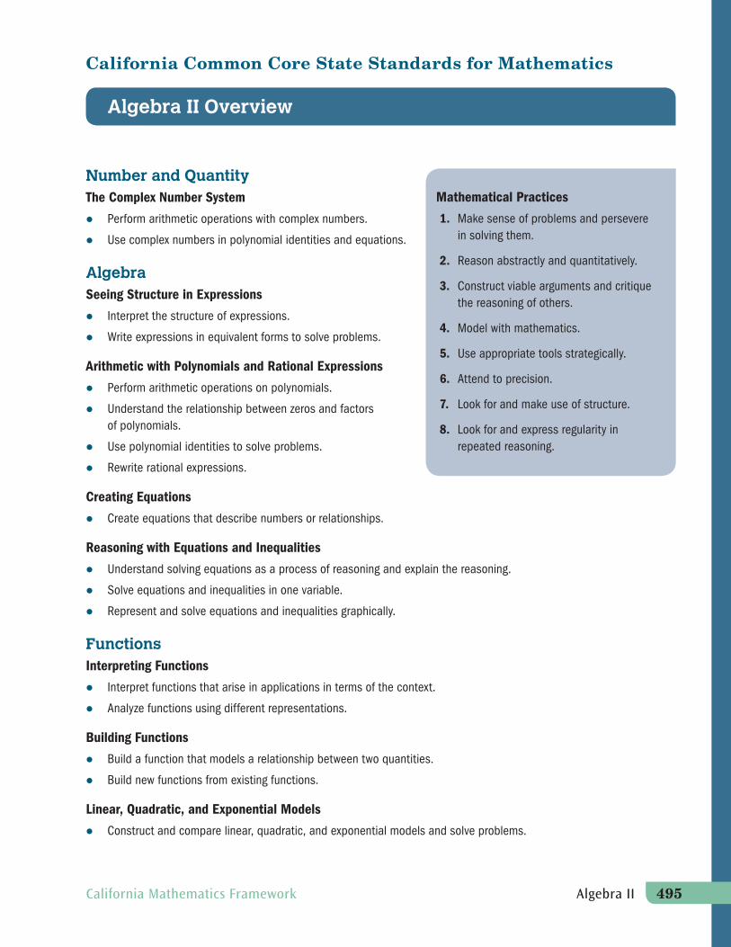
Algebra II Overview

California Common Core State Standards for Mathematics

Number and QuantityThe Complex Number System


Use complex numbers in polynomial identities and equations.

AlgebraSeeing Structure in Expressions

Interpret the structure of expressions.

Write expressions in equivalent forms to solve problems.

Arithmetic with Polynomials and Rational Expressions

Perform arithmetic operations on polynomials.

Understand the relationship between zeros and factorsof polynomials.


Rewrite rational expressions.

Creating Equations

Create equations that describe numbers or relationships.

Reasoning with Equations and Inequalities

Understand solving equations as a process of reasoning and explain the reasoning.


Represent and solve equations and inequalities graphically.

FunctionsInterpreting Functions

Interpret functions that arise in applications in terms of the context.

Analyze functions using different representations.

Building Functions

Build a function that models a relationship between two quantities.

Build new functions from existing functions.

Linear, Quadratic, and Exponential Models


Mathematical Practices

1. Make sense of problems and perseverein solving them.

2. Reason abstractly and quantitatively.

3. Construct viable arguments and critiquethe reasoning of others.

4. Model with mathematics.

5. Use appropriate tools strategically.

6. Attend to precision.

7. Look for and make use of structure.

8. Look for and express regularity inrepeated reasoning.


Algebra II Overview (continued)

Trigonometric Functions




GeometryExpressing Geometric Properties with Equations


Statistics and ProbabilityInterpreting Categorical and Quantitative Data


Making Inferences and Justifying Conclusions



Using Probability to Make Decisions

Use probability to evaluate outcomes of decisions.


Algebra IIA2

Number and Quantity

The Complex Number System N-CN


1. Know there is a complex number such that , and every complex number has the form with and real.

2. Use the relation and the commutative, associative, and distributive properties to add, subtract, and multiply

complex numbers.

Use complex numbers in polynomial identities and equations. [Polynomials with real coefficients]

7. Solve quadratic equations with real coefficients that have complex solutions.

8. Extend polynomial identities to the complex numbers. For example, rewrite as .

9. Know the Fundamental Theorem of Algebra; show that it is true for quadratic polynomials.

Algebra

Seeing Structure in Expressions A-SSE

Interpret the structure of expressions. [Polynomial and rational]

1. Interpret expressions that represent a quantity in terms of its context.

a. Interpret parts of an expression, such as terms, factors, and coefficients.

b. Interpret complicated expressions by viewing one or more of their parts as a single entity. For example,interpret as the product of and a factor not depending on .

2. Use the structure of an expression to identify ways to rewrite it.

Write expressions in equivalent forms to solve problems.

4. Derive the formula for the sum of a finite geometric series (when the common ratio is not 1), and use the formula tosolve problems. For example, calculate mortgage payments.


Perform arithmetic operations on polynomials. [Beyond quadratic]

1. Understand that polynomials form a system analogous to the integers, namely, they are closed under the operationsof addition, subtraction, and multiplication; add, subtract, and multiply polynomials.

Understand the relationship between zeros and factors of polynomials.

2. Know and apply the Remainder Theorem: For a polynomial and a number , the remainder on division by is , so if and only if is a factor of .

3. Identify zeros of polynomials when suitable factorizations are available, and use the zeros to construct a rough graphof the function defined by the polynomial.


A2Algebra II


4. Prove polynomial identities and use them to describe numerical relationships. For example, the polynomial identity can be used to generate Pythagorean triples.2

5. Know and apply the Binomial Theorem for the expansion of in powers of and for a positive integer , where and are any numbers, with coefficients determined for example by Pascal’s Triangle.3

Rewrite rational expressions. [Linear and quadratic denominators]

6. Rewrite simple rational expressions in different forms; write in the form , where , , , and are polynomials with the degree of less than the degree of , using inspection, long

division, or, for the more complicated examples, a computer algebra system.

7. Understand that rational expressions form a system analogous to the rational numbers, closed under addition,subtraction, multiplication, and division by a non-zero rational expression; add, subtract, multiply, and divide rationalexpressions.


Create equations that describe numbers or relationships. [Equations using all available types of expressions, including

simple root functions]

1. Create equations and inequalities in one variable including ones with absolute value and use them to solveproblems. Include equations arising from linear and quadratic functions, and simple rational and exponentialfunctions. CA

2. Create equations in two or more variables to represent relationships between quantities; graph equations oncoordinate axes with labels and scales.

3. Represent constraints by equations or inequalities, and by systems of equations and/or inequalities, and interpretsolutions as viable or non-viable options in a modeling context.

4. Rearrange formulas to highlight a quantity of interest, using the same reasoning as in solving equations.


Understand solving equations as a process of reasoning and explain the reasoning. [Simple radical and rational]

2. Solve simple rational and radical equations in one variable, and give examples showing how extraneous solutionsmay arise.


3.1 Solve one-variable equations and inequalities involving absolute value, graphing the solutions and interpreting them in context. CA

Note: Indicates a modeling standard linking mathematics to everyday life, work, and decision making. (+) Indicates additional mathematics to prepare students for advanced courses.3. The Binomial Theorem can be proved by mathematical induction or by a combinatorial argument.


11. Explain why the x -coordinates of the points where the graphs of the equations y = f (x) and y = g(x) intersect arethe solutions of the equation f (x) = g(x); find the solutions approximately, e.g., using technology to graph thefunctions, make tables of values, or find successive approximations. Include cases where f (x) and/or g(x) arelinear, polynomial, rational, absolute value, exponential, and logarithmic functions.

f

-

Algebra IIA2


Represent and solve equations and inequalities graphically. [Combine polynomial, rational, radical, absolute value, and exponential functions.]

Functions

Interpreting Functions F-IF

Interpret functions that arise in applications in terms of the context. [Emphasize selection of appropriate models.]

4. For a function that models a relationship between two quantities, interpret key features of graphs and tables interms of the quantities, and sketch graphs showing key features given a verbal description of the relationship. Keyfeatures include: intercepts; intervals where the function is increasing, decreasing, positive, or negative; relativemaximums and minimums; symmetries; end behavior; and periodicity.

5. Relate the domain of a function to its graph and, where applicable, to the quantitative relationship it describes.

6. Calculate and interpret the average rate of change of a function (presented symbolically or as a table) over aspecified interval. Estimate the rate of change from a graph.

Analyze functions using different representations. [Focus on using key features to guide selection of appropriate type omodel function.]

7. Graph functions expressed symbolically and show key features of the graph, by hand in simple cases and usingtechnology for more complicated cases.

b. Graph square root, cube root, and piecewise-defined functions, including step functions and absolute valuefunctions.

c. Graph polynomial functions, identifying zeros when suitable factorizations are available, and showing end behavior.

e. Graph exponential and logarithmic functions, showing intercepts and end behavior, and trigonometric functions,showing period, midline, and amplitude.

8. Write a function defined by an expression in different but equivalent forms to reveal and explain different propertiesof the function.

9. Compare properties of two functions each represented in a different way (algebraically, graphically, numerically intables, or by verbal descriptions).

Building Functions F-BF

Build a function that models a relationship between two quantities. [Include all types of functions studied.]

1. Write a function that describes a relationship between two quantities.

b. Combine standard function types using arithmetic operations. For example, build a function that models thetemperature of a cooling body by adding a constant function to a decaying exponential, and relate thesefunctions to the model.

A2Algebra II

Build new functions from existing functions. [Include simple radical, rational, and exponential functions; emphasize common effect of each transformation across function types.]

3. Identify the effect on the graph of replacing f (x) by f (x)+ k , kf (x), f (kx), and f (x + k) for specific values of k(both positive and negative); find the value of k given the graphs. Experiment with cases and illustrate an explana-tion of the effects on the graph using technology. Include recognizing even and odd functions from their graphs andalgebraic expressions for them.

4. Find inverse functions.

a. Solve an equation of the form for a simple function that has an inverse and write an expression for the inverse. For example, or for .

Linear, Quadratic, and Exponential Models F-LE


4. For exponential models, express as a logarithm the solution to where , , and are numbers and the base is 2, 10, or ; evaluate the logarithm using technology. [Logarithms as solutions for exponentials]

4.1 Prove simple laws of logarithms. CA

4.2 Use the definition of logarithms to translate between logarithms in any base. CA

4.3 Understand and use the properties of logarithms to simplify logarithmic numeric expressions and to identify their approximate values. CA

Trigonometric Functions F-TF


1. Understand radian measure of an angle as the length of the arc on the unit circle subtended by the angle.

2. Explain how the unit circle in the coordinate plane enables the extension of trigonometric functions to all real num-bers, interpreted as radian measures of angles traversed counterclockwise around the unit circle.

2.1 Graph all 6 basic trigonometric functions. CA


5. Choose trigonometric functions to model periodic phenomena with specified amplitude, frequency, and midline.


8. Prove the Pythagorean identity sin2( ) + cos2( ) = 1 and use it to find sin ( ), cos ( ), or tan ( ) given sin ( ),cos( ), or tan ( ) and the quadrant of the angle.



3.1 Given a quadratic equation of the form , use the method for completing the square to put the equation into standard form; identify whether the graph of the equation is a circle, ellipse, parabola, or hyperbola and graph the equation. [In Algebra II, this standard addresses only circles and parabolas.] CA

Geometry



Statistics and Probability



4. Use the mean and standard deviation of a data set to fit it to a normal distribution and to estimate population percentages. Recognize that there are data sets for which such a procedure is not appropriate. Use calculators, spreadsheets, and tables to estimate areas under the normal curve.



1. Understand statistics as a process for making inferences about population parameters based on a random sample from that population.

2. Decide if a specified model is consistent with results from a given data-generating process, e.g., using simulation. For example, a model says a spinning coin falls heads up with probability 0.5. Would a result of 5 tails in a row cause you to question the model?


3. Recognize the purposes of and differences among sample surveys, experiments, and observational studies; explain how randomization relates to each.

4. Use data from a sample survey to estimate a population mean or proportion; develop a margin of error through the use of simulation models for random sampling.

5. Use data from a randomized experiment to compare two treatments; use simulations to decide if differences between parameters are significant.

6. Evaluate reports based on data.


Use probability to evaluate outcomes of decisions. [Include more complex situations.]

6. Use probabilities to make fair decisions (e.g., drawing by lots, using a random number generator).

7. Analyze decisions and strategies using probability concepts (e.g., product testing, medical testing, pulling a hockey goalie at the end of a game).

Algebra IIA2




Using Probability to Make Decisions S-M

This page intentionally blank.