Embed Size (px)
Citation preview
8/10/2019 algebra and calculus.pdf
http://slidepdf.com/reader/full/algebra-and-calculuspdf 1/135
8/10/2019 algebra and calculus.pdf
http://slidepdf.com/reader/full/algebra-and-calculuspdf 2/135
ii
c The University of Southern Queensland, 2007.
Published by
The University of Southern QueenslandToowoomba Qld 4350Australia
http://www.usq.edu.au
Copyrighted materials reproduced herein are used under the provisions of theCopyright Act 1968 as amended, or as a result of application to the copyrightowner.
No part of this publication may be reproduced, stored in a retrieval system ortransmitted in any form or by any means electronic, mechanical, photocopying,recording or otherwise without prior permission.
Produced using L ATEX in the USQ style.
8/10/2019 algebra and calculus.pdf
http://slidepdf.com/reader/full/algebra-and-calculuspdf 3/135
Preface
Welcome to Algebra & Calculus I! We look forward to meeting you, in-troducing you to a wonderful wide range of mathematical techniques andapplications, and assisting you to build academic and professional skills andunderstanding via these studies!
You will study two modules, Algebra and Calculus, in parallel, and thisStudy Book is intended to direct your path through the prescribed texts,readings and activities for each module. Use it in conjunction with yourIntroductory Book which has the weekly Study Schedule.
Reading your Study Book and texts is just the start! You will be required todevelop and demonstrate a broad range of skills. Your goal will be to applythe course concepts and processes to both new and familiar situations, andto communicate your methods and results using the appropriate terminologyand notation.
The assignment tasks alone will offer hopelessly inadequate practice. Youwill need to do a wide selection of exercises to build your experience, gaincondence, and learn to work quickly.
Besides this Study Book, the prescribed texts are
ELEMENTARY LINEAR ALGEBRA , 5th Edition (2004), by Larson, Ed-wards & Falvo, published by Houghton Mifflin; and
CALCULUS: Concepts & Contexts , 3rd Edition (2004 or 2005), by JamesStewart, published by Brooks/Cole.
iii

8/10/2019 algebra and calculus.pdf
http://slidepdf.com/reader/full/algebra-and-calculuspdf 4/135
iv
8/10/2019 algebra and calculus.pdf
http://slidepdf.com/reader/full/algebra-and-calculuspdf 5/135
Table of Contents
I POWERFUL AND FASCINATING ALGEBRA 1
0 Preliminary Work on Vectors in the Plane and in Space 7
0.1 Vectors in the Plane . . . . . . . . . . . . . . . . . . . . . . . 9
0.2 The Scalar Product and Projections in R2 . . . . . . . . . . . 11
0.3 Vectors in Space . . . . . . . . . . . . . . . . . . . . . . . . . 17
0.4 The Cross Product of Two Vectors . . . . . . . . . . . . . . . 18
0.5 Lines and Planes in Space . . . . . . . . . . . . . . . . . . . . 20
0.6 Summary: Vectors . . . . . . . . . . . . . . . . . . . . . . . . 28
1 Systems of Linear Equations 29
1.1 Introduction to Systems of Linear Equations . . . . . . . . . 30
1.2 Gaussian Elimination and Gauss-Jordan Elimination . . . . . 34
1.3 Application of Systems of Linear Equations . . . . . . . . . . 36
1.4 Chapter Summary: Systems of Linear Equations. . . . . . . . 37
2 Matrices 39
2.1 Operations with Matrices . . . . . . . . . . . . . . . . . . . . 40
v
8/10/2019 algebra and calculus.pdf
http://slidepdf.com/reader/full/algebra-and-calculuspdf 6/135
vi Table of Contents
2.2 Properties of Matrix Operations . . . . . . . . . . . . . . . . 41
2.3 The Inverse of a Matrix . . . . . . . . . . . . . . . . . . . . . 42
2.4 Elementary Matrices . . . . . . . . . . . . . . . . . . . . . . . 43
2.5 Applications of Matrix Operations . . . . . . . . . . . . . . . 43
2.6 Summary: Matrices . . . . . . . . . . . . . . . . . . . . . . . 44
3 Determinants 45
3.1 The Determinant of a Matrix . . . . . . . . . . . . . . . . . . 46
3.2 Evaluation of a Determinant using Elementary Operations . . 48
3.3 Properties of Determinants . . . . . . . . . . . . . . . . . . . 49
3.4 Chapter Summary on Determinants. . . . . . . . . . . . . . . 50
4 Complex Numbers 51
4.1 Complex Numbers: Definition . . . . . . . . . . . . . . . . . . 52
4.2 Conjugates and Division of Complex Numbers . . . . . . . . 53
4.3 Polar Form and de Moivre’s Theorem . . . . . . . . . . . . . 54
4.4 Euler’s Form of a Complex Number . . . . . . . . . . . . . . 56
4.5 Solving Equations . . . . . . . . . . . . . . . . . . . . . . . . 62
4.6 Functions of Complex Variable z . . . . . . . . . . . . . . . . 68
4.7 Summary: Complex Numbers . . . . . . . . . . . . . . . . . . 73
II CLEVER CALCULUS 75
1 Functions and Models 79
1.1 Four Ways to Represent a Function . . . . . . . . . . . . . . . 80
1.2 Mathematical Models: a Catalog of Essential Functions . . . 81
1.3 New Functions From Old Functions. . . . . . . . . . . . . . . 83
1.4 Graphing Calculators and Computers . . . . . . . . . . . . . 84
8/10/2019 algebra and calculus.pdf
http://slidepdf.com/reader/full/algebra-and-calculuspdf 7/135
Table of Contents vii
1.5 Exponential Functions . . . . . . . . . . . . . . . . . . . . . . 84
1.6 Inverse Functions and Logarithms . . . . . . . . . . . . . . . 85
2 Limits and Derivatives 87
2.1 The Tangent and Velocity Problems . . . . . . . . . . . . . . 88
2.2 The Limit of a Function . . . . . . . . . . . . . . . . . . . . . 88
2.3 Calculating Limits Using the Limit Laws . . . . . . . . . . . . 89
2.4 Continuity . . . . . . . . . . . . . . . . . . . . . . . . . . . . . 90
2.5 Limits Involving Innity . . . . . . . . . . . . . . . . . . . . . 91
2.6 Tangents, Velocities, and Other Rates of Change . . . . . . . 91
2.7 Derivatives . . . . . . . . . . . . . . . . . . . . . . . . . . . . 92
2.8 The Derivative as a Function . . . . . . . . . . . . . . . . . . 93
2.9 What does f say about f ? . . . . . . . . . . . . . . . . . . . 95
3 Differentiation Rules 97
3.1 Derivatives of Polynomials and Exponential Functions . . . . 98
3.2 The Product and Quotient Rules . . . . . . . . . . . . . . . . 99
3.3 Rates of Change in the Natural and Social Sciences . . . . . . 100
3.4 Derivatives of Trigonometric Functions . . . . . . . . . . . . . 101
3.5 The Chain Rule . . . . . . . . . . . . . . . . . . . . . . . . . . 101
3.6 Implicit Differentiation . . . . . . . . . . . . . . . . . . . . . . 102
3.7 Derivatives of Logarithmic Functions . . . . . . . . . . . . . . 103
4 Applications of Differentiation 105
4.1 Related Rates . . . . . . . . . . . . . . . . . . . . . . . . . . . 106
4.2 Maximum and Minimum Values . . . . . . . . . . . . . . . . 106
4.3 Derivatives and the Shapes of Curves . . . . . . . . . . . . . . 107
4.4 Graphing with Calculus and Calculators . . . . . . . . . . . . 108
8/10/2019 algebra and calculus.pdf
http://slidepdf.com/reader/full/algebra-and-calculuspdf 8/135
viii Table of Contents
4.5 Indeterminate Forms and l’Hospital’s Rule . . . . . . . . . . . 108
4.6 Optimisation Problems . . . . . . . . . . . . . . . . . . . . . . 108
4.7 Applications to Business and Economics . . . . . . . . . . . . 109
4.8 Newton’s Method . . . . . . . . . . . . . . . . . . . . . . . . . 109
4.9 Antiderivatives . . . . . . . . . . . . . . . . . . . . . . . . . . 109
5 Integrals 111
5.1 Areas and Distances . . . . . . . . . . . . . . . . . . . . . . . 112
5.2 The Denite Integral . . . . . . . . . . . . . . . . . . . . . . . 113
5.3 Evaluating Denite Integrals . . . . . . . . . . . . . . . . . . 114
5.4 The Fundamental Theorem of Calculus . . . . . . . . . . . . . 115
5.5 The Substitution Rule . . . . . . . . . . . . . . . . . . . . . . 116
5.6 Integration by Parts . . . . . . . . . . . . . . . . . . . . . . . 117
5.7 Additional Techniques of Integration . . . . . . . . . . . . . . 118
5.8 Integration Using Tables and Computer Algebra Systems . . 1195.9 Approximate Integration . . . . . . . . . . . . . . . . . . . . . 119
6 Applications of Integration 121
6.1 More about Areas . . . . . . . . . . . . . . . . . . . . . . . . 122
6.2 Volumes . . . . . . . . . . . . . . . . . . . . . . . . . . . . . . 122
6.3 Arc Length . . . . . . . . . . . . . . . . . . . . . . . . . . . . 123
6.4 Average Value of a Function . . . . . . . . . . . . . . . . . . . 1236.5 Applications to Physics and Engineering . . . . . . . . . . . . 123
III APPENDICES A, B and C:Readings for Vectors, Chapter 0 125
8/10/2019 algebra and calculus.pdf
http://slidepdf.com/reader/full/algebra-and-calculuspdf 9/135
Module I
POWERFULAND
FASCINATINGALGEBRA
1

8/10/2019 algebra and calculus.pdf
http://slidepdf.com/reader/full/algebra-and-calculuspdf 10/135
8/10/2019 algebra and calculus.pdf
http://slidepdf.com/reader/full/algebra-and-calculuspdf 11/135
Overview
This module has powerful, wide-reaching and important applications in mostelds of endeavour! Browse overleaf, to see applications of your LinearAlgebra to computer graphics, cryptography, computed tomography to gainimages of the human body, CAT scans, electrical networks, traffic networks,forest management, population growth, genetics, temperature distributions,chaos theory, and games of strategy, to list but a few! Some elementaryapplications will be developed in this course; many more will arise in yourfurther studies.
Two and three-dimensional geometric Vectors were developed to representand study physical phenomena and motion in real-world applications. Welook at their geometric and algebraic properties, see how useful these are for
describing motion, and how readily and easily they can be used to describethe properties and equations of lines and planes in space. The properties wedevelop here extend very easily to vectors of more than 3 dimensions, and soin Algebra & Calculus II we will apply them again to vectors of n-dimensionsin a host of further applications!
Large data sets and big systems of linear equations arise with astonishingfrequency in important scientic, industrial and economic applications. Wewill see how to use matrices to store and manipulate data, and to manageand solve systems of linear equations. We will characterise some importanttypes of matrices, and gain expertise with the different types of solutions
that emerge from linear systems.Complex numbers are a brief and fascinating nale. While they arose his-torically out of attempts to create square roots of negative numbers, theirgeometric and algebraic properties have yielded remarkably practical appli-cations. We look briey at how complex numbers and their functions arecommonly used to analyse real-world phenomena and solve equations.
The title Algebra really is a misnomer for this module, because in parallel wedevelop the vitally important Geometry of vectors, matrices and complex
3
8/10/2019 algebra and calculus.pdf
http://slidepdf.com/reader/full/algebra-and-calculuspdf 12/135
4
numbers. You will see how fruitful all are for applications, learn how to
exploit them, and become aware of strong links between them.
Some Applications of Vectors and Matri-ces
Browse these following pages for a listing of a wide and powerful range of applications of Linear Algebra concepts covered in Algebra & Calculus I andII. They are the index for Chapter 11 of the text Elementary Linear Algebra:Applications Version, Edition 8 , by Anton and Rorres.
Note also that a few of these applications are included in Appendix C of this Study Book, for your perusal.
8/10/2019 algebra and calculus.pdf
http://slidepdf.com/reader/full/algebra-and-calculuspdf 13/135
Module Objectives
By the end of this Module, you should recognise a host of areas of application
of vectors, matrices and complex numbers, be aware of their power andbeauty, and be able to exploit them in other areas and disciplines, as wellas in Algebra & Calculus II.
It is vitally important that you understand the links between these concepts.Always read with pencil in hand, and conrm the steps as you go. Visualisingis a powerful aid: draw diagrams wherever you can!
Use technology where encouraged to do so! It’s fun and helpful, and theweekly tutorial/laboratory tasks and the assignments will help you developthe necessary skills with our careful full support!
At the end of each Chapter you should
• have mastered the concepts covered
• be able to link their algebra and geometry
• be competent with the processes, terminology, and notation
• have mastered a wide range of exercises
• be able to communicate your reasoning well, using correct languageand symbols
• be able to apply the concepts in a range of contexts, new and familiar
At the end of this Module, you should
• see links between vectors, matrices and complex numbers
• recognise contexts in which they are valuable
• be able to manipulate and apply these concepts competently
• be able to demonstrate and communicate those skills appropriately
5

8/10/2019 algebra and calculus.pdf
http://slidepdf.com/reader/full/algebra-and-calculuspdf 14/135
6
8/10/2019 algebra and calculus.pdf
http://slidepdf.com/reader/full/algebra-and-calculuspdf 15/135
Chapter 0Preliminary Work onVectors in the Planeand in Space
A good understanding of geometric Vectors in two and three dimensions isvital for your study of motion and Calculus!
Knowing how to use vectors to describe motion and geometrical objects, isvital before you study Chapters 1 to 3 of your Linear Algebra text, andthat is why we include this preliminary Chapter before moving on to thosesection of Elementary Linear Algebra , Ed 5, Larson, Edwards & Falvo.
This preliminary Chapter 0 also forms a solid foundation for your Calculusstudies in Algebra & Calculus II.
Note that we offer two sets of readings on Vectors, so that youhave really good support and a choice of style.
• Sections 9.1 to 9.5 of your Stewart text Calculus: Concepts and Con-texts , 3nd Edition. These offer concise style and good applications.
• Appendix A of this Study Book, marked by a yellow pages has excerptsfrom Grossman’s Elementary Linear Algebra , 4th Ed. You may preferhis fuller style to Stewart’s, and we support your exercises by includingworked solutions to the odd number questions.
7
8/10/2019 algebra and calculus.pdf
http://slidepdf.com/reader/full/algebra-and-calculuspdf 16/135
8 Chapter 0. Preliminary Work on Vectors in the Plane and in Space
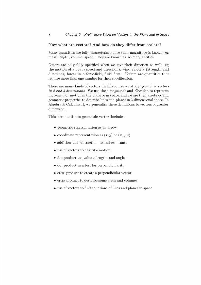
Now what are vectors? And how do they differ from scalars?
Many quantities are fully characterised once their magnitude is known: egmass, length, volume, speed. They are known as scalar quantities.
Others are only fully specied when we give their direction as well: egthe motion of a boat (speed and direction), wind velocity (strength anddirection), forces in a force-eld, uid ow. Vectors are quantities thatrequire more than one number for their specication.
There are many kinds of vectors. In this course we study geometric vectors in 2 and 3 dimensions . We use their magnitude and direction to representmovement or motion in the plane or in space, and we use their algebraic and
geometric properties to describe lines and planes in 3-dimensional space. InAlgebra & Calculus II, we generalise these denitions to vectors of greaterdimension.
This introduction to geometric vectors includes:
• geometric representation as an arrow
• coordinate representation as ( x, y) or (x,y,z )
• addition and subtraction, to nd resultants
• use of vectors to describe motion
• dot product to evaluate lengths and angles
• dot product as a test for perpendicularity
• cross product to create a perpendicular vector
• cross product to describe some areas and volumes
• use of vectors to nd equations of lines and planes in space
8/10/2019 algebra and calculus.pdf
http://slidepdf.com/reader/full/algebra-and-calculuspdf 17/135
0.1. Vectors in the Plane 9
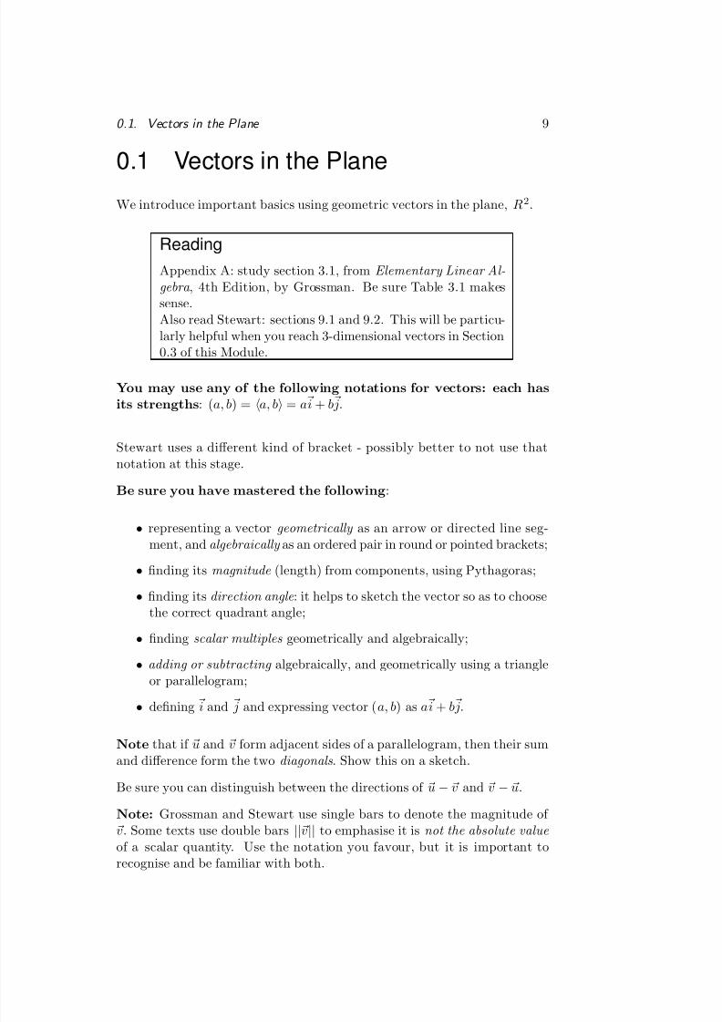
0.1 Vectors in the Plane
We introduce important basics using geometric vectors in the plane, R2.
ReadingAppendix A: study section 3.1, from Elementary Linear Al-gebra , 4th Edition, by Grossman. Be sure Table 3.1 makessense.Also read Stewart: sections 9.1 and 9.2. This will be particu-larly helpful when you reach 3-dimensional vectors in Section
0.3 of this Module.
You may use any of the following notations for vectors: each hasits strengths : (a, b) = a, b = a i + b j.
Stewart uses a different kind of bracket - possibly better to not use thatnotation at this stage.
Be sure you have mastered the following :
• representing a vector geometrically as an arrow or directed line seg-ment, and algebraically as an ordered pair in round or pointed brackets;
• nding its magnitude (length) from components, using Pythagoras;
• nding its direction angle : it helps to sketch the vector so as to choosethe correct quadrant angle;
• nding scalar multiples geometrically and algebraically;
• adding or subtracting algebraically, and geometrically using a triangleor parallelogram;
• dening i and j and expressing vector ( a, b) as a i + b j.
Note that if u and v form adjacent sides of a parallelogram, then their sumand difference form the two diagonals . Show this on a sketch.
Be sure you can distinguish between the directions of u −v and v −u.
Note: Grossman and Stewart use single bars to denote the magnitude of v. Some texts use double bars ||v|| to emphasise it is not the absolute value of a scalar quantity. Use the notation you favour, but it is important torecognise and be familiar with both.
8/10/2019 algebra and calculus.pdf
http://slidepdf.com/reader/full/algebra-and-calculuspdf 18/135
10 Chapter 0. Preliminary Work on Vectors in the Plane and in Space
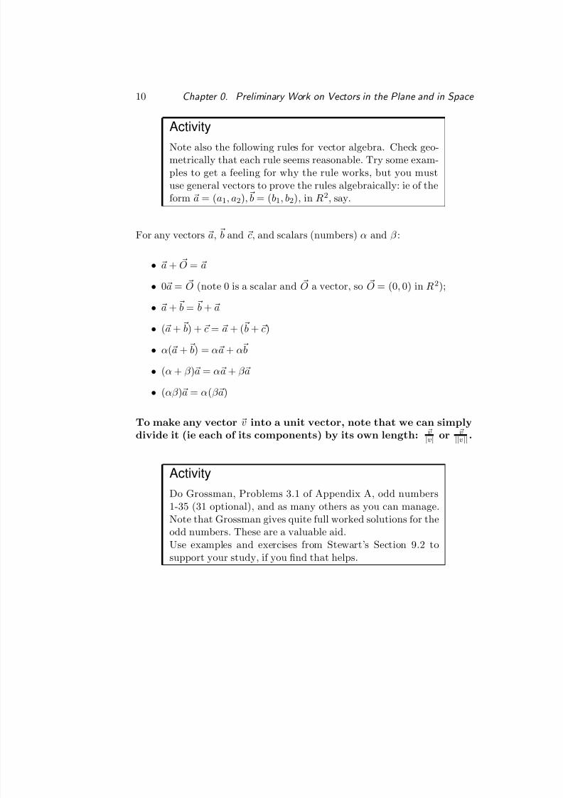
ActivityNote also the following rules for vector algebra. Check geo-metrically that each rule seems reasonable. Try some exam-ples to get a feeling for why the rule works, but you mustuse general vectors to prove the rules algebraically: ie of theform a = ( a1, a2), b = ( b1, b2), in R2, say.
For any vectors a, b and c, and scalars (numbers) α and β :
• a + O = a
• 0a = O (note 0 is a scalar and O a vector, so O = (0 , 0) in R 2);
• a + b = b + a
• (a + b) + c = a + ( b + c)
• α( a + b) = α a + α b
• (α + β ) a = α a + β a
• (αβ ) a = α(β a)
To make any vector v into a unit vector, note that we can simplydivide it (ie each of its components) by its own length: v
|v| or v||v||.
ActivityDo Grossman, Problems 3.1 of Appendix A, odd numbers1-35 (31 optional), and as many others as you can manage.Note that Grossman gives quite full worked solutions for theodd numbers. These are a valuable aid.Use examples and exercises from Stewart’s Section 9.2 to
support your study, if you nd that helps.
8/10/2019 algebra and calculus.pdf
http://slidepdf.com/reader/full/algebra-and-calculuspdf 19/135
0.2. The Scalar Product and Projections in R 2 11
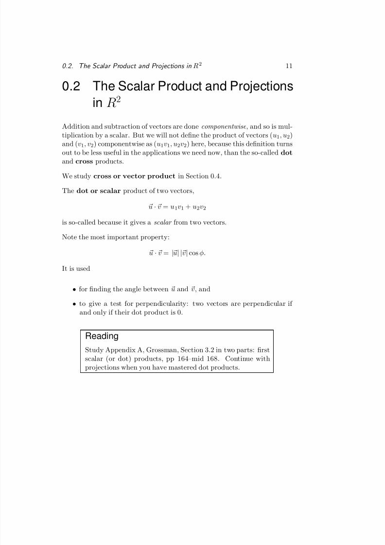
0.2 The Scalar Product and Projectionsin R 2
Addition and subtraction of vectors are done componentwise , and so is mul-tiplication by a scalar. But we will not dene the product of vectors ( u1, u2)and ( v1, v2) componentwise as ( u1v1, u2v2) here, because this denition turnsout to be less useful in the applications we need now, than the so-called dotand cross products.
We study cross or vector product in Section 0.4.
The dot or scalar product of two vectors,
u ·v = u1v1 + u2v2
is so-called because it gives a scalar from two vectors.
Note the most important property:
u ·v = |u| |v|cos φ.
It is used
• for nding the angle between u and v, and
• to give a test for perpendicularity: two vectors are perpendicular if and only if their dot product is 0.
ReadingStudy Appendix A, Grossman, Section 3.2 in two parts: rstscalar (or dot) products, pp 164–mid 168. Continue withprojections when you have mastered dot products.
8/10/2019 algebra and calculus.pdf
http://slidepdf.com/reader/full/algebra-and-calculuspdf 20/135
12 Chapter 0. Preliminary Work on Vectors in the Plane and in Space
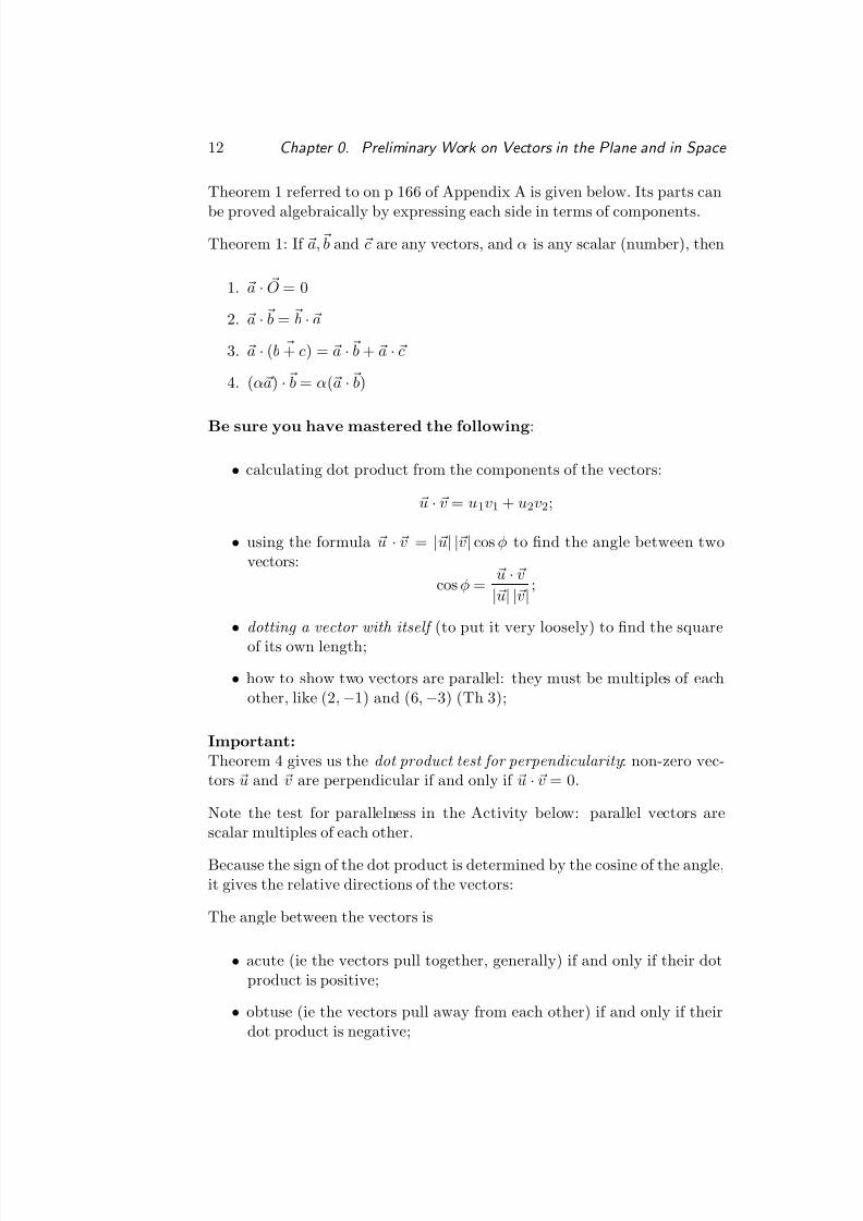
Theorem 1 referred to on p 166 of Appendix A is given below. Its parts can
be proved algebraically by expressing each side in terms of components.Theorem 1: If a, b and c are any vectors, and α is any scalar (number), then
1. a · O = 0
2. a · b = b ·a
3. a · ( b + c) = a · b + a ·c
4. (αa) · b = α( a · b)
Be sure you have mastered the following :
• calculating dot product from the components of the vectors:
u ·v = u1v1 + u2v2;
• using the formula u · v = |u| |v|cos φ to nd the angle between twovectors:
cos φ = u ·v
|u| |v|;
• dotting a vector with itself (to put it very loosely) to nd the squareof its own length;
• how to show two vectors are parallel: they must be multiples of eachother, like (2 , −1) and (6 , −3) (Th 3);
Important:Theorem 4 gives us the dot product test for perpendicularity : non-zero vec-tors u and v are perpendicular if and only if u ·v = 0 .
Note the test for parallelness in the Activity below: parallel vectors arescalar multiples of each other.
Because the sign of the dot product is determined by the cosine of the angle,it gives the relative directions of the vectors:
The angle between the vectors is
• acute (ie the vectors pull together, generally) if and only if their dotproduct is positive;
• obtuse (ie the vectors pull away from each other) if and only if theirdot product is negative;
8/10/2019 algebra and calculus.pdf
http://slidepdf.com/reader/full/algebra-and-calculuspdf 21/135
0.2. The Scalar Product and Projections in R 2 13
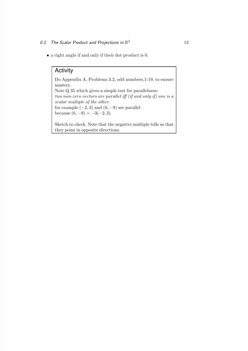
• a right angle if and only if their dot product is 0.
ActivityDo Appendix A, Problems 3.2, odd numbers,1-19, to ensuremastery.Note Q 35 which gives a simple test for parallelness:two non-zero vectors are parallel iff (if and only if) one is a scalar multiple of the other :for example ( −2, 3) and (6 , −9) are parallelbecause (6 , −9) = −3(−2, 3).
Sketch to check. Note that the negative multiple tells us thatthey point in opposite directions.
8/10/2019 algebra and calculus.pdf
http://slidepdf.com/reader/full/algebra-and-calculuspdf 22/135
14 Chapter 0. Preliminary Work on Vectors in the Plane and in Space
Using Vectors to Describe Motion:
ActivityStewart: study section 9.2 and do Exercises 1, 3, 5, 23, 24,25.
Note on Exercise 24 above:
Draw the two vectors for the wind and the plane. To add them, attach thetail of the plane’s vector to the head of the wind’s vector. The resultantcourse is the third side of the triangle, where the base angle is 45+60=105degrees. You can then use the cosine rule to nd this third side. Then youcan use the sine rule to nd the angles of the triangle.
Components and Projections
ReadingStudy components and projections.Use Stewart Section 9.3, or the notes below, to replace Gross-man, Sec 3.2, lower p 168.Denition 4, Grossman p 169, gives a summary of the im-portant results. Study Stewart’s Example 7 and Grossman’sEx 5 & 6, p 170.
Notes replacing lower p 168 of Grossman in Appendix A:
We often want to know how much effect a vector u has in some directionother than its own, say that of vector v; eg how much effect a force vector,
like wind or current, has on the movement of an object in another direction.For examples, see The Dot Product section of the Chapter 9 in your Calculustext, Stewart: section 9.3.
If we start u and v at the same point, we can nd how far u extends inthe direction of v by dropping a perpendicular from the tip of u onto thedirection given by v. See Figure 3.15(a), p 169, Appendix A.
Note how u is then the sum of the two perpendicular (orthogonal) vectorsthat form the sides of the right-angle in the triangle, ie u = proj v u + w.
8/10/2019 algebra and calculus.pdf
http://slidepdf.com/reader/full/algebra-and-calculuspdf 23/135
0.2. The Scalar Product and Projections in R 2 15
We say u can be decomposed (or resolved) into the sum of those two vector
components , one parallel to v and one perpendicular to v.Scalar component:
If θ is the angle between u and v, then the denition of cosine tells us thatthe vector proj v u has length |u|cos θ.
But cos θ may be positive or negative, so |u|cos θ is a signed length expressinghow far u extends in direction v.
We call |u|cos θ the scalar component of u in the direction of v.
Note that dividing by
|v
| in u
·v =
|u
||v
|cos θ, gives
Scalar component = |u|cos θ = u ·v
|v|where the RHS is easier to calculate. See Equation (5),Appendix A p 169.
Vector Projection:
If we write this component as a vector , rather, then we call it the projection of u in the direction of v, or the orthogonal projection of u on v, written proj v u.
This projection vector simply expresses the scalar component, u
·v
|v| or |u|cos θ,as a vector in the direction of v. How can we do that?
Think of a simpler task: to turn scalar -5 into a vector in the direction of the x-axis, we multiply it by a unit vector in that direction, i, to get −5 i.Similarly, a vector 7 units long in the direction of the positive y-axis is givenby the vector 7 j .
To turn a signed scalar length into a vector in a specic direction, all weneed to do is multiply it by a unit vector in the required direction.
Hence scalar component u·v
|v
| must be multiplied by a unit vector in the
direction of v, ie v|v|. We conclude that
proj v u = |u|cos θ v
|v| =
u ·v
|v| v
|v| =
u ·v
|v|2v
which is easier to calculate. See Equation (4), p 169.
Note: We use projections to ”resolve” or ”decompose” u into the sum of two perpendicular vectors, one in the direction of v, the other perpendicularto that, so that u is their sum - ie the hypotenuse of the triangle they form.
8/10/2019 algebra and calculus.pdf
http://slidepdf.com/reader/full/algebra-and-calculuspdf 24/135
16 Chapter 0. Preliminary Work on Vectors in the Plane and in Space
The two vectors proj v u and w that form the decomposition of u are shown
in Figure 3.15, App A p 169.So, to decompose u in this way, nd proj v u rst, using the formula above.Then nd w by subtraction: because u = proj v u + w, we nd w = u − proj v u.)
ActivityYou may nd it helpful now to study Projections in Stewart:section 9.3.Then do Appendix A, Grossman: problems 3.2, odd numbers
1-19, 21-27, 33, 35 and 39. Master more, if you have time.
8/10/2019 algebra and calculus.pdf
http://slidepdf.com/reader/full/algebra-and-calculuspdf 25/135
0.3. Vectors in Space 17
0.3 Vectors in Space
In this section, 2-dimensional geometric vectors in the plane, R2, are ex-tended to 3-dimensional space, R3, by the inclusion of a third component inthe z-direction. The rules and denitions already established for R2 extendeasily, with a little checking.
ReadingRead Appendix A, Grossman, Section 3.3.Take the emphasis off p 177, 178, direction cosines. Example
5 is optional.
Also read Stewart Sec 9.1.
ActivityDo Appendix A, Grossman problems 3.3, odd numbers 1-9,21, 23, odds 27-39. Do as many others as you can manage.
8/10/2019 algebra and calculus.pdf
http://slidepdf.com/reader/full/algebra-and-calculuspdf 26/135
18 Chapter 0. Preliminary Work on Vectors in the Plane and in Space
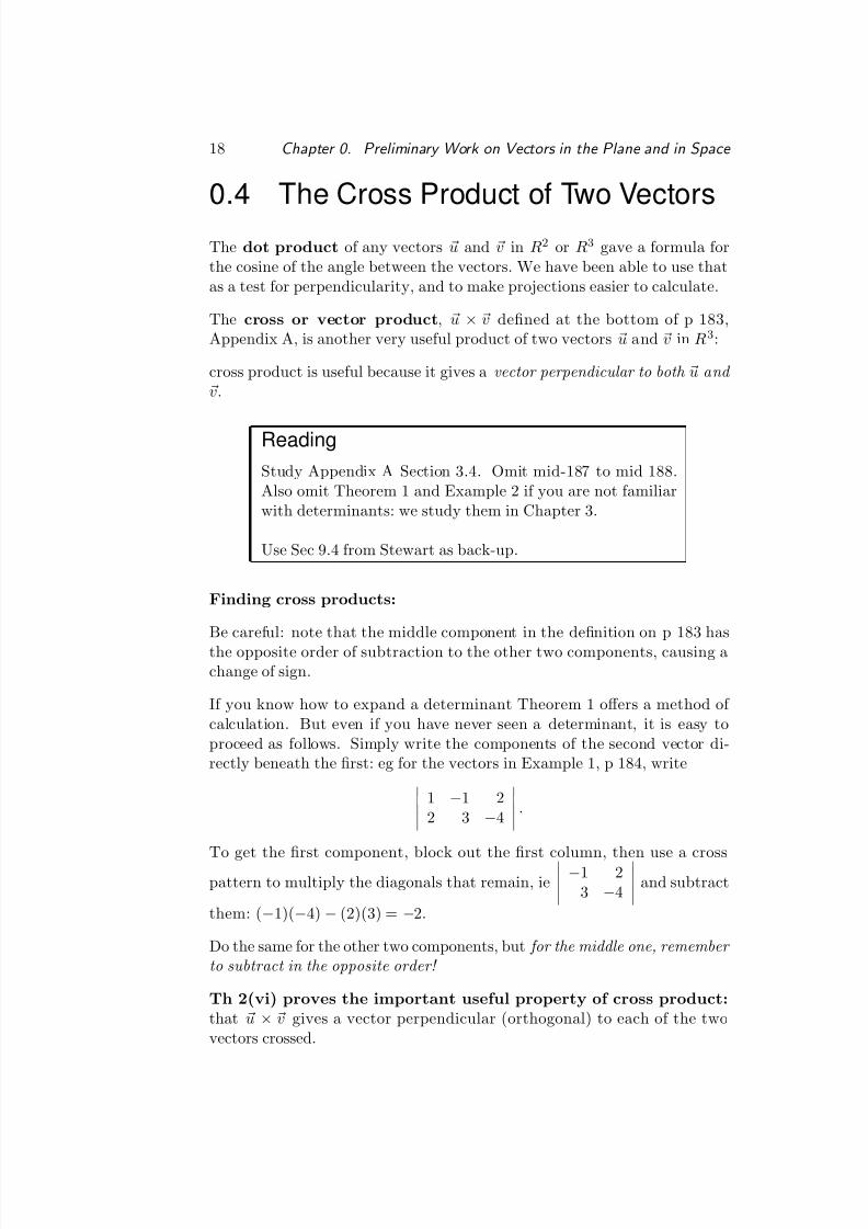
0.4 The Cross Product of Two Vectors
The dot product of any vectors u and v in R2 or R3 gave a formula forthe cosine of the angle between the vectors. We have been able to use thatas a test for perpendicularity, and to make projections easier to calculate.
The cross or vector product , u × v dened at the bottom of p 183,Appendix A, is another very useful product of two vectors u and v in R3:
cross product is useful because it gives a vector perpendicular to both u and v.
ReadingStudy Appendix A Section 3.4. Omit mid-187 to mid 188.Also omit Theorem 1 and Example 2 if you are not familiarwith determinants: we study them in Chapter 3.
Use Sec 9.4 from Stewart as back-up.
Finding cross products:
Be careful: note that the middle component in the denition on p 183 hasthe opposite order of subtraction to the other two components, causing achange of sign.
If you know how to expand a determinant Theorem 1 offers a method of calculation. But even if you have never seen a determinant, it is easy toproceed as follows. Simply write the components of the second vector di-rectly beneath the rst: eg for the vectors in Example 1, p 184, write
1 −1 22 3 −4 .
To get the rst component, block out the rst column, then use a cross
pattern to multiply the diagonals that remain, ie −1 23 −4 and subtract
them: ( −1)(−4) − (2)(3) = −2.
Do the same for the other two components, but for the middle one, remember to subtract in the opposite order!
Th 2(vi) proves the important useful property of cross product:that u × v gives a vector perpendicular (orthogonal) to each of the twovectors crossed.
8/10/2019 algebra and calculus.pdf
http://slidepdf.com/reader/full/algebra-and-calculuspdf 27/135
0.4. The Cross Product of Two Vectors 19
It does this by showing that ( u ×v) · u = 0 and ( u ×v) ·v = 0 .
Note these important results too:
• v×u has magnitude |u| |v|sin φ (like dot product but with sine insteadof cos);
• v ×u has the direction of the thumb in the right-hand rule;
• u ×v = −( v × u) surprisingly;
• the magnitude |u ×v| also gives the area of a parallelogram;
• the absolute value of a scalar triple product | w·( u×v)| gives the volumeof a parallelepiped.
ActivityDo Problems 3.4, Q 3, 5, 9, 17, 19, 21, 23, 35, 29, 31, 33 37.Do as many others as you can manage.Note that you can also use cross product to nd the area of a triangle with adjacent sides u and v: the area is half thatof the parallelogram they dene.
ActivityBrowse through the approach to properties of vectors andtheir uses in the Vectors Chapter in Stewart: sections 9.1 to9.4.
Note the sections on dot and cross product, in particular.
8/10/2019 algebra and calculus.pdf
http://slidepdf.com/reader/full/algebra-and-calculuspdf 28/135
20 Chapter 0. Preliminary Work on Vectors in the Plane and in Space
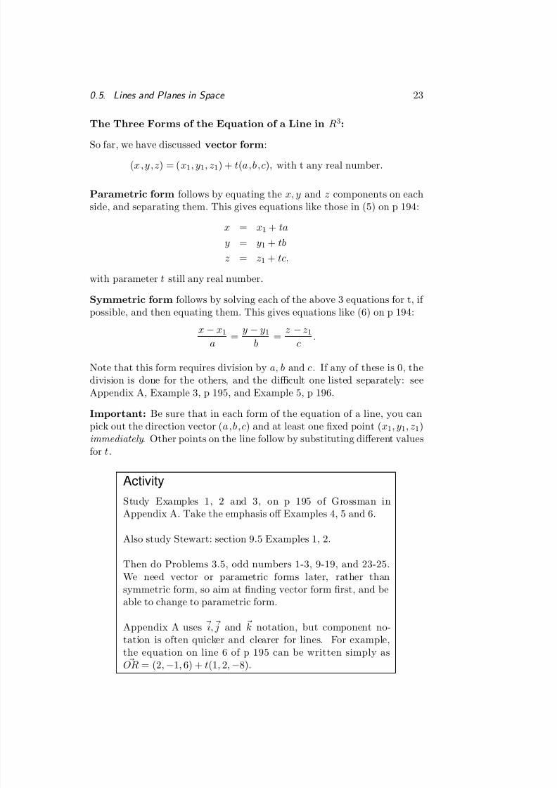
0.5 Lines and Planes in Space
We now use dot and cross products to obtain equations for lines and planesin space. Dot product gives a test for perpendicularity. Cross product givesa vector perpendicular to those we cross.
We ask the following two questions now, in 3-dimensional space, R3:
• What general form of equation describes any given line ?
• What general form describes any plane ?
In the plane, R2, ie two-dimensional space, ax + by = c is the general formof the equation of a line. (Vertical lines of form x = c are not described bythe general slope-intercept form, y = mx + k, but are included in the moregeneral form, ax + by = c, when b = 0.)
As we show below, however, extending ax + by = c in R2 to include theextra variable, ax + by + cz = d, does not give a line in R 3, but describes aplane , rather.
Reading
The notes below replace those on the bottom of Grossman,p 193–194 of Appendix A, Section 3.5.
Stewart Section 9.5 provides further back-up.
The Equation of a Line:
To specify a particular line, in the plane or in space, it is sufficient to know just one point on it, as long as we know its direction.
Suppose we have a line, rstly in the plane for simplicity, with y-intercept
3, and slope 4.Sketch this line here, and convince yourself that because the slope is 4/1, the vector (1,4) is parallel to it.
Notice how we can travel from the origin to any point ( x, y ) on the line,using the known point (0 , 3) (the y-intercept) and the slope or directionvector, (1 , 4):
• Firstly, to reach the line, we can travel along the position vector (0 , 3)to get to the only known point on the line.
8/10/2019 algebra and calculus.pdf
http://slidepdf.com/reader/full/algebra-and-calculuspdf 29/135
8/10/2019 algebra and calculus.pdf
http://slidepdf.com/reader/full/algebra-and-calculuspdf 30/135
22 Chapter 0. Preliminary Work on Vectors in the Plane and in Space
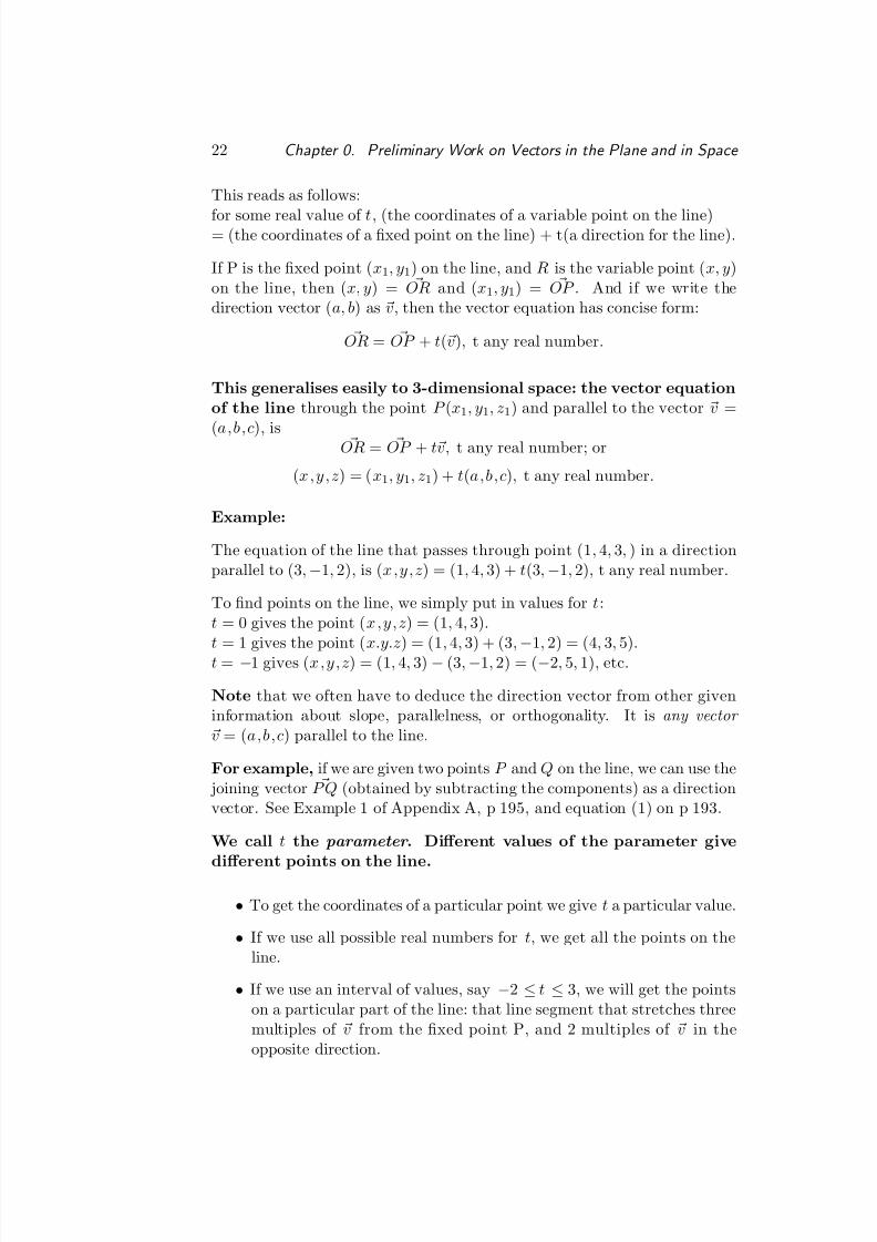
This reads as follows:
for some real value of t , (the coordinates of a variable point on the line)= (the coordinates of a xed point on the line) + t(a direction for the line).
If P is the xed point ( x1, y1) on the line, and R is the variable point ( x, y)on the line, then ( x, y ) = OR and (x1, y1) = OP . And if we write thedirection vector ( a, b) as v, then the vector equation has concise form:
OR = OP + t( v), t any real number.
This generalises easily to 3-dimensional space: the vector equationof the line through the point P (x1, y1, z1) and parallel to the vector v =
(a,b,c), is OR = OP + tv, t any real number; or
(x,y,z ) = ( x1, y1, z1) + t(a,b,c), t any real number.
Example:
The equation of the line that passes through point (1 , 4, 3, ) in a directionparallel to (3 , −1, 2), is (x,y,z ) = (1 , 4, 3) + t(3, −1, 2), t any real number.
To nd points on the line, we simply put in values for t :t = 0 gives the point ( x,y,z ) = (1 , 4, 3).t = 1 gives the point ( x.y.z ) = (1 , 4, 3) + (3 ,
−1, 2) = (4 , 3, 5).
t = −1 gives (x,y,z ) = (1 , 4, 3) − (3, −1, 2) = ( −2, 5, 1), etc.
Note that we often have to deduce the direction vector from other giveninformation about slope, parallelness, or orthogonality. It is any vector v = ( a,b,c) parallel to the line.
For example, if we are given two points P and Q on the line, we can use the joining vector P Q (obtained by subtracting the components) as a directionvector. See Example 1 of Appendix A, p 195, and equation (1) on p 193.
We call t the parameter . Different values of the parameter givedifferent points on the line.
• To get the coordinates of a particular point we give t a particular value.
• If we use all possible real numbers for t, we get all the points on theline.
• If we use an interval of values, say −2 ≤ t ≤ 3, we will get the pointson a particular part of the line: that line segment that stretches threemultiples of v from the xed point P, and 2 multiples of v in theopposite direction.
8/10/2019 algebra and calculus.pdf
http://slidepdf.com/reader/full/algebra-and-calculuspdf 31/135
8/10/2019 algebra and calculus.pdf
http://slidepdf.com/reader/full/algebra-and-calculuspdf 32/135
24 Chapter 0. Preliminary Work on Vectors in the Plane and in Space
We now formalise what we mean by a plane in space , and construct the
equation:The Equation of a Plane in R3:
ReadingThe notes below are a replacement for most of p 197 of AppA, Section 3.5. They are very important.
Study them carefully before reading pp 198 - mid 201. Pp201 and 202 may be omitted, but you may want to come
back to Example 10 when you have learned to row-reduce amatrix.
Stewart Section 9.5 provides further discussion, but you neednot study Examples 7, 9 and 10.
We seek a property that will dene that plane by distinguishing all the pointson it from other points in space.
In R3, a line’s direction is characterised by a direction vector - ie any vectorparallel to it.
Consider what we regard to be a plane in space: a at sheet extendingwithout bound in any direction. Many vectors with different directions areparallel to it, and hence its direction cannot be characterised by a parallel vector.
But note that there is only one direction perpendicular to a plane.
Imagine all vectors perpendicular to a given plane: note that they are par-allel, though some have opposite directions.
We say all such vectors are normal to the plane (normal meaning perpen-dicular) and we call any one of them a normal for that plane.
• A plane has many normals: if you have one, any positive or negativemultiple will also be normal to that plane.
• Parallel planes have parallel normals. Draw some to see this.
• Planes that are not parallel will have normals that are not parallel.Convince yourself: draw some.
8/10/2019 algebra and calculus.pdf
http://slidepdf.com/reader/full/algebra-and-calculuspdf 33/135
0.5. Lines and Planes in Space 25
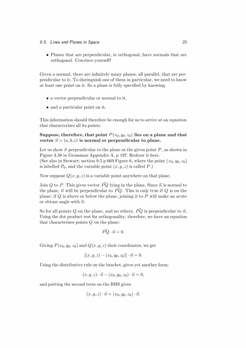
• Planes that are perpendicular, ie orthogonal, have normals that are
orthogonal. Convince yourself!
Given a normal, there are innitely many planes, all parallel, that are per-pendicular to it. To distinguish one of them in particular, we need to knowat least one point on it. So a plane is fully specied by knowing
• a vector perpendicular or normal to it,
• and a particular point on it.
This information should therefore be enough for us to arrive at an equationthat characterises all its points.
Suppose, therefore, that point P (x0, y0, z0) lies on a plane and thatvector n = ( a,b,c) is normal or perpendicular to plane.
Let us show n perpendicular to the plane at the given point P , as shown inFigure 3.38 in Grossman Appendix A, p 197. Redraw it here.(See also in Stewart: section 9.5 p 669 Figure 6, where the point ( x0, y0, z0)is labelled P 0, and the variable point ( x,y,z ) is called P .)
Now suppose Q(x,y,z ) is a variable point anywhere on that plane.
Join Q to P . This gives vector P Q lying in the plane. Since n is normal tothe plane, n will be perpendicular to P Q . This is only true if Q is on theplane: if Q is above or below the plane, joining it to P will make an acuteor obtuse angle with n.
So for all points Q on the plane, and no others, P Q is perpendicular to n.Using the dot product test for orthogonality, therefore, we have an equationthat characterises points Q on the plane:
P Q ·n = 0 .
Giving P (x0, y0, z0) and Q(x,y,z ) their coordinates, we get
[(x,y,z ) − (x0, y0, z0)] ·n = 0 .
Using the distributive rule on the bracket, gives yet another form:
(x,y,z ) ·n − (x0, y0, z0) ·n = 0 ,
and putting the second term on the RHS gives
(x,y,z ) ·n = ( x0, y0, z0) ·n.
8/10/2019 algebra and calculus.pdf
http://slidepdf.com/reader/full/algebra-and-calculuspdf 34/135
26 Chapter 0. Preliminary Work on Vectors in the Plane and in Space
This are all different forms of the equation for the plane, and give us different
ways of nding it. Notice in particular the easy method:(variable point) · (normal) = (xed point) · (normal).
Vector n = ( a,b,c), so this gives
(x,y,z ) · (a,b,c) = ( x0, y0, z0) · (a,b,c),
and taking dot products gives
ax + by + cz = ax 0 + by0 + cz0.
The LHS cannot be simplied because x, y and z are variables. But theRHS will reduce to an answer, d, say.
So in general the equation of a plane has form ax + by + cz = d.
Note also that in this form, the coefficients (a,b,c) give a normal to theplane.
Example:
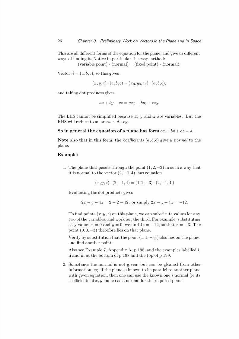
1. The plane that passes through the point (1 , 2, −3) in such a way thatit is normal to the vector (2 ,
−1, 4), has equation
(x,y,z ) · (2, −1, 4) = (1 , 2, −3) · (2, −1, 4.)
Evaluating the dot products gives
2x − y + 4 z = 2 − 2 − 12, or simply 2x − y + 4 z = −12.
To nd points ( x,y,z ) on this plane, we can substitute values for anytwo of the variables, and work out the third. For example, substitutingeasy values x = 0 and y = 0, we nd 4 z = −12, so that z = −3. Thepoint (0 , 0, −3) therefore lies on that plane.
Verify by substitution that the point (1 , 1, −134 ) also lies on the plane,and nd another point.
Also see Example 7, Appendix A, p 198, and the examples labelled i,ii and iii at the bottom of p 198 and the top of p 199.
2. Sometimes the normal is not given, but can be gleaned from otherinformation: eg, if the plane is known to be parallel to another planewith given equation, then one can use the known one’s normal (ie itscoefficients of x, y and z) as a normal for the required plane;
8/10/2019 algebra and calculus.pdf
http://slidepdf.com/reader/full/algebra-and-calculuspdf 35/135
0.5. Lines and Planes in Space 27
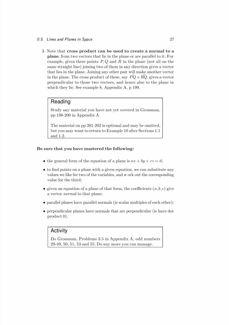
3. Note that cross product can be used to create a normal to a
plane , from two vectors that lie in the plane or are parallel to it. Forexample, given three points P, Q and R in the plane (not all on thesame straight line) joining two of them in any direction gives a vectorthat lies in the plane. Joining any other pair will make another vectorin the plane. The cross product of these, say P Q × RQ , gives a vectorperpendicular to those two vectors, and hence also to the plane inwhich they lie. See example 8, Appendix A, p 199.
ReadingStudy any material you have not yet covered in Grossman,pp 198-200 in Appendix A.
The material on pp 201-202 is optional and may be omitted,but you may want to return to Example 10 after Sections 1.1and 1.2.
Be sure that you have mastered the following:
• the general form of the equation of a plane is ax + by + cz = d;
• to nd points on a plane with a given equation, we can substitute anyvalues we like for two of the variables, and w ork out the correspondingvalue for the third;
• given an equation of a plane of that form, the coefficients ( a,b,c) givea vector normal to that plane;
• parallel planes have parallel normals (ie scalar multiples of each other);
• perpendicular planes have normals that are perpendicular (ie have dotproduct 0).
ActivityDo Grossman, Problems 3.5 in Appendix A, odd numbers29-49, 50, 51, 53 and 55. Do any more you can manage.
8/10/2019 algebra and calculus.pdf
http://slidepdf.com/reader/full/algebra-and-calculuspdf 36/135
28 Chapter 0. Preliminary Work on Vectors in the Plane and in Space
ActivityNote that lines in R2 have many similarities to planes inR3. Plot roughly to scale the lines in R2 with equations2x + y = 5 and 3 x − y = 2. See that vector (2 , 1) is normal(perpendicular) to the rst line, and (3 , −1) is normal to thesecond. Show that the vector ( a, b) is normal to the line withequation ax + by = c, by showing that this line has slope
−a/b , and using the fact that perpendicular lines have slopesthat multiply to give -1.
0.6 Summary: VectorsActivityBrowse through Stewart: sections 9.1 to 9.5 for other per-spectives on vectors.Check Grossman’s Summary on p 205-207 in Appendix A.Where something looks unfamiliar, go back and master it.The condence you gain when the material begins to compactinto something manageable is worth the effort.
Do not neglect to do exercises for each section. Assignments do not offerenough breadth or practice!
8/10/2019 algebra and calculus.pdf
http://slidepdf.com/reader/full/algebra-and-calculuspdf 37/135
Chapter 1Systems of LinearEquations
What are linear equations? What is Linear Algebra?
An equation of form ax + by = c denes a straight line in R2 and is calledlinear. More generally, equations of the form a0x0 + a1x1 + a2x2 + a3x3 +a4x4 + ... + an xn = b are still called linear even though they do not generallydescribe lines.
Linear equations of different kinds arise in computer graphics, satellite datatransmission, population dynamics, electrical networks, chemical reactions,economics, and many areas of science, engineering, technology, business andindustry.
In many cases they represent demands or constraints on variables, and it isoften the case that many such equations must be satised simultaneously.Understanding them, and simplifying and solving them, is vital in theseareas of application.
We now work from your prescribed text, Elementary Linear Algebra , byLarson, Edwards & Falvo. We shall call it Larson et al .
Read p xv and xvi, by way of introduction.
29
8/10/2019 algebra and calculus.pdf
http://slidepdf.com/reader/full/algebra-and-calculuspdf 38/135
30 Chapter 1. Systems of Linear Equations
1.1 Introduction to Systems of Linear Equa-tions
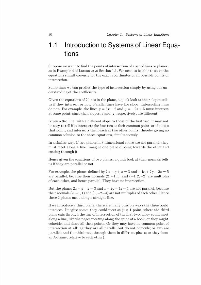
Suppose we want to nd the points of intersection of a set of lines or planes,as in Example 4 of Larson et al Section 1.1. We need to be able to solve theequations simultaneously for the exact coordinates of all possible points of intersection.
Sometimes we can predict the type of intersection simply by using our un-derstanding of the coefficients.
Given the equations of 2 lines in the plane, a quick look at their slopes tellsus if they intersect or not. Parallel lines have the slope. Intersecting linesdo not. For example, the lines y = 3x − 2 and y = −2x + 5 must intersectat some point: since their slopes, 3 and -2, respectively, are different.
Given a 3rd line, with a different slope to those of the rst two, it may notbe easy to tell if it intersects the rst two at their common point, or if missesthat point, and intersects them each at two other points, thereby giving nocommon solution to the three equations, simultaneously.
In a similar way, if two planes in 3-dimensional space are not parallel, theymust meet along a line: imagine one plane dipping towards the other andcutting through it.
Hence given the equations of two planes, a quick look at their normals tellsus if they are parallel or not.
For example, the planes dened by 2 x − y + z = 3 and −4x + 2 y − 2z = 5are parallel, because their normals (2 , −1, 1) and (−4, 2, −2) are multiplesof each other, and hence parallel. They have no intersection.
But the planes 2 x −y + z = 3 and x −2y −4z = 1 are not parallel, becausetheir normals (2 , −1, 1) and (1 , −2−4) are not multiples of each other. Hencethese 2 planes meet along a straight line.
If we introduce a third plane, there are many possible ways the three couldintersect. Imagine some: they could meet at just 1 point, where the thirdplane cuts through the line of intersection of the rst two. They could meetalong a line, like the pages meeting along the spine of a book, or they mightcoincide, and share all their points. Or they may have no common point of intersection at all: eg they are all parallel but do not coincide; or two areparallel, and the third cuts through them in different places; or they forman A-frame, relative to each other).
8/10/2019 algebra and calculus.pdf
http://slidepdf.com/reader/full/algebra-and-calculuspdf 39/135
1.1. Introduction to Systems of Linear Equations 31
Draw some of these possibilities, and see if you can think of others.
ReadingStudy Section 1.1 of Larson et al . All of the material isimportant.
Be sure that you have mastered the following:
• be able to tell whether any given equation is linear or not
• know the general form of a linear equation
• know what is meant by a system of linear equations and its solutions ,if any
• know that consistent means having at least 1 solution, inconsistent means having no solutions at all
• be able to express one variable in terms of all the others in a linearequation
• know what is meant by the terms free variable and parameter
• be able to nd particular solutions for the other variables by substi-tuting arbitrary values for the parameters
Note that to solve a system of linear equations, we try change the systeminto a simpler one that retains the same solutions. Note that we use theelementary row operations to do that because they do not spoil the solutions.
• Know exactly what the three elementary row operations are.
• Aim at obtaining a triangular structure, called row-echelon form, or
else a diagonal form
• If necessary, use back-substitution to nd values for the variables
Note also that solving a system of linear equations of any size and in anynumber of variables, leads to only three possibilities:
• exactly 1 solution,
• innitely many solutions, or
8/10/2019 algebra and calculus.pdf
http://slidepdf.com/reader/full/algebra-and-calculuspdf 40/135
32 Chapter 1. Systems of Linear Equations
• no solutions at all; the system is then called inconsistent .
Example 4 makes the last point clear for 2 equations in 2 variables. Solutionsare the points of intersection, if any, of 2 lines. It is impossible to nd asolution which comprises 2 points, or 10 points, say.
We nd
• exactly 1 point of intersection (when they cross), or
• innitely many (when the lines coincide), or
• none at all (when the lines are parallel).
ActivityConrm that for the intersection of planes in space, we stillonly get three possibilities: one point, or none, or innitelymany. Draw rough sketches of all the possible ways they canintersect. Start with the intersection of just 2 planes. Thentry 3 planes. Examples 7 and 8 illustrate some possibilities.Conrm that there will be
• exactly 1 point of intersection, if the third plane cutsthrough the line of intersection of the rst two
• none at all if the third plane “misses” the line of in-tersection of the other two: ie the planes intersect onlytwo at a time as though they frame an A
• innitely many points of intersection along a line if theplanes meet like the pages of a book
• innitely many along a plane if the 3 planes all coincide
• none at all if all of the planes are parallel
• none at all even if only two are parallel, because thosetwo have no points of intersection
Think about the effect of introducing a fourth plane too.

8/10/2019 algebra and calculus.pdf
http://slidepdf.com/reader/full/algebra-and-calculuspdf 41/135
1.1. Introduction to Systems of Linear Equations 33
ActivitySection 1.1 Exercises, a selection of odd numbers, 1-25,35-37, 43.
Also do Ed 4: 51-59, and 73;or Ed 5: 51-64, 77.
8/10/2019 algebra and calculus.pdf
http://slidepdf.com/reader/full/algebra-and-calculuspdf 42/135
34 Chapter 1. Systems of Linear Equations
1.2 Gaussian Elimination and Gauss-JordanElimination
ReadingStudy Section 1.2 of Larson et al . We use matrix notationto keep the essential information concise when solving linearequations.
• Note how we can use the elementary row operations to reduce a system
to simpler ones without altering the solutions. Always record againsteach row what row operation you did to get it, to help the reader.
• Note the processes referred to as Gaussian elimination and Gauss-Jordan elimination
• that the former leads to row-echelon form and the latter leads to re-duced row-echelon form;
• that using Gauss-Jordan rather than Gaussian elimination may in-crease the number of row-reduction steps, but saves hand-steps later,by reducing the back-substitution necessary to complete the solving.
These systematic processes contain basic ideas that support the reasoningbehind some of our later work, but note that while they lend themselves tomachine computation, they are generally far from efficient, and may leadto problems. Renements like partial or complete pivoting may offer waysof reducing rounding errors, but do not always eliminate the problems, andthere is a need for alternative methods appropriate for different types of systems.
Note
• that perfect triangular or diagonal form with 1’s on the main diagonal,does not always arise
• how to interpret rows of all 0’s as no information at all, and missingrows, as in Examples 8 and 9
• that a row all 0’s except the RHS which is non-zero, leads to a contra-diction, and that system hence has no solutions: eg [0 0 0 − 2] reallymeans 0x + 0 y + 0 z = −2 which cannot be satised by any values of x, y and z

8/10/2019 algebra and calculus.pdf
http://slidepdf.com/reader/full/algebra-and-calculuspdf 43/135
1.2. Gaussian Elimination and Gauss-Jordan Elimination 35
• that a homogeneous system (ie one with RHS’s all 0’s) always has
at least one solution, when all the variables are 0’s (called the triv-ial solution ) but that it may also have others, innitely many of theparametric type. So homogeneous systems are always consistent.
ActivityLook again at Example 8. Imagine that the variables werex, y and z. Then the two equations represent planes, andsolving them simultaneously will nd their point/s of inter-section,i f any. Because they are not parallel, we expect themto meet along a line. Show that the solution found there canbe written in the form ( x,y,z ) = (2 , −1, 0) + t(−5, 3, 1) andhence deduce that this is the equation of the line of intersec-tion of the planes.Then do Section 1.2 Exercises, odd numbers 1, 5, 9, 15-21.Also do Ed 4: 29-43, 59;or Ed 5: 29-45, 61.
8/10/2019 algebra and calculus.pdf
http://slidepdf.com/reader/full/algebra-and-calculuspdf 44/135
36 Chapter 1. Systems of Linear Equations
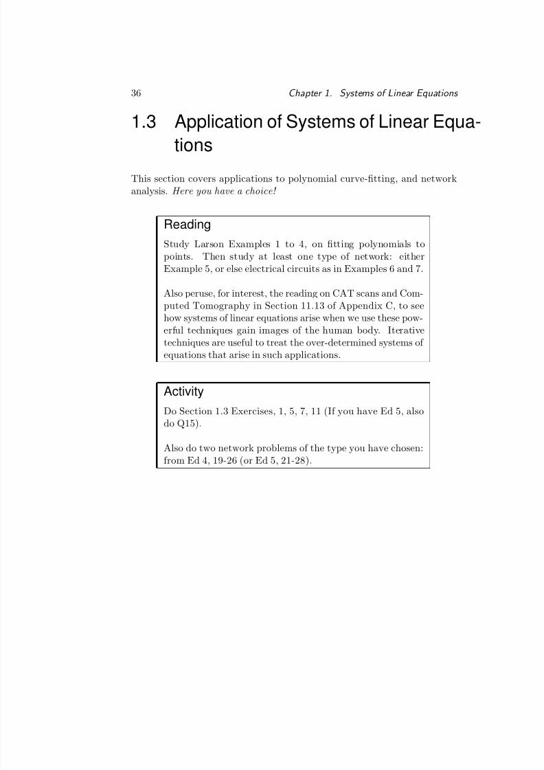
1.3 Application of Systems of Linear Equa-tions
This section covers applications to polynomial curve-tting, and networkanalysis. Here you have a choice!
ReadingStudy Larson Examples 1 to 4, on tting polynomials topoints. Then study at least one type of network: either
Example 5, or else electrical circuits as in Examples 6 and 7.
Also peruse, for interest, the reading on CAT scans and Com-puted Tomography in Section 11.13 of Appendix C, to seehow systems of linear equations arise when we use these pow-erful techniques gain images of the human body. Iterativetechniques are useful to treat the over-determined systems of equations that arise in such applications.
ActivityDo Section 1.3 Exercises, 1, 5, 7, 11 (If you have Ed 5, alsodo Q15).
Also do two network problems of the type you have chosen:from Ed 4, 19-26 (or Ed 5, 21-28).
8/10/2019 algebra and calculus.pdf
http://slidepdf.com/reader/full/algebra-and-calculuspdf 45/135
1.4. Chapter Summary: Systems of Linear Equations. 37
1.4 Chapter Summary: Systems of Lin-ear Equations.
Remind yourself of the Module objectives listed immediately before Chapter0.
ActivityCheck through the summary at the end of Section 1. Youcan nd another on Systems of Linear Equations in the
coloured pages of the Study Guide Appendix A.
Attempt some of the Review Exercises in Larson et al , andlook at the Projects.

8/10/2019 algebra and calculus.pdf
http://slidepdf.com/reader/full/algebra-and-calculuspdf 46/135
38 Chapter 1. Systems of Linear Equations
8/10/2019 algebra and calculus.pdf
http://slidepdf.com/reader/full/algebra-and-calculuspdf 47/135
Chapter 2Matrices
Matrices are two-dimensional arrays that offer a concise way to store es-sential information for any type of application. In this chapter, we developways to manipulate matrices and do matrix algebra that prove useful for
managing and analysing many different types of data-sets. We will also ndlinks between matrices and vectors and their algebra: the rows or columnsof a matrix can be viewed as vectors, and a vector can be viewed as a rowor column matrix.
39
8/10/2019 algebra and calculus.pdf
http://slidepdf.com/reader/full/algebra-and-calculuspdf 48/135
40 Chapter 2. Matrices
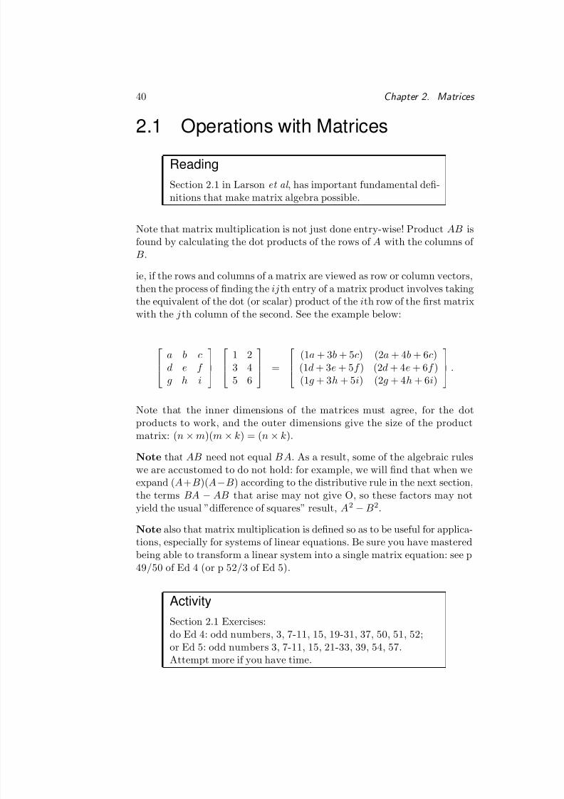
2.1 Operations with Matrices
ReadingSection 2.1 in Larson et al , has important fundamental de-nitions that make matrix algebra possible.
Note that matrix multiplication is not just done entry-wise! Product AB isfound by calculating the dot products of the rows of A with the columns of B .
ie, if the rows and columns of a matrix are viewed as row or column vectors,then the process of nding the ij th entry of a matrix product involves takingthe equivalent of the dot (or scalar) product of the ith row of the rst matrixwith the j th column of the second. See the example below:
a b cd e f g h i
1 23 45 6
=(1a + 3 b + 5 c) (2a + 4 b + 6 c)(1d + 3 e + 5 f ) (2d + 4 e + 6 f )(1g + 3 h + 5 i) (2g + 4 h + 6 i)
.
Note that the inner dimensions of the matrices must agree, for the dotproducts to work, and the outer dimensions give the size of the productmatrix: ( n × m)(m × k) = ( n × k).
Note that AB need not equal BA. As a result, some of the algebraic ruleswe are accustomed to do not hold: for example, we will nd that when weexpand ( A+ B )(A−B ) according to the distributive rule in the next section,the terms BA − AB that arise may not give O, so these factors may notyield the usual ”difference of squares” result, A2 − B2.
Note also that matrix multiplication is dened so as to be useful for applica-tions, especially for systems of linear equations. Be sure you have mastered
being able to transform a linear system into a single matrix equation: see p49/50 of Ed 4 (or p 52/3 of Ed 5).
ActivitySection 2.1 Exercises:do Ed 4: odd numbers, 3, 7-11, 15, 19-31, 37, 50, 51, 52;or Ed 5: odd numbers 3, 7-11, 15, 21-33, 39, 54, 57.Attempt more if you have time.
8/10/2019 algebra and calculus.pdf
http://slidepdf.com/reader/full/algebra-and-calculuspdf 49/135
2.2. Properties of Matrix Operations 41
2.2 Properties of Matrix Operations
Before we use matrix addition and multiplication to manipulate data, weneed to check that we have enough properties to be able to work much likewe do real numbers. We nd that many of the algebraic rules still hold, but not all : a warning to be careful when using matrix algebra.
ReadingStudy Section 2.2 in Larson et al . An easy section, but veryimportant: be careful of the algebraic differences referred to
above, for example those illustrated by Examples 4 and 5,and discussed in the notes between.
Note also that we can write the dot product of two vectors as a matrixmultiplication:
if u and v are both row vectors of equal length, then u ·v can be written asthe matrix product uvT . Explain why it is necessary to transpose v in orderto write this matrix mltiplication.
ActivitySection 2.2 Exercises 3, 5, 9, 13, 17, 18, 19, 22, 23, 26, 27.Also do Ed 4: 29, 36, 39, 53;or else Ed 5: 29 (use technology), 31, 38, 41, 55.
8/10/2019 algebra and calculus.pdf
http://slidepdf.com/reader/full/algebra-and-calculuspdf 50/135
42 Chapter 2. Matrices
2.3 The Inverse of a Matrix
All real numbers except 0 have multiplicative inverses: 2 has multiplicativeinverse 1/2, because (1/2)(2) = 1. We use this inverse as a multiplier onboth sides, to clear the 2 in an equation like 2 x = 5.
For matrix equations, inverses are helpful in an analogous way.
The matrix equivalent of the number 1 is I . The inverse of matrix A will bethat matrix which multiplies by A on either side, left or right, to give I .
But we nd that not all matrices have inverses. For size reasons a matrix
must be square to have an inverse: but even being square is no guaranteethat the matrix will have an inverse!
ReadingStudy Section 2.3 of Larson et al .
Note
• the denition of the inverse of a matrix;
• that when the inverse exists it is unique;
• a method of nding inverses: we can row-reduce [ A : I ];
• the form of the inverse of a 2 × 2 matrix at the bottom of p 69 of Ed4 ( or p 73 of Ed 5). You may want it often enough to make it worthremembering. Verify it by multiplying it by the original to get I .
Notice that the inverse of a bc d cannot exist if ad −bc = 0. This number
ad − bc is called the determinant of the 2 × 2 matrix. We will dene deter-
minants fully later, so that they do indeed determine whether or not A hasan inverse.
ActivityMaster Section 2.3 Exercises, odds 1-19, 21, 23 with technol-ogy, and 27.Also do Ed 4: 29, 35, 37, 42, 43, 45, 46, 49, 50;or else Ed 5: 29 (with tech) 31, 37, 39, 44, 45, 47, 48, 51, 52.
8/10/2019 algebra and calculus.pdf
http://slidepdf.com/reader/full/algebra-and-calculuspdf 51/135
2.4. Elementary Matrices 43
2.4 Elementary Matrices
This section is optional reading . Elementary matrices can be used to provesome useful and important theorems.
2.5 Applications of Matrix Operations
There are many ways in which matrices can be used to facilitate the storing,processing, transmission, and analysis of data. This section introduces just
four of these:
• stochastic matrices of probabilities, used for prediction;
• coding matrices, used for cryptography;
• input-output matrices, used in economics, for industrial output;
• least squares regression, which is covered in Algebra & Calculus II.
Once more you have a choice: study one of the rst three applications listed
above.
ReadingLook through Section 2.5 of Larson et al : study either sto-chastic matrices or cryptography or Leontief input- output models .Browse through Sections 11.7 to 11.12 in Appendix C, to seematrix operations and methods in use for some other appli-cations: computer graphics, forest management, and equilib-rium temperature distributions.
ActivityDo at least two exercises from Section 2.5, on the type of application you selected. Write a summary paragraph of atleast 150 word on how matrices are used in another applica-tion that is of particular interest to you.
8/10/2019 algebra and calculus.pdf
http://slidepdf.com/reader/full/algebra-and-calculuspdf 52/135
8/10/2019 algebra and calculus.pdf
http://slidepdf.com/reader/full/algebra-and-calculuspdf 53/135
Chapter 3Determinants
We know how to clear the factor 3 from the LHS of the equation 3 x = 5 . Wesimply multiply both sides by its multiplicative inverse or reciprocal, 1 / 3.We also say we divide by 3 .
We can clear any factor except 0 in that way. 0 is the only real number thatdoes not have a multiplicative inverse.
Let us apply a similar argument to matrix algebra: suppose we have matrixequation AX = B. Some square matrices A have multiplicative inverses,A−1, but many do not. This means that we cannot always get rid of amatrix factor A in a matrix equation.
That is why we do not dene matrix division: it simply can’t always be done!
To be able to distinguish between those matrices that have inverses and
those that do not, we now dene a number called the determinant of amatrix, so that
• when the determinant of the matrix is 0, the matrix has no inverse;
• when the determinant is not 0, the matrix is invertible (non-singular).
45
8/10/2019 algebra and calculus.pdf
http://slidepdf.com/reader/full/algebra-and-calculuspdf 54/135
46 Chapter 3. Determinants
3.1 The Determinant of a Matrix
First we dene the determinant of a 2 × 2 matrix. Then we extend thedenition to matrices of any size, using a process of expanding by cofactors.
ReadingStudy Larson Ch 3.1. Note the determinant of a 1 ×1 matrix(the entry itself) in Ed 4, top of p 113 (or Ed 5, top of p 121).
Find the determinant of a 2
× 2 matrix in Ed 4, p 112 (or
Ed 5, p 120).
Study how these are extended to dene the determinant of asquare matrices of any size.
Note that you can expand by any row or column : the answer will be thesame. Of course we choose the easiest one: the row or column with the most0’s.
In the next section we will see how we can simplify rows and columns and/orcreate more 0’s, to make this task even easier.
Note that the cofactor of any entry has two parts to it:
• a plus or minus, following a chequerboard pattern, and
• a determinant: that of the matrix left after deleting the row and col-umn containing that entry.
Two warnings on shortcuts:
• Do not use the alternative forward and backwards diagonal method (p117 of Ed 4, or p 125 of Ed 5) on matrices bigger than 3 × 3. It doesnot work because it omits many terms.
• The shortcut for triangular matrices (p 117/8 of Ed 4, or p 126/7 of Ed 5) works for entries on the main diagonal. Be careful if you want toapply it to a triangular matrix where the entries lie on the backwards diagonal: matrices of order 6 or more may need a sign adjustment.

8/10/2019 algebra and calculus.pdf
http://slidepdf.com/reader/full/algebra-and-calculuspdf 55/135
3.1. The Determinant of a Matrix 47
ActivityMaster Section 3.1 Exercises 1, 3, 9, 11, 17, 21, 23, 31.
Also do Ed 4: 35, 39, 41, 43, 47, 48, 51;or Ed 5: 37, 43, 45, 47, 53, 54, 57, and 39 with technology.
8/10/2019 algebra and calculus.pdf
http://slidepdf.com/reader/full/algebra-and-calculuspdf 56/135
8/10/2019 algebra and calculus.pdf
http://slidepdf.com/reader/full/algebra-and-calculuspdf 57/135
3.3. Properties of Determinants 49
3.3 Properties of Determinants
ReadingNote the properties of determinants listed in each of the The-orems in Larson 3.3, particularly Theorem 3.7.Note Example 2: when nding determinants, we draw outfactors from one row or column at a time.This means that if A has 3 rows, 10A has determinant10.10.10 det( A) = 1000det A.
ActivityMaster the Section 3.3 Exercises, 1-31, 32, 35.Also do Ed 4: 37, 47, 48 (or Ed 5: 39, 49, 50).
8/10/2019 algebra and calculus.pdf
http://slidepdf.com/reader/full/algebra-and-calculuspdf 58/135
50 Chapter 3. Determinants
3.4 Chapter Summary on Determinants.
You should browse through Section 3.4 (and Section 3.5 in Ed 5) to gain aquick overview of some ways in which determinants are useful.
Note, however, that you need not study Eigenvalues and other Applicationsof Determinants in this course: we cover those in Algebra & Calculus II.
ActivityYou may nd it useful to review the Chapter 3 Summary on
pp 152/3. Grossman’s summary on Determinants is also in-cluded in the coloured pages in the Study Guide Appendix A.
Note, however, that for this course you are not required tostudy eigenvalues, adjoints, and Cramer’s Rule.
ActivityTry some of the Chapter 3 Review Exercises.The Cumulative Test covers Chapters 1 to 3.
8/10/2019 algebra and calculus.pdf
http://slidepdf.com/reader/full/algebra-and-calculuspdf 59/135
Chapter 4Complex Numbers
We know that there is no real number that squares to give a negative number.Hence there is no real number that is the square root of -1, or -4, etc.
In this chapter we show how creating new numbers whose squares are nega-tive, and using them to build the so-called Complex Numbers , gives a pow-erful extension of our number system.
Scientists, mathematicians and engineers use them for a host of real-worldapplications: to perform rotations, solve equations, and describe physicalphenomena.
In Algebra & Calculus I, we use complex numbers to solve some polynomialequations. In Algebra & Calculus II, you will use complex numbers to solvelinear differential equations in Calculus too.
51
8/10/2019 algebra and calculus.pdf
http://slidepdf.com/reader/full/algebra-and-calculuspdf 60/135
52 Chapter 4. Complex Numbers
4.1 Complex Numbers: Definition
ReadingFind Appendix B at the back of the Study Guide. It is anextract from the 3rd edition of Larson & Edwards, Elemen-tary Linear Algebra . Your newer edition does not includethis chapter.Read Appendix B, Chapter 8.1, pp 431-438. Notice thatwherever possible, we manipulate complex numbers the waywe do real numbers, simply replacing i2 by -1 every time it
arises.
Notice how the complex numbers provide yet another representation of apoint in a plane. We already have cartesian coordinates ( x, y ) and positionvectors x i + y j to describe points in the plane R2. Now we have x + iyto describe points in the Complex plane too, and these numbers offer quitedifferent algebraic strengths.
ActivityDo Appendix B, Section 8.1 Exercises: odds 1-43, 51 and 56.Do more if you can manage, and think about question 58.
8/10/2019 algebra and calculus.pdf
http://slidepdf.com/reader/full/algebra-and-calculuspdf 61/135
4.2. Conjugates and Division of Complex Numbers 53
4.2 Conjugates and Division of ComplexNumbers
The complex numbers a + ib and a −ib are very closely associated. We callthem a complex conjugate pair. The fact that when you multiply them,the answer, a2 + b2, is pure real, can be used to make division by complexnumbers very easy: we simply multiply numerator and denominator by theconjugate of the denominator to make the denominator pure real.
Reading
Study Appendix B, Chapter 8.2, p 439 - 44.
Note also the link with vectors. Some but not all of the geometry of vectorswill extend to complex numbers. We talk about a complex number as havingmodulus . This is equivalent to a vector in R 2 having length or magnitude .
Recall, in particular, that when you subtract two position vectors, a − b,you get the vector that joins their endpoints. Hence ||a − b|| measures thedistance between their endpoints.
Complex numbers z and w also dene two points in the complex plane, so
|z
− w
| measures the distance between them;
eg
|(3 + 2 i) − (1 + i)| measures the distance between points (3 , 2) and (1 , 1);
|z − 2| measures the distance between points z = a + ib and 2 = 2 + 0 i.
We can use these ideas to describe a circle: for example, the equation of thecircle with centre (2 , 1) and radius 3 is:
(x − 2)2 + ( y − 1)2 = 9 in cartesian form,
||r − (2, 1)|| = 3 in vector form
|z − (2 + i)| = 3 in the complex plane
where r is the variable vector ( x, y ) from the origin and z the variable numbera + ib or point ( a, b).
ActivityDo Appendix B, Section 8.2 Exercises, 1, 3, 4, 11, 12, odds13-23, 27, 31, 33.The notes above, on the geometric similarity to vectors, mayhelp you with 31 and 32.Think about how you would prove the results in 29 and 30.Do 34 if you wish.
8/10/2019 algebra and calculus.pdf
http://slidepdf.com/reader/full/algebra-and-calculuspdf 62/135
54 Chapter 4. Complex Numbers
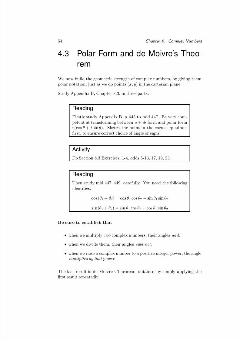
4.3 Polar Form and de Moivre’s Theo-rem
We now build the geometric strength of complex numbers, by giving thempolar notation, just as we do points ( x, y) in the cartesian plane.
Study Appendix B, Chapter 8.3, in three parts:
Reading
Firstly study Appendix B, p 445 to mid 447. Be very com-petent at transforming between a + ib form and polar formr (cos θ + i sin θ). Sketch the point in the correct quadrantrst, to ensure correct choice of angle or signs.
ActivityDo Section 8.3 Exercises, 1-4, odds 5-13, 17, 19, 23.
ReadingThen study mid 447–449, carefully. You need the followingidentities:
cos(θ1 + θ2) = cos θ1 cos θ2 − sin θ1 sin θ2
sin(θ1 + θ2) = sin θ1 cos θ2 + cos θ1 sin θ2
Be sure to establish that
• when we multiply two complex numbers, their angles add ;
• when we divide them, their angles subtract ;
• when we raise a complex number to a positive integer power, the anglemultiplies by that power .
The last result is de Moivre’s Theorem: obtained by simply applying therst result repeatedly.
8/10/2019 algebra and calculus.pdf
http://slidepdf.com/reader/full/algebra-and-calculuspdf 63/135
4.3. Polar Form and de Moivre’s Theorem 55
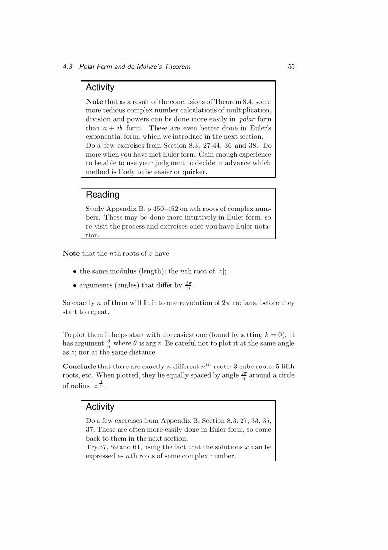
ActivityNote that as a result of the conclusions of Theorem 8.4, somemore tedious complex number calculations of multiplication,division and powers can be done more easily in polar formthan a + ib form. These are even better done in Euler’sexponential form, which we introduce in the next section.Do a few exercises from Section 8.3, 27-44, 36 and 38. Domore when you have met Euler form. Gain enough experienceto be able to use your judgment to decide in advance whichmethod is likely to be easier or quicker.
ReadingStudy Appendix B, p 450–452 on nth roots of complex num-bers. These may be done more intuitively in Euler form, sore-visit the process and exercises once you have Euler nota-tion.
Note that the n th roots of z have
• the same modulus (length): the n th root of |z|;
• arguments (angles) that differ by 2π
n .
So exactly n of them will t into one revolution of 2 π radians, before theystart to repeat.
To plot them it helps start with the easiest one (found by setting k = 0). Ithas argument θ
n where θ is arg z. Be careful not to plot it at the same angleas z; nor at the same distance.
Conclude that there are exactly n different n th roots: 3 cube roots, 5 fthroots, etc. When plotted, they lie equally spaced by angle 2π
n around a circle
of radius |z|1
n .
ActivityDo a few exercises from Appendix B, Section 8.3: 27, 33, 35,37. These are often more easily done in Euler form, so comeback to them in the next section.Try 57, 59 and 61, using the fact that the solutions x can beexpressed as n th roots of some complex number.
8/10/2019 algebra and calculus.pdf
http://slidepdf.com/reader/full/algebra-and-calculuspdf 64/135
56 Chapter 4. Complex Numbers
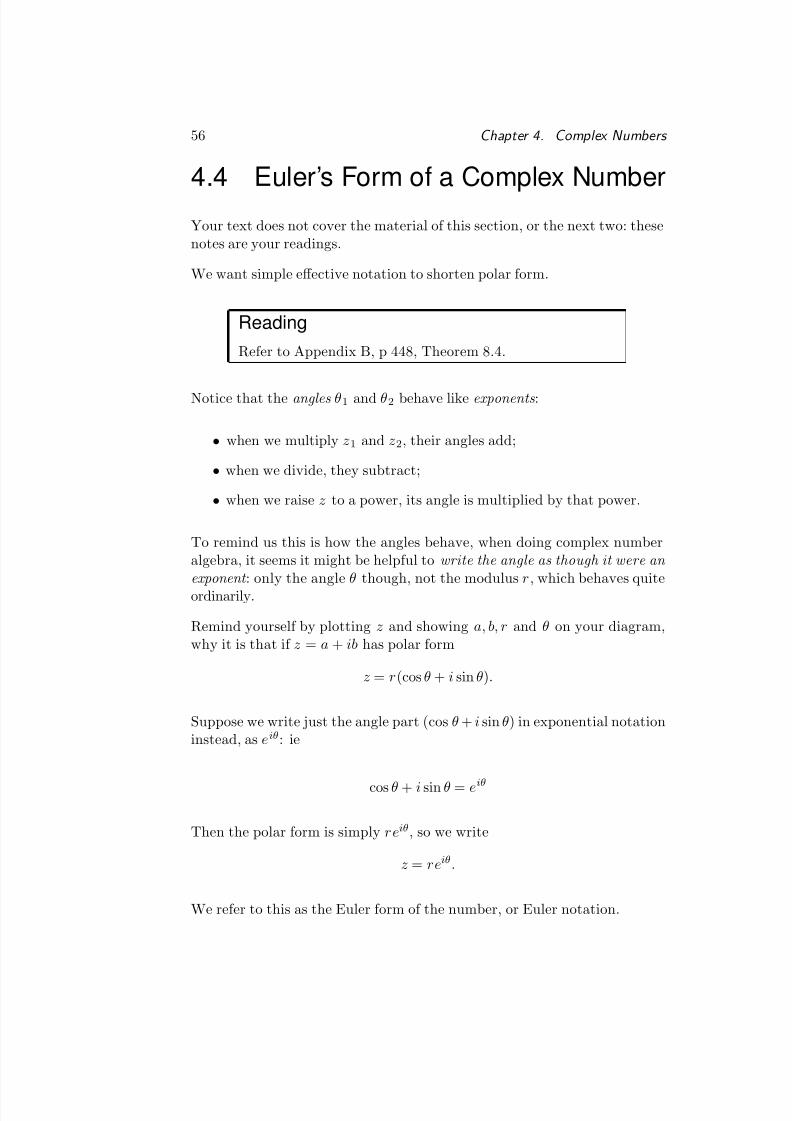
4.4 Euler’s Form of a Complex Number
Your text does not cover the material of this section, or the next two: thesenotes are your readings.
We want simple effective notation to shorten polar form.
ReadingRefer to Appendix B, p 448, Theorem 8.4.
Notice that the angles θ1 and θ2 behave like exponents :
• when we multiply z1 and z2, their angles add;
• when we divide, they subtract;
• when we raise z to a power, its angle is multiplied by that power.
To remind us this is how the angles behave, when doing complex numberalgebra, it seems it might be helpful to write the angle as though it were an exponent : only the angle θ though, not the modulus r , which behaves quiteordinarily.
Remind yourself by plotting z and showing a, b, r and θ on your diagram,why it is that if z = a + ib has polar form
z = r (cos θ + i sin θ).
Suppose we write just the angle part (cos θ + i sin θ) in exponential notationinstead, as eiθ : ie
cos θ + i sin θ = eiθ
Then the polar form is simply re iθ , so we write
z = re iθ .
We refer to this as the Euler form of the number, or Euler notation.
8/10/2019 algebra and calculus.pdf
http://slidepdf.com/reader/full/algebra-and-calculuspdf 65/135
4.4. Euler’s Form of a Complex Number 57
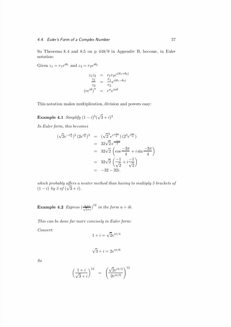
So Theorems 8.4 and 8.5 on p 448/9 in Appendix B, become, in Euler
notation:Given z1 = r1eiθ 1 and z2 = r2eiθ2
z1z2 = r1r 2ei(θ1 + θ2 )
z1
z2=
r1
r 2ei(θ1 −θ2 )
(re iθ )n = rn einθ
This notation makes multiplication, division and powers easy:
Example 4.1 Simplify (1 − i)5(√ 3 + i)3
In Euler form, this becomes
(√ 2e−i π4 )5 (2ei π
6 )3 = ( √ 25ei − 5 π
4 ) (2 3ei 3 π6 )
= 32√ 2 e− 3 iπ
4
= 32√ 2 cos −3π4
+ i sin −3π4
= 32√ 2 −1√ 2 + i−1
√ 2= −32 − 32i.
which probably offers a neater method than having to multiply 5 brackets of (1 − i) by 3 of (√ 3 + i).
Example 4.2 Express ( 1+ i√ 3+ i )12 in the form a + ib.
This can be done far more concisely in Euler form:
Convert:1 + i = √ 2eiπ/ 4
√ 3 + i = 2 eiπ/ 6
So
1 + i√ 3 + i
12=
√ 2eiπ/ 4
2eiπ/ 6
12
8/10/2019 algebra and calculus.pdf
http://slidepdf.com/reader/full/algebra-and-calculuspdf 66/135
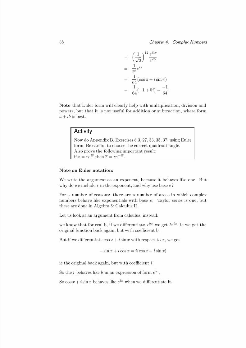
58 Chapter 4. Complex Numbers
= 1
√ 212 ei3π
ei2π
= 1
26 eiπ
= 164
(cos π + i sin π)
= 164
(−1 + 0 i) = −164
.
Note that Euler form will clearly help with multiplication, division andpowers, but that it is not useful for addition or subtraction, where forma + ib is best.
ActivityNow do Appendix B, Exercises 8.3, 27, 33, 35, 37, using Eulerform. Be careful to choose the correct quadrant angle.Also prove the following important result:if z = re iθ then z = re −iθ .
Note on Euler notation:
We write the argument as an exponent, because it behaves like one. Butwhy do we include i in the exponent, and why use base e?
For a number of reasons: there are a number of areas in which complexnumbers behave like exponentials with base e. Taylor series is one, butthese are done in Algebra & Calculus II.
Let us look at an argument from calculus, instead:
we know that for real b, if we differentiate ebx we get bebx , ie we get theoriginal function back again, but with coefficient b.
But if we differentiate cos x + i sin x with respect to x, we get
−sin x + i cos x = i(cos x + i sin x)
ie the original back again, but with coefficient i.
So the i behaves like b in an expression of form ebx.
So cosx + i sin x behaves like eix when we differentiate it.
8/10/2019 algebra and calculus.pdf
http://slidepdf.com/reader/full/algebra-and-calculuspdf 67/135
4.4. Euler’s Form of a Complex Number 59
A Geometric View of Complex Number Multiplication: Rotations
Note that if we use complex number re iθ as a multiplier on another complexnumber z, it changes both the modulus and argument of z:
• cause addition of angle θ to the argument of z, and
• multiply the modulus of z by r .
We conclude that multiplier re iθ will cause rotation through angleθ and lengthen or shorten by factor r .
So complex numbers are useful, as matrices are, for rotating and resizingimages in the plane.
Example 4.3 Check this effect by multiplying the point 1 + i, say, by −1,i, and 2i, and plotting the four complex numbers on the same diagram.
1. The multiplier −1 = 1eiπ will rotate the point through π but keep the distance from origin.
2. Multiplier i = 1 ei π2 will cause no change in distance, but will rotate
points anticlockwise through 90 degrees.
3. Multiplier 2i = 2 eiπ/ 2 will stretch by a factor of 2 and rotate anti-clockwise through a right angle.
n’th roots can also be done in Euler form:
Example 4.4 The general form of the nth roots of ae ib:
To catch all n of them, write the argument (angle) in its most general form,
not just b, but b + k2π, where k is any integer:ae ib = ae i(b+ k2π ) .
Suppose the nth roots are of form re iθ . Then we must have
(re iθ )n = ae i(b+ k2π ).
Sor n einθ = ae i(b+ k2π )
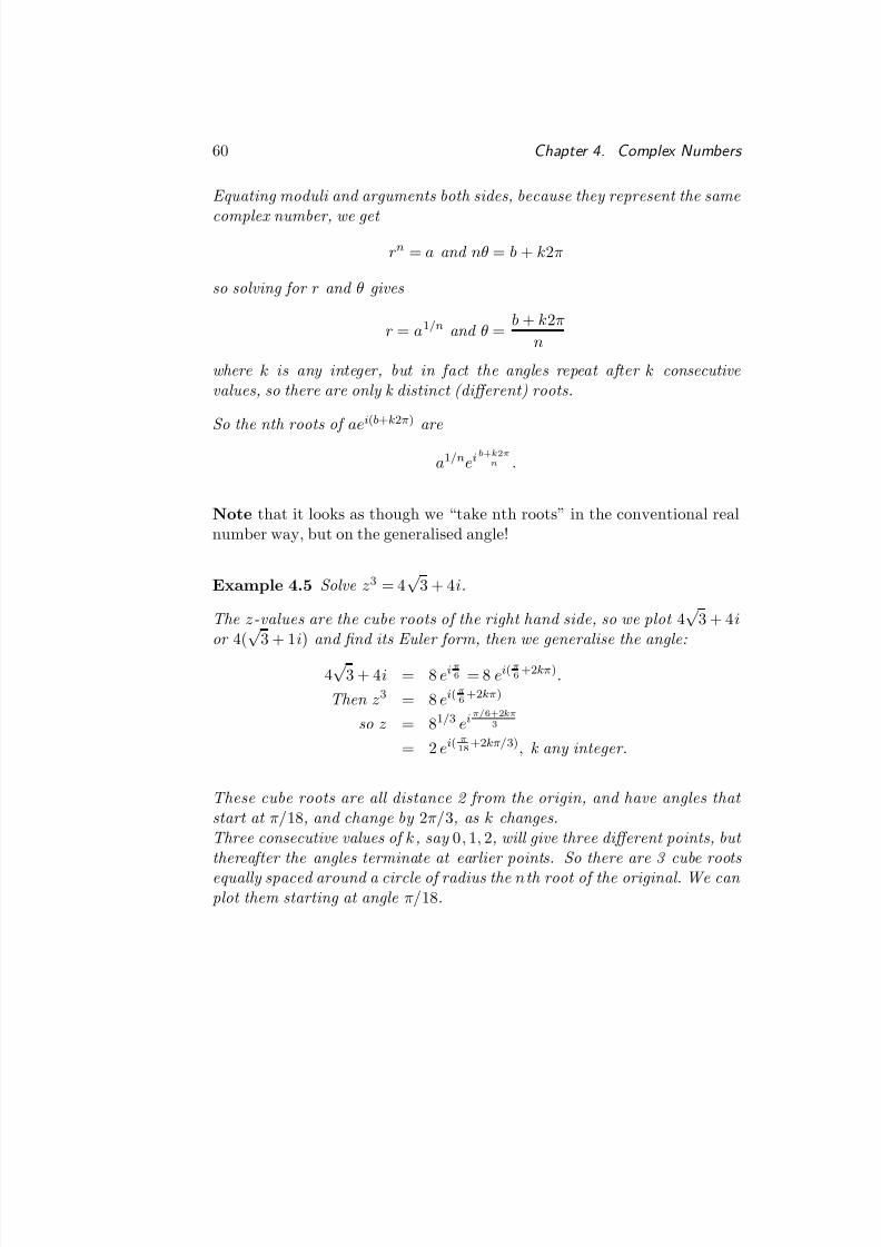
8/10/2019 algebra and calculus.pdf
http://slidepdf.com/reader/full/algebra-and-calculuspdf 68/135
60 Chapter 4. Complex Numbers
Equating moduli and arguments both sides, because they represent the same
complex number, we get
r n = a and nθ = b + k2π
so solving for r and θ gives
r = a1/n and θ = b + k2π
n
where k is any integer, but in fact the angles repeat after k consecutive values, so there are only k distinct (different) roots.
So the nth roots of ae i(b+ k2π ) are
a1/n ei b+ k 2 πn .
Note that it looks as though we “take nth roots” in the conventional realnumber way, but on the generalised angle!
Example 4.5 Solve z3 = 4 √ 3 + 4 i.
The z-values are the cube roots of the right hand side, so we plot 4√ 3 + 4 ior 4(√ 3 + 1 i) and nd its Euler form, then we generalise the angle:
4√ 3 + 4 i = 8 ei π6 = 8 ei( π
6 +2 kπ ) .Then z3 = 8 ei( π
6 +2 kπ )
so z = 8 1/ 3 ei π/ 6+2 kπ3
= 2 ei( π18 +2 kπ/ 3) , k any integer.
These cube roots are all distance 2 from the origin, and have angles that start at π/ 18, and change by 2π/ 3, as k changes.Three consecutive values of k, say 0, 1, 2, will give three different points, but thereafter the angles terminate at earlier points. So there are 3 cube roots equally spaced around a circle of radius the n th root of the original. We can plot them starting at angle π/ 18.
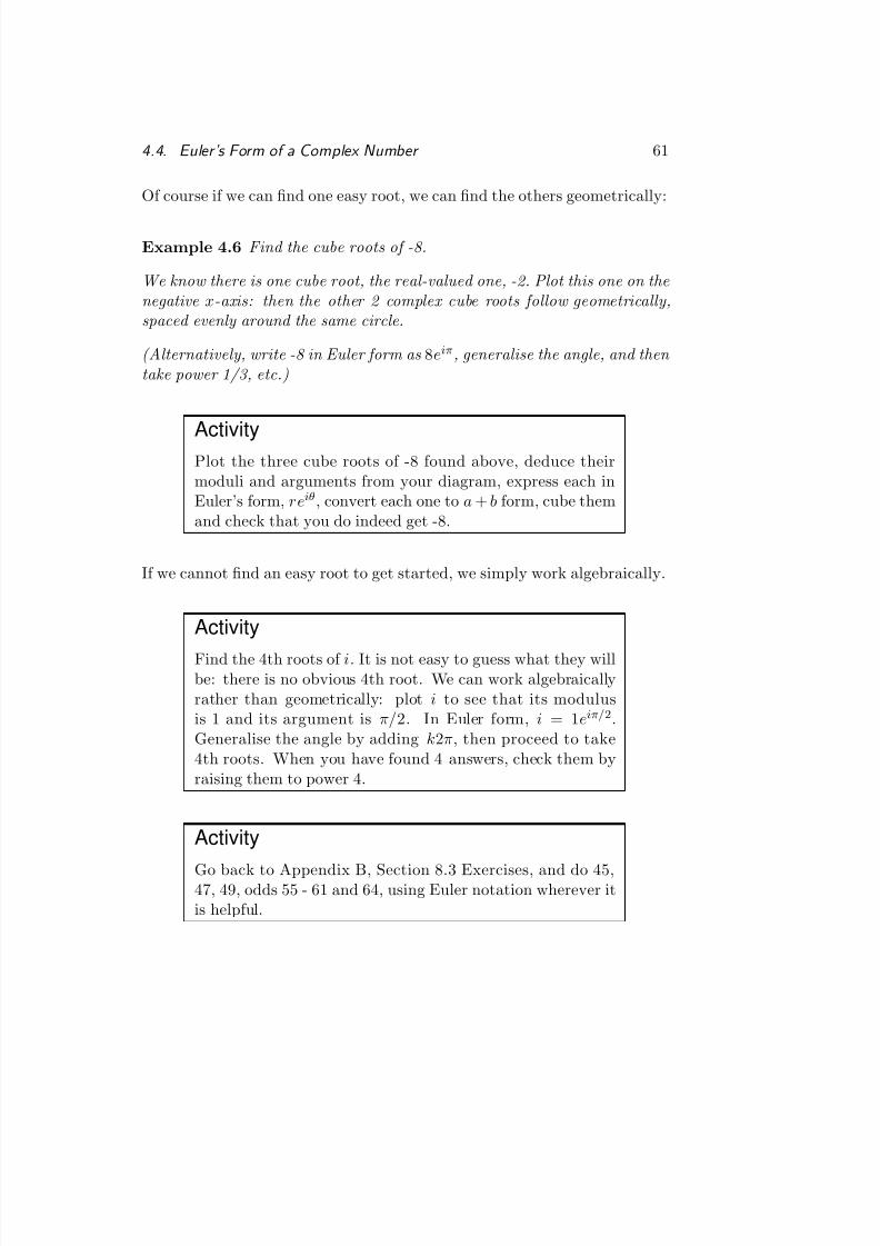
8/10/2019 algebra and calculus.pdf
http://slidepdf.com/reader/full/algebra-and-calculuspdf 69/135
4.4. Euler’s Form of a Complex Number 61
Of course if we can nd one easy root, we can nd the others geometrically:
Example 4.6 Find the cube roots of -8.
We know there is one cube root, the real-valued one, -2. Plot this one on the negative x-axis: then the other 2 complex cube roots follow geometrically,spaced evenly around the same circle.
(Alternatively, write -8 in Euler form as 8eiπ , generalise the angle, and then take power 1/3, etc.)
ActivityPlot the three cube roots of -8 found above, deduce theirmoduli and arguments from your diagram, express each inEuler’s form, re iθ , convert each one to a + b form, cube themand check that you do indeed get -8.
If we cannot nd an easy root to get started, we simply work algebraically.
Activity
Find the 4th roots of i. It is not easy to guess what they willbe: there is no obvious 4th root. We can work algebraicallyrather than geometrically: plot i to see that its modulusis 1 and its argument is π/ 2. In Euler form, i = 1 eiπ/ 2.Generalise the angle by adding k2π, then proceed to take4th roots. When you have found 4 answers, check them byraising them to power 4.
Activity
Go back to Appendix B, Section 8.3 Exercises, and do 45,47, 49, odds 55 - 61 and 64, using Euler notation wherever itis helpful.
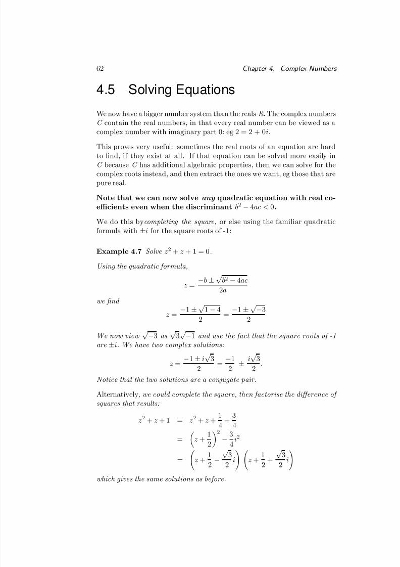
8/10/2019 algebra and calculus.pdf
http://slidepdf.com/reader/full/algebra-and-calculuspdf 70/135
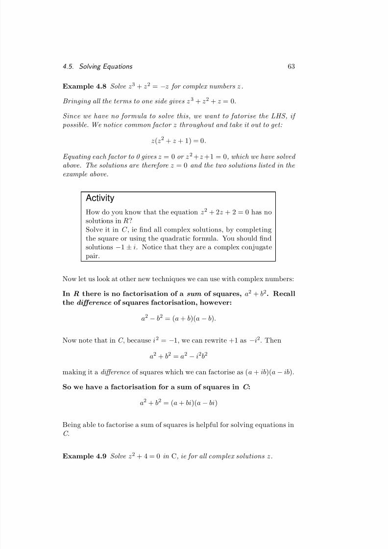
8/10/2019 algebra and calculus.pdf
http://slidepdf.com/reader/full/algebra-and-calculuspdf 71/135
4.5. Solving Equations 63
Example 4.8 Solve z3 + z2 = −z for complex numbers z.
Bringing all the terms to one side gives z3 + z2 + z = 0 .
Since we have no formula to solve this, we want to fatorise the LHS, if possible. We notice common factor z throughout and take it out to get:
z(z2 + z + 1) = 0 .
Equating each factor to 0 gives z = 0 or z2 + z +1 = 0 , which we have solved above. The solutions are therefore z = 0 and the two solutions listed in the example above.
ActivityHow do you know that the equation z2 + 2 z + 2 = 0 has nosolutions in R?Solve it in C , ie nd all complex solutions, by completingthe square or using the quadratic formula. You should ndsolutions −1 ± i. Notice that they are a complex conjugatepair.
Now let us look at other new techniques we can use with complex numbers:
In R there is no factorisation of a sum of squares, a2 + b2. Recallthe difference of squares factorisation, however:
a2 − b2 = ( a + b)(a − b).
Now note that in C , because i2 = −1, we can rewrite +1 as −i2. Then
a2 + b2 = a2 − i2b2
making it a difference of squares which we can factorise as ( a + ib)(a − ib).
So we have a factorisation for a sum of squares in C :
a2 + b2 = ( a + bi)(a − bi)
Being able to factorise a sum of squares is helpful for solving equations inC .
Example 4.9 Solve z2 + 4 = 0 in C, ie for all complex solutions z.
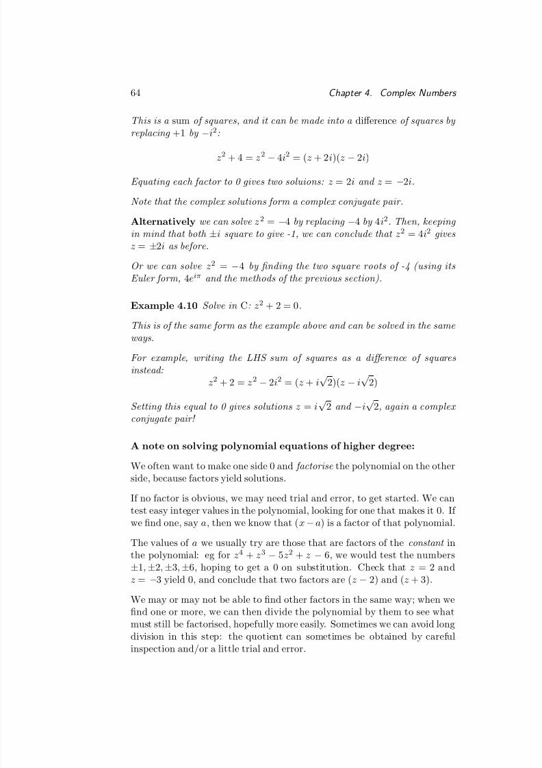
8/10/2019 algebra and calculus.pdf
http://slidepdf.com/reader/full/algebra-and-calculuspdf 72/135
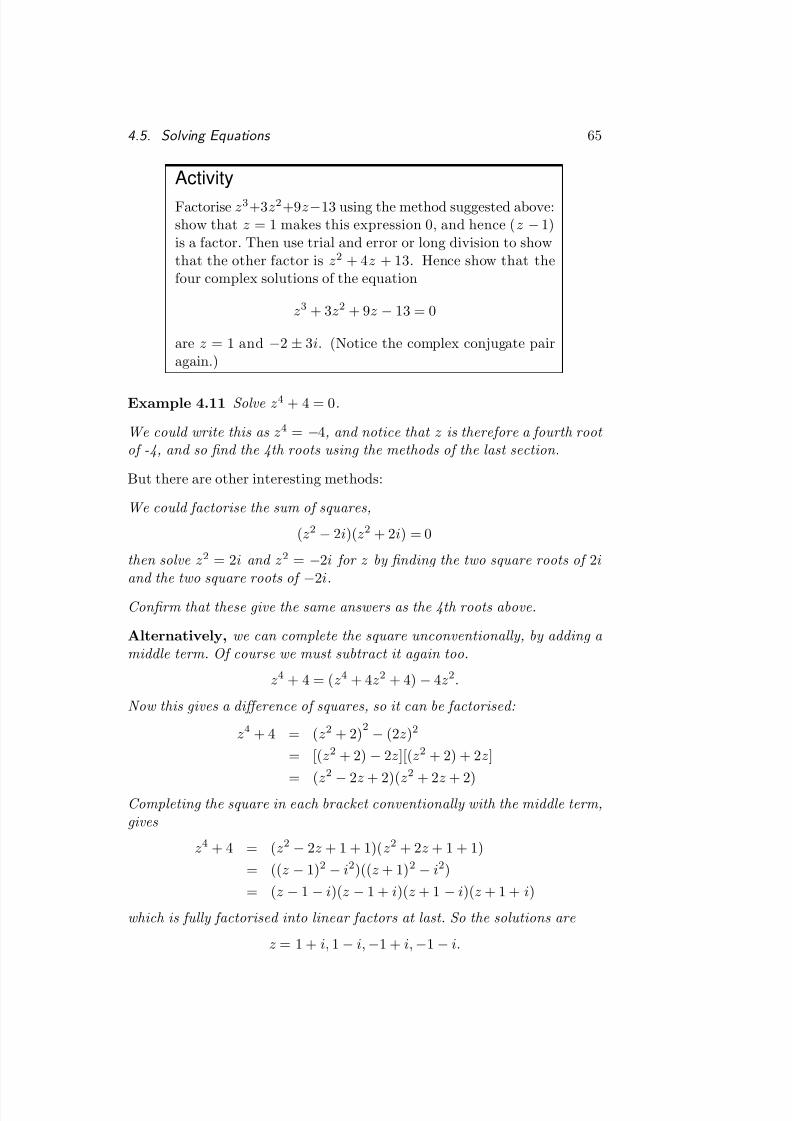
8/10/2019 algebra and calculus.pdf
http://slidepdf.com/reader/full/algebra-and-calculuspdf 73/135
4.5. Solving Equations 65
ActivityFactorise z3+3 z2+9 z−13 using the method suggested above:show that z = 1 makes this expression 0, and hence ( z − 1)is a factor. Then use trial and error or long division to showthat the other factor is z2 + 4 z + 13. Hence show that thefour complex solutions of the equation
z3 + 3 z2 + 9 z − 13 = 0
are z = 1 and −2 ± 3i. (Notice the complex conjugate pairagain.)
Example 4.11 Solve z4 + 4 = 0 .
We could write this as z4 = −4, and notice that z is therefore a fourth root of -4, and so nd the 4th roots using the methods of the last section.
But there are other interesting methods:
We could factorise the sum of squares,
(z2 − 2i)(z2 + 2 i) = 0
then solve z2 = 2 i and z2 = −2i for z by nding the two square roots of 2iand the two square roots of
−2i.
Conrm that these give the same answers as the 4th roots above.
Alternatively, we can complete the square unconventionally, by adding a middle term. Of course we must subtract it again too.
z4 + 4 = ( z4 + 4 z2 + 4) − 4z2.
Now this gives a difference of squares, so it can be factorised:
z4 + 4 = ( z2 + 2) 2
− (2z)2
= [( z2 + 2) − 2z][(z2 + 2) + 2 z]= ( z2
− 2z + 2)( z2 + 2 z + 2)
Completing the square in each bracket conventionally with the middle term,gives
z4 + 4 = ( z2 − 2z + 1 + 1)( z2 + 2 z + 1 + 1)= (( z − 1)2 − i2)(( z + 1) 2 − i2)= ( z − 1 − i)(z − 1 + i)( z + 1 − i)(z + 1 + i)
which is fully factorised into linear factors at last. So the solutions are
z = 1 + i, 1 − i, −1 + i, −1 − i.
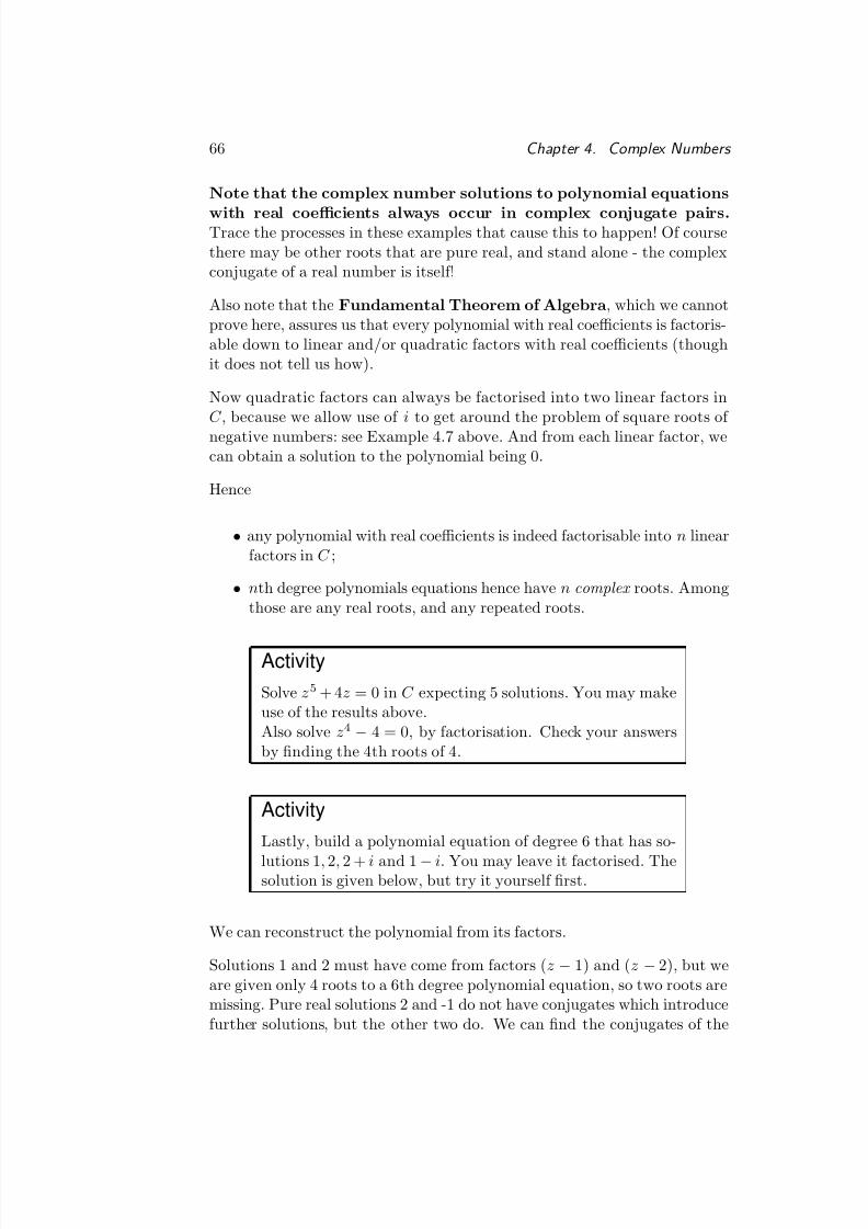
8/10/2019 algebra and calculus.pdf
http://slidepdf.com/reader/full/algebra-and-calculuspdf 74/135
66 Chapter 4. Complex Numbers
Note that the complex number solutions to polynomial equations
with real coefficients always occur in complex conjugate pairs.Trace the processes in these examples that cause this to happen! Of coursethere may be other roots that are pure real, and stand alone - the complexconjugate of a real number is itself!
Also note that the Fundamental Theorem of Algebra , which we cannotprove here, assures us that every polynomial with real coefficients is factoris-able down to linear and/or quadratic factors with real coefficients (thoughit does not tell us how).
Now quadratic factors can always be factorised into two linear factors inC , because we allow use of i to get around the problem of square roots of negative numbers: see Example 4.7 above. And from each linear factor, wecan obtain a solution to the polynomial being 0.
Hence
• any polynomial with real coefficients is indeed factorisable into n linearfactors in C ;
• nth degree polynomials equations hence have n complex roots. Amongthose are any real roots, and any repeated roots.
ActivitySolve z5 + 4 z = 0 in C expecting 5 solutions. You may makeuse of the results above.Also solve z4 − 4 = 0, by factorisation. Check your answersby nding the 4th roots of 4.
ActivityLastly, build a polynomial equation of degree 6 that has so-
lutions 1 , 2, 2 + i and 1 −i. You may leave it factorised. Thesolution is given below, but try it yourself rst.
We can reconstruct the polynomial from its factors.
Solutions 1 and 2 must have come from factors ( z − 1) and ( z − 2), but weare given only 4 roots to a 6th degree polynomial equation, so two roots aremissing. Pure real solutions 2 and -1 do not have conjugates which introducefurther solutions, but the other two do. We can nd the conjugates of the
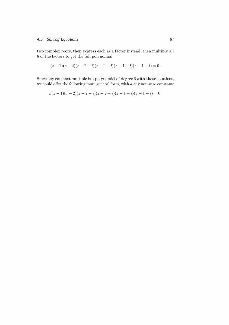
8/10/2019 algebra and calculus.pdf
http://slidepdf.com/reader/full/algebra-and-calculuspdf 75/135
4.5. Solving Equations 67
two complex roots, then express each as a factor instead, then multiply all
6 of the factors to get the full polynomial:
(z − 1)(z − 2)(z − 2 − i)(z − 2 + i)(z − 1 + i)( z − 1 − i) = 0 .
Since any constant multiple is a polynomial of degree 6 with those solutions,we could offer the following more general form, with k any non-zero constant:
k(z − 1)(z − 2)(z − 2 − i)( z − 2 + i)(z − 1 + i)( z − 1 − i) = 0 .
8/10/2019 algebra and calculus.pdf
http://slidepdf.com/reader/full/algebra-and-calculuspdf 76/135
68 Chapter 4. Complex Numbers
4.6 Functions of Complex Variable z
Sometimes we want to use functions of complex numbers, for example trigono-metric, exponential and log, and powers, to describe and analyse the behav-iour of real phenomena, or to solve equations.
In this section, we show briey how familiar denitions can be generalisedto dene useful complex-valued functions of complex variables z.
The exponential function, ez :
We have already dened what we mean by eib for b real. To dene what wemean by ez , ie ea+ ib, we simply extend that:
for z = a + ib, we want
ez = ea+ ib = ea eib = ea (cos b + i sin b),
and so we simply dene ez as that.
Example 4.12
ei(−3−2i) = e(2−i3) = e2 e−i3
= e2 (cos (−3) + i sin(−3))= e2 (cos3 − i sin 3).
We can get an approximate value for this, in a + ib form, by using a calcu-lator.
The trig functions:
For real a, we dened eia
= cos a + i sin a.From this and the fact that cos ( −a) = cos a and sin ( −a) = −sin a, we alsohave
e−ia = cos ( −a) + i sin(−a) = cos a − i sin a.
Writing these two facts together, we have
eia = cos a + i sin a,e−ia = cos a − i sin a.
8/10/2019 algebra and calculus.pdf
http://slidepdf.com/reader/full/algebra-and-calculuspdf 77/135
4.6. Functions of Complex Variable z 69
Adding and subtracting these gives:
cos a = eia + e−ia
2 ,
sin a = eia − e−ia
2i .
We know from the above that this holds for any real number a. But we nowextend these formulae to complex numbers too, by simply dening for anycomplex number z:
cos z = eiz + e−iz
2
sin z = eiz − e−iz
2i .
We know that the right hand side has meaning because of the denitions wehave for eiz and e−iz above.
We then extend to denitions of the other trig functions of z too, in thenatural way: tan z is dened as sin z
cos z , and the other 3 trig functions aredened as the reciprocals of these.
Example 4.13cos (3 + 4 i) = (1 / 2)(ei(3+4 i) + e−i(3+4 i) )
= (1 / 2)(e3i−4 + e−3i+4 )= (1 / 2)(e−4e3i + e4e−3i )= (1 / 2)(e−4(cos 3 + i sin 3) + e4(cos3 − i sin 3))= (1 / 2)[cos 3(e−4 + e4) + i sin3(e−4 + e4)] etc.
The log function:
To dene log z we write z in Euler form and generalise the angle, just as wedid for n th roots:
Suppose z = re it = re i(t+2 kπ ) , k any integer.
We want log z = log re i(t+2 kπ ) .
If we can use the log AB = log A +log B , to separate the logs, and make useof the fact that log ea = a, it seems reasonable to expect that
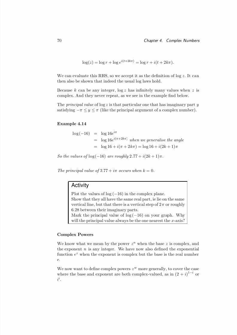
8/10/2019 algebra and calculus.pdf
http://slidepdf.com/reader/full/algebra-and-calculuspdf 78/135
70 Chapter 4. Complex Numbers
log(z) = log r + log ei(t+2 kπ ) = log r + i(t + 2 kπ ).
We can evaluate this RHS, so we accept it as the denition of log z. It canthen also be shown that indeed the usual log laws hold.
Because k can be any integer, log z has innitely many values when z iscomplex. And they never repeat, as we see in the example nd below.
The principal value of logz is that particular one that has imaginary part ysatisfying −π ≤ y ≤ π (like the principal argument of a complex number).
Example 4.14
log(−16) = log 16 eiπ
= log 16 ei(π +2 kπ ) when we generalise the angle = log 16 + i(π + 2 kπ ) = log 16 + i(2k + 1) π
So the values of log(−16) are roughly 2.77 + i(2k + 1) π.
The principal value of 2.77 + iπ occurs when k = 0 .
ActivityPlot the values of log ( −16) in the complex plane.Show that they all have the same real part, ie lie on the samevertical line, but that there is a vertical step of 2 π or roughly6.28 between their imaginary parts.Mark the principal value of log ( −16) on your graph. Whywill the principal value always be the one nearest the x-axis?
Complex PowersWe know what we mean by the power zn when the base z is complex, andthe exponent n is any integer. We have now also dened the exponentialfunction ez when the exponent is complex but the base is the real numbere.
We now want to dene complex powers zw more generally, to cover the casewhere the base and exponent are both complex-valued, as in (2 + i)1−i orii .
8/10/2019 algebra and calculus.pdf
http://slidepdf.com/reader/full/algebra-and-calculuspdf 79/135
4.6. Functions of Complex Variable z 71
We make use of the denition above:
ea+ ib = ea eib = ea (cos b + i sin b).
To apply this denition to zw , we must change the base from z to e.
Taking the natural log we know that log zw = w log z. Rewriting this inexponential form, we get
zw = ew log z .
If we now write w log z in the form a + ib, then we can use the denition of ea+ ib above to nish off, as in the example below.
Example 4.15 Evaluate ii .
Notice that this has complex base and complex exponent.We change the base to e using i i = ei log i , then simplify the exponent, aiming at form a + bi.
Starting with log i, we have
log i = log 1ei(π/ 2+2 kπ )
= log 1 + i(π/ 2 + 2 kπ )
= 0 + i(π/ 2 + 2 kπ ).
This means that i log i = i2(π/ 2 + 2 kπ ) = −π/ 2 − 2kπ.
So ii = ei log i = e−π/ 2−2kπ , k any integer.
Note that in this last step, we could write the exponent as 2kπ instead of
−2kπ , because k represents any integer, positive or negative: either will do.
Substituting values for k gives different values for i i :k = 0 gives 0.208 and k = −1 gives 0.000388, approximately.Of course there are many more values:all real in this case, because no i terms remain in the nal form.
Example 4.16 Evaluate (1 + 3 i)2−i .
This also has form zw , z and w complex, but requires more effort to evaluate than i i does, because the imaginary part of the exponent does not disappear.
Only study this if you are condent with all that has gone before.
Changing the base to e, we get (1 + 3 i)2−i = e(2−i) log (1+3 i) .
8/10/2019 algebra and calculus.pdf
http://slidepdf.com/reader/full/algebra-and-calculuspdf 80/135
72 Chapter 4. Complex Numbers
Now to nd log(1 + 3 i), we use the Euler form of 1 + 3i. The modulus is
√ 10. For simplicity write t for the argument, ie t = arctan3 .Then 1 + 3 i = √ 10 eit = √ 10 ei(t+2 kπ ) .
Hence log (1 + 3i) = log ( √ 10 ei(t+2 kπ ) ) = log √ 10 + i(t + 2 kπ ).
Multiplying this by (2 − i) gives (2 − i)[log √ 10 + i(t + 2 kπ )].
Gathering real and imaginary parts gives
log 10 + t + 2 kπ + i(2t + 4 kπ − (1/ 2)log10)
Putting this exponent back into the power gives
(1 + 3 i)2−i = elog 10+ t+2 kπ + i(2t+4 kπ −(1/ 2)log 10)
Separating real and imaginary parts, aiming at form re it gives
elog 10 et e2kπ ei(2t+4 kπ −(1/ 2)log 10)
= 10 et e2kπ ei(2t−(1/ 2)log 10) ei4kπ
and the last factor is 1. (Check sine and cosine values.)
If we put in an approximate value of t = arctan 3 , ie 1.25, then k = 0 gives an approximate principal value of 7.75 + 34 .00i.
Other values follow by setting k = 1 , 2, 3 ... and k = −1, −2, −3 ...
ActivityTry the above examples yourself: aim at minimal reference.

8/10/2019 algebra and calculus.pdf
http://slidepdf.com/reader/full/algebra-and-calculuspdf 81/135

8/10/2019 algebra and calculus.pdf
http://slidepdf.com/reader/full/algebra-and-calculuspdf 82/135
74 Chapter 4. Complex Numbers
8/10/2019 algebra and calculus.pdf
http://slidepdf.com/reader/full/algebra-and-calculuspdf 83/135
Module IICLEVER
CALCULUS
75

8/10/2019 algebra and calculus.pdf
http://slidepdf.com/reader/full/algebra-and-calculuspdf 84/135
8/10/2019 algebra and calculus.pdf
http://slidepdf.com/reader/full/algebra-and-calculuspdf 85/135

8/10/2019 algebra and calculus.pdf
http://slidepdf.com/reader/full/algebra-and-calculuspdf 86/135
78
8/10/2019 algebra and calculus.pdf
http://slidepdf.com/reader/full/algebra-and-calculuspdf 87/135
Chapter 1Functions and Models
INTRODUCTION
You will need to work rather quickly through this chapter. Most of thefunctions in this chapter will be known to you from high school, althoughthe section on inverses may be new or unfamiliar. The approach taken tothese functions, and the way they are modelled, will probably be new toyou.
This chapter on functions is very important for your success in developingcalculus. All of the so-called elementary functions (powers, polynomials,exponential, logarithmic, and trigonometric) to be used in the course areintroduced here.
The important thing for you is to become familiar with graphical and numer-ical approach to functions which adds so much meaning to common algebraic
methods. The computer package Matlab or its equivalent, is an excellentaid to this. You need to be able to think more graphically about functionsand to be able to read and interpret tables of numerical data. This will helpyou to apply functions in the modelling of real-world phenomena.
There is also a section on constructing new functions from old. How to shift,ip and stretch graphs.
79
8/10/2019 algebra and calculus.pdf
http://slidepdf.com/reader/full/algebra-and-calculuspdf 88/135
80 Chapter 1. Functions and Models
1.1 Four Ways to Represent a Function
Four ways are used here to represent functions. Remember that this meansthat you represent functions by tables, graphs, formulas, and words.
ReadingStudy the set textbook (Stewart) edition 3, chapter 1 section1.1, pp 11-21.
Note the use of the terminology domain/range, independent/dependent vari-able, increasing/decreasing. Also, the interval notation [ a, b] and (a, b) areintroduced early in the section. For example: The set of x values such that1 ≤ x < 3 is written as {x|1 ≤ x < 3} or simply as [1, 3). Using symmetryby recognising even and odd functions can sometimes simplify things.
ActivityDo Stewart exercises Sec 1.1 nos 1, 5, 7, 9, 15, 61, 63.Note that answers are given in the back for many of the oddnumbered questions
Computer ActivityStewart: section 1.4, no 21.
Matlab note: for example
x=0: 0.01: 5;f=10*x.^2;
g=x.^3/10;plot(x,f,x,g)}
Note: for all of these Computer Activities, you are urged to use Matlab
or Scilab. You may of course use any other mathematics package, but wewill only support Matlab and Scilab. Of course you could instead usea graphics calculator or even a scientic calculator to do these ComputerActivities, but it will take longer and is more tedious.
8/10/2019 algebra and calculus.pdf
http://slidepdf.com/reader/full/algebra-and-calculuspdf 89/135
1.2. Mathematical Models: a Catalog of Essential Functions 81
1.2 Mathematical Models: a Catalog ofEssential Functions
In applications, mathematical modelling using functions is the most commonway of representing technical phenomena in the real world. This sectionintroduces modelling and gives a quick look at the important functions tobe used by us in this course.
Linear functions have the property that the function changes by equalamounts for equal changes of the independent variable.
ReadingStewart: study section 1.2, pp 25-29.
ActivityStewart: do sec 1.2 exercises 5,7,11,13.
Computer Activity
A linear supply curve is given by p = 1 .05q + 0 .02, whereq is the quantity of goods and p is the price of the goods.The demand curve is p = 5 .4 −1.1q . Using a computer plot,nd a close approximation to the equilibrium values of p andq where the supply and demand curves intersect. Matlabhint: dene a q set of points between (say) 0 and 10 usingq=0:0.01:10; . This denes a set from 0 to 10 in steps of 0.01.Now the two graphs can be plotted one at a time using holdon to hold the rst plot. For example plot(q,1.05*q+0.02), and when you have plotted the second graph you can usezoom and then click on the intersection a few times to read
off an accurate intersection. Check that the intersection is atabout q = 2 .5 and p = 2 .65.
Polynomials should be quite familiar to you. We normally make use of polynomials up to about power 4. The most commonly used polynomialsare linear functions (degree 1) and quadratic functions (degree 2).
ReadingStewart: study sec 1.2, pp 29-31.
8/10/2019 algebra and calculus.pdf
http://slidepdf.com/reader/full/algebra-and-calculuspdf 90/135
82 Chapter 1. Functions and Models
ActivityStewart: sec 1.2 exercises 3, 9.
Computer ActivityStewart: sec 1.2 no 23.
Power Functions are simply a power of x. For example x3 or √ x = x0.5
or x−1 = 1 /x . The key point in this section is how different powers compareon small and large scales. Basic shapes of graphs of power functions are
developed. Note that it will be seen later that exponential functions grow(and collapse) much more quickly than power functions.
ReadingStewart: study sec 1.2 pp 31-32.
ActivityStewart: do sec 1.2 exercises 1(a),(c),3.
Computer ActivityStewart: do sec 1.4 ex 25.
Rational Functions and Algebraic Functions are now dened.
ReadingStewart: study sec 1.2, pp 32-33.
Trigonometric Functions. This section should be a revision for you of high school. Make sure that your calculators are set on radians. Whenwe write sin x, you must appreciate that x is a number, and so must bein radians. You should not need to use degrees mode on your calculatorwhen x is a number. You can only use degrees mode when x represents thenumber of degrees of rotation, which is not such a good idea in mathematics,since mathematics is based on the study of number. Make sure that youcan sketch the sine curve, showing the amplitude and period. The cosinecurve is then just the same curve shifted back a distance of π/ 2. The tan
8/10/2019 algebra and calculus.pdf
http://slidepdf.com/reader/full/algebra-and-calculuspdf 91/135
1.3. New Functions From Old Functions. 83
curve is more complicated, since it has asymptotes at intervals of π. The
identity cos2
t + sin2
t = 1 is not mentioned here, but is crucial, since itenables you to swap from cos to sin since then cos t = ± 1 − sin2 t andsin t = ±√ 1 − cos2 t . The inverse trig functions will be seen later.
ReadingStewart: See Reference inside front cover and sec1.2 pp 33-34, and Appendix C on Inverse Trigonometric functions (seeStewart page A25-A27).
ActivityUse a calculator to nd one of the solutions to the equation2 = 5sin(3 x). (Answer: sin(3 x) = 2 / 5 = 0 .4, and so 3x =sin−1 0.4 = 0 .4115 (from calculator). Hence, x ≈ 0.1372. If you didn’t get that, check if your calculator is set in radians.Note: in Matlab the inverse sine function sin −1 x is writtenas asin(x).
Computer ActivityStewart: sec 1.4 exercise 9.
Exponential, Logarithmic, and Transcendental Functions are brieydened and introduced, to be seen in detail later.
ReadingStewart: study sec 1.2 pp 34,35.
1.3 New Functions From Old Functions.In this section a summary is given of translations, shifts and stretches, reec-tions, combinations and composite functions (function of a function). Thecomposite function ( f ◦ g)(x) = f (g(x)) is introduced. This is quite oftencalled a function of a function for obvious reasons. For example, if f (x) = x2
and g(x) = sin x, then ( f ◦ g)(x) = f (g(x)) = g2 = sin 2 x. Composition of functions is one of the most useful elements of the study of functions.

8/10/2019 algebra and calculus.pdf
http://slidepdf.com/reader/full/algebra-and-calculuspdf 92/135
84 Chapter 1. Functions and Models
ReadingStewart: study sec 1.3 pp 38-45.
ActivityStewart: do sec 1.3 ex 3, 5, 27, 35, 50.
1.4 Graphing Calculators and Comput-
ersIf you are using a graphics calculator, this section should be of interest toyou. If you are using Matlab you would be better to read the Booklet onan Introduction to Matlab , by Patricia Cretchley. In terms of controllingthe window of the plot in Matlab you can use the command axis equalin order to make the scales the same on the x and y axes. If you just wantto show the plot for the domain −2 ≤ x ≤ 3 and for the range −1 ≤ y ≤ 4,the Matlab command is axis([-2 3 -1 4]) .
ReadingStewart: peruse sec 1.4 pp 49-53. Example 9 on p53 illus-trates how a difficult equation can be accurately solved bygraphical means using the zoom facility. In Matlab justclick on the zoom button on the toolbar of the plot and thenclick on the portion of the plot which you want to enlarge.
1.5 Exponential Functions
Exponential functions have the form f (x) = ax where a is a positive con-stant. Note that x is in the exponent, whereas for power functions xa , xis in the base. Exponential functions have a simple property. The valueof the function changes by equal ratios over equal intervals. That is, asthe independent variable changes by a xed amount, the value of the func-tion changes by a constant factor. For example, given f (x) = ax , thenf (x + 3) = ax+3 = ax a3 = a3f (x) = Cf (x), and f (x + 6) = ax+6 =ax+3 a3 = a3f (x + 3) = Cf (x + 3).
8/10/2019 algebra and calculus.pdf
http://slidepdf.com/reader/full/algebra-and-calculuspdf 93/135
1.6. Inverse Functions and Logarithms 85
ReadingStewart: study section 1.5 pp 55-61
Take particular note of the general graph of the exponential function ax
exemplied by gure 2 for the case when a = 2. You should be able torecognise the important features, ie the curve has a horizontal asymptotefor the negative x axis, it then passes through the y axis at y = 1 and thenclimbs rapidly. Take note of Figure 4 also. For example, if a = 0 .5, then thegraph is y = 1
2x
= 2 −x .
Note that the x (or t) is the independent variable and often denotes position
(or time ) for the function ax (or at ). Take note of families of exponentialfunctions shown in Figure 3, the laws of exponents, and applications. Thenumber e is very special. Remember that it has a value of about 2.718, andthat it is just the value of a which makes ax have a slope of 1 at the point(0,1) on the y axis. We will see soon that the function y = ex is the onlyfunction whose slope at any point ( x, y ) on the curve, is equal to the valueof the function itself. In other words, the rate of change of ex is equal to ex .It is the only function in the entire universe that has this property.
Activity
Stewart: do sec 1.5 exercises 13,17,19.
Computer ActivityStewart: do sec 1.5 exercise 25.
1.6 Inverse Functions and Logarithms
This section may be somewhat new to you. The concept of an inversefunction is important. Make sure that you understand how to use tablesand graphs to represent inverses and take particular note of the way to getformulas for inverses.
ReadingStewart: study sec 1.6 pp 63-67.
8/10/2019 algebra and calculus.pdf
http://slidepdf.com/reader/full/algebra-and-calculuspdf 94/135
86 Chapter 1. Functions and Models
ActivityStewart: do sec 1.6 exercises 3,15,19,21.
Note that the graph of an inverse function is the mirror image of the functionitself reected about the line y = x.Another neat property of inverse functions is that they undo one anotheralgebraically. Thus f (f −1(x)) = f −1(f (x)) = x. For example if f (T ) =4T − 160, then T = f
4 + 40, ie the inverse function is f −1(T ) = T 4 + 40.
Then f (f −1(T )) = 4 f −1(T )−160 = 4( T 4 +40) −160 = T . Also f −1(f (T )) =
f (T )4 + 40 = 4T −160
4 + 40 = T .
Logarithms are inverse functions for exponential functions. Make sure thatyou can sketch the graph of a log function. The easiest way to do that isto remember how to sketch the exponential function, and then just take themirror image about y = x.Take particular note of the three main laws.Note that power functions with positive exponents always increase morerapidly than log functions.We mainly concentrate on the natural logarithm function to base e and willwrite it as ln x. Note that Matlab uses the notation log(x) as the naturallogarithm function.We won’t normally need to change to other logarithm bases, but if you everneed to do that, remember to use formula 10 on the bottom of page 69 of Stewart.
ReadingStewart: study sec 1.6 pp 67-71.
ActivityStewart: sec 1.6 do exercises 23, 25, 37, 49.
Chapter Summary The last section of this Chapter, on parametric curves,is to be omitted. It will be studied in the course MAT2100.This rst chapter is largely a revision of the function work you studied inhigh school. But the material forms a very important basis for the toolsneeded to develop the ideas and the applications of calculus.
8/10/2019 algebra and calculus.pdf
http://slidepdf.com/reader/full/algebra-and-calculuspdf 95/135
Chapter 2Limits and Derivatives
INTRODUCTION
In this chapter, the derivative is introduced as an instantaneous rate of change. Initially, tangents and speed are used to motivate practical exam-ples, and then the limit denition is developed. By the end of the chapteryou should be able to:
(i) understand the notion of an average rate of change;
(ii) understand the notion of a limit and be able to nd the limiting valuefor simple examples;
(iii) nd derivatives numerically by taking arbitrarily ne difference quo-tients;
(iv) visualize derivatives graphically as the slope of the graph when youzoom in (using your computer);
(v) interpret the meaning of rst and second derivatives;
(vi) understand the meaning of an antiderivative.
87
8/10/2019 algebra and calculus.pdf
http://slidepdf.com/reader/full/algebra-and-calculuspdf 96/135
88 Chapter 2. Limits and Derivatives
2.1 The Tangent and Velocity Problems
Most people have a good intuitive idea of how to represent a tangent to acurve at a point on the curve. The tangent line must only touch the curveat a single point. You can approximate the tangent line by taking anotherpoint on the curve and drawing the line segment between it and the giventangent point. The slope of this line segment is easy to calculate, and thenyou can just take the other point closer and closer to the tangent point toget better and better approximations to the exact slope of the tangent.
Instantaneous velocity can be interpreted in two fundamental and relatedways. It is the limit of average velocities, or it is the slope on the positionversus time graph.
Velocity is a measure of change. Change in position over time. If you werelming an accelerating car with a xed background, you can tell where thecar is on a single frame of the lm. However, if you were asked to estimatethe exact speed of the car on one of the frames, you would have to look atthe next (or previous) frame to get some idea. Of course you would alsoneed to know the time between frames. So it takes two frames to estimatethe speed as distance divided by time . If the frames of the lm are veryclose together in time, the estimate of speed would be more accurate. Theexact speed would be some sort of limit of a hypothetical camera as the time
between frames got shorter and shorter.
ReadingStewart: study sec 2.1 pp 93-97.
ActivityStewart: sec 2.1 do exercises 3, 5, 7.
2.2 The Limit of a FunctionWe look now at the limit of a function f (x) as x approaches a particularvalue a. Now, you might expect that the answer is always simply f (a). Butthis is not always the case. For a simple function, such as f (x) = x2, thelimit as x approaches 2 will of course be 2 2 = 4. But if f (x) = x2 −4
x−2 , thereis a problem! In fact f (2) does not even exist in this case. But even so,you will nd that lim x→2 f (x) = lim x→2(x + 2) = 4. To get this, I wrotex2 − 4 = ( x − 2)(x + 2) and cancelled the x − 2.
8/10/2019 algebra and calculus.pdf
http://slidepdf.com/reader/full/algebra-and-calculuspdf 97/135
2.3. Calculating Limits Using the Limit Laws 89
In this section we use numerical tables and graphics to see what the value
of limits might be.
ReadingStewart: study pp 98-105.Example 4 shows that there are some dangers in just guessingthe value of a limit by using a table of some values near thelimiting point. Figure 7 illustrates the complex behaviour of the function when you get near x = 0. Strictly, we requirethat the left-hand and right-hand limits are the same. Thenwe say that the limit of the function exists and is given by
their common values. Examples are given of some weird andwonderful functions. Note: the precise denition of a limitis given in Appendix D. It is indeed precise, but is a ratherabstract denition, and is not examinable.
ActivityStewart: sec 2.2 do exercises 1, 3, 13.
Computer ActivityStewart: sec 2.2 exercise 23. From your answer to part (a),look back at sec 1.5. For part (b), plot for values of x from
−2 to 3.
Matlab Note for sec 2.2 exercise 23 part (b)h=0.001; x=-2:h:3; y=(1+x).^(1./x); plot(x,y)
2.3 Calculating Limits Using the Limit LawsIn this section, we develop methods for nding the exact value of limits. Todo this we basically make use of ve common sense Limit Laws, and theDirect Substitution Property for simpler functions.
8/10/2019 algebra and calculus.pdf
http://slidepdf.com/reader/full/algebra-and-calculuspdf 98/135
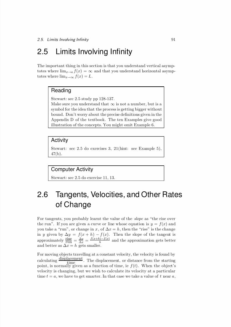
8/10/2019 algebra and calculus.pdf
http://slidepdf.com/reader/full/algebra-and-calculuspdf 99/135
2.5. Limits Involving Innity 91
2.5 Limits Involving Innity
The important thing in this section is that you understand vertical asymp-totes where lim x→a f (x) = ∞ and that you understand horizontal asymp-totes where lim x→∞f (x) = L.
ReadingStewart: sec 2.5 study pp 128-137.Make sure you understand that ∞ is not a number, but is asymbol for the idea that the process is getting bigger without
bound. Don’t worry about the precise denitions given in theAppendix D of the textbook. The ten Examples give goodillustration of the concepts. You might omit Example 6.
ActivityStewart: sec 2.5 do exercises 3, 21(hint: see Example 5),47(b).
Computer ActivityStewart: sec 2.5 do exercise 11, 13.
2.6 Tangents, Velocities, and Other Ratesof Change
For tangents, you probably learnt the value of the slope as “the rise overthe run”. If you are given a curve or line whose equation is y = f (x) and
you take a “run”, or change in x, of ∆ x = h, then the “rise” is the changein y given by ∆ y = f (x + h) − f (x). Then the slope of the tangent isapproximately rise
run = ∆ y∆ x = f (x+ h)−f (x)
h and the approximation gets betterand better as ∆ x = h gets smaller.
For moving objects travelling at a constant velocity, the velocity is found bycalculating displacement
time . The displacement, or distance from the startingpoint, is normally given as a function of time, ie f (t). When the object’svelocity is changing, but we wish to calculate its velocity at a particulartime t = a, we have to get smarter. In that case we take a value of t near a,
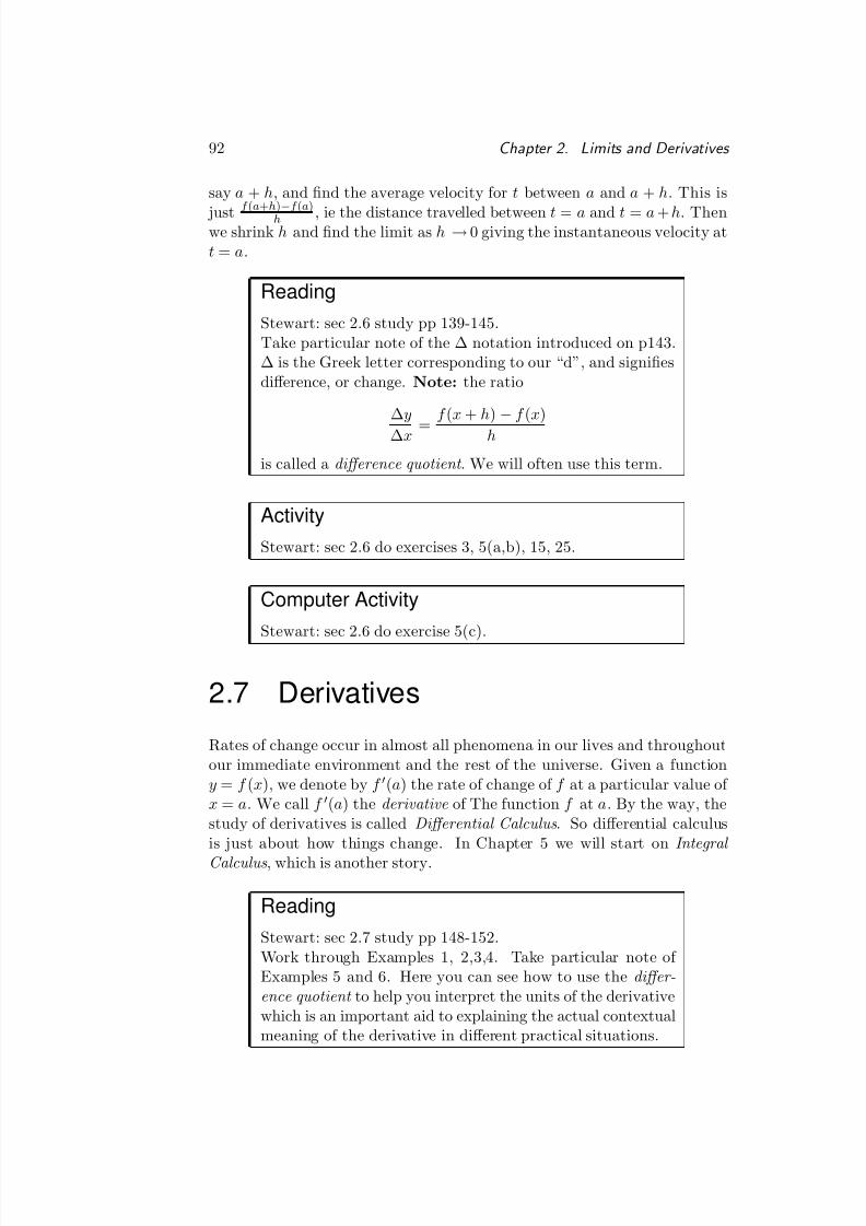
8/10/2019 algebra and calculus.pdf
http://slidepdf.com/reader/full/algebra-and-calculuspdf 100/135
92 Chapter 2. Limits and Derivatives
say a + h, and nd the average velocity for t between a and a + h. This is
just f (a+ h)
−f (a )
h , ie the distance travelled between t = a and t = a + h. Thenwe shrink h and nd the limit as h → 0 giving the instantaneous velocity att = a.
ReadingStewart: sec 2.6 study pp 139-145.Take particular note of the ∆ notation introduced on p143.∆ is the Greek letter corresponding to our “d”, and signiesdifference, or change. Note: the ratio
∆ y∆ x =
f (x + h)
− f (x)
h
is called a difference quotient . We will often use this term.
ActivityStewart: sec 2.6 do exercises 3, 5(a,b), 15, 25.
Computer ActivityStewart: sec 2.6 do exercise 5(c).
2.7 Derivatives
Rates of change occur in almost all phenomena in our lives and throughoutour immediate environment and the rest of the universe. Given a functiony = f (x), we denote by f (a) the rate of change of f at a particular value of x = a. We call f (a) the derivative of The function f at a. By the way, thestudy of derivatives is called Differential Calculus . So differential calculusis just about how things change. In Chapter 5 we will start on Integral Calculus , which is another story.
ReadingStewart: sec 2.7 study pp 148-152.Work through Examples 1, 2,3,4. Take particular note of Examples 5 and 6. Here you can see how to use the differ-ence quotient to help you interpret the units of the derivativewhich is an important aid to explaining the actual contextualmeaning of the derivative in different practical situations.
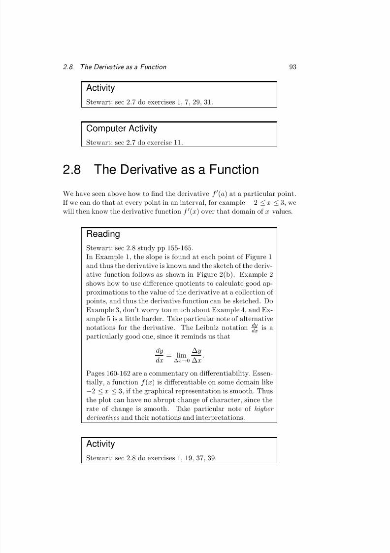
8/10/2019 algebra and calculus.pdf
http://slidepdf.com/reader/full/algebra-and-calculuspdf 101/135
2.8. The Derivative as a Function 93
ActivityStewart: sec 2.7 do exercises 1, 7, 29, 31.
Computer ActivityStewart: sec 2.7 do exercise 11.
2.8 The Derivative as a Function
We have seen above how to nd the derivative f (a) at a particular point.If we can do that at every point in an interval, for example −2 ≤ x ≤ 3, wewill then know the derivative function f (x) over that domain of x values.
ReadingStewart: sec 2.8 study pp 155-165.In Example 1, the slope is found at each point of Figure 1and thus the derivative is known and the sketch of the deriv-ative function follows as shown in Figure 2(b). Example 2shows how to use difference quotients to calculate good ap-proximations to the value of the derivative at a collection of points, and thus the derivative function can be sketched. DoExample 3, don’t worry too much about Example 4, and Ex-ample 5 is a little harder. Take particular note of alternativenotations for the derivative. The Leibniz notation dy
dx is aparticularly good one, since it reminds us that
dydx
= lim∆ x→0
∆ y∆ x
.
Pages 160-162 are a commentary on differentiability. Essen-tially, a function f (x) is differentiable on some domain like
−2 ≤ x ≤ 3, if the graphical representation is smooth. Thusthe plot can have no abrupt change of character, since therate of change is smooth. Take particular note of higher derivatives and their notations and interpretations.
ActivityStewart: sec 2.8 do exercises 1, 19, 37, 39.
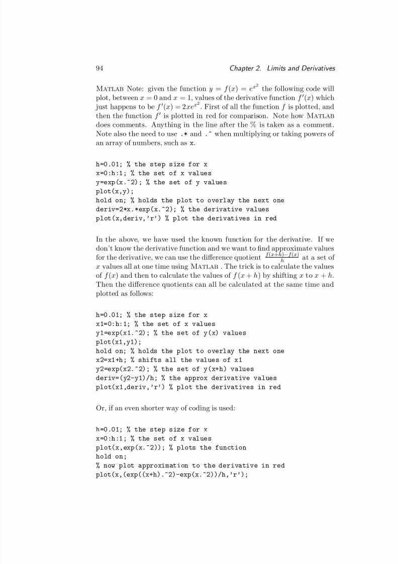
8/10/2019 algebra and calculus.pdf
http://slidepdf.com/reader/full/algebra-and-calculuspdf 102/135
94 Chapter 2. Limits and Derivatives
Matlab Note: given the function y = f (x) = ex2the following code will
plot, between x = 0 and x = 1, values of the derivative function f (x) which just happens to be f (x) = 2 xex2
. First of all the function f is plotted, andthen the function f is plotted in red for comparison. Note how Matlab
does comments. Anything in the line after the % is taken as a comment.Note also the need to use .* and .^ when multiplying or taking powers of an array of numbers, such as x.
h=0.01; % the step size for xx=0:h:1; % the set of x valuesy=exp(x.̂ 2); % the set of y valuesplot(x,y);hold on; % holds the plot to overlay the next onederiv=2*x.*exp(x.^2); % the derivative valuesplot(x,deriv,’r’) % plot the derivatives in red
In the above, we have used the known function for the derivative. If wedon’t know the derivative function and we want to nd approximate valuesfor the derivative, we can use the difference quotient f (x+ h)−f (x)
h at a set of x values all at one time using Matlab . The trick is to calculate the valuesof f (x) and then to calculate the values of f (x + h) by shifting x to x + h.Then the difference quotients can all be calculated at the same time and
plotted as follows:
h=0.01; % the step size for xx1=0:h:1; % the set of x valuesy1=exp(x1.^2); % the set of y(x) valuesplot(x1,y1);hold on; % holds the plot to overlay the next onex2=x1+h; % shifts all the values of x1y2=exp(x2.^2); % the set of y(x+h) valuesderiv=(y2-y1)/h; % the approx derivative valuesplot(x1,deriv,’r’) % plot the derivatives in red
Or, if an even shorter way of coding is used:
h=0.01; % the step size for xx=0:h:1; % the set of x valuesplot(x,exp(x.^2)); % plots the functionhold on;% now plot approximation to the derivative in redplot(x,(exp((x+h).^2)-exp(x.^2))/h,’r’);
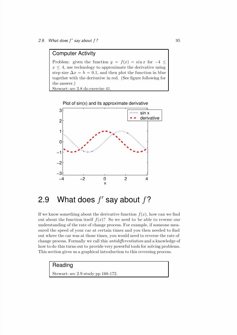
8/10/2019 algebra and calculus.pdf
http://slidepdf.com/reader/full/algebra-and-calculuspdf 103/135
2.9. What does f say about f ? 95
Computer ActivityProblem: given the function y = f (x) = sin x for −4 ≤x ≤ 4, use technology to approximate the derivative usingstep size ∆ x = h = 0 .1, and then plot the function in bluetogether with the derivative in red. (See gure following forthe answer.)Stewart: sec 2.8 do exercise 41.
−4 −2 0 2 4−3
−2
−1
0
1
2
3
Plot of sin(x) and its approximate derivative
sin xderivative
2.9 What does f say about f ?
If we know something about the derivative function f (x), how can we ndout about the function itself f (x)? So we need to be able to reverse ourunderstanding of the rate of change process. For example, if someone mea-sured the speed of your car at certain times and you then needed to ndout where the car was at those times, you would need to reverse the rate of change process. Formally we call this antidifferentiation and a knowledge of how to do this turns out to provide very powerful tools for solving problems.This section gives us a graphical introduction to this reversing process.
ReadingStewart: sec 2.9 study pp 168-172.
8/10/2019 algebra and calculus.pdf
http://slidepdf.com/reader/full/algebra-and-calculuspdf 104/135
96 Chapter 2. Limits and Derivatives
ActivityStewart: sec 2.9 do exercises 1, 7, 27.
Computer ActivityStewart: sec 2.9 do exercise 29.
Matlab Note on exercise 29 above.
x=linspace(0,4*pi,2000); % 200 points between 0 and 4pi
deriv=exp(-x/10).*sin(x);plot(x,deriv);grid; % puts a grid onto the plotxlabel(’x’); % how to do an axis labeltitle(’Now hand plot the function which gives this derivative’);
Chapter SummaryBy now you should have a good idea of the notion of a derivative from agraphical, numerical, and algebraic point of view. Limits are at the basis of this understanding. It is also important for you to be able to use the differ-ence quotient to approximate the value of derivatives and also to interpretpractical meanings of derivatives and to nd the corresponding units of thederivative function.
8/10/2019 algebra and calculus.pdf
http://slidepdf.com/reader/full/algebra-and-calculuspdf 105/135
Chapter 3Differentiation Rules
INTRODUCTION
In this chapter some fundamental rules are developed for working with deriv-atives. If we had to calculate the limit every time we wanted the derivativeof a function, life would be rather boring and inefficient. It was importantfor you to know that the derivative y = f (x) is a limit of a differencequotient, for example:
lim∆ x→0
∆ y∆ x
;
or the same thing
limh→0
f (x + h) − f (x)h
.
But now we develop some rules for making things easier. Firstly we deter-mine the rules for nding the derivative of the elementary functions: poly-
nomials, powers, exponential, trigonometric, and logarithmic. Along theway we develop rules for nding the derivative of sums and differences of functions, products and quotients of functions. The most important differen-tiation rule of all is how to nd the derivative of a function of a function. Forexample, you were told in Section 2.8 that the derivative of y = f (x) = ex2
is y = f (x) = 2 xex2. To do this we use the chain rule which will be devel-
oped in this chapter. Section 3.8 of the textbook is to be omitted. It willbe studied in the next course.
97
8/10/2019 algebra and calculus.pdf
http://slidepdf.com/reader/full/algebra-and-calculuspdf 106/135
98 Chapter 3. Differentiation Rules
3.1 Derivatives of Polynomials and Ex-ponential Functions
This section is an introduction to nding the derivative function for sumsof simple power functions and exponential functions.
ReadingStewart: study sec 3.1 pp 183-190.You will not be required to be able to prove that d
dx xn =
nxn
−1
, except for special cases as shown. The general proof uses the Binomial theorem which should be of interest tomathematics majors.It is of interest to note that the derivative d
dx is a linear operator which means that the Constant Multiple Rule ,the Sum Rule , and the Difference Rule can be combinedinto one to give
ddx
(C 1f (x) ± C 2g(x)) = C 1d
dxf (x) ± C 2
ddx
g(x).
We will see in sec 3.5 that the derivative of an exponential
function of the form ax
is (ln a)ax. When a = e, we get thesimplest of all differentiation rules d
dx ex = ex . On page 189of the textbook, e is dened in a very formal way as a limit.You should be able to recall that e ≈ 2.718.
Remember that if you have an equation like ex+1 = 3, to solve for x you just take natural logs of each side to get ln ex+1 ) = ln 3, and since log isinverse to exponential, you then get x +1 = ln3, x = ln 3 −1 ≈ 0.0986 (frommy Matlab log(3)-1 ). Then you can solve problems like the following:ExampleFind where the tangent to the curve dened by y = ex + 2 x
− 6 is parallel
to the line y = 4 x + 6.Solution The slope at any point on the curve is y = ex + 2 and the slopeof the line is 4. Henceex + 2 = 4, ex = 2, x = ln 2 ≈ 0.6931. At x = ln2, y = eln 2 + 2(ln 2) −6 = 2 + 2 ln 2 − 6 ≈ −2.6137, and so the tangent, at the point ( x, y) ≈(0.6931, −2.6137) on the curve, has slope 4. See following gure.
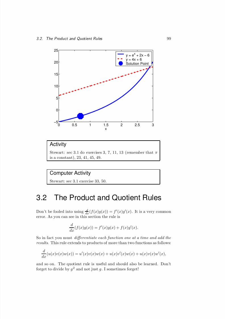
8/10/2019 algebra and calculus.pdf
http://slidepdf.com/reader/full/algebra-and-calculuspdf 107/135
3.2. The Product and Quotient Rules 99
0 0.5 1 1.5 2 2.5 3−5
0
5
10
15
20
25
x
y = ex + 2x − 6y = 4x + 6
Solution Point
ActivityStewart: sec 3.1 do exercises 3, 7, 11, 13 (remember that πis a constant), 23, 41, 45, 49.
Computer ActivityStewart: sec 3.1 exercise 33, 50.
3.2 The Product and Quotient Rules
Don’t be fooled into using ddx (f (x)g(x)) = f (x)g (x). It is a very common
error. As you can see in this section the rule is
ddx
(f (x)g(x)) = f (x)g(x) + f (x)g (x).
So in fact you must differentiate each function one at a time and add the results . This rule extends to products of more than two functions as follows:
ddx
(u(x)v(x)w(x)) = u (x)v(x)w(x) + u(x)v (x)w(x) + u(x)v(x)w (x),
and so on. The quotient rule is useful and should also be learned. Don’tforget to divide by g2 and not just g. I sometimes forget!
8/10/2019 algebra and calculus.pdf
http://slidepdf.com/reader/full/algebra-and-calculuspdf 108/135
100 Chapter 3. Differentiation Rules
ReadingStewart: sec 3.2 study pp 193-198.A note on notation: In Example 3 on p195, g (4) = 3 meansthat the derivative g (x) at x = 4 is 3.
ActivityStewart: sec 3.2 do exercises 1, 3, 5, 13, 29, 31, 37(c), 40, 41.
Computer ActivityStewart: sec 3.2 exercise 23.
3.3 Rates of Change in the Natural andSocial Sciences
In this section, we will only study the subsection on physics. If you arestudying a major in chemistry, biology, business, or another science, you
should be interested to see the applications to those areas.
ReadingStewart: sec 3.3 study pp 200 to the top of p204.The key concept in Example 1 is that if you are given theposition s of an object as a function of time t, then the ve-locity is a measure of change. It is the rate of change of position with respect to time. The average velocity over atime period ∆ t is ∆ s
∆ t and the limit of this ratio as ∆ t → 0is the instantaneous velocity v(t) = ds
dt . The acceleration is
rate of change of velocity a(t) = dvdt which can also be written
as v (t) or s (t), or in the Leibniz notation d2 sdt 2 . Examples
2 and 3 give important applications to density and electriccurrent problems. We will certainly see more about theseapplications in the following course MAT2100.
ActivityStewart: sec 3.3 do exercises 1, 7, 13, 15, 17.
8/10/2019 algebra and calculus.pdf
http://slidepdf.com/reader/full/algebra-and-calculuspdf 109/135
3.4. Derivatives of Trigonometric Functions 101
3.4 Derivatives of Trigonometric Func-tions
The derivatives of sin x and cos x are easy to remember. Check carefully tosee the relationship between the graph of the sine function and its derivative,the cosine function.
ReadingStewart: sec 3.4 study pp 213-218.You will not be expected to formally prove that
limx→0
sin xx
= 1
but the result should not be a surprise, since you alreadyknow that the slope of the graphs of y = x and y = sin x areboth equal to 1 as they pass through x = 0. Consequently,as x → 0 if the graphs look the same, the ratio of x to sin xmust approach 1.The formal proof that d
dx sin x = cos x and ddx cos x = −sin x
will not be required.
The derivatives of sin x, cos x, tan x, csc x, sec x, and cot xshould be memorised.
ActivityStewart: sec 3.4 do exercises 5, 7, 9, 31, 37.
Computer ActivityStewart: sec 3.4 do exercise 19.
3.5 The Chain Rule
The chain rule is the most powerful rule in all of differentiation. So it isessential that you master it. In real life, things are hardly ever simple, soyou will need to be able to handle rates of change of composite functionslike y = F (x) = e(x2 ) . This is a function of a function. The inner function
8/10/2019 algebra and calculus.pdf
http://slidepdf.com/reader/full/algebra-and-calculuspdf 110/135
102 Chapter 3. Differentiation Rules
is g(x) = x2 and the outer function is f (x) = ex , so that F (x) = f (g(x)) =
eg(x)
= ex2
. The chain rule then isdF dx
= dF dg
dgdx
= ( eg)(2x) = 2 xex2.
ReadingStewart: sec 3.5 study pp 220-225.You should take note of the informal proof on page 221, butyou are not required to learn the formal proof on page 227.Take particular note of the power rule for composite functions
given by formula 4 and the proof that the derivative of theexponential function ax is ax ln a given by formula 5.The subsection on tangents to parametric curves is to beomitted.
ActivityStewart: sec 3.5 do exercises 1, 3, 5, 17, 19, 23, 41, 43, 47,59, 79.
Computer ActivityStewart: sec 3.5 do exercise 63.
3.6 Implicit Differentiation
The idea of implicit functions is useful when an equation cannot be solvedexplicitly for y in terms of x or vice versa. For example, the circle equation isx2 + y2 = 4, but you cannot get y as an explicit function of x. The best youcan do is y =
±√ 4
− x2. If you had an equation like x2y3
−x5y7 + x2 + x = 4
you would have no hope. This is an implicit relationship between x and yand it is quite easy to nd the rate of change dy
dx or dxdy for such functions -
as we shall see. By the way take note in passing that
dxdy
= 1dydx
.
8/10/2019 algebra and calculus.pdf
http://slidepdf.com/reader/full/algebra-and-calculuspdf 111/135

8/10/2019 algebra and calculus.pdf
http://slidepdf.com/reader/full/algebra-and-calculuspdf 112/135
104 Chapter 3. Differentiation Rules
Here is one more example of logarithmic differentiation. Find the derivative
of xx, x > 0.
y = xx
ln y = ln xx = x ln x, then differentiate implicitly w.r.t. x,1y
dydx
= 1 × ln x + x1x
= ln x + 1
dydx
= y(ln x + 1) = xx (1 + ln x)
Hence ddx xx = xx (1 + ln x).
ActivityStewart: sec 3.7 do exercises 3, 9, 17, 19, 25, 33.
Chapter Summary
Section 3.8 is to be omitted. Try some of the Review problems on pp 255-257.
In this chapter you have developed some important tools for differentiating
functions. The most powerful of these is the chain rule. Familiarity withthese rules is essential for later courses in solving differential equations andis immediately necessary in this course for the two chapters on integration.

8/10/2019 algebra and calculus.pdf
http://slidepdf.com/reader/full/algebra-and-calculuspdf 113/135
8/10/2019 algebra and calculus.pdf
http://slidepdf.com/reader/full/algebra-and-calculuspdf 114/135
106 Chapter 4. Applications of Differentiation
4.1 Related Rates
Related rates problems are practical applications of the chain rule. Forexample, if you want to know how fast the area of a circle is changing whenthe radius is 2 metres and if the radius is increasing at 0.5 metres per second,then we need to express our variables in composite form. In this case wewrite down the knowns : A = πr 2 and dr
dt = 0 .5, and r = 2. In this case wehave A = f (r ), where r is some function of t .
The chain rule gives:
dA
dt =
dA
dr
dr
dt = 2 πr
× 0.5 = πr.
Now we substitute r = 2, to get dAdt = 2 π ≈ 6.82 square metres per second.
Note that condition r = 2 cannot be used until we calculate some rates of change. Otherwise we would not have been able to nd dA/dr , it wouldhave been zero if r was set to 2.
ReadingStewart: sec 4.1 study pp 263-266.Work through each of Examples 1,2,3. The Strategy givenon page 265 can be very helpful. Note the warning givenabout substituting known values before you have the chanceto work the rates of change. Work through Examples 4 and5.
ActivityStewart: sec 4.1 do exercises 3, 5, 7, 11(note: mi meansmiles), 31*(note: * for harder problems), 37*.
4.2 Maximum and Minimum Values
Optimisation is about things like minimising costs and maximising output.Or minimising stress in a material and maximising safety. Or minimisingdistance while maximising delivery of goods. And so on.
8/10/2019 algebra and calculus.pdf
http://slidepdf.com/reader/full/algebra-and-calculuspdf 115/135
4.3. Derivatives and the Shapes of Curves 107
ReadingStewart: sec 4.2 study pp 269-274.This section introduces some important terminology (ie lan-guage) for discussing maxima, minima, and other criticalpoints. The Closed Interval Method on page 273 gives agood summary of the way to determine absolute extrema.Work through the seven Examples.
ActivityStewart: sec 4.2 do exercises 5, 17, 19, 23, 27, 35, 37, 59*.
4.3 Derivatives and the Shapes of Curves
In this section we develop ideas on the shape of curves using the First Deriv-ative Test and then use a knowledge of concavity to develop the SecondDerivative Test for nding Local Maxima and Minima. The Mean ValueTheorem is to be omitted, but should be read for interest by mathematicsmajors.
ReadingStewart: sec 4.3 study pp 280-284.Increasing/Decreasing functions, The First derivative Test,Concavity, and the Second Derivative Test, are all important.Make sure that you know when a curve is concave up (ief > 0, or the slope is increasing), and when it is concave down (ie f < 0, or the slope is decreasing). Study Examples2,3,4 and 5. You might just read Examples 6, 7, and 8 forinterest.
ActivityStewart: sec 4.3 do exercises 5, 7, 15, 21, 55*.
Computer ActivityStewart: sec 4.3 do exercise 47*.
8/10/2019 algebra and calculus.pdf
http://slidepdf.com/reader/full/algebra-and-calculuspdf 116/135
8/10/2019 algebra and calculus.pdf
http://slidepdf.com/reader/full/algebra-and-calculuspdf 117/135
4.7. Applications to Business and Economics 109
4.7 Applications to Business and Eco-nomics
Omit this section. Unless you want to get rich quick. It will not be examined,but should be read with interest if you are doing a business major.
4.8 Newton’s Method
Omit this section. It is included in a later mathematics course together withmany other powerful numerical techniques.
4.9 Antiderivatives
If I tell you that f (x) = 2 x and ask you to nd the function f (x), you shouldhave no trouble. Because you remember the power rule for differentiation,you will tell me in a ash that f (x) = x2. Careful! f (x) = x2 + 1 also doesthe job. So does f (x) = x2 − 12345π. The general answer is f (x) = x2 + C
where C is an arbitrary constant.In this section, we continue the process of thinking backwards from theknown derivative. To do that we need a very good knowledge of the differ-entiation rules. In the above, I had to use the fact that d
dx x2 = 2 x and thatd
dx C = 0.
We need to think backwards when we know the rate of change of a process,but we want to nd the actual state of the process. For example if you lookat the speedo on a car, you can see what the velocity is, but you might wantto calculate from it your displacement from home in a given time.
Finding antiderivatives means that you have started integrating.
ReadingStewart: sec 4.9 study pp 327-332.
ActivityStewart: sec 4.9 do exercises 1, 9, 15, 23(including ndingthe two constants), 27(careful when you get to x−1), 39, 55*.

8/10/2019 algebra and calculus.pdf
http://slidepdf.com/reader/full/algebra-and-calculuspdf 118/135
110 Chapter 4. Applications of Differentiation
Computer ActivityStewart: sec 4.9 do exercise 32.
Chapter Summary
Work through some of the Review problems, see pp 335-341.
In this chapter we have worked through a wide range of applications of thedifferentiation rules which were developed in the previous chapter. So youcan already see that differential calculus can be very useful. But the storycontinues and the true power of calculus awaits us in the next two chapterswhere we introduce Integration.
8/10/2019 algebra and calculus.pdf
http://slidepdf.com/reader/full/algebra-and-calculuspdf 119/135
8/10/2019 algebra and calculus.pdf
http://slidepdf.com/reader/full/algebra-and-calculuspdf 120/135
112 Chapter 5. Integrals
5.1 Areas and Distances
This section is an important introduction to integration. The idea of calcu-lating areas under curves using thinner and thinner rectangle approximationswill lead to a more general way of summing a wide range of quantities (egvelocity functions).
ReadingStewart: sec 5.1 study pp 343-352.Note that the area can be approximated by rectangles using
the left endpoint of each interval, or using the right interval.When you take the limit as n → ∞, (ie ∆ x → 0), you get thesame answer either way. So it doesn’t matter whether youuse left or right endpoints, in fact you can use any sample of points, one in each subinterval, as discussed on page 348. Tokeep things simpler, we will only use left or right endpoints,or sometimes the midpoint. The last subsection on The Dis-tance Problem shows that we can calculate approximationsto the distance travelled in the same way, ie distance = ve-locity × time. If we assume that v(t) is constant in eachsubinterval ∆ t, we get distance = v(t)
× ∆ t. Then we just
sum all of these values across the domain and then take thelimit as ∆ t → 0, ie the number of subintervals n → ∞. Thiswill give us the exact distance travelled.
Matlab Note:Here is some Matlab code to nd a good approximation to the area underthe curve y = x2 over the domain 0 ≤ x ≤ 1, using the left endpoints.
h=0.001; % the subinterval widthx=0:h:1-h; % the left subinterval endpoints (1000 values)
y=x.^2; % the height of each rectanglearea=sum(y*h) % the sum function just adds up each value of y*h
The answer to this is: area = 0.3328, which is already close to the exactanswer 1 / 3. To get even closer, just take an even smaller value like h =0.0001. If you need to use right endpoints, just change the second code lineto x=h:h:1; , ie x goes from 0 + h in steps of h to 1.
8/10/2019 algebra and calculus.pdf
http://slidepdf.com/reader/full/algebra-and-calculuspdf 121/135
5.2. The Denite Integral 113
ActivityStewart: sec 5.1 do exercises 11, 13, 15, 17.
Computer ActivityStewart: sec 5.1 exercises 6, 7.
5.2 The Denite Integral
In this section the denite integral is introduced as the limit of so-calledRiemann sums . This is crucial to your understanding of the integral andwill help you greatly when you model real life applications which can beexpressed as denite integrals.
ReadingStewart: sec 5.2 study pp 354-364.Take note of the denition of the denite integral
ba f (x) dx
as the limit of a sum of function values multiplied by thestep length ∆ x. Note 1, 2, and 3 are important. Note 4 isinteresting, but we will use equal length values of ∆ x. For-mulas 4,5,6) on page 357 are interesting, but you will notbe required to use them. Study Examples 1,2,3,4 carefully.Note that the denite integral does not necessarily give thearea under the curve. It is positive when the curve is abovethe x-axis and negative when the curve is below. The eightProperties of the Integral are important. By the way, Prop-erties 2,3,4 indicate that the integral is a linear operator , ie
b
a(C 1f (x) + C 2g(x)) dx = C 1
b
af (x) dx + C 2
b
ag(x) dx.
Remember that the derivative is also a linear operator.
Matlab Note:To change the Matlab code for the midpoint rule , just use x=h/2:h:1-h/2;(see code in previous section), ie x goes from h/ 2 (the middle of the rstsubinterval) to 1 − h/ 2 (the middle of the last subinterval), in steps of h.
8/10/2019 algebra and calculus.pdf
http://slidepdf.com/reader/full/algebra-and-calculuspdf 122/135
114 Chapter 5. Integrals
ActivityStewart: sec 5.2 do exercises 1, 7, 11, 17, 27, 33(draw thegraph), 39, 41, 43.
Computer ActivityStewart: sec 5.2 do exercise 9 (use technology and increasen to something big to get more accuracy).
Note on the above Computer Activity: √ x3 + 1 in Matlab is sqrt(x.^3+1) .
5.3 Evaluating Denite Integrals
Suppose you start your car at time t = a at position s(a), and drive in astraight line at velocity v(t) until t = b at position s(b). Then the distancetravelled is trivially s(b) − s(a). But, as we have seen, the integral of thevelocity is distance. Hence we have the very profound result
b
a v(t) dt = s(b) − s(a).
But we know the v(t) = dsdt , so we have
b
as (t) dt = s(b) − s(a),
ie, the total change in position is the integral of its derivative . This illus-trates the remarkable connection between integration and differentiation.In a sense, integration and differentiation are inverse operators, since oneunravels the other.
8/10/2019 algebra and calculus.pdf
http://slidepdf.com/reader/full/algebra-and-calculuspdf 123/135
5.4. The Fundamental Theorem of Calculus 115
ReadingStewart: sec 5.3 study pp 366-373.The Evaluation Theorem formalises the discussion above(where s(t) is in fact the antiderivative of s (t)). You canomit the proof of the Evaluation Theorem on page 367. Takeparticular note of Examples 1,2. A good notation for the an-tiderivative is F (x) = f (x) dx, and is called the indenite integral . It is called indenite, since it is a function, whereasthe denite integral is a single number. The Table of Inde-nite Integrals on page 369 should be familiar to you, since if you differentiate the right hand side, you get the function on
the left. This Table becomes your working set of antideriva-tives. Examples 3,4,5,6 are an excellent introduction to usingthe Table. The last subsection on Applications gives a verygood indicator of various contexts for the integral.
ActivityStewart: sec 5.3 do exercises 1, 3, 7, 9, 15, 23, 27, 37, 41, 47,53, 57.
Computer ActivityStewart: sec 5.3 do exercises 29, 31, 35.
5.4 The Fundamental Theorem of Cal-culus
In this section the two parts of the Fundamental Theorem of Calculus areformulated. A good way to remember each part is to think :
1. ddx f (x) dx = f (x);
2. f (x) dx = f (x).
ReadingStewart: sec 5.4 study pp 377-382.You are not required to learn the proof of the rst part of the fundamental theorem, given in the last subsection.
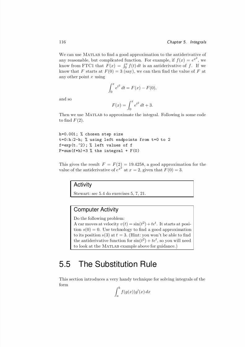
8/10/2019 algebra and calculus.pdf
http://slidepdf.com/reader/full/algebra-and-calculuspdf 124/135
116 Chapter 5. Integrals
We can use Matlab to nd a good approximation to the antiderivative of
any reasonable, but complicated function. For example, if f (x) = ex 2
, weknow from FTC1 that F (x) =
x0 f (t) dt is an antiderivative of f . If we
know that F starts at F (0) = 3 (say), we can then nd the value of F atany other point x using
x
0et 2
dt = F (x) − F (0) ,
and soF (x) =
x
0et 2
dt + 3 .
Then we use Matlab to approximate the integral. Following is some code
to nd F (2).
h=0.001; % chosen step sizet=0:h:2-h; % using left endpoints from t=0 to 2f=exp(t.^2); % left values of fF=sum(f*h)+3 % the integral + F(0)
This gives the result F = F (2) = 19 .4258, a good approximation for thevalue of the antiderivative of ex2
at x = 2, given that F (0) = 3.
ActivityStewart: sec 5.4 do exercises 5, 7, 21.
Computer ActivityDo the following problem:A car moves at velocity v(t) = sin( t2) + te t . It starts at posi-tion s(0) = 0. Use technology to nd a good approximationto its position s(3) at t = 3. (Hint: you won’t be able to ndthe antiderivative function for sin( t2) + te t , so you will needto look at the Matlab example above for guidance.)
5.5 The Substitution Rule
This section introduces a very handy technique for solving integrals of theform
b
af (g(x))g (x) dx
8/10/2019 algebra and calculus.pdf
http://slidepdf.com/reader/full/algebra-and-calculuspdf 125/135
5.6. Integration by Parts 117
by means of substitution. You will note that integrals of this form have
a complicated function f (g(x)), but that they also have the luxury of theaccompanying function g (x) as a partner. These integrals occur very fre-quently. You will remember from the chain rule that this type of combina-tion of functions always result when you differentiate a composite functionf (g(x)). So the method of substitution is really a process for unravellingthe chain rule.
ReadingStewart: sec 5.5 study pp 386-392.Take note of the different types of substitution that can be
used. It is not always obvious how to choose the substitution,so make sure that you work each of the Examples 1 to 8.The last subsection on Symmetry presents ways to sometimesspeed up your calculations.
ActivityStewart: sec 5.5 do exercises 1, 3, 5, 7, 13, 17, 27 (hint: writeas sec2 x sec x tan x), 33, 41, 61.
5.6 Integration by Parts
Integration by parts is really a method for unravelling the derivative of aproduct. You should become very familiar with the equivalent formulas
uv dx = uv − u v dx
or,
u dv = uv − v du.
ReadingStewart: sec 5.6 study pp 393-398.Work Examples 1 and 2. Example 3 shows how you some-times need to apply the integration by parts formula twice.Example 4 shows that you can sometimes use the cyclic be-haviour for trigonometric functions to get there. Take noteof Example 5 which nds the value of the integral and youcan omit Example 6.
8/10/2019 algebra and calculus.pdf
http://slidepdf.com/reader/full/algebra-and-calculuspdf 126/135
118 Chapter 5. Integrals
ActivityStewart: sec 5.6 do exercises 1, 3, 7, 13, 15.
Computer ActivityStewart: sec 5.6 do exercise 41 for the case t = 5 and checkyour answer by calculating a good approximation with Mat-
lab .
Matlab Note : In the above Computer Activity use v=t.^2.*exp(-t) to
get values of the function. See earlier Matlab
code for setting up the leftendpoints and calculating the sum which gives the approximation to thedenite integral.
5.7 Additional Techniques of Integration
There are many other special techniques for nding the integral. In thissection we will only look at methods for trigonometric integrals.
ReadingStewart: sec 5.7 study pp 400-402.Omit the last subsection on Partial Fractions.Example 1 is a good illustration of setting things up fora substitution. Example 2 is interesting if you know thatsin2 x = 0 .5(1 − cos 2x). In this course you don’t need tolearn that
sin2 x dx = 0 .5(x − 0.5sin2x) + C.
Example 3 is worth following since at last you are able toprove that the area of a circle is πr 2. Up until now you havetaken this fact as an article of faith. By the way, Archimedeswas able to nd this over 2000 years ago. And he did not havethe luxury of using the Fundamental Theorem. He mighthave known FTC1 or FTC2. We don’t think he did, but hewas one of the greatest thinkers of all time, so who knows!
8/10/2019 algebra and calculus.pdf
http://slidepdf.com/reader/full/algebra-and-calculuspdf 127/135
5.8. Integration Using Tables and Computer Algebra Systems 119
ActivityStewart: sec 5.7 do exercises 1 (hint: write assin x sin2 x cos2 x and then use sin 2 x = 1 − cos2 x), 7, 29(hint: substitute u = x0.5).
5.8 Integration Using Tables and Com-puter Algebra Systems
We will only have a quick look at this section. We do not use ComputerAlgebra Systems in this course, so you can omit that subsection.
ReadingStewart: sec 5.8 study pp 405-407.Omit the second half of page 407.Work through Examples 2,3,4. Note that the table of inte-grals is on References pp 6-10 at the back of the book.The rest of the section can be omitted.
ActivityStewart: sec 5.8 do exercises 3, 5, 7.
5.9 Approximate Integration
In this section a number of methods are developed for approximating thevalue of denite integrals. We will see them in a later mathematics course,so we will only do the rst page of this section on some, by now, familiarmethods for approximating the integral. We have already seen how to dothe approximation using left and right endpoints and also for the midpointrule.
ReadingStewart: sec 5.9 study page 412 only.
Here is a reminder of the Matlab code for approximating 30 ex2
dx:
8/10/2019 algebra and calculus.pdf
http://slidepdf.com/reader/full/algebra-and-calculuspdf 128/135
120 Chapter 5. Integrals
Left Endpoint Approximation:
h=0.001; % your choice of step lengthx=0:h:3-h; % the left hand endpointsy=exp(x.^2); % the values at the left endpointsleft=sum(y*h) % the answer
Right Endpoint Approximation:
h=0.001; % your choice of step lengthx=h:h:3; % the right hand endpoints
y=exp(x.^2); % the values at the right endpointsright=sum(y*h) % the answer
Midpoint Approximation:
h=0.001; % your choice of step lengthx=h/2:h:3-h/2; % the midpointsy=exp(x.^2); % the values at the midpoints mid=sum(y*h) % the answer
ActivityStewart: sec 5.9 do exercise 5(a). Note: if you want 8 mid-points, you will need to rstly calculate the value of h. Hereit will be h = π−0
8 . In Matlab that is h=(pi-0)/8 .
Chapter Summary
The last section on Improper Integrals may be omitted, but should be readby mathematics majors.
Standard methods of integration have been introduced in this chapter. Thereis much useful material here. You are now equipped with the foundationtools of both differential and integral calculus. This will form the basis of your abilities as a technician of change. If it moves, you can now hit it withcalculus. The next, and nal chapter in this course is the chance to applysome of these skills to more practical situations.
Before moving on, try some of the Review questions at the end of thischapter.
8/10/2019 algebra and calculus.pdf
http://slidepdf.com/reader/full/algebra-and-calculuspdf 129/135
Chapter 6Applications ofIntegration
INTRODUCTION
In this, the nal chapter, we study applications of the denite integral in-cluding nding areas, volumes, averages, as well as some applications tophysics and engineering. We omit some sections and subsections as de-scribed following.
121
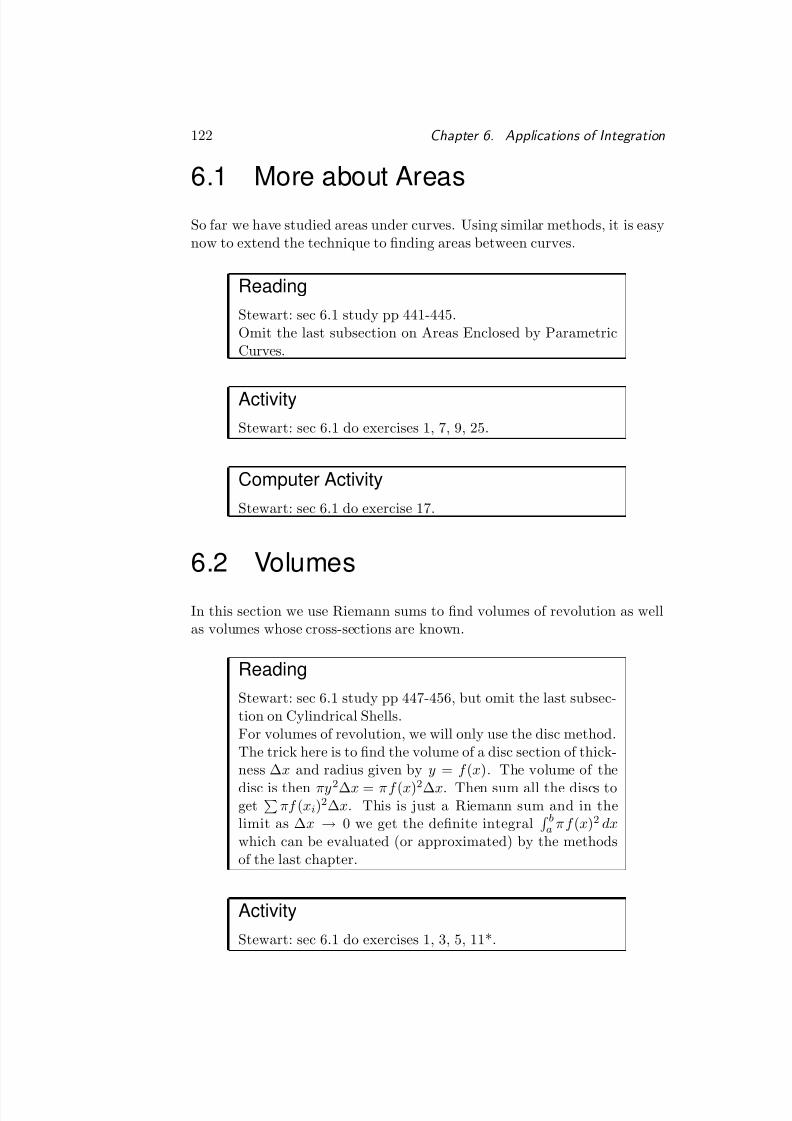
8/10/2019 algebra and calculus.pdf
http://slidepdf.com/reader/full/algebra-and-calculuspdf 130/135
122 Chapter 6. Applications of Integration
6.1 More about Areas
So far we have studied areas under curves. Using similar methods, it is easynow to extend the technique to nding areas between curves.
ReadingStewart: sec 6.1 study pp 441-445.Omit the last subsection on Areas Enclosed by ParametricCurves.
ActivityStewart: sec 6.1 do exercises 1, 7, 9, 25.
Computer ActivityStewart: sec 6.1 do exercise 17.
6.2 Volumes
In this section we use Riemann sums to nd volumes of revolution as wellas volumes whose cross-sections are known.
ReadingStewart: sec 6.1 study pp 447-456, but omit the last subsec-tion on Cylindrical Shells.For volumes of revolution, we will only use the disc method.The trick here is to nd the volume of a disc section of thick-ness ∆ x and radius given by y = f (x). The volume of thedisc is then πy2∆ x = πf (x)2∆ x. Then sum all the discs toget πf (x i)2∆ x. This is just a Riemann sum and in thelimit as ∆ x → 0 we get the denite integral
ba πf (x)2 dx
which can be evaluated (or approximated) by the methodsof the last chapter.
ActivityStewart: sec 6.1 do exercises 1, 3, 5, 11*.
8/10/2019 algebra and calculus.pdf
http://slidepdf.com/reader/full/algebra-and-calculuspdf 131/135
6.3. Arc Length 123
6.3 Arc Length
Omit this section which will be studied in the following course MAT2100.
6.4 Average Value of a Function
The average value of a function f (x), over some domain a ≤ x ≤ b, is quiteeasy to evaluate. It is just
average = 1b − a b
af (x) dx.
ReadingStewart: sec 6.4 study pp 467-469. You may omit the MeanValue Theorem for Integrals and omit Example 2.
ActivityStewart: sec 6.4 do exercises 1, 5, 15.
Computer ActivityStewart: sec 6.4 do exercise 7.
6.5 Applications to Physics and Engineer-ing
Three applications are included in this chapter, Work, Hydrostatic Pressure& Force, and Centres of Mass.
ReadingStewart: sec 6.5 study pp 471-479.Study the three application subsections and work throughExamples 1-7. Further notes follow.
8/10/2019 algebra and calculus.pdf
http://slidepdf.com/reader/full/algebra-and-calculuspdf 132/135
124 Chapter 6. Applications of Integration
Non-uniform density
In the analysis of this section it has been assumed that the density of thematerial or the medium is constant. How do we handle things if the densityis not constant? Here is an example which follows the modelling procedure,develops the integral, and then we solve it.
ExampleConsider a rod from x = 0 to x = 4 whose density at a point x is given byρ(x) = 2 + 1
x+1 kilograms per metre. Find the mass of the rod.
Solution:Split the rod up into n subintervals of length ∆ x. On a typical subin-terval (ie an element of length ∆ x) we then assume the density to haveits value at a point xi on the element (eg the left endpoint) and thus beconstant across the element with value ρ(x i ). The mass of the elementis then just (density) ×(length), or ρ(x i )∆ x. Summing all of the elementsgives ρ(x i )∆ x. This is a left endpoint Riemann sum, and in the limit as∆ x → 0, we get
40 ρ(x) dx.
Thus the mass of the rod is 40 2 + 1
x+1 dx. Evaluating
4
02 +
1x + 1
dx = [2x + ln( x + 1)] 40
= (8 + ln 5)
− (0 + ln 1)
≈ (8 + 1 .6094) − (0 + 0)= 9 .6094kg.
ActivityStewart: sec 6.5 do exercises 1, 15, 23, 35.
Chapter Summary The remainder of this chapter is to be omitted, butif you are majoring in business, biology, or mathematics, you should read
selections of Sections 6.6 or 6.7.We have covered a lot of ground in this course and now it is time to study forthe exam. Good luck and hope to see you in the following course MAT2100.
8/10/2019 algebra and calculus.pdf
http://slidepdf.com/reader/full/algebra-and-calculuspdf 133/135

8/10/2019 algebra and calculus.pdf
http://slidepdf.com/reader/full/algebra-and-calculuspdf 134/135
8/10/2019 algebra and calculus.pdf
http://slidepdf.com/reader/full/algebra-and-calculuspdf 135/135


![Clifford algebra, geometric algebra, and applications · PDF filearXiv:0907.5356v1 [math-ph] 30 Jul 2009 Clifford algebra, geometric algebra, and applications Douglas Lundholm and](https://img.pdfslide.us/doc/110x75/5a7327fa7f8b9aac538e5155/cliord-algebra-geometric-algebra-and-applications-arxiv09075356v1-math-ph.jpg)


![TENSOR NETWORKS AND GRAPHICAL CALCULUS FOR OPEN …deepquantum.ai/.../TENSOR...AND-GRAPHICAL-CALCULUS.pdf · manipulating tensor networks [10] and to generalize quantum circuits [11]](https://img.pdfslide.us/doc/110x75/5f7914771becd87255623278/tensor-networks-and-graphical-calculus-for-open-manipulating-tensor-networks-10.jpg)