Algebra 1 - math.uni-bonn.de · Introduction These are my lecture notes for the course Algebra 1, held by Dr. Thorsten Heidersdorf in the summer term 20191. You can nd the current

Algebra 1

Introduction to Commutative Algebra

Lecture Notes, Summer 2019

Contents

Introduction 4

Chapter 1. Rings 51.1. Ideals . . . . . . . . . . . . . . . . . . . . . . . . . . . . . . . . . . . . . . . . . . . . . . . . . . . . . . . . . 51.2. The Spectrum of a Ring . . . . . . . . . . . . . . . . . . . . . . . . . . . . . . . . . . . . . . 71.3. Radicals . . . . . . . . . . . . . . . . . . . . . . . . . . . . . . . . . . . . . . . . . . . . . . . . . . . . . . 101.4. Local Rings and Rings of Fractions . . . . . . . . . . . . . . . . . . . . . . . . . . . 14

Chapter 2. Modules and Integral Extensions 222.1. Modules - Basics. . . . . . . . . . . . . . . . . . . . . . . . . . . . . . . . . . . . . . . . . . . . . . 222.2. Free and Finitely Generated Modules . . . . . . . . . . . . . . . . . . . . . . . . . 252.3. Algebras . . . . . . . . . . . . . . . . . . . . . . . . . . . . . . . . . . . . . . . . . . . . . . . . . . . . . . 302.4. Localization of Modules . . . . . . . . . . . . . . . . . . . . . . . . . . . . . . . . . . . . . . . 312.5. Integral Extensions . . . . . . . . . . . . . . . . . . . . . . . . . . . . . . . . . . . . . . . . . . . 332.6. Going Up and Going Down . . . . . . . . . . . . . . . . . . . . . . . . . . . . . . . . . . . 352.7. Noether Normalization Lemma . . . . . . . . . . . . . . . . . . . . . . . . . . . . . . . 42

Chapter 3. Hilbert’s Nullstellensatz and some Algebraic Geometry 473.1. Jacobson Rings . . . . . . . . . . . . . . . . . . . . . . . . . . . . . . . . . . . . . . . . . . . . . . . 473.2. Hilbert’s Nullstellensatz . . . . . . . . . . . . . . . . . . . . . . . . . . . . . . . . . . . . . . 483.3. The Dimension of a Ring . . . . . . . . . . . . . . . . . . . . . . . . . . . . . . . . . . . . . 513.4. Zero Sets and Varieties . . . . . . . . . . . . . . . . . . . . . . . . . . . . . . . . . . . . . . . 543.5. The Zariski-Topology on Ank . . . . . . . . . . . . . . . . . . . . . . . . . . . . . . . . . . 573.6. Morphisms of Varieties . . . . . . . . . . . . . . . . . . . . . . . . . . . . . . . . . . . . . . . 603.7. Some examples . . . . . . . . . . . . . . . . . . . . . . . . . . . . . . . . . . . . . . . . . . . . . . . 61

Chapter 4. Noetherian Rings and Modules 624.1. Dimension Theory of Noetherian Rings . . . . . . . . . . . . . . . . . . . . . . . 664.2. Primary Decomposition in Noetherian Rings . . . . . . . . . . . . . . . . . . 70

Chapter 5. Regular Rings 755.1. Valuation Rings . . . . . . . . . . . . . . . . . . . . . . . . . . . . . . . . . . . . . . . . . . . . . . 775.2. Discrete Valuation Rings. . . . . . . . . . . . . . . . . . . . . . . . . . . . . . . . . . . . . . 805.3. Dedekind Rings. . . . . . . . . . . . . . . . . . . . . . . . . . . . . . . . . . . . . . . . . . . . . . . 805.4. The Class Group . . . . . . . . . . . . . . . . . . . . . . . . . . . . . . . . . . . . . . . . . . . . . 835.5. Modules over PIDs and Projective Modules . . . . . . . . . . . . . . . . . . . 85

Appendix A. Prerequisites - Rings 89A.1. Basics . . . . . . . . . . . . . . . . . . . . . . . . . . . . . . . . . . . . . . . . . . . . . . . . . . . . . . . . 89

Appendix B. Categories 90B.1. General Categories and Functors . . . . . . . . . . . . . . . . . . . . . . . . . . . . . 90

2

CONTENTS 3

B.2. Additive and Abelian Categories. . . . . . . . . . . . . . . . . . . . . . . . . . . . . . 91B.3. Some Homological Algebra . . . . . . . . . . . . . . . . . . . . . . . . . . . . . . . . . . . 91

Appendix C. Further Remarks - Modules 93C.1. Projective Modules . . . . . . . . . . . . . . . . . . . . . . . . . . . . . . . . . . . . . . . . . . . 93C.2. Tensor Products . . . . . . . . . . . . . . . . . . . . . . . . . . . . . . . . . . . . . . . . . . . . . 93C.3. Localization of Modules . . . . . . . . . . . . . . . . . . . . . . . . . . . . . . . . . . . . . . 98C.4. Local-Global . . . . . . . . . . . . . . . . . . . . . . . . . . . . . . . . . . . . . . . . . . . . . . . . . 98C.5. Structure Theorems for Modules . . . . . . . . . . . . . . . . . . . . . . . . . . . . . 99

Appendix. Bibliography 100

Appendix. Index 101

Introduction

These are my lecture notes for the course Algebra 1, held by Dr. ThorstenHeidersdorf in the summer term 20191. You can find the current versionon my website (https://pankratius.gitlab.io/notes). There is alsoa version on the course hompage, but it might be outdated. If you findmistakes (there are still a lot) or have suggestions, please send me an e-mailto [email protected]. I want to thank everyone who already pointedsome of them out to me and apologize for the long time it took me to fixthem.

The recomended literature for this course is [AM94], [EE95] and[MR89]. I also like to use [Alu09].

Dr. Heidersdorf introduced categories and (exact) functors in lecture 6.I decided to put this (and a bit more) in a seperate appendix, which will beadded during the semester. For now, the reader is e.g. refered to [Ste19].

Future Aaron here: Me introducing categories and stuff in the appendixdid not happen during the semester. Overall, the appendix is a huge mess. Ihope I will be able to fix this during the summer, before the new semesterstarts. I also plan to add some more stuff which I found interesting (and nottoo far away from the lecture) as well as the missing proof of the last fewlectures. I also want to include the results of the exercise sheets, but stillhave to figure out the right places. The last lecture (lecture 23) was a bigblack box, and I am still not sure up to what detail I will be able to fix this.

And one more thing – I hope I will be able to do the same next semesterfor Algebraic Geometry 1, so stay tuned... .

1Last change: 2019-07-10 10:31:42 +0200; Current commit: 05ab381

https://pankratius.gitlab.io/notes

mailto:[email protected]

CHAPTER 1

Rings

Convention. In this lecture rings are assumed to bei) commutative: for all ab = ba holds for all a, b ∈ R,ii) unital: there is an element 1 = 1R ∈ R such that 1a = a for all

a ∈ R.

Ring homomorphisms f : R → S always respect the unit, i.e. f(1R) = 1Sholds.

1.1. Ideals

Definitionb 1.A. Let I ⊆ R be an ideal. Then I is a proper ideal or properif I 6= R.

Definition 1.1.i) A proper ideal p ( R is a prime ideal if for all x, y ∈ R with xy ∈ p,

already x ∈ p or y ∈ p holds.ii) A proper ideal m ( R is a maximal ideal if there is no ideal I with

m ( I ( R.

Notationb 1.B. I try to follow Dr. Heidersdorf’s way of naming ideals,with one typographical addition: ordinary ideals are denoted as I, J ,..., primeideals as p,... and maximal ideals as m,... .

Lemma 1.2. Let I ⊆ R be an ideal.i) The following are equivalent:

a) I is a prime ideal.b) R/I is an integral domain.

ii) The following are equivalent:a) I is a maximal ideal.b) R/I is a field.

Proof. We denote the coset of an element a ∈ R in R/I by a.i) Let I be a prime ideal, and let x, y ∈ R/I such that 0 = x · y = xy.

This means that xy is in I. As I is prime, x ∈ I or y ∈ I follows,and hence x = 0 or y = 0.

Now assume that R/I is an integral domain. Let x, y ∈ R withxy ∈ I. Hence 0 = xy = x · y, and as R/I is an integral domain,x = 0 or y = 0 follows. So x ∈ I or y ∈ I.

5

6 1. RINGS

ii) Let I be maximal, and x /∈ I. Consider the ideal generated by x andI, 〈I, x〉. As I is maximal and I ⊆ 〈I, x〉, we have 〈I, x〉 = R = 〈1〉.So there are z ∈ I, y ∈ R such that 1 = xy + z. So in R/I, we have

1 = xy + z = x · y + z = x · y,which shows that x is a unit in R/I.

Now assume that R/I is a field and let J be an ideal withI ⊆ J ⊆ R. If there is an x ∈ J such that x /∈ I, then x is invertiblein R/I. So there are z ∈ I, y ∈ R such that 1 = xy + z. As z ∈ Jand x ∈ J this implies 1 ∈ J , and hence J = R.

�

Corollary 1.3. Let I be an ideal. If I is maximal then I is prime.

The following is a consequence of Zorn’s Lemma and the ideal correspon-dence:

Lemma 1.4. Let R 6= 0 be a ring.i) R contains a maximal ideal.ii) Every ideal of R is contained in some maximal ideal.

Corollary 1.5.i) Every x /∈ R× is contained in some maximal ideal of R.ii) The units of R are given by the complement of the union over all

maximal ideals m:

R× = R \⋃

m maximal ideal

m.

iii) Let m ⊆ R be a maximal ideal in a local ring R and x ∈ m. Then1 + x is a unit in R.

Proof.i) Consider the ideal generated by x. As x is not a unit 〈x〉 ( 〈1〉

holds. So by Corollary 1.5, there is a maximal ideal containing 〈x〉,and in particular x.

ii) Let x /∈ m for all maximal ideals m. Then 〈x〉 ( m for all maximalideals m, and hence 〈x〉 = 〈1〉.

�

Example 1.6. Consider the case R = Z. Then the prime ideals are 〈0〉and 〈p〉, for every prime number p.

Lemmab 1.C. LetR be a ring, and consider the polynomial ringR[X1, . . . , Xn]in n variables. Then for every 0 ≤ m ≤ n there is an isomorphism

R[X1, . . . , Xn]/〈X1, . . . , Xm〉 ∼= R[Xm+1, . . . , Xn].

Example 1.7. Let R be an integral domain. Consider the polynomial ringin n variables, R[X1, . . . , Xn]. Letm ≤ n and consider the ideal 〈X1, . . . , Xm〉.Then by Lemmab 1.C, we haveR[X1, . . . , Xn]/〈X1, . . . Xm〉 ∼= R[Xm+1, . . . , Xn].As R is an integral domain, R[Xm+1, . . . , Xn] is too. So by Lemma 1.2,

1.2. THE SPECTRUM OF A RING 7

〈X1, . . . , Xm〉 is a prime ideal. However, 〈X1, . . . , Xm〉 is not necessarilymaximal:

Consider the case m = 2, n = 2: the quotient R[X1, X2]/〈X1, X2〉 isisomorphic to R. So, again by Lemma 1.2, 〈X1, X2〉 is maximal if and onlyif R is a field.

1.2. The Spectrum of a Ring

Definition 1.8. Let R be a ring, M ⊆ R a set. We define

Z(M) :=

{p ⊂ R

∣∣∣∣ p is a prime ideal of R,M ⊆ p.

}.

Lemma 1.9. For every set M ⊆ R

Z (M) = Z (〈M〉)

holds.

Example 1.10.i) Z (〈1〉) = ∅. Z (〈0〉) is the set of all prime ideals.ii) Let m be a maximal ideal. Then Z(m) = {m}. For prime ideals, the

converse is also true: Let p be a prime ideal with Z(p) = {p}.By Lemma 1.4, there is a maximal ideal m containing p. So{p,m} ⊆ Z (p), which implies p = m. Hence p is maximal.

iii) Consider Z, and let n ∈ Z. Then Z (〈n〉) = {p | p prime, p divides n}.

Definition 1.11. Let X be a set, and V a system of subsets of X. We sayV defines a topology on X if the following holds:

i) arbitrary intersections of elements of V are again in V ;ii) finite unions of elements of V are again in V ;iii) X and ∅ are in V .

In this case, the elements of V are called closed sets.

Proposition 1.12. Let I, J ⊆ R be ideals and {Iλ}λ∈Λ a collection ofideals of R.

i) If I ⊆ J then Z(I) ⊇ Z(J);ii) Z(IJ) = Z(I) ∪ Z(J);iii) Z

(∑λ∈Λ Iλ

)=⋂λ∈Λ Z (Iλ).

Proof.i) Every prime ideal that contains J also contains I, hence Z(J) ⊆ Z(I).ii) IJ is a subset of both I and J . So by i), Z(IJ) ⊇ Z(I) and

Z(IJ) ⊇ Z(J); hence Z(IJ) ⊇ Z(I) ∪ Z(J).Let p be a prime ideal with IJ ⊆ p. Assume I * p, and let

x ∈ I be an element with x /∈ p. For all y ∈ J the product xy is anelement of IJ ⊆ p. As p is a prime ideal, y ∈ p follows, and henceJ ⊆ p. This implies Z(IJ) ⊆ Z(I) ∪ Z(J).

8 1. RINGS

iii) Let p be a prime ideal that contains all of the Iλ. As ideals are closedunder addition, p also contains

∑λ∈Λ Iλ. So

⋂λ∈Λ Z(Iλ) ⊆ Z

(∑λ∈Λ Iλ

).

On the other hand, every Iλ is a subset of∑

λ∈Λ Iλ, so every primeideal that contains

∑λ∈Λ Iλ in particular contains each Iλ, and

hence Z(∑

λ∈Λ Iλ)⊆⋂λ∈Λ Z(Iλ).

�

Corollary 1.13. The collection of the Z(I) for all ideals I of R define atopology on the set of all prime ideals of R.

Definition 1.14. The spectrum SpecR of R is the set of all prime ideals ofR with the topology from Corollary 1.13. This topology is called the Zariskitopology.

Definitionb 1.D. The set of all maximal ideals ofR is denoted by MaxSpecR.

Definition 1.15. A set in SpecR is open if it is of the form SpecR \Z(I),for an ideal I.

Recall the following fact about quotient rings:

Proposition 1.16. Let I ⊆ R be an ideal and ϕ : R → R′ a ring homo-morphism such that I ⊆ kerϕ. Then there is a unique ring homomorphismϕ′ : R/I → R′ such that the following diagram commutes:

R R′

R/I

ϕ

ϕ′

In the case I = kerϕ, ϕ′ is a ring isomorphism

R/ kerϕ imϕ.∼

Lemma 1.17. Let ϕ : R → R′ be a ring homomorphism and p ⊂ R′ aprime ideal. Then the preimage ϕ−1 (p) ⊂ R is again a prime ideal.

Proof. Consider the composition

ϕ : R R′ R′/pϕ

.

Then ker ϕ = ϕ−1 (p). By Proposition 1.16, there exists a unique, injectivering homomorphism ϕ′ : R/ϕ−1 (p)→ R′/p such that the diagram

R R′ R′/p

R/ϕ−1 (p)

ϕ

ϕ′

commutes.This identifies R/ϕ−1 (p) with a subring of R′/p. By applying Lemma 1.2

twice, we get that ϕ−1 (p) is indeed a prime ideal. �

Remarkb 1.E. This statement is in general not true for maximal ideals:Consider the embedding Z ↪→ Q. Then the preimage of the maximal ideal〈0〉 ⊆ Q is 〈0〉, but 〈0〉 is not maximal in Z.

1.2. THE SPECTRUM OF A RING 9

Proposition 1.18. Every ring homomorphism ϕ : R → R′ induces acontinous map

ϕ# : SpecR′ −→ SpecR

p 7−→ ϕ−1 (p) .

Proof. By Lemma 1.17, ϕ# is well-defined.Let I ⊆ R be an ideal. Then(

ϕ#)−1

(Z(I)) ={p ∈ SpecR′

∣∣∣ ϕ#(p) ∈ Z(I)}

={p ∈ SpecR′

∣∣ I ⊆ ϕ−1(p)}

={p ∈ SpecR′

∣∣ ϕ (I) ⊆ p}

= Z (ϕ(I)) ,

so ϕ# is continous, as preimages of closed sets are closed. �

Notationb 1.F. The map ϕ# is also denoted as Specϕ.

Corollary 1.19. The assignment of the spectrum to a ring can be in-tepreted as a functor

Spec : CRingop −→ Top.

In particular: Isomorphic rings have homeomorphic spectra.

Remark 1.20.i) Let R be an integral domain. This is equivalent to 〈0〉 being a prime

ideal. Now let p be any prime ideal. Then 〈0〉 is in every opensubset containing p. So SpecR is not Hausdorff.

ii) For any prime ideal p ∈ SpecR,

{p} =⋂I⊆pI ideal

Z(I) = Z(p).

So p is maximal if and only if {p} is closed in SpecR (by Exam-ple 1.10).

iii) Let R be an integral domain. Then 〈0〉 ∈ SpecR is a point with

{〈0〉} = Z (〈0〉) = SpecR.

Remarkb 1.G. Let I ⊆ R be an ideal. Then the projection π : R� R/Iinduces a homeomorphism

π# : Z(I) −→∼ SpecR/I

p 7−→ π(p).

Lemma 1.21. SpecR is quasi-compact : for every covering

SpecR =⋃λ∈Λ

Uλ

10 1. RINGS

where each of the Uλ is an open subset of SpecR and Λ an arbitrary indexset, there are finitely many Uλ1 , . . . , Uλn such that

SpecR =n⋃i=1

Uλi .

Proof. This will be on the first exercise sheet. �

End of Lecture 1

1.3. Radicals

We now want to find an equivalent characterisation of Z(I) = Z(J) fortwo ideals I, J of R.

Definition 1.22. Let I ⊆ R be an ideal. The radical of I is√I := {x ∈ R | there exists an n > 0 such that xn ∈ I} .

Definitionb 1.H. An element x ∈ R is called nilpotent if there is an n > 0such that xn = 0.

Exampleb 1.I.i) The zero element is always nilpotent.ii) In an integral domain, there are no non-zero nilpotent elements.

Lemma 1.23.i)√I is an ideal of R.

ii) I ⊆√I =

√√I.

iii)√I = R if and only if I = R.

iv) R/√I has no non-zero nilpotent elements.

Proof.i) Let x, y ∈

√I and m,n > 0 such that xm, yn ∈ I. Then

(x+ y)m+n−1 =m+n−1∑i=0

(m+ n− 1

i

)xiym+n−1−i.

Now by assumption xi ∈ I for i ≥ m and ym+n−1−i ∈ I for i < m.So the whole sum is in I, and hence x+ y ∈

√I. Furthermore, we

have for any r ∈ R(rx)m = rmxm

which is in I.ii) By setting n = 1, we get I ⊆

√I, and hence

√I ⊆

√√I. For the

reverse inclusion, let x ∈√√

I and n > 0 such that xn ∈ I. Thenthere is a m > 0 such that xnm = (xn)m ∈ I.

iii) As 1n = 1 for all n > 0, 1 ∈ I if and only if 1 ∈√I.

iv) Let z ∈ R/√I with zn = 0. Then zn ∈

√I, so z ∈

√√I =

√I,

which is equivalent to z = 0.

�

1.3. RADICALS 11

Definition 1.24.i) An ideal I is a radical ideal if I =

√I holds.

ii) NilR :=√〈0〉 is the nilradical .

iii) If R has no non-zero nilpotent elements then R is reduced .

Exampleb 1.J. Let I ⊆ R be an ideal and π : R → I the canonicalprojection. Then the nilradical of R/I is given by

NilR/I = {x ∈ R/I | xn = 0 for a n > 0}= {π(x) | x ∈ R, xn ∈ I for a n > 0}

= π(√

I).

Lemma 1.25. An ideal I is a radical ideal if and only if R/I is reduced.

Proof. We have the following equivalences:

I is a radical ideal ⇐⇒ for all x ∈ R, n > 0 with xn it holds that x ∈ I⇐⇒ in R/I : xn = 0 implies x = 0

⇐⇒ R/I is reduced.

�

Definition 1.26. We call Rred := R/NilR the reduced ring associated toR.

Example 1.27. Let R = Z and I = 〈a〉 for an 0 6= a ∈ Z. How does√〈a〉

look like? Consider the decomposition into prime factors

a = pm11 · . . . · pml

l .

Then√〈a〉 = 〈p1 . . . pl〉:

If x ∈√〈a〉, then there is a n > 0 such that xn ∈ 〈a〉. So a divides xn, and

hence p1, . . . pl divide x, which implies x ∈ 〈p1 . . . pl〉. Let now x ∈ 〈p1 . . . pl〉.Choose n ≥ max {m1, . . . ,ml}. Then xn ∈ 〈pn1 . . . pnl 〉 ⊆ 〈p

m11 . . . pml

l 〉 = 〈a〉which implies x ∈

√〈a〉.

Proposition 1.28. For any ideal I√I =

⋂p primeI⊆p

p

holds.

Proof. Let x ∈√I and n > 0 such that xn ∈ I. Let p be a prime ideal

with I ⊆ p. Then xn ∈ p, and as p is a prime ideal, this already impliesx ∈ p.

For the converse, assume that x is in the intersection of all prime idealsthat contain I and that x /∈

√I. We now want to use Zorn’s Lemma in a

non-obvious way to arrive at a contradiction. For that, define

Σ :=

{J ⊂ R

∣∣∣∣ J is an ideal of R,for all n > 0: xn /∈ J .

}.

12 1. RINGS

First note that I ∈ Σ, as x /∈√I; so Σ 6= ∅. Furthermore, Σ is partially

ordered by inclusion. Let (Jt)t∈T be a non-empty chain in Σ and consider

J :=⋃t∈T

Jt.

Then J contains I, is an ideal1 and does not contain xn for any n > 0. So Jis an upper bound of (Jt)t∈T . By Zorn’s Lemma, this implies that Σ containsa maximal element p. We now show that p is a prime ideal:

Let a, b ∈ R \ p. Then 〈a〉+ p, 〈b〉+ p strictly contain p and hence cannotbe in Σ. By definition of Σ, there are now m,n > 0 such that xm ∈ 〈a〉+ pand yn ∈ 〈b〉+ p. So there are c, d ∈ R and r, s ∈ p such that xm = ac+ rand xn = bd+ s. Now

xm+n (ac+ r) · (bd+ s)

= abcd︸︷︷︸∈〈ab〉

+ rbd+ sac+ rs︸︷︷︸∈p

,

so xn+m ∈ 〈ab〉 + p. If ab would be an element of p, then 〈ab〉 ⊆ p, whichwould imply xn+m ∈ p. Therefore ab cannot be an element of p, which isequivalent to p being prime.

But by the original assumption, x ∈⋂

pI⊆p

p, and hence x ∈ p. This is a

contradiction as p is an element of Σ. �

Corollary 1.29.i) The nilradical of R is given the intersection of all prime ideals of R:

NilR =⋂

p prime

p.

ii)b The canonical projection π : R → R/NilR induces a homeomor-phism

π# : SpecR Spec (R/NilR) .∼

Proof. The spectrum of the quotient by NilR is given by

SpecR/NilR = {prime ideals of R/NilR}= {π (p) | p prime, NilR ⊆ p}= {π (p) | p prime} .

�

Exampleb 1.K. Consider R := Z/aZ. Then the nilradical is given by

NilR =⋂

p primep|n

〈p〉 = 〈p1 . . . pm〉,

1Note that in general, unions of ideals are not ideals.

1.3. RADICALS 13

where a = pm11 · . . . · pml

l . Note that this recovers the results of Exampleb 1.Jand Example 1.27.

In particular, this shows that the nilradical of a ring is not necessarily aprime ideal.

Corollary 1.30. For any ideal I of R, Z(I) = Z(√

I)

holds.

Proof. As I ⊆√I, Z

(√I)⊆ Z(I) follows (c.f. Proposition 1.12). On

the other hand, as√I =

⋂p primeI⊆p

p,

every prime ideal that contains I also contains√I. So Z(I) = Z

(√I)

. �

Corollary 1.31. For all ideals I, J the following holds:i) Z(J) ⊆ Z(I) if and only if

√J ⊇√I.

ii) Z(I) = Z(J) if and only if√I =√J .

Proof. By symmetry, it suffices to prove i). If√I ⊆

√J , then by

Proposition 1.12 Z(√

I)⊇ Z

(√J)

holds. Corollary 1.30 now implies

Z(I) ⊇ Z(J).For the other direction, assume Z(J) ⊆ Z(I). Then every prime ideal

that contains J also contains I. Now√I =

⋂p primeI⊆p

p

⊆⋂

p primeJ⊆p

p =√J.

�

We now introduce a notion similar to the nilradical, but for maximalideals:

Definition 1.32. The Jacobson radical JacR is defined as the intersectionof all maximal ideals of R:

JacR :=⋂

m maximal

m.

Proposition 1.33. The Jacobson radical of R is given by

JacR ={x ∈ R

∣∣ 1− ax ∈ R× for all a ∈ R}.

Proof.

”⊆ “: Let x ∈ JacR and a ∈ R. Assume 1− ax is not a unit in R.

Then by Corollary 1.5 there is a maximal ideal m containing 1− ax.But then

1 = (1− ax) + ax

14 1. RINGS

As both summands are in m, 1 ∈ m would follow, which is a contra-diction.

”⊇ “: Let x ∈ R be an element such that 1− ax is a unit for everya ∈ R, and let m be a maximal ideal that does not contain x. Then〈x〉+ m = 〈1〉, so there is a a ∈ R and y ∈ m such that 1 = ax+ y.But then y = 1 − ax would be a unit, which is not possible (asy ∈ m).

�

1.4. Local Rings and Rings of Fractions

Definition 1.34. A ring R is local if it contains exactly one maximal ideal.

Exampleb 1.L.i) Every field is a local ring, with maximal ideal 〈0〉.ii) Let p ⊆ R be a prime ideal, S := R \ p and the localization

Rp := S−1R. Then Rp is a local ring:Consider the ideal

I :={as

∣∣∣ a ∈ p, s ∈ S}.

Let b/t /∈ I. Hence b /∈ p, which implies b ∈ S. So b/t is a unit inRp. This shows that every ideal J ⊆ Rp with J ( I contains a unit.

Lemma 1.35. Let I ( R be an ideal. Then the following are equivalent:i) R is a local ring with maximal ideal I;ii) R \ I ⊆ R×;iii) R \ I = R×.

Proof. This follows from Corollary 1.5. �

End of Lecture 2

Lemma 1.36. Let m ⊂ R be a maximal ideal. If 1 + x is a unit in R forevery x ∈ m, then R is a local ring with maximal ideal m.

Proof. Let b ∈ R \ m. As m is maximal, 〈b〉 + m = R. So there area ∈ R, x ∈ m such that ab+ x = 1. Hence ab = 1− x ∈ R×, by assumption.But then 〈b〉 = 1, and hence b is a unit in R. The claim follows now fromLemma 1.35. �

Lemmab 1.M. Let R be a local ring, with maximal ideal m. Then 1 + xis a unit for every x ∈ m.

Proof. This follows direclty from Proposition 1.33. �

Lemmab 1.N. Let ϕ : R→ k be a surjective ring homomorphism, wherek is a field. Then kerϕ is a maximal ideal of R.

Proof. By Proposition 1.16, there is a unique isomorphism R/ kerϕ ∼= k.The claim now follows from Lemma 1.2. �

1.4. LOCAL RINGS AND RINGS OF FRACTIONS 15

Example 1.37.i) For every prime number p and every n ≥ 1, R := Z/pnZ is a local

ring: The prime ideals in R are in one-to-one, order preservingcorrespondence with the prime ideals in Z that contain 〈pn〉. Butthe only prime ideal that contains 〈pn〉 is 〈p〉. So R has only oneprime ideal, given by 〈p〉, which has to be maximal.

Note that for all n > 1, Z/pnZ is a finite local ring, which isnot an integral domain, so in particular not a field.

ii) Let R be a local ring with maximal ideal m, and consider the ringof formal power series

R[[t]] :=

{ ∞∑i=0

aiti

∣∣∣∣∣ ai ∈ R}

(for more on this ring, see A.1.1).There is a well-defined evaluation map

ev : R[[t]] −→ R/m∞∑i=0

aiti 7−→ a0

with kernel ker (ev) = m + 〈t〉. As ev is surjective, Lemmab 1.Nimplies that ker (ev) is a maximal ideal of R[[t]].

It is also the only maximal ideal: Let f ∈ ker ev, so

f =∞∑i=0

aiti

with a0 ∈ m. Consider now 1 + f . We construct an inverse g for1 + f , so that the claim follows from Lemma 1.36: Let g ∈ R[[t]] bea polynomial of the form

g =

∞∑i=0

biti.

The condition (1 + f)g = 1 is equivalent to requiring (1 + a0)b0 = 1and

(1 + a0) bn + a1bn−1 + . . .+ anb0 = 0 for all n > 0.

By Lemmab 1.M 1 +a0 is a unit in R, so such a b0 exists. Assumingthat b0, . . . bn−1 are already constructed, the equation

(1 + a0) bn + a1bn−1 + . . .+ anb0 = 0

can be re-written as

bn := − (1 + a0)−1 · (anb0 + . . .+ a1bn−1) ,

which is well-defined, as (1 + a0) is a unit. By induction, we obtainan inverse g for 1 + f .

16 1. RINGS

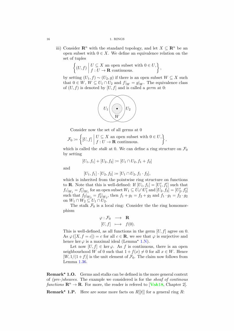
iii) Consider Rn with the standard topology, and let X ⊆ Rn be anopen subset with 0 ∈ X. We define an equivalence relation on theset of tuples{

(U, f)

∣∣∣∣ U ⊆ X an open subset with 0 ∈ U ,f : U → R continuous.

},

by setting (U1, f) ∼ (U2, g) if there is an open subset W ⊆ X suchthat 0 ∈ W , W ⊆ U1 ∩ U2 and f |W = g|W . The equivalence classof (U, f) is denoted by [U, f ] and is called a germ at 0:

W

U1 U2

Consider now the set of all germs at 0

F0 :=

{[U, f ]

∣∣∣∣ U ⊆ X an open subset with 0 ∈ U ,f : U → R continuous.

},

which is called the stalk at 0. We can define a ring structure on F0

by setting

[U1, f1] + [U2, f2] := [U1 ∩ U2, f1 + f2]

and[U1, f1] · [U2, f2] := [U1 ∩ U2, f1 · f2],

which is inherited from the pointwise ring structure on functionsto R. Note that this is well-defined: If [U1, f1] = [U ′1, f

′1] such that

f1|W1= f ′1|W1

for an open subsetW1 ⊆ U1∩U ′1 and [U2, f2] = [U ′2, f′2]

such that f2|W2= f ′2|W2

, then f1 + g1 = f2 + g2 and f1 · g1 = f2 · g2

on W1 ∩W2 ⊆ U1 ∩ U2.The stalk F0 is a local ring: Consider the the ring homomor-

phism

ϕ : F0 −→ R

[U, f ] 7−→ f(0).

This is well-defined, as all functions in the germ [U, f ] agree on 0.As ϕ ([X, f = c]) = c for all c ∈ R, we see that ϕ is surjective andhence kerϕ is a maximal ideal (Lemmab 1.N).

Let now [U, f ] ∈ kerϕ. As f is continuous, there is an openneighbourhood W of 0 such that 1 + f(x) 6= 0 for all x ∈W . Hence[W, 1/(1 +f)] is the unit element of F0. The claim now follows fromLemma 1.36.

Remarkb 1.O. Germs and stalks can be defined in the more general contextof (pre-)sheaves. The example we considered is for the sheaf of continousfunctions Rn → R. For more, the reader is refered to [Vak18, Chapter 2].

Remarkb 1.P. Here are some more facts on R[[t]] for a general ring R:


i) As R-modules the map

R[[t]]→∏N

R,

∞∑i=0

aiti 7→ (ai)i∈N

is a well-defined isomorphism. It is a classical (non-trivial) resultthat the infinite product

∏N Z is not a free.

ii) The units in R[[t]] are of the form a0 + . . ., where a0 is a unit in R.This similar to the case where R is local.

iii) So we can still describe the maximal ideals MaxSpecR[[t]]: by ii),every maximal ideal necessarily contains t and hence correspondsto a maximal ideal of R[[t]]/〈t〉 ∼= R. So we have

MaxSpecR[[t]] = {m + 〈t〉 | m ∈ MaxSpecR} .

Since for any ideal I ⊆ R the maximal ideals over I + 〈t〉 areprecisley of the form m + 〈t〉 for the maximal ideals m over I ⊆ mthe assignment

MaxSpecR[[t]] ←→ MaxSpecR

m 7−→ m ∩Rm + 〈t〉 ←−[ m

is a homeomorphism (where we equip MaxSpecR[[t]] and MaxSpecRwith the subspace topology).

The following is a recollection of basic facts about rings of fractions.More details can be found in [Sch19, 5.17].

Definition 1.38. A subset S ⊆ R is called multiplicative ifi) 1 ∈ S;ii) for all a, b ∈ S it holds that ab ∈ S.

Remark/Definition 1.39. Let S ⊆ R be a multiplicative set. We candefine an equivalence relation on S ×R by

(s, a) ∼ (t, b) if there is a u ∈ S such that u (ta− sb) = 0.

Denote by S−1R the set of equivalence classes of ∼, and by a/s or as the

equivalence class [(s, a)].We can define a ring structure on S−1R by setting

a

s+b

t:=

at+ bs

st

anda

s· bt

:=ab

st.

To show that this is well-defined requires S to be multiplicative and somework, so we will not do this here.

The ring S−1R is called the ring of fractions with respect to S. Mostly,S will be left implicit, so that we refer to S−1R only as the ring of fractions.

Lemma 1.40.

18 1. RINGS

i) The map

η : R −→ S−1R

a 7−→ a

1

is a ring homomorphism. The elements of S are invertible in S−1R:

η (S) ⊆(S−1R

)×.

ii) If R has no zero-divisors, then S−1R has no zero-divisors too.iii) If S has no zero-divisors, then η is injective.

Proof. Ommited. �

Proposition 1.41. Let S ⊆ R be a multiplicative subset and g : R→ R′

a ring homomorphism such that g (S) ⊆ (R′)×. Then g factors over the ringof fractions: there is a unique ring homomorphism g′ : S−1R→ R′ such that

R R′

S−1R

g

ηg′

commutes.

Proof. Ommited. �

Example 1.42.i) Let S = {1}. Then S−1R ∼= R.ii) Let 0 6= a ∈ R be an element and

S := {an | n > 0} .Then Ra := S−1R is called the localization at a.

iii) Let p be a prime ideal and S := R \ p. Then S is a multiplicativesubset. Then Rp := S−1R is the localization at p.

Example 1.43. Consider the case R = Z. Then for any prime number p,the localization at p is given by

Zp =

{a

pn

∣∣∣∣ a ∈ Z, n ≥ 0

}.

The localization at a prime ideal p = 〈p〉 however is given by

Zp ={ab

∣∣∣ a, b ∈ Z, p does not divide b}.

Note that Zp and Zp are different from each other; both are extremly differentfrom Z/pZ!

Lemmab 1.Q. For an element x ∈ R, the following are equivalent:i) x = 0,ii) η(x) = 0 for all prime ideals p ∈ SpecR,iii) η(x) = 0 for all maximal ideals m ∈ MaxSpecR.

Proof. Ommited. �


Definition 1.44. Let ϕ : R→ R′ be a ring homomorphism.i) Let J ⊆ R′ be an ideal. We denote by

J ∩R := ϕ−1(J) ⊆ R

the contraction of J by ϕ.ii) Let I ⊆ R be an ideal. We denote by

IR′ := 〈ϕ(I)〉 ⊆ R′

the extension of I by ϕ.

In both cases, the map ϕ is often left implicit.

Lemma 1.45. Let ϕ : R→ R′ be a ring homomorphism.i) Extensions and contractions of ideals by ϕ are again ideals.ii) For all ideals I ⊆ R and J ⊆ R′, I ⊆ (IR′) ∩ R = I and

J ⊇ (J ∩R)R′ = J holds.

Theorem 1.46. Let S ⊆ R be a multiplicative subset.i) If I ⊆ R is an ideal, then

I(S−1R

)={as

∣∣∣ a ∈ I, s ∈ S} .ii) If I ⊆ R is an ideal, then

I(S−1R

)∩R = {a ∈ R | there is a n ∈ S such that na ∈ I} .

iii) If J ⊆ S−1R is an ideal, then

(J ∩R)S−1R = J.

iv) If p is a prime ideal in R with p ∩ S = ∅, then p(S−1R

)is a prime

ideal in S−1R.v) The maps

SpecS−1R ←→ {p ∈ SpecR | p ∩ S = ∅}q 7−→ q ∩R

p(S−1R

)←− [ p

are mutually inverse and preseve inclusions.

Remarkb 1.R. The statement in v) is actually stronger: If we considerthe set

{p ∈ SpecR | p ∩ S = ∅}with the subspace topology in SpecR, then the map q 7→ q ∩R is actually ahomeomorphism.

Proof. Ommited. �

Remarkb 1.S. In Theorem 1.46, all statements about contractions andextensions of ideals are with respect to the canonical inclusion η : R→ S−1R.

Proof of Theorem 1.46.

20 1. RINGS

i) Let a/s ∈ S−1R with a ∈ I and s ∈ S. Then

a

s=a

1· 1

s

= η(a) · 1

s,

which is in I(S−1R

), as η(a) is.

Let now x ∈ I(S−1R

), so there are ai ∈ I, bi ∈ R and si ∈ S

such that

x =∑i

bisi· ai

1.

Set

s :=∏i

si and a :=∑i

bi

∏i 6=j

sjaj

.

Then s ∈ S, as S is a multiplicative set, and a ∈ I, as I is an ideal.As x = a/s, the claim follows.

ii) Let a ∈(IS−1R

)∩ R. Then a/1 ∈ I

(S−1R

). We now have the

following chain of equivalences a ∈ I(S−1R

)if and only if

there are b ∈ I, t ∈ S, such thata

1=b

t⇐⇒ there are b ∈ I and s, t ∈ S with s(ta− b) = 0

⇐⇒ there is a n ∈ S such that na ∈ I,where the first equivalence follows from i), the second from the defi-nition of the localization and the third from the following argument:

If there are such b, t and s, then (st)a = sb. But n := st is in S(as s and t are) and sb is in I, as b is. On the other hand, if thereis a n ∈ S such that b := na ∈ I, then for t := n and s := 1 we have1 · (na− na) = 0.

iii) (J ∩R)S−1R ⊆ J is always true (Lemma 1.45). For the otherinclusion, let x = a/s ∈ J . Then

a

1=s

1· as

and hence a ∈ J ∩R. So a/s ∈ (J ∩R)S−1R, by i).iv) Let p ∈ SpecR be a prime ideal with p∩S = ∅, and let a/s, b/t ∈ S−1R\p

(S−1R

).

If (ab)/(st) ∈ S−1R \ p(S−1R

). Then there are c ∈ p, u ∈ S such

that (ab)/(st) = c/u (by i). By the definition of the localization,there is now a v ∈ S such that

v (uab− stc) = 0.

So (vu) ab = (vst)c ∈ p, as p is an ideal. But since ab /∈ p thisimplies vu ∈ p ∩ S, contradicting p ∩ S = ∅.

�

Corollary 1.47. Let p ⊆ R be a prime ideal.i) There is a bijection

SpecRp {p′ ∈ SpecR | p′ ∩ (R \ p) = ∅} = {p′ ∈ SpecR | p′ ⊆ p} .


ii) Rp is a local ring with maximal ideal pRp.

Corollary 1.48. The map

Spec η : SpecS−1R SpecR

is injective, with image

{p ∈ SpecR | p ∩ S = ∅} .

Definition 1.49. In the special case S = {an | n ≥ 0} the image of Spec ηis D(a) := SpecR \ Z(〈a〉), which is called a principal open subset .

Remarkb 1.T. The principal open subsets form a basis for the Zariskitopology: for every open subset U ⊆ SpecR and a point x ∈ U there is aprincipal open subset D(a) such that x ∈ D(a) ⊆ U .

End of Lecture 3

CHAPTER 2

Modules and Integral Extensions

2.1. Modules - Basics

Definition 2.1. An R-module M (M,+, ·) is an abelian group (M,+)together with a map

· : R×M −→ M

a, x 7−→ ax

such thati) (a+ b)x = ax+ bx,ii) a(x+ y) = ax+ ay,iii) a(bx) = (ab)x,iv) 1Rx = x

for all x, y ∈M and a, b ∈ R.

Example 2.2.i) Let k be a field. Then k-modules are precisely k-vector spaces.ii) Let I ⊆ R be an ideal. Then I can be regarded as an R-module,

since it is closed under addition and multiplication by elements inR.

iii) Consider R = Z. Let G be an abelian group. Then G is a Z-module,by setting

nx := x+ . . .+ x︸︷︷︸n times

and (−1)x := −x.iv) Let ϕ : R→ R′ be a ring homomorphism and let M be an R′-module.

Then M can be regarded as an R-module, by setting

ay := ϕ(a)y

for all a ∈ R. This is called restriction of scalars.

Definition 2.3. Let M,M ′ be R-modules and f : M → M ′ a map. Wesay f is an R-linear map if

i) f(x+ x′) = f(x) + f(x′),ii) f(ax) = af(x)

for all a ∈ R and x, x′ ∈M .

Remark 2.4.i) Composition of R-linear maps are again R-linear: If f : M → N andg : N → O are R-linear maps, then their composition g◦f : M → Ois R-linear too.

22

2.1. MODULES - BASICS 23

ii) For all R-modules M , the identity map id : M → M, x 7→ x isR-linear.

iii) Let f : M → N be a bijective R-linear map. Then the inversef−1 : N →M is R-linear too. In this case, we say f is an isomor-phism of R-modules.

So we can construct a category R-Mod, where objects are R-modules andmorphisms are R-linear maps.

iv) For two R-modules M,N , the set of R-linear maps

homR (M,N) :={f : M →M ′

∣∣ f is R-linear}

is anR-module, by setting f+g : x 7→ f(x)+g(x) and af : x 7→ f(ax)for all f, g ∈ homR(M,N) and a ∈ R. In the notation, the ring R issometimes ommited and we just write hom(M,N) for homR(M,N).So R-Mod is an abelian and a pre-R-linear category.

v) For anR-moduleM , the set ofR-linear maps EndR(M) := homR(M,M)has also non-commutative ring structure, by setting fg : x 7→ (f◦g)(x)for all f, g ∈ EndR(M). We call EndR(M) the set of R-linear endo-morphism, and f an (R-linear) endomorphism.

Remarkb 2.A. Using the restriction of scalars from Example 2.2, weobtain a functor Fϕ : R′-Mod → R-Mod for all rings R,R′ and ringhomomorphisms ϕ : R → R′. This functor is faithful : for all R′-modulesM,N , the induced map homR′(M,N)→ homR(M,N) is injective.

Example 2.5. Let M be a R-module. The map

M −→ homR(R,M)

x 7−→ [a 7→ ax]

is an isomorphism of R-modules, with inverse

homR(R,M) −→M

f 7−→ f(1).

Example 2.6. Let R be a ring. Then an R[t]-module is”the same“ as an

R-module M , together with an endomorphism f : M →M .If M is an R-module, we can define the an R[t]-structure on M by setting

tm := f(m) for all m ∈M and extending linearly:(n∑i=0

aiti

)(m) :=

n∑i=0

aif(i)(m).

If, on the other hand, M is an R[X]-module, we can regard M as anR-module, by restriction of scalars for the embedding R ↪→ R[t]. We alsoget an endomorphism f : M →M , defined by m 7→ tm.

Definition 2.7. Let M be an R-module. A subset M ′ ⊆ M is an R-submodule if

i) M ′ is a subgroup of (M,+) andii) for all a ∈ R and x ∈M ′, it holds that ax ∈M ′.

If the ring R is clear, we will often refer to M ′ just as a submodule.

24 2. MODULES AND INTEGRAL EXTENSIONS

Exampleb 2.B.i) Let k be a field. Then k-submodules of k-modules are preciselyk-subspaces.

ii) Let I ⊆ R be an ideal. Then I is an R-submodule of R.iii) Let H ⊆ G be a subgroup of an abelian group G. Then H is a

Z-submodule.

Proposition 2.8. Let M ′ ⊆M be a submodule. Then the quotient groupM/M ′ becomes an R-module, by setting

· : R×R/M ′ −→M/M ′

r, x+M ′ −→ (rx) +M ′.

The quotient map M →M/M ′ is R-linear.

Proof. Ommited. �

Definition 2.9. Let f : M → N be an R-linear map.i) The kernel of f is defined as

ker f := {x ∈M | f(x) = 0} .

ii) The image of f is defined as

im f := {f(x) | x ∈M} .

Proposition 2.10. Let f : M → N be an R-linear map. The kernel of fis a submodule of M , the image of f is a submodule of N .

Definition 2.11. Let f : M → N be an R-linear map. The cokernel of fis defined as coker f := N/ im f .

Lemmab 2.C. Let f : M → N be an R-linear map.i) The kernel of f is trivial if and only if f is injective.ii) The cokernel of f is trivial if and only if f is surjective.

Proposition 2.12. Let f : M → N be an R-linear map.i) Let M ′ ⊆ M be a submodule such that M ′ ⊆ ker f . Then there

is a unique R-linear map f : M/M ′ → N such that the followingdiagram commutes:

M N

M/M ′

f

f

2.2. FREE AND FINITELY GENERATED MODULES 25

ii) There is a unique isomorphism f : M/ ker f∼−→ im f such that the

following diagram commutes:

M N

M/ ker f im f

f

f

∼

Proof. Ommited. �

End of Lecture 4

2.2. Free and Finitely Generated Modules

Lemma 2.13. Let M be an R-module, (Mi) a family of submodules of M .Then the intersection

⋂iMi and the sum∑

i

Mi :=

{∑i

mi

∣∣∣∣∣ mi ∈Mi,mi 6= 0 for only finitely many i.

}are submodules of M .

Proof. Ommited. �

Definition 2.14.i) LetM1,M2 ⊆M be submodules of anR-moduleM . IfM1∩M2 = {0}

and M1 +M2 = M , we write M1 ⊕int M2 = M . This constructionis called the (internal) direct sum of M1 and M2.

ii) Let (Mi) be a family of R-modules. Then the product of the {Mi}is defined as the cartesian product

∏iMi, with component-wise

addition and scalar multiplication.iii) Let (Mi) be a family of R-modules. Then the direct sum (or

coproduct) {Mi} is defined as the submodule⊕i

Mi :=

{(mi)

∣∣∣∣ (mi) ∈∏iMi,

mi 6= 0 for only finitely many i.

}⊆∏i

Mi.

Remarkb 2.D.i) If we regard two submodules M1,M2 ⊆M of an R-module M withM1 ⊕int M2 = M as R-modules, then M1 ⊕M2

∼= M = M1 ⊕int M2.So we will not distinguish further between the two notions.

ii) If (Mi) is a finite family of R-modules, then the product and directsum of the Mi are equal.

iii) The product of a family (Mi) is indeed a product in the categoryR-Mod. The coproduct of a family (Mi) is indeed a coprodcut inthe category R-Mod.

Definition 2.15. Let {xi} be a family of elements in an R-module M .


i) We say {xi} is a generating system of M , if every x ∈ M can bewritten as a finite linear combination of xi.

ii) We define the subspace Lin {xi} generated by {xi} as

Lin {xi} :=

{∑aixi

∣∣∣∣ ai ∈ I,ai 6= 0 for only finitely many i.

}.

iii) We say {xi} is linearly independent if for all tuples (x1, . . . , xn) ofelements from {xi} there are no ai ∈ R such that

a1x1 + . . .+ anxn = 0.

iv) We say {xi} is a basis if it is a linearly independent generatingsystem.

v) M is a free R-module if there is an index set I such thatM ∼=⊕

i∈I R.vi) M is a finite-free R-module if there is a finite index set I such that

M ∼=⊕

i∈I R.vii) M is a finitely generated R-module if M has a finite generating

system.

Definitionb 2.E. Let M be an R-module. We say M is finitely presentedor that M is an R-module of finite presentation if there are integers n,mand an exact sequence of the form

Rm Rn M 0

Exampleb 2.F.i) If M is finitely presented then M is already finitely generated.ii) The converse is in general not true: The sequence Rm → Rn →M

being exact is equivalent to saying that Rm → Rn is a kernel forthe projection Rn → M . Consider now any non-noetherian ringand I ⊆ R an ideal which is not finitely generated. Then R/I is notfinitely presented. As a concrete example, there is no presentationfor k[t1, . . .]/〈t1, . . .〉.

Lemmab 2.G. Let M be an R-module.i) M is free if and only if M has a basis.ii) M is finite-free if and only if it is finitely generated and free.

Remarkb 2.H. The alternative characterizations of a basis, as known fromlinear algebra for vector spaces, does not hold for general modules: ConsiderR = Z and M = Z. Then Z has a basis given by {1}. However, the subset{2, 3} is also linear independet, and the subset {2} does not generate all ofZ.


Remark 2.16. Let M be a free R-module with basis {xi}i∈I . Let M ′

be another R-module and {yi}i∈I a subset of M ′. Then there is a uniqueR-linear map f : M →M ′ such that the diagram

M M ′

{xi}i∈I

∃!f

f

commutes. Here, the map of sets f : {xi}i∈I is given by f(xi) := yi for alli ∈ I. This is called the universal property of a free module.

If M ′ is a finitely generated R-module, then in particular there is asurjective map Rn →M ′.

Example 2.17.i) For R = Z and M = Z/pZ, M is not a free Z-module, as every

element has torsion.ii) For R = Z and M = Q, M is not finitely generated as Z-module.

Definition 2.18. Let M be an R-module and I ⊆ R an ideal. We definethe submodule IM as

IM := Lin {am | a ∈ I,m ∈M} .

Lemmab 2.I. Let M be an R-module and I ⊆ R an ideal. Then R/IMhas the structure of an R/I-module.

Lemma 2.19. Let M be an R-module such that

Rn ∼= M ∼= Rm

for n,m ∈ N. Then m = n follows.

Proof. Let m ⊆ R be a maximal ideal, so R/m is a field. Then

dimR/mRM/mM = dimR/mRRn/mRn

= dimR/mR (R/mR)n

= n,

so n is uniquely determined. �

Remark 2.20 (Linear Algebra for Modules). For n,m ∈ N, we can identifyhomR(Rn, Rm) with the set Mat(n×m,R) of n×m-matrices with entriesin R. For an endomorphism f : Rn → Rn, we have that f is an isomorphismif and only if its associated matrix is invertible.

Using the Leibniz formula, we define the determinant of a n× n matrixA = (ai,j) ∈ Mat (n× n,R) as

detA :=∑σ∈Sn

sgn(σ)a1,σ(1) . . . an,σ(n).

Using the determinant, we associate to every matrixA = (ai,j) ∈ Mat(n×n,R)the adjugate matrix adjuM , which is defined as(

(adjuA)i,j

):= (−1)i+j detAj,i


where the matrix Aj,i ∈ Mat ((n− 1)× (n− 1), R) is obtained from A byremoving the j-th row and the i-th column. It then holds that

A adjuA = (adjuA)A = detA · Enwhere En denotes the n × n unit matrix. As the determinant stays multi-plicative for matrices with entries in an arbitrary ring, we have that a matrixwith entries in R is invertible if and only if its determinant is a unit in R.

Proposition 2.21 (Cayley-Hamilton for Modules). Let M be a finitelygenerated R-module, I ⊆ R an ideal and f : M →M an endomorphism, suchthat f(M) ⊆ IM . Then there is a monic polynomial p =

∑ni=0 ait

i ∈ R[t]such that ai ∈ I for i 6= n and p(f) = 0 holds.

Proof. Let {m1, . . . ,mn} be a generating set for M . Then f(mi) ∈ IMfor all 1 ≤ i ≤ n, and so there are aij ∈ I for 1 ≤ i, j ≤ n such that

(∗) f(mj) =n∑i=1

aijmi.

By Example 2.6, we can regard M as an R[t]-module, with the actiontx := f(x) for all x ∈M . The condition (∗) then reads as

n∑i=0

(tδij − aij)mj = 0 for all 1 ≤ j ≤ n.

Consider now the matrices A :=(

(tδij − aij)i,j)

and B := adjuA. Then

BA = detA · En, and hence

det(

(tδij − aij)i,j)

(mj) = 0.

The claim follows for the polynomial p := det(

(tδij − aij)i,j)

. (That p is

monic and the non-leading coefficients are in I follows from the Leibniz-formula.) �

Lemma 2.22. Let M be a finitely generated R-module and f : M →M asurjective R-linear map. Then f is already an isomorphism.

Proof. As in Example 2.6, we consider M as an R[t1] module. Considerthe ideal I := 〈t1〉 ⊆ R[t1]. As f is surjective, IM = M follows. ByProposition 2.21 (for the endomorphism id : M →M), there is a polynomialp = tn2 + an−1t

n−12 + . . . + a0 ∈ R[t1][t2] such that p(id) = 0. So there is a

polynomial q ∈ R[t1] withid = t1q(t1).

Evaluating at f gives the invese. �

We will now state and prove two version of Nakayama’s Lemma:

Lemma 2.23 (Nakayama -”the general one“). Let M be a finitely gener-

ated R-module and I ⊆ R an ideal with IM = M .i) There is an a ∈ I such that am = m for all m ∈M .ii) There is a x ∈ R such that 1− x ∈ I and xM = 0.

Proof.


i) Apply Proposition 2.21 to id : M →M . Then there are a0, . . . , an−1 ∈ Isuch that

id = (−(an−1 + . . .+ a0)) id .

As I is an ideal, −(an−1 + . . .+ a0) ∈ I.ii) For x := 1 + an−1 + . . .+ a0, where the a0, . . . , an−1 are choosen as

in the proof of i), the claim follows.

�

Lemma 2.24 (Nakayama -”the classical one“). Let M be a finitely gen-

erated R-module, and I ⊆ JacR an ideal. Then IM = M if and only ifM = 0.

Proof. If M = 0, then IM = 0. If IM = M , then by Lemma 2.23there is an x ∈ R such that 1 − x ∈ JacR. Now by Proposition 1.33,x = 1 − (1− x) ∈ R×. But this implies 1m = 0 for all m ∈ M . SoM = 0. �

Lemmab 2.J. Let M be a finitely generated R-module, and M ′ a submod-ule. Then M/M ′ is again finitely generated.

Proof. By Remark 2.16, there is a surjective map Rn → M . Extendthis to a surjective map Rn →M →M/M ′. �

Remarkb 2.K. It is in general not true that submodules of finitely gener-ated modules are again finitely generated: Let

I1 ( I2 ( . . . ( R

be a strictly increasing chain of ideals in a ring R. Then the ideal

I :=

∞⋃i=1

Ii

is not finitely generated as an R-module.

Proof. I is an ideal, since it is the union over a chain of ideals. Further-more, I 6= R, since there is no ideal Ii with 1 ∈ Ii. If there were f1, . . . , fnsuch that I = 〈f1, . . . , fn〉 then there would be a m such that f1, . . . , fn ∈ Im.But then I ⊆ Im ( Im+1 ( I, which is not possible. So I is not a finitelygenerated R-module. �

So consider now the polynomial ring in infintely many variables over aring R 6= 0, R′ := R[t1, t2, . . .]. Then the chain of ideals

〈t1〉 ( 〈t1, t2〉 ( . . . ( R′

is strictly increasing, so the submodule 〈t1, t2, . . .〉 is not finitely generatedas an R-module.

This observation leads to the following definition: A ring R is noetherianif it satisfies one of the following equivalent conditions:

i) All ideals I ⊆ R are finitely generated as R-modules.ii) There is no strictly increasing chain of ideals.iii) Every non-empty set M of ideals of R has an inclusion-maximal

element.


We have already encountered noetherian rings: A field is noetherian, sincethere are no proper ideals other than 〈0〉. We showed (without using thename) last semester that PIDs are noetherian (in the proof that PIDs arefactorial, [Sch19, Satz 5.30]).

In the same vein, we call an R-module M noetherian if it satisfies one ofthe following equivalent conditions:

i) Every submodule N ⊆M is finitely generated.ii) There is no strictly increasing chain of submodules.iii) Every non-empty set M of submodules of M has an inclusion-

maximal element.

It can be shown that an R-module M is noetherian if and only if it is finitelygenerated and R/AnnR(M) is a noetherian ring (a proof can be found in[Fra17, 1.3, Prop. 5].)

Corollary 2.25. Let M be a finitely generated R-module, N ⊆ M asubmodule and I ⊆ JacR such that

M = IM +N.

Then M = N holds.

Proof. We have

I(M/N) = (IM +N)/N

= M/N.

Then by Lemmab 2.J and Lemma 2.24, M/N = 0 follows, which impliesM = N . �

End of Lecture 5

Lemma 2.26. Let M be a finitely-generated R-module, m1, . . . ,mn ∈Mand I ⊆ JacR an ideal. Then the following are equivalent:

i) The set {mi}i generates M as an R-module.ii) The set {mi}i generates M/IM as an R/I-module.

Proof. If the set {mi}i generates M/IM as an R/I-module, then italso generates R/I as an R-module, since the canonical map R → R/I issurjective. So

〈m1, . . . ,mn〉+ IM = M

and by Corollary 2.25, 〈m1, . . . ,mn〉 = M follows. �

2.3. Algebras

Definition 2.27. Let R be a ring.i) A R-algebra consists of a tuple (R′, ϕ), where R′ is a ring andϕ : R→ R′ is a ring homomorphism.

2.4. LOCALIZATION OF MODULES 31

ii) Let (R′, ϕ′), (R′′, φ′′) beR-algebras. A ring homomorphism f : R′ → R′′

is an R-algebra homomorphism if the following diagram commutes:

R′ R′′

R

f

ϕ′ ϕ′′

iii) Let R′ be an R-algebra. We say R′ is finitely generated as R-algebraif there is a n ≥ 0 and b1, . . . , bn ∈ R′ such that the evaluation map

evb1,...,bn : R[t1, . . . , tn] −→ R′

ti 7−→ bi

is surjective. In this case, we will also sometimes say that R′ is anR-algebra of finite type.

Remarkb 2.L. The morphism ϕ in the definition of an R-algebra is oftenleft implicit.

Warning 2.28. Being finitely generated as R-module implies being finitelygenerated as an R-algebra. The converse is in general not true: For example,the polynomial ring R[t1, . . . , tn] is not a finitely generated R-module.

2.4. Localization of Modules

Remark/Definition 2.29. Let M be an R-module and S ⊆ R be amultiplicative set. We can define an equivalence relation on S ×M by

(s, x) ∼ (t, y) if there is a u ∈ S such that u (tx− sy) = 0.

Denote by S−1M the set of equivalence classes of ∼, and by x/s or xs the

equivalence class [(s, x)].We can define a S−1R-module structure on S−1M by setting

x

s+y

t:=

tx+ sy

stand

a

s· yt

:=ay

st.

To show that this is well-defined requires S to be multiplicative and isanalogous to the localization of rings.

The module S−1M is called the localization of M by S.

Further remkarks on the localization of modules can be found in C.3.

Proposition 2.30. Localization is functorial: Given a ring R and a multi-plicative subset S, we can define a functor

S−1(−) : R-Mod −→ S−1R-Mod

M 7−→ S−1M

which sends an R-linear map f : M → N to the induced S−1R-linear map

S−1f : S−1M −→ S−1N

x

s7−→ f(x)

s.


Proof. We need to show that S−1f is always a well-defined S−1R-linearmap. We only show well-definedness: Let x/s = y/t in S−1M . So thereexists a u ∈ S such that u(tx − sy) = 0. As f is R-linear, this impliesu (tf(x)− sf(y)) = 0 and hence f(x)/s = f(y)/t. �

Definition 2.31.i) A sequence of the form

. . . Mi−1 Mi Mi+1 . . . ,

where the Mi are R-modules and the fi are R-linear maps is calledexact at i if im fi = ker fi+1. We say this sequence is exact if it isexact at every i.

ii) An exact sequence of the form

0 M ′ M N 0

is a short-exact sequence.

Lemma 2.32.

i) The sequence 0 M ′ Mf

is exact if and only if f is injective.

ii) The sequence M N 0g

is exact if and only if g is surjective.

iii) The sequence 0 M ′ M 0h is exact if and only if h is anisomorphism.

iv) Let M ′ ⊆M be a submodule. Then the sequence

0 M ′ M M/M ′ 0

is short-exact.

Lemmab 2.M. Let

0 M ′ M M ′′ 0

be a short-exact sequence of R-modules. Then: M is finitely generated ifand only if both M ′ and M ′′ are.

Proof. This is on Exercise Sheet 3. �

Lemma 2.33. Let S ⊆ R be a multiplicative set. Then the localization-functor F : R-Mod→ S−1R-Mod is exact.

Proof. F is additive: Let f, f ′ : M → N be two R-linear maps. Then

F(f + f ′

)(x/s) =

(f + f ′) (x)

s

=f(x) + f ′(x)

s

=f(x)

s+f ′(x)

s= F (f) (x/s) + F

(f ′)

(x/s) .

Let now y/t ∈ kerF (g), so g(y)/t = 0. Now by the definition of thelocalization there is a u ∈ S such that ug(y) = 0, and hence uy ∈ ker g. As

2.5. INTEGRAL EXTENSIONS 33

the original sequence is short exact, there is a x ∈M such that f(x) = uy.Then F (f) (x/(ut)) = (uy)/(ut) = y/t, so y/t is in the image of F (f). �

Corollary 2.34. Let N ⊆ M be a submodule of an R-module M . ThenS−1 (M/N) ∼=

(S−1M

)/(S−1N

).

Proof. Consider the short-exact sequence

0 N M M/N 0 .

Since localization is an exact functor, the sequence

0 S−1N S−1M S−1 (M/N) 0

is exact too. Hence S−1M/S−1N ∼= S−1 (M/N). �

End of Lecture 6

2.5. Integral Extensions

Convention. In this and the remaining sections of this chapter, we willconsider R-algebras R′, induced by ring homomorphisms ϕ : R → R′. Inthe notation, ϕ will be ommited, i.e. for a ∈ R and b ∈ R′, ab := ϕ(a)b.If ϕ is injective, we will show this pictorial by a hooked arrow ↪−→. In thiscase we further identify R with a subset of R′. So for an element a ∈ R andϕ : R ↪−→ R′, a ∈ R′ means ϕ(a) ∈ R′.

Definition 2.35. Let R′ be an R-algebra.i) An element a ∈ R′ is integral over R if there is a monic polynomialp ∈ R[t] such that p(a) = 0, i.e. there are cn−1, . . . , c0 ∈ R suchthat

an + cn−1an−1 + . . .+ c0 = 0.

ii) The ring R′ is integral over R if all a ∈ R′ are integral over R.iii) The set

R :={a ∈ R′

∣∣ a integral over R}

is the integral closure of R in R′.iv) The ring R is integraly closed in R′ if R = im (ϕ : R→ R′).v) The ring R′ is finite over R if R′ is finitely generated as R-module.

Example 2.36. Consider the inclusion Z ↪−→ Q: Let a ∈ Q be integralover Z. Then there is a monic polynomial p ∈ Z[t] such that p(a) = 0, i.e.there are cn−1, . . . , c0 ∈ Z such that

0 = an + cn−1an−1 + . . .+ c0.

Let now a = r/s where r, s ∈ Z are coprime. Then

rn = −s(cn−1r

n−1 + . . .+ c0sn)

and hence s divides r. So s ∈× Z = {±1}, which implies a ∈ Z and thusZ = Z.

This argument still holds if we replace Z by a general factorial ring Rand Q by QuotR.


Warning 2.37. Unlike in the special case of fields, the condition that apolynomial p is monic is necessary, as it is in general not possible to invertthe leading coefficient. For example, a = 1/2 ∈ Q is a root of 2t− 1 ∈ Z[t],but still not integral over Z.

Remark/Definition 2.38. Let R′ be an R-algebra and b1, . . . , bn ∈ R′.We denote by

R[b1, . . . , bn] :=

∑i1,...,in

ai1,...,inbi1 . . . bin

∣∣∣∣∣∣ ai1,...,in ∈ R ⊆ R′

the smallest R-subalgebra of R′ which contains all of the b1, . . . , bn.

Lemma 2.39. Let R′ be an R-algebra, b ∈ R′. Then the following areequivalent:

i) b is integral over R.ii) The R-subalgebra R[b] is a finitely generated R-module.

iii) There is a R-subalgebra R ⊆ R′ such that R[b] ⊆ R ⊆ R′, R is a

finitely generated R-module and b ∈ R.

Proof. i) =⇒ ii): Let p = tn + cn−1tn−1 + . . . + c0 ∈ R[t] be a

polynomial such that p(b) = 0. Then the set{

1, b, . . . , bn−1}

generates R[b]as R-module.

ii) =⇒ iii): We can simply choose R := R[b].

iii) =⇒ i): If we regard R as an R-module, left-multiplication with b(i.e. the map fb : R′ → R′, m 7→ b ·m) is an R-linear endomorphism of R′.

As R is finitely generated as an R-module, Cayley-Hamilton (Propo-sition 2.21) implies that there is a monic polynomial p ∈ R[t] such thatp(fb) = 0. So in particular we have 0 = p(fb)(1) = p(b). �

Lemma 2.40. Let ϕ : R→ R′ and ϕ′ : R′ → R′′ be ring homomorphisms,and consider R′ as an R-algebra and R′′ as an R′-algebra.

i) If R′ is finite over R and R′′ is finite over R′, then R′′ is finite overR.

ii) If R′ is integral over R and R′′ is integral over R′, then R′′ is integralover R.

Proof. Ommited. �

Corollary 2.41. Let R′ be an R-algebra. Then the following are equivalent:i) R′ is finite over R.ii) There are elements b1, . . . , bn ∈ R′ which are integral over R such

that R′ = R[b1, . . . , bn].iii) R′ is an R-algebra of finite type and integral over R.

Corollary 2.42. Let R′ be an R-algebra. Then the integral closure R ⊆ R′is an R-subalgebra.

2.6. GOING UP AND GOING DOWN 35

Remarkb 2.N. Let ϕ : R → R′ be a ring homomorphism and let S ⊆ Rbe a multiplicative set. Then the localization of R′ by S as an R-moduleand the localization of R′ by f(S) as a ring are isomorphic as R-algebras.

Lemmab 2.O. LetR′ be anR-algebra via the ring homomorphism ϕ : R→ R′

and S ⊆ R a multiplicative set. Then the localization S−1R′ is still a ringand the induced map of S−1R-modules

S−1 (ϕ) : S−1R −→ S−1R′

a

s7−→ ϕ(a)

s

is also a ring homomorphism.

Lemma 2.43. Let R′ be an R-algebra and R′ integral over R.i) Let I ⊆ R′ be an ideal and J := R ∩ I. Then R′/I is integral overR/J .

ii) Let S ⊆ R be a multiplicative set. We can regard the localizedS−1R-module S−1R′ as an S−1R module via the induced map fromLemmab 2.O. Then S−1R′ is integral over S−1R.

Proof. Ommited. �

2.6. Going Up and Going Down

Definitionb 2.P. Let R′ be an R-algebra via the ring homomorphismϕ : R → R′. If ϕ is injective and R′ integral over R, we say that R′ is anintegral extension of R.

Lemma 2.44. Let R and R′ be integral domains and R′ an integral exten-sion of R. Then R′ is a field if and only if R is a field.

Proof. Assume that R′ is a field and let a ∈ R \ {0}. We want to showthat the inverse b of a, which exists in R′, is an element of R. As b is integralover R, there are c0, . . . , cn−1 ∈ R such that bn =

∑cib

i. Since b = an−1bn,we have

b =

n−1∑i=0

cian−1−i

so b ∈ R. Note that we did not need that R or R′ is an integral domain forthis direction.

Let now a ∈ R′ \ {0}. As a is integral over R, R[a] is a finite dimensionalR-vector space (R is assumed to be a field). Consider now the map

fa : R[a] −→ R[a]

m 7−→ am.

This is R-linear and injective, as R′ is an integral domain, and hence bijective.So there is a b ∈ R′ such that ab = 1. �

Lemma 2.45. Let R′ be an R-algebra which is integral over R and q ⊆ R′a prime ideal. Set p := q ∩R. Then R/p→ R′/q is an integral extension.


Proof. By Lemma 2.43 we have that R′/q is integral over R/p. Letϕ : R→ R′ be the ring homomorphism that induces the R-algebra structureon R′. Then for the composition

ϕ : R R′ R′/qϕ

we have p = R ∩ q = kerϕ. So we get a factorisation of the form

R R′ R′/q

R/p

ϕ

ϕ′

and ϕ′ is injective. So R′/q is an integral extension of R/p. �

Remarkb 2.Q. In the lecture, the claim of Lemma 2.45 was only made forinjective ring homomorphisms ϕ : R ↪−→ R′. But this is not necessary, sincethe induced map ϕ′ is injective, even if ϕ was not (this is also the versionstated in [Fra18b, Prop. 6.8]).

Corollary 2.46. Let R′ be an R-algebra which is interal over R and q ⊆ R′a prime ideal. Set p := q ∩R. Then q is maximal if and only if p is maximal.

Proof. By Lemma 2.45, R/p ↪−→ R′/q is an integral extension. Theclaim now follwos from Lemma 2.44 and Lemma 1.2 �

Lemma 2.47 (3am-Lemma). Let R′ be an integral extension of R andq1 ⊆ q2 ∈ SpecR′ prime ideals with q1 ∩R = q2 ∩R. Then already q1 = q2

holds.

Proof. Let p := q1 ∩ R = q2 ∩ R and consider R′p as the localizedR-module or equivalently the localization by ϕ (p). (We have R′p 6= 0 as ϕ isinjective.) We then have the following commutative diagram

R R′

Rp R′p

ϕ, integral

η η′

ϕ′, integral

with maps

η′ : R′ → R′p, a 7→a

1and

ϕ′ : Rp −→ R′p

a

s7−→ ϕ(a)

ϕ(s)=ϕ(a)

s

where we identify s ∈ R and ϕ(s) ∈ R′.We now have that q′i := qiR

′p is a prime ideal in R′p for i = 1, 2, as

qi ∩ (ϕ (R \ p)) = ∅.By the commutativity of the above diagram we get(

q′i ∩Rp

)∩R =

(q′i ∩R′

)∩R

=((qiR

′p

)∩R′

)∩R.


As p is prime in R, we can use Theorem 1.46, v) to get(qiR

′p

)∩R′ = qi and

hence (q′i ∩Rp

)∩R = qi ∩R

= p.

So, by Theorem 1.46, iii), we have that

pRp =((q′i ∩Rp

)∩R

)Rp

= q′i ∩Rp.

Now by Corollary 1.47, ii) we have that Rp is a local ring with maximal idealpRp, so by Corollary 2.46 we have that both q′1 and q2 are maximal in R′p.But since we assumed q1 ⊆ q2 this implies q′1 = q′2.

Using Theorem 1.46 one last time, we get

q1 =(q1 ·R′p

)∩R′

= q′1 ∩R′

= q′2 ∩R′

= q2,

which finishes the proof. �

Remarkb 2.R. The nickname “3am-Lemma“ comes from a characteri-zation of its proof Dr. Heidersdorf gave in the lecture. A more suitabledescription is that for the induced map ϕ# : SpecR′ → SpecR there is noproper inclusion in thefibres.

Remarkb 2.S. The 3am-lemma should also be true if ϕ : R → R′ is notassumed to be injective, c.f. [Sta19, 00GT]. One way of seeing this shouldbe the following :

Let q1 ⊆ q2 ⊆ R′ be the prime ideals in question, and assume only thatR′ is integral over R. By Lemma 2.45, we get that ϕ : R/p → R′/q1 is anintegral extension. Denote by π′ : R′ → R′/q1 the canonical projection. Wenow can apply our version of the 3am-lemma (Lemma 2.47) to ϕ to get thatπ′(q1) = π′(q2). So by Remarkb 1.G, we get q1 = q2.

End of Lecture 7

Lemma 2.48 (Lying Over). Let ϕ : R ↪−→ R′ be an integral extension ofR. Then for all prime ideals p ∈ SpecR there is a prime ideal q ∈ SpecR′

such that q ∩R = p, i.e. the induced morphism Specϕ : SpecR′ → SpecRis surjective.

Proof. Let p ∈ SpecR be a prime ideal. Consider the commutativediagram

R R′

Rp R′p

ϕ, integral

η η′

ϕ′, integral


We have that ϕ′ is injective, as localization is exact (Lemma 2.33). So inparticular, R′p 6= 0 and there is a maximal ideal n ⊆ R′p. Since ϕ′ is anintegral extension n ∩Rp is again maximal (Corollary 2.46).

By Corollary 1.47, Rp is a local ring with maximal ideal pRp and thusn ∩Rp = pRp. Set q := n ∩R′ ⊆ R′. Then:

q ∩R =(n ∩R′

)∩R

= (n ∩Rp) ∩R= (pRp) ∩R= p.

�

Definition 2.49. Let ϕ : R→ R′ be an algebra.i) We say that ϕ satisfies going up if given a chain of prime ideals

p1 ⊆ p2 ⊆ . . . ⊆ pn

in R and a chain of prime ideals

q1 ⊆ q2 ⊆ . . . qmin R′ with m ≤ n and pi = qi ∩R for all 1 ≤ i ≤ m there are primeideals qm+1, . . . , qn such that the following holds:• pi = qi ∩R for all m+ 1 ≤ i ≤ n; and• the ideals qm+1, . . . , qn fit into the chain

q1 ⊆ . . . ⊆ qm+1 ⊆ . . . ⊆ qn.

ii) We say that ϕ satisfies going down if given a chain of prime ideals

p1 ⊇ p2 ⊇ . . . ⊇ pn

in R and a chain of prime ideals

q1 ⊇ q2 ⊇ . . . qmwith m ≤ n and pi = qi ∩R for all 1 ≤ i ≤ m there are prime idealsqm+1, . . . , qn such that the following holds:• pi = qi ∩R for all m+ 1 ≤ i ≤ n; and• the ideals qm+1, . . . , qn fit into the chain

q1 ⊇ . . . ⊇ qm+1 ⊇ . . . ⊇ qn.

Lemma 2.50. Let ϕ : R→ R′ be a ring homomorphism.i) The following are equivalent:

a) ϕ satisfies going down.b) For all prime ideals q ∈ SpecR′ and p := q ∩ R, the induced

map SpecR′q → SpecRp is surjective.

ii) The following are equivalent:a) ϕ satisfies going up.b) For all prime ideals q ∈ SpecR′ and p := q ∩ R, the induced

map Spec(R/p)→ Spec(R′/q) is surjective.


c) The induced map ϕ# : SpecR′ → SpecR is closed: images ofclosed sets in SpecR′ under ϕ# are closed in SpecR.

Proof. This will be on the 5th exercise sheet. �

Theorem 2.51 (Going Up for Integral Extensions). Let ϕ : R ↪−→ R′ be anintegral extension. Then ϕ satisfies going up.

Proof. Let p1, p2 ∈ SpecR and q1 ∈ SpecR′ be prime ideals such thatp1 ⊆ p2 and q1 ∩R = p1. We now have the following commutative diagram

R R′

R/p1 R′/q1

ϕ, integral

π π′

ϕ′, integral

where ϕ′ is an integral extension by Lemma 2.43 and Lemma 2.45. The idealp2/p1 is prime in R/p1 (Remarkb 1.G) and hence Lying Over (Lemma 2.48)implies that there is a prime ideal q′2 ∈ SpecR′/q1 such that q′2∩R/p1 = p2/p1.

Consider now the prime ideal q2 := q′2 ∩R′. Then q1 ⊆ q2 and

q2 ∩R =(q′2 ∩R′

)∩R

= (p2/p1) ∩R= p2.

�

Remarkb 2.T. There are also extension that are not integral but stillsatisfy going up: A trivial example is the embedding Q ↪−→ R or moregeneraly any field extension that is not algebraic.

As another example, consider the embedding Z ↪−→ Z[t]. This is notintegral (because by Corollary 2.41 this would imply that Z[t] is a finiteZ-module). However, for every prime ideal q ∈ Z the image pZ[t] is primetoo.

Going Down for Integral over Normal.

Definition 2.52. Let ϕ : R→ R′ be an algebra and I ⊆ R an ideal.i) An element b ∈ R′ is integral over I if there is a monic polynomialp ∈ R[t] such that p(b) = 0 and the non-leading coefficients of p arein I.

ii) The set

I :={b ∈ R′

∣∣ b is integral over I}.

is the integral closure of I in R.

Lemmab 2.U. Let ϕ : R → R′ be an algebra and I ⊆ R an ideal. Thenan element b ∈ R′ is integral over I if and only if there is a n > 0 such thatbn is integral over I.

Lemma 2.53. Let ϕ : R→ R′ be an algebra and I ⊆ R an ideal. Consider

the ideal IR ⊆ R. Then I =√IR ⊆ R.


Proof. If b ∈ I ⊆ R then there are a0, . . . , an−1 ∈ I such that

bn = an−1bn−1 + . . .+ a0,

so bn ∈ IR and hence b ∈√IR.

Let now b ∈ IR (this suffices, by Lemmab 2.U), so there are ai, . . . , an ∈ Iand c1, . . . , cn ∈ R such that b = a1c1 + . . .+ ancn. Since the ci are integralover R, the module M := R[c1, . . . , cn] is finitely generated (by Lemma 2.39).Consider now the R-linear map

fb : M −→ M

x 7−→ xbn.

Then im fb ⊆ IM , and hence by Cayley-Hamilton (Proposition 2.21) thereis a monic polynomial p ∈ R[t] with non-leading coefficients in I such thatp(fb) = 0. So in particular, p(bn) = 0, hence b is integral over I (again byLemmab 2.U). �

Definition 2.54. Let R be an integral domain. We say R is normal if Ris integrally closed in its quotient field.

Example 2.55. Every factorial ring is normal.

Lemmab 2.V. Being normal is a local property: For an integral domain,the following are equivalent:

i) R is normal.ii) Rp is normal for all p ∈ SpecR.iii) Rm is normal for all m ∈ MaxSpecR.

Lemmab 2.W. Let ϕ : R ↪−→ R′ be an injective map, with R,R′ integraldomains.

i) This induces a field extension QuotR ↪−→ QuotR′.ii) If R ↪−→ R′ is integral, then QuotR ↪−→ QuotR′ is too,iii) If R ↪−→ R′ is finite, then QuotR ↪−→ QuotR′ is too.

Proof.i) Since ϕ is injective, every non-zero element in R gets mapped to a

unit in QuotR′. So by the univesal property of the localization, weget an induced map

R R′

QuotR QuotR′

ϕ

ii) Localizing R,R′ (as modules) at S := R \ {0} gives an intgegral ex-tension (Lemma 2.43) QuotR = S−1R ↪−→ S−1R′. By Lemma 2.44,we get that S−1R′ is a field, and hence S−1R′ = QuotR′. SoQuotR ↪−→ QuotR′ is algebraic.

iii) Localizing once again at S := R \ {0} gives a finite (localizing isexact) extension QuotR = S−1R ↪−→ S−1R′. Arguing as in ii),


QuotR′ = S−1R′ follows, so S−1R′ is a finite QuotR-vector space.

�

Lemma 2.56. Let ϕ : R ↪−→ R′ be an integral extension, with R,R′ integraldomains and R normal. Let b ∈ R′ be integral over some ideal I ⊆ R. Thenb/1 is algebraic over QuotR and the non-leading coefficients of its minimal

polynomial are already in√I.

Proof. By Lemmab 2.W, there is indeed a minimal polynomial for b.SetK := QuotR, and consider the intermediate fieldK ⊆ K[b] ⊆ QuotR′.

Let L be a field extension of K[b] such that the minimal polynomial p of b isa product of linear factors in L (e.g. the algebraic closure of K[b]). So p hasthe form

p = (t− x1) . . . (t− xn) ,

where the x1, . . . , xn are elements of L.As b is integral over R, there is a monic polynomial f ∈ R[t] ⊆ K[t]

with f(b) = 0. By the minimal property of the minimal polynomial, p | ffollows and hence all roots of p are also roots of f which shows that thex1, . . . , xn are integral over I. Since the non-leading coefficients of p are inK[x1, . . . , xn] we get that they are integral over I too (Lemmab 2.U).

Since we assumed that R is normal, we get that the ai are already in R.By applying Lemmab 2.U to R′ = K, we get I =

√I, so ai ∈

√I. �

Lemma 2.57. Let ϕ : R→ R′ be a ring homomorphism and p ∈ SpecR aprime ideal. Then the following are equivalent:

i) There is a prime ideal q ∈ SpecR′ such that p = ϕ−1(q).ii) It holds that ϕ−1 (ϕ(p)R′) = p.

Proof. This will be on the 5th exercise sheet. �

Theorem 2.58 (Going Down). Let ϕ : R → R′ be an integral extension.Assume that R,R′ are integral domains and that R is normal. Then ϕsatisfies going down.

End of Lecture 8

Proof. Let p1 ⊆ p2 ⊆ R and q2 ⊆ R′ be prime ideals such thatp2 = q2 ∩ R. We want to find a prime ideal q1 ∈ R′ such that p1 = q1 ∩ Rand q1 ⊆ q2:

R′ ∃q1 ⊆ q2

R p1 ⊆ p2

ϕ

Consider now the map

ϕ′ : R R′ R′q2ϕ η

.

We are going to show that under ϕ′,

(∗)(p1R

′q2

)∩R = p1


holds. Assume for now that this is the case. Then Lemma 2.57 implies thatthere is a prime ideal q′1 ⊆ R′q2 such that q′1 ∩R = p1. For q1 := q′1 ∩R′ wehave that q1 ∩R = p1, and q1 ⊆ q2 (by Corollary 1.47, i)), which shows thatϕ satisfies going down.

We now prove (∗): Note first that p1 ⊆(p1R

′q2

)∩R is always true. So it

suffices to show(p1R

′q2

)∩R ⊆ p1. We will do this by contradiction:

Let x ∈(p1R

′q2

)∩R be any element and consider ϕ′(x) ∈ p1R

′q2 , which we

will identify with x. As p1R′q2 = (p1R

′)R′q2 there are y ∈ p1R′ and s ∈ R′ \q2

such that x = y/s (Theorem 1.46, i)). Now by Lemmab 2.U, y is integral

over p1 (we have y ∈ p1R′ ⊆√p1R′ =

√p1R, since R′ is integral over R.).

Let py ∈ (Quot (R)) [t] be the minimal polynomial of y over K := Quot(R)(c.f. Lemmab 2.W). By Lemma 2.56, the non-leading coefficients of py, saya0, . . . , an−1, are in

√p1 = p1 (since p1 is a prime ideal).

Assume now that x /∈ p1, so in particular x 6= 0 and hence s has the formy/x ∈ QuotR′, and 1/x ∈ K. This implies that the minimal polynomial psof s over k has the form

tn +an−1

ttn−1 + . . .+

a0

xn.

Set ai := ai/xn−i for (i = 0, . . . , n− 1). Since s ∈ R′ is integral over R (by

assumption on ϕ), we have by Lemma 2.56 that the ai are already in R.Now in R, we have aix

n−1 = ai ∈ p1, and since we assumed x /∈ p1, thisimplies ai ∈ p1 for all i = 0, . . . , n− 1. But then

sn = −(an−1s

n−1 + . . .+ a0

)∈ p1R ⊆ p2R

′q2,

contradicting s /∈ q2. �

More Examples of Going Down. The proofs for the following propo-sitions will (hopefully) be added in the future.

Theoremb 2.X. Let ϕ : R → R′ be flat, i.e. R′ is flat as an R-module.Then ϕ satisfies going down.

Theoremb 2.Y. Let ϕ : R → R′ be a ring homomorphism such thatSpecϕ : SpecR′ → SpecR is open (i.e. maps open sets to open sets.). Thenϕ satisfies going down.

2.7. Noether Normalization Lemma

Theorem 2.59 (Noether Normalization Lemma (NNL)). Let k be a field,and A a finitely generated k-algebra. Let

I1 ⊆ I2 ⊆ . . . ⊆ Im ( A

be a chain of ideals in A. Then there is a n ≥ 0, a1, . . . , an ∈ A and0 ≤ h1 ≤ . . . ≤ hm ≤ n such that:

i) the elements a1, . . . , an are algebraically independent over k;ii) k[a1, . . . , an] ⊆ A is a finite ring extension; andiii) Il ∩ k[a1, . . . , an] = (a1, . . . , ahl).

We will only prove i) and ii). The proof of iii) can be found in [Fra18b].

2.7. NOETHER NORMALIZATION LEMMA 43

Lemma 2.60. Let k be a field, and 0 6= f ∈ k[t1, . . . , tn] a non-zeropolynomial. Then there are r1, . . . , rn−1 ∈ N such that after the substitutionti := Yi + trin (1 ≤ i ≤ n− 1), the polynomial f has the form

f = ctmn + h1tm−1n + . . .+ hm ∈ k[Y1, . . . , Yn−1, tn],

for a m > 0, c ∈ k× and h1, . . . , hm ∈ k[Y1, . . . , Yn−1].

Proof. Assume f has the form

f =∑σ∈Nn

bσtσ11 . . . tσnn .

After substituting ti := Yi+trin for (yet to be determined) ri ≥ 0, this becomes

f =∑σ∈Nn

bσ (Y1 + tr1n )σ1 . . . (Yn−1 + trn−1n )σn−1 tσnn .

Let now τ ∈ Nn be a specific multi-index. Define

e (τ) := τ1r1 + . . .+ τn−1rn−1 + τn

With this notation, we obtain a factorisation of the τ -summand of f whichreads as follows:

bτ tτnn

n−1∏i=1

(Yi + trin )τi = bτ te(τ)n +

(terms where tn has stricly lower degrees) .

Claim 1. The ri can be choosen in such a way that for each different pair ofmulti-indices σ, τ ∈ Nn, the associated exponents e(σ), e(τ) are different too:

By definition, there is a M > 0 such that bσ = 0 for all multi-indicesσ ∈ Nn\{0, . . . ,M − 1}. Set now r1 := M, r2 := M2, . . . , rn−1 := Mn−1,and let σ ∈ Nn be a multi-index with bσ 6= 0. Then the value of

e(σ) = σn +

n−1∑i=1

σiri = σn + σ1M + . . .+ σn−1Mn−1

is uniquely determined by the values of the σ1, . . . , σn (since the M -adicexpansion of a natural number is unique, and M was chosen in such away that σi < M for all 1 ≤ i ≤ n).

Now for such a choice of ri, there is a unique multi-index σ ∈ Nn such thatthe corresponding exponent e(σ) is maximal and bσ 6= 0. After re-groupingthe expansion of f in decreasing order of powers of tn, the claim follows withm := e(σ) and c := bσ. �

Proof of NNL (Theorem 2.59). Denote by x1, . . . , xm ∈ A a set ofgenerators of A. We want to show that there are algebraically independenta1, . . . , an such that the ring homomorphism k[a1, . . . , an] → A is injec-tive and A is a finitely-generated k[a1, . . . , an]-module. We will do this byinduction on the number m of generators:

The case m = 0 is trivial. So assume NNL holds for m − 1 gener-atos. If the x1, . . . , xm are algebraically independent then the canonicalmap k[x1, . . . , xm] → A is indeed injective, and A is a finitely generatedk[x1, . . . , xm]-module.


If, however, the xi are not algebraically independent, then there is a poly-nomial 0 6= f ∈ k[t1, . . . , tm] such that f(x1, . . . , xm) = 0. Set yi := xi − xrimfor 1 ≤ i ≤ 0 and (yet to be determined) ri. We then have

0 = f(y1 + xr1m , . . . , ym−1 + x

rm−1

m−1

).

But by Lemma 2.60, there is a set of exponents ri such that

0 = f(y1 + xr1m , . . . , ym−1 + xrm−1

m−1 ) = cxdm + h1xd−1m + . . .+ hd

with h1, . . . , hd ∈ k[y1, . . . , ym−1] and c ∈ k×. So xm is integral overk[y1, . . . , ym−1] and k[y1, . . . , ym−1][xm] is a finite k[y1, . . . , ym−1]-module(Corollary 2.41). By induction hypothesis, there are algebraically indepen-dent a1, . . . , an such that k[a1, . . . , an] ↪−→ k[y1, . . . , ym−1] is finite. Hence

k[a1, . . . , an] k[y1, . . . , ym−1] k[y1, . . . , ym−1][xm] = A

is finite (Lemma 2.40), which proves the claim. �

End of Lecture 9

Notation. Let s ∈ R and consider the multiplicative set S :={

1, s, s2, . . .}

.Then the localization of an R-module M at S is denoted by

M [s−1] := S−1M.

Lemmab 2.Z. Let R′ be an R-algebra of finite type, and S ⊆ R a mul-tiplicative subset. Then the localization S−1R′ of R′ (as R-algebra) is anS−1R-algebra of finite type.

Proof. Since R′ is of finite type, there is surjective ring homomorphismR[t1, . . . , tn]� R′. Since localization is exact, we get an induced epimorphism(

S−1R)

[t1, . . . , tn] S−1 (R[t1, . . . , tn]) S−1R′.∼

�

The following is a generalization of NNL to integral domains:

Proposition 2.61. Let R be an integral domain and R′ an R-algebra offinite type.

i) There exists an element s ∈ R \ {0} and elements b1, . . . , bn ∈ R′such that• the elements b1, . . . , bn are algebraically independent over the

fraction field QuotR; and• the ring extension

R[s−1][b1, . . . , bn] R′[s−1]

is finite.ii) For all prime ideals p ⊆ R[s−1] there is a prime ideal q ⊆ R′[s−1]

such that q ∩R[s−1] = p.iii) For all prime ideals p ∈ SpecR[s−1] and the prime ideal q which

was constructed in ii), it holds that

Quot (R/(p ∩R)) = Quot(R[s−1]/p

)⊆ Quot

(R′[s−1]/q

)= Quot

(R′/(q ∩R′)

),

2.7. NOETHER NORMALIZATION LEMMA 45

and the extension is a finite field extension.

Proof.i) Set S := R \ {0}. Then the induced extension

k := QuotR = S−1R S−1R′

is of finite type (Lemmab 2.Z) and we can apply Noethers Normal-ization Lemma (Theorem 2.59) to get algebraically independentelements b′1, . . . , b

′n ∈ S−1R′ such that k[b′1, . . . , b

′n] ↪−→ S−1R′ is a

finite ring extension. Choose now representatives bi ∈ R′ and si ∈ Ssuch that b′i = bi/si. Then the bi are already algebraically indepen-dent over k and k[b1, . . . , bn] = k[b′1, . . . , b

′n] (since 1/si is in k for

all i).As R′ is an R-algebra of finite type, there are c1, . . . , cm ∈ R′

(not necessarily algebraically independent) such thatR[c1, . . . , cm] = R′.As S−1R′ is finite over k[b1, . . . , bn] it is in particular integral overk[b1, . . . , bn] (Corollary 2.41) and hence there are monic polynomialsfi ∈ k[b1, . . . , bn][t] such that fi(ci/1) = 0 in S−1R′ (for 1 ≤ i ≤ m).We can now choose a u ∈ S such that the coefficients of all of thefi are already in the image of the morphism

R[u−1][b1, . . . , bn] −→ k[b1, . . . , bn]

which is induced by the embedding R[u−1] ↪−→ k. Then thereare monic polynomials gi ∈ R[u−1][b1, . . . , bn][t] such that gi getsmapped to fi for all 1 ≤ i ≤ m. Since bi, ci ∈ R′ we havegi ∈ R′[u−1]. So gi ∈ ker

(R′[u−1]→ S−1R′

), as g(ci) gets mapped

to f(ci/1) = 0 (by construction of the fi). Hence there arevi ∈ R\{0} such that vigi(ci) = 0 inR′[u−1]. Define now v := v1 . . . vmand s := vu.

By the universal property of the localization at u and the factthat R[u−1][b1, . . . , bn] we get a morphism

ψ : R[u−1][b1, . . . , bn] −→ R[s−1][b1, . . . , bn],

which also induces a morphism between the corresponding polyno-mial rings. Set hi := ψ(gi) ∈ R[s−1][b1, . . . , bn][t]. Then the hi aremonic, since ψ is a ring homomorphism, and hi(ci)0. So the ci are in-tegral over R[s−1][b1, . . . , bn], and thus R[s−1][b1, . . . , bn] ↪−→ R′[s−1]is finite (note R′[s−1] = R[s−1][c1, . . . , cm] and then apply Corol-lary 2.41).

ii) Let p ∈ SpecR[s−1] be a prime ideal. Define

p′ := pR[s−1][b1, . . . , bn] + 〈b1, . . . , bn〉.

Then p′ ∩R[s−1] = p the map

R[s−1][b1, . . . , bn] −→ R[s−1]/p

1 7−→ 1

bi 7−→ 0


induces an isomorphism

R[s−1][b1, . . . , bn]/p′ −→∼ R[s−1]/p.

(Note that this is well-defined, since the bi are algebraically inde-pendent). As p is a prime ideal, we get that p′ is too.

Using Lying Over (Lemma 2.48) for the finite integral extension(by i))

R[s−1][b1, . . . , bn] R′[s−1]

we get that there is a prime ideal q sin SpecR′[s−1] such thatq ∩R[s−1][b1, . . . , bn] = p′. Thus(

q ∩R[s−1][b1, . . . , bn])∩R[s−1] = p.

iii) Consider the following commutative diagram

R[s−1][b1, . . . , bn] R′[s−1]

R[s−1][b1, . . . , bn]/p′ R′[s−1]/q

finite

integral

Then

R[s−1]/p R′[s−1]/q

is an integral extension too (Lemma 2.45) and finite, since

R[s−1][b1, . . . , bn] R′[s−1]

is.We also have that

QuotR[s−1]/p ↪−→ QuotR′[s−1]/q

is finite, by Lemmab 2.W.As s /∈ p ∩R, we have(

R[s−1])p

/(p ·(R[s−1]

)p

)∼= Rp∩R/(Rp∩R) ,

which implies

QuotR[s−1]/p ∼= QuotR/p ∩R,as for any ringA and b ∈ SpecA it holds that QuotA/b ∼= Ab/ (b ·Ab).

�

CHAPTER 3

Hilbert’s Nullstellensatz and some AlgebraicGeometry

3.1. Jacobson Rings

Definition 3.1. A ring R is a Jacobson ring if for all prime ideals p ⊆ Rit holds that

p =⋂p⊆m

m maximal

m.

Lemma 3.2. For a ring R, the following are equivalent:i) R is a Jacobson ring.ii) For all prime ideals p ⊆ R and a ∈ R \ p, there is a maximal ideal

m such that p ⊆ m and a /∈ m.iii) For all ideals I ⊆ R it holds that

√I =

⋂I⊆m

m maximal

m.

Proof. i) ⇐⇒ iii) follows from Proposition 1.28. �

Example 3.3.i) Fields are Jacobson rings.ii) If R is a local ring, which has only one prime ideal, the R is a

Jacobson ring.

Exampleb 3.A.i) If R be a noetherian domain such that every non-zero prime ideal

is maximal and R has infinitely many maximal ideals, then R isJacobson: Since every non-zero ideal is maximal, it suffices to show〈0〉 = JacR. For that, it suffices that every non-zero x ∈ R is onlycontained in finitely many prime ideals, i.e. that Z(x) is finite. ButZ(x) is isomorphic to SpecR/〈x〉. Now R/〈x〉 is noetherian andevery prime ideal is minimal. It is a general fact that noetherianrings have only finitely many minimal prime ideals so the claimfollows.

ii) Claim i) implies that all factorial rings with infinitly many primeideals are Jacobson (like Z). Note that for a factorial ring thecondition JacR = 0 suffices for being jacobson.

47

48 3. HILBERT’S NULLSTELLENSATZ AND SOME ALGEBRAIC GEOMETRY

iii) Let on the other hand R be a domain which has only finitely manyprime ideals. Then R cannot be Jacobson: We have

0 6= m1 · . . . ·mn ⊆ m1 ∩ . . . ∩mn,

for the maximal ideals m1, . . . ,mn.

Lemma 3.4. Let ϕ : R ↪−→ R′ be an integral extension. Assume R is aJacobson ring. Then R′ is too.

Proof. Let q ∈ SpecR′ be a prime ideal and set

J :=⋂q⊆m

m∈MaxSpecR

m.

We first show that J ∩R = q ∩R := p:Since R is a Jacobson ring p is the intersection of all maximal ideals

containing it. Now for any maximal ideal m ∈ MaxSpecR with p ⊆ m, goingup (Theorem 2.51) implies that there is a prime ideal n ∈ SpecR′ withn ∩ R = m and q ⊆ n. By Lemma 2.44 we get that n is maximal too, andJ ∩R = p follows.

We are now in the following situation:

R R′

Rp R′

integral

integral

p = R ∩ q q

qR′p.

Since q∩R = p, we have ϕ (R \ p)∩q = ∅, so qR′q is prime in R′p. Furthermore,we have qR′p ∩ Rp = pRp. Since pRp is a maximal ideal (Corollary 1.47),Lemma 2.44 implies that qR′p is a maximal ideal.

As q ⊆ J we have qR′p ⊆ JR′p. Since (R ∩ J) ∩ (R \ p) = ∅ we have thatJR′p is a proper ideal, so qR′p = JR′q follows. But now

J ⊆(JR′p

)∩R′ = qR′q ∩R′

= q,

so J = q follows. �

3.2. Hilbert’s Nullstellensatz

Theorem 3.5 (Generalized Hilbert’s Nullstellensatz, GHNS). Let R be aJacobson ring and R′ an R-algebra of finite type. Then

i) R′ is a Jacobson ring too.ii) For all maximal ideals n ⊆ R′ it holds that:

• The ideal m := n ∩R is a maximal ideal.• For this m, R/m ↪−→ R′/n is a finite field extension.

Proof.i) Let q ∈ SpecR′ be a prime ideal and b ∈ R′ \ q. By Lemma 3.2, we

want to show that there is a maximal ideal n ∈ MaxSpecR′ suchthat q ⊆ n and b /∈ n.

3.2. HILBERT’S NULLSTELLENSATZ 49

Consider the ring extension:

R := R/ (q ∩R) R′/q (R′/q) [b−1] =: R′.

Now R is an integral domain and R ↪−→ R′ is an R′-algebra of finitetype. So by Proposition 2.61, there is a s ∈ R \ {0} such that:

For all p ∈ Spec R with s /∈ p there is a

q ∈ Spec R′ such that q ∩ R = p and

the extension Quot(R/p

)↪−→ Quot

(R′/q

)is finite

(∗)

Let s ∈ R be a preimage of s under R� R, so s /∈ q ∩R. Since Ris jacobson, there is a maximal ideal m ∈ MaxSpecR such that

q ∩R ⊆ m and s /∈ m.

Hence s is not contained in the maximal ideal mR ∈ MaxSpec R.By applying (∗) to m := mR we get a prime ideal n ∈ Spec R′ such

that n ∩ R = m.Consider now the finite field extension Quot R ↪−→ Quot R′.

We now have Quot R/m = R/m as m is maximal. We also have

R/m = R/m and R′/n = R′/n (where n := n ∩ R′). So now wearrive at the following commutative diagram:

R R′

R/m R′/n

Quot R/m Quot R′/n

finite

finite

So R/m ↪−→ R′/n is integral, and hence n is a maximal ideal(Lemma 2.44).

Since n is the preimage of a prime ideal in quotient R′/q, itfolows that q ⊆ n.

By the description of prime ideals in the localization (Theo-rem 1.46) we get a bijection:

Spec(R′/q

)[b−1] −→∼

{q′ ∈ SpecR′

∣∣ q ⊆ q′, b /∈ q′}

q 7−→ q ∩R′

So b /∈ n, which concludes the proof.ii) Let q ∈ MaxSpecR′ be a maximal ideal. By applying the con-

struction for b = 1, we get a maximal ideal m ∈ MaxSpecR withq ∩ R ⊆ m and a maximal ideal n ∈ MaxSpecR′ with n ∩ R = mand q ⊆ n. Since q is a maximal ideal, q = n follows. Son ∩R = q ∩R = m, which is maximal.

We also have that Quot R/m ↪−→ Quot R′/n is finite. Since

Quot R/m = R/m and Quot B/n = B/q, the claim follows.

�


End of Lecture 10

Corollary 3.6. Let k be a field and A a k-algebra of finite type. Theni) A is a Jacobson ring.ii) For all maximal ideals m ∈ MaxSpecA the map k → A→ A/m is

a finite field extension.iii) The maximal ideals of A are given by

MaxSpecA = {p ∈ SpecA | k → QuotA/p is finite} .iv) Let f : A→ B be a homomorphism of k-algebras of finite type and

m ∈ MaxSpecB a maximal ideal. Then m ∩A is maximal too.

Proof.i) This is just i) of GHNS (Theorem 3.5).ii) By ii) of GHNS, m ∩ k is a maximal ideal in k. But since k is a

field, this implies that m ∩ k = 〈0〉. So by the second part of ii),k ↪−→ A/m is a finite field extension.

iii) The inclusion”⊆“ is just ii). For the other direction let p ⊆ A be a

prime ideal and assume that in

k A/p QuotA/p

the composition k ↪−→ QuotA/p is a finite field extension. ThenA/p ↪−→ QuotA/p is necessarily finite, and so in particular integral.Now by Lemma 2.44, this implies that A/p is a field, and hence pis a maximal ideal.

iv) Since B is of finite type, it is in particular an A-algebra of finitetype. By applying ii) of GHNS to A→ B, the claim follows.

�

Corollary 3.7. Denote by k-Algf.t. the category whose objects are k-algebras of finite type and whose morphisms are k-algebra homomorphismsmaps. Then MaxSpec(−) induces a contravariant functor

MaxSpec(−) : k-Algf.t. −→ Top

A 7−→ MaxSpecA

which maps k-algebra homomorphisms ϕ : A→ B to the restriction of ϕ#

to MaxSpecB.

Proof. We only show that the restriction of ϕ# is well-defined, i.e. thatwe indeed get a map ϕ# : MaxSpecB → MaxSpecA. But this is just iv) ofCorollary 3.6. �

Theorem 3.8 (Weak Nullstellensatz). Let k be an algebraically closed field.For a tupel x = (x1, . . . , xn) ∈ kn, denote by mx the ideal

mx := 〈t1 − x1, t2 − x2, . . . , tn − xn〉 ⊆ k[t1, . . . , tn].

Then mx is a maximal ideal and the assignment

kn −→ MaxSpec k[t1, . . . , tn]

x 7−→ mx

3.3. THE DIMENSION OF A RING 51

is a bijection.

Proof. As k[t1, . . . , tn]/mx∼= k we find that mx is indeed a maximal

ideal. We also have mx 6= my for x, y ∈ kn with x 6= y.It remains to show the surjectivity: Let m ∈ MaxSpec k[t1, . . . , tn] be a

maximal ideal. Then by Corollary 3.6, we have that k ↪−→ A/m is a finitefield extension. As k is algebraically closed, there are no non-trivial algebraicfield extensions of k, so in particular there are no finite extensions. So wehave k ∼= a/m.

Denote by π the map π : A � A/m −→∼ k and set xi := π(ti). Thenti − xi ∈ kerπ, and so mx = 〈t1 − x1, . . . , tn − xn〉 ⊆ kerπ = m. But as mx

is maximal and m 6= A, it follows that mx = m. �

Remarkb 3.B. That a field satiesfies the Weak Nullstellensatz is equiva-lent to k being algebraically closed, since it implies that every irreduciblepolynomial in k[t] is of the form t− a for a a ∈ k.

3.3. The Dimension of a Ring

Definition 3.9. Let R be a ring.i) The dimension of R is defined as

dimR := sup

{l ∈ N

∣∣∣∣ there is an ascending chain of prime idealsp0 ( p1 ( . . . ( pl

}if it exists and dimR :=∞ otherwise.

ii) Let p ∈ SpecR be a prime ideal. Then the height is defined as

ht p := sup

{l ∈ N

∣∣∣∣ there is an ascending chain of prime idealsp0 ( p1 ( . . . ( pl ⊆ p

}if it exists and ht p :=∞ otherwise.

Example 3.10.i) Let k be a field. Then dim k = 0, as every prime ideal is maximal.ii) Let R be a prinicipal ideal domain which is not a field. Then every

ascending chain of prime ideals in R is of the form 〈0〉 ( 〈p〉, for aprime element p ∈ R. So dimR = 1.

iii) Consider the polynomial ring in n variables over a field k. Then

0 ( 〈t1〉 ( 〈t1, t2〉 ( . . . ( 〈t1, . . . , tn〉is stricly ascending, so dim k[t1, . . . , tn] ≥ n.

Lemma 3.11. Let p ∈ SpecR be a prime ideal.i) It holds that ht p = dimRp.ii) It holds that dimR ≥ dimR/p + ht p.iii) The dimension of R is local in the following sense:

dimR = sup {dimRm | m ∈ MaxSpecR}= sup {htm | m ∈ MaxSpecR} .


Proof.i) By the classification of prime ideals in Rp (Corollary 1.47), there is

a order-preserving bijection

SpecRp {p′ ∈ SpecR | p′ ⊆ p} .∼

Now the statement is now just the definition of height and dimension.ii) This follows from the classification of prime ideals ofR/p (Remarkb 1.G)

and the definition of height and dimension.iii) After localising at a maximal ideal, the image of an ascending chain

is still an ascending chain. Vice versa, every ascending chain in thelocalization at a maximal ideal can be lifted to an ascending chainin R. This shows the first equality. The second equality followsfrom i).

�

Definitionb 3.C. Let p0 ( . . . ( pn be an ascending chain in R. We saythat this chain is maximal if there is no prime ideal p ∈ SpecR with p ( p0

or pi ( p ( pi+1 (for 0 ≤ i ≤ n− 1) or pn ( p.

Lemma 3.12. Let R be a ring with dimR < ∞. Assume all maximalchains in R have the same length. Let p ∈ SpecR be a prime ideal.

i) All maximal chains in R/p have the same length.ii) It holds that dimR = dimR/p + ht p.iii) It holds that dimRp = dimR if p is a maximal ideal.

Proof. Let q0 ( . . . ( qr be a maximal chain in R/p. We can lift thisto a chain in R and complete it to a maximal chain of the form

p0 ( . . . ( pm = p = q0 ( . . . ( qr.

Now ht p ≥ m and dimR/p ≥ r. By the assumption that every maximalchain in R has the same length, it follows that m+r = dimR. By Lemma 3.11ii), we have

dimR ≥ dimR/p + ht p = m+ r = dimR.

So ht p = m and dimR/p = r follows. This shows ii). For i), note that thecompletion of the lift of the ideal chain in R is independend from r, so r hasto be necessarily the same for all prime chains in R/p. Claim iii) now followsfrom ii), since for a maximal ideal, we have dimR/p = 0. �

Proposition 3.13. Let ϕ : R ↪−→ R′ be an integral ring extension.i) It holds that dimR = dimR′.ii) For all q ∈ SpecR′ it holds that dimRq∩R ≥ dimR′q.iii) If ϕ satisfies going down then dimRq∩R = dimR′q.

Proof.i) Let q0 ( . . . ( ql be an ascending chain inR′. Then q0∩R ( . . . ( ql∩R

is an ascending chain in R (That the inclusions are strict followsfrom Lemma 2.47). This shows dimR ≥ dimR′.

3.3. THE DIMENSION OF A RING 53

Let p0 ( . . . ( pd be an ascending chain in R. Then by Ly-ing Over (Lemma 2.48) there is a prime ideal q0 ∈ SpecR′ withq0 ∩R = p. Now by Theorem 2.51 there is a chain q0 ( . . . ( qd inR′ such that the following diagram is commutative:

q0 ( q1 ( . . . ( qd

p0 ( p1 ( . . . ( pd

That the inclusions are strict follows from Lemma 2.47.ii) Let q0 ( . . . ql = q be a chain in R′. This gives a chain of the form

q0 ∩ R ( . . . ( ql ∩ R in R. By applying Lemma 3.11 twice, theclaim follows.

iii) Let p0 ( . . . pl = q ∩R be a chain in R. By applying going up, wecan lift this to a chain of the form

q0 ) ql−1 ) . . . ) q0

q ∩R ) pl−1 ) . . . ) p0

So dimR′q ≥ dimRq∩R. The claim now follows from ii).

�

Lemmab 3.D (Going Between). Let k be a field and R a k-algebra of finitetype. Let R ↪−→ R′ be an integral ring extension. Let p1 ( p2 ( p3 be primeideals in k and q1 ( q3 prime ideals in R′. Assume that q1 ∩ R = p1 andq3∩R = p3. Then there is a prime ideal q2 ∈ SpecR′ satisfying q1 ( q2 ( q3.

Proof. This is on the sixth exercise sheet. �

Remarkb 3.E. Note that in the setting of going between, it does notnecessarily hold that q2 ∩R = p2. A counterexample can also be found inthe solutions to sheet 6.

Theorem 3.14. Let k be a field.i) It holds that dim k[t1, . . . , tn] = n.ii) All maximal chains in k[t1, . . . , tn] = n have the same length.

Proof. We will do this by induction on n. In the case n = 1, k[t] is anintegral domain, and hence has dimension 1. In particular, maximal chainshave necessarily the same length.

In the general case, consider a chain of prime ideals p0 ( . . . ( pm ink[t1, . . . , tn]. Without loss of generality, we can assume that this chain ismaximal. This implies that p = 〈0〉 (since k[t1, . . . , tn] is an integral domain),pm is a maximal ideal and p1 = 〈f〉, where f is an irreducible polynomial(since k[t1, . . . , tn] is factorial). Using Lemma 2.60, we can assume that fis a monic polynomial in tn, with non-leading coefficients in k[t1, . . . , tn−1].


So we get an integral extension k[t1, . . . , tn−1] ↪−→ k[t1, . . . , tn]/〈f〉. Considernow the images of the original chain under the following maps:

π# : Spec k[t1, . . . , tn] −→ Spec k[t1, . . . , tn]/p1

pi 7−→ pi/p1

ϕ# : Spec k[t1, . . . , tn]/p1 −→ Specϕk[t1, . . . , tn−1]

q 7−→ q ∩ k[t1, . . . , tn−1],

for all prime ideals pi in the chain we started with. Then both maps preserveprime ideals (the image of a prime ideal under π# is again prime, since πmaps into a quotient), strict inclusions of prime ideals (ϕ# by Lemma 2.47).Furthermore, maximal chains are mapped to maximal chains:

In the chain

0 ( p2/p1 ∩ k[t1, . . . , tn−1] ( . . . ( pm/p1 ∩ k[t1, . . . , tn−1]

the ideal p2/p1 ∩ k[t1, . . . , tn−1] is again maximal, by Corollary 3.6 iii). Nowby Going Between (Lemmab 3.D), the chain is indeed maximal. But bythe induction hypothesis, the length of a maximal chain in k[t1, . . . , tn−1] isexactly n− 1, for all maximal chains. Using the prime ideal correspondencefor the quotient, the claim follows. �

Let k be a field and A a k-algebra of finite type. Then by the NoetherNormalization Lemma (Theorem 2.59), there are algebraically independetelements e1, . . . , en such that A is integral over k[e1, . . . , en].

Corollary 3.15. In this case, n = dimA holds.

Proof. By Proposition 3.13, we have dimA = dim k[e1, . . . , en] anddim k[e1, . . . , en] = n by Theorem 3.14. �

Corollary 3.16. Let A be a k-algebra of finite type and assume that A isan integral domain. Then all maximal chains in A have the same length.

Proof. Let ϕ : k[t1, . . . , tn] � A, then A ∼= k[t1, . . . , tn]/ kerϕ. SinceA is an integral domain it follows that kerϕ is a prime ideal. Since byTheorem 3.14 all chains in k[t1, . . . , tn] have the same length and kerϕ isprime, the same is true for k[t1, . . . , tn]/ kerϕ (by Lemma 3.12). �

Corollaryb 3.F. Let A be a k-algebra of finite type and integral domain.Then for every maximal ideal m ∈ MaxSpecA, we have dimAm = dimA.

Proof. This now follows from the more general result Lemma 3.12. �

End of Lecture 11

3.4. Zero Sets and Varieties

Definition 3.17.i) Let k be a field and n ≥ 1 an integer. We denote by Ank := kn the

affine space.ii) Let S ⊆ k[t1, . . . , tn] be a subset. We denote by

V (S) := {a ∈ Ank | f(a) = 0 for all f ∈ S} ,

3.4. ZERO SETS AND VARIETIES 55

the vanishing set of S. Here, f(a) = f ((a1, . . . , an)) is a short-handnotation for the image of f under the evaluation morphism Xi 7→ ai.

iii) Subsets of Ank , which are of the form V (T ) for a subset T ⊆ k[t1, . . . , tn],are called varieties or algebraic subsets.

Example 3.18. These are some examples of varieties:i) V (x2 + y2 − 1) =

{(a, b) ∈ k2

∣∣ a2 + b2 = 1}

.

ii) V (x · y) ={

(a, b) ∈ k2∣∣ a = 0 or b = 0

}.

iii) V ({x− a, y − b}) = {(a, b)}.

Lemma 3.19.i) Let S1 ⊆ S2 ⊆ k[t1, . . . , tn]. Then V (S1) ⊇ V (S2).ii) Let S ⊆ k[t1, . . . , tn]. Then V (S) = V (〈S〉).

Proof. Ommited. �

Example 3.20. We want to describe the varieties in A1k for k algebraically

closed. Let I ⊆ k[t] be an ideal. Since k[t] is a prinicipal ideal domain, thereis a f ∈ k[t] such that I = 〈f〉. Then, using Lemma 3.19 we get

V (I) = V ({f})= {x ∈ k | f(x) = 0}= {x ∈ k | (t− a1) · . . . · (t− an) = 0}= {a1, . . . , an} .

Note that it was crucial that k is algebraically closed, since otherwise wewould have not obtained a factorisation of f .

Definition 3.21.i) Let X ⊆ Ank be a subset. Define

I(X) := {f ∈ k[t1, . . . , tn] | f(x) = 0 for all x ∈ X} .

ii) Let X ⊆ Ank be a subset. Define A(X) := k[t1, . . . , tn]/ I(X) as thering of polynomial functions on X or the coordinate ring at X.

Note that A(X) is a finitely-generated k-algebra.

Proof. I(X) is indeed an ideal, so this is well-defined. �

Remarkb 3.G. Note that A (Ank) = k[t1, . . . , tn].

Example 3.22. Let a := (a1, . . . , an) ∈ Ank . Then

I(a) = ma = (t1 − a1, . . . , tn − an) .

Definition 3.23. Let Y ⊆ X ⊆ Ank and S ⊆ A(X).i) The set VX(S) := {x ∈ X | f(x) = 0 for all f ∈ S} is a subvariety

of X.ii) We define IX(Y ) := {f ∈ A(X) | f(y) = 0 for all y ∈ Y } .

Lemma 3.24. Let X ⊆ Ank be a variety, Y, Y ′ ⊆ X and S, S′ ⊆ A(X).


i) If Y ⊆ Y ′, then IX(Y ) ⊇ IX(Y ′). If S ⊂ S′, then VX(S) ⊇ VX(S′).ii) It holds that Y ⊆ VX (IX(Y )) and S ⊆ IX(VX(S)).iii) If Y is a subvariety of X, then Y = VX(IX(Y )).iv) If Y is a subvariety of X, then A(X)/ IX(Y ) = A(Y ).v) It holds that IX(Y1 ∪ Y2) = IX(Y1) ∩ I(Y2).

Proof. i), ii) and v) are clear from the definition. For iii), note that weonly need to show VX(IX(Y )) ⊆ Y , since the other inclusion follows from ii).But since Y is a subvariety of X, there is a S ⊆ A(X) such that Y = VX(S).Then, using i) and ii), we get

Sii)

⊆ IX(VX(S)) = I(Y )i)

=⇒ VX(IX(Y )) ⊆ VX(S) = Y.

For iv), note that the restricion map

A(X) −→ A(Y )

f 7−→ f |Yis well-defined and surjective, with kernel IX(Y ). �

Notation 3.25. In the following, if the subset X is clear, we will ommit itin the notation for I and V.

Remark 3.26. In light of Lemma 3.24 it seems reasonable to ask ifI(V (J)) ⊆ J holds for a general ideal. But in general, this is far frombeing true:

i) For the ideal

J := 〈(t− a1)k1 · . . . · (t− an)kn〉 ⊆ C[t]

with ki ≥ 0 and ai ∈ C, we have V (J) = {a1, . . . , an}. So I(V (J))consists of all polynomials which have each of the factors t− ai atleast once. So if one of the ki is greater than 1 J is a proper subsetof I(V (J)).

ii) Consider

J := 〈t2 + 1〉 ⊆ R[t].

Then I(J) = ∅, so I(V (J)) = I(∅) = R[t].

End of Lecture 12

Lemma 3.27. Let Y ⊆ Ank be a subset. Then V (I (Y )) = Y .

Proof. now that Y ⊆ V (I(Y )), by Lemma 3.24. Since V (I(Y )) isclosed, we get Y ⊆ V (I(Y )).

On the other hand, Y is closed. So by definition, there is an idealJ ⊆ k[t1, . . . , tn] such that Y = V (J). Since J ⊆ I(Y ), we have

Y = V (J) ⊆ V (I(Y )) .

�

We now prove yet another Hilbert’s Nullstellensatz:

3.5. THE ZARISKI-TOPOLOGY ON Ank 57

Theorem 3.28 (Hilbert’s Nullstellensatz). Let J ⊆ k[t1, . . . , tn] be an ideal.

Then I (V (J)) =√J holds.

Proof. We have

V (J) = {a ∈ Ank | f(a) = 0 for all f ∈ J}= {a ∈ Ank | J ⊆ ma := ker (eva : k[t1, . . . , tn]→ k)}

and

I(V (J)) = {f ∈ k[t1, . . . , tn] | f(a) = 0 for all a ∈ V (J)} .Hence f ∈ I(V (J)) if and only if for all a ∈ Ank with J ⊆ ma it holds thatJ ∈ ma, so

I(V (J)) =⋂a∈An

kJ⊆ma

ma.

By the Weak Nullstellensatz (Theorem 3.8) we have

MaxSpec k[t1, . . . , tn] = {ma | a ∈ Ank} ,and hence

I(V (J)) =⋂

m∈MaxSpec k[t1,...,tn]J⊆m

m

=√J,

as k[t1, . . . , tn] is a Jacobson ring (Corollary 3.6, and then Lemma 3.2). �

3.5. The Zariski-Topology on AnkConvention. In the following, k always denote an algebraically closedfield.

Lemma 3.29. Let I, J be ideals in k[t1, . . . , tn] and {Il}l∈L a family ofideals in k[t1, . . . , tn].

i) It holds that V (∑

l Il) =⋂l V (Il).

ii) It holds that V (IJ) = V (I ∩ J) = V (I) ∪ V (J).

Proof.i) We have V (

∑l Il) ⊆ V (Il) for all l ∈ L, by Lemma 3.19. So

V (∑

l Il) ⊆⋂l V (Il).

Let now x ∈⋂l V (Il). Then for any polynomial f ∈

∑l Il,

f(x) = 0, so x ∈ V (∑

l Il).ii) We have V (J) ⊇ V (I ∩ J) ⊇ V (I) ∪ V (J). Let x ∈ V (IJ), with

x /∈ V (I). Then there is a f ∈ I such that f(x) 6= 0. Now for anyg ∈ J , we have fg ∈ IJ and hence (fg)(x) = 0. So g(x) = 0 andthus x ∈ V (J).

�

Proposition 3.30. By the above lemma, the subsets of the form V (I) ⊆ Anksatisfy the axioms of closed sets of a topology on Ank . This topology is theZariski-Topology on Ank


Remark 3.31. The Zariski-Topology on Ank is quite weird:i) Let X :=

{x ∈ A1

C

∣∣ |x| ≤ 1}

be the unit disk in C. As closed

subsets of A1C are finite sets (Example 3.20), we get X = A1

C.ii) Let ϕ : A1

C → A1C be bijective. Then preimages of finite sets are

finite. So ϕ is already continous.

Lemmab 3.H (Prime Avoidance). Let p, p1, . . . , pm ∈ SpecR be primeideals and I, I1, . . . , In ⊆ R ideals.

i) If I ⊆⋂mi=1 pi, then there exists an 1 ≤ i ≤ m such that I ⊆ pi.

ii) If⋂ni=1 Ii ⊆ p, then there is a 1 ≤ i ≤ n such that Ii ⊆ p.

iii) If⋂ni=1 Ii = p, then there is a 1 ≤ i ≤ n such that Ii = p.

iv) Parts ii) also holds if one of the ideals is not prime.

Proof. This is on the seventh exercise sheet. (Part iv) actually not). �

Definitionb 3.I. Let I ⊆ R be an ideal. We say I is a radical ideal if√I = I holds.

Definitionb 3.J. A topological space X is called irreducible if every de-composition X = X1 ∪X2 in closed subsets X1, X2 implies that X1 or X2

equals X.

Theorem 3.32.i) The maps

{varieties in Ank} ←→ {radical ideals in k[t1, . . . , tn]}Y 7−→ I(Y )

V (J) ←− [ J

are mutually inverse bijections.ii) The bijection from i) restricts to a bijection

{closed, irreducible subsets of Ank} ←→ Spec k[t1, . . . , tn].

iii) The bijection from i) restricts to a bijection

{{x} ⊆ Ank} ←→ MaxSpec k[t1, . . . , tn].

Proof.i) Since k is an integral domain, we have

√I(X) = I(X) for all

X ⊆ Ank . If X ⊆ Ank is a variety then by Lemma 3.27, we have

V (I(X)) = X. Since the closed sets in Ank are precisley the varieties,we get V (I(X)) = X.

Let J ⊆ k[t1, . . . , tn] be a radical ideal. By the Nullstellensatz

(Theorem 3.28), we have I(V (J)) =√J = J .

ii) Let Y ⊆ Ank be closed and irreducible. We want to show that I(Y )is a prime ideal. We do this by contradiction:

Assume there are polynomials f, g ∈ k[t1, . . . , tn] \ I(Y ) suchthat fg ∈ I(Y ). Now V (I(Y ) + 〈f〉) , V (I(Y ) + 〈g〉) ⊆ Y are proper

3.5. THE ZARISKI-TOPOLOGY ON Ank 59

subsets of Y , because if V (I(Y ) + 〈f〉) = Y , then f(y) = 0 wouldhold for every y ∈ Y which would mean f ∈ I(Y ).

As Y is irreducible it holds that

V (I(Y ) + 〈f〉) ∪ V (I(Y ) + 〈g〉) ( Y

By Lemma 3.24, we have

V (I(Y ) + 〈f〉) ∪ V (I(Y ) + 〈g〉) = V ((I(Y ) + 〈f〉) · (I(Y ) + 〈g〉))

We also have

(I(Y ) + 〈f〉) · (I(Y ) + 〈g〉) ⊆ I(Y ) + 〈fg〉= I(Y ),

as we assume fg ∈ I(Y ). Putting all of this together, we get

Y = V (I(Y ))

= V (I(Y ) + 〈fg〉)⊆ V (I(Y ) + 〈f〉) ∩ V (I(Y ) + 〈g〉)( Y,

which is not possible. This shows that the I(Y ) is indeed a primeideal.

For the other map, let p ∈ Spec k[t1, . . . , tn] be a prime ideal andassume there is a decomposition V (p) = V (I1) ∩ V (I2) = V (I1I2)for some ideals I1, I2 ⊆ k[t1, . . . , tn]. Using part i), we get

p =√p =

√I1I2 ⊇ I1 ∩ I2,

which implies I1 ⊆ p or I2 ⊆ p (by Prime Avoidance, Lemmab 3.H,ii)). Thus V (p) ⊆ V (I1) or V (p) ⊆ V (I2) and so V (p) is indeedirreducible.

iii) Let m ∈ MaxSpec k[t1, . . . , tn] be a maximal ideal. Then by theWeak Nullstellensatz (Theorem 3.8) it is of the form m = ma for ana ∈ Ank . We now have V (ma) = {a}.

For the other direction, let a ∈ Ank be a point. We then have

I ({a}) = {f ∈ k[t1, . . . , tn] | f(a) = 0} = ma.

�

Corollary 3.33. Let X ⊆ Ank be a variety.i) The maps

{closed subsets of X} ←→ {radical ideals in A(X)}Y 7−→ IX(Y )

VX(J) ←− [ J

are mutually inverse bijections.ii) The bijection from i) restricts to a bijection

{closed, irreducible subsets of X} ←→ SpecA(X).


iii) The bijection from i) restricts to a bijection

{{x} ⊆ X} ←→ MaxSpecA(X).

Definition 3.34. Let X be a topological space. A closed, irreducible subsetC ⊆ X is an irreducible component if for all closed subsets Z ⊆ X withC ⊆ Z already C = Z follows.

Corollary 3.35. Let X ⊆ Ank be a variety. Then the maps

{irreducible components of X} ←→ {minimal prime ideals in A(X)}Y 7−→ IX(Y )

VX(J) ←− [ J

are mutually inverse bijections.

End of Lecture 13

3.6. Morphisms of Varieties

Definition 3.36. Let X ⊆ Ank be a variety and A(X) the coordinate ring.i) We say a function ϕ : X → k is regular if there is a polynomialf ∈ k[t1, . . . , tn] such that ϕ(a) = f(a) for all a ∈ X. We denotethe set of regular functions X → k is denoted by O(X).

ii) Let X,X ′ be varieties, with X ⊆ Ank and X ′ ⊆ Amk . We say afunction (ϕ1, . . . , ϕm) = ϕ : X → X ′ is regular or a morphism ofaffine varieties if all components are regular. We denote the set ofregular functions X → X ′ by Hom(X,X ′).

Remarkb 3.K. The set O(X) has a natural ring structure, which is givenby (f + g)(x) := f(x) + g(x) and (f · g)(x) := f(x)g(x). That’s why it is alsocalled the ring of regular functions on X.

Lemma 3.37. The ring O(X) of regular functions and the coordinate ringA(X) are isomorphic.

Proof. Consider the ring homomorphism

k[t1, . . . , tn] −→ O(X)

f 7−→ (x 7→ f(x)) .

Then by definition of O(X) this map is surjective. The kernel is givenprecisley by I(X), so A(X) = k[t1, . . . , tn]/ I(X) ∼= O(X). �

Theorem 3.38. Let X ⊆ Ank , X ′ ⊆ Amk be varieties. Then there is abijection

Hom(X,X ′) −→∼ hom(O(X ′),O(X)).

3.7. SOME EXAMPLES 61

Proof. Let ϕ : X → X ′ be a morphism of affine varieties, then ϕinduces a ring homomorphism

ϕ∗ : O(X ′) −→ O(X)(X ′

ψ−→ k)7−→

(X

ϕ−→ X ′ψ−→ k

).

We show that the assignment

(−)∗ : Hom(X,X ′) −→ hom(O(X ′),O(X))

ϕ 7−→ ϕ∗

is a bijection:For that, note that ϕ is uniquely determined by ϕ∗: Consider the coordi-

nate function

yi : X ′ −→ k

(y1, . . . , ym) 7−→ yi.

Then ϕ∗(yi) = ϕi for all 1 ≤ i ≤ m. So in particular, ϕ∗ is injective.For the surjectivity of (−)∗, let β : O(X ′)→ O(X) be a ring homomor-

phism. Define a map

ϕ = (ϕ1, . . . , ϕm) : X → Amkby ϕi := β(yi). Then ϕ∗ = β. It remains to show that imϕ ⊆ X ′. Forthat, let a ∈ X. Since X ′ is a variety, it suffices to show ϕ(a) ∈ V (I(X ′)).Using the isomorphism from Lemma 3.37, we can associate to g an elementg ∈ A(X ′) ∼= O(X ′), and as g ∈ I(X ′) we have g = 0. Hence ϕ∗(g) = 0 andthus g(ϕ(a)) = 0 for all a ∈ X. �

3.7. Some examples

This part of the lecture will be added at some point in the future.

CHAPTER 4

Noetherian Rings and Modules

Definition 4.1. Let R be a ring and M be an R-module.i) We say M is noetherian if every ascending chain M0 ⊆M1 ⊆ . . . of

submodules of M terminates after finitely many steps, i.e. there isa n ∈ N such that Mk = Mn for all k ≥ n.

ii) We say M is artinian if every descending chain M0 ⊇M1 ⊇ . . . ofsubmodules of M terminates after finitely many steps, i.e. there isa n ∈ N such that Mk = Mn for all k ≥ n.

iii) We say R is noetherian/artinian if it is noetherian/artinian as anR-module.

Example 4.2.i) Every field is noetherian and artinian.ii) Let V be a vector space. Then V is noetherian if and only if it is

artinian if and only if it is finite dimensional.iii) The ring of integers Z is noetherian: For every chain of ideals

I0 ⊆ I1 ⊆ . . ., the ideal I1 is generated by a single element a ∈ Z.Since Z/aZ is finite, there are only finitely many ideals lying overI1.

However, Z is not artinian: The chain Z ) 2Z ) 4Z ) . . . isstricly descending but does not terminate.

iv) The polynomial in infinitely many variables over a field k[t1, . . .] isneither noetherian nor artinian: The chain 〈t1〉 ( 〈t1, t2〉 ( . . . isstricly increasing but does not terminate; the chain 〈t1〉 ) 〈t21〉 ) . . .is stricly decreasing but does not terminate.

Remarkb 4.A. There are noetherian rings with dimR =∞. An examplecan be found in [EE95, Exercise 9.6].

End of Lecture 14

Lemma 4.3. Let M be an R-module.i) The following are equivalent:

a) M is noetherian.b) Every non-empty family of submodules of M has an inclusion-

maximal element.c) Every submodule of M is finitely generated.

ii) M is artinian if and only if every non-empty family of M has aninclusion-minimal element.

62

4. NOETHERIAN RINGS AND MODULES 63

Proof.i) For a) =⇒ b), let (Ni)i be a family of submodules of M . Then

(Ni) is partially ordered by inclusion, and since M is noetherian,every chain of elements from (Ni) has an upper bound (namely thesubspace that terminates the chain). So by Zorn’s Lemma, there isan inclusion-maximal subspace of (Ni).

For b) =⇒ c), let N be a submodule of M and let (Ni) bethe family of finitely-generated submodules of N . Then (Ni) isnon-empty, since {0} ⊆ N is finitely-generated. So by b), thereis an inclusion-maximal subspace P ∈ (Ni). Assume that P is aproper submodule of N , and let P be generated by the elementsp1, . . . , pk. Then there is an element pk+1 ∈ N \ P . But now thesubspace 〈p1, . . . , pk+1〉 is a finitely-generated submodule of N thathas P as a proper subset. This contradicts the maximality of P .

Finally, for c) =⇒ a), let M0 ( M1 ( . . . be an ascending

chain of submodules of M . Consider the subspace M := ∪Mi. Thenby assumption, M is finitely generated. So there is a i ≥ 0 suchthat the set of generators is in Mk for all k ≥ i. So Mk = Mi forall k ≥ i follows, and hence the chain terminates.

ii) That M being artinian implies that every non-empty family ofsubspaces has an inclusion-minimal element can be shown analogousto a) =⇒ b) in i). For the other direction, note that everydescending chain of submodules of M has an inclusion-minimalelement which necessarily terminates the chain.

�

Corollary 4.4. Every principal ideal domain is a noetherian ring.

Remark 4.5. Let I ⊆ R be an ideal and M an R-module. Then the quo-tient M/IM is both an R/I-module and an R-module. Using the definitionof a noetherian module, we get that M/IM is noetherian as an R-module ifand only if it is noetherian as an R/I-module (since statements about chainsof submodules are independent from the ground ring, and R-submodules areprecisley R/I-submodules).

Lemma 4.6. Let M be an R-module and

0 N M N ′ 0

be a short-exact sequence of R-modules.i) M is noetherian if and only if both N and N ′ are.ii) M is artinian if and only if both N and N ′ are.

Proof. By duality, it suffices to show i). Without loss of generality, wecan assume that N is a submodule of M and that N ′ = M/N . Assume firstthat M is noetherian. Let N0 ⊆ N1 ⊆ N2 ⊆ . . . be a chain of submodulesof M . We can regard this as a chain in N and since M is noetherian, itterminates in M at a module Nn. So the original chain in N terminates inNn too. Analogously, let P0 ⊆ P1 ⊆ . . . be a chain in M/N and denote byq : M �M/N the canonical projection to the quotient. Set Mk := q−1(Pk)

64 4. NOETHERIAN RINGS AND MODULES

for all k. Then M0 ⊆M1 ⊆ . . . is an ascending chain in M , which terminatesin a submodule Mn since M is noetherian. Then the original chain terminatesin Pn = q(Mn) (the equality holds since q is surjective.)

For the other direction, let M0 ⊆ M1 ⊆ . . . be an ascending chain inM . Set Nk := Mk ∩N and Pk := (Mk +N) /N . So we get ascending chainsN0 ⊆ N1 ⊆ . . . and P0 ⊆ P1 ⊆ . . . in N and M/N respectivley. Since N andM/N are noetherian, there is a n > 0 such that Pk = Pn and Nk = Nn forall k ≥ n. Then the original chain in M terminates in n too:

Denote by i : N ↪−→ M the inclusion of N into M and let x ∈ Mk for ak ≥ n. Then there is a x′ ∈Mn such that q(x) = q(x′) (as the chain termi-nates in the quotient and q is surjective). So x− x′ ∈ ker q = im i and hencethere is a y ∈ N such that i(y) = x−x′. This implies y ∈ i−1(Mk) = i−1(Mn).Hence x = i(y) + x′, which implies x ∈Mn, as i(y) and x′ are. �

Corollary 4.7. Let R be a noetherian ring.i) Let M,N be R-modules. Then M ⊕N is noetherian if and only ifM,N are.

ii) Let M be a finitely-generated R-module. Then M is noetherian.

Proof.i) This follows from the previous lemma, using the short-exact sequence

0→M →M ⊕N → N → 0.ii) By i), Rn is noetherian for all n > 0. Since M is finitely-generated

as R-module, it is isomorphic to a quotient of Rn for a n > 0. Soby the previous lemma, M is noetherian.

�

Theorem 4.8 (Hilbert’s Basissatz, HBS). Let R be a noetherian ring.Then the polynomial ring R[t] is also a noetherian ring.

Proof. We will do this by contradiction - assume R[t] is not noetherian.So by Lemma 4.3 there is an ideal I ⊆ R[t] which is not finitely generated.We can now inductivley choose elements f0, f1, . . . ∈ I which have thefollowing properties: The polynomial f0 ∈ I has minimal degree among allpolynomials in I. We then choose fn+1 as a polynomial of minimal degreein I \ 〈f0, . . . , fn〉 for all n > 0.

In this way, we get an infinite sequence

f0, f1, . . . ∈ I such that fn+1 /∈ 〈f0, . . . , fn〉.

Set dn := deg fn. Then, by construction, we have dn+1 ≥ dn. Let now ak bethe leading coefficient of fk = akX

dk +(lower order terms in X). This yieldsthe ascending chain 〈a0〉 ⊆ 〈a0, a1〉 ⊆ . . . in R. Now since R is noetherian,this terminates for a n and hence the leading coefficient of fn+1, i.e. an+1, isof the form

an+1 = c0a0 + . . .+ cnan,

for some c0, . . . , cn ∈ R.

4. NOETHERIAN RINGS AND MODULES 65

Consider now the polynomial

f ′n+1 := fn+1 −n∑k=0

cktdn+1−dkfk.

Then the coefficient of tdn+1 is

an+1 −n∑k=0

ckak = 0,

by the above observation. So f ′n+1 is a polynomial with deg f ′n+1 < deg fn+1

and f ′n+1 /∈ 〈f0, . . . , fn〉 (as otherwise fn = f ′n+1 +∑n

k=0 cktdn+1−dkfk would

also be in 〈f0, . . . , fn〉). But this is a contradiction to the minimality offn+1. �

Corollary 4.9. Let R be a noetherian ring and A an R-algebra of finitetype. Then A is a noetherian ring.

Proof. This is on exercise sheet 8. �

Remark 4.10.i) Let X ⊆ Ank be a variety. Then A(X) is noetherian and hence every

ideal I ⊆ A(X) is finitely generated. So every subvariety of X isalready determined by finitely many polynomial equations.

ii) By the ascending chain condition for A(X), we get that every chainof subvarities X0 ⊇ X1 ⊇ . . . terminates.

iii) Assume X has infinitely many points a1, a2, . . . ∈ X ⊆ Ank . Thisgives an ascending chain of closed subsets, by settingXn :=

⋃k≤n {ak}.

Then this chain corresponds to a descending chain of ideals in A(X)which does not become stationary. So A(X) cannot be artinian.

Proposition 4.11.i) If R is an artinian ring, then R has only finitely many maximal

ideals and all prime ideals are maximal.ii) For a ring R the following are equivalent

a) R is artinian.b) R is noetherian and every prime ideal is maximal.

Proof. This is on exercise sheet 8. �

Proposition 4.12. Let R be a ring and A an R-algebra of finite typewhich is integral over R. Then for p ∈ SpecR, there are only finitely manyprime ideals in A which lie over p. This means that the induced mapSpecA→ SpecR has finite fibre.

Proof. This in on exercise sheet 8. �

End of Lecture 15


4.1. Dimension Theory of Noetherian Rings

Definition 4.13. Let p ∈ SpecR be a prime ideal and n ∈ N. We definep(n) := (pnRp) ∩R which is called the n-th symbolic power of p.

Lemma 4.14. Let p ∈ SpecR be a prime ideal.i) It holds that

p(n) = {a ∈ R | there is a s ∈ R \ p such that sa ∈ pn} .

ii) The chain p(0) ⊇ p(1) ⊇ . . . is descending and p(0) = R, p(1) = p.

iii) It holds that pn ⊆ p(n) for all n ∈ N.iv) It holds that

p(n)Rp = pnRp = (pRp)n .

Proof.i) For the inclusion “⊇“, let a ∈ R and assume that there is a s ∈ R\p

such that sa ∈ pn. Then in Rp we have that a/1 = sa/s ∈ pnRp

and hence a ∈ (pnRp) ∩R.For the reverse inclusion, let a ∈ (pnRp) ∩R. Then a/1 ∈ pnRp

and so there is a b ∈ pn and a t ∈ R \ p such that a/1 = b/t. Hencethere exists a u ∈ R \ p such that uta = ub ∈ pn. So s := ut /∈ p(since p is prime) and sa = ub ∈ pn.

ii) This is clear.iii) This follows from i).iv) The first equality is just Lemma 1.45 applied to p. For the second

equality and the direction “⊆“, let b ∈ pn. Then there are bij ∈ psuch that b =

∑i bi,1 . . . bi,n. For s ∈ R \ p we have

b

s=∑i

bi,1s· bi,2

1. . .

bi,n1∈ (pRp)

n

For the inclusion”⊇“, let c ∈ (pRp)

n. Then there are bi,j ∈ pand si,j ∈ R \ p such that

c =∑i

bi,1si,1

. . .bi,nsi,n

.

Set

s :=∏i,j

si,j and b :=∑i

∏

1≤j≤nj 6=i

sij

n∏j=1

bi,j

.

Then b ∈ R \ p and b ∈ p(n) and thus c = b/s ∈ pnRp.

�

Definitionb 4.B. Let a ∈ R and p ∈ SpecR be a prime ideal. We say thatp is minimal over a if a ∈ p holds and there is no prime ideal q ∈ SpecRsuch that 〈a〉 ⊆ q ( p holds.

4.1. DIMENSION THEORY OF NOETHERIAN RINGS 67

Theorem 4.15 (Krull’s Principal Ideal Theorem). Let R be a noetherianring and p ∈ SpecR be a prime ideal. If there is an element a ∈ R such thatp is minimal over a then dimRp ≤ 1 holds.

Proof. Let q′ ⊆ q ( p be a chain of prime ideals. We want to showq = q′. For that, consider the following simplifications

R R/q′ (R/q′

)p.

Then (R/q′)p is a local noetherian integral domain and by various prime

ideal coefficients, it suffices to show q (R/q′)p = 0. So we show the following:

Let (R, p) be a local noetherian integral domain such that the unique maximalideal p is minimal over an element a ∈ R. Then all other prime idealsq ∈ SpecR \MaxSpecR are zero.

Claim 1. Let q ∈ SpecR be a prime ideal. Then q(n) ⊆ q(n+1) + 〈a〉.

The quotient R/〈a〉 is a noetherian ring and since there are no primeideals between 〈a〉 and m, we have dimR/〈a〉 = 0. So R/〈a〉 is artinian(Proposition 4.11, ii)). Consider now the prime ideal chain(

q(0) + 〈a〉)/〈a〉 ⊇

(q(1) + 〈a〉

)/〈a〉 ⊇ . . .

in R/〈a〉. Then this terminates (as R/〈a〉 is artinian) and so there

is a n ≥ 0 such that q(n) + 〈a〉 ⊆ q(n+1) + 〈a〉, and in particular

q(n) ⊆ q(n+1) + 〈a〉.

Claim 2. In the above situation, it holds that q(n) = q(n+1) + pq(n).

The inclusion ⊇ is clear since q(n+1) ⊆ q(n) (Lemma 4.14). For the other

inclusion let b ∈ q(n). Then by the above claim we have b = c+ ar withc ∈ q(n+1) and r ∈ R. So ar = b − c ∈ q(n). By Lemma 4.14 i), thereis a s ∈ R \ q such that s · ar ∈ qn. As p is minimal over a, we have

a /∈ q and thus sa · r ∈ qn implies r ∈ q(n) (again by Lemma 4.14,i)).

Now this gives b = c+ ar, with c ∈ q(n+1), r ∈ q(n) and a ∈ p and thusb ∈ q(n+1) + pq(n).

We now apply the Nakayama Corollary 2.25 to M := q(n), N := q(n+1)

and I = p (Note that I = JacR, sinceR is a local ring). Then asM = N+IM

we get q(n) = q(n+1).Consider now the localization Rq. By applying Lemma 4.14 iv) twice we

have

(qRq)n = q(n)Rq

= q(n+1)Rq

= (qRq)n+1 .

NoWe now apply the classical Nakayama Lemma (Lemma 2.24) toM = (qRq)n,

I = qRq = JacRq, and since

M = (qRq)n = (qRq)

n+1 = IM


this yields M = 0. As Rq 6= 0, this implies qn = 0 and as R is a domain, thisultimately shows q = 0. �

Lemma 4.16. Let R be an artinian ring. Then the Jacobson ideal JacR

is nilpotent, i.e. there is a k ≥ 1 such that (JacR)k 0.

Proof. As R is an artinian ring, Proposition 4.11 ii) implies thatN := NilR = JacR. The chain N ⊇ N 2 ⊇ . . . is decreasing and henceterminates (as R is artinian). So there is k ≥ 1 such that N k = N k+1 =: a.Assume a 6= 0. Then the set

Σ :=

{b ⊆ R

∣∣∣∣ b is an idealb · a 6= 0

}is not empty as a ∈ Σ. Now Σ is partially ordered by inclusion and R beingartinian implies that Σ has an inclusion-minimal element c (by Lemma 4.3).

Now by the minimality condition c = 〈x〉 for an element x ∈ R (as thereis an x ∈ c with xa 6= 0). We also have xa ⊆ 〈x〉, as (xa) a = xa2 = xa 6= 0and hence xa ⊆ 〈x〉.

So there is a y ∈ a wit x = xy. Hence x = xyk = 0, contradictingx 6= 0. �

Lemma 4.17. Let (R,m) be a local noetherian ring with unique maximalideal m and I ( R a proper ideal. Then the following are equivalent:

i) There is a n ≥ 1 such that mn ⊆ I.ii) For all prime ideals q ∈ SpecR with I ⊆ p it already holds that

p = m.iii) It holds that dimR/I = 0.iv) The ring R/I is artinian.

An ideal satisfying any of the above conditions is called an ideal ofdefinition.

Proof of Lemma 4.17.

Claim 1. Let (R,m) be a local ring such that there is a k ≥ 1 with mk = 0.Then SpecR = {m}.

For all p ∈ SpecR prime we have p ⊆ m. Now let b ∈ m. Then bk = 0 ∈ pand so b ∈ p.

Applying this to R/I proves i) =⇒ ii). Now ii) =⇒ iii) is just the definitionof dimR/I.

iii) =⇒ iv): R/I is still a noetherian ring and dimR/I = 0 is equivalentto all prime ideals of R/I being already maximal. The claim now followsfrom Proposition 4.11.

iv) =⇒ i): By Lemma 4.16 we have that JacR/I is nilpotent. But sinceJacR/I = m, this just means that there is a n ≥ 1 with mn ⊆ I. �

Theorem 4.18. Let (R,m) be a local noetherian ring.i) If I = 〈a1, . . . , al〉 is an ideal of definition, then dimR ≤ l.ii) Assume dimR = d. Then there is an ideal of definition which is

generated by d elements.

4.1. DIMENSION THEORY OF NOETHERIAN RINGS 69

Corollary 4.19. Let R be a noetherian ring, a1, . . . , al ∈ R and p ∈ SpecRbe a minimal prime ideal of 〈a1, . . . , al〉. Then dimRp ≤ l.

Proof. After localising at p the ring Rp is a noetherian local ring. Nowthe ideal 〈a1, . . . , al〉 is an ideal of definition, by Lemma 4.17 ii). �

Corollary 4.20. Let A be a k-algebra of finite type and a domain. Foran element 0 6= x ∈ A, let p be a minimal prime ideal of x. ThendimA/p = dimA− 1.

Proof. By Corollary 4.19 we have dimAp ≤ 1. Now in the casedimAp = 0 this means that p is a minimal prime ideal of A and hencep = 〈0〉 (as A is an integral domain). But then x = 0, contradicting theassumption x 6= 0.

So dimAp = 1. Now by Lemma 3.12 and Corollary 3.16 we havedimA = dimA/p + dimAp and hence

dimA/p = dimA− dimAp = dimA− 1.

�

End of Lecture 16

Lemma 4.21. Let R be a noetherian ring and I ⊆ R an ideal. Then thereare only finitely many prime ideals q ∈ SpecR which are minimal over I.

Proof. This will be on Exercise Sheet 10. �

Proof of Theorem 4.18. We prove both claims by induction, on land d respectivley.

i) The case l = 0 is trivial, and the case l = 1 is precisley Theorem 4.15(Note that m is minimal over 〈a〉 and that dimR = htm holds fora local ring, Lemma 3.11). So assume the claim holds for ideals ofdefinition in local rings which are generated by l − 1 elements.

Let q ∈ SpecR be a prime ideal such that q ( m and that thereis no prime ideal between q and m. So I 6⊆ q (since m is minimalover I) and hence we can assume a1 /∈ q.

Consider now the ideal 〈a1〉+q. Then this is an ideal of definition,by the maximality of q. By Lemma 4.17 there is a n ≥ 1 such thatmn ⊆ 〈a1〉+ q and in particular g2, . . . , gl ∈ q, c2, . . . , cl ∈ R suchthat ani = cia1 + gi for all i ≥ 2.

Claim 1. The ideal 〈g2, . . . , gl, a1〉 is an ideal of definition.

Set r := ln. Then Ir ⊆ 〈a1, g2, . . . , gl〉: An element x ∈ Ir is ofthe form x =

∑ν cνai1,ν . . . air,ν . Now in each of the summands,

each of the ai appears with a power ≥ n, and so the claimfollows from the above observation.

Now since I is an ideal of definition, there is an s > 0 suchthat ms ⊆ I and so in total mrs ⊆ Ir ⊆ 〈a1, g2, . . . , gl〉 follows,which implies that 〈a1, g2, . . . , gl〉 is an ideal of definition.

Consider now the quotientR/〈g2, . . . , gl〉, in which q := q/〈g2, . . . , gl〉and m := m/〈g2, . . . , gl〉 are prime ideals. By Claim 1 we ge get that


a1 /∈ q and hence that m is minimal over a1. Theorem 4.15 nowimplies that dim (R/〈g2, . . . , gl〉)m ≤ 1.

We now have

dim (R/〈g2, . . . , gl〉)m = dimRm/〈g2, . . . , gl〉 and

dim (R/〈g2, . . . , gl〉)q = dimRq/〈g2, . . . , gl〉,

and since q ( m this implies dimRq/〈g2, . . . , gl〉 = 0. So byLemma 4.17, 〈g2, . . . , gl〉 is an ideal of definition in Rq. By theinduction hypothesis, we get dimRq ≤ l − 1.

Let now p0 ( . . . ( pd be a chain in R such that m = pd andthat there is no prime ideal between pd−1 and m. We then havedimRpd−1

≥ d − 1 and by the above reasoning dimRpd−1≤ l − 1.

So d ≤ l, which proves i).ii) Let q ∈ SpecR be prime with ht q = d− 1. Then by the induction

hypothesis, there are b1, . . . , bd−1 ∈ Rq such that 〈b1, . . . , bd−1〉 isan ideal of definition in Rq. Now bi = ai/si for some ai ∈ R andsi ∈ R \ q and so 〈b1, . . . , bd−1〉 = 〈a1/1, . . . , ad−1/1〉. Hence in R,q is minimal over I := 〈a1, . . . , ad−1〉. By Lemma 4.21, there areonly finitely many prime ideals q1, . . . , qr which are minimal over〈a1, . . . , ad−1〉.

Claim 2. We have m 6⊆ q1 ∪ . . . ∪ qr.

If m ⊆ q1 ∪ . . . ∪ qr then by prime avoidance (Lemmab 3.H)there is an i such that m ⊆ qi and hence m = qi. So m is aminimal prime ideal of 〈a1, . . . , ad−1〉 and by i), this would implydimR ≤ d− 1.

Let now ad ∈ m \ (q1 ∪ . . . ∪ qr). Then 〈a1, . . . , ad−1, ad〉 is an idealof definition of R, since otherwise, there would be a prime idealp ∈ SpecR with 〈a1, . . . , ad〉 ⊆ p ( m. But this would give a chainq1 ( pm for an 1 ≤ i ≤ r, contradicting ht qi ≤ d− 1.

�

4.2. Primary Decomposition in Noetherian Rings

Definition 4.22. Let R be a ring and I ( R a proper ideal. We say I is aprimary ideal if for all a, b ∈ R with ab ∈ I it already holds that a ∈ I orbn ∈ I, for a n > 0.

Example 4.23.i) Prime ideals are in particular primary ideals.ii) Let R be a principal ideal domain. Then an ideal I is primary if

and only if I = pn holds, for a n > 0 and a prime ideal p ∈ SpecR.

Lemma 4.24. Let I be a primary ideal. Then√I is a prime ideal.

Proof. Let ab ∈√I. Then there is a n > 0 such that (ab)n ∈ I. So

since I is primary, an ∈ I or bnm ∈ I follows, and hence a ∈√I or b ∈

√I.

So√I is indeed a prime ideal. �

4.2. PRIMARY DECOMPOSITION IN NOETHERIAN RINGS 71

Remark 4.25. Since √I =

⋂p∈SpecRI⊆p

p,

we have that p :=√I is the smallest prime ideal which contains I. For this

p, we say that I is p-primary.

Lemma 4.26. I ( R be a proper ideal. Then I is a primary ideal if andonly if every zero-divisor of R/I is nilpotent.

Proof. Let ab = 0. Then ab ∈ I and hence a ∈ I or bn ∈ I, whichimplies a = 0 or b

n= 0. This works in the other direction as well. �

Lemma 4.27. Let J ⊆ I ( R be ideals. Then I is primary if and only ifI/J is primary in R/J .

Lemma 4.28. Let R be a ring. Then the following are equivalent:i) R has only one prime ideal.ii) Every element in R is either a unit or nilpotent.

iii)√〈0〉 is a maximal ideal.


Lemma 4.29. Let m be a maximal ideal and I ( R an ideal such thati)√I = m; or

ii) mn ⊆ I ⊆ m holds for a n > 0.

Then I is m-primary.

Proof.i) In R/I, the ideal

√〈0〉 is maximal. So the claim follow from

Lemma 4.28.ii) The square root is monotonical increasing, hence p =

√pn ⊆ √p = p,

so√I = p follows. Now this is just i).

�

Definition 4.30. Let I ( R be an ideal. A primary decomposition of I isa finite set of primary ideal I1, . . . , Ir such that I = I1 ∩ . . . ∩ Ir holds.

Theorem 4.31. Let R be a noetherian ring. Then every proper ideal I ( Rhas a primary decomposition.

Proof. Assume there are some ideals that do not have a primary de-composition. Since R is noetherian, there is an ideal I which is maximalwith this property. Then in the ring R′ := R/I, the zero ideal 〈0〉 is the onlyideal which does not have a primary decomposition (Lemma 4.26).

Assume that 〈0〉 is not primary in R′. Then there are a, b ∈ R′ such thatab = 0, but a 6= 0 and bn 6= 0 for all n ≥ 1. Consider now the ascendingchain

Ann b ⊆ Ann b2 ⊆ Ann b3 ⊆ . . . ,which terminates, since R/I is noetherian. So there is a n ≥ 1 such thatAnn bn = Ann bn+1.


Claim 1. For this n, 〈a〉 ∩ 〈bn〉 = 0 holds.

Let x ∈ 〈a〉 ∩ 〈bn〉. Then x = ca = dbn for some c, d ∈ R′ holds.Now by assumption on a, b, we have 0 = cab = dbn+1, and henced ∈ Ann bn+1 = Ann bn. So x = dbn = 0 follows.

Since 〈a〉, 〈bn〉 6= 0, both of them have a primary decomposition, and hence〈a〉 ∩ 〈bn〉 has too. But this contradicts Claim 1.

So 〈0〉 is primary. But this contradicts the original assumption that 〈0〉does not have a primary decomposition. �

Remark 4.32.i) Let A(X) be the coordinate ring of an affine variety X. LetI ( A(X) be an ideal and I = I1 ∩ . . . ∩ Ir a primary decom-position. Then

V (I) = V (I1) ∪ . . . ∪ V (Ir)

= V(√

I1

)∪ . . . ∪ V

(√Ir

).

So the primary decomposition of I induces a decomposition of V (I)into irreducible components.

ii) Let I = 〈(x− a1)k1 . . . (x− an)kn〉. Then V (I) = {a1, . . . , an} anda primary decomposition of I is given by

(x− a1)k1 ∩ . . . ∩ (x− an)kn .

End of Lecture 17

Lemma 4.33. Let p ∈ SpecR be a prime ideal and I1, I2 ⊆ R two p-primary ideals. Then the intersection I1 ∩ I2 is p-primary too.

Proof. It holds that√I1 ∩ I2 =

√I1 ∩√I2 = p.

Furthermore, I1 ∩ I2 is a primary ideal: Let ab ∈ I1 ∩ I2. Then a ∈ I1

or b ∈ p and a ∈ I2 or b ∈ p. So a ∈ I1 ∩ I2 or b ∈ p, showing that I1 ∩ I2 isindeed primary. �

Definition 4.34. Let I = I1 ∩ . . . ∩ Ir be a primary decomposition, withpi :=

√Ii. We say this decomposition is minimal if the following two

conditions are satisfied:i) none of the Ii is redundant: for all 1 ≤ i ≤ r it holds that⋂

i 6=jIj 6⊆ Ii.

ii) The pi are pairwise different: pi 6= pj holds for i 6= j.

Proposition 4.35. If an ideal I ⊆ R in an (arbitrary) ring R has a primarydecomposition, then I has also a minmal primary decomposition.

Proof. Part i) is clear, and part ii) follows from Lemma 4.33. �

4.2. PRIMARY DECOMPOSITION IN NOETHERIAN RINGS 73

Notation 4.36. Let N ⊆M be a submodule and m ∈M . We write

N : m := {a ∈ R | am ∈ N} .

Lemma 4.37. In the above case, N : m is an ideal of R.

Proof. This is immediate. �

Lemma 4.38. Let I be a p-primary ideal. Then for all a ∈ R it holds that√I : a = R if a ∈ R and

√I : a = p if a /∈ I.

Proof. If a ∈ I, then I : a = R and hence√I : a =

√R = R.

In the other case, let b ∈ I : a. Since I is primary, b ∈ p follows. NowI ⊆ I : a ⊆ p and hence

p =√I ⊆√I : a ⊆

√p,

since the square root is monotonical. �

Definition 4.39. Let I ⊆ R be an ideal.i) A prime ideal p ∈ SpecR is associated to I if there is an a ∈ R such

that p =√I : a. The set of prime ideals associated to I is denoted

by Ass(I).ii) The inclusion-minimal prime ideals in Ass(I) are called isolated

prime ideals of I, all others embedded prime ideals of I.

Proposition 4.40. Let I = I1∩. . .∩Ir be a minimal primary decompositionof I, with pi :=

√Ii. Then {p1, . . . , pl} = Ass(I). So in particular, the number

of primary ideals in the decomposition does not depend on the decomposition.

Proof. We first show pi ∈ Ass(I): Since the primary decomposition isminmal, there is an a ∈ R such that a ∈

⋂i 6=j Ij and a /∈ Ii for an 1 ≤ i ≤ r.

Now I : a = (I1 : a) ∩ . . . ∩ (Ir : a) and hence√I : a =

√(I1 : a) ∩ . . . ∩ (Ir : a)

=√I1 : a ∩ . . .

√Ir : a

4.38= R ∩ . . . ∩R ∩

√Ii : a ∩R ∩ . . . ∩R

4.38=√Ii : a = pi,

where we used Lemma 4.38 in the marked equalities. So the inclusion”⊆ “

follows.For the other direction, let p ∈ Ass(I), so there is an a ∈ R with

√I : a.

Now

p =√I : a

=√I1 : a ∩ . . . ∩

√Ir : a.

Now by prime avoidance (Lemmab 3.H) we get p =√Ii : a for an 1 ≤ i ≤ r,

and hence (again by Lemma 4.33) p = pi (since p = R is not possible.) �

Proposition 4.41. Let R be a noetherian ring and I ⊆ R an ideal.i) The isolated prime ideal of I are precisley the minimal prime ideals

over I.


ii) There are only finitely many minimal prime ideals over I.


Lemma 4.42. Let S ⊆ R be multiplicative closed and I a p-primary ideal.Denote by ϕ : R→ S−1R the canonical map into the localization.

i) If S ∩ p 6= ∅, then IS−1R = S−1R.ii) If S ∩ p = ∅, then (IS−1R)∩R = I and IS−1R is pS−1R-primary.

Proof. If S ∩ p 6= ∅, then there is a s ∈ S with s ∈ p =√I. So sn ∈ I

for a n ≥ 1. Now1

1=sn

sn∈ IS−1R

and hence (IS−1R) ∩R = R.Assume now S ∩ p = ∅ and let a ∈ (S−1R) ∩R. Then a/1 ∈ IS−1R and

hence there are q ∈ I, s, n ∈ S such that n(q − as) = 0. Now ans = nq ∈ I.Since I is p-primary, this implies a ∈ I or ns ∈ p, which in this case meansa ∈ I. �

Proposition 4.43. Let I = I1∩. . .∩Ir be a minimal primary decompositionof I, with pi :=

√Ii. If pi is minimal over I, then (IRpi)∩R = Ii. In particular,

the corresponding Ii do not depend on the decomposition.

Proof. Let S ⊆ R be a multiplicative set, then

(I1 ∩ . . . ∩ Ir)S−1R =(I1S−1R

)∩ . . . ∩

(IrS−1R

),

and hence (IS−1R

)=

r⋂i=1

(IiS−1R

).

Set now S := R \ pi, such that pi is minimal over I. Then S ∩ pi = ∅ andS ∩ pj 6= ∅ for i 6= j, since pj 6⊆ pi. Hence by Lemma 4.42 we get

(IRpi) ∩R = (IiRpi) ∩R.�

Remark 4.44. It is possible to defined primary decomposition in the moregeneral context of modules:

i) Let M be an R-module and p ∈ SpecR. We say that p is associatedto M if there is an m ∈ M such that p = Annm (Note that thisdoes not coincide with the definition of an associated prime idealfor an ideal I ⊆ R, regarded as an R-module).

ii) We say that a submodule N ⊆M is primary if it has an associatedprimary ideal. It can be shown that every proper submodule N hasa decomposition N = N1 ∩ . . . ∩Nr into primary submodules (if Ris noetherian).

iii) The uniqueness results are similar to the ones for ideals. (ToDo: dothis in more detail).

CHAPTER 5

Regular Rings

Remarkb 5.A. Let (R,m) be a regular noetherian ring. Then R has finiteKrull-dimension.

Proof. The maximal ideal m is an ideal of definition. Since R is noether-ian, m is finitely generated, and hence dimR ≤ number of generators of m,by Theorem 4.18. �

Notation. Let (R,m) be a local ring. If not otherwise mentioned, wedenote by k := R/m the fraction field of m.

Lemma 5.1. Let (R,m) be a local noetherian ring with d = dimR.i) It holds that d ≤ dimk m/m.ii) We have d = dimk m/m

2 if and only if m is generated by d elements.

Proof. This is on exercise sheet 9 (Hint: Use Nakayama.). �

Definition 5.2.i) Let (R,m) be a local noetherian ring. We say R is regular ifd = dimk m/m

2 holds.ii) We say a noetherian ring R is regular if all localization Rp with

p ∈ SpecR are regular in the sense of i).iii) Let X be a variety. We say a point a ∈ X is regular if A(X)I(a) is

a regular local ring.

Remarkb 5.B.i) Note that regular rings are by definition noetherian.ii) It is not clear that the definitions of regular rings are consistent

(i.e. that for a regular local ring (in the sense of i)) the dimensionequality is satisfied for all localizations at prime ideals). But thisseems to be the case ([Sta19, 00NN]) or [Fra18a, Page 33, Cor. 1]

End of Lecture 18

Lemmab 5.C. Let (R,m) be a local noetherian ring. Then R is a field ifand only if dimk m/m

2 = 0.

Proof. The one direction is clear. If, on the other hand, dimk m/m2 = 0,

then this is equivalent to m = m2. By Nakayama (Lemma 2.24), m = 0follows and hence R is a field. �

75

76 5. REGULAR RINGS

Lemmab 5.D. Let (R,m) be a local noetherian ring and f ∈ m. ThendimR/〈f〉 ≤ dimR − 1. If f is not contained in any of the minimal primeideals of R then equality holds.

Proof. Let x1, . . . , xd be elements in R/〈f〉 such that 〈x1, . . . , xd〉 is anideal of definition and d = dimR/〈f〉 (These exist, by Theorem 4.18, ii)).Then 〈f, x1 . . . , xd〉 is an ideal of definition ofR, and hence dimR ≤ dimR/〈f〉+1(by Theorem 4.18, i)).

If f is not contained in any minimal prime ideal of R, then every chainin R/〈f〉 can be lifted to chain of prime ideals which is at least one primeideal away from being maximal, and hence equality follows. �

Lemmab 5.E. Let (R,m) be a regular local ring and f ∈ m \ 〈0〉.i) Set R := R/〈f〉, m := m/〈f〉 and k := R/m. Then

dimk m/m2 =

{dimR, if f ∈ m2

dimR− 1, if f /∈ m2.

ii) Assume that dimR = dimR− 1. Then R is regular if and only iff /∈ m2.

iii) If f /∈ m2, then dimR = dimR− 1 and R is regular.

Proof. The canonical short-exact sequence

0 〈f〉 m m 0,

where m := m/〈f〉, now induces the following big commutative square:

0 0 0

0 〈f〉 ∩m2 m2 m2 0

0 〈f〉 m m 0

0 〈f〉/(〈f〉 ∩m2

)m/m2 m/m2 0

0 0 0

Now all three columns and the two upper rows are exact, and hence thelower one is too (by the 9-lemma). So it is in particular exact as sequence ofk-vector spaces and hence

dimk m/m2 = dimk〈f〉/

(〈f〉 ∩m2

)+ dimk m/m

2

holds (Note that m/m2 is finite-dimensional, since R is noetherian. Further-more, R/m ∼= R/m, by the third isomorphism theorem.).

Since R is regular, we have dimR = dimk m/m2 and hence

dimk m/m2 = dimk m/m

2 − dimk〈f〉/(〈f〉 ∩m2

)= dimR− dimk〈f〉/

(〈f〉 ∩m2

).

As dimk〈f〉/(〈f〉 ∩m2

)≤ 1 and dimk〈f〉/

(〈f〉 ∩m2

)= 0 if and only if

f ∈ m2, then dimR = dimR− 1 implies that m/m2 is regular if and only iff /∈ m2. This shows i) and ii).

5.1. VALUATION RINGS 77

For iii), note that dimR ≤ dimk m/m2 = dimR−1, by i) and Lemma 5.1.

Furthermore, by Lemmab 5.D, we have dimR ≥ dimR− 1. Hence equalityfollows, and R is regular by ii). �

Corollaryb 5.F. Let (R,m) be a local noetherian integral domain andf ∈ m \ 〈0〉. Then (R/〈f〉,m) is a regular local ring if and only if f /∈ m2.

Proof. By Lemmab 5.D, dimR/〈f〉 = dimR− 1 holds (since f 6= 0 andMinSpecR = {〈0〉}). The claim now follows directly from Lemmab 5.D. �

Proposition 5.3. Every regular local ring is an integral domain.

Proof. We will do this by induction on n := dimR. The case n = 0 isLemmab 5.C, which applies since R is regular.

In the general case n > 0, we will show that 〈0〉 is prime: Denote byp1, . . . , pr the minmal prime ideals over 〈0〉.

Claim 1. We have m 6⊆ m2 ∪ p1 ∪ . . . ∪ pr.

If m ⊆ m2 ∪ . . . ∪ pr, then by Prime Avoidance (Lemmab 3.H), we havem ⊆ m2 or m ⊆ pi for an 1 ≤ i ≤ r. If m2 = m, then dimR = 0 follows,since R is regular.

So assume m = pi. Then already m = pj for all 1 ≤ j ≤ r follows,and hence MinSpecR = MaxSpecR = m follows and hence dimR = 0.

So there is a a ∈ m with a /∈ m2, p1, . . . , pr. By Lemmab 5.E iii), we have thatR := R/〈a〉 is regular with dimR = dimR − 1. The induction hypothesisnow implies that 〈a〉 is prime and hence there is an 1 ≤ i ≤ r such thatpi ⊆ 〈a〉. As a /∈ pi and a ∈ m, we have mpi = pi, which implies pi = 〈0〉 (byNakayama, Lemma 2.24). �

5.1. Valuation Rings

Lemma 5.4. Let (R,m) be a 1-dimensional regular local ring. Then:i) The maximal ideal m is a primary ideal.ii) For every non-zero a ∈ R there is a unique n ≥ 1 such that 〈a〉 = mn.

Proof.i) Since dimk m/m

2 = 1, m is generated by one element (Lemma 5.1,ii)).ii) Since R is an integral domain (Proposition 5.3), 〈0〉 is the only mini-

mal prime ideal andR being 1-dimensional implies SpecR = {〈0〉,m}.So for every non-zero a ∈ R, 〈a〉 is an ideal of definition, and hencethere is a minimal n ≥ 1 such that mn ⊆ 〈a〉 (Lemma 4.17). By i),m = 〈t〉 for a t ∈ R and hence there is a b ∈ R such that tn = ba. Ifb ∈ m, then there is a b′ such that b = b′t and hence tn = b′ta whichwould imply tn−1 = b′a, contradicting the minimality of n. So b isa unit, and hence mn = 〈a〉.

�

Definition 5.5.

78 5. REGULAR RINGS

i) A totally ordered group is an abelian group (G,+) with a total order≤ such that for all pairs m ≤ n and k ∈ G already m+ k ≤ n+ kfollows.

ii) Let G be a totally ordered group. We extend the ordering and groupstrucutre onG to the setG∪{∞} by a ≤ ∞ and a+∞ :=∞+a :=∞for all a ∈ G.

iii) Let K be a field and G a totally ordered group. A valution on K is agroup homomorphism ν : K× → G such that ν(a+b) ≥ min {ν(a), ν(b)}if a+ b 6= 0. We extend ν to K be setting ν(0) :=∞.

iv) Let ν : K× → G be a valuation onK. ThenRν := {a ∈ K | ν(a) ≥ 0}is called the valuation ring of ν.

v) The subgroup ν (K×) ⊆ G is called the valuation subgroup of ν.

Proof. The valuation ring Rν is indeed a ring: We have ν(0) =∞ ≥ 0(by definition), ν(1) = 0 (since ν is a group homomorphism) and for alla, b ∈ K× it holds that ν(a+ b) ≥ min {0, 0} = 0 and ν(ab) = 0 + 0 = 0. �

Notation. More generally, we say that a ring R is a valuation ring if thereis a valuation ν : K → G such that R = Rν .

Example 5.6.i) On every field, there is the trivial valuation K× → {0}.ii) Let R be a factorial ring, set K := QuotR and let p be a prime

element of R. Now for every element b ∈ R, there is a uniquemaximal m ≥ 0 such that b = apm. So every element b′ ∈ k has aunique decomposition of the form b′ = a′pn with n ∈ Z, such thata′ is quotient of two elements from R that are both not divisible byp. Define a map ν : K× → Z, apn 7→ n. Then this is a valuation.The valuation ring is given by

Rν ={apn

∣∣ a ∈× K, n ≥ 0, p 6| a}∪ {0} = R〈p〉,

and the value group is given by Z.iii) Let K be a field and consider the field

L :=

{∑n∈Z

antn

∣∣∣∣∣ an ∈ K, {n ∈ Z | an 6= 0} has a lower bound

}.

Then

L× −→ Z∑ant

n 7−→ min {n ∈ Z | an 6= 0}

is a valuation on L, with valuation ring K[[t]]. Note that this is aspecial case of ii), with R = K[[t]].

End of Lecture 19

Lemma 5.7. Let R = Rν be a valuation ring.i) The ring R is an integral domain.ii) For all a ∈ K× it holds that a ∈ R or a−1 ∈ R.

5.1. VALUATION RINGS 79

iii) For all a, b ∈ R it holds that ν(a) ≤ ν(b) if and only if b ∈ 〈a〉.iv) The group of units of R is given by R× = ker ν.v) It holds that R is a local ring, with unique maximal ideal

m = {a ∈ R | ν(a) > 0} .

vi) The ring R is normal.

Proof.i) Since R is a subring of a field, it is an integral domain.ii) Since ν is a group homomorphism, we have

ν(a) + ν(a−1) = ν(1) = 0.

So ν(a) ≥ 0 or ν(a−1) ≥ 0.iii) Assume that a = 0. Then ν(b) ≥ ∞ if and only if ν(b) =∞ if and

only if b = 0 if and only if b ∈ 〈0〉, since R is an integral domain.So assume a 6= 0. Then ν(a) ≤ ν(b) if and only if ν(b/a) ≥ 0 if

and only if b/a ∈ R if and only if b ∈ 〈a〉.iv) Let a ∈ R \ {0}. Then a ∈ R× if and only if a−1 ∈ R if and only if

ν(a−1) = −ν(a) ≥ 0 if and only if ν(a) = 0.v) Since ν is a group homomorphism, m is an ideal. Let now I ⊆ R be

an ideal such that I 6⊆ m. Then I contains an element a ∈ R suchthat ν(a) = 0, and hence I = 〈1〉, by iv).

vi) The fraction field of R is given by K. Let now a ∈ K× be integralover R. So there are cn−1, . . . , c0 such that

an + cn−1an−1 + . . .+ c0 = 0.

Assume a /∈ R. Then a−1 ∈ R by ii). Hence

a = −(cn−1 + cn−2a

−1 + . . .+ an−1c0

),

and all summands are in R. But this is a contradiction.

�

Proposition 5.8. For a ring R, the following are equivalent:i) R is a valuation ring.ii) R is an integral domain such that for all a ∈ (QuotR)× it holds

that a ∈ R or a−1 ∈ R.

Proof. The direction i) =⇒ ii) follows from Lemma 5.7. For the otherdirection, set K := QuotR, G := K×/R× (as quotient of abelian groups) anddenote by a the image of a ∈ K× in G. We make G into a totally orderedabelian group by setting:

a ≤ b if and only if b/a ∈ R.

Then this is well-defined, since for units c1, c2 ∈ R×, we have a/b ∈ R ifand only if c1/c2 · a/b ∈ R. It is antisymmetric, since a/b ∈ R and b/a ∈ Rimplies that there is a unit c ∈ R× such that a/b = c, transitive and byassumption a ≤ b or b ≤ a always holds. The relation is also compatible withthe group structure on G, since b/a ∈ R implies bc/ac ∈ R for all c ∈ K×.

80 5. REGULAR RINGS

Denote by ν : K× → G the quotient map. Then ν(a) ≤ ν(b) if and onlyif b/a ∈ R. Then ν is indeed a valuation on K×: By construction, ν is agroup homomorphism, and if a/b ∈ R then (a + b)/b = a/b + 1 ∈ R, andhence ν(a+ b) ≥ ν(b) follows. �

Remark 5.9. LetRν ⊆ K be a valuation ring for the valuation ν : K× → G.Then this already determines ν in the following sense: It holds thatK = QuotR,ν (K×) = K×/R× and ν(a) ≤ ν(b) if and only if ν(b/a) ≤ 0 if and onlyb/a ∈ R.

5.2. Discrete Valuation Rings

Proposition 5.10. Let R be a valuation ring with maximal ideal m. Thenthe following are equivalent:

i) R is noetherian but not a field.ii) R is a principal ideal domain but not a field.iii) The valuation group of R is given by Z.

Definition 5.11. In this case, we say that R is a discrete valuation ring

Proof. This will be added in the near future. �

Proposition 5.12. Let R be a local noetherian ring. Then the followingare equivalent:

i) R is a discrete valuation ring.ii) R is a prinicipal ideal domain.iii) R is a one-dimensional factorial ring.iv) R is a one-dimensional normal integral domain.v) R is a one-dimensional regular local ring.

Proof. This will be added in the near future. �

End of Lecture 20

5.3. Dedekind Rings

Definition 5.13. Let R be a one-dimensional noetherian integral domainsuch that all localizations at prime ideals Rp are discrete valuation rings.Then we say that R is a Dedekind domain.

Remarkb 5.G. By Proposition 5.12, this is well-defined.

Remark 5.14. A one-dimensional noetherian integral domain is a Dedekinddomain if and onyl if it is normal.

Proof. By Lemmab 2.V, being normal is a local property. By Proposi-tion 5.12, a localization Rp of R is a discrete valuation ring if and only if itis normal. �

Example 5.15.i) The ring of integers Z, and more generally, every principal ideal

domain is a Dedekind domain.

5.3. DEDEKIND RINGS 81

ii) Let X be a smooth curve. Then the coordinate ring A(X) is aDedekind domain.

Definitionb 5.H. Let Q ↪−→ K be a finite field extension. Then the integralclosure of Z in K is the ring of integers and denoted by OK .

Theorem 5.16. Let Q ↪−→ K be a finite field extension. Then the ring ofintegers OK is a Dedekind domain.

Proof. Since OK is a subring of Q, it is an integral domain. Bydefinition of OK , the extension Z ↪−→ OK is integral and since dim Z = 1 itfollows that dimOK = 1 (by Proposition 3.13). Furthermore, every elementa ∈ QuotOK is integral over Z and so by definition already in OK . Thedifficult part is to show that OK is noetherian – we first need two moreclaims:

Claim 1. Let m ∈ Z be an integer. Then OK/mOK has only finitely manyelements.

Consider first the case m = p for a prime number p. Now R/pR isa Fp-vector space, since OK is a Z-module. So it suffices to show

dimFp OK/pOK ≤ dimQK: Let b1, . . . , bn ∈ OK/pOK be linearly inde-pendent. If there are λ1, . . . , λn ∈ Q such that

λ1b1 + . . .+ λnbn = 0,

then (by factoring out the common denominator) we can assume thatλ1, . . . , λn ∈ Z and that not all λi are divisible by p. But then in OK ,we get

λ1b1 + . . .+ λnbn = 0,

contradicting that b1, . . . , bn are linearly independent. So each linearlyindependet subsest of OK/mOK lifts to a linearly independet subset ofOK ⊆ K and hence dimFp OK/mOK ≤ dimQOK ≤ dimQK.

In the general case, note first that for any ring R a short-exactsequence of R-modules

0 M ′ M M ′′ 0

the module M is finite if and only if both M ′ and M ′′ are finite. Fur-thermore, for a Z-module M and all m1,m2 ∈ Z the sequence

0 M/m1 M/(m1m2)M M/m2M 0

is short-exact.So if m = pk11 , . . . , p

knn for prime number p1, . . . , pn ∈ Z then the

above observations show that for each prime number, OK/pkii is finite

and hence OK/(pn11 . . . pknn )OK is finite too.

Claim 2. Let I ⊆ OK be a non-zero ideal. Then there is a non-zero m ∈ Zsuch that m ∈ I.

82 5. REGULAR RINGS

Assume to the contrary that there is no such m, i.e. I ∩ Z = {0}. Nowthe morphism Z/I ∩ Z ↪−→ OK/I is integral which implies

dimOK/I = dim Z/(I ∩ Z) = dim Z = 1.

But sinceOK is an integral domain and I 6= 0, dimOK/I < dimOK holds.This is a contradiction (we noted earlier that dimOK = dim Z = 1).

We now show that OK is noetherian by showing that every ideal I ⊆ OK isfinitely generated: Let I ⊆ OK be an ideal. By Claim 2, there is a m ∈ I ∩Z.Now I/〈m〉 is a submodule of OK/〈m〉, and by Claim 1 I/〈m〉 is finite, soin particular finitely generated. By Lemmab 2.M, this already implies that Iis finitely generated. �

Theorem 5.17. Let R be a Dedekind domain.i) Let p ∈ MaxSpecR be a maximal ideal and I ⊆ R an ideal. Then I

is p-primary if and only if I = pk for a unique k ≥ 0.ii) Every ideal I has a decomposition of the form

I = pk11 · . . . · pknn

where k1, . . . , kn ≥ 1 and p1, . . . , pn = Ass(I). This decompositionis unique up to permutation.

Proof.i) The direction “ ⇐= “ is true in any ring. For the other direction,

we note that IRp 6= 0 and that (by definition) Rp is a discretevaluation ring. So by Proposition 5.12 and Lemma 5.4 there is a

unique k ≥ 0 such that IRp = (pRp)k = pkRp. Now by Lemma 4.42

I = pk follows.ii) Since R is noetherian, there is a minimal primary decomposition of

I such that I = I1 ∩ . . . In and Ass(I) = {p1, . . . , pn}. By part i),

there are ki ≥ 1 such that Ii = pk1i . Since the pi are maximal andcoprime, we get

pk11 ∩ . . . ∩ pknn = pk11 · . . . · pknn .

�

Lemma 5.18. Let R be a Dedekind domain.i) For all collections p1, . . . , pn of maximal ideals and natural numbersk1, . . . , kn, l1, . . . , ln it holds that

pk11 · . . . · pknn ⊆ pl11 · . . . · p

lnn if and only if li ≤ ki for all i.

ii) Let a ∈ R be non-zero. Then there is a decomposition of the form

〈a〉 = pν1(a)1 · . . . · pνn(a)

n

where {p1, . . . , pn} = Ass(〈a〉) and νi : Rpi → Quot(Rpi) is thevaluation on the localization.

Proof.

5.4. THE CLASS GROUP 83

i) We first need the following basic facts about localizations

Fact 1. Let R be any ring (note necessarily noetherian, ...).a) Let I, J ⊆ R be ideals in an arbitrary ring R. Then I ⊆ J if

and only if IRm ⊆ JRm for all m ∈ MaxSpecR.b) Let R→ R′ be a ring homomorphism. Then

(IJ)R′ = (IR′)(JR′).

Nowpk11 · . . . · p

knn ⊆ pl11 · . . . · p

lnn

if and only if (piRpi)ki ⊆ (piRpi)

li if and only if ki ≤ li (since Rpi isa discrete valuation ring). The result now follows from Fact 1 a)and b) (and the fact that piRpk = Rp for i 6= j).

ii) Let

〈a〉 = pν1(a)1 · . . . · pνn(a)

n

with {p1, . . . , pn} = Ass(〈a〉). Then

〈a〉Rp1 = (piRpi)ki ,

which is exactly νi(a).

�

5.4. The Class Group

Definition 5.19. Let R be an integral domain and set K := QuotR.i) A fractional ideal is an R-submodule of K such that there is a

non-zero a ∈ R with aI ⊆ R.ii) Let a1, . . . , an ∈ K. We denote by

〈a1, . . . , an〉 := Ra1 + . . .+Ran

the fractional ideal which is generated by a1, . . . , an. We say afractional ideal I is finitely generated if there are a1, . . . , an suchthat I = 〈a1, . . . , an〉. We say I is a principal fractional ideal ifthere is a a ∈ K such that I = 〈a〉.

Example 5.20.i) Every ideal of R is a fractional ideal in K.ii) The fractional ideal generated by some elements a1, . . . , an is indeed

a fractional ideal.

Lemma 5.21. Let I be a fractional ideal such that aI ⊆ R is finitelygenerated. Then I is finitely generated as fractional ideal.

Definition 5.22. Let I, J ⊆ R be submodules of K.i) Set

I · J :=

{n∑i=1

aibi

∣∣∣∣∣ n ≥ 0, a ∈ I, b ∈ J

},

84 5. REGULAR RINGS

and

I :K J := {a ∈ K | aJ ⊆ I} .

ii) We say an R-submodule I ⊆ K is invertible if there is an R-submodule J ⊆ K such that I · J = K.

Lemma 5.23. Let I, J ⊆ R be submodules of K.i) Assume I · J = R. Then J = R :K I.ii) If I = 〈a〉 with a 6= 0 is a principal fractional ideal then I is

invertible.iii) If I is invertible then I is a fractional ideal.

Proof.i) Assume R = IJ . We now have

J ⊆ R :K I = (R :K I) (IJ) ⊆ RJ = J

and hence R :K I = J .ii) If I = 〈a〉 then 〈a〉 · 〈1/a〉 = R.iii) Let I be invertible, i.e. I · (R :K I) = R, so there are ai ∈ I and

bi ∈ R :K I such that∑aibi = 1. Let now b ∈ I then b =

∑ai (bib)

with bib ∈ R. Let a be the product of the denominators of the ai,then ab ∈ R and hence aI ⊆ R. So I is a fractional ideal.

�

End of Lecture 21

Technical Remark. The proofs of the statements of this lecture will beadded (hopefully) int the beginnig of September.

Proposition 5.24. Let R be a Dedekind domain. Then every fractionalideal is invertible.

Corollary 5.25. Let R be a Dedekind ring. Then the set of fractionalideals becomes an group with the multiplication of fractional ideals asbinary operation and the ring R as unit. We denote this group by Div(R).Furthermore, Div(R) is abelian.

Lemma 5.26. The set Prin(R) principal fractional ideals are a subgroupof Div(R).

Definition 5.27. The quotient Div(R)/Prin(R) is denoted by Cl(R) andcalled the class group of R.

Remark 5.28. Here are two fun facts about the class group, which we arenot able to prove in this lecture:

i) For every abelian group G there is a Dedekind ring R such thatG ∼= Cl(R).

ii) If OK is the ring of integers of a number field, then Cl(OK) is finite.The class number of K is defined as |Cl(OK)|.

5.5. MODULES OVER PIDS AND PROJECTIVE MODULES 85

Proposition 5.29. Let I be an invertible ideal in a Dedekind ring R. Then

I = pk11 · . . . · pknn

for distinct prime ideals p1, . . . , pn and unique integers k1, . . . , kn ∈ Z. Thisrepresentation is unique up to permutation of maximal ideals.

Corollary 5.30. If R is a Dedekind domain, then the group of fractionalideals is the free abelian group generated by the maximal ideals.

Theorem 5.31. Let R be a Dedekind domain. Then the following areequivalent:

i) R is a prinicipal ideal domain.ii) R is factorial.iii) The class group Cl(R) is trivial.

5.5. Modules over PIDs and Projective Modules

Lemma 5.32. Let R be a principal ideal domain and N a finitely generatedfree R-module. Then every submodule M ⊆ N is free too and rgM ≤ rgN .

Remarkb 5.I. The statement remains true even if N is not finitely gener-ated, although a different proof is needed.

Lemma 5.33. Let R be a principal ideal domain and M a finitely-generatedR-module. Then M is free if and only if it is torsion-free.

Lemma 5.34. Let f : M → N be a surjective R-linear map into a freeR-module N . Then M ∼= ker f ⊕N .

Corollary 5.35. Let M be a finitely generated R-module. Then there isa decomposition M ∼= M ′ ⊕ T (M) with M ′ free.

Definition 5.36. An R-module P is projective if for all R-linear mapsP →M ′′ and surjective R-linear maps M �M ′′ there is an R-linear mapP →M such that the diagram

P

M M ′′

∃

commutes.

Example 5.37. If P is a free R-module, then P is projective.

Definition 5.38. Let

0 M ′ M M ′′ 0f g

be a short-exact sequence of R-modules. A split of g is an R-linear mapσ : M ′′ → M such that gσ = idM ′′ . If there is a split of g, we say that gsplits or that the sequence is split-exact.

Lemma 5.39. Let

0 M ′ M M ′′ 0f g

86 5. REGULAR RINGS

be split-exact. Then there is a unique isomorphism h : M∼−→M ′ ⊕M ′′ such

that the diagram

0 M ′ M M ′′ 0

0 M ′ M M ′′ 0

f g

∼

commutes.

End of Lecture 22

Technical Remark. Dr. Heidersdorf said in the lecture that the content ofthe following is not relevant for the first exam. Moreover, he uses some prettyadvanced facts about modules. I am not sure if I will be able to add theirproofs in the future. The reader can find more on this topic in [Sta19, 05E3].

Lemma 5.40. Let P be an R-module. Then the following are equivalent:i) P is projective.ii) For every surjective map π : M �M ′′ the induced map

π∗ : hom(P,M)→ hom(P,M ′′)

is surjective.iii) For every surjective map π : F �M ′′ with F free the induced map

π∗ : hom(P,M)→ hom(P,M ′′) is surjective.iv) P is a direct summand of a free R-module, i.e. there is an R-module

Q and a free R-module F such that F ∼= P ⊕Q.v) For every surjective map g : M → P the induced sequence

0 ker g M P 0g

splits.

Definition 5.41. Let M be an R-module.i) We sayM is locally finitely-generated if for all prime ideals p ∈ SpecR

there is an element f ∈ R \ p such that Mf is a finitely-generatedRf -module.

ii) We sayM is locally finitely-presented if for all prime ideals p ∈ SpecRthere is an element f ∈ R \ p such that Mf is a finitely-presentedRf -module. We say M is locally free of finite rank if for all primeideals p ∈ SpecR there is an element f ∈ R \ p such that Mf is afinitely-generated free Rf -module.

iii) We say M is locally free of rank n if for all prime ideals p ∈ SpecRthere is an element f ∈ R \ p such that Mf is isomorphic to Rnf .

Theorem 5.42. Let M be an R-module. Then the following are equivalent:i) M is finitely-generated and projective.ii) M is finitely-presented and Mm is a free Rm-module for all maximal

ideals m ∈ MaxSpecR.iii) M is locally-free of finite rank.

5.5. MODULES OVER PIDS AND PROJECTIVE MODULES 87

Definition 5.43. Let M be an R-module. We say M is invertible if thereis an R-module N such that M ⊗RN ∼= R.

Remark 5.44. If R is an integral domain, then the notions of invertiblemodules in the above sense and invertible R-modules in QuotR do notnecessarily coincide.

Lemma 5.45. Let M be an R-module.i) If M is invertible, then M is already finitely-generated.ii) If R is a local ring and M is invertible, then M is free of rank 1.

Lemma 5.46. Let M be an R-module. The following are equivalent:i) M is invertible.ii) M is finitely generated and Mm

∼= Rm for all m ∈ MaxSpecR.iii) R is locally free of rank 1.

In this case, M is already finitely-presented and for every R-module N withM ⊗R N ∼= R it already holds that N ∼= hom(M,R).

Definitionb 5.J. The R-module hom(M,R) is the dual of M and is alsodenoted by M∨.

Lemmab 5.K. If M is a finitely-presented R-module, N any R-moduleand S ⊆ R a multiplicative subset then there is an isomorphism

S−1 (homR(M,N))∼−→ homS−1R

(S−1M,S−1N

). So in particular, if M is a finitely-presented R-module, then

(homR(M,R))m∼= homRm (Mm, Rm)

for all maximal ideals m ∈ MaxSpecR.

Proof. This is [Wei94, 3.3.7]. �

Definition 5.47. Let R be an integral domain and M ⊆ QuotR a frac-tional ideal. Then M is a local principal ideal if Mm is fractional principalideal in QuotRm for all m ∈ MaxSpecR.

Lemma 5.48. Let R be an integral domain and M,N ⊆ QuotR fractionalideals.

i) There is a surjective linear map π : M ⊗RN �M ·N .ii) If M is a local prinicipal ideal, then π is already an isomorphism.

Lemma 5.49. Let R be an integral domain and M an invertible fractionalideal. Then M is finitely generated.

Lemma 5.50. Let R be an integral domain and M a fractional ideal. ThenM is invertible if and only if M is a non-zero fractional principal ideal.

Lemma 5.51. Let R be an integral domain and M a fractional ideal. Thenthe following are equivalent:

i) M is an invertible fractional ideal.ii) M is finitely generated a locally principal ideal.

88 5. REGULAR RINGS

Theorem 5.52. Let R be an intgral domain. Then the following areequivalent:

i) M is an invertible fractional ideal.ii) M is an invertible module.iii) M is projective.

Definition 5.53. Let R be any ring. We define the Picard group Pic(R)of R as the set of isomorphism classes of invertible R-modules, where themultiplication is given by the tensor product.

Lemma 5.54. Let R be an integral domain. Then every invertible moduleis isomorphic to a fractional ideal.

Theorem 5.55. If R is a Dedekind Domain, then Pic(R) is isomorphic tothe class group Cl(R).

End of Lecture 23

End of Algebra 1

APPENDIX A

Prerequisites - Rings

A.1. Basics

We recall some basic facts and definitions about rings which can be foundin [Alu09, Chapter 3],[Str18,Sch19].

Proposition A.1 (Chinese Remainder Theorem). Let R 6= 0 be a ring,and I1, . . . , Ir ⊆ R ideals such that Ii + Ij = R for all i 6= j. Then there is asurjective ring homomorphism

ϕ : R −→ R/I1 × . . .×R/Irr 7−→ (r, . . . , r) ,

and kerϕ = I1 ∩ . . . ∩ Ir. In particular there is a ring isomorphism

R/ (I1 ∩ . . . ∩ Ir) R/I1 × . . .×R/Ir.∼

A.1.1. Formal Power Series. Under construction.

89

APPENDIX B

Categories

This chapter is currently under construction. The reader can find thenecessary (and much more!) material e.g. in [Ste19].

B.1. General Categories and Functors

B.1.1. Yoneda-Lemma.

Lemma B.1 (Yoneda-Lemma).i) Let F : C → Set be a functor and A ∈ C an object. Then for every

element u ∈ F (A), there is a natural transformation

ηu : C (A,−) −→ F

ηu(B) :(A

f−→ B)7−→ F (f)(u) (for all B ∈ C) .

The maps

{natural transformations C (A,−)→ F} −→ F (A)

(η : C (A,−)→ F ) 7−→ ηA (idA)

(ηu : C (A,−)→ F ) ←− [ u

are mutually inverse and natural in F and A.ii) Let F : Cop → Set be a functor and A ∈ C an object. Then for

every element u ∈ F (A), there is a natural transformation

ηu : C (−, A) −→ F

ηu(B) :(A

f−→ B)7−→ F (f)(u) (for all B ∈ C) .

The maps

{natural transformations C (−, A)→ F} −→ F (A)

(η : C (A,−)→ F ) 7−→ ηA (idA)

(ηu : C (A,−)→ F ) ←− [ u

are mutually inverse and natural in F and A.

Lemma B.2 (Yoneda-Embedding). Let C be a category.i) The functor

Cop −→ Fun (C,Set)

X 7−→ C(X,−)

is fully faithful.

90

B.3. SOME HOMOLOGICAL ALGEBRA 91

ii) The functor

C −→ Fun (Cop,Set)

Y 7−→ C(−, Y )

is fully faithful.

Definition B.3. Let F : C → Set be a functor. An object A ∈ C is arepresenting object of F if there is a natural isomorphism

C(A,−) −→∼ F.

B.2. Additive and Abelian Categories

B.3. Some Homological Algebra

B.3.1. Some Diagram Lemmas.

Lemma B.4 (5-Lemma). Let A be an abelian category. Let

0 X1 X2 X3 X4 X5 0

0 Y1 Y2 Y3 Y4 Y5 0

f1 f2 f3 f4 f5

be a commutative diagram in A with exact rows. Theni) If f2, f4 are epimorphisms and f5 is a monomorphism then f3 is an

epimorphisms too.ii) If f2, f4 are monomorphism and f1 is an epimorphisms then f3 is a

monomorphism.iii) If f2, f4 are isomorphisms, f1 an epimorphisms and f5 a monomor-

phism then f3 is an isomorphism.

Proof. Ommited. �

Lemma B.5 (Snake Lemma). Let A be an abelian category. Let

X ′ X X ′′ 0

0 Y ′ Y Y ′′

i

f ′

p

f f ′′

j q

92 B. CATEGORIES

be a commutative diaram in A with exact rows. Then there are inducedmorphisms such that the following diagram commutes

ker f ′ ker f ker f ′′

X ′ X X ′′ 0

0 Y ′ Y Y ′′

coker f ′ coker f coker f ′′

i p

i

f ′

p

f f ′′

j q

j q

i) There is a morphism δ : ker f ′′ → coker f ′ such that the sequence

ker f ′ ker f ker f ′′

coker f ′ coker f coker f ′′

i p

δj q

is exact.ii) If i is a monomorphism, then i is a monomorphism too.iii) If q is an epimorphisms, then q is an epimorphisms too.

Proof. Ommited. �

APPENDIX C

Further Remarks - Modules

C.1. Projective Modules

Definition C.1. Let M be an R-module. We say M is a projective R-module if for all epimorphisms f : X → Y and morphisms p : M → Y thereis a morphism f ′ : M → X such that the diagram

M

X Y 0

pf ′

commutes.

Example C.2.i) Let M be a free R-module. Then M is projective: Let (ei) be a

basis for M . For each epimorphisms f : X → Y and morphismM → Y we can choose for a basis element ei a preimage under f ,say xi. Then the assignment ei 7→ xi can be extended to an R-linearmap M → X, by the universal property of the free module.

ii) The Z-module Z/2Z is not projective: Consider the projectionZ� Z/2Z. Now any lift of the identity

Z/2Z

Z Z/2Z

?

would necessarily be the zero-morphism (a morphism f : Z/2Z→ Zhas to satisfy 2f(1) = f(0) = 0) but then the diagram is far frombeing commutative.

C.2. Tensor Products

Definition C.3. Let M,N,P be R-modules and f : M ×M ′ → P a map.We say h is R-bilinear if for all x ∈M , y ∈ N the maps

f(x,−) : N → P, y′ 7→ f(x, y′)

f(−, y) : M → P, x′ 7→ f(x′, y)

are R-linear.

Proposition C.4 (Existence of Tensor Products 1). Let M,N be R-modules.

93

94 C. FURTHER REMARKS - MODULES

i) Then there exists an R-module M ⊗RN and an R-bilinear mapg : M × N → M ⊗RN such that for all other R-bilinear mapsf : M ×N → P there is a unique R-linear map f ′ : M ⊗RN → Psuch that the diagram

M ×N P

M ⊗RN

f

d ∃!f ′

commutes.ii) The tensor product is unique in the following sense: If there is

another R-module T with an R-bilinear map h : M × N → Tand the property that every R-bilinear map f : M × N → Pfactors uniquely over T , then there exists a unique isomorphism ofR-modules λ : M ⊗RN −→∼ T such that the diagram

M ×N M ⊗RN

T

g

h∃!λ

commutes.

Proof. This is completely analogous to the proof for vector spaces,which can be found in [Sch18, 16.2]. A proof where

”vector space“ is

replaced with”module“ can be found in [Fra18b, Prop. 2.23]. �

There is another way of defining tensor products, c.f. [Bra16]:

Proposition C.5 (Existence of Tensor Products 2). Let M,N be R-modules. Consider the bilinear-functor

bilinR(M,N ;−) : R-Mod→ Set

which sends an R-module P to the set of R-bilinear maps M ×N → P andan R-linear map f : P → Q to the induced map

bilinR(M,N ;P ) −→ bilinR(M,N ;Q)(M ×N h−→ P

)7−→

(M ×N h−→ P

f−→ Q).

Then there exists a representing object M ⊗RN for bilinR(M,N ;−), i.e.a natural isomorphism bilinR(M,N ;−)→ homR(M ×N,−).

The notions of a tensor product from Proposition C.4 and Proposition C.5are the same. We call the R-module M ⊗RN the tensor product of M andN over R.

We will now use the Yoneda-Embedding (Lemma B.2) to show severalproperties of the tensor product:

C.2. TENSOR PRODUCTS 95

Lemma C.6. Let M,N,M ′, N ′ be R-modules and let f : M → M ′,g : N → N ′ be R-linear maps. Then there is a unique R-linear map

M ⊗RN −→ M ′⊗RN ′

a⊗ b 7−→ f(a)⊗ g(b).

Proof. The maps f, g induce a natural transformation

η : bilinR(M ′, N ′;−) −→ bilinR(M,N ;−)

ηP :(M ′ ×N ′ h−→ P

)7−→

(M ×N (f,g)−−−→M ′ ×N ′ h−→ P

),

where the map (f, g) : M ×N → M ′ ×N ′ is given by (a, b) 7→ (f(a), g(b)).This is indeed natural as the diagram

bilinR(M ′, N ′;P ) bilinR(M,N ;P )

bilinR(M ′, N ′;P ′) bilinR(M,N ;P ′)

ηP

g◦− g◦−

ηP ′

commutes for all R-linear maps Pg−→ P ′.

By Proposition C.5 this corresponds to a natural transformation

homR(M ′⊗RN ′,−)→ homR(M ⊗RN,−).

Using the Yoneda embedding (Lemma B.2, i)), this corresponds to a uniqueR-linear map M ⊗RN →M ′⊗RN ′. �

Lemma C.7. Let M,N be R-modules. Then there is a R-linear isomor-phism M ⊗RN −→∼ N ⊗RM .

Proof. There is a natural isomorphism

η : bilinR(M ×N,−) −→ bilinR(N ×M,−)

ηP :

(M ×N (f,g)−−−→ P

)7−→

(N ×M (g,f)−−−→ P

).

So by the Yoneda embedding, this corresponds to a R-linear isomorphismM ⊗RN −→∼ N ⊗RM . �

Proposition C.8 (Tensor-Hom-Adjunction). Let N be an R-module.i) Consider the assignment

F : R-Mod→ R-Mod, M 7→M ⊗RN

which sends an R-linear map f : M →M ′ to the induced R-linearmap F (f) := f ⊗ idN : M ⊗RN → M ′⊗RN from Lemma C.6.Then this defines an additive functor R-Mod→ R-Mod.

ii) Denote by G the covariant hom-functor

G : R-Mod −→ R-Mod

P 7−→ homR(N,P )(P

h−→ P ′)7−→

(homR(N,P )

h∗−→ homR(N,P ′)).


Then for all M,P ∈ R-Mod, there is well-defined map

φ : homR (M ⊗RN,P ) −→ homR (M, homR (N,P ))

f 7−→ (x 7→ (y 7→ f(x⊗ y))) .

iii) The pair (F,G, φ) is an adjunction:For all M,P ∈ R-Mod, the map φ from ii) is an isomorphism

of R-modules, natural in M and P in the sense that the diagrams

homR (M ′⊗RN,P ) homR (M ′, homR (N,P ))

homR (M ⊗RN,P ) homR (M,homR (N,P ))

(f ⊗ id)∗ f∗

and

homR (M ⊗RN,P ) homR (M,homR (N,P ))

homR (M ⊗RN,P ′) homR (M, homR (N,P ′))

g∗ (g∗)∗

commute for all R-linear maps f : M →M ′, g : N → N ′.

Proof. Consider the maps

bilinR (M,N ;P ) ←→ homR (M,homR (N,P ))(M ×N f−→ P

)7−→ (b 7→ f (−, b))

(a× b 7→ ψ (b) (a)) ←− [(b 7→

(M

ψ−→ P))

.

Then these are well-defined natural bijections. So we get for allM,N,P ∈ R-Moda natural isomorphism

bilinR (M ×N,P ) ∼= homR (M, homR (N,P )) .

But since

bilinR (M ×N,P ) ∼= homR (M ⊗RN,P )

by the universal property of the tensor-product, the claim follows. �

Proposition C.9. Let N be an R-module and let

0 M ′ M M ′′ 0f g

be a short-exact sequence of R-modules. Then the sequence

M ′ M M ′′ 0f ⊗ id g⊗ id

is again exact. So the tensor-product functor is right-exact.

Proof. This follows from the fact that the tensor product functor isleft-adjoint. �

Corollary C.10. Let M be an R-module and I ⊆ R an ideal. ThenR/I ⊗RM ∼= M/IM as R-modules.

C.2. TENSOR PRODUCTS 97

Proof. Consider the exact sequence

0 I R R/IR .

Tensoring with M gives the exact sequence

I ⊗RM R⊗RM R/IR⊗RM .

So R/IR⊗M ∼= coker (I ⊗M →M, i⊗ 7→ im), which is precisley M/IM .�

Example C.11. It is in general not true that the tensor product functoris left-exact: For that, consider the injective map Z → Z, x 7→ 2x. Thentensoring with Z/2Z gives an induced morphism

Z⊗Z Z/2Z −→ Z⊗Z Z

x⊗ 1 7−→ 2x⊗ 1.

But now we have 2x⊗ 1 = x⊗ 2 = 0, so the induced homomorphism isthe zero-morphism, and in particular not injective. (Note that we haveZ⊗Z Z/2Z ∼= Z/2Z).

C.2.1. Flat Modules. We saw in Example C.11 that the tensor prod-uct functor is in general not exact. This leads to the following definition:

Definition C.12. An R-module N is flat if the tensor-product functor−⊗RN is exact.

Example C.13.i) The ring R as a module is always flat, since M ⊗RR ∼= N for allR-modules N .

ii) More generally, any projective R-module P is flat. If P is finitelypresented, then the converse is also true.

C.2.2. Extension of Scalars. Let ϕ : R → R′ be a ring homomor-phism and M an R-module. Then ϕ induces the structure of an R-moduleon R′ and hence we can form the tensor product R′⊗RM . Now this inducesthe structure of an R′-module on R′⊗RM given by

r′1(r′2⊗m

):=(r′1r′2

)⊗m,

which can be extended linearly. This is called extensions of scalars or basechange.

Proposition C.14.i) Extension of scalars is functorial: For every R-module homomor-

phism f : M → M ′ there is an induced R′-linear morphismR′⊗RM → R′⊗RM ′. Denote this functor by F : R-Mod→ R′-Mod.

ii) Recall that by Example 2.2, we can regard every R′-module as anR-module. This defines a functor G : R′-Mod→ R-Mod.

iii) The pair F : R-Mod R′-Mod : G defines an adjunction.

Proof.


i) For every R-linear map f : M →M ′, we get an R-bilinear map

R′ ×M −→ R′ ×M ′

r′,m 7−→ r′⊗ f(m).

This induces an R-linear map R′⊗RM → R′⊗M ′, given on ele-mentary tensors by r′ ⊗m 7→ r′ ⊗ f(m). Cleary, this map is alsoR′-linear.

ii) An R′-linear map M →M ′ is in particular R-linear, since the actionof R on M is given by r.m := ϕ(r)m.

iii) The assignment

homR′(M ⊗RR′,M ′) −→ homR(M,M ′)

M ⊗RR′f−→M ′ 7−→ (M

f ′−→M ′, m 7→ f(1⊗m))

is a natural bijection.

�

C.3. Localization of Modules

Proposition C.15. Let M be an R-module, S ⊆ R a multiplicative set.Then the map

S−1M −→∼ S−1R⊗RMx

r7−→ 1

r⊗x

is an isomorphism of S−1R-modules.

C.4. Local-Global

For more, the reader is refered to [Sta19, 00EN].

Proposition C.16 (being zero is local). Let M be an R-module. Thenthe following are equivalent:

i) M = 0.ii) Mp = 0 for all prime ideals p ⊆ R.iii) Mm = 0 for all maximal ideal m ⊆ R.

Proposition C.17 (being injective/surjective is local). Let f : M → Nbe an R-linear map.

i) The following are equivalent:a) f is injective.b) fp : Mp → Np is injective for all prime ideals p ⊆ R.c) fm : Mm → Nm is injective for all maximal ideals m ⊆ R.

ii) The following are equivalent:a) f is surjective.b) fp : Mp → Np is surjective for all prime ideals p ⊆ R.c) fm : Mm → Nm is surjective for all maximal ideals m ⊆ R.

C.5. STRUCTURE THEOREMS FOR MODULES 99

C.5. Structure Theorems for Modules

C.5.1. Modules over PIDs.

Definition C.18. Let R be a ring. We say R is a principal ideal domainif R is an integral domain and every ideal I ⊆ R is of the form 〈a〉 for ana ∈ R.

The following facts about modules over PIDs are taken from [Fra18b,Chapter 4]

Proposition C.19. Let R be a PID and F a free R-module and M ⊆ Fa submodule. Then M is free.

Theorem C.20. Let R be a PID and M a finitely generated R-module.Then there is a r ≥ 0, an r ≥ 0 and prime elements p1, . . . , pn ∈ R such thatfor all 1 ≤ i ≤ n there are 1 ≤ si1 ≤ . . . ≤ siti with

M ∼= Rr⊕ n⊕

i=1

li⊕j=1

A/(psiji

)

Bibliography

[Alu09] Paolo Aluffi, Algebra: chapter 0, Vol. 104, American Mathematical Soc., 2009.[AM94] M.F. Atiyah and I.G. MacDonald, Introduction to commutative algebra, Addison-

Wesley series in mathematics, Avalon Publishing, 1994.[Bra16] M. Brandenburg, Einfuhrung in die kategorientheorie: Mit ausfuhrlichen erklarun-

gen und zahlreichen beispielen, Springer Berlin Heidelberg, 2016.[EE95] D. Eisenbud and P.D. Eisenbud, Commutative algebra: With a view toward

algebraic geometry, Graduate Texts in Mathematics, Springer, 1995.[Fra17] J. Franke, Algebra 1 (lecture notes) (2017), available at https://github.com/

Nicholas42/AlgebraFranke/blob/master/AlgebraI/Alg1.pdf.[Fra18a] , Homological methods in commutative algebra (lecture notes) (2018), avail-

able at https://github.com/Nicholas42/AlgebraFranke/raw/master/HomAlg/

HomAlg.pdf.[Fra18b] H. Franzen, Algebra 1 (lecture notes) (2018), available at https://github.com/

lkempf/AlgebraStroppel.[MR89] H. Matsumura and M. Reid, Commutative ring theory, Cambridge Studies in

Advanced Mathematics, Cambridge University Press, 1989.[Sch18] J. Schroer, Lineare algebra (lecture notes) (2018).[Sch19] , Einfuhrung in die algebra (lecture notes) (2019).[Sta19] The Stacks project authors, The stacks project, 2019.[Ste19] J. Stelzner, Foundations of representation theory (lec-

ture notes) (2019), available at https://github.com/cionx/

foundations-in-representation-theory-notes-ws-18-19.[Str18] C. Stroppel, Einfuhrung in die algebra (lecture notes) (2018), available at https:

//github.com/lkempf/AlgebraStroppel.[Vak18] R. Vakil, MATH 216: Foundations of Algebraic Geometry (2018), available at

http://math.stanford.edu/~vakil/216blog/FOAGnov1817public.pdf.[Wei94] C. Weibel, An introduction to homological algebra, Graduate Texts in Mathematics,

Cambridge University Press, 1994.

100

https://github.com/Nicholas42/AlgebraFranke/blob/master/AlgebraI/Alg1.pdf

https://github.com/Nicholas42/AlgebraFranke/blob/master/AlgebraI/Alg1.pdf

https://github.com/Nicholas42/AlgebraFranke/raw/master/HomAlg/HomAlg.pdf

https://github.com/Nicholas42/AlgebraFranke/raw/master/HomAlg/HomAlg.pdf

https://github.com/lkempf/AlgebraStroppel


https://github.com/cionx/foundations-in-representation-theory-notes-ws-18-19

https://github.com/cionx/foundations-in-representation-theory-notes-ws-18-19



http://math.stanford.edu/~vakil/216blog/FOAGnov1817public.pdf

Index

MaxSpec, 8

affinespace, 54

algebra, 30of finite type, 31

algebraic subset, 55artinian, 62

basisof a module, 26of a topology, 21

bilinearmap of R-modules, 93

class group, 84closure

integral, 33cokernel, 24contraction, 19coordinate ring, 55coproduct

of R-modules, 25

decompositionprimary, 71

Dedekind domain, 80determinant, 27dimension

of a ring, 51direct sum, 25dual

of a module, 87

exactsequence, 32

finite type, 31finitely generated

as algebra, 31as module, 26

formal power series, 15free

module, 26

generating system

of a module, 26germ, 16going down, 38going up, 38group

class, 84totally ordered, 78

heightof a prime ideal, 51

HilbertNullstellensatz, 48

idealcontraction of, 19fractional, 83maximal, 5prime, 5primary, 70proper, 5radical, 11, 58

image, 24integral

over an ideal, 39closure, 33element, 33extension, 35over another ring, 33

integral closureof an ideal, 39

irreduciblecomponent, 60

isomorphismof R-modules, 23

jacobsonring, 47

Jacobson radical, 13

kernel, 24

LemmaNakayama, 28

linear map, 22linearly independent subset, 26local

101

102 INDEX

ring, 14localization

at a prime ideal, 18at an element, 18

lying over, 37

module, 22finitely generated, 26free, 26invertible, 87localization, 31projective, 93

morphismof modules, 22

Nakayama Lemma, 28nilpotent element, 10nilradical, 11noetherian, 62normal

ring, 40

objectrepresenting, 91

of scalarsrestriction, 22

picard group, 88primary

decomposition, 71ideal, 70

primary decompositionminimal, 72

prime idealheight, 51associated, 73embedded, 73isolated, 73

principal open subset, 21product

of R-modules, 25

radical, 10jacobson, 13nil-, 11

regular, 60ring, 75

representing object, 91restriction

of scalars, 22ring

local, 14of formal power series, 15of fractions, 17of polynomial functions, 55PID, 99jacobson, 47reduced, 11regular, 75

sequenceexact, 32short exact, 32

spaceaffine, 54

spectrum, 8split, 85stalk, 16submodule, 23subset

multiplicative, 17subvariety, 55symbolic power, 66

TheoremCayley-Hamilton, 28

theoremChinese Remainer, 89Hilbert’s Nullstellensatz, 48

topology, 7basis of, 21

valuation, 78valuation ring

discrete, 80valution

ring, 78subgroup, 78

variety, 55

Zariski Topologyon An

k ., 57Zariski topology

on SpecR, 8

Documents

Algebra 1 - math.uni-bonn.de · Introduction These are my lecture notes for the course Algebra 1, held by Dr. Thorsten Heidersdorf in the summer term 20191. You can nd the current