Embed Size (px)
Citation preview
AA UU CC II
CCAALLCCUULLUUSS II
NINTH EDITION
BBOOOOKK 22
APPENDICES: QUICK REFERENCE
INTRODUCTION TO THE TI-84
ACTIVITY HINTS AND ANSWERS
SUPPLEMENTAL EXERCISES
QUIZ AND HOMEWORK SETS
ALFRED UNIVERSITY CALCULUS INITIATIVE

CALCULUS I Ninth Edition
BOOK 2
Joseph Petrillo
Division of Mathematics
Alfred University
© 2015
Text, graphs, and figures typeset in Microsoft Word.
Equations created in Microsoft Equation 3.0.
This material is based upon work supported by the National Science Foundation
under Grant No. 1140437.
Any opinions, findings and conclusions or recommendations expressed in this
material are those of the author and do not necessarily reflect the views of
the National Science Foundation.
ALFRED UNIVERSITY CALCULUS INITIATIVE
A U C I

CONTENTS
APPENDIX A QUICK REFERENCE 1
Geometry Formulas 3
Graphs of Common Functions 4
Graphs of Trigonometric Functions and Their Inverses 5
Precalculus Concepts and Formulas 6
Derivative and Integral Formulas 7
APPENDIX B INTRODUCTION TO THE TI-84 9
APPENDIX C ACTIVITY HINTS AND ANSWERS 15
Chapter 1 17
Chapter 2 22
Chapter 3 28
Chapter 4 34
Chapter 5 37
Chapter 6 43
Chapter 7 47
Chapter 8 52
APPENDIX D SUPPLEMENTAL EXERCISES 59
Chapter 1 61
Chapter 2 62
Chapter 3 63
Chapter 4 64
Chapter 5 65
Chapter 6 66
Chapter 7 67
Chapter 8 68
APPENDIX E QUIZ AND HOMEWORK SETS 69
Quiz Sets 71
Homework Sets 113

APPENDIX A
QUICK REFERENCE
2 APPENDIX A: QUICK REFERENCE
APPENDIX A: QUICK REFERENCE 3
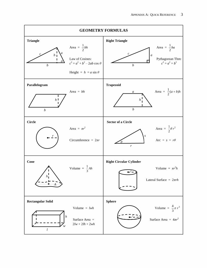
GEOMETRY FORMULAS
Triangle Right Triangle
Area = Area =
Law of Cosines: Pythagorean Thm:
c2 = a
2 + b
2 – 2ab cos θ c
2 = a
2 + b
2
Height = h = a sin θ
Parallelogram Trapezoid
Area = bh Area =
Circle Sector of a Circle
Area = πr2 Area =
Circumference = 2πr Arc = s = rθ
Cone Right Circular Cylinder
Volume = Volume = πr2h
Lateral Surface = 2πrh
Rectangular Solid Sphere
Volume = lwh Volume =
Surface Area = Surface Area = 4πr2
2lw + 2lh + 2wh
bh2
1ba
2
1
hba )(2
1
2 2
1r
Ah3
1
3 3
4r
a
b
h
r
a h
b
c
θ b
a c
h
b
θ r
s
h
A
r
r
l w
h
4 APPENDIX A: QUICK REFERENCE
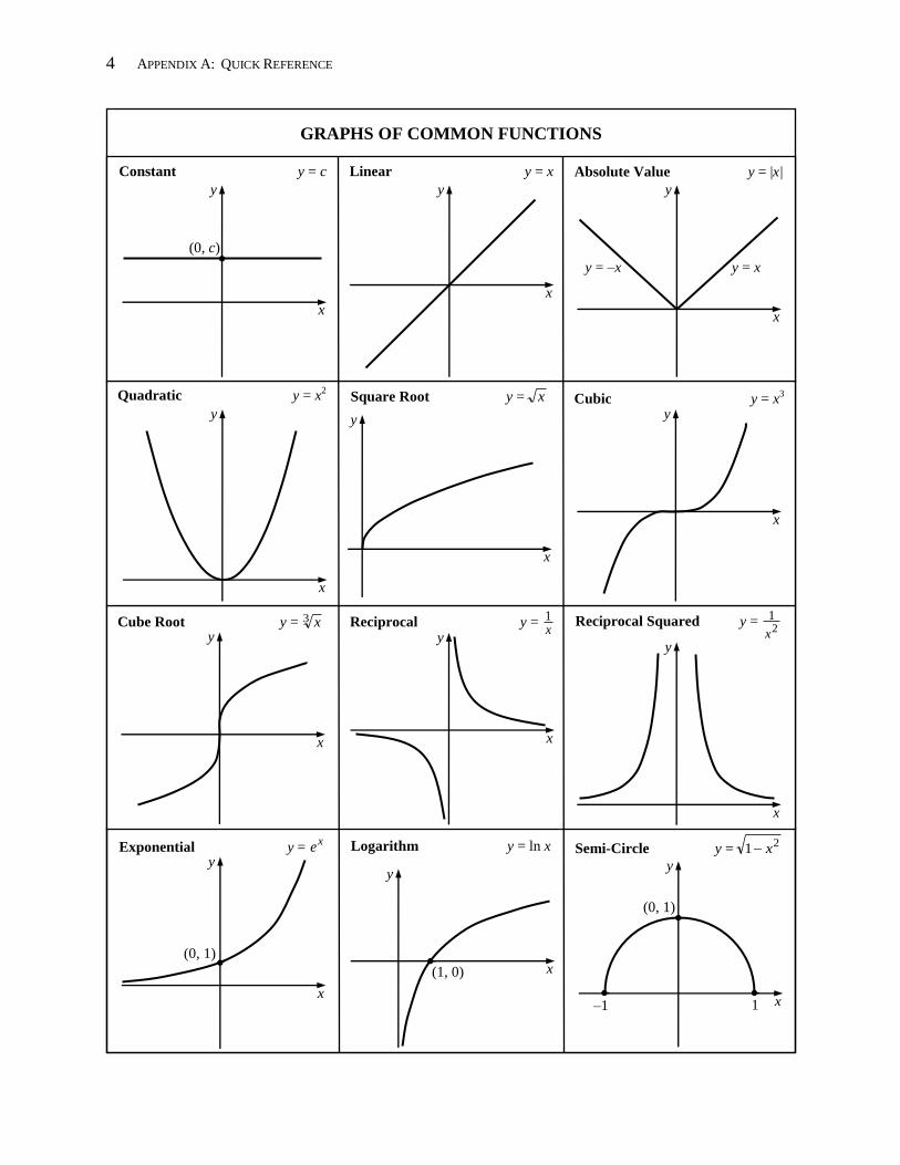
GRAPHS OF COMMON FUNCTIONS
Linear y = x
x
y
Absolute Value y = |x|
y = x y = –x
x
y
Quadratic y = x2
x
y
x
Square Root y = x
y
x
y Cubic y = x
3
x
y Cube Root y = 3 x Reciprocal y =
x1
x
y
x
y
Reciprocal Squared y = 2
1
x
Constant y = c
(0, c)
x
y
Exponential y =
xe
x
y
(0, 1)
Logarithm y = ln x
x
y
(1, 0)
x
y
Semi-Circle y =
21 x
(0, 1)
–1
1
APPENDIX A: QUICK REFERENCE 5
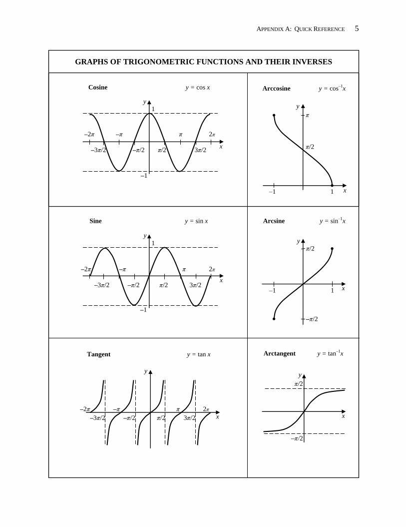
GRAPHS OF TRIGONOMETRIC FUNCTIONS AND THEIR INVERSES
–2π –π π 2π
–3π/2 –π/2 π/2 3π/2
Tangent y = tan x
y
x
Sine y = sin x
1
–2π –π π 2π
–3π/2 –π/2 π/2 3π/2
y
x
–1
1
–2π –π π 2π
–3π/2 –π/2 π/2 3π/2
Cosine y = cos x
y
x
–1
π
π/2
y
–1 1 x
Arccosine y = cos–1
x
y
Arcsine y = sin–1
x
–1 1
π/2
–π/2
x
Arctangent y = tan–1
x
π/2
–π/2
y
x
6 APPENDIX A: QUICK REFERENCE
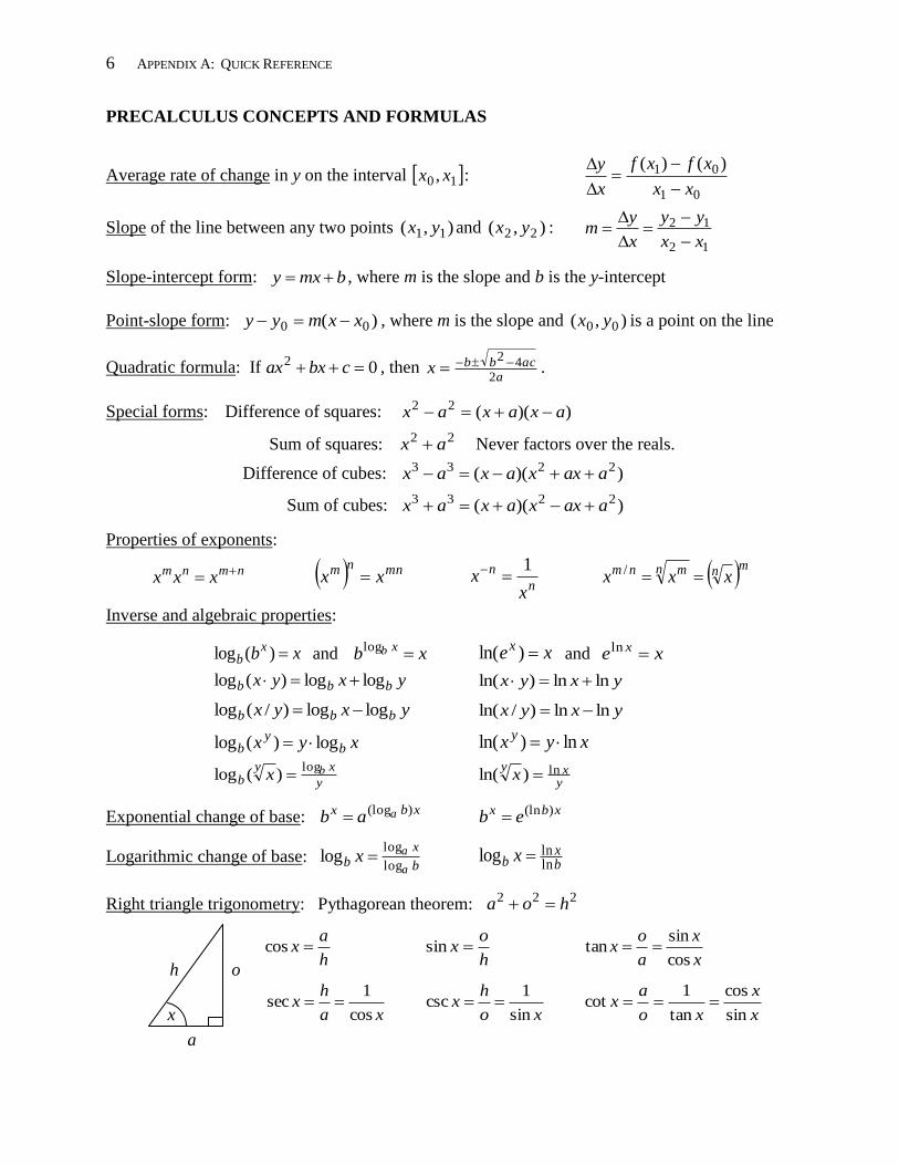
PRECALCULUS CONCEPTS AND FORMULAS
Average rate of change in y on the interval 10 , xx :
Slope of the line between any two points and :
Slope-intercept form: , where m is the slope and b is the y-intercept
Point-slope form: , where m is the slope and is a point on the line
Quadratic formula: If , then .
Special forms: Difference of squares:
Sum of squares: 22 ax Never factors over the reals.
Difference of cubes:
Sum of cubes:
Properties of exponents:
nmnm xxx mnnm xx n
n
xx
1
mnn mnm xxx /
Inverse and algebraic properties:
xbxb )(log and xb
xb log
xex )ln( and xe x ln
yxyx bbb loglog)(log yxyx lnln)ln(
yxyx bbb loglog)/(log yxyx lnln)/ln(
xyx by
b log)(log xyx y ln)ln(
y
xyb
bxlog
)(log yxy
x ln)ln(
Exponential change of base: xbx aab
)(log xbx eb )(ln
Logarithmic change of base: b
xb
a
axlog
loglog
bx
b xlnlnlog
Right triangle trigonometry: Pythagorean theorem:
h
ax cos
h
ox sin
x
x
a
ox
cos
sintan
xa
hx
cos
1sec
xo
hx
sin
1csc
x
x
xo
ax
sin
cos
tan
1cot
01
01 )()(
xx
xfxf
x
y
),( 11 yx ),( 22 yx12
12
xx
yy
x
ym
bmxy
)( 00 xxmyy ),( 00 yx
02 cbxaxa
acbbx2
42
))((22 axaxax
))(( 2233 aaxxaxax
))(( 2233 aaxxaxax
222 hoa
h o
a
x
APPENDIX A: QUICK REFERENCE 7
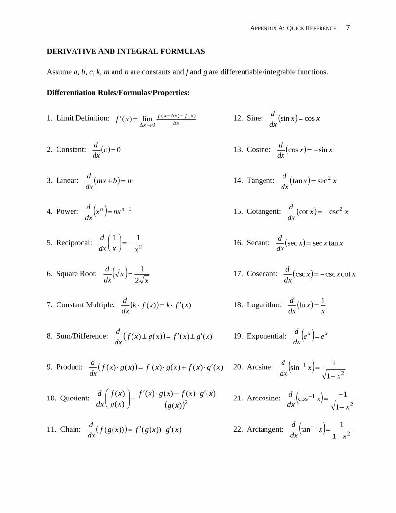
DERIVATIVE AND INTEGRAL FORMULAS
Assume a, b, c, k, m and n are constants and f and g are differentiable/integrable functions.
Differentiation Rules/Formulas/Properties:
1. Limit Definition: 12. Sine:
2. Constant: 13. Cosine:
3. Linear: 14. Tangent:
4. Power: 15. Cotangent:
5. Reciprocal: 16. Secant:
6. Square Root: 17. Cosecant:
7. Constant Multiple: 18. Logarithm:
8. Sum/Difference: 19. Exponential:
9. Product: 20. Arcsine:
10. Quotient: 21. Arccosine:
11. Chain: 22. Arctangent:
x
xfxxf
xxf
)()(
0lim)( xx
dx
dcossin
0cdx
d xx
dx
dsincos
mbmxdx
d xx
dx
d 2sectan
1 nn nxxdx
d xx
dx
d 2csccot
2
11
xxdx
d
xxxdx
dtansecsec
x
xdx
d
2
1 xxx
dx
dcotcsccsc
)()( xfkxfkdx
d
xx
dx
d 1ln
)()()()( xgxfxgxfdx
d xx ee
dx
d
)()()()()()( xgxfxgxfxgxfdx
d
2
1
1
1sin
xx
dx
d
2)(
)()()()(
)(
)(
xg
xgxfxgxf
xg
xf
dx
d
2
1
1
1cos
xx
dx
d
)())(())(( xgxgfxgfdx
d
2
1
1
1tan
xx
dx
d
8 APPENDIX A: QUICK REFERENCE
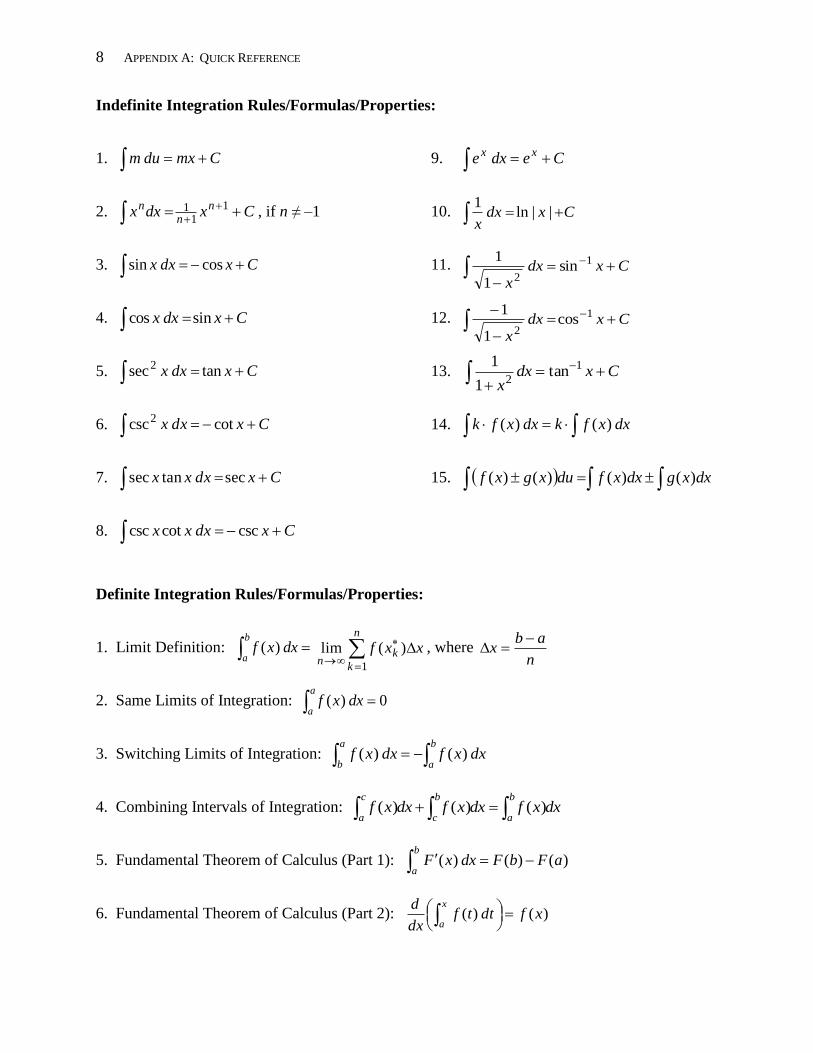
Indefinite Integration Rules/Formulas/Properties:
1. 9.
2. , if n ≠ –1 10.
3. 11.
4. 12.
5. 13. Cxdxx
1
2tan
1
1
6. 14.
7. 15.
8.
Definite Integration Rules/Formulas/Properties:
1. Limit Definition: , where
2. Same Limits of Integration:
3. Switching Limits of Integration:
4. Combining Intervals of Integration:
5. Fundamental Theorem of Calculus (Part 1):
6. Fundamental Theorem of Calculus (Part 2):
Cmxdum Cedxe xx
Cxdxx n
n
n
1
11 Cxdx
x ||ln
1
Cxdxx cos sin Cxdxx
1
2sin
1
1
Cxdxx sin cos Cxdxx
1
2cos
1
1
Cxdxx tan sec2
Cxdxx cot csc2 dxxfkdxxfk )( )(
Cxdxxx sec tansec dxxgdxxfduxgxf )()()()(
Cxdxxx csc cotcsc
b
adxxf )(
n
k
kn
xxf1
)(limn
abx
0 )( a
adxxf
)( )( b
a
a
bdxxfdxxf
dxxfdxxfdxxfb
a
b
c
c
a )()()(
)()( )( aFbFdxxFb
a
)( )( xfdttfdx
d x
a
APPENDIX B
INTRODUCTION TO THE TI-84
10 APPENDIX B: INTRODUCTION TO THE TI-84
APPENDIX B: INTRODUCTION TO THE TI-84 11
Section 1: Calculating
The calculator is programmed to follow the “order of operations”: Parentheses, Exponents,
Multiplication/Division, and Addition/Subtraction. Be sure to use parentheses whenever
necessary and know the difference between subtraction [ – ] and the negative sign [ (-) ].
Press the carat key [ ^ ] to raise values to exponents. Press [2ND] [ x2 ] to obtain a square root.
Other roots can be found in the [MATH] menu or you can convert them to exponents first.
The FRAC command (option 1) in the [MATH] menu will express answers as fractions.
Simply type in the expression to be evaluated followed by the FRAC command.
The following exercises demonstrate common errors. Be sure to focus on the differences
between each pair. Answers are given to three decimal places.
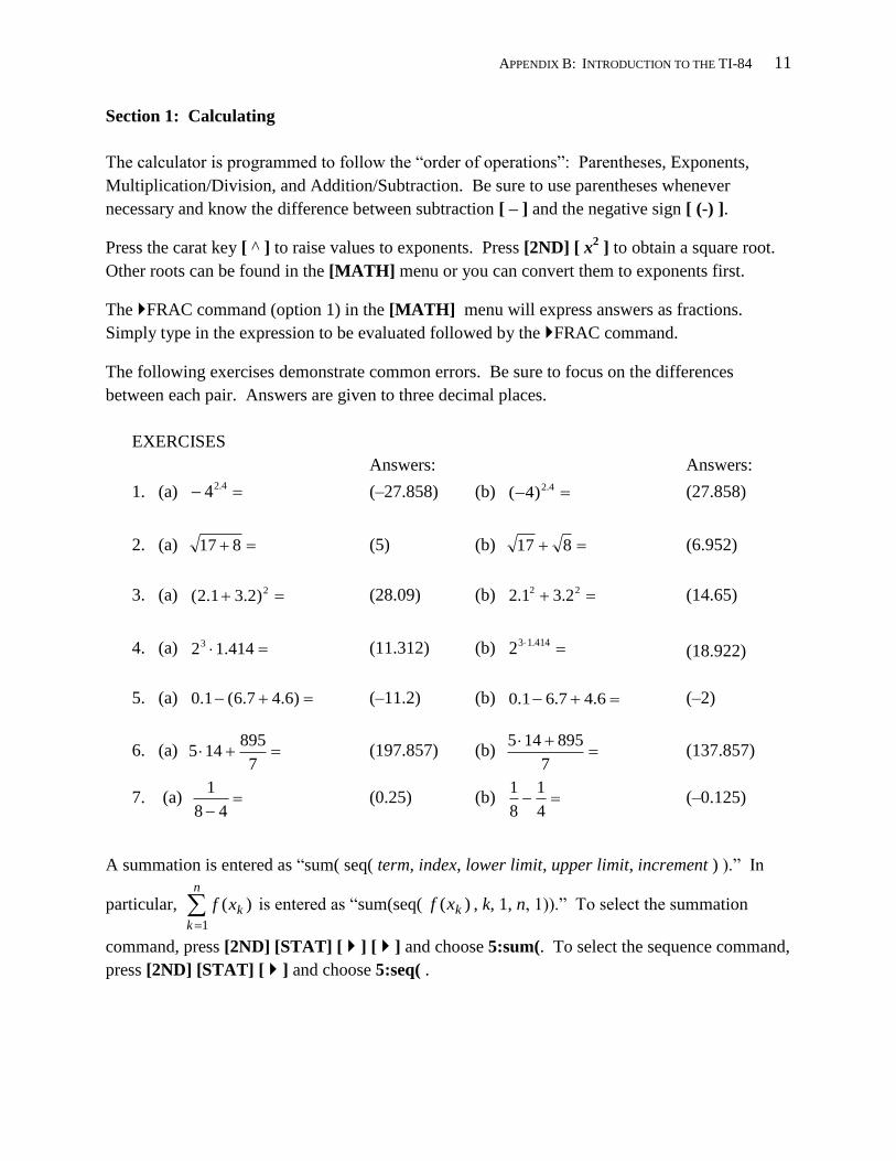
EXERCISES
Answers: Answers:
1. (a) (–27.858) (b) (27.858)
2. (a) (5) (b) (6.952)
3. (a) (28.09) (b) (14.65)
4. (a) (11.312) (b) (18.922)
5. (a) (–11.2) (b) (–2)
6. (a) (197.857) (b)
(137.857)
7. (a) (0.25) (b) (–0.125)
A summation is entered as “sum( seq( term, index, lower limit, upper limit, increment ) ).” In
particular, is entered as “sum(seq( , k, 1, n, 1)).” To select the summation
command, press [2ND] [STAT] [ ] [ ] and choose 5:sum(. To select the sequence command,
press [2ND] [STAT] [ ] and choose 5:seq( .
4.24 4.2)4(
817 817
2)2.31.2( 22 2.31.2
414.123 414.1 32
)6.47.6(1.0 6.47.61.0
7
895145
7
895145
48
1
4
1
8
1
n
k
kxf1
)( )( kxf
12 APPENDIX B: INTRODUCTION TO THE TI-84
Section 2: Graphing
Press the [ Y= ] key and enter the equation(s) you want to graph. Use the [X,T,θ,n] key to type
the variable x. Only the equations which have a black box over the = sign will be graphed.
Move the cursor over the equal sign and press [ENTER] to turn an equation on or off.
Press the [GRAPH] key to view the graph using the current viewing settings. If necessary,
change the viewing window in one of the following ways:
Press the [WINDOW] key to manually set the viewing window.
Press the [ZOOM] key and choose one of the following zoom options:
ZStandard Automatically sets the window from -10 to 10 along the x- and y-
axes.
ZBox Position the cursor at one corner of the region you wish to view
and press [ENTER] . Position the cursor at the opposite corner
and press [ENTER].
ZoomIn/Out Position the cursor at the point where you wish to center the new
window and press [ENTER].
Press [TRACE] to trace the graph(s). An equation will appear at the top of the screen and the x-
and y-coordinates of the cursor position will appear at the bottom. Switch from one graph to the
other by using the up and down arrow keys, and move along a graph by using the right and left
arrow keys. Tracing can be used to get a rough approximation of points, including points of
intersection.
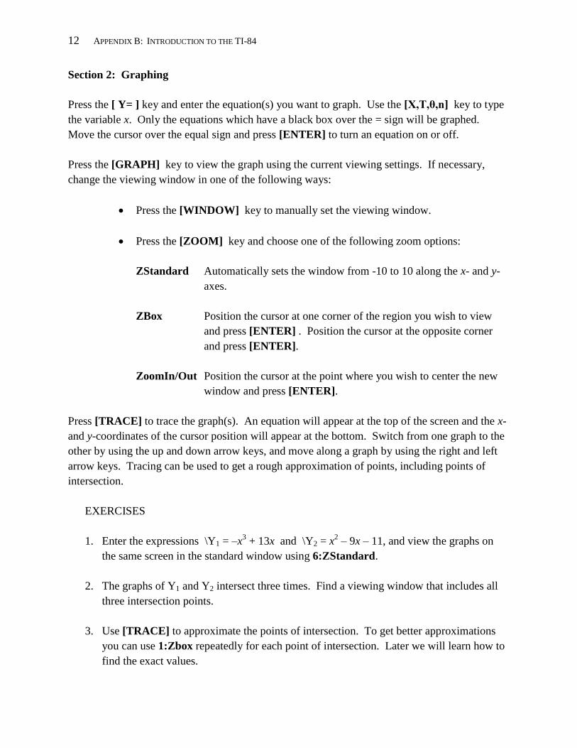
EXERCISES
1. Enter the expressions \Y1 = –x3 + 13x and \Y2 = x
2 – 9x – 11, and view the graphs on
the same screen in the standard window using 6:ZStandard.
2. The graphs of Y1 and Y2 intersect three times. Find a viewing window that includes all
three intersection points.
3. Use [TRACE] to approximate the points of intersection. To get better approximations
you can use 1:Zbox repeatedly for each point of intersection. Later we will learn how to
find the exact values.
APPENDIX B: INTRODUCTION TO THE TI-84 13
Section 3: Evaluating Functions [Find the output given an input.]
Given a function y = f (x) and a number a, we “evaluate f at x = a” by replacing all x’s in the
formula for f with the number a. For example, suppose we want to plug in x = –4.9766, x = 1.25,
and x = 11 into the function Y2 = x2 – 9x – 11. We could evaluate Y2 by using one of (at least)
three options: a trace, a table, or function notation.
Graph the function in a window that includes the given x-value(s). Press [TRACE].
Type –4.9766 and press [ENTER]. The approximate function value will show at the
bottom of the screen. Repeat for the other x-values.
Press [2ND] [WINDOW] to get the TABLE SETUP menu. Be sure Indpnt: is set to
Ask and Depend: is set to Auto. Go to the table by pressing [2ND
] [GRAPH]. Type
–4.9766 and then press [ENTER]. The function value appears in the Y2 column.
Repeat for the other x-values. Note that you could evaluate multiple functions at once.
From the home screen, press [VARS] [Y-VARS]. Choose 1:Function and then 2:Y2.
The expression “Y2” will appear on the home screen. To evaluate Y2 at x = –4.9766,
type Y2(–4.9766) and press [ENTER]. To evaluate Y2 at x = 1.25, press [2ND] then
[ENTER], move inside the parentheses to change the –4.9766 to 1.25, and press
[ENTER]. Repeat with x = 11.
Section 4: Solving Equations [Find the inputs that yield a given output.]
Given a function y = f (x) and a number b, we “solve f (x) = b for x” by finding all values that
yield b when they are plugged in for x. For example, suppose we want to solve the equation
x2 – 9x – 11 = –17. Note that the left side is Y2. Enter the right side as Y3. Graphically, solving
an equation is the same as finding the intersection points of the graphs of the separate sides of the
equation. First graph Y2 and Y3 on the same screen (you might want to temporarily turn off Y1)
making sure that the intersection points are visible. Press [2ND] [TRACE] and then choose
5:intersect. The upper left corner of the screen will show which equation the cursor is on. Place
the cursor on Y2 and press [ENTER], and then on Y3 and press [ENTER]. When prompted to
enter a “Guess,” move the cursor near the desired point of intersection and press [ENTER]. The
result will appear at the bottom of the screen.
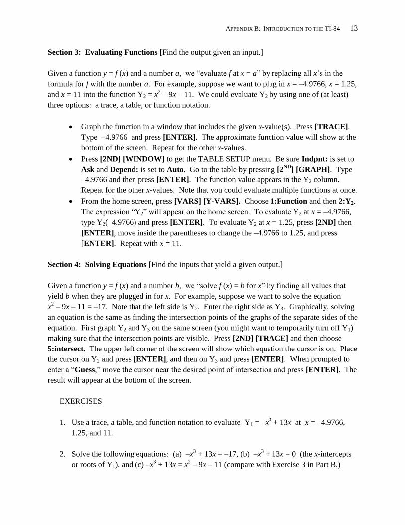
EXERCISES
1. Use a trace, a table, and function notation to evaluate Y1 = –x3 + 13x at x = –4.9766,
1.25, and 11.
2. Solve the following equations: (a) –x3 + 13x = –17, (b) –x
3 + 13x = 0 (the x-intercepts
or roots of Y1), and (c) –x3 + 13x = x
2 – 9x – 11 (compare with Exercise 3 in Part B.)
14 APPENDIX B: INTRODUCTION TO THE TI-84
Section 5: Working with Data
A set of discrete data points can be graphed as a “scatter plot” by typing the inputs and outputs
into lists. Press [STAT] and choose 1:Edit, which will bring you to the list menu. Clear old
data by moving the cursor to the heading of a column, press [CLEAR] [ENTER], and then
move the cursor back down to the top of the list. Type inputs into L1, one at a time, pressing
[ENTER] after each one. Repeat for the outputs into L2.
To view a scatter plot of the data, press [2ND] [ Y= ] to go to the STAT PLOTS menu. Choose
1:Plot1, turn the plot ON, and press [ENTER]. You might want to turn off or clear any other
irrelevant equations. Now press [ZOOM] and choose 9:ZoomStat.
EXERCISES
Input the following data into your calculator as two lists:
x 1995 1998 2001 2004 2007 2010
y 28 34 37 29 19 15
1. View a scatter plot of the data.
2. Sometimes inputs (such as years) are too large to use and we need to “align” inputs to
smaller values. Align the inputs so that x = 0 corresponds to 1995 by doing the
following:
Press [STAT] and choose 1:Edit, which will bring you to the list menu.
Move the cursor to the heading of the input column, say L1, and type L1 – 1995.
Press [ENTER].
View the “new” scatter plot. Why does it look the same?
Section 6: Writing a Regression Model
Study the scatter plot and decide on which function type would be the best fit. Possibilities
include linear, quadratic, cubic, natural logarithm, exponential, and sine. To write and store the
model, press [STAT] and then [ ] to the CALC menu. This will bring you to the list of
regression models. Depending on your calculator model, do one of the following:
Press [2ND] [ 1 ] [ , ] [2ND] [ 2 ] [ , ] [VARS] [ ] [ 1 ] [ 1 ] . You should
see QuadReg L1,L2,Y1 on the home screen; OR
Fill in Xlist (press [2ND] [ 1 ] [ , ]), Ylist (press [2ND] [ 2 ] [ , ]), and Store
RegEQ (press [VARS] [ ] [ 1 ] [ 1 ]).
Press [ENTER]. The model will be stored in the graph menu under Y1. Press [GRAPH] to
view the graph of the model over the scatter plot.
APPENDIX C
ACTIVITY HINTS AND ANSWERS

16 APPENDIX C: ACTIVITY HINTS AND ANSWERS
APPENDIX C : ACTIVITY HINTS AND ANSWERS 17
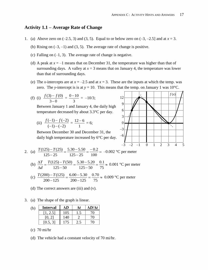
Activity 1.1 – Average Rate of Change
1. (a) Above zero on (–2.5, 3) and (3, 5). Equal to or below zero on (–3, –2.5] and at x = 3.
(b) Rising on (–3, –1) and (3, 5). The average rate of change is positive.
(c) Falling on (–1, 3). The average rate of change is negative.
(d) A peak at x = –1 means that on December 31, the temperature was higher than that of
surrounding days. A valley at x = 3 means that on January 4, the temperature was lower
than that of surrounding days.
(e) The x-intercepts are at x = –2.5 and at x = 3. These are the inputs at which the temp. was
zero. The y-intercept is is at y = 10. This means that the temp. on January 1 was 10°C.
(f) (i) 03
)0()3(
ff =
3
100 = –10/3;
Between January 1 and January 4, the daily high
temperature decreased by about 3.3°C per day.
(ii) )2()1(
)2()1(
ff =
1
612 = 6;
Between December 30 and December 31, the
daily high temperature increased by 6°C per day.
2. (a)
100
2.0
25125
50.530.5
25125
)25()125( TT –0.002 °C per meter
(b)
75
1.0
50125
20.530.5
50125
)50()125( TT
d
T 0.001 °C per meter
(c)
75
70.0
125200
30.500.6
125200
)125()200( TT 0.009 °C per meter
(d) The correct answers are (iii) and (v).
3. (a) The shape of the graph is linear.
(b)
(c) 70 mi/hr
(d) The vehicle had a constant velocity of 70 mi/hr.
Interval ΔD Δt ΔD/Δt
[1, 2.5] 105 1.5 70 [0, 2] 140 2 70
[0.5, 3] 175 2.5 70
–3 –2 –1 0 1 2 3 4 5
12
9
6
3
0
–3
–6
f (x)
18 APPENDIX C: ACTIVITY HINTS AND ANSWERS
Activity 1.2 – Linear Functions
1. (a) y – 5 = 2(x – 4) or f (x) – 5 = 2(x – 4)
(b) y = 2x – 3 or f (x) = 2x – 3
(c) x = 3/2
2. (a) Between 1915 and 1920, the population changed by 3100 – 3250 = –150 people, and
changed at a rate of 3019151920
32503100
people per year. The negative answers represent
a decrease in population.
(b) P(t) = –30t + 3250 people, where t is years after 1915.
(c) P(10) = –30(10) +3250 = 2950 people at the end of 1925.
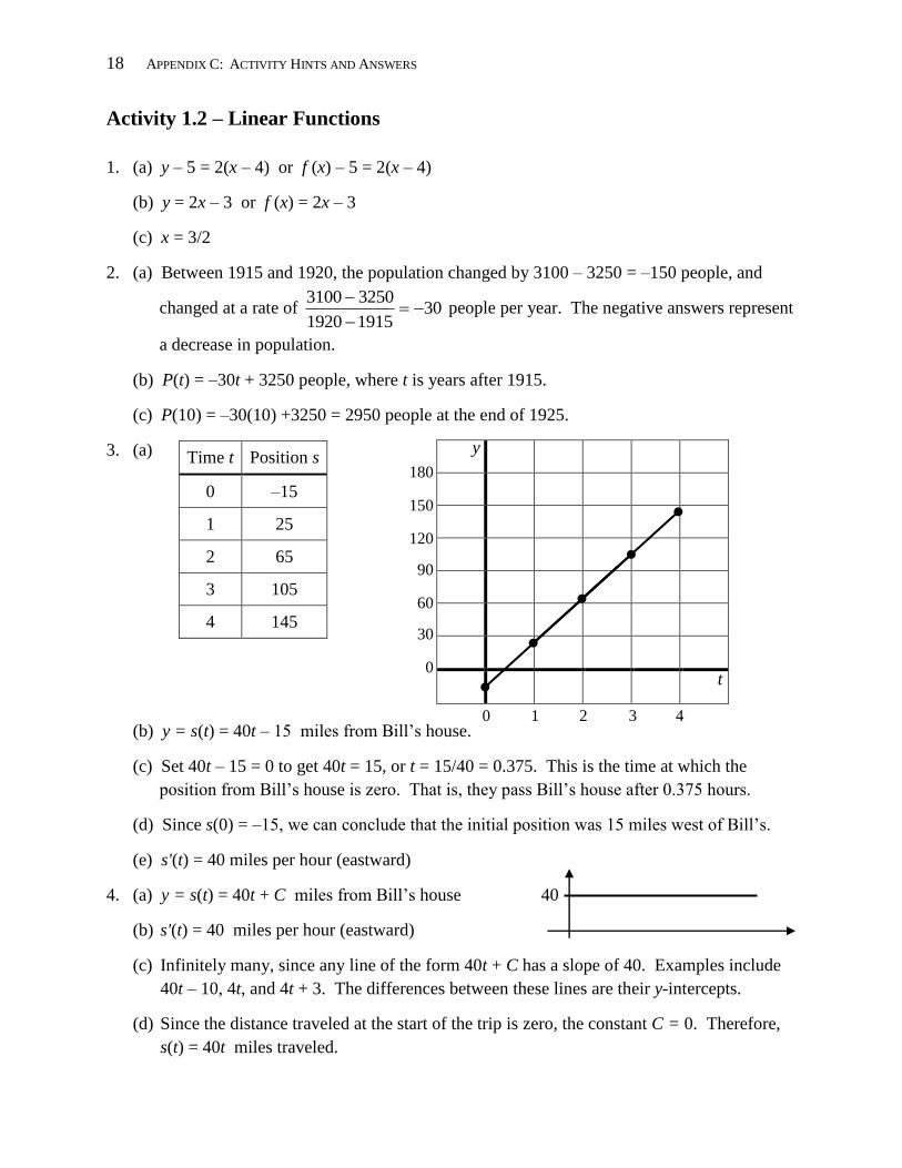
3. (a)
(b) y = s(t) = 40t – 15 miles from Bill’s house.
(c) Set 40t – 15 = 0 to get 40t = 15, or t = 15/40 = 0.375. This is the time at which the
position from Bill’s house is zero. That is, they pass Bill’s house after 0.375 hours.
(d) Since s(0) = –15, we can conclude that the initial position was 15 miles west of Bill’s.
(e) s'(t) = 40 miles per hour (eastward)
4. (a) y = s(t) = 40t + C miles from Bill’s house 40
(b) s'(t) = 40 miles per hour (eastward)
(c) Infinitely many, since any line of the form 40t + C has a slope of 40. Examples include
40t – 10, 4t, and 4t + 3. The differences between these lines are their y-intercepts.
(d) Since the distance traveled at the start of the trip is zero, the constant C = 0. Therefore,
s(t) = 40t miles traveled.
Time t Position s
0 –15
1 25
2 65
3 105
4 145
0 1 2 3 4
180
150
120
90
60
30
0
t
y
APPENDIX C : ACTIVITY HINTS AND ANSWERS 19
Activity 1.3 – Derivatives of Linear Functions
1. (a) 0)( xf
(b) 0)( xg
(c) 0)( xh
(d) mxF )(
(e) 9)( xG
(f) 1)( xH
2. (a) 2)()( tstv ft/s
(b) 2)10( v ft/s
(c) 0)()( tvta ft/s2
3. (a) The given point is (1, 22) and the slope is –0.4. Therefore, )1(4.022 tH , so
4.224.0)( ttH ft3.
(b) 4.22)5(4.0)5( H = 20.4 ft3
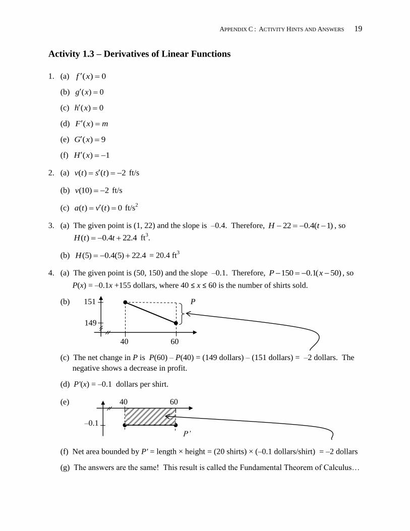
4. (a) The given point is (50, 150) and the slope –0.1. Therefore, )50(1.0150 xP , so
P(x) = –0.1x +155 dollars, where 40 ≤ x ≤ 60 is the number of shirts sold.
(b) 151 P
149
40 60
(c) The net change in P is P(60) – P(40) = (149 dollars) – (151 dollars) = –2 dollars. The
negative shows a decrease in profit.
(d) P'(x) = –0.1 dollars per shirt.
(e) 40 60
–0.1
P’
(f) Net area bounded by P' = length × height = (20 shirts) × (–0.1 dollars/shirt) = –2 dollars
(g) The answers are the same! This result is called the Fundamental Theorem of Calculus…
20 APPENDIX C: ACTIVITY HINTS AND ANSWERS
Activity 1.4 – Integrals of Constant Functions
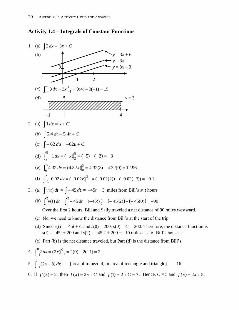
1. (a) dx 3 3x + C
(b) y = 3x + 6
y = 3x
3 y = 3x – 3
1 2
(c) 15)1(3)4(33 3 4
1
4
1
xdx
(d) y = 3
–1 4
2. (a) Cxdx 1
(b) Ctdt 4.5 4.5
(c) Cudu 62 62
(d) 3)2()5()( 1 5
2
5
2 xdx
(e) 96.12)0(32.4)3(32.4)32.4( 32.43
0
3
0 xdx
(f) 1.0))3(02.0())2(02.0()02.0( 02.02
3
2
3
vdv
3. (a) dttv )( = dt 45 = –45t + C miles from Bill’s at t hours
(b) 90)0(45)2(45)45( 45 )(2
0
2
0
2
0 tdtdttv
Over the first 2 hours, Bill and Sally traveled a net distance of 90 miles westward.
(c) No, we need to know the distance from Bill’s at the start of the trip.
(d) Since s(t) = –45t + C and s(0) = 200, s(0) = C = 200. Therefore, the distance function is
s(t) = –45t + 200 and s(2) = –45∙2 + 200 = 110 miles east of Bill’s house.
(e) Part (b) is the net distance traveled, but Part (d) is the distance from Bill’s.
4. 2)1(2)0(2)2( 20
1
0
1
xdx
5. dxx )82(1
1 = – [area of trapezoid, or area of rectangle and triangle] = –16
6. If 2)( xf , then Cxxf 2)( and 72)1( Cf . Hence, C = 5 and 52)( xxf .
APPENDIX C : ACTIVITY HINTS AND ANSWERS 21
Activity 1.5 – Rectilinear Motion
1. Position s(t) = 35 – t feet Position s(5) =30 ft
Velocity v(t) = –1 ft/s Velocity v(5) = –1 ft/s
Speed |v(t)| = 1 ft/s Speed |v(5)| = 1 ft/s
Acceleration a(t) = 0 ft/s2 Acceleration a(5) = 0 ft/s
2
2. (a) s(t) = –20t + 100 m
(b) Setting –20t + 100 = 0 yields t = 5 s.
(c) 60))5.9(20())5.12(20()20(205.12
5.9
5.12
5.9 tdt m
(d) 60)5.9(20)5.12(20)20(205.12
5.9
5.12
5.9 tdt m
3. (a)
(b) Setting 10 – 4t = 0 yields t = 10/4 = 2.5 s.
(c) 8)6)(5.1()10)(5.2()410(21
21
4
0 dtt m
(d) 17)6)(5.1()10)(5.2(|410|21
21
4
0 dtt m
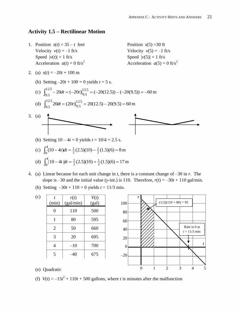
4. (a) Linear because for each unit change in t, there is a constant change of –30 in r. The
slope is –30 and the initial value (y-int.) is 110. Therefore, r(t) = –30t + 110 gal/min.
(b) Setting –30t + 110 = 0 yields t = 11/3 min.
(c)
(e) Quadratic
(f) V(t) = –15t2 + 110t + 500 gallons, where t is minutes after the malfunction
t
(min)
r(t)
(gal/min)
V(t)
(gal)
0 110 500
1 80 595
2 50 660
3 20 695
4 –10 700
5 –40 675
0 1 2 3 4 5
Rate is 0 at
t = 11/3 min
t
r
100
80
60
40
20
0
–20
(1/2)(110 + 80) = 95
22 APPENDIX C: ACTIVITY HINTS AND ANSWERS
Activity 2.1 – Derivatives of Quadratic Functions
1. (a) 19.4 ft/s
(b) 20.84 ft/s
(c) 20.984 ft/s
(d) 21 ft/s
(e) v(t) = 85 – 32t; v(2) = 21 ft/s.
(f) a(t) = –32 ft/s2
2. (a) 104)( xxf ; 4)( xf
(b) wwy 1)( ; 1)( wy
(c) 2432)( rrh ; 32)( rh
3. 348)( ttP bacteria per hour; 50)2( P bacteria per hour
4. (a) f (4) = 5
(b) f’(4) = –2
(c) y – 5 = –2(x – 4)
APPENDIX C : ACTIVITY HINTS AND ANSWERS 23
Activity 2.2 – Analyzing Quadratic Functions
1. (a) x = –4, 4
(b) x = –1, 0, 1
(c) x = 0 (Factor as 022
212 xx , and note that 22
21 x is never zero.)
(d) x = 4/5, 1
(e) x = –3, –1, 1, 3
2. (a) 5°F
(b) 1:00 a.m. and 2:30 a.m.
(c) 74)( ttT ; rising by 5°F per hour
(d) The low temperature occurred at 1:45 a.m. and was approximately –6°F.
(e) Falling on (0, 7/4); rising on (7/4, 4) – + T’
0 7/4 4
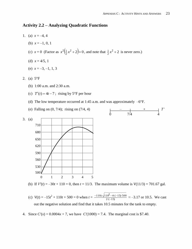
3. (a)
(b) If Vʹ(t) = –30t + 110 = 0, then t = 11/3. The maximum volume is V(11/3) = 701.67 gal.
(c) V(t) = –15t2 + 110t + 500 = 0 when t =
)15(2
500)15(42110110
≈ –3.17 or 10.5. We cast
out the negative solution and find that it takes 10.5 minutes for the tank to empty.
4. Since C'(x) = 0.0004x + 7, we have C'(1000) = 7.4. The marginal cost is $7.40.
0 1 2 3 4 5
710
680
650
620
590
560
530
500
24 APPENDIX C: ACTIVITY HINTS AND ANSWERS
)(
)()(lim
)()(lim)(
0
0
xfk
x
xfxxfk
x
xfkxxfkxfk
x
x
)()(
)()(lim
)()(lim
)()()()(lim
)()()()(lim
)()()()(lim)()(
00
0
0
0
xgxf
x
xgxxg
x
xfxxf
x
xgxxg
x
xfxxf
x
xgxxgxfxxf
x
xgxfxxgxxfxgxf
xx
x
x
x
Activity 2.3 – Definition and Properties of the Derivative
9
9lim
9lim
29299lim
29299lim
292)(9lim)( (a) .1
0
0
0
0
0
x
x
x
x
x
x
x
x
xxx
x
xxx
x
xxxxf
(b) xxf 4)(
(c) 26)( xxf
2
22
0
322
0
33223
0
33
0
3
)33(lim
33lim
33lim
)(lim .2
x
xxxx
x
xxxxx
x
xxxxxxx
x
xxxy
x
x
x
x
3. (a) cbxaxdcxbxaxdcxbxaxxf
23)( 22323
(b) (i) xxxf 26)( 2 ; 212)( xxf
(ii) 6.06.46.3)( 2 xxxg ; 6.42.7)( xxg
4.
APPENDIX C : ACTIVITY HINTS AND ANSWERS 25
Activity 2.4 – Analyzing Cubic Functions
1. (a) The graph is…………………….. Increasing Decreasing
The derivative (slope) is………… Positive Negative
The derivative (slope) is………… Increasing Decreasing
(b) The graph is…………………….. Increasing Decreasing
The derivative is………….…….. Positive Negative
The derivative is………………… Increasing Decreasing
2. (a) The graph is…………………….. Increasing Decreasing
The derivative is………………… Positive Negative
The derivative is………………… Increasing Decreasing
(b) The graph is…………………….. Increasing Decreasing
The derivative is………….…….. Positive Negative
The derivative is………………… Increasing Decreasing
3. 543 2 xxy ; 046 xy yields x = 2/3. A sign test shows that y is concave
up on (2/3, ∞) and concave down on (–∞, 2/3). The inflection point is at x = 2/3 and the
coordinates are (2/3, 56/27).
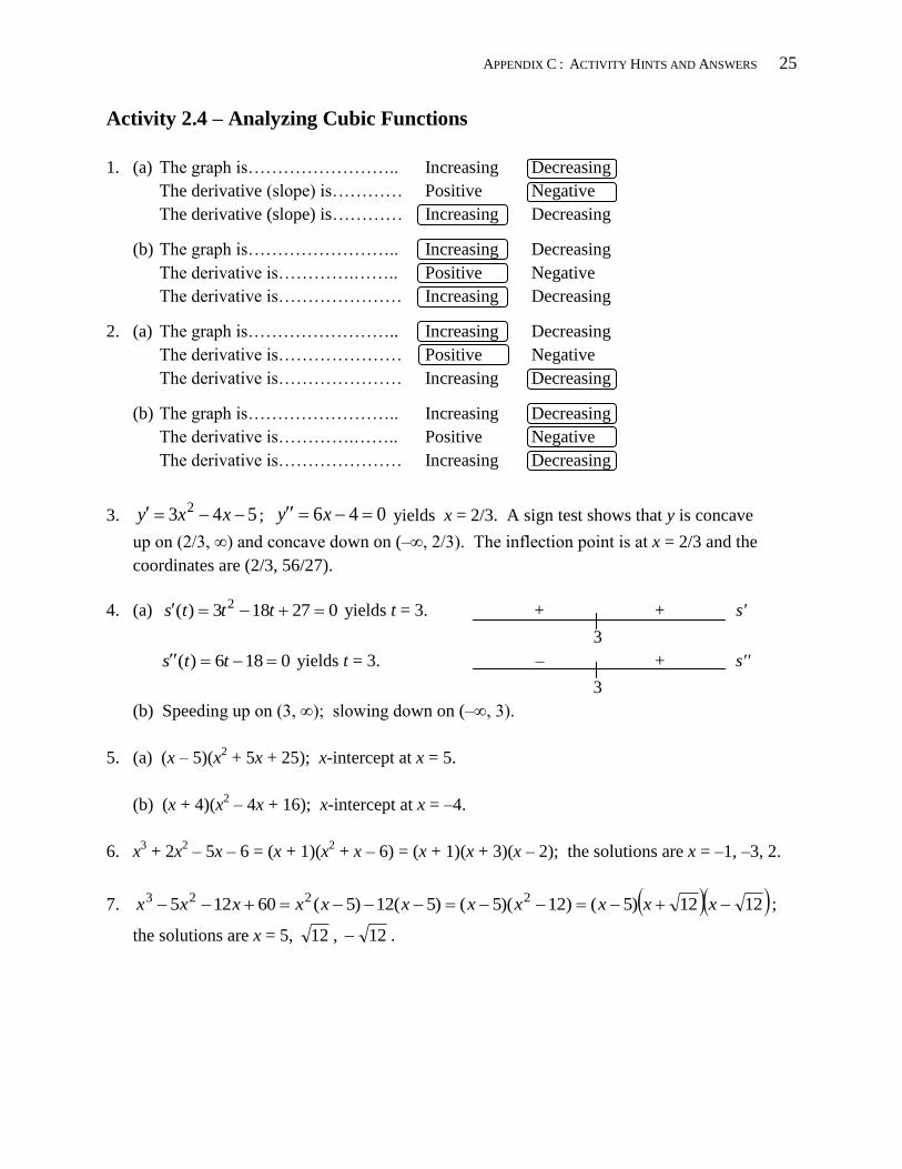
4. (a) 027183)( 2 ttts yields t = 3. + + s'
3
0186)( tts yields t = 3. – + s''
3
(b) Speeding up on (3, ∞); slowing down on (–∞, 3).
5. (a) (x – 5)(x2 + 5x + 25); x-intercept at x = 5.
(b) (x + 4)(x2 – 4x + 16); x-intercept at x = –4.
6. x3 + 2x
2 – 5x – 6 = (x + 1)(x
2 + x – 6) = (x + 1)(x + 3)(x – 2); the solutions are x = –1, –3, 2.
7. 1212)5()12)(5()5(12)5(60125 2223 xxxxxxxxxxx ;
the solutions are x = 5, 12 , 12 .
26 APPENDIX C: ACTIVITY HINTS AND ANSWERS
Activity 2.5 – Linear Approximation
1. (a) xxdx
dy26 2
2122
2
xdx
yd
(b) 8)1(2)1(626 2
1
2
1
xxdx
dyxx
142)1(122121
12
2
x
xdx
ydx
2. (a) Δy = y(2.03) – y(2) = 2(2.03)3 – 2(2)
3 = 0.731
(b) dy = 6x2dx = 6(2)
2(.03) = 0.720
3. (a) f (2) = 4; f '(2) = 12
(b) y – 4 = 12(x – 2); y = 12x – 20
(c) f(2.01) ≈ 12(2.01) – 20 = 4.12
(d) f(2.01) = 2(2.01)3 – 3(2.01)
2 = 4.120902
4. (a) dA = 10xdx = 10(36)(±0.125) = ±45 in2
(b) %69.00069.0)36(5
)125.0)(36(10
5
1022
x
xdx
A
dA
5. dV = 4πr2dr = 4π(19)
2(±0.5) ≈ ±2268.23 cm
3
%89.70789.0)19()3/4(
(±0.5)(19)4
)3/4(
43
2
3
2
r
drr
V
dV
6. dA = 2πrdr = 2π(24)(±0.1) ≈±15.08 cm2
%83.00083.0)24(
(24)(±0.1)2222
r
rdr
A
dA
7. dV = 74πrdr = 74π(12)(±0.15) ≈ ±418.46 m3
%5.2025.0)12(37
)(12)(±0.1547
37
7422
r
rdr
V
dV
APPENDIX C : ACTIVITY HINTS AND ANSWERS 27
Activity 2.6 – Integrals of Linear and Quadratic Functions
1. (a) Cx 25
(b) Ctt 42
23
(c) Cuu 2
21
2. (a) 15)1(5)2(55 222
1
2 x
(b) 2112
232
23
1
0
2
23 )0(4)0()1(4)1(4 tt
(c) 252
212
21
3
2
2
21 )2()2()3()3(
uu
3. (a) Cxxxdxxx 772 2
213
322
(b) Cwwwdwww 3
3122 332632
4. 186)5(4)5(10)8(4)8(10410)810( 228
5
28
5 ttdtt cows
5. (a) 1632)( ttv ft/s
(b) 1751616)( 2 ttts ft
(c) Set 01751616 2 tt and solve for t (using the quadratic formula) to get t = 3.84 s.
(d) v(3.84) ≈ –107 ft/s
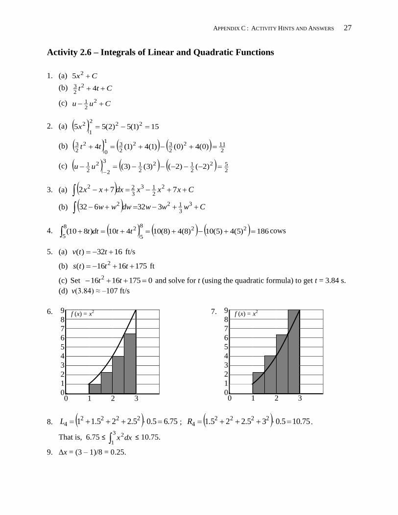
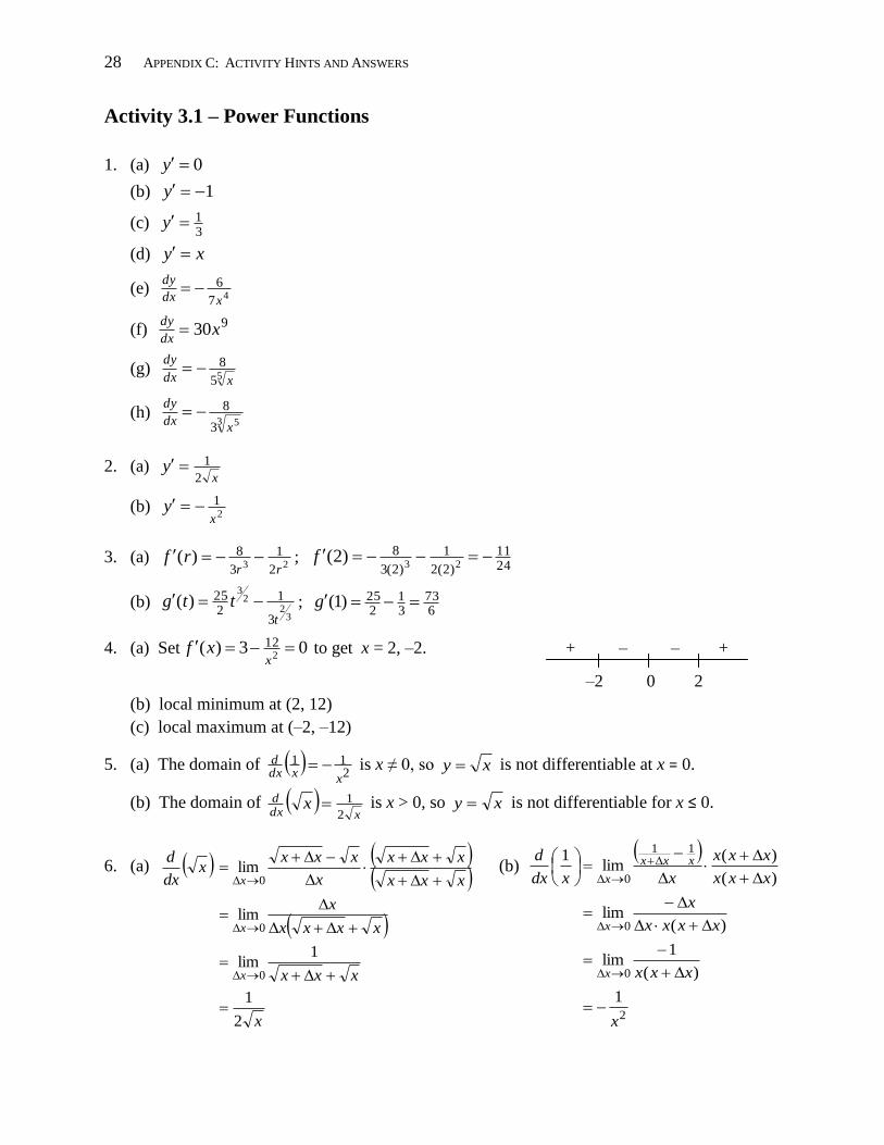
6. 7.
8. 2222
4 75.65.05.225.11 L ; 75.105.035.225.1 22224 R .
That is, 6.75 ≤ dxx3
1
2 ≤ 10.75.
9. Δx = (3 – 1)/8 = 0.25.
9
8
7
6
5
4
3
2
1
0
f (x) = x2
0 1 2 3
9
8
7
6
5
4
3
2
1
0
f (x) = x2
0 1 2 3
28 APPENDIX C: ACTIVITY HINTS AND ANSWERS
x
xxx
xxxx
x
xxx
xxx
x
xxxx
dx
d
x
x
x
2
1
1lim
lim
lim
0
0
0
2
0
0
11
0
1
)(
1lim
)(lim
)(
)(lim
1
x
xxx
xxxx
x
xxx
xxx
xxdx
d
x
x
xxx
x
Activity 3.1 – Power Functions
1. (a) 0y
(b) 1y
(c) 31y
(d) xy
(e) 47
6
xdx
dy
(f) 930x
dx
dy
(g) 55
8
xdx
dy
(h) 3 53
8
xdx
dy
2. (a) x
y2
1
(b) 2
1
xy
3. (a) 23 2
1
3
8)(rr
rf ; 2411
)2(2
1
)2(3
823
)2( f
(b) 3
22
3
3
1225)(
t
ttg ; 673
31
225)1( g
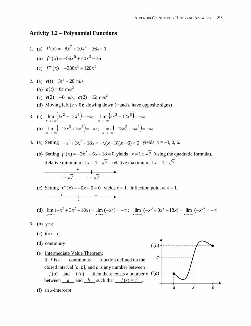
4. (a) Set 03)(2
12 x
xf to get x = 2, –2. + – – +
–2 0 2
(b) local minimum at (2, 12)
(c) local maximum at (–2, –12)
5. (a) The domain of 211
xxdxd
is x ≠ 0, so xy is not differentiable at x = 0.
(b) The domain of xdx
d x2
1
is x > 0, so xy is not differentiable for x ≤ 0.
6. (a) (b)
APPENDIX C : ACTIVITY HINTS AND ANSWERS 29
0)6)(3(183 23 xxxxxx
Activity 3.2 – Polynomial Functions
1. (a) 136108)( 47 xxxxf
(b) 364056)( 36 xxxf
(c) 25 120336)( xxxf
2. (a) 203)( 2 ttv m/s
(b) tta 6)( m/s2
(c) 8)2( v m/s; 12)2( a m/s2
(d) Moving left (v < 0); slowing down (v and a have opposite signs)
3. (a)
62 123lim xxx
;
62 123lim xxx
(b)
25 513lim xxx
;
25 513lim xxx
4. (a) Setting yields x = –3, 0, 6.
(b) Setting 01863)( 2 xxxf yields 71x (using the quadratic formula).
Relative minimum at x = 71 ; relative maximum at x = 71 .
– + –
71 71
(c) Setting 066)( xxf yields x = 1. Inflection point at x = 1.
+ –
1
(d)
)(lim)183(lim 323 xxxxxx
;
)(lim)183(lim 323 xxxxxx
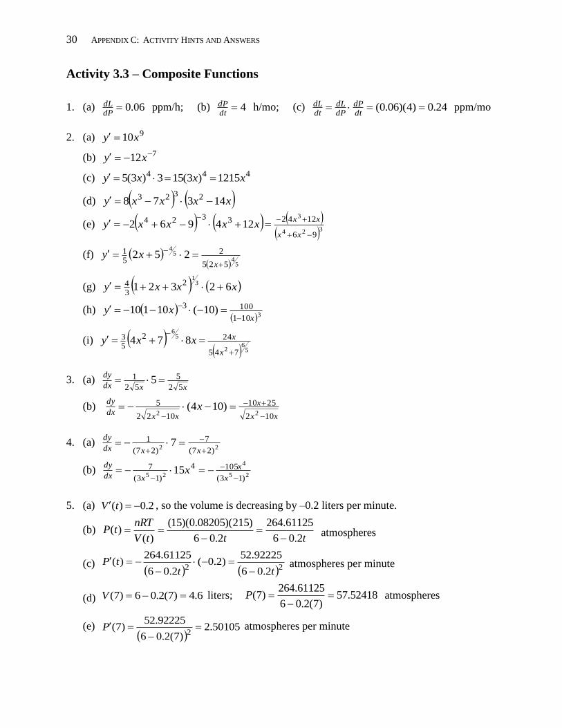
5. (b) yes;
(c) f(x) = c;
(d) continuity
(e) Intermediate Value Theorem:
If f is a continuous function defined on the
closed interval [a, b], and c is any number between
f (a) and f (b) , then there exists a number x
between a and b such that f (x) = c .
(f) an x-intercept a x b
f (b)
c
f (a)
30 APPENDIX C: ACTIVITY HINTS AND ANSWERS
Activity 3.3 – Composite Functions
1. (a) 06.0dPdL ppm/h; (b) 4
dtdP h/mo; (c) 24.0)4)(06.0(
dtdP
dPdL
dtdL ppm/mo
2. (a) 910xy
(b) 712 xy
(c) 444 1215)3(153)3(5 xxxy
(d) xxxxy 14378 2323
(e) 324
3
96
12423324 124962
xx
xxxxxxy
(f) 5
45
4
525
251 252
xxy
(g) xxxy 623213
12
34
(h) 3101
1003)10(10110
xxy
(i) 5
62
56
745
242
53 874
x
xxxy
3. (a) xxdx
dy
52
5
52
1 5
(b) xx
x
xxdx
dyx
102
2510
1022
5
22)104(
4. (a) 22 )27(
7
)27(
1 7
xxdx
dy
(b) 25
4
25 )13(
1054
)13(
7 15
x
x
xdx
dyx
5. (a) 2.0)( tV , so the volume is decreasing by –0.2 liters per minute.
(b) tttV
nRTtP
2.06
61125.264
2.06
)215)(08205.0)(15(
)()(
atmospheres
(c) 22
2.06
92225.52)2.0(
2.06
61125.264)(
tttP
atmospheres per minute
(d) 6.4)7(2.06)7( V liters; 52418.57)7(2.06
61125.264)7(
P atmospheres
(e)
50105.2)7(2.06
92225.52)7(
2
P atmospheres per minute
APPENDIX C : ACTIVITY HINTS AND ANSWERS 31
Activity 3.4 – Products of Functions
1. (a) 2276226)( 2 xxxxxf
(b) 21032252)32(5)(524 xxxxxxg
(c)
8
282
1283)( 32
ttttts
2. (a) 32131092 xxxy
2131032)32(13909282
xxxxxxy
(b) xxy 4273
22
31
42744273
23
52
312
92
xxxxy
3.
Horizontal tangents at x = 9 and at x = 45/19. Vertical tangent at x = 0.
4. (a) )()()()()( tPtStPtStR dollars per day
(b) 405)2)(1290()199)(15()60()60()60()60()60( PSPSR dollars per day;
That is, the revenue was decreasing by $405 per day.
5. (a) )()()()())(( gfgfgfgfggff
(b) )()()()())(()( gfgfgfgfggffgf
(c) gx
f
x
gfg
x
f
x
gfgfgf
x
gf
)()()()(
(d) Since dx
df
exists (is finite), and Δg → 0 as Δx → 0, we have 00lim
0
dx
dfg
x
f
x.
(e) dx
dgfg
dx
dfg
x
f
x
gfg
x
f
x
gfgf
dx
d
xx
00lim
)(lim
72
745
719
757
2
75
272
75
)9(
2)9()9(
)9(29)(
x
xx
xxxx
xxxxxf
32 APPENDIX C: ACTIVITY HINTS AND ANSWERS
–3 –2 –1 0 1 2 3
6
–4
Activity 3.5 – Piecewise Functions
1. (a)
1 if,
1 if,62)(
xa
xxxg
(b) Set 2(–1) – 6 = a to get a = –8; set (–1)2 – 6(–1)+5 = (–8)(–1) + b to get b = 4.
2. a = 1/2; b = 8
3. (a) 6)3( f (b) 2)1( f (c) 1)0( f
(d) 2)1( f (e) 2)5( f
4. (a) 2)(lim1
xfx
(b) 0)(lim1
xfx
(c)
)(lim1
xfx
DNE
(d) 2)(lim1
xfx
(e) 2)(lim1
xfx
(f) 2)(lim1
xfx
(g) No (h) Yes
5.
1 if,1
11 if,1
1 if,2
)(
x
x
xx
xf
6. (a) 2)(lim1
xfx
(b) 1)(lim1
xfx
(c)
)(lim1
xfx
DNE
(d) 1)(lim1
xfx
(e) 1)(lim1
xfx
(f)
)(lim1
xfx
DNE
(g) No (h) No
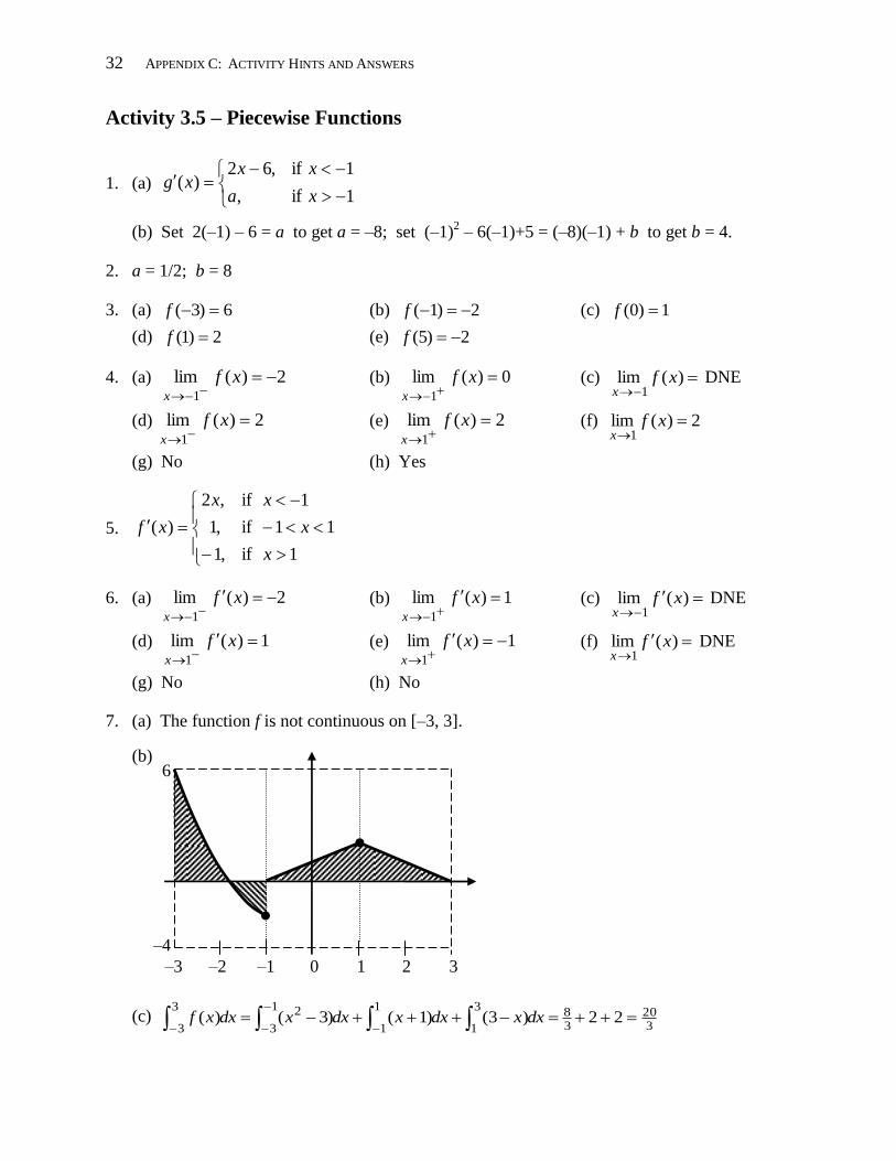
7. (a) The function f is not continuous on [–3, 3].
(b)
(c) 3
2038
3
1
1
1
1
3
23
322)3()1()3()(
dxxdxxdxxdxxf
APPENDIX C : ACTIVITY HINTS AND ANSWERS 33
Activity 3.6 – Integrals of Polynomials
1. (a) Ctttt 42
213
354
21
(b) Cxx 7
59 3
5
(c) Cx 23
32
(d) Cxx 21
34
1043
(e) 144634129231
1
231
1
21
1
2
uuudxuudxu
(f) 29
4
1
84
1
164
1 2
322233
3
1
xxx
x xdxdx
2. (a) CdxxxxFxx 42 2
3
2
753 67)( ; set 3)1(23
27 CF to get C = 5;
5)(42 2
3
2
7 xx
xF
(b) Set 3241
323
87)2( CF to get C =
21 ;
21
2
3
2
742
)( xx
xF
3. Let xxf )( and let xxg )( .
The integral of the product is 3
312 )()( xdxxdxxgxf , but
the product of the integrals is 4
412
212
21 )( )( xxxxdxxdxdxxgdxxf .
4. (a) (i) Since )()( xfkxFkdx
d , it follows that )()( xFkdxxfk .
(ii) Since )()( xfxFdx
d , it follows that )()( xFdxxf .
(iii) From (ii), then (i), dxxfkxFkdxxfk )()()( .
(b) (i) Since )()()()( xgxfxGxFdx
d , we have )()())()(( xGxFdxxgxf .
(ii) Since )()( xfxFdx
d , we have )()( xFdxxf .
(iii) Since )()( xgxGdx
d , we have )()( xGdxxg .
(iv) From (ii) and (iii), then (i), dxxgxfxGxFdxxgdxxf ))()(()()()()( .
34 APPENDIX C: ACTIVITY HINTS AND ANSWERS
Activity 4.1 – Analyzing Rational Functions
1. (a) N(1) = (1)3 – 5(1)
2 + 7(1) – 3 = 0
(b) g(x) = x2 – 4x + 3
(c) N(x) = (x – 1)2(x – 3)
(d) )1)(1(
)3()1()(
2
xx
xxxf
(e) x = 1, –1
(f) x = 3
(g) y = 3
(h) x = –1
(i) x = 1
(j) 1
88)5()(
2
x
xxxf
3. (a) 22 )32(
3
)32(
)2)(()32)(1(
xx
xxy
(b) 2
2
2
2
)4(
128
)4(
)1)(3()4)(32(
x
xx
x
xxxxy
(c) 22
2
22
22
)693(
18249
)693(
)96)(2()693)(2(
xx
xx
xx
xxxxxy
(d)
22
2
22
2
22
1
)9(22
983
)9(
)2(2)9()1(
xx
xx
x
xxx
yx
4. Set 0)4(
)6)(2(
)4(
12822
2
x
xx
x
xxy to get x = –2, –6.
5. (a) C(3) = 0.032 mg/cm3
(b) 22
2
22
2
)6(
96.016.0
)6(
)2)(16.0()6)(16.0()(
t
t
t
ttttC mg/cm
3 per hour
(c) 002.0)3( C mg/cm3 per hour
APPENDIX C : ACTIVITY HINTS AND ANSWERS 35
Activity 4.2 – Horizontal and Vertical Asymptotes
1. Since 29
29
2
9
172
269 limlimlim4
4
4
34
xx
x
xxx
xxx
x, the line y =
29 is a horizontal asymptote.
Similarly for x .
2. (a) 41
41
446
5 limlimlim2
2
2
2
xx
x
xx
xx
x
(b) 0limlimlim31
313
106
5
46
25
xxx
x
xxx
xx
x
(c)
1812 limlimlim
22 x
xxx
xxxx
x
(d) 31
31
3343
1 limlimlimlim22
xxx
xx
x
xx
x
x
3. (a) Since f has a vertical asymptote at x = 2, the limit on either side will be +∞, or –∞.
We only need to check the signs:
If 2x , then 2x and 0)2( x . Therefore,
))((
))((
)3)(2(
)2()1(
22
2
limxx
xx
x
.
If 2x , then 2x and 0)2( x . Therefore,
))((
))((
)3)(2(
)2()1(
22
2
limxx
xx
x
.
Hence, )(lim2
xfx
DNE.
(b) If 3x , then 0)3( x . Therefore,
))((
))((
)3)(2(
)2()1(
32
2
limxx
xx
x
.
If 3x , then 0)3( x . Therefore,
))((
))((
)3)(2(
)2()1(
32
2
limxx
xx
x
.
Hence,
)(lim3
xfx
.
4. (a)
2222
22
100
3000
100
21510030)(
x
x
x
xxxxxf ; f is zero at x = 0 and undefined at x = 10, –10.
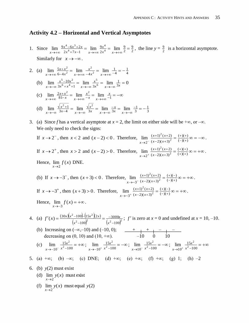
(b) Increasing on (–∞,–10) and (–10, 0); + + – –
decreasing on (0, 10) and (10, +∞). –10 0 10
(c) 100
15
102
2
limx
x
x
; 100
15
102
2
limx
x
x
; 100
15
102
2
limx
x
x
; 100
15
102
2
limx
x
x
5. (a) +∞; (b) –∞; (c) DNE; (d) +∞; (e) +∞; (f) +∞; (g) 1; (h) –2
6. (b) y(2) must exist
(d) existmust )(lim2
xyx
(f) (2) equalmust )(lim2
yxyx
36 APPENDIX C: ACTIVITY HINTS AND ANSWERS
Activity 4.3 – Continuity and L’Hôpital’s Rule
1. (a) 34
3
62
11
56
123
2
limlim
x
x
x
LR
x
xx
x
(0/0)
(b) 23
8666
2483
63
244
43
2limlimlim
2
2
23
23
xx
x
LR
xx
xx
x
LR
xxx
xx
x
(0/0) (0/0)
(c) 3
52
3
3
lim
xxx
x has the form –39/0, so L’Hôpital’s Rule does not apply here. The limit is
either +∞, –∞, or DNE (vert. asymp. at x = 3). We must check left- and right-hand limits:
)(
)(
352
3
3
limx
xx
x;
)(
)(
352
3
3
limx
xx
x; Therefore,
352
3
3
lim
xxx
xDNE.
(d) 0lim40
410
43
027
359
xx
xxx
x
(e) 41
463
5
443
205
4223
limlim
xxx
LR
xxx
x
x
(0/0)
(f) 0limlimlim4
02666
1123
363
11
133
12
2
23
23
xx
x
LR
xx
xx
x
LR
xxx
xxx
x
(0/0) (0/0)
2. (a) 1511
3022
30422
215
7411 limlimlim2
2
x
LR
xx
x
LR
x
xx
x
(+∞/+∞) (+∞/+∞)
(c) (i) 1511
15
11
262215
1041197
97
125497
23397
limlim
x
x
xxxx
xxx
x
(ii) 4limlim5
5
5
235 4
78
34
x
x
xxx
xxx
x
3. (a) (i) 0limlimlim3012
615
412
235
46223
2
xx
LR
xx
x
x
LR
xx
xx
x
(+∞/–∞) (–∞/+∞) (12/–∞)
(ii)
2854
323827
3
2349 limlimlim2
2
23 x
x
LR
xxx
x
LR
xx
xxx
x
(–∞/+∞) (+∞/–∞) (–∞/2)
(b) (i) 0limlimlim2171
50
123371
25950
5
6
5
6
166215
10376
xxx
x
xxxx
xxxx
x
(ii)
199
94021
4102109 6
39
45
8153039
2101745
limlimlim x
xx
x
xxxxxx
xxxx
x
4. Set c(2)2 + 7(2) = (2)
3 – c(2) to get 4c + 14 = 8 – 2c. Therefore, c = –1.
APPENDIX C : ACTIVITY HINTS AND ANSWERS 37
Activity 5.1 – Exponential Growth and Decay
1. (a) If M(t) = at + b, then M(0) = b = 500, M(2) = 2a + 500 = 245, and a = –127.5.
The model is M(t) = –127.5t + 500 mg, where t is hours after the injection.
(b) If M(t) = A(1 – r)t, then M(0) = A = 500, M(2) = 500(1 – r)
2 = 245, and 1 – r = 0.7.
The model is M(t) = 500(0.7)t mg, where t is hours after the injection.
2. (a) m(0) = 90 grams
(b) m(40) ≈ 27 grams
(c) decay rate of 0.03 = 3%
3. P(t) = 77.2e0.016t
million tons, where t is years since 2004
4.
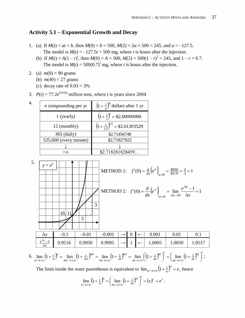
5.
METHOD 1: 1)0(33
0
RUNRISE
x
x
dxd ef
METHOD 2: 11
lim)0(00
x
ee
dx
df
x
xx
x
.
6. r
m
mm
rm
mm
mr
mm
mr
mrr
mr
n
nr
n
111 1lim1lim1lim1lim1lim ;
The limit inside the outer parentheses is equivalent to en
nn 11lim , hence
rrr
m
mm
n
nr
nee
11lim1lim .
n compounding per yr nn11 dollars after 1 yr
1 (yearly) 00000000.2$11
11
12 (monthly) 61303529.2$112
121
365 (daily) 71456748.2$
525,600 (every minute) 71827922.2$
↓ ↓
+∞ $2.718281828459…
Δx –0.1 –0.01 –0.001 → 0 ← 0.001 0.01 0.1
x
e x
1 0.9516 0.9950 0.9995 → 1 ← 1.0005 1.0050 1.0517
3
3
y = ex
(0, 1)
38 APPENDIX C: ACTIVITY HINTS AND ANSWERS
Activity 5.2 – Derivative and Antiderivative of ex
1. (a) xxx eeedx
d 444 20455
(b) 222 3233
teedt
d tttt
(c) 43234242 624241244621621 uuuueuueuueuuedu
d uuuu
(d)
22
222
2
2
19
18192
19
x
xx
xe
exex
e
x
dx
d
(e)
222
222
224
8210410
4
10
x
xxxx
x
x
ex
exeexe
ex
e
dx
d
2. Set 022)2(2)( 36626 222
xxexexexxf xxx to get x = –1, 0, 1.
3. (a) Cexdxex xx 2
25 5
(b) Cedxe xx
2
2525
(c) 11011
0
1
0
e
tt eeedte
4. (a) +∞; (b) 0; (c) 0; (d) +∞; (e) 0; (f) –5;
(g)25
16
40
81
20
4
102
2
2
2
2
2
limlimlim
x
x
x
x
x
x
e
e
x
LR
e
e
x
LR
ex
e
x
5. Set 0102522)( 555 teetetD ttt to get t = 1/5 s.
6. (c) ttU )1289.1( 1496.0)( million users, where t is months since 12/31/2003
(d) 5.50)48( U million users
(e) tt eetU 1213.0 1213.0 0181.01213.01496.0)( million users per month, where t is
months since 12/31/2003
(f) 11.6)48( U million users per month
APPENDIX C : ACTIVITY HINTS AND ANSWERS 39
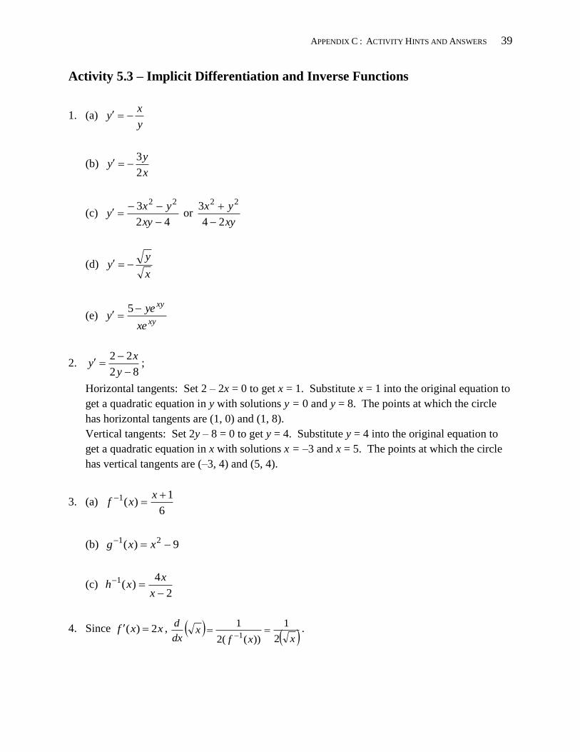
Activity 5.3 – Implicit Differentiation and Inverse Functions
1. (a) y
xy
(b) x
yy
2
3
(c) 42
3 22
xy
yxy or
xy
yx
24
3 22
(d) x
yy
(e) xy
xy
xe
yey
5
2. 82
22
y
xy ;
Horizontal tangents: Set 2 – 2x = 0 to get x = 1. Substitute x = 1 into the original equation to
get a quadratic equation in y with solutions y = 0 and y = 8. The points at which the circle
has horizontal tangents are (1, 0) and (1, 8).
Vertical tangents: Set 2y – 8 = 0 to get y = 4. Substitute y = 4 into the original equation to
get a quadratic equation in x with solutions x = –3 and x = 5. The points at which the circle
has vertical tangents are (–3, 4) and (5, 4).
3. (a) 6
1)(1 x
xf
(b) 9)( 21 xxg
(c) 2
4)(1
x
xxh
4. Since xxf 2)( , xxf
xdx
d
2
1
))((2
11
.
40 APPENDIX C: ACTIVITY HINTS AND ANSWERS
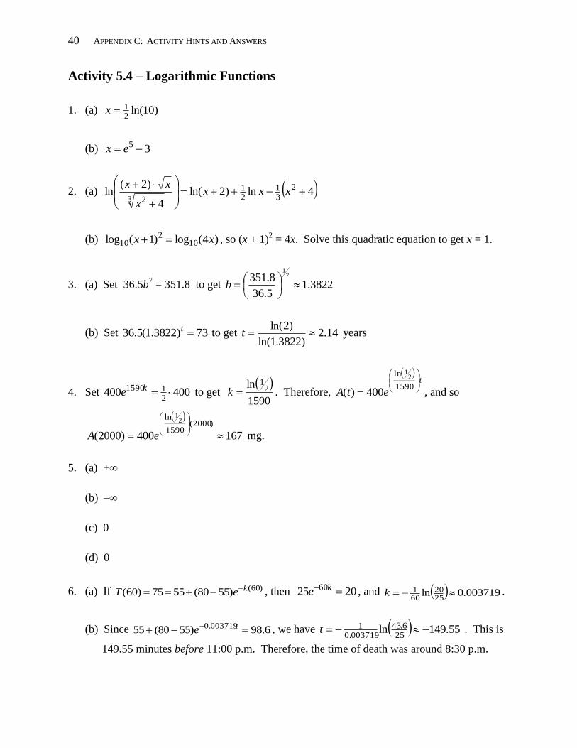
Activity 5.4 – Logarithmic Functions
1. (a) )10ln(21x
(b) 35 ex
2. (a) 4ln)2ln(4
)2(ln 2
31
21
3 2
xxx
x
xx
(b) )4(log)1(log 102
10 xx , so (x + 1)2 = 4x. Solve this quadratic equation to get x = 1.
3. (a) Set 36.5b7 = 351.8 to get 3822.1
5.36
8.351 71
b
(b) Set 73)3822.1(5.36 t to get 14.2)3822.1ln(
)2ln(t years
4. Set 400400211590 ke to get
1590
ln 21
k . Therefore,
t
etA
1590
ln 21
400)( , and so
167400)2000(
)2000(1590
ln 21
eA mg.
5. (a) +∞
(b) –∞
(c) 0
(d) 0
6. (a) If )60()5580(5575)60( keT , then 2025 60 ke , and 0.003719 ln2520
601 k .
(b) Since 6.98)5580(55 0.003719 te , we have 55.149ln25
6.430.003719
1 t . This is
149.55 minutes before 11:00 p.m. Therefore, the time of death was around 8:30 p.m.
APPENDIX C : ACTIVITY HINTS AND ANSWERS 41
J/mol 142.4526190.46
)(
1000
290
1008.102
21051.31
1000
290
53
2
2
1
T
T
cT
TP
TT
dTbTadTTCH
K-J/mol 940.741051.31||ln90.461000
2902
1008.103
1000
290
)(
2
5
3
2
1
T
T
cTaT
T T
TC
TT
dTbdTS P
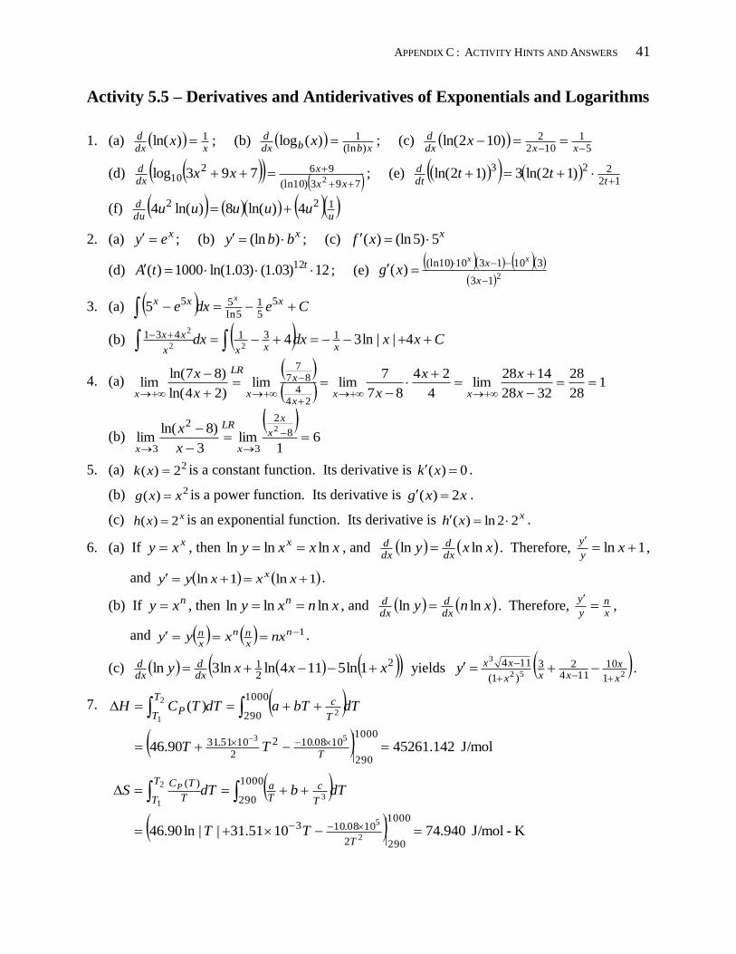
Activity 5.5 – Derivatives and Antiderivatives of Exponentials and Logarithms
1. (a) xdx
d x 1)ln( ; (b) xbbdx
d x)(ln
1)(log ; (c) 5
1102
2)102ln(
xxdx
d x
(d) 793)10(ln
96210 2
793log
xx
xdxd xx ; (e)
12223
)12ln(3)12ln(
tdt
d tt
(f) udu
d uuuuu 122 4)ln(8)ln(4
2. (a) xey ; (b)
xbby )(ln ; (c) xxf 5)5(ln)(
(d) 12)03.1()03.1ln(1000)( 12 ttA ; (e)
213
3101310)10(ln)(
x
x xx
xg
3. (a) Cedxe xxx x
5
51
5ln555
(b) Cxxdxdxxxxx
xx 4||ln34 131431
22
2
4. (a)
128
28
3228
1428lim
4
24
87
7limlim
)24ln(
)87ln(lim
244
877
x
xx
xx
x
xxx
x
x
LR
x
(b)
61
lim3
)8ln(lim 8
2
3
2
3
2
x
x
x
LR
x x
x
5. (a) 22)( xk is a constant function. Its derivative is 0)( xk .
(b) 2)( xxg is a power function. Its derivative is xxg 2)( .
(c) xxh 2)( is an exponential function. Its derivative is xxh 22ln)( .
6. (a) If xxy , then xxxy x lnlnln , and xxydxd
dxd lnln . Therefore, 1ln
x
y
y,
and 1ln1ln xxxyy x .
(b) If nxy , then xnxy n lnlnln , and xnydxd
dxd lnln . Therefore,
xn
y
y
,
and 1 n
xnn
xn nxxyy .
(c) 2
21 1ln5114lnln3ln xxxy
dxd
dxd yields
252
3
1
10114
23
)1(
114
x
xxxx
xxy
.
7.
42 APPENDIX C: ACTIVITY HINTS AND ANSWERS
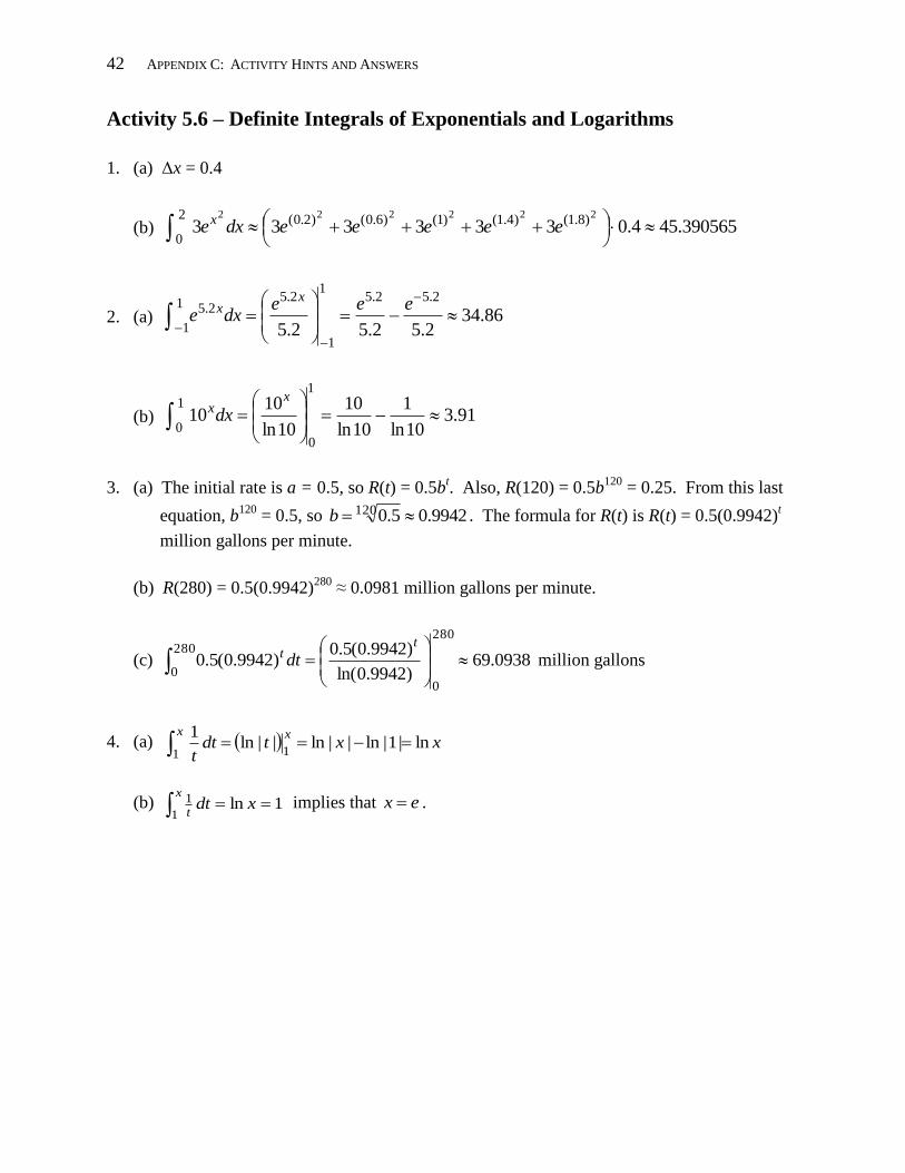
Activity 5.6 – Definite Integrals of Exponentials and Logarithms
1. (a) Δx = 0.4
(b) 390565.454.0333333 222222 )8.1()4.1()1()6.0()2.0(2
0
eeeeedxex
2. (a) 86.342.52.52.5
2.52.5
1
1
2.51
1
2.5
eeedxe
xx
(b) 91.310ln
1
10ln
10
10ln
1010
1
0
1
0
xxdx
3. (a) The initial rate is a = 0.5, so R(t) = 0.5bt. Also, R(120) = 0.5b
120 = 0.25. From this last
equation, b120
= 0.5, so 9942.05.0120 b . The formula for R(t) is R(t) = 0.5(0.9942)t
million gallons per minute.
(b) R(280) = 0.5(0.9942)280
≈ 0.0981 million gallons per minute.
(c) 0938.69)9942.0ln(
)9942.0(5.0)9942.0(5.0
280
0
280
0
tt dt million gallons
4. (a) xxtdtt
xxln|1|ln||ln||ln
1
11
(b) 1ln 1
1 xdtx
t implies that ex .
APPENDIX C : ACTIVITY HINTS AND ANSWERS 43
Activity 6.1 – The Cosine and Sine Functions
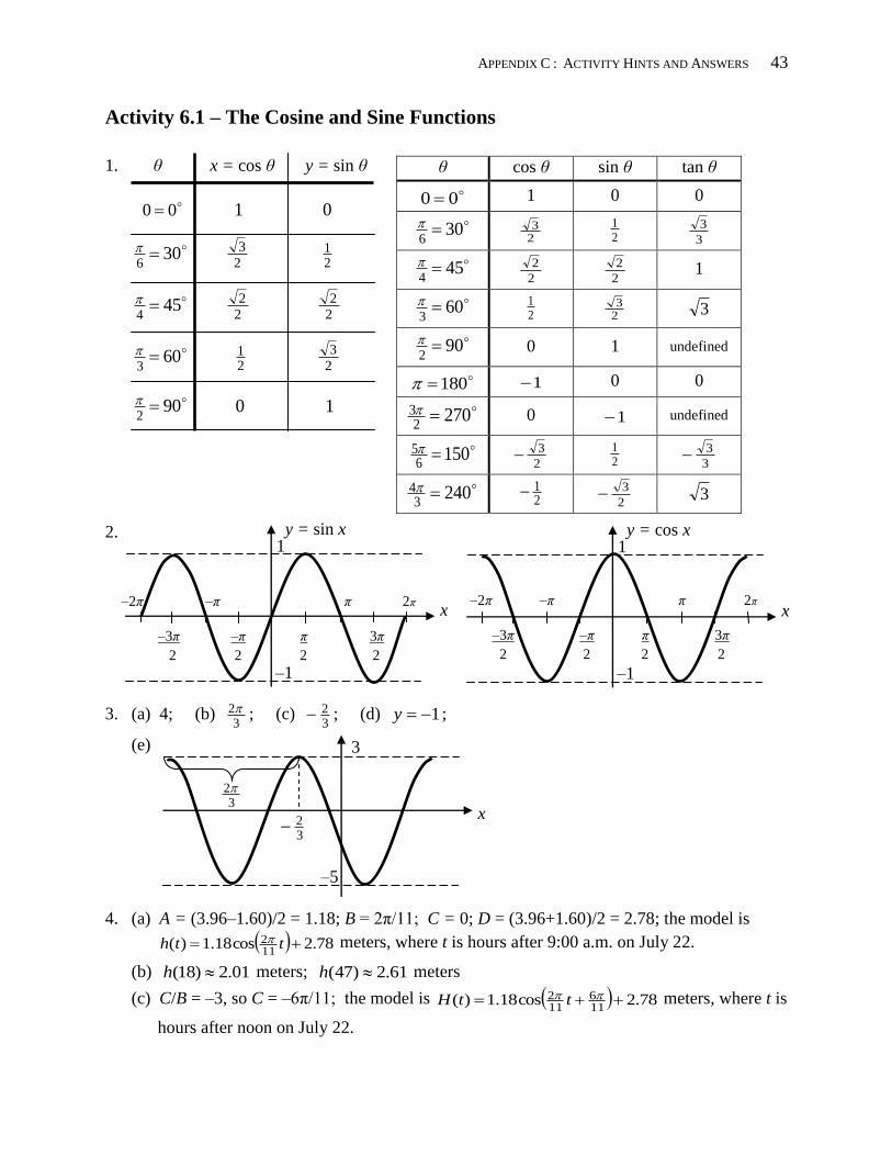
1. θ x = cos θ y = sin θ
00 1 0
30
6
2
3
21
45
4
2
2
2
2
60
3
21
2
3
90
2 0 1
2.
3. (a) 4; (b) 3
2 ; (c) 32 ; (d) 1y ;
(e)
4. (a) A = (3.96–1.60)/2 = 1.18; B = 2π/11; C = 0; D = (3.96+1.60)/2 = 2.78; the model is
78.2cos18.1)(112 tth meters, where t is hours after 9:00 a.m. on July 22.
(b) 01.2)18( h meters; 61.2)47( h meters
(c) C/B = –3, so C = –6π/11; the model is 78.2cos18.1)(116
112 ttH meters, where t is
hours after noon on July 22.
θ cos θ sin θ tan θ
00 1 0 0
306
23
21
3
3
454
2
2 2
2 1
603
21
23 3
902 0 1 undefined
180 1 0 0
2702
3 0 1 undefined
1506
5 2
3
21
3
3
2403
4 21
2
3 3
1
–1
y = sin x
–2π –π π 2π
–3π –π π 3π
2 2 2 2
x
1
–1
y = cos x
x –2π –π π 2π
–3π –π π 3π
2 2 2 2
–5
x
3
32
32
44 APPENDIX C: ACTIVITY HINTS AND ANSWERS
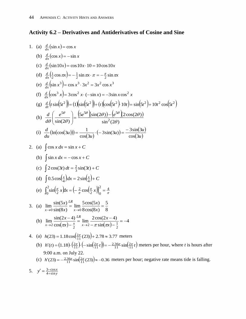
Activity 6.2 – Derivatives and Antiderivatives of Cosine and Sine
1. (a) xxdxd cossin
(b) xxdxd sincos
(c) xxxdxd 10cos101010cos10sin
(d) xxxdxd sinsincos
221
21
(e) 32233 cos33cossin xxxxxdxd
(f) xxxxxdxd 223 cossin3)sin(cos3cos
(g) 222222 5cos105sin105cos5sin15sin tttttttttdtd
(h)
)2(sin
)2cos(2)2sin(5
)2sin( 2
555
eee
d
d
(i)
u
uu
uu
du
d
3cos
3sin3)3sin(3
3cos
13cosln
2. (a) Cxdxx sin cos
(b) Cxdxx cos sin
(c) Ctdtt )3sin( )3cos(232
(d) Cdx xx 44sin2 cos5.0
(e)
42
022
2
0 2cossin xdxx
3. (a) 8
5
)8cos(8
)5cos(5lim
)8sin(
)5sin(lim
00
x
x
x
x
x
LR
x
(b)
4sin
)42cos(2lim
cos
)42sin(lim
212
22
x
x
x
x
x
LR
xx
4. (a) 77.378.2)23(cos18.1)23(112 h meters
(b) ttth112
1136.2
112
112 sinsin18.1)( meters per hour, where t is hours after
9:00 a.m. on July 22.
(c) 36.0)23(sin)23(112
1136.2 h meters per hour; negative rate means tide is falling.
5. yxy
sin4cos3
APPENDIX C : ACTIVITY HINTS AND ANSWERS 45
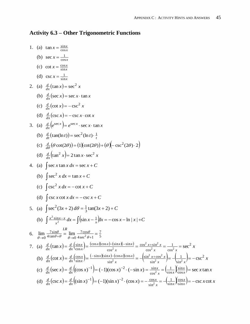
Activity 6.3 – Other Trigonometric Functions
1. (a) xxx
cossintan
(b) x
xcos
1sec
(c) xxx
sincoscot
(d) x
xsin
1csc
2. (a) xxdxd 2sectan
(b) xxxdxd tansecsec
(c) xxdxd 2csccot
(d) xxxdxd cotcsccsc
3. (a) xxee xx
dxd tansecsecsec
(b) tdt
d tt 12 )(lnsec)tan(ln
(c) 2)2(csc)2cot(1)2cot( 2 dd
(d) xxxdxd 22 sectan2tan
4. (a) Cxdxxx sec tansec
(b) Cxdxx tan sec2
(c) Cxdxx cot csc2
(d) Cxdxxx csc cotcsc
5. (a) Cxdx )23tan( )2(3sec312
(b) Cxxdxxdxxx
xxx ||lncossin 1sin
2
2
6. 57
1sec4
cos7
0tan4sin7
02
lim lim
LR
7. (a) xx
xx
xx
x
xxxx
xx
dxd
dxd 2
cos
1
cos
sincos
cos
sinsincoscos
cossin sectan
22
22
2
(b) xxxx
xx
x
xxxx
xx
dxd
dxd 2
sin
1
sin
cossin
sin
coscossinsin
sincos csccot
22
22
2
(c) xxxxxxxx
xx
xdxd
dxd tansec)sin())(cos1()(cossec
cossin
cos1
cos
sin212
(d) xxxxxxxx
xx
xdxd
dxd cotcsc)(cos))(sin1()(sincsc
sincos
sin1
sin
cos212
46 APPENDIX C: ACTIVITY HINTS AND ANSWERS
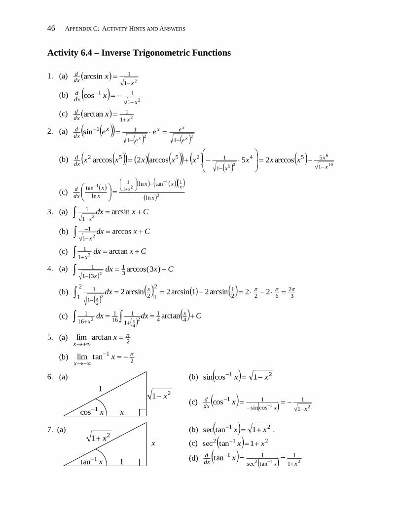
Activity 6.4 – Inverse Trigonometric Functions
1. (a) 21
1arcsinx
dxd x
(b) 21
11cosx
dxd x
(c) 21
1arctanxdx
d x
2. (a) 22
11
11sinx
x
x e
ex
e
x
dxd ee
(b)
10
6
25 1
554
1
12552 arccos25arccos2arccosx
x
xdxd xxxxxxxx
(c)
2
11
21
11
ln
tanln
ln
tan
x
xx
x
x
dxd xx
3. (a) Cxdxx
arcsin21
1
(b) Cxdxx
arccos21
1
(c) Cxdxx
arctan
21
1
4. (a)
Cxdxx
)3arccos( 31
31
1
2
(b)
3
2622
12
12
2
1 1
1 22arcsin21arcsin2arcsin22
2
xdxx
(c)
Cdxdx x
x x
441
1
1161
16
1 arctan 2
4
2
5. (a) 2
arctanlim
xx
(b) 2
1tanlim
x
x
6. (a) (b) 21 1cossin xx
1
(c) 21
1
1
cossin
11cosxxdx
d x
7. (a) (b) 21 1tansec xx .
X x (c) 212 1tansec xx
(d) 212 1
1
tansec
11tanxxdx
d x
xx cos 1
1 tan 1 x
21 x
21 x
APPENDIX C : ACTIVITY HINTS AND ANSWERS 47
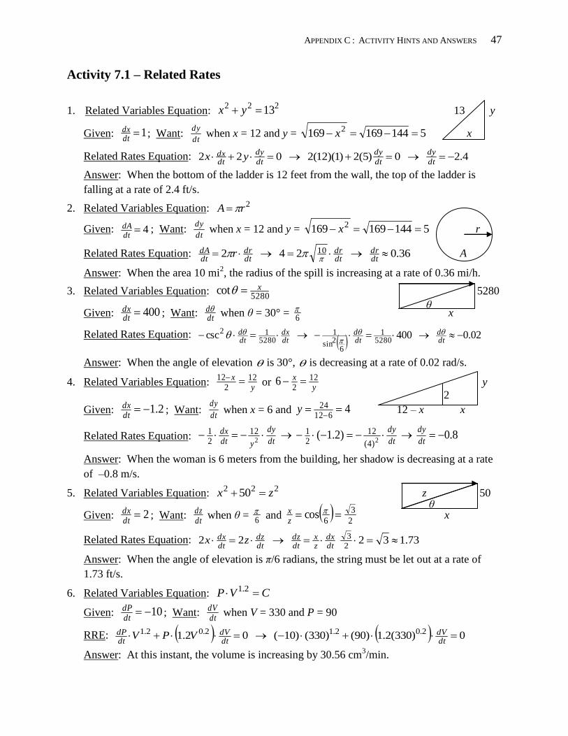
Activity 7.1 – Related Rates
1. Related Variables Equation: 222 13 yx 13 y
Given: 1dtdx ; Want:
dt
dy when x = 12 and y = 5144169169 2 x x
Related Rates Equation: 4.2 0)5(2)1)(12(2 022 dt
dy
dt
dy
dt
dy
dtdx yx
Answer: When the bottom of the ladder is 12 feet from the wall, the top of the ladder is
falling at a rate of 2.4 ft/s.
2. Related Variables Equation: 2rA
Given: 4dt
dA ; Want: dt
dy when x = 12 and y = 5144169169 2 x r
Related Rates Equation: 36.0 24 2 10 dtdr
dtdr
dtdr
dtdA r
A
Answer: When the area 10 mi2, the radius of the spill is increasing at a rate of 0.36 mi/h.
3. Related Variables Equation: 5280
cot x 5280
Given: 400dtdx ; Want:
dtd when θ = 30° =
6 x
Related Rates Equation:
02.0 400 csc5280
1
62sin
15280
12 dtd
dtd
dtdx
dtd
Answer: When the angle of elevation is 30°, is decreasing at a rate of 0.02 rad/s.
4. Related Variables Equation: y
x 122
12 or
yx 122
6 y
Given: 2.1dtdx ; Want:
dt
dy when x = 6 and 4
61224
y 12 – x x
Related Rates Equation: 8.0 )2.1( 22 )4(
122112
21
dt
dy
dt
dy
dt
dy
ydtdx
Answer: When the woman is 6 meters from the building, her shadow is decreasing at a rate
of –0.8 m/s.
5. Related Variables Equation: 222 50 zx z 50
Given: 2dtdx
; Want: dtdz
when θ = 6 and
2
3
6cos
zx
x
Related Rates Equation: 73.132 222
3 dtdx
zx
dtdz
dtdz
dtdx zx
Answer: When the angle of elevation is π/6 radians, the string must be let out at a rate of
1.73 ft/s.
6. Related Variables Equation: CVP 2.1
Given: 10dtdP
; Want: dtdV
when V = 330 and P = 90
RRE: 0)330(2.1)90()330(10)( 02.1 2.02.12.02.1 dtdV
dtdV
dtdP VPV
Answer: At this instant, the volume is increasing by 30.56 cm3/min.
θ
2
θ
48 APPENDIX C: ACTIVITY HINTS AND ANSWERS
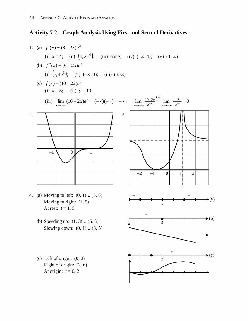
Activity 7.2 – Graph Analysis Using First and Second Derivatives
1. (a) xexxf )28()(
(i) x = 4; (ii) 42 ,4 e ; (iii) none; (iv) (–∞, 4); (v) (4, ∞)
(b) xexxf )26()(
(i) 34 ,3 e ; (ii) (–∞, 3); (iii) (3, ∞)
(c) xexxf )210()(
(i) x = 5; (ii) y = 10
(iii)
))(()210(lim x
xex ; 0limlim 2210
xx ex
LR
e
x
x
2. 3.
4. (a) Moving to left: (0, 1) U (5, 6) – + –
Moving to right: (1, 5)
At rest: t = 1, 5
+ –
(b) Speeding up: (1, 3) U (5, 6)
Slowing down: (0, 1) U (3, 5)
– +
(c) Left of origin: (0, 2)
Right of origin: (2, 6)
At origin: t = 0, 2
3 (a)
–1 0 1
–2 –1 0 1 2
3 (s)
3 (v)
APPENDIX C : ACTIVITY HINTS AND ANSWERS 49
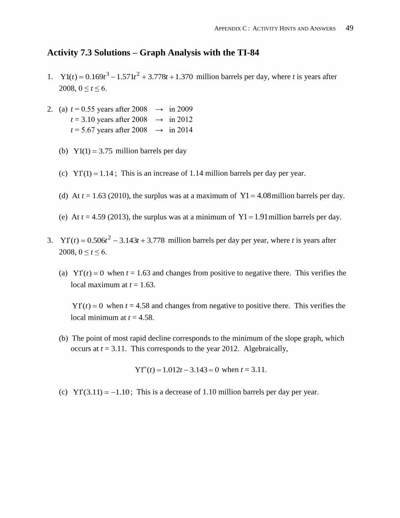
Activity 7.3 Solutions – Graph Analysis with the TI-84
1. 370.1778.3571.1169.0)(1Y 23 tttt million barrels per day, where t is years after
2008, 0 ≤ t ≤ 6.
2. (a) t = 0.55 years after 2008 → in 2009
t = 3.10 years after 2008 → in 2012
t = 5.67 years after 2008 → in 2014
(b) 75.3)1(1Y million barrels per day
(c) 14.1)1(1Y ; This is an increase of 1.14 million barrels per day per year.
(d) At t = 1.63 (2010), the surplus was at a maximum of 08.41Y million barrels per day.
(e) At t = 4.59 (2013), the surplus was at a minimum of 91.11Y million barrels per day.
3. 778.3143.3506.0)(1Y 2 ttt million barrels per day per year, where t is years after
2008, 0 ≤ t ≤ 6.
(a) 0)(1Y t when t = 1.63 and changes from positive to negative there. This verifies the
local maximum at t = 1.63.
0)(1Y t when t = 4.58 and changes from negative to positive there. This verifies the
local minimum at t = 4.58.
(b) The point of most rapid decline corresponds to the minimum of the slope graph, which
occurs at t = 3.11. This corresponds to the year 2012. Algebraically,
0143.3012.1)(1Y tt when t = 3.11.
(c) 10.1)11.3(1Y ; This is a decrease of 1.10 million barrels per day per year.
50 APPENDIX C: ACTIVITY HINTS AND ANSWERS
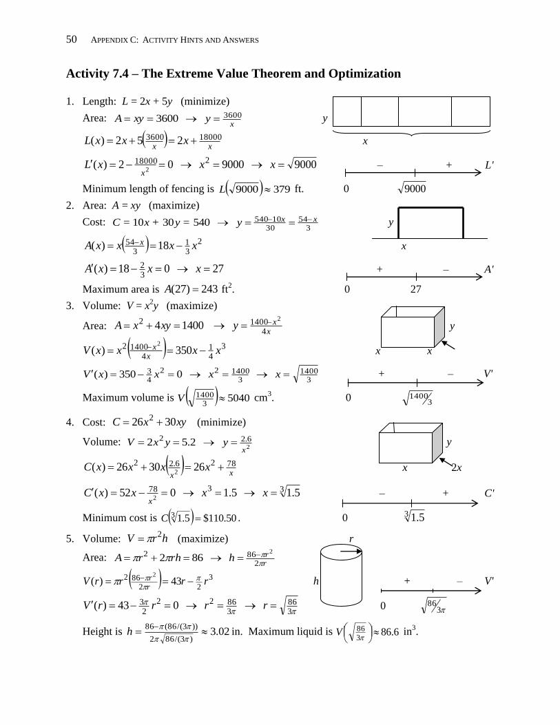
Activity 7.4 – The Extreme Value Theorem and Optimization
1. Length: L = 2x + 5y (minimize)
Area: x
yxyA 3600 3600 y
xx
xxxL 180003600 252)( x
9000 9000 02)( 2180002
xxxLx
– + L'
Minimum length of fencing is 3799000 L ft. 0 9000
2. Area: A = xy (maximize)
Cost: 3
5430
10540 5403010 xxyy = x + C = y
2
31
354 18)( xxxxA x x
27 018)(32 xxxA + – A'
Maximum area is 243)27( A ft2. 0 27
3. Volume: V = x2y (maximize)
Area: x
xyxyxA4
14002 2
14004 y
3
41
414002 350)(
2
xxxxVx
x x x
3
14003
140022
43 0350)( xxxxV + – V'
Maximum volume is 50403
1400 V cm3. 0
31400
4. Cost: xyxC 3026 2 (minimize)
Volume: 2
6.22 2.52x
yyxV y
xx
xxxxC 7826.22 263026)(2
x 2x
3378 5.1 5.1 052)(2
xxxxCx
– + C'
Minimum cost is 50.110$5.13 C . 0 3 5.1
5. Volume: hrV 2 (maximize) r
Area: rrhrhrA
2862 2
862
3
22862 43)(
2
rrrrVrr
h + – V'
386
38622
23 043)( rrrrV 0 3
86
Height is 02.3)3/(862
))3/(86(86
h in. Maximum liquid is 6.86
3
86
V in
3.
APPENDIX C : ACTIVITY HINTS AND ANSWERS 51
Activity 7.5 – Differential Equations
1. (a) teCy 5
0
(b) teCy 3
0
(c) tttt eCeCeCeCy 5
25
125
225
1
(d) tCtCy 15sin 15cos 21
2. ktetT 11570)( ;
17011570)5( )5( keT implies 115100
51 lnk ;
14611570)15()15(ln
115100
51
eT °F.
3. tt eey 4
474
45
4. ttty21
21 sin10cos5.1)( in
5. kyeCkyeCy ktkt 00
6.
tktk eCkeCky 21
kyeCeCkeCkeCky tktktktk
2121
7. tkCktkCky cos sin 21
kytkCtkCktkCktkCky sin cos sin cos 2121
8. (a) Ckt|y| kdtdyy
ln 1
(b) CktCCkty eCeeyeyeCkt|y|
0||ln || ln
52 APPENDIX C: ACTIVITY HINTS AND ANSWERS
Activity 8.1 – Sigma Notation and Summations
1. (a) 16; (b) 13
2. (a) nnnnkknn
n
k
n
k
n
k
2)1(2412424 22
4
)1(
11
3
1
322
(b)
3. (a) 898,256,16632)163()63(24 2263
1
3 k
k
(b)
4. (a)
(b)
5. (a)
(b)
(c)
)12)(1()1(2
44441441
32
6
)12)(1(
2
)1(
1
2
111
2
nnnnnn
nkkkknnnnn
n
k
n
k
n
k
n
k
880,91)1402)(140(40)140(402402132
40
1
2
k
k
2
32
32
32
2
6
)12)(1()1(2
6
)12)(1(12
)1(44
1 1
21
1
44
1
2144
1
1214
1
121
4
1
1
42
n
nn
n
n
nnn
n
nn
nn
n
k
n
kn
n
knn
n
knnn
n
knnn
n
knn
n
kk
kk
kkk
2
32
32
)12)(1(4)1(12
6
)12)(1(242
)1(246
1
224246
1
222
6
113
n
nn
n
n
nnn
n
nn
nn
n
knnn
n
knn
n
kkk
)()(
)()()()()()()()(
03
231201
3
1
1
xFxF
xFxFxFxFxFxFxFxFk
kk
)()(
)()()()()()()()()()(
04
34231201
4
1
1
xFxF
xFxFxFxFxFxFxFxFxFxFk
kk
)()()()( 0
1
1 xFxFxFxF n
n
k
kk
APPENDIX C : ACTIVITY HINTS AND ANSWERS 53
Activity 8.2 – The Definition of Net Area
1. a = 1; b = 2; Δx = nn112 ; kx
nk 1* 1 ; 2
23621 313 kkkxf
nnnk ;
2
33
26312
2363 kkkkxxf
nnnnnnk
2
32
3232
2
)12)(1()1(3
6
)12)(1(32
)1(63
1
23
1
6
1
3
1
2363
1
3
1
n
nn
n
n
nnn
n
nn
nn
n
kn
n
kn
n
kn
n
knnn
n
k
k
n
kkkkxxf
71333limlim 3 22
)12)(1()1(3
1
2
1
2
n
nn
n
n
n
n
k
kn
xxfdxx
2. a = 0; b = 3; Δx = nn303 ; kx
nk 3*; kkkkxf
nnnnk 32183232
2 ;
kkkkxxfnnnnn
k 232
925433218
n
n
n
nn
nn
n
nnn
n
n
kn
n
kn
n
knn
n
k
k kkkkxxf
2
)1(9)12)(1(9
2
)1(96
)12)(1(54
1
9
1
254
1
9254
1
2
232323
227
29
2
)1(9)12)(1(9
1
2
1
2 18limlim 3 2
n
n
n
nn
n
n
k
kn
xxfdxx
3. 3
583
5434
5
2
22
0
25
0
2 2 2 2 dtttdtttdttt m
4. (a) 41)(1
2
dxxf ; (b) 6)(
6
2 dxxg ; (c) 183)( 43 )(4
5
3
5
3
5
3 dxdxxhdxxh
5. (a) 0)(lim)(1
n
kn
aak
n
a
axfdxxf
(b)
b
a
n
kn
abk
n
n
kn
bak
n
a
bdxxfxfxfdxxf )()(lim)(lim)(
11
(c)
b
a
n
kn
abk
n
n
kn
abk
n
b
adxxfkxfkxfkdxxfk )()(lim)(lim)(
11
(d)
b
a
b
a
n
kn
abk
n
n
kn
abk
n
n
kn
abkk
n
b
a
dxxgdxxf
xgxfxgxfdxxgxf
)()(
)(lim)(lim)()(lim)()(111
54 APPENDIX C: ACTIVITY HINTS AND ANSWERS
Activity 8.3 – Rolle’s Theorem and the Mean Value Theorem
1. (a) Set 313)(4
)4(8
)2(2
)2()2(2
ffccf to get
34c in the interval (–2, 2).
(b) Set 151
235
)3()5(1 31
51
2)(
gg
ccg to get 15c , but only 15 is in (3, 5).
2. (a) Since f has a vertical asymptote at x = 0, it is not continuous on [0,4]. Since it is not
continuous at x = 0, it is not differentiable at x = 0.
(b) Since g only has one discontinuity at x = 6, it is continuous on [0, 4]. Since g' is
undefined only at x = 6 (use the quotient rule), g is differentiable everywhere except at
x = 6. In particular, it is differentiable on [0, 4].
(c) Since h has a vertical asymptote at x = –3, it is not continuous on [–4 ,5]. Since it is not
continuous at x = –3, it is not differentiable at x = –3.
(d) Since
3 if,6
3 if,6)(
2
2
xxx
xxxxF , it follows that
3 if,12
3 if,12)(
xx
xxxF .
From the left of 3, F has a slope of –5, and from the right of 3, F has a slope of 5.
Therefore, F is not differentiable at x = 3 (graph has a corner), and hence it is not
differentiable on [1, 4]. It is continuous everywhere, however, as is seen by substituting
x = 3 into the piecewise formulas for F.
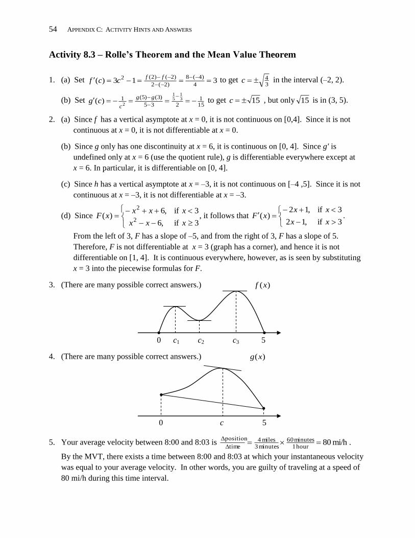
3. (There are many possible correct answers.) )(xf
0 c1 c2 c3 5
4. (There are many possible correct answers.) )(xg
0 c 5
5. Your average velocity between 8:00 and 8:03 is mi/h 80hour 1
minutes 60minutes 3
miles 4time
Δposition
.
By the MVT, there exists a time between 8:00 and 8:03 at which your instantaneous velocity
was equal to your average velocity. In other words, you are guilty of traveling at a speed of
80 mi/h during this time interval.
APPENDIX C : ACTIVITY HINTS AND ANSWERS 55
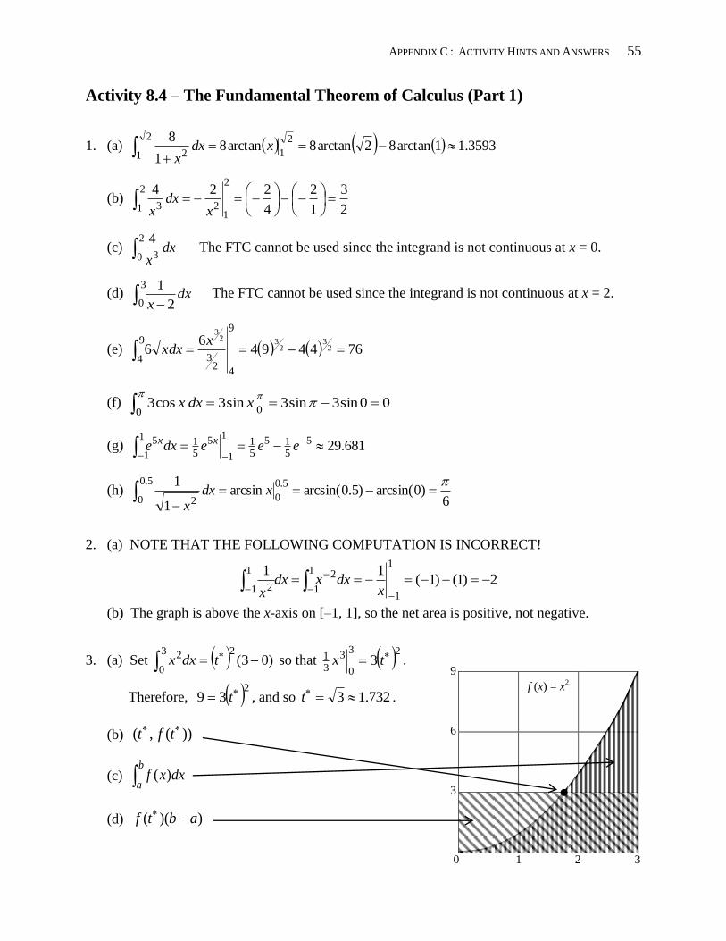
Activity 8.4 – The Fundamental Theorem of Calculus (Part 1)
1. (a) 3593.11arctan82arctan8arctan81
8 2
1
2
1 2
xdx
x
(b) 2
3
1
2
4
2242
12
2
1 3
xdx
x
(c) 2
0 3
4dx
x The FTC cannot be used since the integrand is not continuous at x = 0.
(d)
3
0 2
1dx
x The FTC cannot be used since the integrand is not continuous at x = 2.
(e) 7644946
6 23
232
3 9
42
3
9
4
xdxx
(f) 00sin3sin3sin3 cos300
xdxx
(g) 681.295
515
51
1
1
5
51
1
1
5
eeedxe xx
(h) 6
)0arcsin()5.0arcsin(arcsin1
1 5.0
0
5.0
0 2
xdx
x
2. (a) NOTE THAT THE FOLLOWING COMPUTATION IS INCORRECT!
2)1()1(11
1
1
1
1
21
1 2
xdxxdx
x
(b) The graph is above the x-axis on [–1, 1], so the net area is positive, not negative.
3. (a) Set )03(23
0
2 tdxx so that 23
0
3
31 3 tx .
Therefore, 239 t , and so 732.13 t .
(b) ))(,( tft
(c) b
adxxf )(
(d) ))(( abtf
9
f (x) = x2
6
3
0 1 2 3
56 APPENDIX C: ACTIVITY HINTS AND ANSWERS
Activity 8.5 – The Fundamental Theorem of Calculus (Part 2)
1. (a) 25 5)( xxxf
(b) dte
txy
x
t
1
3
4)( , so
4)(
3
xe
xxy
(c) )104arctan(22)10)2arctan(()( 22 xxxF
(d)
3 23 2 22
1)(
xx
xx
xx ee
ee
ee
xH
(e) dttxgx
25
1)ln(cos)( , so 22 5lncos10105lncos)( xxxxxg
2. (a) 01
1
2
31
dteG t
(b) 292)3( 33)( xx eexG
(c) 33)0(2)0(9 eG
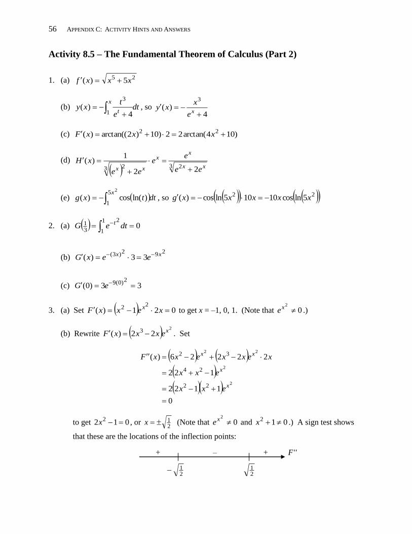
3. (a) Set 021)(22 xexxF x to get x = –1, 0, 1. (Note that 0
2
xe .)
(b) Rewrite 2
22)( 3 xexxxF . Set
0
1122
122
22226)(
2
2
22
22
24
32
x
x
xx
exx
exx
xexxexxF
to get 012 2 x , or 21x (Note that 0
2
xe and 012 x .) A sign test shows
that these are the locations of the inflection points:
+ – + F''
21
21
APPENDIX C : ACTIVITY HINTS AND ANSWERS 57
Activity 8.6 – Integration by Substitution
1. (a) CeCedueduedxe xuuux
54
41
41
41
4154
u = 4x + 5; du = 4dx ; dx = 41 du
(b) CeCedueduedxex xuuux 33
31
31
31
312
u = x3; du = 3x
2dx ; x
2dx =
31 du
(c) CtCudududtuut
|49|ln||ln
91
911
91
911
491
u = 9t + 4; du = 9dt; dt = 91 du
(d) CxxCudududxuuxx
x
|1012|ln||ln 2
21
211
21
211
1012
62
u = x2 + 12x + 10; du = 2x + 12 = 2(x + 6); (x + 6)dx =
21 du
(e) CCuduud 6
616
6155 sin cos sin
u = sin θ; du = cos θ dθ
2. (a) 25
3280
321
3281
3
132
3
1
3
81
3
1 8131
0
343 4
21 uduuduudxxx
u = 1 + 2x4; du = 8x
3dx; x
3 dx =
81 du
x = 0 → u = 1 + 2(0)4 = 1; x = 1 → u = 1 + 2(1)
4 = 3
(b) 2
43
83
83
83
1
483
1
4
3
21
2
1
3 2 33
43
43
4
415 uduudxxx
u = 5 – x2; du = –2xdx; xdx = –
21 du
x = 1 → u = 5 – (1)2 = 4; x = 2 → u = 5 – (2)
2 = 1
(c) 21
2
0
211
21
1
021
1
021
0
)2sin(4 )2cos(
euux eeeduedxxe
u = sin(2x); du = 2cos(2x)dx; cos(2x)dx = 21 du
x = 0 → u = sin(0) = 0; x = π/4 → u = sin(π/2) = 1
3. (a)
CCdudxxuux
x
88
3831
83
1
38228
7
;
163
1
088
31
0 1
3828
7
xx
x dx
u = x8 + 1; du = 8x
7dx; 3x
7dx =
83
du
(b) CxCuduudxx
x
3
313
312)(ln
)(ln2
; 3
31
3
1
3
313
1
)(ln)3(ln)(ln
2
xdxx
x
u = ln x; du =
x1 dx
58 APPENDIX C: ACTIVITY HINTS AND ANSWERS
Activity 8.7 – Modeling Accumulated Change with the TI-84
1. 50793332)( 2 tttr ft3/min, where t is in minutes
2. t = 11.48 min
3. t = 14.58 min; r(14.58) = 7308 ft3/min
4. 41053 5079333210
0
2 dttt ft3
5. CtttdttttA 50750793332)( 2
29333
3322 ; since A(0) = 5000, C = 5000.
Therefore, 5000507)( 2
29333
332 ttttA ft
3, where t is minutes.
6. 1164075000)20(507)20()20()20( 2
29333
332 A ft
3
7. Set 15000050005072
29333
332 ttt to get t = 27.55 min.
APPENDIX D
SUPPLEMENTAL EXERCISES

60 APPENDIX D: SUPPLEMENTAL EXERCISES
APPENDIX D: SUPPLEMENTAL EXERCISES 61
Chapter 1 – Supplemental Exercises
Lesson 1.3
1. Find the derivative of each constant function.
(a) y = b
(b) y = 4
(c) y = –3.1
2. Find the derivative of each linear function.
(a) y = mx + b
(b) y = x – 4
(c) y = –2x
3. Let T(t) = –2.1t + 63 be the temperature in degrees Fahrenheit t hours after noon for 0 ≤ t ≤ 6.
(a) Find the temperature at noon.
(b) Find the temperature at 3:00 p.m.
(c) How fast was the temperature changing at 3:00 p.m.?
Lesson 1.4
4. Find the family of antiderivatives of each constant function.
(a) y = m
(b) y = –9
(c) y = 0.23
5. Use the Fundamental Theorem of Calculus to evaluate each definite integral.
(a) dxmb
a
(b) dx 5
2 6
(c) dx1
21
2.4
6. Stan saves money by stashing $50 per week under his mattress.
(a) Write a definite integral that represents Stan’s total accumulation of savings between the
second and tenth weeks.
(b) Use the Fundamental Theorem of Calculus to evaluate the integral from part (a), and
interpret your answer in context.
Lesson 1.5
7. An ant is walking along a wire with velocity v(t) = 2 in/s on the time interval [0, 2],
v(t) = –t + 4 in/s on the time interval [2, 5], and v(t) = –1 in/s on the time interval [5, 7].
(a) Sketch the graph of the ant’s velocity on the interval [0, 7].
(b) Use geometry to find the ant’s displacement on the interval [0, 7].
(c) Use geometry to find the total distance traveled on the interval [0, 7].
62 APPENDIX D: SUPPLEMENTAL EXERCISES
Chapter 2 – Supplemental Exercises
Lesson 2.1
1. (a) Carefully sketch the graph of f (x) = (x – 3)2 in the interval [0, 4] on the x-axis, and in
the interval [0, 9] on the y-axis. Then sketch the tangent line to the graph of f at x = 1.
(b) Estimate the slope of the tangent line using “rise-over-run.”
(c) Set up a table like Example 2.1.1. Use it to estimate the slope of the tangent line at x = 1.
(d) Expand (x – 3)2 by multiplying (x – 3)(x – 3).
(e) Use the formula for the derivative of a quadratic to find a formula for f ʹ (x).
(f) Use the formula from part (f) to find f ʹ (1). Were your estimates good ones?
Lesson 2.3
2. (a) Write down the limit definition of the derivative of the function f.
(b) Use the limit definition of the derivative to find the derivative of f (x) = 3x2 – 2x.
3. Find the derivative of each quadratic function.
(a) y = ax2 + bx + c
(b) y = 0.5x2 – 10x
(c) y = (2 – x)2
Lesson 2.4
4. Find the derivative of each cubic function.
(a) y = ax3 + bx
2 + cx + d
(b) y = 1 – x + x2 – x
3
(c) y = (x + 2)(x2 – 2x + 4)
Lesson 2.5
5. (a) Find the equation of the tangent line to the graph of f (x) = 2x3 – 5x
2 at x = 2.
(b) Use the tangent line to estimate f (2.1). How close are you to the actual value?
6. A beaker with radius r inches is filled with acid to a height of 4 inches. The radius of the
beaker is measured to be 2 inches with a possible error in measurement of ±0.08 inches.
Estimate the propagated and relative errors in the calculated volume of acid in the beaker.
(Hint: The volume of a right circular cylinder of height 4 is V = 4πr2.)
Lesson 2.6
7. Evaluate each integral.
(a) dtt 3
1 )12(
(b) duu 0
1 )1.22.3(
(c) dwww 1042
APPENDIX D: SUPPLEMENTAL EXERCISES 63
Chapter 3 – Supplemental Exercises
Lesson 3.1
1. Find the derivative of each power function.
(a) y = 2x11
(b) y = 25
7
x
(c) y = 3
1
xx
Lesson 3.2
2. Let f (x) = 24
41 2xx .
(a) Find the x-intercepts of f.
(b) Find the critical points, the intervals of increase/decrease, and the local extrema of f.
(c) Find the intervals of concavity and the inflection points of f.
(d) Determine the end behavior of f.
Lesson 3.3
3. Find the derivative of each composite function.
(a) y = (3x – 4)5
(b) y = 3 2 2xx
(c) y = 42 12
6
xx
(d) y = 109 5 x (use the square-root rule)
(e) y = 17
139 xx
(use the reciprocal rule)
Lesson 3.4
4. Find the derivative of each product function.
(a) y = 235 1044 xxx
(b) y = 35 1 xx
Lesson 3.6
5. Evaluate each integral.
(a) dxxxx 3
(b) 1
0
59 243 dxxx
6. Let f (x) = 26 32
xx
. Find an antiderivative F of f that passes through the point (2, –5).
64 APPENDIX D: SUPPLEMENTAL EXERCISES
Chapter 4 – Supplemental Exercises
Lesson 4.1
1. Use the quotient rule to find the derivative of each function.
(a) y = 23
xx
(b) y = 12
42
x
x
(c) y = 74
232
3
x
xx
Lesson 4.2
2. Evaluate the following limits.
(a) 742
10325
4
lim
xx
xx
x
(b) 3
3
102
471limxx
xx
x
(c) 4
52
821
739limxx
xx
x
(d) 25
892 3
lim
xxx
x
(e) 12
32
lim xx
x
x
3. Evaluate the following limits.
(a) 3
74
2
2
lim
xxx
x
(b) xx
x
x 2
1
02
3
lim
(c) xxx
xx
x
23
5
2
232
1lim
Lesson 4.3
4. Evaluate the following limits. Use L’Hôpital’s Rule if necessary.
(a) 1
32
03
2
lim
x
xx
x
(b) 352
65
32
23
lim
xx
xxx
x
(c) xx
x
x 104
4
23
3 2
lim
(d) 2
1lim
x
x
x
APPENDIX D: SUPPLEMENTAL EXERCISES 65
Chapter 5 – Supplemental Exercises
Lesson 5.2
1. Find the derivative of each function.
(a) y = xe
(b) y = xex 2
(c) y = 2
2
31
5
t
et
2. Evaluate each integral.
(a) dxex
(b) dxekx
(c) dte t510
Lesson 5.3
3. Use implicit differentiation to find yʹ = dx
dy.
(a) 23 24 yxyx
(b) 111 yx
(c) xyxe y 35
Lesson 5.5
4. Find the derivative of each function.
(a) xy ln
(b) xy blog
(c) xxy 43ln 2
(d) tty ln
(e) 310log xy
(f) xby
(g) ty )03.1(1000
Lesson 5.6
5. Evaluate each definite integral.
(a) due u
1
0
22.1
(b) dttt
4
2
3102
66 APPENDIX D: SUPPLEMENTAL EXERCISES
Chapter 6 – Supplemental Exercises
Lesson 6.2
1. Find the derivative of each function.
(a) xey cos
(b) 518 3sin5.16 ty
2. Evaluate each integral.
(a) dxx )sin(5
(b) 1
1 1)2cos( dtt
Lesson 6.3
3. Find the derivative of each function.
(a) )ln(tan xy
(b) )3(sec3 y
(c) tty tan2
4. Evaluate each integral.
(a) dtt )14(sec2
(b) dxxx tansec4
0
5. Evaluate each limit.
(a) )5tan(
)10sin(
0lim
x
x
x
(b) )2sin(
)3cos(lim
x
xx
x
Lesson 6.4
6. Find the derivative of each function.
(a) )arctan(ln xy
(b) xxy 1sin
7. Evaluate each integral.
(a) dxx
2)2(1
1
(b) dxx
29
2
(c) dxx
24
1
APPENDIX D: SUPPLEMENTAL EXERCISES 67
Chapter 7 – Supplemental Exercises
Lesson 7.1
1. A spherical balloon is inflated so that the volume is increasing by 8 in3/s. How fast is the
radius of the balloon changing when the volume is 512 in3?
2. A boat is pulled toward a dock by a rope attached to a pulley on the dock. The dock is 12
feet above the point on the bow of the boat at which the rope is attached. If the rope is pulled
through the pulley at a rate of 10 ft/min, how fast is the boat approaching the dock when 50
feet of rope remain?
3. A man 6 ft tall is walking at a rate of 2 ft/s toward a stationary spotlight 20 ft high. How fast
is his shadow length changing? How fast is the tip of his shadow moving?
Lesson 7.2
4. Determine each of the following for the function 16
822
2
x
xy .
(a) Domain, x-intercepts, y-intercept
(b) Vertical asymptotes and nearby behavior
(c) Horizontal asymptotes
(d) Critical points
(e) Intervals of increase/decrease, and local extrema
(f) Intervals of concavity and inflection points
(g) Sketch of the graph
Lesson 7.4
5. A cylindrical can with no top must be constructed using 300 in2 of material. Find the height
and radius of the can having the greatest volume.
6. A fenced-in garden is to be laid out in a rectangular area and partitioned into two sections
with fencing parallel to one side. The fencing for the perimeter costs $10 per foot, while the
fencing for the partition costs $5 per foot. Find the largest area that can be enclosed for a
cost of $500.
7. A window consisting of a rectangle topped by a semicircle is to have a perimeter of 20 feet.
Find the radius of the semicircle that maximizes the area of the window.
Lesson 7.5
8. A mass attached to a vertical spring has position y(t) meters after t seconds, where y satisfies
yʹʹ = –0.25y. Positions below equilibrium and downward motion are considered positive.
Find the position function y if the initial position is –0.3 m and the initial velocity is 2 m/s.
9. Find the general solution to the differential equation ydt
dy125.0 .
10. Find the general solution to the differential equation 0105 yy .
68 APPENDIX D: SUPPLEMENTAL EXERCISES
Chapter 8 – Supplemental Exercises
Lesson 8.2
1. Evaluate dxxx 23
1
2 using the limit definition of the definite integral.
2. Use the properties of the definite integral to evaluate dxxx 23 2
0
2 .
Lesson 8.4
3. If possible, use Part 1 of the Fundamental Theorem to evaluate each integral.
(a) dxx
2
0
1
(b) dxx
1
0 231
(c) dxx tan0
Lesson 8.5
4. Use Part 2 of the Fundamental Theorem to find the derivative of each function.
(a) dteyx t 0
2
(b) dtyx t
t 2
sin1cos1
(c) dttyx
)arctan(ln0
3 2
5. Let dttxFx
cos)(2
0 .
(a) Find F(0).
(b) Find Fʹ(x)
(c) Find Fʹ(π)
Lesson 8.6
6. Use the method of u-substitution to evaluate each integral.
(a) 1
0
32 13 dxxx
(b)
2
1 63
12
dxxx
x
(c) dxx
x
)(lnsec2
(d) dxx
x 22 )32(1
(e) dxxx cos sin3
APPENDIX E
QUIZ AND HOMEWORK SETS
70 APPENDIX E: QUIZ AND HOMEWORK SETS
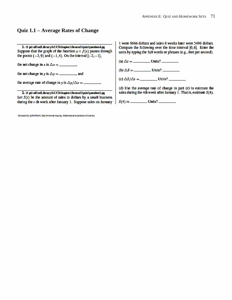
APPENDIX E: QUIZ AND HOMEWORK SETS 71
Quiz 1.1 – Average Rates of Change
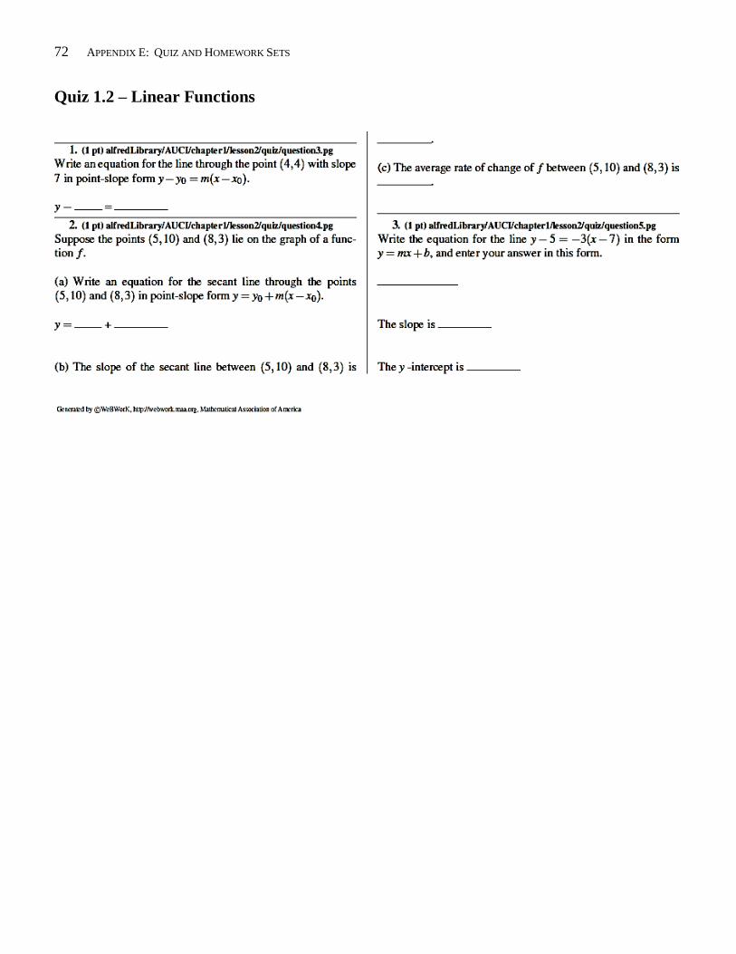
72 APPENDIX E: QUIZ AND HOMEWORK SETS
Quiz 1.2 – Linear Functions
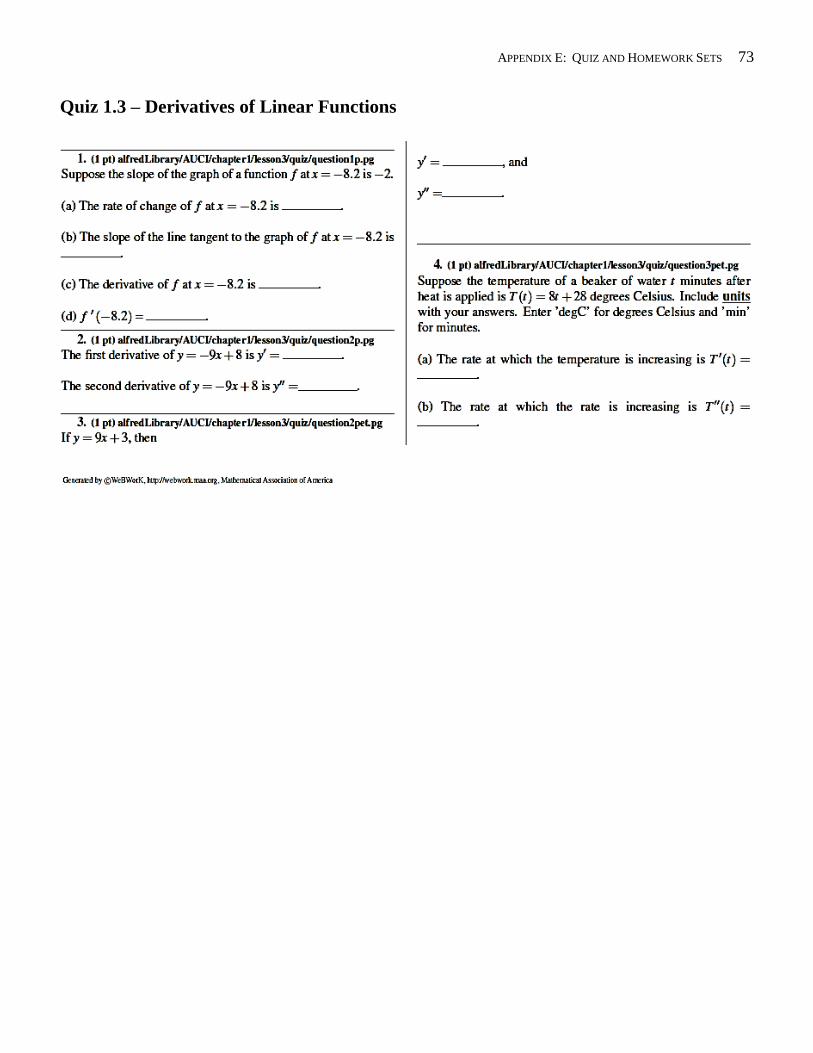
APPENDIX E: QUIZ AND HOMEWORK SETS 73
Quiz 1.3 – Derivatives of Linear Functions
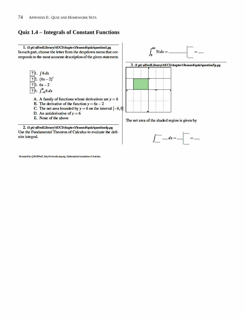
74 APPENDIX E: QUIZ AND HOMEWORK SETS
Quiz 1.4 – Integrals of Constant Functions
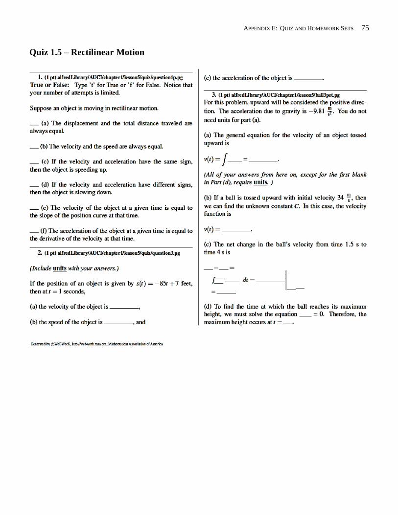
APPENDIX E: QUIZ AND HOMEWORK SETS 75
Quiz 1.5 – Rectilinear Motion
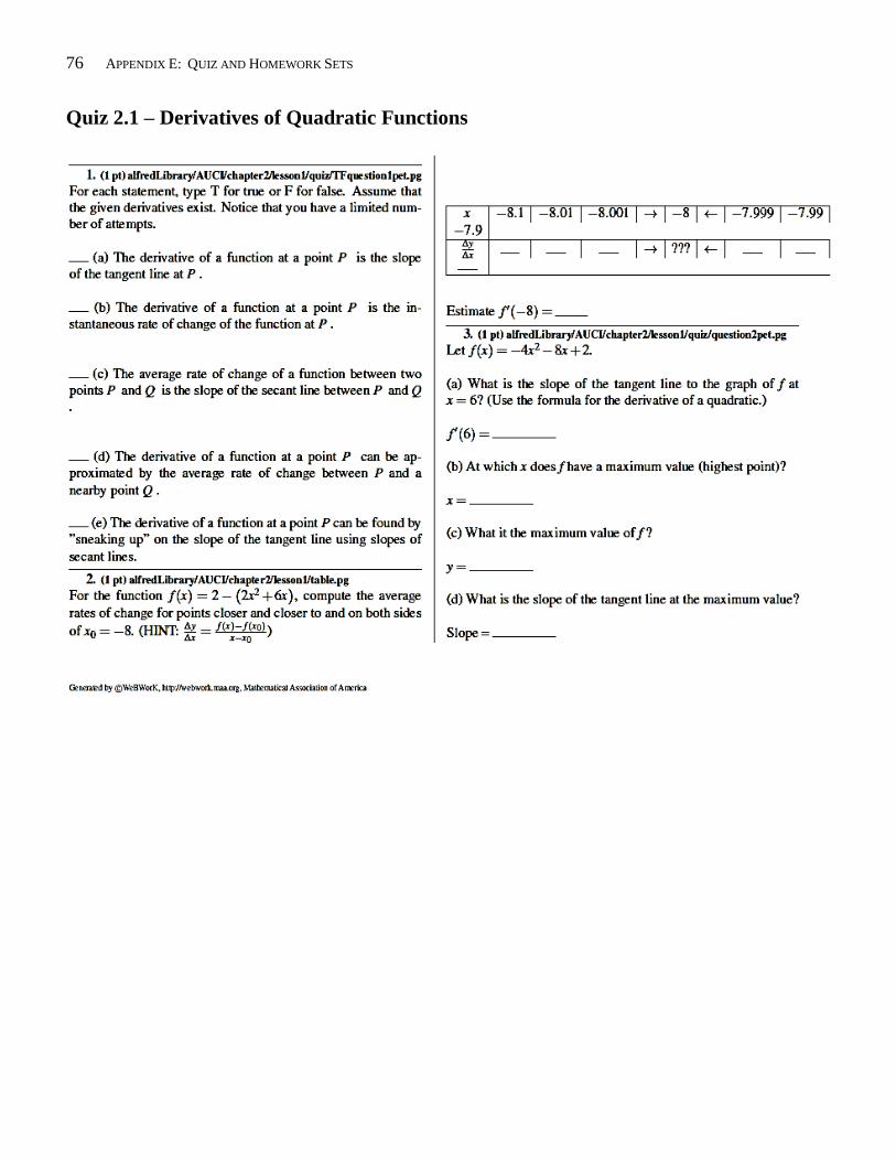
76 APPENDIX E: QUIZ AND HOMEWORK SETS
Quiz 2.1 – Derivatives of Quadratic Functions
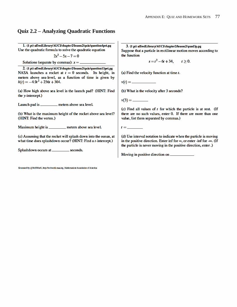
APPENDIX E: QUIZ AND HOMEWORK SETS 77
Quiz 2.2 – Analyzing Quadratic Functions
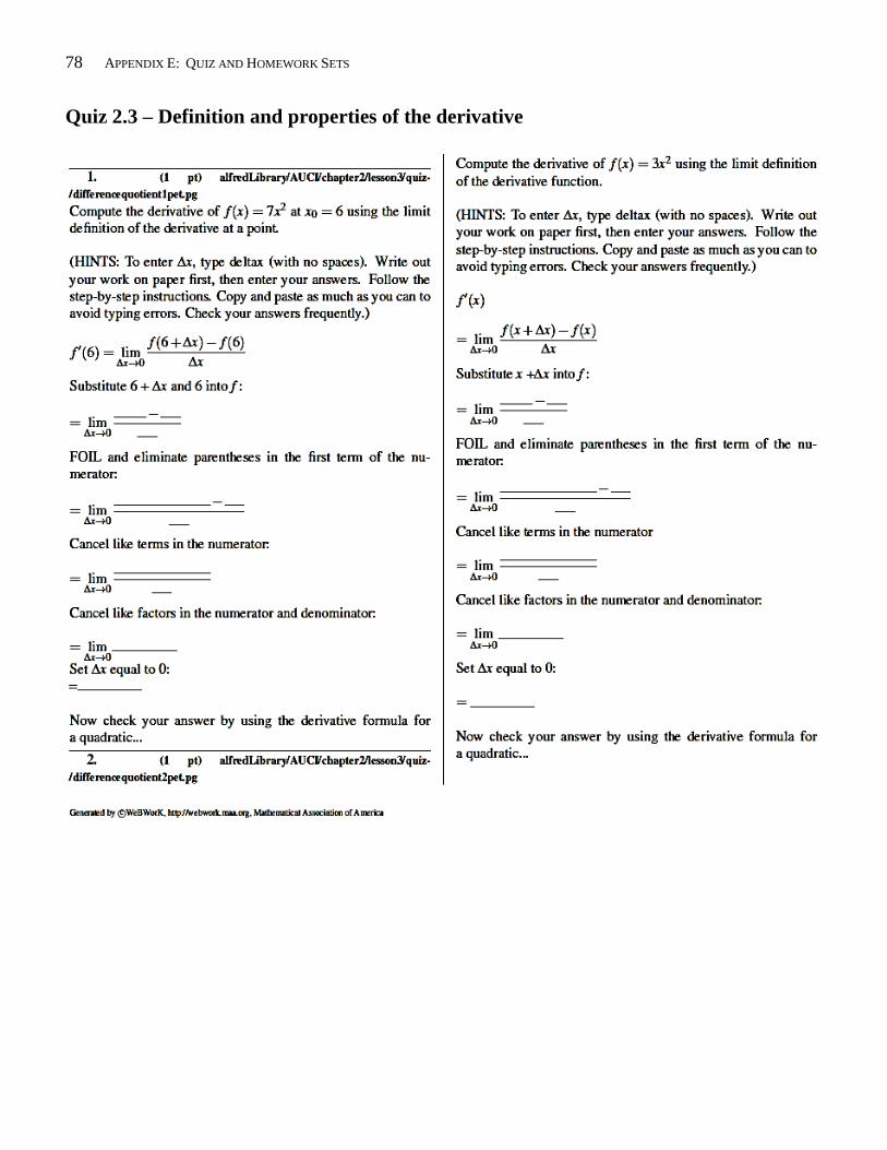
78 APPENDIX E: QUIZ AND HOMEWORK SETS
Quiz 2.3 – Definition and properties of the derivative
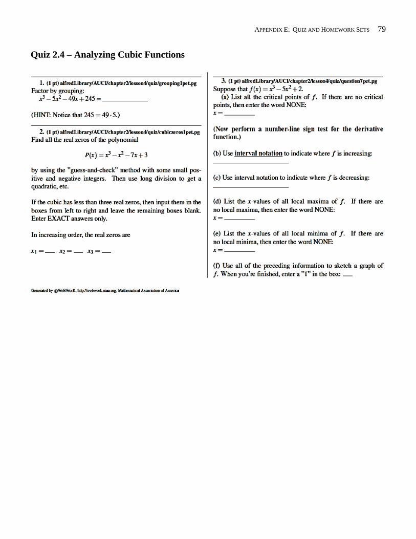
APPENDIX E: QUIZ AND HOMEWORK SETS 79
Quiz 2.4 – Analyzing Cubic Functions
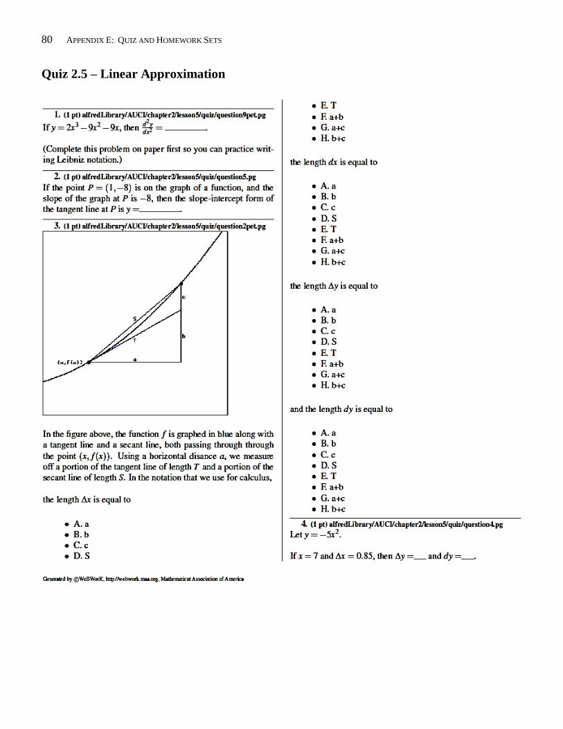
80 APPENDIX E: QUIZ AND HOMEWORK SETS
Quiz 2.5 – Linear Approximation
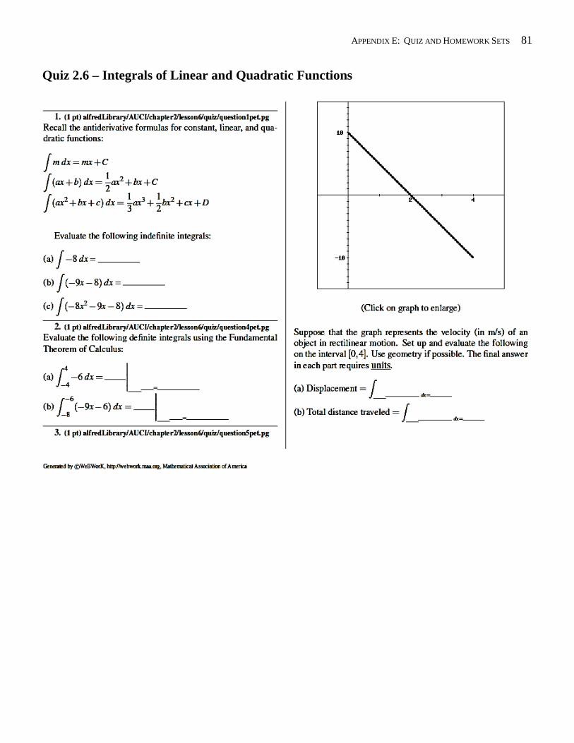
APPENDIX E: QUIZ AND HOMEWORK SETS 81
Quiz 2.6 – Integrals of Linear and Quadratic Functions
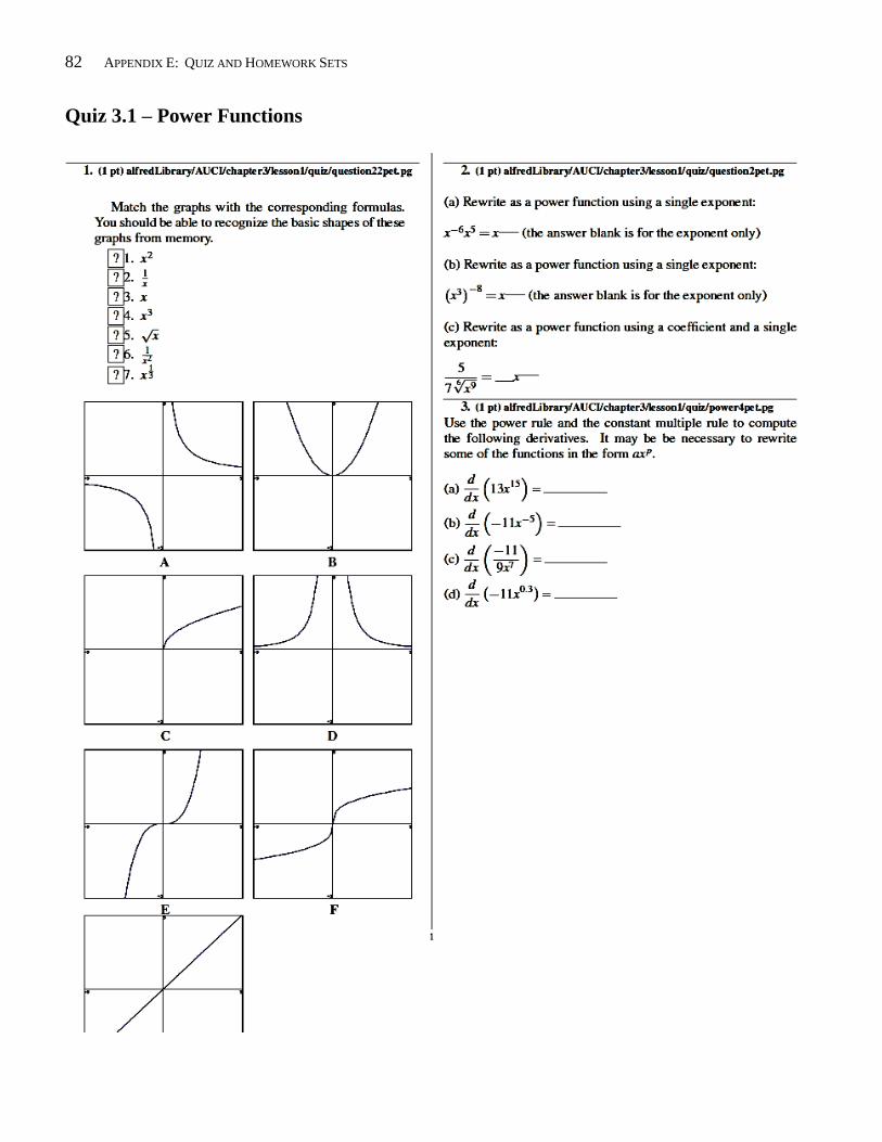
82 APPENDIX E: QUIZ AND HOMEWORK SETS
Quiz 3.1 – Power Functions
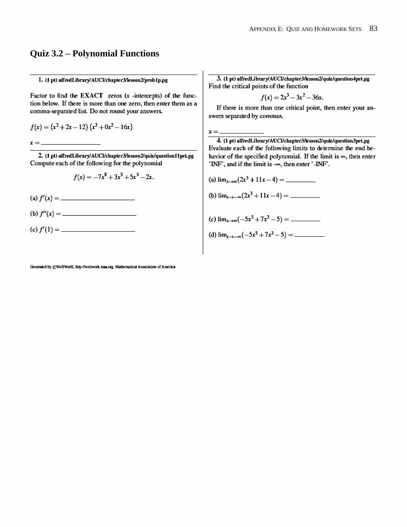
APPENDIX E: QUIZ AND HOMEWORK SETS 83
Quiz 3.2 – Polynomial Functions
84 APPENDIX E: QUIZ AND HOMEWORK SETS
Quiz 3.3 – Composite Functions
APPENDIX E: QUIZ AND HOMEWORK SETS 85
Quiz 3.4 – Products of Functions
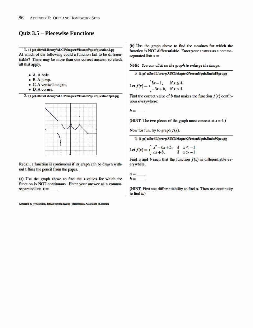
86 APPENDIX E: QUIZ AND HOMEWORK SETS
Quiz 3.5 – Piecewise Functions
APPENDIX E: QUIZ AND HOMEWORK SETS 87
Quiz 3.6 – Integrals of Polynomials
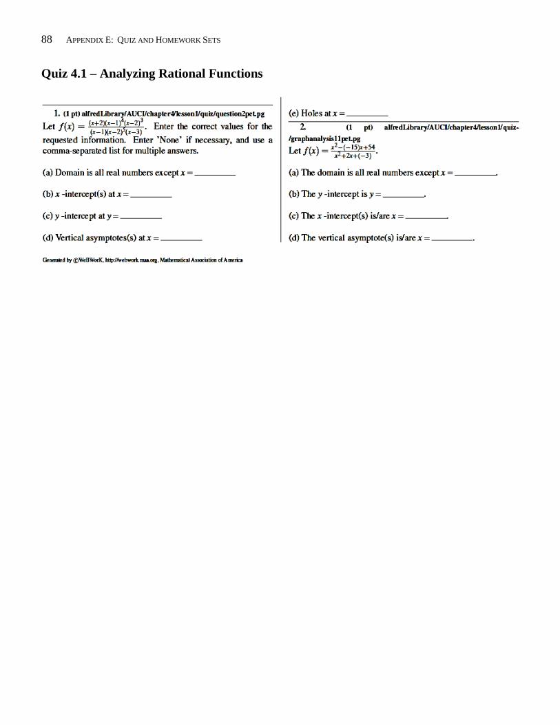
88 APPENDIX E: QUIZ AND HOMEWORK SETS
Quiz 4.1 – Analyzing Rational Functions
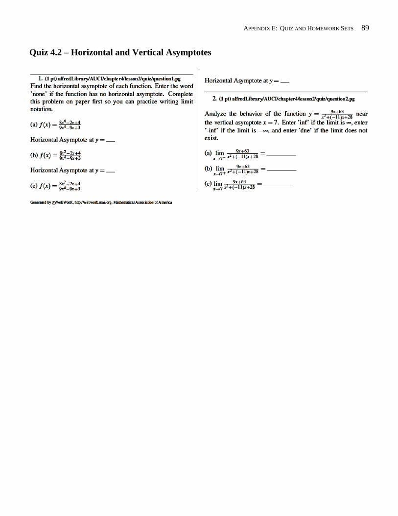
APPENDIX E: QUIZ AND HOMEWORK SETS 89
Quiz 4.2 – Horizontal and Vertical Asymptotes
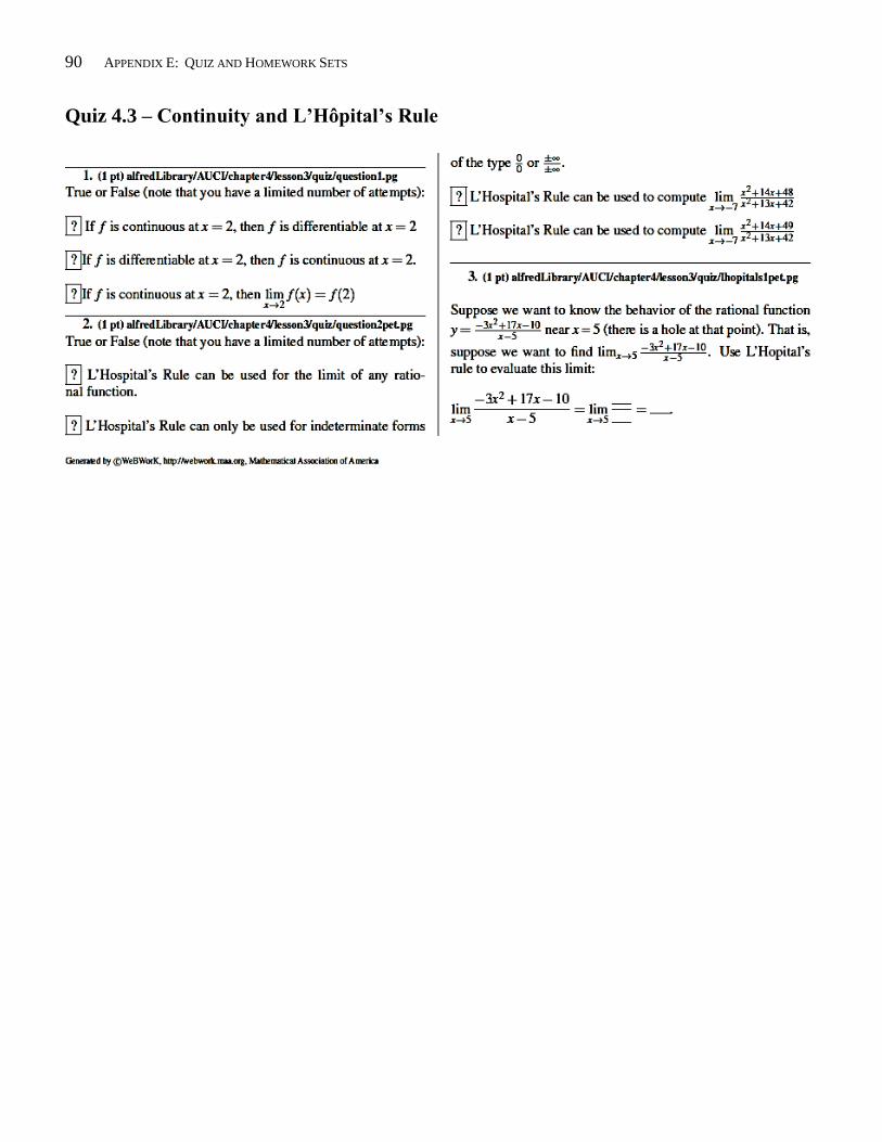
90 APPENDIX E: QUIZ AND HOMEWORK SETS
Quiz 4.3 – Continuity and L’Hôpital’s Rule
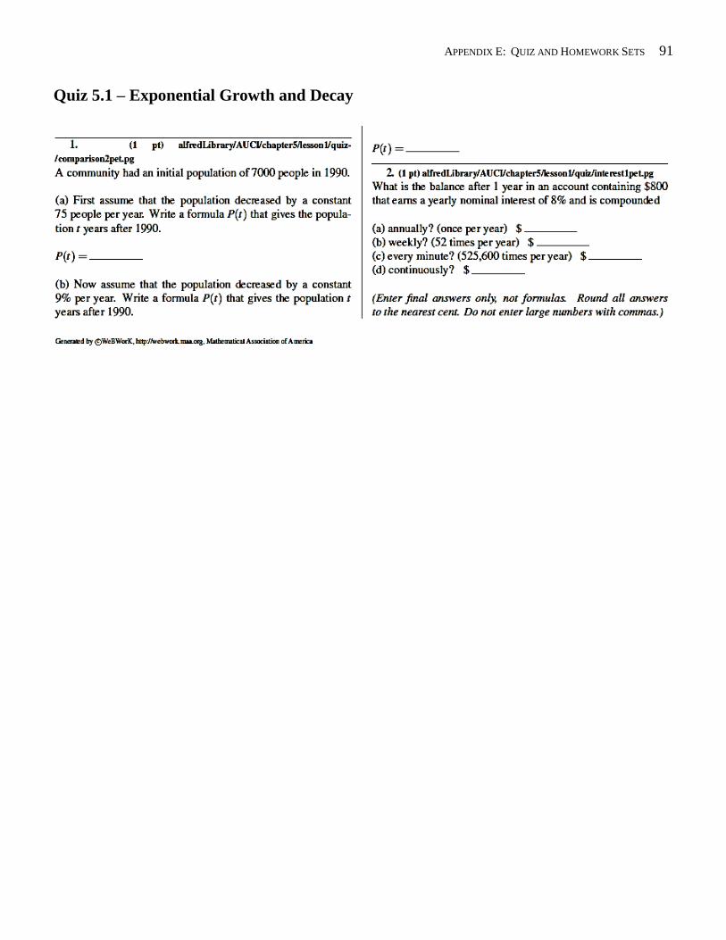
APPENDIX E: QUIZ AND HOMEWORK SETS 91
Quiz 5.1 – Exponential Growth and Decay
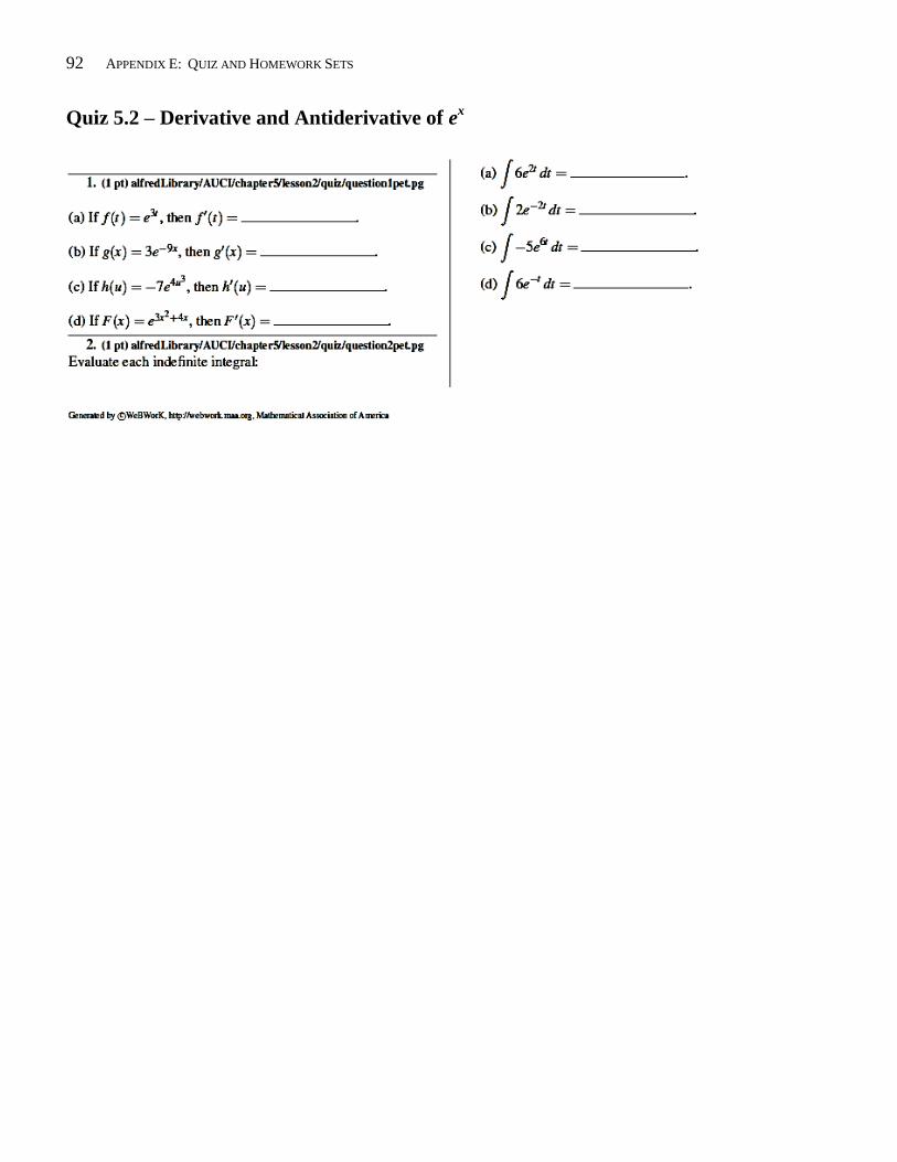
92 APPENDIX E: QUIZ AND HOMEWORK SETS
Quiz 5.2 – Derivative and Antiderivative of ex
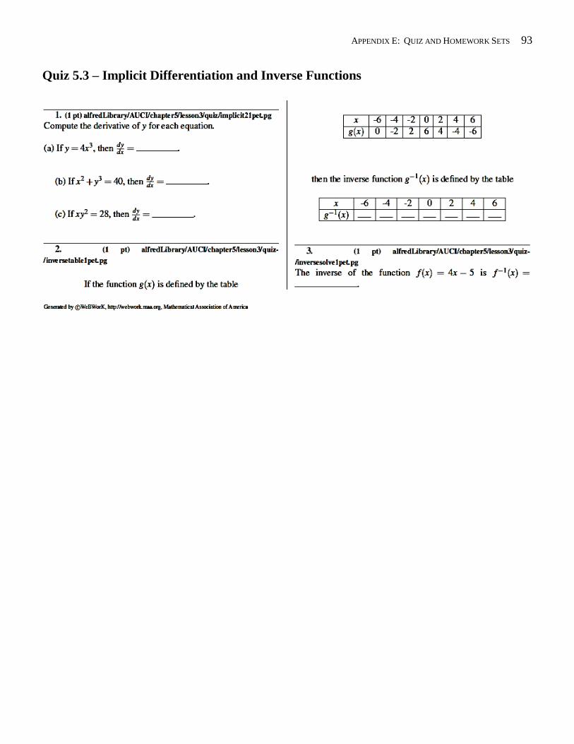
APPENDIX E: QUIZ AND HOMEWORK SETS 93
Quiz 5.3 – Implicit Differentiation and Inverse Functions
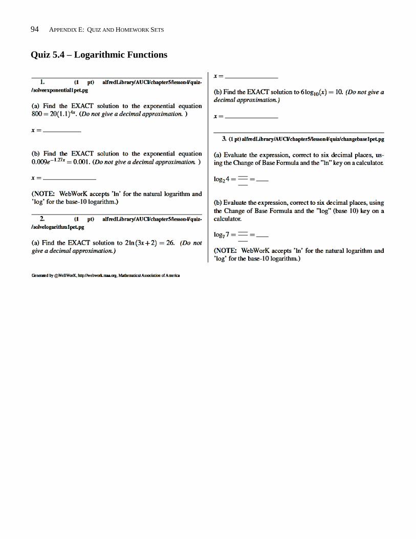
94 APPENDIX E: QUIZ AND HOMEWORK SETS
Quiz 5.4 – Logarithmic Functions
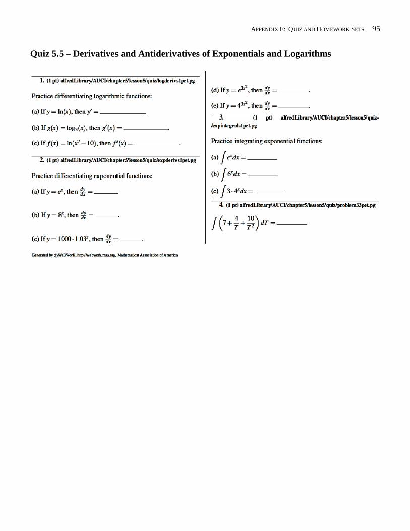
APPENDIX E: QUIZ AND HOMEWORK SETS 95
Quiz 5.5 – Derivatives and Antiderivatives of Exponentials and Logarithms
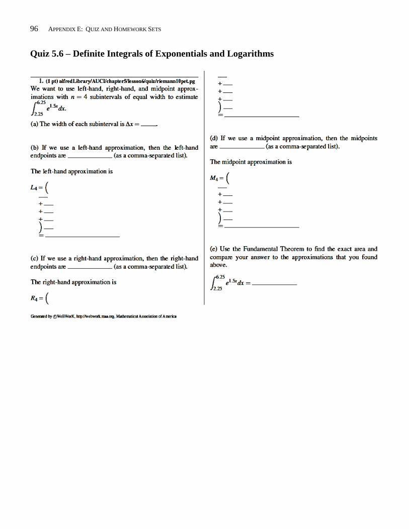
96 APPENDIX E: QUIZ AND HOMEWORK SETS
Quiz 5.6 – Definite Integrals of Exponentials and Logarithms
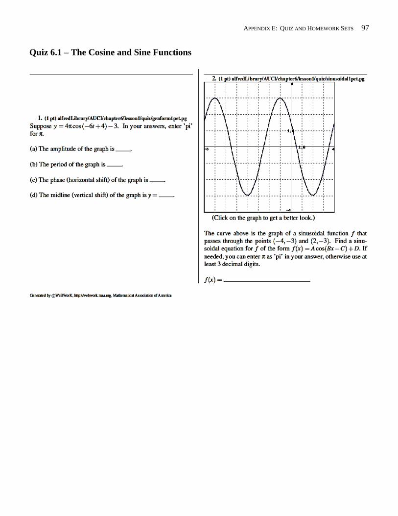
APPENDIX E: QUIZ AND HOMEWORK SETS 97
Quiz 6.1 – The Cosine and Sine Functions
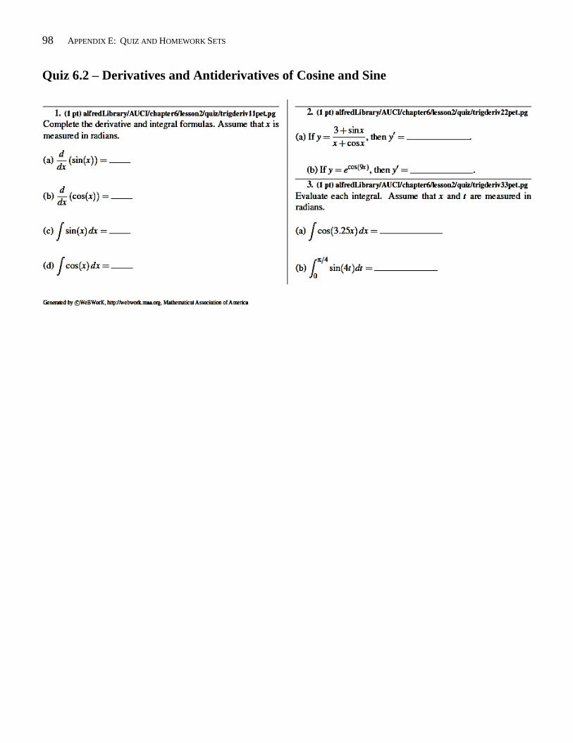
98 APPENDIX E: QUIZ AND HOMEWORK SETS
Quiz 6.2 – Derivatives and Antiderivatives of Cosine and Sine
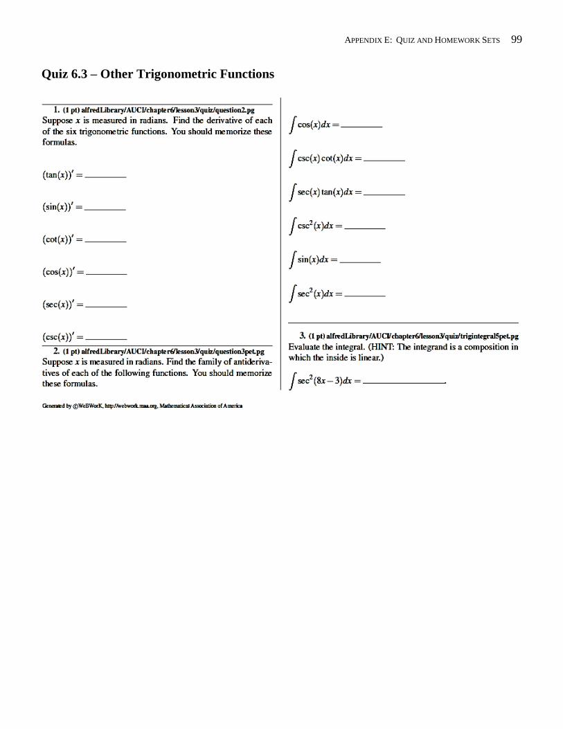
APPENDIX E: QUIZ AND HOMEWORK SETS 99
Quiz 6.3 – Other Trigonometric Functions
100 APPENDIX E: QUIZ AND HOMEWORK SETS
Quiz 6.4 – Other Trigonometric Functions
APPENDIX E: QUIZ AND HOMEWORK SETS 101
Quiz 7.1 – Related Rates
102 APPENDIX E: QUIZ AND HOMEWORK SETS
Quiz 7.2 – Graph Analysis Using First and Second Derivatives
APPENDIX E: QUIZ AND HOMEWORK SETS 103
Quiz 7.3 – Graph Analysis with the TI-84
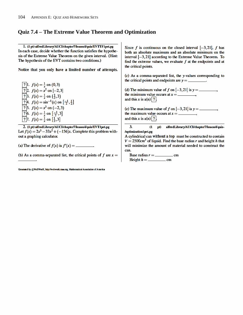
104 APPENDIX E: QUIZ AND HOMEWORK SETS
Quiz 7.4 – The Extreme Value Theorem and Optimization
APPENDIX E: QUIZ AND HOMEWORK SETS 105
Quiz 7.5 – Differential Equations
106 APPENDIX E: QUIZ AND HOMEWORK SETS
Quiz 8.1 – Sigma Notation and Summations
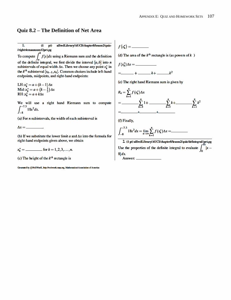
APPENDIX E: QUIZ AND HOMEWORK SETS 107
Quiz 8.2 – The Definition of Net Area
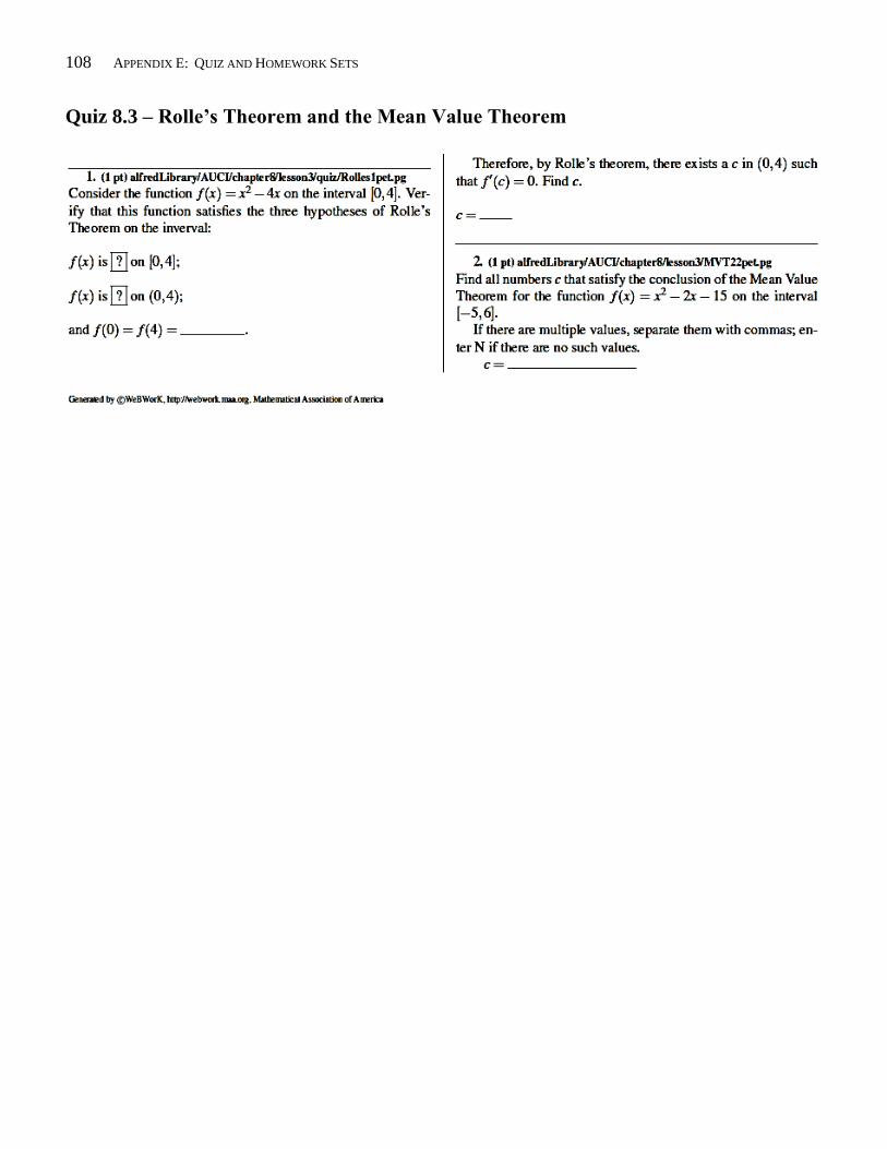
108 APPENDIX E: QUIZ AND HOMEWORK SETS
Quiz 8.3 – Rolle’s Theorem and the Mean Value Theorem
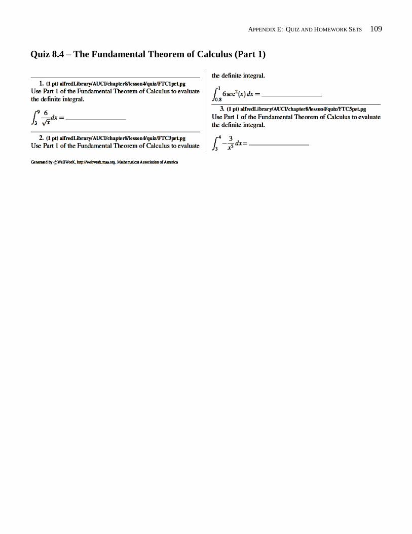
APPENDIX E: QUIZ AND HOMEWORK SETS 109
Quiz 8.4 – The Fundamental Theorem of Calculus (Part 1)
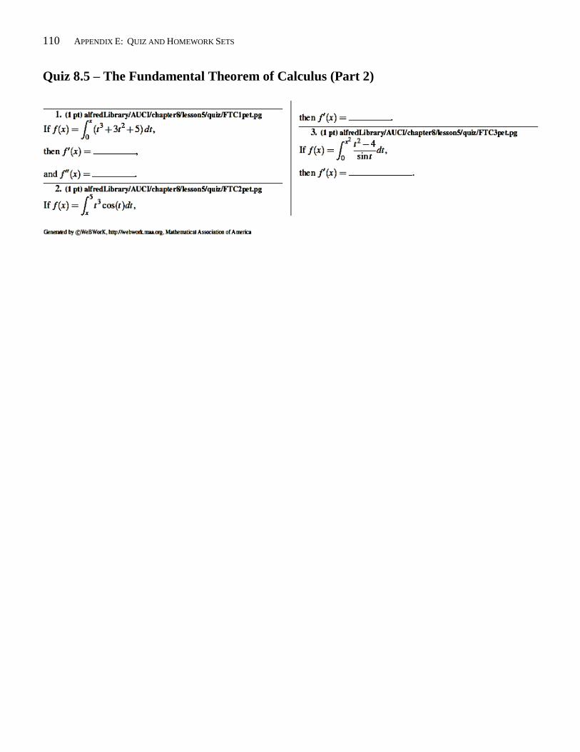
110 APPENDIX E: QUIZ AND HOMEWORK SETS
Quiz 8.5 – The Fundamental Theorem of Calculus (Part 2)
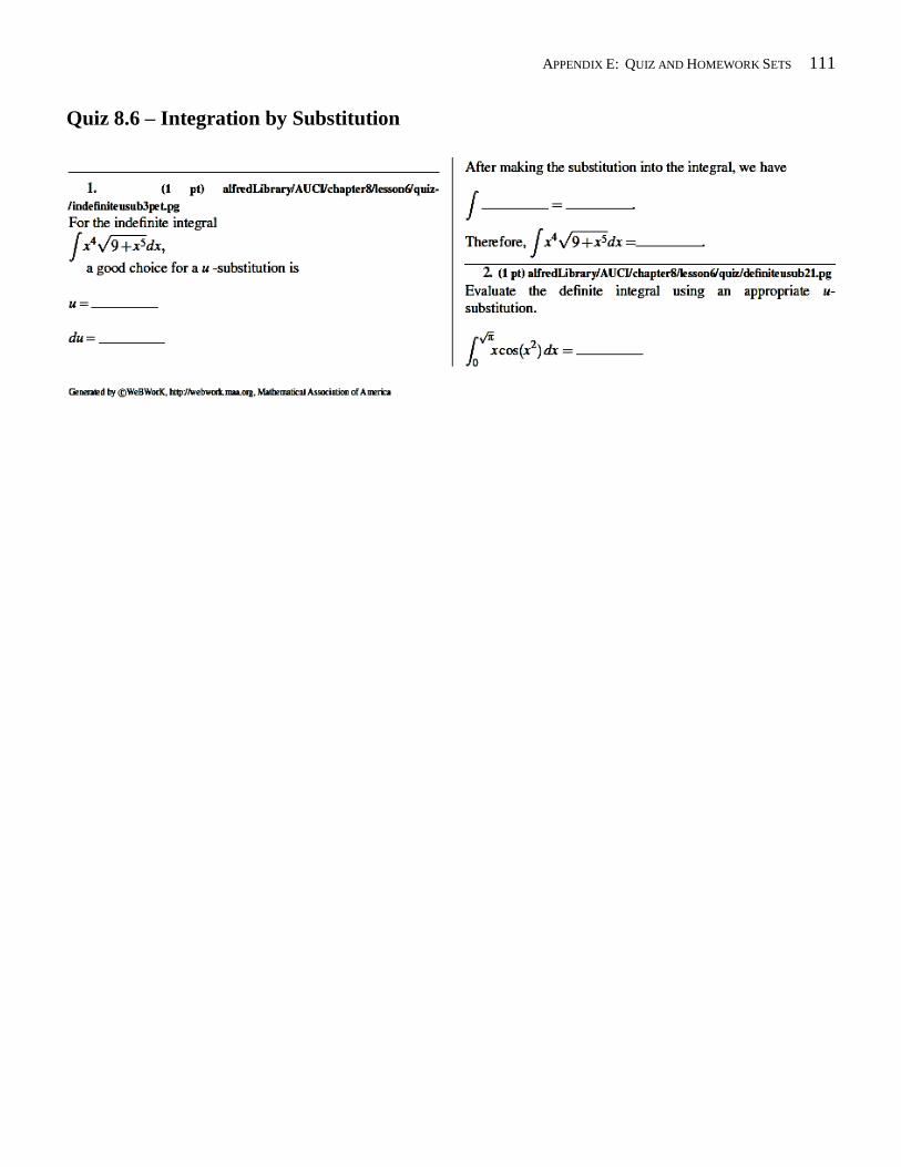
APPENDIX E: QUIZ AND HOMEWORK SETS 111
Quiz 8.6 – Integration by Substitution
112 APPENDIX E: QUIZ AND HOMEWORK SETS
Quiz 8.7 – Modeling Accumulated Change with the TI-84
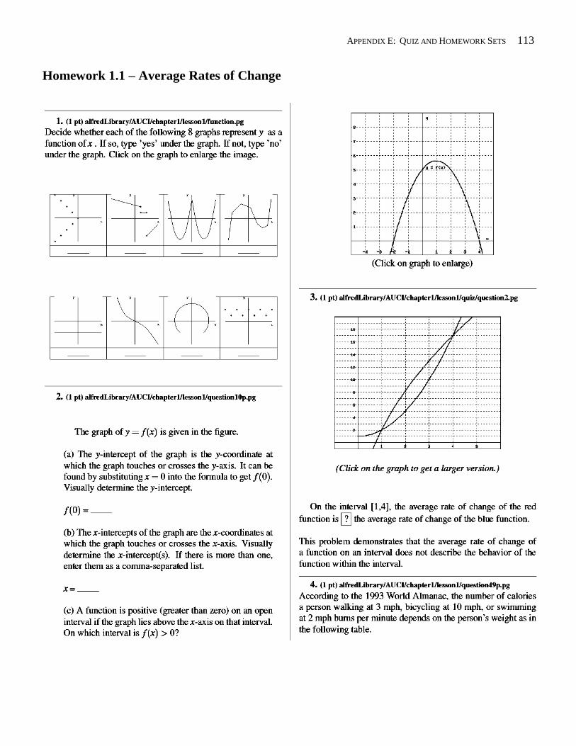
APPENDIX E: QUIZ AND HOMEWORK SETS 113
Homework 1.1 – Average Rates of Change
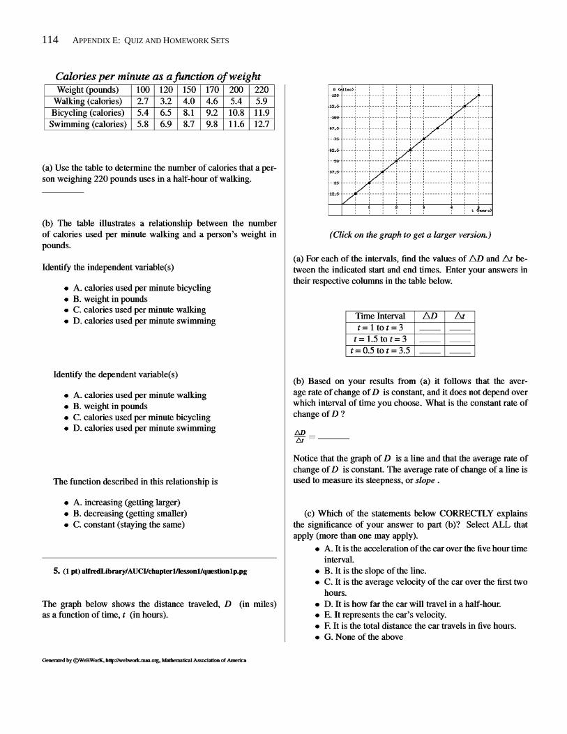
114 APPENDIX E: QUIZ AND HOMEWORK SETS
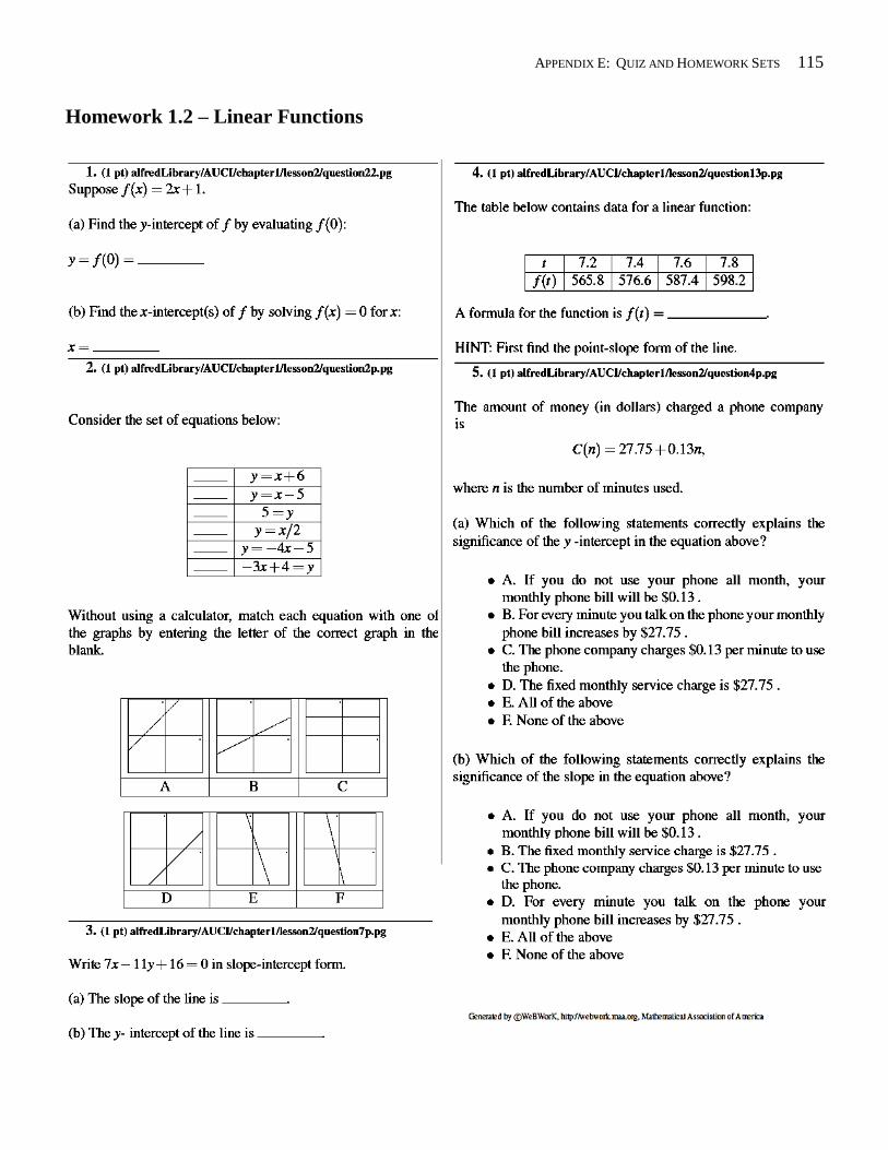
APPENDIX E: QUIZ AND HOMEWORK SETS 115
Homework 1.2 – Linear Functions
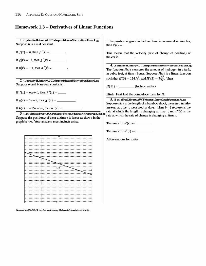
116 APPENDIX E: QUIZ AND HOMEWORK SETS
Homework 1.3 – Derivatives of Linear Functions
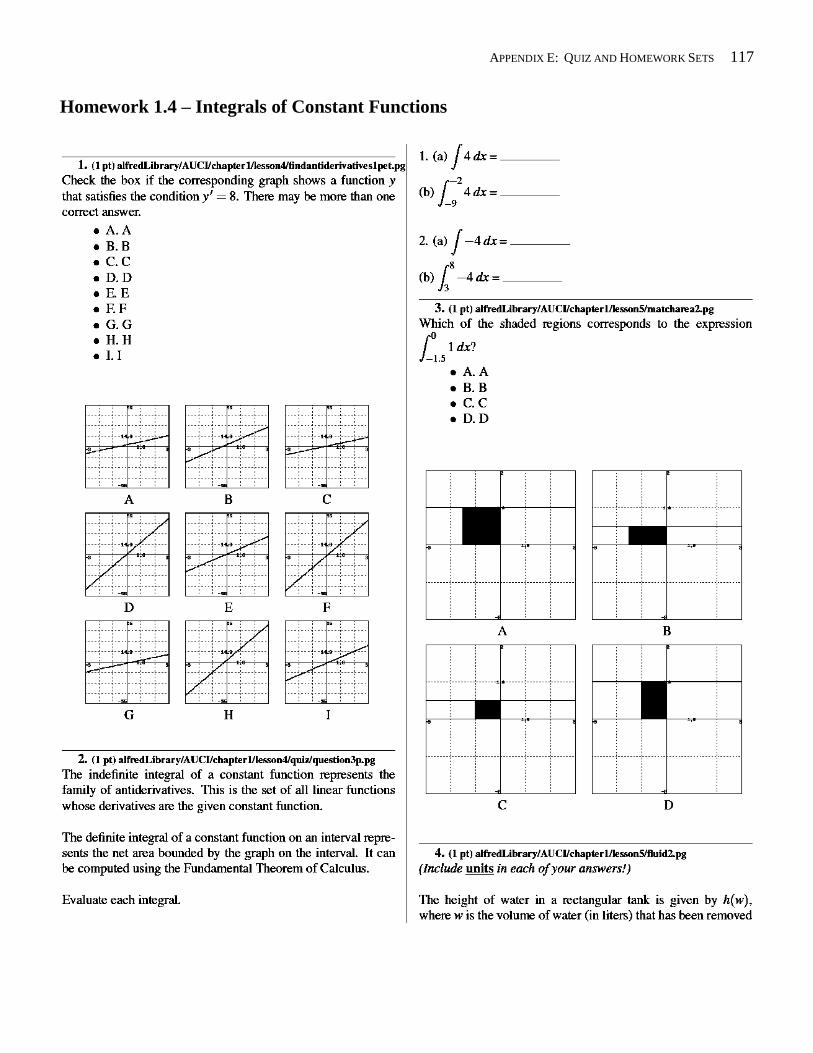
APPENDIX E: QUIZ AND HOMEWORK SETS 117
Homework 1.4 – Integrals of Constant Functions
118 APPENDIX E: QUIZ AND HOMEWORK SETS
APPENDIX E: QUIZ AND HOMEWORK SETS 119
Homework 1.5 – Rectilinear Motion
120 APPENDIX E: QUIZ AND HOMEWORK SETS
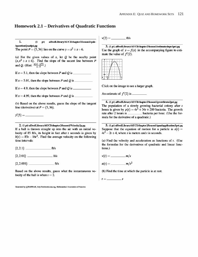
APPENDIX E: QUIZ AND HOMEWORK SETS 121
Homework 2.1 – Derivatives of Quadratic Functions
122 APPENDIX E: QUIZ AND HOMEWORK SETS
Homework 2.2 – Analyzing Quadratic Functions
APPENDIX E: QUIZ AND HOMEWORK SETS 123
Homework 2.3 – Definition and properties of the derivative
124 APPENDIX E: QUIZ AND HOMEWORK SETS
Homework 2.4 – Analyzing Cubic Functions
APPENDIX E: QUIZ AND HOMEWORK SETS 125
Homework 2.5 – Linear Approximation
126 APPENDIX E: QUIZ AND HOMEWORK SETS
Homework 2.6 – Integrals of Linear and Quadratic Functions
APPENDIX E: QUIZ AND HOMEWORK SETS 127
Homework 3.1 – Power Functions
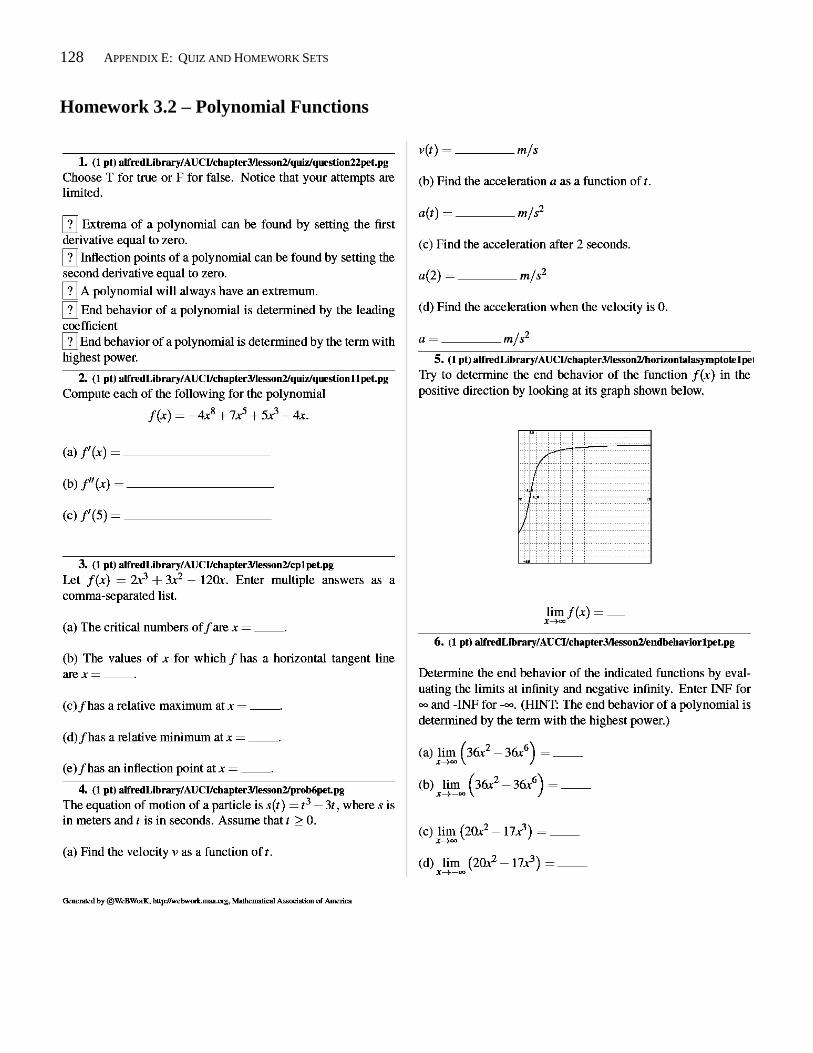
128 APPENDIX E: QUIZ AND HOMEWORK SETS
Homework 3.2 – Polynomial Functions
APPENDIX E: QUIZ AND HOMEWORK SETS 129
Homework 3.3 – Composite Functions
130 APPENDIX E: QUIZ AND HOMEWORK SETS
Homework 3.4 – Products of Functions
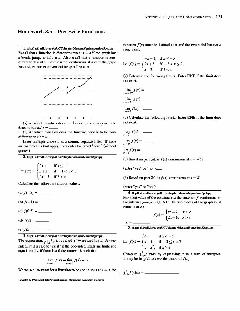
APPENDIX E: QUIZ AND HOMEWORK SETS 131
Homework 3.5 – Piecewise Functions
132 APPENDIX E: QUIZ AND HOMEWORK SETS
Homework 3.6 – Integrals of Polynomials
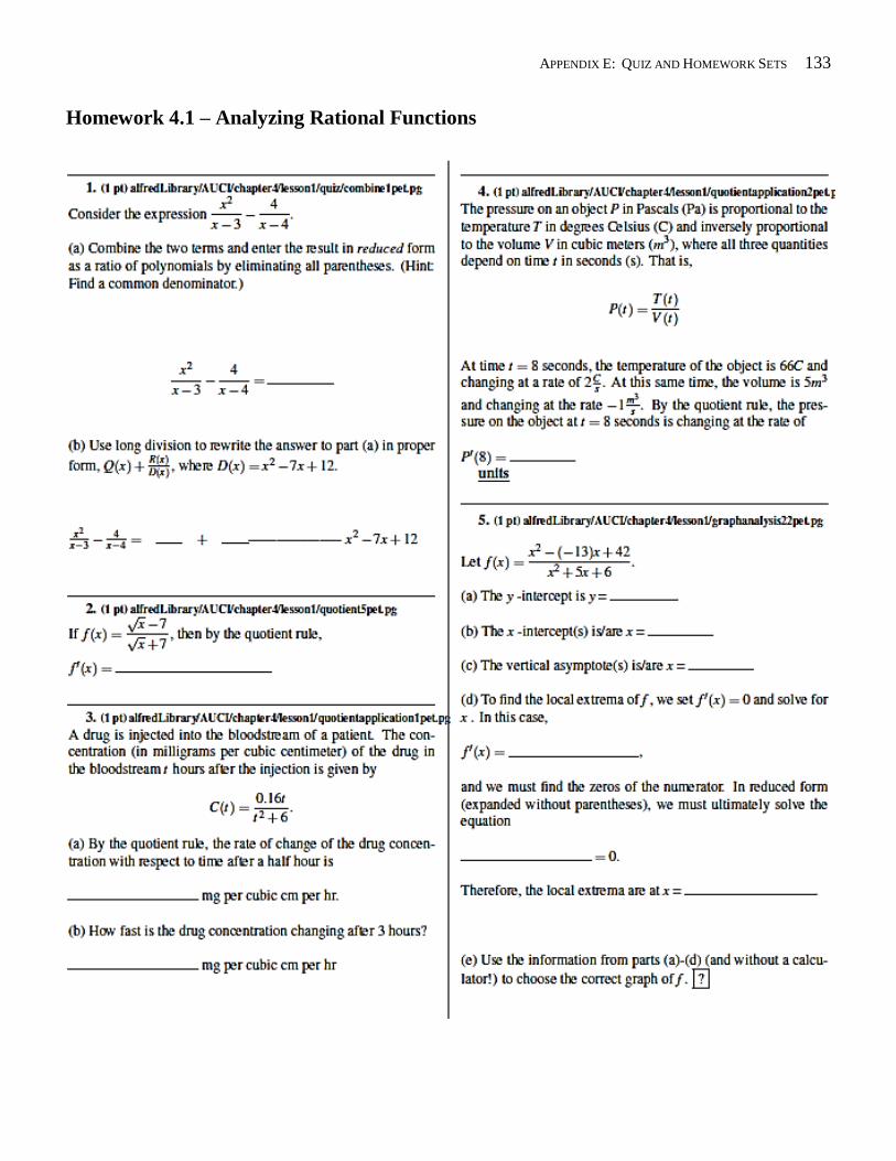
APPENDIX E: QUIZ AND HOMEWORK SETS 133
Homework 4.1 – Analyzing Rational Functions
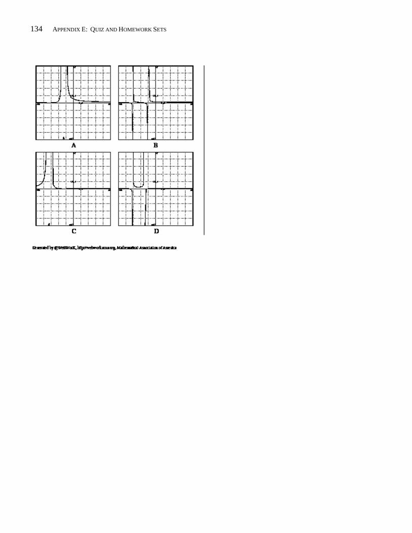
134 APPENDIX E: QUIZ AND HOMEWORK SETS
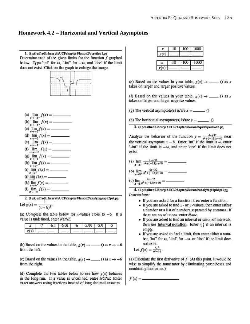
APPENDIX E: QUIZ AND HOMEWORK SETS 135
Homework 4.2 – Horizontal and Vertical Asymptotes
136 APPENDIX E: QUIZ AND HOMEWORK SETS
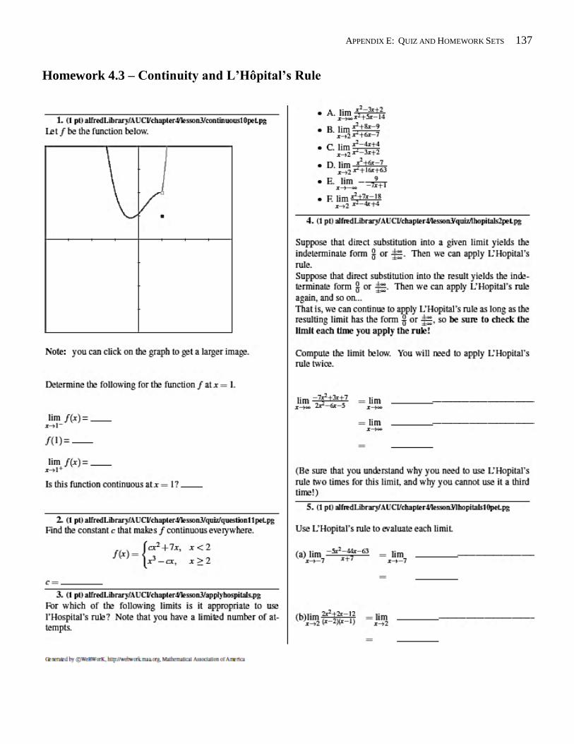
APPENDIX E: QUIZ AND HOMEWORK SETS 137
Homework 4.3 – Continuity and L’Hôpital’s Rule
138 APPENDIX E: QUIZ AND HOMEWORK SETS
Homework 5.1 – Exponential Growth and Decay
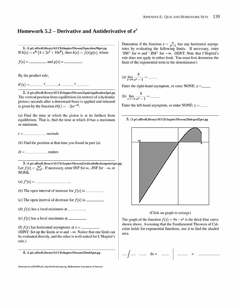
APPENDIX E: QUIZ AND HOMEWORK SETS 139
Homework 5.2 – Derivative and Antiderivative of ex
140 APPENDIX E: QUIZ AND HOMEWORK SETS
Homework 5.3 – Implicit Differentiation and Inverse Functions
APPENDIX E: QUIZ AND HOMEWORK SETS 141
Homework 5.4 – Logarithmic Functions
142 APPENDIX E: QUIZ AND HOMEWORK SETS
Homework 5.5 – Derivatives and Antiderivatives of Exponentials and Logarithms
APPENDIX E: QUIZ AND HOMEWORK SETS 143
Homework 5.6 – Definite Integrals of Exponentials and Logarithms
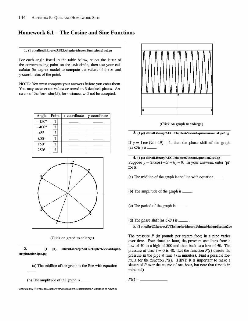
144 APPENDIX E: QUIZ AND HOMEWORK SETS
Homework 6.1 – The Cosine and Sine Functions
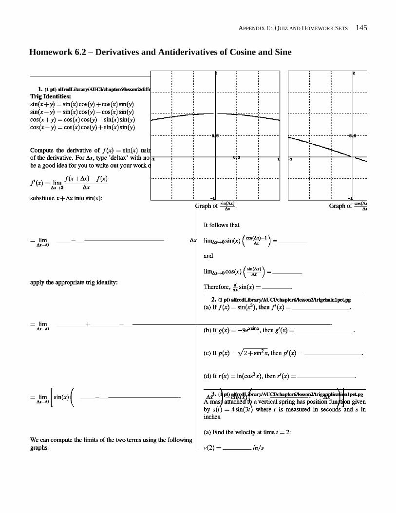
APPENDIX E: QUIZ AND HOMEWORK SETS 145
Homework 6.2 – Derivatives and Antiderivatives of Cosine and Sine
146 APPENDIX E: QUIZ AND HOMEWORK SETS
APPENDIX E: QUIZ AND HOMEWORK SETS 147
Homework 6.3 – Other Trigonometric Functions
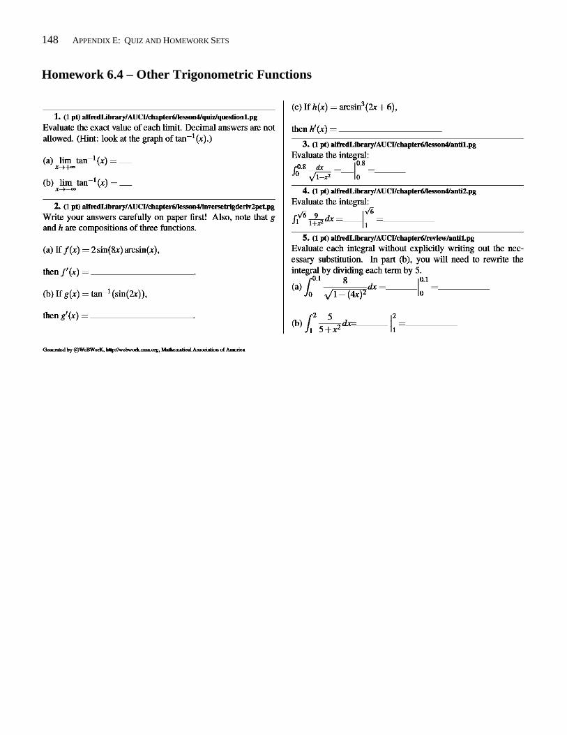
148 APPENDIX E: QUIZ AND HOMEWORK SETS
Homework 6.4 – Other Trigonometric Functions
APPENDIX E: QUIZ AND HOMEWORK SETS 149
Homework 7.1 – Related Rates
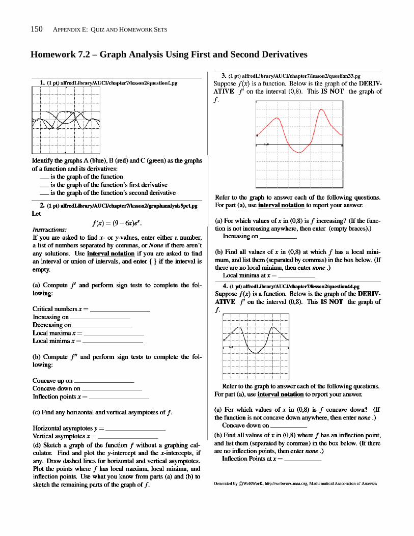
150 APPENDIX E: QUIZ AND HOMEWORK SETS
Homework 7.2 – Graph Analysis Using First and Second Derivatives
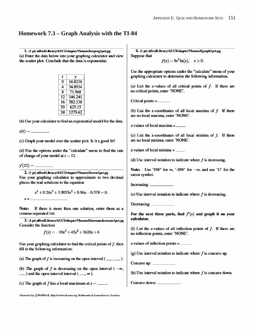
APPENDIX E: QUIZ AND HOMEWORK SETS 151
Homework 7.3 – Graph Analysis with the TI-84
152 APPENDIX E: QUIZ AND HOMEWORK SETS
Homework 7.4 – The Extreme Value Theorem and Optimization
APPENDIX E: QUIZ AND HOMEWORK SETS 153
Homework 7.5 – Differential Equations
154 APPENDIX E: QUIZ AND HOMEWORK SETS
Homework 8.1 – Sigma Notation and Summations
APPENDIX E: QUIZ AND HOMEWORK SETS 155
Homework 8.2 – The Definition of Net Area
156 APPENDIX E: QUIZ AND HOMEWORK SETS
Homework 8.3 – Rolle’s Theorem and the Mean Value Theorem
APPENDIX E: QUIZ AND HOMEWORK SETS 157
Homework 8.4 – The Fundamental Theorem of Calculus (Part 1)
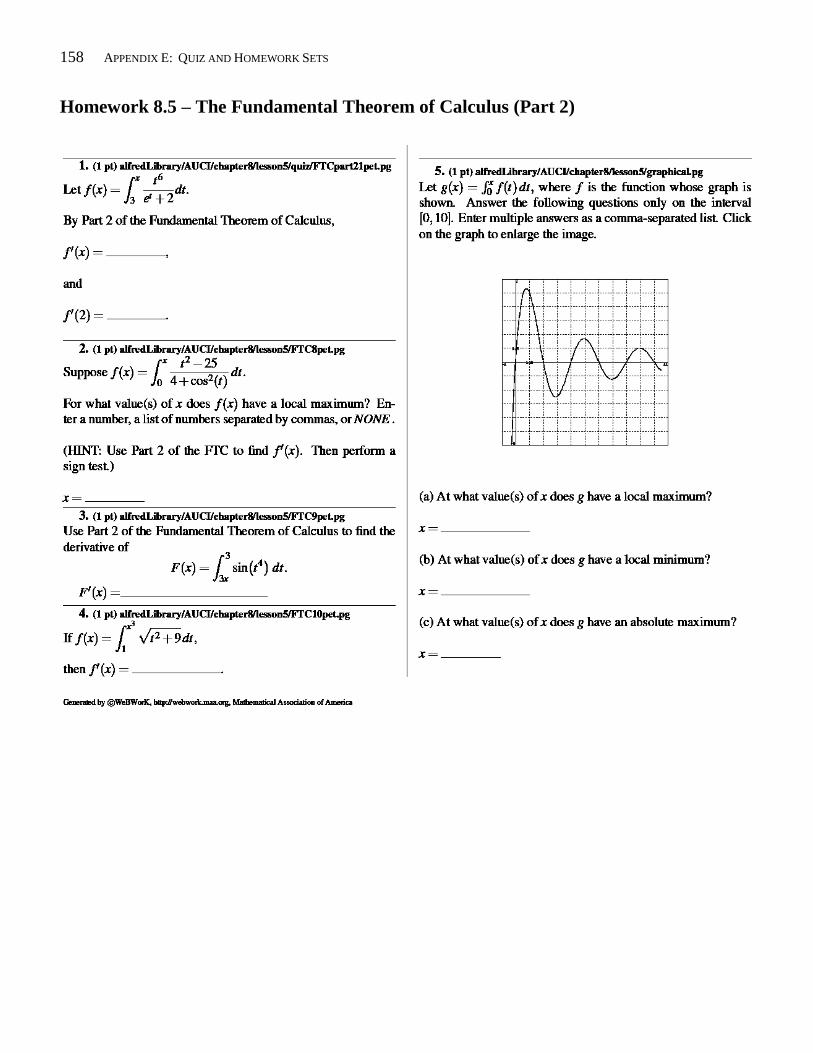
158 APPENDIX E: QUIZ AND HOMEWORK SETS
Homework 8.5 – The Fundamental Theorem of Calculus (Part 2)
APPENDIX E: QUIZ AND HOMEWORK SETS 159
Homework 8.6 – Integration by Substitution
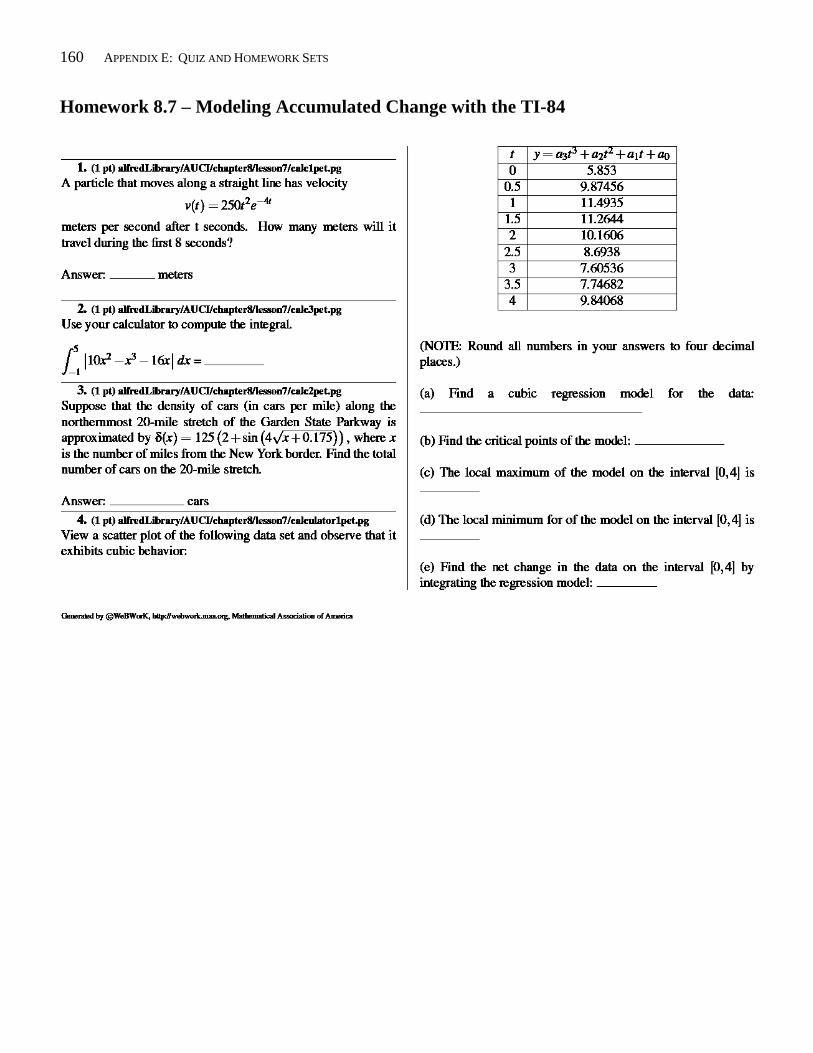
160 APPENDIX E: QUIZ AND HOMEWORK SETS
Homework 8.7 – Modeling Accumulated Change with the TI-84